Embed Size (px)
Citation preview

STOCHASTIC OPTIMAL CONTROL OF pH NEUTRALISATION
PROCESS IN A WATER TREATMENT PLANT
Elena Roxana TUDOROIU*, Sorin Mihai RADU
*, Wilhelm KECS
*, Nicolae
ILIAS*, and Nicolae TUDOROIU
**
*University of Petrosani ([email protected]) **
John Abbott College, Montreal, Canada ([email protected])
Abstract: This paper opens a new research exploration direction in a real time
MATLAB/SIMULINK simulation environment to optimize the pH neutralization process level of a
generic wastewater treatment plant following a stochastic approach. The control system design
of pH neutralization process is a very difficult task to be accomplished due to its severe
nonlinearity and complexity characterized by a persistent change in the chemical systems with
complex kinetic and thermodynamic reactions, nonlinear responses, a sensitive environment
uncertain results and large variety of operating conditions to be covered. Furthermore, the
standard control strategies design fail unfortunately when the system performance is concerned.
In the new approach the proposed control strategy proved its effectiveness and high accuracy in
terms of its performance compare to the traditional control mechanisms. To validate all these
results a simplified intuitive nonlinear model of the neutralization reactor from the literature is
considered. The solution of the optimization problem is found in a Linear Quadratic Gaussian
optimization framework. In this new approach the nonlinear dynamics of the neutralization
reactor must be linearized around an equilibrium point, the cost function is quadratic, and the
process and measurement noises are white Gaussian noises, independent, of zero mean, and
normally distributed. The system’s control is Markovian and linear as a combination of
observable or estimated states. In addition the implementation of stochastic optimal control
approach is more restrictive by introducing a few key concepts and requirements such as
controllability, stabilizability, observability, and the certainty-equivalence principle, as well as
the well-known separation principle between optimal estimation and optimal control.
Keywords: LQG stochastic control, control system optimization, Linear Quadratic regulator,
Linear quadratic estimator, neutralization reactor, MATLAB/SIMULINK
1. INTRODUCTION
The acidity of any solution is assessed by measuring its pH level (e.g. the
concentration of positive Hydrogen ions ( H ) in the solution) that ranges in a scale from
1 to 14. The value of 7 for the pH level in any solution at room temperature indicates that the
solution is neutral. According to this scale if the pH of the solution at the room temperature is
less than 7, the concentration of Hydrogen ions ( H ) in the solution is high, and the solution
is considered to be acid [1]. On the other hand if the pH level of the solution at room
temperature is greater than 7, the concentration of negative hydroxyl ions ( OH ) in the
solution is high and the solution is considered to be alkaline or a base [1]. According to
environmental safety standards for industry all treated water effluents must have the pH level
of either 8 or 6 [1]. The control system design of pH neutralization process is a very difficult
task to be accomplished due to the following reasons [1, 2, 3]:

1) the dynamics of pH neutralization process is severely nonlinear and of high
complexity as is shown in Fig. 1(a, b) for a particular case of the titration curve
for acid-base process reaction [1].
2) a persistent changes in the chemical systems
3) complex kinetic and thermodynamic reactions
4) nonlinear response of the process,
5) a sensitive environment uncertain results
6) a large variety of operating conditions to be covered.
8. (b)
Fig. 1. Titration curve for acid-base process reaction (a snapshot from [1], p.36)
(a) Hydrochloric acid
(b) Phosphoric acid
The classical control strategies design fail in the majority of the cases when the system
performance is concerned. In the new stochastic approach the proposed optimal control
strategy proved its effectiveness and high accuracy in terms of its performance compare to
the traditional control mechanisms. To find an optimal solution to this optimization problem a
Linear Quadratic Gaussian (LQG) control strategy is proposed. To implement the new LQG
strategy the following requirements need to be satisfied [4, 5, 6, 7, 8]:
(1) the nonlinear dynamics of the neutralization reactor must be linearized around an
equilibrium point
(2) the cost function is quadratic
(3) the process and measurement noises are white Gaussian, independent, of zero
mean, and normally distributed
(4) the system’s control is Markovian and linear as a combination of observable or
estimated states.
The optimization problem consists of two distinct parts, that can be easily implemented
in MATLAB/SIMULINK framework [4, 5, 6, 7]:
(a) Linear Quadratic Regulation (LQR) problem
(b) Linear Quadratic Estimation (LQE) problem
Combining the solutions of the both LQR and LQE problems is a practical real time
implementation tool of the LQG control strategy in a feedback closed-loop control system to
find the optimal values of the pH level for a neutralization reactor based on a nonlinear
intuitive generic model [4, 5, 6, 7, 8].
2. THE NEUTRALIZATION REACTOR DESCRIPTION
In Figure 2 is shown the layout of a simple neutralization reactor used in the chemical
industry, where an alkaline input flow (fluent) is neutralized with acid (reagent) in a
continuously stirred tank reactor (CSTR) [2]. For this case study the waste water enters the
reactor with a federate of ][2000h
lV
dt
dVF
F at a 13FpH (strongly alkaline); the input

acid AA V
dt
dV and base BB V
dt
dV flows are dosed and controlled by a PI regulator. A
pH-probe measures pH-actual value of the neutralized solution inside the reactor during
the transient and steady state neutralization process, transmitting its feedback to the
controller with a lag time of 50 seconds. The reactor volume is assumed to be constant,
with a capacity of ],[4000 l and the maximum value of the HCl-acid flow with a 25%
concentration is ].[30h
l The pH target value is 10 and to simplify the dynamic model only
acid addition is considered, due to the fact that the waste water is already alkaline.
Fig.2. Neutralization CSTR reactor (a snapshot from [2], p.2 )
3. FORMULATION OF THE CONTROL OPTIMIZATION PROBLEM
The control optimization problem is formulated based on the well-known optimality
principle [4, 5, 6, 7]. According to this principle the optimization problem consists in a
sequence of consecutive stages such that “from any point on an optimal trajectory, the
remaining trajectory is optimal for the corresponding problem initiated at that point” [4].
The optimality principle is a key concept for defining a control optimization problem
(COP) by the following elements [4]:
1. The dynamics of the plant represented in continuous and discrete state-equation
(law motion):
),,(1 tuxfx ttt (1)
where ,...2,1,0t is the discrete-time that takes integer values, n
tx is the value of the
control system state vector at time t , calculable from known quantities and obeys a law
motion (1), m
tu is the control system input vector value at time t , that is chosen on
basis of knowing the set of previous controls up to time 1t , },...,,{ 0211 uuuU ttt .
2. The cost function to be optimized:
)(),,(1
0
ss
s
t
tt xCtuxcC
(2)
by a suitable choice of the set of controls },...,,{ 0211 uuuU sss
3. An optimal control law attached to the law motion (1) and the cost function (2),

known as the optimality equation (dynamic programming equation (DP) or equivalent
Bellman equation) to find the optimal value of the control (optimal actuator effort of the
control system):
)]1,,,(),,([inf),( ttuxfFtuxctxF ttttu
tt
, for st (3)
with the terminal condition: )(),( sst xCsxF
where the future cost function defined in (2) from time t onwards is defined as:
)(),,(1
ss
s
t
t xCuxcC
(4)
with the minimal value calculated as solution of an optimization problem over the
sequence of controls },...,,{ 21 tss uuu :
][inf),(},...,,{ 21
tuuu
t CtxFtss
(5)
Furthermore the DP equation (3) defines an optimal control problem that is related
also to a feedback or closed – loop control, defined as:
),( txku tt , (6)
so function only of tx and t , in contrast to open-loop control system where the sequence
of controls },...,,{ 021 uuuU sss must be calculated all once at time 0t [4].
Closing, the DP equation expresses the optimal control solution in close form as in
(6) and is also a recursive backward equation in time that gives the optimal control
solution 021 ,...,, uuu ss , recursively at the time moments 0,....2,1 ss , governed by a
simple rule that the latter control policy is decided first [4]. Let now to consider the
stochastic evolution of the neutralization reactor plant by introducing two sequences
},,...,,{ 01 xxxX ttt and },...,,{ 01 uuuU ttt that incorporate the history of evolution at
time t of plant states and controls, x and u respectively. More precisely, you can say
that the evolution of any process is described by a state vector denoted by a variable x
that takes the value tx at time t , and has the following properties [4]:
1. The state vector incorporates a Markov dynamics, i.e. the stochastic version of the
dynamics equation of the plant, given by:
),|(),|( 11 tttttt uxxPUXxP (7)
2. The COP cost function is decomposable with respect to tt UX , , as is shown in (2).
3. The current values of all state vector components tx are observable, i.e. tx is
known at the time at which the control tu must be chosen.
Let us now to designate the observed history of the plant evolution at time t by
),( 1 ttt UXW , (8)
that is related to the cost function C given in (2) at time s [4]:
)( sWCC (9)
Also, the minimal expected cost function from time t onwards is defined as [4]:
]|[inf)( ttt WCEWF
(10)
where ][.E is the stochastic expectance operator (stochastic average) of the conditional cost tC
with respect to tW , and is a control policy, i.e. a rule to chose the plant control sequence
01,...,uus .

Based on this preparatory elements can be formulated the following remarkable result from
the control optimality (see Theorem 1.3 in [4], p. 4):
“The minimal expected cost )( tWF is a function of tx and t alone, let say
),()( txFWF tt , that obeys the optimality DP equation (3):
]},|1,[),,({inf),( 1 ittttu
t uxtxFEtuxctxFt
for st (11)
with the terminal condition
)(),( sss xCsxF (12)
Moreover, the minimizing value of the control ),( txku tt in (11) is optimal”.
The stochastic approach from this section is useful in the next section to develop a
particular case of linear quadratic Gaussian optimization problem.
4. THE LINEAR QUADTRATIC REGULATION OPTIMIZATION
PROBLEM
In this section the Linear Quadratic Regulation (LQR) optimization problem will be
defined, and in the next section LQR will be implemented in a MATLAB/SIMULINK
simulation environment to control the pH level of feedback closed-loop control system
CSTR chosen as case study.
Using the preliminary theoretical results from previous section the LQR optimization
problem will be defined based on the following elements [4]:
(a) The process dynamics linearized in a state-space representation, including the
process and measurement noise:
tttt
tttt
vDuCxy
wBuAxx
1 (13)
with tt vw , the process ( tw ) and measurement ( tv ) white Gaussian noises (i.e., with
normal distribution functions) at time t , of zero mean, independent, and the
covariance matrices wQ , and vR respectively :
E[ tw ] = 0, E[ tv ] = 0, w
T
tt QwwE ][ , v
T
tt RvvE ][ , 0][ T
stwwE , 0][ T
stvvE , for ts (14)
and, also
0][ T
ttvwE , (15)
for independent stochastic noise variables, A, B, C, D are matrices of dimensions
,,, npmnnn and mp respectively. The variable p
ty from equations (13)
represents the measurable plant output.
(b) which one of the nth
– components of the state vector n
tx are observable
(measurable) at a given time t
(c) an optimization criterion, that is quadratic of the following form:
)(),,(1
0
ss
s
t
tt xJtuxcJ
(16)
with one step ahead and a terminal costs
SPPu
x
PP
PP
u
xuPuuPxxPuxPxuxc uxxu
uuux
T
xuxx
T
uu
TT
xu
T
ux
T
xx
T
,),( (17)
T
ss xxxJ )( (terminal quadratic cost) , nn
s
(18)

It is worth to mention that all the quadratic forms xxP , S , uuP of appropriate
dimensions are non-negative definite (i.e., ,0xPx xx
T )0,0 uSxSxu TTT and in
addition uuP is positive definite (i.e., uPu uu
T>0). Also, there is no loss of generality if a
new assumption is added, by considering that the matrices xxP , uuP , and s are symmetric
[4].
This model is suitable for control system regulation for which the state trajectory x is
controlled by u such that to end in the point (0, 0) (i.e., steering to a critical value) [4].
The closed form of optimal solution of the COP defined in (13)-(18) is given for free
noise by a combination of Lemma 7.1 and Theorem 7.2 well documented and proved in
[4], p. 25. From the Theorem 7.2 adapted to the noise disturbances included in the
dynamic model of the plant the following information can be gathered [4]:
1. The optimality DP equation has the following form:
]}1,[),({inf),( twBuAxFEuxctxF wu
(19)
2. Since, by definition ),( sxF is given by T
sxxsxF
),( then you can try a solution
of the following closed form:
s
tj
jw
T
tt
T
t QtrxxxxtxF1
][),( (20)
with ][][ wwEQtr T
jw representing the trace of the matrices product (the sum
of the diagonal elements of the matrices product)
3. The optimal control is a linear combination of the plant states:
ttt xKu , where the matrix gain nm
tK , and t < s. (21)
The matrix t is a solution of the following algebraic recursive Riccati equation:
)())(( 1
1
111 ABSBBPBASAAP t
T
t
T
uut
TT
t
T
xxt
(22)
with s having the value prescribed in equation (18).
4. The matrix gain nm
tK is given by:
)()( 1
1
1 ABSBBRK t
T
t
T
ut
for t < s (23)
It is easy to see that the last term in (20) can be viewed as the cost of correcting future
noise, and the first cost term penalizes the transient evolution of the system on the state
trajectory x [4].
5. KALMAN FILTER – CERTAINTY EQUIVALENCE AND SEPARATION
PRINCIPLES
In this section is introduced the famous Kalman Filtering concept concerning the
stochastic state estimation, and also two of the most used principles in a stochastic
control system optimization will be related to the this concept:
(a) the certainty equivalence principle
(b) the separation principle
The Kalman Filter is a powerful and popular tool for the stochastic state estimation
that was proposed by R.E. Kalman in 1960. It can be viewed as an important moment in
the evolution of control system theory related to that time.
The full Linear Quadratic Gaussian (LQG) model is based on four main assumptions
[4]:

(1) The dynamics of the process is linearized (i.e., represented by stochastic
differential equations given in (13))
tttt
tttt
vDuCxy
wBuAxx
1 (24)
(2) The cost function is quadratic (given in (16)-(17))
uPuSxuxPxuxc uu
TT
xx
T 2),( (25)
(3) The process and measurement noises are Gaussian (normal distributions,
),0(),,0( vtwt RNvQNw ) with tt vw , the process ( tw ) and measurement ( tv )
white Gaussian noises (i.e., with normal distribution functions) at time t , of
zero mean, independent (uncorrelated), and the covariance matrices wQ , and vR
respectively :
E[ tw ] = 0, E[ tv ] = 0, w
T
tt QwwE ][ , v
T
tt RvvE ][ , 0][ T
stwwE , 0][ T
stvvE , for
ts , and 0][ T
ttvwE , since stochastic noise variables are independent
(4) The imperfect state observations (i.e., no all the components of the state vector of
the process are observable (measurable).
A remarkable result related to the Gaussian random variables is provided by
Lemma11.1 together with its proof in [4], p. 41.
This Lemma makes the link between Gaussian nature of the random variables and the
stochastic state estimation, well-known in the literature as “linear least squares
estimates”. According to this Lemma if x and y are two Gaussian random variables
jointly normal distributed with zero mean and the covariance matrix:
yyyx
xyxx
VV
VV
y
xyx
y
xE cov])[( (26)
then the distribution of x conditional on y is also Gaussian, with:
yVVyxE yyxx
1)|( (conditional mean), and (27)
yxyyxyxx VVVVyx 1)|cov( (conditional covariance) (28)
The linear least square estimate of x in terms of y (also, known for Gaussian case as
the maximum likelihood estimator) is defined as [4]:
yPPHyx yyxy
1ˆˆˆ , with 1ˆˆ yyxyPPH (29)
Remark: Even without the assumption that x and y are jointly normal distributed,
this linear function of y has a smaller covariance matrix than any other unbiased estimate
for x that is a linear function of y [4].
Let us to denote by ),( 1 ttt UYW the past history of the plant outputs and inputs
)},...,,();,...,,{( 02101 uuuyyy tttt . Thus the distribution of state tx as linear combination
of unknown sequence of Gaussian noise and known sequence of plant controls
021 ,...,, uuu tt , conditional on tW must be normal Gaussian, )ˆ,ˆ( ,txxtt PxNx , i.e., with
some mean tx̂ (estimated mean) and state covariance matrix txxP ,ˆ (estimated state matrix
covariance). Following the same rule, the distribution of initial value of the plant state
0x is also conditional on 0W normal Gaussian, )ˆ,ˆ( 0,00 xxPxNx .
Closing, the control system state trajectory starts from the initial state 0x distributed
conditional on 0W as normal Gaussian, )ˆ,ˆ( 0,00 xxPxNx , and obeys together with the
observable plant outputs to the recursions of the full LQG model given in a discrete state-
space stochastic equations (24). Then conditional on tW ,the actual current state is
Gaussian normal distributed )ˆ,ˆ( ,txxtt PxNx . The conditional mean and variance obey
the following updating recursions [4] (see Theorem 11.2, p.42):
)ˆ(ˆˆ111 tttttt xCyKBuxAx (30)
)())(( 1,
1
1,1,1,,
T
txx
T
wv
T
txxv
T
txxwv
T
txxwtxx ACPLCCPRCAPLAAPQP
(31)
and the Kalman matrix gain tK is given by:
v
T
txxwvt RCAPLK )(( 1,
1
1, )
T
txx CCP (32)
The equations (30)-(32) are developed based on the following assumption:
v
T
wv
wvw
tt
t
t
t
t
RL
LQvw
v
wE
v
wcov (33)
and, also taking into account that at the moment 1t when the plant control 1tu becomes
known but the plant output observation ty is not available (known) yet the distribution
),( tt yx conditional on ),( 11 tt uW is jointly normal with the means:
1111ˆ),|( ttttt BuxAuWxE (Markov stochastic process also) (34)
111ˆ),|( tttt xCuWyE (35)
For the independent sequences of noises ),( tt vw the matrix covariance becomes more
simple
v
w
t
t
R
Q
v
w
0
0cov , a diagonal matrix that simplify also the equations (30)-(32),
very useful for algorithm implementation in practice.
The main idea of equivalent uncertainty principle is that “the optimal control tu is
exactly the same as it would be if all unknowns were known and took values equal to their
linear least square estimates (equivalently, their conditional means) based upon
observations up to time t” [4].
Finally, the following two main issues concerning the state estimation and optimal
control can be considered:
(1) The state estimate tx̂ can be calculated recursively from the Kalman
Filter stochastic equation (30):
)ˆ(ˆˆ111 ttttt xCyLBuxAx
that contains two main terms: 11ˆ
tt BuxA , and 1ˆ( tt xCyL that seems to reproduce the
noise contaminated plant dynamics, L representing the estimated observer gain:
tttt wBuAxx 1
where the process noise tw is given now by an innovation stochastic process:
1ˆ~~ tttt xCyyw (36)
that can be viewed as a colored noise rather than a white noise.
(2) If the controlled plant is complete observable in terms of the
components of the plant state vector, i.e., tt xy the optimal plant
control is given by:
ttt xKu , as linear combination of the plant states, (37)
then if the controlled plant is partially observable the optimal plant control is given by:
ttt xKu ˆ , (38)

as a linear combination of the best linear least squares state estimates of tx based on the
available input-output measurements (observations) ),( 1tt UY at time t.
A remarkable result can be obtained by evaluating the residual of the state:
tttttttt xxCyLBuxAxx )ˆ(ˆˆ111 ….
111111ˆ)(ˆ)( tttttttt AxLCxxLCABuAxLCxBuxLCA , (39)
The residual of the state given by (39) does not depend on the sequence of the past
history of plant controls 1tU . This result is very important to decouple the optimal
control from optimal estimation, well known in the control systems literature as
separation principle [4, 5, 6, 7, 8] corresponding to a control system structure shown in
Fig. 3. This structure it is also easy to be implemented in real time MATLAB/SIMULINK
simulation environment.
KALMAN FILTER ESTIMATOR
CONTROL LAW BLOCK
ttt
tttt
vCxy
wBuAxx
1
PLANT (DYNAMICS): state
twtv
PROCESS AND
MEASUREMENT NOISES
GENERATION
)ˆ(ˆˆ111 ttttt xCyLBuxAx
ttt xKu ˆ
Process Noise Measurement Noise
Reference Input
-
The estimate of the state
tx
tK KALMAN FILTER GAIN
FEEDBACK PATH
Plant Output ty
Fig. 3. Separation Principle Control System Structure
A consequence of the separation principle is that the observer and controller can be
designed separately–the controller gain K can be computed independently of the estimated
Kalman observer gain, L, with two decoupled dynamics: the control plant dynamics
controlled by the dynamics of the observer estimator through its optimal gain as is shown in
Fig. 4, and from SIMULINK model in Fig.5.:

A
C
A
C
B
Kest
Kreg
B
nIs
1
nIs
1
Set point
ysp
DYNAMICS OF OPEN-PLANT
DYNAMICS OF THE KALMAN
FILTER OBSERVER ESTIMATOR
y
u
u=ysp-Kregxhat
++
+ +
-
x
xhat yhat
-
+
y- yhat
-Kregxhat
u
Integrator Block
Integrator Block
OPTIMAL CONTROL
GAIN REGULATOR
Fig. 4. Detailed Decouple Dynamics of Control System Structure
6. THE CASE STUDY – NEUTRALIZATION REACTOR INTUITIVE
GENERIC MODEL
The dynamic and steady state simulation model for pH neutralization process consists of a
system of equations based on mass and charge balances on the continuous stirred tank reactor
(CSTR). An intuitive simple and complete generic dynamic model of CSTR in a state-space
representation is developed in [2], very useful to implement the proposed optimal control
system strategy and to evaluate its effectiveness in a stochastic approach. In the document
paper [2] the modeling part is quite fast implemented and validated in SIMULINK
environment, but it is quite difficult to propose a stable feedback control closed-loop for this
highly non-linear system [2]. The following two crucial issues in developing a pH
neutralization reactor dynamic model which describes the nonlinearity of the neutralization
process have emerged from published literature research [2]:
(1) The positive hydrogen ion ( H ) or negative hydroxyl ion concentrations ( OH )
from material balances equations is extremely difficult to record, due to the fact that
the dissociation of water and resultant (effluent) slight change in water concentration
must be accounted.
(2) Instead, the material balances equations are performed on all other atomic species and
all supplementary equilibrium interactions are used in addition with the electro-
neutrality principle of the positive and negative ion concentrations to simplify the
equations.

The dynamic model of the neutralization process is developed based on the component
material balance and the equilibrium equations under the following assumptions [2, 3]:
(a) The acid-base reactions inside the CSTR system are ionic and take place at a constant
reaction rates.
(b) The CSTR system is ideal without any pollutant influence.
(c) Linear mixing volume (i.e., no miscibility gap) of acid and waste water.
(d) The valve dynamics are much faster compared to the neutralization process dynamics,
therefore is neglected.
(e) The pH sensor dynamics is represented by a first order lag element with a delay time
of 50 seconds.
(f) The volume V of the tank is constant.
The basic intuitive model developed in [2] is suitable for this case study since it is very
simple and captures with enough precision the sharp nonlinear characteristics of a single
acid-single base continuous stirred tank reactor (CSTR) neutralization process.
6.1The nonlinear dynamics of CSTR – The nonlinear intuitive model The nonlinear dynamics of the CSTR neutralization process shown in Fig. 2 is described
in [2] by following first-order state-space differential equation:
))(),(),(()())(1
()()(
211 tututxfV
bVtu
V
btx
Vtx
V
V
dt
tdx FFAF
(40)
))(()]104)()((5.0[log)( 142
10 txgtxtxty (41)
where:
- the process state
l
molOHCHCtx ][][)( (the difference between the positive
ions
concentration ][ HC and negative ions concentration ][ OHC )
- FV is the waste water feed flow
h
l
- the neutralization process inputs AVtu )(1 (HCl-acid flow) and V
bVtu FF
)(2 as a new
constant step input (disturbance).
- ][][ OHCHCb FFF (the difference between the positive ions concentration
][ HCF and negative ions concentration ][ OHCF in the waste water feed flow FV )
- ][][ OHCHCb AAA (the difference between the positive ions concentration
][ HCA and negative ions concentration ][ OHCA in the HCl-acid flow AV )
-the neutralization process output pHty )(
- gf , are two nonlinear functions used to describe in a compact form the nonlinear
dynamics of the neutralization process and of the observable process output
respectively.
- V is the constant volume of the CSTR [l]
6.2 The linearized dynamics of CSTR – The linear intuitive model
A standard linearized version of the intuitive CSTR model can be obtained by
linearizing the nonlinear functions f and g around an operating point (i.e., an equilibrium
point obtained in steady state, when ), keeping only the linear terms from a Taylor series

development. In state-space representation standard form the intuitive linear model of
CSTR neutralization process is the same with those developed in scalar form as in[2]:
)()()(
tButAxdt
tdx (42)
)()( tCxty (43)
with the Jacobean matrices (scalars) given by:
V
xbux
u
fB
V
uVux
x
fA eA
eeeF
ee
),(,),(
142 104
1
)10ln(
1),(
e
ee
xux
x
gC (44)
eA
FeF
A
FFee
xb
bxV
b
bVux
4
44
10
10,10
In the linear standard state-space representation the free term from the nonlinear
intuitive CSTR model V
bVtu FF
)(2 is removed and can be viewed as a constant
disturbance (i.e., a new step input).
6.3 The nonlinear CSTR Reactor step response – Simulation results
The step response simulation results for the nonlinear and linearized CSTR intuitive
models are shown in Fig.5 to Fig.8 with the following process parameters values set to
the same values as those given in [2]:
-the feed rate of the waste water ],[3000h
lVF
-the pH in the waste water feed rate is ,13FpH
-the concentration of the H positive ions in the waste water is 131010][ FpH
F HC ,
-the concentration of the OH negative ions is 1][
14
1010][
HCFOHC ,
-
l
mol
l
molOHCHCbF 1.01010])[][( 113 ,
-maximum feed rate of the HCl-acid pump is
h
lQ pumpacid 45_
-HCl-acid mass concentration is %25, mAC ,
- HCl-acid mol weight is
mol
gC wtA 46.36. ,
- HCl-acid density is 1284.1119037
100037
)37( ,,
,
mAmA
A
CCC [g/l]
-the concentration of the H positive ions in the HCl-acid is
l
molCCCHC wtAAmAA 7371.7/100/][ ,,, ,

- the concentration of the OH negative ions in the HCl-acid is
l
moleOHC
HC
AA 152925.11010][
1171.6
8
][
14
-
l
mol
l
molOHCHCb AAA 7371.7])[][(
- the volume of CSTR V=3000[l],
- the initial value of pH is ,130 FpHpH
- the initial value of the concentration of the positive ions H of the solution inside
the reactor is
l
molHC
pH
CSTR
13
0, 1010][ 0 ,
- the initial value of the concentration of the negative ions OH of the solution inside
the reactor is
l
molOHC
pH
CSTR
1)14(
0, 1010][ 0 ,
-
l
mol
l
molOHCHCb CSTRCSTRCSTR 1.0])[][( 0,0,0,
- the set point value of the pH for linearized intuitive model is ,11sppH
- the plant output equilibrium point is ,11 spe pHy
- the steady-state equilibrium point is ,1.010101010 111)14( spsp pHpH
ex
and 01.00492.0
)1.01.0(3000)(
eA
FeFe
xb
bxVu ,
-initial value of CSTR state is 1.00 Fbx , so closed enough to the equilibrium
point.
In Fig. 5 is shown the step response of the open-loop nonlinear intuitive model that
behaves as the titration nonlinear curve of the dynamics of the neutralization process.
This step response correspond to a maximum step value of the HCl acid flow variation
shown in Fig. 6. (i.e., 45 l/h HCl).
Fig. 5. The nonlinear titration curve of CSTR neutralization reactor – Step response

Fig. 6. The HCl CSTR Flow step function
For the linearized CSTR dynamics of the neutralization process similar results are
shown in Fig. 7 to a HCl step flow shown in Fig. 8.
Fig. 7. The step response of linear CSTR neutralization reactor
Fig. 8. The HCl of linear CSTR Flow step function

In Fig. 9 is shown the SIMULINK model of intuitive CSTR nonlinear model, similar
to those presented in [2] , used as experiment set up to determine the nonlinear titration
curve. Of the neutralization process, as is shown in Fig.5.
Fig. 9. The SIMULINK model of intuitive CSTR nonlinear model
7. IMPLEMENTATION IN REAL TIME OF LQR CONTROL STRUCTURE IN
MATLAB/SIMULINK – SIMULATION RESULTS
According to the development from section 4 and based on the optimal control
structure shown in Fig. 3, the complete LQG model is well defined by the following
elements:
1. The discrete time linearized process dynamics of the intuitive CSTR model in
state-space representation obtained from (42) – (43) by replacing the derivative of
the state using the Euler approximation:
s
tt
T
xx
dt
tdx 1)(
, (45)
were sT is the sampling time [s], NkkTt ,...,2,1,0, - the discrete-time moments
ttt
ttstst
vCxy
wBuTxTAx
)1(1 (46)
v
w
tt
t
t
t
t
R
Qvw
v
wE
v
w
0
0cov , tw , tv -white Gaussian process and
measurement noises, zero mean and independent, with the covariance matrices wQ and
vR respectively.
2. Quadratic optimization criterion:
uJ min0 )()2(
1
0
ss
s
t
uu
TT
xx
T xJuPuSxuxPxE
, (47)
3. The recursive stochastic Kalman Filter state estimate equation:
)ˆ(ˆˆ111 tttttt xCyKBuxAx (48)

4. The optimal value of the plant control:
ttt xKu ˆ (49)
The scalars A, B, C from description (42)-(43) of the intuitive linearized CSTR model
are given in the section 7.3. The combined decoupled LQG SIMULINK control structure
in LQR and LQE for linearized CSTR dynamics is shown in Fig. 10. To eliminate the
steady-state error between the pH input set point and the output pH actual level in the
LQG structure it will be also integrated a PI controller. In the unit feedback path between
the pH sensor and the comparator it will be integrated a Transport delay block, with a
time delay of 50 seconds. The subsystems of full control structure are shown as
SIMULINK blocks in Fig. 11 to Fig. 13.
Fig. 10. The SIMULINK model of the decoupled combination LQR and LQE of the intuitive CSTR
nonlinear model
Fig. 11. The SIMULINK model of linear dynamics of LQR CSTR control system

Fig. 12. The SIMULINK model of linear dynamics of LQE CSTR control system
Fig. 13. The SIMULINK model of the optimal control block of the LQG control system
Starting with a pH13 as initial level of the CSTR pH and choosing as a set point of
pH level as pH11 in a combined control structure LQG with a PI controller tuned for an
integration time coefficient to 3936.0iK and proportionality coefficient to
7736.9pK the simulation results are shown in Fig. 14 to Fig. 17. To eliminate the
variations of high frequency in the useful signal a Moving Average Filter (MAV) it will
be used. The windows lengths for MAV are set randomly to 50, and 100 respectively

Fig. 14. The control of pH value for the linearized CSTR neutralization plant from pH13 to pH11 using
LQG control combined with PI controller (no filtered)
The filtered pH waste water level and the states are shown in Fig. 15 to Fig.16, and in Fig.
17 it shown the actuator effort to keep this pH level to pH11.
Fig. 15. The control of pH value for the linearized CSTR neutralization plant from pH13 to pH11 using
LQG control combined with PI controller (filtered by using a Moving Average Filter)
Fig. 16. The filtered model and estimated states for the linearized CSTR neutralization plant from pH13 to
pH11 using LQG control combined with PI controller (filtered by using a Moving Average Filter)
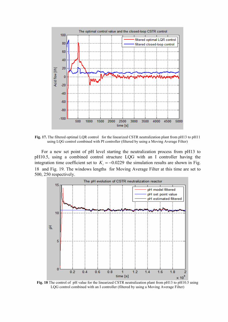
Fig. 17. The filtered optimal LQR control for the linearized CSTR neutralization plant from pH13 to pH11
using LQG control combined with PI controller (filtered by using a Moving Average Filter)
For a new set point of pH level starting the neutralization process from pH13 to
pH10.5, using a combined control structure LQG with an I controller having the
integration time coefficient set to 0229.0iK the simulation results are shown in Fig.
18 and Fig. 19. The windows lengths for Moving Average Filter at this time are set to
500, 250 respectively.
Fig. 18 The control of pH value for the linearized CSTR neutralization plant from pH13 to pH10.5 using
LQG control combined with an I controller (filtered by using a Moving Average Filter)

In figure 18 it is easy to see the good accuracy of the controlled level of the CSTR pH
neutralization plant from pH13 to pH10.5 with a controller effort shown in Fig.19. After
almost 600 seconds the optimal effort of the LQR controller becomes very small.
Fig. 19. The filtered optimal LQR control for the linearized CSTR neutralization plant from pH13 to
pH10.5 using LQG control combined with an I controller (filtered by using a Moving Average Filter)
CONCLUSIONS
In this research paper is developed a stochastic LQG approach to solve a particular
optimization problem, such as the optimal control of pH level of the waste water CSTR
neutralization plant. The control system design of pH neutralization process is a very
difficult task to be accomplished since the model of CSTR neutralization plant is highly
nonlinear (see the titration curve), and also it is very complex. Furthermore, the standard
control strategies design fail unfortunately when the system performance is concerned. In
the new approach the proposed control strategy proved its effectiveness and high
accuracy in terms of its performance compare to the traditional control mechanisms. The
simulations results are carried out in an attractive real-time MATLAB/SIMULINK
environment and presented in detailed in the last two sections.
REFERENCES [1] Irene Martina Jebarani. D, T. Rammohan, Fuzzy Logic based PID Controller for pH Neutralization
process, International Journal of Computer Applications, vol. 95, no. 6, pp. 36-40, 2014;
[2] S. Zihlmann, Modelling of a simple continuous neutralization reactor, February 2015. Available at
http://thirdway.ch/files/neutralisation/NeutralisationModeling.pdf, accessed on 16 Feb. 2017;
[3] Ahmmed Saadi Ibrehem, Modified Mathematical Model For Neutralization System In Stirred Tank
Reactor - Research Article, Bulletin of Chemical Reaction Engineering & Catalysis, vol. 6, no. 1, pp. 47 –
52, 2011;
[4] R.Weber, Optimization and Control, Lectures notes Manuscript. Available at
http://www.statslab.cam.ac.uk/~rrw1/oc/La5.pdf , accessed on 24 Feb. 2017;

[5] Bo Bernhardsson, K.J. Åström, Control System Design-LQG, Lecture – LQG.ppt, Lund University,
http://www.control.lth.se/media/Education/DoctorateProgram/2016/Control%20System%20Synthesis/l
qg.pdf , accessed on 17 Feb.2017;
[6] J. M. Athans and P. L. Falb, Optimal Control: An Introduction to the Theory and Its Applications,
McGraw- Hill, New York, 1996;
[7] R.M. Murray, Optimization-Based Control, DRAFT Manuscript v2.1a, February 2010, California
Institute of Technology. Available at http://www.cds.caltech.edu/~murray/books/AM08/pdf/obc-
optimal_04Jan10.pdf , accessed on 17 February 2017;
[8] G.F. Franklin, J. David Powell, Michael L. Workman, Digital Control of Dynamic Systems, Second
Edition, ADDISON-WESLEY PUBLISHING COMPANY Series in Electrical and Computer
Engineering: Control Engineering, USA, 1990;