Embed Size (px)
Citation preview
Probabilistic Constrained Optimization: Methodology and Applications (S. P. Uryasev,Editor), pp. 67-101
Stochastic Optimization inAsset & Liability Management:A Model for Non-Maturing Accounts1
Karl FrauendorferUniversity of St. GallenInstitute of Operations ResearchSt. Gallen, Switzerland
Michael SchurleUniversity of St. GallenInstitute of Operations ResearchSt. Gallen, Switzerland
Abstract
A multistage stochastic optimization model for the management of non-ma-turing account positions like savings deposits and variable-rate mortgages isintroduced which takes the risks induced by uncertain future interest rates andcustomer behavior into account. Stochastic factors are discretized using thebarycentric approximation technique. This generates two scenario trees whoseassociated deterministic equivalent programs provide exact upper and lowerbounds to the original problem. Practical experience from the application in amajor Swiss bank is reported.
Keywords: Stochastic programming, approximation, asset & liability man-
agement.
1 Introduction
Stochastic programming has received increasing attention from financial institutionsrecently since the shortcomings of traditional approaches that are widely used inpractice came to light. For instance, in portfolio optimization the mean-variance
1Research for this paper was supported by the Swiss National Science Foundation, GrantNo. 21-39’575.93.
67
framework due to Markowitz [48] captures the volatility and correlations among fi-nancial instruments but may generate solutions that do not seem like a reasonablemix to achieve the indicated risk and return (cf. [22]) and are highly sensitive to theinput, i.e., expectations and covariances (cf. [3, 8]). Moreover, it does not take intoaccount the possibility of future rebalancing transactions of the portfolio or additionalin- and outflows of cash that occur during the planning period. In many problems inthe field of asset and liability management (ALM), the increased volatility in financialmarkets since the 70s and the introduction of derivatives revealed severe deficienciesof popular portfolio immunization strategies which match the duration and, possibly,the convexity of both assets and liabilities (cf. [67]). These approaches hedge onlyagainst relatively small shifts in interest rates and are not appropriate to deal withthe complex cash flow structures of new financial instruments (cf. [53]).
1.1 Stochastic optimization for financial decision making
For obvious reasons, stochastic optimization models seem to be a natural approachin order to address the requirements of a large number of financial planning problems(e.g., see [15, 49, 50] for an overview of applications, [4, 12, 14, 52] for general ALMmodel formulations or [23, 24, 36, 37, 40, 64, 65, 66, 67] for fixed-income problems).On one hand, the models allow the reflection of uncertainty in future prices, yieldsand exchange rates, volatilities etc. by generating scenarios of their possible futureoutcomes. These scenarios quantify the impact of changes in the underlying riskfactors on the return of investment strategies or the deviation from a certain targetposition like an index, a benchmark portfolio, a liability etc.
On the other hand, a stochastic program reflects not only the dynamics of uncer-tain data but also of decisions more appropriately since transactions may take placeat discrete points in time until the end of some predefined planning horizon. For allscenarios under consideration, a decision must be taken at each stage based on real-izations of random data and earlier actions. This allows the correction of an initialpolicy, e.g., if it does not achieve the investment goal for certain scenarios.
In general, a stochastic optimization model yields a large-scale program since ithas to include a high number of scenarios to reflect the entire universe of possiblefuture outcomes of risk factors and cash flows. The first models for financial planningappearing in the 80s (cf. [44, 45]) could not meet this requirement due to limitationsof the computational resources available at this time.
However, the dramatic improvement in powerful hardware as well as the devel-opment of efficient algorithms, in particular if they exploit the special structure andhigh sparsity inherent to stochastic programs, now provide the basis to solve problemswhere the number of scenarios is between some thousands and one million, depend-ing on the problem structure and the system architecture (cf. [25]). Moreover, newtheoretical models from the financial literature and related empirical evidence havesharpened the understanding of the dynamics of risk factors such as interest and ex-
68

change rates, prices of financial instruments etc. Both of these developments allowthe modeling of complex problems more realistically. In this way, the fields of Financeand Optimization come closer together.
1.2 Review of current approaches
Meanwhile, a large number of stochastic optimization models has been introduced forvarious applications in Finance. Among them are the Russell-Yasuda-Kasai modeldue to Carino et al. [4, 5], which can be seen as the first successful commercialapplication of multistage stochastic programming, the models for ALM and fixed-income portfolio management of Zenios et al. [36, 66, 67] and Dupacova et al. [18],or the multistage portfolio optimization models due to Dantzig and Infanger [11] andSteinbach [61], to mention just a few.
In general, one starts from assumptions about the distribution of risk factors whichis typically continuous. Since scenarios are used as input for stochastic programs todescribe the uncertainty, a discrete subset of possible realizations of the random datamust be determined that is “representative” for the entire universe of future outcomes.Loosely speaking, this means that the solution of such an approximated problemcomes “as close as possible” to the exact (but unknown) optimum of a problem withthe true distribution.
Simulation is a widely exploited approach for the selection of scenarios and canbe easily combined with decomposition methods (cf. [10, 38]). Since the solutiondepends heavily on the choice of the scenario set, a statistical analysis is essential toassess the accuracy and stability of the problem (cf. [16, 17]). Although the amountof computational effort is independent of the dimension of random data, Monte Carlomethods often suffer from a low convergence rate of the order 1/
√s as implied by
the central limit theorem, where s is the sample size. Therefore, variance reductiontechniques like importance sampling are helpful to reduce the error of estimates for theobjective. For multistage problems, the expected value of perfect information (EVPI)(cf. [7, 13]) is a useful criterion for the selection of an enhanced set of representativescenarios. In any case, simulation based approaches provide only probabilistic errorbounds.
Approximation schemes are based on partitioning the domain of random datainto cells and using representative points within them (cf. [1, 19, 20, 26, 32, 43]).Exploiting certain properties of the stochastic program, mainly convexity of valuefunctions, allows the determination of exact lower and upper bounds to the originalproblem. As a consequence, the error induced by the approximation can be quanti-fied more precisely, and the accuracy may be improved by deliberately adding newscenarios. Careful control of this process is necessary since the number of scenariosgrows exponentially with the dimension size and accuracy.
69

1.3 Contribution of this paper
In this paper, a stochastic optimization model for an application from the field ofALM is introduced which was developed in co-operation with a major Swiss bankfor the management of so-called “non-maturing account” positions. This includessavings deposits as well as a special type of non-fixed mortgages which is common inSwitzerland. Their characteristic feature is that there exists no contractual maturityon such products but bank customers are allowed to withdraw their investmentsor prepay their mortgages, respectively, at any point in time at no penalty. Asa consequence, the volume of both positions fluctuates heavily as customers reactto changes in the market environment, e.g., rising or falling yields, or the relativeattractiveness of alternative investment opportunities.
Therefore, in the formulation of the stochastic program uncertainty affects notonly the coefficients in the objective (future interest rates) but also on the right-hand-side of constraints (volume change). Moreover, both may be correlated to reflect adependency between interest rates and volume. All these aspects can be addressedby the barycentric approximation technique introduced in the sequel to derive exactbounds for value functions corresponding to convex multistage stochastic programs.An approximation technique is preferred for this type of application since statisticalanalysis implies that the dynamics of interest rates can be described by at most threefactors in order to explain more than 95 % of the variance. These factors controllevel, curvature, and steepness of the yield curve (cf. [46]). This enables keeping theproblem size relatively moderate even in a multistage model.
The remainder of the paper is organized as follows: The next section introduces theformulation of the optimization model for non-maturing accounts. In section 3, thestructural properties of convex multistage stochastic programs are outlined. Section 4introduces the barycentric approximation scheme that is used to derive scenario treesassociated with upper and lower bounds to the original problem. Numerical resultsfor the approximation are also given. Section 5 reports practical experience from theapplication of the model compared to traditional approaches. The main results aresummarized in section 6 together with an outlook to possible improvements of themodel as well as future directions of research.
2 A model for uncertain maturities
2.1 Problem characteristics
As outlined above, non-maturing accounts can be characterized as follows: (1) Thereis no contractual maturity on these positions since bank customers are allowed towithdraw or repay their investments and credits at any point in time. (2) The cus-tomer rate is not indexed to certain interest rates or prices of traded instruments butadjustable to market conditions as a matter of policy. The most common examples
70
include some forms of savings accounts or non-fixed mortgages that are widespreadin Europe and the U.S. The management of such account positions is a particularlyambitious task since these assets and liabilities are not only sensitive to changes ininterest rates but have also embedded call or put options that may be exercised bythe customer. For example, a homeowner has the option to prepay the outstandingbalance of his mortgage and call the security.
It can be observed that customer behavior depends strongly on the current mar-ket environment. In case of variable-rate mortgages, changes in the total volume arepositively correlated with interest rates. When the latter are low, there is a sharpdrop in demand since customers switch to fixed-rate mortgages in order to hedgethemselves against a future rise (prepayment risk). In case of savings deposits, thevolume increases since their yields are relatively attractive when compared to alter-native short-term securities, and even institutional investors like pension funds preferthese deposits instead of direct investments in the money market. This results in anegative correlation between interest rates and volume change. In such a situation, itis difficult for financial management to find a combination of fixed-income instrumentsthat provides a sufficient margin and takes into account the risk that a significantportion of the deposits is withdrawn (withdrawal risk).
During a period of high interest rates, homeowners’ demand for non-fixed mort-gages rises significantly while investors shift their assets from variable-rate savingsaccounts to bonds with long maturities. As a consequence, the mortgages must berefinanced on the money and capital market at increased funding costs. Moreover,there is a political cap on the mortgage rate in Switzerland, and numerous bankswere not able to refinance their mortgages at a positive margin at the beginning ofthe 90s. These difficulties caused a broad discussion among practitioners from thefinancial industry about the management of non-maturing account positions and therisks induced by the embedded options.
Clearly, the use of duration matching does not apply here since one cannot findadequate duration measures due to the volume fluctuations, beside other shortcom-ings of this concept. This has motivated the replicating portfolio approach which isbased on the idea of mimicing the behavior of the target position in order to cap-ture its characteristics. The objective is to find a portfolio of fixed-income securitieswhose return replicates the customer rate of the relevant asset or liability positionplus a margin. Transaction costs remain low since liquid money market instrumentsand swaps are used that are held until maturity to avoid a rebalancing. Maturingfunds are always renewed at the same maturity. Prepayment and withdrawal risksare implicitly taken into account as the volume of the replicating portfolio has tocoincide with the volume of the target position at all points in time. The weights aredetermined through minimizing the tracking error for a historic sample period andremain constant over time.
By means of this approach, uncertain cash flows are transformed into (apparently)certain ones, allowing the bank to manage them like normal maturing accounts. These
71
replicating portfolios are implemented as passive investment and refinancing strate-gies. However, the question arises whether a dynamic policy with active reactions tochanges in the market environment and customer behavior could increase the bank’sprofit. In particular, it remains to be clarified if the correlation between interestrates and volume can be exploited more appropriately to manage the inherent risks.Clearly, a stochastic optimization model is able to address most of these requirements.
2.2 Model formulation
For simplicity, only the problem of reinvesting savings accounts on the market isinvestigated here since the model for refinancing mortgages is equivalent and can bederived easily from it. The formulation of the optimization model is straightforward:D = 1, 2, . . . , D denotes a set of maturity dates for fixed-income securities heldin the portfolio. Investment opportunities are given by a set of traded standardmaturities DS ⊂ D. Let ϕd,+
t be the discounted accrued interest payments for aninvestment of $1 in maturity d ∈ DS at time t. The model has also the option toraise funds which are reinvested in addition to the total savings volume. The sum ofinterest payments for $1 of such a short position is given by ϕd,−
t . Clearly, except fort = 0 these coefficients depend on future interest rates and, hence, are uncertain.
The underlying interest rate model used here to describe the evolution of interestrates resembles the idea of key rates analogously to the duration model of Ho [39].It is assumed that the yield curve can be segmented into Kt different sections whererates move in the same direction. These segments are represented by Kt key rates ofdifferent maturities whose dynamics can be described by correlated Brownian motionswith (possibly time-dependent) drift. This results in normally distributed interest ratechanges. Rates for the remaining maturities are interpolated.
The coefficients ϕd,+t (ηt) and ϕd,−
t (ηt) for all d ∈ DS are functions of this Kt-dimensional Brownian motion (ηt; t = 1, . . . , T ) in discrete time driving the evolutionof the yield curve. Here, Kt = K = 3 as a three factor model is sufficient to reflecta great variety of term structure movements. The functional relationship between ηt
and ϕd,+t , ϕd,−
t incorporates the sensitivity of interest rates subject to changes in therisk factors, transactions costs, a bid-ask spread as well as the discount mechanism.Only payments within the planning horizon are considered, i.e., those that are inducedby an investment or borrowing in t ≤ T but occur after T +1 are neglected. A formalspecification of the relation between risk factors and coefficients in the objective isomitted here since the notation is rather cumbersome. Note that the current valuesof η0 can be derived from market observations.
At each point in time t = 0, . . . , T , decisions on the amount xd,+t ≥ 0 of long
and xd,−t ≥ 0 of short positions in maturity d have to be made subject to budget
constraints
72

xdt − xd+1
t−1 − xd,+t + xd,−
t = 0 t = 0, . . . , T ; ∀d ∈ DS
xdt − xd+1
t−1 = 0 t = 0, . . . , T ; ∀d ∈ D \ DS.
The latter constraint ensures that the sum of all long and short positions xdt ∈ IR
maturing after d periods is equal to the corresponding value in the previous periodfor non-traded maturity dates while the former corrects it by the new long and shortsales in t for traded maturities. Note that xd
−1 indicates the amount of maturity d inthe initial portfolio from decisions in the past. At time t, the portfolio has to matchthe total savings volume vt ∈ IR:
vt =∑
d∈D
xdt t = 0, . . . , T.
The total savings volume is given by its value in the previous period t− 1, correctedby the stochastic volume change ξt in t:
vt = vt−1 + ξt t = 1, . . . , T.
Again, the volume change is modeled by a Brownian motion with drift in discrete time(ξt; t = 1, . . . , T ) of dimension Lt = L = 1. It may be correlated with the componentsof the stochastic process ηt to reflect a relation between changes in interest rates andvolume.
Raising short positions and reinvesting them in addition to the savings volumemay be viewed as some speculative strategy. Therefore, short sales can be restrictedto an amount equal to the sum of funds maturing at t + 1, . . . , t + m, where m > 0is defined by the decision maker (m = 1 prohibits any borrowings):
∑
d∈DS
xd,+t ≤ ξt +
m∑
d=1
xdt−1 t = 1, . . . , T.
Depending on the current interest rate curve and the amount that has to be reinvested,a situation might occur where the optimal investment strategy cannot be implementeddue to liquidity restrictions in the Swiss market, in particular if the model finds apolicy that is not broadly diversified over different maturities. This is addressed byimposing upper limits ℓd,+
t , ℓd,−t for investments and borrowings:
0 ≤ xd,+t ≤ ℓd,+
t t = 0, . . . , T ; ∀d ∈ DS
0 ≤ xd,−t ≤ ℓd,−
t t = 0, . . . , T ; ∀d ∈ DS.
The restrictions above must hold for all observations of ηt and ξt, t = 1, . . . , T .Moreover, decisions xd,+
t , xd,−t have to be made independent of future outcomes of
ηt+1, . . . , ηT and ξt+1, . . . , ξT since these are unknown at time t. Hence, investmentpolicies must not anticipate any information that becomes known in the future. Thisis incorporated in the optimization model by additional nonanticipativity constraints.
73
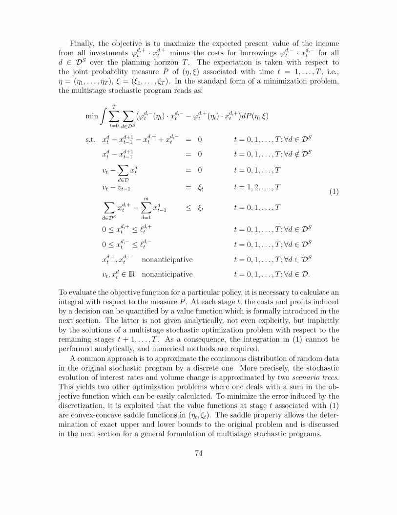
Finally, the objective is to maximize the expected present value of the incomefrom all investments ϕd,+
t · xd,+t minus the costs for borrowings ϕd,−
t · xd,−t for all
d ∈ DS over the planning horizon T . The expectation is taken with respect tothe joint probability measure P of (η, ξ) associated with time t = 1, . . . , T , i.e.,η = (η1, . . . , ηT ), ξ = (ξ1, . . . , ξT ). In the standard form of a minimization problem,the multistage stochastic program reads as:
min
∫ T∑
t=0
∑
d∈DS
(
ϕd,−t (ηt) · xd,−
t − ϕd,+t (ηt) · xd,+
t
)
dP (η, ξ)
s.t. xdt − xd+1
t−1 − xd,+t + xd,−
t = 0 t = 0, 1, . . . , T ; ∀d ∈ DS
xdt − xd+1
t−1 = 0 t = 0, 1, . . . , T ; ∀d /∈ DS
vt −∑
d∈D
xdt = 0 t = 0, 1, . . . , T
vt − vt−1 = ξt t = 1, 2, . . . , T
∑
d∈DS
xd,+t −
m∑
d=1
xdt−1 ≤ ξt t = 0, 1, . . . , T
0 ≤ xd,+t ≤ ℓd,+
t t = 0, 1, . . . , T ; ∀d ∈ DS
0 ≤ xd,−t ≤ ℓd,−
t t = 0, 1, . . . , T ; ∀d ∈ DS
xd,+t , xd,−
t nonanticipative t = 0, 1, . . . , T ; ∀d ∈ DS
vt, xdt ∈ IR nonanticipative t = 0, 1, . . . , T ; ∀d ∈ D.
(1)
To evaluate the objective function for a particular policy, it is necessary to calculate anintegral with respect to the measure P . At each stage t, the costs and profits inducedby a decision can be quantified by a value function which is formally introduced in thenext section. The latter is not given analytically, not even explicitly, but implicitlyby the solutions of a multistage stochastic optimization problem with respect to theremaining stages t + 1, . . . , T . As a consequence, the integration in (1) cannot beperformed analytically, and numerical methods are required.
A common approach is to approximate the continuous distribution of random datain the original stochastic program by a discrete one. More precisely, the stochasticevolution of interest rates and volume change is approximated by two scenario trees.This yields two other optimization problems where one deals with a sum in the ob-jective function which can be easily calculated. To minimize the error induced by thediscretization, it is exploited that the value functions at stage t associated with (1)are convex-concave saddle functions in (ηt, ξt). The saddle property allows the deter-mination of exact upper and lower bounds to the original problem and is discussedin the next section for a general formulation of multistage stochastic programs.
74
3 Multistage stochastic programs
3.1 Formal description
Formally, the evolution of uncertain data over the planning horizon T in a multistagestochastic program can be described by a multi-dimensional stochastic process (ωt, t =1, . . . , T ) in discrete time on a common Borel space (Ω,BM) with compact Ω ⊂IRM (cf. [27, 28, 29]). Let P represent the (regular) joint probability measure ofω := (ω1, . . . , ωT ). The associated conditional measure with respect to ωt is denotedPt(·|ωt−1) for t = 1, . . . , T . For reasons of compactness, ωt := (ω1, . . . , ωt) representsthe sequence of observations of ωt ∈ Ωt ⊂ IRMt up to time t, where Ω1× . . .×ΩT = Ω,M1 + . . . + MT = M . Note that ω0 denotes those data that are currently observedand, hence, deterministic.
At time t = 0, a decision u0 ∈ IRn0 is made without knowing ωt for the subsequentstages t = 1, . . . , T . After ωt was observed at time t > 0, the initial policy may becorrected by a new decision ut ∈ IRnt based on the known history of observations ωt
and decisions ut := (u0, u1, . . . , ut) ∈ IRnt
, nt = n0 + . . . + nt. In particular, ut hasto be independent of future outcomes ωt+1, . . . , ωT . Therefore, the solution of theunderlying stochastic optimization problem is a recourse function with the property
u(ω) =(
u0, u1(ω1), . . . , uT (ωT )
)
∈ IRn, n = n0 + n1 + . . .+ nT ,
known as nonanticipativity. The initial decision u0 induces some (non-random) costsρ0. For the subsequent stages t = 1, . . . , T , the costs ρt(u
t, ωt) are determined by thesequence of earlier decisions ut and realizations of ωt. The feasible set is assumed to beconvex, compact, and non-empty for any ω. Again, it depends on previous decisionsand observations for t > 0 and can be characterized by the system of inequalities
f0(u0) ≤ 0ft(u
t, ωt) ≤ 0 t = 1, . . . , T.(2)
f0(·) and ft(·, ·) are vector-valued and ρ0(·) and ρt(·, ·) are real-valued functions de-fined on the corresponding Euclidian spaces. Furthermore, ρt(·, ·) are supposed tobe convex in ut for any random outcome ωt. The objective is to find a nonanticipa-tive recourse function u(·) that minimizes the expected total costs over the planninghorizon and satisfies the constraints (2):
min
ρ0(u0) +∫
Ω
[∑T
t=1 ρt(ut, ωt)
]
dP (ω)
s.t. f0(u0) ≤ 0ft(u
t, ωt) ≤ 0, t = 1, . . . , T,u(·) nonanticipative.
(3)
The meaning of the last (nonanticipativity) constraint is: Let ωt and ut satisfyf0(u0) ≤ 0, f1(u
1, ω1) ≤ 0, . . . , ft(ut, ωt) ≤ 0, then there always exists a sequence
75

ut+1, . . . , uT for any (ωt+1, . . . , ωT ), so that u = (u0, u1, . . . , uT ) is feasible with re-spect to (2). As a consequence, there is always a feasible completion of the prob-lem (3) for the remaining stages t + 1, . . . , T independent of the realizations of ωτ ,τ = t + 1, . . . , T , provided that the decisions uτ in τ = 0, 1, . . . , t are feasible. Thiscan be seen as a counterpart to the case of relatively complete recourse in two-stagestochastic programming (cf. [62]).
3.2 Saddle property of value functions
In order to distinguish those uncertain data that affect the objective from thoseinfluencing the constraints, the random vectors for t = 1, . . . , T are decomposedaccording to ωt = (ηt, ξt), where ηt ∈ Θt ⊂ IRKt , ξt ∈ Ξt ⊂ IRLt , Ωt = Θt × Ξt,Mt = Kt + Lt. The functions defining the feasible set in the second line of (2) canthen be written as f1(u
1, ξ1) ≤ 0, . . . , fT (uT , ξT ) ≤ 0, and the costs are now of theform ρt(u
t, ηt). In case such a decomposition of ωt into ηt and ξt is not obvious,one may augment the probability space (for details, see [27]). In order to write theproblem without stating the constraints explicitly, the function
gt(ut, ηt, ξt) :=
ρt(ut, ηt) if ft(u
t, ξt) ≤ 0
+∞ otherwise,
is introduced. For the following analysis, it is useful to consider the dynamic versionof problem (3) stated in terms of recourse or value functions. These can be obtainedif the multistage program is written as a series of nested two-stage programs, startingin the last stage T with
φT (uT−1, ηT , ξT ) = minuT≥0
gT (uT−1, uT , ηT , ξT ) (4)
and then backwards for t = T − 1, . . . , 0
φt(ut−1, ηt, ξt) = min
ut≥0gt(u
t−1, ut, ηt, ξt)
+
∫
Θt+1×Ξt+1
φt+1(ut−1, ut, η
t, ξt, ηt+1, ξt+1)dP (ηt+1, ξt+1|ηt, ξt). (5)
Again, (η0, ξ0) are currently observed data, whereas u−1 represents decisions from thepast. Here, ut = (ut−1, ut) is decomposed in two parts to emphasize that decisionsut−1 were already made in the preceding stages and only ut must be determinedin (5). The optimal decision for the current stage represents a trade-off between theimminent costs ρt in t and the expected future costs for the remaining periods inducedby ut. According to [28], based on arguments in [54], to ensure that the problems (4)and (5) can be solved the following assumptions are required for t = 1, . . . , T :
(i) Θt × Ξt is compact, convex, and covers the support of (ηt, ξt).
76
(ii) ρt(ut, ηt) is a continuous saddle function on IRnt ×Θt which is convex in ut and
concave in ηt.
Note that this is satisfied, e.g., if ρt is bilinear.
(iii) The feasible sets u0|f0(u0) ≤ 0 and (ut, ξt)|ξ ∈ Ξ, ft(ut, ξt) ≤ 0 are compact,
convex subsets of IRnt × Ξt.
In particular, this covers the case that the constraints can be written in the form
ft(ut−1, ut, ξ
t) = dt(ut) − et(ut−1, ξt)
with dt convex and et linear affine.As outlined before, approximation schemes are based on the convexity or, if un-
certainty affects the objective and the right-hand-sides of constraints, saddle propertyof value functions which allows the derivation of lower and upper bounds based onthe inequalities due to Jensen [42] and Edmundson-Madansky [21, 47]. Barycentricapproximation is a generalization of these concepts for bounding the expectation ofsaddle functions in the case of dependent random variables which was introduced in[27] in the context of two-stage stochastic programming. It remains to clarify underwhich conditions it can be extended to the multistage case.
According to (i), the problem (4) for the final stage T is a convex optimizationproblem with parameters (uT−1, ηT , ξT ). Assumption (ii) implies that the objectivefunction gT in (4) is a lower closed saddle function. Therefore, the corresponding valuefunction φT (uT , ηT , ξT ) is also a saddle function, convex in (xT−1, ξT ) and concave inηT . In order to derive bounds for the expectation of (5), the saddle property of thevalue function in T must be “inherited” to the remaining stages T − 1, . . . , 1. Whencalculating the expected recourse costs
Etφt(ut−2, ut−1, η
t−1, ξt−1) =∫
Θt×Ξt
φt(ut−2, ut−1, η
t−1, ξt−1, ηt, ξt)dPt(ηt, ξt|ηt−1, ξt−1), (6)
the probability measure Pt depends on (ηt−1, ξt−1). As a consequence, the saddleproperty of φt(x
t−2, xt−1, ηt−1, ξt−1, ηt, ξt) is not inherited in general due to the inte-
gration with respect to Pt(ηt, ξt|ηt−1, ξt−1). However, if the distribution functions areof the form
Qt
(
(ηt, ξt) +Ht(ηt−1, ξt−1)
)
, (7)
where Qt is a regular distribution function over (Θt × Ξt,BKt+Lt) and Ht is a linearmapping, the integral in (6) can be written as
∫
Θt×Ξt
φt
(
ut−2, ut−1, ηt−1, ξt−1, (ηt, ξt) −Ht(η
t−1, ξt−1))
dQt(ηt, ξt)
77

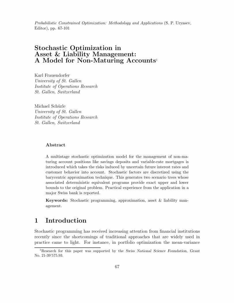
A BCDFigure 1: Saddle property of value functions
(note that the integration is now performed with respect to a measure independentof (ηt−1, ξt−1)). Then, it can be easily verified that the expectation in (6) is a saddlefunction on its domain Θt ×(ut−1, ξt)|ξt ∈ Θt, fτ (u
τ , ξτ) ≤ 0, τ = 1, . . . , t− 1 whichis convex in (ut−2, ut−1, ξ
t−1) and concave in ηt−1 (for details see [28]). Together withthe convexity of gt(u
t, ηt) implied by (ii), this results in the saddle property of theobjective function of problem (5),
gt(ut−1, ut, η
t, ξt) + Et+1φt+1(ut−1, ut, η
t, ξt, ηt+1, ξt+1). (8)
Hence, for stages t = T − 1, . . . , 1 the value functions φt(ut−1, ηt, ξt) are lower
closed saddle functions on their domain. An illustration is given in Figure 1 whereφt(u
t−1, ηt−1, ηt, ξt−1, ξt) is shown for (ηt, ξt) ∈ Θt ×Ξt ⊂ IR× IR, i.e., one-dimensional
distributions for the coefficients in objective and right-hand-sides. Note that thevalue function quantifies the imminent costs for the current stage t plus the expectedfuture costs provided that the subsequent decisions are optimal. Therefore, it cannotbe represented analytically but is given implicitly for each (ut−1, ηt, ξt) as the solutionof a multistage stochastic program with respect to the remaining stages t+ 1, . . . , T .
3.3 Solvability of stochastic programs
To ensure that the multistage stochastic program can be solved, it is required thatthe corresponding value functions are continuous. A sufficient condition for thisis that value functions are subdifferentiable which is given if the Slater conditionholds: For the last stage T , there must be a point uT depending on (uT−1, ξT ) withfT (uT−1, uT , ξ
T ) < 0. Calculating the expectation in (6) preserves continuity since the
78
uZZZZZZZZuHHHHHHHHuXXXXXXXXu
u((((((((hhhhhhhhu((((((((hhhhhhhhu((((((((hhhhhhhhu((((((((hhhhhhhhu((((((((hhhhhhhhu((((((((hhhhhhhh
uuuuuuuuuuuu
!t1 !t!T
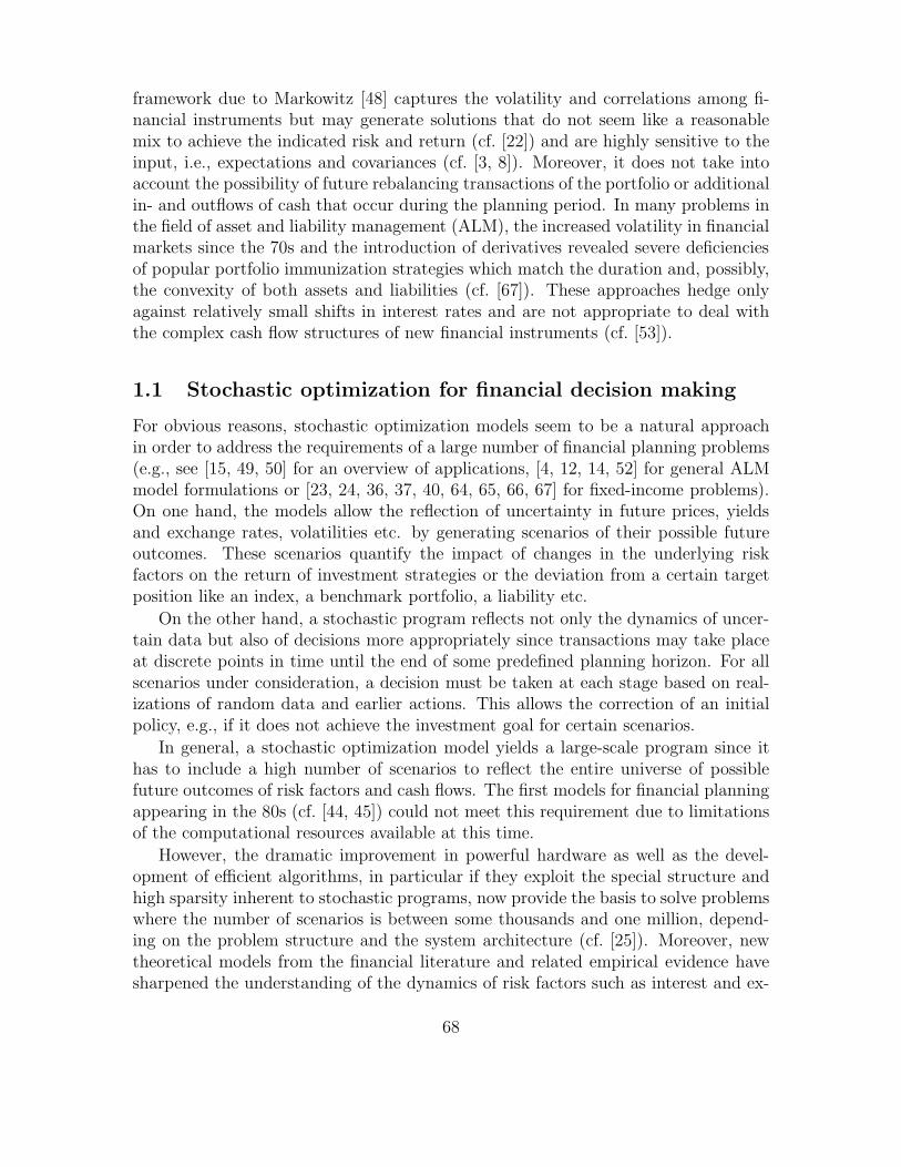
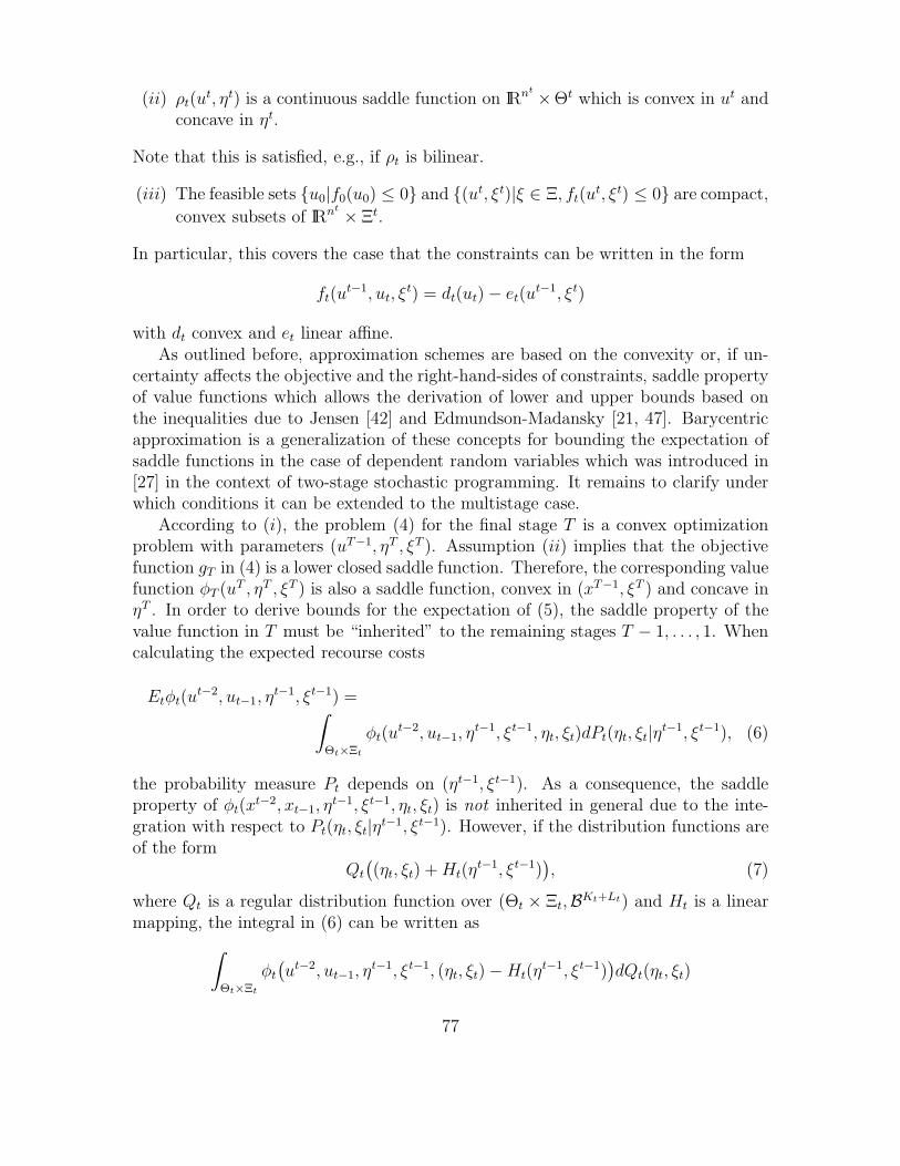
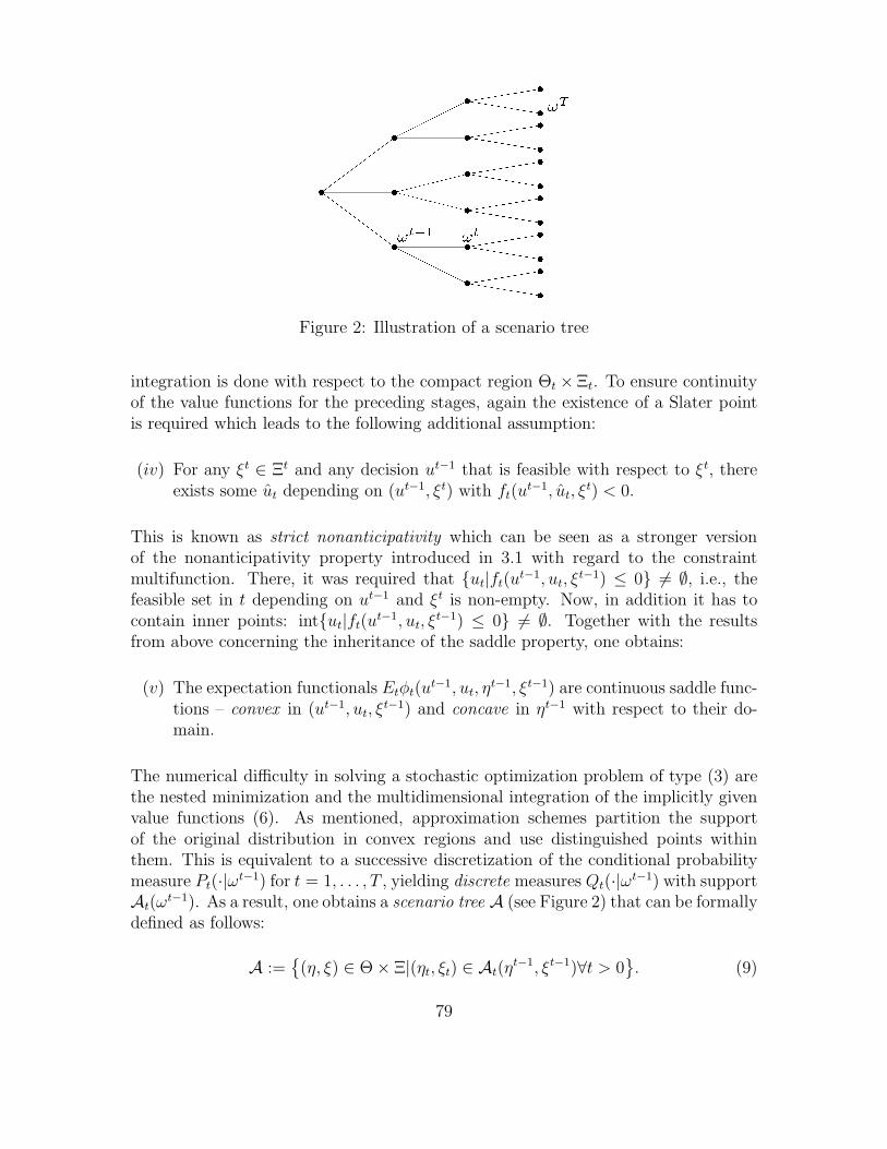
Figure 2: Illustration of a scenario tree
integration is done with respect to the compact region Θt ×Ξt. To ensure continuityof the value functions for the preceding stages, again the existence of a Slater pointis required which leads to the following additional assumption:
(iv) For any ξt ∈ Ξt and any decision ut−1 that is feasible with respect to ξt, thereexists some ut depending on (ut−1, ξt) with ft(u
t−1, ut, ξt) < 0.
This is known as strict nonanticipativity which can be seen as a stronger versionof the nonanticipativity property introduced in 3.1 with regard to the constraintmultifunction. There, it was required that ut|ft(u
t−1, ut, ξt−1) ≤ 0 6= ∅, i.e., the
feasible set in t depending on ut−1 and ξt is non-empty. Now, in addition it has tocontain inner points: intut|ft(u
t−1, ut, ξt−1) ≤ 0 6= ∅. Together with the results
from above concerning the inheritance of the saddle property, one obtains:
(v) The expectation functionals Etφt(ut−1, ut, η
t−1, ξt−1) are continuous saddle func-tions – convex in (ut−1, ut, ξ
t−1) and concave in ηt−1 with respect to their do-main.
The numerical difficulty in solving a stochastic optimization problem of type (3) arethe nested minimization and the multidimensional integration of the implicitly givenvalue functions (6). As mentioned, approximation schemes partition the supportof the original distribution in convex regions and use distinguished points withinthem. This is equivalent to a successive discretization of the conditional probabilitymeasure Pt(·|ωt−1) for t = 1, . . . , T , yielding discrete measures Qt(·|ωt−1) with supportAt(ω
t−1). As a result, one obtains a scenario tree A (see Figure 2) that can be formallydefined as follows:
A :=
(η, ξ) ∈ Θ × Ξ|(ηt, ξt) ∈ At(ηt−1, ξt−1)∀t > 0
. (9)
79
Each path in this tree represents a scenario for the evolution of ηt and ξt over theplanning horizon T , and the associated probabilities are given by
q(η, ξ) :=
T∏
t=1
qt(ηt, ξt|ηt−1, ξt−1). (10)
Clearly, when the conditional probability measure is discrete in time and space, thestochastic two-stage program (5) has a characteristic block structure. As a conse-quence, the multistage problem (3) can be written as a mathematical program withdynamic block structure and high sparsity whose size depends on the number of sce-narios within the tree. Powerful decomposition algorithms have been developed whichexploit this special structure (see [2, 51, 55, 56, 57, 58, 59] for example).
4 Barycentric approximation
4.1 Discretization of distributions
In this section, it is shown how the original probability measure Pt(·|ηt−1, ξt−1) can bediscretized using so-called generalized barycenters. These are calculated with respectto a cross-simplex (or briefly: ×-simplex), i.e., the Cartesian product of two simplicesthat cover the support of random data in the objective and the constraints, respec-tively. To this end, it is assumed that Θt(η
t−1, ξt−1) ∈ IRKt and Ξt(ηt−1, ξt−1) ∈ IRLt
are regular simplices covering the support of ηt and ξt (in the sequel, the depen-dency on previous observations may be omitted in the notation for simplicity). Theirvertices are denoted
uνt(ηt−1, ξt−1) =
(
u1,νt(ηt−1, ξt−1), . . . , uKt,νt
(ηt−1, ξt−1))′ ∈ Θt
vµt(ηt−1, ξt−1) =
(
v1,µt(ηt−1, ξt−1), . . . , vLt,µt
(ηt−1, ξt−1))′ ∈ Ξt.
for νt = 0, . . . , Kt, µt = 0, . . . , Lt. The barycentric weights
λt(ηt|ηt−1, ξt−1) =(
λt,0(ηt|ηt−1, ξt−1), . . . , λt,Kt(ηt|ηt−1, ξt−1)
)′
of ηt with respect to Θt(ηt−1, ξt−1) are those nonnegative barycentric coordinates that
allow the representation of ηt as a linear combination of the vertices uνt(ηt−1, ξt−1)
and sum up to one:
λt,0 + λt,1 + . . . + λt,Kt= 1
ut,0λt,0 + ut,1λt,1 + . . . +ut,Ktλt,Kt
= ηt.
Analogously, the barycentric weights
τt(ξt|ηt−1, ξt−1) =(
τt,0(ξt|ηt−1, ξt−1), . . . , τt,Lt(ξt|ηt−1, ξt−1)
)′
80
of ξt with respect to Ξt(ηt−1, ξt−1) are defined. Briefly, they are given as the unique
solution of the systems
Ut(ηt−1, ξt−1) · λt =
(
1ηt
)
∀ηt ∈ Θt(ηt−1, ξt−1) (11)
Vt(ηt−1, ξt−1) · τt =
(
1ξt
)
∀ξt ∈ Ξt(ηt−1, ξt−1), (12)
where Ut(ηt−1, ξt−1) is a regular (Kt + 1) × (Kt + 1)-matrix and Vt(η
t−1, ξt−1) is aregular (Lt + 1) × (Lt + 1)-matrix whose columns contain the vertices of Θt and Ξt,respectively:
Ut(ηt−1, ξt−1) =
(
1 1 . . . 1u0(η
t−1, ξt−1) u1(ηt−1, ξt−1) . . . uKt
(ηt−1, ξt−1)
)
Vt(ηt−1, ξt−1) =
(
1 1 . . . 1v0(η
t−1, ξt−1) v1(ηt−1, ξt−1) . . . vLt
(ηt−1, ξt−1)
)
.
Hence, the barycentric weights are obtained by inverting (11) and (12):
λt(ηt|ηt−1, ξt−1) =(
Ut(ηt−1, ξt−1)
)−1 ·(
1ηt
)
(13)
τt(ξt|ηt−1, ξt−1) =(
Vt(ηt−1, ξt−1)
)−1 ·(
1ξt
)
. (14)
The key element of the approximation procedure is the determination of the general-ized barycenters and corresponding probabilities. The probability measure Pt inducesmass distributions Mνt
on the Lt-dimensional simplices uνt × Ξt with associated
generalized barycenters
ξνt=
[
Mνt(uνt
× Ξt)]−1 ·
Lt∑
µt=0
vµt
∫
λµt(ηt) · τνt
(ξt)dPt(ηt, ξt|ηt−1, ξt−1), (15)
where
Mνt(uνt
× Ξt) =
∫
τνt(ξt)dPt(ηt, ξt|ηt−1, ξt−1) (16)
is the mass assigned to (uνt, ξνt
). For νt = 0, . . . , Kt these mass distributions addup to a conditional probability distribution. In this way, one obtains a discreteprobability measure Ql
t on Θt × Ξt when probability Mνt(uνt
× Ξt) is assigned topoint (uνt
, ξνt). Analogously, the probability measure Pt induces mass distributions
Mµtwith generalized barycenters
ηµt=
[
Mµt(Θt × vµt
)]−1 ·
Kt∑
νt=0
uνt
∫
λµt(ηt) · τνt
(ξt)dPt(ηt, ξt|ηt−1, ξt−1) (17)
81
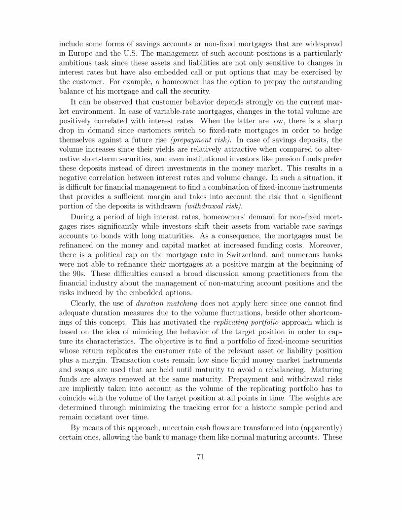
A BCD(a) Vertices of ×-simplex
10
(b) Barycenters for η
0 1(c) Barycenters for ξ
Figure 3: Determination of barycenters for a two-dimensional correlated distribution
on the Kt-dimensional simplices Θt × bµt. Again, for µt = 0, . . . , Lt the mass
Mµt(Θt × vµt
) =
∫
λµt(ηt)dPt(ηt, ξt|ηt−1, ξt−1) (18)
is assigned to the points (ηµt, vµt
), and the mass distributions Mµtadd up to a
conditional probability distribution, yielding a discrete probability measure Qut on
Θt×Ξt. Note that the integrand λµt(ηt) · τνt
(ξt) in (15) and (17) is a bilinear functionin (ηt, ξt) since the barycentric weights λµt
and τνtare linear in their components. In
this way, a discretization of the conditional probability measure Pt is derived. Thetwo discrete measures Ql and Qu have support
suppQlt =
(
uνt(ηt−1, ξt−1), ξνt
(ηt−1, ξt−1))
∣
∣
∣νt = 0, . . . , Kt
(19)
suppQut =
(
ηµt(ηt−1, ξt−1), vµt
(ηt−1, ξt−1))
∣
∣
∣µt = 0, . . . , Lt
, (20)
and according to equations (16) and (18), the corresponding probabilities are givenby ql
t(uνt, ξνt
) := Mνt(uνt
× Ξt) and qut (ηµt
, vµt) := Mµt
(Θt × uνt).
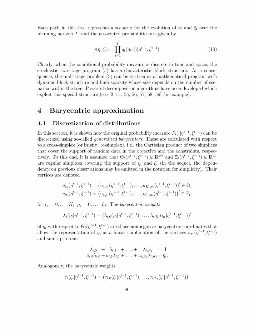
An illustration of the discretization is given in Figure 3 (a). The samples representthe joint distribution of η and ξ for K = L = 1 (the time index is omitted for sim-plicity). Note that the sampling indicates (negative) correlation between the randomdata. Obviously, in the one-dimensional case the simplices covering the support ofη and ξ are edges which results in a ×-simplex of rectangular shape. For instance,the edges AB and CD cover the support of η (the interest rate risk factor in thesavings application under consideration), i.e., A and D correspond to vertex u0 whileB and C are equivalent to u1. Analogously, AD and BC represent the domain of(the volume change) ξ and, hence, correspond to a simplex in IR with vertices v0 andv1.
It can be seen from Figure 3 (b) and (c) that projecting the distribution massonto AB and CD, taking into account the distance from each sample point to theedges, yields the barycenters η0 and η1. On the other hand, the barycenters ξ0 and ξ1are obtained from a projection of the mass onto AD and BC, respectively. In both
82
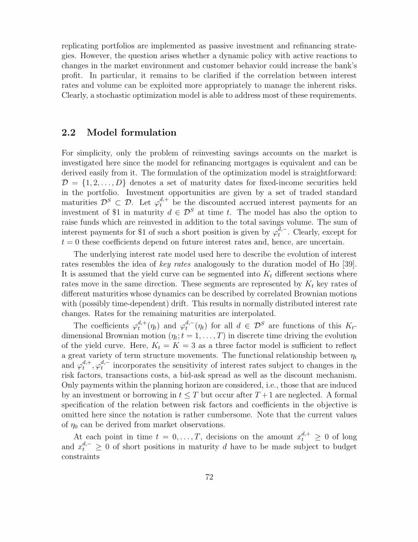
(a) ×-Simplex im IR3 (b) Barycenters for η (c) Barycenters for ξ
Figure 4: Simplizial coverage for K = 2 und L = 1
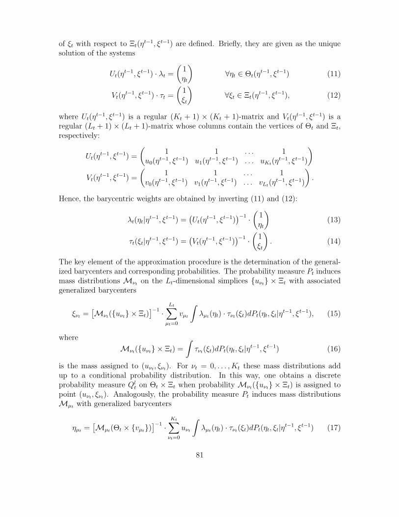
cases, the difference in the coordinates of the barycenters reflects the correlation ofthe original distribution. Another example is shown in Figure 4 for K = 2 and L = 1where the support of the joint distribution of η and ξ is covered by a ×-simplex inIR3. Again, the distribution mass is projected onto the simplices, taking into accountthe distance from each sample to the corresponding simplex. For each simplex, thebarycenter is determined as the “center of gravity” of the projected mass, and itsprobability is equivalent to the proportion of the projection to the total mass.
4.2 Barycentric scenario trees
Applying the barycentric approximation technique introduced in the last subsectionfor the conditional distributions on all stages yields a stochastic process describingthe evolution of random data under the new measures. As outlined in 3.3, anystochastic process which is discrete in both time and state can be represented as ascenario tree. From the measures Ql and Qu, two scenario trees can be constructedwhose associated deterministic equivalent problems are lower and upper bounds tothe original multistage stochastic program. For simplicity, the distinction betweenrandom data affecting the objective and the constraints is no longer maintained inthe notation from now on. Using the notation introduced in (9), the support of thediscretized distributions for t > 1 is denoted
Alt(ω
t−1) = suppQlt(·|ωt−1)
Aut (ω
t−1) = suppQut (·|ωt−1).
Starting from currently observed data Al0 = Au
0 = ω0, the two scenario trees areformally defined as
Al = ωl,T | ωlt ∈ Al
t(ωl,t−1) ∀t > 0
Au = ωu,T | ωut ∈ Au
t (ωu,t−1) ∀t > 0.
Here, ωl,t := (ωl1, . . . , ω
lt) and ωu,t := (ωu
1 , . . . , ωut ) are paths from the root to a node of
the scenario trees at stage t determined with the approximation technique introduced
83
6
-
tt0 1 2
(a) Upper approximation
6
-
tt0 1 2
(b) Lower approximation
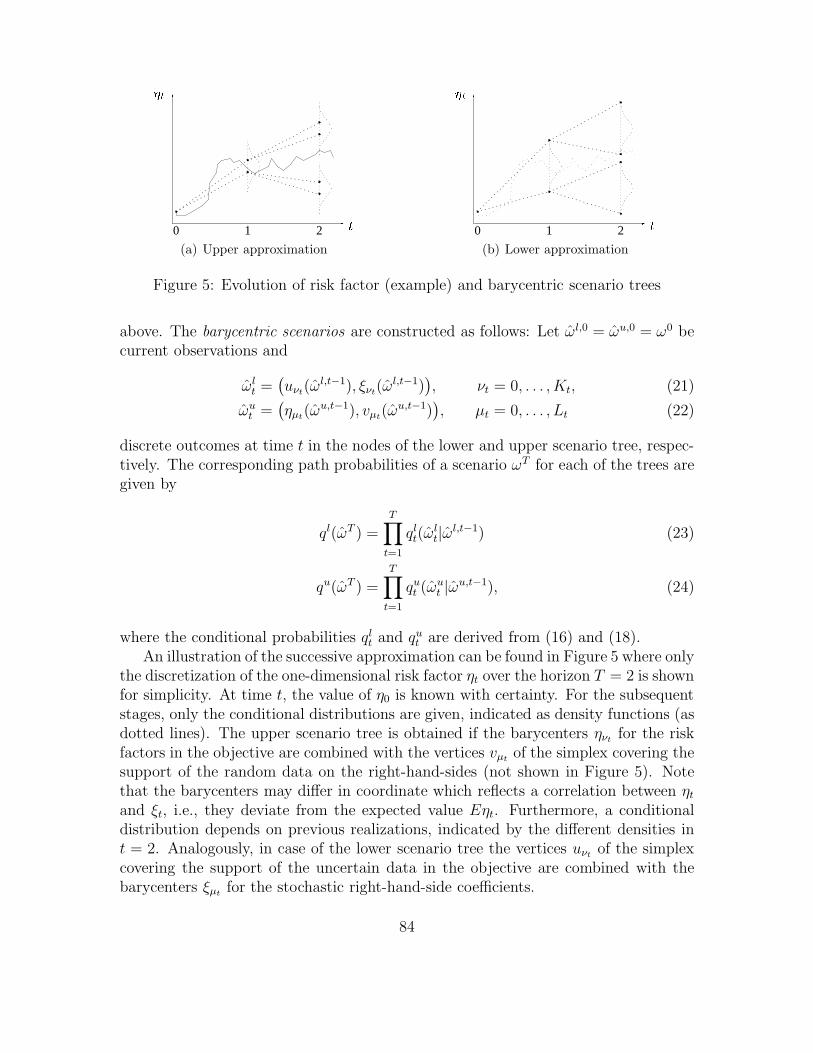
Figure 5: Evolution of risk factor (example) and barycentric scenario trees
above. The barycentric scenarios are constructed as follows: Let ωl,0 = ωu,0 = ω0 becurrent observations and
ωlt =
(
uνt(ωl,t−1), ξνt
(ωl,t−1))
, νt = 0, . . . , Kt, (21)
ωut =
(
ηµt(ωu,t−1), vµt
(ωu,t−1))
, µt = 0, . . . , Lt (22)
discrete outcomes at time t in the nodes of the lower and upper scenario tree, respec-tively. The corresponding path probabilities of a scenario ωT for each of the trees aregiven by
ql(ωT ) =T
∏
t=1
qlt(ω
lt|ωl,t−1) (23)
qu(ωT ) =T
∏
t=1
qut (ωu
t |ωu,t−1), (24)
where the conditional probabilities qlt and qu
t are derived from (16) and (18).An illustration of the successive approximation can be found in Figure 5 where only
the discretization of the one-dimensional risk factor ηt over the horizon T = 2 is shownfor simplicity. At time t, the value of η0 is known with certainty. For the subsequentstages, only the conditional distributions are given, indicated as density functions (asdotted lines). The upper scenario tree is obtained if the barycenters ηνt
for the riskfactors in the objective are combined with the vertices vµt
of the simplex covering thesupport of the random data on the right-hand-sides (not shown in Figure 5). Notethat the barycenters may differ in coordinate which reflects a correlation between ηt
and ξt, i.e., they deviate from the expected value Eηt. Furthermore, a conditionaldistribution depends on previous realizations, indicated by the different densities int = 2. Analogously, in case of the lower scenario tree the vertices uνt
of the simplexcovering the support of the uncertain data in the objective are combined with thebarycenters ξµt
for the stochastic right-hand-side coefficients.
84
4.3 Bounds for value functions
Recall the formulation of the original problem (3):
min g0(u0) +
∫
Ω
[
T∑
t=1
gt(ut, ωt)
]
dP (ω). (25)
Replacing the probability measure P by its discrete approximations Ql and Qu yieldsthe multistage stochastic programs
ψ0 = min g0(u0) +
∫
Ω
[
T∑
t=1
gt(ut, ωt)
]
dQl(ω) (26)
Ψ0 = min g0(u0) +
∫
Ω
[
T∑
t=1
gt(ut, ωt)
]
dQu(ω). (27)
It is shown in [28] that for the corresponding value functions
ψt(ut−1, ωt) = min
ut
gt(ut, ωt) +
∫
Ωt+1
ψt+1(ut, ωt+1)dQl
t+1(ωt+1|ωt)
Ψt(ut−1, ωt) = min
ut
gt(ut, ωt) +
∫
Ωt+1
Ψt+1(ut, ωt+1)dQu
t+1(ωt+1|ωt)
for t = 0, . . . , T with ψT+1(·) = ΨT+1(·) := 0, the following relation holds:
ψt(ut−1, ωt) ≤ φt(u
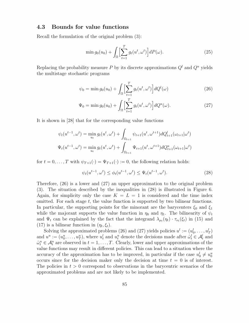
t−1, ωt) ≤ Ψt(ut−1, ωt). (28)
Therefore, (26) is a lower and (27) an upper approximation to the original problem(3). The situation described by the inequalities in (28) is illustrated in Figure 6.Again, for simplicity only the case K = L = 1 is considered and the time indexomitted. For each stage t, the value function is supported by two bilinear functions.In particular, the supporting points for the minorant are the barycenters ξ0 and ξ1while the majorant supports the value function in η0 and η1. The bilinearity of ψt
and Ψt can be explained by the fact that the integrand λµt(ηt) · τνt
(ξt) in (15) and(17) is a bilinear function in (ηt, ξt).
Solving the approximated problems (26) and (27) yields policies ul := (ul0, . . . , u
lT )
and uu := (uu0 , . . . , u
uT ), where ul
t and uut denote the decisions made after ωl
t ∈ Alt and
ωut ∈ Au
t are observed in t = 1, . . . , T . Clearly, lower and upper approximations of thevalue functions may result in different policies. This can lead to a situation where theaccuracy of the approximation has to be improved, in particular if the case ul
0 6= uu0
occurs since for the decision maker only the decision at time t = 0 is of interest.The policies in t > 0 correspond to observations in the barycentric scenarios of theapproximated problems and are not likely to be implemented.
85
A BCD 1 0(a) Upper bound
A BCD 0 1(b) Lower bound
Figure 6: Bilinear approximations of value functions
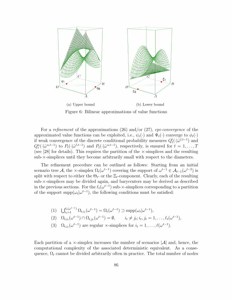
For a refinement of the approximations (26) and/or (27), epi-convergence of theapproximated value functions can be exploited, i.e., ψt(·) and Ψt(·) converge to φt(·)if weak convergence of the discrete conditional probability measures Ql
t(·|ωl,t−1) andQu
t (·|ωu,t−1) to Pt(·|ωl,t−1) and Pt(·|ωu,t−1), respectively, is ensured for t = 1, . . . , T(see [28] for details). This requires the partition of the ×-simplices and the resultingsub-×-simplices until they become arbitrarily small with respect to the diameters.
The refinement procedure can be outlined as follows: Starting from an initialscenario tree A, the ×-simplex Ωt(ω
t−1) covering the support of ωt−1 ∈ At−1(ωt−2) is
split with respect to either the Θt- or the Ξt-component. Clearly, each of the resultingsub-×-simplices may be divided again, and barycenters may be derived as describedin the previous sections. For the ℓt(ω
t−1) sub-×-simplices corresponding to a partitionof the support supp(ωt|ωt−1), the following conditions must be satisfied:
(1)⋃ℓt(ωt−1)
it=1 Ωt,it(ωt−1) = Ωt(ω
t−1) ⊃ supp(ωt|ωt−1),
(2) Ωt,it(ωt−1) ∩ Ωt,jt
(ωt−1) = ∅, it 6= jt; it, jt = 1, . . . , ℓt(ωt−1),
(3) Ωt,it(ωt−1) are regular ×-simplices for it = 1, . . . , ℓ(ωt−1).
Each partition of a ×-simplex increases the number of scenarios |A| and, hence, thecomputational complexity of the associated deterministic equivalent. As a conse-quence, Ωt cannot be divided arbitrarily often in practice. The total number of nodes
86

!t1 !t(a) No refinements
!t1 !t(b) Refinement in ωt−1
!t1 !t(c) Refinement in ωt
(d) Split of Θ or Ξ (e) Alternative edges (f) Alternative points
Figure 7: Possible refinements of scenario tree and ×-simplex
in the scenario trees at stage t = 1, . . . , T is given by
|Al,t| =∑
ωl,t−1∈Al,t−1
(
ℓt(ωl,t−1) − 1
)
(Kt + 1) (29)
|Au,t| =∑
ωu,t−1∈Au,t−1
(
ℓt(ωu,t−1) − 1
)
(Lt + 1). (30)
Therefore, the refinement process must be carefully monitored, particularly in themultistage case, in order to identify those nodes in the scenario trees where thelargest approximation error
ǫt(ωt) = Ψt(u
t−1, ωt) − ψt(ut−1, ωt) (31)
is observed. On the other hand, if ǫt(·) = 0 for a certain node, the approximation ofthe value function φt(·) is exact and further refinements of the partition correspondingto this node will not improve the accuracy of the approximation. For an efficientimplementation of refinement strategies, the following aspects must be considered:
(1) In which node should the scenario tree be refined (i.e., what is the amount ofthe approximation error to refine the existing partition; this has an immediateimpact to the number of scenarios and, hence, the problem size, see Figure 7(a)–(c)),
(2) does a division of Ωt with respect to Θt or Ξt yield a higher accuracy (seeFigure 7 (d)),
(3) which is the edge where the simplex is split (see Figure 7 (e)) and
87
(4) where does this edge have to be divided (see Figure 7 (f))?
For a detailed discussion and solution techniques, see [33].
4.4 Computational results
To complete the introduction of the barycentric approximation technique, some nu-merical results are presented. Two- and three-dimensional Brownian motions in dis-crete time are used to model the evolution of key rates ηt and one-dimensional Brown-ian motions for the volume change ξt in order to illustrate the influence of correlationsand the dimension size on the accuracy of the approximation with respect to differentrefinement strategies. In particular, the distribution of (ηt, ξt) at time t induced bythese Brownian motions are independent of the realizations in t − 1. This case iscovered by the general type of distribution functions (7) that is required to ensurethe saddle property of value functions.
In the first case ‘2U’, two uncorrelated processes for key rates of maturity 1 and12 months are considered with σ1 = 0.179 and σ12 = 0.125, rates for the remainingmaturities are interpolated. Both risk factors are independent of the volume change ξtwhose variance is given by σV = 341′056. The second case ‘2C’ uses the same volatilityfor interest rate and volume changes, together with covariances of σ1,12 = 0.117between both key rates as well as σ1,V = 44.247 and σ12,V = 37.682 between key ratesand volume. Intuitively, such a model is able to reflect parallel and tilt movementsof the yield curve.
Taking a third factor into account, e.g., the rate of an intermediate maturity, alsoallows the modeling of changes in the curvature of the term structure. In the lastcase ‘3C’, the 3 month rate with variance σ3 = 0.141 and covariances σ1,3 = 0.151,σ3,12 = 0.121, σ3,V = 43.2379 is considered in addition to the 1 and 12 month keyrates. These parameter estimates were taken from the description of a collection oftest problems for multistage stochastic programs in [30] and are derived from moneymarket rates for the Swiss Franc. All drifts of the Brownian motions are equal tozero. Note that in the context of a real savings application, the correlation betweeninterest rates and volume has a negative sign.
In section 3.2, it was assumed that the ×-simplex Θt×Ξt is compact and covers thesupport of (ηt, ξt). However, the normal distributions at each point in time associatedwith the Brownian motions under consideration have unbounded support. In thiscase, one must ensure that Pt(Θt × Ξt|ηt−1, ξt−1) ≥ 1 − ε for sufficiently small ε > 0and substitute Pt(·|ηt−1, ξt−1) by its normalized truncation (see [35]).
The procedure for the determination of a simplicial coverage is only conceptuallyoutlined here. First, consider a K-dimensional standard normal distribution. Asphere with radius δ around the origin contains a percentage of 2Φ(δ) − 1 of thetotal mass distribution, where Φ denotes the c.d.f. This sphere can be covered by asimplex in IRK with K + 1 vertices. In the one-dimensional case, the simplex reducesto an interval [−δ, δ], and for K = 2 to a triangle with vertices u0 = (−
√3δ, δ)′, u1 =
88
-2 -1 0 1 2
-1
-0.5
0
0.5
1
1.5
(a) Uncorrelated distribution ‘2U’
-1 0 1 2
-1
-0.5
0
0.5
1
1.5
(b) Correlated distribution ‘2C’
Figure 8: Simplicial coverage of two-dimensional distributions
7 0 0 0
8 0 0 0
9 0 0 0
1 0 0 0 0
0 1 2 3 4n o . r e f i n e m e n t s
obj. v
alue
W 2 U , W 2 C , W 3 C L BW 2 U ( r o o t ) U BW 2 U ( e r r o r ) U BW 2 C ( r o o t + e r r o r ) U BW 3 C ( r o o t ) U BW 3 C ( e r r o r ) U B
Figure 9: Objective values for different key rate distributions and refinement strategies
(√
3δ, δ)′ and u2 = (0,−2δ)′. It is well known that a standard normally distributedrandom variable Z ∈ IRK may be transformed into a N (µ,Σ)-distributed randomvariable Y ∈ IRK using the lower triangular matrix of the Cholesky decomposition Lof the covariance matrix Σ, i.e., Σ = L ·L′. According to this rule, the vertices uY
i ofthe simplicial coverage for Y are given by
uYi = µ+ L · uZ
i , i = 0, . . . , K.
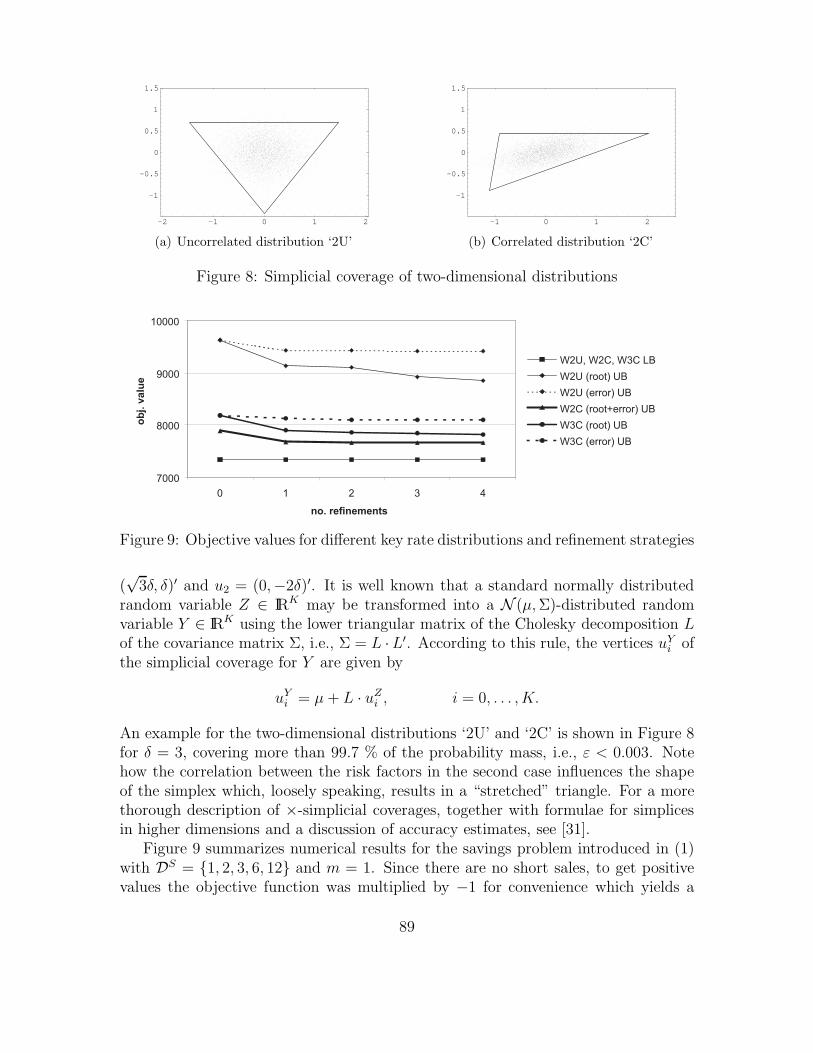
An example for the two-dimensional distributions ‘2U’ and ‘2C’ is shown in Figure 8for δ = 3, covering more than 99.7 % of the probability mass, i.e., ε < 0.003. Notehow the correlation between the risk factors in the second case influences the shapeof the simplex which, loosely speaking, results in a “stretched” triangle. For a morethorough description of ×-simplicial coverages, together with formulae for simplicesin higher dimensions and a discussion of accuracy estimates, see [31].
Figure 9 summarizes numerical results for the savings problem introduced in (1)with DS = 1, 2, 3, 6, 12 and m = 1. Since there are no short sales, to get positivevalues the objective function was multiplied by −1 for convenience which yields a
89
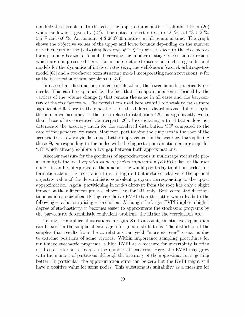
maximization problem. In this case, the upper approximation is obtained from (26)while the lower is given by (27). The initial interest rates are 5.0 %, 5.1 %, 5.2 %,5.5 % and 6.0 %. An amount of $ 200’000 matures at all points in time. The graphshows the objective values of the upper and lower bounds depending on the numberof refinements of the (sub-)simplices Θt(·|ηt−1, ξt−1) with respect to the risk factorsfor a planning horizon of T = 4. Increasing the number of stages yields similar resultswhich are not presented here. For a more detailed discussion, including additionalmodels for the dynamics of interest rates (e.g., the well-known Vasicek arbitrage-freemodel [63] and a two-factor term structure model incorporating mean reversion), referto the description of test problems in [30].
In case of all distributions under consideration, the lower bounds practically co-incide. This can be explained by the fact that this approximation is formed by thevertices of the volume change ξt that remain the same in all cases and the barycen-ters of the risk factors ηt. The correlations used here are still too weak to cause moresignificant difference in their positions for the different distributions. Interestingly,the numerical accuracy of the uncorrelated distribution ‘2U’ is significantly worsethan those of its correlated counterpart ‘2C’. Incorporating a third factor does notdeteriorate the accuracy much for the correlated distribution ‘3C’ compared to thecase of independent key rates. Moreover, partitioning the simplices in the root of thescenario trees always yields a much better improvement in the accuracy than splittingthose Θt corresponding to the nodes with the highest approximation error except for‘2C’ which already exhibits a low gap between both approximations.
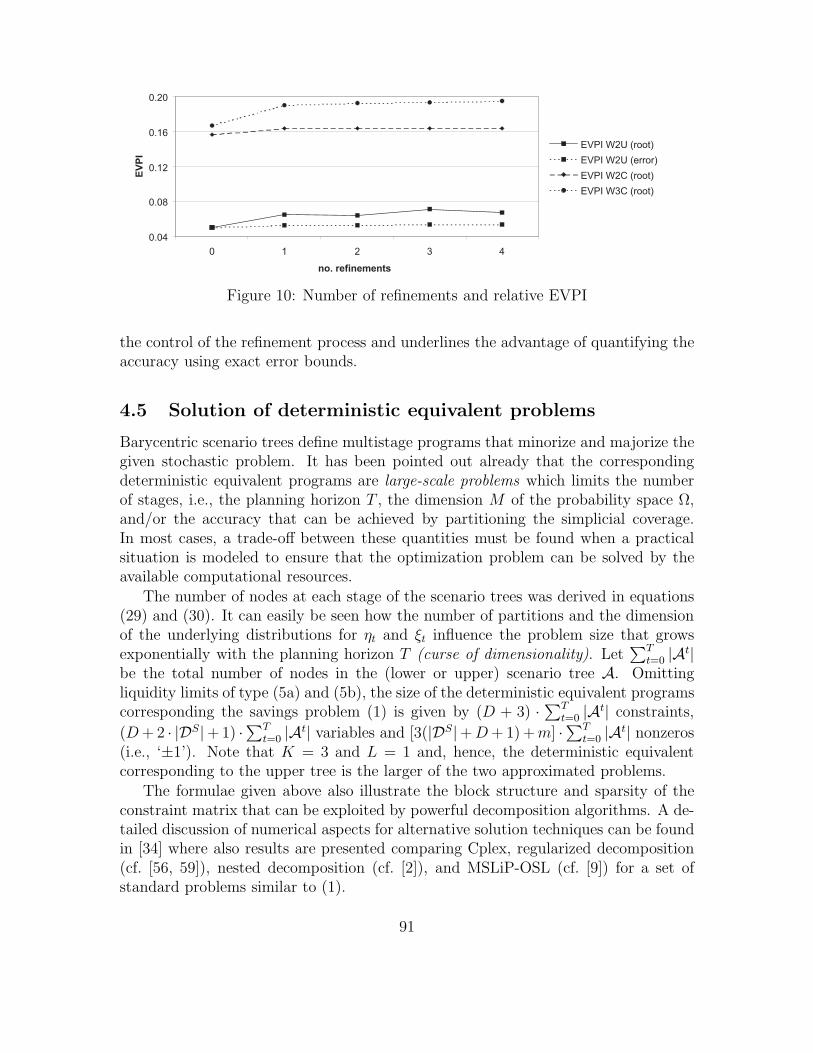
Another measure for the goodness of approximations in multistage stochastic pro-gramming is the local expected value of perfect information (EVPI) taken at the rootnode. It can be interpreted as the amount one would pay today to obtain perfect in-formation about the uncertain future. In Figure 10, it is stated relative to the optimalobjective value of the deterministic equivalent program corresponding to the upperapproximation. Again, partitioning in nodes different from the root has only a slightimpact on the refinement process, shown here for ‘2U’ only. Both correlated distribu-tions exhibit a significantly higher relative EVPI than the latter which leads to thefollowing – rather surprising – conclusion: Although the larger EVPI implies a higherdegree of stochasticity, it becomes easier to approximate the stochastic programs bythe barycentric deterministic equivalent problems the higher the correlations are.
Taking the graphical illustrations in Figure 8 into account, an intuitive explanationcan be seen in the simplicial coverage of original distributions. The distortion of thesimplex that results from the correlations can yield “more extreme” scenarios dueto extreme positions of some vertices. Within importance sampling procedures formultistage stochastic programs, a high EVPI as a measure for uncertainty is oftenused as a criterion to increase the number of scenarios. Here, the EVPI may growwith the number of partitions although the accuracy of the approximation is gettingbetter. In particular, the approximation error can be zero but the EVPI might stillhave a positive value for some nodes. This questions its suitability as a measure for
90
0 . 0 4
0 . 0 8
0 . 1 2
0 . 1 6
0 . 2 0
0 1 2 3 4n o . r e f i n e m e n t s
EVPI
E V P I W 2 U ( r o o t )E V P I W 2 U ( e r r o r )E V P I W 2 C ( r o o t )E V P I W 3 C ( r o o t )
Figure 10: Number of refinements and relative EVPI
the control of the refinement process and underlines the advantage of quantifying theaccuracy using exact error bounds.
4.5 Solution of deterministic equivalent problems
Barycentric scenario trees define multistage programs that minorize and majorize thegiven stochastic problem. It has been pointed out already that the correspondingdeterministic equivalent programs are large-scale problems which limits the numberof stages, i.e., the planning horizon T , the dimension M of the probability space Ω,and/or the accuracy that can be achieved by partitioning the simplicial coverage.In most cases, a trade-off between these quantities must be found when a practicalsituation is modeled to ensure that the optimization problem can be solved by theavailable computational resources.
The number of nodes at each stage of the scenario trees was derived in equations(29) and (30). It can easily be seen how the number of partitions and the dimensionof the underlying distributions for ηt and ξt influence the problem size that growsexponentially with the planning horizon T (curse of dimensionality). Let
∑T
t=0 |At|be the total number of nodes in the (lower or upper) scenario tree A. Omittingliquidity limits of type (5a) and (5b), the size of the deterministic equivalent programscorresponding the savings problem (1) is given by (D + 3) · ∑T
t=0 |At| constraints,
(D+ 2 · |DS|+ 1) ·∑T
t=0 |At| variables and [3(|DS|+D+ 1) +m] ·∑T
t=0 |At| nonzeros(i.e., ‘±1’). Note that K = 3 and L = 1 and, hence, the deterministic equivalentcorresponding to the upper tree is the larger of the two approximated problems.
The formulae given above also illustrate the block structure and sparsity of theconstraint matrix that can be exploited by powerful decomposition algorithms. A de-tailed discussion of numerical aspects for alternative solution techniques can be foundin [34] where also results are presented comparing Cplex, regularized decomposition(cf. [56, 59]), nested decomposition (cf. [2]), and MSLiP-OSL (cf. [9]) for a set ofstandard problems similar to (1).
91
volume
PSfrag repla ements
1 Y5 Y
volume
2%3%4%5%6%7%8%9%10%
10 20 30 40 50 60 70 80month 25.027.530.032.535.037.540.042.545.0
Figure 11: Interest rates (left) and savings volume (bio. CHF, right)
5 Reinvestment of savings accounts
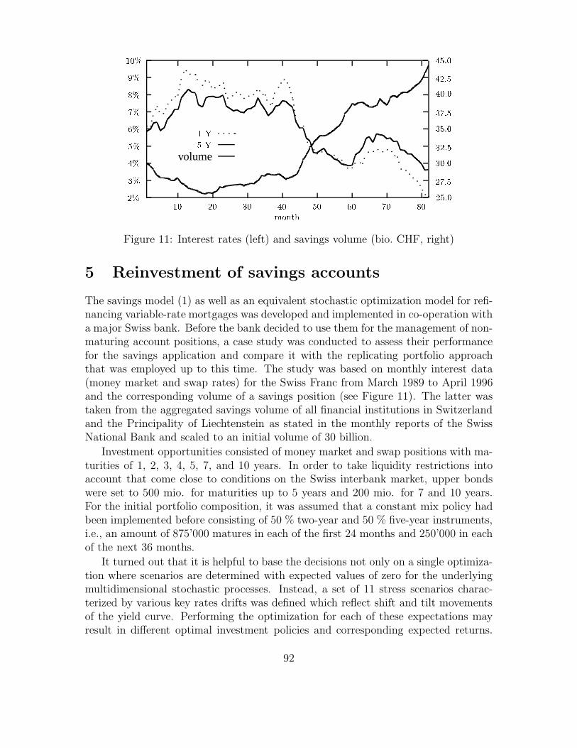
The savings model (1) as well as an equivalent stochastic optimization model for refi-nancing variable-rate mortgages was developed and implemented in co-operation witha major Swiss bank. Before the bank decided to use them for the management of non-maturing account positions, a case study was conducted to assess their performancefor the savings application and compare it with the replicating portfolio approachthat was employed up to this time. The study was based on monthly interest data(money market and swap rates) for the Swiss Franc from March 1989 to April 1996and the corresponding volume of a savings position (see Figure 11). The latter wastaken from the aggregated savings volume of all financial institutions in Switzerlandand the Principality of Liechtenstein as stated in the monthly reports of the SwissNational Bank and scaled to an initial volume of 30 billion.
Investment opportunities consisted of money market and swap positions with ma-turities of 1, 2, 3, 4, 5, 7, and 10 years. In order to take liquidity restrictions intoaccount that come close to conditions on the Swiss interbank market, upper bondswere set to 500 mio. for maturities up to 5 years and 200 mio. for 7 and 10 years.For the initial portfolio composition, it was assumed that a constant mix policy hadbeen implemented before consisting of 50 % two-year and 50 % five-year instruments,i.e., an amount of 875’000 matures in each of the first 24 months and 250’000 in eachof the next 36 months.
It turned out that it is helpful to base the decisions not only on a single optimiza-tion where scenarios are determined with expected values of zero for the underlyingmultidimensional stochastic processes. Instead, a set of 11 stress scenarios charac-terized by various key rates drifts was defined which reflect shift and tilt movementsof the yield curve. Performing the optimization for each of these expectations mayresult in different optimal investment policies and corresponding expected returns.
92

key rate shifts opt. objective valuesscen.
#1 #2 #3 sol. P1 P2. . .
0 - - - - - - P1 668’734.7 668’672.2 . . .
1 - - - P2 890’117.8 890’209.2 . . .
2 - - - - P2 902’151.4 902’156.8 . . .
3 - - 0 P1 975’132.0 975’051.5 . . .
4 - 0 + P3 1’174’434.0 1’174’193.0 . . .
5 0 0 0 P4 1’152’769.0 1’152’613.0 . . .
6 + 0 - P4 1’379’315.0 1’378’796.0 . . .
7 + + 0 P4 1’421’833.0 1’421’339.0 . . .
8 ++ + 0 P4 1’648’060.0 1’647’201.0 . . .
9 + + + P4 1’421’833.0 1’421’339.0 . . .
10 ++ ++ ++ P4 1’691’181.0 1’690’350.0 . . .
Table 1: Stress scenarios and risk analysis of different investment policies
This allows the assessment of the sensitivity of the solution with respect to differ-ent distribution assumptions and, in particular, to quantify the impact of “extremalevents” that may be chosen by the decision maker.
An example for this set of stress scenarios is given in Table 1. Each ‘+’ and‘-’ represents a decrease or increase in a key rate by one standard deviation. Ingeneral, the 11 optimization runs result in more than one solution. Then, the first-stage decision is fixed, and the optimization is repeated with respect to the remainingstages for all policies and all different key rate drifts. In other words, for the selectedstress scenarios the consequences of suboptimal initial decisions and the costs for theircorrection in the subsequent periods are determined. This allows an analysis of therisk associated with the different solutions, taking into account non-anticipated shiftand tilt movements of the term structure. In this way, one obtains a sort of profitand loss pattern which helps to identify dominant policies for the first-stage decision.For instance, in Table 1 policy P2 performs only slightly better than P1 for scenario 1and 2 but is clearly inferior in all other cases. A pairwise comparison of the restrictedsolutions reveals the investment policy that is finally implemented.
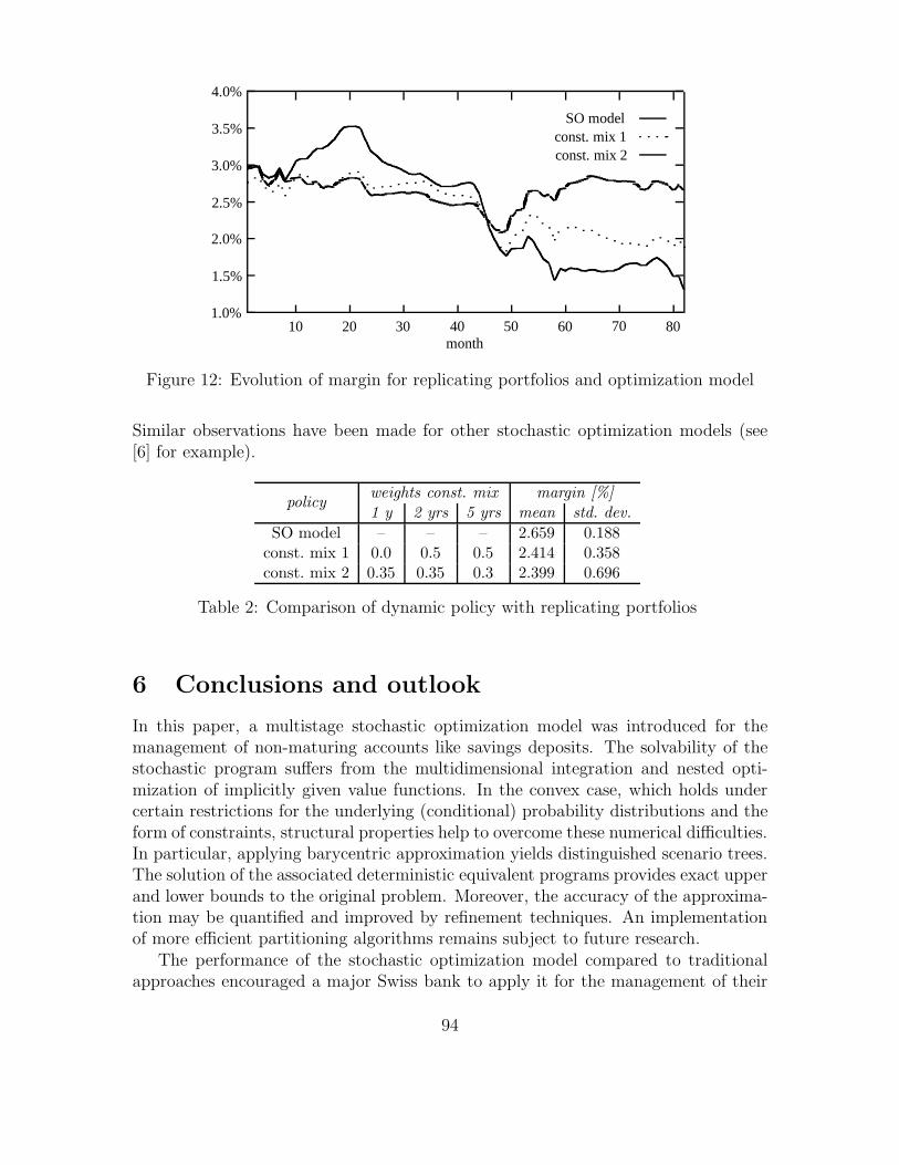
The evolution of the margin between the return of the portfolio and the customerrate over the sample period is shown in Figure 12 for the dynamic policies determinedby the stochastic optimization model with subsequent risk analysis and is compared totwo constant mix strategies. The latter were determined by the replicating portfolioapproach. In case of CM2, portfolio weights were derived under the assumption of aconstant volume, i.e., it tracks only the customer rate and not the total volume. Notethat this results in a lower and more volatile margin. According to Table 2, the averagemargin could be improved by 25 basis points compared to the better constant mixpolicy. In particular, the standard deviation of the margin was reduced significantlyalthough volatility is not considered explicitly in the model’s objective. However, itis incorporated by the high number of scenarios in the tree of the stochastic program.
93
SO modelconst. mix 1const. mix 2
1.0%
1.5%
2.0%
2.5%
3.0%
3.5%
4.0%
10 20 30 40 50 60 70 80month
Figure 12: Evolution of margin for replicating portfolios and optimization model
Similar observations have been made for other stochastic optimization models (see[6] for example).
weights const. mix margin [%]policy
1 y 2 yrs 5 yrs mean std. dev.
SO model – – – 2.659 0.188const. mix 1 0.0 0.5 0.5 2.414 0.358const. mix 2 0.35 0.35 0.3 2.399 0.696
Table 2: Comparison of dynamic policy with replicating portfolios
6 Conclusions and outlook
In this paper, a multistage stochastic optimization model was introduced for themanagement of non-maturing accounts like savings deposits. The solvability of thestochastic program suffers from the multidimensional integration and nested opti-mization of implicitly given value functions. In the convex case, which holds undercertain restrictions for the underlying (conditional) probability distributions and theform of constraints, structural properties help to overcome these numerical difficulties.In particular, applying barycentric approximation yields distinguished scenario trees.The solution of the associated deterministic equivalent programs provides exact upperand lower bounds to the original problem. Moreover, the accuracy of the approxima-tion may be quantified and improved by refinement techniques. An implementationof more efficient partitioning algorithms remains subject to future research.
The performance of the stochastic optimization model compared to traditionalapproaches encouraged a major Swiss bank to apply it for the management of their
94
non-maturing account positions. Two important conclusions can be drawn from thecase study presented above: First, the results indicate that a dynamic policy is supe-rior to a static one since portfolios selected with the stochastic program clearly out-perform constant mix strategies. Second, the stochastic optimization model hedgesagainst the various sources of uncertainty inherent to non-maturing accounts like in-terest rate and prepayment/withdrawal risk more appropriately than the replicatingportfolio approach. In particular, it is able to take the dependencies between interestrates and volume for dynamic portfolio strategies into account.
Stochastic programming is well suited for a broad class of problems within assetand liability management (ALM) that are characterized by cross and/or serial cor-relations between risk factors, e.g., cash management in insurance companies wherepremium payments exhibit a seasonal behavior. Other types of risk (credit, cur-rency etc.) may also be considered if appropriate. Clearly, the Brownian motionsexploited here to model the evolution of interest rates and volume may be viewed asa rather simple approach to model the uncertainty of the relevant risk factors. Moresophisticated models have been proposed in the financial literature and are currentlyunder investigation. Schurle [60] examines alternative term structure models for thegeneration of interest rate scenarios and a trend-stationary process for evolution ofsavings deposits. In the latter case, using the risk factors driving the yield curve asexplanatory variables allows for a good description of the aggregated savings volumepublished by the Swiss National Bank (see also [41] and the references herein for a dis-cussion of alternative processes for the evolution of demand deposits). It is expectedthat the integration of more sophisticated models for the generation of interest rateand volume scenarios in the stochastic program will yield an additional improvementin the performance. However, different types of distribution functions for the randomdata might not preserve the inheritance of the saddle property of value functions.
The savings account model introduced here may be seen as a first step towardsa general ALM model for a bank’s complete balance sheet to optimize investmentand refinancing decisions with respect to interest rate and volume risk. Additionalconstraints may be imposed to limit the absolute risk exposure of certain positions inorder to comply with regulatory restrictions concerning capital requirements. Mul-tistage stochastic programming helps to overcome many difficulties in modeling dy-namic decision making. It can be seen as a versatile tool for financial planningproblems under uncertainty.
References
[1] J.R. Birge and R.J.-B. Wets. Designing approximation schemes for stochas-tic optimization problems, in particular for stochastic programs with recourse.Mathematical Programming Study, 27:54-102, 1986.
95
[2] J.R. Birge, C.J. Donohue, D.F. Holmes, and O.G. Svintsitski. A parallel imple-mentation of the nested decomposition algorithm for multistage stochastic linearprograms. Mathematical Programming, 75:327-352, 1995.
[3] M. Britton-Jones. The sampling error in estimates of mean-variance efficientportfolio weights. Journal of Finance, 54:655-671, 1999.
[4] D.R. Carino, T. Kent, D.H. Myers, C. Stacy, M. Sylvanus, A.L. Turner, K.Watanabe, and W.T. Ziemba. The Russell-Yasuda Kasai model: An as-set/liability model for a Japanese insurance company using multistage stochasticprogramming. Interfaces, 24:29-49, 1994.
[5] D.R. Carino, D.H. Myers, and W.T. Ziemba. Conceps, technical issues, anduses of the Russell-Yasuda Kasai financial planning model. Operations Research,46:450-462, 1998.
[6] D.R. Carino and W.T. Ziemba. Formulation of the Russell-Yasuda Kasai finan-cial planning model. Operations Research, 46:433-449, 1998.
[7] Z. Chen, G. Consigli, M.A.H. Dempster, and N. Hicks-Pedron. Towards sequen-tial sampling algorithms for dynamic portfolio management. In: C. Zopounidis(ed.), Operational Tools in the Management of Financial Risks, pp. 197-211.Kluwer, 1998.
[8] V.K. Chopra and W.T. Ziemba. The effect of errors in means, variances, andcovariances on optimal portfolio choice. Journal of Portfolio Management, 20:6-11, 1993.
[9] G. Consigli and M.A.H. Dempster. Solving dynamic portfolio problems usingstochastic programming. Zeitschrift fur Angewandte Mathematik und Mechanik(Supplement), 77:S 535-S 536, 1997.
[10] G.B. Dantzig and G. Infanger. Large-scale stochastic linear programs: Impor-tance sampling and Benders decomposition. Technical Report SOL 91-4, Stan-ford University, 1991.
[11] G.B. Dantzig and G. Infanger. Multi-stage stochastic linear programs for port-folio optimization. Annals of Operations Research, 45:59-76, 1993.
[12] R. Dembo. Scenario optimization. Annals of Operations Research, 30:63-80,1991.
[13] M.A.H. Dempster. The expected value of perfect information in the optimal evo-lution of stochastic problems. In: M. Arato, D. Vermes, and A.V. Balakrishnan(eds.), Stochastic Differential Systems, pp. 25-40. Springer, 1981.
96

[14] C.L. Dert. Asset liability management for pension funds: A multistage chanceconstraint programming approach. Phd thesis, Erasmus University, Rotterdam,1995.
[15] J. Dupacova. Stochastic programming models in banking. Working paper,IIASA, Laxenburg, 1991.
[16] J. Dupacova. Postoptimality for multistage stochastic linear programs. Annalsof Operations Research, 56:65-78, 1995.
[17] J. Dupacova. Scenario-based stochastic programs: Resistance with respect tosample. Annals of Operations Research, 64:21-38, 1996.
[18] J. Dupacova, M. Bertocchi, and V. Moriggia. Postoptimality for scenario basedfinancial planning models with an application to bond portfolio management. In:W.T. Ziemba and J.M. Mulvey (eds.), World Wide Asset and Liability Modeling,pp. 263-285. Cambridge University Press, Cambridge, 1998.
[19] N.C.P. Edirisinghe. New second-order bounds on the expectation of saddle func-tions with applications to stochastic linear programming. Operations Research,44:909-922, 1996.
[20] N.C.P. Edirisinghe and W.T. Ziemba. Bounds for two-stage stochastic programswith fixed recourse. Mathematics of Operations Research, 19:292-313, 1994.
[21] H.P. Edmundson. Bounds on the expectation of a convex function of a randomvariable. Technical Report 982, RAND Corporation, 1957.
[22] D. Eichhorn, F. Gupta, and E. Stubbs. Using constraints to improve the robust-ness of asset allocation. Journal of Portfolio Management, 24:41-48, 1998.
[23] S.-E. Fleten, K. Høyland, and S.W. Wallace. The performance of stochasticdynamic and fixed mix portfolio models. Working paper, Norwegian Universityof Science and Technology, Trondheim, 1998.
[24] B. Forrest, K. Frauendorfer, and M. Schurle. A stochastic optimization modelfor the investment of savings account deposits. In: P. Kischka et al. (eds.),Operations Research Proceedings 1997, pp. 382-387, Springer, 1998.
[25] E. Fragniere, J. Gondzio, and J.-P. Vial. A planning model with one millionscenarios solved on an affordable parallel machine. Technical Report 1998.11,Logilab, University of Geneva, 1998.
[26] K. Frauendorfer. Solving SLP recourse problems with arbitrary multivariatedistributions: The dependent case. Mathematics of Operations Research, 13:377-394, 1988.
97
[27] K. Frauendorfer. Stochastic Two-Stage Programming. Springer, 1992.
[28] K. Frauendorfer. Multistage stochastic programming: Error analysis for theconvex case. ZOR – Mathematical Methods of Operations Research, 39:93-122,1994.
[29] K. Frauendorfer. Barycentric scenario trees in convex multistage stochastic pro-gramming. Mathematical Programming, 75:277-293, 1996.
[30] K. Frauendorfer and G. Haarbrucker. Test problems in stochastic multistageprogramming. Optimization, to appear.
[31] K. Frauendorfer and F. Hartel. On the goodness of discretizing diffusion processesfor stochastic programming. Working paper, Institute of Operations Research,University of St. Gallen, 1995.
[32] K. Frauendorfer and P. Kall. A solution method for SLP recourse problems witharbitrary multivariate distributions: The independent case. Problems of Controland Information Theory, 17:177-205, 1988.
[33] K. Frauendorfer and C. Marohn. Refinement issues in stochastic multistage linearprogramming. In: K. Marti and P. Kall (eds.), Stochastic Programming Meth-ods and Technical Applications (Proceedings of the 3rd GAMM/IFIP Workshop1996), pp. 305-328, Springer, 1998.
[34] K. Frauendorfer, C. Marohn, and M. Schurle. SG-portfolio test problems forstochastic multistage linear programming (II). Working paper, Institute of Op-erations Research, University of St. Gallen, 1997.
[35] K. Frauendorfer and M. Schurle. Barycentric approximation of stochastic interestrate processes. In: W.T. Ziemba and J.M. Mulvey (eds.), Worldwide Asset andLiability Modeling, pp. 231-262. Cambridge University Press, Cambridge, 1998.
[36] B. Golub, M. Holmer, R. McKendall, L. Pohlman, and S.A. Zenios. A stochasticprogramming model for money management. European Journal of OperationalResearch, 85:282-296, 1995.
[37] T. Hakala. A Stochastic Optimization Model for Multi-Currency Bond PortfolioManagement. Phd thesis, Helsinki School of Economics and Business Adminis-tration, 1996.
[38] J.L. Higle and S. Sen. Stochastic Decomposition – A Statistical Method for LargeScale Stochastic Linear Programming. Kluwer, 1996.
[39] T. Ho. Key rate durations: Measures of interest rate risks. Journal of FixedIncome, 2:29-44, 1992.
98

[40] M.R. Holmer. The asset-liability management strategy system at Fannie Mae.Interfaces, 24:3-21, 1994.
[41] R.A. Jarrow and D.R. van Deventer. The arbitrage-free valuation and hedgingof demand deposits and credit card loans. Journal of Banking and Finance,22:249-272, 1998.
[42] J.L. Jensen. Sur les fonctions convexes et les inegalites entre les valeurs moyennes.Acta Mathematica, 30:175-193, 1906.
[43] P. Kall, A. Ruszczynski, and K. Frauendorfer. Approximation techniques instochastic programming. In: Y. Ermoliev and R.J.-B. Wets (eds.), NumericalTechniques for Stochastic Optimization, pp. 33-64. Springer, 1988.
[44] J.G. Kallberg, R.W. White, and W.T. Ziemba. Short term financial planningunder uncertainty. Management Science, 28:670-682, 1982.
[45] M.I. Kusy and W.T. Ziemba. A bank asset and liability management model.Operations Research, 34:356-376, 1986.
[46] R. Litterman and J. Scheinkman. Common factors affecting bond returns. Jour-nal of Fixed Income, 1:54-61, 1991.
[47] A. Madansky. Bounds on the expectation of a convex function of a multivariaterandom variable. Annals of Mathematical Statistics, 30:743-746, 1959.
[48] H.M. Markowitz. Portfolio Selection: Efficient Diversification of Investment.Wiley, 1959.
[49] J.M. Mulvey. Financial planning via multi-stage stochastic programs. In: J.R.Birge and K.G. Murty (eds.), Mathematical Programming: State of the Art 1994,pp. 151-171. University of Michigan, Ann Arbor, 1994.
[50] J.M. Mulvey. Multi-stage financial planning systems. In: R.L. D’Ecclesia andS.A. Zenios (eds.), Operations Research Models in Quantitative Finance, pp. 18-35. Physica, 1994.
[51] J.M. Mulvey and A. Ruszczynski. A new scenario decomposition method forlarge-scale stochastic optimization. Operations Research, 43:477-490, 1995.
[52] J.M. Mulvey and A.E. Thorlacius. The Towers Perrin global capital marketscenario generation system. In: W.T. Ziemba and J.M. Mulvey (eds.), WorldwideAsset and Liability Modeling, pp. 286-312. Cambridge University Press, 1998.
[53] J.M. Mulvey and S.A. Zenios. Capturing the correlations of fixed-income instru-ments. Management Science, 40:1329-1342, 1994.
99
[54] R. T. Rockafellar and R.J.-B. Wets. Nonanticipativity and L1-martingales instochastic optimization problems. Mathematical Programming Study, 6:170-187,1976.
[55] C.H. Rosa and A. Ruszczynski. On augmented Lagrangian decomposition meth-ods for multistage stochastic programs. Annals of Operations Research, 64:289-309, 1996.
[56] A. Ruszczynski. On the regularized decomposition method for stochastic pro-gramming problems. In: K. Marti and P. Kall (eds.), Stochastic Programming:Numerical Techniques and Engineering Applications, pp. 93-108, Springer, 1993.
[57] A. Ruszczynski. Parallel decomposition of multistage stochastic programmingproblems. Mathematical Programming, 58:201-228, 1993.
[58] A. Ruszczynski. Decomposition methods in stochastic programming. Mathemat-ical Programming, 79:333-353, 1997.
[59] A. Ruszczynski and A. Swietanowski. On the regularized decomposition methodfor two-stage stochastic linear problems. Working Paper WP-96-014, IIASA,Laxenburg, 1996.
[60] M. Schurle. Zinsmodelle in der stochastischen Optimierung. Haupt, 1998.
[61] M. Steinbach. Recursive direct algorithms for multistage stochastic programs infinancial engineering. In: P. Kall and H.-J. Luthi (eds.), Operations ResearchProceedings 1998, pp. 241-250, Springer, 1999.
[62] P. Varaiya and R.J.-B. Wets. Stochastic dynamic optimization - approaches andcomputation. Working Paper WP-88-87, IIASA, Laxenburg, 1988.
[63] O. Vasicek. An equilibrium characterization of the term structure. Journal ofFinancial Economics, 5:177-188, 1977.
[64] C. Vassiadou-Zeniou and S.A. Zenios. Robust optimization models for managingcallable bond portfolios. European Journal of Operational Research, 91:264-273,1996.
[65] K.J. Worzel, C. Vassiadou-Zeniou, and S.A. Zenios. Integrated simulation andoptimization models for tracking indices of fixed-income securities. OperationsResearch, 42:223-233, 1994.
[66] S.A. Zenios. A model for portfolio management with mortgage-backed securities.Annals of Operations Research, 43:337-356, 1993.
[67] S.A. Zenios. Asset/liability management under uncertainty for fixed-income se-curities. Annals of Operations Research, 59:77-97, 1995.
100