Southern Methodist University Southern Methodist University

SMU Scholar SMU Scholar

Electrical Engineering Theses and Dissertations Electrical Engineering

Fall 12-21-2019

Stochastic Orthogonalization and Its Application to Machine Stochastic Orthogonalization and Its Application to Machine

Learning Learning

Yu Hong Southern Methodist University, hongy@smu.edu

Follow this and additional works at: https://scholar.smu.edu/engineering_electrical_etds

Part of the Artificial Intelligence and Robotics Commons, and the Theory and Algorithms Commons

Recommended Citation Recommended Citation Hong, Yu, "Stochastic Orthogonalization and Its Application to Machine Learning" (2019). Electrical Engineering Theses and Dissertations. 31. https://scholar.smu.edu/engineering_electrical_etds/31

This Thesis is brought to you for free and open access by the Electrical Engineering at SMU Scholar. It has been accepted for inclusion in Electrical Engineering Theses and Dissertations by an authorized administrator of SMU Scholar. For more information, please visit http://digitalrepository.smu.edu.

STOCHASTIC ORTHOGONALIZATION

AND ITS

APPLICATION TO MACHINE LEARNING

A Master Thesis Presented to the Graduate Faculty of the

Lyle School of Engineering

Southern Methodist University

in

Partial Fulfillment of the Requirements

for the degree of

Master of Science

in Electrical Engineering

by

Yu Hong

B.S., Electrical Engineering, Tianjin University 2017

December 21, 2019

Copyright (2019)

Yu Hong

All Rights Reserved

iii

ACKNOWLEDGMENTS

First, I want to thank Dr. Douglas. During this year of working with him, I have learned

a lot about how to become a good researcher. He is creative and hardworking, which sets

an excellent example for me. Moreover, he has always been patient with me and has spend

a lot of time discuss this thesis with me. I would not have finished this thesis without him.

Then, thanks to Dr. Larson for giving me the inspiration to do this thesis. Last year,

I had just started with machine learning and was doing some preliminary simulation. On

research day, Dr. Larson enlightened me with his talk and sent me a paper which inspired

me to write this thesis.

Finally, thanks to Dr. Rohrer, who has given me lots of freedom to work on this thesis.

I have had bad health condition this year and really appreciate the understanding. I am

looking forward to learn more from him.

iv

Hong, Yu B.S., Electrical Engineering, Tianjin University

Stochastic Orthogonalization

and Its

Application to Machine Learning

Advisor: Scott C. Douglas

Master of Science degree conferred December 21, 2019

Master Thesis completed December 19, 2019

Orthogonal transformations have driven many great achievements in signal process-

ing. They simplify computation and stabilize convergence during parameter training. Re-

searchers have introduced orthogonality to machine learning recently and have obtained

some encouraging results. In this thesis, three new orthogonal constraint algorithms based

on a stochastic version of an SVD-based cost are proposed, which are suited to training large-

scale matrices in convolutional neural networks. We have observed better performance in

comparison with other orthogonal algorithms for convolutional neural networks.

v

TABLE OF CONTENTS

CHAPTER 1: INTRODUCTION . . . . . . . . . . . . . . . . . . . . . . . . . . . . . . . . . . . . . . . . . . . . . . . . . . . 1

1.1. Introduction to Machine Learning . . . . . . . . . . . . . . . . . . . . . . . . . . . . . . . . . . . . . . . . 1

1.2. Convolutional Neural Networks . . . . . . . . . . . . . . . . . . . . . . . . . . . . . . . . . . . . . . . . . . . 2

1.3. Challenges in CNN System Design . . . . . . . . . . . . . . . . . . . . . . . . . . . . . . . . . . . . . . . 6

1.4. Contribution of Thesis . . . . . . . . . . . . . . . . . . . . . . . . . . . . . . . . . . . . . . . . . . . . . . . . . . . 8

1.5. Outline of Thesis. . . . . . . . . . . . . . . . . . . . . . . . . . . . . . . . . . . . . . . . . . . . . . . . . . . . . . . . . 9

CHAPTER 2: PRINCIPLES OF ORTHOGONALITY . . . . . . . . . . . . . . . . . . . . . . . . . . . . . . 10

2.1. Overview of Orthogonality . . . . . . . . . . . . . . . . . . . . . . . . . . . . . . . . . . . . . . . . . . . . . . . 10

2.2. Orthogonality Applied to CNNs . . . . . . . . . . . . . . . . . . . . . . . . . . . . . . . . . . . . . . . . . . 14

2.3. Applications of Orthogonality in Machine Learning . . . . . . . . . . . . . . . . . . . . . . . 16

2.4. Other Orthogonal Regularization . . . . . . . . . . . . . . . . . . . . . . . . . . . . . . . . . . . . . . . . . 18

CHAPTER 3: STOCHASTIC ORTHOGONALIZATION . . . . . . . . . . . . . . . . . . . . . . . . . . . . 21

3.1. Introduction . . . . . . . . . . . . . . . . . . . . . . . . . . . . . . . . . . . . . . . . . . . . . . . . . . . . . . . . . . . . . 21

3.2. Derivations and Analysis . . . . . . . . . . . . . . . . . . . . . . . . . . . . . . . . . . . . . . . . . . . . . . . . . 21

CHAPTER 4: APPLICATION TO DEEP LEARNING. . . . . . . . . . . . . . . . . . . . . . . . . . . . . . 30

4.1. Description of Experiments . . . . . . . . . . . . . . . . . . . . . . . . . . . . . . . . . . . . . . . . . . . . . . . 30

4.2. Results . . . . . . . . . . . . . . . . . . . . . . . . . . . . . . . . . . . . . . . . . . . . . . . . . . . . . . . . . . . . . . . . . . 34

CHAPTER 5: CONCLUSION AND FUTURE WORK . . . . . . . . . . . . . . . . . . . . . . . . . . . . . 37

5.1. Conclusion . . . . . . . . . . . . . . . . . . . . . . . . . . . . . . . . . . . . . . . . . . . . . . . . . . . . . . . . . . . . . . . 37

5.2. Future Work . . . . . . . . . . . . . . . . . . . . . . . . . . . . . . . . . . . . . . . . . . . . . . . . . . . . . . . . . . . . . 37

REFERENCES . . . . . . . . . . . . . . . . . . . . . . . . . . . . . . . . . . . . . . . . . . . . . . . . . . . . . . . . . . . . . . . . . . . . . 38

vi

CHAPTER 1

INTRODUCTION TO MACHINE LEARNING

1.1. Introduction to Machine Learning

We are living in a world of data and information. The books you read, the photos

of journalists and the sounds of broadcasts are all data. A good understanding of the

information around us enables us to make better choices in response to our surroundings

and brings us better, more comfortable lives. It is impossible, however, for a human to

memorize everything around them and take action based on the information. So, people

are considering the use of computers to do it for us. This portends the rise of machine

learning.

Machine learning (ML) is a branch of Artificial Intelligence (AI) and includes some of

the most vital methods to implement AI. Through ML, computers can process, learn from,

and draw insights of big data. For really big data, computers already are more effective

than humans. When one opens a website to search for something, massive supercomputers

almost instantly provide the information that is most interesting. When one talks to a live

AI in computers and other devices, it can recognize what is said and execute commands.

When one looks at an expensive smartphone, it can recognize the user and unlock itself.

Already, highly developed AI can do simple works in place of a human.

Research in ML has experienced a transformation from focusing on the inference pro-

cess, the knowledge to make choices, and finally the learning method. It has become a

combination of probability theory, statistics and approximation theory. Generally, the goal

of machine learning is to find the strong relationship data-sets and make predictions based

on them.

Data and learning methods are two critical components of ML. According to the type of

available data, ML could be classified as either supervised learning or unsupervised learning.

How do we know a cat is a cat? First, we make a definition based on the features of a cat:

1

small animal, fuzzy, meows, and catches mice. The more features we know about cats, the

more accurately we can recognize them. For supervised learning, a computer learns on the

features of the data already known and later uses this knowledge to classify the unknown.

For unsupervised learning, unknown features are classified based on how different they are.

ML can also be parsed by architecture, such as neural network, decision tree, dimensionality

reduction, metric learning, clustering, and Bayesian classifier as some examples, based on

the learning method and the algorithm used to analyze the data.

Artificial neural networks were developed decades ago and they have become the most

popular method of supervised learning recently due to their freely designed architectures,

high prediction accuracy, and speed. Years ago, computers had neither large memories nor

high-speed processors, so neural networks were hard to test and evaluate. Most recently

there have been rapid advances in computer architecture and associated hardware that

provides the possibility to run neural networks on many devices.

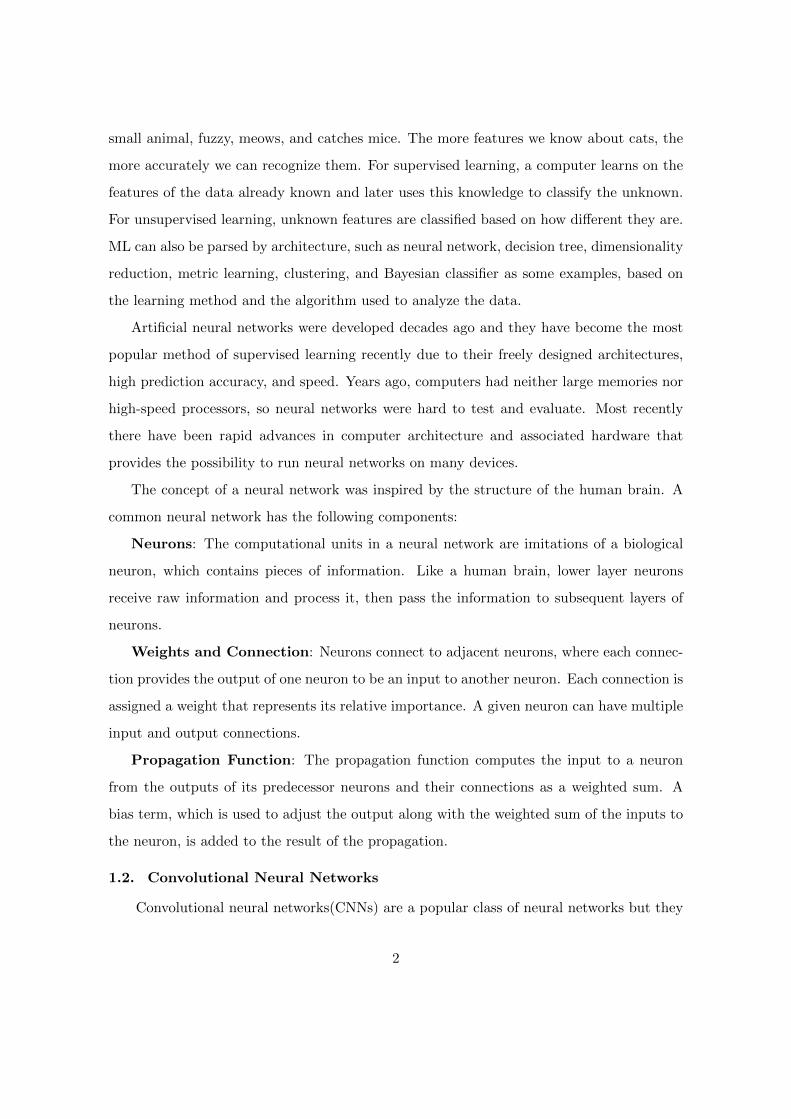
The concept of a neural network was inspired by the structure of the human brain. A

common neural network has the following components:

Neurons: The computational units in a neural network are imitations of a biological

neuron, which contains pieces of information. Like a human brain, lower layer neurons

receive raw information and process it, then pass the information to subsequent layers of

neurons.

Weights and Connection: Neurons connect to adjacent neurons, where each connec-

tion provides the output of one neuron to be an input to another neuron. Each connection is

assigned a weight that represents its relative importance. A given neuron can have multiple

input and output connections.

Propagation Function: The propagation function computes the input to a neuron

from the outputs of its predecessor neurons and their connections as a weighted sum. A

bias term, which is used to adjust the output along with the weighted sum of the inputs to

the neuron, is added to the result of the propagation.

1.2. Convolutional Neural Networks

Convolutional neural networks(CNNs) are a popular class of neural networks but they

2

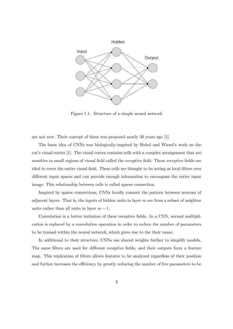
Figure 1.1. Structure of a simple neural network

are not new. Their concept of them was proposed nearly 30 years ago [1].

The basic idea of CNNs was biologically-inspired by Hubel and Wiesel’s work on the

cat’s visual cortex [1]. The visual cortex contains cells with a complex arrangement that are

sensitive to small regions of visual field called the receptive field. Those receptive fields are

tiled to cover the entire visual field. These cells are thought to be acting as local filters over

different input spaces and can provide enough information to encompass the entire input

image. This relationship between cells is called sparse connection.

Inspired by sparse connections, CNNs locally connect the pattern between neurons of

adjacent layers. That is, the inputs of hidden units in layer m are from a subset of neighbor

units rather than all units in layer m− 1.

Convolution is a better imitation of these receptive fields. In a CNN, normal multipli-

cation is replaced by a convolution operation in order to reduce the number of parameters

to be trained within the neural network, which gives rise to the their name.

In additional to their structure, CNNs use shared weights further to simplify models.

The same filters are used for different receptive fields, and their outputs form a feature

map. This replication of filters allows features to be analyzed regardless of their position

and further increases the efficiency by greatly reducing the number of free parameters to be

3

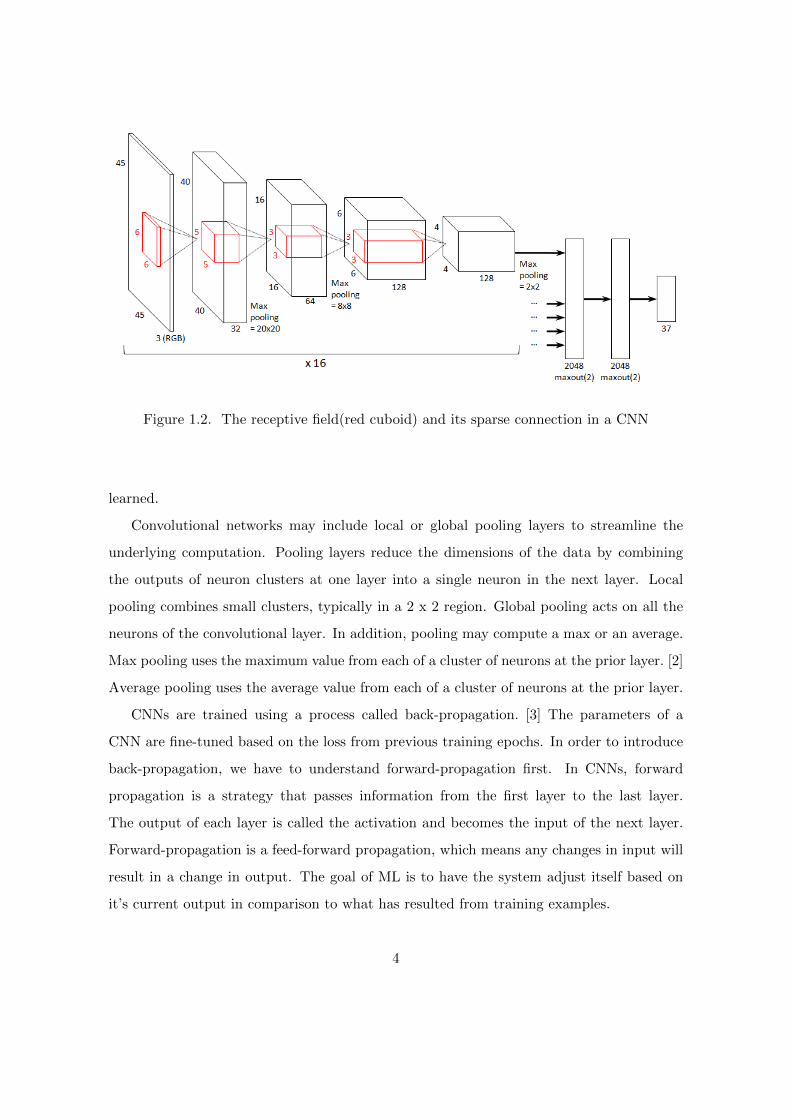
Figure 1.2. The receptive field(red cuboid) and its sparse connection in a CNN

learned.

Convolutional networks may include local or global pooling layers to streamline the

underlying computation. Pooling layers reduce the dimensions of the data by combining

the outputs of neuron clusters at one layer into a single neuron in the next layer. Local

pooling combines small clusters, typically in a 2 x 2 region. Global pooling acts on all the

neurons of the convolutional layer. In addition, pooling may compute a max or an average.

Max pooling uses the maximum value from each of a cluster of neurons at the prior layer. [2]

Average pooling uses the average value from each of a cluster of neurons at the prior layer.

CNNs are trained using a process called back-propagation. [3] The parameters of a

CNN are fine-tuned based on the loss from previous training epochs. In order to introduce

back-propagation, we have to understand forward-propagation first. In CNNs, forward

propagation is a strategy that passes information from the first layer to the last layer.

The output of each layer is called the activation and becomes the input of the next layer.

Forward-propagation is a feed-forward propagation, which means any changes in input will

result in a change in output. The goal of ML is to have the system adjust itself based on

it’s current output in comparison to what has resulted from training examples.

4

Figure 1.3. Example of max-pooling

Back-propagation is a process whereby the parameters of a CNN are updated according

to the difference between the network’s output labels and the labels it is supposed to

produce. The difference is the error and the measure of the total error is the loss. We

take the derivative of the loss with respect to the parameters and subtract a portion of that

gradient from the old parameters to obtain the new parameters in an iterative process.

The underlying approach to training is called stochastic gradient descent, often abbre-

viated as SGD. It is an iterative method for optimizing an objective function with suitable

smoothness properties. It can be regarded as a stochastic approximation of gradient descent

optimization, since it replaces the actual gradient calculated from the entire data set by an

estimate thereof calculated from a randomly selected subset of the data. Especially in big

data applications, this reduces the computational burden, achieving faster computational

iterations.

The mathematical expression of SGD is:

Wnew = Wold − µ∂Loss(Wold)

∂Wold(1.1)

where W are the weight matrices, and the parameter µ is the step size. Then, as the loss

5

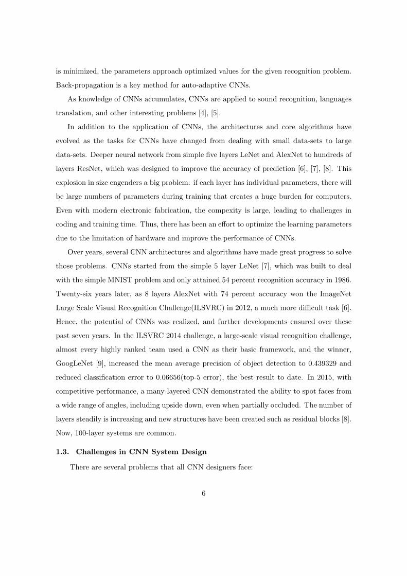
is minimized, the parameters approach optimized values for the given recognition problem.

Back-propagation is a key method for auto-adaptive CNNs.

As knowledge of CNNs accumulates, CNNs are applied to sound recognition, languages

translation, and other interesting problems [4], [5].

In addition to the application of CNNs, the architectures and core algorithms have

evolved as the tasks for CNNs have changed from dealing with small data-sets to large

data-sets. Deeper neural network from simple five layers LeNet and AlexNet to hundreds of

layers ResNet, which was designed to improve the accuracy of prediction [6], [7], [8]. This

explosion in size engenders a big problem: if each layer has individual parameters, there will

be large numbers of parameters during training that creates a huge burden for computers.

Even with modern electronic fabrication, the compexity is large, leading to challenges in

coding and training time. Thus, there has been an effort to optimize the learning parameters

due to the limitation of hardware and improve the performance of CNNs.

Over years, several CNN architectures and algorithms have made great progress to solve

those problems. CNNs started from the simple 5 layer LeNet [7], which was built to deal

with the simple MNIST problem and only attained 54 percent recognition accuracy in 1986.

Twenty-six years later, as 8 layers AlexNet with 74 percent accuracy won the ImageNet

Large Scale Visual Recognition Challenge(ILSVRC) in 2012, a much more difficult task [6].

Hence, the potential of CNNs was realized, and further developments ensured over these

past seven years. In the ILSVRC 2014 challenge, a large-scale visual recognition challenge,

almost every highly ranked team used a CNN as their basic framework, and the winner,

GoogLeNet [9], increased the mean average precision of object detection to 0.439329 and

reduced classification error to 0.06656(top-5 error), the best result to date. In 2015, with

competitive performance, a many-layered CNN demonstrated the ability to spot faces from

a wide range of angles, including upside down, even when partially occluded. The number of

layers steadily is increasing and new structures have been created such as residual blocks [8].

Now, 100-layer systems are common.

1.3. Challenges in CNN System Design

There are several problems that all CNN designers face:

6

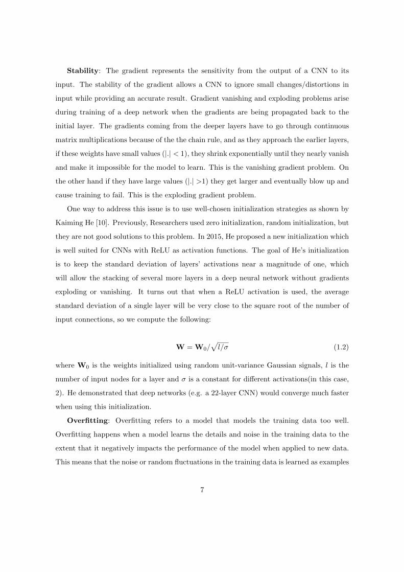
Stability: The gradient represents the sensitivity from the output of a CNN to its

input. The stability of the gradient allows a CNN to ignore small changes/distortions in

input while providing an accurate result. Gradient vanishing and exploding problems arise

during training of a deep network when the gradients are being propagated back to the

initial layer. The gradients coming from the deeper layers have to go through continuous

matrix multiplications because of the the chain rule, and as they approach the earlier layers,

if these weights have small values (|.| < 1), they shrink exponentially until they nearly vanish

and make it impossible for the model to learn. This is the vanishing gradient problem. On

the other hand if they have large values (|.| >1) they get larger and eventually blow up and

cause training to fail. This is the exploding gradient problem.

One way to address this issue is to use well-chosen initialization strategies as shown by

Kaiming He [10]. Previously, Researchers used zero initialization, random initialization, but

they are not good solutions to this problem. In 2015, He proposed a new initialization which

is well suited for CNNs with ReLU as activation functions. The goal of He’s initialization

is to keep the standard deviation of layers’ activations near a magnitude of one, which

will allow the stacking of several more layers in a deep neural network without gradients

exploding or vanishing. It turns out that when a ReLU activation is used, the average

standard deviation of a single layer will be very close to the square root of the number of

input connections, so we compute the following:

W = W0/√l/σ (1.2)

where W0 is the weights initialized using random unit-variance Gaussian signals, l is the

number of input nodes for a layer and σ is a constant for different activations(in this case,

2). He demonstrated that deep networks (e.g. a 22-layer CNN) would converge much faster

when using this initialization.

Overfitting: Overfitting refers to a model that models the training data too well.

Overfitting happens when a model learns the details and noise in the training data to the

extent that it negatively impacts the performance of the model when applied to new data.

This means that the noise or random fluctuations in the training data is learned as examples

7

by the model. The problem is that these examples do not apply to new data and negatively

impact the model’s ability to generalize.

In order to address this problem, several approaches have been developed:

1). Using a very large input data-set. A large data-set includes more details to be

learned, which enables the network to better ignore the noise and better to recognize all the

features. However, training a neural network with a large data-set as input greatly increases

training time.

2). Introduce dropout [11]. Dropout, which refers to randomly ignoring neurons in neu-

ral networks during training, prevents units from co-adapting too much. This significantly

reduces overfitting and provides some improvement. Dropout roughly doubles the number

of iterations required to converge. However, training time for each epoch is less.

3). Using a well-designed weight regularization. A weight regularization will add a cost

to the loss function of the network for large weights. As a result, the model is simplified

and will be forced to learn only the relevant patterns in the train data.

Orthogonality preserves the energy for a filter bank in signal processing. One idea

is to impose orthogonality on a CNN to stabilize the gradient. Actually, a orthogonal

initialization of each layer’s parameters already has made a breakthrough for this problem

[12].

1.4. Contribution of Thesis

This thesis proposes a new class of iterative orthogonalization methods called stochastic

orthogonalization, which are designed to make the columns of matrices to be orthogonal.

It is designed for large-scale matrices orthogonalization. When applied to large matrices,

our method saves computations at each iteration.

Unlike common iterative orthogonal algorithms that change the gradient update function

directly, we impose orthogonality by using a stochastic version of a loss function. Based

on our first algorithm, we also derive two similar algorithms, one of which has even less

computational complexity.

Then we apply our stochastic orthogonalization to Machine Learning training, specif-

ically the training of CNNs, and have obtained encouraging results. As designed, our

8

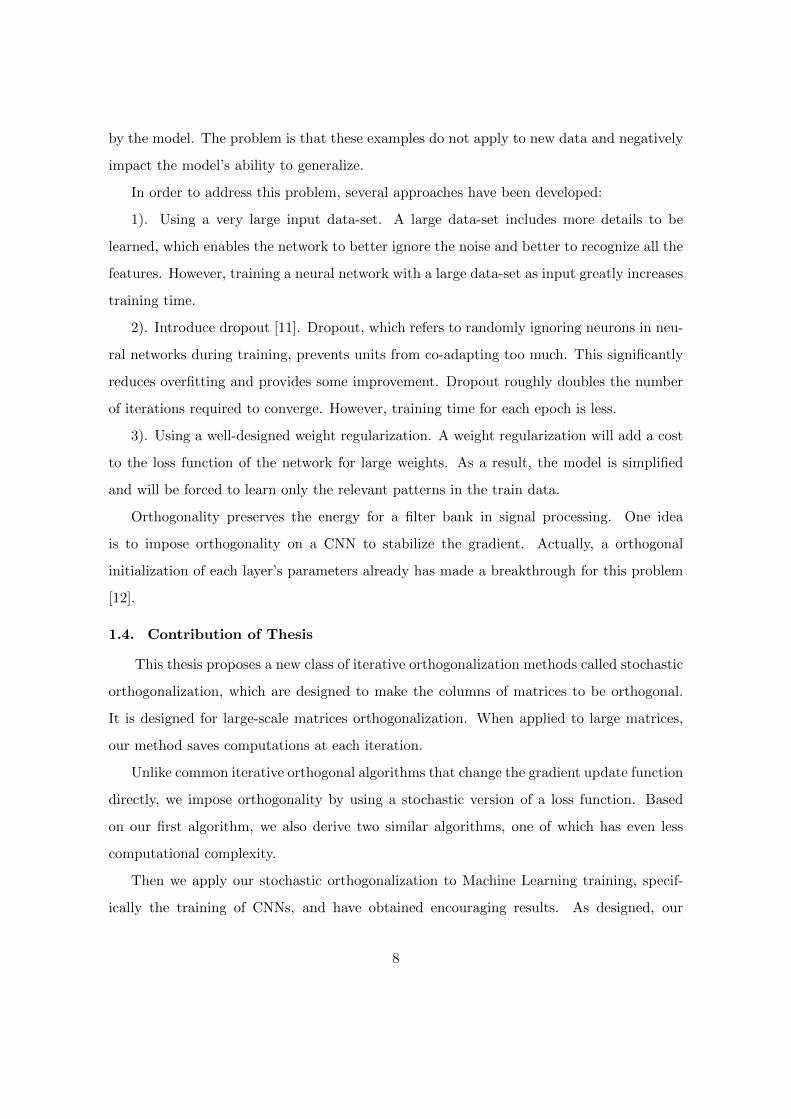
method runs faster than a well-performing algorithm in [13], which imposes orthogonality

by introducing an additional cost to cost function, and also exhibits better accuracy.

1.5. Outline of Thesis

Chapter 2 introduces the theory of orthogonal matrices and reviews its application in

Principal Component Analysis(PCA), Independent Component Analysis(ICA), and neural

networks. Then we review the use of advanced orthogonalization algorithms applied to

CNNs.

Chapter 3 presents the derivation of the stochastic orthogonalization methods and de-

rives three new algorithms based on it. We show those algorithm’s strengths and weaknesses.

In Chapter 4, stochastic orthogonalization is imposed to one of the modern convolutional

neural networks, ResNet. We analyse the performance of the method and make comparisons

to algorithms of others.

Chapter 5 presents the conclusions and briefly describes future work.

9

CHAPTER 2

PRINCIPLES OF ORTHOGONALITY

2.1. Overview of Orthogonality

The term orthogonal is derived from a Greek word ’othogonios’——-’ortho’ means right

and ’gon’ means angle. Orthogonality, the synonym to perpendicularity, has been studied in

linear algebra, Euclidean geometry, and spherical trigonometry for a long time. In Euclidean

space, two lines are orthogonal when they are perpendicular at their intersection point. Two

vectors are orthogonal if and only if the inner product is zero, or

aTb = 0,

where a and b are vectors in an n-dimensional Euclidean space. Orthogonality can be

extended as a concept to sets of vectors. These concepts can be extended further. For

example, for two matrices A and B, if each vector in A is orthogonal to each vector in B,

we call them jointly orthogonal matrices; such that ATB = 0

In some cases, normal could also be used to augment orthogonal. The term, orthonor-

mality, is an extension of orthogonality to unit length vectors. In linear algebra, two vectors

in an inner product space are orthonormal if they are orthogonal and are each of unit length.

This leads to a concept of an orthonormal matrix. A n×m matrix A is orthonormal if

ATA = I (2.1)

where AT is the transpose of matrix A and I is a m ×m identity matrix. That means, if

A is also square, m = n, the matrix A is always invertible such that

A−1 = AT (2.2)

Thus, in this case,

AAT = I. (2.3)

10

In addition, the columns of an orthogonal matrix come from an orthogonal subspace. That

is, columns of an orthogonal matrix are mutually perpendicular.

Orthonormality also has a strong relationship with the singular value decomposition(SVD)

in linear algebra. SVD is an approach to factorize a real or complex matrix, to obtain a

specific decomposition. Suppose W is a matrix in real space Rn×m. Then, the singular

value decomposition of W has the form:

W = UΣVT (2.4)

where U is a unitary matrix, whose inverse equals it conjugate transpose, and the n × n

orthogonal matrix, V is also a unitary and m ×m orthogonal matrix , and Σ is a unique

diagonal matrix with non-negative real singular values on the diagonal where the singular

values are placed in descending order.

Orthogonality and orthonormality are important mathematical properties for vectors

and matrices, and they have been explored in some detection and estimation tasks.

For example, PCA, a statistical factor analysis procedure, uses an orthogonal transfor-

mation to convert a large set of possibly correlated variables into a small set of linearly

uncorrelated variables to maintain the important information among a large data set. The

smaller-dimensional data-set are called principal components. Mathematically, the trans-

formation could be defined by a set of m n-dimensional vectors of weights wi in a matrix

W = [w1 w2 ... wm]. Given a set of vector x(n), 1 ≤ n ≤ N , PCA maps each vector to a

new vector of principal components y as:

y(n) = WTx(n) (2.5)

Developed in 1901 by Karl Pearson [14], PCA has been refined over the last century. Now,

PCA is applied in many fields as an exploratory data analysis method, and we can build

predictive models based on it [15].

Orthogonality also plays an important role in independent component analysis (ICA).

ICA is a computational method to separate a set of mixed signals and transform them to

11

many independent components. ICA is based on a linear mixing model of the form

x(n) = Ws(n) (2.6)

where s(n) is an m-dimensional set of independent signals and W is an n×m mixing matrix.

The goal is to separate the mixed signals in x(n) using a linear transformation. When a

prewhitening step is performed, it turns out that the matrix W has orthonormal columns,

such that a separation step of the form

y(n) = WTx(n) (2.7)

can be used.

For both PCA and ICA, we use weight vectors W = [w1 w2 ... wm] to represent the

orthogonal transformation, and these weight vectors have the property:

wTi wj =

1 i = j

0 i 6= j

. (2.8)

In the case of ICA, these constraints are imposed in certain algorithms, such as the

well-known FastICA algorithm [16], to solve a joint diagonalization task. More recently,

orthonormality has been proposed as a parameter constraint to improve the performance

of both recurrent neural networks and deep learning systems for real-world classification

tasks [17], an issue we will consider in depth in this thesis.

Since the orthogonality transformation is important, the ways of imposing orthogonality

on vectors have been extensively explored. Orthogonal weight matrices render analysis easy

and are an important property of these matrices, but we are usually given an non-orthogonal

matrix. So, an algorithm is necessary to transform W to an orthogonal set, WTnewWnew = I,

is required. The most well-known approach is the Gram-Schmidt procedure [18]. Given any

vector set w, the Gram-Schmidt orthogonalization process can form an orthogonal set wnew

as

wk = wk − (α1,kw1,new + ...+ αk−1,kwk−1,new), 1 ≤ k ≤ n (2.9)

αj,k = wTj,newwk (2.10)

12

wk,new =wk

||wk||(2.11)

Based on the knowledge of SVD, there is a better approach to imposing orthonormality on

the matrix W. From Eqn(2.4), we know the left and right singular vectors of U and V are

orthogonal vectors and have unit length. So if we want to make an arbitrary matrix W

orthogonal, we can do:

Wnew = UmVT (2.12)

where U and V are computed from the original W, Um is composed of the first m columns

of U, and the new W is also orthonormal.

The concept of this SVD-based orthonormalization method is easy though it is hard to

do the computation. Fortunately, there is an iterative way to implement it. One simple

Newton-based approach is [19]

Wnew =3

2W − 1

2WWTW (2.13)

The above iterative equation converges fast and finally fulfill Wfinal = UmVT .

Joint orthogonality of a set of vectors plays an important role in many estimation,

detection, and classification tasks. In signal processing, orthogonality is employed in di-

mensionality reduction when searching for signal or noise subspaces, in the design of filter

banks for signal coding tasks [20], [21], and in the specification of beamformers for array

processing systems [22]. In these applications, classic techniques for orthogonalization are

often used.

Recently, coefficient orthogonality has been leveraged to improve the performance of

deep learning architectures when applied to classification tasks. In this application, or-

thogonality is used to influence the adaptation of each weight matrix W associated with

a specific layer within the architecture. In [23], random orthogonal weight matrix initial-

ization is indicated to provide depth-independent learning dynamics; additional studies on

orthogonal matrix initialization are in [12] [24]. Numerous works have sought to impose

some measure of orthogonality on the weight matrices during adaptation as well, usually by

augmenting the cost function at each layer with an additional term λJ (W), where J (W)

is the orthogonality regularization cost and λ is its associated weight for the given layer at

13

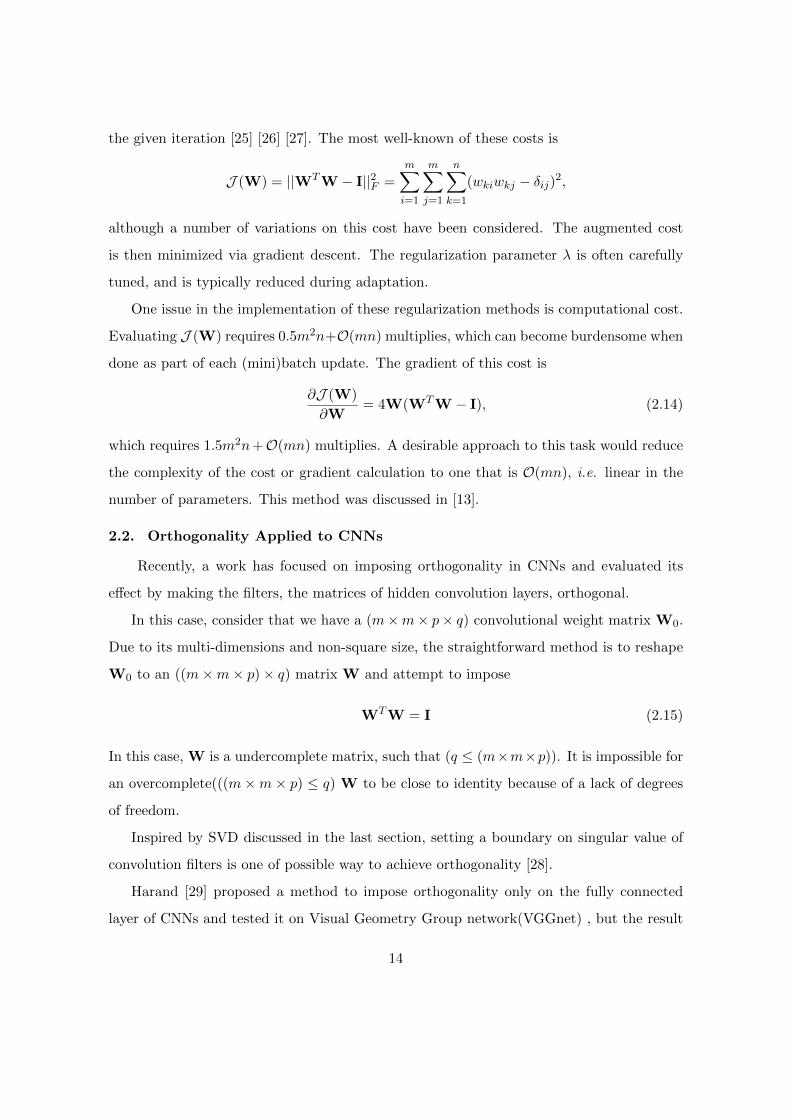
the given iteration [25] [26] [27]. The most well-known of these costs is

J (W) = ||WTW − I||2F =m∑i=1

m∑j=1

n∑k=1

(wkiwkj − δij)2,

although a number of variations on this cost have been considered. The augmented cost

is then minimized via gradient descent. The regularization parameter λ is often carefully

tuned, and is typically reduced during adaptation.

One issue in the implementation of these regularization methods is computational cost.

Evaluating J (W) requires 0.5m2n+O(mn) multiplies, which can become burdensome when

done as part of each (mini)batch update. The gradient of this cost is

∂J (W)

∂W= 4W(WTW − I), (2.14)

which requires 1.5m2n+O(mn) multiplies. A desirable approach to this task would reduce

the complexity of the cost or gradient calculation to one that is O(mn), i.e. linear in the

number of parameters. This method was discussed in [13].

2.2. Orthogonality Applied to CNNs

Recently, a work has focused on imposing orthogonality in CNNs and evaluated its

effect by making the filters, the matrices of hidden convolution layers, orthogonal.

In this case, consider that we have a (m×m× p× q) convolutional weight matrix W0.

Due to its multi-dimensions and non-square size, the straightforward method is to reshape

W0 to an ((m×m× p)× q) matrix W and attempt to impose

WTW = I (2.15)

In this case, W is a undercomplete matrix, such that (q ≤ (m×m×p)). It is impossible for

an overcomplete(((m×m× p) ≤ q) W to be close to identity because of a lack of degrees

of freedom.

Inspired by SVD discussed in the last section, setting a boundary on singular value of

convolution filters is one of possible way to achieve orthogonality [28].

Harand [29] proposed a method to impose orthogonality only on the fully connected

layer of CNNs and tested it on Visual Geometry Group network(VGGnet) , but the result

14

is not very good. Inspired by the property of Stiefel manifold, Huang [27] formulated an

Optimization over Multiple Dependent Stiefel Manifolds (OMDSM) and enforced the weight

filters across channels in convolutional layers to be orthogonal. However, this approach did

not improve the performance of the CNN and lead to a slow training resulting from many

SVD computations.

In [30], an approximation of the reshaped weight W is used through a singular value

study. The original 4-d weight matrices were reshaped to 2-d weight matrices and the

largest singular value was used for their orthogonal regularization.

The above method for specifying the matrix W for CNNs does not take into account

the operator norm of the linear transformation associated with the filters in the matrix W

in each layer. In [28], the authors consider this linear transformation, expanding each filter

to the same size as the that of the input features via Fourier transformation. Then, they

compute the singular values of the filters. Their work shows that a well-performing CNN

does not impose orthogonality on the filter operations. Instead, singular values are bounded

but not restricted to values near unity.

Figure 2.1. Plot of the singular values of the linear operators associated with the convolu-

tional layers of the pretrained ”ResNetV2” from the TensorFlow website.

Figure 2.1 shows the singular values of 4-d weight filters from some chosen convolutional

15

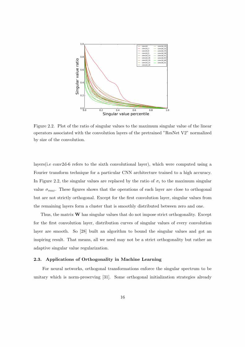
Figure 2.2. Plot of the ratio of singular values to the maximum singular value of the linear

operators associated with the convolution layers of the pretrained ”ResNet V2” normalized

by size of the convolution.

layers(i.e conv2d-6 refers to the sixth convolutional layer), which were computed using a

Fourier transform technique for a particular CNN architecture trained to a high accuracy.

In Figure 2.2, the singular values are replaced by the ratio of σi to the maximum singular

value σmax. These figures shows that the operations of each layer are close to orthogonal

but are not strictly orthogonal. Except for the first convolution layer, singular values from

the remaining layers form a cluster that is smoothly distributed between zero and one.

Thus, the matrix W has singular values that do not impose strict orthogonality. Except

for the first convolution layer, distribution curves of singular values of every convolution

layer are smooth. So [28] built an algorithm to bound the singular values and got an

inspiring result. That means, all we need may not be a strict orthogonality but rather an

adaptive singular value regularization.

2.3. Applications of Orthogonality in Machine Learning

For neural networks, orthogonal transformations enforce the singular spectrum to be

unitary which is norm-preserving [31]. Some orthogonal initialization strategies already

16

showed advantages in neural network training [32]. The benefit of imposing orthogonality

have been proved on RNN and DNN [33]. Recently, researchers have been trying to improve

CNN by imposing orthogonal constraints, normalization and regularization.

Orthogonal matrices have been actively explored in Recurrent Neural Networks(RNNs).

[33], [17], [34]. Orthogonality helps to avoid the gradient vanishing and explosion problems

in RNNs due to its energy preservation property [35]. However, the orthogonal matrix

here is limited to be square for the hidden-to-hidden transformations in RNNs. The more

general setting of the learning of orthogonal rectangular matrix is not well studied in DNNs

[29],especially in deep Convolutional Neural Networks [26].

Recently several works [29] [25] [13] have shown that imposing orthogonal regularization

or constraints throughout training lead to an encouraging result. In [8], an initialization

method which pre-initialize weights of each convolution layer with orthonormal matrices is

proposed. In [25], an algorithm constraining the weight matrices in the orthogonal feasible

set during the entire whole process of network training is proposed, which is achieved by

singular value bounding.

Bansal at el [13] proposed an orthonormal regularization to improve the accuracy and

training speed of deep ResNet. The researchers added a regularization to the loss function of

CNNs and through training the loss function would be minimized such that orthogonality

is imposed to the system. They tested their orthogonality regularization on ImageNet,

CIFAR-10, CIFAR-100 and observe the constraints and remarkable accuracy boost (e.g.:

2.31 percent for top-1 accuracy on CIFAR).

Most recently, [36] introduced the algorithms of Orthogonal Deep Neural Networks (Or-

thDNNs) to connect with recent interest of spectrally regularized deep learning methods.

They prove that the optimal bound with respect to the degree of isometry is attained when

each weight matrix has a spectrum of equal singular values. OrthDNNs with weight matri-

ces of orthonormal rows or columns are thus the most straightforward choice. Based on such

analysis, they presented algorithms of strict and approximate OrthDNNs, and propose a

simple yet effective algorithm called Singular Value Bounding. They also proposed Bounded

Batch Normalization, which is a technique to improve accuracy and speed up training, to

17

make compatible use of batch normalization with OrthDNNs. Experiments on benchmark

image classication show the efficiency and robustness of OrthDNNs.

However, a completed examination on the effect of orthogonality to CNNs and reasonable

theory remains missing.

This thesis shows a new adaptive orthogonal regularization method, stochastic orthogo-

nalization, which is inspired by a well-know orthogonalization algorithm in signal processing,

could improve the performance of CNNs. It maintains the high accuracy while requiring

less training time each iteration.

2.4. Other Orthogonal Regularization

Bansal et al [13] proposed a good orthogonality implementation method which can be in-

corporated with other advanced strategies such as He-normalization or batch-normalization,

in almost any architecture of CNNs. In their paper, three means of implementating orthog-

onality were disscussed and tested on three state-of-the-art of CNNs: ResNet, ResNeXt and

WideResNet. Remarkable accuracy improvement on accuracy was observed with a fast and

stable convergence. This method can enforce orthogonality on non-squared weight matrices

without changing the architecture of the original CNN. Their work show that orthogonality

still provides significant potential to improve the performance of CNNs.

Among three type of orthogonal constraints they discussed, the Spectrum Restricted

Isometry Property (SRIP) based method works best for large and deeper CNNs. The

mechanism [13] uses to impose orthogonality on the weight matrix of a convolutional layer

is to add a term σ(WTW − I) to the original loss function of the CNN, where W is the

reshaped weight matrix. Assume the weight matrix M ∈ RN×N×I×O is a 4-dimensional

matrix, where N , I, O denotes the weights length( weights heights usually equals weight

length in a convolutional layer), number of input channels, number of output channels.

Then M is reshaped to W with shape m by n, where m = N ×N × I and n = O.

The RIP condition assumes the following:

For all vector z ∈ Rn that is k-sparse, there exists a small δw ∈ (0, 1) s.t (1−δw) ≤ ‖Wz‖‖z‖

With every set of columns of weight matrices W no larger than k, it shall behave like a

orthogonal system.

18

Especially when k = n, the entire W would be close to orthogonal according to to RIP.

In this case, the RIP equation we mentioned above could be rewritten as∣∣∣∣‖Wz‖‖z‖

− 1

∣∣∣∣ ≤ δw (2.16)

They defined the spectral norm of weight matrices W as σ(W) = ‖Wz‖‖z‖ . So the spectral

norm of the term WTW − I is σ(WTW − I) = |‖Wz‖‖z‖ − 1|. Notice that when W is

approaching orthogonality, σ(WTW − I) is also approaching zero, so it is claimed that

enforcing orthogonality mathematically is equivalent to minimizing the spectral norm of

WTW − I:

(SRIP ) : σ(WTW − I) ≤ δw (2.17)

The above term is added to the original loss function of CNN and through the training

the loss of entire CNN along with σ(WTW − I) is minimized, so the system approaches

orthogonality.

They also introduced a mechanism to reduce the computation of the gradient of SRIP

by initializing a random uniform distributed vector v ∈ Rn and then use the following

procedure:

u0 = (WTW − I)v (2.18)

v1 = (WTW − I)u0 (2.19)

σ(WTW − I) ≈ ‖v1‖‖u0‖

=‖(WTW − I)(WTW − I)v‖

‖(WTW − I)v‖(2.20)

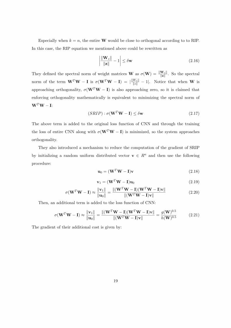
Then, an additional term is added to the loss function of CNN:

σ(WTW − I) ≈ ‖v1‖‖u0‖

=‖(WTW − I)(WTW − I)v‖

‖(WTW − I)v‖=g(W)0.5

h(W)0.5(2.21)

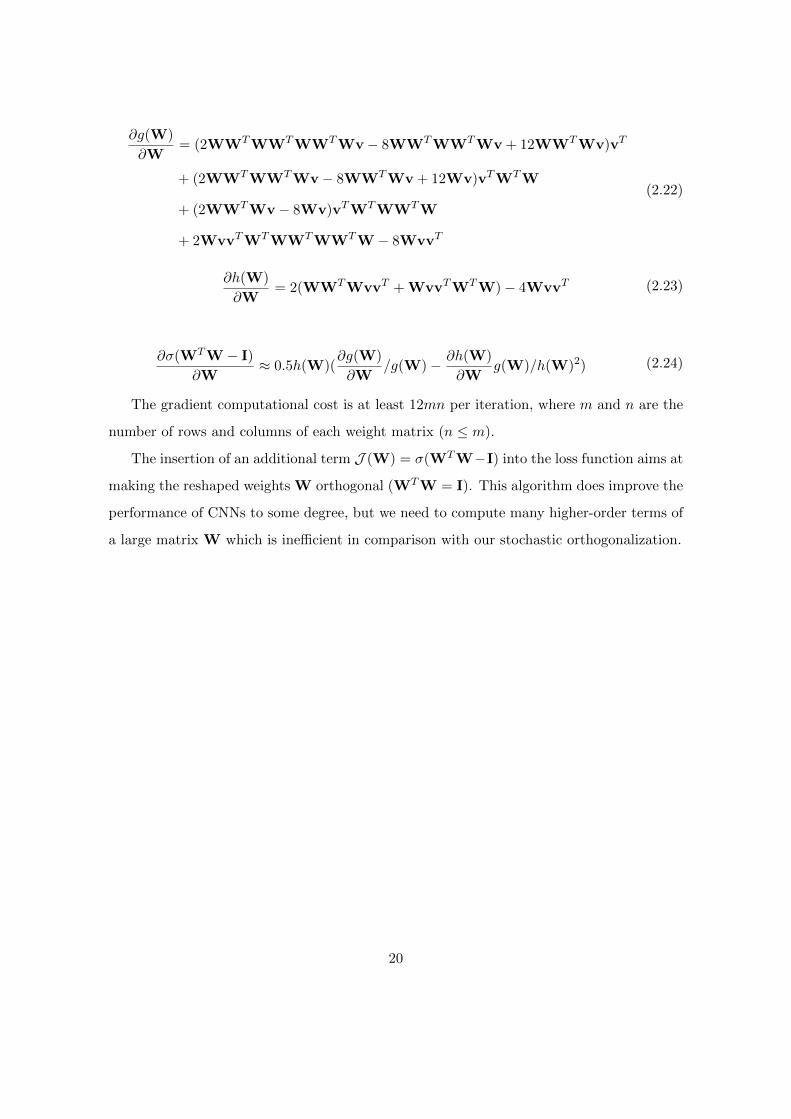
The gradient of their additional cost is given by:

19

∂g(W)

∂W= (2WWTWWTWWTWv− 8WWTWWTWv + 12WWTWv)vT

+ (2WWTWWTWv− 8WWTWv + 12Wv)vTWTW

+ (2WWTWv− 8Wv)vTWTWWTW

+ 2WvvTWTWWTWWTW − 8WvvT

(2.22)

∂h(W)

∂W= 2(WWTWvvT + WvvTWTW)− 4WvvT (2.23)

∂σ(WTW − I)

∂W≈ 0.5h(W)(

∂g(W)

∂W/g(W)− ∂h(W)

∂Wg(W)/h(W)2) (2.24)

The gradient computational cost is at least 12mn per iteration, where m and n are the

number of rows and columns of each weight matrix (n ≤ m).

The insertion of an additional term J (W) = σ(WTW−I) into the loss function aims at

making the reshaped weights W orthogonal (WTW = I). This algorithm does improve the

performance of CNNs to some degree, but we need to compute many higher-order terms of

a large matrix W which is inefficient in comparison with our stochastic orthogonalization.

20

CHAPTER 3

STOCHASTIC ORTHOGONALIZATION

3.1. Introduction

In this chapter, we describe a set of algorithms that perform stochastic orthogonalization

of the columns of a matrix W. These algorithms minimize a stochastic version of J (W)

using m-dimensional uncorrelated signals as part of the processing. In these algorithms,

the inner products of the columns of W are never computed, the lengths of each of the

columns are never computed, and weights are never scaled by any multiplicative factor. In

addition, the computational complexity of each algorithm is linear in the number of entries

of W and is between 3mn+O(m) and 5mn+O(m) multiplications at each iteration. The

theory of stochastic orthogonalization is carefully described, and stability issues regarding

the choice of step size or regularization parameter are considered. Performance comparison

of our proposed method with competing approaches show the viability of the techniques in

deep learning classfication tasks.

3.2. Derivations and Analysis

Three proposed algorithms for stochastic orthogonalization are derived in this section.

We employ a simplified notation whereby all time indices are suppressed. Furthermore,

gradient descent of the matrix W on a specified cost J (W) is represented as

Wnew = W − γ ∂J (W)

∂W, (3.1)

where Wnew are the updated parameters and γ is a chosen step size. With the above

notation, gradient descent on (2.14) with µ = γ/4 yields the well-known iterative Newton-

based algorithm

Wnew = W + µ(W −WWTW

). (3.2)

21

We summarize three existing results about (3.2) below.

1. For µ = 0.5, the algorithm was originally described in [37]. It is an approximate Newton’s

method for this parameter choice and has fast convergence.

2. This algorithm only changes the singular values of W; the left- and right-singular vectors

of W remain unchanged throughout adaptation [19].

3. Let the maximum singular value of the initial value of W be σmax. If

σmax <

√2 + µ

µ, (3.3)

this algorithm causes WTW to converge to I according to the decoupled nonlinear equations

for each singular value of W given by

σi,new =∣∣1 + µ(1− σ2i )

∣∣σi. (3.4)

All algorithms in this chapter approximate (3.2) without direct evaluation of J (W)

or its gradient. These algorithms employ an m-dimensional vector signal sequence x with

uncorrelated elements xi, such that

E{xi} = 0 and E{xxT } = I, (3.5)

where E{·} denotes statistical expectation. Now, for any (m×m) matrix A with diagonal

entries aii, 1 ≤ i ≤ m,

E{xTAx} = tr[A] =m∑i=1

aii. (3.6)

Therefore, let us define

A = (WTW − I)(WTW − I), (3.7)

such that

E{xTAx}=tr[(WTW−I)(WTW−I)]=J (W) (3.8)

Therefore, an equivalent cost to (2.14) above is J (W) = E{xTAx}. Expanding the ex-

pression, we have

xTAx = xTWTWWTWx− 2xTWTWx + xTx

= ||u||2 − 2||y||2 + ||x||2

22

where we have defined

y = Wx, (3.9)

u = WTy = WTWx, (3.10)

v = Wu = WWTWx. (3.11)

Then, we have that

J (W) = E{||u||2 − 2||y||2 + ||x||2}. (3.12)

Eqn. (3.12) is a cost function identical to that in (2.14) that depends on the first- and

second-order statistics of x.

A gradient descent algorithm minimizing the cost in (3.12) can be derived by noting

that1

2

∂{||u||2 − 2||y||2 + ||x||2}∂W

= WxxTWTW + WWTWxxT−2WxxT

= y[u− x]T + [v − y]xT .

Therefore, this gradient algorithm is

Wnew=W +µ

2E{y[x− u]T + [y − v]xT }. (3.13)

This algorithm depends on the statistics of x, not on the sequence x itself.

To obtain data-dependent algorithms, we employ the classic approximation used in

stochastic gradient adaptation by dropping the expectation from the above relation. Before

giving the algorithm forms, we also note via a simple analysis that

E{y[x− u]T } = WE{xxT }(I−WTW)

= W(I−WTW).(3.14)

E{[y − v]xT } = W(I−WTW)E{xxT }

= W(I−WTW).(3.15)

Thus, we can describe three algorithms that approximately minimize J (W) in (3.12), each

with slightly different algorithmic complexities (denoted in brackets) and behaviors. Note

that y, u, and v are computed via (3.9)–(3.11) above, where needed.

23

Algorithm 1 [5mn+O(m)]:

Wnew = W +µ

2

(y[x− u]T + [y − v]xT

). (3.16)

Algorithm 2 [3mn+O(m)]:

Wnew = W + µ(y[x− u]T

). (3.17)

Algorithm 3 [4mn+O(m)]:

Wnew = W + µ([y − v]xT

). (3.18)

Remark #1: The three algorithms above preserve the linear span of W in Wnew. However,

unlike (3.2), these algorithms do not maintain the left- and right-singular vectors of W. As

µ is reduced, the deviations between the behaviors of the above algorithms and (3.2) are

reduced.

Remark #2: It is possible to perform an analysis of each update to determine step size

bounds that maintain stability. We shall focus on Algorithm 2 due to its reduced complexity.

We can show after some algebra that Algorithm 2 admits the following update relation on

J (W).

First, we take Algorithm 2 and define y and u as

Wnew = W + µy[x− u]T

y = Wx

u = WTy = WTWx

(3.19)

Then, we square the WTnewWnew − I matrix and take its trace.

WTnewWnew − I = WTW − I + µ

(u[x− u]T + [x− u]uT

)+ µ2||y||2[x− u][x− u]T

(3.20)

24

tr[(WTnewWnew − I)2] = tr[(WTW − I)2]

+ µ2tr[(u[x− u]T + [x− u]uT

) (u[x− u]T + [x− u]uT

)]

+ µ4||y||4tr[[x− u][x− u]T [x− u][x− u]T ]

+ 2µtr[(WTW − I)(u[x− u]T + [x− u]uT

)]

+ 2µ2||y||2tr[(WTW − I)[x− u][x− u]T ]

+ 2µ3||y||2tr[(u[x− u]T + [x− u]uT

)[x− u][x− u]T ]

We define:

e = x− u. (3.21)

Then, the trace becomes:

tr[(WTnewWnew − I)2] = tr[(WTW − I)2]

+ µ2tr[(ueT + euT

) (ueT + euT

)]

+ µ4||y||4tr[eeTeeT ]

+ 2µtr[(WTW − I)(ueT + euT

)]

+ 2µ2||y||2tr[(WTW − I)eeT ]

+ 2µ3||y||2tr[(ueT + euT

)eeT ]

tr[(WTnewWnew − I)2] = tr[(WTW − I)2]

+ 2µ2[||u||2||e||2 + (uTe)2

]+ µ4||y||4||e||4

+ 4µ[uTWTWe− uTe

]+ 2µ2||y||2

[eTWTWe− ||e||2

]+ 4µ3||y||2||e||2uTe

25

Now, since the common cost function uses squared error we set:

||e||2 = J (W)

uTe = uT [x− u]

= ||y||2 − ||u||2

uTWTWe = uTWTW[x− u]

= ||u||2 − ||v||2

eWTWe = [x− u]TWTW[x− u]

= ||y||2 − 2||u||2 + ||v||2.

(3.22)

26

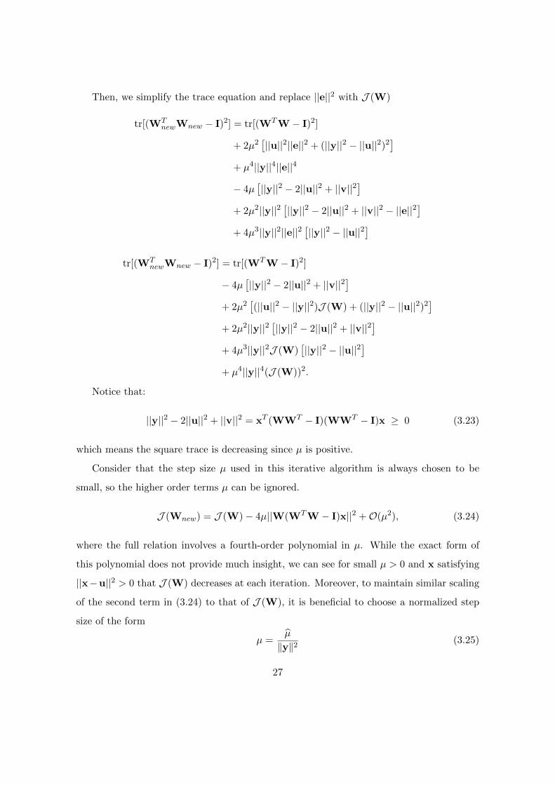
Then, we simplify the trace equation and replace ||e||2 with J (W)

tr[(WTnewWnew − I)2] = tr[(WTW − I)2]

+ 2µ2[||u||2||e||2 + (||y||2 − ||u||2)2

]+ µ4||y||4||e||4

− 4µ[||y||2 − 2||u||2 + ||v||2

]+ 2µ2||y||2

[||y||2 − 2||u||2 + ||v||2 − ||e||2

]+ 4µ3||y||2||e||2

[||y||2 − ||u||2

]tr[(WT

newWnew − I)2] = tr[(WTW − I)2]

− 4µ[||y||2 − 2||u||2 + ||v||2

]+ 2µ2

[(||u||2 − ||y||2)J (W) + (||y||2 − ||u||2)2

]+ 2µ2||y||2

[||y||2 − 2||u||2 + ||v||2

]+ 4µ3||y||2J (W)

[||y||2 − ||u||2

]+ µ4||y||4(J (W))2.

Notice that:

||y||2 − 2||u||2 + ||v||2 = xT (WWT − I)(WWT − I)x ≥ 0 (3.23)

which means the square trace is decreasing since µ is positive.

Consider that the step size µ used in this iterative algorithm is always chosen to be

small, so the higher order terms µ can be ignored.

J (Wnew) = J (W)− 4µ||W(WTW − I)x||2 +O(µ2), (3.24)

where the full relation involves a fourth-order polynomial in µ. While the exact form of

this polynomial does not provide much insight, we can see for small µ > 0 and x satisfying

||x−u||2 > 0 that J (W) decreases at each iteration. Moreover, to maintain similar scaling

of the second term in (3.24) to that of J (W), it is beneficial to choose a normalized step

size of the form

µ =µ

‖y‖2(3.25)

27

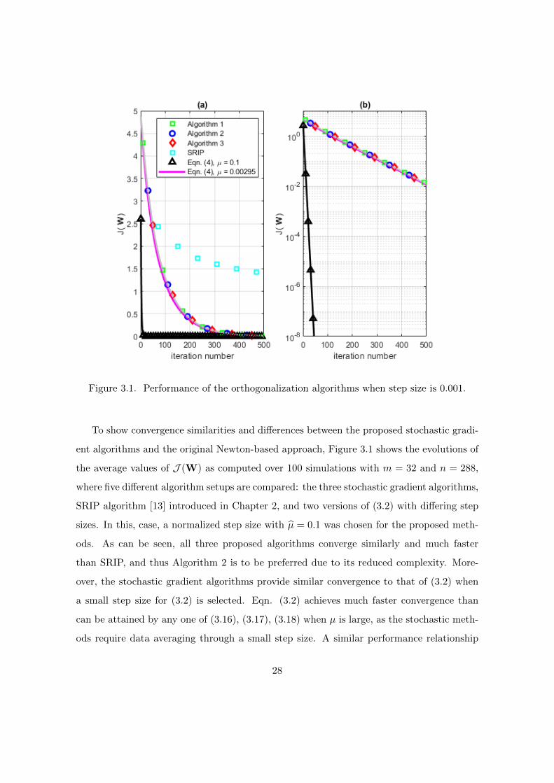
Figure 3.1. Performance of the orthogonalization algorithms when step size is 0.001.

To show convergence similarities and differences between the proposed stochastic gradi-

ent algorithms and the original Newton-based approach, Figure 3.1 shows the evolutions of

the average values of J (W) as computed over 100 simulations with m = 32 and n = 288,

where five different algorithm setups are compared: the three stochastic gradient algorithms,

SRIP algorithm [13] introduced in Chapter 2, and two versions of (3.2) with differing step

sizes. In this, case, a normalized step size with µ = 0.1 was chosen for the proposed meth-

ods. As can be seen, all three proposed algorithms converge similarly and much faster

than SRIP, and thus Algorithm 2 is to be preferred due to its reduced complexity. More-

over, the stochastic gradient algorithms provide similar convergence to that of (3.2) when

a small step size for (3.2) is selected. Eqn. (3.2) achieves much faster convergence than

can be attained by any one of (3.16), (3.17), (3.18) when µ is large, as the stochastic meth-

ods require data averaging through a small step size. A similar performance relationship

28

can be found between least-squares methods and the least-mean-square algorithm in lin-

ear adaptive filtering [38] and is to be expected. The overall advantage of the stochastic

gradient methods is the combination of computational simplicity and adequate adaptation

capabilities to achieve the desired performance characteristics.

29

CHAPTER 4

APPLICATION TO DEEP LEARNING

4.1. Description of Experiments

To demonstrate the capabilities of stochastic orthogonalization in deep learning tasks,

we apply the method to ResNet, a popular convolutional neural network architecture, to

evaluate its performance on the CIFAR-10 and CIFAR-100 image classification tasks.

CIFAR-10: The CIFAR-10 dataset consists of 60,000 32× 32 color images of 10 object

categories (50,000 training and 10,000 testing ones). We use raw images without preprocess-

ing. Data augmentation follows the standard manner in [39]: during training, we zero-pad

4 pixels along each image side, and sample a 32× 32 region crop from the padded image or

its horizontal flip; during testing, we use the original non-padded image.

CIFAR-100: This dataset is just like the CIFAR-10, except it has 100 classes containing

600 images each. There are 500 training images and 100 testing images per class. The 100

classes in the CIFAR-100 are grouped into 20 superclasses. Each image comes with a ”fine”

label (the class to which it belongs) and a ”coarse” label (the superclass to which it belongs).

In each case, we employ the original training protocols in all pre-processing steps, in-

cluding data augmentation, training/validation/testing data splitting, and common step

size schedules.

We use ResNet as our testing architecture. Each network starts with a convolutional

layer of 16 (3 × 3) filters, and then sequentially stacks three types of convolutional layers

of (3 × 3) filters, each of which has the feature map sizes of 32, 16, and 8, and filter

numbers of 16, 32, and 64, respectively; spatial sub-sampling of feature maps is achieved

by convolutional layers of stride 2; the network ends with a global average pooling and a

fully-connected layer [8].

ResNet has a different structure in comparison with common CNNs, such as:

Shortcut: A shortcut connection is inserted which turn the network into its counterpart

30

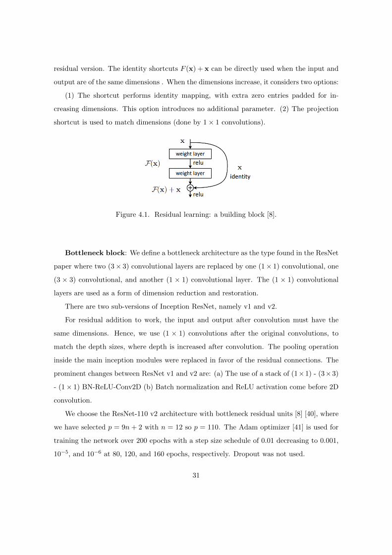
residual version. The identity shortcuts F (x) + x can be directly used when the input and

output are of the same dimensions . When the dimensions increase, it considers two options:

(1) The shortcut performs identity mapping, with extra zero entries padded for in-

creasing dimensions. This option introduces no additional parameter. (2) The projection

shortcut is used to match dimensions (done by 1× 1 convolutions).

Figure 4.1. Residual learning: a building block [8].

Bottleneck block: We define a bottleneck architecture as the type found in the ResNet

paper where two (3× 3) convolutional layers are replaced by one (1× 1) convolutional, one

(3 × 3) convolutional, and another (1 × 1) convolutional layer. The (1 × 1) convolutional

layers are used as a form of dimension reduction and restoration.

There are two sub-versions of Inception ResNet, namely v1 and v2.

For residual addition to work, the input and output after convolution must have the

same dimensions. Hence, we use (1 × 1) convolutions after the original convolutions, to

match the depth sizes, where depth is increased after convolution. The pooling operation

inside the main inception modules were replaced in favor of the residual connections. The

prominent changes between ResNet v1 and v2 are: (a) The use of a stack of (1×1) - (3×3)

- (1× 1) BN-ReLU-Conv2D (b) Batch normalization and ReLU activation come before 2D

convolution.

We choose the ResNet-110 v2 architecture with bottleneck residual units [8] [40], where

we have selected p = 9n + 2 with n = 12 so p = 110. The Adam optimizer [41] is used for

training the network over 200 epochs with a step size schedule of 0.01 decreasing to 0.001,

10−5, and 10−6 at 80, 120, and 160 epochs, respectively. Dropout was not used.

31

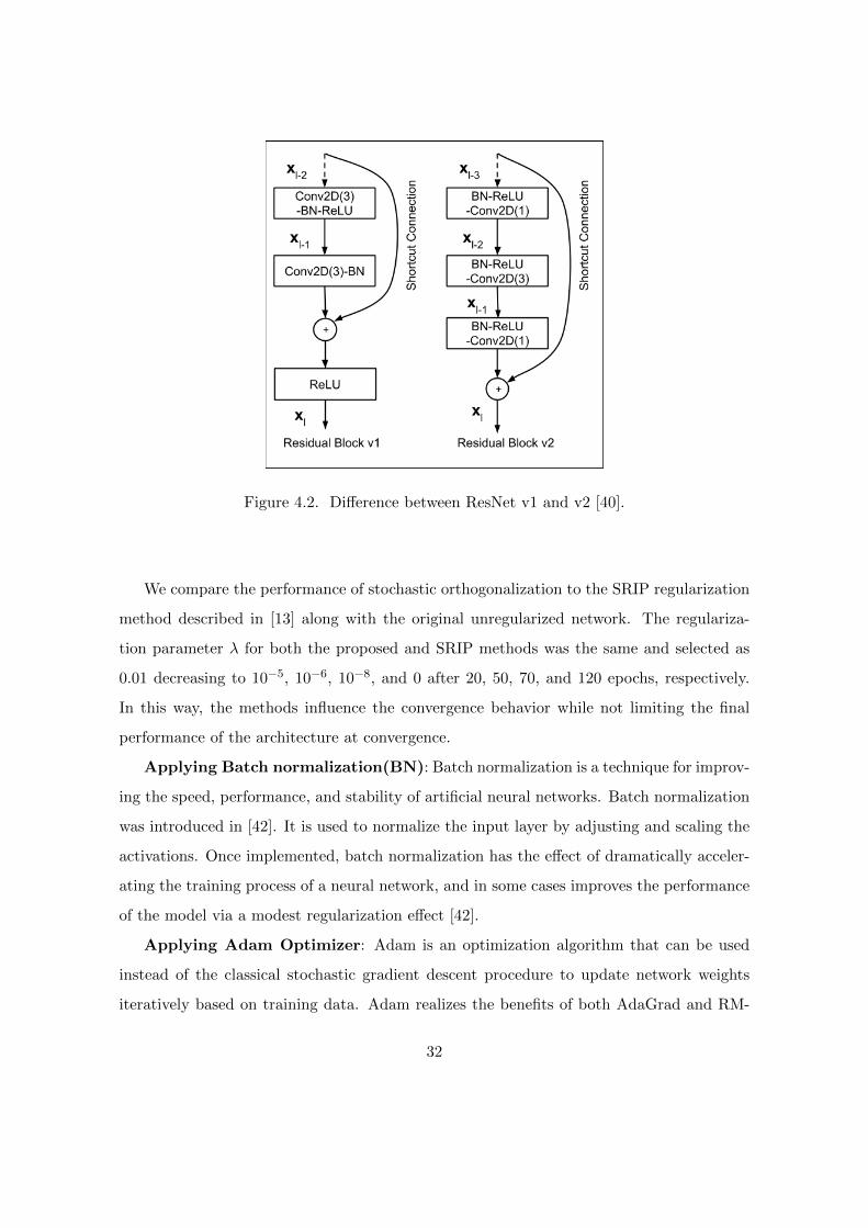
Figure 4.2. Difference between ResNet v1 and v2 [40].

We compare the performance of stochastic orthogonalization to the SRIP regularization

method described in [13] along with the original unregularized network. The regulariza-

tion parameter λ for both the proposed and SRIP methods was the same and selected as

0.01 decreasing to 10−5, 10−6, 10−8, and 0 after 20, 50, 70, and 120 epochs, respectively.

In this way, the methods influence the convergence behavior while not limiting the final

performance of the architecture at convergence.

Applying Batch normalization(BN): Batch normalization is a technique for improv-

ing the speed, performance, and stability of artificial neural networks. Batch normalization

was introduced in [42]. It is used to normalize the input layer by adjusting and scaling the

activations. Once implemented, batch normalization has the effect of dramatically acceler-

ating the training process of a neural network, and in some cases improves the performance

of the model via a modest regularization effect [42].

Applying Adam Optimizer: Adam is an optimization algorithm that can be used

instead of the classical stochastic gradient descent procedure to update network weights

iteratively based on training data. Adam realizes the benefits of both AdaGrad and RM-

32

SProp [43] [44]. Instead of adapting the parameter learning rates based on the average first

moment (the mean) as in RMSProp, Adam also makes use of the average of the second

moments of the gradients (the uncentered variance) [41].

Applying Mini-batch gradient descent: Mini-batch gradient descent is a variation

of the gradient descent algorithm that splits the training dataset into small batches that are

used to calculate model error and update model coefficients. Implementations may choose

to sum the gradient over the mini-batch which further reduces the variance of the gradient.

Mini-batch gradient descent seeks to find a balance between the robustness of stochastic

gradient descent and the efficiency of batch gradient descent. The model update frequency

is higher than batch gradient descent which allows for a more robust convergence, avoiding

local minima. The batching allows both the efficiency of not having all training data in

memory and algorithm implementations.

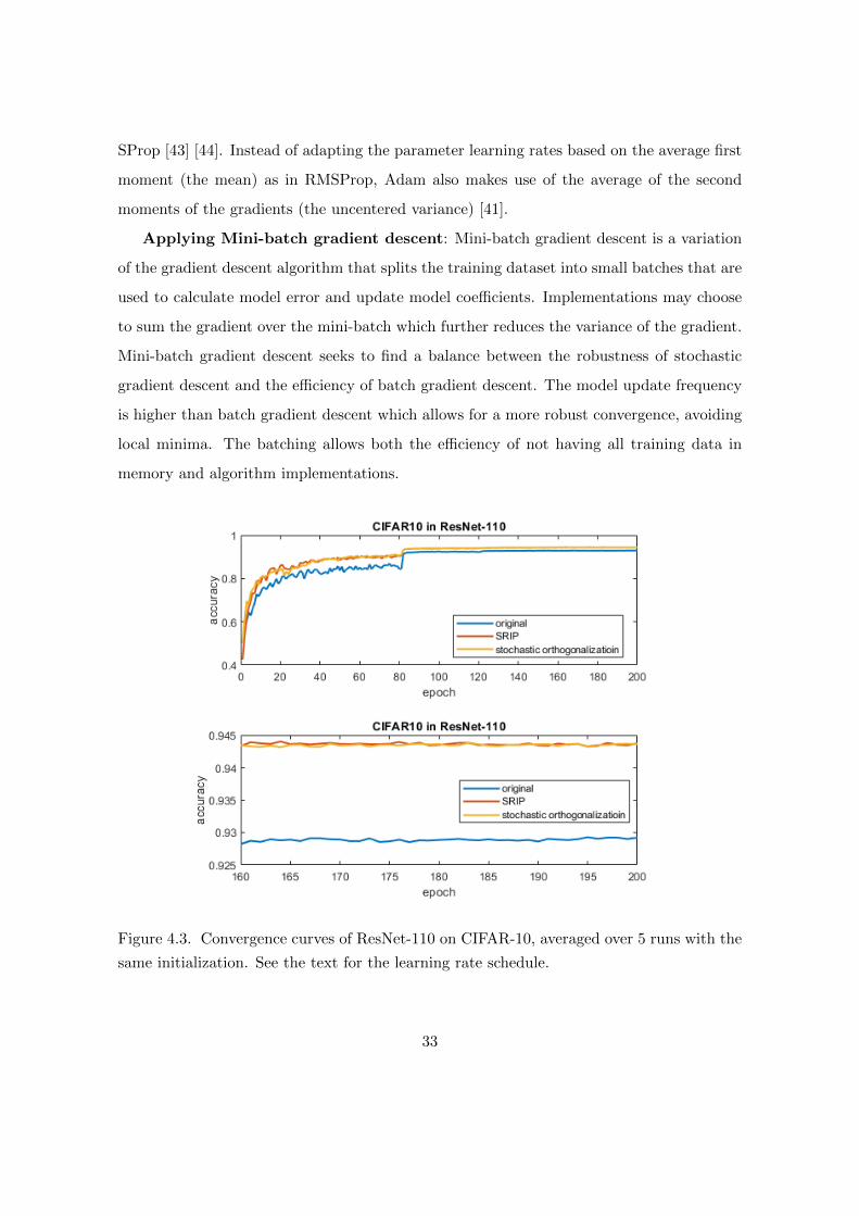
Figure 4.3. Convergence curves of ResNet-110 on CIFAR-10, averaged over 5 runs with the

same initialization. See the text for the learning rate schedule.

33

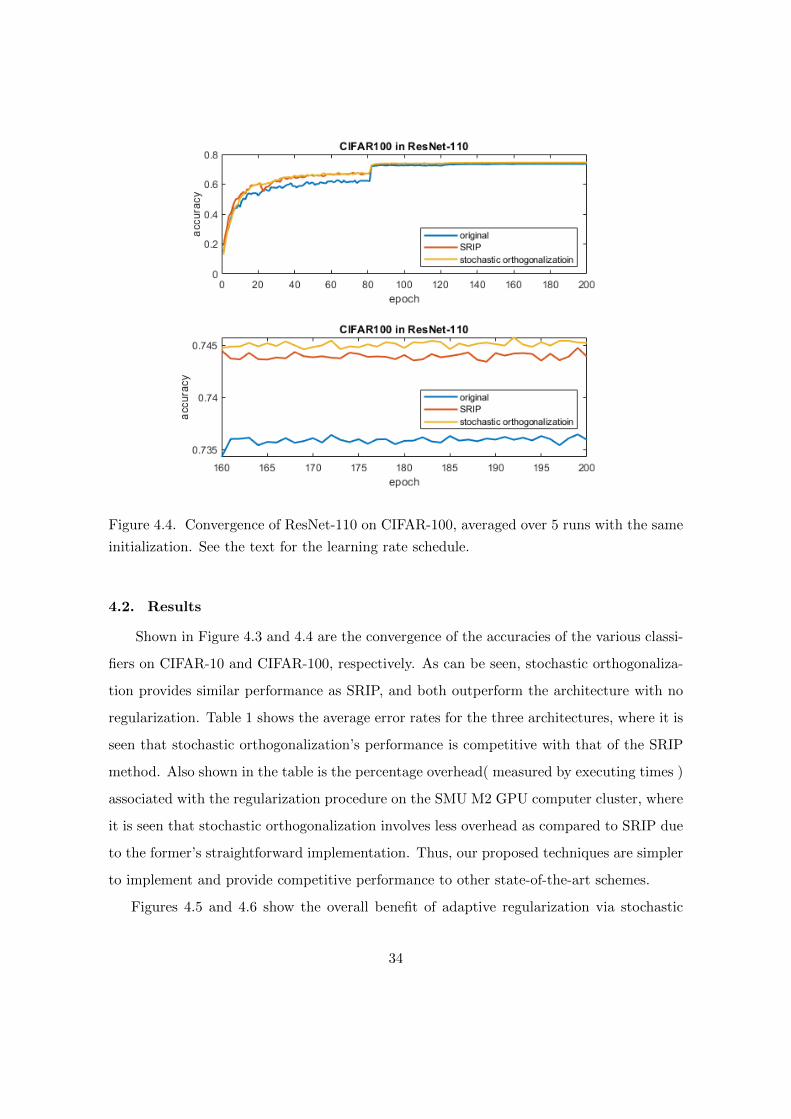
Figure 4.4. Convergence of ResNet-110 on CIFAR-100, averaged over 5 runs with the same

initialization. See the text for the learning rate schedule.

4.2. Results

Shown in Figure 4.3 and 4.4 are the convergence of the accuracies of the various classi-

fiers on CIFAR-10 and CIFAR-100, respectively. As can be seen, stochastic orthogonaliza-

tion provides similar performance as SRIP, and both outperform the architecture with no

regularization. Table 1 shows the average error rates for the three architectures, where it is

seen that stochastic orthogonalization’s performance is competitive with that of the SRIP

method. Also shown in the table is the percentage overhead( measured by executing times )

associated with the regularization procedure on the SMU M2 GPU computer cluster, where

it is seen that stochastic orthogonalization involves less overhead as compared to SRIP due

to the former’s straightforward implementation. Thus, our proposed techniques are simpler

to implement and provide competitive performance to other state-of-the-art schemes.

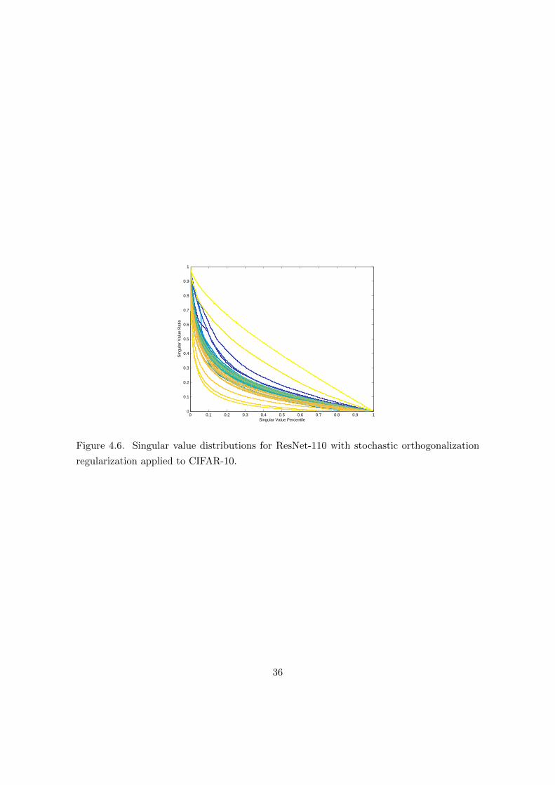
Figures 4.5 and 4.6 show the overall benefit of adaptive regularization via stochastic

34

Regulari- Error Rate (%) Over-

zation CIFAR-10 CIFAR-100 head (%)

None 7.10 26.40 0

SRIP 5.76 25.60 27.9

Stoch. Orth. 5.74 25.50 19.6

Table 4.1. Error rates and overhead (%) for ResNet-110 architectures with and without

regularization.

0 0.1 0.2 0.3 0.4 0.5 0.6 0.7 0.8 0.9 10

0.1

0.2

0.3

0.4

0.5

0.6

0.7

0.8

0.9

1

Singular Value Percentile

Sin

gula

r V

alue

Rat

io

Figure 4.5. Singular value distributions for ResNet-110 with no regularization applied to

CIFAR-10.

orthogonalization. These plots show the singular value ratio defined as σi/σmax for selected

weight matrices W throughout the ResNet-110 architecture applied to CIFAR-10, where

layers closer to the input are plotted with colors with a greater share of blue. As can be

seen, the layers nearest the output in the unregularized system have weight matrices that

are rank-deficient, whereas the system with stochastic orthogonalization regularization has

weight matrices that do not suffer this rank deficiency throughout the architecture. It has

been observed that singular value ratio distributions similar to those shown in Figure 4.6

are an indicator of improved performance in deep learning classification tasks [28].

35

0 0.1 0.2 0.3 0.4 0.5 0.6 0.7 0.8 0.9 10

0.1

0.2

0.3

0.4

0.5

0.6

0.7

0.8

0.9

1

Singular Value Percentile

Sin

gula

r V

alue

Rat

io

Figure 4.6. Singular value distributions for ResNet-110 with stochastic orthogonalization

regularization applied to CIFAR-10.

36

CHAPTER 5

CONCLUSION AND FUTURE WORK

5.1. Conclusion

In this thesis, we have introduced stochastic orthogonalization as a computationally-

simple way to impose regularization on the distributions of the singular values of weight

matrices in convolutional neural networks. The technique appears to work like singular-

value bounding in that it raises low singular values and decreases high singular values.

Unlike other approaches which focus on imposing orthogonality, the methods in this thesis

cause the weight matrices to have a smooth singular value distribution but are not all equal

to unity.

In addition, the methods proposed in this thesis have a low computational cost. Thus,

they are well-suited to deep neural network architectures.

5.2. Future Work

Future work in this area could include the following:

The methods could be tested on a wider range of CNN architectures, such as Wide-

ResNet and ResNext [13]. In some cases, these architectures have a large increase in channels

from layer to layer, causing the weight matrices to be overcomplete when considered in

traditional form. Thus, a modification to stochastic orthogonalization would be needed.

The methods for directly updating the W matrices within each structure could be used

in place of the cost function approach, such that Algorithms 2 and 3 could be tested and

explored for use within CNNs.

Optimization of the weight decay coefficient to improve performance further could be

performed.

37

References

[1] D. H. Hubel and T. N. Wiesel, “Receptive fields and functional architecture of monkey

striate cortex.,” The Journal of physiology, vol. 195 1, pp. 215–43, 1968.

[2] K. Yamaguchi, K. Sakamoto, T. Akabane, and Y. Fujimoto, A neural network for

speaker-independent isolated word recognition. 1990.

[3] Y. LeCun, B. E. Boser, J. S. Denker, D. Henderson, R. E. Howard, W. E. Hubbard,

and L. D. Jackel, Handwritten Digit Recognition with a Back-Propagation Network.

1989.

[4] A. Khamparia, D. K. Gupta, N. G. Nguyen, A. Khanna, B. Pandey, and P. Tiwari,

“Sound classification using convolutional neural network and tensor deep stacking

network,” IEEE Access, vol. 7, pp. 7717–7727, 2019.

[5] Y. Kim, Convolutional Neural Networks for Sentence Classification. 2014.

[6] A. Krizhevsky, I. Sutskever, and G. E. Hinton, ImageNet Classification with Deep

Convolutional Neural Networks. 2012.

[7] Y. LeCun, L. Bottou, Y. Bengio, and P. Haffner, “Gradient-based learning applied to

document recognition,” 1998.

[8] K. He, X. Zhang, S. Ren, and J. Sun, “Deep residual learning for image recognition,”

2016 IEEE Conference on Computer Vision and Pattern Recognition (CVPR),

pp. 770–778, 2015.

[9] C. Szegedy, W. Liu, Y. Jia, P. Sermanet, S. Reed, D. Anguelov, D. Erhan, V. Van-

houcke, and A. Rabinovich, “Going deeper with convolutions,” 2015 IEEE Con-

ference on Computer Vision and Pattern Recognition (CVPR), pp. 1–9, 2014.

[10] K. He, X. Zhang, S. Ren, and J. Sun, “Delving deep into rectifiers: Surpassing human-

level performance on imagenet classification,” 2015 IEEE International Conference

on Computer Vision (ICCV), pp. 1026–1034, 2015.

[11] N. Srivastava, G. E. Hinton, A. Krizhevsky, I. Sutskever, and R. Salakhutdinov,

“Dropout: a simple way to prevent neural networks from overfitting,” J. Mach.

Learn. Res., vol. 15, pp. 1929–1958, 2014.

38

[12] D. Mishkin and J. E. S. Matas, “All you need is a good init,” CoRR,

vol. abs/1511.06422, 2015.

[13] N. Bansal, X. Chen, and Z. Wang, “Can we gain more from orthogonality regulariza-

tions in training deep networks?,” in NeurIPS, 2018.

[14] K. Pearson, “Liii. on lines and planes of closest fit to systems of points in space,” The

London, Edinburgh, and Dublin Philosophical Magazine and Journal of Science

(Series 6), pp. 559–572, 1901.

[15] K. I. Diamantaras and S.-Y. Kung, “Principal component neural networks: Theory

and applications,” 1996.

[16] A. Hyvarinen and E. Oja, “A fast fixed-point algorithm for independent component

analysis,” Neural Computation, vol. 9, pp. 1483–1492, 1997.

[17] S. Wisdom, T. Powers, J. R. Hershey, J. L. Roux, and L. E. Atlas, “Full-capacity

unitary recurrent neural networks,” in NIPS, 2016.

[18] G. H. Golub and C. V. Loan, “Matrix computations (3rd ed.),” 1996.

[19] S. Douglas, “On the singular value manifold and numerical stabilization of algorithms

with orthogonality constraints,” Fourth IEEE Workshop on Sensor Array and

Multichannel Processing, 2006., pp. 195–199, 2006.

[20] P. P. Vaidyanathan, “Multirate systems and filter banks,” 1992.

[21] J. Zhou, M. N. Do, and J. Kovacevic, “Special paraunitary matrices, cayley transform,

and multidimensional orthogonal filter banks,” IEEE Transactions on Image Pro-

cessing, vol. 15, pp. 511–519, 2006.

[22] D. G. Manolakis, V. K. Ingle, and S. M. Kogon, “Statistical and adaptive signal process-

ing: Spectral estimation, signal modeling, adaptive filtering and array processing,”

1999.

[23] A. M. Saxe, J. L. McClelland, and S. Ganguli, “Exact solutions to the nonlinear dy-

namics of learning in deep linear neural networks,” CoRR, vol. abs/1312.6120,

2013.

[24] D. Xie, J. Xiong, and S. Pu, “All you need is beyond a good init: Exploring better

solution for training extremely deep convolutional neural networks with orthonor-

mality and modulation,” 2017 IEEE Conference on Computer Vision and Pattern

Recognition (CVPR), pp. 5075–5084, 2017.

[25] K. Jia, D. Tao, S. Gao, and X. Xu, “Improving training of deep neural networks via

singular value bounding,” 2017 IEEE Conference on Computer Vision and Pattern

Recognition (CVPR), pp. 3994–4002, 2016.

39

[26] M. Ozay and T. Okatani, “Optimization on submanifolds of convolution kernels in

cnns,” ArXiv, vol. abs/1610.07008, 2016.

[27] L. Huang, X. Liu, B. Lang, A. W. Yu, and B. Li, “Orthogonal weight normalization:

Solution to optimization over multiple dependent stiefel manifolds in deep neural

networks,” ArXiv, vol. abs/1709.06079, 2017.

[28] H. Sedghi, V. Gupta, and P. M. Long, “The singular values of convolutional layers,”

ArXiv, vol. abs/1805.10408, 2018.

[29] M. Harandi and B. Fernando, “Generalized backpropagation, etude de cas: Orthogo-

nality,” ArXiv, vol. abs/1611.05927, 2016.

[30] Y. Yoshida and T. Miyato, “Spectral norm regularization for improving the generaliz-

ability of deep learning,” ArXiv, vol. abs/1705.10941, 2017.

[31] Q. V. Le, N. Jaitly, and G. E. Hinton, “A simple way to initialize recurrent networks

of rectified linear units,” ArXiv, vol. abs/1504.00941, 2015.

[32] M. Henaff, A. Szlam, and Y. LeCun, “Orthogonal rnns and long-memory tasks,” ArXiv,

vol. abs/1602.06662, 2016.

[33] M. Arjovsky, A. Shah, and Y. Bengio, “Unitary evolution recurrent neural networks,”

in ICML, 2015.

[34] E. Vorontsov, C. Trabelsi, S. Kadoury, and C. J. Pal, “On orthogonality and learning

recurrent networks with long term dependencies,” ArXiv, vol. abs/1702.00071,

2017.

[35] V. D. Dorobantu, P. A. Stromhaug, and J. Renteria, “Dizzyrnn: Reparameter-

izing recurrent neural networks for norm-preserving backpropagation,” ArXiv,

vol. abs/1612.04035, 2016.

[36] K. Jia, S. Li, Y. Wen, T. Liu, and D. Tao, “Orthogonal deep neural networks,” IEEE

transactions on pattern analysis and machine intelligence, 2019.

[37] A. Bjorck and C. Bowie, “An iterative algorithm for computing the best estimate of

an orthogonal matrix,” 1971.

[38] S. Haykin, “Adaptive filter theory 5th edition,” 2005.

[39] C.-Y. Lee, P. W. Gallagher, and Z. Tu, “Generalizing pooling functions in convolutional

neural networks: Mixed, gated, and tree,” in AISTATS, 2015.

[40] K. He, X. Zhang, S. Ren, and J. Sun, “Identity mappings in deep residual networks,”

ArXiv, vol. abs/1603.05027, 2016.

40

[41] D. P. Kingma and J. Ba, “Adam: A method for stochastic optimization,” CoRR,

vol. abs/1412.6980, 2014.

[42] S. Ioffe and C. Szegedy, “Batch normalization: Accelerating deep network training by

reducing internal covariate shift,” ArXiv, vol. abs/1502.03167, 2015.

[43] J. C. Duchi, E. Hazan, and Y. Singer, “Adaptive subgradient methods for online learn-

ing and stochastic optimization,” J. Mach. Learn. Res., vol. 12, pp. 2121–2159,

2010.

[44] S. Ruder, “An overview of gradient descent optimization algorithms,” ArXiv,

vol. abs/1609.04747, 2016.

41