Embed Size (px)
Citation preview

Stochastic Processes and the Mathematics of
Finance
Jonathan Block
April 1, 2008
4
Syllabus
1. Probability theory. The following material will not be covered in class.I am assuming familiarity with this material (from Stat 430). I willhand out notes regarding this material for those of you who are rusty,or for those of you who have not taken a probability course but thinkthat you can become comfortable with this material.
(a) Probability spaces and random variables.
(b) Basic probability distributions.
(c) Expectation and variance, moments.
(d) Bivariate distributions.
(e) Conditional probability.
2. Derivatives.
(a) What is a derivative security?
(b) Types of derivatives.
(c) The basic problem: How much should I pay for an option? Fairprice.
(d) Expectation pricing. Einstein and Bachelier, what they knewabout derivative pricing. And what they didn’t know.
(e) Arbitrage and no arbitrage. The simple case of futures. Arbitragearguments.
(f) The arbitrage theorem.
(g) Arbitrage pricing and hedging.
3. Discrete time stochastic processes and pricing models.
(a) Binomial methods without much math. Arbitrage and reassigningprobabilities.

5
(b) A first look at martingales.
(c) Stochastic processes, discrete in time.
(d) Conditional expectations.
(e) Random walks.
(f) Change of probabilities.
(g) Martingales.
(h) Martingale representation theorem.
(i) Pricing a derivative and hedging portfolios.
(j) Martingale approach to dynamic asset allocation.
4. Continuous time processes. Their connection to PDE.
(a) Wiener processes.
(b) Stochastic integration..
(c) Stochastic di↵erential equations and Ito’s lemma.
(d) Black-Scholes model.
(e) Derivation of the Black-Scholes Partial Di↵erential Equation.
(f) Solving the Black Scholes equation. Comparison with martingalemethod.
(g) Optimal portfolio selection.
5. Finer structure of financial time series.

6
Chapter 1
Basic Probability
The basic concept in probability theory is that of a random variable. Arandom variable is a function of the basic outcomes in a probability space.To define a probability space one needs three ingredients:
1. A sample space, that is a set S of “outcomes” for some experiment.This is the set of all “basic” things that can happen. This set can bea discrete set (such as the set of 5-card poker hands, or the possibleoutcomes of rolling two dice) or it can be a continuous set (such as aninterval of the real number line for measuring temperature, etc).
2. A sigma-algebra (or �-algebra) of subsets of S. This means a set ⌦ ofsubsets of S (so ⌦ itself is a subset of the power set P(S) of all subsetsof S) that contains the empty set, contains S itself, and is closed undercountable intersections and countable unions. That is when E
j
2 ⌦,for j = 1, 2, 3, . . . is a sequence of subsets in ⌦, then
1[
j=1
Ej
2 ⌦
and1\
j=1
Ej
2 ⌦
In addition, if E 2 ⌦ then its complement is too, that is we assumeEc 2 ⌦
7

8 CHAPTER 1. BASIC PROBABILITY
The above definition is not central to our approach of probability but itis an essential part of the measure theoretic foundations of probabilitytheory. So we include the definition for completeness and in case youcome across the term in the future.
When the basic set S is finite (or countably infinite), then ⌦ is oftentaken to be all subsets of S. As a technical point (that you shouldprobably ignore), when S is a continuous subset of the real line, thisis not possible, and one usually restricts attention to the set of subsetsthat can be obtained by starting with all open intervals and takingintersections and unions (countable) of them – the so-called Borel sets[or more generally, Lebesgue measurable subsets of S). ⌦ is the collec-tion of sets to which we will assign probabilities and you should thinkof them as the possible events. In fact, we will most often call themevents.
3. A function P from ⌦ to the real numbers that assigns probabilities toevents. The function P must have the properties that:
(a) P (S) = 1, P (;) = 0.
(b) 0 P (A) 1 for every A 2 ⌦(c) If A
i
, i = 1, 2, 3, . . . is a countable (finite or infinite) collection ofdisjoint sets (i.e., A
i
\ Aj
= ; for all i di↵erent from j), thenP ([A
i
)) =P
P (Ai
).
These axioms imply that if Ac is the complement of A, then P (Ac) =1� P (A), and the principle of inclusion and exclusion: P (A [B) = P (A) +P (B)� P (A \B), even if A and B are not disjoint.
General probability spaces are a bit abstract and can be hard to dealwith. One of the purposes of random variables, is to bring things back tosomething we are more familiar with. As mentioned above, a random variableis a function X on a probability space (S,⌦, P ) is a function that to everyoutcome s 2 S gives a real number X(s) 2 R. For a subset A ⇢ R let’sdefine X�1(A) to be the following subset of S:
X�1(A) = {s 2 S|X(s) 2 A}
It may take a while to get used to what X�1(A) means, but do not think ofX�1 as a function. In order for X�1 to be a function we would need X to be

9
one-one, which we are not assuming. X�1(A) is just a subset of S as definedabove. The point of this definition is that if A ⇢ R then X�1(A) ⇢ S,that is X�1(A) is the event that X of the outcome will be in A. If forA = (a, b) ⇢ R an inverval, X�1(A) 2 ⌦ (this is a techinical assumption onX, called measurability, and should really be part of the definition of randomvariable.) then we can define P
X
(A) = P (X�1(A)).
Proposition 1.0.1. PX
is a probability function on R.
So we have in some sense transferred the probability function to the realline. P
X
is called the probability density of the random variable X.In practice, it is the probability density that we deal with and mention
of (S,⌦, P ) is omitted. They are lurking somewhere in the background.
1.0.1 Discrete Random Variables
These take on only isolated (discrete) values, such as when you are countingsomething. Usually, but not always, the values of a discrete random variableX are (subset of the) integers, and we can assign a probability to any subsetof the sample space, as soon as we know the probability of any set containingone element, i.e., P ({X = k}) for all k. It will be useful to write p(k) =P ({X = k}) — set p(k) = 0 for all numbers not in the sample space. p(k)is called the probability density function (or pdf for short) of X. We repeat,for discrete random variables, the value p(k) represents the probability thatthe event {X = k} occurs. So any function from the integers to the (real)interval [0, 1] that has the property that
1X
k=�1
p(k) = 1
defines a discrete probability distribution.
1.0.2 Finite Discrete Random Variables
1. Uniform distribution – This is often encountered, e.g., coin flips, rollsof a single die, other games of chance: S is the set of whole numbersfrom a to b (this is a set with b � a + 1 elements!), ⌦ is the set of allsubsets of S, and P is defined by giving its values on all sets consistingof one element each (since then the rule for disjoint unions takes over

10 CHAPTER 1. BASIC PROBABILITY
to calculate the probability on other sets). “Uniform” means that thesame value is assigned to each one-element set. Since P (S) = 1, thevalue that must be assigned to each one element set is 1/(b� a + 1).
For example, the possible outcomes of rolling one die are {1}, {2}, {3}, {4}, {5}and {6}. Each of these outcomes has the same probability, namely1/6. We can express this by making a table, or specifying a functionf(k) = 1/6 for all k = 1, 2, 3, 4, 5, 6 and f(k) = 0 otherwise. Usingthe disjoint union rule, we find for example that P ({1, 2, 5}) = 1/2,P ({2, 3}) = 1/3, etc..
2. Binomial distribution – flip n fair coins, how many come up heads?i.e., what is the probability that k of them come up heads? Or do asample in a population that favors the Democrat over the Republican60 percent to 40 percent. What is the probability that in a sample ofsize 100, more than 45 will favor the Republican?
The sample space S is 0, 1, 2, ....n since these are the possible outcomes(number of heads, number of people favoring the Republican [n=100in this case]). As before, the sigma algebra ⌦ is the set of all subsetsof S. The function P is more interesting this time:
P ({k}) =
�n
k
�
2n
where n
k
is the binomial coe�cient
⇣n
k
⌘=
n!
k!(n� k)!
which equals the number of subsets of an n-element set that have ex-actly k elements.
1.0.3 Infinite Discrete Random Variables
3. Poisson distribution (with parameter ↵) – this arises as the number of(random) events of some kind (such as people lining up at a bank, orGeiger-counter clicks, or telephone calls arriving) per unit time. Thesample space S is the set of all nonnegative integers S = 0, 1, 2, 3, ....,

11
and again ⌦ is the set of all subsets of S. The probability function on⌦ is derived from:
P ({k}) = e�↵
↵k
k!Note that this is an honest probability function, since we will have
P (S) = P ([1k=1
{k}) =1X
k=1
e�↵
↵k
k!= e�↵
1X
k=1
↵k
k!= e�↵e↵ = 1
1.0.4 Continuous Random Variables
A continuous random variable can take on only any real values, such as whenyou are measuring something. Usually the values are (subset of the) reals,and for technical reasons, we can only assign a probability to certain subsetsof the sample space (but there are a lot of them). These subsets, eitherthe collection of Borel sets ((sets that can be obtained by taking countableunions and intersections of intervals)) or Lebesgue-measurable sets ((Borelsplus a some other exotic sets)) comprise the set ⌦. As soon as we know theprobability of any interval, i.e., P ([a, b]) for all a and b, we can calculate theprobabililty of any Borel set. Recall that in the discrete case, the probabilitieswere determined once we knew the probabilities of individual outcomes. Thatis P was determined by p(k). In the continuous case, the probability of asingle outcome is always 0, P ({x}) = 0. However, it is enough to knowthe probabilities of “very small” intervals of the form [x, x + dx], and wecan calculate continuous probabilities as integrals of “probability densityfunctions”, so-called pdf’s. We think of dx as a very small number and thentaking its limit at 0. Thus, in the continuous case, the pdf is
p(x) = limdx!0
1
dxP ([x, x + dx])
so that
P [a, b] =
Zb
a
p(x)dx (1.0.1)
This is really the defining equation of the continuous pdf and I can not stresstoo strongly how much you need to use this. Any function p(x) that takeson only positive values (they don’t have to be between 0 and 1 though), andwhose integral over the whole sample space (we can use the whole real lineif we assign the value p(x) = 0 for points x outside the sample space) is

12 CHAPTER 1. BASIC PROBABILITY
equal to 1 can be a pdf. In this case, we have (for small dx) that p(x)dxrepresents (approximately) the probability of the set (interval) [x, x + dx](with error that goes to zero faster than dx does). More generally, we havethe probability of the set (interval) [a, b] is:
p([a, b]) =
Zb
a
p(x) dx
So any nonnegative function on the real numbers that has the property that
Z 1
�1p(x) dx = 1
defines a continuous probability distribution.
Uniform distribution
As with the discrete uniform distribution, the variable takes on values insome interval [a, b] and all variables are equally likely. In other words, allsmall intervals [x, x + dx] are equally likely as long as dx is fixed and onlyx varies. That means that p(x) should be a constant for x between a andb, and zero outside the interval [a, b]. What constant? Well, to have theintegral of p(x) come out to be 1, we need the constant to be 1/(b� a). It iseasy to calculate that if a < r < s < b, then
p([r, s]) =s� r
b� a
The Normal Distribution (or Gaussian distribution)
This is the most important probability distribution, because the distributionof the average of the results of repeated experiments always approaches anormal distribution (this is the “central limit theorem”). The sample spacefor the normal distribution is always the entire real line. But to begin, weneed to calculate an integral:
I =
Z 1
�1e�x
2dx
We will use a trick that goes back (at least) to Liouville: Now note that

13
I2 =
✓Z 1
�1e�x
2dx
◆·✓Z 1
�1e�x
2dx
◆(1.0.2)
=
✓Z 1
�1e�x
2dx
◆·✓Z 1
�1e�y
2dy
◆(1.0.3)
=
Z 1
�1
Z 1
�1e�x
2�y
2dxdy (1.0.4)
because we can certainly change the name of the variable in the second in-tegral, and then we can convert the product of single integrals into a doubleintegral. Now (the critical step), we’ll evaluate the integral in polar coordi-nates (!!) – note that over the whole plane, r goes from 0 to infinity as ✓goes from 0 to 2⇡, and dxdy becomes rdrd✓:
I2 =
Z2⇡
0
Z 1
0
e�r
2rdrd✓ =
Z2⇡
0
1
2e�r
2|10
d✓ =
Z2⇡
0
1
2d✓ = ⇡
Therefore, I =p⇡. We need to arrange things so that the integral is 1, and
for reasons that will become apparent later, we arrange this as follows: define
N(x) =1p2⇡
e�x
2/2
Then N(x) defines a probability distribution, called the standard normal dis-tribution. More generally, we define the normal distribution with parametersµ and � to be
p(x) =1
�N(
x� µ
�) =
1p2⇡�
e�(x�µ)2
2�
2
Exponential distribution (with parameter ↵)
This arises when measuring waiting times until an event, or time-to-failurein reliability studies. For this distribution, the sample space is the positivepart of the real line [0,1) (or we can just let p(x) = 0 for x < 0). Theprobability density function is given by p(x) = ↵e�↵x. It is easy to checkthat the integral of p(x) from 0 to infinity is equal to 1, so p(x) defines abona fide probability density function.

14 CHAPTER 1. BASIC PROBABILITY
1.1 Expectation of a Random Variable
The expectation of a random variable is essentially the average value it isexpected to take on. Therefore, it is calculated as the weighted average ofthe possible outcomes of the random variable, where the weights are just theprobabilities of the outcomes. As a trivial example, consider the (discrete)random variable X whose sample space is the set {1, 2, 3} with probabilityfunction given by p(1) = 0.3, p(2) = 0.1 and p(3) = 0.6. If we repeated thisexperiment 100 times, we would expect to get about 30 occurrences of X = 1,10 of X = 2 and 60 of X = 3. The average X would then be ((30)(1) +(10)(2) + (60)(3))/100 = 2.3. In other words, (1)(0.3) + (2)(0.1) + (3)(0.6).This reasoning leads to the defining formula:
E(X) =X
x2S
xp(x)
for any discrete random variable. The notation E(X) for the expectation ofX is standard, also in use is the notation hXi.
For continuous random variables, the situation is similar, except the sumis replaced by an integral (think of summing up the average values of x bydividing the sample space into small intervals [x, x + dx] and calculating theprobability p(x)dx that X fall s into the interval. By reasoning similar tothe previous paragraph, the expectation should be
E(X) = limdx!0
X
x2S
xp(x)dx =
Z
S
xp(x)dx.
This is the formula for the expectation of a continuous random variable.
Example 1.1.1. :
1. Uniform discrete: We’ll need to use the formula forP
k that you
1.1. EXPECTATION OF A RANDOM VARIABLE 15
learned in freshman calculus when you evaluated Riemann sums:
E(X) =bX
k=a
k · 1
b� a + 1(1.1.1)
=1
b� a + 1
bX
k=0
k �a�1X
k=0
k
!(1.1.2)
=1
b� a + 1
✓b(b + 1)
2� (a� 1)a
2
◆(1.1.3)
=1
2
1
b� a + 1(b2 + b� a2 + a) (1.1.4)
=1
2
1
b� a + 1(b� a + 1)(b + a) (1.1.5)
=b + a
2(1.1.6)
which is what we should have expected from the uniform distribution.
2. Uniform continuous: (We expect to get (b + a)/2 again, right?). Thisis easier:
E(X) =
Zb
a
x1
b� adx (1.1.7)
=1
b� a
b2 � a2
2=
b + a
2(1.1.8)
3. Poisson distribution with parameter ↵: Before we do this, recall theTaylor series formula for the exponential function:
ex =1X
k=0
xk
k!
Note that we can take the derivative of both sides to get the formula:
ex =1X
k=0
kxk�1
k!
If we multiply both sides of this formula by x we get
xex =1X
k=0
kxk
k!

16 CHAPTER 1. BASIC PROBABILITY
We will use this formula with x replaced by ↵.
If X is a discrete random variable with a Poisson distribution, then itsexpectation is:
E(X) =1X
k=0
ke�↵↵k
k!= e�↵
1X
k=0
k↵k
k!
!= e�↵ (↵e↵) = ↵.
4. Exponential distribution with parameter ↵. This is a little like thePoisson calculation (with improper integrals instead of series), and wewill have to integrate by parts (we’ll use u = x so du = dx, anddv = e�↵xdx so that v will be � 1
↵
e�↵x ):
E(X) =
Z 1
0
x↵e�↵xdx = ↵
✓� 1
↵xe�↵x � 1
↵2
e�↵x
◆|10
=1
↵.
Note the di↵erence between the expectations of the Poisson and expo-nential distributions!!
5. By the symmetry of the respective distributions around their “centers”,it is pretty easy to conclude that the expectation of the binomial dis-tribution (with parameter n) is n/2, and the expectation of the normaldistribution (with parameters µ and �) is µ.
6. Geometric random variable (with parameter r): It is defined on thesample space {0, 1, 2, 3, ...} of non-negative integers and, given a fixedvalue of r between 0 and 1, has probability function given by
p(k) = (1� r)rk
The geometric series formula:
1X
k=0
ark =a
1� r
shows that p(k) is a probability function. We can compute the expec-tation of a random variable X having a geometric distribution withparameter r as follows (the trick is reminiscent of what we used on thePoisson distribution):
E(X) =1X
k=0
k(1� r)rk = (1� r)r1X
k=0
krk�1

1.1. EXPECTATION OF A RANDOM VARIABLE 17
= (1� r)rd
dr
1X
k=0
rk = (1� r)rd
dr
1
1� r=
r
1� r
7. Another distribution defined on the positive integers {1, 2, 3, ...} bythe function p(k) = 6
⇡
2k
2 . This is a probability function based on thefamous formula due to Euler :
1X
k=1
1
k2
=⇡2
6
But an interesting thing about this distribution concerns its expecta-tion: Because the harmonic series diverges to infinity, we have that
E(X) =6
⇡2
1X
k=1
k
k2
=6
⇡2
1X
k=1
1
k= 1
So the expectation of this random variable is infinite (Can you interpretthis in terms of an experiment whose outcome is a random variable withthis distribution?)
If X is a random variable (discrete or continuous), it is possible to definerelated random variables by taking various functions of X, say X2 or sin(X)or whatever.
If Y = f(X) for some function f , then the probability of Y being in someset A is defined to be the probability of X being in the set f�1(A).
As an example, consider an exponentially distributed random variableX with parameter ↵=1. Let Y = X2. Since X can only be positive, theprobability that Y is in the interval [a, b] is the same as the probability thatX is in the interval [
pa,p
b].We can calculate the probability density function p(y) of Y by recalling
that the probability that Y is in the interval [0, y] (actually (�1, y]) is theintegral of p(y) from 0 to y. In other words, p(y) is the integral of the functionh(y), where h(y) = the probability that Y is in the interval [0, y]. But h(y)is the same as the probability that X is in the interval [0,
py]. We calculate:
p(y) =d
dy
Z py
0
e�xdx =d
dy
⇣�e�x|
py
0
⌘=
d
dy(1� e�
py) =
1
2p
ye�p
y
There are two ways to calculate the expectation of Y . The first is obvious:we can integrate yp(y). The other is to make the change of variables y = x2 in

18 CHAPTER 1. BASIC PROBABILITY
this integral, which will yield (Check this!) that the expectation of Y = X2
is
E(Y ) = E(X2) =
Z 1
0
x2e�xdx
Theorem 1.1.2. (Law of the unconscious statistician) If f(x) is any function,then the expectation of the function f(X) of the random variable X is
E(f(X)) =
Zf(x)p(x)dx or
X
x
f(x)p(x)
where p(x) is the probability density function of X if X is continuous, or theprobability density function of X if X is discrete.
1.2 Variance and higher moments
We are now lead more or less naturally to a discussion of the “moments” ofa random variable.
The rth moment of X is defined to be the expected value of Xr. Inparticular the first moment of X is its expectation. If s > r, then havinga finite sth moment is a more restrictive condition than having and rth one(this is a convergence issue as x approaches infinity, since xr > xs for largevalues of x.
A more useful set of moments is called the set of central moments. Theseare defined to be the rth moments of the variable X � E(X). In particular,the second moment of X � E(X) is called the variance of X and is denoted�2(X). (Its square root is the standard deviation.) It is a crude measure ofthe extent to which the distribution of X is spread out from its expectationvalue. It is a useful exercise to work out that
�2(X) = E((X � E(X))2) = E(X2)� (E(X))2.
As an example, we compute the variance of the uniform and exponentialdistributions:
1. Uniform discrete: If X has a discrete uniform distribution on the in-terval [a, b], then recall that E(X) = (b + a)/2. We calculate Var(X)as follows:
Var(X) = E(X2)�✓
b + a
2
◆2
=bX
k=a
k2
b� a + 1�✓
b + a
2
◆2
=1
12(b�a+2)(b�a).

1.3. BIVARIATE DISTRIBUTIONS 19
2. Uniform continuous: If X has a continuous uniform distribution on theinterval [a, b], then its variance is calculated as follows:
�2(X) =
Zb
a
x2
b� adx�
✓b + a
2
◆2
=1
12(b� a)2.
3. Exponential with parameter ↵: If X is exponentially distributed withparameter ↵, recall that E(X) = 1/↵. Thus:
Var(x) =
Z 1
0
x2↵e�↵xdx� 1
↵2
=1
↵2
The variance decreases as ↵ increases; this agrees with intuition gainedfrom the graphs of exponential distributions shown last time.
1.3 Bivariate distributions
It is often the case that a random experiment yields several measurements (wecan think of the collection of measurements as a random vector) – one simpleexample would be the numbers on the top of two thrown dice. When there areseveral numbers like this, it is common to consider each as a random variablein its own right, and to form the joint probability density (or joint probability)function p(x, y, z, ...). For example, in the case of two dice, X and Y arediscrete random variables each with sample space S = {1, 2, 3, 4, 5, 6}, andp(x, y) = 1/36 for each (x, y) in the cartesian product S⇥S. More generally,we can consider discrete probability functions p(x, y) on sets of the formS⇥ T , where X ranges over S and Y over T . Any function p(x, y) such thatp(x, y) is between 0 and 1 for all (x, y) and such that
X
x2S
X
y2T
p(x, y) = 1
defines a (joint) probability function on S ⇥ T .For continuous functions, the idea is the same. p(x, y) is the joint pdf of
X and Y if p(x, y) is non-negative and satisfies
Z 1
�1
Z 1
�1p(x, y)dxdy = 1

20 CHAPTER 1. BASIC PROBABILITY
We will use the following example of a joint pdf throughout the rest of thissection:
X and Y will be random variables that can take on values (x, y) in thetriangle with vertices (0, 0), (2, 0) and (2, 2). The joint pdf of X and Y willbe given by p(x, y) = 1/(2x) if (x, y) is in the triangle and 0 otherwise. Tosee that this is a probability density function, we need to integrate p(x, y)over the triangle and get 1:
Z2
0
Zx
0
1
2xdydx =
Z2
0
⇣ y
2x
⌘|x0
dx =
Z2
0
1
2dx = 1.
For discrete variables, we let p(i, j) be the probability that X = i andY = j, P (X = i \ Y = j). This give a function p, the joint probabilityfunction, of X and Y that is defined on (some subset of) the set of pairs ofintegers and such that 0 p(i, j) 1 for all i and j and
1X
i=�1
1X
j=�1
p(i, j) = 1
When we find it convenient to do so, we will set p(i, j) = 0 for all i and joutside the domain we are considering.
For continuous variables, we define the joint probability density functionp(x, y) on (some subset of) the plane of pairs of real numbers. We interpretthe function as follows: p(x, y)dxdy is (approximately) the probability thatX is between x and x + dx and Y is between y and y + dy (with error thatgoes to zero faster than dx and dy as they both go to zero). Thus, p(x, y)must be a non-negative valued function with the property that
Z 1
�1
Z 1
�1p(x, y) dxdy = 1
As with discrete variables, if our random variables always lie in some subsetof the plane, we will define p(x, y) to be 0 for all (x, y) outside that subset.
We take one simple example of each kind of random variable. For thediscrete random variable, we consider the roll of a pair of dice. We assumethat we can tell the dice apart, so there are thirty-six possible outcomes andeach is equally likely. Thus our joint probability function will be
p(i, j) = 1/36 if 1 i 6, 1 j 6

1.4. MARGINAL DISTRIBUTIONS 21
and p(i, j) = 0 otherwise.For our continuous example, we take the example mentioned at the end
of the last lecture:
p(x, y) =1
2x
for (x, y) in the triangle with vertices (0, 0), (2, 0) and (2, 2), and p(x, y) = 0otherwise. We checked last time that this is a probability density function(its integral is 1).
1.4 Marginal distributions
Often when confronted with the joint probability of two random variables,we wish to restrict our attention to the value of just one or the other. Wecan calculate the probability distribution of each variable separately in astraightforward way, if we simply remember how to interpret probabilityfunctions. These separated probability distributions are called the marginaldistributions of the respective individual random variables.
Given the joint probability function p(i, j) of the discrete variables X andY , we will show how to calculate the marginal distributions p
X
(i) of X andp
Y
(j) of Y . To calculate pX
(i), we recall that pX
(i) is the probability thatX = i. It is certainly equal to the probability that X = i and Y = 0, orX = i and Y = 1, or . . . . In other words the event X = i is the union of theevents X = i and Y = j as j runs over all possible values. Since these eventsare disjoint, the probability of their union is the sum of the probabilities ofthe events (namely, the sum of p(i, j)). Thus:
pX
(i) =1X
j=�1
p(i, j)
. Likewise,
pY
(j) =1X
i=�1
p(i, j)
Make sure you understand the reasoning behind these two formulas!An example of the use of this formula is provided by the roll of two
dice discussed above. Each of the 36 possible rolls has probability 1/36 of

22 CHAPTER 1. BASIC PROBABILITY
occurring, so we have probability function p(i, j) as indicated in the followingtable:
i\j 1 2 3 4 5 6 pX
(i)
1 1/36 1/36 1/36 1/36 1/36 1/36 1/62 1/36 1/36 1/36 1/36 1/36 1/36 1/63 1/36 1/36 1/36 1/36 1/36 1/36 1/64 1/36 1/36 1/36 1/36 1/36 1/36 1/65 1/36 1/36 1/36 1/36 1/36 1/36 1/66 1/36 1/36 1/36 1/36 1/36 1/36 1/6
pY
(j) 1/6 1/6 1/6 1/6 1/6 1/6
The marginal probability distributions are given in the last column and lastrow of the table. They are the probabilities for the outcomes of the first (respsecond) of the dice, and are obtained either by common sense or by addingacross the rows (resp down the columns).
For continuous random variables, the situation is similar. Given the jointprobability density function p(x, y) of a bivariate distribution of the tworandom variables X and Y (where p(x, y) is positive on the actual samplespace subset of the plane, and zero outside it), we wish to calculate themarginal probability density functions of X and Y . To do this, recall thatp
X
(x)dx is (approximately) the probability that X is between x and x + dx.So to calculate this probability, we should sum all the probabilities that bothX is in [x, x + dx] and Y is in [y, y + dy] over all possible values of Y . In thelimit as dy approaches zero,this becomes an integral:
pX
(x)dx =
✓Z 1
�1p(x, y) dy
◆dx
In other words,
pX
(x) =
Z 1
�1p(x, y) dy
Similarly,
pY
(y) =
Z 1
�1p(x, y) dx
Again, you should make sure you understand the intuition and the reasoningbehind these important formulas.
We return to our example:
p(x, y) =1
2x

1.5. FUNCTIONS OF TWO RANDOM VARIABLES 23
for (x, y) in the triangle with vertices (0, 0), (2, 0) and (2, 2), and p(x, y) = 0otherwise, and compute its marginal density functions. The easy one is p
X
(x)so we do that one first. Note that for a given value of x between 0 and 2, yranges from 0 to x inside the triangle:
pX
(x) =
Z 1
�1p(x, y) dy =
Zx
0
1
2xdy
=⇣ y
2x
⌘���y=x
y=0
=1
2
if 0 x 2, and pX
(x) = 0 otherwise. This indicates that the values of Xare uniformly distributed over the interval from 0 to 2 (this agrees with theintuition that the random points occur with greater density toward the leftside of the triangle but there is more area on the right side to balance thisout).
To calculate pY
(y), we begin with the observation that for each value ofy between 0 and 2, x ranges from y to 2 inside the triangle:
pY
(y) =
Z 1
�1p(x, y) dx =
Z2
x
1
2xdx
=
✓1
2ln(x)
◆����x=2
x=y
=1
2(ln(2)� ln(y))
if 0 y 2 and pY
(y) = 0 otherwise. Note that pY
(y) approaches infinity asy approaches 0 from above, and p
Y
(y) approaches 0 as y approaches 2. Youshould check that this function is actually a probability density function onthe interval [0, 2], i.e., that its integral is 1.
1.5 Functions of two random variables
Frequently, it is necessary to calculate the probability (density) function ofa function of two random variables, given the joint probability (density)function. By far, the most common such function is the sum of two randomvariables, but the idea of the calculation applies in principle to any functionof two (or more!) random variables.
The principle we will follow for discrete random variables is as follows:to calculate the probability function for F (X, Y ), we consider the events

24 CHAPTER 1. BASIC PROBABILITY
{F (X, Y ) = f} for each value of f that can result from evaluating F atpoints of the sample space of (X, Y ). Since there are only countably manypoints in the sample space, the random variable F that results is discrete.Then the probability function p
F
(f) is
pF
(f) =X
{(x,y)2S|F (x,y)=f}
p(x, y)
This seems like a pretty weak principle, but it is surprisingly useful whencombined with a little insight (and cleverness).
As an example, we calculate the distribution of the sum of the two dice.Since the outcome of each of the dice is a number between 1 and 6, theoutcome of the sum must be a number between 2 and 12. So for each fbetween 2 and 12:
pF
(f) =1X
x=�1p(x, f � x) =
min(6,f�1)X
max(1,f�6)
1
36=
1
36(6� |f � 7|)
A table of the probabilities of various sums is as follows:
f 2 3 4 5 6 7 8 9 10 11 12p
F
(f) 1/36 2/36 3/36 4/36 5/36 6/36 5/36 4/36 3/36 2/36 1/36
The ”tent-shaped” distribution that results is typical of the sum of (inde-pendent) uniformly distributed random variables.
For continuous distributions, our principle will be a little more compli-cated, but more powerful as well. To enunciate it, we recall that to calculatethe probability of the event F < f , we integrate the pdf of F from �1 to f :
P (F < f) =
Zf
�1p
F
(g) dg
Conversely, to recover the pdf of F , we can di↵erentiate the resulting func-tion:
pF
(f) =d
df
Zf
�1p
F
(g) dg
(this is simply the first fundamental theorem of calculus). Our principle forcalculating the pdf of a function of two random variables F (X, Y ) will be tocalculate the probabilities of the events {F (X, Y ) < f} (by integrating the

1.5. FUNCTIONS OF TWO RANDOM VARIABLES 25
joint pdf over the region of the plane defined by this inequality), and thento di↵erentiate with respect to f to get the pdf.
We apply this principle to calculate the pdf of the sum of the randomvariables X and Y in our example:
p(x, y) =1
2x
for (x, y) in the triangle T with vertices (0, 0), (2, 0) and (2, 2), and p(x, y) = 0otherwise. Let Z = X + Y . To calculate the pdf p
Z
(z), we first note thatfor any fixed number z, the region of the plane where Z < z is the halfplane below and to the left of the line y = z�x. To calculate the probabilityP (Z < z), we must integrate the joint pdf p(x, y) over this region. Of course,for z 0, we get zero since the half plane z < 0 has no points in commonwith the triangle where the pdf is supported. Likewise, since both X andY are always between 0 and 2 the biggest the sum can be is 4. ThereforeP (Z < z) = 1 for all z � 4.
For z between 0 and 4, we need to integrate 1/2x over the intersection ofthe half-plane x + y < z and the triangle T. The shape of this intersection isdi↵erent, depending upon whether z is greater than or less than 2: If 0 z 2, the intersection is a triangle with vertices at the points (0, 0), (z/2, z/2)and (z, 0). In this case, it is easier to integrate first with respect to x andthen with respect to y, and we can calculate:
P (Z < z) =
Zz/2
0
Zz�y
y
1
2xdxdy =
1
2
Zz/2
0
�ln(x)|x=z�y
x=y
�dy
=1
2
Zz/2
0
(ln(z � y)� ln(y)) dy =1
2(z� (z� y) ln(z� y)� y ln(y))|y=z/2
y=0
=1
2z ln(2)
And since the (cumulative) probability that Z < z is 1
2
z ln(2) for 0 < z < 2,
the pdf over this range is pZ
(z) = ln(2)
2
.The calculation of the pdf for 2 z 4 is somewhat trickier because
the intersection of the half-plane x + y < z and the triangle T is morecomplicated. The intersection in this case is a quadrilateral with verticesat the points (0, 0), (z/2, z/2), (2, z � 2) and (2, 0). We could calculateP (Z < z) by integrating p(x,y) over this quadrilateral. But we will be a
26 CHAPTER 1. BASIC PROBABILITY
little more clever: Note that the quadrilateral is the ”di↵erence” of two sets.It consists of points inside the triangle with vertices (0, 0), (z/2, z/2), (z, 0)that are to the left of the line x = 2. In other words it is points inside thislarge triangle (and note that we already have computed the integral of 1/2xover this large triangle to be 1
2
z ln(2)) that are NOT inside the triangle withvertices (2, 0), (2, z � 2) and (z, 0). Thus, for 2 z 4, we can calculateP (Z < z) as
P (Z < z) =1
2z ln(2)�
Zz
2
Zz�x
0
1
2xdydx
=1
2z ln(2)�
Zz
2
⇣ y
2x|y=z�x
y=0
⌘dx
=1
2z ln(2)�
Zz
2
z � x
2xdx =
1
2ln(2) +
1
2(z ln(x)� x)|x=z
x=2
=1
2z ln(2)� 1
2(z ln(z)� z � z ln(2) + 2)
= z ln(2)� 1
2z ln(z) +
1
2z � 1
To get the pdf for 2 < z < 4, we need only di↵erentiate this quantity, to get
pZ
(z) =d
dz(z ln(2)� 1
2z ln(z) +
1
2z � 1) = ln(2)� 1
2ln(z)
Now we have the pdf of Z = X + Y for all values of z. It is pZ
(z) = ln(2)/2for 0 < z < 2, it is p
Z
(z) = ln(2)� 1
2
ln(z) for 2 < z < 4 and it is 0 otherwise.It would be good practice to check that the integral of p
Z
(z) is 1.The following fact is extremely useful.
Proposition 1.5.1. If X and Y are two random variables, then E(X+Y ) =E(X) + E(Y ).
1.6 Conditional Probability
In our study of stochastic processes, we will often be presented with situationswhere we have some knowledge that will a↵ect the probability of whethersome event will occur. For example, in the roll of two dice, suppose we alreadyknow that the sum will be greater than 7. This changes the probabilitiesfrom those that we computed above. The event F � 8 has probability
1.6. CONDITIONAL PROBABILITY 27
(5 + 4 + 3 + 2 + 1)/36 = 15/36. So we are restricted to less than half of theoriginal sample space. We might wish to calculate the probability of gettinga 9 under these conditions. The quantity we wish to calculate is denotedP (F = 9|F � 8), read ”the probability that F=9 given that F � 8”.
In general to calculate P (A|B) for two events A and B (it is not necessarythat A is a subset of B), we need only realize that we need to compute thefraction of the time that the event B is true, it is also the case the A is true.In symbols, we have
P (A|B) =P (A \B)
P (B)
For our dice example (noting that the event F = 9 is a subset of the eventF � 8), we get
P (F = 9|F � 8) =P (F = 9)
P (F � 8)=
4/36
15/36=
4
15.
As another example (with continuous probability this time), we calculatefor our 1/2x on the triangle example the conditional probabilities: P (X >1|Y > 1) as well as P (Y > 1|X > 1) (just to show that the probabilities ofA given B and B given A are usually di↵erent).
First P (X > 1|Y > 1). This one is easy! Note that in the triangle withvertices (0, 0), (2, 0) and (2, 2) it is true that Y > 1 implies that X > 1.Therefore the events (Y > 1) \ (X > 1) and Y > 1 are the same, so thefraction we need to compute will have the same numerator and denominator.Thus P (X > 1|Y > 1) = 1.
For P (Y > 1|X > 1) we actually need to compute something. But notethat Y > 1 is a subset of the event X > 1 in the triangle, so we get:
P (Y > 1|X > 1) =P (Y > 1)
P (X > 1)=
Z2
1
Zx
1
1
2xdydx
Z2
1
Zx
0
1
2xdydx
=1
2
(1� ln(2))1
2
= 1� ln(2)
Two events A and B are called independent if the probability of A givenB is the same as the probability of A (with no knowledge of B) and viceversa. The assumption of independence of certain events is essential to manyprobabilistic arguments. Independence of two random variables is expressedby the equations:
P (A|B) = P (A) P (B|A) = P (B)
28 CHAPTER 1. BASIC PROBABILITY
and especiallyP (A \B) = P (A) · P (B)
Two random variables X and Y are independent if the probability thata < X < b remains una↵ected by knowledge of the value of Y and vice versa.This reduces to the fact that the joint probability (or probability density)function of X and Y ”splits” as a product:
p(x, y) = pX
(x)pY
(y)
of the marginal probabilities (or probability densities). This formula is astraightforward consequence of the definition of independence and is left asan exercise.
Proposition 1.6.1. 1. If X is a random variable, then �2(aX) = a2�2(X)for any real number a.
2. If X and Y are two independent random variables, then �2(X + Y ) =�2(X) + �2(Y ).
1.7 Law of large numbers
The point of probability theory is to organize the random world. For manycenturies, people have noticed that, though certain measurements or pro-cesses seem random, one can give a quantitative account of this randomness.Probability gives a mathematical framework for understanding statementslike the chance of hitting 13 on a roulette wheel is 1/38. This belief aboutthe way the random world works is embodied in the empirical law of aver-ages. This law is not a mathematical theorem. It states that if a randomexperiment is performed repeatedly under identical and independent condi-tions, then the proportion of trials that result in a given outcome convergesto a limit as the number of trials goes to infinity. We now state for futurereference the strong law of large numbers. This theorem is the main rigorousresult giving credence to the empirical law of averages.
Theorem 1.7.1. (The strong law of large numbers) Let X1
, X2
, . . . be a se-quence of independent random variables, all with the same distribution,whose expectation is µ. Then
P ( limn!1
Pn
i=1
Xi
n! µ) = 1

1.7. LAW OF LARGE NUMBERS 29
Exercises
1. Make your own example of a probability space that is finite and discrete.Calculate the expectation of the underlying random variable X.
2. Make your own example of a probability space that is infinite anddiscrete. Calculate the expectation of the underlying random variableX.
3. Make your own example of a continuous random variable. Calculateits expectation.
4. Prove that the normal distribution function
�(x; µ,�) =1
�p
2⇡e�(x�µ)2
2�
2
is really a probability density function on the real line (i.e., that itis positive and that its integral from �1 to 1 is 1). Calculate theexpectation of this random variable.
5. What is the relationship among the following partial derivatives? @�
@�
,@
2�
@x
2 , and @�
@t
, where t = �2 (for the last one, rewrite � as a function ofx, µ and t).
6. Consider the experiment of picking a point at random from a uniformdistribution on the disk of radius R centered at the origin in the plane(“uniform” here means if two regions of the disk have the same area,then the random point is equally likely to be in either one). Calculatethe probability density function and the expectation of the randomvariable D, defined to be the distance of the random point from theorigin.
7. Prove the principle of inclusion and exclusion, p(A[B) = p(A)+p(B)�p(A \B) and p(Ac) = 1� p(A).
8. If S is a finite set with n elements, how many elements are in P(S)the power set of S. (Hint, try it for the first few values of n, and don’tforget to count the empty set.)

30 CHAPTER 1. BASIC PROBABILITY
9. Show that for a function f : S ! R that for A1
, A2
, A3
, . . ., a collectionof subsets of the real numbers, that
f�1([1j=1
Aj
) = [1j=1
f�1(Aj
)
Use this to prove that if f is a random variable on a probability space(S,⌦, P then its distribution P
f
as defined above is also a probability.
10. For each of the examples of random variables you gave in problems 1,2 and 3 calculate the expectation and the variance, if they exist.
11. Calculate the variance of the binomial, Poisson and normal distribu-tions. The answer for the normal distribution is �2.
12. Let X be any random variable with finite second moment. Considerthe function f(a) defined as follows: f(a) = E((X � a)2). Show thatthe minimum value of f occurs when a = E(X).
13. Fill in the details of the calculation of the variance of the uniform andexponential distributions. Also, prove that
�2(X) = E((X � E(X))2) = E(X2)� (E(X))2.
14. Let X be a random variable with the standard normal distribution.find the mean and variance of each of the following:|X|, X2 and etX .
15. Let X be the sine of an angle in radians chosen uniformly from theinterval (�⇡/2, ⇡/2). Find the pdf of X, its mean and its variance.
16. Calculate the variance of the binomial, Poisson and normal distribu-tions. The answer for the normal distribution is �2.
17. Let p(x, y) be the uniform joint probability density on the unit disk,i.e.,
p(x, y) =1
⇡if x2 + y2 < 1
and p(x, y) = 0 otherwise. Calculate the pdf of X + Y .
18. Suppose X and Y are independent random variables, each distributedaccording to the exponential distribution with parameter ↵. Find thejoint pdf of X and Y (easy). Find the pdf of X + Y . Also find themean and variance of X + Y .

Chapter 2
Aspects of finance andderivatives
The point of this book is to develop some mathematical techniques that canbe used in finance to model movements of assets and then to use this to solvesome interesting problems that occur in concrete practice.
Two of the problems that we will encounter is asset allocation and deriva-tive valuation. The first, asset allocation, asks how do we allocate our re-sources in various assets to achieve our goals? These goals are usually phrasedin terms of how much risk we are willing to acquire, how much income wewant to derive from the assets and what level of return we are looking for.The second, derivative valuation, asks to calculate an intrinsic value of aderivative security (for example, an option on a stock). Though it mightseem more esoteric, the second question is actually more basic than the first(at least in our approach to the problem). Thus we will attack derivativevaluation first and then apply it to asset allocation.
2.1 What is a derivative security?
What is a derivative security? By this we mean any financial instrumentwhose value depends on (i.e. is derived from ) an underlying security. Theunderlying in theory could be practically anything: a stock, a stock index,a bond or much more exotic things. Our most fundamental example is anoption on a stock. An options contract gives the right but not the obligationto the purchaser of the contract to buy (or sell) a specified (in our case ) stock
31

32 CHAPTER 2. ASPECTS OF FINANCE AND DERIVATIVES
at a specific price at a specific future time. For example, I could buy a (call)option to buy 100 shares of IBM at $90 a share on January 19. Currently,this contract is selling for $191
2
. The seller of this option earns the $191
2
(theprice (premium) of the options contract) and incurs the obligation to sell me100 shares of IBM stock on January 31 for $90 if I should so choose. Ofcourse, when January 19 rolls around, I would exercise my option only if theprice of IBM is more than $90.
Another well known and simpler example is a forward. A forward contractis an agreement/contract between two parties that gives the right and theobligation to one of the parties to purchase (or sell) a specified commodity(or financial instrument) at a specified price at a specific future time. Nomoney changes hands at the outset of the agreement.For example, I could buy a June forward contract for 50,000 gallons of frozenorange juice concentrate for $.25/gallon. This would obligate me to takedelivery of the frozen orange juice concentrate in June at that price. Nomoney changes hands at the establishment of the contract.
A similar notion is that of a futures contract. The di↵erence between a for-ward and a future contract is that futures are generally traded on exchangesand require other technical aspects, such as margin accounts.
2.2 Securities
The two most common types of securities are an ownership stake or a debtstake in some entity, for example a company or a government. You becomea part owner in a company by buying shares of the company’s stock. A debtsecurity is usually acquired by buying a company’s or a government’s bonds.A debt security like a bond is a loan to a company in exchange for interestincome and the promise to repay the loan at a future maturity date.
Securities can either be sold in a market (an exchange) or over the counter.When sold in an exchange the price of the security is subject to market forces.When sold over the counter, the price is arrived at through negotiation bythe parties involved.
Securities sold on an exchange are generally handled by market makersor specialists. These are traders whose job it is to always make sure thatthe security can always be bought or sold at some price. Thus they provideliquidity for the security involved. Market makers must quote bid prices (theamount they are willing to buy the security for)and ask prices (the amount

2.3. TYPES OF DERIVATIVES 33
they are willing to sell the security for) of the securities. Of course the bidprice is usually greater than the ask and this is one of the main ways marketmakers make their money. The spot price is the amount that the security iscurrently selling for. That is, we will usually assume that the bid and askprices are the same. This is one of many idealizations that we will make aswe analyze derivatives.
2.3 Types of derivatives
A European call option (on a stock) is a contract that gives the buyer theright but not the obligation to buy a specified stock for a specified price K,the strike price, at a specified date, T , the expiration date from the seller ofthe option. If the owner of the option can exercise the option any time upto T , then it is called an American call.
A put is just the opposite. It gives the owner of the contract the right tosell. It also comes in the European and American varieties.
Some terminology: If one owns an asset, one is said to have a long positionin that asset. Thus is I own a share of IBM, I am long one share in IBM.
The opposite position is called short. Thus if I owe a share of IBM, I amshort one share of IBM. Short selling is a basic financial maneuver. To shortsell, one borrows the stock (from your broker, for example), sells it in themarket. In the future, one must return the stock (together with any dividendincome that the stock earned). Short selling allows negative amounts of astock in a portfolio and is essential to our ability to value derivatives.
One can have long or short positions in any asset, in particular in options.Being long an option means owning it. Be short an option means that youare the writer of the option.
These basic call and put options are sold on exchanges and their pricesare determined by market forces.
There are also many types of exotic options.Asian options: these are options allowing one to buy a share of stock for theaverage value of the stock over the lifetime of the option. Di↵erent versionsof these are based on calculating the average in di↵erent ways. An interestingfeature of these is that their pay o↵ depends not only on the value of thestock at expiration, but on the entire history of the stock’s movements. Wecall this feature path dependence.Barrier options: These are options that either go into e↵ect or out of e↵ect if

34 CHAPTER 2. ASPECTS OF FINANCE AND DERIVATIVES
the stock value passes some threshold. For example, a down and out optionis an option that expires worthless if the barrier X is reached from abovebefore expiration. There are also down and in, up and in, up and out, andyou are encouraged to think what these mean. These are path dependent.Lookback options: Options whose pay-o↵ depends on the the maximum orminimum value of the stock over the lifetime of the option.
2.4 The basic problem: How much should Ipay for an option? Fair value
A basic notion of modern finance is that of risk. Contrary to common par-lance, risk is not only a bad thing. Risk is what one gets rewarded for infinancial investments. Quantifying risk and the level of reward that goesalong with a given level of risk is a major activity in both theoretical andpractical circles in finance. It is essential that every individual or corporationbe able to select and manipulate the level of risk for a given transaction. Thisredistribution of risk towards those who are willing and able to assume it iswhat modern financial markets are about.
Options can be used to reduce or increase risk. Markets for optionsand other derivatives are important in the sense that agents who anticipatefuture revenues or payments can ensure a profit above a certain level or insurethemselves against a loss above a certain level.
It is pretty clear that a prerequisite for e�cient management of risk isthat these derivative products are correctly valued, and priced. Thus ourbasic question: How much should I pay for an option?
We make a formal distinction between value and price. The price is whatis actually charged while the value is what the thing is actually worth.
When a developer wants to figure out how much to charge for a newhouse say, he calculates his costs: land, material and labor, insurance, costof financing etc.. This is the houses value. The developer, wanting to makea profit, adds to this a markup. The total we call the price. Our problem isto determine the value of an option.
In 1997, the Nobel Prize in economics was awarded to Robert Mertonand Myron Scholes, who along with Fischer Black, wrote down a solutionto this problem. Black died in his mid-fifties in 1995 and was thereforenot awarded the Nobel prize. Black and Scholes wrote down there formula,

2.5. EXPECTATION PRICING. EINSTEIN AND BACHELIER, WHAT THEY KNEW ABOUT DERIVATIVE PRICING. AND WHAT THEY DIDN’T KNOW35
the Black-Scholes Formula in 1973. They had a di�cult time getting theirpaper published. However, within a year of its publication, Hewlett Packardhad a calculator with this formula hardwired into it. Today this formula isan indispensable tool for thousands of traders and investors to value stockoptions in markets throughout the world.
Their method is quite general and can be used and modified to handlemay kinds of exotic options as well as to value insurance contracts, and evenhas applications outside of finance.
2.5 Expectation pricing. Einstein and Bache-lier, what they knew about derivative pric-ing. And what they didn’t know
As opposed to the case of pricing a house, an option seems more like pricingbets in a casino. That is, the amount the casino charges for a given betis based on models for the payo↵s of the bets. Such models are of coursestatistical/probabilistic.
As an example, suppose we play a (rather silly) game of tossing a dieand the casino pays the face value on the upside of the die in dollars. Howmuch should the casino charge to play this game. Well, the first thing isto figure out the fair value. The casino of course is figuring that peoplewill play this game many many times. Assuming that the die is fair, (i.e.P (X = i) = 1/6, for i = 1, 2, . . . , 6 and that each roll of the die doesn’t a↵ect(that is independent of ) any other roll, the law of large numbers says that ifthere are n plays of the game, that the average of the face values on the diewill be with probability close to 1
E(X) = 1 · 1/6 + 2 · 1/6 + · · · + 6 · 1/6 = 21/6
Thus after n plays of the game, the casino feels reasonably confident thatthey will be paying o↵ something close to $21/6 ·n. So 21/6 is the fair valuerper game. The casino desiring to make a profit sets the actual cost to playat 4. Not too much higher than the fair value or no would want to play, theywould lose their money too fast.
This is an example of expectation pricing. That is, the payo↵ of someexperiment is random. One models this payo↵ as a random variable and uses

36 CHAPTER 2. ASPECTS OF FINANCE AND DERIVATIVES
the strong law of large numbers to argue that the fair value is the expectationof the random variable. This works much of the time.
Some times it doesn’t. There are a number of reasons why the actual valuemight not be the expectation price. In order for the law of large numbersto kick in, the experiment has to be performed many times, in independenttrials. If you are o↵ered to play a game once, it might not be a very goodvalue. What’s the fair value to play Russian Roulette? As we will see below,there are more subtle and interesting reason why the fair value is not enforcedin the market.
Thinking back to stocks and options, what would be the obvious way touse expectation pricing to value an option. The first order of business wouldbe to model the movement of the underlying stock. Unfortunately, the bestwe can do here as well is to give a probabilistic model.
The French mathematician Louis Bachelier in his doctoral dissertationaround 1900 was one of the earliest to attempt to model stock movements.He did so by what we now call a Random Walk (discrete version) or a Wienerprocess (continuous version). This actually predated the use of these to modelBrownian motion, (for which Einstein got his Nobel Prize ). Bachelier’s thesisadvisor, Jacques Hadamard did not have such high regard for Bachelier’swork.
2.5.1 Payo↵s of derivatives
We will have a lot to say in the future about models for stock movements.But for now, let’s see how might we use this to value an option. Let usconsider a European call option C to buy a share of XYZ stock with strikeprice K at time T . Let S
t
denote the value of the stock at time t.The onetime we know the value of the option is at expiration. At expiration thereare two possibilities. If the value of the stock at expiration is less than thestrike price S
T
K, we don’t exercise our option and expires worthless. IfS
T
> K then it makes sense to exercise the option, paying K for the stock,and selling it on the market for S
T
, the whole transaction netting $ST
�K.Thus, the option is worth max(S
t
� K, 0). This is what we call the payo↵of the derivative. It is what the derivative pays at expiration, which in thiscase only depends on the value of the stock at expiration.
On your own, calculate the payo↵ of all the derivatives defined in section2.3.

2.6. THE SIMPLE CASE OF FORWARDS. ARBITRAGE ARGUMENTS37
Assuming a probabilistic model for St
we would arrive at a random vari-able S
T
describing in a probabilistic way the value of XYZ at time T . Thusthe value of the option would be the random variable max(S
T
�K, 0). And ex-pectation pricing would say that the fair price should be E(max(S
T
�K, 0)).(I am ignoring the time value of money, that is, I am assuming interest ratesare 0. )
Bachelier attempted to value options along these lines, unfortunately, itturns out that expectation pricing (naively understood at least) does notwork. There is another wrinkle to option pricing. It’s called arbitrage.
2.6 The simple case of forwards. Arbitragearguments
I will illustrate the failure of expectation pricing with the example of a for-ward contract. This time I will also keep track of the time value of money.The time value of money is expressed by interest rates. If one has $B attime t , then at time T > t it will be worth $ exp(r(T � t))B. Bonds are themarket instruments that express the time value of money. A zero-couponbond is a promise of a specific amount of money (the face or par value) atsome specified time in the future, the expiration date. So if a bond promisesto pay $B
T
at time T , then its current value Bt
can be expressed as BT
discounted by some interest rate r, that is Bt
= exp(�r(T � t))BT
. For themeanwhile, we will assume that the interest rate r is constant. This makessome sense. Most options are rather short lived, 3 months to a year or so.Over this period, the interest rates do no vary so much.
Now suppose that we enter into a forward contract with another person tobuy one share of XYZ stock at time T. We want to calculate what the forwardprice $F is. Thus at time T , I must buy a share of XYZ for $F from him andhe must sell it to me for $F . So at time T , the contract is worth $S
T
� F .According to expectation pricing, and adjusting for the time value of money,this contract should at time t be worth $ exp(r(T � t))E(S
T
�F ). Since thecontract costs nothing to set up, if this is not zero, it would lead to profits orlosses over the long run, by the law of large numbers. So expectation pricingsays F = E(S
T
).On the other hand, consider the following strategy for the party who
must deliver the stock at time T . If the stock is now, at time t worth $St
,

38 CHAPTER 2. ASPECTS OF FINANCE AND DERIVATIVES
he borrows the money at the risk free interest rate r, buys the stock now,and holds the stock until time T . At time T he can just hand over the stock,collect $F and repay the loan exp(r(T � t))S
t
. After the transaction is overhe has $(F � exp(r(T � t))S
t
. At the beginning of the contract, it is worthnothing; no money changes hands. So he starts with a contract costing nomoney to set up, and in the end has $(F �exp(r(T � t))S
t
. If this is positive,then we have an arbitrage opportunity. That is a risk free profit. No matterhow small the profit is on any single transaction, one can parley this intounlimited profits by performing the transaction in large multiples. On theother hand, what will happen in practice if this is positive. Someone else willcome along and o↵er the same contract but with a slightly smaller F stillmaking a positive (and thus a potentially unlimited) positive. Therefore, aslong as $(F � exp(r(T � t))S
t
> 0 someone can come along and undercuthim and still make unlimited money. So $(F � exp(r(T � t))S
t
0If $(F � exp(r(T � t))S
t
< 0 you can work it from the other side. Thatis, the party to the contract who must buy the stock for F at time T , canat time t short the stock (i.e. borrow it) and sell it in the market for $S
t
.Put the money in the risk free instrument. At time T , buy the stock for $F ,return the stock, and now has exp(r(T � t))S
t
in the risk free instrument. Soagain, at time t the contract costs nothing to set up, and at time T she has$(exp(r(T � t))S
t
�F ) which is positive. Again, an arbitrage opportunity. Asimilar argument as in the paragraph above shows that $(exp(r(T � t))S
t
�F ) 0. So we arrive at F = exp(r(T � t))S
t
. So we see something veryinteresting. The forward price has nothing to do with the expected valueof the stock at time S
T
. It only has to do with the value of the stock atthe time of the beginning of the contract. This is an example of the basicarbitrage argument. In practice, the price arrived at by expectation pricingF = E(S
T
) would be much higher than the price arrived at by the arbitrageargument.
Let’s give another example of an arbitrage argument. This is also a basicresult expressing the relationship between the value of a call and of a put.
Proposition 2.6.1. (Put-Call parity) If St
denotes the value of a stock XYZat time t, and C and P denote the value of a call and put on XYZ withthe same strike price K and expiration T , then at time t, P + S
t
= C +K exp(�r(T � t)).
Proof: By now, you should have calculated that the payo↵ on a put ismax(K �S
T
, 0). Now form the portfolio P + S�C. That is, long a share of

2.7. ARBITRAGE AND NO-ARBITRAGE 39
stock, and a put, and short a call. Then at time T we calculate.
Case 1: ST
K. Then P +S�C = max(K�ST
, 0)+ST
�max(ST
�K, 0) =K � S
T
+ ST
� 0 = K
Case 2: ST
> K. Then P +S�C = max(K�ST
, 0)+ST
�max(ST
�K, 0) =0 + S
T
� (ST
�K) = KSo the payo↵ at time T from this portfolio is K no matter what. That is it’srisk free. Regardless of what S
T
is, the portfolio is worth K at time T . Whatother financial entity has this property? A zero-coupon bond with par valueK. Hence the value of this portfolio at time t is K exp(�r(T � t)). Givingthe theorem.Q.E.D.
2.7 Arbitrage and no-arbitrage
Already we have made arguments based on the fact that it is natural forcompeting players to undercut prices as long as they are guaranteed a pos-itive risk free profit, and thus able to generate large profits by carrying outmultiple transactions. This is formalized by the no arbitrage hypothesis. (Weformalize this even more in the next section.) An arbitrage is a portfolio thatguarantees an (instantaneous) risk free profit. It is important to realize thata zero-coupon bond is not an arbitrage. It is risk free to be sure, but thegrowth of the risk free bond is just an expression of the time value of money.Thus the word instantaneous in the definition is equivalent to saying thatthe portfolio is risk free and grows faster than the risk-free interest rate.
Definition 2.7.1. The no-arbitrage hypothesis is the assumption that arbi-trage opportunities do not exist.
What is the sense of this? Of course arbitrage opportunities exist. Thereexist people called arbitrageurs whose job it is to find these opportunities.(And some of them make a lot of money doing it.)
Actually, a good discussion of this is in Malkiel’s book, along with thee�cient market hypothesis. But Malkiel and others would insist that inactual fact, arbitrage opportunities don’t really exist. But even if you don’tbuy this, it seems to be a reasonable assumption (especially in view of thereasonable arguments we made above.) as a starting point.

40 CHAPTER 2. ASPECTS OF FINANCE AND DERIVATIVES
In fact, the existence of arbitrageurs makes the no-arbitrage argumentmore reasonable. The existence of many people seeking arbitrage opportu-nities out means that when such an opportunity arises, it closes all the morequickly. On publicly traded stocks the existence of arbitrage is increasinglyrare. So as a basic principle in valuing derivatives it is a good starting point.Also, if one sees derivatives mispriced, it might mean the existence of arbi-trage opportunities. So you have a dichotomy; you can be right (about theno-arbitrage hypothesis), in which case your evaluation of derivative pricesis better founded, or you can make money (having found an arbitrage oppor-tunity).
2.8 The arbitrage theorem
In this section we establish the basic connection between finance and mathe-matics. Our first goal is to figure out what arbitrage means mathematicallyand for this we model financial markets in the following way. We considerthe following situation. Consider N possible securities, labeled {1, . . . , N}.These may be stocks, bonds, commodities, options, etc. Suppose that now, attime 0, these securities are selling at S
1
, S2
, S3
, . . . , SN
units of account (saydollars if you need closure). Note that this notation is di↵erent than notationin the rest of the notes in that subscript does not denote time but indexes thedi↵erent securities. Consider the column vector S whose components are theS
j
’s. At time 1, the random nature of financial markets are represented bythe possible states of the world, which are labeled 1, 2, 3, 4, . . . ,M . That is,from time 0 to time 1 the world has changed from its current state (reflectedin the securities prices S), to one of M possible states. Each security, say ihas a payo↵ d
ij
in state j. This payo↵ reflects any change in the security’sprice, any dividends that are paid or any possible change to the over all worthof the security. We can organize these payo↵s into an N ⇥M matrix,
D =
0
BB@
d1,1
d1,2
. . . d1,M
d2,1
d2,2
. . . d2,M
. . . . . . . . . . . .d
N,1
dN,2
. . . dN,M
1
CCA (2.8.1)

2.8. THE ARBITRAGE THEOREM 41
Our portfolio is represented by a N ⇥ 1 column matrix
✓ =
0
BB@
✓1
✓2
. . .✓
N
1
CCA (2.8.2)
where ✓i
represents the number of copies of security i in the portfolio. Thiscan be a negative number, indicating short selling.
Now, the market value of the portfolio is ✓ · S = ✓T S. The pay-o↵ of theportfolio can be represented by the M ⇥ 1 matrix DT ✓
=
0
BBB@
PN
j=1
dj,1
✓jP
N
j=1
dj,2
✓j
. . .PN
j=1
dj,M
✓j
1
CCCA(2.8.3)
where the ith row of the matrix, which we write as (DT ✓)i
represents thepayo↵ of the portfolio in state i. The portfolio is riskless if the payo↵ of theportfolio is independent of the state of the world, i.e. (DT ✓)
i
= (DT ✓)j
forany states of the world i and j.
LetRn
+
= {(x1
, . . . , xn
)|xi
� 0 for all i}and
Rn
++
= {(x1
, . . . , xn
)|xi
> 0 for all i}. We write v � 0 if v 2 Rn
+
and v > 0 if v 2 Rn
++
.
Definition 2.8.1. An arbitrage is a portfolio ✓ such that either
1. ✓ · S 0 and DT ✓ > 0 or
2. ✓ · S < 0 and DT ✓ � 0
These conditions express that the portfolio goes from being worthless(respectively, less that worthless) to being worth something (resp. at leastworth nothing), regardless of the state at time 1. In common parlance, anarbitrage is an (instantaneous) risk free profit, in other words, a free-lunch.
Definition 2.8.2. A state price vector is a M ⇥1 column vector such that > 0 and S = D .
42 CHAPTER 2. ASPECTS OF FINANCE AND DERIVATIVES
Theorem 2.8.1. (Arbitrage theorem) There are no arbitrage portfolios if andonly if there is a state price vector.
Before we prove this theorem, we need an abstract theorem from linearalgebra. Let’s recall that a subset C ⇢ Rn is called convex if the line betweenany two points of C is completely contained in C. That is, for any two pointsx, y 2 C and any t 2 [0, 1] one has
x + t(y � x) 2 C
Theorem 2.8.2. (The separating hyperplane theorem) Let C be a compactconvex subset of Rn and V ⇢ RN a vector subspace such that V \ C = ;.Then there exists a point ⇠
0
2 Rn such that ⇠0
· c > 0 for all c 2 C and⇠0
· v = 0 for all v 2 V .
First we need a lemma.
Lemma 2.8.3. Let C be a closed and convex subset of Rn not containing 0.Then there exists ⇠
0
2 C such that ⇠0
· c � ||⇠0
||2 for all c 2 C.
Proof: Let r > 0 be such that Br
(0) \ C 6= ;. Here Br
(x) denotes all thosepoints a distance r or less from x. Let ⇠
0
2 C \ Br
(0) be an element whichminimizes the distance from the origin for elements in C \B
r
(0). That is,
||⇠0
|| ||c|| (2.8.4)
for all c 2 Br
(0) \ C. Such a ⇠0
exists by the compactness of C \ Br
(0).Then it follows that (2.8.4) holds for all c 2 C since if c 2 C \ B
r
(0) then||⇠
0
|| r ||c||.Now since C is convex, it follows that for any c 2 C, we have ⇠
0
+t(c�⇠0
) 2C so that
||⇠0
||2 ||⇠0
+ t(c� ⇠0
)||2 = ||⇠0
||2 + 2t⇠0
· (c� ⇠0
) + t2||c� ⇠0
||2
Hence2||⇠
0
||2 � t||c� ⇠0
|| 2⇠0
· cfor all t 2 [0, 1]. So ⇠
0
· c � ||⇠0
||2QED.
Proof (of the separating hyperplane theorem) Let C be compact and convex,V ⇢ Rn as in the statement of the theorem. Then consider
C � V = {c� v | c 2 C, v 2 V }

2.8. THE ARBITRAGE THEOREM 43
This set is closed and convex. (Here is where you need C be compact.) Thensince C \V = ; we have that C �V doesn’t contain 0. Hence by the lemmathere exists ⇠
0
2 C � V such that ⇠0
· x � ||⇠0
||2 for all x 2 C � V . But thisimplies that for all c 2 C, v 2 V that ⇠
0
· c� ⇠0
· v � ||⇠0
||2. Or that
⇠0
· c > ⇠0
· v
for all c 2 C and v 2 V . Now note that since V is a linear subspace, thatfor any v 2 V , av 2 V for all a 2 R. Hence ⇠
0
· c > ⇠0
· av = a⇠0
· v for all a.But this can’t happen unless ⇠
0
· v = 0. So we have ⇠0
· v = 0 for all v 2 Vand also that ⇠
0
· c > 0.QED.Proof (of the arbitrage theorem): Suppose S = D , with > 0. Let ✓ be aportfolio with S · ✓ 0. Then
0 � S · ✓ = D · ✓ = · DT ✓
and since > 0 this implies DT ✓ 0. The same argument works to handlethe case that S · ✓ < 0.
To prove the opposite implication, let
V = {(�S · ✓, DT ✓) | ✓ 2 RN} ⇢ RM+1
Now consider C = R+
⇥ RM
+
. C is closed and convex. Now by definition,there exists an arbitrage exactly when there is a non-zero point of intersectionof V and C. Now consider
C1
= {(x0
, x1
, . . . , xM
) 2 C | x0
+ · · · + xM
= 1}
C1
is compact and convex. Hence there exists according to (2.8.2) x 2 C1
with
1. x · v = 0 for all v 2 V and
2. x · c > 0 for all c 2 C1
.
Then writing x = (x0
, x1
, . . . , xM
) we have that x · v = 0 implies that for all✓ 2 RN , (�S ·✓)x
0
+DT ✓ ·(x1
, . . . , xM
)T = 0. So DT ✓ ·(x1
, . . . , xM
)T = x0
S ·✓or ✓ · D(x
1
, . . . , xM
)T = x0
S · ✓. Hence letting
=(x
1
, . . . , xM
)T
x0

44 CHAPTER 2. ASPECTS OF FINANCE AND DERIVATIVES
we have ✓ ·D = S · ✓ for all ✓. Thus D = S and is a state price vector.Q.E.D.
Let’s consider the following example. A market consisting of two stocks1, 2. And two states 1, 2. Suppose that S
1
= 1 and S2
= 1. And
D =
✓1 11
2
2
◆(2.8.5)
So security 1 pays o↵ 1 regardless of state and security 2 pays of 1/2 in state1 and 2 in state 2. Hence if
✓ =
✓✓1
✓2
◆(2.8.6)
is a portfolio its payo↵ will be DT ✓✓✓1
+ ✓2
/2✓1
+ 2✓2
◆(2.8.7)
Is there a with S = D . One can find this matrix easily by matrix inversionso that ✓
11
◆=
✓1 11
2
2
◆✓
1
2
◆(2.8.8)
So that ✓
1
2
◆=
✓4/3 �2/3
�1/3 2/3
◆✓11
◆=
✓2/31/3
◆(2.8.9)
Now we address two natural and important questions.
What is the meaning of the state price vector?
How do we use this to value derivatives?
We formalize the notion of a derivative.
Definition 2.8.3. A derivative (or a contingency claim) is a function on theset of states.
We can write this function as an M ⇥ 1 vector. So if h is a contingencyclaim, then h will payo↵ h
j
if state j is realized. To see how this compareswith what we have been talking about up until now, let us model a call on

2.8. THE ARBITRAGE THEOREM 45
security 2 in the example above. Consider a call with strike price 11
2
onsecurity 2 with expiration at time 1. Then h
j
= max(d2,j
� 11
2
, 0). Or
h =
✓h
1
h2
◆=
✓01
2
◆(2.8.10)
So our derivatives are really nothing new here, except that it allows thepossibility of a payo↵ depending on a combination of securities, which iscertainly a degree of generality that we might want.
To understand what the state price vector means, we introduce someimportant special contingency claims. Let ✏j be a contingency claim thatpays 1 if state change occurs, and 0 if any other state occurs. So
✏j =
0
BBBBBB@
00· · ·1 in the jth row· · ·0
1
CCCCCCA(2.8.11)
These are often called binary options. It is just a bet paying o↵ 1 that statej occurs. How much is this bet worth? Suppose that we can find a portfolio✓j such that DT ✓j = ✏j. Let be a state price vector. Then the marketvalue of the portfolio ✓j is
S · ✓j = D · ✓j = · DT ✓j = · ✏j = j
Hence we have shown, that the market value of a portfolio whose payo↵ is ✏j
is j
. So the state price vector is the market value of a bet that state j willbe realized. This is the meaning of .
Now consider
B =MX
j=1
✏j =
0
BB@
11· · ·1
1
CCA (2.8.12)
This is a contingency claim that pays 1 regardless of state. That is, B isa riskless zero-coupon bond with par value 1 and expiration at time 1. Itsmarket value will then be R =
PM
j=1
j
. So this R is the discount factor forriskless borrowing. (you might want to think of R as (1+ r)�1 where r is the

46 CHAPTER 2. ASPECTS OF FINANCE AND DERIVATIVES
interest rate.) Now we can form a vector Q = 1
R
. Note that Q 2 R++
andPM
j=1
qj
= 1. So Q can be interpreted as a probability function on the statespace. It is important to remark that these probabilities are not thereal world probabilities that might be estimated for the states j.They are probabilities that are derived only from the no-arbitragecondition. They are therefore often called pseudo-probabilities.
Coming back to our problem of valuing derivatives, consider a derivativeh. If ✓ is a portfolio whose payo↵ is h, i.e. DT ✓ = h, we say that ✓ replicatesh. Then the market value of ✓ is
S · ✓ = D · ✓ = · DT ✓
= · h = RQ · h = DMX
j=1
qj
hj
= REQ
(h)
That is, the market value of ✓ (and therefore the derivative) is the discountedexpectation of h with respect to the pseudo-probability Q. Hence, we haveregained our idea that the value of a contingency claim should bean expectation, but with respect to probabilities derived from onlyfrom the no-arbitrage hypothesis, not from any actual probabilitiesof the states occurring.
Let us go back to the example above. Let’s go ahead and value the optionon security number 2. R = 1 in this example, so the value of h is
REQ
(h) = 1 · (02
3+
1
2
1
3) = 1/6
Coming back to general issues, there is one further thing we need to dis-cuss. When is there a portfolio ✓ whose payo↵ DT ✓ is equal to a contingencyclaim h. For this we make the following
Definition 2.8.4. A market is complete if for each of the ✏j there is a portfolio✓j with DT ✓j = ✏j.
Now we see that if a market is complete, then for any contingency claimh, we have that for ✓ =
PM
j=1
hj
✓j that DT ✓ = h. That is, a market iscomplete if and only if every claim can be replicated.
We state this and an additional fact as a
Theorem 2.8.4. 1. A market is complete if and only if every contingencyclaim can be replicated.

2.8. THE ARBITRAGE THEOREM 47
2. An arbitrage free market is complete if and only if the state price vectoris unique.
Proof: Having proved the first statement above we prove the second. Itis clear from the first statement that if a market is complete then DT :RN ! RM is onto, that is has rank M . Thus if 1 and 2 are two stateprice vectors, then D( 1 � 2) · ✓ = (S � S) · ✓ = 0 for all ✓. But then0 = D( 1 � 2) · ✓ = ( 1 � 2) · DT ✓. Since DT is onto, this means that( 1 � 2) · v = 0 for all v 2 RN which means that 1 � 2 = 0.
We prove the other direction by contradiction. So assume that the marketis not complete, and 1 is a state price vector. Then DT is not onto. So wecan find a vector ⌧ orthogonal to the image, i.e. DT ✓ · ⌧ = 0 for all ✓. Then✓ ·D⌧ = 0 for all ✓ so D⌧ = 0 and 2 = 1 + ⌧ is another state price vector.QED.

48 CHAPTER 2. ASPECTS OF FINANCE AND DERIVATIVES
Exercises
1. Consider a variant of the game described above, tossing a die and thecasino pays the face value on the upside of the die in dollars. Exceptthis time, if the player doesn’t like her first toss, she is allowed oneadditional toss and the casino then pays the face value on the secondtoss. What is the fair value of this game?.
2. Suppose a stock is worth $S� just before it pays a dividend, $D. Whatis the value of the stock S
+
just after the dividend? Use an arbitrageargument.
3. Suppose that stock XY Z pays no dividends, and C is an Americancall on XY Z with strike price K and expiration T . Show, using anarbitrage argument, that it is never advantageous to exercise early, thatis, for any intermediate time t < T , C
t
> St
�K. (Hint: Calculate thepayo↵ of the option as seen from the same time T in two cases: 1) Ifyou exercise early at time t < T , 2) If you hold it until expiration. Tofinance the first case, you borrow K at time t to buy the stock, buy thestock, and repay the loan at time T . Calculate this portfolio at timeT . The other case you know the payo↵. Now compare and set up anarbitrage if S
t
�K � Ct
.)
4. Suppose that C is a call on a non-dividend paying stock S, with strikeprice K and expiration T . Show that for any time t < T that C
t
>S
t
� exp(�r(T � t))K.
5. Suppose that C and D are two calls on the same stock with the sameexpiration T , but with strike prices K < L respectively. Show by anarbitrage argument that C
t
� Dt
for all t < T .
6. Suppose that C and D are two calls on the same stock with the samestrike price K, but with expirations T
1
< T2
, respectively. Show by anarbitrage argument that D
t
� Ct
for all t < T1
.
7. Using the arbitrage theorem, show that there can only be one bondprice. That is, if there are 2 securities paying $1, regardless of state,then their market value is the same.
8. Consider the example of the market described in section (2.7). Let hbe a put on security 2 with strike price 1
2
. Calculate its market value.

2.8. THE ARBITRAGE THEOREM 49
9. Make up your own market, and show that there is a state price vector.Consider a specific derivative (of your choice) and calculate its marketvalue.

50 CHAPTER 2. ASPECTS OF FINANCE AND DERIVATIVES

Chapter 3
Discrete time
In this chapter, we proceed from the one period model of the last chapter tothe mutli-period model.
3.1 A first look at martingales
In this section I would like to give a very intuitive sense of what a martingaleis, why they come up in option pricing, and then give an application tocalculating expected stopping times.
The concept of a martingale is one of primary importance in the moderntheory of probability and in theoretical finance. Let me begin by stating theslogan that a martingale is a mathemical model for a fair game. In fact, theterm martingale derives from the well known betting strategy (in roulette)of doubling ones bet after losing. First let’s think about what we mean by afair game.
Giorolamo Cardano, an Italian, was one of the first mathematicians tostudy the theory of gambling. In his treatise, The Book of Games of Chancehe wrote: ”The most fundamental principle of all in gambling is simply equalconditions, for example, of opponents, of bystanders, of money, of situation,of the dice box, and of the die itself. To the extent to which you depart fromthat equality, if it is in your opponent’s favor, you are a fool, and if in yourown, you are unjust.” (From A. Hald, A History of Probability and Statisticsand their applications before 1750, John Wiley and Sons, New York.)
How do we mathematically model this notion of a fair game, that is, ofequal conditions? Consider a number of gamblers, say N , playing a gambling
51

52 CHAPTER 3. DISCRETE TIME
game. We will assume that this game is played in discrete steps called hands.We also assume that the gamblers make equal initial wagers and the winnerwins the whole pot. It is reasonable to model each gambler as the gamblers’current fortunes. That is, this is the only information that we really need totalk about. Noting the gamblers’ fortunes at a single time is not so useful,so we keep track of their fortunes at each moment of time. So let F
n
denotefortune of one of the gamblers after the nth hand. Because of the randomnature of gambling we let F
n
be a random variable for each n. A sequenceof random variables, F
n
is what is called a stochastic process.Now for the equal conditions. A reasonable way to insist on the equal
conditions of the gamblers is to assume that each of the gamblers’ fortuneprocesses are distributed (as random variables) in exactly the same way. Thatis, if p
n
(x) denotes the probability density function of Fn
, and Gn
is any ofthe other gamblers’ fortunes, with pdf q
n
(x), then we have pn
(x) = qn
(x) forall n and x.
What are the consequences of this condition? The amount that the gam-bler wins in hand n is the random variable ⇠
n
= Fn
� Fn�1
and the equaldistribution of the gamblers’ fortunes implies that the gamblers’ wins in thenth hand are also equally distributed. From the conditions on the gamblinggame described above, we must have E(⇠
n
) = 0. Think about this. Hencewe have that
E(Fn
) = E(Fn�1
+ ⇠n
) = E(Fn�1
) + E(⇠n
) = E(Fn�1
)
So the expected fortunes of the gambler will not change over time. This isclose to the Martingale condition. The same analysis says that if the gamblerhas F
n�1
after the n � 1 hand, then he can expect to have Fn�1
after thenth hand. That is, E(F
n
|Fn�1
) = Fn�1
. (Here E(Fn
|Fn�1
) = Fn�1
denotesa conditional expectation, which we explain below.) This is closer to theMartingale condition which says that E(F
n
|Fn�1
, Fn�1
, · · · , F0
) = Fn�1
.
O Romeo, Romeo! wherefore art thou Romeo?Deny thy father and refuse thy name;
Or, if thou wilt not, be but sworn my love,And I’ll no longer be a Capulet.
-Juliet

3.1. A FIRST LOOK AT MARTINGALES 53
Now let me describe a very pretty application of the notion of martingaleto a simple problem. Everyone has come accross the theorem in a basicprobability course that a monkey typing randomly at a typewriter with aprobability of 1/26 of typing any given letter (we will always ignore spaces,capitals and punctuation) and typing one letter per second will eventuallytype the complete works of Shakespeare with probability 1. But how longwill it take. More particularly, let’s consider the question of how long it willtake just to type: ”O Romeo, Romeo”. Everyone recognizes this as Juliet’sline in Act 2 scene 2 of Shakespeare’s Romeo and Juliet. Benvloio also saysthis in Act 3 scene 1. So the question more mathematically is what is theexpected time for a monkey to type ”O Romeo Romeo”, ignoring spacesand commas. This seems perhaps pretty hard. So let’s consider a couple ofsimilar but simpler questions and also get our mathematical juices going.
1. Flipping a fair coin over and over, what is the expected number of timesit takes to flip before getting a Heads and then a Tails: HT ?
2. Flipping a fair coin over and over, what is the expected number of timesit takes to flip two Heads in a row: HH ?
We can actually calculate these numbers by hand. Let T1
denote the randomvariable of expected time until HT and T
2
the expected time until HH.Then we want to calculate E(T
1
) and E(T2
). If T denotes one of these RV’s(random variables) then
E(T ) =1X
n=1
nP (T = n)
We then have
P (T1
= 1) = 0P (T
1
= 2) = P ({HT}) = 1/4P (T
1
= 3) = P ({HHT, THT}) = 2/8P (T
1
= 4) = P ({HHHT, THHT, TTHT}) = 3/16P (T
1
= 5) = P ({HHHHT, THHHT,TTHHT, TTTHT}) = 4/32
P (T1
= 6) = P ({HHHHHT, THHHHT,TTHHHT, TTTHHT, TTTTHT}) = 5/64
(3.1.1)
54 CHAPTER 3. DISCRETE TIME
We can see the pattern P (T1
= n) = n�1
2
n
and so
E(T1
) =1X
n=2
n(n� 1)/2n
. To sum this, let’s write down the ”generating function”
f(t) =1X
n=1
n(n� 1)tn
so that E(T1
) = f(1/2) To be able to calculate with such generating functionsis a useful skill. First not that the term n(n� 1) is what would occur in thegeneral term after di↵erentiating a power series twice. On the other hand,this term sits in front of tn instead of tn�2 so we need to multiply a secondderivative by t2. At this point, we make some guesses and then adjustmentsto see that
f(t) = t2(1X
n=0
tn)00
so it is easy to see that
f(t) =2t2
(1� t)3
and that E(T1
) = f(1/2) = 4.So far pretty easy and no surprises. Let’s do E(T
2
). Here
P (T2
= 1) = 0P (T
2
= 2) = P ({HH}) = 1/4P (T
2
= 3) = P ({THH}) = 1/8P (T
2
= 4) = P ({T � THH,H � THH} = 2/16P (T
2
= 5) = P ({TT � THH,HT � THH, TH � THH}) = 3/32P (T
2
= 6) = P ({TTT � THH, TTH � THH, THT � THH,HTT � THH,HTH � THH}) = 5/64
P (T2
= 7) = P ({TTTT � THH, TTTH � THH, TTHT � THH,THTT � THH,HTTT � THH, THTH � THH,HTHT � THH,HTTH � THH} = 8/128
(3.1.2)Again the pattern is easy to see: P (T
2
= n) = fn�1
/2n where fn
denotesthe nth Fibonacci number (Prove it!).(Recall that the Fibonacci numbers are

3.1. A FIRST LOOK AT MARTINGALES 55
defined by the recursive relationship, f1
= 1, f2
= 1 and fn
= fn�1
+ fn�2
.)So
E(T2
) =1X
n=2
nfn�1
/2n
Writing g(t) =P1
n=1
nfn�1
tn we calculate in a similar manner (but morecomplicated) that
g(t) =2t2 � t3
(1� t� t2)2
and that E(T2
) = g(1/2) = 6. A little surprising perhaps.What is accounting for the fact that HH takes longer? A simple answer
is that if we are awaiting the target string (HT or HH) then if we succeedto get the first letter at time n but then fail at time n + 1 to get the secondletter, the earliest we can succeed after that is n + 2 in the case of HT butis n + 3 in the case of HH.
The same kind of analysis could in theory be done for ”OROMEOROMEO”but it would probably be hopelessly complicated.
To approach ”OROMEOROMEO” let’s turn it into a game. Let T denotethe random variable giving me the expected time until ”OROMEOROMEO”.I walk into a casino and sitting at a table dressed in the casino’s standarduniform is a monkey in front of a typewriter. People are standing around thetable making bets on the letters of the alphabet. Then the monkey strikesa key at random (it is a fair monkey) and the people win or lose accordingto whether their bet was on the letter struck. If their letter came up, theyare paid o↵ at a rate of 26 to 1. The game then continues. For simplicity,assume that a round of monkey typing takes exactly one minute. Clearly theodds and the pay-o↵ are set up to yield a ”fair game”: this is an example ofa martingale. I know in my mathematical bones that I can not expect to dobetter on average than to break even. That is:
Theorem 3.1.1. No matter what strategy I adopt, on average, I can never dobetter than break even.
Eventually this will be a theorem in martingale theory (and not a veryhard one at that). Together a group of gamblers conspire together on thefollowing betting scheme. On the first play, the first bettor walks up tothe table and bets one Italian Lira (monkey typing is illegal in the UnitedStates) ITL 1 that the first letter is an ”O”. If he wins, he gets ITL 26 andbets all ITL 26 on the second play that the second letter is an ”R”. If he

56 CHAPTER 3. DISCRETE TIME
wins he bets all ITL 262 that on the third play the letter is an ”O”. Ofcourse if at some point he loses, all the money is confiscated and he walksaway with a net loss of the initial ITL 1. Now in addition to starting theabove betting sequence on the first play, the second bettor begins the samebetting sequence starting with the second play, that is, regardless of whathas happened on the first play, she also bets ITL 1 that the second play willbe an O, etc. One after another, the bettors (there are a lot of them) initiatea new betting sequence at each play. If at some point one of the bettors getsthrough ”OROMEOROMEO”, the game ends, and the conspirators walkaway with their winnings and losses which they share. Then they calculatetheir total wins and losses.
Again, because the game is fair, the conspirators expected wins is goingto be 0. On the other hand, let’s calculate the amount they’ve won once”OROMEOROMEO” has been achieved. Because they got through, thebetting sequence beginning ”OROMEOROMEO” has yielded ITL 2611. Inaddition to this though, the sequence starting with the final ”O” in the firstROMEO and continuing through the end has gone undefeated and yieldsITL 266. And finally the final ”O” earns an additional ITL 26. On the otherhand, at each play, ITL 1 the betting sequence initiated at that play has beendefeated, except for those enumerated above. Each of these then counts asa ITL 1 loss. How many such losses are there? Well, one for each play ofmonkeytyping. Therefore, their net earnings will be
2611 + 266 + 26� T
Since the expected value of this is 0, it means that the expected value E(T ) =2611 + 266 + 26. A fair amount of money even in Lira.
Try this for the ”HH” problem above to see more clearly how this works.
3.2 Introducing stochastic processes
A stochastic process which is discrete in both space and time is a sequence ofrandom variables, defined on the same sample space (that is they are jointlydistrubuted) {X
0
, X1
, X2
, . . .} such that the totality of values of all the Xn
’scombined form a discrete set. The di↵erent values that the X
n
’s can takeare called the states of the stochastic process. The subscript n in X
n
is to bethought of as time.

3.2. INTRODUCING STOCHASTIC PROCESSES 57
We are interested in understanding the evolution of such a process. Oneway to describe such a thing is to consider how X
n
depends on X0
, X1
, . . . , Xn�1
.
Example 3.2.1. Let Wn
denote the position of a random walker. That is, attime 0, W
0
= 0 say and at each moment in time, the random walker has aprobability p of taking a step to the left and a probability 1 � p of takinga step to the right. Thus, if at time n, W
n
= k then at time n + 1 there isprobability p of being at k � 1 and a probability 1 � p of being at k + 1 attime n + 1. We express this mathematically by saying
P (Wn+1
= j|Wn
= k) =
8<
:
p if j = k � 11� p if j = k + 1
0 otherwise(3.2.1)
In general, for a stochastic process Xn
we might specify
P (Xn+1
= j|Xn
= kn
, Xn�1
= kn�1
, · · · , X0
= k0
)
If as in the case of a random walk
P (Xn+1
= j|Xn
= kn
, Xn�1
= kn�1
, · · · , X0
= k0
) = P (Xn+1
= j|Xn
= kn
)
the process is called a Markov process. We write
pjk
= P (Xn+1
= k|Xn
= j)
The numbers pjk
form a matrix (an infinite by infinite matrix if the randomvariables X
n
are infinite), called the matrix of transition probabilities. Theysatisfy (merely by virtue of being probabilities )
1. pjk
� 0
2.P
k
pjk
= 1 for each j.
The matrix pjk
as we’ve defined it tells us how the probabilities change fromthe nth to the n + 1st step. So p
jk
a priori depends on n. If it doesn’t,then the process is called a stationary Markov process. Let’s reiterate: p
jk
represents the probability of going from state j to state k in one time step.Thus, if X
n
is a stationary Markov process, once we know the pjk
the onlyinformation left to know is the initial probability distribution of X
0
, that isp
0
(k) = P (X0
= k). The basic question is: Given p0
and pjk
what is the

58 CHAPTER 3. DISCRETE TIME
probability distribution of Xn
? Towards this end we introduce the ”higher”transition probablilities
p(n)
jk
= P (Xn
= k|X0
= j)
which by stationarity also equals P (Xm+n
= k|Xm
= j) the probability ofgoing from j to k in n steps.
Proposition 3.2.1.p(n)
jk
=X
h
p(n�1)
jh
phk
Proof:p(n)
jk
= P (Xn
= k|X0
= j)
Now a process that goes from state j to state k in n steps, must land some-where on the n� 1st step. Suppose it happens to land on the state h. Thenthe probability
P (Xn
= k|Xn�1
= h) = P (X1
= k|X0
= h) = phk
by stationarity. Now the probability of going from state j to state h in n� 1steps and then going from state h to state k in one step is
P (Xn�1
= h|X0
= j)P (Xn
= k|Xn�1
= h) = p(n�1)
jh
phk
Now the proposition follows by summing up over all the states one couldhave landed upon on the n� 1st step. Q.E.D.
It follows by repeated application of the preceding proposition that
p(n+m)
jk
=X
h
p(n)
jh
p(m)
hk
This is called the Chapman-Kolmogorov equation. Expressed in terms ofmatrix mulitplication, it just says that if P = p
jk
denotes the matrix oftransition probabilities from one step to the next, then P n the matrix raisedto the nth power represents the higher transition probabilities and of courseP n+m = P nPm.
Now we can answer the basic question posed above. If P (X0
= j) = p0
(j)is the initial probability distribution of a stationary Markov process withtransition matrix P = p
jk
then
P (Xn
= k) =X
j
p0
(j)p(n)
jk

3.2. INTRODUCING STOCHASTIC PROCESSES 59
3.2.1 Generating functions
Before getting down to some examples, I want to introduce a technique fordoing calculations with random variables. Let X be a discrete random vari-able whose states are any integer j and has distribution p(k). We introduceits generating function
FX
(t) =X
k
p(k)tk
At this point we do not really pay attention to the convergence of FX
, we willdo formal manipulations with F
X
and therefore FX
is called a formal powerseries (or more properly a formal Laurent series since it can have negativepowers of t). Here are some of the basic facts about the generating functionof X;
1. FX
(1) = 1 since this is just the sum over all the states of the probabil-ities, which must be 1.
2. E(X) = F 0X
(1). Since F 0X
(t) =P
k
kp(k)tk�1. Now evaluate at 1.
3. Var(X) = F 00X
(1) + F 0X
(1) � (F 0X
(1))2. This is an easy calculation aswell.
4. If X and Y are independent random variables, then FX+Y
(t) = FX
(t)FY
(t).
Before going on, let’s use these facts to do some computations.
Example 3.2.2. Let X be a Random variable representing a Bernoulli trial,that is P (X = �1) = p, P (X = 1) = 1 � p and P (X = k) = 0 otherwise.Thus F
X
= pt�1 + (1� p)t. Now a Random walk can be described by
Wn
= X1
+ · · · + Xn
where each Xk
is an independent copy of X: Xk
represents taking a step tothe left or right at the kth step. Now according to fact 4) above, since theX
k
are mutually independent we have
FW
n
= FX1FX2 · · ·FX
n
= (FX
)n = (pt�1 + (1� p)t)n
=nX
j=0
(n
j)(pt�1)j((1� p)t)n�1

60 CHAPTER 3. DISCRETE TIME
=nX
j=0
(n
j)pj(1� p)n�jtn�2j
Hence the distribution for the random walk Wn
can be read o↵ as the co-
e�cients of the generating function. So P (Wn
= n � 2j) = (n
j)pj(1 � p)n�j
for j = 0, 1, 2, . . . , n and is zero for all other values. (Note: This is ourthird time calculating this distribution.) Also, E(W
n
) = F 0W
n
(1). F 0W
n
(t) =d
dt
(pt�1 + (1 � p)t)n = n(pt�1 + (1 � p)t)n�1((1 � p) � pt�2) and evaluatingat 1 gives n(p + (1� p))((1� p)� p) = n((1� p)� p). Similarly, F 00
W
n
= n(n� 1)(pt�1 +(1� p)t)n�2((1� p)� pt�2)2 +n(pt�1 +(1� p)t)n�1(2pt�3)
and evaluating at 1 gives n(n� 1)((1� p)� p)2 + n2p. So Var(Wn
)
= F 00W
n
(1) + F 0W
n
(1)� F 0W
n
(1)2
= n(n� 1)((1� p)� p)2 + 2np + n((1� p)� p)� n2((1� p)� p)2
= �n((1� p)� p)2 + 2np + n((1� p)� p)
= n((1� p)� p)(1� ((1� p)� p)) + 2np = 2pn((1� p)� p) + 2np
= 2np(1� p)� 2np2 + 2np = 2np(1� p) + 2np(1� p) = 4np(1� p)
Consider the following experiment. Roll two dice and read o↵ the sumon them. Then flip a coin that number of times and count the number ofheads. This describes a random variable X. What is its distribution? Wecan describe X mathematically as follows. Let N denote the random variableof the sum on two dice. So according to a calculation in a previous set ofnotes, P (N = n) = 1
36
(6� |7�n|) for n = 2, 3, ...12 and is 0 otherwise. Also,let Y count the number of heads in one toss, so that P (Y = k) = 1
2
if k = 0or 1 and is 0 otherwise. Hence our random variable X can be written as
X =NX
j=1
Yj
(3.2.2)
where Yj
are independent copies of Y and note that the upper limit of thesum is the random variable N . This is an example of a composite randomvariable, that is, in general a composite random variable is one that canbe expressed by (3.2.2)where N and Y are general random variables. Thegenerating function of such a composite is easy to calculate.

3.2. INTRODUCING STOCHASTIC PROCESSES 61
Proposition 3.2.2. Let X be the composite of two random variables N andY . Then F
X
(t) = FN
(FY
(t)) = FN
� FY
.
Proof:
P (X = k) =1X
n=0
P (N = n)P (nX
j=1
Yj
= k)
Now, FPn
j=1 Y
j
= (FY
(t))n since the Yj
’s are mutually independent. Therefore
FX
=1X
n=1
P (N = n)(FY
(t))n = FN
(FY
(t))
Q.E.D.So in our example above of rolling dice and then flipping coins, F
N
=P1
n=2
2 1
36
(6�|7�n|)tn and FY
(t) = 1/2+1/2t. Therefore FX
(t) =P
12
n=2
1
36
(6�|7� n|)(1/2 + 1/2t)n from which one can read o↵ the distribution of X.
The above sort of compound random variables appear naturally in thecontext of branching processes. Suppose we try to model a population (ofamoebae, of humans, of subatomic particles) in the following way. We denotethe number of members in the nth generation by X
n
. We start with a singleindividual in the zeroth generation. So X
0
= 1. This individual splits into(or becomes) X
1
individuals (o↵spring) in the first generation. The numberof o↵spring X
1
is a random variable with a certain distribution P (X1
= k) =p(k). p(0) is the probability that X
0
dies. p(1) is the probability that X0
hasone descendent, p(2), 2 descendants etc. Now in the first generation we haveX
1
individuals, each of which will produce o↵spring according to the sameprobability distribution as its parent. Thus in the second generation,
X2
=X1X
n=1
X1,n
where X1,n
is an independent copy of X1
. That is, X2
is the compoundrandom variable of X
1
and itself. Continuing on, we ask that in the nthgeneration, each individual will produce o↵spring according to the same dis-tribution as its ancestor X
1
. Thus
Xn
=X
n�1X
n=1
X1,n

62 CHAPTER 3. DISCRETE TIME
Using generating functions we can calculate the distribution of Xn
. So westart with F
X1(t). Then by the formula for the generating function of acompound random variable,
FX2(t) = F
X1(FX1(t))
and more generally,
FX
n
= FX1 � · · · n- times � F
X1
Without generating functions, this expression would be quite di�cult.
3.3 Conditional expectation
We now introduce a very subtle concept of utmost importance to us: condi-tional expectation. We will begin by defining it in its simplest incarnation:expectation of a random variable conditioned on an event. Given an eventA, define its indicator to be the random variable
1A
=
⇢1 if ! 2 A,
0 if ! /2 A.
�
Define
E(X|A) =E(X · 1
A
)
P (A).
In the discrete case, this equals
X
x
xP (X = x|A)
and in the continous case Zxp(x|A) dx
Some basic properties of conditional expectation are
Proposition 3.3.1. (Properties of conditional expectation)
1. E(X + Y |A) = E(X|A) + E(Y |A).
2. If X is a constant c on A, then E(XY |A) = cE(Y |A).

3.3. CONDITIONAL EXPECTATION 63
3. If B =Q
n
i=1
Ai
, then
E(X|B) =nX
i=1
E(X|Ai
)P (A
i
)
P (B)
(Jensen’s inequality) A function f is convex if for all t 2 [0, 1] and x < y fsatisfies the inequality
f((1� t)x + ty) (1� t)f(x) + tf(y)
Then for f convex, E(f(X)) � f(E(X)) and E(f(X)|A) � f(E(X|A)) .
If X and Y are two random variables defined on the same sample space,then we can talk of the particular kind of event {Y = j}. Hence it makessense to talk of E(X|Y = j). There is nothing really new here. But a moreuseful way to think of the conditional expectation of X conditioned on Y is asa random variable. As j runs over the values of the variable Y , E(X|Y = j)takes on di↵erent values. These are the values of a new random variable.Thus we make the following
Definition 3.3.1. Let X and Y be two random variables defined on thesame sample space. Define a random variable called E(X|Y ) and called theexpectation of X conditioned on Y . The values of this random variable areE(X|Y = j) as j runs over the values of Y . Finally
P [E(X|Y ) = e] =X
{j|E(X|Y =j)=e}
P [Y = j]
More generally, if Y0
, Y1
, . . . , Yn
are a collection of random variables, wemay define E(X|Y
0
= y0
, Y1
= y1
, . . . , Yn
= yn
) and E(X|Y0
, , Y1
, . . . , Yn
).Some basic properties of the random variable E(X|Y ) are listed in the
following proposition.
Proposition 3.3.2. Let X, Y be two random variables defined on the samesample space. Then
1. (Tower property) E(E(X|Y )) = E(X).
2. If X, Y are independent, then E(X|Y ) = E(X).
3. Letting Z = f(Y ), then E(ZX|Y ) = ZE(X|Y )

64 CHAPTER 3. DISCRETE TIME
Proof:1.
P (E(X|Y ) = e) =X
{j|E(X|Y =j)=e}
P (Y = j)
Then
E(E(X|Y )) =P
e
eP (E(X|Y ) = e)=P
j
E(X|Y = j)P (Y = j)=P
j
(P
k
kP (X = k|Y = j)) P (Y = j)=P
j
Pk
k(P ((X = k) \ (Y = j))/P (Y = j))P (Y = j)=P
j
Pk
kP ((X = k) \ (Y = j)) =P
k
Pj
kP ((X = k) \ (Y = j))
=P
k
kP ((X = k) \⇣S
j
Y = j⌘) =
Pk
kP (X = k) = E(X)
(3.3.1)2. If X, Y are independent, then E(X|Y ) = E(X). So
E(X|Y = j) =P
k
kP (X = k|Y = j)=P
k
kP (X = k) = E(X).(3.3.2)
This is true for all j so the conditional expectation if a constant.3. We have
E(ZX|Y = j) =P
k,l
klP ((Z = k) \ (X = l)|Y = j)=P
k,l
klP ((f(Y ) = k) \ (X = l)|Y = j)= f(j)
Pl
lP (X = l|Y = j) = ZE(X|Y = j).(3.3.3)
Q.E.D.We also have an analogous statement for conditioning on a set of variables.
Proposition 3.3.3. Let X, Y0
, . . . , Yn
be random variables defined on thesame sample space. Then
1. (Tower property) E(E(X|Y0
, . . . , Yn
)) = E(X).
2. If X is independent of Y0
, . . . , Yn
, then E(X|Y0
, . . . , Yn
) = E(X).
3. Letting Z = f(Y0
, . . . , Yn
), then E(ZX|Y0
, . . . , Yn
) = ZE(X|Y0
, . . . , Yn
)
Proof: See exercises.

3.4. DISCRETE TIME FINANCE 65
3.4 Discrete time finance
Now let us return to the market. If Sn
denotes the value of a security attime n, is S
n
a Martingale? There are two reasons why not. The first reasonis the time value of money. If S
n
were a Martingale, no one would buy it.You might as well just put your money under your mattress. What aboutthe discounted security process? This would turn a bank account into aMartingale. But any other security would not be. If the discounted stockvalue were a Martingale, you would expect to make as much money as inyour bank account and people would just stick their money in the bank. Thesecond reason why the discounted stock price process is not a Martingale isthe non-existence of arbitrage opportunities.
Let’s go back to our model of the market from the last chapter. Thus wehave a vector of securities S and a pay-o↵ matrix D = (d
ij
) where security ipays o↵ d
ij
in state j. In fact, let’s consider a very simple market consisting oftwo securities, a bond S
1
and a stock S2
. Then the value of the stock at time1 is d
2j
if state j occurs. Under the no-arbitrage condition, there is a stateprice vector so that S = D . Setting R =
Pj
j
and qj
= j
/R as in thelast chapter, we have
Pj
qj
= 1 and the qj
’s determine a probability Q on theset of states. Now the value of the stock at time 1 is a random variable, whichwe will call d
2
with respect to the probabilities Q, thus, P (d2
= d2j
) = qj
.The expected value with respect to Q of the stock at time 1 is
EQ
(d2
) =X
j
d2,j
qj
= (D( /R))2
= (S/R)2
= S2
/R
In other words, E(Rd2
) = S2
. That is, the expected discounted stock priceat time 1 is the same as the value at time 0, with respect to the probabilitiesQ which were arrived at by the no-arbitrage assumption. This is the firststep to finding Q such that the discounted stock prices are martingales. Thisis the basic phenomena that we will take advantage of in the rest of thischapter to value derivatives.We’ve seen that the no-arbitrage hypothesis led to the existence of a stateprice vector, or to what is more or less the same thing, to a probability on theset of states such that the expected value of the discounted price of the stockat time 1 is the same as the stock price at time 0. The arbitrage theoremof last chapter only gives us an existence theorem. It does not tell us howto find Q in actual practice. For this we will simplify our market drasticallyand specify a more definite model for stock movements.

66 CHAPTER 3. DISCRETE TIME
Our market will consist of a single stock S and a bond B.Let us change notation a little. Now, at time 0, the stock is worth S
0
andthe bond is worth B
0
. At time 1, there will be only two states of nature, u(up) or d (down). That is, at time 1 · �t, the stock will either go up to somevalue Su
1
or down to Sd
1
. The bond will go to er�tB0
.
Su
1
%S
0
, B0
! er�tB0
&Sd
1
(3.4.1)
According to our picture up there we need to find a probability Q suchthat E
Q
(e�r�tS1
) = S0
. Let q be the probability that the stock goes up. Thenwe want
S0
= EQ
(e�r�tS1
) = qe�r�tSu
1
+ (1� q)e�r�tSd
1
Thus we needq(e�r�tSu
1
� e�r�tSd
1
) + e�r�tSd
1
= S0
So
q =er�tS
0
� Sd
1
Su
1
� Sd
1
1� q =Su
1
� er�tS0
Su
1
� Sd
1
(3.4.2)
If h is a contingency claim on S, then according to our formula of lastchapter, the value the derivative is
V (h) = REQ
(h(S1
))
= e�r�t(qh(Su
1
) + (1� q)h(Sd
1
))
= e�r�t
⇢✓er�tS
0
� Sd
1
Su
1
� Sd
1
◆h(Su
1
) +
✓Su
1
� er�tS0
Su
1
� Sd
1
◆h(Sd
1
)
�
= e�r�t
⇢h(Su
1
)
✓er�tS
0
� Sd
1
Su
1
� Sd
1
◆+ h(Sd
1
)
✓Su
1
� er�tS0
Su
1
� Sd
1
◆�.
Let’s rederive this based on an ab initio arbitrage argument for h.Let’s try to construct a replicating portfolio for h, that is, a portfolio
consisting of the stock and bond so that no matter whether the stock goes

3.4. DISCRETE TIME FINANCE 67
up or down, the portfolio is worth the same as the derivative. Thus, supposeat time 0 we set up a portfolio
✓ =
✓�
◆(3.4.3)
� units of stock S0
and units of bond B0
.At time �t, the value of this portfolio is worth either �Su
1
+ er�tB0
if thestate is u, or �Sd
1
+ er�tB0
if the state is d. We want this value to be thesame as h(S
1
). So we solve for � and :
�Su
1
+ er�tB0
= h(Su
1
)�Sd
1
+ er�tB0
= h(Sd
1
)(3.4.4)
Subtracting,�(Su
1
� Sd
1
) = h(Su
1
)� h(Sd
1
).
So we find
� =h(Su
1
)� h(Sd
1
)
Su
1
� Sd
1
while
=h(Su
1
)� �Su
1
er�tB0
=h(Su
1
)� h(S
u
1 )�h(S
d
1 )
S
u
1�S
d
1Su
1
er�tB0
=h(Su
1
)Su
1
� h(Su
1
)Sd
1
� h(Su
1
)Su
1
+ h(Sd
1
)Su
1
er�tB0
(Su
1
� Sd
1
)
=h(Su
1
)Su
1
� h(Su
1
)Sd
1
er�tB0
(Su
1
� Sd
1
)
Thus, the value of the portfolio at time 0 is
�S0
+ B0
= h(S
u
1 )�h(S
d
1 )
S
u
1�S
d
1· S
0
+ h(S
d
1 )S
u
1�h(S
u
1 )S
d
1
e
r�t
B0(S
u
1�S
d
1 )
· B0
=⇣
e
r�t
(h(S
u
1 )�h(S
d
1 ))
e
r�t
(S
u
1�S
d
1 )
⌘· S
0
+ h(S
d
1 )S
u
1�h(S
u
1 )S
d
1
e
r�t
(S
u
1�S
d
1 )
= e�r�t
⇣h(Su
1
)⇣
e
r�t
S0�S
d
1
S
u
1�S
d
1
⌘+ h(Sd
1
)⇣
S
u
1�e
r�t
S0
S
u
1�S
d
1
⌘⌘.
(3.4.5)

68 CHAPTER 3. DISCRETE TIME
Since the value of this portfolio and the derivative are the same at time 1, bythe no-arbitrage hypothesis, they must be equal at time 0. So we’ve arrivedthe value of the derivative by a somewhat di↵erent argument.Now we move on to a multi-period model. We are interested in defining areasonably flexible and concrete model for the movement of stocks.We now want to divide the time period from now, time 0 to some horizon T ,which will often be the expiration time for a derivative, into N periods, eachof length �t so that N�t = T .One Step Redo with �t .
Su
�t
q
%S
0
1�q
&Sd
�t
(3.4.6)
q =S
0
er�t � Sd
�t
Su
�t
� Sd
�t
, 1� q =Su
�t
� S0
er�t
Su
�t
� Sd
�t
Then for a contigency claim h we have V (h) = e�r�tEQ
(h).Two Steps
•uu
q
u
1
%•
u
1�q
u
1! •ud
q0
%•
1�q0
&
•d
1�q
d
1! •du
q
d
1
&•dd
(3.4.7)
qd
1
=er�tSd
1�t
� Sdd
2�t
Sdu
2�t
� Sdd
2�t
, 1� qd
1
=Sdu
2�t
� er�tSd
1�t
Sdu
2�t
� Sdd
2�t
qu
1
=er�tSu
1�t
� Sud
2�t
Suu
2�t
� Sud
2�t
, 1� qu
1
=Suu
2�t
� er�tSu
1�t
Suu
2�t
� Sud
2�t

3.4. DISCRETE TIME FINANCE 69
q0
=er�tS
0
� Sd
1�t
Su
1�t
� Sd
1�t
, 1� q0
=Su
1�t
� er�tS0
Su
1�t
� Sd
1�t
Suppose h is a contingency claim, and that we know h(S2�t
). Then wehave
h(Su
1�t
) = e�r�t(qu
1
h(Suu
2�t
) + (1� qu
1
)h(Sud
2�t
)),
h(Sd
1�t
) = e�r�t(qd
1
h(Sdu
2�t
) + (1� qd
1
)h(Sdd
2�t
)).
Finally,h(S
0
) = e�r�t(q0
h(Su
1�t
) + (1� q0
)h(Sd
1�t
))
= e�r�t(q0
(e�r�t(qu
1
h(Suu
2�t
)+(1�qu
1
)h(Sud
2�t
)))+(1�q0
)(e�r�t(qd
1
h(Sdu
2�t
)+(1�qd
1
)h(Sdd
2�t
)))
= e�2r�t(q0
qu
1
h(Suu
2�t
)+q0
(1�qu
1
)h(Sud
2�t
)+(1�q0
)qd
1
h(Sdu
2�t
)+(1�q0
)(1�qd
1
)h(Sdd
2�t
)).
Let’s try to organize this into an N-step tree.First, let’s notice what the coe�cients of h(S••
2�t
) are. q0
qu
1
representsgoing up twice. q
0
(1 � qu
1
) represents going up, then down, etc.. That is,these coe�cients are the probability of ending up at a particular node of thetree. Thus, if we define a sample space
= {uu, ud, du, dd}
P (uu) = q0
qu
1
, P (ud) = q0
(1�qu
1
), P (du) = (1�q0
)qd
1
, P (dd) = (1�q0
)(1�qd
1
).We check that this is a probability on the final nodes of the two step tree:
P (uu) + P (ud) + P (du) + P (dd)
= q0
qu
1
+ q0
(1� qu
1
) + (1� q0
)qd
1
+ (1� q0
)(1� qd
1
)
= q0
(qu
1
+ 1� qu
1
) + (1� q0
)(qd
1
+ 1� qd
1
) = q0
+ 1� q0
= 1.
Now h(S2
) is a random variable depending on w0
w1
2 . Hence we have
V (h) = e�2r�tEQ
(h(S2
)).
So what’s the general case?For N steps, the sample space is = {w
0
w1
. . . wN�1
|wi
= u or d}.
P (w0
w1
. . . wN�1
) =N�1Y
j=0
P (wj
)

70 CHAPTER 3. DISCRETE TIME
where
P (w0
) =
⇢q0
if w0
= u1� q
0
if w0
= d
�
and more generally
P (wj
) = (q
w0···wj�1
1
if wj
= u1� q
w0···wj�1
1
ifwj
= d
V (h) = e�rN�tEQ
(h(SN
))
3.5 Basic martingale theory
We will now begin our formal study of martingales.
Definition 3.5.1. Let Mn
be a stochastic process. We say Mn
is a Martingaleif
1. E(|Mn
|) < 1, and
2. E(Mn+1
|Mn
= mn
, Mn�1
= mn�1
, . . . ,M0
= m0
) = mn
.
Noting that E(Mn+1
|Mn
= mn
, Mn�1
= mn�1
, . . . ,M0
= m0
) are thevalues of a random variable which we called E(M
n+1
|Mn
, Mn�1
, . . . ,M0
) wemay write the condition 2. Above as E(M
n+1
|Mn
, Mn�1
, . . . ,M0
) = Mn
.We also define a stochastic process M
n
to be a supermartingale if
1. E(|Mn
|) < 1, and
2. E(Mn+1
|Mn
= mn
, Mn�1
= mn�1
, . . . ,M0
= m0
) mn
(or equiva-lently E(M
n+1
|Mn
, Mn�1
, . . . ,M0
) Mn
).
We say Mn
is a submartingale if
1. E(|Mn
|) < 1, and
2. E(Mn+1
|Mn
= mn
, Mn�1
= mn�1
, . . . ,M0
= m0
) � mn
. (or equiva-lently E(M
n+1
|Mn
, Mn�1
, . . . ,M0
) � Mn
.
The following theorem is one expression of the fair game aspect of mar-tingales.

3.5. BASIC MARTINGALE THEORY 71
Theorem 3.5.1. If Yn
is a
1. supermartingale, then E(Yn
) E(Ym
) for n � m.
2. submartingale, then E(Yn
) � E(Ym
) for n � m.
3. martingale E(Yn
) = E(Ym
) for n,m.
Proof
1. For n � m, the tower property of conditional expectation impliesE(Y
n
) = E(E(Yn
|Ym
, Ym�1
, . . . , Y0
)) E(Ym
).
2. is similar.
3. is implied by 1. and 2. together.
Q.E.D.It will often be useful to consider several stochastic processes at once, or
to express a stochastic process in terms of other ones. But we will usuallyassume that there is some basic or driving stochastic process and that othersare expressed in terms of this one and defined on the same sample space.Thus we make the following more general definition of a martingale.
Definition 3.5.2. (Generalization) Let Xn
be a stochastic process. A stochas-tic process M
0
, M1
, . . . is a martingale relative to X0
, . . . , Xn
if
1. E(|Mn
|) < 1 and
2. E(Mn+1
�Mn
|X0
= x0
, . . . , Xn
= xn
) = 0.
Examples
1. Let Xn
= a + ⇠1
+ · · · ⇠n
where ⇠i
are independent random variableswith E(|⇠
i
|) < 1 and E(⇠i
) = 0. Then Xn
is a martingale. ForE(X
n+1
|X0
= x0
, . . . , Xn
= xn
)
= E(Xn
+ ⇠n+1
|X0
= x0
, . . . , Xn
= xn
)
= E(Xn
|X0
= x0
, . . . , Xn
= xn
) + E(⇠n+1
|X0
= x0
, . . . , Xn
= xn
)
Now by property 1 of conditional expectation for the first summandand property 2 for the second this is
= Xn
+ E(⇠n+1
) = Xn

72 CHAPTER 3. DISCRETE TIME
and thus a martingale.
A special case of this is when ⇠i
are IID with P (⇠i
= +1) = 1/2, andP (⇠
i
= �1) = 1/2, the symmetric random walk.
2. There is a multiplicative analogue of the previous example. Let Xn
=a⇠
1
· ⇠2
· · · ⇠n
where ⇠i
are independent random variables with E(|⇠i
|) <1 and E(⇠
i
) = 1. Then Xn
is a martingale. We leave the verificationof this to you.
3. Let Sn
= S0
+⇠1
+· · ·+⇠n
, S0
constant, ⇠i
independent random variables,E(⇠
i
) = 0, �2(⇠i
) = �2
i
. Set vn
=P
n
i=1
�2
i
. Then Mn
= S2
n
� vn
is amartingale relative to S
0
, . . . , Sn
.
ForM
n+1
= (S2
n+1
� vn+1
)� (S2
n
� vn
)= (S
n
+ ⇠n+1
)2 � S2
n
� (vn+1
� vn
)= 2S
n
⇠n+1
+ ⇠2
n+1
� �2
n+1
,(3.5.1)
and thus E(Mn+1
�Mn
|S0
, S1
, . . . , Sn
)
= E(2Sn
⇠n+1
+ ⇠2
n+1
� �2
n+1
|S0
, . . . , Sn
)
= 2Sn
E(⇠n+1
) + �2
n+1
� �2
n+1
= 0
4. There is a very general way to get martingales usually ascribed to Levy.This will be very important to us. Let X
n
be a driving stochasticprocess and let Y be a random variable defined on the same samplespace. Then we may define Y
n
= E(Y |Xn
, . . . , X0
). Then Yn
is amartingale. For by the tower property of conditional expectation, wehave E(Y
n+1
|Xn
, . . . , X0
) is by definition
E(E(Y |Xn+1
, . . . , X0
)|Xn
, . . . , X0
)) = E(Y |Xn
, . . . , X0
) = Yn
We now introduce a very useful notation. Let F(X0
, . . . , Xn
) be the col-lection of random variables that can be written as g(X
0
, . . . , Xn
) for somefunction g of n + 1 variables. More compactly, given a stochastic processX
k
, we let Fn
= F(X0
, . . . , Xn
). Fn
represents all the information that isknowable about the stochastic process X
k
at time n and we call it the filtra-tion induced by X
n
. We write E(Y |Fn
) for E(Y |X0
, . . . , Xn
). We restateProposition (3.3.3) in this notation. We also have an analogous statementfor conditioning on a set of variables.

3.5. BASIC MARTINGALE THEORY 73
Proposition 3.5.1. Let X, X0
, . . . , Xn
, . . . be a stochastic process with fil-tration F
n
, and X a random variable defined on the same sample space.Then
1. E(E(X|Fn
)|Fm
) = E(X|Fm
) if m n.
2. If X, X0
, . . . , Xn
are independent, then E(X|Fn
) = E(X).
3. Letting X 2 Fn
. So X = f(X0
, . . . , Xn
), then E(XY |Fn
) = XE(Y |Fn
)
Definition 3.5.3. Let Xn
be a stochastic process and Fn
its filtration. Wesay a process �
n
is
1. adapted to Xn
(or to Fn
) if �n
2 Fn
for all n.
2. previsible relative to Xn
(or Fn
) if � 2 Fn�1
.
We motivate the definitions above and the following construction bythinking of a gambling game. Let S
n
be a stochastic process representingthe price of a stock at the nth tick. Suppose we are playing a game and thatour winnings per unit bet in the nth game is X
n
�Xn
�1. Let �n
denote theamount of our bet on the nth hand. It is a completely natural assumptionthat �
n
should only depend on the history of the game up to time n�1. Thisis the previsible hypothesis. Given a bet of �
n
on the nth hand our winningsplaying this game up til time n will be
�1
(X1
�X0
) + �2
(X2
�X1
) + · · ·�n
(Xn
�Xn�1
=nX
j=1
�j
(Xj
�Xj�1
=nX
j=1
�j
�Xj
This is called the martingale transform of � with respect to Xn
. We denoteit more compactly by (
P��X)
n
. The name comes from the second theorembelow, which gives us yet another way of forming new martingales from old.
Theorem 3.5.2. Let Yn
be a supermartingale relative to X0
, X1
, . . ., Fn
thefiltration associated to X
n
. Let �n
be a previsible process and 0 �n
cn
.Then G
n
= G0
+P
n
m=1
�m
(Ym
� Ym�1
) is an Fn
-supermartingale.

74 CHAPTER 3. DISCRETE TIME
Proof Gn+1
= Gn
+ �n+1
(Yn+1
� Yn
). Thus
E(Gn+1
�Gn
)|X0
, . . . , Xn
) = E(�n+1
(Yn+1
� Yn
)|X0
, . . . , Xn
)= �
n+1
E(Yn+1
� Yn
|X0
, . . . , Xn
) �
n+1
· 0 0.(3.5.2)
Q.E.D.
Theorem 3.5.3. If �n+1
2 Fn
, |�n
| cn
, and Yn
is a martingale relative toX
i
, then Gn
= G0
+P
n
m=1
�m
(Ym
� Ym�1
) is a martingale.
Definition 3.5.4. T , a random variable, is called a stopping time relativeto X
i
, if the event {T = n} is determined by X0
, . . . , Xn
.
Example: In this example, we define a simple betting strategy of betting 1until the stopping time tells us to stop. Thus, set
�n
(!) =
⇢1 if T (!) � n,0 if T (!) < n.
�(3.5.3)
Let’s check that �n
2 F(X0
, . . . , Xn
). By definition, {T (!) = n} is de-termined by X
0
, . . . , Xn
. Now {�n
(!) = 0} = {T n� 1} =S
n�1
k=0
{T = k}is determined by X
0
, . . . , Xn�1
.Let T ^ n be the minimum of T and n. Thus
(T ^ n)(!) =
⇢T (!) if T (!) < n,= n if T (!) � n.
�(3.5.4)
Theorem 3.5.2. 1. Let Yn
be a supermartingale relative to Xi
and T astopping time. Then Y
T^n
is a supermartingale.
2. Let Yn
be a submartingale relative to Xi
and T a stopping time. ThenY
T^n
is a submartingale.
3. Let Yn
be a martingale relative to Xi
and T a stopping time. ThenY
T^n
is a martingale.
Proof: Let �n
be the previsible process defined above, i.e.,
�n
=
⇢1 if n T,0 if n > T.
�(3.5.5)

3.5. BASIC MARTINGALE THEORY 75
Then
Gn
= Y0
+P
n
m=1
�m
(Ym
� Ym�1
)= Y
0
+ �1
(Y1
� Y0
) + �2
(Y2
� Y1
) + · · · + �n
(Yn
� Yn�1
)
=
⇢Y
n
if n TY
T
if n > T.
�
= YT^n
(3.5.6)
So it follows by the above.Q.E.D.Example: The following betting strategy of doubling after each loss is knownto most children and is in fact THE classic martingale, the object that givesmartingales their name.
Let P (⇠ = ±1) = 1
2
, ⇠i
are independent, identically distributed randomvariables, X
n
=P
n
i=1
⇠i
, which is a martingale. Now �n
is the previsibleprocess defined in the following way: �
1
= 1. To define �n
we set inductively�
n
= 2�n�1
if ⇠n�1
= �1 and �n
= 1 if ⇠n�1
= 1. Then �n
is previsible. Nowdefine and T = min{n|⇠
n
= 1}. Now consider the process Gn
= (P��X)
n
.Then G
n
is a martingale by a previous theorem. On the other hand, E(GT
) =1, that is, when you finely win according to this betting strategy, you alwayswin 1. This seems like a sure fire way to win. But it requires an arbitrarilypot to make this work. Under more realistic hypotheses, we find
Theorem 3.5.4. (Doob’s optional stopping theorem) Let Mn
be a martingalerelative to X
n
, T a stopping time relative to Xn
with P (T⇠
< 1) = 1. Ifthere is a K such that |M
T^n
| K for all n, then E(MT
) = E(M0
).
Proof We know that E(MT^n
) = E(M0
) since by the previous theorem MT^n
is a martingale. Then
|E(M0
)� E(MT
)| = |E(MT^n
)� E(MT
)| 2KP (T > n) ! 0
as n !1.Q.E.D.
An alternative version is
Theorem 3.5.5. If Mn
is a martingale relative to Xn
, T a stopping time,|M
n+1
�Mn
| K and E(T ) < 1, then E(MT
) = E(M0
).
We now discuss one last theorem before getting back to the finance. Thisis the martingale representation theorem. According to what we provedabove, if X
n
is a martingale and �n
is previsible then the martingale transform

76 CHAPTER 3. DISCRETE TIME
(P��X)
n
is also a martingale. The martingale representation theorem isa converse of this. It gives conditions under which a martingale can beexpressed as a martingale transform of a given martingale. For this, we needa condition on our driving martingale. Thus we define
Definition 3.5.5. A generalized random walk or binomial process is a stochas-tic process X
n
in which at each time n, the value of Xn+1
�Xn
can only beone of two possible values.
This like an ordinary random walk in that at every step the random walkercan take only 2 possible steps, but what the steps she can take depend onthe path up to time n. Thus
Xn+1
= Xn
+ ⇠n+1
(X1
, X2
, . . . , Xn
)
Hence assume that
P (⇠n+1
(X1
, . . . , Xn
) = a) = p
and
P (⇠n+1
(X1
, . . . , Xn
) = b) = 1� p
where I am being a little sloppy in that a, b, and p are all dependent onX
1
, . . . , Xn
. Then
E(Xn+1
|Fn
) = E(Xn
+ ⇠n
(X0
, . . . , Xn
)|Fn
)= X
n
+ E(⇠n
(X0
, . . . , Xn
)|Fn
) = Xn
+ pa + (1� p)b(3.5.7)
So in order that Xn
be a martingale we need
pa + (1� p)b = 0 (3.5.8)
Theorem 3.5.6. Let X0
, X1
, . . . be a generalized random walk with associatedfiltration F
n
. Let Mn
be a Martingale relative to Fn
. Then there exists aprevisible process �
n
such that
Mn
=nX
i=1
�i
(Xi
�Xi�1
) = (X
��X)n

3.5. BASIC MARTINGALE THEORY 77
Proof Since Mn
is adapted to Xn
, there exist functions fn
such that Mn
=f
n
(X0
, . . . , Xn
). By induction, we need to show there exists �n+1
2 Fn
withM
n+1
= �n+1
(Xn+1
�Xn
) + Mn
. Now
0 = E(Mn+1
�Mn
|Fn
)= E(f
n+1
(X0
, . . . , Xn+1
)� fn
(X0
, . . . , Xn
)|Fn
)= E(f
n+1
(X0
, . . . , Xn+1
|Fn
)� fn
(X0
, . . . , Xn
).(3.5.9)
Now by assumption, Xn+1
can take on only 2 possible values: Xn
+ a, withprobability p, and X
n
+b, with probability 1�p. So E(fn+1
(X0
, . . . , Xn+1
)|Fn
)
= fn+1
(X0
, . . . , Xn
, Xn
+ a) · p + fn+1
(X0
, . . . , Xn
, Xn
+ b) · (1� p).
So continuing the earlier calculation,
0 = E(fn+1
(X0
, . . . , Xn+1
|Fn
)� fn
(X0
, . . . , Xn
)= (f
n+1
(X0
, . . . , Xn
, Xn
+ a)� fn
(X0
, . . . , Xn
)) · p+ (f
n+1
(X0
, . . . , Xn
, Xn
+ b)� fn
(X0
, . . . , Xn
)) · (1� p)
= (f
n+1(X0,...,X
n
,X
n
+a)�f
n
(X0,...,X
n
))
a
ap
+ (f
n+1(X0,...,X
n
,X
n
+b)�f
n
(X0,...,X
n
))
b
b(1� p)
= (f
n+1(X0,...,X
n
,X
n
+a)�f
n
(X0,...,X
n
))
a
ap
+ (f
n+1(X0,...,X
n
,X
n
+b)�f
n
(X0,...,X
n
))
b
(�ap).
(3.5.10)
since b(1 � p) = �ap by (3.5.8). Or equivalently, (assuming neither a nor pare zero,
(fn+1
(X0
, . . . , Xn
, Xn
+ a)� fn
(X0
, . . . , Xn
))
a
=(f
n+1
(X0
, . . . , Xn
, Xn
+ b)� fn
(X0
, . . . , Xn
))
b
Set �n+1
to be equal to this common value. Clearly, �n+1
only depends onX
0
, . . . , Xn
and is therefore previsible. Now we have to cases to consider: ifX
n+1
= Xn
+ a or Xn+1
= Xn
+ b. Both calculations are the same. So ifX
n+1
= Xn
+ a then
�n+1
(Xn+1
�Xn
) + Mn
= �n+1
a + Mn
= Mn+1
Q.E.D.

78 CHAPTER 3. DISCRETE TIME
3.6 Pricing a derivative
We now discuss the problem we were originally out to solve: to value aderivative. So suppose we have a stock whose price process we denote by S
n
,where each tick of the clock represents some time interval �t. We will assume,to be concrete, that our riskless bond is given by the standard formula,B
n
= enr�tB0
. We use the following notation. If Vn
represents some priceprocess, then V
n
= e�nr�tVn
is the discounted price process. Suppose hdenotes the payo↵ function from a derivative on S
n
.There are three steps to pricing h.Step 1: Find Q such that S
n
= e�rn�tSn
is a Q-martingale. Let Fn
denotethe filtration corresponding to S.Step 2: Set V
n
= E(e�rN�th(SN
)|Fn
), then Vn
is a martingale as well. Bythe martingale representation theorem there exists a previsible �
i
such that
Vn
= V0
+nX
i=1
�i
(Si
� Si�1
).
Step 3: Construct a self-financing hedging portfolio. Just as in the oneperiod case, we will form a portfolio ⇧ consisting of the stock and bond.Thus ⇧
n
= �n
Sn
+ n
Bn
, where Bn
= ern�tB0
. So ⇧n
= �n
Sn
+ n
B0
. Werequire two conditions on ⇧.
1. �n
and n
should be previsible. From a financial point of view this is acompletely reasonable assumption, since decisions about what to holdduring the nth tick must be made prior to the nth tick.
2. The portfolio ⇧ should be self financing. This too is financially justified.In order for the portfolio to be viewed as equivalent to the claim h, itmust act like the claim. The claim needs no infusion of money andprovides no income until expiration. And this is also what we requireof the portfolio.
The self-financing condition is derived from the following considerations. Af-ter tick n � 1 the protfolio is worth ⇧
n�1
= �n�1
Sn�1
+ n�1
Bn�1
Betweentick n�1 and n we readjust the portfolio in anticipation of the nth tick. Butwe only want to use the resources that are available to us via the portfolioitself. Also, between the n � 1st and nth tick, the stock is still worth S
n�1
.Therefore we require
(SFC1) �n
Sn�1
+ n
Bn�1
= �n�1
Sn�1
+ n�1
Bn�1
.

3.6. PRICING A DERIVATIVE 79
Another equivalent formulation of the self-financing condition is arrived atby
(�⇧)n
= ⇧n
� ⇧n�1
= �n
Sn
+ n
Bn
� (�n�1
Sn�1
+ n�1
Bn�1
)= �
n
Sn
+ n
Bn
� (�n
Sn�1
+ n
Bn�1
)= �
n
(Sn
� Sn�1
)� n
(Bn
�Bn�1
)= �
n
(�S)n
+ n
(�B)n
(3.6.1)
So we have
(SCF2) (�⇧)n
= �n
(�S)n
+ n
(�B)n
.
Now we have Vn
= EQ
(e�rN�th(SN
)|Fn
) and we can write
Vn
= V0
+nX
i=1
�i
�Si
,
for some previsible �i
. Now we want ⇧n
= �n
Sn
+ n
B0
to equal Vn
. So set
n
= (Vn
� �n
Sn
)/B0
or equivalently
n
= (Vn
� �n
Sn
)/Bn
Clearly, ⇧n
= �n
Sn
+ n
B0
= Vn
.We now need to check two things:
1. previsibility of �n
and n
;
2. self-financing of the portfolio.
1. Previsibility: �n
is previsible by the martingale representation theorem.As for
n
, we have
n
=V
n
� �n
Sn
B0
=�
n
(Sn
� Sn�1
) +P
n�1
j=1
�j
(Sj
� Sj�1
)� �n
Sn
B0
=��
n
Sn�1
+P
n�1
j=1
�j
(Sj
� Sj�1
)
B0

80 CHAPTER 3. DISCRETE TIME
which is manifestly independent of Sn
, hence n
is previsible.2. Self-financing: We need to verify
�n
Sn�1
+ n
Bn�1
= �n�1
Sn�1
+ n�1
Bn�1
or what is the same thing
(SFC3) (�n
� �n�1
)Sn�1
+ ( n
� n�1
)B0
= 0
We calculate the right term ( n
� n�1
)B0
= (V
n
� �n
Sn
B0
� Vn�1
� �n�1
Sn�1
B0
)B0
= Vn
� Vn�1
+ �n�1
Sn�1
� �n
Sn
= �n
(Sn
� Sn�1
) + �n�1
Sn�1
� �n
Sn
= �(�n
� �n�1
)Sn�1
which clearly implies (SFC3).So finally we have constructed a self-financing hedging strategy for the deriva-tive h. By the no-arbitrage hypothesis, we must have that the value of hat time n (including time 0 or now) is V (h)
n
= ⇧n
= Vn
= ern�tVn
=ern�tE
Q
(e�rN�th(SN
))= e�r(N�n)�tE
Q
(h(SN
))
3.7 Dynamic portfolio selection
In this section we will use our martingale theory and derivative pricing theoryto solve a problem in portfolio selection. We will carry this out in a rathersimplified situation, but the techniques are valid in much more generality.
Thus suppose that we want to invest in a stock, Sn
and the bond Bn
.In our first go round, we just want to find a portfolio ⇧
n
= (�n
, n
) whichmaximizes something. To maximize the expected value of ⇧
N
where N rep-resents the time horizon, will just result in investing everything in the stock,because it has a higher expected return. This does not take into accountour aversion to risk. It is better to maximize E(U(⇧
n
)) where U is a (dif-ferentiable) utility function that encodes our risk aversion. U is required tosatisfy two conditions:

3.7. DYNAMIC PORTFOLIO SELECTION 81
1. U should be increasing, which just represents that more money is betterthan less, and means U 0(x) > 0
2. U 0 should be decreasing, that is U 00 < 0 which represents that theutility of the absolute gain is decreasing, that is the utility of goingfrom a billion dollars to a billion and one dollars is less than the utilityof going from one hundred dollars to one hundred and one dollars.
Some common utility functions are
U0
(x) = ln(x)
Up
(x) =xp
pfor 0 6= p < 1
(3.7.1)
We will carry out the problem for U(x) = U0
(x) = ln(x) and leave thecase of U
p
(x) as a problem.So our problem is to now maximize E
P
(ln(⇧n
)) but we have constraints.Here P represents the real world probabilities, since we want to maximizein the real world, not the risk neutral one. First, want that the value ofour portfolio at time 0 is the amount that we are willing to invest in it. Sowe want ⇧
0
= W0
for some initial wealth W0
. Second, if we want to letthis portfolio go, with no other additions or withdrawals, then we want itto be self financing. Thus ⇧
n
should satisfy SFC. And finally, for ⇧n
to berealistically tradeable, it also must satisfy that it is previsible.
In chapter 3 we saw that there was an equivalence between two sets ofobjects:
1. Self-financing previsible portfolio processes ⇧n
and
2. derivatives h on the stock S.
If in addition we want the value of the portfolio to satisfy ⇧0
= W0
then ourproblem
max(EP
(ln(⇧N
))) subject to ⇧0
= 0
can be reformulated as
max(EP
(ln(h))) subject to the value of h at time 0 is W0

82 CHAPTER 3. DISCRETE TIME
And now we may use our derivative pricing formula to look at this condition,since the value of a derivative h at time 0 is
EQ
(exp(�rT )h)
where Q is the risk neutral probabilities. Thus the above problem becomes
max(EP
(ln(h))) subject to EQ
(exp(�rT )h)) = W0
Now we are in a position where we are really using two probabilities at thesame time. We need the following theorem which allows us to compare them.
Theorem 3.7.1. (Radon-Nikodym) Given two probabilities P and Q assumethat if P (E) = 0 then Q(E) = 0 for any event E. Then there exists a randomvariable ⇠ such that
EQ
(X) = EP
(⇠X)
for any random variable X.
Proof. In our discrete setting this theorem is easy. For each outcome !, set⇠(!) = Q(!)/P (!), if P (!) 6= 0 and 0 otherwise. Then
EQ
(X) =X
!
X(!)Q(!)
=X
!
X(!)P (!)Q(!)
P (!)= E
P
(⇠X)
So now our problem is
max(EP
(ln(h))) subject to EP
(⇠ exp(�rT )h)) = W0
We can now approach this extremal problem by the method of Lagrangemultipliers.
According to this method, to find an extremum of the function
max(EP
(ln(h))) subject to EP
(⇠ exp(�rT )h)) = W0
we introduce the mutliplier �. And we solve
d
d✏|✏=0
(EP
(ln(h + ✏v)))� �EP
(⇠ exp(�rT )(h + ✏v))) = 0

3.7. DYNAMIC PORTFOLIO SELECTION 83
for all random variables v. Now the left hand side is
EP
(d
d✏|✏=0
ln(h + ✏v))� �EP
(d
d✏|✏=0
⇠ exp(�rT )(h + ✏v)) =
EP
(1
hv � �⇠ exp(�rT )v) =
EP
([1
h� �⇠ exp(�rT )]v) =
(3.7.2)
and we want this to be 0 for all random variables v. In order for this expec-tation to be 0 for all v, it must be the case that
1
h� �⇠ exp(�rT ) = 0
almost surely. Hence h = exp(rT )/(�⇠). To calculate � we put h back intothe constraint: W
0
= EP
(⇠ exp(�rT )h)
=EP
(⇠ exp(�rT ) · exp(rT )/(�⇠))
=EP
(1/�)(3.7.3)
So � = 1/W0
and thus finally we have
h = W0
exp(rT )/⇠
To go further we need to write down a specific model for the stock. Thuslet X
1
, X2
, . . . , be IID with law P (Xj
= ±1) = 1/2. Set S0
be the initialvalue of the stock and inductively
Sn
= Sn�1
(1 + µ · �t + �p�tX
n
)
In other words, Sn
is just a binomial stock model with
u = (1 + µ · �t + �p�t)
andd = (1 + µ · �t� �
p�t)
The sample space for this process can be taken to be sequences x1
x2
x3
· · ·xN
where xi
is u or d representing either an up move or a down move.Then by our formula for the risk neutral probability
q =exp r�t� d
u� d=
r�t� (µ�t� �p�t)
(µ�t + �p�t)� (µ�t� �
p�t)

84 CHAPTER 3. DISCRETE TIME
up to first order in �t. So
q =1
2
✓1 + (
r � µ
�)p�t
◆
and
1� q =1
2
✓1� (
r � µ
�)p�t
◆
This then determines the random variable ⇠ in the Radon-Nikodym theorem,3.7.1:
⇠(x1
x2
x3
· · ·xN
) = ⇠1
(x1
)⇠2
(x2
) · · · ⇠N
(xN
)
where xi
denotes either u or d and
⇠n
(u) =q
p=
✓1 + (
r � µ
�)p�t
◆(3.7.4)
and
⇠n
(d) =1� q
1� p=
✓1� (
r � µ
�)p�t
◆
We now know which derivative has as its replicating portfolio the portfoliothat solves our optimization problem. We now calculate what the replicatingportfolio actually is. For this we use our theory from chapter 3 again. Thistells us that we take
eVn
= EQ
(exp(�rT )h|Fn
)
Then by the martingale representation theorem there is a previsible process�
n
such that
eVn
= eV0
+nX
k=1
�k
(eSk
� eSk�1
)
Moreover, it tells us how pick �n
,
�n
=eV
n
� eVn�1
eSn
� eSn�1
Now let’s recall that by the fact that eSn
is a martingale with respect to Q
eSn�1
= EQ
(eSn
|Fn�1
) = q eSu
n
+ (1� q)eSd
n

3.7. DYNAMIC PORTFOLIO SELECTION 85
where eSu
n
denotes the value of eSn
if S takes an uptick at time n. Similarly,we have
eVn�1
= EQ
(eVn
|Fn�1
) = qeV u
n
+ (1� q)eV d
n
From this, we see that if S takes an uptick at time n that
�n
=eV
n
� eVn�1
eSn
� eSn�1
=eV u
n
� (qeV u
n
+ (1� q)eV d
n
)eSu
n
� (q eSu
n
+ (1� q)eSd
n
)=eV u
n
� eV d
n
eSu
n
� eSd
n
A similar check will give the same exact answer if S took a downtick at timen. (After all, �
n
must be previsible and therefore independent of whether Stakes an uptick or downtick at time n.) Finally let’s remark that �
n
can beexpressed in terms of the undiscounted prices
�n
=eV u
n
� eV d
n
eSu
n
� eSd
n
=V u
n
� V d
n
Su
n
� Sd
n
since both the numerator and the denominator are expressions at the sametime n and therefore the discounting factor for the numerator and the de-nominator cancel.
Now we use the following refinement of the Radon-Nikodym theorem.
Theorem 3.7.2. Given two probabilities P and Q assume that if P (E) = 0then Q(E) = 0 for any event E. Let ⇠ be the random variable such that
EQ
(X) = EP
(⇠X)
for any random variable X. Then for any event A, we have
EQ
(X|A) =E
P
(⇠X|A)
EP
(⇠|A)
I will ask you to prove this.From this theorem it follows that
eVn
= EQ
(eh|Fn
) =E
P
(⇠eh|Fn
)
EP
(⇠|Fn
)
Therefore we see that
eVn
=eV
n�1
⇠n
(xn
)

86 CHAPTER 3. DISCRETE TIME
recalling that xn
denotes the nth tick and ⇠n
is given by (3.7.4).
Now we are ready to finish our calculation. eVn
=eV
n�1
⇠
n
(x
n
)
so
eV u
n
=eV
n�1
⇠n
(u)=
eVn�1⇣
1 + ( r�µ
�
)p�t⌘
eV d
n
=eV
n�1
⇠n
(d)=
eVn�1⇣
1� ( r�µ
�
)p�t⌘
We also haveSu
n
= Sn�1
(1 + µ�t + �p�t)
soeSu
n
= eSn�1
(1 + (µ� r)�t + �p�t)
up to first order in �t. Similarly
eSd
n
= eSn�1
(1 + (µ� r)�t� �p�t)
to first order in �t. So we have
�n
=eV u
n
� eV d
n
eSu
n
� eSd
n
=
eVn�1
✓1
(1+(
r�µ
�
)
p�t)� 1
(1�(
r�µ
�
)
p�t)
◆
eSn�1
(2�p�t)
=eV
n�1
eSn�1
8<
:
⇣1� ( r�µ
�
)p�t⌘�⇣1 + ( r�µ
�
)p�t⌘
�1� ( r�µ
�
)2�t�2�p�t
9=
;
=eV
n�1
eSn�1
(�
2( r�µ
�
)p�t
2�p�t
)
(3.7.5)
up to terms of order �t. So we have
�n
=eV
n�1
(µ�r
�
2 )
eSn�1
=V
n�1
(µ�r
�
2 )
Sn�1
(3.7.6)
the last equality is because the quotient of the two discounting factors cancel.V
n�1
represents the value of the portfolio at time n � 1, and �n
represents

3.7. DYNAMIC PORTFOLIO SELECTION 87
the number of shares of stock in this portfolio. Hence the amount of moneyinvested in the stock is �
n
Sn�1
= (µ�r
�
2 )Vn�1
. Thus formula (3.7.6) expressesthe fact that at every tick, you should have the proportion µ�r
�
2 of your port-folio invested in the stock.
Over the 50 year period from 1926 to 1985, the S&P 500 has had excessreturn µ� r over the short term treasury bills of about .058 with a standarddeviation of � of .216. Doing the calculation with the values above yields.058/(.216)2 = 1.23 = 123%. That is, with log utility, the optimal portfoliois one where one invests all ones wealth in the S&P 500, and borrows anadditional 23% of current wealth and invests it also in the S&P.

88 CHAPTER 3. DISCRETE TIME
3.8 Exercises
1. Let S0
, Su
1
, Sd
1
be as in class, for the one-step binomial model. Forthe pseudo-probabilities q of going up and 1� q of going down that wecalculated in class, what is E
Q
(S1
).
2. We arrived at the following formula for discounting. If B is a bondwith par value 1 at time T , then at time t < T the bond is worthexp(�r(T � t)) assuming constant interest rates. Now assume thatinterest rates are not constant but are described by a known functionof time r(t). Recalling the derivation of the formula above for constantinterest rate, calculate the value of the same bond under the interestrate function r(t). Your answer should have an integral in it.
3. A fair die is rolled twice. Let X denote the sum of the values. What isE(X|A) where A is the event that the first roll was a 2.
4. Toss a nickel, a dime and a quarter. Let Bi
denote the event that i ofthe coins landed heads up, i = 0, 1, 2, 3. Let X denote the sum of theamount shown, that is, a coin says how much it is worth only on thetales side, so X is the sum of the values of the coins that landed talesup. What is E(X|B
i
).
5. Let X be a random variable with pdf p(x) = ↵ exp(�↵x), (a continuousdistribution.) Calculate E(X|{X � t}).
In the next three problems calculate E(X|Y ) for the two random vari-ables X and Y . That is, describe E(X|Y ) as a function of the valuesof Y . Also, construct the pdf for this random variable.
6. A die is rolled twice. X is the sum of the values, and Y is the value onthe first roll.
7. From a bag containing four balls numbered 1, 2, 3 and 4 you draw twoballs. If at least one of the balls is numbered 2 you win $1 otherwise

3.8. EXERCISES 89
you lose a $1. Let X denote the amount won or lost. Let Y denote thenumber on the first ball chosen.
8. A bag contains three coins, but one of them is fake and has two heads.Two coins are drawn and tossed. Let X be the number of heads tossedand Y denote the number of honest coins drawn.
9. Let Wn
denote the symmetric random walk starting at 0, that is p = 1/2and W
0
= 0. Let X denote the number of steps to the right the randomwalker takes in the first 6 steps. Calculate
(a) E(X|W1
= �1).
(b) E(X|W1
= 1).
(c) E(X|W1
= 1, W2
= �1)
(d) E(X|W1
= 1, W2
= �1, W3
= �1)
10. We’ve seen that if ⇠n
are independent with expectations all 0, then
Mn
=nX
j=1
⇠j
is a Martingale. It is not necessary for the ⇠j
’s to be independent.In this exercise you are asked to prove that, though they may not beindependent, they are uncorrelated. Thus, let M
n
be a Martingale andlet ⇠
j
= Mj
�Mj�1
be its increments. Show
(a) E(⇠j
) = 0 for all j.
(b) E(⇠j
⇠k
) = 0 for all j 6= k. (This means that ⇠j
and ⇠k
have 0covariance, since their expectations are 0.) (Hint: You will haveto use several of the properties of conditional expectations.)
In the following three problems, you are asked to derive what is calledthe gambler’s ruin using techniques from Martingale theory.
Suppose a gambler plays a game repeatedly of tossing a coin with prob-ability p of getting heads, in which case he wins $1 and 1� p of gettingtails in which case he loses $1. Suppose the gambler begins with $a

90 CHAPTER 3. DISCRETE TIME
and keeps gambling until he either goes bankrupt or gets $b, a < b.Mathematically, let ⇠
j
, j = 1, 2, 3, . . . be IID random variables withdistribution P (⇠
j
= 1) = p and P (⇠j
= �1) = 1� p, where 0 < p < 1.Let S
n
denote the gamblers fortune after the nth toss, that is
Sn
= a + ⇠1
+ · · · + ⇠n
Define the stopping time, T = min{n|Sn
= 0 or b} that is, T is thetime when the gambler goes bankrupt or achieves a fortune of b. DefineA
n
= Sn
� n(2p� 1) and Mn
= (1�p
p
)S
n .
11. Show An
and Mn
are Martingales.
12. Calculate P (ST
= 0), the probability that the gambler will eventuallygo bankrupt, in the following way. Using Doob’s optional stoppingtheorem, calculate E(M
T
). Now use the definition of E(MT
) in termsof P (S
T
= j) to express P (ST
= 0) in terms of E(MT
) and solve forP (S
T
= 0).
13. Calculate E(ST
).
14. Calculate E(T ) the expected time till bust or fortune in the follow-ing way: calculate E(A
T
) by the optional stopping theorem. ExpressE(A
T
) in terms of E(ST
) and E(T ). Solve for E(T ).
In the following problems, you are asked to find an optimal bettingstrategy using Martingale methods.
Suppose a gambler is playing a game repeatedly where the winnings ofa $1 bet pay-o↵ $1 and the probability of winning each round is p > 1/2is in the gambler’s favor. (By counting cards, blackjack can be madesuch a game.) What betting strategy should the gambler adopt. It isnot hard to show that if the gambler wants to maximize his expectedfortune after n trials, then he should bet his entire fortune each round.This seems counter intuitive and in fact doesn’t take into much accountthe gambler’s strong interest not to go bankrupt. It turns out to makemore sense to maximize not ones expected fortune, but the expectedvalue of the logarithm his fortune.
As above, let ⇠j
be IID with P (⇠j
= 1) = p and P (⇠j
= �1) = 1 � pand assume this time that p > 1/2. Let F
n
denote the fortune of the

3.8. EXERCISES 91
gambler at time n. Assume the gambler starts with $a and adopts abetting strategy �
j
, (a previsible process), that is, in the jth round hebets $�
j
. Then we can express his fortune
Fn
= a +nX
j=1
�j
⇠j
We assume that 0 < �n
< Fn�1
, that is the gambler must bet at leastsomething to stay in the game, and he doesn’t ever want to bet hisentire fortune. Let e = p ln(p) + (1� p) ln(1� p) + ln 2.
15. Show Ln
= ln(Fn
)�ne is a super Martingale and thus E(ln(Fn
/F0
)) ne.
16. Show that for some strategy, Ln
is a Martingale. What is the strategy?(Hint: You should bet a fixed percentage of your current fortune.)
17. Carry out a similar analysis to the above using the utility functionU
p
(x) = x
p
p
, p < 1 not equal to 0. Reduce to terms of order �t. Youwill have to use Taylor’s theorem. Your answer should not have a �t init.

92 CHAPTER 3. DISCRETE TIME

Chapter 4
Stochastic processes andfinance in continuous time
In this chapter we begin our study of continuous time finance. We coulddevelop it similarly to the model of chapter 3 using continuous time martin-gales, martingale representation theorem, change of measure, etc. But theprobabilistic infra structure needed to handle this is more formidable. An ap-proach often taken is to model things by partial di↵erential equations, whichis the approach we will take in this chapter. We will however discuss contin-uous time stochastic processes and their relationship to partial di↵erentialequations in more detail than most books.
We will warm up by progressing slowly from stochastic processes discretein both time and space to processes continuous in both time and space.
4.1 Stochastic processes continuous in time,discrete in space
We segue from our completely discrete processes by now allowing the timeparameter to be continuous but still demanding space to be discrete. Thusour second kind of stochastic process we will consider is a process X
t
wherethe time t is a real-valued deterministic variable and at each time t, thesample space of the random variable X
t
is a (finite or infinite) discrete set.In such a case, a state X of the entire process is described as a sequence ofjump times (⌧
1
, ⌧2
, . . .) and a sequence of values of X (elements of the common
93

94 CHAPTER 4. CONTINUOUS TIME
discrete state space) j0
, j1
, . . .. These describe a ”path” of the system throughS given by X(t) = j
0
for 0 < t < ⌧1
, Xt
= j1
for ⌧1
< t < ⌧2
, etc... BecauseX moves by a sequence of jumps, these processes are often called ”jump”processes.
Thus, to describe the stochastic process, we need, for each j 2 S, a contin-uous random variable F
j
that describes how long it will be before the process(starting at X = j) will jump, and a set of discrete random variables Q
j
thatdescribe the probabilities of jumping from j to other states when the jumpoccurs. We will let Q
jk
be the probability that the state starting at j willjump to k (when it jumps), so
X
k
Qjk
= 1 and Qjj
= 0
We also define the function Fj
(t) to be the probability that the processstarting at X = j has already jumped at time t, i.e.,
Fj
(t) = P (⌧1
< t |X0
= j).
All this is defined so that
1.P (⌧
1
< t, X⌧1 = k|X
0
= j) = Fj
(t)Qjk
(4.1.1)
(this is an independence assumption: where we jump to is independentof when we jump).
Instead of writing P (. . . |X0
= j), we will begin to write Pj
(. . . ).
We will make the usual stationarity and Markov assumptions as follows:We assume first that
2.P
j
(⌧1
< s,X⌧1 = k, ⌧
2
� ⌧1
< t, X⌧2 = l)
= P (⌧1
< s,X⌧1 = k, ⌧
2
� ⌧1
< t, X⌧2 = l |X
0
= j)
= Fj
(s)Qjk
Fk
(t)Qkl
.
It will be convenient to define the quantity Pjk
(t) to be the probabilitythat X
t
= k, given that X0
= j, i.e.,
Pjk
(t) = Pj
(Xt
= k).

4.1. CONTINUOUS TIME, DISCRETE SPACE 95
3. The Markov assumption is
P (Xt
= k|Xs1 = j
1
, . . . , Xs
n
= jn
, Xs
= j) = Pjk
(t� s).
The three assumptions 1, 2, 3 will enable us to derive a (possibly infinite)system of di↵erential equations for the probability functions P
jk
(t) for j andk 2 S. First, the stationarity assumption M1 tells us that
Pj
(⌧1
> t + s | ⌧1
> s) = Pj
(⌧1
> t).
This means that the probability of having to wait at least one minute morebefore the process jumps is independent of how long we have waited already,i.e., we can take any time to be t = 0 and the rules governing the processwill not change. (From a group- theoretic point of view this means that theprocess is invariant under time translation). Using the formula for conditionalprobability (P (A|B) = P (A \ B)/P (B)), the fact that the event ⌧
1
> t + sis a subset of the event ⌧
1
> s, we translate this equation into
1� Fj
(t + s)
1� Fj
(s)= 1� F
j
(t)
This implies that the function 1-Fj
(t) is a multiplicative function, i.e., itmust be an exponential function. It is decreasing since F
j
(t) represents theprobability that something happens before time t, and F
j
(0)=0, so we musthave that 1-F
j
(t)=e�q
j
t for some positive number qj
. In other words,F
j
is exponentially distributed with probability density function
fj
(t) = qj
e�q
j
t for t � 0
To check this, note that
Pj
(⌧1
> t) = 1� Fj
(t) =
Z 1
t
qj
e�q
j
sds = e�q
j
t
so the two ways of computing Fj
(t) agree .The next consequence of our stationarity and Markov assumptions are the
Chapman-Kolmorgorov equations in this setting:
Pjk
(t + s) =X
l2S
Pjl
(t)Plk
(s).

96 CHAPTER 4. CONTINUOUS TIME
They say that to calculate the probability of going from state j to state kin time t + s, one can sum up all the ways of going from j to k via any l atthe intermediate time t. This is an obvious consistency equation, but it willprove very useful later on.
Now we can begin the calculations that will produce our system of di↵er-ential equations for P
jk
(t). The first step is to express Pjk
(t) based on thetime of the first jump from j. The result we intend to prove is the following:
Pjk
(t) = �jk
e�q
j
t +
Zt
0
qj
eq
j
s
X
l 6=j
Qjl
Plk
(t� s)
!ds
As intimidating as this formula looks, it can be understood in a fairly intuitiveway. We take it a term at a time:�jk
e�q
j
t: This term is the probability that the first jump hasn’t happenedyet, i.e., that the state has remained j from the start. That is why theKronecker delta symbol is there (recall that �
jk
= 1 if j = k and = 0 if j isdi↵erent from k). This term is zero unless j = k, in which case it gives theprobability that ⌧
1
> t, i.e., that no jump has occurred yet.The integral term can be best understood as a ”double sum”, and then
by using the Chapman Kolmorgorov equation. For any s between 0 andt, the definition of f
j
(t) tells us that the probability that the first jumpoccurs between time s and time s+ds is (approximately) f
j
(s)ds = qj
e�q
j
sds(where the error in the approximation goes to zero faster than ds as dsgoes to zero). Therefore, the probability that for l di↵erent from j, the firstjump occurs between time s and time s+ds and the jump goes from j to lis (approximately) q
j
e�q
j
sQjl
ds. Based on this, we see that the probabilitythat the first jump occurs between time s and time s+ds, and the jump goesfrom j to l, and in the intervening time (between s and t) the process goesfrom l to k is (approximately)
qj
e�q
j
sQjl
Plk
(t� s)ds
To account for all of the ways of going from j to k in time t, we need to addup these probabilities over all possible times s of the first jump (this gives anintegral with respect to ds in the limit as ds goes to 0), and over all possibleresults l di↵erent from j of the first jump. This reasoning yields the secondterm of the formula.
We can make a change of variables in the integral term of the formula: lets be replaced by t-s. Note that this will transform ds into -ds, but it will

4.1. CONTINUOUS TIME, DISCRETE SPACE 97
also reverse the limits of integration. The result of this change of variablesis (after taking out factors from the sum and integral that depend neitherupon l nor upon s) :
Pjk
(t) = �jk
e�q
j
t + qj
e�q
j
t
Zt
0
eq
j
s
X
l 6=j
Qjl
Plk
(s)
!ds
= e�q
j
t
�jk
+ qj
Zt
0
eq
j
s
X
l 6=j
Qjl
Plk
(s)
!ds
!
Now Pjk
(t) is a continuous function of t because it is defined as the productof a continuous function with a constant plus a constant times the integralof a bounded function of t (the integrand is bounded on any bounded tinterval). But once P
jk
is continuous, we can di↵erentiate both sides of thelast equation with respect to t and show that P
jk
(t) is also di↵erentiable.We take this derivative (and take note of the fact that when we di↵erentiate
the first factor we just get a constant times what we started with) using thefundamental theorem of calculus to arrive at:
P 0jk
(t) = �qj
Pjk
(t) + qj
X
l 6=j
Qjl
Plk
(t).
A special case of this di↵erential equation occurs when t=0. Note if weknow that X
0
= j, then it must be true that Pjk
(0) = �jk
. This observationenables us to write:
P 0jk
(0) = �qj
Pjk
(0) + qj
X
l 6=j
Qjl
Plk
(0)
= �qj
�jk
+ qj
X
l 6=j
Qjl
�lk
= �qj
�jk
+ qj
Qjk
.
One last bit of notation! Let qjk
= P 0jk
(0). So qjj
= �qj
and qjk
= qj
Qjk
ifj 6= k. (Note that this implies that
X
k 6=j
qjk
= qj
= �qjj

98 CHAPTER 4. CONTINUOUS TIME
so the sum of the qjk
as k ranges over all of S is 0. the constants qjk
a recalled the infinitesimal parameters of the stochastic process.
Given this notation, we can rewrite our equation for P 0jk
(t) given above asfollows:
P 0jk
(t) =X
l2S
qjl
Plk
(t)
for all t > 0. This system of di↵erential equations is called the backwardequation of the process.
Another system of di↵erential equations we can derive is the forward equa-tion of the process. To do this, we di↵erentiate both sides of the ChapmanKolmogorov equation with respect to s and get
P 0jk
(t + s) =X
l2S
Pjl
(t)P 0lk
(s)
If we set s=0 in this equation and use the definition of qjk
, we get the forwardequation:
P 0jk
(t) =X
l2S
qlk
Pjl
(t).
4.2 Examples of Stochastic processes contin-uous in time, discrete in space
The simplest useful example of a stochastic process that is continuous in timebut discrete in space is the Poisson process. The Poisson process is a specialcase of a set of processes called birth processes. In these processes, the samplespace for each random variable X
t
is the set of non-negative integers, and foreach non-negative integer j, we choose a positive real parameter �
j
which willbe equal to both q
j,j+1
and �qj
. Thus, in such a process, the value of X caneither jump up by 1 or stay the same. The time until the process jumps upby one, starting from X=j, is exponentially distributed with parameter �
j
.So if we think of X as representing a population, it is one that experiencesonly births (one at a time) at random times, but no deaths.
The specialization in the Poisson process is that �j
is chosen to have thesame value, �, for all j. Since we move one step to the right (on the j-axis)

4.2. EXAMPLES 99
according to the exponential distribution, we can conclude without muchthought that
Pjk
(t) = 0 for k < j and t > 0
and thatP
jj
(t) = e��t
for all t > 0. To learn any more, we must consider the system of di↵erentialequations (the ”forward equations”) derived in the preceding lecture.
Recall that the forward equation
P 0jk
(t) =X
l2S
qlk
Pjl
(t)
gave the rate of change in the probability of being at k (given that the processstarted at j) in terms of the probabilities of jumping to k from any l just attime t (the terms of the sum for l 6= k) and (minus) the probability of alreadybeing at k an d jumping away just at time t (recall that q
kk
is negative.For the Poisson process, the forward equations simplify considerably, be-
cause qjk
is nonzero only if j = k or if k = j + 1. And for these values wehave:
qjj
= �qj
= �� and qj,j+1
= �
Therefore the forward equation reduces to:
P 0jk
(t) =1X
l=0
qlk
Pjl
(t) = qk�1,k
Pj,k�1
(t) + qkk
Pjk
(t)
= �Pj,k�1
(t)� �Pjk
(t).
Since we already know Pjk
(t) for k j, we will use the preceding di↵erentialequation inductively to calculate P
jk
(t) for k > j, one k at a time.To do this, though, we need to review a little about linear first-order dif-
ferential equations. In particular, we will consider equations of the form
f 0 + �f = g
where f and g are functions of t and � is a constant. To solve such equa-tions, we make the left side have the form of the derivative of a product bymultiplying through by e�t:
e�tf 0 + �e�tf = e�tg
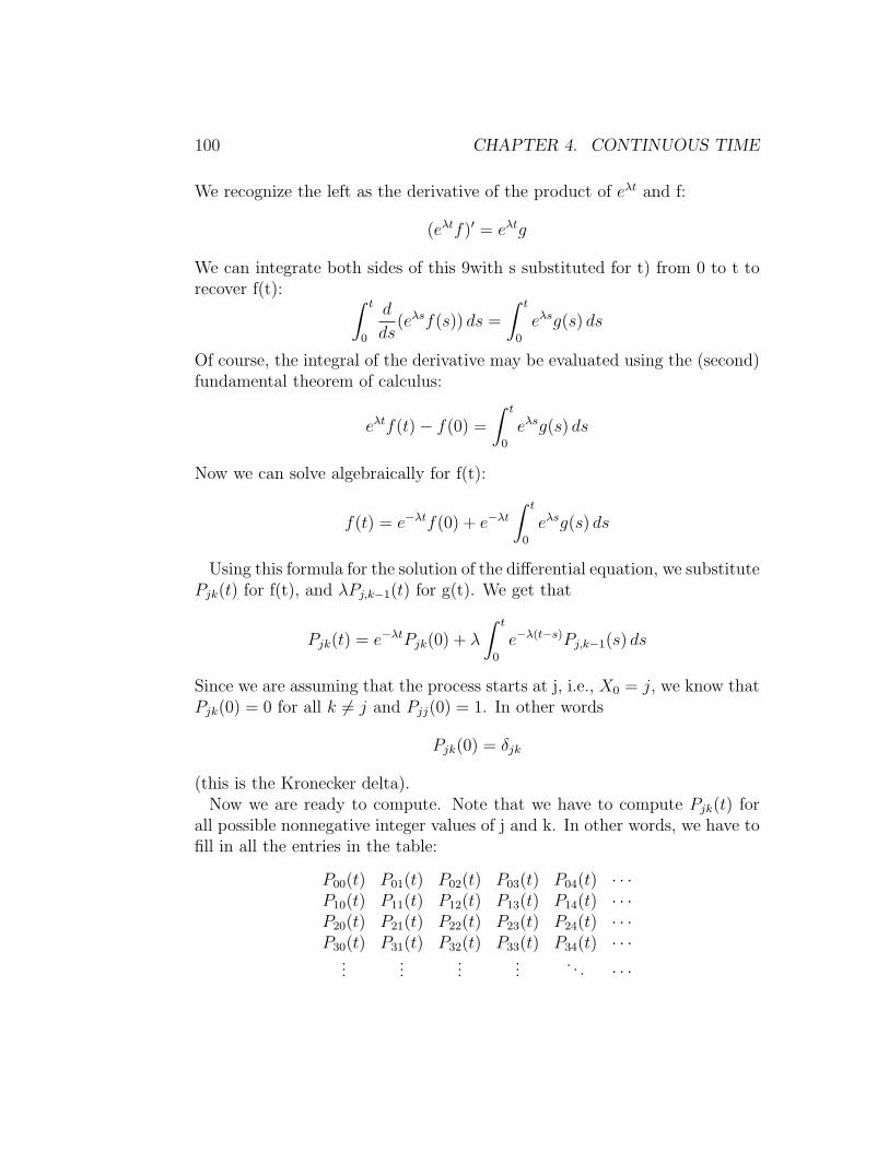
100 CHAPTER 4. CONTINUOUS TIME
We recognize the left as the derivative of the product of e�t and f:
(e�tf)0 = e�tg
We can integrate both sides of this 9with s substituted for t) from 0 to t torecover f(t): Z
t
0
d
ds(e�sf(s)) ds =
Zt
0
e�sg(s) ds
Of course, the integral of the derivative may be evaluated using the (second)fundamental theorem of calculus:
e�tf(t)� f(0) =
Zt
0
e�sg(s) ds
Now we can solve algebraically for f(t):
f(t) = e��tf(0) + e��t
Zt
0
e�sg(s) ds
Using this formula for the solution of the di↵erential equation, we substituteP
jk
(t) for f(t), and �Pj,k�1
(t) for g(t). We get that
Pjk
(t) = e��tPjk
(0) + �
Zt
0
e��(t�s)Pj,k�1
(s) ds
Since we are assuming that the process starts at j, i.e., X0
= j, we know thatP
jk
(0) = 0 for all k 6= j and Pjj
(0) = 1. In other words
Pjk
(0) = �jk
(this is the Kronecker delta).Now we are ready to compute. Note that we have to compute P
jk
(t) forall possible nonnegative integer values of j and k. In other words, we have tofill in all the entries in the table:
P00
(t) P01
(t) P02
(t) P03
(t) P04
(t) · · ·P
10
(t) P11
(t) P12
(t) P13
(t) P14
(t) · · ·P
20
(t) P21
(t) P22
(t) P23
(t) P24
(t) · · ·P
30
(t) P31
(t) P32
(t) P33
(t) P34
(t) · · ·...
......
.... . . · · ·

4.2. EXAMPLES 101
Of course, we already know part of the table:
e��t P01
(t) P02
(t) P03
(t) P04
(t) · · ·0 e��t P
12
(t) P13
(t) P14
(t) · · ·0 0 e��t P
23
(t) P24
(t) · · ·0 0 0 e��t P
34
(t) · · ·...
......
.... . . · · ·
So we begin the induction:We know that P
jj
= e��t, so we can use the di↵erential equation
P 0j,j+1
(t) + �Pj,j+1
(t) = �Pjj
(t)
to get that
Pj,j+1
(t) = �
Zt
0
e��(t�s)e��sds = �te��t
Note that this fills in the next diagonal of the table.Then we can use the di↵erential equation
P 0j,j+2
(t) + �Pj,j+2
(t) = �Pj,j+1
(t)
to get that
Pj,j+2
(t) = �
Zt
0
e��(t�s)�se��sds =(�t)2
2e��t
Continuing by induction we get that
Pjk
(t) =(�t)k�j
(k � j)!e��t
provided 0 j k and t > 0. This means that the random variable Xt
(this is the infinite discrete random variable that gives the value of j at timet, i.e., tells how many jumps have happened up until time t, has a Poissondistribution with parameter �t This is the important connection between theexponential distribution and the Poisson distribution.

102 CHAPTER 4. CONTINUOUS TIME
4.3 The Wiener process
4.3.1 Review of Taylor’s theorem
Taylor series are familiar to every student of calculus as a means writingfunctions as power series. The real force of Taylor series is what is calledTaylor’s theorem which tells one how well the Taylor polynomials approxi-mate the function. We will be satisfied with the following version of Taylor’stheorem. First, we introduce some notation.
Definition 4.3.1. For two functions f and g, we say that f(h) is o(g(h))(as h ! 0) (read ”f is little o of g) if
limh!0
f(h)/g(h) = 0
It of course means that f(h) is smaller than g(h) (as h gets small) but ina very precise manner.
As an example, note that another way to say that f 0(a) = b is to say that
f(a + h)� (f(a) + bh) = o(h)
That is, that the di↵erence between the function h 7! f(a+h) and the linearfunction h 7! f(a) + bh is small as h ! 0.
Taylor’s theorem is just the higher order version of this statement.
Theorem 4.3.1. Let f be a function defined on an interval (↵, �) be n timescontinuously di↵erentiable. Then for any a 2 (↵, �)
f(a + h) = f(a) + f 0(a)h +f 00(a)
2!h2 +
f (3)(a)
3!h3 + · · · + f (n)(a)
n!hn + o(hn)
We will in fact need a multivariable version of this, but only of low order.
Theorem 4.3.2. Let f(x, y) be a function of two variables defined on anopen set of O ⇢ R2. Then for any point (a, b) 2 O one has
f(a + k, b + k) = f(a, b) +@f
@x(a, b)h +
@f
@y(a, b)k
+1
2(@2f
@x2
(a, b)h2 + 2@2f
@x@y(a, b)kh +
@2f
@y2
(a, b)k2) + o(h2, k2, hk)

4.3. THE WIENER PROCESS 103
4.3.2 The Fokker-Plank equation
We will give a derivation of the Fokker-Planck equation, which governs theevolution of the probability density function of a random variable-valuedfunction X
t
that satisfies a ”first-order stochastic di↵erential equation”. Thevariable evolves according to what in the literature is called a Wiener process,named after Norbert Wiener, who developed a great deal of the theory ofstochastic processes during the first half of this century.
We shall begin with a generalized version of random walk (an ”unbalanced”version where the probability of moving in one direction is not necessarilythe same as that of moving in the other). Then we shall let both the spaceand time increments shrink in such a way that we can make sense of the limitas both �x and �y approach 0.
Recall from the previous sections the one-dimensional random walk (onthe integers) beginning at W
0
= 0. We fix a parameter p, and let p be theprobability of taking a step to the right, so that 1 � p is the probability oftaking a step to the left, at any (integer-valued) time n. In symbols, this is:
p = P (Wn+1
= x + 1|Wn
= x) and 1� p = P (Wn+1
= x� 1|Wn
= x).
ThusW
n
= ⇠1
+ · · · + ⇠n
where ⇠j
are IID with P (⇠j
= 1) = p and P (⇠j
= �1) = 1 � p. Since weare given that W
0
= 0, we know that the probability function of Wn
will beessentially binomially distributed (with parameters n and p, except that attime n, x will go from �n to +n, skipping every other integer as discussedearlier). We will set v
x,n
= P (Wn
= x). Then
vx,n
=
✓n
1
2
(n + x)
◆p
12 (n+x)(1� p)
12 (n�x)
for x = �n,�(n� 2), . . . , (n� 2), n and vx,n
= 0 otherwise.For use later, we calculate the expected value and variance of W
n
. First,
E(Wn
) =nX
x=�n
xvx,n
=nX
k=0
(2k � n)vx,2k�n
=nX
k=0
(2k � n)⇣n
k
⌘pk(1� p)n�k
= n(2p� 1)

104 CHAPTER 4. CONTINUOUS TIME
(it’s an exercise to check the algebra; but the result is intuitive). Also,
Var(Wn
) =nX
k=0
(2k � n)2vx,2k�n
=nX
k=0
(2k � n2)⇣n
k
⌘pk(1� p)n�k
= 4np(1� p)
(another exercise!).Now lets form a new stochastic process W� and we let the space steps �x
and time steps �t be di↵erent from 1. W� is a shorthand for W�t,�x.First, the time steps. We will take time steps of length �t. This will havelittle e↵ect on our formulas, except everywhere we will have to note that thenumber n of time steps needed to get from time 0 to time t is
n =t
�t
Each step to the left or right has length �x instead of length 1. This hasthe e↵ect of scaling W by the factor �x. Since multiplying a random variableby a constant has the e↵ect of multiplying its expected value by the sameconstant, and its variance by the square of the constant.
Therefore, the mean and variance of the total displacement in time t are:
E(W�
t
) =t
�t(2p� 1)�x and Var(W�
t
) = 4p(1� p)t(�x)2
�t
We want both of these quantities to remain finite for all fixed t, since wedon’t want our process to have a positive probability of zooming o↵ to infinityin finite time, and we also want Var(W (t)) to be non-zero. Otherwise theprocess will be completely deterministic.
We need to examine what we have control over in order to achieve theseends. First o↵, we don’t expect to let�x and�t to go to zero in any arbitrarymanner. In fact, it seems clear that in order for the variance to be finite andnon-zero, we should insist that �t be roughly the same order of magnitudeas (�x)2. This is because we don’t seem to have control over anything elsein the expression for the variance. It is reasonable that p and q vary with�x, but we probably don’t want their product to approach zero (that wouldforce our process to move always to the left or always to the right), and itcan’t approach infinity (since the maximum value of p(1� p) is 1/4). So we

4.3. THE WIENER PROCESS 105
are forced to make the assumption that (�x)
2
�t
remain bounded as they bothgo to zero. In fact, we will go one step further. We will insist that
(�x)2
�t= 2D (4.3.1)
for some (necessarily positive) constant D.Now, we are in a bind with the expected value. The expected value will
go to infinity as �x ! 0, and the only parameter we have to control it is2p� 1. We need 2p� 1 to have the same order of magnitude as �x in orderto keep E(W�
t
) bounded. Since p = 1 � p when p = 1/2, we will make theassumption that
p =1
2+
c
2D�x (4.3.2)
for some real (positive, negative or zero) constant c, which entails
1� p =1
2� c
2D�x
The reason for the choice of the parameters will become apparent. D is calledthe di↵usion coe�cient, and c is called the drift coe�cient.
Note that as �x and �t approach zero, the values vn,k
= P (W�
n�t
=k�x) = p(k�x, n�t) specify values of the function p at more and morepoints in the plane. In fact, the points at which p is defined become moreand more dense in the plane as �x and �t approach zero. This means thatgiven any point in the plane, we can find a sequence of points at which such anp is defined, that approach our given point as �x and �t approach zero. Wewould like to be able to assert the existence of the limiting function, and thatit expresses how the probability of a continuous random variable evolves withtime. We will not quite do this, but, assuming the existence of the limitingfunction, we will derive a partial di↵erential equation that it must satisfy.Then we shall use a probabilistic argument to obtain a candidate limitingfunction. Finally, we will check that the candidate limiting function is asolution of the partial di↵erential equation. This isn’t quite a proof of theresult we would like, but it touches on the important steps in the argument.
We begin with the derivation of the partial di↵erential equation. To dothis, we note that for the original random walk, it was true that v
x,n
satisfiesthe following di↵erence equation:
vk,n+1
= pvk�1,n
+ (1� p)vk+1,n

106 CHAPTER 4. CONTINUOUS TIME
This is just the matrix of the (infinite discrete) Markov process that definesthe random walk. When we pass into the �x, �t realm, and use p(x, t)notation instead of v
k�x,n�t
, this equation becomes:
(⇤) p(x, t +�t) = pp(x��x, t) + (1� p)p(x +�x, t)
Next, we need Taylor’s expansion for a function of two variables. As we dothe expansion, we must keep in mind that we are going to let �t ! 0, and aswe do this, we must account for all terms of order up to and including thatof �t. Thus, we must account for both �x and (�x)2 terms (but (�x)3 and�t�x both go to zero faster than �t).
We expand each of the three expressions in equation (*) around the point(x, t), keeping terms up to order �t and (�x)2. We get:
p(x, t +�t) = p(x, t) +�(t)@p
@t(x, t) + · · ·
p(x +�x, t) = p(x, t) +�(x)@p
@x(x, t) +
(�x)2
2
@2p
@x2
(x, t) + · · ·
p(x��x, t) = p(x, t)��(x)@p
@x(x, t) +
(�x)2
2
@2p
@x2
(x, t) + · · ·
We substitute these three equations into (*), recalling that p + (1� p) = 1,we get
�t@p
@t= �(2p� 1)�x
@p
@x+
(�x)2
2
@2p
@x2
(where all the partial derivatives are evaluated at (x, t)). Finally, we dividethrough by �t, and recall that (�x)2/�t = 2D, and 2p � 1 = �xc/D toarrive at the equation:
@p
@t= �2c
@p
@x+ D
@2p
@x2
This last partial di↵erential equation is called the Fokker-Planck equation.To find a solution of the Fokker-Planck equation, we use a probabilistic
argument to find the limit of the random walk distribution as �x and �tapproach 0. The key step in this argument uses the fact that the binomialdistribution with parameters n and p approaches the normal distributionwith expected value np and variance np(1 � p) as n approaches infinity. Interms of our assumptions about �x, �t, p and 1� p, we see that at time t,the binomial distribution has mean
t(2p� 1)�x
�t= 2ct

4.3. THE WIENER PROCESS 107
and variance
4p(1� p)t(�x)2
�t
which approaches 2Dt as �t ! 0. Therefore, we expect Wt
in the limit to benormally distributed with mean 2ct and variance 2Dt. Thus, the probabilitythat W
t
< x is
P (Wt
< x) =1p2⇡
Z x�2ctp2Dt
�1e�
12y
2dy
Therefore the pdf of Wt
is the derivative of this with respect to x, whichyields the pdf
p(x, t) =1
2p⇡Dt
e�(x�2ct)2
4Dt
A special case of this is when c = 0 and D = 1
2
. The corresponding processis called the Wiener process (or Brownian motion). The following propertiescharacterize the Wiener process, which we record as a theorem.
Theorem 4.3.3. 1. W0
= 0 with probability 1.
2. Wt
is a continuous function of t with probability 1.
3. For t > s Wt
�Ws
is normally distributed with mean 0 and variancet� s.
4. For T � s � t � u � v, Ws
�Wt
and Wu
�Wv
are independent.
5. The probability density for Wt
is
p(x, t) =1p2⇡t
e�x
2
2t
Proof: Let’s discuss these points.1. This is clear since we defined W
t
as a limit of random walks which allstarted at 0.3. This we derived from the Fokker-Plank equation.4. Again, we defined W
t
as a limit of random walks, W�. Now W�
t
=�x(⇠
1
+ · · · ⇠n
) where n = t/�t. So if t = n�t, s = m�t, u = k�t andv = l�t where n � m � k � l then we have
Wt
�Ws
= �x(⇠m+1
+ ⇠m+2
+ · · · ⇠n
)

108 CHAPTER 4. CONTINUOUS TIME
andW
u
�Wv
= �x(⇠l+1
+ · · · ⇠k
)
which are independent.2. This fact is beyond the scope of our discussion but is intuitive.Q.E.D.While, according to 2. above, the paths W
t
are continuous, they are veryrough and we see according to the next proposition that they are not di↵er-entiable, with probability 1.
Proposition 4.3.4. For all t > 0 and all n = 1, 2, . . .,
limh!0
P (|Wt+h
�Wt
| > n|h|) = 1
so that Wt
is nowhere di↵erentiable.
Proof: Assume without loss of generality that h > 0. Then
P (|Wt+h
�Wt
| > nh) = P (|Wh
| > nh)
by 3) of ??. Now this gives
1� P (|Wh
| nh)
Now
P (|Wh
| nh)) =1p2⇡h
Znh
�nh
e�x
2
2t dx
1p2⇡h
Znh
�nh
1dx 1p2⇡h
2hn
=
r2h
⇡
which converges to 0 as h ! 0 for any n. Q.E.D.Almost everything we use about the Wiener process will follow from ??.
We now do some sample computations to show how to manipulate the Wienerprocess and some of which will be useful later.1. Calculate the expected distance of the Wiener process from 0.Solution: This is just E(|W
t
|) which isZ 1
�1|x| 1p
2⇡te�
x
2
2t

4.3. THE WIENER PROCESS 109
= 2
Z 1
0
x1p2⇡t
e�x
2
2t
Changing variables, u = x2/(2t) this integral becomes
2tp2⇡t
Z 1
0
e�udu =p
2t/⇡
2. Calculate E(Wt
Ws
).Solution: Assume without loss of generality that t > s. Then
E(Wt
Ws
) = E((Wt
�Ws
)Ws
+ W 2
s
) = E((Wt
�Ws
)Ws
) + E(W 2
s
)
Now Wt
�Ws
is independent of Ws
since t > s and Ws
has mean 0, thereforewe get
E(Wt
�Ws
)E(Ws
) + �2(Ws
) = s
since Wt
�Ws
has mean 0.
The Wiener Process Starting at y, W y
The defining properties of W y
t
= Wt
+ y, the Wiener process starting at y,are:
1. W y
0
= y.
2. W y
t
is continuous with probability 1.
3. W y
t
is normally distributed with µ = y, �2 = t.
4. W y
t
�W y
s
is normally distributed with µ = 0, �2 = t� s, t > s.
5. W y
t
�W y
s
, W y
u
�W y
v
are independent for t � s � u � v.
6. The pdf is given by
p(x, t|y) =1p2⇡t
e�(x�y)
2
2t
P (a W y
t
b) =1p2⇡t
Zb
a
e�(x�y)
2
2t dx

110 CHAPTER 4. CONTINUOUS TIME
How do we use Wiener Process to model stock movements?
We would like to make sense of the idea thatdS
t
dt= µS
t
+noise(�, St
), where
if the noise term were absent then St
is a bank account earning interest u.There are two obvious problems:(1) THe Wiener process is di↵erentiable nowhere, so why should S
t
bedi↵erentiable anywhere?(2) “Noise” is very di�cult to make rigorous.
To motivate our way out of these problems let us look at deterministicmotion. The most general 1st order di↵erential equation is
df
dt= �(f(t), t) .
By integrating both sides we arrive at the following integral equation
f(t)� f(t0
) =
Zt
t0
df
dtdt =
Zt
t0
�(f(t), t) dt .
That is,
f(t) = f(t0
) +
Zt
t0
�(f(t), t) dt .
Theoretically integral equations are better behaved than di↵erential equa-tions (they tend to smooth out bumps). So we try to make the correspondingconversion from di↵erential to integral equation in the stochastic world.
Our first goal is just to define a reasonable notion of stochastic integral.We had the Martingale Transform: If S
n
was a stock, �n
denoted theamount of stock at tick n, then the gain from tick 0 to tick N was
NX
i=1
�i
(Si
� Si�1
)
It is these sorts of sums that become integrals in continuous time.Recall the Riemann integral
Rb
a
f(x) dx: Take a partition of [a, b], P ={a = t
0
< t1
< · · · < tn
= b}.Theorem 4.3.5. (Riemann’s Theorem) Let f be a function such that theprobability of choosing a point of discontinuity is 0. Let mesh P = max{|t
i
� ti�1
| |i =1, . . . , n}, let t
i�1
< ⇠i
< ti
, then let
RS(f,P) =nX
i=1
f(⇠i
)(ti
� ti�1
) .

4.3. THE WIENER PROCESS 111
(RS stands for Riemann sum). Then
limmeshP!0
RS(f,P)
exists, and is independent of the choices of ⇠i
within their respective intervals.We call this limit the Riemann integral
Zb
a
f(x)dx
Note that the summation is beginning to look like a martingale transform.The next level of integral technology is the Riemann-Stieltjes integral.
Suppose �(x) is a non decreasing function, P a partition, and ⇠i
values be-tween partition points. Let
RSS(f,P ,�) =nX
i=1
f(⇠i
)(�(ti
)� �(ti�1
)) .
(“RSS” stands for Riemann-Stieltjes sum.) If limmeshP!0
RSS(f,P ,�) ex-
ists, then by definition,R
b
a
f(t) d�(t) is this limit. Assuming � is di↵eren-tiable, the corresponding Riemann’s theorem holds, namely
limmeshP!0
RSS(f,P ,�)
exists (and is independent of the choices of ⇠i
).
Proposition 4.3.6. If � is di↵erentiable,R
b
a
f(t) d�(t) =R
b
a
f(t)�0(t) dt.
Proof. Let P = {a = t0
< t1
< · · · < tn
= b}.
RSS(f,P ,�) =P
n
i=1
f(⇠i
)(�(ti
)� �(ti�1
))
=P
n
i=1
f(⇠i
)�(t
i
)��(t
i�1)
t
i
�t
i�1(t
i
� ti�1
)
=P
n
i=1
f(⇠i
)(�0(ti
) + o(|ti
� ti�1
|2))(ti
� ti�1
)
(4.3.3)
and so limmeshP!0
Pn
i=1
f(⇠i
)�0(ti
)(ti
� ti�1
) =R
b
a
f(t)�0(t) dt.
Example. Let �(x) be di↵erentiable.
Zb
a
�(t) d�(t) =
Zb
a
�(t)�0(t) dt =1
2�(b)2 � 1
2�(a)2 .

112 CHAPTER 4. CONTINUOUS TIME
A stochastic integral is formed much like the Riemann-Stieltjes integral,with one twist.
For Xt
and �t
stochastic processes,
Zb
a
�t
dXt
is to be a random variable. In the Riemann and Riemann-Stieltjes cases, thechoices of the points ⇠
i
in the intervals were irrelevant, in the stochastic case itis very much relevant. As an example, take P = {a = t
0
< t1
< · · · < tn
= b}.Consider
nX
i=1
�⇠
i
(Xt
i
�Xt
i�1) .
Let’s work out the above sum for Xt
= �t
= Wt
, where Wt
is the Wienerprocess, using two di↵erent choices for the ⇠
i
’s.First, let ⇠
i
= ti�1
, the left endpoint. Then
E⇣P
n
i=1
Wt
i�1(Wt
i
�Wt
i�1)⌘
=P
n
i=1
E(Wt
i�1(Wt
i
�Wt
i�1))
=P
n
i=1
E(Wt
i�1)E(Wt
i
�Wt
i�1) = 0 ,
using independence.Second, let ⇠
i
= ti
, the right endpoint. Then
E⇣P
n
i=1
Wt
i
(Wt
i
�Wt
i�1)⌘
=P
n
i=1
E(Wt
i
(Wt
i
�Wt
i�1)) =P
n
i=1
E(Wt
i
2 �Wt
i
Wt
i�1)
=P
n
i=1
E(Wt
i
2)� E(Wt
i
Wt
i�1)=
Pn
i=1
ti
� ti�1
= (t1
� t0
) + (t2
� t1
) + · · · + (tn
� tn�1
)= t
n
� t0
= b� a .
Which endpoint to choose? Following Ito, one uses the left-hand endpoint.One defines the Ito sum
IS(�t
,P , Xt
) =nX
i=1
�t
i�1(Xt
i
�Xt
i�1)
.There are two motivations for this choice.

4.3. THE WIENER PROCESS 113
1. The lefthand choice looks a little like a previsibility condition. Forexample, if X
t
is a stock-process and �t
a portfolio process then theleft-hand choice embodies the idea that our gains from time T
i�1
totime t
i
should be based on a choice made at time ti�1
.
2. It turns out, that if Xt
is a Martingale, then the Ito sum will be aMartingale as well.
Following Stratonovich, one takes ⇠i
= 1
2
(ti�1
+ ti
), the midpoint. As anadvantage, the resulting Stratonovich calculus looks like traditional calculus.As a disadvantage, the derived stochastic process is not a martingale.
Let Xt
be a stochastic process. Let �t
be another stochastic process definedon the same sample space as X
t
.
Definition 4.3.2. �t
is adapted to Xt
if �t
is independent of Xs
�Xt
fors > t.
Then we define the Ito integral
Zt
a
�s
dXs
⌘ limmeshP!0
IS(�,P , X) = limmeshP!0
nX
i=1
�t
i�1(Xt
i
�Xt
i�1) .
Let us call a random variable with finite first and second moments sqaureintegrable. One knows that for X, Y square integrable random variablesdefined on the same sample space, P (X = Y ) = 1 i↵ E(X) = E(Y ) andVar(X � Y ) = 0. Now Var(X � Y ) = E((X � Y )2)� (E(X � Y ))2, so
P (X = Y ) = 1 i↵ E((X � Y )2) = 0 .
This is a criterion for checking whether two square integrable random vari-ables are equal (almost surely).
Definition 4.3.3. A sequence X↵ of square integrable random variablesconverges in mean-square to X if E((X �X↵)2) ! 0 as ↵! 0. In symbols,lim X↵ = X. This is equivalent to E(X↵) ! E(X) and Var(X �X↵) ! 0.
This is the sense of the limit in the definition of the stochastic integral.Here is a sample computation of a stochastic integral. Let’s evaluate
Zb
a
Wt
dWt

114 CHAPTER 4. CONTINUOUS TIME
We need the following facts: E(Wt
) = 0, E(Wt
2) = t, E(Wt
3) = 0, andE(W
t
4) = 3t2.
IS(Wt
,P , Wt
) =P
n
i=1
Wt
i�1 ·�Wt
i
=P
n
i=1
Wt
i�1(Wt
i
�Wt
i�1)= 1
2
Pn
i=1
(Wt
i�1 +�Wt
i
)2 �Wt
i�1
2 � (�Wt
i
)2
= 1
2
Pn
i=1
Wt
i
2 �Wt
i�1
2 � 1
2
Pn
i=1
(�Wt
i
)2
= 1
2
((Wt1
2 �Wt0
2) + (Wt2
2 �Wt1
2) + · · ·+(W
t
n
2 �Wt
n�12))� 1
2
Pn
i=1
(�Wt
i
)2
= 1
2
(Wb
2 �Wa
2)� 1
2
Pn
i=1
(�Wt
i
)2 .
The first part is recognizable as what the Riemann-Stieltjes integral givesformally. But what is
Pn
i=1
(�Wt
i
)2 as meshP ! 0? The simple calculation
E⇣ nX
i=1
(�Wt
i
)2
⌘=
nX
i=1
E((�Wt
i
)2)
=nX
i=1
E((Wt
i
�Wt
i�1)2) =
nX
i=1
ti
� ti�1
= b� a
leads us to theClaim:
limmeshP!0
E(nX
i=1
(�Wt
i
)2) = b� a
and thereforeZ
b
a
Wt
dWt
=1
2(W
b
2 �Wa
2)� 1
2(b� a) .
Proof.
E⇣(
nX
i=1
(�Wt
i
)2 � (b� a))2
⌘
= E⇣(P
n
i=1
(�Wt
i
2))2 � 2(b� a)P
n
i=1
(�Wt
i
)2 + (b� a)2
⌘
= E⇣P
n
i=1
(�Wt
i
)4 + 2P
i<j
(�Wt
i
)2(�Wt
j
)2 � 2(b� a)P
n
i=1
(�Wt
i
)2 + (b� a)2
⌘
=P
n
i=1
3(�ti
)2 + 2P
i<j
E((�Wt
i
)2)E((�Wt
j
)2)� E(2(b� a)P
n
i=1
(�Wt
i
)2 + (b� a)2)= 3
Pn
i=1
(�ti
)2 + 2P
i<j
(�ti
)(�tj
)� 2(b� a)P
n
i=1
�ti
+ (b� a)2
= 2P
n
i=1
(�ti
)2 +hP
n
i=1
(�ti
)2 + 2P
i<j
(�ti
)(�tj
)i� 2(b� a)
Pn
i=1
�ti
+ (b� a)2
= 2P
n
i=1
(�ti
)2 +⇣P
n
i=1
(�ti
)⌘
2
� 2(b� a)P
n
i=1
�ti
+ (b� a)2
= 2P
n
i=1
(�ti
)2 +⇣P
n
i=1
�ti
� (b� a)⌘
2
= 2P
n
i=1
(�ti
)2

4.3. THE WIENER PROCESS 115
Now for each i, �ti
meshP , so (�ti
)2 �ti
· meshP . (Note that onlyone �t
i
is being rounded up.) Summing i = 1 to n, 0 P
n
i=1
(�ti
)2 �Pn
i=1
�ti
�· meshP = (b� a) · meshP ! 0 as meshP ! 0. So
limmeshP!0
nX
i=1
(�ti
)2 = 0 .
Intuitively, �ti
⇡ meshP ⇡ 1
n
, so limmeshP!0
Pn
i=1
(�ti
)2 ⇡ limn!1 n ·
( 1
n
)2 ! 0.The underlying reason for the di↵erence of the stochastic integral and the
Stieltjes integral is that �Wt
i
is, with high probability, of orderp�t
i
.
Slogan of the Ito Calculus: dWt
2 = dt.
In deriving the Wiener Process,(�X)2
�t= 1, so (�X)2 = (�W )2 = �t.
dW 2
t
= dt is only given precise sense through its integral form:
Theorem 4.3.7. . If �s
is adapted to Ws
, thenR
t
a
�s
(dWs
)2 =R
t
a
�s
ds.
Moreover, for n > 2,R
t
a
�s
(dWs
)n = 0.
Proving this will be in the exercises.Properties of the Ito Integral. If �
s
, s
are adapted to the given process(X
s
or Ws
), then
(1)
Zt
a
dXs
= Xt
�Xa
,
(2)
Zt
a
(�s
+ s
) dXs
=
Zt
a
�s
dXs
+
Zt
a
s
dXs
,
(3) E⇣Z
t
a
�s
dWs
⌘= 0 and
(4) E⇣(
Zt
a
�s
dWs
)2
⌘= E
⇣Zt
a
�s
2 ds⌘
.
Proof.

116 CHAPTER 4. CONTINUOUS TIME
1. For any partition P = {a = s0
< s1
< · · · < sn
= t}, IS(1,P , Xs
) =Pn
i=1
1 · (Xs
i
� Xs
i�1), which telescopes to Xs
n
� Xs0 = X
t
� Xa
. Sothe limit as meshP ! 0 is X
t
�Xa
.
2. It is obvious for any partition P that IS(�s
+ s
,P , Xs
) = IS(�s
,P , Xs
)+IS(
s
,P , Xs
). Now take the limit as meshP ! 0.
3. Given a partition P , IS(�s
,P , Ws
) =P
n
i=1
�s
i�1(Ws
i
�Ws
i�1). Takingexpected values gives
E(IS(�s
,P , Ws
)) = E⇣P
n
i=1
�s
i�1(Ws
i
�Ws
i�1)⌘
=P
n
i=1
E(�s
i�1(Ws
i
�Ws
i�1))
=P
n
i=1
E(�s
i�1)E(Ws
i
�Ws
i�1) = 0 .
Taking the limit as meshP ! 0 gives the result.
4. Given a partition P ,E(IS(�
s
,P , Ws
)2)
= E⇣(P
n
i=1
�s
i�1(Ws
i
�Ws
i�1))2
⌘
= E⇣P
n
i=1
�s
i�1
2(Ws
i
�Ws
i�1)2 + 2
Pi<j
�s
i�1�s
j�1(Ws
i
�Ws
i�1)(Ws
j
�Ws
j�1)⌘
= E⇣P
n
i=1
�s
i�1
2(�Ws
i
)2
⌘+ 2
Pi<j
E(�s
i�1�s
j�1(Ws
i
�Ws
i�1)(Ws
j
�Ws
j�1))
= E⇣P
n
i=1
�s
i�1
2(�Ws
i
)2
⌘+ 2
Pi<j
E(�s
i�1�s
j�1(Ws
i
�Ws
i�1)) · E(Ws
j
�Ws
j�1)
=P
n
i=1
E(�s
i�1
2)�si
+ 2P
i<j
E(�s
i�1�s
j�1(Ws
i
�Ws
i�1)) · 0=
Pn
i=1
E(�s
i�1
2)�si
= IS(�s
2,P , s) .
Now take the limit as meshP ! 0.
4.3.3 Stochastic Di↵erential Equations.
A first-order stochastic di↵erential equation is an expression of the form
dXt
= a(Xt
, t) dt + b(Xt
, t) dWt
,
where a(x, t), b(x, t) are functions of two variables.A stochastic process X
t
is a solution to this SDE if
Xt
�Xa
=
Zt
a
dXs
=
Zt
a
a(Xs
, s) ds + b(Xs
, s) dWs
.

4.3. THE WIENER PROCESS 117
Lemma 4.3.8. (Ito’s Lemma). Suppose we are given a twice di↵erentiablefunction f(x), and a solution X
t
to the SDE dXt
= a dt+b dWt
. Then f(Xt
)is a stochastic process, and it satisfies the SDE
df(Xt
) = [f 0(Xt
)a +1
2f 00(X
t
)b2] dt + f 0(Xt
)b dWt
.
More generally, if f(x, t) a function of two variables, twice di↵erentiable inx, once di↵erentiable in t, one has df(X
t
, t)
= [@f
@t(X
t
, t) +@f
dx(X
t
, t)a +1
2
@2f
@x2
(Xt
, t)b2] dt +@f
@x(X
t
, t)b dWt
.
Proof. This is just a calculation using two terms of the Taylor’s series forf , and the rules dW
t
2 = dt and dWt
n = 0 for n > 2. (Note that dt dWt
=dW
t
3 = 0 and dt2 = dWt
4 = 0.)
df(Xt
) = f(Xt+dt
)� f(Xt
) = [f(Xt
+ dXt
)]� f(Xt
)= [f(X
t
) + f 0(Xt
) dXt
+ 1
2
f 00(Xt
)(dXt
)2 + o((dXt
)3)]� f(Xt
)= f 0(X
t
) dXt
+ 1
2
f 00(Xt
)(dXt
)2
= f 0(Xt
)[a(Xt
, t) dt + b(Xt
, t) dWt
] + 1
2
f 00(Xt
)[a2 dt2 + 2ab dt dWt
+ b2 dWt
2]= [f 0(X
t
)a(Xt
, t) + 1
2
f 00(Xt
)(b(Xt
, t))2] dt + f 0(Xt
)b(Xt
, t) dWt
Example. To calculateR
t
a
Wt
dWt
, show that is equal toR
t
a
dXt
= Xt
�Xa
for some Xt
. That is, find f(x) such that Wt
dWt
= d(f(Wt
)). SinceR
x dx =1
2
x2, consider f(x) = 1
2
x2. Then f 0(x) = x and f 00(x) = 1, so Ito’s lemma,applied to dW
t
= 0 · dt + 1 · dWt
, gives
d(f(Wt
)) = f 0(Wt
) dWt
+1
2f 00(W
t
) dt = Wt
dWt
+1
2· 1 dt = W
t
dWt
+1
2dt .
Equivalently, Wt
dWt
= df(Wt
)� 1
2
dt. Therefore,R
t
a
Ws
dWs
=R
t
a
d(f(Ws
))�Rt
a
1
2
dt = f(Wt
)� f(Wa
)� 1
2
(t� a) = 1
2
Wt
2 � 1
2
Wa
2 � 1
2
(t� a).
Example. CalculateR
t
a
Ws
2 dWs
. SinceR
x2 dx = 1
3
x3, consider f(x) = 1
3
x3.Then f 0(x) = x2 and f 00(x) = 2x. Ito’s lemma implies
d(1
3x3) = W
s
2 dWs
+1
2· 2W
s
ds = Ws
2 dWs
+ Ws
ds ,
or Ws
2 dWs
= d(1
3
Ws
3)�Ws
ds, so
Zt
a
Ws
2 dWs
=1
3W
t
2 � 1
3W
a
2 �Z
t
a
Ws
ds .

118 CHAPTER 4. CONTINUOUS TIME
(The last integrand does not really simplify.)Example. Solve dX
s
= 1
2
Xs
ds + Xs
dWs
. Consider f 0(Xs
) · Xs
= 1. Withordinary variables, this is f 0(x)·x = 1, or f 0(x) = 1
x
. So we are led to considerf(x) = ln x, with f 0(x) = 1
x
, and f 00(x) = � 1
x
2 .Then, using dX
s
= 1
2
Xs
ds + Xs
dWs
and dXs
2 = Xs
2 ds,
d(ln Xs
) = 1
X
s
dXs
+ 1
2
(� 1
X
s
2 )(dXs
)2
= 1
2
ds + dWs
� 1
2
ds = dWs
.
Now integrate both sides, gettingR
t
a
d(ln Xs
) =R
t
a
dWs
= Wt
�Wa
or
ln⇣
X
t
X
a
⌘= W
t
�Wa
and so
Xt
= Xa
eW
t
�W
a .
Asset Models
The basic model for a stock is the SDE
dSt
= µSt
dt + �St
dWt
,
where µ is the short-term expected return, and � is the standard deviationof the the short-term returns, called volatility.
Note that if � = 0, the model simplifies to dSt
= µSt
dt, implying St
=S
a
eµt, which is just the value of an interest-bearing, risk-free security.Compared with the generic SDE
dXt
= a(Xt
, t) dt + b(Xt
, t) dWt
the stock model uses a(x, t) = µx and b(x, t) = �x. We have dSt
2 = �2St
2 dt.The model SDE is similar to the last example, and the same change of vari-ables will work. Using f(x) = ln x, f 0(x) = 1
x
, and f 00(x) = � 1
x
2 , Ito’s lemmagives
d(ln St
) = 1
S
t
dSt
+ 1
2
(� 1
S
t
2 )(dSt
)2
= µ dt + � dWt
� 1
2
�2 dt= (µ� 1
2
�2) dt + � dWt
.
Integrating both sides givesR
t
0
d(ln Ss
) =R
t
0
(µ� 1
2
�2) ds + � dWs
ln St
� ln S0
= (µ� 1
2
�2)t + �Wt
S
t
S0= e(µ�
1
2
�2)t + �Wt
St
= S0
e(µ�1
2
�2)t + �Wt .

4.3. THE WIENER PROCESS 119
The expected return of St
is
E(ln(St
/S0
)) = E((µ� 1
2�2)t + �W
t
) = (µ� 1
2�2)t .
Vasicek’s interest rate model is drt
= a(b�rt
) dt+� dWt
. It satisfies “meanreversion”, meaning that if r
t
< b, then drt
> 0, pulling rt
upwards, while ifrt
> b, then drt
< 0, pushing rt
downwards.The Cox-Ingersoll-Ross model is dr
t
= a(b�rt
) dt+�p
rt
dWt
. It has meanreversion, and a volatility that grows with r
t
.Ornstein-Uhlenbeck Process. An O-U process is a solution to
dXt
= µXt
dt + � dWt
with an initial condition X0
= x0
.This SDE is solved by using the integrating factor e�µt. First,
e�µt dXt
= µe�µtXt
dt + �e�µt dWt
holds just by multiplying the given SDE. Letting f(x, t) = xe�µt, then
@f
@t= �µe�µtX
t
dt ,@f
@x= e�µt , and
@2f
@x2
= 0 .
Ito’s lemma gives
df(Xt
, t) = @f
@t
(Xt
, t) dt + @f
@x
(Xt
, t) dXt
+ @
2f
@x
2 (Xt
, t) dXt
2
d(e�µtXt
) = �µe�µtXt
dt + e�µt dXt
ore�µt dX
t
= d(e�µtXt
) + µe�µtXt
dt .
So the SDE, with integrating factor, rewrites as
d(e�µtXt
) + µe�µtXt
dt = µe�µtXt
dt + �e�µt dWt
d(e�µtXt
) = �e�µt dWt
.
Now integrate both sides from 0 to t:
Rt
0
d(e�µsXs
) =R
t
0
�e�µs dWs
e�µtXt
�X0
=R
t
0
�e�µs dWs
Xt
= eµtX0
+ eµt
Rt
0
�e�µs dWs
.

120 CHAPTER 4. CONTINUOUS TIME
Let’s go back to the stock model
dSt
= µSt
dt + �St
dWt
with solution
St
= S0
e(µ�1
2
�2)t + �Wt .
We calculate the pdf of St
as follows. First,
P (St
S) = P (S0
e(µ�1
2
�2)t + �Wt S)
= P (e(µ�1
2
�2)t + �Wt S/S
0
)= P ((µ� 1
2
�2)t + �Wt
ln(S/S0
))
= 1p2⇡�
2t
Rln(S/S0)
�1 e�(x�(µ� 1
2�
2)t)
2
2�
2t dx .
Second, the pdf is the derivative of the above with respect to S. The funda-mental theorem of calculus gives us derivatives of the form d
du
Ru
a
�(x) dx =�(u). The chain rule gives us, where u = g(S), a derivative
d
dS
Zg(S)
a
�(x) dx = (d
du
Zu
a
�(x) dx) · du
dS= �(u) · g0(S) = �(g(S)) · g0(S) .
In the case at hand, g(S) = ln(S/S0
) = ln S � ln S0
, so g0(S) = 1/S, and thepdf is
d
dS
P (St
S) = d
dS
1p2⇡�
2t
Rln(S/S0)
�1 e�(x�(µ� 1
2�
2)t)
2
2�
2t dx
= 1
S
p2⇡�
2t
e�(ln(S/S0)�(µ� 1
2�
2)t)
2
2�
2t
for S > 0 and identically 0 for S 0.Pricing Derivatives in Continuous Time
Our situation concerns a stock with price stochastic variable St
, and aderivative security, assumed to have expiration T , and further assumed thatits (gross) payo↵ depends only on T and S
T
. Let V (ST
, T ) denote this payo↵.More generally, let V (S
t
, t) denote the payo↵ for this derivative if it expiresat time t with stock price S
t
. In particular, V (St
, t) depends only on t andS
t
. That is, we have a deterministic function V (s, t), and are plugging in astochastic process S
t
and getting a stochastic process V (St
, t).To price V , construct a self-financing, hedging portfolio for V . That is, set
up a portfolio consisting of �t
units of stock St
and t
units of bond Bt
⇧t
= �t
St
+ t
Bt
,

4.3. THE WIENER PROCESS 121
such that the terminal value of the portfolio equals the derivative payo↵
⇧T
= VT
,
subject to the self-financing condition
SFC1 ⇧t
= ⇧0
+
Zt
0
�s
dSs
+ s
dBs
.
The pricing of the portfolio is straightforward, and the no-arbitrage as-sumption implies ⇧
t
= Vt
for all t T .Recall, also, the self-financing condition in the discrete case:
(�⇧)n
= �n
�Sn
+ n
�Bn
.
The continuous limit is
SFC2 d⇧t
= �t
dSt
+ t
dBt
.
We now model the stock and bond. The stock is dSt
= µSt
dt + �St
dWt
,while the bond is dB
t
= rBt
dt.
Theorem 4.3.9. (Black-Scholes). Given a derivative as above, there existsa self-financing, hedging portfolio ⇧
t
= �t
St
+ t
Bt
with ⇧t
= V (St
, t) if andonly if
(BSE)@V
@t+
1
2�2S2
@2V
@S2
+ rS@V
@S� rV = 0,
and furthermore, �t
= @V
@S
.
Proof. Let’s calculate dV (St
, t) = d⇧t
two ways. First, by Ito’s lemma
dV (St
, t) =@V
@t(S
t
, t) dt +@V
@S(S
t
, t) dSt
+1
2
@2V
@S2
(St
, t)(dSt
)2 ,
or, suppressing the St
, t arguments,
dVt
= @V
@t
dt + @V
@S
dSt
+ 1
2
@
2V
@S
2 (dSt
)2
= (@V
@t
+ µSt
@V
@S
+ 1
2
�2St
2
@
2V
@S
2 ) dt + @V
@S
�St
dWt
.
On the other hand, using our stock and bond model on a portfolio, the selffinancing condition (SFC2) says that V
t
= ⇧t
= �t
St
+ t
Bt
,
dVt
= d⇧t
= �t
dSt
+ t
dBt
= (�t
µSt
+ t
rBt
) dt + �t
�St
dWt
.

122 CHAPTER 4. CONTINUOUS TIME
If these are to be equal, the coe�cients of dt and of dWt
must be equal.Equating the coe�cients of dW
t
gives
�t
�St
=@V
@S�S
t
, hence �t
=@V
@S,
and equating the coe�cients of dt gives
�t
µSt
+ t
rBt
=@V
@t+ µS
t
@V
@S+
1
2�2S
t
2
@2V
@S2
,
hence
t
rBt
=@V
@t+
1
2�2S
t
2
@2V
@S2
.
Since t
Bt
= ⇧t
� �t
St
= Vt
� @V
@S
St
we have
r(Vt
� @V
@SS
t
) =@V
@t+
1
2�2S
t
2
@2V
@S2
,
or in other works (BSE), completing the proof.In summary, to construct a self-financing, replicating portfolio for a deriva-
tive, you need the value of the derivative Vt
= V (St
, t) to satisfy the Black-Scholes equation and for the stock holding to be �
t
= @V
@S
.The theory of partial di↵erential equations tells us that in order to get
unique solutions, we need boundary and temporal conditions. Since the BSEis first order in t, we need one time condition. And since the BSE is secondorder in S, we need two boundary conditions.
The time condition is simply the expiration payo↵ V (ST
, T ) = h(ST
).(Usually, one has an “initial” condition, corresponding to time 0. Here, onehas a “final” or “terminal” condition.) The boundary conditions are usuallybased on S = 0 and S !1.
For example, consider a call. h(S) = max(S � K, 0) is, by definition,the payo↵ of a call at expiry, so V (S
T
, T ) = max(ST
� K, 0) is the finalcondition. If the stock price is zero, a call is worthless, hence V (0, t) = 0 isone boundary condition. If the stock price grows arbitrarily large, the call isessentially worth the same as the stock, that is V (S, t) ⇠ S.The One-Dimensional Heat Equation
Let the temperature of a homogeneous one-dimensional object at positionx, time t be given by u(x, t). The heat equation is
@u
@t= k
@2u
@x2
.

4.3. THE WIENER PROCESS 123
where k is a constant, the thermal conductivity of the object’s material.k = 1
2
gives the Fokker-Planck equation for a Wiener path, with solution
u(x, t) =1p2⇡t
e�x
2
2t .
If we let k = 1, the solution is
u(x, t) =1p4⇡t
e�x
2
4t .
What is limt!0
u(x, t), the initial temperature distribution? To answer this,we use the following notion.Definition. A Dirac �-function is a one-parameter family �
t
, indexed byt � 0, of piecewise smooth functions such that
(1) �t
(x) � 0 for all t, x,(2)
R1�1 �t(x) dx = 1 for all t,
(3) limt!0
�t
(x) = 0 for all x 6= 0.
Example. Consider
�t
= { 0 , if x < �t or x > t ,1
2t
, if � t x t .
Important Example. The solutions to the heat equation
�t
(x) = u(x, t) =1p4⇡t
e�x
2
4t
are a Dirac �-function.Proposition. If f is any bounded smooth function, �
t
any Dirac �-function,then
limt!0
Z 1
�1�t
(x)f(x) dx = f(0) ,
more generally,
limt!0
Z 1
�1�t
(x� y)f(x) dx = f(y) .
Intuitively, this can be seen as follows. Every Dirac �-function is somethinglike the first example, and on a small interval, continuous functions are ap-proximately constant, so lim
t!0
R1�1 �t(x�y)f(x) dx ⇡ lim
t!0
Rt�y
�t�y
1
2t
f(x) dx ⇡lim
t!0
2t · 1
2t
· f(y) ⇡ f(y).

124 CHAPTER 4. CONTINUOUS TIME
Proceeding, the Heat Equation
@u
@t=@2u
@x2
,
with initial condition u(x, 0) = �(x) and boundary conditions u(1, t) =u(�1, t) = 0, will be solved using
�t
=1p4⇡t
e�x
2
4t ,
which is both a Dirac �-function and a solution to the Heat Equation fort > 0.
Let
v(y, t) =1p4⇡t
Z 1
�1e�
(x�y)
2
4t · �(x) dx for t > 0 .
Claim. limt!0
v(x, t) = �(x). This is just an example of the previous proposi-tion:
limt!0
1p4⇡t
Z 1
�1e�
(x�y)
2
4t · �(x) dx = limt!0
Z 1
�1�t
(x� y)�(x) dx = �(y) .
Claim. v satisfies the Heat Equation.
@v
@t
= @
@t
R1�1 e�
(x�y)
2
4t · �(x) dx
=R1�1
@
@t
(e�(x�y)
2
4t ) · �(x) dx
=R1�1
@
2
@y
2 (e� (x�y)
2
4t ) · �(x) dx
= @
2
@y
2
R1�1 e�
(x�y)
2
4t · �(x) dx = @
2v
@y
2 .
Back to the Black-Scholes equation
@V
@t+
1
2�2S2
@2V
@S2
+ rS@V
@S� rV = 0 .
Note that µ, the expected return of S, does not appear explicitly in theequation. This is called risk neutrality. The particulars of the derivativeare encoded in the boundary conditions. For a call C(S, t) one has
@C
@t+
1
2�2S2
@2C
@S2
+ rS@C
@S� rV = 0 ,

4.3. THE WIENER PROCESS 125
C(S, T ) = max(S �K, 0) ,
C(0, t) = 0 for all t, C(S, t) ⇠ S as S !1 .
And for a put P (S, t) one has
@P
@t+
1
2�2S2
@2P
@S2
+ rS@P
@S� rV = 0 ,
P (S, T ) = max(K � S, 0) ,
P (0, t) = K for all t, P (S, t) ! 0 as S !1 .
Black-Scholes Formula
The solution to the the call PDE above is
C(S, t) = SN(d+
)�Ke�r(T�t)N(d�) ,
whered
+
=ln(
S
K
)+(r+
12�
2)(T�t)
�
pT�t
,
d� =ln(
S
K
)+(r� 12�
2)(T�t)
�
pT�t
,
and
N(x) =1p2⇡
Zx
�1e�
s
2
2 ds =1p2⇡
Z 1
�x
e�s
2
2 ds
is the cumulative normal distribution.If you are given data, including the market price for derivatives, and nu-
merically solve the Black-Scholes formula for �, the resulting value is calledthe implied volatility.
We derive the Black-Scholes formula from the Black-Scholes equation, byusing a change of variables to obtain the heat equation, whose solutions wehave identified, at least in a formal way.
The first di↵erence is the heat equation has an initial condition at t = 0,while the Black-Scholes equation has a final condition at t = T . This can becompensated for by letting ⌧ = T � t. Then in terms of ⌧ , the final conditionat t = T is an initial condition at ⌧ = 0.
The second di↵erence is that the Black-Scholes equation has S2
@
2V
@S
2 while
the heat equation has@2u
@x2
. If we let S = ex, or equivalently, x = ln S, then
@
@x
= @S
@x
@
@S
= ex
@
@S
= S @
@S
@
2
@x
2 = S2
@
2
@S
2 + · · ·

126 CHAPTER 4. CONTINUOUS TIME
The third di↵erence is that the Black-Scholes equation has @V
@S
and V terms,but the heat equation has no @u
@x
or u terms. An integrating factor caneliminate such terms, as follows. Suppose we are given
@u
@t=@2u
@x2
+ a@u
@x+ bu .
Letu(x, t) = e↵x+�tv(x, t) ,
with ↵, � to be chosen later. Then
@u
@t= �e↵x+�tv + e↵x+�t
@v
@t,
@u
@x= ↵e↵x+�tv + e↵x+�t
@v
@x,
@2u
@x2
= ↵2e↵x+�tv + 2↵e↵x+�t
@v
@x+ e↵x+�t
@2v
@x2
.
So@u
@t=@2u
@x2
+ a@u
@x+ bu
becomes
e↵x+�t(�v+@v
@t) = e↵x+�t(↵2v+2↵
@v
@x+@2v
@x2
)+a·e↵x+�t(↵v+@v
@x)+b·e↵x+�tv ,
or
�v +@v
@t= ↵2v + 2↵
@v
@x+@2v
@x2
+ a · (↵v +@v
@x) + b · v ,
hence,@v
@t=@2v
@x2
+ (a + 2↵)@v
@x+ (↵2 + a↵+ b� �)v .
With a and b given, one can set a + 2↵ = 0 and ↵2 + a↵ + b � � = 0 andsolve for ↵ and �. One gets ↵ = �1
2
a and � = b � ↵2 = b � 1
4
a2. In otherwords, if v(x, t) is a solution to
@v
@t=@2v
@x2
,

4.3. THE WIENER PROCESS 127
then u(x, t) = e�1
2
ax + (b� 1
4
a2)tv(x, t) satisfies
@u
@t=@2u
@x2
+ a@u
@x+ bu .
With these three di↵erences accounted for, we will now solve the Black-Scholes equation for a European call. We are considering
@C
@t+
1
2�2S2
@2C
@S2
+ rS@C
@S� rV = 0
with final conditionC(S, T ) = max(S �K, 0) .
First make the change of variables S = Kex, or equivalently, x = ln(S/K) =ln S � ln K, and also let ⌧ = 1
2
�2(T � t), so C(S, t) = Ku(x, ⌧). Then
1.@C
@t=@C
@⌧· d⌧
dt= (K
@u
@⌧) · (�1
2�2) = �1
2�2K
@u
@⌧,
2.@C
@S=@C
@x· dx
dS= (K
@u
@x) · 1
S=
K
S
@u
@x,
3.@2C
@S2
=@
@S(K
S
@u
@x) = �K
S2
@u
@x+
K
S
@
@S(@u
@x)
= �K
S2
@u
@x+
K
S
@
@x(@u
@x)@x
@S= �K
S2
@u
@x+
K
S2
@2u
@x2
.
Substituting this into the Black-Scholes equation, we have
�1
2�2K
@u
@⌧+
1
2�2S2(�K
S2
@u
@x+
K
S2
@2u
@x2
) + rS(K
S
@u
@x)� rKu = 0
or1
2�2
@u
@⌧=
1
2�2
@2u
@x2
� 1
2�2
@u
@x+ r
@u
@x� ru
or@u
@⌧=@2u
@x2
+ (2r
�2
� 1)@u
@x� 2r
�2
u .

128 CHAPTER 4. CONTINUOUS TIME
Set k = 2r
�
2 . The equation becomes
@u
@⌧=@2u
@x2
+ (k � 1)@u
@x� ku .
And the final condition C(S, T ) = max(S �K, 0) becomes the initial condi-tion Ku(x, 0) = max(Kex �K, 0), which becomes u(x, 0) = max(ex � 1, 0).
As we saw, this reduces to the heat equation if we let u(x, ⌧) = e↵x+�⌧v(x, ⌧),with ↵ = �1
2
(k � 1) and � = �k � 1
4
(k � 1)2 = �1
4
(k + 1)2. And the initialcondition u(x, 0) = max(ex � 1, 0) becomes
e�12 (k�1)xv(x, 0) = max(ex � 1, 0)
or equivalently,
v(x, 0) = max(ex · e 12 (k�1)x � e
12 (k�1)x, 0) = max(e
12 (k+1)x � e
12 (k�1)x, 0) .
Recall that the heat equation
@v
@⌧=@2v
@x2
v(x, 0) = �(x)
is solved by
v(x, ⌧) =1p4⇡⌧
Z 1
�1e�
(y�x)
2
4⌧ �(y) dy ,
which in this case has �(y) = max(e12 (k+1)y � e
12 (k�1)y, 0).
Now, e12 (k+1)y > e
12 (k�1)y if and only if e
12 (k+1)y/e
12 (k�1)y > 1 if and only if
ey > 1 if and only if y > 0. So in our situation, we can write
�(y) =
(e
12 (k+1)y � e
12 (k�1)y if y > 0
0 if y 0
Now make the change of variables s = (y � x)/p
2⌧ . Then ds = dy/p
2⌧ ,so dy =
p2⌧ ds. Then since �(
p2⌧s + x) = 0 when
p2⌧s + x < 0, that is,
when s < �xp2⌧
,
v(x, ⌧) =p
2⌧p4⇡⌧
R1�1 e�
(x�(
p2⌧s+x))
2
4⌧ �(p
2⌧s + x) ds
= 1p2⇡
R1�1 e�
2⌧s
2
4⌧ �(p
2⌧s + x) ds
= 1p2⇡
R1�1 e�
s
2
2 �(p
2⌧s + x) ds
= 1p2⇡
R1� xp
2⌧
e�s
2
2 (e12 (k+1)(
p2⌧s+x) � e
12 (k�1)(
p2⌧s+x)) ds
= I+
� I�,

4.3. THE WIENER PROCESS 129
where
I± =1p2⇡
Z 1
� xp2⌧
e�12 s
2+
12 (k±1)(
p2⌧s+x)ds .
We calculate I+
by completing the square inside the exponent.
I+
= 1p2⇡
R1� xp
2⌧
e�12 s
2+
12 (k+1)(
p2⌧s+x)ds
= 1p2⇡
· e 12 (k+1)x
R1� xp
2⌧
e�12 s
2+
12 (k+1)
p2⌧sds
= e
12 (k+1)xp
2⇡
R1� xp
2⌧
e�12 (s� 1
2 (k+1)
p2⌧)
2+
14 (k+1)
2⌧ds
= e
12 (k+1)x+1
4 (k+1)2⌧
p2⇡
R1� xp
2⌧
e�12 (s� 1
2 (k+1)
p2⌧)
2ds
= e
12 (k+1)x+1
4 (k+1)2⌧
p2⇡
R1� xp
2⌧
� 12 (k+1)
p2⌧
e�12 t
2dt
= e
12 (k+1)x+1
4 (k+1)2⌧
p2⇡
R xp2⌧
+
12 (k+1)
p2⌧
�1 e�12 t
2dt
= e12 (k+1)x+
14 (k+1)
2⌧ · N(d
+
) = ex�↵x��⌧N(d+
) .
using ↵ = �1
2
(k�1) and � = �1
4
(k+1)2 and where d+
= xp2⌧
+ 1
2
(k + 1)p
2⌧ .The second to last line was arrived at since
Z 1
a
e�t
2/2dt =
Z �a
�1e�t
2/2dt
Now S = Kex and 2⌧ = �2(T � t), so
d+
= xp2⌧
+ 1
2
(k + 1)p
2⌧
= ln(S/K)
�
pT�t
+ 1
2
( 2r
�
2 + 1)�p
T � t
=ln(
S
K
)+(r+
12�
2)(T�t)
�
pT�t
.
The integral I� is treated in the same manner and gives
I� = e12 (k�1)+
14 (k�1)
2⌧N(d�)
= e�↵x��⌧�k⌧N(d�)
where d� = xp2⌧
+ 1
2
(k � 1)p
2⌧ =ln(
S
K
)+(r� 12�
2)(T�t)
�
pT�t
. So with v(x, ⌧) =
I+
� I� established, we have substituting everything back in: x = ln(S/K),

130 CHAPTER 4. CONTINUOUS TIME
⌧ = �
2
2
(T � t) and k = 2r
�
2 .
C(S, t) = Ku(x, ⌧) = Ke↵x+�⌧v(x, ⌧)= Ke↵x+�⌧ (I
+
� I�)= Ke↵x+�⌧ex�↵x��⌧ · N(d
+
)�Ke↵x+�⌧e�↵x��⌧�k⌧N(d�)= KexN(d
+
)�Ke�k⌧N(d�)= SN(d
+
)�Ke�r(T�t)N(d�)
4.4 Exercises
1. Draw some graphs of the distribution of a Poisson process Xt
for variousvalues of t (and �). What happens as t increases?
2. Since for a Poisson process Pjk
(t) = P0,k�j
(t) for all positive t, showthat if X
0
= j, then the random variable Xt
� j has a Poisson distri-bution with parameter �t. Then, use the Markov assumption to provethat X
t
�Xs
has Poisson distribution with parameter �(t� s).
3. Let Tm
be the continuous random variable that gives the time to themth jump of a Poisson process with parameter �. Find the pdf of T
m
.
4. For a Poisson process with parameter �, find P (Xs
= m|Xt
= n), bothfor the case
0 n m and 0 t s
and the case
0 m n and 0 s t
5. Verify that the expected value and variance of W�
t
are as claimed inthe text.
6. Memorize the properties of the Wiener process and close your notesand books and write them on them down.
7. Verify that the function p(x, t) obtained at the end of the section sat-isfies the Fokker-Planck equation.
8. Calculate E(e�W
t).

4.4. EXERCISES 131
9. Suppose a particle is moving along the real line following a Wienerprocess. At time 10 you observe the position of the particle is 3. Whatis the probability that at time 12 the particle will be found in theinterval [5, 7]. (Write down the expression and then use a computer, ora table if you must, to estimate this value.)
10. On a computer (or a calculator), find the smallest value of n = 1, 2, 3, · · ·such that P (|W
1
| n) is calculated as 0.
11. What is E(W 2
s
Wt
). You must break up the cases s < t and s > t.
The following three problems provide justification for the Ito calculusrule (dW
s
)2 = ds. This problems is very similar to the calculation ofthe Ito integral
RW
t
dWt
. Recall that for a process �t
adapted to Xt
how the Ito integral Zt
t0
�s
dXs
is defined. First, for a partition P = {t0
< t1
< t2
< · · · tn
= t} wedefine the Ito sum
I(�s
,P , dXs
) =nX
j=1
�t
j�1�Xt
j
where �Xt
j
= Xt
j
�Xt
j�1 . Then one forms the limit as the mesh sizeof the partitions go to zero,
Zt
t0
�s
dXs
= limmesh P!0
I(�s
,P , dXs
)
12. Let Wt
be the Wiener process. Show
(a) Show E((�Wt
i
)2) = �ti
.
(b) Show E(((�Wt
i
)2 ��ti
)2) = 2(�ti
)2.
13. For a partition P as above, calculate the mean square di↵erence whichis by definition
E((I(�s
,P , (dWs
)2)� I(�s
,P , dt))2)

132 CHAPTER 4. CONTINUOUS TIME
= E((nX
j=1
�t
j�1(�Wt
j
)2 �nX
j=1
�t
j�1�tj
)2)
and show that it equals
2nX
j=1
E(�2
t
j�1)(�t
j
)2
14. Show that for an adapted process �s
such that E(�2
s
) M for someM > 0 and for all s, that the limit as the mesh P ! 0 of this expressionis 0 and thus that for any adapted �
s
Zt
t0
�s
(dWs
)2 =
Zt
t0
�s
ds
15. Calculate Zt
0
W n
s
dWs
16. (a) Solve the stock model SDE
dSt
= µSt
dt + �St
dWt
(b) Find the pdf of St
.
(c) If µ = .1 and � = .25 and S0
= 100 what is
P (S1
� 110)
.
17. What is d(sin(Wt
))
18. Solve the Vasicek model for interest rates
drt
= a(b� rt
)dt + �dWt
subject to the initial condition r0
= c. (Hint: You will need to use amultiplier similar to the one for the Ornstein-Uhlenbeck process.)

4.4. EXERCISES 133
19. This problem is long and has many parts. If you can not do one part,go onto the next.
In this problem, you will show how to synthesize any derivative (whosepay-o↵ only depends on the final value of the stock) in terms of callswith di↵erent strikes. This allows us to express the value of any deriva-tive in terms of the Black-Scholes formula.
(a) Consider the following functions: Fix a number h > 0. Define
�h
(x) =
8><
>:
0 if |x| � h
(x + h)/h2 if x 2 [�h, 0]
(h� x)/h2 if x 2 [0, h]
9>=
>;(4.4.1)
Show that collection of functions �h
(x) for h > 0 forms a �-function.
Recall that this implies that for any continuous function f that
f(y) = limh!0
Z 1
�1f(x)�
h
(x� y)dx
(b) Consider a non-divdend paying stock S. Suppose European callson S with expiration T are available with arbitrary strike pricesK. Let C(S, t, K) denote the value at time t of the call with strikeK. Thus, for example, C(S, T, K) = max(S �K, 0).
Show
�h
(S�K) =1
h2
(C(S, T, K + h)� 2C(S, T, K) + C(S, T, K � h))
(c) Let h(S) denote the payo↵ function of some derivative. Then wecan synthesize the derivative by
h(S) = limh!0
Z 1
0
h(K)�h
(S �K)dK
If V (S, t) denotes the value at time t of the derivative with payo↵function h if stock price is S (at time t) then why is V (S, t) =
limh!0
Z 1
0
h(K)1
h2
(C(S, T, K + h)� 2C(S, T, K) + C(S, T, K � h)) dK

134 CHAPTER 4. CONTINUOUS TIME
(d) Using Taylor’s theorem, show that
limh!0
1
h2
(C(S, T, K + h)� 2C(S, T, K) + C(S, T, K � h))
=@2C(S, t, K)
@K2
(e) Show that V (S, t) is equal to
h(K)@C(S, t, K)
@K|1K=0
�h0(K)C(S, t, K)|1K=0
+
Z 1
0
h00(K)C(S, t, K)dK
(Hint: Integrate by parts.)