Embed Size (px)
Citation preview
Stochastic programming
with applications to
power systems
Trine Krogh Kristoffersen
PhD thesis, April 2007


Stochastic programmingwith applications topower systems
Trine Krogh Kristoffersen, Department of Operations Research, University ofAarhus, Denmark.
PhD dissertation, April 2007.
Dissertation committee:
Jørgen Aase Nielsen, University of Aarhus, Jørgen Tind, University of Copen-hagen, Stein William Wallace, Molde University College.
Advisor:
Kim Allan Andersen, Aarhus School of Business.

Trine Krogh KristoffersenDepartment of Operations ResearchUniversity of AarhusNy MunkegadeBuilding 1530DK-8000 Aarhus [email protected]
Subject classification:MSC2000 : Primary: 90C15, 90C90; secondary: 37M10.OR/MS : Stochastic programming, Applications, Time series.

Preface
This thesis presents the results of my work in stochastic programming during mytime as a Ph.D. student at Department of Operations Research at the Universityof Aarhus. The primary focus of my studies has been applications to power sys-tems, including the development and analysis of electricity models to approachthe problems that emerged with the incipient restructuring of the power sector inthe last decade.
In the course of a three months visit at the University in Duisburg-Essen, Ibegan working on a theoretical problem under the supervision of Prof. Dr. RudigerSchultz. The problem was motivated by the needs of incorporating risk manage-ment into stochastic programming and considered the inclusion of certain riskmeasures that were shown to preserve a number of properties and allow for algo-rithmic treatment in two-stage stochastic linear programming. The work, entitledDeviation measures in linear two-stage stochastic programming, was subsequentlypublished in Mathematical Methods of Operations Research, Vol. 62, No. 2, 2005.
By Prof. Schultz I was briefly introduced to the potential of stochastic pro-gramming in energy. Later, I started a collaboration with Associate ProfessorStein-Erik Fleten, who is working in the field, and became the very interested inelectricity applications, which therefore provided a basis for the rest of my work.As a natural consequence of Stein-Erik Fleten’s location in Tronheim, my workwith him involved the major electricity source of Norway, hydro-power.
The starting point of our work was a planning problem presented by the hydro-power company, TrønderEnergi, near Trondheim. In the liberalized power market,a power producer faces the problem of bidding into the day-ahead market withonly limited information on the market price. Thus, we proposed a stochastic pro-gramming model that sought to reflect the Nordic market conditions as closely aspossible, including market price uncertainty and, contrary to the existing literatureon the subject, both so-called hourly bids and block bids. The computational re-sults offered valuable insight into the advantages of using a stochastic approach foroptimizing bidding strategies. A presentation can be found in the paper Stochasticprogramming for optimizing bidding strategies of a Nordic hydro-power producerpublished in European Journal of Operational Research, Vol. 181, 2007.
i

ii Preface
The short-term hydro rescheduling problem, that has not previously been ad-dressed in the literature, came about from same collaboration with Stein-ErikFleten and TrønderEnergi. Following the completion of the day-ahead bidding,the model establishes a daily production plan that complies with the day-aheadcommitments. Uncertainties in both reservoir inflows and market prices were in-vestigated and special effort was made to generate the scenarios that serve asinput to the stochastic programming problem. The paper Short-term hydro-powerproduction planning by stochastic programming is in press for Computers and Op-erations Research.
In contrast to the planning problems of a small power producer, the Danishpower system operator, Energinet.dk, introduced a problem of a price-taker. Inorder for the system operator to determine the amount of reserves necessary forbalancing supply and demand, we established a stochastic programming modelthat was able to include the price determination process and account for supplyand demand uncertainty. The resulting paper Power reserve management by two-stage stochastic programming is joint work with Camilla Schaumbug-Muller andis submitted to an operations research journal.
Finally, the survey The development in stochastic programming models forpower production and trading must be considered work in progress.
Arhus, April 2007Trine Krogh Kristoffersen
Acknowledgments
Several people have contributed to the progress of this work.Foremost, I wish to thank my adviser Kim Allan Andersen for his encouraging
way of guiding me through the process. His insightful comments and suggestionshas been a significant motivation.
During my Ph.D. program I had the pleasure of staying three months by Prof.Dr. Rudiger Schultz at the University of Duisburg-Essen. I am deeply indebtedfor his supreme supervision and the privilege to draw from his superior knowledgein the field of stochastic programming. Also, I wish to express my gratitude forthe hospitality and the socially enjoyable environment both to him and the otherpeople at the Department of Mathematics.
I owe a large debt of thanks to Associate Professor Stein-Erik Fleten at theNorwegian University of Science and Technology. I highly appreciate our work to-gether within the stochastic programming application area of electricity. Throughvisits in Trondheim and constant mail correspondence, I was able to benefit greatlyfrom our discussions and gained from him a deeper understanding not only on en-ergy modeling but also in other relevant subject matters. At the same time I wish

Acknowledgments iii
to thank Nina Detleflefsen for establishing both this and other contacts and ingeneral for her willingness to help when possible.
I am thankful to Camilla Schaumburg-Muller from the Technical Universityof Copenhagen for our fruitful work together and for her everlasting enthusiasm.Moreover, I would like to thank her supervisor Hans Ravn for his indispensableadvice during our work.
Special thanks goes to my former colleagues at the University of Aarhus, Ras-mus Vinther Rasmussen and Christian Roed, who have provided an ideal workingatmosphere in always being ready to help with new ideas and in sharing our ev-eryday stories (and sweets) to cheer up life in the office. At the Department ofMathematical Sciences, I would like to thank Randi Mosegaard for linguistic sup-port. Furthermore, I have benefited from very helpful statisticians, among thosePreben Blæsild and Anders Holst Andersen.
The main work of my Ph.D. program has focused on applications of stochasticprogramming to power systems. However, this would never have been possiblewithout Energinet.dk and TrønderEnergi who both generously shared their dataand extensive knowledge. I would like to give my thanks to Peter Børre, HenningParbo and Jens Petersen as well as Berhard Kvaal, Gunnar Aronsen and LarsOlav Hoset.
Last but not least, I want to thank my family and friends for their continu-ous and outstanding support and Wouter in particular for his understanding andendless time to listen (in spite of the reflection on the phone bill).


Contents
Preface i
Acknowledgments . . . . . . . . . . . . . . . . . . . . . . . . . . . . . . . ii
Summary ix
I Stochastic recourse problems 1
1 An introduction to stochastic programming 3
1.1 Random optimization . . . . . . . . . . . . . . . . . . . . . . . . . 41.2 Two-stage stochastic programs with recourse . . . . . . . . . . . . 41.3 Multi-stage stochastic programs with recourse . . . . . . . . . . . . 71.4 Solution approaches . . . . . . . . . . . . . . . . . . . . . . . . . . 11
1.4.1 Two-stage linear programs . . . . . . . . . . . . . . . . . . . 111.4.2 Two-stage mixed-integer programs . . . . . . . . . . . . . . 151.4.3 Multi-stage linear programs . . . . . . . . . . . . . . . . . . 181.4.4 Multi-stage mixed-integer programs . . . . . . . . . . . . . 20
2 Deviation measures in two-stage stochastic linear programming 23
2.1 Introduction . . . . . . . . . . . . . . . . . . . . . . . . . . . . . . . 232.2 The two-stage linear stochastic program . . . . . . . . . . . . . . . 242.3 Prerequisites . . . . . . . . . . . . . . . . . . . . . . . . . . . . . . 262.4 Structure . . . . . . . . . . . . . . . . . . . . . . . . . . . . . . . . 292.5 Stability . . . . . . . . . . . . . . . . . . . . . . . . . . . . . . . . . 362.6 Algorithm . . . . . . . . . . . . . . . . . . . . . . . . . . . . . . . . 38
II Stochastic programming in power systems 45
3 The development in stochastic recourse models for power pro-
duction and trading 47
v
vi Contents
3.1 Introduction to the power system . . . . . . . . . . . . . . . . . . . 473.2 From regulated to deregulated markets . . . . . . . . . . . . . . . . 493.3 Stochastic programming electricity models . . . . . . . . . . . . . . 503.4 Short-term power production . . . . . . . . . . . . . . . . . . . . . 513.5 Production on market conditions . . . . . . . . . . . . . . . . . . . 583.6 Solution approaches . . . . . . . . . . . . . . . . . . . . . . . . . . 603.7 Physical trading and bidding . . . . . . . . . . . . . . . . . . . . . 653.8 Risk . . . . . . . . . . . . . . . . . . . . . . . . . . . . . . . . . . . 71
4 Stochastic programming for optimizing bidding strategies of a
Nordic hydro-power producer 73
4.1 Introduction . . . . . . . . . . . . . . . . . . . . . . . . . . . . . . . 734.2 Day-ahead bidding . . . . . . . . . . . . . . . . . . . . . . . . . . . 764.3 Daily hydro-power production . . . . . . . . . . . . . . . . . . . . . 794.4 Day-ahead bidding under uncertainty . . . . . . . . . . . . . . . . . 844.5 Scenario generation . . . . . . . . . . . . . . . . . . . . . . . . . . . 864.6 Case study . . . . . . . . . . . . . . . . . . . . . . . . . . . . . . . 88
5 Short-term hydro-power production planning by stochastic pro-
gramming 95
5.1 Introduction . . . . . . . . . . . . . . . . . . . . . . . . . . . . . . . 955.2 Short-term hydro-power production . . . . . . . . . . . . . . . . . . 975.3 Day-ahead market commitments . . . . . . . . . . . . . . . . . . . 1005.4 The stochastic programming model . . . . . . . . . . . . . . . . . . 1025.5 Scenario generation . . . . . . . . . . . . . . . . . . . . . . . . . . . 1035.6 Numerical results . . . . . . . . . . . . . . . . . . . . . . . . . . . . 106
6 Managing power reserves by two-stage stochastic programming 113
6.1 Introduction . . . . . . . . . . . . . . . . . . . . . . . . . . . . . . . 1136.2 Power reserves . . . . . . . . . . . . . . . . . . . . . . . . . . . . . 1146.3 The problem of managing power reserves . . . . . . . . . . . . . . . 116
6.3.1 Procuring reserves . . . . . . . . . . . . . . . . . . . . . . . 1176.3.2 Purchasing regulation . . . . . . . . . . . . . . . . . . . . . 1176.3.3 Balancing . . . . . . . . . . . . . . . . . . . . . . . . . . . . 120
6.4 Introducing uncertainty . . . . . . . . . . . . . . . . . . . . . . . . 1216.5 Solution procedure . . . . . . . . . . . . . . . . . . . . . . . . . . . 1236.6 Computation results . . . . . . . . . . . . . . . . . . . . . . . . . . 1246.7 Discussion . . . . . . . . . . . . . . . . . . . . . . . . . . . . . . . . 126
7 Scenario generation in stochastic programming electricity models 129
7.1 Subjective approaches and data manipulation . . . . . . . . . . . . 1307.2 Matching statistical properties . . . . . . . . . . . . . . . . . . . . 131

Contents vii
7.3 Sampling from statistical models . . . . . . . . . . . . . . . . . . . 1337.4 Tree construction and reduction . . . . . . . . . . . . . . . . . . . . 1347.5 Internal sampling . . . . . . . . . . . . . . . . . . . . . . . . . . . . 1397.6 Evaluating scenario generation methods . . . . . . . . . . . . . . . 142
8 Uncertainty modeling for the short-term management of hydro-
power systems 145
8.1 Introduction . . . . . . . . . . . . . . . . . . . . . . . . . . . . . . . 1458.2 Univariate ARMA modeling . . . . . . . . . . . . . . . . . . . . . . 147
8.2.1 Day-ahead market prices . . . . . . . . . . . . . . . . . . . . 1508.2.2 Reservoir inflows . . . . . . . . . . . . . . . . . . . . . . . . 155
8.3 Multivariate ARMA modeling . . . . . . . . . . . . . . . . . . . . . 1598.3.1 Simultaneity of prices and inflows . . . . . . . . . . . . . . . 160
8.4 Conclusions . . . . . . . . . . . . . . . . . . . . . . . . . . . . . . . 1628.4.1 Further improvement . . . . . . . . . . . . . . . . . . . . . . 164
Bibliography 165
Subject index 177
Notation index 181


Summary
The field of stochastic programming is concerned with the study of mathemati-cal programming problems subjected to uncertainty. During the past 50 years,stochastic programming problems have encouraged a significant amount of re-search into structural properties such as continuity, differentiability, convexityand stability, mainly to facilitate the development of efficient solution approaches.In their linear versions, stochastic programming problems have proved particu-larly suited for decomposition. Mixed-integer formulations, however, are generallyfound to be computational challenging and the contributions within the literatureare fewer. Instead, the area of applications have appeared to attract an increasingattention.
At the same time, with the decentralization of the electricity generation and thederegulation of the power markets, many previous procedures have changed andnew planning and operating problems have emerged, making advances in poweroptimization highly relevant. Furthermore, the presence of uncertainty have beenwidely acknowledged, motivating applications of stochastic optimization.
Backed up by several studies, applications to power systems successfully illus-trate the strengths of stochastic programming. By virtue of the sequential decisionprocess, the stochastic programming models incorporate the information flow ofprices, costs, resources etc. and the ability of production and trading decisions to“hedge” against future uncertainty, the result being increases in profit or decreasesin risk.
In Chapter 1 of the thesis, we begin with an introduction to the most basicand widely applied stochastic programming problems, two-stage and multi-stagestochastic recourse problems, and state the approximations that allow for com-putational tractability. We present some of the general solution approaches forlinear and mixed-integer two-stage and multi-stage programs, which are applica-ble to the problems of this thesis and from which some of the suggested solutionmethods originate.
Chapter 2 continues with two-stage linear recourse problems and in particularthe inclusion of the risk measures known as deviation measures. In line with thepresentation in Kristoffersen (2005), we show that the resulting mean-risk models
ix

x Summary
inherit the properties of continuity, differentiability, convexity and stability fromthe traditional model and can be handled algorithmically by a modification ofthe L-shaped method. The capability of deviation measures to comply with alinear formulation is utilized in the power optimization models of the followingchapters, in which the downside measures, semideviation and expected excess oftarget, come into play.
The remainder of the thesis is dedicated to power optimization problems withinthe area of stochastic programming applications. Chapter 3 provides an overviewof stochastic programming models in short-term power production and tradingwith special emphasis on the development prompted by the restructuring of thepower sector. The contents of the chapter is work in progress, which at its currentstage can be found in Kristoffersen (2007). The subsequent Chapters 4-6 eachpresent a power optimization problem within the most important short-term ac-tivities, day-ahead bidding, rescheduling and intra-day balancing, that has becomerelevant with the restructuring.
Chapter 4 concerns the problem of bidding into the day-ahead electricity mar-ket from the perspective of a price-taking Nordic hydro-power producer that issubjected to market price uncertainty. With a time horizon of an operation day,market prices are revealed at once, and we therefore present a two-stage stochasticprogramming model. The model includes the main features of the Nordic powermarket by including both so-called hourly bids and block bids, which allows usto analyze the impact of uncertainty on the structure of the bids. The work is aslightly modified version of that by Fleten and Kristoffersen (2007).
In extension of the problem in Chapter 4, Chapter 5 addresses the problem ofdetermining a daily hydro-power production plan that complies with the day-aheadcommitments of the previous day, which is a way of rescheduling. Basically, theproblem becomes a matter of spatial distribution of water between the reservoirswhen market prices and reservoir inflows are uncertain. To fully capture thefuture effects of current water releases from the reservoirs, we propose a multi-stage stochastic programming model. The model was first presented in Fleten andKristoffersen (2006).
In spite of rescheduling, actual production may not match the day-ahead mar-ket commitments completely and intra-day balancing is necessary. To ensure suf-ficiency of balancing resources, however, reserves must be purchased in advance.Chapter 6 presents an application of stochastic programming to the problem ofmanaging such reserves when the imbalances are uncertain at the time of purchas-ing the reserves. Since this task is the responsibility of the power system operator,the price determination process was included in the model. Still, the model main-tains a structure that allows for a solution approach close to common practice.The chapter is a modification of Kristoffersen and Schaumburg-Muller (2007).
Being an important part of modeling, we have dedicated the remainder of thethesis to scenario generation. Chapter 7 gives a selected overview on scenario

Summary xi
generation and reduction methods potentially suitable for applications to powersystems. The chapter serves to justify the approach of Chapters 4 and 5 andexplains the method used into details. In short, scenario generation starts from astatistical model, from which sampling is possible, and is combined with a scenarioreduction method.
A specific description of the statistical models can be found in Chapter 8. Themodels that determine the distribution of the uncertain data are derived from timeseries analysis. The univariate distributions describe market prices and reservoirinflows as autoregressive moving average processes, which is also the case for themultivariate distribution.
The main contributions of this thesis are found in Chapters 2, 4 and 5. The con-tributions of Chapter 2 are within theoretical aspects of stochastic programming,whereas Chapters 4, 5 and 6 contribute within the area of stochastic programmingmodels and applications. The overview of this topic in Chapter 3 is intended toprovide a basis for future work and cannot be considered complete. The sameapplies to Chapter 8 that is ongoing work in scenario generation.
When going through the chapters, we assume the reader is familiar with thebasics of probability and measure theory such as probability spaces, random vari-ables and expectations. We further assume some prior knowledge of convex anal-ysis, linear programming as well as mixed-integer linear programming. Finally, anacquaintance with classical statistics is an advantage.
The intension is to maintain a consistent notation throughout the thesis. A listof notation can be found in the back. We include the most important symbols used.Still, since additional notation is sometimes necessary and for ease of exposition,we have explained the notation when used. In cases of ambiguity, the proper useshould therefore be clear from the context.

Part I
Stochastic recourse problems
1


Chapter 1
An introduction to stochastic
programming
In this chapter we give a short introduction to the field of stochastic program-ming, the most commonly known classes of stochastic programming problems andthe corresponding terminology and notation. To keep the exposition in line withthe rest of the thesis, we restrict the discussion to stochastic mixed-integer linearprogramming problems. As the of major part of the thesis is devoted to applica-tions, we will not present the structural properties of the stochastic programmingproblems except for the those of the most basic class. It is worth noting, though,that many results are basically generalizations and follow in rather similar ways.However, we present the most fundamental solution approaches to such problemsand include some of the major findings in the development of algorithms.
The field of stochastic programming is concerned with optimization under un-certainty. As the name suggests, its modeling approaches and algorithmic tech-niques are inherited from mathematical programming, which separates it fromthe related fields of decision analysis, stochastic control theory and Markov de-cision processes. Although, mathematical programming is highly recognized andwidely used, uncertainty can only be handled by sensitivity or parametric anal-ysis. Stochastic programming overcomes this drawback by including uncertaintyexplicitly into mathematical programming. Essentially, a stochastic program is amathematical program in which uncertain data is represented by random variablesand an appropriate optimization criterion is selected.
In the following we will confine ourselves to the class of stochastic programmingproblems referred to as stochastic recourse problems and present the two-stage andmulti-stage versions. For other stochastic programming problems such as chanceconstrained programs, we refer the reader to Prekopa (1995).
3

4 An introduction to stochastic programming
1.1 Random optimization
The starting point of stochastic programming is random optimization. We for-malize the analysis by the following random mixed-integer linear programmingproblem, where uncertainty is reflected in data being represented by random vari-ables.
mincx | Ax = b, T (ω)x = h(ω), x ∈ X. (1.1.1)
As is also the case in the remainder of the thesis, transposes have been elimi-nated. We consider a costs minimization framework and let all components haveconformable dimensions. X ⊆ R
n1+ has the property that its convex hull is poly-
hedral, which allows for integrality restrictions on some of the variables x ∈ Rn1+ .
In a mixed-integer framework the set can thus, without loss of generality, itself beassumed to be polyhedral. We let R
n be the space of real n-vectors and Rm×n
the space of real m × n-matrices. c ∈ Rn1 and b ∈ R
m1 are known vectorsand A ∈ R
m1×n1 is a known matrix. h : Ω → Rm2 is a random vector and
T : Ω → Rm2×n1 is a random matrix on some probability space (Ω,F ,P) . As ω
denotes an element of Ω, realization of h and T are denoted h(ω) and T (ω).On one hand, the problem (1.1.1) may represent a distribution problem that
serves to determine the distributional characteristics of the optimal solutions andobjective function values. In a distribution problem, decisions are made afteruncertainty is observed, as is the case in sensitivity and parametric analysis. Onthe other hand, the problem (1.1.1) may be regarded as a so-called anticipatoryproblem, a category into which stochastic recourse problems fall. The challenge ofanticipatory problems is to make decisions without anticipating future realizationsof the random variables. With these restrictions, however, problem (1.1.1) isnot well-defined. To redefine the problem, it is crucial to select an optimizationcriterion that values future realizations of the random variables and at the sametime reflects the preferences of the decision-maker.
Stochastic recourse problems incorporate corrective actions in response to thenon-anticipative decisions and employ an optimization criterion that includes thecosts of both decision types. Early attempts to formulate the recourse problemswere found already in Danzig (1955). We proceed with the presentation of thetwo-stage and multi-stage stochastic programs with recourse.
1.2 Two-stage stochastic programs with recourse
The most basic stochastic recourse problem is the two-stage stochastic programwith recourse. To state the problem, assume that non-anticipative decisions rep-resent the main decisions that have already been made and that a temporaryviolation of the random constraints is allowed. Feasibility is restored through re-course actions that are deferred until the realization of uncertainty is observed. In
1.2. Two-stage stochastic programs with recourse 5
this fashion, the decisions are partitioned into two stages according to the informa-tion flow and we therefore refer to them as first-stage and second-stage decisions.It should be remarked that the partitioning of decisions need not actually re-flect the separation of main decisions and recourse actions but may simply reflectthe timing of the decisions such that first-stage decisions are to be made imme-diately, whereas second-stage decisions can be deferred. Still, we use the termsrecourse actions and second-stage decisions interchangeably. Assume further thatthe decision-maker seeks to minimize direct and expected future costs. Then thetwo-stage stochastic recourse problem with recourse can be stated as
mincx+ E[q(ω)y(ω)] | Ax = b,Wy(ω) + T (ω)x = h(ω)
x ∈ X, y(ω) ∈ Y P.a.a.ω. (1.2.1)
We denote the expectation operator by E[·]. Y ⊆ Rn2+ is a non-empty polyhedron
that may contain integrality restrictions on some of the variables y ∈ Rn2+ . The
dependency of y on ω reflects the fact that the decisions differ for different realiza-tions of the random variables. W ∈ R
m2×n2 is a known matrix and q : Ω → Rn2
is a random vector on the probability space (Ω,F ,P). We refer to x and y asfirst-stage and second-stage decisions, respectively. c and q are called first-stageand second-stage costs. The first-stage constraints are defined by A and b andthe second-stage constraints by the recourse matrix W , the technology matrix Tand the right-hand side h. The second-stage constraints are assumed to hold forP-almost all ω, i.e. for ω ∈ Ω\Ω′, where P(Ω′) = 0. The assumption of a knownrecourse matrix is referred to as fixed recourse. Occasionally, we use the followingnotation for the expected value of a random variable or vector ξ
E[ξ(ω)] =
∫
Ω
ξ(ω)P(dω).
Moreover, we let ξ : Ω → RN be the random vector whose components constitute
the uncertain data, i.e. ξ = (q, h, T1, . . . , Tm2), where , T1, . . . , Tm2 denote the rowsof T andN = n2+m2+m2×n1. To ease notation, we introduce the image measureµ = P ξ−1 on R
N and change variables, so that for instance∫
Ω
ξ(ω)P(dω) =
∫
RN
ξ µ(dξ).
To fully illustrate the dynamics of the two-stage decision process, consider thefollowing scheme
decide on x → observe q, h, T → decide on y.
As mentioned above, first-stage decisions must be made with limited informationon the future realization of the random data and such as to minimize direct first-stage costs and expected second-stage costs. As the realization of the random

6 An introduction to stochastic programming
data is revealed, the second-stage decisions can be based on the actual realizationand the second stage costs are determined. The dynamics can be demonstratedby formulating of the stochastic recourse program (1.2.1) in terms of dynamicprogramming. The two-stage stochastic program with recourse is
minQ(x) | Ax = b, x ∈ X, (1.2.2)
with the recourse function
Q(x) := cx+ E[Φ(q, h− Tx)] (1.2.3)
and the second-stage value function
Φ(q, h− Tx) := minqy |Wy = h− Tx, y ∈ Y . (1.2.4)
The dynamic programming formulation (1.2.2)-(1.2.4) illustrates the difficul-ties in solving the two-stage stochastic program with recourse. Due to the recoursefunction (1.2.3), (1.2.2) is a non-linear programming problem that involves theevaluation of an integral. Even for an absolutely continuous distribution of therandom variables, the problem is non-convex. Most solution approaches thereforerely on an approximation by a discrete distribution with finite support. We as-sume the approximation of ξ = (q, h, T ) is given by a set of scenarios 1, . . . , Sthat corresponds to the realizations ξs = (qs, hs, T s), s = 1, . . . , S and probabili-ties πs, s = 1 . . . , S. The resulting two-stage stochastic program is often referredto as the deterministic equivalent .
z = min cx+S
∑
s=1
πsqsys (1.2.5)
s.t. Wys + T sx = hs, Ax = b, x ∈ X, ys ∈ Y. (1.2.6)
For an illustration of two-stage stochastic programming scenarios, see Fig. 1.1.The nodes represent decisions points; the node to right first-stage decisions andthose to the left scenario-dependent second-stage decisions.
Remark 1.2.1 Stochastic programming is founded on the assumption of a knownprobability distribution of the random data, which may seem as a rather strongassumption. Mostly, the distribution is approximated by some discrete distributionwith finite support. Nevertheless, mathematical programming assumes the data tobe known and specified in advance, which can be seen as specifying a distributionof only one mass point and hence is most likely outperformed by a distributionwith a number of mass points. The finite number of mass points that determinesthe random stochastic programming data define the set of scenarios. Throughoutthe thesis, we refer to the set of scenarios interchangeably as 1, . . . , S or S. Fordifferent approaches to approximating the probability distribution, see Chapter 7.

1.3. Multi-stage stochastic programs with recourse 7
Figure 1.1: Two-stage scenario paths.
So far, we have implicitly assumed a risk neutral decision-maker, who seeks tominimize an expectation-based objective. In the case of other preferences and inparticular another attitude towards risk, the objective takes a different form. Forsimplicity, however, we will in general state the stochastic program as
minQ(x) | Ax = b, x ∈ X.
To further simplify the notation, we will sometimes suppress the representation ofthe constraints.
Structural properties such as continuity, differentiability, convexity and stabil-ity of the two-stage stochastic programs with linear recourse are given in Chapter2. The results contain the cases of both expectation-based and risk-adjusted ob-jectives. For mixed-integer recourse, see Louveaux and Schultz (2003) for theexpectation-based and Markert and Schultz (2005) for the risk-adjusted case.
For a more general and exhaustive introduction to two-stage stochastic pro-gramming, we refer the reader to Birge and Louveaux (1997), Kall and Wallace(1994) and Prekopa (1995).
1.3 Multi-stage stochastic programs with recourse
The multi-stage stochastic program with recourse relies on the same ideas as thetwo-stage version. Decisions are made without anticipating future realizations ofuncertain data, which forces a partitioning of decisions into stages according tothe information flow. The realization of uncertain data is, however, only graduallyrevealed and decisions are therefore made dynamically. Since non-anticipativityallows a temporary violation of the random constraints at a stage, feasibility isrestored through recourse actions at the following stages at the expense of recoursecosts. We assume that the overall aim is to minimize expected future costs.
Initially we formulate the problem by introducing measurability conditions tostate the fact that decisions at a stage depend only on the available information

8 An introduction to stochastic programming
at this point in time.
min
E[c(ω)x1(ω) + · · · + cT (ω)xT (ω)]∣
∣
∣
∑
t′≤t
Wtt′(ω)xt′ (ω) = ht(ω),
t = 2, . . . , T, At(ω)xt(ω) = bt(ω), xt(ω) ∈ Xt,
t = 1, . . . , T P.a.a.ω, xt measurable w.r.t Ft
. (1.3.1)
We consider a finite time horizon indexed by 1, . . . , T. Occasionally, we alsorefer to the set of time points as T . For now, we let the time points index thestages. The stages represent points in time at which new information arrives andshould not be confused with points of decision-making. However, to avoid highlycomplex notation throughout the rest of the thesis, we use only a single set ofindices and leave it to the reader to extract the meaning from the context. Xt
are non-empty polyhedra that may contain integrality restrictions on some of thevariables xt ∈ R
nt , t = 1, . . . , T . We let the variables xt at time t depend on therealization ω of the random data and set xt = (x1, . . . , xt). For t = 1, . . . , T ,ct : Ω → R
nt and ht : Ω → Rmt , bt : Ω → R
m′
t are random vectors and Wtt′ : Ω →R
mt×nt′ , t′ ≤ t, At : Ω → Rm′
t×nt are random matrices on the probability space(Ω,F ,P). We refer to the constraints determined by Wtt′ , t
′ ≤ t, ht, t = 1, . . . , Tas coupling constraints and those determined by Xt, At, bt, t = 1, . . . , T as stage-specific constraints. If a solution satisfies both the coupling and stage-specificconstraints, it is called admissible. For t = 1, . . . , T , we let ξt : Ω → R
Nt be therandom vector ξt = (ct, ht, bt,Wt1, . . . ,Wtt, At) where, as in the remainder of thethesis, the matrices are to be read as listed in rows and where Nt = nt +mt +m
′t +
mt×n1+· · ·+mt×nt+m′t×nt. Information is described by the stochastic process
ξtTt=1, and specifically information available at time t by ξt = (ξ1, . . . , ξt). We
denote by Ft ⊆ F the σ-algebra generated by ξt and assume that the σ-algebrasform a filtration such that Ft ⊆ Ft+1, t = 1, . . . , T − 1 and F1 = ∅,Ω andFT = F . Non-anticipativity is expressed as measurability of xt with respectto Ft which can also be expressed as xt = E[xt|Ft], where E[·|·] denotes thecondition expectation. Solutions that comply with the non-anticipativity are calledimplementable. Letting PFt−1 be a regular conditional probability measure onFt−1×Ω, we introduce the image measure µt = PFt−1 (ξt)−1 on R
Nt , t = 1, . . . , Tand change variables.
The alternating decision process of decisions and observations of the randomdata, can be summarized in the scheme
decide on x1 → · · · → observe ct, ht, bt,Wt1, . . . ,Wtt, At →
decide on xt → · · · → decide on xT .

1.3. Multi-stage stochastic programs with recourse 9
The dynamics are made clear in the formulation of the stochastic recourse programby the use of dynamic programming. To write problem (1.3.1) as a dynamicprogram, the multi-stage stochastic program with recourse is
minQ2(x1, ξ1) | A1x1 = b1, x1 ∈ X1, (1.3.2)
with the recourse function
Qt(xt−1, ξt−1) := ct−1xt−1 + E[Φt(x
t−1, ξt)|Ft−1], t = 2, . . . , T (1.3.3)
QT+1(xT , ξT ) := cTxT (1.3.4)
and the value function
Φt(xt−1, ξt) := min
Qt+1(xt, ξt)
∣
∣
∣
t∑
t′=1
Wtt′xt′ = ht,
Atxt = bt, xt ∈ Xt
, t = 2, . . . , T. (1.3.5)
Due to the computational difficulties in (1.3.2)-(1.3.5), the probability distri-bution is mostly approximated by a discrete distribution with finite support. Theapproximation may result in a scenario formulation or a scenario tree formulationof the multi-stage stochastic program.
As concerns the scenario formulation, we assume the approximate distributionof the stochastic process ξtT
t=1 = (ct, ht, bt,Wt1, . . . ,Wtt, At)Tt=1 is given by the
scenario paths ξst
Tt=1 = (cst , h
st , b
st ,W
st1, . . . ,W
stt, A
st )
Tt=1, s = 1, . . . , S and the
scenario probabilities πs, s = 1, . . . , S. Non-anticipativity is explicitly expressedas linear constraints that force decision variables to have the same value if theyare based on the same information. This can be formulated by means of so-calledscenario bundles. At each stage, non-anticipativity induces a partitioning of thescenarios. Two scenarios are said to be members of the same bundle B at time tif the scenarios contain the same information up to time t. In this fashion, everyscenario s is a member of exactly one bundle B(s, t) at time t. Based on this, thescenario formulation takes the form
z = minS
∑
s=1
T∑
t=1
πscstxst (1.3.6)
s.t.
t∑
t′=1
W stt′x
st′ = hs
t , t = 2, . . . , T, s = 1 . . . , S (1.3.7)
Astx
st = bst , x
st ∈ Xt, t = 1, . . . , T, s = 1 . . . , S (1.3.8)
if B(s1, t′) = B(s2, t
′), t′ ≤ t, t′, t = 1, . . . , T, s1, s2 = 1 . . . , S

10 An introduction to stochastic programming
Figure 1.2: Multi-stage scenariopaths.
then xs1t = xs2
t , t = 1, . . . , T, s1, s2 = 1 . . . , S. (1.3.9)
Unbundled scenario paths are shown in Fig. 1.2, in which the nodes again representpoints of decison-making.
The scenario tree formulation arises when clustering the scenario paths to a sce-nario tree, so that branching occurs with the arrival of new information. In otherwords, decision variables at a stage are aggregated according to the available infor-mation. Decision variables that are based on the same information are replaced bya single variable and thereby automatically have the same values. Since informa-tion reveals only gradually, the aggregation of variables induces a tree structure.The non-anticipativity is implicitly given in this tree structure. The scenario treeis built of a set of nodes N . We assume branching occurs at t = 1, . . . , T , although,as already mentioned, the arrival of new information may not occur as often asdecision-making. The root node corresponds to time interval t = 1. The remainingnodes all have an ascendant node and a set of descendant nodes. For node n, theimmediate ascending node is termed n−1 with the transition probability πn/n−1 ,i.e. the probability that n is the descendant of n−1. The probabilities of the nodesare given recursively by π1 = 1 and πn = πn/n−1πn−1 , n > 1. The immediatedescendants of node n are N+1(n) and nodes with N+1(n) = ∅ are called leaves.Moreover, the path from the root node to node n is denoted by path(n) and t(n)is its length. Nt is the set n ∈ N : t(n) = t and nodes of NT constitute theleaves. Each path from the root node to a leaf represents a scenario and hence thescenario probabilities are πn, n ∈ NT . Conversely, given the scenario probabilities,the remaining node and transition probabilities are given by πn =
∑
n+∈N+(n) πn+
and πn+/n = πn+/πn, n+ ∈ N+(n). The ascendant node of node n at t > 1 timeintervals back in time is n−t with t(n−t) = t(n) − t. Finally, for t = 1, . . . , Tthe realizations of the uncertain data ξt = (ct, ht, bt,Wt1, . . . ,Wtt, At) are de-noted ξnn∈Nt
= (cn, hn, bn,Wn1, . . . ,Wnn, An)n∈Nt. Now the scenario tree
formulation reads
z = min∑
n∈N
πncnxn (1.3.10)

1.4. Solution approaches 11
Figure 1.3: Multi-stage scenario tree.
s.t.∑
0≤t′≤t(n)−1
Wnn−t′xn
−t′ = hn, n ∈ N , (1.3.11)
Anxn = bn, xn ∈ Xt(n). (1.3.12)
A scenario tree is illustrated in Fig. 1.3. The nodes represent points of decison-making and arrival of new information.
We extend the general formulation of the two-stage stochastic program to themulti-stage version so that the problem
minQ(x) | Ax = b, x ∈ X
in general refers to a stochastic program. As previously, the constraints may notbe explicitly displayed.
For an introduction to multi-stage stochastic programming, we again referto the general textbooks on stochastic programming Birge and Louveaux (1997),Kall and Wallace (1994) and Prekopa (1995) as well as the specific paper on multi-stage stochastic mixed-integer linear programming terminology by Romisch andSchultz (2001). The last paper also provide a number of references on structuralproperties.
1.4 Solution approaches
Solution approaches to stochastic programming problems often divide into primaland dual decomposition methods. Primal methods aim at decomposing a problemaccording to stages, whereas dual methods decompose with respect to scenarios.We discuss some major contributions within solution approaches to linear andmixed-integer two-stage and multi-stage stochastic programs.
1.4.1 Two-stage linear programs
The starting point for many stochastic programming solution approaches is the L-shaped method introduced by Slyke and Wets (1969) and based on the principles
12 An introduction to stochastic programming
A
T 1
T 2
TS
W
W
W
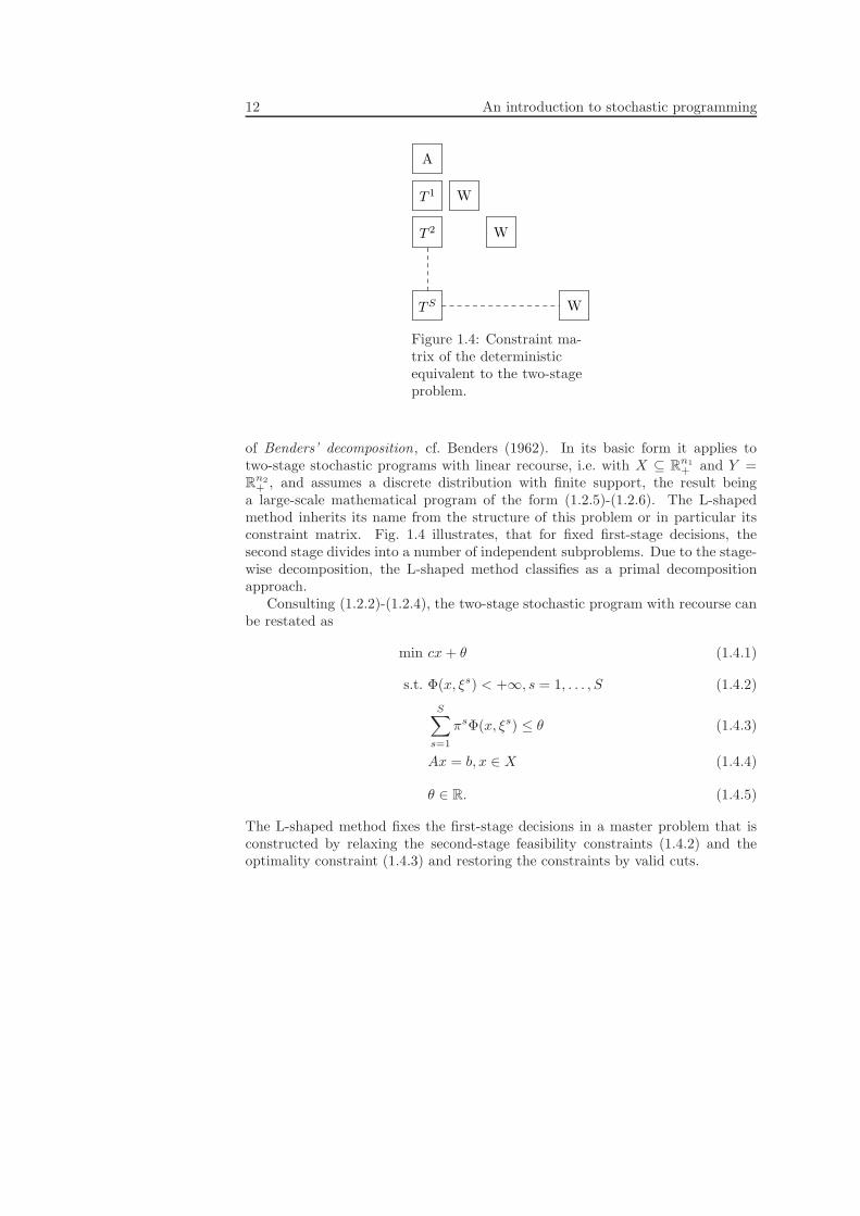
Figure 1.4: Constraint ma-trix of the deterministicequivalent to the two-stageproblem.
of Benders’ decomposition, cf. Benders (1962). In its basic form it applies totwo-stage stochastic programs with linear recourse, i.e. with X ⊆ R
n1+ and Y =
Rn2+ , and assumes a discrete distribution with finite support, the result being
a large-scale mathematical program of the form (1.2.5)-(1.2.6). The L-shapedmethod inherits its name from the structure of this problem or in particular itsconstraint matrix. Fig. 1.4 illustrates, that for fixed first-stage decisions, thesecond stage divides into a number of independent subproblems. Due to the stage-wise decomposition, the L-shaped method classifies as a primal decompositionapproach.
Consulting (1.2.2)-(1.2.4), the two-stage stochastic program with recourse canbe restated as
min cx+ θ (1.4.1)
s.t. Φ(x, ξs) < +∞, s = 1, . . . , S (1.4.2)
S∑
s=1
πsΦ(x, ξs) ≤ θ (1.4.3)
Ax = b, x ∈ X (1.4.4)
θ ∈ R. (1.4.5)
The L-shaped method fixes the first-stage decisions in a master problem that isconstructed by relaxing the second-stage feasibility constraints (1.4.2) and theoptimality constraint (1.4.3) and restoring the constraints by valid cuts.

1.4. Solution approaches 13
Consider some iteration i of the algorithm and solve the master problem. Ifthe problem is infeasible, so is the original problem and the algorithm terminates.A slight modification of the following analysis will suffice if the problem is un-bounded. Finally, if neither infeasible nor unbounded, an optimal solution xi ofthe master problem is found.
Feasibility cuts are derived from a number of linear subproblems defined fors = 1, . . . , S and x ∈ R
n1 by
Φ(x, ξs) := mines1 + es2 |Wy + Is1 − Is2 = hs − T sx,
y ∈ Rn2+ , s1, s2 ∈ R
m2+ , (1.4.6)
where e = (1, . . . , 1), I is the m2 ×m2 identity matrix and s1, s2 ∈ Rm2+ are slack
variables. Evidently, the subproblems can be solved separately. If the solution xi
causes the second-stage problem Φ(xi, ξs) to be infeasible for some s ∈ 1, . . . , S,then 0 < Φ(xi, ξs) = σi,s(hs − T sxi) for a dual optimal solution σi,s to Φ(xi, ξs).Thus, xi will be cut off by adding the feasibility cut
σi,s(hs − T sx) ≤ 0. (1.4.7)
Feasibility cuts of the form (1.4.7) are added until Φ(xi, ξs) are feasible for alls = 1, . . . , S. By duality, (1.4.7) is a valid inequality for (1.4.1) − (1.4.5) for allx ∈ R
n1 that do not violate second-stage feasibility.Having restored second-stage feasibility, the algorithm proceeds by solving the
subproblems. If for some s ∈ 1, . . . , S, Φ(xi, ξs) is unbounded, so is the originalproblem and the algorithm terminates. Otherwise, for s = 1, . . . , S let σi,s bea dual optimal solution to Φ(xi, ξs). If xi is such that θi <
∑Ss=1 π
sΦ(xi, ξs) =∑S
s=1 πsσi,s(hs − T sxi) for some s ∈ 1, . . . , S, then xi is not optimal in the
original problem. Hence, (xi, θi) will be cut off by adding the optimality cut
S∑
s=1
πsσi,s(hs − T sx) ≤ θ (1.4.8)
Again, by duality, the optimality cut is a valid inequality to (1.4.1) − (1.4.5).Having restored both feasibility and optimality, the algorithm terminates with anoptimal solution to the original problem.
The algorithm can be stated as follows
Algorithm 1.4.1
Step 0 (Initialization). Set i = 0 and let the current master problem be
min cx+ θ
s.t. θ ∈ R

14 An introduction to stochastic programming
Step 1 (Solve master problem). Set i = i + 1. Solve the current master problemand let (xi, θi,1, . . . , θi,S) be an optimal solution (If θs = −∞ for somes ∈ 1, . . . , S the variable is ignored in the computation.)
Step 2 (Add feasibility cuts). For s = 1, . . . , S, solve problem (1.4.6) with x = xi
and let σi,s be a corresponding dual solution. If σi,s(hs − T sxi) > 0 forsome s = 1, . . . , S, add a feasibility cut (1.4.7) to the master problem andreturn to step 2.
Step 3 (Add optimality cuts). For s = 1, . . . , S, solve the problem (1.2.4) with
x = xi and let σi,s be a corresponding dual solution. If∑S
s=1 πsσi,s(hs −
T sxi) > θi, add an optimality cut (1.4.8) to the master problem and returnto step 2.
Step 4 (Termination). Stop. The current solution is optimal.
If it exists, Algorithm 1.4.1 terminates with an optimal solution in a finite num-ber of iterations. Otherwise, the algorithm proves unboundedness or infeasibilityof the problem.
There is a different way of considering the use of cutting planes. Dualityarguments may prove the recourse function (1.2.3) to be piecewise linear andconvex. It is thus possible to build an outer linearization of the function and theoptimality cuts can be regarded as supporting hyperplanes in this respect.
In contrast to the optimality cuts (1.4.8) that rely on aggregated information,Wets (1983) and Birge and Louveaux (1988) suggested the use of disaggregatedcuts. The idea was to replace the single cut by a number of cuts derived fromseparate subproblems or so-called bunches of subproblems. Cuts derived fromseparate subproblems have the form
σi,s(hs − T sx) ≤ θs.
Since the disaggregated cuts contain more information, it is expected that the useof the so-called multi-cut method involves less iterations and often outperforms thetraditional L-shaped method, which is supported by the numerical tests of Birgeand Louveaux (1988). Further improvements to the L-shaped method in this di-rection include regularized decomposition proposed by Ruszczynsky (1986). Themethod combines the multi-cut version of L-shaped decomposition with the in-clusion of a quadratic regularizing objective function term, the resulting objectivebeing
cx+
S∑
s=1
πsθs + 0.5α‖x− xi−1‖2,

1.4. Solution approaches 15
where α > 0. This prevents initial solutions from oscillating and allows for cutremoval in order to avoid final degeneracy in the master problem. The quadraticobjective function term ensures strict convexity which provides for finite conver-gence of the algorithm.
Among other methods that emanate from the L-shaped method is stochasticdecomposition by Higle and Sen (1991). The authors use an internal sampling pro-cedure for approximating the probability distribution, and solve the subproblemsat only one sample point. The cuts provided by the internal sampling procedureare statistical estimates that converge to the supporting hyperplanes of the originalobjective function. Finally, the most direct alternative decomposition approach isthe method of Dantzig and Wolfe (1960). Dantzig-Wolfe decomposition can be re-garded as solving the dual to the L-shaped master problem and uses, in contrast toouter linearization and cut generation, inner linearization and column generation.In most cases, the L-shaped method outperforms Dantzig-Wolfe decompositiondue to smaller bases of the master problem.
1.4.2 Two-stage mixed-integer programs
We next discuss solution approaches to two-stage stochastic programs with mixed-integer recourse, i.e. problems on the form (1.2.5)-(1.2.6) with X ⊆ R
n1+ and
Y ⊆ Rn2+ that may contain integrality restrictions on some variables. By virtue
of the integrality, the convexity properties that apply to stochastic linear pro-grams are lost, which makes stochastic mixed-integer program challenging from acomputational point of view.
Independent of convexity, any mixed-integer linear stochastic program canbe stated as its deterministic equivalent, the result being a large-scale problemamenable to LP-based branch and bound . The branch and bound may then beconducted by commercial software such as the CPLEX callable library, cf. CplexOptimization Inc. (2006).
A number of attempts were made at adapting the L-shaped method to two-stage stochastic mixed-integer programs, which lead to a branch and cut proce-dure known as the integer L-shaped method . Laporte and Louveaux (1993) firstproposed the derivation of cuts for two-stage programs with purely binary firststage. Based on general duality theory, Carøe and Tind (1998) later provideda full characterization of the integer L-shaped method and derived cuts for two-stage programs with integer first and second stage. Finally, Norkin, Pflug, andRuszczynski (1998) and Norkin, Ermoliev, and Ruszczynski (1998) suggested thestochastic branch and bound principles using statistical estimates of the recoursefunction instead of ordinary evaluation.
As a contrast to the primal approaches, we present a dual solution approach.The approach is due to Carøe and Schultz (1999) and rests on an idea of variablesplitting and Lagrangian relaxation that has won great attention. To present the

16 An introduction to stochastic programming
A
A
T 1
TS
W
W
H
Figure 1.5: Constraint matrixof the two-stage problem withexplicit non-anticipativity con-straints.
so-called dual decomposition, we proceed as follows.Defining for s = 1, . . . , S the sets
χs = (x, ys) | Ax = b, x ∈ X,Wys + T sx = hs, ys ∈ Y s,
the deterministic equivalent (1.2.5)-(1.2.6) can be restated as
z = min
cx+
S∑
s=1
πsqsys∣
∣
∣(x, ys) ∈ χs, s = 1, . . . , S
. (1.4.9)
We assume the problem is feasible and bounded. The variable splitting applies tothe first-stage variables x and consists in the introduction of copies xs, s = 1, . . . , S.With such copies, non-anticipativity can be explicitly expressed and (1.4.9) isequivalent to
z = min
S∑
s=1
πs(cxs + qsys)∣
∣
∣(xs, ys) ∈ χs, s = 1, . . . , S, x1 = · · · = xS
. (1.4.10)
We further assume that the non-anticipativity constraints are represented by theequality
∑Ss=1M
sxs = 0, where = (M1, . . . ,MS) is a suitable l × n1S matrix. Itshould be remarked that except for the non-anticipativity constraints, the problem(1.4.10) decomposes according to scenarios. For an illustration of the structureof the constraint matrix and its decomposition potential, see Fig. 1.5. We relaxthe non-anticipativity constraints using Lagrangian relaxation. The Lagrangian

1.4. Solution approaches 17
function is
L(x, y;λ) :=
S∑
s=1
(
πs(cxs + qsys) + λM sxs)
,
with the corresponding dual function
D(λ) := minL(x, y;λ) | (xs, ys) ∈ χs, s = 1, . . . , S. (1.4.11)
The Lagrangian dual is therefore
maxD(λ) | λ ∈ Rl.
The Lagrangian relaxation decomposes into scenario subproblems, such that thedual function (1.4.11) is
D(λ) =
S∑
s=1
Ds(λ),
with
Ds(λ) = minπs(cxs + qsys) + λM sxs | (xs, ys) ∈ χs.
For now, we leave out further details on Lagrangian relaxation and state thebranch and cut procedure.
Algorithm 1.4.2
Step 0 (Initialization). Set z = ∞ and let the L consist of
min Q(x)
s.t. Ax = b, x ∈ X
Step 1 (Termination). If L = ∅, then stop. The solution x with z = Q(x) isoptimal.
Step 2 (Node selection). Select and delete a problem P from L. If P is infeasible,go to step 1. Otherwise, solve the Lagrangian dual to obtain the lowerbound z(P ) and go step 3.
Step 3 (Bounding). If z(P ) ≥ z, then go to step 1. Otherwise,
(i) if the scenario solutions xs, s = 1, . . . , S are identical, let z = minsz,Q(xs), delete from L all P ′ with z(P ′) ≥ z and go to step 1.

18 An introduction to stochastic programming
(ii) if the scenario solutions xs, s = 1, . . . , S differ, then compute the av-erage x and round it. If x is feasible, let z = minz, Q(x), deletefrom L all P ′ with z(P ′) ≥ z and go to step 4.
Step 4 (Branching). Select a component xj of x and add two new problems toL obtained from P by adding the constraints xj ≤ ⌊xj⌋ and xj ≥ ⌈xj⌉,respectively (integer component) or xj ≤ xj−ε and xj ≥ xj +ε, respectively(continuous component), where x is the average and ε > 0.
1.4.3 Multi-stage linear programs
The primal solution approach to two-stage linear programs, Benders’ decomposi-tion or the L-shaped method, extends to multi-stage linear programs. The nestedBenders decomposition was suggested by Birge (1985) and applies to multi-stagestochastic programs with Xt = R
nt
+ , t = 1, . . . , T and a discrete distribution withfinite support, stated using the scenario tree formulation (1.3.10)-(1.3.12).
The algorithm relies on the dynamic programming formulation (1.3.2)-(1.3.4)and especially the definition of subproblems for every node n ∈ N of the scenariotree
min cnxn + θn (1.4.12)
s.t. Φn+(xn, ξn+) < +∞, n+ ∈ N+(n) (1.4.13)
∑
n+∈N+(n)
πn+/nΦn+(xn, ξn+) ≤ θn (1.4.14)
∑
0≤t′≤t(n)−1
Wnn−t′xn
−t′ = hn (1.4.15)
Anxn = bn, xn ∈ Xt(n) (1.4.16)
θn ∈ R. (1.4.17)
A master problem is obtained for every node by relaxing the feasibility constraints(1.4.13) and the optimality constraint (1.4.14) and restoring the constraints byvalid cuts derived from the descendant nodes. Both feasibility and optimalitycuts are derived in the same fashion as for the two-stage case. The extensionto multi-stage stochastic programs lies in determining the order of solving thesubproblems and deriving the cuts. This order is determined by the directions,forward DIR = FORE and backward DIR = BACK, in which the scenariotree is traversed. We state the algorithm as a so-called “fast-forward-fast-back”procedure

1.4. Solution approaches 19
Algorithm 1.4.3
Step 0 (Initialization). Set n = 1 and DIR = FORE. Let the master problem ofnode 1 be
min c1x1 + θ1
s.t. A1x1 = b1, x1 ∈ Xt(1)
θ1 ∈ R+
Step 1 (Solve master problem and add feasibility cuts). Solve the master problemof node n.
(i) If infeasible and n = 1, stop. The problem (1.3.2)-(1.3.4) is infeasible.
(ii) If infeasible and n > 1, use the current node to derive a feasibility cutthat is added to the master problem of the ascendant node n−1. SetDIR = BACK, n = n−1 and return to step 1.
(iii) If feasible, let (xn, θn) be an optimal solution (if θn = ∞, the variableis ignored in the computation). If not all n ∈ Nt have been visited,then select a node that has not been visited and return to step 1. Ifall n ∈ Nt have been visited, DIR = FORE and t(n) < T , thenset t = t + 1 and return to step 1. If all n ∈ Nt have been visited,DIR = BACK and t(n) < T , then go to step 2. If all n ∈ Nt havebeen visited and t(n) = T , then DIR = BACK and go to step 2.
Step 2 (Add feasibility cuts). For all n ∈ Nt−1 do the following. Use the ascendantnodes N+(n) to derive an optimality cut.
(i) If necessary, add the optimality cut to the master problem of node n,let t = t− 1 and go to step 1.
(ii) If unnecessary to add an optimality cut and t > 1, then set t = t− 1and select an n ∈ Nt. If t = 1, then DIR = FORE. Return to step1.
(iii) If unnecessary to add an optimality cut and t = 1, then stop. Thesolution x1 is optimal.
With only few additional assumptions, the algorithm converges finitely. As forthe two-stage L-shaped method, the speed of convergence may improve with theuse of multi-cuts and regularization.
Like as traditional Benders’ decomposition, nested Benders’ decomposition re-lies on an outer linearization. Although this is generally preferred in the literature,inner linearizations have also been suggested. Other approaches to multi-stage lin-ear programs are Lagrangian relaxation procedures such as progressive hedging and
20 An introduction to stochastic programming
augmented Lagrangian decomposition. For linear stochastic programs, both algo-rithms converge. The augmented Lagrangian decomposition approach by Mulveyand Ruszczynski (1995) rests on a diagonal quadratic approximation of the La-grangian and a proposal to solve the resulting subproblems by an interior pointmethod. In contrast to the progressive hedging algorithm, the non-anticipativityto be relaxed is determined by scenario branching. Since the progressive hedg-ing applies more generally to multi-stage mixed-integer programs, we defer thediscussion of this approach to the next section.
1.4.4 Multi-stage mixed-integer programs
To address mixed-integer recourse problems, i.e. problems with Xt ⊆ Rnt
+ , t =1, . . . , T , where integrality restrictions may apply to some variables, we considerthe scenario formulation (1.3.6)-(1.3.9).
To some extent, the dual decomposition approach is similar in spirit to theprogressive hedging algorithm suggested by Rockafellar and Wets (1991). Bothapproaches are motivated by relaxation of the non-anticipativity constraints. Thedual decomposition approach, however, automatically produces admissible solu-tions and resolves implementability by branch and bound, whereas progressivehedging iterates between admissible and implementable solutions. We briefly statethe components of the progressive hedging approach.
Introduce the copies (xs1, . . . , x
sT ), s ∈ S and divide the scenarios into bundles.
For every bundle B, set
xBt =∑
s:B(s,t)=B
πsxst
/
∑
s:B(s,t)=B
πs
and let the non-anticipativity constraints be expressed as
if B(s, t) = B then xst = xBt .
Making non-anticipative decisions may be regarded as a means of “hedging”against uncertainty, thus the name progressive hedging.
Define for s = 1, . . . , S the sets
χs =
(xs1, . . . , x
sT )
∣
∣
∣
t∑
t′=1
W stt′x
st′ = hs
t , t = 2, . . . , T,
Astx
st = bst , x
st ∈ Xt, t = 2, . . . , T
and, motivated by the augmented Lagrangian relaxation, let
L(x;λ) :=
S∑
s=1
T∑
t=1
πs(
cstxst + λs
txst + 0.5α(xs
t − xB(s,t)t )2
)
.

1.4. Solution approaches 21
Then the algorithm seeks to solve the quadratic problem
minL(x;λ) | (xs1, . . . , x
sT ) ∈ χs, s = 1, . . . , S
by decomposition it into the scenario subproblems given by
min
T∑
t=1
(
cstxst + λs
txst + 0.5α(xs
t − xB(s,t)t )2
)
∣
∣
∣(xs
1, . . . , xsT ) ∈ χs
.
Now the progressive hedging algorithm reads
Algorithm 1.4.4
Step 0 (Initialization). Set i = 0. Let (λ0,s1 , . . . , λ0,s
T ) = 0, s = 1, . . . , S. Solve the
scenario subproblems without the augmenting term and let
(xs1, . . . , x
sT ), s = 1, . . . , S be an optimal solution. Compute the solution
(x0,B(s,1)1 , . . . , x
0,B(s,T )T ), s = 1, . . . , S. Let the current problem be
min
S∑
s=1
T∑
t=1
πs(
cstxst + λi−1,s
t xst + 0.5α(xs
t − xi−1,B(s,t)t )2
)
s.t. (xs1, . . . , x
sT ) ∈ χs, s = 1, . . . , S
Step 1 (Admissibility). Set i = i+ 1. Solve the current problem and let(xi,s
1 , . . . , xi,sT ), s = 1, . . . , S be an optimal solution. The solution is admis-
sible but not necessarily implementable.
Step 2 (Implementability). Compute the solution (xi,B(s,1)1 , . . . , x
i,B(s,T )T ), s =
1, . . . , S. The solution is implementable but not necessarily admissible.
Step 3 (Termination). If some termination criteria are met, stop. Otherwise, gostep 4.
Step 4 (Multiplier update). Let λi,st = λi−1,s
t + α(xi,st − x
i,B(s,t)t ), t = 1, . . . , T, s =
1, . . . , S and return to step 1.
The progressive hedging algorithm ensures implementable solutions in all it-erations and potentially convergence towards admissibility. As for possible ter-mination criteria, iterations may be continued until a predefined limit is reached,implementable solutions remain nearly unchanged or the integer components ofthe solutions do not change from iteration to iteration.
Løkketangen and Woodruff (1996) have tested the performance of the pro-gressive hedging algorithm and use tabu search for solving the quadratic scenario

22 An introduction to stochastic programming
subproblems close to optimality. The results are found to be very encouraging andindicate convergence in practice.
The authors of the related Lagrangian relaxation approach, dual decomposi-tion, state the extension from two-stage problems to multi-stage problems, al-though they admit the extension may suffer from dimensionality problems. La-grangian relaxation also finds its use in relation to certain coupling constraints.For suitable applications and further discussion, see Chapter 3.
Chapter 2
Deviation measures in two-stage
stochastic linear programming
The present chapter addresses the inclusion of risk measures in two-stage stochasticrecourse programs and the its impact on structural properties and algorithmictreatment.
As a starting point we consider a two-stage stochastic program with linearrecourse. Whereas optimization in the traditional setting is based solely on expec-tation, we include risk measures that reflect dispersions of the random objective.Presenting the resulting mean-risk models, we aim to extend existing results forthe expectation-based model. In particular, we discuss structural properties suchas continuity, differentiability and convexity and address stability issues. Further-more, we propose algorithmic treatment with a slight variation of the L-shapedmethod.
2.1 Introduction
Stochastic programming deals with optimization under uncertainty. Starting froma random optimization problem, the corresponding stochastic program dependsheavily on the criteria for selecting an optimal solution. Traditionally, optimalityrests on the expectation of the random objective. In many respects, however, it isappropriate to take risk into consideration. Combining expectation and risk, themodel is referred to as a mean-risk model.
Risk measures treated in the literature encompass probabilities, dispersionsand conditional expectations. Still, given the variety, no risk measure is unam-biguously recommendable. For recent overviews on the topic, see e.g. Schultz(2003) on the probability of exceeding target, semideviation and conditional valueat risk and Eichhorn and Romisch (2005) on risk measures within the class of
23

24 Deviation measures in two-stage stochastic linear programming
so-called polyhedral risk measures. A wide range of issues are covered, amongthese smoothness and convexity properties, compatibility with asymptotic resultsas well as algorithmic potential.
In this chapter we employ three dispersion measures; central deviation, semide-viation and expected excess of target, all referred to as deviation measures. Themotivation behind deviation measures is their consistency with stochastic domi-nance principles, an attractive behavior of the mean-risk models as well as theirpractical tractability. The above dispersion measures were already investigated inMarkert and Schultz (2005) in the case of mixed-integer linear programs and inAhmed (2004) in the case of linear programs, the latter with emphasis on compu-tational issues.
The idea is to extend existing results from the expectation-based frameworkto the mean-risk models considered here. Thus, we will aim at confirming thatthe models are well-posed, posses a number of useful analytical properties and areindeed in tune with stability results. As the deviation measures are based on piece-wise linear operations they enable algorithmic treatment when the distribution ofthe random variables is discrete. Although the mean-risk models do not imme-diately possess the usual decomposable structure, computational accessibility bysimple modifications of standard solution approaches is possible.
The chapter is organized as follows. In section 2.2 we extend the traditionallinear two-stage stochastic recourse program to mean-risk models and put theseinto perspective with stochastic dominance. Section 2.3 contains prerequisitesknown from the expectation-based case and in section 2.4 and 2.5 similar structureand stability properties for the mean-risk models are analyzed. Algorithmic issuesare presented in section 2.6.
2.2 The two-stage linear stochastic program
As should be clear from Chapter 1, a stochastic recourse program reflects a way ofincluding uncertainty into optimization, the two-stage version being the most basicone. As the name indicates, decisions are made stage-wise. By non-anticipativity,first-stage decisions are to be taken independently of uncertain data, whereasthe second stage allows for recourse actions when uncertainty has been disclosed.The aim of the stochastic program is to select first-stage decisions in an optimalway, optimality depending on which criterion is applied. To formalize this, as inChapter 1, we are given the random linear program
mincx+ q(ω)y | T (ω)x+Wy = h(ω), Ax = b, x ∈ X, y ∈ Rn2+ . (2.2.1)
As before, X ⊆ Rn1+ is a polyhedron, which we further assume is nonempty. More-
over, the costs q : Ω → Rn2 and the right-hand side h : Ω → R
m2 are randomvectors and the technology matrix T : Ω → R
m2×n1 is a random matrix on some
2.2. The two-stage linear stochastic program 25
probability space (Ω,A,P) as previously defined. The value function
Φ(t1, t2) = mint1y |Wy = t2, y ∈ Rn2+ (2.2.2)
is essential in the formulation of the corresponding stochastic program. Accordingto the two-stage framework, the variables x and y of (2.2.1) are to be fixed beforeand after observing h(ω), q(ω), T (ω), respectively, and, therefore, the total costsof the sequential decision process compute as cx+Φ(q(ω), h(ω)−T (ω)x). Findingan optimal x ∈ x ∈ X | Ax = b may be understood as selecting the “best”random objective from the indexed family (cx+ Φ(q(·), h(·) − T (·)x))x∈X:Ax=b.
Considering the expectation-based criterion
QE(x) :=
∫
Ω
(cx+ Φ(q(ω), h(ω) − T (ω)x))P(dω), (2.2.3)
the traditional stochastic program is the optimization problem
minQE(x) | Ax = b, x ∈ X. (2.2.4)
From a stochastic viewpoint, optimizing an expectation tacitly implies repeat-ing the decision process several times and safety issues are addressed only inade-quately. This has lead to the concept of mean-risk models. Here, we measure riskby quantitative deviations of the random objectives from either the mean or somepreselected target. We introduce the central deviation
QD(x) :=
∫
Ω
∣
∣cx+ Φ(q(ω), h(ω) − T (ω)x) −QE(x)∣
∣P(dω), (2.2.5)
the semideviation
QD+(x) :=
∫
Ω
max
cx+ Φ(q(ω), h(ω) − T (ω)x) −QE(x), 0
P(dω) (2.2.6)
and the expected excess of a given target η ∈ R
QDη(x) :=
∫
Ω
max
cx+ Φ(q(ω), h(ω) − T (ω)x) − η, 0
P(dω). (2.2.7)
Accordingly, problem (2.2.4) extends into the mean-risk model
minQE(x) + QR(x) | Ax = b, x ∈ X, (2.2.8)
where ∈ R+ is a suitable weight factor and QR is the risk term, i.e. R = D,R = D+ or R = Dη.
In having to select the “best” of a family of random variables, the stochas-tic dominance approach deserves attention. Although allowing a simple trade-off
26 Deviation measures in two-stage stochastic linear programming
analysis, mean-risk models are unable to capture the entire gamut of risk-aversepreferences. Nevertheless, for the above deviation measures, the mean-risk ap-proach is consistent with second order stochastic dominance (provided that certainconditions on are met). For some aspects of stochastic dominance, see Ogryczakand Ruszczynski (1999) and Ogryczak and Ruszczynski (2001).
We briefly outline stochastic dominance results for the deviation measures(2.2.5)–(2.2.7). Considering the random variables f(x, ·) = cx + Φ(q(·), h(·) −T (·)x), x ∈ x ∈ X | Ax = b, stochastic dominance suggests a partial ordering bypoint-wise comparisons of performance functions constructed from the distributionfunctions. Relevant performance functions are
F (1)x (z) := P(ω ∈ Ω | f(x, ω) ≤ z), z ∈ R,
F (2)x (z) :=
∫ +∞
z
(1 − F (1)x (z′))dz′, z ∈ R.
As smaller outcomes are preferred over larger, the relation of second degree stochas-tic dominance is defined as follows
f(x1, ·) ≻(2) f(x2, ·) ⇐⇒ F (2)x1
(z) ≤ F (2)x2
(z), ∀z ∈ R.
Recall that QE(x) and QR(x) denote the mean and the risk of f(x, ·). Now themean-risk model is said to be consistent with second degree stochastic dominanceif
f(x1, ·) ≻(2) f(x2, ·) ⇒ QE(x1) + QR(x1) ≤ QE(x2) + QR(x2),
i.e. if the mean-risk model inherits a ranking already existing with respect tostochastic dominance. Provided the random variables f(x, ·), x ∈ x ∈ X | Ax =b have finite first moments, the mean-risk models resulting from R = D, R = D+
and R = Dη are indeed consistent with second degree stochastic dominance when ∈ [0, 1/2], ∈ [0, 1] and for all ≥ 0, respectively, cf. Ogryczak and Ruszczynski(1999), proposition 7.
2.3 Prerequisites
Again, as previously, let ξ : Ω → RN be the random vector whose components
constitute the random data, i.e. ξ = (q, h, T1, . . . , Tm2), where T1, . . . , Tm2 denotethe rows of T and N = n2 +m2 +m2 ×n1. Moreover, let P(RN ) represent the setof all probability measures on R
N and introduce from this set the image measureµ = P ξ−1. Changing variables in (2.2.3),
QE(x, µ) =
∫
RN
f(x, ξ)µ(dξ) (2.3.1)

2.3. Prerequisites 27
and similarly for (2.2.5)–(2.2.7), where f(x, ξ) = cx+ Φ(q, h− Tx) for x ∈ Rn1 .
As the results below concern continuity of the objective function with respectto x alone, µ alone and (x, µ) jointly, dependence of both x and µ is markedexplicitly.
We will impose the assumptions
(A1) (Complete recourse) For all t ∈ Rm2 , there exists a y ∈ R
n2+ such that
Wy = t.
(A2) (Dual feasibility) For µ-almost all ξ ∈ RN , there exists a σ ∈ R
m2 such thatσW ≤ q.
(A3) (Finite second moment)∫
RN ‖ξ‖2µ(dξ) < +∞.
The assumptions (A1) and (A2) ensure feasibility and boundedness of problemΦ(q, h−Tx) for all x ∈ R
n1 and µ-almost all ξ ∈ RN and are sufficient to establish
certain properties of the value function Φ.The following basis decomposition theorem applies, cf. Walkup (1969),
Proposition 2.3.1 Let posW := t ∈ Rm2 | ∃y ∈ R
n2+ : Wy = t and D := t ∈
Rn2 | ∃σ ∈ R
m2 : σW ≤ t. Then Φ : D × posW → R is a real-valued continuousfunction. In addition, there exist R
m2 × Rn2 matrices Bj , j = 1, . . . , J and full
dimensional cones Kj , j = 1, . . . , J such that
∪Jj=1Kj = D × posW, intKi ∩ intKj = ∅, i 6= j,
and
Φ(t1, t2) = t1B−1j t2 ∀(t1, t2) ∈ Kj .
For fixed t1 ∈ Rn2 , the function Φ(t1, ·) is convex. For fixed t2 ∈ R
m2 , the functionΦ(·, t2) is concave.
Prerequisites comprise results on the expectation-based model (2.2.4). Lips-chitz estimates of the integrand of (2.3.1) can be derived from Proposition 2.3.1and are found in Romisch (2003).
Proposition 2.3.2 Assume (A1)–(A2). Then there exist constants L1, L2,K1 >0 such that for all x, x1, x2 ∈ R
n1 and µ-almost all ξ, ξ1, ξ2 ∈ RN
(i) |f(x, ξ1) − f(x, ξ2)| ≤ L1‖x‖max1, ‖ξ1‖, ‖ξ2‖‖ξ1 − ξ2‖,
(ii) |f(x1, ξ) − f(x2, ξ)| ≤ L2 max1, ‖ξ‖2‖x1 − x2‖,
(iii) |f(x, ξ)| ≤ K1‖x‖max1, ‖ξ‖2.

28 Deviation measures in two-stage stochastic linear programming
From Wets (1974) and Kall (1976), we get
Proposition 2.3.3 Assume (A1)–(A3).
(i) Then QE(·, µ) : Rn1 → R is a real-valued, convex and Lipschitzian function.
(ii) Suppose further that µ is absolutely continuous with respect to the Lebesguemeasure on R
N . Then QE(·, µ) : Rn1 → R is continuously differentiable.
Remark 2.3.1 In the case where only the right-hand side is random, results onstrong and strict convexity appear in Schultz (1994). Let q ∈ R
n2 be a knownvector, h : Ω → R
m2 be a random vector with the corresponding image measureµ = P h−1. Moreover, let QE(χ, µ) :=
∫
Rm2Φ(q, h − χ)µ(dh) be a function of
the tender variable χ. (i) Assume (A1) and that µ has finite first moment andis absolutely continuous with respect to the Lebesgue measure on R
m2 . Supposefurther that there exists a σ ∈ R
m2 such that σW < q component-wise. ThenQE(·, µ) is strictly convex on any open convex subset V ⊆ R
m2 of the support ofµ. (ii) Assume further that there exist a convex open set V ⊆ R
m2 , constantsc1 > 0, c2 > 0 and a density g of µ such that g(z) ≥ c1 for all z ∈ R
m2 withdist(z, V ) := inf‖z − v‖ | v ∈ V ≤ c2. Then QE(·, µ) is strongly convex on V .
The remaining continuity properties are relevant to stability results of thestochastic programs. Such results divide into qualitative and quantitative results.When qualitative stability is brought into focus, joint continuity is of crucial im-portance. A notion of convergence of probability measures is required, and weakconvergence will prove sufficiently general while it still allows for substantial state-ments. A sequence µn ⊆ P(RN ) is said to converge weakly to µ ∈ P(RN), i.e.
µnw−→ µ, if for any bounded continuous function h : R
N → R, it holds that
∫
RN
h(ξ)µn(dξ) →
∫
RN
h(ξ)µ(dξ),
cf. Billingsley (1968). Restricting measures to the set
∆r,K(RN ) :=
ν ∈ P(RN )∣
∣
∣
∫
RN
‖ξ‖rν(dξ) ≤ K
,
we get the following, cf. Kall (1987) and Robinson and Wets (1987),
Proposition 2.3.4 Assume (A1)–(A2) and let µ ∈ ∆r,K(RN ) for some r > 2,K > 0. Then QE : R
n1 × ∆r,K(RN ) → R is jointly continuous at (x, µ).
To arrive at quantitative stability results, we consider a so-called distance withd-structure, given as a uniform distance between expectations of functions froma class of measurable functions. Working with functions that share analytical
2.4. Structure 29
properties with the integrand of (2.3.1), we obtain an ideal metric, optimallyadjusted to the model, cf. Romisch (2003). Let F2(R
N ) := F : RN → R |
|F (ξ1) − F (ξ2)| ≤ c2(ξ1, ξ2)‖ξ1 − ξ2‖ ∀ξ1, ξ2 ∈ RN denote the class of locally
Lipschitz continuous functions with constant c2(ξ1, ξ2) := max1, ‖ξ1‖, ‖ξ2‖ andP2(R
N ) := ν ∈ P(RN ) |∫
RN ‖ξ‖2ν(dξ) < +∞ the set of measures having finitesecond moments. For µ, ν ∈ P2(R
N ) define the pseudo-metric
d2(µ, ν) := supF∈F2(RN )
∣
∣
∣
∫
RN
F (ξ1)µ(dξ1) −
∫
RN
F (ξ2)ν(dξ2)∣
∣
∣.
The pseudo-metric is referred to as the Fortet-Mourier metric of second order. TheLipschitz estimates of QE(x, ·) for all x ∈ R
n1 can be found in Romisch (2003).
Proposition 2.3.5 Assume (A1)–(A2) and let x ∈ X | Ax = b be nonemptyand bounded. Then there exists a constant L > 0 such that the estimate
supx∈X:Ax=b|QE(x, µ) −QE(x, ν)| ≤ Ld2(µ, ν)
is valid whenever µ, ν ∈ P2(RN ).
2.4 Structure
The following identities are obtained by straightforward computation, cf. Markertand Schultz (2005),
QE(x, µ) + QD(x, µ) = E[f(x, ξ)] + E[|f(x, ξ) − E[f(x, ξ)]|]
= (1 − 2)E[f(x, ξ)] + 2E[maxf(x, ξ),E[f(x, ξ)]], (2.4.1)
QE(x, µ) + QD+(x, µ) = E[f(x, ξ)] + E[maxf(x, ξ) − E[f(x, ξ)], 0]
= (1 − )E[f(x, ξ)] + E[maxf(x, ξ),E[f(x, ξ)]], (2.4.2)
QE(x, µ) + QDη(x, µ) = E[f(x, ξ)] + E[maxf(x, ξ) − η, 0]
= E[f(x, ξ)] + E[maxf(x, ξ), η] − η. (2.4.3)
Evidently, the mean-risk objective functions are linear combinations of QE(x, µ)and either
Qmax(x, µ) :=
∫
RN
maxf(x, ξ), QE(x, µ)µ(dξ) (2.4.4)
or the more simple version
Qmax,η(x, µ) :=
∫
RN
maxf(x, ξ), ηµ(dξ). (2.4.5)

30 Deviation measures in two-stage stochastic linear programming
Remark 2.4.1 The integrals (2.4.4) and (2.4.5) make sense for measurable func-tions only. Let therefore x ∈ R
n1 . Since Φ(t1, t2) is continuous in (t1, t2) and(q, h − Tx) is linear in ξ, f(x, ξ) = cx + Φ(q, h − Tx) is continuous in ξ. Byanother continuity argument, maxf(x, ·), QE(x, µ) and maxf(x, ·), η are mea-surable.
The purpose of this section is to obtain continuity, differentiability and con-vexity properties of the mean-risk objective functions. Keeping the reformulations(2.4.1)–(2.4.3) in mind and having examined the behavior of Qmax, Qmax,η andQE, the desired results will follow immediately. The following investigations con-cern Qmax only, since the results carry over to Qmax,η in a similar fashion and thestructural properties of QE were already given in Section 2.3
We start by giving Lipschitz estimates of the integrand.
Proposition 2.4.1 Assume (A1)–(A3). Then for the constants L1, L2,K1 > 0of Proposition 2.3.2 and for all x, x1, x2 ∈ R
n1 and µ-almost all ξ, ξ1, ξ2 ∈ RN
(i) |maxf(x, ξ1), QE(x, µ) − maxf(x, ξ2), QE(x, µ)| ≤
L1‖x‖max1, ‖ξ1‖, ‖ξ2‖‖ξ1 − ξ2‖,
(ii) |maxf(x1, ξ), QE(x1, µ) − maxf(x2, ξ), QE(x2, µ)| ≤
maxL2 max1, ‖ξ‖2, LE‖x1 − x2‖,
where LE denotes the Lipschitz constant of QE(·, µ),
(iii) |maxf(x, ξ), QE(x, µ)| ≤ K1‖x‖max1, ‖ξ‖2 + |QE(x, µ)|.
Proof. Apply Proposition 2.3.2 and the following lemma from Donchev (1986):Let gi, i = 1, . . . , I be Lipschitzian functions with constants Li, i = 1, . . . , I andlet g be defined as some continuous selection of giI
i=1. Then g is a Lipschitzianfunction with constant L = maxi=1,...,ILi.
Proposition 2.4.2 Assume (A1)–(A3). Then Qmax(·, µ) : Rn1 → R is a real-
valued, convex and Lipschitzian function.
Proof. Throughout the proof we apply proposition 2.4.1. For x ∈ Rn1 ,
|Qmax(x, µ)| ≤ E[|maxf(x, ξ), QE(x, µ)|]
≤ K1‖x‖(1 + E[‖ξ‖2]) + |QE(x, µ)| < +∞,
which verifies that Qmax(·, µ) is real-valued.Since Φ(t1, ·) is convex for all t1 ∈ R
n2 and h−Tx is linear in x, f(x, ξ) := cx+Φ(q, h−Tx) is convex in x. Moreover, as both the maximum and the expectationoperators preserve convexity, Qmax(·, µ) is convex.

2.4. Structure 31
Denote the Lipschitz constant of QE(·, µ) by LE. For x1, x2 ∈ Rn1 ,
|Qmax(x1, µ) −Qmax(x2, µ)|
≤ E[|maxf(x1, ξ), QE(x1, µ) − maxf(x2, ξ), QE(x2, µ)|]
≤ E[maxL2 max1, ‖ξ‖2, LE]‖x1 − x2‖,
where E[maxL2 max1, ‖ξ‖2, LE] ≤ L2(1 + E[‖ξ‖2]) + LE < +∞, and we haveestablished Lipschitz continuity of Qmax(·, µ).
Remark 2.4.2 Together, continuity of QE(·, µ) + QR(·, µ) and compactness ofx ∈ X | Ax = b ensure that the minimum in (2.2.8) is attained.
Remark 2.4.3 For R = D, let ∈ [0, 1/2), for R = D+, let ∈ [0, 1) and forR = Dη let ≥ 0. Consider the reformulations (2.4.1)–(2.4.3). Then QE(·, µ) +QR(·, µ) is seen to be convex. In the case of only a random right-hand side,both strict and strong convexity is inherited, cf. Remark 2.3.1. To see this, defineQE(χ, µ) as above and define the risk measures QR(χ, µ) similarly. Provided thatthe assumptions of the expectation-based case are fulfilled, the mean-risk objectiveQE(·, µ) + QR(·, µ) is strictly and strongly convex.
Example 1 The following example demonstrates that the function QE(·, µ) +QD+(·, µ) is in general nonconvex for > 1. Let Φ(h − x) = miny | y ≥h − x, y ≥ 0 = maxh− x, 0 and f(x, h) = x + maxh − x, 0. Assume µ(h =2) = 1/2, µ(h = 3) = 1/2 and = 3. Now QE(x, µ) + QD+(x, µ) = x −14 max2 − x, 0 + 5
4 max3 − x, 0. Consider the points x1 = −1, x2 = 3 anda convex combination of the two, x = 1
2x1 + 12x2 = 1. The relation QE(x, µ) +
QD+(x, µ) = 134 > 25
8 = 12 (QE(x1, µ)+QD+(x1, µ))+ 1
2 (QE(x2, µ)+QD+(x2, µ))shows that QE(·, µ)+QD+(·, µ) fails to be convex. The same data refute convexityof QE(·, µ) + QD(·, µ) for > 1/2.
Proposition 2.4.3 Assume (A1)–(A3) and that µ is absolutely continuous withrespect to the Lebesgue measure on R
N . Then Qmax(·, µ) : Rn1 → R is continu-
ously differentiable.
Proof. Let x ∈ Rn1 and denote by E(x) the set of points (q, h, T ) in which
Φ(q, h−Tx) is non-differentiable in x. It is shown by Kall (1976) that µ(E(x)) = 0.Hence, Φ(q, h − Tx) is differentiable in x for µ-almost all ξ ∈ R
N and the sameholds for f(x, ξ). Moreover, by Proposition 2.3.3, Q(x, µ) is differentiable. Definethe sets
E>(x) := ξ ∈ RN | f(x, ξ) > QE(x, µ),

32 Deviation measures in two-stage stochastic linear programming
E<(x) := ξ ∈ RN | f(x, ξ) < QE(x, µ),
E=(x) := ξ ∈ RN | f(x, ξ) = QE(x, µ).
Then, if x denotes the gradient in x,
x maxf(x, ξ), QE(x, µ) =
xf(x, ξ), if ξ ∈ E>(x)\E(x)
xQE(x, µ), if ξ ∈ E<(x).(2.4.6)
Observe that, according to Proposition 2.3.1,
Φ(q, h− Tx) =
J∑
j=1
qB−1j (h− Tx)1Kj(x)(q, h, T ),
since ∪Jj=1Kj(x) = R
N and Ki(x) ∩ Kj(x) = ∅, i 6= j, where Kj(x) := (q, h, T ) |
(q, h− Tx) ∈ Kj\ ∪j−1i=1 Ki. Hence, the following inclusion applies
E=(x) : =
(q, h, T )∣
∣
∣cx+
J∑
j=1
qB−1j (h− Tx)1Kj(x)(q, h, T ) = QE(x, µ)
⊆ ∪Jj=1Hj(x),
where
Hj(x) := (q, h, T ) | cx+ qB−1j (h− Tx) = QE(x, µ), j = 1, . . . , J.
For j = 1, . . . , J , we aim to show that Hj(x) has Lebesgue measure zero. Notethat
Hj(x) = H1j (x) ∪H2
j (x),
where
H1j (x) := (q, h, T ) | q 6= 0, cx+ qB−1
j (h− Tx) = QE(x, µ)
and
H2j (x) := (0, h, T ) | cx = QE(x, µ).
Letting
H1j (x, q, T ) : = h | (q, h, T ) ∈ H1
j (x)
= h | q 6= 0, qB−1j h = qB−1
j Tx− cx+QE(x, µ),

2.4. Structure 33
it is clear that this is a hyperplane and, thus, has Lebesgue measure zero. Now asH1
j (x, q, T ) is a section of H1j (x), H1
j (x) has Lebesgue measure zero, cf. Theorem0.25 by Kall (1976). Also, either
H2j (x) = ∅ or H2
j (x) = 0 ∪ Rm2+m2×n1 .
In both cases, H2j (x) has a dimension lower than N = n2 + m2 + m2 × n1 and,
therefore, has Lebesgue measure zero. Brought together, Hj(x) has Lebesguemeasure zero and since µ is absolute continuous with respect to the Lebesguemeasure, µ(Hj(x)) = 0. As a consequence, maxf(x, ξ), QE(x, µ) is differentiablewith gradient (2.4.6) for all ξ ∈ R
N\(E(x)∪E=(x)), where µ(E(x) ∪E=(x)) = 0.From Proposition 2.4.1,
|maxf(x1, ξ), QE(x1, µ) − maxf(x2, ξ), QE(x2, µ)|/‖x1 − x2‖
is dominated by an integrable constant and Lebesgue dominated convergence im-plies existence of the gradient
xE[maxf(x, ξ), QE(x, µ)] = E[x maxf(x, ξ), QE(x, µ)].
Finally, as Qmax(x, µ) is convex and differentiable, it is continuously differentiable,cf. Theorem 25.5 Rockafellar (1997).
As in Section 2.3, we restrict measures to the set
∆r,K(RN ) :=
ν ∈ P(RN )∣
∣
∣
∫
RN
‖ξ‖rν(dξ) ≤ K
.
Proposition 2.4.4 Assume (A1)–(A2) and let µ ∈ ∆r,K(RN ) for some r > 2,K > 0. Then Qmax : R
n1 × ∆p,K(RN ) → R is jointly continuous w.r.t. (x, µ).
Proof. Let x, xn ∈ Rn1 , xn → x and µn, µ ∈ ∆r,K(RN ), µn
w−→ µ. We intent to
show
Qmax(xn, µn) → Qmax(x, µ), n→ ∞.
Defining g(ξ) := maxf(x, ξ), QE(x, µ) and gn(ξ) := maxf(xn, ξ), QE(xn, µn),this is equivalent to
∫
RN
gn(ξ)µn(dξ) →
∫
RN
g(ξ)µ(dξ), n→ ∞. (2.4.7)
Initially, we aim to show
µn g−1n
w−→ µ g−1 (2.4.8)

34 Deviation measures in two-stage stochastic linear programming
or, equivalently,
∫
RN
h(ξ)µn g−1n (dξ) →
∫
RN
h(ξ)µ g−1(dξ), n→ ∞
for any bounded continuous function h : RN → R. Changing variables,
∫
RN
h(gn(ξ))µn(dξ) →
∫
RN
h(g(ξ))µ(dξ), n→ ∞,
this follows directly from µnw−→ µ, since h gn and h g are bounded continuous
functions. The proof is completed by applying Theorem 5.4 by Billingsley (1968)according to which (2.4.8) and uniform integrability imply (2.4.7). A sufficientcondition for uniform integrability is the moment condition
supn
∫
RN
|gn(ξ)|qµn(dξ) < +∞ (2.4.9)
for some q > 1. Now, from Proposition 2.4.1, there exists a constant K1 > 0, suchthat
|gn(ξ)|q = |maxf(xn, ξ), QE(xn, µn)|q
≤ (K1‖xn‖max1, ‖ξ‖2 + |QE(xn, µn)|)q.
The sequence ‖xn‖ has an upper bound, κ1. Likewise, joint continuity of QE(·, ·)ensures an upper bound, κ2, of |QE(xn, µn)|. Consequently, we continue theestimate
|gn(ξ)|q ≤ ((K1κ1)(1 + ‖ξ‖2) + κ2)q ≤ (4K1κ1)
q(1 + ‖ξ‖2q) + 2qκq2. (2.4.10)
Recall that µ ∈ ∆r,K(RN ) for some r > 2. Letting q = 12r, (2.4.10) finally gives
us∫
RN
|gn(ξ)|qµn(dξ) ≤ (4K1κ1)q(1 +K) + 2qκq
2 < +∞.
Thus, (2.4.9) is verified.
Proposition 2.4.5 Assume (A1)–(A2) and let x ∈ X : Ax = b be nonemptyand bounded. Then there exists a constant L > 0 such that the estimate
supx∈X:Ax=b|Qmax(x, µ) −Qmax(x, ν)| ≤ Ld2(µ, ν)
is valid whenever µ, ν ∈ P2(RN ).

2.4. Structure 35
Proof. Let x ∈ Rn1 and µ, ν ∈ P2(R
N ). The following evaluations hold
|Qmax(x, µ) −Qmax(x, ν)| (2.4.11)
=∣
∣
∣
∫
RN
maxf(x, ξ), QE(x, µ)µ(dξ) −
∫
RN
maxf(x, ξ), QE(x, ν)ν(dξ)∣
∣
∣
≤∣
∣
∣
∫
RN
maxf(x, ξ), QE(x, µ)µ(dξ) −
∫
RN
maxf(x, ξ), QE(x, µ)ν(dξ)∣
∣
∣
+∣
∣
∣
∫
RN
maxf(x, ξ), QE(x, µ)ν(dξ) −
∫
RN
maxf(x, ξ), QE(x, ν)ν(dξ)∣
∣
∣.
Consider the first term of (2.4.11). Recall the definition of c2(ξ1, ξ2). Accordingto Proposition 2.4.1, for some constant L1 > 0,
|maxf(x, ξ1), QE(x, µ) − maxf(x, ξ2), QE(x, µ)|
≤ L1‖x‖max1, ‖ξ1‖, ‖ξ2‖‖ξ1 − ξ2‖
≤ L1(supx∈X:Ax=b‖x‖)c2(ξ1, ξ2)‖ξ1 − ξ2‖
for µ-almost all ξ1, ξ2 ∈ RN and hence, there exists a constant L2 > 0 such that the
function (1/L2)maxf(x, ξ), QE(x, µ) belongs to the set F2(RN ). Consequently,
∣
∣
∣
∫
RN
maxf(x, ξ), QE(x, µ)µ(dξ) −
∫
RN
maxf(x, ξ), QE(x, µ)ν(dξ)∣
∣
∣
≤ L2supF∈F2(RN )
∣
∣
∣
∫
RN
F (ξ)µ(dξ) −
∫
RN
F (ξ)ν(dξ)∣
∣
∣= L2d2(µ, ν). (2.4.12)
For the second term of (2.4.11), we have∣
∣
∣
∫
RN
maxf(x, ξ), QE(x, µ)ν(dξ) −
∫
RN
maxf(x, ξ), QE(x, ν)ν(dξ)∣
∣
∣
≤
∫
RN
∣
∣
∣maxf(x, ξ), QE(x, µ) − maxf(x, ξ), QE(x, ν)
∣
∣
∣ν(dξ)
and applying the inequality |maxa, b − maxa, c| ≤ |b− c|,∫
RN
|maxf(x, ξ), QE(x, µ) − maxf(x, ξ), QE(x, ν)|ν(dξ)
≤
∫
RN
|QE(x, µ) −QE(x, ν)|ν(dξ) = |QE(x, µ) −QE(x, ν)|.
From Proposition 2.3.5, we have some constant L3 > 0 such that
|QE(x, µ) −QE(x, ν)| ≤ L3d2(µ, ν). (2.4.13)
The final result now follows from (2.4.12) and (2.4.13).

36 Deviation measures in two-stage stochastic linear programming
Remark 2.4.4 Propositions 2.4.1, 2.4.2, 2.4.3, 2.4.4, 2.4.5 are valid for Qmax,η,also. In fact, with minor modifications, the proofs still hold, replacing QE(x, µ) bythe constant η.
Corollary 2.4.1 For R = D, let ∈ [0, 1/2]; for R = D+, let ∈ [0, 1] and forR = Dη, let ≥ 0. Then the statements of propositions 2.4.2, 2.4.3, 2.4.4, 2.4.5are valid for the mean-risk objective QE(x, µ) + QR(x, µ).
2.5 Stability
In many practical applications of stochastic programming, the probability distri-bution is not fully known. In such cases, the true measure has to be replacedby some suitable estimate, e.g. an empirical measure. Even if the true distribu-tion is indeed fully known, an approximate measure may be required to facilitatecomputations. This justifies the examination of stability issues in stochastic pro-gramming. More specifically, we analyze the situation in which the underlyingprobability measure is subjected to perturbations. For recent surveys on stabilityin two-stage stochastic programming, see Romisch (2003) and Schultz (2000).
Considering the problem
P (µ) : minQE(x, µ) + QR(x, µ) | Ax = b, x ∈ X,
stability results take the form of continuity properties of the optimal value functionand the solution set mapping defined as
φ(µ) := infQE(x, µ) + QR(x, µ) | Ax = b, x ∈ X,
ϕ(µ) := x ∈ X | Ax = b,QE(x, µ) + QR(x, µ) = φ(µ).
The primary result of qualitative stability follows directly from Corrolary 2.4.1 andparametric optimization, cf. Berge (1963), Theorem 1.1, 1.2 and the MaximumTheorem,
Proposition 2.5.1 Assume (A1)–(A2) and µ ∈ ∆r,K(RN ) for some r > 2, K >0. Suppose further that x ∈ X | Ax = b is nonempty and bounded. For R = D,let ∈ [0, 1/2]; for R = D+, let ∈ [0, 1] and for R = Dη, let ≥ 0. Then
(i) φ : ∆r,K(RN ) → R is continuous where ∆r,K(RN ) is equipped with weakconvergence of probability measures.
(ii) ϕ : ∆r,K(RN ) → 2Rn1
is Berge upper semicontinuous, i.e. for any µ ∈∆r,K(RN ) and any open set V ⊂ R
n1 with V ⊇ ϕ(µ), there exists a neigh-borhood V of µ in ∆r,K(RN ) such that ϕ(ν) ⊆ V for all ν in V.

2.5. Stability 37
Remark 2.5.1 From Proposition 2.5.1 stability results involving discrete approx-imations of the true probability measure can be derived in the same way as appliesto the expectation-based case. Such approximations include empirical measures ormeasures that are close to the true one with respect to some (pseudo) metric. Thelatter is associated with optimal scenario generation and optimal scenario reduc-tion, cf. Romisch (2003), Pflug (2004) and Heitsch and Romisch (2006b). Forfurther reference on scenario generation and reduction, see Chapter 7.
Example 2 The example shows that the uniform integrability assumption inProposition 2.4.4 is indispensable for qualitative stability. Let Φ(h−x) = miny |y ≥ h− x, y ≥ 0 = maxh− x, 0, f(x, h) = maxh− x, 0 and x ∈ X | Ax =b = [0, 1]. Denote by δǫ the measure that places unit mass at ǫ ∈ R. Let µ = δ0and µn = (1 − 1
n )δ0 + 1nδn, n ∈ N. Then µn
w−→ µ. Consider R = D+ and define
the optimal value function φ(µ) := infQE(x, µ) + QR(x, µ) | x ∈ X,Ax = b.Whereas φ(µ) = 0, φ(µn) = 1− 1
n +(1− 2n + 1
n2 ). But then φ(µn) 9 φ(µ), n → ∞.Considering the same data, sufficiency of uniform integrability in the case R = Dis clear.
In consequence of the continuity results, quantitative stability is based on theFortet-Mourier metric of second order.
Proposition 2.5.2 Assume (A1)–(A2) and let x ∈ X | Ax = b be nonemptyand bounded. Then there exists a constant L > 0 such that the estimate
|φ(µ) − φ(ν)| ≤ Ld2(µ, ν)
is valid whenever µ, ν ∈ P2(RN ).
Proof. Let µ, ν ∈ P2(RN ). Since QE(x, µ)+ QR(x, µ) and QE(x, ν)+ QR(x, ν)
are continuous in x and x ∈ X | Ax = b is nonempty and compact, ϕ(µ) 6= ∅and ϕ(ν) 6= ∅. Therefore, we can choose xµ ∈ ϕ(µ) and xν ∈ ϕ(ν). Together,
φ(µ) ≤ QE(xν , µ) + QR(xν , µ)
≤ φ(ν) + |(QE(xν , µ) + QR(xν , µ)) − (QE(xν , ν) + QR(xν , ν))|
and
φ(ν) ≤ QE(xµ, ν) + QR(xµ, ν)
≤ φ(µ) + |(QE(xµ, ν) + QR(xµ, ν)) − (QE(xµ, µ) + QR(xµ, µ))|
imply
|φ(µ) − φ(ν)| ≤ supx∈X:Ax=b|(QE(x, µ) − QR(x, µ)) − (QE(x, ν) + QR(x, ν))|.
We get the desired result from Corollary 2.4.1.
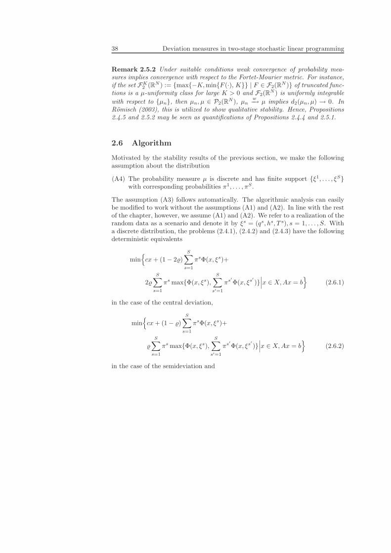
38 Deviation measures in two-stage stochastic linear programming
Remark 2.5.2 Under suitable conditions weak convergence of probability mea-sures implies convergence with respect to the Fortet-Mourier metric. For instance,if the set FK
2 (RN ) := max−K,minF (·), K | F ∈ F2(RN ) of truncated func-
tions is a µ-uniformity class for large K > 0 and F2(RN ) is uniformly integrable
with respect to µn, then µn, µ ∈ P2(RN ), µn
w−→ µ implies d2(µn, µ) → 0. In
Romisch (2003), this is utilized to show qualitative stability. Hence, Propositions2.4.5 and 2.5.2 may be seen as quantifications of Propositions 2.4.4 and 2.5.1.
2.6 Algorithm
Motivated by the stability results of the previous section, we make the followingassumption about the distribution
(A4) The probability measure µ is discrete and has finite support ξ1, . . . , ξSwith corresponding probabilities π1, . . . , πS .
The assumption (A3) follows automatically. The algorithmic analysis can easilybe modified to work without the assumptions (A1) and (A2). In line with the restof the chapter, however, we assume (A1) and (A2). We refer to a realization of therandom data as a scenario and denote it by ξs = (qs, hs, T s), s = 1, . . . , S. Witha discrete distribution, the problems (2.4.1), (2.4.2) and (2.4.3) have the followingdeterministic equivalents
min
cx+ (1 − 2)
S∑
s=1
πsΦ(x, ξs)+
2
S∑
s=1
πs maxΦ(x, ξs),
S∑
s′=1
πs′
Φ(x, ξs′
)∣
∣
∣x ∈ X,Ax = b
(2.6.1)
in the case of the central deviation,
min
cx+ (1 − )
S∑
s=1
πsΦ(x, ξs)+
S∑
s=1
πs maxΦ(x, ξs),
S∑
s′=1
πs′
Φ(x, ξs′
)∣
∣
∣x ∈ X,Ax = b
(2.6.2)
in the case of the semideviation and

2.6. Algorithm 39
min
cx+
S∑
s=1
πsΦ(x, ξs)+
S∑
s=1
πs maxΦ(x, ξs), η∣
∣
∣x ∈ X,Ax = b
− η (2.6.3)
in the case of expected excess of target.Observe that problem (2.6.1) is equivalent to
min cx+ (1 − 2)
S∑
s=1
πsθs + 2
S∑
s=1
πsvs (2.6.4)
s.t. Φ(x, ξs) ≤ θs,S
∑
s′=1
πs′
θs′
≤ vs, θs ≤ vs, x ∈ X, Ax = b,
vs, θs ∈ R, s = 1, . . . , S,
problem (2.6.2) to
min cx+ (1 − )
S∑
s=1
πsθs +
S∑
s=1
πsvs (2.6.5)
s.t. Φ(x, ξs) ≤ θs,S
∑
s′=1
πs′
θs′
≤ vs, θs ≤ vs, x ∈ X, Ax = b
vs, θs ∈ R, s = 1, . . . , S
and problem (2.6.3) to
min cx+
S∑
s=1
πsθs +
S∑
s=1
πsvs − η
s.t. Φ(x, ξs) ≤ θs, η ≤ vs, θs ≤ vs, x ∈ X, Ax = b
vs, θs ∈ R, s = 1, . . . , S
The block structure of the problems (2.6.4) and (2.6.5) does not fit into exist-ing schemes of stochastic programming. In contrast to the traditional two-stagestochastic program, the mean-risk problems contain explicit coupling between the

40 Deviation measures in two-stage stochastic linear programming
scenario-dependent variables which prevents most well-known algorithms fromworking. Nevertheless, by regarding some of the scenario-dependent variablesas first-stage variables, we are able to restore a certain degree of separability. It ispossible to decompose the problems with respect to stages and work scenario-wiseby means of a cutting plane algorithm.
Another cutting plane algorithm is proposed by Ahmed (2004), who derivescuts in a fashion inspired by subgradient methods from convex optimization. Usingparametric analysis with respect to the objective coefficients, the efficient frontiercan be constructed by varying the trade-off coefficient, , in the appropriate range.It should be clear from the following that this feature also applies to the presentalgorithm. The main difference between the two algorithms is the number of cutsadded in an iteration and the information within each cuts.
For simplicity, we state the algorithm for central deviation. It works in asimilar fashion for semideviation and expected excess of target. The idea is torelax the constraints Φ(x, ξs) ≤ θs, s = 1, . . . , S and iteratively reinforce them bymeans of optimality cuts. Consider some iteration i of the algorithm and let thecorresponding solution be xi. Then Φ(xi, ξs), s = 1, . . . , S is feasible and bounded.For s = 1, . . . , S let σi,s be a dual optimal solution of Φ(xi, ξs). If xi is such thatθi,s < Φ(xi, ξs) = σi,s(hs − T sxi) for some s ∈ 1, . . . , S, then (xi, θi,1, . . . , θi,S)is cut off by adding the optimality cut
σi,s(hs − T sx) ≤ θs. (2.6.6)
By duality, Φ(x, ξs) ≥ σi,s(hs − T sx) for all x ∈ Rn1 , showing that the optimality
cut is a valid inequality to (2.6.4). The algorithm proceeds as follows
Algorithm 2.6.1
Step 0 (Initialization). Set i = 0 and let the current master problem be
min cx+ (1 − 2)
S∑
s=1
πsθs + 2
S∑
s=1
πsvs
s.t.S
∑
s=1
πsθs ≤ vs, θs ≤ vs, x ∈ X, Ax = b
vs, θs ∈ R, s = 1, . . . , S.
Step 1 (Solve master problem). Set i = i + 1. Solve the current master problemand let (xi, vi,1, . . . , vi,S , θi,1, . . . , θi,S) be an optimal solution (If θs = −∞or vs = −∞ for some s ∈ 1, . . . , S the variable is ignored in the compu-tation.)

2.6. Algorithm 41
Step 2 (Add optimality cuts). For each s = 1, . . . , S, solve the second-stage prob-lem with x = xi and let σi,s be a corresponding dual solution. If σi,s(hs −T sxi) > θi,s for some s ∈ 1, . . . , S, add an optimality cut (2.6.6) to themaster problem and return to step 2.
Step 3 (Termination). Stop. The current solution is optimal.
We obtain a lower bound to the mean-risk problem by means of the relaxationprovided by the master problem and eventually also an upper bound by a feasiblesolution. In that the bounds coincide, the master problem in this fashion producesan optimal solution to the mean-risk problem. Indeed, we have the following,
Proposition 2.6.1 Assume (A1)-(A2), (A4) and that x ∈ X | Ax = b isnonempty and bounded. Then Algorithm 2.6.1 terminates with an optimal solutionto the mean-risk problem in a finite number of iterations.
Proof. By remark 2.4.2, an optimal solution to the mean-risk problem (2.6.4)exists. Let x∗ be a such solution and let z∗ be the optimal value. Since the masterproblem is a relaxation of (2.6.4), the optimal value zi of the master problem initeration i is a lower bound on z∗, i.e.
zi ≤ z∗. (2.6.7)
Now if in iteration i for some s ∈ 1, . . . , S, σi,s(hs − T sxi) > θs, an optimalitycut will be added and the algorithm proceeds. Only a finite number of cuts can begenerated since the number of dual extreme points of (2.2.2) is finite. Moreover,no cut will be generated twice as a cut already present would not cut off a currentsolution. Eventually, for some iteration i′, Φ(xi′ , ξs) ≤ θi′,s, s = 1, . . . , S and thealgorithm terminates. Upon termination in iteration i′, we have
zi′ = cxi′ + (1 − 2)
S∑
s=1
πsθi′,s + 2
S∑
s=1
πsvi′,s ≥ (2.6.8)
cxi′ + (1 − 2)
S∑
s=1
πsθi′,s + 2
S∑
s=1
πs max
θi′,s,
S∑
s′=1
πs′
θi′,s′
≥
cxi′ + (1 − 2)S
∑
s=1
πsΦ(xi′ , ξs) + 2S
∑
s=1
πs max
Φ(xi′ , ξs),S
∑
s′=1
πs′
Φ(xi′ , ξs′
)
≥
cx∗ + (1 − 2)
S∑
s=1
πsΦ(x∗, ξs) + 2
S∑
s=1
πs max
Φ(x∗, ξs),
S∑
s′=1
πs′
Φ(x∗, ξs′
)
= z∗

42 Deviation measures in two-stage stochastic linear programming
since xi′ is feasible to (2.6.1). From (2.6.7) and (2.6.8), zi′ = z∗ and xi′ is opti-mal.
Note that the above algorithm shows strong resemblance to the ordinary L-shaped method, and, therefore, may suffer from some of the same drawbacks.Of particular importance is the tendency of the solutions to oscillate heavily inearly iterations, resulting in slow convergence towards an optimal solution. Thisdrawback is circumvented by regularized decomposition . The basic idea is, initeration i, to add a regularizing term α‖x−xi−1‖2 with α > 0 to the objective inorder to penalize divergence from the current solution, xi−1. For further detailson the expectation-based case, see Ruszczynsky (1986) and Birge and Louveaux(1997). To avoid a nonlinear formulation, we implemented a modified versionof regularized decomposition and replaced the quadratic term by 0.5α
∑n1
j=1 |xj −
xi−1j |. Moreover, we used regularization only in the first iterations of the algorithm.
To examine the practicability, Algorithm 2.6.1 was implemented in C++ uti-lizing procedures from the callable library of CPLEX 9.0, cf. Cplex OptimizationInc. (2006). For testing, we used the linear relaxation of a mixed-integer schedul-ing problem in chemical production. The problem contains 12 variables and noconstraints in the first stage and 204 variables and 182 constraints in the secondstage. We ran the algorithm with a varying number of scenarios; 50, 100, 200,500 and 1000, and with the three different deviation measures, abbreviated CD(central deviation), SD (semideviation) and EE (expected excess). Each of theresulting test problems was run with two versions of the algorithm, one statedexactly as above and one augmented with regularization, referred to as ALG2.6.1and ALG2.6.1REG, respectively. Results are reported in Tables 2.1, 2.2 and 2.3.For every run we recorded the optimal value, the number of iterations performed,the number of cuts generated and the CPU time spent by the algorithm. Allcomputations were carried out on a Intel Xeon 2.67 GHz processor with 4 GBRAM.
The effect of regularization is moderate in the case of central deviation andsemideviation. In general, the number of cuts is reduced, which however doesnot seem to cohere with fewer iterations and lower computing times. In the caseof expected excess of target, the results show small time savings in most runs.Moreover, in all runs the number of iterations and cuts is reduced by the use ofregularization.
As a final remark, the mean-risk model can be seen as a scalarization of thebi-criteria optimization problem
min(QE(x), QR(x)) | x ∈ X,Ax = b.
Optimality in multi-criteria optimization is captured in the concept of efficiency.A point x∗ ∈ x ∈ X | Ax = b is said to be efficient if there is no other
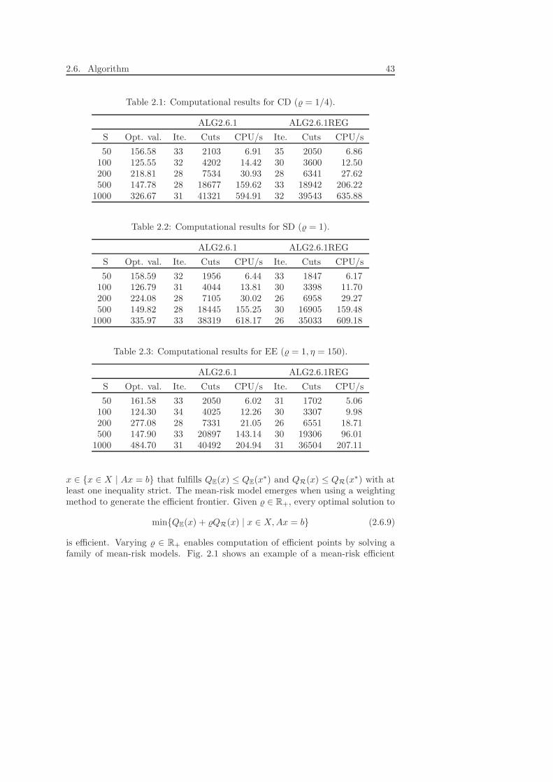
2.6. Algorithm 43
Table 2.1: Computational results for CD ( = 1/4).
ALG2.6.1 ALG2.6.1REG
S Opt. val. Ite. Cuts CPU/s Ite. Cuts CPU/s
50 156.58 33 2103 6.91 35 2050 6.86100 125.55 32 4202 14.42 30 3600 12.50200 218.81 28 7534 30.93 28 6341 27.62500 147.78 28 18677 159.62 33 18942 206.22
1000 326.67 31 41321 594.91 32 39543 635.88
Table 2.2: Computational results for SD ( = 1).
ALG2.6.1 ALG2.6.1REG
S Opt. val. Ite. Cuts CPU/s Ite. Cuts CPU/s
50 158.59 32 1956 6.44 33 1847 6.17100 126.79 31 4044 13.81 30 3398 11.70200 224.08 28 7105 30.02 26 6958 29.27500 149.82 28 18445 155.25 30 16905 159.48
1000 335.97 33 38319 618.17 26 35033 609.18
Table 2.3: Computational results for EE ( = 1, η = 150).
ALG2.6.1 ALG2.6.1REG
S Opt. val. Ite. Cuts CPU/s Ite. Cuts CPU/s
50 161.58 33 2050 6.02 31 1702 5.06100 124.30 34 4025 12.26 30 3307 9.98200 277.08 28 7331 21.05 26 6551 18.71500 147.90 33 20897 143.14 30 19306 96.01
1000 484.70 31 40492 204.94 31 36504 207.11
x ∈ x ∈ X | Ax = b that fulfills QE(x) ≤ QE(x∗) and QR(x) ≤ QR(x∗) with atleast one inequality strict. The mean-risk model emerges when using a weightingmethod to generate the efficient frontier. Given ∈ R+, every optimal solution to
minQE(x) + QR(x) | x ∈ X,Ax = b (2.6.9)
is efficient. Varying ∈ R+ enables computation of efficient points by solving afamily of mean-risk models. Fig. 2.1 shows an example of a mean-risk efficient
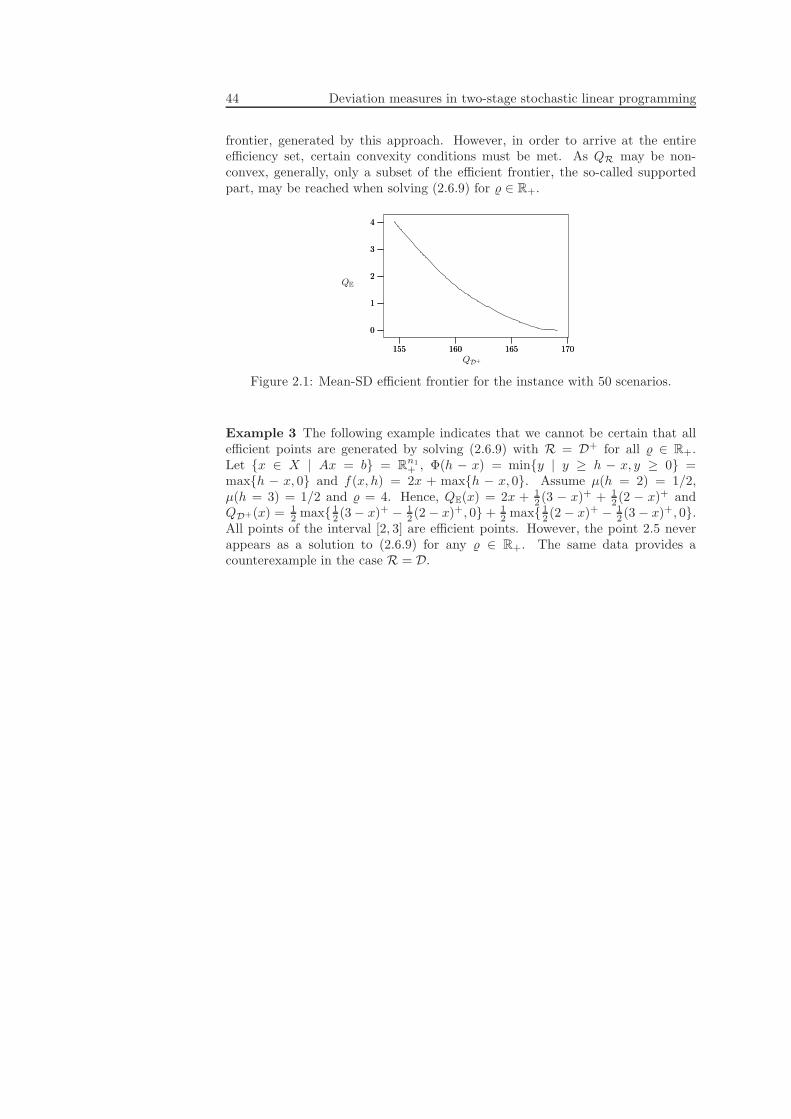
44 Deviation measures in two-stage stochastic linear programming
frontier, generated by this approach. However, in order to arrive at the entireefficiency set, certain convexity conditions must be met. As QR may be non-convex, generally, only a subset of the efficient frontier, the so-called supportedpart, may be reached when solving (2.6.9) for ∈ R+.
0
1
2
3
4
155 160 165 170155 160 165 170
0
1
2
3
4
QD+
QE
Figure 2.1: Mean-SD efficient frontier for the instance with 50 scenarios.
Example 3 The following example indicates that we cannot be certain that allefficient points are generated by solving (2.6.9) with R = D+ for all ∈ R+.Let x ∈ X | Ax = b = R
n1+ , Φ(h − x) = miny | y ≥ h − x, y ≥ 0 =
maxh − x, 0 and f(x, h) = 2x + maxh − x, 0. Assume µ(h = 2) = 1/2,µ(h = 3) = 1/2 and = 4. Hence, QE(x) = 2x + 1
2 (3 − x)+ + 12 (2 − x)+ and
QD+(x) = 12 max 1
2 (3 − x)+ − 12 (2 − x)+, 0 + 1
2 max 12 (2 − x)+ − 1
2 (3 − x)+, 0.All points of the interval [2, 3] are efficient points. However, the point 2.5 neverappears as a solution to (2.6.9) for any ∈ R+. The same data provides acounterexample in the case R = D.

Part II
Stochastic programming in power
systems
45


Chapter 3
The development in stochastic
recourse models for power
production and trading
3.1 Introduction to the power system
This chapter considers the deregulation in the power sector, consisting in thereduction or removal of the government regulations on the industry. To fullyunderstand the subsequent chapters on stochastic programming applications topower systems, we begin this chapter by listing some of the main componentsof a deregulated power system, including a physical transmission system and asystem operator, power producers and consumers, and several markets covering aday-ahead and an intra-day market as well as financial markets.
Transmission system
The transmission system, which is also referred to as the grid, is established forthe transferring of electric power from place to place, often from a power plant toa smaller station before distributed to the consumers. Electricity is usually trans-mitted through overhead power transmission lines although occasionally they maybe underground. As power transmission lines come with certain capacities, gridcongestion is possible. Nowadays, transmission and generation are separated and,most places, transmission is the responsibility of an independent, though state-approved, power system operator. The system operator maintains the grid, pro-vides access to the suppliers, distributors and consumers and collects transmissiontariffs. Moreover, the system operator ensures security of supply by balancing thephysical delivery of power and the actual consumption.
47
48 The development in stochastic recourse models for power
Producers
Production includes thermal power , hydro-power and other kinds of renewablepower such as wind power. In a thermal power plant, power is produced by unitsthat transform thermal energy, most often by burning fuel, into electrical energy.Thermal power plants are classified according to the type of fuel and generatingunits. Examples are fossil-fuel powered plants using coal-fired and gas-burningthermal units, nuclear power plants and renewable energy plants. A hydro-powerplant consists of a number of water reservoirs, possibly connected in cascade or ina more complex network, and corresponding power stations that contain turbines,also referred to as hydro-power units. As water is released from the reservoirs, itflows to the turbines, in which electricity is generated by converting the potentialenergy of the water into electrical energy. To some extent, hydro-power genera-tion provides a possibility to “store” energy in the sense that water releases canbe put on hold. In many respects, it is beneficial to coordinate thermal power pro-duction and hydro-power generation, exploiting the flexibility of hydro-power andstability thermal power. Hydro-thermal production refers to the cooperation ofthermal power plants and hydro-power plants, either of the type described aboveor so-called pumped storage hydro-power plants. In pumped storage plants theunits serve to store excess energy by utilizing electricity to pump up water into areservoir and save it for future hydro-power generation.
In general, producers range from small local stations to large plants coveringwide areas. The producers can dispose of power through direct trading or throughorganized wholesale markets, in which they either act as price-takers or are ableto influence market prices.
Consumers
End-users of electricity are industrial or household consumers who buy the com-modity directly from power producers, wholesale markets or retailers. Retailersengage in physical trading directly with producers or in wholesale markets.
Markets
Direct physical trading between two parties is done by means of bilateral contracts.However, physical trading is also possible through organized markets that servedifferent purposes. The spot market is a wholesale market, established for the im-mediate delivery of power from producer to consumer and is, due to the practiceof bidding and committing a day in advance, also referred to as the day-aheadmarket. A market operator collects the supply and demand bids and calculatesprices of the following day and the corresponding quantities to be dispatched byboth producers and consumers. When organizing a power market with a central-

3.2. From regulated to deregulated markets 49
ized dispatching and pricing mechanism, the power market is also referred to asan electricity pool.
Unlike the spot market, the regulating or the balancing market is an intra-daymarket that handles supply and demand imbalances by means of so-called regula-tion. Producers and consumers bid on the supply and demand side, respectively,while the balancing is generally handled by the system operator. Less organizedmarkets may comprise markets for investments, reserve markets and markets forother ancillary services.
As a contrast to the markets that imply immediate delivery of the physical com-modity, the financial markets for derivatives, such as forwards, futures, contractsof differences and options, serve as instruments for hedging risk. Furthermore,there may be markets for trade in environmental products, the market contractsbeing electricity certificates.
3.2 From regulated to deregulated markets
We continue this chapter with an overview of stochastic programming models inshort-term power production and trading, where special emphasis is placed on thedevelopment prompted by the restructuring of the power sector.
Traditional applications of stochastic programming to power systems representa well-developed research area. The setting is motivated by the wish to controlsystem reliability and is based on centralized operation and regulated markets inwhich many local producers enjoy monopoly. Since the earlier applications, themarkets have been reformed and operating procedures have changed. The area ofapplications within the new environment of decentralized operation, deregulatedmarkets, and competition is therefore a developing field of stochastic programming.
The present chapter aims at illustrating the impacts of the restructuring onstochastic power optimization problems. We confine ourselves mainly to short-term problems and restrict attention to power production and physical trading.The idea is to explain how traditional models can be adopted to the new envi-ronment and newer novel models become highly relevant. To discuss such modelsfrom a practical point of view, we include a number of applications, consider com-putational aspects such as problem sizes and decomposition potential, introducethe most common solution approaches and present some numerical results.
As already indicated, the main field from which the models of this chapterare derived is stochastic programming. Since, however, stochastic programmingis closely related to decision analysis, stochastic control theory, Markov decisionprocesses, dynamic programming and optimization of discrete event simulations,the models may stem from any of these fields.
The outline of the remainder of the chapter is as follows. Sections 3.4 and 3.5are confined to power production and contain the models that are valid before and

50 The development in stochastic recourse models for power
after the transition from regulated to deregulated markets, respectively. Section3.6 investigates the ability of the models to decompose and state the most basicsolution approaches. The models for physical power trading, that have mainlyarisen with liberalization, are presented in Section 3.7, which also includes theindividual solution approaches.
3.3 Stochastic programming electricity models
Muckstadt and Koenig (1977) were among the first to address the unit commit-ment problem by mathematical programming, and to solve it by Lagrangian de-composition. Reflecting the continuing interest in this problem, Fahd and Sheble(1994) provided an overview of the following solution methods, ranging from enu-meration and priority lists over dynamic, linear and mixed-integer programmingas well as branch and bound to Lagrangian relaxation.
Given the progress in stochastic programming, the stochastic extension of thedeterministic unit commitment problem began to take form with Birge et al. (1994)being the first to formulate the problem in terms of stochastic mixed-integerprogramming. As part of a larger information system the authors presented amulti-stage model for dynamic unit commitment under uncertainty with respectto electricity load and unit failures.
Early attempts to formulate and solve stochastic versions of short-term poweroptimization problems further included Bunn and Paschentis (1986), who devel-oped a two-stage recourse model for economic dispatch by allowing under- andover-dispatching in the second stage and Terry et al. (1986), who described theimplementation of stochastic dynamic programming for coordinating operation ina large real-world hydro-power system.
The development in stochastic programming electricity models continuedthroughout the remainder of the century and into the beginning of the next. Atpresent it has become of major interest due to the restructuring of the powersector in the last decades and the following liberalization of the markets that hasencouraged efficient operation of the system and competitiveness of the industry.
In general, stochastic power optimization problems are categorized accordingto their time horizons. Long-term problems usually have a time horizon of up toseveral years, medium-term problems of a few months to a few years and short-termproblems of a day to a week.
Concerning the longer term, most problems involve technology investment andcapacity expansion matters, cf. Bienstock and Shapiro (1988) and Gorenstin andCampodonico (1993), and some include environmental planning issues such aspollutant emission control. Formulated as stochastic programs, such problemsmay contain various sources of uncertainty. The category covers the building ofthermal units, the construction of hydro reservoirs and turbines and multi-year

3.4. Short-term power production 51
hydro-thermal scheduling, cf. Sherkat et al. (1985). Due to their aggregation level,the long-term problems often allow for the application of the classical solutionapproaches, Benders’ decomposition and dynamic programming.
Problems of the medium-term embrace hydro-thermal coordination problems,cf. Dentcheva and Romisch (1998), and reservoir management problems, cf. Jacobset al. (1995), the complexity of which calls for more advanced solution methods.In this context, the most significant sources of uncertainty stem from electricitydemand and reservoir inflows. As explained by Fosso et al. (1999), the medium-term problems are relevant in their own right, but at the same time provide inputdata to the short-term models through reservoir storage boundaries, values ofstored water etc.
Well-known traditional short-term planning and operation problems includethermal unit commitment and economic dispatch. Short-term hydro-thermal andpure hydro scheduling are often handled as dynamic operation problems on adaily or weekly basis, which may also be the case for hydro unit commitment.Uncertainty in the traditional problems covers electricity demand, unit failures,fuel costs and potentially reservoir inflows. Newer short-term planning problemsconsist in the day-ahead physical trading and the trading of ancillary services andadd market prices uncertainty to the problems.
For an excellent yet more general survey on stochastic programming problemsin energy, see Wallace and Fleten (2003), who consider both electricity, oil and gas.The authors present long-term, medium-term and short-term problems and discusstheir development with the transition from regulated to deregulated markets. Bothphysical and financial markets are considered and much of the survey is devotedto risk management. The emphasis is placed on modeling alone and so solutionapproaches and other computational aspects are only briefly addressed.
3.4 Short-term power production
Due to the previous regulation by legal restrictions, decision-making was usuallyeffected on a centralized level for several producers voluntarily or legally coordi-nated and obligated to satisfy demand within their areas. Contracts were predom-inantly bilateral contracts of which the terms were set by administrative decrees,the result being that cost minimization was pursued.
In line with this, the models of this section are traditional short-term powerproduction models that rest on costs minimization subject to demand constraints.The multi-stage stochastic programs are presented in their scenario tree formula-tions. For further reference on the notation, see Chapter 1.
52 The development in stochastic recourse models for power
Thermal unit commitment and hydro-thermal scheduling
As a starting point, we address the thermal unit commitment problem from theperspective of a regulated utility. The problem consists in the scheduling of start-ups and shut-downs of the thermal units and the determination of correspondingoperation levels such as to minimize the associated costs and meet the electricitydemand over some finite time horizon. To formalize this, we let I index the ther-mal units. We denote the on/off-decisions of the units un
i , i ∈ I ∈ 0, 1, n ∈ Nand let the pn
i ∈ R+, i ∈ I, n ∈ N represent the corresponding operating levels.Total costs account for operational fuel costs and start-up costs and are modeledby the functions FCi(·), i ∈ I and SCi(·), i ∈ I in (3.4.1). The functions areoccasionally approximated by piecewise linear functions in order for the problemto comply with a linear formulation. According to (3.4.2), generation is subjectto lower and upper bounds, pmin
i , pmaxi , i ∈ I, resulting from the capacities of the
thermal units. To prevent thermal stress and high maintenance costs of the units,minimum up- and down-time constraints apply. These are given by (3.4.3), and(3.4.4), where τup
i , τdoi , i ∈ I denote the minimum up- and down-times. Although
not included, must-on/-off constraints can easily be included. A regulated util-ity is forced to satisfy demand by means of generation only, which leads to theconstraints (3.4.5), where the demand is denoted by dn, n ∈ N . Finally, the factthat reserves are the responsibility of the utility induces the constraints (3.4.6),where the reserve requirements are denoted by rn, n ∈ N . The reserves are so-called spinning reserves that ensure excess system capacity in the case of failure.Uncertainty may relate to both demand and reserve requirements. With this nota-tion, the thermal unit commitment problem formulated as a multi-stage stochasticprogram takes the form of
min∑
n∈N
∑
i∈I
πn(
FCi(pni , u
ni ) + SCi(u
ni , u
n−1
i ))
(3.4.1)
s.t. uni p
mini ≤ pn
i ≤ uni p
maxi , i ∈ I, n ∈ N (3.4.2)
un−τ
i − un−(τ+1)
i ≤ uni , τ = 1, . . . , τup
i − 1, i ∈ I, n ∈ N (3.4.3)
un−(τ+1)
i − un−τ
i ≤ 1 − uni , τ = 1, . . . , τdo
i − 1, i ∈ I, n ∈ N (3.4.4)
∑
i∈I
pni ≥ dn, n ∈ N (3.4.5)
∑
i∈I
(uni p
maxi − pn
i ) ≥ rn, n ∈ N (3.4.6)
pni ≥ 0, un
i ∈ 0, 1, i ∈ I, n ∈ N (3.4.7)

3.4. Short-term power production 53
The stochastic problem is a direct extension of the deterministic unit commit-ment problem and can be found in a very similar version by Takriti et al. (1996).The authors only consider demand uncertainty and leave out reserve requirements.Whether reserve constraints should be included in a stochastic model depends onwhether failures are explicitly incorporated in the scenarios as decreased capacityor increased demand corresponding to the capacities of disrupted units.
With a fixed configuration of the units, the problem becomes that of distribut-ing the production among them and is known as the economic dispatch problem.Both Bunn and Paschentis (1986) and Growe et al. (1995) formulate the prob-lem as a two-stage simple recourse problem, where the second stage penalizesdeviations between scheduled production and uncertain demand. In solving theproblem, both rely on separability of the recourse function and the possibility toevaluate only a one-dimensional integral. However, whereas Bunn and Paschentis(1986) assume normal demand distributions and use discretization of the distri-bution to solve the economic dispatch problem, Growe et al. (1995) approximatethe distributions by certain kernel estimators that allow explicit calculation of theintegrals.
The thermal unit commitment problem can be extended to the hydro-thermalscheduling problem that involves cooperation of thermal power and hydro-powerpumped storage plants. Like the thermal unit commitment problem, the problemconsists in the scheduling of thermal power production. However, there is a pos-sibility of using electricity to store water in the reservoirs for future hydro-powergeneration. The objective is therefore to minimize the thermal operational costsas well as the opportunity costs of hydro-power generation that arise since watercould be saved for future use. We let J index the pumped storage plants. Theopportunity costs are measured as the future value of stored water, captured bythe functions Vj(·), j ∈ J , as in (3.4.8). Including water values is an attempt toavoid end effects such as the tendency of the multi-stage stochastic programmingproblem to empty the system in the final stage. We let the notation be the sameas before. Moreover, we let the variables vn
j , snj , l
nj ∈ R+, j ∈ J , n ∈ N represent
the reservoir discharge levels, pumping levels and storage levels. Apart from thethermal constraints, hydro-thermal scheduling involves bounds on these variables,(3.4.10)-(3.4.12), enforced by vmin
j , vmaxj , smin
j , smaxj , lmin
j , lmaxj , j ∈ J . Reservoir
discharges, pumping levels and storage levels are related through the reservoir bal-ance equations, (3.4.13), where νn
j , j ∈ J , n ∈ N denote reservoir inflows. Finally,demand can be satisfied from thermal generation and hydro-power generationthat is not used for pumping. This gives rise to the constraints (3.4.14) in whichηj , γj , j ∈ J denote the hydro-power generation and pumping efficiencies, respec-tively. To simplify the modeling, water discharges and hydro-power generation areoften assumed to be proportional. As should be clear from the notation, uncer-tainty may concern demand and reserve requirements as well as reservoir inflows.Formulated as a stochastic programming problem, the hydro-thermal scheduling
54 The development in stochastic recourse models for power
problem of a regulated utility is therefore
min∑
n∈N
∑
i∈I
πn(
FCi(pni , u
ni ) + SCi(u
ni , u
n−1
i ))
−∑
n∈NT
∑
j∈J
πnVj(lnj ) (3.4.8)
s.t. uni p
mini ≤ pn
i ≤ uni p
maxi , i ∈ I, n ∈ N (3.4.9)
vminj ≤ vn
j ≤ vmaxj , j ∈ J , n ∈ N (3.4.10)
sminj ≤ sn
j ≤ smaxj , j ∈ J , n ∈ N (3.4.11)
lminj ≤ lnj ≤ lmax
j , j ∈ J , n ∈ N (3.4.12)
lnj − ln−1
j + vnj − sn
j = νnj , j ∈ J , n ∈ N (3.4.13)
∑
i∈I
pni +
∑
j∈J
ηj(vnj − γjs
nj ) ≥ dn, n ∈ N (3.4.14)
∑
i∈I
(uni p
maxi − pn
i ) ≥ rn, n ∈ N (3.4.15)
pni , v
nj , s
nj , l
nj ≥ 0, un
i ∈ 0, 1, i ∈ I, j ∈ J , n ∈ N . (3.4.16)
Short-term hydro-thermal scheduling models in stochastic programming arefound several places in the literature. Dentcheva and Romisch (1998), Growe-Kuska et al. (2000), Growe-Kuska et al. (2002) and Nowak and Romisch (2000)all suggest models that take the form of the above with a time horizon of a week.Their studies represent different options in modeling. The authors propose tomodel the operational costs as linear, piecewise linear, piecewise linear convex orconvex quadratic, whereas start-up costs can be fixed or down-time dependent.Furthermore, the authors include either minimum down-time constraints or bothup- and down-time constraints. None of the studies include a water value func-tion. Instead, to avoid undesired end effects due to a finite time horizon, thefinal storage levels are constrained. The models are all validated on data from aGerman utility and solved by the use of stochastic Lagrangian relaxation of theunit coupling constraints, which will be further discussed in the subsequent sec-tions. As a representative example of the model sizes in this section, the modelcontains 4200 binary variables, 6652 continuous variables and 13441 constraintsas a deterministic problem. With 10 scenarios and 756 nodes in the scenario treeformulation of the stochastic problem, the numbers are 18900, 34776 and 60490and with 100 scenarios and 4200 nodes, the numbers mount to 105000, 193200and 336100, making decomposition of the stochastic problem highly relevant.
3.4. Short-term power production 55
Similar in spirit to the hydro-thermal scheduling models, are the two-stageunit commitment models of Carøe and Schultz (1998) and Gollmer et al. (2000),that are also validated on the German data. Like the above, the models seekto find a unit commitment schedule for thermal units in a hydro-thermal utility.However, since coal-fired units have longer start-up times than gas-burning units,the on-/off-decisions of the coal-fired units are assigned to the first stage, whereascorresponding decisions of the gas-burning units are set aside for the second stage.For other two-stage hydro-thermal planning problems, see also Dentcheva andRomisch (1998) and Nowak et al. (2000), who assign a full schedule in the firststage and a compensation schedule in the second stage.
Hydro scheduling and unit commitment
When hydro scheduling is addressed from the point of view of a regulated utility,the problem consists in the spatial distribution of water releases between differenthydro reservoirs in order to satisfy electricity demand. Since direct operatingcosts of hydro-power generation are negligible, the determining of water releasesis a matter of striking a balance between the immediate and future value of theremaining reservoir contents. Hence, the overall objective of hydro scheduling isto maximize the value of water stored in the reservoirs (3.4.17) subject to thedemand constraints (3.4.23). The challenge is that, when reservoirs are connectedby a network, upstream releases contribute to the downstream inflows with sometime delay. For simplicity, we assume that the hydro reservoirs are connectedin cascade, although more complex networks also exist. We proceed with thesame notation as before and let J index the hydro reservoirs. We model therelation between reservoir discharges and turbine generation in more detail thanabove and, thus, introduce the variables wn
j ∈ R+, j ∈ J , n ∈ N to representgeneration explicitly. If ignoring head variation effects on the generation, therelation is usually given by concave functions Gj(·), j ∈ J as in (3.4.22), suchfunctions often being approximated by piecewise linear functions to support alinear formulation. The turbine generation is subjected to the bounds (3.4.18)induced by the generation capacities wmin
j , wmaxj , j ∈ J . In the reservoir balance
equations we include spills rnj , j ∈ J , n ∈ N , and like other releases, upstream
spills contribute to the downstream inflows. Uncertainty may arise with respectto reservoir inflow and electricity demand, which makes the multi-stage stochasticprogramming formulation of the hydro scheduling problem take the form
min −∑
n∈NT
∑
j∈J
πnVj(lnj ) (3.4.17)
s.t. wminj ≤ wn
j ≤ wmaxj , j ∈ J , n ∈ N (3.4.18)
vminj ≤ vn
j ≤ vmaxj , j ∈ J , n ∈ N (3.4.19)
56 The development in stochastic recourse models for power
lminj ≤ lnj ≤ lmax
j , j ∈ J , n ∈ N (3.4.20)
lnj − ln−1
j + vnj + rn
j = vn−1
j−1 + rn−1
j−1 + νnj , j ∈ J , n ∈ N (3.4.21)
wj = Gj(vj), j ∈ J , n ∈ N (3.4.22)
∑
j∈J
wnj ≥ dn, n ∈ N (3.4.23)
wnj , v
nj , r
nj , l
nj ≥ 0 j ∈ J , n ∈ N . (3.4.24)
Although formulated as medium-term hydro scheduling, Jacobs et al. (1995)present a model similar to the above. The model facilitates the development ofa stochastic hydro scheduling module of a larger system in an American gas andelectricity company. To fully describe the system and the operating restrictions inpractice, the model includes an entire network of lakes, reservoirs, water courses,tunnels, junctions and power houses. The company also operates a thermal system,which is why the major costs concern those of avoiding thermal generation. Evenfor the deterministic model, the number of variables and constraints are in therange of 4650–8686 and 1180–2230, respectively. With as few as 45 scenarios and64–66 nodes in the scenario tree formulation of the stochastic model, the numbersbecome 140284–265242 and 35736–68012, which obviously motivates the need fordecomposition.
For a general overview of reservoir operation models within stochastic pro-gramming and related areas, see Reznicek and Cheng (1991), who include Markovchains, dynamic programming, stochastic programming with recourse and chanceconstrained stochastic programming.
The hydro unit commitment problem introduces individual units and theirstart-ups and shut-downs into the hydro scheduling problem. It follows that theproblem consists in determining on/off-schedules and corresponding generationlevels of the units so as to balance current costs and future water values. Mostdirect operating costs can be ignored such that current costs account for start-upcosts alone. Still, hydro start-up costs are much lower than thermal start-up costs.We again consider hydro reservoirs in cascade. We let J index the hydro reservoirsand stations and let Ij , j ∈ J index the associated turbines. The start-up costs,SCi(·), i ∈ I are added to the objective function (3.4.25). We denote the on/off-decisions of the hydro units un
i ∈ 0, 1, i ∈ Ij , j ∈ J , n ∈ N and the generationlevels wn
i , n ∈ N . Generation must submit to the bounds wmini , wmax
i , i ∈ I in(3.4.26). We define the discharges vn
i , n ∈ N on a unit basis and modify thebounds as in (3.4.27) accordingly. The balance equations must be modified in asimilar fashion as shown in (3.4.29). The hydro unit commitment problem now

3.4. Short-term power production 57
reads
min∑
n∈N
∑
j∈J
∑
i∈Ij
πnSCi(uni , u
n−1
i ) −∑
n∈NT
∑
j∈J
πnVj(lnj ) (3.4.25)
s.t. uni w
mini ≤ wn
i ≤ uni w
maxi , i ∈ Ij , j ∈ J , n ∈ N (3.4.26)
vminj ≤
∑
i∈Ij
vni ≤ vmax
j , j ∈ J , n ∈ N (3.4.27)
lminj ≤ lnj ≤ lmax
j , j ∈ J , n ∈ N (3.4.28)
lnj − ln−1
j +∑
i∈Ij
vni + rn
j =∑
i∈Ij−1
vn−1
i + rn−1
j−1 + νnj , j ∈ J , n ∈ N (3.4.29)
wi = Gi(vi), i ∈ Ij , j ∈ J , n ∈ N (3.4.30)
∑
j∈J
∑
i∈Ij
wi ≥ dn, n ∈ N (3.4.31)
wni , v
ni , r
nj , l
nj ≥ 0, un
i ∈ 0, 1 i ∈ Ij , j ∈ J , n ∈ N . (3.4.32)
To our knowledge, hydro unit commitment has been addressed only few timesin the literature. The authors of Hreinsson (1988) and Tufegdzic et al. (1996)present a short-term operation problem of a hydro-power system modeled as adeterministic problem, whereas Philpott et al. (2000) consider the problem subjectto uncertain demand and formulates a multi-stage stochastic program. Hreinsson(1988) argues that if the hydro reservoirs are almost unaffected by short-termoperations, water scheduling and hydro-power generation can be separated. Byaddressing only hydro power generation, the problem reduces to something verysimilar to the thermal unit commitment problem. Tufegdzic et al. (1996) onthe other hand describe a full hydro-power generation problem involving unitcommitment and water scheduling. The problem arose with the development ofan energy management system for the Tasmanian hydro electric commission andthe corresponding model is therefore rather detailed, including a hydro networkof reservoirs, stations, tunnels and canals and piecewise linear approximations ofsome constraints and costs. Finally, Philpott et al. (2000) present a hydro unitcommitment model similar to the above and illustrates it with a case study fromNew Zealand. The relations between reservoir discharges and turbine generationare given by concave functions that are combined and approximated by piecewiselinear functions.

58 The development in stochastic recourse models for power
3.5 Production on market conditions
The lack of organized markets during regulation was argued to make power tradingrather inflexible. To achieve economic efficiency, the markets began to reform anda new regulatory administration was introduced for the purpose of promotingcompetition. Prices were left to be determined by the market conditions throughthe establishment of a power exchange. Moreover, previous obligations to satisfydemand were replaced by the opportunity of power producers to buy and sell theirproduction at this power exchange. Producers reacted by reorganizing operationsto facilitate decentralized decision-making and began maximizing profit, whileexperiencing an increasing price uncertainty. For a general overview of the changesin the power sector in response to the restructuring, see Hobbs (1995), who includesthe growing uncertainty and increased competition.
The models of this section represent the adaption of the traditional powerproduction models to the new environment in terms of profit maximization withoutdemand constraints. As before, the multi-stage stochastic programs are presentedusing the scenario tree formulation and the corresponding notation is found inChapter 1.
Thermal unit commitment and hydro-thermal scheduling
We will explain how the traditional models of Section 3.4 can be adapted tothe new environment using the thermal unit commitment model for illustration.Changes to the hydro-thermal scheduling model will follow in a similar fashion.
We apply the ideas of Wallace and Fleten (2003). With the possibility oftrading in the physical and financial markets, the electricity production can bedisposed of through traditional bilateral contracts and through newer market con-tracts. Furthermore, power producers can purchase electricity from the samemarkets. We denote by dn, n ∈ N the bilateral contracts and let the variablesy+,n, y−,n ∈ R+, n ∈ N represent the market contracts for selling and buying,respectively. With no constraints on the market contracts, these provide the flex-ibility necessary for production, purchases and disposals to match, which leads tothe equality constraints
∑
i∈I
pni = dn + y+,n − y−,n, n ∈ N . (3.5.1)
The revenues of market disposals amount to∑
n∈N
πnρn(y+,n − y−,n), (3.5.2)
where ρn, n ∈ N denote the market prices. By substitution of y+,n, y−,n, n ∈ Nin (3.5.2), the demand constraints (3.5.1) are eliminated. After substitution, the

3.5. Production on market conditions 59
constant term of the objective function can be ignored, which corresponds to anassumption of no bilateral trades and pure market disposals. Reserve constraintscan also be eliminated from the model, the reason being that reserves market arebeginning to appear. As an effect of eliminating demand and reserve constraints,the model decouples with respect to thermal units and, thus, decision-making canbe conducted on a single-unit basis. With the introduction of revenues from marketdisposals, the objective shifts from cost minimization to profit maximization andmarket price uncertainty comes into play. The thermal single-unit problem is themulti-stage stochastic program
max∑
n∈N
πn(
ρnpn − FC(pn, un) − SC(un, un−1))
s.t. (3.4.2) − (3.4.4)
pn ≥ 0, un ∈ 0, 1, n ∈ N .
Takriti et al. (2000) addresses the multi-stage stochastic thermal unit commit-ment problem and include both buying and selling of electricity to a power poolthat serves as a spot market. The spot market is modeled as two additional units;one unit representing buying and one unit representing selling. If the utility buyspower, demand decreases, and if it sells power, demand increases as shown above.The bounds on the buying and selling units are automatically imposed, whichallows for the substitution. However, the model decoupling is not carried out.
As already stated, the hydro-thermal scheduling problem is modified in thesame way as the thermal unit commitment problem. However, when the demandand reserve constraints are eliminated, the model separates thermal power produc-tion from hydro-power generation and decouples further with respect to pumpedhydro storage plants.
Hydro scheduling and unit commitment
To illustrate how the traditional models of Section 3.4 can be modified, we considerthe hydro scheduling problem. Similar modifications apply to the hydro unitcommitment problem.
Since also hydro-power generation can be disposed of by bilateral contracts ofa fixed volume and market contracts of a variable volume, the traditional demandconstraints are replaced by the equality constraints
∑
j∈J
wnj = dn + y+,n − y−,n, n ∈ N ,
60 The development in stochastic recourse models for power
and the revenues of market disposals,∑
n∈N
πnρn(y+,n − y−,n),
are added to the traditional objective function, which is then based on profitmaximization and includes market prices uncertainty. For the same reasons aspreviously, the demand constraints can be eliminated. If, however, the reservoirsare connected, the balance equations prevent the hydro scheduling problem fromdecoupling with respect to reservoirs.
The paper of Fosso et al. (1999) gives an overview of the deregulated electricitysystem in Norway and the corresponding long-term, medium-term and short-termmodels used for hydro scheduling. In particular, it is explained how water valuecalculations can be adapted to the system. The long-term model is a stochasticprogram that is able to handle uncertainties in market prices and reservoir inflowsand provides water values for the medium-term models. The authors suggest tocalculate marginal water values as derivatives of stochastic dynamic programmingvalue functions with respect to reservoir storage levels. The medium-term modelsare deterministic scenario problems producing water values for a detailed short-term model that includes nonlinear generation efficiency curves, head variationeffects, tunnels branching into pipes etc.
The adaptation of the hydro unit commitment problem to a market-orientatedsystem has not been found in the literature until recently, where a stochasticprogramming version has appeared by Garcıa-Gonzalez et al. (2006). More inter-estingly, however, an alternative to handling head variation effects is proposed. Aprocedure iteratively produces reservoir net heads as a function of storage levelsand solves the stochastic programming problem with a relation between reservoirdischarge and turbine generation that depends only on a fixed net head.
In Chapter 5, we describe a new hydro unit commitment problem that hasbecome relevant with the introduction of market dispatch. The problem consists inhydro-power production planning that complies with the day-ahead commitmentsand illustrates the necessity of the demand constraints in the very short term. Incontrast to dynamic unit commitment, the aim is to determine a daily productionplan that values the current market prices and reservoir inflows against the future.With fixed day-ahead commitments, the production planning becomes a matterof spatial distribution of water among the reservoirs.
3.6 Solution approaches
Thermal unit commitment
The solution approaches to stochastic power production problems are extensionsfrom the deterministic case. Primal approaches mainly rely on LP based branch

3.6. Solution approaches 61
and bound, this method being highly supported by the advances in hardware andthe development of software implementations. At present, general purpose pack-ages can combine the LP methodology with a variety of options for arranging thebranch and bound. The package allows for fast heuristics to obtain initial feasiblesolutions, specific branching rules and techniques from combinatorial optimiza-tion such as valid inequalities. Most importantly, the LP-based branch and boundworks with ample enrichment as long as the model is expressed in mixed-integerlinear terms. A critical drawback is the full handling of the model which maybecome prohibitive with the sizes illustrated in the previous sections. This pavesthe way for decomposition methods.
For an example on the application of LP-based branch and bound to determin-istic thermal unit commitment and hydro-thermal scheduling, see Gollmer et al.(1999). The authors argue that the method shows its strengths with complexconstraints interconnecting generating units in contrast to dual approaches thathave their merits with nonlinearities.
Among the dual approaches, Lagrangian relaxation has proved to be a strongtool because of the algorithmic progress for solving the Lagrangian dual, the usu-ally small duality gap and the advance of fast Lagrangian heuristics to close thisgap. For references on the application of Lagrangian relaxation in the determin-istic case, see Feltenmark et al. (1997) and Gollmer et al. (1999).
To illustrate Lagrangian relaxation, we develop the Lagrangian dual of themulti-stage stochastic programming version of the thermal unit commitment prob-lem (3.4.1)-(3.4.7) and its scenario tree formulation. The problem is nearly separa-ble with respect to thermal units as only the constraints (3.4.5) and (3.4.6) involvedifferent units. This property may be utilized by stochastic Lagrangian relaxationof the unit coupling constraints. Assigning non-negative stochastic Lagrange mul-tipliers that inherit the tree structure from dn, rn, n ∈ N , the Lagrangian functionis given by
L(u, p;λ1, λ2) :=∑
n∈N
∑
i∈I
πn(FCi(pni , u
ni ) + SCi(u
ni , u
n−1
i ))+
∑
n∈N
πnλn1
(
dn −∑
i∈I
pni
)
+
∑
n∈N
πnλn2
(
rn −∑
i∈I
(uni p
maxi − pn
i ))
,
where u = (uni )i∈In∈N and p = (pn
i )i∈In∈N and the corresponding dual functionis
D(λ1, λ2) := minu,p
L(u, p;λ1, λ2) | (3.4.2) − (3.4.4)
(3.6.1)
62 The development in stochastic recourse models for power
The Lagrangian dual now reads
max
D(λ1, λ2) | (λ1, λ2) ∈ R2|N |+
. (3.6.2)
Due to integrality constraints, the primal problem is non-convex. The dual prob-lem therefore only provides a lower bound to the primal problem. Still, the La-grangian relaxation provides a tighter bound than the continuous relaxation.
The problem (3.6.1) decomposes into multi-stage single-unit subproblems. Inthis fashion the dual function
D(λ1, λ2) =∑
i∈I
Di(λ1, λ2) +∑
n∈N
πn(
λn1d
n + λn2 r
n)
is evaluated by solving subproblems of the form
Di(λ1, λ2) = minui
∑
n∈N
πn(
minpn
i
FCi(pni , u
ni ) − (λn
1 − λn2 )pn
i | (3.4.2)
+ SCi(uni , u
n−1
i ) − λn2u
ni p
maxi
)
∣
∣
∣(3.4.3)− (3.4.4)
,
where ui = (uni )n∈N . The single-unit subproblems are solvable by stochastic
dynamic programming. For an outline of the approach, including how to copewith minimum up- and down-times, see for instance Nowak and Romisch (2000).
Since the dual function (3.6.1) is concave and non-differentiable, the Lagrangiandual (3.6.2) was originally solved with subgradient procedures. Currently more re-fined methods such as cutting plane or bundle methods have been successfully ap-plied. An example is the proximal bundle method used in Dentcheva and Romisch(1998), Nowak and Romisch (2000) and Growe-Kuska et al. (2002). Based on func-tion and subgradient information, the method constructs a bundle of linearizationsof the dual function. In order to replace the original dual function, the resultingpiecewise linear upper approximation is added a proximity term before being min-imized.
Mostly the dual solution provided by the cutting plane or bundle method vio-lates the demand and reserve constraints and produces a duality gap. Lagrangianheuristics are therefore used to determine a feasible and hopefully nearly optimalsolution of the primal problem. In most cases, the heuristic seeks to find a unitcommitment solution that induces economic dispatch. The heuristic suggested inGrowe-Kuska et al. (2002) starts from an initial set of Lagrange multipliers andperturbs the multipliers such as to obtain primal feasible unit commitment sched-ules. Most binary variables do not change and can be fixed in order to decreasethe size of the problem, whereas the remaining variables are switched off one ata time as long as feasibility persists. Dentcheva and Romisch (1998) provide abound on the duality gap that depends on the number of demand and reserve

3.6. Solution approaches 63
constraints. The duality gaps decreases in the case of a larger power plant or afiner discretization of the probability distribution.
The authors Dentcheva and Romisch (1998), Nowak and Romisch (2000) andGrowe-Kuska et al. (2002) employ the stochastic Lagrangian relaxation to thestochastic hydro-thermal scheduling problem. This prompts a decomposition intoboth single-unit thermal and hydro subproblems and opens the possibility ofheuristics that exploit the additional flexibility of the hydro-power pumped stor-age plants. Since the test problem from the German utility involves 25 thermalunits and 7 hydro reservoirs, it decomposes into 32 subproblems. For the instanceof 100 scenarios and 4200 nodes, the thermal subproblems each have 4200 binaryvariables, 4200 continuous variables and 8400 constraints and the hydro subprob-lems 12600 continuous variables and 8500 constraints. The instance can be solvedwithin an optimality gap of approximately 0.1% in about 1000 seconds of comput-ing time. The two-stage problems by Dentcheva and Romisch (1998) and Nowaket al. (2000) are solved on similar lines by Lagrangian relaxation of the unit cou-pling constraints, the result being a similar decomposition into thermal and hydrosubproblems.
Relaxation of unit coupling constraints is also possible by means of the aug-mented Lagrangian technique as suggested by Carpentier et al. (1996). However,to facilitate decomposition, it is necessary to linearize the Lagrangian. Other dualsolution approaches to stochastic power production problems include Lagrangianrelaxation of the non-anticipativity constraints, which usually decomposes theproblems into a larger number of smaller deterministic subproblems. In this way,Takriti et al. (1996) and Takriti et al. (2000) solve the multi-stage stochastic unitcommitment problem by progressive hedging and seem to outperform the aboveapproach. Carøe and Schultz (1998) and Gollmer et al. (2000) solve the two-stageversion of the problem by dual decomposition are thereby, in principle, able toclose the duality gap by branch and bound. For further references on Lagrangianrelaxation of the non-anticipativity constraints, see Chapter 1.
Hydro scheduling
For a long time, stochastic hydro scheduling problems have been solved by stochas-tic dynamic programming, which has also occasionally been used for stochastichydro unit commitment problems. The application of dynamic programming issupported by the sequential structure of the decision-making process and justi-fied by the fact that the problems have relatively few constraints interconnectingdifferent stages. We attempt to illustrate the dynamic programming recursion onthe hydro scheduling problem (3.4.17)-(3.4.24) for reservoirs in cascade. The no-tation of the preceding sections will be modified to fit the framework. We assumethat the uncertain data consists of random demands dt, t ∈ T and random inflowsνjt, j ∈ J , t ∈ T . For reservoirs in cascade, the storage levels can be redefined

64 The development in stochastic recourse models for power
to include delayed inflows from upstream reservoirs. The dynamic programmingstates are defined by these storage levels, still denoted lt = (ljt)j∈J , t ∈ T , andby the uncertain data ξt = (νt, dt), t ∈ T , where νt = (νjt)j∈J , t ∈ T . Theaction space consists of reservoir discharges, turbine generation levels and spillsvt = (vjt)j∈J , wt = (wjt)j∈J , rt = (rjt)j∈J , t ∈ T . With these definitions, theexpected future value function of stage T compute as
FT (lT−1, ξT−1) = EξT |ξT−1
[
maxvT ,wT ,rT
−∑
j∈J
Vj(ljT − vj−1T − rj−1T )∣
∣
(3.4.18)− (3.4.20), ljT − vj−1T − rj−1T + vjT + rjT =
ljT−1 + νjT , j ∈ J , (3.4.22) − (3.4.24)]
and the stage t expected future value as
Ft(lt−1, ξt−1) = Eξt|ξt−1
[
maxvt,wt,rt
Ft+1(lt, ξt)∣
∣ (3.4.18)− (3.4.20),
ljt − vj−1t − rj−1t + vjt + rjt = ljt−1 + νjt, j ∈ J , (3.4.22)− (3.4.24)]
.
In dynamic programming, the continuous reservoir storage levels are oftendiscretized in order to facilitate computations. With the discretization of thestate space, however, the full dynamic programming approach is known to sufferfrom the curse of dimensionality and is only able to handle a few reservoirs. Inorder to restrict the state space, it has been proposed to aggregate reservoirs andpower stations or to decompose the dynamic programming problem according toreservoirs. As an alternative, Archibald et al. (2001) suggest that an appropriatedefinition of the state space for multi-reservoir systems allows for a simplificationof the solution method on the basis of information on an optimal policy.
Another way of avoiding the curse of dimensionality is to describe the dynamicprogramming value function by supporting hyperplanes, which is utilized in nestedBenders’ decomposition. The method has been applied by Jacobs et al. (1995),who suggest a number of algorithmic enhancements that are further explored inMorton (1996). The enhancements include the use of warm start bases, initialcut generation, disaggregated cuts and decision tree traversing strategies. Theperformance of the enhanced algorithm is tested on a collection of multi-stagestochastic hydro scheduling problems. The algorithm is outperformed by generalLP optimizers if applied to single scenario problems but is preferable as the numberof scenarios increases. As an example, the previously mentioned problem by Jacobset al. (1995) decomposes into 45 nodal subproblems of 57–1273 variables and 271–6279 constraints - a significant reduction in size - and is solved in 200–400 secondsof CPU time.

3.7. Physical trading and bidding 65
For further inspections of algorithms for multi-stage stochastic hydro schedul-ing problems, the authors Archibald et al. (1996) compare the revised simplexmethod, full dynamic programming, dynamic programming decomposition andnested Benders’ decomposition. Only the revised simplex method and nestedBenders’ decomposition provide exact optimal solutions. Furthermore, the au-thors find the nested Benders’ decomposition approach to be the fastest followedby dynamic programming decomposition, the revised simplex method and, finally,full dynamic programming. Although most results favor the nested Benders’ de-composition, the approach fails to solve stochastic programs having many stagesdue to the explosion in the number of nodes.
The major drawbacks of dynamic programming and nested Benders’ decom-positions are avoided in the stochastic dual dynamic programming algorithm pro-posed by Pereira and Pinto (1991). In a backward run, the algorithm approximatesthe dynamic programming value function by Benders’ cuts induced by trial pointsthat are determined in a forward run by sampling from the set of scenarios. Sincestate space discretization is unnecessary, the curse of dimensionality is not an is-sue and because of sampling, the effects of the explosion in the number of nodesare reduced. The stochastic dual dynamic programming, however, is not capableof incorporating market price uncertainty due to lack of convexity in the statespace, whereas both dynamic programming and nested Benders’ decompositionare applicable to the models for hydro scheduling on market conditions.
The stochastic hydro unit commitment problems have to be solved by dy-namic programming, Philpott et al. (2000) being an example, or more generalapproaches applicable to mixed-integer linear stochastic programming problems.An example of the application of commercial mixed-integer linear programmingsoftware is given in Chapter 5, where we consider a multi-stage stochastic hydrounit commitment problem and succeed in solving its scenario tree formulation of267 scenarios, 11777 nodes, 141846 variables and 261254 constraints to optimalityin less than 30 seconds of CPU time.
3.7 Physical trading and bidding
With the liberalization of power markets, new planning problems have arisen andintroduced the need for corresponding optimization models. Of great importanceare especially the problems of physical trading and bidding in power marketslike the spot and the reserve markets. This section presents some of the modelsthat have recently been proposed within the field of stochastic programming andrelated areas of stochastic optimization. A major difference between the models isthe handling of offers or bidding curves submitted to the market. Some models arebased on smooth, linear or piece-wise linear bidding curves, while others include afinite number of offers which results in step functions. Another crucial difference
66 The development in stochastic recourse models for power
is the extent to which the current market participant has market power. Somemodels operate on a price-taker assumption, whereas other models assume themarket participant is able to influence market prices. If, however, competitorsrespond to the offers of each other, a game theoretic approach should replace thestochastic programming approach. No general solution approach appears to applyto the newer problems of physical trading and bidding.
The day-ahead market
Most models for bidding into the spot or day-ahead market involve one-periodsealed auctions in an electricity market that is organized as a pool and for which auniform clearing price rule applies. Within this framework, Fleten and Pettersen(2005) propose a two-stage stochastic mixed-integer linear program for construct-ing piece-wise linear bidding curves to be submitted to the Nordic day-aheadmarket. The problem is addressed from the perspective of a price-taking retailerwho supplies to price-sensitive end users under both price and demand uncertainty.Since the problem consists in demand-side bidding, decision-making can be madeon an hourly basis. First-stage decisions involve the bids to be submitted, whereasthe second stage accounts for the actual dispatch and the settlement of day-aheadand intra-day market costs and risks. The modeling of Chapter 4 resembles thisapproach in some respects. However, although also assuming a price-taker, theproblem is approached from the point of view of a hydro-power producer facingthe coordination of day-ahead market trading and hydro-power generation. Thecomplexity of the problem increases in that the time coupling due to reservoir bal-ances and turbine start-up costs forces decision-making to be effected on a dailybasis. As before, first-stage decisions relate to day-ahead bidding, whereas thesecond stage now comprises the dispatch of the system, the settlement of costsand risk and the relatively flexible hydro-power generation to be undertaken inreal-time. By formulating the deterministic equivalent of the two-stage stochasticprogram, the problem of Chapter 5 is solvable by standard mixed-integer linearprogramming software within small computing times, which also applies to theproblem by Fleten and Pettersen (2005). A slightly different two-stage stochasticmixed-integer linear programming model is presented by Nowak et al. (2005). Themodel describes simultaneous power production and day-ahead power trading of ahydro-thermal producer who is able to influence market prices. The price clearingmechanism is based on the equilibrium between demand and supply and is mod-eled by the use of logical constraints and binaries. The price clearing serves as thesecond stage, whereas the first stage consists in bidding and production planning.The producer is subjected to uncertainty with respect to foreign bids, althoughthe question remains as to whether a producer would have market informationsufficiently detailed to estimate the necessary distribution. The extensive use ofbinaries significantly increases the model complexity and in spite of applying de-

3.7. Physical trading and bidding 67
composition, the solution time is about 3 hours for a test problem with as few as10 scenarios.
To illustrate the modeling of bidding curves, define a bid as a price-volume pair(x, p). The problem of selecting both a price p and a volume x is nonlinear. Tocircumvent this problem, the studies mentioned above all discretize the continuousprice range into a finite number of fixed price points p1 ≤ · · · ≤ pH . Feasible bidsare then (x1, p1), . . . , (xH , pH) of which only the volumes x1, . . . , xH ∈ R+ haveto be selected. Let the bidding curve be defined by the relation between volumeand price, denoted by y and ρ respectively. Now Nowak et al. (2005) suggest theuse of hourly block bids which results in the following bidding curve with respectto selling bids
y =
x1 , if p1 ≤ ρ < p2
...∑
h′≤h−1 xh′ , if ph−1 ≤ ρ < ph
...∑
h′≤H xh′ , if ρ = pH .
As should be clear, the bidding curve is a nondecreasing step function. In contrast,Fleten and Pettersen (2005) perform a linear interpolation between the price-volume points and construct the following piece-wise linear nondecreasing biddingcurve that is consistent with the rules of the Nordic day-ahead market
y =
ρ−p1
p2−p1x2 + p2−ρ
p2−p1x1 , if p1 ≤ ρ < p2
...ρ−ph−1
ph−ph−1xh + ph−ρ
ph−ph−1xh−1 , if ph−1 ≤ ρ < ph
...ρ−pH−1
pH−pH−1xH−1 + pH−ρ
pH−pH−1xH , if pH−1 ≤ ρ ≤ pH .
In Chapter 4, the modeling of the Nordic day-ahead market is further extendedto include block bids of a duration longer than an hour.
Although the authors do not apply stochastic programming, Wen and David(2001b) present a related approach to the problem of deriving optimal biddingstrategies. In the same spirit as above, the problem concerns a supplier submit-ting hourly bidding curves to the day-ahead market. Since the supplier has marketpower, the price clearing mechanism is included in the hourly bidding problem for-mulated as a nonlinear stochastic optimization problem in which foreign supplycurves are uncertain. For the complete bidding strategy, the hourly bidding prob-lem must be coordinated with unit commitment to account for the time coupling

68 The development in stochastic recourse models for power
induced by start-up costs. This is done by means of a heuristic. An extension tothe same problem is provided by Wen and David (2001a), who consider both largeproducers and consumers trading in the day-ahead market.
The bidding curves suggested by Wen and David (2001b) and Wen and David(2001a) are linear functions of the form
ρ = α+ βy
in the case of selling bids and, similarly, in the case of buying bids. The coefficientsα, β ∈ R+ are optimization variables of the bidding problem. The coefficients ofthe foreign bidding curves are random variables assumed to have a joint distri-bution. Again, it is unclear whether it would be possible to estimate the jointdistribution of the foreign bidding curves.
For other studies on bidding, Neame et al. (2003) consider a price-taking gen-erator making offers into an electricity spot market under uncertainty in marketprices. According to the market rules, offers are restricted to hourly block bids.In that the generator does not affect market prices, the optimal offers reflect themarginal costs of generation, although the market rules only allow an approxima-tion. The solution of the proposed nonlinear programming problem is illustratedin combination with thermal unit commitment and hydro scheduling in a NewZealand river system. Prichard and Zakeri (2003) further address the coordina-tion of hydro scheduling and bidding of a price-taking producer. However, theauthors argue that since the costs of hydro-power generation include only oppor-tunity costs of released water, there is no simple way to determine marginal costsand bid accordingly. Instead they suggest to use stochastic dynamic programmingfor deriving bidding curves on the general form
y(ρ), ρ ∈ [0,∞).
In a different study, Anderson and Philpott (2002) investigate strategies forgenerators having market power. In formulating the bidding problem of the gen-erator, the bidding curve is modeled as a continuous parametrized curve
σ = (y(k), ρ(k)), 0 ≤ k ≤ K,
where y(·), ρ(·) are increasing functions. The authors analyze both smooth curvesand the step functions that arise in the case of a finite number of bids. The clear-ing of the spot market is established in a separate network flow model from whichspot prices can be obtained as marginal values. The generator is able to influenceclearing prices by providing input to this model. Market prices are further affectedby random demand and supply of competitors. To encapsulate the effects of uncer-tainty on the dispatch of the current generator, the so-called market distributionfunction ϕ(y, ρ) comes into play. This function alone is sufficient to determine the

3.7. Physical trading and bidding 69
stochastic behavior of the market and is defined as the probability of not beingfully dispatched in the market if offering the volume y at a price of ρ. However,the authors admit the difficulties in estimating such a function. The bidding prob-lem itself is that of selecting the bidding curve that maximizes expected profit interms of the market distribution function and can be formulated as a nonlinearoptimal control problem. Philpott and Schultz (2006) integrate the frameworkwith thermal production and unit commitment in particular. The authors pro-pose two two-stage decision problems for determining optimal offers of either asingle or several thermal units. The first stage of the single-unit problem seeks todetermine offers of a must-run auction for generating units, while the second stagecomputes the optimal spot market offers given the results. Considering severalgenerating units, the first stage optimizes the spot market offers and the secondstage determines the units to run in order to meet the dispatch. In both cases,the unit commitment part of the problems is solved by dynamic programming,whereas the bidding part is handled by optimality conditions.
A common aim of most bidding problems from the literature is that of selectingbidding curves that maximize expected profit. Profit amounts to
P (y, ρ) = yρ− C(y),
where yρ are revenues from market dispatch and the function C(y) accounts foroperational costs and possibly start-up and shut-down costs as well as opportu-nity costs. Profit may also involve revenues from more long-term physical andfinancial contracts. Neame et al. (2003) first analyze general cost functions andderive optimality conditions for local optima, and second explore piece-wise lin-ear cost functions and the application of dynamic programming to locate globaloptima. Anderson and Philpott (2002) consider only smooth operating costs,whereas Philpott and Schultz (2006) extend the situation to allow for a fixednumber of jump discontinuities due to start-up and shut-down costs. In bothcases, they express the expected profit as an integral with respect to the mar-ket distribution function. In particular, if the market distribution function ϕ iscontinuous, the expected profit can be calculated as
∫
σ
P (y, ρ)ϕ(dy, dρ).
While stochastic programming practitioners usually discretize the distribution ofthe random components to facilitate computations, Anderson and Philpott (2002)and Philpott and Schultz (2006) seek to solve the problems directly by derivingoptimality conditions.

70 The development in stochastic recourse models for power
Ancillary services
In relation to the relatively new practice of physical trading and bidding, thederegulation of the markets has called for more ancillary services in the powersystem, such as spinning reserves, non-spinning reserves, balancing power etc.which in turn has made new markets arise. However, the literature on ancillaryservice problems is limited.
Among the rather few contributions, the problem of Wen and David (2001b)is extended by Wen and David (2002) to account for the coordinated biddinginto the day-ahead energy market and the spinning reserves market. A suppliersubmits hourly linear supply functions to the two markets separately. Still, fromthe perspective of a supplier, day-ahead and reserve markets exchanges are inter-dependent due to production capacity limits. A similar problem is addressed byTriki et al. (2005), who consider the simultaneous bidding into the spinning andnon-spinning reserve markets, the day-ahead market, an inter-mediate adjustmentmarket and an intra-day balancing market. A price-taking generating unit submitsan offer to each of the markets while faced with uncertain prices. The multi-auctionproblem is therefore formulated as a multi-stage stochastic programming problemin which the different auctions constitute the stages. In most cases the problemis separable with respect to generating units and can be solved with commercialsoftware.
With the restructuring, generation and transmission have been separated andtransmission has become the responsibility of an independent system operator,who at the same time ensures security of supply. This involves the task of balanc-ing demand and supply and that of procuring reserves to facilitate the balancing.The paper by Yu et al. (2005) addresses the problem of procuring and pricingreserves in the day-ahead market from the point of view of the power systemoperator. Hence, social welfare is optimized taking into account the costs of avail-able reserve capacity in the day-ahead market, the costs of the resources actuallyused for matching demand and supply, the expenses of excess demand as well asthe benefits of procuring reserves. Since demand is uncertain, the problem is astochastic optimization problem. By defining the reliability level as the probabilityof shortage in reserve capacity, the paper provides a trade-off analysis between thecapacity and reliability levels. The application in Chapter 6 includes two modelsthat involve some of the same features in objectives and constraints. However,the stochastic programming models in this chapter seek to determine the optimalpurchases of regulating reserves to be used in the real-time balancing of demandand supply. The two models incorporate pay-as-bid pricing and marginal pricing,respectively, since the intra-day balancing market of the particular application iscurrently undergoing a transition from one pricing scheme to another. The priceclearing mechanisms are explicitly included in the linear mixed-integer models bythe use of logical constraints and binaries. The two problems are solved with

3.8. Risk 71
procedures that utilize the structure of stochastic programming problems but aresimilar in spirit to those of common practice.
3.8 Risk
Financial risk management is often a high priority for participants in a deregu-lated electricity market due to the substantial price and volume risk caused byprice volatility, demand peaks and supply shortages. To protect themselves fromvolatility, producers and consumers therefore enter into hedge contract with eachother through the financial markets in which contracts have been developed tomeet different needs, such contracts including forwards, futures, options and con-tracts of differences. The risk management deserves further attention in relationto the liberalized power markets that is the case in this chapter.


Chapter 4
Stochastic programming for
optimizing bidding strategies of a
Nordic hydro-power producer
As discussed in Chapter 3, a highly relevant power optimization problem that hasarisen with the deregulation of the power markets in the last decade is the problemof bidding. The current chapter suggests a way of handling the problem using theframework of stochastic programming which appears to be very suitable for thepurpose.
Considering a price-taking hydro-power producer participating in the day-ahead power market and for whom market prices are highly uncertain, the chapterprovides a model for determining optimal bidding strategies taking this uncertaintyinto account. In particular, market price scenarios are generated and a stochasticmixed-integer linear programming model that involves both hydro-power produc-tion and physical trading aspects is developed. The idea is to explore the effectsof including uncertainty explicitly into optimization by comparing the stochasticapproach to a deterministic version. The model is illustrated with data from aNorwegian hydro-power producer and the Nordic power market at Nord Pool.
4.1 Introduction
The increased interest in power optimization problems within recent years hasbeen stimulated by the tendency to decentralize and deregulate the power sector.Whereas traditional operating and planning procedures were based on centralizedoptimization, novel approaches rest on independent optimization of separate powerplants. In addition, the liberalization of markets has forced former procedures toconform to more market oriented approaches.
73

74 Stochastic programming for optimizing bidding strategies
With the pioneering act of 1990 Norway was among the first countries in theworld to deregulate and already in 1991 a Norwegian power market was estab-lished. From 1996 to 2000 the national Norwegian power market developed into amulti-national Nordic power market that also encompassed the three neighboringcountries, Sweden, Finland and Denmark. Today, the Nordic power market hassuccessfully adapted to the new competitive environment and serves as a modelfor the restructuring of other power markets.
An important component of the Nordic power market is the presence of apower exchange that facilitates physical trading and is effective immediately. Thespot market, Elspot, at the Nordic power exchange Nord Pool, takes the form ofa pool-based market in which market participants exchange power contracts forphysical delivery the following operation day and is referred to as the day-aheadmarket. In 2004 a total of 167 TWh was exchanged at Elspot, representing 421
percent of the overall consumption in the Nordic region.Inevitably, physical trading is of vital importance in the economic activity of
the power sector with the so-called bidding problem being a major challenge inthis respect. Bidding involves the submission of sales and purchase bids to thepower exchange a day ahead of physical trading. Since day-ahead market clearingprices are determined by the balance between sales and purchase bids, biddingtakes place ahead of market clearing and, thus, with only limited information onday-ahead market prices. As a result, bidding is a rather complicated task. In thefollowing, we will refer to the problem of submitting bids to the day-ahead marketas the bidding problem.
In the Nordic region, power production comprises thermal power in additionto hydro power and other kinds of renewable power such as wind. Sweden andFinland use nuclear, fossil-fuel and hydro-power production, Denmark makes useof conventional thermal power plants, combined heat and power facilities andaccounts for most of the wind power, while almost Norway almost only relieson hydro-power. In general, thermal power production is located in the south,whereas hydro-power production is found in the northern parts of the Nordic regionand is transmitted to the heavily populated south. Approving of the comparativelylow costs of hydro-power production, the market prefers this energy source overthermal power. The number of hydro-power producers participating in Nord Poolamounts to around 48 and the total hydro-power based generation in the Nordicregion is 191 TWh or 49% of the total generation in 20042.
A crucial difference between thermal power and hydro-power production is thepossibility of “storing” energy by holding water back. If production is disposedof in the power market, this possibility allows the producer to respond to the
1 Reference: www.nordel.org and www.nordpool.no
2 Reference: www.nordel.org

4.1. Introduction 75
development in market prices. When prices are high, water is released and en-ergy is produced and sold immediately, whereas when prices are low, the wateris held back and the energy is saved for future disposal at higher prices. More-over, in contrast to thermal production, hydro-power generation has the ability toquickly start and stop and is therefore typically applied to peak-load demand. Theflexibility makes bidding strategies extremely relevant to hydro-power producers.
To address the bidding problem, we will present a model of a price-takinghydro-power producer bidding into the day-ahead market under market price un-certainty. The model is motivated by the needs of small Nordic hydro-powerproducers although its major parts are applicable in general to price-taking powerproducers acting in a pool-based day-ahead market.
As already implied, the bidding problem of a hydro-power producer involvesboth hydro-power generation and day-ahead market exchange. Bidding decisionstake place with only limited information on day-ahead market prices, whereas pro-duction decisions may be deferred until the information has been fully disclosed. Ineffect, the decision process is divided into stages and, more specifically, the biddingproblem fits the framework of two-stage stochastic programming. The objective isto maximize sales and production profits subject to a number of bidding and oper-ational constraints. The first stage decisions concern day-ahead market exchangeswhile the second stage includes real-time hydro-power generation. Uncertainty ofthe day-ahead market prices is represented by a known probability distribution.Formally speaking, the probability distribution is obtained by the modeling of astochastic process calibrated from historical data.
In practice power planning and operation is often based on deterministic opti-mization tools, such as the Short-term Hydro Operation Planning (SHOP) model,cf. Fosso et al. (1999), used in Norway. Moreover, the setting up of bidding tablesrests on skills and experience of the operating engineers. Until now, uncertaintyhas not been handled explicitly neither when planning and operating nor whenbidding. Current practice is limited to the selection of appropriate critical quan-tiles of the uncertain data and the following solution of a number of deterministicproblems in order for the planner to identify decisions that hedge against adversityat a few probability levels.
The chapter aims at comparing the stochastic approach to a deterministic ver-sion. The idea is to explore the effects of including uncertainty explicitly into theoptimization model and, in particular, to examine its objective function value andsolutions. It has already been shown, cf. Birge and Louveaux (1997), that higherexpected profits are obtained by the stochastic approach than by the deterministicversion. The difference in profits is however highly relevant. Moreover, we expectthe bidding structure of the stochastic approach to differ from that of the deter-ministic version. Most likely, the deterministic model suggests the use of hourlybids only, whereas the stochastic model combines hourly bids and block bids.
The outline of the chapter is as follows. We explain the composition of the
76 Stochastic programming for optimizing bidding strategies
day-ahead market and model the bidding process in Section 4.2. In Section 4.3we describe the hydro-power plant and model production. Section 4.4 introducesuncertainty and the resulting stochastic programming model, whereas Section 4.5is devoted to scenario generation. Section 4.6 illustrates the model with a casestudy from a Norwegian hydro-power producer and the Nordic power exchange,Nord Pool.
4.2 Day-ahead bidding
Elspot at Nord Pool is a spot market in which contracts for physical delivery thefollowing operation day are exchanged. The power exchange offers an access tothe physical market at low transaction costs as well as a possibility of settlementclose to real-time operation. The Elspot contracts are power obligations to deliveror receive power of a duration of one hour or longer. Contracts are divided intohourly bids, block bids and flexible hourly bids and all bids consist of a priceand a volume. When submitting hourly bids, the procedure is the same for allhours. Sales bids have to be listed in ascending order and purchase bids in de-scending order according to price. Consistent with the rules, Elspot will makea linear interpolation between the price-volume points to construct the biddingcurve. The volume dispatched is determined by the point on the bidding curvethat corresponds to the market price and all transactions are settled at marketprice. Block bids are aggregated bids valid for a number of consecutive hours andassociated with only one price and volume. The so-called mean price conditiondetermines whether a block bid is either rejected or accepted as a whole. If theprice of a sales bid is less than or equal to the average market price or if the priceof a purchase bid is greater than or equal to the average market price of the hoursof the block, the bid is accepted. All transactions are settled at the mean price.Flexible hourly bids are basically hourly bids that are accepted in the hour withthe highest price, provided this price exceeds a certain threshold. Here, such bidsare omitted, since the bids are mainly used by companies able to close down powerintensive production. Participants post the price-differentiated bids for all hoursof the following operation day before deadline at noon.
It is important to note that the volumes dispatched and the prices at whichtransactions are settled are unknown until the market has cleared and marketclearing prices have been determined. Once this is done, the participants receivesa notification of the volumes dispatched. The market price calculations are thesame for each individual hour. The bidding curves that are sales or purchasecurves, are collocated to an aggregated demand curve and an aggregated sup-ply curve, respectively. The intersection of the demand curve and the supplycurve defines a candidate of the unconstrained market price. Through an iterativeprocess, the bidding curves are updated according to certain priority rules that
4.2. Day-ahead bidding 77
include accepted block bids and accepted flexible hourly bids until a new uncon-strained market price is found. The Nordic grid is however divided into fixed pricezones. Sweden, Finland, East and West Denmark are each one zone and Norwayis divided into four zones. If the contractual flow between zones does not exceedthe allocated grid capacity, the unconstrained market price simply applies to allzones. Otherwise, separate prices are established through counter purchases andcorresponding iterations of price calculations in order to relieve grid congestion.We assume a single price applies, which is justified in the case of local physicaltrading or more generallly by assuming no grid congestion.
The following model should work as a tool of a price-taking hydro-power pro-ducer bidding into the day-ahead market and producing in accordance. We assumew.l.g. that the hydro-power producer does not participate in bilateral exchange,but instead disposes of the entire production in the day-ahead and real-time mar-kets. We further assume that the producer only participate in the day-aheadmarket on the supply side and not on the demand side.
The time horizon of 24 hours is divided into hourly time intervals and is denotedT = 1, . . . , T with T = 24. From this the set of blocks A = a1, . . . , aA isconstructed. A block is a number of minimum two consecutive hours and thetotal number of such blocks within 24 hours is therefore A = 276. Examples ofblocks are a140 = 1, . . . , 7, a165 = 8, . . . , 18 and a265 = 19, . . . , 24.
Regarding the modeling of the bidding process, the problem of selecting bothbid prices and bid volumes is nonlinear. However, we have chosen to work with alinear formulation. The reason is that the problem, even formulated as a mixed-integer linear program, is relatively hard to solve in terms of computing times.Moreover, the linear formulation is amenable to standard mathematical program-ming software packages and specially designed stochastic programming algorithms.Nonlinearities are avoided by fixing prices in advance such that only volumeshave to be selected. Let H = 1, . . . , H index the possible bid prices and de-note these prices ph, h ∈ H, where ph ≤ ph+1. The corresponding bid volumesare represented by the variables xht ∈ R+, h ∈ H, t ∈ T for hourly bids andxha ∈ R+, h ∈ H, a ∈ A for block bids. The variables yt ∈ R+, t ∈ T andya ∈ R+, a ∈ A are the volumes dispatched, for hourly bids and block bids respec-tively. The hourly market prices are denoted ρt, t ∈ T and average market pricesfor the blocks ρa, a ∈ A, where ρa = (1/|a|)
∑
t∈a ρt.Disposing of hydro-power production in the day-ahead market, total sales rev-
enues accumulate to∑
t∈T
ρtyt +∑
a∈A
ρaya.
Hourly bids are handled in a spirit similar to that of Fleten and Pettersen(2005). The bidding curve is assumed to cover the entire plant, although biddingon a single-reservoir basis causes no further difficulty in modeling. For each hour,

78 Stochastic programming for optimizing bidding strategies
t ∈ T , the bids (xht, ph), h ∈ H are interpreted as price-volume points on a biddingcurve that determines the relation between volumes bid and volumes dispatched.The curve is constructed by making a linear interpolation between the points, theresult being a piecewise linear curve. Thus, in terms of prices, the bidding curvecan be expressed as
ρt =
p1 + p2−p1
x2t−x1t(yt − x1t) , if x1t ≤ yt < x2t
...
ph−1 + ph−ph−1
xht−xh−1t(yt − xh−1t) , if xh−1t ≤ yt < xht
...
pH−1 + pH−pH−1
xHt−xH−1t(yt − xH−1t) , if xH−1t ≤ yt ≤ xHt
or equivalently, in terms of volumes,
yt =
ρt−p1
p2−p1x2t + p2−ρt
p2−p1x1t , if p1 ≤ ρt < p2
...ρt−ph−1
ph−ph−1xht + ph−ρt
ph−ph−1xh−1t , if ph−1 ≤ ρt < ph
...ρt−pH−1
pH−pH−1xHt + pH−ρt
pH−pH−1xH−1t , if pH−1 ≤ ρt ≤ pH .
(4.2.1)
For an illustration, see Fig. 4.1. In the case of sales bids, the bidding curves wouldnaturally be non-decreasing although the market rules does not explicitly dictatethis. Monotonicity constraints may therefore in principle be omitted. In practice,decreasing bidding curves are rare and we include the constraints
xht ≤ xh+1t, h ∈ H\H, t ∈ T . (4.2.2)
p1
p2
ρt
p3
p4
x1t x2t yt x3t x4t
Price
Volume
Figure 4.1: Bidding curve of a given time interval t ∈ T .
4.3. Daily hydro-power production 79
For each b ∈ A, the block bids are (xha, ph), h ∈ H and the relation betweenvolumes bid and volumes dispatched is
ya =∑
j:pj≤ρa
xja, a ∈ A (4.2.3)
i.e. in a given block, the volume dispatched comprises the volumes of acceptedbids. For example, consider the block a140 = 1, . . . , 7. If two bids are givenby (x1,140, p1) = (50, 100) and (x2,140, p2) = (100, 200) and the mean price isρ140 = 175, then only one bid is accepted and the volume dispatched is y140 = 50.
4.3 Daily hydro-power production
Modeling the hydro-power production side more or less follows the lines of forexample Philpott et al. (2000). The section presents a simple but illustrative modelof a small Norwegian hydro-power plant. Still, it is relatively straightforward tocombine a different modeling of the hydro-power plant with the modeling of thebidding process in Section 4.2. The plant consists of two reservoirs in cascade; alarger upper reservoir and a smaller lower reservoir. There is a time delay betweenthe two reservoirs. The combination of time delay and size differences restrictsthe flexibility of the system, which contributes to understanding the importanceof including uncertainty and will be discussed later. Each reservoir is connectedto a power station that contains a single generator. Hydro-power productionworks as follows. Upstream water reaching the plant flows to the upper reservoirwhere it is stored until released for generation. When released, the water fromthe upper reservoir flows to the lower reservoir and is again stored until usedfor generation. Electricity is generated by converting the potential energy of thewater into electrical energy. Water that is not discharged on purpose and used forgeneration is considered spill. Leaving the plant, the water proceeds downstream.For an illustration, see Fig. 4.2.
To model the production side, let J = 1, 2 index the reservoirs, let thevariables ujt ∈ 0, 1, j ∈ J , t ∈ T represent the on/off states of the generators,wjt ∈ R+, j ∈ J , t ∈ T the generation levels and vjt ∈ R+, j ∈ J , t ∈ T thecorresponding discharges from the reservoirs. Moreover, let the variables ljt ∈R+, j ∈ J , t ∈ T be the reservoir storage levels and rjt ∈ R+, j ∈ J , t ∈ T thespill.
Direct costs of hydro-power production include only start-up costs since oper-ating costs are negligible. Start-up costs amount to
∑
t∈T
∑
j∈J
SCj(ujt−1, ujt),

80 Stochastic programming for optimizing bidding strategies
Power station
Power station
Lower reservoir
Upper reservoir
Figure 4.2: Two hydro-power reservoirs in cascade.
with the cost functions being
SCj(ujt−1, ujt) = cj maxujt − ujt−1, 0, j ∈ J , t ∈ T ,
where cj , j ∈ J are the unit start-up costs. Note that the cost functions areconsistent with a mixed-integer linear formulation. The initial conditions uj0 =uj,init, j ∈ J must be added.
Costs also include opportunity costs of releasing water as the water could bestored and saved for future disposal. Such costs are measured as the value of storedwater, which is usually available from more long-term models. As estimates of thewater values we have used an average of prices of futures contracts and prices onforward contracts.
For reservoirs in cascade the potential for future disposals of stored waterdepends on the progress of water releases downstream. Since the reservoirs areserially connected, the water value of the upper reservoir accounts for the oppor-tunity of releasing water from both the upper and the lower reservoirs. However,the possibility of releasing water from the upper reservoir depends on the storagelevel of the lower reservoir.
We begin with the lower reservoir. In computing the value of stored water, wefirst determine the marginal water value. As a starting point, we have
∂V2(l2t)/∂l2t =
0.5FO + 0.5FU , if l2t = lmin2
0 , if l2t = lmax2 ,
where FO,FU are the prices on forwards and futures and ∂/∂ denotes the partialderivative. The reasoning is that in case of an empty reservoir the storage contentscan be disposed of at any time in the future, whereas in the case of a full reservoiradditional storage is spilled. We make a linear interpolation between the end points
4.3. Daily hydro-power production 81
so that the marginal water value is given by the linear non-decreasing function
∂V2(l2t)/∂l2t = (0.5FO + 0.5FU)(l2t − lmax2 )/(lmin
2 − lmax2 )
and the water value function can be obtained by integration
∫ l2t
0
(∂V2(l′2t)/∂l
′2t)dl
′2t.
To account for the fact that the water value of the upper reservoir depends onthe storage level of the lower reservoir, Terry et al. (1986) assume certain operatingrules as for instance the upper reservoir must be completely empty before releasingwater from the lower or the lower reservoir is always emptied before the upper.We however employ a slightly different approach and determine the water value ofthe upper reservoir on the assumption that the lower is half full when the waterof the upper reservoir reaches the lower. The result is then
∂V1(l1t)/∂l1t = (0.5FO + 0.5FU)(
(l1t − lmax1 )/(lmin
1 − lmax1 )+
(l1t + 0.5l2t − lmax2 )/(lmin
2 − lmax2 )
)
, if l1t + 0.5l2 ≤ lmax2
and
∂V1(l1t)/∂l1t = (0.5FO + 0.5FU)(l1t − lmax1 )/(lmin
1 − lmax1 ),
if l1t + 0.5l2 ≥ lmax2 .
To avoid dependency of ∂V1(l1t)/∂l1t on l2t, we replace it by l2,init. Althoughslightly more complex, the water value function is again obtained by integration.
The water value functions of the upper and lower reservoirs of the case studyare displayed in Fig. 4.3. In general, the opportunity costs are given by
∑
j∈J
(Vj(lj0) − Vj(ljT ))
and the concave water value functions are approximated by piecewise linear func-tions to be consistent with a mixed-integer linear formulation
Vj(ljt) = mink∈K
d1kj ljt + d2
kj, j ∈ J , t ∈ T ,
where d1kj , d
2kj , k ∈ K, j ∈ J are the coefficients.
The following bounds are imposed on the water discharges. The upper reservoiris either not in operation or operated at maximum capacity, which leads to theconstraints
w1t = u1twmax1 , t ∈ T ,

82 Stochastic programming for optimizing bidding strategies
0
1
2
3
4
5
0 5 10 15 20 250 5 10 15 20 25
0
1
2
3
4
5
0 5 10 15 20 25
1
2
3
4
5
106m3
106EURO
(a) Upper reservoir.
0
1
2
3
4
5
0 20 40 60 80 100 1200 20 40 60 80 100 120
0
1
2
3
4
5
0 20 40 60 80 100 120
1
2
3
4
5
106m3
106EURO
(b) Lower reservoir.
Figure 4.3: Water value functions for two hydro-power reservoirs in cascade.
where wmax1 is the maximum generation level. The lower reservoir, however, can
be operated anywhere between its minimum and maximum capacity so that
u2twmin2 ≤ w2t ≤ u2tw
max2 , t ∈ T ,
where wmin2 and wmax
2 are the minimum and maximum generation levels. Similarbounds apply to the discharges, i.e.
vminj ≤ vjt ≤ vmax
j , j ∈ J , t ∈ T .
Here, vminj , j ∈ J and vmax
j , j ∈ J are the minimum and maximum discharges.Finally, the storage levels have to adhere to the bounds
lminj ≤ ljt ≤ lmax
j , j ∈ J , t ∈ T ,
where lminj , j ∈ J and lmax
j , j ∈ J denote the minimal and maximal storage levels.As a reservoir has to balance, storage from the previous period and reservoir
inflow either appear as storage, discharge or spill. In the case of the upper reservoirthe balance equations are
l1t − l1t−1 + v1t + r1t = ν1t, t ∈ T ,
in which ν1t, t ∈ T are the inflows from upstream. The initial storage level isl10 = l1,init. In the case of the lower reservoir, the balance equations are
l2t − l2t−1 + v2t + r2t = v1t−τ , t ∈ T ,
where τ is the time delay between the upper and lower reservoirs. Note thatupstream discharges appear as downstream inflows. However, we have assumed

4.3. Daily hydro-power production 83
that upstream spill is lost and does not appear downstream. Again, the initialstorage level is l20 = l2,init.
Generation and discharge are essentially proportional if ignoring that genera-tion efficiency is in fact non-constant and omitting effects of the reservoir storagelevels on both generation and discharge. This leads to the constraints
wjt = ηjvjt, j ∈ J , t ∈ T ,
in which ηj , j ∈ J are the generation efficiency coefficients. For the case study,the assumption of proportional generation and discharge is justified by Fig. 5.3 ofChapter 5.
Imbalances between volumes produced and volumes dispatched in the day-ahead market are settled in an intra-day balancing market. As the day-aheadmarket should work as a de facto spot market planned imbalances are not allowed.Hence, a hydro-power producer cannot save water and postpone production fordisposal in the intra-day balancing market since then the day-ahead market wouldno longer reflect the physical conditions of the system. The primary focus in theshort-term planning of a hydro-power plant is therefore by all means the day-aheadmarket. Justified by the discussion, we approximate the balancing effects of theintra-day market. We impose a penalty or a reward on imbalances. The penaltyis higher than the day-ahead market price and paid if volumes dispatched exceedthe volumes produced, i.e. in hours of up-regulation, and the reward is lower thanthe day-ahead market price and is paid if volumes produced exceed the volumesdispatched, i.e. in hours of down-regulation. By imposing a penalty or a reward,the producer retains flexibility to ramp up or down and to bid this flexible capacityinto the balancing market close to real-time. This way of modeling does notprevent the producer from participating in the balancing market, but is alone anattempt to avoid planned imbalances. As penalty and reward, we take the averageintra-day market price of hours in which the market has been up-regulated anddown-regulated, respectively. Such penalties and rewards would apply in Norwayif the producer is always regulated in the same direction as the market. In reality,a producer is very rarely regulated in the opposite direction of the local market.For a different modeling approach, see also Fleten and Pettersen (2005). Let thevariables yup
t , ydot ∈ R+, t ∈ T represent the imbalances and let pup
t , pdot , t ∈ T
denote the corresponding penalty and reward. Then the total penalty and rewardamount to
∑
t∈T
(pupt yup
t − pdot y
dot )
and the balance constraints are
yt +∑
a∈A:t∈a
ya −∑
j∈J
wjt = yupt − ydo
t , t ∈ T .

84 Stochastic programming for optimizing bidding strategies
It should be remarked that most problems from the literature on bidding into theday-ahead market simply ignore the trading in a intra-day balancing market andthereby the consequences of a mismatch between production and dispatch.
4.4 Day-ahead bidding under uncertainty
The model of the preceding sections does not take into considerations the uncer-tainty of the data, which can arise with respect to reservoir inflows and marketprices. As the idea is to analyze uncertainty that relates directly to bidding, weignore the possibility of inflows to be stochastic and confine ourselves to pricestochasticity. For a price-taker, the market clearing process is governed by thebehavior of other participants and, in that the day-ahead market is organized asa sealed auction, such market conditions are undisclosed. However, market pricesare determined by clearing the market, which makes prices unknown at the timeof bidding.
Uncertainty can be handled by means of stochastic programming. As decisionsare to be made before and after observing uncertainty, respectively, a two-stagerecourse model is appropriate. The first stage involves bidding and the secondstage concerns production aspects. Since bids are submitted before the markethas cleared, prices are unknown at the time of first-stage decision-making. Incontrast, second-stage decision-making is put off until the market has clearedand take advantage of the additional information from observing prices. Theoverall aim is to obtain optimal bidding strategies in terms of expected sales andproduction profits.
To incorporate uncertainty, we assume market prices ρtt∈T form a stochasticprocess on some probability space. We further assume that the multivariate dis-tribution is known and in particular that it is discrete with a finite number of real-izations S = 1, . . . , S referred to as scenarios. The scenario probabilities are de-noted by πs, s ∈ S and the corresponding market prices by ρs
tt∈T s∈S . First-stagedecisions xht, xha, h ∈ H, t ∈ T , a ∈ A are the volumes bid and should be indepen-dent of future market prices. Second-stage decisions ys
t , ysa, q
up,st , qdo,s
t , vsjt, w
sjt, l
sjt,
rsjt ∈ R+, u
sjt ∈ 0, 1, s ∈ S are the volumes dispatched and the production deci-
sions. These are allowed to depend on the realization of future market prices, re-flected in the scenario superscript. The stochastic program consists in maximizingthe expected sales and production profits subject to the bidding and operationalconstraints. The constraints (4.2.1)-(4.2.3) couple first-stage and second-stage de-cisions through the relation between volumes bid and volumes dispatched, whereasthe constraints (4.4.3)-(4.4.10) apply to second-stage decisions only and modelhydro-power production. The two-stage stochastic mixed-integer linear programstated as its deterministic equivalent is then
4.4. Day-ahead bidding under uncertainty 85
max∑
s∈S
πs(
∑
t∈T
ρsty
st +
∑
a∈A
ρsay
sa −
∑
t∈T
(pupt qup,s
t − pdot q
do,st )− (4.4.1)
∑
t∈T
∑
j∈J
SCj(usjt−1, u
sjt) −
∑
j∈J
(Vj(lsj0) − Vj(l
sjT ))
)
s.t. (4.2.1) − (4.2.3) (4.4.2)
ws1t = us
1twmax1 , t ∈ T , s ∈ S (4.4.3)
us2tw
min2 ≤ ws
2t ≤ us2tw
max2 , t ∈ T , s ∈ S (4.4.4)
vminj ≤ vs
jt ≤ vmaxj , j ∈ J , t ∈ T , s ∈ S (4.4.5)
lminj ≤ lsjt ≤ lmax
j , j ∈ J , t ∈ T , s ∈ S (4.4.6)
ls1t − ls1t−1 + vs1t + rs
1t = νs1t, t ∈ T , s ∈ S (4.4.7)
ls2t − ls2t−1 + vs2t + rs
2t = vs1t−τ , t ∈ T , s ∈ S (4.4.8)
wsjt = ηjv
sjt, j ∈ J , t ∈ T , s ∈ S (4.4.9)
yst +
∑
a∈A:t∈a
ysa −
∑
j∈J
wsjt = qup,s
t − qdo,st , t ∈ T , s ∈ S (4.4.10)
xht, xha ∈ R+, h ∈ H, t ∈ T , a ∈ A (4.4.11)
yst , y
sa, q
up,st , qdo,s
t ∈ R+, t ∈ T , a ∈ A, s ∈ S (4.4.12)
vsjt, w
sjt, l
sjt, r
sjt ∈ R+, u
sjt ∈ 0, 1, j ∈ J , t ∈ T , s ∈ S. (4.4.13)
It should be remarked that (4.2.1) and (4.2.3) can be simplified. Consider afixed t ∈ T and s ∈ S. If the price points ph, h ∈ H are fixed in advance, therealized market price ρs
t is located between two adjacent points. The remainingprice points are irrelevant for determining the volume to be dispatched. Lettingh(t, s) = maxh ∈ H : ph ≤ ρs
t, the point of dispatch (yst , ρ
st ) is located on the
line segment between (xh(t,s)t, ph(t,s)) and (xh(t,s)+1t, ph(t,s)+1). From this, (4.2.1)is equivalent to
yst =
ρst − ph(t,s)
ph(t,s)+1 − ph(t,s)xh(t,s)+1t +
ph(t,s)+1 − ρst
ph(t,s)+1 − ph(t,s)xh(t,s)t, t ∈ T , s ∈ S.
86 Stochastic programming for optimizing bidding strategies
Similarly, letting h(a, s) = maxh ∈ H : ph ≤ ρsa, (4.2.3) can be rewritten as
ysa = xh(a,s)a, a ∈ A, s ∈ S,
the reason being that for a fixed a ∈ A and s ∈ S, the same dispatch is obtainedby bidding just below the realized market price.
Remark 4.4.1 We operate with two different ways of fixing the price points ph, h ∈H in advance, one way being to fix equidistant price points and the other beingto fix price points such that the number of realized market prices ρs
t , t ∈ T , s ∈ Sbetween any two points is always the same. The latter reflects the distribution ofmarket prices and consequently the price graduation is more crude in areas wheremarket prices are less likely. We refer to the price points as distributional. Inthe last case we examined the effect on the optimal bidding curves of varying thenumber of price points. In general, the more crude the price graduation, the morecrude the bidding curves, although small changes in the number of price pointsdid not alter the curves. Also, we found that equidistant price points may gener-ally induce rather fine bidding curves. However, within the interval of realized ofmarket prices, the bidding curves are in fact cruder than those derived from thedistributional price points.
4.5 Scenario generation
To describe the behavior of day-ahead market prices, the ARMA methodologymay be applied. Basically, ARMA processes comprise a specific class of stochasticprocesses adopted for the analysis of time series. Here, ARMA processes providea statistical model from which price scenarios can be generated by sampling. Asimilar approach is applied by Growe-Kuska et al. (2000) and Growe-Kuska et al.(2002), who generate electricity demand scenarios and by Eichhorn et al. (2005)who consider electricity demand, heat demand and day-ahead market prices. Forfurther details on the ARMA methodology and the application to electricity prices,see Chapter 8.
We briefly sketch the application of the ARMA methodology. An ARMAmodel can be formulated as
ψ(B)ρt = γ(B)et, t ∈ Z,
where ψ(B) and γ(B) are polynomials of the form ψ(B) = 1 −∑
k ψkBk and
γ(B) = 1−∑
k γkBk and B denotes the back-shift operator, i.e. Bkρt = ρt−k. The
innovations ett∈Z are assumed a Gaussian white noise process, i.e. et, t ∈ Z areindependent normally distributed random variables with zero mean and constantvariance. The development of the ARMA model follows the steps

4.5. Scenario generation 87
1. Identify a statistical model of the historical data.
2. Estimate the parameters of the model.
3. Validate the model.
1. An hourly price profile of a year is given. In the creation of a trial model thedata is made stationary by a transformation of the original data. The logarithm isapplied to attain a stable variance and the inclusion of the factors (1−B), (1−B24)and (1 −B168) is used to stabilize the mean. The structure of the polynomials isdetermined by considering seasonalities and investigating the autocorrelations andpartial autocorrelations of the transformed data. When refined, the final so-calledseasonal integrated ARMA (SARIMA) model is identified as
(1 −B)(1 −B24)(1 −B168) log ρt =
(1 − γ1B1 − · · · − γ7B
7)(1 − γ23B23 − · · · − γ25B
25−
γ47B47 − · · · − γ49B
49)(1 − γ168B168)et, t ∈ Z.
2. Having completed the identification, parameter estimates may be computedby the use of maximum likelihood optimization.
3. The model is validated by testing the assumptions of a Gaussian white noiseprocess made on the innovations.
Price scenarios ρst
Tt=1, s = 1, . . . , S can be generated by drawing the starting
values ρt, t = −192, . . . , 0 and et, t = −223, . . . , 0 from the historical data andsampling from the independent identically and normally distributed random vari-ables et, t ∈ Z. Monte Carlo sampling has been used to generate a large numberof scenarios. An example of some sample scenarios is shown in Fig. 4.4a.
Steps 1-3 are all carried out by the statistical software package SAS, version 8.2,see SAS Institute Inc. (1999). The Monte Carlo sampling has been implementedin C++.
Due to computational limitations, the number of scenarios has been reducedusing the scenario reduction approach of Heitsch and Romisch (2006a). The ap-proach rests on the selection and clustering of scenarios that are close with respectto a certain distance. Here, we have used the euclidean distance. For the basicconcepts, see Chapter 7. We have implemented the scenario reduction approachin C++.
Remark 4.5.1 Although in practice the distribution of electricity prices is contin-uous, it is approximated by a discrete distribution with finite support by samplinga number of scenarios. The quality of the approximation is directly linked to thequality of the scenarios and it is therefore relevant to evaluate the scenario gen-eration method. For practical performance, cf. Chapter 7, the in-sample and the
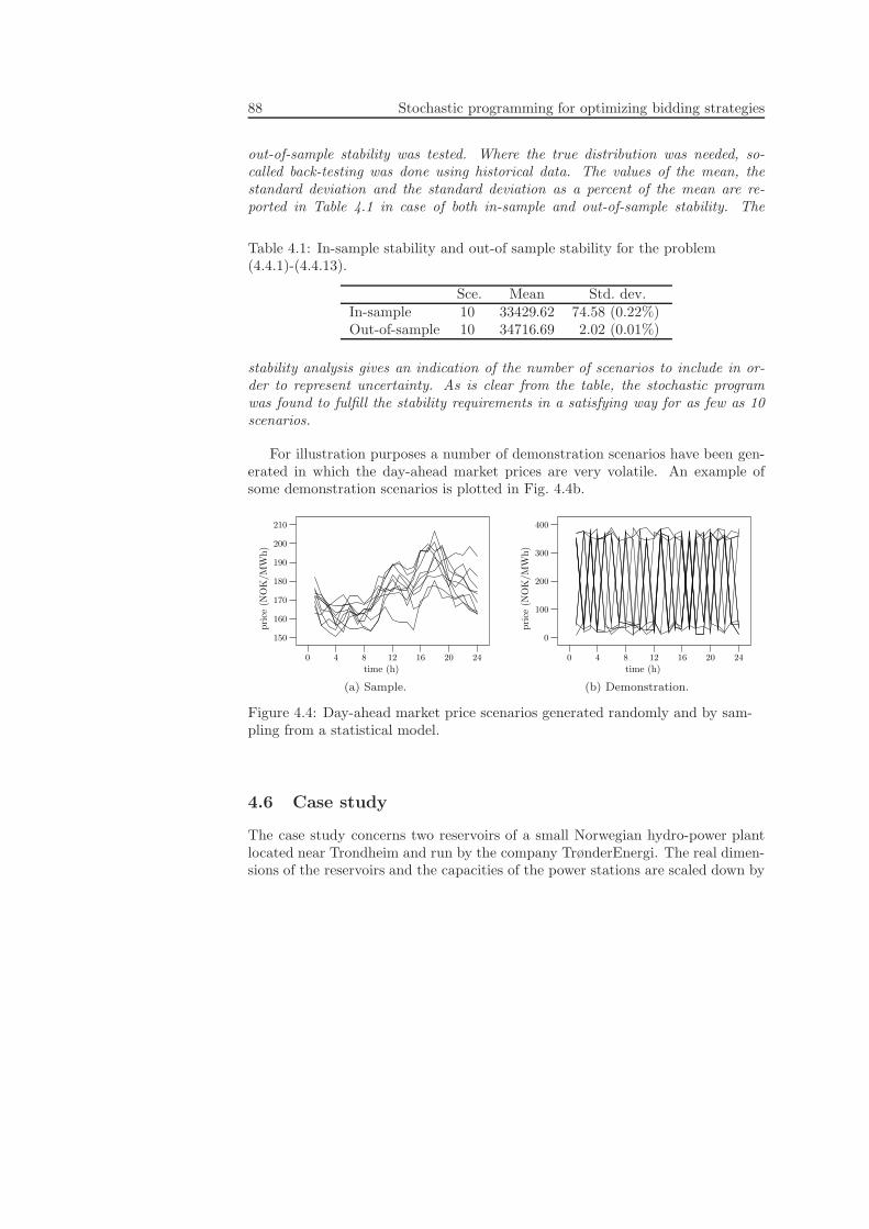
88 Stochastic programming for optimizing bidding strategies
out-of-sample stability was tested. Where the true distribution was needed, so-called back-testing was done using historical data. The values of the mean, thestandard deviation and the standard deviation as a percent of the mean are re-ported in Table 4.1 in case of both in-sample and out-of-sample stability. The
Table 4.1: In-sample stability and out-of sample stability for the problem(4.4.1)-(4.4.13).
Sce. Mean Std. dev.In-sample 10 33429.62 74.58 (0.22%)Out-of-sample 10 34716.69 2.02 (0.01%)
stability analysis gives an indication of the number of scenarios to include in or-der to represent uncertainty. As is clear from the table, the stochastic programwas found to fulfill the stability requirements in a satisfying way for as few as 10scenarios.
For illustration purposes a number of demonstration scenarios have been gen-erated in which the day-ahead market prices are very volatile. An example ofsome demonstration scenarios is plotted in Fig. 4.4b.
0 4 8 12 16 20 24
150
160
170
180
190
200
210
time (h)
pri
ce(N
OK
/MW
h)
(a) Sample.
0 4 8 12 16 20 24
0
100
200
300
400
time (h)
pri
ce(N
OK
/MW
h)
(b) Demonstration.
Figure 4.4: Day-ahead market price scenarios generated randomly and by sam-pling from a statistical model.
4.6 Case study
The case study concerns two reservoirs of a small Norwegian hydro-power plantlocated near Trondheim and run by the company TrønderEnergi. The real dimen-sions of the reservoirs and the capacities of the power stations are scaled down by

4.6. Case study 89
a factor ten for computational reasons. Initial reservoir levels and reservoir inflowsare the real data from a typical day of 2005. To generate day-ahead market pricesin 2005, Elspot at Nord Pool has provided the real data from 2004 that appliedto the Norwegian prize zone NO2, which is the Trondheim area.
The two-stage stochastic programming problem contains 18300 continuousvariables and 1440 constraints in the first stage and 590 continuous variables,48 binary variables and 740 constraints in the second stage. Stated as its de-terministic equivalent, (4.4.1)-(4.4.13), the problem is a large-scale mixed-integerlinear program solvable by standard software. The problem was solved with themixed-integer linear programming solver from OPL Studio version 3.7, ILOG Inc.(2003), calling CPLEX 9.0, Cplex Optimization Inc. (2006), on an Intel Xeon 2.67GHz processor with 4 GB RAM. The time of compiling and solving the problemvaried between 1 and 3000 seconds since no special effort was made to make thecode efficient. As the problem is a two-stage stochastic mixed-integer linear pro-gram special-purpose solution methods such as the dual decomposition algorithmof Carøe and Schultz (1999) might prove useful.
The rest of this section compares the stochastic approach to the bidding prob-lem with a deterministic version. The idea is to explore the effects of includinguncertainty explicitly into the optimization model and, in particular, to examineits objective function value and solutions.
To consider the structure of the bids, we solved the bidding problem as astochastic problem and as a deterministic problem. The former is the two-stagerecourse problem and the latter the corresponding expected value problem formedby replacing random prices by expected prices. Moreover, we computed the ex-pected result of using the expected value solution. For more information on theexpected value problem and the expected result of using the expected value solu-tion, see also Birge and Louveaux (1997).
Some results are reported in Table 4.2. EVP denotes the expected value prob-lem and RP the recourse problem. H. disp. and B. disp. represent the volumedispatched of hourly bids and block bids, respectively, and Prod. refers to thevolumes produced. Finally, Imbal. denotes the imbalances between total volumesdispatched and produced. The table illustrates the difference in the structure ofthe bids between the expected value problem and the recourse problem. In over-all terms, the deterministic model suggests the use of hourly bids, whereas thestochastic model combines hourly bids and block bids.
For details, consider the deterministic bidding problems for one reservoir andfor two reservoirs in cascade. In both cases, the structure of the solution is simpleand hourly bids are sufficient. With the market price being known in advance,only two hourly bids are relevant. The relevant bids determine the part of thebidding curve that passes through the point given by the optimal production leveland the market price. However, the resulting bidding curve may be very sensitiveto changes in the market price. In some scenarios the deviations from the expected

90 Stochastic programming for optimizing bidding strategies
market price may enforce heavy balancing as dispatches are far from being met byproduction. An example is given in Table 4.2 in which the imbalances of a givenhour between the total volumes dispatched and the volumes produced are ratherlarge in some scenarios (scenario 3,6 and 10).
For the stochastic bidding problems the structure of the solution is more com-plex. In the one-reservoir-case, the structure of the solution depends on whetherstart-up costs are included or not. Without start-up costs hourly bids are suf-ficient. With start-up costs both hourly bids and block bids are necessary. Toexplain, note that hourly bids follow prices closely. These are, however, acceptedindependently of each other and do not consider intertemporalities due to start-ups. Block bids, on the other hand, are valid for a number of consecutive hoursand thus tend to support a regular production schedule with less start-ups. Inthe two-reservoir-case the structure of the solution likewise depends on whetherstart-up costs are included or not. With the size differences between the reservoirs,the presence of a system bottleneck has further impact on the structure of the so-lution. A bottleneck occurs when the capacity of the upper reservoir exceeds thecapacity of the lower reservoir. Obviously, water is released from both the upperand the lower reservoirs in hours of a high market price. Due to combination ofthe bottleneck and the time delay between the reservoirs, however, excessive waterreleases from the upper reservoir may lead to forced releases in the lower reservoirin hours of a low market price. Without a bottleneck hourly bids are sufficient,whereas with a bottleneck both hourly bids and block bids are necessary. Anexplanation could be the following. Since hourly bids are accepted independentlythey ignore intertemporalities generated by dependencies between the reservoirs.On the other hand, as block bids are valid for a number of consecutive hours suchbids can be used as protection against major price fluctuations over time.
Note that with different formulations of the problems hourly bids and blockbids might be relevant both in the deterministic and the stochastic problems. Still,from the present formulation it is clear that uncertainty is one way of justifyingthe use of block bids and that block bids provide motivation for the inclusion ofuncertainty into the bidding problem.
Based on 10 demonstration scenarios and 10 sample scenarios respectively,we have drawn bidding curves in Fig. 4.5. The curves are shown for both thedeterministic problem (EVP), cf. the dashed lines, and the stochastic problem(RP), cf. full-drawn lines. The grey lines represent block bids and the black linesrepresent hourly bids. Although the bidding curves appear as piece-wise constant,the curves are in fact piece-wise linear. Nearly piece-wise constant bidding curves,however, are consistent with the bidding practice of the current application andreflects an almost price insensitive behavior between certain price levels.
The figures illustrate the discussion above. Consider Fig. 4.5b. For an expectedmarket price of 261.90 NOK/MWh the dispatch is the same in the deterministicand the stochastic problems, i.e. 2.24 MWh. Nevertheless, as already stated, the
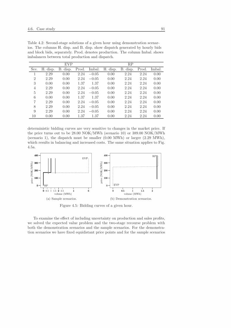
4.6. Case study 91
Table 4.2: Second-stage solutions of a given hour using demonstration scenar-ios. The columns H. disp. and B. disp. show dispatch generated by hourly bidsand block bids, separately. Prod. denotes production. The column Imbal. showsimbalances between total production and dispatch.
EVP RPSce. H. disp. B. disp. Prod. Imbal. H. disp. B. disp. Prod. Imbal.
1 2.29 0.00 2.24 −0.05 0.00 2.24 2.24 0.002 2.29 0.00 2.24 −0.05 0.00 2.24 2.24 0.003 0.00 0.00 1.37 1.37 0.00 2.24 2.24 0.004 2.29 0.00 2.24 −0.05 0.00 2.24 2.24 0.005 2.29 0.00 2.24 −0.05 0.00 2.24 2.24 0.006 0.00 0.00 1.37 1.37 0.00 2.24 2.24 0.007 2.29 0.00 2.24 −0.05 0.00 2.24 2.24 0.008 2.29 0.00 2.24 −0.05 0.00 2.24 2.24 0.009 2.29 0.00 2.24 −0.05 0.00 2.24 2.24 0.00
10 0.00 0.00 1.37 1.37 0.00 2.24 2.24 0.00
deterministic bidding curves are very sensitive to changes in the market price. Ifthe price turns out to be 28.00 NOK/MWh (scenario 10) or 389.00 NOK/MWh(scenario 1), the dispatch must be smaller (0.00 MWh) or larger (2.29 MWh),which results in balancing and increased costs. The same situation applies to Fig.4.5a.
RP
EVP
0
100
200
300
400
0 0.5 1 1.5 2 2.5
0
100
200
300
400
0 2 4 60 2 4 6
0
100
200
300
400
volume (MWh)
pri
ce(N
OK
/MW
h)
(a) Sample scenarios.
RP
EVP0
100
200
300
400
0 0.5 1 1.5 20 0.5 1 1.5 2
0
100
200
300
400
volume (MWh)
pri
ce(N
OK
/MW
h)
(b) Demonstration scenarios.
Figure 4.5: Bidding curves of a given hour.
To examine the effect of including uncertainty on production and sales profits,we solved the expected value problem and the two-stage recourse problem withboth the demonstration scenarios and the sample scenarios. For the demonstra-tion scenarios we have fixed equidistant price points and for the sample scenarios

92 Stochastic programming for optimizing bidding strategies
distributional price points. We recorded the optimal value of the recourse prob-lem as well as the expected result of using the expected value solution (EEV). Tocompare the two we calculated the difference which we refer to as the value ofthe stochastic solution (VSS). The VSS measures the effect of including stochas-tic prices explicitly into the bidding problem rather than simply using expectedprices. Averages of 10 different runs are reported in Tables 4.3 and 4.4. We focuson the computational results from using the sample scenarios. Although the mon-etary gains may seem moderate on a per day basis, the gains accumulate with theproblem being solved every day of the year. Moreover, recall that the dimensionof the power plant has been scaled down by a factor ten. The percentual VSS is7.93% on average. We conclude that significant profits can be earned by applyingstochastic programming.
Table 4.3: Computational results for demonstration scenarios.
S Opt. val. EEV VSS10 34801.51 33821.17 980.34
Table 4.4: Computational results for sample scenarios.
S Opt. val. EEV VSS10 33395.45 30992.49 2402.9630 33420.60 30676.07 2744.5350 33405.75 30805.37 2600.39
100 33419.60 30566.44 2853.17
It should be remarked that, in terms of the bidding problem, the expected valueproblem produces rather simple solutions inducing a very optimistic value of thestochastic solution. However, rather than using expected values, current practiceoften relies upon the selection of appropriate critical quantiles of the uncertaindata and the following solution of a number of deterministic problems. Thismay provide decisions that better hedge against adversity and results in a moremoderate value of the stochastic solution. Still, the comparison of the expectedvalue problem with the stochastic programming problem illustrates the effects ofincluding uncertainty explicitly into optimization.
As concluded, solutions are less sensitive to changes in the data in the stochasticapproach than in the deterministic version. Still, the expectation-based stochasticprogram lacks robustness in the sense that solutions tend to be unstable. Almostequal objection function values are obtained by structurally different solutionswhich indicates a flat objective function. Although structurally different, the so-lutions are equally good as long as the expectation-based objective criterion is

4.6. Case study 93
acknowledged. However, the expectation-based objective criterion can be claimedto ignore both risk attributes and profit distribution issues. In order to obtain amore robust stochastic programming model a risk measure can be included in theobjective function. The result is the so-called mean-risk model. The inclusion ofthe downside risk measure semideviation penalizes deviations from the expectedvalue and has the advantage of being consistent with a mixed-integer linear for-mulation. With semideviation, the objective function of (4.4.1)-(4.4.13) turns into
∑
s∈S
πszs − λ∑
s∈S
πs max
∑
s∈S
πszs − zs, 0
with
zs =∑
t∈T
ρsty
st +
∑
a∈A
ρsay
sa −
∑
t∈T
(pupt qup,s
t − pdot q
do,st )−
∑
t∈T
∑
j∈J
Sj(usjt−1, u
sjt) −
∑
j∈J
(Vj(lsj0) − Vj(l
sjT ))
where λ is a suitable weight. For more information on semideviation and other riskmeasures that are consistent with a linear formulation, see Chapter 2. The mean-risk problem ensures more stable solutions and a more equal profit distributionamong the scenarios. In Table 4.5 we report the expected value and the risk foraverages of 10 different runs using sample scenarios. Since the objective functionis flat stable solutions can be obtained with only very small profit reductions.
We have solved the mean-risk problem for varying weights λ ∈ R+. The pointsdefined by the selected weights are efficient points of the bi-criteria mean-riskproblem and gives an indication of the efficient frontier, that can be obtained bysolving the mean-risk problem for all λ ∈ R+. Still, even the efficient frontieris insufficient to fully describe the entire efficiency set. For more on the efficientfrontier and the efficiency set, see also Chapter 2.
Finally, note that the inclusion of the downside risk measure semideviationdoes not alter the structure of the solution in a way that contradicts the analysisalready made.
Table 4.5: Computational results for semideviation using simulation scenarios.
λ 0.001 1 10 100 1000Exp. val. 33389.34 33389.34 33192.04 32922.73 32716.62Risk 107.56 107.56 7.94 1.02 0.00


Chapter 5
Short-term hydro-power
production planning by stochastic
programming
The present chapter presents a short-term production planning problem not pre-viously addressed in the literature. As in Chapter 4, the problem has becomerelevant with the restructuring of the power sector and the introduction of theday-ahead market.
Within the framework of multi-stage stochastic mixed-integer linear program-ming, the aim is to develop a short-term production plan for a price-taking hydro-power plant operating under uncertainty. Current production must however com-ply with the day-ahead commitments of the previous day which makes short-termproduction planning a matter of spatial distribution among the reservoirs of theplant. Day-ahead market prices and reservoir inflows are uncertain beyond thecurrent operation day and, hence, water must be allocated among the reservoirsin order to strike a balance between current profits and expected future profits.A case study is based on data from a Norwegian hydro-power producer and theNordic power market at Nord Pool.
5.1 Introduction
As is also the case in other regions of the world, hydro-power production accountsfor a significant share of the total power production in the Nordic countries. Asan example, the countries within Nordel produced 191 TWh hydro-power out ofa total production of 387 TWh in 20041.
1 Reference: www.nordel.org
95

96 Short-term hydro-power production planning by stochastic programming
12.00 24.00 24.00
day-aheadbidding
one-dayplanning
real-timebalancing
Figure 5.1: Time schedule for short-term power planning and operation.
In the process of planning hydro-power production, problems are usually cate-gorized according to their time horizon; long-term, medium-term and short-term.Short-term hydro-power production planning mainly involves the physical oper-ation of the plant within a time horizon of a day or a week and with a timeresolution of an hour or shorter. The most important activities that come intoplay are
• the day-ahead commitments, i.e. the bidding of the production into a powerexchange a day in advance.
• the establishment of a production plan that complies with the day-aheadcommitments.
• the intra-day balancing, i.e. the continuous corrections of deviations betweenthe commitments and the actual production.
The focus of the present paper is the establishment of a one-day production planthat complies with the day-ahead commitments of the previous day. From theperspective of this study, the day-ahead bidding has been completed whereas real-time balancing considerations will be postponed until actual production has beenobserved. For an illustration of the time schedule, see Fig. 5.1.
When the results of the day-ahead auction are known, the classical hydro-power problem, that consists in scheduling of water through time, is no longer anissue. The challenge in making a production plan for the following operation dayis rather the scheduling of water through space, which involves the allocation ofproduction between various parts of the plant to achieve effective and efficientoperation. Since, however, short-term planning is strongly coupled to more long-term planning, the value of current decisions must be evaluated against futureconsequences. Therefore, in determining the spatial distribution of the followingoperation day, production is usually considered in a longer time span such as sevendays.
Day-ahead market prices and reservoir inflows are both subject to data un-certainty caused by non-anticipated market conditions and unpredictable weathersituations. We propose the stochastic programming framework to handle this un-certainty. Indeed, as information evolves over time and uncertainty is disclosed instages, a multi-stage stochastic program is appropriate. In line with the above,the first stage relates to the one-day production plan and the remaining stagesto the production of the following six days. It follows that the overall objective

5.2. Short-term hydro-power production 97
of the stochastic program is to establish a one-day production plan that strikes abalance between current profits and expected future profits subject to a numberof operational constraints.
Existing approaches to short-term production planning comprise both simula-tion and optimization. As simulation is often based on adjusting manual sugges-tions until a convincing plan is found, this approach is highly user dependent anddoes not guarantee an optimal plan. On the contrary, optimization represents arelatively impartial way of identifying an optimal plan. Whichever approach isused, most practical applications do not explicitly include data uncertainty.
The outline of the paper is the following. Sections 5.2 and 5.3 present a mixed-integer linear programming problem for the development of a one-day productionplan that complies with the day-ahead commitments. Section 5.4 introduces datauncertainty and presents a stochastic programming formulation of the problem,whereas Section 5.5 explains how to generate scenarios that serve as input to thestochastic program. Finally, Section 5.6 illustrates the problem with a case study.
5.2 Short-term hydro-power production
The starting point for modeling is short-term hydro-power production. Modelingis restricted to mixed-integer linear programming and follows along the lines of forexample Philpott et al. (2000). For illustration purposes, the case study is keptrather simple and the model concerns only a very small hydro-power plant. Someexamples of non-modeled features are constraints that apply to the network ofwatercourses and junctions, the distinction between baseload and load-followingpower stations, reserve requirements as well as legal requirements, see Jacobs et al.(1995). Nevertheless, it should be clear that including additional hydrologicalconstraints or modeling a larger hydro-power plant is possible by means of mixed-integer linear programming.
As in Chapter 4, the hydro-power plant of the case study consists of two reser-voirs in cascade; a larger upper reservoir and a smaller lower reservoir. However,each reservoir now has its own inflow stream. Furthermore, each reservoir is con-nected to a power station that contains a number of turbines. As upstream waterreaches the plant, it is stored in the reservoirs until released through the turbines.In the turbines, electricity is generated by converting potential energy into electri-cal energy, before the water proceeds downstream. Water released from the upperreservoir flows to the lower reservoir with some time delay on its way. Waterthat is not discharged on purpose and used for generation is considered spill. Thesize differences of the reservoirs restrict the flexibility of the system in that waterreleases from the upper reservoir may force releases in the lower reservoir or mayeven lead to spill. For an illustration of the plant, see Fig. 5.2. The model ispresented in slightly more general terms than the case study requires.
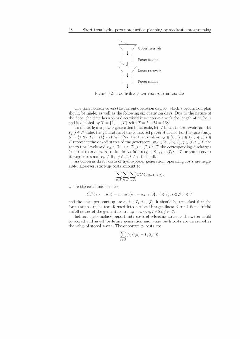
98 Short-term hydro-power production planning by stochastic programming
Power station
Power station
Lower reservoir
Upper reservoir
Figure 5.2: Two hydro-power reservoirs in cascade.
The time horizon covers the current operation day, for which a production planshould be made, as well as the following six operation days. Due to the nature ofthe data, the time horizon is discretized into intervals with the length of an hourand is denoted by T = 1, . . . , T with T = 7 × 24 = 168.
To model hydro-power generation in cascade, let J index the reservoirs and letIj , j ∈ J index the generators of the connected power stations. For the case study,J = 1, 2, I1 = 1 and I2 = 2. Let the variables uit ∈ 0, 1, i ∈ Ij , j ∈ J , t ∈T represent the on/off states of the generators, wit ∈ R+, i ∈ Ij , j ∈ J , t ∈ T thegeneration levels and vit ∈ R+, i ∈ Ij , j ∈ J , t ∈ T the corresponding dischargesfrom the reservoirs. Also, let the variables ljt ∈ R+, j ∈ J , t ∈ T be the reservoirstorage levels and rjt ∈ R+, j ∈ J , t ∈ T the spill.
As concerns direct costs of hydro-power generation, operating costs are negli-gible. However, start-up costs amount to
∑
t∈T
∑
j∈J
∑
i∈Ij
SCi(uit−1, uit),
where the cost functions are
SCi(uit−1, uit) = ci maxuit − uit−1, 0, i ∈ Ij , j ∈ J , t ∈ T
and the costs per start-up are ci, i ∈ Ij , j ∈ J . It should be remarked that theformulation can be transformed into a mixed-integer linear formulation. Initialon/off states of the generators are ui0 = ui,init, i ∈ Ij , j ∈ J .
Indirect costs include opportunity costs of releasing water as the water couldbe stored and saved for future generation and, thus, such costs are measured asthe value of stored water. The opportunity costs are
∑
j∈J
(Vj(lj0) − Vj(ljT )),
5.2. Short-term hydro-power production 99
where
Vj(ljt) = mink∈K
d1kj ljt + d2
kj, j ∈ J , t ∈ T
and the coefficients of the concave water value functions are d1kj , d
2kj , k ∈ K, j ∈ J .
The formulation is consistent with a linear formulation. For further remarks onthe derivation of the water value functions, see Chapter 4.
The following bounds are imposed on the generation levels
wmini uit ≤ wit ≤ wmax
i uit, i ∈ Ij , j ∈ J , t ∈ T ,
where wmini , i ∈ Ij , j ∈ J and wmax
i , i ∈ Ij , j ∈ J are the minimum and maximumgeneration levels. The water discharges have to comply with similar bounds, sothat
vminj ≤
∑
i∈Ij
vit ≤ vmaxj , j ∈ J , t ∈ T ,
where vminj , j ∈ J and vmax
j , j ∈ J are the minimum and maximum discharges.Finally, the following bounds apply to the storage levels
lminj ≤ ljt ≤ lmax
j , j ∈ J , t ∈ T ,
where lminj , j ∈ J and lmax
j , j ∈ J denote minimal and maximal storage levels.According to the reservoir balances, inflow and storage from previous periods
either appear as discharge, storage or spill in the following period. The upperreservoir balance equations are therefore
l1t − l1t−1 +∑
i∈I1
vit + r1t = ν1t, t ∈ T ,
in which ν1t, t ∈ T are the inflows from upstream. The initial storage level isl10 = l1,init. The lower reservoir balance equations are
ljt − ljt−1 +∑
i∈Ij
vit + rjt =∑
i∈Ij−1
vit−τ + νjt, j ∈ J \1, t ∈ T ,
in which νjt, j ∈ J \1, t ∈ T are the direct inflows from upstream. Note that,for reservoirs in cascade, releases from the upper reservoirs are inflows of the lowerreservoirs. It is, however, assumed that upstream spill does not contribute to thedownstream inflows. τ is the time delay between the reservoirs. Again, the initialstorage level is lj0 = lj,init, j ∈ J \1.
The generation level is a function of the water discharge from the reservoirand the net water head of the power station. The net water head is the difference

100 Short-term hydro-power production planning by stochastic programming
between the headwater elevation and the tailwater elevation and, whereas theformer is a function of the reservoir storage level, the latter is a function of thedischarge. It is, however, assumed that the net water head only varies with thedischarge over the course of the short-term planning horizon. The assumption isjustified in the case of relatively small storage level variations compared to thenet head, which holds for the case study. By ignoring some head variation effects,the relation between generation and discharge can be approximated by a concavefunction. Hence,
wit = Gi(vit), i ∈ Ij , j ∈ J , t ∈ T ,
where
Gi(vit) = mink∈K
e1kivit + e2ki, i ∈ Ij , j ∈ J , t ∈ T
and the coefficients of the concave functions are e1ki, e2ki, k ∈ K, i ∈ Ij , j ∈ J . For
an illustration of the generating functions of the case study, see Fig. 5.3. It is clearthat the generation and discharge could in fact be assumed to be proportional inthe case study.
0
2
4
6
8
0 20 40 600 20 40 60
0
2
4
6
8
0 10 20 30 40 50 60 70
0
1
2
3
4
5
6
7
8
103m3/h
MW
(a) Upper reservoir.
0
10
20
30
40
0 20 40 600 20 40 60
0
10
20
30
40
0 10 20 30 40 50 60 70
0
5
10
15
20
25
30
35
103m3/h
MW
(b) Lower reservoir.
Figure 5.3: Generation functions for two different hydro-power turbines.
5.3 Day-ahead market commitments
Norway was among the first countries in the world to undertake the deregulationof the power markets. In the beginning of the nineties a Norwegian power marketwas established and has since then developed into an overall Nordic power market.An essential component of the power market is the presence of the power exchangethat facilitates physical trading activity on a day-per-day basis. The spot market,

5.3. Day-ahead market commitments 101
Elspot, at the Nordic power exchange, Nord Pool, is a pool-based market in whichmarket participants exchange power contracts for physical delivery the followingoperation day and is referred to as the day-ahead market. In 2004, a total of 167TWh or 42 percent of the Nordel power production was traded at Elspot2.
Elspot contracts are commitments to sell or purchase power of a duration ofone hour or longer. To use such contracts, the market participants post price-differentiated bids for every hour of the following operation day before deadlineat noon. The hourly market prices are then determined by equilibrium betweensales and purchases. Once the market prices have been announced, the marketparticipants receive a notification of the winning bids and the hourly commitmentsof the following operation day. Real-time operation and physical delivery is doneaccording to the day-ahead commitments to the extent possible.
The value of electricity production should be measured on the basis of day-ahead market prices. We assume w.l.g. that the entire production is sold in theday-ahead market and that bilateral contracts are left out. Day-ahead marketsales give rise to the revenues
∑
t∈T
∑
j∈J
∑
i∈Ij
ρtwit,
where ρt, t ∈ T are the day-ahead market prices. By assuming that the produceris a price-taker, market prices can be modeled as exogenous. To justify the price-taker assumption, the producer should be sufficiently small to have only limitedmarket power. In the case of significant market power the concepts of game theory,monopoly or oligopoly becomes important and the complexity of the model mayincrease.
The production of the first day has to meet the hourly commitments in theday-ahead market. As the day-ahead commitments are fixed a day in advance,these are given as data to the model and may be obtained from more long-termplanning models such as the day-ahead bidding model of Chapter 4. This givesrise to the constraints
∑
j∈J
∑
i∈Ij
wit = dt, t ∈ T1,
where T1 indexes the hours of the first day and dt, t ∈ T1 are the day-aheadcommitments of the first day. If a producer relies on portfolio bidding and placescompound bids that apply to a number of plants, the modeling of a larger hydro-power system comes into play. Still, it should be straightforward to extend themodel.
2 Reference: www.nordel.org and www.nordpool.no

102 Short-term hydro-power production planning by stochastic programming
If production deviates from the day-ahead commitments, the imbalances aresettled in an intra-day balancing market. Since, however, the purpose of the modelis production planning rather than market exchange, intra-day balancing is notincluded. Moreover, since planned imbalances are forbidden by the market opera-tors, producers are not allowed to hold back production for the balancing market.Although intra-day balancing is left out of production planning, a producer canalways ramp down or, in the case of spare capacity, ramp up while actually pro-ducing and thereby participate in the real-time balancing market. For a way ofincorporating balancing market considerations, see Chapter 4.
5.4 The stochastic programming model
Both day-ahead market prices and reservoir inflows are rather volatile and hardto predict because of unexpected market conditions and unforeseen weather situa-tions. The model of the previous sections does not reflect the fact that new infor-mation about the uncertain data arrives along the planning horizon. Nevertheless,this can be handled by the application of multi-stage stochastic programming.
To facilitate modeling, we assume the uncertain data evolves over time ac-cording to a multivariate stochastic process and the probability information isapproximated by a scenario tree. Consistent with the notation of multi-stagestochastic programming problems introduced in Chapter 1, the realizations of theuncertain prices and inflows ρt, ν1t, ν2tt∈T are denoted ρn, νn
1 , νn2 n∈N .
By assuming that information is revealed only at the beginning of an operationday, the scenario tree consists of seven stages or operation days that each consistof 24 time intervals or hours. The assumption is valid for day-ahead market pricesthat are announced a day prior to physical delivery. Furthermore, it is justifiedin the case of daily readings on the reservoir inflow measuring instruments or atleast as an effort to limit the size of the scenario tree. An example of a scenariotree is shown in Fig. 5.4.
1 2 3 22 23 24
25 26 27 46 47 48
49 50 51 70 71
Figure 5.4: An illustration of a scenario tree for day-ahead market prices andreservoir inflows.
The inclusion of seven stages ensures the coupling between short-term and morelong-term planning. While the first stage determines the one-day production plan,
5.5. Scenario generation 103
the remaining six stages serve to evaluate the impact of the plan on future produc-tion. In line with this, the overall objective of the multi-stage stochastic programis to determine the one-day production plan that strikes a balance between cur-rent and expected future profits. In its scenario tree formulation, the multi-stagestochastic program is the following
max∑
n∈N
∑
j∈J
∑
i∈Ij
πn(
ρnwni − SCi(u
n−1
i , uni )
)
+ (5.4.1)
∑
n∈NT
∑
j∈J
πnVj(lnj ) −
∑
j∈J
Vj(lj,init)
s.t.∑
j∈J
∑
i∈Ij
wni = dn, n ∈ Nt, t ∈ T1 (5.4.2)
uni w
mini ≤ wn
i ≤ uni w
maxi , i ∈ Ij , j ∈ J , n ∈ N (5.4.3)
vmini ≤
∑
i∈Ij
vni ≤ vmax
i , i ∈ Ij , j ∈ J , n ∈ N (5.4.4)
lminj ≤ lnj ≤ lmax
j , j ∈ J , n ∈ N (5.4.5)
ln1 − ln−1
1 +∑
i∈I1
vni + rn
1 = νn1 , n ∈ N (5.4.6)
lnj − ln−1
j +∑
i∈Ij
vni + rn
j =∑
i∈Ij−1
vn−τ
i + νnj , j ∈ J \1, n ∈ N (5.4.7)
wni = Gi(v
ni ), i ∈ Ij , j ∈ J , n ∈ N (5.4.8)
uni ∈ 0, 1, wn
i , vni , l
nj , r
nj ≥ 0, i ∈ Ij , j ∈ J , n ∈ N . (5.4.9)
Note that the multi-stage stochastic program may be approximated by a two-stage stochastic program. A natural two-stage approximation would consist of afirst stage that determines the one-day production plan and a second stage thatcomprises the remaining six days.
5.5 Scenario generation
The modeling of day-ahead market prices and reservoir inflows is based on timeseries analysis. Time series models have the advantage of being derived fromlimited information and still allow for both forecasting and sampling. As shown

104 Short-term hydro-power production planning by stochastic programming
in Chapter 8, the ARMA time series framework provides an appropriate modelfor hourly prices, whereas the modeling of hourly inflows requires development.Nevertheless, also in this case, we find the ARMA time series models sufficient todemonstrate the usefulness of stochastic programming.
The multivariate stochastic process of hourly day-ahead market prices andwater inflows constitutes a time series3 characterized by seasonal changes andstochastic variations that are mainly due to the market conditions and the weatherpatterns. In general, a multivariate stochastic process can be modeled as a vectorARMA (VARMA) process
ψ(B)ξt = γ(B)et, t ∈ Z,
where ψ(B) and γ(B) are the polynomials ψ(B) = 1 −∑
k ψkBk and γ(B) =
1 −∑
k γkBk with the parameter matrices ψk and γk and where B denotes the
back-shift operator, i.e. Bkξt = ξt−k. ξt and et are vectors, where et, t ∈ Z areassumed to be independent normally distributed random vectors with zero meanand constant covariance matrix Σ.
We consider the three-dimensional stochastic process ρt, ν1t, ν2tt∈T of day-ahead market prices and reservoir inflows. An inspection of the cross correlationsindicates that the innovations of prices and inflows are uncorrelated and, thus,prices and inflows can be modeled separately. For inflows, the innovations canbe assumed only contemporaneously correlated and the inflows can therefore bemodeled by a so-called contemporaneous ARMA (CARMA) model. For furtherreferences on CARMA models and stream-flows, we refer to Chapter 8. As aresult, three univariate ARMA models may be fitted independently and combinedto a multivariate model. The development of the three univariate ARMA modelsfollows the steps
1. Identify a statistical model of the data.
2. Estimate the parameters of the model.
3. Validate the model.
1. In the identification step the data is made stationary and the orders ofthe polynomials are determined. The seasonal ARMA (SARIMA) models areidentified as
(1 − ψ1B)(1 −B)(1 −B24)(1 −B168)ρt =
(1 − γ1B)(1 − γ24B24)(1 − γ168B
168)et, t ∈ Z (5.5.1)
3 Data sources: Nord Pool (prices) and TrønderEnergi (inflows)

5.5. Scenario generation 105
for day-ahead market prices and
(1 − ψj1B)(1 −B)νjt =
(1 − γj1B − γj
2B2)(1 − γj
41B41)ejt, j = 1, 2, t ∈ Z. (5.5.2)
for water inflows.2. Parameter estimation is based on maximum likelihood optimization.3. Finally, diagnostic checks are applied to validate the assumptions of inde-
pendence and normality.We assume that the innovations of (5.5.1) and (5.5.2), i.e. ett∈Z and e1t,
e2tt∈Z, are uncorrelated and, since normally distributed, independent. Further-more, we assume the innovations of (5.5.2), i.e. e1tt∈Z and e2tt∈Z, are onlycontemporaneously correlated. In order to obtain completely uncorrelated innova-tions, we let (e1t, e2t)
T = C(ǫ1t, ǫ2t)T , where CCT = Σ, C is an upper triangular
matrix, Σ is the covariance matrix of the innovations and ǫ1t, ǫ2tt∈Z are indepen-dent normally distributed random vectors with zero mean and constant covariancematrix I2. A multivariate ARMA model that describes the three-dimensional pro-cess of day-ahead market prices and reservoir inflows has then been fitted. Athorough discussion of the application of VARMA and CARMA to the day-aheadmarket prices and reservoir inflows is found in Chapter 8.
The development of the time series models in steps 1-3, is accomplished by thestatistical software package SAS, version 8.2., see SAS Institute Inc. (1999).
There are various approaches for approximating what is actually a continuousprobability distribution of the uncertain data by a discrete and finite distributionrepresented by a scenario tree. For a general overview on the construction of sce-nario trees, see Chapter 7. With available historical data, is possible to samplefrom the statistical model and convert the resulting scenario paths into a scenariotree. As a starting point, we therefore generate 1000 scenario paths using MonteCarlo sampling from the multivariate ARMA model. Examples of a few scenariopaths are shown in Fig. 5.5. The scenario paths are combined to a scenario treeby applying the conditional clustering algorithm of Heitsch and Romisch (2006b).For multi-stage stochastic linear programs, the method is supported by stabil-ity results and consequently, the quality of the constructed scenario tree can becontrolled by certain error bounds. Although, the current problem is actually amixed-integer linear multi-stage stochastic program, we still use the method, thereason being that the conditional clustering is intuitively appealing. Moreover,only few scenario generation methods apply to multi-stage stochastic programsthat involves multivariate stochastic processes. The Monte Carlo sampling wasimplemented in C++, whereas the method of Heitsch and Romisch (2006b) wasmost kindly made available by the authors.
Remark 5.5.1 When approximating a continuous probability distribution by adiscrete distribution, the quality of the approximation should be evaluated. How-

106 Short-term hydro-power production planning by stochastic programming
ever, the error bounds controlling the quality of the scenario tree constructionmethod of Heitsch and Romisch (2006b) are found to be quite loose. Furthermore,due to the mixed-integer linear formulation, the bounds may not actually be valid.For these reasons, a different evaluation of the practical performance is relevant.We have tested in-sample stability and out-of-sample stability of the stochastic pro-gramming problem. For further details on evaluating scenario generation methodsand the relation to the particular scenario tree construction method, see Chapter 7.We have generated ten different scenario trees, formulated the stochastic program-ming problems and solved them. For in-sample stability, we report the optimalvalues. For out-of-sample stability, we have used back-testing and evaluated theoptimal solutions on the historical data. We report the mean, the standard devia-tion and the standard deviation as a percent of the mean for the optimal values inTable 5.1. The out-of sample values have a smaller standard deviation than thein-sample values since in-sample stability is evaluated on different trees, whereasout-of-sample stability is evaluated on the same tree based on historical data. Notealso that the out-of-sample value is much higher than the in-sample value. Thiswould usually be a sign of poor approximate solutions. Here, it could be explainedby the fact that, as the historical data includes the weeks of one year, the datadoes not suitably represent the true probability distribution of a specific week. Un-fortunately, due to lack of data, we were unable to consider the specific week ina number of different years. As an overall conclusion, we find the stochastic pro-gramming problem to be sufficiently stable with respect to the scenario generationmethod in use.
Table 5.1: In-sample stability and out-of sample stability for the problem(5.4.1)-(5.4.9).
Sce. Nodes Mean Std. dev.In-sample 264 11681 564162.43 3919.77 (0.69%)Out-of-sample 273 12096 945564.23 0.00 (0.00%)
In addition to sample scenarios, demonstration scenarios have been generatedto illustrate various effects of day-ahead prices and reservoir inflows. The demon-stration scenarios allow for prices and inflows to be significantly higher and lowerthan the real observations of the data.
5.6 Numerical results
The case study is based on data from a small Norwegian hydro-power plant lo-cated south of Trondheim and run by the company TrønderEnergi. The reservoir

5.6. Numerical results 107
120
140
160
180
200
220
240
260
0 24 48 72 96 120 144 168
time (h)
pri
ce(NOK/M
Wh)
(a) Day-ahead marketprices.
0 24 48 72 96 120 144 168
0
20
40
60
time (h)
inflow
(100
0m
3/h
)
(b) Reservoir inflows, up-per reservoir.
0 24 48 72 96 120 144 168
0
10
20
30
time (h)
inflow
(100
0m
3/h
)
(c) Reservoir inflows, lowerreservoir.
Figure 5.5: Scenarios generated by sampling from a statistical model.
capacity of all power plants of this company amount to 0.7 TWh, the annual in-flows to 1.5 TWh and the generation capacity to 334 MW4. Still, the case studyconcerns only two reservoirs and two power stations with each one turbine whichcorresponds a reservoir capacity of 24.6 GWh, annual inflows of 69.6 GWh anda generation capacity of 33.9 MW. The initial conditions of the plant are givenby the data from a typical week of 2005 and the same applies for the day-aheadcommitments. The generation of reservoir inflows for 2005 is based on observa-tions from the year 2004. To generate corresponding day-ahead market prices for2005, Nord Pool has provided the data from 2004 that applied to the Norwegianprize zone NO2, which includes the Trondheim area. Basically, NO2 consists ofnine large hydro-power producers and a number of very small producers. Thecompany TrønderEnergi accounts for 3 percent of the reservoir capacity, 5 percentof the annual inflows and 5 percent of the generation capacity of the area5 and istherefore considered a price-taker of the area.
The multi-stage stochastic program (5.4.1)-(5.4.9) contains 12 variables, 1 bi-nary and 11 continuous, and 22 constraints per node of the scenario tree, exceptfor a few extra variables and constraints in the first and the last stages. Hence, itis a mixed-integer linear program which size depends on the number of scenariosand nodes of the scenario tree. We have solved the problem with the mixed-integerlinear programming solver from OPL Studio version 3.7, ILOG Inc. (2003), callingCPLEX 9.0, Cplex Optimization Inc. (2006), on an Intel Xeon 2.67 GHz proces-sor with 4 GB RAM. Direct application of CPLEX is no longer possible whenthe number of scenarios and nodes of the scenario tree is further increased. Weconsider the scenario tree to be sufficiently large to appropriately approximatethe probability distribution . Moreover, regarding traditional solution approachesto stochastic hydro scheduling problems, dynamic programming may suffer fromthe curse of dimensionality and as shown in Archibald et al. (1996) may be un-
4 Norwegian Competition Authority, 2002
5 Norwegian Competition Authority, 2002

108 Short-term hydro-power production planning by stochastic programming
able to outperform linear programming methods. Also, due to the mixed-integerformulation, the problem is not amenable to nested Benders’ decomposition. Itmay, however, be suitable for some of the general decomposition approaches thatapply to multi-stage stochastic mixed-integer linear programming problems. So-lution approaches worth investigating comprise those based on Lagrangian relax-ation of non-anticipativity constraints, cf. progressive hedging by Løkketangen andWoodruff (1996) or nodal coupling constraints, cf. Dentcheva and Romisch (2004).
While varying the level of clustering in the scenario tree construction method,we have recorded the number of scenarios and nodes of the scenario tree, thetotal number of variables and constraints of the problem, the optimal objectivefunction value and the computing time spent to solve the problem, cf. Table 5.2.All numbers reported are averages of 10 different runs and all computations arebased on sample scenarios. Test runs indicate that the two-stage approximation tothe multi-stage stochastic program may provide first-stage solutions of a significantquality in terms of objective function values.
Table 5.2: Computational results for sample scenarios.
Sce. Nodes Var. Con. Obj. val./NOK CPU/s267 11777 141846 261254 562207.50 28.71493 43709 525494 965566 567086.91 203.81782 103144 1239304 2275470 566645.83 764.35
In hydro-power production, planning is coupled in time. The time coupling canbe explained mainly by the storage balancing between the reservoirs. The storagebalancing and the capacities of the reservoirs determine the spatial distributionof water between the reservoirs of the hydro-power plant. Therefore, the spatialdistribution depends on future day-ahead market prices and reservoir inflows. Toillustrate this, consider the case where both reservoirs are close to empty. If day-ahead market prices for the following six days are expected to be high, there is apotential for future generation and current production takes place in downstreamreservoirs. This ensures future water releases from all reservoirs in cascade andhigher future generation levels. If, on the other hand, day-ahead market pricesfor the following six days are expected to be low, current production is allocatedaccording to water values and start-up costs. Now, consider the case where bothreservoirs are almost full. If reservoir inflows for the following six days are expectedto be high, current production takes place in downstream reservoirs in order toempty the system and accommodate future generation. If reservoir inflows for thefollowing six days are expected to be low, current production is again allocatedaccording to water values and start-up costs.
The dependence of the spatial distribution on the future day-ahead marketprices and reservoir inflow levels is depicted in Figs. 5.6-5.7. The figures repre-
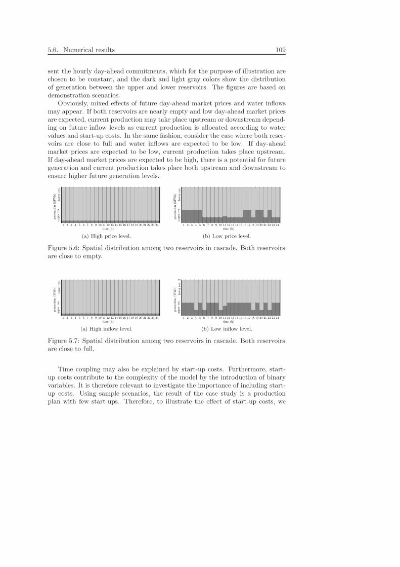
5.6. Numerical results 109
sent the hourly day-ahead commitments, which for the purpose of illustration arechosen to be constant, and the dark and light gray colors show the distributionof generation between the upper and lower reservoirs. The figures are based ondemonstration scenarios.
Obviously, mixed effects of future day-ahead market prices and water inflowsmay appear. If both reservoirs are nearly empty and low day-ahead market pricesare expected, current production may take place upstream or downstream depend-ing on future inflow levels as current production is allocated according to watervalues and start-up costs. In the same fashion, consider the case where both reser-voirs are close to full and water inflows are expected to be low. If day-aheadmarket prices are expected to be low, current production takes place upstream.If day-ahead market prices are expected to be high, there is a potential for futuregeneration and current production takes place both upstream and downstream toensure higher future generation levels.
low
erre
s.upper
res.
gener
atio
n(M
Wh)
time (h)1 2 3 4 5 6 7 8 9 10 11 12 13 14 15 16 17 18 19 20 21 22 23 24
(a) High price level.
low
erre
s.upper
res.
gener
atio
n(M
Wh)
time (h)1 2 3 4 5 6 7 8 9 10 11 12 13 14 15 16 17 18 19 20 21 22 23 24
(b) Low price level.
Figure 5.6: Spatial distribution among two reservoirs in cascade. Both reservoirsare close to empty.
low
erre
s.upper
res.
gener
atio
n(M
Wh)
time (h)1 2 3 4 5 6 7 8 9 10 11 12 13 14 15 16 17 18 19 20 21 22 23 24
(a) High inflow level.
low
erre
s.2
upper
res.
gener
atio
n(M
Wh)
time (h)1 2 3 4 5 6 7 8 9 10 11 12 13 14 15 16 17 18 19 20 21 22 23 24
(b) Low inflow level.
Figure 5.7: Spatial distribution among two reservoirs in cascade. Both reservoirsare close to full.
Time coupling may also be explained by start-up costs. Furthermore, start-up costs contribute to the complexity of the model by the introduction of binaryvariables. It is therefore relevant to investigate the importance of including start-up costs. Using sample scenarios, the result of the case study is a productionplan with few start-ups. Therefore, to illustrate the effect of start-up costs, we
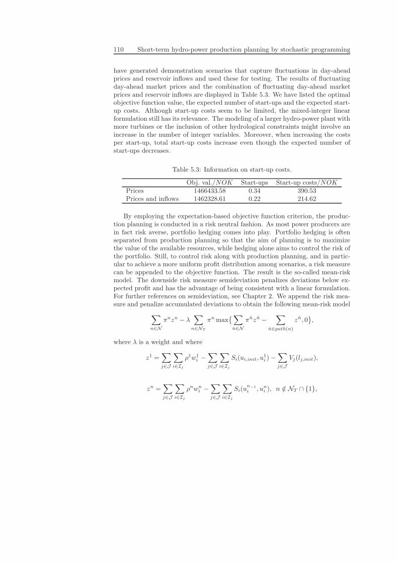
110 Short-term hydro-power production planning by stochastic programming
have generated demonstration scenarios that capture fluctuations in day-aheadprices and reservoir inflows and used these for testing. The results of fluctuatingday-ahead market prices and the combination of fluctuating day-ahead marketprices and reservoir inflows are displayed in Table 5.3. We have listed the optimalobjective function value, the expected number of start-ups and the expected start-up costs. Although start-up costs seem to be limited, the mixed-integer linearformulation still has its relevance. The modeling of a larger hydro-power plant withmore turbines or the inclusion of other hydrological constraints might involve anincrease in the number of integer variables. Moreover, when increasing the costsper start-up, total start-up costs increase even though the expected number ofstart-ups decreases.
Table 5.3: Information on start-up costs.
Obj. val./NOK Start-ups Start-up costs/NOKPrices 1466433.58 0.34 390.53Prices and inflows 1462328.61 0.22 214.62
By employing the expectation-based objective function criterion, the produc-tion planning is conducted in a risk neutral fashion. As most power producers arein fact risk averse, portfolio hedging comes into play. Portfolio hedging is oftenseparated from production planning so that the aim of planning is to maximizethe value of the available resources, while hedging alone aims to control the risk ofthe portfolio. Still, to control risk along with production planning, and in partic-ular to achieve a more uniform profit distribution among scenarios, a risk measurecan be appended to the objective function. The result is the so-called mean-riskmodel. The downside risk measure semideviation penalizes deviations below ex-pected profit and has the advantage of being consistent with a linear formulation.For further references on semideviation, see Chapter 2. We append the risk mea-sure and penalize accumulated deviations to obtain the following mean-risk model
∑
n∈N
πnzn − λ∑
n∈NT
πn max
∑
n∈N
πnzn −∑
n∈path(n)
zn, 0
,
where λ is a weight and where
z1 =∑
j∈J
∑
i∈Ij
ρ1w1i −
∑
j∈J
∑
i∈Ij
Si(ui,init, u1i ) −
∑
j∈J
Vj(lj,init),
zn =∑
j∈J
∑
i∈Ij
ρnwni −
∑
j∈J
∑
i∈Ij
Si(un−1
i , uni ), n /∈ NT ∩ 1,

5.6. Numerical results 111
zn =∑
j∈J
∑
i∈Ij
ρnwni −
∑
j∈J
∑
i∈Ij
Si(un−1
i , uni ) +
∑
j∈J
Vj(lnj ), n ∈ NT .
It should be remarked that it is possible to include a multi-period risk measure,which does not alone focus on accumulated profit but also take into account in-termediate time periods. For some examples on multi-period risk measures, seeEichhorn et al. (2005).
We have solved the problem for varying weights and recorded the expectedvalue along with the risk, cf. Table 5.4. By solving for all positive weights, wewould obtain the efficient frontier. Still, the efficient frontier does not representthe entire efficiency set and therefore we display only a selected set of weightsand their corresponding records. All numbers reported are averages of 10 differentruns and all computations are based on simulation scenarios.
Table 5.4: Computational results for semideviation using sample scenarios.
λ 0.001 1 10 100 1000Exp. val. 563110.56 563110.54 495984.66 467811.71 457764.42Risk 21906.52 21906.26 1480.32 43.03 0.00
From Table 5.4 it can be seen that when employing the expectation-basedobjective function criterion in short-term production planning, the downside riskis significant. Also, a reduction in risk requires a considerable reduction in profit.In the long run, however, hydro-power producers have a natural hedge. Whereasprices and inflow are uncorrelated in the short run, they are usually negativelycorrelated in a longer time span. If inflows decrease, prices tend to increase andcompensate for this and vice versa.


Chapter 6
Managing power reserves by
two-stage stochastic programming
With the restructuring of the power sector, the reliability of the system has to agreat extent become the responsibility of the system operator. This, among otherthings, includes the balancing of power supply and demand and the managementof reserves to facilitate it.
Although the physical transaction of power through bilateral trade or spot mar-ket exchange aims at balancing supply and demand, real-time imbalances may stilloccur due to non-anticipated supply and demand behavior. The real-time balanceis the responsibility of the power system operator and is achieved by means ofregulation that is purchased in the regulating market. To ensure sufficient regula-tion in the market, the system operator has the possibility of reserving regulatingpower in advance. As reserves are purchased prior to actual operation, however,reserve decisions are subject to supply and demand uncertainty. Regulation deci-sions on the other hand can be deferred until uncertainty has been revealed andthe system is operating. In the present paper this is formalized by formulatingthe problem of managing regulating reserves as a two-stage stochastic program.A case study that concerns the system operator of Western Denmark is discussedin detail.
6.1 Introduction
In a power system that comprises several participants on both the supply andthe demand side, it is the task of the system operator to balance productionand consumption by means of regulation purchased in the regulating market. A
113
114 Managing power reserves by two-stage stochastic programming
major part of the balancing is however the management of regulation reserves, assufficient amounts of regulation are not necessarily available in the market unlessreserved in advance. Considering the challenges of uncertain supply and demand,the problem of managing regulating power reserves can be handled by meansof stochastic programming. Moreover, previous studies show how similar poweroptimization problems can be handled successfully by mathematical programmingand stochastic programming in particular, see Chapter 3.
The paper is organized as follows. The problem of managing power reservesis presented in Section 6.3. Section 6.4 explains how uncertainty affects reservemanagement and formulates the problem as a two-stage stochastic program. Byassuming a discrete distribution of the random data, the problem is transformedinto a large-scale mathematical program that is solved by a specially designedsolution procedure in Section 6.5. A specific instance of the problem is addressedusing data from the power system operator of Western Denmark and computa-tional results are reported in Section 6.6.
6.2 Power reserves
The project grew out of a collaboration with the former Eltra1, which is thepower system operator of Western Denmark. Due to decentralization of the powergeneration and deregulation of the power markets, many procedures have eitherbeen modified recently or will be within the near future. In particular, Eltra madeplans to improve the model on which power reserve management is based, whichmakes reserves a topic of current interest.
It is necessary to distinguish between different types of reserves
(i) Automatic regulation reserves: Reserves that cover imbalances from the timeof appearance until a regulation bid is activated. The reserves are providedby running plants capable of adjusting upwards and consumers capable ofadjusting downwards. Activation begins automatically within two to threeminutes.
(ii) Manual regulation reserves: Reserves in the form of regulation resourcesthat suppliers are obligated to sell in the regulating market. The reservesare activated manually within 10 minutes.
(iii) Running and available plants: Reserves for ensuring supply in spite of trans-mission lines or units falling out. Consist of available plants that can bestarted, running plants that can adjust upwards and consumers that canadjust downwards. Running and available plants are activated either auto-matically or manually.
1 now a part of the overall Danish power and gas system operator Energinet.dk, www.energinet.dk

6.2. Power reserves 115
(iv) Emergency start plants: Reserves reestablishing the system in case of black-out.
We here confine ourselves to manual regulation reserves. The reason why man-ual regulating reserves are relevant should be clear from the following. In a typicalpower system the operator is responsible for balancing supply and demand. Priorto operation, predicted supply and demand are balanced by resources provided bybilateral trades and spot market exchanges. Still, supply and demand often differfrom the predictions and imbalances occur when the system is operating. To over-come such real-time imbalances, the system operator compensates suppliers andconsumers for adjusting production and demand accordingly. The imbalances arecovered by so-called regulation resources, that are traded in a regulating market,established by system operators to serve this purpose. Suppliers either increase ordecrease power production above or below the amounts committed through bilat-eral and spot market contracts and offer the adjustments to the regulating marketas so-called up- and down-regulation, respectively. Consumers offer power demandadjustments to the regulating market in a similar fashion. The system operatorpurchases up-regulation in the case of excess demand and down-regulation in thecase of excess supply. In some cases, though, the amounts of resources provided bythe regulating market are insufficient to fully cover imbalances. This may happenif
(i) Imbalances are substantial due to extreme supply and demand behaviorcaused by failure in supplying, unforeseen weather changes leading to un-predicted wind production or non-anticipated heat demand etc.
(ii) Spot market prices are sufficiently high to prevent market participants fromsaving resources for trading in the less secure regulating market.
(ii) Considerable failures occur during transmission, e.g. important transmissionlines fall out.
To ensure that sufficient amounts of resources are available even when facingsuch critical situations, regulation can be reserved prior to trading in the regulatingmarket. The system operator may secure the right of purchasing regulation withreserver supplier. This right is a type of option in that the system operator paysfor the possibility of purchasing regulation in the market without being forced todo so. The reserve supplier is obligated to bid an amount of regulation into themarket. As a result, the system operator faces the trade-off between purchasingregulation at the market price only, thereby risking insufficiency of resources,and paying both the market price and an additional fixed price to ensure thatregulation is available. We refer to the first and the second type of regulation asdirect and reserved regulation, respectively.

116 Managing power reserves by two-stage stochastic programming
14.00 24.00 24.00
reservemanagement
day-aheadcommitment
real-timebalancing
Figure 6.1: Time schedule for the activities involved in power balancing.
The major problem of managing regulating reserves is that of procuring priorto observing supply and demand imbalances. On the one hand, the reserve ca-pacity may turn out to be insufficient to fully cover the imbalances not coveredby direct regulation, which means additional regulation resources must be pro-cured elsewhere at considerable costs, otherwise the system simply breaks down.On the other hand, reserves constitute serious costs, which makes excess reservecapacity unwanted. Stochastic programming provides a tool for determining regu-lation reserve levels that ”hedge” against the non-anticipated supply and demandbehavior.
The rest of the chapter is motivated by a case study based on the powersystem of Western Denmark as well as the local and Nordic power markets. Inmany respects, however, the discussion applies in general to other power systems.
As already explained, different power markets come into play when balancingpower supply and demand. To fully understand the interactions of the systemoperator with the markets, we consider the following time schedule. The systemoperator procures regulating reserves for a longer time period. In Western Den-mark, a formal reserve market has not yet been fully established. Currently, thelength of the period is at least one month though a reduction is planned. The re-maining actions concern a 24-hour operation day. By noon bids must be submittedto the spot market, which in the Danish case is the Nordic Market at Nord Pool2.Having balanced predicted supply and demand, activated bids are announced by14:00. Finally, from 24:00 to 24:00 actual supply and demand imbalances are con-tinuously corrected by trading in the intra-day regulating market. For the casestudy, the regulating market is still the local market, although integration into theNordic market is planned. For an illustration of the time schedule, see Fig. 6.1.
6.3 The problem of managing power reserves
In stating the problem, consider a given planning horizon. Although in practice,the power balance should be maintained at every point in time, the horizon isdiscretized in order to facilitate computations. Since the bids to the regulatingmarked have a duration of a number of full hours, the horizon is discretized intohourly time intervals. The finite set of such intervals is denoted by T = 1, . . . , T.
2 www.nordpool.no

6.3. The problem of managing power reserves 117
The planning horizon for purchasing regulating reserves may range from one toseveral months. In Western Denmark some reserve contracts have long durations,whereas other contracts are traded regularly on a monthly basis. The planninghorizon of the case study is set to one month, i.e. T = 24 × 30 = 720. However,to increase the flexibility of the system, it is intended to reduce the horizon, asis already the case in Eastern Denmark where reserve contracts are traded on adaily basis.
6.3.1 Procuring reserves
At present, the system operator of Western Denmark procures regulation reservesmostly locally. Although not fully formalized, regulation reserves are traded ona monthly auction or as individual contracts of a longer duration. A regulationreserve bid consists of an offer period, a volume to be available throughout the offerperiod, a variable price that applies to the portion of the volume that is activatedand a fixed price for activation of the bid. We assume for the application thatregulation reserves are traded solely on the auction so that the offer period isalways one month. According to the above, the system operator pays the variableprice for the actual amount of regulation used and the fixed price for the availabilityof regulation.
Regulation reserves are modeled as follows. Regulation divides into up- ordown-regulation, and so do regulation reserves; thus, the superscripts up and do.The indices H = 1, . . . , H are adopted to represent different reserve bids. Thevariables xup
h , xdoh ∈ 0, 1, h ∈ H indicate whether the reserve bids are activated or
not and the prices for activation are denoted cuph , cdo
h , h ∈ H. Then fixed regulationreserve purchase costs compute as
∑
h∈H
(cuph xup
h + cdoh x
doh ).
6.3.2 Purchasing regulation
A larger power system may share a common regulating market. The Nordic systemoperators, the Swedish Svenska Kraftnat, the Norwegian Statnett and the DanishEnerginet.dk, have established such a common market, in which Western Denmarkwas the last to begin integration in January 2006. Still, although full integration ison its way, Western Denmark trades regulation mostly locally. Before July 2006,the regulating market of Western Denmark was a pay-as-bid market. Now, as astep towards integration, the general rule is to use local marginal prices as marketprices and finally, Nordic marginal prices should be fully in use by January 2008.
When purchasing regulation and regulation reserves outside Western Denmark,transmission capacity limits may apply. Such limits are due to physical limitations

118 Managing power reserves by two-stage stochastic programming
or political agreements. Since, for the current application, however, regulation ismostly purchased locally, we have omitted transmission capacity limits and ingeneral assumed no grid congestion.
The suppliers to the regulating market are power balance providers submit-ting bids to the market. Such regulation bids divide into up-regulation and down-regulation bids. Upward regulation makes consumers decrease demand or suppli-ers increase production (system operators “buy” power) and downward regulationmakes suppliers decrease production or consumers increase demand (system op-erators “sell” power). A regulation bid consists of an offer period, a price anda volume. The offer period may be a number of full hours. During the offerperiod, the volume is constant whereas the price may vary between hours. Wehowever assume that regulation bids have an offer period of only one hour and thusboth the volume and the price are constant. Generally, the up-regulation priceis specified as the system spot price (assuming no grid congestion) and a raise,i.e. the up-regulation price is always above the system price. Similarly, the down-regulation price is calculated as the system price (assuming no grid congestion)and a deduction, i.e. the down-regulation price is always below the system price.Since prices are usually given as positive numbers unless the system operator sellsup-regulation or buys down-regulation, prices are always assumed to be positive.
Regulation comprises direct purchases in the regulating market and purchasesreserved in advance. In the case of reserved purchases, recall that the indicesH = 1, . . . , H are included to represent different bids. Up- and down-regulationvolumes are denoted yup
h , ydoh , h ∈ H. We assume no failure of supply and, hence,
all reserved purchases will be available in the regulating market. Correspond-ing prices are denoted pup
ht , pdoht, h ∈ H, t ∈ T . In the case of direct purchases,
K = H + 1, . . . , H + K are included to index different bids. Up- and down-regulation volumes are denoted yup
ht , ydoht , h ∈ K, t ∈ T and corresponding prices
are pupht , p
doht, h ∈ K, t ∈ T . Note that reserved purchases are independent of time,
whereas direct purchases are time dependent. Furthermore, for reserved purchases,prices should stay between predefined limits, whereas for direct purchases, pricescan vary freely. Finally, a bid is not necessarily activated completely. Actualpurchases are represented by the variables yup
ht , yupht ∈ R+, h ∈ H ∪ K, t ∈ T .
Pay-as-bid pricing
Costs of purchasing regulation, whether reserved or direct, consist of up-regulationexpenses and down-regulation income
∑
t∈T
∑
h∈H∪K
(pupht q
upht − pdo
htydoht ).

6.3. The problem of managing power reserves 119
The following bounds concern reserved purchases
yupht ≤ yup
h xuph , ydo
ht ≤ ydoh xdo
h , h ∈ H, t ∈ T , (6.3.1)
whereas direct purchases must submit to the bounds
yupht ≤ yup
ht , ydoht ≤ ydo
ht , h ∈ K, t ∈ T . (6.3.2)
Marginal pricing
For each hour the marginal price is determined as the price of the last bid activatedin the direction in which the system is regulated. If the system is up-regulated, themarginal price is the highest price of the activated up-regulation bids. Likewise, ifthe system is down-regulated, the marginal price is the lowest price of the activateddown-regulation bids. The variables δup
ht , δdoht ∈ 0, 1, h ∈ H ∪K indicate whether
the regulation bids are activated or not for both reserved and direct regulation.Moreover, the variables pup
t , pdot ∈ R
n1+ represent the marginal prices. In the case
of up-regulation, the marginal price is pupt = maxpup
ht δupht : h ∈ H ∪K and in the
case of down-regulation, the marginal price is pdot = minpdo
htδdoht : h ∈ H ∪K.
Costs of purchasing reserved and direct regulation amount to
∑
t∈T
(
pupt
∑
h∈H∪K
yupht − pdo
t
∑
h∈H∪K
ydoht
)
. (6.3.3)
Evidently, (6.3.3) is nonlinear. In order to be consistent with a mixed-integerlinear formulation, we introduce the variables ρup
t , ρdot ∈ R
n1+ , t ∈ T and replace
(6.3.3) by
∑
t∈T
(ρupt − ρdo
t )
and
ρupt ≥ pup
ht
∑
h∈H∪J
yupht −M(1 − δup
ht ), h ∈ H ∪K, t ∈ T , (6.3.4)
ρdot ≤ pdo
ht
∑
h∈H∪K
ydoht +M(1 − δdo
ht ), h ∈ H ∪K, t ∈ T , (6.3.5)
with
M = max
pupht
(
∑
h∈K
yupht +
∑
h∈H
yupt
)
, pdoht
(
∑
h∈K
ydoht +
∑
h∈H
ydot
)
: h ∈ H ∪ K, t ∈ T
.

120 Managing power reserves by two-stage stochastic programming
For both reserved and direct purchases, the volumes activated cannot exceed thevolumes bid
yupht ≤ yup
ht δupht , y
doht ≤ ydo
htδupht , h ∈ H ∪ K, t ∈ T . (6.3.6)
Reserved regulation cannot be activated unless the regulation reserve bids areactivated
∑
t∈T
δupht ≤ xup
h ,∑
t∈T
δdoht ≤ xdo
h , h ∈ H. (6.3.7)
Note that we model the price determination process in terms of mixed-integerlinear programming with the introduction of binary variables indicating activationor not. An alternative to avoiding nonlinearities would have been to discretize thecontinuous price range into a number of price levels and associate with each pricelevel one or more binary variables. The approach is seen in Nowak et al. (2005),who address the bidding problem of a power producer being able to influencemarket prices. The number of price levels, however, is likely to exceed the numberof bids to be considered for activation. For this reason, the above formulation hasits advantages.
6.3.3 Balancing
The system operator takes care of the power balancing during actual operation. Ifactual demand exceeds actual supply, the system operator purchases up-regulationand if supply exceeds demand, down-regulation is purchased. Imbalances betweendemand and supply are usually fully covered by regulation purchased directly orreserved in advance. In the case of insufficient regulation, however, excess demandand supply may result in irregular in- and out-flows from abroad that are hardlypenalized. Such in- and out-flows can be avoided by forcing consumers to decreasedemand, by forcing power plants to shut down generating units or by stopping windturbines, in which cases severe costs are also paid. Let the variables eup
t , edot , t ∈ T
denote excess demand and supply. If bupt , bdo
t , t ∈ T denote penalty costs, excessdemand and supply give rise to the following costs
∑
t∈T
(bupt eup
t + bdot e
dot ).
The power balance constraints are∑
h∈H∪K
(yupht − ydo
ht ) + eupt − edo
t = ∆t, t ∈ T , (6.3.8)
where ∆t, t ∈ T denote the imbalances between demand and supply. If ∆t > 0,demand exceeds supply and if ∆t < 0, vice versa. Note that supply includescentral, decentral and wind production as well as import and that demand consistsof national consumption and export.

6.4. Introducing uncertainty 121
6.4 Introducing uncertainty
The problem presented in the preceding sections is deterministic. The real prob-lem, however, involves uncertainties in the data and would therefore be suited forstochastic optimization. Uncertainties relate to the regulating prices and volumesthat can be changed until an hour before operation. Moreover, demand and sup-ply uncertainty arises because of failure in supplying, unforeseen weather changesleading to unpredicted wind production or non-anticipated heat demand. Since,however, the system imbalances are caused by demand and supply, we restrict theattention to demand and supply uncertainty.
Uncertainty is handled by means of stochastic programming. Although infor-mation evolves over time and a multi-stage stochastic program could be relevant,we approximate the problem by a two-stage stochastic program. We find thisapproximation sufficient to capture the interplay between reserves and regulationpurchases. As reserves must be purchased a month in advance, reserve decisionsare first-stage. Decisions have to be made before operation and thus with incom-plete knowledge of future supply and demand. In contrast, regulation bids havean activation period of at most ten minutes and can therefore be purchased veryclose to operation, which makes regulation decisions second-stage. The objectiveis to minimize reserve costs and expected future regulation and penalty costs.
The uncertain data is represented by a stochastic process on some probabilityspace. To make the problem computationally tractable, we assume a discretemultivariate distribution with finite support. The realizations of uncertainty willbe referred to as scenarios, indexed by S = 1, . . . , S and denoted by (∆s
t )t∈T s∈S .The corresponding probabilities will be denoted by πs, s ∈ S. First-stage reservedecisions are xup
h , xdoh ∈ 0, 1, h ∈ H, whereas second-stage regulation decisions
are indexed yup,sht , ydo,s
ht , pup,sht , pdo,s
ht , eupt , edo
t ≥ 0, h ∈ H ∪K, t ∈ T , s ∈ S.The two-stage stochastic programming formulation of the regulating reserve
management is the following problem, depending on whether pay-as-bid or marginalpricing applies. The extension to market integration should be straightforward.
Pay-as-bid pricing
min∑
h∈H
(cuph xup
h + cdoh x
doh )+ (6.4.1)
∑
s∈S
∑
t∈T
∑
h∈H∪K
πs(pup,sht yup,s
ht − pdo,sht ydo,s
ht )+
∑
s∈S
∑
t∈T
πs(bupt eup,s
t + bdot e
do,st )
s.t. (6.3.1)− (6.3.2), (6.3.8)

122 Managing power reserves by two-stage stochastic programming
xuph , xdo
h ∈ 0, 1, h ∈ H
yup,sht , ydo,s
ht , pup,sht , pdo,s
ht , eup,st , edo,s
t ≥ 0, h ∈ H ∪ K, t ∈ T , s ∈ S.
Marginal pricing
min∑
h∈H
(cuph xup
h + cdoh x
doh )+ (6.4.2)
∑
s∈S
∑
t∈T
πs(ρup,st − ρdo,s
t )+
∑
s∈S
∑
t∈T
πs(bupt eup,s
t + bdot e
do,st )
s.t. (6.3.4) − (6.3.7), (6.3.8)
xuph , xdo
h ∈ 0, 1, h ∈ H
yup,sht , ydo,s
ht , pup,sht , pdo,s
ht , ρup,st , ρdo,s
t , eup,st , edo,s
t ≥ 0,
δup,sht , δdo,s
ht ∈ 0, 1, h ∈ H ∪ K, t ∈ T , s ∈ S.
The scenario generation has been kept rather simple. The imbalances betweendemand and supply constitute a time series and have, thus, been analyzed bymeans of the field. In order to capture the future behavior of demand and sup-ply imbalances and in particular model the imbalances as a stochastic process,historical data profiles have been used. Because demand and supply show strongcorrelations over time, the stochastic process is chosen as an autoregressive (AR)process. For proof of concept, the order of the AR process is chosen to be one.The AR process, cf. Box and Jenkins (1976), is the following
∆t = ψ∆t−1 + et, t ∈ Z, (6.4.3)
where ett∈Z is a Gaussian white noise process. The time series may be more ap-propriately described by higher order autoregressive moving average (ARMA) pro-cesses, able to describe seasonal variations in the data. For examples on seasonalARMA models and electricity demand, see Growe-Kuska et al. (2000), Growe-Kuska et al. (2002) and Eichhorn et al. (2005). Scenarios of future demand andsupply imbalances ∆s
tt∈T ,s∈S are generated by sampling from (6.4.3). To reflectthe true probability distribution, a large number of scenarios has been generatedusing Monte Carlo sampling.
6.5. Solution procedure 123
6.5 Solution procedure
The problems (6.4.1) and (6.4.2) may be handled as large-scale mixed-integer lin-ear problems solvable by standard software packages or stochastic mixed-integerlinear programs amenable to decomposition approaches such as the integer L-shaped method by Laporte and Louveaux (1993) or the dual decomposition algo-rithm by Carøe and Schultz (1999). Being able to solve the problems as mixed-integer linear programs is valuable since this approach is very flexible. Addingfurther linear constraints is uncomplicated and becomes particularly relevant withconstraints that introduce time dependencies. However, with the current simplic-ity of the model, it can be solved by a procedure that utilizes the structure ofthe problem. The solution procedure is motivated by the current practice of thesystem operator and applies in the case of both pay-as-bid pricing and marginalpricing.
If formalized, the problems (6.4.1) and (6.4.2) can be stated as
min
cx+∑
s∈S
∑
t∈T
πsΦst (x), x ∈ B
n1
,
Φst (x) = minqy|Wy = hs
t − Tx, y ∈ Rn2 × B
n′
2,
where x ∈ Bn1 represents the first-stage decisions, y ∈ R
n2 × Bn′
2 representsthe second-stage decisions and data vectors and matrices are derived from theproblems.
As the number of reserve bids often reduces to less than ten, the set of first-stage decisions is limited and enumeration is possible. The enumeration determineswhich reserve bids should be activated.
Algorithm 6.5.1 Enumeration
Step 0 (Initialization) Let z = ∞.
Step 1 (Enumeration) Select a first-stage solution, x.
Step 2 (Evaluation) Let
z = min
z, cx+∑
s∈S
∑
t∈T
πsΦst (x)
,
where, for t ∈ T , s ∈ S, Φst (x) is determined by Algorithm 6.5.2. Return
to step 1.

124 Managing power reserves by two-stage stochastic programming
Having fixed the first-stage decisions, the problem decomposes into subproblemsaccording to both scenarios and time intervals. A subproblem is solvable by inspec-tion. After the reserve bids have been activated, the regulating bids are selectedone at a time according to the so-called order of merit until imbalances are covered.We state the procedure only for up-regulation as the case of down-regulation willfollow in a similar fashion. We assume that the penalty costs of excess supply anddemand exceed all bid prices, although the procedure could be easily adjusted toaccount for other relationships between penalty costs and bid prices.
Algorithm 6.5.2 Order of merit
Step 0 (Initialization) If ∆st > 0, the system must be up-regulated. Let
Hup,0 = h ∈ H : xuph = 1
index the activated reserve bids. Available regulation bids are then indexedby Hup,0 ∪ K0. Go to step 1.
Step 1 (Ranking) Set i=i+1. If ∆st > 0, activate (fully unless the imbalance is
covered by less) the regulation bid (pupkt , y
up,skt ) defined by
pupkt ∈ arg minpup
ht : h ∈ Hup,i−1 ∪ Ki−1.
Set Hup,i ∪ Ki := Hup,i−1 ∪ Ki−1\k. If the imbalance is covered, stop.If Hup,i ∪ Ki = ∅, the remaining imbalance is excess demand. Otherwise,return to step 1.
6.6 Computation results
As already stated, the case study concerns the problem of managing regulatingreserves in Western Denmark. The data dates back to June 2006, just beforethe transition from pay-as-bid pricing to marginal pricing. Hence, we solve theproblem with both pay-as-bid pricing (6.4.1) and local marginal pricing (6.4.2).Reserve bids comprise bids of the June auction as well as individual contracts ofa potentially longer duration. As the system operator intends to reduce the offerperiod of reserve bids, we assume that such individual contracts have an offerperiod of only one month. The reserve bids consist of seven up-regulation bidsand one down-regulating bid. The volumes and the fixed prices of the reserve bidsare released by Energinet.dk3. The variable prices have been randomly generatedbased on the announced regulating market prices. Regarding regulating bids tothe market, ten bids have been constructed. Both volumes and prices have been
3 www.energinet.dk

6.6. Computation results 125
randomly generated on the basis of the regulating market prices and the totalamounts of up- and down-regulation bid into the market. All data has beenprovided by Nord Pool4. The penalties for excess demand and supply are bothset sufficiently high to prevent uncovered imbalances on a regular basis.
With the current data, the problem (6.4.1) contains eight binary variablesand no constraints in the first stage and 53280 continuous variables and 13680constraints in the second stage. The problem (6.4.2) contains the same number ofvariables and constraints in the first stage and 54720 continuous variables, 12960binary variables and 39608 constraints in the second stage. The Procedures 6.5.1and 6.5.2 were implemented in C++ and computations were carried out on anIntel Xeon 2.67 GHz processor with 4 GB RAM.
We have solved the problems (6.4.1) and (6.4.2) with the Procedures 6.5.1and 6.5.2 and listed the results. For a varying number of scenarios, Table 6.1displays the average optimal values and CPU times of ten different runs. Obvi-ously, marginal pricing results in a higher optimal value than pay-as-bid pricing.The first column of Table 6.2 shows the total balancing costs divided into reservecosts, regulation costs and penalty costs. Recall that regulation costs consist ofup-regulation expenses and down-regulation income and costs may therefore beboth positive and negative. The second column of Table 6.2 gives the total im-balances divided into regulation and excess supply and demand along with thereserved regulation that is available but not necessarily activated. Regulationconsists of both up- and down-regulation. All numbers are based on 100 scenariosand are averages of ten different runs. It is clear that for both pay-as-bid pricingand marginal pricing, reserves are highly necessary for the optimal covering of im-balances. Finally, Table 6.4 lists the reserve bids and indicate whether activationis effected or not. All ten runs for both pay-as-bid pricing and marginal pricingshow the same result and support the use of reserves.
To compare the stochastic programming approach to a deterministic approach,we have solved the expected value problems (EVP), in which stochastic demandand supply imbalances have been replaced by their expected values. Moreover, wehave computed the expected results of using the expected value solutions (EEV).For further reference on the expected value problem, see Birge and Louveaux(1997). The average EEVs and CPU times of ten different runs are displayed inTable 6.1. Generally, the EEVs exceed the optimal values of the stochastic pro-grams, which is confirmed. In Table 6.3 the total balancing costs and the totalimbalances are divided into reserves, regulation and excess supply and demand.Table 6.4 indicate whether activation of the reserve bids is effected or not. Sinceimbalances often cancel out on average, no reserve bids are activated in the deter-ministic case. However, the expected result of using the expected value solutions isa need for a larger amount of direct regulation and if not available, larger excess de-
4 www.nordpool.no
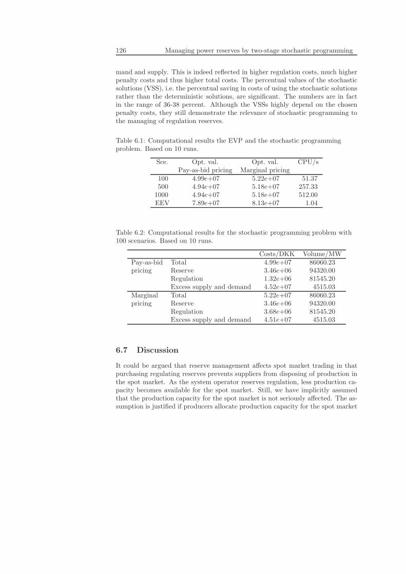
126 Managing power reserves by two-stage stochastic programming
mand and supply. This is indeed reflected in higher regulation costs, much higherpenalty costs and thus higher total costs. The percentual values of the stochasticsolutions (VSS), i.e. the percentual saving in costs of using the stochastic solutionsrather than the deterministic solutions, are significant. The numbers are in factin the range of 36-38 percent. Although the VSSs highly depend on the chosenpenalty costs, they still demonstrate the relevance of stochastic programming tothe managing of regulation reserves.
Table 6.1: Computational results the EVP and the stochastic programmingproblem. Based on 10 runs.
Sce. Opt. val. Opt. val. CPU/sPay-as-bid pricing Marginal pricing
100 4.99e+07 5.22e+07 51.37500 4.94e+07 5.18e+07 257.33
1000 4.94e+07 5.18e+07 512.00EEV 7.89e+07 8.13e+07 1.04
Table 6.2: Computational results for the stochastic programming problem with100 scenarios. Based on 10 runs.
Costs/DKK Volume/MWPay-as-bid Total 4.99e+07 86060.23pricing Reserve 3.46e+06 94320.00
Regulation 1.32e+06 81545.20Excess supply and demand 4.52e+07 4515.03
Marginal Total 5.22e+07 86060.23pricing Reserve 3.46e+06 94320.00
Regulation 3.68e+06 81545.20Excess supply and demand 4.51e+07 4515.03
6.7 Discussion
It could be argued that reserve management affects spot market trading in thatpurchasing regulating reserves prevents suppliers from disposing of production inthe spot market. As the system operator reserves regulation, less production ca-pacity becomes available for the spot market. Still, we have implicitly assumedthat the production capacity for the spot market is not seriously affected. The as-sumption is justified if producers allocate production capacity for the spot market

6.7. Discussion 127
and the regulating market separately. However, it would be valuable to furtherinvestigate the matter by incorporating the present model in a larger model thatincludes the spot market.
Table 6.3: Computational results for the EVP. Based on 10 runs.
Costs/DKK Volume/MWPay-as-bid Total 7.89e+07 86226.71pricing Reserve 0e+00 0.00
Regulation 1.56e+06 78496.00Excess supply and demand 7.73e+07 7730.71
Marginal Total 8.13e+07 86226.71pricing Reserve 0e+00 0.00
Regulation 3.94e+06 78496.00Excess supply and demand 7.73e+07 7730.71
Table 6.4: Computational results the EVP and the stochastic programmingproblem with 100 scenarios. Based on 10 runs.
Up-reg.Price/DKK 288000 625000 384000 330000Volume/MW 25 16 11 298Activation 100 sce. 1 1 1 0
EVP 0 0 0 0Up-reg. Down-reg.
Price/DKK 10298880 714000 966450 152000Volume/MW 12 21 30 16Activation 100 sce. 1 1 1 1
EVP 0 0 0 0


Chapter 7
Scenario generation in stochastic
programming electricity models
Being an important part of establishing a stochastic programming model, theremainder of the thesis is dedicated to scenario generation. The idea is to explainthe methods used for scenario generation and reduction in Chapters 4 and 5 andput these into perspectives with the existing literature on the subject.
The task of generating the scenarios that serve as input to a stochastic pro-gramming model can be handled in many ways, depending on the available infor-mation and data and on the required output. In generating scenarios, some of thefollowing requirements could be taken into account. Ideally, the scenarios should
• reflect the actual background and be linked with the purpose of the appli-cation.
• approximate the true probability distribution or represent the uncertain datain some other way.
• utilize the information of historical data and at the same time be capable ofincluding exogenous knowledge and extreme situations and capture futureeffects such as trends and expectations.
• from a computational point of view, result in a problem of a manageablesize, that still produces solutions of sufficient quality.
To illustrate different requirements, this chapter gives a selected overview of sce-nario generation methods from the literature. We present scenario generationmethods that are based on experts’ opinions or data manipulation alone, methodsthat aim to represent the probability distribution by matching statistical proper-ties and methods that approximate the probability distribution by sampling froma statistical model. We briefly mention a method suitable for including additional
129
130 Scenario generation in stochastic programming electricity models
scenarios. Furthermore, we examine in greater detail methods that reduce thestochastic programming problem to a manageable size, and, finally, we discuss theevaluation of scenario generation methods in terms of solution quality. The mainfocus is scenario generation methods that have found use in stochastic program-ming applications to power systems. To complete the overview, however, somemajor advances in scenario generation will be included. This also serves to justifythe choice of the scenario generation methods in Chapter 4 and 5. For a generalsurvey on scenario generation methods, see Dupacova et al. (2000).
Recall from Chapter 1 that the random components of a general stochasticprogramming problem is described by a random vector ξ on some probabilityspace (Ω,F ,P). The probability distribution of ξ is given by the image measureµ = P ξ−1 and is referred to as the probability distribution of the stochastic pro-gramming problem. We define ζ as a similar random vector on (Ω,F ,P) and let theprobability distribution of ζ be given by the image measure ν = Pζ−1. In the fol-lowing, we will use ξ and ζ in terms of both two-stage and multi-stage stochasticprogramming. When specifically addressing only two-stage or multi-stage pro-grams, however, we will adjust notation accordingly. For discrete a approximationwith finite support, recall that the approximation of ξ is given by the scenariosξ1, . . . , ξS and corresponding probabilities π1, . . . , πS . When referring to a fixedvalue such as a single realization or the mean value of ξ, we often denote it ξ.This chapter aims at approximating the probability distribution of a stochasticprogramming problem by a discrete distribution with finite support.
7.1 Subjective approaches and data manipulation
Application specific methods for generating scenarios are not necessarily theo-retically founded but may rely on subjective judgment, experts’ opinion or datamanipulation.
An obvious scenario generation method is simple data manipulation. Takritiet al. (1996) present an example that relies alone on historical data but is stilldistributions-free. The authors generate demand scenarios for a multi-stage stoch-astic programming formulation of the unit commitment problem subjected to un-certainty of demand and generator failures. The scenarios are based on historicalobservations under comparable circumstances and are adjusted by incorporatingfuture expectations and demand peaks that corresponds to unavailable generatorcapacity.
Another method that rests on a rather simple use of historical data is presentedby Nowak and Romisch (2000) who develop a multi-stage stochastic programmingproblem for planning the weekly generation of electric power in a hydro-thermalsystem under demand uncertainty. Starting from a reference scenario based onreal data, a scenario tree is constructed by randomly selecting branching points

7.2. Matching statistical properties 131
and creating identical scenarios that branch from these. Then a Brownian motionis added to each node of the scenario tree.
In contrast to the above, the integration of scenario generation into mathe-matical programming and, in particular, stochastic programming input formats,has prompted more general scenario generation devices. The stochastic extensionof the mathematical programming standard, MPS, the SMPS, can be combinedwith an external scenario generator. In addition, although relatively simple, thestandard itself offers some scenario generation features.
In the initial version of the SMPS, Birge et al. (1987) provide a framework forgenerating and organizing uncertain data for multi-stage stochastic programmingproblems. The authors propose an input format that incorporates sampling from anumber of univariate distributions by specifying the appropriate parameters. Theinput format allows for different kinds of dependencies in data, e.g. independence,interstage dependence and dependence on past data.
To overcome some of the shortcomings of the initial version, Gassmann andSchweitzer (2001) have upgraded the SMPS to handle multi-stage stochastic pro-gramming problems with chance constraints. Furthermore, the user is now ableto choose between a scenario representation or a nodal representation of the data.A multivariate distribution has been added to the built-in distributions of theupgraded version.
To include additional scenarios in a scenario tree, the contamination methodfinds its use. The scenarios may be extreme scenarios or scenarios that reflectexogenous knowledge given by experts. The contaminated probability distributionresults from the initial distribution ν and the distribution µ governed by theadditional scenarios in the following way
(1 − λ)ν + λµ,
where λ ∈ [0, 1]. In bounding the optimal value of the multi-stage stochasticprogramming problem the effect of including additional scenarios can be evaluated.The contamination method does not depend on assumptions on the probabilitydistribution. For further references, see Dupacova et al. (2000).
7.2 Matching statistical properties
Among the scenario generation methods that can be applied in spite of only limitedinformation on the probability distribution, are the methods of matching statisti-cal properties. The overall idea is to generate a discrete approximation such thatcertain statistical properties of the approximation match statistical properties cal-culated from data or specified to include future expectations.
The method of Høyland and Wallace (2001) for matching statistical propertiescan handle multivariate distributions in both two-stage and multi-stage stochas-

132 Scenario generation in stochastic programming electricity models
tic programming. The discrete approximation is found as the solution to a leastsquares problem that minimizes the distance between the specified properties andthe corresponding properties of the approximation. The solution of the leastsquares problem allows for inconsistencies in the specifications at the expense of aprecise matching between the properties. To formulate the least squares problem,letK be the number of properties to match. For k ∈ K, let wk be a weight assignedto property k and denote by TARk the k’th target property specified. Let theapproximate distribution be given by the vectors ξ and π, denote by TARk(ξ, π)the k’th property of the approximation. Then the problem is
minξ,π
K∑
k=1
wk(TARk(ξ, π) − TARk)2|π is a probability distribution
.
The properties needed to find a good approximation are highly problem dependentand may be hard to determine. Also, a good match can be difficult to achievesince non-convexity of the problem calls for advanced solution procedures.
In order to match specific statistical properties, Høyland et al. (2003) presenta scenario generation method based on moment matching. With the purposeof reducing computing times, the least squares problem of Høyland and Wallace(2001) is decomposed by generating univariate distributions separately and com-bining these to a multivariate distribution. In contrast to the method of Høylandand Wallace (2001), the method of Høyland et al. (2003) relies primarily on trans-formations.
Starting from an N -dimensional random vector, ξ = (ξ1, . . . , ξN ), the goal isto generate a discrete approximation, whose first four moments and correlationsmatch the specified targets given by the vector TAR and the matrix Σ, respec-tively. The basics of the matching are the following.
• Construct N discrete random variables.
• Obtain the target moments, TAR, by a cubic transformation.
• Combine the N random variables to an N -dimensional random vector.
• Obtain the target correlations, Σ, by a matrix transformation.
The distributions of N discrete random variables, ζn, n = 1, . . . , N , are generatedseparately by sampling. Then, to obtain the target moments, the cubic transfor-mation
ξn = an + bnζn + cnζ2n + dnζ
3n
is applied before the moments of ζn, n = 1, . . . , N are matched to the targetmoments of ξn, n = 1, . . . , N in the same fashion as in Høyland and Wallace (2001).The coefficients an, bn, cn, dn are constants. Next, the univariate distributions of
7.3. Sampling from statistical models 133
ξn, n = 1, . . . , N are combined to a multivariate distribution of ξ. A specifiedcorrelation matrix is achieved by means of the so-called matrix transformation.By applying this transformation, the random vector
ζ = Cξ
has correlation matrix Σ, where C is the Cholesky decomposition of Σ. In general,the cubic transformation matches moments but changes correlations, whereas thematrix transformation matches correlations but changes moments. In order forboth moments and correlations to almost match the targets, Høyland et al. (2003)propose an algorithm that iterates between random vectors of the correct momentsand correct correlations. So far, theoretical convergence of the algorithm is leftunproved, but empirical tests are promising.
The moment matching method applies to two-stage stochastic programming.However, although capable of handling correlations, the method is not suitable forpreserving time series properties such as correlation over time and the applicationto multi-stage stochastic programming should be further developed.
The methods of matching statistical properties has been used for stochasticprogramming applications to power systems in the papers of Fleten et al. (2002)and Fleten and Pettersen (2005), both papers employing moment matching.
7.3 Sampling from statistical models
With sufficient historical data, it may be possible to represent the probability dis-tribution by a statistical model that is suitable for sampling. The modeling of theprobability distribution can be done by the use of time series analysis and advancedstochastic processes such as simple and multiple regressions, autoregressive andmoving average processes etc. Many examples are found within the applicationareas of water resources and power systems.
The paper of Jacobs et al. (1995) describes the progress of a Canadian genera-tion scheduling system designed to manage medium-term hydro-power generationin coordination with other energy sources. Special emphasis is placed on the devel-opment in modeling the underlying multi-stage stochastic programming problemand the corresponding flow scenarios. It is assumed that different stream-flowsare uncorrelated in the medium term due to the Canadian precipitation patterns.Each stream-flow is modeled as a simple regression on precipitation. The regres-sion includes future precipitation and thereby provides an opportunity to quicklystudy the consequences of expected future events. Seasonal flows are disaggre-gated to monthly flows that are specified in terms of remaining seasonal flows andflows of the previous month.
Due to lack of data, regression may not always be possible and an alternativeis autoregressive and moving average processes , an example of which is found
134 Scenario generation in stochastic programming electricity models
Chapter 8. For the use in short-term hydro-power production, both univariateand multivariate distributions of hourly electricity prices and reservoir inflowsare modeled. Prices and inflows can be assumed to be uncorrelated in the shortterm and hence can be modeled separately. For inflows, it is possible to retainthe details of the univariate models in the multivariate model by assuming theunivariate models are statically related to each other only at the same time. Theinflow model that comes to play is a so-called contemporaneous autoregressivemoving average process.
In general, with multidimensional distributions, computations quickly becomevery cumbersome. Another way to overcome this difficulty, is to reduce dimen-sion by factor analysis or principal component analysis . Both approaches aim toexplain the correlation structure of the uncertain data by a small number of inde-pendent factors or components. For reference, see for example Infanger (1994).
To arrive at a discrete approximation of the probability distribution, samplingfinds its use. The most basic sampling procedure is the Monte Carlo sampling inwhich samples are all assigned the same probabilities. Among many others, theMonte Carlo sampling procedure is applied by Shapiro (2003) who extends theprocedure to a conditional sampling procedure that immediately induces the treestructure suitable for multi-stage stochastic programming problems. At the sametime, it is shown that conditional sampling provides a valid statistical lower boundfor the original stochastic programming problem and that this bound convergesif the number of samples tends towards infinity. Conditional Monte Carlo sam-pling is likewise adopted by Shapiro (2006). A more advanced sampling procedurefor use in multi-stage stochastic programming is suggested by Pennanen (2005)and employs so-called integration quadratures . The procedure applies to a vari-ety of time series models in which the random variables are uniquely determinedby uniformly distributed random variables. Among others, such time series mod-els cover autoregressive moving average processes and autoregressive conditionallyheteroscedastic processes. Instead of sampling from the original random variables,it is proposed to sample from univariate uniform distributions, combine the uni-variate sample to a multivariate and, finally, apply the inverse mapping from theuniform to original random variables. The result is a scenario tree that provides adiscrete approximation of the distribution. It is shown that as the discretizationis made finer, the optimal value of the multi-stage stochastic programming prob-lem converges. The sampling procedure of Pennanen (2005) is further explored inPennanen and Koivu (2005).
7.4 Tree construction and reduction
The sampling procedures of Section 7.3 all generates scenario paths. Such scenariopaths may serve as direct input to two-stage stochastic programming problems
7.4. Tree construction and reduction 135
and scenario formulations of multi-stage stochastic programming problems. Fortree formulations of multi-stage stochastic programming problems, however, thescenario paths must be converted into scenario trees. As many rely on the samebasic principles, we discuss only a few approaches. It should be remarked that forthe approaches to work, the scenario paths do not necessarily have to be generatedby sampling.
A simple approach to converting paths into trees is to partition the pathsaccording to “high” or “low”, “dry”, “medium” or ”wet” or the like. The rootnode is assigned all paths and the tree is constructed so that the descendants ofa node correspond to a partitioning of the paths assigned to it. The conditionalprobability of a node is its fraction of paths assigned to the ascending node. Foran example of this approach, see Jacobs et al. (1995).
The approach is related to cluster analysis. It starts by clustering accordingto the first components ξ1 of ξ, continue by conditional clustering according tothe second components ξ2 of ξ and so on. For clustering, a dissimilarity measuresuch as
T∑
t=1
wt‖ξs1t − ξs2
t ‖
is evaluated for each pair of scenario paths ξs1 = (ξs1t )T
t=1 and ξs2 = (ξs2t )T
t=1, wherewt ≥ 0 are suitable weights. By clustering according to ξ1, the result is K1 clustersC1
1 , . . . , CK11 represented by ξk
1 , k = . . . ,K1. ξk1 may be the mean value of the
scenarios included in cluster k. The probability of ξk1 is the sum of probabilities of
the scenarios included in cluster k. Replacing ξ1 by ξk1 , the clustering continues for
each cluster Ck1 separately. For a survey on cluster analysis from a mathematical
programming point of view, see Hansen and Jaumard (1997).The method we refer to as optimal scenario reduction is presented by Heitsch
and Romisch (2006b) and is among the approaches founded in probability theory.Starting from a set of scenario paths, forward and backward approaches facilitatethe construction and reduction of a scenario tree. Basically, the approaches consistin conditional clustering of scenarios forward or backward in time. However, bothapproaches are justified by qualitative stability analysis and rely on the followingresult from Heitsch et al. (2005). We state only the forward approach as thebackward is similar in spirit.
For notational convenience, let a general stochastic programming problem begiven as
φ(µ) = minQ(x, µ) | Ax = b, x ∈ X,
where the dependency of φ and Q on µ is emphasized. A stability estimate restson the Lr-distance
136 Scenario generation in stochastic programming electricity models
‖ζ‖r :=(
T∑
t=1
E[‖ζt‖r]
)1/r(7.4.1)
for some r ≥ 1, a time dependent variant of this, ‖ ·‖r,t, and the filtration distance
D(µ, ν) := supε∈(0,β]
inf
T−1∑
t=2
max
‖xt − E[xt|Ft]‖r′ , ‖x′t − E[x′t‖Gt]‖r′
:
x : Q(µ, x) ≤ φ(µ) + ε, x′ : Q(ν, x′) ≤ φ(ν) + ε
, (7.4.2)
where r′ is problem dependent and where Ft and Gt are the σ-algebras generatedby ξt and ζt.
Theorem 7.4.1 Assume x ∈ X | Ax = b is bounded, relatively complete re-
course locally around ξ, levelboundness locally uniformly at ξ and ξ ∈
Lr(Ω,F ,P; RP
Tt=1 Nt) for some r ≥ 1. Then there exists positive constants L,α
and β such that the estimate
|φ(µ) − φ(ν)| ≤ L(‖ξ − ζ‖r +D(µ, ν))
holds for all ζ ∈ Lr(Ω,F ,P; RP
Tt=1 Nt) with ‖ξ − ζ‖ ≤ α.
Based on the set of scenario paths ζ, the approach seeks to construct and reducethe scenario tree ξ and at the same time bound the distances (7.4.1) and (7.4.2).In this fashion, the optimal values φ(µ) and φ(ν) of the multi-stage stochasticprograms are kept sufficiently close.
The conditional clustering forward or backward in time make use of certainscenario reduction heuristics referred to as forward selection and backward re-duction. As for the clustering, we confine ourselves to the forward approach.Foremost, the scenario reduction calls for a scenario redistribution rule, an opti-mal reduction problem and a maximal reduction strategy. To state this, let S1
t
and S2t index the selected and deleted scenarios at stage t. Given S1
t and S2t , the
optimal redistribution is determined by
min
lr(ξss∈S1
t−1, ξss∈S1
t)∣
∣
∣
∑
s∈S1t
πt,s = 1, πt,s ≥ 0, s ∈ S1t
=
(
∑
s2∈S2t
πt−1,s2 mins1∈S1
t
‖ξs1 − ξs2‖r)
1r
,

7.4. Tree construction and reduction 137
where lr is the Lr-minimal metric, also referred to as the Wasserstein distance oforder r, cf. Heitsch and Romisch (2006b). The solution provides the redistributionrule of probabilities
πt,s = πt−1,s +∑
s2∈S2t (s)
πt−1,s2 , s ∈ S1t ,
where
S2t (s) :=
s2 ∈ S2t |s = st(s2)
, st(s2) ∈ arg mins1∈S1
t
‖ξs1 − ξs2‖r.
In other words, the probability of a selected scenario is the sum of its formerprobability and of all probabilities of deleted scenarios that are closest in termsof the Lr-minimal metric. The optimal set S2
t for scenario reduction with fixedcardinality |S2
t | = K is given by the solution of the optimal reduction problem
min
∑
s2∈S2t
πt−1,s2 mins1∈S1
t
‖ξs1 − ξs2‖r∣
∣
∣S2
t ⊂ S1t−1, |S
2t | = K
.
Approximate solutions can be found by the following heuristic, iteratively selectinga scenario at a time.
Algorithm 7.4.1 (Forward selection)
Step 0 Let S1,0t := ∅.
Step 1 Set i = i+ 1 and let
si ∈ arg mins3∈S2,t−1
∑
s2∈S2,t−1t \s3
πt−1,s2 mins1∈S1,t−1
t ∪s3‖ξs1 − ξs2‖r.
S1,tt := S1,t−1
t ∪ si
If i < K − k + 1, return to step 1. Otherwise, go to step 2.
Step 2 Do optimal redistribution.
The maximal reduction strategy serves to determine the set S2t with maximal
cardinality |S2t | such that
∑
s2∈S2t
πt−1,s mins1∈S1
t
‖ξs1 − ξs2‖r = ‖ξt − ξt−1‖rr ≤ εt.
where
ξt,s :=
ξt−1,s , s ∈ S1t
ξt−1,st(s) , s ∈ S2t .
138 Scenario generation in stochastic programming electricity models
and εt is a given tolerance.In stating the forward scenario generation approach, let r ≥ 1 and let εt, t =
2 . . . , T be given. The forward tree construction algorithm is then
Algorithm 7.4.2 (Forward scenario generation)
Step 0 Let C1 = 1, . . . , S be the 1st stage partitioning of 1, . . . , S and letξ1 := ζ be the 1st stage scenario tree. Set t = 0.
Step 1 Set t = t + 1. Let Ct = C1t , . . . , C
Kt
t be the stage-t partitioning of
1, . . . , S. Determine the disjoint index sets S1,kt+1 and S2,k
t+1 of stage t+1
with S1,kt+1 ∪S2,k
t+1 = Ckt and the stage t+1 scenario tree ξt+1 with scenarios
ξt+1,st1 =
ζβt1 (s)t1 , t1 ≤ t+ 1
ζst1 , t1 > t+ 1,
where
βt(s) =
skt (s) , s ∈ S2,k
t , k = 1, . . . ,Kt−1
s , otherwise,
by applying the maximal reduction strategy to stage t such that ‖ξt+1 −
ξt‖r,t+1 ≤ εt. Set Ct+1 = β−1t+1(s1) | s1 ∈ S1,k
t+1, k = 1, . . . ,Kt. If t < T ,
return to step 1. Otherwise, go to step 2.
Step 2 Let CT = C1T , . . . , C
KT
T be the stage-T partitioning of 1, . . . , S. Con-
struct a scenario tree ξ having KT scenarios such that ξkt := ζ
βt(s)t for
s ∈ CkT , k =
1, . . . ,KT , t = 1, . . . , T .
It is shown that if ξ is constructed according to Algorithm 7.4.2, then we have thebound
‖ξ − ζ‖r ≤T
∑
t=2
‖ξt − ξt−1‖rr,t ≤
T∑
t=2
εt.
As the Lr-distance can be bounded by including conditions into Algorithm 7.4.2,so can the filtration distance and we are thereby able to control the precision ofprocess.
The optimal scenario reduction has been introduced to the GAMS Distribu-tion 20.6 and is contained in the library SCENRED.GAMS/SCENRED, cf. GAMSSoftware GmbH (2002). To test the approach, Growe-Kuska et al. (2003) considera hydro-thermal generation system of a German utility. In one case study, scenario

7.5. Internal sampling 139
paths are given by historical data of electrical loads and prices and in another byelectrical loads sampled from a statistical model. Both case studies show encour-aging computational result.
The forward scenario generation method using the forward selection approachis applied in Chapter 5. The scenario paths are samples from a stochastic processdescribing the future development in hourly electricity prices and reservoir inflows.The resulting scenario tree serves as input to a multi-stage stochastic programmingproblem for the short-term production planning of a Nordic hydro-power plant.
As already stated, the optimal scenario reduction integrates the scenario treereduction within the construction. However, the method can be used for scenarioreduction alone and then applies to both two-stage and multi-stage stochasticprogramming problems. This was already suggested by Dupacova et al. (2003)and Heitsch and Romisch (2006a), who proposed a variant of Algorithm 7.4.1that rests on forward selection of single scenarios. An application to two-stagestochastic programming can be found in Chapter 4. The scenarios are samplesfrom a statistical model of hourly electricity prices, while the corresponding two-stage stochastic programming problem determines the commitment of a Nordichydro-power producer bidding into the electricity market. For another exampleon forward selection of single scenarios in two-stage stochastic programming andpower management, see Growe-Kuska et al. (2000).
The approach by Heitsch and Romisch (2006b) is closely related to the optimaldiscretization approach by Pflug (2004). Both approaches aim at generating ascenario tree that is optimal in the sense that it minimizes the distance betweenthe optimal values corresponding to the true and the approximate distributions,respectively. Moreover, the distances used by Heitsch and Romisch (2006b) andPflug (2004) are both deriven from the same so-called Wasserstein distance.
Since the sampling procedures of Section 7.3 as well as the scenario tree con-struction and reduction methods are all used to generate stochastic programminginput before solving the problem, the methods are classified as external. As acontrast to the external sampling procedures, the next section discusses internalsampling procedures.
7.5 Internal sampling
When using the scenario generation methods that approximate the probabilitydistribution by external sampling, it is implicitly assumed that the distributionis known and the problem is solved with an adaption of a deterministic solutionprocedure. In contrast, scenario generation methods based on internal samplingare integrated into a more general framework that iteratively refines an approx-imation, possibly by incorporating sampling into the solution procedure. Thecomponents of the iterative framework are
140 Scenario generation in stochastic programming electricity models
• Scenario generation by sampling.
• Formulation of a stochastic programming problem that takes the scenariosas input.
• Optimization, potentially interfaced with sampling.
The stochastic quasi-gradient method by Ermoliev and Gaivoronski (1992) rep-resents one way of incorporating sampling into a solution method. The algorithmiteratively determines new solutions to a stochastic programming problem by mov-ing in the direction of the gradient, which is estimated by sampling a few pointsor potentially only one point in each iteration.
Partly based on this, Higle and Sen (1991) suggested another algorithmic inter-face between optimization and sampling, referred to as stochastic decomposition.The cutting plane algorithm applies to two-stage stochastic linear programs withcomplete recourse and combines the principles of the deterministic decomposi-tion procedures such as Benders’ decomposition method with those of stochasticapproximation procedures such as quasi-gradient methods. Inspired by Benders’decomposition, the algorithm successively generates cuts that are statistical esti-mates of supports of the objective function. Like quasi-gradient methods, eachiteration of the algorithm requires the solution of a subproblem at only one sam-ple point. Convergence is established in the sense that certain subsequences ofestimated supports accumulate at the support of the original objective function.Conditional stochastic decomposition by Higle et al. (1994) extends stochasticdecomposition to a multi-cut version, in which the cuts support the conditionalexpected objective function terms.
A very similar way of interfacing Benders’ decomposition with sampling is pre-sented by Infanger (2005). Instead of using a single sample point in each iterationof the algorithm, a limited number of sample points is used in an importance sam-pling based heuristic. The method is applied to an expansion planning problem ofa network of electric utilities with uncertainty in the availability of transmissionlines and generators.
Like stochastic decomposition is interfaced with Benders’ decomposition fortwo-stage stochastic programming problems, sequential importance sampling canbe combined with nested Benders’ decomposition for multi-stage stochastic pro-gramming problems.
In its basic form, the sequential importance sampling algorithm serves to con-struct scenario trees. The initial tree structure is defined through a scenario treenodal matrix. As the algorithm progresses one stage at a time, scenario pathsare generated by a conditional resampling that is consistent with the scenario treenodal matrix. The resamplings are usually conducted by conditional Monte Carlosampling from a statistical model as described in Section 7.3. Given the result-ing scenario tree, the stochastic programming problem is formulated and solved.
7.5. Internal sampling 141
Then, nodal values of an importance sampling criterion are evaluated at the cur-rent stage. A new tree structure is defined through an update of the scenario treenodal matrix such that the new scenario tree will be enriched with the relevantscenario paths at this stage according to the importance sampling criterion.
Dempster (2004) employs expected value of perfect information EVPI as im-portance sample criterion. The stage t EVPI is defined as
ψt(xt−1, ξt) := Φt(x
t−1, ξt) − Φt(xt−1, ξt),
where
Φt(xt−1, ξt) = min
xt
E[
ctxt + Φt+1(xt, ξt+1)|Ft
]
, (7.5.1)
Φt(xt−1, ξt) = E
[
minxt
ctxt + Φt+1(xt, ξt+1)|Ft
]
(7.5.2)
are the optimal values of the stage t stochastic programming problem and theexpected value of the associated wait-and-see problem, cf. Birge et al. (1987).The nodal values of EVPI are evaluated when solving the discrete approximations(7.5.1) and (7.5.2). Using resampling, each descendant of a node with a small or alarge EVPI is replaced by one new or a number of new descendants, respectively.Since the EVPI measures the value of future information, a small EVPI indicatesthat future scenario information cannot be effectively utilized and that a deter-ministic future will suffice. In the process of importance sampling, both solutionsand objective function values are shown to converge to those of the original prob-lem when the number of descendants tends towards infinity. For a small samplesize, the error in objective function values can be estimated, provided an upperbound on the original problem is at hand.
A parallel version of the EVPI-based sequential importance sampling algorithmis developed by Dempster and Thompson (1999). The parallel version combinesparallel nested Benders’ decomposition and a parallel approach to evaluating nodalEVPI.
From test runs, the EVPI-based sequential importance sampling is shown torequire quite long computing times. Some success has been obtained with theparallel version, although the authors admit that further progress is still possible.
Whereas an external scenario generation method can be used with an ex-plicit scenario reduction method to limit the number of scenarios before solving aproblem, the internal scenario generation method of importance sampling can beviewed as an implicit attempt to reduce the potentially very large dimensionality ofstochastic programming problems by only including scenarios that are importantin the process of solving.

142 Scenario generation in stochastic programming electricity models
7.6 Evaluating scenario generation methods
For computational purposes, the true probability distribution is mostly approx-imated by a finite number of scenarios and the quality of the approximation istherefore determined by the quality of the scenarios. To assess the suitabilityof a scenario generation method, Kaut and Wallace (2003) suggest some qualityrequirements that should be fulfilled and show how to test the requirements.
The definition of a ”good” approximation is to be understood in various ways.In a statistical sense, the discrete distribution should converge to the true distri-bution as the number of realizations tends towards infinity. Due to computationaltractability, however, convergence may be hard to achieve. From an optimizationpoint of view, the approximation should be evaluated by the quality of the solu-tions and the objective function values. Continuity of the solution set mappingand the optimal value function address such stability issues in a theoretical fash-ion. Still, to facilitate computations, this often involves empirical measures thatconverge as the number of observations tends towards infinity. From a practicalviewpoint, a ”good” approximation is given by a limited number of representativescenarios.
We consider a given stochastic programming problem, its true probability dis-tributions denoted by µ and an approximation denoted by ν. Using the true orapproximate distributions, we refer to the corresponding problems as the true orapproximate problems. To evaluate the quality of the solutions, define the fol-lowing error in the true objective function value at the optimal solutions of theapproximate and true problems
e(µ, ν) := Q(argminxQ(x, ν), µ) −Q(arg min
xQ(x, µ), µ). (7.6.1)
The optimal solutions are not compared directly. The reason for comparing thesolutions by their objective function values is that the objective function is oftenflat and different solutions have very similar values. The quality requirements arebased on the idea of a small error, (7.6.1).
We can compare the practical stability requirements to theoretical continuityresults from the literature. According to Pflug (2004), we obtain the followingcontinuity estimate with respect to the Fortet-Mourier metric of order r. If thefunctions Q(x, ·) are Lipschitz continuous with a constant of order r uniformly inx, we get the estimate
e(µ, ν) ≤ L supx
|Q(x, µ) −Q(x, ν)| ≤ Lrdr(µ, ν)
for some constants L,Lr and where dr denotes the Fortet-Mourier metric or orderr. The continuity estimates provides an upper bound on (7.6.1).
7.6. Evaluating scenario generation methods 143
In view of this, the optimal scenario reduction of Section 7.4 seeks to minimizeto an upper bound on the error (7.6.1) in that
e(µ, ν) ≤ L supx
|Q(x, µ) −Q(x, ν)| ≤ L1l1(µ, ν) ≤ L1‖ξ − ζ‖1
for some constants L,L1. The inequalities are valid due to the equivalence of theWasserstein l1 and Fortet-Mourier d1 metrics of first order. The optimal scenarioreduction can therefore be regarded as an attempt to minimize the error (7.6.1).The upper bound, nevertheless, is often quite loose for problems of manageablesizes. Furthermore, in minimizing the upper bound, the link between the opti-mization problem and the scenario generation method is lost and the practicalevaluation of the scenario generation method maintains its relevance.
Likewise, the convergence of scenario generation methods such as the con-ditional Monte Carlo sampling and the sampling via integration quadratures inSection 7.3 does not preclude the need for testing the practical performance of anumber of representative scenarios.
The suggested quality requirements of a scenario generation method are in-sample stability and out-of-sample stability. In-sample and out-of-sample stabilityrequire that the discrete approximations νk, k = 1, . . . ,K of a given distribution µproduce optimal solutions with the same objective function values of the approx-imate and true problems, respectively. Therefore, denote by x∗k, k = 1, . . . ,K theoptimal solutions of the discrete approximations. Then in-sample stability can bestated as
Q(x∗k1, νk1) ≈ Q(x∗k2
, νk2), k1, k2 = 1, . . . ,K
and out-of-sample stability as
Q(x∗k1, µ) ≈ Q(x∗k2
, µ), k1, k2 = 1, . . . ,K.
To test in-sample stability, the approximate problems have to be solved. To testout-of-sample stability, the true objective function should be evaluated at a givensolution, which requires full knowledge of the true distribution. If the true distri-bution is known, simulation is a possibility. Otherwise, another scenario genera-tion method can provide a reference distribution representing the true distributionor if historical data is available, back-testing may be appropriate. It should beremarked that in-sample stability does not imply out-of-sample stability or viceversa and testing both types is recommended. In addition to being stable, a sce-nario generation method should produce unbiased solutions in the sense that thesolution of the approximate problem should be a solution to the true problem. Totest this, denote by x∗ν and x∗µ the optimal solutions of the approximate and thetrue problem. Then the requirement of unbiased solutions reads
Q(x∗ν , µ) ≈ Q(x∗µ, µ).

144 Scenario generation in stochastic programming electricity models
Computing the optimal value of the true problem can be done by the use of areference distribution from an unbiased scenario generation method or by utilizingall available historical data.
The way to improve performance of an in-stable or biased scenario generationmethod depend on the type of scenario generation method employed. For samplingmethods, the number of scenarios should be increased or the sampling methoditself should be improved. For methods of matching statistical properties, anoption is to increase the number of statistical properties to match or the numberof scenarios, although the latter is not guaranteed to work.
Examples of testing practical performance of the scenario generation methodsare presented in Chapters 4 and 5. In Chapter 4 electricity price scenarios havebeen generated by sampling from a statistical model. Tests for in-sample andout-of-sample stability of the solutions are found to be satisfiable for a sampleof limited size. Likewise, in Chapter 5, scenario paths that consist of electricityprices and reservoir inflows have been generated by sampling and converted into ascenario tree by optimal scenario reduction. Again, tests for stability do well evenfor limited sample sizes.

Chapter 8
Uncertainty modeling for the
short-term management of
hydro-power systems
As the selected overview of Chapter 7 indicates, there are several methods forgenerating scenarios in stochastic programming. With extensive historical datarecords, one possibility is to represent the probability distribution of the uncer-tain data by a statistical model suitable for sampling. This method is especiallyuseful for handling uncertain data that develops over time by means of time seriesanalysis. The sample paths can be used directly as scenarios or scenario paths intwo-stage and multi-stage stochastic programming or converted into the scenariotrees for use in multi-stage stochastic programming. Moreover, the method isfound as a part of both external and internal scenario generation methods, as wasexplained in Chapter 7.
This chapter aims to determine time series models that are relevant to theshort-term management of hydro-power systems and further illustrates the abilitiesof the models to capture the development in the uncertain data over time. Resultsfrom the Nordic power exchange Nord Pool and a Norwegian power plant arepresented.
8.1 Introduction
In the short-term management of a hydro-power plant, the uncertainty of thefuture surroundings is a major challenge. In many respects, uncertainty of theinflows to the reservoirs of the plant is essential. Moreover, uncertainty withrespect to the electricity demand was of vital importance in the traditional setting.Demand uncertainty, however, has become less prominent with the deregulation
145

146 Uncertainty modeling for the short-term management
of electricity markets, as a plant is no longer obligated to satisfy demand, but canresort to market exchange. The exchange through short-term markets has calledfor profit maximization, and market price uncertainty has become highly relevant.
Reservoir inflow uncertainty mainly stems from non-anticipated precipitationand melt of snow. Market price uncertainty is driven by demand and supply.Demand uncertainty is mostly caused by temperature unpredictability and unpre-dicted customer behavior, whereas supply uncertainty may be due to unexpectedfailures. Nevertheless, a common feature of inflows and prices is that currentobservations show strong dependencies on past observations, and therefore thestochastic processes of inflows and prices can be handled by means of time seriesanalysis. The time series analysis serves to gain insight into the empirical timeseries, to model the underlying stochastic processes and the development of dataover time in particular, and to understand future data values.
For modeling uncertainty in electricity prices and water stream-flows, thereare several frameworks within the ares of engineering, economics and statistics.Engineering approaches include bottom-up models for power systems and neuralnetworks for the modeling of hydrological processes. Statistical methods mostnotably embrace time series analysis, possibly combined with other statisticaltools. Finally, econometric approaches to analyze time series are mostly developedto analyze top-down models such as aggregated models for electricity prices.
One of the most common time series models is the ARMA model and its vari-ants; for instance the integrated ARMA model, the fractional integrated ARMAmodel, the seasonal ARMA model, the vector ARMA model, the transfer modeland the contemporaneous model, the ARCH and the GARCH models, some ofwhich will be discussed in this chapter.
If stochastic processes are appropriately represented by time series models, themodels can be used to forecast and simulate future data values. The short-termmanagement of hydro-power systems may be based on forecasts and simulationsdirectly or the procedures may be used as input to other instruments such as opti-mization tools. Often, optimization tools are based on mathematical programmingand take the form of large-scale deterministic or stochastic programs. For exam-ples of time series models in optimization, see Eichhorn et al. (2005), Growe-Kuskaet al. (2000), Growe-Kuska et al. (2001), Growe-Kuska et al. (2002) and Chapters4 and 5.
The chapter is organized as follows. In Section 8.2 an ARMA model and someextensions are introduced. The ARMA time series analysis is applied to day-aheadelectricity prices and reservoir inflows by first analyzing the univariate time seriesin Subsections 8.2.1 and 8.2.2, and secondly the multivariate time series in Section8.3 and Subsection 8.3.1.
8.2. Univariate ARMA modeling 147
8.2 Univariate ARMA modeling
An empirical time series consists of observations made at equidistant time points,so that an observation is dependent on the past development of the process andtherefore on past observations. Autoregressive moving average (ARMA) processesthat were introduced by Box and Jenkins (1976) constitute a class of stochasticprocesses for the purpose of analyzing such time series. An ARMA process con-sists of two parts; an autoregressive (AR) part and a moving average (MA) part,that, loosely speaking, describe the deterministic and stochastic components ofthe process, as it evolves over time.
To formalize the concept of ARMA processes, note that a weakly stationaryprocess is defined as a process of random variables with constant mean value andautocovariances that are invariant under translation in time. Moreover, a whitenoise process is defined as a process of uncorrelated random variables with meanvalues zero and constant variances. We will refer to these random variables as theinnovations. The, an ARMA process can be defined as follows, cf. Andersen andBlæsild (2003a) and Andersen and Blæsild (2003b).
Definition 8.2.1 Let ett∈Z be a white noise process with variance σ2 and letξtt∈Z be a weakly stationary stochastic process that solves
ψ(B)ξt = γ(B)et, t ∈ Z,
where ψ(z) = 1 −∑p
k=1 ψkzk and γ(z) = 1 −
∑qk=1 γkz
k are polynomials withp, q ∈ N0, ψ(z) 6= 0 and γ(z) 6= 0 for |z| ≤ 1, ψ(z) and γ(z) have no commonroots, and B is the back-shift operator, i.e. Bkξt = ξt−k. Then ξtt∈Z is calledan ARMA process of order (p, q) with parameters σ2, ψ1, . . . , ψp, γ1, . . . , γq.
An extension of an ARMA process that is not a weakly stationary process is anintegrated ARMA process (ARIMA) defined as below.
Definition 8.2.2 Let ξtt∈Z be a stochastic process, d ∈ N0, ∆ = 1 − B and∆dξtt∈Z an ARMA process of order (p, q). Then ξtt∈Z is called an ARIMAprocess of order (p, d, q).
A seasonal ARMA process (SARMA) is obtained as a special case of an ARMAprocess that exhibits periodic behavior.
Definition 8.2.3 Let ett∈Z be a white noise process with variance σ2 and letξtt∈Z be a weakly stationary stochastic process that solves
ψ(B)Ψ(Bs)ξt = γ(B)Γ(Bs)et, t ∈ Z,
where ψ(z) = 1 −∑p
k=1 ψkzk, γ(z) = 1 −
∑qk=1 γkz
k,Ψ(z) = 1 −∑P
k=1 Ψkzk and
Γ(z) = 1 −∑Q
k=1 Γkzk are polynomials with p, q, P,Q, s ∈ N0, ψ(z) 6= 0,Ψ(z) 6=
148 Uncertainty modeling for the short-term management
0, γ(z) 6= 0 and Γ(z) 6= 0 for |z| ≤ 1, ψ(z) and γ(z) have no common roots, Ψ(z)and Γ(z) have no common roots, and B is the back-shift operator, i.e. Bkξt = ξt−k.Then ξtt∈Z is called a SARMA process of order (p, q, P,Q, s) with parametersσ2, ψ1, . . . , ψp,Ψ1, . . . ,ΨP , γ1, . . . , γq,Γ1, . . . ,ΓQ.
Regarding lack of stationarity, a similar extension of a SARMA process to anintegrated SARMA process (SARIMA) applies.
Definition 8.2.4 Let ξtt∈Z be a stochastic process, d,D ∈ N0, ∆ = 1−B,∆s =1−Bs and ∆d∆D
s ξtt∈Z a SARMA process of order (p, q, P,Q, s). Then ξtt∈Z
is called a SARIMA process of order (p, d, q, P,D,Q, s).
It is straightforward to generalize the SARMA and SARIMA processes to a largerclass of seasonal processes by taking in more than one season. In the following weassume that the involved white noise processes are Gaussian.
Having observed the process ξtt∈Z until time t, ξt′ , t′ ≤ t, it is interesting to
predict or forecast future values of the process, ξt+l, l = 1, 2, 3, . . . . The predictedvalue of ξt+l from time t is denoted ξt(l), where l is referred to as the lead time.In a stationary process such as an ARMA or a SARMA process, the forecastingrelies on a mean square error approach that consists in minimizing the squareddifference between ξt+l and ξt(l) in the conditional distribution given ξt′ , t
′ ≤ t,i.e.
E[(ξt+l − ξt(l))2|ξt′t′≤t].
The minimum is attained for the so-called minimum mean square predictor
ξt(l) = E[ξt+l|ξt′t′≤t].
If ξtt∈Z is an ARMA(p, q) process, and ζtt∈Z is an ARIMA(p, d, q) process,the forecast is determined by
ξt(l) = ∆dζt(l)
and likewise, if ξtt∈Z is a SARMA(p, q, P,Q, s) process and ζtt∈Z is aSARIMA(p, d, q, P,D,Q, s) process, then
ξt(l) = ∆d∆Ds ζt(l).
In an ARMA process ξtt∈Z observed until time t, ξt′ , t′ ≤ t, the simulating of
future values ξt+l, l = 1, 2, 3, . . . rests on drawing samples from the conditionaldistributions given ξt, t ≤ t. In particular, a simulated value of ξt+l from time t isgiven by a sample from the distribution of the random variable denoted by ξt(l)and determined by
ξt(l) ∼
p∑
k=1
ψkBkξt+l + et+l +
p∑
k=1
γkBket+l
∣
∣
∣ξt′t′≤t,

8.2. Univariate ARMA modeling 149
where the innovations are independent random variables since they constitute aGaussian white noise process. Simulating future values of an ARIMA, a SARMAor a SARIMA process is similar in spirit to the way of forecasting.
A standard application of the ARMA time series analysis comprises the generalsteps of model identification, parameter estimation, model control along with in-sample and out-of-sample validation of the model.
Model identification: Identifying the class of models starts with detectingpossible seasonalities. If periodic behavior is expected, the period is typicallydetermined by the way the data has been collected and is therefore closely relatedto the design of the experiment. In this respect, either the ARMA or SARMAmodel comes into play.
Under the assumptions made, both ARMA and SARMA processes are com-pletely determined by their mean value and autocovariances. Further model iden-tification may therefore be based on the study of the empirical autocorrelationfunction and the partial autocorrelation function, where the latter is a function ofthe former.
The next step is to consider stationarity issues. A weakly stationary processsuch as an ARMA or a SARMA process is characterized by a constant mean valueand an autocovariance function invariant under translation in time. Moreover,the empirical autocorrelation function and partial autocorrelation function decayexponentially to zero, whereas a slow decay to zero is a sign of non-stationarity.If the original empirical time series does not appear to be stationary, the propertymay apply to the differences. The original series then constitutes an ARIMA or aSARIMA model.
When the class of models has been identified, the order of the correspondingARMA or SARMA process must be determined. For an ARMA process of or-der (p, q), the following is valid and can be used as a guideline. If p 6= 0, theautocorrelation function is a sum of exponentially decreasing terms and exponen-tially damped sine waves, whereas if p = 0 and the MA process is of order q,the lagged-k autocorrelations are zero for k > q. In the same fashion, if q 6= 0,the partial autocorrelation function is nearly a sum of exponentially decreasingterms and exponentially damped sine waves, whereas if q = 0 and the AR processis of order p, the lagged-k partial autocorrelations are zero for k > p. Similarresults hold for a SARMA process of order (p, q, P,Q, s) where p+ sP replaces pand q + sQ replaces q. Furthermore, for a SARMA process, the autocorrelationscorresponding to the lags 1, 2, 3, . . . behave like an ARMA process of order (p, q)and the autocorrelations corresponding to the lags 1s, 2s, 3s, . . . behave like anARMA process of order (P,Q).
Parameter estimation: With an appropriate model at hand, the parame-ters have to be estimated. By accepting that the model is stationary, the mostcommon estimating methods include maximum likelihood estimation, in whichthe log likelihood function is maximized with respect to the parameters. Other
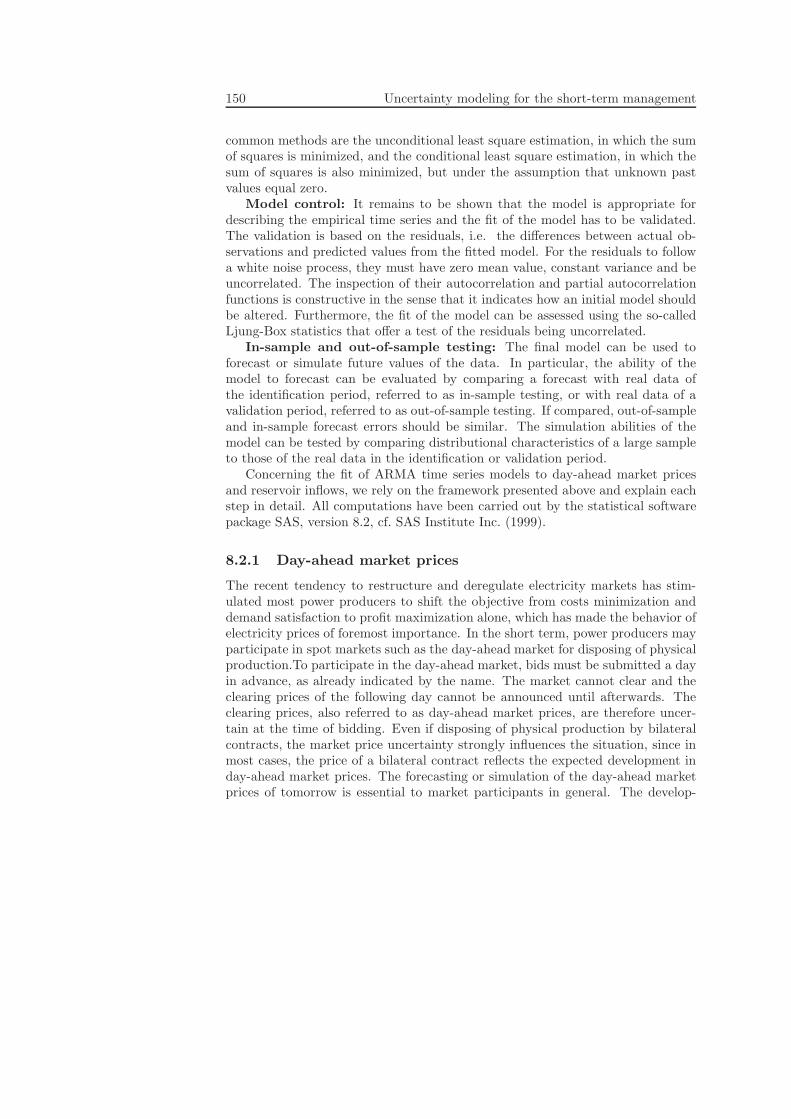
150 Uncertainty modeling for the short-term management
common methods are the unconditional least square estimation, in which the sumof squares is minimized, and the conditional least square estimation, in which thesum of squares is also minimized, but under the assumption that unknown pastvalues equal zero.
Model control: It remains to be shown that the model is appropriate fordescribing the empirical time series and the fit of the model has to be validated.The validation is based on the residuals, i.e. the differences between actual ob-servations and predicted values from the fitted model. For the residuals to followa white noise process, they must have zero mean value, constant variance and beuncorrelated. The inspection of their autocorrelation and partial autocorrelationfunctions is constructive in the sense that it indicates how an initial model shouldbe altered. Furthermore, the fit of the model can be assessed using the so-calledLjung-Box statistics that offer a test of the residuals being uncorrelated.
In-sample and out-of-sample testing: The final model can be used toforecast or simulate future values of the data. In particular, the ability of themodel to forecast can be evaluated by comparing a forecast with real data ofthe identification period, referred to as in-sample testing, or with real data of avalidation period, referred to as out-of-sample testing. If compared, out-of-sampleand in-sample forecast errors should be similar. The simulation abilities of themodel can be tested by comparing distributional characteristics of a large sampleto those of the real data in the identification or validation period.
Concerning the fit of ARMA time series models to day-ahead market pricesand reservoir inflows, we rely on the framework presented above and explain eachstep in detail. All computations have been carried out by the statistical softwarepackage SAS, version 8.2, cf. SAS Institute Inc. (1999).
8.2.1 Day-ahead market prices
The recent tendency to restructure and deregulate electricity markets has stim-ulated most power producers to shift the objective from costs minimization anddemand satisfaction to profit maximization alone, which has made the behavior ofelectricity prices of foremost importance. In the short term, power producers mayparticipate in spot markets such as the day-ahead market for disposing of physicalproduction.To participate in the day-ahead market, bids must be submitted a dayin advance, as already indicated by the name. The market cannot clear and theclearing prices of the following day cannot be announced until afterwards. Theclearing prices, also referred to as day-ahead market prices, are therefore uncer-tain at the time of bidding. Even if disposing of physical production by bilateralcontracts, the market price uncertainty strongly influences the situation, since inmost cases, the price of a bilateral contract reflects the expected development inday-ahead market prices. The forecasting or simulation of the day-ahead marketprices of tomorrow is essential to market participants in general. The develop-

8.2. Univariate ARMA modeling 151
ment of bidding strategies may simply be based on reliable price forecasts andsimulations, or the procedures may be used in combination with other instru-ments. Moreover, for power producers in particular, the prediction of day-aheadmarket prices plays a major role in the short-term planning of the power plant,since physical production is disposed of mostly when prices are profitable.
For applications of the ARMA framework to predict day-ahead electricityprices, we refer to the following contributions within the literature. The authors ofContreras et al. (2003) present SARIMA models for day-ahead electricity prices ofthe Spanish and Californian markets, whereas Nogales et al. (2002) fit transfer andregression models in which electricity load has been included as an explanatoryvariable and Garcia et al. (2005) focus on GARCH models of the same markets.Another application of the GARCH framework is presented by Escribano et al.(2002), who also consider time-dependent jumps in electricity prices and consid-ers the markets of Argentina, Australia, New Zealand, U.S., Spain as well as theNordic market. In a similar spirit, the authors of Haldrup and Nielsen (2004)develop a model from within the class of long memory models. The ARFIMAmodel for the Nordic day-ahead electricity market includes regime switching.
The ARMA time series analysis of day-ahead market prices is performed onobservations from the spot market Elspot at the Nordic power exchange Nord Pool,and more precisely from the so-called price zone NO2, which is the Trondheim areain Norway. The empirical time series contains hourly observations from the year of2004, of which the first 40 weeks are used for model identification and the following10 weeks for model validation.
Model identification: To identify an appropriate model, the first step is todetect seasonalities. As day-ahead market prices are partly driven by electricitydemand which exhibits a daily and a weekly pattern, both daily and weekly peri-odic behavior is to be expected. This is supported by the fact that the day-aheadmarket clears every day of the week except in weekends. The periodicities arevisible from Fig. 8.1a. The class of SARMA models provides a base for identifyinga model.
A non-constant mean indicates non-stationarity of the time series data. Thisis further justified by empirical autocorrelations that decay very slowly to zero.The factors (1 − B), (1 − B24) and (1 − B168) are included in order to stabilizethe mean, (1 − B24) and (1 − B168) to remove seasonality, and the process ofdifferences can then be accepted as being stationary, cf. Fig. 8.1b. Experimentswas made with a logarithmic tranformation to stabilize the variance. However,the best results were obtained without this transformation. The original processcan therefore be described by a SARIMA model.
Inspecting the empirical autocorrelation and partial autocorrelation functions,the order of the process of differences can be determined. The functions are shownin Figs. 8.2. The autocorrelations corresponding to the lags 1, 2, 3, . . . give an in-dication of an ARMA(2, 2) process. The autocorrelations of the lags 24, 48, 72, . . .
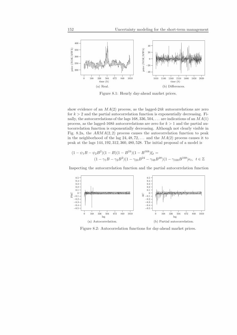
152 Uncertainty modeling for the short-term management
0 168 336 504 672 840 1010
200
250
300
350
400
time (h)
pri
ce(NOK/M
Wh)
(a) Real.
1010 1180 1340 1510 1680 1850 2020
−40
−20
0
20
40
time (h)
pri
ce(NOK/M
Wh)
(b) Differences.
Figure 8.1: Hourly day-ahead market prices.
show evidence of an MA(2) process, as the lagged-24k autocorrelations are zerofor k > 2 and the partial autocorrelation function is exponentially decreasing. Fi-nally, the autocorrelations of the lags 168, 336, 504, . . . are indications of anMA(1)process, as the lagged-168k autocorrelations are zero for k > 1 and the partial au-tocorrelation function is exponentially decreasing. Although not clearly visible inFig. 8.2a, the ARMA(2, 2) process causes the autocorrelation function to peakin the neighborhood of the lag 24, 48, 72, . . . and the MA(2) process causes it topeak at the lags 144, 192, 312, 360, 480, 528. The initial proposal of a model is
(1 − ψ1B − ψ2B2)(1 −B)(1 −B24)(1 −B168)ξt =
(1 − γ1B − γ2B2)(1 − γ24B
24 − γ48B48)(1 − γ168B
168)et, t ∈ Z
Inspecting the autocorrelation function and the partial autocorrelation function
0 168 336 504 672 840 1010
−0.5
−0.4
−0.3
−0.2
−0.10
0.1
0.2
0.3
0.4
0.5
lag
PA
C
(a) Autocorrelation.
0 168 336 504 672 840 1010
−0.5
−0.4
−0.3
−0.2
−0.10
0.1
0.2
0.3
0.4
0.5
lag
AC
(b) Partial autocorrelation.
Figure 8.2: Autocorrelation functions for day-ahead market prices.

8.2. Univariate ARMA modeling 153
of the residuals, the model can be further refined to
(1 − ψ1B − ψ2B2)(1 −B)(1 −B24)(1 −B168)ξt =
(1 − γ1B − γ2B2)(1 − γ23B
23 − γ24B24 − γ25B
25
− γ47B47 − γ48B
48 − γ49B49)(1 − γ168B
168)et, t ∈ Z.
The model is an extension of those of the preceding sections. It is, nevertheless,sufficiently general to include the main characteristics of day-ahead market prices.
Parameter estimation: Parameter estimates are obtained by the use of max-imum likelihood estimation. Estimates based on data of the model identificationperiod can be found in Table 8.1.
Table 8.1: Maximum likelihood estimates for day-ahead market prices
Parameter ψ1 ψ2 γ1 γ2 γ24 γ25
Estimate 0.3120 0.3758 0.3942 0.5382 −0.0826 0.6888Parameter γ26 γ47 γ48 γ49 γ168 σEstimate −0.0748 0.0553 0.1834 0.0388 0.9810 5.0487
Model control: To validate the model, the assumption of a white noise pro-cess on the residuals must be confirmed. A plot of the residuals is given in Fig.8.3a. It should be clear that the mean value can be assumed to be zero and thatthe variance appears to be constant. Furthermore, the autocorrelation and partialautocorrelation functions of the residuals, cf. Figs. 8.3b and 8.3c, are both closeto zero as is the case for a white noise process. The Ljung-Box statistics back upthe fit of the model.
1010 1180 1340 1510 1680 1850 2020
−60
−40
−20
0
20
40
60
time (h)
resi
dual
s
(a) Residuals.
0 168 336 504 672 840 1010
−0.2−0.2
−0.1
0
0.1
0.2
lag
AC
(b) Autocorrelation.
0 168 336 504 672 840 1010
−0.2
−0.1
0
0.1
0.2
lag
PA
C
(c) Partial autocorrelation.
Figure 8.3: Residuals of day-ahead market prices.
Out-of-sample testing: Before using forecasts and simulations as tools forplanning purposes, both procedures are suitable for further validation of the model.Out-of-sample tests are performed and, hence, the model is tested on the data ofthe validation period by forecasting and simulating into this period.

154 Uncertainty modeling for the short-term management
Table 8.2: Weekly forecast errors for day-ahead market prices.
Week 41 42 43 44 45MPE 0.73 −0.34 0.09 −0.11 −0.16MAPE 3.00 1.72 2.51 2.95 2.19MSE 72.32 36.22 58.82 436.67 47.15Week 46 47 48 49 50MPE 0.48 0.25 0.51 −0.52 −0.25MAPE 1.87 1.80 2.08 2.25 2.66MSE 31.81 44.39 37.51 45.88 61.95
Table 8.3: Weekly descriptive statistics for day-ahead market prices.
Week 41 42 43 44 45Sim. Mean value 228.46 245.55 242.18 246.32 239.12
Std. dev. 16.26 13.84 11.87 11.35 11.91Real Mean value 229.68 244.55 240.96 246.57 238.59
Std. dev. 11.46 6.97 4.75 18.67 12.29Week 46 47 48 49 50
Sim. Mean value 227.95 241.05 236.40 226.20 215.93Std. dev. 14.74 13.22 13.87 13.45 14.68
Real Mean value 229.10 241.83 238.95 225.23 215.65Std. dev. 14.67 10.37 11.50 14.49 13.57
The forecast errors of the validation period, i.e. the weeks 41-50 or the hours6721-8400, are reported in Table 8.2. The mean percentual error (MPE), meanabsolute percentual error (MAPE) as well as the mean square error (MSE) aredisplayed on a weekly basis. It should be remarked that the estimation of thevalidation period has been conducted on a 24-hour basis using an adaptive ap-proach, cf. Contreras et al. (2003) and Nogales et al. (2002). The estimation ofthe first 24 hours, i.e. the hours 6721-6744, is based on data of the hours 1-6720.Moving the time window 24 hours, the estimation of the next 24 hours, i.e. thehours 6745-6768, is based on data of the hours 24-6744 etc. The forecast errorsare seen to be rather small and therefore the model is suitable for forecasting.
Descriptive statistics for a simulation of 1000 samples are shown in Table 8.3along with the same information on the real observations of the validation period.Concerning the preservation of the descriptive statistics, the mean value is wellpreserved, whereas the standard deviation is generally over-estimated.
Forecast and simulation: Starting from the end of the validation period,forecasts and simulations can be generated further into the future. As an example

8.2. Univariate ARMA modeling 155
of a short-term use of the procedures, hourly prices are forecasted and simulateda week ahead, i.e. into week 51. A plot of the forecasts and the real observationscan be found in Fig. 8.4a. Moreover, the forecast and its confidence intervals areplotted in Fig. 8.4b. Examples of a few simulated sample paths are displayed inFig. 8.4c.
0 24 48 72 96 120 144 168
160
180
200
220
240
260
time (h)
pri
ce(NOK/M
Wh)
(a) Forecast and real data.
0 24 48 72 96 120 144 168
160
180
200
220
240
260
time (h)
pri
ce(NOK/M
Wh)
(b) Confidence interval ofthe forecast.
0 24 48 72 96 120 144 168
160
180
200
220
240
260
time (h)
pri
ce(NOK/M
Wh)
(c) Simulation.
Figure 8.4: Forecasted and simulated day-ahead market prices.
8.2.2 Reservoir inflows
As water inflows to hydro reservoirs are often highly uncertain, the forecasting orsimulation of future values is crucial in the short-term planning of hydro-powerplants. In the management of reservoirs, the scheduling of water releases dependamong other things on the current reservoir levels. Water releases in turn affectunit commitment and production level decisions, which makes the knowledge offuture reservoir inflows very valuable. Early applications of the ARMA frameworkto forecast and simulate stream-flows can be found in Camacho et al. (1985a),Camacho et al. (1985b), Camacho et al. (1987), Salas et al. (1980) and Salaset al. (1985). Newer applications comprise Kuo and Sun (1996), who establish asection model for ten-days average stream-flows in which each section is a separateARMA model. Concerning more long-term models, Mohan and Vedula (1995) fita SARIMA model for forecasting monthly inflows into a reservoir system, whereasJardim et al. (2001) simulate monthly stream-flows from a periodic ARMA modelto alleviate mid-term planning in a hydro-power plant.
For the ARMA time series analysis of water inflows to reservoirs, the dataconsists of hourly observations from the same hydro-power plant located in thearea of Trondheim in Norway and run by the company TrønderEnergi. The datadates back to 2004, which is again divided into a model identification period of 40weeks and a model validation period of 10 weeks.
Typically, even smaller hydro-power plants consist of more than one reservoir.Therefore, it is highly relevant to consider multiple reservoir inflow series. Inflowsto different reservoirs may stem from the same stream or from different streams.
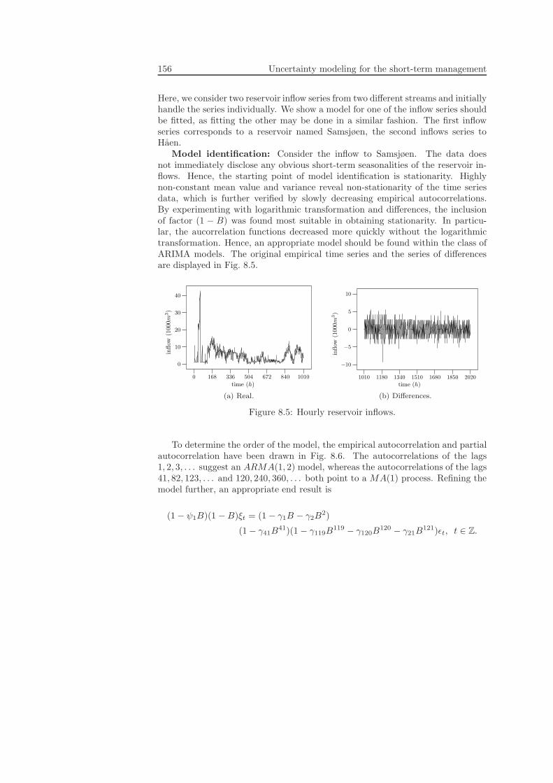
156 Uncertainty modeling for the short-term management
Here, we consider two reservoir inflow series from two different streams and initiallyhandle the series individually. We show a model for one of the inflow series shouldbe fitted, as fitting the other may be done in a similar fashion. The first inflowseries corresponds to a reservoir named Samsjøen, the second inflows series toHaen.
Model identification: Consider the inflow to Samsjøen. The data doesnot immediately disclose any obvious short-term seasonalities of the reservoir in-flows. Hence, the starting point of model identification is stationarity. Highlynon-constant mean value and variance reveal non-stationarity of the time seriesdata, which is further verified by slowly decreasing empirical autocorrelations.By experimenting with logarithmic transformation and differences, the inclusionof factor (1 − B) was found most suitable in obtaining stationarity. In particu-lar, the aucorrelation functions decreased more quickly without the logarithmictransformation. Hence, an appropriate model should be found within the class ofARIMA models. The original empirical time series and the series of differencesare displayed in Fig. 8.5.
0 168 336 504 672 840 1010
0
10
20
30
40
time (h)
inflow
(100
0m
3)
(a) Real.
1010 1180 1340 1510 1680 1850 2020
−10
−5
0
5
10
time (h)
inflow
(100
0m
3)
(b) Differences.
Figure 8.5: Hourly reservoir inflows.
To determine the order of the model, the empirical autocorrelation and partialautocorrelation have been drawn in Fig. 8.6. The autocorrelations of the lags1, 2, 3, . . . suggest an ARMA(1, 2) model, whereas the autocorrelations of the lags41, 82, 123, . . . and 120, 240, 360, . . . both point to a MA(1) process. Refining themodel further, an appropriate end result is
(1 − ψ1B)(1 −B)ξt = (1 − γ1B − γ2B2)
(1 − γ41B41)(1 − γ119B
119 − γ120B120 − γ21B
121)ǫt, t ∈ Z.

8.2. Univariate ARMA modeling 157
0 168 336 504 672 840 1010
−0.5
−0.4
−0.3
−0.2
−0.10
0.1
0.2
0.3
0.4
0.5
lag
AC
(a) Autocorrelation.
0 168 336 504 672 840 1010
−0.5
−0.4
−0.3
−0.2
−0.10
0.1
0.2
0.3
0.4
0.5
lag
PA
C
(b) Partial autocorrelation.
Figure 8.6: Autocorrelation functions for reservoir inflows.
Parameter estimation: Parameter estimates are obtained using maximumlikelihood estimation. Estimates based on data of the model identification periodare found in Table 8.4.
Table 8.4: Maximum likelihood estimates for reservoir inflows.
Parameter ψ1 γ1 γ2 γ41
Estimate 0.9879 1.2698 −0.3095 0.8385Parameter γ119 γ120 γ121 σEstimate 0.1729 −0.1742 −0.0691 3049.4570
Model control: The model is validated by testing the assumption of a whitenoise process on the residuals and is confirmed by the behavior of the autocorre-lation and partial autocorrelation functions as well as by the Ljung-Box statistics,none of which is displayed here.
Out-of-sample testing: Further validation of the model is based on forecastsand simulations. Again, we do out-of-sample testing. Forecast errors are shown inTable 8.5. We find forecasts to be useful for high inflow weeks, i.e. weeks 41 and 45-50. However, for low inflow weeks, i.e. weeks 42-44, the forecasts are rather poor.The descriptive statistics of the simulations, cf. Table 8.6, show that the mean ismore or less preserved, whereas the standard deviation is highly overestimated.
Forecast and simulation: With the validated model at hand, short-termforecasts and simulations of hourly inflows can be made. Plots of the forecast andthe real data as well as the forecast and its corresponding confidence interval aweek ahead are shown in Fig. 8.7a and 8.7b. Examples of a few simulated samplepaths are shown in Fig. 8.7c.
Model identification and parameter estimation: Consider now the inflow

158 Uncertainty modeling for the short-term management
Table 8.5: Weekly forecast errors for reservoir inflows.
Week 41 42 43 44 45MPE −7.74 −52.36 15.88 6.78 9.22MAPE 16.10 116.10 115.78 57.10 15.15MSE 12.78×10⁶ 13.89×10⁶ 12.95×10⁶ 10.73×10⁶ 62.16×10⁶
Week 46 47 48 49 50MPE 1.97 0.31 −5.22 3.32 5.46MAPE 11.76 10.05 11.07 10.55 9.68MSE 46.75×10⁶ 9.73×10⁶ 6.36×10⁶ 7.17×10⁶ 22.97×10⁶
Table 8.6: Weekly descriptive statistics for reservoir inflows
Week 41 42 43 44 45Sim. Mean value 19053.45 9346.40 9077.62 6458.55 50638.26
Std. dev. 10224.38 10116.10 10102.11 10348.29 10348.29Real Mean value 17896.71 6323.36 8995.71 6960.00 44862.86
Std. dev. 4818.84 3597.40 4677.30 3386.63 17653.88Week 46 47 48 49 50
Sim. Mean value 50638.26 24185.43 19574.73 17772.61 38566.49Std. dev. 12882.12 10196.85 10178.67 9570.64 10407.45
Real Mean value 45686.57 24573.21 19284.64 21884.79 40509.64Std. dev. 8933.57 6164.27 6311.45 8864.11 11268.43
0 24 48 72 96 120 144 168
−10
0
10
20
30
40
50
60
70
80
0
20
40
60
80
time (h)
inflow
(100
0m
3)
(a) Forecast and real data.
0 24 48 72 96 120 144 168
−10
0
10
20
30
40
50
60
70
80
time (h)
inflow
(100
0m
3)
(b) Confidence interval ofthe forecast.
0 24 48 72 96 120 144 168
−10
0
10
20
30
40
50
70
80
0
20
40
60
80
time (h)
pri
ce(NOK/M
Wh)
(c) Simulation.
Figure 8.7: Forecasted and simulated reservoir inflows.
to Haen. The model fitted for the corresponding inflow series is
(1 − ψ1B)(1 −B)ξt = (1 − γ1B − γ2B2)(1 − γ41B
41)et, t ∈ Z,
with the parameter estimates of Table 8.7.
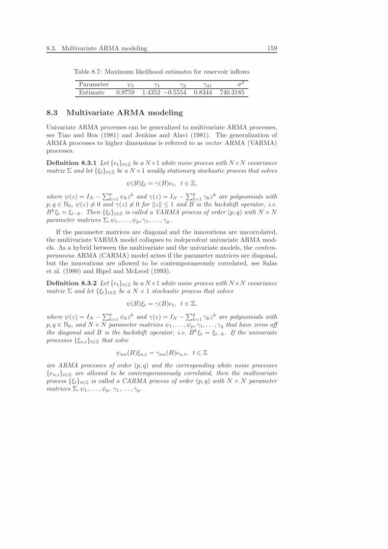
8.3. Multivariate ARMA modeling 159
Table 8.7: Maximum likelihood estimates for reservoir inflows
Parameter ψ1 γ1 γ2 γ41 σ2
Estimate 0.9759 1.4352 −0.5554 0.8344 740.3185
8.3 Multivariate ARMA modeling
Univariate ARMA processes can be generalized to multivariate ARMA processes,see Tiao and Box (1981) and Jenkins and Alavi (1981). The generalization ofARMA processes to higher dimensions is referred to as vector ARMA (VARMA)processes.
Definition 8.3.1 Let ett∈Z be a N×1 white noise process with N×N covariancematrix Σ and let ξtt∈Z be a N×1 weakly stationary stochastic process that solves
ψ(B)ξt = γ(B)et, t ∈ Z,
where ψ(z) = IN −∑p
k=1 ψkzk and γ(z) = IN −
∑qk=1 γkz
k are polynomials withp, q ∈ N0, ψ(z) 6= 0 and γ(z) 6= 0 for ‖z‖ ≤ 1 and B is the backshift operator, i.e.Bkξt = ξt−k. Then ξtt∈Z is called a VARMA process of order (p, q) with N ×Nparameter matrices Σ, ψ1, . . . , ψp, γ1, . . . , γq.
If the parameter matrices are diagonal and the innovations are uncorrolated,the multivariate VARMA model collapses to independent univariate ARMA mod-els. As a hybrid between the multivariate and the univariate models, the contem-poraneous ARMA (CARMA) model arises if the parameter matrices are diagonal,but the innovations are allowed to be contemporaneously correlated, see Salaset al. (1980) and Hipel and McLeod (1993).
Definition 8.3.2 Let ett∈Z be a N×1 white noise process with N×N covariancematrix Σ and let ξtt∈Z be a N × 1 stochastic process that solves
ψ(B)ξt = γ(B)et, t ∈ Z,
where ψ(z) = IN −∑p
k=1 ψkzk and γ(z) = IN −
∑qk=1 γkz
k are polynomials withp, q ∈ N0, and N ×N parameter matrices ψ1, . . . , ψp, γ1, . . . , γq that have zeros offthe diagonal and B is the backshift operator, i.e. Bkξt = ξt−k. If the univariateprocesses ξn,tt∈Z that solve
ψnn(B)ξn,t = γnn(B)en,t, t ∈ Z
are ARMA processes of order (p, q) and the corresponding white noise processesen,tt∈Z are allowed to be contemporaneously correlated, then the multivariateprocess ξtt∈Z is called a CARMA process of order (p, q) with N ×N parametermatrices Σ, ψ1, . . . , ψp, γ1, . . . , γq.
160 Uncertainty modeling for the short-term management
Motivated by the fact that the VARMA model is difficult to estimate, especiallyfor higher order models in which the number of parameters is large, the moresimple CARMA model finds its relevance. The main advantage of the CARMAmodel is its decoupling of the multivariate model into univariate models thatfacilitates the application of specially designed parameter estimation proceduresbased on the univariate estimates. In spite of its simplicity, the CARMA modelincorporates correlation among the univariate models by allowing the innovationsto be instantaneously correlated.
Salas et al. (1980) propose an alternative formulation of the CARMA model asa VARMA model. Let ξtt∈Z be a CARMA process of order (p, q) with parametermatrices Σ, ψ1, . . . , ψp, γ1, . . . , γq and an upper triangular matrix C that satisfiesCCT = Σ. Let ǫtt∈Z be a N × 1 white noise process with covariance matrix IN .Then ξtt∈Z is a N × 1 weakly stationary stochastic process that solves
ψ(B)ξt = γ(B)Cǫt, t ∈ Z.
Hence, ξtt∈Z is a VARMA process of order (p, q) with parameter matricesIN , ψ1, . . . , ψp, γ1C, . . . , γqC.
Multivariate ARMA time series modeling includes the same general steps asfor univariate models, which is model identification, parameter estimation, modelcontrol and validation as well as forecasting and simulation.
Model identification: To fix the structure of a multivariate model, the de-pendencies between the univariate series must be identified. Whether the seriesexhibit contemporaneous, unidirectional, bidirectional relationships, mixtures ofthese or no dependencies at all, dependencies are disclosed by the cross-correlationsof the series. For contemporaneous models, the cross-correlations are zero exceptat lag zero, for unidirectional relationships, the cross-correlations are zero at neg-ative lags but significant at the remaining ones, whereas for bidirectional relation-ships the cross-correlations are significant at all lags. When the structure of themodel has been fixed, the order can be determined. For contemporaneous ARMAmodels, univariate procedures can be used. For vector ARMA models in general,the cross-correlation matrices and the partial correlation matrices complement theautocorrelation and partial autocorrelation functions in the order determination.
Parameter estimation and model control: Parameter estimation, modelcontrol, forecasting and simulation in the multivariate case is an extension that inthe univariate case.
8.3.1 Simultaneity of prices and inflows
If hourly day-ahead market prices and reservoir inflows are considered simultane-ously, the time series is multidimensional. We illustrate the fitting of a multivariatemodel with the day-ahead market price series and the two reservoir inflow seriesof the preceding sections.

8.3. Multivariate ARMA modeling 161
Examples from the literature on VARMA modeling in stream-flows includeCamacho et al. (1985a) and Salas et al. (1980) and on CARMA modeling especiallyCamacho et al. (1985b) and Salas et al. (1985).
Model identification: The VARMA model could be adopted to fit the mul-tivariate model. The three-dimensional VARMA model, however, simplifies asday-ahead market prices and reservoir inflows may be assumed uncorrelated inthe short term. This is supported by the plot of day-ahead market prices versusreservoir inflows in Fig. 8.8a. It should be clearer from Figs. 8.8b and 8.8c, whichdisplay cross-correlations between the residuals of prices and inflows from one ofthe streams. Corresponding cross-correlations between the residuals of prices andinflows from the other stream are similar. The figures reveal uncorrelated residu-als. Consequently, day-ahead market prices and reservoir inflows can be handledseparately. For the day-ahead market prices, we refer to the preceding sections.
0 168 336 504 672 840 1010
200
250
300
350
400
0 168 336 504 672 840 1010
0
10
20
30
40
time (h)
inflow
(100
0m
3)
pri
ce(NOK/M
Wh)
(a) Prices and inflows.
0 24 48
−0.06
−0.04
0.02
0
0.02
0.04
0.06
−0.06
−0.04
−0.02
0
0.02
0.04
0.06
lag
(b) Serial cross correlation.
0 24 48
−0.06
−0.04
0.02
0
0.02
0.04
0.06
−0.06
−0.04
−0.02
0
0.02
0.04
0.06
lag
(c) Serial cross correlation.
Figure 8.8: Correlation between day-ahead market price and reservoir inflowseries.
We proceed with the reservoir inflows. Inflow series from different streamsare correlated and cannot be treated separately. The correlation between thetwo inflow series should be visible from Fig. 8.9a. Therefore, the simultaneousmodeling of multiple inflow series, in principle, relies upon the VARMA model.Nevertheless, unidirectional dependencies often occur in the case of connectedstreams, whereas, if the streams are not connected, contemporaneous dependenciesmay apply. Within reasonable limits, the cross-correlations between the residualsof the two inflow series depicted in Figs. 8.9b and 8.9c support the use of a CARMAmodel.
Parameter estimation: We use the univariate estimates, although a multi-variate estimation procedure, applying only to CARMA models, may reduce thevariance of the estimates. Some parameter estimates were given in Tables 8.4 and8.7. Moreover, Table 8.8 shows the maximum likelihood estimates for the covari-ance matrix of the innovations Σ and the corresponding upper triangular matrixC.
Model control: The univariate models have been validated in the precedingsections.

162 Uncertainty modeling for the short-term management
0 168 336 504 672 840 1010
0
10
20
30
40
time (h)
inflow
(100
0m
3)
(a) Inflows.
0 24 48
−0.06
−0.04
0.02
0
0.02
0.04
0.06
−0.06
−0.04
−0.02
0
0.02
0.04
0.06
lag
(b) Serial cross correlation.
0 24 48
−0.06
−0.04
0.02
0
0.02
0.04
0.06
−0.06
−0.04
−0.02
0
0.02
0.04
0.06
lag
(c) Serial cross correlation.
Figure 8.9: Correlation between reservoir inflows series.
Table 8.8: Maximum likelihood estimates for reservoir inflow.
Parameter Σ11 Σ12 Σ21 Σ22
Estimate 9270446 104030 104030 547131Parameter C11 C12 C21 C22
Estimate 3044.74 0.00 34.17 738.89
Forecast and simulation: Forecasts and simulations can be based on thealternative formulation of the multivariate model. The forecasts are shown in Fig.8.10 and the simulations in Fig. 8.11. The correlation between the two univariateinflow series should be visible from both the forecasts and the simulations.
0 24 48 72 96 120 144 168
−15
0
15
30
45
60
time (h)
inflow
(100
0m
3)
(a) Upper reservoir.
0 24 48 72 96 120 144 168
0
5
10
15
20
25
time (h)
inflow
(100
0m
3)
(b) Lower reservoir.
Figure 8.10: Forecasted and real reservoir inflows.
8.4 Conclusions
The results of the previous sections illustrate the ability of ARMA time seriesmodels to forecast and simulate hourly day-ahead electricity prices and reservoir

8.4. Conclusions 163
0 24 48 72 96 120 144 168
−15
0
15
30
45
60
time (h)
inflow
(100
0m
3)
(a) Upper reservoir.
0 24 48 72 96 120 144 168
0
5
10
15
20
25
time (h)
inflow
(100
0m
3)
(b) Lower reservoir.
Figure 8.11: Simulated reservoir inflows.
inflows. As already indicated, forecasts and simulations are suitable as input foroptimization problems such as deterministic and stochastic planning problems thatfuture values of data as input.
An example of using simulated day-ahead electricity prices in a stochasticplanning problem is found in Chapter 4. The problem consists in day-aheadbidding of a hydro-power plant under price uncertainty and simulated hourly day-ahead market prices serve as scenarios in a corresponding stochastic program. Ina similar fashion, Chapter 5 uses simulated hourly day-ahead market prices andreservoir inflows as scenarios in a stochastic program that determines the spatialdistribution of water among reservoirs of a hydro-power plant.
In practice, power producers rely upon so-called fundamental models that in-volve detailed physical relationships. Although the forecast performance may ingeneral be superior to time series models, the fundamental models are not capableof simulating and the time series models still have their relevance.
The literature has previously reported on the success of forecasting or simu-lating hourly day-ahead market prices by ARMA models and the current resultsshow the same potential. However, ARMA models have been used mostly to de-scribe monthly and annual stream-flows, whereas the use of ARMA models toforecast or simulate hourly stream-flows has occurred only rarely in the literature.By a direct application of the ARMA framwork it may not be possible to captureintermittency and the current results show a moderate performance with respectto the hourly stream-flows.
Although the ability to forecast or simulate day-ahead market prices and reser-voir inflows can be improved, we consider ARMA time series models sufficient forillustrating the usefulness of stochastic programming, as in Chapters 4 and 5.

164 Uncertainty modeling for the short-term management
8.4.1 Further improvement
To improve the time series models for reservoir inflows, we suggest to combine along-term model, that is able to capture memory, persistence and periodicity prop-erties, with a short-term model suitable for describing intermittency. A possibleoutline is the following.
Since the ARMA framework has been successfully applied for modeling morelong-term stream-flows, performance may improve with a time resolution of a dayor a week. This point of view is supported by the ability of the ARMA processesto model the general trend in the data, as seen in Figs. 8.7a and 8.10. The idea istherefore to describe the aggregated daily or weekly inflows by means of ARMAprocesses in the same way as the hourly inflows were described. With a daily timeresolution, the “long-term” model is based on the means
ξ⌈t/24⌉, t ∈ Z
and similarly for a weekly time resolution.The daily or weekly data then has to be disaggregated into hourly data. Several
disaggregation techniques can be found in the literature. Still, many techniquesare not suitable for hourly disaggregation due to the intermittency of stream-flows,whereas others are unable to preserve the time series properties at the disaggre-gated level. However, the availability of both “long-term” (daily or weekly) andshort-term (hourly) data gives rise to models of different time resolutions, andthe aggregation-disaggregation reduces to a matter of combining the models. Thelong-term and the short-term models can be combined by considering
ζt = ξt/ξ⌈t/24⌉ or ζt = ξt − ξ⌈t/24⌉, t ∈ Z
in the short-term model, cf. Eichhorn et al. (2005) and Growe-Kuska et al. (2001).The short-term model allows for a partitioning of the data set into smaller sets.
Stream-flows can be categorized according to the seasons or according to dry orwet periods of time. The categories may be determined by clustering methods,each cluster being used to construct a standard profile or a stochastic submodelbased for instance on regression on time.
The time series models for day-ahead market prices may likewise be improvedby combining a long-term model with a short-term model. Fig. 8.4a indicates thatthe ARMA processes are able to model the development in prices except for thegeneral trend in the data. It may be therefore be relevant to establish a morelong-term model based on weekly or daily means and a short-term model in whichprices are partitioned into smaller sets. Prices may contain the categories spring,summer, fall and winter and for each of them workday, Saturday and Sunday.
.

Bibliography
Ahmed, S. (2004). Mean-risk objectives in stochastic programming. .http://hera.rz.hu-berlin.de/speps/contents04.html.
Andersen, A. H. and P. Blæsild (2003a). Time Series Analysis, Volume 1. Arhus,Denmark: University of Aarhus.
Andersen, A. H. and P. Blæsild (2003b). Time Series Analysis, Volume 2. Arhus,Denmark: University of Aarhus.
Anderson, E. J. and A. B. Philpott (2002). Optimal offer construction in electricitymarkets. Mathematics of Operations Research 27 (1), 82–100.
Archibald, T. W., C. S. Buchanan, K. I. M. McKinnon, and L. C. Thomas (1996).Nested Benders decomposition and dynamic programming for reservoir opti-mization. Journal of the Operations Research Society 50, 468–479.
Archibald, T. W., C. S. Buchanan, L. C. Thomas, and K. I. M. McKinnon(2001). Controlling multi-reservoir systems. European Journal of OperationalResearch 129, 619–626.
Benders, J. F. (1962). Partitioning procedures for solving mixed-variables pro-gramming problems. Numerische Mathematik 4, 238–252.
Berge, C. (1963). Topological spaces. Edinburgh: Oliver & Boyd.
Bienstock, D. and J. F. Shapiro (1988). Optimizing resource acquisition decisionsby stochastic programming. Management Science 34 (2), 215–229.
Billingsley, P. (1968). Convergence of Probability Measures. New York: Wiley.
Birge, J. R. (1985). Decomposition and partitioning methods for multistagestochastic linear programs. Operations Research 33 (5), 989–1007.
Birge, J. R., M. A. H. Dempster, H. I. Gassmann, E. A. Gunn, A. J. King, andS. W. Wallace (1987). A standard input format for multiperiod stochastic linearprograms. COAL Newsletter 17, 1–19.
165
166 Bibliography
Birge, J. R. and F. Louveaux (1997). Introduction to Stochastic Programming.New York: Springer.
Birge, J. R. and F. V. Louveaux (1988). A multicut algorithm for two-stagestochastic linear programs. European Journal of Operational Research 34, 384–392.
Birge, J. R., S. Takriti, and E. Long (1994). Intelligent unified control of unit com-mitment and generation allocation. Technical report, Department of Industrialand Operations Engineering, The University of Michigan.
Box, G. E. P. and G. M. Jenkins (1976). Time Series Analysis: Forecasting andControl. San Fransisco: Holden Day.
Bunn, D. W. and S. N. Paschentis (1986). Development of a stochastic modelfor the economic dispatch of electric power. European Journal of OperationalResearch 27, 179–191.
Camacho, F., A. I. McLeod, and K. W. Hipel (1985a). Contemporaneous autore-gressive - moving average (CARMA) modeling in hydrology. Water ResourcesBulletin 21 (4), 709–720.
Camacho, F., A. I. McLeod, and K. W. Hipel (1985b). Developments in multivari-ate arma modeling in hydrology. In International Symposium on MultivariateAnalysis of Hydrologic Process, Fort Collins, Colorado.
Camacho, F., A. I. McLeod, and K. W. Hipel (1987). Multivariate contemporane-ous arma model with hydrological applications. Hydrology and Hydraulics 1 (2),141–154.
Carøe, C. C. and R. Schultz (1998). A two-stage stochastic program forunit commitment under uncertainty in a hydro-thermal power system. cite-seer.ist.psu.edu/caroe98twostage.html.
Carøe, C. C. and R. Schultz (1999). Dual decomposition in stochastic integerprogramming. Operations Research Letters 24, 37–45.
Carøe, C. C. and J. Tind (1998). L-shaped decomposition of two-stage stochasticprograms with integer recourse. Mathematical Programming Series A 83 (3),451–464.
Carpentier, P., G. Cohen, J. C. Culioli, and A. Renaud (1996). Stochastic opti-mization of unit commitment: A new decomposition framework. IEEE Trans-actions on Power Systems 11 (2), 1067–1073.

Bibliography 167
Contreras, J., R. Espinola, and F. J. Nogales (2003). Arima models to predictnext-day electricity prices. IEEE Transactions on Power Systems 18 (3), 1014–1020.
Cplex Optimization Inc. (2006). ILOG CPLEX 10.0 User’s Manual.
Dantzig, G. B. and P. Wolfe (1960). Decomposition principles for linear programs.Operations Research 8 (1), 101–111.
Danzig, G. B. (1955). Linear programming under uncertainty. Management Sci-ence 1 (3/4), 197–206.
Dempster, M. A. H. (2004). Sequential importance sampling algorithms for dy-namic stochastic programming. Zap. Nauchn. Sem. S.-Peterburg. Otdel. Mat.Inst. Steklov. (POMI) 312, 94–129, 312–313.
Dempster, M. A. H. and R. T. Thompson (1999). EVPI-based importance sam-pling solution procedures for multistage stochastic linear programmes on parallelMIMD architectures. Annals of Operations Research 90, 161–184.
Dentcheva, D. and W. Romisch (1998). Optimal power generation under uncer-tainty via stochastic programming. In Stochastic Programming Methods andTechnical Applications, Volume 458 of Lecture Notes in Economics and Mathe-matical Systems, pp. 22–56. Springer-Verlag.
Dentcheva, D. and W. Romisch (2004). Duality gaps in nonconvex stochasticoptimization. Mathematical Programming 101, 25–53.
Donchev, A. L. (1986). On the regularity of the kuhn-tucker curve. SIAM Journalof Control and Optimization 24, 169–176.
Dupacova, J., G. Consigli, and S. W. Wallace (2000). Scenarios for multistagestochastic programs. Annals of Operations Research 100 (1-4), 25–53.
Dupacova, J., N. Growe-Kuska, and W. Romisch (2003). Scenario reduction instochastic programming: An approach using probability metrics. MathematicalProgramming Series A 95, 493–511.
Eichhorn, A. and W. Romisch (2005). Polyhedral risk measures in stochasticprogramming. SIAM Journal of Optimization 16 (1), 69–95.
Eichhorn, A., W. Romisch, and I. Wegner (2005). Mean-risk optimization ofelectricity portfolios using polyhedral risk measures. In PowerTech ConferenceProceedings, St. Petersburg. IEEE.

168 Bibliography
Ermoliev, Y. M. and A. A. Gaivoronski (1992). Stochastic quasigradient methodsfor optimization of discrete event systems. Annals of Operations Research 39 (1),1–39.
Escribano, A., J. I. Pena, and P. Villaplana (2002). Modeling electricity prices:International evidence. Economics Ser. 80, Working Papers, Universidad CarlosIII, Departamento de Economıa.
Fahd, G. N. and G. B. Sheble (1994). Unit commitment literature synopsis. IEEETransactions on Power Systems 9 (1), 128–135.
Feltenmark, S., K. C. Kiwiel, and P.-O. Lindberg (1997). Solving unit commitmentproblems in power production planning. In Operations Research Proceedings (U.Zimmermann ed.)., pp. 236–241. Berlin: Springer-Verlag.
Fleten, S.-E. and T. K. Kristoffersen (2006). Short-term hydropower productionplanning by stochastic programming. In press, Computers and Operations Re-search.
Fleten, S.-E. and T. K. Kristoffersen (2007). Stochastic programming for optimiz-ing bidding strategies of a Nordic hydropower producer. European Journal ofOperational Research 181, 916–928.
Fleten, S.-E. and E. Pettersen (2005). Constructing bidding curves for a price-taking retailer in the Norwegian electricity market. IEEE Transactions on PowerSystems 20 (2), 701–708.
Fleten, S.-E., S. W. Wallace, and W. T. Ziemba (2002). Hedging electricity port-folios via stochastic programming. In C. Greengard and A. Ruszczynski (Eds.),Decision Making Under Uncertainty: Energy and Power, Volume 128 of IMAVolumes on Mathematics and Its Applications, pp. 71–93. New York: Springer-Verlag.
Fosso, O. B., A. Gjelsvik, A. Haugstad, B. Mo, and I. Wagensteen (1999). Gener-ation scheduling in a deregulated system. The Norwegian case. IEEE Transac-tions on Power Systems 14 (1), 75–81.
GAMS Software GmbH (2002). GAMS/SCENRED Dokumentation.
Garcia, R. C., J. Contreras, M. van Akkeren, and J. B. C. Garcia (2005). A garchforecasting model to predict day-ahead electricity prices. IEEE Transactions onPower Systems 20 (2), 867–874.
Garcıa-Gonzalez, J., E. Parrilla, and A. Mateo (2006). Risk-averse profit-basedoptimal scheduling of a hydro-chain in the day-ahead electricity market. Inpress, European Journal of Operational Research.

Bibliography 169
Gassmann, H. I. and E. Schweitzer (2001). A comprehensive input format forstochastic linear programs. Annals of Operations Research 104, 89–125.
Gollmer, R., A. Moller, M. P. Nowak, W. Romisch, and R. Schultz (1999). Primaland dual methods for unit commitment in a hydro-thermal power system. InProceedings of the 13th Power Systems Computation Conference, Trondheim,pp. 724–730.
Gollmer, R., M. P. Nowak, W. Romisch, and R. Schultz (2000). Unit commitmentin power generation - a basic model and some extensions. Annals of OperationsResearch 96 (1-4), 167–189.
Gorenstin, B. G. and N. M. Campodonico (1993). Power system expansion plan-ning under uncertainty. IEEE Transactions on Power Systems 8 (1), 129–155.
Growe, N., W. Romisch, and R. Schultz (1995). A simple recourse model for powerdispatch under uncertain demand. Annals of Operations Research 59, 135–164.
Growe-Kuska, N., H. Heitsch, and W. Romisch (2003). Scenario reduction andscenario tree construction for power management problems. In PowerTech Con-ference Proceedings, Volume 3, Bologna, pp. 7–14. IEEE.
Growe-Kuska, N., K. C. Kiwiel, M. P. Nowak, W. Romisch, and I. Wegner (2002).Power management in a hydro-thermal system under uncertainty by Lagrangianrelaxation. In A. R. C. Greengard (Ed.), Decision Making under Uncertainty:Energy and Power, Volume 128 of IMA Volumes in Mathematics and its Appli-cations, pp. 39–70. New York: Springer-Verlag.
Growe-Kuska, N., M. P. Nowak, and I. Wegner (2001). Modeling of uncertainty forthe real-time management of power systems. In M. Grotschel, S. Krumke, andJ. Rambau (Eds.), Online Optimization of Large-Scale Systems, pp. 621–645.Berlin: Springer.
Growe-Kuska, N., W. Romisch, and M. P. Nowak (2000). Power managementunder uncertainty by Lagrangian relaxation. In Proceedings of the 6th Inter-national Conference Probabilistic Methods Applied to Power Systems PMAPS2000, Volume 2, INESC Porto.
Haldrup, N. and M. O. Nielsen (2004). A regime switching long memory modelfor electricity prices. In press, Journal of Econometrics.
Hansen, P. and B. Jaumard (1997). Cluster analysis and mathematical program-ming. Mathematical Programming 79 (1-3), 191–215.

170 Bibliography
Heitsch, H. and W. Romisch (2006a). A note on scenario reduction for two-stagestochastic programs. Preprint 335, DFG Research Center Matheon ”Mathemat-ics for key technologies”, Humboldt University Berlin.
Heitsch, H. and W. Romisch (2006b). Scenario tree modelling for multistagestochastic programs. http://edoc.hu-berlin.de/docviews/abstract.php?
lang=ger&id=27364.
Heitsch, H., W. Romisch, and C. Strugarek (2005). Stability of multistage stochas-tic programs. Preprint 255, DFG Research Center MATHEON ”Mathematicsfor key technologies”, Humboldt University Berlin.
Higle, J. L., W. W. Lowe, and R. Odio (1994). Conditional stochastic decom-position: An algorithmic interface for optimization and simulation. OperationsResearch 42 (2), 311–322.
Higle, J. L. and S. Sen (1991). Stochastic decomposition: An algorithm for two-state linear programs with recourse. Mathematics of Operations Research 16 (3),650–669.
Hipel, K. W. and A. McLeod (1993). Time-series Modelling of Water Resourcesand Environmental Systems. Elsevier.
Hobbs, B. F. (1995). Optimization methods for electric utility resource planning.European Journal of Operational Research 83, 1–20.
Høyland, K., M. Kaut, and S. W. Wallace (2003). A heuristic for moment-matching scenario generation. Computational Optimization and Applica-tions 24 (2-3), 169–185. Stochastic programming.
Høyland, K. and S. W. Wallace (2001). Generating scenario trees for multistagedecision problems. Management Science 47 (2), 295–307.
Hreinsson, E. B. (1988). Optimal short term operation of a purely hydroelectricsystem. IEEE Transactions on Power Systems 3 (3), 1072–1077.
ILOG Inc. (2003). OPL Studio 3.7 User’s Manual.
Infanger, G. (1994). Planning under uncertainty. Solving large scale stochasticlinear programs, Volume 108. Andover, Hempshire: The Scientific Press.
Infanger, G. (2005). Monte Carlo (importance) sampling within a benders de-composition algorithm for stochastic linear programs. Annals of OperationsResearch 39 (1), 69–95.
Bibliography 171
Jacobs, J., G. Freeman, J. Grygier, D. Morton, G. Schultz, K. Staschus, andJ. Stedinger (1995). SOCRATES: A system for scheduling hydroelectric gener-ation under uncertainty. Annals of Operations Research 59, 99–133. Models forplanning under uncertainty.
Jardim, D. L. D. D., M. E. P. Maceira, and D. M. Falcao (2001). Stochasticstreamflow model for hydroelectric systems using clustering techniques. In IEEEPorto Power Tech, Porto, Portugal.
Jenkins, G. M. and A. S. Alavi (1981). Some aspects of modeling and forecastingmultivariate time series. Journal of Time series Analysis 2, 1–47.
Kall, P. (1976). Stochastic Linear Programming. Berlin: Springer.
Kall, P. (1987). On approximations and stability in stochastic programming.In J. Guddat, T. H. Jongen, B. Kummer, and F. Nozicka (Eds.), ParametricOptimization and Related Topics, pp. 387–407. Berlin: Akademie-Verlag.
Kall, P. and S. W. Wallace (1994). Stochastic Programming. Chichester: Wiley.
Kaut, M. and S. W. Wallace (2003). Evaluation of scenario-generation methodsfor stochastic programming. In press, Pacific Journal of Optimization.
Kristoffersen, T. K. (2005). Deviation measures in linear two-stage stochasticprogramming. Mathematical Methods of Operations Research 62 (2), 255–274.
Kristoffersen, T. K. (2007). The development in stochastic programming modelsfor power production and trading. Working paper.
Kristoffersen, T. K. and C. Schaumburg-Muller (2007). Power reserve managementby two-stage stochastic programming. Submitted.
Kuo, J.-T. and Y.-H. Sun (1996). An ARMA-type section model for averageten-day streamflow synthesis. Water Resources Management 10, 333–354.
Laporte, G. and F. V. Louveaux (1993). The integer L-shaped method for stochas-tic integer programs with complete recourse. Operations Research Letters 13,133—142.
Løkketangen, A. and D. L. Woodruff (1996). Progressive hedging and tabu searchapplied to mixed integer (0,1) multistage stochastic programming. Journal ofHeuristics 2, 111–128.
Louveaux, F. V. and R. Schultz (2003). Stochastic integer programming. Hand-books in OR & MS 10, 213–266.

172 Bibliography
Markert, A. and R. Schultz (2005). Deviation measures in stochastic integer pro-gramming. Operations Research Letters 33, 441–449.
Mohan, S. and S. Vedula (1995). Multiplicative seasonal arima model for longtermforecasting of inflows. Water Reources Management 9, 115–126.
Morton, D. P. (1996). An enhanced decomposition algorithm for multistagestochastic hydroelectric scheduling. Annals of Operations Research 64, 211–235.
Muckstadt, J. A. and S. A. Koenig (1977). An application of Lagrangian relaxationto scheduling in power generation systems. Operations Research 25 (3), 387–403.
Mulvey, J. M. and A. Ruszczynski (1995). A new scenario decomposition methodfor large-scale stochastic optimization. Operations Research 43 (3), 477–490.
Neame, P. J., A. B. Philpott, and G. Pritchard (2003). Offer stack optimizationin electricity pool markets. Operations Research 51 (3), 397–408.
Nogales, F. J., J. Contreras, and A. J. Conjeno (2002). Forecasting next-day elec-tricity prices by time series models. IEEE Transactions on power systems 17 (2),342–348.
Norkin, V. I., Y. M. Ermoliev, and A. Ruszczynski (1998). On optimal allocationof indivisibles under uncertainty. Operations Research 46, 381–395.
Norkin, V. I., G. C. Pflug, and A. Ruszczynski (1998). A branch and boundmethod for stochastic global optimization. Mathematical Programming SeriesA 83 (3), 425–450.
Nowak, M. P., R. Nurnberg, W. Romisch, R. Schultz, and M. Westphalen (2000).Stochastic programming for power production and trading under uncertainty.Submitted.
Nowak, M. P. and W. Romisch (2000). Stochastic Lagrangian relaxation appliedto power scheduling in a hydro-thermal system under uncertainty. Annals ofOperations Research 100 (1-4), 251–272.
Nowak, M. P., R. Schultz, and M. Westphalen (2005). A stochastic integer pro-gramming model for incorporating day-ahead trading of electricity into hydro-thermal unit commitment. Optimization and Engineering 6, 163–176.
Ogryczak, W. and A. Ruszczynski (1999). From stochastic dominance to mean-risk models: Semideviations as risk measures. European Journal of OperationalResearch 116, 33–50.
Bibliography 173
Ogryczak, W. and A. Ruszczynski (2001). On consistency of stochastic dominanceand mean-semideviation models. Mathematical Programming 89, 217–232.
Pennanen, T. (2005). Epi-convergent discretizations of multistage stochastic pro-grams. Mathematics of Operations Research 30 (1), 245–256.
Pennanen, T. and M. Koivu (2005). Epi-convergent discretizations of stochasticprograms via integration quadratures. Numerical Mathematics 100 (1), 141–163.
Pereira, M. V. F. and L. M. V. G. Pinto (1991). Multi-stage stochastic optimizationapplied to energy planning. Mathematical Programming 52, 359–375.
Pflug, G. C. (2004). Optimal tree generation for multiperiod financial optimizationby optimal discretization. Mathematical Programming 89 (2), 251–271.
Philpott, A. and R. Schultz (2006). Unit commitment in electricity pool markets.Mathematical Programming Series B(108), 313–337.
Philpott, A. B., M. Craddock, and H. Waterer (2000). Hydro-electric unit com-mitment subject to uncertain demand. European Journal of Operational Re-search 125, 410–424.
Prekopa, A. (1995). Stochastic Programming. Dordrecht: Kluwer.
Prichard, G. and G. Zakeri (2003). Market offering strategies for hydroelectricgenerators. Operations Research 51 (3), 602–612.
Reznicek, K. and T. C. E. Cheng (1991). Stochastic modeling in reservoir opera-tions. European journal of Operational Research 50, 235–248.
Robinson, S. M. and R. J.-B. Wets (1987). Stability in two-stage stochastic pro-gramming. SIAM Journal of Control and Optimization 26 (6), 1409–1416.
Rockafellar, R. T. (1997). Convex Analysis. Princeton.
Rockafellar, R. T. and R. J.-B. Wets (1991). Scenarios and policy aggregationunder uncertainty. Mathematics of Operations Research 16 (1), 119–147.
Romisch, W. (2003). Stability of stochastic programming problems. .In A. Ruszczynsky and A. Shapiro (Eds.), Handbooks in Operations Researchand Management Science, Volume 10 of Stochastic Programming, pp. 483–554.Amsterdam: Elsevier.
Romisch, W. and R. Schultz (2001). Multi-stage stochastic integer programs -an introduction. http://edoc.hu-berlin.de/docviews/abstract.php?id=
26658.

174 Bibliography
Ruszczynsky, A. (1986). A regularized decomposition method for minimizing asum of polyhedral functions. Mathematical Programming 35, 309–333.
Salas, J. D., J. W. Delleur, V. Yevjevich, and W. L. Lane (1980). Applied modelingof hydrologic time series. Littleton, Colorado: Water Resources Publications.
Salas, J. D., G. D. Tabois, and P. Bartolini (1985). Approaches to multivariatemodeling of water resources time series. Water Resources Bulletin 21, 683–708.
SAS Institute Inc. (1999). SAS Onliedoc.
Schultz, R. (1994). Strong convexity in stochastic programs with complete re-course. Journal of Computational and Applied Mathematics 56, 3–22.
Schultz, R. (2000). Some aspects of stability in stochastic programming. Annalsof Operations Research 100, 55–84.
Schultz, R. (2003). Stochastic programming with integer variables. MathematicalProgramming 97 (1–2), 285–310.
Shapiro, A. (2003). Statistical inference of multistage stochastic programmingproblems. Mathematical Methods of Operations Research 58 (1), 57–68.
Shapiro, A. (2006). On complexity of multistage stochastic programs. OperationsResearch Letters 34 (1), 1–8.
Sherkat, V. R., R. Campo, K. Moslehi, and E. O. Lo (1985). Stochastic long-termhydrothermal optimization for a multireservoir system. IEEE Transactions onPower Apparatus and Systems 104 (8), 2040–2049.
Slyke, R. M. V. and R. Wets (1969). L-shaped linear programs with applica-tions to optimal control and stochastic programming. SIAM Journal of AppliedMathematics 17 (4), 638–663.
Takriti, S., J. R. Birge, and E. Long (1996). A stochastic model for the unitcommitment problem. IEEE Transactions on Power Systems 11 (3), 1497–1508.
Takriti, S., B. Krasenbrink, and L. S.-Y. Wu (2000). Incorporating fuel constraintsand electricity spot prices into the stochastic unit commitment problem. Oper-ations Research 48 (2), 268–280.
Terry, L. A., M. V. F. Pereira, T. A. A. Neto, L. E. C. A. Pinto, and P. R. H.Sales (1986). Coordinating the energy generation of the Brazilian national hy-drothermal electrical generating system. INTERFACES 16 (1), 16–38.
Tiao, G. C. and G. E. P. Box (1981). Modeling multiple time series with applica-tions. Journal of American Statistical Association 75, 802–816.
Bibliography 175
Triki, C., P. Beraldi, and G. Gross (2005). Optimal capacity allocation in multi-auction electricity markets under uncertainty. Computers and Operations Re-search 32, 201–217.
Tufegdzic, N., R. J. Frowd, and W. O. Stadlin (1996). A coordinated approachfor real-time short term hydro scheduling. IEEE Transactions on Power Sys-tems 11 (4), 1698–1272.
Walkup, D. W. (1969). Stochastic programs with fixed recourse: The equivalentdeterministic program. SIAM review 16 (3), 309–338.
Wallace, S. W. and S.-E. Fleten (2003). Stochastic programming models in energy.In A. Ruszczynski and A. Shapiro (Eds.), Stochastic programming, Volume 10of Handbooks in OR & MS, pp. 637–677. North-Holland: Elsevier.
Wen, F. and A. K. David (2002). Coordination of bidding strategies in day-aheadenergy and spinning reserve markets. Electrical Power and Energy Systems 24,251–161.
Wen, F. S. and A. K. David (2001a). Optimal bidding strategies for competitivegenerators and large consumers. Electrical Power and Energy Systems 23, 37–43.
Wen, F. S. and A. K. David (2001b). Strategic bidding for electricity supply in aday-ahead energy market. Electric Power Systems Research 59, 197–206.
Wets, R. J.-B. (1974). Stochastic programs with fixed recourse: The equivalentdeterministic program. SIAM review 16, 309–338.
Wets, R. J.-B. (1983). Stochastic programming: Solution techniques and approx-imation schemes. In A. Bachem, M. Groetschel, and B. Korte (Eds.), Mathe-matical Programming, Volume 1982 of State-of-the-Art, pp. 506–603. Springer.
Yu, C. W., X. S. Zhao, F. S. Wen, C. Y. Chung, T. S. Chung, and M. X. Huang(2005). Pricing and procurement of operating reserves in competitive pool-basedelectricity markets. Electric Power Systems Research 73, 37–43.


Subject index
A
Ancillary services, 70, 114ARIMA processes, 147
ARMA processes, 86, 122, 133, 147
Augmented Lagrangian decomposi-tion, 20
B
Benders’ decomposition, 12
Bidding, 66, 67–70, 74, 76, 77, 79,89, 90
Branch and bound, 15, 61, 89, 107
C
CARMA processes, 104, 105, 159
Central deviation, 25
Cluster analysis, 135
Conditional Monte Carlo sampling,134, 143
Conditional stochastic decomposi-tion, 140
Contamination method, 131
Continuity, 28, 30Convexity, 28, 30
D
Dantzig-Wolfe decomposition, 15
Data manipulation, 130
Day-ahead commitment, 66, 67–69,74, 76, 77, 79, 100, 101
Day-ahead market, 48, 66–70, 74,76, 77, 79, 100, 101, 116
Demand uncertainty, 115, 121Deregulated markets, 58, 73, 100,
114Deviation measures, 24, 93, 110Differentiability, 28, 31Dual decomposition, 11, 16, 19, 20,
22, 61, 63Dual dynamic programming, 65
Dynamic programming, 6, 9
E
Economic dispatch, 53
Evaluating scenario generation, 87,105, 142
Expectation-based problem, 25, 92,110
Expected excess, 25
F
Factor analysis, 134
Forecast, 148
Fortet-Mourier metric, 29, 143
H
Hydro scheduling, 55, 59, 63, 79,80, 82, 83, 96–99
Hydro unit commitment, 56, 60, 63,65, 79, 80, 82, 83, 96–99,109
Hydro-power, 48, 74, 95Hydro-thermal scheduling, 53, 59,
63
177
178 Subject index
I
Inflow uncertainty, 96, 102, 145,146, 155, 160
In-sample stability, 87, 105, 143,144
Integer L-shaped method, 15
Integration quadratures, 134, 143Internal sampling, 139
Intra-day balancing, 70, 83, 101,113, 115, 117, 118, 120
Intra-day market, 49, 70, 83, 101,113, 116–118
L
Lagrangian relaxation, 15, 19, 22,61, 63
Long-term power problems, 51
L-shaped method, 11, 42
M
Matching statistical properties, 131,133, 144
Mean-risk problems, 24, 25, 42, 93,110
Medium term power problems, 116medium-term power problems, 51
Moment matching, 132, 133Monte Carlo sampling, 87, 105, 122,
134
Multi-cut method, 14
Multi-stage programs, 8, 96, 102,103
Linear, 18
Mixed-integer, 20, 107Scenario formulation, 9
Scenario tree formulation, 10,103
N
Nested Benders’ decomposition, 18,64
O
Optimal discretization, 139
Optimal scenario reduction, 87, 105,135, 143
Out-of-sample stability, 87, 105,143, 144
P
Parallel importance sampling, 141
Power system, 47
Consumers, 48
Markets, 48
Producers, 48
Transmission system, 47
Price uncertainty, 75, 84, 96, 102,145, 146, 150, 151, 160
Primal decomposition, 11, 12, 15,18, 60
Principal component analysis, 134
Progressive hedging, 19, 20, 63
Q
Qualitative stability, 28, 33, 36
Quantitative stability, 29, 34, 37
R
Regression processes, 133
Regularized decomposition, 14, 42Regulated markets, 51, 73Reserve market, 49, 70, 116, 117Reserves, 70, 113–115, 117, 125Risk, 23, 25, 92, 110Risk measures, 23
S
Sampling from statistical models,87, 105, 122, 133, 144
SARIMA processes, 87, 104, 148
SARMA processes, 147
Scenario generation, 86, 103, 122,129
Semideviation, 25, 93, 110Sequential importance sampling,
140

Subject index 179
Short-term power problems, 51, 79,80, 82, 83, 95, 97–99
Simulation, 87, 105, 122, 148
Spatial distribution, 96, 108, 109Stochastic branch and bound, 15
Stochastic decomposition, 15, 140
Stochastic dominance, 25
Stochastic dynamic programming,63
Stochastic Lagrangian relaxation,61
Stochastic quasi-gradient method,140
Subjective scenario generation, 131
Supply uncertainty, 115, 121
T
Thermal power, 48
Thermal unit commitment, 52, 58,61
Time series analysis, 86, 103, 122,133, 145, 146
Tree construction and reduction, 87,105, 134
Two-stage programs, 5, 24, 84, 85,121
Deterministic equivalent, 6, 15,38, 85, 121
Linear, 11, 24Mixed-integer, 15, 89, 123
U
Unbiased solutions, 143
V
VARMA processes, 104, 105, 159
W
Wasserstein metric, 137, 143

Notation index
Symbols
γ(·) Moving average polynomial,147
γj Pumping efficiency of reservoirj, 53
γk Moving average coefficient k,147
Γ(·) Moving average polynomial,147
Γk Moving average coefficient k,147
δupht , δ
doht Up- and down regulatingactivation h in time period t,119
∆t Imbalances between demandand supply in time period t,120
ǫt White noise term, 160
ζ Random vector, 130
ηj Generation efficiency of reservoirj, 53
θ Ancillary variable, 12
λ Lagrangian multiplier, 17
µ Probability measure on RN , 5
µt Probability measure on RNt , 8
ν Probability measure on RN , 130
νjt Direct inflow to reservoir j intime period t, 53
ξ Random data vector, 5
ξn Realization of node n, 10
ξs Realization of scenario s, 6
ξt Random stage-t data vector, 8
ξst Realization of scenario s in time
period t, 9
πn Probability of node n, 10
πs Probability of scenario s, 6
Bi-criteria weight, 25
σ Vector of dual variables, 13
τmini , τmax
i Minimum up- anddown-times of thermal uniti, 52
φ(·) Optimal value function, 36
ϕ(·) Solution set mapping, 36
Φ(·, ·) Value function, 6
Φt(·, ·) Stage-t value function, 9
ψ(·) Autoregressive polynomial,147
ψk Autoregressive coefficient k,147
181
182 Subject index
Ψ(·) Autoregressive polynomial,147
Ψk Autoregressive coefficient k,147
ω Sample outcome, 4
Ω Sample space, 4
A
A First-stage constraint matrix, 5
a Bidding block, 77
At Stage-t constraint matrix, in-cluding stage-specific con-straints, 8
A Set of bidding blocks, 77
B
b First-stage right-hand-side, 5
B Scenario bundle, 9
bupt , bdo
t Penalty costs in time pe-riod t, 120
C
c First-stage cost vector, 5
cuph , cdo
h Up- and down-regulatingreserve prices h, 117
ct Stage-t random cost vector, 8
Ckt Scenario cluster k in time pe-
riod t, 138
Ct Scenario partitioning in timeperiod t, 138
D
D(·) Dual function, 17
d2(·, ·) Fortet-Mourier metric ofsecond order, 29
dt Demand in time period t, 52
D Central deviation, 25
D+ Semideviation, 25
Dη Expected excess, 25
E
E[·] Expectation operator, 5
e(·, ·) Objective function error be-tween approximate and trueproblems, 142
et White noise term, 147
E[·|·] Conditional expectation oper-ator, 8
eupt , edo
t Excess demand and supplyin time period t, 120
F
FCi(·) Fuel costs of thermal unit i,52
F σ-algebra, 4
F2(RN ) Set of second order locallyLipschitzian functions on R
N ,29
Ft σ-algebra generated by ξt, 8
G
Gj(·) Generating function of reser-voir j, 55
H
H Bid indices, 77
h Second-stage random right-hand-side, 5
ht Stage-t random right-hand-side,8

Subject index 183
I
I Thermal unit indices, 52
Ij Hydro unit indices of reservoirj, 56
J
J Reservoir indices, 53
L
L(·; ·) Lagrangian function, 17
ljt Storage level of reservoir j inperiod t, 53
lminj , lmax
j Minimum and maximumstorage levels of reservoir j,53
M
M Non-anticipativity matrix, 16
m1 No. first-stage constraints, 5
m2 No. second-stage constraints, 5
mt No. stage-t stage-specific con-straints, 8
m′t No. stage-t coupling con-
straints, 8
N
N No. random entries, 5
n1 No. first-stage decisions, 5
n2 No. second-stage decisions, 5
Nt No. random stage-t entries, 8
nt No. stage-t decisions, 8
n−1 Ascending node of node n, 10
N Set of nodes, 10
Nt Set of stage-t nodes, 10
N+1(n) Descending nodes of noden, 10
P
P Probability measure on Ω, 4
pmini , pmax
i Minimum and max-imum generation levels ofthermal unit i, 52
ph Bid price h, 77
pupt , pdo
t Up- and down marginalregulating prices in time pe-riod t, 119
pit Generation level of thermal uniti in time period t, 52
path(n) Path of node n, 10
pupht , p
doht Up- and down-regulatingprices h in time period t, 118
P(RN ) Set of probability measureson R
N , 26
Q
q Second-stage random cost vector,5
Q(·) Recourse function, 6
Qt(·) Stage-t recourse function, 9
QD(·) Recourse function based oncentral deviation, 25
QE(·) Expectation-based recoursefunction, 25
QD+(·) Recourse function based onsemidevation, 25
QDη(·) Recourse function based onexpected excess, 25
R

184 Subject index
rt Reserve requirement in time pe-riod t, 52
S
S = 1, . . . , S Set of scenarios, 6
sjt Pumping level of reservoir j inperiod t, 53
sminj , smax
j Minimum and maxi-mum pumping levels of reser-voir j, 53
SCi(·) Start-up costs of thermalunit i, 52
SCi(·) Start-up costs of hydro uniti, 56
S1t ,S
2t Selected and deleted scenar-ios in time period t, 136
T
T Random technology matrix, 5
t(n) Length of path(n), 10
T = 1, . . . , T Set of time periods,8
U
uit On/off state of thermal unit iin time period t, 52
uit on/off state of hydro unit i inperiod t, 56
V
Vj(·) Water value function of reser-voir j, 53
vit Inflow to unit i in period t, 56
vjt Discharge from reservoir j inperiod t, 53
vminj , vmax
j Minimum and maxi-mum discharge levels of reser-voir j, 53
W
W Recourse matrix, 5
Wt Stage-t random constraint ma-trix, including coupling con-straints, 8
wit Generation level of hydro unit iin period t, 56
wmini , wmax
i Minimum and maxi-mum generation level of hy-dro unit i, 56
wjt Generation from reservoir j inperiod t, 55
X
X Polyhedral set, 4
x First-stage decision vector, 5
xuph , xdo
h Up- and down-regulationreserve activation h, 117
Xt Polyhedral set, 8
xt Stage-t decision vector, 8
xat Bid volume h in block a, 77
xht Bid volume h in time period t,77
Y
yuph , yup
h Up- and down-regulationreserve volumes h, 118
yupht , y
upht Up- and down-regulatingvolumes h in time period t,118
Y Polyhedral set, 5
y Second-stage decision vector, 5

Subject index 185
ya Volume dispatched in block a,77
yt Volume dispatched in time pe-riod t, 77
yupth , y
upth Activated up- and down-regulating volumes h in timeperiod t, 118