Embed Size (px)
Citation preview

Stochastic quantization equations
Hao Shen (Columbia University)
February 23, 2016
Page 1/25

Stochastic quantizationStochastic quantization: consider a Euclidean quantum field theorymeasure as a stationary distribution of a stochastic process.
exp(�S(�))D�/Z ) @t� = ��S(�)/��+ ⇠
where ⇠ is space-time white noise E[⇠(x , t)⇠(x , t)] = �(d)(x � x)�(t � t).
I Ornstein-Uhlenbeck (d=0): S(X ) = 12X
2
dXt = �Xtdt + dBt
I �4 model: S(�) =´ 1
2(r�(x))2 + 14�(x)
4d
dx
@t� = ��� �3 + ⇠
I Sine-Gordon (d=2): S(�) =´ 1
2� (r�(x))2 + cos(�(x))d2x
@tu =12�u + sin(�u) + ⇠
Page 2/25

Stochastic quantization: questions & difficulties
I Field theory: construct the measure exp(�S(�))D�/Z
I Stochastic PDE: study well-posedness.
@t� = ��� �3 + ⇠
@tu =12�u + sin(�u) + ⇠
I The solution to the linear equation (when d � 2) is a.s. adistribution – so �3 and sin(�u) are meaningless!
I Let ⇠" be smooth noise and ⇠" ! ⇠
@tu" =12�u" + sin(�u") + ⇠"
Then u" does not converge to any nontrivial limit as " ! 0.
Page 3/25

Two solution theories
@t� = ��� �3 + ⇠
@tu =12�u + sin(�u) + ⇠
I Da Prato - Debussche method:I �4
in 2D (Da Prato & Debussche ’03),I
sine-Gordon with �2 < 4⇡ (Hairer & S. ’14).
I Hairer’s regularity structure theory:I �4
in 3D (Hairer ’13),I
sine-Gordon with for 4⇡ �2 < 16⇡3 (Hairer & S. ’14) (expect to
apply to all �2 < 8⇡; in progress).
I Alternative theories: Dirichlet forms for �4 in 2D (Albeverio &Rockner ’91); Paracontrolled distribution method by Gubinelli et al, for�4 in 3D (Catellier & Chouk ’13); Renormalization group method for �4
in 3D (Kupiainen ’14).
Page 4/25

Outline
I Sine-Gordon equationI �2 < 4⇡: Apply Da Prato - Debussche method
I4⇡ �2 < 16⇡/3: Apply regularity structure
I �4 equationI Equation from gauge theory
Page 5/25

Da Prato - Debussche method
@tu" =12�u" + sin(�u") + ⇠"
Write u" = �" + v" where
@t�" =12��" + ⇠"
Then v" satisfies
@tv" =12�v" + sin(��") cos(�v") + cos(��") sin(�v")
New random input: exp(i��") = cos(��") + i sin(��").
I If exp(i��") had nontrivial limit (actually not!) then
@tv =12�v + f (v)
Page 6/25

PDE argumentLet f be a smooth function, and 2 C
� with � > �1,
@tv =12�v + f (v)
Let K = (@t � 12�)�1 be the heat kernel. Then:
M : v 7! K ⇤ ( f (v))
defines a map from C
1 to C
1 itself:I Young’s Thm: g 2 C
↵, h 2 C
� , ↵+ � > 0) gh 2 C
min(↵,�)
f (v) 2 C
� (� > �1)
(Example of ↵+ � < 0: BdB with B 2 C
12�� Brownian motion)
I Schauder’s estimate: “heat kernel gives two more regularities”
Mv 2 C
�+2 ✓ C
1
Page 7/25

Da Prato - Debussche method
I Back to our equation
@tv✏ =12�v✏ + sin(��") cos(�v") + cos(��") sin(�v")
Q: Does exp(i��") converge to a limit in C
� with � > �1?
I Kolmogorov: To show random processes F" ! F 2 C
� ,
(E��hF", '�
z i��p . ��p
���p E��hF" � F , '�
z i��p ! 0
for 8p � 1.I
z
�
'�z
Page 8/25

Da Prato - Debussche method: second momentQuestion e
i��" !? in C
� with � > �1
I Want: Eh���´'�(z)e i��"(z)
dz
���2i. �2�
I Using characteristic function of Gaussian
E⇥e
i��"(z)e
�i��"(z 0)⇤
= e
��22 E
⇥(�"(z)��"(z 0))2
⇤
(E⇥�"(z)�"(z 0)
⇤⇠ � 1
2⇡ log(|z � z
0|+ ")
E⇥�"(z)2
⇤⇠ � 1
2⇡ log " ! 1
Renormalise: e
i��" "def= "��2/(4⇡)
e
i��"
Eh "(z) "(z
0)i⇠ (|z � z
0|+ ")��22⇡ indicates " ! 2 C
��22⇡
Page 9/25
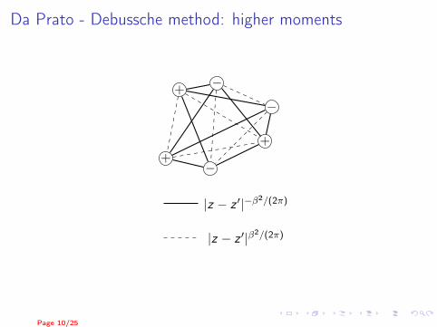
Da Prato - Debussche method: higher moments
+ �
+�
+
�
|z � z
0|��2/(2⇡)
|z � z
0|�2/(2⇡)
Page 10/25

Da Prato - Debussche method: higher moments
+ �
+�
+
�.
+ �
+�
+
�
|z � z
0|��2/(2⇡)
|z � z
0|�2/(2⇡)
Conclusion: @tv = 12�v + Im( ) cos(�v) + Re( ) sin(�v) is
locally well-posed for �2 < 4⇡. Solutions of
@tu" =12�u" + "��2/(4⇡) sin(�u") + ⇠"
converge to a limit u. (Recall u = �+ v)Page 11/25

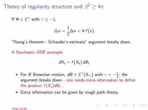
Theory of regularity structure and �2 � 4⇡
If 2 C
� with � �1,
@tv =12�v + f (v)
“Young’s theorem - Schauder’s estimate” argument breaks down.
A Stochastic ODE example:
dXt = f (Xt) dBt
I For B Brownian motion, dB 2 C
�(R+) with � < �12 ; the
argument breaks down - one needs extra information to definethe product f (Xt)dBt .
I Extra information can be given by rough path theory.
Page 12/25

Stochastic ODE example
For smooth function f
dXt = f (Xt) dBt
IX locally “looks like” Brownian motion
Xt � Xt0 = gt0 · (Bt � Bt0) + sth. smoother
I If X is as above, then so is f (X ), and furthermore´ t0 f (Xs) dBs is also as above.
I Only need to define one product B dB .
Page 13/25

Theory of regularity structure and �2 � 4⇡
dXt = f (Xt) dBt @tv =12�v + f (v)
dB 2 C
�1/2�" 2 C
�1�"
The solutions, at small scale, behave like
X ⇠ B =
ˆ t
0dBs analogous v ⇠ K ⇤
where K = (@t � 12�)�1.
I Only need to define one product · (K ⇤ ).I A whole theory (Theory of regularity structures recently
developed by Martin Hairer) behind this “analogy”.
Page 14/25

Regularity structure and �2 � 4⇡: moments of (K ⇤ )I First moment:
Eh (z)
ˆR2+1
K (z�w) (w)dwi=
ˆR2+1
K (z�w) |z�w |��22⇡dw
For �2 � 4⇡ non-integrable singularity at z ⇡ w .I Renormalization: define the product to be
(K⇤ ) def= lim
✏!0
h ✏(K⇤ ✏)�C"
i(C" =
ˆK (z) |z |�
�22⇡dz)
I Need to analyze p-th moment of (K ⇤ ) for arbitrary p.I This renormalization amounts to change of equation
@tv✏ =12�v✏ +
⇣Im( ✏) cos(�v✏)�C✏ cos(�v✏) cos0(�v✏)
⌘
+⇣Re( ✏) sin(�v✏)�C✏ sin(�v✏) sin0(�v✏)
⌘
The two red terms cancel.
Page 15/25

Regularity structure and �2 � 4⇡: moments of (K ⇤ )I First moment:
Eh (z)
ˆR2+1
K (z�w) (w)dwi=
ˆR2+1
K (z�w) |z�w |��22⇡dw
For �2 � 4⇡ non-integrable singularity at z ⇡ w .I Renormalization: define the product to be
(K⇤ ) def= lim
✏!0
h ✏(K⇤ ✏)�C"
i(C" =
ˆK (z) |z |�
�22⇡dz)
I Need to analyze p-th moment of (K ⇤ ) for arbitrary p.I This renormalization amounts to change of equation
@tv✏ =12�v✏ +
⇣Im( ✏) cos(�v✏)�C✏ cos(�v✏) cos0(�v✏)
⌘
+⇣Re( ✏) sin(�v✏)�C✏ sin(�v✏) sin0(�v✏)
⌘
The two red terms cancel.Page 15/25
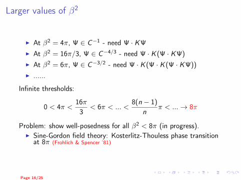
Larger values of �2
I At �2 = 4⇡, 2 C
�1 - need · K I At �2 = 16⇡/3, 2 C
�4/3 - need · K ( · K )I At �2 = 6⇡, 2 C
�3/2 - need · K ( · K ( · K ))I ......
Infinite thresholds:
0 < 4⇡ <16⇡3
< 6⇡ < ... <8(n � 1)
n
⇡ < ... ! 8⇡
Problem: show well-posedness for all �2 < 8⇡ (in progress).I Sine-Gordon field theory: Kosterlitz-Thouless phase transition
at 8⇡ (Frohlich & Spencer ’81)
Page 16/25

Outline
I Sine-Gordon equationI �2 < 4⇡: Apply Da Prato - Debussche method
I4⇡ < �2 < 16⇡/3: Apply regularity structure
I �4 equationI Equation from gauge theory
Page 17/25
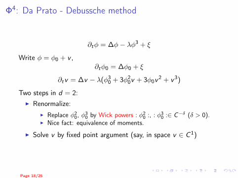
�4: Da Prato - Debussche method
@t� = ��� ��3 + ⇠
Write � = �0 + v ,@t�0 = ��0 + ⇠
@tv = �v � �(�30 + 3�2
0v + 3�0v2 + v
3)
Two steps in d = 2:I Renormalize:
IReplace �2
0, �30 by Wick powers : �2
0 :, : �30 :2 C
��(� > 0).
INice fact: equivalence of moments.
I Solve v by fixed point argument (say, in space v 2 C
1)
This method breaks down in 3D, where : �20 :2 C
�1�� (� > 0)
Page 18/25

�4: Da Prato - Debussche method
@t� = ��� ��3 + ⇠
Write � = �0 + v ,@t�0 = ��0 + ⇠
@tv = �v � �(�30 + 3�2
0v + 3�0v2 + v
3)
Two steps in d = 2:I Renormalize:
IReplace �2
0, �30 by Wick powers : �2
0 :, : �30 :2 C
��(� > 0).
INice fact: equivalence of moments.
I Solve v by fixed point argument (say, in space v 2 C
1)This method breaks down in 3D, where : �2
0 :2 C
�1�� (� > 0)
Page 18/25

�4 in 3D: regularity structures
Regularity structure theory:I fixed point argument in space of functions/distributions with
delicate descriptions of local behavior, i.e. locally behave likeBrownian path or K ⇤ etc.
I only need to define a few objects (often throughrenormalization procedure).
For �4 equation in 3D, write � = �0 + ��1 + R where
@t�0 = ��0 + ⇠
@t�1 = ��1 � �30
with ansatzR ⇠ K ⇤ (�2
0) 2 C
1�� (� > 0)
Need to define �20 · (K ⇤ (�2
0)) - another renormalization.
Page 19/25

Remarks
Some other results:I Global solution / solution on entire space: �4 (Mourrat &
Weber) (Hairer & Matetski)
I Weak universality results: KPZ (Hairer & Quastel), �4 (Hairer &Xu) (Xu & S.)
I Non-Gaussian noises and central limit theorems: KPZ (Hairer &S.), �4 (Xu & S.)
I Convergence from particle systems: �4 (Mourrat & Weber)
Page 20/25

Stochastic quantization of Maxwell Eq.
d = 2. Let (A1,A2) be a vector field. Let FA = @1A2 � @2A1.
exp⇣� 1
2
ˆF
2A dx
⌘DA = exp
⇣� 1
2
ˆ(@1A2 � @2A1)
2dx
⌘DA
The stochastic PDE:
@tA1 = �@2FA + ⇠1 = @22A1 � @1@2A2 + ⇠1
@tA2 = @1FA + ⇠2 = @21A2 � @1@2A1 + ⇠2
I Not parobolic.I Gauge symmetry: For any function f (x) let Aj = Aj + @j f .
ThenFA = @1A2 � @2A1 = @1A2 � @2A1 = FA
therefore A satisfies the same equation.
Page 21/25

Stochastic quantization of Maxwell Eq.
@tA1 = �@2FA + ⇠1 = @22A1 � @1@2A2 + ⇠1
@tA2 = @1FA + ⇠2 = @21A2 � @1@2A1 + ⇠2
“De Turck trick": Let B solves
@tBj = �Bj + ⇠j (j = 1, 2)
Then letA1(t) = B1(t)�
ˆ t
0@1r · B(s) ds
A2(t) = B2(t)�ˆ t
0@2r · B(s) ds
We can check:
@tA1 = �@2FB + ⇠1, @tA2 = @1FB + ⇠2
and, FA = @1A2 � @2A1 = @1B2 � @2B1 = FB
Page 22/25

Nonlinear SPDE with gaugeConsider quantum field theory for vector A and complex valued �
exp⇣� 1
2
ˆ �F
2A +
X
j=1,2
|DAj �|2
�dx
⌘DAD�
The stochastic PDE:
@tA1 = @22A1 � @1@2A2 � i�
⇣�DA
1 �� �DA1 �
⌘+ ⇠1
@tA2 = @21A2 � @1@2A1 � i�
⇣�DA
2 �� �DA2 �
⌘+ ⇠2
@t� =X
j
D
Aj D
Aj �+ ⇣
where D
Aj is gauge covariant derivative:
D
Aj � = @j�� i�Aj� (j = 1, 2)
I Let (A("),�(")) solve the smooth noise Eq, show limit " ! 0.Page 23/25

Nonlinear SPDE with gauge
@tA1 = @22A1 � @1@2A2 � i�
⇣�DA
1 �� �DA1 �
⌘+ ⇠1
@tA2 = @21A2 � @1@2A1 � i�
⇣�DA
2 �� �DA2 �
⌘+ ⇠2
@t� =X
j
D
Aj D
Aj �+ ⇣
De Turck trick:
@tB(")j = �B
(")j � i�
⇣ (")
D
B(")
j (") � (")D
B(")
j (")⌘+ ⇠(")j
@t (") =
X
j
D
B(")
j D
B(")
j (") + i�(r · B(")) (") + e
i�´ t0 r·B(")(s) ds⇣(")
Then define
A
(")j (t) = B
(")j (t)�
ˆ t
0@jr · B(")(s) ds
�(")(t) = e
�i�´ t0 r·B(")(s) ds (")(t)
Page 24/25

Nonlinear SPDE with gauge
@tA1 = @22A1 � @1@2A2 � i�
⇣�DA
1 �� �DA1 �
⌘+ ⇠1
@tA2 = @21A2 � @1@2A1 � i�
⇣�DA
2 �� �DA2 �
⌘+ ⇠2
@t� =X
j
D
Aj D
Aj �+ ⇣
Expected result: Let (A("),�(")) solve the smooth noise Eq. Thereexists a family (parametrized by time) of gauge transformationsG(")t such that G(")
t (A("),�(")) converges to a nontrivial limit.
Page 25/25


![Stochastic Schrodinger equations¨maassen/papers/StochSchr.pdf · Stochastic Schrodinger equations ... stochastic differential equation in the sense of [22]. Belavkin [6] was the](https://img.pdfslide.net/doc/110x75/5f0483607e708231d40e578b/stochastic-schrodinger-equations-maassenpapers-stochastic-schrodinger-equations.jpg)


![Stochastic Differential Dynamic Logic for …3 Stochastic Differential Equations We consider stochastic differential equations [Øks07, KP10] to describe stochastic continuous system](https://img.pdfslide.net/doc/110x75/5f397c2e99ca7b6adc05f296/stochastic-differential-dynamic-logic-for-3-stochastic-differential-equations-we.jpg)