Embed Size (px)
Citation preview
UNIVERSITY OF CALIFORNIASanta Barbara
Stochastic Search and Surveillance Strategiesfor Mixed Human-Robot Teams
A Dissertation submitted in partial satisfactionof the requirements for the degree of
Doctor of Philosophy
in
Mechanical Engineering
by
Vaibhav Srivastava
Committee in Charge:
Professor Francesco Bullo, Chair
Professor Bassam Bamieh
Professor Joao P. Hespanha
Professor Sreenivasa R. Jammalamadaka
Professor Jeff Moehlis
December 2012
The Dissertation ofVaibhav Srivastava is approved:
Professor Bassam Bamieh
Professor Joao P. Hespanha
Professor Sreenivasa R. Jammalamadaka
Professor Jeff Moehlis
Professor Francesco Bullo, Committee Chairperson
October 2012

Stochastic Search and Surveillance Strategiesfor Mixed Human-Robot Teams
Copyright c© 2012by
Vaibhav Srivastava
iii

to my family
iv
Acknowledgements
This dissertation would not have been possible without the support and en-couragement of several people. First and foremost, I express my most sinceregratitude towards my advisor, Prof Francesco Bullo, for his exceptional mentor-ship, constant encouragement, impeccable support, and the complete liberty, hegranted me throughout my PhD. I have been fortunate to learn the art of researchunder his excellent tutelage.
I thank Prof Sreenivasa Rao Jammalamadaka for his exceptional guidancethroughout my masters work and for teaching me to think from a statistical per-spective. I thank my other committee members, Prof Bassam Bamieh, Prof JoaoHespanha, and Prof Jeff Moehlis, for their help and support throughout my PhD.
I thank all my collaborators for all their help throughout my PhD. I thank DrKurt Plarre for his help in the sensor selection project. I thank Prof Jeff Moehlisfor his encouragement, help, and support in the bifurcations project. I thankProf Cedric Langbort and Prof Ruggero Carli for all the helpful discussions andtheir encouragement during the attention allocation project. I thank Dr FabioPasqualetti for all his help and support throughout my PhD and especially, inthe stochastic surveillance project. I thank Dr Luca Carlone and Prof GiuseppeCalafiore for all their help in the distributed random convex programming project.I thank Christopher J. Ho for all his work on the interface design for humanexperiments. I thank Dr Amit Surana for inviting me for the internship at UTRCand for all the helpful discussions on the attention allocation in mixed teams.
I thank the current and the previous members of the Prof Bullo’s lab for theirfriendship, for the intellectually stimulating discussions in the lab and for all thefun activities outside of it. I thank Dr Shaunak Bopardikar for convincing me tojoin UCSB. It was indeed a great decision. I thank Dr Andrzej Banaszuk and DrLuca Bertucelli for all the discussions during my internship at UTRC.
I thank all my teachers at my pre-secondary and secondary schools, my teach-ers at IIT Bombay, and my teachers at UCSB for instilling in me a quest forknowledge and an appreciation for details. I particularly thank Prof ShashikanthSuryanarayanan at IIT Bombay who instigated my interest in controls.
My stay at UCSB and earlier at IIT Bombay has been blessed with greatfriends. I thank you all for all your support over the years. Thank you Shaunakand Dhanashree Bopardikar for all the tea sessions and all the wonderful food.Thank you Vibhor Jain for all the trips and all the fun activities. Thank youGargi Chaudhuri for the wonderful radio jockeying time at KCSB. Thank youSumit Singh and Sriram Venkateswaran for the Friday wine sessions. Thank youAnahita Mirtabatabei for all the activities you organized. Thank you G Kartikfor the fun time at IIT Bombay.
v

No word of thanks would be enough for the unconditional love and the ardentsupport of my family. I thank my parents for the values they cultivated in me.Each day, I more understand the sacrifices, they made while bringing me up. Mybrother and my sisters have been a great guidance and support for me through theyears. I thank them for standing by me in tough times. This achievement wouldbe impossible without the efforts of my uncle, Mr Marut Kumar Srivastava, whoinculcated in me an appreciation for mathematics at a tender age. He has beena tremendous support and an inspiration in all my academic endeavors. I thankhim for being there whenever I needed him. My family has been a guiding lightfor me and continues to inspire me in my journey ahead. I endlessly thank myfamily for all they have done for me.
vi
Curriculum VitæVaibhav Srivastava
Education
M.A. in Statistics, UCSB, USA. (2012)Specialization: Mathematical Statistics
M.S. in Mechanical Engineering, UCSB, USA. (2011)Specialization: Dynamics, Control, and Robotics
B.Tech. in Mechanical Engineering, IIT Bombay, India. (2007)
Research Interests
Stochastic analysis and design of risk averse algorithms for uncertain systems,including (i) mixed human-robot networks, (ii) robotic and mobile sensornetworks; and (iii) computational networks.
Professional Experience
• Graduate Student Researcher (April 2008 – present)Department of Mechanical Engineering, UCSB
• Summer Intern (August – September 2011)United Technologies Research Center, East Hartford, USA
• Design Consultant (May – July 2006)General Electrical HealthCare, Bangalore, India
Outreach
• Graduate Student Mentor (July – August 2009)SABRE, Institute of Collaborative Biosciences, UCSB
• Senior Undergraduate Mentor (July 2006 – April 2007)Department of Mechanical Engineering, IIT Bombay
vii
Teaching Experience
• Teaching Assistant, Control System Design (Fall 2007, Spring 2010)Department of Mechanical Engineering, UCSB
• Teaching Assistant, Vibrations (Winter 2008)Department of Mechanical Engineering, UCSB
• Teaching Assistant, Engineering Mechanics: Dynamics (Spring 2011)Department of Mechanical Engineering, UCSB
• Guest Lecture: Distributed Systems and Control (Spring 2012)Department of Mechanical Engineering, UCSB
Undergraduate Supervision
• Christopher J. Ho (Undergraduate student, ME UCSB)
• Lemnyuy ’Bernard’ Nyuykongi (Summer intern, ICB UCSB)
Publications
Journal articles
[1]. V. Srivastava and F. Bullo. Knapsack problems with sigmoid utility: Ap-proximation algorithms via hybrid optimization. European Journal of Op-erational Research, October 2012. Sumitted.
[2]. L. Carlone, V. Srivastava, F. Bullo, and G. C. Calafiore. Distributedrandom convex programming via constraints consensus. SIAM Journal onControl and Optimization, July 2012. Submitted.
[3]. V. Srivastava, F. Pasqualetti, and F. Bullo. Stochastic surveillance strate-gies for spatial quickest detection. International Journal of Robotics Re-search, October 2012. to appear.
[4]. V. Srivastava, R. Carli, C. Langbort, and F. Bullo. Attention allocationfor decision making queues. Automatica, February 2012. Submitted.
[5]. V. Srivastava, J. Moehlis, and F. Bullo. On bifurcations in nonlinearconsensus networks. Journal of Nonlinear Science, 21(6):875–895, 2011.
viii
[6]. V. Srivastava, K. Plarre, and F. Bullo. Randomized sensor selection insequential hypothesis testing. IEEE Transactions on Signal Processing,59(5):2342–2354, 2011.
Refereed conference proceedings
[1]. V. Srivastava, A. Surana, and F. Bullo. Adaptive attention allocation inhuman-robot systems. In American Control Conference, pages 2767–2774,Montreal, Canada, June 2012.
[2]. L. Carlone, V. Srivastava, F. Bullo, and G. C. Calafiore. A distributed al-gorithm for random convex programming. In Int. Conf. on Network Games,Control and Optimization (NetGCooP), pages 1–7, Paris, France, October2011.
[3]. V. Srivastava and F. Bullo. Stochastic surveillance strategies for spatialquickest detection. In IEEE Conf. on Decision and Control and EuropeanControl Conference, pages 83–88, Orlando, FL, USA, December 2011.
[4]. V. Srivastava and F. Bullo. Hybrid combinatorial optimization: Sampleproblems and algorithms. In IEEE Conf. on Decision and Control and Eu-ropean Control Conference, pages 7212–7217, Orlando, FL, USA, December2011.
[5]. V. Srivastava, K. Plarre, and F. Bullo. Adaptive sensor selection in se-quential hypothesis testing. In IEEE Conf. on Decision and Control andEuropean Control Conference, pages 6284–6289, Orlando, FL, USA, Decem-ber 2011.
[6]. V. Srivastava, R. Carli, C. Langbort, and F. Bullo. Task release control fordecision making queues. In American Control Conference, pages 1855–1860,San Francisco, CA, USA, June 2011.
[7]. V. Srivastava, J. Moehlis, and F. Bullo. On bifurcations in nonlinearconsensus networks. Journal of Nonlinear Science, 21(6):875–895, 2011.
Thesis
[1]. V. Srivastava. Topics in probabilistic graphical models. Master’s thesis,Department of Statistics, University of California at Santa Barbara, Septem-ber 2012.
ix

Services
Organizer/Co-Organizer2011 Santa Barbara Control Workshop.
ReviewerProceedings of IEEE, IEEE Transactions on Automatic Controls, IEEETransactions on Information Theory, Automatica, International Journal ofRobotics Research, International Journal of Robust and Nonlinear Control,European Journal of Control, IEEE Conference on Decision and Control(CDC), American Controls Conference (ACC), IEEE International Confer-ence on Distributed Computing in Sensor Systems (DCOSS).
Chair/Co-ChairSession on Fault Detection, IEEE Conf. on Decision and Control and Eu-ropean Control Conference, Orlando, FL, USA, December 2011.
Professional Membership
• Student Member, Institute of Electrical and Electronics Engineers (IEEE)
• Student Member, Society of Industrial and Applied Mathematics (SIAM)
x
Abstract
Stochastic Search and Surveillance Strategies
for Mixed Human-Robot TeamsVaibhav Srivastava
Mixed human-robot teams are becoming increasingly important in complexand information rich systems. The purpose of the mixed teams is to exploit thehuman cognitive abilities in complex missions. It has been evident that the infor-mation overload in these complex missions has a detrimental effect on the humanperformance. The focus of this dissertation is design of efficient human-robotteams. It is imperative for an efficient human-robot team to handle informationoverload and to this end, we propose a two-pronged strategy: (i) for the robots, wepropose strategies for efficient information aggregation; and (ii) for the operator,we propose strategies for efficient information processing. The proposed strategiesrely on team objective as well as cognitive performance of the human operator.
In the context of information aggregation, we consider two particular missions.First, we consider information aggregation for a multiple alternative decision mak-ing task and pose it as a sensor selection problem in sequential multiple hypothesistesting. We design efficient information aggregation policies that enable the hu-man operator to decide in minimum time. Second, we consider a surveillanceproblem and design efficient information aggregation policies that enable the hu-man operator detect a change in the environment in minimum time. We studythe surveillance problem in a decision-theoretic framework and rely on statisticalquickest change detection algorithms to achieve a guaranteed surveillance perfor-mance.
In the context of information processing, we consider two particular scenar-ios. First, we consider the time-constrained human operator and study optimalresource allocation problems for the operator. We pose these resource allocationproblems as knapsack problems with sigmoid utility and develop constant factoralgorithms for them. Second, we consider the human operator serving a queueof decision making tasks and determine optimal information processing policies.We pose this problem in a Markov decision process framework and determineapproximate solution using certainty-equivalent receding horizon framework.
xi
Contents
Acknowledgements v
Abstract xi
1 Introduction 11.1 Literature Synopsis . . . . . . . . . . . . . . . . . . . . . . . . . . 3
1.1.1 Sensor Selection . . . . . . . . . . . . . . . . . . . . . . . . 31.1.2 Search and Surveillance . . . . . . . . . . . . . . . . . . . 41.1.3 Time-constrained Attention Allocation . . . . . . . . . . . 51.1.4 Attention Allocation in Decision Making Queues . . . . . . 6
1.2 Contributions and Organization . . . . . . . . . . . . . . . . . . . 7
2 Preliminaries on Decision Making 122.1 Markov Decision Process . . . . . . . . . . . . . . . . . . . . . . . 12
2.1.1 Existence on an optimal policy . . . . . . . . . . . . . . . 132.1.2 Certainty-Equivalent Receding Horizon Control . . . . . . 132.1.3 Discretization of the Action and the State Space . . . . . . 14
2.2 Sequential Statistical Decision Making . . . . . . . . . . . . . . . 152.2.1 Sequential Binary Hypothesis Testing . . . . . . . . . . . . 152.2.2 Sequential Multiple hypothesis Testing . . . . . . . . . . . 172.2.3 Quickest Change Detection . . . . . . . . . . . . . . . . . . 18
2.3 Speed Accuracy Trade-off in Human Decision Making . . . . . . . 192.3.1 Pew’s Model . . . . . . . . . . . . . . . . . . . . . . . . . . 202.3.2 Drift-Diffusion Model . . . . . . . . . . . . . . . . . . . . . 20
3 Randomized Sensor Selection in Sequential Hypothesis Testing 233.1 MSPRT with randomized sensor selection . . . . . . . . . . . . . . 253.2 Optimal sensor selection . . . . . . . . . . . . . . . . . . . . . . . 32
3.2.1 Optimization of conditioned decision time . . . . . . . . . 333.2.2 Optimization of the worst case decision time . . . . . . . . 34
xii
3.2.3 Optimization of the average decision time . . . . . . . . . 393.3 Numerical Illustrations . . . . . . . . . . . . . . . . . . . . . . . . 433.4 Conclusions . . . . . . . . . . . . . . . . . . . . . . . . . . . . . . 46
4 Stochastic Surveillance Strategies for Spatial Quickest Detection 474.1 Spatial Quickest Detection . . . . . . . . . . . . . . . . . . . . . . 51
4.1.1 Ensemble CUSUM algorithm . . . . . . . . . . . . . . . . 514.2 Randomized Ensemble CUSUM Algorithm . . . . . . . . . . . . . 53
4.2.1 Analysis for single vehicle . . . . . . . . . . . . . . . . . . 534.2.2 Design for single vehicle . . . . . . . . . . . . . . . . . . . 554.2.3 Analysis for multiple vehicles . . . . . . . . . . . . . . . . 594.2.4 Design for multiple vehicles . . . . . . . . . . . . . . . . . 60
4.3 Adaptive ensemble CUSUM Algorithm . . . . . . . . . . . . . . . 624.4 Numerical Results . . . . . . . . . . . . . . . . . . . . . . . . . . . 654.5 Experimental Results . . . . . . . . . . . . . . . . . . . . . . . . . 724.6 Conclusions and Future Directions . . . . . . . . . . . . . . . . . 774.7 Appendix: Probabilistic guarantee to the uniqueness of critical point 78
5 Operator Attention Allocation via Knapsack Problems 815.1 Sigmoid Function and Linear Penalty . . . . . . . . . . . . . . . . 825.2 Knapsack Problem with Sigmoid Utility . . . . . . . . . . . . . . 83
5.2.1 KP with Sigmoid Utility: Problem Description . . . . . . . 835.2.2 KP with Sigmoid Utility: Approximation Algorithm . . . . 84
5.3 Generalized Assignment Problem with Sigmoid Utility . . . . . . 925.3.1 GAP with Sigmoid Utility: Problem Description . . . . . . 925.3.2 GAP with Sigmoid Utility: Approximation Algorithm . . . 93
5.4 Bin-packing Problem with Sigmoid Utility . . . . . . . . . . . . . 965.4.1 BPP with Sigmoid Utility: Problem Description . . . . . . 965.4.2 BPP with Sigmoid Utility: Approximation Algorithm . . . 98
5.5 Conclusions and Future Directions . . . . . . . . . . . . . . . . . 100
6 Attention Allocation in Decision Making Queues 1026.1 Static queue with latency penalty . . . . . . . . . . . . . . . . . . 103
6.1.1 Problem description . . . . . . . . . . . . . . . . . . . . . 1036.1.2 Optimal solution . . . . . . . . . . . . . . . . . . . . . . . 1046.1.3 Numerical Illustrations . . . . . . . . . . . . . . . . . . . . 104
6.2 Dynamic queue with latency penalty . . . . . . . . . . . . . . . . 1056.2.1 Problem description . . . . . . . . . . . . . . . . . . . . . 1056.2.2 Properties of optimal solution . . . . . . . . . . . . . . . . 107
6.3 Receding Horizon Solution to dynamic queue with latency penalty 108
xiii
6.3.1 Certainty-equivalent finite horizon optimization . . . . . . 1086.3.2 Performance of receding horizon algorithm . . . . . . . . . 1106.3.3 Numerical Illustrations . . . . . . . . . . . . . . . . . . . . 112
6.4 Conclusions . . . . . . . . . . . . . . . . . . . . . . . . . . . . . . 1136.5 Appendix: Finite horizon optimization for identical tasks . . . . . 114
Bibliography 119
xiv
Chapter 1
Introduction
The emergence of mobile and fixed sensor networks operating at differentmodalities, mobility, and coverage has enabled access to an unprecedented amountof data. In a variety of complex and information rich systems, this informationis processed by a human operator [17, 31]. The inherent inability of the humanoperator to handle the plethora of available information has detrimental effectson their performance and may lead to unpleasant consequences [84]. To alleviatethis loss in performance of the human operator, the recent national robotic initia-tive [38] emphasizes collaboration of humans with robotic partners, and envisionsa symbiotic co-robot that facilitates efficient interaction of the human operatorwith the automaton. Given the complex interaction that can arise between the op-erator and the automaton, such a co-robotic partner will enable better interactionbetween the automaton and the operator by exploiting the operator’s strengthswhile taking into account their inefficiencies, such as erroneous decisions, fatigueand the loss of situational awareness. This encourages an investigation into algo-rithms that enable the co-robot to aid the human partner to focus their attentionto the pertinent information and direct the automaton to efficiently collect theinformation.
The problems of interest in this dissertation are the search and the persistentsurveillance. The search problem involves ascertaining the true state of natureamong several possible state of natures. The objective of the search problem isto ascertain the true state of nature in minimum time. The persistent surveil-lance involves continuous search of target regions with a team of fixed and mobilesensors. An efficient persistent surveillance policy has multiple objectives, e.g.,minimizing the time between subsequent visit to a region, minimizing the detec-tion delay at each region, maximize visits to regions with high likelihood of target,etc. The fundamental trade-off in persistent surveillance is between the evidencecollected from the visited region and the resulting delay in evidence collection
1
Chapter 1. Introduction
from other regions. The search and the persistent surveillance missions may befully autonomous or may involve a human operator that processes the collectedevidence and accordingly modifies the search and surveillance policy, respectively.The latter is called the mixed human-robot team search/surveillance. The purposeof the mixed teams is to exploit human cognitive abilities in complex missions,and therefore, an effective model of human cognitive performance is fundamentalto the team design. Moreover, such a model should be efficiently integrated withthe automaton design enabling an effective team performance.
As a consequence of the growing interest in the mixed teams, a significant efforthas been made to model human cognitive performance and integrate it with theautomaton. Broadly speaking, there have been two approaches to mixed team de-sign. In the first approach, the human is allowed to respond freely and the automa-ton is adaptively controlled to cater to the human operator’s cognitive require-ments. The second approach, both the human and the automaton are controlled,for instance, the human operator is told the time-duration they should spendon each task, and their decision is utilized to adaptively control the automaton.The first approach typically captures human performance via their free-responsereaction times on each task. The fundamental research questions in this ap-proach include (i) optimal scheduling of automaton [65, 12, 11, 80, 81, 29, 66, 67];(ii) controlling operator utilization to enable shorter reaction times [78, 79]; and(iii) design of efficient work-shift design to counter fatigue effects on the oper-ator [73]. The second approach captures the human performance as the prob-ability of making the correct decision given the time spent on the task. Thefundamental research questions in this approach include (i) optimal duration al-location to each task [93, 94, 90]; (ii) controlling operator utilization to enablebetter performance [98]; and (iii) controlling the automaton to collect relevantinformation [95, 97, 96, 98].
In this dissertation, we focus on the latter approach, although most of theconcepts can be easily extended to the former approach. The objective of thisdissertation is to illustrate the use of systems theory to design mixed human-robot teams. We illustrate the design principles for the mixed teams with aparticular application to mixed-team surveillance. One of the major challengesin mixed human-robot teams is information overload. The information overloadcan be handled/avoided by (i) only selecting pertinent sources of information; (ii)only collecting pertinent information; and (iii) efficiently allocating the operator’sattention. To this end, first, we study a sensor selection problem for the humanoperator. The objective of this problem is to identify pertinent sources such thatthe operator decides in a minimum time. Second, we then study a persistentsurveillance problem and design surveillance strategies that result in collection of
2
Chapter 1. Introduction
the pertinent information. Third, we focus on on attention allocation problems forthe human operator. We study attention allocation for a time-constraint operatoras well as attention allocation for an operator serving a queue of decision makingtasks.
1.1 Literature Synopsis
In this section, we review the literature in areas relevant to this dissertation.We organize the literature according to the broad topics of interest in this disser-tation.
1.1.1 Sensor Selection
One of the key focuses in this dissertation is the sensor selection problem insequential hypothesis testing. Recent years have witnessed a significant interestin the problem of sensor selection for optimal detection and estimation. Tay etal. [99] discuss the problem of censoring sensors for decentralized binary detection.They assess the quality of sensor data by the Neyman-Pearson and a Bayesianbinary hypothesis test and decide on which sensors should transmit their obser-vation at that time instant. Gupta et al. [39] focus on stochastic sensor selectionand minimize the error covariance of a process estimation problem. Isler et al. [49]propose geometric sensor selection schemes for error minimization in target detec-tion. Debouk et al. [30] formulate a Markovian decision problem to ascertain someproperty in a dynamical system, and choose sensors to minimize the associatedcost. Williams et al. [107] use an approximate dynamic program over a rollingtime horizon to pick a sensor-set that optimizes the information-communicationtrade-off. Wang et al. [104] design entropy-based sensor selection algorithms fortarget localization. Joshi et al. [50] present a convex optimization-based heuristicto select multiple sensors for optimal parameter estimation. Bajovic et al. [5]discuss sensor selection problems for Neyman-Pearson binary hypothesis testingin wireless sensor networks. Katewa et al. [53] study sequential binary hypothe-sis testing using multiple sensors. For a stationary sensor selection policy, theydetermine the optimal sequential hypothesis test. Bai et al. [4] study an off-linerandomized sensor selection strategy for sequential binary hypothesis testing prob-lem constrained with sensor measurement costs. In contrast to above works, wefocus on sensor selection in sequential multiple hypothesis testing.
3
Chapter 1. Introduction
1.1.2 Search and Surveillance
Another key focus in this dissertation is efficient vehicle routing policies forsearch and surveillance. This problem belongs to the broad class of routing for in-formation aggregation which has recently attracted significant attention. Klein etal. [56] present a vehicle routing policy for optimal localization of an acousticsource. They consider a set of spatially distributed sensors and optimize thetrade-off between the travel time required to collect a sensor observation and theinformation contained in the observation. They characterize the information in anobservation by the volume of the Cramer-Rao ellipsoid associated with the covari-ance of an optimal estimator. Hollinger et al. [46] study routing for an AUV tocollect data from an underwater sensor network. They developed approximationalgorithms for variants of the traveling salesperson problem to determine efficientpolicies that maximize the information collected while minimizing the travel time.Zhang et al. [108] study the estimation of environmental plumes with mobile sen-sors. They minimize the uncertainty of the estimate of the ensemble Kalmanfilter to determine optimal trajectories for a swarm of mobile sensors. We focuson decision theoretic surveillance which has also received some interest in the liter-ature. Castanon [22] poses the search problem as a dynamic hypothesis test, anddetermines the optimal routing policy that maximizes the probability of detectionof a target. Chung et al. [26] study the probabilistic search problem in a deci-sion theoretic framework. They minimize the search decision time in a Bayesiansetting. Hollinger et al. [45] study an active classification problem in which anautonomous vehicle classifies an object based on multiple views. They formulatethe problem in an active Bayesian learning framework and apply it to underwaterdetection. In contrast to the aforementioned works that focus on classification orsearch problems, our focus is on the quickest detection of anomalies.
The problem of surveillance has received considerable attention recently. Pre-liminary results on this topic have been presented in [25, 33, 55]. Pasqualetti etal. [70] study the problem of optimal cooperative surveillance with multiple agents.They optimize the time gap between any two visits to the same region, and thetime necessary to inform every agent about an event occurred in the environ-ment. Smith et al. [86] consider the surveillance of multiple regions with changingfeatures and determine policies that minimize the maximum change in featuresbetween the observations. A persistent monitoring task where vehicles move on agiven closed path has been considered in [87, 69], and a speed controller has beendesigned to minimize the time lag between visits of regions. Stochastic surveil-lance and pursuit-evasion problems have also fetched significant attention. In anearlier work, Hespanha et al. [43] studied multi-agent probabilistic pursuit eva-sion game with the policy that, at each instant, directs pursuers to a location
4
Chapter 1. Introduction
that maximizes the probability of finding an evader at that instant. Grace etal. [37] formulate the surveillance problem as a random walk on a hypergraphand parametrically vary the local transition probabilities over time in order toachieve an accelerated convergence to a desired steady state distribution. Sak etal. [77] present partitioning and routing strategies for surveillance of regions fordifferent intruder models. Srivastava et al. [89] present a stochastic surveillanceproblem in centralized and decentralized frameworks. They use Markov chainMonte Carlo method and message passing based auction algorithm to achieve thedesired surveillance criterion. They also show that the deterministic strategiesfail to satisfy the surveillance criterion under general conditions. We focus onstochastic surveillance policies. In contrast to aforementioned works on stochasticsurveillance that assume a surveillance criterion is known, this work concerns thedesign of the surveillance criterion.
1.1.3 Time-constrained Attention Allocation
In this dissertation, we also focus on attention allocation policies for a timeconstrained human operator. The resource allocation problems with sigmoid util-ity well model the situation of a time constrained human operator. To this end, wepresent versions of the knapsack problem, the bin-packing problem, and the gener-alized assignment problem in which each item has a sigmoid utility. If the utilitiesare step functions, then these problems reduce to the standard knapsack prob-lem, the bin-packing problem, and the generalized assignment problem [57, 61],respectively. Similarly, if the utilities are concave functions, then these problemsreduce to standard convex resource allocation problems [48]. We will show thatwith sigmoid utilities the optimization problem becomes a hybrid of discrete andcontinuous optimization problems.
The knapsack problems [54, 57, 61] have been extensively studied. Consider-able emphasis has been on the discrete knapsack problem [57] and the knapsackproblems with concave utilities; a survey is presented in [16]. Non-convex knap-sack problems have also received significant attention. Kameshwaran et al. [52]study knapsack problems with piecewise linear utilities. More et al. [63] andBurke et al. [18] study knapsack problem with convex utilities. In an early work,Ginsberg [36] studies a knapsack problem in which each item has identical sigmoidutility. Freeland et al. [34] discuss the implication of sigmoid functions on deci-sion models and present an approximation algorithm for the knapsack problemwith sigmoid utilities that constructs a concave envelop of the sigmoid functionsand thus solves the resulting convex problem. In a recent work, Agrali et al. [1]consider the knapsack problem with sigmoid utility and show that this problem
5
Chapter 1. Introduction
is NP-hard. They relax the problem by constructing a concave envelope of thesigmoid function and then determine the global optimal solution using branchand bound techniques. They also develop an FPTAS for the case in which thedecision variable is discrete. In contrast to above works, we determine constantfactor algorithms for the knapsack problem, the bin-packing problem, and thegeneralized assignment problem with sigmoid utility.
1.1.4 Attention Allocation in Decision Making Queues
The last focus of this dissertation is on attention allocation policies for a hu-man operator serving a queue of decision making tasks (decision making queues).There has been a significant interest in the study of the performance of a humanoperator serving a queue. In an early work, Schmidt [82] models the human asa server and numerically studies a queueing model to determine the performanceof a human air traffic controller. Recently, Savla et al. [81] study human super-visory control for unmanned aerial vehicle operations: they model the system bya simple queuing network with two components in series, the first of which is aspatial queue with vehicles as servers and the second is a conventional queue withhuman operators as servers. They design joint motion coordination and operatorscheduling policies that minimize the expected time needed to classify a targetafter its appearance. The performance of the human operator based on their uti-lization history has been incorporated to design maximally stabilizing task releasepolicies for a human-in-the-loop queue in [79, 78]. Bertuccelli et al. [12] study thehuman supervisory control as a queue with re-look tasks. They study the policiesin which the operator can put the tasks in an orbiting queue for a re-look later. Anoptimal scheduling problem in the human supervisory control is studied in [11].Crandall et al. [29] study optimal scheduling policy for the operator and discuss ifthe operator or the automation should be ultimately responsible for selecting thetask. Powel et al. [73] model mixed team of humans and robots as a multi-serverqueue and incorporate a human fatigue model to determine the performance of theteam. They present a comparative study of the fixed and the rolling work-shiftsof the operators. In contrast to the aforementioned works in queues with humanoperator, we do not assume that the tasks require a fixed (potentially stochastic)processing time. We consider that each task may be processed for any amount oftime, and the performance on the task is known as a function of processing time.
The optimal control of queueing systems [83] is a classical problem in queue-ing theory. There has been significant interest in the dynamic control of queues;e.g., see [51] and references therein. In particular, Stidham et al. [51] study theoptimal servicing policies for an M/G/1 queue of identical tasks. They formu-
6
Chapter 1. Introduction
late a semi-Markov decision process, and describe the qualitative features of thesolution under certain technical assumptions. In the context of M/M/1 queues,George et al. [35] and Adusumilli et al. [2] relax some of technical assumptionsin [51]. Hernandez-Lerma et al. [42] determine optimal servicing policies for theidentical tasks and some arrival rate. They adapt the optimal policy as the ar-rival rate is learned. The main differences between these works and the problemconsidered in this dissertation are: (i) we consider a deterministic service process,and this yields an optimality equation quite different from the optimality equationobtained for Markovian service process; (ii) we consider heterogeneous tasks whilethe aforementioned works consider identical tasks.
1.2 Contributions and Organization
In this section, we outline the organization of the chapters in this dissertationand detail the contributions in each chapter.Chapter 2: In this chapter, we review some decision making concepts. Westart with a review of Markov decision processes (Section 2.1). We then reviewsequential statistical decision making (Section 2.2). We close the chapter with areview of human decision making (Section 2.3).Chapter 3: In this chapter, we analyze the problem of time-optimal sequentialdecision making in the presence of multiple switching sensors and determine arandomized sensor selection strategy to achieve the same. We consider a sensornetwork where all sensors are connected to a fusion center. Such topology is foundin numerous sensor networks with cameras, sonars or radars, where the fusioncenter can communicate with any of the sensors at each time instant. The fusioncenter, at each instant, receives information from only one sensor. Such a situationarises when we have interfering sensors (e.g., sonar sensors), a fusion center withlimited attention or information processing capabilities, or sensors with sharedcommunication resources. The sensors may be heterogeneous (e.g., a camerasensor, a sonar sensor, a radar sensor, etc), hence, the time needed to collect,transmit, and process data may differ significantly for these sensors. The fusioncenter implements a sequential hypothesis test with the gathered information.The material in this chapter is from [97] and [96].
The major contributions of this work are twofold. First, we develop a version ofthe MSPRT algorithm in which the sensor is randomly switched at each iterationand characterize its performance. In particular, we determine the asymptoticexpressions for the thresholds and the expected sample size for this sequential test.We also incorporate the random processing time of the sensors into these modelsto determine the expected decision time (Section 3.1). Second, we identify the set
7
Chapter 1. Introduction
of sensors that minimize the expected decision time. We consider three differentcost functions, namely, the conditioned decision time, the worst case decisiontime, and the average decision time. We show that, to minimize the conditionedexpected decision time, the optimal sensor selection policy requires only one sensorto be observed. We show that, for a generic set of sensors and M underlyinghypotheses, the optimal average decision time policy requires the fusion centerto consider at most M sensors. For the binary hypothesis case, we identify theoptimal set of sensors in the worst case and the average decision time minimizationproblems. Moreover, we determine an optimal probability distribution for thesensor selection. In the worst case and the average decision time minimizationproblems, we encounter the problem of minimization of sum and maximum oflinear-fractional functionals. We treat these problems analytically, and provideinsight into their optimal solutions (Section 3.2).Chapter 4: In this chapter, we study persistent surveillance of an environmentcomprising of potentially disjoint regions of interest. We consider a team of au-tonomous vehicles that visit the regions, collect information, and send it to a con-trol center. We study a spatial quickest detection problem with multiple vehicles,that is, the simultaneous quickest detection of anomalies at spatially distributedregions when the observations for anomaly detection are collected by autonomousvehicles. We design vehicle routing policies to collect observations at differentregions that result in quickest detection of anomalies at different regions. Thematerial in this chapter is from [95] and [91].
The main contributions of this chapter are fivefold. First, we formulate thestochastic surveillance problem for spatial quickest detection of anomalies. Wepropose the ensemble CUSUM algorithm for a control center to detect concurrentanomalies at different regions from collected observations (Section 4.1). For theensemble CUSUM algorithm we characterize lower bounds for the expected de-tection delay and for the average (expected) detection delay at each region. Ourbounds take into account the processing times for collecting observations, the priorprobability of anomalies at each region, and the anomaly detection difficulty ateach region.
Second, for the case of stationary routing policies, we provide bounds on theexpected delay in detection of anomalies at each region (Section 4.2). In partic-ular, we take into account both the processing times for collecting observationsand the travel times between regions. For the single vehicle case, we explicitlycharacterize the expected number of observations necessary to detect an anomalyat a region, and the corresponding expected detection delay. For the multiplevehicles case, we characterize lower bounds for the expected detection delay andthe average detection delay at the regions. As a complementary result, we show
8
Chapter 1. Introduction
that the expected detection delay for a single vehicle is, in general, a non-convexfunction. However, we provide probabilistic guarantees that it admits a uniqueglobal minimum.
Third, we design stationary vehicle routing policies to collect observations fromdifferent regions (Section 4.2). For the single vehicle case, we design an efficientstationary policy by minimizing an upper bound for the average detection delayat the regions. For the multiple vehicles case, we first partition the regions amongthe vehicles, and then we let each vehicle survey the assigned regions by usingthe routing policy as in the single vehicle case. In both cases we characterizethe performance of our policies in terms of expected detection delay and average(expected) detection delay.
Fourth, we describe our adaptive ensemble CUSUM algorithm, in which therouting policy is adapted according to the learned likelihood of anomalies in theregions (Section 4.3). We derive an analytic bound for the performance of ouradaptive policy. Finally, our numerical results show that our adaptive policyoutperforms the stationary counterpart.
Fifth and finally, we report the results of extensive numerical simulations and apersistent surveillance experiment (Sections 4.4 and 4.5). Besides confirming ourtheoretical findings, these practical results show that our algorithms are robustagainst realistic noise models, and sensors and motion uncertainties.Chapter 5: In this chapter, we study optimization problems with sigmoid func-tions. We show that sigmoid utility renders a combinatorial element to the prob-lem and resource allocated to each item under optimal policy is either zero ormore than a critical value. Thus, optimization variable has both continuous anddiscrete features. We exploit this interpretation of the optimization variable andmerge algorithms from continuous and discrete optimization to develop efficienthybrid algorithms. We study versions of the knapsack problem, the generalizedassignment problem and the bin-packing problem in which the utility is a sigmoidfunction. These problems model situations where human operators are lookingat the feeds from a camera network and deciding on the presence of some mali-cious activity. The first problem determines the optimal fraction of work-hoursan operator should allocate to each feed such that their overall performance isoptimal. The second problem determines the allocations of the tasks to identicaland independently working operators as well as the optimal fraction of work-hourseach operator should allocate to each feed such that the overall performance ofthe team is optimal. Assuming that the operators work in an optimal fashion, thethird problem determines the minimum number of operators and an allocationof each feed to some operator such that each operator allocates non-zero fraction
9
Chapter 1. Introduction
of work-hours to each feed assigned to them. The material in this chapter isfrom [90] and [92].
The major contributions of this chapter are fourfold. First, we investigate theroot-cause of combinatorial effects in optimization problems with sigmoid utility(Section 5.1). We show that for a sigmoid function subject to a linear penalty, theoptimal allocation jumps down to zero with increasing penalty rate. This jumpin the optimal allocation imparts a combinatorial effect to the problems involvingsigmoid functions.
Second, we study the knapsack problem with sigmoid utility (Section 5.2). Weexploit the above combinatorial interpretation of the sigmoid functions and utilizea combination of approximation algorithms for the binary knapsack problems andalgorithms for continuous univariate optimization to determine a constant factorapproximation algorithm for the knapsack problem with sigmoid utility.
Third, we study the generalized assignment problem with sigmoid utility (Sec-tion 5.3). We first show that the generalized assignment problem with sigmoidutility is NP-hard. We then exploit a knapsack problem based algorithm for binarygeneralized assignment problem to develop an equivalent algorithm for generalizedassignment problem with sigmoid utility.
Fourth and finally, we study bin-packing problem with sigmoid utility (Sec-tion 5.4). We first show that the bin-packing problem with sigmoid utility isNP-hard. We then utilize the solution of the knapsack problem with sigmoid util-ity to develop a next-fit type algorithm for the bin-packing problem with sigmoidutility.Chapter 6: In this chapter, we study the problem of optimal time-durationallocation in a queue of binary decision making tasks with a human operator. Werefer to such queues as decision making queues. We assume that tasks come withprocessing deadlines and incorporate these deadlines as a soft constraint, namely,latency penalty (penalty due to delay in processing of a task). We consider twoparticular problems. First, we consider a static queue with latency penalty. Here,the human operator has to serve a given number of tasks. The operator incurs apenalty due to the delay in processing of each task. This penalty can be thought ofas the loss in value of the task over time. Second, we consider a dynamic queue ofthe decision making tasks. The tasks arrive according to a stochastic process andthe operator incurs a penalty for the delay in processing each task. In both theproblems, there is a trade-off between the reward obtained by processing a taskand the penalty incurred due to the resulting delay in processing other tasks. Weaddress this particular trade-off. The material in this chapter is from [93] and [94].
The major contributions of this chapter are fourfold. First, we determinethe optimal duration allocation policy for the static decision making queue with
10
Chapter 1. Introduction
latency penalty (Section 6.1). We show that the optimal policy may not processall the tasks in the queue and may drop a few tasks.
Second, we pose a Markov decision process (MDP) to determine the optimalallocations for the dynamic decision making queue (Section 6.2). We then establishsome properties of this MDP. In particular, we show an optimal policy exists andit drops task if queue length is greater than a critical value.
Third, we employ certainty-equivalent receding horizon optimization to ap-proximately solve this MDP (Section 6.3). We establish performance bounds onthe certainty-equivalent receding horizon solution.
Fourth and finally, we suggest guidelines for the design of decision makingqueues (Section 6.3). These guidelines suggest the maximum expected arrival rateat which the operator expects a new task to arrive soon after optimally processingthe current task.
11
Chapter 2
Preliminaries on Decision Making
In this chapter, we survey decision making in three contexts: (i) optimal de-cision making in Markov decision processes, (ii) sequential statistical decisionmaking, and (iii) human decision making.
2.1 Markov Decision Process
A Markov decision process (MDP) is a stochastic dynamic system describedby five elements: (i) a Borel state space X ; (ii) a Borel action space U ; (iii) a set ofadmissible actions defined by a strict, measurable, compact-valued multifunctionU : X 7→ B(U), where B(·) represents the Borel sigma-algebra; (iv) a Borelstochastic transition kernel P(X|·) : K → [0, 1], for each X ∈ B(X ), whereK ∈ B(X ×U); and (v) a measurable one stage reward function g : K ×W → R,where W ∈ B(W) and W is a Borel space of random disturbance.
We focus on discrete time MDPs. The objective of the MDP is to maximizethe infinite horizon reward called the value function. There are two formulationsfor the value function: (i) α-discounted value function; and (ii) average valuefunction. For a discount factor α ∈ (0, 1), the α-discounted value function Jα :X × Ustat(X , U)→ R is defined by
Jα(x, ustat) = maxustat∈Ustat
E[ ∞∑`=1
α`−1g(x`, ustat(x`), w`)],
where Ustat(X , U) is the space of functions defined from X to U , ustat is thestationary policy, x1 = x, and the expectation is over the uncertainty w` that mayonly depend on x` and ustat(x`). Note that a stationary policy is a function thatallocates a unique action to each state.
12
Chapter 2. Preliminaries on Decision Making
The average value function Javg : X × Ustat(X , U)→ R is defined by
Javg(x, ustat) = maxustat∈Ustat
limN→+∞
1
NE[ N∑`=1
g(x`, ustat(x`), w`)].
2.1.1 Existence on an optimal policy
For the MDP with a compact action space, the optimal discounted value func-tion exists if the following conditions hold [3]:
(i). the reward function E[g(·, ·, w)] is bounded above and continuous for eachstate and action;
(ii). the transition kernel P(X|K) is weakly continuous in K, i.e., for a continuousand bounded function h : X → R, the function hnew : K → R defined by
hnew(x, u) =∑X∈X
h(X)P(X|x, u),
is a continuous and bounded function.
(iii). the multifunction U is continuous.
Let J∗α : X → R be the optimal α-discounted value function. The optimalaverage value function exists if there exists a finite constant M ∈ R such that
|J∗α(x)− J∗α(x)| < M,
for each α ∈ (0, 1), for each x ∈ X , and for some x ∈ X , and the transition kernelP is continuous in action variable [3].
If the optimal value function for the MDP exists, then it needs to be efficientlycomputed. The exact computation of the optimal value function is in generalintractable and approximation techniques are employed [9]. We now present onsome standard techniques to approximately solve the discounted value MDP. Thecase of average value MDP follows analogously.
2.1.2 Certainty-Equivalent Receding Horizon Control
We now focus on certainty-equivalent receding horizon control [9, 23, 62] toapproximately compute the optimal average value function. According to thecertainty-equivalent approximation, the future uncertainties in the MDP are re-placed by their nominal values. The receding horizon control approximates the
13
Chapter 2. Preliminaries on Decision Making
infinite-horizon average value function with a finite horizon average value function.Therefore, under certainty-equivalent receding horizon control, the approximateaverage value function Javg : X → R is defined by
Javg(x) = maxu1,...,uN
1
N
N∑`=1
g(x`, u`, w`),
where x` is the certainty-equivalent evolution of the system, i.e., the evolution ofthe system obtained by replacing the uncertainty in the evolution at each stage byits nominal value, x1 = x, and w` is the nominal value of the uncertainty at stage`. The certainty-equivalent receding horizon control at a given state x computesthe approximate average value function Javg(x), implements the first control ac-tion u1, lets the system evolve to a new state x′, and repeats the procedure at thenew state. There are two salient features the approximate average value functioncomputation: (i) it approximates the value function at a given state by a deter-ministic dynamic program; and (ii) it utilizes a open loop strategy, i.e., the actionvariables u` do not depend on x`.
2.1.3 Discretization of the Action and the State Space
Note that the certainty-equivalent evolution x` may not belong to X , for in-stance, X may be the set of natural numbers and x` may be a positive realnumber. In general, certainty-equivalent state x` will belong to a compact anduncountable set and therefore, the finite-horizon deterministic dynamic programassociated with the computation of the approximate average value function in-volves compact and uncountable action and state space. A popular technique toapproximately solve such dynamic programs involve discretization of action andstate space followed by the standard backward induction algorithm. We now focuson efficiency of such discretization. Let the certainty-equivalent evolution of thestate be represented by x`+1 = evol(x`, u`, w`), where evol : X`×U`×W` → X`+1
represents the certainty-equivalent evolution function, X` represents the compactspace to which the certainty-equivalent state at stage ` belongs, U` is the compactaction space at stage ` and W` is the disturbance space at stage `. Let the actionspace and the state space be discretized (see [10] for details of discretization pro-cedure) such that ∆x and ∆u are the maximum grid diameter in the discretizedstate and action space, respectively. Let J∗avg : X → R be the approximate aver-age value function obtained via discretized state and action space. If the actionand state variables are continuous and belong to compact sets, and the rewardfunctions and the state evolution functions are Lipschitz continuous, then
|J∗avg(x)− J∗avg(x)| ≤ β(∆x+ ∆u),
14
Chapter 2. Preliminaries on Decision Making
for each x ∈ X , where β is some constant independent of the discretizationgrid [10].
2.2 Sequential Statistical Decision Making
We now present sequential statistical decision making problems. Opposedto the classical statistical procedures in which the number of available observa-tions are fixed, the sequential analysis collects observations sequentially until somestopping criterion is met. We focus on three statistical decision making problems,namely, sequential binary hypothesis testing, sequential multiple hypothesis test-ing, and quickest change detection. We first define the notion of Kullback-Leiblerdivergence that will be used throughout this section.
Definition 2.1 (Kullback-Leibler divergence, [28]). Given two probabilitymass functions f1 : S → R≥0 and f2 : S → R≥0, where S is some countable set,the Kullback-Leibler divergence D : L1 × L1 → R∪+∞ is defined by
D(f1, f2) = Ef1[log
f1(X)
f2(X)
]=
∑x∈supp(f1)
f1(x) logf1(x)
f2(x),
where L1 is the set of integrable functions and supp(f1) is the support of f1. It isknown that (i) 0 ≤ D(f1, f2) ≤ +∞, (ii) the lower bound is achieved if and onlyif f1 = f2, and (iii) the upper bound is achieved if and only if the support of f2 isa strict subset of the support of f1. Note that equivalent statements can be givenfor probability density functions.
2.2.1 Sequential Binary Hypothesis Testing
Consider two hypotheses H0 and H1 with their conditional probability distri-bution functions f 0(y) := f(y|H0) and f 1(y) := f(y|H1). Let π0 ∈ (0, 1) andπ1 ∈ (0, 1) be the associated prior probabilities. The objective of the sequentialhypothesis testing is to determine a rule to stop collecting further observationsand make a decision on the true hypothesis. Suppose that the cost of collectingan observation be c ∈ R≥0 and penalties L0 ∈ R≥0 and L1 ∈ R≥0 are imposed fora wrong decision on hypothesis H0 and H1, respectively. The optimal stoppingrule determined through an MDP. The state of this MDP is the probability ofhypothesis H0 being true and the action space comprises of three actions, namely,declare H0, declare H1, and continue sampling. Let the state at stage τ ∈ N of
15
Chapter 2. Preliminaries on Decision Making
Algorithm 2.1: Sequential Probability Ratio Test
Input : threshold η0, η1, pdfs f0, f1 ;Output : decision on true hypothesis ;
1 at time τ ∈ N, collect sample yτ ;
2 compute the log likelihood ratio λτ := log f1(yτ )f0(yτ )
3 integrate evidence up to current time Λτ :=∑τt=1 λt
% decide only if a threshold is crossed
4 if Λτ > η1 then accept H1;
5 else if Λτ < η0 then accept H0;
6 else continue sampling (step 1)
the MDP be pτ and an observation Yτ be collected at stage τ . The value functionassociated with sequential binary hypothesis testing at its τ -th stage is
Jτ (pτ ) = minpL1, (1− p)L0, c+ Ef∗ [Jτ+1(pτ+1(Yτ ))],
where the argument of min operator comprises of three components associatedwith three possible decisions, f ∗ = pτf
0 + (1− pτ )f 1, Ef∗ denote expected valuewith respect to the measure f ∗, p1 = π0, and pτ+1(Yτ ) is the posterior probabilitydefined by
pτ+1(Yτ ) =pτf
0(Yτ )
pτf 0(Yτ ) + (1− pτ )f 1(Yτ ).
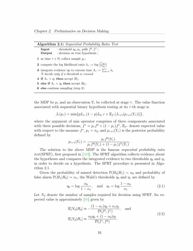
The solution to the above MDP is the famous sequential probability ratiotest(SPRT), first proposed in [103]. The SPRT algorithm collects evidence aboutthe hypotheses and compares the integrated evidence to two thresholds η0 and η1
in order to decide on a hypothesis. The SPRT procedure is presented in Algo-rithm 2.1.
Given the probability of missed detection P(H0|H1) = α0 and probability offalse alarm P(H1|H0) = α1, the Wald’s thresholds η0 and η1 are defined by
η0 = logα0
1− α1
, and η1 = log1− α0
α1
. (2.1)
Let Nd denote the number of samples required for decision using SPRT. Its ex-pected value is approximately [85] given by
E[Nd|H0] ≈ −(1− α1)η0 + α1η1
D(f 0, f 1), and
E[Nd|H1] ≈ α0η0 + (1− α0)η1
D(f 1, f 0).
(2.2)
16
Chapter 2. Preliminaries on Decision Making
The approximations in equation (2.2) are referred to as the Wald’s approxima-tions [85]. According to the Wald’s approximation, the value of the aggregatedSPRT statistic is exactly equal to one of the thresholds at the time of decision.It is known that the Wald’s approximation is accurate for large thresholds andsmall error probabilities.
2.2.2 Sequential Multiple hypothesis Testing
Consider M hypotheses Hk ∈ 0, . . . ,M−1 with their conditional probabilitydensity functions fk(y) := f(y|Hk). The sequential multiple hypothesis testingproblem is posed similar to the binary case. Suppose the cost of collecting anobservation be c ∈ R≥0 and a penalty Lk ∈ R≥0 is incurred for wrongly acceptinghypothesis Hk. The optimal stopping rule determined through an MDP. The stateof this MDP is the probability of each hypothesis being true and the action spacecomprises of M + 1 actions, namely, declare Hk, k ∈ 0, . . . ,M − 1, and continuesampling. Let the state at stage τ ∈ N of the MDP be pτ = (p0
τ , . . . , pM−1τ ) and
an observation Yτ be collected at stage τ . The value function associated withsequential multiple hypothesis testing at its τ -th iteration is
Jτ (pτ ) = min(1− p0τ )L0, . . . , (1− pM−1
τ )LM−1, c+ Ef∗ [Jτ+1(pτ+1(Yτ ))],
where the argument of min operator comprises of M + 1 components associatedwith M + 1 possible decisions, f ∗ =
∑M−1k=0 pkf
k, Ef∗ denote expected value withrespect to the measure f ∗ and pτ+1(Yτ ) is the posterior probability defined by
pkτ+1(Yτ ) =pkτf
k(Yτ )∑M−1j=0 pjf
j(Yτ ), for each k ∈ 0, . . . ,M − 1. (2.3)
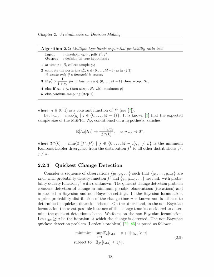
Opposed to the binary hypothesis case, there exists no closed form algorithmicsolution to the above MDP for M > 2. In particular, the optimal stopping ruleno longer comprises of constant functions, rather it comprises of curves in statespace that are difficult to characterize explicitly. However, in the asymptoticregime, i.e., when the cost of observations c → 0+ and the penalties for wrongdecisions are identical, these curves can be approximated by constant thresholds.In this asymptotic regime, a particular solution to the above MDP is the multiplehypothesis sequential probability ratio test (MSPRT) proposed in [7]. Note that theMSPRT reduces to SPRT for M = 2. The MSPRT is described in Algorithm 2.2.
The thresholds ηk are designed as functions of the frequentist error probabilities(i.e., the probabilities to accept a given hypothesis wrongly) αk, k ∈ 0, . . . ,M −1. Specifically, the thresholds are given by
ηk =αkγk, (2.4)
17
Chapter 2. Preliminaries on Decision Making
Algorithm 2.2: Multiple hypothesis sequential probability ratio test
Input : threshold η0, η1, pdfs f0, f1 ;Output : decision on true hypothesis ;
1 at time τ ∈ N, collect sample yτ ;
2 compute the posteriors pkτ , k ∈ 0, . . . ,M−1 as in (2.3)% decide only if a threshold is crossed
3 if phτ >1
1 + ηhfor at least one h ∈ 0, . . . ,M − 1 then accept H1;
4 else if Λτ < η0 then accept Hk with maximum pkτ ;
5 else continue sampling (step 1)
where γk ∈ (0, 1) is a constant function of fk (see [7]).Let ηmax = maxηj | j ∈ 0, . . . ,M − 1. It is known [7] that the expected
sample size of the MSPRT Nd, conditioned on a hypothesis, satisfies
E[Nd|Hk]→− log ηkD∗(k)
, as ηmax → 0+,
where D∗(k) = minD(fk, f j) | j ∈ 0, . . . ,M − 1, j 6= k is the minimumKullback-Leibler divergence from the distribution fk to all other distributions f j,j 6= k.
2.2.3 Quickest Change Detection
Consider a sequence of observations y1, y2, . . . such that y1, . . . , yυ−1 arei.i.d. with probability density function f 0 and yυ, yυ+1, . . . are i.i.d. with proba-bility density function f 1 with υ unknown. The quickest change detection problemconcerns detection of change in minimum possible observations (iterations) andin studied in Bayesian and non-Bayesian settings. In the Bayesian formulation,a prior probability distribution of the change time υ is known and is utilized todetermine the quickest detection scheme. On the other hand, in the non-Bayesianformulation the worst possible instance of the change time is considered to deter-mine the quickest detection scheme. We focus on the non-Bayesian formulation.Let υdet ≥ υ be the iteration at which the change is detected. The non-Bayesianquickest detection problem (Lorden’s problem) [72, 85] is posed as follows:
minimize supυ≥1
Eυ[υdet − υ + 1|υdet ≥ υ]
subject to Ef0 [υdet] ≥ 1/γ,(2.5)
18
Chapter 2. Preliminaries on Decision Making
Algorithm 2.3: Cumulative Sum Algorithm
Input : threshold η, pdfs f0, f1 ;Output : decision on change
1 at time τ ∈ N, collect sample yτ ;
2 integrate evidence Λτ := (Λτ−1 + log f1(yτ )f0(yτ ) )+
% decide only if a threshold is crossed
3 if Λτ > η then declare change is detected;
4 else continue sampling (step 1)
where Eυ[·] represents the expected value with respect to the distribution of ob-servation at iteration υ, and γ ∈ R>0 is a large constant and is called the falsealarm rate.
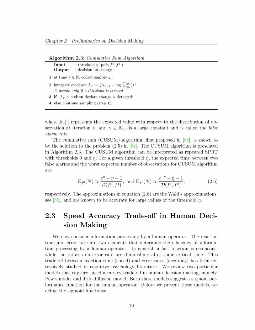
The cumulative sum (CUSUM) algorithm, first proposed in [68], is shown tobe the solution to the problem (2.5) in [64]. The CUSUM algorithm is presentedin Algorithm 2.3. The CUSUM algorithm can be interpreted as repeated SPRTwith thresholds 0 and η. For a given threshold η, the expected time between twofalse alarms and the worst expected number of observations for CUSUM algorithmare
Ef0(N) ≈ eη − η − 1
D(f 0, f 1), and Ef1(N) ≈ e−η + η − 1
D(f 1, f 0), (2.6)
respectively. The approximations in equation (2.6) are the Wald’s approximations,see [85], and are known to be accurate for large values of the threshold η.
2.3 Speed Accuracy Trade-off in Human Deci-
sion Making
We now consider information processing by a human operator. The reactiontime and error rate are two elements that determine the efficiency of informa-tion processing by a human operator. In general, a fast reaction is erroneous,while the returns on error rate are diminishing after some critical time. Thistrade-off between reaction time (speed) and error rates (accuracy) has been ex-tensively studied in cognitive psychology literature. We review two particularmodels that capture speed-accuracy trade-off in human decision making, namely,Pew’s model and drift-diffusion model. Both these models suggest a sigmoid per-formance function for the human operator. Before we present these models, wedefine the sigmoid functions:
19
Chapter 2. Preliminaries on Decision Making
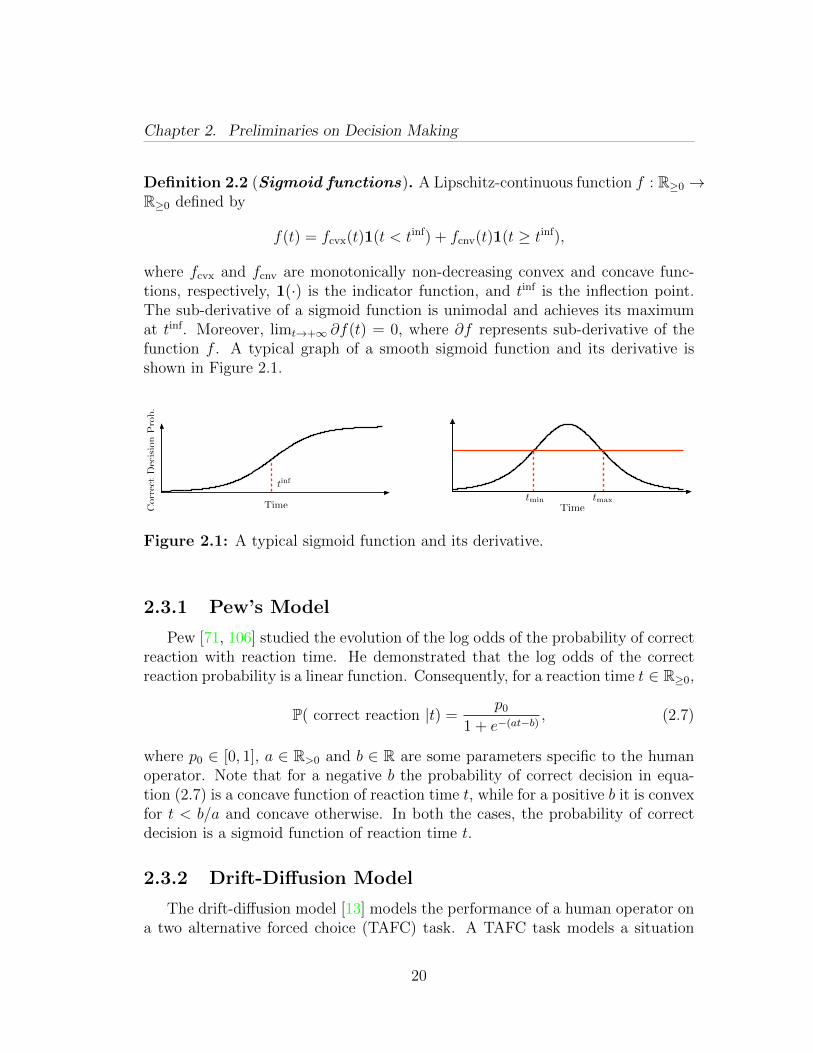
Definition 2.2 (Sigmoid functions). A Lipschitz-continuous function f : R≥0 →R≥0 defined by
f(t) = fcvx(t)1(t < tinf) + fcnv(t)1(t ≥ tinf),
where fcvx and fcnv are monotonically non-decreasing convex and concave func-tions, respectively, 1(·) is the indicator function, and tinf is the inflection point.The sub-derivative of a sigmoid function is unimodal and achieves its maximumat tinf. Moreover, limt→+∞ ∂f(t) = 0, where ∂f represents sub-derivative of thefunction f . A typical graph of a smooth sigmoid function and its derivative isshown in Figure 2.1.
Time
Time
tinf
tmin tmax
Cor
rect
Dec
isio
nP
rob.
Time
Time
tinf
tmin tmax
Cor
rect
Dec
isio
nP
rob.
Figure 2.1: A typical sigmoid function and its derivative.
2.3.1 Pew’s Model
Pew [71, 106] studied the evolution of the log odds of the probability of correctreaction with reaction time. He demonstrated that the log odds of the correctreaction probability is a linear function. Consequently, for a reaction time t ∈ R≥0,
P( correct reaction |t) =p0
1 + e−(at−b) , (2.7)
where p0 ∈ [0, 1], a ∈ R>0 and b ∈ R are some parameters specific to the humanoperator. Note that for a negative b the probability of correct decision in equa-tion (2.7) is a concave function of reaction time t, while for a positive b it is convexfor t < b/a and concave otherwise. In both the cases, the probability of correctdecision is a sigmoid function of reaction time t.
2.3.2 Drift-Diffusion Model
The drift-diffusion model [13] models the performance of a human operator ona two alternative forced choice (TAFC) task. A TAFC task models a situation
20
Chapter 2. Preliminaries on Decision Making
in which an operator has to decide among one of the two alternative hypotheses.The TAFC task models rely on three assumptions: (a) evidence is collected overtime in favor of each alternative; (b) the evidence collection process is random;and (c) a decision is made when the collected evidence is sufficient to choose onealternative over the other. A TAFC task is well modeled by the drift-diffusionmodel (DDM) [13]. The DDM captures the evidence aggregation in favor of analternative by
dx(t) = µdt+ σdW (t), x(0) = x0, (2.8)
where µ ∈ R in the drift rate, σ ∈ R>0 is the diffusion rate, W (·) is the standardWeiner process, and x0 ∈ R is the initial evidence. For an unbiased operator, theinitial evidence x0 = 0, while for a biased operator x0 captures the odds of priorprobabilities of alternative hypotheses; in particular, x0 = σ2 log(π/(1 − π))/2µ,where π is the prior probability of the first alternative.
For the information aggregation model (2.8), the human decision making isstudied in two paradigms, namely, free response and interrogation. In the freeresponse paradigm, the operator take their own time to decide on an alterna-tive, while in the interrogation paradigm, the operator works under time pressureand needs to decide within a given time. The free response paradigm is modeledvia two thresholds (positive and negative) and the operator decides in favor offirst/second alternative if the positive (negative) threshold is crossed from below(above). Under the free response, the DDM is akin to the SPRT and is in factthe continuum limit to the SPRT [13]. The reaction times under the free responseparadigm is a random variable with a unimodal probability distribution that isskewed to right. Such unimodal skewed reaction time probability distributions alsocapture human performance in several other tasks as well [88]. In this paradigm,the operator’s performance is well captured by the cumulative distribution func-tion of the reaction time. The cumulative distribution function associated with aunimodal probability distribution function is also a sigmoid function.
The interrogation paradigm is modeled via a single threshold. In particular, fora given deadline t ∈ R>0, the operator decides in favor of first (second) alternativeif the evidence collected by time t, i.e., x(t) is greater (smaller) than a thresholdν ∈ R. If the two alternatives are equally likely, then the threshold ν is chosento be zero. According to equation (2.8), the evidence collected until time t isa Gaussian random variable with mean µt + x0 and variance σ2t. Thus, theprobability to decide in favor of first alternative is
P(x(t) > ν) = 1− P(x(t) < ν) = 1− Φ(ν − µt− x0
σ√t
),
where Φ(·) is the standard normal cumulative distribution function. The proba-bility of making the correct decision at time t is P(x(t) > ν) and is a metric that
21
Chapter 2. Preliminaries on Decision Making
captures the operator’s performance. For an unbiased operator x0 = 0, and theperformance P(x(t) > ν) is a sigmoid function of allocated time t.
In addition to the above decision making performance, the sigmoid functionalso models the quality of human-machine communication [106], the human perfor-mance in multiple target search [47], and the advertising response function [102].
22
Chapter 3
Randomized Sensor Selection inSequential Hypothesis Testing
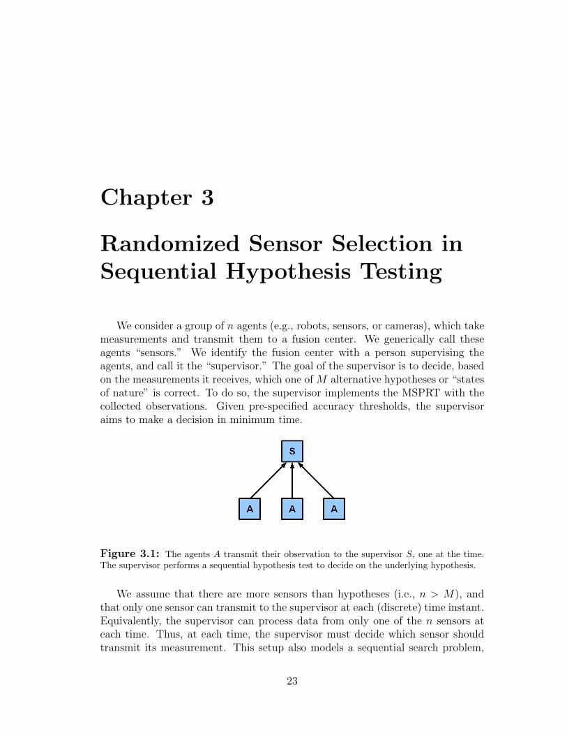
We consider a group of n agents (e.g., robots, sensors, or cameras), which takemeasurements and transmit them to a fusion center. We generically call theseagents “sensors.” We identify the fusion center with a person supervising theagents, and call it the “supervisor.” The goal of the supervisor is to decide, basedon the measurements it receives, which one of M alternative hypotheses or “statesof nature” is correct. To do so, the supervisor implements the MSPRT with thecollected observations. Given pre-specified accuracy thresholds, the supervisoraims to make a decision in minimum time.
Figure 3.1: The agents A transmit their observation to the supervisor S, one at the time.The supervisor performs a sequential hypothesis test to decide on the underlying hypothesis.
We assume that there are more sensors than hypotheses (i.e., n > M), andthat only one sensor can transmit to the supervisor at each (discrete) time instant.Equivalently, the supervisor can process data from only one of the n sensors ateach time. Thus, at each time, the supervisor must decide which sensor shouldtransmit its measurement. This setup also models a sequential search problem,
23
Chapter 3. Randomized Sensor Selection in Sequential Hypothesis Testing
where one out of n sensors is sequentially activated to establish the most likelyintruder location out of M possibilities; see [22] for a related problem. In thischapter, our objective is to determine the optimal sensor(s) that the supervisormust observe in order to minimize the decision time.
We adopt the following notation. Let H0, . . . , HM−1 denote the M ≥ 2hypotheses. The time required by sensor s ∈ 1, . . . , n to collect, process andtransmit its measurement is a random variable Ts ∈ R>0, with finite first andsecond moment. We denote the mean processing time of sensor s by Ts ∈ R>0.Let st ∈ 1, . . . , n indicate which sensor transmits its measurement at time t ∈ N.The measurement of sensor s at time t is y(t, s). For the sake of convenience, wedenote y(t, st) by yt. For k ∈ 0, . . . ,M−1, let fks : R→ R denote the probabilitydensity function of the measurement y at sensor s conditioned on the hypothesisHk. Let fk : 1, . . . , n × R → R be the probability density function of the pair(s, y), conditioned on hypothesis Hk. For k ∈ 0, . . . ,M − 1, let αk denote thedesired bound on probability of incorrect decision conditioned on hypothesis Hk.We make the following standard assumption:
Conditionally-independent observations: Conditioned on hypothesisHk, themeasurement y(t, s) is independent of y(t, s), for (t, s) 6= (t, s).
We adopt a randomized strategy in which the supervisor chooses a sensor ran-domly at each time instant; the probability to choose sensor s is stationary andgiven by qs, for s ∈ 1, . . . , n. Also, the supervisor uses the data collected fromthe randomized sensors to execute a multi-hypothesis sequential hypothesis test.For the stationary randomized strategy, note that fk(s, y) = qsf
ks (y). We study
our proposed randomized strategy under the following assumptions about thesensors.
Distinct sensors: There are no two sensors with identical conditioned probabil-ity density fks (y) and mean processing time Ts. (If there are such sensors, weclub them together in a single node, and distribute the probability assignedto that node equally among them.)
Finitely-informative sensors: Each sensor s ∈ 1, . . . , n has the followingproperty: for any two hypotheses k, j ∈ 0, . . . ,M − 1, k 6= j,
(i). the support of fks is equal to the support of f js ,
(ii). fks 6= f js almost surely in fks , and
(iii). conditioned on hypothesisHk, the first and second moment of log(fks (Y )/f js (Y ))are finite.
24
Chapter 3. Randomized Sensor Selection in Sequential Hypothesis Testing
Remark 3.1 (Finitely informative sensors). The finitely-informative sen-sors assumption is equivalently restated as follows: each sensor s ∈ 1, . . . , nsatisfies 0 < D(fks , f
js ) < +∞ for any two hypotheses k, j ∈ 0, . . . ,M − 1,
k 6= j.
Remark 3.2 (Stationary policy). We study a stationary policy because it issimple to implement, it is amenable to rigorous analysis and it has intuitively-appealing properties (e.g., we show that the optimal stationary policy requiresthe observation of only as many sensors as the number of hypothesis). On thecontrary, if we do not assume a stationary policy, the optimal solution wouldbe based on dynamic programming and, correspondingly, would be complex toimplement, analytically intractable, and would lead to only numerical results.
3.1 MSPRT with randomized sensor selection
We call the MSPRT with the data collected from n sensors while observingonly one sensor at a time as the MSPRT with randomized sensor selection. Foreach sensor s, define D∗s(k) = minD(fks , f
js ) | j ∈ 0, . . . ,M − 1, j 6= k. The
sensor to be observed at each time is determined through a randomized policy,and the probability of choosing sensor s is stationary and given by qs. Assumethat the sensor st ∈ 1, . . . , n is chosen at time instant t, then the posteriorprobability after the observations yt, t ∈ 1, . . . , τ, is given by
pkτ = P(Hk|y1, . . . , yτ ) =
∏τt=1 f
k(st, yt)∑M−1j=0
∏τt=1 f
j(st, yt)
=
∏τt=1 qstf
kst(yt)∑M−1
j=0
∏τt=1 qstf
jst(yt)
=
∏τt=1 f
kst(yt)∑M−1
j=0
∏τt=1 f
jst(yt)
, (3.1)
and, at any given time τ , the hypothesis with maximum posterior probability pkτis the one maximizing
∏τt=1 f
kst(yt). Note that the sequence (st, yt)t∈N is an i.i.d.
realization of the pair (s, Ys), where Ys is the measurement of sensor s.For thresholds ηk, k ∈ 0, . . . ,M − 1, defined in equation (2.4), the MSPRT
with randomized sensor selection is defined identically to the Algorithm 2.2, wherethe first two instructions (steps 1 and 2) are replaced by:
1 at time τ ∈ N, select a random sensor sτ according to the probability vector q and collecta sample yτ
2 compute the posteriors pkτ , k ∈ 0, . . . ,M−1 as in (3.1)
25
Chapter 3. Randomized Sensor Selection in Sequential Hypothesis Testing
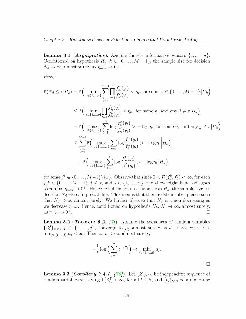
Lemma 3.1 (Asymptotics). Assume finitely informative sensors 1, . . . , n.Conditioned on hypothesis Hk, k ∈ 0, . . . ,M − 1, the sample size for decisionNd →∞ almost surely as ηmax → 0+.
Proof.
P(Nd ≤ τ |Hk) = P(
mina∈1,...,τ
M−1∑j=1
j 6=v
a∏t=1
f jst(yt)
f vst(yt)< ηv, for some v ∈ 0, . . . ,M − 1
∣∣Hk
)
≤ P(
mina∈1,...,τ
a∏t=1
f jst(yt)
f vst(yt)< ηv, for some v, and any j 6= v
∣∣Hk
)= P
(max
a∈1,...,τ
a∑t=1
logf vst(yt)
f jst(yt)> − log ηv, for some v, and any j 6= v
∣∣Hk
)≤
M−1∑v=0v 6=k
P(
maxa∈1,...,τ
a∑t=1
logf vst(yt)
fkst(yt)> − log ηv
∣∣∣∣Hk
)
+ P(
maxa∈1,...,τ
a∑t=1
logfkst(yt)
f j∗st (yt)
> − log ηk∣∣Hk
),
for some j∗ ∈ 0, . . . ,M−1\k. Observe that since 0 < D(fks , fjs ) <∞, for each
j, k ∈ 0, . . . ,M − 1, j 6= k, and s ∈ 1, . . . , n, the above right hand side goesto zero as ηmax → 0+. Hence, conditioned on a hypothesis Hk, the sample size fordecision Nd →∞ in probability. This means that there exists a subsequence suchthat Nd → ∞ almost surely. We further observe that Nd is a non decreasing aswe decrease ηmax. Hence, conditioned on hypothesis Hk, Nd →∞, almost surely,as ηmax → 0+.
Lemma 3.2 (Theorem 5.2, [7]). Assume the sequences of random variablesZj
t t∈N, j ∈ 1, . . . , d, converge to µj almost surely as t → ∞, with 0 <minj∈1,...,d µj <∞. Then as t→∞, almost surely,
−1
tlog( d∑j=1
e−tZjt
)→ min
j∈1,...,dµj.
Lemma 3.3 (Corollary 7.4.1, [76]). Let Ztt∈N be independent sequence ofrandom variables satisfying E[Z2
t ] <∞, for all t ∈ N, and btt∈N be a monotone
26

Chapter 3. Randomized Sensor Selection in Sequential Hypothesis Testing
sequence such that bt →∞ as t→∞. If∑∞
i=1 Var (Zi/bi) <∞, then∑ti=1 Zi − E[
∑ti=1 Zi]
bt→ 0, almost surely as t→∞.
Lemma 3.4 (Theorem 2.1, [40]). Let Ztt∈N be a sequence of random vari-ables and τ(a)a∈R≥0
be a family of positive, integer valued random variables.Suppose that Zt → Z almost surely as t → ∞, and τ(a) → ∞ almost surely asa→∞. Then Zτ(a) → Z almost surely as a→∞.
We now present the main result of this section, whose proof is a variation ofthe proofs for MSPRT in [7].
Theorem 3.5 (MSPRT with randomized sensor selection). Assume finitely-informative sensors 1, . . . , n, and independent observations conditioned on hy-pothesis Hk, k ∈ 0, . . . ,M − 1. For the MSPRT with randomized sensor selec-tion, the following statements hold:
(i). conditioned on a hypothesis, the sample size for decision Nd is finite almostsurely;
(ii). conditioned on hypothesis Hk, the sample size for decision Nd, as ηmax → 0+,satisfies
Nd
− log ηk→ 1∑n
s=1 qsD∗s(k)almost surely;
(iii). the expected sample size satisfies
E[Nd|Hk]
− log ηk→ 1∑n
s=1 qsD∗s(k), as ηmax → 0+; (3.2)
(iv). conditioned on hypothesis Hk, the decision time Td, as ηmax → 0+, satisfies
Td− log ηk
→∑n
s=1 qsTs∑ns=1 qsD∗s(k)
almost surely;
(v). the expected decision time satisfies
E[Td|Hk]
− log ηk→
∑ns=1 qsTs∑n
s=1 qsD∗s(k)≡ q · Tq ·Dk
, (3.3)
where T ,Dk ∈ Rn>0 are arrays of mean processing times Ts and minimum
Kullback-Leibler distances D∗s(k).
27
Chapter 3. Randomized Sensor Selection in Sequential Hypothesis Testing
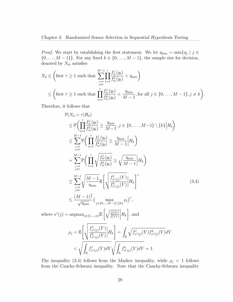
Proof. We start by establishing the first statement. We let ηmin = minηj | j ∈0, . . . ,M − 1. For any fixed k ∈ 0, . . . ,M − 1, the sample size for decision,denoted by Nd, satisfies
Nd ≤(
first τ ≥ 1 such thatM−1∑j=0
j 6=k
τ∏t=1
f jst(yt)
fkst(yt)< ηmin
)
≤(
first τ ≥ 1 such thatτ∏t=1
f jst(yt)
fkst(yt)<
ηmin
M − 1, for all j ∈ 0, . . . ,M − 1, j 6= k
).
Therefore, it follows that
P(Nd > τ |Hk)
≤ P( τ∏t=1
f jst(yt)
fkst(yt)≥ ηmin
M−1, j ∈ 0, . . . ,M−1 \ k
∣∣∣Hk
)
≤M−1∑j=0
j 6=k
P( τ∏
t=1
f jst(yt)
fkst(yt)≥ ηmin
M − 1
∣∣∣∣Hk
)
=M−1∑j=0
j 6=k
P( τ∏
t=1
√f jst(yt)
fkst(yt)≥√
ηmin
M − 1
∣∣∣∣Hk
)
≤M−1∑j=0
j 6=k
√M − 1
ηmin
E
[√√√√f js∗(j)(Y )
fks∗(j)(Y )
∣∣∣∣Hk
]τ(3.4)
≤ (M − 1)32
√ηmin
(max
j∈0,...,M−1\kρj)τ,
where s∗(j) = argmaxs∈1,...,nE[√
fjs (Y )fks (Y )
∣∣∣∣Hk
], and
ρj = E
[√√√√f js∗(j)(Y )
fks∗(j)(Y )
∣∣∣∣Hk
]=
∫R
√f js∗(j)(Y )fks∗(j)(Y )dY
<
√∫Rf js∗(j)(Y )dY
√∫Rfks∗(j)(Y )dY = 1.
The inequality (3.4) follows from the Markov inequality, while ρj < 1 followsfrom the Cauchy-Schwarz inequality. Note that the Cauchy-Schwarz inequality
28

Chapter 3. Randomized Sensor Selection in Sequential Hypothesis Testing
is strict because f js∗(j) 6= fks∗(j) almost surely in fks∗(j). To establish almost sureconvergence, note that
∞∑τ=1
P(Nd > τ |Hk) ≤∞∑τ=1
(M − 1)32
√ηmin
(max
j∈0,...,M−1\kρj)τ<∞.
Therefore, by Borel-Cantelli lemma [76], it follows that
P(lim supτ→∞
[Nd > τ ]) = 1− P(lim infτ→∞
[Nd ≤ τ ]) = 0.
Thus, for τ large enough, all realizations in the set lim infτ→∞[Nd ≤ τ ], convergein finite number of steps. This proves the almost sure convergence on the MSPRTwith randomized sensor selection.
To prove the second statement, for hypothesis Hk, let
Nd =
(first τ ≥ 1 such that
M−1∑j=0
j 6=k
τ∏t=1
f jst(yt)
fkst(yt)< ηk
),
and, accordingly, note that
M−1∑j=0
j 6=k
Nd−1∏t=1
f jst(yt)
fkst(yt)≥ ηk, and
M−1∑j=0
j 6=k
Nd∏t=1
f jst(yt)
fkst(yt)< ηk.
Some algebraic manipulations on these inequalities yield
−1
Nd − 1log
(M−1∑j=0
j 6=k
E(−Nd−1∑t=1
logfkst(yt)
f jst(yt)
))≤ − log ηk
Nd − 1,
−1
Nd
log
(M−1∑j=0
j 6=k
E(−
Nd∑t=1
logfkst(yt)
f jst(yt)
))>− log ηk
Nd
.
(3.5)
Observe that Nd ≥ Nd, hence from Lemma 3.1, Nd → ∞ almost surely asηmax → 0+. In the limit Nd →∞, the supremum and infimum in inequalities (3.5)converge to the same value. From Lemma 3.3, and Lemma 3.4
1
Nd
Nd∑t=1
logfkst(yt)
f jst(yt)→ 1
Nd
Nd∑t=1
E[
logfkst(yt)
f jst(yt)
∣∣∣∣Hk
]→
n∑s=1
qsD(fks , fjs ), almost surely,
29
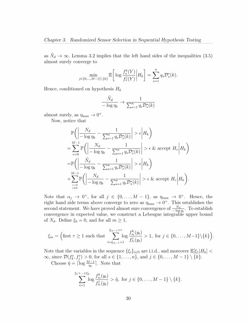
Chapter 3. Randomized Sensor Selection in Sequential Hypothesis Testing
as Nd → ∞. Lemma 3.2 implies that the left hand sides of the inequalities (3.5)almost surely converge to
minj∈0,...,M−1\k
E[
logfks (Y )
f js (Y )
∣∣∣∣Hk
]=
n∑s=1
qsD∗s(k).
Hence, conditioned on hypothesis Hk
Nd
− log ηk→ 1∑n
s=1 qsD∗s(k)
almost surely, as ηmax → 0+.Now, notice that
P(∣∣∣∣ Nd
− log ηk− 1∑n
s=1 qsD∗s(k)
∣∣∣∣ > ε
∣∣∣∣Hk
)=
M−1∑v=0
P(∣∣∣∣ Nd
− log ηk− 1∑n
s=1 qsD∗s(k)
∣∣∣∣ > ε & accept Hv
∣∣∣∣Hk
)=P(∣∣∣∣ Nd
− log ηk− 1∑n
s=1 qsD∗s(k)
∣∣∣∣ > ε
∣∣∣∣Hk
)+M−1∑v=0v 6=k
P(∣∣∣∣ Nd
− log ηk− 1∑n
s=1 qsD∗s(k)
∣∣∣∣ > ε & accept Hv
∣∣∣∣Hk
).
Note that αj → 0+, for all j ∈ 0, . . . ,M − 1, as ηmax → 0+. Hence, theright hand side terms above converge to zero as ηmax → 0+. This establishes thesecond statement. We have proved almost sure convergence of Nd
− log ηk. To establish
convergence in expected value, we construct a Lebesgue integrable upper boundof Nd. Define ξ0 = 0, and for all m ≥ 1,
ξm =(
first τ ≥ 1 such that
ξm−1+τ∑t=ξm−1+1
logfkst(yt)
f jst(yt)> 1, for j ∈ 0, . . . ,M−1\k
).
Note that the variables in the sequence ξii∈N are i.i.d., and moreover E[ξ1|Hk] <∞, since D(f sk , f
sj ) > 0, for all s ∈ 1, . . . , n, and j ∈ 0, . . . ,M − 1 \ k.
Choose η = dlog M−1ηke. Note that
ξ1+...+ξη∑t=1
logfkst(yt)
f jst(yt)> η, for j ∈ 0, . . . ,M − 1 \ k.
30
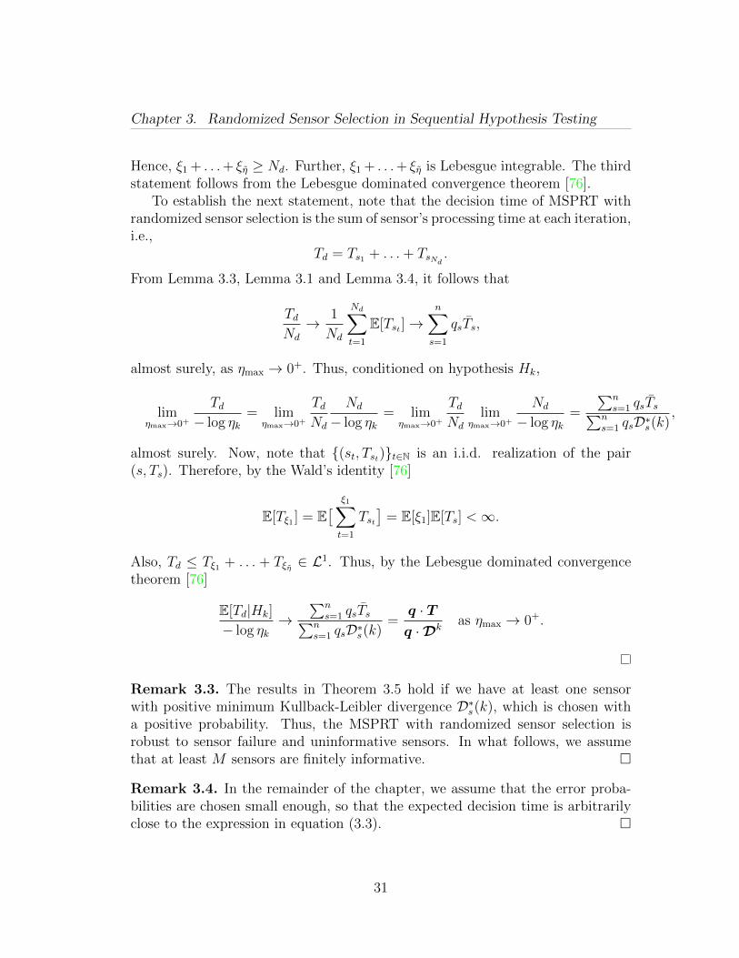
Chapter 3. Randomized Sensor Selection in Sequential Hypothesis Testing
Hence, ξ1 + . . .+ ξη ≥ Nd. Further, ξ1 + . . .+ ξη is Lebesgue integrable. The thirdstatement follows from the Lebesgue dominated convergence theorem [76].
To establish the next statement, note that the decision time of MSPRT withrandomized sensor selection is the sum of sensor’s processing time at each iteration,i.e.,
Td = Ts1 + . . .+ TsNd .
From Lemma 3.3, Lemma 3.1 and Lemma 3.4, it follows that
TdNd
→ 1
Nd
Nd∑t=1
E[Tst ]→n∑s=1
qsTs,
almost surely, as ηmax → 0+. Thus, conditioned on hypothesis Hk,
limηmax→0+
Td− log ηk
= limηmax→0+
TdNd
Nd
− log ηk= lim
ηmax→0+
TdNd
limηmax→0+
Nd
− log ηk=
∑ns=1 qsTs∑n
s=1 qsD∗s(k),
almost surely. Now, note that (st, Tst)t∈N is an i.i.d. realization of the pair(s, Ts). Therefore, by the Wald’s identity [76]
E[Tξ1 ] = E[ ξ1∑t=1
Tst]
= E[ξ1]E[Ts] <∞.
Also, Td ≤ Tξ1 + . . . + Tξη ∈ L1. Thus, by the Lebesgue dominated convergencetheorem [76]
E[Td|Hk]
− log ηk→
∑ns=1 qsTs∑n
s=1 qsD∗s(k)=q · Tq ·Dk
as ηmax → 0+.
Remark 3.3. The results in Theorem 3.5 hold if we have at least one sensorwith positive minimum Kullback-Leibler divergence D∗s(k), which is chosen witha positive probability. Thus, the MSPRT with randomized sensor selection isrobust to sensor failure and uninformative sensors. In what follows, we assumethat at least M sensors are finitely informative.
Remark 3.4. In the remainder of the chapter, we assume that the error proba-bilities are chosen small enough, so that the expected decision time is arbitrarilyclose to the expression in equation (3.3).
31
Chapter 3. Randomized Sensor Selection in Sequential Hypothesis Testing
Remark 3.5. The MSPRT with randomized sensor selection may not be theoptimal sequential test. In fact, this test corresponds to a stationary open-loopstrategy. In this chapter we wish to determine a time-optimal stationary open-loopstrategy, as motivated in Remark 3.2.
Remark 3.6. If the minimum Kullback-Leibler divergence D∗s(k) is the same forany given s ∈ 1, . . . , n, and for each k ∈ 0, . . . ,M − 1, and all thresholdsηk are identical, then the expected decision time is the same conditioned on anyhypothesis Hk. For example, if conditioned on hypothesis Hk, k ∈ 0, . . . ,M−1,and sensor s ∈ 1, . . . , n, the observation is generated from a Gaussian distribu-tion with mean k and variance σ2
s , then the minimum Kullback-Leibler divergencefrom hypothesis k, for sensor s is D∗s(k) = 1/2σ2
s , which is independent of k.
3.2 Optimal sensor selection
In this section we consider sensor selection problems with the aim to mini-mize the expected decision time of a sequential hypothesis test with randomizedsensor selection. As exemplified in Theorem 3.5, the problem features multipleconditioned decision times and, therefore, multiple distinct cost functions are ofinterest. In Section 3.2.1 below, we aim to minimize the decision time conditionedupon one specific hypothesis being true; in Section 3.2.2 and 3.2.3 we will considerworst-case and average decision times. In all three scenarios the decision variablestake values in the probability simplex.
Minimizing decision time conditioned upon a specific hypothesis may be ofinterest when fast reaction is required in response to the specific hypothesis beingindeed true. For example, in change detection problems one aims to quicklydetect a change in a stochastic process; the CUSUM algorithm (also referred to asPage’s test) [68] is widely used in such problems. It is known [6] that, with fixedthreshold, the CUSUM algorithm for quickest change detection is equivalent toan SPRT on the observations taken after the change has occurred. We considerthe minimization problem for a single conditioned decision time in Section 3.2.1below and we show that, in this case, observing the best sensor each time is theoptimal strategy.
In general, no specific hypothesis might play a special role in the problem and,therefore, it is of interest to simultaneously minimize multiple decision times overthe probability simplex. This is a multi-objective optimization problem, and mayhave Pareto-optimal solutions. We tackle this problem by constructing a singleaggregate objective function. In the binary hypothesis case, we construct twosingle aggregate objective functions as the maximum and the average of the two
32
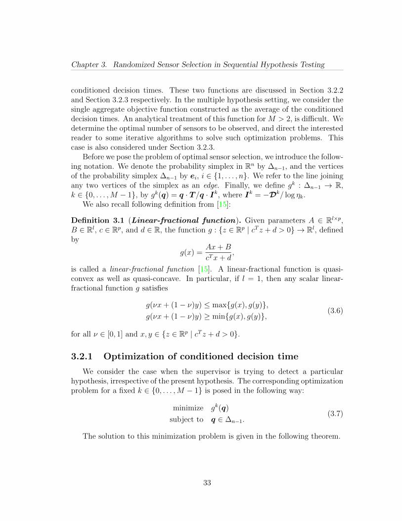
Chapter 3. Randomized Sensor Selection in Sequential Hypothesis Testing
conditioned decision times. These two functions are discussed in Section 3.2.2and Section 3.2.3 respectively. In the multiple hypothesis setting, we consider thesingle aggregate objective function constructed as the average of the conditioneddecision times. An analytical treatment of this function for M > 2, is difficult. Wedetermine the optimal number of sensors to be observed, and direct the interestedreader to some iterative algorithms to solve such optimization problems. Thiscase is also considered under Section 3.2.3.
Before we pose the problem of optimal sensor selection, we introduce the follow-ing notation. We denote the probability simplex in Rn by ∆n−1, and the verticesof the probability simplex ∆n−1 by ei, i ∈ 1, . . . , n. We refer to the line joiningany two vertices of the simplex as an edge. Finally, we define gk : ∆n−1 → R,k ∈ 0, . . . ,M − 1, by gk(q) = q · T /q · Ik, where Ik = −Dk/ log ηk.
We also recall following definition from [15]:
Definition 3.1 (Linear-fractional function). Given parameters A ∈ Rl×p,B ∈ Rl, c ∈ Rp, and d ∈ R, the function g : z ∈ Rp | cT z + d > 0 → Rl, definedby
g(x) =Ax+B
cTx+ d,
is called a linear-fractional function [15]. A linear-fractional function is quasi-convex as well as quasi-concave. In particular, if l = 1, then any scalar linear-fractional function g satisfies
g(νx+ (1− ν)y) ≤ maxg(x), g(y),g(νx+ (1− ν)y) ≥ ming(x), g(y),
(3.6)
for all ν ∈ [0, 1] and x, y ∈ z ∈ Rp | cT z + d > 0.
3.2.1 Optimization of conditioned decision time
We consider the case when the supervisor is trying to detect a particularhypothesis, irrespective of the present hypothesis. The corresponding optimizationproblem for a fixed k ∈ 0, . . . ,M − 1 is posed in the following way:
minimize gk(q)
subject to q ∈ ∆n−1.(3.7)
The solution to this minimization problem is given in the following theorem.
33
Chapter 3. Randomized Sensor Selection in Sequential Hypothesis Testing
Theorem 3.6 (Optimization of conditioned decision time). The solutionto the minimization problem (3.7) is q∗ = es∗ , where s∗ is given by
s∗ = argmins∈1,...,n
TsIks,
and the minimum objective function is
E[T ∗d |Hk] =Ts∗
Iks∗. (3.8)
Proof. We notice that objective function is a linear-fractional function. In thefollowing argument, we show that the minima occurs at one of the vertices of thesimplex.
We first notice that the probability simplex is the convex hull of the vertices,i.e., any point q in the probability simplex can be written as
q =n∑s=1
αses,n∑s=1
αs = 1, and αs ≥ 0.
We invoke equation (3.6), and observe that for some β ∈ [0, 1] and for any s, r ∈1, . . . , n
gk(βes + (1− β)er) ≥ mingk(es), gk(er), (3.9)
which can be easily generalized to
gk(q) ≥ mins∈1,...,n
gk(es), (3.10)
for any point q in the probability simplex ∆n−1. Hence, minima will occur at oneof the vertices es∗ , where s∗ is given by
s∗ = argmins∈1,...,n
gk(es) = argmins∈1,...,n
TsIks.
3.2.2 Optimization of the worst case decision time
For the binary hypothesis testing, we consider the multi-objective optimizationproblem of minimizing both decision times simultaneously. We construct singleaggregate objective function by considering the maximum of the two objective
34
Chapter 3. Randomized Sensor Selection in Sequential Hypothesis Testing
functions. This turns out to be a worst case analysis, and the optimization problemfor this case is posed in the following way:
minimize maxg0(q), g1(q)
,
subject to q ∈ ∆n−1.(3.11)
Before we move on to the solution of above minimization problem, we statethe following results.
Lemma 3.7 (Monotonicity of conditioned decision times). The functionsgk, k ∈ 0, . . . ,M − 1 are monotone on the probability simplex ∆n−1, in thesense that given two points qa, qb ∈ ∆n−1, the function gk is monotonically non-increasing or monotonically non-decreasing along the line joining qa and qb.
Proof. Consider probability vectors qa, qb ∈ ∆n−1. Any point q on line joining qaand qb can be written as q(ν) = νqa+(1−ν)qb, ν ∈ ]0, 1[. We note that gk(q(ν))is given by:
gk(q(ν)) =ν(qa · T ) + (1− ν)(qb · T )
ν(qa · Ik) + (1− ν)(qb · Ik).
The derivative of gk along the line joining qa and qb is given by
d
dνgk(q(ν)) =
(gk(qa)− gk(qb)
) (qa · Ik)(qb · Ik)(ν(qa · Ik) + (1− ν)(qb · Ik))2
.
We note that the sign of the derivative of gk along the line joining two pointsqa, qb is fixed by the choice of qa and qb. Hence, the function gk is monotoneover the line joining qa and qb. Moreover, note that if gk(qa) 6= gk(qb), then gk isstrictly monotone. Otherwise, gk is constant over the line joining qa and qb.
Lemma 3.8 (Location of min-max ). Define g : ∆n−1 → R≥0 by g = maxg0, g1.A minimum of g lies at the intersection of the graphs of g0 and g1, or at somevertex of the probability simplex ∆n−1.
Proof. The idea of the proof is illustrated in Figure 3.2. We now prove it rigor-ously.Case 1: The graphs of g0 and g1 do not intersect at any point in the simplex ∆n−1.
In this case, one of the functions g0 and g1 is an upper bound to the otherfunction at every point in the probability simplex ∆n−1. Hence, g = gk, for somek ∈ 0, 1, at every point in the probability simplex ∆n−1. From Theorem 3.6, we
35
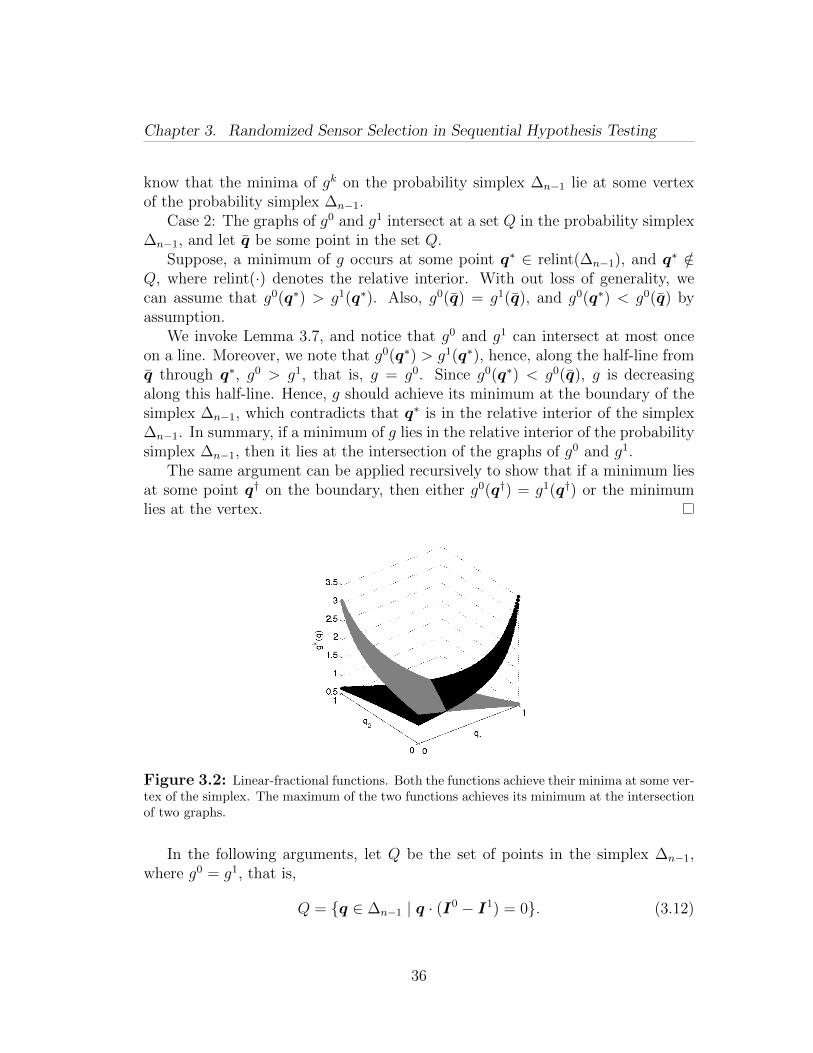
Chapter 3. Randomized Sensor Selection in Sequential Hypothesis Testing
know that the minima of gk on the probability simplex ∆n−1 lie at some vertexof the probability simplex ∆n−1.
Case 2: The graphs of g0 and g1 intersect at a set Q in the probability simplex∆n−1, and let q be some point in the set Q.
Suppose, a minimum of g occurs at some point q∗ ∈ relint(∆n−1), and q∗ /∈Q, where relint(·) denotes the relative interior. With out loss of generality, wecan assume that g0(q∗) > g1(q∗). Also, g0(q) = g1(q), and g0(q∗) < g0(q) byassumption.
We invoke Lemma 3.7, and notice that g0 and g1 can intersect at most onceon a line. Moreover, we note that g0(q∗) > g1(q∗), hence, along the half-line fromq through q∗, g0 > g1, that is, g = g0. Since g0(q∗) < g0(q), g is decreasingalong this half-line. Hence, g should achieve its minimum at the boundary of thesimplex ∆n−1, which contradicts that q∗ is in the relative interior of the simplex∆n−1. In summary, if a minimum of g lies in the relative interior of the probabilitysimplex ∆n−1, then it lies at the intersection of the graphs of g0 and g1.
The same argument can be applied recursively to show that if a minimum liesat some point q† on the boundary, then either g0(q†) = g1(q†) or the minimumlies at the vertex.
Figure 3.2: Linear-fractional functions. Both the functions achieve their minima at some ver-tex of the simplex. The maximum of the two functions achieves its minimum at the intersectionof two graphs.
In the following arguments, let Q be the set of points in the simplex ∆n−1,where g0 = g1, that is,
Q = q ∈ ∆n−1 | q · (I0 − I1) = 0. (3.12)
36
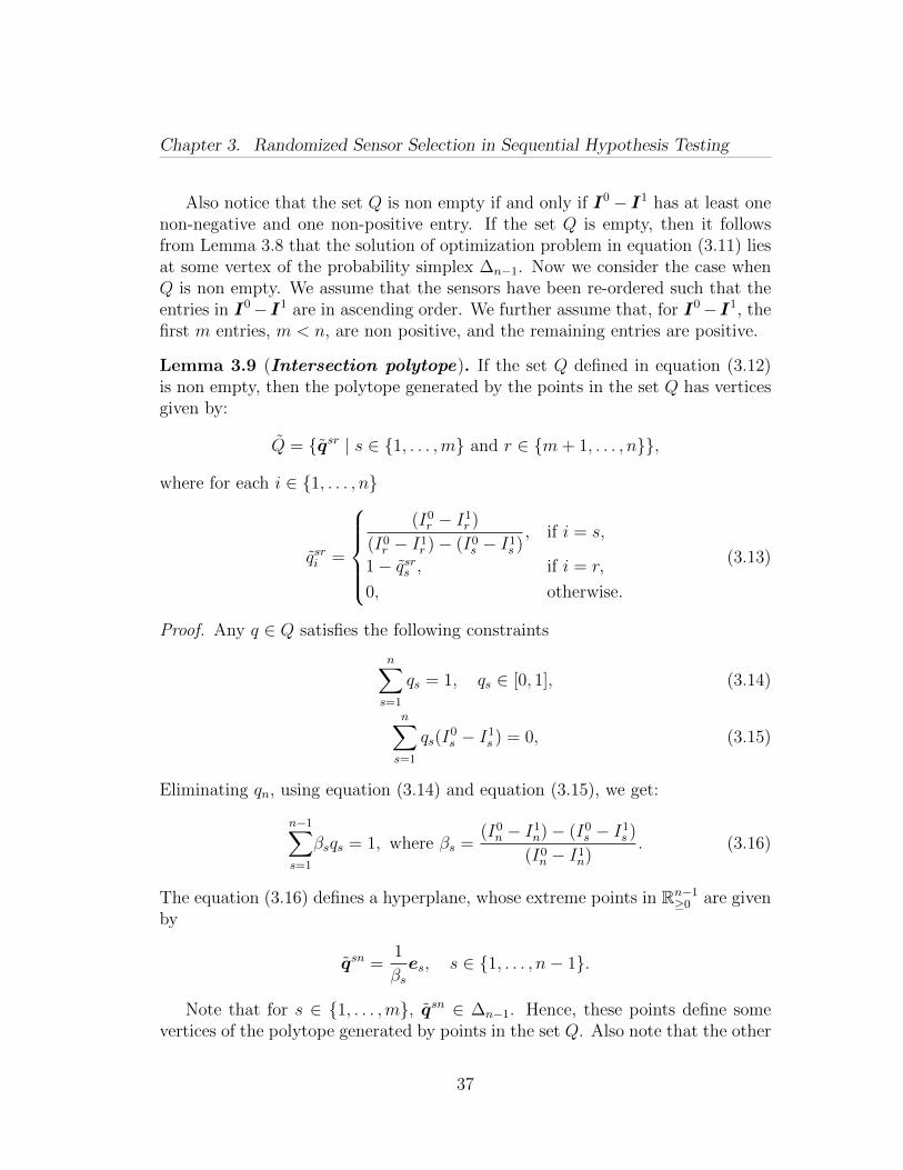
Chapter 3. Randomized Sensor Selection in Sequential Hypothesis Testing
Also notice that the set Q is non empty if and only if I0− I1 has at least onenon-negative and one non-positive entry. If the set Q is empty, then it followsfrom Lemma 3.8 that the solution of optimization problem in equation (3.11) liesat some vertex of the probability simplex ∆n−1. Now we consider the case whenQ is non empty. We assume that the sensors have been re-ordered such that theentries in I0−I1 are in ascending order. We further assume that, for I0−I1, thefirst m entries, m < n, are non positive, and the remaining entries are positive.
Lemma 3.9 (Intersection polytope). If the set Q defined in equation (3.12)is non empty, then the polytope generated by the points in the set Q has verticesgiven by:
Q = qsr | s ∈ 1, . . . ,m and r ∈ m+ 1, . . . , n,
where for each i ∈ 1, . . . , n
qsri =
(I0r − I1
r )
(I0r − I1
r )− (I0s − I1
s ), if i = s,
1− qsrs , if i = r,
0, otherwise.
(3.13)
Proof. Any q ∈ Q satisfies the following constraints
n∑s=1
qs = 1, qs ∈ [0, 1], (3.14)
n∑s=1
qs(I0s − I1
s ) = 0, (3.15)
Eliminating qn, using equation (3.14) and equation (3.15), we get:
n−1∑s=1
βsqs = 1, where βs =(I0n − I1
n)− (I0s − I1
s )
(I0n − I1
n). (3.16)
The equation (3.16) defines a hyperplane, whose extreme points in Rn−1≥0 are given
by
qsn =1
βses, s ∈ 1, . . . , n− 1.
Note that for s ∈ 1, . . . ,m, qsn ∈ ∆n−1. Hence, these points define somevertices of the polytope generated by points in the set Q. Also note that the other
37
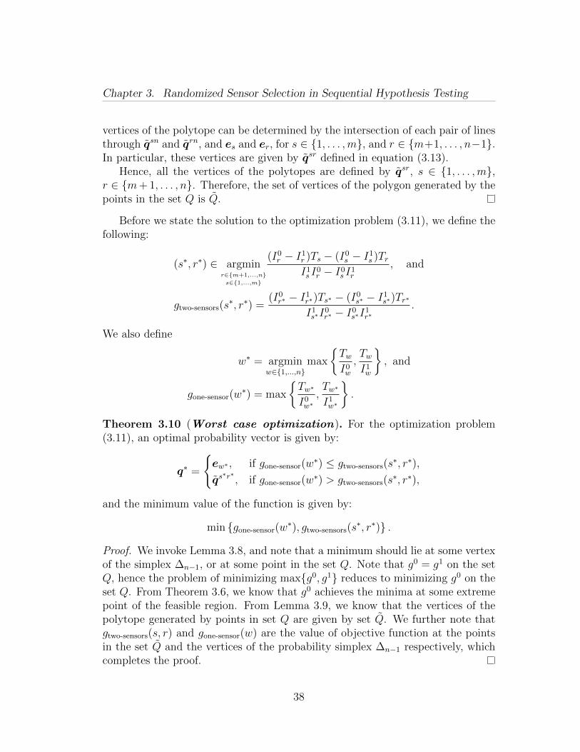
Chapter 3. Randomized Sensor Selection in Sequential Hypothesis Testing
vertices of the polytope can be determined by the intersection of each pair of linesthrough qsn and qrn, and es and er, for s ∈ 1, . . . ,m, and r ∈ m+1, . . . , n−1.In particular, these vertices are given by qsr defined in equation (3.13).
Hence, all the vertices of the polytopes are defined by qsr, s ∈ 1, . . . ,m,r ∈ m+ 1, . . . , n. Therefore, the set of vertices of the polygon generated by thepoints in the set Q is Q.
Before we state the solution to the optimization problem (3.11), we define thefollowing:
(s∗, r∗) ∈ argminr∈m+1,...,ns∈1,...,m
(I0r − I1
r )Ts − (I0s − I1
s )TrI1s I
0r − I0
s I1r
, and
gtwo-sensors(s∗, r∗) =
(I0r∗ − I1
r∗)Ts∗ − (I0s∗ − I1
s∗)Tr∗
I1s∗I
0r∗ − I0
s∗I1r∗
.
We also define
w∗ = argminw∈1,...,n
max
TwI0w
,TwI1w
, and
gone-sensor(w∗) = max
Tw∗
I0w∗,Tw∗
I1w∗
.
Theorem 3.10 (Worst case optimization). For the optimization problem(3.11), an optimal probability vector is given by:
q∗ =
ew∗ , if gone-sensor(w
∗) ≤ gtwo-sensors(s∗, r∗),
qs∗r∗ , if gone-sensor(w
∗) > gtwo-sensors(s∗, r∗),
and the minimum value of the function is given by:
min gone-sensor(w∗), gtwo-sensors(s
∗, r∗) .
Proof. We invoke Lemma 3.8, and note that a minimum should lie at some vertexof the simplex ∆n−1, or at some point in the set Q. Note that g0 = g1 on the setQ, hence the problem of minimizing maxg0, g1 reduces to minimizing g0 on theset Q. From Theorem 3.6, we know that g0 achieves the minima at some extremepoint of the feasible region. From Lemma 3.9, we know that the vertices of thepolytope generated by points in set Q are given by set Q. We further note thatgtwo-sensors(s, r) and gone-sensor(w) are the value of objective function at the pointsin the set Q and the vertices of the probability simplex ∆n−1 respectively, whichcompletes the proof.
38
Chapter 3. Randomized Sensor Selection in Sequential Hypothesis Testing
3.2.3 Optimization of the average decision time
For the multi-objective optimization problem of minimizing all the decisiontimes simultaneously on the simplex, we formulate the single aggregate objec-tive function as the average of these decision times. The resulting optimizationproblem, for M ≥ 2, is posed in the following way:
minimize1
M(g0(q) + . . .+ gM−1(q)),
subject to q ∈ ∆n−1.(3.17)
In the following discussion we assume n > M , unless otherwise stated. Weanalyze the optimization problem in equation (3.17) as follows:
Lemma 3.11 (Non-vanishing Jacobian). The objective function in opti-mization problem in equation (3.17) has no critical point on ∆n−1 if the vectorsT , I0, . . . , IM−1 ∈ Rn
>0 are linearly independent.
Proof. The Jacobian of the objective function in the optimization problem inequation (3.17) is
1
M
∂
∂q
M−1∑k=0
gk = Γψ(q),
where Γ =1
M
[T −I0 . . . −IM−1
]∈ Rn×(M+1), and
ψ : ∆n−1 → RM+1 is defined by
ψ(q) =
[M−1∑k=0
1
q · Ikq · T
(q · I0)2. . .
q · T(q · IM−1)2
]T
.
For n > M , if the vectors T , I0, . . . , IM−1 are linearly independent, then Γis full rank. Further, the entries of ψ are non-zero on the probability simplex∆n−1. Hence, the Jacobian does not vanish anywhere on the probability simplex∆n−1.
Lemma 3.12 (Case of Independent Information). For M = 2, if I0 andI1 are linearly independent, and T = α0I
0 + α1I1, for some α0, α1 ∈ R, then the
following statements hold:
(i). if α0 and α1 have opposite signs, then g0 + g1 has no critical point on thesimplex ∆n−1, and
39
Chapter 3. Randomized Sensor Selection in Sequential Hypothesis Testing
(ii). for α0, α1 > 0, g0 + g1 has a critical point on the simplex ∆n−1 if and onlyif there exists v ∈ ∆n−1 perpendicular to the vector
√α0I
0 −√α1I1.
Proof. We notice that the Jacobian of g0 + g1 satisfies
(q · I0)2(q · I1)2 ∂
∂q(g0 + g1)
= T((q · I0)(q · I1)2 + (q · I1)(q · I0)2
)− I0(q · T )(q · I1)2 − I1(q · T )(q · I0)2.
(3.18)
Substituting T = α0I0 + α1I
1, equation (3.18) becomes
(q · I0)2(q · I1)2 ∂
∂q(g0 + g1)
=(α0(q · I0)2 − α1(q · I1)2
) ((q · I1)I0 − (q · I0)I1
).
Since I0, and I1 are linearly independent, we have
∂
∂q(g0 + g1) = 0 ⇐⇒ α0(q · I0)2 − α1(q · I1)2 = 0.
Hence, g0 + g1 has a critical point on the simplex ∆n−1 if and only if
α0(q · I0)2 = α1(q · I1)2. (3.19)
Notice that, if α0, and α1 have opposite signs, then equation (3.19) can not besatisfied for any q ∈ ∆n−1, and hence, g0 + g1 has no critical point on the simplex∆n−1.
If α0, α1 > 0, then equation (3.19) leads to
q · (√α0I
0 −√α1I
1) = 0.
Therefore, g0 + g1 has a critical point on the simplex ∆n−1 if and only if thereexists v ∈ ∆n−1 perpendicular to the vector
√α0I
0 −√α1I1.
Lemma 3.13 (Optimal number of sensors). For n > M , if each (M + 1)×(M + 1) sub-matrix of the matrix
Γ =[T −I0 . . . −IM−1
]∈ Rn×(M+1)
is full rank, then the following statements hold:
(i). every solution of the optimization problem (3.17) lies on the probabilitysimplex ∆M−1 ⊂ ∆n−1; and
40
Chapter 3. Randomized Sensor Selection in Sequential Hypothesis Testing
(ii). every time-optimal policy requires at most M sensors to be observed.
Proof. From Lemma 3.11, we know that if T , I0, . . . , IM−1 are linearly indepen-dent, then the Jacobian of the objective function in equation (3.17) does notvanish anywhere on the simplex ∆n−1. Hence, a minimum lies at some simplex∆n−2, which is the boundary of the simplex ∆n−1. Notice that, if n > M andthe condition in the lemma holds, then the projections of T , I0, . . . , IM−1 on thesimplex ∆n−2 are also linearly independent, and the argument repeats. Hence, aminimum lies at some simplex ∆M−1, which implies that optimal policy requiresat most M sensors to be observed.
Lemma 3.14 (Optimization on an edge). Given two vertices es and er,s 6= r, of the probability simplex ∆n−1, then for the objective function in theproblem (19) with M = 2, the following statements hold:
(i). if g0(es) < g0(er), and g1(es) < g1(er), then the minima, along the edgejoining es and er, lies at es, and optimal value is given by 1
2(g0(es)+g1(es));
and
(ii). if g0(es) < g0(er), and g1(es) > g1(er), then the minima, along the edgejoining es and er, lies at the point q∗ = (1− ν∗)es + ν∗er, where
ν∗ = min
1,( 1
1 + µ
)+,
µ =I0r
√TsI1
r − TrI1s − I1
r
√TrI0
s − TsI0r
I1s
√TrI0
s − TsI0r − I0
s
√TsI1
r − TrI1s
,
and the optimal value is given by12(g0(es) + g1(es)), if ν∗ = 0,
12(g0(er) + g1(er)), if ν∗ = 1,
12
(√TsI1r−TrI1sI0s I
1r−I0r I1s
+√
TrI0s−TsI0rI0s I
1r−I0r I1s
)2
, otherwise.
Proof. We observe from Lemma 5 that both g0, and g1 are monotonically non-increasing or non-decreasing along any line. Hence, if g0(es) < g0(er), andg1(es) < g1(er), then the minima should lie at es. This concludes the proof of thefirst statement. We now establish the second statement. We note that any pointon the line segment connecting es and er can be written as q(ν) = (1−ν)es+νer.The value of g0 + g1 at q is
g0(q(ν)) + g1(q(ν)) =(1− ν)Ts + νTr(1− ν)I0
s + νI0r
+(1− ν)Ts + νTr(1− ν)I1
s + νI1r
.
41

Chapter 3. Randomized Sensor Selection in Sequential Hypothesis Testing
Differentiating with respect to ν, we get
g0′(q(ν)) + g1′(q(ν)) =I0sTr − TsI0
r
(I0s + ν(I0
r − I0s ))2
+I1sTr − TsI1
r
(I1s + ν(I1
r − I1s ))2
. (3.20)
Notice that the two terms in equation (3.20) have opposite sign. Setting thederivative to zero, and choosing the value of ν in [0, 1], we get ν∗ = min1, 1/(1 +µ)+, where µ is as defined in the statement of the theorem. The optimal valueof the function can be obtained, by substituting ν = ν∗ in the expression for12(g0(q(ν)) + g1(q(ν))).
Theorem 3.15 (Optimization of average decision time). For the optimiza-tion problem (3.17) with M = 2, the following statements hold:
(i). if I0, I1 are linearly dependent, then the solution lies at some vertex of thesimplex ∆n−1;
(ii). if I0 and I1 are linearly independent, and T = α0I0 + α1I
1, α0, α1 ∈ R,then the following statements hold:
(a) if α0 and α1 have opposite signs, then the optimal solution lies at someedge of the simplex ∆n−1;
(b) if α0, α1 > 0, then the optimal solution may lie in the interior of thesimplex ∆n−1;
(iii). if every 3 × 3 sub-matrix of the matrix[T I0 I1
]∈ Rn×3 is full rank,
then a minimum lies at an edge of the simplex ∆n−1.
Proof. We start by establishing the first statement. Since, I0 and I1 are linearlydependent, there exists a γ > 0 such that I0 = γI1. For I0 = γI1, we haveg0 + g1 = (1 + γ)g0. Hence, the minima of g0 + g1 lies at the same point where g0
achieves the minima. From Theorem 3.6, it follows that g0 achieves the minimaat some vertex of the simplex ∆n−1.
To prove the second statement, we note that from Lemma 3.12, it follows thatif α0, and α1 have opposite signs, then the Jacobian of g0 + g1 does not vanishanywhere on the simplex ∆n−1. Hence, the minima lies at the boundary of thesimplex. Notice that the boundary, of the simplex ∆n−1, are n simplices ∆n−2.Notice that the argument repeats till n > 2. Hence, the optima lie on one of the(n2
)simplices ∆1, which are the edges of the original simplex. Moreover, we note
that from Lemma 3.12, it follows that if α0, α1 > 0, then we can not guaranteethe number of optimal set of sensors. This concludes the proof of the secondstatement.
42
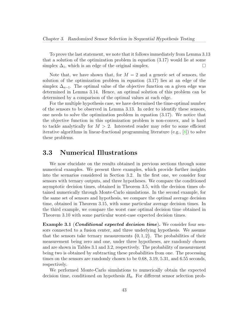
Chapter 3. Randomized Sensor Selection in Sequential Hypothesis Testing
To prove the last statement, we note that it follows immediately from Lemma 3.13that a solution of the optimization problem in equation (3.17) would lie at somesimplex ∆1, which is an edge of the original simplex.
Note that, we have shown that, for M = 2 and a generic set of sensors, thesolution of the optimization problem in equation (3.17) lies at an edge of thesimplex ∆n−1. The optimal value of the objective function on a given edge wasdetermined in Lemma 3.14. Hence, an optimal solution of this problem can bedetermined by a comparison of the optimal values at each edge.
For the multiple hypothesis case, we have determined the time-optimal numberof the sensors to be observed in Lemma 3.13. In order to identify these sensors,one needs to solve the optimization problem in equation (3.17). We notice thatthe objective function in this optimization problem is non-convex, and is hardto tackle analytically for M > 2. Interested reader may refer to some efficientiterative algorithms in linear-fractional programming literature (e.g., [8]) to solvethese problems.
3.3 Numerical Illustrations
We now elucidate on the results obtained in previous sections through somenumerical examples. We present three examples, which provide further insightsinto the scenarios considered in Section 3.2. In the first one, we consider foursensors with ternary outputs, and three hypotheses. We compare the conditionedasymptotic decision times, obtained in Theorem 3.5, with the decision times ob-tained numerically through Monte-Carlo simulations. In the second example, forthe same set of sensors and hypothesis, we compare the optimal average decisiontime, obtained in Theorem 3.15, with some particular average decision times. Inthe third example, we compare the worst case optimal decision time obtained inTheorem 3.10 with some particular worst-case expected decision times.
Example 3.1 (Conditional expected decision time). We consider four sen-sors connected to a fusion center, and three underlying hypothesis. We assumethat the sensors take ternary measurements 0, 1, 2. The probabilities of theirmeasurement being zero and one, under three hypotheses, are randomly chosenand are shown in Tables 3.1 and 3.2, respectively. The probability of measurementbeing two is obtained by subtracting these probabilities from one. The processingtimes on the sensors are randomly chosen to be 0.68, 3.19, 5.31, and 6.55 seconds,respectively.
We performed Monte-Carlo simulations to numerically obtain the expecteddecision time, conditioned on hypothesis H0. For different sensor selection prob-
43
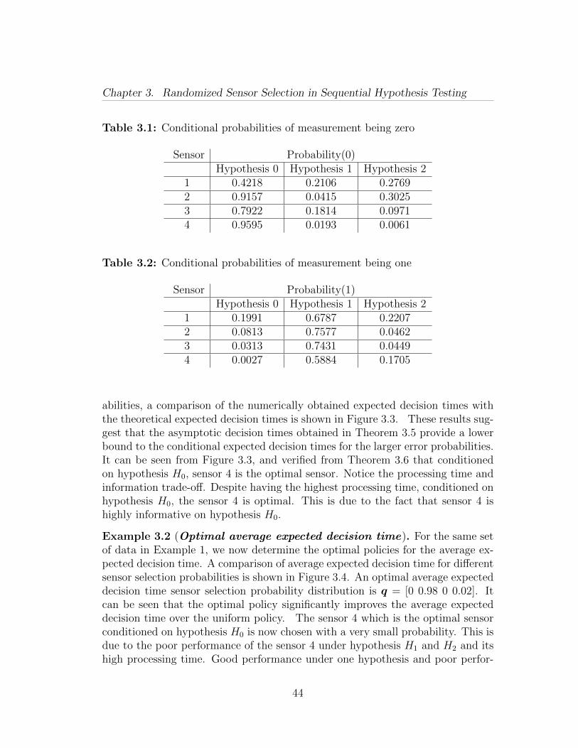
Chapter 3. Randomized Sensor Selection in Sequential Hypothesis Testing
Table 3.1: Conditional probabilities of measurement being zero
Sensor Probability(0)Hypothesis 0 Hypothesis 1 Hypothesis 2
1 0.4218 0.2106 0.27692 0.9157 0.0415 0.30253 0.7922 0.1814 0.09714 0.9595 0.0193 0.0061
Table 3.2: Conditional probabilities of measurement being one
Sensor Probability(1)Hypothesis 0 Hypothesis 1 Hypothesis 2
1 0.1991 0.6787 0.22072 0.0813 0.7577 0.04623 0.0313 0.7431 0.04494 0.0027 0.5884 0.1705
abilities, a comparison of the numerically obtained expected decision times withthe theoretical expected decision times is shown in Figure 3.3. These results sug-gest that the asymptotic decision times obtained in Theorem 3.5 provide a lowerbound to the conditional expected decision times for the larger error probabilities.It can be seen from Figure 3.3, and verified from Theorem 3.6 that conditionedon hypothesis H0, sensor 4 is the optimal sensor. Notice the processing time andinformation trade-off. Despite having the highest processing time, conditioned onhypothesis H0, the sensor 4 is optimal. This is due to the fact that sensor 4 ishighly informative on hypothesis H0.
Example 3.2 (Optimal average expected decision time). For the same setof data in Example 1, we now determine the optimal policies for the average ex-pected decision time. A comparison of average expected decision time for differentsensor selection probabilities is shown in Figure 3.4. An optimal average expecteddecision time sensor selection probability distribution is q = [0 0.98 0 0.02]. Itcan be seen that the optimal policy significantly improves the average expecteddecision time over the uniform policy. The sensor 4 which is the optimal sensorconditioned on hypothesis H0 is now chosen with a very small probability. This isdue to the poor performance of the sensor 4 under hypothesis H1 and H2 and itshigh processing time. Good performance under one hypothesis and poor perfor-
44
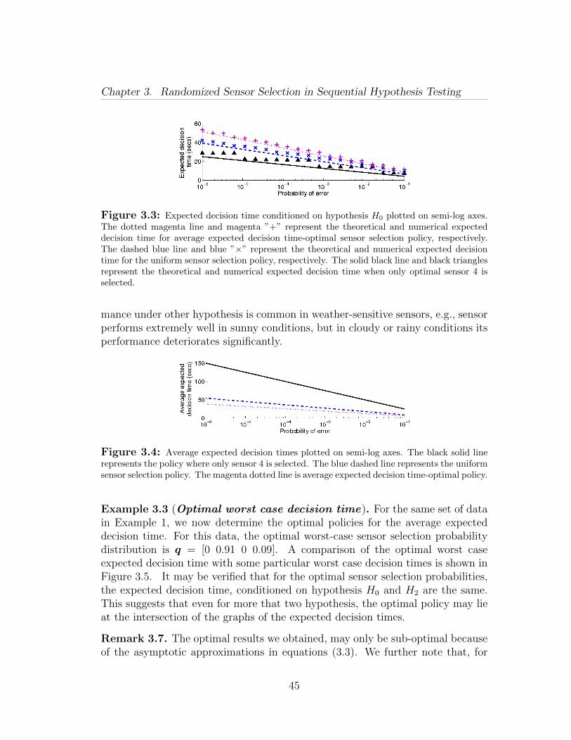
Chapter 3. Randomized Sensor Selection in Sequential Hypothesis Testing
Figure 3.3: Expected decision time conditioned on hypothesis H0 plotted on semi-log axes.The dotted magenta line and magenta ”+” represent the theoretical and numerical expecteddecision time for average expected decision time-optimal sensor selection policy, respectively.The dashed blue line and blue ”×” represent the theoretical and numerical expected decisiontime for the uniform sensor selection policy, respectively. The solid black line and black trianglesrepresent the theoretical and numerical expected decision time when only optimal sensor 4 isselected.
mance under other hypothesis is common in weather-sensitive sensors, e.g., sensorperforms extremely well in sunny conditions, but in cloudy or rainy conditions itsperformance deteriorates significantly.
Figure 3.4: Average expected decision times plotted on semi-log axes. The black solid linerepresents the policy where only sensor 4 is selected. The blue dashed line represents the uniformsensor selection policy. The magenta dotted line is average expected decision time-optimal policy.
Example 3.3 (Optimal worst case decision time). For the same set of datain Example 1, we now determine the optimal policies for the average expecteddecision time. For this data, the optimal worst-case sensor selection probabilitydistribution is q = [0 0.91 0 0.09]. A comparison of the optimal worst caseexpected decision time with some particular worst case decision times is shown inFigure 3.5. It may be verified that for the optimal sensor selection probabilities,the expected decision time, conditioned on hypothesis H0 and H2 are the same.This suggests that even for more that two hypothesis, the optimal policy may lieat the intersection of the graphs of the expected decision times.
Remark 3.7. The optimal results we obtained, may only be sub-optimal becauseof the asymptotic approximations in equations (3.3). We further note that, for
45
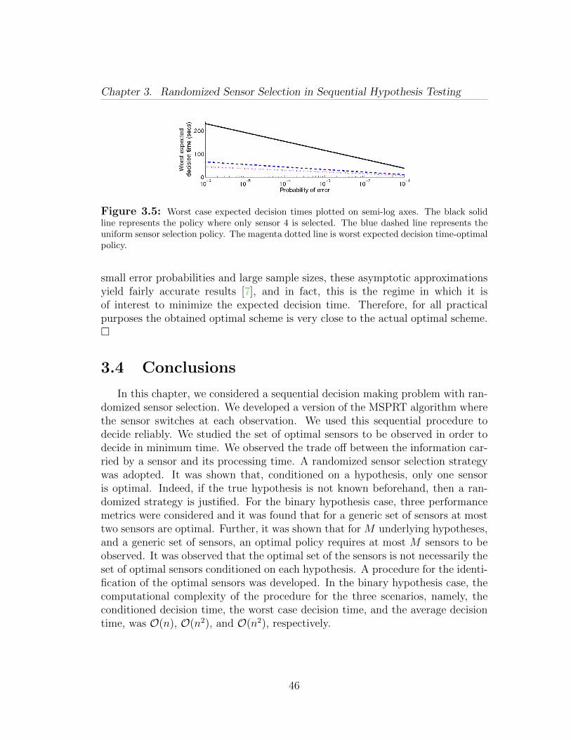
Chapter 3. Randomized Sensor Selection in Sequential Hypothesis Testing
Figure 3.5: Worst case expected decision times plotted on semi-log axes. The black solidline represents the policy where only sensor 4 is selected. The blue dashed line represents theuniform sensor selection policy. The magenta dotted line is worst expected decision time-optimalpolicy.
small error probabilities and large sample sizes, these asymptotic approximationsyield fairly accurate results [7], and in fact, this is the regime in which it isof interest to minimize the expected decision time. Therefore, for all practicalpurposes the obtained optimal scheme is very close to the actual optimal scheme.
3.4 Conclusions
In this chapter, we considered a sequential decision making problem with ran-domized sensor selection. We developed a version of the MSPRT algorithm wherethe sensor switches at each observation. We used this sequential procedure todecide reliably. We studied the set of optimal sensors to be observed in order todecide in minimum time. We observed the trade off between the information car-ried by a sensor and its processing time. A randomized sensor selection strategywas adopted. It was shown that, conditioned on a hypothesis, only one sensoris optimal. Indeed, if the true hypothesis is not known beforehand, then a ran-domized strategy is justified. For the binary hypothesis case, three performancemetrics were considered and it was found that for a generic set of sensors at mosttwo sensors are optimal. Further, it was shown that for M underlying hypotheses,and a generic set of sensors, an optimal policy requires at most M sensors to beobserved. It was observed that the optimal set of the sensors is not necessarily theset of optimal sensors conditioned on each hypothesis. A procedure for the identi-fication of the optimal sensors was developed. In the binary hypothesis case, thecomputational complexity of the procedure for the three scenarios, namely, theconditioned decision time, the worst case decision time, and the average decisiontime, was O(n), O(n2), and O(n2), respectively.
46
Chapter 4
Stochastic Surveillance Strategiesfor Spatial Quickest Detection
In this chapter we consider the persistent surveillance of a set of n disjointregions with a team of m < n identical1 autonomous vehicles capable of sensing,communicating, and moving from one region to another. In persistent surveillance,the vehicles visit the regions according to some routing policy, collect evidence(sensor observation), and send it to a control center. The control center runsan anomaly detection algorithm with the evidence collected by the vehicles todetermine the likelihood of an anomaly being present at some region (the controlcenter declares an anomaly if substantial evidence is present). Finally, the controlcenter utilizes the likelihood of an anomaly at each region to determine a vehiclerouting policy. The objective of the control center is to detect an anomaly atany region in minimum time subject to a desired bound on the expected timebetween any two subsequent false alarms. Notice that the time required to detectan anomaly depends on the anomaly detection algorithm and the time vehiclestake to travel the regions. Thus, the control center needs to minimize the anomalydetection time jointly over anomaly detection policies and vehicle routing policies.Our problem setup is shown in Fig. 4.1.
We adopt the standard motion planning notation in [59]. We denote the k-thregion by Rk, k ∈ 1, . . . , n, and r-th vehicle by Ur, r ∈ 1, . . . ,m. Let thelikelihood of an anomaly at region Rk be πk ∈ (0, 1). We study the persistentsurveillance problem under the following assumptions.
Regarding the vehicles, we do not assume any specific dynamics and we assumethat:
1The vehicle routing policies designed in this chapter also work for non-identical vehicles.We make this assumption for the convenience of analysis.
47
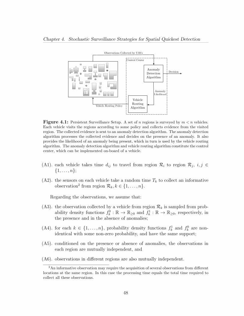
Chapter 4. Stochastic Surveillance Strategies for Spatial Quickest Detection
AnomalyDetectionAlgorithm
VehicleRouting
Algorithm
Decision
AnomalyLikelihood
Control Center
Observations Collected by UAVs
Vehicle Routing Policy
Figure 4.1: Persistent Surveillance Setup. A set of n regions is surveyed by m < n vehicles.Each vehicle visits the regions according to some policy and collects evidence from the visitedregion. The collected evidence is sent to an anomaly detection algorithm. The anomaly detectionalgorithm processes the collected evidence and decides on the presence of an anomaly. It alsoprovides the likelihood of an anomaly being present, which in turn is used by the vehicle routingalgorithm. The anomaly detection algorithm and vehicle routing algorithm constitute the controlcenter, which can be implemented on-board of a vehicle.
(A1). each vehicle takes time dij to travel from region Ri to region Rj, i, j ∈1, . . . , n;
(A2). the sensors on each vehicle take a random time Tk to collect an informativeobservation2 from region Rk, k ∈ 1, . . . , n.
Regarding the observations, we assume that:
(A3). the observation collected by a vehicle from region Rk is sampled from prob-ability density functions f 0
k : R → R≥0 and f 1k : R → R≥0, respectively, in
the presence and in the absence of anomalies;
(A4). for each k ∈ 1, . . . , n, probability density functions f 1k and f 0
k are non-identical with some non-zero probability, and have the same support;
(A5). conditioned on the presence or absence of anomalies, the observations ineach region are mutually independent, and
(A6). observations in different regions are also mutually independent.
2An informative observation may require the acquisition of several observations from differentlocations at the same region. In this case the processing time equals the total time required tocollect all these observations.
48
Chapter 4. Stochastic Surveillance Strategies for Spatial Quickest Detection
Regarding the anomaly detection algorithm at the control center, we employthe cumulative sum (CUSUM) algorithm (see Section 2.2) for anomaly detectionat each region. In particular, we run n parallel CUSUM algorithms (one for eachregion) and declare an anomaly being present at a region as soon as a substantialevidence is present. We refer to such parallel CUSUM algorithms by ensembleCUSUM algorithm.
Remark 4.1 (Knowledge of distributions). For the ease of presentation,we assume that the probability density functions in presence and absence of ananomaly are known. In general, only the probability density function in absenceof any anomaly may be known, or both the probability density functions may beunknown. In the first case, the CUSUM algorithm can be replaced by the weightedCUSUM algorithm or the Generalized Likelihood Ratio (GLR) algorithm, see [6],while in the second case, it can be replaced by the robust minimax quickest changedetection algorithm proposed in [101]. The ideas presented in this chapter extendto these cases in a straightforward way. A related example is in Section 4.4.
Remark 4.2 (Independence of observations). For the ease of presentation,we assume that the observations collected from each region are independent con-ditioned on the presence and absence of anomalies. In general, the observationsmay be dependent and the dependence can be captured through an appropriatehidden Markov model. If the observations can be modeled as a hidden Markovmodel, then the CUSUM like algorithm in [24] can be used instead of the stan-dard CUSUM algorithm. The analysis presented in this chapter holds in thiscase as well but in an asymptotic sense, i.e., in the limit when a large number ofobservations are needed for anomaly detection.
We also assumed that the observations collected from different regions aremutually independent. Although the ideas in this chapter also work when theobservations at different regions are dependent, the performance can be improvedwith a slight modification in the procedure presented here (see Remark 4.4). Inthis case the algorithm performance improves because each observation is nowinformative about more than one region.
Regarding the vehicle routing policy, we propose the randomized routing policy,and the adaptive routing policy. In the randomized routing policy, each vehicle(i) selects a region from a stationary distribution, (ii) visits that region, (iii)collects evidence, and (iv) transmits this evidence to the control center and iteratesthis process endlessly. In the randomized routing policy, the evidence collectedby the vehicles is not utilized to modify their routing policy. In other words,there is no feedback from the anomaly detection algorithm to the vehicle routingalgorithm. In the adaptive routing policy, instead, the evidence collected by the
49
Chapter 4. Stochastic Surveillance Strategies for Spatial Quickest Detection
vehicles is used to modify the routing policy, and thus, the loop between the vehiclerouting algorithm and the anomaly detection algorithm is closed. The adaptiverouting policy follows the same steps as in the randomized routing policy, with theexception that the distribution in step (i) is no longer stationary and is adaptedbased on the collected evidence.
For brevity of notation, we will refer to the joint anomaly detection and vehiclerouting policy comprising of the ensemble CUSUM algorithm and the random-ized routing policy by randomized ensemble CUSUM algorithm. We will show thatthe randomized ensemble CUSUM algorithm provides a solution that is within afactor of optimality. Similarly, we refer to the joint anomaly detection and ve-hicle routing policy comprising of the ensemble CUSUM algorithm and adaptiverouting policy by adaptive ensemble CUSUM algorithm. We will show that adap-tive ensemble CUSUM algorithm makes the vehicles visit anomalous regions withhigh probability, and thus it improves upon the performance of the randomizedensemble CUSUM algorithm.
Remark 4.3 (Randomized routing policy). The randomized routing policysamples regions to visit from a stationary distribution; this assumes that eachregion can be visited from another region in a single hop. While this is the casefor aerial vehicles, it may not be true for ground vehicles. In the latter case,the motion from one region to another can be modeled as a Markov chain. Thetransition probabilities of this Markov chain can be designed to achieve a desiredstationary distribution. This can optimally be done, for instance, by picking thefastest mixing Markov chain proposed in [14] or heuristically by using the stan-dard Metropolis-Hastings algorithm, see [105]. Related examples are presentedin Section 4.4 and 4.5. It should be noted that under the randomized routingpolicy, the desired stationary distribution of the Markov chain is fixed, and theMarkov chain converges to this distribution exponentially. Thus, the policy de-signed using Markov chain is arbitrarily close to the desired policy. However, inthe case of adaptive routing policy, the desired stationary distribution keeps onchanging, and the performance of the Markov chain based policy depends on rateof convergence of the Markov chain and the rate of change of desired stationarydistribution.
We now introduce some notations that will be used throughout the chapter.We denote the probability simplex in Rn by ∆n−1, and the space of vehicle routingpolicies by Ω. For the processing time Tk, we let Tk denote its expected value.Consider m realizations of the processing time Tk, we denote the expected valueof the minimum of these m realized values by Tm-smlst
k . Note that T 1-smlstk = Tk.
We also define Tmax = maxTk | k ∈ 1, . . . , n and Tmin = minTk | k ∈
50
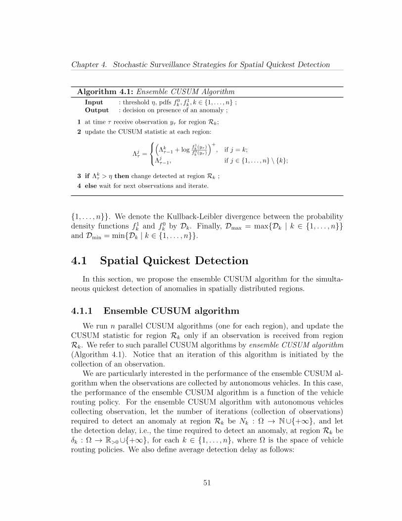
Chapter 4. Stochastic Surveillance Strategies for Spatial Quickest Detection
Algorithm 4.1: Ensemble CUSUM Algorithm
Input : threshold η, pdfs f0k , f
1k , k ∈ 1, . . . , n ;
Output : decision on presence of an anomaly ;
1 at time τ receive observation yτ for region Rk;
2 update the CUSUM statistic at each region:
Λjτ =
(
Λkτ−1 + logf1k(yτ )
f0k(yτ )
)+
, if j = k;
Λjτ−1, if j ∈ 1, . . . , n \ k;
3 if Λkτ > η then change detected at region Rk ;
4 else wait for next observations and iterate.
1, . . . , n. We denote the Kullback-Leibler divergence between the probabilitydensity functions f 1
k and f 0k by Dk. Finally, Dmax = maxDk | k ∈ 1, . . . , n
and Dmin = minDk | k ∈ 1, . . . , n.
4.1 Spatial Quickest Detection
In this section, we propose the ensemble CUSUM algorithm for the simulta-neous quickest detection of anomalies in spatially distributed regions.
4.1.1 Ensemble CUSUM algorithm
We run n parallel CUSUM algorithms (one for each region), and update theCUSUM statistic for region Rk only if an observation is received from regionRk. We refer to such parallel CUSUM algorithms by ensemble CUSUM algorithm(Algorithm 4.1). Notice that an iteration of this algorithm is initiated by thecollection of an observation.
We are particularly interested in the performance of the ensemble CUSUM al-gorithm when the observations are collected by autonomous vehicles. In this case,the performance of the ensemble CUSUM algorithm is a function of the vehiclerouting policy. For the ensemble CUSUM algorithm with autonomous vehiclescollecting observation, let the number of iterations (collection of observations)required to detect an anomaly at region Rk be Nk : Ω → N∪+∞, and letthe detection delay, i.e., the time required to detect an anomaly, at region Rk beδk : Ω → R>0 ∪+∞, for each k ∈ 1, . . . , n, where Ω is the space of vehiclerouting policies. We also define average detection delay as follows:
51

Chapter 4. Stochastic Surveillance Strategies for Spatial Quickest Detection
Definition 4.1 (Average detection delay). For any vector of weights (w1, . . . , wn) ∈∆n−1, define the average detection delay δavg : Ω→ R>0 ∪+∞ for the ensembleCUSUM algorithm with autonomous vehicles collecting observations by
δavg(ω) =n∑k=1
wkE[δk(ω)]. (4.1)
For the ensemble CUSUM algorithm with m vehicles collecting observation,define δm-min
k and δm-minavg by
δm-mink = infE[δk(ω)] | ω ∈ Ω, and
δm-minavg = infδavg(ω) | ω ∈ Ω,
respectively. Note that δm-mink and δm-min
avg are lower bounds for the expected detec-tion delay and average detection delay at region Rk, respectively, independentlyof the routing policy. Let η = e−η +η−1. We now state lower bounds on the per-formance of the ensemble CUSUM algorithm with autonomous vehicles collectingobservations.
Lemma 4.1 (Global lower bound). The following statements hold for theensemble CUSUM algorithm with m vehicles collecting information:
(i). the lower bound δm-mink for the expected detection delay at regionRk satisfies
δm-mink ≥ η Tm-smlst
k
mDk;
(ii). the lower bound δm-minavg for the average detection delay satisfies
δm-minavg ≥ η Tm-smlst
min
mDmax
,
where Tm-smlstmin = minTm-smlst
k | k ∈ 1, . . . , n.
Proof. We start by establishing the first statement. We note that a lower boundon the expected detection delay at region Rk is obtained if all the vehicles al-ways stay at region Rk. Since, each observation is collected from region Rk,the number of iterations of the ensemble CUSUM algorithm required to detectan anomaly at region Rk satisfies E[Nk] = η/Dk. Let T rk (b) be realized valueof the processing time of vehicle Ur at its b-th observation. It follows thatTm-smlstk (b) = minT rk (b) | r ∈ 1, . . . ,m is a lower bound on the processing
52
Chapter 4. Stochastic Surveillance Strategies for Spatial Quickest Detection
time of each vehicle for its b-th observation. Further, Tm-smlstk (b) is identically dis-
tributed for each b and E[Tm-smlstk (b)] = Tm-smlst
k . Consider a modified stochasticprocess where the realized processing time of each vehicle for its b-th observationin Tm-smlst
k (b). Indeed, such a stochastic process underestimates the time requiredto collect each observation and, hence, provides a lower bound to the expecteddetection delay. Therefore, the detection delay satisfies the following bound
δk(ω) ≥dNk/me∑b=1
Tm-smlstk (b), for each ω ∈ Ω.
It follows from Wald’s identity, see [76], that
E[δk(ω)] ≥ Tm-smlstk E[dNk/me] ≥ Tm-smlst
k E[Nk]/m.
This proves the first statement.The second statement follows from Definition 4.1 and the first statement.
Remark 4.4 (Dependence across regions). We assumed that the observa-tions collected from different regions are mutually independent. If the observationsfrom different regions are dependent, then, at each iteration, instead of updatingonly one CUSUM statistic, the CUSUM statistic at each region should be updatedwith an appropriate marginal distribution.
4.2 Randomized Ensemble CUSUM Algorithm
We now study the persistent surveillance problem under randomized ensembleCUSUM algorithm. First, we derive an exact expression for the expected detectiondelay for the randomized ensemble CUSUM algorithm with a single vehicle, anduse the derived expressions to develop an efficient stationary policy for a singlevehicle. Second, we develop a lower bound on the expected detection delay forthe randomized ensemble CUSUM algorithm with multiple vehicles, and develop ageneric partitioning policy that (i) constructs a complete and disjoint m-partitionof the regions, (ii) allocates one partition each to a vehicle, and (iii) lets eachvehicle survey its assigned region with some single vehicle policy. Finally, we showthat the partitioning policy where each vehicle implements the efficient stationarypolicy in its regions is within a factor of an optimal policy.
4.2.1 Analysis for single vehicle
Consider the randomized ensemble CUSUM algorithm with a single vehicle.Let qk ∈ [0, 1] denote the probability to select regionRk, and let q = (q1, . . . , qn) ∈
53
Chapter 4. Stochastic Surveillance Strategies for Spatial Quickest Detection
∆n−1. Let the threshold for the CUSUM algorithm at each region be uniform andequal to η ∈ R>0. We note that for the randomized ensemble CUSUM algorithmwith a single vehicle the space of vehicle routing policies is Ω = ∆n−1.
Theorem 4.2 (Single vehicle randomized ensemble CUSUM ). For therandomized ensemble CUSUM algorithm with a single vehicle and stationary rout-ing policy q ∈ ∆n−1, the following statements hold:
(i). the number of observations Nk(q) required to detect a change at region Rk
satisfies
Ef1k [Nk(q)] =η
qkDk;
(ii). the detection delay δk(q) at region Rk satisfies
Ef1k [δk(q)] =( n∑i=1
qiTi +n∑i=1
n∑j=1
qiqjdij
)Ef1k [Nk(q)].
Proof. Let τ ∈ 1, . . . , Nk be the iterations at which the vehicle collects andsends information about the regions, where Nk denotes the iteration at which ananomaly is detected at region Rk. Let the log likelihood ratio at region Rk atiteration τ be λkτ . We have
λkτ =
log
f1k (yτ )
f0k (yτ ), with probability qk,
0, with probability 1− qk.
Therefore, conditioned on the presence of an anomaly, λkττ∈N are i.i.d., and
Ef1k [λkτ ] = qkDk.
The remaining proof of the first statement follows similar to the proof for CUSUMin [85].
To prove the second statement, note that the information aggregation timeT agr comprises of the processing time and the travel time. At an iteration thevehicle is at region Ri with probability qi and picks region Rj with probabilityqj. Additionally, the vehicle travels between the two regions in dij units of time.Thus, the average travel time at each iteration is
E[Ttravel] =n∑i=1
n∑j=1
qiqjdij.
54
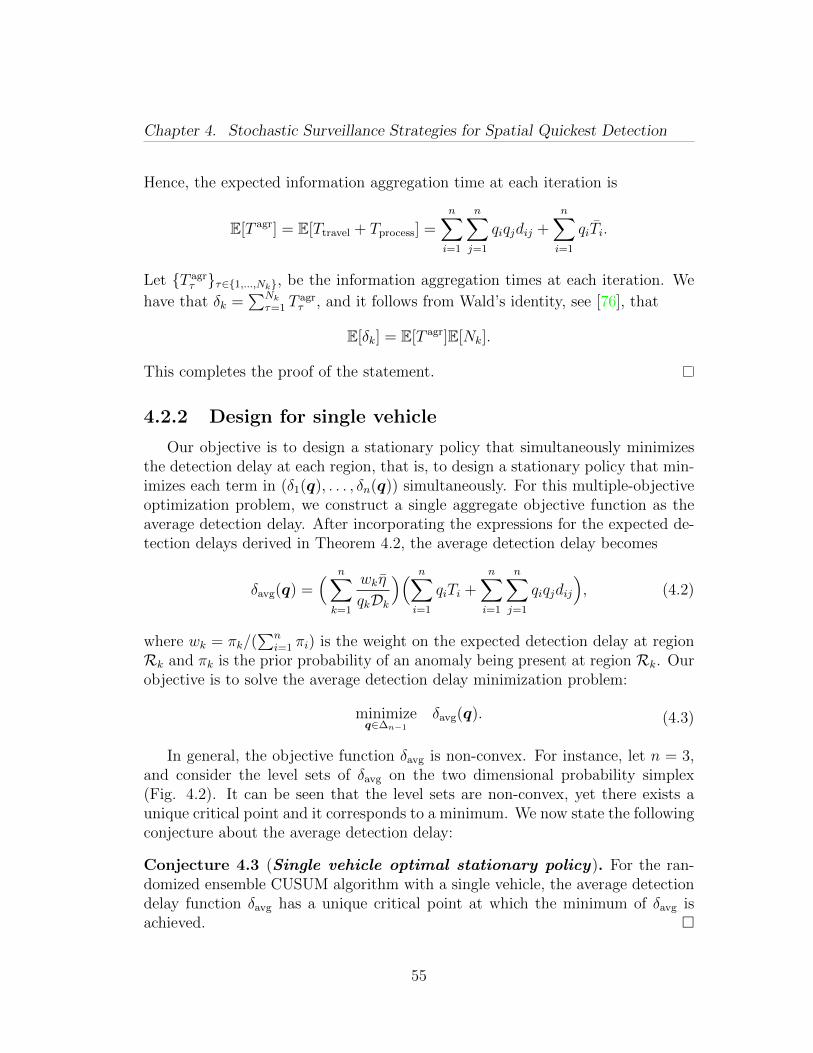
Chapter 4. Stochastic Surveillance Strategies for Spatial Quickest Detection
Hence, the expected information aggregation time at each iteration is
E[T agr] = E[Ttravel + Tprocess] =n∑i=1
n∑j=1
qiqjdij +n∑i=1
qiTi.
Let T agrτ τ∈1,...,Nk, be the information aggregation times at each iteration. We
have that δk =∑Nk
τ=1 Tagrτ , and it follows from Wald’s identity, see [76], that
E[δk] = E[T agr]E[Nk].
This completes the proof of the statement.
4.2.2 Design for single vehicle
Our objective is to design a stationary policy that simultaneously minimizesthe detection delay at each region, that is, to design a stationary policy that min-imizes each term in (δ1(q), . . . , δn(q)) simultaneously. For this multiple-objectiveoptimization problem, we construct a single aggregate objective function as theaverage detection delay. After incorporating the expressions for the expected de-tection delays derived in Theorem 4.2, the average detection delay becomes
δavg(q) =( n∑k=1
wkη
qkDk
)( n∑i=1
qiTi +n∑i=1
n∑j=1
qiqjdij
), (4.2)
where wk = πk/(∑n
i=1 πi) is the weight on the expected detection delay at regionRk and πk is the prior probability of an anomaly being present at region Rk. Ourobjective is to solve the average detection delay minimization problem:
minimizeq∈∆n−1
δavg(q). (4.3)
In general, the objective function δavg is non-convex. For instance, let n = 3,and consider the level sets of δavg on the two dimensional probability simplex(Fig. 4.2). It can be seen that the level sets are non-convex, yet there exists aunique critical point and it corresponds to a minimum. We now state the followingconjecture about the average detection delay:
Conjecture 4.3 (Single vehicle optimal stationary policy). For the ran-domized ensemble CUSUM algorithm with a single vehicle, the average detectiondelay function δavg has a unique critical point at which the minimum of δavg isachieved.
55
Chapter 4. Stochastic Surveillance Strategies for Spatial Quickest Detection
q1
q 2
0 0.2 0.4 0.6 0.8 10
0.1
0.2
0.3
0.4
0.5
0.6
0.7
0.8
0.9
1
q1
q2
Figure 4.2: Level-sets of the objective function in problem (4.3). It can be seen that thelevel sets are not convex.
In the Appendix of this chapter we provide probabilistic guarantees that, fora particular stochastic model of the parameters in δavg, with at least confidencelevel 99.99% and probability at least 99%, the optimization problem (4.3) has aunique critical point at which the minimum is achieved. Such a minimum can becomputed via standard gradient-descent methods, see [15].
We now construct an upper bound for the expected detection delay. We willshow that minimization of this upper bound yields a policy that is within a factorof an optimal policy. From equation (4.2), we define the upper bound δupper :∆n−1 → R>0 ∪+∞ as
δavg(q) ≤ δupper(q) =( n∑k=1
wkη
qkDk
)(Tmax + dmax),
where dmax = maxdij | i, j ∈ 1, . . . , n.
Theorem 4.4 (Single vehicle efficient stationary policy). The followingstatements hold for the randomized ensemble CUSUM algorithm with single ve-hicle:
(i). the upper bound on the expected detection delay satisfies
minq∈∆n−1
δupper(q) =( n∑k=1
√wkDk
)2
η(Tmax + dmax),
56
Chapter 4. Stochastic Surveillance Strategies for Spatial Quickest Detection
and the minimum is achieved at q† defined by
q†k =
√wk/Dk∑n
j=1
√wj/Dj
, k ∈ 1, . . . , n;
(ii). the average detection delay satisfies the following lower bound
δavg(q) ≥( n∑k=1
√wkDk
)2
η Tmin,
for all q ∈ ∆n−1;
(iii). the stationary policy q† is within a factor of optimal, that is
δavg(q†)
δavg(q∗)≤ Tmax + dmax
Tmin
, and
δavg(q†)
δ1-minavg
≤ nTmax + dmax
Tmin
Dmax
Dmin
,
where q∗ is an optimal stationary policy;
(iv). the expected detection delay at region Rk under policy q† satisfy
E[δk(q†)]
δ1-mink
≤ (Tmax + dmax)
Tk
√nDk
wkDmin
.
Proof. We start by establishing the first statement. It follows from the sta-tionarity conditions on the Lagrangian that the minimizer q† of δupper satisfy
q†k ∝√wkη/Dk, for each k ∈ 1, . . . , n. Incorporating this fact into
∑nk=1 q
†k = 1
yields the expression for q†k. The expression for δupper(q†) can be verified by sub-
stituting the expression for q† into δupper.To prove the second statement, we construct a lower bound δlower : ∆n−1 →
R>0 ∪+∞ to the average detection delay δavg defined by δlower(q) =∑n
k=1 wkηTmin/Dkqk.It can be verified that δlower also achieves its minimum at q†, and
δlower(q†) =
( n∑k=1
√wkDk
)2
η Tmin.
We note that
δlower(q†) ≤ δlower(q
∗) ≤ δavg(q∗) ≤ δavg(q),∀q ∈ ∆n−1.
57
Chapter 4. Stochastic Surveillance Strategies for Spatial Quickest Detection
Thus, the second statement follows.To prove the first part of the third statement, we note that
δlower(q†) ≤ δavg(q∗) ≤ δavg(q†) ≤ δupper(q
†).
Therefore, the policy q† is within δupper(q†)/δlower(q
†) = (Tmax + dmax)/Tmin factorof optimal stationary policy.
To prove the second part of the third statement, we note
δavg(q†)
δ1-minavg
≤ Dmax(Tmax + dmax)
DminTmin
(√w1 + . . .+
√wn)2
≤ nTmax + dmax
Tmin
Dmax
Dmin
,
where the last inequality follows from the fact: max√w1 + . . .+√wn | w1 + . . .+
wn = 1 =√n.
To establish the last statement, we note that
E[δk(q†)]
δ1-mink
≤ (Tmax + dmax)
q†kTk
≤ (Tmax + dmax)
Tk
√Dk
wkDmin
(√w1 + . . .+
√wn)
≤ (Tmax + dmax)
Tk
√nDk
wkDmin
.
This concludes the proof of the theorem.
In the following, we would refer to q† as the single vehicle efficient stationarypolicy.
Remark 4.5 (Efficient stationary policy). As opposed to the average de-tection delay δavg, the upper bound δupper does not depend upon any travel timeinformation. Then, our efficient policy does not take this information into account,and it may not be optimal. Instead, an optimal policy allocates higher visitingprobabilities to regions that are located more centrally in the environment. Weresort to the efficient policy because (i) if the problem (4.3) does not admit aunique minimum, then the optimal policy can not be computed efficiently; and(ii) efficient policy has an intuitive, tractable, and closed form expression.
58
Chapter 4. Stochastic Surveillance Strategies for Spatial Quickest Detection
4.2.3 Analysis for multiple vehicles
We now consider the randomized ensemble CUSUM with m > 1 vehicles. Inthis setting the vehicles operate in an asynchronous fashion. This asynchronicity,which did not occur in the single vehicle case, is due to (i) different travel timesbetween two different pair of regions, and (ii) different realized value of processingtime at each iteration. Such an asynchronous operation makes the time durationsbetween two subsequent iterations non-identically distributed and makes it dif-ficult to obtain closed form expressions for the expected detection delay at eachregion.
Motivated by the above discussion, we determine a lower bound on the ex-pected detection delay for the randomized ensemble CUSUM algorithm with mul-tiple vehicles. Let qr = (qr1, . . . , q
rn) ∈ ∆n−1 denote the stationary policy for
vehicle Ur, i.e., the vector of probabilities of selecting different regions for vehicleUr, and let ~qm = (q1, . . . , qm) ∈ ∆m
n−1. We note that for the randomized en-semble CUSUM algorithm with m vehicles the space of vehicle routing policiesis Ω = ∆m
n−1. We construct a lower bound on the processing times at differ-ent regions for different vehicles in the following way. Let Ξ be the set of allthe sets with cardinality m in which each entry is an arbitrarily chosen region;equivalently, Ξ = R1, . . . ,Rnm. Let a realization of the processing times at theregions in a set ξ ∈ Ξ be tξ1, . . . , t
ξm. We now define a lower bound Tone to the
expected value of the minimum of the processing times at m arbitrary regions asTone = minE[mintξ1, . . . , tξm] | ξ ∈ Ξ.
Theorem 4.5 (Multi-vehicle randomized ensemble CUSUM ). For therandomized ensemble CUSUM algorithm with m vehicles and stationary regionselection policies qr, r ∈ 1, . . . ,m, the detection delay δk at region Rk satisfies:
Ef1k [δk(~qm)] ≥ η Tone∑mr=1 q
rkDk
.
Proof. We construct a modified stochastic process to determine a lower bound onthe expected detection delay. For the randomized ensemble CUSUM algorithmwith multiple vehicles, let tbr be the the processing time for the vehicle Ur duringits b-th visit to any region. We assume that the sampling time for each vehicle atits b-th visit in the modified process is mintb1, . . . , tbm. Therefore, the samplingtime for the modified process is the same at each region. Further, it is identicallydistributed for each visit and has expected value greater than or equal to Tone. Wefurther assume that the distances between the regions are zero. Such a processunderestimates the processing and travel time required to collect each observationin the randomized ensemble CUSUM algorithm. Hence, the expected detection
59
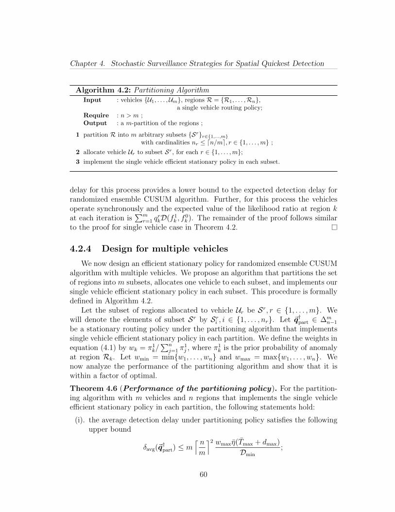
Chapter 4. Stochastic Surveillance Strategies for Spatial Quickest Detection
Algorithm 4.2: Partitioning AlgorithmInput : vehicles U1, . . . ,Um, regions R = R1, . . . ,Rn,
a single vehicle routing policy;Require : n > m ;Output : a m-partition of the regions ;
1 partition R into m arbitrary subsets Srr∈1,...,mwith cardinalities nr ≤ dn/me, r ∈ 1, . . . ,m ;
2 allocate vehicle Ur to subset Sr, for each r ∈ 1, . . . ,m;3 implement the single vehicle efficient stationary policy in each subset.
delay for this process provides a lower bound to the expected detection delay forrandomized ensemble CUSUM algorithm. Further, for this process the vehiclesoperate synchronously and the expected value of the likelihood ratio at region kat each iteration is
∑mr=1 q
rkD(f 1
k , f0k ). The remainder of the proof follows similar
to the proof for single vehicle case in Theorem 4.2.
4.2.4 Design for multiple vehicles
We now design an efficient stationary policy for randomized ensemble CUSUMalgorithm with multiple vehicles. We propose an algorithm that partitions the setof regions into m subsets, allocates one vehicle to each subset, and implements oursingle vehicle efficient stationary policy in each subset. This procedure is formallydefined in Algorithm 4.2.
Let the subset of regions allocated to vehicle Ur be Sr, r ∈ 1, . . . ,m. Wewill denote the elements of subset Sr by Sri , i ∈ 1, . . . , nr. Let ~q†part ∈ ∆m
n−1
be a stationary routing policy under the partitioning algorithm that implementssingle vehicle efficient stationary policy in each partition. We define the weights inequation (4.1) by wk = π1
k/∑n
j=1 π1j , where π1
k is the prior probability of anomalyat region Rk. Let wmin = minw1, . . . , wn and wmax = maxw1, . . . , wn. Wenow analyze the performance of the partitioning algorithm and show that it iswithin a factor of optimal.
Theorem 4.6 (Performance of the partitioning policy). For the partition-ing algorithm with m vehicles and n regions that implements the single vehicleefficient stationary policy in each partition, the following statements hold:
(i). the average detection delay under partitioning policy satisfies the followingupper bound
δavg(~q†part) ≤ m⌈ nm
⌉2 wmaxη(Tmax + dmax)
Dmin
;
60
Chapter 4. Stochastic Surveillance Strategies for Spatial Quickest Detection
(ii). the average detection delay satisfies the following lower bound
δavg(~qm) ≥( n∑k=1
√wkDk
)2 ηTone
m,
for any ~qm ∈ ∆mn−1;
(iii). the stationary policy ~q†part is within a factor of optimal, and
δavg(~q†part)
δavg(~q∗m)≤ 4wmax
wmin
(Tmax + dmax)
Tone
Dmax
Dmin
, and
δavg(~q†part)
δm-minavg
≤ m2⌈ nm
⌉(Tmax + dmax)
Tm-smlstmin
Dmax
Dmin
,
where ~q∗m is optimal stationary policy;
(iv). the expected detection delay at region Rk under the stationary policy ~q†part
satisfies
E[δk(~q†part)]
δm-mink
≤ m(Tmax + dmax)
Tm-smlstk
√⌈ nm
⌉ DkwkDmin
.
Proof. We start by establishing the first statement. We note that under thepartitioning policy, the maximum number of regions a vehicle serves is dn/me. Itfollows from Theorem 4.4 that for vehicle Ur and the associated partition Sr, theaverage detection delay is upper bounded by
δavg(qrpart) ≤( nr∑i=1
√wiDi
)2
η(Tmax + dmax)
≤⌈ nm
⌉2 ηwmax(Tmax + dmax)
Dmin
.
Therefore, the overall average detection delay satisfies δavg(~q†part) ≤ mδavg(qrpart).This establishes the first statement.
To prove the second statement, we utilize the lower bounds obtained in Theo-rem 4.5 and construct a lower bound to the average detection delay δmlower : ∆m
n−1 →R>0 ∪+∞ defined by δmlower(~qm) =
∑nk=1(vkTone/
∑mr=1 q
rk). It can be verified that
min~qm∈∆m
n−1
δmlower(~qm) =( n∑k=1
√wkDk
)2 ηTone
m.
61
Chapter 4. Stochastic Surveillance Strategies for Spatial Quickest Detection
We now establish the first part of the third statement. Note that
δavg(~q†part)
δavg(~q∗m)≤ dn/me
2
(n/m)2
wmax
wmin
(Tmax + dmax)
Tone
Dmax
Dmin
≤ 4wmax
wmin
(Tmax + dmax)
Tone
Dmax
Dmin
,
where the last inequality follows from the fact that (dn/me)/(n/m) ≤ 2.The remainder of the proof follows similar to the proof of Theorem 4.4.
4.3 Adaptive ensemble CUSUM Algorithm
The stationary vehicle routing policy does not utilize the real-time informationregarding the likelihood of anomalies at the regions. We now develop an adap-tive policy that incorporates the anomaly likelihood information provided by theanomaly detection algorithm. We consider the CUSUM statistic at a region asa measure of the likelihood of an anomaly at that region, and utilize it at eachiteration to design new prior probability of an anomaly for each region. At eachiteration, we adapt the efficient stationary policy using this new prior probability.This procedure results in higher probability of visiting an anomalous region and,consequently, it improves the performance of our efficient stationary policy. InSection 4.4 we provide numerical evidence showing that the adaptive ensembleCUSUM algorithm improves the performance of randomized ensemble CUSUMalgorithm.
Our adaptive ensemble CUSUM algorithm is formally presented in Algorithm 4.3for the single vehicle case. For the case of multiple vehicles we resort to thepartitioning Algorithm 4.2 that implements the single vehicle adaptive ensembleCUSUM Algorithm 4.3 in each partition. Let us denote the adaptive routing policyfor a single vehicle by a and the policy obtained from the partitioning algorithmthat implements single vehicle adaptive routing policy in each partition by apart.We now analyze the performance of the adaptive ensemble CUSUM algorithm.Since, the probability to visit any region varies with time in the adaptive ensembleCUSUM algorithm, we need to determine the number of iterations between twoconsecutive visit to a region, i.e., the number of iterations for the recurrence of theregion. We first derive a bound on the expected number of samples to be drawnfrom a time-varying probability vector for the recurrence of a particular state.
Lemma 4.7 (Mean observations for region recurrence). Consider a se-quence xττ∈N, where xτ is sampled from a probability vector pτ ∈ ∆n−1. If the
62
Chapter 4. Stochastic Surveillance Strategies for Spatial Quickest Detection
Algorithm 4.3: Single Vehicle Adaptive Ensemble CUSUM
Input : parameters η, Dk, pdfs f0k , f
1k , for each k ∈ 1, . . . , n ;
Output : decision on anomaly at each region ;
1 set Λj0 = 0, for all j ∈ 1, . . . , n, and τ = 1;
while true do
2 set new prior π1k = eΛkτ /(1 + eΛkτ ), for each k ∈ 1, . . . , n
3 set qk =
√π1k/Dk∑n
j=1
√π1j/Dj
, for each k ∈ 1, . . . , n;
4 sample a region from probability distribution (q1, . . . , qn);
5 collect sample yτ from region k;
6 update the CUSUM statistic at each region
Λjτ =
(
Λkτ−1 + logf1k(yτ )
f0k(yτ )
)+
, if j = k;
Λjτ−1, if j ∈ 1, . . . , n \ k;
if Λkτ > η then
7 anomaly detected at region Rk;
8 set Λkτ = 0;
9 set τ = τ + 1 ;
k-th entry of pτ satisfy pτk ∈ (αk, βk), for each τ ∈ N and some αk, βk ∈ (0, 1), thenthe number of iterations Ik for the recurrence of state k satisfy E[Ik] ≤ βk/α
2k.
Proof. The terms of the sequence xττ∈N are statistically independent. Further,the probability mass function pτ is arbitrary. Therefore, the bound on the expectediterations for the first occurrence of state k is also a bound on the subsequentrecurrence of state k. The expected number of iterations for first occurrence ofregion k are
E[Ik] =∑i∈N
ipik
i−1∏j=1
(1− pjk) ≤ βk∑i∈N
i(1− αk)i−1 = βk/α2k.
This establishes the statement.
We utilize this upper bound on the expected number of iterations for recurrenceof a region to derive performance metrics for the adaptive ensemble CUSUMalgorithm. We now derive an upper bound on the expected detection delay ateach region for adaptive ensemble CUSUM algorithm. We derive these boundsfor the expected evolution of the CUSUM statistic at each region.
63
Chapter 4. Stochastic Surveillance Strategies for Spatial Quickest Detection
Theorem 4.8 (Adaptive ensemble CUSUM algorithm). Consider the ex-pected evolution of the CUSUM statistic at each region. For the partitioningalgorithm that implements single vehicle adaptive ensemble CUSUM algorithm(Algorithm 4.3) in each subset of the partition, the following statement holds:
E[δk(apart)] ≤( η
Dk+
2(dn/me − 1)eη/2√Dk(1− e−η/2)√
Dmin(1− e−Dk/2)
+(dn/me − 1)2eηDk(1− e−η)
Dmin(1− e−Dk)
)(Tmax + dmax).
Proof. We start by deriving expression for a single vehicle. Let the number ofiterations between the (j−1)th and jth visit to region Rk be Ikj .
Let the observation during the jth visit to region Rk be yj and the CUSUMstatistic at region Rk after the visit be Ck
j . It follows that the probability to visitregion Rk between (j−1)th and jth visit is greater than
pj−1k =
eCkj−1/2/
√Dk
eCkj−1/2/
√Dk + (n− 1)eη/2/
√Dmin
.
Therefore, it follows from Lemma 4.7 that
E[Ikj ] ≤ (1 + (n− 1)e(η−Ckj−1)/2√Dk/Dmin)2.
Note that Ckj = max0, Ck
j−1+log(f 1k (yj)/f
0k (yj)). Since, maximum of two convex
function is a convex function, it follows from Jensen inequality, see [76], that
E[Ckj ] ≥ max0,E[Ck
j−1] +Dk ≥ E[Ckj−1] +Dk.
Therefore, E[Ckj ] ≥ jDk and for expected evolution of the CUSUM statistics
E[Ikj ] ≤ (1 + (n− 1)e(η−(j−1)Dk)/2√Dk/Dmin)2.
Therefore, the total number of iterations Nk required to collect Nobsk observa-
tions at region Rk satisfy
E[Nk(a)|Nobsk ] =
Nobsk∑j=1
(1 + (n− 1)e(η−(j−1)Dk)/2√Dk/Dmin)2
= Nobsk +
2(n− 1)eη/2√Dk(1− e−DkN
obsk /2)√
Dmin(1− e−Dk/2)
+(n− 1)2eηDk(1− e−DkN
obsk )
Dmin(1− e−Dk).
64
Chapter 4. Stochastic Surveillance Strategies for Spatial Quickest Detection
Note that the number of observations Nobsk required at regionRk satisfy E[Nobs
k ] =η/Dk. It follows from Jensen’s inequality that
E[Nk(a)] ≤ η
Dk+
2(n− 1)eη/2√Dk(1− e−η/2)√
Dmin(1− e−Dk/2)
(n− 1)2eηDk(1− e−η)Dmin(1− e−Dk)
.
Since the expected time required to collect each evidence is smaller Tmax + dmax,it follows that
E[δk(a)] ≤ (Tmax + dmax)E[Nk(a)].
The expression for the partitioning policy that implement single vehicle adap-tive routing policy in each partition follow by substituting dn/me in the aboveexpressions. This completes the proof of the theorem.
Remark 4.6 (Performance bound). The bound derived in Theorem 4.8 isvery conservative. Indeed, it assumes the CUSUM statistic at each region to befixed at its maximum value η, except for the region in consideration. This ispractically never the case. In fact, if at some iteration the CUSUM statistic isclose to η, then it is highly likely that the vehicle visits that region at the nextiteration, so that the updated statistic crosses the threshold η and resets to zero.
4.4 Numerical Results
We now elucidate on the concepts developed in this chapter through somenumerical examples. We first validate the expressions for expected detection delayobtained in Section 4.2.
Example 4.1 (Expected detection delay). Consider a set of 4 regions sur-veyed by a single vehicle. Let the location of the regions be (10, 0), (5, 0), (0, 5),and (0, 10), respectively. The vector of processing times at each region is (1, 2, 3, 4).Under the nominal conditions, the observations at each region are sampled fromnormal distributionsN (0, 1),N (0, 1.33),N (0, 1.67) andN (0, 2), respectively, whileunder anomalous conditions, the observations are sampled from normal distribu-tions with unit mean and same variance as in nominal case. Let the prior prob-ability of anomaly at each region be 0.5. An anomaly appears at each regionat time 50, 200, 350, and 500, respectively. Assuming that the vehicle is holo-nomic and moves at unit speed, the expected detection delay at region R1 andthe average detection delay are shown in Fig. 4.3. It can be seen that the theoret-ical expressions provide a lower bound to the expected detection delay obtainedthrough Monte-Carlo simulations. This phenomenon is attributed to the Wald’sapproximation.
65
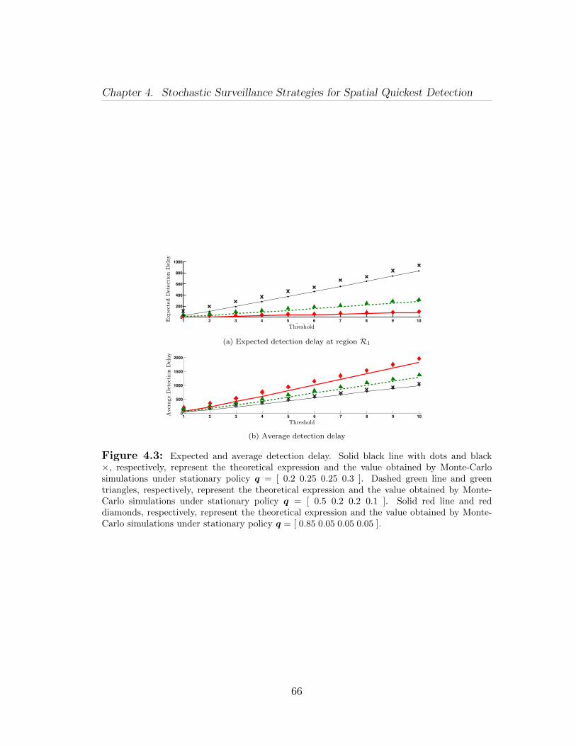
Chapter 4. Stochastic Surveillance Strategies for Spatial Quickest Detection
1 2 3 4 5 6 7 8 9 100
200
400
600
800
1000
Threshold
Expe
cted
det
ectio
n de
lay
Threshold
Expec
ted
Det
ecti
onD
elay
(a) Expected detection delay at region R1
1 2 3 4 5 6 7 8 9 100
500
1000
1500
2000
Threshold
Aver
age
dete
ctio
n de
lay
Threshold
Ave
rage
Det
ecti
onD
elay
(b) Average detection delay
Figure 4.3: Expected and average detection delay. Solid black line with dots and black×, respectively, represent the theoretical expression and the value obtained by Monte-Carlosimulations under stationary policy q = [ 0.2 0.25 0.25 0.3 ]. Dashed green line and greentriangles, respectively, represent the theoretical expression and the value obtained by Monte-Carlo simulations under stationary policy q = [ 0.5 0.2 0.2 0.1 ]. Solid red line and reddiamonds, respectively, represent the theoretical expression and the value obtained by Monte-Carlo simulations under stationary policy q = [ 0.85 0.05 0.05 0.05 ].
66
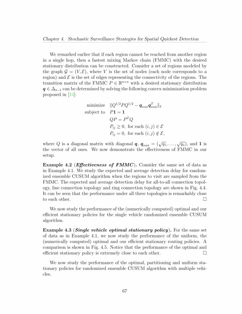
Chapter 4. Stochastic Surveillance Strategies for Spatial Quickest Detection
We remarked earlier that if each region cannot be reached from another regionin a single hop, then a fastest mixing Markov chain (FMMC) with the desiredstationary distribution can be constructed. Consider a set of regions modeled bythe graph G = (V, E), where V is the set of nodes (each node corresponds to aregion) and E is the set of edges representing the connectivity of the regions. Thetransition matrix of the FMMC P ∈ Rn×n with a desired stationary distributionq ∈ ∆n−1 can be determined by solving the following convex minimization problemproposed in [14]:
minimize ‖Q1/2PQ1/2 − qrootqTroot‖2
subject to P1 = 1
QP = P TQ
Pij ≥ 0, for each (i, j) ∈ EPij = 0, for each (i, j) /∈ E ,
where Q is a diagonal matrix with diagonal q, qroot = (√q1, . . . ,
√qn), and 1 is
the vector of all ones. We now demonstrate the effectiveness of FMMC in oursetup.
Example 4.2 (Effectiveness of FMMC ). Consider the same set of data asin Example 4.1. We study the expected and average detection delay for random-ized ensemble CUSUM algorithm when the regions to visit are sampled from theFMMC. The expected and average detection delay for all-to-all connection topol-ogy, line connection topology and ring connection topology are shown in Fig. 4.4.It can be seen that the performance under all three topologies is remarkably closeto each other.
We now study the performance of the (numerically computed) optimal and ourefficient stationary policies for the single vehicle randomized ensemble CUSUMalgorithm.
Example 4.3 (Single vehicle optimal stationary policy). For the same setof data as in Example 4.1, we now study the performance of the uniform, the(numerically computed) optimal and our efficient stationary routing policies. Acomparison is shown in Fig. 4.5. Notice that the performance of the optimal andefficient stationary policy is extremely close to each other.
We now study the performance of the optimal, partitioning and uniform sta-tionary policies for randomized ensemble CUSUM algorithm with multiple vehi-cles.
67
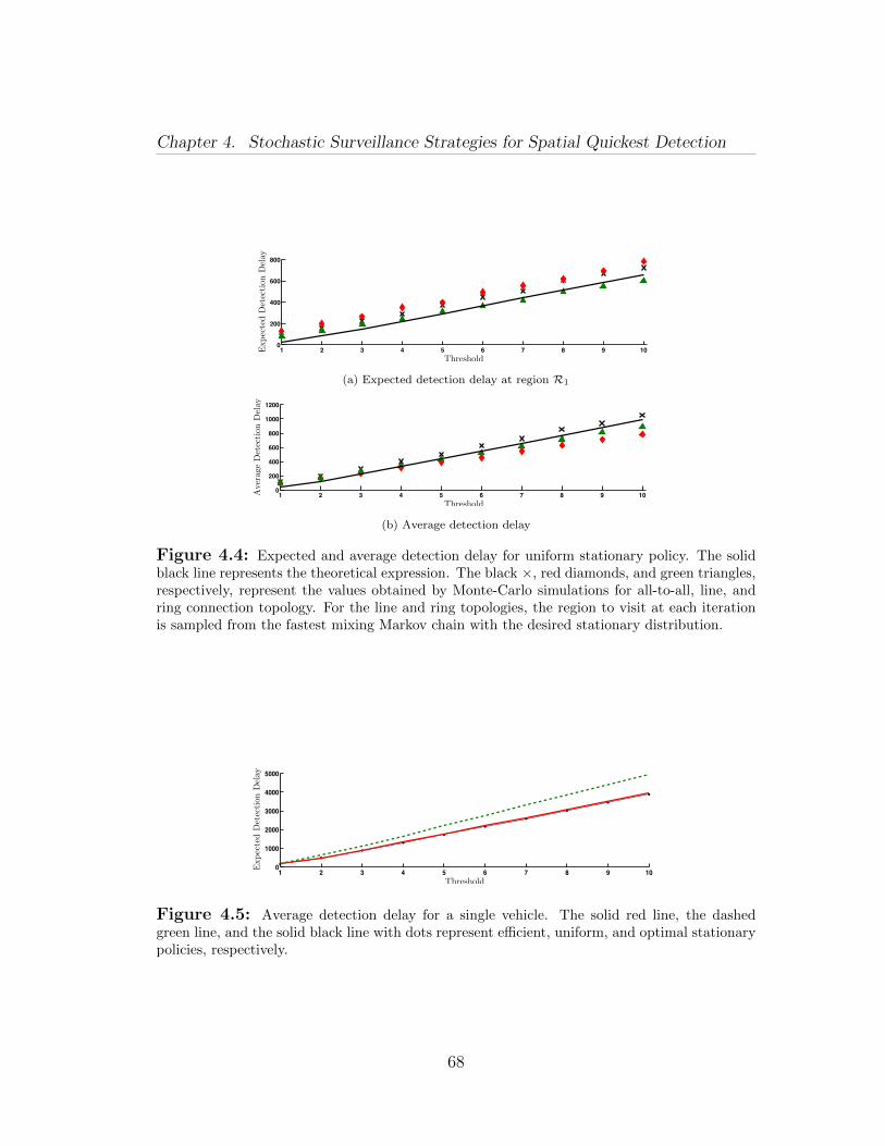
Chapter 4. Stochastic Surveillance Strategies for Spatial Quickest Detection
1 2 3 4 5 6 7 8 9 100
200
400
600
800
Threshold
Expe
cted
det
ectio
n de
lay
Threshold
Expec
ted
Det
ecti
on
Del
ay
(a) Expected detection delay at region R1
1 2 3 4 5 6 7 8 9 100
200
400
600
800
1000
1200
Threshold
Aver
age
dete
ctio
n de
lay
Threshold
Ave
rage
Det
ecti
onD
elay
(b) Average detection delay
Figure 4.4: Expected and average detection delay for uniform stationary policy. The solidblack line represents the theoretical expression. The black ×, red diamonds, and green triangles,respectively, represent the values obtained by Monte-Carlo simulations for all-to-all, line, andring connection topology. For the line and ring topologies, the region to visit at each iterationis sampled from the fastest mixing Markov chain with the desired stationary distribution.
1 2 3 4 5 6 7 8 9 100
1000
2000
3000
4000
5000
Expe
cted
det
ectio
n de
lay
ThresholdThreshold
Expec
ted
Det
ecti
onD
elay
Figure 4.5: Average detection delay for a single vehicle. The solid red line, the dashedgreen line, and the solid black line with dots represent efficient, uniform, and optimal stationarypolicies, respectively.
68
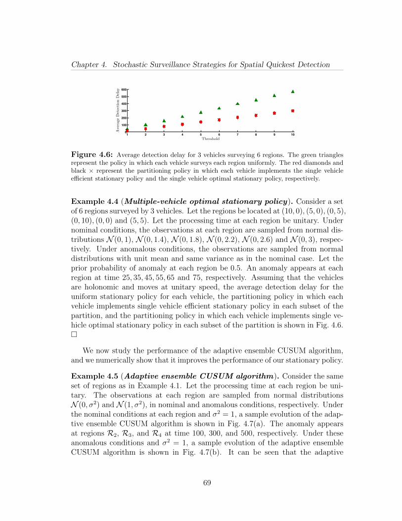
Chapter 4. Stochastic Surveillance Strategies for Spatial Quickest Detection
1 2 3 4 5 6 7 8 9 100
100
200
300
400
500
600
Threshold
Avg
Det
Del
ay
Threshold
Ave
rage
Det
ecti
on
Del
ay
Figure 4.6: Average detection delay for 3 vehicles surveying 6 regions. The green trianglesrepresent the policy in which each vehicle surveys each region uniformly. The red diamonds andblack × represent the partitioning policy in which each vehicle implements the single vehicleefficient stationary policy and the single vehicle optimal stationary policy, respectively.
Example 4.4 (Multiple-vehicle optimal stationary policy). Consider a setof 6 regions surveyed by 3 vehicles. Let the regions be located at (10, 0), (5, 0), (0, 5),(0, 10), (0, 0) and (5, 5). Let the processing time at each region be unitary. Undernominal conditions, the observations at each region are sampled from normal dis-tributions N (0, 1), N (0, 1.4), N (0, 1.8), N (0, 2.2), N (0, 2.6) and N (0, 3), respec-tively. Under anomalous conditions, the observations are sampled from normaldistributions with unit mean and same variance as in the nominal case. Let theprior probability of anomaly at each region be 0.5. An anomaly appears at eachregion at time 25, 35, 45, 55, 65 and 75, respectively. Assuming that the vehiclesare holonomic and moves at unitary speed, the average detection delay for theuniform stationary policy for each vehicle, the partitioning policy in which eachvehicle implements single vehicle efficient stationary policy in each subset of thepartition, and the partitioning policy in which each vehicle implements single ve-hicle optimal stationary policy in each subset of the partition is shown in Fig. 4.6.
We now study the performance of the adaptive ensemble CUSUM algorithm,and we numerically show that it improves the performance of our stationary policy.
Example 4.5 (Adaptive ensemble CUSUM algorithm). Consider the sameset of regions as in Example 4.1. Let the processing time at each region be uni-tary. The observations at each region are sampled from normal distributionsN (0, σ2) and N (1, σ2), in nominal and anomalous conditions, respectively. Underthe nominal conditions at each region and σ2 = 1, a sample evolution of the adap-tive ensemble CUSUM algorithm is shown in Fig. 4.7(a). The anomaly appearsat regions R2, R3, and R4 at time 100, 300, and 500, respectively. Under theseanomalous conditions and σ2 = 1, a sample evolution of the adaptive ensembleCUSUM algorithm is shown in Fig. 4.7(b). It can be seen that the adaptive
69
Chapter 4. Stochastic Surveillance Strategies for Spatial Quickest Detection
ensemble algorithm samples a region with high likelihood of anomaly with highprobability, and, hence, it improves upon the performance of the stationary policy.
We now study the expected detection delay under adaptive ensemble CUSUMalgorithm and compare it with the efficient stationary policy. The anomaly at eachregion appears at time 50, 200, 350 and 500, respectively. The expected detectiondelay obtained by Monte-Carlo simulations for σ2 = 1 and different thresholds isshown in Fig. 4.8(a). It can be seen that the adaptive policy improves the detectiondelay significantly over the efficient stationary policy for large thresholds. It shouldbe noted that the detection delay minimization is most needed at large thresholdsbecause the detection delay is already low at small thresholds. Furthermore,frequent false alarms are encountered at low thresholds and hence, low thresholdsare not typically chosen. The expected detection delay obtained by Monte-Carlosimulations for different value of σ2 and threshold η = 5 is shown in Fig. 4.8(b).Note that for a given value of σ2, the Kullback-Leibler divergence betweenN (1, σ2)and N (0, σ2) is 1/2σ2. It can be seen that the adaptive policy improves theperformance of the stationary policy for each value of noise.
We now apply the adaptive ensemble CUSUM algorithm to a more generalscenario where the anomalous distribution is not completely known. As remarkedearlier, in this case, the CUSUM algorithm should be replaced with the GLRalgorithm. Given the nominal probability density function f 0
k and the anomalousprobability density function f 1
k (·|θ) parameterized by θ ∈ Θ ⊆ R`, for some ` ∈ N,the GLR algorithm, see [6], works identically to the CUSUM algorithm, exceptthat the CUSUM statistic is replaced by the statistic
Λkτ = max
t∈1,...,τsupθ∈Θ
τ∑i=t
logf 1k (yi|θ)f 0k (yi)
.
Example 4.6 (Generalized Likelihood Ratio). For the same set of data asin Example 4.5, assume that there are three types of potential anomalies at eachregion. Since any combination of these anomalies can occur simultaneously, thereare 7 potential distributions under anomalous conditions. We characterize thesedistributions as different hypothesis and assume that the observations under eachhypothesis h ∈ 1, . . . , 8 are sampled from a normal distribution with mean µhand covariances Σh. Let
µ1 =[
000
], µ2 =
[100
], µ3 =
[010
], µ4 =
[001
],
µ5 =[
110
], µ6 =
[011
], µ7 =
[101
], µ8 =
[111
], and
70
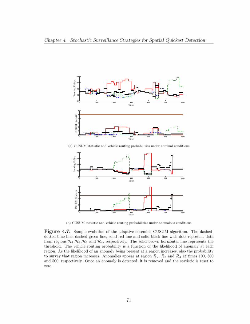
Chapter 4. Stochastic Surveillance Strategies for Spatial Quickest Detection
0 100 200 300 400 500 6000.1
0.2
0.3
0.4
0.5
Time
Rou
ting
polic
y
0 100 200 300 400 500 6000
1
2
3
4
5
6
Time
CU
SUM
Sta
tistic
Time
Time
Rou
ting
Policy
CU
SU
MSta
tist
ic
(a) CUSUM statistic and vehicle routing probabilities under nominal conditions
0 100 200 300 400 500 6000
0.2
0.4
0.6
0.8
Time
Rou
ting
polic
y
0 100 200 300 400 500 6000
2
4
6
8
Time
CU
SUM
sat
istic
Time
Time
Rou
ting
Pol
icy
CU
SU
MSta
tist
ic
(b) CUSUM statistic and vehicle routing probabilities under anomalous conditions
Figure 4.7: Sample evolution of the adaptive ensemble CUSUM algorithm. The dashed-dotted blue line, dashed green line, solid red line and solid black line with dots represent datafrom regions R1,R2,R3 and R4, respectively. The solid brown horizontal line represents thethreshold. The vehicle routing probability is a function of the likelihood of anomaly at eachregion. As the likelihood of an anomaly being present at a region increases, also the probabilityto survey that region increases. Anomalies appear at region R2, R3 and R4 at times 100, 300and 500, respectively. Once an anomaly is detected, it is removed and the statistic is reset tozero.
71
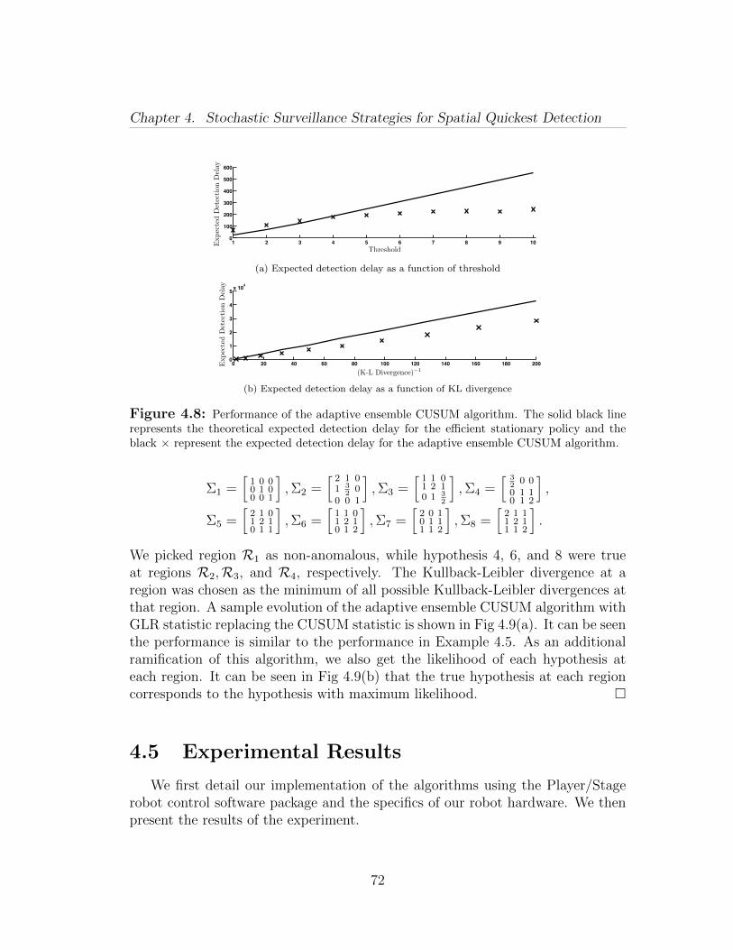
Chapter 4. Stochastic Surveillance Strategies for Spatial Quickest Detection
1 2 3 4 5 6 7 8 9 100
100
200
300
400
500
600
Threshold
Expe
cted
det
ectio
n de
lay
Expec
ted
Det
ecti
on
Del
ay
Threshold
(a) Expected detection delay as a function of threshold
0 20 40 60 80 100 120 140 160 180 2000
1
2
3
4
5 x 10⁴
(K L Divergence) 1
Expe
cted
det
ectio
n de
lay
(K-L Divergence)−1
Expec
ted
Det
ecti
onD
elay
(b) Expected detection delay as a function of KL divergence
Figure 4.8: Performance of the adaptive ensemble CUSUM algorithm. The solid black linerepresents the theoretical expected detection delay for the efficient stationary policy and theblack × represent the expected detection delay for the adaptive ensemble CUSUM algorithm.
Σ1 =[
1 0 00 1 00 0 1
],Σ2 =
[ 2 1 01 3
20
0 0 1
],Σ3 =
[ 1 1 01 2 10 1 3
2
],Σ4 =
[ 32
0 00 1 10 1 2
],
Σ5 =[
2 1 01 2 10 1 1
],Σ6 =
[1 1 01 2 10 1 2
],Σ7 =
[2 0 10 1 11 1 2
],Σ8 =
[2 1 11 2 11 1 2
].
We picked region R1 as non-anomalous, while hypothesis 4, 6, and 8 were trueat regions R2,R3, and R4, respectively. The Kullback-Leibler divergence at aregion was chosen as the minimum of all possible Kullback-Leibler divergences atthat region. A sample evolution of the adaptive ensemble CUSUM algorithm withGLR statistic replacing the CUSUM statistic is shown in Fig 4.9(a). It can be seenthe performance is similar to the performance in Example 4.5. As an additionalramification of this algorithm, we also get the likelihood of each hypothesis ateach region. It can be seen in Fig 4.9(b) that the true hypothesis at each regioncorresponds to the hypothesis with maximum likelihood.
4.5 Experimental Results
We first detail our implementation of the algorithms using the Player/Stagerobot control software package and the specifics of our robot hardware. We thenpresent the results of the experiment.
72
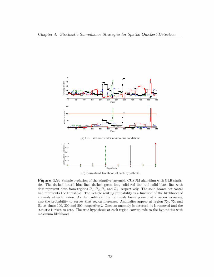
Chapter 4. Stochastic Surveillance Strategies for Spatial Quickest Detection
0 50 100 150 200 250 300 350 400 450 500 5500
0.2
0.4
0.6
0.8
1
Time
Rou
ting
Polic
y
0 50 100 150 200 250 300 350 400 450 500 5500
5
10
15
Time
GLR
Sta
tistic
Time
Time
Rou
ting
Policy
GLR
Sta
tist
ic
(a) GLR statistic under anomalous conditions
1 2 3 4 5 6 7 80
0.2
0.4
0.6
0.8
1
Hypothesis
Post
erio
r Pro
babi
lity
Hypothesis
Nor
mal
ized
Lik
elih
ood
(b) Normalized likelihood of each hypothesis
Figure 4.9: Sample evolution of the adaptive ensemble CUSUM algorithm with GLR statis-tic. The dashed-dotted blue line, dashed green line, solid red line and solid black line withdots represent data from regions R1,R2,R3 and R4, respectively. The solid brown horizontalline represents the threshold. The vehicle routing probability is a function of the likelihood ofanomaly at each region. As the likelihood of an anomaly being present at a region increases,also the probability to survey that region increases. Anomalies appear at region R2, R3 andR4 at times 100, 300 and 500, respectively. Once an anomaly is detected, it is removed and thestatistic is reset to zero. The true hypothesis at each region corresponds to the hypothesis withmaximum likelihood
73

Chapter 4. Stochastic Surveillance Strategies for Spatial Quickest Detection
Rear caster
ComputerRangefinder
Drive wheel
Figure 4.10: Erratic mobile robot with URG-04LX laser rangefinder.
Robot hardware
We use Erratic mobile robots from Videre Design shown in Fig. 4.10. Therobot platform has a roughly square footprint (40cm× 37cm), with two differentialdrive wheels and a single rear caster. Each robot carries an on-board computerwith a 1.8Ghz Core 2 Duo processor, 1 GB of memory, and 802.11g wirelesscommunication. For navigation and localization, each robot is equipped with aHokuyo URG- 04LX laser rangefinder. The rangefinder scans 683 points over240at 10Hz with a range of 5.6 meters.
Localization
We use the amcl driver in Player which implements Adaptive Monte-CarloLocalization, see [100]. The physical robots are provided with a map of our labwith a 15cm resolution and told their starting pose within the map (Fig. 4.11).We set an initial pose standard deviation of 0.9m in position and 12 in orientation,and request updated localization based on 50 of the sensors range measurementsfor each change of 2cm in robot position or 2 in orientation. We use the mostlikely pose estimate by amcl as the location of the robot.
Navigation
Each robot uses the snd driver in Player for the Smooth Nearness Diagramnavigation, see [32]. For the hardware, we set the robot radius parameter to 22cm,obstacle avoidance distance to 0.5m, and maximum speed to 0.2m/s. We let arobot achieve its target when it is within 10cm of the target.
Experiment setup
For our experiment we employed our team of 3 Erratic robots to survey ourlaboratory. As in Fig. 4.11, a set of 8 important regions have been chosen and
74
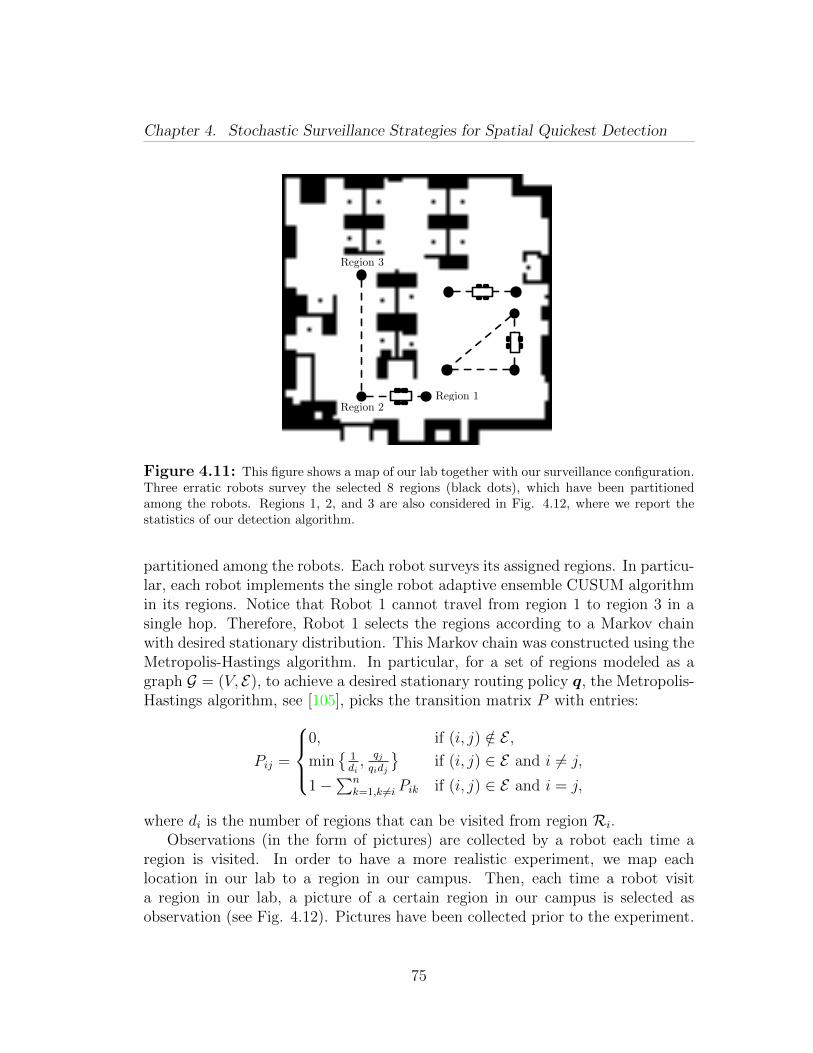
Chapter 4. Stochastic Surveillance Strategies for Spatial Quickest Detection
Region 1Region 2
Region 3
Figure 4.11: This figure shows a map of our lab together with our surveillance configuration.Three erratic robots survey the selected 8 regions (black dots), which have been partitionedamong the robots. Regions 1, 2, and 3 are also considered in Fig. 4.12, where we report thestatistics of our detection algorithm.
partitioned among the robots. Each robot surveys its assigned regions. In particu-lar, each robot implements the single robot adaptive ensemble CUSUM algorithmin its regions. Notice that Robot 1 cannot travel from region 1 to region 3 in asingle hop. Therefore, Robot 1 selects the regions according to a Markov chainwith desired stationary distribution. This Markov chain was constructed using theMetropolis-Hastings algorithm. In particular, for a set of regions modeled as agraph G = (V, E), to achieve a desired stationary routing policy q, the Metropolis-Hastings algorithm, see [105], picks the transition matrix P with entries:
Pij =
0, if (i, j) /∈ E ,min
1di,qjqidj
if (i, j) ∈ E and i 6= j,
1−∑n
k=1,k 6=i Pik if (i, j) ∈ E and i = j,
where di is the number of regions that can be visited from region Ri.Observations (in the form of pictures) are collected by a robot each time a
region is visited. In order to have a more realistic experiment, we map eachlocation in our lab to a region in our campus. Then, each time a robot visita region in our lab, a picture of a certain region in our campus is selected asobservation (see Fig. 4.12). Pictures have been collected prior to the experiment.
75
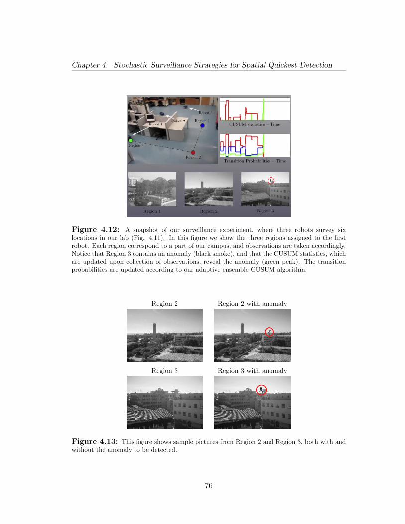
Chapter 4. Stochastic Surveillance Strategies for Spatial Quickest Detection
Region 3
Region 2
Region 1Robot 1
Robot 2
Robot 3
Figure 4.12: A snapshot of our surveillance experiment, where three robots survey sixlocations in our lab (Fig. 4.11). In this figure we show the three regions assigned to the firstrobot. Each region correspond to a part of our campus, and observations are taken accordingly.Notice that Region 3 contains an anomaly (black smoke), and that the CUSUM statistics, whichare updated upon collection of observations, reveal the anomaly (green peak). The transitionprobabilities are updated according to our adaptive ensemble CUSUM algorithm.
Region 2 Region 2 with anomaly
Region 3 with anomalyRegion 3
Figure 4.13: This figure shows sample pictures from Region 2 and Region 3, both with andwithout the anomaly to be detected.
76
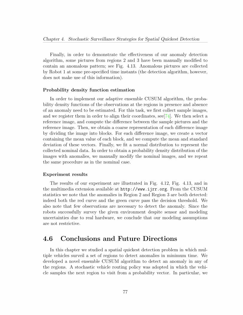
Chapter 4. Stochastic Surveillance Strategies for Spatial Quickest Detection
Finally, in order to demonstrate the effectiveness of our anomaly detectionalgorithm, some pictures from regions 2 and 3 have been manually modified tocontain an anomalous pattern; see Fig. 4.13. Anomalous pictures are collectedby Robot 1 at some pre-specified time instants (the detection algorithm, however,does not make use of this information).
Probability density function estimation
In order to implement our adaptive ensemble CUSUM algorithm, the proba-bility density functions of the observations at the regions in presence and absenceof an anomaly need to be estimated. For this task, we first collect sample images,and we register them in order to align their coordinates, see[74]. We then select areference image, and compute the difference between the sample pictures and thereference image. Then, we obtain a coarse representation of each difference imageby dividing the image into blocks. For each difference image, we create a vectorcontaining the mean value of each block, and we compute the mean and standarddeviation of these vectors. Finally, we fit a normal distribution to represent thecollected nominal data. In order to obtain a probability density distribution of theimages with anomalies, we manually modify the nominal images, and we repeatthe same procedure as in the nominal case.
Experiment results
The results of our experiment are illustrated in Fig. 4.12, Fig. 4.13, and inthe multimedia extension available at http://www.ijrr.org. From the CUSUMstatistics we note that the anomalies in Region 2 and Region 3 are both detected:indeed both the red curve and the green curve pass the decision threshold. Wealso note that few observations are necessary to detect the anomaly. Since therobots successfully survey the given environment despite sensor and modelinguncertainties due to real hardware, we conclude that our modeling assumptionsare not restrictive.
4.6 Conclusions and Future Directions
In this chapter we studied a spatial quickest detection problem in which mul-tiple vehicles surveil a set of regions to detect anomalies in minimum time. Wedeveloped a novel ensemble CUSUM algorithm to detect an anomaly in any ofthe regions. A stochastic vehicle routing policy was adopted in which the vehi-cle samples the next region to visit from a probability vector. In particular, we
77
Chapter 4. Stochastic Surveillance Strategies for Spatial Quickest Detection
studied (i) stationary policy: the probability vector is a constant function of time;and (ii) adaptive policy: the probability vector is adapted with time based on thecollected observations. We designed an efficient stationary policy that depends onthe travel time of the vehicles, the processing time required to collect informationat each region, and the anomaly detection difficulty at each region. In adaptivepolicy, we modified the efficient stationary policy at each iteration to ensure thatthe regions with high likelihood of anomaly are visited with high probability, andthus, improved upon the performance of the stationary policy. We also mentionedthe methods that extend the ideas in this chapter immediately to the scenario inwhich the distributions of the observations in presence and absence of anomaly arenot completely known, but belong to some parametrized family, or to the scenarioin which the observations collected from each region are not independent (e.g., inthe case of dynamic anomalies).
There are several possible extensions of the ideas considered here. First, in thecase of dependent observations at each region, the current method assumes knowndistributions in the presence and absence of anomalies. An interesting directionis to design quickest detection strategies that are robust to the uncertainties inthese distributions. Second, the anomalies considered in this chapter are alwayscontained in the same region. It would be of interest to consider anomalies thatcan move from one region to another. Third, the policy presented in this chapterconsiders an arbitrary partition that satisfy some cardinality constraints. It is ofinterest to come up with smarter partitioning policies that take into considerationthe travel times, and the difficulty of detection at each region. Last, to constructthe fastest mixing Markov chain with desired stationary distribution, we relied ontime-homogeneous Markov chains. A time varying Markov chain may achieve afaster convergence to the desired stationary distribution, see [37]. This is also aninteresting direction to be pursued.
4.7 Appendix: Probabilistic guarantee to the
uniqueness of critical point
We now provide probabilistic guarantee for Conjecture 4.3. The average de-tection delay for a single vehicle under a stationary policy q is
δavg(q) =( n∑i=1
viqi
)( n∑i=1
qiTi +n∑i=1
n∑j=1
qiqjdij
),
78
Chapter 4. Stochastic Surveillance Strategies for Spatial Quickest Detection
where vi = wiη/Di for each i ∈ 1, . . . , n. A local minimum of δavg can be canbe found by substituting qn = 1−
∑n−1j=1 qj, and then running the gradient descent
algorithm from some initial point q0 ∈ ∆n−1 on the resulting objective function.Let v = (v1, . . . , vn) and T = (T1, . . . , Tn). We assume that the parameters
v,T , D, n in a given instance of optimization problem (4.3) and the choseninitial point q0 are realizations of random variables sampled from some spaceK. For a given realization κ ∈ K, let the realized value of the parameters bev(κ),T (κ), D(κ), n(κ), and the chosen initial point be q0(κ). The associatedoptimization problem is:
minimizeq∈∆n(κ)−1
δavg(q |κ), (4.4)
where, for a given realization κ ∈ K, δavg(· |κ) : ∆n(κ)−1 → R>0 ∪+∞ is definedby
δavg(q |κ) =( n(κ)∑i=1
vi(κ)
qi
)(n(κ)∑i=1
qiTi(κ) +
n(κ)∑i=1
n(κ)∑j=1
qiqjdij(κ)).
For a given realization κ, let gd(· |κ) : ∆n(κ)−1 → ∆n(κ)−1 be the function thatdetermines the outcome of the gradient descent algorithm applied to the functionobtained by substituting qn(κ) = 1 −
∑n(κ)−1j=1 qj in δavg(q |κ). In other words,
the gradient descent algorithm starting from point q0(κ) converges to the pointgd(q0(κ) |κ). Consider N1 realizations κ1, . . . , κN1 ∈ KN1 . Let qoptimal(κ) =gd( 1
n(κ)1n(κ) |κ), and define
γ = max‖gd(q0(κs) |κs)− qoptimal(κs)‖ | s ∈ 1, . . . , N1.
It is known from [19] that if N1 ≥ −(log ν1)/µ1, for some µ1, ν1 ∈ ]0, 1[, then,with at least confidence 1− ν1, it holds
P(q0(κ)∈∆n(κ)−1 | ‖gd(q0(κ) |κ)− qoptimal(κ)‖ ≤ γ) ≥ 1− µ1,
for any realization κ ∈ K.We sample the following quantities: the value n as uniformly distributed in
3, . . . , 12; each coordinate of the n regions in two dimensional space from thenormal distribution with mean 0 and variance 100; the value Ti, for each i ∈1, . . . , n, from the half normal distribution with mean 0 and variance 100; andthe value vi, for each i ∈ 1, . . . , n, uniformly from ]0, 1[. For a realized value ofn, we chose q0 uniformly in ∆n−1. Let the matrix D be the Euclidean distancematrix between the n sampled regions.
We considered N1 = 1000 realizations of the parameters v,T , D, n andinitial value q0. The sample sizes were determined for µ1 = 0.01 and ν1 = 10−4.
79

Chapter 4. Stochastic Surveillance Strategies for Spatial Quickest Detection
The value of γ obtained was 10−4. Consequently, the gradient descent algorithmfor the optimization problem (4.3) starting from any feasible point yields thesame solution with high probability. In other words, with at least confidence level99.99% and probability at least 99%, the optimization problem (4.3) has a uniquecritical point at which the minimum is achieved.
80
Chapter 5
Operator Attention Allocationvia Knapsack Problems
In this chapter we study knapsack problems with sigmoid utility. The timeevolution of the performance of a human operator is well modeled by a sigmoidfunction (see Section 2.3) and consequently, the knapsack problems with sigmoidutility well model the resource (attention) allocation problem of a time-constrainedhuman operator. We study three particular knapsack problems with sigmoid util-ity, namely, the knapsack problem with sigmoid utility, the generalized assignmentproblem with sigmoid utility, and the bin-packing problem with sigmoid utility.These problems model situations where human operators are looking at the feedsfrom a camera network and deciding on the presence of some malicious activ-ity. The first problem determines the optimal fraction of work-hours an operatorshould allocate to each feed such that their overall performance is optimal. Thesecond problem determines the allocations of the tasks to identical and inde-pendently working operators as well as the optimal fraction of work-hours eachoperator should allocate to each feed such that the overall performance of theteam is optimal. Assuming that the operators work in an optimal fashion, thethird problem determines the minimum number of operators and an allocation ofeach feed to some operator such that each operator allocates non-zero fraction ofwork-hours to each feed assigned to them. We study these knapsack problemsunder following assumptions on the sigmoid functions:
(A1). Smooth sigmoid functions: For the ease of the presentation, we focus onsmooth sigmoid functions. The analysis presented here extends immediatelyto non-smooth functions by using the sub-derivative instead of the derivativein the following analysis.
81
Chapter 5. Operator Attention Allocation via Knapsack Problems
(A2). Monotonic sigmoid functions: We assume that the sigmoid functions asso-ciated with the problem are non-decreasing. In several interesting budgetallocation problems, e.g. [75], the sigmoid utility is not a non-decreasingfunction. The approach in this chapter extends to the case of a generalsigmoid utility. The algorithms proposed in this chapter also involve certainheuristics that improve the constant-factor solution. These heuristics exploitthe monotonicity of the sigmoid function and will not hold for a general sig-moid function. We note that even without the performance improvementheuristics the solution is within a constant factor of optimal.
Note that both these assumptions hold true for sigmoid functions associated withhuman performance.
5.1 Sigmoid Function and Linear Penalty
In order to gain insight into the behavior of sigmoid functions, we start witha simple problem with a very interesting result. We study the maximization of asigmoid function subject to a linear penalty. Consider a sigmoid function f anda penalty rate c ∈ R>0, and the following optimization problem:
maximizet≥0
f(t)− ct. (5.1)
The derivative of a sigmoid function is not a one to one mapping and hence, notinvertible. We define the pseudo-inverse of the derivative of a sigmoid function fwith inflection point tinf, f † : R>0 → R≥0 by
f †(y) =
maxt ∈ R≥0 | f ′(t) = y, if y ∈ (0, f ′(tinf)],
0, otherwise.(5.2)
Notice that the definition of the pseudo-inverse is consistent with Figure 2.1. Wenow present the solution to the problem (5.1).
Lemma 5.1 (Sigmoid function with linear penalty). For the optimizationproblem (5.1), the optimal allocation t∗ is
t∗ := argmaxf(β)− cβ | β ∈ 0, f †(c).
Proof. The global maximum lies at the point where first derivative is zero or at theboundary. The first derivative of the objective function is f ′(t)− c. If f ′(tinf) < c,then the objective function is a decreasing function of time and the maximum
82
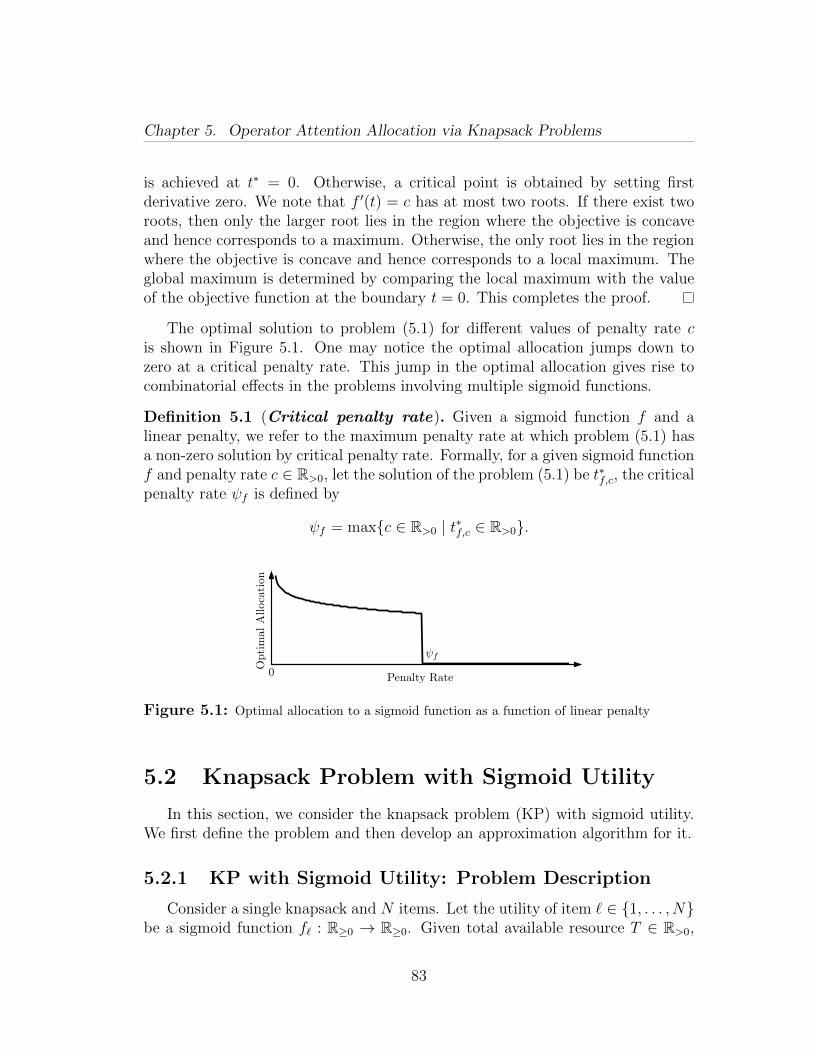
Chapter 5. Operator Attention Allocation via Knapsack Problems
is achieved at t∗ = 0. Otherwise, a critical point is obtained by setting firstderivative zero. We note that f ′(t) = c has at most two roots. If there exist tworoots, then only the larger root lies in the region where the objective is concaveand hence corresponds to a maximum. Otherwise, the only root lies in the regionwhere the objective is concave and hence corresponds to a local maximum. Theglobal maximum is determined by comparing the local maximum with the valueof the objective function at the boundary t = 0. This completes the proof.
The optimal solution to problem (5.1) for different values of penalty rate cis shown in Figure 5.1. One may notice the optimal allocation jumps down tozero at a critical penalty rate. This jump in the optimal allocation gives rise tocombinatorial effects in the problems involving multiple sigmoid functions.
Definition 5.1 (Critical penalty rate). Given a sigmoid function f and alinear penalty, we refer to the maximum penalty rate at which problem (5.1) hasa non-zero solution by critical penalty rate. Formally, for a given sigmoid functionf and penalty rate c ∈ R>0, let the solution of the problem (5.1) be t∗f,c, the criticalpenalty rate ψf is defined by
ψf = maxc ∈ R>0 | t∗f,c ∈ R>0.
00 Penalty Rate
Opti
mal
Alloca
tion
ψf
Figure 5.1: Optimal allocation to a sigmoid function as a function of linear penalty
5.2 Knapsack Problem with Sigmoid Utility
In this section, we consider the knapsack problem (KP) with sigmoid utility.We first define the problem and then develop an approximation algorithm for it.
5.2.1 KP with Sigmoid Utility: Problem Description
Consider a single knapsack and N items. Let the utility of item ` ∈ 1, . . . , Nbe a sigmoid function f` : R≥0 → R≥0. Given total available resource T ∈ R>0,
83
Chapter 5. Operator Attention Allocation via Knapsack Problems
the objective of the KP with sigmoid utility is to determine the resource allocationto each item such that the total utility of the knapsack is maximized. Formally,the KP with sigmoid utility is posed as:
maximizet0
N∑`=1
f`(t`)
subject toN∑`=1
t` ≤ T.
(5.3)
The KP with sigmoid utility models the situation where a human operatorhas to perform N decision making tasks within time T . If the performance ofthe human operator on task ` is given by sigmoid function f`, then the optimalduration allocation to each task is determined by the solution of problem (5.3).We remark that the objective function in problem (5.3) can be a weighted sumof performance functions as well. Such weights can be absorbed into the perfor-mance functions yielding a new sigmoid performance function. We now state thefollowing proposition from [1]:
Proposition 5.2 (Hardness of KP with sigmoid utility). The KP withsigmoid utility is NP-hard, unless P = NP.
5.2.2 KP with Sigmoid Utility: Approximation Algorithm
We now develop an approximation algorithm for the KP with sigmoid utility.We define the Lagrangian L : RN
>0 × R≥0 × RN≥0 → R for the knapsack problem
with sigmoid utility (5.3) by
L(t, α,µ) =N∑`=1
f`(t`) + α(T −N∑`=1
t`) + µTt.
Let tinf` be the inflection point of sigmoid function f` and f †` be the pseudo-
inverse of its derivative as defined in equation (5.2). We define the maximumvalue of the derivative of sigmoid function f` by α` = f ′`(t
inf` ). We also define
αmax = maxα` | ` ∈ 1, . . . , N. We will later show that αmax is the maximumpossible value of the Lagrange multiplier α.
We define the set of inconsistent sigmoid functions by I = ` ∈ 1, . . . , N | tinf` >
T. Similarly and accordingly, we define the set of consistent sigmoid functionsas 1, . . . , N \ I. We denote the j-th element of the standard basis of RN by ej.
84
Chapter 5. Operator Attention Allocation via Knapsack Problems
Define F : (0, αmax] → R≥0 as the optimal value of the objective function inthe following α-parametrized KP:
maximizeN∑`=1
x`f`(f†` (α))
subject toN∑`=1
x`f†` (α) ≤ T
x` ∈ 0, 1, ∀` ∈ 1, . . . , N.
(5.4)
Define FLP : (0, αmax]→ R≥0 as the optimal value of the objective function inthe following α-parametrized fractional KP:
maximizeN∑`=1
x`f`(f†` (α))
subject toN∑`=1
x`f†` (α) ≤ T
x` ∈ [0, 1], ∀` ∈ 1, . . . , N.
(5.5)
For a given α, the solution to problem (5.5) is obtained in the following way:
(i). sort tasks such that
f1(f †1(α))
f †1(α)≥ f2(f †2(α))
f †2(α)≥ . . . ≥ fN(f †N(α))
f †N(α);
(ii). find k := minj ∈ 1, . . . , N |∑j
i=1 f†i (α) ≥ T;
(iii). the solution is xLP1 = xLP
2 = . . . = xLPk−1 = 1, xLP
k = (T −∑k−1
i=1 f†i (α))/f †k(α),
and xLPk+1 = xLP
k+2 = . . . = xLPN = 0.
A 2-factor solution to the binary KP (5.4) is obtained by picking the better ofthe sets of tasks 1, . . . , k − 1 and k (see [54, 57] for details). Let Fapprox :(0, αmax] → R≥0 be the value of the objective function in the α-parametrizedknapsack problem under such 2-factor solution.
We now state the following important property of the function FLP:
Lemma 5.3 (Discontinuity of FLP). The maximal set of points of discontinuityof the function FLP is α1, . . . , αN.
85
Chapter 5. Operator Attention Allocation via Knapsack Problems
Proof. For each α ∈ [0, αmax], the α-parametrized fractional KP is a linear pro-gram, and the solution lies at one of the vertex of the feasible simplex. Notethat if f †` (α) is a continuous function for each ` ∈ 1, . . . , N, then the verticesof the feasible simplex are continuous functions of α. Further, the objective func-tion is also continuous if f †` (α) is a continuous function for each ` ∈ 1, . . . , N.Therefore, the function FLP may be discontinuous only if f †` (α) is discontinuousfor some `, i.e., α ∈ α1, . . . , αN.
We will show that if each sigmoid function is consistent, then the allocation toeach sigmoid function can be written in terms of the Lagrange multiplier α, andthe KP with sigmoid utility (5.3) reduces to α-parametrized KP (5.4). Further,the optimal Lagrange multiplier α∗ can be searched in the interval ]0, αmax], andthe α∗-parametrized KP can be solved using standard approximation algorithmsto determine a solution within a constant factor of optimality. The search ofthe optimal Lagrange multiplier is a univariate continuous optimization problemand a typical optimization algorithm will determine the exact optimal Lagrangemultiplier only asymptotically, but it will converge to an arbitrarily small neigh-borhood of the optimal Lagrange multiplier in finite number of iterations. Thus,a factor of optimality within an ε neighborhood of the desired factor of optimality,for any ε > 0, can be achieved in a finite number of iterations. We utilize theseideas to develop a (2 + ε)-factor approximation algorithm for KP with sigmoidutility in Algorithm 5.1. This algorithm searches for the Lagrange multiplier thatmaximizes the optimal value function FLP of the α-parametrized fractional KPand truncates the associated solution to determine a constant-factor solution tothe knapsack problem with sigmoid utility. This algorithm also involves a per-formance improvement heuristic in which the unemployed resource is allocated tothe most beneficial task amongst those with zero resource. We note that if thesigmoid utilities are non-smooth, then the standard KKT conditions in the follow-ing analysis are replaced with the KKT conditions for non-smooth optimizationproblems [44].
We define an ε-approximate maximizer of a function as a point in the domainof the function at which the function attains a value within ε of its maximumvalue. We now analyze Algorithm 5.1.
Theorem 5.4 (KP with sigmoid utility). The following statements hold forthe KP with sigmoid utility (5.3) and the solution obtained via Algorithm 5.1:
(i). the solution is within factor of optimality (2 + ε), for any ε > 0;
(ii). if ε-approximate maximizer over each continuous piece of FLP can be searchedusing a constant number of function evaluations, then the Algorithm 5.1 runsin O(N2) time.
86
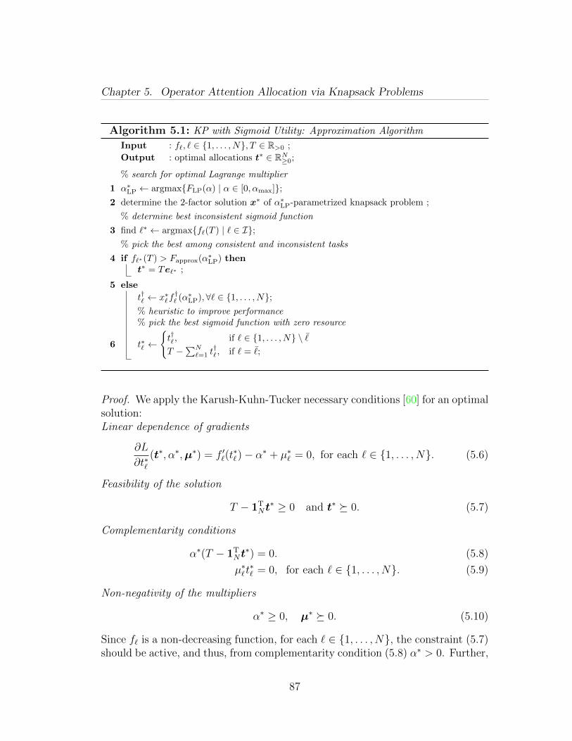
Chapter 5. Operator Attention Allocation via Knapsack Problems
Algorithm 5.1: KP with Sigmoid Utility: Approximation Algorithm
Input : f`, ` ∈ 1, . . . , N, T ∈ R>0 ;
Output : optimal allocations t∗ ∈ RN≥0;
% search for optimal Lagrange multiplier
1 α∗LP ← argmaxFLP(α) | α ∈ [0, αmax];2 determine the 2-factor solution x∗ of α∗LP-parametrized knapsack problem ;
% determine best inconsistent sigmoid function
3 find `∗ ← argmaxf`(T ) | ` ∈ I;% pick the best among consistent and inconsistent tasks
4 if f`∗(T ) > Fapprox(α∗LP) thent∗ = Te`∗ ;
5 else
t†` ← x∗`f†` (α∗LP),∀` ∈ 1, . . . , N;
% heuristic to improve performance% pick the best sigmoid function with zero resource
6 t∗` ←
t†`, if ` ∈ 1, . . . , N \ ¯
T −∑N`=1 t
†`, if ` = ¯;
Proof. We apply the Karush-Kuhn-Tucker necessary conditions [60] for an optimalsolution:Linear dependence of gradients
∂L
∂t∗`(t∗, α∗,µ∗) = f ′`(t
∗`)− α∗ + µ∗` = 0, for each ` ∈ 1, . . . , N. (5.6)
Feasibility of the solution
T − 1TNt∗ ≥ 0 and t∗ 0. (5.7)
Complementarity conditions
α∗(T − 1TNt∗) = 0. (5.8)
µ∗` t∗` = 0, for each ` ∈ 1, . . . , N. (5.9)
Non-negativity of the multipliers
α∗ ≥ 0, µ∗ 0. (5.10)
Since f` is a non-decreasing function, for each ` ∈ 1, . . . , N, the constraint (5.7)should be active, and thus, from complementarity condition (5.8) α∗ > 0. Further,
87
Chapter 5. Operator Attention Allocation via Knapsack Problems
from equation (5.9), if t∗` 6= 0, then µ∗` = 0. Therefore, if a non-zero resource is al-located to sigmoid function fη, η ∈ 1, . . . , N, then it follows from equation (5.6)
f ′η(t∗η) = α∗. (5.11)
Assuming each f` is consistent, i.e., tinf` ≤ T , for each ` ∈ 1, . . . , N, the second
order condition [60] yields that a local maxima exists at t∗ only if
f ′′η (t∗η) ≤ 0 ⇐⇒ t∗η ≥ tinfη . (5.12)
The equations (5.11) and (5.12) yield that optimal non-zero allocation to sigmoidfunction fη is
t∗η = f †η(α∗). (5.13)
Given the optimal Lagrange multiplier α∗, the optimal non-zero allocation tothe sigmoid function fη is given by equation (5.13). Further, the optimal set ofsigmoid functions with non-zero allocations is the solution to the α∗-parametrizedknapsack problem (5.4). We now show that α∗ is maximizer of F . Since, atleast one task is processed, w`f
′`(t∗`) = α, for some ` ∈ 1, . . . , N. Thus, α ∈
[0, αmax]. By contradiction assume that α is the maximizer of F , and F (α) >F (α∗). This means that the allocation corresponding to α yields higher rewardthan the allocation corresponding to α∗. This contradictions equation (5.13).
If tinf` > T , for some ` ∈ 1, . . . , N, then equation (5.12) does not hold for
any t` ∈ [0, T ]. Since, f` is convex in the interval [0, T ], the optimal allocationfor maximum is at the boundary, i.e., t` ∈ 0, T. Therefore, as exemplifiedin Figure 5.2, the optimal allocation is either Te` or lies at the projection of thesimplex on the hyperplane t` = 0. The projection of the simplex on the hyperplanet` = 0 is again a simplex and the argument holds recursively.
To establish the first statement we note that α∗LP is maximizer of FLP, andthe α-parametrized fractional knapsack problem is relaxation of α-parametrizedknapsack problem, hence
FLP(α∗LP) ≥ FLP(α∗) ≥ F (α∗). (5.14)
We further note that α∗ is maximizer of F and Fapprox is sub-optimal value of theobjective function, hence
F (α∗) ≥ F (α∗LP) ≥ Fapprox(α∗LP) ≥ 1
2FLP(α∗LP), (5.15)
where the last inequality follows from the construction of Fapprox (see 2-factorpolicy for binary knapsack problem [57]). The value of objective function at
88
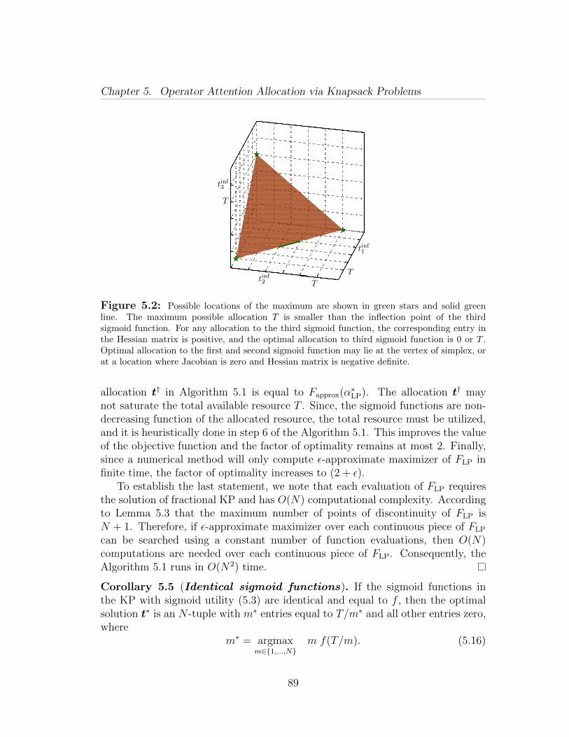
Chapter 5. Operator Attention Allocation via Knapsack Problems
T
T
T
tinf1
tinf2
tinf3
Figure 5.2: Possible locations of the maximum are shown in green stars and solid greenline. The maximum possible allocation T is smaller than the inflection point of the thirdsigmoid function. For any allocation to the third sigmoid function, the corresponding entry inthe Hessian matrix is positive, and the optimal allocation to third sigmoid function is 0 or T .Optimal allocation to the first and second sigmoid function may lie at the vertex of simplex, orat a location where Jacobian is zero and Hessian matrix is negative definite.
allocation t† in Algorithm 5.1 is equal to Fapprox(α∗LP). The allocation t† maynot saturate the total available resource T . Since, the sigmoid functions are non-decreasing function of the allocated resource, the total resource must be utilized,and it is heuristically done in step 6 of the Algorithm 5.1. This improves the valueof the objective function and the factor of optimality remains at most 2. Finally,since a numerical method will only compute ε-approximate maximizer of FLP infinite time, the factor of optimality increases to (2 + ε).
To establish the last statement, we note that each evaluation of FLP requiresthe solution of fractional KP and has O(N) computational complexity. Accordingto Lemma 5.3 that the maximum number of points of discontinuity of FLP isN + 1. Therefore, if ε-approximate maximizer over each continuous piece of FLP
can be searched using a constant number of function evaluations, then O(N)computations are needed over each continuous piece of FLP. Consequently, theAlgorithm 5.1 runs in O(N2) time.
Corollary 5.5 (Identical sigmoid functions). If the sigmoid functions inthe KP with sigmoid utility (5.3) are identical and equal to f , then the optimalsolution t∗ is an N -tuple with m∗ entries equal to T/m∗ and all other entries zero,where
m∗ = argmaxm∈1,...,N
m f(T/m). (5.16)
89
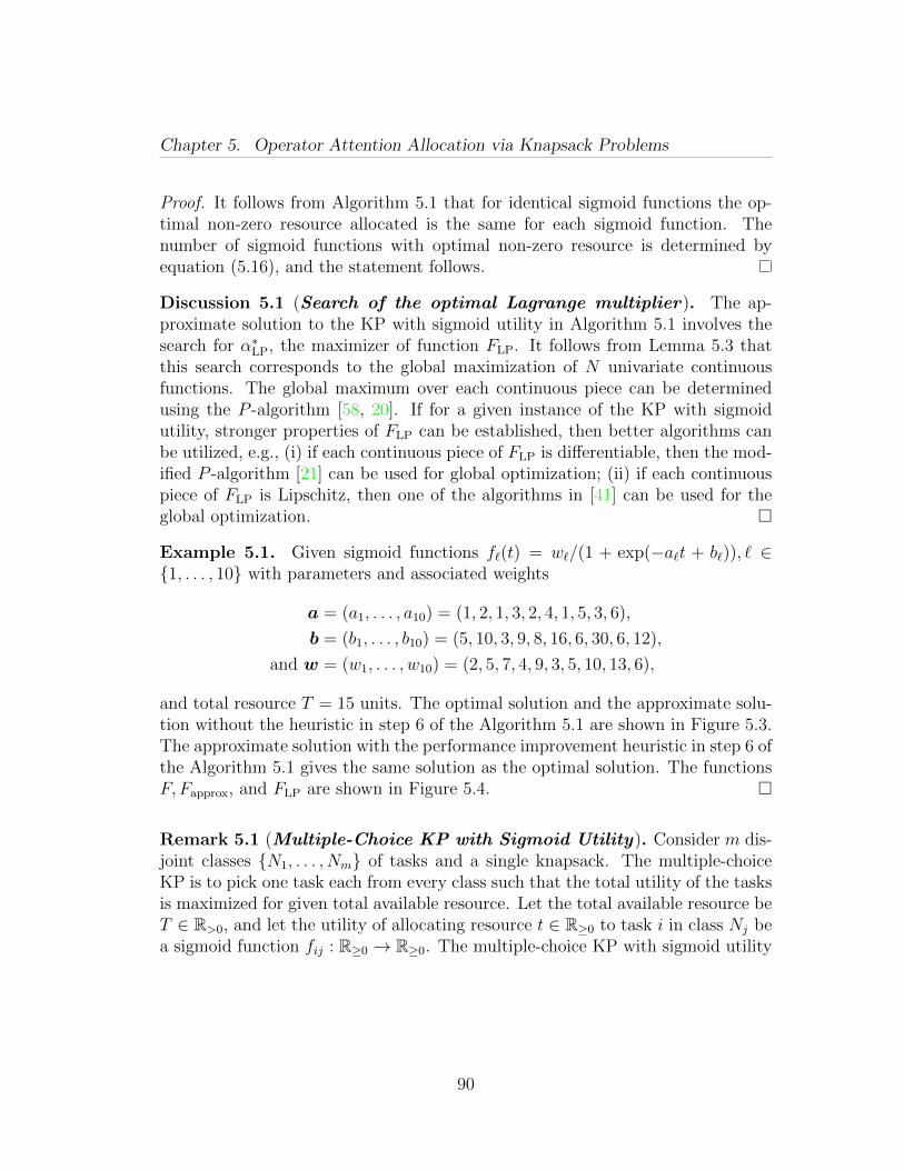
Chapter 5. Operator Attention Allocation via Knapsack Problems
Proof. It follows from Algorithm 5.1 that for identical sigmoid functions the op-timal non-zero resource allocated is the same for each sigmoid function. Thenumber of sigmoid functions with optimal non-zero resource is determined byequation (5.16), and the statement follows.
Discussion 5.1 (Search of the optimal Lagrange multiplier). The ap-proximate solution to the KP with sigmoid utility in Algorithm 5.1 involves thesearch for α∗LP, the maximizer of function FLP. It follows from Lemma 5.3 thatthis search corresponds to the global maximization of N univariate continuousfunctions. The global maximum over each continuous piece can be determinedusing the P -algorithm [58, 20]. If for a given instance of the KP with sigmoidutility, stronger properties of FLP can be established, then better algorithms canbe utilized, e.g., (i) if each continuous piece of FLP is differentiable, then the mod-ified P -algorithm [21] can be used for global optimization; (ii) if each continuouspiece of FLP is Lipschitz, then one of the algorithms in [41] can be used for theglobal optimization.
Example 5.1. Given sigmoid functions f`(t) = w`/(1 + exp(−a`t + b`)), ` ∈1, . . . , 10 with parameters and associated weights
a = (a1, . . . , a10) = (1, 2, 1, 3, 2, 4, 1, 5, 3, 6),
b = (b1, . . . , b10) = (5, 10, 3, 9, 8, 16, 6, 30, 6, 12),
and w = (w1, . . . , w10) = (2, 5, 7, 4, 9, 3, 5, 10, 13, 6),
and total resource T = 15 units. The optimal solution and the approximate solu-tion without the heuristic in step 6 of the Algorithm 5.1 are shown in Figure 5.3.The approximate solution with the performance improvement heuristic in step 6 ofthe Algorithm 5.1 gives the same solution as the optimal solution. The functionsF, Fapprox, and FLP are shown in Figure 5.4.
Remark 5.1 (Multiple-Choice KP with Sigmoid Utility). Consider m dis-joint classes N1, . . . , Nm of tasks and a single knapsack. The multiple-choiceKP is to pick one task each from every class such that the total utility of the tasksis maximized for given total available resource. Let the total available resource beT ∈ R>0, and let the utility of allocating resource t ∈ R≥0 to task i in class Nj bea sigmoid function fij : R≥0 → R≥0. The multiple-choice KP with sigmoid utility
90
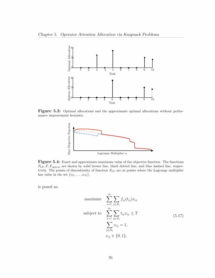
Chapter 5. Operator Attention Allocation via Knapsack Problems
2 4 6 8 101 3 5 7 90
3
6
Opt
imal
allo
c
2 4 6 8 101 3 5 7 90
3
6
Apro
x. a
lloc
Opti
mal
Alloca
tion
Appro
xA
lloca
tion
Task
Task
1
1
5
52
2
3
3 4
4
6
6 7
7
8
8
9
9
10
10
3
3
6
6
0
02 4 6 8 101 3 5 7 9
0
3
6
Opt
imal
allo
c
2 4 6 8 101 3 5 7 90
3
6
Apro
x. a
lloc
Opti
mal
Alloca
tion
Appro
xA
lloca
tion
Task
Task
1
1
5
52
2
3
3 4
4
6
6 7
7
8
8
9
9
10
10
3
3
6
6
0
0
Figure 5.3: Optimal allocations and the approximate optimal allocations without perfor-mance improvement heuristic.
Lagrange Multiplier αMax
Obje
ctiv
eFunct
ion
Figure 5.4: Exact and approximate maximum value of the objective function. The functionsFLP, F, Fapprox are shown by solid brown line, black dotted line, and blue dashed line, respec-tively. The points of discontinuity of function FLP are at points where the Lagrange multiplierhas value in the set α1, . . . , αN.
is posed as:
maximizem∑i=1
∑j∈Ni
fij(tij)xij
subject tom∑i=1
∑j∈Ni
tijxij ≤ T∑j∈Ni
xij = 1,
xij ∈ 0, 1,
(5.17)
91
Chapter 5. Operator Attention Allocation via Knapsack Problems
for each i ∈ 1, . . . ,m and j ∈ Ni. The multiple-choice KP with sigmoid utilitymodels a situation where a human operator has to process one task each from agiven classes of tasks within time T . The performance of the operator on taski from class Nj is given by sigmoid function fij. The different tasks in a givenclass may be, e.g., observations collected from different sensors in a given region.The methodology developed in this section extends to a multiple-choice KP withsigmoid utility (5.17). In particular, the problem (5.17) can be reduced to anα-parameterized multiple-choice knapsack problem, and the LP relaxation based2-factor approximation algorithm for the binary multiple choice knapsack prob-lem [54] can be utilized to determine a 2-factor algorithm for the problem (5.17).
5.3 Generalized Assignment Problem with Sig-
moid Utility
In this section, we consider the generalized assignment problem (GAP) withsigmoid utility. We first define the problem and then develop an approximationalgorithm for it.
5.3.1 GAP with Sigmoid Utility: Problem Description
Consider M bins (knapsacks) and N items. Let Tj be the capacity of binj ∈ 1, . . . ,M. Let the utility of item i ∈ 1, . . . , N when allocated to bin i bea sigmoid function fij : R≥0 → R≥0 of the allocated recourse tij. The GAP withsigmoid utility determines the optimal assignment of the items to bins such thatthe total utility of the bins is maximized. Formally, the GAP with sigmoid utilityis posed as:
maximizeM∑j=1
N∑i=1
fij(tij)xij
subject toN∑i=1
tijxij ≤ Tj,
M∑j=1
xij ≤ 1,
xij ∈ 0, 1,
(5.18)
92
Chapter 5. Operator Attention Allocation via Knapsack Problems
for each i ∈ 1, . . . , N and j ∈ 1, . . . ,M. The GAP with sigmoid utility modelsa situation where M human operators have to independently serve N tasks. Theoperator j works for a duration Tj. The performance of human operator j on taski is given by sigmoid function fij. The solution to the GAP determines optimalassignments of the tasks to the operators and the optimal time-duration to beallocated to each processed task. We now state the following result about thehardness of the GAP with sigmoid utility:
Proposition 5.6 (Hardness of GAP with sigmoid utility). The generalizedassignment problem with sigmoid utility is NP-hard, unless P = NP.
Proof. The statement follows from the fact that knapsack problem with sigmoidutility is a special case of the generalized assignment problem with sigmoid utility,and is NP -hard according to Proposition 5.2.
5.3.2 GAP with Sigmoid Utility: Approximation Algo-rithm
We now propose an approximation algorithm for the GAP with sigmoid utility.This algorithm is an adaptation of the 3-factor algorithm for the binary GAPproposed in [27] and is presented in Algorithm 5.2. In Algorithm 5.2, F is the
matrix of sigmoid functions fij, F(j)∗1 represents first column of matrix F (j), and
E2∗2:M−j+1 represents matrix E2 with first column removed. Similarly, FIunprocj
represents the vector with entries Fij, i ∈ Iunproc, and tAj represents the vectorwith entries tij, i ∈ A. The algorithm calls a recursive function, namely, GAP(·, ·)(defined in Algorithm 5.3) to compute the solution of GAP with sigmoid utility.The solution comprises of a set A describing assignment of tasks to bins and tdescribes associated duration allocations. The function GAP utilizes the solutionto KP with sigmoid utility at each recursion to compute the solution to the GAPwith sigmoid utility. In particular, the function KP(·, ·) determines the set of tasksto be processed A, and allocations t according to Algorithm 5.1. The key elementof the algorithm is the decomposition of the performance matrix at each recursion.In particular, the performance matrix F is decomposed into E1 and E2 at eachrecursion, where E1 corresponds to the current bin and allocations to it accordingto Algorithm 5.1, and E2 corresponds to a GAP with smaller number of bins. Theperformance is efficient with respect to the component E1 due to effectiveness ofAlgorithm 5.1, while component E2 recursively reduces to the single bin case,i.e., to the KP with sigmoid utility. The algorithm also involves a performanceimproving heuristic. According to this heuristic, if the resource of a bin is notcompletely utilized and there are tasks that are not assigned to any bin, then a
93
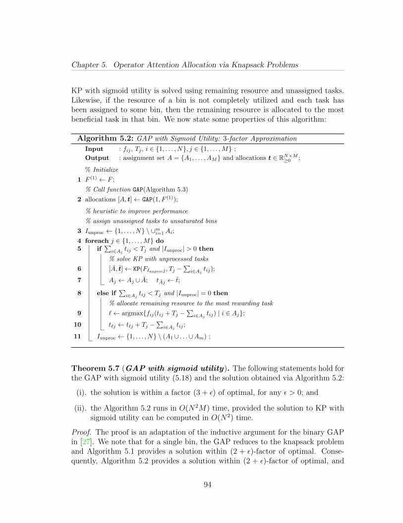
Chapter 5. Operator Attention Allocation via Knapsack Problems
KP with sigmoid utility is solved using remaining resource and unassigned tasks.Likewise, if the resource of a bin is not completely utilized and each task hasbeen assigned to some bin, then the remaining resource is allocated to the mostbeneficial task in that bin. We now state some properties of this algorithm:
Algorithm 5.2: GAP with Sigmoid Utility: 3-factor Approximation
Input : fij , Tj , i ∈ 1, . . . , N, j ∈ 1, . . . ,M ;
Output : assignment set A = A1, . . . , AM and allocations t ∈ RN×M≥0 ;
% Initialize
1 F (1) ← F ;
% Call function GAP(Algorithm 5.3)
2 allocations [A, t]← GAP(1, F (1));
% heuristic to improve performance
% assign unassigned tasks to unsaturated bins
3 Iunproc ← 1, . . . , N \ ∪mi=1Ai;
4 foreach j ∈ 1, . . . ,M do5 if
∑i∈Aj tij < Tj and |Iunproc| > 0 then
% solve KP with unprocessed tasks
6 [A, t]← KP(FIunprocj , Tj −∑i∈Aj tij);
7 Aj ← Aj ∪ A; tAj ← t;
8 else if∑i∈Aj tij < Tj and |Iunproc| = 0 then
% allocate remaining resource to the most rewarding task
9 `← argmaxfij(tij + Tj −∑i∈Aj tij) | i ∈ Aj;
10 t`j ← t`j + Tj −∑i∈Aj tij ;
11 Iunproc ← 1, . . . , N \ (A1 ∪ . . .∪Am) ;
Theorem 5.7 (GAP with sigmoid utility). The following statements hold forthe GAP with sigmoid utility (5.18) and the solution obtained via Algorithm 5.2:
(i). the solution is within a factor (3 + ε) of optimal, for any ε > 0; and
(ii). the Algorithm 5.2 runs in O(N2M) time, provided the solution to KP withsigmoid utility can be computed in O(N2) time.
Proof. The proof is an adaptation of the inductive argument for the binary GAPin [27]. We note that for a single bin, the GAP reduces to the knapsack problemand Algorithm 5.1 provides a solution within (2 + ε)-factor of optimal. Conse-quently, Algorithm 5.2 provides a solution within (2 + ε)-factor of optimal, and
94
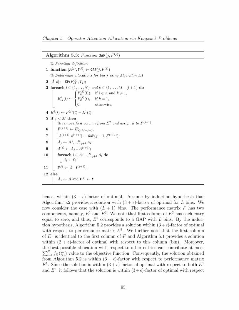
Chapter 5. Operator Attention Allocation via Knapsack Problems
Algorithm 5.3: Function GAP(j, F (j))
% Function definition
1 function [A(j), t(j)]← GAP(j, F (j))
% Determine allocations for bin j using Algorithm 5.1
2 [A, t]← KP(F(j)∗1 , Tj);
3 foreach i ∈ 1, . . . , N and k ∈ 1, . . . ,M − j + 1 do
E1ik(t)←
F
(j)i1 (ti), if i ∈ A and k 6= 1,
F(j)i1 (t), if k = 1,
0, otherwise;
4 E2(t)← F (j)(t)− E1(t);
5 if j < M then% remove first column from E2 and assign it to F (j+1)
6 F (j+1) ← E2∗2:M−j+1;
7 [A(j+1), t(j+1)]← GAP(j + 1, F (j+1));
8 Aj ← A \ ∪Mi=j+1Ai;
9 A(j) ← Aj ∪A(j+1);
10 foreach i ∈ A∩∪Mi=j+1Ai doti ← 0;
11 t(j) ← [t t(j+1)];
12 else
Aj ← A and t(j) ← t;
hence, within (3 + ε)-factor of optimal. Assume by induction hypothesis thatAlgorithm 5.2 provides a solution with (3 + ε)-factor of optimal for L bins. Wenow consider the case with (L + 1) bins. The performance matrix F has twocomponents, namely, E1 and E2. We note that first column of E2 has each entryequal to zero, and thus, E2 corresponds to a GAP with L bins. By the induc-tion hypothesis, Algorithm 5.2 provides a solution within (3 + ε)-factor of optimalwith respect to performance matrix E2. We further note that the first columnof E1 is identical to the first column of F and Algorithm 5.1 provides a solutionwithin (2 + ε)-factor of optimal with respect to this column (bin). Moreover,the best possible allocation with respect to other entries can contribute at most∑N
i=1 fi1(t∗i1) value to the objective function. Consequently, the solution obtainedfrom Algorithm 5.2 is within (3 + ε)-factor with respect to performance matrixE1. Since the solution is within (3 + ε)-factor of optimal with respect to both E1
and E2, it follows that the solution is within (3+ ε)-factor of optimal with respect
95
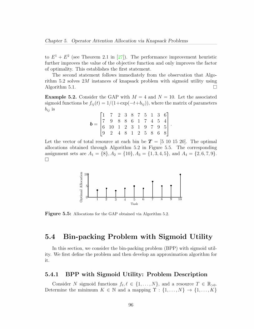
Chapter 5. Operator Attention Allocation via Knapsack Problems
to E1 + E2 (see Theorem 2.1 in [27]). The performance improvement heuristicfurther improves the value of the objective function and only improves the factorof optimality. This establishes the first statement.
The second statement follows immediately from the observation that Algo-rithm 5.2 solves 2M instances of knapsack problem with sigmoid utility usingAlgorithm 5.1.
Example 5.2. Consider the GAP with M = 4 and N = 10. Let the associatedsigmoid functions be fij(t) = 1/(1+exp(−t+bij)), where the matrix of parametersbij is
b =
1 7 2 3 8 7 5 1 3 67 9 8 8 6 1 7 4 5 46 10 1 2 3 1 9 7 9 59 2 4 8 1 2 5 8 6 8
.Let the vector of total resource at each bin be T = [5 10 15 20]. The optimalallocations obtained through Algorithm 5.2 in Figure 5.5. The correspondingassignment sets are A1 = 8, A2 = 10, A3 = 1, 3, 4, 5, and A4 = 2, 6, 7, 9.
2 4 6 8 101 3 5 7 90
5
10
1 52 3 4 6 7 8 9 10
10
5
0
Opti
mal
Alloca
tion
Task
Figure 5.5: Allocations for the GAP obtained via Algorithm 5.2.
5.4 Bin-packing Problem with Sigmoid Utility
In this section, we consider the bin-packing problem (BPP) with sigmoid util-ity. We first define the problem and then develop an approximation algorithm forit.
5.4.1 BPP with Sigmoid Utility: Problem Description
Consider N sigmoid functions f`, ` ∈ 1, . . . , N, and a resource T ∈ R>0.Determine the minimum K ∈ N and a mapping Υ : 1, . . . , N → 1, . . . , K
96
Chapter 5. Operator Attention Allocation via Knapsack Problems
such that, for each i ∈ 1, . . . , K, the optimal solution to the KP with sigmoidutility
maximize∑`∈Ai
f`(t`)
subject to∑`∈Ai
t` ≤ T,(5.19)
where Ai = j | Υ(j) = i, allocates non-zero resource to each sigmoid functionf`, ` ∈ Ai.
The BPP with sigmoid utility models a situation where one needs to determinethe minimum number of identical operators, each working for time T , required tooptimally serve each of the N tasks characterized by functions f`, ` ∈ 1, . . . , N.
We denote the critical penalty rate for sigmoid function f` by ψ`, ` ∈ 1, . . . , N,and let ψmin = minψ` | ` ∈ 1, . . . , N. We now state a relevant property of thesolution to the KP with sigmoid utility:
Lemma 5.8 (Non-zero allocations). A solution to the optimization prob-lem (5.19) allocates non-zero resource to each sigmoid function f`, ` ∈ Ai, i ∈1, . . . , K, if
T ≥∑`∈Ai
f †` (ψmin).
Proof. It suffices to prove that if T =∑
`∈Ai f†` (ψmin), then ψmin is the optimal
Lagrange multiplier α∗ in Algorithm 5.1. Note that if a non-zero duration is allo-cated to each task, then the solution obtained from Algorithm 5.1 is the optimalsolution. Since, t∗` = f †` (ψmin), ` ∈ Ai are feasible non-zero allocations, ψmin is aLagrange multiplier. We now prove that ψmin is the optimal Lagrange multiplier.Let Ai = 1, . . . , ai. By contradiction, assume that t∗ is not the globally optimalallocation. Without loss of generality, we assume that the global optimal policyallocates zero resource to sigmoid function fai , and let t be the globally optimal
97
Chapter 5. Operator Attention Allocation via Knapsack Problems
allocation. We observe that
ai−1∑`=1
f`(t`) + fai(0)
≤ai−1∑`=1
f`(t`) + fai(t∗ai
)− ψmint∗ai
(5.20)
≤ai∑`=1
f`(t∗`) +
ai−1∑`=1
f ′`(t∗`)(t` − t∗`)− ψmint
∗ai
(5.21)
=
ai∑`=1
f`(t∗`) +
ai∑`=1
ψmin(t` − t∗`)
=
ai∑`=1
f`(t∗`),
where inequalities (5.20) and (5.21) follow from the definition of critical penaltyand the concavity to the sigmoid function at t∗` , respectively. This contradictsour assumption. Hence, t∗ is the global optimal allocation and this completes theproof.
We now state the following result about the hardness of the BPP with sigmoidutility:
Proposition 5.9 (Hardness of BPP with sigmoid utility). The BPP withsigmoid utility is NP -hard, unless P = NP .
Proof. Consider an instance of standard BPP with items of size ai ≤ T, i ∈1, . . . , N and bins of size T . It is well known [57] that BPP is NP -hard. With-out loss of generality, we can pick N sigmoid functions fi, i ∈ 1, . . . , N suchthat f †i (ψmin) = ai, for each i ∈ 1, . . . , N and some ψmin ∈ R>0. It followsfrom Lemma 5.8 that such an instance of BPP with sigmoid utility is in one-to-one correspondence with the aforementioned standard BPP. This establishes thestatement.
5.4.2 BPP with Sigmoid Utility: Approximation Algo-rithm
We now develop an approximation algorithm for BPP with sigmoid utility.The proposed algorithm is similar to the standard next-fit algorithm [57] for the
98
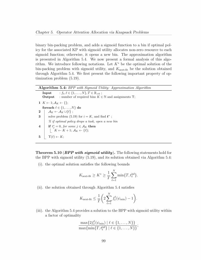
Chapter 5. Operator Attention Allocation via Knapsack Problems
binary bin-packing problem, and adds a sigmoid function to a bin if optimal pol-icy for the associated KP with sigmoid utility allocates non-zero resource to eachsigmoid function; otherwise, it opens a new bin. The approximation algorithmis presented in Algorithm 5.4. We now present a formal analysis of this algo-rithm. We introduce following notations. Let K∗ be the optimal solution of thebin-packing problem with sigmoid utility, and Knext-fit be the solution obtainedthrough Algorithm 5.4. We first present the following important property of op-timization problem (5.19).
Algorithm 5.4: BPP with Sigmoid Utility: Approximation Algorithm
Input : f`, ` ∈ 1, . . . , N, T ∈ R>0 ;Output : number of required bins K ∈ N and assignments Υ;
1 K ← 1;AK ← ;foreach ` ∈ 1, . . . , N do
2 AK ← AK ∪` ;
3 solve problem (5.19) for i = K, and find t∗ ;
% if optimal policy drops a task, open a new bin
4 if t∗j = 0, for some j ∈ AK thenK ← K + 1; AK ← `;
5 Υ(`)← K;
Theorem 5.10 (BPP with sigmoid utility). The following statements hold forthe BPP with sigmoid utility (5.19), and its solution obtained via Algorithm 5.4:
(i). the optimal solution satisfies the following bounds
Knext-fit ≥ K∗ ≥ 1
T
N∑`=1
minT, tinf` .
(ii). the solution obtained through Algorithm 5.4 satisfies
Knext-fit ≤1
T
(2
N∑`=1
f †` (ψmin)− 1
).
(iii). the Algorithm 5.4 provides a solution to the BPP with sigmoid utility withina factor of optimality
max2f †` (ψmin) | ` ∈ 1, . . . , NmaxminT, tinf
` | ` ∈ 1, . . . , N;
99
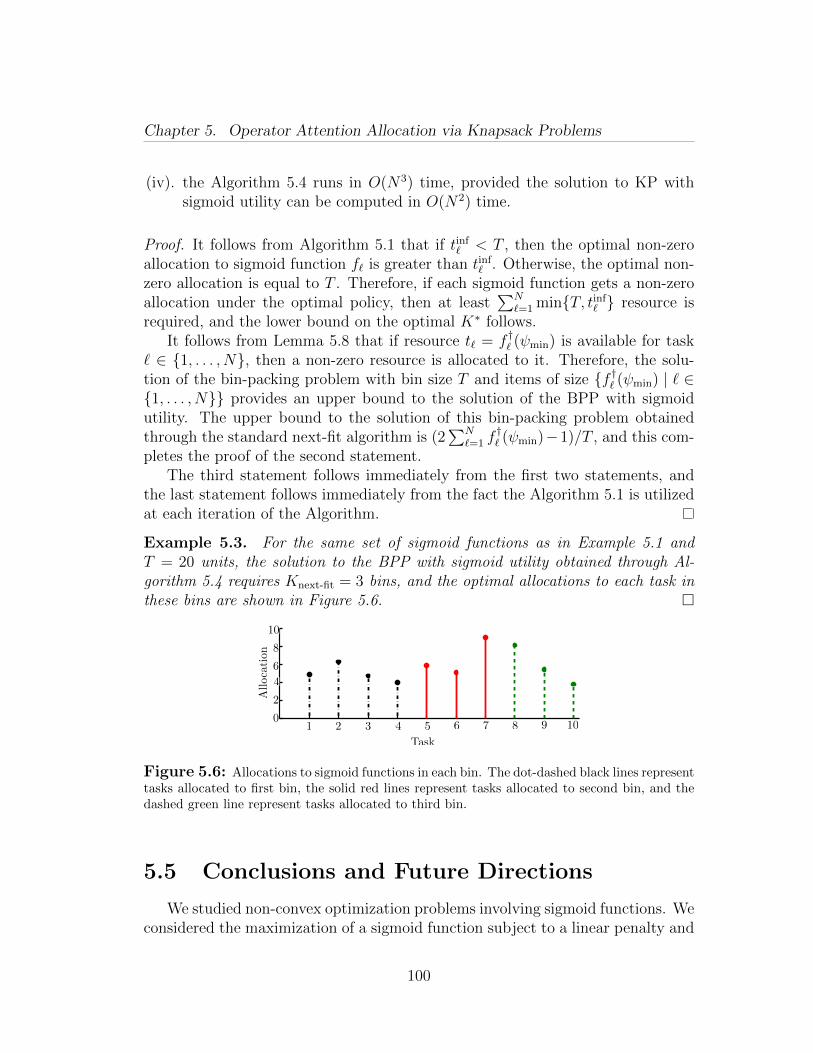
Chapter 5. Operator Attention Allocation via Knapsack Problems
(iv). the Algorithm 5.4 runs in O(N3) time, provided the solution to KP withsigmoid utility can be computed in O(N2) time.
Proof. It follows from Algorithm 5.1 that if tinf` < T , then the optimal non-zero
allocation to sigmoid function f` is greater than tinf` . Otherwise, the optimal non-
zero allocation is equal to T . Therefore, if each sigmoid function gets a non-zeroallocation under the optimal policy, then at least
∑N`=1 minT, tinf
` resource isrequired, and the lower bound on the optimal K∗ follows.
It follows from Lemma 5.8 that if resource t` = f †` (ψmin) is available for task` ∈ 1, . . . , N, then a non-zero resource is allocated to it. Therefore, the solu-tion of the bin-packing problem with bin size T and items of size f †` (ψmin) | ` ∈1, . . . , N provides an upper bound to the solution of the BPP with sigmoidutility. The upper bound to the solution of this bin-packing problem obtainedthrough the standard next-fit algorithm is (2
∑N`=1 f
†` (ψmin)−1)/T , and this com-
pletes the proof of the second statement.The third statement follows immediately from the first two statements, and
the last statement follows immediately from the fact the Algorithm 5.1 is utilizedat each iteration of the Algorithm.
Example 5.3. For the same set of sigmoid functions as in Example 5.1 andT = 20 units, the solution to the BPP with sigmoid utility obtained through Al-gorithm 5.4 requires Knext-fit = 3 bins, and the optimal allocations to each task inthese bins are shown in Figure 5.6.
1 2 3 4 5 6 7 8 9 100
2
4
6
8
10
Task
Alloca
tion
1 2 3 4 5 6 7 8 9 100
2
4
6
8
10
Figure 5.6: Allocations to sigmoid functions in each bin. The dot-dashed black lines representtasks allocated to first bin, the solid red lines represent tasks allocated to second bin, and thedashed green line represent tasks allocated to third bin.
5.5 Conclusions and Future Directions
We studied non-convex optimization problems involving sigmoid functions. Weconsidered the maximization of a sigmoid function subject to a linear penalty and
100
Chapter 5. Operator Attention Allocation via Knapsack Problems
showed that the optimal allocation jumps down to zero at a critical penalty rate.This jump in the allocation imparts combinatorial effects to the constrained opti-mization problems involving sigmoid functions. We studied three such problems,namely, the knapsack problem with sigmoid utility, the generalized assignmentproblem with sigmoid utility, and the bin-packing problem with sigmoid util-ity. We merged approximation algorithms from discrete optimization with algo-rithm from continuous optimization to develop hybrid approximation algorithmsfor these problems.
There are many possible extensions of this work. A similar strategy for ap-proximate optimization could be adopted for other problems involving sigmoidfunctions, e.g., the network utility maximization problem, where the utility ofeach source is a sigmoid function. Other extensions include problems involvinggeneral non-convex functions and optimization in queues with sigmoid character-istics.
101

Chapter 6
Attention Allocation in DecisionMaking Queues
In this chapter we consider the problem of optimal time duration allocationfor a human operator. The decision making tasks arrive at a given rate and arestacked in a queue. A human operator processes these tasks on the first-come first-serve basis (see Figure 6.1.) The human operator receives a unit reward for thecorrect decision, while there is no penalty for a wrong decision. We assume thatthe tasks can be parametrized by some variable and the variable takes value in afinite set D ⊆ R. Let the performance of the operator on a task with parameterd ∈ D be a function fd : R≥0 → [0, 1) of the duration operator allocates to thetask. As discussed in Section 2.3, the human performance function fd is wellmodeled by a sigmoid function. In this chapter we only consider smooth sigmoidfunctions.
We study two particular problems. First, in Section 6.1, we consider a staticqueue with latency penalty, that is, the scenario where the human operator hasto perform N ∈ N decision making tasks, but each task loses value at a constantrate per unit delay in its processing. Second, in Sections 6.2 and 6.3 we consider adynamic queue of decision making tasks where each task loses value at a constantrate per unit delay in its processing. The loss in the value of a task may occurdue to the processing deadline on the task. In other words, the latency penaltyis a soft constraint that captures the processing deadline on the task. For such adecision making queue, we are interested in the optimal time-duration allocationto each task. Alternatively, we are interested in the arrival rate that will result inthe desired accuracy for each task. We intend to design a decision support systemthat tells the human operator the optimal time-duration allocation to each task.
We remark that the processing deadlines on the tasks can be incorporated ashard constraints as well, but the resulting optimization problem is combinatorially
102
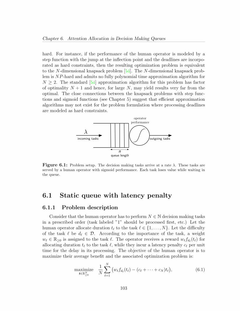
Chapter 6. Attention Allocation in Decision Making Queues
hard. For instance, if the performance of the human operator is modeled by astep function with the jump at the inflection point and the deadlines are incorpo-rated as hard constraints, then the resulting optimization problem is equivalentto the N -dimensional knapsack problem [54]. The N -dimensional knapsack prob-lem is NP -hard and admits no fully polynomial time approximation algorithm forN ≥ 2. The standard [54] approximation algorithm for this problem has factorof optimality N + 1 and hence, for large N , may yield results very far from theoptimal. The close connections between the knapsack problems with step func-tions and sigmoid functions (see Chapter 5) suggest that efficient approximationalgorithms may not exist for the problem formulation where processing deadlinesare modeled as hard constraints.
λincoming tasks outgoing tasks
queue lengthn
operatorperformance
Figure 6.1: Problem setup. The decision making tasks arrive at a rate λ. These tasks areserved by a human operator with sigmoid performance. Each task loses value while waiting inthe queue.
6.1 Static queue with latency penalty
6.1.1 Problem description
Consider that the human operator has to perform N ∈ N decision making tasksin a prescribed order (task labeled ”1” should be processed first, etc.) Let thehuman operator allocate duration t` to the task ` ∈ 1, . . . , N. Let the difficultyof the task ` be d` ∈ D. According to the importance of the task, a weightw` ∈ R≥0 is assigned to the task `. The operator receives a reward w`fd`(t`) forallocating duration t` to the task `, while they incur a latency penalty c` per unittime for the delay in its processing. The objective of the human operator is tomaximize their average benefit and the associated optimization problem is:
maximizet∈RN≥0
1
N
N∑`=1
(w`fd`(t`)− (c` + · · ·+ cN)t`
), (6.1)
103
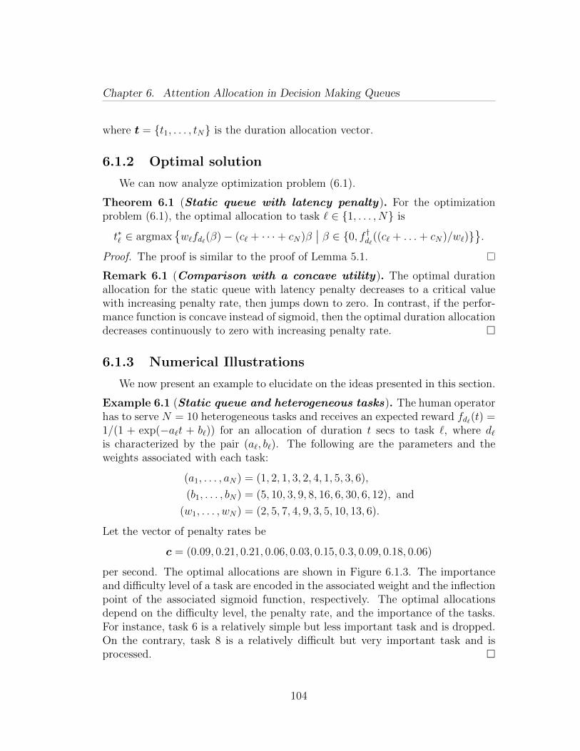
Chapter 6. Attention Allocation in Decision Making Queues
where t = t1, . . . , tN is the duration allocation vector.
6.1.2 Optimal solution
We can now analyze optimization problem (6.1).
Theorem 6.1 (Static queue with latency penalty). For the optimizationproblem (6.1), the optimal allocation to task ` ∈ 1, . . . , N is
t∗` ∈ argmaxw`fd`(β)− (c` + · · ·+ cN)β
∣∣ β ∈ 0, f †d`((c` + . . .+ cN)/w`).
Proof. The proof is similar to the proof of Lemma 5.1.
Remark 6.1 (Comparison with a concave utility). The optimal durationallocation for the static queue with latency penalty decreases to a critical valuewith increasing penalty rate, then jumps down to zero. In contrast, if the perfor-mance function is concave instead of sigmoid, then the optimal duration allocationdecreases continuously to zero with increasing penalty rate.
6.1.3 Numerical Illustrations
We now present an example to elucidate on the ideas presented in this section.
Example 6.1 (Static queue and heterogeneous tasks). The human operatorhas to serve N = 10 heterogeneous tasks and receives an expected reward fd`(t) =1/(1 + exp(−a`t + b`)) for an allocation of duration t secs to task `, where d`is characterized by the pair (a`, b`). The following are the parameters and theweights associated with each task:
(a1, . . . , aN) = (1, 2, 1, 3, 2, 4, 1, 5, 3, 6),
(b1, . . . , bN) = (5, 10, 3, 9, 8, 16, 6, 30, 6, 12), and
(w1, . . . , wN) = (2, 5, 7, 4, 9, 3, 5, 10, 13, 6).
Let the vector of penalty rates be
c = (0.09, 0.21, 0.21, 0.06, 0.03, 0.15, 0.3, 0.09, 0.18, 0.06)
per second. The optimal allocations are shown in Figure 6.1.3. The importanceand difficulty level of a task are encoded in the associated weight and the inflectionpoint of the associated sigmoid function, respectively. The optimal allocationsdepend on the difficulty level, the penalty rate, and the importance of the tasks.For instance, task 6 is a relatively simple but less important task and is dropped.On the contrary, task 8 is a relatively difficult but very important task and isprocessed.
104
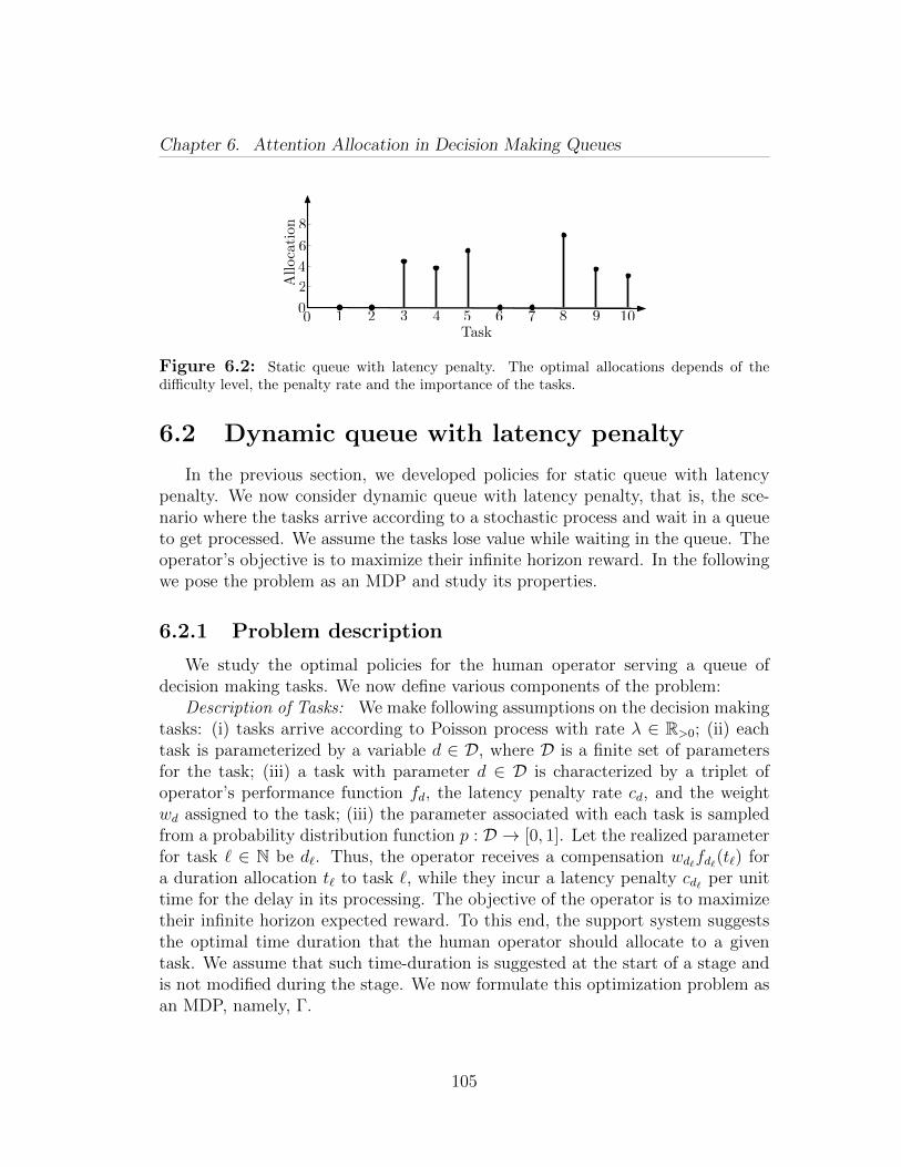
Chapter 6. Attention Allocation in Decision Making Queues
1 2 3 4 5 6 7 8 9 100
2
4
6
8
2
0
4
5 100Task
Alloca
tion
6
8
1 3 7 92 4 6 8
Figure 6.2: Static queue with latency penalty. The optimal allocations depends of thedifficulty level, the penalty rate and the importance of the tasks.
6.2 Dynamic queue with latency penalty
In the previous section, we developed policies for static queue with latencypenalty. We now consider dynamic queue with latency penalty, that is, the sce-nario where the tasks arrive according to a stochastic process and wait in a queueto get processed. We assume the tasks lose value while waiting in the queue. Theoperator’s objective is to maximize their infinite horizon reward. In the followingwe pose the problem as an MDP and study its properties.
6.2.1 Problem description
We study the optimal policies for the human operator serving a queue ofdecision making tasks. We now define various components of the problem:
Description of Tasks: We make following assumptions on the decision makingtasks: (i) tasks arrive according to Poisson process with rate λ ∈ R>0; (ii) eachtask is parameterized by a variable d ∈ D, where D is a finite set of parametersfor the task; (iii) a task with parameter d ∈ D is characterized by a triplet ofoperator’s performance function fd, the latency penalty rate cd, and the weightwd assigned to the task; (iii) the parameter associated with each task is sampledfrom a probability distribution function p : D → [0, 1]. Let the realized parameterfor task ` ∈ N be d`. Thus, the operator receives a compensation wd`fd`(t`) fora duration allocation t` to task `, while they incur a latency penalty cd` per unittime for the delay in its processing. The objective of the operator is to maximizetheir infinite horizon expected reward. To this end, the support system suggeststhe optimal time duration that the human operator should allocate to a giventask. We assume that such time-duration is suggested at the start of a stage andis not modified during the stage. We now formulate this optimization problem asan MDP, namely, Γ.
105
Chapter 6. Attention Allocation in Decision Making Queues
Description of MDP Γ: Let the stage ` ∈ N of the MDP Γ be initiated withthe processing of task `. We now define the elements of the MDP Γ:
(i) Action and State variables: We choose the action variable at stage ` as thetime-duration to be allocated to task `, denoted by t` ∈ R≥0. We choose the statevariable at stage ` as the vector of parameters d` ∈ Dn` associated with each taskin the queue, where n` ∈ N is the queue length at stage `. Note that the definitionof the stage and the state variable are consistent under the following assumption:
Assumption 6.1 (Non-empty queue). Without loss of generality, we assumethat the queue is never empty. If queue is empty at some stage, then the operatorwaits for the next task to arrive, and there is no penalty for such waiting time.
(ii) Reward Structure: We define the reward r : Dn` × R≥0 → R obtained byallocating duration t to the task ` by
r(d`, t) = wd`fd`(t)−1
2
( `+n`−1∑i=`
cdi +
`+n′`−1∑j=`
cdj
)t,
where d` ∈ Dn′` is the vector of penalty rates for the tasks in the queue and n′` is
the queue length just before the end of stage `.Note that the queue length while a task is processed may not be constant,
therefore, the latency penalty is computed as the average of the latency penaltyfor the tasks present at the start of processing the task and the latency penalty forthe tasks present at the end of processing the task. Such averaging is consistentwith the expected number of arrivals being a linear function of time for Poissonprocess.
(iii) Value function:The MDP with finite horizon length N ∈ N maximizes the value function
VN : Dn1 × B(1, . . . , N × D∞,R≥0)→ R defined by
VN(d1, tfinite) =
N∑`=1
E[r(d`, tfinite(`,d`))],
where n1 ∈ N is the initial queue length, D∞ = ∪i∈NDi, and B(1, . . . , N ×D∞,R≥0) is the space of bounded below functions defined from 1, . . . , N ×D∞to R≥0. B(1, . . . , N × D∞,R≥0) represents the space of policies, that is, theduration allocation as a function of stage and state. We will focus on stationarypolicies and for stationary policies, the policy space reduces to B(D∞,R≥0)
Under a stationary policy tstat, the infinite horizon average value function ofthe MDP Vavg : Dn1 × B(D∞,R≥0)→ R is defined by
Vavg(d1, tstat) = lim
N→+∞
1
NVN(d1, t
stat).
106
Chapter 6. Attention Allocation in Decision Making Queues
We also define the infinite horizon discounted value function Vα : Dn1×B(D∞,R≥0)→R by
Vα(d1, tstat) =
+∞∑`=1
α`−1E[r(d`, tstat(d`))],
where α ∈ (0, 1) is the discount factor.
6.2.2 Properties of optimal solution
We now study some properties of the MDP Γ and its solution. Let V ∗α :Dn1 → R≥0 denote the optimal infinite horizon α-discounted value function. Wealso define Nmax = bmaxwdψfd/cd | d ∈ Dc.
Lemma 6.2 (Properties of MDP Γ). The following statements hold for theMDP Γ and its infinite horizon average value function:
(i). there exists a solution to the MDP Γ;
(ii). an optimal stationary policy allocates zero duration to the task ` if n` >Nmax;
Proof. It can be verified that the conditions presented in Section 2.1 hold for MDPΓ and the optimal discounted value function exists. To prove the existence of asolution to the the average value formulation of the MDP Γ, we note that
Vα(d1, t) =+∞∑`=1
α`−1E[r(d`, t`)] ≤wmax − cmin
(1− α),
for each d1 ∈ Dn1 , where n1 is initial queue length, wmax = maxwd | d ∈ D andcmin = mincd | d ∈ D. Therefore, V ∗α (d1) ≤ (wmax − cmin)/(1 − α). Moreover,V ∗α (d1) ≥ Vα(d1,0) = 0. Hence, |V ∗α (d1) − V ∗α (d0)| ≤ 2|wmax − cmin|/(1 − α), forany d0 ∈ Dn0 , n0 ∈ N. Thus, the conditions of Theorem 5.2 in [3] hold and thisestablishes the first statement.
We now establish the second statement. We note that for a state associatedwith queue length n > Nmax, the reward is non-positive and is zero only if theallocation at that stage is zero. Moreover, for a Poisson arrival process, theprobability that the queue length is non-decreasing increases with the allocation atcurrent stage. Thus a positive allocation increases the probability of non-positivereward at future stages. Therefore, a zero duration allocation for n > Nmax
maximizes the reward at current stage and maximizes the probability of gettingpositive rewards at future stages. Consequently, the optimal stationary policyallocates zero duration for a queue length greater than Nmax.
107
Chapter 6. Attention Allocation in Decision Making Queues
6.3 Receding Horizon Solution to dynamic queue
with latency penalty
We rely on the certainty-equivalent receding horizon framework [9, 23, 62] toapproximately solve the MDP Γ. In the certainty-equivalent approximation, thefuture uncertainties are replaced with their expected values [9]. For an allocationof duration t` at stage `, the expected number of arrivals for a Poisson processwith rate λ is λt`. Accordingly, the evolution of the queue length under certainty-equivalent approximation is
n`+1 = max1, n` − 1 + λt`,
where n` represents predicted queue length at stage ` under certainty-equivalentapproximation, and n1 = n1. The certainty-equivalent approximation also re-places the parameters of tasks that have not yet arrived by their expected values,and accordingly, assigns them the expected performance function f : R≥0 → [0, 1),the expected importance w, and the expected latency penalty c defined by
f(t) =1
wEp[wdfd(t)],
w = Ep[wd], and c = Ep[cd], respectively, where Ep[·] represents the expected valuewith respect to the measure p.
The receding horizon framework solves a finite horizon optimization problemat each iteration. We denote the receding horizon policy that solves a N -horizoncertainty-equivalent problem at each stage by N -RH policy. We now study suchcertainty-equivalent finite horizon optimization problem.
6.3.1 Certainty-equivalent finite horizon optimization
We now study the finite horizon optimization problem with horizon lengthN that the certainty-equivalent receding horizon policy solves at each iteration.Given horizon length N , current queue length n`, the realization of the sigmoidfunctions f1, . . . , fn` , the associated latency penalties c1, . . . , cn` and the impor-tance levels w1, . . . , wn` . In certainty-equivalent problem, the true parameters ofthe tasks are used for the tasks that have already arrived, while the expectedvalues of the parameters are used for the tasks that have not yet arrived. In par-ticular, if current queue length is less than the horizon length, i.e., n` < N , thenwe define the reward associated with task j ∈ 1, . . . , N by
rj =
rrlzdj , if 1 ≤ j ≤ n`,
rexpj , if n` + 1 ≤ j ≤ N,
(6.2)
108
Chapter 6. Attention Allocation in Decision Making Queues
where rrlzdj = wjfj(tj) − (
∑n`i=j ci + (nj − n` − j + 1)c)tj − cλt2j/2 is the reward
computed using the realized parameters, and rexpj = wf(tj)−c(n`−j+1)tj−cλt2j/2
is the reward computed using the expected values of the parameters. If the currentqueue length is greater than the horizon length, i.e., n` ≥ N , then we define allthe reward using realized parameters, i.e., rj = rrlzd
j , for each j ∈ 1, . . . , N.
maximizet0
1
N
N∑j=1
rj
subject to nj+1 = max1, nj − 1 + λtj, n1 = n`,
(6.3)
where t = t1, . . . , tN is the duration allocation vector.The optimization problem (6.3) is difficult to handle analytically. For the
special case in which tasks are identical, we provide a procedure to determine theexact solution to problem (6.3) in the Appendix of this chapter. This procedurealso provides insights into the implication of sigmoid performance function on theoptimal policy. For the general case, we resort to the discretization of the actionand the state space and utilize the backward induction algorithm to approximatelysolve the dynamic program (6.3). Let us define maximum allocation to any taskτmax = maxf †d(cd/wd) | d ∈ D. We now state the following results on theefficiency of discretization:
Lemma 6.3 (Discretization of state and action space). For the optimiza-tion problem (6.3) and the discretization of the action and the state space with auniform grid of width ε > 0, the following statements hold:
(i). the state space and the action space can be restricted to compact spaces[1, Nmax + 1], and [0, τmax], respectively;
(ii). the policy obtained through the discretized state and action space in withinO(ε) of optimal;
(iii). the computational complexity of the solution is O(N/ε2).
Proof. It follows from Lemma 5.1 that for nj > maxwdψfd/cmin | d ∈ D, rj +cλt2j/2 achieves its global maximum at tj = 0. Hence, for nj > maxwdψfd/cmin | d ∈D, rj achieves its global maximum at tj = 0. Moreover, the certainty-equivalentqueue length at a stage k > j is a non-decreasing function of of the allocation atstage j. Thus, the reward at stage k > j decreases with allocation tj. Therefore,the optimal policy for the optimization problem (6.3) allocates zero duration atstage j if nj > maxwdψfd/cmin | d ∈ D, and subsequently, the queue lengthdecreases by unity at next stage. Thus, any certainty-equivalent queue length
109

Chapter 6. Attention Allocation in Decision Making Queues
greater than maxwdψfd/cmin | d ∈ D can be mapped to Nmax + frac, wherefrac is the fractional part of the certainty-equivalent queue length. Consequently,the state space can be restricted to the compact set [1, Nmax + 1]. Similarly, fortj > τmax, the reward at stage j in optimization problem (6.3) is a decreasingfunction of the allocation tj, and the rewards at stages k > j are decreasing func-tion of allocation tj. Therefore, the allocation to each task is less than τmax. Thiscompletes the proof of the first statement.
Since the action variable and the state variable in problem (6.3) belong to com-pact sets and the reward function and the state evolution function is Lipschitz, itfollows from Section 2.1 that the value function obtained using the discretized ac-tion and state space is within O(ε) of the optimal value function. This establishesthe second statement.
The third statement is an immediate consequence of the fact that computa-tional complexity of a finite horizon dynamic program is the sum over stages of theproduct of cardinalities of the state space and the action space in each stage.
6.3.2 Performance of receding horizon algorithm
We now derive performance bounds on the receding horizon procedure. First,we determine a global upper bound on the performance of any policy for the MDPΓ. Then, we develop a lower bound on the performance of 1-RH policy. Withoutloss of generality, we assume that the initial queue length is unity. If the initialqueue length is non-unity, then we drop tasks till queue length is unity. Note thatthis does not affect the infinite horizon average value function. We also assumethat the latency penalty is small enough to ensure an optimal non-zero durationallocation if only one task is present in the queue, that is, cd ≤ wdψfd , for eachd ∈ D. We now introduce some notation. For a given λ and d ∈ D, define
ccritd = min
c ∈ R>0 | argmaxt ∈ R≥0 | wdfd(t)− ct− cλt2/2 = 0
.
Moreover, let cmaxd be the optimal value of the following optimization problem:
maximizexid∈0,1
Nmax−1∑i=1
∑d∈D
cdxid
subject toNmax−1∑i=1
∑d∈D
cdxid < ccritd − cd∑
d∈D
xid ≤ 1, for each i ∈ 1, . . . , Nmax − 1.
110
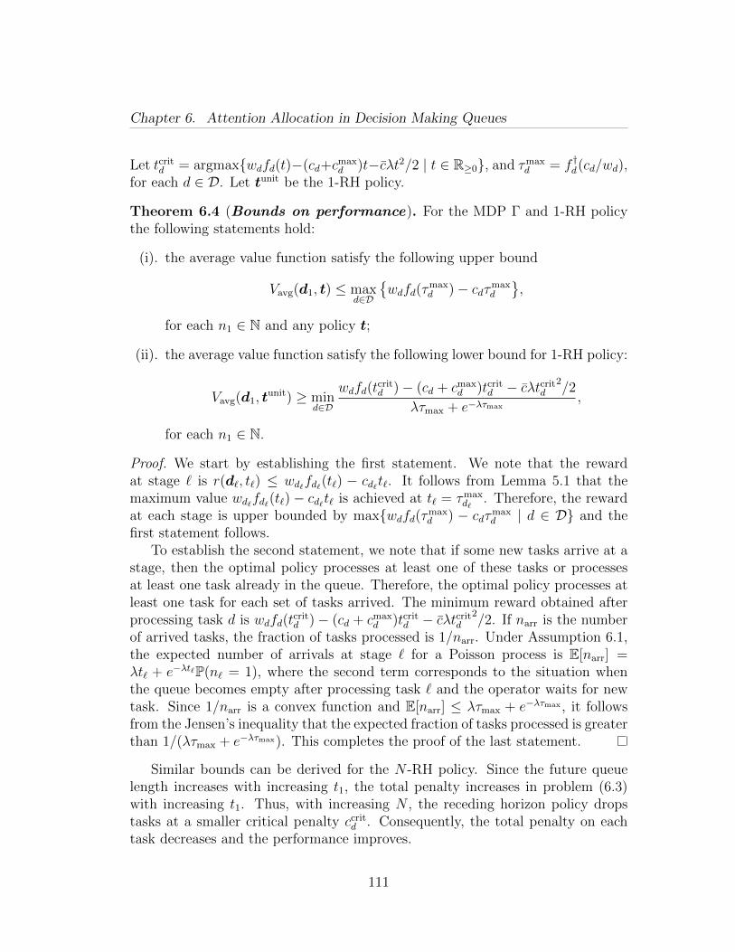
Chapter 6. Attention Allocation in Decision Making Queues
Let tcritd = argmaxwdfd(t)−(cd+c
maxd )t−cλt2/2 | t ∈ R≥0, and τmax
d = f †d(cd/wd),for each d ∈ D. Let tunit be the 1-RH policy.
Theorem 6.4 (Bounds on performance). For the MDP Γ and 1-RH policythe following statements hold:
(i). the average value function satisfy the following upper bound
Vavg(d1, t) ≤ maxd∈D
wdfd(τ
maxd )− cdτmax
d
,
for each n1 ∈ N and any policy t;
(ii). the average value function satisfy the following lower bound for 1-RH policy:
Vavg(d1, tunit) ≥ min
d∈D
wdfd(tcritd )− (cd + cmax
d )tcritd − cλtcrit
d2/2
λτmax + e−λτmax,
for each n1 ∈ N.
Proof. We start by establishing the first statement. We note that the rewardat stage ` is r(d`, t`) ≤ wd`fd`(t`) − cd`t`. It follows from Lemma 5.1 that themaximum value wd`fd`(t`)− cd`t` is achieved at t` = τmax
d`. Therefore, the reward
at each stage is upper bounded by maxwdfd(τmaxd ) − cdτ
maxd | d ∈ D and the
first statement follows.To establish the second statement, we note that if some new tasks arrive at a
stage, then the optimal policy processes at least one of these tasks or processesat least one task already in the queue. Therefore, the optimal policy processes atleast one task for each set of tasks arrived. The minimum reward obtained afterprocessing task d is wdfd(t
critd )− (cd + cmax
d )tcritd − cλtcrit
d2/2. If narr is the number
of arrived tasks, the fraction of tasks processed is 1/narr. Under Assumption 6.1,the expected number of arrivals at stage ` for a Poisson process is E[narr] =λt` + e−λt`P(n` = 1), where the second term corresponds to the situation whenthe queue becomes empty after processing task ` and the operator waits for newtask. Since 1/narr is a convex function and E[narr] ≤ λτmax + e−λτmax , it followsfrom the Jensen’s inequality that the expected fraction of tasks processed is greaterthan 1/(λτmax + e−λτmax). This completes the proof of the last statement.
Similar bounds can be derived for the N -RH policy. Since the future queuelength increases with increasing t1, the total penalty increases in problem (6.3)with increasing t1. Thus, with increasing N , the receding horizon policy dropstasks at a smaller critical penalty ccrit
d . Consequently, the total penalty on eachtask decreases and the performance improves.
111
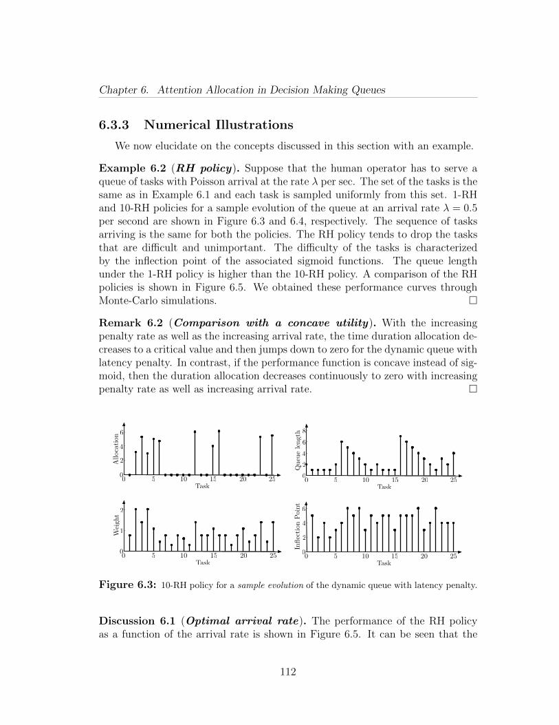
Chapter 6. Attention Allocation in Decision Making Queues
6.3.3 Numerical Illustrations
We now elucidate on the concepts discussed in this section with an example.
Example 6.2 (RH policy). Suppose that the human operator has to serve aqueue of tasks with Poisson arrival at the rate λ per sec. The set of the tasks is thesame as in Example 6.1 and each task is sampled uniformly from this set. 1-RHand 10-RH policies for a sample evolution of the queue at an arrival rate λ = 0.5per second are shown in Figure 6.3 and 6.4, respectively. The sequence of tasksarriving is the same for both the policies. The RH policy tends to drop the tasksthat are difficult and unimportant. The difficulty of the tasks is characterizedby the inflection point of the associated sigmoid functions. The queue lengthunder the 1-RH policy is higher than the 10-RH policy. A comparison of the RHpolicies is shown in Figure 6.5. We obtained these performance curves throughMonte-Carlo simulations.
Remark 6.2 (Comparison with a concave utility). With the increasingpenalty rate as well as the increasing arrival rate, the time duration allocation de-creases to a critical value and then jumps down to zero for the dynamic queue withlatency penalty. In contrast, if the performance function is concave instead of sig-moid, then the duration allocation decreases continuously to zero with increasingpenalty rate as well as increasing arrival rate.
0 5 10 15 20 250
2
4
6
2
0
4
5 10 15 20 250Task
Alloca
tion
6
0 5 10 15 20 250
2
4
6
8
2
0
4
5 10 15 20 250Task
Queu
ele
ngt
h
6
8
0 5 10 15 20 250
1
2
1
0
2
5 10 15 20 250Task
Wei
ght
0 5 10 15 20 250
2
4
6
2
0
4
5 10 15 20 250Task
Inflec
tion
Poi
nt
6
Figure 6.3: 10-RH policy for a sample evolution of the dynamic queue with latency penalty.
Discussion 6.1 (Optimal arrival rate). The performance of the RH policyas a function of the arrival rate is shown in Figure 6.5. It can be seen that the
112
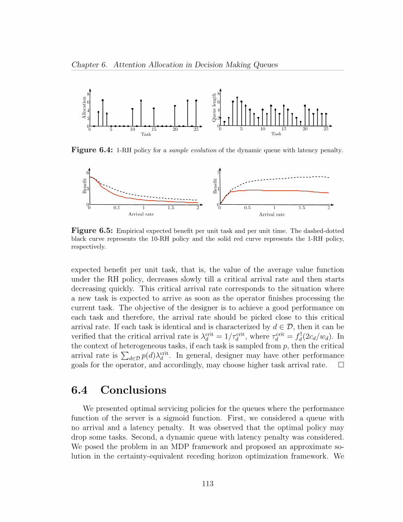
Chapter 6. Attention Allocation in Decision Making Queues
0 5 10 15 20 250
2
4
6
8
2
0
4
5 10 15 20 250Task
Alloca
tion 6
8
0 5 10 15 20 250
2
4
6
8
2
0
4
5 10 15 20 250Task
Queu
ele
ngth
6
8
Figure 6.4: 1-RH policy for a sample evolution of the dynamic queue with latency penalty.
0 0.5 1 1.5 20
6
3
3
0
6
0.5 1 1.5 20
Arrival rate
Ben
efit
0 0.5 1 1.5 20
1
2
1
0
2
0.5 1 1.5 20
Arrival rateB
enefi
t
Figure 6.5: Empirical expected benefit per unit task and per unit time. The dashed-dottedblack curve represents the 10-RH policy and the solid red curve represents the 1-RH policy,respectively.
expected benefit per unit task, that is, the value of the average value functionunder the RH policy, decreases slowly till a critical arrival rate and then startsdecreasing quickly. This critical arrival rate corresponds to the situation wherea new task is expected to arrive as soon as the operator finishes processing thecurrent task. The objective of the designer is to achieve a good performance oneach task and therefore, the arrival rate should be picked close to this criticalarrival rate. If each task is identical and is characterized by d ∈ D, then it can beverified that the critical arrival rate is λcrit
d = 1/τ critd , where τ crit
d = f †d(2cd/wd). Inthe context of heterogeneous tasks, if each task is sampled from p, then the criticalarrival rate is
∑d∈D p(d)λcrit
d . In general, designer may have other performancegoals for the operator, and accordingly, may choose higher task arrival rate.
6.4 Conclusions
We presented optimal servicing policies for the queues where the performancefunction of the server is a sigmoid function. First, we considered a queue withno arrival and a latency penalty. It was observed that the optimal policy maydrop some tasks. Second, a dynamic queue with latency penalty was considered.We posed the problem in an MDP framework and proposed an approximate so-lution in the certainty-equivalent receding horizon optimization framework. We
113
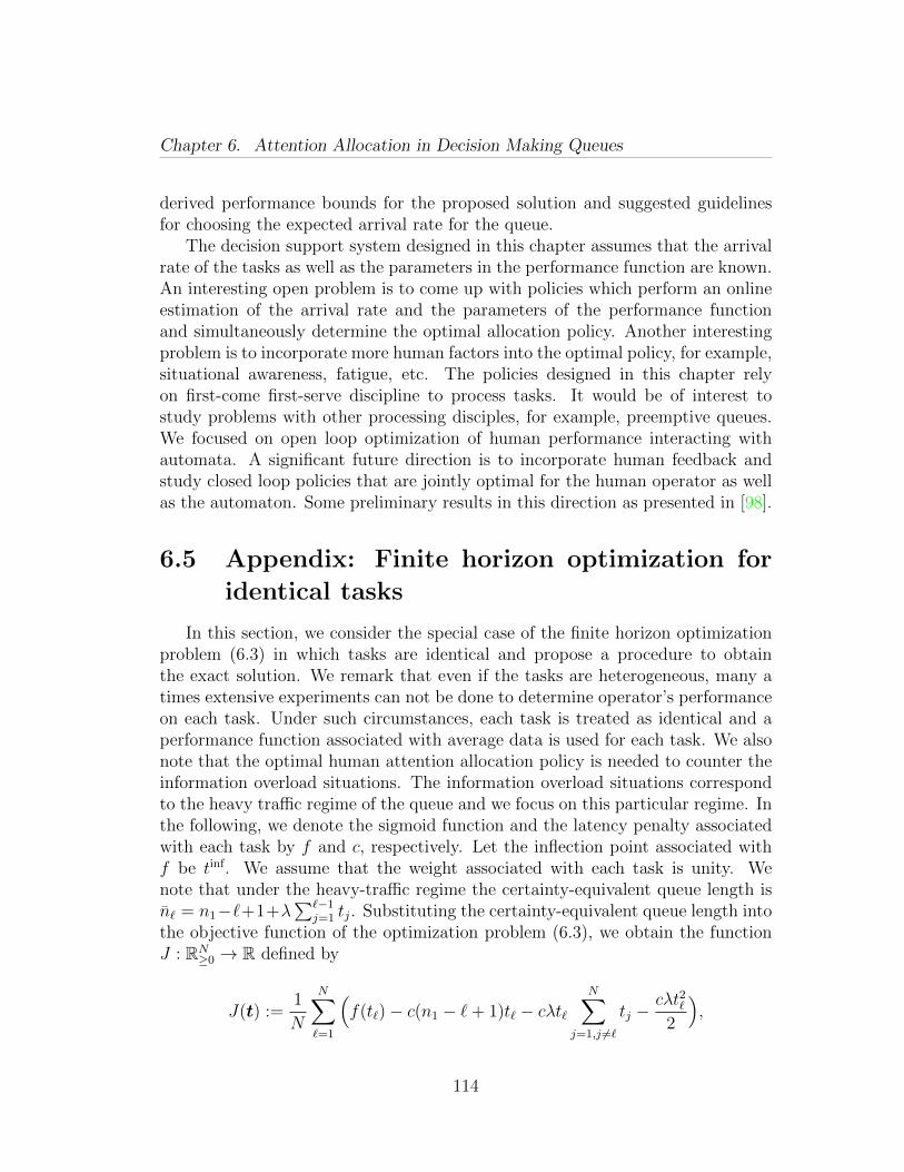
Chapter 6. Attention Allocation in Decision Making Queues
derived performance bounds for the proposed solution and suggested guidelinesfor choosing the expected arrival rate for the queue.
The decision support system designed in this chapter assumes that the arrivalrate of the tasks as well as the parameters in the performance function are known.An interesting open problem is to come up with policies which perform an onlineestimation of the arrival rate and the parameters of the performance functionand simultaneously determine the optimal allocation policy. Another interestingproblem is to incorporate more human factors into the optimal policy, for example,situational awareness, fatigue, etc. The policies designed in this chapter relyon first-come first-serve discipline to process tasks. It would be of interest tostudy problems with other processing disciples, for example, preemptive queues.We focused on open loop optimization of human performance interacting withautomata. A significant future direction is to incorporate human feedback andstudy closed loop policies that are jointly optimal for the human operator as wellas the automaton. Some preliminary results in this direction as presented in [98].
6.5 Appendix: Finite horizon optimization for
identical tasks
In this section, we consider the special case of the finite horizon optimizationproblem (6.3) in which tasks are identical and propose a procedure to obtainthe exact solution. We remark that even if the tasks are heterogeneous, many atimes extensive experiments can not be done to determine operator’s performanceon each task. Under such circumstances, each task is treated as identical and aperformance function associated with average data is used for each task. We alsonote that the optimal human attention allocation policy is needed to counter theinformation overload situations. The information overload situations correspondto the heavy traffic regime of the queue and we focus on this particular regime. Inthe following, we denote the sigmoid function and the latency penalty associatedwith each task by f and c, respectively. Let the inflection point associated withf be tinf. We assume that the weight associated with each task is unity. Wenote that under the heavy-traffic regime the certainty-equivalent queue length isn` = n1−`+1+λ
∑`−1j=1 tj. Substituting the certainty-equivalent queue length into
the objective function of the optimization problem (6.3), we obtain the functionJ : RN
≥0 → R defined by
J(t) :=1
N
N∑`=1
(f(t`)− c(n1 − `+ 1)t` − cλt`
N∑j=1,j 6=`
tj −cλt2`
2
),
114
Chapter 6. Attention Allocation in Decision Making Queues
where c is the penalty rate, λ is the arrival rate, and n1 is the initial queue length.Thus, the optimization problem (6.3) is equivalent to
maximizet0
J(t). (6.4)
Assume that the solution to the optimization problem (6.3) allocates a strictlypositive time only to the tasks in the set Tproc ⊆ 1, . . . , N, which we call theset of processed tasks. (Accordingly, the policy allocates zero time to the tasks in1, . . . , N \ Tproc). Without loss of generality, assume
Tproc := η1, . . . , ηm,
where η1 < · · · < ηm and m ≤ N . A duration allocation vector t is said to beconsistent with Tproc if only the tasks in Tproc are allocated non-zero duration.
Lemma 6.5 (Properties of maximum points). For the optimization prob-lem (6.4), and a set of processed tasks Tproc, the following statements hold:
(i). a global maximum point t∗ satisfy t∗η1 ≥ t∗η2 ≥ . . . ≥ t∗ηm ;
(ii). a local maximum point t† consistent with Tproc satisfies
f ′(t†ηk) = c(n1 − ηk + 1) + cλm∑i=1
t†ηi , for all k ∈ 1, . . . ,m; (6.5)
(iii). the system of equations (6.5) can be reduced to
f ′(t†η1) = P(t†η1), and t†ηk = f †(f ′(t†η1)− c(ηk − η1)),
for each k ∈ 2, . . . ,m, where P : R>0 → R∪+∞ is defined by
P(t) =
p(t), if f ′(t) ≥ c(ηm − η1),
+∞, otherwise,
where p(t) = c(n1 − η1 + 1 + λt+ λ∑m
k=2 f†(f ′(t)− c(ηk − η1)));
(iv). a local maximum point t† consistent with Tproc satisfies
f ′′(tηk) ≤ cλ, for all k ∈ 1, . . . ,m.
115
Chapter 6. Attention Allocation in Decision Making Queues
Proof. We start by proving the first statement. Assume t∗ηj < t∗ηk and define the
allocation vector t consistent with Tproc by
tηi =
t∗ηi , if i ∈ 1, . . . ,m \ j, k,t∗ηj , if i = k,
t∗ηk , if i = j.
It is easy to see that
J(t∗)− J(t) = (ηj − ηk)(t∗ηj − t∗ηk
) < 0.
This inequality contradicts the assumption that t∗ is a global maximum of J .To prove the second statement, note that a local maximum is achieved at the
boundary of the feasible region or at the set where the Jacobian of J is zero. Atthe boundary of the feasible region RN
≥0, some of the allocations are zero. Giventhe m non-zero allocations, the Jacobian of the function J projected on the spacespanned by the non-zero allocations must be zero. The expressions in the theoremare obtained by setting the Jacobian to zero.
To prove the third statement, we subtract the expression in equation (6.5) fork = j from the expression for k = 1 to get
f ′(tηj) = f ′(tη1)− c(ηj − η1). (6.6)
There exists a solution of equation (6.6) if and only if f ′(tη1) ≥ c(ηj − η1). Iff ′(tη1) < c(ηj − η1) + f ′(0), then there exists only one solution. Otherwise, thereexist two solutions. It can be seen that if there exist two solutions t±j , witht−j < t+j , then t−j < tη1 < t+j . From the first statement, it follows that only possible
allocation is t+j . Notice that t+j = f †(f ′(tη1)−c(ηj−η1)). This choice yields feasibletime allocation to each task ηj, j ∈ 2, . . . ,m parametrized by the time allocationto the task η1. A typical allocation is shown in Figure 6.7(a). We further note thatthe effective penalty rate for the task η1 is c(n1− η1 + 1) + cλ
∑mj=1 tηj . Using the
expression of tηj , j ∈ 2, . . . ,m, parametrized by tη1 , we obtain the expressionfor P .
To prove the last statement, we observe that the Hessian of the function J is
∂2J
∂t2= diag(f ′′(tη1), . . . , f
′′(tηm))− cλ1m1Tm,
where diag(·) represents a diagonal matrix with the argument as diagonal entries.For a local maximum to exist at non-zero duration allocations tη1 , . . . , tηm, theHessian must be negative semidefinite. A necessary condition for Hessian to benegative semidefinite is that diagonal entries are non-positive.
116
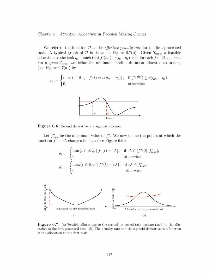
Chapter 6. Attention Allocation in Decision Making Queues
We refer to the function P as the effective penalty rate for the first processedtask. A typical graph of P is shown in Figure 6.7(b). Given Tproc, a feasibleallocation to the task η1 is such that f ′(tη1)−c(ηj−η1) > 0, for each j ∈ 2, . . . ,m.For a given Tproc, we define the minimum feasible duration allocated to task η1
(see Figure 6.7(a)) by
τ1 :=
mint ∈ R≥0 | f ′(t) = c(ηm − η1), if f ′(tinf) ≥ c(ηm − η1),
0, otherwise.
0
0
0Time
0
δ1 δ2
Figure 6.6: Second derivative of a sigmoid function.
Let f ′′max be the maximum value of f ′′. We now define the points at which thefunction f ′′ − cλ changes its sign (see Figure 6.6):
δ1 :=
mint ∈ R≥0 | f ′′(t) = cλ, if cλ ∈ [f ′′(0), f ′′max],
0, otherwise,
δ2 :=
maxt ∈ R≥0 | f ′′(t) = cλ, if cλ ≤ f ′′max,
0, otherwise.
00 Allocation to first processed task
Alloc
to2n
dpro
cta
sk
τ1
(a)
00 Allocation to first processed task
Rew
.&
pen
.ra
te
(b)
Figure 6.7: (a) Feasible allocations to the second processed task parametrized by the allo-cation to the first processed task. (b) The penalty rate and the sigmoid derivative as a functionof the allocation to the first task.
117
Chapter 6. Attention Allocation in Decision Making Queues
Theorem 6.6 (Finite horizon optimization). Given the optimization prob-lem (6.4), and a set of processed tasks Tproc. The following statements are equiv-alent:
(i). there exists a local maximum point consistent with Tproc;
(ii). one of the following conditions hold
f ′(δ2) ≥ P(δ2), or (6.7)
f ′(τ1) ≤ P(τ1), f ′(δ1) ≥ P(δ1), and δ1 ≥ τ1. (6.8)
Proof. A critical allocation to task η1 is located at the intersection of the graphof the reward rate f ′(tη1) and the effective penalty rate P(tη1). From Lemma 6.5,a necessary condition for the existence of a local maximum at a critical point isf ′′(tη1) ≤ cλ, which holds for tη1 ∈ (0, δ1]∪ [δ2,∞). It can be seen that if condi-tion (6.7) holds, then the function f ′(tη1) and the effective penalty function P(tη1)intersect in the region [δ2,∞[. Similarly, condition (6.8) ensures the intersection ofthe graph of the reward function f ′(tη1) with the effective penalty function P(tη1)in the region (0, δ1].
118

Bibliography
[1] S. Agrali and J. Geunes. Solving knapsack problems with S-curve returnfunctions. European Journal of Operational Research, 193(2):605–615, 2009.
[2] K. M. Adusumilli and J. J. Hasenbein. Dynamic admission and service ratecontrol of a queue. Queueing Systems, 66(2):131–154, 2010.
[3] A. Arapostathis, V. S. Borkar, E. Fernandez-Gaucherand, M. K. Ghosh, andS. I. Marcus. Discrete-time controlled Markov processes with average costcriterion: A survey. SIAM Journal on Control and Optimization, 31(2):282–344, 1993.
[4] C. Z. Bai, V. Gupta, and Y. F. Huang. Sequential hypothesis testing withoff-line randomized sensor selection strategy. In Acoustics, Speech and SignalProcessing (ICASSP), 2012 IEEE International Conference on, pages 3269–3272, 2012.
[5] D. Bajovic, B. Sinopoli, and J. Xavier. Sensor selection for hypothesistesting in wireless sensor networks: a Kullback-Leibler based approach. InIEEE Conf. on Decision and Control, pages 1659–1664, Shanghai, China,December 2009.
[6] M. Basseville and I. V. Nikiforov. Detection of Abrupt Changes: Theory andApplication. Prentice Hall, 1993.
[7] C. W. Baum and V. V. Veeravalli. A sequential procedure for multihypoth-esis testing. IEEE Transactions on Information Theory, 40(6):1994–2007,1994.
[8] H. P. Benson. On the global optimization of sums of linear fractional func-tions over a convex set. Journal of Optimization Theory & Applications,121(1):19–39, 2004.
119
Bibliography
[9] D. Bertsekas. Dynamic programming and suboptimal control: A surveyfrom ADP to MPC. European Journal of Control, 11(4-5):310–334, 2005.
[10] D. P. Bertsekas. Convergence of discretization procedures in dynamic pro-gramming. IEEE Transactions on Automatic Control, 20(6):415–419, 1975.
[11] L. F. Bertuccelli, N. W. M. Beckers, and M. L. Cummings. Developingoperator models for UAV search scheduling. In AIAA Conf. on Guidance,Navigation and Control, Toronto, Canada, August 2010.
[12] L. F. Bertuccelli, N. Pellegrino, and M. L. Cummings. Choice modelingof relook tasks for UAV search missions. In American Control Conference,pages 2410–2415, Baltimore, MD, USA, June 2010.
[13] R. Bogacz, E. Brown, J. Moehlis, P. Holmes, and J. D. Cohen. Thephysics of optimal decision making: A formal analysis of performance intwo-alternative forced choice tasks. Psychological Review, 113(4):700–765,2006.
[14] S. Boyd, P. Diaconis, and L. Xiao. Fastest mixing Markov chain on a graph.SIAM Review, 46(4):667–689, 2004.
[15] S. Boyd and L. Vandenberghe. Convex Optimization. Cambridge UniversityPress, 2004.
[16] K. M. Bretthauer and B. Shetty. The nonlinear knapsack problem–algorithms and applications. European Journal of Operational Research,138(3):459–472, 2002.
[17] W. M. Bulkeley. Chicago’s camera network is everywhere. The Wall StreetJournal, November 17, 2009.
[18] G. J. Burke, J. Geunes, H. E. Romeijn, and A. Vakharia. Allocating procure-ment to capacitated suppliers with concave quantity discounts. OperationsResearch Letters, 36(1):103–109, 2008.
[19] G. C. Calafiore, F. Dabbene, and R. Tempo. Research on probabilisticmethods for control system design. Automatica, 47(7):1279–1293, 2011.
[20] J. Calvin. Convergence rate of the P-algorithm for optimization of continu-ous functions. In P. M. Pardalos, editor, Approximation and Complexity inNumerical Optimization: Continuous and Discrete Problems. Kluwer Aca-demic, 1999.
120
Bibliography
[21] J. Calvin and A. Zilinskas. On the convergence of the P-algorithm forone-dimensional global optimization of smooth functions. Journal of Opti-mization Theory and Applications, 102(3):479–495, 1999.
[22] D. A. Castanon. Optimal search strategies in dynamic hypothesis testing.IEEE Transactions on Systems, Man & Cybernetics, 25(7):1130–1138, 1995.
[23] H. S. Chang and S. I. Marcus. Approximate receding horizon approach forMarkov decision processes: Average reward case. Journal of MathematicalAnalysis and Applications, 286(2):636–651, 2003.
[24] B. Chen and P. Willett. Detection of hidden Markov model transient signals.IEEE Transactions on Aerospace and Electronic Systems, 36(4):1253–1268,2000.
[25] Y. Chevaleyre. Theoretical analysis of the multi-agent patrolling problem.In IEEE/WIC/ACM Int. Conf. on Intelligent Agent Technology, pages 302–308, Beijing, China, September 2004.
[26] T. H. Chung and J. W. Burdick. Analysis of search decision making usingprobabilistic search strategies. IEEE Transactions on Robotics, 28(1):132–144, 2012.
[27] R. Cohen, L. Katzir, and D. Raz. An efficient approximation for the gener-alized assignment problem. Information Processing Letters, 100(4):162–166,2006.
[28] T. M. Cover and J. A. Thomas. Elements of Information Theory. Wiley,1991.
[29] J. W. Crandall, M. L. Cummings, M. Della Penna, and P. M. A. de Jong.Computing the effects of operator attention allocation in human controlof multiple robots. IEEE Transactions on Systems, Man & Cybernetics.Part A: Systems & Humans, 41(3):385–397, 2011.
[30] R. Debouk, S. Lafortune, and D. Teneketzis. On an optimization problemin sensor selection. Discrete Event Dynamic Systems, 12(4):417–445, 2002.
[31] C. Drew. Military taps social networking skills. The New York Times, June7, 2010.
[32] J. W. Durham and F. Bullo. Smooth nearness-diagram navigation. InIEEE/RSJ Int. Conf. on Intelligent Robots & Systems, pages 690–695, Nice,France, September 2008.
121
Bibliography
[33] Y. Elmaliach, A. Shiloni, and G. A. Kaminka. A realistic model of frequency-based multi-robot polyline patrolling. In International Conference on Au-tonomous Agents, pages 63–70, Estoril, Portugal, May 2008.
[34] J. R. Freeland and C. B. Weinberg. S-Shaped response functions: Impli-cations for decision models. Journal of the Operational Research Society,31(11):1001–1007, 1980.
[35] J. M. George and J. M. Harrison. Dynamic control of a queue with adjustableservice rate. Operations Research, 49(5):720–731, 2001.
[36] W. Ginsberg. The multiplant firm with increasing returns to scale. Journalof Economic Theory, 9(3):283–292, 1974.
[37] J. Grace and J. Baillieul. Stochastic strategies for autonomous roboticsurveillance. In IEEE Conf. on Decision and Control and European ControlConference, pages 2200–2205, Seville, Spain, December 2005.
[38] E. Guizzo. Obama commanding robot revolution announces major roboticsinitiative. IEEE Spectrum, June 2011.
[39] V. Gupta, T. H. Chung, B. Hassibi, and R. M. Murray. On a stochasticsensor selection algorithm with applications in sensor scheduling and sensorcoverage. Automatica, 42(2):251–260, 2006.
[40] A. Gut. Stopped Random Walks: Limit Theorems and Applications.Springer, 2009.
[41] P. Hansen, B. Jaumard, and S. H. Lu. Global optimization of univariateLipschitz functions: I. Survey and properties. Mathematical Programming,55(1):251–272, 1992.
[42] O. Hernandez-Lerma and S. I. Marcus. Adaptive control of service in queue-ing systems. Systems & Control Letters, 3(5):283–289, 1983.
[43] J. P. Hespanha, H. J. Kim, and S. S. Sastry. Multiple-agent probabilisticpursuit-evasion games. In IEEE Conf. on Decision and Control, pages 2432–2437, Phoenix, AZ, USA, December 1999.
[44] J. B. Hiriart-Urruty. On optimality conditions in nondifferentiable program-ming. Mathematical Programming, 14(1):73–86, 1978.
122
Bibliography
[45] G. A. Hollinger, U. Mitra, and G. S. Sukhatme. Active classification: Theoryand application to underwater inspection. In International Symposium onRobotics Research, Flagstaff, AZ, USA, August 2011.
[46] G. A. Hollinger, U. Mitra, and G. S. Sukhatme. Autonomous data collec-tion from underwater sensor networks using acoustic communication. InIEEE/RSJ Int. Conf. on Intelligent Robots & Systems, pages 3564–3570,San Francisco, CA, USA, September 2011.
[47] S. K. Hong and C. G. Drury. Sensitivity and validity of visual search modelsfor multiple targets. Theoretical Issues in Ergonomics Science, 3(1):85–110,2002.
[48] T. Ibaraki and N. Katoh. Resource Allocation Problems: Algorithmic Ap-proaches. MIT Press, 1988.
[49] V. Isler and R. Bajcsy. The sensor selection problem for bounded uncer-tainty sensing models. IEEE Transactions on Automation Sciences andEngineering, 3(4):372–381, 2006.
[50] S. Joshi and S. Boyd. Sensor selection via convex optimization. IEEETransactions on Signal Processing, 57(2):451–462, 2009.
[51] S. Stidham Jr. and R. R. Weber. Monotonic and insensitive optimal poli-cies for control of queues with undiscounted costs. Operations Research,37(4):611–625, 1989.
[52] S. Kameshwaran and Y. Narahari. Nonconvex piecewise linear knapsackproblems. European Journal of Operational Research, 192(1):56–68, 2009.
[53] V. Katewa and V. Gupta. On the optimality of sequential test with multiplesensors. In American Control Conference, pages 282–287, Montreal, Canada,2012.
[54] H. Kellerer, U. Pferschy, and D. Pisinger. Knapsack Problems. Springer,2004.
[55] D. B. Kingston, R. W. Beard, and R. S. Holt. Decentralized perime-ter surveillance using a team of UAVs. IEEE Transactions on Robotics,24(6):1394–1404, 2008.
[56] D. J. Klein, J. Schweikl, J. T. Isaacs, and J. P. Hespanha. On UAV routingprotocols for sparse sensor data exfiltration. In American Control Confer-ence, pages 6494–6500, Baltimore, MD, USA, June 2010.
123
Bibliography
[57] B. Korte and J. Vygen. Combinatorial Optimization: Theory and Algo-rithms, volume 21 of Algorithmics and Combinatorics. Springer, 4 edition,2007.
[58] H. J. Kushner. A new method of locating the maximum point of an arbitrarymultipeak curve in the presence of noise. Journal of Basic Engineering,86(1):97–106, 1964.
[59] S. M. LaValle. Planning Algorithms. Cambridge University Press, 2006.Available at http://planning.cs.uiuc.edu.
[60] D. G. Luenberger. Linear and Nonlinear Programming. Addison-Wesley, 2edition, 1984.
[61] S. Martello and P. Toth. Knapsack Problems: Algorithms and ComputerImplementations. Wiley, 1990.
[62] J. Mattingley, Y. Wang, and S. Boyd. Receding horizon control: Automaticgeneration of high-speed solvers. IEEE Control Systems Magazine, 31(3):52–65, 2011.
[63] J. J. More and S. A. Vavasis. On the solution of concave knapsack problems.Mathematical Programming, 49(1):397–411, 1990.
[64] G. V. Moustakides. Optimal stopping times for detecting changes in distri-butions. The Annals of Statistics, 14(4):1379–1387, 1986.
[65] C. Nehme, B. Mekdeci, J. W. Crandall, and M. L. Cummings. The impactof heterogeneity on operator performance in futuristic unmanned vehiclesystems. The International C2 Journal, 2(2):1–30, 2008.
[66] C. E. Nehme. Modeling Human Supervisory Control in Heterogeneous Un-manned Vehicle Systems. PhD thesis, Department of Aeronautics and As-tronautics, MIT, February 2009.
[67] A. Ortiz, D. Kingston, and C. Langbort. Multi-UAV Velocity and TrajectoryScheduling Strategies for Target Classification by a Single Human Operator.Journal of Intelligent & Robotic Systems, pages 1–20, 2012.
[68] E. S. Page. Continuous inspection schemes. Biometrika, 41(1/2):100–115,1954.
124
Bibliography
[69] F. Pasqualetti, J. W. Durham, and F. Bullo. Cooperative patrolling viaweighted tours: Performance analysis and distributed algorithms. IEEETransactions on Robotics, 28(5):1181–1188, 2012.
[70] F. Pasqualetti, A. Franchi, and F. Bullo. On cooperative patrolling: Opti-mal trajectories, complexity analysis and approximation algorithms. IEEETransactions on Robotics, 28(3):592–606, 2012.
[71] R. W. Pew. The speed-accuracy operating characteristic. Acta Psychologica,30:16–26, 1969.
[72] H. V. Poor and O. Hadjiliadis. Quickest Detection. Cambridge UniversityPress, 2008.
[73] N. D. Powel and K. A. Morgansen. Multiserver queueing for supervisorycontrol of autonomous vehicles. In American Control Conference, pages3179–3185, Montreal, Canada, June 2012.
[74] R. J. Radke, S. Andra, O. Al-Kofahi, and B. Roysam. Image change detec-tion algorithms: A systematic survey. IEEE Transactions on Image Pro-cessing, 14(3):294–307, 2005.
[75] A. G. Rao and M. R. Rao. Optimal budget allocation when response isS-shaped. Operations Research Letters, 2(5):225–230, 1983.
[76] S. I. Resnick. A Probability Path. Birkhauser, 1999.
[77] T. Sak, J. Wainer, and S. Goldenstein. Probabilistic multiagent patrolling.In Brazilian Symposium on Artificial Intelligence, Advances in ArtificialIntelligence, pages 124–133, Salvador, Brazil, 2008. Springer.
[78] K. Savla and E. Frazzoli. Maximally stabilizing task release control policy fora dynamical queue. IEEE Transactions on Automatic Control, 55(11):2655–2660, 2010.
[79] K. Savla and E. Frazzoli. A dynamical queue approach to intelligent taskmanagement for human operators. Proceedings of the IEEE, 100(3):672–686,2012.
[80] K. Savla, C. Nehme, T. Temple, and E. Frazzoli. On efficient cooperativestrategies between UAVs and humans in a dynamic environment. In AIAAConf. on Guidance, Navigation and Control, Honolulu, HI, USA, 2008.
125
Bibliography
[81] K. Savla, T. Temple, and E. Frazzoli. Human-in-the-loop vehicle routingpolicies for dynamic environments. In IEEE Conf. on Decision and Control,pages 1145–1150, Cancun, Mexico, December 2008.
[82] D. K. Schmidt. A queuing analysis of the air traffic controller’s work load.IEEE Transactions on Systems, Man & Cybernetics, 8(6):492–498, 1978.
[83] L. I. Sennott. Stochastic Dynamic Programming and the Control of QueueingSystems. Wiley, 1999.
[84] T. Shanker and M. Richtel. In new military, data overload can be deadly.The New York Times, January 16, 2011.
[85] D. Siegmund. Sequential Analysis: Tests and Confidence Intervals. Springer,1985.
[86] S. L. Smith and D. Rus. Multi-robot monitoring in dynamic environmentswith guaranteed currency of observations. In IEEE Conf. on Decision andControl, pages 514–521, Atlanta, GA, USA, December 2010.
[87] S. L. Smith, M. Schwager, and D. Rus. Persistent robotic tasks: Monitoringand sweeping in changing environments. IEEE Transactions on Robotics,28(2):410–426, 2012.
[88] D. N. Southern. Human-guided management of collaborating unmanned ve-hicles in degraded communication environments. Master’s thesis, ElectricalEngineering and Computer Science, Massachusetts Institute of Technology,May 2010.
[89] K. Srivastava, D. M. Stipanovic, and M. W. Spong. On a stochastic roboticsurveillance problem. In IEEE Conf. on Decision and Control, pages 8567–8574, Shanghai, China, December 2009.
[90] V. Srivastava and F. Bullo. Hybrid combinatorial optimization: Sampleproblems and algorithms. In IEEE Conf. on Decision and Control and Eu-ropean Control Conference, pages 7212–7217, Orlando, FL, USA, December2011.
[91] V. Srivastava and F. Bullo. Stochastic surveillance strategies for spatialquickest detection. In IEEE Conf. on Decision and Control and EuropeanControl Conference, pages 83–88, Orlando, FL, USA, December 2011.
126
Bibliography
[92] V. Srivastava and F. Bullo. Knapsack problems with sigmoid utility: Ap-proximation algorithms via hybrid optimization. European Journal of Op-erational Research, October 2012. Submitted.
[93] V. Srivastava, R. Carli, F. Bullo, and C. Langbort. Task release control fordecision making queues. In American Control Conference, pages 1855–1860,San Francisco, CA, USA, June 2011.
[94] V. Srivastava, R. Carli, C. Langbort, and F. Bullo. Attention allocation fordecision making queues. Automatica, February 2012. Submitted.
[95] V. Srivastava, F. Pasqualetti, and F. Bullo. Stochastic surveillance strategiesfor spatial quickest detection. International Journal of Robotics Research,April 2012. to appear.
[96] V. Srivastava, K. Plarre, and F. Bullo. Adaptive sensor selection in se-quential hypothesis testing. In IEEE Conf. on Decision and Control andEuropean Control Conference, pages 6284–6289, Orlando, FL, USA, Decem-ber 2011.
[97] V. Srivastava, K. Plarre, and F. Bullo. Randomized sensor selection insequential hypothesis testing. IEEE Transactions on Signal Processing,59(5):2342–2354, 2011.
[98] V. Srivastava, A. Surana, and F. Bullo. Adaptive attention allocation inhuman-robot systems. In American Control Conference, pages 2767–2774,Montreal, Canada, June 2012.
[99] W. P. Tay, J. N. Tsitsiklis, and M. Z. Win. Asymptotic performance ofa censoring sensor network. IEEE Transactions on Information Theory,53(11):4191–4209, 2007.
[100] S. Thrun, D. Fox, W. Burgard, and F. Dellaert. Robust Monte Carlo local-ization for mobile robots. Artificial Intelligence, 128(1-2):99–141, 2001.
[101] J. Unnikrishnan, V. V. Veeravalli, and S. P. Meyn. Minimax robust quickestchange detection. IEEE Transactions on Information Theory, 57(3):1604–1614, 2011.
[102] D. Vakratsas, F. M. Feinberg, F. M. Bass, and G. Kalyanaram. The shape ofadvertising response functions revisited: A model of dynamic probabilisticthresholds. Marketing Science, 23(1):109–119, 2004.
127
Bibliography
[103] A. Wald. Sequential tests of statistical hypotheses. The Annals of Mathe-matical Statistics, 16(2):117–186, 1945.
[104] H. Wang, K. Yao, G. Pottie, and D. Estrin. Entropy-based sensor selectionheuristic for target localization. In Symposium on Information Processingof Sensor Networks, pages 36–45, Berkeley, CA, April 2004.
[105] L. Wasserman. All of Statistics: A Concise Course in Statistical Inference.Springer, 2004.
[106] C. D. Wickens and J. G. Hollands. Engineering Psychology and HumanPerformance. Prentice Hall, 3 edition, 2000.
[107] J. L. Williams, J. W. Fisher, and A. S. Willsky. Approximate dynamicprogramming for communication-constrained sensor network management.IEEE Transactions on Signal Processing, 55(8):4300–4311, 2007.
[108] D. Zhang, C. Colburn, and T. Bewley. Estimation and adaptive observationof environmental plumes. In American Control Conference, pages 4821–4286, San Francisco, CA, USA, June 2011.
128