Stochastic volatility, convex prices and bubbles

Stochastic volatility, convex prices and bubbles

Thorir Bjarnason

U.U.D.M. Project Report 2007:20

Examensarbete i matematik, 20 poäng

Handledare och examinator: Johan Tysk

Juni 2007

Department of Mathematics

Uppsala University

STOCHASTIC VOLATILITY,CONVEX PRICES AND BUBBLES

THORIR BJARNASON

Abstract. The relatively new SABR-model is a stochastic vola-tility model, where the parameters constitute the name, StochasticAlpha Beta Rho. The model has become quite popular in the worldof finance so it is only natural to examine if a claim price for con-vex contract functions is convex as a function of the underlyingasset, modeled by the SABR-model. In this article the aim is toexamine for what values of the parameters, if any, the model pre-serves convexity in this sense. First we give some background onBrownian motion, volatility and convexity. Then we proceed withan introduction to bubbles. Bubbles are said to occur if the mar-ket is overvalued in a precise mathematical sense. Continuing byusing the Monte Carlo method to simulate the price of a Europeancall option we proceed by plotting the data to see if the prices areconvex and if bubbles occur.

By the simulation trials it is indicated that convexity is preservedfor the model. In one case, bubbles were detected, i.e. the valueof the call option is lower than the final payoff.

1

2 THORIR BJARNASON

Contents

1. Introduction 32. Geometric Brownian Motion and Black-Scholes Formula 42.1. Geometric Brownian Motion 42.2. Black-Scholes formula 63. Volatility 83.1. Implied and Local volatility 83.2. Stochastic volatility 104. Convexity 115. Bubbles 146. Monte Carlo method 156.1. The method 156.2. Variance reduction techniques 166.3. History of the Monte Carlo method 177. Results 177.1. Reading the data 177.2. Results 188. Conclusions & Discussion 209. Acknowledgements 21Appendix A. Appendix 22References 26

STOCHASTIC VOLATILITY, CONVEX PRICES AND BUBBLES 3

1. Introduction

For several hundred years the market has been evolving. From the firstcontract being written until now, millions of contracts have been writ-ten. The main goal of most of them, is to ensure a safe trade betweentwo traders at a predetermined price. Since risk is everexisting in themarket, the stock market for one, it is very attractive to be able tohedge against any risk present. Hedging against the underlying asset isdone by decreasing the ∆ and Γ of the claim to zero or near-zero. Forthis part in particular it is good to know if the claim price is convex asa function of the underlying asset. Convexity gives us bounds on the∆, i.e. bounds on the stock position, and bounds on the value for thenon-stock position. By the definition of convexity, Γ can be used as ameasure of convexity. Also from convexity we get that the price of theclaim increases if the volatility increases. This brings us to the subjectat hand.

We want to look at the SABR-model from a convex point of view, orrather, investigate for what parameter values the prices might be con-vex. The parameters, α > 0, 0 ≤ β ≤ 1 and −1 < ρ < 1, have quitethe freedom of variation, hence it is reasonable to believe that not allvalues are fitting when it comes to convexity.

By the Monte Carlo method, several simulations with different param-eter values will be conducted. The data will be examined, whereuponconclusions will be drawn as to for what parameter values the priceis convex. The manner of simulations will not be with respect to thesecond derivative of the claim, instead we simulate the value of a Euro-pean call option as it is rather easy to see non-convexity in the graphsof the claim price.

The upcoming section will give us some background on GeometricBrownian motion and the Black-Scholes formula. In Section 3 we willaddress volatility in its different appearances within models. Somewords about volatility skew and volatility smiles are in there as well.In Section 4 convexity is brought to our attention and some rather in-teresting results are stated on convexity in stochastic volatility models.However, those results do not apply to the SABR-model so we turnto the subject of Section 6. Here we give a short introduction to theMonte Carlo method and how it is applied to the problem. Section7 gives the results and some conclusions. The main reference for thisarticle is [1].

4 THORIR BJARNASON

2. Geometric Brownian Motion and Black-ScholesFormula

2.1. Geometric Brownian Motion. The future is unpredictable.Still we are almost obsessive about knowing what is to come. He whoknows the future has the power in a sense. The matter of fact thoughis that no one knows the future but we are getting pretty good at esti-mating parts of it, such as finance. Via various algorithms, which arecontinuously evolving, we can derive good estimations, or even exactvalues to our present knowledge, of future values of say options. Oneof these algorithms is the Brownian model.

The history of Brownian motion starts with Robert Brown in 1827. Hediscovered that particles suspended in a fluid were ceaselessly movingrandomly. By later scientists, this motion was called Brownian motion.Around 1900, in the center of finance at that time, Paris, Louis Bache-lier used the concept of Brownian motion in stock models. He assumedthat the movements of stock price was random, identically indepen-dently distributed (i.i.d.) with independent time increments. His workin finance did not receive much attention though as that particularsubject (being finance) was not in high regards with mathematiciansat the time. Nevertheless, this was the catalyst for using geometricBrownian motion in financial mathematics.

It was not until 1905 that Brownian motion got the attention. It wasthen that Einstein, independently of Bachelier, stated the laws govern-ing the movements of particles suspended in liquid or gas. (NorbertWiener stated the laws and a full mathematical description of Brown-ian motion in 1923, hence the use of Wiener process when referring toBrownian motion.) Brownian motion was now a mathematical model,applicable in the world of physics and mathematics. Some fields ofapplication are medical imaging, robotics and finance.

The equation governing geometric Brownian motion (shorthand GBM),being one of two natural generalizations of the simplest linear ordinarydifferential equations (shorthand ODE), looks as follows:

dXt = αXtdt+ σXtdWt (2.1)

X0 = x0 (2.2)

By dividing (2.1) with dt we get the slightly sloppy notation

Xt = (α+ σWt)Xt

where Wt is the time derivative of the Wiener process. It is only naturalat this point to state a definition for this process.


Definition 1. A stochastic process W is called a Wiener process ifthe following conditions hold:

(1) W (0) = 0.(2) The process W has independent increments, i.e. if r < s ≤

t < u then W (u) − W (t) and W (s) − W (r) are independentstochastic variables.

(3) For s < t the stochastic variable W (t)−W (s) has the Gaussiandistribution N (0,

√t− s).

(4) W has continuous trajectories.

The solution to (2.1) is given by the following proposition.

Proposition 1. The solution to the equation

dXt = αXtdt+ σXtdWt (2.3)

X0 = x0 (2.4)

is given by

Xt = x0 · exp{

(α− 1

2σ2)t+ σWt

}. (2.5)

The expected value is given by

E[Xt] = x0eαt. (2.6)

Proof. Let Zt = lnXt = ln x0 + (α− 12σ2)t+ σWt, then

dZt =(α− 1

2σ2

)dt+ σdWt.

Apply Ito’s formula,

df =δf

δtdt+

δf

δzdZt +

1

2

δ2f

δz2(dZt)

2, (2.7)

to f(t, Zt) = eZt and obtain

df =(α− 1

2σ2

)eZt(dt)2 + σeZtdtdWt

+eZt

((α− 1

2σ2

)dt+ σdWt

)+

1

2eZt

[(α− 1

2σ2

)2

(dt)2

+2σ(α− 1

2σ2

)dtdWt + σ2(dWt)

2]. (2.8)

By the following multiplication table (dt)2 = 0dt · dWt = 0(dWt)

2 = dt(2.9)

we getdf = αeZtdt+ σeZtdWt, (2.10)

6 THORIR BJARNASON

hence the solution is given by (2.5).

To prove (2.6), rewrite (2.3) as

Xt = x0 + α

∫ t

0

Xsds+ σ

∫ t

0

XsdWs. (2.11)

Take expected value of (2.11) and set E[Xt] = m(t)

m(t) = x0 + α

∫ t

0

m(t)ds.

Rewriting gives us a linear ODE

m(t) = αm(t) (2.12)

m(0) = x0 (2.13)

which is easily solved obtaining what is sought after,

E[Xt] = m(t) = x0eαt. �

For a realization of a GBM with R-code, see the appendix.

2.2. Black-Scholes formula. In the market there are market instru-ments such as bills, bonds, notes and options. Trading these instru-ments, in general referred to as financial instruments, can be comparedto trading rice or silver, but they are not real goods in the sense of hav-ing intrinsic value. They are traded as pieces of paper or as entries ina computer database.

One financial instrument, out of many, is the European call option.For this option we have an analytic formula, which was presented byFischer Black and Myron Scholes in 1973. The formula was derivedunder the following key assumptions:

• The price of the underlying instrument St follows a GeometricBrownian motion with constant drift r and volatility σ

• It is possible to short sell the underlying stock• There are no arbitrage opportunities• Trading in the stock is continuous• There are no transaction costs or taxes• All securities are perfectly divisible (e.g. it is possible to buy

1/100th of a share)• It is possible to borrow and lend money at a constant risk-free

interest rate.

Here is the model which Black and Scholes chose as their market

dBt = rBtdt (2.14)

dSt = rStdt+ σStdWt. (2.15)


Figure 1. The price of a European call option in theBlack-Scholes setting

With the above assumptions and model they derived the following for-mula for non-dividend paying European call options

F (t, s) = sN [d1(t, s)]−Ke−r(T−t)N [d2(t, s)] (2.16)

where N is the cumulative distribution function for the N (0, 1) distri-bution and

d1(t, s) =1

σ√T − t

{ln

(s

K

)+

(r +

1

2σ2

)(T − t)

}(2.17)

d2(t, s) = d1(t, s)− σ√T − t. (2.18)

The value of a European put option with the same strike price K andthe same maturity T as a European call option can be obtained via theput-call parity, p(t, s) = Ke−r(T−t) + c(t, s) − s. Naturally p(t, s) andc(t, s) denote the price of the put and call option respectively.

Ever since the formula was introduced in 1973 it has been and still isin the game, even though empirical studies time and time again showthat it is flawed. The mismodeling, assuming that σ is constant, cangenerate a phenomenon called a volatility smile. You can read moreabout this below.

8 THORIR BJARNASON

3. Volatility

Most instruments have a value which varies stochastically over time anda measure of the variance is the volatility. More accurately, volatilityrefers to the standard deviation of the change in the value of a financialinstrument over a specific time horizon. It is however more commonto see volatility as a quantifier of risk in an instrument, i.e. the higherthe volatility, the more the price can change.

In the Black-Scholes formula (2.16) we have, by assumption, constantvolatility but when a European call is priced in a concrete situation wedo not know the volatility explicitly. The other parameters, r, s, T andt, we can read off of the market but we have to estimate the volatility.

People working with financial instruments rarely talk about the value ofdifferent financial instruments. The value is decided by the volatilityimplied by the market, hence it is more natural to see a particularinstrument’s value in the light of volatility. As was written above, thehigher the volatility, the more the price can change, hence it is naturalto say that a claim with high volatility is more expensive then a claimwith low volatility.

3.1. Implied and Local volatility.

3.1.1. Implied volatility. Finding the implied volatility can be done bygetting market price data on a “benchmark” option with the sameexpiration date, written on the same underlying stock as the optionwe want to value. More explicitly, let c(s, t, T, r, σ,K) be the value ofthe call option which we are evaluating and let p be the price of thebenchmark option. Solve the following equation for σ

p = c(s, t, T, r, σ,K).

The obtained value of σ is the volatility implied by the market, i.e.implied volatility. Then, to get the value of our option we use the ob-tained value for the benchmark. This is best put as “using the wrongnumber in the wrong formula, obtaining the ‘right’ price”.

Common phenomena occurring when using the implied volatility arethe volatility skew and volatility smile. These anomalies can be seenby observing market price data for some quantity of European calls,with the same exercise date, written on a single stock, with constantvolatility as an assumption. Take the implied volatility as a functionof strike price and plot it. You should get some kind of smiley curve,see Figure (2). This kind of behaviour implies that the volatility isnot constant. If it were constant, we would see a horizontal line in theplots instead of the curves. With this implication though, we are led tothink of the volatility as a function or perhaps as a stochastic variable.


Figure 2. Volatility smile and skew

3.1.2. Local Volatility. Local (or deterministic, for instantaneous valuesof S) volatility sets for example σ = σ(t, s), i.e. as a function of timeand the underlying asset’s value. By doing so we have a volatility thatis not constant but varying, as the time to maturity and the underlier’svalue changes. An example of such a volatility is

σ(t, s) = S−α,

for some real α ∈ [0, 1]. The market will still be complete, since we arenot introducing a non-traded random source. This can be seen in themeta-theorem.

Remark 1. The meta-theorem simply gives us the relation between ar-bitrage free- and complete models, i.e. we have a complete and arbitragefree model if and only if the number of underlying traded assets in themodel excluding the risk free asset is equal to the number of randomsources, see [1] for further information.

One of the problems with letting σ = σ(t, s) is of course the choiceof function. A formula has been derived to obtain a function, whichgives the volatility for different strikes and maturities. The volatilityfunction depends on what kind of option we are evaluating. This hasbeen shown in [2].

This kind of volatility is not without shortcomings though. First, thefunction can fit the historical volatility perfectly but this is not a desiredfit as it can have too many parameters. Second, it would probably notgive a good estimation of future volatility. In light of this and empiricalstudies implying that the volatility varies randomly, a more naturalcharacterisation of volatility would be

dσt = αS,t,σdt+ βS,t,σdVt, (3.1)

i.e. to let volatility be driven by a random source of its own. This kindof volatility will be referred to as stochastic volatility.

10 THORIR BJARNASON

Hull-White model dσt = µσσtdt+ σtξdVt

Heston-model dσt = (ω − θσt)dt+ ξ√σtdVt

Garch-model dσt = (ω − θσt)dt+ ξσtdVt

3/2-model dσt = (ω − θσt)dt+ ξσ32t dVt

Scott-model d ln(σ2t ) =

(ω − θln(σ2

t ))dt+ ξdVt

Table 1. List of SV models

3.2. Stochastic volatility.

3.2.1. Basic model. Let us look at the basic model of the asset oncemore

dSt = rStdt+ σtStdWt. (3.2)

Above we have let the volatility be constant and a function of timeand asset price. Both of these approaches have their advantages andof course setbacks. As mentioned above, empirical studies show thatvolatility varies somewhat randomly. This together with the setbacksof the other two approaches lead us forward in our search of a volatilitymodel that suits the market. Thus, presented below is the basic modelof stochastic volatility (shorthand SV).

dσt = αS,t,σdt+ βS,t,σdVt (3.3)

Here, αS,t,σ and βS,t,σ are some functions such that the model is a well-defined stochastic differential equation (shorthand SDE).

Remark 2. When inserting a new random source without a trade-ableasset we do not have a complete market, but it is free of arbitrage inaccordance with the meta-theorem.

Remark 3. The coefficient in front the diffusion term in the volatilityprocess is usually called volvol, since it is the volatility of the volatility.

3.2.2. Some widely used models. In Table 1 some stochastic volatilitymodels are listed. dVt is a Brownian motion. ω is the long-term meanvolatility, θ is the rate at which the process reverts towards ω and ξ isthe (constant) volatility of the volatility process.

3.2.3. Stochastic alpha beta rho (SABR). The model which is of inter-est in this paper is the SABR model. The name of the model comesfrom the parameters and the stochastic volatility. It looks as follows.

dSt = rStdt+ σtSβt dWt (3.4)

dσt = ασtdVt (3.5)

In this model α > 0 and 0 ≤ β ≤ 1. The Brownian motions arecorrelated, dWtdVt = ρdt with −1 < ρ < 1. It is a relatively newmodel, originally intended for interest rate derivatives where it worksvery well, but it is quickly becoming a model used in various fields offinance.


4. Convexity

Definition 2. Suppose we have a continuous function f defined on aninterval I. The function f is convex if and only if

f(θa+ (1− θ)b

)≤ θf(a) + (1− θ)f(b) (4.1)

for any θ ∈ [0, 1] and any a, b ∈ I. If f is twice differentiable, then itis convex when f ′′ ≥ 0.

Since, by definition, we have convexity if f ′′ ≥ 0, then it seems simpleenough to see whether a contingent claim, v(s, σ, t), is convex or notin the price of the underlying asset’s price for a given model. Theproblem with this approach is of course that we have to know thepricing formula for the contingent claim in order to obtain any Greekfor analyzing. Thus it is lucky for us that there are other sufficientcriterions to check for convexity in European contingent claims.

Remark 4. The Greeks are the different derivatives of the contingentclaim. They are ∆,Γ,Θ, ρ and ν. ∆ is the first derivative with respectto the underlying asset, Γ is the second derivative with respect to thesame. Both of these quantities are important when we are hedging aportfolio or a claim. The goal is to immunize the portfolio or claimagainst small changes in the underlying asset, so we want both Γ and∆ to be very small or zero. (For the other three see [1].)

For a different perspective on how to find convex properties of claimswe go to [3]. This article, in which the no-crossing lemma is moreor less a building block for the important results therein, the authorshave considered two general cases, one- and two-dimensional diffusions.For our purposes we view the second case as the stochastic volatilitysetting. Here are the models.

dSt = θ(·)dt+ σ(St, t)StdWt (4.2)

for the local or constant volatility setting (one-dimensional) and

dSt = θ(·)dt+ σ(St, y, t)StdWt (4.3)

dy = αS,y,tdt+ βS,y,tdVt (4.4)

for the SV setting, where dWtdVt = ρdt is the correlation betweenthe GBMs and (4.4) is the volatility process. Coming up next is theno-crossing lemma and two theorems about bounds and convexity.

Lemma 1. (no-crossing) In the one-dimensional case, s′ ≥ s′′ impliesthat, with probability 1, ξs′,t

τ ≥ ξs′′,tτ for all τ ≥ t.

Here s′ ≥ s′′ are just two starting points and ξs′,tτ is the risk-neutralized

process, the diffusion, starting at the level s′ at time t and then obeying

dξs′,tτ = r(τ)ξτdτ + σ(ξτ , τ)ξτdBτ . (4.5)

12 THORIR BJARNASON

Bτ is a standard Brownian motion. It is important to note that theno-crossing property is always fulfilled in the one-dimensional setting,given that it is Markovian and continuous, i.e. a diffusion. It followsthereof that a claim’s price inherits monotonicity from the contrac-tual payoff function. Note that in the lemma it does not say anythingabout the two-dimensional case. Do not be alarmed though, restric-tions needed for the two-dimensional case to be valid will be given inTheorem 1.

Proof. In one idea for a proof of the no-crossing lemma we use theproperties of GBM, continuity and the Markov-property (independenttime increments). Thus, if we let two GBMs start at different levelss′ ≥ s′′, then either the paths do not intersect or they will. If the pathsdo not intersect we are done, so let the paths intersect. Then from thepoint of intersection the two processes will follow the same path, sincetheir future path depends only on the present location and not on thepath before that point. �

Theorem 1. Let the payoff function g be differentiable on its domain.

(i) Suppose st follows a one-dimensional diffusion. Then, for all sand t,

infqg1(q) ≤ v1(s, t) ≤ sup

qg1(q). (4.6)

(ii) If st follows a two-dimensional diffusion with the property thatthe drift and diffusion parameters of the risk neutralized processfor y do not depend on s, then v1(s, y, t) is similarly bounded.

The subindex denotes the derivate with respect to the underlying asset.The restrictions are simple and easy to remember and they are sufficientto ensure the no-crossing property of the SV setting. The proof belowis given for (ii) and is quite similar for (i).

Proof. To establish the no-crossing property for stochastic volatilitymodels we use the Feynman-Kac theorem, knowing that the value ofthe contingent claim can be expressed as

v(s, σ, t) = Ee−∫ T

t r(τ)dτg(ξ1,s,σ,tT ), (4.7)

where ξ1,s,σ,tT and ξ2,s,σ,t

T solve the system of SDEs

dξ1τ = r(τ)ξ1

τdτ + σ(ξ1τ , ξ

2τ , τ)ξ

1τdWτ (4.8)

dξ2τ =

(α(ξ1

τ , ξ2τ , τ)− λ(ξ1

τ , ξ2τ , τ)β(ξ1

τ , ξ2τ , τ)

)dτ

+β(ξ1τ , ξ

2τ , τ)ξ

2τdVτ , (4.9)

with dWτdVτ = ρ(ξ1τ , ξ

2τ , τ)dτ and initial condition s and σ at time

t. The restriction in the theorem implies that there are two func-tions such that they do not depend on ξ1

τ and they replace the driftand diffusion terms in (4.9). Thus we have independence of s in the


volatility process and are able to generate values for σ. By lettingdWτ = ρ(ξ1

τ , ξ2τ , τ)dVτ +

√1− [ρ(ξ1

τ , ξ2τ , τ)]

2dBτ , where Bτ is a stan-dard Brownian motion independent of Vτ , we can construct a path forξ1τ . By construction, two paths for ξ1

τ always share a common realiza-tion of the ξ2

τ process and the rest of the proof for No-crossing followsby equivalent reasoning as for the one-dimensional case.

Now, for the bounds we define the random variable H := ξ1,s′,tT −

ξ1,s′′,tT , which is nonnegative by the no-crossing property that we have

established. Let g be the payoff function. We get g(ξ1,s′′,tT + H) =

g(ξ1,s′′,tT )+Hg1(ψ) ≥ g(ξ1,s′′,t

T )+H infq g1(q), where ψ ∈ (ξ1,s′′,tT , ξ1,s′′,t

T +H). It follows that

v(s′, y, t) = Ee−∫ T

t r(τ)dτg(ξ1,s′′,tT +H)

≥ Ee−∫ T

t r(τ)dτg(ξ1,s′′,tT ) + Ee−

∫ Tt r(τ)dτ inf

qg1(q)H

= v(s′′, y, t) + infqg1(q)(s

′ − s′′) (4.10)

and we get the lower bound by the definition of derivatives. The upperbound is attained in a similar manner. �

The second theorem of importance states that if ρ(s, y, t)·σ(s, y, t) doesnot depend on s and the restrictions from Theorem 1 are fulfilled then,“if a claim’s contractual payoff function is convex (concave), the claimprice is convex (concave) as a function of the concurrent underlyingasset price”. The proof of the theorem, which is rather lengthy, will beomitted, but the basic idea of the proof is to combine the Feynman-Kactheorem with the no-crossing property of the relevant SDEs.

Here is now a theorem which gives sufficient conditions on a model toinquire whether the price of a claim is convex or not. When we put itto use we see for instance that European claim’s written on the modelsin Table 1 are convex under the condition that the correlation betweenthe Brownian motions of the asset and the volatility is independent ofs. For the SABR model on the other hand, some of the restrictionsare not met. Let us take a look at the model when it is written in thesame fashion as in [3].

dSt = θ(·)dt+ σ(St, y, t)StdWt (4.11)

dy = βS,y,tdVt (4.12)

where θ(·) = rSt, σ(St, y, t) = ySβ−1t and β(St, y, t) = αy. As before

dWtdVt = ρdt where ρ ∈ (−1, 1), α > 0 and β ≤ 1. Looking a little bitcloser on the restrictions we find that one in particular is not satisfied,σ(St, y, t) = ySβ−1

t depends on S and ρ does not depend on S in such away that S is canceled out. Hence we can not say whether the SABR

14 THORIR BJARNASON

model exhibits the convex property or not.

We are thus interested in finding out for what parameters — α, β and ρ— the SABR model preserves convexity. As mentioned above, we cananalytically obtain a formula for the price of the claim written on themodel and then just take the second derivative with respect to the un-derlying asset, thus obtaining a function which should be nonnegativefor all parameters. This is not a simple task as analytical formulas aresometimes very hard to evaluate. There are other methods of course,one being the Monte Carlo method and another one is the finite differ-ence method. The latter method uses finite difference approximationsof partial derivatives. The former mentioned simulates the price pro-cess a finite number of times so that we can take an average and thendiscount back to present time. More about the Monte Carlo (short-hand MC) method in the next section. The point in mentioning thesemethods is that sometimes it is easier to approximate derivatives ofcontingent claims by numerical means instead of going head to headwith the analytical formulas.

5. Bubbles

Ever so often we experience a crash in the stock market, i.e. prices ofstocks just fall leaving the respective companies bankrupt and a lot ofpeople broke. There is however something that precedes a crash andthat is a bubble, i.e. the price of a stock is much higher than what thestock is actually worth. The reasons for this increase in the price can bemany. If we take a look at any major technology breakthrough in thetwentieth century we find for example the transistor radio, the internetamong other things. The belief that these products would revolutionizethe world made traders invest and sell the stocks for respective com-panies, pushing up the prices until the market crashed.

One of the earliest examples from financial history is the Dutch tulipmania. What happened was that the demand for tulips was muchhigher than the supply and this drove up the prices skyhigh. This wasin the early seventeenth century, the average yearly income was around150 deutsch mark and one bulb could cost 1000 deutsch mark, just togive you an idea of how big a bubble it is possible to create.

Another reason why prices are pushed up is “the greater fool theory”.One fool buys an asset at an already high price and then sells it foran even higher price to the greater fool which in turn sells it to thegreater fool and so on until the greatest fool is reached. Here is wherethe chain stops ending with a burst of the bubble, i.e. crash.


To connect the concept of bubbles to this paper, take a look at Figure5. That is an example of a bubble. The actual price of the option islower than the final payoff function. Expressed in mathematical terms,the price process of the stock is a strict local martingale, i.e. not amartingale. For a definition and more examples of bubbles we refer thereader to [9].

6. Monte Carlo method

Today’s modern computers can easily give random numbers from dif-ferent distributions, without breaking a sweat. To be correct, randomshould be put as pseudo-random, since computers use algorithms togenerate numbers which may very well seem random but are not. Thedifferent algorithms have evolved alot since the MC method came intouse, because random numbers are the main ingredient in the simula-tions. The method is described in more detail below.

This is the method with which convexity for the SABR model will bechecked. The main reference for this section is [4].

6.1. The method. The main ingredient is random numbers and thenwhat? Computers. The second ingredient is access to a computer,preferably a modern one. The method uses random numbers to sim-ulate the path of a price process, which is simulated N times. Foreach simulation we calculate the value of the function which we wantto evaluate, the function being the final payoff function. Then, a dis-counted average of the values is taken to obtain the answer. The aimis to let the computer execute as few simulations as possible with acorrect answer as the output. The correct answer is given, that is forsure, but the number of simulations determines the accuracy of theanswer. To see this, consider a given Monte Carlo estimator v as theaverage of many individual draws of the random variate V, i.e.

vN =1

N

N∑i=1

vi. (6.1)

We know that for large N , by the central limit theorem,

vNi.d.−→ N

(µ,

σ√N

). (6.2)

In general, we do not know the variance σ2 of the random variate Vbut thanks to the central limit theorem and the continuous mappingtheorem we can use the following estimate for the variance:

σN =

√√√√( 1

N

N∑i=1

v2i

)−

( 1

N

N∑i=1

vi

)2

. (6.3)

16 THORIR BJARNASON

This leads us to the definition of the standard error :

εN =σN√N. (6.4)

From this definition we see that for a halvation of the error in theanswer we need to quadruple the number of simulations.

6.1.1. Numerical solutions. There are many kinds of numerical schemesfor calculating the price of a stochastic process, two of which are givenbelow. The model used to describe the schemes is

dS = rSdt+ σSdW. (6.5)

W is of course a Wiener process, r and σ can be functions of time andthe process variable S.

The Euler Scheme. This scheme is a workhorse, often used as a testerof other schemes, with a strong convergence order of 1

2. The idea is

to divide the total time T into n equal step sizes ∆t, such that thesolution at time n1 · ∆t is given by S(tn1). Then the Euler scheme isgiven by

S(tn+1) = S(tn) + rS(tn)∆t+ σS(tn)z√

∆t (6.6)

where z ∼ N (0, 1) and z√

∆t = ∆W . For a simulation graph, see theappendix.

The Milstein Scheme. In this scheme we add the next order terms ofthe Ito-Taylor expansion of the equation (6.5). This gives the followingscheme

S(tn+1) = S(tn) ·{

1 + σz√

∆t+(r +

1

2σ2[z2 − 1]

)∆t

}. (6.7)

As above z ∼ N (0, 1).

6.2. Variance reduction techniques. We always want the answeras quickly as possible and this requires clever code writing, resultingin quick convergence to the correct price. This is not as simple as itseems and therefore there are many techniques available for differentproblems. Just to mention some of them, we have stratified sampling,importance sampling and path construction. There is one though thatis particularly easy to implement.

6.2.1. Antithetic sampling. The basics of it is to use each generatedrandom number ,z, twice, once as it is and once using its negation,−z. In this way, some stray samples are restrained and we get a moreaccurate result with fewer simulations. How do we calculate the stan-dard error then if we have dependence between draws? This is solvedby counting the pairwise average, v(z) = 1

2(v(z) + v(−z)), of the sim-

ulated sample. In this way we do not have to worry since the pairwise


averages are independent. (v is just any contingent claim)

6.3. History of the Monte Carlo method. One of the early usesof the Monte Carlo method was as early as in 1930, by Enrico Fermi.He used a random method to calculate the properties of the newly-discovered neutron. Of course his method was severely limited sincethe MC method is known to require many simulations to obtain asatisfying answer. It was not until the arrival of the programmablecomputers that the method came in to better use but one should tryto grasp the tedious work which was required to implement the MonteCarlo method. In the year 1947 the most advanced input/output de-vice available was a punch card reader and a card puncher. With thattechnology at hand it took about nine weeks to generate one millionrandom digits. Certainly we have come a long way since then.

The method’s name, Monte Carlo, is a reference to the casinos inMonaco and the fact that the roulette wheel represented the archetypi-cal random number generator. Other contributions to the name is saidto be that early mathematicians who contributed to the developmentof statistics and probability theory did so in the pursuit of riches atthe gambling tables.

7. Results

As was concluded in Section 4 there are sufficient conditions for convex-ity in stochastic volatility models, but those conditions did not includethe SABR-model. Thus another approach is chosen, namely the MonteCarlo method. As was written in the previous section the MC-methodsimulates paths of the underlying asset process. After each simula-tion the value of the payoff function is calculated and by taking thediscounted average of those values we get today’s value of the claimwritten on the underlying asset. This is basically what has been doneto attain the results. By simulating the underlying asset process, mod-eled by the SABR-model, and then using the payoff-function of theEuropean call option, we can either look at the raw data or plot thedata and look at the graphs to see if the option price is convex.

7.1. Reading the data. Let us first have a look at the graph of theBlack-Scholes formula. In Figure 1 on page 7 you can easily see thatthe curve is convex and this will be our approach to see if the SABR-model preserves convexity.

To explain the data, let us have a look at a data sample.alpha 0.35 beta 1 rho -0.75 starting value of sigma 0.2

[1] 0.000000e+00 0.000000e+00 0.000000e+00 0.000000e+00 0.000000e+00

[6] 0.000000e+00 0.000000e+00 0.000000e+00 0.000000e+00 0.000000e+00

[11] 0.000000e+00 0.000000e+00 0.000000e+00 3.647888e-04 8.754299e-03

18 THORIR BJARNASON

[16] 4.649642e-02 1.720675e-01 4.378585e-01 8.910687e-01 1.491493e+00

[21] 2.230926e+00 3.056474e+00 3.968718e+00 4.904615e+00 5.869373e+00

[26] 6.845729e+00 7.832810e+00 8.824260e+00 9.822727e+00 1.081276e+01

[31] 1.182337e+01 1.281621e+01 1.382315e+01 1.480728e+01 1.581573e+01

[36] 1.681746e+01 1.781334e+01 1.881668e+01 1.981622e+01 2.081597e+01

[41] 2.180975e+01 2.281556e+01 2.381568e+01 2.482039e+01 2.582064e+01

[46] 2.682116e+01 2.780843e+01 2.881742e+01 2.981377e+01 3.081295e+01

[51] 3.181218e+01 3.281440e+01 3.381374e+01 3.481839e+01 3.581769e+01

[56] 3.682820e+01 3.780850e+01 3.880199e+01 3.981565e+01 4.081809e+01

[61] 4.181223e+01 4.280852e+01 4.382834e+01 4.482206e+01 4.581206e+01

[66] 4.682295e+01 4.781183e+01 4.883065e+01 4.979903e+01 5.081760e+01

[71] 5.181331e+01 5.281667e+01 5.381065e+01 5.482475e+01 5.580924e+01

[76] 5.681000e+01 5.780927e+01 5.880583e+01 5.981358e+01 6.081341e+01

Here we see the values of the discounted payoff function at 80 points,each point corresponding to the value of the underlying asset, i.e. valuenr 25 in the table, 5.869373e+00, corresponds to the value of the optionwhen today’s value of the underlying asset is 25. Now, when we plotthe data we hope to get something similar to the dashed line in Figure1 on page 7. When we are using numerical methods though, we haveto remember that the results are exposed to the standard error. Now,let us take a look at the results.

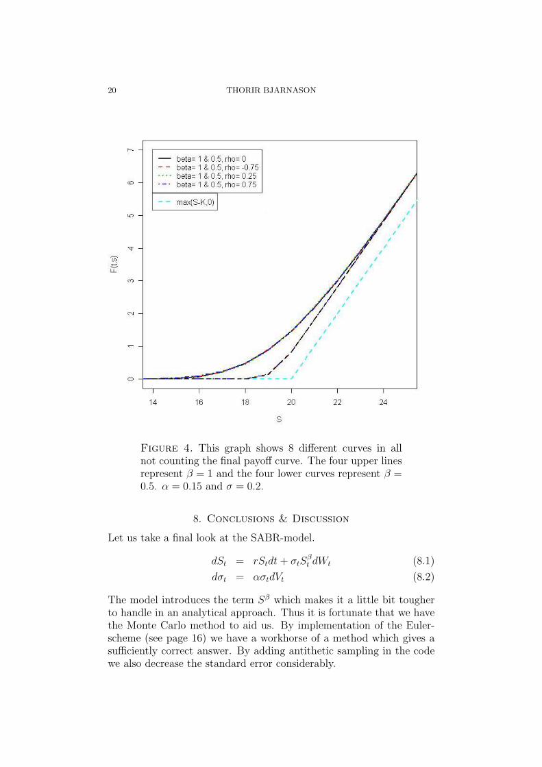
7.2. Results. Unless otherwise stated the strike price K is 20, theinterest rate r is 0.1 and the time to maturity T is 5/12. Regardlessof the value of the parameter values, the curves all seem to be convex.Thus it can be said that convexity is preserved for the SABR-model.Notice in the Figures 3 and 4 that all curves converge to a specific lineabove the final payoff curve. Below, a short description of how eachparameter affects the value of the option will be given.

7.2.1. Alpha - α. Or the volvol if you will. This parameter adjusts thefluctuation of the volatility process (3.5). Because of this the volvolwas restricted to the interval (0, 1) but most of the simulations wereconducted with α ≤ 0.55. For the volatility itself two values were usedas todays value of the volatility for the simulations. Mostly, these val-ues have been referred to as the starting values of σ and they are 0.2and 0.4.

After simulating for various values of the parameters it seems as thoughthe volvol did the least bit of difference. An increase in the value ofthe volvol was reflected poorly in the value of the option. The onlynoticeable difference was that the value of the option started fluctuatingmore for higher values of α, especially for large values of S in the assetprocess (3.4).

7.2.2. Beta - β. This parameter regulates the size of the diffusion termin (3.4) and therefore also the risk in the value of the asset. Thus itis only natural that small β gives small fluctuations and hence a lowervalue of the option and for large β we get greater fluctuations yielding


Figure 3. Four different price curves for the Europeancall option along with the final payoff function. α = 0.15.

a higher value of the option. The difference in price is accentuatedat-the-money, i.e. around the strike price. Take a look at Figures 3and 4 in which you can clearly see the difference in value.

7.2.3. Rho - ρ. For the above described setting it does not seem tomake any difference what correlation we use, positive, negative or zero.This you can see in Figure 4 where the price curves coincide, four upperand four lower, only depending on β. For β = 1 we have the uppercurves, all with different correlation coefficient but they all lay on topof each other, as do they for β = 0.5.

If we set β = 1, the interest rate to zero and focus on positive correla-tion we get a bubble, just as in Figure 5. The value of the option dropsdown below the final payoff, yielding a bubble. This is as in [9].

20 THORIR BJARNASON

Figure 4. This graph shows 8 different curves in allnot counting the final payoff curve. The four upper linesrepresent β = 1 and the four lower curves represent β =0.5. α = 0.15 and σ = 0.2.

8. Conclusions & Discussion

Let us take a final look at the SABR-model.

dSt = rStdt+ σtSβt dWt (8.1)

dσt = ασtdVt (8.2)

The model introduces the term Sβ which makes it a little bit tougherto handle in an analytical approach. Thus it is fortunate that we havethe Monte Carlo method to aid us. By implementation of the Euler-scheme (see page 16) we have a workhorse of a method which gives asufficiently correct answer. By adding antithetic sampling in the codewe also decrease the standard error considerably.


Figure 5. Here is an example curve of a bubble. We seethat today’s value of the option is, at some points, lowerthan the final payoff. α = 0.35, β = 1, ρ = 0.75, σ = 0.2.

Finally, is all of this plausible? Of course it is. This is not the ultimatetest for convexity regardless of the model we are testing. A better testwould be to numerically calculate Γ for the claim of choice and fromthere, proceed with the analysis. A reason though for not choosingthat approach is that it demands lots and lots of simulations to getvalues considered to be accurate and this is extremely time consuming.

Parameter values Property or behaviour

α β ρ(0, 1) [0, 1] (−1, 1) Convexity preserved(0, 1) [0, 1] (−1, 1) Increasing in volatility(0, 1) 1 (0, 1) Bubble

Table 2. Here we can see the results in short.

Now to the results. In Table 2 you can see the results, perhaps some-what abbreviated. The rightmost column describes what behaviour wemight expect to see when we use the parameter values set in the firstthree columns. In the second row we have that for all parameter valuesthere is an increase in the value of the option but this is only at-the-money. As was written above, all curves converge towards a straightline above the final payoff curve.

Remark 5. The last row is only true when we have zero interest rate.

9. Acknowledgements

Thanks to my supervisor Johan Tysk for his guidance, support anddiscussions and thanks to Erik Ekstrom for his help on the codewrit-ing.

22 THORIR BJARNASON

Appendix A. Appendix

Below we have some graphs and the source code (written in R) for thegraphs and the MC simulation.

Figure 6. Brownian motion (Random walk)

Brownian motionn <- 500

T <- 1

h <- T/n

t <- (0:n)*h

X <- c(0,cumsum(rnorm(n,mean=0,sd=1)*sqrt(h)))

plot(t,X,type="l",xlab="t",ylab="W(t)", ylim=c(-1.5,1.5))

Geometric Brownian motionn <- 500

T <- 1

h <- T/n

t <- (0:n)*h

X <- c(1,1:n)

sigma <- 0.2

alpha <- 1

W <- c(cumsum(rnorm(n,0,1)*sqrt(h)))

for(i in 1:n) X[i+1] <- exp((alpha-0.5*sigma^2)*t[i+1]+sigma*W[i])

plot(t,X,type="l",xlab="t",ylab="GBM")

lines(t,exp(t))

Stock processn <- 250

T <- 1

h <- T/n

t <- (0:n)*h


Figure 7. Geometric Brownian motion: α = 1, σ = 0.2

Figure 8. Simulation of a stock using the Euler scheme

24 THORIR BJARNASON

r <- 0.1

sigma <- 0.2

S <- array(0,n+1)

S[1] <- 50

for (i in 1:n)

S[i+1] <- S[i] + r*S[i]*h + sigma*S[i]*rnorm(1,0,1)*sqrt(h)

plot(t,S,type="l", xlab="t", ylab="S")

Code for the graph on page 7S <- (1:100)

K <- 25

sigma <- 0.8

r <- 0.1

T <- 5/12

d1 <- 0

for (i in 1:100) {

d1[i] <- 1/(sigma*sqrt(T))*(log(S[i]/K)+(r+0.5*sigma^2)*T)

}

d2 <- d1-sigma*sqrt(T)

F <- 0

for (i in 1:100) {

F[i] <- S[i+1]*pnorm(d1[i])-exp(-r*T)*K*pnorm(d2[i])

}

f <- 0

for (i in 1:100) f[i] <- max(S[i+1]-K,0)

x11()

plot(S[-1],F,type="l", lty=3, xlab="S", ylab="F(t,S)")

lines(S[-1],f,lty=1,col=2)


The code for simulating the datan <- 80

m <- 15000

T <- 5/12

h <- T/n

r <- 0.1

K <- 20

P <- 0

rho <- value in (-1,1)

beta <- value in [0,1]

alpha <- value in (0,1)

for (k in 1:80) {

summa <- 0

for (j in 1:m) {

S <- k

S2 <- S

Sigma <- 0.2

Sigma2 <- Sigma

dW <- rnorm(n,mean=0,sd=1)*sqrt(h)

dV <- rho*dW+sqrt(1-rho^2)*rnorm(n,mean=0,sd=1)*sqrt(h)

for (i in 1:n) {

S <- S+r*S*h+Sigma*(S^beta)*dW[i]

Sigma <- Sigma*exp(-0.5*h*alpha^2+alpha*dV[i])

if(S<=0) {S <- 0}

S2 <- S2+r*S2*h+Sigma2*(S2^beta)*-dW[i]

Sigma2 <- Sigma2*exp(-0.5*h*alpha^2+alpha*-dV[i])

if(S2<=0) {S2 <- 0}

if(S<=0 && S2<=0) {break}

}

summa <- summa+max(S-K,0)+max(S2-K,0)

}

P[k] <- exp(-r*T)*summa/(2*m)

}

print(alpha);print(beta);print(rho);print(0.2)

print(P)

26 THORIR BJARNASON

References

[1] Bjork, Tomas, Arbitrage theory in continuous time. Oxford university press,Oxford, 1998.

[2] Dupire, Bruno, Pricing with a smile. Risk vol 7, pp. 18-20, 1994.

[3] Y. Z. Bergman, B. D. Grundy and Z. Wiener, General properties ofoption prices. The Journal of Finance, vol 51, No. 5. pp. 1573-1610. 1996.

[4] Jackel, Peter, Monte Carlo Methods in Finance. John Wiley & Sons, LTD,2002.

[5] McLeish, Don L., Monte Carlo simulation and finance. Hoboken NJ, JohnWiley & Sons, 2005.

[6] Peter E. Kloeden, Eckhard Platen and Henri Schurz, Numericalsolution of SDE through computer experiments. Springer-Verlag, Germany,1994.

[7] Glasserman, Paul, Monte Carlo Methods in Financial Engineering. Springer,United States of America, 2004.

[8] Y.K. Lee, Kelvin Hoon, Brownian motion, the research goes on...www.doc.ic.ac.uk/~nd/surprise_95/journal/vol4/ykl/report.html

[9] David G. Hobson and Alexander M. G. Cox, Local Martingales, Bubblesand Option Prices http://people.bath.ac.uk/masdgh/publications.html

[10] Luenberger, David G., Investement science. Oxford university press, NewYork Oxford, 1998.

Documents

Stochastic volatility, convex prices and bubbles