Stochastic Volatility Demand Systems�

Apostolos Serletisy and Maksim IsakinDepartment of EconomicsUniversity of Calgary

Canada

Forthcoming in: Econometric Reviews

September 22, 2014

Abstract:

We address the estimation of stochastic volatility demand systems. In particular, werelax the homoscedasticity assumption and instead assume that the covariance matrix of theerrors of demand systems is time-varying. Since most economic and �nancial time series arenonlinear, we achieve superior modeling using parametric nonlinear demand systems in whichthe unconditional variance is constant but the conditional variance, like the conditional mean,is also a random variable depending on current and past information. We also prove animportant practical result of invariance of the maximum likelihood estimator with respect tothe choice of equation eliminated from a singular demand system. An empirical applicationis provided, using the BEKK speci�cation to model the conditional covariance matrix of theerrors of the basic translog demand system.

JEL classi�cation: C32, E52, E44.

Keywords: Flexible functional forms; Volatility.

�We would like to thank two anonymous referees for comments that greatly improved the paper.yCorresponding author. Phone: (403) 220-4092; Fax: (403) 282-5262; E-mail: Serletis@ucalgary.ca; Web:

http://econ.ucalgary.ca/serletis.htm.

1

1 Introduction

The measurement of consumer preferences and the estimation of demand systems has beenone of the most interesting and rapidly expanding areas of recent research. FollowingDiewert�s (1971) in�uential paper, a large part of the empirical demand literature has takenthe approach of using a �exible functional form for the underlying aggregator function.Flexible functional forms have revolutionized microeconometrics, by providing access to allneoclassical microeconomic theory in econometric applications. They include the locally�exible generalized Leontief of Diewert (1971), translog of Christensen et al. (1975), AlmostIdeal Demand System (AIDS) of Deaton and Muellbauer (1980), Quadratic AIDS (QUAIDS)of Banks et al. (1997), Min�ex Laurent (ML) model of Barnett (1983), Normalized Quadratic(NQ) of Diewert and Wales (1988), exact a¢ ne Stone index (EASI) implicit Marshalliandemand system recently introduced by Lewbel and Pendakur (2010), and the globally �exibleFourier functional form of Gallant (1981) and Asymptotically Ideal Model (AIM) of Barnettand Jonas (1983) and Barnett and Yue (1988). See Lewbel (1997) and Barnett and Serletis(2008) for an up-to-date survey of the state-of-the art in consumer demand analysis.In recent years, economists and �nance theorists have also been creating new models in

which stochastic variables are assumed to have a time-dependent variance (and are called�heteroscedastic�, as opposed to �homoscedastic�). In fact, recent leading-edge research in�nancial econometrics has applied the autoregressive conditional heteroscedasticity (ARCH)model, developed by Engle (1982), to estimate time-varying variances in commodity prices.Other models include Bollerslev�s (1986) generalized ARCH (GARCH) model and Nelson�s(1991) exponential GARCH (EGARCH) model. The univariate volatility models havealso been generalized to the multivariate case. The multivariate models are similar to theunivariate ones, except that they also specify equations of how the conditional covariancesand correlations move over time. See Bauwens et al. (2006) and Silvennoinen and Teräsvirta(2011) for surveys of this literature.In this paper we merge the empirical demand systems literature with the recent �nancial

econometrics literature. Our primary interest lies in the estimation of stochastic volatilitydemand systems. In particular, we relax the homoscedasticity assumption and insteadassume that the covariance matrix of the errors of demand systems is time-varying. Sincemost economic and �nancial time series are nonlinear and time-varying, we expect to achievesuperior modeling using parametric nonlinear demand systems in which the unconditionalvariance is constant but the conditional variance, like the conditional mean, is also a randomvariable depending on current and past information.Although most of the applications in the literature on consumer demand systems use

cross sections (or a set of pooled cross sections), there is increasing interest in the methodsdealing with time series data. For example, Lewbel and Ng (2005) propose a modi�cation ofthe translog demand system that can be applied in the presence of nonstationary prices withpossibly nonstationary errors. The focus of our paper is on the estimation of demand sys-

2

tems with explicit account for intertemporal structure of (unobserved) error term volatility.In particular, we analyze the simultaneous estimation of a demand system and a GARCHspeci�cation for the error term using time series data. While empirical models often revealheteroscedasticity, the sources of the volatility dynamics might be di¤erent. For example,the intertemporal structure of volatility might be a result of the aggregation of heterogeneouspreferences. Granger (1980) shows how the aggregation of simple dynamic preferences mightlead to complicated long-memory processes. At the same time, the current cross sectiondemand literature focuses on dealing with unobserved heterogeneity � see, for example,Hoderlein (2011), Blundell, Kristensen and Matzkin (2013) and Hoderlein and Stoye (2014).In some functional (Gorman) forms aggregable in income, like the AIDS, unobserved hetero-geneity might also result in heteroscedastic error terms [see Lewbel (2001)], albeit this typeof heteroscedasticity is beyond the scope of our paper.The paper is organized as follows. Section 2 brie�y reviews the neoclassical theory

of consumer choice whereas Section 3 provides a discussion of stochastic volatility demandsystems. Section 4 considers a model based on the Baba, Engle, Kraft, and Kroner (BEKK)representation [see Engle and Kroner (1995)] for the conditional covariance matrix of thebasic translog demand system. Section 5 provides an empirical application of this modelusing monthly data on monetary asset quantities and their user costs recently produced byBarnett et al. (2013) and maintained within the Center of Financial Stability (CFS) programAdvances in Monetary and Financial Measurement (AMFM). The �nal section concludes.

2 Neoclassical Demand Theory

Consider n consumption goods that can be selected by a consuming household. The house-hold�s problem is

maxxu(x) subject to p0x = y

where x is the n � 1 vector of goods; p is the corresponding vector of prices; and y isthe household�s total expenditure on goods (often just called �nominal income�in this litera-ture). The solution of the �rst-order conditions for utility maximization are the Marshallianordinary demand functions,

x = x(p; y).

Demand systems are often expressed in budget share form, s = (s1; :::; sn)0, where si =

pixi(p; y)=y is the expenditure share of good i.The maximum level of utility at given prices and income, h(p; y) = u [x(p; y)] ; is the

indirect utility function. The direct utility function and the indirect utility function areequivalent representations of the underlying preference preordering. Using h(p; y), we canderive the demand system by straightforward di¤erentiation, without having to solve a sys-tem of simultaneous equations, as would be the case with the direct utility function �rst

3

order conditions. In particular, Diewert�s (1974, p. 126) modi�ed version of Roy�s identity,

si(v) =vjrh(v)v0rh(v) ; i = 1; :::; n (1)

can be used to derive the budget share equations, where v = [v1; :::; vn]� is a vector of ex-penditure normalized prices, with the jth element being vj = pj=y, and rh(v) = @h(v)=@v.See Barnett and Serletis (2008) for more details.Suppose that the indirect utility function h and, therefore, the share equation system, is

de�ned up to the set of parameters �. In order to estimate share equation systems usingobservations of prices and shares (vt; st)

Tt=1, a stochastic version is speci�ed. Also, since

only exogenous variables appear on the right-hand side of such systems, it seems reasonableto assume that at time t the observed share in the ith equation deviates from the true shareby an additive disturbance term �it. Thus, the share equation system at time t is writtenin matrix form as

st = s(vt;�) + �t (2)

where �t = (�1t; :::; �nt)0 and � is the parameter vector to be estimated. It has also been

typically assumed that�t � N (0;) (3)

where 0 is n-dimensional null vector and is the n � n symmetric positive de�nite errorcovariance matrix.Finally, since the demand system (1) satis�es the adding-up property, i.e., the budget

shares sum to 1, the error covariance matrix is singular. Barten (1969) shows thatmaximum likelihood estimates can be obtained by arbitrarily dropping any equation in thesystem. McLaren (1990) also establishes invariance by virtue of observational equivalenceof the subsystems with di¤erent deleted equations.

3 Stochastic Volatility Demand Systems

In this paper, we relax the homoscedasticity assumption in (3) and instead assume that

�t � F (0;t) (4)

where F is a distribution from the family of elliptical distributions andt is the time-varyingcovariance matrix of the errors.As before, the error terms of the demand system sum to zero, (t)

Tt=1 are singular and

we can drop one equation to avoid singularity. The natural question is whether it matterswhich equation is deleted. The following theorem establishes the result.

4

Theorem 1 Let the rank of the covariance matrices be n� 1. Then any two subsystemsobtained from (2) by deleting di¤erent conditional mean equations, under assumption (4),are observationally equivalent, in the sense that they have the same likelihood for any possiblesample.

The proof is given in Appendix A. Theorem 1 is the counterpart of the invariance claim inBarten (1969) and McLaren (1990) for the case when the covariance matrix varies over time.The theorem posits that it does not matter which equation is eliminated from the demandsystem (2) in order to avoid singularity. Moreover, under assumption (4), the covariancematrices of the di¤erent subsystems are related by equation (17) in Appendix A.Although Theorem 1 is a nice theoretical result, it is not very attractive empirically,

because it assumes no intertemporal dependence between the covariance matrices (H t)Tt=1.

If one introduces a particular GARCH representation for the covariance matrix, the observa-tional equivalence does not hold in general, although it does hold for some particular cases.In other words, whether invariance holds depends on the intertemporal structure imposed onthe covariance matrix. In the next section we show that the invariance result is correct for theGARCH BEKK speci�cation. In particular, we consider a case, with the conditional meanequation given by the basic translog demand system and the conditional variance equationparameterized by a GARCH BEKK.

4 A Speci�c Case

Consider the basic translog (BTL) reciprocal indirect utility function of Christensen et al.(1975)

lnh(v) = �0 +nXk=1

�k ln vk +1

2

nXk=1

nXj=1

jk ln vk ln vj (5)

where � = [ ij] is an n� n symmetric matrix of parameters and � = (�0; :::; �n) is a vectorof other parameters, for a total of (n2 + 3n+ 2) =2 parameters. The BTL share equations,derived using the logarithmic form of Roy�s identity, are

si =

�i +nXk=1

ik log vk

nXk=1

�k +

nXk=1

nXj=1

jk log vk

; i = 1; : : : ; n. (6)

Estimation of (6) requires some parameter normalization, as the share equations are homo-geneous of degree zero in the ��s. Usually the normalization

Xn

i=1�k = 1 is used.

5

As before, consider a stochastic version of the demand system (in matrix form)

st = s(vt;�) + �t (7)

where �t = (�1t; :::; �nt)0 is an additive disturbance term and � is the parameter vector to be

estimated. Assume that the n-dimensional error vector is normally distributed with zeromean and time-varying covariance matrix

�tjIt�1 � N (0;t) (8)

where t is measurable with respect to information set It�1. To avoid singularity, delete(any) one equation from (7) and consider the corresponding (n � 1) � (n � 1) covariancematrix �t of the error vector.We assume the Baba, Engle, Kraft, and Kroner (BEKK) GARCH(p; q) representation

for the (n� 1)� (n� 1) covariance matrix of the error vector with generality parameter K[see Engle and Kroner (1995)]

�t = C0C +

KXi=1

pXi=1

B0ik�t�iBik +

KXk=1

qXi=1

A0ikut�iu

0t�iAik. (9)

The BEKKmodel has the attractive property of having the conditional covariance matrix,H t, positive de�nite by construction. This model has [n (n+ 3)� 2] =2 free parametersin the conditional mean equations (6) and (n� 1)n=2 + K2pqn2 free parameters in theconditional variance equations (9), for a total of (K2pq + 1)n2+n�1 free parameters. Thefollowing theorem claims the invariance of the maximum likelihood (ML) estimator withrespect to the deleted equation for this model.

Theorem 2 Let the covariance matrices (t)Tt=0 have rank n� 1 and the initial covariance

matrix 0 = �. Then any two subsystems of (7) consisting of n � 1 equations with thecorresponding conditional variance equation (9) are observationally equivalent. Also, theML estimates of the parameters of one subsystem can be recovered from the ML estimates ofthe parameters of another subsystem.

The proof is given in Appendix B. Theorem 2 states that the result of the maximumlikelihood estimation of the system does not depend on the choice of the n � 1 equationsto be estimated from the n equations of the demand system in the following sense. Theestimators of the conditional mean equations are the same for any set of n�1 equations; theestimators of the conditional variance equations for any set of n�1 equations can be obtainedfrom the estimators of any other set of n�1 equations, using the linear transformation (25)-(27) in Appendix B.

6

5 Empirical Application

Consider the model de�ned in the previous section with n = 3. Since (6) is a singular systemwe delete one equation (say the third equation) and consider the following two conditionalmean equations

s1 =�1 + 11 log v1 + 12 log v2 + 13 log v3

nXk=1

�k +nXk=1

nXj=1

jk log vk

+ e1; (10)

s2 =�2 + 12 log v1 + 22 log v2 + 23 log v3

nXk=1

�k +nXk=1

nXj=1

jk log vk

+ e2. (11)

We assume a BEKK GARCH(1,1) with K = 1 representation for the covariance matrixof e1 and e2 in (10) and (11). In particular, the 2� 2 covariance matrix of the errors can bewritten as

H t = C0C +B0H t�1B +A0et�1e

0t�1A. (12)

Thus, the BTL demand system with a BEKK speci�cation for the covariance matrixH t, con-sists of the conditional mean equations (10) and (11) and the following conditional varianceand covariance equations

h11;t = c211 + b

211h11;t�1 + 2b11b21h12;t�1 + b

221h22;t�1

+ a211e21;t�1 + 2a11a21e1;t�1e2;t�1 + a

221e

22;t�1; (13)

h12;t = c11c12 + b11b12h11;t�1 + (b11b22 + b12b21)h12;t�1 + b21b22h22;t�1

+ a11a12e21;t�1 + (a11a22 + a12a21) e1;t�1e2;t�1 + a21a22e

22;t�1; (14)

h22;t = c212 + c

222 + b

212h11;t�1 + 2b12b22h12;t�1 + b

222h22;t�1

+ a212e21;t�1 + 2a12a22e1;t�1e2;t�1 + a

222e

22;t�1. (15)

This model has a total of 19 free parameters to be estimated.Applied demand analysis uses two types of data, time series data and cross sectional

data. Time series data o¤er substantial variation in relative prices and less variation in in-come whereas cross sectional data o¤er limited variation in relative prices and substantialvariation in income levels. In this application, we use the monthly time series data on mon-etary asset quantities and their user costs recently produced by Barnett et al. (2013) and

7

maintained within the Center of Financial Stability (CFS) program Advances in Monetaryand Financial Measurement (AMFM). The sample period is from 1967:2 to 2011:12 (a totalof 539 observations). For a detailed discussion of the data and the methodology for the calcu-lation of user costs, see Barnett et al. (2013) and http://www.centerfor�nancialstability.org.In particular, we model the demand for three monetary assets: demand deposits (x1),

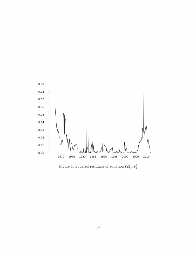
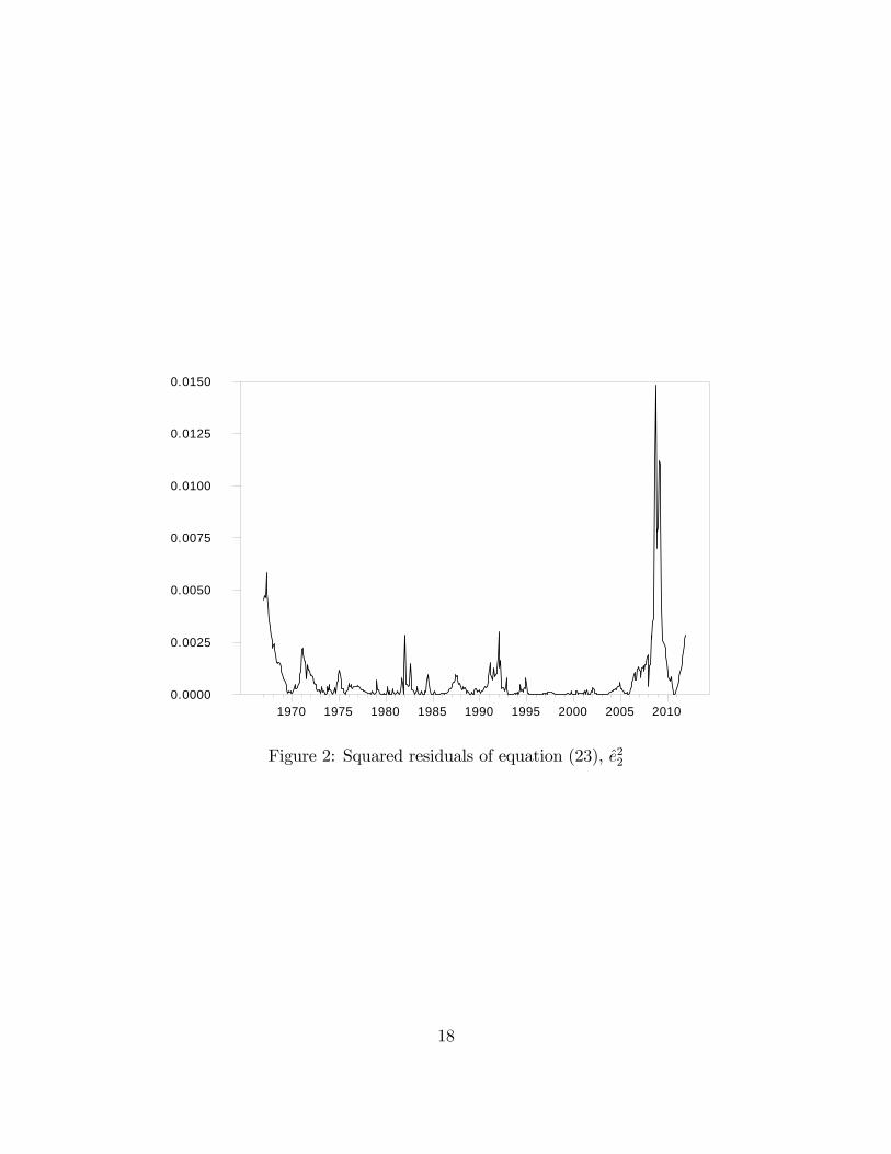
small time deposits at commercial banks (x2), and large time deposits (x3). As we requirereal per capita asset quantities for the empirical work, we divided each quantity series bythe CPI (all items) and total population. The estimation is performed in Estima RATS.We �rst estimate equations (10) and (11) under the homoscedasticity assumption in (3) andreport the results in Table 1. To verify the presence of ARCH e¤ects in the residuals of(10) and (11), estimated under the homoscedasticity assumption (3), we plot the estimatedsquared residuals e21 and e

22 in Figures 1 and 2, respectively. Moreover, Lagrange multiplier

tests for ARCH in each of e1 and e2 indicate signi�cant evidence of ARCH e¤ects; the nullhypotheses of no ARCH (of di¤erent orders) in each of e1 and e2 are rejected with p-valuesless than 0:000001.Next, we estimate the model under the heteroscedasticity assumption in (4), assum-

ing the BEKK speci�cation (12) for the error covariance matrix, H t. That is, we esti-mate the conditional mean equations, (10) and (11), and the conditional variance equa-tions, (13)-(15). The estimation results are reported in Table 2. We also estimatedthe model using the subsystems with the second and �rst equations deleted (see Table 3and 4, respectively). Consistent with Theorem 2 the parameters of the mean equations(�1; �2; �3; �11; �12; �13; �21; �22; �23; �31; �32; �33) are exactly the same in all three estima-tions (see panels A in Tables 2-4). The parameters of the variance equations are related byequations (25)-(27) in Appendix B.It is worth mentioning that the log likelihood function of the described model exhibits

manifold local maxima. To ensure reliability of the result it is necessary to implement theoptimization with di¤erent initial parameters (e.g. randomly assigned from the predeter-mined area) and/or di¤erent eliminated equations. Furthermore, in most cases it is helpfulto perform derivative-free search (such as Simplex algorithm) as a preliminary step for thederivative-based optimization.

6 Conclusion

Uncertainty is a very important concept in economics and �nance, if not the most important.Motivated by the fact that the current demand systems literature ignores the role of uncer-tainty, in this paper we introduce recent advances in �nancial econometrics to model thecovariance matrix of the errors of �exible demand systems, thereby improving the �exibilityof these systems to capture certain important features of the data. We prove an importantpractical result of invariance of the ML estimator with respect to the deleted equation for

8

the BTL demand system with conditional variance in the BEKK form. We also provide anempirical application based on the use of this model.Although we study the BEKK speci�cation of the error covariance matrix of the basic

translog, our approach could be applied to any other known demand system (includingthose mentioned in the Introduction). Moreover, other variance speci�cations could be usedsuch as, for example, the VECH model of Bollerslev et al. (1988), the constant conditionalcorrelation (CCC) model of Bollerslev (1990), as well as the dynamic conditional correlation(DCC) models of Engle (2002) and Tse and Tsui (2002). Extension of the methodology todemand systems that focus on cross-sectional data or pooled cross-sectional data is an areafor potential productive future research.

9

Appendix AProof of Theorem 1Since the rank of t is n� 1, the covariance matrix for any subsystem of n� 1 equations

is not singular. Moreover, the error term of the deleted equation can be recovered fromthe error terms of the other n � 1 equations using a linear injection (one-to-one mapping).Therefore, the vector of n � 1 error terms, with the nth error term being deleted, denotedby ut, can be transformed to any other vector of n � 1 error terms by eliminating the itherror term (i = 1; :::; n� 1), denoted by et, as follows

et = Tut (16)

where T is a unity (n� 1)� (n� 1) transformation matrix with the ith row replaced by avector of �1. The transformation matrix T has the property that TT = I and, therefore,T = T�1. Hence, the time-varying covariance matrices �t and H t of the error vectors utand et, respectively, are linked by the following

�t = T�1H t (T

0)�1= TH tT

0. (17)

Moreover, the Jacobian of the transformation is

J (T ) = �1. (18)

We assume that the error term (4) is elliptically distributed. Therefore, its marginaldistributions are also elliptical with characteristic functions of the form

� (t) = E[eit0e] = (t0H tt)

for some function which does not depend on n, and its density function can be expressedas

f (et) = jH tj�1=2 g (e0tH tet;n� 1) (19)

where g(�;n� 1) is a univariate function with parameter (n� 1).The log likelihood function associated with equation (19) is given by

L (#) =TXt=1

lt (#)

where # is the set of parameters � of the mean equation (2) and covariance matrices (H t)Tt=1

andlt (#) = �

1

2ln jH tj+ ln g (u0tH tut;n� 1)

10

with error vectors (ut)Tt=1 determined by the subsystem of (2) without the nth equation.

Using (16), (17), (18) and the fact that���T�1H t (T

0)�1��� = jH tj, we can write (19) as

f (et) =���T�1H t (T

0)�1����1=2 g�e0t �T�1H t (T

0)�1��1

et;n� 1�

= j�tj�1=2g�u0t�

�1t ut;n� 1

�= f (ut) :

Therefore, the log likelihood functions based on observations of the error vectors ut and etare the same. This proves the theorem. Q.E.D.

11

Appendix BProof of Theorem 2Without loss of generality, we provide the proof for the case of a GARCH(1,1) BEKK

with K = 1 representation for the conditional variance equation. Consider the subsystemof (7) with the last equation deleted, i.e. the error vector is ut = (�1t; �2t; :::; �n�1;t). TheGaussian log likelihood function based on the sample (vt; st)

Tt=1 can be written as

L��j (ut)Tt=1

�= �T (N � 1)

2log(2�)� 1

2

TXt=1

�log j�tj+ u0t��1t ut

�(20)

where�t = C

0C +B0�t�1B +A0ut�1u0t�1A (21)

and � = (�; vech(� ); vech(C); vec(B); vec(A)) is the vector of all parameters to be esti-mated and (ut)

Tt=1 is determined by the subsystem (7) without the nth equation.

As before, consider the subsystem of (7) without the ith equation and corresponding errorvector et = (�1t; :::; �i�1;t; �i+1;t; :::; �nt). It has been shown that the error vectors ut and et arelinked by the non-singular linear transformation (16). The Gaussian log likelihood functionfor this subsystem is

L�e� ���(et)Tt=1� = �T (N � 1)2

log(2�)� 12

TXt=1

�log jH tj+ e0t (H t)

�1 et�

(22)

whereH t = ~C

0 ~C +�~B�0H t�1 ~B +

�~A�0et�i (et�i)

0 ~A (23)

and e� = (e�; vech(e�); vech( ~C); vec( ~B); vec( ~A)) is the vector of all the parameters.Using (16), (18), and the fact that

���T�1H t (T0)�1��� = jH tj we can write the log likelihood

function (??)-(??) as

L�e� ���(et)Tt=1� = �T (N � 1)2

log(2�)�12

TXt=1

�log���T�1H t (T

0)�1���+ u0t �T�1H t (T

0)�1��1

ut

�with

T�1H t (T0)�1= T�1 ~C

0 ~C (T 0)�1+ T�1 ~B

0T�T�1H t�1 (T

0)�1�T 0 ~B (T 0)

�1

+ T�1 ~A0Tet�ie

0t�iT

0 ~A (T 0)�1:

12

Now we observe that systems (20)-(21) and (22)-(23) are identical if the following conditionshold

�t = T�1H t (T

0)�1 (24)

C = Cholesky�T�1 ~C

0 ~C (T 0)�1�

(25)

B = T 0 ~B (T 0)�1 (26)

A = T 0 ~A (T 0)�1 (27)

where Cholesky(�) stands for the Cholesky decomposition.Clearly, the ML estimators of � and e� are related as follows. The parameters of the

conditional mean equations are the same: � = e� and � = e� whereas the parameters of theconditional variance equations are related through (25)-(27). Note that condition (24) issatis�ed for the initial covariance matrices which are predetermined by �. In addition, sinceboth C and ~C are triangular matrices in the BEKK representation, in order to preserve thetriangular form, equation (25) involves transformation using Cholesky decomposition.Hence, the likelihood functions of di¤erent subsystems of (7) consisting of n � 1 equa-

tions with corresponding conditional variance equation (9) are the same up to the parame-ters transformation which relates the maximum likelihood estimators for these subsystems.Q.E.D.

13

References

[1] Banks, J., R. Blundell, and A. Lewbel. �Quadratic Engel Curves and Consumer De-mand.�Review of Economics and Statistics 79 (1997), 527-539.

[2] Barnett, W.A. �De�nitions of Second-Order Approximation and of Flexible FunctionalForm.�Economics Letters 12 (1983), 31-35.

[3] Barnett, W.A. and A. Jonas. �The Müntz-Szatz Demand System: An Application of aGlobally Well Behaved Series Expansion.�Economics Letters 11 (1983), 337-342.

[4] Barnett, W.A. and A. Serletis. �Consumer Preferences and Demand Systems.�Journalof Econometrics 147 (2008), 210-224.

[5] Barnett, W.A. and P. Yue. �Seminonparametric Estimation of the Asymptotically IdealModel: The AIM demand system.�In: G.F. Rhodes and T.B. Fomby, (Eds.), Nonpara-metric and Robust Inference: Advances in Econometrics, Vol. 7. JAI Press, GreenwichCT (1988).

[6] Barnett, W.A., J. Liu, R.S. Mattson, and J. van den Noort. �The New CFS Divisia Mon-etary Aggregates: Design, Construction, and Data Sources.�Open Economies Review24 (2013), 101-124.

[7] Barten, A.P. �Maximum Likelihood Estimation of a Complete System of Demand Equa-tions.�European Economic Review 1 (1969), 7-73.

[8] Bauwens, L., S. Laurent, and J.V.K. Rombouts. �Multivariate GARCH Models: ASurvey.�Journal of Applied Econometrics 21 (2006), 79-109.

[9] Blundell, R., D. Kristensen, and R. Matzkin. �Stochastic Demand and Revealed Pref-erence.�Journal of Econometrics (2014, forthcoming).

[10] Bollerslev, T. �Generalized Autoregressive Conditional Heteroskedasticity.�Journal ofEconometrics 31 (1986), 307-27.

[11] Bollerslev, T. �Modeling the Coherence in Short-Term Nominal Exchange Rates: AMultivariate Generalized ARCH Approach.� Review of Economics and Statistics 72(1990), 498-505.

[12] Bollerslev, T., R.F. Engle, and J. Wooldridge. �A Capital Asset Pricing Model withTime-Varying Covariances.�Journal of Political Economy 96 (1988), 116-131.

[13] Christensen, L.R., D.W. Jorgenson, and L.J. Lau. �Transcendental Logarithmic UtilityFunctions.�American Economic Review 65 (1975), 367-383.

14

[14] Deaton, A. and J.N. Muellbauer. �An Almost Ideal Demand System.�American Eco-nomic Review 70 (1980), 312-326.

[15] Diewert, W.E. �An Application of the Shephard Duality Theorem: A Generalized Leon-tief Production Function.�Journal of Political Economy 79 (1971), 481-507.

[16] Diewert, W.E. �Applications of Duality Theory.�In Frontiers of Quantitative Economics(Vol. 2), eds. M.D. Intriligator and D.A. Kendrick, Amsterdam: North-Holland (1974),pp. 106-171.

[17] Diewert, W.E. and T.J. Wales. �Normalized Quadratic Systems of Consumer DemandFunctions.�Journal of Business and Economic Statistics 6 (1988), 303-312.

[18] Engle, R.F. �Autoregressive Conditional Heteroscedasticity with Estimates of the Vari-ance of U.K. In�ation.�Econometrica 50 (1982), 987�1008.

[19] Engle, R.F. �Dynamic Conditional Correlation: A Simple Class of Multivariate GARCHModels.�Journal of Business and Economic Statistics 20 (2002), 339-350.

[20] Engle, R.F. and K.F. Kroner. �Multivariate Simultaneous Generalized ARCH.�Econo-metric Theory 11 (1995), 122-150.

[21] Gallant, A.R. �On the Bias in Flexible Functcional Forms and an Essentially UnbiasedForm: The Fourier Flexible Form.�Journal of Econometrics 15 (1981), 211-245.

[22] Granger, C.W.J. �Long Memory Relationships and the Aggregation of Dynamic Mod-els.�Journal of Econometrics 14 (1980), 227-238.

[23] Hoderlein, S. �How Many Consumers are Rational?� Journal of Econometrics 164(2011), 294-309.

[24] Hoderlein, S. and J. Stoye. �Revealed Preferences in a Heterogeneous Population.�Review of Economics and Statistics (2014, forthcoming).

[25] Lewbel, A. �Consumer Demand Systems and Household Equivalent Scales.�In PesaranM.H. and P. Schmidt (Eds.), Handbook of Applied Econometrics, Volume II Microeco-nomics. Oxford: Blackwell Publishers Ltd. (1997).

[26] Lewbel, A. �Demand Systems with and without Errors.�American Economic Review91 (2001), 611-618.

[27] Lewbel, A. and S. Ng. �Demand Systems with Nonstationary Prices.�Review of Eco-nomics and Statistics 87 (2005), 479-494.

15

[28] Lewbel, A. and K. Pendakur. �Tricks with Hicks: The EASI Demand System.�Ameri-can Economic Review 99 (2009), 827-863.

[29] McLaren, K.R. �A Variant on the Arguments for the Invariance of Estimators in aSingular System of Equations.�Econometric Reviews 9 (1990), 91-102.

[30] Nelson, D.B. �Conditional Heteroskedasticity in Asset Returns.� Econometrica 59(1991), 347-370.

[31] Silvennoinen, A. and T. Teräsvirta. �Multivariate GARCH Models.�In T.G. Andersen,R.A. Davis, J.-P. Kreiss, and T. Mikosch (Eds.), Handbook of Financial Time Series.New York: Springer (2011).

[32] Tse, Y.K. and A.K.C. Tsui. �A Multivariate GARCH Model with Time-Varying Cor-relations.�Journal of Business and Economic Statistics 20 (2002), 351-362.

16

1970 1975 1980 1985 1990 1995 2000 2005 20100.00

0.01

0.02

0.03

0.04

0.05

0.06

0.07

0.08

0.09

Figure 1: Squared residuals of equation (22), e21

17

1970 1975 1980 1985 1990 1995 2000 2005 20100.0000

0.0025

0.0050

0.0075

0.0100

0.0125

0.0150

Figure 2: Squared residuals of equation (23), e22

18

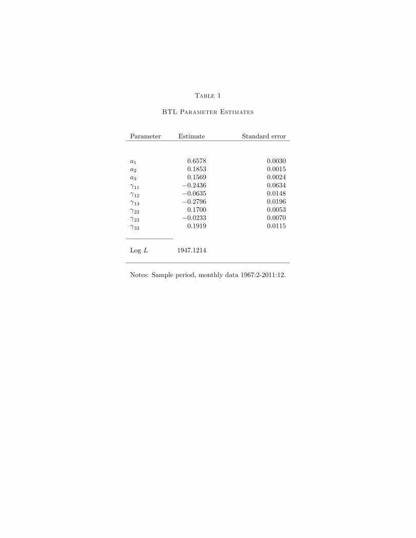
Table 1

BTL Parameter Estimates

Parameter Estimate Standard error

a1 0:6578 0:0030a2 0:1853 0:0015a3 0:1569 0:0024 11 �0:2436 0:0634 12 �0:0635 0:0148 13 �0:2796 0:0196 22 0:1700 0:0053 23 �0:0233 0:0070 33 0:1919 0:0115

Log L 1947:1214

Notes: Sample period, monthly data 1967:2-2011:12.

Table 2

Estimates Of BTL With BEKK Errors

Parameter Estimate Standard error

Mean equations:

a1 0:6199 0:0005a2 0:1843 0:0006a3 0:1958 0:0008 11 0:0229 0:0141 12 �0:0402 0:0028 13 �0:3469 0:0042 22 0:1618 0:0019 23 �0:0922 0:0019 33 0:0437 0:0029

Variance equations (with the 3rd mean equation deleted):

c11 0:0038 0:0003c12 �0:0010 0:0002c13 0:0017 0:0001a11 0:5225 0:0244a12 �0:0258 0:0046a21 0:1455 0:0297a22 0:2867 0:0493b11 0:9302 0:0316b12 0:0113 0:0021b21 �0:0474 0:0220b22 1:0249 0:0237

Log L 3080:6445

Notes: Sample period, monthly data 1967:2-2011:12.

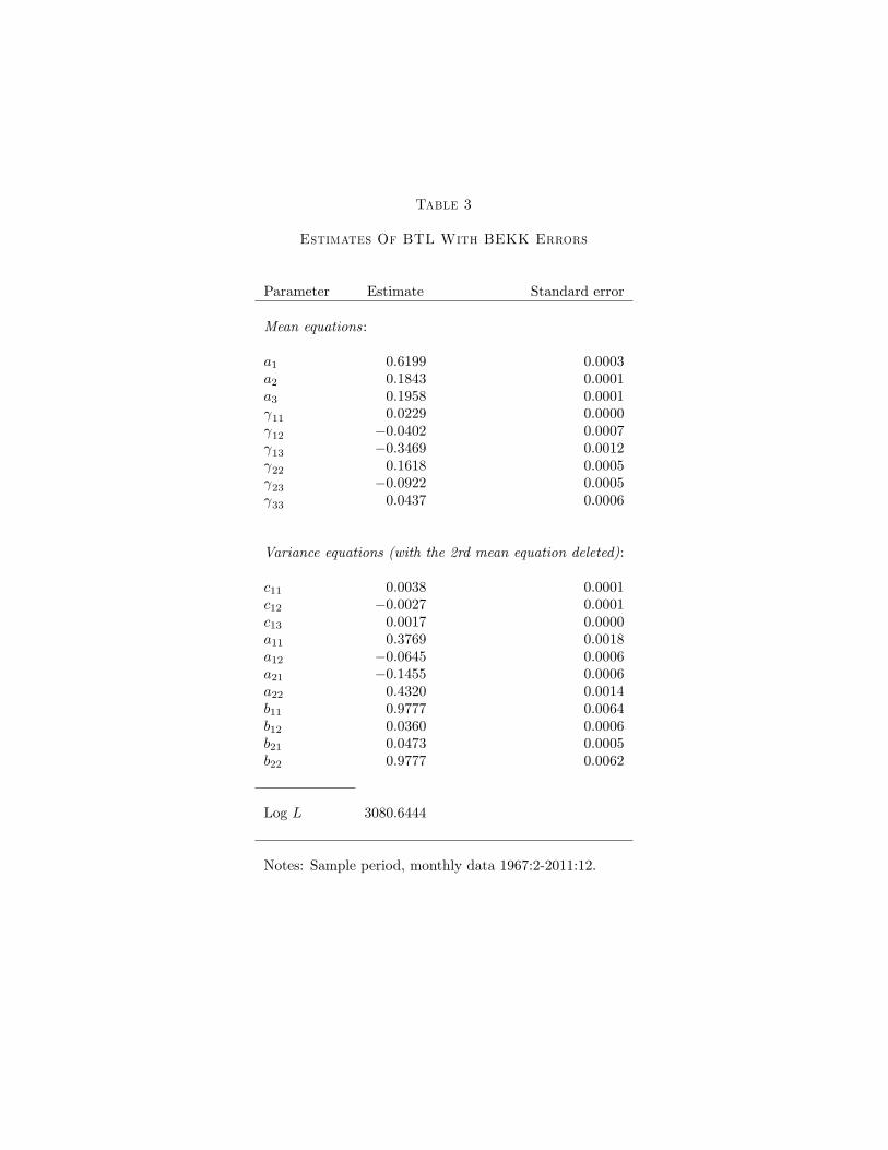
Table 3

Estimates Of BTL With BEKK Errors

Parameter Estimate Standard error

Mean equations:

a1 0:6199 0:0003a2 0:1843 0:0001a3 0:1958 0:0001 11 0:0229 0:0000 12 �0:0402 0:0007 13 �0:3469 0:0012 22 0:1618 0:0005 23 �0:0922 0:0005 33 0:0437 0:0006

Variance equations (with the 2rd mean equation deleted):

c11 0:0038 0:0001c12 �0:0027 0:0001c13 0:0017 0:0000a11 0:3769 0:0018a12 �0:0645 0:0006a21 �0:1455 0:0006a22 0:4320 0:0014b11 0:9777 0:0064b12 0:0360 0:0006b21 0:0473 0:0005b22 0:9777 0:0062

Log L 3080:6444

Notes: Sample period, monthly data 1967:2-2011:12.

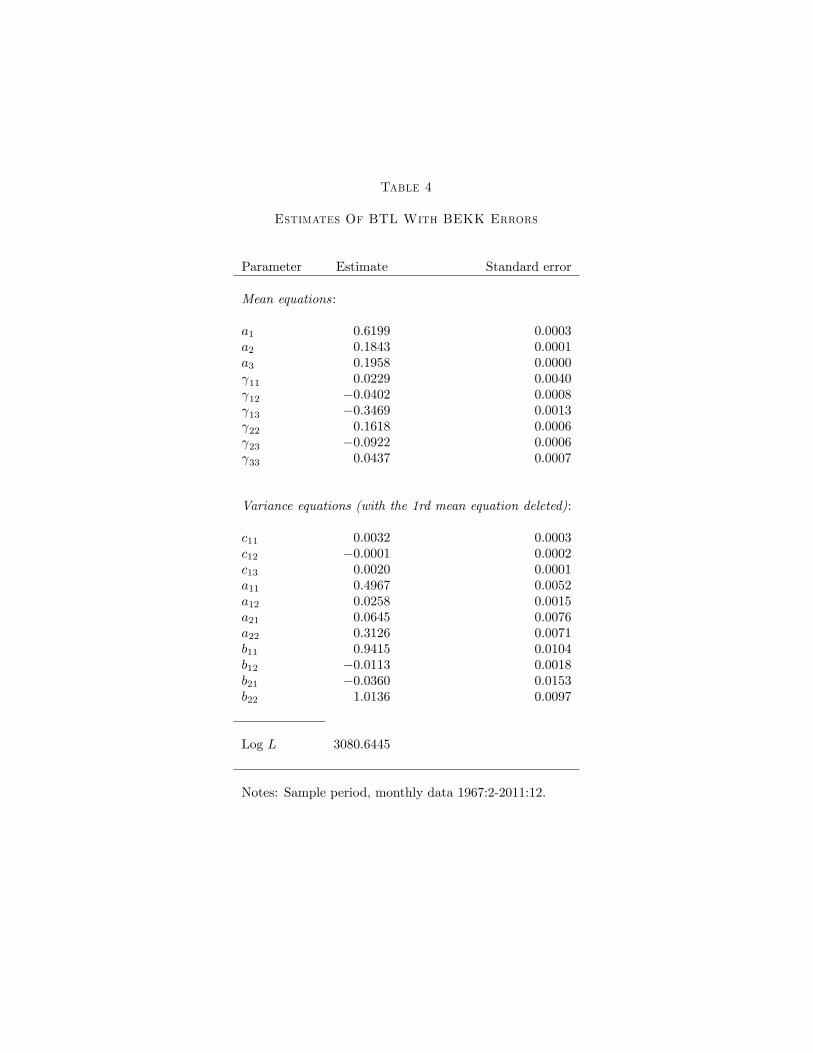
Table 4

Estimates Of BTL With BEKK Errors

Parameter Estimate Standard error

Mean equations:

a1 0:6199 0:0003a2 0:1843 0:0001a3 0:1958 0:0000 11 0:0229 0:0040 12 �0:0402 0:0008 13 �0:3469 0:0013 22 0:1618 0:0006 23 �0:0922 0:0006 33 0:0437 0:0007

Variance equations (with the 1rd mean equation deleted):

c11 0:0032 0:0003c12 �0:0001 0:0002c13 0:0020 0:0001a11 0:4967 0:0052a12 0:0258 0:0015a21 0:0645 0:0076a22 0:3126 0:0071b11 0:9415 0:0104b12 �0:0113 0:0018b21 �0:0360 0:0153b22 1:0136 0:0097

Log L 3080:6445

Notes: Sample period, monthly data 1967:2-2011:12.