Embed Size (px)
Citation preview
arX
iv:0
903.
3554
v2 [
astr
o-ph
.CO
] 7
Jul
200
9Mon. Not. R. Astron. Soc. 000, 1–21 (2009) Printed 29 October 2018 (MN LATEX style file v2.2)
Stochasticity in N-body Simulations of Disc Galaxies
J. A. Sellwood1⋆
and Victor P. Debattista2†
1Rutgers University, Department of Physics & Astronomy, 136 Frelinghuysen Road, Piscataway, NJ 08854-8019, USA2Jeremiah Horrocks Institute for Astrophysics and Supercomputing, University of Central Lancashire, Preston, PR1 2HE, UK
29 October 2018
ABSTRACT
We demonstrate that the chaotic nature of N -body systems can lead to macroscopicvariations in the evolution of collisionless simulations containing rotationally sup-ported discs. The unavoidable stochasticity that afflicts all simulations generally causesmild differences between the evolution of similar models but, in order to illustrate thatthis is not always true, we present a case that shows extreme bimodal divergence. Thedivergent behaviour occurs in two different types of code and is independent of allnumerical parameters. We identify and give explicit illustrations of several sources ofstochasticity, and also show that macroscopic variations in the evolution can originatefrom differences at the round-off error level. We obtain somewhat more consistentresults from simulations in which the halo is set up with great care compared withthose started from more approximate equilibria, but we have been unable to eliminatediverging behaviour entirely because the main sources of stochasticity are intrinsicto the disc. We show that the divergence is only temporary and that halo friction ismerely delayed, for a substantial time in some cases. We argue that the delays areunlikely to arise in real galaxies, and that our results do not affect dynamical frictionconstraints on halo density. Stochastic variations in the evolution are inevitable inall simulations of disc-halo systems, irrespective of how they were created, althoughtheir effect is generally far less extreme than we find here. The possibility of divergentbehaviour complicates comparison of results from different workers.
Key words: galaxies: evolution – galaxies: haloes – galaxies: kinematics and dynamics– galaxies: spiral
1 INTRODUCTION
Miller (1964) pointed out that all gravitational N-body sys-tems are chaotic, in the sense that the trajectories of allparticles in two systems that differ initially by a small shiftin the starting position or velocity of even a single particlewill diverge exponentially over time. Thus, two simulationsstarted from the same initial conditions will follow identicalevolutionary paths only if the arithmetic operations are per-formed with the same precision and in the same order, sothat round off error is identical. These statements are truefor every code, irrespective of the algorithm used for thecomputations, and no matter how many particles are em-ployed. In particular, a simulation can never be reproducedexactly when run with a different code.
Microscopic chaos is unimportant for many applicationsbecause the different evolutionary paths of almost identi-cal simulations lead to similar macroscopic properties suchas mass profiles, overall shape, etc., which therefore consti-
⋆ E-mail: [email protected]† E-mail: [email protected]
tute firm results. Binney & Tremaine (2008, hereafter BT08,p. 344) make this argument and cite a test by Frenk et al.
(1999) which indeed shows that many different codes yieldsimilar key properties after following the collapse of a darkmatter halo. In fact, results generally converge in tests thatvary the numerical grid, softening, and/or number of par-ticles (e.g. Power et al. 2003; Diemand et al. 2004), whichthey would not do if there were a large element of stochas-ticity. Sellwood (2008) also demonstrated exquisitely repro-ducible evolution of halo models that were perturbed byexternally imposed bars, in sharp contrast to the results pre-sented here.
Simulations with active discs of particles, on the otherhand, are not so well behaved. Sellwood & Debattista (2006)reported some minor differences, and one major, in a set ofexperiments using different numerical parameters but thesame file of initial coordinates. We show here that simula-tions with discs can, at least for certain models, exhibit bi-modally divergent macroscopic results, even between casesthat differ only at the round-off error level. The reason forthis qualitative difference for discs is because collective insta-bilities and vigorous responses develop from particle noise.
c© 2009 RAS
2 J. A. Sellwood and V. P. Debattista
Here we identify a number of distinct causes of stochasticbehaviour in discs, and demonstrate explicitly how the evo-lution is affected.
We show that the principal sources of divergent be-haviour are: (a) multiple in-plane global modes, (b) swingamplified noise, (c) bending instabilities, (d) suppression ofdynamical friction, and (e) the truly chaotic nature of N-body systems. We also show that the distribution of evolu-tionary paths taken in simulations of different realizationsof the same model varies systematically with the care takento set up the initial coordinates of halo particles.
We deliberately choose to illustrate just how large thedifferences can be for one particular unstable equilibriummodel. Stochasticity is present in all simulations and its ef-fects are always noticeable in those containing discs, butgenerally variations in the evolution show less scatter thanin the case studied here. We show that the range of be-haviour is similar in two quite distinct N-body codes andillustrate the sensitivity to differences at the round-off errorlevel. We also show that increasing the number of particlesdoes not reduce the spread of measured properties.
Real galaxies are assembled and evolve in a compli-cated manner, and certainly do not pass through a well-constructed axisymmetric, equilibrium phase that is unsta-ble, although such a model is commonly used as a startingpoint of simulations. The objectives of experiments of thistype are therefore (1) to determine whether plausible ax-isymmetric galaxy models are globally stable and (2) to de-velop an understanding of the dynamical evolution of mod-els that form bars and other non-axisymmetric structures.While we adopt a model of this type in this paper, its re-markable behaviour has implications for all simulations ofdisc-halo models, regardless of how they were created.
The main part of the paper demonstrates the role of thefive above-named sources of stochasticity in the evolution ofdisc models. We also explicitly show the effects of differentparticle selection techniques on the robustness of the be-haviour. Stochastic divergence has been reported elsewhere,but not recognized as an intrinsic aspect of these models;e.g., Klypin et al. (2008) attributed divergent evolution toinadequate numerical care, whereas stochasticity could bethe cause. Appendix B reports extensive tests that confirmthat the results we report here do not depend on any nu-merical parameters.
2 SELECTION OF PARTICLES
The selection of initial particle positions and velocities of anequilibrium model requires careful attention. Random selec-tion of even many millions of particles will lead to shot noisevariations in both the density and velocity distributions ofa model. Here we summarize the available techniques to se-lect initial coordinates of particles, with a focus on disc-halomodels. These methods generally yield a set of particles thatare not specific to any particular N-body code.
2.1 Selecting from a DF
Jeans theorem requires that an equilibrium model shouldhave a distribution function (DF) that is a function of theisolating integrals (BT08, p. 283). Thus the best way to
realize an equilibrium set of particles for an initial model isto select from a DF, when one is available.
While random selection of particles may be com-mon practice, it immediately discards a large part ofthis potential advantage. One widely used technique (e.g.Holley-Bockelmann et al. 2005; Weinberg & Katz 2007;Zhang & Magorrian 2008; Dubinski et al. 2009) is to acceptor reject candidate particles based on a comparison of arandom variable with the value of the DF at the phase-space position of each particle, which introduces shot noisein the density of particles in integral space. The evolutionof the simulation will be that of the selected DF, not theintended one, and different random realizations lead to sig-nificant variations in the measured frequencies of the insta-bilities in the linear regime (Sellwood 1983) and substantialdifferences in the non-linear regime. It is therefore best toadopt a deterministic procedure for particle selection froma DF.
A scheme to select particles smoothly in this way,first used in Sellwood (1983) and described more fully inSellwood & Athanassoula (1986), is summarized in the Ap-pendix of Debattista & Sellwood (2000). We divide integral,generally (E,L), space into n areas in such a way that∫ ∫
FdEdL over each small area is exactly 1/nth of theintegral over the total accessible ranges of E & L. HereF (E,L) is the differential distribution after integration overthe other phase space variables (BT08, pp. 292, 299). Re-quiring that one particle lies within each area ensures thatthe selected set of particles is as close as possible to rep-resenting the desired particle density in integral space. Wechoose the precise position of a selected particle within eacharea quasi-randomly in order to ensure that the particles donot lie on an exact raster in integral space. We describe thisscheme as deterministic selection from the DF, a term thatignores this minor random element.
This scheme is readily adapted to select particles of un-equal masses if desired. To select particles having massesproportional to a weight function w(E,L), one simplyweights the DF by w−1, which automatically adjusts thesubdivision of (E,L)-space into areas of equal weighted DF,as described in Sellwood (2008).
The phases of the particles around the orbit definedby these integrals can be selected at random. We have noevidence that the choice of radial phase, either for flat discsor for spheres, causes significant variations in the outcomeand we discuss the choice of azimuthal phases in Section 2.3below.
Debattista & Sellwood (2000) describe the similar pro-cedure for 2-integral spheroidal models.
2.2 When No Simple DF Is Available
Comparatively few useful mass models have known DFs,and the realization of an equilibrium set of particles fora general model presents a significant challenge. Some au-thors (e.g. Shlosman & Noguchi 1993) have simply createda rough N-body system, which they then evolve in the pres-ence of a frozen disc, thereby allowing the halo to relax to-wards some nearby equilibrium.
Hernquist (1993) advocates solving the Jeans equa-tions for each component in the combined poten-tial of all mass components. His method is widely
c© 2009 RAS, MNRAS 000, 1–21
Stochasticity in N-body Discs 3
used (e.g. Valenzuela & Klypin 2003; Athanassoula 2003;El-Zant et al. 2004; Klypin et al. 2008), but the resultingequilibrium is approximate.
In general, it is better to derive an approximateDF for aspherical or spheroidal system. An isotropic DF for a spher-ical system can usually be obtained by Eddington inversion(BT08, p. 289), although it is important to verify that thefunction is positive for all energies (which it generally is, forreasonable mass models).
Creating an equilibrium DF for a multi-component sys-tem presents a greater challenge, for which three effec-tive approaches have been developed. Raha et al. (1991),Kuijken & Dubinski (1995) and Debattista & Sellwood(2000) employ the method of Prendergast & Tomer (1970)to derive the mass distribution for a halo having some as-sumed DF that will be in equilibrium in the presence of oneor more other mass components. Alternatively, one can useEddington’s inversion formula for the halo only in the poten-tial of the combined disc and halo (Holley-Bockelmann et al.
2005). A third possibility, as here, is to start from a knownspherical halo with a known DF and compress it by addinga disc and/or a bulge using Young’s (1980) method (seeSellwood & McGaugh 2005), and then to select particlesfrom the compressed DF. Even though the last two methodsuse only the monopole term for the disc, all three methodsyield a spheroidal system that is close to detailed equilib-rium everywhere.
In general, it is more difficult to construct a good equi-librium for a disc component. The circular speed in the discmid-plane as a function of radius is determined by the to-tal mass distribution and, commonly, one specifies Q(R)(Toomre 1964) to determine the radial velocity spread ateach radius. The Jeans equations in the epicycle approxi-mation (BT08, p. 326) generally yield a poor equilibriumexcept when the radial dispersion is a small fraction of thecircular speed, and the asymmetric drift formula may haveno solution near the centres of hot discs. Shu (1969) de-scribes an approximate DF for a warm disc with a givenradial velocity dispersion that we, and Kuijken & Dubinski(1995), have found to be quite serviceable. Again in caseswhere the radial velocity dispersion stretches the validity ofthe epicycle approximation, radial gradients can lead to adisc surface density after integration over all velocities thatdiffers slightly from that specified, as shown in Section 3.1.
The vertical structure of an isothermal stellar sheetis given by the formulae developed by Spitzer (1942) andCamm (1950), and BT08 (p. 321) describe a generaliza-tion of the in-plane DF to include this feature, which theydescribe as the Schwarzschild DF. The Spitzer-Camm for-mulae assume full Newtonian gravity and no radial densityor dispersion gradient. Force softening has an increasinglydetrimental effect on the vertical balance as the ratio of discthickness to softening length is reduced, we therefore pre-fer to construct a vertical equilibrium from the 1D verticalJeans equation in the actual force field of the softened discpotential, which leads to a better equilibrium.
2.3 Quiet Starts
The quiet start technique is a valuable addition to the set upprocess only when the model has a few vigorous, large-scaleinstabilities, such as arise in a cool, massive disc with a rota-
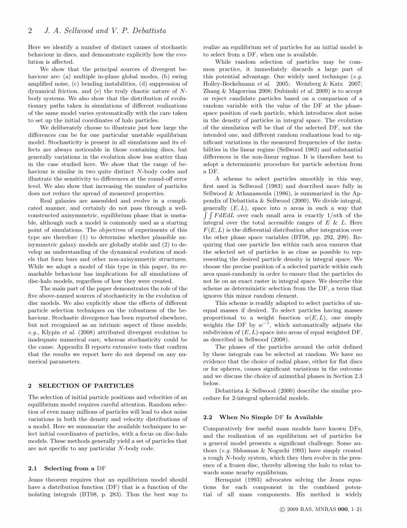
Figure 1. The inner rotation curve of our standard model (solid).The separate contributions of the disc (dashed) and halo (dotted)are also shown.
tion curve that rises approximately linearly from the centre.It is of little help when linear stability theory predicts themodel to be responsive but (almost) stable (e.g. Sellwood1989; Sellwood & Evans 2001). In these latter cases, collec-tive responses to residual noise grow more vigorously thanany global modes, and the particle arrangement randomizesquickly.
For a quiet start, one reproduces each selected masterparticle multiple times in a symmetrical arrangement, withimage particles having the identical radius and velocity com-ponents in polar coordinates. We restrict the meaning of thephrase “quiet start” to this symmetrical arrangement of par-ticles – i.e. a quiet start can be used no matter how the co-ordinates of the master particles are selected. Conversely, a“noisy start” means only that azimuthal coordinates are se-lected at random, again independent of how the master par-ticles are selected. The procedures for discs and spheroidalcomponents differ slightly.
For discs, we place image particles at the corners of analmost regular polygon in 2D, centred on the model centre.The polygon is not exactly regular because we nudge theparticles away from exact n-fold symmetry by a randomfraction of a small angle, typically 0.02. When the disc hasa finite thickness, the polygon must be duplicated with asecond on the opposite side of the mid-plane for which boththe vertical position z and velocity vz of every particle ineach of the two polygons have opposite signs.
When the force-determination method is based aroundan expansion in sectoral harmonics that is truncated at loworder, mmax, and the number of sides to the polygon n >
2mmax + 1, azimuthal forces in the initial model are muchlower than would arise from particle shot noise – hence thelabel “quiet start”.
We have not tried quiet starts for other force methods,but they could still offer a significant advantage providedthat the number of corners adopted for the polygon exceedsthe azimuthal order of all the strong instabilities and non-axisymmetric responses (Section 5.3) by at least a factortwo.
We adopt a similar procedure for spheroidal compo-nents, except that we create image particles by rotating theinitial position and velocity vectors using the usual rotationmatrix for the adopted set of Euler angles (e.g. Arfken 1985,p. 199). The set of Euler angles used creates an n-fold ro-tationally symmetric set of particles, which is also reflection
c© 2009 RAS, MNRAS 000, 1–21
4 J. A. Sellwood and V. P. Debattista
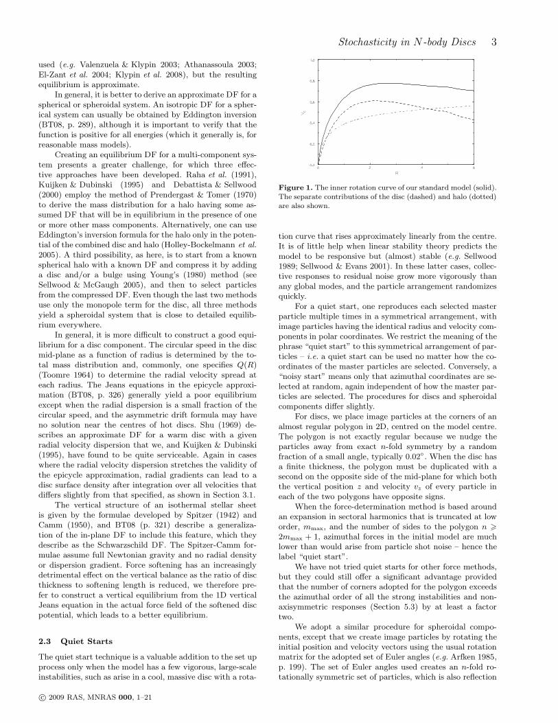
Figure 2. Details of the approximate DF for the disc. Panels (a) and (b) show respectively the variation of f with radial velocity andazimuthal velocity at five different radii. Panel (c) shows the radial variations of the rms azimuthal speed (vφ solid) and radial speed (vrdashed), (d) compares the circular speed (dotted) with the mean vφ (solid) to illustrate the asymmetric drift. Panels (e) and (f) comparerespectively the actual surface density and Q profiles (solid) with the desired profiles (dashed). The DF does not reproduce these curvesperfectly, but the departures are minor.
symmetric about the mid-plane, and has zero net momen-tum with a centre of mass at the model centre; each masterparticle is therefore inserted 2n times. It is reasonable toadopt n & 4.
3 MODELS
Here we describe all the various galaxy models we use in thispaper.
3.1 Standard Galaxy Model
Our standard model is a composite disc-halo system withthe rotation curve shown in Fig. 1. The two mass compo-nents are an exponential disc and a compressed, stronglytruncated, Hernquist halo.
The initial surface density of the disc has the usual ex-ponential form
Σ(R) =Md
2πR2
d
e−R/Rd , (1)
where Md is the nominal disc mass. We truncate the discat R = 5Rd, leaving an active disc mass of ≈ 0.96Md. Thedisc particles are set in orbital motion with a radial velocityspread so as to make Toomre’s Q = 1.5. For most mod-els, we determine the approximate equilibrium velocities bysolving the Jeans equations in the epicycle approximationas described in Section 2.2.
In some cases we adopt Shu’s approximate DF instead,and select disc particles deterministically from it. Propertiesof the DF and the radial variations of the low-order veloc-ity moments are shown in Fig. 2. While the radial velocitydistributions are nicely Gaussian, the azimuthal velocity dis-tributions (2b) are markedly skewed. This aspect, and thedepartures of the surface density and Q profiles from the de-sired values all decrease for models with less dominant discsor with lower values of Q.
For fully 3D simulations, the density profile normal tothe disc plane is Gaussian, with a constant scale height of0.05Rd and appropriate vertical velocities in the numericallydetermined vertical force profile.
We construct a halo in equilibrium with the disc in thefollowing manner. We start from the initial density profilesuggested by Hernquist (1990)
ρ0(r) =Mhrs
2πr(rs + r)3, (2)
which has total mass Mh and scale radius rs, with theisotropic distribution function (DF) also given by Hernquist.We strongly truncate this halo by eliminating all particleswith enough energy to reach r > 2rs, causing the densityto taper gently to zero at this radius, and an actual halomass of ≈ 0.25Mh. Since most of the discarded mass is atlarge radii, there is little change to the central attraction atr < 2rs and the model remains close to equilibrium.
For our standard model, we choose rs = 40Rd and setMh = 80Md so that the halo mass is approximately 19 times
c© 2009 RAS, MNRAS 000, 1–21
Stochasticity in N-body Discs 5
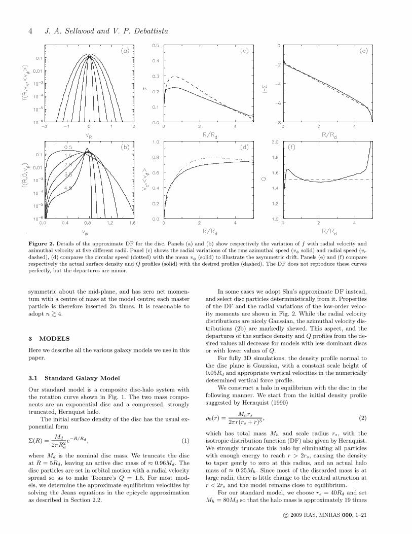
Figure 3. The frequency distribution of halo particle masses, inunits of the disc particle mass.
that of the disc. We then employ the halo compression algo-rithm described by Sellwood & McGaugh (2005) to computea new, mildly anisotropic, DF for the compressed halo thatresults from including the above disc. The rotation curve,Fig. 1, shows that the disc dominates the central attractionover most of the inner part and the total rotation curve isapproximately flat at large radii.
We adopt a system of units such that G = Md = ad =1, where G is Newton’s constant, Md is the mass of theuntruncated disc, and ad is the length scale for the type ofdisc adopted. Therefore distances are in units of ad, massesare in units of Md, one dynamical time τ = (a3
d/GMd)1/2,
and velocities are in units of v = (GMd/ad)1/2 ≡ ad/τ . One
possible scaling to physical units is to choose the dynamicaltime to be 10 Myr and ad = 3 kpc, which implies Md =5.98 × 10¹⁰ M⊙. The velocity unit v = 293 km s−1, and thepeak circular speed in Fig. 1 is approximately 235 km s−1.
We also present results for two other disc-halo modelsfor which we choose rs = 30Rd and rs = 50Rd, i.e. thatbracket our standard case. The more extended halo leads toa more dominant disc, while the disc is less dominant in themore concentrated halo.
We select halo particles from the compressed DF usingthe smooth procedure summarized in Section 2.1, with theweight function for particle masses being w(L) = 0.5+ 20L,where L = |LLL| is the total specific angular momentum. Alldisc particles have equal masses, but the masses of halo par-ticles range from 0.7 to 14.6 times the mass of the disc parti-cles. Fig. 3 shows the frequency distribution of halo particlemasses.
As a result of this careful procedure, both the disc andhalo components are very close to equilibrium in the com-bined potential and the initial ratio of kinetic to the virial ofClausius (measured from the particles) is T/|W | = 0.498. Atthe same time, the phases of the particles in their carefullyselected orbits are chosen at random, so that the model in-deed starts from the usual level of shot noise resulting fromthe random locations of the particles.
3.2 Isochrone Disc
We also present results using the isochrone disc with no halo.The potential (BT08, p. 65) has a simple form
Table 1. Numerical parameters for our standard runs
Cylindrical grid Spherical grid
Grid size (NR, Nφ, Nz)= (127, 192, 125) nr = 500
Angular compnts 0 6m 6 8 0 6 l 6 4Outer radius 6.076Rd 80Rd
z-spacing 0.01Rd
Softening rule cubic spline noneSoftening length ǫ = 0.05Rd
Number of particles 500 000 2 500 000Equal masses yes no (see Fig. 3)
Shortest time step 0.0125(R3
d/GM)1/2 0.0125(R3
d/GM)1/2
Time step zones 5 5
Φ(R) = −GMd
a
[
x+ (1 + x2)1/2]−1
, (3)
while the surface density is
Σ(R) =Mda
2πr3
log[
x+ (1 + x2)1/2]
−x
(1 + x2)1/2
. (4)
Here a is a length scale, and x = r/a; note Σ(0) =Md/(6πa
2). Kalnajs (1976) describes a convenient familyof DFs characterized by a parameter mK ; we refer to eachmodel as the isochrone/mK disc. He (Kalnajs 1978) alsopresents some preliminary results for the normal modes,which were confirmed in simulations (Earn & Sellwood1995). The local stability parameter (Toomre 1964) for theisochrone/5 disc has an near constant value of Q ≃ 1.6, andis Q ≃ 1.2 for the isochrone/8 model.
4 RESULTS
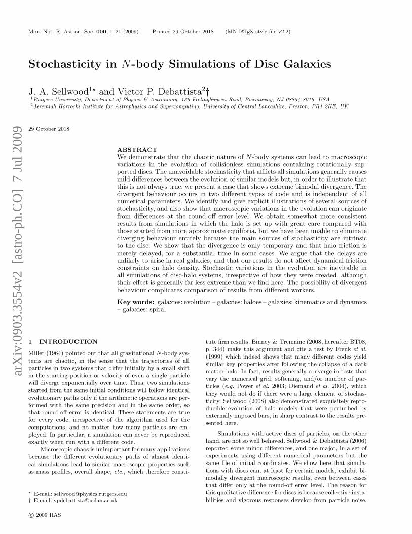
We begin by showing just how much variation can occur. Wefirst present the evolution of our standard disc/halo modelwhose rotation curve is shown in Fig. 1. Note that the discequilibrium in these models is set by solving the Jeans equa-tions, while the halo particles are selected deterministicallyfrom a DF. Fig. 4 shows results from 16 separate runs withSellwood’s (2003) hybrid grid code using fixed numerical pa-rameters, given in Table 1, but with different random seedsfor the initial coordinates of the disc particles only. We plotthe evolution of both the amplitude and pattern speed ofthe bar, measured as described in Appendix A. Even thoughthe initial particles are selected from the same distributions,with different random seeds for the disc only, the amplitudeevolution differs greatly from run to run and there is con-siderable spread in the evolution of the pattern speed.
In order to demonstrate immediately that the scatterin Fig. 4 is not a numerical artefact of our grid code, Fig. 5shows the results of a similar test with 5 runs using thetree code PKDGRAV (Stadel 2001) using an opening angleθ = 0.7. PKDGRAV is a multi-stepping code, with timesteps refined such that δt = ∆t/2n < η(ǫ/a)1/2, where ǫ isthe softening and a is the acceleration at a particle’s currentposition. We use base time step ∆t = 0.01 and η = 0.2,which gives identical time steps for all particles. The resultsshow a comparable spread in the evolution of both the am-plitude and pattern speeds. Results from the two codes withidentical initial coordinates for all the particles do not com-pare in detail. For this problem, the tree code runs about
c© 2009 RAS, MNRAS 000, 1–21
6 J. A. Sellwood and V. P. Debattista
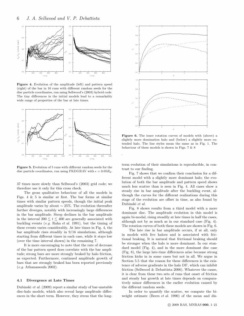
Figure 4. Evolution of the amplitude (left) and pattern speed(right) of the bar in 16 runs with different random seeds for thedisc particle coordinates, run using Sellwood’s (2003) hybrid code.
The tiny differences in the initial models lead to a remarkablywide range of properties of the bar at late times.
Figure 5. Evolution of 5 runs with different random seeds for thedisc particle coordinates, run using PKDGRAV with ǫ = 0.05Rd.
37 times more slowly than Sellwood’s (2003) grid code; wetherefore use it only for this cross check.
The gross qualitative behaviour of all the models inFigs. 4 & 5 is similar at first. The bar forms at similartimes with similar pattern speeds, though the initial peakamplitude varies by about ∼ 25%. The evolution thereafterfurther diverges, notably with increasingly large differencesin the bar amplitude. Steep declines in the bar amplitudein the interval 200 . t . 400 are generally associated withbuckling events (e.g. Raha et al. 1991), but the timing ofthese events varies considerably. At late times in Fig. 4, thebar amplitude rises steadily in 9/16 simulations, althoughstarting from different times in each case, while it stays low(over the time interval shown) in the remaining 7.
It is more encouraging to note that the rate of decreaseof the bar pattern speed does correlate with the bar ampli-tude; strong bars are more strongly braked by halo friction,as expected. Furthermore, continued amplitude growth ofbars that are strongly braked has been reported previously(e.g. Athanassoula 2002).
4.1 Divergence at Late Times
Dubinski et al. (2009) report a similar study of bar-unstabledisc-halo models, which also reveal large amplitude differ-ences in the short term. However, they stress that the long-
Figure 6. The inner rotation curves of models with (above) aslightly more domination halo and (below) a slightly more ex-tended halo. The line styles mean the same as in Fig. 1. Thebehaviour of these models is shown in Figs. 7 & 8
.
term evolution of their simulations is reproducible, in con-trast to our finding.
Fig. 7 shows that we confirm their conclusion for a dif-ferent model with a slightly more dominant halo; the evo-lution of both the bar amplitude and pattern speed showsmuch less scatter than is seen in Fig. 4. All cases show asteady rise in bar amplitude after the buckling event, al-though the curves for the different realizations during thisstage of the evolution are offset in time, as also found byDubinski et al.
Fig. 8 shows results from a third model with a moredominant disc. The amplitude evolution in this model isagain bi-modal, rising steadily at late times in half the cases,although not by as much as in our standard case (Fig. 4).The rotation curves of both these models are shown in Fig. 6.
The late rise in bar amplitude occurs, if at all, onlyin models with live haloes and is associated with fric-tional braking. It is natural that frictional braking shouldbe stronger when the halo is more dominant. In our stan-dard model (Fig. 4), and in the more dominant disc case(Fig. 8), the large late-time differences arise because strongfriction kicks in in some cases but not in all. We argue inSection 5.5 that the reason for these differences is the exis-tence of adverse gradients in the halo DF, which can inhibitfriction (Sellwood & Debattista 2006). Whatever the cause,it is clear from these two sets of runs that onset of frictionand steady bar growth at late times depends on compara-tively minor differences in the earlier evolution caused bythe different random seeds.
In order to quantify the scatter, we compute the bi-weight estimate (Beers et al. 1990) of the mean and dis-
c© 2009 RAS, MNRAS 000, 1–21
Stochasticity in N-body Discs 7
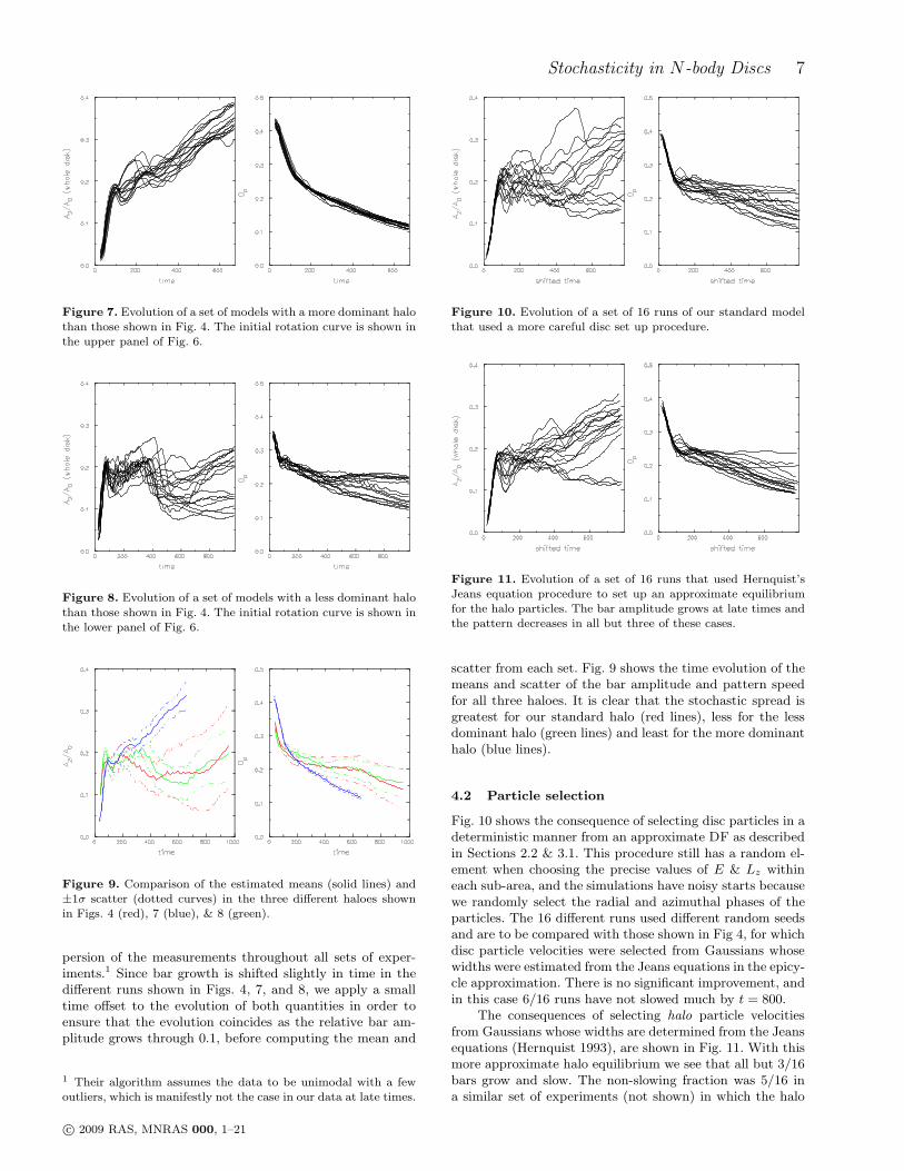
Figure 7. Evolution of a set of models with a more dominant halothan those shown in Fig. 4. The initial rotation curve is shown inthe upper panel of Fig. 6.
Figure 8. Evolution of a set of models with a less dominant halo
than those shown in Fig. 4. The initial rotation curve is shown inthe lower panel of Fig. 6.
Figure 9. Comparison of the estimated means (solid lines) and±1σ scatter (dotted curves) in the three different haloes shownin Figs. 4 (red), 7 (blue), & 8 (green).
persion of the measurements throughout all sets of exper-iments.1 Since bar growth is shifted slightly in time in thedifferent runs shown in Figs. 4, 7, and 8, we apply a smalltime offset to the evolution of both quantities in order toensure that the evolution coincides as the relative bar am-plitude grows through 0.1, before computing the mean and
1 Their algorithm assumes the data to be unimodal with a fewoutliers, which is manifestly not the case in our data at late times.
Figure 10. Evolution of a set of 16 runs of our standard modelthat used a more careful disc set up procedure.
Figure 11. Evolution of a set of 16 runs that used Hernquist’sJeans equation procedure to set up an approximate equilibriumfor the halo particles. The bar amplitude grows at late times andthe pattern decreases in all but three of these cases.
scatter from each set. Fig. 9 shows the time evolution of themeans and scatter of the bar amplitude and pattern speedfor all three haloes. It is clear that the stochastic spread isgreatest for our standard halo (red lines), less for the lessdominant halo (green lines) and least for the more dominanthalo (blue lines).
4.2 Particle selection
Fig. 10 shows the consequence of selecting disc particles in adeterministic manner from an approximate DF as describedin Sections 2.2 & 3.1. This procedure still has a random el-ement when choosing the precise values of E & Lz withineach sub-area, and the simulations have noisy starts becausewe randomly select the radial and azimuthal phases of theparticles. The 16 different runs used different random seedsand are to be compared with those shown in Fig 4, for whichdisc particle velocities were selected from Gaussians whosewidths were estimated from the Jeans equations in the epicy-cle approximation. There is no significant improvement, andin this case 6/16 runs have not slowed much by t = 800.
The consequences of selecting halo particle velocitiesfrom Gaussians whose widths are determined from the Jeansequations (Hernquist 1993), are shown in Fig. 11. With thismore approximate halo equilibrium we see that all but 3/16bars grow and slow. The non-slowing fraction was 5/16 ina similar set of experiments (not shown) in which the halo
c© 2009 RAS, MNRAS 000, 1–21
8 J. A. Sellwood and V. P. Debattista
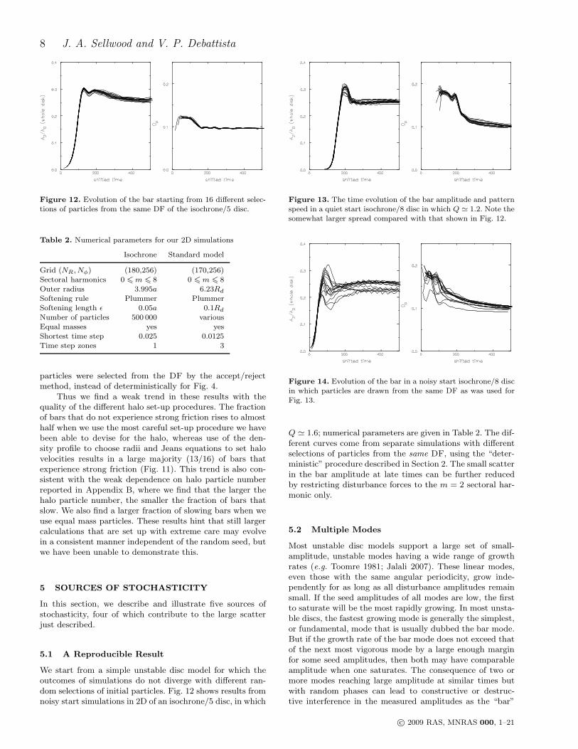
Figure 12. Evolution of the bar starting from 16 different selec-tions of particles from the same DF of the isochrone/5 disc.
Table 2. Numerical parameters for our 2D simulations
Isochrone Standard model
Grid (NR, Nφ) (180,256) (170,256)Sectoral harmonics 0 6m 6 8 0 6m 6 8Outer radius 3.995a 6.23Rd
Softening rule Plummer PlummerSoftening length ǫ 0.05a 0.1Rd
Number of particles 500 000 variousEqual masses yes yesShortest time step 0.025 0.0125Time step zones 1 3
particles were selected from the DF by the accept/rejectmethod, instead of deterministically for Fig. 4.
Thus we find a weak trend in these results with thequality of the different halo set-up procedures. The fractionof bars that do not experience strong friction rises to almosthalf when we use the most careful set-up procedure we havebeen able to devise for the halo, whereas use of the den-sity profile to choose radii and Jeans equations to set halovelocities results in a large majority (13/16) of bars thatexperience strong friction (Fig. 11). This trend is also con-sistent with the weak dependence on halo particle numberreported in Appendix B, where we find that the larger thehalo particle number, the smaller the fraction of bars thatslow. We also find a larger fraction of slowing bars when weuse equal mass particles. These results hint that still largercalculations that are set up with extreme care may evolvein a consistent manner independent of the random seed, butwe have been unable to demonstrate this.
5 SOURCES OF STOCHASTICITY
In this section, we describe and illustrate five sources ofstochasticity, four of which contribute to the large scatterjust described.
5.1 A Reproducible Result
We start from a simple unstable disc model for which theoutcomes of simulations do not diverge with different ran-dom selections of initial particles. Fig. 12 shows results fromnoisy start simulations in 2D of an isochrone/5 disc, in which
Figure 13. The time evolution of the bar amplitude and patternspeed in a quiet start isochrone/8 disc in which Q ≃ 1.2. Note thesomewhat larger spread compared with that shown in Fig. 12.
Figure 14. Evolution of the bar in a noisy start isochrone/8 discin which particles are drawn from the same DF as was used forFig. 13.
Q ≃ 1.6; numerical parameters are given in Table 2. The dif-ferent curves come from separate simulations with differentselections of particles from the same DF, using the “deter-ministic” procedure described in Section 2. The small scatterin the bar amplitude at late times can be further reducedby restricting disturbance forces to the m = 2 sectoral har-monic only.
5.2 Multiple Modes
Most unstable disc models support a large set of small-amplitude, unstable modes having a wide range of growthrates (e.g. Toomre 1981; Jalali 2007). These linear modes,even those with the same angular periodicity, grow inde-pendently for as long as all disturbance amplitudes remainsmall. If the seed amplitudes of all modes are low, the firstto saturate will be the most rapidly growing. In most unsta-ble discs, the fastest growing mode is generally the simplest,or fundamental, mode that is usually dubbed the bar mode.But if the growth rate of the bar mode does not exceed thatof the next most vigorous mode by a large enough marginfor some seed amplitudes, then both may have comparableamplitude when one saturates. The consequence of two ormore modes reaching large amplitude at similar times butwith random phases can lead to constructive or destruc-tive interference in the measured amplitudes as the “bar”
c© 2009 RAS, MNRAS 000, 1–21
Stochasticity in N-body Discs 9
saturates. Non-linear effects then cause such differences topersist.
We use the slightly cooler mK = 8 isochrone disc todemonstrate this behaviour explicitly and, to avoid addi-tional complications, we restrict disturbance forces to thosearising from the m = 2 sectoral harmonic only. Figs. 13 &14 illustrate the dependence of the outcome on the initialnoise amplitude. The quiet start simulations in Fig. 13 aregood enough that the growth rates of the two most rapidlygrowing m = 2 modes can be estimated by fitting to datafrom the extensive period of evolution before growth ends(e.g. Sellwood & Athanassoula 1986). We find the growthrate of the second mode to be some 85% of that of the barmode and that its amplitude (peak δΣ/Σ) can be within afactor of a few of the dominant mode as the bar saturates.The consequence is a slight increase in the scatter of thelater bar amplitudes in this case compared with the case forthe hotter disc shown in Fig. 12.
The mild scatter in Fig. 13 requires a quiet start, whichdecreases the seed amplitude of all non-axisymmetric dis-turbances that grow for ∼ 100 time units before the risingamplitudes even become discernible in the figure. The muchlarger seed amplitudes when noisy starts are used do notallow the dominant mode to outgrow all others before sat-uration, with the consequences illustrated in Fig. 14. Thesame sets of particles were used as for the results shown inFig. 13, but we placed the image particles at random az-imuths, instead of evenly. The period of rising amplitude istoo short to allow more than very rough measurments ofthe growing modes, but it is clear that multiple unstablemodes having comparable growth rates are seeded at largeinitial amplitudes by the shot noise. With such high seedamplitudes, there is not enough time for the most rapidlygrowing mode to outgrow the others, which therefore leadsto very substantial variations in the final bar amplitudes.Note that this did not happen in the warmer disc (Fig. 12),which also used a noisy start, since in that case all growthrates are lower, while the growth rate of the dominant barmode exceeds that of all others by a larger margin.
Notice also that not only is there greater scatter in boththe bar amplitude and pattern speed in Fig. 14, but bothquantities scatter to lower values. We find indications thatruns having lower pattern speed have the more dominantsecond mode. The fundamental bar mode, when it has timeto outgrow the second mode, peaks at a greater amplitudeand then relaxes back to lower value, as always happens inFig. 13. But when the second mode is competitive, the baramplitude generally has a lower initial peak, and may evenrise subsequently.
5.3 Swing-amplified noise
Our standard model is more complicated than the isolatedisochrone disc. In particular, the inner rotation curve (Fig. 1)rises steeply where the halo density cusp dominates. Recallthat a mode is a standing wave oscillation of the system,which can be neutral, growing, or decaying. The dominantlinear global modes, known as cavity modes, in bar unstablediscs are standing waves between the centre and corotationthat must have a high enough pattern speed to avoid any in-ner Lindblad resonances (Toomre 1981; Binney & Tremaine2008, pp. 508-518). The consequence of a steeply rising rota-
tion curve is to make the maximum of the function Ω− κ/2rise to high values near the centre, requiring any linearbisymmetric modes to have very high pattern speeds, smallcorotation radii, and to have very low growth rates (becausethe inner disc is not all that responsive).
The outer disc, on the other hand, is highly responsivebut has no cavity-type modes. We see evidence for weakedge-type modes, which arise from a steep density gradient(Toomre 1981) at the sharply truncated outer edge, but theyare sufficiently far out and of low enough frequency to bedecoupled from the bar forming process in the inner disc.
Shot noise from the particles is vigorously amplified,but transient swing-amplified responses should be dampedat the inner Lindblad resonance (ILR) of the disturbance(Toomre 1981; Binney & Tremaine 2008, p. 510), as long asthe amplitude remains tiny. Large amplitude waves are notdamped, however, and trap disc particles near the ILR intoa bar-like feature (Sellwood 1989).
Bar formation through amplified noise inevitably leadsto a range of bar properties, but it is fortunate that therange turns out to be surprisingly narrow. To illustrate this,we study bar formation in our standard model in simplifiedsimulations in which the motions of disc particles are con-fined to a plane, and the halo particles are replaced by a rigidmass component that simply provides the extra central at-traction to yield the same rotation curve as shown in Fig. 1.This approach has several advantages: the calculations areless expensive in computer time, but more importantly thedynamics is simpler because both bar buckling and halo fric-tion are eliminated, enabling us to isolate the bar formationprocess from these other complicating aspects of the overallevolution.
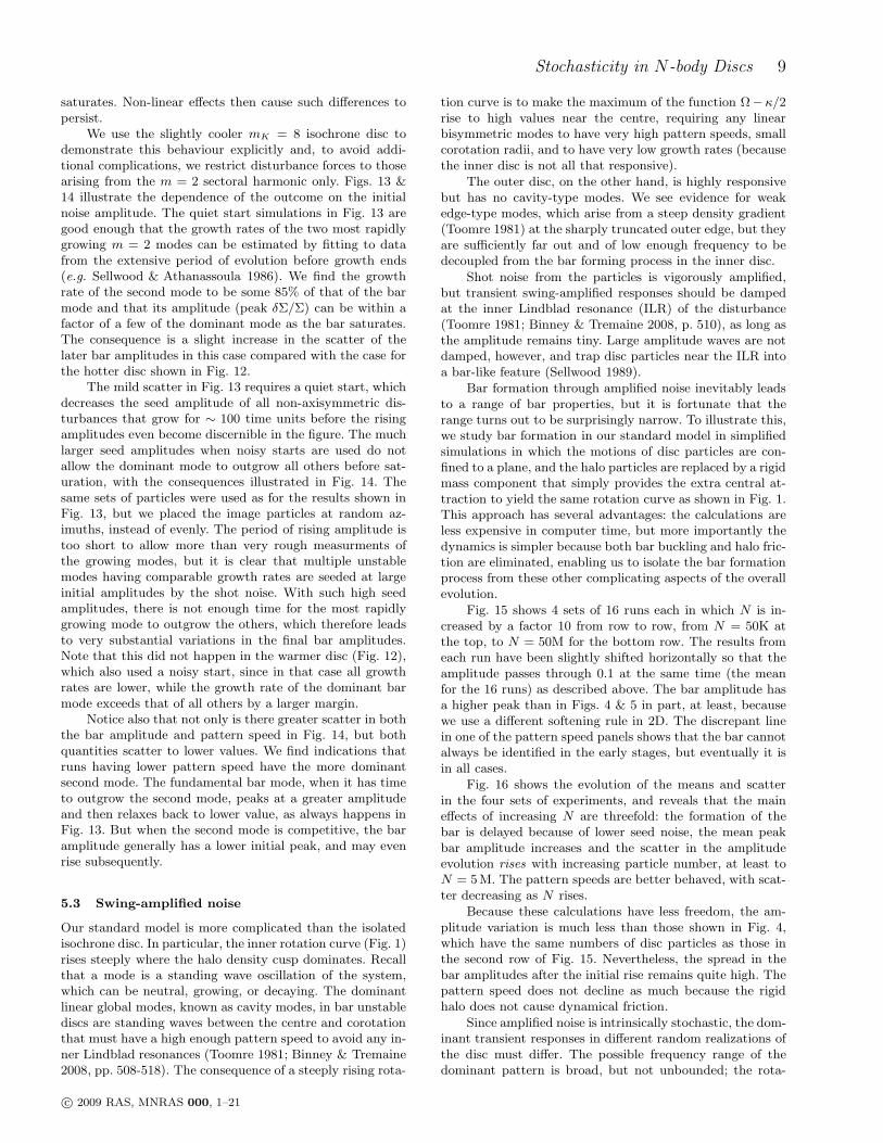
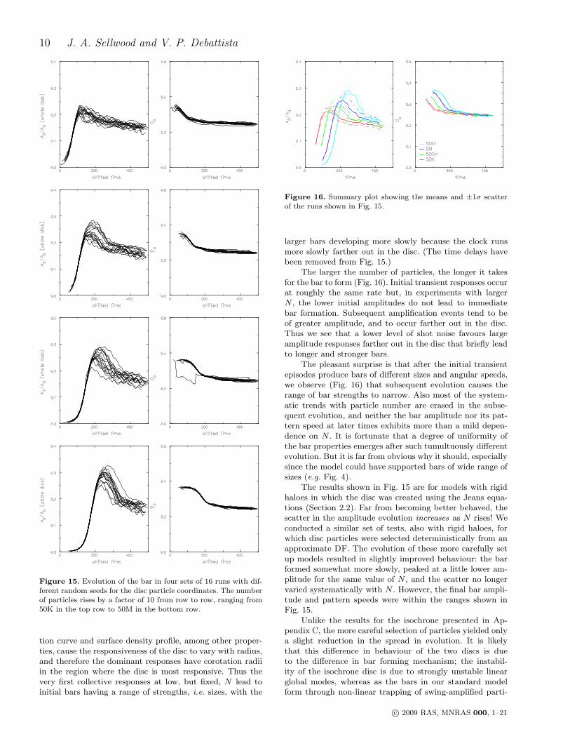
Fig. 15 shows 4 sets of 16 runs each in which N is in-creased by a factor 10 from row to row, from N = 50K atthe top, to N = 50M for the bottom row. The results fromeach run have been slightly shifted horizontally so that theamplitude passes through 0.1 at the same time (the meanfor the 16 runs) as described above. The bar amplitude hasa higher peak than in Figs. 4 & 5 in part, at least, becausewe use a different softening rule in 2D. The discrepant linein one of the pattern speed panels shows that the bar cannotalways be identified in the early stages, but eventually it isin all cases.
Fig. 16 shows the evolution of the means and scatterin the four sets of experiments, and reveals that the maineffects of increasing N are threefold: the formation of thebar is delayed because of lower seed noise, the mean peakbar amplitude increases and the scatter in the amplitudeevolution rises with increasing particle number, at least toN = 5M. The pattern speeds are better behaved, with scat-ter decreasing as N rises.
Because these calculations have less freedom, the am-plitude variation is much less than those shown in Fig. 4,which have the same numbers of disc particles as those inthe second row of Fig. 15. Nevertheless, the spread in thebar amplitudes after the initial rise remains quite high. Thepattern speed does not decline as much because the rigidhalo does not cause dynamical friction.
Since amplified noise is intrinsically stochastic, the dom-inant transient responses in different random realizations ofthe disc must differ. The possible frequency range of thedominant pattern is broad, but not unbounded; the rota-
c© 2009 RAS, MNRAS 000, 1–21
10 J. A. Sellwood and V. P. Debattista
Figure 15. Evolution of the bar in four sets of 16 runs with dif-ferent random seeds for the disc particle coordinates. The numberof particles rises by a factor of 10 from row to row, ranging from50K in the top row to 50M in the bottom row.
tion curve and surface density profile, among other proper-ties, cause the responsiveness of the disc to vary with radius,and therefore the dominant responses have corotation radiiin the region where the disc is most responsive. Thus thevery first collective responses at low, but fixed, N lead toinitial bars having a range of strengths, i.e. sizes, with the
Figure 16. Summary plot showing the means and ±1σ scatterof the runs shown in Fig. 15.
larger bars developing more slowly because the clock runsmore slowly farther out in the disc. (The time delays havebeen removed from Fig. 15.)
The larger the number of particles, the longer it takesfor the bar to form (Fig. 16). Initial transient responses occurat roughly the same rate but, in experiments with largerN , the lower initial amplitudes do not lead to immediatebar formation. Subsequent amplification events tend to beof greater amplitude, and to occur farther out in the disc.Thus we see that a lower level of shot noise favours largeamplitude responses farther out in the disc that briefly leadto longer and stronger bars.
The pleasant surprise is that after the initial transientepisodes produce bars of different sizes and angular speeds,we observe (Fig. 16) that subsequent evolution causes therange of bar strengths to narrow. Also most of the system-atic trends with particle number are erased in the subse-quent evolution, and neither the bar amplitude nor its pat-tern speed at later times exhibits more than a mild depen-dence on N . It is fortunate that a degree of uniformity ofthe bar properties emerges after such tumultuously differentevolution. But it is far from obvious why it should, especiallysince the model could have supported bars of wide range ofsizes (e.g. Fig. 4).
The results shown in Fig. 15 are for models with rigidhaloes in which the disc was created using the Jeans equa-tions (Section 2.2). Far from becoming better behaved, thescatter in the amplitude evolution increases as N rises! Weconducted a similar set of tests, also with rigid haloes, forwhich disc particles were selected deterministically from anapproximate DF. The evolution of these more carefully setup models resulted in slightly improved behaviour: the barformed somewhat more slowly, peaked at a little lower am-plitude for the same value of N , and the scatter no longervaried systematically with N . However, the final bar ampli-tude and pattern speeds were within the ranges shown inFig. 15.
Unlike the results for the isochrone presented in Ap-pendix C, the more careful selection of particles yielded onlya slight reduction in the spread in evolution. It is likelythat this difference in behaviour of the two discs is dueto the difference in bar forming mechanism; the instabil-ity of the isochrone disc is due to strongly unstable linearglobal modes, whereas as the bars in our standard modelform through non-linear trapping of swing-amplified parti-
c© 2009 RAS, MNRAS 000, 1–21
Stochasticity in N-body Discs 11
Figure 17. Comparison of the time evolution of two runs thatdiffer only in the imposition of reflection symmetry about themidplane. The solid curves are for a model taken from Fig. 4in which vertical forces are unrestricted while the dashed curvesshow the evolution of the same initial model when vertical forcesfrom the disc are constrained to be symmetric about the mid-plane.
cle noise that would be less affected by the quality of theequilibrium.
Thus far we have discussed only bisymmetric instabili-ties, but other low-order instabilities may also be competi-tive. In fact, we find some evidence for lop-sidedness, whichwe describe in the next subsection.
5.4 Bending modes
The bars in most 3D simulations suffer from buckling in-stabilities that, when they saturate, thicken the bar in thevertical direction (e.g. Combes & Sanders 1981; Raha et al.
1991). In many, but not all, cases the evolution of this bend-ing mode is quite violent and weakens the bar significantly,while the central density of the bar rises, as reported byRaha et al. The radial rearrangement of mass evidently lib-erates the energy needed to puff up the bar in the verticaldirection.
The time of saturation of the buckling mode dependson a variety of factors, such as the formation time of thebar, and the initial seed amplitude of the bending mode,the strength of the bar, etc. Several of these factors will inturn depend on the already stochastic formation of the bar.It is hardly surprising therefore, that this event occurs overa wide range of times and with a wide range of severity(Fig. 4), thereby compounding the overall level of stochas-ticity.
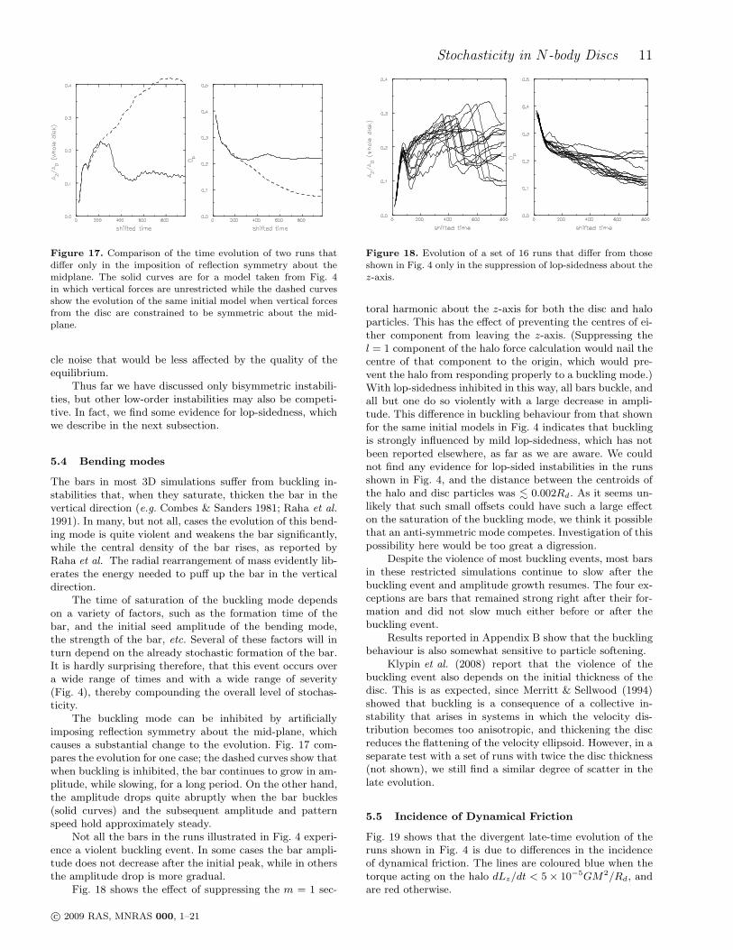
The buckling mode can be inhibited by artificiallyimposing reflection symmetry about the mid-plane, whichcauses a substantial change to the evolution. Fig. 17 com-pares the evolution for one case; the dashed curves show thatwhen buckling is inhibited, the bar continues to grow in am-plitude, while slowing, for a long period. On the other hand,the amplitude drops quite abruptly when the bar buckles(solid curves) and the subsequent amplitude and patternspeed hold approximately steady.
Not all the bars in the runs illustrated in Fig. 4 experi-ence a violent buckling event. In some cases the bar ampli-tude does not decrease after the initial peak, while in othersthe amplitude drop is more gradual.
Fig. 18 shows the effect of suppressing the m = 1 sec-
Figure 18. Evolution of a set of 16 runs that differ from thoseshown in Fig. 4 only in the suppression of lop-sidedness about thez-axis.
toral harmonic about the z-axis for both the disc and haloparticles. This has the effect of preventing the centres of ei-ther component from leaving the z-axis. (Suppressing thel = 1 component of the halo force calculation would nail thecentre of that component to the origin, which would pre-vent the halo from responding properly to a buckling mode.)With lop-sidedness inhibited in this way, all bars buckle, andall but one do so violently with a large decrease in ampli-tude. This difference in buckling behaviour from that shownfor the same initial models in Fig. 4 indicates that bucklingis strongly influenced by mild lop-sidedness, which has notbeen reported elsewhere, as far as we are aware. We couldnot find any evidence for lop-sided instabilities in the runsshown in Fig. 4, and the distance between the centroids ofthe halo and disc particles was . 0.002Rd. As it seems un-likely that such small offsets could have such a large effecton the saturation of the buckling mode, we think it possiblethat an anti-symmetric mode competes. Investigation of thispossibility here would be too great a digression.
Despite the violence of most buckling events, most barsin these restricted simulations continue to slow after thebuckling event and amplitude growth resumes. The four ex-ceptions are bars that remained strong right after their for-mation and did not slow much either before or after thebuckling event.
Results reported in Appendix B show that the bucklingbehaviour is also somewhat sensitive to particle softening.
Klypin et al. (2008) report that the violence of thebuckling event also depends on the initial thickness of thedisc. This is as expected, since Merritt & Sellwood (1994)showed that buckling is a consequence of a collective in-stability that arises in systems in which the velocity dis-tribution becomes too anisotropic, and thickening the discreduces the flattening of the velocity ellipsoid. However, in aseparate test with a set of runs with twice the disc thickness(not shown), we still find a similar degree of scatter in thelate evolution.
5.5 Incidence of Dynamical Friction
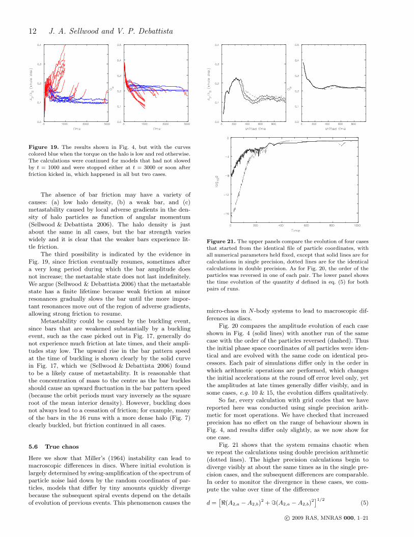
Fig. 19 shows that the divergent late-time evolution of theruns shown in Fig. 4 is due to differences in the incidenceof dynamical friction. The lines are coloured blue when thetorque acting on the halo dLz/dt < 5× 10⁻⁵GM2/Rd, andare red otherwise.
c© 2009 RAS, MNRAS 000, 1–21
12 J. A. Sellwood and V. P. Debattista
Figure 19. The results shown in Fig. 4, but with the curvescolored blue when the torque on the halo is low and red otherwise.The calculations were continued for models that had not slowedby t = 1000 and were stopped either at t = 3000 or soon afterfriction kicked in, which happened in all but two cases.
The absence of bar friction may have a variety ofcauses: (a) low halo density, (b) a weak bar, and (c)metastability caused by local adverse gradients in the den-sity of halo particles as function of angular momentum(Sellwood & Debattista 2006). The halo density is justabout the same in all cases, but the bar strength varieswidely and it is clear that the weaker bars experience lit-tle friction.
The third possibility is indicated by the evidence inFig. 19, since friction eventually resumes, sometimes aftera very long period during which the bar amplitude doesnot increase; the metastable state does not last indefinitely.We argue (Sellwood & Debattista 2006) that the metastablestate has a finite lifetime because weak friction at minorresonances gradually slows the bar until the more impor-tant resonances move out of the region of adverse gradients,allowing strong friction to resume.
Metastability could be caused by the buckling event,since bars that are weakened substantially by a bucklingevent, such as the case picked out in Fig. 17, generally donot experience much friction at late times, and their ampli-tudes stay low. The upward rise in the bar pattern speedat the time of buckling is shown clearly by the solid curvein Fig. 17, which we (Sellwood & Debattista 2006) foundto be a likely cause of metastability. It is reasonable thatthe concentration of mass to the centre as the bar bucklesshould cause an upward fluctuation in the bar pattern speed(because the orbit periods must vary inversely as the squareroot of the mean interior density). However, buckling doesnot always lead to a cessation of friction; for example, manyof the bars in the 16 runs with a more dense halo (Fig. 7)clearly buckled, but friction continued in all cases.
5.6 True chaos
Here we show that Miller’s (1964) instability can lead tomacroscopic differences in discs. Where initial evolution islargely determined by swing-amplification of the spectrum ofparticle noise laid down by the random coordinates of par-ticles, models that differ by tiny amounts quickly divergebecause the subsequent spiral events depend on the detailsof evolution of previous events. This phenomenon causes the
Figure 21. The upper panels compare the evolution of four casesthat started from the identical file of particle coordinates, withall numerical parameters held fixed, except that solid lines are forcalculations in single precision, dotted lines are for the identicalcalculations in double precision. As for Fig. 20, the order of theparticles was reversed in one of each pair. The lower panel showsthe time evolution of the quantity d defined in eq. (5) for bothpairs of runs.
micro-chaos in N-body systems to lead to macroscopic dif-ferences in discs.
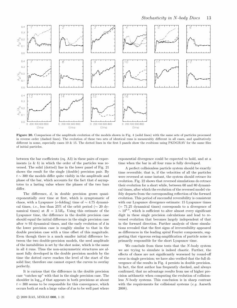
Fig. 20 compares the amplitude evolution of each caseshown in Fig. 4 (solid lines) with another run of the samecase with the order of the particles reversed (dashed). Thusthe initial phase space coordinates of all particles were iden-tical and are evolved with the same code on identical pro-cessors. Each pair of simulations differ only in the order inwhich arithmetic operations are performed, which changesthe initial accelerations at the round off error level only, yetthe amplitudes at late times generally differ visibly, and insome cases, e.g. 10 & 15, the evolution differs qualitatively.
So far, every calculation with grid codes that we havereported here was conducted using single precision arith-metic for most operations. We have checked that increasedprecision has no effect on the range of behaviour shown inFig. 4, and results differ only slightly, as we now show forone case.
Fig. 21 shows that the system remains chaotic whenwe repeat the calculations using double precision arithmetic(dotted lines). The higher precision calculations begin todiverge visibly at about the same times as in the single pre-cision cases, and the subsequent differences are comparable.In order to monitor the divergence in these cases, we com-pute the value over time of the difference
d =[
ℜ(A2,a −A2,b)2 + ℑ(A2,a − A2,b)
2]1/2
(5)
c© 2009 RAS, MNRAS 000, 1–21
Stochasticity in N-body Discs 13
Figure 20. Comparison of the amplitude evolution of the models shown in Fig. 4 (solid lines) with the same sets of particles processedin reverse order (dashed lines). The evolution of these two sets of identical runs is measurably different in all cases, and qualitativelydifferent in some, especially cases 10 & 15. The dotted lines in the first 5 panels show the evoltions using PKDGRAV for the same filesof initial particles.
between the bar coefficients (eq. A3) in these pairs of exper-iments (a & b) in which the order of the particles was re-versed. The solid (dotted) line in the lower panel of Fig. 21shows the result for the single (double) precision pair. Byt ∼ 300 the models differ quite visibly in the amplitude andphase of the bar, which accounts for the fact that d asymp-totes to a lasting value where the phases of the two barsdiffer.
The difference, d, in double precision grows quasi-exponentially over time at first, which is symptomatic ofchaos, with a Lyapunov (e-folding) time of ∼ 4.75 dynami-cal times, i.e., less than 25% of the orbit period (∼ 20 dy-namical times) at R = 2.5Rd. Using this estimate of theLyapunov time, the difference in the double precision caseshould equal the initial difference in the single precision caseafter ≈ 93 dynamical times, and the early evolution of d inthe lower precision case is roughly similar to that in thedouble precision case with a time offset of this magnitude.Even though there is a much smaller initial difference be-tween the two double-precision models, the seed amplitudeof the instabilities is set by the shot noise, which is the samein all 4 runs. Thus the non-axisymmetric structures are al-most fully developed in the double precision models by thetime the dotted curve reaches the level of the start of thesolid line; therefore one cannot expect the curves to overlayperfectly.
It is curious that the difference in the double precisioncase “catches up” with that in the single precision case. Theshoulder in log
10d that appears in both precisions at about
t = 300 seems to be responsible for this convergence, whichoccurs both at such a large value of d as to be well past where
exponential divergence could be expected to hold, and at atime when the bar in all four runs is fully developed.
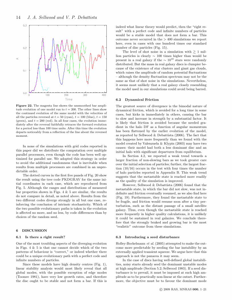
A perfect collisionless particle system should be exactlytime reversible; that is, if the velocities of all the particleswere reversed at some instant, the system should retrace itsevolution. Fig. 22 shows that reversed simulations do retracetheir evolution for a short while, between 60 and 80 dynami-cal times, after which the evolution of the reversed model vis-ibly departs from the corresponding reflection of the forwardevolution. This period of successful reversibility is consistentwith our Lyapunov divergence estimate: 15 Lyapunov times(= 71.25 dynamical times) corresponds to a divergence of∼ 106.5, which is sufficient to alter almost every significantdigit in these single precision calculations and lead to re-versed evolution that becomes largely independent of thatin the forward direction. Further analysis of these simula-tions revealed that the first signs of irreversibility appearedas differences in the leading spiral Fourier components, sug-gesting that vigorous swing-amplification of particle noise isprimarily responsible for the short Lyapunov time.
We conclude from these tests that the N-body systemwe are trying to simulate is indeed chaotic. Further, theeffects of chaos are not significantly worsened by round-offerror in single precision; we have also verified that the full di-vergence of the results in Fig. 4 persists in double precision.In fact, the first author has frequently checked, and alwaysconfirmed, that no advantage results from use of higher pre-cision arithmetic when computing the evolution of collision-less N-body systems. This conclusion is in sharp contrastwith the requirements for collisional systems (e.g. Aarseth2008).
c© 2009 RAS, MNRAS 000, 1–21
14 J. A. Sellwood and V. P. Debattista
Figure 22. The magenta line shows the unsmoothed bar ampli-tude evolution of one model run to t = 200. The other lines showthe continued evolution of the same model with the velocities ofall the particles reversed at t = 50 (cyan), t = 100 (blue), t = 150(green), and t = 200 (red). In all four cases, the evolution imme-diately after the reversal faithfully retraces the forward evolutionfor a period less than 100 time units. After this time the evolutiondeparts noticeably from a reflection of the line about the reversedmoment.
In none of the simulations with grid codes reported inthis paper did we distribute the computation over multipleparallel processors, even though the code has been well op-timized for parallel use. We adopted this strategy in orderto avoid the additional randomness that is inevitable whenresults from multiple processors are combined in an unpre-dictable order.
The dotted curves in the first five panels of Fig. 20 showthe result using the tree code PKDGRAV for the same ini-tial coordinates in each case, which are reproduced fromFig. 5. Although the ranges and distributions of measuredbar properties shown in Figs. 4 & 5 are similar, the resultsdo not compare in detail, as noted above. Results from thetwo different codes diverge strongly in all but one case, re-inforcing the conclusion of intrinsic stochasticity. Which ofthe two possible evolutionary paths is taken in the evolutionis affected no more, and no less, by code differences than bychoices of the random seed.
6 DISCUSSION
6.1 Is there a right result?
One of the most troubling aspects of the diverging evolutionin Figs. 4 & 5 is that one cannot decide which of the twopatterns of behaviour is “correct,” or indeed whether therecould be a unique evolutionary path with a perfect code andinfinite numbers of particles.
Since these models have high density centres (Fig. 1),linear stability analysis would most likely reveal that allglobal modes, with the possible exception of edge modes(Toomre 1981), have very low growth rates, and thereforethe disc ought to be stable and not form a bar. If this is
indeed what linear theory would predict, then the “right re-sult” with a perfect code and infinite numbers of particleswould be a stable model that does not form a bar. Thisoutcome never occurred in the > 400 simulations we reporthere, even in cases with one hundred times our standardnumber of disc particles (Fig. 15).
The level of shot noise in a simulation with & 1 mil-lion particles is clearly ∼ 100 times higher than would bepresent in a real galaxy if the ∼ 1010 stars were randomlydistributed. But the mass in real galaxy discs is clumpier be-cause of the existence of star clusters and giant gas clouds,which raises the amplitude of random potential fluctuations– although the density fluctuation spectrum may not be thesame as that of shot noise in the simulations. Nevertheless,it seems most unlikely that a real galaxy closely resemblingthe model used in our simulations could avoid being barred.
6.2 Dynamical Friction
The greatest source of divergence is the bimodal nature ofdynamical friction, which is avoided for a long time in somecases, but kicks in immediately in others, causing the barto slow and increase in strength by a substantial factor. Itis likely that friction is avoided because the needed gra-dient in the halo DF as a function of angular momentumhas been flattened by the earlier evolution of the model,as reported by Sellwood & Debattista (2006). The fact thatthis happens here more frequently than we found with themodel created by Valenzuela & Klypin (2003) may have twocauses: their model had both a less dominant disc and aninitial halo with significant departures from equilibrium.
In Section 4.2, we reported a weak trend towards alarger fraction of non-slowing bars as we took greater careover the initial selection of particles; further, the largest frac-tion (10/16) occurs in the test with four times the numberof halo particles reported in Appendix B. This weak trendsuggests that the metastable state is reached more readilyas the quality of the simulation is improved.
However, Sellwood & Debattista (2006) found that themetastable state, in which the bar did not slow, was not in-definite and friction eventually resumed, as we also find here(Fig. 19). Furthermore, they found the metastable state tobe fragile, and friction would resume soon after a tiny per-turbation, such as the distant passage of a small satellitegalaxy. Thus, even though the metastable state is reachedmore frequently in higher quality calculations, it is unlikelyit could be sustained in real galaxies. We conclude there-fore that the strongly braked and growing bar is the most“realistic” outcome from these simulations.
6.3 Introducing a seed disturbance
Holley-Bockelmann et al. (2005) attempted to make the out-come more predictable by seeding the bar instability by anexternally applied transient squeeze. We argue here that thisapproach is not the panacea it may seem.
In the case of discs having well-defined global instabili-ties, noisy starts already seed the dominant unstable modesat high amplitude (Section 5.2; Sellwood 1983). If a seed dis-turbance is to prevail, it must be imposed at such high am-plitude as to be practically non-linear at the outset. Further-more, the objective must be to favour the dominant mode
c© 2009 RAS, MNRAS 000, 1–21
Stochasticity in N-body Discs 15
over the others, which cannot be achieved by a simple per-turbation. Instead, one must impose both the detailed radialshape and perturbed velocities of the mode, which are gen-erally not known. A more generic disturbance, such as a“squeeze” will simply raise the amplitude of all the modesand transients, giving less time for the dominant mode tooutgrow the others. Quiet starts (Section 2.3; Sellwood 1983;Sellwood & Athanassoula 1986), however, have the effect ofreducing the initial amplitudes of all non-axisymmetric dis-turbances to such an extent that there is ample time for themost rapidly growing mode to prevail. Thus the outcome ofa quiet start experiment is tolerably reproducible withoutthe need to apply an additional seed (Fig. 13).
The situation is far more difficult in the case, as in thepresent study, where the disc has no prevailing global insta-bilities, since the evolution of a simulation is dominated byswing-amplified shot noise. Quiet starts are all but useless inthese circumstances also, since they break up rapidly as thetiny seed noise is swing amplified, with similar outcomes,only slightly delayed, to those from noisy starts. Crankingup the particle number does not reduce variations in the baramplitude at later times (they actually increased in Fig. 15),but does delay bar formation. Because of this, perhaps asuitable seed disturbance in a very large N disc may prevailover the amplified shot noise and lead to a more reproducibleoutcome. We have not explored this idea here and leave itfor a future study.
7 CONCLUSIONS
We have shown that simulations over a fixed evolutionaryperiod of a simple disc-halo galaxy model can vary widelybetween cases that differ only in the random seed used togenerate the particles, even though they are drawn fromidentical distributions. Fig. 4 shows that the late-time am-plitude of the bar can differ by a factor of three or more whilethe stronger bars may have half the pattern speed of theweaker ones. Fig. 19 shows that the largest differences areonly temporary, however. We have deliberately focused ourstudy on a case which displays this extreme bad behaviour.Stochastic variations are inevitable, but evolution is gener-ally less divergent; e.g., when the halo has both higher andlower density (e.g. Fig. 9).
We have shown that the divergent outcomes do not re-sult from a numerical artefact, since they are independent ofnumerical parameters (Appendix B). Also, similar behaviouroccurs with a code of a totally different type (PKDGRAV,see Fig. 5). Instead, this extreme stochasticity results froma number of physical causes that we have identified and il-lustrated. The most important for our model are: swing-amplified particle noise, the variations in the incidence andseverity of buckling, and the incidence of dynamical friction.We have separately shown (Fig. 14) that other disc modelshaving a well-defined spectrum of global modes can have arange of outcomes because of the coexistence of competinginstabilities.
The calculations in Fig. 4 are of models that were setup with considerable care so as to be as close as possibleto equilibrium. An additional level of unpredictability canresult from less careful set-up procedures, as illustrated inAppendix C.
We have been aware for many years that simulationsincluding disc components can be reproduced exactly onlyif the arithmetic operations are performed in the same orderto the same precision, and that differences at the round-offerror level can lead to visibly different evolution. However,we have been surprised by the strongly divergent behaviourof the particular model studied here. The pairs of divergentresults in Fig. 20 are the stellar dynamical equivalents of thepossible macroscopic atmospheric consequences of Lorenz’sbutterfly flapping its wings. Because the system is chaotic,improved precision arithmetic is of no help in reducing thescatter in the outcomes.
The divergence in different realizations of our standardcase arises from a temporary delay in the incidence of dy-namical friction, which is determined by minor details ofthe early evolution. Strong friction causes the bar to bothslow and grow; in some cases this occurs right after barformation, but in others the bar rotates steadily at an al-most constant amplitude for a protracted period. Frictionis avoided when the earlier evolution causes an inflexion inthe angular momentum density gradient of the halo. We(Sellwood & Debattista 2006) previously described this asa metastable state because it did not last indefinitely evenwhen the evolution was unperturbed, and we also showedthat mild perturbations could cause friction to resume. Wefind that the fraction of initially non-slowing bars increasesas greater care is taken over the initial set up because thesmaller fluctuations in such models are less likely to nudgethe model out of the metastable state.
We argue in Section 6 that the most realistic outcomeof these experiments is the slowing and growing bar, despitethe fact that we find the delayed friction result increasinglyoften as we improve the quality of the initial set-up andof the simulation. Since most real galaxies are likely to besubjected to frequent mild perturbations, we conclude thatslowing and growing bars are in fact the more realistic out-come.
Since the possible evolution of the simulation is notunique, multiple experiments of essentially the same modelare needed in order to demonstrate that the behaviour isrobust. Furthermore, the failure of an experiment by onegroup to reproduce the results of a similar experiment byanother may not be the result of errors or artefacts in ei-ther or both codes, but rather a reflection of a fundamentalstochasticity of the system under study.
Klypin et al. (2008) report a similar, but less extensive,comparison between two tree codes and an adaptive meshmethod, and conclude that all the codes produce “nearlythe same” results in simulations performed with sufficientnumerical care. However, inspection of the comparativelyshort evolution shown in their Fig. 8 reveals slowly diverg-ing outcomes, even between two simulations run with treecodes. They also report (their Fig. 1) a strongly divergentresult when the time step was varied; the sharp decrease inbar strength in this one case was clearly a consequence of amore violent buckling event than in their comparison cases.Such a difference could have easily arisen from stochasticvariations of the kind discussed here, and the conclusionthat the shorter time step is required no longer follows. Weshow here (Appendix B), as do Dubinski et al. (2009), thatresults are robust to wide variations in time step. Clearlywhen stochasticity can lead to sharply divergent results, pa-
c© 2009 RAS, MNRAS 000, 1–21
16 J. A. Sellwood and V. P. Debattista
rameter tests that throw up surprises are conclusive onlyafter ensembles of particle realizations have been simulated.This must also be a requirement for meaningful comparisonsbetween codes or workers.
Since the principal sources of stochasticity are con-nected to disc dynamics, they are unrelated to the halo par-ticle number question raised by Weinberg & Katz (2007).Not only has Sellwood (2008) already shown that frictioncan be captured adequately with moderate particle num-bers, but we have found here that the expected bar frictionarises more readily in haloes with fewer or equal mass haloparticles, or in haloes that are not set up with great care –which is not the expected behaviour were particle scatteringdominant. Instead, small departures from equilibrium canupset the delicate metastable state in which bars can rotatewithout friction (Sellwood & Debattista 2006).
It should be noted that bars that slow through dy-namical friction also grow in length, as reported earlier byAthanassoula (2002). Nevertheless, for these models the ra-tio of corotation radius to bar semi-axis R > 1.4, as expectedfor a moderate-density halo (Debattista & Sellwood 2000).Those bars that avoid friction for a long period, however,have R < 1.4, as also found by Valenzuela & Klypin (2003),but this metastable state is fragile and unlikely to arise inreal galaxies (Sellwood & Debattista 2006).
Since all N-body simulations are intrinsically chaotic,they can be reproduced exactly only if the same arithmeticoperations are performed in the same order with the sameprecision, as noted in the introduction, and borne out inFig. 20. These requirements dictate the use of the samecode, compiler, operating system, and hardware. Further,if the calculation is stopped and then resumed, it is impor-tant to save sufficient information so that the accelerationused to advance each particle at the next step is identi-cal, to machine precision, to that it would have been hadthe calculation not been interrupted. This can be arrangedwithout too much difficulty, if the calculation is run on asingle processor. However, simulations that distribute workover parallel processors in computer clusters would be ex-actly reproducible only if care is taken to ensure that thework is distributed and the results are combined in a fullypredictable manner.
Provided the divergence is slight, exact reproducibilityis of little scientific interest, although such a capability isuseful to the practitioner. But when, as described here, themodel under test can have strongly divergent behaviour thatarises from differences that begin at the round off level withthe same code on the same machine, comparison of resultsbetween different codes and on different platforms becomesmuch less likely to produce agreement, even when the simu-lations share the same file of initial coordinates. It is ironicthat the model used here was in fact that selected as a testcase for code comparison; fortunately, the authors discov-ered its unsuitability in time!
ACKNOWLEDGMENTS
We thank Scott Tremaine, Tom Quinn, and the referee, Mar-tin Weinberg, for helpful comments on the manuscript andJuntai Shen for discussions. This work was supported bygrants to JAS from the NSF (AST-0507323) and from NASA
(NNG05GC29G) and by a Livesey Grant from the Univer-sity of Central Lancashire to VPD. The PKDGRAV simula-tions were performed at the Arctic Region SupercomputingCenter (ARSC).
REFERENCES
Aarseth, S. J. 2008, in “The Cambridge N-Body Lectures”,Lecture Notes in Physics, 760 (Springer-Verlag: BerlinHeidelberg), p. 1
Arfken, G. 1985, Mathematical Methods for Physicists, 3rded. (Orlando: Academic Press)
Athanassoula, E. 2002, ApJL, 569, L83Athanassoula, E. 2003, MNRAS, 341, 1179Beers, T. C., Flynn, K. & Gebhardt, K. 1990, AJ, 100, 32Binney, J. & Tremaine, S. 2008, Galactic Dynamics 2ndedition (Princeton: Princeton University Press) (BT08)
Camm, G. L, 1950, MNRAS, 110, 305Combes, F. & Sanders, R. H. 1981, A&A, 96, 164Debattista, V. P. & Sellwood, J. A. 2000, ApJ, 543, 704Dehnen, W. 2001, MNRAS, 324, 273Diemand, J., Moore, B., Stadel, J. 2004, MNRAS, 353, 624Dubinski, J., Berentzen, I. & Shlosman, I. 2009, ApJ, 697,293
Earn, D. J. D. & Sellwood, J. A. 1995, ApJ, 451, 533El-Zant, A., Hoffman, Y., Primack, J., Combes, F. & Shlos-man, I. 2004, ApJL, 607, L75
Erickson, S. A. 1975, PhD thesis, MIT.Frenk, C. S., et al. 1999, ApJ, 525, 554Hernquist, L. 1990, ApJ, 356, 359Hernquist, L. 1993, ApJS, 86, 389Holley-Bockelmann, K., Weinberg, M. & Katz, N. 2005,MNRAS, 363, 991
Jalali, M. A. 2007, ApJ, 669, 218Kalnajs, A. J. 1976, ApJ, 205, 751Kalnajs, A. J. 1978, in Structure and Properties of Nearby
Galaxies IAU Symposium 77 eds. E. M. Berkhuisjen & R.Wielebinski (Dordrecht:Reidel) p. 113
Klypin, A., Valenzuela, O, Colın, P. & Quinn, T. 2008,arXiv:0808.3422
Kuijken, K. & Dubinski, J. 1995, MNRAS, 277, 1341McGlynn, T. A. 1984, ApJ, 281, 13Merritt, D. & Sellwood, J. A. 1994, ApJ, 425, 551Miller, R. H. 1964, ApJ, 140, 250Monaghan, J. 1992, ARAA, 30, 543Monaghan, J. & Lattanzio, 1985, A&A, 149, 135Power, C., Navarro, J. F., Jenkins, A., Frenk, C. S. &White, S. D. M. 2003, MNRAS, 338, 14
Prendergast, K. H. & Tomer, E. 1970 AJ, 75, 674Raha, N., Sellwood, J. A., James, R. A. & Kahn, F. D.1991, Nature, 352, 411
Romeo, A. 1992, MNRAS, 256, 307Sellwood, J. A. 1981, A&A, 99, 362Sellwood, J. A. 1983, J. Comp. Phys., 50, 337Sellwood, J. A. 1985, MNRAS, 217, 127Sellwood, J. A. 1989, MNRAS, 238, 115Sellwood, J. A. 2003, ApJ, 587, 638Sellwood, J. A. 2008, ApJ, 679, 379Sellwood, J. A. & Athanassoula, E. 1986, MNRAS, 221,195
Sellwood, J. A. & Debattista, V. P. 2006, ApJ, 639, 868
c© 2009 RAS, MNRAS 000, 1–21
Stochasticity in N-body Discs 17
Sellwood, J. A. & Evans, N. W. 2001, ApJ, 546, 176Sellwood, J. A. & McGaugh, S. S. 2005, ApJ, 634, 70Sellwood, J. A. & Merritt, D. 1994, ApJ, 425, 530Shlosman, I. & Noguchi, M. 1993, ApJ, 414, 474Shu, F. H. 1969, ApJ, 158, 505Spitzer, L. 1942, ApJ, 95, 329Stadel, J. G., 2001, Ph.D. thesis, University of Washington.Toomre, A. 1964, ApJ, 139, 1217Toomre, A. 1981, in The Structure and Evolution of Normal
Galaxies, eds. S. M. Fall & D. Lynden-Bell (Cambridge:Cambridge University Press), p. 111
Valenzuela, O. & Klypin, A. 2003, MNRAS, 345, 406Vandervoort, P. O. 1970, ApJ, 161, 87Weinberg, M. D. & Katz, N. 2007, MNRAS, 375, 460Young, P. 1980, ApJ, 242, 1232Zhang, M. & Magorrian, J, 2008, MNRAS, 387, 1719
APPENDIX A: CODES AND SOFTENING
RULES
A1 Force Determination Methods
The accelerations to be applied to particles in an N-bodysimulation can be determined in many different ways thatfall into two broad classes. Direct pair wise summation, usu-ally with a tree algorithm to improve efficiency, and methodsthat solve for the gravitational field over a volume. Threecommon methods in the latter category are: (1) solving afinite difference approximation to the Poisson equation ona grid, (2) convolution between the source distribution anda Green function on a grid, and (3) expansion of the fieldin multipoles, with either a basis set to represent the radialpart or a grid on which the contributions of interior and ex-terior masses are tabulated. Grid and field methods are farmore efficient than tree codes, albeit at the cost of ease ofuse and versatility.
All grid methods assign masses to a spatial raster ofpoints and tabulate the field at the same points. Sensibleinterpolation schemes to treat particles between grid pointslead to forces between particles that decrease smoothly atseparations below one grid space, reaching zero for coinci-dent particles.
Finite difference methods solve an approximation to thePoisson equation directly, yielding a potential arising fromthe mass distribution. Acceleration components, which haveto be estimated from a finite difference approximation to thegradient operator, lead to forces that approximate the fullNewtonian value at distances of greater than a few meshspaces, but which are significantly weaker at short range(e.g. appendix of Sellwood & Merritt 1994).
Convolution methods, on the other hand, can be usedto compute the acceleration components directly, withoutthe need to difference a potential. The Green function is theforce field of a unit mass, which requires a separate convo-lution for each coordinate direction. However, the force lawneeds to be softened at short range both to prevent accel-eration components from varying so steeply across a gridcell that simple interpolation rules become inadequate andalso to limit the maximum possible acceleration, particularlywhere grid cells become very small near the centres of polargrids.
A2 Softening Rules
Since any arbitrary softening rule can be adopted in convo-lution methods, physical considerations can be used to selectthe optimum rule for a particular application. The Plummersoftening rule for a unit mass uses the density profile andpotential
ρ(x) =3
4πǫ3(1+x2)−5/2; φ(x) = −
G
ǫ(1+x2)−1/2, (A1)
where x = r/ǫ, with ǫ denoted the softening length. This ruleis optimal when particles are confined to a plane, because ityields in-plane accelerations that would result if the razor-thin mass distribution were displaced vertically by the soft-ening length. The forces can be thought of as approximatingthose from a disc of finite thickness since softening affectsthe dispersion relation for spiral waves (e.g. Vandervoort1970; Erickson 1975; Romeo 1992) in much the same wayas does finite thickness. We therefore employ this rule whenparticle motion is confined to a plane.
The disadvantage of the Plummer softening rule in 3Dsimulations is that it weakens forces on all scales and otherrules that avoid this shortcoming have become popular. Theprecise short-range behaviour is of little importance for re-laxation, since inverse square-law forces imply scattering isdominated by the cumulative effect of long-range encoun-ters (e.g. BT08, p. 36). For our 3D simulations we adopt thesomewhat clumsy cubic spline density kernel used in theoriginal version of the tree code PKDGRAV (Stadel 2001),which has the form
ρ(x) =1
4πǫ3
4− 6x2 + 3x3 0 6 x 6 1(2− x)3 1 6 x 6 20 otherwise,
(A2)
as suggested by Monaghan & Lattanzio (1985).2 The den-sity has continuous second derivatives, while the potential isgiven by a messy expression at short range but is, of course,that of a unit point mass when x > 2.
A3 Codes
For fully 3D simulations, we use the hybrid grid methoddescribed elsewhere (Sellwood 2003). It solves for the fieldby convolution on a 3D cylindrical polar grid for the discparticles, with the softening rule (eq. A2), while the acceler-ations of the halo particles are computed using method (3)of Section A1 on a spherical grid.
We also report a number of results using both polar andCartesian 2D grids, where we use the Plummer softeninglaw.
In most experiments, we shift the centre of both gridsto a new location every 16 time steps. The new centre islocation of the particle centroid (McGlynn 1984). The esti-mate of the change in this location is determined by Newton-Raphson iteration, which is repeated until the shift at eachiteration is less than 10−3Rd. This process is unnecessarywhen any lop-sidedness in the mass distribution does notcontribute to the accelerations and when Cartesian grids ortree codes are used.
2 Their expression omits the square of x in the first line, but thistypo is corrected in Monaghan (1992).
c© 2009 RAS, MNRAS 000, 1–21
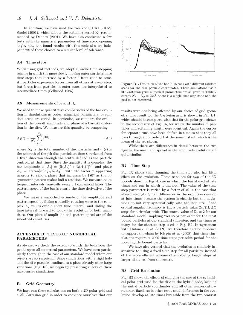
18 J. A. Sellwood and V. P. Debattista
In addition, we have used the tree code, PKDGRAV
Stadel (2001), which adopts the softening kernel K1 recom-mended by Dehnen (2001). We have also conducted a fewtests with the numerical parameters of time step, openingangle, etc., and found results with this code also are inde-pendent of these choices to a similar level of tolerance.
A4 Time steps
When using grid methods, we adopt a 5-zone time steppingscheme in which the more slowly moving outer particles havetime steps that increase by a factor 2 from zone to zone.All particles experience forces from all others at every step,but forces from particles in outer zones are interpolated tointermediate times (Sellwood 1985).
A5 Measurements of A and Ωp
We need to make quantitative comparisons of the bar evolu-tion in simulations as codes, numerical parameters, or ran-dom seeds are varied. In particular, we compare the evolu-tion of the overall amplitude and phase of a bar-like distor-tion in the disc. We measure this quantity by computing
A2(t) =1
Nd
Nd∑
j=1
e2iθj . (A3)
where Nd is the total number of disc particles and θj(t) isthe azimuth of the jth disc particle at time t, reckoned froma fixed direction through the centre defined as the particlecentroid at that time. Since the quantity A is complex, thebar amplitude is |A2| = [ℜ(A2)
2 + ℑ(A2)2]1/2 and phase
2θb = arctan[ℑ(A2)/ℜ(A2)], with the factor 2 appearingin order to yield a phase that increases by 180 as the bi-symmetric pattern makes half a rotation. We measure A2 atfrequent intervals, generally every 0.1 dynamical times. Thepattern speed of the bar is clearly the time derivative of thephase
We make a smoothed estimate of the amplitude andpattern speed by fitting a steadily rotating wave to the com-plex A2 values over a short time interval, and sliding thetime interval forward to follow the evolution of both quan-tities. Our plots of amplitude and pattern speed are of thesmoothed quantities.
APPENDIX B: TESTS OF NUMERICAL
PARAMETERS
As always, we check the extent to which the behaviour de-pends upon all numerical parameters. We have been partic-ularly thorough in the case of our standard model where ourresults are so surprising. Since simulations with a rigid haloand the disc particles confined to a plane already show largevariations (Fig. 15), we begin by presenting checks of theseinexpensive simulations.
B1 Grid Geometry
We have run these calculations on both a 2D polar grid anda 2D Cartesian grid in order to convince ourselves that our
Figure B1. Evolution of the bar in 16 runs with different randomseeds for the disc particle coordinates. These simulations use a2D Cartesian grid: numerical parameters are as given in Table 2except Nx ×Ny = 2562, there is a single time step zone and thegrid is not recentred.
results were not being affected by our choice of grid geom-etry. The result for the Cartesian grid is shown in Fig. B1,which should be compared with that for the polar grid shownin the second row of Fig. 15, for which the number of par-ticles and softening length were identical. Again the curvesfor separate runs have been shifted in time so that they allpass through amplitude 0.1 at the same instant, which is themean of the set shown.
While there are differences in detail between the twofigures, the mean and spread in the amplitude evolution arequite similar.
B2 Time Step
Fig. B2 shows that changing the time step also has littleeffect on the evolution. These tests are for two of the 3Dmodels shown in Fig. 4, one in which the bar slowed at latetimes and one in which it did not. The value of the timestep parameter is varied by a factor of 40 in the case thatslowed strongly. Small differences in the evolution developat late times because the system is chaotic but the devia-tions do not vary systematically with the step size. If theorbital angular frequency is Ωc, a particle takes 2π/(Ωc∆t)steps for a circular orbit. The central value of Ωc ≃ 2 for ourstandard model, implying 250 steps per orbit for the mostbound particles at our standard time-step, and ten times asmany for the shortest step used in Fig. B2. In agreementwith Dubinski et al. (2009), we therefore find no evidenceto support the claim by Klypin et al. (2008) that these sim-ulations require > 2000 time steps per orbit period for themost tightly bound particles.
We have also verified that the evolution is similarly in-sensitive to using a fixed time step for all particles, insteadof the more efficient scheme of employing longer steps atlarger distances from the centre.
B3 Grid Resolution
Fig. B3 shows the effects of changing the size of the cylindri-cal polar grid used for the disc in the hybrid code, keepingthe initial particle coordinates and all other numerical pa-rameters fixed. As in other tests, small differences in the evo-lution develop at late times but aside from the two coarsest
c© 2009 RAS, MNRAS 000, 1–21
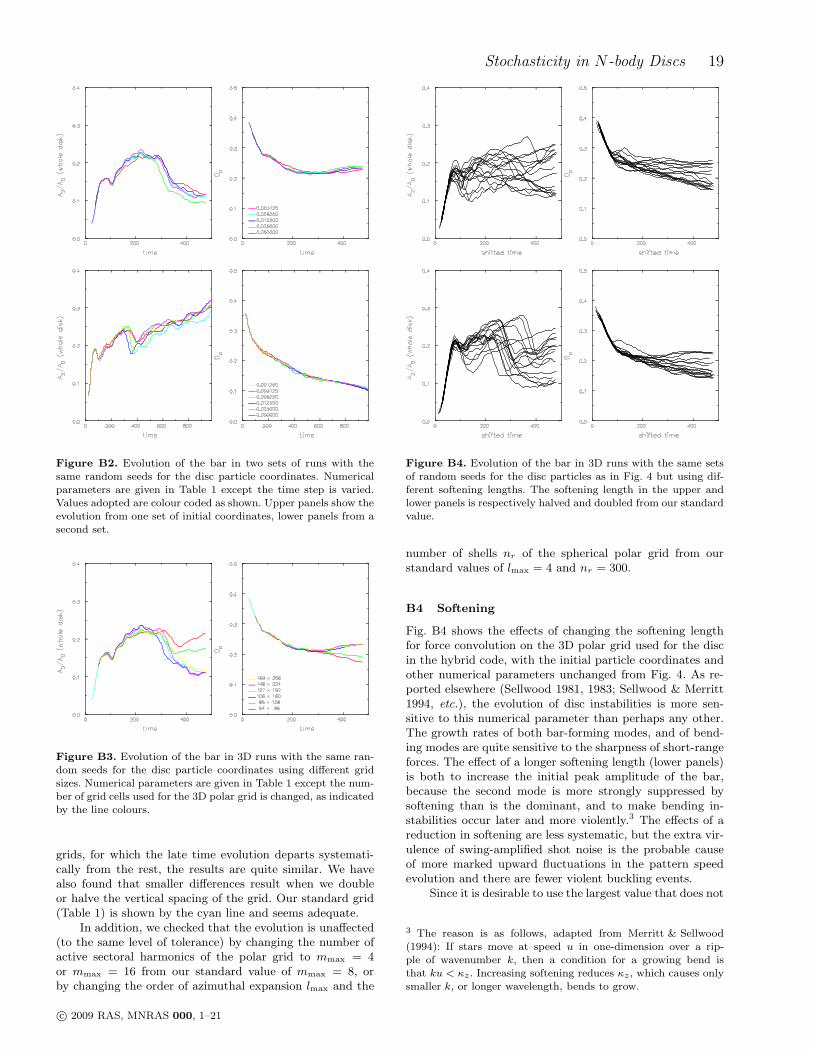
Stochasticity in N-body Discs 19
Figure B2. Evolution of the bar in two sets of runs with thesame random seeds for the disc particle coordinates. Numericalparameters are given in Table 1 except the time step is varied.Values adopted are colour coded as shown. Upper panels show theevolution from one set of initial coordinates, lower panels from asecond set.
Figure B3. Evolution of the bar in 3D runs with the same ran-dom seeds for the disc particle coordinates using different gridsizes. Numerical parameters are given in Table 1 except the num-ber of grid cells used for the 3D polar grid is changed, as indicatedby the line colours.
grids, for which the late time evolution departs systemati-cally from the rest, the results are quite similar. We havealso found that smaller differences result when we doubleor halve the vertical spacing of the grid. Our standard grid(Table 1) is shown by the cyan line and seems adequate.
In addition, we checked that the evolution is unaffected(to the same level of tolerance) by changing the number ofactive sectoral harmonics of the polar grid to mmax = 4or mmax = 16 from our standard value of mmax = 8, orby changing the order of azimuthal expansion lmax and the
Figure B4. Evolution of the bar in 3D runs with the same setsof random seeds for the disc particles as in Fig. 4 but using dif-ferent softening lengths. The softening length in the upper andlower panels is respectively halved and doubled from our standardvalue.
number of shells nr of the spherical polar grid from ourstandard values of lmax = 4 and nr = 300.
B4 Softening
Fig. B4 shows the effects of changing the softening lengthfor force convolution on the 3D polar grid used for the discin the hybrid code, with the initial particle coordinates andother numerical parameters unchanged from Fig. 4. As re-ported elsewhere (Sellwood 1981, 1983; Sellwood & Merritt1994, etc.), the evolution of disc instabilities is more sen-sitive to this numerical parameter than perhaps any other.The growth rates of both bar-forming modes, and of bend-ing modes are quite sensitive to the sharpness of short-rangeforces. The effect of a longer softening length (lower panels)is both to increase the initial peak amplitude of the bar,because the second mode is more strongly suppressed bysoftening than is the dominant, and to make bending in-stabilities occur later and more violently.3 The effects of areduction in softening are less systematic, but the extra vir-ulence of swing-amplified shot noise is the probable causeof more marked upward fluctuations in the pattern speedevolution and there are fewer violent buckling events.
Since it is desirable to use the largest value that does not
3 The reason is as follows, adapted from Merritt & Sellwood(1994): If stars move at speed u in one-dimension over a rip-ple of wavenumber k, then a condition for a growing bend isthat ku < κz. Increasing softening reduces κz, which causes onlysmaller k, or longer wavelength, bends to grow.
c© 2009 RAS, MNRAS 000, 1–21
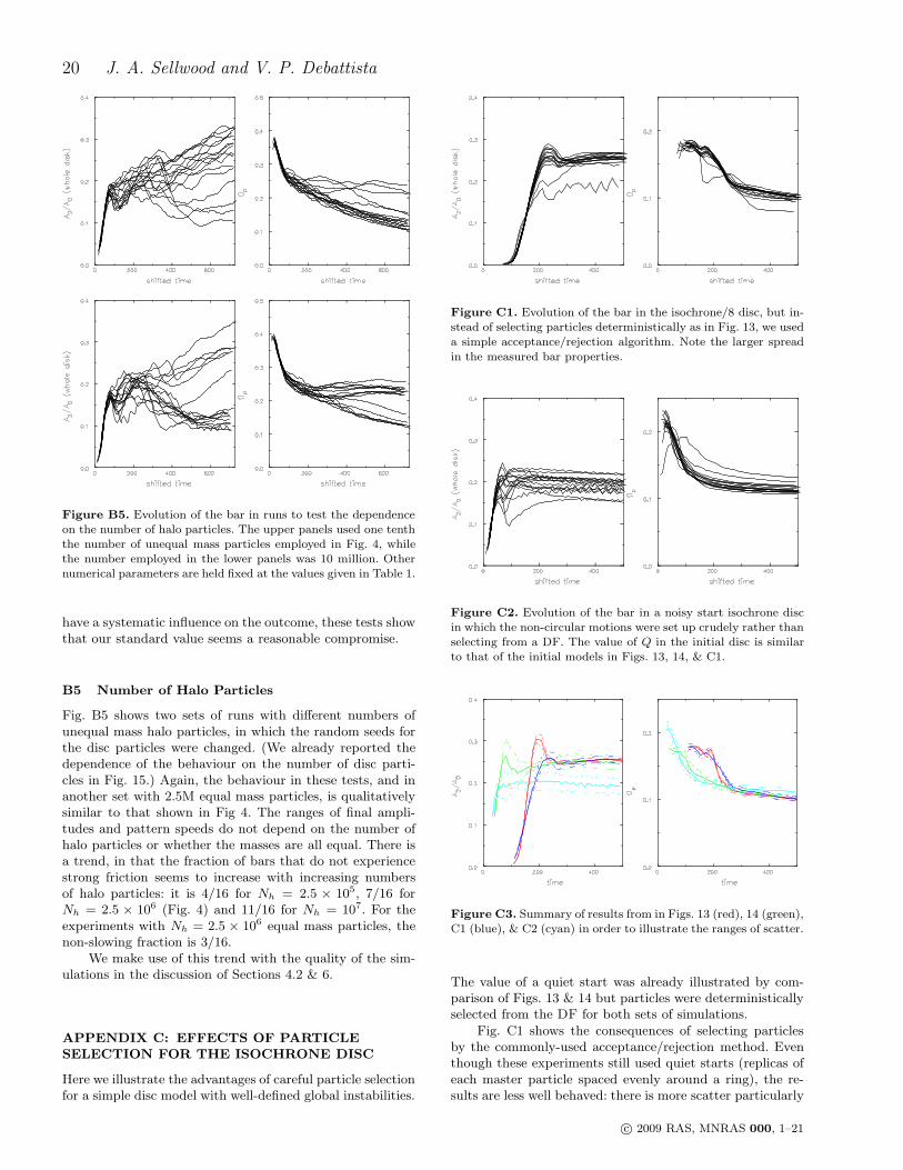
20 J. A. Sellwood and V. P. Debattista
Figure B5. Evolution of the bar in runs to test the dependenceon the number of halo particles. The upper panels used one tenththe number of unequal mass particles employed in Fig. 4, whilethe number employed in the lower panels was 10 million. Othernumerical parameters are held fixed at the values given in Table 1.
have a systematic influence on the outcome, these tests showthat our standard value seems a reasonable compromise.
B5 Number of Halo Particles
Fig. B5 shows two sets of runs with different numbers ofunequal mass halo particles, in which the random seeds forthe disc particles were changed. (We already reported thedependence of the behaviour on the number of disc parti-cles in Fig. 15.) Again, the behaviour in these tests, and inanother set with 2.5M equal mass particles, is qualitativelysimilar to that shown in Fig 4. The ranges of final ampli-tudes and pattern speeds do not depend on the number ofhalo particles or whether the masses are all equal. There isa trend, in that the fraction of bars that do not experiencestrong friction seems to increase with increasing numbersof halo particles: it is 4/16 for Nh = 2.5 × 10⁵, 7/16 forNh = 2.5 × 10⁶ (Fig. 4) and 11/16 for Nh = 107. For theexperiments with Nh = 2.5 × 10⁶ equal mass particles, thenon-slowing fraction is 3/16.
We make use of this trend with the quality of the sim-ulations in the discussion of Sections 4.2 & 6.
APPENDIX C: EFFECTS OF PARTICLE
SELECTION FOR THE ISOCHRONE DISC
Here we illustrate the advantages of careful particle selectionfor a simple disc model with well-defined global instabilities.
Figure C1. Evolution of the bar in the isochrone/8 disc, but in-stead of selecting particles deterministically as in Fig. 13, we useda simple acceptance/rejection algorithm. Note the larger spread
in the measured bar properties.
Figure C2. Evolution of the bar in a noisy start isochrone discin which the non-circular motions were set up crudely rather thanselecting from a DF. The value of Q in the initial disc is similarto that of the initial models in Figs. 13, 14, & C1.
Figure C3. Summary of results from in Figs. 13 (red), 14 (green),C1 (blue), & C2 (cyan) in order to illustrate the ranges of scatter.
The value of a quiet start was already illustrated by com-parison of Figs. 13 & 14 but particles were deterministicallyselected from the DF for both sets of simulations.
Fig. C1 shows the consequences of selecting particlesby the commonly-used acceptance/rejection method. Eventhough these experiments still used quiet starts (replicas ofeach master particle spaced evenly around a ring), the re-sults are less well behaved: there is more scatter particularly
c© 2009 RAS, MNRAS 000, 1–21
Stochasticity in N-body Discs 21
in the bar amplitude, with one or two significantly anoma-lous results.
Fig. C2 shows the results from experiments in which theset up procedure for the random speeds of the disc particlesstemmed simply from the requirement that Q = 1.2 every-where, with the azimuthal dispersion and asymmetric driftdetermined by Jeans equations in the epicycle approxima-tion, as suggested by Hernquist (1993). Although this maybe the most commonly used method, the outcome of suchexperiments shows the greatest degree of scatter.
The effects of quiet and noisy starts, and other particleselection issues are summarized in Fig. C3. Generally, ex-periments with noisy starts show considerably more scatterthan do those with quiet starts, and deterministic selectingfrom a DF is superior to random sampling or not using aDF at all.
c© 2009 RAS, MNRAS 000, 1–21