Embed Size (px)
Citation preview
1
Stock-Bond Correlation and Duration Risk Allocation
Feb/2014 Edition
Liu X, Fan H
ABSTRACT
Using weekly stock-bond correlations estimated with high-frequency data, the
authors find that a lower (more negative) stock-bond correlation forecasts falling 10
-year interest rates over the coming weeks, and it also forecasts a falling 1-year
interest rates over the next year. The reverse is true when the stock-bond correlation is
higher (more positive). Therefore, investors, in particular those with long-term
bond-like liabilities, should take greater duration risk when the recent stock-bond
correlations are lower. The authors propose two possible explanations of such
predictive power: (1) the markets and/or policymakers’ under-reaction to the changing
economic conditions implied by the stock-bond correlation; and (2) the markets’
initial under-reaction to the long-term bonds’ safe-haven status.
2
Using weekly stock-bond correlations estimated with high-frequency (HF) data,
we find that a lower (more negative) stock-bond correlation (SB-Correl henceforth)
forecasts falling yield on the 10-year US Treasury bond (bond henceforth) over the
coming weeks, and falling yield on the 1-year bond over the next year. The reverse is
true when the SB-Correl is higher (more positive). For brevity, we refer to such
predictive power of the SB-Correl as the correlation effect. Investors, in particular
those with long-term bond-like liabilities, should take greater duration risk when the
recent SB-Correl is lower.
The empirical results are obtained using a simple decile portfolio that is based on
a straightforward ranking of the weekly HF SB-Correl on its historical values. The
procedure for our study is intentionally simple, transparent and easily replicable.
The contribution of our findings is threefold: (1) we document a strong predictive
power of HF SB-Correl over bond returns; (2) we document an inverse relationship
between the 10-year bond’s time-varying equity betas and returns, and; (3) we provide
possible explanations for the correlation effect, which include policymakers/markets’
under-reactions to the changing economic conditions, and markets’ initial
under-reaction to the changing safe-haven status of the long-term bond.
DATA AND METHODOLOGY
A number of researchers use daily price data to estimate SB-Correls. To study
both short-term and cyclical dynamics, we reduce information latency by using HF
futures price data.
From Jan/11/1985 till Sep/06/2013, we obtain one correlation estimate per week
with no overlapping window, totaling 1,496 weekly observations. The realized weekly
correlations are obtained using S&P 500 futures and 10-year Treasury bond futures
price data with 10-minute frequency from tickdata.com. A frequency of 10-minutes is
still of a low enough frequency to avoid microstructure noise. The futures delivery
months for all of the contracts are March, June, September and December. To ensure
good liquidity of the futures, we always use the contract closest to expiration,
switching to the next maturity contract five business days before expiration, and we
3
use electronic futures contracts when they are liquid enough (Exhibit 1).
E X H I B I T 1
Futures Contacts Used
Date
from to
Futures contract used
for S&P 500
Futures contract used
for US 10-year Treasury
Jan/04/1985 Jan/02/2004
SP futures open outcry; CME
TY futures open outcry; CBOT
Jan/05/2004 Sep/06/2013
E-mini futures elec; CME Globex
ZN futures elec; CME Globex
We also obtain 3-month, 1-year, 2-year, 5-year and 10-year constant-maturity
Treasury yields from the FRED database of the Federal Reserve Bank of St. Louis.
Forward rates and zero coupon bond log returns are estimated by constructing
zero-coupon yield curves with a linear interpolation method. We obtain equity log
returns using S&P 500 Total Return Index (SPTR) and 3-month Treasury yields. From
1985 to 1987, SPTR is not available and the S&P 500 Index is used as the proxy.
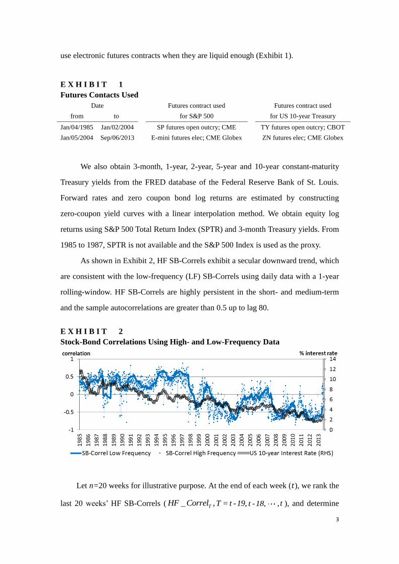
As shown in Exhibit 2, HF SB-Correls exhibit a secular downward trend, which
are consistent with the low-frequency (LF) SB-Correls using daily data with a 1-year
rolling-window. HF SB-Correls are highly persistent in the short- and medium-term
and the sample autocorrelations are greater than 0.5 up to lag 80.
E X H I B I T 2
Stock-Bond Correlations Using High- and Low-Frequency Data
Let n=20 weeks for illustrative purpose. At the end of each week (𝑡), we rank the
last 20 weeks’ HF SB-Correls ( _ THF Correl , T = t -19, t -18, , t ), and determine
4
the decile of _ tHF SB Correl , or tDecile20 accordingly. For convenience, we also
refer to week ( 𝑡 ) as week 0 and week ( 𝑡 + 1 ) as week 1. A simple HF
SB-Correl-sorted portfolio allocates greater weight to bond on week 1 when the decile
is lower on week 0:
1tweight20
1 2( 1) / (10 1)tDecile20 . (1)
Because of the secular downward trend of the SB-Correls, over the long run, the
weights above sum slightly above zero.
To show a more representative result, we may use different sampling windows
and use the averages of their deciles. As HF SB-Correls are highly persistent, we may
also use equally weighted moving averages of the deciles. A portfolio is hence defined
by its underlying asset, the object used for ranking, the sampling windows and
corresponding lag terms. For example:
[ Asset=Bond10Yr; RankObj=HF_Correl; n=20,40; Lag=1, 4] means
1
1
4
1
1
1 1 1
1 1
1
*
1 2 1 10 1
11, 4,
2
1, 2
4,
i
i
t t t
t t
t t t
t it t
t it
R Weight Return 10YrBond
Weight Decile
Decile Round MA Decile20 MA Decile40
MA Decile20 Decile 0 Decile20
MA Decile40 Decile40
(2)
For the resulting time series of returns, we calculate averages, standard deviations,
and Sharpe ratios. To test for the statistical significance of the Sharpe ratios and decile
differences, we use a bootstrap to estimate the t-values. For a given decile (or other
quantile) strategy, suppose we have a sample of T weekly observations of SB-Correl,
the associated contemporary excess return and the date (timestamp). To estimate the
P-value, we draw 10,000N samples of T observations (with replacement) from
the empirical distribution. For each boostrap sample, we sort the observations
sequentially according to their timestamps. We then use the defined SB-Correl-sorted
decile strategy, re-established a new portfolio and calculate the mean for each decile.
5
The P-values are given by:
# (D10 D1) 0(D10 D1)
# (D10 Other D) 0(D10 Other D)
# (Sharpe ratio 0) 0(Sharperatio) .
meansP
N
meansP
N
meansP
N
(3)
And the t-values are given by: 1 1t N p , where N is the cdf of the normal
distribution with zero mean and unit variance.
We also use a simple regression to disentangle the correlation effect from other
factors. The factor portfolios are constructed in a similar manner to the SB-Correl-
sorted portfolio. We define curve spread as the difference between 10-year and 1-year
interest rates. In Equation (2), instead of letting RankObj=HF_Correl, we let
RankObj=Yield, RankObj= –Curve_Spread and RankObj= –VIX respectively. And the
resulting time series of returns _Yield Momentum
R , _Curve Spread
R and VIXR are used
as the yield momentum, curve spread and stock market uncertainty factors
respectively. By regressing the returns of the HF SB-Correl-sorted portfolio to the
underlying bond returns, the equity returns as well as these factors, we control for
possible systematic exposures to bond, equity and these factors:
_ _
_ _
Bond Bond Yield Momentum Yield Momentum
VIX VIX Equity EquityCurve Spread Curve Spread
R R R
R R R
(4)
where R is the returns of the HF SB-Correl-sorted portfolio; is the adjusted alpha;
BondR is the returns of the underlying bond; EquityR is the returns of the SPTR index;
and _Yield Momentum ,
_Curve Spread and VIX are the estimated factor exposures
1.
Following Ilmanen [2003], Campbell et al. [2013a], Johnson et al. [2013] and a
number of other studies, we consider a potential structural break in 1997. We also
consider another potential structural break in Dec/2008, when the fed funds rate is
essentially zero. The two potential structural breaks divide the sample into three
1 The t-value of the alpha and betas are estimated using the closed form formula for OLS instead of simulation.
6
sub-periods, and we may study them separately depending on the context.
EMPIRICAL RESULTS
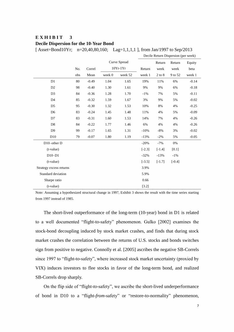
Exhibit 3 shows the correlation effect over the 10-year bond from 1997 to 2013.
We choose a geometric series: [20, 40, 80, 160] weeks as the sampling windows, such
that we are not showing too specific results of a sampling window2. We use no lag
terms for Exhibit 3. The 10-year bond underperforms exceptionally in the
bottom-deciles. Compared to other deciles, in D10, the 10-year bond returns are -20%
on week 1 and -7% per week on average from week 2 to week 8 (all returns are
annualized). The 10-year bond also outperforms considerably in the top-deciles. The
decile dispersion (D10–D1) is short-lived and is absent from week 9 to week 52. The
Sharpe ratio of a simple SB-Correl-sorted strategy is 0.66.
2 We find that the empirical results would be much weaker if we use only past-week Stock-Bond correlations or
other shorter windows. This is because there is too much noise with short windows. The exhibit will be available
online.
7
E X H I B I T 3
Decile Dispersion for the 10-Year Bond
[ Asset=Bond10Yr; n=20,40,80,160; Lag=1,1,1,1 ], from Jan/1997 to Sep/2013
Decile Return Dispersion (per week)
No.
obs
Correl
Mean
Curve Spread
10Yr-1Yr
week 0 week 52
Return
week 1
Return
week
2 to 8
Return
week
9 to 52
Equity
beta
week 1
D1 80 -0.49 1.04 1.65 19% 11% 6% -0.14
D2 98 -0.40 1.30 1.61 9% 9% 6% -0.18
D3 84 -0.36 1.28 1.70 -1% 7% 5% -0.11
D4 85 -0.32 1.59 1.67 3% 9% 5% -0.02
D5 95 -0.30 1.32 1.53 10% 8% 4% -0.25
D6 83 -0.24 1.45 1.48 11% 4% 5% -0.09
D7 83 -0.31 1.60 1.53 14% 7% 4% -0.26
D8 84 -0.22 1.77 1.46 6% 4% 4% -0.26
D9 99 -0.17 1.65 1.31 -10% -8% 3% -0.02
D10 79 -0.07 1.80 1.19 -13% -2% 5% -0.05
D10–other D
-20% -7% 0%
(t-value)
[-2.3] [-1.4] [0.1]
D10–D1
-32% -13% -1%
(t-value)
[-3.5] [-1.7] [-0.4]
Strategy excess returns
3.9%
Standard deviation
5.9%
Sharpe ratio
0.66
(t-value)
[3.2]
Note: Assuming a hypothesized structural change in 1997, Exhibit 3 shows the result with the time series starting
from 1997 instead of 1985.
The short-lived outperformance of the long-term (10-year) bond in D1 is related
to a well documented “flight-to-safety” phenomenon. Gulko [2002] examines the
stock-bond decoupling induced by stock market crashes, and finds that during stock
market crashes the correlation between the returns of U.S. stocks and bonds switches
sign from positive to negative. Connolly et al. [2005] ascribes the negative SB-Correls
since 1997 to “flight-to-safety”, where increased stock market uncertainty (proxied by
VIX) induces investors to flee stocks in favor of the long-term bond, and realized
SB-Correls drop sharply.
On the flip side of “flight-to-safety”, we ascribe the short-lived underperformance
of bond in D10 to a “flight-from-safety” or “restore-to-normality” phenomenon,
8
where investors bid down the price of the “safe” long-term bond, in times of increased
SB-Correls, inducing corresponding negative returns of the long-term bond.
For each decile in Exhibit 3, we estimate the equity market beta by regressing the
excess bond returns on week 1 to their contemporary equity market excess returns.
For D1 and D10, the stock betas are -0.14 and -0.05, while the excess bond returns are
19% and -13% annualized respectively. A plot of the results reported in Exhibit 3
would show that there is an inverse relationship between the 10-year bond’s equity
betas and returns. Hence, the 10-year bond has higher return when it is less risky, if
risk is measured by its time-varying equity betas.
As warned by Dopfel [2003], the various strategic and tactical asset allocation
issues related to a continued low correlation environment have an impact on investor
welfare in an asset-only and an asset-liability framework. For investors, a low
SB-Correl is beneficial in an asset-only context, but detrimental in the case of a
long-term bond-like liability context. From a surplus optimization perspective, a
lower SB-Correl increases surplus risk.
Our empirical findings suggest that lower SB-Correl (D1) is the best of both
worlds of return and risk for an asset only investor, especially if the investor is
allowed to take leveraged positions in bonds. Not only does a lower SB-Correl
indicate lower risk for a stock-bond portfolio, it also forecasts higher bond returns in
the short run. On the other hand, a lower SB-Correl is a double whammy for an
investor with a long-term bond-like liability, especially if the investor invests
aggressively in equities and not allowed to use leverage. From an asset-liability
perspective, not only does a lower SB-Correl increase surplus risk, it also forecasts an
increased liability in the short run. Therefore, investors should take greater duration
risk when the recent SB-Correls are lower, either with cash bond positions or with
derivatives if leverage is allowed.
We replicate the analysis for a short-term (1-year) bond. Differently from Exhibit
3, we exclude data from 2009 onwards as the Fed funds rate has been kept close to
zero since 2009. Exhibit 4 shows the correlation effect for the 1-year bond from 1997
to 2008. The 1-year bond considerably outperforms in the top-deciles and
9
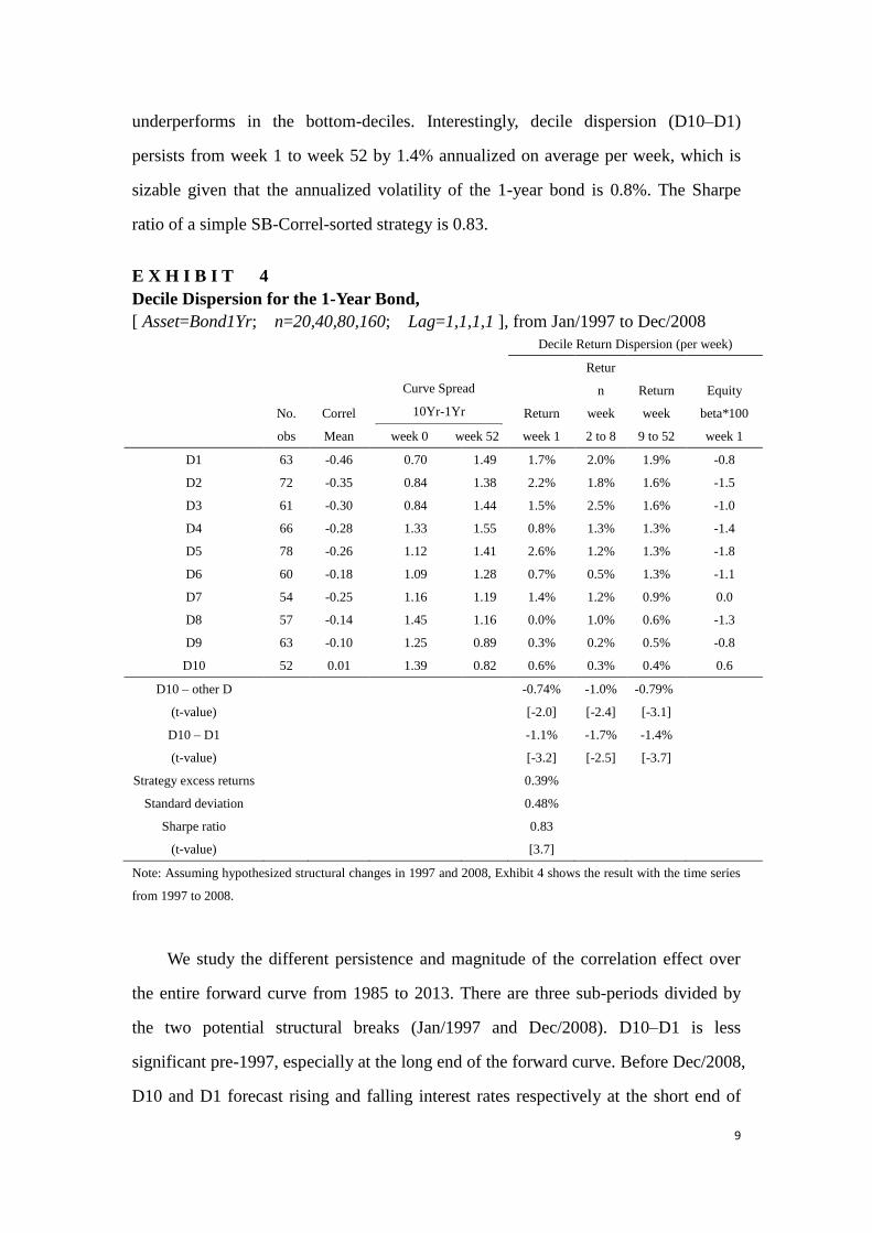
underperforms in the bottom-deciles. Interestingly, decile dispersion (D10–D1)
persists from week 1 to week 52 by 1.4% annualized on average per week, which is
sizable given that the annualized volatility of the 1-year bond is 0.8%. The Sharpe
ratio of a simple SB-Correl-sorted strategy is 0.83.
E X H I B I T 4
Decile Dispersion for the 1-Year Bond,
[ Asset=Bond1Yr; n=20,40,80,160; Lag=1,1,1,1 ], from Jan/1997 to Dec/2008
Decile Return Dispersion (per week)
No.
obs
Correl
Mean
Curve Spread
10Yr-1Yr
week 0 week 52
Return
week 1
Retur
n
week
2 to 8
Return
week
9 to 52
Equity
beta*100
week 1
D1 63 -0.46 0.70 1.49 1.7% 2.0% 1.9% -0.8
D2 72 -0.35 0.84 1.38 2.2% 1.8% 1.6% -1.5
D3 61 -0.30 0.84 1.44 1.5% 2.5% 1.6% -1.0
D4 66 -0.28 1.33 1.55 0.8% 1.3% 1.3% -1.4
D5 78 -0.26 1.12 1.41 2.6% 1.2% 1.3% -1.8
D6 60 -0.18 1.09 1.28 0.7% 0.5% 1.3% -1.1
D7 54 -0.25 1.16 1.19 1.4% 1.2% 0.9% 0.0
D8 57 -0.14 1.45 1.16 0.0% 1.0% 0.6% -1.3
D9 63 -0.10 1.25 0.89 0.3% 0.2% 0.5% -0.8
D10 52 0.01 1.39 0.82 0.6% 0.3% 0.4% 0.6
D10 – other D
-0.74% -1.0% -0.79%
(t-value)
[-2.0] [-2.4] [-3.1]
D10 – D1
-1.1% -1.7% -1.4%
(t-value)
[-3.2] [-2.5] [-3.7]
Strategy excess returns
0.39%
Standard deviation
0.48%
Sharpe ratio
0.83
(t-value)
[3.7]
Note: Assuming hypothesized structural changes in 1997 and 2008, Exhibit 4 shows the result with the time series
from 1997 to 2008.
We study the different persistence and magnitude of the correlation effect over
the entire forward curve from 1985 to 2013. There are three sub-periods divided by
the two potential structural breaks (Jan/1997 and Dec/2008). D10–D1 is less
significant pre-1997, especially at the long end of the forward curve. Before Dec/2008,
D10 and D1 forecast rising and falling interest rates respectively at the short end of
10
the forward curve for about 52 weeks. The results are available online.
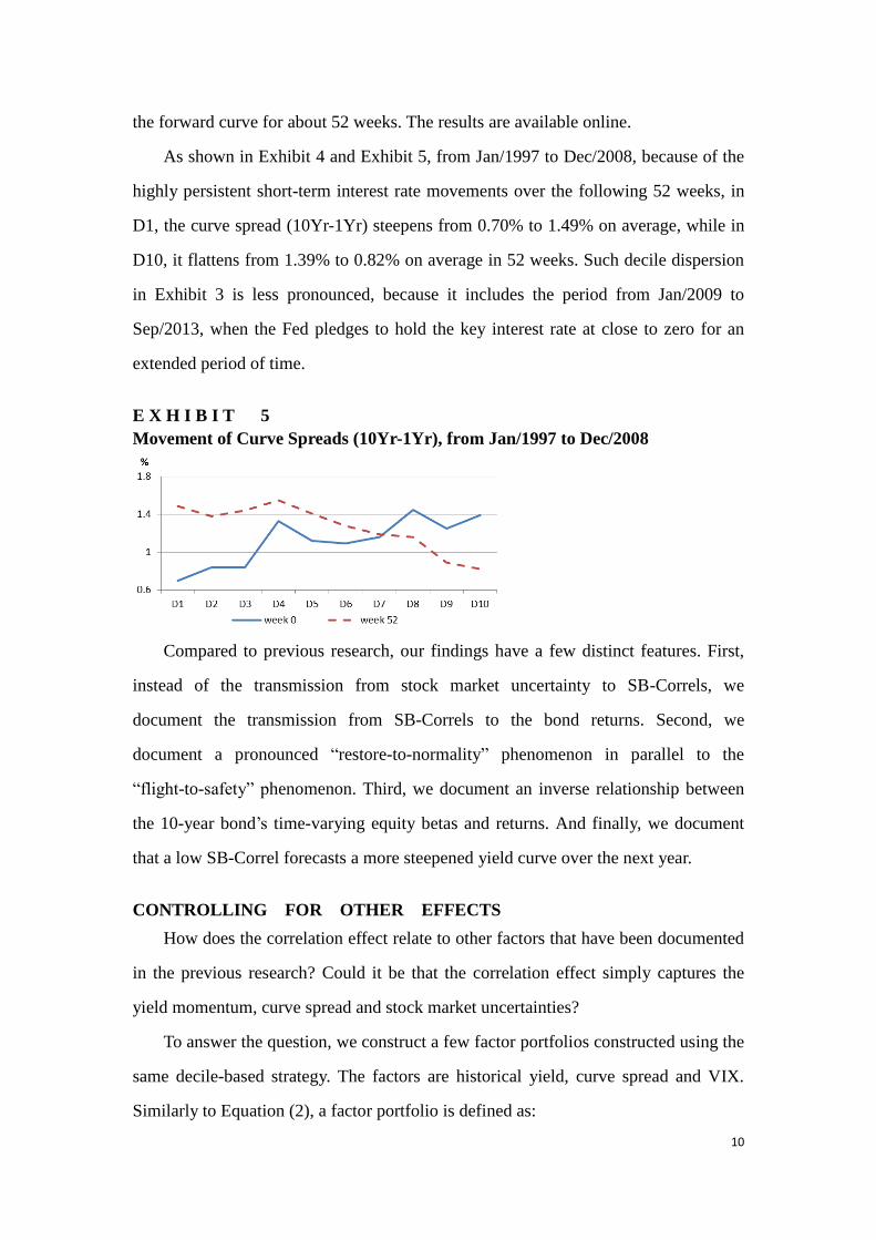
As shown in Exhibit 4 and Exhibit 5, from Jan/1997 to Dec/2008, because of the
highly persistent short-term interest rate movements over the following 52 weeks, in
D1, the curve spread (10Yr-1Yr) steepens from 0.70% to 1.49% on average, while in
D10, it flattens from 1.39% to 0.82% on average in 52 weeks. Such decile dispersion
in Exhibit 3 is less pronounced, because it includes the period from Jan/2009 to
Sep/2013, when the Fed pledges to hold the key interest rate at close to zero for an
extended period of time.
E X H I B I T 5
Movement of Curve Spreads (10Yr-1Yr), from Jan/1997 to Dec/2008
Compared to previous research, our findings have a few distinct features. First,
instead of the transmission from stock market uncertainty to SB-Correls, we
document the transmission from SB-Correls to the bond returns. Second, we
document a pronounced “restore-to-normality” phenomenon in parallel to the
“flight-to-safety” phenomenon. Third, we document an inverse relationship between
the 10-year bond’s time-varying equity betas and returns. And finally, we document
that a low SB-Correl forecasts a more steepened yield curve over the next year.
CONTROLLING FOR OTHER EFFECTS
How does the correlation effect relate to other factors that have been documented
in the previous research? Could it be that the correlation effect simply captures the
yield momentum, curve spread and stock market uncertainties?
To answer the question, we construct a few factor portfolios constructed using the
same decile-based strategy. The factors are historical yield, curve spread and VIX.
Similarly to Equation (2), a factor portfolio is defined as:
11
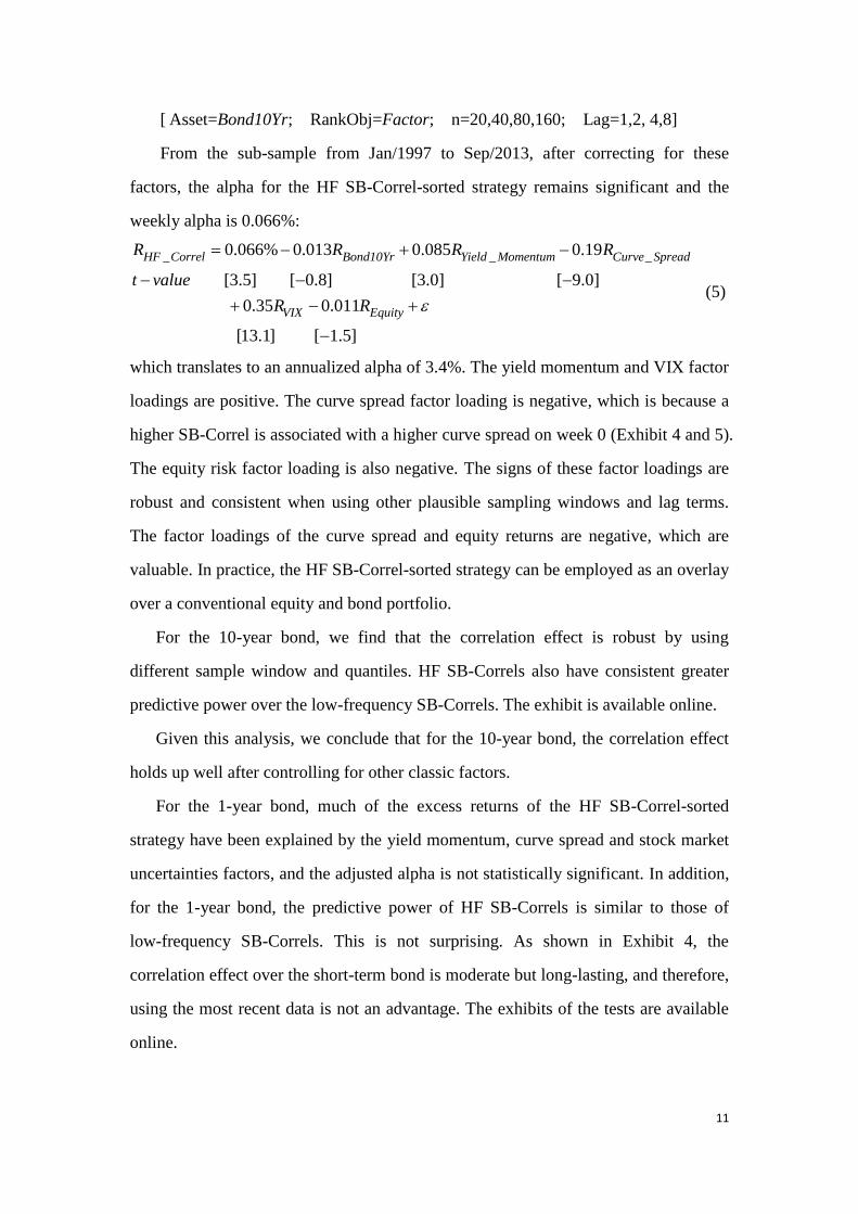
[ Asset=Bond10Yr; RankObj=Factor; n=20,40,80,160; Lag=1,2, 4,8]
From the sub-sample from Jan/1997 to Sep/2013, after correcting for these
factors, the alpha for the HF SB-Correl-sorted strategy remains significant and the
weekly alpha is 0.066%:
_ _ _0.066% 0.013 0.085 0.19
[3.5] [ 0.8] [3.0] [ 9.0]
0.35 0.011
[13.1] [ 1.5]
HF Correl Bond10Yr Yield Momentum Curve Spread
VIX Equity
R R R R
t value
R R
(5)
which translates to an annualized alpha of 3.4%. The yield momentum and VIX factor
loadings are positive. The curve spread factor loading is negative, which is because a
higher SB-Correl is associated with a higher curve spread on week 0 (Exhibit 4 and 5).
The equity risk factor loading is also negative. The signs of these factor loadings are
robust and consistent when using other plausible sampling windows and lag terms.
The factor loadings of the curve spread and equity returns are negative, which are
valuable. In practice, the HF SB-Correl-sorted strategy can be employed as an overlay
over a conventional equity and bond portfolio.
For the 10-year bond, we find that the correlation effect is robust by using
different sample window and quantiles. HF SB-Correls also have consistent greater
predictive power over the low-frequency SB-Correls. The exhibit is available online.
Given this analysis, we conclude that for the 10-year bond, the correlation effect
holds up well after controlling for other classic factors.
For the 1-year bond, much of the excess returns of the HF SB-Correl-sorted
strategy have been explained by the yield momentum, curve spread and stock market
uncertainties factors, and the adjusted alpha is not statistically significant. In addition,
for the 1-year bond, the predictive power of HF SB-Correls is similar to those of
low-frequency SB-Correls. This is not surprising. As shown in Exhibit 4, the
correlation effect over the short-term bond is moderate but long-lasting, and therefore,
using the most recent data is not an advantage. The exhibits of the tests are available
online.
12
POSSIBLE EXPLANATIONS
The correlation effect on the 1-year bond is moderate but long-lasting, and we
think a possible explanation is related to the economic scenarios implied by the
SB-Correls. On the other hand, the correlation effect on the 10-year bond is strong but
short-lived, and a possible explanation is the markets’ initial under-reactions to the
attractiveness of bonds. We first provide a possible explanation for the 1-year bond by
assuming negligible bond risk premia (BRP), then we provide a possible explanation
for the 10-year bond.
We assume that bond and stock prices are driven by two economic drivers —
expected growth and inflation. Then SB-Correls are driven by the following:
a) Sensitivities to economic drivers. Higher expected inflation drives both bond and
stock prices down; higher expected economic growth drives bond price down but
drives stock price up.
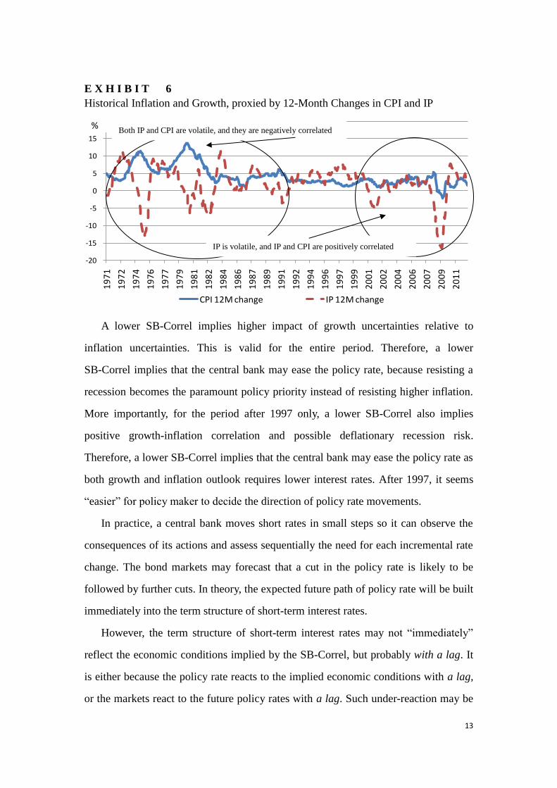
b) The relative volatility of the expected inflation and growth. SB-Correl is low
when the uncertainty of growth dominates the inflation uncertainty. As shown in
Exhibit 6, while growth is volatile for both the pre-1997 and post-1997 periods,
the level dependent inflation volatility has subsided since the 1990s. Post-1997,
SB-Correls are low as growth uncertainties drive stock and bond in the opposite
directions while the impact of inflation uncertainties is relatively muted.
c) Growth-inflation correlation. SB-Correl is low when growth and inflation is
positively correlated. As shown in Exhibit 6, in the 1970s and 1980s, supply
shocks move inflation and growth in the opposite directions, making bond returns
pro-cyclical, but since the 1990s, demand shocks make bond returns largely
countercyclical.
13
E X H I B I T 6
Historical Inflation and Growth, proxied by 12-Month Changes in CPI and IP
A lower SB-Correl implies higher impact of growth uncertainties relative to
inflation uncertainties. This is valid for the entire period. Therefore, a lower
SB-Correl implies that the central bank may ease the policy rate, because resisting a
recession becomes the paramount policy priority instead of resisting higher inflation.
More importantly, for the period after 1997 only, a lower SB-Correl also implies
positive growth-inflation correlation and possible deflationary recession risk.
Therefore, a lower SB-Correl implies that the central bank may ease the policy rate as
both growth and inflation outlook requires lower interest rates. After 1997, it seems
“easier” for policy maker to decide the direction of policy rate movements.
In practice, a central bank moves short rates in small steps so it can observe the
consequences of its actions and assess sequentially the need for each incremental rate
change. The bond markets may forecast that a cut in the policy rate is likely to be
followed by further cuts. In theory, the expected future path of policy rate will be built
immediately into the term structure of short-term interest rates.
However, the term structure of short-term interest rates may not “immediately”
reflect the economic conditions implied by the SB-Correl, but probably with a lag. It
is either because the policy rate reacts to the implied economic conditions with a lag,
or the markets react to the future policy rates with a lag. Such under-reaction may be
-20
-15
-10
-5
0
5
10
15
20
19
71
19
72
19
74
19
76
19
77
19
79
19
81
19
82
19
84
19
86
19
87
19
89
19
91
19
92
19
94
19
96
19
97
19
99
20
01
20
02
20
04
20
06
20
07
20
09
20
11
CPI 12M change IP 12M change
Both IP and CPI are volatile, and they are negatively correlated
IP is volatile, and IP and CPI are positively correlated
%
14
more persistent since 1997 because of the positive growth-inflation correlation and
hence “easier” policy rate directional decision, and because of the increased
persistence of monetary policy since 1997 [Campbell et al. 2013a].
The above is a possible explanation on the correlation effect on the 1-year bond.
How about the 10-year bond? Differently from the 1-year bond, the BRP is no longer
negligible but pivotal for the 10-year bond. Following Ilmanen [2011, Chapter 9] and
in the spirit of Campbell et al. [2013b], we let the BRP be primarily dependent on (1)
a level-dependent inflation uncertainty; and (2) safe-haven status, also known as the
equity and/or recession-hedging ability:
10 3Y inflation risk safe havenE avgM BRP BRP
where BRP is the average expected return of the bond over its life in excess of a
sequence of riskless 3-month cash investment; inflation riskBRP is the premia for
bearing the inflation uncertainties; and safe havenBRP is the premia paid by the
bond holder if the bond return covariates negatively with equity.
With the introduction of BRP, the explanations for correlation effect on the
10-year bond are much more complicated than the 1-year bond. There are many
possible explanations, some circumstances lend themselves to clearer interpretations
than others, and there are many pitfalls. Our following discussion is limited to the
possible markets’ initial under-reactions to the bond’s changing safe-haven premia.
We then extend our discussion to explain why the correlation effect is more
pronounced after 1997.
Traditional “efficient markets” thinking suggests that asset prices should
completely and instantaneously reflect movements in underlying fundamentals. But
such thinking needs not conform to the reality. We use the performance of the 10-year
bond in the middle of 2013 as an example. We consider a 60/40 stock-bond portfolio
as the market portfolio. We do not consider skewness. As of Apr/19/2013, the 10-year
interest rate is 1.73%. Let the stock and bond weight, correlation and volatility be:
0.6
0.4
ω , 1 0.6
0.6 1
C ,
12 0
0 6
Ω .
15
Then the marginal contribution to portfolio risk is
1/2
11.4
1.9'
portfolio
portfolio
ΩCΩωMCTR β
ω ω ΩCΩω .
If the portfolio is the tangency portfolio whose Sharpe ratio is maximized, then
Exp Return of Equity Exp Return of Bond= =Portfolio's Sharpe
MCTR of Equity MCTR of Bond.
Let Exp Return of Equity = 5% , then Exp Return of Bond = 0.83% . Given the
same volatility, and same equity expected return, Exhibit 7 shows the mapping from
SB-Correls to the bond’s expected returns.
E X H I B I T 7
Stock-Bond Correlations and Expected Bond Excess Returns
Stock-Bond Correl -0.8 -0.6 -0.4 -0.2 0 0.2 0.4 0.6 0.8
Expected Bond Ret -1.59% -0.83% -0.19% 0.36% 0.83% 1.25% 1.62% 1.94% 2.24%
As of Jun/21/2013, the 10-year interest rate is 2.52%, and the realized HF
SB-Correl has increased to 0.12. For simplicity, let 0 , and let other inputs be the
same, then according to Exhibit 7, Exp Return of Bond = 0.83% , which is about 1.66%
higher than when 0.6 . In this case, the bond yield has to be 1.66% higher
instantaneously (without considering roll-down), which translates to an immediate
and substantial bond price depreciation. But empirically, the yield only increases by
(2.52% – 1.73% = 0.79%) from Apr/19/2013 to Jun/21/2013, much less than 1.66%.
Subsequently, the 10-year interest rate climbs to 2.73% two weeks later and to 2.94%
eleven weeks later, while the realized HF SB-Correls remain close to zero. It is
possible that the markets learn about the evolving riskiness and safe-haven status of
bonds and incorporate them into bond prices and expected returns with a lag.
The above is a hypothetical example for illustrative purpose only, because the real
correlations, volatilities and the expected returns of equity are unknown.
According to this line of argument, we provide two additional arguments to
explain why the correlation effect over the 10-year bond is more pronounced after
16
1997.
First, quantitatively, the 10-year bond’s expected returns are more sensitive to
SB-Correls when SB-Correls are already low. As shown in Exhibit 7, the bond’s
expected return increases by 1.85% when increases from -0.8 to -0.2, but it
increases by only 1% when increases from 0.2 to 0.8. The average HF SB-Correl
is 0.35 pre-1997 and is –0.30 post-1997, which is a substantial difference. On the
other hand, the standard deviation of HF SB-Correl is 0.23 pre-1997 and 0.22
post-1997, which is a minor difference. Therefore, post-1997, the changing SB-Correl
is a greater driver of the bond’s theoretical expected returns. If the markets’ initial
under-reaction is roughly proportional to the changing bond’s theoretical expected
returns, then post-1997, the changing SB-Correl is also a greater driver of the bond’s
subsequent returns.
Second, qualitatively, post-1997, bond’s safe-haven status matters more to the
investors. As a result, it is possible that investors are more motivated to revalue the
10-year bond according to its changing safe-haven status, though with a lag. We
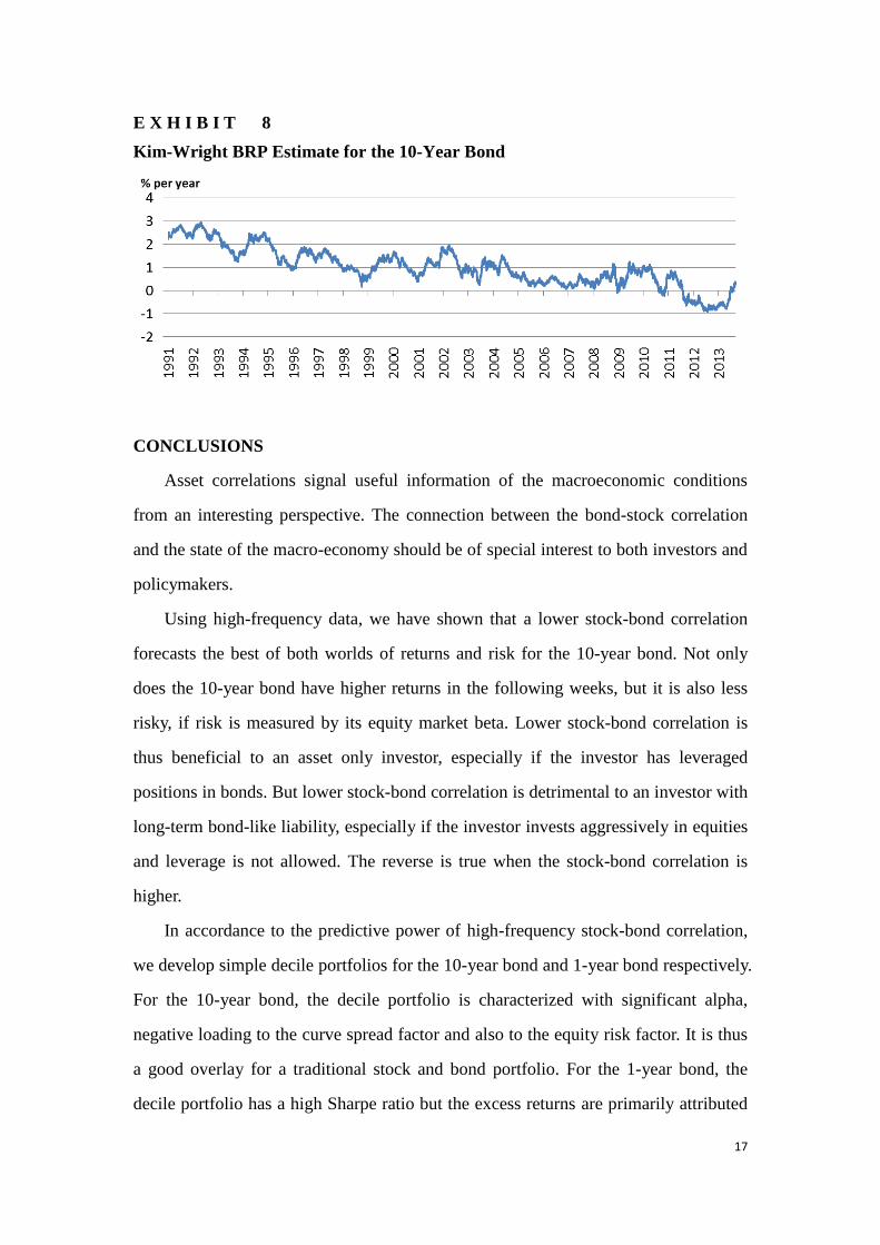
follow Kim et al. [2005] that explicitly incorporates investors’ expectations3. Exhibit
8 plots the survey anchored BRP estimate for the 10-year bond. There is a secular
downward trend of BRP, and it dips further into the negative territory in 2011 and
2012. It suggests that investors expect that the cumulative returns for holding cash are
similar or may be even higher than holding a 10-year bond to maturity. According to
Campbell et al. [2013b], in recent years, with BRP at such a depressed level, instead
of an inflationary bet, investors regard the long-term bond as a deflationary
(safe-haven) hedge.
3 In addition, compared to the classic C-P BRP by Cochrane et al. [2005], a survey anchored BRP may be less
prone to possible unrealistic BRP estimate.
17
E X H I B I T 8
Kim-Wright BRP Estimate for the 10-Year Bond
CONCLUSIONS
Asset correlations signal useful information of the macroeconomic conditions
from an interesting perspective. The connection between the bond-stock correlation
and the state of the macro-economy should be of special interest to both investors and
policymakers.
Using high-frequency data, we have shown that a lower stock-bond correlation
forecasts the best of both worlds of returns and risk for the 10-year bond. Not only
does the 10-year bond have higher returns in the following weeks, but it is also less
risky, if risk is measured by its equity market beta. Lower stock-bond correlation is
thus beneficial to an asset only investor, especially if the investor has leveraged
positions in bonds. But lower stock-bond correlation is detrimental to an investor with
long-term bond-like liability, especially if the investor invests aggressively in equities
and leverage is not allowed. The reverse is true when the stock-bond correlation is
higher.
In accordance to the predictive power of high-frequency stock-bond correlation,
we develop simple decile portfolios for the 10-year bond and 1-year bond respectively.
For the 10-year bond, the decile portfolio is characterized with significant alpha,
negative loading to the curve spread factor and also to the equity risk factor. It is thus
a good overlay for a traditional stock and bond portfolio. For the 1-year bond, the
decile portfolio has a high Sharpe ratio but the excess returns are primarily attributed
18
to the yield momentum, curve spread and equity market uncertainties factors. For the
1-year bond, a possible explanation for the correlation effect is the markets or policy
markers’ under-reaction to the changing economic conditions implied by the
stock-bond correlations. For the 10-year bond, a possible explanation of the
correlation effect is the markets’ initial under-reaction to the 10-year bond’s
safe-haven status implied by the stock-bond correlations.
References
Campbell, J. Y., Pflueger, C., and Viceira, L. M. “Monetary Policy Drivers of Bond
and Equity Risks.”NBER Working Papers, 2013a
Campbell J. Y, Sunderam A, and Viceira L. M. “Inflation Bets or Deflation Hedges?
The Changing Risks of Nominal Bonds.”NBER Working Papers, 2013b
Cochrane, J. H., and Piazzesi, M. “Bond Risk Premia.” The American Economic
Review, 95 (1), (2005), pp. 138-160.
Connolly, R., Stivers, C., Sun, L.“Stock Market Uncertainty and the Stock–Bond
Return Relation.” Journal of Financial and Quantitative Analysis, 40(1), (2005), pp.
161–194.
Dopfel, F. E.“Asset Allocation in a Lower Stock-Bond Correlation Environment”, The
Journal of Portfolio Management , 30(1), (2003), pp. 25-38
Gulko, L. “Decoupling.” Journal of Portfolio Management, 28(3), (2002), pp. 59-66
Ilmanen, A. “Stock–Bond Correlations.” Journal of Fixed Income, 13 (2), (2003), pp.
55–66.
---.“Expected Returns: An Investor's Guide to Harvesting Market Rewards.” (2011).
Wiley.

19
Johnson. N., Naik. V., Page. S., Pedersen. N., and Sapra. S. “The Stock-Bond
Correlation”, PIMCO, Quantitative Research. Nov/2013
Kim, D., and Wright, J. H. “An Arbitrage-Free Three-Factor Term Structure Model
and the Recent Behavior of Long-Term Yields and Distant-Horizon Forward Rates.”
Finance and Economics Discussion Series, 2005
20
Online Appendices
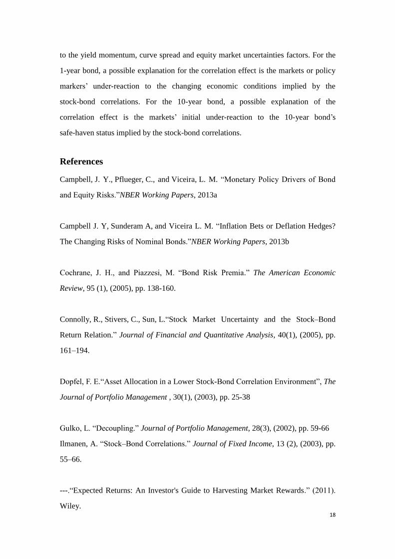
E X H I B I T APPENDIX 1
Decile Dispersion of the Forward Curve, Top-Panel = D10, Bottom-Panel = D1,
Movements per Week
1988-1996 1997-2008 2009 to 2013
Note: all forward rates movements have been detrended from 1988 to 2013.
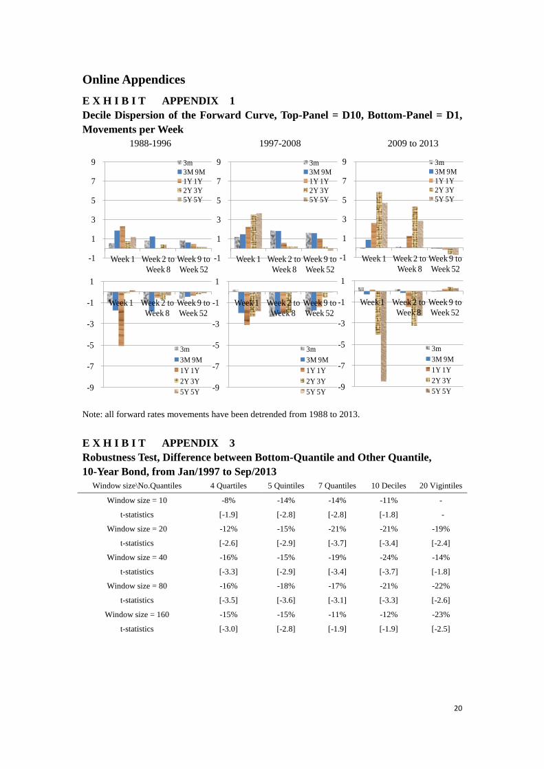
E X H I B I T APPENDIX 3
Robustness Test, Difference between Bottom-Quantile and Other Quantile,
10-Year Bond, from Jan/1997 to Sep/2013
Window size\No.Quantiles 4 Quartiles 5 Quintiles 7 Quantiles 10 Deciles 20 Vigintiles
Window size = 10 -8% -14% -14% -11% -
t-statistics [-1.9] [-2.8] [-2.8] [-1.8] -
Window size = 20 -12% -15% -21% -21% -19%
t-statistics [-2.6] [-2.9] [-3.7] [-3.4] [-2.4]
Window size = 40 -16% -15% -19% -24% -14%
t-statistics [-3.3] [-2.9] [-3.4] [-3.7] [-1.8]
Window size = 80 -16% -18% -17% -21% -22%
t-statistics [-3.5] [-3.6] [-3.1] [-3.3] [-2.6]
Window size = 160 -15% -15% -11% -12% -23%
t-statistics [-3.0] [-2.8] [-1.9] [-1.9] [-2.5]
-1
1
3
5
7
9
Week 1 Week 2 to
Week 8
Week 9 to
Week 52
3m
3M 9M
1Y 1Y
2Y 3Y
5Y 5Y
-9
-7
-5
-3
-1
1
Week 1 Week 2 to
Week 8
Week 9 to
Week 52
3m
3M 9M
1Y 1Y
2Y 3Y
5Y 5Y
-1
1
3
5
7
9
Week 1 Week 2 to
Week 8
Week 9 to
Week 52
3m
3M 9M
1Y 1Y
2Y 3Y
5Y 5Y
-9
-7
-5
-3
-1
1
Week 1 Week 2 to
Week 8
Week 9 to
Week 52
3m
3M 9M
1Y 1Y
2Y 3Y
5Y 5Y
-1
1
3
5
7
9
Week 1 Week 2 to
Week 8
Week 9 to
Week 52
3m
3M 9M
1Y 1Y
2Y 3Y
5Y 5Y
-9
-7
-5
-3
-1
1
Week 1 Week 2 to
Week 8
Week 9 to
Week 52
3m
3M 9M
1Y 1Y
2Y 3Y
5Y 5Y
21
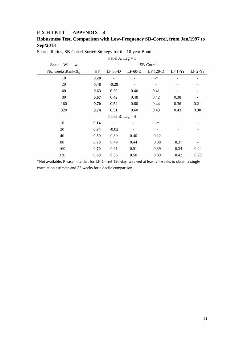
E X H I B I T APPENDIX 4
Robustness Test, Comparison with Low-Frequency SB-Correl, from Jan/1997 to
Sep/2013
Sharpe Ratios, SB-Correl-Sorted Strategy for the 10-year Bond
Panel A: Lag = 1
Sample Window SB-Correls
No. weeks\RankObj HF LF 30-D LF 60-D LF 120-D LF 1-Yr LF 2-Yr
10 0.28 - - -* - -
20 0.48 -0.29 - - - -
40 0.63 0.20 0.40 0.41 - -
80 0.67 0.42 0.48 0.42 0.38 -
160 0.70 0.52 0.60 0.44 0.36 0.21
320 0.74 0.51 0.60 0.43 0.43 0.30
Panel B: Lag = 4
10 0.14 - - -* - -
20 0.34 -0.02 - - - -
40 0.59 0.30 0.40 0.22 - -
80 0.70 0.49 0.44 0.38 0.37 -
160 0.70 0.61 0.51 0.39 0.34 0.24
320 0.60 0.55 0.50 0.39 0.42 0.28
*Not available. Please note that for LF-Correl 120-day, we need at least 24 weeks to obtain a single
correlation estimate and 33 weeks for a decile comparison.