Stock Market Rumors and Credibility

Daniel Schmidt∗

November 21, 2018

Abstract

Stock prices occasionally move in response to unveri�ed rumors. I propose a

cheap talk model in which a rumormonger's incentives to tell the truth depend on

the interaction between her investment horizon and the information acquisition

decisions of message-receiving investors. The model's key prediction is that short

investment horizons can facilitate credible information sharing between investors,

thereby accelerating the information capitalization into market prices. Analyzing

a dataset of takeover rumors covered by US newspapers, I �nd suggestive evidence

in support of this prediction.

JEL Classi�cation: G11, G14

Keywords: rumors, cheap talk, investment horizons, information e�ciency

∗HEC Paris, 1 Rue de la Libération, 78350 Jouy-en-Josas, France. Phone: (+33) 139 67 9408. Fax:(+33) 139 67 7085. Email: schmidt@hec.fr. A previous version of this paper was circulated underthe title �Communication in Financial Markets� and was part of my 2013 dissertation at INSEAD.For helpful comments I thank Marija Djordjevic, Bernard Dumas, Thierry Foucault, Denis Gromb,Alexander Guembel, Johan Hombert, Alexander Ljungqvist, Stefano Lovo, Vlad Mares, Clemens Otto,Joël Peress, Rémy Praz, Ioanid Rosu, David Schumacher, Christophe Spaenjers, Edward Van Wesep(SFS discussant), Timothy Van Zandt, and two anonymous referees as well as participants at the2014 SFS Cavalcade, the 2014 Labex Finance Conference, the 2012 BPP PhD Camp (Paris), and theINSEAD brownbag. I am also grateful to William Fisk for helping me with the data collection. I aloneam responsible for any errors.

1 Introduction

Stock prices occasionally move in response to unveri�ed rumors. On 14 December

2005, for example, the Wall Street Journal reported that �the stock price of Univision

Communications Inc. has surged 30% in recent weeks amid renewed speculation of a

possible sale or merger of the largest Spanish-language broadcaster in the US.� This

article is far from unusual. Analyzing a sample of 1,084 takeover rumors covered in the

media, I �nd that stock returns and share turnover surge precipitously around the days

of the initial rumor coverage (see Figure 4). As CNBC stock expert Herb Greenberg

succinctly observed: �Takeover rumors have always been part of the game of Wall Street,

but there are times they �y so quickly you don't have time to consider the sources.�

Why do investors trade based on unveri�ed rumors? After all, a de�ning feature

of such rumors is that their ultimate source is unknown (Peterson and Gist, 1951) and

hence they possibly originate from malicious rumormongers attempting to manipulate

the stock market. Yet, a surprisingly large fraction of the takeover rumors in my sample

come true in the sense that they are actually followed by a merger bid for the rumored

target stock. In many cases, investors would have therefore been right to trade on these

rumors. This paper o�ers the �rst rationalization of these phenomena. Speci�cally,

I develop a model in which information sharing can be credible in equilibrium, despite

investors not knowing the precise origin of that information�as is the case for stock

market rumors. The key intuition is that a short-term investor in possession of long-

term information has an incentive to share this information in order to accelerate its

capitalization into market prices; as a result, investors who receive such messages have

the incentive to trust and trade on the rumor.

In the model, a small investor who is privately informed about a stock's fair value

may send a �cheap talk� message to other investors (Crawford and Sobel, 1982). Exam-

ples of such messages include a rumor relayed by word-of-mouth, an investor �talking

her book,� and stock tips transmitted via social media.1 In choosing her message,

1Web platforms enabling investors to share stock tips have become popular enough to attract the

1

the rumormonger contemplates the costs and bene�ts of a lie. My main result is to

show that this cost�bene�t analysis depends critically on the rumormonger's investment

horizon: if she is short-term, truthful information sharing is more attractive because it

ensures that the rumor is in line with subsequent information arrivals and thus maxi-

mizes short-term price impact. If she is long-term, however, lying dominates because a

successful market manipulation results in a price reversal when the true state is even-

tually revealed. Being long-term, she can trade on�and pro�t from�this predictable

reversal.

For concreteness, assume that a stock currently trades at $100 and that the rumor-

monger knows the stock's long-term fair value to be (say) $150. Absent communication,

she expects the price to drift toward this value as other investors gradually become in-

formed. She further expects that a buy message, being reinforced by those information

arrivals, pushes the stock's price to (say) $130 over the short term; in contrast, a sell

message goes against the information acquired by other investors and thus leads to a

lower absolute price change, resulting in a short-term price of (say) $80. If the rumor-

monger is short-term�meaning that she must liquidate her position before the stock's

fair value is revealed�she wants to buy and tell the truth in order to maximize the

capitalization of her information in the liquidation price (resulting in a per-share pro�t

of $30 compared to a per-share pro�t of $20 from lying and going short). However, if

the rumormonger is long-term�meaning that she can remain invested until the stock's

fair value becomes publicly known�she prefers to go short and lie as this strategy al-

lows her to pro�t twice: �rst when buying back at the lower price of $80 and second

when going long to capture the ensuing price reversal up to $150. Lying thus results

in a total per-share pro�t of $90 ($20 from shorting plus $70 from the reversal), which

exceeds the pro�t of $50 that can be earned by going long and telling the truth. In

the example, therefore, the short-term rumormonger has the incentive to tell the truth,

attention of institutional investors, data providers, and regulators alike. Indeed, hedge funds and�nancial data providers are constantly sifting through Twitter for sentiment and news (New YorkTimes, 2010; Thomson Reuters, 2013). The SEC has issued guidance on the use of social media byinvestment advisers (see SEC, 2012).

2

while the long-term rumormonger wants to lie. Anticipating this, the message-receiving

investors only trust the message when they are su�ciently sure that it originates from

an informed sender with a short investment horizon.

I derive the truth-telling condition that describes when a rumormonger with an

intermediate trading horizon has the incentive�and thus the credibility�to truthfully

share her information. I �nd that this condition is more likely to be satis�ed the shorter

the rumormonger's investment horizon and the more verifying information is expected

to arrive. Hence the model predicts that short investment horizons can improve stock

price e�ciency by facilitating credible information sharing among investors, thereby

complementing a large literature that focuses on the negative e�ects of excessive short-

termism such as managerial myopia (Stein, 1996; Bushee, 1998; Chen et al., 2007b;

Derrien et al., 2013), the ampli�cation of market shocks, and return anomalies (Cella

et al., 2013; Cremers and Pareek, 2015). The result also runs counter to Dow and

Gorton (1994), who argue that short-term investors forgo trading on their long-term

information when they fear that it will not be re�ected in prices soon enough, thereby

lowering price e�ciency. I show that, in this very situation, investors have the incentive

and thus the credibility to share their information, which can possibly overturn the

Dow and Gorton (1994) result.

Existing work on strategic communication in asset markets focuses on the sender's

reputation as a source of credibility (Benabou and Laroque, 1992; Van Bommel, 2003).

My model di�ers by proposing a new channel for credibility based on the interplay

between a rumormonger's investment horizon and subsequent information arrivals. Im-

portantly, for this channel to work, investors must have some information about the

average investment horizon among the population of potential senders, but�unlike for

a reputation channel�they do not need to know the exact identity of the sender.2 My

model is thus the �rst to explain why investors trade on stock market rumors. In prac-

2To make this point explicit, Internet Appendix 1.2 considers a variant of my model in which therumormonger is drawn from a continuous distribution of potential rumormongers with di�erent invest-ment horizons. I show that assuming that investors know the distribution of potential rumormongers(rather than the exact identity of the rumormonger drawn from that distribution) is su�cient forobtaining the intuition that short investment horizons foster credibility.

3

tice, beliefs about the average trading horizon of potential senders could come from the

portfolio churn rates of a stock's institutional owners, from suspicious trading activity

by corporate insiders and short-sellers,3 or from the timing of a rumor (e.g., whether

it spreads at a time when speculation is rampant, so that a rumormonger may plan on

quickly moving to the next investment opportunity). Moreover, the circumstances of a

rumor may sometimes allow investors to narrow down the list of potential rumormon-

gers. For instance, some takeover rumors cite suspicious activity at the target �rm's

headquarter (e.g., a visit by executives of the alleged bidder) and so the rumormonger

may be found among shareholders that are geographically close to or have ties with

high-placed individuals at the target �rm.4

I verify the robustness of the horizon channel by considering several extensions of

the baseline model. First, I allow for the rumormonger to receive a noisy signal and

endogenize her choice of signal precision. I �nd that a short investment horizon reduces

the sender's incentives to acquire information but can nonetheless render prices more

e�cient by fostering credible information sharing among investors. Second, I allow for

the presence of multiple messages and show that this only strengthens the case for

truth-telling. Intuitively, the rumormonger is less able to e�ectively manipulate the

price when there is a second message and so truth-telling becomes more attractive.

Third, I relax the assumption that the rumormonger is a price taker and show how this

a�ects her incentives to communicate. I �nd that price impact gives her another reason

to lie: if she is long-term, a false message�by triggering an order �ow against which

she can trade�enables her to gradually establish a position at lower price impact costs.

However, this additional motive does not alter the conclusion that short investment

horizons facilitate credible information sharing. Additional extensions are provided

3Insider traders naturally want to hide their identity and may therefore leak information by spread-ing anonymous rumors. For instance, in an article dated 28 May 1998, the Wall Street Journal opinedthat �people planning to trade on inside information may be using the Internet to cover their tracks,by posting some of their information anonymously. If later quizzed by regulators, they could point tothe Web posting as the impetus for their decision to trade the stock or option.�

4In that same article, theWall Street Journal reported on suspicious Internet message-board activityprior to the acquisition of US Surgical Corp. by Tyco International Ltd, citing a message posted onYahoo talking about �a whole bunch of activity and a lot of meetings at US Surgical.�

4

in the Internet Appendix. For instance, I show there that the horizon mechanism is

robust to allowing for an uninformed sender who may blu� (i.e., who can pretend to be

informed), to a stock fundamental with a non-binary payo�, to endogenous information

acquisition by message receivers, and to short-sale constraints.

I shed a �rst light on the model's empirical relevance by compiling a dataset of news-

paper articles on takeover rumors, which are (by de�nition) unveri�ed and of unknown

origin at publication�allowing me to test the horizon channel without a potentially

confounding reputation e�ect.5 I �rst show that takeover rumors are associated with

a strong surge in trading activity and returns prior to and on the day of the rumor's

publication, suggesting that such rumors indeed move prices. Second, I show that the

takeover rumors are more likely to come true (in the sense that they are followed by

actual takeover bid announcements) and elicit a stronger market response if the target

stock's institutional owners appear to be more short-term. Taken together, these re-

sults provide support for my model's key intuition: takeover rumors for stocks held by

short-term investors are perceived as�and turn out to be�more credible.

This paper contributes to the literature on information transmission in �nancial

markets. One strand of this literature studies optimal information sales to competitive

investors (Admati and P�eiderer, 1986, 1988, 1990; Veldkamp, 2006; Cespa, 2008), and

another strand analyzes how information percolates through a large investor community

(Du�e and Manso, 2007; Du�e et al., 2009; Andrei and Cujean, 2017). A common

assumption in these two lines of work is that investors are precluded from lying op-

portunistically. While certainly useful for tractability, this assumption is arguably not

realistic in �nancial markets where investors gain at the expense of others. My model is

among the �rst to relax this assumption, thereby o�ering a potential microfoundation

for the abovementioned work. As already mentioned, the other notable exceptions with

strategic communication are Benabou and Laroque (1992) and Van Bommel (2003),

both of which obtain credibility from reputation concerns and thus require information

5In environments in which the sender's identity is known, both the horizon and the reputationchannel co-exist and, as I argue in Subsection 2.5, may oppose or even reinforce each other dependingon the context. The analysis of the interplay between these two channels is left for future research.

5

about the sender's identity. In contrast, the horizon channel developed here requires

only that investors hold su�ciently short-term beliefs about the average investment

horizon of potential senders�and thus o�ers a �rst explanation of why rumors from

unknown sources can occasionally move prices.

My model is further related to recent work by Kovbasyuk and Pagano (2015) and

Pasquariello and Wang (2018). The former paper proposes a model to explain why

small arbitrageurs concentrate their e�orts to advertise investment ideas on one target

company at a time; the latter paper shows that institutional investors concerned with

the intermediate value of their portfolios have an incentive to disclose some of their

information to the detriment of long-term pro�ts. Both papers assume that investors

can pre-commit to a given signal structure and justify this assumption citing reputation

concerns. In contrast, I focus on an anonymous sender without reputation. I further

di�er by considering the interplay between the sender's investment horizon and subse-

quent information arrivals. It is this interplay that gives rise to credible information

sharing without the need to make an assumption about pre-commitment to a speci�c

signal structure.

Finally, I contribute to the empirical literature on information disclosure and stock

market rumors. Early papers examining selected samples of stock tips, takeover rumors,

and Internet message-board postings �nd evidence for the predictability of trading and

volatility but not of returns.6 More recently, Ljungqvist and Qian (2016) identify a set

of small arbitrageurs who are able to disclose credible negative reports about seemingly

overvalued companies, and Chen et al. (2014) and Bartov et al. (2018) document that

comments published on social media platforms such as SeekingAlpha.com or Twitter

predict future earnings and stock returns. While reputation concerns are arguably

important in these contexts, short holding periods and the desire to accelerate price

discovery may contribute to explaining the credibility of these messages. With regard to

takeover rumors, Ahern and Sosyura (2015) provide an in-depth study of �sensational�

6See Lloyd-Davies and Canes (1978); Liu et al. (1990); Pound and Zeckhauser (1990); Barber andLoe�er (1993); Tumarkin and Whitelaw (2001); Dewally (2003); Antweiler and Frank (2004).

6

media coverage and �nd that the stock prices of target �rms jump sharply on the day of

a rumor's publication. I extend their analysis and, guided by the theory, analyze how

rumor accuracy and stock market responses relate to proxies for the average investment

horizon of target stock investors.

The paper proceeds as follows. Section 2 introduces and solves the baseline model,

and Section 3 discusses a number of extensions. Section 4 presents a brief empirical

analysis for a sample of takeover rumors covered by US newspapers. Section 5 o�ers

concluding thoughts. Unless noted otherwise, proofs are collected in the Appendix.

2 Baseline Model

Subsection 2.1 sets up the baseline model. Subsection 2.2 solves the no-communication

benchmark. Subsections 2.3 and 2.4 derive the conditions under which there exists a

credible communication equilibrium in pure- and mixed-strategies, respectively. Sub-

section 2.5 discusses the model's key prediction regarding investment horizons and price

e�ciency and relates it to alternative channels proposed in the literature.

2.1 Setup

A single stock is traded for two periods (t = 0 and t = 1) before it pays o� (t = 2). The

stock's payo� θ is either −1 or +1 with equal probability.

As in Kyle (1985), competitive market makers, henceforth denoted M , receive in-

vestors' market orders and set prices so as to break even on the net order �ow ωt:

pt = E(θ |ωt)

There is a continuum of competitive (i.e., price-taking) investors. Prices move only when

many investors trade in the same direction. For simplicity, I assume that investors are

risk-neutral and capital-constrained. Speci�cally, in each period, an investor's trading

position lies in the interval [−x , x] with x < 1. It follows that investors take their

7

maximum long (resp. short) position whenever the price is below (resp. above) their

expectation of the �nal dividend.

One investor from the continuum, henceforth labeled L (for �leader�), can send a

message m ∈ {−1,+1} to the other investors�denoted F (for �followers�)�at no cost.

m can be interpreted in several ways. First, m may refer to word-of-mouth commu-

nication. Shiller (2000) writes that the �word-of-mouth transmission of ideas appears

to be an important contributor to day-to-day or hour-to-hour stock market �uctua-

tions� (p. 155).7 Second, m can be interpreted as stock tips shared on social media.

Starting with early message boards such as RagingBull.com, web talk about stocks has

proliferated with the emergence of new and increasingly sophisticated platforms.8 Fi-

nally, to the extent that asset holdings are di�cult to verify, m may also represent an

investor �talking his book� (Bhattacharya and Nanda, 2013; Pasquariello and Wang,

2018). I assume that L knows θ before trading in period t = 0.9 The message-receiving

investors F may learn about θ from m. In addition, at t = 1, each investor has the

chance to become informed with probability µ ∈ [0, 1]. With a continuum of investors,

the fraction of investors that end up knowing θ equals µ almost surely (see Sun, 2006,

for a precise de�nition). This assumption captures the intuitive idea that information

gradually becomes available as the �nal date approaches, and it plays a key role in

determining L's incentives to lie or to tell the truth as explained below.

I assume that L faces the risk of having to leave the market prematurely. That is,

with probability λ ∈ [0, 1], L is subject to a liquidity shock that forces her to close her

position in t = 1. If λ = 0, she can hold out until the dividend is realized in t = 2; if

λ = 1, she must exit in t = 1. λ is common knowledge. Because L's expected trading

pro�t is essentially a weighted average of short-term and long-term pro�ts, I refer to λ

7See Hong et al. (2005); Ivkovic and Weisbenner (2007) for more examples on the ubiquity ofword-of-mouth in �nancial markets.

8For instance, the tone of comments on SeekingAlpha.com, one of the most popular investment-related social media websites, has been shown to predict future stock returns and earnings surprises(Chen et al., 2014). In view of these developments, �nancial data provider Thomson Reuters nowallows its users to �track activity in real time across Twitter and StockTwits [a social network for the�nancial community] by analyzing the sentiment behind the tweets� (Thomson Reuters, 2013, p. 2).

9Internet Appendix 1.1 covers the case where L may be uninformed with some probability.

8

as a measure of L's investment horizon.

To prevent the order �ow from being fully informative, I assume that noise traders

submit random market orders. For tractability, noise trader demand is assumed to

be uniformly distributed, st ∼ U(−1, 1).10 Let qit denote investor i's market order in

period t. The order �ow observed by market makers M is

ωt =

∫i

qit di+ st .

Message m is cheap talk (Crawford and Sobel, 1982). In other words, investor L is

free to tell the truth or to lie about her information. The message-receiving investors F

assess the credibility of m; they trade in direction of m when (i) they believe that L has

an incentive to tell the truth and (ii) they pro�t from doing so. Thus, as is common in

the cheap talk literature, the credibility of m depends on the alignment of preferences

between sender L and receivers F . While all investors maximize trading pro�ts, such

preference alignment arises endogenously from the model's trading environment.

Note that L could potentially send a message at any time. However, it turns out

that only a message sent between t = 0 and t = 1 can be credible. To see this, suppose

that L knows θ = 1 and therefore wants to buy. If L can send a credible message

before t = 0 then she can ensure to buy low by sending m = −1, thereby inducing

other investors to sell. Because there is no risk of her lie being uncovered in t = 0, this

strategy is a sure way to boost her pro�ts. It follows that no rational investor would

expect the early message to be true. I therefore focus on messages sent between t = 0

and t = 1. Figure 1 summarizes the model setup.

2.2 No-communication benchmark

I start by solving for the trading equilibrium when investors F believe thatm is uninfor-

mative. L might then just as well send an uninformative message, thereby vindicating

10The exact width of the noise trading interval matters only in relation to x, the severity of investors'capital constraints. st ∼ U(−1, 1) together with x < 1 ensures that the order �ow is not fullyinformative.

9

F s' beliefs. This is the so-called �babbling� equilibrium that exists in any cheap talk

model (see e.g. Farrell and Rabin, 1996). Another interpretation is that L is simply

prevented from sending a message.

To construct the equilibrium, I �rst derive prices as a function of conjectured de-

mands and then verify that the conjectured demands are indeed optimal.

Prices At t = 0, investor L trades qL0. Given that her trade has no price impact, she

can establish her position secretly. The other investors remain uninformed and refrain

from trading. Order �ow is uninformative about θ (i.e., ω0 = s0), and market makers

set p0 = E(θ |ω0) = 0.

At t = 1, a fraction µ of the other investors F becomes informed. Risk neutrality

together with capital constraints imply that informed investors buy qi1 = x (sell qi1 =

−x) when they learn that θ = 1 (θ = −1). Summing over individual demands is not,

which renders the order �ow informative:

ωb1 =

µx+ s1 when θ = 1

−µx+ s1 when θ = −1

where superscript b stands for babbling (i.e., when m is uninformative). Market makers

set the stock price equal to the expected value of θ conditional on the order �ow ωb1.

When ωb1 > −µx + 1, M understand that the informed F must have bought, which

implies θ = 1. Similarly, when ωb1 < µx − 1, M infer that θ = −1. When µx − 1 ≤

ωb1 ≤ −µx + 1, both cases are possible and so Ms' prior about θ remains unchanged.

The price function is:

pb1(ωb1)

=

1 if − µx+ 1 < ωb1 ≤ µx+ 1

0 if µx− 1 ≤ ωb1 ≤ −µx+ 1

−1 if −µx− 1 ≤ ωb1 < µx− 1

(1)

10

Optimal trading strategy When submitting their orders at t = 1, investors form

expectations about p1. For example, consider the case of an investor who knows θ = 1.

He expects other informed investors to buy, implying that order �ow is distributed

according to ωb1 ∼ U(µx − 1, µx + 1). Using (1), the investor calculates the expected

price E(pb1 | θ = 1

)= µx < 1, which con�rms that the investor pro�ts from buying

when θ = 1. The case of θ = −1 is analogous.

Proposition 1. In the �babbling� equilibrium (i.e., when m is uninformative), informed

investors trade in direction of their information, uninformed investors refrain from

trading, and prices are given by (1).

2.3 Pure-strategy communication equilibrium

In this subsection, I derive the Bayesian Equilibrium in pure strategies of the trading

game with credible communication. I conjecture that F andM believe that L truthfully

reportsm = θ. In turn, L believes that investors F trade in the direction ofm as long as

it is not contradicted by their private signals. I now construct an equilibrium consistent

with these beliefs.

Prices As before, we have p0 = E(θ |ω0) = 0. A fraction µ of the other investors F

learns θ directly and thus knows whether (or not) L has told the truth. The remaining

fraction (1 − µ) relies on m and, given their beliefs, concludes that θ = m. Hence the

order �ow is given by

ω1 =

x+ s1 when m = 1 and θ = 1

−x+ s1 when m = −1 and θ = −1

11

Market makers set prices conditional on ω1. This leads to the following price function:

p1(ω1) =

1 if −x+ 1 < ω1 ≤ x+ 1

0 if x− 1 ≤ ω1 ≤ −x+ 1

−1 if −x− 1 ≤ ω1 < x− 1

(2)

When choosing their demand for the stock, investors form expectations about p1.

Suppose, for example, that investor L knows θ = 1 and considers sending the message

m = 1. She then anticipates an order �ow of ω1 ∼ U(x − 1, x + 1). Given (2), she

calculates an expected price of E(p1 |m = 1, θ = 1) = x. Now suppose that L decides

to lie; that is, reporting m = −1 even though θ = 1. This strategy leads to an expected

price of E(p1 |m = −1, θ = 1) = −x(1− 2µ). The other cases are symmetric.

Optimal trading strategy I now derive investor L's optimal trading policy. It is

instructive to start with the case where L is strictly long-term (λ = 0). I show that, in

this case, L prefers to lie as long as µ < 12. For concreteness, suppose that θ = 1. Given

her long horizon, L is certain to close her position at this price at t = 2; and because

p1 ≤ θ, she wants to be long in the stock after trading in t = 1 (i.e., qL1 = x). Thus

L has an incentive to manipulate the intermediate transaction price p1. In particular,

by reporting m = −1 she seeks to induce other investors to sell, thereby de�ating the

price p1. This has two bene�ts. First, at t = 1, she can buy the asset at a greater

discount. Second, by selling short at t = 0, she can �ride� the initial price decline

caused by the negative rumor.

Next, consider the case where L is strictly short-term (λ = 1). In this case, L prefers

to tell the truth as long as µ is strictly positive. As argued previously, lying is attractive

because it moves the stock price away from its fundamental value, thereby creating a

price reversal. Yet because L is a short-term investor, she must liquidate her position

before the reversal occurs. Hence her pro�t is now determined solely by the short-

term stock return between periods t = 0 and t = 1. The magnitude of this return is

12

maximized by truth-telling because this strategy ensures that her message is con�rmed

by subsequent information arrivals.

Equilibrium I now explore the case of an intermediate trading horizon (0 < λ < 1)

for θ = 1 (θ = −1 is symmetric). L's expected pro�t is a weighted average of her short-

term and long-term pro�ts. Hence her expected per-share pro�t from truth-telling is

E (p1 |m = θ = 1) + (1− λ) (1− E (p1 |m = θ = 1)) , (3)

whereas her expected per-share pro�t from lying (m = −θ) is

− E (p1 |m = −1, θ = 1) + (1− λ) (1− E (p1 |m = −1, θ = 1)) . (4)

L prefers to share her information truthfully when the expected pro�t in (3) exceeds

its counterpart in (4), which implies

− E (p1 |m = θ = 1)

E (p1 |m = −1, θ = 1)≥ 2− λ

λ. (5)

When condition (5) is satis�ed, the postulated beliefs about L's communication behav-

ior are vindicated. Moreover, given that m is true, the uninformed investors F bene�t

from trading on it.11

Proposition 2. A pure-strategy communication equilibrium exists if and only if

µ

1− 2µ≥ 1− λ

λ. (6)

In this equilibrium, prices are given by (2) and L truthfully shares her information

(m = θ) and trades accordingly. At t = 1, investors F trade in the direction of θ, which

they learn either directly or through m.

11In Internet Appendix 1.1, I allow for L to be potentially uninformed, in which case she pretendsto be informed. I show that, in this case, the uninformed F then trade more cautiously in order tocurb their losses from trading on L's blu�.

13

Condition (6) demarcates the parameter region in which a pure-strategy communi-

cation equilibrium exists. If (6) does not hold, then there cannot be an equilibrium in

which L always reveals her information. This follows from the misalignment of L's and

F s' preferences: whereas the investors F want to trade in the direction of θ, L wants

them to do the opposite. Thus, given some conjecture about F s' responses to m, L

prefers sending a message m to which F s' conjectured response is not optimal. But

then F will want to deviate.

Corollary 3. A pure-strategy communication equilibrium is more likely to be feasible

when L has a short investment horizon (λ large) and when a larger fraction of the other

investors F learn verifying information (µ large).

Proof. Inspection of (6) reveals that the left-hand side is increasing in µ while the

right-hand side is decreasing in λ.

Two key results follow from condition (6). First, credible communication is more

likely when L has a short investment horizon (λ large). The reason is that truth-telling

pays o� faster than does a false-rumor strategy, which generates its pro�ts from the

ensuing reversal. A short-term investor L cares only about the expected price change

between t = 0 and t = 1, which is maximized when she tells the truth because her

message is then in line with subsequent information arrivals.

Second, credible communication is more likely when a larger fraction of message-

receiving investors obtains verifying information from other sources. Intuitively, when

µ is large, there are fewer investors to be fooled by a false-rumor strategy and at the

same time more informed investors who trade against a false rumor. As a result, L has

less incentive to lie.12

12In Internet Appendix 1.4, I allow for endogenous information acquisition by F . In that appendixI show that a communication equilibrium does still exist provided that (i) the costs of informationacquisition are not too high and (ii) the fundamental can take on more than two values.

14

2.4 Mixed-strategy communication equilibrium

I next solve for a mixed-strategy communication equilibrium in which L tells the truth

(m = θ) with probability ρ ∈ [0, 1]. Since this implies that L lies with probability 1−ρ,

the uninformed F can lose from trading on m and may thus trade more cautiously. Let

φ ∈ [0, 1] denote their trading aggressiveness, meaning that they buy (sell) φx (−φx)

upon observing m = 1 (m = −1).

Prices As before, we have p0 = E(θ |ω0) = 0. A fraction µ of the other investors F

learns θ directly. These investors will trade with or against the message m depending

on whether L told the truth or lied. The remaining fraction (1− µ) trades on m with

intensity φ. The order �ow is given by:

ω1 =

((1− µ)φ+ µ)x+ s1 when m = 1 and θ = 1

((1− µ)φ− µ)x+ s1 when m = 1 and θ = −1

−((1− µ)φ− µ)x+ s1 when m = −1 and θ = 1

−((1− µ)φ+ µ)x+ s1 when m = −1 and θ = −1

Market makers set prices conditional on ω1. I conjecture that (1 − µ)φ ≥ µ, since

otherwise L cannot bene�t from lying because her message is ine�ective in manipulating

the price away from the stock's fundamental value. This leads to the following price

15

function:

p1(ω1) =

1 if ((1− µ)φ− µ)x+ 1 < ω1 ≤ ((1− µ)φ+ µ)x+ 1

2ρ− 1 if −((1− µ)φ− µ)x+ 1 < ω1 ≤ ((1− µ)φ− µ)x+ 1

ρ2−ρ if −((1− µ)φ+ µ)x+ 1 < ω1 ≤ −((1− µ)φ− µ)x+ 1

0 if ((1− µ)φ+ µ)x− 1 ≤ ω1 ≤ −((1− µ)φ+ µ)x+ 1

− ρ2−ρ if ((1− µ)φ− µ)x− 1 ≤ ω1 < ((1− µ)φ+ µ)x− 1

−(2ρ− 1) if −((1− µ)φ− µ)x− 1 ≤ ω1 < ((1− µ)φ− µ)x− 1

−1 if −((1− µ)φ+ µ)x− 1 ≤ ω1 < −((1− µ)φ− µ)x− 1

(7)

where 2ρ−1, for example, is the expected value of θ conditional on knowing that m = 1

and either θ = 1 (with probability 12ρ) or θ = −1 (with probability 1

2(1 − ρ)). Given

this price function, L calculates the expected prices given m and θ, E (p1 |m, θ).

For L to play a mixed strategy, she must be indi�erent between truth-telling and

lying. Hence condition (5) must be satis�ed with equality, which pins down ρ as a

function of µ, λ, and φ. Taking ρ as given, the uninformed investors F calculate E (θ |m)

and choose φ to maximize their expected pro�ts. The following proposition summarizes

the resulting mixed-strategy communication equilibrium.

Proposition 4. A mixed-strategy communication equilibrium exists i� there exists a

12< ρ < 1 such that the following two conditions are satis�ed:

µ

(1− µ)φ− µ=

1− λλ

(2− ρ)(2ρ− 1) (8)

xµ ≤ (2− ρ)(2ρ− 1)

2ρ. (9)

In this equilibrium, L tells the truth (lies) with probability ρ (1− ρ) and trades accord-

ingly. When investor F is informed, he buys (sells) x when θ = 1 (θ = −1). When F

remains uninformed, he buys (sells) an amount φx when m = 1 (m = −1), where φ is

16

given by

φ =

φ if φ ≤ 1

1 if φ > 1

(10)

with φ = 11−µ

[1x−(

2ρ(2−ρ)(2ρ−1) − 1

)µ].

Condition (9) follows from the requirement that, for there to be a mixed-strategy

communication equilibrium, lies must be e�ective enough to potentially manipulate the

price away from the fundamental. Intuitively, the uninformed F trade more aggressively

when m is more likely to be true. Note also that Proposition 4 gives only an implicit

solution for the fraction ρ of truthful messages. Nevertheless, the following corollary is

easy to establish.

Corollary 5. In a mixed-strategy communication equilibrium, the fraction ρ of truth-

ful messages is decreasing in L's investment horizon (i.e., is increasing in λ) and is

increasing in the fraction µ of other investors F that obtain verifying information.

Figure 2 illustrates the feasible equilibria that exist for di�erent λ-µ pairs (hold-

ing x constant). As is common in cheap talk models, there always exists a babbling

equilibrium. The �gure's solid line represents the truth-telling condition (6). For λ-µ

pairs above this line, there exists a pure-strategy communication equilibrium in which

L truthfully shares her information and this is anticipated by F and M . For λ-µ

pairs between the solid line and the dashed line, complete truth-telling is not incen-

tive compatible; however, there exist mixed-strategy communication equilibria in which

market participants expect L to tell the truth with probability ρ and L, being indi�er-

ent between truth-telling and lying, conforms to these beliefs. The dotted line further

partitions the mixed-strategy equilibrium space into those equilibria in which the un-

informed F fully exploit their capital constraints when trading on m (φ = 1) and those

in which they curb their trading aggressiveness (φ < 1) in order to limit their collective

price impact.

In sum, I �nd that mixed-strategy and pure-strategy equilibria do not co-exist. That

17

is, for a given set of parameter values, L either always tells the truth or randomizes

between lying and truth-telling. Furthermore, and in line with the intuition from the

pure-strategy communication equilibrium, short investment horizons and subsequent

information arrivals induce more information sharing.

2.5 Model predictions and related literature

Since noise trading is exogenous, I cannot make statements about how information shar-

ing a�ects overall welfare. Instead, I show that credible information sharing accelerates

informed trading and tends to improve price e�ciency.

Proposition 6. In any pure-strategy communication equilibrium, there is more trading

activity and prices at t = 1 are informationally more e�cient compared to the babbling

equilibrium (i.e., when m is not credible). In any mixed-strategy communication equilib-

rium, there is more trading activity and, for ρ > 23, prices at t = 1 are informationally

more e�cient compared to the babbling equilibrium:

E[∣∣ω1

∣∣] > E[∣∣ωb1 ∣∣]

E[V ar

(θ | p1

)]< E

[V ar

(θ | pb1

)]Following Kyle (1985), I measure price e�ciency by E [V ar (θ | p)]. The smaller this

measure, the more information is incorporated into the price, which lowers the residual

uncertainty faced by investors and�to the extent that prices convey information to real

decision makers (see e.g. Luo, 2005; Chen et al., 2007a; Foucault and Fresard, 2012;

Dessaint et al., 2018)�promotes real e�ciency.13

The model's key contribution is to show that short investment horizons together

with subsequent information arrivals can lead to credible information sharing among

13See Bond et al. (2012) for a survey of the literature on the real e�ects of �nancial markets.A counterexample to the bene�cial e�ects of information sharing via disclosure is given by Goldsteinand Yang (2017), who present a model in which disclosure regarding a variable that the real decisionmaker cares to learn can reduce price informativeness and hence real e�ciency.

18

investors, which tends to improve price e�ciency.14 However, there are other channels

through which investment horizons may a�ect price e�ciency. For instance, exist-

ing work on strategic disclosures by investment gurus (Benabou and Laroque, 1992;

Van Bommel, 2003), boutique hedge funds (Kovbasyuk and Pagano, 2015; Ljungqvist

and Qian, 2016) or fund managers (Pasquariello and Wang, 2018) rely on reputation

concerns to explain why such disclosures can be credible. Since long horizons make

reputation more valuable, these papers predict that long investment horizons induce

more truth-telling.15 Yet reputation can matter only if the sender's identity is known

and hence this mechanism cannot explain why investors would ever want to trade on

stock rumors�which is the focus of this paper.

Arbitrage risk is another important reason why short investment horizons are thought

to reduce price e�ciency. Speci�cally, Dow and Gorton (1994) argue that a short-term

investor forgoes trading on her long-term information if the likelihood of other investors

subsequently trading on that information is too low. My contribution is to show that, in

this exact situation, the short-term investor has an incentive and thus the credibility to

share her information. It follows that allowing the short-term investor to send a cheap

talk message�hardly a controversial assumption�can overturn the Dow and Gorton

(1994) result. To show this formally, Internet Appendix 1.7 establishes the Dow and

Gorton (1994) equilibrium in a trading model very similar to theirs and then shows

14An exception can occur for mixed-strategy communication equilibria with low levels of ρ. Here,price e�ciency can even be lower than in the babbling equilibrium because the trading induced by anoisy message blurs the order �ow signal for market makers. However, since ρ increases with λ, anincrease in λ that is large enough to induce a communication equilibrium with ρ > 2

3 will necessarilyimprove price e�ciency.

15The horizon channel and the reputation channel need not oppose each other, however. To see this,note that reputation really hinges on the investment horizon of the sender, whereas the horizon channelonly requires a short-term perspective for the individual stock holding under consideration�and thesetwo notions of horizon are not the same. For example, an investor may well plan to communicaterepeatedly with market participants and thus care about her reputation, while having at the same timea short-term perspective in a particular stock due to the desire to free-up capital for another investmentidea or due to recall risk in the case of a short position. Hence, the two channels can work hand inhand to facilitate credible information sharing�a point which I make formally in Internet Appendix 1.6using a repeated game setting. Suggestive evidence for this argument can be gleaned from Zuckerman(2012)'s analysis of public announcements by hedge funds. Speci�cally, he �nds that, although hedgefund managers publish both buy and sell recommendations, only their sell recommendations predictreturns, which may be explained by hedge funds having a shorter holding period for their short positions(e.g., due to lending fees and recall risk).

19

how voluntary information sharing represents a pro�table deviation for a short-term

arbitrageur that would otherwise not act on her information.16

The e�ect of investment horizon on price e�ciency may depend also on the incentives

to acquire information and the possible real e�ects of information disclosure. Indeed,

long-term investors are expected to acquire more information, which they impound into

prices with their trades. Such investors may also care more about the e�ciency of �rms'

investment decisions, giving them stronger incentives for truth-telling. Both of these

e�ects would tend to improve price e�ciency.

In short, while there are many channels through which investment horizons can a�ect

price e�ciency, the preceding discussion suggests that the horizon channel is more likely

to dominate when reputation is not at stake and when private information is due to

(say) insider tips rather than costly investment research. Section 4 o�ers empirical

support for this idea by examining stock market rumors about imminent takeovers.

3 Model Extensions

This section presents several extensions of the baseline model. In Subsection 3.1, I relax

the assumption that L has perfect information about θ and let her instead choose the

precision of a noisy signal about θ. In Subsection 3.2, I allow for the presence of a second

rumormonger and show that this strengthens the case for credibility. In Subsection 3.3,

I analyze how the communication equilibrium is a�ected when L has price impact.

Additional extensions are collected in the Internet Appendix.17

16It is also possible to recast the Dow and Gorton (1994) result within the framework of my model:suppose that investor L is short-term and faces a per-share transaction cost τ (if she buys x, she paysτx in transaction costs). It is easy to show that, if L engages in no communication, then she will wantto trade at t = 0 only when µ is large enough (i.e., µ ≥ τ/x). Thus, when subsequent informationarrivals are not su�ciently probable, L refrains from trading. However, I show that L prefers to shareher information in this case, thereby accelerating price discovery.

17Speci�cally, I show there that the model can be extended (i) to allow for an uninformed L pre-tending to be informed, (ii) to allow the sender to be drawn from a pool of heterogeneous senders,(iii) to feature a non-binary �nal payo�, (iv) to allow for endogenous information acquisition by mes-sage receivers, (v) to accommodate short-sale constraints, (vi) to allow for reputation (for a known L)in a repeated game setting and (vii) that information sharing can be credible in a multi-period modelin the spirit of Dow and Gorton (1994). In all these extensions, I focus on communication equilibriain pure strategies.

20

3.1 Noisy signals and endogenous information acquisition

The baseline model was solved under the assumption that L has perfect knowledge of θ.

In this subsection, I instead assume that L has access to an imperfect signal about θ

and then endogenize L's choice of signal precision.

Speci�cally, I assume that, before trading at t = 0, L receives a noisy signal S

about θ with Pr(θ = 1 |S = 1) = π, where π > 12denotes the signal precision.

For simplicity, I continue to assume that, before trading at t = 1, a fraction µ of

other investors F (but not L) observes θ perfectly.18 Because S and therefore m may

be wrong, the uninformed F can lose from trading on m and so they may choose

a lower trading aggressiveness φ ∈ [0, 1]. The following proposition shows how the

communication equilibrium is a�ected.

Proposition 7. When L receives a noisy signal S with precision Pr(θ = 1 |S = 1) =

π > 12, an equilibrium with credible communication exists if the following two conditions are

satis�ed:

(2π − 1)µ

(2− π)(2π − 1)((1− µ)φ− µ) + 2(1− π)µ>

1− λλ

(11)

µx ≤ (2− π)(2π − 1)

2π. (12)

In this equilibrium, L truthfully shares her signal (m = s) and trades accordingly. When

investor F is informed, he buys (sells) x when θ = 1 (θ = −1). When investor F

remains uninformed, he buys (sells) an amount φx when m = 1 (m = −1), where φ is

given by

φ =

φ if φ ≤ 1

1 if φ > 1

(13)

with φ = 11−µ

[1x−(

2π(2−π)(2π−1) − 1

)µ].

As before, the truth-telling condition (11) is more likely to be satis�ed when L has a

18Assuming that investors F receive noisy signals or that L also has the chance to become perfectlyinformed at t = 1 only complicates the analysis but does not a�ect its conclusions.

21

shorter investment horizon (λ large) and when subsequent information arrivals are more

likely (µ large). Moreover, it turns out that truth-telling is more likely when L has a

more informative signal (π large). Intuitively, if S is noisy, L �nds it easier to pro�t from

the short-term price pressure induced by a false rumor.19 The trading aggressiveness

of the uninformed F takes the same form as in the mixed-strategy equilibrium from

Proposition 4. Indeed, to an uninformed F it does not matter whether m is not true

because L deliberately lied or because L relayed a false signal.

I next assume that, in order to acquire a signal with precision π, L faces the cost

C(π) = c(π2 − 1

4

)with c > 0.20 The following proposition characterizes L's optimal

information acquisition choice.

Proposition 8. Suppose that, when L invests C(π) = c(π2 − 1

4

)with c > 0, she obtains

a signal S with precision Pr(θ = 1 |S = 1) = π. Given the equilibrium strategies

described above, it is optimal for L to choose

π∗ =

π if π ≤ 1

1 if π > 1

(14)

with

π =1

2c

[(1− λ)x+ 2c−

√((1− λ)x+ 2c)2 − 4c (µλx2 + (1− λ)2x)

].

An equilibrium with credible communication and endogenous information acquisition

exists if condition (11) from Proposition 7 is satis�ed for π = π∗.

The proposition shows that L acquires some information as long as doing so is not

in�nitely costly and acquires all the available information if c is su�ciently small. The

implication is that, for every λ < 1 and µ < 12, there exists a c small enough to en-

19To see this, note that for π = 12 , L is uninformed about θ. In this case, she can only hope to pro�t

by trading on the price pressure that results from sending a false message. Hence L behaves like anuninformed investor who pretends to be informed (see Internet Appendix 1.1).

20Subtracting 14c from the cost function ensures that L incurs no information acquisition costs when

choosing to remain uninformed (π = 12 ).

22

sure that L acquires a su�cient amount of information to make the communication

equilibrium viable. In the Appendix, I show further that, compared to the babbling

equilibrium, L acquires weakly less information when she has the possibility to commu-

nicate. Intuitively, a credible messagem always increases expected pro�ts (by increasing

information capitalization at t = 1, when L might have to exit), but it does so relatively

more for imprecise signals (because, given that the uninformed F trade on m, L can

predict p1 even when her signal is imprecise). As a result, she acquires less information

overall. Even so, prices typically become more e�cient when communication is credible.

The reason is that a credible message induces followers to trade, and this has a �rst-

order e�ect on price e�ciency. Therefore, any increase in λ that makes communication

credible is likely to improve price e�ciency.

3.2 Multiple messages

In this extension, I allow for a second message from another trader. It turns out that

this modi�cation only strengthens the case for truth-telling. Intuitively, when there is

more than one sender, e�ective communication requires coordination and it is easier for

senders to coordinate around the truth.

Let α ∈ [0, 1] be the probability with which there is another sender L2 and let χ = 1

(χ = 0) denote the state in which L2 is (is not) present. At the time of sending m1,

L1 (now indexed with 1 to distinguish her from L2) does not know whether there will

be a second message. I continue to assume that L1�and L2 if present�receive noisy

signals S1 and S2, respectively. For simplicity, I assume that S1 and S2 have the same

precision and uncorrelated signal errors.

When there are two messages, the uninformed investors F form their expectations

about θ and p1 based on both m1 and m2; otherwise, they rely only on m1. I conjecture

that F and market makers M believe that m1 = S1 and, if present, m2 = S2. I further

conjecture that the uninformed F buy (sell) φx when m1 = m2 = 1 (m1 = m2 = −1)

and refrain from trading when m1 6= m2.

23

Proposition 9. When there is a second message with probability α, an equilibrium with

credible communication exists if

− (1− α)E(p1 |S1, m1 = S1, χ = 0) + αE(p1 |S1, m1 = S1, χ = 1)

(1− α)E(p1 |S1, m1 = −S1, χ = 0) + αE(p1 |S1, m1 = −S1, χ = 1)>

2− λλ

.

(15)

In this equilibrium, prices are given by (18) in the Appendix and both senders truthfully

share their signals. If the two messages are aligned, the uninformed investors F trade

in that direction at t = 1; if the two messages contradict each other, the uninformed

investors F abstain from trading.

I show in the Appendix that condition (15) is more likely to hold when α is high. In

the extreme case of α = 1 and π = 1 (i.e., when there are always two senders with perfect

information), the communication equilibrium can always be supported (regardless of λ

and µ). The intuition is straightforward: if L expects m2 to reveal θ, then a lie on her

part has no chance of manipulating the price away from θ (e.g., depressing the price

when θ = 1). In the more realistic case of π < 1, however, a long-term rumormonger

will typically prefer to lie even when there is another message for sure (α = 1).

To conclude, like a larger µ, a larger α �disciplines� L by increasing her incentive

to tell the truth. In any event, truth-telling is always more likely to occur when λ is

larger (except for the special case α = 1 and π = 1).

3.3 Price impact

In the baseline model, L is a price taker. This assumption allows to focus on how L's

communication strategy can a�ect the equilibrium price. In practice, however, L may

also a�ect the price with her trades. To allow for L to have price impact, I assume

that L represents a fraction α of the unit mass of traders.21 I continue to assume that

all traders (including L) face a position limit of x < 1, so that this extension nests

the baseline model without price impact for α → 0. For tractability, I assume that

21I thank an anonymous referee for suggesting this setup.

24

L is not too large, α ≤ 13. This assumption ensures that L's position limit is binding

in any truth-telling equilibrium.22 As before, I assume that L faces a liquidity shock

with probability λ, forcing her to liquidate her position at t = 1. Let η = 1 designate

the state of the world in which L faces a liquidity shock (i.e., Pr(η = 1) = λ). For

simplicity, I assume that η is commonly observed before trading commences at t = 1.23

The next proposition shows how the communication equilibrium is a�ected.

Proposition 10. A truth-telling equilibrium exists i� the condition

x(1− αx) (1− λ(1− x(1− 2α))) > λy∗0(1− αx) ((1− α)(1− 2µ)x− αy∗0)

+(1− λ)x (1 + αy∗0) + (1− λ) (1− αx) (x+ y∗0) ((1− α)(1− 2µ)x− α(x+ y∗0))

(16)

is satis�ed for α ≤ 13. The term y∗0 denotes L's pro�t-maximizing trade at t = 0 when

she deviates to lying and is given by

y∗0 =

+x if y > x

y if − x ≤ y ≤ x

−x if y < −x

with

y =x [(1− 2µ)(1− αx) + xα2(3− 2(λ+ µ))− α(2(1− µ)− λ)]

2α(1− αx).

In this equilibrium, L takes the maximum long or short position in period t = 0 and

sends a truthful message to the other investors (m = θ). At t = 1, she closes her

position if she faces a liquidity shock and otherwise keeps her position open. At t = 1,

the other investors trade in the direction of θ, either because they have learned θ directly

or because they trade on L's message.

22Without this assumption, an equilibrium in pure trading strategies does not exist in my setting(even if cheap talk were not allowed)�making it prohibitively di�cult to solve for an equilibriumcommunication strategy.

23Absent this assumption, the learning problem of market makers is substantially more complicatedbecause they would then need to learn from the t = 1 order �ow about both θ and η. Nevertheless,the model's key predictions are unlikely to change when this assumption is relaxed.

25

Note that for α→ 0, condition (16) reduces to µ1−2µ >

1−λλ; that is, the truth-telling

condition from the baseline model without price impact. Moreover, the comparative

statics of the condition with price impact are unchanged. It thus remains true that the

truth-telling condition is more likely to be satis�ed when L is short-term (large λ) and

when there are many investors F that learn θ directly (large µ).

Figure 3 illustrates the truth-telling condition in µ-λ-space given x = 12for di�erent

levels of price impact (i.e., for di�erent levels of α). Above each line, truth-telling is

more pro�table and thus incentive compatible for L. The graph's solid line shows the

truth-telling condition for the model without price impact (α = 0); the dashed line

plots that condition under intermediate price impact (α = 0.15); and the dotted line is

for large price impact (α = 0.3). Observe �rst that all these lines are downward sloping,

implying that truth-telling is less likely to be incentive compatible when λ is low.

The �gure also shows that price impact a�ects the truth-telling condition's shape

in subtle ways. For low levels of λ, price impact makes the truth-telling equilibrium

less supportable. This is because, with price impact, L has another reason to lie. In the

baseline model, lying was bene�cial only if L was able to manipulate the price away

from the fundamental value (e.g., when sending m = −1 for θ = 1 had the e�ect of

lowering the expected price). Here, lying can be attractive even if this is not the case.

Indeed, by triggering an order �ow against which she can trade, a false message allows

L to gradually build up her position with less price impact.24 For intermediate levels

of λ, however, price impact makes lying less attractive. In this region, L's lying strategy

consists of short-selling at t = 0 and �ipping the position at t = 1 (provided she has

not encountered a liquidity shock). Intuitively, this strategy requires more trading than

direct truth-telling (where L takes a position only once) and is therefore more a�ected

by price impact costs.

Taken together, the extensions detailed in this section suggest that the model's key

24This new motive manifests itself in the term y∗0 from Proposition 10. Without price impact, a lyingstrategy always entails trading on the false rumor before �ipping the position. With price impact,L may instead undertake some trading in the direction of θ (and thus against the false message) att = 0 and then trade the rest of her position limit at t = 1.

26

intuition�short investment horizons facilitate credible information sharing�is likely

to survive in a richer model that incorporates multiple senders with noisy signals and

price impact.

4 Empirical Analysis

In this brief empirical section, I document that stock prices respond strongly to takeover

rumors and provide suggestive evidence for the prediction that short-investment hori-

zons improve a rumor's credibility.

4.1 Data and descriptive statistics

Takeover rumors Using Factiva, I construct a sample of media-covered takeover

rumors concerning US-listed target companies during the 1995-2014 period. A subset

of this sample was previously studied in Ahern and Sosyura (2015).25 To extend the

sample, I follow Ahern and Sosyura (2015) and search for articles mentioning both a

takeover-related keyword and a rumor-related keyword among Factiva's �major news

and business publications�, which include the 30 largest US newspapers.26 This search

yields a large set of articles, which I read to arrive at the �nal set of articles about

takeover rumors.27 See Ahern and Sosyura (2015) for more details on the construction

of this dataset.

Many articles discuss the same rumor and are clustered in time. To distinguish

among di�erent rumors, I de�ne as a rumor episode all articles about the same target

stock that are no more than one year apart. Hence, the �rst article that is not preceded

by another rumor article in the previous 12 months marks the beginning of a new rumor

episode and becomes the event date for the subsequent analysis. For each takeover

25I thank Kenneth Ahern for providing me with the takeover rumors used in their study.26The keywords are taken from Ahern and Sosyura (2015). Those related to takeovers are �acquire�,

�acquisition�, �merger�, �deal�, �takeover�, �buyout�, and �bid�. The rumor-related keywords are �rumor�,�rumour�, �speculation�, �said to be�, and �talks�.

27For example, I eliminate articles that talk about both a merger and an unrelated rumor. I also �lterout articles in which a previously rumored merger is either con�rmed or denied. Hence the resultingsample includes only those takeover rumors whose accuracy is uncertain at the time of publication.

27

rumor episode, I verify whether or not the rumor comes true by checking whether

it is followed (within 12 months) by a merger bid announcement in the SDC global

merger database. My �nal sample comprises 1,084 takeover rumor episodes, of which

374 (34.5%) are followed by a merger announcement.28 Panel A of Table 1 shows the

distribution of these rumor events over time. Although there is a surge in takeover

rumors in the late 1990s, this rise is commensurate with the elevated takeover activity

during that period. The fraction of rumors that come true is, in fact, fairly stable over

time.

Investor horizon proxies Testing my model requires measuring investment horizons

of the potential rumormongers behind takeover rumors. Here, I employ widely-used

horizon measures calculated from institutional holdings data (13F Spectrum). Institu-

tional investors own the majority of shares in today's market and, to the extent that

their investment horizons correlate with that of other investors, these horizon mea-

sures can be understood as proxying for the average horizon of the entire population of

investors holding the rumored target stock�among which the actual rumormonger is

likely to be found.29

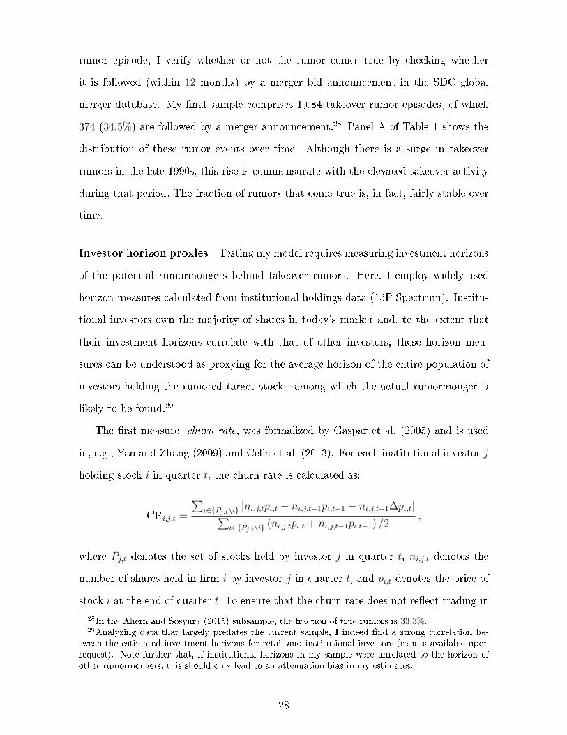
The �rst measure, churn rate, was formalized by Gaspar et al. (2005) and is used

in, e.g., Yan and Zhang (2009) and Cella et al. (2013). For each institutional investor j

holding stock i in quarter t, the churn rate is calculated as:

CRi,j,t =

∑ι∈{Pj,t\i} |nι,j,tpι,t − nι,j,t−1pι,t−1 − nι,j,t−1∆pι,t|∑

ι∈{Pj,t\i} (nι,j,tpι,t + nι,j,t−1pι,t−1) /2,

where Pj,t denotes the set of stocks held by investor j in quarter t, ni,j,t denotes the

number of shares held in �rm i by investor j in quarter t, and pi,t denotes the price of

stock i at the end of quarter t. To ensure that the churn rate does not re�ect trading in

28In the Ahern and Sosyura (2015) subsample, the fraction of true rumors is 33.3%.29Analyzing data that largely predates the current sample, I indeed �nd a strong correlation be-

tween the estimated investment horizons for retail and institutional investors (results available uponrequest). Note further that, if institutional horizons in my sample were unrelated to the horizon ofother rumormongers, this should only lead to an attenuation bias in my estimates.

28

the rumor stock i, I exclude stock i before calculating churn rates for investors holding

that stock. Finally, churn rates are averaged at the stock level:

CRi,t =∑j∈Si,t

ωi,j,t

(1

20

20∑τ=1

CRi,j,t−τ

),

where Si,t denotes the set of institutional investors holding stock i in quarter t and ωi,j,t

denotes each investor's relative stake.

The second horizon measure, portfolio turnover, was used by Wermers (2000) and

Brunnermeier and Nagel (2004) and is based on the minimum of the absolute values of

buys and sells divided by the previous quarter's holdings for each institutional investor.

Portfolio turnover is then averaged across the previous 20 quarters and across investors.

The third horizon proxy, introduced by Cremers and Pareek (2015), measures the

average duration of a stock in an investors' portfolio. For each stock i in investor j's

portfolio in quarter t, duration is calculated as

Durationi,j,t =t−1∑

τ=t−W+1

((t− τ − 1)αi,j,τHi,j +Bi,j

)+

(W − 1)Hi,j

Hi,j +Bi,j

,

where Bi,j is the total percentage of stock i bought by institution j between t−W and

t − 1, Hi,j is the percentage of stock i held by institution j at time t −W , and αi,j,τ

is the percentage of stock i bought or sold by institution j between τ − 1 and τ . I set

W = 20. See Cremers and Pareek (2015) for more intuition on this measure. Duration

is averaged across stocks in the institutional investor's portfolio (excluding the rumor

stock), before being averaged across institutions that hold the rumor stock. Finally,

I multiply the duration by −1 in order to obtain a measure that is decreasing in investor

horizon (like churn rate and portfolio turnover).

My fourth proxy for investor horizon is based on the transient investor classi�cation

by Bushee (1998) and Bushee and Noe (2000),30 which are de�ned as institutions with

high portfolio turnover, high portfolio diversi�cation, and a focus on short-term trading

30Available at http://acct.wharton.upenn.edu/faculty/bushee/IIclass.html

29

pro�ts. In my analysis, I de�ne transient investors as the percentage of a stock's

institutional investors that are classi�ed as transient. It is important to bear in mind

that (i) all four horizon proxies are pre-determined with respect to the rumor event and

(ii) both duration and the churn rate are calculated while excluding the rumor stock.

Hence these measures are not in�uenced by the trading response to the rumor.

Control variables As control variables, I use: �rm size (log of total assets), the

book-to-market ratio, advertising expenses, and R&D expenses (all from Compustat

and winsorized at the 1% level), the fraction and the concentration of institutional

holdings (from 13F Spectrum), analyst coverage and analyst forecast dispersion (from

I/B/E/S), as well as cumulated returns and average share turnover over the 90 days

preceding the rumor's publication (from CRSP). Descriptive statistics for the investor

horizon measures and control variables are given in Panel B of Table 1. For example,

the average churn rate of 35.7% in the quarters prior to a rumor event implies that

institutional investors turn over about 18% of their portfolios per quarter.

[[ Insert Table 1 about here. ]]

4.2 Event study for stock rumors

I conduct an event study to see how investors respond to the occurrence of takeover

rumors. Figure 4 traces the evolution of returns and trading activity from 20 days prior

to the publication of the �rst rumor article to 40 days after the article�for all takeover

rumors combined (solid line) as well as separately for true rumors (dashed line) and false

rumors (dotted line). The graph for cumulative abnormal returns in Panel (a) reveals a

strong stock market reaction to takeover rumors: average returns start to climb several

days prior to the �rst media article and jump exponentially on the day of that article's

publication, after which they fall back slightly. For rumors that turn out to be true,

the run-up in returns is stronger and, if anything, returns drift slightly upward after

publication. In contrast, false rumors see a modest reversal in returns. Consistently

30

with the strong return reaction, Panel (b) shows a dramatic spike in share turnover,

which remains elevated after publication of the article.

Table 2 reports the statistical signi�cance of these results (standard errors are clus-

tered at the event-date level). For instance, Panel (a) shows that there is strongly

signi�cant run-up in returns of about 4.4% in the �ve days prior to the rumor's publi-

cation. Returns jump by another 6.3% on the day of publication, after which they revert

by about 1.7% over the next 40 days; see column (1). However, the return reversal is

signi�cant only for rumors that turn out to be false (column (3)); for true rumors, there

is instead a small but insigni�cant return continuation (column (2)). Panel (b) shows

a concurrent and strongly signi�cant surge in trading activity. Turnover on publication

day is increased by about 4.3 percentage points, corresponding to 280% relative to the

average daily turnover during the 120 days preceding the event window.

[[ Insert Table 2 about here. ]]

Overall, the evidence strongly suggests that investors respond to takeover rumors.

First, the surge in both returns and turnover before and at publication suggests that

some investors were already trading on the rumor and that many more investors joined

in after reading about it in the newspaper. Second, this interpretation is consistent

with how takeover rumors are reported in the media. Indeed, a large number of arti-

cles explicitly mention unusual market activity as being caused by takeover rumors.31

Finally, about a third of the takeover rumors in my sample come true within one year,

thereby justifying the large and fairly persistent rise in the rumored stock's price. This

observation also makes it unlikely that rumors are simply �invented� by journalists in

order to account for otherwise inexplicable stock activity.

31The Wall Street Journal report about the Univision takeover rumor mentioned at the start of theintroduction is typical of such articles.

31

4.3 Investment horizon and rumor accuracy

My model predicts that rumors about stocks held by short-term investors should be

more accurate than rumors about stocks held by long-term investors. Here I test this

prediction by estimating linear probability models in which the dependent variable is

the rumor true dummy, an indicator set to 1 if the takeover rumor is followed by a

merger bid announcement within 12 months (and set to 0 otherwise).32 Speci�cally, I

run regressions of the following type:

rumor true dummyi,t = α + β × investor horizon proxyi,t−1 + γ × χi,t−1

+ year �xed-e�ects + industry �xed-e�ects + εi,t

where �rm i and date t identify a given takeover rumor. The variables of interest are the

previously described proxies for investor horizon. χi,t−1 is the matrix of pre-determined

control variables. All regressions include year and industry �xed e�ects (using the

Fama�French 48-industry classi�cation). Standard errors are double-clustered by day

and �rm.

[[ Insert Table 3 about here. ]]

Table 3 shows that the e�ect of investor horizon on the likelihood of a rumor coming

true is statistically signi�cant and economically important for all horizon proxies. For

instance, a one�standard increase in churn rate is associated with a 3.9 percentage

points higher likelihood of the takeover coming true, corresponding to a 11% increase

over the baseline rumor accuracy. The other horizon proxies yield e�ects of a similar

economic magnitude. In terms of control variables, only �rm size and advertising

have signi�cantly negative coe�cients, con�rming Ahern and Sosyura (2015)'s �nding

that the media tilts its coverage to large and visible �rms at the expense of accurate

32In the Internet Appendix, I show that the results presented here are robust to estimating a logitmodel instead (Internet Appendix 2.1) and to using an alternative de�nition of rumor accuracy thatclassi�es a rumor as being true if it is followed by a merger bid announcement within 6 months (InternetAppendix 2.2).

32

reporting.

4.4 Investment horizon and rumor response

In the model, investors respond only to those rumors that originate from a su�ciently

short-term rumormonger. I thus expect to observe that investors react more strongly

to takeover rumors for stocks held by short-term investors. I test this prediction by

running regressions of the type:

rumor responsei,t = α + β × investor horizon proxyi,t−1 + γ × χi,t−1

+ year �xed-e�ects + industry �xed-e�ects + εi,t

where rumor responsei,t is the abnormal return (or the abnormal turnover) on the day

of the rumor publication (t = 0); the speci�cation is otherwise similar to the previous

one. Panels (a) and (b) of Table 4 report results for the abnormal return and the

abnormal turnover, respectively.

[[ Insert Table 4 about here. ]]

Both panels reveal a signi�cantly positive association between investment hori-

zons and the trading and return responses to takeover rumors. In terms of returns,

a one�standard deviation increase in horizon proxies leads to an increase in the abnor-

mal return of roughly 0.5 percentage points�or 8% relative to the average abnormal

return documented earlier. With regard to abnormal turnover, a one�standard devia-

tion increase in investor horizon leads to an even greater relative increase of about 11%.

In conclusion, stocks held by short-term investors exhibit a stronger rumor response in

terms of both trading and returns, in line with the prediction that takeover rumors

issued by short-term investors are more credible.

33

4.5 Alternative explanations

Takeover rumors are not random and hence my analysis is not free of endogeneity

concerns. For instance, one concern is that �rm-speci�c factors may simultaneously

attract short-term investors and rumor coverage. Unfortunately, very few �rms exhibit

more than one takeover rumor, making it impossible to control for time-invariant �rm-

level heterogeneity with the inclusion of �rm �xed e�ects.33 In my main regression

speci�cation, I instead control for a host of �rm-speci�c variables gathered from ac-

counting, ownership, analyst, and stock market data (as well as for year and industry

�xed e�ects). In this subsection, I further mitigate endogeneity concerns by carefully

examining alternative explanations for my �ndings.

I start with media selection. Ahern and Sosyura (2015) �nd that the media skews

its rumor coverage toward large �rms with high advertising expenditures (I control

for these e�ects in my regressions). Yet, one does not expect the media to report

on every far-fetched rumor about a high-pro�le company because readers ultimately

care about the consequences of takeovers that do come true. On balance, I expect the

media sample to primarily consist of rumors deemed to be at least somewhat credible

by journalists�and thus presumably by investors. Hence my analysis should not be

confounded by rumors that were immediately dismissed by investors.

In any case, what matters in the context of my tests is whether media coverage de-

cisions are systematically correlated with the employed investment horizon proxies. For

instance, short-term investors might have a high demand for sensational media coverage

involving takeover rumors, perhaps because they are more credulous. In this case, one

would expect the media to cater to this demand and hence to give greater coverage to

target stocks held by short-term investors. In Internet Appendices 3.1 and 3.2, I report

two pieces of evidence that are consistent with this interpretation: short-term institu-

tional investors (compared to long-term investors) trade more aggressively on takeover

33Similarly�and despite there being a voluminous literature on the subject (e.g., Bushee, 1998;Bushee and Noe, 2000; Brunnermeier and Nagel, 2004; Gaspar et al., 2005; Yan and Zhang, 2009; Cellaet al., 2013; Cremers and Pareek, 2015)�I know of no clean instrument or quasi-natural experimentthat would allow to make causal statements about the implications of short-term investment horizons.

34

rumors; and takeover bids for stocks held by short-term investors are comparatively

more likely to be preceded by rumor coverage. However, media pandering to short-

term investors should lead to less accurate rumors for �rms held by these investors and

is thus at odds with my �nding that rumors for stocks held by short-term investors are

actually more accurate. Moreover, the large fraction of published takeover rumors that

do come true as well as the sizable and largely persistent jump in the price of rumored

stocks suggest that the media focuses on covering credible rumors. In this respect, the

media's more extensive coverage of takeover rumors involving stocks held by short-term

investors can also be interpreted as supporting my model�i.e., as evidence that the

media views short investment horizons as an informative signal about rumor credibility.

One might alternatively argue that takeover rumors for stocks held by long-term

investors are less accurate because the media's coverage is actually slanted toward

these investors. However, it is di�cult to argue that the media caters to long-term

investors when short-term investors are the ones responding more strongly to takeover

rumors (Internet Appendix 3.1) and when takeover rumors for stocks held by short-

term investors are more likely to be covered by the media (Internet Appendix 3.2).

Moreover, catering to long-term investors would not explain why takeover rumors for

stocks held by short-term investors elicit a larger return and price response.

In sum, it is di�cult to spin an alternative explanation that can jointly account

for the facts that (i) the media is more likely to cover rumors for target stocks held by

short-term investors; (ii) that market participants consider these rumors to be relatively

more credible, as indicated by trading and return reactions; and (iii) that these rumors

turn out to be more accurate ex post. However, these facts are all consistent with the

model's proposed mechanism: rumors potentially originating from short-term investors

are more credible, therefore explaining why they receive more media coverage, elicit a

stronger market response, and turn out to be more accurate.

35

5 Conclusion

An old Wall Street adage advises investors to �buy on the rumor and sell on the news.�

This paper presents a simple model of stock rumors�de�ned as potentially informative

signals from an unknown source�that con�rms this classic advice. In the model, a

rumormonger's investment horizon interacts with information arrivals to yield credible

information sharing. Interestingly, I �nd that a short-term rumormonger has an incen-

tive to share information truthfully, whereas a long-term rumormonger prefers to lie.

Hence, in contrast to an extensive literature propounding the negative aspects of in-

vestors' myopia (see Stein, 1996; Bushee, 1998; Chen et al., 2007b; Derrien et al., 2013),

my paper highlights an overlooked bene�t of short investment horizons: they encourage

information sharing among investors.

Exploiting data on media-covered takeover rumors, I �nd suggestive evidence con-

sistent with this idea. First, stock prices indeed move in response to rumors: in the days

surrounding the rumor coverage, cumulative abnormal returns increase by more than

10% on average. Second, both rumor accuracy and the return response are greater for

rumors about stocks that are predominantly held by short-term investors�in line with

the intuition that rumors spread by short-term investors can be more credible.

More generally, this paper serves as a reminder to carefully rethink the strategic

microfoundation for information exchanges in �nancial markets. For example, when

information is shared via social media (where the sender's identity is often not veri�-

able), the horizon channel put forth in this paper predicts that short horizons may be

conducive for credibility. In contrast, when the sender's identity is known, reputation

concerns come into play and should become more important with long horizons. How

these two channels interact is an interesting avenue for future research.

36

References

Admati, A., P�eiderer, P., 1986. A monopolistic market for information. Journal ofEconomic Theory 39, 400�438.

Admati, A., P�eiderer, P., 1988. Selling and trading on information in �nancial markets.American Economic Review P&P 78, 96�103.

Admati, A., P�eiderer, P., 1990. Direct and indirect sale of information. Econometrica58, 901�928.

Ahern, K. R., Sosyura, D., 2015. Rumor has it: Sensationalism in �nancial media.Review of Financial Studies 28, 2050�2093.

Andrei, D., Cujean, J., 2017. Information percolation, momentum, and reversal. Journalof Financial Economics 123, 617�645.

Antweiler, W., Frank, M. Z., 2004. Is all that talk just noise? The information contentof internet stock message boards. Journal of Finance 59, 1259�1294.

Barber, B. M., Loe�er, D., 1993. The dartboard column: Second-hand information andprice pressure. Journal of Financial and Quantitative Analysis 28, 273�284.

Bartov, E., Faurel, L., Mohanram, P. S., 2018. Can twitter help predict �rm-levelearnings and stock returns? Accounting Review 93, 25�57.

Benabou, R., Laroque, G., 1992. Using privileged information to manipulate markets:Insiders, gurus, and credibility. Quarterly Journal of Economics 107, 921�958.

Bhattacharya, S., Nanda, V., 2013. Portfolio pumping, trading activity and fund per-formance. Review of Finance 17, 885�919.

Bond, P., Edmans, A., Goldstein, I., 2012. The real e�ects of �nancial markets. AnnualReview of Financial Economics 4, 339�360.

Brunnermeier, M. K., Nagel, S., 2004. Hedge funds and the technology bubble. Journalof Finance 59, 2013�2040.

Bushee, B. J., 1998. The in�uence of institutional investors on myopic R&D investmentbehavior. The Accounting Review 73, 305�333.

Bushee, B. J., Noe, C. F., 2000. Corporate disclosure practices, institutional investors,and stock return volatility. Journal of Accounting Research 38, 171�202.

Cella, C., Ellul, A., Giannetti, M., 2013. Investors' horizons and the ampli�cation ofmarket shocks. Review of Financial Studies 26, 1607�1648.

Cespa, G., 2008. Information sales and insider trading with long-lived information.Journal of Finance 63, 639�672.

Chen, H., De, P., Hu, Y., Hwang, B.-H., 2014. Wisdom of crowds: The value of stockopinions transmitted through social media. Review of Financial Studies 27, 1367�1403.

37

Chen, Q., Goldstein, I., Jiang, W., 2007a. Price informativeness and investment sensi-tivity to stock price. Review of Financial Studies 20, 619�650.

Chen, X., Harford, J., Li, K., 2007b. Monitoring: Which institutions matter? Journalof Financial Economics 86, 279�305.

Crawford, V. P., Sobel, J., 1982. Strategic information transmission. Econometrica 50,1431�1451.

Cremers, M., Pareek, A., 2015. Short-term trading and stock return anomalies: Mo-mentum, reversal, and share issuance. Review of Finance 19, 1649�1701.

Derrien, F., Kecskes, A., Thesmar, D., 2013. Investor horizons and corporate policies.Journal of Financial and Quantitative Analysis 48, 1755�1780.

Dessaint, O., Foucault, T., Fresard, L., Matray, A., 2018. Noisy stock prices and cor-porate investment, Working Paper.

Dewally, M., 2003. Internet investment advice: Investing with a rock of salt. FinancialAnalysts Journal 59, 65�77.

Dow, J., Gorton, G., 1994. Arbitrage chains. Journal of Finance 49, 819�849.

Du�e, D., Malamud, S., Manso, G., 2009. Information percolation with equilibriumsearch dynamics. Econometrica 77, 1513�1574.

Du�e, D., Manso, G., 2007. Information percolation in large markets. American Eco-nomic Review P&P 97, 203�209.

Farrell, J., Rabin, M., 1996. Cheap talk. Journal of Economic Perspectives 10, 103�118.

Foucault, T., Fresard, L., 2012. Cross-listing, investment sensitivity to stock price, andthe learning hypothesis. Review of Financial Studies 25, 3305�3350.

Gaspar, J. M., Massa, M., Matos, P., 2005. Shareholder investment horizons and themarket for corporate control. Journal of Financial Economics 76, 135�165.

Goldstein, I., Yang, L., 2017. Good disclosure, bad disclosure. Journal of FinancialEconomics forthcoming.

Hong, H., Kubik, J. D., Stein, J. C., 2005. Thy neigbor's portfolio: Word-of-mouthe�ects in the holdings and trades of money managers. Journal of Finance 60, 2800�2824.

Ivkovic, Z., Weisbenner, S., 2007. Information di�usion e�ects in individual investors'common stock purchases: Covet thy noighbors' investment choices. Review of Finan-cial Studies 20, 1327�1357.

Kovbasyuk, S., Pagano, M., 2015. Advertising arbitrage, Working Paper.

Kyle, A., 1985. Continuous auctions and insider trading. Econometrica 53, 1461�1484.

38

Liu, P., Smith, S. D., Syed, A. A., 1990. Stock price reactions to the wall street journal'ssecurities recommendations. Journal of Financial and Quantitative Analysis 25, 399�410.

Ljungqvist, A., Qian, W., 2016. How constraining are limits to arbitrage? Review ofFinancial Studies 29, 1975�2028.

Lloyd-Davies, P., Canes, M., 1978. Stock prices and the publication of second-handinformation. Journal of Business 51, 43�56.

Luo, Y., 2005. Do insiders learn from outsiders? Evidence from mergers and acquisi-tions. Journal of Finance 60, 1951�1982.

New York Times, 2010. Computers that trade on the news, available athttp://www.nytreprints.com.

Pasquariello, P., Wang, Y., 2018. Speculation with information disclosure, WorkingPaper.

Peterson, W. A., Gist, N. P., 1951. Rumor and public opinion. American Journal ofSociology 57, 159�167.

Pound, J., Zeckhauser, R., 1990. Clearly heard on the street: The e�ect of takeoverrumors on stock price. Journal of Business 63, 291�308.

SEC, 2012. Investment adviser use of social media. National Examination Risk Alert 2,1�7.

Shiller, R. J., 2000. Irrational Exuberance. Princeton University Press.

Stein, J. C., 1996. Rational capital budgeting in an irrational world. Journal of Business69, 429�455.

Sun, Y., 2006. The exact law of large numbers via Fubini extension and characterizationof insurable risks. Journal of Economic Theory 126, 31�69.

Thomson Reuters, 2013. Annual review, available at http://ar.thomsonreuters.com.

Tumarkin, R., Whitelaw, R. F., 2001. News or noise? Internet message board activityand stock prices. Financial Analysts Journal 57, 41�51.

Van Bommel, J., 2003. Rumors. Journal of Finance 58, 1499�1519.

Veldkamp, L., 2006. Media frenzies in markets for �nancial information. AmericanEconomic Review 96, 577�601.

Wermers, R., 2000. Mutual fund performance: An empirical decomposition into stock-picking talent, style, transaction costs, and expenses. Journal of Finance 55, 1655�1695.

Yan, X., Zhang, Z., 2009. Institutional investors and equity returns: Are short-terminstitutions better informed? Review of Financial Studies 22, 893�924.

Zuckerman, R., 2012. Synchronized arbitrage and the value of public information, Work-ing Paper.

39

Figure 1: Model setupBefore t = 0, nature draws the asset payo� θ. At t = 0, L privately learns the state θ and tradesqL0. After trading, she sends a message m to the other investors. With probability λ, L experiences aliquidity shock which forces her to exit at t = 1. Otherwise, she trades an amount qL1 at t = 1. Themessage-receiving investors F rationally assess the credibility of m. A fraction µ of them learns θ fromother sources before trading in t = 1. Each investor then trades an amount qit at t = 1 (which mayor may not depend on m, depending on whether m is credible). Market makers observe the order �owω1 and set prices accordingly. Finally, in period t = 2, the asset pays o� and consumption takes place.

40

Figure 2: Feasibility of truth-telling equilibrium

This �gure illustrates the feasible equilibria that exist for di�erent λ-µ pairs (holding x constant at 0.75;the graph looks very similar for other levels of x). As is typical for cheap talk models, the �babbling�equilibrium exists everywhere. Above the solid line, which represents the truth-telling condition fromequation (6), is the region in which there also exists a pure-strategy communication equilibrium suchthat L truthfully shares her information. For λ-µ pairs between the solid and the dashed line completetruth-telling is not incentive compatible; however, there exist mixed-strategy communication equilibriaas described in Proposition 4 in which market participants expect L to tell the truth with probability ρand L, being indi�erent between telling the truth and lying, conforms to these beliefs. The dotted linefurther partitions the mixed-strategy equilibrium space into those in which the uninformed message-receivers fully exploit their capital constraints when trading on m (φ = 1) and those in which theycurb their trading aggressiveness (φ < 1) in order to limit their collective price impact. The dashed(dotted) line is obtained by calculating the smallest possible ρ neccessary to ensure that φ ≥ µ

1−µ(φ = 1), which is then plugged back into (8). Moving to the left along these lines implies decreasing ρuntil ρ = 1

2 for µ = 0.

only "bb" eq

pure-strategy

"com" eq

mixed-strategy

"com" eq

(ϕ=1)

(ϕ<1)

0.0 0.2 0.4 0.6 0.8

0.0

0.2

0.4

0.6

0.8

1.0

μ

λ

41

Figure 3: Truth-telling condition for di�erent levels of price impact

This �gure shows the truth-telling condition in µ-λ space given x = 12 for di�erent levels of price

impact (i.e., for di�erent levels of α). The lines represent sets of parameter values for which (pure)

truth-telling and lying are equally pro�table for di�erent values of α. Above these lines truth-telling

is more pro�table, so that a pure strategy communication equilibrium exists. The solid line shows the

truth-telling condition for the model without price impact (α = 0), the dashed line shows the truth-

telling condition for intermediate price impact (α = 0.15), the dotted line shows the truth-telling

condition for large price impact (α = 0.3).

truth-telling is

more profitable

lying is

more profitable

0.0 0.2 0.4 0.6 0.8

0.0

0.2

0.4

0.6

0.8

1.0

μ

λ

42

Figure 4: Trading Activity and Price Response around Takeover RumorsThis �gure traces the evolution of returns and trading activity around takeover rumors. The event-day(t = 0) is the day of the �rst media article mentioning the stock as a rumored takeover target. Panel (a)shows cumulative abnormal returns (CAR), where abnormal returns are de�ned as the stock returnminus the CRSP value-weighted return index. Panel (b) shows abnormal turnover, which is de�ned asstock turnover (number of shares trading over number of shares outstanding) minus the average stockturnover over days t = −140 to t = −21. In both graphs, the solid line represents all takeover rumors,the dashed line represents takeover rumors that turn out to be true (i.e., that are followed by a mergerbid announcement within 12 months), and the dotted line represents takeover rumors that turn out tobe false (i.e., not followed by a merger bid announcement within 12 months).

0.0

5.1

.15

.2C

AR

−20 0 20 40Day relative to rumor publication

All rumors

True rumors

False rumors

(a) Cumulative abnormal returns in event-time

0.0

1.0

2.0

3.0

4A

bnorm

al T

urn

over

−20 0 20 40Day relative to Rumor Publication

All rumors

True rumors

False rumors

(b) Abnormal turnover in event-time

43

Table 1: Sample Statistics

This table presents sample statistics for the takeover rumor sample. Panel (a) shows the numberof takeover rumors and the number of a�ected �rms over time. A takeover rumor for a given �rm isconsidered to be true if it is followed by a merger bid announcement within 12 months. Panel (b) showsdescriptive statistics for all variables used in the analysis. Rumor True Dummy is a dummy variabletaking the value one if the rumor comes true (as de�ned above). Abn. return is the stock return on theday of the takeover rumor publication minus the CRSP value-weighted return index. Abn. turnoveris the share turnover on the day of the takeover rumor publication minus the average stock turnoverover days t = −140 to t = −21. Churn Rate is the average investor turnover calculated as in Gasparet al. (2005). Portfolio Turnover is the average of the minimum of absolute values of buys and sellsdivided by prior holdings (Wermers, 2000 and Brunnermeier and Nagel, 2004). Duration*(-1) is thenegative of investors' average holding duration (Cremers and Pareek, 2015). Transient Investors is thefraction of �transient� institutions according to the classi�cation of Bushee (1998) and Bushee and Noe(2000). See main text for more details on these investor horizon measures. Log Size is the logarithmof total assets. Book-to-market is the ratio of book equity to market value. Advertising is advertisingexpenses scaled by total book assets. R&D is research and development expenses scaled by total bookassets. All these variables are from Compustat as reported for the end of the previous �scal year.Institutional Owhnership is the fraction of outstanding shares owned by institutional investors at theend of the previous quarter. Institutional HHI is the Her�ndahl concentration index of institutionalholdings at the end of the previous quarter. Log # Analyst is the logarithm of one plus the numberof analysts following the stock at the end of the previous month. Analyst dispersion is the standarddeviation of analyst forecasts at the end of the previous month. Return[-90,-1] is the cumulated stockreturn over the 90 days prior to the rumor publication. Turnover[-90,-1] is the average share turnoverover the 90 days prior to the rumor publication.

44

45

Table 2: Event Study around Takeover Rumors

This table presents event study results for takeover rumor episodes. The event-day (t = 0) is the day of

the �rst media article mentioning the stock as a rumored takeover target. Panel (a) shows cumulative

abnormal returns (CAR) for di�erent event windows together with the abnormal return (AR) for

t = 0. Abnormal returns are de�ned as the stock return minus the CRSP value-weighted return

index. Panel (b) shows (average) abnormal turnover for di�erent event windows, which is de�ned as

stock turnover (number of shares trading over number of shares outstanding) minus the average stock

turnover over days t = −140 to t = −21. Column (1) shows results for all takeover rumors. Columns

(2) and (3) show results for true and false rumors, respectively. A takeover rumor for a given �rm is

considered to be true if it is followed by a merger bid announcement within 12 months. t-statistics are

based on standard errors adjusted for clustering by day. ∗∗∗, ∗∗ and ∗ indicate statistical signi�cance

at the 1%, 5% and 10% level, respectively.

46

Table 3: Investment Horizon and Rumor Accuracy

This table estimates linear probability models in which the dependent variable is Rumor True

Dummy , a dummy variable that takes the value one if the takeover rumor is followed by a merger

bid announcement within 12 months. Churn Rate is the average investor turnover calculated

as in Gaspar et al. (2005). Portfolio Turnover is the average of the minimum of absolute val-

ues of buys and sells divided by prior holdings (Wermers, 2000 and Brunnermeier and Nagel,

2004). Duration*(-1) is the negative of investors' average holding duration (Cremers and Pareek,

2015). Transient Investors is the fraction of �transient� institutions according to the classi�ca-

tion of Bushee (1998) and Bushee and Noe (2000). See main text for more details on these in-

vestor horizon measures. See Table 1 for a de�nition of the control variables. All regressions

include year �xed e�ects and industry �xed e�ects using the Fama-French 48 industry classi�ca-

tion. t-statistics are based on standard errors adjusted for double-clustering at the day and stock

level. ∗∗∗, ∗∗ and ∗ indicate statistical signi�cance at the 1%, 5% and 10% level, respectively.

47

Table 4: Investment Horizon and Rumor Response

This table presents results of regressing investors' responses to the takeover rumor on stock char-

acteristics. In panel (a), the dependent variable is abnormal return on the rumor publication

date (or the next trading day when the publication falls on a weekend). In panel (b), the de-

pendent variable is the abnormal share turnover. Churn Rate is the average investor turnover

calculated as in Gaspar et al. (2005). Portfolio Turnover is the average of the minimum of ab-

solute values of buys and sells divided by prior holdings (Wermers, 2000 and Brunnermeier and

Nagel, 2004). Duration*(-1) is the negative of investors' average holding duration (Cremers and

Pareek, 2015). Transient Investors is the fraction of �transient� institutions according to the clas-

si�cation of Bushee (1998) and Bushee and Noe (2000). See main text for more details on these

investor horizon measures. See Table 1 for a de�nition of the control variables. All regressions

include year �xed e�ects and industry �xed e�ects using the Fama-French 48 industry classi�ca-

tion. t-statistics are based on standard errors adjusted for double-clustering at the day and stock

level. ∗∗∗, ∗∗ and ∗ indicate statistical signi�cance at the 1%, 5% and 10% level, respectively.

48

49

A Appendix

A.1 Proof of Proposition 1: No-communication equilibrium

Given the postulated trading behavior that leads to the order �ow ωb1 given in the text, market makersback out the information about θ. For instance, when ωb1 > −µx+1, it is clear that informed investorsmust have bought the stock, which implies θ = 1. Similarly, for ωb1 < µx− 1, informed investors musthave sold. For µx− 1 ≤ ωb1 ≤ −µx+ 1, both cases are possible. This gives the price function in (1).

Price expectations For L and the informed F , two cases are to consider. When θ = 1, order �ow isdistributed ω1 ∼ U(µx−1, µx+1). Given the price function in (1), these investors calculate E(p1 | θ =1) = 1×Pr (ω1 > −µx+ 1 | θ = 1, m = 1) = µx. When θ = −1, order �ow is ω1 ∼ U(−µx−1, −µx+1)and informed investors calculate E(p1 | θ = −1) = −µx. Since the uninformed F know nothing aboutθ when m is uninformative, they expect E(p1) = 0.

L's optimal trading strategy L wants to go long (short) at t = 0 when θ = 1 (θ = −1) and, whenshe is long-term, stay long (short) at t = 1: qL0 = x (qL0 = −x) and qL1 = 0. This yields an expectedpro�t of E(Πb

L) = x (1− λ (1− µx)).

Informed F's optimal trading strategy The informed F want to go long qF1 = x (short qF1 =−x) at t = 1 when θ = 1 (θ = −1), leading to an expected pro�t of E(Πb

F ) = xµ (1− µx).

Uninformed F's optimal trading strategy The uninformed F have no information about θ.Hence they refrain from trading and make zero expected pro�t.

A.2 Proof of Proposition 2: Communication equilibrium

Market makers infer information about θ from the order �ow ω1. For example, when ω1 > −x + 1,market makers know that m = 1 and thus expect θ = 1 (since they expect m to be true). Similararguments give rise to the price function in (2).

Price expectations For L and the informed F , four cases are to consider. When θ = 1 and m = 1,order �ow is distributed ω1 ∼ U(x−1, x+1). Given the price function in (2), these investors calculateE(p1 | θ = 1, m = 1) = 1 × Pr (ω1 > −x+ 1 | θ = 1, m = 1) = x. When θ = −1 and m = −1, order�ow is ω1 ∼ U(−x − 1, −x + 1) and informed investors calculate E(p1 | θ = −1, m = −1) = −x.When θ = 1 and m = −1, order �ow is ω1 ∼ U(−(1 − 2µ)x − 1, −(1 − 2µ)x + 1) and informedinvestors expect E(p1 | θ = 1, m = −1) = −(1− 2µ)x. Finally, when θ = −1 and m = 1, order �ow isω1 ∼ U((1−2µ)x−1, (1−2µ)x+1) and informed investors expect E(p1 | θ = 1, m = −1) = (1−2µ)x.

For the uninformed F (which know m but not θ), two cases are to consider. When m = 1, uninformedinvestors infer that θ = 1 (since they expect m to be true) and thus expect an order �ow of ω1 ∼U(x − 1, x + 1). Uninformed investors thus expect E(p1 |m = 1) = E(p1 | θ = 1, m = 1) = x. Whenm = −1, similar calculations give E(p1 |m = −1) = −x.

L's optimal trading strategy When θ = 1 (θ = −1) and L tells the truth, her expected price p1

is positive (negative). L then wants to go long (short) at t = 0 and, when she is long-term, stay long(short) at t = 1: qL0 = x (qL0 = −x) and qL1 = 0. This yields an expected pro�t given by (3) in thetext. When θ = 1 (θ = −1) and L lies, the expected price p1 is negative (positive) as long as µ ≤ 1

2 . Lthen wants to go short (long) at t = 0 and, when she is long-term, �ip her position at t = 1: qL0 = −x(qL0 = x) and qL1 = 2x (qL1 = −2x), so that her net position at the end of t = 1 is qL0 + qL1 = x(qL0 + qL1 = −x). This results in an expected pro�t of (4). Truth-telling is incentive compatible ifexpected pro�ts in (3) exceed (4), which gives rise to condition (5). Plugging in the expected pricesderived above, we get the incentive compatibility constraint for truth-telling given in (6). This is L'sincentive compatibility constraint.

L's expected pro�t Taking into account the unconditional probabilities for the di�erent states,unconditional expected pro�ts for investor L are given by

E (ΠL) = x (1− λ(1− x))

50

Note that this expected pro�t always exceeds her pro�t E(ΠbL) from the no-communication equilibrium.

Thus L's participation constraint is satis�ed.

Uninformed F's optimal trading strategy An investor who has heard m but did not learn θfrom other sources believes either E(θ |m = 1) = 1 or E(θ |m = −1) = −1. Taken together with hisexpectations of p1 conditional on m, his expected pro�t from going long qF1 = x (short qF1 = −x)after receiving m = 1 (m = −1) is (1 − x)x, which is positive given the assumption x < 1. Hence,uninformed F pro�t from trading in the direction of m, proving that their incentive compatibilityconstraint is satis�ed.

Informed F's optimal trading strategy When θ = 1 (θ = −1) and L told the truth, the informedF want to long qF1 = x (short qF1 = −x) the stock, leading to an expected pro�t of (1− x)x. In thebaseline model, L lies with probability zero. It is nonetheless important to verify that in this case theinformed F want to trade against m as postulated. When L lied, the informed investors long qF1 = x(short qF1 = −x) when m = −1 (m = 1). This gives an expected pro�t of (1−2µ)x2, which is positivegiven the assumption µ ≤ 1

2 .

F's expected pro�ts In the baseline model, an investor F makes the same expected pro�t E (ΠF ) =(1− x)x, regardless of whether he ends up learning θ directly or only indirectly through m. Note thatE (ΠF ) > 0, proving that investors F s' participation constraint is satis�ed.

A.3 Proof of Proposition 4: Mixed-strategy equilibrium

Price expectations For L and the informed F , four cases are to consider. When θ = 1 and m = 1,informed investors calculate E (p1 |m = 1, θ = 1) = (2ρ − 1)((1 − µ)φ − µ)x + 2

2−ρµx. When θ = −1

andm = −1, informed investors calculate E (p1 |m = −1, θ = −1) = −(2ρ−1)((1−µ)φ−µ)x− 22−ρµx.

When θ = −1 andm = 1, informed investors calculate E (p1 |m = 1, θ = −1) = (2ρ−1)((1−µ)φ−µ)x.Finally, when θ = 1 and m = −1, informed investors calculate E (p1 |m = −1, θ = 1) = −(2ρ−1)((1−µ)φ− µ)x.

For the uninformed F (which know m but not θ), two cases are to consider. When m = 1, theuninformed F calculate:

E(p1 |m = 1) = Pr (θ = 1 |m = 1) E(p1 | θ = 1, m = 1)

+Pr (θ = −1 |m = 1) E(p1 | − θ = 1, m = 1)

= (2ρ− 1)((1− µ)φ− µ)x+2ρ

2− ρµx

When m = −1, they calculate analogously E(p1 |m = −1) = −(2ρ− 1)((1− µ)φ− µ)x− 2ρ2−ρµx.

L's optimal trading strategy For L to play a mixed strategy, condition (5) must be satis�ed withequality. Plugging in the price expectations above, one obtains equation (8) from Proposition 4.

Uninformed F's optimal trading strategy An investor who has heard m but does not know θcalculates E(θ |m = 1) = 2ρ − 1 or E(θ |m = −1) = −(2ρ − 1). For such an investor to trade onm = 1, it must thus be E(θ |m = 1) ≥ E (p1 |m = 1, θ = 1). Hence:

(2ρ− 1) ≥ (2ρ− 1)((1− µ)φ− µ)x+2ρ

2− ρµx

Note that in choosing his own φi, an uninformed investor F takes φ, the average trading aggressivenessof the the other uninformed F , as given. Whenever there is a strict inequality, he will thus want tochoose φi = 1. When there is an equality, he is indi�erent and may as well choose φi = φ, whichpins down a symmetric equilibrium. Solving the equality for φ gives the expression for φ in (10).Finally, note that condition (8) is derived under the assumption that a lying L wants to trade on thefalse rumor at t = 0 and then �ips her position at t = 0. Such a trading strategy is only optimalwhen her lie is e�ective enough in manipulating the price away from the fundamental (i.e., whenE (p1 |m = 1, θ = −1) > 0 and E (p1 |m = −1, θ = 1) < 0). If this were not the case, a lying L wouldalways prefer trading in direction of θ (regardless of m) and hence would never want to lie, ruling out

51

a mixed-strategy equilibrium. This veri�es the conjecture φ ≥ µ1−µ . Setting φ ≥

µ1−µ and simplifying

gives condition (9). This condition is also su�cient to ensure that the uninformed F make non-negativepro�ts from trading on m.

Properties of equilibrium Together, equations (8) and (10) pin down the equilibrium ρ. There aretwo cases to consider: φ = 1 or φ < 1. Consider �rst φ = 1 and de�ne f1(φ) ≡ 1

(2−ρ)(2ρ−1) . Note that

f1 is decreasing in φ for the region 12 ≤ ρ ≤ 1. Condition (8) can then be written as f1(φ) = 1−λ

λ1−2µµ .

Hence, when λ or µ increase, φ has to increase as well in order to keep satisfying the equality. Consider

next φ < 1. After plugging φ = 11−µ

[1x −

(2ρ

(2−ρ)(2ρ−1) − 1)µ]into (8) and simplifying, one obtains

f2(φ, µ) = 1−λλ with f2(φ, µ) ≡ µ

1x (2−ρ)(2ρ−1)−2ρµ

. Note that f2 is decreasing in φ and increasing in

µ for the relevant parameter region. Hence, when λ or µ increase, φ has again to increase in order tomaintain the equilibrium.

A.4 Proof of Proposition 6: Trading activity and price e�ciency

Trading activity in the no-communication equilibrium Let z ∼ U(a−1, a+1), then E [| z |] =12

(a2 + 1

). Using this, it is straightforward to calculate:

E[∣∣ωb1 ∣∣] = Pr (θ = 1) E [|µx+ s1 |] + Pr (θ = −1) E [| −µx+ s1 |]

=1

2

(1 + (µx)

2)

Trading activity in the communication equilibrium

E [|ω1 |] = Pr (θ = 1 ∩ m = 1) E [| ((1− µ)φ+ µ)x+ s1 |]+Pr (θ = 1 ∩ m = −1) E [| −((1− µ)φ− µ)x+ s1 |]+Pr (θ = −1 ∩ m = −1) E [| −((1− µ)φ+ µ)x+ s1 |]+Pr (θ = −1 ∩ m = 1) E [| −((1− µ)φ− µ)x+ s1 |]

=1

2

(1 + ρ (((1− µ)φ+ µ)x)

2+ (1− ρ) (((1− µ)φ− µ)x)

2)

Note that E [|ω1 |] is increasing in φ. Setting φ = µ1−µ (its smallest possible value in an communication

equilibrium) gives E [|ω1 |] = 12

(1 + ρ (2µx)

2)> E

[∣∣ωb1 ∣∣] for all ρ > 12 .

Price e�ciency in the no-communication equilibrium

E[V ar

(θ | pb1

)]= E

[(θ − pb1

)2]= Pr

(θ = 1 ∩ pb1 = 0

)+ Pr

(θ = −1 ∩ pb1 = 0

)= 1− µx

52

Price e�ciency in the communication equilibrium

E [V ar (θ | p1)] = E[(θ − p1)

2]

= Pr (θ = 1 ∩ p1 = 2ρ− 1) (1− (2ρ− 1))2

+Pr (θ = 1 ∩ p1 = ρ/2−ρ) (1− ρ/2−ρ)2

+Pr (θ = 1 ∩ p1 = 0)

+Pr (θ = 1 ∩ p1 = −ρ/2−ρ) (1 + ρ/2−ρ)2

+Pr (θ = 1 ∩ p1 = −(2ρ− 1)) (1 + (2ρ− 1))2

+Pr (θ = −1 ∩ p1 = 2ρ− 1) (1 + (2ρ− 1))2

+Pr (θ = −1 ∩ p1 = ρ/2−ρ) (1 + ρ/2−ρ)2

+Pr (θ = −1 ∩ p1 = 0)

+Pr (θ = −1 ∩ p1 = −ρ/2−ρ) (1− ρ/2−ρ)2

+Pr (θ = −1 ∩ p1 = −(2ρ− 1)) (1− (2ρ− 1))2

E [V ar (θ | p1)] = ρ((1− µ)φ− µ)x (2(1− ρ))2

+ µx

(2(1− ρ)

2− ρ

)2

+1− ((1− µ)φ+ µ)x+ (1− ρ)µx

(2

2− ρ

)2

+(1− ρ)((1− µ)φ− µ)x (2ρ)2

= 1− ((1− µ)φ+ µ)x+ 4((1− µ)φ− µ)xρ(1− ρ)

+4µx1− ρ2− ρ

First, note that for ρ = 1 and φ = 1, E [V ar (θ | p1)] reduces to 1 − x, which is clearly less thanE[V ar

(θ | pb1

)]. Hence, in a pure-strategy communication equilibrium, prices are more informa-

tive than in the babbling equilibrium. Second, note that E [V ar (θ | p1)] is decreasing in φ. Hence,E [V ar (θ | p1)] is highest when φ is lowest, which is φ = µ

1−µ (as for φ < µ1−µ , a mixed-strategy

communication equilibrium cannot exist; see above). Setting φ = µ1−µ , it is easy to show that

E [V ar (θ | p1)] < E[V ar

(θ | pb1

)]for any ρ > 2

3 .

A.5 Proof of Proposition 7: Noisy Signal

Beliefs I conjecture that L tells the truth (m = S). Since S and therefore m may be wrong, theuninformed F can lose from trading on m and may thus trade more cautiously. Let φ ∈ [0, 1] denotetheir trading aggressiveness, meaning that they buy (sell) φx (−φx) upon observing m = 1 (m = −1).

Prices As before, we have p0 = E(θ |ω0) = 0. Consider the case θ = 1. A fraction µ of the otherinvestors F learns θ directly. Depending on whether L's signal was correct or not, they will eithertrade with or against the message m. The remaining fraction (1 − µ) trades on m with intensity φ.The order �ow is given by:

ω1 =

((1− µ)φ+ µ)x+ s1 when m = 1 and S = θ = 1

((1− µ)φ− µ)x+ s1 when m = S = 1 and θ = −1

−((1− µ)φ− µ)x+ s1 when m = S = −1 and θ = 1

−((1− µ)φ+ µ)x+ s1 when m = −1 and S = θ = −1

Market makers set prices conditional on ω1. I conjecture that (1− µ)φ ≥ µ (otherwise L cannot hope

53

to bene�t from lying). This leads to the following price function:

p1(ω1) =

1 if ((1− µ)φ− µ)x+ 1 < ω1 ≤ ((1− µ)φ+ µ)x+ 1

2π − 1 if −((1− µ)φ− µ)x+ 1 < ω1 ≤ ((1− µ)φ− µ)x+ 1π

2−π if −((1− µ)φ+ µ)x+ 1 < ω1 ≤ −((1− µ)φ− µ)x+ 1

0 if ((1− µ)φ+ µ)x− 1 ≤ ω1 ≤ −((1− µ)φ+ µ)x+ 1

− π2−π if ((1− µ)φ− µ)x− 1 ≤ ω1 < ((1− µ)φ+ µ)x− 1

−(2π − 1) if −((1− µ)φ− µ)x− 1 ≤ ω1 < ((1− µ)φ− µ)x− 1

−1 if −((1− µ)φ+ µ)x− 1 ≤ ω1 < −((1− µ)φ− µ)x− 1

where 2π − 1, for example, is the expected value of θ conditional on knowing that m = 1, whichhappens either because S = θ = 1 (probability π) or because S = 1 despite of θ = −1 (probability1− π).

Price expectations For L, four cases are to consider. When S = 1 and m = 1, L knows that hersignal is correct with probability π (in which case order �ow is ω1 = ((1 − µ)φ + µ)x + s1) and falsewith probability 1−π (in which case order �ow is ω1 = ((1−µ)φ−µ)x+ s1). Given the price functionabove, L calculates:

E(p1 |S = 1, m = 1) = π E(p1 | θ = 1, m = 1) + (1− π)E(p1 | θ = −1, m = 1)

= π

[(2π − 1)((1− µ)φ− µ) +

2

2− πµ

]x

+(1− π) [(2π − 1)((1− µ)φ− µ)]x

=

[(2π − 1)((1− µ)φ− µ) +

2π

2− πµ

]x

When S = 1 and m = −1, L calculates:

E(p1 |S = 1, m = −1) = π E(p1 | θ = 1, m = −1) + (1− π)E(p1 | θ = −1, m = −1)

= π (−1) [(2π − 1)((1− µ)φ− µ)]x

+(1− π) (−1)

[(2π − 1)((1− µ)φ− µ) +

2

2− πµ

]x

= −[(2π − 1)((1− µ)φ− µ) +

2(1− π)

2− πµ

]x

Similar calculations give the price expectations in the remaining two cases: E(p1 |S = −1, m = −1) =

−[(2π − 1)((1− µ)φ− µ) + 2π

2−πµ]x and E(p1 |S = −1, m = 1) =

[(2π − 1)((1− µ)φ− µ) + 2(1−π)

2−π µ]x.

For the uninformed F (which know m but not θ), two cases are to consider. When m = 1, uninformedinvestors infer that S = 1 (since they expect L to tell the truth). Hence:

E(p1 |m = 1) = E(p1 |S = 1, m = 1)

=

[(2π − 1)((1− µ)φ− µ) +

2π

2− πµ

]x

Similarly, when m = −1, they calculate E(p1 |m = −1) = −[(2π − 1)((1− µ)φ− µ) + 2π

2−πµ]x.

L's optimal communication strategy and expected pro�t Truth-telling condition (5) stillholds. Plugging in price expectations and simplifying gives equation (11) given in Proposition 7.Unconditional expected pro�ts for investor L are given by

E (ΠL) = [λE(p1 |S = 1, m = 1) + (1− λ)E(θ |S = 1)]x

=

[(2π − 1)((1− µ)φ− µ) +

2π

2− πµ

]λx2 + (2π − 1)(1− λ)x (17)

54

Uninformed F's optimal trading strategy An investor who has heard m but did not learn θfrom other sources believes either E(θ |m = 1) = (2π− 1) or E(θ |m = −1) = −(2π− 1). For such aninvestor to trade on m = 1, it must thus be E(θ |m = 1) ≥ E (p1 |m = 1, θ = 1). Hence:

(2π − 1) ≥ (2π − 1)((1− µ)φ− µ)x+2π

2− πµx

Note that in choosing his own φi, an uninformed investor F takes φ, the average trading aggressivenessof the the other uninformed F , as given. Whenever there is a strict inequality, he will thus want tochoose φi = 1. When there is an equality, he is indi�erent and may as well choose φi = φ, whichpins down a symmetric equilibrium. Solving the equality for φ gives the expression for φ in (13).

Finally, recall that condition (11) is only valid under the conjecture φ ≥ µ1−µ . Setting φ ≥ µ

1−µ and

simplifying gives condition (13). This condition is also su�cient to ensure that the uninformed F makenon-negative pro�ts from trading on m.

A.6 Proof of Proposition 8: Information acquisition by L

Let C(π) = c(π2 − 1

4

)with c > 0 be the cost of a acquiring a signal with precision π. To solve for

the optimal signal precision, it becomes important to distinguish between L's choice of π and marketmakers' belief about π, henceforth denoted by π. Given equation (17) and making use of the fact thatL chooses π for a given π, one can write L's optimization problem as follows:

maxπ

2π

2− πµλx2 + (2π − 1)(1− λ)x− cπ2

The �rst-order condition is 12−πµλx

2 + (1 − λ)x = cπ. In equilibrium, market makers belief π mustequal L's choice of π. Plugging-in and solving for π gives two solutions. One of these solutions can beruled out since it always gives π > 1 in the relevant parameter region. The other solution simpli�es to

π ≡ 1

2c

[(1− λ)x+ 2c−

√((1− λ)x+ 2c)

2 − 4c (µλx2 + (1− λ)2x)

].

Hence, L chooses π? = π when π ≤ 1 and chooses π? = 1 when π > 1.

Comparison to babbling equilibrium Extending the babbling equilibrium of Proposition 1 tothe case of noisy signals, it is easy to show that L's expected pro�t is given by E

(ΠbL

)= λ(2π −

1)µx2 + (1 − λ)(2π − 1)x. Using the same cost function as before, one obtains the following optimalsignal precision

πb =λµx2 + (1− λ)x

c

When L is long-term (λ = 0), one obtains π? = πb. This makes sense: when L is fully long-term,there are no bene�ts to being able to communicate. Given that lying cannot be an equilibrium, thebest L can do is to establish her position at t = 0 and to wait until the payo� date t = 2, giving herthe same expected pro�t than in the babbling equilibrium. For any λ > 1, one can show π? < πb.Intuitively, there are two opposing forces at work: On the one hand, L makes a higher pro�t in thecommunication equilibrium compared to the babbling one (because her credible message ensures thatmore of her information is impounded in the price at t = 1), prompting her to acquire more information.On the other hand, in the communication equilibrium, L makes a positive expected pro�t even whenshe is uninformed (π = 1

2 ), making it relatively more attractive to acquire a less precise signal. Thesetwo e�ects are linked: when the bene�t of extra price impact from investors trading on m is large,the expected pro�t from having a relatively uninformative signal is similarly large. It thus turns outthat the �rst e�ect can never outweigh the second, implying that L acquires more information in thebabbling equilibrium.

Finally, it is easy to see that any parameter change that renders communication viable tends toincrease price e�ciency: since L is in�nitesimal, neither her investment horizon nor her choice of πa�ect the price e�ciency in the babbling equilibrium. Since price e�ciency tends to be higher whencommunication is credible, price e�ciency will typically improve even when the parameter change

55

pushes L to acquire less information. Intuitively, sharing an imprecise signal is better than not sharinga precise one.

A.7 Proof of Proposition 9: Multiple messages

Two messages Consider the case when there are two senders L1 and L2, each of them receiving anoisy signal about θ. Denote Lj 's signal Sj for j ∈ {1, 2}. Assume further that both signals have thesame precision Pr(θ |Sj) = π ≥ 1

2 and that signal noises are independent. Since I am interested in thefeasibility of equilibria that feature credible information sharing, I conjecture that F and M believethat L1 and L2 tell the truth (meaning that m1 = S1 and m2 = S2), as well as that Lj believes thatL¬j tells the truth. I further conjecture that the uninformed F buy (sell) an amount φx (−φx) uponreceiving m1 = m2 = 1 (m1 = m2 = −1) and abstain from trading otherwise (m1 6= m2).

Six cases can occur: {θ = 1, m1 = m2 = 1} with probability 12π

2, {θ = 1, m1 6= m2 = 1} withprobability π(1 − π), {θ = 1, m1 = m2 = −1} with probability 1

2 (1 − π)2, {θ = −1, m1 = m2 = −1}with probability 1

2π2, {θ = −1, m1 6= m2 = 1} with probability π(1 − π), {θ = −1, m1 = m2 = 1}

with probability 12 (1− π)2.

Prices As before, we have p0 = E(θ |ω0) = 0. I conjecture that φ ≥ µ1−µ (for otherwise L would

never want to lie). At t = 1, we have the following order �ow:

ω1 =

((1− µ)φ+ µ)x+ s1 when θ = 1 and m1 = m2 = 1

((1− µ)φ− µ)x+ s1 when θ = −1 and m1 = m2 = 1

µx+ s1 when θ = 1 and m1 6= m2

−µx+ s1 when θ = −1 and m1 6= m2

−((1− µ)φ− µ)x+ s1 when θ = 1 and m1 = m2 = −1

−((1− µ)φ+ µ)x+ s1 when θ = −1 and m1 = m2 = −1

The resulting price function depends on whether ((1−µ)φ−µ) ≥ µ or ((1−µ)φ−µ) < µ. In the �rstcase, the price is given by:

p1(ω1) =

1 if ((1− µ)φ− µ)x+ 1 < ω1 ≤ ((1− µ)φ+ µ)x+ 12π−1

1−2π(1−π) if µx+ 1 < ω1 ≤ ((1− µ)φ− µ)x+ 1

(2π − 1) + 2π(1− π) if −µx+ 1 < ω1 ≤ µx+ 12π−1

1+2π(1−π) if −((1− µ)φ− µ)x+ 1 < ω1 ≤ −µx+ 1π2

2−π2 if −((1− µ)φ+ µ)x+ 1 < ω1 ≤ −((1− µ)φ− µ)x+ 1

0 if ((1− µ)φ+ µ)x− 1 ≤ ω1 ≤ −((1− µ)φ+ µ)x+ 1

− π2

2−π2 if ((1− µ)φ− µ)x− 1 ≤ ω1 < ((1− µ)φ+ µ)x− 1

− 2π−11+2π(1−π) if µx− 1 ≤ ω1 < ((1− µ)φ− µ)x− 1

−(2π − 1)− 2π(1− π) if −µx− 1 ≤ ω1 < µx− 1

− 2π−11−2π(1−π) if −((1− µ)φ− µ)x− 1 ≤ ω1 < −µx− 1

−1 if −x((1− µ)φ+ µ)− 1 ≤ ω1 < −((1− µ)φ− µ)x− 1

(18)

56

In the second case, the price is given by:

p1(ω1) =

1 if µx+ 1 < ω1 ≤ ((1− µ)φ+ µ)x+ 1

1 if ((1− µ)φ− µ)x+ 1 < ω1 ≤ µx+ 1

(2π − 1) + 2π(1− π) if −((1− µ)φ− µ)x+ 1 < ω1 ≤ ((1− µ)φ− µ)x+ 1(2−π)π

2(1−π)+π2 if −µx+ 1 < ω1 ≤ −((1− µ)φ− µ)x+ 1π2

2−π2 if −((1− µ)φ+ µ)x+ 1 < ω1 ≤ −µx+ 1

0 if ((1− µ)φ+ µ)x− 1 ≤ ω1 ≤ −((1− µ)φ+ µ)x+ 1

− π2

2−π2 if µx− 1 ≤ ω1 < ((1− µ)φ+ µ)x− 1

− (2−π)π2(1−π)+π2 if ((1− µ)φ− µ)x− 1 ≤ ω1 < µx− 1

−(2π − 1)− 2π(1− π) if −((1− µ)φ− µ)x− 1 ≤ ω1 < ((1− µ)φ− µ)x− 1

−1 if −µx− 1 ≤ ω1 < −((1− µ)φ− µ)x− 1

−1 if −x((1− µ)φ+ µ)− 1 ≤ ω1 < −µx− 1

In what follows, I focus on the �rst case ((1− µ)φ− µ ≥ µ) as this is the case in which µ is relativelylow, which makes lying more attractive. I show that the presence of a second message strengthensthe incentives for truth-telling, but that the horizon mechanism remains intact in the sense that along-term L1 may prefer to lie even though she expects L2 to tell the truth. Hence, it remains truethat messages by short-term rumormongers are more credible than those by long-term rumormongers(except for the case when both L1 and L2 are perfectly informed, π = 1, in which case even long-termrumormongers want to tell the truth, rendering the horizon channel negligible).

Price expectations Given the price function (18), the computation of price expectations is straight-forward:

E (p1 | θ = 1, m1 = m2 = 1) = µx+2π − 1

1− 2π(1− π)

(1

2(1− µ)φ− µ

)x

+ (2π − 1 + 2π(1− π))µx+2π − 1

1 + 2π(1− π)

(1

2(1− µ)φ− µ

)x+

π2

2− π2µx

E (p1 | θ = −1, m1 = m2 = −1) = −µx− 2π − 1

1− 2π(1− π)

(1

2(1− µ)φ− µ

)x

− (2π − 1 + 2π(1− π))µx− 2π − 1

1 + 2π(1− π)

(1

2(1− µ)φ− µ

)x− π2

2− π2µx

E (p1 | θ = 1, m1 = −1, m2 = 1) = (2π − 1 + 2π(1− π))µx

E (p1 | θ = −1, m1 = −1, m2 = 1) = − (2π − 1 + 2π(1− π))µx

E (p1 | θ = 1, m1 = m2 = −1) = − 2π − 1

1− 2π(1− π)

(1

2(1− µ)φ− µ

)x

− (2π − 1 + 2π(1− π))µx− 2π − 1

1 + 2π(1− π)

(1

2(1− µ)φ− µ

)x

E (p1 | θ = −1, m1 = m2 = 1) =2π − 1

1− 2π(1− π)

(1

2(1− µ)φ− µ

)x

+ (2π − 1 + 2π(1− π))µx+2π − 1

1 + 2π(1− π)

(1

2(1− µ)φ− µ

)x

These expectations are then plugged into the truth-telling condition of Proposition 9, which itselffollows from extending (5) for the case of there being two messages. Clearly, the right-hand-side ofthe condition is decreasing in λ, whereas the left-hand-side continues to be indendent of λ. Takentogether, this implies that a shorter investment horizon facilitates truth-telling.

I now show that a long-term L1 may continue lying even if she expects L2 to tell the truth. Settingλ = 1 and using the fact that E (p1 |m1 = S1, m2 = S2) > E (p1 |m1 = −S1, m2 = S2) shows that L1

57

will prefer to lie i� E (p1 |m1 = −S1, m2 = S2) < 0.

E (p1 |S1 = 1, m1 = −1) = Pr(θ = 1|S2 = 1)

[Pr(S2 = 1|θ = 1)E(p1|θ = 1,m1 = −1,m2 = 1)

Pr(S2 = −1|θ = 1)E(p1|θ = 1,m1 = −1,m2 = −1)

]+Pr(θ = −1|S2 = 1)

[Pr(S2 = 1|θ = −1)E(p1|θ = −1,m1 = −1,m2 = 1)

Pr(S2 = −1|θ = −1)E(p1|θ = −1,m1 = −1,m2 = −1)

]= π2E(p1|θ = 1,m1 = −1,m2 = 1)︸ ︷︷ ︸

>0

+ π(1− π)E(p1|θ = 1,m1 = −1,m2 = −1)︸ ︷︷ ︸<0

+(1− π)2E(p1|θ = −1,m1 = −1,m2 = 1)︸ ︷︷ ︸<0

+π(1− π)E(p1|θ = −1,m1 = −1,m2 = −1)︸ ︷︷ ︸<0

Plugging in the price expectations above, it is straightforward to see that E (p1 |m1 = −S1, m2 = S2)may well be negative as long as π < 1 (Below, I also show that, by choosing x small enough, one cansimultaneously ensure that (1− µ)φ− µ ≥ µ, so that the conjecture that the uninformed F trade onthe messages is veri�ed). However, when L1 and L2 have perfect information (π = 1), the expectedfrom lying when is still positive: instead of a predicted price reversal, there is only a pronouncedunderreaction. Hence, L1 will never want to lie when π = 1 and when there is another message forsure.

Uninformed F's optimal trading strategy An investor who has not learnt θ directly, but hasheard m1 = m2 = 1 (and conjectures that m1 = S1 and m2 = S2), calculates:

E (p1 |m1 = m2 = 1) = Pr(θ = 1|m1 = m2 = 1)E(p1|θ = 1,m1 = 1,m2 = 1)

+Pr(θ = −1|m1 = m2 = 1)E(p1|θ = −1,m1 = 1,m2 = 1)

=π2

1− 2π(1− π)E(p1|θ = 1,m1 = 1,m2 = 1)

+1− 2π + π2

1− 2π(1− π)E(p1|θ = −1,m1 = 1,m2 = 1)

E (θ |m1 = m2 = 1) = Pr(θ = 1|m1 = m2 = 1)− Pr(θ = −1|m1 = m2 = 1)

=2π − 1

1− 2π(1− π)

Such an investor will trade on these messages when E (θ |m1 = m2 = 1) ≥ E (p1 |m1 = m2 = 1). It iseasy to see that this inequality can be satis�ed for any π > 1

2 and (1−µ)φ−µ ≥ µ. Indeed, since onlythe right-hand-side of this inequality depends on x, the inequality can be strictly satis�ed by choosingx small enough. When it is, the uninformed L will want to trade maximally on m1 = m2 = 1, whichveri�es (1− µ)φ− µ ≥ µ.

Another message with probability α Let there now be second message with probability α. Letχ = 1 (χ = 0) denote the state in which L2 is (is not) present. When L1 decides m1, she does notknow whether there will be another sender L2 and another message m2, but if there is, she expects itto be true (m2 = S2). Her price expectation and pro�t is then a weighted average of the model fromSubsection 3.1 (with a single message) and the two-sender model described above. When S1 = 1, thisimplies (the case S2 = −1 is symmetric):

E(p1 |S1 = 1, m1 = 1) = (1− α)E(p1 |S1 = 1, m1 = 1, χ = 0) + αE(p1 |S1 = 1, m1 = 1, χ = 1)

E(p1 |S1 = 1, m1 = −1) = (1− α)E(p1 |S1 = 1, m1 = −1, χ = 0) + αE(p1 |S1 = 1, m1 = −1, χ = 1)

Note that, for π > 12 , one has E(p1 |S1 = 1, m1 = 1, χ = 1) > E(p1 |S1 = 1, m1 = 1, χ = 0) > 0

(when L1 expects L2 to tell the truth, she expects more price discovery in direction of S1 when L2

is present) and E(p1 |S1 = 1, m1 = −1, χ = 1) > E(p1 |S1 = 1, m1 = −1, χ = 0) (L1 expects m2,if present, to make her lie less e�ective). Moreover, conjecture that E(p1 |S1 = 1, m1 = −1) < 0(otherwise L1 does not want to lie).

58

The truth-telling condition in Proposition 9 follows from (5) together with these new expectations.Clearly, the right-hand-side of the condition is decreasing in λ, implying that a shorter investmenthorizon facilitates truth-telling. Given the facts just mentioned, the left-hand-side of this conditioncan be expressed as A+Bα

C−Dα with A, B, C and D > 0. Hence, the left-hand-side is increasing in α,implying that a higher probability of another message facilitates truth-telling.

A.8 Price Impact

This proof proceeds in three steps. First, I show that the short-term rumormonger continues to prefertruth-telling despite of price impact. Second, I show that price impact only strengthens the conclusionthat the long-term rumormonger prefers lying. Third, I derive the truth-telling condition for the caseof an intermediate investment horizon.

A.8.1 Short-term Rumormonger

Beliefs I �rst consider the case when L is short-term (λ = 1). I conjecture and verify a BayesianEquilibrium (BE) in which L tells the truth (m = θ).

Trading in Period 0 At t = 0, M expect ω0 = αx+ s0 if θ = 1 and ω0 = −αx+ s0 if θ = −1. Theprice function is:

p0(ω0) =

+1 if − αx+ 1 < ω0 ≤ αx+ 1

0 if αx− 1 ≤ ω0 ≤ −αx+ 1

−1 if − αx− 1 ≤ ω0 < αx− 1

Trading in Period 1 Trading choices and the price function at t = 1 depend on the realization ofp0. When p0 = 0, the price at t = 0 is uninformative about θ. At t = 1, M expect L to close herposition and other investors F to trade in the direction of θ (which they have either learnt directly orthrough m). Speci�cally, M expect ω1 = (1− 2α)x+ s1 when θ = 1 and ω1 = −(1− 2α)x+ s1 whenθ = −1. Conjecture that (1− 2α) > 0. The price function is:

p1(ω1 | p0 = 0) =

+1 if − (1− 2α)x+ 1 < ω1 ≤ (1− 2α)x+ 1

0 if (1− 2α)x− 1 ≤ ω1 ≤ −(1− 2α)x+ 1

−1 if − (1− 2α)x− 1 ≤ ω1 < (1− 2α)x− 1

When p0 = 1, then M believe that p0 already reveals θ = 1. For simplicity, I assume that M do notchange this belief regardless of the order �ow at t = 1. This is essentially an assumption about out-ofequilibrium beliefs. Similarly, I assume that p1 = −1 when p0 = −1. Therefore, M makes no pro�twhenever p0 = 1 or p0 = −1 so that the trade-o� between truth-telling and lying remains una�ected.

Truth-telling Consider the case when θ = 1 (the case θ = −1 is symmetric). I now solve for L'soptimal trading strategy and resulting expected pro�t conditional on telling the truth. At t = 0, Lbuys an amount x0. When p0 = 0, L expects to make a pro�t by sending the message m = 1 as themessage results in expected buying pressure of E(ω1 | p0 = 0, θ = 1) = −αx0 + (1 − α)x at t = 1.When p0 = 1, L is unlucky in that she will not make a pro�t (since the price cannot rise further).Her expected pro�t thus equals x0 P(p0 = 0 | θ = 1)E(p1 | p0 = 0, θ = 1, m = 1), which simpli�es to

x0(1 − αx) ((1 − α)x − αx0). Solving for the pro�t-maximizing trading quantity yields x∗0 = (1−α)2α x.

The assumption that L's position constraint binds implies that x∗0 ≥ x. Plugging in and re-arrangingyields α ≤ 1

3 . Hence, the assumption that α ≤ 13 implies that L's position constraint is binding and

she buys x (sells −x) whenever she knows θ = 1 (θ = −1). Note that α ≤ 13 also veri�es the conjecture

(1− 2α) > 0. L's expected pro�t with the truth-telling strategy is given by x2(1− αx)(1− 2α).

Lying Consider again the case θ = 1. A lying strategy consists of short-selling an amount −y0 att = 0 and sending a sell message m = −1 (as L is short-term, there is nothing to gain from sendingm = −1 and buying at t = 0). When p0 = 0, L then expects an order �ow of E(ω1 | p0 = 0, θ = 1) =αy0 − (1 − α)(1 − 2µ)x at t = 1. I conjecture that α(x − y0) < (1 − α)2µx, which implies that the

59

order �ow from lying at t = 1 is not outside of the interval [−(1 − 2α)x − 1, (1 − 2α)x + 1] (as thiswould reveal to market makers that L was lying).

Given these conjectures, L calculates E(p1 | p0 = 0, θ = 1, m = −1) = αy0 − (1− α)(1− 2µ)x. Lyingthen yields an expected pro�t of y0 P(p0 = 0 | θ = 1)E(p1 | p0 = 0, θ = 1, m = −1) = y0(1− αx) ((1−α)(1 − 2µ)x − αy0), which is maximized for y∗0 = (1−α)

2α (1 − 2µ)x. Hence, conditional on θ = 1 andsending m = −1, L maximizes pro�ts by short-selling the stock for any µ < 1

2 and longing the stockfor µ > 1

2 (since, for µ > 12 , −y

∗0 becomes positive). Note also that, given the assumption α ≤ 1

3 , theconjecture from the previous paragraph is always satis�ed and | y∗0 | ≤ x as required. The expectedpro�t from lying is y∗0(1− αx) ((1− α)(1− 2µ)x− αy∗0).

Comparing truth-telling and lying L prefers truth-telling over lying i�

x2(1− 2α) > y∗0((1− α)(1− 2µ)x− αy∗0) .

This condition is satis�ed in the region α ≤ 13 for any µ > 0. To see this, note that, by assumption,

the position limit is binding for the truth-telling strategy (x∗0 ≥ x). This implies that, when L tells thetruth, her pro�ts from trading x exceed her pro�ts from trading any amount less than x. Therefore,x2(1 − 2α) ≥ y∗0((1 − α)x − αy∗0) and the latter part is strictly larger than the expected pro�t fromlying for any 0 < µ < 1. Intuitively, price impact does not change the trade-o� between telling thetruth and lying when L is short-term. All it does is to lower L's expected (per-share) pro�t fromboth strategies, and it may lead L to potentially choose a lower trading quantity for the lying strategy(for truth-telling, her position limit is binding by assumption). Note also that, as L's price impactdecreases (α → 0), her expected pro�ts approach the ones from the baseline model in which L wasassumed to be a price taker.

A.8.2 Long-term Rumormonger

Beliefs Consider the case when L is long-term (λ = 0). I assume that M and F believe that L tellsthe truth and show below that, given these beliefs, L has an incentive to deviate to lying, proving thatthere does not exist an equilibrium in which L truthfully reveals her information.I assume that L's position limit is binding in both trading periods and verify below that this is indeedthe case for α ≤ 1

3 .

Trading in Period 0 Given that t = 0 is the only period in which L trades exclusively on herinformation, she takes the maximum long- or short-position in that period. M therefore expect ω0 =αx+ s0 if θ = 1 and ω0 = −αx+ s0 if θ = −1. The price function is:

p0(ω0) =

+1 if − αx+ 1 < ω0 ≤ αx+ 1

0 if αx− 1 ≤ ω0 ≤ −αx+ 1

−1 if − αx− 1 ≤ ω0 < αx− 1

Trading in Period 1 Trading choices and the price function at t = 1 depend on the realization ofp0. When p0 = 0, the price at t = 0 is uninformative about θ. At t = 1, M expect L to hold on toher position and other investors F to trade in direction of θ (which they have either learnt directly orthrough m). Speci�cally, M expect ω1 = (1 − α)x + s1 when θ = 1 and ω1 = −(1 − α)x + s1 whenθ = −1. The price function is:

p1(ω1 | p0 = 0) =

+1 if − (1− α)x+ 1 < ω1 ≤ (1− α)x+ 1

0 if (1− α)x− 1 ≤ ω1 ≤ −(1− α)x+ 1

−1 if − (1− α)x− 1 ≤ ω1 < (1− α)x− 1

When p0 = 1, M believe that p0 already reveals θ = 1. As before, I assume that M do not change thisbelief regardless of the order �ow at t = 1. Similarly, I assume that p1 = −1 when p0 = −1.

Truth-telling Consider the case when θ = 1 (the case θ = −1 is symmetric). I now solve for L'soptimal trading strategy and resulting expected pro�t conditional on telling the truth. At t = 0, L

60

buys an amount x0. When p0 = 0 or p0 = −1, L closes her existing position at t = 1 and establishes anew one of amount x1, resulting in a sure pro�t at t = 2. When p0 = 1, L is unlucky in that she willnot make a pro�t (since the price cannot rise further). Given this behavior, L expects an order �ow ofE(ω0 | θ = 1) = αx0 at t = 0 and E(ω1 | p0 = 0, θ = 1) = α(x1− x0) + (1−α)x at t = 1. Her expectedpro�t equals P(p0 = 0 | θ = 1) [x1 − (x1 − x0)E(p1 | p0 = 0, θ = 1, m = 1)] + P(p0 = −1 | θ = 1) 2x1,where the former part describes L's pro�t when p0 = 0 and the latter part follows from the fact that,given Ms' out-of-equilibrium beliefs for the case p0 = −1, L knows she can trade at the price p1 = −1in this case.

Knowing θ = 1, L computes the following probabilities and price expectations: P(p0 = 0 | θ = 1) =1 − αx, P(p0 = −1 | θ = 1) = α

2 (x − x0) and E(p1 | p0 = 0, θ = 1, m = 1) = (1 − α)x + α(x1 − x0).Plugging-in, her expected pro�t is:

(1− αx) [x1 − (x1 − x0) ((1− α)x+ α(x1 − x0))] + α(x− x0)x1

L solves for the optimal trading quantities by backward induction. Given x0, it is easy to solve forthe optimal x1. By assumption, L's position limit is binding, meaning that L must want to choose ax1 larger than x. This turns indeed out to be the case for any x0, x and α ≤ 1

3 . Hence, L optimallychooses x1 = x at t = 1. Next, L chooses the optimal x0 given x1 = x. The resulting quadraticequation in x0 has a unique solution for x0, which turns out to be above x for any x < 1 and α ≤ 1

3 .Hence, L optimally chooses x0 = x at t = 0. In other words, when L is not too large (α < 1

3 ), L's bestcourse of action conditional on telling the truth is to take a maximum position at t = 0. Her expectedpro�t from this strategy is (1− αx)x.

Lying Consider the case θ = 1 so that lying entails sending a sell message m = −1. Let −y0

designate the amount that L short-sells at t = 0, implying that she buys an amount y0 + y1 at t = 1,where yt ≤ x for t ∈ {0, 1}. Given this behavior, L expects an order �ow of E(ω0 | θ = 1) = −αy0 att = 0 and E(ω1 | p0 = 0, θ = 1) = α(y1 + y0)− (1− α)(1− 2µ)x at t = 1. Her expected pro�t is:

(1− αx) [y1 + (y1 + y0) ((1− α)(1− 2µ)x− α(y1 + y0))] + α(x+ y0)y1

Taking y0 as given, L solves for the optimal y1. The resulting interior solution is larger than x for any| y0 | ≤ x, µ < 9

10 , and α <13 . Hence, L chooses y∗1 = x at t = 1. Next, L chooses the optimal y0 given

y∗1 = x. The optimal y∗0 is given by

y∗0 =

+x if y > x

y if − x < y < x

−x if y < −x

with

y ≡x[(1− 2µ)(1− αx) + xα2(3− 2µ)− 2α(1− µ)

]2α(1− αx)

.

For small µ, y∗0 is positive, meaning that L short-sells at t = 1 and then �ips her position at t = 1.This is the equivalent of the lying strategy from the baseline model without price impact (with thedi�erence that L does not always short-sell to the maximum). Interestingly, as µ approaches 1

2 (so thatthe false message deceives only half of the other investors), y∗0 becomes negative but remains largerthan −x, meaning that L gradually buys the stock at t = 0 and t = 1. This e�ect is exacerbatedwhen α is large and is due to L's price impact. Before, lying was only attractive to the degree thatit manipulated the price away from the stock's fundamental (i.e., by causing a negative price movebetween t = 0 and t = 1 when L knows θ = 1), as this allowed L to pro�t from the ensuing pricereversal. With price impact, there is another bene�t to lying. Indeed, the selling pressure induced bythe false message can help L to establish her position more cheaply. When her price impact is large,she in fact prefers to exploit her lie to build her position gradually over time rather than to short-sellat t = 0 and to �ip her position at t = 1. The expected pro�t from lying is

(1− αx) [x+ (x+ y∗0) ((1− α)(1− 2µ)x− α(x+ y∗0))] + α(x+ y∗0)x .

61

Comparing truth-telling and lying L prefers truth-telling over lying i�

(1− αx)x > (1− αx) [x+ (x+ y∗0) ((1− α)(1− 2µ)x− α(x+ y∗0))] + α(x+ y∗0)x .

It turns out that this condition is not satis�ed in the parameter region considered. To see this, notethat, with the lying strategy, the pro�t from trading y0 = y∗0 at t = 0 (and y1 = x at t = 1) exceedsthe pro�t from trading any other amount at t = 0. In particular, it will also exceed the pro�t fromtrading y0 = −x, in which case the expected pro�t from lying exactly reduces to the maximum pro�tthat L can make when she tells the truth. This is intuitive: when y0 = −x, L is essentially not tradingat t = 1 (since y0 + y1 = 0) and therefore it doesn't matter to L's long-term pro�t whether she lies ortells the truth. However, for any other y0, L does trade at t = 1 and lying will then always help herestablish her �nal position more cheaply.

To sum up, when L is long-term, L always prefers lying over telling the truth. Hence, there doesnot exist a BE in which L truthfully shares her information. The fact that L has price impact onlystrengthens this conclusion. Indeed, with price impact, L strictly prefers lying even if µ ≥ 1

2 (as longas y∗0 > −x), when she was indi�erent between lying and telling the truth without price impact (sinceher lie was then ine�ective in manipulating the price away from the fundamental). Intuitively, thelong-term rumormonger always prefers lying since any lying-induced trading pressure helps to reduceher price impact.

A.8.3 Intermediate-term Rumormonger

I now consider the case where L faces a liquidity shock (i.e., is short-term) with probability λ, forcingher to liquidate her position at t = 1, and can hold-on to her position (i.e., is long-term) with probability1−λ. Let η = 1 designate the state of the world in which L faces a liquidity shock and η = 0 designatethe state in which she does not. As in the baseline model, I assume that, at the time of sendingthe message, L does not know yet whether she will face the liquidity shock or not (i.e., L does notknow the realization of η before sending m). For simplicity, I further assume that it becomes commonknowledge before trading at t = 1 whether or not L faces a liquidity shock. In other words, at thetime of observing the order �ow ω1 at t = 1, M know whether L has to liquidate her position or not.

Beliefs I conjecture a BE in whichM believe L tells the truth (m = θ) and derive below the conditionunder which this belief is vindicated.

Trading in Period 0 As before, the price function at t = 0 is:

p0(ω0) =

+1 if − αx+ 1 < ω0 ≤ αx+ 1

0 if αx− 1 ≤ ω0 ≤ −αx+ 1

−1 if − αx− 1 ≤ ω0 < αx− 1

(19)

Trading in Period 1 The price function at t = 1 depends on the realization of p0 and on the factwhether or not L faces a liquidity shock.When p0 = 0 and η = 1, the price function is

p1(ω1 | p0 = 0, η = 1) =

+1 if − (1− 2α)x+ 1 < ω1 ≤ (1− 2α)x+ 1

0 if (1− 2α)x− 1 ≤ ω1 ≤ −(1− 2α)x+ 1

−1 if − (1− 2α)x− 1 ≤ ω1 < (1− 2α)x− 1

.

When p0 = 0 and η = 0, the price function is

p1(ω1 | p0 = 0, η = 0) =

+1 if − (1− α)x+ 1 < ω1 ≤ (1− α)x+ 1

0 if (1− α)x− 1 ≤ ω1 ≤ −(1− α)x+ 1

−1 if − (1− α)x− 1 ≤ ω1 < (1− α)x− 1

.

As before, I assume that p1 = 1 (p1 = −1) when p0 = 1 (p0 = −1). This holds regardless of η.

62

Truth-telling Consider the case when θ = 1. When L tells the truth (m = 1), L optimally buysx0 = x regardless of whether she will be hit by a liquidity shock or not. At t = 1, she either liquidatesher position (x1 = 0; when she faces a liquidity shock) or she stays invested (x1 = x; when she doesnot). Her (ex-ante) expected pro�t from telling the truth is

x(1− αx) (1− λ(1− x(1− 2α))) . (20)

Lying Consider the case θ = 1 so that lying entails sending a sell message m = −1. When L doesnot face a liquidity shock, she will take a maximum long position at t = 1, y1 = x (recall that Ihad derived this above for an arbitrary y0 given µ < 9

10 and α ≤ 13 ). The question then only is

what amount y0 to trade at t = 0. L expects to be forced to close her position with probabilityλ, in which case she expects to make a pro�t of y0(1 − αx) ((1 − α)(1 − 2µ)x − αy0). With prob-ability 1 − λ, L will be able to buy y1 = x at t = 1, in which case she expects to make a pro�tof (1− αx) [x+ (x+ y0) ((1− α)(1− 2µ)x− α(x+ y0))] + α(x + y0)x. Putting the two together andmaximizing with respect to y0 gives

y∗0 =

+x if y > x

y if − x < y < x

−x if y < −x

with

y ≡x[(1− 2µ)(1− αx) + xα2(3− 2(λ+ µ))− α(2(1− µ)− λ)

]2α(1− αx)

.

As before, y∗0 can be positive (meaning that L goes short) or negative (meaning that L goes long)depending on parameters. In particular, the larger µ, the less e�ective is the lie, and the more likelyit is that L will need to go long in order to maximize pro�ts. Note further that y∗0 is increasing in λ.Moreover, when α becomes small enough, y∗0 = x or y∗0 = −x depending on whether µ < 1

2 or µ > 12 .

The expected pro�t is

λy∗0(1− αx) ((1− α)(1− 2µ)x− αy∗0) + (1− λ)x (1 + αy∗0)+(1− λ) (1− αx) (x+ y∗0) ((1− α)(1− 2µ)x− α(x+ y∗0)) .

(21)

Comparing truth-telling and lying L prefers truth-telling over lying i� (20) exceeds (21), givenrise to condition (16) in the proposition. In this case, M and F s beliefs about L telling the truth arevindicated and the uninformed F indeed bene�t from trading in direction of m.

63