Embed Size (px)
Citation preview

THE JOURNAL OF FINANCE • VOL. LXXI, NO. 1 • FEBRUARY 2016
Stock Market Volatility and Learning
KLAUS ADAM, ALBERT MARCET, and JUAN PABLO NICOLINI∗
ABSTRACT
We show that consumption-based asset pricing models with time-separable prefer-ences generate realistic amounts of stock price volatility if one allows for small de-viations from rational expectations. Rational investors with subjective beliefs aboutprice behavior optimally learn from past price observations. This imparts momen-tum and mean reversion into stock prices. The model quantitatively accounts for thevolatility of returns, the volatility and persistence of the price-dividend ratio, and thepredictability of long-horizon returns. It passes a formal statistical test for the overallfit of a set of moments provided one excludes the equity premium.
Investors, their confidence and expectations buoyed by past price increases,bid up speculative prices further, thereby enticing more investors to do thesame, so that the cycle repeats again and again.
Robert Shiller, Irrational Exuberance (2005, p. 56)
IN THIS PAPER, WE SHOW that a simple asset pricing model is able to quantita-tively reproduce a variety of stylized asset pricing facts if one allows for slightdeviations from rational expectations (RE). We thus provide new evidence thatthe quantitative asset pricing implications of the standard model are not robustto small departures from RE and that this nonrobustness is empirically veryencouraging.
We study a simple variant of the Lucas (1978) model with standard time-separable consumption preferences. It is well known that the asset pricing
∗Klaus Adam is with University of Mannheim and CEPR; Albert Marcet is with Institut d’AnalisiEconomica CSIC, ICREA, MOVE, Barcelona GSE, UAB, and CEPR; and Juan Pablo Nicolini iswith Universidad Di Tella and Federal Reserve Bank of Minneapolis. We thank Bruno Biais, PeterBossaerts, Tim Cogley, Davide Debortoli, Luca Dedola, George Evans, Lena Gerko, KatharinaGreulich, Seppo Honkapohja, Bruce McGough, Bruce Preston, Tom Sargent, Ken Singleton, Hans-Joachim Voth, Ivan Werning, and Raf Wouters for comments and suggestions. We particularlythank Philippe Weil for a helpful and stimulating discussion. Sofıa Bauducco, Oriol Carreras, andDavide Debortoli provided outstanding research assistance. Klaus Adam acknowledges supportfrom the European Research Council Starting Grant (Boom, and Bust Cycles) No. 284262. AlbertMarcet acknowledges support from the European Research Council Advanced Grant (APMPAL)No. 324048, AGAUR (Generalitat de Catalunya), Plan Nacional project ECO2008-04785/ECON(Ministry of Science and Education, Spain), CREI, Axa Research Fund, Programa de Excelenciadel Banco de Espana, and the Wim Duisenberg Fellowship from the European Central Bank. Theviews expressed herein are those of the authors and do not necessarily those of the EuropeanCentral Bank, the Federal Reserve Bank of Minneapolis, or the Federal Reserve System. Theauthors have no conflicts of interest, as identified in the Discloser Policy.
DOI: 10.1111/jofi.12364
33

34 The Journal of Finance R©
implications of this model under RE are at odds with basic facts, such as theobserved high persistence and volatility of the price-dividend (PD) ratio, thehigh volatility of stock returns, the predictability of long-horizon excess stockreturns, and the risk premium.
Using Lucas’s framework, we relax the standard assumption that agentshave perfect knowledge about the pricing function that maps each history offundamental shocks to a market outcome for the stock price.1 In particular,we assume that investors hold subjective beliefs about all payoff-relevant ran-dom variables that are beyond their control; this includes beliefs about modelendogenous variables, such as prices, as well as model exogenous variables,such as the dividend and income processes. Given these subjective beliefs, in-vestors maximize utility subject to their budget constraints. We call such agents“internally rational,” because they know all internal aspects of their individ-ual decision problem and maximize utility given this knowledge. Furthermore,their system of beliefs is “internally consistent,” in the sense that it specifies forall periods the joint distribution of all payoff-relevant variables (i.e., dividends,income, and stock prices), but these probabilities differ from those implied bythe model in equilibrium. We then consider systems of beliefs implying only asmall deviation from RE, as we explain further below.
We show that, given the subjective beliefs we specify, subjective utility maxi-mization dictates that agents update subjective expectations about stock pricebehavior using realized market outcomes. Consequently, agents’ stock priceexpectations influence stock prices, and observed stock prices feed back intoagents’ expectations. This self-referential aspect of the model turns out to bekey for generating stock price volatility of the kind observed in the data. Morespecifically, the model succeeds empirically whenever agents learn about thegrowth rate of stock prices (i.e., the capital gains from their investments) usingpast observations of capital gains.
We first demonstrate the ability of the model to produce data-like behavior byderiving analytical results about the stock price behavior implied by a generalclass of belief-updating rules encompassing most learning algorithms usedin the learning literature. Specifically, we show that learning from marketoutcomes imparts “momentum” on stock prices around their RE value, whichgives rise to sustained deviations of the PD ratio from its mean, as can beobserved in the data. Such momentum arises because, if agents’ expectationsabout stock price growth increase in a given period, the actual growth rateof prices has a tendency to increase beyond the fundamental growth rate,thereby reinforcing the initial belief of higher stock price growth through thefeedback from outcomes to beliefs. At the same time, the model displays “mean-reversion” over longer horizons, so that, even if subjective expectations aboutstock price growth are very high (or very low) at a given point in time, they will
1 Lack of knowledge of the pricing function may arise from a lack of common knowledge ofinvestors’ preferences, price beliefs, and dividend beliefs, as explained in detail in Adam andMarcet (2014).

Stock Market Volatility and Learning 35
eventually return to fundamentals. The model thus displays price cycles of thekind described in the opening quote above.
We next consider a specific system of beliefs that allows for subjective prioruncertainty about the average growth rate of stock market prices, given thevalues for all exogenous variables. As we show, internal rationality (i.e., stan-dard utility maximization given these beliefs) dictates that agents’ expectationsabout price growth react to the realized growth rate of market prices. In par-ticular, the subjective prior prescribes that agents should update conditionalexpectations of one-step-ahead risk-adjusted price growth using a constant gainmodel of adaptive learning. This constant gain model belongs to the generalclass of learning rules that we study analytically above and therefore displaysmomentum and mean reversion.
The resulting beliefs represent only a small deviation from RE beliefs. Tosee this, we first show that, for the special case in which prior uncertaintyabout price growth converges to zero, the learning rule delivers RE beliefs,and prices under learning converge to RE prices. In our empirical section, wethen find that the asset pricing facts can be explained by a small amount ofprior uncertainty. Second, using an econometric test that exhausts the second-moment implications of agents’ subjective model of price behavior, we showthat agents’ price beliefs would not be rejected by the data. Third, using thesame test but applying it to artificial data generated by the estimated model,we show that it is difficult to detect that price beliefs differ from the actualbehavior of prices in equilibrium.
To quantitatively evaluate the learning model, we first consider how wellit matches asset pricing moments individually, just as many papers on stockprice volatility do. We use formal structural estimation based on the methodof simulated moments (MSMs), adapting the results of Duffie and Singleton(1993). We find that the model can individually match all the asset pricingmoments we consider, including the volatility of stock market returns; themean, persistence, and volatility of the PD ratio; and the predictability ofexcess returns over long horizons. Using t-statistics derived from asymptotictheory, we cannot reject the hypothesis that any of the individual model mo-ments differ from the moments in the data in one of our estimated models (seeTable II in Section IV.B). The model also delivers an equity premium of up toone-half of the value observed in the data. All this is achieved even though weuse time-separable CRRA preferences and a relatively low degree of relativerisk aversion equal to five.
We also perform a formal econometric test for the overall goodness of fit of ourconsumption-based asset pricing model. This is a considerably more stringenttest than individually matching asset pricing moments as in calibration exer-cises (e.g., Campbell and Cochrane (1999)) but is a natural one to explore givenour MSM strategy. As it turns out, the overall goodness of fit test is much morestringent, rejecting the model if one includes both the risk-free rate and themean stock returns. However, if we leave out the risk premium by excludingthe risk-free rate from the estimation, the p-value of the model is a respectable7.1% (see Table III in Section IV.B).

36 The Journal of Finance R©
Our general conclusion is that, for moderate risk aversion, the model canquantitatively account for all asset pricing facts except the equity premium.For a sufficiently high risk aversion as in Campbell and Cochrane (1999), themodel can also replicate the equity premium, whereas, under RE, it explainsonly one-quarter of the observed value. This is a remarkable improvementrelative to the performance of the model under RE and suggests that allowingfor small departures from RE is a promising avenue for research.
The paper is organized as follows. In Section I, we discuss related litera-ture. Section II presents the stylized asset pricing facts we seek to match. Weoutline the asset pricing model in Section III, where we also derive analyticresults showing that, for a general class of belief systems, our model can quali-tatively deliver the stylized asset pricing facts described in Section II. Section IVpresents the MSM estimation and testing strategy that we use and documentsthat the model with subjective beliefs can quantitatively reproduce the stylizedfacts. Readers interested in a summary of the quantitative performance of ourone-parameter extension of the RE model may jump directly to Tables II to IVin Section IV.B. Section V investigates the robustness of our findings to a num-ber of alternative modeling assumptions, as well as the degree to which agentscould detect whether they are making systematic forecast errors. Section VIbriefly summarizes and concludes.
I. Related Literature
A large body of literature documents that the basic asset pricing model withtime-separable preferences and RE has great difficulty matching the observedvolatility of stock returns.2
Models of learning have long been considered a promising avenue to matchstock price volatility. Stock price behavior under Bayesian learning has beenstudied by Timmermann (1993, 1996), Brennan and Xia (2001), Cecchetti, Lam,and Mark (2000), and Cogley and Sargent (2008), among others. Some papersin this vein study agents who have asymmetric information or asymmetricbeliefs; examples include Biais, Bossaerts, and Spatt (2010) and Dumas, Kur-shev, and Uppal (2009). Agents in these papers learn about the dividend orincome process and then set the asset price equal to the discounted expectedsum of dividends. As explained in Adam and Marcet (2014), this amounts to as-suming that agents know exactly how dividend and income histories map intoprices, so that there is a rather asymmetric treatment of the issue of learning:while agents learn about the model driving dividends and income, they areassumed to know perfectly the stock price process, conditional on the realiza-tion of dividends and income. As a result, stock prices in these models typicallyrepresent redundant information given agents’ assumed knowledge, and thereexists no feedback from market outcomes (stock prices) to beliefs. Since agentsare thus learning about exogenous processes only, their beliefs are anchored bythe exogenous processes, and the volatility effects resulting from learning are
2 See Campbell (2003) for an overview.

Stock Market Volatility and Learning 37
generally limited when considering standard time-separable preference speci-fications. In contrast, we largely abstract from learning about the dividend andincome processes and focus on learning about stock price behavior. Price beliefsand actual price outcomes then mutually influence each other. It is preciselythis self-referential nature of the learning problem that imparts momentum toexpectations and is key for explaining stock price volatility.
A number of papers within the adaptive learning literature study agentswho learn about stock prices. Bullard and Duffy (2001) and Brock and Hommes(1998) show that learning dynamics can converge to complicated attractors andthat the RE equilibrium may be unstable under learning dynamics.3 Branchand Evans (2010) study a model where agents’ algorithm to form expectationsswitches depending on which of the available forecast models is performingbest. Branch and Evans (2011) study a model with learning about returns andreturn risk. Lansing (2010) shows that near-rational bubbles can arise underlearning dynamics when agents forecast a composite variable involving futureprice and dividends. Boswijk, Hommes, and Manzan (2007) estimate a modelwith fundamentalist and chartist traders whose relative shares evolve accord-ing to an evolutionary performance criterion. Timmermann (1996) analyzesa case with self-referential learning, assuming that agents use dividends topredict future price.4 Marcet and Sargent (1992) also study convergence to REin a model in which agents use today’s price to forecast the price tomorrowin a stationary environment with limited information. Carceles-Poveda andGiannitsarou (2008) show that assuming that agents know the mean stockprice, learning does not then significantly alter the behavior of asset prices.Chakraborty and Evans (2008) show that a model of adaptive learning canaccount for the forward premium puzzle in foreign exchange markets.
We contribute to the adaptive learning literature by deriving the learning andasset pricing equations from internally rational investor behavior. In addition,we use formal econometric inference and testing to show that the model canquantitatively match the observed stock price volatility. Finally, our paper alsoshows that the key issue for matching the data is that agents learn about themean growth rate of stock prices from past stock price observations.
In contrast to the RE literature, the behavioral finance literature seeks tounderstand the decision-making process of individual investors by means ofsurveys, experiments, and microevidence, exploring the intersection betweeneconomics and psychology; see Shiller (2005) for a nontechnical summary. Weborrow from this literature an interest in deviating from RE, but we makeonly a minimal deviation from the standard approach: we assume that agentsbehave optimally given an internally consistent system of subjective beliefsthat is close (but not equal) to RE beliefs.
3 Stability under learning dynamics is defined in Marcet and Sargent (1989).4 Timmerman (1996) reports that this form of learning delivers even lower volatility than in
settings with learning about the dividend process only. It is thus crucial for our results that agentsuse information on past price growth behavior to predict future price growth.
38 The Journal of Finance R©
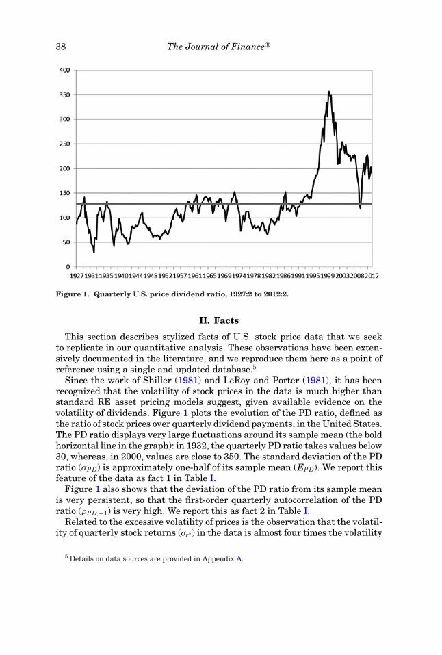
Figure 1. Quarterly U.S. price dividend ratio, 1927:2 to 2012:2.
II. Facts
This section describes stylized facts of U.S. stock price data that we seekto replicate in our quantitative analysis. These observations have been exten-sively documented in the literature, and we reproduce them here as a point ofreference using a single and updated database.5
Since the work of Shiller (1981) and LeRoy and Porter (1981), it has beenrecognized that the volatility of stock prices in the data is much higher thanstandard RE asset pricing models suggest, given available evidence on thevolatility of dividends. Figure 1 plots the evolution of the PD ratio, defined asthe ratio of stock prices over quarterly dividend payments, in the United States.The PD ratio displays very large fluctuations around its sample mean (the boldhorizontal line in the graph): in 1932, the quarterly PD ratio takes values below30, whereas, in 2000, values are close to 350. The standard deviation of the PDratio (σPD) is approximately one-half of its sample mean (EPD). We report thisfeature of the data as fact 1 in Table I.
Figure 1 also shows that the deviation of the PD ratio from its sample meanis very persistent, so that the first-order quarterly autocorrelation of the PDratio (ρPD,−1) is very high. We report this as fact 2 in Table I.
Related to the excessive volatility of prices is the observation that the volatil-ity of quarterly stock returns (σrs ) in the data is almost four times the volatility
5 Details on data sources are provided in Appendix A.
Stock Market Volatility and Learning 39
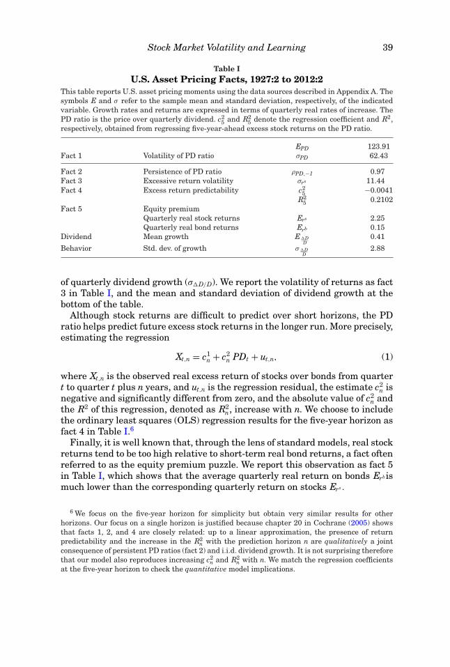
Table IU.S. Asset Pricing Facts, 1927:2 to 2012:2
This table reports U.S. asset pricing moments using the data sources described in Appendix A. Thesymbols E and σ refer to the sample mean and standard deviation, respectively, of the indicatedvariable. Growth rates and returns are expressed in terms of quarterly real rates of increase. ThePD ratio is the price over quarterly dividend. c2
5 and R25 denote the regression coefficient and R2,
respectively, obtained from regressing five-year-ahead excess stock returns on the PD ratio.
EPD 123.91Fact 1 Volatility of PD ratio σPD 62.43
Fact 2 Persistence of PD ratio ρPD,−1 0.97Fact 3 Excessive return volatility σrs 11.44Fact 4 Excess return predictability c2
5 −0.0041R2
5 0.2102Fact 5 Equity premium
Quarterly real stock returns Ers 2.25Quarterly real bond returns Erb 0.15
Dividend Mean growth E�DD
0.41
Behavior Std. dev. of growth σ �DD
2.88
of quarterly dividend growth (σ�D/D). We report the volatility of returns as fact3 in Table I, and the mean and standard deviation of dividend growth at thebottom of the table.
Although stock returns are difficult to predict over short horizons, the PDratio helps predict future excess stock returns in the longer run. More precisely,estimating the regression
Xt,n = c1n + c2
n PDt + ut,n, (1)
where Xt,n is the observed real excess return of stocks over bonds from quartert to quarter t plus n years, and ut,n is the regression residual, the estimate c2
n isnegative and significantly different from zero, and the absolute value of c2
n andthe R2 of this regression, denoted as R2
n, increase with n. We choose to includethe ordinary least squares (OLS) regression results for the five-year horizon asfact 4 in Table I.6
Finally, it is well known that, through the lens of standard models, real stockreturns tend to be too high relative to short-term real bond returns, a fact oftenreferred to as the equity premium puzzle. We report this observation as fact 5in Table I, which shows that the average quarterly real return on bonds Erbismuch lower than the corresponding quarterly return on stocks Ers .
6 We focus on the five-year horizon for simplicity but obtain very similar results for otherhorizons. Our focus on a single horizon is justified because chapter 20 in Cochrane (2005) showsthat facts 1, 2, and 4 are closely related: up to a linear approximation, the presence of returnpredictability and the increase in the R2
n with the prediction horizon n are qualitatively a jointconsequence of persistent PD ratios (fact 2) and i.i.d. dividend growth. It is not surprising thereforethat our model also reproduces increasing c2
n and R2n with n. We match the regression coefficients
at the five-year horizon to check the quantitative model implications.

40 The Journal of Finance R©
Table I reports 10 statistics. As we show in Section IV, we can replicate thesestatistics using a model that has only four free parameters.
III. The Model
In Section III.A, we describe a Lucas (1978) asset pricing model with agentswho hold subjective prior beliefs about stock price behavior. We show thatthe presence of subjective uncertainty implies that utility-maximizing agentsupdate their beliefs about stock price behavior using observed stock price real-izations.7 Using a generic updating mechanism in Section III.B, we show thatsuch learning gives rise to oscillations of asset prices around their fundamentalvalue and qualitatively helps reconcile the Lucas asset pricing model with theempirical evidence. In Section III.C, we introduce a specific system of prior be-liefs that gives rise to constant gain learning—we employ this system of beliefsin our empirical work in Section IV— and we derive conditions under whichthis system of beliefs gives rise to small deviations from RE.
A. Model Description
The Environment: Consider an economy populated by a unit mass of infinitelylived investors, endowed with one unit of a stock that can be traded on acompetitive stock market and that pays dividend Dt, consisting of a perishableconsumption good. Dividends evolve according to
Dt
Dt−1= aεd
t , (2)
for t = 0, 1, 2, . . . , where log εdt ∼ iiN (− s2
d2 , s2
d) and a ≥ 1. This implies E(εdt ) = 1,
E�DD
≡ E( Dt−Dt−1Dt−1
) = a − 1, and σ 2�DD
≡ var( Dt−Dt−1Dt−1
) = a2(es2d − 1). To capture the
fact that the empirically observed consumption process is considerably lessvolatile than the dividend process and to replicate the correlation between div-idend and consumption growth, we assume that each agent also receives anendowment Yt of perishable consumption goods. Total supply of consumptiongoods in the economy is given by the feasibility constraint Ct = Yt + Dt. Fol-lowing the consumption-based asset pricing literature, we impose assumptionsdirectly on the aggregate consumption supply process,8
Ct
Ct−1= aεc
t , (3)
where log εct ∼ iiN (− s2
c2 , s2
c ) and (log εct , log εd
t ) are jointly normal. FollowingCampbell and Cochrane (1999), in our empirical application, we choose sc = 1
7 sd
and set the correlation between log εct and log εd
t to ρc,d = 0.2.
7 This draws on the results in the work of Adam and Marcet (2014).8 The process for Yt is then implied by feasibility.
Stock Market Volatility and Learning 41
Objective Function and Probability Space: Agent i ∈ [0, 1] has standard time-separable expected utility function9
EP0
∞∑t=0
δt
(Ci
t
)1−γ
1 − γ,
where γ ∈ (0,∞) and Cit denotes the consumption demand of agent i. The
expectation is taken using a subjective probability measure P that assignsprobabilities to all external variables (i.e., all payoff-relevant variables that arebeyond the agent’s control). Importantly, Ci
t denotes the agent’s consumptiondemand, and Ct denotes the aggregate supply of consumption goods in theeconomy.
The competitive stock market assumption and the exogeneity of the dividendand income processes imply that investors consider the process for stock prices{Pt} and the income and dividends processes {Yt, Dt} as exogenous to theirdecision problem. The underlying sample (or state) space � thus consists of thespace of realizations for prices, dividends, and income. Specifically, a typicalelement ω ∈ � is an infinite sequence ω = {Pt, Yt, Dt}∞t=0. As usual, we let �t
denote the set of histories from period ∅ up to period t, where ωt is its typicalelement. The underlying probability space is thus given by (�,B,P) with Bdenoting the corresponding σ -algebra of Borel subsets of � and P the agent’ssubjective probability measure over (�,B).
The probability measure P specifies the joint distribution of {Pt, Yt, Dt}∞t=0 atall dates and is fixed at the outset. Although the measure is fixed, investors’beliefs about unknown parameters describing the stochastic processes of thesevariables, as well as investors’ conditional expectations of future values ofthese variables, will change over time in a way that is derived from P and thatdepends on realized data. This specification thus encompasses settings in whichagents learn about the stochastic processes describing Pt, Yt, and Dt. Moreover,unlike in the anticipated utility framework proposed in Kreps (1998), agentsare fully aware of the fact that beliefs will be revised in the future. Although theprobability measure P is not equal to the distribution of {Pt, Yt, Dt}∞t=0 impliedby the model in equilibrium, it is chosen such that it is close to this distributionin a sense that we make precise in Sections III.C and V.B.
Based on the above, expected utility is defined as
EP0
∞∑t=0
δt
(Ci
t
)1−γ
1 − γ≡∫
�
∞∑t=0
δt Cit (ω
t)1−γ
1 − γdP(ω). (4)
Our specification of the probability space is more general than the one usedin other modeling approaches because we also include price histories in therealization ωt. Standard practice is to assume instead that agents know theexact mapping from a history of incomes and dividends to equilibrium as-set prices, Pt(Y t, Dt), so that market prices carry only redundant information.
9 We assume standard preferences so as to highlight the effect of learning on asset price volatility.

42 The Journal of Finance R©
This allows us to exclude prices from the underlying state space without loss ofgenerality. This practice is standard in models of RE, models with rational bub-bles, in Bayesian RE models such as those described in the second paragraphof Section I, and in models incorporating robustness concerns. This standardpractice amounts to imposing a singularity in the joint density over prices, in-come, and dividends, which is equivalent to assuming that agents know exactlythe equilibrium pricing function Pt(·). Although a convenient modeling device,assuming exact knowledge of this function is very restrictive: it implies thatagents have very detailed knowledge of how prices are formed. As a result, it isof interest to study the implications of (slightly) relaxing the assumption thatagents know the function Pt(·). Adam and Marcet (2014) show that rational be-havior is indeed perfectly compatible with agents not knowing the exact formof the equilibrium pricing function Pt(·).10
Choice Set and Constraints: Agents make contingent plans for consumptionCi
t , bond holdings Bit, and stock holdings Si
t , that is, they choose the functions(Ci
t , Sit , Bi
t
): �t → R3 (5)
for all t ≥ 0. Agents’ choices are subject to the budget constraint
Cit + Pt Si
t + Bit ≤ (Pt + Dt) Si
t−1 + (1 + rt−1) Bit−1 + Yt (6)
for all t ≥ 0, where rt−1 denotes the real interest rate on riskless bonds issuedin period t − 1 and maturing in period t. The initial endowments are givenby Si
−1 = 1 and Bi−1 = 0, so that bonds are in zero net supply. To avoid Ponzi
schemes and to ensure the existence of a maximum, the following bounds areassumed to hold:
S ≤ Sit ≤ S (7)
B ≤ Bit ≤ B.
We only assume that the bounds S, S, B, and Bare finite and satisfy S < 1 < S,
B < 0 < B.Maximizing Behavior (Internal Rationality): The investor’s problem then
consists of choosing the sequence of functions {Cit , Si
t , Bit}∞t=0 to maximize (4)
subject to the budget constraint (6) and the asset limits (7), where all con-straints have to hold for all t almost surely in P. Below, we will specify theprobability measure P through some perceived law of motion describing theagent’s view about the evolution of (P, Y , D) over time, together with a priordistribution about the parameters governing this law of motion. Optimal behav-ior will then entail learning about these parameters, in the sense that agentsupdate their posterior beliefs about the unknown parameters in the light of
10 Specifically, they show that, with incomplete markets (i.e., in the absence of state-contingentforward markets for stocks), agents cannot simply learn the equilibrium mapping Pt(·) by observingmarket prices. Furthermore, if the preferences and beliefs of agents in the economy fail to be com-mon knowledge, then agents cannot deduce the equilibrium mapping from their own optimizationconditions.
Stock Market Volatility and Learning 43
new price, income, and dividend observations. For the moment, this learningproblem remains hidden in the belief structure P.
Optimality Conditions: Since the objective function is concave and the fea-sible set is convex, the agent’s optimal plan is characterized by the first-orderconditions (
Cit
)−γPt = δEP
t
[(Ci
t+1
)−γPt+1
]+ δEP
t
[(Ci
t+1
)−γDt+1
], (8)
(Ci
t
)−γ = δ(1 + rt)EPt
[(Ci
t+1
)−γ]. (9)
These conditions are standard except for the fact that the conditional expecta-tions are taken with respect to the subjective probability measure P.
B. Asset Pricing Implications: Analytical Results
This section presents analytical results that explain why the asset pricingmodel with subjective beliefs can explain the asset pricing facts presented inTable I.
Before doing so, we briefly review the well-known result that, under RE, themodel is at odds with these asset pricing facts. A routine calculation shows thatthe unique RE solution of the model is given by
P REt = δa1−γ ρε
1 − δa1−γ ρε
Dt, (10)
where
ρε = E[(εc
t+1)−γ εdt+1
]= eγ (1+γ ) s2
c2 e−γρc,dscsd .
The PD ratio is then constant, return volatility equals approximately thevolatility of dividend growth, and there is no (excess) return predictability,so the model misses facts 1–4 listed in Table I. This holds independent of theparameterization of the model. Furthermore, even for very high degrees ofrelative risk aversion, say γ = 80, the model implies a fairly small risk pre-mium. This emerges because of the low correlation between the innovations toconsumption growth and dividend growth in the data (ρc,d = 0.2).11 The modelthus also misses fact 5 in Table I.
We now characterize the equilibrium outcome under learning. One may betempted to argue that Ci
t+ j can be substituted by Ct+ j for j = 0, 1 in the first-order conditions (8) and (9), simply because Ci
t = Ct holds in equilibrium for
11 Under RE, the risk-free rate is given by 1 + r = (δa−γ eγ (1+γ ) s2c2 )−1 and the expected equity re-
turn equals Et[(Pt+1 + Dt+1)/Pt] = (δa−γ ρε)−1. For ρc,d = 0, therefore, there is no equity premium,independent of the value for γ .

44 The Journal of Finance R©
all t.12 However, outside of strict RE, we may have EPt [Ci
t+1] �= EPt [Ct+1] even
if in equilibrium Cit = Ct holds ex post.13 To understand how this arises, con-
sider the following simple example. Suppose agents know the aggregate pro-cess for Dt and Yt. In this case, EP
t [Ct+1] is a function of only the exogenousvariables (Y t, Dt). At the same time, EP
t [Cit+1] is generally also a function of
price realizations, since, from the perspective of the agent, optimal future con-sumption demand depends on future prices and therefore also on today’s priceswhenever agents are learning about price behavior. As a result, in general,EP
t [Cit+1] �= EP
t [Ct+1], so that one cannot routinely substitute individual by ag-gregate consumption on the right-hand side of the agent’s first-order conditions(8) and (9).
Nevertheless, if, in any given period t, the optimal plan for period t + 1from the viewpoint of the agent is such that (Pt+1(1 − Si
t+1) − Bit+1)/(Yt + Dt) is
expected to be small according to the agent’s expectations EPt , then agents with
beliefsP realize in period t that Cit+1/Ci
t ≈ Ct+1/Ct with very high P-probability.This follows from the flow budget constraint for period t + 1 and the fact thatSi
t = 1, Bit = 0, and Ci
t = Ct in equilibrium in period t. One can then rely on theapproximations
EPt
[(Ct+1
Cit
)−γ
(Pt+1 + Dt+1)
]� EP
t
[(Ci
t+1
Cit
)−γ
(Pt+1 + Dt+1)
], (11)
EPt
[(Ct+1
Cit
)−γ]
� EPt
[(Ci
t+1
Cit
)−γ]. (12)
The following assumption provides sufficient conditions for this to be the case:
ASSUMPTION 1: We assume that Yt is sufficiently large, and that EPt Pt+1/Dt <
M for some M < ∞, such that, given finite asset bounds S, S, B, and B, theapproximations (11) and (12) hold with sufficient accuracy in equilibrium.
Intuitively, for high enough income Yt, the agent’s asset trading decisionsmatter little for the agents’ stochastic discount factor (Ci
t+1
Cit
)−γ . This implies that,from the consumer’s point of view at t, individual consumption growth in t + 1must be very close to aggregate consumption growth in t + 1 in equilibrium.14
The bound on subjective price expectations imposed in Assumption 1 is justifiedby the fact that the PD ratio will be bounded in equilibrium, so that the objectiveexpectation Et Pt+1/Dt will also be bounded.15
12 The equality Cit = Ct follows from market clearing and the fact that all agents are identical.
13 This is the case because the preferences and beliefs of agents are not assumed to be commonknowledge, so that agents do not know that Ci
t = Ct must hold in equilibrium.14 Note that, independent from their tightness, the asset holding constraints never prevent
agents from marginally trading or selling securities in any period t along the equilibrium path,where Si
t = 1 and Bit = 0 holds for all t.
15 To see this, note that Pt+1/Dt+1 < PD implies Et[Pt+1]/Dt < aPD < ∞, where a denotes themean dividend growth rate.
Stock Market Volatility and Learning 45
Under Assumption 1, and if we plug the equilibrium condition Cit = Ct into
the first-order conditions, the risk-free interest rate solves
1 = δ(1 + rt)EPt
[(Ct+1
Ct
)−γ]
. (13)
Furthermore, defining the subjective expectations of risk-adjusted stock pricegrowth
βt ≡ EPt
((Ct+1
Ct
)−γ Pt+1
Pt
)(14)
and the subjective expectations of risk-adjusted dividend growth
βDt ≡ EP
t
((Ct+1
Ct
)−γ Dt+1
Dt
),
the first-order condition for stocks (8) implies that the equilibrium stock priceunder subjective beliefs is given by
Pt = δβDt
1 − δβtDt, (15)
provided that βt < δ−1. The equilibrium stock price is thus increasing in both(subjective) expected risk-adjusted dividend growth and expected risk-adjustedprice growth.
For the special case in which agents know the RE growth rates βt = βDt =
a1−γ ρε for all t, equation (15) delivers the RE price outcome (10). Furthermore,when agents hold subjective beliefs about risk-adjusted dividend growth butobjectively rational beliefs about risk-adjusted price growth, then βD
t = βt and(15) deliver the pricing implications derived in the Bayesian RE asset pricingliterature, as reviewed in Section I.
To highlight the fact that the improved empirical performance of the presentasset pricing model derives exclusively from subjective beliefs about risk-adjusted price growth, we entertain assumptions that are orthogonal to thosemade in the Bayesian RE literature. Specifically, we assume that agents knowthe true process for risk-adjusted dividend growth:
ASSUMPTION 2: Agents know the process for risk-adjusted dividend growth, thatis, βD
t ≡ a1−γ ρε for all t.
Under this assumption, the asset pricing equation (15) simplifies to16
Pt = δa1−γ ρε
1 − δβtDt. (16)
16 Some readers may be tempted to believe that entertaining subjective price beliefs whileentertaining objective beliefs about the dividend process is inconsistent with individual rationality.Adam and Marcet (2014) show, however, that there exists no such contradiction as long as thepreferences and beliefs of agents in the economy are not common knowledge.
46 The Journal of Finance R©
Stock Price Behavior under Learning: We now derive a number of analyticalresults regarding the behavior of asset prices over time. We start with a generalobservation about the volatility of prices and then derive results about thebehavior of prices over time for a general belief-updating scheme.
The asset pricing equation (16) implies that fluctuations in subjective priceexpectations can contribute to fluctuations in actual prices. As long as thecorrelation between βt and the last dividend innovation εd
t is small (as occursfor the updating schemes for βt that we consider in this paper), equation (16)implies
var(
lnPt
Pt−1
)� var
(ln
1 − δβt−1
1 − δβt
)+ var
(ln
Dt
Dt−1
). (17)
The previous equation shows that even small fluctuations in subjective pricegrowth expectations can significantly increase the variance of price growth,and thus the variance of stock price returns, if βt fluctuates around valuesclose to but below δ−1.
To determine the behavior of asset prices over time, one needs to take a standon how the subjective price expectations βt are updated over time. To improveour understanding of the empirical performance of the model and to illustratethat the results in our empirical application do not depend on the specific beliefsystem considered, we now derive analytical results for a general nonlinearbelief-updating scheme.
Given that βt denotes the subjective one-step-ahead expectation of risk-adjusted stock price growth, it appears natural to assume that the measureP implies that rational agents revise βt upward (downward) if they under-predicted (overpredicted) the risk-adjusted stock price growth ex post. Thisprompts us to consider measures P that imply updating rules of the form17
�βt = ft
((Ct−1
Ct−2
)−γ Pt−1
Pt−2− βt−1; βt−1
)(18)
for given nonlinear updating functions ft : R2 → R with the properties
ft(0; β) = 0 (19)
ft (·; β) increasing (20)
0 < β + ft (x; β) < βU (21)
for all (t, x), β ∈ (0, βU ), and some constant βU ∈ (a1−γ ρε, δ−1). Properties (19)
and (20) imply that βt is adjusted in the same direction as the last prediction
17 Note that βt is determined from observations up to period t − 1 only. This simplifies theanalysis and avoids simultaneity of price and forecast determination. This lag in the informationis common in the learning literature. Difficulties emerging with simultaneous information sets inmodels of learning are discussed in Adam (2003).

Stock Market Volatility and Learning 47
error, where the strength of the adjustment may depend on the current levelof beliefs, as well as on the calendar time (e.g., on the number of observationsavailable to date). Property (21) is needed to guarantee that positive equilib-rium prices solving (16) always exist.
In Section III.C, we provide an explicit system of beliefs P in which agentsoptimally update beliefs according to a special case of equation (18). Updatingrule (18) is more general and nests a range of learning schemes considered inthe literature on adaptive learning, for example, least-squares learning andthe switching-gains learning schemes used by Marcet and Nicolini (2003).
To derive the equilibrium behavior of price expectations and price realiza-tions over time, we first use (16) to determine realized price growth
Pt
Pt−1=(
a + aδ �βt
1 − δβt
)εd
t . (22)
Combining the previous equation with the belief-updating rule (18), one obtains
�βt+1 = ft+1
(T (βt,�βt)
(εc
t
)−γεd
t − βt; βt
), (23)
where
T (β,�β) ≡ a1−γ + a1−γ δ �β
1 − δβ.
Given initial conditions (Y0, D0, P−1) and initial expectations β0, equation (23)completely characterizes the equilibrium evolution of the subjective price ex-pectations βt over time. Given that there is a one-to-one relationship betweenβt and the PD ratio (see equation (16)), the previous equation also character-izes the evolution of the equilibrium PD ratio under learning. High- (low)-pricegrowth expectations are thereby associated with high (low) values for the equi-librium PD ratio.
The properties of the second-order difference equation (23) can be illustratedin a two-dimensional phase diagram for the dynamics of (βt, βt−1), which isshown in Figure 2 for the case in which the shocks (εc
t )−γ εdt assume their un-
conditional mean value ρε.18 The effects of different shock realizations for thedynamics are discussed separately below.
The arrows in Figure 2 indicate the direction in which the vector (βt, βt−1)evolves over time according to equation (23), and the solid lines indicate theboundaries of these areas.19 Since we have a difference equation rather than adifferential equation, we cannot plot the evolution of expectations exactly be-cause the difference equation gives rise to discrete jumps in the vector (βt, βt−1)over time. Yet, if agents update beliefs only relatively weakly in response toforecast errors, as is the case for our estimated model discussed below, then forsome areas in the figure, these jumps will be correspondingly small, as we nowexplain.
18 Appendix B explains the construction of the phase diagram in detail.19 The vertical solid line close to δ−1 is meant to illustrate the restriction β < δ−1.

48 The Journal of Finance R©
B
A
βt
βt-1
βt = βt-1
a1-γρε(REE belief)
δ-1
βt+1 = βt
C
D
Figure 2. Phase diagram illustrating momentum and mean-reversion.
Consider, for example, region A in the diagram. In this area, βt < βt−1 andβt keep decreasing, which shows that there is momentum in price changes.This holds true even if βt is already at or below its fundamental value a1−γ ρε.Provided the updating gain is small, beliefs in region A will slowly move abovethe 45º line in the direction of the lower left corner of the graph. Yet, oncethey enter area B, βt starts to increase, so that, in the next period, beliefs willdiscretely jump into area C. In region C, we have βt > βt−1 and βt continuesto increase, so that beliefs display upward momentum. This manifests in anupward and rightward change in beliefs over time, until they reach area D.There, beliefs βt start to decrease, so that ultimately discretely jump back intoarea A, and thereby display mean reversion. The elliptic movements of beliefsaround a1−γ ρε imply that expectations (and thus the PD ratio) are likely tooscillate in sustained and persistent swings around the RE value.
The effect of the stochastic disturbances (εct )−γ εd
t is to shift the curve labeledas “βt+1 = βt” in Figure 2. Specifically, for realizations (εc
t )−γ εdt > ρε, this curve
is shifted upward. As a result, beliefs are more likely to increase, which is thecase for all points below this curve. Conversely, for (εc
t )−γ εdt < ρε, this curve
shifts downward, making it more likely that beliefs decrease from the currentperiod to the next.
The previous results show that learning causes beliefs and the PD ratioto stochastically oscillate around its RE value. Such behavior will be key inexplaining the observed volatility and serial correlation of the PD ratio (i.e.,facts 1 and 2 in Table I). Also, from the discussion around equation (17), itshould be clear that such behavior makes stock returns more volatile than

Stock Market Volatility and Learning 49
dividend growth, which contributes to replicating fact 3. As discussed inCochrane (2005), a serially correlated and mean-reverting PD ratio gives riseto excess return predictability, so it contributes to matching fact 4.
The momentum of changes in beliefs around the RE value of beliefs, as wellas the overall mean-reverting behavior, are formally captured in the followingresults:20
Momentum. If �βt > 0 and
βt ≤ a1−γ(εc
t
)−γεd
t , (24)
then �βt+1 > 0. This also holds if all inequalities are reversed.Therefore, up to a linear approximation of the updating function f ,
Et−1[�βt+1] > 0,
whenever �βt > 0 and βt ≤ a1−γ ρε. Beliefs thus have a tendency to increase(decrease) further following an initial increase (decrease) whenever beliefs areat or below (above) the RE value.
The following result shows formally that stock prices would eventually returnto their (deterministic) RE value in the absence of further disturbances and thatsuch reverting behavior occurs monotonically.21
Mean Reversion. Consider an arbitrary initial belief βt ∈ (0, βU ). In the absenceof further disturbances (εd
t+ j = εct+ j = 0 for all j ≥ 0),
limt→∞ sup βt ≥ a1−γ ≥ lim
t→∞ inf βt.
Furthermore, if βt > a1−γ , there is a period t′ ≥ t such that βt is nondecreasingbetween t and t′ and nonincreasing between t′ and t′′, in which t′′ is the firstperiod where βt′′ is arbitrarily close to a1−γ . The results are symmetric for βt <
a1−γ .The previous result implies that, absent any shocks, βt cannot stay away
from the RE value forever. Beliefs either converge to the deterministic RE value(when lim sup = lim inf) or fluctuate around it forever (when lim sup > lim inf).Any initial deviation, however, is eventually eliminated with the reversionprocess being monotonic. This result also implies that an upper bound on pricebeliefs cannot be an absorbing point: if beliefs βt go up and they get close to theupper bound βU , they will eventually bounce off this upper bound and returntoward the RE value.
Summing up, the previous results show that, for a general set of belief up-dating rules, stock prices and beliefs fluctuate around their RE values in a waythat helps qualitatively account for facts 1–4 listed in Table I.
20 The momentum result follows from the fact that condition (24) implies that the first argumentin the f function on the right-hand side of equation (23) is positive (negative if the inequalities arereversed).
21 See Appendix C for the proof under an additional technical assumption.

50 The Journal of Finance R©
C. Optimal Belief Updating: Constant-Gain Learning
We now introduce a fully specified probability measure P and derive theoptimal belief-updating equation it implies. We employ this belief-updatingequation in our empirical work in Section IV. Below, we show in which sensethis system of beliefs represents a small deviation from RE.
In line with Assumption 2, we consider agents who hold RE about the div-idend and aggregate consumption processes. At the same time, we allow forsubjective beliefs about risk-adjusted stock price growth by allowing agents toentertain the possibility that risk-adjusted price growth may contain a smalland persistent time-varying component. This is motivated by the observationthat, in the data, there are periods in which the PD ratio increases persistently,as well as periods in which the PD ratio decreases persistently (see Figure 1).In an environment with unpredictable innovations to dividend growth, thisimplies the existence of persistent and time-varying components in stock pricegrowth. For this reason, we consider agents who think that the process forrisk-adjusted stock price growth is the sum of a persistent component bt and atransitory component εt,
(Ct
Ct−1
)−γ Pt
Pt−1= bt + εt (25)
bt = bt−1 + ξt,
for εt ∼ iiN(0, σ 2ε ) and ξt ∼ iiN(0, σ 2
ξ ) independent of each other and also jointlyi.i.d. with εd
t and εct .22 The latter implies E[(εt, ξt)|It−1] = 0, where It−1 includes
all the variables in the agents’ information set at t − 1, including all prices,endowments, and dividends dated t − 1 or earlier.
The previous setup encompasses RE equilibrium beliefs as a special case. Inparticular, when agents believe σ 2
ξ = 0 and assign probability 1 to b0 = a1−γ ρε,we have that βt = a1−γ ρε for all t ≥ 0 and prices are as given by RE equilibriumprices in all periods.
In what follows we allow for a nonzero variance σ 2ξ , that is, for the presence of
a persistent time-varying component in price growth. The setup then gives riseto a learning problem because agents observe the realizations of risk-adjustedprice growth, but not the persistent and transitory components separately. Thelearning problem consists of optimally filtering out the persistent componentof price growth bt. Assuming that agents’ prior beliefs b0 are centered at theRE value and given by
b0 ∼ N(a1−γ ρε, σ20 ),
22 Notice that we use the notation Ct = Yt + Dt, so that equation (25) contains only payoff-relevant variables that are beyond the agent’s control.
Stock Market Volatility and Learning 51
and setting σ 20 equal to the steady-state Kalman filter uncertainty about bt,
which is given by
σ 20 =
−σ 2ξ +
√(σ 2
ξ
)2 + 4σ 2ξ σ 2
ε
2,
agents’ posterior beliefs at any time t are given by
bt ∼ N(βt, σ0).
Optimal updating then implies that βt, defined in equation (14), recursivelyevolves according to
βt = βt−1 + 1α
((Ct−1
Ct−2
)−γ Pt−1
Pt−2− βt−1
). (26)
The optimal (Kalman) gain is given by 1/α = (σ 20 + σ 2
ξ )/(σ 20 + σ 2
ξ + σ 2ε ), which
captures the strength with which agents optimally update their posteriors inresponse to surprises.23
These beliefs constitute a small deviation from RE beliefs in the limiting casewith vanishing innovations to the random walk process (σ 2
ξ → 0). Agents’ prioruncertainty then vanishes (σ 2
0 → 0), and the optimal gain converges to zero(1/α → 0). As a result, βt → a1−γ ρε in distribution for all t, so that one recoversthe RE equilibrium value for risk-adjusted price growth expectations. Thisshows that, for any given distribution of asset prices, agents’ beliefs are closeto RE beliefs whenever the gain parameter (1/α) is sufficiently small. We showbelow that this continues to be true when using the equilibrium distribution ofasset prices generated by sufficiently small gain parameters.
For our empirical application, we need to modify the updating equation (26)slightly to guarantee that the bound βt < βU holds for all periods and equilib-rium prices always exist. The exact way in which this bound is imposed matterslittle for our empirical result because the moments we compute do not changemuch as long as βt is rarely close to βU over the sample length considered. Toimpose this bound, we consider in our empirical application a concave, increas-ing, and differentiable function w : R+ → (0, βU ) and modify the belief-updatingequation (26) to24
βt = w
(βt−1 + 1
α
[(Ct−1
Ct−2
)−γ Pt−1
Pt−2− βt−1
]), (27)
23 In line with equation (18), we incorporate information with a lag so as to eliminate thesimultaneity between prices and price growth expectations. The lag in the updating equationcould be justified by a specific information structure where agents observe some of the laggedtransitory shocks to risk-adjusted stock price growth.
24 The exact functional form for w that we use in the estimation is provided in Appendix E.
52 The Journal of Finance R©
where
w(x) = x if x ∈ (0, βL)
for some βL ∈ (a1−γ ρε, βU ). Beliefs thus continue to evolve according to (26) as
long as they are below the threshold βL, whereas, for higher beliefs, we havethat w(x) ≤ x. The modified algorithm (27) satisfies the constraint (21) andcan be interpreted as an approximate implementation of a Bayesian updatingscheme where agents have a truncated prior that puts probability zero onbt > βU .25
We now show that, for a small value of the gain (1/α), agents’ beliefs areclose to RE beliefs when using the equilibrium distribution of prices gener-ated by these beliefs. More precisely, the setup gives rise to a stationary andergodic equilibrium outcome in which expectations about risk-adjusted stockprice growth have a distribution that is increasingly centered at the RE valuea1−γ ρε as the gain parameter becomes vanishingly small. From equation (16),it then follows that actual equilibrium prices also become increasingly concen-trated at their RE value, so that the difference between beliefs and outcomesbecomes vanishingly small as 1/α → 0.Stationarity, Ergodicity, and Small Deviations from RE. Suppose agents’ pos-terior beliefs evolve according to equation (27) and equilibrium prices aredetermined according to equation (16). Then, βt is geometrically ergodic forsufficiently large α. Furthermore, as 1/α → 0, we have E[βt] → a1−γ ρε andVAR(βt) → 0.
The proof is based on results from Duffie and Singleton (1993) and containedin Appendix D. Geometric ergodicity implies the existence of a unique sta-tionary distribution for βt that is ergodic and that is reached from any initialcondition. Geometric ergodicity is required for estimation by MSM.
In Section V, we further explore the connection between agents’ beliefs andmodel outcomes, using the estimated models from the subsequent section.
IV. Quantitative Model Performance
This section evaluates the quantitative performance of the asset pricingmodel with subjective price beliefs and shows that it can robustly replicatefacts 1–4 listed in Table I. We formally estimate and test the model using theMethod of Simulated Moments (MSM). This approach to structural estimation
25 The issue of bounding beliefs so as to ensure that expected utility remains finite arises in manyapplications of both Bayesian and adaptive learning to asset prices. The literature typically dealswith this issue by using a projection facility, assuming that agents simply ignore observations thatwould imply updating beliefs beyond the required bound. See Timmermann (1993, 1996), Marcetand Sargent (1989), or Evans and Honkapohja (2001). This approach has two problems. First, itdoes not arise from Bayesian updating. Second, it introduces a discontinuity into the simulatedmoments and creates difficulties for our MSM estimation in Section IV, prompting us to pursuethe differentiable approach to bounding beliefs described above.

Stock Market Volatility and Learning 53
and testing helps us focus on the ability of the model to explain the specificmoments of the data described in Table I.26
We first evaluate the model’s ability to explain the individual moments, whichis the focus of much of the literature on matching stock price volatility. We findthat the model can explain the individual moments well. Using t-statisticsbased on formal asymptotic distribution, we find that, in some versions ofthe model, all t-statistics are at or below two in absolute value, even with amoderate relative risk aversion of γ = 5. Moreover, with this degree of riskaversion, the model can explain up to 50% of the equity premium, which ismuch higher than under RE.
We next turn to the more demanding task of testing whether all the momentsare accepted jointly by computing χ2 test statistics. Due to their stringency,such test statistics are rarely reported in the consumption-based asset pricingliterature. A notable exception is Bansal, Kiku, and Yaron (2013), who testthe overidentifying restrictions of a long-run risk model. In contrast to ourapproach, they test equilibrium conditions instead of matching statistics. Also,they use a diagonal weighting matrix instead of the optimal weighting matrixin the objective function (29) introduced below.
We find that, with a relative risk aversion of γ = 5, the model fails to passan overall goodness of fit as long as one includes the equity premium. However,the test reaches a moderate p-value of 2.5% when we exclude the risk-freerate from the set of moments to be matched, confirming that it is the equitypremium that poses a quantitative challenge to the model.27 With a relativerisk aversion of γ = 3, the p-value increases even further to 7.1% when weagain exclude the risk-free rate.
Finally, we allow for a very high risk aversion coefficient. Specifically, weset γ = 80, which is the steady-state value of relative risk aversion used inCampbell and Cochrane (1999).28 The model then replicates all moments inTable I, including the risk premium. In particular, the model generates aquarterly equity premium of 2.0%, slightly below the 2.1% per quarter ob-served in U.S. data, while still replicating all other asset pricing moments.
Section IV.A explains the MSM approach for estimating the model and theformal statistical test for evaluating the goodness of fit. Section IV.B reports onthe estimation and test outcomes.
26 A popular alternative approach in the asset pricing literature is to test whether agents’ first-order conditions hold in the data. Hansen and Singleton (1982) pioneered this approach for REmodels, and Bossaerts (2004) provides an approach that can be applied to models of learning. Wepursue the MSM estimation approach here because it naturally provides additional informationon how the formal test for goodness of fit relates to the model’s ability to match the moments ofinterest. The results are then easily interpretable, as they point out which parts of the model fitwell and which parts do not, thus providing intuition about possible avenues for improving themodel fit.
27 The literature suggests a number of other model ingredients that, once added, would generatea higher equity premium. See, for example, ambiguity aversion in Collard et al. (2011), initiallypessimistic expectations in Cogley and Sargent (2008), or habits in consumption preferences.
28 This value is reported on page 244 in their paper.

54 The Journal of Finance R©
A. MSM Estimation and Statistical Test
This section outlines the MSM approach and the formal test for evaluatingthe fit of the model. This is a simple adaptation of standard MSM to includematching of statistics that are functions of simple moments by using the deltamethod (see Appendix F for details).
For a given value of the coefficient of relative risk aversion, there are four freeparameters left in the model, namely, the discount factor δ, the gain parameter1/α, and the mean and standard deviation of dividend growth, denoted by aand σ�D
D, respectively. We summarize these parameters in the vector
θ ≡(δ, 1/α, a, σ�D
D
).
These 4 parameters will be chosen so as to match some or all of the 10 samplemoments in Table I:29(
Ers , EPD, σrs , σPD, ρPD,−1, c52, R2
5, Erb, E�DD
, σ �DD
). (28)
Let SN ∈ Rs denote the subset of sample moments in (28) that will be matchedin the estimation, with N denoting the sample size and s ≤ 10.30 Furthermore,let S(θ ) denote the moments implied by the model for some parameter value θ .The MSM parameter estimate θN is defined as
θN ≡ arg minθ
[SN − S(θ )]′
�−1S,N
[SN − S(θ )], (29)
where �S,N is an estimate of the variance-covariance matrix of the samplemoments SN. The MSM estimate θN chooses the model parameter such thatthe model moments S(θ ) fit the observed moments SN as closely as possiblein terms of a quadratic form with weighting matrix �−1
S,N . We estimate �S,Nfrom the data in the standard way. Adapting standard results from MSM, onecan prove that, for a given list of moments included in SN, the estimate θNis consistent and is the best estimate among those obtained with differentweighting matrices.
The MSM estimation approach also provides an overall test of the model.Under the null hypothesis that the model is correct, we have
WN ≡ N[SN − S (θN)
]′�−1
S,N
[SN − S (θN)]→ χ2
s−4 as N → ∞, (30)
where convergence is in distribution. Furthermore, we obtain a proper asymp-totic distribution for each element of the deviations SN − S (θN), so that we
29 Many elements listed in (28) are not sample moments, but they are nonlinear functions ofsample moments. For example, the R2 coefficient is a function of sample moments. This means wehave to use the delta method to adapt standard MSM (see Appendix F). It would be more preciseto refer to the elements in (28) as “sample statistics,” as we do in Appendix F. For simplicity, weavoid this terminology in the main text.
30 As discussed before, we exclude the risk premium from some estimations; in those cases,s < 10.
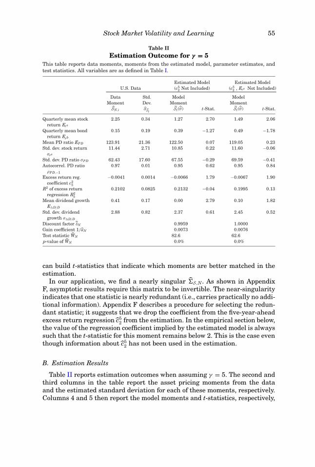
Stock Market Volatility and Learning 55
Table IIEstimation Outcome for γ = 5
This table reports data moments, moments from the estimated model, parameter estimates, andtest statistics. All variables are as defined in Table I.
Estimated Model Estimated ModelU.S. Data (c5
2 Not Included) (c52 , Ers Not Included)
Data Std. Model ModelMoment Dev. Moment Moment
SN,i σSiSi (θ ) t-Stat. Si (θ ) t-Stat.
Quarterly mean stockreturn Ers
2.25 0.34 1.27 2.70 1.49 2.06
Quarterly mean bondreturn Erb
0.15 0.19 0.39 −1.27 0.49 −1.78
Mean PD ratio EPD 123.91 21.36 122.50 0.07 119.05 0.23Std. dev. stock return
σrs
11.44 2.71 10.85 0.22 11.60 −0.06
Std. dev. PD ratio σPD 62.43 17.60 67.55 −0.29 69.59 −0.41Autocorrel. PD ratio
ρPD,−1
0.97 0.01 0.95 0.62 0.95 0.84
Excess return reg.coefficient c2
5
−0.0041 0.0014 −0.0066 1.79 −0.0067 1.90
R2 of excess returnregression R2
5
0.2102 0.0825 0.2132 −0.04 0.1995 0.13
Mean dividend growthE�D/D
0.41 0.17 0.00 2.79 0.10 1.82
Std. dev. dividendgrowth σ�D/D
2.88 0.82 2.37 0.61 2.45 0.52
Discount factor δN 0.9959 1.0000Gain coefficient 1/αN 0.0073 0.0076Test statistic WN 82.6 62.6p-value of WN 0.0% 0.0%
can build t-statistics that indicate which moments are better matched in theestimation.
In our application, we find a nearly singular �S,N. As shown in AppendixF, asymptotic results require this matrix to be invertible. The near-singularityindicates that one statistic is nearly redundant (i.e., carries practically no addi-tional information). Appendix F describes a procedure for selecting the redun-dant statistic; it suggests that we drop the coefficient from the five-year-aheadexcess return regression c5
2 from the estimation. In the empirical section below,the value of the regression coefficient implied by the estimated model is alwayssuch that the t-statistic for this moment remains below 2. This is the case eventhough information about c5
2 has not been used in the estimation.
B. Estimation Results
Table II reports estimation outcomes when assuming γ = 5. The second andthird columns in the table report the asset pricing moments from the dataand the estimated standard deviation for each of these moments, respectively.Columns 4 and 5 then report the model moments and t-statistics, respectively,

56 The Journal of Finance R©
when estimating the model using all asset pricing moments (except for c52,
which has been excluded for reasons explained in the previous section). Allestimations impose the restriction δ ≤ 1.
The estimated model reported in columns 4 and 5 of Table II quantitativelyreplicates the volatility of stock returns (σrs ), the large volatility and high per-sistence of the PD ratio (σPD, ρPD−1), as well as the excess return predictability(c2
5, R25). This is a remarkable outcome given the assumed time-separable pref-
erence structure. The model has some difficulty in replicating the mean stockreturn and dividend growth, but t-statistics for all other moments have an ab-solute value well below two, and more than half of the t-statistics are belowone.
The last two columns in Table II report the estimation outcome when drop-ping the mean stock return Ers from the estimation and restricting δ to one,which tends to improve the ability of the model to match individual moments.All t-statistics are then close to or below two, including the t-statistics for themean stock return and for c5
2 that have not been used in the estimation, and themajority of the t-statistics are below one. This estimation outcome shows thatthe subjective beliefs model successfully matches individual moments with arelatively low degree of risk aversion. The model also delivers an equity pre-mium of 1% per quarter, nearly half of the value observed in U.S. data (2.1%per quarter).
The measure for the overall goodness of fit WN and its p-value are reportedin the last two rows of Table II. The statistic is computed using all momentsthat are included in the estimation. The reported values of WN are off the chartof the χ2 distribution, implying that the overall fit of the model is rejectedeven if all moments are matched individually.31 This indicates that some ofthe joint deviations observed in the data are unlikely to happen given theobserved second moments. It also shows that the overall goodness of fit test isconsiderably more stringent.
To show that the equity premium is indeed the source of the difficulty forpassing the overall test, columns 4 and 5 in Table III report results obtainedwhen we repeat the estimation excluding the risk-free rate Erb instead of thestock returns Ers from the estimation. The estimation imposes the constraintδN ≤ 1, since most economists believe that values above one are unacceptable.This constraint turns out to be binding. The t-statistics for the individual mo-ments included in the estimation are quite low, but the model fails to replicatethe low value for the bond return Erb, which has not been used in the estima-tion. Despite larger t-statistics, the model now comfortably passes the overallgoodness of fit test at the 1% level, as the p-value for the reported WN =12.87statistic is 2.5%. The last two columns in Table III repeat the estimation when
31 The χ2 distribution has five degrees of freedom for the estimations in Table II, where the lasttwo columns drop a moment but also fix δ = 1. For the estimation in Table III, we exclude c5
2 andErb from the estimation, but the constraint δ ≤ 1 is either binding or imposed, so that we continueto have five degrees of freedom. Similarly, we have five degrees of freedom for the estimation inTable IV.

Stock Market Volatility and Learning 57
Table IIIEstimation Outcome for γ = 5 and γ = 3
This table reports data moments, moments from the estimated model, parameter estimates, andtest statistics. All variables are as defined in Table I.
Estimated Model Estimated Modelγ = 5 γ = 3
U.S. Data (c52, Erb Not Included) (c5
2, Erb Not Included)
Data Model ModelMoment Moment MomentSN,i Si (θ ) t-Stat. Si (θ) t-Stat.
Quarterly mean stock return Ers 2.25 1.32 2.50 1.51 2.00Quarterly mean bond return Erb 0.15 1.09 −4.90 1.30 −5.98Mean PD ratio EPD 123.91 109.66 0.69 111.28 0.58Std. dev. stock return σrs 11.44 5.34 2.25 5.10 2.33Std. dev. PD ratio σPD 62.43 40.09 1.33 39.11 1.31Autocorrel. PD ratio ρPD,−1 0.97 0.96 0.30 0.96 0.23Excess return reg. coefficient c2
5 −0.0041 −0.0050 0.64 −0.0050 0.60R2 of excess return regression R2
5 0.2102 0.2282 −0.22 0.2302 −0.24Mean dividend growth E�D/D 0.41 0.22 1.14 0.43 −0.09Std. dev. dividend growth σ�D/D 2.88 1.28 1.95 1.23 2.00Discount factor δN 1.0000 1.0000Gain coefficient 1/αN 0.0072 0.0071Test statistic WN 12.87 11.07p-value of WN 2.5% 7.1%
imposing γ = 3 and δN = 1. The performance in terms of matching the momentsis then very similar with γ = 5, but the p-value of the WN statistic increases to7.1%.
Figure 3 shows realizations of the time-series outcomes for the PD ratiogenerated from simulating the estimated model from Table III with γ = 5,for the same number of quarters as the number of observations in our datasample. The simulated time series displays price booms and busts, similar tothose displayed in Figure 1 for the actual data, so that the model also passesan informal “eyeball test.”
The estimated gain coefficients in Tables II and III are fairly small. Theestimate in Table III implies that agents’ risk-adjusted return expectationsrespond only 0.7% in the direction of the last observed forecast error, suggest-ing that the system of price beliefs in our model does indeed represent onlya small deviation from RE beliefs. Under strict RE, the reaction to forecasterrors is zero, but the model then provides a very bad match with the data: itcounterfactually implies σrs ≈ σ�D/D, σPD = 0, and R2
5 = 0.To further examine what it takes to match the risk premium and to more
carefully compare our results with the performance of other models in the lit-erature, we now assume a high degree of risk aversion of γ = 80, in line withthe steady-state degree of risk aversion assumed in Campbell and Cochrane(1999). Furthermore, we use all asset pricing moments listed in equation

58 The Journal of Finance R©
Figure 3. Simulated PD ratio, estimated model from Table III (γ = 5).
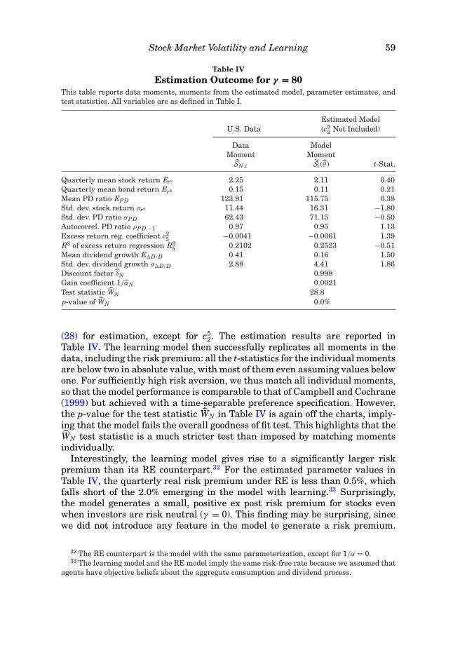
Stock Market Volatility and Learning 59
Table IVEstimation Outcome for γ = 80
This table reports data moments, moments from the estimated model, parameter estimates, andtest statistics. All variables are as defined in Table I.
Estimated ModelU.S. Data (c5
2 Not Included)
Data ModelMoment MomentSN,i Si (θ) t-Stat.
Quarterly mean stock return Ers 2.25 2.11 0.40Quarterly mean bond return Erb 0.15 0.11 0.21Mean PD ratio EPD 123.91 115.75 0.38Std. dev. stock return σrs 11.44 16.31 −1.80Std. dev. PD ratio σPD 62.43 71.15 −0.50Autocorrel. PD ratio ρPD,−1 0.97 0.95 1.13Excess return reg. coefficient c2
5 −0.0041 −0.0061 1.39R2 of excess return regression R2
5 0.2102 0.2523 −0.51Mean dividend growth E�D/D 0.41 0.16 1.50Std. dev. dividend growth σ�D/D 2.88 4.41 1.86Discount factor δN 0.998Gain coefficient 1/αN 0.0021Test statistic WN 28.8p-value of WN 0.0%
(28) for estimation, except for c52. The estimation results are reported in
Table IV. The learning model then successfully replicates all moments in thedata, including the risk premium: all the t-statistics for the individual momentsare below two in absolute value, with most of them even assuming values belowone. For sufficiently high risk aversion, we thus match all individual moments,so that the model performance is comparable to that of Campbell and Cochrane(1999) but achieved with a time-separable preference specification. However,the p-value for the test statistic WN in Table IV is again off the charts, imply-ing that the model fails the overall goodness of fit test. This highlights that theWN test statistic is a much stricter test than imposed by matching momentsindividually.
Interestingly, the learning model gives rise to a significantly larger riskpremium than its RE counterpart.32 For the estimated parameter values inTable IV, the quarterly real risk premium under RE is less than 0.5%, whichfalls short of the 2.0% emerging in the model with learning.33 Surprisingly,the model generates a small, positive ex post risk premium for stocks evenwhen investors are risk neutral (γ = 0). This finding may be surprising, sincewe did not introduce any feature in the model to generate a risk premium.
32 The RE counterpart is the model with the same parameterization, except for 1/α = 0.33 The learning model and the RE model imply the same risk-free rate because we assumed that
agents have objective beliefs about the aggregate consumption and dividend process.

60 The Journal of Finance R©
To understand why this occurs, note that the realized gross stock return be-tween period 0 and period N can be written as the product of three terms:
N∏t=1
Pt + Dt
Pt−1=
N∏t=1
Dt
Dt−1︸ ︷︷ ︸=R1
·(
PDN + 1PD0
)︸ ︷︷ ︸
=R2
·N−1∏t=1
PDt + 1PDt︸ ︷︷ ︸
=R3
.
The first term (R1) is independent of the way prices are formed and thus cannotcontribute to explaining the emergence of an equity premium in the modelwith learning. The second term (R2), which is the ratio of the terminal over thestarting value of the PD ratio, could potentially generate an equity premiumbut is, on average, below one in our simulations of the learning model, whereasit is slightly larger than one under RE.34 The equity premium in the learningmodel must thus be due to the last component (R3). This term is convex in thePD ratio, so that a model that generates higher volatility of the PD ratio (butthe same mean value) will also give rise to a higher equity premium. Therefore,because our learning model generates a considerably more volatile PD ratio, italso gives rise to a larger ex post risk premium.
V. Robustness of Results
This section discusses the robustness of our findings with regard to differ-ent learning specifications and parameter choices (Section V.A), analyzes indetail the extent to which agents’ forecasts could be rejected by the data or theequilibrium outcomes of the model (Section V.B), and finally offers a discus-sion of the rationality of agents’ expectations about their own future choices(Section V.C).
A. Different Parameters and Learning Specifications
We explore robustness of the model along a number of dimensions. Perfor-mance turns out to be robust as long as agents are learning in some way aboutprice growth using past price growth observations. For example, Adam, Marcet,and Beutel (2014) use a model in which agents learn directly about price growth(without risk adjustment) using observations of past price growth and docu-ment a very similar quantitative performance. Adam and Marcet (2010) con-sider learning about returns using past observations of returns and show howthis leads to asset price booms and busts. Furthermore, within the setting an-alyzed in this paper, results are robust to relaxing Assumption 2. For example,the asset pricing moments are virtually unchanged when considering agentswho also learn about risk-adjusted dividend growth, using the same weight1/α for the learning mechanism as for risk-adjusted price growth rates. Indeed,given the estimated gain parameter, adding learning about risk-adjusted divi-dend growth contributes close to nothing in replicating stock price volatility. We
34 For the learning model, we choose the RE-PD ratio as our starting value.

Stock Market Volatility and Learning 61
also explore a model of learning about risk-adjusted price growth that switchesbetween OLS learning and constant gain-learning, as in Marcet and Nicolini(2003). Again, model performance turns out to be robust. Taken together, thesefindings suggest that the model continues to deliver an empirically appealingfit, as long as expected capital gains are positively affected by past observationsof capital gains.
The model fails to deliver a good fit with the data if one assumes that agentslearn only about the relationship between prices and dividends, say aboutthe coefficient in front of Dt in the RE pricing equation (10), using the pastobserved relationship between prices and dividends (see Timmermann (1996)).Stock price volatility then drops significantly below that observed in the data,illustrating that the asset pricing results are sensitive to the kind of learningintroduced in the model. Our finding is that introducing uncertainty about thegrowth rate of prices is key for understanding asset price volatility.
Similarly, for lower degrees of relative risk aversion around two, we find thatthe model continues to generate substantial volatility in stock prices but notenough to quantitatively match the data.
At the same time, it is not difficult to obtain an even better fit than thatreported in Section IV.B. For example, we impose the restriction δN ≤ 1 in theestimations reported in Table III. In a setting with output growth and un-certainty, however, values above one are easily compatible with a well-definedmodel and positive real interest rates. Reestimating Table III for γ = 5 withoutimposing the restriction on the discount factor, one obtains δN = 1.0094 and ap-value of 4.3% for the overall fit instead of the 2.5% reported. The fit couldsimilarly be improved by changing the parameters of the projection facility.Choosing (βL, βU ) = (200, 400) for the estimation in Table III with γ = 5 in-stead of the baseline values (βL, βU ) = (250, 500) raises the p-value from 2.5%to 3.1%.35
B. Testing for the Rationality of Price Expectations
In Section III.C, we present limiting results that guarantee that agents’beliefs constitute only a small deviation from RE, in the sense that, for anarbitrarily small gain, the agents’ beliefs are close to the beliefs of an agent inan RE model. This section studies the extent to which agents could discoverthat their system of beliefs is not exactly correct by observing the process for(Pt, Dt, Ct).36 We study this issue for the beliefs implied by the estimated modelsfrom Section IV.B.
In a first step, we derive a set of testable restrictions implied by agents’beliefs system (2), (3), and (25). Importantly, under standard assumptions, anyprocess satisfying these testable restrictions can be generated, in terms of itsautocovariance function, by the postulated system of beliefs. The set of derived
35 Choosing (βL, βU ) = (300, 600) causes the p-value to decrease to 1.8%.36 Here, Ct denotes aggregate consumption, that is, Ct = Yt − Dt, which agents take as given.

62 The Journal of Finance R©
restrictions thus fully characterizes the second-moment implications of thebeliefs system.
In a second step, we test the derived restrictions against the data. We showthat the data uniformly accept all testable second-order restrictions. This con-tinues to be the case when we consider certain higher-order or nonlinear teststhat go beyond second-moment implications. Based on this result, we concludethat the agents’ belief system is reasonable: given the behavior of actual data,the belief system is one that agents could have entertained.
In a third step, we test the derived restrictions against simulated model data.Again, we find that the restrictions are often accepted in line with the signifi-cance level of the test, although, for some of the models and some of the tests,we obtain more rejections than implied by the significance level, especiallywhen considering longer samples of artificial data. Since the testable implica-tions are accepted by the actual data, rejections obtained from simulated dataindicate areas in which the asset pricing model could be improved further.
B.1. Testable Restrictions
To routinely use asymptotic theory, we transform the variables into station-ary variables and consider the joint implications of the belief system (2), (3),and (25) for the vector xt = (et, Dt/Dt−1, Ct/Ct−1), where
et ≡ �
(Ct
Ct−1
)−γ Pt
Pt−1, (31)
with � denoting the difference operator.37 The following proposition presentsa set of testable restrictions about {xt}.38
PROPOSITION 1: (Necessity of Restrictions 1–4): If {xt} follows the system of beliefs(2), (3), and (25), then
Restriction 1 : E(xt−iet) = 0 for all i ≥ 2,
Restriction 2 : E((
Dt
Dt−1+ Dt−1
Dt−2,
Ct
Ct−1+ Ct−1
Ct−2
)et
)= 0,
Restriction 3 : b′DC �DC bDC + E(et et−1) < 0,
Restriction 4 : E(et) = 0,
37 One might be tempted to test (31) using an augmented Dickey-Fuller (ADF) test, whichinvolves running a regression with a certain number of lags, and whether the residual is seriallycorrelated. This approach is problematic in our application. As shown in Appendix G, we haveet = εt − εt−1 + ξt; since the gain is small in the estimates in Tables II to IV, we also have thatσ 2
ξ /σ 2ε is small, so that the moving average representation of et has a near-unit root. In this case,
the true autoregressive representation of �( CtCt−1
)−γ PtPt−1
has coefficients that decay very slowlywith the lag length. As a result, the ADF test does not work: if we introduce only a few lags intothe regression, then the error would be serially correlated and the test would be asymptoticallyinvalid; if we introduce many lags, then the test has little power for reasonable sample lengths.
38 Appendix G provides a proof.

Stock Market Volatility and Learning 63
where �DC ≡ var( DtDt−1
, CtCt−1
) and bDC ≡ �−1DC E[( Dt
Dt−1, Ct
Ct−1)′et].
Given standard assumptions entertained in the asset pricing literature, itturns out that Restrictions 1–4 in the previous proposition are also sufficientfor {xt} to be consistent with the belief system in terms of second-momentimplications. In particular, suppose the following assumption holds.
ASSUMPTION 3: (i) xt is second-order stationary; (ii) ( DtDt−1
, CtCt−1
) is serially uncor-
related and E( DtDt−1
) = E( CtCt−1
); and (iii) ( DtDt−1
, CtCt−1
) is uncorrelated with et− j forall j > 1.
Conditions (i)–(iii) in Assumption 3 hold true in our asset pricing model.We do not question their validity when testing the belief system using ac-tual data because they are working assumptions maintained by much of theconsumption-based asset pricing literature. Appendix G then proves the fol-lowing result.
PROPOSITION 2: (Sufficiency of Restrictions 1–4): Suppose the stochastic process{xt} satisfies Assumption 3. If this process also satisfies Restrictions 1–4 statedin Proposition 1, then there exists a belief system of the forms (2), (3), and (25)whose autocovariance function is identical to that of {xt}.
Proposition 2 shows that, conditional on Assumption 3 being satisfied, anyprocess satisfying Restrictions 1–4 in Proposition 1 can be generated, in termsof its second-moment implications, from the belief system.
One can derive additional higher-moment implications from the belief sys-tem, based on the observation that et in equation (31) has an MA(1) structure,as we show in Appendix G, and all variables in the belief system are jointlynormally distributed. Under normality, the absence of serial correlation impliesindependence, so that we have
E[zt−iet] = 0, (32)
where zt−i can be any stationary nonlinear transformation of variables con-tained in the t − i information set of agents with i ≥ 2. Obviously, due to thelarge number of possible instruments zt−i, it is impossible to provide an ex-haustive test of (32). We thus simply report tests of (32) based on some naturalinstruments zt−i.
We test the moment restrictions from Proposition 1 in a standard way, asdescribed in detail in Appendix H. Testing Restriction 1 involves an infinitenumber of variables and therefore requires some discretionary choice regardingthe set of instruments. We proceed by running separate tests with each of thethree elements in xt−2, also including a constant and three lags of the consideredelement.39
39 We also performed joint tests that include as instruments a constant, the entire vector xt−2,
and three lags of the vector. This leads to very similar conclusions, but in case of a rejection is lessinformative about which element in x delivers the rejection.
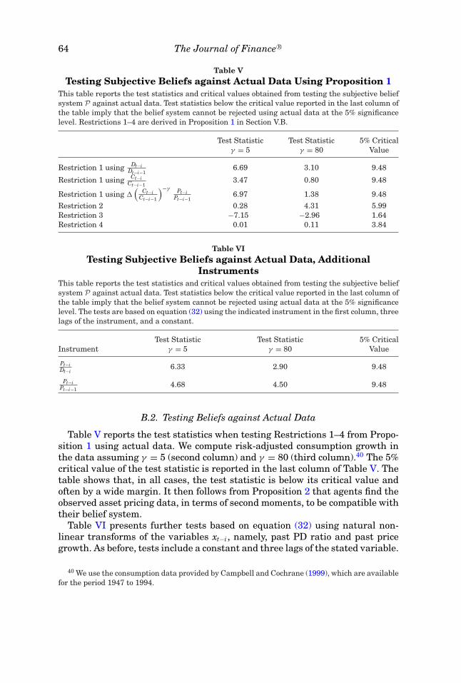
64 The Journal of Finance R©
Table VTesting Subjective Beliefs against Actual Data Using Proposition 1
This table reports the test statistics and critical values obtained from testing the subjective beliefsystem P against actual data. Test statistics below the critical value reported in the last column ofthe table imply that the belief system cannot be rejected using actual data at the 5% significancelevel. Restrictions 1–4 are derived in Proposition 1 in Section V.B.
Test Statistic Test Statistic 5% Criticalγ = 5 γ = 80 Value
Restriction 1 using Dt−iDt−i−1
6.69 3.10 9.48
Restriction 1 using Ct−iCt−i−1
3.47 0.80 9.48
Restriction 1 using �(
Ct−iCt−i−1
)−γ Pt−iPt−i−1
6.97 1.38 9.48
Restriction 2 0.28 4.31 5.99Restriction 3 −7.15 −2.96 1.64Restriction 4 0.01 0.11 3.84
Table VITesting Subjective Beliefs against Actual Data, Additional
InstrumentsThis table reports the test statistics and critical values obtained from testing the subjective beliefsystem P against actual data. Test statistics below the critical value reported in the last column ofthe table imply that the belief system cannot be rejected using actual data at the 5% significancelevel. The tests are based on equation (32) using the indicated instrument in the first column, threelags of the instrument, and a constant.
Test Statistic Test Statistic 5% CriticalInstrument γ = 5 γ = 80 Value
Pt−iDt−i
6.33 2.90 9.48
Pt−iPt−i−1
4.68 4.50 9.48
B.2. Testing Beliefs against Actual Data
Table V reports the test statistics when testing Restrictions 1–4 from Propo-sition 1 using actual data. We compute risk-adjusted consumption growth inthe data assuming γ = 5 (second column) and γ = 80 (third column).40 The 5%critical value of the test statistic is reported in the last column of Table V. Thetable shows that, in all cases, the test statistic is below its critical value andoften by a wide margin. It then follows from Proposition 2 that agents find theobserved asset pricing data, in terms of second moments, to be compatible withtheir belief system.
Table VI presents further tests based on equation (32) using natural non-linear transforms of the variables xt−i, namely, past PD ratio and past pricegrowth. As before, tests include a constant and three lags of the stated variable.
40 We use the consumption data provided by Campbell and Cochrane (1999), which are availablefor the period 1947 to 1994.

Stock Market Volatility and Learning 65
Table VIITest of Restriction 1 Using Simulated Data
This table reports the rejection frequencies obtained from testing Restriction 1 from Proposition 1at the 5% significance level using simulated data of length T from the indicated estimated model.The tests are performed using the instruments indicated in the first column and the lag lengthindicated in the second column. The set of instruments always includes a constant.
T
60 100 200 340
Instrument # of lags Model from Table III, γ = 5
Dt−iDt−i−1
1 5.0% 6.9% 13.5% 19.6%3 4.9% 9.7% 18.5% 26.2%
Ct−iCt−i−1
1 2.3% 3.7% 6.0% 5.8%3 5.3% 5.7% 9.9% 11.3%
�(
Ct−iCt−i−1
)−γ Pt−iPt−i−1
1 1.8% 1.9% 1.3% 0.8%
3 4.3% 4.6% 9.0% 16.0%Model from Table IV
Dt−iDt−i−1
1 1.7% 2.1% 2.5% 1.4%3 3.6% 3.7% 3.4% 2.8%
Ct−iCt−i−1
1 10.3% 18.7% 29.0% 44.0%3 12.0% 21.3% 38.0% 56.7%
�(
Ct−iCt−i−1
)−γ Pt−iPt−i−1
1 5.8% 10.9% 13.8% 18.5%
3 9.0% 12.6% 25.1% 36.5%
Test statistics are again below the 5% critical value in all cases. Taken togetherwith the evidence from Table V, this shows that agents’ belief systems are veryreasonable given the way the data actually behave.
B.3. Testing Beliefs against Simulated Data
Table VII reports the rejection frequencies for Restriction 1 when using sim-ulated model data.41 Specifically, the table reports the likelihood of rejectingRestriction 1 at the 5% significance level, using simulated data based on thepoint estimates from Tables III (γ = 5) and IV (γ = 80). Rejection frequenciesare shown for different instruments, different sample lengths T of simulatedquarterly data, and different numbers of lags in the tests. The longest samplelength corresponds to the length of the data sample.
Obviously, one cannot expect that this test is never rejected. Even the correctmodel would be rejected because of Type I errors (i.e., about 5% of the time). Onecan evaluate agents’ subjective beliefs within the model by checking whetherthe rejection frequencies exceed the 5% significance level.
41 The rejection frequencies are obtained from simulating 1,000 random samples of the specifiedlength.
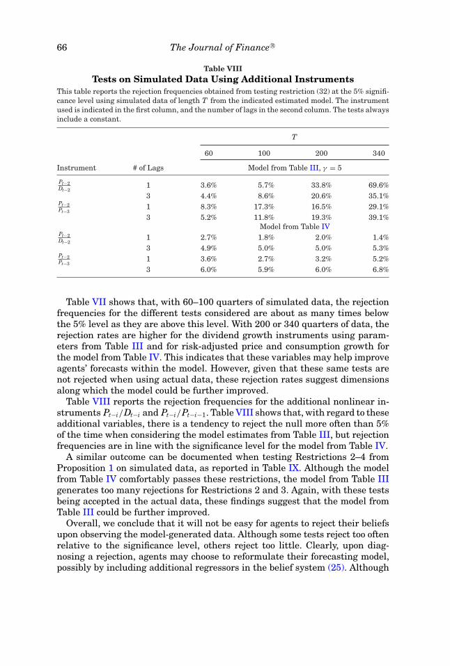
66 The Journal of Finance R©
Table VIIITests on Simulated Data Using Additional Instruments
This table reports the rejection frequencies obtained from testing restriction (32) at the 5% signifi-cance level using simulated data of length T from the indicated estimated model. The instrumentused is indicated in the first column, and the number of lags in the second column. The tests alwaysinclude a constant.
T
60 100 200 340
Instrument # of Lags Model from Table III, γ = 5
Pt−2Dt−2
1 3.6% 5.7% 33.8% 69.6%3 4.4% 8.6% 20.6% 35.1%
Pt−2Pt−3
1 8.3% 17.3% 16.5% 29.1%3 5.2% 11.8% 19.3% 39.1%
Model from Table IVPt−2Dt−2
1 2.7% 1.8% 2.0% 1.4%3 4.9% 5.0% 5.0% 5.3%
Pt−2Pt−3
1 3.6% 2.7% 3.2% 5.2%3 6.0% 5.9% 6.0% 6.8%
Table VII shows that, with 60–100 quarters of simulated data, the rejectionfrequencies for the different tests considered are about as many times belowthe 5% level as they are above this level. With 200 or 340 quarters of data, therejection rates are higher for the dividend growth instruments using param-eters from Table III and for risk-adjusted price and consumption growth forthe model from Table IV. This indicates that these variables may help improveagents’ forecasts within the model. However, given that these same tests arenot rejected when using actual data, these rejection rates suggest dimensionsalong which the model could be further improved.
Table VIII reports the rejection frequencies for the additional nonlinear in-struments Pt−i/Dt−i and Pt−i/Pt−i−1. Table VIII shows that, with regard to theseadditional variables, there is a tendency to reject the null more often than 5%of the time when considering the model estimates from Table III, but rejectionfrequencies are in line with the significance level for the model from Table IV.
A similar outcome can be documented when testing Restrictions 2–4 fromProposition 1 on simulated data, as reported in Table IX. Although the modelfrom Table IV comfortably passes these restrictions, the model from Table IIIgenerates too many rejections for Restrictions 2 and 3. Again, with these testsbeing accepted in the actual data, these findings suggest that the model fromTable III could be further improved.
Overall, we conclude that it will not be easy for agents to reject their beliefsupon observing the model-generated data. Although some tests reject too oftenrelative to the significance level, others reject too little. Clearly, upon diag-nosing a rejection, agents may choose to reformulate their forecasting model,possibly by including additional regressors in the belief system (25). Although
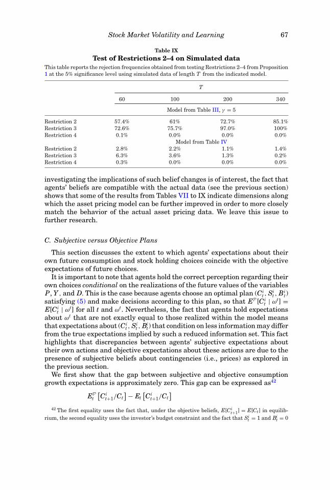
Stock Market Volatility and Learning 67
Table IXTest of Restrictions 2–4 on Simulated data
This table reports the rejection frequencies obtained from testing Restrictions 2–4 from Proposition1 at the 5% significance level using simulated data of length T from the indicated model.
T
60 100 200 340
Model from Table III, γ = 5
Restriction 2 57.4% 61% 72.7% 85.1%Restriction 3 72.6% 75.7% 97.0% 100%Restriction 4 0.1% 0.0% 0.0% 0.0%
Model from Table IVRestriction 2 2.8% 2.2% 1.1% 1.4%Restriction 3 6.3% 3.6% 1.3% 0.2%Restriction 4 0.3% 0.0% 0.0% 0.0%
investigating the implications of such belief changes is of interest, the fact thatagents’ beliefs are compatible with the actual data (see the previous section)shows that some of the results from Tables VII to IX indicate dimensions alongwhich the asset pricing model can be further improved in order to more closelymatch the behavior of the actual asset pricing data. We leave this issue tofurther research.
C. Subjective versus Objective Plans
This section discusses the extent to which agents’ expectations about theirown future consumption and stock holding choices coincide with the objectiveexpectations of future choices.
It is important to note that agents hold the correct perception regarding theirown choices conditional on the realizations of the future values of the variablesP, Y , and D. This is the case because agents choose an optimal plan (Ci
t , Sit , Bi
t)satisfying (5) and make decisions according to this plan, so that EP [Ci
t | ωt] =E[Ci
t | ωt] for all t and ωt. Nevertheless, the fact that agents hold expectationsabout ωt that are not exactly equal to those realized within the model meansthat expectations about (Ci
t , Sit , Bi
t) that condition on less information may differfrom the true expectations implied by such a reduced information set. This facthighlights that discrepancies between agents’ subjective expectations abouttheir own actions and objective expectations about these actions are due to thepresence of subjective beliefs about contingencies (i.e., prices) as explored inthe previous section.
We first show that the gap between subjective and objective consumptiongrowth expectations is approximately zero. This gap can be expressed as42
EPt
[Ci
t+1/Ct]− Et
[Ci
t+1/Ct]
42 The first equality uses the fact that, under the objective beliefs, E[Cit+1] = E[Ct] in equilib-
rium, the second equality uses the investor’s budget constraint and the fact that Sit = 1 and Bi
t = 0

68 The Journal of Finance R©
= EPt
[Ci
t+1/Ct]− Et
[Ct+1/Ct
]= EP
t
[Pt+1(1 − Si
t+1) − Bit+1 + Dt+1 + Yt
Dt + Yt
]− Et
[Ct+1/Ct
]= EP
t
[Pt+1(1 − Si
t+1) − Bit+1
Dt + Yt
].
Since the choices for Sit+1 and Bi
t are bounded, we have that Pt+1(1 − Sit+1) −
Bit+1 is bounded whenever beliefs about future values of the price Pt+1 are
bounded. Assumption 1 in Section III.B then ensures that the subjective expec-tations in the last line of the preceding equation will be approximately equalto zero for every state, so that the gap between the subjective and the objectiveconsumption expectations vanishes under the maintained assumptions.
The situation is different when considering subjective stock holding plans.Assuming an interior solution for stock holdings in period t, in equilibrium, theagent’s first-order condition satisfies
Pt = δEPt
[(Ci
t+1
Ct
)−γ
(Pt+1 + Dt+1)
].
With Cit+1/Ct converging to Ct+1/Ct under Assumption 1, this equation recovers
our pricing equation. However, if this equation were to hold almost surely foreach period and each contingency in the future under the agent’s subjectiveplan, then one could iterate forward on this equation and obtain (under asuitable transversality condition) that the equilibrium price must equal thepresent value of dividends. Since the equilibrium price is different, it must bethe case that the agent expects that, with positive probability, either Si
t = S orSi
t = S will hold in the future. These expectations, however, will not be fulfilledin equilibrium because the agent will never buy or sell, as we have Si
t = 1 forall t along the equilibrium path. Further research can explore the extent towhich this gap between agents’ expectations and equilibrium outcomes can bereduced by introducing agent heterogeneity in terms of preferences or beliefsand thus trade in equilibrium.
VI. Conclusion
A simple consumption-based asset pricing model is able to quantitativelyreplicate a number of important asset pricing facts, provided that one slightlyrelaxes the assumption that agents perfectly know how stock prices are formedin the market. We assume that agents are internally rational, in the sense thatthey formulate their doubts about market outcomes using a consistent set ofsubjective beliefs about prices and maximize expected utility given this set of
in equilibrium in t, and the last equality uses the fact that agents have RE about the processes foraggregate consumption.

Stock Market Volatility and Learning 69
beliefs. The system of beliefs is internally consistent in the sense that it spec-ifies a proper joint distribution of prices and fundamental shocks at all dates.Furthermore, the perceived distribution of price behavior, although differentfrom the true distribution, is nevertheless close to it and the discrepancies arehard to detect.
In such a setting, optimal behavior dictates that agents learn about theequilibrium price process from past price observations. This gives rise to aself-referential model of learning about prices that imparts momentum andmean-reversion behavior into the PD ratio. As a result, sustained departuresof asset prices from their fundamental (RE) value emerge, even though allagents act rationally in light of their beliefs.
We also submit our consumption-based asset pricing model to a formal econo-metric test based on MSM. The model performs remarkably well, despite itssimplicity. Although the model gives rise to a significant equity premium, itfails to fully match the empirical premium for reasonable degrees of relativerisk aversion. When risk aversion is as high as in some of the previous work,the model can also replicate the equity premium, but we leave a full treatmentof this issue to future research.
Given the difficulties documented in the empirical asset pricing literature inaccounting for stock price volatility in a setting with time-separable preferencesand RE, our results suggest that learning about price behavior may be a crucialingredient in understanding stock price volatility. Indeed, the most convincingcase for models of learning can be made by explaining facts that appear puzzlingfrom the RE viewpoint, as we attempt to do in this paper.
A natural question arising within our setting is to what extent can thepresent theory be used to price other assets, say, the term structure of interestrates or the cross-section of stock returns. Exploring these pricing implicationsappears to be an interesting avenue for further research.
The finding that large asset price fluctuations can result from optimizingagents with subjective beliefs is also relevant from a policy perspective. Thedesirability of policy responding to asset price fluctuations will depend to alarge extent on whether asset price fluctuations are fundamentally justified.
Initial submission: March 12, 2013; Final version received: August 19, 2015Editor: Bruno Biais
Appendix A: Data Sources
Our data are for the United States and have been downloaded from theGlobal Financial Database (http://www.globalfinancialdata.com). The periodcovered is 1925:4 to 2012:2. For the subperiod 1925:4 to 1998:4, our data setcorresponds very closely to Campbell’s (2003) handbook data set available athttp://scholar.harvard.edu/campbell/data.
In the estimation part of the paper, we use moments based on the samenumber of observations as we have data points. Since we seek to match the

70 The Journal of Finance R©
return predictability evidence at the five-year horizon (c25 and R2
5), we can onlyuse data points up to 2007:1. For consistency, the effective sample end for allother moments reported in Table I has been shortened by five years to 2007:1.In addition, due to the seasonal adjustment procedure for dividends describedbelow and the way we compute the standard errors for the moments describedin Appendix F, the effective starting date was 1927:2. The names of the dataseries used are reported below.
To obtain real values, nominal variables are deflated using the USA BLSConsumer Price Index (Global Fin code CPUSAM). We transform the monthlyprice series into a quarterly series by taking the index value of the last monthof the considered quarter.
The nominal stock price series is the SP 500 Composite Price Index (w/GFDextension) (Global Fin code SPXD). The weekly (up to the end of 1927) anddaily series are transformed into quarterly data by taking the index value ofthe last week/day of the considered quarter. Moreover, we normalize the seriesto 100 in 1925:4.
As the nominal interest rate we use the 90-day T-bill secondary market(Global Fin code ITUSA3SD). The monthly (up to the end of 1933), weekly(1934 to the end of 1953), and daily series are transformed into quarterlyseries using the interest rate corresponding to the last month/week/day of theconsidered quarter and are expressed in quarterly rates (not annualized).
We compute nominal dividends as follows:
Dt =(
ID(t)/ID(t − 1)IND(t)/IND(t − 1)
− 1)
IND(t),
where IND denotes the SP 500 Composite Price Index (w/GFD extension) de-scribed above and ID is the SP 500 Total Return Index (w/GFD extension)(Global Fin code SPXTRD). We first compute monthly dividends and then quar-terly dividends by adding up the monthly series. Following Campbell (2003),we deseasonalize dividends by taking averages of the actual dividend paymentsover the current and preceding three quarters.
Appendix B: Details on the Phase Diagram
The second-order difference equation (23) describes the evolution of beliefsover time and allows us to construct the directional dynamics in the (βt, βt−1)plane, as shown in Figure 2 for the case (εc
t )−γ εdt = 1. Here, we show the algebra
leading to the arrows displayed in this figure as well as the effects of realiza-tions (εc
t )−γ εdt ≶ 1. Define x′
t ≡ (x1,t, x2,t) ≡ (βt, βt−1). The dynamics can then bedescribed by
xt+1 =(
x1,t + ft+1
((a1−γ + a1−γ δ(x1,t−x2,t)
1−δx1,t
) (εc
t
)−γεd
t − x1,t, x1,t
)x1,t
).

Stock Market Volatility and Learning 71
The points in Figure 2 where there is no change in each of the elements of xare as the follows: we have �x2 = 0 at points x1 = x2, so that the 45º line givesthe point of no change in x2, and �x2 < 0 above this line. We have �x1 = 0 forx2 = 1
δ− x1(1−δx1)
a1−γ δ(εc)−γ εd . For (εc)−γ εd = ρε, this is the curve labeled as “βt+1 = βt” inFigure 2, and we have �x1 > 0 below this curve. So, for (εc)−γ εd = ρε, the zeroesfor �x1 and �x2 intersect at x1 = x2 = a1−γ ρε, which is the RE equilibria (REE)value and also at x1 = x2 = δ−1, which is the limit of rational bubble equilibria.These results give rise to the directional dynamics, as shown in Figure 2.Finally, for (εc)−γ εd > ρε ((εc)−γ εd < ρε), the curve “βt+1 = βt” in Figure 2 isshifted upward (downward), as indicated by the function x2 = 1
δ− x1(1−δx1)
a1−γ δ(εc)−γ εd .
Appendix C: Proof of Mean Reversion
To prove mean reversion for the general learning scheme (18), we need thefollowing additional technical assumption on the updating function ft:
ASSUMPTION C1: There is a η > 0 such that ft(·, β) is differentiable in the inter-val (−η, η) for all t and all β.
Furthermore, letting
Dt ≡ inf�∈(−η,η),β∈(0,βU )
∂ ft(�,β)∂�
,
we have∞∑
t=0
Dt = ∞.
Assumption C1 is satisfied by all the updating rules considered in this paperand by most algorithms used in the stochastic control literature. For example,it is guaranteed in the OLS case where Dt = 1/(t + α1) and in the constant-gain case where Dt = 1/α for all t, β. The assumption would fail and
∑Dt < ∞,for example, if the weight given to the error in the updating scheme is 1/t2.
In that case, beliefs could get stuck away from the fundamental value simplybecause updating of beliefs ceases to incorporate new information for t largeenough. In this case, the growth rate would be a certain constant, but agentswould forever believe that the growth rate is another constant, different fromthe truth. Hence, in this case, agents would make systematic mistakes forever.Therefore, Assumption C1 is likely to be satisfied by any system of beliefs thatadds a “grain of truth” to the RE equilibrium.
The statement about limsup is equivalent to saying that, if βt > a in someperiod t, then for any η > 0 sufficiently small, there is a finite period t′′ > t suchthat βt′′ < a + η.
Fix η > 0 such that η < min(η, (βt − a)/2), where η is as in Assumption A1.We first prove that there exists a finite t′ ≥ t such that
�βt ≥ 0 for all t such that t < t < t′, and (C.1)

72 The Journal of Finance R©
�βt′ < 0. (C.2)
To prove this, choose ε = η(1 − δβU ). Since βt < βU and ε > 0, it is impossiblethat �βt ≥ ε for all t > t. Let t ≥ t be the first period in which �βt < ε.
There are two possible cases: either (i) �βt < 0 or (ii) �βt ≥ 0.
In case (i), we have that (C.1) and (C.2) hold if we take t′ = t.In case (ii), βt cannot decrease between t and t so that
βt ≥ βt > a + η.
Furthermore, we have
T (βt,�βt) = a + �βt
1 − δβt< a + ε
1 − δβt
< a + ε
1 − δβU = a + η,
where the first equality follows from the definition of T in the main text. Theprevious two relations imply
βt > T (βt,�βt).
Therefore,
�βt+1 = ft+1(T (βt,�βt) − βt; βt
)< 0,
and in case (ii) we have that (C.1) and (C.2) hold for t′ = t + 1.This shows that (C.1) and (C.2) hold for a finite t′, as in the first part of the
statement of mean reversion in the text. Now we need to show that beliefseventually fall below a + η and do decrease monotonically.
Consider η as defined above. First, notice that given any j ≥ 0, if
�βt′+ j
< 0 and (C.3)
βt′+ j
> a + η, (C.4)
then
�βt′+ j+1 = ft′+ j+1
(a + �βt′+ j
1 − δβt′+ j− βt′+ j, βt′+ j
)< ft′+ j+1
(a − βt′+ j, βt′+ j
)< ft′+ j+1
(−η, βt′+ j) ≤ −ηDt′+ j+1 ≤ 0, (C.5)
where the first inequality follows from (C.3), the second inequality from (C.4),and the third from the mean value theorem, η > 0 and Dt′+ j+1 ≥ 0. Assume,toward a contradiction, that (C.4) holds for all j ≥ 0. Since (C.3) holds for

Stock Market Volatility and Learning 73
j = 0, it follows by induction that �βt′+ j ≤ 0 for all j ≥ 0, and therefore (C.5)holds for all j ≥ 0. Hence,
βt′+ j =j∑
i=1
�βt′+i + βt′ ≤ −η
j∑i=1
Dt′+i + βt′
for all j > 0. Assumption C1 above then implies βt → −∞, showing that (C.4)cannot hold for all j. Therefore, there is a finite j such that βt′+ j will go belowa + η and β is decreasing from t′ until it goes below a + η.
For the case βt < a − η, choosing ε = η, one can use a symmetric argumentto construct the proof. �
Appendix D: Proof of Geometric Ergodicity
Defining ηt ≡ (εct )−γ εd
t and using (22) and (27), we can write the learningalgorithm that gives the dynamics of βt as[
βt�βt
]= F
[βt−1
�βt−1, ηt−1
],
where the first element of F, denoted as F1, is given by the right side of (27)and F2(β,�β, ηt−1) ≡ F1(β,�β, ηt−1) − β. Therefore,
F′t ≡ ∂F (·, ηt−1)
∂[βt �βt
] = w′t ·[
At, 1 − 1α
+ Bt
At, − 1α
+ 1α
Bt
],
for At = 1α
aδηt−11−δβt−1
and Bt = 1α
aδ �βt−1ηt−1(1−δβt−1)2 , with w′
t denoting the derivative of w atperiod t. The eigenvalues of the matrix in brackets are
λ+t , λ−
t =At + 1 − 1
α+ Bt ±
√(At + 1 − 1
α+ Bt
)2 − 4At
2.
Since At, Bt → 0 for large α, we have that λ+t is the larger eigenvalue in modulus
and the radicand is positive. We like to find a uniform bound for λ+t , because,
given that∣∣w′
t
∣∣ < 1, this will be a uniform bound for the largest eigenvalue ofF ′
t . Such a bound will play the role of ρθ (εt) in the definition of the “L2 unitcircle condition” on page 942 in Duffie and Singleton (1993) (henceforth DS).
Consider the function fa(x) = x + a +√
(x + a)2 − 4a for some constant a > 0and x large enough for the radicand to be positive. For ε > 0, the mean valuetheorem implies
fa(x + ε) ≤⎛⎝1 + x√
(x + a)2 − 4a
⎞⎠ ε + fa(x).

74 The Journal of Finance R©
Evaluating this expression at a = At, ε = Bt, and x = 1 − 1/α, we have
λ+t ≤ Bt + fAt
(1 − 1
α
)2
< Bt + 1 − 1α
for �βt−1 ≥ 0, (D.1)
where we use
fAt
(1 − 1
α
)< At + 1 − 1
α+√(
At + 1 − 1α
)2
− 4At
(1 − 1
α
)= 2
(1 − 1
α
).
Since fAt (·) is monotonic, using the expression for Bt, we have
λ+t ≤ 1
2fAt
(1 − 1
α+ Bt
)≤ fAt (1 − 1
α)
2< 1 − 1
αfor �βt−1 < 0. (D.2)
From (27), we have
�βt ≤ 1α
(ηt−1a1−γ
[1 + �βt−1
1 − δβt−1
]− βt−1
). (D.3)
So, if �βt−1 ≥ 0, using βt−1 > 0, we have
�βt ≤ 1α
ηt−1a1−γ
[1 + |�βt−1|
1 − δβt−1
].
Therefore, adding the right side of this inequality to (D.2) and using the in-equality for (D.1), we have that for all �βt−1,
λ+t ≤ 1
α
a1−γ δ
(1 − δβt−1)2
(a1−γ
αηt−2
[1 + |�βt−2|
1 − δβt−2
])ηt−1 + 1 − 1
α
≤ 1α2 Kηt−2ηt−1 + 1 − 1
α,
for a constant 0 < K < ∞, where we use |�βt−2| , and βt−1, βt−2 < βU .Since w′ ≤ 1, it is clear from the mean value theorem that K
α2 ηt−2ηt−1 + 1 − 1α
plays the role of ρθ (εt) in the definition of the “L2 unit circle condition” of DS,where our α plays the role of θ and ηt−1ηt−2 the role of εt in DS. Therefore,we need to check that E( K
α2 ηtηt−1 + 1 − 1α)2 < 1 for α large enough. A routine
calculation shows that
E
(Kα2 ηtηt−1 + 1 − 1
α
)2
= 1 − 1α
− 1α
[1 − 1
α− 2
(1 − 1
α
)Kα
E (ηtηt−1) − K2
α3 E(η2
t η2t−1
)],
which is smaller than one for large enough α.This proves that, for large α, the variable βt satisfies the L2 unit-circle con-
dition in DS and hence satisfies the asymptotic unit circle (AUC) condition inDS, and Lemma 3 in DS guarantees that βt is geometrically ergodic.

Stock Market Volatility and Learning 75
Now, adding a1−γ ηt−1 to both sides of (D.3) and taking expectations at theergodic distribution, we have
E(βt−1 − ηt−1a1−γ
) ≤ E(
�βt−1
1 − δβt−1ηt−1a1−γ
). (D.4)
Our previous argument shows that the right side is arbitrarily small for α large;therefore, Eβt−1 ≤ Eηt−1a1−γ . A similar argument shows that varβt goes to zeroas α → ∞. Therefore, for α large, βt ≤ βL with arbitrarily large probability sothat (D.3) holds as an equality with an arbitrarily large probability. Takingexpectations on both sides for the realizations in which this holds as an equality,we have that Eβt → Eηt−1a1−γ = βRE as α → ∞, which completes the proof. �
Appendix E: Differentiable Projection Facility
The function w used in the differentiable projection facility (27) is
w(x) ={
x if x ≤ βL
βL + x−βL
x+βU −2βL (βU − βL) if βL < x.(E.1)
Clearly w is continuous; the only point where continuity is questionable is atx = βL, but it is easy to check that
limx↗βL
w(x) = limx↘βL
w(x) = βL,
limx↗βL
w′(x) = limx↘βL
w′(x) = 1,
limx→∞ w(x) = βU .
In our numerical applications, we choose βU so that the implied PD rationever exceeds U PD = 500 and βL = δ−1 − 2(δ−1 − βU ), which implies that thedampening effect of the projection facility starts to come into effect for valuesof the PD ratio above 250. Therefore, this dampening is applied in few obser-vations. Although the projection facility might suggest that profitable tradingrules could be devised, this is true only if one assumes that the parametersβU and βL are fixed and unchanging over time, as we do here for simplicity.In a slightly more realistic model, it would be difficult for agents to time stockpurchases and stock sales to exploit the projection facility.
Appendix F: Details on the MSM Procedure
The estimation method and the proofs adapt the results from a standardMSM estimation. The Internet Appendix contains a much more detailed ac-count of these results.43
43 The Internet Appendix is available in the online version of the article on the Journal ofFinance website.

76 The Journal of Finance R©
We use the definitions introduced at the beginning of Section IV. Let N be thesample size and (y1, . . . , yN) the observed data sample, with yt containing mvariables. Define sample moments MN ≡ 1
N
∑Nt=1 h(yt) for a given moment func-
tion h : Rm → Rq. Sample statistics SN shown in (28) are not exactly momentsof the data. For example, MN contains the sample moments var(Pt/Dt) andcov(Pt/Dt, Pt−1/Dt−1), and SN contains the serial correlation of Pt/Dt, which is afunction of these moments. The sample statistics can be written as SN ≡ S(MN)for a statistics function S : Rq → Rs. The h, S mappings in our application arewritten explicitly in the Internet Appendix.
Let yt(θ ) be the series generated by our model of learning for parameter valuesθ and some realization of the underlying shocks. Denote the true parametervalue θ0. Let M(θ ) ≡ E[h(yt(θ ))] be the moments for parameter values θ at thestationary distribution of yt(θ ), let M0 ≡ M(θ0) be the true moments, and letS(θ ) ≡ S(M(θ )) be the statistics for parameter θ. Denote by M j
0 the true jth
autocovariance:
M j0 ≡ E
[h(yt(θ0)) − M0
] [h(yt− j(θ0)) − M0
]′.
Define Sw ≡∑∞j=−∞ M j
0 . A consistent estimator Sw,N → Sw is found by usingstandard Newey-West estimators. The variance for the sample statistics SNreported in the second column of Table I is given by
�S,N ≡ ∂S(MN)∂M′ Sw,N
∂S(MN)′
∂M.
Note that the model is not needed for this estimator; we use only observed data.The exact form of ∂S(M)
∂M′ can be found in the Internet Appendix.DS show that, to apply standard MSM asymptotics, one needs geometric
ergodicity. We show that this holds in our model in Section III.C. Note that thesmooth bounding function w in equation (27) guarantees that a Monte Carloapproximation to S is differentiable, as is required for an MSM asymptoticdistribution.
Letting �S be the asymptotic variance-covariance matrix of the sample statis-tics, under standard assumptions, it can be shown that
�S,N → �S and θN → θ0 a.s. as N → ∞. (F.1)
Also, letting B0≡ ∂M′(θ0)∂θ
∂S ′(M0)∂M , it can be shown that
√N[θN − θ0
]→ N (0,(B0�
−1S B0
)−1), (F.2)
√N[SN − S(M(θN))
]→ N (0, �S − B′0(B0�
−1S B′
0)−1B0), (F.3)
and
WN ≡ N[SN − S (θ )
]′�−1
S,N
[SN − S (θ)]→ χ2
s−n (F.4)

Stock Market Volatility and Learning 77
in distribution as N → ∞. Also, the weighting matrix �−1S,N is optimal among
all weighting matrices of the statistics. The t-statistics in Tables II to IV usevariances from (F.3), and the p-values for WN are based on (F.4).
As can be seen from the above formula, we need to invert �S,N and its limit�S . A nearly singular �S,N presents problems because the distribution of WNis nearly ill-defined, and the distribution in short samples is not close to a χ2.As explained at the end of Section IV.A, our application displays this feature.This singularity occurs because one of the statistics in SN is nearly perfectlycorrelated with all the others. This only means that this is a redundant statistic,so we can drop it from SN in the estimation. To select the redundant statistic,we predict each element of SN with all the others according to �S,N and dropthe statistic for which the R2 is less than 1%. As it turns out, this occurs onlyfor c5
2 with an R2 = 0.006.
Appendix G: Proof of Propositions 1 and 2
PROOF OF PROPOSITION 1: Note that the system of beliefs implies that et, definedin equation (31), is given by
et = εt + ξt − εt−1, (G.1)
so that Restriction 1 holds.We also have E( Dt
Dt−1et) = E(εD
t εt) = E(εDt−1εt−1) = −E( Dt−1
Dt−2et).44 Together with
the analogous derivation for consumption growth, this delivers Restriction 2.From (G.1) we get
E(ε2t ) = −E(etet−1) = E(ε2
t−1). (G.2)
Let Proj(X|Y ) denote the linear projection of a random variable X on a ran-dom vector Y . Then, Proj(εt|εD
t , εCt ) = (εD
t , εCt )bDC and using properties of linear
projections, we have
E(ε2t ) > var
(Proj(εt|εD
t , εCt ))
= b′DC �DC bDC .
Together with (G.2), this implies Restriction 3. Restriction 4 follows directlyfrom (25). �PROOF OF PROPOSITION 2: Consider a process {xt}∞−∞ = {et, Dt/Dt−1,Ct/Ct−1}∞−∞satisfying Assumption 3 and Restrictions 1–4 from Proposition 1, where As-sumption 3(i) ensures that well-defined second moments exist. We show how
44 We slightly abuse notation in the proof because dividend and consumption growth follow
Dt/Dt−1 = a + a(εDt − 1),
Ct/Ct−1 = a + a(εCt − 1),
where the last terms are mean zero innovations. When writing εDt and εC
t in the proof, we actuallyhave in mind a(εD
t − 1) and a(εCt − 1), respectively.

78 The Journal of Finance R©
to construct a stationary process {xt}∞−∞ = {et, ˜Dt/Dt−1, ˜Ct/Ct−1}∞−∞ consistentwith the belief system (2), (3), and (25) that has the same autocovariance func-tion as {xt}∞−∞. In particular, let
{εD
t , εCt , ξt, ηt
}∞−∞ denote a white noise sequence,
in which (ξt, ηt) are uncorrelated contemporaneously with each other and with(εD
t , εCt ), and var(εD
t , εCt ) = �DC . The variances of ξt and ηt are determined from
observable moments as follows:
σ 2ξ
= σ 2e + 2σe,−1,
σ 2η = −σe,−1 − b′
DC �DC bDC ,
where σe,−1 ≡ E(et et−1) and σ 2e = E[e2
t ].Since x satisfies Restriction 3, it follows that σ 2
η > 0. To see that σ 2ξ
≥ 0 holds,note that Restriction 1 implies that the observed univariate process et is MA(1).Hence, we can write
et = ut − θut−1, (G.3)
for some constant |θ | ≤ 1 and some white noise ut. We thus have
σ 2e = σ 2
u (1 + θ2) ≥ 2θσ 2u = −2σe,−1,
where the last equality holds because (G.3) implies σe,−1 = −θσ 2u . Hence, σ 2
ξ≥
0. This proves that, under the assumptions of this proposition, one can build aprocess
{εD
t , εCt , ξt, ηt
}∞−∞ satisfying all the properties we have assumed about
this process.In line with (2) and (3), we then let
˜Dt/Dt−1 = E[Dt/Dt−1] + εDt ,
˜Ct/Ct−1 = E[Ct/Ct−1] + εCt .
Part (ii) of Assumption 3 then implies that {Dt/Dt−1, Ct/Ct−1}∞t=−∞ and
{ ˜Dt/Dt−1, ˜Ct/Ct−1}∞t=−∞ have the same autocovariance functions. All that re-mains to be shown is that, for some process et consistent with the system ofbeliefs, the covariances of this process with leads and lags of both itself and( ˜Dt/Dt−1, ˜Ct/Ct−1) are the same as in the autocovariance function of {xt}∞−∞ .
We construct et; in line with (25), we let
et = εt + ξt − εt−1, (G.4)
where
εt =(εD
t , εCt
)bDC + ηt.
It is easy to check that, by construction, the autocovariance function of {et}∞−∞is identical to that of {et}∞−∞, since both are MA(1) with the same variance andautocovariance.
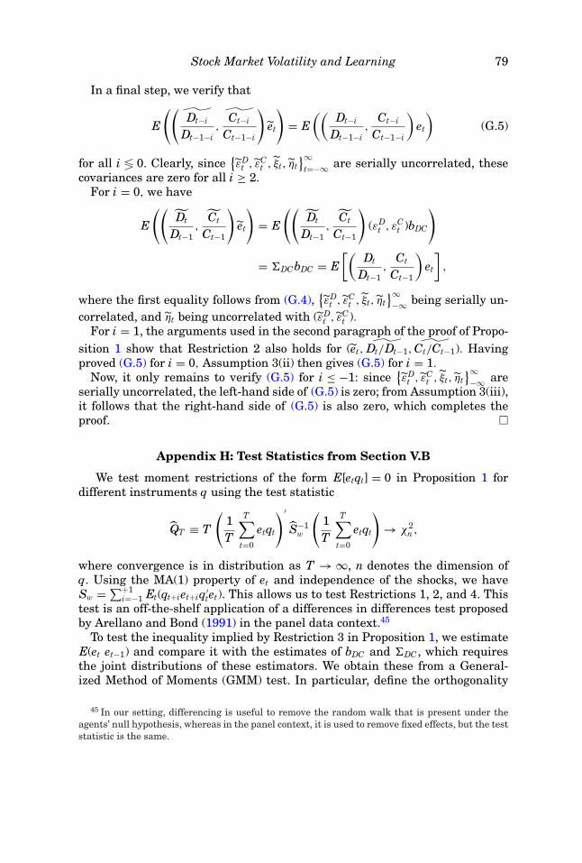
Stock Market Volatility and Learning 79
In a final step, we verify that
E
((˜Dt−i
Dt−1−i,
˜Ct−i
Ct−1−i
)et
)= E
((Dt−i
Dt−1−i,
Ct−i
Ct−1−i
)et
)(G.5)
for all i ≶ 0. Clearly, since{εD
t , εCt , ξt, ηt
}∞t=−∞ are serially uncorrelated, these
covariances are zero for all i ≥ 2.For i = 0, we have
E
((Dt
Dt−1,
Ct
Ct−1
)et
)= E
((Dt
Dt−1,
Ct
Ct−1
)(εD
t , εCt )bDC
)
= �DCbDC = E[(
Dt
Dt−1,
Ct
Ct−1
)et
],
where the first equality follows from (G.4),{εD
t , εCt , ξt, ηt
}∞−∞ being serially un-
correlated, and ηt being uncorrelated with (εDt , εC
t ).For i = 1, the arguments used in the second paragraph of the proof of Propo-
sition 1 show that Restriction 2 also holds for (et, ˜Dt/Dt−1, ˜Ct/Ct−1). Havingproved (G.5) for i = 0, Assumption 3(ii) then gives (G.5) for i = 1.
Now, it only remains to verify (G.5) for i ≤ −1: since{εD
t , εCt , ξt, ηt
}∞−∞ are
serially uncorrelated, the left-hand side of (G.5) is zero; from Assumption 3(iii),it follows that the right-hand side of (G.5) is also zero, which completes theproof. �
Appendix H: Test Statistics from Section V.B
We test moment restrictions of the form E[etqt] = 0 in Proposition 1 fordifferent instruments q using the test statistic
QT ≡ T
(1T
T∑t=0
etqt
)′
S−1w
(1T
T∑t=0
etqt
)→ χ2
n ,
where convergence is in distribution as T → ∞, n denotes the dimension ofq. Using the MA(1) property of et and independence of the shocks, we haveSw =∑+1
i=−1 Et(qt+iet+iq′tet). This allows us to test Restrictions 1, 2, and 4. This
test is an off-the-shelf application of a differences in differences test proposedby Arellano and Bond (1991) in the panel data context.45
To test the inequality implied by Restriction 3 in Proposition 1, we estimateE(et et−1) and compare it with the estimates of bDC and �DC , which requiresthe joint distributions of these estimators. We obtain these from a General-ized Method of Moments (GMM) test. In particular, define the orthogonality
45 In our setting, differencing is useful to remove the random walk that is present under theagents’ null hypothesis, whereas in the panel context, it is used to remove fixed effects, but the teststatistic is the same.

80 The Journal of Finance R©
conditions
g1(α, bDC ; xt, xt−1) ≡([
Dt
Dt−1,
Ct
Ct−1
]bDC − et−1
)et − α
g2(α, bDC ; xt, xt−1) ≡[
Dt
Dt−1,
Ct
Ct−1
]′ ([ Dt
Dt−1,
Ct
Ct−1
]bDC − et
),
and let g = (g1, g2). We then obtain from
E(g(α, bDC ; xt, xt−1)) = 0
three orthogonality conditions to estimate the three parameters (α, bDC). GMMsets bDC,T to the OLS estimator of a regression of et on Dt
Dt−1, Ct
Ct−1and αT esti-
mates b′DC �DC bDC − E(et et−1). Therefore, Restriction 3 in Proposition 1 calls
for testing the null hypothesis H0 : α < 0. Standard asymptotic distributiongives
√T[
αT − α
bDC,T − bDC
]→ N(0, B−1Sw(B′)−1) as T → ∞
B =[
−1 E([
DtDt−1
, CtCt−1
]et
)0 �DC
]
Sw =∞∑
j=−∞E(g(bDC, α; xt, xt−1) g(bDC, α; xt− j, xt−1− j)′).
Substituting all moments by sample moments delivers the distribution for αT .
REFERENCES
Adam, Klaus, 2003, Learning and equilibrium selection in a monetary overlapping generationsmodel with sticky prices, Review of Economic Studies 70, 887–908.
Adam, Klaus, and Albert Marcet, 2010, Booms and busts in asset prices, IMES Discussion PaperSeries 10-E-02, Institute for Monetary and Economic Studies, Bank of Japan.
Adam, Klaus, and Albert Marcet, 2014, Internal rationality, imperfect market knowledge and assetprices, Journal of Economic Theory 146, 1224–1252.
Adam, Klaus, Albert Marcet, and Johannes Beutel, 2014, Stock price booms and expected capitalgains, Working paper, University of Mannheim.
Arellano, Manuel, and Stephen Bond, 1991, Some tests of specification for panel data: Monte Carloevidence and an application to the employment equations, Review of Economic Studies 58,277–297.
Bansal, Ravi, Dana Kiku, and Amir Yaron, 2013, Risks for the long run: Estimation with timeaggregation, Working paper, University of Pennsylvania.
Biais, Bruno, Peter Bossaerts, and Chester Spatt, 2010, Equilibrium asset pricing and portfoliochoice under asymmetric information, Review of Financial Studies 23, 1503–1543.
Bossaerts, Peter, 2004, Filtering returns for unspecified biases in priors when testing asset pricingtheory, Review of Economic Studies 71, 63–86.
Boswijk, Peter, Cars H. Hommes, and Sebastiano Manzan, 2007, Behavioral heterogeneity in stockprices, Journal of Economic Dynamics and Control 31, 1938–1970.
Branch, William, and George W. Evans, 2010, Asset return dynamics and learning, Review ofFinancial Studies 23, 1651–1680.

Stock Market Volatility and Learning 81
Branch, Willam, and George W. Evans, 2011, Learning about risk and return: A simple model ofbubbles and crashes, American Economic Journal: Macroeconomics 3, 159–191.
Brennan, Michael J., and Yihong Xia, 2001, Stock price volatility and equity premium, Journal ofMonetary Economics 47, 249–283.
Brock, William A., and Cars H. Hommes, 1998, Heterogeneous beliefs and routes to chaos in asimple asset pricing model, Journal of Economic Dynamics and Control 22, 1235–1274.
Bullard, Jim, and John Duffy, 2001, Learning and excess volatility, Macroeconomic Dynamics 5,272–302.
Campbell, John Y., 2003, Consumption-based asset pricing, in George M. Constantinides, MiltonHarris, and Rene Stulz, eds.: Handbook of Economics and Finance (Elsevier, Amsterdam).
Campbell, John Y., and John H. Cochrane, 1999, By force of habit: A consumption-based explana-tion of aggregate stock market behavior, Journal of Political Economy 107, 205–251.
Carceles-Poveda, Eva, and Chryssi Giannitsarou, 2008, Asset pricing with adaptive learning,Review of Economic Dynamics 11, 629–651.
Cecchetti, Stephen, Pok-Sang Lam, and Nelson C. Mark, 2000, Asset pricing with distorted beliefs:Are equity returns too good to be true? American Economic Review 90, 787–805.
Chakraborty, Avik, and George W. Evans, 2008, Can perpetual learning explain the forward pre-mium puzzle? Journal of Monetary Economics 55, 477–490.
Cochrane, John H., 2005, Asset Pricing (Revised Edition) (Princeton University Press, Princeton,NJ).
Cogley, Timothy, and Thomas J. Sargent, 2008, The market price of risk and the equity premium:A legacy of the great depression? Journal of Monetary Economics 55, 454–476.
Collard, Fabrice, Sujoy Mukerji, Kevin Sheppard, and Jean-Marc Tallon, 2011, Ambiguity and thehistorical equity premium, Working paper, University of Bern.
Duffie, Darell, and Kenneth J. Singleton, 1993, Simulated moments estimation of Markov modelsof asset prices, Econometrica 61, 929–952.
Dumas, Bernard, Alexander Kurshev, and Raman Uppal, 2009, Equilibrium portfolio strategies inthe presence of sentiment risk and excess volatility, Journal of Finance 64, 579–629.
Evans, George W., and Seppo Honkapohja, 2001, Learning and Expectations in Macroeconomics(Princeton University Press, Princeton, NJ).
Hansen, Lars P., and Kenneth J. Singleton, 1982, Generalized instrumental variables estimationof nonlinear rational expectations models, UK, Econometrica 50, 1269–1286.
Kreps, David, 1998, Anticipated utility and dynamic choice, in Donald P. Jacobs, Ehud Kalai, andMorton I. Kamien, eds.: Frontiers of Research in Economic Theory (Cambridge UniversityPress, Cambridge, UK).
Lansing, Kevin J., 2010, Rational and near-rational bubbles without drift, Economic Journal 120,1149–1174.
LeRoy, Stephen F., and Richard Porter, 1981, The present-value relation: Test based on impliedvariance bounds, Econometrica 49, 555–574.
Lucas, Robert E., 1978, Asset prices in an exchange economy, Econometrica 46, 1426–1445.Marcet, Albert, and Juan P. Nicolini, 2003, Recurrent hyperinflations and learning, American
Economic Review 93, 1476–1498.Marcet, Albert, and Thomas J. Sargent, 1989, Convergence of least squares learning mechanisms
in self referential linear stochastic models, Journal of Economic Theory 48, 337–368.Marcet, Albert, and Thomas J. Sargent, 1992, The convergence of vector autoregressions to rational
expectations equilibria, in Alessandro Vercelli and Nicola Dimitri, eds.: Macroeconomics: ASurvey of Research Strategies (Oxford University Press, Oxford, UK).
Shiller, Robert J., 1981, Do stock prices move too much to be justified by subsequent changes individends? American Economic Review 71, 421–436.
Shiller, Robert J., 2005, Irrational Exuberance, 2nd edition (Princeton University Press, Princeton,NJ).
Timmermann, Alan, 1993, How learning in financial markets generates excess volatility and pre-dictability in stock prices, Quarterly Journal of Economics 108, 1135–1145.
Timmermann, Alan, 1996, Excess volatility and predictability of stock prices in autoregressivedividend models with learning, Review of Economic Studies 63, 523–557.

82 The Journal of Finance R©
Supporting Information
Additional Supporting Information may be found in the online version of thisarticle at the publisher’s website:
Appendix S1: Internet Appendix.