Stopping Games in Continuous Time

Rida Laraki ∗ and Eilon Solan† ‡

August 11, 2002

Abstract

We study two-player zero-sum stopping games in continuous time

and infinite horizon. We prove that the value in randomized stopping

times exists as soon as the payoff processes are right-continuous. In

particular, as opposed to existing literature, we do not assume any

conditions on the relations between the payoff processes. We also show

that both players have simple ε-optimal randomized stopping times;

namely, randomized stopping times which are small perturbations of

non-randomized stopping times.

Keywords: Dynkin games, stopping games, optimal stopping, stochastic

analysis, continuous time.

∗CNRS and Laboratoire d’Econometrie de l’Ecole Polytechnique, 1, rue Descartes,

75005 Paris, France. Email: laraki@poly.polytechnique.fr†MEDS Department, Kellogg School of Management, Northwestern University, and

School of Mathematical Sciences, Tel Aviv University, Tel Aviv 69978, Israel. Email:

eilons@post.tau.ac.il‡The results presented in this paper were proven while the authors attended the work-

shop on “Stochastic Methods in Decision and Game Theory”, organized by Marco Scarsini

in June 2002, Erice, Sicily, Italy. The research of the second author was supported by the

Israel Science Foundation (grant No. 03620191).

1

1 Introduction

Stopping games in discrete time were introduced by Dynkin (1969) as a vari-

ation of optimal stopping problems. In Dynkin’s (1969) setup, two players

observe the realization of two discrete time processes (xt, rt)t∈N. Player 1

chooses a stopping time µ such that µ = t ⊆ rt ≥ 0 for every t ∈ N, and

player 2 chooses a stopping time ν such that ν = t ⊆ rt < 0 for every

t ∈ N. Thus, players are not allowed to stop simultaneously. Player 2 then

pays player 1 the amount xminµ,ν1minµ,ν<+∞, where 1 is the indicator

function. This amount is a random variable. Denote the expected payoff

player 1 receives by

γ(µ, ν) = E[xminµ,ν1minµ,ν<+∞].

Dynkin (1969) proved that the game admits a value; that is,

supµ

infνγ(µ, ν) = inf

νsupµγ(µ, ν).

Since then many authors generalized this basic result, both in discrete

time and in continuous time.

In discrete time, Neveu (1975) allows the players to stop simultane-

ously, that is, he introduces three uniformly integrable adapted processes

(at, bt, ct)t∈N, the two players choose stopping times µ and ν respectively,

and the payoff player 2 pays player 1 is

aµ1µ<ν + bν1µ>ν + cµ1µ=ν<+∞.

Neveu (1975) provides sufficient conditions for the existence of the value.

One of the conditions he imposes is the following:

• Condition C: ct = at ≤ bt for every t ≥ 0.

It is well known that in general the value need not exist when condi-

tion C is not satisfied. Rosenberg et al. (2001) allow the players to choose

randomized stopping times, and they prove, in discrete time again, the ex-

istence of the value in randomized stopping times. This result was recently

2

generalized by Shmaya & Solan (2002) to the existence of an ε-equilibrium

in the non-zero-sum problem.

Several authors, including Bismut (1979), Alario-Nazaret et al. (1982)

and Lepeltier & Maingueneau (1984) studied the problem in continuous

time. That is, the processes (at, bt, ct)t≥0 are in continuous time, and the

stopping times the players choose are [0,+∞]-valued. The literature pro-

vides sufficient conditions, that include condition C, for the existence of the

value in pure (i.e. non randomized) stopping times.

Touzi & Vieille (2002) study the problem in continuous time, without

condition C, played on a bounded interval [0, T ]; that is, players must stop

before or at time T . They prove that if (at)t≥0 and (bt)t≥0 are semimartin-

gales continuous at T , and if ct ≤ bt for every t ∈ [0, T ], then the game

admits a value in randomized stopping times.

In the present paper we prove that every stopping game in continuous

time where (at)t≥0 and (bt)t≥0 are right-continuous, and (ct)t≥0 is progres-

sively measurable, admits a value in randomized stopping times. In addition,

we construct ε-optimal strategies which are as close as one wishes to a pure

(non randomized) stopping time; roughly speaking, there is a stopping time

µ such that for every δ sufficiently small there is an ε-optimal strategy that

stops with probability 1 between times µ and µ+δ. Finally, we construct an

ε-optimal strategy in the spirit of Dynkin (1969) and we extend the model

by introducing cumulative payoffs and final payoffs.

Stopping games in continuous time were applied in various contexts. The

one player stopping problem (the Snell envelope) is used in finance for the

pricing of the American option, see, e.g., Bensoussan (1984) and Karatzas

(1988). More recently Cvitanic & Karatzas (1996) used stopping games

for the study of backward stochastic differential equation with reflecting

barriers, and Ma & Cvitanic (2001) for the pricing of “the American game

option”. Ghemawat and Nalebuff (1985) used stopping games to study

strategic exit from a shrinking market.

3

2 Model, literature and main result

A two-player zero-sum stopping game in continuous time Γ is given by:

• A probability space (Ω,A, P ): (Ω,A) is a measurable space and P is

a σ-additive probability measure on (Ω,A) .

• A filtration in continuous time F = (Ft)t≥0 satisfying “the usual con-

ditions”; that is, F is right-continuous, and F0 contains all P -null sets:

for every B ∈ A with P (B) = 0 and every A ⊂ B, one has A ∈ F0.

Denote F∞ := ∨t≥0Ft. Assume without loss of generality that F∞ =

A. Hence (Ω,A, P ) is a complete probability space.

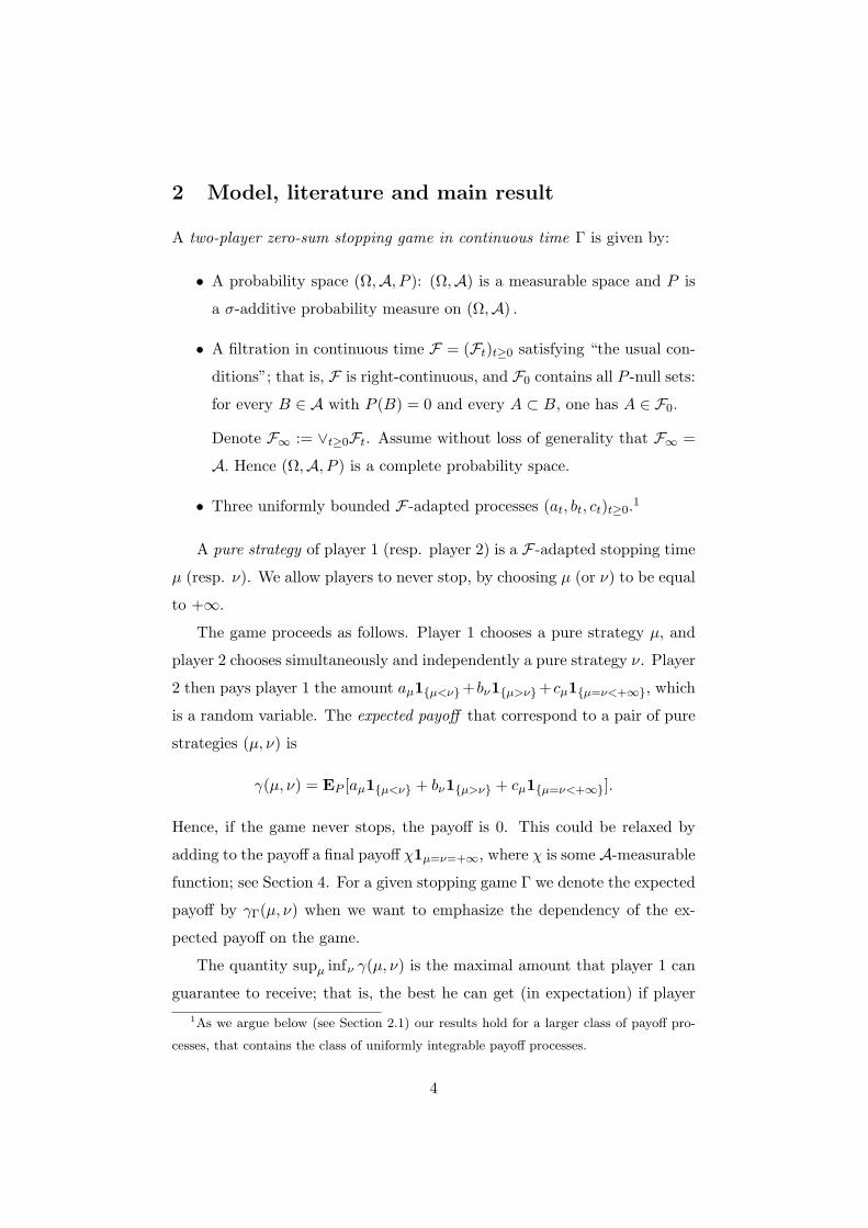
• Three uniformly bounded F-adapted processes (at, bt, ct)t≥0.1

A pure strategy of player 1 (resp. player 2) is a F-adapted stopping time

µ (resp. ν). We allow players to never stop, by choosing µ (or ν) to be equal

to +∞.

The game proceeds as follows. Player 1 chooses a pure strategy µ, and

player 2 chooses simultaneously and independently a pure strategy ν. Player

2 then pays player 1 the amount aµ1µ<ν+bν1µ>ν+cµ1µ=ν<+∞, which

is a random variable. The expected payoff that correspond to a pair of pure

strategies (µ, ν) is

γ(µ, ν) = EP [aµ1µ<ν + bν1µ>ν + cµ1µ=ν<+∞].

Hence, if the game never stops, the payoff is 0. This could be relaxed by

adding to the payoff a final payoff χ1µ=ν=+∞, where χ is some A-measurable

function; see Section 4. For a given stopping game Γ we denote the expected

payoff by γΓ(µ, ν) when we want to emphasize the dependency of the ex-

pected payoff on the game.

The quantity supµ infν γ(µ, ν) is the maximal amount that player 1 can

guarantee to receive; that is, the best he can get (in expectation) if player1As we argue below (see Section 2.1) our results hold for a larger class of payoff pro-

cesses, that contains the class of uniformly integrable payoff processes.

4

2 knows the strategy chosen by player 1 before he has to choose his own

strategy. Similarly, by playing properly, player 2 can guarantee to pay no

more than infν supµ γ(µ, ν).

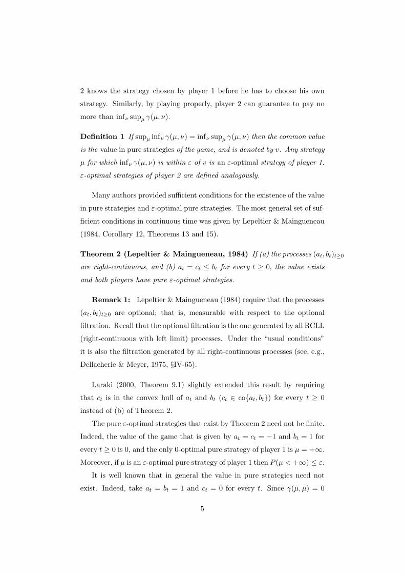
Definition 1 If supµ infν γ(µ, ν) = infν supµ γ(µ, ν) then the common value

is the value in pure strategies of the game, and is denoted by v. Any strategy

µ for which infν γ(µ, ν) is within ε of v is an ε-optimal strategy of player 1.

ε-optimal strategies of player 2 are defined analogously.

Many authors provided sufficient conditions for the existence of the value

in pure strategies and ε-optimal pure strategies. The most general set of suf-

ficient conditions in continuous time was given by Lepeltier & Maingueneau

(1984, Corollary 12, Theorems 13 and 15).

Theorem 2 (Lepeltier & Maingueneau, 1984) If (a) the processes (at, bt)t≥0

are right-continuous, and (b) at = ct ≤ bt for every t ≥ 0, the value exists

and both players have pure ε-optimal strategies.

Remark 1: Lepeltier & Maingueneau (1984) require that the processes

(at, bt)t≥0 are optional; that is, measurable with respect to the optional

filtration. Recall that the optional filtration is the one generated by all RCLL

(right-continuous with left limit) processes. Under the “usual conditions”

it is also the filtration generated by all right-continuous processes (see, e.g.,

Dellacherie & Meyer, 1975, §IV-65).

Laraki (2000, Theorem 9.1) slightly extended this result by requiring

that ct is in the convex hull of at and bt (ct ∈ coat, bt) for every t ≥ 0

instead of (b) of Theorem 2.

The pure ε-optimal strategies that exist by Theorem 2 need not be finite.

Indeed, the value of the game that is given by at = ct = −1 and bt = 1 for

every t ≥ 0 is 0, and the only 0-optimal pure strategy of player 1 is µ = +∞.

Moreover, if µ is an ε-optimal pure strategy of player 1 then P (µ < +∞) ≤ ε.

It is well known that in general the value in pure strategies need not

exist. Indeed, take at = bt = 1 and ct = 0 for every t. Since γ(µ, µ) = 0

5

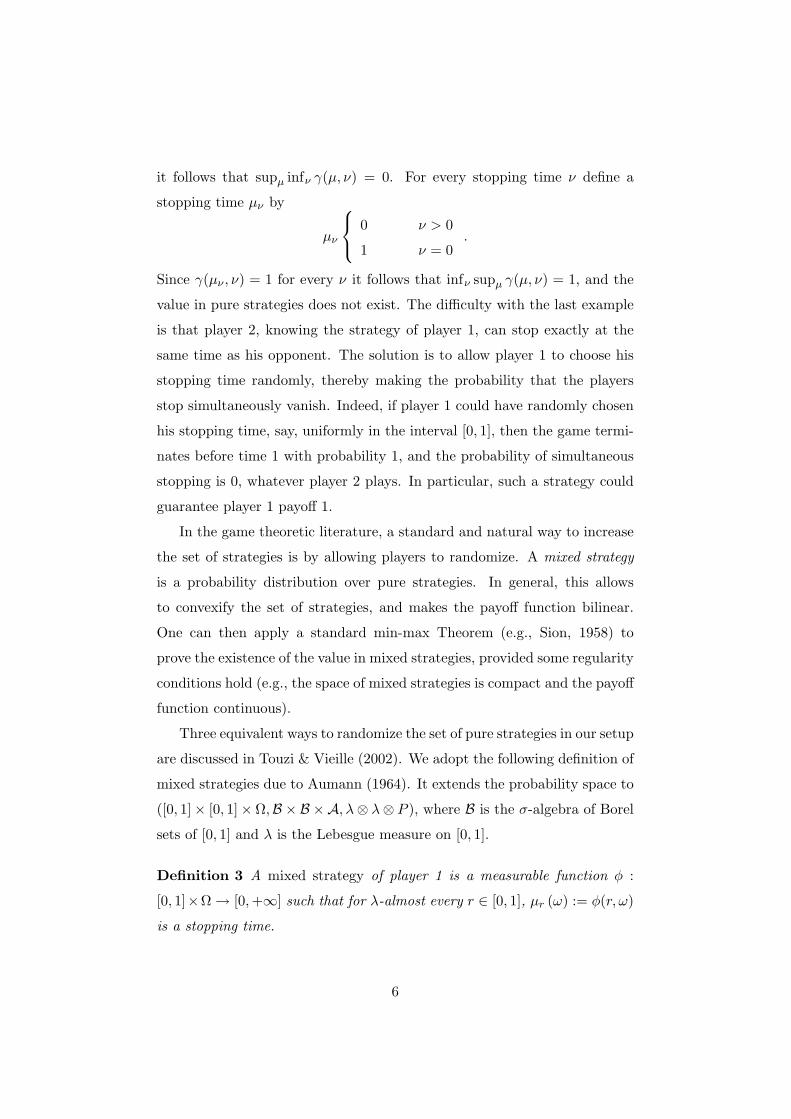
it follows that supµ infν γ(µ, ν) = 0. For every stopping time ν define a

stopping time µν by

µν

0 ν > 0

1 ν = 0.

Since γ(µν , ν) = 1 for every ν it follows that infν supµ γ(µ, ν) = 1, and the

value in pure strategies does not exist. The difficulty with the last example

is that player 2, knowing the strategy of player 1, can stop exactly at the

same time as his opponent. The solution is to allow player 1 to choose his

stopping time randomly, thereby making the probability that the players

stop simultaneously vanish. Indeed, if player 1 could have randomly chosen

his stopping time, say, uniformly in the interval [0, 1], then the game termi-

nates before time 1 with probability 1, and the probability of simultaneous

stopping is 0, whatever player 2 plays. In particular, such a strategy could

guarantee player 1 payoff 1.

In the game theoretic literature, a standard and natural way to increase

the set of strategies is by allowing players to randomize. A mixed strategy

is a probability distribution over pure strategies. In general, this allows

to convexify the set of strategies, and makes the payoff function bilinear.

One can then apply a standard min-max Theorem (e.g., Sion, 1958) to

prove the existence of the value in mixed strategies, provided some regularity

conditions hold (e.g., the space of mixed strategies is compact and the payoff

function continuous).

Three equivalent ways to randomize the set of pure strategies in our setup

are discussed in Touzi & Vieille (2002). We adopt the following definition of

mixed strategies due to Aumann (1964). It extends the probability space to

([0, 1]× [0, 1]×Ω,B × B ×A, λ⊗ λ⊗ P ), where B is the σ-algebra of Borel

sets of [0, 1] and λ is the Lebesgue measure on [0, 1].

Definition 3 A mixed strategy of player 1 is a measurable function φ :

[0, 1]×Ω → [0,+∞] such that for λ-almost every r ∈ [0, 1], µr (ω) := φ(r, ω)

is a stopping time.

6

The interpretation is the following: player 1 chooses randomly r ∈ [0, 1],

and then stops the game at time µr = φ(r, ·). Mixed strategies of player

2 are denoted by ψ, and, for every s ∈ [0, 1], the s-section is denoted by

νs := ψ (s, ·).

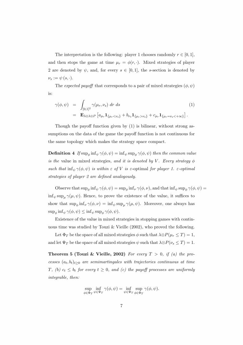
The expected payoff that corresponds to a pair of mixed strategies (φ, ψ)

is:

γ(φ, ψ) =∫

[0,1]2γ(µr, νs) dr ds (1)

= Eλ⊗λ⊗P[aµr1µr<νs + bνs1µr>νs + cµr1µr=νs<+∞

].

Though the payoff function given by (1) is bilinear, without strong as-

sumptions on the data of the game the payoff function is not continuous for

the same topology which makes the strategy space compact.

Definition 4 If supφ infψ γ(φ, ψ) = infψ supφ γ(φ, ψ) then the common value

is the value in mixed strategies, and it is denoted by V . Every strategy φ

such that infψ γ(φ, ψ) is within ε of V is ε-optimal for player 1. ε-optimal

strategies of player 2 are defined analogously.

Observe that supφ infψ γ(φ, ψ) = supφ infν γ(φ, ν), and that infψ supφ γ(φ, ψ) =

infψ supµ γ(µ, ψ). Hence, to prove the existence of the value, it suffices to

show that supφ infν γ(φ, ν) = infψ supµ γ(µ, ψ). Moreover, one always has

supφ infψ γ(φ, ψ) ≤ infψ supφ γ(φ, ψ).

Existence of the value in mixed strategies in stopping games with contin-

uous time was studied by Touzi & Vieille (2002), who proved the following.

Let ΦT be the space of all mixed strategies φ such that λ⊗P (µr ≤ T ) = 1,

and let ΨT be the space of all mixed strategies ψ such that λ⊗P (νs ≤ T ) = 1.

Theorem 5 (Touzi & Vieille, 2002) For every T > 0, if (a) the pro-

cesses (at, bt)t≥0 are semimartingales with trajectories continuous at time

T , (b) ct ≤ bt for every t ≥ 0, and (c) the payoff processes are uniformly

integrable, then:

supφ∈ΦT

infψ∈ΨT

γ(φ, ψ) = infψ∈ΨT

supφ∈ΦT

γ(φ, ψ).

7

Touzi & Vieille (2002) prove that under conditions (a) and (b) of The-

orem 5 it is sufficient to restrict the players to certain subclasses of mixed

strategies. They then apply Sion’s (1958) min-max theorem to the restricted

game.

Remark 2: By Dellacherie and Meyer (1980, §VII-23), under the “usual

conditions”, a semimartingle is always RCLL (right-continuous with left

limit).

One class of mixed strategies will play a special role along the paper.

Definition 6 Let δ > 0. A mixed strategy φ is δ-almost pure if there exists

a stopping time µ and a set A ∈ Fµ such that for every r ∈ [0, 1], φ(r, ·) = µ

on A, and φ(r, ·) = µ+ rδ on Ac.

Recall that a process (xt)t≥0 is progressively measurable if for every

t ≥ 0 the function (s, ω) 7→ xs(ω) from [0, t]×Ω is measurable with respect

to B([0, t]) × Ft, where B([0, t]) is the σ-algebra of Borel subsets of [0, t].

Recall also that an optional process is progressively measurable (see, e.g.,

Dellacherie & Meyer, 1975, §IV-64).

The main result we present is the following.

Theorem 7 If the processes (at)t≥0 and (bt)t≥0 are right-continuous and if

(ct)t≥0 is progressively measurable then the value in mixed strategies exists.

Moreover, for every ε > 0 there is δ0 ∈ (0, 1) such that for every δ ∈ (0, δ0)

both players have δ-almost pure ε-optimal strategies.

Our proof heavily relies on the result of Lepeltier & Maingueneau (1984),

where they extend the discrete time variational approach of Neveu (1975)

to continuous time.

2.1 On the payoff processes

A F-adapted process x = (xt)t≥0 is in the class D (see, e.g., Dellacherie &

Meyer, 1980, §VI-20) if the set xσ1σ<+∞, σ is a F-adapted stopping time

8

is uniformly integrable (see, e.g., Dellacherie & Meyer, 1975, §II-17). That is,

if for every bounded stopping time σ, EP [|xσ|1Xσ≥r] converges uniformly

to 0 as r goes to +∞.

This implies that the set EP [|xσ|1σ<+∞], σ is a F-adapted stopping time

is uniformly bounded (see, e.g., Dellacherie & Meyer, 1975, §II-19). Observe

that every uniformly bounded process as well as every uniformly integrable

process is in the class D (see, e.g., Dellacherie & Meyer, 1975, §II-18)).

For a measurable process (xt)t≥0 and r ≥ 0 define the process (xrt )t≥0

by:

xrt (ω) := xt(ω)1|xt(ω)|≤r + r1xt(ω)>r − r1xt(ω)<−r.

By Dellacherie & Meyer (1975, §II-17), x ∈ D if and only if for every

ε > 0 there exists r > 0 such that for every stopping time σ one has

E[|xσ − xrσ|1σ<+∞

]< ε. The process (xrt )t≥0 is uniformly bounded by r,

and, in addition, if (xt)t≥0 is right-continuous or F-adapted so is (xrt )t≥0 .

If the payoff processes (at)t≥0, (bt)t≥0 and (ct)t≥0 are not necessarily

bounded but are in the class D then for every ε > 0 there exists r > 0 such

that

EP

[(|aσ − arσ|+ |bσ − brσ|+ |cσ − crσ|)1σ<+∞

]< ε.

Hence, if the game Γ = (Ω,A, P ;F , (at, bt, ct)t≥0) satisfies the assumptions

of Theorem 7, it admits a value. Moreover, every ε-optimal strategy in

Γr := (Ω,A, P ;F , (art , brt , crt )t≥0) is 2ε-optimal in Γ.

In particular, all the existence results that are proved for uniformly

bounded payoff processes (Lepeltier & Maingueneau (1984)) or uniformly

integrable payoff processes (Touzi & Vieille (2002)) are valid for payoff pro-

cesses in the class D as well.

3 Proof

In the present section the main result of the paper is proven. From now

on we fix a stopping game Γ such that (at, bt)t≥0 are right-continuous and

(ct)t≥0 is progressively measurable.

9

3.1 Preliminaries

The following Lemma will be used in the sequel.

Lemma 8 For every F-adapted stopping time τ and every ε > 0 there is

δ > 0 such that p (|at − aτ | < ε ∀t ∈ [τ, τ + δ]) > 1− ε.

A similar statement holds when one replaces the process (at)t≥0 by the

process (bt)t≥0.

Proof. Since (at)t≥0 is right-continuous, it is progressively measurable

(see, e.g., Dellacherie & Meyer, 1975, §IV-15).

Let δτ(ω)(ω) = infs ≥ τ(ω) : |as(ω) − aτ (ω)| ≥ ε. The progressive

measurability of (at)t≥0 implies that δτ(ω)(ω) is measurable with respect to

F∞ (see, e.g., Dellacherie & Meyer, 1975, §III-44).

The right-continuity of (at)t≥0 implies that P (ω : δτ(ω)(ω) > 0) = 1.

Since P is σ-additive and ω : δτ(ω)(ω) > 0 = ∪n>0ω : δτ(ω)(ω) > 1n, the

lemma follows by choosing δ > 0 sufficiently small so that P (ω : δτ(ω)(ω) >

δ) > 1− ε.

By Lemma 8 and since the payoff processes are uniformly bounded, one

obtains the following.

Corollary 9 Let a stopping time τ and ε > 0 be given. There exists δ > 0

sufficiently small such that for every set A ∈ Fτ and every stopping time µ

that satisfies τ ≤ µ ≤ τ + δ,

|EP [aµ1A]−EP [aτ1A]| ≤ 2ε.

3.2 The case at ≤ bt for every t ≥ 0

Definition 10 Let δ > 0. A mixed strategy φ is δ-pure if there exists a

stopping time µ such that

φ(r, ·) = µ+ rδ ∀r ∈ [0, 1]. (2)

10

Observe that a δ-pure mixed strategy is in particular δ-almost pure.

When µ is a stopping time, we sometime denote the δ-pure mixed strategy

defined in (2) simply by µ+ rδ.

In this section we prove the following result: when at ≤ bt for every t ≥ 0

the value in mixed strategies exists, it is independent of (ct)t≥0, and both

players have δ-pure ε-optimal strategies, provided δ is sufficiently small.

The idea is the following. Assume player 1 decides to stop at time t.

If ct ≤ at, player 1 wants to mask the exact time in which he stops, so

that both players do not stop at the same time. Since payoffs are right-

continuous, he can stop randomly in a small interval after time t. Similarly,

if ct > at, player 2 prefers that player 1 stops alone at time t rather than to

stop simultaneously with player 1 at time t.

Proposition 11 If at ≤ bt for every t ≥ 0 then the value in mixed strategies

exists. Moreover, the value is independent of the process (ct)t≥0, and for

every ε > 0 there is δ0 > 0 such that for every δ ∈ (0, δ0) both players

have δ-pure ε-optimal strategies. If at ≤ ct ≤ bt for every t ≥ 0 then the

value in pure strategies exists, and there are ε-optimal strategies which are

independent of (ct)t≥0.

Proof. Consider an auxiliary stopping game Γ∗ = (Ω,A, P ;F , (a∗t , b∗t , c∗t )t≥0),

where a∗t = at and b∗t = c∗t = bt for every t ≥ 0.

By Theorem 2 the game Γ∗ has a value in pure strategies v∗. We will

prove that v∗ is the value in mixed strategies of the original game. Since

v∗ is independent of the process (ct)t≥0, the second claim in the proposition

will follow.

Fix ε > 0. Let µ be an ε-optimal strategy of player 1 in Γ∗. In particular,

infν γΓ∗(µ, ν) ≥ v∗ − ε.

We now construct a mixed strategy φ that satisfies infν γΓ(φ, ν) ≥ v∗−5ε.

By Lemma 8 there is δ > 0 such that p(|at−aµ| < ε ∀t ∈ [µ, µ+δ]) > 1−ε.

Define a δ-pure mixed strategy φ by

φ(r, ·) = µ+ rδ ∀r ∈ [0, 1].

11

Let ν be any stopping time. Since µ is ε-optimal in Γ∗, by the definition

of Γ∗, and since λ⊗ P (µ+ rδ = ν) = 0,

v∗ − ε ≤ γΓ∗(µ, ν)

= EP [aµ1µ<ν + bν1µ≥ν] (3)

= Eλ⊗P [aµ1µ+rδ<ν + aµ1µ<ν<µ+rδ + bν1µ≥ν].

Since λ⊗ P (µ+ rδ = ν) = 0 and (ct)t≥0 is progressively measurable,

γΓ(φ, ν) = Eλ⊗P[aµ+rδ1µ+rδ<ν + bν1µ+rδ>ν + cν1µ+rδ=ν<+∞

]= Eλ⊗P

[aµ+rδ1µ+rδ<ν + bν1µ+rδ>ν

](4)

= Eλ⊗P[aµ+rδ1µ+rδ<ν + bν1µ<ν<µ+rδ + bν1µ≥ν

].

By Corollary 9, and since at ≤ bt for every t ≥ 0,

Eλ⊗P [aµ1µ<ν<µ+rδ] ≤ Eλ⊗P [aν1µ<ν<µ+rδ]+2ε ≤ Eλ⊗P [bν1µ<ν<µ+rδ]+2ε.

(5)

Corollary 9 implies in addition that

Eλ⊗P [aµ1µ+rδ<ν] ≤ Eλ⊗P [aµ+rδ1µ+rδ<ν] + 2ε. (6)

By (3)-(6),

v∗ − ε ≤ γΓ∗(µ, ν) ≤ γΓ(φ, ν) + 4ε.

Since ν is arbitrary, infν γΓ(φ, ν) ≥ v∗ − 5ε.

Consider an auxiliary stopping game Γ∗∗ = (Ω,A, P ;F , (a∗∗t , b∗∗t , c∗∗t )t≥0),

where a∗∗t = c∗∗t = at and b∗∗t = bt for every t ≥ 0.

A symmetric argument to the one provided above proves that the game

Γ∗∗ has a value v∗∗, and that player 2 has a mixed strategy ψ which satisfies

supµ γΓ(µ, ψ) ≤ v∗∗ + 5ε.

Since c∗∗t = at ≤ bt = c∗t for every t ≥ 0, v∗∗ ≤ v∗. Since supµ γΓ(µ, ψ) ≥

γΓ(φ, ψ) ≥ infν γΓ(φ, ν),

v∗ ≥ v∗∗ ≥ supµγΓ(µ, ψ)− 5ε ≥ inf

νγΓ(φ, ν)− 5ε ≥ v∗ − 10ε.

12

Since ε is arbitrary, v∗ = v∗∗, so that v∗ is the value in mixed strategies of

Γ, and φ and ψ are 5ε-optimal mixed strategies of the two players.

If at ≤ ct ≤ bt for every t ≥ 0 then γΓ∗∗(µ, ν) ≤ γΓ(µ, ν) ≤ γΓ∗(µ, ν) for

every pair of pure strategies (µ, ν). Hence

v∗∗ = supµ

infνγΓ∗∗(µ, ν) ≤ sup

µinfνγΓ(µ, ν)

≤ infν

supµγΓ(µ, ν) ≤ inf

νsupµγΓ∗(µ, ν) = v∗ = v∗∗

Thus supµ infν γΓ(µ, ν) = infν supµ γΓ(µ, ν) : the value in pure strategies

exists. Moreover, any ε-optimal strategy of player 1 (resp. player 2) in

Γ∗ (resp. Γ∗∗) is also ε-optimal in Γ. In particular, if at ≤ ct ≤ bt for

every t ≥ 0, both players have ε-optimal strategies which are independent

of (ct)t≥0.

3.3 Proof of Theorem 7

Define τ by

τ = inft ≥ 0, at ≥ bt,

where the infimum of an empty set is +∞. Since (at−bt)t≥0 is progressively

measurable with respect to (Ft)t≥0, τ is an F-adapted stopping time (see,

e.g., Dellacherie & Meyer, 1975, §IV-50).

The idea is the following. We show that it is optimal for both players to

stop at or around time τ (provided the game does not stop before time τ).

Hence the problem reduces to the game between times 0 and τ . Since for

t ∈ [0, τ [, at ≤ bt, Proposition 11 can be applied.

The following notation will be useful in the sequel. For a pair of pure

strategies (µ, ν) and a set A ∈ A, we define

γΓ(µ, ν;A) = EP [1A(aµ1µ<ν + bµ1µ>ν + cµ1µ=ν<+∞)]

This is the expected payoff restricted to A. For a pair of mixed strategies

(φ, ψ) we define

γΓ(φ, ψ;A) =∫

[0,1]2γΓ(µr, νs;A)dr ds,

13

where µr and νs are the sections of φ and ψ respectively.

Set

A0 = τ = +∞,

A1 = τ < +∞ ∩ cτ ≥ aτ ≥ bτ,

A2 = τ < +∞ ∩ aτ > cτ ≥ bτ, and

A3 = τ < +∞ ∩ aτ ≥ bτ > cτ.

Observe that (A0, A1, A2, A3) is an Fτ -measurable partition of Ω.

Define a Fτ -measurable function w by

w = aτ1A1 + cτ1A2 + bτ1A3 .

Define a stopping game Γ∗ = (Ω,A, P, (Ft)t≥0, (a∗t , b∗t , c

∗t )t≥0) by:

a∗t =

at t < τ

w t ≥ τ, b∗t =

bt t < τ

w t ≥ τ, c∗t =

ct t < τ

w t ≥ τ.

That is, the payoff is set to w at and after time τ .

The game Γ∗ satisfies the assumptions of Proposition 11, hence it has a

value in mixed strategies V . Moreover, for every ε > 0 both players have

δ-pure ε-optimal strategies, provided δ > 0 is sufficiently small.

We now prove that V is the value of the game Γ as well. Fix ε > 0. We

only show that player 1 has a mixed strategy φ such that infν γΓ(φ, ν) ≥

V − 7ε. An analogous argument shows that player 2 has a mixed strategy

ψ such that supµ γΓ(µ, ψ) ≤ V + 7ε. Since ε is arbitrary, V is indeed the

value in mixed strategies of Γ.

Assume δ is sufficiently small so that the following conditions hold (by

the proofs of Lemma 8 and Proposition 11 such δ exists).

C.1 Player 1 has a δ-pure ε-optimal strategy φ∗ = µ+ rδ in Γ∗.

C.2 P (µ+ δ < τ) ≥ P (µ < τ)− ε/M , where M ∈]0,+∞[ is a uniform

bound of the payoff processes.

C.3 P (|at − aτ | < ε, |bt − bτ | < ε ∀t ∈ [τ, τ + δ]) > 1− ε.

14

We now claim that one can choose µ so that µ ≤ τ . Indeed, assume that

P (µ > τ) > 0. The set µ > τ is Fτ -measurable. Define a stopping time

µ′ = minµ, τ. We will prove that the δ-pure strategy φ′ = µ′ + rδ is also

ε-optimal in Γ∗, which establishes the claim. Given a stopping time ν define

a stopping time ν ′ as follows: ν ′ = τ over µ > τ, and ν ′ = ν otherwise.

Then

V − ε ≤ γΓ∗(µ+ rδ, ν ′) = γΓ∗(µ+ rδ, ν ′; µ > τ) + γΓ∗(µ+ rδ, ν ′; µ ≤ τ).

However, γΓ∗(µ + rδ, ν ′; µ > τ) = Eλ⊗P [w1µ>τ] = γΓ∗(µ′ + rδ, ν; µ >

τ), and since µ = µ′ and ν = ν ′ over µ ≤ τ, γΓ∗(µ + rδ, ν ′; µ ≤ τ) =

γΓ∗(µ′ + rδ, ν; µ ≤ τ. Therefore

γΓ∗(µ′ + rδ, ν) = γΓ∗(µ+ rδ, ν ′) ≥ V − ε.

Since ν is arbitrary, µ′ + rδ is ε-optimal, as desired.

Define a mixed strategy φ as follows.

φ(r, ·) =

µ+ rδ µ < τ ∪A0,

τ µ = τ ∩ (A1 ∪A2) ,

µ+ rδ µ = τ ∩A3.

Observe that φ is δ-almost pure.

The mixed strategies φ and φ∗ differ only over the set µ = τ ∩

(A1 ∪A2). Since over this set the payoff in Γ∗ is w provided the game

terminates after time τ , whatever the players play, φ is an ε-optimal mixed

strategy in Γ∗.

Let ν be an arbitrary pure strategy of player 2. Define a partition

(B0, B1, B2) of [0, 1]× Ω by

B0 = µ+ δ < τ ∪ ν < τ,

B1 = µ < τ < µ+ δ ∩ ν ≥ τ, and

B2 = (µ = τ or µ = +∞) ∩ ν ≥ τ.

Over B0 the game terminates before time τ under (φ, ν). In particular,

γΓ(φ, ν;B0) = γΓ∗(φ, ν;B0). (7)

15

By (C.2) λ⊗ P (B1) < ε/M , so that

γΓ(φ, ν;B1) ≥ γΓ∗(φ, ν;B1)− 2ε. (8)

Over B2 ∩A0 the game never terminates under (φ, ν), so that

γΓ(φ, ν;B2 ∩A0) = γΓ∗(φ, ν;B2 ∩A0) = 0. (9)

Over A1 ∪A2, minaτ , cτ ≥ w, so that

γΓ(φ, ν;B2 ∩ (A1 ∪A2)) = Eλ⊗P [1B2∩(A1∪A2)(aτ1τ<ν + cτ1τ=ν)]

≥ Eλ⊗P [w1τ≤ν∩B2∩(A1∪A2)] (10)

= γΓ∗(φ, ν;B2 ∩ (A1 ∪A2)).

Finally, since λ ⊗ P (µ + rδ = ν) = 0, by Corollary 9, since (ct)t≥0 is

progressively measurable, and since aτ ≥ bτ = w over A3,

γΓ(φ, ν;B2 ∩A3) = Eλ⊗P [1B2∩A3(aµ+rδ1µ+rδ<ν + bν1µ+rδ>ν + cν1µ+rδ=ν)]

= Eλ⊗P [1B2∩A3(aµ+rδ1µ+rδ<ν + bν1µ+rδ>ν)]

≥ Eλ⊗P [1B2∩A3(aτ1µ+rδ<ν + bτ1µ+rδ>ν)]− 4ε (11)

≥ Eλ⊗P [w1B2∩A3 ]− 4ε

= γΓ∗(φ, ν;B2 ∩A3).

Summing Eqs. (7)-(11), and using the ε-optimality of φ∗ in Γ∗, gives us

V − ε ≤ γΓ∗(φ, ν) ≤ γΓ(φ, ν) + 6ε,

as desired.

4 Extensions

In the present section we construct specific ε-optimal strategies in the spirit

of Dynkin (1969) or Rosenberg et al. (2001) and we give conditions for the

existence of the value in pure strategies. We then provide two extensions to

the basic model.

16

4.1 Construction of an ε-optimal strategy

Let Γ = (Ω,A, P, (Ft)t≥0, (at, bt, ct)t≥0) satisfy conditions of Theorem 7.

Define τ, (A0, A1, A2, A3), w and Γ∗ = (Ω,A, P, (Ft)t≥0, (a∗t , b∗t , c

∗t )t≥0)

as in the proof of Theorem 7.

For any stopping time σ let Γ∗σ = (Ω,A, P, (Ft)t≥0, (a∗t , b∗t , c

∗t )t≥0) be the

game starting at time σ; that is, players are restricted to choose strategies

that stop with probability 1 at or after time σ.

Lepeltier & Mainguenau (1984, Theorem 13) and Proposition 11 show

that this game has a value in mixed strategies X∗σ. Moreover, the value is

independent of (c∗t )t≥0.

Using a general result of Dellacherie & Lenglart (1982), Lepeltier &

Mainguenau (1984, Theorem 7) show the existence of a right-continuous

process (V ∗t )t≥0 such that V ∗

σ = X∗σ for every stopping time σ.

For every ε > 0 define a stopping time

µ∗ε = inft ≥ 0 : V ∗

t ≤ a∗t +ε

35

.

By definition of τ and Γ∗, one has µ∗ε ≤ τ.

Lepeltier & Mainguenau (1984, Theorem 13) and Proposition 11 imply

that µ∗ε is ε35 -optimal for Player 1 in any game Γ = (Ω,A, P, (Ft)t≥0, (a∗t , b

∗t , dt)t≥0),

provided that the process (dt)t≥0 satisfies a∗t ≤ dt ≤ b∗t for any t ≥ 0.

Let δ be such that P (|at−aµ∗ε | <ε35 , ∀t ∈ [µ∗ε, µ

∗ε + δ]) > 1− ε

35 . From

the proof of Proposition 11 we deduce that µ∗ε + rδ is ε7 -optimal for player

1 in Γ∗.

Now, assume that δ is sufficiently small so that

• P (µ∗ε + δ < τ) ≥ P (µ∗ε < τ)− ε7M , and

• P (|at − aτ | < ε7 , |bt − bτ | < ε

7 ∀t ∈ [τ, τ + δ]) > 1− ε7 .

Define a mixed strategy φε as follows.

φε(r, ·) =

µ∗ε + rδ µ∗ε < τ ∪A0,

τ µ∗ε = τ ∩ (A1 ∪A2) ,

µ∗ε + rδ µ∗ε = τ ∩A3.

17

The proof of Theorem 7 imply that φε is ε-optimal for player 1 in Γ.

Assume that cτ ≥ bτ a.s. (or equivalently, A1 ∪ A2 = Ω). By the

proof of Proposition 11, it is 0-optimal for Player 1 in Γ to stop at time

τ , provided the game reaches time τ . If in addition one has at ≤ ct ≤

bt for every t ∈ [0, τ [, by the proof of Proposition 11 and Lepeltier &

Mainguenau (1984, Theorem 13) we deduce that the pure stopping time

inf t ≥ 0 : V ∗t ≤ a∗t + ε is ε-optimal for Player 1 in Γ. Hence one obtains

the following.

Proposition 12 If ct ∈ coat, bt for every t ∈ [0, τ ] then the value exists in

pure strategies. An ε-optimal strategy for Player 1 is inf t ≥ 0 : V ∗t ≤ a∗t + ε,

and an ε-optimal strategy for Player 2 is inf t : V ∗t ≥ b∗t − ε .

Corollary 13 Every stopping game such that (at, bt, ct)t≥0 are continuous

and satisfies c0 ∈ coa0, b0 admits a value in pure strategies.

4.2 On final payoff

Our convention is that the payoff is 0 if no player ever stops. In fact, one

can add a final payoff as follows. Let χ be an A-measurable and integrable

function. The expected payoff that corresponds to a pair of pure strategies

(µ, ν) is:

EP [aµ1µ<ν + bν1µ>ν + cµ1µ=ν<+∞ + χ1µ=ν=+∞].

The expected payoff can be written as:

EP [χ] + EP

[(aµ −EFµ

P

[χ])

1µ<ν +(bν −EFν

P [χ])1µ>ν

+(cµ −EFµ

P [χ])1µ=ν<+∞

],

where EFµ

P [χ] is the conditional expectation of χ given the σ-algebra Fµ.

Define a process dt := EFtP [χ] . Since the filtration satisfies the “usual

conditions”, (dt)t≥0 is a right-continuous martingale (see, e.g., Dellacherie

& Meyer, 1980, §VI-4). Hence we are reduced to the study of the standard

stopping game Γ∗ = (Ω,A, P, (Ft)t≥0, (a∗t , b∗t , c

∗t )t≥0) with a∗t = bt − dt, b

∗t =

bt − dt and c∗t = ct − dt.

18

4.3 On cumulative payoff

In our definition, players receive no payoff before the game stops. One can

add a cumulative payoff as follows. Let (xt)t≥0 be a progressively measurable

process satisfying EP

[∫ +∞0 |xt| dt

]< +∞, and suppose that the expected

payoff that corresponds to a pair of pure strategies (µ, ν) is given by

EP

[aµ1µ<ν + bν1µ>ν + cµ1µ=ν<+∞ +

∫ minµ,ν

0xtdt

].

The expected payoff can be written as

EP

[(aµ +

∫ µ

0xtdt

)1µ<ν +

(bν +

∫ ν

0xtdt

)1µ>ν +

(cµ +

∫ µ

0xtdt

)1µ=ν<+∞

].

Thus, the game is equivalent to the stopping game Γ∗ = (Ω,A, P, (Ft)t≥0, (a∗t , b∗t , c

∗t )t≥0),

where a∗t = bt + dt, b∗t = bt + dt, c∗t = ct + dt, and dt =

∫ t0 xsds.

19

References

[1] M. Alario-Nazaret, J.P. Lepeltier & B. Marchal (1982) Dynkin games,

Stochastic Differential Systems (Bad Honnef), 23-32, Lecture notes in

Control and Information Sciences, 43, Springer Verlag.

[2] R.J. Aumann (1964) Mixed and behavior strategies in infinite exten-

sive games, in Advances in Game Theory, M. Dresher, L.S. Shapley

and A.W. Tucker (eds), Annals of Mathematics Study 52, Princeton

University Press.

[3] A. Bensoussan (1984),On the theory of option pricing. Acta Applicandae

Mathematicae, 2, 139-158.

[4] J.M. Bismut (1977) Sur un probleme de Dynkin. Z. Warsch. V. Geb.,

39,31-53.

[5] J. Cvitanic & I. Karatzas. Backward stochastic differential equations

with reflection and Dynkin games. Ann. Prob., 24, 2024-2056, 1996.

[6] C. Dellacherie & E. Lenglart (1982) Sur des problemes de regularisation,

de recollement et d’interpolation en theorie generale des processus.

Seminaire de Probabilites XVI, Lecture Notes. Springer Verlag.

[7] C. Dellacherie & P.-A. Meyer (1975) Probabilites et potentiel, Chapitres

I a IV, Hermann. English translation: Probabilities and poten-

tial. North-Holland Mathematics Studies, 29. North-Holland Pub-

lishing Co., Amsterdam-New York; North-Holland Publishing Co.,

Amsterdam-New York, 1978.

[8] C. Dellacherie & P.-A. Meyer (1980) Probabilites et potentiel, Chapitres

V a VIII, Theorie des Martingales, Hermann. English translation: Prob-

abilities and potential. B. Theory of martingales. North-Holland Math-

ematics Studies, 72. North-Holland Publishing Co., Amsterdam, 1982.

[9] E.B. Dynkin (1969) Game variant of a problem on optimal stopping,

Soviet Math. Dokl., 10, 270-274.

20

[10] Ghemawat P. and Nalebuff B. (1985) Exit, RAND J. Econ., 16, 184-194

[11] I. Karatzas (1988) On the princing of American options, Appli. Math.

Optimization, 17, 37-60.

[12] R. Laraki (2000) Jeux repetes a information incomplete: approche vari-

ationnelle, These de Doctorat de l’Universite Paris 6, France.

[13] J.P. Lepeltier & M.A. Mainguenau (1984) Le jeu de Dynkin en theorie

generale sans l’hypothese de Mokobodsky. Stochastics, 13, 25-44.

[14] J. Ma & J. Cvitanic (2001) Reflected forward-backward SDE’s and

obstacle problems with boundary conditions. Journal of Applied Math-

ematics & Stocastic Analysis, 14, 113-138.

[15] Neveu J. (1975) Discrete-Parameter Martingales, North-Holland, Am-

sterdam

[16] D. Rosenberg, E. Solan, & N. Vieille (2001) Stopping games with

randomized strategies. Prob. Th. Rel. Fields., 119, 433-451.

[17] E. Shmaya & E. Solan (2002) Two player non zero-sum stopping games

in discrete time, Discussion Paper, 1347, The Center for Mathematical

Studies in Economics and Management Science, Northwestern Univer-

sity.

[18] M. Sion (1958) On general minmax theorems. Pacific Journal of Math-

ematics, 8, 171-176.

[19] N. Touzi & N. Vieille (2002) Continuous-time Dynkin games with mixed

strategies. SIAM J. Cont. Opt., forthcoming.

21