Embed Size (px)
Citation preview
Storage Capacity and Injection Rate Estimates for
CO2 Sequestration in Deep Saline Aquifers in the
Conterminous United States
by
Michael Lawrence Szulczewski
Submitted to the Department of Civil and Environmental Engineeringin partial fulfillment of the requirements for the degree of
Master of Science in Civil and Environmental Engineering
at the
MASSACHUSETTS INSTITUTE OF TECHNOLOGY
June 2009
c© Massachusetts Institute of Technology 2009. All rights reserved.
Author . . . . . . . . . . . . . . . . . . . . . . . . . . . . . . . . . . . . . . . . . . . . . . . . . . . . . . . . . . . . . .Department of Civil and Environmental Engineering
May 8, 2009
Certified by. . . . . . . . . . . . . . . . . . . . . . . . . . . . . . . . . . . . . . . . . . . . . . . . . . . . . . . . . .Ruben Juanes
Assistant Professor, Civil and Environmental EngineeringThesis Supervisor
Accepted by . . . . . . . . . . . . . . . . . . . . . . . . . . . . . . . . . . . . . . . . . . . . . . . . . . . . . . . . .Daniele Veneziano
Chairman, Department Committee on Graduate Students

2
Storage Capacity and Injection Rate Estimates for CO2
Sequestration in Deep Saline Aquifers in the Conterminous
United States
by
Michael Lawrence Szulczewski
Submitted to the Department of Civil and Environmental Engineeringon May 8, 2009, in partial fulfillment of the
requirements for the degree ofMaster of Science in Civil and Environmental Engineering
Abstract
A promising method to mitigate global warming is injecting CO2 into deep salineaquifers. In order to ensure the safety of this method, it is necessary to understandhow much CO2 can be injected into an aquifer and at what rate. Since offsettingnationwide emissions requires storing very large quantities of CO2, these propertiesmust be understood at the large scale of geologic basins.
In this work, we develop simple models of storage capacity and injection rate atthe basin scale. We develop a storage capacity model that calculates how much CO2
an aquifer can store based on how the plume of injected CO2 migrates. We alsodevelop an injection rate model that calculates the maximum rate at which CO2 canbe injected into an aquifer based on the pressure rise in the aquifer. We use thesemodels to estimate storage capacities and maximum injection rates for a varietyof reservoirs throughout the United States, and compare the results to predictedemissions from coal-burning power plants over the next twenty-five years and fiftyyears. Our results suggest that the United States has enough storage capacity tosequester all of the CO2 emitted from coal-burning plants over the next 25 years.Furthermore, our results indicate that CO2 can be sequestered at the same rate itis emitted for this time period without fracturing the aquifers. For emissions overthe next 50 years, however, the results are less clear: while the United States willlikely have enough capacity, maintaining sufficiently high injection rates could beproblematic.
Thesis Supervisor: Ruben JuanesTitle: Assistant Professor, Civil and Environmental Engineering
3

4

Acknowledgments
The ideas in this work are not all mine. Many people contributed on many levels.
It would probably take another thesis to fully recognize all of them, so I humbly
apologize to the people who I do not have the space to thank here.
On an academic level, the biggest contributors were my advisor Ruben Juanes
and my friend and colleague Chris MacMinn. I sincerely thank both of them for their
help and many discussions. On an emotional level, the biggest contributors were my
family and my girlfriend. I sincerely thank them for their constant support and for
understanding that good work takes a long time. On a spiritual level, I thank God.
5

6

Contents
1 Introduction 17
1.1 Deep Saline Aquifers and Trapping Mechanisms . . . . . . . . . . . . 18
1.2 Previous Work . . . . . . . . . . . . . . . . . . . . . . . . . . . . . . 20
1.3 Scope of Thesis . . . . . . . . . . . . . . . . . . . . . . . . . . . . . . 21
2 Mathematical Models 23
2.1 Storage Capacity Model . . . . . . . . . . . . . . . . . . . . . . . . . 23
2.1.1 Geologic Setting and Conceptual Model . . . . . . . . . . . . 23
2.1.2 Governing Equations . . . . . . . . . . . . . . . . . . . . . . . 26
2.1.3 Dimensionless Form of the Equations . . . . . . . . . . . . . . 28
2.1.4 Solutions to the Model . . . . . . . . . . . . . . . . . . . . . . 29
2.1.5 Storage Capacity . . . . . . . . . . . . . . . . . . . . . . . . . 34
2.2 Injection Rate Model . . . . . . . . . . . . . . . . . . . . . . . . . . . 36
2.2.1 Geologic Setting and Injection Scenario . . . . . . . . . . . . . 37
2.2.2 Governing Equations . . . . . . . . . . . . . . . . . . . . . . . 38
2.2.3 Dimensionless Form of the Equations . . . . . . . . . . . . . . 39
2.2.4 Analytical Solution . . . . . . . . . . . . . . . . . . . . . . . . 40
2.2.5 Maximum Injection Rate . . . . . . . . . . . . . . . . . . . . . 44
2.2.6 Fracture Overpressure . . . . . . . . . . . . . . . . . . . . . . 46
3 Application to Individual Geologic Reservoirs 53
3.1 lower Potomac aquifer . . . . . . . . . . . . . . . . . . . . . . . . . . 54
3.1.1 Geology and Hydrogeology . . . . . . . . . . . . . . . . . . . . 54
7
3.1.2 Storage Capacity . . . . . . . . . . . . . . . . . . . . . . . . . 57
3.1.3 Injection Rate . . . . . . . . . . . . . . . . . . . . . . . . . . . 75
3.2 Lawson Formation and lower Cedar Keys Formation . . . . . . . . . . 82
3.2.1 Geology and Hydrogeology . . . . . . . . . . . . . . . . . . . . 82
3.2.2 Storage Capacity . . . . . . . . . . . . . . . . . . . . . . . . . 83
3.2.3 Injection Rate . . . . . . . . . . . . . . . . . . . . . . . . . . . 84
3.3 Mt. Simon Formation . . . . . . . . . . . . . . . . . . . . . . . . . . . 88
3.3.1 Geology and Hydrogeology . . . . . . . . . . . . . . . . . . . . 88
3.3.2 Storage Capacity . . . . . . . . . . . . . . . . . . . . . . . . . 89
3.3.3 Injection Rate . . . . . . . . . . . . . . . . . . . . . . . . . . . 91
3.4 Madison Limestone . . . . . . . . . . . . . . . . . . . . . . . . . . . . 100
3.4.1 Geology and Hydrogeology . . . . . . . . . . . . . . . . . . . . 100
3.4.2 Storage Capacity . . . . . . . . . . . . . . . . . . . . . . . . . 100
3.4.3 Injection Rate . . . . . . . . . . . . . . . . . . . . . . . . . . . 102
3.5 Frio Formation . . . . . . . . . . . . . . . . . . . . . . . . . . . . . . 108
3.5.1 Geology and Hydrogeology . . . . . . . . . . . . . . . . . . . . 108
3.5.2 Storage Capacity . . . . . . . . . . . . . . . . . . . . . . . . . 109
3.5.3 Injection Rate . . . . . . . . . . . . . . . . . . . . . . . . . . . 110
4 Results 117
4.1 Storage Capacity . . . . . . . . . . . . . . . . . . . . . . . . . . . . . 117
4.2 Efficiency Factor . . . . . . . . . . . . . . . . . . . . . . . . . . . . . 117
4.3 Injection Rate . . . . . . . . . . . . . . . . . . . . . . . . . . . . . . . 118
5 Discussion and Conclusions 123
5.1 Estimation of Future US Emissions . . . . . . . . . . . . . . . . . . . 123
5.2 Comparison with Storage Capacity . . . . . . . . . . . . . . . . . . . 125
5.3 Comparison with Injection Rate . . . . . . . . . . . . . . . . . . . . . 127
A Data 129
A.1 lower Potomac aquifer . . . . . . . . . . . . . . . . . . . . . . . . . . 130
8
A.2 Lawson Formation and Cedar Keys Formation . . . . . . . . . . . . . 131
A.3 Mt. Simon Sandstone . . . . . . . . . . . . . . . . . . . . . . . . . . 132
A.3.1 Region a . . . . . . . . . . . . . . . . . . . . . . . . . . . . . . 132
A.3.2 Region b . . . . . . . . . . . . . . . . . . . . . . . . . . . . . . 133
A.3.3 Region c . . . . . . . . . . . . . . . . . . . . . . . . . . . . . . 134
A.4 Madison Limestone . . . . . . . . . . . . . . . . . . . . . . . . . . . . 135
A.4.1 Region a . . . . . . . . . . . . . . . . . . . . . . . . . . . . . . 135
A.4.2 Region b . . . . . . . . . . . . . . . . . . . . . . . . . . . . . . 136
A.5 Frio Formation . . . . . . . . . . . . . . . . . . . . . . . . . . . . . . 137
A.5.1 Region a . . . . . . . . . . . . . . . . . . . . . . . . . . . . . . 137
A.5.2 Region b . . . . . . . . . . . . . . . . . . . . . . . . . . . . . . 138
A.5.3 Region c . . . . . . . . . . . . . . . . . . . . . . . . . . . . . . 139
9

10
List of Figures
1-1 Map of sedimentary basins in the United States . . . . . . . . . . . . 19
2-1 Schematic of the basin-scale model of CO2 injection . . . . . . . . . . 24
2-2 Conceptual representation of the two different periods of CO2 migra-
tion: injection and post injection . . . . . . . . . . . . . . . . . . . . 25
2-3 Illustration of the definition of ξtotal . . . . . . . . . . . . . . . . . . . 32
2-4 Accuracy of the numerical solution as compared to the analytical solution 33
2-5 Effect of diffusion on the efficiency factor . . . . . . . . . . . . . . . . 34
2-6 Effect of diffusion on the mobile plume for different ratios of the gravity
number to the flow number . . . . . . . . . . . . . . . . . . . . . . . 35
2-7 Illustration of our model of CO2 injection rate as a function of time . 37
2-8 Plot of the basic dimensionless pressure solution in a semi-infinite
aquifer with a linearly increasing injection rate . . . . . . . . . . . . . 41
2-9 Plot of the dimensionless pressure solution at the injection well array 42
2-10 Method-of-images solution to the case of a semi-infinite aquifer with a
no-flow boundary condition . . . . . . . . . . . . . . . . . . . . . . . 43
2-11 Method-of-images solution to the case of a semi-infinite aquifer with a
constant-pressure boundary condition . . . . . . . . . . . . . . . . . . 44
2-12 Plot of the maximum dimensionless pressure and the time at which it
occurs for semi-infinite aquifers having a no-flow or constant-pressure
boundary . . . . . . . . . . . . . . . . . . . . . . . . . . . . . . . . . 45
2-13 Picture of the three fracture modes . . . . . . . . . . . . . . . . . . . 47
11
2-14 Graph of the total stress, hydrostatic pressure, and effective stress as
a function of depth . . . . . . . . . . . . . . . . . . . . . . . . . . . . 48
2-15 Mohr’s circle construction for the injection rate model . . . . . . . . . 49
2-16 Map of different stress provinces in the United States . . . . . . . . . 50
3-1 Map of the North Atlantic Coastal Plain aquifer system . . . . . . . . 54
3-2 Cross sections of the North Atlantic Coastal Plain aquifer system . . 55
3-3 Flow direction in the lower Potomac aquifer . . . . . . . . . . . . . . 56
3-4 Chart showing types of reservoir boundaries, the features they mark,
and their symbols . . . . . . . . . . . . . . . . . . . . . . . . . . . . . 60
3-5 Location of salt diapirs in the northern Gulf Basin . . . . . . . . . . . 62
3-6 Depth map for the lower Potomac aquifer showing the data boundary
and depth boundary . . . . . . . . . . . . . . . . . . . . . . . . . . . 63
3-7 Map of fresh ground water withdrawals in the lower Potomac aquifer
and the corresponding hydraulic boundary . . . . . . . . . . . . . . . 64
3-8 Map of depth contours and streamlines in the lower Potomac aquifer
with an outline of the model domain . . . . . . . . . . . . . . . . . . 66
3-9 Map of transmissivity in the lower Potomac aquifer . . . . . . . . . . 68
3-10 Cross section through the model domain in the lower Potomac aquifer
showing transmissivity . . . . . . . . . . . . . . . . . . . . . . . . . . 69
3-11 Model domain superimposed on a map of net sandstone thickness in
the lower Potomac aquifer . . . . . . . . . . . . . . . . . . . . . . . . 70
3-12 CO2 footprint in the lower Potomac aquifer . . . . . . . . . . . . . . 72
3-13 Difference between the density of brine and CO2 as a function of depth
for different geothermal gradients . . . . . . . . . . . . . . . . . . . . 73
3-14 Viscosity of brine and CO2 as a function of depth for different geother-
mal gradients . . . . . . . . . . . . . . . . . . . . . . . . . . . . . . . 74
3-15 Effect of permeability heterogeneity on the migration of injected CO2 76
3-16 Chart showing types of pressure boundaries, the features they mark,
and their symbols. . . . . . . . . . . . . . . . . . . . . . . . . . . . . 78
12
3-17 Actual and modeled pressure boundaries for the lower Potomac aquifer.
Location of outcrops taken from [82, Fig.8]. . . . . . . . . . . . . . . 79
3-18 Map of the South Florida Basin . . . . . . . . . . . . . . . . . . . . . 85
3-19 Depth and thickness of the lower Cedar Keys and Lawson formations 85
3-20 Flow direction in the lower Cedar Keys and Lawson formations . . . 86
3-21 Boundary and model domain for the lower Cedar Keys and Lawson
formations . . . . . . . . . . . . . . . . . . . . . . . . . . . . . . . . . 86
3-22 CO2 footprint in the lower Cedar Keys and Lawson formations . . . . 87
3-23 Pressure boundary for the lower Cedar Keys and Lawson formations . 87
3-24 Map of the Appalachian Basin with cross section . . . . . . . . . . . 92
3-25 Map of the Michigan Basin with cross section . . . . . . . . . . . . . 93
3-26 Map of the Illinois Basin with cross section . . . . . . . . . . . . . . . 94
3-27 Depth and thickness of the Mt. Simon Formation . . . . . . . . . . . 95
3-28 Flow direction in the Mt. Simon Formation . . . . . . . . . . . . . . . 96
3-29 Boundaries and model domains for the Mt. Simon Sandstone . . . . . 97
3-30 CO2 footprints in the Mt. Simon Formation . . . . . . . . . . . . . . 98
3-31 Pressure boundaries in the Mt. Simon Formation . . . . . . . . . . . 99
3-32 Map of the Williston Basin with cross section . . . . . . . . . . . . . 104
3-33 Depth and thickness of the Madison Limestone . . . . . . . . . . . . . 105
3-34 Flow direction in the Madison Limestone . . . . . . . . . . . . . . . . 105
3-35 Total thickness of evaporites in the Charles Formation . . . . . . . . 106
3-36 Porosity data for the Madison Limestone . . . . . . . . . . . . . . . . 106
3-37 Outline of the Williston Basin showing faults and the extent of the Big
Snowy Group caprock . . . . . . . . . . . . . . . . . . . . . . . . . . 107
3-38 Boundaries and model domains in the Madison Limestone . . . . . . 107
3-39 CO2 footprints in the Madison Limestone . . . . . . . . . . . . . . . . 107
3-40 Pressure boundaries in the Madison Limestone . . . . . . . . . . . . . 108
3-41 Map of the Gulf Basin showing outcrops of the Frio Formation . . . . 112
3-42 Depth, thickness, net sandstone thickness, and porosity maps for the
Frio Formation . . . . . . . . . . . . . . . . . . . . . . . . . . . . . . 113
13
3-43 Boundaries of the Frio Formation . . . . . . . . . . . . . . . . . . . . 114
3-44 Isopotential contours and model domains in the Frio Formation . . . 114
3-45 Faults in the caprock of the Frio Formation . . . . . . . . . . . . . . . 115
3-46 CO2 footprints in the Frio Formation . . . . . . . . . . . . . . . . . . 115
3-47 Pressure boundaries in the Frio Formation . . . . . . . . . . . . . . . 116
4-1 Map of the CO2 footprints in the United States . . . . . . . . . . . . 119
4-2 Histogram of average storage capacities . . . . . . . . . . . . . . . . . 120
4-3 Histogram of average efficiency factors . . . . . . . . . . . . . . . . . 120
4-4 Histogram of maximum injection rates . . . . . . . . . . . . . . . . . 121
5-1 Plot of estimated US emissions of CO2 over the next 50 years . . . . 125
5-2 Illustration of how requiring the CO2 plume to fit in the reservoir leads
to a low estimation of the reservoir’s capacity . . . . . . . . . . . . . 126
14

List of Tables
2.1 Undrained Poisson ratio for various sandstones and limestones . . . . 51
3.1 List of input parameters for the storage capacity model . . . . . . . . 57
3.2 Summary of CO2–brine relative permeability experiments involving
both drainage and imbibition . . . . . . . . . . . . . . . . . . . . . . 58
3.3 Summary of N2–water relative permeability experiments involving both
drainage and imbibition . . . . . . . . . . . . . . . . . . . . . . . . . 58
3.4 Values of CO2–brine displacement parameters used in our three trap-
ping scenarios . . . . . . . . . . . . . . . . . . . . . . . . . . . . . . . 58
3.5 Calculation of permeability from transmissivity data for the lower Po-
tomac aquifer . . . . . . . . . . . . . . . . . . . . . . . . . . . . . . . 67
3.6 Ranges of porosity for rocks in which we model CO2 storage . . . . . 69
3.7 Storage capacity results for the lower Potomac aquifer . . . . . . . . . 71
3.8 List of input parameters for the injection rate model and how they are
set. . . . . . . . . . . . . . . . . . . . . . . . . . . . . . . . . . . . . . 75
3.9 Compressibility of various sandstones and limestones . . . . . . . . . 81
4.1 Efficiency factors, storage capacities, and maximum injection rates for
every reservoir . . . . . . . . . . . . . . . . . . . . . . . . . . . . . . . 122
A.1 Parameters for lower Potomac aquifer . . . . . . . . . . . . . . . . . . 130
A.2 Parameters for the Lawson and Cedar Keys Formation . . . . . . . . 131
A.3 Parameters for Region a of the Mt. Simon Sandstone . . . . . . . . . 132
A.4 Parameters for Region b of the Mt. Simon Sandstone . . . . . . . . . 133
15
A.5 Parameters for Region c of the Mt. Simon Sandstone . . . . . . . . . 134
A.6 Parameters for Region a of the Madison Limestone . . . . . . . . . . 135
A.7 Parameters for Region b of the Madison Limestone . . . . . . . . . . 136
A.8 Parameters for Region a of the Frio Formation . . . . . . . . . . . . . 137
A.9 Parameters for Region b of the Frio Formation . . . . . . . . . . . . . 138
A.10 Parameters for Region c of the Frio Formation . . . . . . . . . . . . . 139
16
Chapter 1
Introduction
There is growing and, by now, almost overwhelming evidence that anthropogenic car-
bon dioxide emissions are a main contributor to global warming [39]. Unless these
emissions are aggressively reduced, studies predict that atmospheric CO2 concentra-
tions will rise throughout the century and exacerbate the problem [31, 91]. Drastically
reducing CO2 emissions, however, is a major challenge. This is because emissions are
largely due to burning fossil fuels, and fossil fuels supply 85% of the primary power
consumed on the planet [30].
The solution to reducing emissions will likely not involve discontinuing the use of
fossil fuels. This is because renewable energy technologies like wind or solar power
have numerous shortcomings such as high cost and low areal power density. Nu-
clear energy is an unlikely panacea due to well-known problems of waste disposal
and weapons proliferation [30]. As a result, an attractive solution to reducing CO2
emissions is not to stop using fossil fuels, but rather to effectively store the CO2 they
produce until a broad portfolio of other energy resources is more fully developed.
A promising technology for storing CO2 is geological carbon sequestration (GCS) [49,
76]. In GCS, CO2 is captured and stored away from the atmosphere in deep geologic
reservoirs like saline aquifers. After injection, a number of mechanisms will cause the
CO2 to remain trapped for long times, in some of the same ways that the natural
gas or oil was originally trapped. The recent MIT Coal Study identified GCS as the
critical enabling technology for coal in a carbon-constrained world [61].
17
While GCS is a promising technology, a big challenge is the scale at which it must
be implemented. In order to offset current worldwide emissions of about 28 Gton
of CO2 per year [57], large amounts of CO2 must be injected at high rates. This
observation raises questions about what mass of CO2 the subsurface can store [6] and
what injection rates it can sustain. Due to the large quantities and rates involved,
answering these questions requires understanding GCS at the large scales of geologic
basins.
1.1 Deep Saline Aquifers and Trapping Mechanisms
Deep saline aquifers are subsurface layers of permeable rock that are saturated with
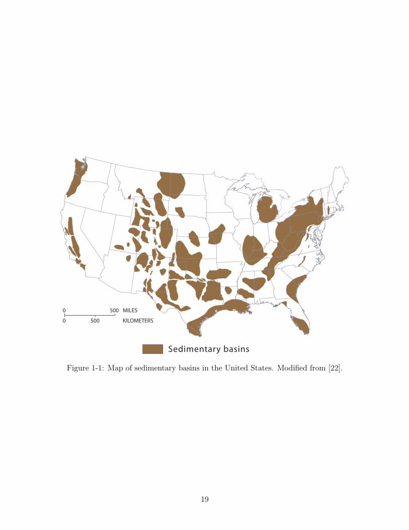
water [7, 39]. They are located in sedimentary basins throughout the United States
(Fig. 1-1) and are typically one to four kilometers deep. They are bounded above by
a layer of low-permeability rock called a caprock, and may also be bounded below by
low-permeability rock.
When CO2 is injected into a deep saline aquifer, a number of physical–chemical
mechanisms cause it to remain trapped for long times [39]. In a mechanism called
structural trapping, the upward migration of buoyant CO2 is suppressed by the low-
permeability caprock [7]. In another mechanism called capillary trapping, CO2 breaks
up into small ganglia that are immobilized by capillary forces [48, 43]. In solution
trapping, CO2 dissolves in the formation brine [70]. Lastly, in mineral trapping,
dissolved CO2 reacts with reservoir rocks and ions in the brine to precipitate carbonate
minerals [25].
18
5000
5000 MILES
KILOMETERS
Sedimentary basins
Figure 1-1: Map of sedimentary basins in the United States. Modified from [22].
19
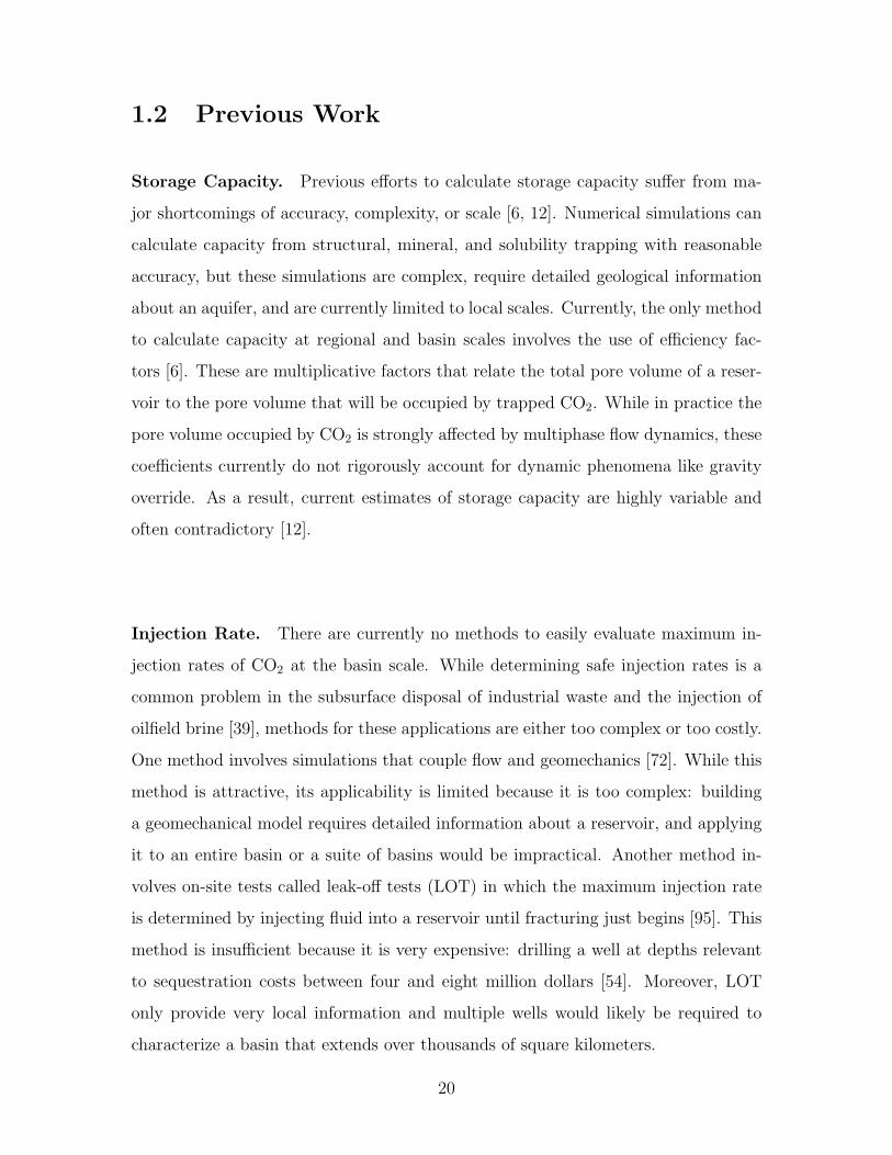
1.2 Previous Work
Storage Capacity. Previous efforts to calculate storage capacity suffer from ma-
jor shortcomings of accuracy, complexity, or scale [6, 12]. Numerical simulations can
calculate capacity from structural, mineral, and solubility trapping with reasonable
accuracy, but these simulations are complex, require detailed geological information
about an aquifer, and are currently limited to local scales. Currently, the only method
to calculate capacity at regional and basin scales involves the use of efficiency fac-
tors [6]. These are multiplicative factors that relate the total pore volume of a reser-
voir to the pore volume that will be occupied by trapped CO2. While in practice the
pore volume occupied by CO2 is strongly affected by multiphase flow dynamics, these
coefficients currently do not rigorously account for dynamic phenomena like gravity
override. As a result, current estimates of storage capacity are highly variable and
often contradictory [12].
Injection Rate. There are currently no methods to easily evaluate maximum in-
jection rates of CO2 at the basin scale. While determining safe injection rates is a
common problem in the subsurface disposal of industrial waste and the injection of
oilfield brine [39], methods for these applications are either too complex or too costly.
One method involves simulations that couple flow and geomechanics [72]. While this
method is attractive, its applicability is limited because it is too complex: building
a geomechanical model requires detailed information about a reservoir, and applying
it to an entire basin or a suite of basins would be impractical. Another method in-
volves on-site tests called leak-off tests (LOT) in which the maximum injection rate
is determined by injecting fluid into a reservoir until fracturing just begins [95]. This
method is insufficient because it is very expensive: drilling a well at depths relevant
to sequestration costs between four and eight million dollars [54]. Moreover, LOT
only provide very local information and multiple wells would likely be required to
characterize a basin that extends over thousands of square kilometers.
20
1.3 Scope of Thesis
In this work, we evaluate the storage capacity and maximum injection rate of five deep
saline aquifers located throughout the conterminous United States. We overcome the
shortcomings of current methods to calculate storage capacity and injection rate by
developing models that are simple, dynamic, and applicable at the basin scale. Our
storage capacity model is simple in that it is one-dimensional and dynamic in that
it accounts for multiphase flow phenomena like gravity override. Our injection rate
model is also one-dimensional and is dynamic in that it calculates the maximum
injection rate based on how pressure increases in an aquifer over time due to CO2
injection.
This thesis is organized into five chapters. In Chapter 2, we derive the storage
capacity and injection rate models. In Chapter 3, we apply the models. This chapter
is divided into five sections in which we present relevant hydrogeologic data for each
aquifer we study and explain how we apply the models in detail. In Chapter 4, we
present the storage capacity and injection rate results from each aquifer. Lastly, in
Chapter 5, we discuss these results in the context of projected CO2 emissions from
the United States.
21

22

Chapter 2
Mathematical Models
2.1 Storage Capacity Model
2.1.1 Geologic Setting and Conceptual Model
Our storage capacity model is based on a previous model that captures the migration
of CO2 due to natural ground water flow in an aquifer []. Our model extends this
model by also accounting for migration due to a sloped caprock.
To explain our model, we first describe the geologic setting for which the model
is developed. This geologic setting is shown in Fig. 2-1, and has three key features.
The first key feature is scale: our model applies to CO2 sequestration at the basin
scale, which typically involves lengths of tens to hundreds of kilometers. The second
key feature is the presence of natural groundwater flow: in our model, CO2 is injected
into a deep reservoir (blue) and, after injection, migrates in a direction determined by
the groundwater flow. While migration due to groundwater flow has been modeled
previously [42, 80], we also model migration due to the slope of the caprock. The
third key feature is the pattern of injection well arrays (red): we model injection
from a line-drive pattern of wells for which flow does not vary greatly in the direction
parallel to the line drive (north to south). This allows us to study the flow using a
one-dimensional model.
To develop our model, we divide the study of CO2 migration into two periods,
23

100 km
1 km
Injection wells
N
S
W E
Figure 2-1: Schematic of the basin-scale model of CO2 injection. The CO2 is injectedin a deep formation (blue) that has a sloped caprock (dark brown) and a naturalgroundwater flow (west to east in the diagram). The injection wells (red) are placedforming a linear pattern in the deepest section of the aquifer. Under these conditions,the north–south component of the flow is negligible, and is not accounted for in theone-dimensional flow model developed here. Reproduced from [42].
24
hg
H Qρ
ρ + ∆ρ
CO2 injection
Q Q
UH
(a)
brine
mobile gas
trapped gas hg
hg,max
(Sg = Sgr)
(Sg = 1 – Swc)
(b)
groundwater flow
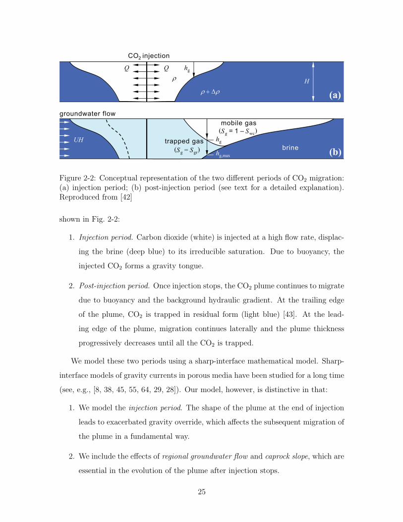
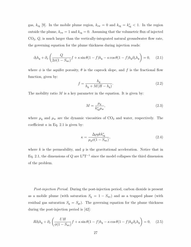
Figure 2-2: Conceptual representation of the two different periods of CO2 migration:(a) injection period; (b) post-injection period (see text for a detailed explanation).Reproduced from [42]
shown in Fig. 2-2:
1. Injection period. Carbon dioxide (white) is injected at a high flow rate, displac-
ing the brine (deep blue) to its irreducible saturation. Due to buoyancy, the
injected CO2 forms a gravity tongue.
2. Post-injection period. Once injection stops, the CO2 plume continues to migrate
due to buoyancy and the background hydraulic gradient. At the trailing edge
of the plume, CO2 is trapped in residual form (light blue) [43]. At the lead-
ing edge of the plume, migration continues laterally and the plume thickness
progressively decreases until all the CO2 is trapped.
We model these two periods using a sharp-interface mathematical model. Sharp-
interface models of gravity currents in porous media have been studied for a long time
(see, e.g., [8, 38, 45, 55, 64, 29, 28]). Our model, however, is distinctive in that:
1. We model the injection period. The shape of the plume at the end of injection
leads to exacerbated gravity override, which affects the subsequent migration of
the plume in a fundamental way.
2. We include the effects of regional groundwater flow and caprock slope, which are
essential in the evolution of the plume after injection stops.
25
2.1.2 Governing Equations
Before developing the governing equations, we state our assumptions and approxima-
tions. These will be explained in detail throughout the text.
1. We use the sharp-interface approximation. In this approximation [38], the
medium is assumed to either be filled with water (water saturation Sw = 1),
or filled with CO2 (gas1 saturation Sg = 1 − Swc, where Swc is the irreducible
connate water saturation).
2. We use the vertical flow equilibrium approximation [9], which assumes that the
dimension of the aquifer is much larger horizontally than vertically.
3. We assume that during injection, buoyancy has a negligible effect on the plume
migration. As a result, we neglect transport due to up-slope migration and
buoyancy-driven flow during injection.
4. We assume that the aquifer is homogeneous and isotropic.
5. We assume that dissolution into brine and leakage through the caprock are
negligible.
6. We assume that fluid densities and viscosities are constant (Figs. 3-13 and 3-14.
Indeed, compressibility and thermal expansion effects counteract each other,
leading to a fairly constant supercritical CO2 density over a significant range of
depths [5].
Injection Period. Consider the encroachment of injected CO2 into an aquifer, as
shown in Fig. 2-2(a). Let ρ be the density of CO2, which is lower than that of the
brine, ρ+∆ρ. Let hg be the thickness of the (mobile) CO2 plume, and H be the total
thickness of the aquifer.
The horizontal volumetric flux of each fluid is calculated by the multiphase flow
extension of Darcy’s law, which involves the relative permeability to water, krw, and
1We will sometimes refer to the CO2 phase as “gas”, even though it is normally present as asupercritical fluid.
26
gas, krg [9]. In the mobile plume region, krw = 0 and krg = k∗
rg < 1. In the region
outside the plume, krw = 1 and krg = 0. Assuming that the volumetric flux of injected
CO2, Q, is much larger than the vertically-integrated natural groundwater flow rate,
the governing equation for the plume thickness during injection reads:
∂thg + ∂x
(Q
2φ(1 − Swc)f + κ sin θ(1 − f)hg − κ cos θ(1 − f)hg∂xhg
)
= 0, (2.1)
where φ is the aquifer porosity, θ is the caprock slope, and f is the fractional flow
function, given by:
f =hg
hg + M(H − hg). (2.2)
The mobility ratio M is a key parameter in the equation. It is given by:
M =µg
k∗
rgµw
, (2.3)
where µg and µw are the dynamic viscosities of CO2 and water, respectively. The
coefficient κ in Eq. 2.1 is given by:
κ =∆ρgkk∗
rg
µgφ(1 − Swc), (2.4)
where k is the permeability, and g is the gravitational acceleration. Notice that in
Eq. 2.1, the dimensions of Q are L2T−1 since the model collapses the third dimension
of the problem.
Post-injection Period. During the post-injection period, carbon dioxide is present
as a mobile plume (with saturation Sg = 1 − Swc) and as a trapped phase (with
residual gas saturation Sg = Sgr). The governing equation for the plume thickness
during the post-injection period is [42]:
R∂thg + ∂x
(UH
φ(1 − Swc)f + κ sin θ(1 − f)hg − κ cos θ(1 − f)hg∂xhg
)
= 0, (2.5)
27
where U is the groundwater Darcy velocity and R is the accumulation coefficient:
R =
1 if ∂thg > 0 (drainage),
1 − Γ if ∂thg < 0 (imbibition).
(2.6)
Γ is the trapping coefficient, which is defined as:
Γ =Sgr
1 − Swc
. (2.7)
This equation is almost identical to Eq. 2.1, but has two notable differences: (1) the
coefficient in the accumulation term is discontinuous; and (2) the advection term
scales with the integrated groundwater flux, UH, and not with the injected CO2 flow
rate, Q.
2.1.3 Dimensionless Form of the Equations
To make the equations non-dimensional, we define the following dimensionless vari-
ables:
h =hg
H, τ =
t
T, ξ =
x
L, (2.8)
where T is the injection time and L is the characteristic injection distance, defined
to be:
L =QT
2Hφ(1 − Swc). (2.9)
With these variables, the governing equation during injection becomes:
∂τh + ∂ξ (f + Ns(1 − f)h − Ng(1 − f)h∂ξh) = 0, (2.10)
where we define the slope number Ns and the gravity number Ng to be:
Ns =2κHφ(1 − Swc) sin θ
Q=
2∆ρgkλgH sin θ
Q, (2.11)
28
Ng =4κH3φ2(1 − Swc)
2 cos θ
Q2T=
4∆ρgkλgH3φ(1 − Swc) cos θ
Q2T. (2.12)
Equation 2.10 is a nonlinear advection–diffusion equation, where the second-order
term comes from buoyancy forces, not physical diffusion. As mentioned previously,
we neglect the effect of buoyancy during injection and set Ns and Ng to zero. The
governing equation then becomes:
∂τh + ∂ξf = 0. (2.13)
During the post-injection period, the governing equation is:
R∂τh + ∂ξ (Nff + Ns(1 − f)h − Ng(1 − f)h∂ξh) = 0, (2.14)
where Nf is the flow number, defined to be:
Nf =2UH
Q. (2.15)
2.1.4 Solutions to the Model
The model for the injection period is a hyperbolic partial differential equation (PDE)
and has an analytic solution. Written in the primitive form, it is:
∂τh + f ′∂ξh = 0. (2.16)
This form shows that each height h advects at a constant velocity:
f ′ =M
(h + M(1 − h))2. (2.17)
The position of each height at the end of injection is then given by:
ξ(h) =M
(h + M(1 − h))2τ. (2.18)
29
According to our scaling (Eq. 2.8), τ = 1 at the end of injection. Since the plume is
assumed to be symmetric about the well array at ξ = 0, the position of each height
at the end of injection is given by:
ξ(h) =
−M(h+M(1−h))2
left of the array,
M(h+M(1−h))2
right of the array.
(2.19)
We solve the model for the post-injection period using standard numerical meth-
ods. While the solution to the post-injection period has been solved analytically in
previous work [42, 80], our extension of the model to include aquifer slope makes the
solution more difficult. For our numerical method, we discretize in space using the
finite volume method and we discretize in time using the forward Euler method [18].
The initial condition is the analytic solution to the injection-period model (Eq. 2.19).
When running a simulation with the discretized model, the CO2 plume will mi-
grate until the plume length and thickness are zero. In practice, however, the plume
will become trapped at a finite length and thickness. This will occur when capillary
forces, which cause trapping, become similar in magnitude to viscous and buoyancy
forces, which cause migration due to ground water flow and caprock slope, respec-
tively. To determine when the plume becomes trapped during a simulation, we could,
in principle, compare these forces using the Bond number and the capillary num-
ber [37]. However, we do not pursue this approach. This is because the dimensions
of the trapped plume calculated using this method are unrealistically large com-
pared to experimentally determined dimensions of trapped globules of nonaqueous
phase liquids (NAPLs), which should behave similarly to trapped globules of super-
critical CO2 [58]. Even though the NAPL experiments are performed at capillary
numbers and Bond numbers that are often not applicable to sequestration, the large
discrepancy makes the method suspect. Unfortunately, there are no experiments at
conditions relevant to sequestration with which to resolve the discrepancy. As an al-
ternative, we consider the plume to be trapped when its height is 0.1% of the reservoir
thickness. Since most reservoirs we study have thicknesses on the order of hundreds
30

of meters, we are assuming that the thickness of the trapped plume is on the order
of ten centimeters to one meter.
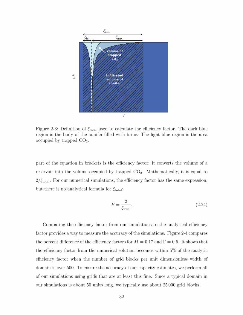
Accuracy. We evaluate the accuracy of our numerical solution by comparing it to
the analytical solution for the case in which transport occurs only due to groundwater
flow (only Nf 6= 0 in Eq. 2.14). Specifically, we compare a number called the efficiency
factor: the ratio of the volume of trapped CO2 to the volume of infiltrated pore space,
where the definition of infiltrated pore space is shown in Fig. 2-3.
As mentioned earlier, the analytic solution to the model based only on ground
water flow has been found previously [80, 41]. The solution during the injection
period is the same as we have derived in Eq. 2.19. From this equation, the maximum
distance of the plume from the well array is at the end of injection is:
ξinj =1
M. (2.20)
This quantity characterizes the injection footprint; it is illustrated in Fig. 2-3. The
maximum distance of the plume from the well array at the end of the post-injection
period is [80, 41]:
ξmax =(2 − Γ)(1 − M(1 − Γ))
MΓ2. (2.21)
This quantity characterizes the trapped footprint; it is also illustrated in Fig. 2-3.
The sum of ξinj and ξmax is ξtotal:
ξtotal =(2 − Γ)(1 − M(1 − Γ)) + Γ2
MΓ2. (2.22)
The dimensional counterpart to ξtotal is Ltotal, the total dimensional extent of the
plume. By substituting ξtotal and Ltotal into our scaling equation (Eq. 2.8), we obtain
an expression for the trapped volume of CO2:
V =
[2MΓ2
Γ2 + (2 − Γ)(1 − M + MΓ)
]
(1 − Swc)φHLtotal, (2.23)
where V is the volume of trapped CO2 per unit width of the injection well array. The
31
ξ
1-h
ξtotal
Volume of
trapped
CO2
In�ltrated
volume of
aquifer
ξmaxξinj
Figure 2-3: Definition of ξtotal used to calculate the efficiency factor. The dark blueregion is the body of the aquifer filled with brine. The light blue region is the areaoccupied by trapped CO2.
part of the equation in brackets is the efficiency factor: it converts the volume of a
reservoir into the volume occupied by trapped CO2. Mathematically, it is equal to
2/ξtotal. For our numerical simulations, the efficiency factor has the same expression,
but there is no analytical formula for ξtotal:
E =2
ξtotal
. (2.24)
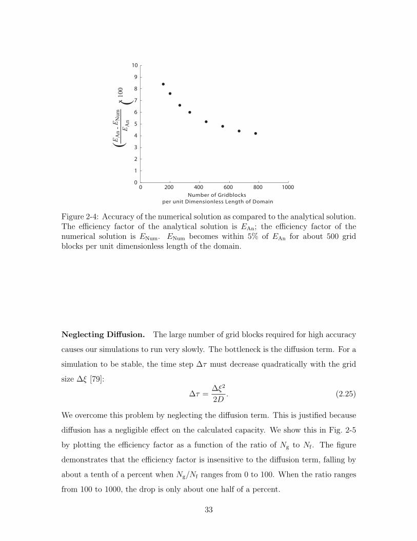
Comparing the efficiency factor from our simulations to the analytical efficiency
factor provides a way to measure the accuracy of the simulations. Figure 2-4 compares
the percent difference of the efficiency factors for M = 0.17 and Γ = 0.5. It shows that
the efficiency factor from the numerical solution becomes within 5% of the analytic
efficiency factor when the number of grid blocks per unit dimensionless width of
domain is over 500. To ensure the accuracy of our capacity estimates, we perform all
of our simulations using grids that are at least this fine. Since a typical domain in
our simulations is about 50 units long, we typically use about 25 000 grid blocks.
32
0 200 400 600 800 10000
1
2
3
4
5
6
7
8
9
10
Number of Gridblocks
per unit Dimensionless Length of Domain
EA
n
EA
n -
EN
um
(
(
10
0x
Figure 2-4: Accuracy of the numerical solution as compared to the analytical solution.The efficiency factor of the analytical solution is EAn; the efficiency factor of thenumerical solution is ENum. ENum becomes within 5% of EAn for about 500 gridblocks per unit dimensionless length of the domain.
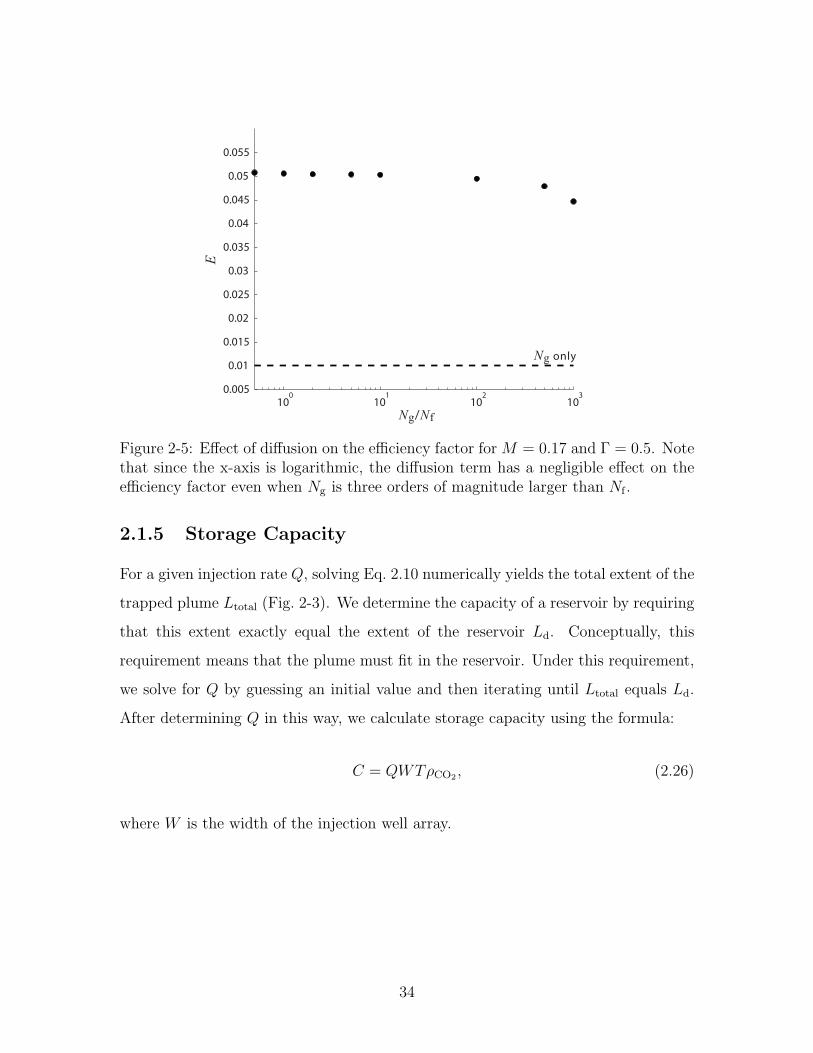
Neglecting Diffusion. The large number of grid blocks required for high accuracy
causes our simulations to run very slowly. The bottleneck is the diffusion term. For a
simulation to be stable, the time step ∆τ must decrease quadratically with the grid
size ∆ξ [79]:
∆τ =∆ξ2
2D. (2.25)
We overcome this problem by neglecting the diffusion term. This is justified because
diffusion has a negligible effect on the calculated capacity. We show this in Fig. 2-5
by plotting the efficiency factor as a function of the ratio of Ng to Nf . The figure
demonstrates that the efficiency factor is insensitive to the diffusion term, falling by
about a tenth of a percent when Ng/Nf ranges from 0 to 100. When the ratio ranges
from 100 to 1000, the drop is only about one half of a percent.
33
100
101
102
103
0.005
0.01
0.015
0.02
0.025
0.03
0.035
0.04
0.045
0.05
0.055
E
Ng/Nf
Ng only
Figure 2-5: Effect of diffusion on the efficiency factor for M = 0.17 and Γ = 0.5. Notethat since the x-axis is logarithmic, the diffusion term has a negligible effect on theefficiency factor even when Ng is three orders of magnitude larger than Nf .
2.1.5 Storage Capacity
For a given injection rate Q, solving Eq. 2.10 numerically yields the total extent of the
trapped plume Ltotal (Fig. 2-3). We determine the capacity of a reservoir by requiring
that this extent exactly equal the extent of the reservoir Ld. Conceptually, this
requirement means that the plume must fit in the reservoir. Under this requirement,
we solve for Q by guessing an initial value and then iterating until Ltotal equals Ld.
After determining Q in this way, we calculate storage capacity using the formula:
C = QWTρCO2, (2.26)
where W is the width of the injection well array.
34

Post Injection, τ = 2
Ng/Nf = 10
Ng/Nf = 100
0 10 20 30 40 50
ξ
1−h
0
1
0
1
0
1
1−h
1−h
Ng/Nf = 1000
Figure 2-6: Effect of diffusion on the mobile plume for three different values of Ng\Nf
when M = 0.17 and Γ = 0.5. The mobile plume is shown in white and the trappedplume is shown in light blue. Diffusion only changes the shape of the mobile plume,and has a negligible effect on the location of the leading edge (shown by red dashedline).
35
2.2 Injection Rate Model
In addition to the storage capacity model developed above, we develop a model for
the maximum rate at which CO2 can be injected at the basin scale. The model is
based on how the pressure in a reservoir increases due to injection. The key constraint
of the model is the fracture overpressure: we define the maximum injection rate of
CO2 as the rate at which a fracture in the reservoir is created or propagated. This
constraint is generally used to limit injection pressures during enhanced oil recovery
(EOR) and the subsurface disposal of industrial wastes [39, p.232].
While limiting injection rates based on fracturing is common, it is a conservative
constraint. It is conservative because fractures will not necessarily have a negative
impact on sequestration. For example, fractures could aid sequestration if they prop-
agate only into the body of the reservoir, creating high-permeability channels that
would increase CO2 sweep efficiency. These types of fractures are routinely created
in EOR to raise production [83]. Fracturing, however, could also seriously undermine
the security or safety of sequestration [15]. For example, fractures may propagate into
the caprock and allow CO2 to leak to the surface, or at least cause contamination
of overlying strata, which could be freshwater aquifers used for drinking water. An-
other possibility is that activating fractures and faults could induce seismicity [78, 95].
There are many examples from the oil and gas industry that subsurface fluid injec-
tion can cause seismicity of varying magnitudes [23]. In the Rongchang gas field in
China, for example, injections of wastewater at depths relevant to sequestration have
been correlated to more than 32 000 earthquakes [51]. In the Wilmington oil field in
California and at The Goose Creek oil field in Texas, induced seismicity has caused
railroad tracks to buckle or the surface to rupture [93]. While these severe cases may
be regarded as rare in the oil industry, there is unfortunately no understanding of
how basin-scale injection of CO2 could trigger seismicity, or what the magnitude of
that seismicity would be.
36
Q(t)
Qmax
T 2T0 t
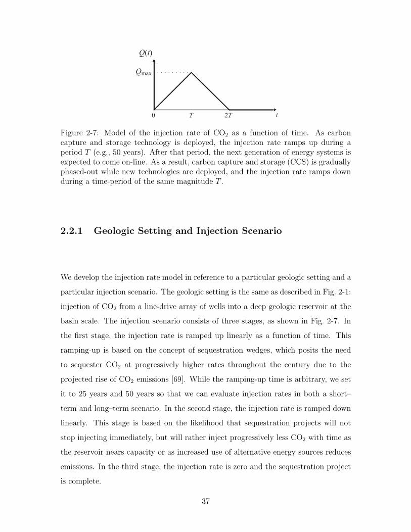
Figure 2-7: Model of the injection rate of CO2 as a function of time. As carboncapture and storage technology is deployed, the injection rate ramps up during aperiod T (e.g., 50 years). After that period, the next generation of energy systems isexpected to come on-line. As a result, carbon capture and storage (CCS) is graduallyphased-out while new technologies are deployed, and the injection rate ramps downduring a time-period of the same magnitude T .
2.2.1 Geologic Setting and Injection Scenario
We develop the injection rate model in reference to a particular geologic setting and a
particular injection scenario. The geologic setting is the same as described in Fig. 2-1:
injection of CO2 from a line-drive array of wells into a deep geologic reservoir at the
basin scale. The injection scenario consists of three stages, as shown in Fig. 2-7. In
the first stage, the injection rate is ramped up linearly as a function of time. This
ramping-up is based on the concept of sequestration wedges, which posits the need
to sequester CO2 at progressively higher rates throughout the century due to the
projected rise of CO2 emissions [69]. While the ramping-up time is arbitrary, we set
it to 25 years and 50 years so that we can evaluate injection rates in both a short–
term and long–term scenario. In the second stage, the injection rate is ramped down
linearly. This stage is based on the likelihood that sequestration projects will not
stop injecting immediately, but will rather inject progressively less CO2 with time as
the reservoir nears capacity or as increased use of alternative energy sources reduces
emissions. In the third stage, the injection rate is zero and the sequestration project
is complete.
37
2.2.2 Governing Equations
Before developing the model, we explain our assumptions and approximations. These
assumptions and approximations will be discussed in more detail throughout the text.
1. We assume that the pressure in the reservoir is initially uniform.
2. We assume that permeability, bulk compressibility, and viscosity are constant
and homogeneous.
3. We approximate the pressure response of the reservoir to CO2 injection as the
pressure response due to brine injection alone. This is justified since the sweep
efficiency of the CO2 in the reservoir is low, typically on the order of about 5%
of the reservoir volume.
4. We assume the following time-dependent behavior for the injection rate: it will
increase linearly in time, then decrease linearly, and then remain at zero (see
Fig. 2-7).
As mentioned above, we model the pressure response of a reservoir to CO2 injection
as the pressure response due to brine injection alone. This approximation is not
novel [63]. Conceptually, it is based on the observation that the sweep and storage
efficiency of CO2 is low, typically on the order of about 5% (Fig. 2-3). It is also
based on the assumption of negligible capillary pressure and the assumption that a
single, constant bulk compressibility can be used to characterize the system. The
latter assumption is somewhat dubious and will be discussed later in grater detail.
We develop our mathematical model in three steps. In the first step, we develop
the model for a semi-infinite aquifer during the first stage of injection. In the second
step, we use superposition in time to obtain solutions for the later stages of injection.
In the third step, we obtain the solution for an infinite aquifer, and use superposition
in space to obtain solutions for arbitrary boundary conditions.
38
The evolution of pressure in a semi-infinite, one-dimensional aquifer is governed
by the diffusion equation [9]:
c∂tp − k
µ∂xxp = 0, 0 < x < ∞, t > 0, (2.27)
where c is the bulk compressibility of the fluid-solid system, k is the intrinsic per-
meability, and µ is the brine viscosity. Let CO2 be injected at x = 0 at a rate of
Q(t) = Qmaxt/T [L3T−1], where T is the initial injection period (see Fig. 2-7). The
boundary condition at the well array is:
−k
µ∂xp
∣∣x=0
=Qmaxt
HWT, t > 0, (2.28)
where H is the net aquifer thickness and W is the width of the well array. The
boundary condition at infinity is:
p∣∣x→∞
→ 0, ∂xp∣∣x→∞
→ 0, t > 0, (2.29)
We assume that the pore pressure is initially uniform, so the initial condition is:
p(x, t = 0) = p0, 0 < x < ∞. (2.30)
2.2.3 Dimensionless Form of the Equations
To make the problem non-dimensional, we define the dimensionless variables:
τ =t
T, ξ =
x
L, p =
p − p0
P, (2.31)
where
L =
(kT
µc
)1/2
(2.32)
39
is a characteristic injection distance, and
P =
√
µT
kc
Qmax
HW. (2.33)
is a characteristic pressure drop. With these variables, the non-dimensional form of
the problem reads:
∂τ p − ∂ξξp = 0, 0 < ξ < ∞, τ > 0, (2.34)
− ∂ξp∣∣ξ=0
= τ, p∣∣ξ→∞
→ 0, ∂ξp∣∣ξ→∞
→ 0, τ > 0, (2.35)
p(ξ, τ = 0) = 0, 0 < ξ < ∞. (2.36)
2.2.4 Analytical Solution
We find the analytical solution to Eqs. 2.34–2.36 by the method of Laplace transforms.
Let U(ξ, s) be the Laplace transform of the dimensionless pressure p(ξ, τ). For each ξ,
the solution must satisfy:
sU − p(ξ, 0)︸ ︷︷ ︸
=0
−∂ξξU = 0, (2.37)
∂ξU∣∣ξ=0
= − 1
s2, U
∣∣ξ→∞
→ 0. (2.38)
The solution to this problem, in Laplace space, is:
U(ξ, s) =exp(−ξ
√s)
s2√
s. (2.39)
The solution in physical space is given by the inverse Laplace transform of Eq. 2.39:
p(ξ, τ) =4τ 3/2
3√
π
[
1 +ξ2
4τ
]
exp
(
− ξ2
4τ
)
− ξτ
[
1 +ξ2
6τ
]
erfc
(ξ
2√
τ
)
. (2.40)
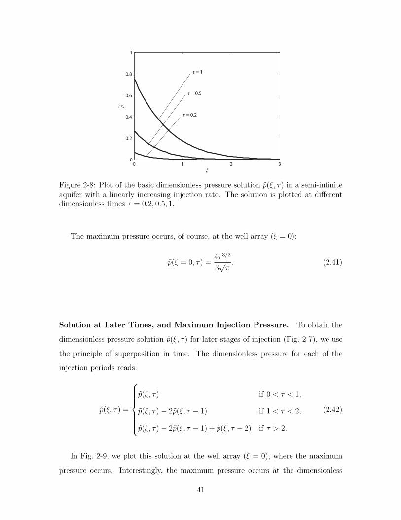
We plot this basic solution in Fig. 2-8 for different values of the dimensionless time τ .
40
0 1 2 30
0.2
0.4
0.6
0.8
1
τ = 0.2
τ = 0.5
τ = 1
ξ
p~
Figure 2-8: Plot of the basic dimensionless pressure solution p(ξ, τ) in a semi-infiniteaquifer with a linearly increasing injection rate. The solution is plotted at differentdimensionless times τ = 0.2, 0.5, 1.
The maximum pressure occurs, of course, at the well array (ξ = 0):
p(ξ = 0, τ) =4τ 3/2
3√
π. (2.41)
Solution at Later Times, and Maximum Injection Pressure. To obtain the
dimensionless pressure solution p(ξ, τ) for later stages of injection (Fig. 2-7), we use
the principle of superposition in time. The dimensionless pressure for each of the
injection periods reads:
p(ξ, τ) =
p(ξ, τ) if 0 < τ < 1,
p(ξ, τ) − 2p(ξ, τ − 1) if 1 < τ < 2,
p(ξ, τ) − 2p(ξ, τ − 1) + p(ξ, τ − 2) if τ > 2.
(2.42)
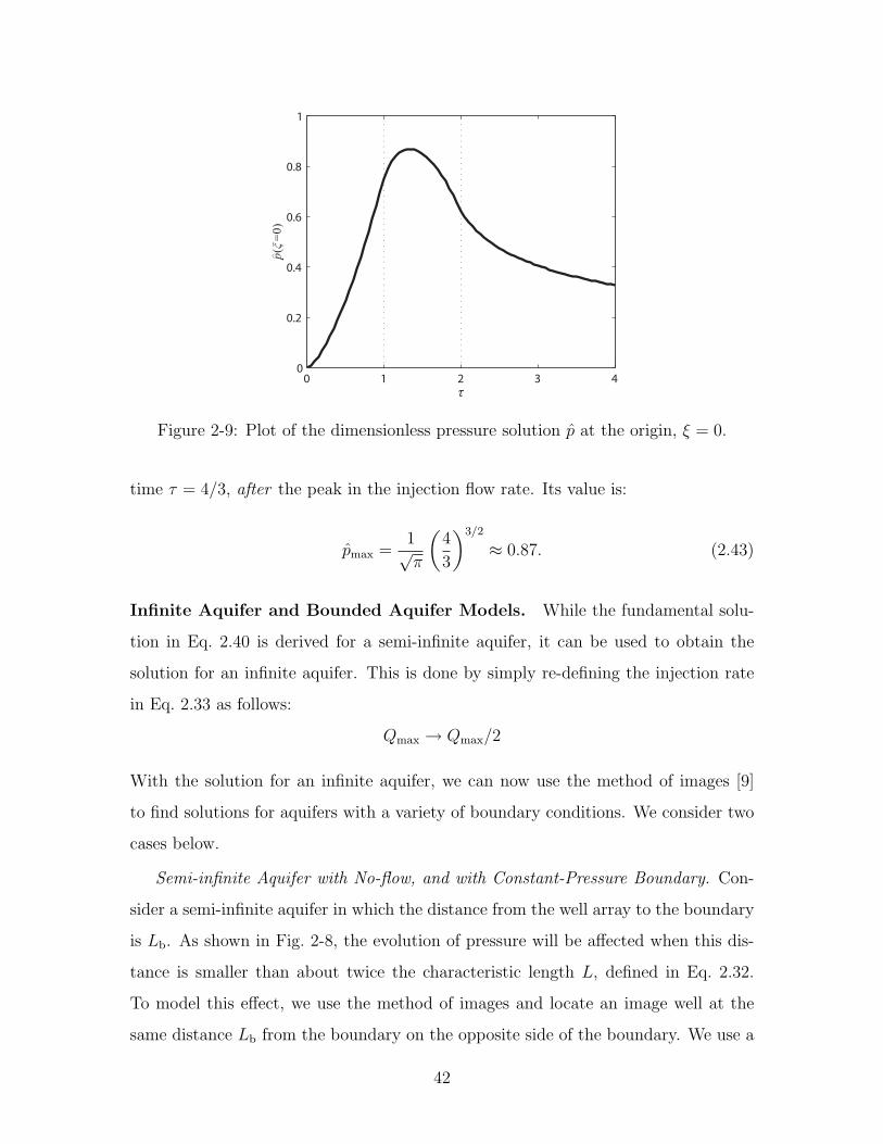
In Fig. 2-9, we plot this solution at the well array (ξ = 0), where the maximum
pressure occurs. Interestingly, the maximum pressure occurs at the dimensionless
41
0 1 2 3 40
0.2
0.4
0.6
0.8
1
τ
p(ξ
=0
)^
Figure 2-9: Plot of the dimensionless pressure solution p at the origin, ξ = 0.
time τ = 4/3, after the peak in the injection flow rate. Its value is:
pmax =1√π
(4
3
)3/2
≈ 0.87. (2.43)
Infinite Aquifer and Bounded Aquifer Models. While the fundamental solu-
tion in Eq. 2.40 is derived for a semi-infinite aquifer, it can be used to obtain the
solution for an infinite aquifer. This is done by simply re-defining the injection rate
in Eq. 2.33 as follows:
Qmax → Qmax/2
With the solution for an infinite aquifer, we can now use the method of images [9]
to find solutions for aquifers with a variety of boundary conditions. We consider two
cases below.
Semi-infinite Aquifer with No-flow, and with Constant-Pressure Boundary. Con-
sider a semi-infinite aquifer in which the distance from the well array to the boundary
is Lb. As shown in Fig. 2-8, the evolution of pressure will be affected when this dis-
tance is smaller than about twice the characteristic length L, defined in Eq. 2.32.
To model this effect, we use the method of images and locate an image well at the
same distance Lb from the boundary on the opposite side of the boundary. We use a
42
x
p (t)
Q(t)Q(t)
0 L b−L b
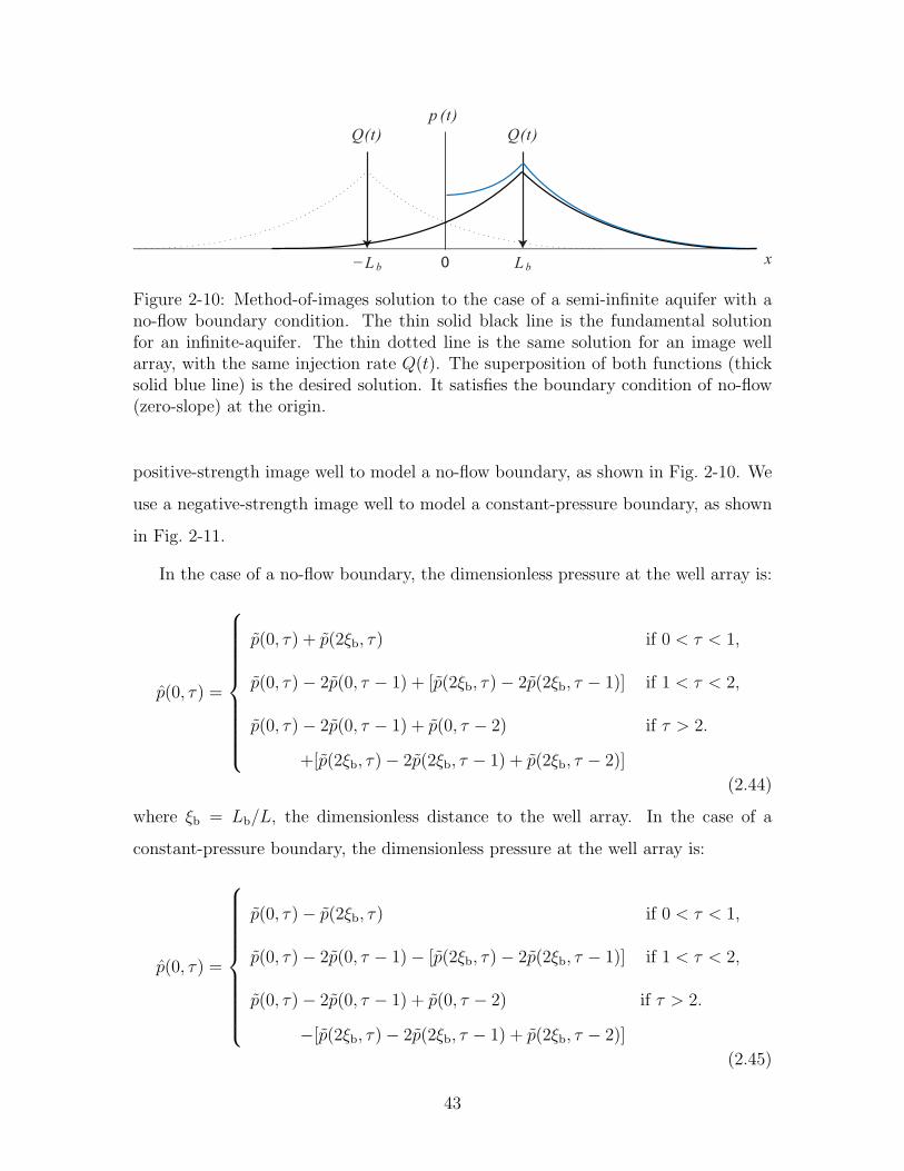
Figure 2-10: Method-of-images solution to the case of a semi-infinite aquifer with ano-flow boundary condition. The thin solid black line is the fundamental solutionfor an infinite-aquifer. The thin dotted line is the same solution for an image wellarray, with the same injection rate Q(t). The superposition of both functions (thicksolid blue line) is the desired solution. It satisfies the boundary condition of no-flow(zero-slope) at the origin.
positive-strength image well to model a no-flow boundary, as shown in Fig. 2-10. We
use a negative-strength image well to model a constant-pressure boundary, as shown
in Fig. 2-11.
In the case of a no-flow boundary, the dimensionless pressure at the well array is:
p(0, τ) =
p(0, τ) + p(2ξb, τ) if 0 < τ < 1,
p(0, τ) − 2p(0, τ − 1) + [p(2ξb, τ) − 2p(2ξb, τ − 1)] if 1 < τ < 2,
p(0, τ) − 2p(0, τ − 1) + p(0, τ − 2) if τ > 2.
+[p(2ξb, τ) − 2p(2ξb, τ − 1) + p(2ξb, τ − 2)]
(2.44)
where ξb = Lb/L, the dimensionless distance to the well array. In the case of a
constant-pressure boundary, the dimensionless pressure at the well array is:
p(0, τ) =
p(0, τ) − p(2ξb, τ) if 0 < τ < 1,
p(0, τ) − 2p(0, τ − 1) − [p(2ξb, τ) − 2p(2ξb, τ − 1)] if 1 < τ < 2,
p(0, τ) − 2p(0, τ − 1) + p(0, τ − 2) if τ > 2.
−[p(2ξb, τ) − 2p(2ξb, τ − 1) + p(2ξb, τ − 2)]
(2.45)
43
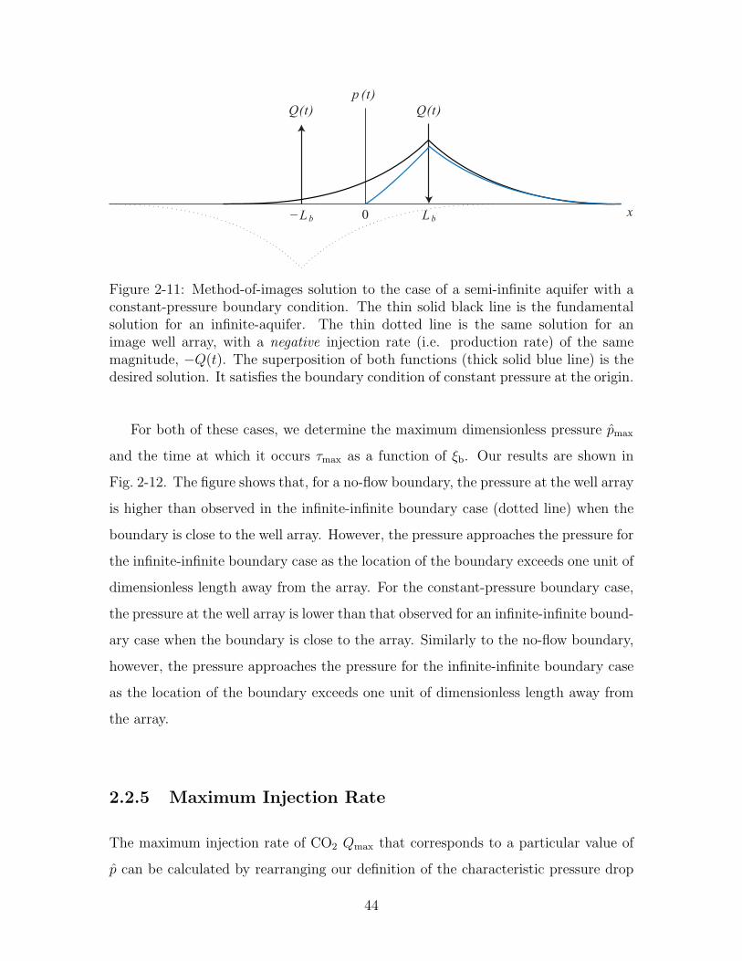
x
p (t)
Q(t)Q(t)
0 L b−L b
Figure 2-11: Method-of-images solution to the case of a semi-infinite aquifer with aconstant-pressure boundary condition. The thin solid black line is the fundamentalsolution for an infinite-aquifer. The thin dotted line is the same solution for animage well array, with a negative injection rate (i.e. production rate) of the samemagnitude, −Q(t). The superposition of both functions (thick solid blue line) is thedesired solution. It satisfies the boundary condition of constant pressure at the origin.
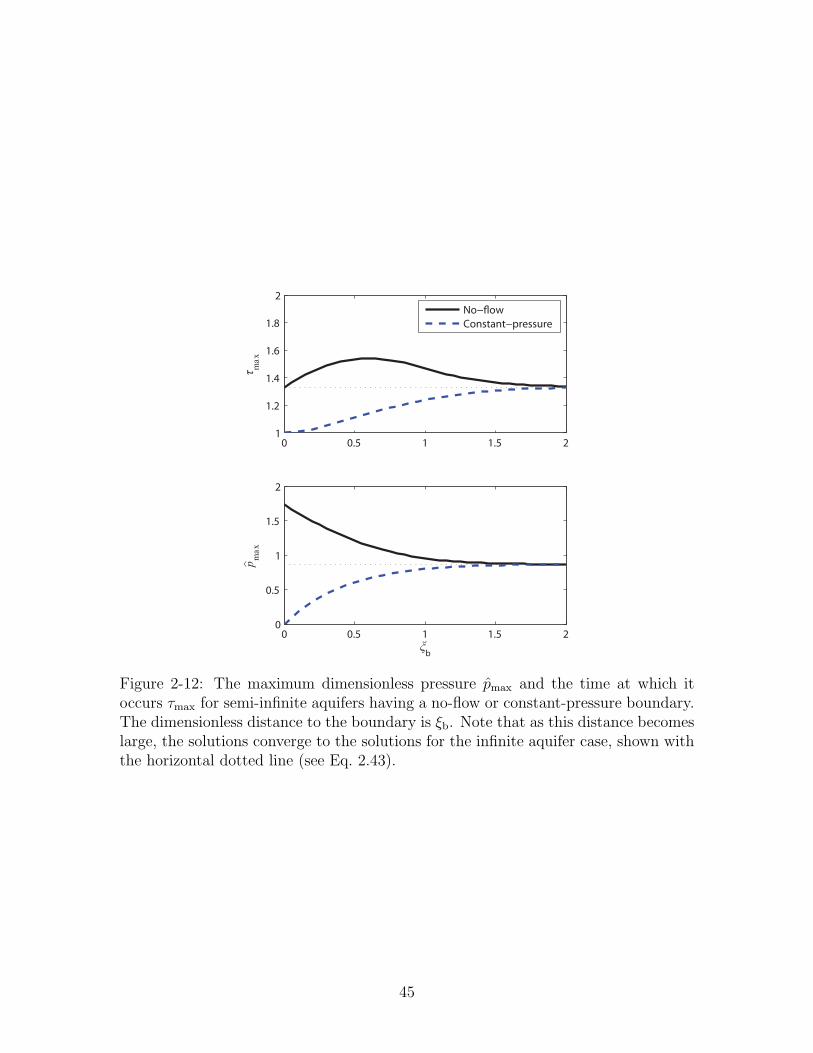
For both of these cases, we determine the maximum dimensionless pressure pmax
and the time at which it occurs τmax as a function of ξb. Our results are shown in
Fig. 2-12. The figure shows that, for a no-flow boundary, the pressure at the well array
is higher than observed in the infinite-infinite boundary case (dotted line) when the
boundary is close to the well array. However, the pressure approaches the pressure for
the infinite-infinite boundary case as the location of the boundary exceeds one unit of
dimensionless length away from the array. For the constant-pressure boundary case,
the pressure at the well array is lower than that observed for an infinite-infinite bound-
ary case when the boundary is close to the array. Similarly to the no-flow boundary,
however, the pressure approaches the pressure for the infinite-infinite boundary case
as the location of the boundary exceeds one unit of dimensionless length away from
the array.
2.2.5 Maximum Injection Rate
The maximum injection rate of CO2 Qmax that corresponds to a particular value of
p can be calculated by rearranging our definition of the characteristic pressure drop
44
0 0.5 1 1.5 21
1.2
1.4
1.6
1.8
2
τ ma
x
No−"ow
Constant−pressure
0 0.5 1 1.5 20
0.5
1
1.5
2
ξb
pm
ax
^
Figure 2-12: The maximum dimensionless pressure pmax and the time at which itoccurs τmax for semi-infinite aquifers having a no-flow or constant-pressure boundary.The dimensionless distance to the boundary is ξb. Note that as this distance becomeslarge, the solutions converge to the solutions for the infinite aquifer case, shown withthe horizontal dotted line (see Eq. 2.43).
45
(Eq. 2.33):
Qmax = 2HW
√
kc
µT
p − p0
p(2.46)
We obtain an expression for the maximum mass injection rate in two steps. First,
we multiply by ρCO2. Secondly, we equate the pressure difference p − p0 to the
fracture overpressure of the reservoir Pfrac. In this way, we obtain an expression for
the maximum rate at which CO2 can be injected without activating a fault in the
reservoir:
Qmax = 2ρCO2HW
√
kc
µT
Pfrac
p(2.47)
2.2.6 Fracture Overpressure
The fracture overpressure Pfrac is difficult to calculate rigorously. One source of dif-
ficulty is uncertainty about the failure mechanism: overpressurizing a reservoir may
cause new fractures, or may cause displacement along pre-existing fractures. If the
mechanism is slip along a pre-existing fractures, the problem is that data about the
location and orientation of the fractures—in addition to data about whether they
are well-cemented—is often absent. If the mechanism is the formation of new frac-
tures, the problem is uncertainty about the fracture mode and the strength of the
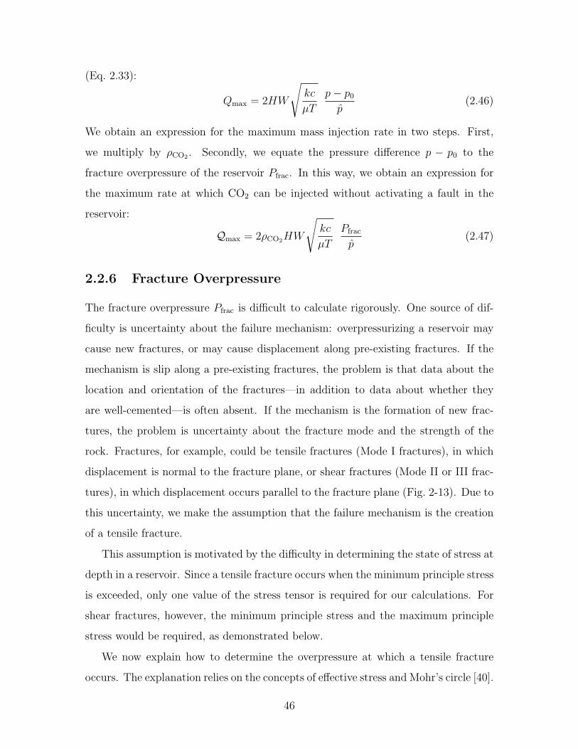
rock. Fractures, for example, could be tensile fractures (Mode I fractures), in which
displacement is normal to the fracture plane, or shear fractures (Mode II or III frac-
tures), in which displacement occurs parallel to the fracture plane (Fig. 2-13). Due to
this uncertainty, we make the assumption that the failure mechanism is the creation
of a tensile fracture.
This assumption is motivated by the difficulty in determining the state of stress at
depth in a reservoir. Since a tensile fracture occurs when the minimum principle stress
is exceeded, only one value of the stress tensor is required for our calculations. For
shear fractures, however, the minimum principle stress and the maximum principle
stress would be required, as demonstrated below.
We now explain how to determine the overpressure at which a tensile fracture
occurs. The explanation relies on the concepts of effective stress and Mohr’s circle [40].
46
Mode I Mode II Mode III
Figure 2-13: The three fracture modes. We assume that the overpressure from injec-tion causes only Mode I fractures.
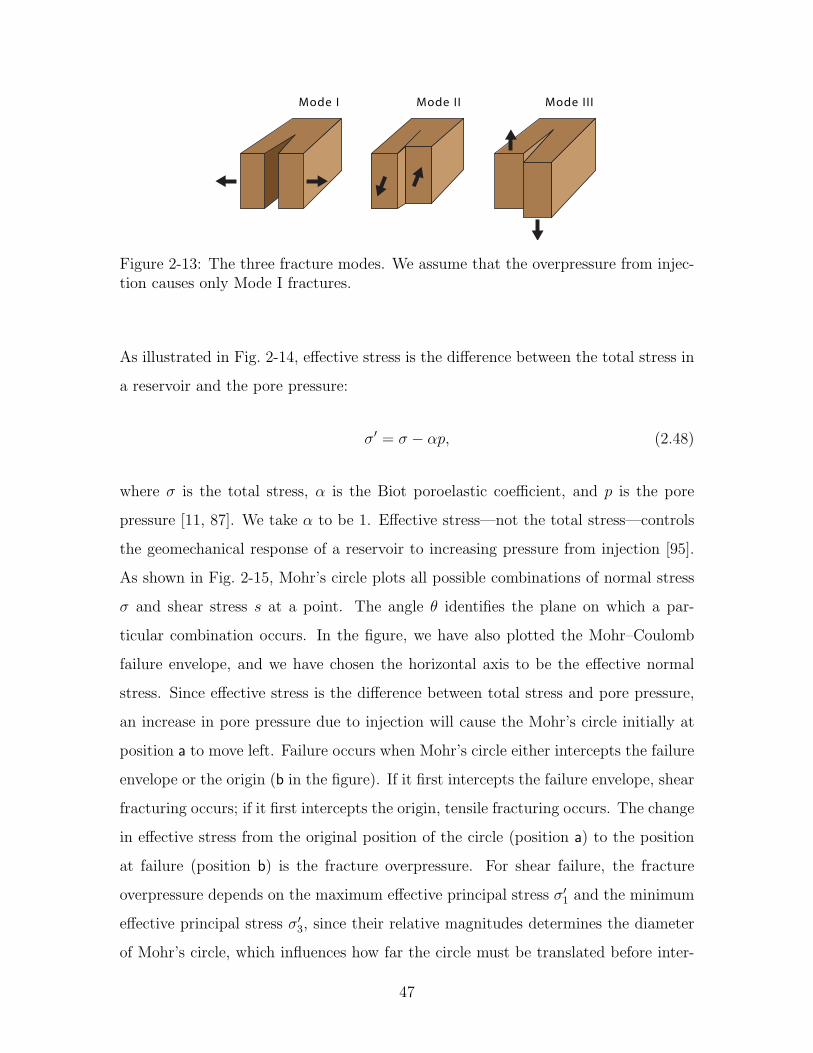
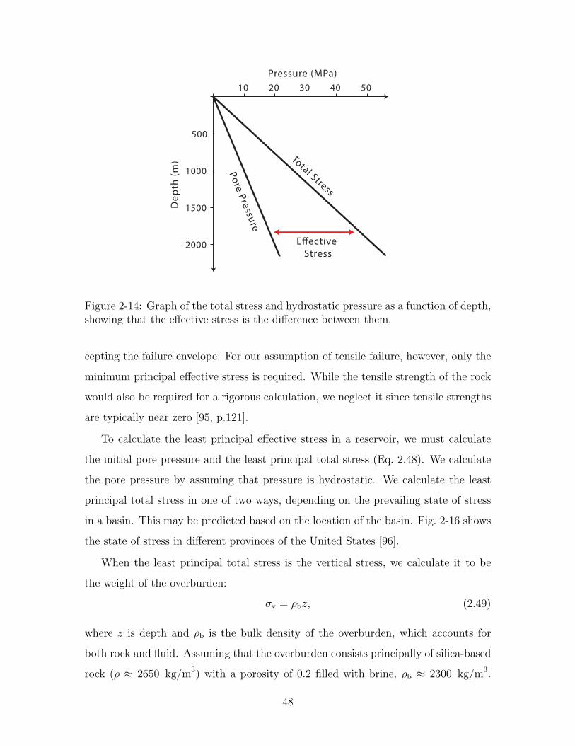
As illustrated in Fig. 2-14, effective stress is the difference between the total stress in
a reservoir and the pore pressure:
σ′ = σ − αp, (2.48)
where σ is the total stress, α is the Biot poroelastic coefficient, and p is the pore
pressure [11, 87]. We take α to be 1. Effective stress—not the total stress—controls
the geomechanical response of a reservoir to increasing pressure from injection [95].
As shown in Fig. 2-15, Mohr’s circle plots all possible combinations of normal stress
σ and shear stress s at a point. The angle θ identifies the plane on which a par-
ticular combination occurs. In the figure, we have also plotted the Mohr–Coulomb
failure envelope, and we have chosen the horizontal axis to be the effective normal
stress. Since effective stress is the difference between total stress and pore pressure,
an increase in pore pressure due to injection will cause the Mohr’s circle initially at
position a to move left. Failure occurs when Mohr’s circle either intercepts the failure
envelope or the origin (b in the figure). If it first intercepts the failure envelope, shear
fracturing occurs; if it first intercepts the origin, tensile fracturing occurs. The change
in effective stress from the original position of the circle (position a) to the position
at failure (position b) is the fracture overpressure. For shear failure, the fracture
overpressure depends on the maximum effective principal stress σ′
1 and the minimum
effective principal stress σ′
3, since their relative magnitudes determines the diameter
of Mohr’s circle, which influences how far the circle must be translated before inter-
47
Pressure (MPa)
De
pth
(m
)
500
1000
1500
2000
10 20 30 40 50
Total Stress
Po
re P
ressu
re
E!ective
Stress
Figure 2-14: Graph of the total stress and hydrostatic pressure as a function of depth,showing that the effective stress is the difference between them.
cepting the failure envelope. For our assumption of tensile failure, however, only the
minimum principal effective stress is required. While the tensile strength of the rock
would also be required for a rigorous calculation, we neglect it since tensile strengths
are typically near zero [95, p.121].
To calculate the least principal effective stress in a reservoir, we must calculate
the initial pore pressure and the least principal total stress (Eq. 2.48). We calculate
the pore pressure by assuming that pressure is hydrostatic. We calculate the least
principal total stress in one of two ways, depending on the prevailing state of stress
in a basin. This may be predicted based on the location of the basin. Fig. 2-16 shows
the state of stress in different provinces of the United States [96].
When the least principal total stress is the vertical stress, we calculate it to be
the weight of the overburden:
σv = ρbz, (2.49)
where z is depth and ρb is the bulk density of the overburden, which accounts for
both rock and fluid. Assuming that the overburden consists principally of silica-based
rock (ρ ≈ 2650 kg/m3) with a porosity of 0.2 filled with brine, ρb ≈ 2300 kg/m3.
48
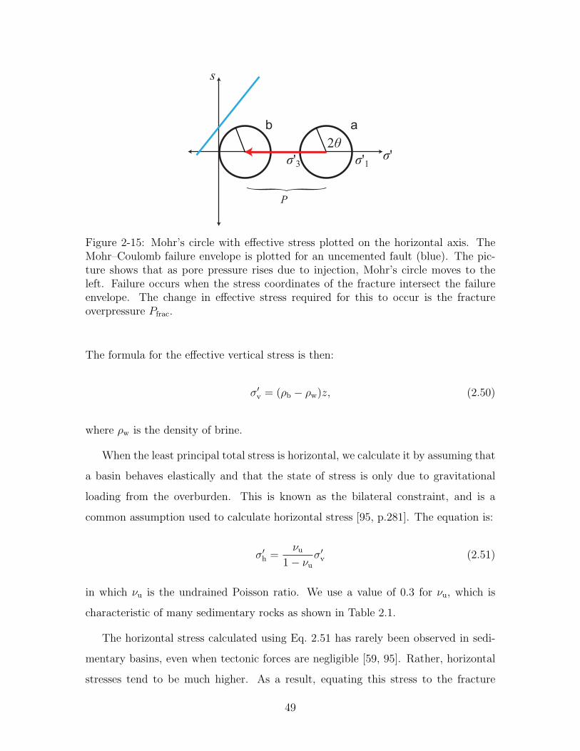
s
σ'σ'1σ'3
2θ}
P
ab
Figure 2-15: Mohr’s circle with effective stress plotted on the horizontal axis. TheMohr–Coulomb failure envelope is plotted for an uncemented fault (blue). The pic-ture shows that as pore pressure rises due to injection, Mohr’s circle moves to theleft. Failure occurs when the stress coordinates of the fracture intersect the failureenvelope. The change in effective stress required for this to occur is the fractureoverpressure Pfrac.
The formula for the effective vertical stress is then:
σ′
v = (ρb − ρw)z, (2.50)
where ρw is the density of brine.
When the least principal total stress is horizontal, we calculate it by assuming that
a basin behaves elastically and that the state of stress is only due to gravitational
loading from the overburden. This is known as the bilateral constraint, and is a
common assumption used to calculate horizontal stress [95, p.281]. The equation is:
σ′
h =νu
1 − νu
σ′
v (2.51)
in which νu is the undrained Poisson ratio. We use a value of 0.3 for νu, which is
characteristic of many sedimentary rocks as shown in Table 2.1.
The horizontal stress calculated using Eq. 2.51 has rarely been observed in sedi-
mentary basins, even when tectonic forces are negligible [59, 95]. Rather, horizontal
stresses tend to be much higher. As a result, equating this stress to the fracture
49
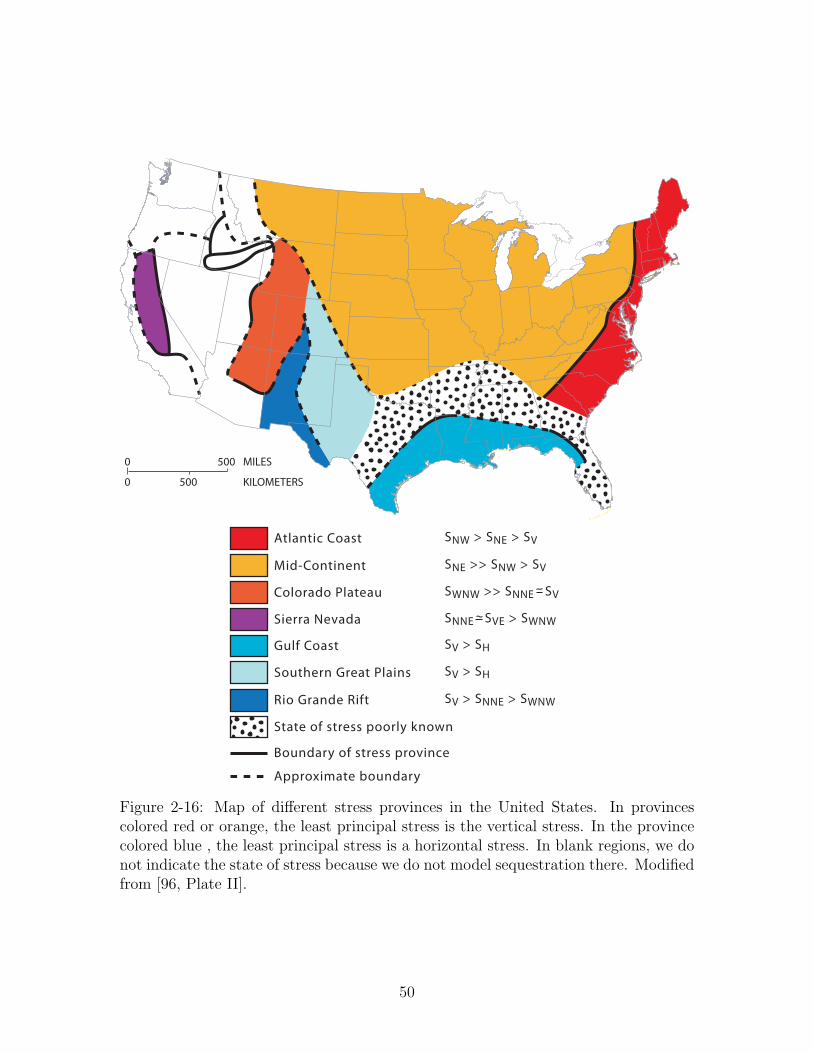
5000
5000 MILES
KILOMETERS
State of stress poorly known
Atlantic Coast SNW > SNE > SV
Gulf Coast SV > SH
Mid-Continent SNE >> SNW > SV
Colorado Plateau SWNW >> SNNE SV
Southern Great Plains SV > SH
Rio Grande Rift SV > SNNE > SWNW
Sierra Nevada SNNE SVE > SWNW
Boundary of stress province
Approximate boundary
Figure 2-16: Map of different stress provinces in the United States. In provincescolored red or orange, the least principal stress is the vertical stress. In the provincecolored blue , the least principal stress is a horizontal stress. In blank regions, we donot indicate the state of stress because we do not model sequestration there. Modifiedfrom [96, Plate II].
50
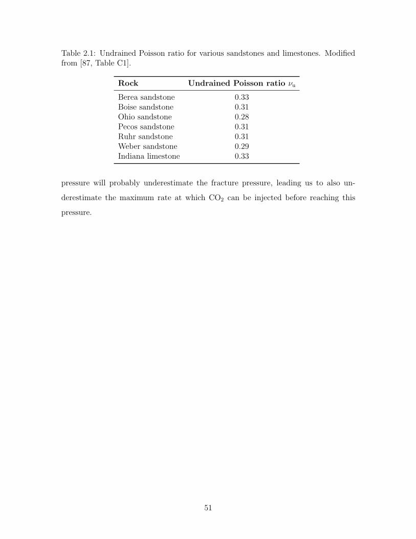
Table 2.1: Undrained Poisson ratio for various sandstones and limestones. Modifiedfrom [87, Table C1].
Rock Undrained Poisson ratio νu
Berea sandstone 0.33Boise sandstone 0.31Ohio sandstone 0.28Pecos sandstone 0.31Ruhr sandstone 0.31Weber sandstone 0.29Indiana limestone 0.33
pressure will probably underestimate the fracture pressure, leading us to also un-
derestimate the maximum rate at which CO2 can be injected before reaching this
pressure.
51

52
Chapter 3
Application to Individual Geologic
Reservoirs
We apply the storage capacity and injection rate models to five reservoirs located
throughout the conterminous United States. To select the reservoirs, we first compile
a geologic map of the United States [44]. This map shows the major faults in the
country and major sedimentary basins [22]. It also shows where sedimentary rocks are
greater than 800 m thick [21]. This feature is important for locating suitable reservoirs
because thickness suggests depth, and CO2 must be injected at depths greater than
800 m to be stored efficiently in a high-density supercritical state. Using this map as
a guide, we choose the following reservoirs on the basis of size and continuity for our
study: the lower Potomac aquifer, the Mt. Simon Sandstone, the Paluxy Sandstone,
the Frio Formation, and the Madison Limestone. Other selection criteria includes
depth and availability of data. We select these reservoirs to be representative, not
exhaustive.
We apply our models to these reservoirs in three steps. First, we characterize
the geology and hydrogeology of the reservoir. Next, we apply the storage capacity
model. Lastly, we apply the injection rate model. We demonstrate our procedure
step-by-step on the lower Potomac aquifer.
53
Approximate onshore
extent of the lower
Potomac aquifer
0 5025 MILES0 5025 KILOMETERS
A’A
B
B’
WE S TV I R G I N I A
N O R T H C A R O L I N A
P E N N S Y LVA N I A
MDF
all
Lin
e
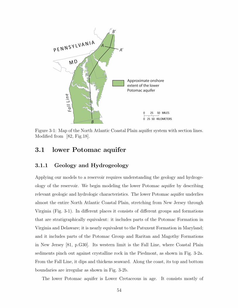
Figure 3-1: Map of the North Atlantic Coastal Plain aquifer system with section lines.Modified from [82, Fig.18].
3.1 lower Potomac aquifer
3.1.1 Geology and Hydrogeology
Applying our models to a reservoir requires understanding the geology and hydroge-
ology of the reservoir. We begin modeling the lower Potomac aquifer by describing
relevant geologic and hydrologic characteristics. The lower Potomac aquifer underlies
almost the entire North Atlantic Coastal Plain, stretching from New Jersey through
Virginia (Fig. 3-1). In different places it consists of different groups and formations
that are stratigraphically equivalent: it includes parts of the Potomac Formation in
Virginia and Delaware; it is nearly equivalent to the Patuxent Formation in Maryland;
and it includes parts of the Potomac Group and Raritan and Magothy Formations
in New Jersey [81, p.G30]. Its western limit is the Fall Line, where Coastal Plain
sediments pinch out against crystalline rock in the Piedmont, as shown in Fig. 3-2a.
From the Fall Line, it dips and thickens seaward. Along the coast, its top and bottom
boundaries are irregular as shown in Fig. 3-2b.
The lower Potomac aquifer is Lower Cretaceous in age. It consists mostly of
54

0 20 MILES
KILOME TERS0 20
New JerseyA A’
Se
ctio
n
B-B’
Atlantic Ocean
EXPLANATION
Sur !cia l aqui fer
Con!ning unit
Chesapeake aquifer
Cast le Hayne -Aquia aquifer
S evern-Magothy aquifer
Potomac aquifer
Cr ysta l l ine rock
Sea Level
Alt
itu
de
(m
)
305
610
915
1220
1525
(a) Cross section A-A’
0 40 MILES
KILOMETERS0 40
Se
ctio
n
A-A’
New Jersey
B
Virginia Maryland Del
B’
Alt
itiu
de
(m
) 305
610
1220
Sea Level
915
EXPLANATION
Sur !cia l aqui fer
Con!ning unit
Chesapeake aquifer
Cast le Hayne -Aquia aquifer
S evern-Magothy aquifer
Potomac aquifer
Cr ysta l l ine rock
Peedee -upper Cape Fear aqui fer
Bend in sec t ion
(b) Cross section B-B’
Figure 3-2: Cross sections of the North Atlantic Coastal Plain. (a) Modified from[82, Fig.19]. (b) Modified from [82, Fig.20].
55
0 50 MILES
0 50 KILOMETERS
PNNJ
MD
VA
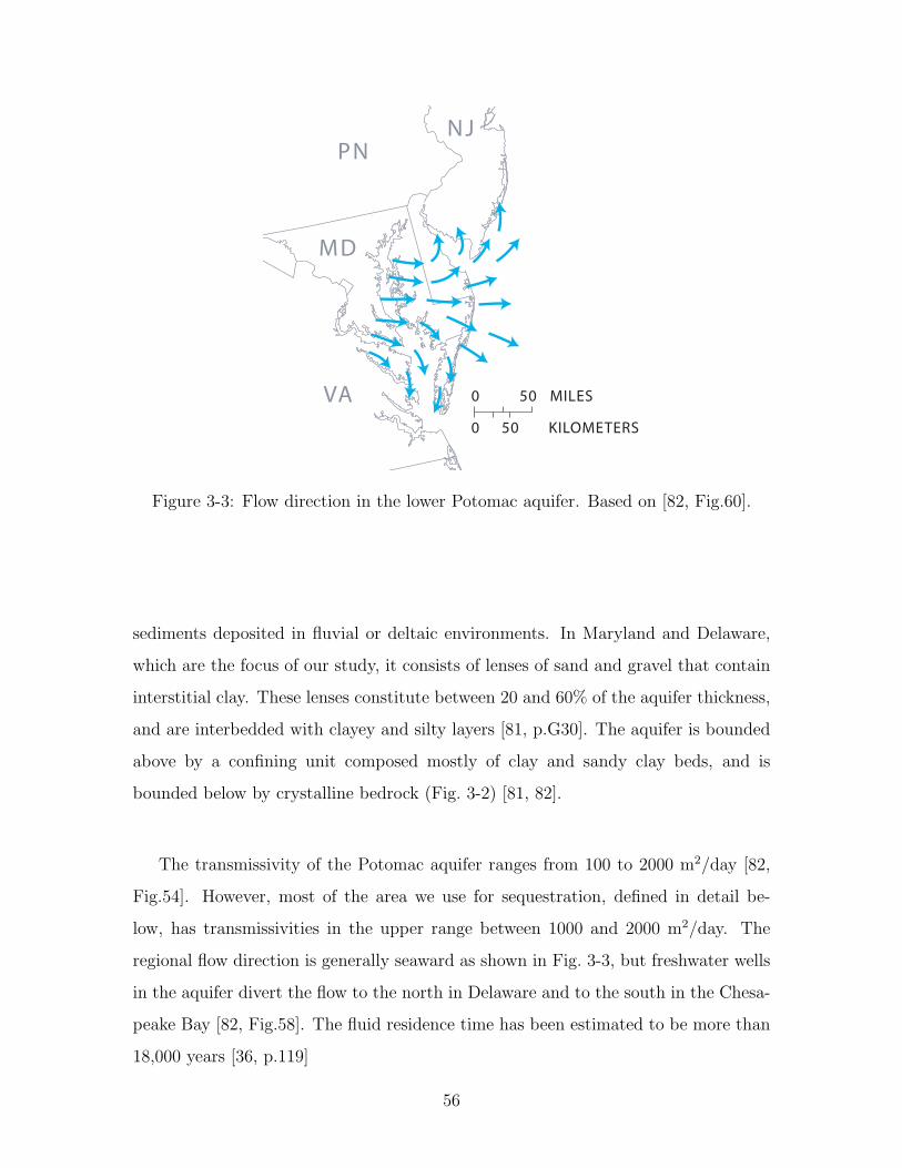
Figure 3-3: Flow direction in the lower Potomac aquifer. Based on [82, Fig.60].
sediments deposited in fluvial or deltaic environments. In Maryland and Delaware,
which are the focus of our study, it consists of lenses of sand and gravel that contain
interstitial clay. These lenses constitute between 20 and 60% of the aquifer thickness,
and are interbedded with clayey and silty layers [81, p.G30]. The aquifer is bounded
above by a confining unit composed mostly of clay and sandy clay beds, and is
bounded below by crystalline bedrock (Fig. 3-2) [81, 82].
The transmissivity of the Potomac aquifer ranges from 100 to 2000 m2/day [82,
Fig.54]. However, most of the area we use for sequestration, defined in detail be-
low, has transmissivities in the upper range between 1000 and 2000 m2/day. The
regional flow direction is generally seaward as shown in Fig. 3-3, but freshwater wells
in the aquifer divert the flow to the north in Delaware and to the south in the Chesa-
peake Bay [82, Fig.58]. The fluid residence time has been estimated to be more than
18,000 years [36, p.119]
56
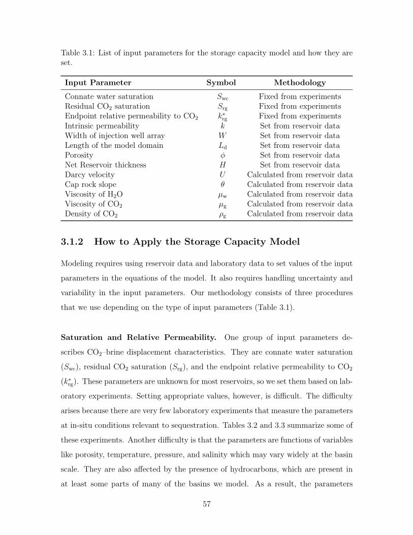
Table 3.1: List of input parameters for the storage capacity model and how they areset.
Input Parameter Symbol Methodology
Connate water saturation Swc Fixed from experimentsResidual CO2 saturation Srg Fixed from experimentsEndpoint relative permeability to CO2 k∗
rg Fixed from experimentsIntrinsic permeability k Set from reservoir dataWidth of injection well array W Set from reservoir dataLength of the model domain Ld Set from reservoir dataPorosity φ Set from reservoir dataNet Reservoir thickness H Set from reservoir dataDarcy velocity U Calculated from reservoir dataCap rock slope θ Calculated from reservoir dataViscosity of H2O µw Calculated from reservoir dataViscosity of CO2 µg Calculated from reservoir dataDensity of CO2 ρg Calculated from reservoir data
3.1.2 How to Apply the Storage Capacity Model
Modeling requires using reservoir data and laboratory data to set values of the input
parameters in the equations of the model. It also requires handling uncertainty and
variability in the input parameters. Our methodology consists of three procedures
that we use depending on the type of input parameters (Table 3.1).
Saturation and Relative Permeability. One group of input parameters de-
scribes CO2–brine displacement characteristics. They are connate water saturation
(Swc), residual CO2 saturation (Srg), and the endpoint relative permeability to CO2
(k∗
rg). These parameters are unknown for most reservoirs, so we set them based on lab-
oratory experiments. Setting appropriate values, however, is difficult. The difficulty
arises because there are very few laboratory experiments that measure the parameters
at in-situ conditions relevant to sequestration. Tables 3.2 and 3.3 summarize some of
these experiments. Another difficulty is that the parameters are functions of variables
like porosity, temperature, pressure, and salinity which may vary widely at the basin
scale. They are also affected by the presence of hydrocarbons, which are present in
at least some parts of many of the basins we model. As a result, the parameters
57
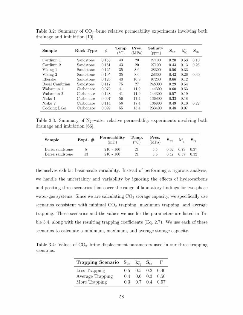
Table 3.2: Summary of CO2–brine relative permeability experiments involving bothdrainage and imbibition [10].
Sample Rock Type φTemp.
(◦C)Pres.
(MPa)Salinity
(ppm)Swc k∗
rg Srg
Cardium 1 Sandstone 0.153 43 20 27100 0.20 0.53 0.10Cardium 2 Sandstone 0.161 43 20 27100 0.43 0.13 0.25Viking 1 Sandstone 0.125 35 8.6 28300 0.56 0.33Viking 2 Sandstone 0.195 35 8.6 28300 0.42 0.26 0.30Ellerslie Sandstone 0.126 40 10.9 97200 0.66 0.12Basal Cambrian Sandstone 0.117 75 27 248000 0.29 0.54Wabamun 1 Carbonate 0.079 41 11.9 144300 0.60 0.53Wabamun 2 Carbonate 0.148 41 11.9 144300 0.57 0.19Nisku 1 Carbonate 0.097 56 17.4 136800 0.33 0.18Nisku 2 Carbonate 0.114 56 17.4 136800 0.49 0.10 0.22Cooking Lake Carbonate 0.099 55 15.4 233400 0.48 0.07
Table 3.3: Summary of N2–water relative permeability experiments involving bothdrainage and imbibition [66].
Sample Expt. #Permeability
(mD)Temp.
(◦C)Pres.
(MPa)Swc k∗
rg Srg
Berea sandstone 8 210 - 160 21 5.5 0.62 0.73 0.37Berea sandstone 13 210 - 160 21 5.5 0.47 0.57 0.32
themselves exhibit basin-scale variability. Instead of performing a rigorous analysis,
we handle the uncertainty and variability by ignoring the effects of hydrocarbons
and positing three scenarios that cover the range of laboratory findings for two-phase
water-gas systems. Since we are calculating CO2 storage capacity, we specifically use
scenarios consistent with minimal CO2 trapping, maximum trapping, and average
trapping. These scenarios and the values we use for the parameters are listed in Ta-
ble 3.4, along with the resulting trapping coefficients (Eq. 2.7). We use each of these
scenarios to calculate a minimum, maximum, and average storage capacity.
Table 3.4: Values of CO2–brine displacement parameters used in our three trappingscenarios.
Trapping Scenario Swc k∗
rg Srg Γ
Less Trapping 0.5 0.5 0.2 0.40Average Trapping 0.4 0.6 0.3 0.50More Trapping 0.3 0.7 0.4 0.57
58
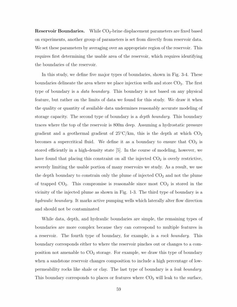
Reservoir Boundaries. While CO2-brine displacement parameters are fixed based
on experiments, another group of parameters is set from directly from reservoir data.
We set these parameters by averaging over an appropriate region of the reservoir. This
requires first determining the usable area of the reservoir, which requires identifying
the boundaries of the reservoir.
In this study, we define five major types of boundaries, shown in Fig. 3-4. These
boundaries delineate the area where we place injection wells and store CO2. The first
type of boundary is a data boundary. This boundary is not based on any physical
feature, but rather on the limits of data we found for this study. We draw it when
the quality or quantity of available data undermines reasonably accurate modeling of
storage capacity. The second type of boundary is a depth boundary. This boundary
traces where the top of the reservoir is 800m deep. Assuming a hydrostatic pressure
gradient and a geothermal gradient of 25◦C/km, this is the depth at which CO2
becomes a supercritical fluid. We define it as a boundary to ensure that CO2 is
stored efficiently in a high-density state [5]. In the course of modeling, however, we
have found that placing this constraint on all the injected CO2 is overly restrictive,
severely limiting the usable portion of many reservoirs we study. As a result, we use
the depth boundary to constrain only the plume of injected CO2 and not the plume
of trapped CO2. This compromise is reasonable since most CO2 is stored in the
vicinity of the injected plume as shown in Fig. 1-3. The third type of boundary is a
hydraulic boundary. It marks active pumping wells which laterally alter flow direction
and should not be contaminated
While data, depth, and hydraulic boundaries are simple, the remaining types of
boundaries are more complex because they can correspond to multiple features in
a reservoir. The fourth type of boundary, for example, is a rock boundary. This
boundary corresponds either to where the reservoir pinches out or changes to a com-
position not amenable to CO2 storage. For example, we draw this type of boundary
when a sandstone reservoir changes composition to include a high percentage of low-
permeability rocks like shale or clay. The last type of boundary is a leak boundary.
This boundary corresponds to places or features where CO2 will leak to the surface,
59

Data
Boundary
Depth
Boundary
Hydraulic
Boundary
Leak
Boundary
Rock
Boundary
Wells
Faults
Caprock
compostion
change
Caprock
pinchout
Outcrops
Reservoir
pinchout
Reservoir
composition
change
Boundary
TypeSymbol
Limit of
available
data
800m
depth
contour
Feature
Marked
Figure 3-4: Chart showing types of reservoir boundaries, the features they mark, andtheir symbols.
60
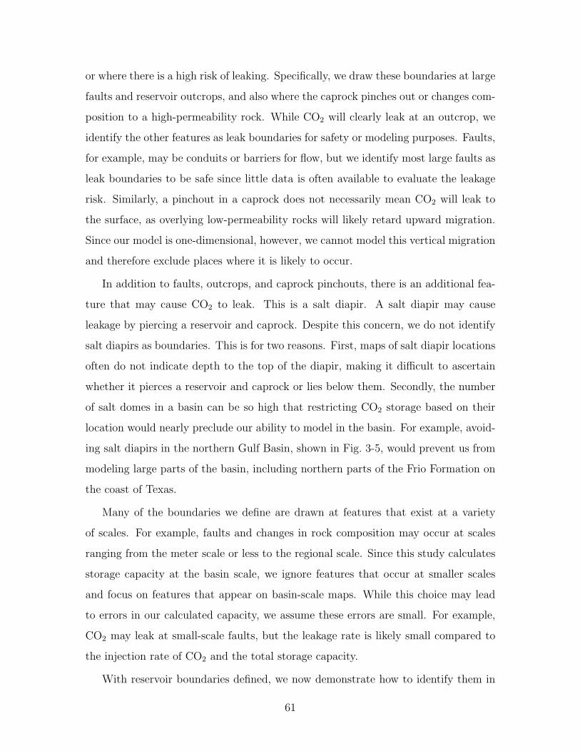
or where there is a high risk of leaking. Specifically, we draw these boundaries at large
faults and reservoir outcrops, and also where the caprock pinches out or changes com-
position to a high-permeability rock. While CO2 will clearly leak at an outcrop, we
identify the other features as leak boundaries for safety or modeling purposes. Faults,
for example, may be conduits or barriers for flow, but we identify most large faults as
leak boundaries to be safe since little data is often available to evaluate the leakage
risk. Similarly, a pinchout in a caprock does not necessarily mean CO2 will leak to
the surface, as overlying low-permeability rocks will likely retard upward migration.
Since our model is one-dimensional, however, we cannot model this vertical migration
and therefore exclude places where it is likely to occur.
In addition to faults, outcrops, and caprock pinchouts, there is an additional fea-
ture that may cause CO2 to leak. This is a salt diapir. A salt diapir may cause
leakage by piercing a reservoir and caprock. Despite this concern, we do not identify
salt diapirs as boundaries. This is for two reasons. First, maps of salt diapir locations
often do not indicate depth to the top of the diapir, making it difficult to ascertain
whether it pierces a reservoir and caprock or lies below them. Secondly, the number
of salt domes in a basin can be so high that restricting CO2 storage based on their
location would nearly preclude our ability to model in the basin. For example, avoid-
ing salt diapirs in the northern Gulf Basin, shown in Fig. 3-5, would prevent us from
modeling large parts of the basin, including northern parts of the Frio Formation on
the coast of Texas.
Many of the boundaries we define are drawn at features that exist at a variety
of scales. For example, faults and changes in rock composition may occur at scales
ranging from the meter scale or less to the regional scale. Since this study calculates
storage capacity at the basin scale, we ignore features that occur at smaller scales
and focus on features that appear on basin-scale maps. While this choice may lead
to errors in our calculated capacity, we assume these errors are small. For example,
CO2 may leak at small-scale faults, but the leakage rate is likely small compared to
the injection rate of CO2 and the total storage capacity.
With reservoir boundaries defined, we now demonstrate how to identify them in
61
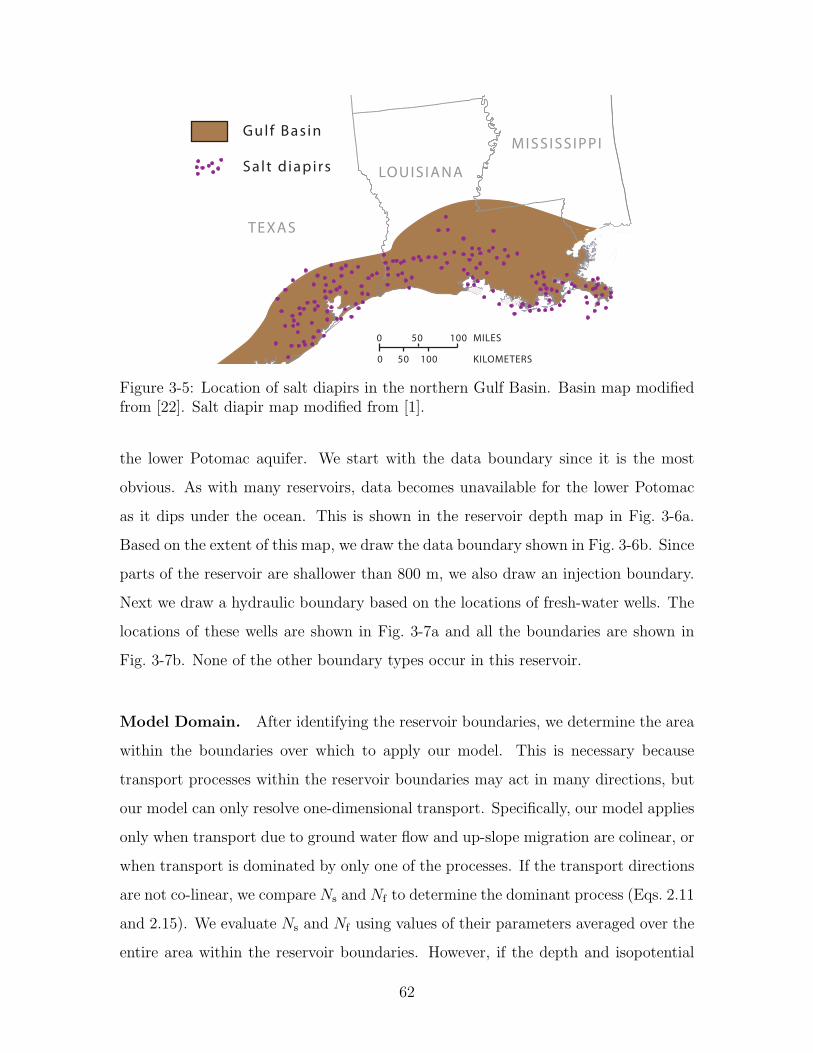
LOUISIANA
TEXAS
MISSISSIPPIGulf Bas in
Salt d iapirs
0
0 50
100
100
50 MILES
KILOMETERS
Figure 3-5: Location of salt diapirs in the northern Gulf Basin. Basin map modifiedfrom [22]. Salt diapir map modified from [1].
the lower Potomac aquifer. We start with the data boundary since it is the most
obvious. As with many reservoirs, data becomes unavailable for the lower Potomac
as it dips under the ocean. This is shown in the reservoir depth map in Fig. 3-6a.
Based on the extent of this map, we draw the data boundary shown in Fig. 3-6b. Since
parts of the reservoir are shallower than 800 m, we also draw an injection boundary.
Next we draw a hydraulic boundary based on the locations of fresh-water wells. The
locations of these wells are shown in Fig. 3-7a and all the boundaries are shown in
Fig. 3-7b. None of the other boundary types occur in this reservoir.
Model Domain. After identifying the reservoir boundaries, we determine the area
within the boundaries over which to apply our model. This is necessary because
transport processes within the reservoir boundaries may act in many directions, but
our model can only resolve one-dimensional transport. Specifically, our model applies
only when transport due to ground water flow and up-slope migration are colinear, or
when transport is dominated by only one of the processes. If the transport directions
are not co-linear, we compare Ns and Nf to determine the dominant process (Eqs. 2.11
and 2.15). We evaluate Ns and Nf using values of their parameters averaged over the
entire area within the reservoir boundaries. However, if the depth and isopotential
62
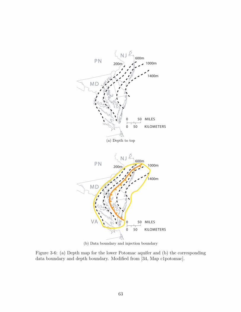
1400m
1000m
600m
200m
0 50 MILES
0 50 KILOMETERS
PNNJ
MD
(a) Depth to top
1400m
1000m600m
200m
0 50 MILES
0 50 KILOMETERS
PNNJ
MD
VA
(b) Data boundary and injection boundary
Figure 3-6: (a) Depth map for the lower Potomac aquifer and (b) the correspondingdata boundary and depth boundary. Modified from [34, Map c1potomac].
63
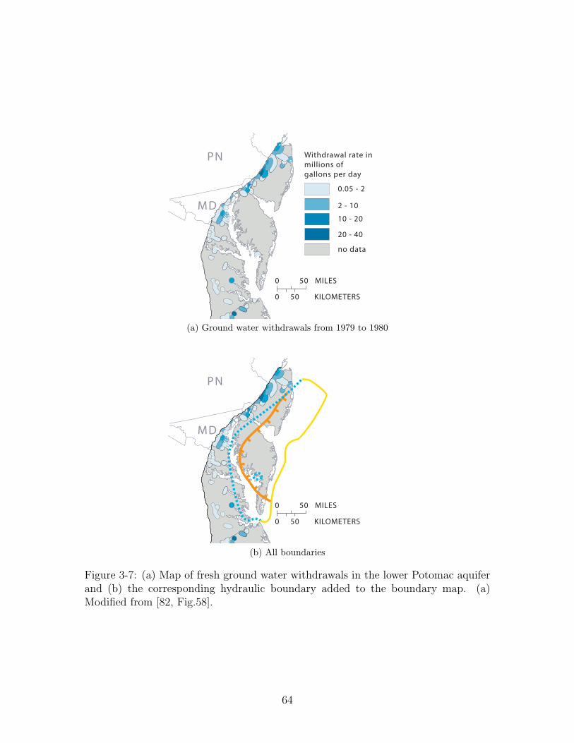
Withdrawal rate in
millions of
gallons per day
0.05 - 2
2 - 10
10 - 20
20 - 40
no data
..
.
0 50 MILES
0 50 KILOMETERS
PN
MD
(a) Ground water withdrawals from 1979 to 1980
..
.
0 50 MILES
0 50 KILOMETERS
PN
MD
(b) All boundaries
Figure 3-7: (a) Map of fresh ground water withdrawals in the lower Potomac aquiferand (b) the corresponding hydraulic boundary added to the boundary map. (a)Modified from [82, Fig.58].
64
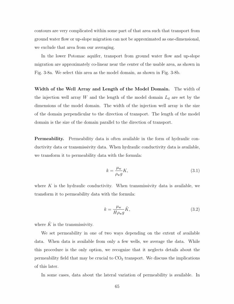
contours are very complicated within some part of that area such that transport from
ground water flow or up-slope migration can not be approximated as one-dimensional,
we exclude that area from our averaging.
In the lower Potomac aquifer, transport from ground water flow and up-slope
migration are approximately co-linear near the center of the usable area, as shown in
Fig. 3-8a. We select this area as the model domain, as shown in Fig. 3-8b.
Width of the Well Array and Length of the Model Domain. The width of
the injection well array W and the length of the model domain Ld are set by the
dimensions of the model domain. The width of the injection well array is the size
of the domain perpendicular to the direction of transport. The length of the model
domain is the size of the domain parallel to the direction of transport.
Permeability. Permeability data is often available in the form of hydraulic con-
ductivity data or transmissivity data. When hydraulic conductivity data is available,
we transform it to permeability data with the formula:
k =µw
ρwgK, (3.1)
where K is the hydraulic conductivity. When transmissivity data is available, we
transform it to permeability data with the formula:
k =µw
HρwgK, (3.2)
where K is the transmissivity.
We set permeability in one of two ways depending on the extent of available
data. When data is available from only a few wells, we average the data. While
this procedure is the only option, we recognize that it neglects details about the
permeability field that may be crucial to CO2 transport. We discuss the implications
of this later.
In some cases, data about the lateral variation of permeability is available. In
65
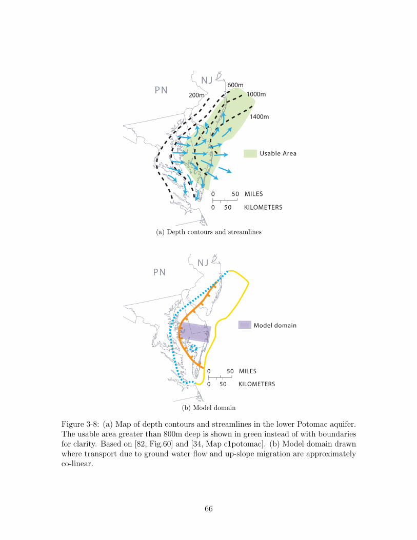
1400m
1000m
600m
200mPN
NJ
0 50 MILES
0 50 KILOMETERS
Usable Area
(a) Depth contours and streamlines
0 50 MILES
0 50 KILOMETERS
PNNJ
Model domain
(b) Model domain
Figure 3-8: (a) Map of depth contours and streamlines in the lower Potomac aquifer.The usable area greater than 800m deep is shown in green instead of with boundariesfor clarity. Based on [82, Fig.60] and [34, Map c1potomac]. (b) Model domain drawnwhere transport due to ground water flow and up-slope migration are approximatelyco-linear.
66
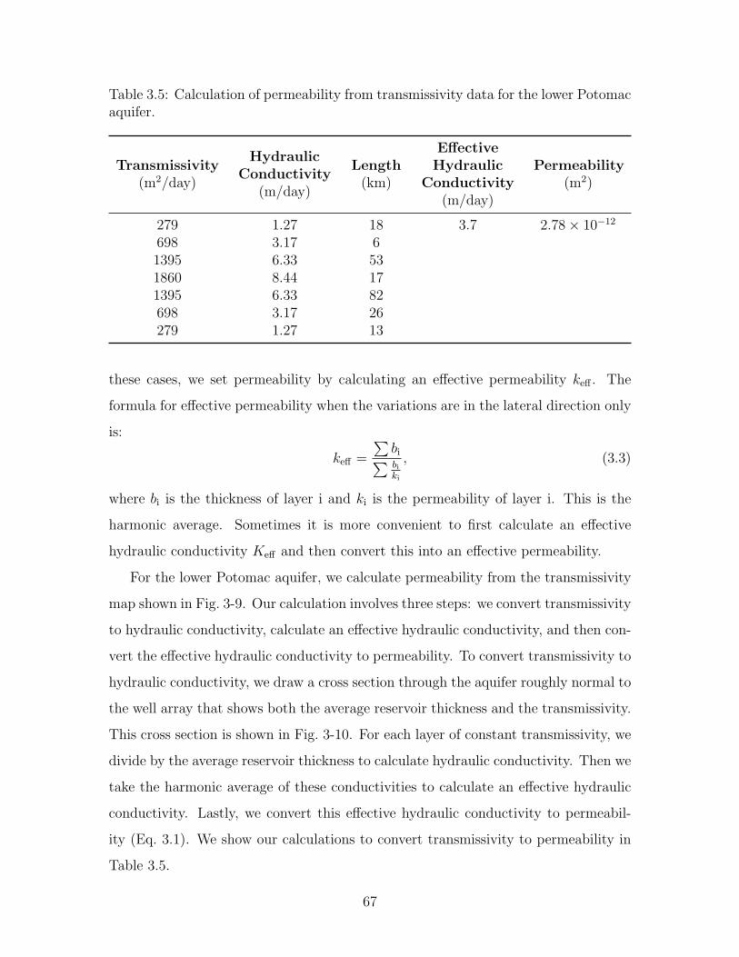
Table 3.5: Calculation of permeability from transmissivity data for the lower Potomacaquifer.
Transmissivity
(m2/day)
Hydraulic
Conductivity
(m/day)
Length
(km)
Effective
Hydraulic
Conductivity
(m/day)
Permeability
(m2)
279 1.27 18 3.7 2.78 × 10⁻¹²
698 3.17 61395 6.33 531860 8.44 171395 6.33 82698 3.17 26279 1.27 13
these cases, we set permeability by calculating an effective permeability keff . The
formula for effective permeability when the variations are in the lateral direction only
is:
keff =
∑bi
∑ biki
, (3.3)
where bi is the thickness of layer i and ki is the permeability of layer i. This is the
harmonic average. Sometimes it is more convenient to first calculate an effective
hydraulic conductivity Keff and then convert this into an effective permeability.
For the lower Potomac aquifer, we calculate permeability from the transmissivity
map shown in Fig. 3-9. Our calculation involves three steps: we convert transmissivity
to hydraulic conductivity, calculate an effective hydraulic conductivity, and then con-
vert the effective hydraulic conductivity to permeability. To convert transmissivity to
hydraulic conductivity, we draw a cross section through the aquifer roughly normal to
the well array that shows both the average reservoir thickness and the transmissivity.
This cross section is shown in Fig. 3-10. For each layer of constant transmissivity, we
divide by the average reservoir thickness to calculate hydraulic conductivity. Then we
take the harmonic average of these conductivities to calculate an effective hydraulic
conductivity. Lastly, we convert this effective hydraulic conductivity to permeabil-
ity (Eq. 3.1). We show our calculations to convert transmissivity to permeability in
Table 3.5.
67
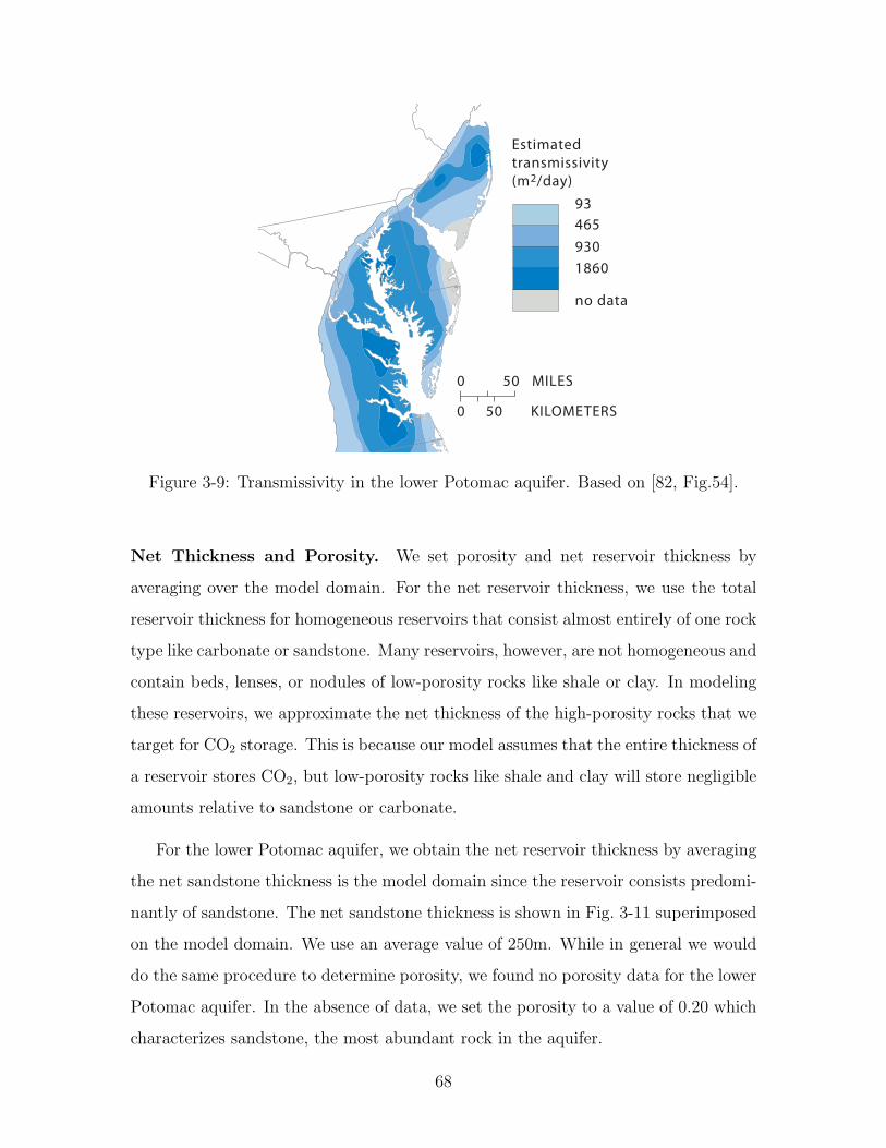
.
..
..
.
.
.
.
.
..
Estimated
transmissivity
(m2/day)
93
465
930
1860
no data
0 50 MILES
0 50 KILOMETERS
Figure 3-9: Transmissivity in the lower Potomac aquifer. Based on [82, Fig.54].
Net Thickness and Porosity. We set porosity and net reservoir thickness by
averaging over the model domain. For the net reservoir thickness, we use the total
reservoir thickness for homogeneous reservoirs that consist almost entirely of one rock
type like carbonate or sandstone. Many reservoirs, however, are not homogeneous and
contain beds, lenses, or nodules of low-porosity rocks like shale or clay. In modeling
these reservoirs, we approximate the net thickness of the high-porosity rocks that we
target for CO2 storage. This is because our model assumes that the entire thickness of
a reservoir stores CO2, but low-porosity rocks like shale and clay will store negligible
amounts relative to sandstone or carbonate.
For the lower Potomac aquifer, we obtain the net reservoir thickness by averaging
the net sandstone thickness is the model domain since the reservoir consists predomi-
nantly of sandstone. The net sandstone thickness is shown in Fig. 3-11 superimposed
on the model domain. We use an average value of 250m. While in general we would
do the same procedure to determine porosity, we found no porosity data for the lower
Potomac aquifer. In the absence of data, we set the porosity to a value of 0.20 which
characterizes sandstone, the most abundant rock in the aquifer.
68
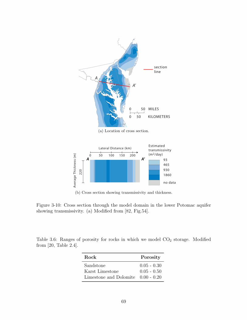
.
..
..
.
.
.
.
.
.
.
.
0 50 MILES
0 50 KILOMETERS
A
A’
section
line
(a) Location of cross section.
0 50 100 150 200
Lateral Distance (km)Estimated
transmissivity
(m2/day)
93
465
930
1860
no data
A A’
Av
era
ge
Th
ick
ne
ss (
m)
22
0
(b) Cross section showing transmissivity and thickness.
Figure 3-10: Cross section through the model domain in the lower Potomac aquifershowing transmissivity. (a) Modified from [82, Fig.54].
Table 3.6: Ranges of porosity for rocks in which we model CO2 storage. Modifiedfrom [20, Table 2.4].
Rock Porosity
Sandstone 0.05 - 0.30Karst Limestone 0.05 - 0.50Limestone and Dolomite 0.00 - 0.20
69
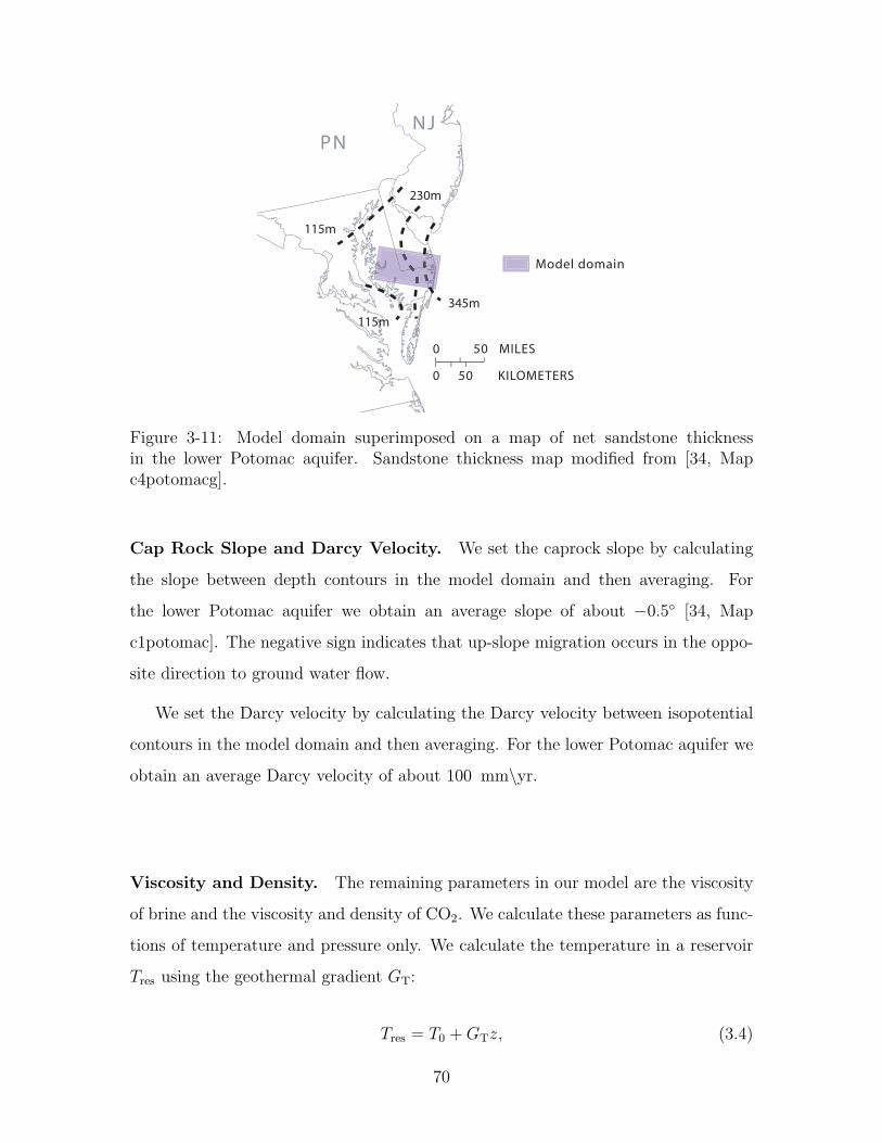
115m
230m
345m
115m
0 50 MILES
0 50 KILOMETERS
PNNJ
Model domain
Figure 3-11: Model domain superimposed on a map of net sandstone thicknessin the lower Potomac aquifer. Sandstone thickness map modified from [34, Mapc4potomacg].
Cap Rock Slope and Darcy Velocity. We set the caprock slope by calculating
the slope between depth contours in the model domain and then averaging. For
the lower Potomac aquifer we obtain an average slope of about −0.5◦ [34, Map
c1potomac]. The negative sign indicates that up-slope migration occurs in the oppo-
site direction to ground water flow.
We set the Darcy velocity by calculating the Darcy velocity between isopotential
contours in the model domain and then averaging. For the lower Potomac aquifer we
obtain an average Darcy velocity of about 100 mm\yr.
Viscosity and Density. The remaining parameters in our model are the viscosity
of brine and the viscosity and density of CO2. We calculate these parameters as func-
tions of temperature and pressure only. We calculate the temperature in a reservoir
Tres using the geothermal gradient GT:
Tres = T0 + GTz, (3.4)
70
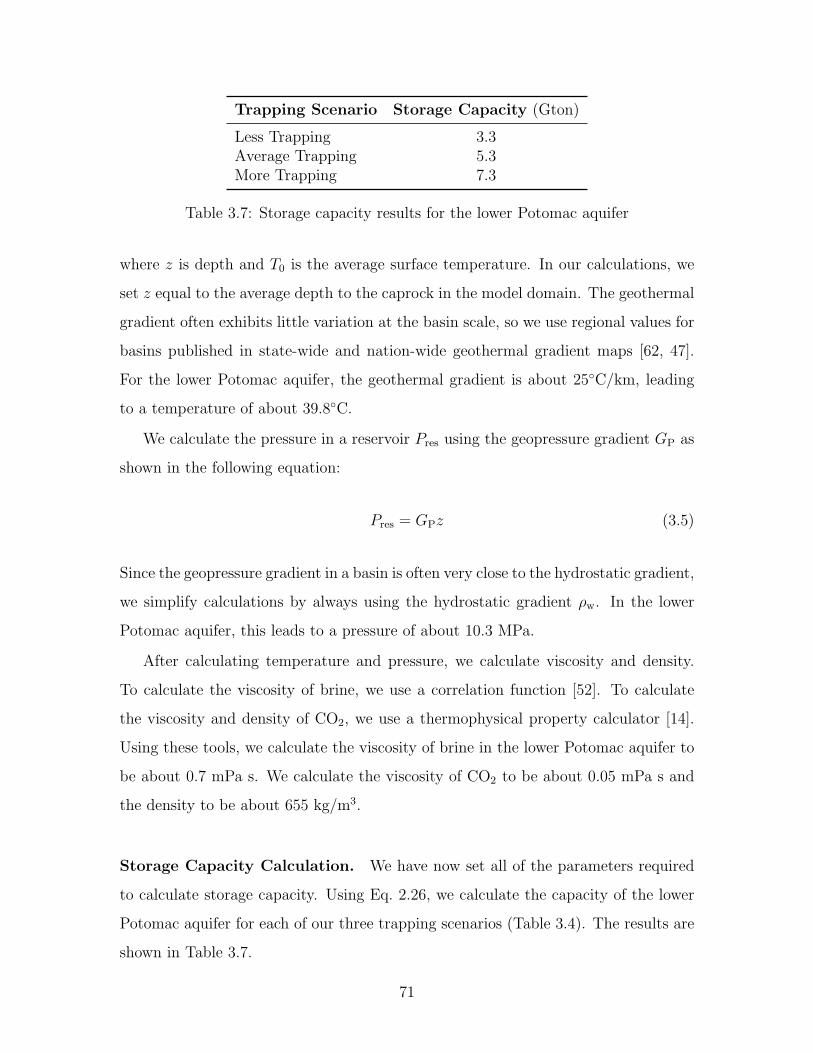
Trapping Scenario Storage Capacity (Gton)
Less Trapping 3.3Average Trapping 5.3More Trapping 7.3
Table 3.7: Storage capacity results for the lower Potomac aquifer
where z is depth and T0 is the average surface temperature. In our calculations, we
set z equal to the average depth to the caprock in the model domain. The geothermal
gradient often exhibits little variation at the basin scale, so we use regional values for
basins published in state-wide and nation-wide geothermal gradient maps [62, 47].
For the lower Potomac aquifer, the geothermal gradient is about 25◦C/km, leading
to a temperature of about 39.8◦C.
We calculate the pressure in a reservoir Pres using the geopressure gradient GP as
shown in the following equation:
Pres = GPz (3.5)
Since the geopressure gradient in a basin is often very close to the hydrostatic gradient,
we simplify calculations by always using the hydrostatic gradient ρw. In the lower
Potomac aquifer, this leads to a pressure of about 10.3 MPa.
After calculating temperature and pressure, we calculate viscosity and density.
To calculate the viscosity of brine, we use a correlation function [52]. To calculate
the viscosity and density of CO2, we use a thermophysical property calculator [14].
Using these tools, we calculate the viscosity of brine in the lower Potomac aquifer to
be about 0.7 mPa s. We calculate the viscosity of CO2 to be about 0.05 mPa s and
the density to be about 655 kg/m3.
Storage Capacity Calculation. We have now set all of the parameters required
to calculate storage capacity. Using Eq. 2.26, we calculate the capacity of the lower
Potomac aquifer for each of our three trapping scenarios (Table 3.4). The results are
shown in Table 3.7.
71

0 50 MILES
0 50 KILOMETERS
PNNJ
Injection footprint
Trapped footprint
Well array
Figure 3-12: CO2 footprint in the lower Potomac aquifer.
Footprint. In addition to a capacity estimate, our model yields the extent of the
injection plume ξinj and the extent of the trapped plume ξtrap. We multiply by the
characteristic length L (Eq. 2.8) to determine the dimensional plume extents (Linj
and Ltrap), and use these values to draw the footprint of the CO2 plume. We first
draw the injection footprint by measuring out the distance Linj on both sides of the
well array. We then draw the trapped footprint by measuring out the distance Ltrap
from the well in the direction of transport. For the lower Potomac aquifer, we draw
the CO2 footprints as shown in Figure 3-12. We use the same convention for drawing
footprints in all other figures in this paper and omit the legend in the future for
clarity.
Parameter Variability. The parameters in our model may vary widely at the
basin scale. This variability will affect the accuracy of our capacity calculations.
While a rigorous analysis of this effect is beyond the scope of this work, we briefly
discuss the variability of some of the parameters and speculate as to the effect on our
calculations.
Some parameters vary marginally at the basin scale. For example, porosity prob-
ably changes by a factor of seven at most, likely from about 0.05 to 0.35 (Table 3.6).
Since we have defined to usable area of the reservoir to exclude any large-scale com-
72
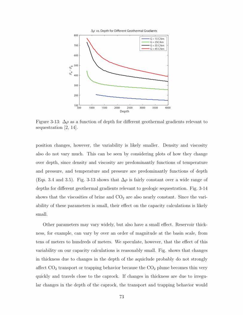
500 1000 1500 2000 2500 3000 3500 4000100
200
300
400
500
600
700
800
Δρ vs. Depth for Di!erent Geothermal Gradientss
Depth
ρ w −
ρg
G = 15 C/km
G = 25C/km
G = 35 C/km
G = 45 C/km
Figure 3-13: ∆ρ as a function of depth for different geothermal gradients relevant tosequestration [2, 14].
position changes, however, the variability is likely smaller. Density and viscosity
also do not vary much. This can be seen by considering plots of how they change
over depth, since density and viscosity are predominantly functions of temperature
and pressure, and temperature and pressure are predominantly functions of depth
(Eqs. 3.4 and 3.5). Fig. 3-13 shows that ∆ρ is fairly constant over a wide range of
depths for different geothermal gradients relevant to geologic sequestration. Fig. 3-14
shows that the viscosities of brine and CO2 are also nearly constant. Since the vari-
ability of these parameters is small, their effect on the capacity calculations is likely
small.
Other parameters may vary widely, but also have a small effect. Reservoir thick-
ness, for example, can vary by over an order of magnitude at the basin scale, from
tens of meters to hundreds of meters. We speculate, however, that the effect of this
variability on our capacity calculations is reasonably small. Fig. shows that changes
in thickness due to changes in the depth of the aquiclude probably do not strongly
affect CO2 transport or trapping behavior because the CO2 plume becomes thin very
quickly and travels close to the caprock. If changes in thickness are due to irregu-
lar changes in the depth of the caprock, the transport and trapping behavior would
73
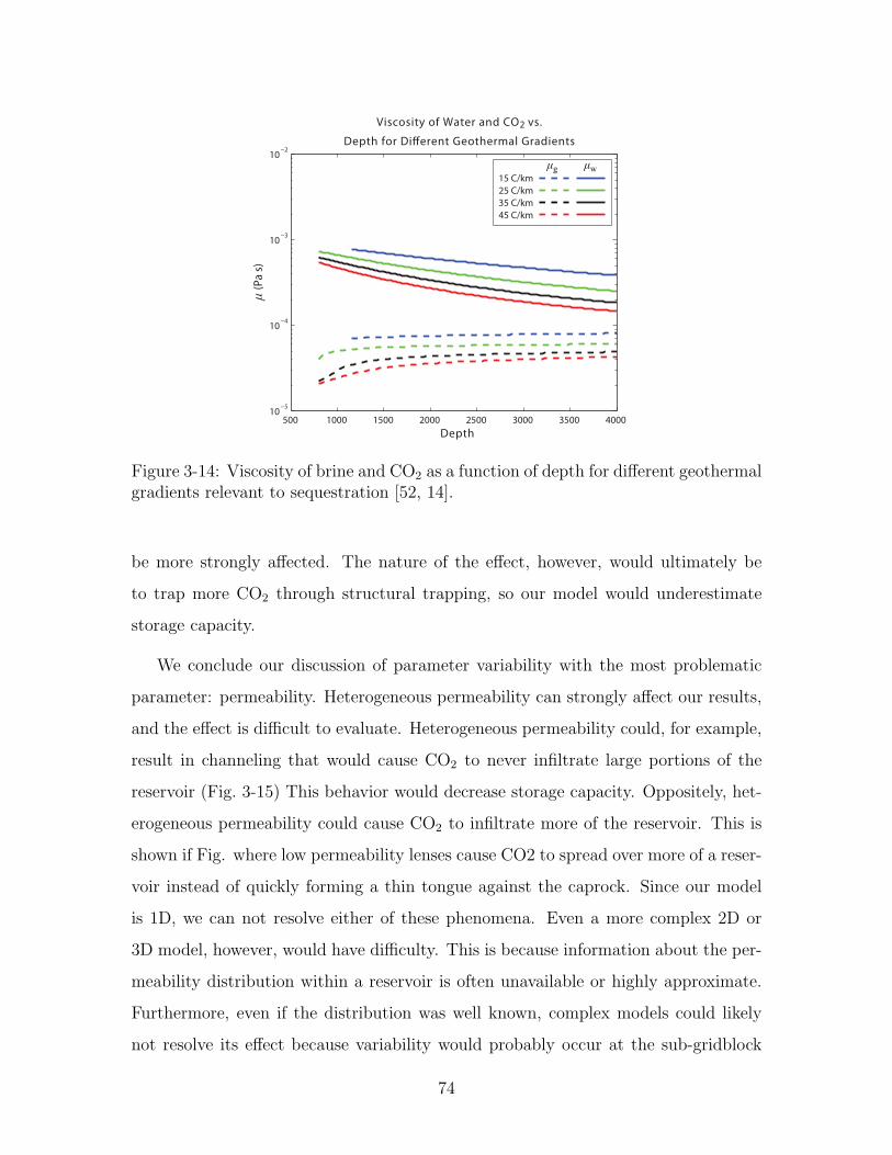
500 1000 1500 2000 2500 3000 3500 400010
−5
10−4
10−3
10−2
Viscosity of Water and CO2 vs.
Depth for Di"erent Geothermal Gradients
Depth
μ (Pa s)
15 C/km
25 C/km
35 C/km
45 C/km
μg μw
Figure 3-14: Viscosity of brine and CO2 as a function of depth for different geothermalgradients relevant to sequestration [52, 14].
be more strongly affected. The nature of the effect, however, would ultimately be
to trap more CO2 through structural trapping, so our model would underestimate
storage capacity.
We conclude our discussion of parameter variability with the most problematic
parameter: permeability. Heterogeneous permeability can strongly affect our results,
and the effect is difficult to evaluate. Heterogeneous permeability could, for example,
result in channeling that would cause CO2 to never infiltrate large portions of the
reservoir (Fig. 3-15) This behavior would decrease storage capacity. Oppositely, het-
erogeneous permeability could cause CO2 to infiltrate more of the reservoir. This is
shown if Fig. where low permeability lenses cause CO2 to spread over more of a reser-
voir instead of quickly forming a thin tongue against the caprock. Since our model
is 1D, we can not resolve either of these phenomena. Even a more complex 2D or
3D model, however, would have difficulty. This is because information about the per-
meability distribution within a reservoir is often unavailable or highly approximate.
Furthermore, even if the distribution was well known, complex models could likely
not resolve its effect because variability would probably occur at the sub-gridblock
74
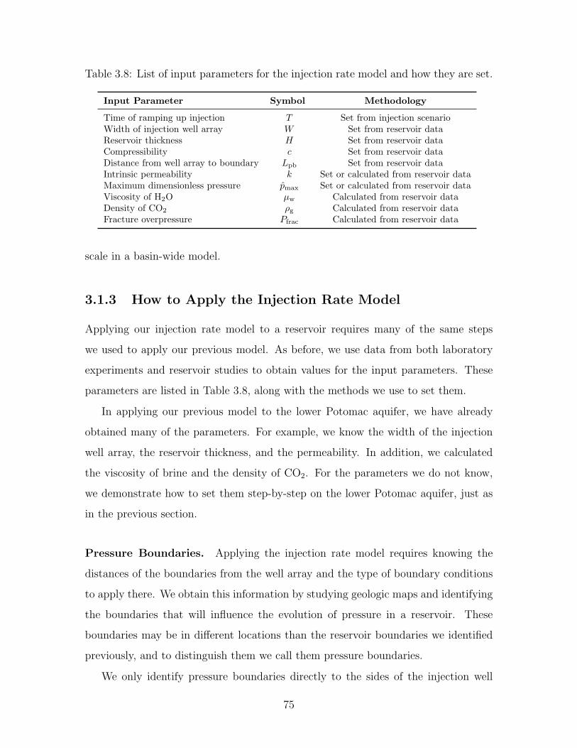
Table 3.8: List of input parameters for the injection rate model and how they are set.
Input Parameter Symbol Methodology
Time of ramping up injection T Set from injection scenarioWidth of injection well array W Set from reservoir dataReservoir thickness H Set from reservoir dataCompressibility c Set from reservoir dataDistance from well array to boundary Lpb Set from reservoir dataIntrinsic permeability k Set or calculated from reservoir dataMaximum dimensionless pressure pmax Set or calculated from reservoir dataViscosity of H2O µw Calculated from reservoir dataDensity of CO2 ρg Calculated from reservoir dataFracture overpressure Pfrac Calculated from reservoir data
scale in a basin-wide model.
3.1.3 How to Apply the Injection Rate Model
Applying our injection rate model to a reservoir requires many of the same steps
we used to apply our previous model. As before, we use data from both laboratory
experiments and reservoir studies to obtain values for the input parameters. These
parameters are listed in Table 3.8, along with the methods we use to set them.
In applying our previous model to the lower Potomac aquifer, we have already
obtained many of the parameters. For example, we know the width of the injection
well array, the reservoir thickness, and the permeability. In addition, we calculated
the viscosity of brine and the density of CO2. For the parameters we do not know,
we demonstrate how to set them step-by-step on the lower Potomac aquifer, just as
in the previous section.
Pressure Boundaries. Applying the injection rate model requires knowing the
distances of the boundaries from the well array and the type of boundary conditions
to apply there. We obtain this information by studying geologic maps and identifying
the boundaries that will influence the evolution of pressure in a reservoir. These
boundaries may be in different locations than the reservoir boundaries we identified
previously, and to distinguish them we call them pressure boundaries.
We only identify pressure boundaries directly to the sides of the injection well
75
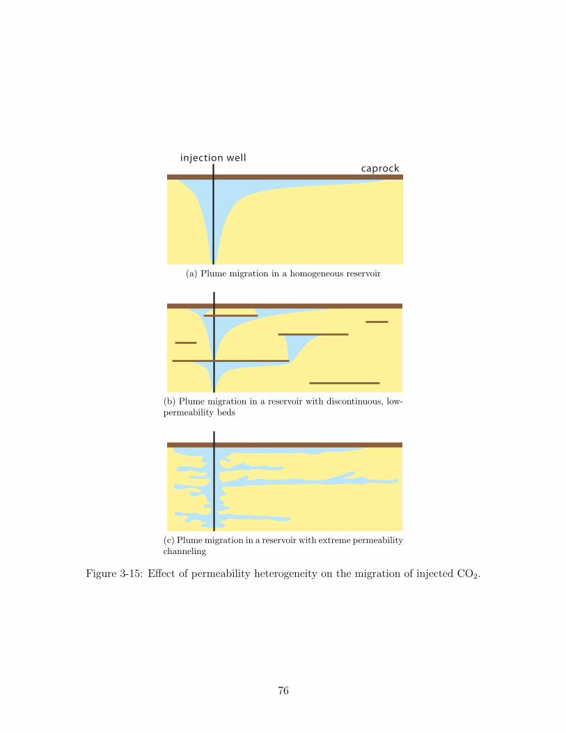
caprockinjection well
(a) Plume migration in a homogeneous reservoir
(b) Plume migration in a reservoir with discontinuous, low-permeability beds
(c) Plume migration in a reservoir with extreme permeabilitychanneling
Figure 3-15: Effect of permeability heterogeneity on the migration of injected CO2.
76
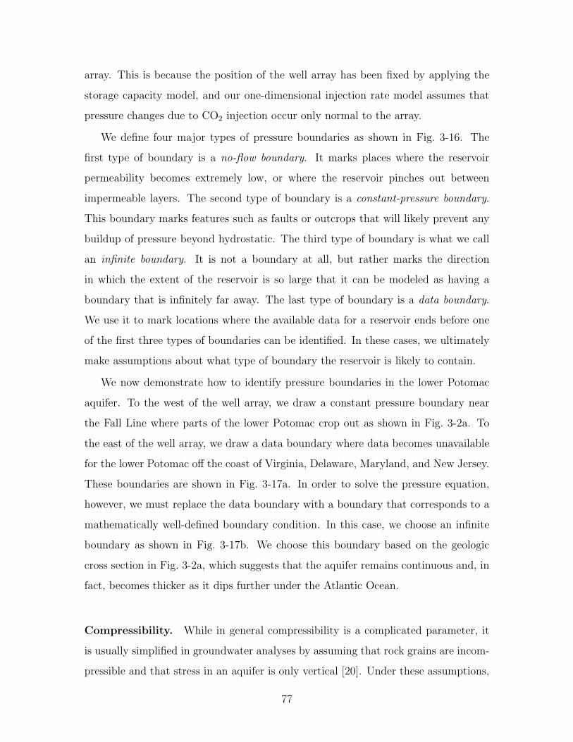
array. This is because the position of the well array has been fixed by applying the
storage capacity model, and our one-dimensional injection rate model assumes that
pressure changes due to CO2 injection occur only normal to the array.
We define four major types of pressure boundaries as shown in Fig. 3-16. The
first type of boundary is a no-flow boundary. It marks places where the reservoir
permeability becomes extremely low, or where the reservoir pinches out between
impermeable layers. The second type of boundary is a constant-pressure boundary.
This boundary marks features such as faults or outcrops that will likely prevent any
buildup of pressure beyond hydrostatic. The third type of boundary is what we call
an infinite boundary. It is not a boundary at all, but rather marks the direction
in which the extent of the reservoir is so large that it can be modeled as having a
boundary that is infinitely far away. The last type of boundary is a data boundary.
We use it to mark locations where the available data for a reservoir ends before one
of the first three types of boundaries can be identified. In these cases, we ultimately
make assumptions about what type of boundary the reservoir is likely to contain.
We now demonstrate how to identify pressure boundaries in the lower Potomac
aquifer. To the west of the well array, we draw a constant pressure boundary near
the Fall Line where parts of the lower Potomac crop out as shown in Fig. 3-2a. To
the east of the well array, we draw a data boundary where data becomes unavailable
for the lower Potomac off the coast of Virginia, Delaware, Maryland, and New Jersey.
These boundaries are shown in Fig. 3-17a. In order to solve the pressure equation,
however, we must replace the data boundary with a boundary that corresponds to a
mathematically well-defined boundary condition. In this case, we choose an infinite
boundary as shown in Fig. 3-17b. We choose this boundary based on the geologic
cross section in Fig. 3-2a, which suggests that the aquifer remains continuous and, in
fact, becomes thicker as it dips further under the Atlantic Ocean.
Compressibility. While in general compressibility is a complicated parameter, it
is usually simplified in groundwater analyses by assuming that rock grains are incom-
pressible and that stress in an aquifer is only vertical [20]. Under these assumptions,
77
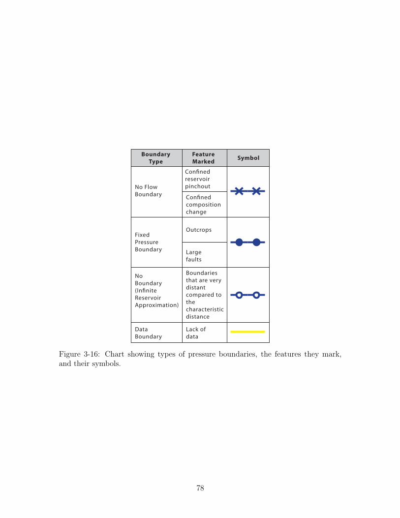
No
Boundary
(In�nite
Reservoir
Approximation)
No Flow
Boundary
Con�ned
reservoir
pinchout
Con�ned
composition
change
Boundary
TypeSymbol
Fixed
Pressure
Boundary
Outcrops
Large
faults
Feature
Marked
Boundaries
that are very
distant
compared to
the
characteristic
distance
Data
Boundary
Lack of
data
Figure 3-16: Chart showing types of pressure boundaries, the features they mark,and their symbols.
78
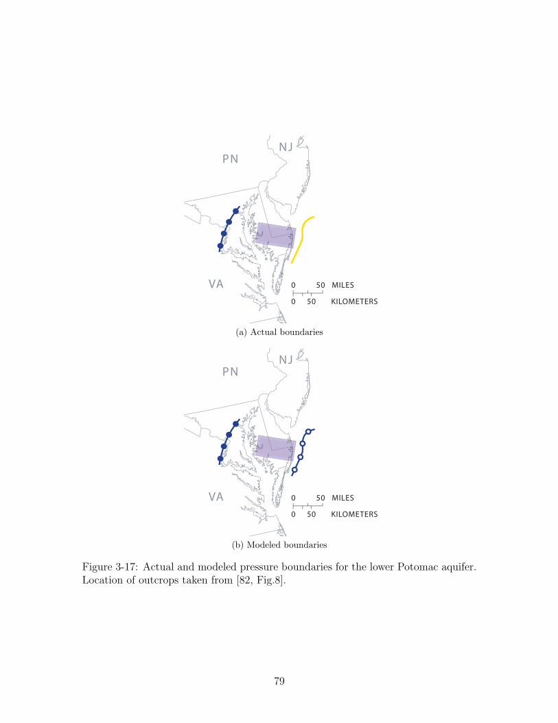
VA 0 50 MILES
0 50 KILOMETERS
PNNJ
(a) Actual boundaries
VA 0 50 MILES
0 50 KILOMETERS
PNNJ
(b) Modeled boundaries
Figure 3-17: Actual and modeled pressure boundaries for the lower Potomac aquifer.Location of outcrops taken from [82, Fig.8].
79
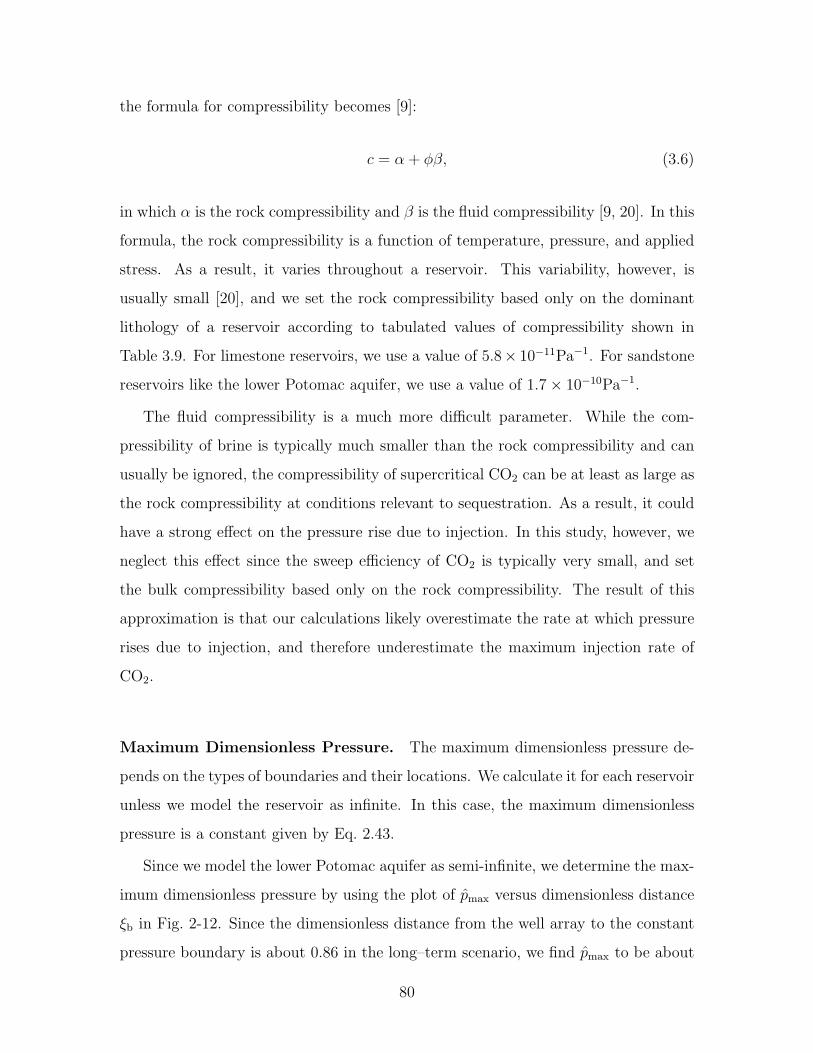
the formula for compressibility becomes [9]:
c = α + φβ, (3.6)
in which α is the rock compressibility and β is the fluid compressibility [9, 20]. In this
formula, the rock compressibility is a function of temperature, pressure, and applied
stress. As a result, it varies throughout a reservoir. This variability, however, is
usually small [20], and we set the rock compressibility based only on the dominant
lithology of a reservoir according to tabulated values of compressibility shown in
Table 3.9. For limestone reservoirs, we use a value of 5.8× 10⁻¹¹Pa−1. For sandstone
reservoirs like the lower Potomac aquifer, we use a value of 1.7 × 10⁻¹⁰Pa−1.
The fluid compressibility is a much more difficult parameter. While the com-
pressibility of brine is typically much smaller than the rock compressibility and can
usually be ignored, the compressibility of supercritical CO2 can be at least as large as
the rock compressibility at conditions relevant to sequestration. As a result, it could
have a strong effect on the pressure rise due to injection. In this study, however, we
neglect this effect since the sweep efficiency of CO2 is typically very small, and set
the bulk compressibility based only on the rock compressibility. The result of this
approximation is that our calculations likely overestimate the rate at which pressure
rises due to injection, and therefore underestimate the maximum injection rate of
CO2.
Maximum Dimensionless Pressure. The maximum dimensionless pressure de-
pends on the types of boundaries and their locations. We calculate it for each reservoir
unless we model the reservoir as infinite. In this case, the maximum dimensionless
pressure is a constant given by Eq. 2.43.
Since we model the lower Potomac aquifer as semi-infinite, we determine the max-
imum dimensionless pressure by using the plot of pmax versus dimensionless distance
ξb in Fig. 2-12. Since the dimensionless distance from the well array to the constant
pressure boundary is about 0.86 in the long–term scenario, we find pmax to be about
80
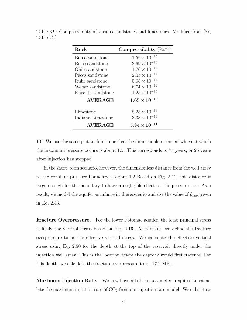
Table 3.9: Compressibility of various sandstones and limestones. Modified from [87,Table C1]
Rock Compressibility (Pa−1)
Berea sandstone 1.59 × 10⁻¹⁰
Boise sandstone 3.69 × 10⁻¹⁰
Ohio sandstone 1.76 × 10⁻¹⁰
Pecos sandstone 2.03 × 10⁻¹⁰
Ruhr sandstone 5.68 × 10⁻¹¹
Weber sandstone 6.74 × 10⁻¹¹
Kayenta sandstone 1.25 × 10⁻¹⁰
AVERAGE 1.65 × 10⁻¹⁰
Limestone 8.28 × 10⁻¹¹
Indiana Limestone 3.38 × 10⁻¹¹
AVERAGE 5.84 × 10⁻¹¹
1.0. We use the same plot to determine that the dimensionless time at which at which
the maximum pressure occurs is about 1.5. This corresponds to 75 years, or 25 years
after injection has stopped.
In the short–term scenario, however, the dimensionless distance from the well array
to the constant pressure boundary is about 1.2 Based on Fig. 2-12, this distance is
large enough for the boundary to have a negligible effect on the pressure rise. As a
result, we model the aquifer as infinite in this scenario and use the value of pmax given
in Eq. 2.43.
Fracture Overpressure. For the lower Potomac aquifer, the least principal stress
is likely the vertical stress based on Fig. 2-16. As a result, we define the fracture
overpressure to be the effective vertical stress. We calculate the effective vertical
stress using Eq. 2.50 for the depth at the top of the reservoir directly under the
injection well array. This is the location where the caprock would first fracture. For
this depth, we calculate the fracture overpressure to be 17.2 MPa.
Maximum Injection Rate. We now have all of the parameters required to calcu-
late the maximum injection rate of CO2 from our injection rate model. We substitute
81

these parameters into Eq. 2.47 and calculate the maximum injection rate to be about
360 Mton/yr in the short–term scenario and 220 Mton/yr in the long–term scenario.
Now that we have demonstrated how to apply our models, we repeat the steps
to model storage capacity and injection rate in each of remaining 16 reservoirs we
study. In many cases, they are repeated exactly as we have demonstrated on the
lower Potomac aquifer. In some cases, however, there are changes. When there are
changes, we explain the changes in the following sections that address the reservoirs
individually. In these sections, the number preceding the reservoir name refers to the
number marking the reservoir’s footprint in our Hydrogeologic Footprint Map.
3.2 Lawson Formation and lower Cedar Keys For-
mation
3.2.1 Geology and Hydrogeology
The Lawson Formation and lower Cedar Keys Formation occur in the South Florida
Basin (Fig. 3-18). Due to limited studies, however, their exact extent is difficult to
determine. In general, data suggests they are continuous from the southern tip of
Florida to at least the panhandle [3, Figs.7,8]. Data also suggests they dip to the
south and thicken to the south, as shown in Fig. 3-19.
The Lawson Formation is Upper Cretaceous in age [3, Table 1]. It consists of two
members. Its lower member is mostly white chalk that is irregularly interbedded with
chalky dolomite or dolomitic chalk. Its upper member is finely to coarsely crystalline
dolomite that contains gypsum and anhydrite [4, p.G26-G27]. The Lawson Forma-
tion overlies unnamed carbonate beds of Taylor age. Over the Florida peninsula,
these beds consist mostly of chalky dolomite interbedded with few beds of shale or
marlstone [3]. We choose these beds to be the bottom boundary in our model since
we found almost no information about them.
The Lawson Formation is unconformably overlain by the lower Cedar Keys Forma-
tion. The lower Cedar Keys Formation is Tertiary in age and consists of limestone [4].
82
It is overlain by the middle Cedar Keys Formation, which is composed of massively
bedded anhydrite [36, p.72]. These anhydrite beds are nearly impermeable and rep-
resent the caprock in our model [60].
Porosity and permeability in the Lawson and lower Cedar Keys formations are
poorly studied. We found data for only one well in which porosity ranged from 24.5
to 28% and permeability ranged from about 5 to 28 mD [27, quoted in [36]]. In the
absence of additional data, we use mean values of 26% and 16 mD to characterize the
formations. The flow direction in the formations is unknown, but the fluid residence
time has been estimated to be more than 20,000 years [36, p.74].
3.2.2 Storage Capacity
We make a number of assumptions in modeling the Lawson and lower Cedar Keys
formations. First, we assume that the formations are continuous across peninsular
Florida. Secondly, we assume that the amount of gypsum and anhydrite in the
formations is small and negligibly affects their storage capacity. Lastly, since the
flow direction is unknown, we assume that it is similar to the flow direction in the
overlying Floridan aquifer [60, Fig.60]. Under this assumption, ground water moves
from central Florida toward the coast as shown in Fig. 3-20.
We identify boundaries in the lower Cedar Keys and Lawson formations as shown
in Fig. 3-21a. Since the reservoir is poorly studied, we draw most of the boundary as
a data boundary along the coast, beyond which we found no information about the
reservoir. We draw a smaller part of the boundary as a hydraulic boundary to the
northwest, corresponding to a cone of depression in the potentiometric surface [60,
Fig.60]. Lastly, we draw a leak boundary to the north at the limit of the caprock for
the overlying Floridan aquifer. While we previously identified the middle Cedar Keys
Formation as a caprock, we place the boundary according to the Floridan aquifer
caprock as an extra precaution to limit the probability of CO2 leakage. We take
this precaution because, although a map of the middle Cedar Keys shows that it
contains very thick beds of anhydrite in northern Florida, this map could be very
inaccurate [34, Map c7cedarkeyg]. This is because it is not based on regional well
83
data, but is instead extrapolated from percent-anhydrite maps and the thickness of
the total Cedar Keys Formation.
Based on the depth map and the assumed flow direction shown in Figs. 5-2a and 3-
20, transport due to groundwater flow and caprock slope in the reservoir will likely
not be colinear. As a result, we evaluate the ratio of the flow number Nf to the slope
number Ns to determine the dominant mechanism (Eqs. 2.15 and 2.11). Since this
ratio is about 0.09, we neglect transport due to groundwater flow and only model
transport due to up-slope migration.
We select the domain for our model as shown in Fig. 3-21b. We calculate the
average storage capacity to be 16.0 Gton of CO2 and draw the CO2 footprint as
shown in Fig. 3-22.
3.2.3 Injection Rate
We set the compressibility of the Lawson and Cedar Keys formations to 5.84×10⁻¹¹ Pa−1
based on Table 3.9 since they consist mostly of carbonate. We identify pressure
boundaries as shown in Fig. 3-23. We place infinite boundaries along the reservoir
border because, although the distance from the well array to the border changes
along the array, the dimensionless distance is at least greater than 1.5 along most of
the array in both the short-term and long–term scenarios. According to Fig. 2-12,
boundaries at this distance will have a small impact on the evolution of pressure at
the well array.
We now calculate the fracture overpressure in the lower Cedar Keys and Lawson
formations. We define this pressure to be the effective horizontal stress. Although
there is no available data in Florida to indicate the relative magnitudes of the principle
stresses [96], we assume that the horizontal stress is the least principal stress since
Florida sits in the Gulf Coast physiographic province as shown in Fig. 2-16. Using
Eq. 2.51, we calculate the effective horizonal stress to be about 8.5 MPa. We use
Eq. 2.47 to calculate the maximum injection rate for the lower Cedar Keys and Lawson
formations to be about 22 Mton/yr in the short–term scenario and 15 Mton/yr in
the long–term scenario.
84
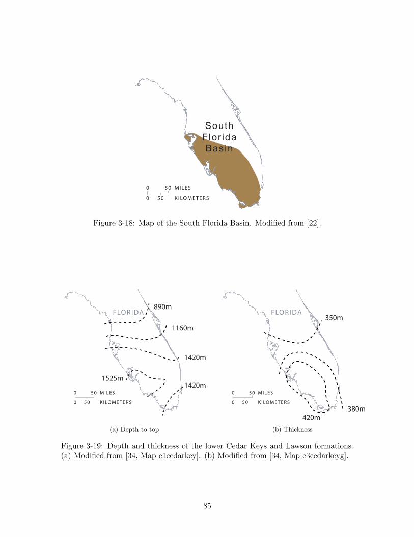
South
Flor ida
Basin
MILES
KILOME TERS
0 50
0 50
Figure 3-18: Map of the South Florida Basin. Modified from [22].
FLORIDA890m
1160m
1420m
1420m1525m
MILES
KILOME TERS
0 50
0 50
(a) Depth to top
FLORIDA350m
380m420m
MILES
KILOME TERS
0 50
0 50
(b) Thickness
Figure 3-19: Depth and thickness of the lower Cedar Keys and Lawson formations.(a) Modified from [34, Map c1cedarkey]. (b) Modified from [34, Map c3cedarkeyg].
85
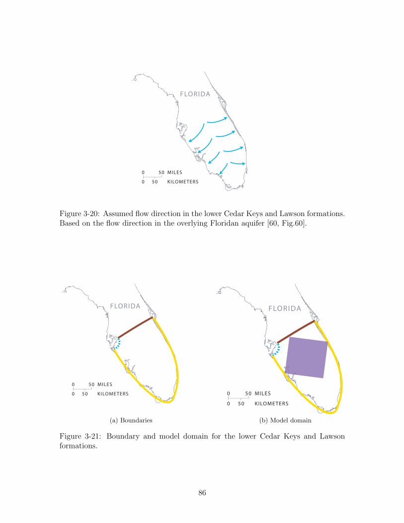
FLORIDA
MILES
KILOME TERS
0 50
0 50
Figure 3-20: Assumed flow direction in the lower Cedar Keys and Lawson formations.Based on the flow direction in the overlying Floridan aquifer [60, Fig.60].
FLORIDA
MILES
KILOME TERS
0 50
0 50
(a) Boundaries
FLORIDA
MILES
KILOME TERS
0 50
0 50
(b) Model domain
Figure 3-21: Boundary and model domain for the lower Cedar Keys and Lawsonformations.
86
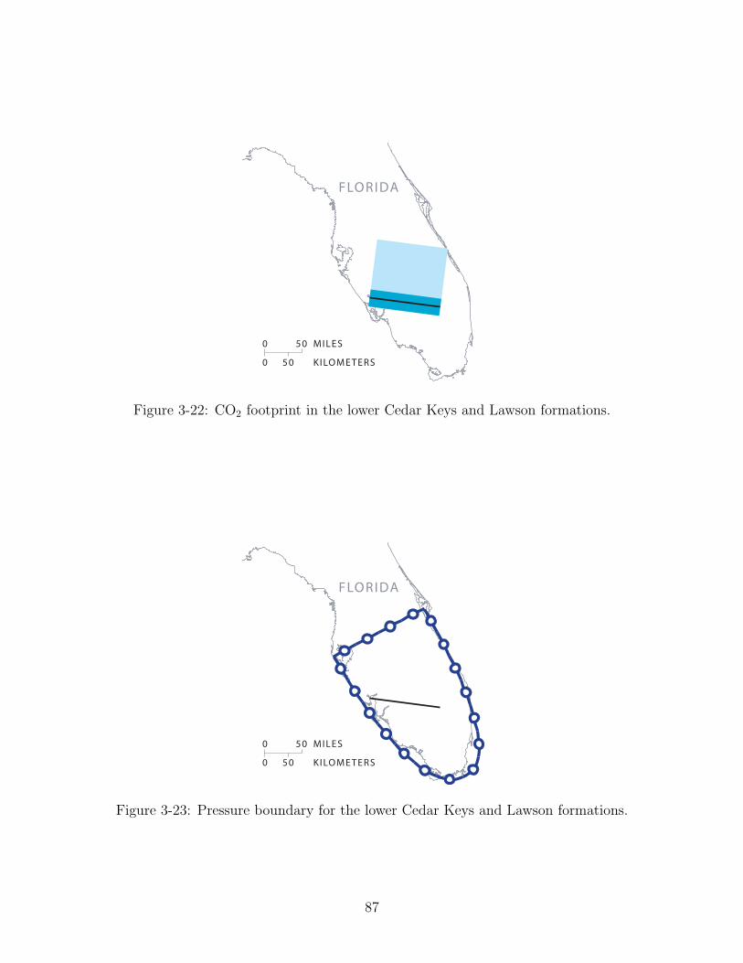
FLORIDA
MILES
KILOME TERS
0 50
0 50
Figure 3-22: CO2 footprint in the lower Cedar Keys and Lawson formations.
FLORIDA
MILES
KILOME TERS
0 50
0 50
Figure 3-23: Pressure boundary for the lower Cedar Keys and Lawson formations.
87
3.3 Mt. Simon Formation
3.3.1 Geology and Hydrogeology
The Mt. Simon Formation is widespread in the Midwestern United States. In this
study, we model sequestration in deep parts of the formation that lie in the Ap-
palachian, Michigan, and Illinois basins.
The Appalachian Basin starts at the Canadian Shield in the north and tapers
to the south in between thrust faults and the Nashville Dome (Fig. 3-24a). In the
west, it begins at a contiguous series of domes and arches in Ohio, Kentucky, and
Tennessee, and it extends to the Blue Ridge province in the east. In general, it dips
and thickens to the east as shown in Figure 3-24b.
The Michigan Basin underlies Michigan and northern parts of Illinois and Ohio
(Fig. 3-25a). It dips and thickens toward the center of the basin as shown in the
generalized cross section in Figure 3-25b.
The Illinois Basin underlies parts of Illinois, Indiana, and Kentucky (Fig. 3-26a).
It also dips and thickens towards the center of the basin as shown in Figure 3-26b.
The geology of the Mt. Simon Formation is fairly uniform across these basins.
The formation is Cambrian in age and consists mostly of quartzose sandstone. The
grains of the sandstone range from fine to very coarse and are poorly to moderately
sorted [94, p.B13]. Near its base, the formation tends to contain a strongly arkosic
zone that is as much as 100m thick and can be conglomeratic with igneous pebbles [92,
36]. Lenses of shale are interbedded in the lower part of the formation in Illinois, and
in the upper part of the formation throughout the Midwest [94, p.B13].
The Mt. Simon Formation is overlain by the Eau Claire Formation, which is
composed of silty dolomites, dolomitic sandstones, and shale. This formation has
been identified as a regional confining unit by a number of authors [65, 94, 56].
The Mt. Simon unconformably overlies Precambrian igneous and metamorphic rocks,
which we take as an aquiclude [92, 36].
88
3.3.2 Storage Capacity
Modeling sequestration in the Mt. Simon Formation is difficult due to a lack of data.
We found no single formation thickness map that covers the Michigan, Illinois, and
Appalachian basins, and we found no data on net sandstone thickness. For the
formation thickness, we construct the map shown in Figure 3-27b from three different
maps: a map for Indiana [85, Fig.8], a map for Illinois [84, Fig.25], and a map
for Michigan and Ohio [34, Map c3mtsimong]. We use this map as a proxy for a
net sandstone thickness map since we found no net sandstone thickness data. This
approximation is justified because the Mt. Simon consists mostly of sandstone.
While we found no net sandstone thickness data, we found limited porosity and
permeability data data. The only data we found comes from one well in the Michigan
Basin, in which porosity was measured for four samples of the Mt. Simon Sandstone.
The porosity of these samples ranges from 13.1 to 15.8%, with a mean of about
14% [13, p.140]. Measurements from the same well indicate that permeability ranges
from 29.5 to 117.0 mD [13, p.140], with a mean of about 52 mD. In the absence of
additional data, we assume the mean porosity and permeability are characteristic of
the Mt. Simon.
While we found limited porosity data for the Mt. Simon, we found no regional
flow direction map that covers all the basins. Instead, we found maps that cover only
one basin or parts of a basin, and the data in these maps often lead to contradictory
flow directions in between the basins. As a result, we ignore regions in between basins
and model sequestration in the basins only, where flow direction is better understood.
Flow directions in the basins are shown in Figure 3-28.
With the flow direction identified, we draw boundaries for the Mt. Simon Forma-
tion as shown in Figure 3-29a. In the Appalachian Basin, the southwestern part of
the boundary is a fault boundary, drawn along faults shown in a nation-wide geologic
map [77]. The eastern part is a data boundary, corresponding to the edge of the For-
mation Thickness Map [34, Map c3mtsimong]. The northern and western parts are
also data boundaries, corresponding to where the flow direction becomes uncertain
89

at the edge of the basin. Within these boundaries, we select the model domain as
shown in Fig. 3-29b. We calculate an average storage capacity of 4.4 Gton of CO2
and draw the CO2 footprint as shown in Fig. 3-30.
In the Michigan Basin, the southern part of the boundary is a data boundary due
to uncertainties in flow direction between the basins (Fig. 3-29a). The eastern part of
the boundary is a caprock pinchout boundary, corresponding to where the Eau Claire
Formation pinches out [34, Map c7mtsimonallg]. The western part of the boundary
contains fault boundaries [77]. It also contains hydraulic boundaries at depressions
in the potentiometric surface due to pumping in major cities [67, Fig.127].
Within this basin, transport due to groundwater flow and up-slope migration will
not be colinear. To determine the dominant mechanism, we compare the flow number
Nf to the slope number Ns (Eqs. 2.11 and 2.15). Since the average value of Nf\Ns
is about 0.3, we conclude that up-slope migration is dominant and ignore the effect
of ground water flow in our model. Since we ignore ground water flow, we select the
model domain based only on the constraint of nearly linear, parallel depth contours,
which is required for one-dimensional up-slope transport (Fig. 3-29b ). We calculate
the average storage capacity to be 48.5 Gton of CO2 and draw the CO2 footprint as
shown in Fig. 3-30.
In the Illinois Basin, the southern and eastern parts of the boundary are fault
boundaries (Fig. 3-29a) [77]. The northern part is a hydraulic boundary, correspond-
ing to depressions in the potentiometric surface from pumping in major cities [56,
Fig.33A]. The western part is a data boundary, corresponding to the edge of the
Mt. Simon Depth Map [34, Map c3mtsimong] and the edge of the Mt. Simon isopach
map [84]. Within these boundaries, we select the model domain as shown in Fig. 3-
29b, based on the region over which transport due to ground water flow and up-slope
migration are colinear. We calculate an average storage capacity of 21.7 Gton of CO2
and draw the CO2 footprint as shown in Fig. 3-30.
90
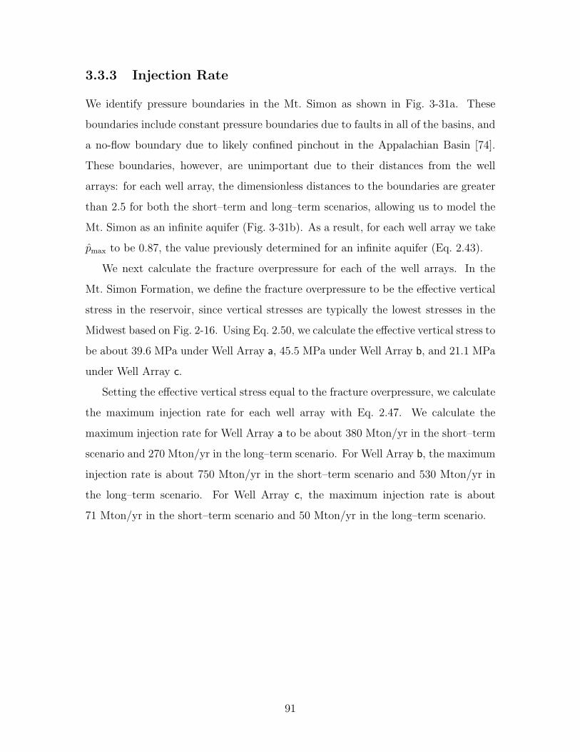
3.3.3 Injection Rate
We identify pressure boundaries in the Mt. Simon as shown in Fig. 3-31a. These
boundaries include constant pressure boundaries due to faults in all of the basins, and
a no-flow boundary due to likely confined pinchout in the Appalachian Basin [74].
These boundaries, however, are unimportant due to their distances from the well
arrays: for each well array, the dimensionless distances to the boundaries are greater
than 2.5 for both the short–term and long–term scenarios, allowing us to model the
Mt. Simon as an infinite aquifer (Fig. 3-31b). As a result, for each well array we take
pmax to be 0.87, the value previously determined for an infinite aquifer (Eq. 2.43).
We next calculate the fracture overpressure for each of the well arrays. In the
Mt. Simon Formation, we define the fracture overpressure to be the effective vertical
stress in the reservoir, since vertical stresses are typically the lowest stresses in the
Midwest based on Fig. 2-16. Using Eq. 2.50, we calculate the effective vertical stress to
be about 39.6 MPa under Well Array a, 45.5 MPa under Well Array b, and 21.1 MPa
under Well Array c.
Setting the effective vertical stress equal to the fracture overpressure, we calculate
the maximum injection rate for each well array with Eq. 2.47. We calculate the
maximum injection rate for Well Array a to be about 380 Mton/yr in the short–term
scenario and 270 Mton/yr in the long–term scenario. For Well Array b, the maximum
injection rate is about 750 Mton/yr in the short–term scenario and 530 Mton/yr in
the long–term scenario. For Well Array c, the maximum injection rate is about
71 Mton/yr in the short–term scenario and 50 Mton/yr in the long–term scenario.
91
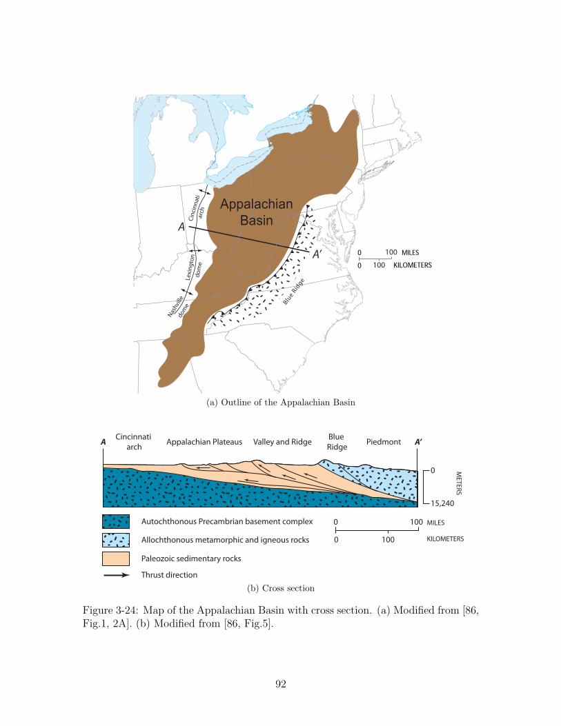
A’
A
0 MILESKILOMETERS
100
0 100
Appalachian
Basinarch
Cin
cin
nat
i d
om
e
Lexi
ng
ton
dom
e
Nas
hvill
e
Blu
e Rid
ge
(a) Outline of the Appalachian Basin
0
15,240
ME
TE
RS
Cincinnati
archAppalachian Plateaus Valley and Ridge
Blue
RidgePiedmontA A’
Allochthonous metamorphic and igneous rocks
Autochthonous Precambrian basement complex
Paleozoic sedimentary rocks
Thrust direction
0
1000
100 MILES
KILOMETERS
(b) Cross section
Figure 3-24: Map of the Appalachian Basin with cross section. (a) Modified from [86,Fig.1, 2A]. (b) Modified from [86, Fig.5].
92
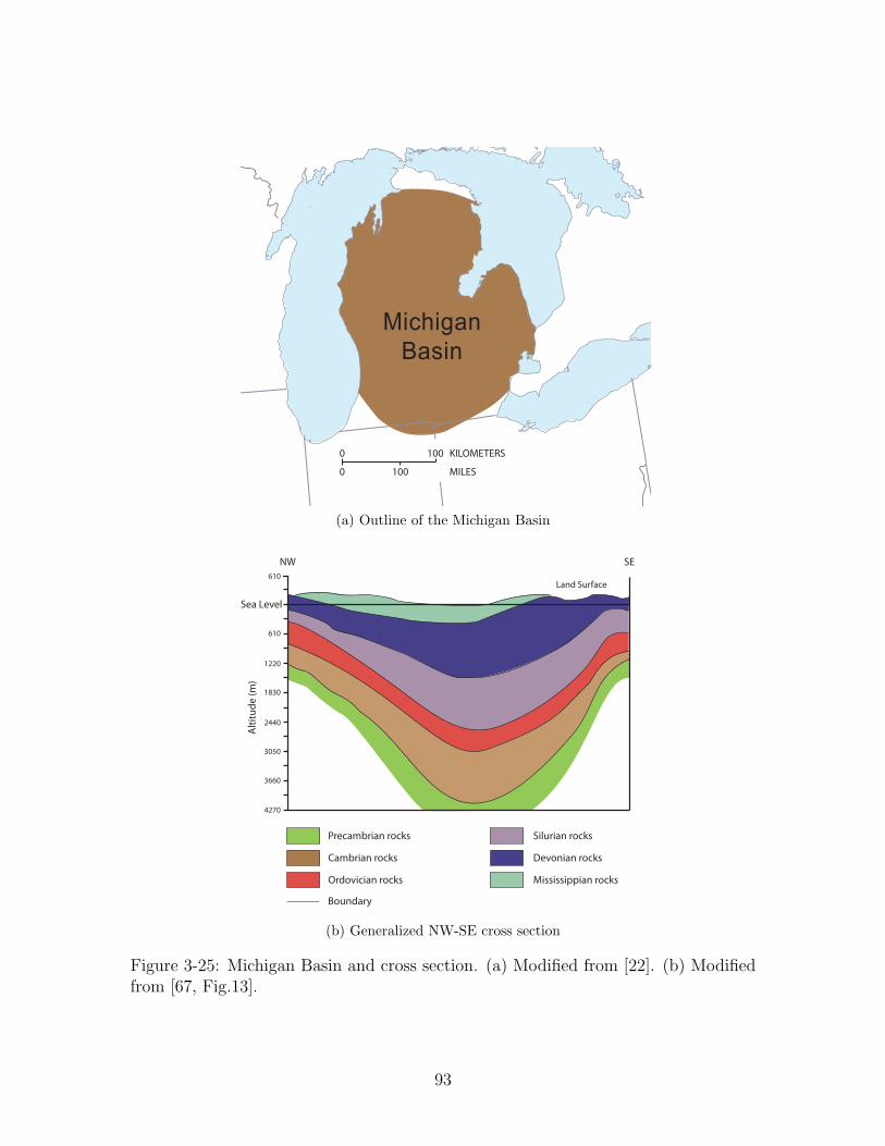
100
100
0
0 MILES
KILOMETERS
Michigan
Basin
(a) Outline of the Michigan Basin
Land Surface
610
1220
1830
2440
3050
4270
3660
610
Sea Level
Alt
itu
de
(m
)
NW SE
Silurian rocks
Cambrian rocks
Ordovician rocks
Precambrian rocks
Boundary
Devonian rocks
Mississippian rocks
(b) Generalized NW-SE cross section
Figure 3-25: Michigan Basin and cross section. (a) Modified from [22]. (b) Modifiedfrom [67, Fig.13].
93
AA’
100
100
0
0 MILES
KILOMETERS
Illinois
Basin
(a) Outline of the Illinois Basin
305
610
915
1220
1525
1830
2135
Sea Level
Alt
itu
de
(m
)
A A’
Kaskaskia Sequence
Sauk Sequence
Tippecanoe Sequence
0
0 40
40
MILES
KILOMETERS
Precambrian
Sequence boundary
Absaroka Sequence
(b) Cross section A
Figure 3-26: Illinois Basin and cross section. (a) Modified from [71, Fig.1]. (b) TheMt. Simon Formation and the Eau Claire Formation are the lowermost units in theSauk Sequence. Modified from [46, Fig.2-4].
94
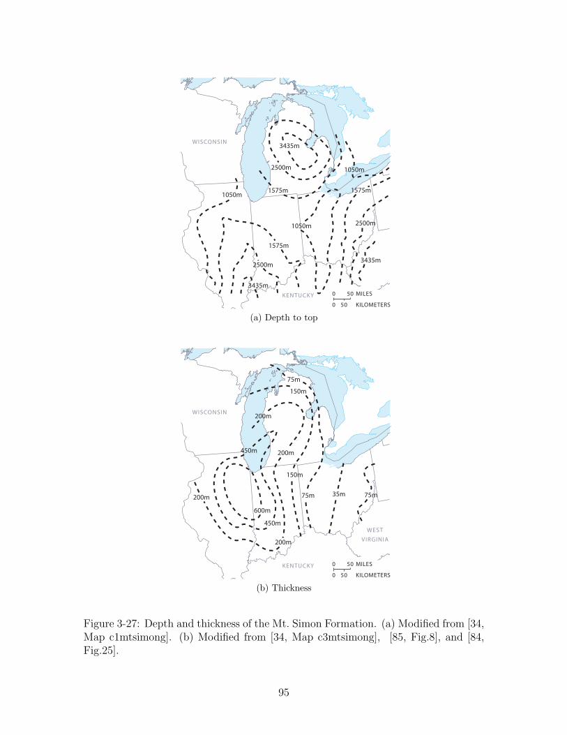
0 50 MILES
KILOMETERS0 50
1050m
1050m
1050m
1575m
1575m
1575m
2500m
2500m
2500m
3435m
3435m
3435mWISCONSIN
KENTUCKY
(a) Depth to top
0 50 MILES
KILOMETERS0 50
75m35m
150m
75m
200m
150m
200m
450m
600m
200m
200m
75m
450m
WISCONSIN
KENTUCKY
WEST
VIRGINIA
(b) Thickness
Figure 3-27: Depth and thickness of the Mt. Simon Formation. (a) Modified from [34,Map c1mtsimong]. (b) Modified from [34, Map c3mtsimong], [85, Fig.8], and [84,Fig.25].
95
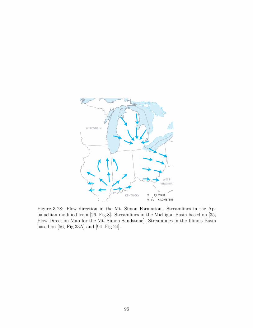
0 50 MILES
KILOMETERS0 50
WISCONSIN
KENTUCKY
WEST
VIRGINIA
Figure 3-28: Flow direction in the Mt. Simon Formation. Streamlines in the Ap-palachian modified from [26, Fig.8]. Streamlines in the Michigan Basin based on [35,Flow Direction Map for the Mt. Simon Sandstone]. Streamlines in the Illinois Basinbased on [56, Fig.33A] and [94, Fig.24].
96
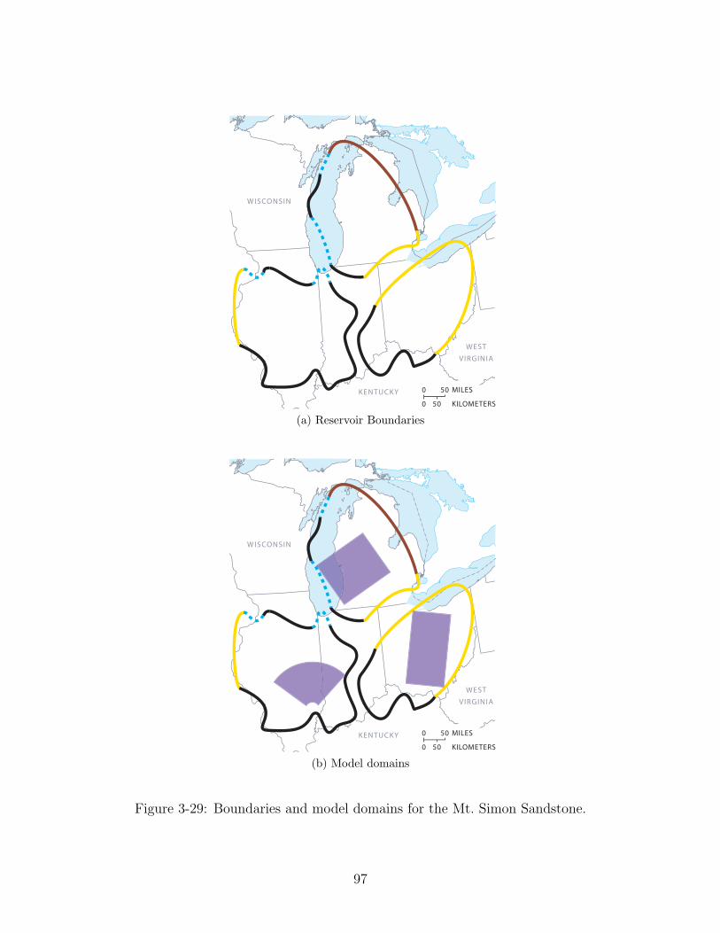
0 50 MILES
KILOMETERS0 50
WISCONSIN
KENTUCKY
WEST
VIRGINIA
(a) Reservoir Boundaries
0 50 MILES
KILOMETERS0 50
WISCONSIN
KENTUCKY
WEST
VIRGINIA
(b) Model domains
Figure 3-29: Boundaries and model domains for the Mt. Simon Sandstone.
97

0 50 MILES
KILOMETERS0 50
WISCONSIN
KENTUCKY
WEST
VIRGINIAa
b
c
Figure 3-30: CO2 footprints in the Mt. Simon Formation.
98
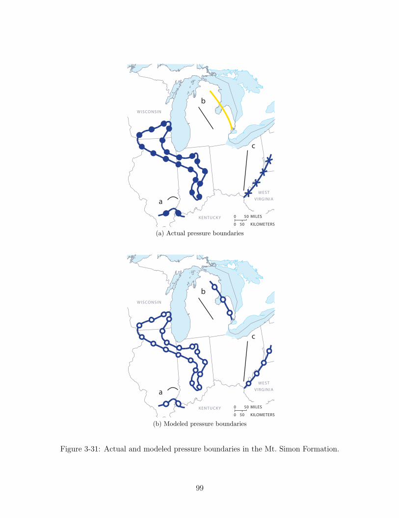
0 50 MILES
KILOMETERS0 50
WISCONSIN
KENTUCKY
WEST
VIRGINIAa
b
c
(a) Actual pressure boundaries
0 50 MILES
KILOMETERS0 50
WISCONSIN
KENTUCKY
WEST
VIRGINIAa
b
c
(b) Modeled pressure boundaries
Figure 3-31: Actual and modeled pressure boundaries in the Mt. Simon Formation.
99
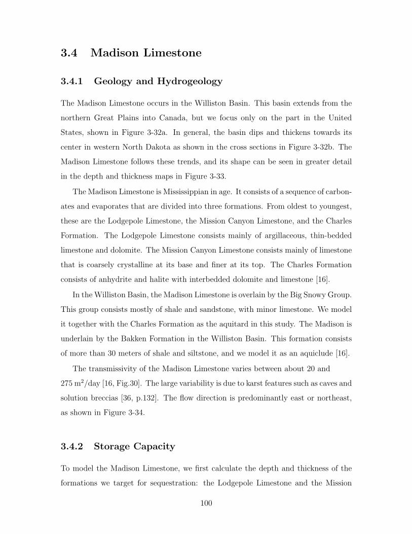
3.4 Madison Limestone
3.4.1 Geology and Hydrogeology
The Madison Limestone occurs in the Williston Basin. This basin extends from the
northern Great Plains into Canada, but we focus only on the part in the United
States, shown in Figure 3-32a. In general, the basin dips and thickens towards its
center in western North Dakota as shown in the cross sections in Figure 3-32b. The
Madison Limestone follows these trends, and its shape can be seen in greater detail
in the depth and thickness maps in Figure 3-33.
The Madison Limestone is Mississippian in age. It consists of a sequence of carbon-
ates and evaporates that are divided into three formations. From oldest to youngest,
these are the Lodgepole Limestone, the Mission Canyon Limestone, and the Charles
Formation. The Lodgepole Limestone consists mainly of argillaceous, thin-bedded
limestone and dolomite. The Mission Canyon Limestone consists mainly of limestone
that is coarsely crystalline at its base and finer at its top. The Charles Formation
consists of anhydrite and halite with interbedded dolomite and limestone [16].
In the Williston Basin, the Madison Limestone is overlain by the Big Snowy Group.
This group consists mostly of shale and sandstone, with minor limestone. We model
it together with the Charles Formation as the aquitard in this study. The Madison is
underlain by the Bakken Formation in the Williston Basin. This formation consists
of more than 30 meters of shale and siltstone, and we model it as an aquiclude [16].
The transmissivity of the Madison Limestone varies between about 20 and
275 m2/day [16, Fig.30]. The large variability is due to karst features such as caves and
solution breccias [36, p.132]. The flow direction is predominantly east or northeast,
as shown in Figure 3-34.
3.4.2 Storage Capacity
To model the Madison Limestone, we first calculate the depth and thickness of the
formations we target for sequestration: the Lodgepole Limestone and the Mission
100
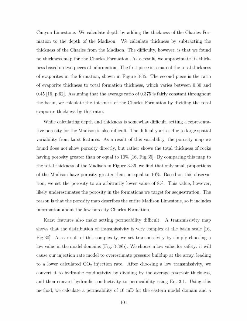
Canyon Limestone. We calculate depth by adding the thickness of the Charles For-
mation to the depth of the Madison. We calculate thickness by subtracting the
thickness of the Charles from the Madison. The difficulty, however, is that we found
no thickness map for the Charles Formation. As a result, we approximate its thick-
ness based on two pieces of information. The first piece is a map of the total thickness
of evaporites in the formation, shown in Figure 3-35. The second piece is the ratio
of evaporite thickness to total formation thickness, which varies between 0.30 and
0.45 [16, p.62]. Assuming that the average ratio of 0.375 is fairly constant throughout
the basin, we calculate the thickness of the Charles Formation by dividing the total
evaporite thickness by this ratio.
While calculating depth and thickness is somewhat difficult, setting a representa-
tive porosity for the Madison is also difficult. The difficulty arises due to large spatial
variability from karst features. As a result of this variability, the porosity map we
found does not show porosity directly, but rather shows the total thickness of rocks
having porosity greater than or equal to 10% [16, Fig.35]. By comparing this map to
the total thickness of the Madison in Figure 3-36, we find that only small proportions
of the Madison have porosity greater than or equal to 10%. Based on this observa-
tion, we set the porosity to an arbitrarily lower value of 8%. This value, however,
likely underestimates the porosity in the formations we target for sequestration. The
reason is that the porosity map describes the entire Madison Limestone, so it includes
information about the low-porosity Charles Formation.
Karst features also make setting permeability difficult. A transmissivity map
shows that the distribution of transmissivity is very complex at the basin scale [16,
Fig.30]. As a result of this complexity, we set transmissivity by simply choosing a
low value in the model domains (Fig. 3-38b). We choose a low value for safety: it will
cause our injection rate model to overestimate pressure buildup at the array, leading
to a lower calculated CO2 injection rate. After choosing a low transmissivity, we
convert it to hydraulic conductivity by dividing by the average reservoir thickness,
and then convert hydraulic conductivity to permeability using Eq. 3.1. Using this
method, we calculate a permeability of 16 mD for the eastern model domain and a
101
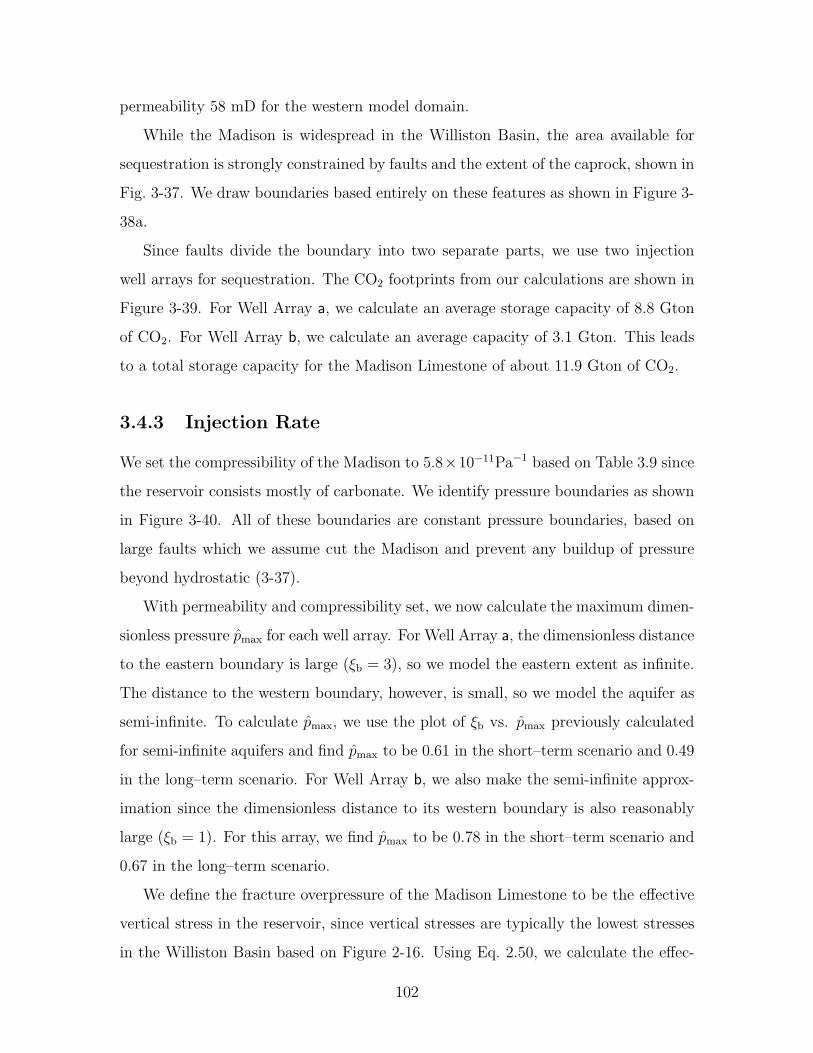
permeability 58 mD for the western model domain.
While the Madison is widespread in the Williston Basin, the area available for
sequestration is strongly constrained by faults and the extent of the caprock, shown in
Fig. 3-37. We draw boundaries based entirely on these features as shown in Figure 3-
38a.
Since faults divide the boundary into two separate parts, we use two injection
well arrays for sequestration. The CO2 footprints from our calculations are shown in
Figure 3-39. For Well Array a, we calculate an average storage capacity of 8.8 Gton
of CO2. For Well Array b, we calculate an average capacity of 3.1 Gton. This leads
to a total storage capacity for the Madison Limestone of about 11.9 Gton of CO2.
3.4.3 Injection Rate
We set the compressibility of the Madison to 5.8×10⁻¹¹Pa−1 based on Table 3.9 since
the reservoir consists mostly of carbonate. We identify pressure boundaries as shown
in Figure 3-40. All of these boundaries are constant pressure boundaries, based on
large faults which we assume cut the Madison and prevent any buildup of pressure
beyond hydrostatic (3-37).
With permeability and compressibility set, we now calculate the maximum dimen-
sionless pressure pmax for each well array. For Well Array a, the dimensionless distance
to the eastern boundary is large (ξb = 3), so we model the eastern extent as infinite.
The distance to the western boundary, however, is small, so we model the aquifer as
semi-infinite. To calculate pmax, we use the plot of ξb vs. pmax previously calculated
for semi-infinite aquifers and find pmax to be 0.61 in the short–term scenario and 0.49
in the long–term scenario. For Well Array b, we also make the semi-infinite approx-
imation since the dimensionless distance to its western boundary is also reasonably
large (ξb = 1). For this array, we find pmax to be 0.78 in the short–term scenario and
0.67 in the long–term scenario.
We define the fracture overpressure of the Madison Limestone to be the effective
vertical stress in the reservoir, since vertical stresses are typically the lowest stresses
in the Williston Basin based on Figure 2-16. Using Eq. 2.50, we calculate the effec-
102
tive vertical stress to be about 29.7 MPa for Well Array a and 35.6 MPa for Well
Array b. Setting these equal to the fracture overpressures, we calculate the maximum
injection rate for Well Array a to be about 190 Mton/yr in the short–term scenario
and 168.9 Mton/yr in the long–term scenario. For Well Array b, we calculate the
maximum injection rate to be about 180 Mton/yr in the short–term scenario and
150 Mton/yr in the long–term scenario.
103

P o w d e r
R i v e r
B a s i n
Black
H il ls
Uplif t
W i l l i s t o n
B a s i n
Litt le
Ro ck y
M ountains
Sioux
Uplif t
A
A’
M O N T A N A
W Y O M I N G
S O U T H
D A K O T A
B B’
0 50 MILES
KILOMETERS0 50
(a) Map of Williston Basin
10000
5000
Sea Level
5000
feet Black Hills
UpliftWilliston Basin
A A’
B B’
10000
5000
Sea Level
5000
feet
0 50 100 MILES
KILOMETERS0 50 100
Little Rocky
Mountains Williston Basin
MO
NT
AN
A
NO
RT
H
DA
KO
TA
Tertiary sedimentary rocks
Paleozoic sedimentary rocks
Mesozoic sedimentary rocks
Precambrian igneouss and metamorphic rocks
Be
nd
s in
Se
cti
on
Tertiary intrusive &volcanic rocks
Be
nd
s in
Se
cti
on
(b) Cross sections A and B
Figure 3-32: Outline of the Williston Basin with cross section. (a) Modified from [90,Fig.12]. (b) Modified from [90, Fig.11].
104
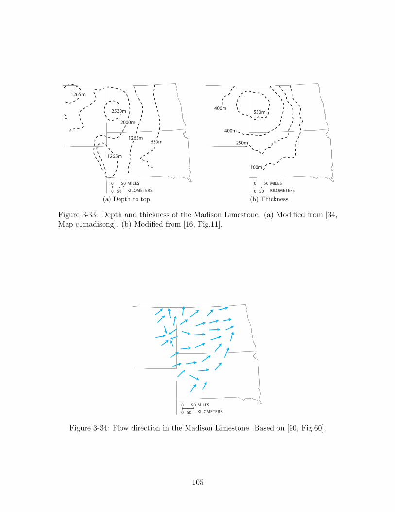
0 50 MILES
KILOMETERS0 50
630m1265m
2000m
2530m
1265m
1265m
(a) Depth to top
0 50 MILES
KILOMETERS0 50
250m
400m
550m400m
100m
(b) Thickness
Figure 3-33: Depth and thickness of the Madison Limestone. (a) Modified from [34,Map c1madisong]. (b) Modified from [16, Fig.11].
0 50 MILES
KILOMETERS0 50
Figure 3-34: Flow direction in the Madison Limestone. Based on [90, Fig.60].
105
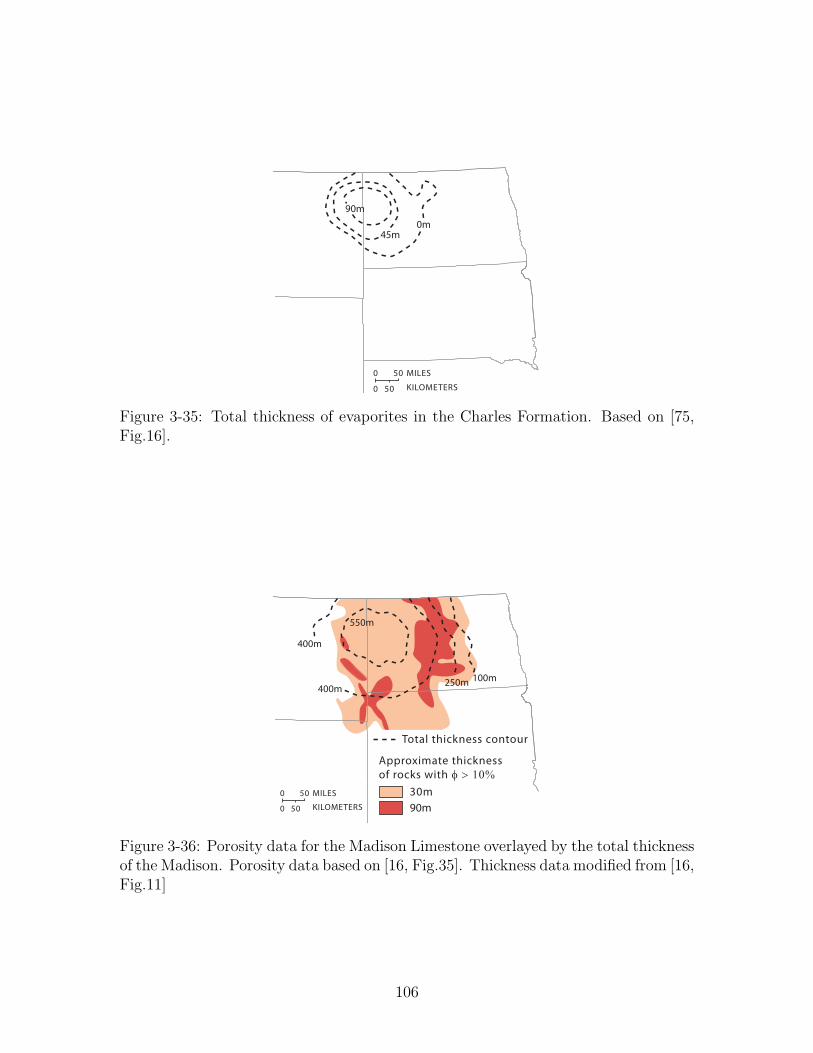
0 50 MILES
KILOMETERS0 50
90m
45m0m
Figure 3-35: Total thickness of evaporites in the Charles Formation. Based on [75,Fig.16].
Approximate thickness
of rocks with φ > 10%
30m
90m
0 50 MILES
KILOMETERS0 50
250m400m
550m
400m
100m
Total thickness contour
Figure 3-36: Porosity data for the Madison Limestone overlayed by the total thicknessof the Madison. Porosity data based on [16, Fig.35]. Thickness data modified from [16,Fig.11]
106
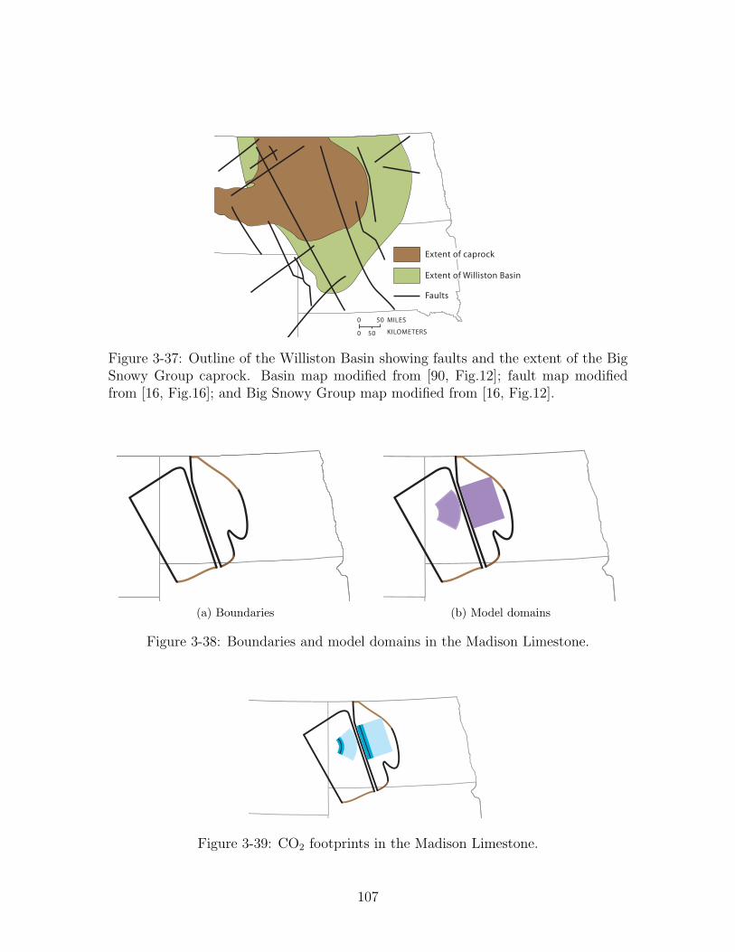
Extent of caprock
Extent of Williston Basin
Faults
0 50 MILES
KILOMETERS0 50
Figure 3-37: Outline of the Williston Basin showing faults and the extent of the BigSnowy Group caprock. Basin map modified from [90, Fig.12]; fault map modifiedfrom [16, Fig.16]; and Big Snowy Group map modified from [16, Fig.12].
(a) Boundaries (b) Model domains
Figure 3-38: Boundaries and model domains in the Madison Limestone.
Figure 3-39: CO2 footprints in the Madison Limestone.
107
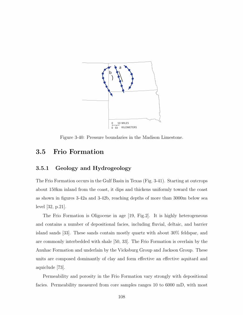
0 50 MILES
KILOMETERS0 50
ba
Figure 3-40: Pressure boundaries in the Madison Limestone.
3.5 Frio Formation
3.5.1 Geology and Hydrogeology
The Frio Formation occurs in the Gulf Basin in Texas (Fig. 3-41). Starting at outcrops
about 150km inland from the coast, it dips and thickens uniformly toward the coast
as shown in figures 3-42a and 3-42b, reaching depths of more than 3000m below sea
level [32, p.21].
The Frio Formation is Oligocene in age [19, Fig.2]. It is highly heterogeneous
and contains a number of depositional facies, including fluvial, deltaic, and barrier
island sands [33]. These sands contain mostly quartz with about 30% feldspar, and
are commonly interbedded with shale [50, 33]. The Frio Formation is overlain by the
Anuhac Formation and underlain by the Vicksburg Group and Jackson Group. These
units are composed dominantly of clay and form effective an effective aquitard and
aquiclude [73].
Permeability and porosity in the Frio Formation vary strongly with depositional
facies. Permeability measured from core samples ranges 10 to 6000 mD, with most
108
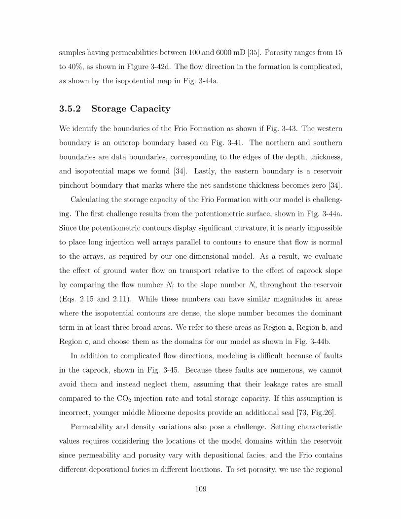
samples having permeabilities between 100 and 6000 mD [35]. Porosity ranges from 15
to 40%, as shown in Figure 3-42d. The flow direction in the formation is complicated,
as shown by the isopotential map in Fig. 3-44a.
3.5.2 Storage Capacity
We identify the boundaries of the Frio Formation as shown if Fig. 3-43. The western
boundary is an outcrop boundary based on Fig. 3-41. The northern and southern
boundaries are data boundaries, corresponding to the edges of the depth, thickness,
and isopotential maps we found [34]. Lastly, the eastern boundary is a reservoir
pinchout boundary that marks where the net sandstone thickness becomes zero [34].
Calculating the storage capacity of the Frio Formation with our model is challeng-
ing. The first challenge results from the potentiometric surface, shown in Fig. 3-44a.
Since the potentiometric contours display significant curvature, it is nearly impossible
to place long injection well arrays parallel to contours to ensure that flow is normal
to the arrays, as required by our one-dimensional model. As a result, we evaluate
the effect of ground water flow on transport relative to the effect of caprock slope
by comparing the flow number Nf to the slope number Ns throughout the reservoir
(Eqs. 2.15 and 2.11). While these numbers can have similar magnitudes in areas
where the isopotential contours are dense, the slope number becomes the dominant
term in at least three broad areas. We refer to these areas as Region a, Region b, and
Region c, and choose them as the domains for our model as shown in Fig. 3-44b.
In addition to complicated flow directions, modeling is difficult because of faults
in the caprock, shown in Fig. 3-45. Because these faults are numerous, we cannot
avoid them and instead neglect them, assuming that their leakage rates are small
compared to the CO2 injection rate and total storage capacity. If this assumption is
incorrect, younger middle Miocene deposits provide an additional seal [73, Fig.26].
Permeability and density variations also pose a challenge. Setting characteristic
values requires considering the locations of the model domains within the reservoir
since permeability and porosity vary with depositional facies, and the Frio contains
different depositional facies in different locations. To set porosity, we use the regional
109
porosity map shown in Fig. 3-42d and select an average value for each domain. Set-
ting permeability is slightly more difficult because it exhibits higher variability. Maps
show that permeability varies laterally from less than 10 mD to about 6000 mD at
scales much smaller than the model domain [35]. Variability is also large in the ver-
tical dimension, with permeability ranging from about 1 to 10,000 mD [53, Fig.27].
To characterize the Frio Formation, we choose a permeability of 500 mD, which is
approximately the mode of the data. We note, however, that this is a significant sim-
plification: as discussed previously, the large variations in permeability could greatly
affect our results.
For Region a, we calculate an average storage capacity of 9.7 Gton of CO2. For
Region b, we calculate an average capacity of 13.4 Gton of CO2. For Region c, we
calculate an average capacity of 12.7 Gton of CO2. Summing these capacities leads
to a total average capacity of 35.8 Gton of CO2 for the Frio Formation. The CO2
footprints from our calculations are shown in Fig. 3-46.
3.5.3 Injection Rate
We set the compressibility of the Frio Formation to 1.7×10⁻¹⁰ Pa−1 since the aquifer
consists mostly of sandstone (Table 3.9). We identify pressure boundaries as shown in
Fig. 3-47a. The eastern boundary is a no-flow boundary based on the where the net
sandstone thickness becomes zero as shown in Fig. 3-42c. While the net-sandstone
thickness map does not show a sandstone thickness of zero in the very southern part
of the reservoir, we assume that it becomes zero beyond the edges of the map for
consistency with the lithology of the central and northern parts of the reservoir. This
assumption is safe because it will cause us to underestimate the maximum injection
rate. The western boundary is a constant-pressure boundary based on the location of
outcrops shown in Fig. 3-41. Since the dimensionless distances from the well arrays
to this boundary are very large (ξb > 1.2), however, we model this boundary as an
infinite boundary as shown in Fig. 3-47b.
With the pressure boundaries identified, we now determine the maximum dimen-
sionless pressure pmax for each well array. We use the plot in Fig. 2-12 which shows
110
pmax as a function of ξb for semi-infinite reservoirs. For Well Array a, pmax is about
1.38 in the short–term scenario based on a dimensionless distance of about 0.32; in
the long–term scenario, pmax is about 1.47 based on a dimensionless distance of about
0.23. For Well Array b, pmax is about 1.2 in the short–term scenario based on a
dimensionless distance of about 0.49; in the long–term scenario, pmax is about 1.35
based on a dimensionless distance of about 0.34. For Well Array c, pmax is about 1.3
in the short–term scenario based on a dimensionless distance of about 0.40; in the
long–term scenario, pmax is about 1.4 based on a dimensionless distance of about 0.29
We define the fracture overpressure in the Frio Formation to be the smallest
effective horizontal stress in the reservoir, since horizontal stresses are typically the
lowest stresses in the Gulf Basin based on Fig 2-16. Using Eq. 2.51, we calculate the
effective horizontal stress to be about 9.1 MPa under well arrays a and b, and about
11.3 MPa under Well Array c.
Setting the fracture overpressure equal to the effective horizontal stress, we cal-
culate the maximum injection rate for each well array. We calculate the maximum
injection rate for Well Array a to be about 110 Mton/yr and 70 Mton/yr of CO2 in
the short–term and long–term scenarios, respectively. For Well Array b, it is about
140 Mton/yr and 87 Mton/yr in the short–term and long–term scenarios, respectively.
For Well Array c, it is about 130 Mton/yr and 88 Mton/yr in the short–term and
long–term scenarios, respectively.
111
Gulf Basin
Frio Formation
outcrop
TEXAS
0
0 50
100
100
50 MILES
KILOMETERS
Figure 3-41: Map of the Gulf Basin showing outcrops of the Frio Formation. Basinmap modified from [22]. Outcrops modified from [34, Map friooutcrop].
112
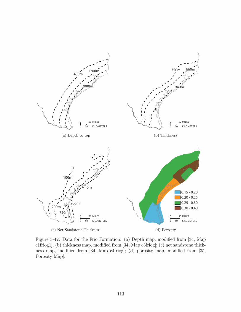
50
500
0 MILES
KILOMETERS
400m1200m
2000m
(a) Depth to top
50
500
0 MILES
KILOMETERS
1940m
660m350m
(b) Thickness
50
500
0 MILES
KILOMETERS
100m
200m200m
0m
750m
(c) Net Sandstone Thickness
0.15 - 0.20
0.20 - 0.25
0.25 - 0.30
0.30 - 0.40
50
500
0 MILES
KILOMETERS
(d) Porosity
Figure 3-42: Data for the Frio Formation. (a) Depth map, modified from [34, Mapc1friog1]; (b) thickness map, modified from [34, Map c3friog]; (c) net sandstone thick-ness map, modified from [34, Map c4friog]; (d) porosity map, modified from [35,Porosity Map].
113

50
500
0 MILES
KILOMETERS
Figure 3-43: Boundaries of the Frio Formation.
50
500
0 MILES
KILOMETERS
High head
Low head
(a) Isopotential contours
50
500
0 MILES
KILOMETERS
High head
Low head
a
b
c
(b) Model domains
Figure 3-44: Isopotential contours and model domains in the Frio Formation. Wechoose the model domains in regions in which isopotential contours are sparse so thattransport is dominated by up-slope migration. (a) Modified from [34, Map 1frio].
114
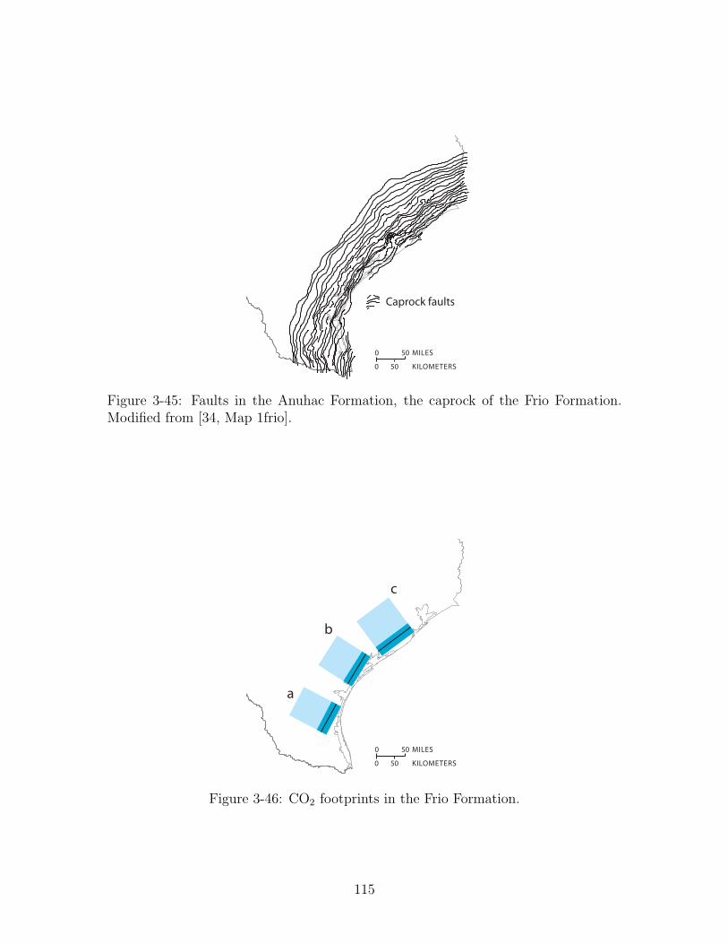
50
500
0 MILES
KILOMETERS
Caprock faults
Figure 3-45: Faults in the Anuhac Formation, the caprock of the Frio Formation.Modified from [34, Map 1frio].
50
500
0 MILES
KILOMETERS
a
b
c
Figure 3-46: CO2 footprints in the Frio Formation.
115

50
500
0 MILES
KILOMETERS
(a) Actual pressure boundaries
50
500
0 MILES
KILOMETERS
(b) Modeled pressure boundaries
Figure 3-47: Actual and modeled pressure boundaries in the Frio Formation. Wemodel the western boundary as an infinite boundary since it is very far away fromthe well arrays.
116
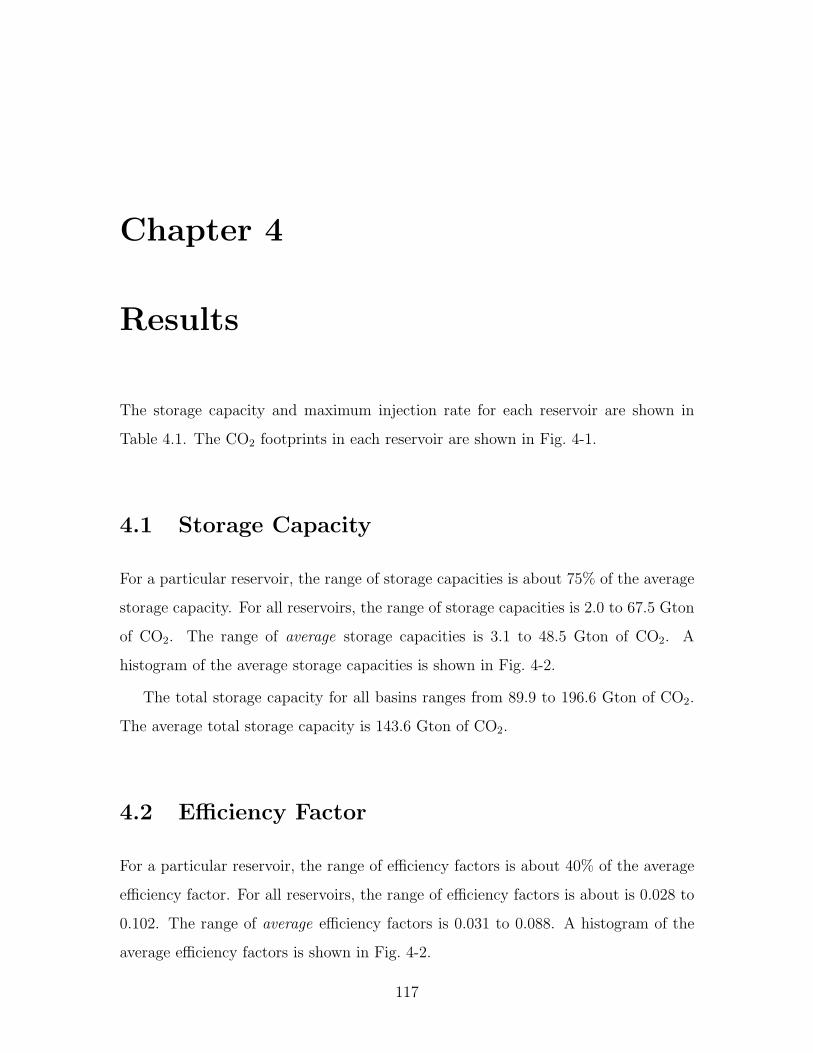
Chapter 4
Results
The storage capacity and maximum injection rate for each reservoir are shown in
Table 4.1. The CO2 footprints in each reservoir are shown in Fig. 4-1.
4.1 Storage Capacity
For a particular reservoir, the range of storage capacities is about 75% of the average
storage capacity. For all reservoirs, the range of storage capacities is 2.0 to 67.5 Gton
of CO2. The range of average storage capacities is 3.1 to 48.5 Gton of CO2. A
histogram of the average storage capacities is shown in Fig. 4-2.
The total storage capacity for all basins ranges from 89.9 to 196.6 Gton of CO2.
The average total storage capacity is 143.6 Gton of CO2.
4.2 Efficiency Factor
For a particular reservoir, the range of efficiency factors is about 40% of the average
efficiency factor. For all reservoirs, the range of efficiency factors is about is 0.028 to
0.102. The range of average efficiency factors is 0.031 to 0.088. A histogram of the
average efficiency factors is shown in Fig. 4-2.
117
4.3 Injection Rate
The injection rates we calculate are defined with respect to a particular injection
scenario: for the short–term scenario, the injection rates are the peak rates after a 25
year period of linearly ramping up injection; for the long–term scenario, they are the
peak rates after a 50 year period of linearly ramping up injection (see Fig. 2-7). For the
short–term scenario, maximum injection rates range from 22 to 750 Mton/yr of CO2,
with a mean of 230 Mton/yr. The cumulative maximum injection rate for all reservoirs
is 2300 Mton/yr of CO2. For the long–term scenario, maximum injection rates range
from 15 to 530 Mton/yr of CO2, with a mean of 160 Mton/yr. In this scenario, the
cumulative maximum injection rate is 1700 Mton/yr of CO2. A histogram of the
results is shown in Fig. 4-4.
118
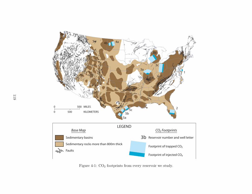
5000
5000 MILES
KILOMETERS
1
2
3c
3a
3b
4a
5a
5b5c
4b
Base Map CO2 FootprintsLEGEND
Sedimentary basins
Sedimentary rocks more than 800m thick
Faults
3b
Footprint of trapped CO2
Footprint of injected CO2
Reservoir number and well letter
Figure 4-1: CO2 footprints from every reservoir we study.
119
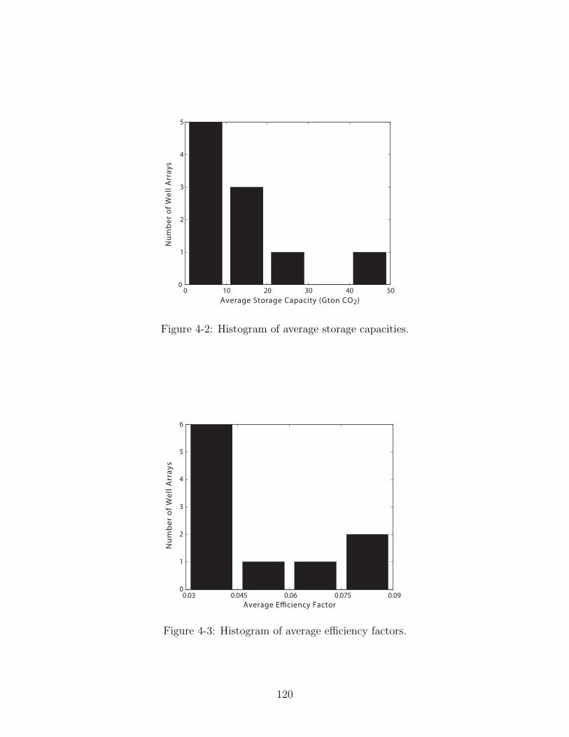
0 10 20 30 40 50 0
1
2
3
4
5
Average Storage Capacity (Gton CO2)
Nu
mb
er
of
We
ll A
rra
ys
Figure 4-2: Histogram of average storage capacities.
0.03 0.045 0.06 0.075 0.090
1
2
3
4
5
6
Average E!ciency Factor
Nu
mb
er
of
We
ll A
rra
ys
Figure 4-3: Histogram of average efficiency factors.
120
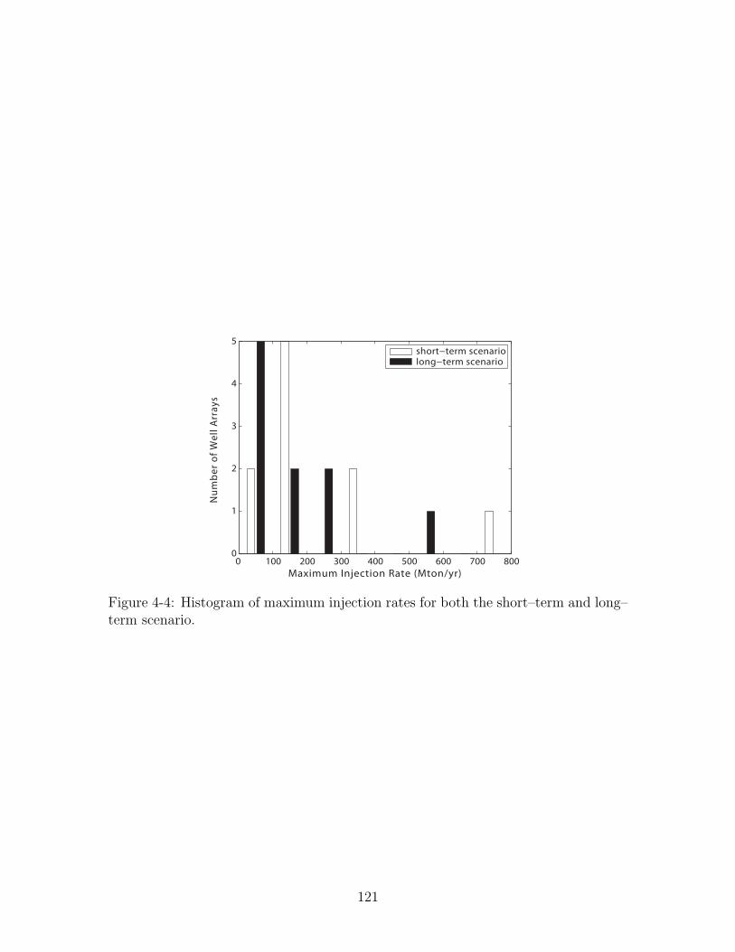
0 100 200 300 400 500 600 700 8000
1
2
3
4
5
Maximum Injection Rate (Mton/yr)
Nu
mb
er
of
We
ll A
rra
ys
short−term scenariolong−term scenario
Figure 4-4: Histogram of maximum injection rates for both the short–term and long–term scenario.
121
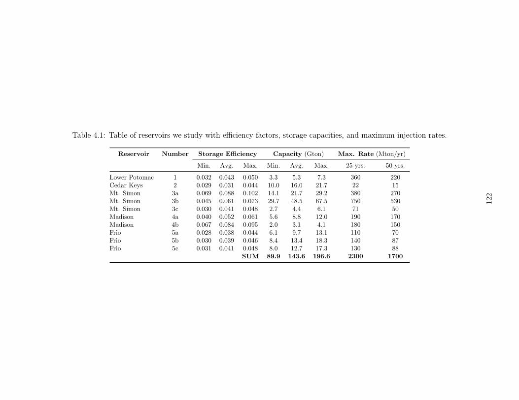
Table 4.1: Table of reservoirs we study with efficiency factors, storage capacities, and maximum injection rates.
Reservoir Number Storage Efficiency Capacity (Gton) Max. Rate (Mton/yr)
Min. Avg. Max. Min. Avg. Max. 25 yrs. 50 yrs.
Lower Potomac 1 0.032 0.043 0.050 3.3 5.3 7.3 360 220Cedar Keys 2 0.029 0.031 0.044 10.0 16.0 21.7 22 15Mt. Simon 3a 0.069 0.088 0.102 14.1 21.7 29.2 380 270Mt. Simon 3b 0.045 0.061 0.073 29.7 48.5 67.5 750 530Mt. Simon 3c 0.030 0.041 0.048 2.7 4.4 6.1 71 50Madison 4a 0.040 0.052 0.061 5.6 8.8 12.0 190 170Madison 4b 0.067 0.084 0.095 2.0 3.1 4.1 180 150Frio 5a 0.028 0.038 0.044 6.1 9.7 13.1 110 70Frio 5b 0.030 0.039 0.046 8.4 13.4 18.3 140 87Frio 5c 0.031 0.041 0.048 8.0 12.7 17.3 130 88
SUM 89.9 143.6 196.6 2300 1700
122
Chapter 5
Discussion and Conclusions
5.1 Estimation of Future US Emissions
We compare our results with estimates of CO2 emissions from the United States
over the next 50 years. Our estimates have four main features. First, we consider
only emissions from coal-burning power plants. This simplification is justified for
three reasons. First, we focus on emissions from energy consumption because these
emissions account for most emissions in the United States: since 2000, the CO2
emitted due to energy consumption has been at least 99% by mass of the total CO2
emitted [17, Table 5]. Second, we focus on power plants because they are large point
sources where CO2 capture technology will likely first be deployed [39]. Third, we
focus on coal-burning power plants because they emit more CO2 than any other type
of power plant: since 2000, coal-burning plants have emitted at least 80% by mass of
the total CO2 emitted by electricity–producing power plants [17, 61].
The second key feature in our estimation is the emission scenario: we consider
a high-emissions, end-member scenario derived from Monte Carlo simulations that
consider how 100 parameters such as energy-usage trends and fossil fuel availability
contribute to future emissions [88]. In this scenario, coal consumption grows by a
factor of 2.7 over the next 50 years. We also assume that emissions grow by an
additional factor of 1.3 to based on the increased energy demands of CO2 capture
processes [88].
123
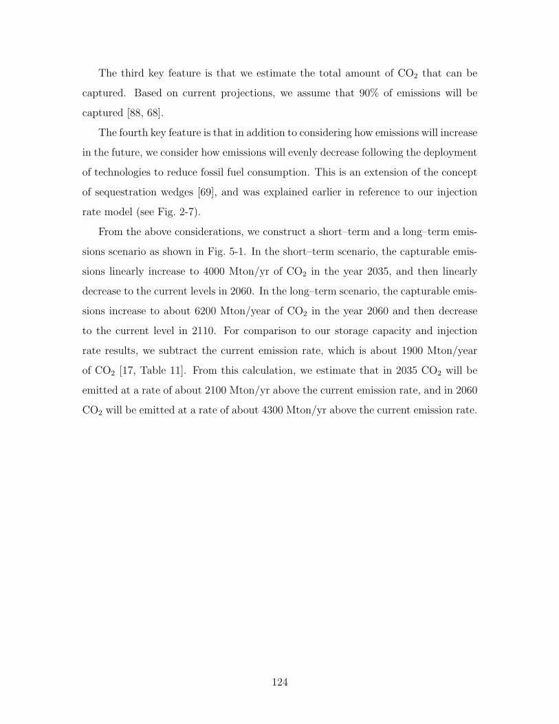
The third key feature is that we estimate the total amount of CO2 that can be
captured. Based on current projections, we assume that 90% of emissions will be
captured [88, 68].
The fourth key feature is that in addition to considering how emissions will increase
in the future, we consider how emissions will evenly decrease following the deployment
of technologies to reduce fossil fuel consumption. This is an extension of the concept
of sequestration wedges [69], and was explained earlier in reference to our injection
rate model (see Fig. 2-7).
From the above considerations, we construct a short–term and a long–term emis-
sions scenario as shown in Fig. 5-1. In the short–term scenario, the capturable emis-
sions linearly increase to 4000 Mton/yr of CO2 in the year 2035, and then linearly
decrease to the current levels in 2060. In the long–term scenario, the capturable emis-
sions increase to about 6200 Mton/year of CO2 in the year 2060 and then decrease
to the current level in 2110. For comparison to our storage capacity and injection
rate results, we subtract the current emission rate, which is about 1900 Mton/year
of CO2 [17, Table 11]. From this calculation, we estimate that in 2035 CO2 will be
emitted at a rate of about 2100 Mton/yr above the current emission rate, and in 2060
CO2 will be emitted at a rate of about 4300 Mton/yr above the current emission rate.
124
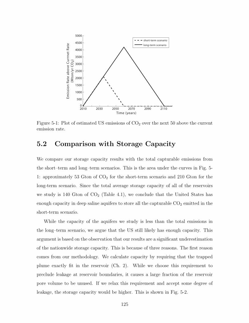
2010 2030 2050 2070 2090 21100
500
1000
1500
2000
2500
3000
3500
4000
4500
5000
Time (years)
Em
issi
on
Ra
te a
bo
ve
Cu
rrn
et
Ra
te
(Mto
n/y
r C
O2
)
long-term scenario
short-term scenario
Figure 5-1: Plot of estimated US emissions of CO2 over the next 50 above the currentemission rate.
5.2 Comparison with Storage Capacity
We compare our storage capacity results with the total capturable emissions from
the short–term and long–term scenarios. This is the area under the curves in Fig. 5-
1: approximately 53 Gton of CO2 for the short-term scenario and 210 Gton for the
long-term scenario. Since the total average storage capacity of all of the reservoirs
we study is 140 Gton of CO2 (Table 4.1), we conclude that the United States has
enough capacity in deep saline aquifers to store all the capturable CO2 emitted in the
short-term scenario.
While the capacity of the aquifers we study is less than the total emissions in
the long–term scenario, we argue that the US still likely has enough capacity. This
argument is based on the observation that our results are a significant underestimation
of the nationwide storage capacity. This is because of three reasons. The first reason
comes from our methodology. We calculate capacity by requiring that the trapped
plume exactly fit in the reservoir (Ch. 2). While we choose this requirement to
preclude leakage at reservoir boundaries, it causes a large fraction of the reservoir
pore volume to be unused. If we relax this requirement and accept some degree of
leakage, the storage capacity would be higher. This is shown in Fig. 5-2.
125
0 10 20 30 40 500
1
ξ
1-h
-10
Re
se
rvo
ir Bo
un
da
ry
(a) Plume fits in the reservoir
0 10 20 30 40 500
1
ξ
1-h
Re
se
rvo
ir Bo
un
da
ry
-10
Leaked CO2
(b) Plume exceeds the reservoir
Figure 5-2: Illustration of how requiring the CO2 plume to fit in the reservoir leadsto a low estimation of the reservoir’s capacity. (a) When the plume fits exactly inthe reservoir, no CO2 is lost to leakage, but a large fraction of the reservoir is notinfiltrated by CO2 and is not used for storage. (b) When the plume exceeds the sizeof the reservoir, some CO2 is lost to leakage, but more of the reservoir is infiltratedby CO2 and is used for storage.
The second reason that we underestimate capacity is that we do not model the
whole reservoir. As discussed in Ch. 3, the area of a reservoir that we can model is
limited because our model is one dimensional. Typically, the area that we model is no
more than 50% of the area within the reservoir boundaries. As a result, the capacity
of a reservoir is likely at least twice as large as the capacity we calculate.
The final reason that we underestimate the country’s capacity is that we model
only a small fraction of available reservoirs: we model reservoirs in only five basins,
but there are over thirty basins in the conterminous United States (Fig. 1-1). Many of
them, such as the Anadarko Basin, are large and equally amenable to sequestration.
In addition, we model only one reservoir in each basin we do study. In most cases,
however, a basin contains many reservoirs that could be used for sequestration. The
Illinois Basin, for example, contains the St. Peter Sandstone, and the Gulf Coast
Basin contains the Jasper Interval [36].
126
5.3 Comparison with Injection Rate
We compare our injection rate results with the maximum emission rates in the short–
term and long–term scenarios. These are the emission rates at the peaks in Fig. 5-1:
2100 Mton/year of CO2 in the short–term scenario and 4200 Mton/yr in the long–
term scenario. Since the cumulative maximum injection rate we calculate for all the
aquifers in the short–term scenario is 2300 Mton/yr of CO2, we conclude that the
United States can sequester CO2 at the same rate it is emitted in the short–term
scenario. The cumulative maximum injection rate for all the aquifers in the long–
term scenario (1700 Mton/yr), however, is smaller than the peak emissions rate in the
long–term scenario (4200 Mton/year). This suggests that for the long–term scenario,
the US would not be able to sequester CO2 at the same rate it is emitted without
risking fracturing one or more of the aquifers.
127

128

Appendix A
Data
This appendix lists all input data to our models. As discussed in the text, values for
depth, net thickness, porosity, caprock slope, Darcy velocity, intrinsic permeability,
density, viscosity, and compressibility are averages over the model domain. Negative
values for slope indicate that up-slope migration occurs in the opposite direction of
transport due to ground water flow.
129
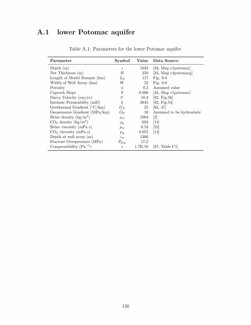
A.1 lower Potomac aquifer
Table A.1: Parameters for the lower Potomac aquifer.
Parameter Symbol Value Data Source
Depth (m) z 1033 [34, Map c1potomac]Net Thickness (m) H 250 [34, Map c4potomacg]Length of Model Domain (km) Ld 117 Fig. 3-8Width of Well Array (km) W 52 Fig. 3-8Porosity φ 0.2 Assumed valueCaprock Slope θ 0.006 [34, Map c1potomac]Darcy Velocity (cm/yr) U 10.3 [82, Fig.56]Intrinsic Permeability (mD) k 2845 [82, Fig.54]Geothermal Gradient (◦C/km) GT 25 [62, 47]Geopressure Gradient (MPa/km) GP 10 Assumed to be hydrostaticBrine density (kg/m3) ρw 1004 [2]CO2 density (kg/m3) ρg 683 [14]Brine viscosity (mPa s) µw 0.53 [52]CO2 viscosity (mPa s) µg 0.055 [14]Depth at well array (m) zw 1300Fracture Overpressure (MPa) Pfrac 17.2Compressibility (Pa−1) c 1.7E-10 [87, Table C1]
130

A.2 Lawson Formation and Cedar Keys Formation
Table A.2: Parameters for the Lawson and Cedar Keys Formation.
Parameter Symbol Value Data Source
Depth (m) z 1368 [34, Map c1cedarkey]Net Thickness (m) H 383 [34, Map c3cedarkeyg]Length of Model Domain (km) Ld 147 Fig. 3-21bWidth of Well Array (km) W 155 Fig. 3-21bPorosity φ 0.26 [36]Caprock Slope θ 0.003 [34, Map c1cedarkey]Darcy Velocity (cm/yr) U 1.75 [60, Fig.60]Intrinsic Permeability (mD) k 15 [27, quoted in [36]]Geothermal Gradient (◦C/km) GT 59 [24]Geopressure Gradient (MPa/km) GP 10 Assumed to be hydrostaticBrine density (kg/m3) ρw 963 [2]CO2 density (kg/m3) ρg 307 [14]Brine viscosity (mPa s) µw 0.30 [52]CO2 viscosity (mPa s) µg 0.027 [14]Depth at well array (m) zw 1500Fracture Overpressure (MPa) Pfrac 8.5Compressibility (Pa−1) c 5.84E-11 [87, Table C1]
131
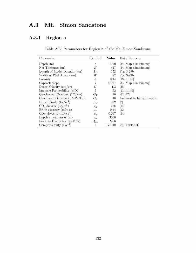
A.3 Mt. Simon Sandstone
A.3.1 Region a
Table A.3: Parameters for Region b of the Mt. Simon Sandstone.
Parameter Symbol Value Data Source
Depth (m) z 1920 [34, Map c1mtsimong]Net Thickness (m) H 417 [34, Map c3mtsimong]Length of Model Domain (km) Ld 152 Fig. 3-29bWidth of Well Array (km) W 82 Fig. 3-29bPorosity φ 0.14 [13, p.140]Caprock Slope θ 0.007 [34, Map c1mtsimong]Darcy Velocity (cm/yr) U 1.3 [35]Intrinsic Permeability (mD) k 52 [13, p.140]Geothermal Gradient (◦C/km) GT 20 [62, 47]Geopressure Gradient (MPa/km) GP 10 Assumed to be hydrostaticBrine density (kg/m3) ρw 992 [2]CO2 density (kg/m3) ρg 768 [14]Brine viscosity (mPa s) µw 0.44 [52]CO2 viscosity (mPa s) µg 0.067 [14]Depth at well array (m) zw 3000Fracture Overpressure (MPa) Pfrac 39.6Compressibility (Pa−1) c 1.7E-10 [87, Table C1]
132

A.3.2 Region b
Table A.4: Parameters for Region b of the Mt. Simon Sandstone.
Parameter Symbol Value Data Source
Depth (m) z 2667 [34, Map c1mtsimong]Net Thickness (m) H 317 [34, Map c3mtsimong]Length of Model Domain (km) Ld 213 Fig. 3-29bWidth of Well Array (km) W 181 Fig. 3-29bPorosity φ 0.14 [13, p.140]Caprock Slope θ 0.012 [34, Map c1mtsimong]Darcy Velocity (cm/yr) U 5.1 [35]Intrinsic Permeability (mD) k 52 [13, p.140]Geothermal Gradient (◦C/km) GT 20 [62, 47]Geopressure Gradient (MPa/km) GP 10 Assumed to be hydrostaticBrine density (kg/m3) ρw 991 [2]CO2 density (kg/m3) ρg 769 [14]Brine viscosity (mPa s) µw 0.42 [52]CO2 viscosity (mPa s) µg 0.068 [14]Depth at well array (m) zw 3450Fracture Overpressure (MPa) Pfrac 45.5Compressibility (Pa−1) c 1.7E-10 [87, Table C1]
133
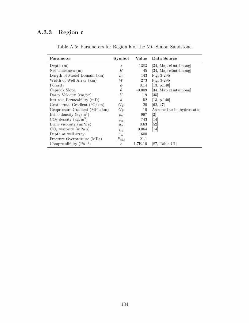
A.3.3 Region c
Table A.5: Parameters for Region b of the Mt. Simon Sandstone.
Parameter Symbol Value Data Source
Depth (m) z 1383 [34, Map c1mtsimong]Net Thickness (m) H 45 [34, Map c3mtsimong]Length of Model Domain (km) Ld 143 Fig. 3-29bWidth of Well Array (km) W 273 Fig. 3-29bPorosity φ 0.14 [13, p.140]Caprock Slope θ -0.009 [34, Map c1mtsimong]Darcy Velocity (cm/yr) U 1.9 [35]Intrinsic Permeability (mD) k 52 [13, p.140]Geothermal Gradient (◦C/km) GT 20 [62, 47]Geopressure Gradient (MPa/km) GP 10 Assumed to be hydrostaticBrine density (kg/m3) ρw 997 [2]CO2 density (kg/m3) ρg 743 [14]Brine viscosity (mPa s) µw 0.63 [52]CO2 viscosity (mPa s) µg 0.064 [14]Depth at well array zw 1600Fracture Overpressure (MPa) Pfrac 21.1Compressibility (Pa−1) c 1.7E-10 [87, Table C1]
134
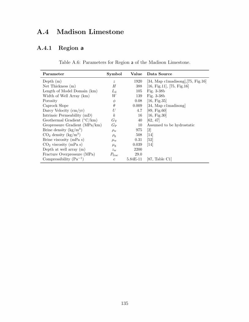
A.4 Madison Limestone
A.4.1 Region a
Table A.6: Parameters for Region a of the Madison Limestone.
Parameter Symbol Value Data Source
Depth (m) z 1920 [34, Map c1madisong],[75, Fig.16]Net Thickness (m) H 388 [16, Fig.11], [75, Fig.16]Length of Model Domain (km) Ld 105 Fig. 3-38bWidth of Well Array (km) W 139 Fig. 3-38bPorosity φ 0.08 [16, Fig.35]Caprock Slope θ 0.009 [34, Map c1madisong]Darcy Velocity (cm/yr) U 4.7 [89, Fig.60]Intrinsic Permeability (mD) k 16 [16, Fig.30]Geothermal Gradient (◦C/km) GT 40 [62, 47]Geopressure Gradient (MPa/km) GP 10 Assumed to be hydrostaticBrine density (kg/m3) ρw 975 [2]CO2 density (kg/m3) ρg 508 [14]Brine viscosity (mPa s) µw 0.31 [52]CO2 viscosity (mPa s) µg 0.039 [14]Depth at well array (m) zw 2200Fracture Overpressure (MPa) Pfrac 29.0Compressibility (Pa−1) c 5.84E-11 [87, Table C1]
135

A.4.2 Region b
Table A.7: Parameters for Region b of the Madison Limestone.
Parameter Symbol Value Data Source
Depth (m) z 2801 [34, Map c1madisong],[75, Fig.16]Net Thickness (m) H 309 [16, Fig.11], [75, Fig.16]Length of Model Domain (km) Ld 71 Fig. 3-38bWidth of Well Array (km) W 65 Fig. 3-38bPorosity φ 0.08 [16, Fig.35]Caprock Slope θ 0.003 [34, Map c1madisong]Darcy Velocity (cm/yr) U 31 [89, Fig.60]Intrinsic Permeability (mD) k 58 [16, Fig.30]Geothermal Gradient (◦C/km) GT 40 [62, 47]Geopressure Gradient (MPa/km) GP 10 Assumed to be hydrostaticBrine density (kg/m3) ρw 954 [2]CO2 density (kg/m3) ρg 535 [14]Brine viscosity (mPa s) µw 0.22 [52]CO2 viscosity (mPa s) µg 0.042 [14]Depth at well array (m) zw 2700Fracture Overpressure (MPa) Pfrac 35.6Compressibility (Pa−1) c 5.84E-11 [87, Table C1]
136
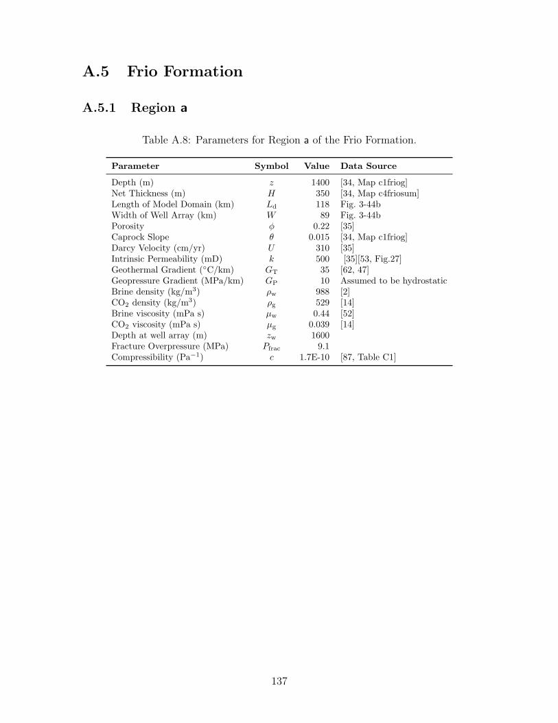
A.5 Frio Formation
A.5.1 Region a
Table A.8: Parameters for Region a of the Frio Formation.
Parameter Symbol Value Data Source
Depth (m) z 1400 [34, Map c1friog]Net Thickness (m) H 350 [34, Map c4friosum]Length of Model Domain (km) Ld 118 Fig. 3-44bWidth of Well Array (km) W 89 Fig. 3-44bPorosity φ 0.22 [35]Caprock Slope θ 0.015 [34, Map c1friog]Darcy Velocity (cm/yr) U 310 [35]Intrinsic Permeability (mD) k 500 [35][53, Fig.27]Geothermal Gradient (◦C/km) GT 35 [62, 47]Geopressure Gradient (MPa/km) GP 10 Assumed to be hydrostaticBrine density (kg/m3) ρw 988 [2]CO2 density (kg/m3) ρg 529 [14]Brine viscosity (mPa s) µw 0.44 [52]CO2 viscosity (mPa s) µg 0.039 [14]Depth at well array (m) zw 1600Fracture Overpressure (MPa) Pfrac 9.1Compressibility (Pa−1) c 1.7E-10 [87, Table C1]
137

A.5.2 Region b
Table A.9: Parameters for Region b of the Frio Formation.
Parameter Symbol Value Data Source
Depth (m) z 1467 [34, Map c1friog]Net Thickness (m) H 350 [34, Map c4friosum]Length of Model Domain (km) Ld 111 Fig. 3-44bWidth of Well Array (km) W 98 Fig. 3-44bPorosity φ 0.28 [35]Caprock Slope θ 0.016 [34, Map c1friog]Darcy Velocity (cm/yr) U 203 [35]Intrinsic Permeability (mD) k 500 [35][53, Fig.27]Geothermal Gradient (◦C/km) GT 35 [62, 47]Geopressure Gradient (MPa/km) GP 10 Assumed to be hydrostaticBrine density (kg/m3) ρw 987 [2]CO2 density (kg/m3) ρg 537 [14]Brine viscosity (mPa s) µw 0.43 [52]CO2 viscosity (mPa s) µg 0.040 [14]Depth at well array (m) zw 1600Fracture Overpressure (MPa) Pfrac 9.1Compressibility (Pa−1) c 1.7E-10 [87, Table C1]
138

A.5.3 Region c
Table A.10: Parameters for Region c of the Frio Formation.
Parameter Symbol Value Data Source
Depth (m) z 1533 [34, Map c1friog]Net Thickness (m) H 250 [34, Map c4friosum]Length of Model Domain (km) Ld 121 Fig. 3-44bWidth of Well Array (km) W 112 Fig. 3-44bPorosity φ 0.28 [35]Caprock Slope θ 0.017 [34, Map c1friog]Darcy Velocity (cm/yr) U 180 [35]Intrinsic Permeability (mD) k 500 [35][53, Fig.27]Geothermal Gradient (◦C/km) GT 35 [62, 47]Geopressure Gradient (MPa/km) GP 10 Assumed to be hydrostaticBrine density (kg/m3) ρw 986 [2]CO2 density (kg/m3) ρg 544 [14]Brine viscosity (mPa s) µw 0.42 [52]CO2 viscosity (mPa s) µg 0.041 [14]Depth at well array (m) zw 2000Fracture Overpressure (MPa) Pfrac 11.3Compressibility (Pa−1) c 1.7E-10 [87, Table C1]
139

140
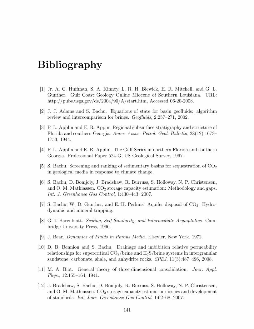
Bibliography
[1] Jr. A. C. Huffman, S. A. Kinney, L. R. H. Biewick, H. R. Mitchell, and G. L.Gunther. Gulf Coast Geology Online–Miocene of Southern Louisiana. URL:http://pubs.usgs.gov/ds/2004/90/A/start.htm, Accessed 06-20-2008.
[2] J. J. Adams and S. Bachu. Equations of state for basin geofluids: algorithmreview and intercomparison for brines. Geofluids, 2:257–271, 2002.
[3] P. L. Applin and E. R. Appin. Regional subsurface stratigraphy and structure ofFlorida and southern Georgia. Amer. Assoc. Petrol. Geol. Bulletin, 28(12):1673–1753, 1944.
[4] P. L. Applin and E. R. Applin. The Gulf Series in northern Florida and southernGeorgia. Professional Paper 524-G, US Geological Survey, 1967.
[5] S. Bachu. Screening and ranking of sedimentary basins for sequestration of CO2
in geological media in response to climate change.
[6] S. Bachu, D. Bonijoly, J. Bradshaw, R. Burruss, S. Holloway, N. P. Christensen,and O. M. Mathiassen. CO2 storage capacity estimation: Methodology and gaps.Int. J. Greenhouse Gas Control, 1:430–443, 2007.
[7] S. Bachu, W. D. Gunther, and E. H. Perkins. Aquifer disposal of CO2: Hydro-dynamic and mineral trapping.
[8] G. I. Barenblatt. Scaling, Self-Similarity, and Intermediate Asymptotics. Cam-bridge University Press, 1996.
[9] J. Bear. Dynamics of Fluids in Porous Media. Elsevier, New York, 1972.
[10] D. B. Bennion and S. Bachu. Drainage and imbibition relative permeabilityrelationships for supercritical CO2/brine and H2S/brine systems in intergranularsandstone, carbonate, shale, and anhydrite rocks. SPEJ, 11(3):487–496, 2008.
[11] M. A. Biot. General theory of three-dimensional consolidation. Jour. Appl.Phys., 12:155–164, 1941.
[12] J. Bradshaw, S. Bachu, D. Bonijoly, R. Burruss, S. Holloway, N. P. Christensen,and O. M. Mathiassen. CO2 storage capacity estimation: issues and developmentof standards. Int. Jour. Greenhouse Gas Control, 1:62–68, 2007.
141
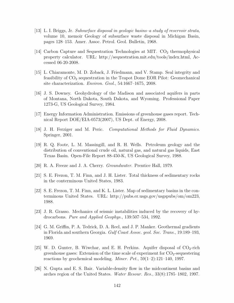
[13] L. I. Briggs, Jr. Subsurface disposal in geologic basins–a study of reservoir strata,volume 10, memoir Geology of subsurface waste disposal in Michigan Basin,pages 128–153. Amer. Assoc. Petrol. Geol. Bulletin, 1968.
[14] Carbon Capture and Sequestration Technologies at MIT. CO2 thermophysicalproperty calculator. URL: http://sequestration.mit.edu/tools/index.html, Ac-cessed 06-20-2008.
[15] L. Chiaramonte, M. D. Zoback, J. Friedmann, and V. Stamp. Seal integrity andfeasibility of CO2 sequestration in the Teapot Dome EOR Pilot: Geomechanicalsite characterization. Environ. Geol., 54:1667–1675, 2008.
[16] J. S. Downey. Geohydrology of the Madison and associated aquifers in partsof Montana, North Dakota, South Dakota, and Wyoming. Professional Paper1273-G, US Geological Survey, 1984.
[17] Energy Information Administration. Emissions of greenhouse gases report. Tech-nical Report DOE/EIA-0573(2007), US Dept. of Energy, 2008.
[18] J. H. Ferziger and M. Peric. Computational Methods for Fluid Dynamics.Springer, 2001.
[19] R. Q. Foote, L. M. Massingill, and R. H. Wells. Petroleum geology and thedistribution of conventional crude oil, natural gas, and natural gas liquids, EastTexas Basin. Open-File Report 88-450-K, US Geological Survey, 1988.
[20] R. A. Freeze and J. A. Cherry. Groundwater. Prentice Hall, 1979.
[21] S. E. Frezon, T. M. Finn, and J. H. Lister. Total thickness of sedimentary rocksin the conterminous United States, 1983.
[22] S. E. Frezon, T. M. Finn, and K. L. Lister. Map of sedimentary basins in the con-terminous United States. URL: http://pubs.er.usgs.gov/usgspubs/om/om223,1988.
[23] J. R. Grasso. Mechanics of seismic instabilities induced by the recovery of hy-drocarbons. Pure and Applied Geophys., 139:507–534, 1992.
[24] G. M. Griffin, P. A. Tedrick, D. A. Reel, and J. P. Manker. Geothermal gradientsin Florida and southern Georgia. Gulf Coast Assoc. geol. Soc. Trans., 19:189–193,1969.
[25] W. D. Gunter, B. Wiwchar, and E. H. Perkins. Aquifer disposal of CO2-richgreenhouse gases: Extension of the time scale of experiment for CO2-sequesteringreactions by geochemical modeling. Miner. Pet., 59(1–2):121–140, 1997.
[26] N. Gupta and E. S. Bair. Variable-density flow in the midcontinent basins andarches region of the United States. Water Resour. Res., 33(8):1785–1802, 1997.
142
[27] J. Haberfeld. personal communication, 2000. Cited in Hovorka et. al. 2003. Brineformation database.
[28] M. A. Hesse, H. A. Tchelepi, B. J. Cantwel, and F. M. Orr, Jr. Gravity currentsin horizontal porous layers: transition from early to late self-similarity. J. FluidMech., 577:363–383, 2007.
[29] M. A. Hesse, H. A. Tchelepi, and F. M. Orr, Jr. Scaling analysis of the migrationof CO2 in saline aquifers. In SPE Annual Technical Conference and Exhibition,San Antonio, TX, September 24–27 2006. (SPE 102796).
[30] M. Hoffert, K. Caldeira, G. Benford, D. Criswell, C. Green, H. Herzog, A. Jain,H. Kheshgi, K. Lackner, J. Lewis, H. Douglas Lightfoot, W. Manheimer,J. Mankins, M. Mauel, L. J. Perkins, M. E. Schlesinger, T. Volk, and T. M. L.Wigley. Advanced technology paths to global climate stability: Energy for agreenhouse planet. Science, 298:981–987, 2002.
[31] M. I. Hoffert, K. Caldeira, A. K. Jain, E. F. Haites, L. D. D. Harvey, S. D.Potter, M. E. Schlesinger, S. H. Schneider, R. G. Watts, T. M. L. Wigley, andD. J. Wuebbles. Energy implications of future stabilization of atmospheric CO2
content. Nature, 395(6704):881–884, 1998.
[32] S. D. Hovorka. Optimal geological environments for carbon dioxide disposalin saline aquifers in the United States. Contract Report DE-AC26-98FT40417,Bureau of Economic Geology, The University of Texas at Austin, 1999.
[33] S. D. Hovorka, C. Doughty, P. R. Knox, C. T. Green, K. Pruess, and S. M. Ben-son. Evaluation of brine-bearing sands of the Frio Formation, Upper Texas GulfCoast for geologic sequestration of CO2. Technical report, Bureau of EconomicGeology, 2001.
[34] S. D. Hovorka, M. L. Romero, A. G. Warne, W. A. Ambrose, T. A. Trem-blay, R. H. Trevino, and D. Sasson. Brine-formation database. URL:http://www.beg.utexas.edu/environqlty/co2seq/dispslsalnt01.htm, Accessed 06-26-2008., November 2003.
[35] S. D. Hovorka, M. L. Romero, A. G. Warne, W. A. Ambrose, T. A. Trem-blay, R. H. Trevino, and D. Sasson. Brine-formation database. URL:http://www.beg.utexas.edu/environqlty/co2seq/, Accessed 06-26-2008., Novem-ber 2003.
[36] S. D. Hovorka, M. L. Romero, A. G. Warne, W. A. Ambrose, T. A. Tremblay,R. H. Trevino, and D. Sasson. Sequestration of greenhouse gases in brine forma-tions. URL: http://www.beg.utexas.edu/environqlty/co2seq/dispslsalnt01.htm,November 2003. Accessed 05-20-2008.
[37] J. R. Hunt, N. Sitar, and K. S. Udell. Nonaqueous phase liquid transport andcleanup: 1. Analysis of mechanisms. Water Resour. Res., 24(8):1247–1258, 1988.
143
[38] H. E. Huppert and A. W. Woods. Gravity-driven flows in porous media. J. FluidMech., 292:55–69, 1995.
[39] IPCC. Special Report on Carbon Dioxide Capture and Storage, B. Metz et al.(eds.). Cambridge University Press, 2005.
[40] J. Jaeger, N. G. Cook, and R. Zimmerman. Fundamentals of Rock Mechanics.Wiley-Blackwell, 2007.
[41] R. Juanes, C. MacMinn, and M. Szulczewski. The footprint of the co2 plumeduring carbon dioxide storage in saline aquifers: storage efficiency for capillarytrapping at the basin scale. Transp. Porous. Media, 2009. Accepted manuscript.
[42] R. Juanes and C. W. MacMinn. Upscaling of capillary trapping under gravityoverride: Application to CO2 sequestration in aquifers. In SPE/DOE Symposiumon Improved Oil Recovery, Tulsa, OK, April 19–23, 2008. (SPE 113496).
[43] R. Juanes, E. J. Spiteri, F. M. Orr, Jr., and M. J. Blunt. Impact of relativepermeability hysteresis on geological CO2 storage.
[44] P. B. King and H. M. Beikman. Geologic map of the United States. US GeologicalSurvey, 1974.
[45] I. N. Kochina, N. N. Mikhailov, and M. V. Filinov. Groundwater mound damp-ing. Int. J. Eng. Sci., 21:413–421, 1983.
[46] D. R. Kolata. Interior Cratonic Basins, chapter 2, pages 59–73. Amer. Assoc.Petrol. Geol. Bulletin, 1990.
[47] A. Kron and G. Heiken. Geothermal gradient map of the United States. Technicalreport, Los Alamos National Lab, 1980.
[48] A. Kumar, R. Ozah, M. Noh, G. A. Pope, S. Bryant, K. Sepehrnoori, and L. W.Lake. Reservoir simulation of CO2 storage in deep saline aquifers. Soc. Pet. Eng.J., 10(3):336–348, September 2005.
[49] K. S. Lackner. A guide to CO2 sequestration. Science, 300(5626):1677–1678,2003.
[50] L. S. Land and G. L. Macpherson. Origin of saline formation water, Cenozoicsection, Gulf of Mexico Sedimentary Basin. Amer. Assoc. Petrol. Geol. Bulletin,76(9):1344–1362, 1992.
[51] X. Lei, G. Yu, S. Ma, X. Wen, and Q. Wang. Earthquakes induced by waterinjection at 3km depth within the Rongchang gas field, Chongqing, China. JGR,113:B10310, 2008.
[52] E. R. Likhachev. Dependence of water viscosity on temperature and pressure.Technical Physics, 48(4):514–515, 2003.
144
[53] R. G. Loucks, M. M. Dodge, and W. E. Galloway. Clastic Diagenesis, chapterRegional controls on diagenesis and reservoir quality in lower Tertiary sandstonesalong the lower Texas Gulf Coast, pages 15–45. Amer. Assoc. Petrol. Geol.Bulletin, 1984.
[54] A. Lucier and M. Zoback. Assessing the economic feasbility of regional deep salineaquifer CO2 injection and storage: a geomechanics-based workflow applied to theRose Run Sandstone in eastern Ohio, USA. Int. Jour. Greenhouse Gas Control,2:230–247, 2008.
[55] S. Lyle, H. E. Huppert, M. Hallworth, M. Bickle, and A. Chadwick. Axisym-metric gravity currents in a porous medium. J. Fluid Mech., 543:293–302, 2005.
[56] R. J. Mandle and A. L. Kontis. Simulation of regional ground-water flow in theCambrian-Ordovician aquifer system in the northern Midwest, United States.Professional Paper 1405-C, US Geological Survey, 1992.
[57] G. Marland, B. Andres, and T. Boden. Global CO2 emissions from fossil-fuel burning, cement manufacture, and gas flaring: 1751–2005. URL:http://cdiac.ornl.gov/ftp/ndp030/global.1751 2005.ems, August 2008.
[58] A. S. Mayer and C. T. Miller. An experimental investigation of pore-scale dis-tributions of nonaqueous phase liquids at residual saturation. Transp. PorousMedia, 10(1):57–80, 1993.
[59] A. McGarr and N. C. Gay. State of stress in the Earth’s crust. Ann. Rev. EarthPlanet. Sci., 6:405–436, 1978.
[60] J. A. Miller. The ground water atlas of the UnitedStates: Alabama, Florida, Georgia, South Carolina. URL:http://capp.water.usgs.gov/gwa/ch g/index.html, 1990. Accessed 05-20-2008.
[61] MIT. The Future of Coal – An Interdisciplinary MIT Study, J. Deutch and E.J. Moniz (eds.). MIT Press, 2007.
[62] M. Nathenson and M. Guffanti. Geothermal gradients in the conterminousUnited States. J. Geophys. Res., 93:6437–6450, 1988.
[63] J. Nicot. Evaluation of large-scale CO2 storage on fresh-water sections of aquifers:An example from the Texas Gulf Coast Basin. Int. J. Greenhouse Gas Control,2:582–593, 2008.
[64] J. M. Nordbotten, M. A. Celia, and S. Bachu. Analytical solution for CO2 plumeevolution during injection.
[65] Jr. O. B. Lloyd and W. L. Lyke. The ground water atlas of theUnited States: Illinois, Indiana, Kentucky, Ohio, Tennessee. URL:http://capp.water.usgs.gov/gwa/ch k/index.html, 1995. Accessed 05-20-2008.
145
[66] M. J. Oak, L. E. Baker, and D. C. Thomas. Three-phase relative permeabilityof Berea sandstone. J. Pet. Technol., 42(8):1054–1061, August 1990.
[67] P. G. Olcott. The ground water atlas of the United States: Iowa, Michigan,Minnesota, Wisconsin. URL: http://capp.water.usgs.gov/gwa/ch j/index.html,1992. Accessed 05-20-2008.
[68] V. M. Otto and J. Reilly. Directed technical change and the adoption of CO2
abatement technology: the case of CO2 capture and storage. MIT Joint ProgramReport 139, MIT, 2006.
[69] S. Pacala and R. Socolow. Stability wedges: Solving the climate problem for thenext 50 years with current technologies. Science, 305:968–972, 2004.
[70] K. Pruess and J. Garcıa. Multiphase flow dynamics during CO2 disposal intosaline aquifers.
[71] J. Ridgley. A rebirth of the Illinois Basin. Fact Sheet FS-023-97, US GeologicalSurvey, 1997.
[72] J. Rutqvist, J. Birkholzer, F. Cappa, and C. F. Tsang. Estimating maximumsustainable injection pressure during geological sequestration of CO2 using cou-pled fluid flow and geomechanical fault-slip analysis. Energy Conv. Manag.,48:1798–1807, 2007.
[73] P. D. Ryder and A. F. Ardis. Hydrology of the Texas Gulf Coast aquifer systems.Open-File Report 91-64, US Geological Survey, 1991.
[74] R. T. Ryder, J. E. Repetski, A. G. Harris, and E. E. Lent. Stratigraphic frame-work of Cambrian and Ordovician rocks in the central Appalachian Basin fromCampbell County, Kentucky, to Tazwell County, Virginia. IMAP 2530, US Ge-ological Survey, 2004.
[75] C. A. Sandberg. Geology of the Williston Basin, North Dakota, Montana, andSouth Dakota, with reference to subsurface disposal of radioactive wastes. Open-File Report 62-115, US Geological Survey, 1962.
[76] D. P. Schrag. Preparing to capture carbon. Science, 315:812–813, 2007.
[77] P.G. Schruben, R. E. Arndt, and W. J. Bawiec. Geology of theconterminous United States at 1:2,500,000 scale–a digital representa-tion of the 1974 P.B. King and H.M. Beikman map, 1998. URL:http://pubs.usgs.gov/dds/dds11/index.html, Accessed 06-01-2008.
[78] J. Sminchak and N. Gupta. Aspects of induced seismic activity and deep-wellsequestration. Environ. Geol., 10(2):81–89, 2003.
[79] G. Strang. Computational Science and Engineering. Wellesley Cambridge Press,2007.
146
[80] M. Szulczewski and R. Juanes. A simple but rigorous model for calculating CO2
storage capacity in deep saline aquifers at the basin scale. In Energy Procedia,volume 1, pages 3307–3314, 2008.
[81] H. Trapp, Jr. Hydrogeologic framework of the Northern Atlantic Coastal Plainin parts of North Carolina, Virginia, Maryland, Delaware, New Jersey, and NewYork. Professional Paper 1404-G, US Geological Survey, 1992.
[82] H. Trapp, Jr. and M. A. Horn. The ground water atlas of the United States:Delaware, Maryland, New Jersey, North Carolina, Pennsylvania, Virginia, WestVirginia. URL: http://capp.water.usgs.gov/gwa/ch l/index.html, 1997. Ac-cessed 05-20-2008.
[83] P. Valko and M. J. Economides. Hydraulic Fracture Mechanics. Wiley, 1995.
[84] T. L. Vaught. An assessment of the geothermal resources of Illinois based onexisting geologic data. Report 10072-2, U.S.D.O.E., December 1980.
[85] T. L. Vaught. An assessment of the geothermal resources of Indiana based onexisting geologic data. Report 10072-3, U.S.D.O.E., December 1980.
[86] Jr. W. de Witt. Principal oil and gas plays in the Appalachian Basin (Province131). Bulletin 1839-I, US Geological Survey, 1993.
[87] H. F. Wang. Theory of Linear Poroelasticity with Applications to Geomechanicsand Hydrogeology. Princeton University Press, 2000.
[88] M. D. Webster, S. Paltsev, J. E. Parsons, J. M. Reilly, and H. D. Jacoby. Uncer-tainty in greenhouse gas emissions and costs of atmospheric stabilization. MITJoint Program Report 165, MIT, 2008.
[89] R. L. Whitehead. The ground water atlas of the United States: Idaho, Oregon,Washington. URL: http://capp.water.usgs.gov/gwa/ch h/index.html, 1994. Ac-cessed 05-20-2008.
[90] R. L. Whitehead. The ground water atlas of the UnitedStates: Montana, North Dakota, South Dakota, Wyoming. URL:http://capp.water.usgs.gov/gwa/ch i/index.html, 1996. Accessed 05-20-2008.
[91] T. M. L. Wigley, R. Richels, and J. A. Edmonds. Economic and environ-mental choices in the stabilization of atmospheric CO2 concentrations. Nature,379(6562):240–243, 1996.
[92] H. B. Willman, E. Atherton, T. C. Buschbach, C. Collinson, J. C. Frye, M. E.Hopkins, J. A. Lineback, and J. A. Simon. Handbook of Illinois Stratigraphy.Number Bulletin 95. Illinois State Geological Survey, 1975.
[93] R. F. Yerkes and R. O. Castle. Seismicity and faulting attributable to fluidextraction. Eng. Geol., 10:151–167, 1976.
147

[94] H. L. Young and D. I. Siegel. Hydrogeology of the Cambrian-Ordovician aquifersystem in the northern Midwest, United States, with a section on ground-waterquality. Professional Paper 1405-B, US Geological Survey, 1992.
[95] M. D. Zoback. Reservoir Geomechanics. Cambridge University Press, 2007.
[96] M. L. Zoback and M. Zoback. State of stress in the conterminous United States.J. Geophys. Res., 85(B11):6113–6156, 1980.
148