Embed Size (px)
Citation preview
Storage ring beam dynamics with two-frequency crab cavities
Xiaobiao Huang SLAC
Presented by Alexander ZholentsNOCE 2017, Arcidosso, Italy,
September 20, 2017
2
Outline
• Crab cavity for short pulse Concept- The new two-frequency crab cavity scheme- Components, system layout, and parameters
• Short pulse performance- What affect short pulse performance?- Two types of beamline optics
• Equilibrium distribution of tilted beam- Tilted distribution- Increase of vertical emittance
• Discussion of (selected) practical issues
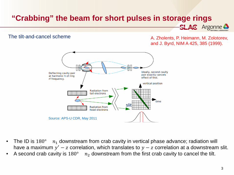
Source: APS-U CDR, May 2011
“Crabbing” the beam for short pulses in storage rings
A. Zholents, P. Heimann, M. Zolotorev, and J. Byrd, NIM A 425, 385 (1999).
slit
The tilt-and-cancel scheme
• The ID is 180° × 𝑛𝑛1 downstream from crab cavity in vertical phase advance; radiation will have a maximum 𝑦𝑦′ − 𝑧𝑧 correlation, which translates to 𝑦𝑦 − 𝑧𝑧 correlation at a downstream slit.
• A second crab cavity is 180° × 𝑛𝑛2 downstream from the first crab cavity to cancel the tilt.
3
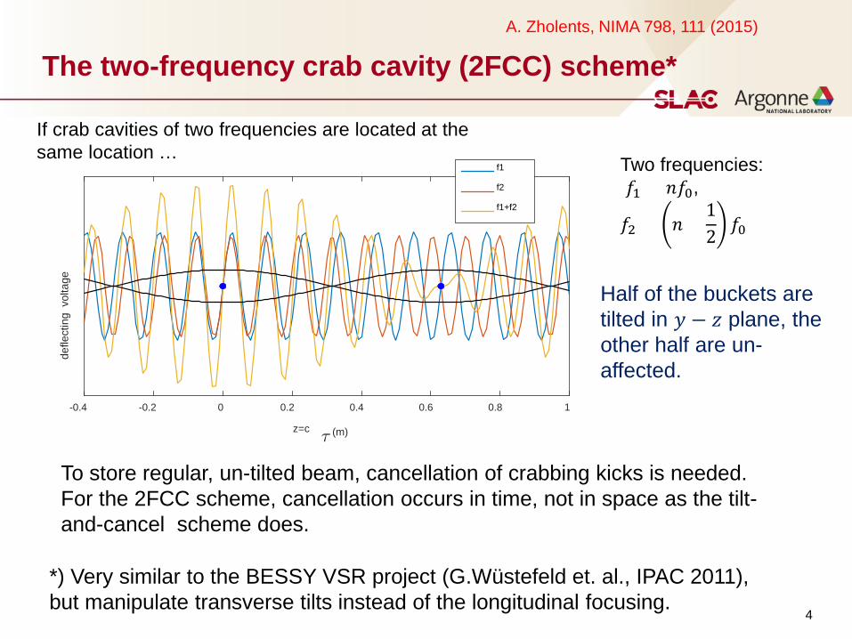
The two-frequency crab cavity (2FCC) scheme*A. Zholents, NIMA 798, 111 (2015)
z=c (m)
-0.4 -0.2 0 0.2 0.4 0.6 0.8 1
defle
ctin
g v
olta
ge
f1
f2
f1+f2
Two frequencies:𝑓𝑓1 = 𝑛𝑛𝑓𝑓0,
𝑓𝑓2 = 𝑛𝑛 +12
𝑓𝑓0
Half of the buckets are tilted in 𝑦𝑦 − 𝑧𝑧 plane, the other half are un-affected.
4
If crab cavities of two frequencies are located at the same location …
To store regular, un-tilted beam, cancellation of crabbing kicks is needed. For the 2FCC scheme, cancellation occurs in time, not in space as the tilt-and-cancel scheme does.
*) Very similar to the BESSY VSR project (G.Wüstefeld et. al., IPAC 2011), but manipulate transverse tilts instead of the longitudinal focusing.

5
Advantages of the new scheme
• Short pulses are available all around the ring. • No strict phase advance requirement for lattices. • Crab cavities occupy only one straight section (and only one cryostat for
SRF)• Both cavities contribute to tilting and hence less total deflecting voltage
is required.• Beamlines can easily switch between short pulse mode and regular
mode. • Crab cavity can be used to separate short pulses from regular pulses.
Disadvantages:• Crab cavities (and power source) of a second frequency are needed. • Crab cavities add additional contribution to vertical emittance of the tilted bunch
(to be discussed later), degrading X-ray flux and brightness.
6
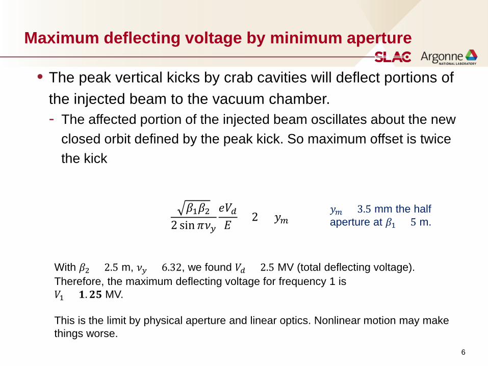
Maximum deflecting voltage by minimum aperture
• The peak vertical kicks by crab cavities will deflect portions of the injected beam to the vacuum chamber. - The affected portion of the injected beam oscillates about the new
closed orbit defined by the peak kick. So maximum offset is twice the kick
𝛽𝛽1𝛽𝛽22 sin𝜋𝜋𝜈𝜈𝑦𝑦
𝑒𝑒𝑉𝑉𝑑𝑑𝐸𝐸 × 2 = 𝑦𝑦𝑚𝑚
𝑦𝑦𝑚𝑚 = 3.5 mm the half aperture at 𝛽𝛽1 = 5 m.
With 𝛽𝛽2 = 2.5 m, 𝜈𝜈𝑦𝑦 = 6.32, we found 𝑉𝑉𝑑𝑑 = 2.5 MV (total deflecting voltage). Therefore, the maximum deflecting voltage for frequency 1 is𝑉𝑉1 = 𝟏𝟏.𝟐𝟐𝟐𝟐 MV.
This is the limit by physical aperture and linear optics. Nonlinear motion may make things worse.
7
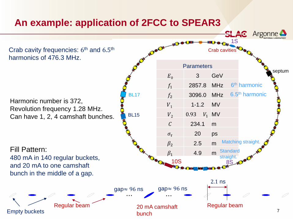
An example: application of 2FCC to SPEAR3
Crab cavities
Parameters
𝐸𝐸0 3 GeV
𝑓𝑓1 2857.8 MHz
𝑓𝑓2 3096.0 MHz
𝑉𝑉1 1-1.2 MV
𝑉𝑉2 0.93 × 𝑉𝑉1 MV
𝐶𝐶 234.1 m
𝜎𝜎𝜏𝜏 20 ps
𝛽𝛽2 2.5 m
𝛽𝛽1 4.9 m
6th harmonic6.5th harmonic
Crab cavity frequencies: 6th and 6.5th
harmonics of 476.3 MHz.
1S
8S
Standard straight.
Matching straight.
10S
septum
BL15
BL17Harmonic number is 372, Revolution frequency 1.28 MHz.Can have 1, 2, 4 camshaft bunches.
Regular beam Regular beam20 mA camshaft bunchEmpty buckets
⋯ ⋯gap≈ 96 ns gap≈ 96 ns
2.1 ns
Fill Pattern:480 mA in 140 regular buckets, and 20 mA to one camshaft bunch in the middle of a gap.
8
Short pulse performance
• Short pulse performance measures- Minimum photon pulse duration- Photon flux vs. pulse duration
• Two types of photon optics for short pulse selection- Drift and slit system- Imaging and slit system- There could be hybrid optics (not discussed here)
• What parameters affect short pulse performance?- Equilibrium distribution of tilted bunch- Lattice choice and impact- Crab cavity parameter choice
9
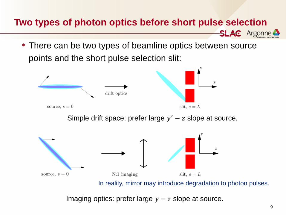
Two types of photon optics before short pulse selection
• There can be two types of beamline optics between source points and the short pulse selection slit:
Simple drift space: prefer large 𝑦𝑦′ − 𝑧𝑧 slope at source.
Imaging optics: prefer large 𝑦𝑦 − 𝑧𝑧 slope at source.
In reality, mirror may introduce degradation to photon pulses.
10
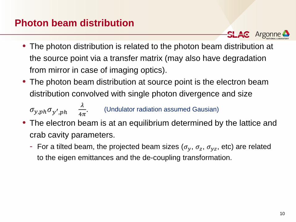
Photon beam distribution
• The photon distribution is related to the photon beam distribution at the source point via a transfer matrix (may also have degradation from mirror in case of imaging optics).
• The photon beam distribution at source point is the electron beam distribution convolved with single photon divergence and size
𝜎𝜎𝑦𝑦,𝑝𝑝𝑝𝜎𝜎𝑦𝑦′,𝑝𝑝𝑝 = 𝜆𝜆4𝜋𝜋
.
• The electron beam is at an equilibrium determined by the lattice and crab cavity parameters.- For a tilted beam, the projected beam sizes (𝜎𝜎𝑦𝑦, 𝜎𝜎𝑧𝑧, 𝜎𝜎𝑦𝑦𝑧𝑧, etc) are related
to the eigen emittances and the de-coupling transformation.
(Undulator radiation assumed Gausian)
11
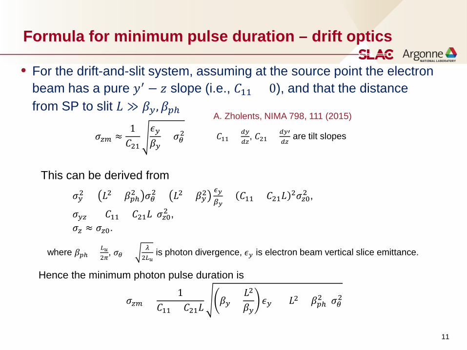
Formula for minimum pulse duration – drift optics
• For the drift-and-slit system, assuming at the source point the electron beam has a pure 𝑦𝑦′ − 𝑧𝑧 slope (i.e., 𝐶𝐶11 = 0), and that the distance from SP to slit 𝐿𝐿 ≫ 𝛽𝛽𝑦𝑦,𝛽𝛽𝑝𝑝𝑝
𝜎𝜎𝑦𝑦2 = 𝐿𝐿2 + 𝛽𝛽𝑝𝑝𝑝2 𝜎𝜎𝜃𝜃2 + 𝐿𝐿2 + 𝛽𝛽𝑦𝑦2𝜖𝜖𝑦𝑦𝛽𝛽𝑦𝑦
+ 𝐶𝐶11 + 𝐶𝐶21𝐿𝐿 2𝜎𝜎𝑧𝑧02 ,
𝜎𝜎𝑦𝑦𝑧𝑧 = (𝐶𝐶11 + 𝐶𝐶21𝐿𝐿)𝜎𝜎𝑧𝑧02 , 𝜎𝜎𝑧𝑧 ≈ 𝜎𝜎𝑧𝑧0.
Hence the minimum photon pulse duration is
𝜎𝜎𝑧𝑧𝑚𝑚 =1
𝐶𝐶11 + 𝐶𝐶21𝐿𝐿𝛽𝛽𝑦𝑦 +
𝐿𝐿2
𝛽𝛽𝑦𝑦𝜖𝜖𝑦𝑦 + (𝐿𝐿2 + 𝛽𝛽𝑝𝑝𝑝2 )𝜎𝜎𝜃𝜃2
where 𝛽𝛽𝑝𝑝𝑝 = 𝐿𝐿𝑢𝑢2𝜋𝜋
, 𝜎𝜎𝜃𝜃 = 𝜆𝜆2𝐿𝐿𝑢𝑢
is photon divergence, 𝜖𝜖𝑦𝑦 is electron beam vertical slice emittance.
𝜎𝜎𝑧𝑧𝑚𝑚 ≈1𝐶𝐶21
𝜖𝜖𝑦𝑦𝛽𝛽𝑦𝑦
+ 𝜎𝜎𝜃𝜃2A. Zholents, NIMA 798, 111 (2015)
This can be derived from
𝐶𝐶11 = 𝑑𝑑𝑦𝑦𝑑𝑑𝑧𝑧
, 𝐶𝐶21 = 𝑑𝑑𝑦𝑦′𝑑𝑑𝑧𝑧
are tilt slopes

12
Formula for imaging optics
• With imaging optics, we slit the image of photon beam at source point. Ignoring the mirror induced degradation, the minimum pulse duration is
𝜎𝜎𝑧𝑧𝑚𝑚 ≈ 1𝐶𝐶11
𝛽𝛽𝑦𝑦𝜖𝜖𝑦𝑦 + 𝜎𝜎𝑝𝑝𝑝,𝑦𝑦2 , with 𝜎𝜎𝑝𝑝𝑝,𝑦𝑦 = 𝜆𝜆
4𝜋𝜋𝜎𝜎𝜃𝜃
It’s desirable to maximize the 𝑦𝑦-𝑧𝑧 slope for the imaging optics case. Since for SPEAR3 𝛽𝛽𝑝𝑝𝑝 = 𝐿𝐿𝑢𝑢
2𝜋𝜋≈ 0.5 m is very small, for the imaging case, pulse duration is
much LESS affected by diffraction than for the drift-and-slit case.
In any case, the equilibrium electron bunch distribution at source point is key to the short pulse performance. This requires the understanding of beam motion with crab cavity.
13
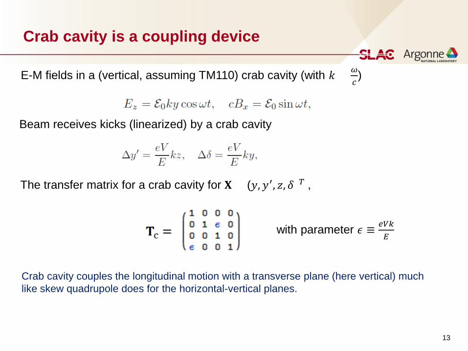
Crab cavity is a coupling device
E-M fields in a (vertical, assuming TM110) crab cavity (with 𝑘𝑘 = 𝜔𝜔𝑐𝑐)
Beam receives kicks (linearized) by a crab cavity
The transfer matrix for a crab cavity for 𝐗𝐗 = (𝑦𝑦,𝑦𝑦′, 𝑧𝑧, 𝛿𝛿)𝑇𝑇 ,
Crab cavity couples the longitudinal motion with a transverse plane (here vertical) much like skew quadrupole does for the horizontal-vertical planes.
with parameter 𝜖𝜖 ≡ 𝑒𝑒𝑒𝑒𝑒𝑒𝐸𝐸
14
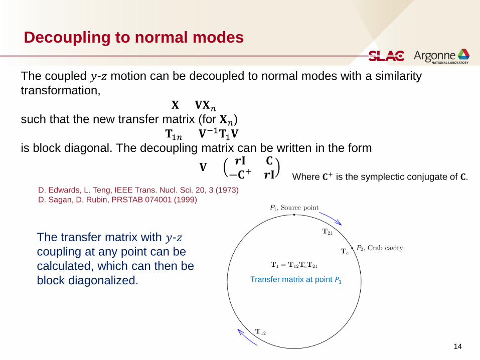
Decoupling to normal modes
Transfer matrix at point 𝑃𝑃1
The coupled 𝑦𝑦-𝑧𝑧 motion can be decoupled to normal modes with a similarity transformation,
𝐗𝐗 = 𝐕𝐕𝐗𝐗𝑛𝑛such that the new transfer matrix (for 𝐗𝐗𝑛𝑛)
𝐓𝐓1𝑛𝑛 = 𝐕𝐕−1𝐓𝐓1𝐕𝐕is block diagonal. The decoupling matrix can be written in the form
𝐕𝐕 = 𝒓𝒓𝐈𝐈 𝐂𝐂−𝐂𝐂+ 𝒓𝒓𝐈𝐈
D. Edwards, L. Teng, IEEE Trans. Nucl. Sci. 20, 3 (1973)D. Sagan, D. Rubin, PRSTAB 074001 (1999)
Where 𝐂𝐂+ is the symplectic conjugate of 𝐂𝐂.
The transfer matrix with 𝑦𝑦-𝑧𝑧coupling at any point can be calculated, which can then be block diagonalized.
15
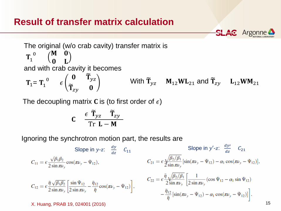
Result of transfer matrix calculation
The original (w/o crab cavity) transfer matrix is𝐓𝐓1
(0) = 𝐌𝐌 𝟎𝟎𝟎𝟎 𝐋𝐋
and with crab cavity it becomes
𝐓𝐓1= 𝐓𝐓1(0) + 𝜖𝜖
𝟎𝟎 �𝐓𝐓𝑦𝑦𝑧𝑧�𝐓𝐓𝑧𝑧𝑦𝑦 𝟎𝟎
With �𝐓𝐓𝑦𝑦𝑧𝑧 = 𝐌𝐌12𝐖𝐖𝐋𝐋21 and �𝐓𝐓𝑧𝑧𝑦𝑦 = 𝐋𝐋12𝐖𝐖𝐌𝐌21
The decoupling matrix 𝐂𝐂 is (to first order of 𝜖𝜖)
𝐂𝐂 =𝜖𝜖(�𝐓𝐓𝑦𝑦𝑧𝑧 + �𝐓𝐓𝑧𝑧𝑦𝑦)
Tr(𝐋𝐋 −𝐌𝐌)
Ignoring the synchrotron motion part, the results areSlope in 𝑦𝑦′-𝑧𝑧: 𝑑𝑑𝑦𝑦′
𝑑𝑑𝑧𝑧= 𝐶𝐶21Slope in 𝑦𝑦-𝑧𝑧: 𝑑𝑑𝑦𝑦
𝑑𝑑𝑧𝑧= 𝐶𝐶11
X. Huang, PRAB 19, 024001 (2016)
16
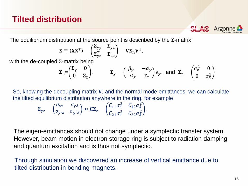
Tilted distribution
The equilibrium distribution at the source point is described by the Σ-matrix
𝚺𝚺 ≡ 𝐗𝐗𝐗𝐗𝑇𝑇 =𝚺𝚺yy 𝚺𝚺y𝑧𝑧𝚺𝚺y𝑧𝑧𝑇𝑇 𝚺𝚺z𝑧𝑧
= 𝐕𝐕𝚺𝚺n𝐕𝐕T,
with the de-coupled Σ-matrix being
𝚺𝚺n=𝚺𝚺y 𝟎𝟎0 𝚺𝚺z
, 𝚺𝚺y =𝛽𝛽𝑦𝑦 −𝛼𝛼𝑦𝑦−𝛼𝛼𝑦𝑦 𝛾𝛾𝑦𝑦
𝜖𝜖𝑦𝑦, and 𝚺𝚺z =𝜎𝜎𝑧𝑧2 00 𝜎𝜎𝛿𝛿
2
So, knowing the decoupling matrix 𝐕𝐕, and the normal mode emittances, we can calculate the tilted equilibrium distribution anywhere in the ring, for example
𝚺𝚺yz =𝜎𝜎yz 𝜎𝜎y𝛿𝛿𝜎𝜎y′z 𝜎𝜎y′𝛿𝛿 ≈ 𝐂𝐂𝚺𝚺z =
𝐶𝐶11𝜎𝜎𝑧𝑧2 𝐶𝐶12𝜎𝜎𝛿𝛿2
𝐶𝐶21𝜎𝜎𝑧𝑧2 𝐶𝐶22𝜎𝜎𝛿𝛿2 .
The eigen-emittances should not change under a symplectic transfer system. However, beam motion in electron storage ring is subject to radiation damping and quantum excitation and is thus not symplectic.
Through simulation we discovered an increase of vertical emittance due to tilted distribution in bending magnets.
17
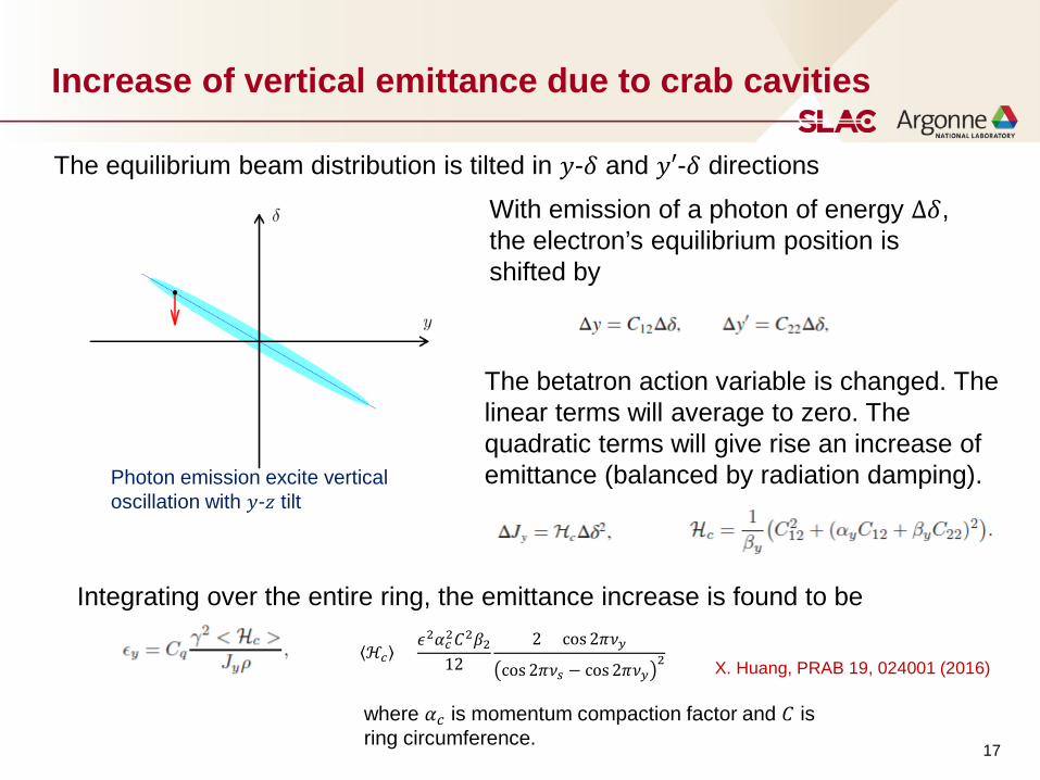
Increase of vertical emittance due to crab cavities
Photon emission excite vertical oscillation with 𝑦𝑦-𝑧𝑧 tilt
The equilibrium beam distribution is tilted in 𝑦𝑦-𝛿𝛿 and 𝑦𝑦′-𝛿𝛿 directions
With emission of a photon of energy Δ𝛿𝛿, the electron’s equilibrium position is shifted by
The betatron action variable is changed. The linear terms will average to zero. The quadratic terms will give rise an increase of emittance (balanced by radiation damping).
Integrating over the entire ring, the emittance increase is found to be
where 𝛼𝛼𝑐𝑐 is momentum compaction factor and 𝐶𝐶 is ring circumference.
X. Huang, PRAB 19, 024001 (2016)ℋ𝑐𝑐 =
𝜖𝜖2𝛼𝛼𝑐𝑐2𝐶𝐶2𝛽𝛽212
2 + cos2𝜋𝜋𝜈𝜈𝑦𝑦cos 2𝜋𝜋𝜈𝜈𝑠𝑠 − cos2𝜋𝜋𝜈𝜈𝑦𝑦
2
18
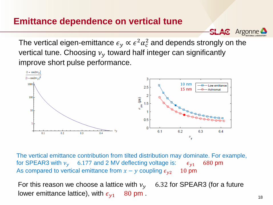
Emittance dependence on vertical tune
The vertical eigen-emittance 𝜖𝜖𝑦𝑦 ∝ 𝜖𝜖2𝛼𝛼𝑐𝑐2 and depends strongly on the vertical tune. Choosing 𝜈𝜈𝑦𝑦 toward half integer can significantly improve short pulse performance.
10 nm15 nm
The vertical emittance contribution from tilted distribution may dominate. For example, for SPEAR3 with 𝜈𝜈𝑦𝑦 = 6.177 and 2 MV deflecting voltage is: 𝜖𝜖𝑦𝑦1 = 680 pm As compared to vertical emittance from 𝑥𝑥 − 𝑦𝑦 coupling 𝜖𝜖𝑦𝑦2 = 10 pm
For this reason we choose a lattice with 𝜈𝜈𝑦𝑦 = 6.32 for SPEAR3 (for a future lower emittance lattice), with 𝜖𝜖𝑦𝑦1 = 80 pm .
19
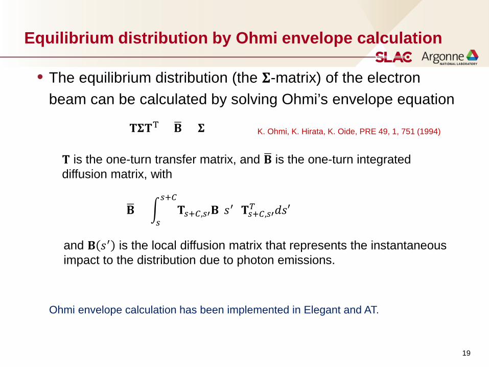
Equilibrium distribution by Ohmi envelope calculation
• The equilibrium distribution (the 𝚺𝚺-matrix) of the electron beam can be calculated by solving Ohmi’s envelope equation
𝐓𝐓𝚺𝚺𝐓𝐓T + �𝐁𝐁 = 𝚺𝚺
𝐓𝐓 is the one-turn transfer matrix, and �𝐁𝐁 is the one-turn integrated diffusion matrix, with
�𝐁𝐁 = �𝑠𝑠
𝑠𝑠+𝐶𝐶𝐓𝐓𝑠𝑠+𝐶𝐶,𝑠𝑠′𝐁𝐁(𝑠𝑠′)𝐓𝐓𝑠𝑠+𝐶𝐶,𝑠𝑠′
𝑇𝑇 𝑑𝑑𝑠𝑠′
and 𝐁𝐁 𝑠𝑠′ is the local diffusion matrix that represents the instantaneous impact to the distribution due to photon emissions.
K. Ohmi, K. Hirata, K. Oide, PRE 49, 1, 751 (1994)
Ohmi envelope calculation has been implemented in Elegant and AT.
20
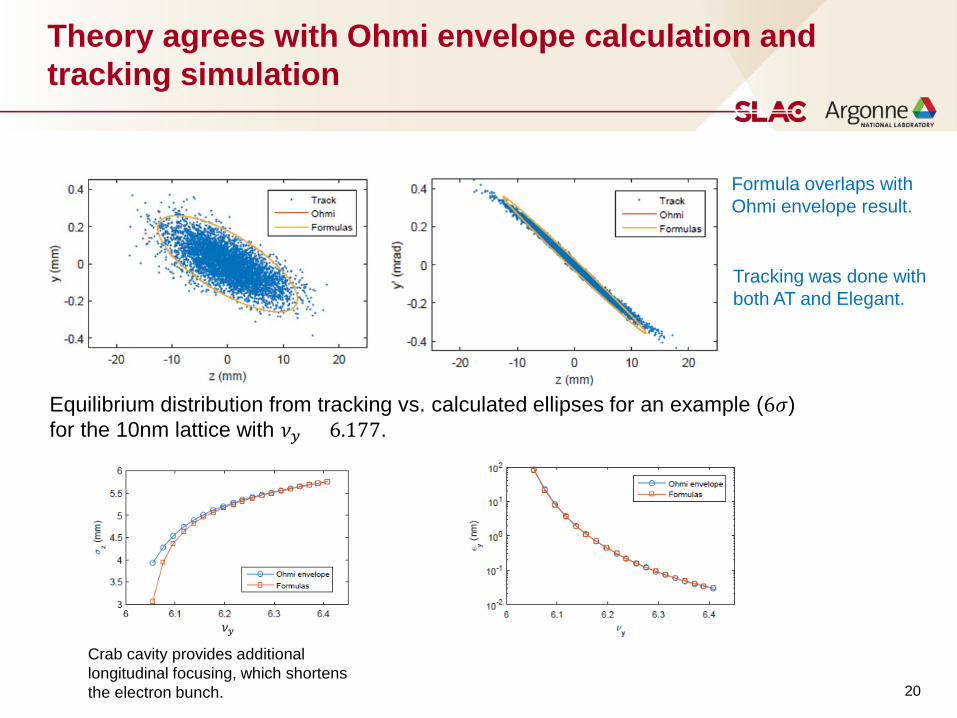
Theory agrees with Ohmi envelope calculation and tracking simulation
Equilibrium distribution from tracking vs. calculated ellipses for an example (6𝜎𝜎) for the 10nm lattice with 𝜈𝜈𝑦𝑦 = 6.177.
𝜈𝜈𝑦𝑦
Crab cavity provides additional longitudinal focusing, which shortens the electron bunch.
Tracking was done with both AT and Elegant.
Formula overlaps with Ohmi envelope result.
21
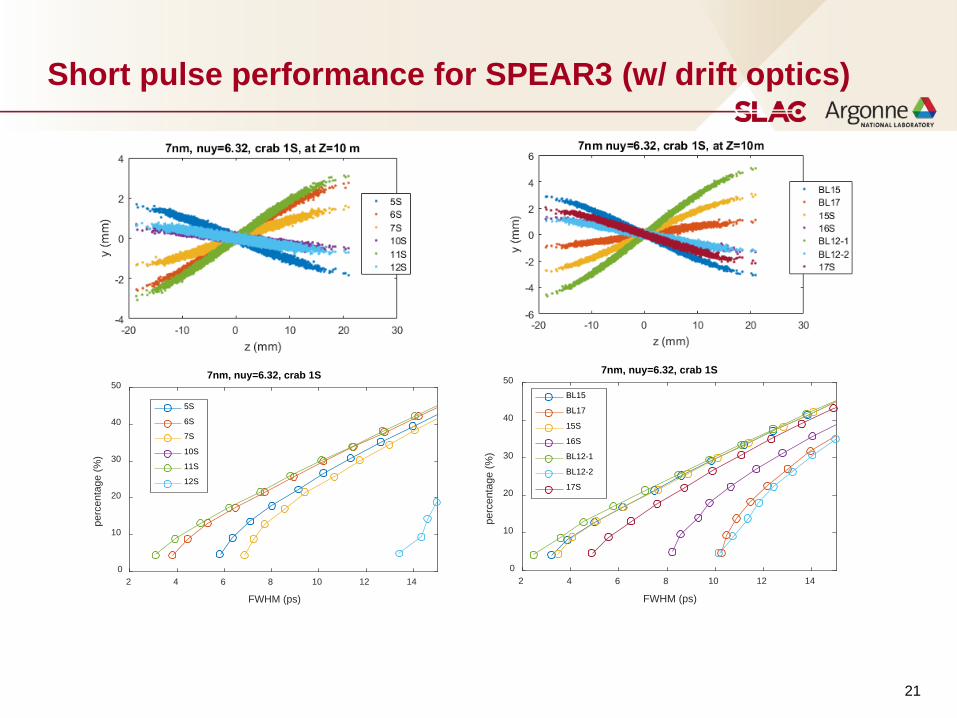
Short pulse performance for SPEAR3 (w/ drift optics)
2 4 6 8 10 12 14
FWHM (ps)
0
10
20
30
40
50
perc
enta
ge (%
)
7nm, nuy=6.32, crab 1S
5S
6S
7S
10S
11S
12S
2 4 6 8 10 12 14
FWHM (ps)
0
10
20
30
40
50
perc
enta
ge (%
)
7nm, nuy=6.32, crab 1S
BL15
BL17
15S
16S
BL12-1
BL12-2
17S
22
Many other beam dynamics aspects have been studied
• Impact to regular beam users- RF amplitude and phase noise- Phase shift by bunch train gap transient
• Injection into tilted buckets• Beam lifetime (tilted, high current bunch)• Crab cavity field requirements• Separation of short pulse and long pulse• Collective effects
- Coupled bunch instabilities.- Single bunch current threshold (TMCI)- Microbunching instability.
We do not intend to cover these topics in this talk.
Summary
• The two-frequency crab cavity approach for short pulse generation in storage rings has many advantages over previous approaches.
• We have studied the coupled motion between the longitudinal and transverse directions due to crab cavities.
• Design study at SPEAR3 has made significant progress.
23
24
Acknowledgement
• Thanks to M. Borland for help in setting up Elegant tracking with crab cavities.
• Many input from SPEAR3 2FCC study team- Valery Dolgashev, Kelly Gaffney, Bob Hettel, Zenghai Li, Tom
Rabedeau, James Safranek, Jim Sebek, Kai Tian.