Stored Electromagnetic Energy and Quality Factor ofRadiating StructuresMiloslav Capek1, Lukas Jelinek1 and Guy A. E. Vandenbosch2

1Department of Electromagnetic Field, Faculty of Electrical Engineering, Czech Technical

University in Prague, Technicka 2, 16627, Prague, Czech Republic2Department of Electrical Engineering, Division ESAT-TELEMIC (Telecommunications and

Microwaves), Katholieke Universiteit Leuven, B-3001, Leuven, Belgium

AbstractThis paper deals with the old yet unsolved problem of defining and evaluating the stored

electromagnetic energy – a quantity essential for calculating the quality factor, which reflects theintrinsic bandwidth of the considered electromagnetic system. A novel paradigm is proposed todetermine the stored energy in the time domain leading to the method, which exhibits positivesemi-definiteness and coordinate independence, i.e. two key properties actually not met by thecontemporary approaches. The proposed technique is compared with two up-to-date frequencydomain methods that are extensively used in practice. All three concepts are discussed andcompared on the basis of examples of varying complexity, starting with lumped RLC circuitsand finishing with realistic radiators.

1. IntroductionIn physics, an oscillating system is traditionally characterized [1] by its oscillation frequency andquality factor Q, which gives a measure of the lifetime of free oscillations. At its high values, thequality factor Q is also inversely proportional to the intrinsic bandwidth in which the oscillatingsystem can effectively be driven by external sources [2, 3].

The concept of quality factor Q as a single frequency estimate of relative bandwidth ismost developed in the area of electric circuits [4] and electromagnetic radiating systems [3]. Itsevaluation commonly follows two paradigms. As far as the first one is concerned, the qualityfactor is evaluated from the knowledge of the frequency derivative of input impedance [5, 6, 7].As for the second paradigm, the quality factor is defined as 2π times the ratio between the cyclemean stored energy and the cycle mean lost energy [5, 8]. Generally, these two concepts yielddistinct results, but come to identical results in the case of vanishingly small losses, the reasonbeing the Foster’s reactance theorem [9, 10].

The evaluation of quality factor by means of frequency derivative of input impedance wasmade very popular by the work of Yaghjian and Best [11] and is widely used in engineeringpractice [12, 13] thanks to its property of being directly measurable. Recently, this concept ofquality factor has also been expressed as a bilinear form of source current densities [14], which isvery useful in connection with modern numerical software tools [15]. Regardless of the mentionedadvantages, the impedance concept of quality factor suffers from a serious drawback of being zeroin specific circuits [16, 17] and/or radiators [17, 18] with evidently non-zero energy storage. Thisunfortunately prevents its usage in modern optimization techniques [19].

The second paradigm, in which the quality factor is evaluated via the stored energy and lostenergy, is not left without difficulties either. In the case of non-dispersive components, the cyclemean lost energy does not pose a problem and may be evaluated as a sum of the cycle meanradiated energy and the cycle mean energy dissipated due to material losses [20]. Unfortunately,in the case of a non-stationary electromagnetic field associated with radiators, the definition ofstored (non-propagating) electric and magnetic energies presents a problem that has not yet been

arX

iv:1

403.

0572

v3 [

phys

ics.

clas

s-ph

] 9

Sep

201

5

2satisfactorily solved [3]. The issue comes from the radiation energy, which does not decay fastenough in radial direction, and is in fact infinite in stationary state [21].

In order to overcome the infinite values of total energy, the evaluation of stored energyin radiating systems is commonly accompanied by the technique of extracting the divergentradiation component from the well-known total energy of the system [20]. This method issomewhat analogous to the classical field [22] re-normalization. Most attempts in this directionhave been performed in the domain of time-harmonic fields. The pioneering work in this directionis the equivalent circuit method of Chu [21], in which the radiation and energy storage arerepresented by resistive and reactive components of a complex electric circuit describing eachspherical mode. This method was later generalized by several works of Thal [23, 24]. Althoughpowerful, this method suffers from fundamental drawback of spherical harmonics expansion,which is unique solely in the exterior of the sphere bounding the sources. Therefore, the circuitmethod cannot provide any information on the radiation content of the interior region, nor on theconnection of energy storage with the actual shape of radiator.

The radiation extraction for spherical harmonics has also been performed directly at the fieldlevel. The classical work in this direction comes from Collin and Rothschild [25]. Their proposalleads to good results for canonical systems [25, 26, 27], and has been analytically shown self-consistent outside the radian-sphere [28]. Similarly to the work of Chu, this procedure is limitedby the use of spherical harmonics to the exterior of the circumscribing sphere.

The problem of radiation extraction around radiators of arbitrary shape has been for the firsttime attacked by Fante [29] and Rhodes [30], giving the interpretation to the Foster’s theorem [10]in open problems. The ingenious combination of the frequency derivative of input impedanceand the frequency derivative of far-field radiation pattern led to the first general evaluation ofstored energy. Fante’s and Rhodes’ works have been later generalized by Yaghjian and Best [11],who also pointed out an unpleasant fact that this method is coordinate-dependent. A schemefor minimisation of this dependence has been developed [11], but it was not until the workof Vandenbosch [31] who, generalizing the expressions of Geyi for small radiators [32] andrewriting the extraction technique into bilinear forms of currents, was able to reformulate theoriginal extraction method into a coordinate-independent scheme. A noteworthy discussion ofvarious forms of this extraction technique can be found in the work of Gustafsson and Jonsson[33]. It was also Gustafsson et al. who emphasized [19] that under certain conditions, thisextraction technique fails, giving negative values for specific current distributions. Hence theaforementioned approach remains incomplete too [34].

The problem of stored energy has seldom been addressed directly in the time domain.Nevertheless, there are some interesting works dealing with time-dependent energies. Shlivinskiexpanded the fields into spherical waves in time domain [35, 36], introducing time domainquality factor that qualifies the radiation efficiency of pulse-fed radiators. Collarday [37] proposeda brute force method utilizing the finite differences technique. In [38], Vandenbosch derivedexpressions for electric and magnetic energies in time domain that however suffer from anunknown parameter called storage time. A notable work of Kaiser [39] then introduced theconcept of rest electromagnetic energy, which resembles the properties of stored energy, but isnot identical to it [40].

The knowledge of the stored electromagnetic energy and the capability of its evaluation arealso tightly connected with the question of its minimization [21, 41, 42, 43, 44]. Such lower boundof the stored energy would imply the upper bound to the available bandwidth, a parameter ofgreat importance for contemporary communication devices.

In this paper, a scheme for radiation energy extraction is proposed following a novel line ofreasoning in the time domain. The scheme aims to overcome the handicaps of the previouslypublished works, and furthermore is able to work with general time-dependent source currents ofarbitrary shape. It is presented together with the two most common frequency domain methods,the first being based on the time-harmonic expressions of Vandenbosch [31] and the second usingthe input impedance approximation introduced by Yaghjian and Best [11]. All three concepts are

3

S1 V1

R0 Zin

device withunknown Q

R0

power supply

i0(t )

u0(t )

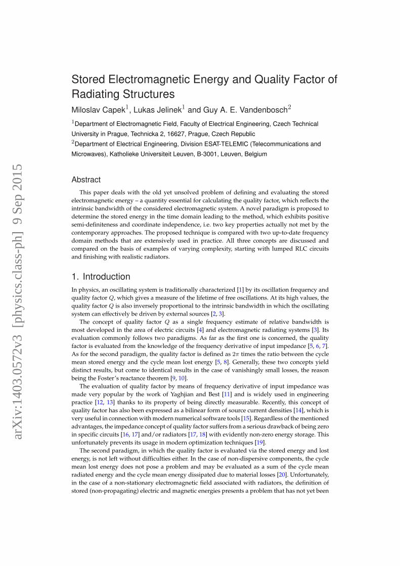
Figure 1. A device with unknown Q that is fed by a shielded power source with internal resistance R0.

closely investigated and compared on the basis of examples of varying complexity. The workingout of all three concepts starts solely from the currents flowing on a radiator, which are usuallygiven as a result in modern electromagnetic simulators. This raises challenging possibilities ofmodal analysis [45] and optimization [46].

The paper is organized as follows. Two different concepts of quality factor Q that are basedon electromagnetic energies (in both, the frequency and time domain), are introduced in §2.Subsequently, the quality factor Q derived from the input impedance is formulated in terms ofcurrents on a radiator in §3. The following two sections present numerical examples: §4 treatsnon-radiating circuits and §5 deals with radiators. The results are discussed in §6 and the paperis concluded in §7.

2. Energy concept of quality factor QIn the context of energy, the quality factor is most commonly defined as

Q= 2π〈Wsto (t)〉Wlost

= 2πWsto

Wlost, (2.1)

where a time-harmonic steady state with angular frequency ω0 is assumed, with Wsto (t) asthe electromagnetic stored energy, 〈Wsto (t)〉=Wsto as the cycle mean of Wsto (t) and Wlost asthe lost electromagnetic energy during one cycle [20]. In conformity with the font conventionintroduced above, in the following text, the quantities defined in the time domain are stated incalligraphic font, while the frequency domain quantities are indicated in the roman font.

A typical Q-measurement scenario is depicted in figure 1, which shows a radiator fed by ashielded power source. The input impedance in the time-harmonic steady state at the frequencyω0 seen by the source is Zin. Assuming that the radiator is made of conductors with ideal non-dispersive conductivity σ and lossless non-dispersive dielectrics, we can state that the lost energyduring one cycle, needed for (2.1), can be evaluated as

Wlost =

α+T∫α

i0 (t)u0 (t) dt=π

ω0Re{Zin}I2

0 =Wr +Wσ, (2.2)

where I0 is the amplitude of i0 (t) (see figure 1), Wr represents the cycle mean radiation loss andWσ stands for the energy lost in one cycle via conduction. The part Wσ of (2.2) can be calculated

4as

Wσ =π

ω0

∫V

σ |E (r, ω0)|2 dV, (2.3)

with V being the shape of radiator and E being the time-harmonic electric field intensity underthe convention E (t) =Re{E (ω) eiωt}, i =

√−1. At the same time, the near-field of the radiator

[47] contains the stored energyWsto (t), which is bound to the sources and does not escape fromthe radiator towards infinity. The evaluation of the cycle mean energy Wsto is the goal of thefollowing §2(a) and §2(b), in which the power balance [10] is going to be employed.

(a) Stored energy in time domainThis subsection presents a new paradigm of stored energy evaluation. The first step consists inimagining the spherical volume V1 (see figure 1) centred around the system, whose radius is largeenough to lie in the far-field region [47]. The total electromagnetic energy content of the sphere (italso contains heat Wσ) is

W (V1, t) =Wsto (t) +Wr (V1, t) , (2.4)

whereWr (V1, t) is the energy contained in the radiation fields that have already escaped from thesources. Let us assume that the power source is switched on at t=−∞, bringing the system intoa steady state, and then switched off at t= toff . For t∈ [toff ,∞) the system is in a transient state,during which all the energyW (V1, toff) will either be transformed into heat at the resistorR0 andthe radiator’s conductors or radiated through the bounding envelope S1. Explicitly, Poynting’stheorem [10] states that the total electromagnetic energy at time toff can be calculated as

W (V1, toff) = R0

∞∫toff

i2R0(t) dt+

∞∫toff

∫V

E (r, t) ·J (r, t) dV dt

+

∞∫toff

∮S1

(Efar (r, t)×Hfar (r, t)

)· dS1 dt,

(2.5)

in which S1 lies in the far-field region.As a special yet important example, let us assume a radiating device made exclusively of

perfect electric conductors (PEC). In that case, the far-field can be expressed as [20]

Hfar (r, t) =−1

4πc0

∫V ′

n0 × J̇(r′, t′

)R

dV ′, (2.6a)

Efar (r, t) =−µ

4π

∫V ′

J̇(r′, t′

)−(n0 · J̇

(r′, t′

))n0

RdV ′ (2.6b)

in which c0 is the speed of light, R=∣∣r − r′

∣∣, n0 =(r − r′

)/R, t′ = t−R/c0 stands for the

retarded time and the dot represents the derivative with respect to the time argument, i.e.

J̇(r′, t′

)=∂J

(r′, τ

)∂τ

∣∣∣∣∣τ=t′

. (2.7)

Since we consider the far-field, we can further write [48] R≈ r for amplitudes, R≈ r − r0 · r′

for time delays, with n0 ≈ r0 and r= |r|. Using (2.6a)–(2.7) and the above-mentioned

5S1

(a)

S1

(b) (c)

u(t)

S1

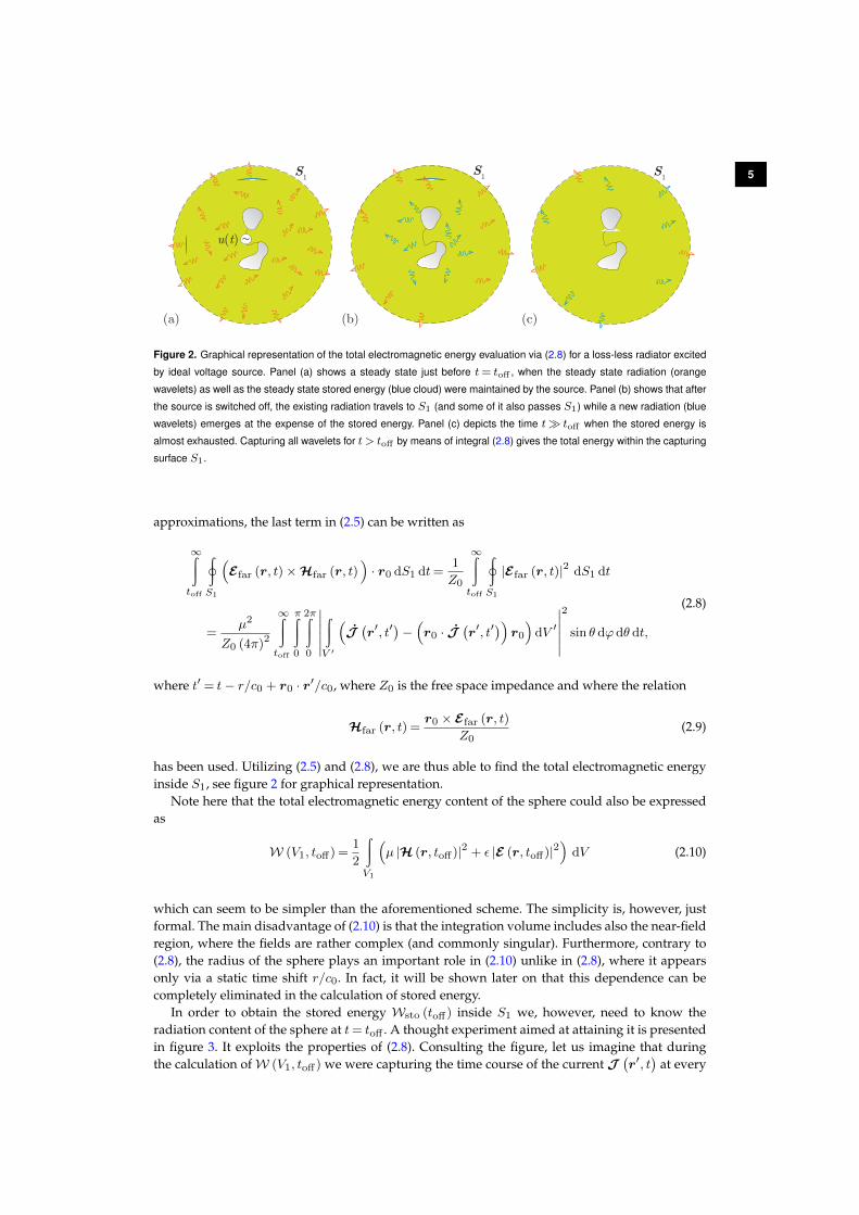
Figure 2. Graphical representation of the total electromagnetic energy evaluation via (2.8) for a loss-less radiator excited

by ideal voltage source. Panel (a) shows a steady state just before t= toff , when the steady state radiation (orange

wavelets) as well as the steady state stored energy (blue cloud) were maintained by the source. Panel (b) shows that after

the source is switched off, the existing radiation travels to S1 (and some of it also passes S1) while a new radiation (blue

wavelets) emerges at the expense of the stored energy. Panel (c) depicts the time t� toff when the stored energy is

almost exhausted. Capturing all wavelets for t > toff by means of integral (2.8) gives the total energy within the capturing

surface S1.

approximations, the last term in (2.5) can be written as

∞∫toff

∮S1

(Efar (r, t)×Hfar (r, t)

)· r0 dS1 dt=

1

Z0

∞∫toff

∮S1

|Efar (r, t)|2 dS1 dt

=µ2

Z0 (4π)2

∞∫toff

π∫0

2π∫0

∣∣∣∣∣∣∫V ′

(J̇(r′, t′

)−(r0 · J̇

(r′, t′

))r0

)dV ′

∣∣∣∣∣∣2

sin θ dϕdθ dt,

(2.8)

where t′ = t− r/c0 + r0 · r′/c0, where Z0 is the free space impedance and where the relation

Hfar (r, t) =r0 × Efar (r, t)

Z0(2.9)

has been used. Utilizing (2.5) and (2.8), we are thus able to find the total electromagnetic energyinside S1, see figure 2 for graphical representation.

Note here that the total electromagnetic energy content of the sphere could also be expressedas

W (V1, toff) =1

2

∫V1

(µ |H (r, toff)|2 + ε |E (r, toff)|2

)dV (2.10)

which can seem to be simpler than the aforementioned scheme. The simplicity is, however, justformal. The main disadvantage of (2.10) is that the integration volume includes also the near-fieldregion, where the fields are rather complex (and commonly singular). Furthermore, contrary to(2.8), the radius of the sphere plays an important role in (2.10) unlike in (2.8), where it appearsonly via a static time shift r/c0. In fact, it will be shown later on that this dependence can becompletely eliminated in the calculation of stored energy.

In order to obtain the stored energy Wsto (toff) inside S1 we, however, need to know theradiation content of the sphere at t= toff . A thought experiment aimed at attaining it is presentedin figure 3. It exploits the properties of (2.8). Consulting the figure, let us imagine that duringthe calculation ofW (V1, toff) we were capturing the time course of the current J

(r′, t

)at every

6

(a)

S1

(b)

S1

(c)

S1

u(t)

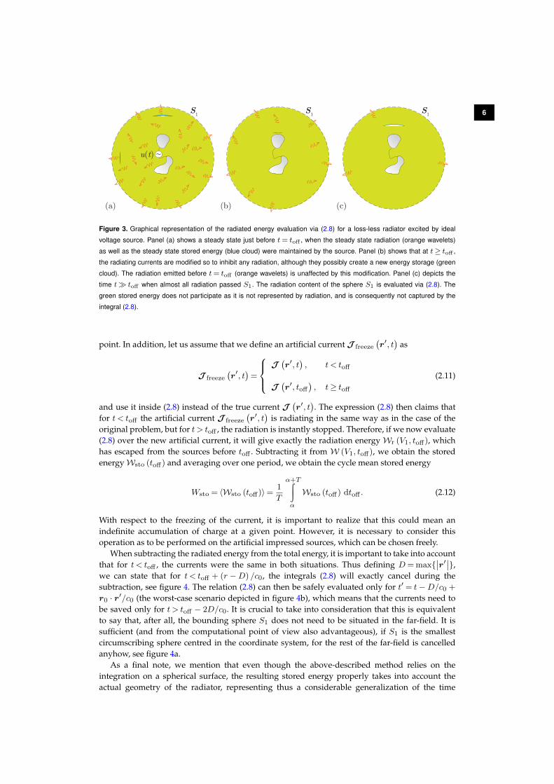
Figure 3. Graphical representation of the radiated energy evaluation via (2.8) for a loss-less radiator excited by ideal

voltage source. Panel (a) shows a steady state just before t= toff , when the steady state radiation (orange wavelets)

as well as the steady state stored energy (blue cloud) were maintained by the source. Panel (b) shows that at t≥ toff ,

the radiating currents are modified so to inhibit any radiation, although they possibly create a new energy storage (green

cloud). The radiation emitted before t= toff (orange wavelets) is unaffected by this modification. Panel (c) depicts the

time t� toff when almost all radiation passed S1. The radiation content of the sphere S1 is evaluated via (2.8). The

green stored energy does not participate as it is not represented by radiation, and is consequently not captured by the

integral (2.8).

point. In addition, let us assume that we define an artificial current J freeze

(r′, t

)as

J freeze

(r′, t

)=

J(r′, t

), t < toff

J(r′, toff

), t≥ toff

(2.11)

and use it inside (2.8) instead of the true current J(r′, t

). The expression (2.8) then claims that

for t < toff the artificial current J freeze

(r′, t

)is radiating in the same way as in the case of the

original problem, but for t > toff , the radiation is instantly stopped. Therefore, if we now evaluate(2.8) over the new artificial current, it will give exactly the radiation energyWr (V1, toff), whichhas escaped from the sources before toff . Subtracting it from W (V1, toff), we obtain the storedenergyWsto (toff) and averaging over one period, we obtain the cycle mean stored energy

Wsto = 〈Wsto (toff)〉=1

T

α+T∫α

Wsto (toff) dtoff . (2.12)

With respect to the freezing of the current, it is important to realize that this could mean anindefinite accumulation of charge at a given point. However, it is necessary to consider thisoperation as to be performed on the artificial impressed sources, which can be chosen freely.

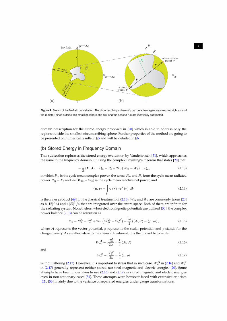
When subtracting the radiated energy from the total energy, it is important to take into accountthat for t < toff , the currents were the same in both situations. Thus defining D=max{

∣∣r′∣∣},we can state that for t < toff + (r −D) /c0, the integrals (2.8) will exactly cancel during thesubtraction, see figure 4. The relation (2.8) can then be safely evaluated only for t′ = t−D/c0 +

r0 · r′/c0 (the worst-case scenario depicted in figure 4b), which means that the currents need tobe saved only for t > toff − 2D/c0. It is crucial to take into consideration that this is equivalentto say that, after all, the bounding sphere S1 does not need to be situated in the far-field. It issufficient (and from the computational point of view also advantageous), if S1 is the smallestcircumscribing sphere centred in the coordinate system, for the rest of the far-field is cancelledanyhow, see figure 4a.

As a final note, we mention that even though the above-described method relies on theintegration on a spherical surface, the resulting stored energy properly takes into account theactual geometry of the radiator, representing thus a considerable generalization of the time

7far-field

r 'x

y

x®¥

y®¥

sourcepoint r '

observationpoint r

rD

(a) (b)

exac

tca

ncelat

ion

S1

S1

r®¥

Figure 4. Sketch of the far-field cancellation. The circumscribing sphere S1 can be advantageously stretched right around

the radiator, since outside this smallest sphere, the first and the second run are identically subtracted.

domain prescription for the stored energy proposed in [28] which is able to address only theregions outside the smallest circumscribing sphere. Further properties of the method are going tobe presented on numerical results in §5 and will be detailed in §6.

(b) Stored Energy in Frequency DomainThis subsection rephrases the stored energy evaluation by Vandenbosch [31], which approachesthe issue in the frequency domain, utilizing the complex Poynting’s theorem that states [20] that

− 1

2〈E,J〉= Pm − Pe + 2iω (Wm −We) = Pin, (2.13)

in which Pin is the cycle mean complex power, the terms Pm and Pe form the cycle mean radiatedpower Pm − Pe and 2ω (Wm −We) is the cycle mean reactive net power, and

〈u,v〉=∫V

u (r) · v∗ (r) dV (2.14)

is the inner product [49]. In the classical treatment of (2.13), Wm and We are commonly taken [20]as µ |H|2 /4 and ε |E|2 /4 that are integrated over the entire space. Both of them are infinite forthe radiating system. Nonetheless, when electromagnetic potentials are utilized [50], the complexpower balance (2.13) can be rewritten as

Pin = PAm − Pϕe + 2iω

(WA

m −Wϕe

)=

iω

2(〈A,J〉 − 〈ϕ, ρ〉) , (2.15)

where A represents the vector potential, ϕ represents the scalar potential, and ρ stands for thecharge density. As an alternative to the classical treatment, it is then possible to write

WAm − i

PAm

2ω=

1

4〈A,J〉 (2.16)

and

Wϕe − i

Pϕe2ω

=1

4〈ϕ, ρ〉 (2.17)

without altering (2.13). However, it is important to stress that in such case, WAm in (2.16) and Wϕ

e

in (2.17) generally represent neither stored nor total magnetic and electric energies [20]. Someattempts have been undertaken to use (2.16) and (2.17) as stored magnetic and electric energieseven in non-stationary cases [51]. These attempts were however faced with extensive criticism[52], [53], mainly due to the variance of separated energies under gauge transformations.

8Regardless of the aforementioned issues, (2.16) and (2.17) were modified [31] in an attempt toobtain the stored magnetic and electric energies. This modification reads

W̃m ≡WAm +

Wrad

2, (2.18a)

W̃e ≡Wϕe +

Wrad

2, (2.18b)

where the particular term

Wrad = Im{k(k2 〈LradJ ,J〉 − 〈Lrad∇ · J ,∇ · J〉

)}(2.19)

is associated with the radiation field, and the operator

LradU =1

16πεω2

∫V ′

U(r′)e−ikR dV ′ (2.20)

is defined using k= ω/c0 as the wavenumber. The electric currents J are assumed to flow in avacuum. For computational purposes, it is also beneficial to use the radiation integrals for vectorand scalar potentials [47], and rewrite (2.16), (2.17) as [14]

WAm − i

PAm

2ω= k2 〈LJ ,J〉 (2.21)

and

Wϕe − i

Pϕe2ω

= 〈L∇ · J ,∇ · J〉 , (2.22)

with

LU =1

16πεω2

∫V ′

U(r′) e−ikR

RdV ′. (2.23)

It is suggested in [31] that W̃sto = W̃m + W̃e is the stored energy Wsto. Yet this statementcannot be considered absolutely correct, since as it was shown in [19, 54], W̃sto can be negative.Consequently, it is necessary to conclude that W̃sto, defined by the frequency domain concept[31], can only approximately be equal to the stored energy Wsto, resulting in

W̃sto ≈Wsto, (2.24)

and then by analogy with (2.1)

Q̃= 2πW̃sto

Wlost= 2π

W̃m + W̃e

Wlost≈Q (2.25)

is defined.

3. Fractional bandwidth concept of quality factor QIt is well-known that for Q� 1, the quality factor Q is approximately inversely proportional tothe fractional bandwidth (FBW)

QZ ≈χ

FBW, (3.1)

where χ is a given constant and FBW= (ω+ − ω−)/ω0, [11]. The quality factor Q, which isknown to fulfil (3.1), was found by Yaghjian and Best [11] utilizing an analogy with RLC circuitsand using the transition from conductive to voltage standing wave ratio bandwidth. Its explicitdefinition reads

QZ =ω

2Re{Pin}

∣∣∣∣∂Pin

∂ω

∣∣∣∣= |QR + iQX | , (3.2)

where the total input current at the radiator’s port is assumed to be normalized to I0 = 1A.

9The differentiation of the complex power in the form of (2.15) can be used to find the sourcedefinition of (3.2), and leads to [14]

QR =π

ω

PAm + Pϕe + Prad + P∂ω

Wlost, (3.3a)

QX = 2πW̃sto +W∂ω

Wlost, (3.3b)

in which

Prad

2ω=Re

{k(k2 〈LradJ ,J〉 − 〈Lrad∇ · J ,∇ · J〉

)}, (3.4)

and

W∂ω − iP∂ω2ω

= k2 (〈LJ , DJ〉+⟨LJ∗, DJ∗

⟩)−(〈L∇ · J , D∇ · J〉+

⟨L∇ · J∗, D∇ · J∗

⟩).

(3.5)The operator D is defined as

DU = ω∂U

∂ω. (3.6)

As particular cases of (3.3b), we obtain the Rhodes’ definition [5] of the quality factor Q as |QX |and the definition (2.25) as QX , omitting the W∂ω term from (3.3b).

For the purposes of this paper, we can observe in (2.1), (3.2), (3.3a) and (3.3b) that the storedenergy in the case of the FBW concept is equivalent to

WFBWsto ≡ 1

2

∣∣∣∣∂Pin

∂ω

∣∣∣∣=∣∣∣∣∣W̃sto +W∂ω − i

PAm + Pϕe + Prad + P∂ω

2ω

∣∣∣∣∣ , (3.7)

but we remark here that (3.7) was not intended to be the stored energy [11].

4. Non-radiating circuitsThe previous §§2 and 3 have defined three generally different concepts of stored energy, namelyWsto, W̃sto and WFBW

sto . Given that Wlost is uniquely defined, we can benefit from the use of thecorresponding dimensionless quality factorsQ, Q̃ andQZ for comparing them. This is performedin §4 for non-radiating circuits and in §5 for radiating systems. Particularly, in §4, we assumepassive lossy but non-dispersive and non-radiating one-ports.

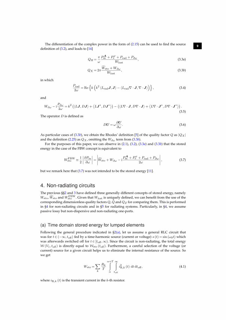
(a) Time domain stored energy for lumped elementsFollowing the general procedure indicated in §2(a), let us assume a general RLC circuit thatwas for t∈ (−∞, toff) fed by a time-harmonic source (current or voltage) s (t) = sin (ω0t) whichwas afterwards switched off for t∈ [toff ,∞). Since the circuit is non-radiating, the total energyW (V1, toff) is directly equal to Wsto (toff). Furthermore, a careful selection of the voltage (orcurrent) source for a given circuit helps us to eliminate the internal resistance of the source. Sowe get

Wsto =∑k

RkT

α+T∫α

∞∫toff

i2R,k (t) dt dtoff , (4.1)

where iR,k (t) is the transient current in the k-th resistor.

10The currents iR,k are advantageously evaluated in the frequency domain. The Fouriertransform of the source reads [55]

S (ω) =iπ

2(δ (ω + ω0)− δ (ω − ω0)) +

e−iωtoff

2

(eiω0toff

ω − ω0− e−iω0toff

ω + ω0

). (4.2)

We can then write IR,k (ω) = TRk(ω)S (ω), where TRk

(ω) represents the transfer function.Consequently

iR,k (t) =1

2π

∞∫−∞

TRk(ω)S (ω) eiωt dω

=1

2Im{TRk

(ω0) eiω0t

}+

ω

4π

∞∫−∞

TRk(ω)

(eiω0toff

ω − ω0− e−iω0toff

ω + ω0

)eiω(t−toff ) dω.

(4.3)

As the studied circuit is lossy, TRk(ω) has no poles on the real ω-axis and the second integral

can be evaluated by the standard contour integration in the complex plane of ω along the semi-circular contour in the upper ω half-plane, while omitting the points ω=±ω0. The result of thecontour integration for t > toff can be written as

iR,k (t) =i

2

∑m

resω→ωm,k

{TRk

(ω)

(eiω0toff

ω − ω0− e−iω0toff

ω + ω0

)eiω(t−toff )

}, (4.4)

where ωm,k are the poles of TRk(ω) with Im

{ωm,k

}> 0. The substitution of (4.4) into (4.1) gives

the mean stored energy. It is also important to realize that in this case, it is easy to analyticallycarry out both integrations involved in (4.1). The result is obviously identical to the cycle mean ofthe classical definition of stored energy.

Wsto (toff) =1

2

(∑m

Lmi2L,m (toff) +

∑n

Cnu2C,n (toff)

), (4.5)

which is the lumped circuit form of (2.10), with iL,m (t) being the current in them-th inductor Lmand uC,n (t) being the voltage on the n-th capacitor Cn.

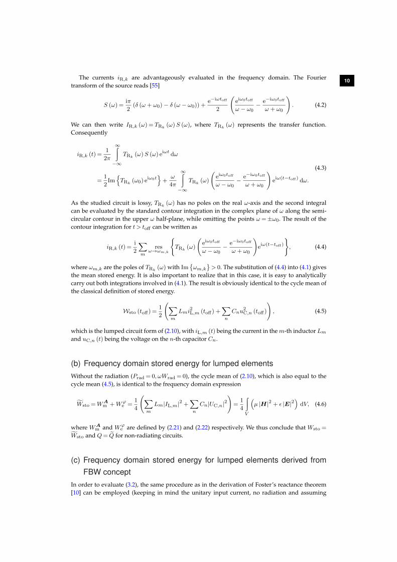
(b) Frequency domain stored energy for lumped elementsWithout the radiation (Prad = 0, ωWrad = 0), the cycle mean of (2.10), which is also equal to thecycle mean (4.5), is identical to the frequency domain expression

W̃sto =WAm +Wϕ

e =1

4

(∑m

Lm|IL,m|2 +∑n

Cn|UC,n|2)

=1

4

∫V

(µ |H|2 + ε |E|2

)dV, (4.6)

where WAm and Wϕ

e are defined by (2.21) and (2.22) respectively. We thus conclude that Wsto =

W̃sto and Q= Q̃ for non-radiating circuits.

(c) Frequency domain stored energy for lumped elements derived fromFBW concept

In order to evaluate (3.2), the same procedure as in the derivation of Foster’s reactance theorem[10] can be employed (keeping in mind the unitary input current, no radiation and assuming

11

1C

1L

inZ

R0

0i

0u

R1

0Z

2C

2L

inZ

R0

0i

0u

R2

0Z

(a) (b)

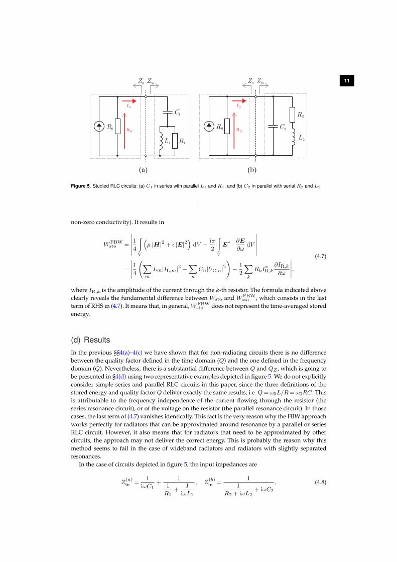
Figure 5. Studied RLC circuits: (a) C1 in series with parallel L1 and R1, and (b) C2 in parallel with serial R2 and L2

.

non-zero conductivity). It results in

WFBWsto =

∣∣∣∣∣∣14∫V

(µ |H|2 + ε |E|2

)dV − iσ

2

∫V

E∗ · ∂E∂ω

dV

∣∣∣∣∣∣=

∣∣∣∣∣14(∑m

Lm|IL,m|2 +∑n

Cn|UC,n|2)− i

2

∑k

RkI∗R,k

∂IR,k∂ω

∣∣∣∣∣,(4.7)

where IR,k is the amplitude of the current through the k-th resistor. The formula indicated aboveclearly reveals the fundamental difference between Wsto and WFBW

sto , which consists in the lastterm of RHS in (4.7). It means that, in general,WFBW

sto does not represent the time-averaged storedenergy.

(d) ResultsIn the previous §§4(a)–4(c) we have shown that for non-radiating circuits there is no differencebetween the quality factor defined in the time domain (Q) and the one defined in the frequencydomain (Q̃). Nevertheless, there is a substantial difference between Q and QZ , which is going tobe presented in §4(d) using two representative examples depicted in figure 5. We do not explicitlyconsider simple series and parallel RLC circuits in this paper, since the three definitions of thestored energy and quality factor Q deliver exactly the same results, i.e. Q= ω0L/R= ω0RC. Thisis attributable to the frequency independence of the current flowing through the resistor (theseries resonance circuit), or of the voltage on the resistor (the parallel resonance circuit). In thosecases, the last term of (4.7) vanishes identically. This fact is the very reason why the FBW approachworks perfectly for radiators that can be approximated around resonance by a parallel or seriesRLC circuit. However, it also means that for radiators that need to be approximated by othercircuits, the approach may not deliver the correct energy. This is probably the reason why thismethod seems to fail in the case of wideband radiators and radiators with slightly separatedresonances.

In the case of circuits depicted in figure 5, the input impedances are

Z(a)in =

1

iωC1+

11

R1+

1

iωL1

, Z(b)in =

11

R2 + iωL2+ iωC2

, (4.8)

12

0 1 2 3 4 5 60

1

2

3

Q(a) QZ(a) QX

(a)

Q(b) QZ(b) QX

(b)

qual

ity

fact

or Q

RiCi

2C

2L

R2

1C

1L R1

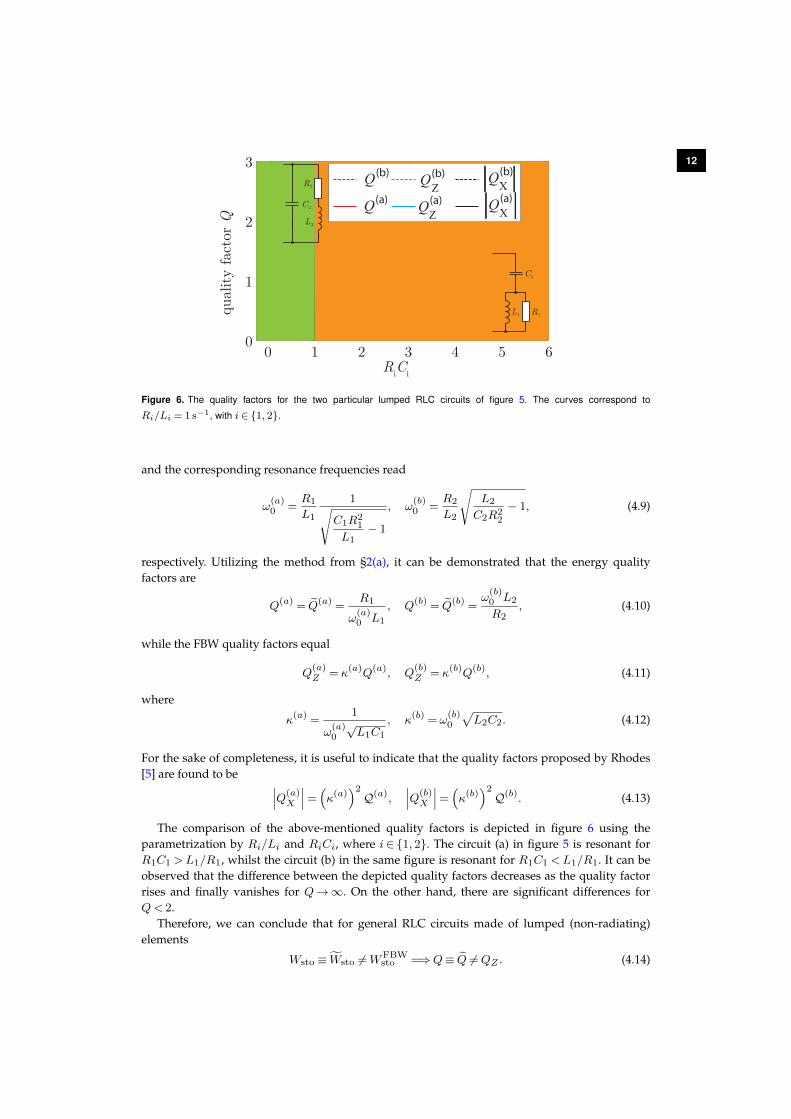
Figure 6. The quality factors for the two particular lumped RLC circuits of figure 5. The curves correspond to

Ri/Li = 1 s−1, with i∈ {1, 2}.

and the corresponding resonance frequencies read

ω(a)0 =

R1

L1

1√C1R

21

L1− 1

, ω(b)0 =

R2

L2

√L2

C2R22

− 1, (4.9)

respectively. Utilizing the method from §2(a), it can be demonstrated that the energy qualityfactors are

Q(a) = Q̃(a) =R1

ω(a)0 L1

, Q(b) = Q̃(b) =ω

(b)0 L2

R2, (4.10)

while the FBW quality factors equal

Q(a)Z = κ(a)Q(a), Q

(b)Z = κ(b)Q(b), (4.11)

where

κ(a) =1

ω(a)0

√L1C1

, κ(b) = ω(b)0

√L2C2. (4.12)

For the sake of completeness, it is useful to indicate that the quality factors proposed by Rhodes[5] are found to be ∣∣∣Q(a)

X

∣∣∣= (κ(a))2Q(a),

∣∣∣Q(b)X

∣∣∣= (κ(b))2Q(b). (4.13)

The comparison of the above-mentioned quality factors is depicted in figure 6 using theparametrization by Ri/Li and RiCi, where i∈ {1, 2}. The circuit (a) in figure 5 is resonant forR1C1 >L1/R1, whilst the circuit (b) in the same figure is resonant for R1C1 <L1/R1. It can beobserved that the difference between the depicted quality factors decreases as the quality factorrises and finally vanishes for Q→∞. On the other hand, there are significant differences forQ< 2.

Therefore, we can conclude that for general RLC circuits made of lumped (non-radiating)elements

Wsto ≡ W̃sto 6=WFBWsto =⇒Q≡ Q̃ 6=QZ . (4.14)

13

iR0(t)

(r ¢,t )

(r ¢,t )a

R0

S1

Numerical simulation

Post-processing

(r ¢,t)

toff

t

i (t)

iR0(t)

freeze(r ¢,t)

freeze(r ¢,t) = (r ¢,t) Û t < toff

freeze(r ¢,t) = (r ¢,toff) Û t ³ toff

-

+R0(iR0

)

rad(freeze )

sto(t)sto =ò sto(t) dtWsto = ásto(toff)ñ

sto

rad( )S1

rad S1

¥

toff

power dissipatedin the resistor R0

instantaneous power radiatedthrough the surface S1

instantaneous stored energy

S1

R0

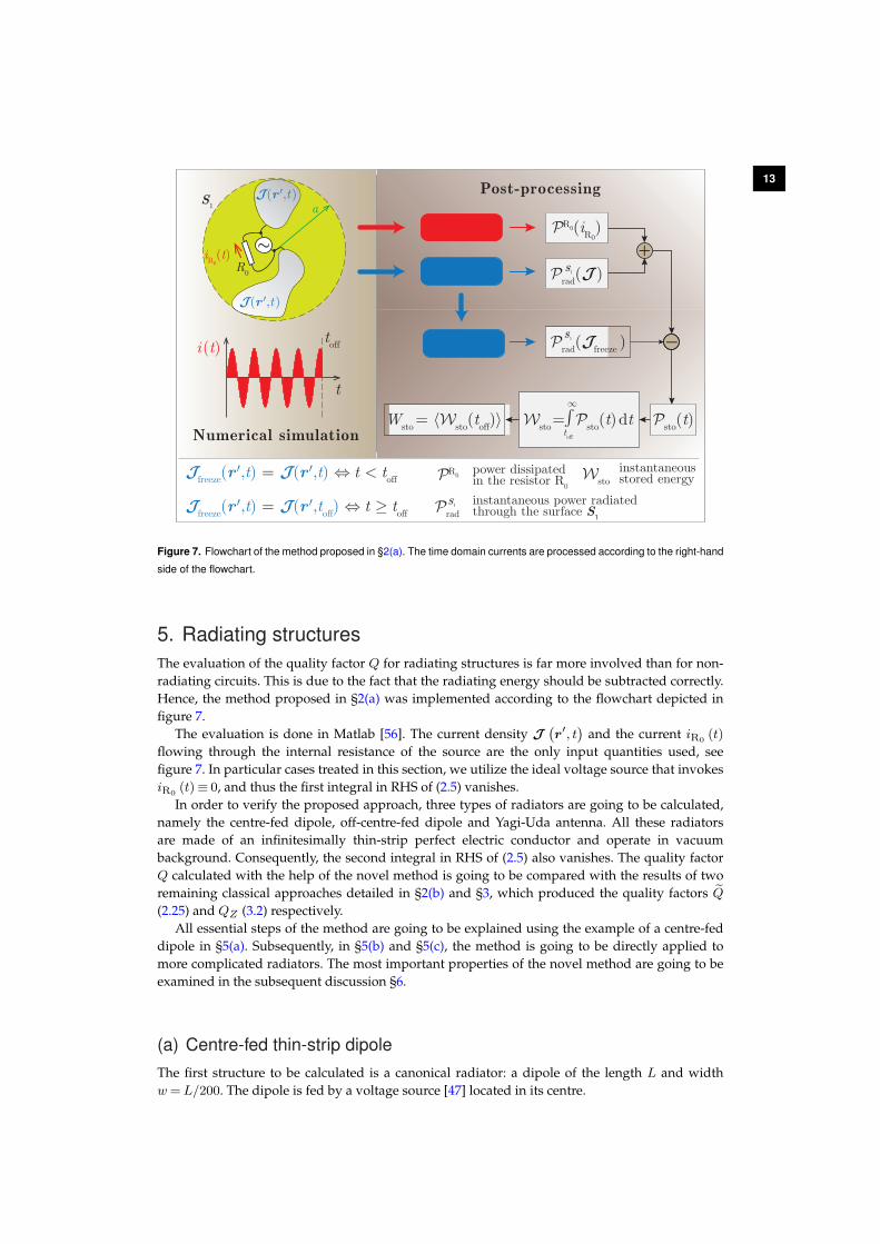
Figure 7. Flowchart of the method proposed in §2(a). The time domain currents are processed according to the right-hand

side of the flowchart.

5. Radiating structuresThe evaluation of the quality factor Q for radiating structures is far more involved than for non-radiating circuits. This is due to the fact that the radiating energy should be subtracted correctly.Hence, the method proposed in §2(a) was implemented according to the flowchart depicted infigure 7.

The evaluation is done in Matlab [56]. The current density J(r′, t

)and the current iR0

(t)

flowing through the internal resistance of the source are the only input quantities used, seefigure 7. In particular cases treated in this section, we utilize the ideal voltage source that invokesiR0

(t)≡ 0, and thus the first integral in RHS of (2.5) vanishes.In order to verify the proposed approach, three types of radiators are going to be calculated,

namely the centre-fed dipole, off-centre-fed dipole and Yagi-Uda antenna. All these radiatorsare made of an infinitesimally thin-strip perfect electric conductor and operate in vacuumbackground. Consequently, the second integral in RHS of (2.5) also vanishes. The quality factorQ calculated with the help of the novel method is going to be compared with the results of tworemaining classical approaches detailed in §2(b) and §3, which produced the quality factors Q̃(2.25) and QZ (3.2) respectively.

All essential steps of the method are going to be explained using the example of a centre-feddipole in §5(a). Subsequently, in §5(b) and §5(c), the method is going to be directly applied tomore complicated radiators. The most important properties of the novel method are going to beexamined in the subsequent discussion §6.

(a) Centre-fed thin-strip dipoleThe first structure to be calculated is a canonical radiator: a dipole of the length L and widthw=L/200. The dipole is fed by a voltage source [47] located in its centre.

14

i (t)

[A

]

steady state

t w / (2p)0-1 1 3 5 7

−0.1

−0.05

0

0.05

0.1

transient state

0 2 4 6

Lw

(r ¢,t)freeze(r ¢,t)t off

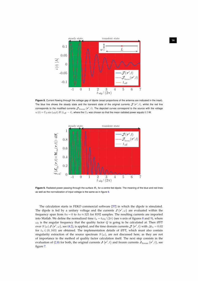
Figure 8. Current flowing through the voltage gap of dipole (exact proportions of the antenna are indicated in the inset).

The blue line shows the steady state and the transient state of the original currents J (r′, t), whilst the red line

corresponds to the modified currents J freeze (r′, t). The depicted curves correspond to the source with the voltage

u (t) =U0 sin (ω0t)H (toff − t), where the U0 was chosen so that the mean radiated power equals 0.5W.

0

0.2

0.4

0.6

0.8

1

0 42 6

steady state transient state

t w / (2p)0

(r ¢,t)freeze(r ¢,t)t off

-1 1 3 5 7

(

(r,t)´

(r,t))

· dS

1fa

rfa

rò S 1

Figure 9. Radiated power passing through the surface S1 for a centre-fed dipole. The meaning of the blue and red lines

as well as the normalization of input voltage is the same as in figure 8.

The calculation starts in FEKO commercial software [57] in which the dipole is simulated.The dipole is fed by a unitary voltage and the currents J

(r′, ω

)are evaluated within the

frequency span from ka= 0 to ka≈ 325 for 8192 samples. The resulting currents are importedinto Matlab. We define the normalized time tn = tω0/ (2π) (see x-axis of figures 8 and 9), whereω0 is the angular frequency that the quality factor Q is going to be calculated at. Then iFFTover S (ω)J

(r′, ω

), see (4.2), is applied, and the time domain currents J

(r′, t

)with ∆tn = 0.02

for tn ∈ (0, 163) are obtained. The implementation details of iFFT, which must also containsingularity extraction of the source spectrum S (ω), are not discussed here, as they are notof importance to the method of quality factor calculation itself. The next step consists in theevaluation of (2.8) for both, the original currents J

(r′, t

)and frozen currents J freeze

(r′, t

), see

figure 7.

15

qual

ity

fact

or Q

ka

0

5

10

15

20

1 2 3 4 5 6 7

Q Q Q Z

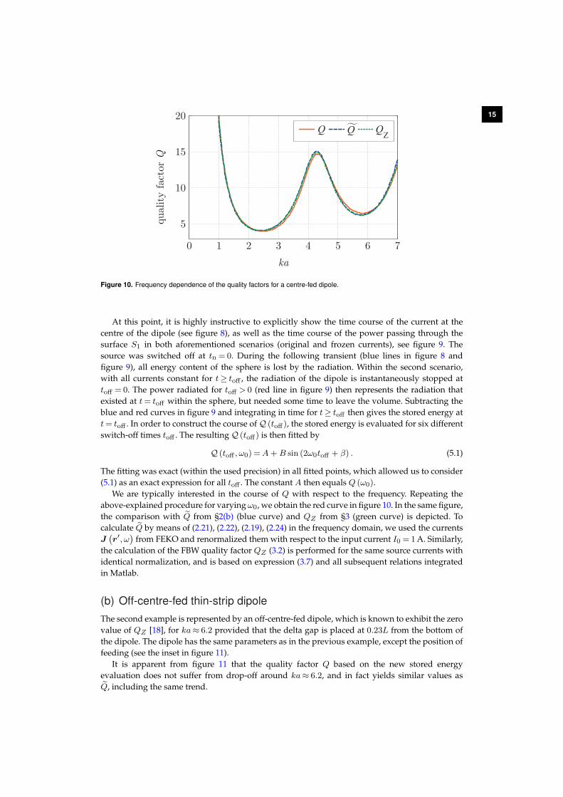
Figure 10. Frequency dependence of the quality factors for a centre-fed dipole.

At this point, it is highly instructive to explicitly show the time course of the current at thecentre of the dipole (see figure 8), as well as the time course of the power passing through thesurface S1 in both aforementioned scenarios (original and frozen currents), see figure 9. Thesource was switched off at tn = 0. During the following transient (blue lines in figure 8 andfigure 9), all energy content of the sphere is lost by the radiation. Within the second scenario,with all currents constant for t≥ toff , the radiation of the dipole is instantaneously stopped attoff = 0. The power radiated for toff > 0 (red line in figure 9) then represents the radiation thatexisted at t= toff within the sphere, but needed some time to leave the volume. Subtracting theblue and red curves in figure 9 and integrating in time for t≥ toff then gives the stored energy att= toff . In order to construct the course ofQ (toff), the stored energy is evaluated for six differentswitch-off times toff . The resultingQ (toff) is then fitted by

Q (toff , ω0) =A+B sin (2ω0toff + β) . (5.1)

The fitting was exact (within the used precision) in all fitted points, which allowed us to consider(5.1) as an exact expression for all toff . The constant A then equals Q (ω0).

We are typically interested in the course of Q with respect to the frequency. Repeating theabove-explained procedure for varying ω0, we obtain the red curve in figure 10. In the same figure,the comparison with Q̃ from §2(b) (blue curve) and QZ from §3 (green curve) is depicted. Tocalculate Q̃ by means of (2.21), (2.22), (2.19), (2.24) in the frequency domain, we used the currentsJ(r′, ω

)from FEKO and renormalized them with respect to the input current I0 = 1A. Similarly,

the calculation of the FBW quality factor QZ (3.2) is performed for the same source currents withidentical normalization, and is based on expression (3.7) and all subsequent relations integratedin Matlab.

(b) Off-centre-fed thin-strip dipoleThe second example is represented by an off-centre-fed dipole, which is known to exhibit the zerovalue of QZ [18], for ka≈ 6.2 provided that the delta gap is placed at 0.23L from the bottom ofthe dipole. The dipole has the same parameters as in the previous example, except the position offeeding (see the inset in figure 11).

It is apparent from figure 11 that the quality factor Q based on the new stored energyevaluation does not suffer from drop-off around ka≈ 6.2, and in fact yields similar values asQ̃, including the same trend.

16

ka

6.2 6.4 6.6 6.8

0

2

4

6

8

Q Q Q Z

6.56.36.1 6.7

Lwqual

ity

fact

or Q

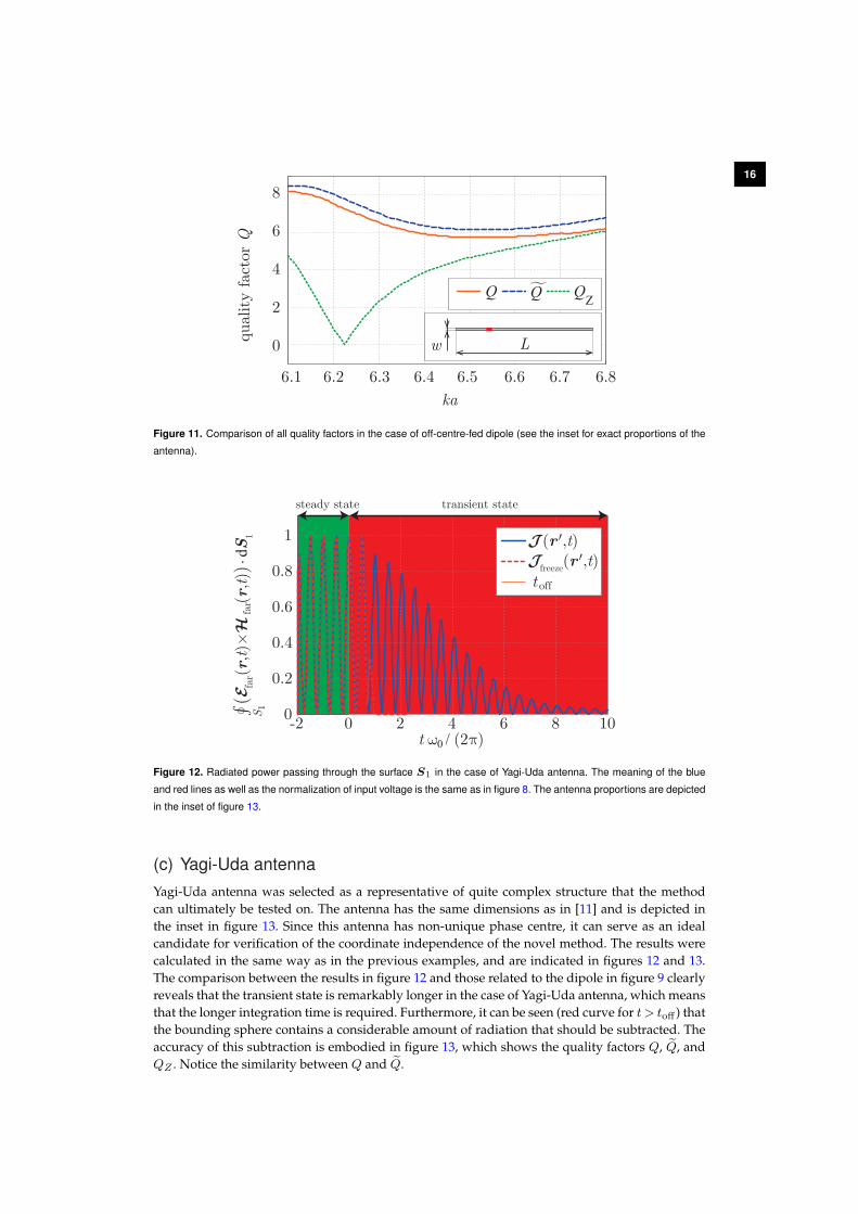
Figure 11. Comparison of all quality factors in the case of off-centre-fed dipole (see the inset for exact proportions of the

antenna).

0

0.2

0.4

0.6

0.8

1

(

(r,t)´

(r,t))

· dS

1fa

rfa

rò S 1

steady state transient state

t w / (2p)0

-2 0 2 4 6 8 10

(r ¢,t)freeze(r ¢,t)t off

Figure 12. Radiated power passing through the surface S1 in the case of Yagi-Uda antenna. The meaning of the blue

and red lines as well as the normalization of input voltage is the same as in figure 8. The antenna proportions are depicted

in the inset of figure 13.

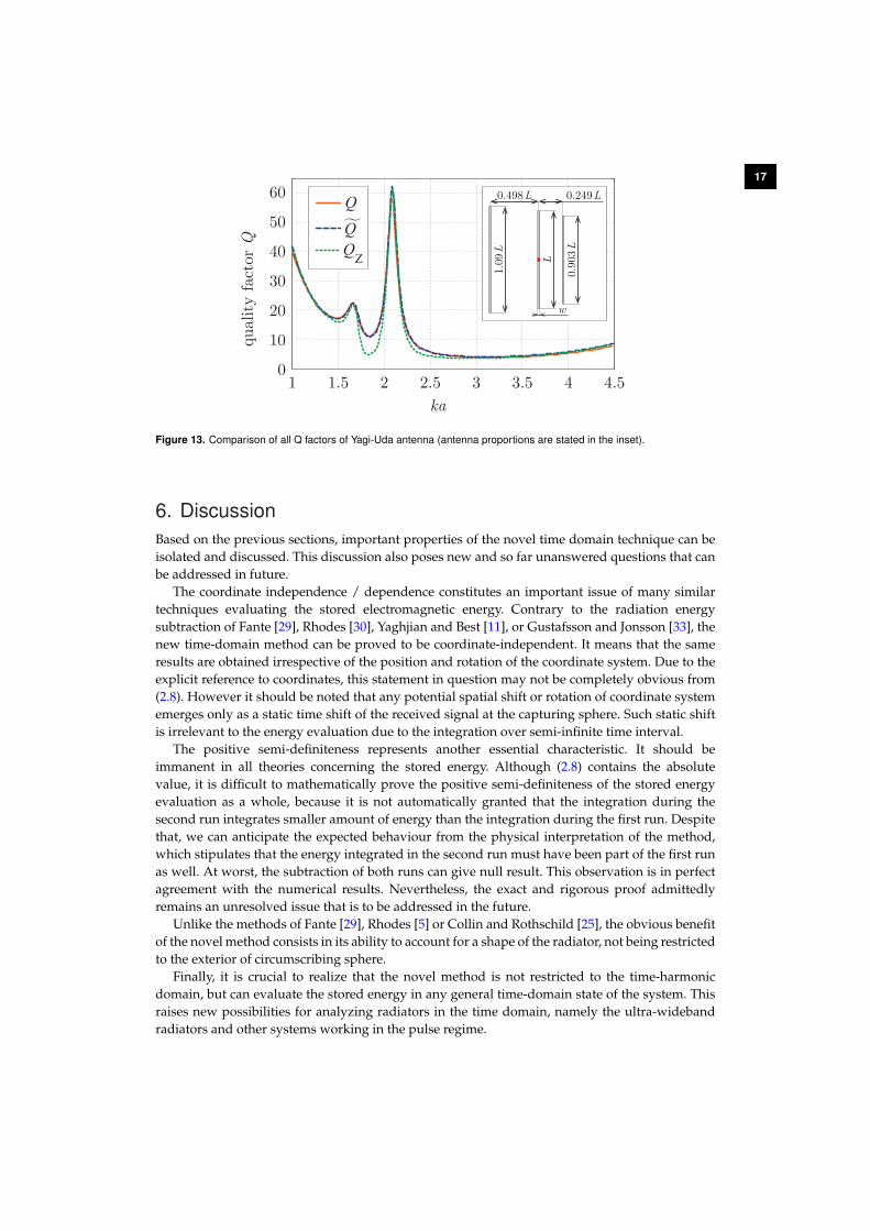
(c) Yagi-Uda antennaYagi-Uda antenna was selected as a representative of quite complex structure that the methodcan ultimately be tested on. The antenna has the same dimensions as in [11] and is depicted inthe inset in figure 13. Since this antenna has non-unique phase centre, it can serve as an idealcandidate for verification of the coordinate independence of the novel method. The results werecalculated in the same way as in the previous examples, and are indicated in figures 12 and 13.The comparison between the results in figure 12 and those related to the dipole in figure 9 clearlyreveals that the transient state is remarkably longer in the case of Yagi-Uda antenna, which meansthat the longer integration time is required. Furthermore, it can be seen (red curve for t > toff ) thatthe bounding sphere contains a considerable amount of radiation that should be subtracted. Theaccuracy of this subtraction is embodied in figure 13, which shows the quality factors Q, Q̃, andQZ . Notice the similarity between Q and Q̃.

17

ka1 1.5 2 2.5 3 3.5 4 4.5

0

10

20

30

40

50

60 QQQ Z L

w

1.09

L

0.90

3 L

0.498 L 0.249 L

qual

ity

fact

or Q

Figure 13. Comparison of all Q factors of Yagi-Uda antenna (antenna proportions are stated in the inset).

6. DiscussionBased on the previous sections, important properties of the novel time domain technique can beisolated and discussed. This discussion also poses new and so far unanswered questions that canbe addressed in future.

The coordinate independence / dependence constitutes an important issue of many similartechniques evaluating the stored electromagnetic energy. Contrary to the radiation energysubtraction of Fante [29], Rhodes [30], Yaghjian and Best [11], or Gustafsson and Jonsson [33], thenew time-domain method can be proved to be coordinate-independent. It means that the sameresults are obtained irrespective of the position and rotation of the coordinate system. Due to theexplicit reference to coordinates, this statement in question may not be completely obvious from(2.8). However it should be noted that any potential spatial shift or rotation of coordinate systememerges only as a static time shift of the received signal at the capturing sphere. Such static shiftis irrelevant to the energy evaluation due to the integration over semi-infinite time interval.

The positive semi-definiteness represents another essential characteristic. It should beimmanent in all theories concerning the stored energy. Although (2.8) contains the absolutevalue, it is difficult to mathematically prove the positive semi-definiteness of the stored energyevaluation as a whole, because it is not automatically granted that the integration during thesecond run integrates smaller amount of energy than the integration during the first run. Despitethat, we can anticipate the expected behaviour from the physical interpretation of the method,which stipulates that the energy integrated in the second run must have been part of the first runas well. At worst, the subtraction of both runs can give null result. This observation is in perfectagreement with the numerical results. Nevertheless, the exact and rigorous proof admittedlyremains an unresolved issue that is to be addressed in the future.

Unlike the methods of Fante [29], Rhodes [5] or Collin and Rothschild [25], the obvious benefitof the novel method consists in its ability to account for a shape of the radiator, not being restrictedto the exterior of circumscribing sphere.

Finally, it is crucial to realize that the novel method is not restricted to the time-harmonicdomain, but can evaluate the stored energy in any general time-domain state of the system. Thisraises new possibilities for analyzing radiators in the time domain, namely the ultra-widebandradiators and other systems working in the pulse regime.

187. ConclusionThree different concepts aiming to evaluate the stored electromagnetic energy and the resultingquality factorQ of radiating system were investigated. The novel time domain scheme constitutesthe first one, while the second one utilizes time-harmonic quantities and classical radiation energyextraction. The third one is based on the frequency variation of radiator?s input impedance. Allmethods were subject to in-depth theoretical comparison and their differences were presented ongeneral non-radiating RLC networks as well as common radiators.

It was explicitly shown that the most practical scheme based on the frequency derivativeof the input impedance generally fails to give the correct quality factor, but may serve as avery good estimate of it for structures that are well approximated by series or parallel resonantcircuits. In contrast, the frequency domain concept with far-field energy extraction was foundto work correctly in the case of general RLC circuits and simple radiators. Unlike the newlyproposed time domain scheme, it could however yield negative values of stored energy, which isactually known to happen for specific current distributions. In this respect, the novel time domainmethod proposed in this paper could be denoted as reference, since it exhibits the coordinateindependence, positive semi-definiteness, and most importantly, takes into account the actualradiator shape. Another virtue of the novel scheme is constituted by the possibility to use it outof the time-harmonic domain, e.g. in the realm of radiators excited by general pulse.

The follow-up work should focus on the radiation characteristics of separated parts ofradiators or radiating arrays, the investigation of different time domain feeding pulses and theirinfluence on performance of ultra-wideband radiators and, last but not least, on the theoreticalformulation of the stored energy density generated by the new time domain method.

Data accessibility. This manuscript does not contain primary data and as a result has no supporting materialassociated with the results presented.

Authors’ contributions. All authors contributed to the formulation, did numerical simulations and draftedthe manuscript. All authors gave final approval for publication.

Acknowledgements. The authors are grateful to Ricardo Marques (Department of Electronics andElectromagnetism, University of Seville) and Raul Berral (Department of Applied Physics, University ofSeville) for many valuable discussions that stimulated some of the core ideas of this contribution. The authorsare also grateful to Jan Eichler (Department of Electromagnetic Field, Czech Technical University in Prague)for his help with the simulations.

Funding statement. The authors would like to acknowledge the support of COST IC1102 (VISTA) actionand of project 15-10280Y funded by the Czech Science Foundation.

Conflict of interests. We declare to have no competing interests.

References1 Morse, P. M. & Feshbach, H. 1953 Methods of Theoretical Physics. McGraw-Hill.2 Hallen, E. 1962 Electromagnetic Theory. Chapman & Hall.3 Volakis, J. L., Chen, C. & Fujimoto, K. 2010 Small Antennas: Miniaturization Techniques &

Applications. McGraw-Hill.4 Collin, R. E. 1992 Foundations for Microwave Engineering. John Wiley - IEEE Press, 2nd edn.5 Rhodes, D. R. 1976 Observable stored energies of electromagnetic systems. J. Franklin Inst.,

302(3), 225–237. doi:10.1016/0016-0032(79)90126-1.6 Kajfez, D. & Wheless, W. P. 1986 Invariant definitions of the unloaded Q factor. IEEE Antennas

Propag. Magazine, 34(7), 840–841.7 Harrington, R. F. 1958 On the gain and beamwidth of directional antennas. IRE Trans. Antennas

Propag., 6(3), 219–225. doi:10.1109/TAP.1958.1144605.8 Standard definitions of terms for antennas 145 - 1993.9 Foster, R. M. 1924 A reactance theorem. Bell System Tech. J., 3, 259–267. doi:10.1098/rspa.1977.

0018.

1910 Harrington, R. F. 2001 Time-Harmonic Electromagnetic Fields. John Wiley - IEEE Press, 2nd edn.11 Yaghjian, A. D. & Best, S. R. 2005 Impedance, bandwidth and Q of antennas. IEEE Trans.

Antennas Propag., 53(4), 1298–1324. doi:10.1109/TAP.2005.844443.12 Best, S. R. & Hanna, D. L. 2010 A performance comparison of fundamental small-antenna

designs. IEEE Antennas Propag. Magazine, 52(1), 47–70. doi:10.1109/MAP.2010.5466398.13 Sievenpiper, D. F., Dawson, D. C., Jacob, M. M., Kanar, T., Sanghoon, K., Jiang, L. & Quarfoth,

R. G. 2012 Experimental validation of performance limits and design guidelines for smallantennas. IEEE Trans. Antennas Propag., 60(1), 8–19. doi:10.1109/TAP.2011.2167938.

14 Capek, M., Jelinek, L., Hazdra, P. & Eichler, J. 2014 The measurable Q factor and observableenergies of radiating structures. IEEE Trans. Antennas Propag., 62(1), 311–318. doi:10.1109/TAP.2013.2287519.

15 Jin, J.-M. 2010 Theory and Computation of Electromagnetic Fields. John Wiley.16 Gustafsson, M. & Nordebo, S. 2006 Bandwidth, Q factor and resonance models of antennas.

Progress In Electromagnetics Research, 62, 1–20. doi:10.2528/PIER06033003.17 Capek, M., Jelinek, L. & Hazdra, P. 2015 On the functional relation between quality factor and

fractional bandwidth. IEEE Trans. Antennas Propag., 63(6), 2787–2790. doi:10.1109/TAP.2015.2414472.

18 Gustafsson, M. & Jonsson, B. L. G. 2015 Antenna Q and stored energy expressed in the fields,currents, and input impedance. IEEE Trans. Antennas Propag., 63(1), 240–249. doi:10.1109/TAP.2014.2368111.

19 Gustafsson, M., Cismasu, M. & Jonsson, B. L. G. 2012 Physical bounds and optimal currentson antennas. IEEE Trans. Antennas Propag., 60(6), 2672–2681. doi:10.1109/TAP.2012.2194658.

20 Jackson, J. D. 1998 Classical Electrodynamics. John Wiley, 3rd edn.21 Chu, L. J. 1948 Physical limitations of omni-directional antennas. J. Appl. Phys., 19, 1163–1175.

doi:10.1063/1.1715038.22 Dirac, P. A. M. 1938 Classical theory of radiating electrons. Proc. of Royal Soc. A, 167, 148–169.

doi:10.1098/rspa.1938.0124.23 Thal, H. L. 1978 Exact circuit analysis of spherical waves. IEEE Trans. Antennas Propag., 26(2),

282–287. doi:10.1109/TAP.1978.1141822.24 Thal, H. L. 2012 Q bounds for arbitrary small antennas: A circuit approach. IEEE Trans.

Antennas Propag., 60(7), 3120–3128. doi:10.1109/TAP.2012.2196920.25 Collin, R. E. & Rothschild, S. 1964 Evaluation of antenna Q. IEEE Trans. Antennas Propag., 12(1),

23–27. doi:10.1109/TAP.1964.1138151.26 McLean, J. S. 1996 A re-examination of the fundamental limits on the radiation Q of electrically

small antennas. IEEE Trans. Antennas Propag., 44(5), 672–675.27 Manteghi, M. 2010 Fundamental limits of cylindrical antennas. Tech. Rep. 1, Virginia Tech.28 Collin, R. E. 1998 Minimum Q of small antennas. Journal of Electromagnetic Waves and

Applications, 12(10), 1369–1393. doi:10.1163/156939398X01457.29 Fante, R. L. 1969 Quality factor of general ideal antennas. IEEE Trans. Antennas Propag., 17(2),

151–157. doi:10.1109/TAP.1969.1139411.30 Rhodes, D. R. 1977 A reactance theorem. Proc. R. Soc. Lond. A., 353, 1–10. doi:10.1098/rspa.

1977.0018.31 Vandenbosch, G. A. E. 2010 Reactive energies, impedance, and Q factor of radiating structures.

IEEE Trans. Antennas Propag., 58(4), 1112–1127. doi:10.1109/TAP.2010.2041166.32 Geyi, W. 2003 A method for the evaluation of small antenna Q. IEEE Trans. Antennas Propag.,

51(8), 2124–2129. doi:10.1109/TAP.2003.814755.33 Gustafsson, M. & Jonsson, B. L. G. 2014 Stored electromagnetic energy and antenna Q. Prog.

Electromagn. Res., 150, 13–27.34 Vandenbosch, G. A. E. 2013 Reply to “Comments on ‘Reactive energies, impedance, and Q

factor of radiating structures’". IEEE Trans. Antennas Propag., 61(12), 6268. doi:10.1109/TAP.2013.2281573.

35 Shlivinski, A. & Heyman, E. 1999 Time-domain near-field analysis of short-pulse antennas -part I: Spherical wave (multipole) expansion. IEEE Trans. Antennas Propag., 47(2), 271–279.doi:10.1109/8.761066.

2036 Shlivinski, A. & Heyman, E. 1999 Time-domain near-field analysis of short-pulse antennas- part II: Reactive energy and the antenna Q. IEEE Trans. Antennas Propag., 47(2), 280–286.doi:10.1109/8.761067.

37 Collardey, S., Sharaiha, A. & Mahdjoubi, K. 2006 Calculation of small antennas quality factorusing FDTD method. IEEE Antennas Wireless Propag. Lett., 5, 191–194. doi:10.1109/LAWP.2006.873947.

38 Vandenbosch, G. A. E. 2013 Radiators in time domain, part I: Electric, magnetic, and radiatedenergies. IEEE Trans. Antennas Propag., 61(8), 3995–4003. doi:10.1109/TAP.2013.2261044.

39 Kaiser, G. 2011 Electromagnetic inertia, reactive energy and energy flow velocity. J. Phys. A.:Math. Theor., 44, 1–15. doi:10.1088/1751-8113/44/34/345206.

40 Capek, M. & Jelinek, L. 2015 Various interpretations of the stored and the radiated energydensity. Submitted, arXiv: 1503.06752.

41 Harrington, R. F. 1960 Effects of antenna size on gain, bandwidth, and efficiency. J. Nat. Bur.Stand., 64-D, 1–12.

42 Yaghjian, A. D., Gustafsson, M. & Jonsson, B. L. G. 2013 Minimum Q for lossy and losselesselectrically small dipole antenna. Progress In Electromagnetics Research, 143, 641–673. doi:10.2528/PIER13103107.

43 Jonsson, B. L. G. & Gustafsson, M. 2015 Stored energies in electric and magnetic currentdensities for small antennas. Proc. of Royal Soc. A, 471, 1–23. doi:10.1098/rspa.2014.0897.

44 Jelinek, L., Capek, M., Hazdra, P. & Eichler, J. 2015 An analytical evaluation of the quality factorQZ for dominant spherical modes. IET Microw. Antennas Propag., 9(10), 1096–1103. doi:10.1049/iet-map.2014.0302. ArXiv: 1311.1750v1.

45 Capek, M., Hazdra, P. & Eichler, J. 2012 A method for the evaluation of radiation Q basedon modal approach. IEEE Trans. Antennas Propag., 60(10), 4556–4567. doi:10.1109/TAP.2012.2207329.

46 Gustafsson, M. & Nordebo, S. 2013 Optimal antenna currents for Q, superdirectivity, andradiation patterns using convex optimization. IEEE Trans. Antennas Propag., 61(3), 1109–1118.doi:10.1109/TAP.2012.2227656.

47 Balanis, C. A. 1989 Advanced Engineering Electromagnetics. John Wiley.48 Balanis, C. A. 2005 Antenna Theory Analysis and Design. John Wiley, 3rd edn.49 Akhiezer, N. I. & Glazman, I. M. 1993 Theory of Linear Operators in Hilbert Space. Dover, 2nd

edn.50 Morgenthaler, F. R. 2011 The Power and Beauty of Electromagnetic Fields. Wiley-IEEE Press.51 Carpenter, C. J. 1989 Electromagnetic energy and power in terms of charges and potentials

instead of fields. Proc. of IEE A, 136(2), 55–65.52 Uehara, M., Allen, J. E. & Carpenter, C. J. 1992 Comments to ‘Electromagnetic energy and

power in terms of charges and potentials instead of fields’. Proc. of IEE A, 139(1), 42–44.53 Endean, V. G. & Carpenter, C. J. 1992 Comments to ‘Electromagnetic energy and power in

terms of charges and potentials instead of fields’. Proc. of IEE A, 139(6), 338–342.54 Jelinek, L., Capek, M., Hazdra, P. & Eichler, J. 2014 Lower bounds of the quality factor QZ .

In IEEE International Symposium on Antennas and Propagation and USNC-URSI Radio ScienceMeeting. Accepted.

55 Rothwell, E. J. & Cloud, M. J. 2001 Electromagnetics. CRC Press.56 The MathWorks 2015 The Matlab.57 EM Software & Systems-S.A. FEKO.