Embed Size (px)
Citation preview

Storing and Querying
Large XML Instances
Christian Grun
Dissertation zur Erlangung des akademischen GradesDoktor der Naturwissenschaften (Dr. rer. nat.)
Fachbereich Informatik und InformationswissenschaftMathematisch-Naturwissenschaftliche Sektion
Universitat Konstanz
Referenten:
Prof. Dr. Marc H. Scholl
Prof. Dr. Marcel Waldvogel
Tag der mundlichen Prufung: 22. Dezember 2010


Abstract
After its introduction in 1998, XML has quickly emerged as the de facto exchange format
for textual data. Only ten years later, the amount of information that is being processed
day by day, locally and globally, has virtually exploded, and no end is in sight. Corre-
spondingly, many XML documents and collections have become much too large for being
retrieved in their raw form – and this is where database technology gets into the game.
This thesis describes the design of a full-fledged XML storage and query architecture,
which represents the core of the Open Source database system BASEX. In contrast to
numerous other works on XML processing, which either focus on theoretical aspects
or practical implementation details, we have tried to bring the two worlds together:
well-established and novel concepts from database technology and compiler constructionare consolidated to a powerful and extensible software architecture that is supposed to
both withstand the demands of complex real-life applications and comply with all the
intricacies of the W3C Recommendations.
In the Storage chapter, existing tree encodings are explored, which allow XML documents
to be mapped to a database. The Pre/Dist/Size triple is chosen as the most suitable
encoding and further optimized by merging all XML node properties into a single tuple,
compactifying redundant information, and inlining attributes and numeric values. The
address ranges of numerous large-scale and real-life XML instances are analyzed to find
an optimal tradeoff between maximum document and minimum database size. The
process of building a database is described in detail, including the import of tree data
other than XML and the creation of main memory database instances. As one of the
distinguishing features, the resulting storage is enriched by light-weight structural, value
and full-text indexes, which speed up query processing by orders of magnitudes.
The Querying chapter is introduced with a survey on state of the art XML query lan-
guages. We give some insight into the design of an XQuery processor and then focus on
the optimization of queries. Beside classical concepts, such as constant folding or statictyping, many optimizations are specific to XML: location paths are rewritten to access
less XML nodes, and FLWOR expressions are reorganized to reduce the algorithmic com-
iii

plexity. A unique feature of our query processor represents the dynamic rewriting of
location paths to take advantage of available index structures. Next, we examine the
evaluation of queries and propose an adaptive approach to benefit from both the iter-ative and atomic processing paradigm. Based on the evaluation of location paths, it is
illustrated how databases are accessed by the query processor. The concluding summary
gives an overview on the optimizations that have been applied to the most important
XQuery expressions.
In the Performance chapter, we demonstrate the efficiency and scalability of the result-
ing database system BASEX. The storage and query capabilities are tested and compared
with other database systems and query processors. The benchmark results show that the
proposed architecture and its interplay between the storage and query components em-
braces some qualities that are, to the best of our knowledge, unique and unprecedented
among comparable products.
iv

Zusammenfassung (German Abstract)
Nachdem XML 1998 das Licht der Welt erblickt hat, hat es sich sehr schnell zum Quasi-Standard fur den Austausch textueller Daten entwickelt. Nur zehn Jahre spater sind
die Informationsmengen, die tagtaglich lokal und global verarbeitet werden, explodiert,
und ein Ende der Entwicklung ist noch nicht abzusehen. Demzufolge sind auch viele
XML-Dokumente und -Kollektionen langst zu groß geworden, um Sie in ihrer Rohform
abzufragen – und hier kommt Datenbanktechnologie zum Einsatz.
Diese Dissertation beschreibt das Design einer ausgereiften XML-Speicher- und Query-
Architektur, die zugleich den Kern des Open-Source Datenbanksystems BASEX darstellt.
Im Gegensatz zu zahlreichen anderen Publikationen uber XML, die sich entweder the-
oretischen Teilaspekten oder praktischen Implementierungsdetails verschreiben, wurde
in dieser Arbeit versucht, beide Welten zusammenzufuhren: wohlbekannte und neuar-
tige Konzepte der Datenbanktechnologie und des Compiler-Baus bilden die Basis fur eine
machtige und offene Software-Architektur, die sowohl den Anforderungen komplexer,
realer Anwendungen standhalten als auch die Feinheiten der W3C-Empfehlungen beruck-
sichtigen und einhalten soll.
Im Storage-Kapitel werden existierende Baum-Kodierungen untersucht, die die Spei-
cherung von XML-Dokumenten in Datenbanken ermoglichen. Das Pre/Dist/Size-Tripel
wird als die geeignetste Kodierung ausgewahlt und weiter optimiert: alle Eigenschaften
eines XML-Knotens werden in einem Tupel abgebildet, redundante Information wer-
den kompaktifiziert und Attribute und numerische Werte werden gelinlined, d.h. di-
rekt innnerhalb der Tupel abgespeichert. Die Adressbereiche zahlreicher großer, realer
XML-Instanzen werden analysiert, um einen optimalen Kompromiss zwischen maxi-
maler Dokument- und minimaler Datenbankgroße zu finden. Die Erzeugung neuer
Datenbankinstanzen wird im Detail vorgestellt; dabei werden auch hauptspeicherorien-
tierte Datenbanken und andere hierarchische Datentypen neben XML betrachtet. Eine
Besonderheit der diskutierten Speicherarchitektur stellt die Erweiterung durch schlanke
struktur-, inhalts- und volltextbasierte Indexstrukturen dar, die die Anfragegeschwindig-
keit um mehrere Großenordnungen beschleunigen konnen.
v

Das Querying-Kapitel beginnt mit einem Uberblick uber die relevanten XML-Anfrage-
sprachen und beschreibt den Aufbau eines XQuery-Prozessors. Die Optimierung von An-
fragen steht anschließend im Mittelpunkt. Klassische Techniken wie Constant Foldingoder Statische Typisierung werden durch XML-spezifische Optimierungen erganzt: Doku-
mentpfade werden umgeschrieben, um die Zahl der adressierten XML-Knoten zu re-
duzieren, und FLWOR-Ausdrucke werden reorganisiert, um die algorithmischen Kosten
zu senken. Ein einzigartiges Feature des vorgestellten Query-Prozessors stellt die flex-
ible Umschreibung von Dokumentpfaden fur indexbasierte Anfragen dar. Als nachstes
wird die Evaluierung von Anfragen untersucht und ein adaptiver Ansatz vorgestellt, der
die Vorteile der iterativen und atomaren Anfrageverarbeitung vereinigt. Anhand der
Evaluierung von Dokumentpfaden wird der Zugriff auf die Datenbank veranschaulicht.
Der abschließende Uberblick fasst die Optimierungsschritte zusammen, die auf die wich-
tigsten XQuery-Ausdrucke angewandt wurden.
Die Effizienz und Skalierbarkeit des Datenbanksystems BASEX ist Schwerpunkt des Per-formance-Kapitels. Die Speicher- und Anfrage-Architektur wird getrennt voneinander
analysiert und mit anderen Datenbank-Systemen und Query-Prozessoren verglichen.
Die Ergebnisse sollen demonstrieren, dass die vorgestellte Architektur und das Zusam-
menspiel zwischen den Speicher- und Query-Komponenten uber bestimmte Qualitaten
verfugt, die unserem Kenntnisstand nach einzigartig unter vergleichbaren Produkten
sind.
vi

Acknowledgments
Most certainly, this thesis would not have been completed without the continuous help,
support and inspirations of some persons, which I am pleased to mention in the follow-
ing:
First of all, I owe my deepest gratitude to my supervisor Marc H. Scholl, who has given
me all the time and freedom I could have possibly asked for to develop and pursue
my own ideas – a privilege that I know many postgraduates can only dream of. At the
same time, Marc has always had time for discussions, and I learned a lot from both his
guidance and vast expertise. Whenever I had doubts whether I was on the right path –
or any path at all – it was Marc who backed me, and confirmed me to go on.
Next, I would like to thank Marcel Waldvogel and his disy Group. The exchange be-
tween his and our group consisted in numerous fruitful debates, joint publications and,
as I believe, brought the work of all of us forward more quickly. Another thank you is
directed to Harald Reiterer, who was the first in Konstanz to get me enthusiastic about
scientific work. The cooperation between his HCI Group and ours lasts till the present
day.
It was my colleague Alexander Holupirek who I shared most prolific ideas with during
the last years, and some more drinks in the evenings. He gave me regular feedback
on my flights of fancy (or figments), and many of the contributions presented in this
work are due to his invaluable inspirations. I am also indebted to Marc Kramis, whose
visionary approach has advised me to remain open for new ideas, and Sebastian Graf,
who has triggered our most recent cooperation with the disy Group.
The collaboration with all the students working in my project was one of the most ful-
filling experiences, and I learnt a lot about what it means to lead a project, and how
productive real team work can be. In particular, I’d like to say thank you to Volker
Wildi, Tim Petrowski, Sebastian Gath, Bastian Lemke, Lukas Kircher, Andreas Weiler,
Jorg Hauser, Michael Seiferle, Sebastian Faller, Wolfgang Miller, Elmedin Dedovic, Lukas
Lewandowski, Oliver Egli, Leonard Worteler, Rositsa Shadura, Dimitar Popov, Jens Erat,
vii

and Patrick Lang. I have chosen a somewhat chronological order, assuming that all of
you know how much I value your individual contributions. Another big thank you goes
to Barbara Luthke, our secretary with excellent language skills who deliberately spent
countless hours proof-reading the entire thesis.
Last but not least, words cannot express my appreciation to my parents, my brother
Achim, and Milda. Your endless emotional support was the real driving force behind
this work. To give it at least another try: Danke and Aciu!
viii

Contents
Contents
1 Introduction 1
1.1 Motivation . . . . . . . . . . . . . . . . . . . . . . . . . . . . . . . . . . . . 1
1.2 Contribution . . . . . . . . . . . . . . . . . . . . . . . . . . . . . . . . . . 2
1.3 Outline . . . . . . . . . . . . . . . . . . . . . . . . . . . . . . . . . . . . . 3
1.4 Publications . . . . . . . . . . . . . . . . . . . . . . . . . . . . . . . . . . . 4
2 Storage 5
2.1 Introduction . . . . . . . . . . . . . . . . . . . . . . . . . . . . . . . . . . . 5
2.2 History . . . . . . . . . . . . . . . . . . . . . . . . . . . . . . . . . . . . . . 5
2.3 XML Encodings . . . . . . . . . . . . . . . . . . . . . . . . . . . . . . . . . 7
2.3.1 Document Object Model . . . . . . . . . . . . . . . . . . . . . . . . 7
2.3.2 Pre- and Postorder . . . . . . . . . . . . . . . . . . . . . . . . . . . 8
2.3.3 Level Depth . . . . . . . . . . . . . . . . . . . . . . . . . . . . . . . 10
2.3.4 Number of Descendants . . . . . . . . . . . . . . . . . . . . . . . . 10
2.3.5 Parent Reference . . . . . . . . . . . . . . . . . . . . . . . . . . . . 11
2.3.6 Node Properties . . . . . . . . . . . . . . . . . . . . . . . . . . . . . 12
2.3.7 Namespaces . . . . . . . . . . . . . . . . . . . . . . . . . . . . . . . 13
2.4 Pre/Dist/Size Mapping . . . . . . . . . . . . . . . . . . . . . . . . . . . . . 14
2.4.1 Address Ranges . . . . . . . . . . . . . . . . . . . . . . . . . . . . . 15
2.4.1.1 Analysis . . . . . . . . . . . . . . . . . . . . . . . . . . . . 15
2.4.1.2 XML Instances . . . . . . . . . . . . . . . . . . . . . . . . 17
2.4.2 Table Mapping . . . . . . . . . . . . . . . . . . . . . . . . . . . . . 19
2.4.2.1 Attribute Inlining . . . . . . . . . . . . . . . . . . . . . . . 19
2.4.2.2 Bit Ranges . . . . . . . . . . . . . . . . . . . . . . . . . . 20
2.4.2.3 Compactification . . . . . . . . . . . . . . . . . . . . . . . 21
2.4.2.4 Integer Inlining . . . . . . . . . . . . . . . . . . . . . . . . 21
2.4.2.5 Updates . . . . . . . . . . . . . . . . . . . . . . . . . . . . 23
2.5 Database Architecture . . . . . . . . . . . . . . . . . . . . . . . . . . . . . 25
2.5.1 Database Construction . . . . . . . . . . . . . . . . . . . . . . . . . 25
ix

Contents
2.5.2 Generic Parsing . . . . . . . . . . . . . . . . . . . . . . . . . . . . . 28
2.5.3 Main Memory vs Persistent Storage . . . . . . . . . . . . . . . . . . 29
2.6 Index Structures . . . . . . . . . . . . . . . . . . . . . . . . . . . . . . . . 31
2.6.1 Names . . . . . . . . . . . . . . . . . . . . . . . . . . . . . . . . . . 31
2.6.2 Path Summary . . . . . . . . . . . . . . . . . . . . . . . . . . . . . 33
2.6.3 Values . . . . . . . . . . . . . . . . . . . . . . . . . . . . . . . . . . 35
2.6.3.1 Compression . . . . . . . . . . . . . . . . . . . . . . . . . 36
2.6.3.2 Construction . . . . . . . . . . . . . . . . . . . . . . . . . 36
2.6.3.3 Main Memory Awareness . . . . . . . . . . . . . . . . . . 37
2.6.4 Full-Texts . . . . . . . . . . . . . . . . . . . . . . . . . . . . . . . . 37
2.6.4.1 Fuzzy Index . . . . . . . . . . . . . . . . . . . . . . . . . 39
2.6.4.2 Trie Index . . . . . . . . . . . . . . . . . . . . . . . . . . . 40
3 Querying 43
3.1 XML Languages . . . . . . . . . . . . . . . . . . . . . . . . . . . . . . . . . 43
3.1.1 XPath . . . . . . . . . . . . . . . . . . . . . . . . . . . . . . . . . . 44
3.1.2 XQuery . . . . . . . . . . . . . . . . . . . . . . . . . . . . . . . . . 46
3.1.3 XQuery Full Text . . . . . . . . . . . . . . . . . . . . . . . . . . . . 47
3.1.4 XQuery Update . . . . . . . . . . . . . . . . . . . . . . . . . . . . . 49
3.2 Query Processing . . . . . . . . . . . . . . . . . . . . . . . . . . . . . . . . 50
3.2.1 Analysis . . . . . . . . . . . . . . . . . . . . . . . . . . . . . . . . . 50
3.2.2 Compilation . . . . . . . . . . . . . . . . . . . . . . . . . . . . . . . 52
3.2.3 Evaluation . . . . . . . . . . . . . . . . . . . . . . . . . . . . . . . . 52
3.2.4 Serialization . . . . . . . . . . . . . . . . . . . . . . . . . . . . . . 53
3.3 Optimizations . . . . . . . . . . . . . . . . . . . . . . . . . . . . . . . . . . 53
3.3.1 Static Optimizations . . . . . . . . . . . . . . . . . . . . . . . . . . 54
3.3.1.1 Constant Folding/Propagation . . . . . . . . . . . . . . . 54
3.3.1.2 Variable/Function Inlining . . . . . . . . . . . . . . . . . 56
3.3.1.3 Dead Code Elimination . . . . . . . . . . . . . . . . . . . 57
3.3.1.4 Static Typing . . . . . . . . . . . . . . . . . . . . . . . . . 58
3.3.1.5 Location Path Rewritings . . . . . . . . . . . . . . . . . . 59
3.3.1.6 FLWOR expressions . . . . . . . . . . . . . . . . . . . . . 61
3.3.2 Index Optimizations . . . . . . . . . . . . . . . . . . . . . . . . . . 64
3.3.2.1 Database Context . . . . . . . . . . . . . . . . . . . . . . 65
3.3.2.2 Predicate Analysis . . . . . . . . . . . . . . . . . . . . . . 66
3.3.2.3 Path Inversion . . . . . . . . . . . . . . . . . . . . . . . . 68
x

Contents
3.3.3 Runtime Optimizations . . . . . . . . . . . . . . . . . . . . . . . . . 70
3.3.3.1 Direct Sequence Access . . . . . . . . . . . . . . . . . . . 71
3.3.3.2 General Comparisons . . . . . . . . . . . . . . . . . . . . 72
3.4 Evaluation . . . . . . . . . . . . . . . . . . . . . . . . . . . . . . . . . . . . 73
3.4.1 Iterative Processing . . . . . . . . . . . . . . . . . . . . . . . . . . . 74
3.4.1.1 Caching . . . . . . . . . . . . . . . . . . . . . . . . . . . . 76
3.4.1.2 Adaptive Approach . . . . . . . . . . . . . . . . . . . . . . 78
3.4.1.3 Expressions . . . . . . . . . . . . . . . . . . . . . . . . . . 81
3.4.2 Location Paths . . . . . . . . . . . . . . . . . . . . . . . . . . . . . 83
3.4.2.1 Staircase Join . . . . . . . . . . . . . . . . . . . . . . . . . 84
3.4.2.2 Path Traversal . . . . . . . . . . . . . . . . . . . . . . . . 86
3.4.2.3 Optimizations . . . . . . . . . . . . . . . . . . . . . . . . 90
3.5 Summary . . . . . . . . . . . . . . . . . . . . . . . . . . . . . . . . . . . . 92
3.6 Examples . . . . . . . . . . . . . . . . . . . . . . . . . . . . . . . . . . . . 100
3.6.1 Index Access . . . . . . . . . . . . . . . . . . . . . . . . . . . . . . 100
3.6.2 XMark . . . . . . . . . . . . . . . . . . . . . . . . . . . . . . . . . . 101
4 Performance 107
4.1 Storage . . . . . . . . . . . . . . . . . . . . . . . . . . . . . . . . . . . . . 108
4.2 Querying . . . . . . . . . . . . . . . . . . . . . . . . . . . . . . . . . . . . 111
4.2.1 XQuery . . . . . . . . . . . . . . . . . . . . . . . . . . . . . . . . . 113
4.2.2 XMark . . . . . . . . . . . . . . . . . . . . . . . . . . . . . . . . . . 116
4.2.2.1 Main Memory Processing . . . . . . . . . . . . . . . . . . 116
4.2.2.2 Database Processing . . . . . . . . . . . . . . . . . . . . . 118
4.2.2.3 XMark Queries . . . . . . . . . . . . . . . . . . . . . . . . 122
4.2.3 XQuery Full Text . . . . . . . . . . . . . . . . . . . . . . . . . . . . 126
4.3 Statistics . . . . . . . . . . . . . . . . . . . . . . . . . . . . . . . . . . . . . 130
5 Conclusion 133
Appendix 135
Bibliography . . . . . . . . . . . . . . . . . . . . . . . . . . . . . . . . . . . . . 135
List of Figures . . . . . . . . . . . . . . . . . . . . . . . . . . . . . . . . . . . . . 146
List of Tables . . . . . . . . . . . . . . . . . . . . . . . . . . . . . . . . . . . . . 148
xi


1 Introduction
1.1 Motivation
“XML is bulky”, “XML processing is slow”, “XML documents are small”: my first encoun-
ters with XML would never have pointed into the direction which I have pursued for the
past years. XML, the Extensible Markup Language introduced by the W3 Consortium in
1998 [BPSM+08], evolved from the SGML ISO standard. The initial notion was to offer
a generic meta markup language for documents. Since then, XML has become a de facto
standard for the industrial and scientific exchange of textual information.
XML allows for a hierarchic mapping of contents by representing all data in a tree struc-
ture. This flexibility led to challenges – and preconceptions – that were unfamiliar to the
world of relational databases:
• XML is bulky? Indeed: meta data in XML documents, which are encoded as
element names, attributes, comments or processing instructions, can result in a
verbose representation.
• XML processing is slow? Compared to tabular data, the processing of hierarchic
structures is not straight-forward and demands more sophisticated query algo-
rithms.
As a first consequence, XML documents were considered to be a suitable format for
handling small amounts of data, but dismissed for database storage. If we regard the
situation in 2010 – twelve years after the publication of the first edition of the XML Rec-
ommendation – this has drastically changed: The strict limitations of two-dimensional
tabular data have been more and more abandoned to give way to the paradigm of semi-structured data [Abi97, Bun97]. Numerous DBMS are now available that support, or are
specialized in, the storage of large XML instances. Big players like DB2 and Oracle offer
native storage of XML documents, and many free and commercial text corpora – such
as Wikipedia, SwissProt or MedLine, all occupying several gigabytes of raw data – are
distributed via XML.
1
1.2. Contribution
A language for searching such large amounts of data was the next task. Many ef-
forts have been made to query XML documents [AQM+97, DFF+99, CRF00], and XPath
[CD99] and XQuery [BCF+07] have become the official W3C Recommendations. While
most of these approaches focus on the structure, it has been observed that many in-
stances are rather document-centric, containing mixed content and full-texts [BBB00].
As a result, language extensions have been proposed to bring the database and infor-
mation retrieval world closer together [TW02, GSBS03, TS04, BSAY04], a development
which eventually led to the definition of the W3C XQuery and XPath Full Text Can-
didate Recommendation [AYBB+09]. Similar to SQL, update statements are essential
in database languages. First attempts described in [LM03], [TIHW01] and [SHS04]
eventually ended up in the XQuery Update Candidate Recommendation [CDF+09]. The
success of XML has led to quite a number of other specifications, ranging from the early
XSL Transformation language [Cla99] to the upcoming Scripting Extension [CEF+08].
1.2 Contribution
In a nutshell, this thesis is about the storage and query architecture of a full-fledged
native XML database. While this might not be the first attempt, we believe that a major
contribution of this work is the thorough consideration and consequent consolidation
of both theoretical and practical aspects. Over the past years, we have observed that
numerous theoretical approaches have failed to reach a mature level, as the proposed
ideas could not cope with the complexity of real-life demands. As an example, opti-
mizations for basic features of XPath and XQuery could not be scaled and adopted to
complex query expressions. At the same time, many existing implementations would
clearly yield much better performance and scalability if they were based on a solid the-
oretical foundation (to quote Kurt Lewin: “There is nothing more practical than a good
theory.” [Lew51]). In this work, we have tried to bring the two worlds closer together.
All concepts were scrutinized not only for their efficiency and scalability, but also for
their universality. Accordingly, the resulting database architecture was supposed to:
• withstand the demands of real workloads and complex applications,
• comply with all the subtleties and intricacies of the W3C Recommendations, and
• show unique performance and scalability.
Single contributions have been summarized in the Conclusion (Chapter 5).
2

1.3. Outline
1.3 Outline
The work is structured as follows:
• Chapter 2 starts off with a short historical overview of XML storage techniques.
Various tree encodings are analyzed, and the Pre/Dist/Size encoding, which is cho-
sen as favorite, is presented in more detail. Real-life, large-scale XML documents
and collections are examined to get a feeling for the optimal tradeoff between
maximum document and minimum database size. Various optimizations are then
performed on the encoding, including the merge of all XML node properties into
a single tuple, the compactification of redundant information, and the inlining of
attributes and numerical values in the tuple. Next, the process of constructing a
database is illustrated step by step. Additional indexes are proposed as a comple-
ment to the main database structures to speedup both structural and content-based
queries.
• Chapter 3 is introduced with a survey on the most relevant XML query languages.
Some insight into the design of an XQuery processor is given, followed by a section
on static and dynamic query optimizations. Beside classical compiler concepts,
such as Constant Folding, Dead Code Elimination or Static Typing, XML specific
optimizations are described, including the rewriting of FLWOR expressions and lo-cation paths. Special attention is directed to expressions that can be rewritten for
index access. Next, an adaptive approach is proposed for query evaluation, which
combines the advantages of the iterative and atomic processing paradigm. An ex-
tra section is devoted to the database-supported traversal of location paths. The
chapter is concluded with a summary, highlighting the optimizations of the most
important XQuery expressions, and the presentation of some original and opti-
mized query plans.
• Chapter 4 demonstrates that the proposed architecture yields excellent perfor-
mance and scalability: both the storage and query capabilities are tested and com-
pared with competing systems.
BASEX, an Open Source XML database system, is the practical offspring of this thesis
[GHK+06, GGHS09b, Gru10]. The deliberate focus on a real-life system with a steadily
growing user community allowed us to benefit from a wide range of real-life scenar-
ios, and to continuously review and ponder the usefulness of new software features.
In retrospect, feedback from the Open Source community was a decisive factor in the
development of BASEX.
3

1.4. Publications
1.4 Publications
The following texts were published as a result of this research project:
1. Sebastian Graf, Lukas Lewandowski, and Christian Grun. JAX-RX – Unified REST
Access to XML Resources. Technical Report, KN-2010-DiSy-01, University of Kon-
stanz, Germany, June 2010
2. Christian Grun, Sebastian Gath, Alexander Holupirek, and Marc H. Scholl. INEX
Efficiency Track meets XQuery Full Text in BaseX. In Pre-Proceedings of the 8th INEXWorkshop, pages 192–197, 2009
3. Christian Grun, Sebastian Gath, Alexander Holupirek, and Marc H. Scholl. XQuery
Full Text Implementation in BaseX. In XSym, volume 5679 of Lecture Notes in Com-puter Science, pages 114–128. Springer, 2009
4. Alexander Holupirek, Christian Grun, and Marc H. Scholl. BaseX & DeepFS – Joint
Storage for Filesystem and Database. In EDBT, volume 360 of ACM InternationalConference Proceedings Series, pages 1108–1111. ACM, 2009
5. Christian Grun, Alexander Holupirek, and Marc H. Scholl. Visually Exploring and
Querying XML with BaseX. In BTW, volume 103 of LNI, pages 629–632. GI, 2007
6. Christian Grun, Alexander Holupirek, and Marc H. Scholl. Melting Pot XML –
Bringing File Systems and Databases One Step Closer. In BTW, volume 103 of LNI,pages 309–323. GI, 2007
7. Christian Grun, Alexander Holupirek, Marc Kramis, Marc H. Scholl, and Marcel
Waldvogel. Pushing XPath Accelerator to its Limits. In ExpDB. ACM 2006
8. Christian Grun. Pushing XML Main Memory Databases to their Limits. In Grund-lagen von Datenbanken. Institute of Computer Science, Martin-Luther-University,
2006
BASEX contains numerous other features that are only partially reflected in this thesis,
or not all. The client-/server architecture is presented in Weiler’s master thesis [Wei10];
details on the XQuery Full Text implementation are covered in Gath’s master thesis
[Gat09], and Kircher’s bachelor thesis gives some insight into the implementation of
XQuery Update [Kir10]. As an addition, a user-friendly GUI interface contains several
query facilities and visualizations and offers a tight coupling between the visual frontend
and the database backend (see [GHS07], or Hauser’s bachelor thesis for details on the
TreeMap visualization [Hau09]).
4

2 Storage
2.1 Introduction
XML documents are based on tree structures. Trees are connected acyclic graphs; as
such, they need specialized storage structures, which will be discussed in this chapter.
Section 2.2 gives a short introduction to the historical development of XML storage
techniques, Section 2.3 will analyze various XML encodings, and Section 2.4 will present
the Pre/Dist/Size encoding and its optimizations in depth. An overview on the proposed
database architecture is given in Section 2.5, and Section 2.6 will conclude the chapter
with the description of additional light-weight index structures, which will speed up
many queries by orders of magnitudes.
2.2 History
Semi-structured data, as defined by [Abi97] and [Bun97], came into play when re-
lational database systems were the standard storage technology, and object-oriented
databases were in the limelight. STORED (Semistructured TO RElational Data) was one
of the first systems that focused on the storage of semi-structured documents [DFS99].
The proposed algorithm to analyze the input data was inspired by data mining tech-
niques. Regularities in the data were utilized to define a relational schema. The database
structure resulted in a mixed schema, containing relational tables for regular data and
graphs to store remaining, irregular structures. This approach worked out particularly
well for regular data instances, but reached its limits if the input was primarily irregular.
Even before, another system to enter the stage was LORE [MAG+97]. The “Lightweight
Object Repository” was based on the Object Exchange Model (OEM). OEM was intro-
duced by TSIMMIS [PGMW95], another system developed in Stanford; it served as a
unified data model for representing and exchanging semi-structured data between dif-
ferent systems. The textual OEM interchange format, as defined in [GCCM98], offered
a simple way to manually edit and modify existing data structures.
5

2.2. History
While many features were rather classical, the great benefit of LORE was that it did not
enforce a pre-defined schema on the input data. The underlying storage allowed all in-
coming data instances to have different structures. The idea to operate without schema
on the data (i.e., schema-oblivious, [KKN03]) differed fundamentally from traditional,
relational database systems, which postulated a “schema first” approach. Another inter-
esting and still up-to-date feature of the LORE architecture, such as DataGuides [GW97],
will be discussed in more detail in 2.6.2.
NATIX [KM00] was one of the first engines to incorporate the tree structure of semi-
structured data in its underlying physical storage. A tree storage manager was applied to
map complete and partial documents (subtrees) into low-level record units. Three types
of records were defined: aggregate nodes represented inner nodes of a tree, literal nodes
contained raw document contents, and proxy nodes were used to reference different
records for larger documents. In contrast to other approaches, database updates were
already taken into consideration; depending on the number of expected occupancy of
records, the maintenance policy could be fine-tuned.
In [FK99], Florescu and Kossmann analyzed various approaches for mapping XML data
to tables in relational database management systems (RDBMS), all schema-oblivious.
All element nodes were labeled with a unique oid. The Edge table referenced all edges
of a document by storing the source oid, a target reference, the edge label and an ordinal
number, which denoted the original order of the target nodes. A second, Binary mapping
scheme, inspired by [vZAW99], grouped all nodes with the same label into one table,
and the third Universal scheme, which corresponds to a full outer join of Binary tables,
stored all edges and contents in a single table. Two alternative ways were proposed to
store attribute values and text nodes: depending on the data type, separate value tables
were created and linked with the main tables. Alternatively, values were “inlined”, i.e.,
directly stored in the structure tables. A benchmark was performed, using a commercial
RBDMS, in which the binary approach with inlined values yielded the best results. Fur-
ther research has revealed that other storage patterns are often superior to the binary
mapping (see e.g. [GC07]). It can be assessed, however, that the general idea to map
XML documents to tabular relational table structures has found many supporters, as will
be shown in the following.
6

2.3. XML Encodings
2.3 XML Encodings
As outlined in the introduction, trees are the underlying structure of XML documents.
Tree encodings have a long history in computer science. To map XML trees to another
representation, we need to find an encoding E that matches the following demands:
1. The encoding must be capable of mapping a document to a database and exactly
reconstructing the original document (E−1).
2. As node order is essential in semi-structured data, such as full-texts, the encoding
must reflect the original node order.
3. Tree traversal is important in XML processing and querying, and must be efficiently
supported.
The properties, which will be analyzed in the following, represent single properties of
tree nodes. The combination of the properties results in different encodings E , the values
of which form tuples. While the tuples can be stored in different ways, we will focus on
the two following variants:
1. set-based: as a relation, i.e., a set of tuples, in a database. Here, sets are unordered
collections of distinct tuples.
2. sequential: as a sequence of tuples. In our context, sequences are ordered lists of
distinct tuples.
The set-based variant will also be called relational, as a traditional relational database
(RDBMS) with SQL as query language is assumed to exist as backend (see e.g. [STZ+99]
or [Gru02]). In contrast, the sequential variant will sometimes be referred to as the na-tive approach, as it will be based on specially tailored storage structures to support inher-
ent XML characteristics. While the distinction may seem clear at first glance, different
approaches exist in practice that cannot be uniquely assigned to either approach: a rela-
tional database can be tuned to sequentially process nodes (as pursued by the StaircaseJoin algorithms [GvKT03]), and native database backends can be extended by relational
paradigms (as done in the MONETDB database), and so on.
2.3.1 Document Object Model
The DOM, short for Document Object Model, is the most popular representation for XML
documents. It is used to map XML instances to a main memory tree structure [ABC+99].
7

2.3. XML Encodings
1
2 5
3 4 6
6
3 5
1 2 4
4
2 5
1 3 6
Figure 2.1: Preorder, postorder, and inorder traversal
With its help, the structure and contents of a document can be accessed directly and
updated dynamically. All XML nodes are represented as transient objects, which contain
direct references to parent and child nodes and have additional properties, dependent
on their node kind. While the flexible DOM structure serves well to process smaller
documents, many issues arise when data has to be permanently stored. Some early,
discontinued approaches for persistently storing DOM can be found in [HM99, EH00].
2.3.2 Pre- and Postorder
It was Knuth in his well-known monograph [Knu68] who coined the terms preorder,postorder and inorder to describe different traversals of binary trees (see Figure 2.1). By
nature, tree traversals are defined in a recursive manner. In preorder, the root node is
visited first. Next, a preorder traversal is performed on all child nodes from left to right.
In postorder, the root is visited after traversing all children, and in inorder, the root is
touched after the left and before the right child is traversed. From these traversals, pre-
and postorder are relevant in the context of XML, as they are also applicable to trees
with more than two children.
Preorder corresponds to the natural document order, i.e., the order in which XML nodes
are sequentially parsed and new nodes are encountered. Postorder can be sequentially
constructed as well if the post value is assigned and incremented every time a node is
closed. Hence, both encodings can be assigned in a single run and in linear time. A SAX
parser [MB04] can be used to parse XML documents; details are found in 2.5.1.
As depicted in Figure 2.2, pre and post values of an XML document can be visualized in
a two-dimensional coordinate system, the so-called pre/post plane [Gru02]. This plane
visualizes interesting hierarchical relationships between XML nodes.
Dietz was the first to discover that preorder and postorder can be utilized to determine
ancestor and descendant relationships in trees [Die82]: “A vertex x is an ancestor of y
iff x occurs before y in the preorder traversal of T and after y in the postorder traver-
sal”. This observation was applied to XML and formalized for all XPath axes in Grust’s
8
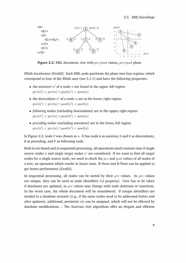
2.3. XML Encodings
<A>
<B/>
<C>
<D/><E/>
</C>
<F/>
</A>
A
B FC
D E
pre:1 post:6
2 1 3 4 6 5
4 2 5 3 B
C
DE
F
pre
post
A
1
2
3
4
5
6
1 2 3 4 5 6
Figure 2.2: XML document, tree with pre/post values, pre/post plane
XPath Accelerator [Gru02]. Each XML node partitions the plane into four regions, which
correspond to four of the XPath axes (see 3.1.1) and have the following properties:
• the ancestors n′ of a node n are found in the upper, left region:
pre(n′) < pre(n) ∧ post(n′) > post(n)
• the descendants n′ of a node n are in the lower, right region:
pre(n′) > pre(n) ∧ post(n′) < post(n)
• following nodes (excluding descendants) are in the upper, right region:
pre(n′) > pre(n) ∧ post(n′) > post(n)
• preceding nodes (excluding ancestors) are in the lower, left region:
pre(n′) < pre(n) ∧ post(n′) < post(n)
In Figure 2.2, node C was chosen as n. It has node A as ancestor, D and E as descendants,
B as preceding, and F as following node.
Both in set-based and in sequential processing, all operations need constant time if single
source nodes n and single target nodes n′ are considered. If we want to find all target
nodes for a single source node, we need to check the pre and post values of all nodes of
a tree, an operation which results in linear costs. B-Trees and R-Trees can be applied to
get better performance [Gru02].
In sequential processing, all nodes can be sorted by their pre values. As pre values
are unique, they can be used as node identifiers (id property). Care has to be taken
if databases are updated, as pre values may change with node deletions or insertions.
In the worst case, the whole document will be renumbered. If unique identifiers are
needed in a database scenario (e.g., if the same nodes need to be addressed before and
after updates), additional, persistent ids can be assigned, which will not be affected by
database modifications. – The Staircase Join algorithms offer an elegant and efficient
9

2.3. XML Encodings
approach to speed up axis evaluation [GvKT03]. It will be described in more detail in
Section 3.4.2.
2.3.3 Level Depth
Not all relationships between XML nodes can be determined exclusively with pre and
post. The level is another property that represents the depth of a node within a tree, i.e.,
the length of the path from the root to the given node. It can be used to evaluate four
other XPath axes:
• the parent n′ of a node n is an ancestor, the level of which is smaller by one:
pre(n′) < pre(n) ∧ post(n′) > post(n) ∧ level(n′) = level(n)− 1
• the children n′ of a node n are descendants with a level bigger by one:
pre(n′) > pre(n) ∧ post(n′) < post(n) ∧ level(n′) = level(n) + 1
• the following siblings n′ of a node n are following nodes that have the same parent
node p and, hence, are on the same level:
pre(n′) > pre(n) ∧ post(n′) > post(n) ∧ post(n′) < post(p) ∧ level(n′) = level(n)
• correspondingly, all preceding nodes with the same parent are the preceding sib-lings n′ of a node n:
pre(n′) < pre(n) ∧ post(n′) < post(n) ∧ pre(n′) > pre(p) ∧ level(n′) = level(n)
Similar to pre and post, the operations can be performed in constant time for single
source and target nodes, and linear time is needed for a set-based evaluation of several
target nodes.
While the self axis in XPath is trivial, the two axes descendant-or-self and ancestor-or-selfare combinations of the existing axes. The evaluation of the remaining attribute and
namespace axes are not considered in this context, as it depends on the specific design
of an implementation and does not pose any particular challenges that differ from the
existing ones1.
2.3.4 Number of Descendants
Li and Moon noticed early that the preorder and postorder encoding is expensive when
trees are to be updated [LM01]. They proposed an alternative encoding, namely the
1note that the namespace axis has been marked deprecated with XPath 2.0 [CD07]
10
2.3. XML Encodings
combination of an extended preorder and the range of descendants. In the extended pre-
order, gaps are left for new nodes, and the size property encapsulates the number of
descendant nodes. While the proposed encoding leads to new updating issues, which
arise as soon as all gaps are filled (costs on updates will be further detailed in Section
2.4.2.5), the size property brings in helpful properties, which are only partially covered
in the publication itself:
• n′ is a descendant of n if
pre(n) < pre(n′) ≤ pre(n) + size(n)
• n′ is the following sibling of n if
pre(n′) = pre(n) + size(n) + 1 ∧ level(n′) = level(n)
• correspondingly, n′ is the preceding sibling of n if
pre(n′) = pre(n)− size(n′)− 1 ∧ level(n′) = level(n)
A direct relationship exists towards pre, post and level. The size property can be calcu-
lated as follows [GT04]:
size(n) = post(n)− pre(n) + level(n)
The size property is particularly beneficial if tuples are sequentially stored and evalu-
ated. As an example, all children of a node can be traversed by a simple loop:
Algorithm 1 ProcessChildren(node: Node)
1 for c := pre(node) + 1 to pre(node) + size(node) step size(c) do2 process child with c ≡ pre(child)3 end for
2.3.5 Parent Reference
The parent of a node can be retrieved via pre, post and level. This operation is expen-
sive, however, as it results in linear costs, particularly if nodes are stored in a set-based
manner and if no additional index structures are created. Obviously, costs for the re-
verse parent and ancestor axes can be reduced to constant time if the parent reference is
directly stored.
As proposed in [GHK+06, Gru06], the pre value of the parent node can be used as
parent reference. Four of the XPath axes can now be evaluated as follows:
• n′ is a child of n if parent(n′) = pre(n)
11

2.3. XML Encodings
• n′ is a parent of n if pre(n′) = parent(n)
• n′ is a following-sibling of n if pre(n′) > pre(n) ∧ parent(n′) = parent(n)
• n′ is a preceding-sibling of n if pre(n′) < pre(n) ∧ parent(n′) = parent(n)
In set-based processing, post or size values are needed to evaluate the descendant, an-cestor, following, and preceding axes. In sequential processing, however, the combination
of pre and parent constitutes a minimal encoding to traverse all existing XPath axes and
reconstruct the original document. Next, the Staircase Join algorithms can be rewritten
to utilize the parent property, as will be shown in 3.4.2.
As a slight, yet powerful variation, the absolute parent reference can be replaced with
the relative distance to the parent node. In [GGHS09b], it has been shown that this dist
property is update-invariant: subtrees preserve their original distance values if they are
moved to or inserted in new documents. In contrast, absolute parent references to pre
values need to be completely renumbered.
2.3.6 Node Properties
Some other properties are necessary to map XML documents to a database and restore
the original representation. Location steps consist of XPath axes, which are further
refined by a kind test. The kind property represents the type of an XML node and
can be document-node, element, attribute, text, comment, or processing-instruction. Each
node kind has specific properties that have to be additionally referenced or stored in a
database [FMM+07]:
• Each XML document has a non-visible document node on top. A document has
a unique document uri property, which serves as a reference to the original docu-
ment location. Next, document nodes may have an arbitrary number of children
(elements, processing instructions, and comments), but only one root element.
• Elements contain all contents between an element’s start and end tag. Tags are
represented by angle brackets (e.g. <name>...</name>). An element has a name,
a unique parent, and an arbitrary number of children (elements, processing in-
structions, comments, and texts) and attributes. While children have a fixed order
and may contain duplicates, attributes may be serialized in a different order, but
their names need to be unique. Next, namespaces may be defined for an element
node and its descendants.
12
2.3. XML Encodings
• An attribute is owned by an element, i.e., its parent is always an element. At-
tributes have a name and a value and no children. They are serialized within
element start tags: <node name="value"/>
• Texts are usually enclosed by start and end tags. They have a content property,
which contains the actual textual data: <...>content</...>.
• Processing instructions can occur all around a document. They are used to keep
information for other processors and languages unchanged in an XML document,
and they have a parent, target, and content property: <?target text?>
• Similar to processing instructions, comments may be placed anywhere in a docu-
ment. They consist of a parent and content property: <!--text-->
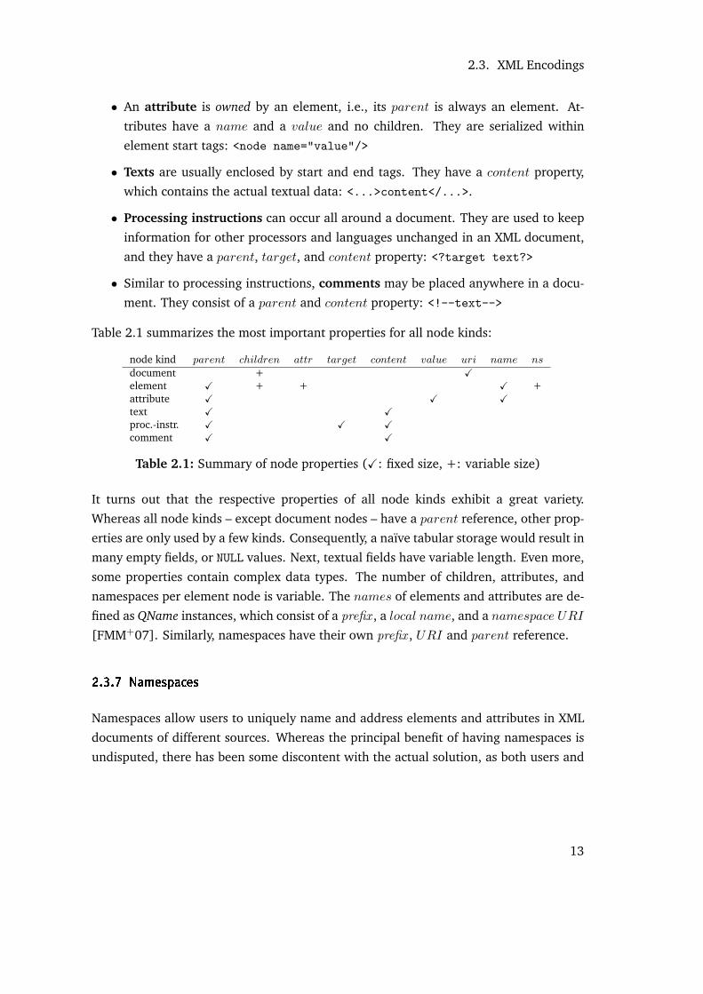
Table 2.1 summarizes the most important properties for all node kinds:
node kind parent children attr target content value uri name ns
document + Xelement X + + X +attribute X X Xtext X Xproc.-instr. X X Xcomment X X
Table 2.1: Summary of node properties (X: fixed size, +: variable size)
It turns out that the respective properties of all node kinds exhibit a great variety.
Whereas all node kinds – except document nodes – have a parent reference, other prop-
erties are only used by a few kinds. Consequently, a naıve tabular storage would result in
many empty fields, or NULL values. Next, textual fields have variable length. Even more,
some properties contain complex data types. The number of children, attributes, and
namespaces per element node is variable. The names of elements and attributes are de-
fined as QName instances, which consist of a prefix , a local name, and a namespace URI
[FMM+07]. Similarly, namespaces have their own prefix , URI and parent reference.
2.3.7 Namespaces
Namespaces allow users to uniquely name and address elements and attributes in XML
documents of different sources. Whereas the principal benefit of having namespaces is
undisputed, there has been some discontent with the actual solution, as both users and
13

2.4. Pre/Dist/Size Mapping
developers are frequently confused by its intricate details and complexity2. In a nutshell,
namespaces consist of an optional prefix and a URI. The URI serves as unique node iden-
tifier across multiple nodes and documents, whereas the prefix can be used to bind a URI
to certain nodes. As a consequence, two documents can have the same prefix and still
reference different URIs. New namespaces can be defined for each element, and they
are valid for all descendant elements unless they are overwritten by another namespace.
Prefixed names of elements or attributes are bound to the correspondent local name-
space. Elements without prefix are bound to the global namespace URI, and attributes
without prefix do not belong to any namespace. If the URI is empty, namespaces are
undeclared and reset to their default. The flexible nature of namespaces demands addi-
tional efforts on a database storage. Some details on storing namespaces can be found
in 2.4.1.1.
2.4 Pre/Dist/Size Mapping
In this section, as a result of the discussion on different mappings, the combination of
pre, dist, and size will be presented in more detail, as it both represents a compact
storage pattern and efficiently supports all XPath axes. Some normalization steps will
now be proposed to minimize the memory consumption and, as a corollary, access time.
The title of this thesis might raise the question what “large XML instances” actually are
[WG09]. In Computer Science, address spaces are always limited: no data structure can
have infinite size. Regarding Moore’s Law, the notion of size is closely intertwined with
technical progress; at the time of writing, XML documents with a few megabytes were
still regarded as large by many publications.
In the scope of this work, we propose a data structure that allows mapping up to 500
gigabytes of XML data to a single database instance. In practice, the actual size of an
instance will usually be smaller, as additional document properties may restrict the max-
imum size. As will be shown in the following, the chosen limits represent a compromise
between execution speed and the size of real-life documents. The address space of the
presented data structure can be easily extended to meet future demands.
2see www.stylusstudio.com/xmldev/201004/post40000.html, orwww.jclark.com/xml/xmlns.htm for examples
14

2.4. Pre/Dist/Size Mapping
2.4.1 Address Ranges
2.4.1.1 Analysis
The pre property has been presented as node identifier. A pre value is sequentially
assigned to each node in the document. As a result, all pre values will be dense and
sorted. The number of assigned pre values (which will be referred to as document sizefrom now on) is dependent on the document structure: the larger text nodes are, the less
pre values are needed. As a consequence, an address limit for pre values will be reached
earlier if a document has short texts. If nodes are sequentially stored in a database, the
pre value does not have to be stored at all, as it will be implicitly given by the node
offset. If updates are performed, the virtual pre value will not cause any extra costs.
The dist property represents the relative distance to the pre value of the parent node.
While its value will be small for many XML nodes, it can get as large as the current pre
value if a node references the root of a document. In practice, the dist value gets large
for all node kinds, except for attribute nodes, as elements have a relatively small number
of attributes. As a consequence, a smaller address range can be reserved to store the dist
values for attributes. For document nodes, the dist property can be discarded.
The size property reflects the number of descendants. For the root node, it will equal
the document size. Nodes with a small level depth (i.e., which are close to the root
node) have a larger size value than nodes that are deeply nested. The range of the size
value varies, dependent on the node kind: texts, comments, processing instructions and
attributes will never have children. Accordingly, their size value is always 0 and does
not have to be physically stored. If only one document is stored in a database, the size
value of a document node equals the document size and can be discarded as well.
If attributes are inlined in the main database structure (see 2.4.2.1 for details), an asize
property can be added to map the number of attributes. As elements are the only kinds
that have attributes, the property can be omitted for all other kinds. As a counterpart to
the dist value of attributes, asize will always be small, compared to the standard size
value.
The id property serves as unique node identifier. While its value equals the pre value if
the document is initially traversed, it will differ as soon as nodes are deleted or inserted
in the database. Its maximum value corresponds to the number of document nodes, and
increases with each node insertion. Consequently, a renumbering of the id values may
become necessary when the limit of the address space is reached. As will be discussed in
15
2.4. Pre/Dist/Size Mapping
2.6, the id is only required if both additional, content-based index structures are created
and updates need to be performed. In other words, it can be omitted if all database
operations will be read-only, or if updates are performed, but no content-based index
structures are needed to speed up queries.
The remaining node properties are independent from a specific XML encoding: Most
textual XML content is addressed by the text property, which exists for text, comment,
and processing instruction nodes. Attributes have a similar value property, which, in this
context, will be treated as text. To further unify the representation, the target values
of processing instructions will be merged with the text values, and the document uri of
document nodes will as well be treated as text. A single 0 byte is used as delimiter to
separate all strings from each other.
As text lengths can be highly variable, it seems appropriate to only store a pointer in the
main database structure. Several solutions exist for such a reference:
1. All strings can be organized by an additional index structure. As the number of
(both total and distinct) texts is always smaller than the total document size, the
index reference will never exceed the maximum pre value, respectively its address
range.
2. The indexing of complete text node imposes some overhead to the database con-
struction process – particularly if documents are too large to fit in main memory.
A straightforward alternative is to sequentially store all texts to disk. A simple
directory maps the database references to text offsets.
3. While the second solution offers a clean abstraction between document structure
and textual content, the directory structure occupies a considerable amount of
additional space. Memory can be saved if the text offset is directly referenced from
the database. The address range for textual references will have to be extended as,
in most cases, the total text length will be greater than the number of pre values.
For disk-based storage, Solution 3 will be pursued in the following, due to its simplicity
and compactness, although it is worth mentioning that the other solutions could speed
up querying and be more flexible regarding updates. For instance, Solution 1 seems
more appropriate for a main memory database representation, as lookup times are very
fast in primary storage (see 2.5.3 for details).
Both elements and attributes have a name property. As name strings have variable sizes
as well, all names are indexed, and a fixed-size numeric reference is used as database
entry. As the number of distinct names is much smaller than the actual number of
16

2.4. Pre/Dist/Size Mapping
elements and attributes, a small address space suffices to store the name reference. Each
element and attribute node has a unique namespace, the URI of which is also stored in
an index. As documents and collections have a limited number of namespaces, all index
references can be usually mapped to a small address space3.
Namespaces, which are specified by element start tags, also result in a tree. Likewise,
common namespace structures are comparatively small. As they are frequently accessed
by XPath and XQuery requests, they are kept in main memory as a conventional tree
structure. For each element node, an additional ns flag is added to the storage to indicate
if an element introduces new namespaces.
node kind dist size asize id text name uri ns
document c + c + +element + + – + – – –attribute – c c + + – –text + c c + +proc.-instr. + c c + +comment + c c + +
Table 2.2: Summary of normalized node properties.+/–: large/small address space, c: constant value
A normalized distribution of all node properties is shown in Table 2.2, along with a
first and approximate estimation of the required address space. Compared to Table 2.1,
the number of unused cells has been reduced, and all variable-sized entries have been
externalized and replaced by numeric references. Cells with constant values need not be
stored in the table, but are indicated as well.
2.4.1.2 XML Instances
To refine the optimal address range for all node properties, it is mandatory to take a look
at real-world XML documents. In our context, the following document characteristics are
relevant:
• the number of XML nodes (#nodes) is needed to determine the address space for
the pre, dist, and size property.
• the number of attributes (#atr) reflects the maximum number of attribute nodes
3No official rules have been specified on how XML documents should be built or designed. Outliers,however, are generally regarded as malformed or – as Michael Kay puts it – “pathological” [Kay08]
17

2.4. Pre/Dist/Size Mapping
of a single element node. It defines the address space for the asize property, and
the dist property for attributes.
• the number of distinct element names (#eln) and attribute names (#atn), includ-
ing namespace prefixes, serves as upper limit for the numeric name reference.
• the number of distinct namespace URIs (#uri) defines an upper limit for the nu-
meric uri reference.
• the total length of text nodes (ltxt) and attribute values (latr) indicates the ad-
dress range for the text property. For simplification, processing instructions and
comments have been conflated with text nodes.
In Section 4.3, a great variety of XML instances is analyzed in detail. Table 2.3 summa-
rizes the statistical results for the instances that yield maximum values for the focused
node properties. Note that the table is meant to sound out the limits of the discussed
encoding. In practice, most instances handled by our database system are much smaller:
INSTANCES file size #nodes #atr #eln #atn #uri ltxt latrRUWIKIHIST 421 GiB 324,848,508 3 21 6 2 411 GiB 186 MiBIPROCLASS 36 GiB 1,631,218,984 3 245 4 2 14 GiB 102 MiBINEX2009 31 GiB 1,336,110,639 15 28,034 451 1 9.3 GiB 6.0 GiBINTERPRO 14 GiB 860,304.235 5 7 15 0 19 B 6.2 GiBEURLEX 4.7 GiB 167,328,039 23 186 46 1 2.6 GiB 236 MiBWIKICORPUS 4.4 GiB 157,948,561 12 1,257 2,687 1 1.5 GiB 449 MiBDDI 76 MiB 2,070,157 7 104 16 21 6 MiB 1 MiB
Table 2.3: Value ranges for XML documents and collections.See Table 4.5 for a complete survey
As demonstrated by the RUWIKIHIST and IPROCLASS databases, a larger file size does
not necessarily result in a larger number of database nodes: the large size of individual
text nodes in the Wikipedia corpus leads to a relatively small node structure. Other do-
cument characteristics, such as long element and attribute names and structuring white-
spaces, may as well contribute to larger file sizes without affecting the node number. The
file size/nodes ratio of all tested 59 databases amounts to the average of 90 Bytes/node
and a standard deviation of 229. This ratio can be used as a guideline to estimate how
many nodes a database will have for an average XML document: the average maximum
input document size amounts to 181 GiB.
Next, most documents have a small number of attributes per element (#atr). In our test
results, the EURLEX document – a heterogeneous dataset that has been assembled from
many different sources – has a maximum of 23 attributes. As a result, a small address
18

2.4. Pre/Dist/Size Mapping
space suffices for the asize property, and for the dist property of attribute nodes. The
number of element and attribute names (#eln and #atn) is small for single documents,
but may increase if multiple documents are stored in a single database. This can be
observed for the INEX2009 collection, embracing around 2,7 million documents. Name-
space URIs have similar characteristics: their distinct number, however, is smaller. Most
documents do not specify more than two namespaces, or none at all. In our test doc-
uments, the maximum number of namespaces was encountered in the DDI document
collection. Other examples for XML datasets with up to 20 namespaces are OpenDocu-
ment [Wei09] and Open Office XML [ECM06] documents.
2.4.2 Table Mapping
In Section 2.3, a distinction was made between set-based and sequential processing. From
now on, we will focus on a sequential and native storage variant with the following key
properties:
1. The structure of XML documents is mapped to a flat table representation.
2. An XML node is represented as a fixed-size tuple (record).
3. The tuple order reflects the original node order.
4. The offset (row number) serves as pre value.
After an analysis of the concrete bit ranges that have to be supplied, a node will be rep-
resented in a fixed number of bits, which can later be directly mapped to main memory
and disk. Some optimizations will be detailed that further reduce the size of the eventual
data structure and speed up querying.
2.4.2.1 Attribute Inlining
By definition, XML attributes have elements as parent nodes. Yet, attributes are not
treated as ordinary child nodes, as they are owned by an element and have no fixed
order. Next, the attribute names of a single element must not contain duplicates. As a
consequence, attributes are stored in a different way than child nodes by many imple-
mentations, such as e.g. Natix [FHK+02] or MONETDB/XQUERY [BMR05]. An alterna-
tive approach, which has been pursued in this work, consists in treating attributes the
same way as child nodes and inline them in the main table. A big advantage of inlining
is that no additional data structure needs to be organized in order to store, query and
update attributes. An additional benefit is that queries on attributes will be executed
19

2.4. Pre/Dist/Size Mapping
faster, as the memory and disk access patterns are simplified, leading to less random re-
quests. A drawback may be that the size property cannot be utilized anymore to request
the number of XPath descendants of a node, as it now comprises all attributes in the
subtree. Instead, the asize property returns the exact number of attributes per node.
2.4.2.2 Bit Ranges
Some maximum ranges are now defined to map documents to memory areas. In Ta-
ble 2.4, the value ranges from Table 2.3 are broken down to bit ranges. The #nodes col-
umn indicates that the pre, dist, size and id values of the IPROCLASS and the INEX2009
database take up to 31 bits, thus occupying the full range of a signed 32 bit integer. This
means that integer pointers can be used to reference table entries. Depending on the
programming language, the address range could be doubled by using unsigned integers.
Next, by switching to 64 bit, the address range could be extended to a maximum of 16
exabytes. In the context of this work, we decided not to further extend the address range
as, on the one hand, array handling is still optimized for 32 bit in some programming
environments4 and, on the other hand, most real-life database instances did not come
close to our limits.
INSTANCES file size #nodes #atr #eln #atn #uri ltxt latrRUWIKIHIST 421 GiB 29 2 5 3 1 39 28IPROCLASS 36 GiB 31 2 8 2 1 34 27INEX2009 31 GiB 31 4 15 9 1 34 33INTERPRO 14 GiB 30 3 3 4 0 5 33EURLEX 4.7 GiB 28 5 8 6 1 32 28WIKICORPUS 4.4 GiB 28 4 11 12 1 31 29DDI 76 MiB 21 3 7 4 5 23 21
Table 2.4: Bits needed to allocate value ranges
The maximum length for texts and attribute values, as shown in the #ltxt and #latr
column, defines the limit for the text property, and takes 39 bits. Element and at-
tributes names are referenced by the name property and are limited to 15 and 12 bits,
as indicated by #eln and #atn, respectively. The asize and the uri properties occupy a
maximum of 5 bits (see #atr and #uri).
4See e.g. http://bugs.sun.com/view bug.do?bug id=4963452 for details on current limitations ofpointer handling in Java. In short, array pointers are limited to 31 bit (signed integers) in Java. Thislimit would enforce additional pointer indirections if all table data is kept in main memory, and slowdown processing. It does not lead to restrictions, however, if the table is stored on disk.
20

2.4. Pre/Dist/Size Mapping
2.4.2.3 Compactification
Table 2.5 is an updated version of Table 2.2. It contains concrete bit range limits for all
node properties. Two columns have been added: the kind property adds 3 additional
bits, which are needed to reference the six different node kinds. The #bits column adds
up the bit ranges. It summarizes how many bits are needed to map all properties of
a specific node kind to memory. The ns property, which is only defined for elements,
indicates if namespaces are defined for the respective element. As such, it needs a single
bit.
node kind kind dist size asize id text name uri ns #bitsdocument 3 0 31 0 31 40 105element 3 31 31 5 31 16 8 1 126attribute 3 5 0 0 31 40 16 95text 3 31 0 0 31 40 105proc.-instr. 3 31 0 0 31 40 105comment 3 31 0 0 31 40 105
Table 2.5: Concrete bit ranges for all node kinds
As can be derived from the resulting compilation, the element node demands most
memory. While the optional asize property could be discarded, all other properties
are mandatory for processing. In spite of their name/value combination, attribute nodes
take up the least number of bits, as they have no children and a small distance to their
parent node. All other node kinds occupy the same bit range in our representation, as
their textual properties have been merged in the text property.
The #bits column suggests that a single element node can be represented within 16
bytes. As 16 is a power of 2, it represents a convenient size for storing entries in fixed-
size memory, such as blocks on disk. To map other node kinds to the same bit range, an
individual bit distribution was defined for each node kind. The three kind bits serve as
indicator where the value of a specific property is placed. An exemplary bit distribution,
which has been applied in Version 6 of our database system, is shown in Figure 2.3.
2.4.2.4 Integer Inlining
Values of text and attribute nodes may belong to specific data types that can be specified
by a schema language, such as DTD or XML Schema. Whereas some database systems
opt to store texts dependent on their type (such as PTDOM [WK06]), most systems
choose a schema-oblivious approach, as the complexity of schema languages and the
21

2.4. Pre/Dist/Size Mapping
elementdocument
proc.-instr.text
comment
attribute
0 1286432 96
id
id
idid
idid
size
size
textk
k
kk
kk
a
d
name
name
uri dist
text
dist
text
text
text
dist
dist
Figure 2.3: Bitwise distribution of node properties in BASEX 6.0.Note: the ns bit is located to the right of the uri property
flexible structure of documents complicate a type-aware implementation. It is one key
feature of XML that no schema needs to be defined at all – and, at the same time, a
drawback, as relational database systems can benefit from the fact that data types are
known in advance. In our architecture, by default, texts are stored as UTF8 strings,
suffixed by a 0 byte and linked by a reference from the main table, which means that,
for instance, a single integer value may take up to 16 instead of 4 bytes in the storage5.
A different storage strategy can be applied for data types that can be dynamically recog-
nized by analyzing the incoming data. Integer values are the easiest ones to detect: if a
string comprises up to 10 digits, it can be inlined, i.e., treated as a number and stored
in the main table instead of the textual reference. In our representation, up to 11 bytes
can be saved for each integer. The uppermost bit of the reference can be used as a flag
to state if the text value is to be treated as pointer or actual value. This way, no extra
lookup is necessary to determine the type. If all contents of a document are numeric,
no additional text structures will be created at all. A positive side effect of inlining is
that even strings that were not supposed to be handled as integers can be stored more
economically.
The inlining technique could be extended to various other data types. In the scope of this
work, it was limited to integers in order to minimize the parsing effort while building
databases and requesting textual data. Next, to comply with the first encoding require-
ment that has been specified in 2.3, we need to guarantee that the original document
is exactly reconstructed. This means that no normalization steps may be performed on
the input data, such as stripping whitespaces, or removing upper and lower case. As a
consequence, strings such as "true", " true ", and "TRUE" cannot be simplified and
55 bytes are needed for the reference, up to 10 bytes for the string representation of an integer (232 =4294967296), and an additional byte for the null byte suffix.
22

2.4. Pre/Dist/Size Mapping
treated as the same boolean value.
2.4.2.5 Updates
A wide range of numbering schemes have been discussed to support updates in XML
documents [CKM02, SCCS09]. ORDPATH [OOP+04] is the most popular prefix labelingscheme that has been derived from the Dewey Order [TVB+02]. The document order
and hierarchy is preserved by the labeling scheme, and new nodes can be added and
deleted without relabeling the existing nodes. As hierarchic labels have variable length
and can get very memory consuming for deeply nested nodes, ORDPATH labels are ad-
ditionally compressed and represented as bit strings. Although the proposed scheme has
experienced numerous tweaks and variations to save space [AS08, AS09] and to cover
navigational and locking issues [HHMW07], it can still be considered as rather bulky:
all labels have to be organized by at least one additional index structure.
As the basic pre/size/dist encoding has primarily been designed with the objective of
minimizing the storage overhead and the number of data structures, it needs to be ex-
tended as well to support efficient updates. A naıve attempt to delete a node from the
main table demonstrates that the current architecture is insufficient. Let n be the pre
value of the node to be deleted and size(db) the total number of database nodes6:
1. all tuples in the range [n + size(n), size(db)] need to be moved by −size(n)
2. size(n) needs to be subtracted from the size value of all ancestors of n
While the second operation is cheap, as only a number of height(n − 1) tuples have to
be touched, the first operation yields high physical costs, and a worst case O(size(db)) if
updates occur at the beginning of the document.
A classical solution to circumvent the problem is the introduction of logical pages. Sev-
eral tuples are mapped to blocks with fixed size, and a flat directory is added that con-
tains the first pre values (fpre) and references to all pages (page). This way, tuple shifts
can be limited to the affected blocks. All tuples are contiguously stored from the begin-
ning of the page to avoid additional lookup operations for free and used page entries.
The number of tuples of a page p is calculated by subtracting the current from the sub-
sequent fpre value: fpre(p + 1)−fpre(p).
6Note that insert operations lead to similar costs.
23

2.4. Pre/Dist/Size Mapping
0
…
2
1
0
…
512
256
pagefpre
0
…
2
1
0
…
412
156
pagefpre
0
…
1
5
0
…
356
256
pagefpre
Figure 2.4: Directory of logical pages: a) initial state for a page size of 4096 bytes,b) deletion of 100 nodes, and c) insertion of 100 nodes
Figure 2.4 illustrates an exemplary directory, for which the size of a logical page was set
to 4096 bytes, in compliance with the size of a typical disk page. As one tuple occupies
16 bytes, a maximum of 256 tuples is stored per page. In 2.4 b), a node n has been
deleted; its 99 descendants (size(n) = 100) have all been located in the first page p.
After the deletion and the update of all size values of the ancestors of node n, size(n) is
subtracted from all subsequent entries p + 1 in the directory. Example 2.4 c) shows the
mapping after an insert operation: 100 nodes are inserted at pre = 256, resulting in the
creation of a new page (here: 5) at the end of the existing pages and the insertion of a
new entry in the directory.
Even for large databases, the directory will stay comparatively small, so that it can be
usually kept in main memory. Let P be the number of tuples per page, which is the page
size divided by the tuple size, and max(db) the maximum database size. If n values need
to be stored per dictionary entry, a total of n·max(db)P values needs to be handled, yielding
2 · 231/(4096/16) = 16777216 integers and a memory consumption of 64 MiB in our rep-
resentation. Although the deletion and insertion of dictionary entries requires copying
large main memory areas, the operation is cheap, compared to update operations on
disk. If even larger pre ranges are to be supported, or if update performance proves to
be too inefficient for large database instances, the dictionary structure can be extended
to a conventional B-Tree and stored on disk [BM72].
MONETDB/XQUERY, which is based on the pre/size/level encoding, offers a similar
solution by adding a new pos/size/level table to the storage, which is divided into logical
pages [BMR05]. The original table serves as a view on the new table with all pages in
order. A new node property resembles the id property in our representation and serves
as unique node identifier. As attributes are stored in extra tables, an additional table
maps node to pos values. Pages may contain gaps to improve page locking behavior for
the update of ancestor nodes. – A different solution has been chosen in our context, as
the presented directory is very light-weight and does not require extra tables. Next, the
24

2.5. Database Architecture
dist property, which is absent in MONETDB/XQUERY, allows constant access to parent
nodes, which makes updates on ancestors a very cheap operation. An id/pre mapping
(the equivalent to node/pos) can be omitted as well, as attributes are inlined in the main
table. Last but not least, the directory can initially be omitted, and created on-the-fly
as soon as the first update operation is performed. Consequently, there is no need to
explicitly differentiate between read-only and updatable databases.
2.5 Database Architecture
DirectoryMeta Data
…
doc
pre kind dist size asize id text name uri ns
elem
attr
text
proc
com
Main Table
Texts
…
offset value
...
fpre page
...
Attribute Values
…
offset value
Tags
…
key value
Attribute Names
URIs
…
key value…
key value
Namespaces
...
key value
namesize
dirtyheighttime
Figure 2.5: Main structure of a database instance
Figure 2.5 summarizes the last paragraphs and shows the overall structure of a single
database instance. Virtual columns, which are not explicitly stored, are indicated only
by their header. The main table contains numeric keys to the tags, namespace URIs,
and attribute name indexes. Texts (incl. processing instructions, comments, and URIs
of document nodes) and attribute values are stored in extra files or arrays, the offsets
of which are referenced from the main table. The directory contains pointers to the first
pre value of each table page. Various information is supplied as meta data, such as the
name of the database, its size, modified time, tree height, or dirtiness after updates. A
main memory tree, which is backed by additional prefix/URI indexes, provides access to
namespaces.
2.5.1 Database Construction
The tabular representation of XML can be constructed in linear time. An event-driven
SAX parser [MB04] is applied to build a database instance. While pre and post (and most
25

2.5. Database Architecture
other) values can be sequentially stored in the table in a single run7, the size value has
to be subsequently updated as soon as the number of descendants of the correspondent
node is known.
Table
TAGS: NamesTEXTS: ContentsATTRIBUTE_NAMES: NamesATTRIBUTE_VALUES: Contents
AddDocument(pre: int, uri: String)AddElement(pre: int, dist: int, asize: int, name: String)AddAttribute(pre: int, dist: int, name: String, value: String)AddText(pre: int, text: String)SetSize(pre: int, size: int)
Builder
TABLE: TableSTACK: StackPRE: int
StartDocument(uri: String)EndDocument()StartElement(name: String, attr: Attribute[])EndElement()Text(text: String)
Contents
Add(text: String): long
Names
Index(name: String): int
Parser
BUILDER: Builder
parse()
Figure 2.6: Class diagram for building a database with a SAX parser
Figure 2.6 depicts the most relevant classes for building a database via SAX. A new
PARSER instance is created by the central BUILDER instance, which in turn notifies the
builder of XML events to be processed. A global PRE value serves as counter for new
nodes to be stored in the table, and a STACK is used to cache the pre values of current
ancestor nodes. Processed node values are passed on to the TABLE instance, which passes
on textual values to the CONTENTS and NAMES objects. We will now have a closer look
on the most important SAX events; for the sake of simplicity, advanced issues such as
namespaces and common implementation details for SAX parsers will be omitted, and
database creation will be restricted to a single document.
Algorithm 2 Builder.StartDocument(uri: String)
1 initialize TABLE and STACK
2 PRE := 03 TABLE.AddDocument(PRE, uri)4 STACK.Push(PRE)5 PRE := PRE + 1
Algorithm 2 is called by the parser when the document is opened: The global TABLE
and STACK instances are initialized, the PRE counter is set to 0, and the document tuple
{pre/text} is added to the table. Next, PRE is pushed to the stack and incremented by
one.
In Algorithm 3, the distance to the parent node (dist) is calculated by subtracting the pre
value of the last parent node, located on top of the stack, from the current PRE counter.
7SAX algorithms for the pre/post encoding are found in [Gru02]
26

2.5. Database Architecture
Algorithm 3 Builder.StartElement(name: String, attr: Attribute[])
1 dist := PRE − STACK.peek()2 asize := #attr + 13 TABLE.AddElement(PRE, dist, asize, name)4 STACK.Push(PRE)5 PRE := PRE + 16 for a := 0 to #attr − 1 do7 dist := a + 18 TABLE.AddAttribute(PRE, dist, attr[a].name, attr[a].value)9 PRE := PRE + 110 end for
asize is set to the number of attributes, and 1 is added so that pre + asize will point
to the first node behind the attribute list. The resulting {pre/dist/asize/name} tuple is
added to the table and, once again, PRE is pushed to the stack and incremented. Next,
all attribute tuples {pre/dist/name/text} are added. The dist value equals the current
offset counter added by 1.
Algorithm 4 Builder.EndElement()
1 size := PRE − STACK.pop()2 TABLE.SetSize(PRE, size)
If an element is closed, as shown in Algorithm 4, the most recent stack value (which is
the pre value of the corresponding opening element) is popped. The difference between
the PRE counter and the stack value is the size value, and is stored in the table.
Algorithm 5 for storing text nodes is even simpler: a tuple pre/text is added to the
table, and the PRE counter is incremented. The events for processing instructions and
comments are nearly identical.
Algorithm 5 Builder.Text(text: String)
1 TABLE.AddText(PRE, text)2 PRE := PRE + 1
Finally, in Algorithm 6, the document node is closed, and the size value of the root node
is updated. – Note that subsequent tables updates might slow down a sequential disk
storage. As a straightforward optimization, the size values can be cached and written to
the database in a second run.
Before a tuple can be stored, strings need to be dissolved into references and stored in
27

2.5. Database Architecture
Algorithm 6 Builder.EndDocument()
1 size := PRE − STACK.pop()2 TABLE.SetSize(PRE, size)
extra data structures. Algorithm 7 demonstrates this process for attributes: the name of
the attribute is indexed, and its key is stored in the main table.
Algorithm 7 Table.AddAttribute(pre: int, dist: int, name: String, value: String)
1 attn := ATTRIBUTE NAMES.Index(name)2 attv := ATTRIBUTE VALUES.Add(value)3 add attribute tuple {pre, dist, attn, attv} to storage
As detailed in Section 2.4.2.4 and shown in Algorithm 8, the file or array offset is used
as reference for text values. If the value is numeric, it is converted to its numeric repre-
sentation and flagged with a number bit (here: NUMBERMASK), which is the highest bit
of the selected bit range.
Algorithm 8 Contents.Add(text: String): long
1 v := convert text to integer2 if v is valid then3 v := v | NUMBERMASK
4 else5 add text to storage6 v := offset to stored text7 end if8 return v
2.5.2 Generic Parsing
The presented database construction process is limited to single XML documents. In
order to process multiple files and directories, the Builder and Table algorithms can be
extended to add the dist values of document nodes to the storage, and to perform the
initialization of the global variables before the first call of Algorithm 2.
To go further, we can observe that XML is just one possible textual representation of tree
hierarchies: a multitude of other representations have been proposed, such as JSON
[Cro06] or OGDL [Vee09]. Even more, arbitrary tree structures can be converted to
XML. The presented SAX interface allows all kinds of sources to be used as input for
the database builder. While, by default, one or more XML documents are sent to and
28

2.5. Database Architecture
processed in the existing architecture, the existing parser can be defined as abstract
and extended by a range of specific implementations. Some examples for parsers (or
importers), which have been realized in our project, are listed in the following:
• Most filesystems exhibit a hierarchic structure, which can be mapped to XML in
a straightforward manner. A filesystem parser recursively traverses all directories
and triggers events to add directory and file elements to the database. The idea
has been pursued in the DeepFS project [HGS09].
• MAB2 is a flat, textual exchange format for German library meta data [Bib99],
which can be converted to XML. The resulting tree structure facilitates an easier
access to hierarchic relations for multi-part volumes and series. An importer for
MAB2 data has been added for the MEDIOVIS project [GGJ+05].
• HTML is a markup language that has been inspired by SGML. As the majority of
real-life HTML documents are malformed, they usually cannot be read by XML
parsers. Instead, converters like TagSoup [Cow08] can be applied on the input as
a pre-processing step to create a well-formed XML document, which can then be
processed by the actual XML parser.
• the CSV format can be used to store tables as plain text. One line of text contains
a single record, and all fields are separated by commas. An importer for CSV
files consists of a few lines of code, as tables can be easily represented as a tree
structure.
2.5.3 Main Memory vs Persistent Storage
External storage is known to be slower than main memory by some orders of magnitude.
In practice, the distinction is often not perceived by end users anymore, as much of
the data, which has been read at least once, is automatically remembered in disk and
main memory caches, the size of which has steadily increased over the last years. The
difference shrinks even more with the popularization of solid state disks, which have
much better random access times. At the same time, the available main memory in
today’s personal computers has reached a size which is, for many use cases, large enough
to hold complete database instances.
An obvious advantage of mapping databases to main memory is that the execution time
for queries can be further minimized. While the buffer management of the operating sys-
tem generically speeds up access to frequently requested data, a main memory database
29
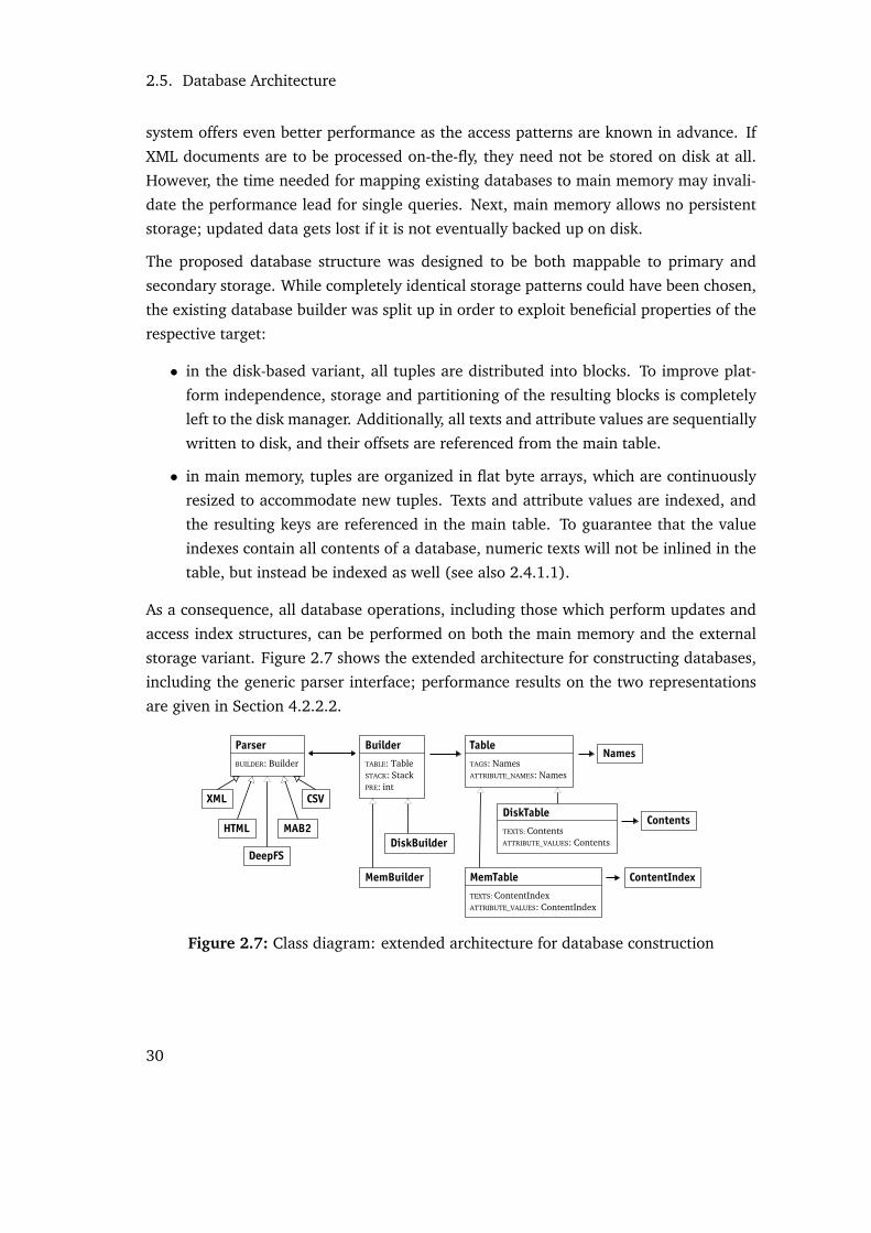
2.5. Database Architecture
system offers even better performance as the access patterns are known in advance. If
XML documents are to be processed on-the-fly, they need not be stored on disk at all.
However, the time needed for mapping existing databases to main memory may invali-
date the performance lead for single queries. Next, main memory allows no persistent
storage; updated data gets lost if it is not eventually backed up on disk.
The proposed database structure was designed to be both mappable to primary and
secondary storage. While completely identical storage patterns could have been chosen,
the existing database builder was split up in order to exploit beneficial properties of the
respective target:
• in the disk-based variant, all tuples are distributed into blocks. To improve plat-
form independence, storage and partitioning of the resulting blocks is completely
left to the disk manager. Additionally, all texts and attribute values are sequentially
written to disk, and their offsets are referenced from the main table.
• in main memory, tuples are organized in flat byte arrays, which are continuously
resized to accommodate new tuples. Texts and attribute values are indexed, and
the resulting keys are referenced in the main table. To guarantee that the value
indexes contain all contents of a database, numeric texts will not be inlined in the
table, but instead be indexed as well (see also 2.4.1.1).
As a consequence, all database operations, including those which perform updates and
access index structures, can be performed on both the main memory and the external
storage variant. Figure 2.7 shows the extended architecture for constructing databases,
including the generic parser interface; performance results on the two representations
are given in Section 4.2.2.2.
XML
DeepFS
HTML MAB2
CSV
Parser
BUILDER: BuilderNames
Table
TAGS: NamesATTRIBUTE_NAMES: Names
DiskTable
TEXTS: ContentsATTRIBUTE_VALUES: Contents
MemTable
TEXTS: ContentIndexATTRIBUTE_VALUES: ContentIndex
Contents
ContentIndex
Builder
TABLE: TableSTACK: StackPRE: int
DiskBuilder
MemBuilder
Figure 2.7: Class diagram: extended architecture for database construction
30

2.6. Index Structures
2.6 Index Structures
In short, databases indexes exist to speed up query evaluation. In relational databases,
usual index structures are value indexes, and column-based, i.e., applied on one or more
attributes, of a table. In XML, due to the complexity of tree structures, a wide range of
index structures exists, for which different classifications can be found in the literature
[MWA+98, CMV05]. In the scope of this work, we will focus on the following three
index types:
1. Name indexes organize frequently occurring strings, such as tag or attribute names,
in small main memory structures.
2. Path, or structural indexes facilitate the access to all unique document paths of
a document. Path indexes have initially been proposed for object-oriented and
nested relational databases [BK89].
3. Value or content indexes are comparable to index structures of relational databases.
Texts and attribute values of documents are indexed for faster access. Full-text
indexes are a specialized type of value indexes.
2.6.1 Names
Repeating tag and attribute names are the main reason why XML has become notorious
for its verbosity. In XML databases, the most straightforward approach to reduce space
is to introduce a name index, which replaces variable-size names by numeric ids (see
[JAKC+02] or [Mei02] for examples). This can be done by storing all names in a main
memory based associative array, such as a hash or binary search tree. In the scope of
this work, separate indexes are created for elements and attributes. As shown in Section
2.4.2.2, 16 bits, or short values, suffice to reference single names in a document.
Name indexes could be enhanced with the pre/id values of all corresponding elements
or attributes. This approach would allow a direct lookup of all descendant nodes that
use a specific tag or attribute name, as e.g. needed for the simple XPath query //name.
Due to the substantial space overhead of such an index and additional maintenance
operations necessary for each update, we discarded the storage of pre values in an early
stage. Instead, statistical meta information on nodes were added to the name indexes,
which can later be utilized by the query compiler to choose between different execution
plans:
31

2.6. Index Structures
• A counter property states how often a name occurs in the database.
• A leaf flag indicates if an element is a leaf node, i.e., if it has no more elements as
descendants.
• A length property stores the maximum length of the associated child text or at-
tribute value.
• A kind property reflects if the associated values are numbers, string categories, or
strings.
• min and max values contain the lower and upper limits of numeric values.
Algorithm 9 Name.UpdateStatistics(String value)
Require:MAXCATS := number of maximum allowed categoriesinitialize CATEGORIES, KIND := INTEGER, MIN :=∞, MAX := −∞ before first call
1 if KIND 6= STRING and #CATEGORIES < MAXCATS then2 add value to CATEGORIES
3 end if4 if KIND = INTEGER then5 v := convert value to integer6 if v is valid then7 if MIN > v then MIN := v end if8 if MAX < v then MAX := v end if9 else10 KIND := CATEGORY
11 end if12 end if13 if KIND = CATEGORY then14 if #CATEGORIES = MAXCATS then15 KIND := STRING
16 end if17 end if
All information can be iteratively collected while a database is created. Algorithm 9
demonstrates how string categories and the min, max, and kind values are generated for
a single element or attribute. The function is initialized with the strictest precondition,
which assumes that all values are integers in the empty range (∞,−∞). As soon as the
first value arrives, it will be added to CATEGORIES, an array that stores a limited number
of distinct strings. Next, as the current kind is INTEGER, the value is converted to an
integer. If the conversion is successful, min and max will be set to this new value. If
more integers are found in subsequent calls, min and max will be updated each time.
32

2.6. Index Structures
If an incoming string is no integer, CATEGORY will be set as new kind. If more distinct
strings have been collected than are allowed by the MAXCATS constant, the kind is set to
the most general STRING kind. In the last case, no more checks will be performed on the
remaining strings.
If updates are performed, the statistics lose their accuracy, but continue to serve as
guideline for the query compiler. As an example, kind =INTEGER, min = 1, and max = 2
for the c attribute in the following document:
<A><B c="1"/><B c="2"/><B c="2"/></A>
The query compiler can speed up query evaluation by replacing a subquery @c<1 with the
static boolean value false, as the comparison will never be true for the given document.
If the node <B c="1"/> is deleted in a next step, the new actual minimum for attribute c
will be 2. The index statistics will not be updated, however, as the complete database –
or at least all nodes that use the name in question – would have to be scanned in order
to calculate the new lower limit. Instead, the given subquery will be rewritten the same
way as before, while the subquery @c<2 will be evaluated in full, and still yield correct
results, as no attribute will be found that fulfills the test. If new nodes are inserted, or
if existing nodes are modified in the database, the same methods as for creating a new
database can be used to update the existing meta information.
More details on exploiting the index information during query compilation can be found
in 3.3.1.5.
2.6.2 Path Summary
While the name index collects atomic information on tag and attribute names of the
same name – no matter where they occur in a document – a path summary organizes
all distinct element and attribute paths that occur in a document or database. Path
summaries are also called path indexes or structural summaries [RM01, CMS02]. They
are all derived from the DataGuide [GW97], a data structure that has first been applied
in the LORE system [MAG+97], which has been introduced in 2.2.
If schema information is predefined by a DTD or XML Schema, it can be used to build
a path summary for a given document. A predefined (static) schema can reduce the
implementation effort:
• The actual input does not need to be parsed to build the summary.
33

2.6. Index Structures
• If update queries will only be processed if their results comply with the given
schema, the path summary needs not be updated at all.
Dynamic schemas, however, which are built from the actual input, have some advantages
as well:
• Many static, real-life schemas are bulky and contain paths that are not actually
used by a document. As a consequence, dynamic schemas will be more accurate
for a specific document/database.
• As a document needs to be parsed anyway if a new database is created, the path
summary can be built in the same run and enriched with additional, input specific
meta information.
<A> <B a="0"/> <C/> <B><C/><C/></B> <C>text</C> <B/></A>
A
B BB
C C
C C
#@a
A
B
@a1
#
C
C2 1
3 2
1
Figure 2.8: XML document, tree representation, path summary incl. cardinalities
Figure 2.8 depicts a path summary for a simple XML document. As a summary is usually
very small, compared to the original document, it is represented as a main memory tree
structure. Similar to the name index, nodes of a path summary could be enriched with
references to the XML nodes that match the location paths. Again, this approach was
discarded in our architecture to minimize the overhead for storing and updating the
database. To further reduce memory consumption, the path nodes reference the keys of
the existing tag and attribute name index.
The path summary is useful in numerous applications. In the visual frontend of our
database, which will not be further detailed in this work, path completions can be sug-
gested while XQuery expressions are typed in by the user. Next, the summary is queried
by the Scatterplot, Table and Explorer view to verify how many nodes exist in the tree
hierarchy, or if certain nodes have descendants. Section 3.3.1.5 will demonstrate how
the summary is used by the query compiler.
34

2.6. Index Structures
2.6.3 Values
In the relational world, classical index structures are value (or content) indexes, which
facilitate content-based queries in sub-linear time. Most value indexes rely on standard
tree or hash structures with key and value pairs. As the use and construction of these
indexes are well-known concepts, we will focus on features that are specific to XML and
the discussed storage. Values in this context are strings from texts or attribute values.
Different variants of value indexes can be found in existing XML databases [GGHS09b]:
• Keys can be indexed on document level, an approach which is usually taken by
relational engines. Queries on many small documents may be accelerated by this
approach, whereas there is no benefit for single and large documents.
• Certain location paths can be pre-selected for being indexed. While this approach
seems promising at first glance, and might reduce the size of the index structures,
it often fails when queries are nested or getting more complex. Moreover, indexes
must be manually added, and database users need explicit knowledge on the avail-
able index structures.
• Implementation-specific XQuery functions can be added to directly access the index
structures. Again, knowledge on database internals is required, and a compiler
will not be able to benefit from the indexes, as the user alone chooses whether the
index is to be used.
To support a wider range of optimizations, we decided to index all text nodes by default,
regardless of their position in the document structure. In Section 3.3.2, the query opti-
mizer is presented. It will rewrite and invert location paths and predicates whenever an
index access is possible and (potentially) cheaper than a conventional query execution.
Due to our tabular encoding, sorted lists of pre values – which are identical to id values
as long as no updates are performed – will be used as pointers to the main table. As the
index structure, which will be discussed in the following, has been optimized for per-
formance and low memory consumption, update operations are not supported. Instead,
the following optimizations will be applied to reduce the index size to a minimum:
1. pre values will be compressed before they are stored in the index.
2. Instead of the absolute values, distances between pre values will be stored.
3. As common user queries contain short keywords – compared to the maximum
length of text nodes in a document – the index size can be reduced by ignoring all
strings that exceed a specified maximum length.
35

2.6. Index Structures
4. The variable-length keys need not be stored in the index at all; instead, they can
be looked up in the main table by following the first referenced pre value.
2.6.3.1 Compression
A fast and simple compression mechanism, inspired by the UTF-8 encoding, is applied
to all pre values in the index structure. As summarized in Table 2.6, the first two bits of
a byte are used to define the range of the next integer to be parsed. Depending on the
bit code, a single integer will occupy 1-5 bytes in its compressed representation: small
integers will take less space, whereas large integers will occupy one additional byte.
Encoding (binary) Range (hex) Description00bbbbbb 00 - 3F 1 byte maps 26 values01bbbbbb B 40 - 3FFF 2 bytes map 214 values10bbbbbb B B B 4000 - 3FFFFFFF 4 bytes map 230 values11000000 B B B B 40000000 - FFFFFFFF 5 bytes map 232 values
Table 2.6: Compression of numeric values. b represents a bit, B represents a byte
If the second optimization of 2.6.3 is applied, which suggests to replace absolute values
by distances, the total index size will further shrink, as distances are much smaller than
absolute values and thus can be better compressed.
2.6.3.2 Construction
A quick insight is given on how the value index is constructed for either texts or attribute
values: The main table is sequentially scanned. If a node with the addressed kind is
encountered, and if the length of the string to be indexed does not exceed the maximum,
predefined length, the string and current pre value are passed on to the index builder.
The values are added to a main memory, balanced binary tree. After all nodes were
scanned, the binary tree is traversed in preorder, and the index data is stored to disk in
two files, or entities:
• a values file contains all variable-size lists with compressed pre distances.
• a keys file contains a simple array with offsets to the pre lists.
As the binary tree has been processed in preorder, all stored offsets will be sorted by
the lexicographical order of their keys. This means that binary search can be applied by
index requests to find the pre values for a given string in logarithmic time. As the actual
36

2.6. Index Structures
strings (keys) are not stored in the index themselves, they are looked up by following
the offset to the current pre list and accessing the main table via the first pre value.
2.6.3.3 Main Memory Awareness
Although the presented index builder was designed to be conservative in terms of mem-
ory consumption, it will eventually hit main memory limits if the processed documents
get too large. In general, 20-30% of the size of the documents needs to be provided as
main memory to guarantee a successful index construction. Depending on the charac-
teristics of the input, either keys or values may be responsible for memory overflows.
If many identical strings are found (i.e., if few categories exist, as introduced in Section
2.6.1), most space will be consumed for the pre value lists. If the document contents are
rather heterogeneous, the keys are likely to dominate memory consumption.
To support for even larger inputs, the existing index builder can be rewritten to take the
available amount of main memory into consideration. The resulting approach is loosely
inspired by classical algorithms, such as External Sort [Knu73] or Sort-Based Inversion
[WMB99]. It supports all kinds of document types and, yet, is fast and straightforward:
As soon as the available main memory is exhausted, the current tree structure is written
to disk, and a new, empty tree is created, which stores new keys and values. After all
nodes have been processed, the temporarily written index structures are merged into
one single tree. The merge can be performed in a single run as, thanks to the sequential
construction process, all pre values in the intermediate index files are sorted. This way,
the index size will only be limited by the free disk space, no matter how much main
memory is left. If enough memory is available, there will be no need to write temporary
index instances to disk at all.
2.6.4 Full-Texts
While value indexes have been a classical feature of relational databases, full-text in-
dexes have originally been developed for Information Retrieval applications. Today, all
major relational database systems include implementation specific extensions to query
textual corpora. In XML, however, the XQuery Full Text (XQFT) language extension was
developed to offer a standardized and unified way for accessing and retrieving full-texts
[AYBB+09] (see 3.1.3 for more).
Full-text indexes are applied to speed up queries on single words of documents. Before
texts can be indexed, they need to be tokenized, i.e., split into atomic units (tokens),
37

2.6. Index Structures
which serve as keys for future index requests. The tokenization process might include
various language dependent normalization steps, all of which are also defined in XQFT:
• Case sensitivity (lower and upper case) is removed.
• Diacritics (umlauts, accents, etc.) are removed.
• Tokens are stemmed via algorithms or dictionaries.
• A thesaurus may be applied on the tokens.
• Eventually, tokens are skipped that are defined in an optional stop word list.
The resulting dictionary, which contains all tokens of a document, will usually have
much less keys than values, as the number of distinct words is limited for most text
corpora8. Values will occupy much more space, as single words are contained in several
text nodes, and even contained several times in single nodes. The token positions within
a text node will be denoted by the pos property: they are stored as well to efficiently
support advanced XQFT features such as phrase, distance or window queries.
Full-text queries can be performed on arbitrary inputs, such as attribute values or dy-
namically generated strings. In this section, we will focus on the index construction of
text nodes, as this is the most frequent use case in practice (note that the XQFT imple-
mentation, which is detailed in Section 3.1.3, supports queries on arbitrary inputs). The
following document is derived from Gath’s master thesis [Gat09]. It will serve as input
for the upcoming index structures:
<PAGE>
<TITLE>Fuzzy String Searching!</TITLE>
<TEXT>Fuzzy string search is the name that is used for a category of techniques
for string searching/finding strings that approximately match some given pattern
string (approximate or inexact matching).</TEXT>
</PAGE>
After removing case and some stop words, the tokenization process yields the following
terms (token positions pos are shown in superscript):
<PAGE>
<TITLE>fuzzy0 string1 searching2</TITLE>
<TEXT>fuzzy0 string1 search2 name5 used8 category11 techniques13
string15 searching16 finding17 strings18 approximately20 match21 pattern24
8Exceptions are input that are not based on natural language, such as genome sequences. Texts corpora ofthis kind are dependent on specialized tokenizers, as linguistic normalization steps will lead to uselesstokens and dictionaries.
38

2.6. Index Structures
string25 approximate26 inexact27 matching28</TEXT>
</PAGE>
In the following, two full-text index structures will be outlined, which have been devel-
oped in the scope of this work: while the first one is centered on specialized approximate
matches, and the second one supports wildcard queries, both versions yield very fast re-
sults for exact queries. Again, the presented index structures are read-only, as the clear
focus was set on performance, memory consumption, and full scalability.
2.6.4.1 Fuzzy Index
id key (i) values (pre/pos)0 name 5/51 used 5/6
2 fuzzy 3/0, 5/03 match 5/21
4 search 5/25 string 3/1, 5/1, 5/15, 5/25
6 finding 5/167 inexact 5/278 pattern 5/249 strings 5/18
10 category 5/1111 matching 5/28
12 searching 3/2, 5/16
13 techniques 5/13
14 approximate 5/26
15 approximately 5/20
length |i| id
4 05 26 47 68 109 1210 1311 1413 15
Table 2.7: Fuzzy Index instance, sorted by token length and lexicographical order
The main memory predecessor of the fuzzy index was a structure named FUZZEARCH. It
was developed in the course of the MEDIOVIS project [GGJ+05] to query approximate
user search terms in a library catalog in sub-linear time. In this index structure, all index
terms w ∈W are sorted first by their token length |w| and second by their lexicographic
order. A second table references the first id for each token length. For exact searches
on term t, it suffices to perform a binary search on all index terms that have the same
length as the input term (i.e., |t| = |w|). For approximate searches, an optimized variant
[Ukk85] of the Damerau-Levenshtein edit distance [Dam64, Lev66] is applied on the
index terms as follows: let k > 0 be the maximum number of errors allowed. All index
terms with length from this range [|t| − k; |t|+ k] may be possible hits, which means that
terms with |w| < |t| − k or |w| > |t| + k need not be considered as potential results. In
39

2.6. Index Structures
usual scenarios, a small value is chosen for k (e.g., b|t| ÷ 4c) to ignore terms that differ
too much from the original string.
Table 2.7 shows the index for the given XML sample. If the search term t="fuzz" is
specified in a query, and if one error is allowed (|t| = 4, b|t| ÷ 4c = 1), it is sufficient
to calculate the edit distance for all terms w with |w| ∈ [3; 5], which are all terms with
id ∈ {0, ..., 5}. The index term "fuzzy" will be accepted as a hit, and two pre/pos
combinations {3/0, 5/0} will be returned as results.
2.6.4.2 Trie Index
The Patricia trie [Mor68], a compressed tree structure derived from the classical trie
[Fre60], is a well-established data structure for building string dictionaries. Tries have
linear costs, regarding the length of the search term. In addition to the fuzzy index, they
also support queries with wildcards. As a drawback, however, the flexible structure of
tries leads to a noticeable memory overhead.
id key substring children (id/first character) values (pre/pos)0 1:a, 3:c, 4:f, 7:i, 8:m, 10:n, 11:p, 12:s, 17:t, 18:u1 approximate 2:l 5/262 ly 5/203 category 5/114 f 5:i,6:u5 inding 5/166 uzzy 3/0, 5/07 inexact 5/278 match 9:i 5/219 ing 5/2810 name 5/511 pattern 5/2412 s 13:e,15:t13 earch 14 5/214 ing 3/2, 5/1615 tring 16:t 3/1, 5/1, 5/15, 5/2516 s 5/1817 techniques 5/1318 used 5/6
Table 2.8: Trie Index instance, tabular representation
In the presented index structure, memory consumption is reduced by compressing pre
and pos values, as was done for the value index (see 2.6.3.1). Next, as motivated e.g.
in [AMS92], the trie structure is flattened and stored in arrays. Similar to the storage of
XML documents, trie nodes are mapped to a flat table, thus reducing pointer handling to
40

2.6. Index Structures
a minimum. A table entry contains the respective key substring, links to all child nodes
and the first letters of their substrings, and pre/pos value combinations. By caching the
first letters, the next child node can be found without traversing all other child entries.
approximate
ly
category f
inding uzzy
inexact match
ing
name pattern s
earch
ing
tring
s
techniques used
Figure 2.9: Trie representation of the XML sample document
Figure 2.9 depicts the trie mapping for the XML sample, which is represented in tabular
form in Table 2.8. To find all results for the wildcard pattern "search.*", the table
entries 0, 12, 13, and 14 need to be touched. The last two entries match the search
pattern and thus yield the pre/pos combinations {3/2, 5/2, 5/16}.
41


3 Querying
3.1 XML Languages
Every storage architecture, no matter how lightweight or powerful, requires an interface
for accessing its data. By introducing SEQUEL (a “structured English query language”
[CB74]) for relational data, Chamberlin and Boyce acknowledged early that a unified
query language may help both users to communicate with database systems1. With
the advent of tree data, new languages were proposed to do justice to the upcoming
challenges. Resulting from a number of attempts, which were based on SQL and OQL,
XML-QL was the first language that focused on XML [DFF+98]. Element patterns could
be defined to match data in documents. The following sample query prints all authors
from books published by BooxX, which are found in a library.xml document:
WHERE <book>
<publisher>BooxX</publisher>
<author>$a</author>
</book>
IN "library.xml"
CONSTRUCT $a
Next, XQL was proposed [RLS98]. As summarized in Table 3.1, one or more XML doc-
uments are now defined as input, and the document’s tree structure is the data model
which is mapped by a query. To represent hierarchical relationships, the child (/) and
descendant (//) operators were added to the language. A filter operator [...] could
be appended to further refine the result. By specifying numbers in the filter, results were
filtered by their context position.
1The notion of what “users” actually are is a popular subject for discussion, and it has changed over theyears. Today, much more people have profound computer knowledge than forty years ago. At thesame time, user interfaces have advanced a lot, which means that most end-users will hardly come intocontact with low-level interfaces anymore. As for SQL, it has become the most popular language fordevelopers and programmers to interact with relational databases.
43

3.1. XML Languages
SQL XQL
The database is a set of tables. The database is a set of one or more XML documents.Queries are done in SQL, a query language thatuses the structure of tables as a basic model.
Queries are done in XQL, a query language that usesthe structure of XML documents as a basic model.
The FROM clause determines the tables whichare examined by the query.
A query is given a list of input nodes from one ormore documents.
The result of a query is a table containing a setof rows; this table may serve as the basis forfurther queries.
The result of a query is a list of XML documentnodes, which may serve as the basis for furtherqueries.
Table 3.1: Comparison between SQL and XQL (taken from [RLS98])
The following subsections are supposed to give a brief overview on the languages XPath
and XQuery, that resulted from XML-QL and XQL, and their Full Text and Update ex-
tensions. XSLT will not be part of this survey. Its expressiveness is similar to XQuery
[Kay04], and it has been shown that XSLT expressions can be compiled into XQuery
[FRSV05]. It is primarily used for transforming smaller XML fragments into other for-
mats, and not for querying large XML instances, which is the focus of this chapter.
3.1.1 XPath
Due to its status as W3C Recommendation [CD99], and due to its simplicity, XPath 1.0
has become the de facto standard for traversing XML documents. It serves as a subset for
other languages, namely XQuery and XSLT. The most important XPath expression in our
context is the location path, which is composed by one or more location steps separated
by slashes. A single step consists of three components:
• the axis specifies the tree relationship between the incoming and resulting nodes,
• the node test defines the node type or name of a resulting node, and
• optional predicates further refine the result set.
A location step consumes an incoming node set (which might initially be a single docu-
ment node) and generates a new node set by traversing the specified axis and filtering
the resulting nodes by the node test and predicates. Thirteen axes are defined in XPath:
• Forward axes contain nodes that occur after the initial node in document order:
child, attribute, descendant, descendant-or-self, following, and following-sibling be-
long to this category.
• Reverse axes yield nodes before the initial node: these are parent, ancestor, ancestor-or-self, preceding, and preceding-sibling.
44

3.1. XML Languages
• The self axis returns the original node, and the namespace axis (obsolete since
XPath 2.0) returns namespaces.
Axis and node tests are separated by two colons. A node test filters nodes by their type:
• node() accepts all nodes,
• text(), comment(), processing-instruction() accepts the respective type,
• a QName (which consists of an optional namespace prefix and a local name) filters
attributes and elements by their name, and
• an asterisk (*) serves as wildcard for all attribute and element names.
Predicates are arbitrary expressions enclosed by brackets [...]. If the boolean result
of an expression yields true, a node is accepted. If the result is numeric, a predicate
is called positional: a node will be accepted if the current context position equals this
number. For instance, if the predicate evaluates to the integer 3, all nodes except for the
third will be discarded.
An abbreviated syntax improves the legibility of XPath expressions. The most prominent
abbreviations are the following:
• attribute:: can be represented by the at sign @.
• child:: can be omitted as child is the default axis.
• a period . is equivalent to self::node().
• two periods .. are equivalent to parent::node().
• /descendant-or-self::node()/ can be written as two slashes //.
Contrary to XQL, the two slashes frequently lead to misunderstandings, as they are often
mixed up with the descendant axis: as //node() contains an additional abbreviated
child step, it can be rewritten to /descendant::node(). In contrast, the location path
//self:node() is the same as /descendant-or-self::node() (see also 3.3.1.5).
XPath offers additional expressions, such as boolean connectives, comparison operators,
calculation expressions, or simple functions. A location path can be introduced by an ar-
bitrary expression, e.g., by a function for opening a document. In XPath 2.0, expressions
can occur anywhere inside a path.
The XML-QL example from the beginning of this chapter can be written in XPath as
compact and simple as follows:
doc("library.xml")//book[publisher = "BooxX"]/author
45

3.1. XML Languages
3.1.2 XQuery
XQuery is a direct successor of the Quilt query language [CRF00]. It was not until 2007
that Version 1.0 was finalized as W3C Recommendation [BCF+07]. Due to its versatility,
XQuery is increasingly called “Information Processing Language” [ABF+09]. It offers
many more features than a pure query language, and it poses more challenges to a
query optimizer, as will be discussed later:
• With XQuery, new contents and XML fragments can be generated. In contrast,
XPath or SQL is typically used to extract contents from existing resources.
• An arbitrary number of documents and collections can be accessed by a single
query. Names of documents to be queried can be generated at runtime.
• Similar to object-oriented languages, functions and modules can be defined in
XQuery to make complex queries more readable and reusable.
• As the input data to be processed might not be known in advance, XQuery 3.0
introduces nondeterministic functions, which do not always return the same result.
The following definitions will be used throughout this chapter: A single XQuery has a
root expression, which may have an arbitrary number of sub-expressions. Each expres-
sion evaluates to a value. All values are flat sequences, i.e., ordered collections of zero
or more items. An item has a fixed data type, which is either an atomic value (string,
integer, etc.) or a node (element, attribute, text, etc.).
Apart from some exceptions, XQuery is regarded as a functional language. As such,
functions do not have side-effects, and variables are immutable once they are assigned.
The iterative FLWOR expression can be used to bind intermediate values to variables,
and to formulate nested, join-like queries. As higher-order functions are an important
feature of functional languages, XQuery 3.0 will also allow functions to be passed on as
arguments.
Again, the XML-QL example is rewritten to XQuery, using a FLWOR iterator. As XPath is
a subset of the language, the XPath expression shown before is valid XQuery as well:
for $book in doc("library.xml")//book
where $book/publisher = "BooxX"
return $book/author
In contrast to SQL, XQuery has no explicit database logic: two functions doc($string)
and collection($string) are provided to address resources. As the specified string
46

3.1. XML Languages
argument may point to any resource, such as a remote file, or a local file or directory,
it depends on the implementation if resources will always be looked up in a database
or dynamically retrieved from the specified URI. In the scope of this work, we pursue a
hybrid approach: a database is opened if a database instance exists for the given URI.
Otherwise, a temporary database instance is created for the original file. This way, both
databases and XML documents can be accessed by a single query.
More details are found in the official language specification [BCF+07]. In the next
sections, this document will serve as standard reference for XQuery.
3.1.3 XQuery Full Text
In the introduction of this thesis, it has been indicated that many XML documents are
document-centric [BBB00], i.e., contain large semi-structured texts. As such, full-text
capability is needed to perform content-based queries. While, at the time of writing,
many implementations offer their own retrieval extensions, the official W3C XQuery
Full Text 1.0 Recommendation (XQFT, to be finalized in 2010 or 2011) will serve as a
new standard for bringing the XML and Information Retrieval world closer together.
XQuery contains some basic functions to find substrings. The evaluation of a full-text
expression is a much more elaborated process: The incoming query and input strings
are tokenized, i.e., split into atomic units (tokens), and then compared one by one. As
detailed in 2.6.4, the tokenization process can include several operations, which are
dependent on the natural language of the input, such as the removal of case sensitivity or
diacritics, or stemming. Differences between a simple substring search and tokenization
are supposed to be illustrated by two examples:
• XQuery: contains("ab", "a") → true
XQFT: "ab" contains text "a" → false
• XQuery: contains("Traume", "traum") → false
XQFT: "Traume" contains text "traum"
using stemming using language "de" → true
The contains text keyword pair introduces a full-text selection in XQFT. The left and
the right side of the expression can contain arbitrary sub-expressions. For the Mondial
document2, this query will yield true:
2Source: http://www.cs.washington.edu/research/xmldatasets/www/repository.html
47

3.1. XML Languages
"This text contains country names, such as Japan and Korea."
contains text { doc("mondial-3.0.xml")//country/name }
Along with the boolean query result, an implementation-defined score value is calcu-
lated, which allows an ordering of the results by relevance. The order clause of a FLWOR
iterator can be used to sort score values. In the following query, all country names will
be sorted according to a score value that is calculated by the full-text expression:
let $doc := doc("mondial-3.0.xml")
for $p score $s in $doc//country[religions contains text "Catholic"]
order by $s descending
return <hit score="{ $s }">{ $p/name/text() }</hit>
XQFT boasts numerous optional operators, filters and options to allow users to specify a
full-text search as concisely as possible:
• Logical connectives ftor, ftand, ftnot, and not in (mild not) can be used to
combine several tokens.
• Using the weight keyword, individual weights can be attached to single tokens.
• The way how containment is checked can be specified by any, all, or phrase. As
an example, all words demands that all words of a token sequence are found in
the input.
• The occurs keyword indicates cardinality selections, which determine how often
a token needs to occur in the input.
• Match options, introduced by the using keyword, influence how the tokenizer
works. Possible options are stemming, case sensitive, wildcards, and others.
• An additional language match option can be used to perform tokenization for the
specified language.
• Positional filters specify the distance between single tokens. Tokens can be con-
strained to appear ordered, in a specified window, within a given distance, or in
a certain scope (sentence or paragraph).
Our BASEX query processor was the first – and, at the time of writing, is still one of the
few – to fully support the XQuery Full Text Recommendation [AYBB+09]3. All optional
3An XPath/XQuery Test Suite is offered by the W3C to test the conformance of an imple-mentation. All implementations, for which test results have been submitted, are listed atthis link: http://dev.w3.org/2007/xpath-full-text-10-test-suite/PublicPagesStagingArea/
ReportedResults/XQFTTSReportSimple.html
48
3.1. XML Languages
features have been implemented as well, except for the ignore option. Among developers,
the upcoming XQFT Recommendation is being met with mixed reactions. While some
appreciate its complexity, others criticize precisely this property. As the specification
opens the way to arbitrarily combine and nest all available options, the resulting queries
may get difficult or even impossible to optimize, particularly if the expressions are meant
to be processed by an optional full-text index. Some XML databases, such as EXIST
or SEDNA, circumvent this dilemma by offering simple XQuery full-text functions. In
this work, we decided to choose the rocky path by supporting the full range of XQFT
features, and optimizing all kinds of queries to access available index structures as often
as possible.
General insight on query rewriting for index access is given in 3.3.2, and performance
results are presented in 4.2.3. For detailed information on the intricacies of XQFT, the
reader is referred to Gath’s master thesis [Gat09].
3.1.4 XQuery Update
While full-text functionality may be regarded as an optional feature – at least for users
coming from the relational corner – update capability is a core requirement of each
database language. The first intent to standardize updates in XML was XUpdate [LM03],
in which updating expressions were represented in XML itself. With the following snip-
pet, a phone element is inserted after the name element of an address:
<xupdate:modifications version="1.0"
xmlns:xupdate="http://www.xmldb.org/xupdate">
<xupdate:insert-after select="//address[@id = 1]/name" >
<xupdate:element name="phone">+1-22-334455</xupdate:element>
</xupdate:insert-before>
</xupdate:modifications>
The rather verbose syntax was adopted by early XML database systems and is now grad-
ually replaced by the upcoming W3C XQuery Update Facility (XQUF), which allows for
a more concise syntax and is more complete. The above query can be represented in a
single-line expression:
insert node <phone>+1-22-334455</phone> after //address[@id = 1]/name
With XQUF, nodes can be deleted and inserted, existing nodes can be updated without
their node identity being changed, and existing nodes can be copied to intermediate
instances, and modified. A query is defined as one snapshot: all update expressions
49

3.2. Query Processing
that occur in a query are not immediately processed, but instead collected in a pendingupdate list, which is executed only at the end of the query execution. While this solution
seems unfamiliar at first glance, it helps to simplify error handling and to minimize side
effects, which are caused by the heterogeneity of XML documents.
Another advantage is that pre values, which may occur as intermediate references to
other database nodes, need not be changed during query execution. As has been shown
in 2.4.2.5, deletions and insertions only affect database nodes n with n ≥ pre. As a
consequence, before updates are carried out, all operations are sorted by the pre value
of the target nodes. All updates are then applied in a backward manner: the operation
with the largest pre value is executed first, followed by the remaining operations with
decreasing pre values. This way, all used pre values will remain valid until the end of
query execution.
Implementation details and performance results on XQUF are beyond the scope of this
work and can be looked up in Kircher’s bachelor thesis [Kir10].
3.2 Query Processing
A raw XPath or XQuery is represented as a simple string, and classical compiler tech-
niques are needed to convert the input into executable code. As literature on compila-
tion construction offers a broad terminology for classifying the necessary transformation
steps, we will base our wording on the XQuery Recommendation, which divides query
processing into the two phases: Static Analysis and Dynamic Evaluation [BCF+07]. As
an extension, the first phase was split up into two transformation steps, namely analysisand compilation. The second phase is represented by the evaluation and serializationstep.
3.2.1 Analysis
Before a query can be executed, the input is interpreted and transformed into an exe-
cutable data structure. The process of splitting the incoming byte stream into atomic
tokens is called lexical analysis. In the subsequent syntax analysis step, an expression treeis built from the tokens, using a formal grammar. The grammar of XQuery and other
XML Recommendations is based on the EBNF notation [Wir77] and can be parsed by an
50

3.2. Query Processing
LL(1) parser4 in a rather straightforward manner.
The division into lexical and syntax analysis can help to keep the resulting code more
readable. The complexity of XQuery, however, requires a lexical scanner to have knowl-
edge on its current lexical state, as e.g. detailed in a W3C working draft on parsing XPath
and XQuery [Boa05]. The following list demonstrates that a simple token "for" can
have different semantics, as it might occur in a:
• FLWOR expression: for $i in 1 to 10 return $i
• text node: <xml>marked for delivery</xml>
• comment: (: needed for result output :)
• node constructor: element for { "text" }
• variable: declare variable $for := 1;
• location path: /xml/for/sub
• string: "for all of us"
To avoid the distinction between too many different lexical states, which all lead to
different scanning branches, it is common to merge the two steps and scan and convert
the input by a single parser. While existing analyzers and parser generators, such as
FLEX, BISON, or JAVACC, could have been used to convert the XQuery grammar to an
executable parser, we decided to write our own parser to get better performance – an
approach that has also been taken by other query processors, such as SAXON or QIZX.
The parser performs the following steps:
• The static context is initialized. It contains global information on the query, such
as default namespaces, variables, functions, or statically known documents.
• The input is analyzed and converted to expressions, all of which form the expres-sion tree (synonymous: query plan).
• Parse errors are raised if the input does not comply with the LL1 grammar and
extra-grammatical constraints.
• As a function may call another function that has not yet been declared in a query,
all function calls need to be verified after the whole query has been parsed.
Figure 3.1 depicts some of the expressions that are created by the parsing step, or will
be computed by the evaluation step. All expressions are derived from the abstract Ex-pression class. A Value is either an Item or Sequence. Items of type Node may either
4LL(1) means: Left to right, Leftmost derivation, one look-ahead
51

3.2. Query Processing
Value SequenceItem
ComputeSet Function
Boolean Position Number ...
Expression
...Union Intersect Except Filter Path Step FLWOR
String IntegerDateDiskNode MemNode ... ItemSequence NodeSequence RangeSequence
Node
Figure 3.1: Class diagram with expression types
refer to a database node or a main-memory fragment, created by a node constructor.
Sequences are further subdivided into ItemSequence, NodeSequence, and RangeSequencetypes, which offer optimizations for items of a specific type. All other expressions, such
as Set and its subtypes, Filter, etc. are derived from the Compute expression.
3.2.2 Compilation
Formal Semantics were defined for XQuery 1.0 [DFF+07] as an intent to standardize
the normalization of queries, including the atomization of effective boolean values, or
static typing. Due to the complexity of the language and its subtleties, this effort was
discontinued with Version 3.0. All implementations may choose their own compilation
steps as long as the query results conform to the specification.
Compilation includes all steps that simplify and optimize the expression tree (details will
be discussed in 3.3):
• Static operations will be pre-evaluated.
• Expressions will be rewritten if their arguments always yield true or false.
• FLWOR expressions and location paths will be simplified.
• Predicates will be rewritten to access available index structures.
• Unknown tags or attributes will be removed.
• Static type checks will be performed before the query is evaluated.
3.2.3 Evaluation
In the evaluation step, the resulting item sequence of an expression is computed. For
simple and static queries, all necessary computation steps might have been performed
in the optimization step, and the root expression to be evaluated might already contain
52
3.3. Optimizations
the final result. For more complex expressions and queries that rely on dynamic input,
such as XML documents or fragments, most of the total time for processing will be taken
by the evaluation step.
3.2.4 Serialization
After the expression has been computed, the serializer transforms the result into a read-
able, textual format. The process of serializing the query result has been formalized as
well in another W3C Recommendation [BKT+07], which defines a set of parameters to
control the textual representation. However, the serialization interface is not mandatory
for a XQuery implementation: In many scenarios, it is recommendable to pass on and
process a result in its object representation.
In a processing pipeline, iterative query evaluation will speed up evaluation in many
cases, as large intermediate results can be avoided. If an XQuery expression is pro-
cessed in an iterative manner, query results will be discarded as soon as they have been
processed. Accordingly, if the results are passed on to a serializer, the evaluation and
serialization step will be closely intertwined, as each resulting item will be directly se-
rialized and discarded after serialization. Details on the iterative processing model are
found in 3.4.1.
3.3 Optimizations
In spite of the complexity of the language, more than fifty XQuery processors are avail-
able by now5. While a high conformance with the specification is an important indicator
for the quality of an implementation6, the speed of an implementation might be even
more relevant for users, particularly if large XML documents are to be processed.
Query optimization is an established area of research in the database community (see
[Ioa96] for an overview), and it seems obvious that many existing techniques can be
adapted and applied to XML as well. This has already been proven by a number of
other implementations: Once more, LORE was the first XML system to integrate both
5An list of all implementations is found on the W3C XQuery homepage: http://www.w3.org/XML/Query6The XQuery Test Suite with around 15,000 queries is used to test the conformance of an implementation:http://dev.w3.org/2006/xquery-test-suite/PublicPagesStagingArea/XQTSReportSimple.html.As of August 2010, only SAXON reaches 100% of the test suite, followed by BASEX with 9 failed tests.
53

3.3. Optimizations
logical and physical query optimization [MW99]. Query rewritings for the BIZQUERY
system were presented in [GK02] and served as input for SEDNA. Other optimizations
were discussed for the BEA [FHK+04] and SAXON [Kay08] XQuery processors. The
wide variety of optimization proposals illustrates that many optimizations depend on
concrete implementation issues. As an example, reverse axis steps are expensive in
a streaming environment, but need constant time if a reference to the parent node is
available. Another example is the construction of fragments, which is regarded to be an
expensive operation for many implementations, but is relatively cheap if main memory
representations are built.
In this section, we present the most important optimizations that have been integrated
in our query processor. As XQuery is not just a query language, many optimization con-
cepts have rather been inspired by classical compiler construction than database theory.
Even more, the classical division into logical and physical query optimization has been
completely dropped: query rewriting and database- and cost-related optimizations have
been merged into one step to benefit from database specific meta data (such as statis-
tics or the availability of indexes) at an early stage. Subsequently, optimizations will be
discussed that are performed just-in-time during evaluation. A summary on the most
important XQuery expressions along with their optimizations is found in the last section
of this chapter.
Before going into detail, we would like to emphasize that user feedback from the Open
Source community around BASEX has played an essential role in making the system
efficient and flexible enough for a wide variety of use cases and workloads. Whereas
some optimization approaches have been theoretically appealing while developing the
compiler, they have turned out to be rather irrelevant in practice.
3.3.1 Static Optimizations
3.3.1.1 Constant Folding/Propagation
Many sub-expressions in a query are values, or have values as arguments. As such, they
will always evaluate to the same result and can be pre-evaluated once at compile time.
To unfold the full potential, this process, which is known as constant folding, needs to be
recursively evaluated on all expressions of the query tree. A complete recursive traversal
of the expression tree is required for many other compilation steps; otherwise, opti-
mizations will only be locally performed, or aborted for the arguments of an expression
54

3.3. Optimizations
that does not support a particular optimization. Algorithm 10 is called by the compiler.
It is very simple and demonstrates how constant folding works: First, the method is
recursively called for all arguments, and the resulting expression is assigned as new ar-
gument. Next, all arguments are checked for their type. If all arguments are values, the
expression is pre-evaluated, and the resulting value is returned. Otherwise, the existing
expression is returned.
Algorithm 10 Expression.Fold() : Expression
1 for a in ARGUMENTS do2 a = a.Fold()3 end for4 if all ARGUMENTS are values then5 return Evaluate()6 else7 return this8 end if
Calculation
operator: +
xs:integer
value: 1
Calculation
operator: *
xs:integer
value: 2
xs:integer
value: 3
On the right, the query plan for the query 1+2*3 is shown. First,
2*3 will be pre-evaluated. The resulting value 6 will be added
with 1, yielding 7. As a result, the final value was computed
before the actual evaluation is started.
If constant folding is applied to functions as well, such as the
doc() and collection() function in XQuery, static document
references will be resolved and computed at compile time. This
way, meta information and statistics on touched databases will be available to subse-
quent optimization steps.
Constant propagation is a technique related to folding: whenever a variable turns out to
have a constant value, it can be statically bound to all its references in the query. Recog-
nition of static variables is a straightforward operation in most functional languages, as
all global variables are immutable and thus constant.
Some XQuery expressions, such as value comparisons, return an empty sequence if one
of the arguments yields an empty sequence, and implementations are free to choose
if the remaining arguments are ignored or evaluated. Algorithm 10 can be easily ex-
tended for all expressions of this kind to return an empty sequence whenever one of the
arguments is empty.
55

3.3. Optimizations
3.3.1.2 Variable/Function Inlining
Variable expressions can also be bound to their references if they have not yet been
evaluated to values. In XQuery, variables and functions without arguments are mostly
similar, except that variables cannot be recursively called. Consequently, functions with-
out function calls and arguments can be treated equally to variables. If variable and
functions calls are replaced by their declarations (i.e., inlined), the resulting code may
be subject to further local optimizations. For example, a conditional expression may be
pre-evaluated to eliminate a sub-expression that will never be called. One more singular-
ity of XQuery needs to be observed, though: node constructors generate XML fragments
with unique ids. If a variable declaration contains a node constructor, the resulting nodes
will have different node ids if they are evaluated several times:
declare variable $n := <xml/>; $n is $n→ true
<xml/> is <xml/>→ false
To guarantee that queries such as the first one return true, global variables will always
be pre-evaluated before they are inlined.
In FLWOR expressions, variables will be dynamically assigned during runtime. While
the resulting items of LET will be bound to the associated variable as sequence once,
FOR iterates over the sequence, binding the items one by one. Hence, LET variables
are immutable within their scope and can be treated similar to global variables – as
long as they are independent, which means that they must not depend on other dynamic
variables in the same scope. If variable references are replaced by their expressions,
other variables can get independent, which are substituted next. If static typing indicates
that a FOR variable will return a single item (see 3.3.1.4), it can be treated the same as
LET.
FLWOR
Let
var: $a
Let
var: $bReturn
xs:integer
value: 5
Calculation
operator: *
VarRef
name: $a
VarRef
name: $a
VarRef
name: $b
The query plan shown below depicts the following query:
let $a := 5 let $b := $a * $a return $b
Five steps are performed to simplify the query:
• The integer value 5 is statically bound to $a.
• All subsequent variable references for $a are substi-
tuted by its value.
• Calculation 5 * 5 is pre-evaluated.
• The result 25 is statically bound to the (now) inde-
pendent variable $b.
56

3.3. Optimizations
• The $b reference is substituted by its value.
• FLWOR is substituted by its return value 25.
Function inlining is a complex issue on its own, especially when it comes to recursive
functions. For the time being, all functions can be inlined in our implementation that
have values as arguments and hence can be pre-evaluated. For further studies on recur-
sive inlining, helpful information is found in [PMC02] and [GL04].
3.3.1.3 Dead Code Elimination
After the expression tree has been simplified and rewritten, there may remain sub-
expressions that will have no effect on the query results, or are not accessed at all.
Eliminating sub-trees will reduce the tree size and – even more important – reduce eval-
uation time by avoiding the execution of irrelevant operations.
As shown in the previous paragraphs, inlining will make variable declarations within
FLWOR expressions obsolete, and the subsequent removal of all declarations in questions
will speed up execution, as the repeated process of binding values to variables can be
skipped. If no declarations are left, the complete FLWOR expression is replaced by the
RETURN expression. If WHERE has been specified, the return value is wrapped by an IF
expression.
In conditional expressions, such as if/then/else, branches can be discarded if they are
known to be never accessed. If the main condition yields true, the else branch can be
eliminated, and vice versa. If both branches yield the same result – which can happen
after numerous simplifications of the original code – the condition itself need not be
executed.
Figure 3.2 shows a query plan for another expression that can be completely evaluated
at compile time. It includes a function declaration, global and local variables, and an IF
expression:
declare function local:a() { 10 + 30 };
declare variable $b := 20 - local:a() div 10;
let $c := $b * 5
let $d := if($c > 60) then $c - 60 else $c
return $d * (20 div local:a())
The single optimization steps, which are dumped by the compiler, are as follows:
57

3.3. Optimizations
QueryPlan
Functions Variables FLWOR
Declaration
name: local:a(...)
Calculation
operator: +
xs:integer
value: 10
xs:integer
value: 30
Var
name: $b
Calculation
operator: -
xs:integer
value: 20
Calculation
operator: div
FuncCall
name: local:a(...)
xs:integer
value: 10
Let
var: $c
Let
var: $dReturn
Calculation
operator: *
VarRef
name: $b
xs:integer
value: 5
If
Comparison
operator: >Then Else
VarRef
name: $c
xs:integer
value: 60
Calculation
operator: -
VarRef
name: $c
xs:integer
value: 60
VarRef
name: $c
Calculation
operator: *
VarRef
name: $d
Calculation
operator: div
xs:integer
value: 20
FuncCall
name: local:a(...)
Figure 3.2: Query with a function declaration, variables,arithmetic expressions, and a conditional branch
1. pre-evaluating 10 + 302. inlining function local:a(. . . )3. pre-evaluating 40 div 104. pre-evaluating 20 – 45. pre-evaluating 16 ∗ 56. binding static variable $c
7. pre-evaluating 80 > 608. pre-evaluating 80 – 609. pre-evaluating
if(true()) then 80 – 60 else $c10. binding static variable $d11. inlining function local:a(. . . )
12. pre-evaluating 20 div 4013. pre-evaluating 20 ∗ 0.514. removing variable $c15. removing variable $d16. simplifying flwor17. result: xs:integer(10)
A second conditional expression in XQuery is typeswitch, which evaluates the type of
its input and selects one of several expressions as result. To pre-evaluate this expression,
the types of the returned values must be known at compile time – which can be realized
via static typing.
3.3.1.4 Static Typing
XQuery is a strongly typed language, embracing a total 23 of primitive types (strings,
booleans, integers, etc.; see Figure 3.3). Along with the type, a value is further specified
by its sequence type, which also includes the cardinality (number of returned items). Val-
ues can also be untyped: if no XML schema is given for a specific document, all incoming
strings will be of type xs:untypedAtomic. If an untyped value is to be processed by an
expression, it will be dynamically cast to the required type. As an example, arithmetic
operators convert untyped values to xs:double (whereas typed values will be processed
without additional cast), and a dynamic error is raised if the cast fails.
58

3.3. Optimizations
Figure 3.3: Type hierarchy of the XMLData Model [FMM+07]
To reduce the number of checks for runtime er-
rors, static typing can be used to validate be-
forehand if an operation will always be suc-
cessful, and to reduce the number of run-
time checks. If both types of the arithmetic
operators are numeric, they can always be
added, subtracted, etc., whereas values of type
xs:string and xs:integer will always result
in a type error. Next, as this operator returns
an empty sequence if one of the operands is
empty, the expression can be pre-evaluated
and substituted by an empty sequence if at
least one operand has a cardinality of zero.
If values contain more than one item, the com-
mon super type is stored as a sequence type.
As a result, the exact types of single items
needs to be interpreted at runtime. In the fil-
ter expression (1,"a")[.], the sequence is of
type item()+. The first sequence item will cause a numeric predicate test, followed by
a boolean test for the string. In contrast, if all sequence items are known to be numeric,
the expression can be optimized in advance to skip the runtime test and always perform
a positional test.
The existence of static types is beneficial in a number of other cases: path expressions
that are composed of certain types will never yield results and need not be evaluated
at all. As an example, the query //@*/node() will always return an empty sequence,
as attributes cannot have child nodes. Next, the root node of a path expression must
always yield nodes to be correctly evaluated.
3.3.1.5 Location Path Rewritings
As supplement to static typing, and surrogate for schema information, the path summary
facilitates the validation of location paths (see 2.6.2 for a reminder). If the root of a
path expression points to an existing database, or if the root context can be evaluated at
compile time, as shown in 3.3.2.1, the path summary of the referenced document can
be used to match the document paths against the query. If a query path is not found in
59

3.3. Optimizations
the summary, it can be eliminated and replaced by an empty result. If the path is too
complex to be compared, or contains references to the dynamic query context, the name
indexes (presented in 2.6.1) are accessed to check if single tag and attribute names occur
in the database.
Moreover, the summary can be applied to speed up a path expression. In most imple-
mentations, the descendant step is expensive, as all descendants of the root node need to
be touched, either recursively or in a linear run. If the expression is replaced by multiple
child steps, the number of touched nodes is reduced to the distinct node paths. Four
different cases may occur if a path expression //ELEM is to be optimized:
1. If the summary contains one single node with the element name ELEM, the path to
this node is transformed into a location path with multiple child steps.
2. If several nodes exist with ELEM as element name, and if all nodes are located on
the same level (i.e., if all node paths have the same length), the paths are used
as input for a single location path. The paths are analyzed level by level: if the
element names of all paths on a level are equal, a child step with this element name
is generated. Otherwise, a wildcard * is used as node test to match all elements.
3. If occurrences of ELEM are found on different levels, all distinct paths will be re-
turned and combined with a union expression.
4. If the element name ELEM is unknown, an empty sequence is returned.
Figure 3.4 includes an XML document, its tree representation and path summary. For
each of the four cases, an example query is given. The fifth query was added to indicate
that the example can be iteratively applied to several descendant steps.
<A>
<B><C></B>
<D><C></D>
<D><D></D>
</A>
A
B D D
C C D
A
B D
C C D
# path optimized1 //B /A/B
2 //C /A/*/C
3 //D /A/D | /A/D/D
4 //E ()
5 //A//C /A/*/C
Figure 3.4: XML document, tree representation, summary, and path expressions
Path rewriting can also be applied if a location path is further refined by predicates. For
example, the following two expressions are equivalent for the given document:
//A[1]//C[text() or comment()] ≡ /A[1]/*/C[text() or comment()]
60

3.3. Optimizations
In the introduction to XPath (Section 3.1.1), the two slashes (//) were introduced as an
abbreviation for the construct /descendant-or-self::node()/. This construct is very
expensive, as all nodes of a document are selected and, in most cases, reduced to a much
smaller number of results in the subsequent location step. A simple, but very efficient
optimization is to rewrite a descendant-or-self and child step to a single descendant step.
The following queries are equivalent, but the second version is much cheaper, as the
intermediate materialization of all nodes is avoided:
//x = /descendant-or-self::node()/child::x ≡ /descendant::x
An expression with predicates can be rewritten as well, as long as they are not positional.
Positions always refer to the last location step:
//x[1] 6≡ /descendant::x[1]
The original query will select each first child element of all addressed nodes, whereas
the second expression will only return the first descendant element of the document. If
the location path is enclosed by parentheses, the query can safely be rewritten:
(//x)[1] ≡ (/descendant::x)[1]
Another optimization worth mentioning can be applied to the descendant-or-self and
attribute steps. As only element nodes can have attributes, the node() test of the first
step is rewritten to an element test (*):
//@x ≡ /descendant-or-self::*/attribute::x
3.3.1.6 FLWOR expressions
In XQuery, numerous other equivalences exist, a fact which makes the language very
flexible. For instance, many queries can be written as either pure XPath, using location
paths, or XQuery, using the iterative FLWOR expression. The latter is more verbose, but
some consider it to be more easily readable, particularly if queries get more complex:
for $item in doc(’xmark’)/descendant::item
where $item/payment = ’Creditcard’
return $item
The following XPath expression will yield the same result:
doc(’xmark’)/descendant::item[payment = ’Creditcard’]
Some FLWOR queries exist that cannot be expressed in XPath. As an example, no XPath
equivalent exists for the ORDER clause, which sorts iterated values. Next, XQuery is
needed to post-process items one by one, as shown in this example:
61

3.3. Optimizations
for $n in 1 to 10 return $n * 2
To avoid that query optimizations have to be implemented twice, both variants are first
normalized to one common representation. The existing XPath representation appears
to be most appropriate in our scope, as the predicate tests are already part of the ex-
pressions that might be suitable for index rewritings. Accordingly, FLWOR queries are
normalized by rewriting the optional WHERE clause to one or more predicates and at-
taching them to the expressions defined by the variable declarations. Before the clause
can be rewritten, two preconditions must be met:
1. All FOR clauses must not specify a positional or a full-text scoring variable.
2. A recursive algorithm checks if all occurrences of the variables, which are intro-
duced by FOR, can be removed from the WHERE expression and substituted with
a context item expression (.). The substitution is prohibitive whenever the new
context item reference conflicts with an update of the context item at runtime,
which is e.g. the case if the checked variable is enclosed in a deeper predicate,
or specified in the middle of a path expression. The occurrence test can be safely
skipped for sub-expressions if the variable is shadowed by another variable with
the same name.
If the checks are successful, WHERE is rewritten as shown in Algorithm 11:
• Line 1: The WHERE expression is stored in tests. If it is a logical AND expression,
it is replaced by its arguments, as single predicates can be optimized more easily
in subsequent steps7.
• Line 2: An array targets is created, which, for all tests, contains pointers to the
variable bindings (i.e., the expression of the FOR or LET clause). By default, all
pointers are set to 0 and thus reference the first (outermost) binding.
• Line 3-13: The most suitable FOR binding is now chosen for all tests, and will be
stored in best: A second loop starts from the innermost binding. If the binding is a
FOR clause, it is selected as new best candidate. If the current test uses the variable
in question at least once, the binding referenced as best is chosen as target for
attaching the test, and the check of the remaining, outer bindings is skipped. If no
best target candidate has been selected yet, which happens, e.g., if the innermost
7A single predicate, in which multiple tests are combined with an AND expression, can as well be repre-sented via multiple predicates, provided that no positional predicates are used.
62

3.3. Optimizations
Algorithm 11 FLWOR.CompileWhere()
1 tests := expressions specified in WHERE clause2 targets := integer array, initialized with 03 for t := 0 to #tests – 1 do4 best := null
5 for b := #BINDINGS – 1 to 0 do6 best := b if BINDINGS[b] is a For clause7 if tests[t] uses BINDINGS[b].VAR then8 return if best = null
9 targets[t] := best10 break11 end if12 end for13 end for14 for t := 0 to #tests – 1 do15 bind := BINDINGS[targets[t]]16 expr := tests[t] with all bind.VAR references replaced by a context item17 wrap expr with fn:boolean() function if type is numeric18 add expr as predicate to bind.EXPR
19 end for20 eliminate WHERE clause
variable is declared by a LET clause, the optimization is canceled. If none of the
variables is used by the test, it will be evaluated by the outermost binding.
• Line 14-17: In a second loop over all tests, the target binding for the current test
is stored in bind. All references of the target variable in the test are recursively
substituted by a context item. If static typing indicates that the expression expr
will yield a numeric result, it is wrapped with a fn:boolean() function to prevent
that the evaluated value will be mistaken as a positional test.
• Line 18: If the existing expression bind.EXPR is a path expression, expr will be
attached as a predicate to the last axis step. If the expression is a filter expression,
expr will be added as a predicate to this expression. Otherwise, the expression will
be converted to a filter expression with expr attached as single predicate.
• Line 20: Finally, WHERE is removed from the FLWOR expression.
As indicated before, the substitution process will never attach predicates to inner LET
clauses. The following query demonstrates the need to differ between FOR and LET:
Original: for $a in 1 let $b := 2 where $b = 3 return $a
Modified: for $a in 1 let $b := 2[. = 3] return $a
63

3.3. Optimizations
The first query returns an empty sequence, as the comparison in the WHERE clause will
never be true. The second query, in which the WHERE expression has been attached
to the LET clause, returns 1, as LET will always cause one iteration, no matter if zero
or more items are bound to b. If a WHERE expression is attached to an outermost LET
clause, however, the query remains correct as the attached predicate will be independent
from all inner bindings.
After the WHERE clause has been replaced, the inlining of variables, as described in
3.3.1.2, might lead to a complete elimination of the FLWOR expression: The query
presented in the beginning of this section will be automatically rewritten to its XPath
equivalent; see Figure 3.5 for the original and the optimized query plans.
Original: FLWOR
For
var: $itemWhere Return
Path
Function
name: doc(string)
Step
axis: descendant
test: item
xs:string
value: xmark
Comparison
operator: =
Pathxs:string
value: Creditcard
VarRef
name: $item
Step
axis: child
test: payment
VarRef
name: $item
Compiled: Path
document-node()
name: xmark
Step
axis: descendant
test: item
Comparison
operator: =
Pathxs:string
value: Creditcard
Step
axis: child
test: payment
Figure 3.5: FLWOR expression: original and optimized query
3.3.2 Index Optimizations
Many location paths contain predicates with comparison operators to match XML ele-
ments or attributes with specific contents. The expression //country[@name="Japan"]
is an example for a query with a comparison operator, which returns all country ele-
ments of a document with a name attribute and a value Japan. As indicated in Section
2.6.3, value indexes can be used to speed up queries of this kind, if meta data and
the statistics of a database indicate that an index access is possible and expected to be
cheaper than scan-based query evaluation.
64
3.3. Optimizations
Strictly speaking, in the context of this work, the index-supported rewriting of expres-
sions is a static query optimization. An extra subsection has been added, though, to do
justice to its complexity. The challenges are threefold:
1. A path expression needs to be uniquely correlated with a database, or documents
in a database, at compile time.
2. Predicates of all steps of a path expression need to be analyzed if they are candi-
dates for index access.
3. The path expression needs to be rewritten, such that the index access will be per-
formed first, followed by the evaluation of the inverted location path.
With regard to relational databases, Step 2 bears some resemblance with the rewriting of
selections, whereas Step 1 and 3 would be void operations, as relational data is limited
to flat tables, with indexes being uniquely coupled with columns of these tables. Next,
XQuery is more versatile than SQL – which is both an advantage and a drawback. As
an example, the following query cannot be rewritten to access the index of a single
database, as it defines various documents and paths as input:
for $in in (doc(’input’)/path/to/relevant/nodes,
doc(’http://remote.input’)//section,
<xml>dynamically created input</xml>)
where $in/text() = ’one’
return <hit>{ $in }</hit>
3.3.2.1 Database Context
Algorithm 12 shows a (simplified) solution for Challenge 1. It returns the initial context
value for an expression, which might in turn contain the reference to the database that
will be accessed at runtime:
The query context, containing both static and dynamic information on the query, is passed
on as an argument. It includes a reference to the current context value8. The algorithm
will return a value that depends on the kind of the first step of the path expression:
8The XQuery Specification [BCF+07] defines a context item, which is the currently processed item duringquery evaluation. In the scope of this work, the concept was generalized, and the item was replaced bya context value, which may contain several items such as, e.g., a sequence of document nodes. Note thatthis modification has no effects on the conformance with the other language features.
65

3.3. Optimizations
Algorithm 12 Path.GetContext(context: QueryContext) : Value
Require: STEPS = array with all path steps1 first:=STEPS[0]2 if first is a Root then3 return first .evaluate(context.VALUE)4 else if first is a Value then5 return first as Value6 else if first is an AxisStep then7 return context.VALUE
8 end if9 return null
• Line 2-3: if the step is a root expression, the document node of the current context
value is evaluated and returned.
Example: /node consists of a root expression and a child step.
• Line 4-5: if the first step is a value, it will be returned as a result. This value might
be a document node resulting from a pre-evaluated doc() function.
Example: doc(’input’)/node consists of a document function and a child step.
• Line 6-7: if the first step is an ordinary axis step, the current context value is
returned, as it will be used for evaluating this step.
Example: node consists of a single child step.
• Line 9: null is returned, if none of the cases applies.
The context value will be temporarily set to this new value, and will be reset to its
original value after the remaining optimization steps have been performed. If all items
of the value are nodes that refer to the same database, this database reference will serve
as input for the subsequent steps; if not, the process is canceled.
3.3.2.2 Predicate Analysis
Expressions that are suitable for index rewritings may occur in all predicates of all steps
of a path. Numerous kinds of expressions are of interest, such as:
• Equality expressions: /library/medium[type = (’Journal’, ’Paper’)]
• Range expressions: //year[text() > 2000]/../title
• Full-text requests: //medium/title[text() contains text "L’Etranger"]
• Logical expressions (AND, OR): //medium[(type = ’DVD’ or type = ’Video’)
and title contains text ’chien andalou’]
66

3.3. Optimizations
If all predicates have been parsed, multiple rewriting candidates might be found. While
it is possible to convert all of those predicates to access indexes, various real-life work-
loads have shown that, on average, much better results can be expected if only one
predicate is rewritten9. This is what happens in Algorithm 13: All steps and predicates
of a path expression are parsed. An index context c is created, containing meta informa-
tion for rewriting a predicate for index access. If a predicate can be rewritten, c is chosen
as a new return candidate if no other candidate has been found yet or if it is cheaper
than the previous candidate. Finally, the context variable is returned, which contains
the optimal index candidate, or a null reference.
Algorithm 13 Path.IndexContext(data: Data) : IndexContext
Require: STEPS = array with all path steps1 context := null
2 for step in STEPS do3 continue if step is no AxisStep4 for pred in step.PREDICATES do5 c := new IndexContext(data, pred, step)6 continue if not pred.IndexAccessible(c)7 if context = null or c.costs < context.costs then8 context := c9 return context if context.costs = 010 end if11 end for12 end for13 return context
In the scope of our work, costs are defined as positive integer values, representing the
exact or estimated number of returned index results. If costs are zero (costs = 0), the
index will return no results at all, and the whole path expression can be replaced with
an empty sequence at compile time. If the estimated costs exceed a certain maximum
value, such as the number of text nodes in the database, index access can be skipped in
favor of a standard query execution.
By default, the IndexAccessible(c) method returns false. It is overwritten by all ex-
pressions that enable the query to be rewritten. Due to the complexity of XQuery, many
additional checks have to be performed to decide if index access is possible, and what
costs it will cause. For equality tests, which are defined by the general comparison ex-
9Note that a single predicate may still result in several index calls, e.g., if several equality comparisons arespecified within a logical expression.
67

3.3. Optimizations
pression, the following preconditions must be given (examples for invalid expressions
have been added):
1. The operator tests for equality(=). Invalid: [text() != ’A’]
2. One of the operands is a path with axis steps only, concluded with a text() or
attribute step. Invalid: [replace(@id, ’A’, ’’) = ’123’] or [step = ’A’]
3. Depending on the kind test of the last step, the database has an up-to-date indexstructure for texts or attribute values.
4. The second operand contains no reference to the current context item or position.
Invalid: [text() = .]
5. All resulting items of the second operand are strings, or untyped atomics (including
nodes) that can be cast to strings. Invalid: [text() = (’A’, 123)]
If all tests are successful, and if the strings to be matched are atomic values, the index
can be accessed in advance to evaluate the exact number of results, which will be set as
costs for the index operation. If multiple strings are specified, the number of results will
be summarized. Otherwise, if the search strings are unknown at compile time (e.g. if the
search expression is a variable), a constant percentage of the number of database nodes
will be set to indicate that an index access is assumed to be cheaper than sequential
database scanning. – More details on individual expressions, which can be rewritten for
index access, are included in the summary in Section 3.5.
3.3.2.3 Path Inversion
In the scope of this work, a bottom-up approach is pursued, in which the index is ac-
cessed first, followed by the evaluation of all other predicate tests and axis steps. All
location steps in the selected predicate and the main path have to be inverted to ensure
that the expression yields the correct results. This inversion is possible for many paths, as
numerous symmetries exist between location paths. For example, the following location
paths are equivalent [OMFB02]:
1. descendant-or-self::m[child::n] ≡ descendant::n/parent::m
2. p[self::n]/parent::m ≡ p/self::n/parent::m
3. self::m[child::n] ≡ child::n/parent::m
As the three cited equivalences imply, it is not sufficient to just replace all steps with
their inverse counterparts. Instead, some steps will be enclosed by a new predicate, and
others will be moved out of an existing predicate. Some queries with a descendant step
and a predicate, which can be rewritten for index access, are the following:
68

3.3. Optimizations
4. /descendant::m[child::text() = e] ≡ TI(e)/parent::m
5. /descendant::m[descendant::text() = e] ≡ TI(e)/ancestor::m
6. /descendant::m[child::n/child::text() = e] ≡ TI(e)/parent::n/parent::m
7. /descendant::m[descendant::n/child::text() = e] ≡ TI(e)/parent::n/ancestor::m
8. /descendant::m[child::n/descendant::text() = e] ≡ TI(e)/ancestor::n/parent::m
Note that all expressions start from the root node. TI(e) is a shortcut for a index function
that returns all text nodes from the index, matching the string value of e. The expression
is rewritten from right to left: the axis of each step is inverted and combined with the
node test of its left-hand step. The first step is ignored, as all descendant nodes have a
root node. The rewritings have similar characteristics for attribute tests:
9. /descendant::m[attribute::* = e] ≡ AI(e)/parent::m
10. /descendant::m[attribute::n = e] ≡ AI(e, n)/parent::m
AI(e) represents an index function for attribute values. While Query 9 selects all at-
tributes to be included in the equality test, an additional argument is added in the index
function in Query 10 to filter the results to the specified attribute. The following query
contains a full-text expression:
11. /descendant::m[child::text() contains text e] ≡ FI(e)/parent::m
FI(e) is a placeholder for the index-based evaluation of all kinds of full-text queries.
As indicated in 3.1.3, XQuery Full Text offers much more features than simple term
lookups. As most of the full-text index operations comply with the general rewritings10,
the following equivalence rules will be restricted to text nodes. In the following queries,
additional steps are attached to the main path:
12. /descendant::m/child::n[child::text() = e] ≡ TI(e)/parent::n[parent::m]
13. /descendant::m/child::n/child::o[child::text() = e] ≡TI(e)/parent::o[parent::n/parent::m]
The added steps trigger the creation of a new predicate: Let s be the step that defines
the predicate relevant for index access. All steps before s are inverted in the same way
as already shown, and the resulting path is enclosed in a new predicate. An additional
root test has to be attached to the predicate if the path starts with a child step:
14. /child::m[child::text() = e] ≡ TI(e)/parent::m[parent::document-node()]
10The only exception to this rule is the handling of negated queries, such as e.g. //*[text() contains
text ftnot ’A’], in which a hybrid approach is taken to both benefit from the index and sequen-tial processing. More specifics on evaluating full-text predicates, and its implications for index-basedprocessing, are found in [Gat09] and [GGHS09a].
69

3.3. Optimizations
15. /child::m/child::n[child::text() = e] ≡TI(e)/parent::n[parent::m/parent::document-node()]
16. /child::m/descendant::n[child::text() = e] ≡TI(e)/parent::n[ancestor::m/parent::document-node()]
The final document-node() test filters all nodes that do not start from the root node.
The following example demonstrates the difference between descendant and child steps:
Document: <a>X<b>X</b></a>
Query: /descendant::*[child::text() = ’X’]
Compiled: TI(’X’)/parent::*
Result: <a>X<b>X</b></a>, <b>X</b>
Query: /child::*[child::text() = ’X’]
Compiled: TI(’X’)/parent::*[parent::document-node()]
Result: <a>X<b>X</b></a>
TI(’X’) returns two text nodes as result, and the subsequent location step yields the
parent elements. While the [ancestor::document-node()] predicate can be omitted
for the first query, as all elements have a document node as ancestor, the document test
is mandatory for the second query to filter out the second result node.
17. /child::m[child::text() = e][p] ≡ TI(e)/parent::m[parent::document-node()][p]
18. /child::m[child::text() = e]/s ≡ TI(e)/parent::m[parent::document-node()]/s
19. /descendant::m[child::text() = e][p]/s ≡ TI(e)/parent::m[p]/s
20. /descendant::n[p]/child::m[child::text() = e]/s ≡TI(e)/parent::m[parent::n[p]]/s
The last four queries show that remaining predicates and steps need no special treat-
ment. They are simply added to the newly created expression. The same accounts for
predicates of inverted steps, which are adopted without changes.
Concluding this section, we observed that the index rewritings have turned out to be the
most important optimizations to make the system capable of answering queries on very
large documents in interactive time. The speedup of equi-joins is particularly helpful if
the equality operands are not fully known and evaluated at runtime, which is e.g. the
case if the string to be matched is wrapped into a variable. Section 3.6 will present some
examples of queries that benefit from index rewritings.
3.3.3 Runtime Optimizations
All static optimizations, which have been presented throughout this section, have con-
stant or logarithmic costs and will be cheaper than the query evaluation step, at least in
70

3.3. Optimizations
most cases. Next to that, they will only be performed once at compile time. As not all
properties of the touched data will be known before the query is evaluated – or cannot
be used for optimizations – some decisions have to be taken at runtime, or just-in-time.
As an example, a sequence might include items of different types, and an expression will
need to choose between different evaluation plans at runtime. Next, the contents of a
document may be used as input for another doc() function, as the following example
demonstrates:
for $db in doc(’list.xml’)//database/@name return doc($db)
Dynamic query processing is a well-known topic in the database world; see [GW89] for
an important contribution on dynamic evaluation plans. A major challenge is to quickly
decide which evaluation alternative will possibly yield the fastest results: otherwise, the
costs for finding the cheapest step might outweigh the costs for evaluating the original,
unoptimized query expression.
In the scope of this work, two practical runtime optimizations have been picked out to
demonstrate that simple runtime tests, backed by appropriate extensions of the evalu-
ation framework, can have a strong impact on the execution time. Some benchmark
results are listed in 4.2.1.
3.3.3.1 Direct Sequence Access
XQuery allows users to write code that looks similar to procedural code:
declare variable $data := doc(’input.xml’)//data
for $i in 1 to count($data)
return $data[$i]
The query example generates a sequence of data elements, and the subsequent FLWOR
expressions returns all items of the sequence11. While the bracket notation looks like
a classical array offset, it is in fact a predicate containing a positional test – which is a
special case in XQuery, as a predicate may contain arbitrary expressions. Hence, if the
query is evaluated in a straightforward manner, and if data has n elements, the predicate
will be matched against all items of the sequence n times, resulting in Θ(n2) (both best
and worst case).
11Obviously, the variable reference $data would yield the same result as the FLWOR expression.
71

3.3. Optimizations
As a positional predicate will never yield more than one result, a first optimization con-
sists in adding a skip mechanism to the predicate test, which will be triggered at runtime
after the first positional test has been successful. This will reduce costs to an average
of O(n2
2 ). In practice, however, this optimization yields much better costs as results are
often limited to the first m elements of a sequence, in which case the costs are further
lowered to O(m2
2 ).
If all items of a sequence are available at runtime, the data structure storing the sequence
can be extended by methods to directly access items by their offset. While this concept
does not harmonize with iterative, pipelined query evaluation (see 3.4.1), it perfectly
goes hand in hand with pre-evaluated sequences, such as found in global variables, or
in parts of the query which are repeatedly evaluated and thus cached, and the resulting
costs will be O(n).
To decide if positional access is possible in a filter expression, such as the one shown in
the example and described in the Summary (3.5), the predicate is evaluated at runtime.
If it yields a single positive integer – which might as well be true for a double number
without fractional digits, a case which cannot be covered with static typing – and if the
value of the main expression has already been evaluated and is fully available for posi-
tional access, i.e., if the sequence contains a method for direct access, the relevant item
is requested and returned as single result. If no direct access is available, a new iterator
is created, which will be aborted as soon as the first result has been returned. If the
predicate is not numeric, or if the predicate expression depends on the current context,
or if more than one predicate has been defined for the filter expression, the standard
evaluation path is taken, which supports both positional and boolean predicates.
3.3.3.2 General Comparisons
General comparisons are one of the most frequently used expressions in XQuery; ac-
cordingly, small optimizations can lead to significant performance boosts. In the spec-
ification, they are defined as “existentially quantified comparisons”, which atomize the
items of both its operands and return true if one single comparison is successful. As a
result, comparisons with empty sequences, such as () = () or () != (), return false
whereas (1,2) > (2,1) returns true. As a general comparison with m ∗ n items will
have a worst case of O(m ∗ n), one of the item sequences needs to be iterated several
times, and better performance can be expected if the intermediate results are cached.
Caching may be suboptimal, however, if only single items are to be compared (which
72
3.4. Evaluation
are the types of comparisons that occur most often in practice). Depending on the cardi-
nality of the operands, the best evaluation variant can be chosen step by step at runtime
(note that details on iterative processing can be found in the upcoming Section 3.4.1):
1. If static typing indicates that both operands will yield 0 or 1 results, the expression
can be optimized at compile time: the atomic values from both operands can be
directly compared without further cardinality checks.
2. Otherwise, an iterator iter1 is requested for the first operand. If iter1 indicates
that 0 results are expected, false is returned.
3. If iter1 indicates 1 result, and if static typing indicates that the second operand
will return 0 or 1 results, the first item of iter1 will be compared with the atomic
value of the second operand. Otherwise, the second iterator iter2 is requested,
and false is returned if the iterator will return 0 results.
4. If both iterators indicate 1 result, the firsts items that are returned by the iterators
are compared.
5. If the number of results for iter1 is unknown, and if iter2 will return 1 result, all
items from iter1 are compared with the first item from iter2.
6. If none of the cases applies, all results from iter1 are compared with the first item
from iter2 and cached for repeated access. If no comparison was successful, the
cached items are compared with all other items from iter2.
While each of the listed conditions, except for the first, adds some computation overhead
at runtime, it does not outbalance the time needed for caching or reiterating all items of
an iterator.
3.4 Evaluation
After all normalizations and optimizations have been performed, the resulting expres-
sion tree contains all information needed to evaluate the query. In the evaluation step,
all data will be handled that cannot be statically processed. As was shown in the pre-
vious section on query optimization, this step can be reduced to simply returning the
result of a compiled query – which is often the case if the query is supposed to return
statistical information on a database, using the fn:count() function, or if a query does
not use database references at all.
73

3.4. Evaluation
Note that classical teaching on compiler construction allows for an additional code gen-
eration step, which transforms an expression tree into executable code. This step is
mandatory if the compiled code is materialized and executed later. In the context of
XQuery, it has been applied to Qexo [Bot04], BEA/XQRL [FHK+03] and the Pathfinder
[GMR+07]. Next, the commercial version of SAXON includes an option to generate Java
byte code, which promises an average speedup of 25% [Kay08]. In the scope of this
work, code generation is skipped. Instead, the generated expression tree is always eval-
uated directly after it has been compiled and optimized.
3.4.1 Iterative Processing
Iterative query processing is a well-known evaluation strategy in query languages [FG89,
Gra93]. In the literature on XQuery, no clear distinction is made between iterative,
streaming, and pipelined processing. In this work, the term iterative has been selected as
favorite term, as it constitutes a link to original database publications, which share many
commonalities with today’s algorithms. Ideally, iterative processing results in constant
CPU and I/O costs, as no intermediate results are generated that end up in much smaller
final results. As an example, the query (1 to 100*1000*1000)[1] consists of a filter
expression with one predicate. It returns the first of 100 million items. If the query is
executed in a trivial way, the range expression will generate a sequence of 100 million
integers. In the second step, all integers will be filtered by the predicate, and only the
first one will be accepted as result. While the presented query may seem hypothetical,
it is supposed to demonstrate that queries on large documents can cause out-of-memory
errors, even if the final results are very small. Lazy evaluation is a related concept,
which is made possible by iterative evaluation [Joh84]: computation of values can be
delayed, or completely avoided, if they will not contribute to the final result. In the upper
example, only the first item needs to be generated and tested, as the remaining values
can be skipped (see also Section 3.3.3.1 on optimizations for speeding up positional
predicates).
In its core, an iterator can be reduced to a single Next() method, which returns the
next item of a computed expression, or a null reference if the iterator is exhausted
and no more items are available. The iterator method can either be directly added
to each expression or wrapped into an iterator object. In the iterator model of the
presented query architecture, the latter variant was chosen: Each expression is extended
by an Iterator() method, which creates and returns a new iterator instance with a Next()method. While the instantiation of new iterator objects consumes additional CPU time
74

3.4. Evaluation
and memory resources, it enables the use of singleton expressions and values, which are
used in different contexts throughout the expression tree. As an example, the compiled
version of the arithmetic expression 1 + 1 can be easily optimized to reference the same
integer object in memory. If the iterator was part of the expression, the first call to Next()call would return the integer in question, and another call for the second operand would
return null. The adaptive approach presented in 3.4.1.2 will show how the costs for
creating new objects can be amortized in practice.
The iterator interface is extended by additional, optional methods:
• Size() returns the number of iterated items, or -1 if the size is unknown.
• Get(int) retrieves the specified item if the number of items is known, or null if no
positional access is possible.
• Reset() resets the iterator to the first item and returns true, or false if reset is not
supported.
• Reverse() reverses the order of the iterated items and returns true, or false if
reversion is not supported.
• Finish() returns a sequence with all (remaining) iterated items.
While a default iterator is restricted to return only the next item of an expression, some
iterators can pass on existing information on the expected output. For instance, the
range expression returns a sequence of consecutive integers. As the minimum and maxi-
mum values are known when the iterator is created, the implementation of Size(), Get(),
and Reset() is trivial. Size() will e.g. be called by the XQuery fn:count() function, the
evaluation of which is shown in Algorithm 14: If the iterator, which is returned by the
function’s argument, is a value different to -1, it represents the final results. Otherwise,
all items need to be iterated and counted. This way, expressions such as count(1 to
100) can be evaluated in constant time.
Size() and Get(int) are called by a number of other expressions:
• If the iterator size is known, and if a positional predicate is specified in the pred-
icate of a path or filter expression, the requested item can be directly accessed
and returned. If the fn:last() function is used, the last returned item can be
accessed by calling iter.Get(iter.Size()−1). As a consequence, the query (1 to
100)[last()] can be evaluated without actually touching the iterator items.
• The fn:subsequence($e,$s,$l) function takes expression $e and returns a new
subsequence of length $l, starting at position $s. Again, the relevant items are
75

3.4. Evaluation
Algorithm 14 Count.Item() : Item
Require: EXPR := argument of the count function1 iter := EXPR.Iterator()2 c := iter.Size()3 if c = −1 then4 repeat5 c := c + 16 until iter.Next() = null
7 end if8 return new Integer(c)
directly accessed with Get(int). Next(), Size() and Get() are also implemented in
the iterator, which is returned by the fn:subsequence() function. As a result,
nested expressions such as fn:count(fn:subsequence(1 to 100, 10, 20)) can
as well be evaluated in constant time.
• The fn:reverse($e) function reverses the order of all items from expression $e.
If all items can be accessed with Get(int), there is no need to cache the incoming
sequence.
Reset() is needed to iterate through the same sequence several times. This method is
e.g. called by the general comparison, which compares two sequences item by item
(see 3.3.3.2). If the available iterator cannot be reset, the items are first cached in
a general-purpose iterator (see 3.4.1.1), which supports all mandatory and optional
iterator methods.
The Reverse() method is called by the fn:reverse($e) function. If the items of a se-
quence can be reversed, no additional operation is necessary, as the same iterator can be
returned. The range expression can be easily reversed by swapping the minimum and
maximum value. As a result, the query reverse(1 to 100) causes no extra costs.
3.4.1.1 Caching
The caching of items cannot always be avoided. It is needed for blocking operators,
which repeatedly access the same items returned by an iterator. Examples are the OR-
DER or GROUP clause in the FLWOR expression, the general comparison, some filter
expression with multiple predicates, or variables, which are referenced multiple times in
a query.
76

3.4. Evaluation
While most expressions contain their own iterator implementations, some iterators have
been added that cache the iterated items and support all sequence operations. The
ItemIterator is a general-purpose implementation of the iterator interface. An Add(item)method allows to cache single items. Add(iterator) consumes and caches all items of the
specified iterator. If the specified iterator is already an ItemIterator instance, its cached
items will be directly adopted. The cached items can be converted to a result sequence
without being copied.
Algorithm 15 NodeIterator.Add(Node n)
Require:NODES := array with cached nodesORDERED indicates if cached nodes are ordered and duplicate-free (normalized)RANDOM indicates if incoming nodes may invalidate order
1 iter := EXPR.Iterator()2 c := iter.Size()3 if RANDOM and ORDERED and #NODES > 0 then4 diff := n.ID − NODES[#NODES - 1].ID5 if diff = 0 then6 return7 else if diff < 0 then8 ORDERED = false9 end if10 end if11 add n to NODES
According to the specification, the resulting nodes of location steps and combining node
operators (union, intersect, except) have to fulfill two properties: they must be in docu-
ment order and free of duplicates [BCF+07]. These requirements may cause additional
costs and should thus be skipped if nodes are known to be sorted and duplicate-free (for
the sake of simplicity, we will call a set of nodes ordered if both properties are true).
If this guarantee can be given at compile time, the nodes will not be cached at all; in-
stead, expressions will be iteratively evaluated (see 3.4.1.3 for details). Otherwise, the
NodeIterator is applied, which ensures that all returned nodes will be ordered. If a new
instance of this iterator is created, an ORDERED flag is set to true, indicating that, by
default, all cached nodes are ordered. A RANDOM flag is set by the calling expression to
indicate that the incoming nodes might destroy document order. If a new node is added
via Add(Node) (see Algorithm 15), and if both the ORDERED and RANDOM flag is true, the
77

3.4. Evaluation
id value of the node is compared with the id of its predecessor12. If the ids are equal,
the new node can be ignored, as it has already been cached. Otherwise, if the new id is
smaller, the ORDERED flag is invalidated, and the cached nodes will be sorted and freed
from duplicates as soon as the first node is requested via the iterator methods. If the
nodes will not be accessed, sorting and duplicate removal can be completely avoided.
3.4.1.2 Adaptive Approach
For non-blocking operators, it appears reasonable at first glance to apply iterative query
processing whenever possible. There are some cases, however, in which the iterative
concept turns out to be suboptimal. First of all, care must be taken with expressions that
perform disk-based operations: if a single iterator call can trigger a selective disk-access,
and if it is followed by a second selective access somewhere else on disk, this can lead to
pseudo-random access patterns, which are much slower than sequential calls. The index
equivalents of the following queries demonstrate the difference:
1. //text()[. = ("a", "z")] ≡ TextIndex("a") | TextIndex("z")
2. //*[text() = "a"] ≡ TextIndex("a")/parent::*
The first query performs two index operations, the results of which are joined by a
union expression, and the second expression accesses an index and passes on the results
to a parent step. Preliminary performance tests on these queries were indicating that
the iterative retrieval of single index results (which essentially are pre values, possibly
followed by pos values for full-text requests) performed much worse than a conventional
retrieval, in which the cached pre values are wrapped by an iterator.
Next, many expressions, such as arithmetic operators or value comparisons, expect sin-
gle items as input. If the resulting item of an operand is first wrapped into an iterator,
which is later requested by a single item call, the iterator concept represents an obvious
overhead needed to fulfill the demands of the overall architecture.
An adaptive approach has been chosen in our architecture to overcome the potential
bottlenecks: The abstract Expression class, which is the super class of all expressions,
is extended by an additional Item() method, which returns the evaluated value as a
single item, or a null reference for an empty sequence. If the expression evaluates to
12For fragments, ids are generated at runtime; for disk-based nodes, the database reference and the prevalue is used to compute equality.
78

3.4. Evaluation
more than one item, a type error is raised. This method is called by all expressions
that accept at most one item as result, and it is implemented by all expressions that
are guaranteed to return at most one result. As a complement, the Iterator() method
is only implemented if more than one item may be returned, and it is only called by
expressions that expect sequences as result. At least one of the two methods needs to be
implemented by each expression.
There will be many cases in which an expression requests a single item, but the called
expression offers only an iterator implementation, or, the other way round, in which
expressions request a sequence whereas the operand is only prepared to return single
items. To guarantee that all expressions will be correctly served, the Expression class
offers standard implementations for both methods, which come into play if they are not
overwritten by the implementing expression:
Algorithm 16 Expression.Iterator() : Iterator
1 item := Item()2 if item is null then3 return empty iterator4 else5 return item.Iterator()6 end if
In Algorithm 16, the Item() method of the expression is called and an iterator is wrapped
around the evaluated item. If the expression is a null reference, an empty iterator is
returned.
Algorithm 17 Expression.Item() : Item
1 iter := Iterator()2 item := iter.Next()3 if item is null then4 return null
5 else if iter.Next() is null then6 return item7 else8 raise type error (XPTY0004)9 end if
Algorithm 17 calls the Iterator() method of the expression and requests the first item.
null is returned if the iterator is exhausted after the first call. If the iterator returns no
second item, the first item is returned as result. Otherwise, a type error is raised, which
indicates that at most one item is allowed at this stage.
79

3.4. Evaluation
Algorithm 18 Expression.Ebv() : boolean
1 if expression returns zero items then2 return false
3 else if expression returns one item then4 return Item().Boolean()5 else6 iter := Iterator()7 item := iter.Next()8 if item is null then9 return false
10 else if item is no node and iter.Next() is not null then11 raise type error (FORG0006)12 else13 return item.Boolean()14 end if15 end if
Two supplementary methods have been added to speed up the non-iterative evaluation.
Algorithm 18 computes the effective boolean value of an expression: If static typing indi-
cates that zero items will be returned, evaluation is skipped and false is returned. If one
item can be expected, the boolean value of the result of Item() is computed. Otherwise,
if the exact number of results is unknown or more than one, Iterator() is called, and the
first item is requested. false is returned if this item is a null reference. In accordance
with the specification, an error is raised if the first item is no node, and if the iterator
returns additional items. Otherwise, the boolean value of the first item is returned.
Algorithm 19 Expression.Value() : Value
1 if expression returns zero items then2 return empty sequence3 else if expression returns one item then4 return Item()5 else6 return Iterator().Finish()7 end if
Algorithm 19 is called whenever the complete value of an expression is needed. This is
e.g. the case for global variables, which are only evaluated once. Again, the iterator will
only be called if the expression might return more than one item.
80

3.4. Evaluation
3.4.1.3 Expressions
As XQuery embraces more than 50 expressions and operators, and more than 100 func-
tions, a complete listing of all iterative implementations and optimizations would be
soporific. Instead, we picked out distinctive expressions to demonstrate the general
benefits of iterative processing. In 3.4.2, additional details are given on the iterative
traversal of location paths.
Algorithm 20 Intersect.Iterator.Next() : Node
Require: ITERATORS := array with iterators on all operands1 nodes := array with cached nodes2 for i := 0 to #ITERATORS−1 do3 nodes[i] := ITERATORS[i].Next()4 return null if nodes[i] is null5 end for6 i := 17 while i < #nodes do8 diff := nodes[0].ID – nodes[i].ID9 if diff < 0 then10 nodes[0] :=ITERATORS[0].Next()11 return null if nodes[0] is null12 i := 113 else if diff > 0 then14 nodes[i] :=ITERATORS[i].Next()15 return null if nodes[i] is null16 else17 i := i + 118 end if19 end while20 return nodes[0]
The classical database operators, which can be processed in a streamlined fashion if
the incoming items are ordered (see 3.4.1.1), are Union, Intersect and Except. The
Intersect expression is described in more detail: Algorithm 20 depicts the Next() function
of the returned iterator. First, all nodes are cached, which are returned by calls to the
Next() method of the iterators of the operands. As soon as one operand returns a null
reference in this and all subsequent steps, evaluation is stopped, as intersect will return
no more results. In the following while loop, the node identity (ID) of all cached nodes
is compared one by one. If a node has a smaller ID than the others, its successor is
requested. If all nodes have the same ID, one node is returned, and the others are
81

3.4. Evaluation
discarded.
Algorithm 21 Filter.Iterator.Next() : Item
Require:PREDS := filter predicatesCONTEXT := query contextITERATOR := iterator, generated on the input sequencePOS := 0 (current context position)
1 cache context value and position2 loop3 POS := POS + 14 item := ITERATOR.Next()5 break if item = null
6 CONTEXT.VALUE := item7 CONTEXT.POS := POS
8 for pred in PREDS do9 break if the truth value of pred is false10 end for11 break if all predicates tests were successful12 end loop13 restore context value and position14 return item
The filter expression was chosen as second example; its iterative variant is presented
in Algorithm 21. A filter is introduced by a primary expression and followed by one
or more predicates. If more than one position test is specified in the predicate list,
the context position may be different for each predicate. As an example, the query (1
to 3)[2][1] will yield 2, as the context position in the second predicate refers to the
results of the first predicate. This is why the depicted iterator only yields valid results
if the positional test is defined as first predicate, or if no position predicate is specified
at all. If the Next() method is called, the current context value and position are cached.
In the infinite loop, the next item from the primary iterator is set as new context item,
along with the updated context position. All predicates are then applied on the current
context. If a predicate test fails, the remaining tests are skipped. If all tests have been
successful, however, the loop is interrupted, the old context is restored and the result is
returned. The same happens if the iterator does not return any more results.
XQuery functions may benefit from iterative processing as well. The following func-
tions – and many others – consume and return sequences:
• index-of($seq, $item) returns the positions of a specific item in a sequence.
82
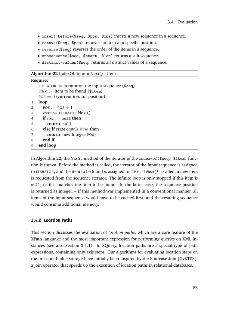
3.4. Evaluation
• insert-before($seq, $pos, $ins) inserts a new sequence in a sequence.
• remove($seq, $pos) removes an item at a specific position.
• reverse($seq) reverses the order of the items in a sequence.
• subsequence($seq, $start, $len) returns a sub-sequence.
• distinct-values($seq) returns all distinct values of a sequence.
Algorithm 22 IndexOf.Iterator.Next() : Item
Require:ITERATOR := iterator on the input sequence ($seq)ITEM := item to be found ($item)POS := 0 (current iterator position)
1 loop2 POS := POS + 13 item := ITERATOR.Next()4 if item = null then5 return null
6 else if ITEM equals item then7 return new Integer(POS)8 end if9 end loop
In Algorithm 22, the Next() method of the iterator of the index-of($seq, $item) func-
tion is shown. Before the method is called, the iterator of the input sequence is assigned
to ITERATOR, and the item to be found is assigned to ITEM. If Next() is called, a new item
is requested from the sequence iterator. The infinite loop is only stopped if this item is
null, or if it matches the item to be found. In the latter case, the sequence position
is returned as integer. – If this method was implemented in a conventional manner, all
items of the input sequence would have to be cached first, and the resulting sequence
would consume additional memory.
3.4.2 Location Paths
This section discusses the evaluation of location paths, which are a core feature of the
XPath language and the most important expression for performing queries on XML in-
stances (see also Section 3.1.1). In XQuery, location paths are a special type of path
expressions, containing only axis steps. Our algorithms for evaluating location steps on
the presented table storage have initially been inspired by the Staircase Join [GvKT03],
a join operator that speeds up the execution of location paths in relational databases.
83

3.4. Evaluation
AA
B
BA
X
post
1
2
3
4
5
6
pre1 2 3 4 5 6
AA
B
BA
X
post
1
2
3
4
5
6
pre1 2 3 4 5 6
AA
B
BA
X
post
1
2
3
4
5
6
pre1 2 3 4 5 6
AA
B
BA
X
post
1
2
3
4
5
6
pre1 2 3 4 5 6
Figure 3.6: pre/post planes; descendant step for the three A elements:a) conventional, b) with Pruning, c) with Partitioning, d) with Skipping
3.4.2.1 Staircase Join
The Staircase Join comprises three “tree aware” optimization strategies, namely Pruning,
Partitioning, and Skipping, which complement each other and which speed up the eval-
uation of XPath axes for a given context node sequence. Figure 3.6 shows four pre/post
planes (see 2.3.2 for a reminder). The gray rectangles depict the regions that have to
be scanned from left to right to evaluate a descendant step, starting from the three A
elements with pre values 2, 3, and 6. In the first plane, some areas are scanned multiple
times, resulting in quadratic costs and duplicate results. In the second region, pruningis applied: the axis evaluation is only performed for the first and third node: as the
second node is a descendant of the first node (which can be derived from its pre and
post values), it is ignored, as all its descendants will already be traversed by the first
node. In the partitioned plane, the scanned areas are made disjunct, i.e., scanning is
canceled whenever the pre value of the currently scanned node equals the pre value of
the next context node. In the rightmost skipping plane, scanning is stopped as soon as
the post values indicate that all descendants of the context node have been visited. For
more details on the Staircase Join algorithms, the reader is referred to Grust’s original
publications [Gru02, GvKT03, GT04].
The Staircase Join techniques can also be adapted to other encodings: Algorithm 23
demonstrates the traversal of the descendant axis, based on the pre/dist/size encod-
ing. Skipping is not necessary at all, as the size property of a node directly reflects the
number of descendants (see 2.3.4). Next, nodes can be pruned on-the-fly: n1 and n2
designate a successive pair of context nodes. The main loop reflects the partitioningstep. The inner loop visits all descendant nodes of n1 and adds them to the result array.
If pre equals the pre value of the next context node n2, n2 is discarded and overwritten
by its successor. If all descendants of n1 have been traversed, the loop is continued with
n2 until all context nodes have been processed.
84

3.4. Evaluation
Algorithm 23 Axis.Descendant(nodes : NodeSequence) : NodeSequence
1 result := new NodeIterator()2 n1 := nodes.Next()3 while n1 is not null do4 n2 := nodes.Next()5 for pre := n1.pre to n1.pre + n1.size− 1 do6 add new Node(pre) to result7 if n2.pre = pre then8 n2 := nodes.Next()9 end if10 end for11 n1 := n2
12 end while13 return result
Algorithm 24 Axis.Child(nodes : NodeSequence) : NodeSequence
1 result := new NodeIterator()2 for n in nodes do3 for pre := n.pre + n.asize to n.pre + n.size step Size(pre) do4 add new Node(pre) to result5 end for6 end for7 return result.Sort()
The traversal of the parent and ancestor axes is very simple, as the dist property offers a
direct reference to the relevant nodes. The evaluation of the child axis never generates
duplicates, as each node has a unique parent. Therefore, pruned child nodes would yield
wrong results, as all nodes of the input context need to be considered for traversal. In
Algorithm 24, the children of all input nodes are evaluated. The pre counter in the inner
loop is initialized with the sum of the pre value of the context node and its asize value,
which represents the number of attributes. By incrementing pre by the size value of the
currently visited node, using Size(pre), all descendants of the child nodes are skipped,
and only the relevant nodes are touched. The document order of the nodes might get
lost in the resulting sequence, however, as the following query shows:
<X><X>a</X>b</X>/descendant::X/child::text()
The first location step generates two context nodes X, which both have a single text node
as child. As the text child of the first X element is placed after the text of the subordinate
X element, the resulting text nodes (b, a) need to be sorted before they are returned.
To avoid sorting, a stack can be added to the algorithm, which caches all nodes that
85

3.4. Evaluation
are ancestors of the currently traversed parent node (see [Rod03] for the corresponding
algorithm on the pre/post encoding).
In practice, we observed that the Staircase Join optimizations (and particularly the prun-ing step) are relevant in only a few cases, as most queries will not generate any dupli-
cates, or will return small result sets instead, which can be sorted and freed from du-
plicates without considerable overhead. Next, many location paths can be optimized in
advance to avoid the generation of duplicate nodes at runtime. The most common ex-
ample represent queries with two location steps descendant::node()/child::*, which
would clearly benefit from pruning, but can also be rewritten to a single location step
descendant::* (details on rewriting location paths have been discussed in 3.4). As
pruning cannot be applied to location steps with position predicates [GVK04], and as
XQuery allows arbitrarily complex expressions as predicates, the presented algorithms
have eventually been replaced with simplified, iterative versions of the algorithms, which
process context nodes one by one. If the incoming nodes are known to be sorted, and
if the axis steps preserve orderedness and generate no duplicates, the complete location
path can be evaluated in an iterative manner (details on the detection of duplicates and
orderedness in location path can be looked up in [HMV05]). Otherwise, the steps are
evaluated one after another, and the results are added to a NodeIterator instance, which
only sorts the nodes if necessary (see Section 3.4.1.1).
3.4.2.2 Path Traversal
EvalPath IterPath
LocationPath
ROOT: ExpressionSTEPS: AxisStep[]
Iterator() : Iterator
IterStepEvalStep
Kind
ATTRIBUTECOMMENTDOCUMENT-NODEELEMENTPROCESSING-INSTR.TEXT
AnyKindTest
KindTest
KIND: Kind
AxisStep
TEST: NodeTestAXIS: AxisPREDS: Expression[]
Iterator() : Iterator
Axis
ANCESTORANCESTOR-OR-SELFATTRIBUTECHILDDESCENDANT...
Iterator(Node) : Iterator
NameTest
NAME: QName
NodeTest
Matches(Node)
Node
Ancestor() : IteratorAncestorOrSelf() : Iterator...
MemNode
DiskNode
DATA: DataPRE: int
Figure 3.7: Class diagram: location path expressions
Figure 3.7 depicts the most important expressions of location paths. In this work, a
LocationPath is specified as an expression with an optional root Expression and several
AxisSteps, and an AxisStep consists of an Axis, a NodeTest and zero or more Expressions as
predicates. Both the conventional and iterative versions of the LocationPath and AxisStep
86

3.4. Evaluation
Algorithm 25 DiskNode iterators
Require: DATA := database reference, PRE := pre value, P := PRE (pre cursor)
Child.Next() : NodeRequire: P := P + DATA.ASize(P)1 if P = PRE + DATA.Size(PRE)2 return null
3 end if4 node := new DiskNode(DATA, P)5 P := P + DATA.Size(P)6 return node
Parent.Next() : Node1 if P != PRE
2 return null
3 end if4 P := P − DATA.Dist(P)5 return new DiskNode(DATA, P)
Descendant.Next() : Node1 P := P + DATA.ASize(P)2 if P = PRE + DATA.Size(PRE)3 return null
4 end if5 return new DiskNode(DATA, P)
AncestorOrSelf.Next() : Node1 if P = −12 return null
3 end if4 node := new DiskNode(DATA, P)5 P := P − DATA.Dist(P)6 return node
Following.Next() : NodeRequire: P := P + DATA.Size(P)1 if P = DATA.META.SIZE
2 return null
3 end if4 node := new DiskNode(DATA, P)5 P := P + DATA.ASize(P)6 return node
Attribute.Next() : Node1 P := P + 12 if P = PRE + DATA.ASize(PRE)3 return null
4 end if5 return new DiskNode(DATA, P)
Self.Next() : NodeRequire: EVAL := false
1 if EVAL
2 return null
3 end if4 EVAL := true
5 return new DiskNode(DATA, P)
DescendantOrSelf.Next() : Node1 if P = PRE + DATA.Size(PRE)2 return null
3 end if4 node := new DiskNode(DATA, P)5 P := P + DATA.ASize(P)6 return node
Ancestor.Next() : Node1 P := P − DATA.Dist(P)2 if P = −13 return null
4 end if5 return new DiskNode(DATA, P)
FollowingSibling.Next() : NodeRequire: P := P + DATA.Size(P)
PAR := PRE – DATA.Dist(PRE)1 if P = PAR + DATA.Size(PAR)2 return null
3 end if4 node := new DiskNode(DATA, P)5 P := P + DATA.Size(P)6 return node
87

3.4. Evaluation
expressions (prefixed with Eval and Iter) have an Iterator() method, which returns the
evaluated next node, or null if all no more results are found. The Iterator() method
of the Axis enumeration returns an iterator for the specified Node. NodeTest.Matches()returns true if the specified node complies with the test. A test may accept all nodes
(AnyKindTest), nodes of a specific Kind (KindTest), or elements and attributes with a
certain name (NameTest)13. If the test is successful, the predicates are evaluated.
We will now have a closer look on the individual expressions, starting bottom-up with
the axis implementations. Both database (DiskNode) and constructed (MemNode) nodes
offer particular implementations for all XPath axes: while the memory-based iterators
are similar to conventional tree traversals, the database variants have been derived from
the Staircase Join algorithms and, hence, are more interesting in this context.
Algorithm 25 lists the Next() methods of the iterators of 10 of the 12 XPath axes, which
all can be implemented without considerable effort. As indicated in the last section, all
nodes are traversed one by one. A simple integer (P) references the current pre value.
null is returned if an axis will return no more nodes. Otherwise, P is updated, and
a new Node instance is created and returned. For some axes, which do not return a
self reference, the pre cursor needs to be initialized differently. As an example, in the
prolog of the Following.Next() method, the descendants of the initial node are skipped;
after that, the cursor is incremented by the node’s attribute size (asize). All algorithms
are optimal in the sense that only the relevant nodes are touched (in contrast, e.g., the
pre/post/level encoding requires a traversal of all descendants to find child nodes).
The two missing axes are preceding and preceding-sibling. As the nodes of the axes are
to be returned in reverse document order (as is the case with the ancestor axes), and
as no direct reference to left siblings is available in our encoding, a NodeIterator is used
to cache the results in ascending order, and then return them in backward direction.
Even so, only the nodes will be touched that contribute to the final result. To avoid
caching, the database table can as well be traversed backwards, and all touched nodes
can be matched against the axis. A reverse traversal is much slower, however, as many
irrelevant nodes are touched (including attributes, which will never be addressed by the
preceding axes). Next, usual prefetching strategies on hard disk are optimized for reading
forward. As preceding and following axes are rarely used in practice, implementation
details are skipped, and the reader is referred to the source code of BASEX [Gru10].
13The XQuery specification specifies more advanced tests for element, attribute and document nodes, whichhave been excluded from this overview.
88

3.4. Evaluation
On the next, higher level, the IterStep expression loops through all nodes that are re-
turned by the axis iterator. Its Next() method has many similarities with the Filter vari-
ant, which has been presented in 3.4.1.3. Algorithm 26 will only yield valid results
if at most one positional test is specified, which must additionally be placed as first
predicate. Note that this limitation is not intrinsic to iterative processing; instead, it
was introduced to simplify the presented pseudo-code. If a separate context position is
managed and cached for each predicate, the algorithm will be able to process arbitrary
positional predicates.
Algorithm 26 IterStep.Iterator.Next() : Node
Require:AXIS := XPath axisTEST := node testPREDS := filter predicatesCONTEXT := query contextITERATOR := node iterator, generated from the AXIS and input nodePOS := 0 (current context position)
1 loop2 POS := POS + 13 node := ITERATOR.Next()4 if node = null then5 return null
6 else if TEST.Matches(node) then7 CONTEXT.VALUE := node8 CONTEXT.POS := POS
9 for pred in PREDS do10 break if the truth value of pred is false11 end for12 return node if all predicates tests were successful13 end if14 end loop
In contrast to the filter expression, the step iterator additionally performs the node test
before the predicates are considered. Next, the context item and position is not reset, as
this will be done once for all steps by the path expression.
Finally, Algorithm 27 shows the Next() method of the IterPath, which creates and triggers
the axis step iterators and returns the results of the last step. The ITERATORS variable
contains references to the step iterators, the first of which is initialized before the first
call (the optional root expression is excluded from this algorithm; it is treated the same
way as the axis steps). The original context value and position are cached before and
89

3.4. Evaluation
Algorithm 27 IterPath.Iterator.Next() : Node
Require:ITERATORS := iterator arrayCONTEXT := query contextITERATORS[0] = STEPS[0].Iterator()P := 0 (index on current iterator)
1 cache context value and position2 loop3 node := ITERATORS[P].Next()4 if node = null then5 P := P − 16 break if P < 07 else if p < #ITERATORS – 1 then8 P := P + 19 CONTEXT.VALUE := node10 ITERATORS[P] = STEPS[P].Iterator()11 else12 break13 end if14 end loop15 restore context value and position16 return node
restored after the evaluation. In the main loop, the next item is requested from the
current iterator, which is referenced by P. If the iterator is exhausted, the next higher
iterator is addressed by decrementing P. If the leftmost iterator (i.e., the first location
step) returns null, the loop is canceled, as the location path will return no more results.
Otherwise, if the current iterator is not the rightmost, P is incremented, the evaluated
node is set as context node and the iterator of the next location step is initialized. If P
points to the last location step, the evaluated node is returned as result.
3.4.2.3 Optimizations
The proposed framework offers room for numerous tweaks and improvements, both
conceptual and technical, which will further speed up the evaluation of location paths.
Some of the most important optimizations are sketched in the following. First of all, the
IterStep algorithm is clearly suboptimal, regarding the evaluation of positional predicates:
• All nodes are iterated, even if a position test is specified that filters the result-
ing nodes to a small subset. In the example query descendant::node()[1], the
90

3.4. Evaluation
iterator could be canceled after the first hit.
• Predicates using the last() function (which returns the last item of a sequence)
are not supported, as the number of results is not known in advance. As the
last() function will reduce the processed nodes to a single item, the conventional
evaluation, which caches all nodes, is highly undesirable.
Algorithm 28 IterStep.Iterator.Next() : Node
Require: see Algorithm 26, plus:POSITION := position expression (optional)RETURNLAST := flag for returning the last node (optional)SKIP := false
1 return null if SKIP
2 last := null
3 loop4 POS := POS + 15 node := ITERATOR.Next()6 if node = null then7 SKIP := RETURNLAST
8 return last9 else if TEST.Matches(node) then10 CONTEXT.VALUE := node11 CONTEXT.POS := POS
12 for pred in PREDS do13 break if the truth value of pred is false14 end for15 if all predicates tests were successful then16 SKIP := POSITION.Skip(CONTEXT)17 return node18 end if19 if RETURNLAST then20 last := node21 end if22 end if23 end loop
Algorithm 28 includes optimizations for the two requirements: RETURNLAST will be true
if the step contains a single last() predicate, and POSITION will be assigned if the
first predicate is an implementation-defined POSITION expression (see Section 3.5 for its
definition). The SKIP flag indicates that the iterator will return no more results. It is
set to true if the iterator is exhausted and the RETURNLAST flag is true, or if the Skip()method of the position expression returns true for the given context, indicating that
91

3.5. Summary
the context position has surpassed the given range. The last variable caches the last
node that has been accepted by the node test. Note that both optimizations can also be
applied to the filter iterator (Algorithm 21).
Another improvement can be applied to the evaluation of location paths: The iterative
evaluation of path expressions is limited to descendant paths that follow certain patterns
[HMV05]: parent steps may yield duplicate nodes, even if they are evaluated on ordered
and duplicate-free node sets, as nodes can have the same parents. Still, the proposed
IterPath method can be easily extended to also evaluate parent steps: Before a node is
returned, it is cached by the iterator. If a cached node already exists, its node identity
is compared with the new node. If both nodes have the same identity, the new node is
ignored. This optimization is particularly helpful if a query is rewritten for index access,
in which case child steps are inverted to parent steps.
Another simple yet effective optimization concerns the instantiation of new objects,
which is an expensive operation in most programming languages. The proposed axis
iterators continuously create new DiskNode objects, most of which will not contribute to
the final result. This can be avoided by creating a single, initial node instance, which is
updated with the current iterator values. If this node is accepted by a step expression, a
copy of it is returned as result.
3.5 Summary
This section summarizes the optimizations and rewritings that have been applied to the
most important XQuery expressions; we hope that they might serve as inspiration for
other implementors of XQuery, and similar languages. The expression syntax is inspired
by the W3C Recommendations, in which further details on the expressions can be looked
up [BCF+07, MMW07]). To save space, the following abbreviations are used for the
summary of each expression:
S contains the semantics of an expression.
P describes operations in the parsing step that differ from the proposals in the speci-
fication (of course, all expression will continue to comply with the specification).
C contains query compilation steps. If an expression is “returned”, it will replace the
original expression in the query plan.
I includes information how an expression is rewritten for index access, and how
costs will be estimated.
92
3.5. Summary
E refers to evaluation/runtime optimizations.
X adds examples to illustrate how some of the compilation steps work. Numbers
have been added to the compilation steps and examples to show their relationship.
The following keywords are used as placeholders for returned expressions in the compi-
lation step:
• EMPTY designates the empty item sequence ().
• TRUE and FALSE are equivalents for the boolean items true and false.
Some optimizations are skipped in this context, as they have already been described in
the previous sections. For example, details on constant folding would be mostly redun-
dant, as this optimization can be applied to nearly all operators. Next, some expressions
will be introduced that have no equivalent in the specifications, as they result from com-
piling other expressions. Consequently, their proposed syntax and semantics is specific
to our implementation.
ARITHMETIC: o1 {+|-|*|div|idiv|mod} o2 → item()?
S The arithmetic operator is applied to the atomized operands. Besides numbers,
also dates and durations can be computed and returned, according to the Operator
Mapping of the specification.
C1 EMPTY is returned if one operand will never yield results.
E Evaluation of the second operand is skipped if the first yields an empty sequence.
X1 1 + (10 to 1) → ()
CONDITIONAL: if(c) then e1 else e2 → item()*
S If the effective boolean value of condition c yields true, e1 is evaluated. Otherwise,
e2 is evaluated.
C1 If the condition is a value, the correct branch is selected and returned.
C2 If both branches are identical, the condition is ignored and the identical result is
returned. This optimization assumes that the condition causes no side-effects.
C3 If the first branch is true and the second is false, the expression is replaced by a
function fn:boolean(c).
C4 If the first branch is false and the second is true, the expression is replaced by a
function fn:not(c).
C5 If the condition is enclosed by fn:not(c), the function is removed and the branches
are swapped.
X1 if(1) then local:run() else error() → local:run()
93

3.5. Summary
X2 if(local:process()) then ’ok’ else ’ok’ → ’ok’
X3 if(tp:desc()) then true() else false() → boolean(tp:desc())
X5 if(not(tp:desc())) then 0 else 1 → if(tp:desc()) then 1 else 0
EXCEPT: o1 except o2 → node()*
S All nodes of the first evaluated operand are returned that are not contained in the
second.
P Consecutive except operators are parsed into one expression.
C EMPTY is returned if the first operand yields an empty sequence. Other operands
yielding empty sequences are removed. If one operand is left that yields sorted
and duplicate-free nodes, this operand is returned.
FILTER: e[p1]...[pn]→ item()*
S The resulting items of an expression are filtered by one or more predicates.
C1 If the expression will never return results, EMPTY is returned.
C2 All predicate values yielding true are removed. If no predicates remain, the orig-
inal expression is returned. EMPTY is returned if one of the predicates yields
false.
C3 Numeric predicates are rewritten to POSITION expressions.
X1 (//*[text() = ’not found in the index’])[1] → ()
X2 <xml/>[true()][’ok’] → <xml/>
FLWOR: (for...|let...)+ (where w)? (order by o)? return r → item()*
S Values are iteratively mapped to variables, filtered, ordered, and returned.
C1 The WHERE clause is rewritten to one or more predicates, which are attached to
an innermost FOR clause; see 3.3.1.6 for details.
C2 LET clauses and FOR clauses with one result are statically bound to their refer-
ences.
C3 If WHERE will always yield true, it is removed. EMPTY is returned if it always
yields false.
C4 If one FOR clause will never yield results, EMPTY is returned.
C5 Declarations of statically bound variables are eliminated. If no variable declara-
tion is left, the return expression is returned. If a WHERE clause is specified, a
CONDITIONAL expression is returned.
C6 Expressions with one FOR/LET clause, no WHERE/ORDER clause and a single
variable reference in the RETURN clause are simplified.
X1 for $n in //Medium where $n/Type = ’DVD’ return $n/Title
94

3.5. Summary
→ for $n in //Medium[Type = ’DVD’] return $n/Title
X3 for $n in 1 to 10 where 3 < 2 return $n → ()
X4 for $n in () let $l := (1,2,3) return ($n, $l) → ()
X5 let $l := 1 where <x/> return $n → if(<x/>) then $1 else ()
X6 for $i in //item return $i → //item
FUNCTION CALL: $n(a1, ..., an)→ item()*
S The function named n is evaluated with the specified arguments a1, ..., an.
C1 If all function arguments are values, and if the function result is a value, this value
is returned.
C2 Functions that are never referenced at compile time, or have been inlined, will be
eliminated.
X1 declare function math:pi() { 3.14159265 }; math:pi() → 3.14159265
GENERAL COMPARISON: o1 {=|!=|<|<=|>=|>} o2 → xs:boolean
S All items of the evaluated operands are compared to each other, according to the
Operator Mapping of the specification. TRUE is returned if one of the comparisons
yields true.
C1 FALSE is returned if one operand will never yield results.
C2 Identical to the VALUE COMPARISON, just as C3, C4, and C5.
C5 Additionally, a POSITION expression is returned for a fn:position() function
and a range expression.
C6 If possible, a RANGE COMPARISON expression is returned for numeric compar-
isons. This expression can be combined with other range tests more easily, or
rewritten for range index access.
C7 A boolean flag SINGLE is set to indicate if all operands will yield single items.
I1 If possible, the operator is rewritten for index access; see 3.3.2.2 for details.
I2 If several expressions are specified as search terms, a UNION expression with mul-
tiple index operators will be returned. Index requests with zero results are ignored.
E If the SINGLE flag was set to true, all operands will be directly evaluated to single
items. Otherwise, TRUE is returned as soon as a comparison is positive (see 3.3.3
for more details on evaluating general comparisons).
X5 address[position() = 1 to 5] → address[1...5]
X6 salary[text() > 1000] → salary[1000 < text() < ∞]
INTERSECT: o1 intersect o2 → node()*
S All nodes are returned that occur in all of the evaluated operands.
95
3.5. Summary
P Consecutive intersect operators are parsed into one expression.
C EMPTY is returned if one of the operands will never yields results.
LOGICAL AND: o1 and o2 → xs:boolean
S The operands are evaluated to their effective boolean values. true is returned if all
booleans are true. Otherwise, the result is false.
P Consecutive and operators (o1 and . . . and on) are parsed into one expression.
This flattens the operator tree and allows for an easier optimization.
C1 All values yielding true are removed. If no operands remain, TRUE is returned. If
one operand remains, it is returned as new expression. If this operand yields no
boolean value, it is wrapped in a fn:boolean() function. FALSE is returned if at
least one of the values yields false.
C2 Multiple POSITION expressions are merged. If the merged position range will
never yield true, FALSE is returned.
C3 Multiple RANGE COMPARISON expressions are merged. If the merged expression
will result in an impossible range, FALSE is returned.
I1 If all operands can benefit from an index, an INTERSECT expression will be re-
turned, containing all operands rewritten for index access.
I2 Costs for index access are summarized. All index operations will be sorted by their
costs in an ascending order to evaluate the cheapest index operation first. If one
index operation will yield zero hits, EMPTY is returned.
E FALSE is returned as soon as one operand yields false.
X1 1 and ’two’ and xs:boolean(true()) → true
X2 node[position() >= 1 and position() <= 10] → node[1...10]
X3 //person[@income >= 1000 and @income < 5000] →//person[1000 <= @income < 5000]
LOGICAL OR: o1 or o2 → xs:boolean
S The operands are evaluated to their effective boolean values. false is returned if
all booleans are false. Otherwise, true is returned.
P Same as LOGICAL AND: consecutive or operators are parsed into one expression.
C1 In analogy to AND: All values yielding false are removed. If no operands remain,
FALSE is returned. If one operand remains, it is returned as new expression. If this
operand yields no boolean value, it is wrapped in a fn:boolean() function. TRUE
is returned if at least one of the values yields true.
C2 Multiple GENERAL COMPARISON expressions are merged if their left operand is
identical. Expressions of this kind can better be rewritten for index access.
96

3.5. Summary
I1 If all operands can benefit from an index, an UNION expression will be returned,
containing all operands rewritten for index access.
I2 Costs for index access are summarized. If a single index operation will yield zero
hits, it is ignored. If no index operation will yield any hits, EMPTY is returned.
E true is returned as soon as one operand yields true.
X2 //node[text() = ’A’ or text() = ’B’] → //node[text() = (’A’, ’B’)]
NODE COMPARISON: o1 {<<|is|>>} o2 → xs:boolean?
S The operands are evaluated to nodes and compared in terms of their node identity.
C EMPTY is returned if one operand will never yield results.
E Evaluation of the second operand is skipped if the first yields an empty sequence.
X //text() is //text()/text() → ()
POSITION: min ... max→ xs:boolean
S This implementation specific expression is a normalized representation of posi-
tional predicates, containing a minimum and maximum integer value. true is
returned if the current context position lies within the given range. An additional
Skip() method checks if the context position surpasses the range.
RANGE: o1 to o2 → xs:integer*
S A sequence of consecutive integers is created, ranging from o1 to o2. Range ex-
pressions will never be pre-evaluated if the result would include more than one
integer; instead, light-weight iterators are created at runtime.
C1 If either operand will never yield values, or if the first operand yields an integer
larger than the second, EMPTY is returned.
C2 If both operands yield the same integers, that integer is returned.
X1 10 to 1 → ()
X2 1 to 1 → 1
RANGE COMPARISON: min {<|<=} o {<|<=} max: xs:boolean
S Some comparisons are rewritten into this implementation specific expression, which
contains an operand to be evaluated and a minimum and maximum double value.
true is returned if expression e lies within the given range.
I1 The operator is rewritten for index access, similar to step I1 of the GENERAL
COMPARISON.
I2 In accordance with the database statistics, if possible, the minimum and maximum
values are reduced for the tested text or attribute name.
97

3.5. Summary
I3 20% of the number of database nodes is set as costs to indicate that sequential
access might be faster if several index operations are to be performed.
TYPESWITCH: typeswitch (c) ({case t|default} return e)+→ item()*
S Depending on the type of expression c, one of the specified branches is evaluated
and returned. The syntax shown above is simplified.
C1 If the type of the condition is known due to static typing, the correct branch is
selected and returned.
C2 If all conditions specify the same result, the condition is ignored and the result is
returned. This optimization assumes that the condition causes no side-effects.
X1 typeswitch(xs:int(’1’)) case xs:int return 2 default return 3 → 2
X2 typeswitch(’a’) case xs:string return () default return () → ()
UNION: o1 union o2 → node()*
S All nodes are returned that occur in either of the evaluated operands.
P Consecutive union operators are parsed into one expression.
C All operands yielding empty sequences are removed. If no operand is left, EMPTY
is returned. If one operand is left that yields sorted and duplicate-free nodes, it is
returned as new expression.
VALUE COMPARISON: o1 (eq|ne|lt|le|ge|gt) o2 → xs:boolean?
S The operands are evaluated to items and compared to each other, according to the
Operator Mapping of the specification.
C1 EMPTY is returned if one operand will never yield results.
C2 If values and non-values are specified as operands, the expression is normalized:
the value is specified as second operand, and the operator is inversed.
C3 text() steps are added to location paths if database meta data indicates that the
result will be identical. Atomization will be cheaper, and expressions can be better
rewritten for index access (see Section 3.3.2).
C4 if possible, fn:count() functions are rewritten to fn:empty() or fn:exist(). The
latter functions may be cheaper, as only the first resulting item need to be touched.
C5 if possible, fn:position() functions are rewritten to an implementation specific
POSITION expression.
E Evaluation of the second operand is skipped if the first yields an empty sequence.
X2 node[123 lt text()] → node[text() gt 123]
X3 city[name eq ’Roma’] → city[name/text() eq ’Roma’]
X4 count(//item) gt 0 and count(//person) eq 0
98

3.5. Summary
→ exists(//item) and empty(//person)
X5 address[position() le 10] → address[1...10]
VARIABLE REFERENCE: $v → item()*
S The expression, which is bound to v, is evaluated and returned.
C1 If variables are global, specify a fragment, or contain a function call, they will be
pre-evaluated by the compiler if they are referenced for the first time.
C2 Variables that are never referenced at compile time will be eliminated.
X2 declare variable $x := doc(’input.xml’); <xml/> → <xml/>
99
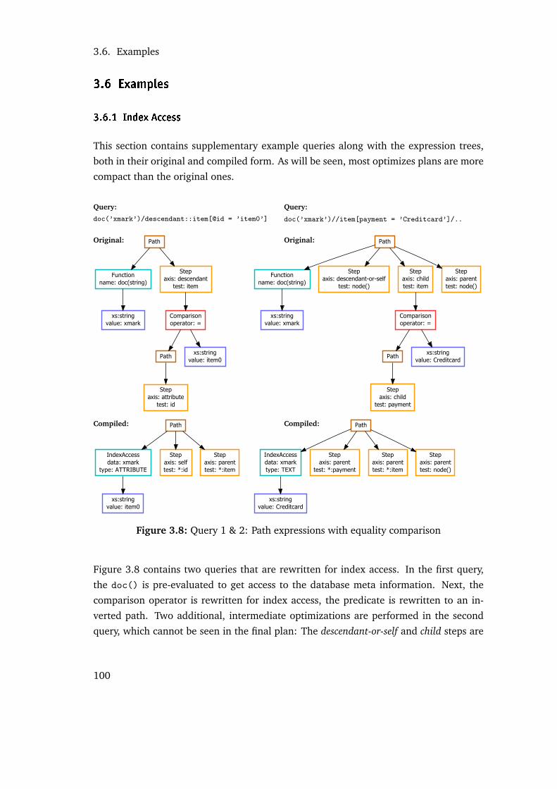
3.6. Examples
3.6 Examples
3.6.1 Index Access
This section contains supplementary example queries along with the expression trees,
both in their original and compiled form. As will be seen, most optimizes plans are more
compact than the original ones.
Query:
doc(’xmark’)/descendant::item[@id = ’item0’]
Original: Path
Function
name: doc(string)
Step
axis: descendant
test: item
xs:string
value: xmark
Comparison
operator: =
Pathxs:string
value: item0
Step
axis: attribute
test: id
Compiled: Path
IndexAccess
data: xmark
type: ATTRIBUTE
Step
axis: self
test: *:id
Step
axis: parent
test: *:item
xs:string
value: item0
Query:
doc(’xmark’)//item[payment = ’Creditcard’]/..
Original: Path
Function
name: doc(string)
Step
axis: descendant-or-self
test: node()
Step
axis: child
test: item
Step
axis: parent
test: node()
xs:string
value: xmark
Comparison
operator: =
Pathxs:string
value: Creditcard
Step
axis: child
test: payment
Compiled: Path
IndexAccess
data: xmark
type: TEXT
Step
axis: parent
test: *:payment
Step
axis: parent
test: *:item
Step
axis: parent
test: node()
xs:string
value: Creditcard
Figure 3.8: Query 1 & 2: Path expressions with equality comparison
Figure 3.8 contains two queries that are rewritten for index access. In the first query,
the doc() is pre-evaluated to get access to the database meta information. Next, the
comparison operator is rewritten for index access, the predicate is rewritten to an in-
verted path. Two additional, intermediate optimizations are performed in the second
query, which cannot be seen in the final plan: The descendant-or-self and child steps are
100

3.6. Examples
merged to a single descendant step. Next, based on the information given in the database
statistics, the Comparison operator attaches a text() to the payment step to indicate the
index rewriter that this step has only leaf nodes.
Query:
(for $i in doc(’xmark’)//item
where $i/payment = ’Creditcard’
return $i)/..
Compilation:
1. rewriting where clause to predicate
2. pre-evaluating doc("xmark")
3. adding text() step
4. merging descendant-or-self step(s)
5. applying text index
6. simplifying flwor
7. merging axis paths
Path
FLWOR
Step
axis: parent
test: node()
For
var: $iWhere Return
Path
Function
name: doc(string)
Step
axis: descendant-or-self
test: node()
Step
axis: child
test: item
xs:string
value: xmark
Comparison
operator: =
Pathxs:string
value: Creditcard
VarRef
name: $i
Step
axis: child
test: payment
VarRef
name: $i
Figure 3.9: Query 3: FLWOR expression with equality comparison
Another query is shown in Figure 3.9, which yields the same optimized plan as Query
2. The query is written as a FLWOR expression; as such, the compiler first attaches the
WHERE clause as predicate to the location step of the FOR clause. After all other opti-
mizations have been performed, the FLWOR expression is eliminated, and the resulting
index path is merged with the suffixed parent step.
3.6.2 XMark
The following plans depict some of the XMark Benchmark queries [SWK+02] (see Sec-
tion 4.2.2.3 for a list of all queries). In Figure 3.10, XMark Query 1 is depicted, which
bears some similarities with the previous expressions. The outer FLWOR expression,
which only contains a LET clause defining the input document, is eliminated, and the
location path of the inner FOR clause is rewritten to an index access. Note that the
index access smoothly integrates in the remaining FLWOR expression: each index result
is iteratively bound to the variable of the FOR clause.
101

3.6. Examples
Original: FLWOR
Let
$auctionReturn
Function
doc(string)
xs:string
xmark
FLWOR
For
$bReturn
Path
VarRef
$auction
Step
child
site
Step
child
people
Step
child
person
Comparison
=
Pathxs:string
person0
Step
attribute
id
Path
VarRef
$b
Step
child
name
Step
child
text()
Query:
let $auction := doc("xmark") return
for $b in $auction/site/people/person[@id = "person0"]
return $b/name/text()
Compilation:
1. pre-evaluating doc("xmark")
2. binding static variable $auction
3. applying attribute index
4. removing variable $auction, simplifying flwor
Compiled: FLWOR
For
$bReturn
Path
IndexAccess
xmark
ATTV
Step
self
*:id
Step
parent
*:person
xs:string
person0Path
Step
parent
*:people
Step
parent
*:site
Step
parent
doc()
Path
VarRef
$b
Step
child
name
Step
child
text()
Figure 3.10: XMark Query 1: Original and optimized query plan
Figure 3.11 is presented in XMark Query 7, which is similar to the query shown in
3.3.1.3, as it can be completely pre-evaluated at compile time. The three fn:count()
functions yield the number of nodes of a sub-tree of the document. The most important
compilation steps are as follows:
Many of the optimizations in this query are due to the path summary: after the docu-
ment reference has been pre-evaluated (1) and the $auction variable has been statically
bound to its references (2), the expression of the FOR clause is bound to the variable
$p (3): the path summary indicates that the document only contains one site ele-
ment, which means that variable $p will only return one single value and, hence, can
be statically bound. Next, the descendant-or-self and child steps are rewritten to a simple
descendant step (4), and the path summary is once more accessed to compute the num-
ber of elements for the resulting path /child::site/descendant::description (5).
The same steps are performed for the remaining paths, and the number of final results
is calculated by pre-evaluating the calculation operators.
102

3.6. Examples
Compilation:
1. pre-evaluating doc("xmark")
2. binding static variable $auction
3. binding static variable $p
4. merging descendant-or-self step
5. pre-evaluating count(...)
6. merging descendant-or-self step
7. pre-evaluating count(...)
8. pre-evaluating 45 + 22
9. merging descendant-or-self step
10. pre-evaluating count(...)
11. pre-evaluating 67 + 25
12. removing variable $p
13. simplifying flwor
14. removing variable $auction
15. simplifying flwor
FLWOR
Let
$auctionReturn
Function
doc(string)
xs:string
xmark
FLWOR
For
$pReturn
Path
VarRef
$auction
Step
child
site
Calculation
+
Calculation
+
Function
count(item)
Function
count(item)
Function
count(item)
Path
VarRef
$p
Step
descendant-or-self
node()
Step
child
description
Path
VarRef
$p
Step
descendant-or-self
node()
Step
child
annotation
Path
VarRef
$p
Step
descendant-or-self
node()
Step
child
emailaddress
Query:
let $auction := doc(’xmark’) return
for $p in $auction/site return
count($p//description) +
count($p//annotation) +
count($p//emailaddress)
Figure 3.11: XMark Query 7: Original query plan
XMark queries 8-12 contain nested loops and yield quadratic costs if they are evaluated
without optimizations. XMark Query 9 is presented in more detail: it includes six FLWOR
expressions, only three of which remain after the query has been compiled: First of all,
the input document is pre-evaluated and statically bound to all its references. Next, the
expressions of the LET variables $ca and $ei are bound. After the first WHERE clause
has been converted to a predicate, and the arguments of the comparison operator have
been swapped, the first path can be rewritten for index access. Similar optimizations
are applied to the second WHERE clause and equality comparison, resulting in a simpli-
fication of the embracing FLWOR expression. Finally, after the removal of the obsolete
variable declarations, two other FLWOR expressions are eliminated. As a result, the
costs for the query are decreased from O(n2) to O(n ∗ log n), provided that the applied
indexes yield results in logarithmic time.
An additional XMark Query 21 has been added to this section, which is not part of the
benchmark, but which demonstrates the flexibility of the rewriting mechanism for the
WHERE clause: The query depicted in Figure 3.13 comprises one FLWOR expression
103

3.6. Examples
Compilation:
1. pre-evaluating doc("xmark")
2. binding static variable $auction
3. binding static variable $ca
4. binding static variable $ei
5. rewriting where clause
6. swapped: buyer/@person = $p/@id
7. applying attribute index
8. rewriting where clause
9. swapped: @id = $t/itemref/@item
10. applying attribute index
11. simplifying flwor
12. removing variable $ei
13. removing variable $ca
14. simplifying flwor
15. removing variable $auction
16. simplifying flwor
Query:
let $auction := doc("xmark") return
let $ca := $auction/site/closed_auctions/
closed_auction return
let $ei :=
$auction/site/regions/europe/item
for $p in $auction/site/people/person
let $a :=
for $t in $ca
where $p/@id = $t/buyer/@person
return
let $n := for $t2 in $ei
where $t/itemref/@item = $t2/@id
return $t2
return <item>{$n/name/text()}</item>
return <person name="{$p/name/text()}">{ $a }</person>
FLWOR
Let
$auctionReturn
Function
doc(string)
xs:string
xmark
FLWOR
Let
$caReturn
Path
VarRef
$auction
Step
child
site
Step
child
closed_auctions
Step
child
closed_auction
FLWOR
Let
$ei
For
$p
Let
$aReturn
Path
VarRef
$auction
Step
child
site
Step
child
regions
Step
child
europe
Step
child
item
Path
VarRef
$auction
Step
child
site
Step
child
people
Step
child
person
FLWOR
For
$tWhere Return
VarRef
$ca
Comparison
=
Path Path
VarRef
$p
Step
attribute
id
VarRef
$t
Step
child
buyer
Step
attribute
person
FLWOR
Let
$nReturn
FLWOR
For
$t2Where Return
VarRef
$ei
Comparison
=
Path Path
VarRef
$t
Step
child
itemref
Step
attribute
item
VarRef
$t2
Step
attribute
id
VarRef
$t2
CElem
xs:QName
itemPath
VarRef
$n
Step
child
name
Step
child
text()
CElem
xs:QName
personCAttr
VarRef
$a
xs:QName
namePath
VarRef
$p
Step
child
name
Step
child
text()
FLWOR
For
$p
Let
$aReturn
Path
document-node()
xmark
Step
child
*:site
Step
child
*:people
Step
child
*:person
FLWOR
For
$tReturn
Path
IndexAccess
xmark
ATTV
Step
self
*:person
Step
parent
*:buyer
Step
parent
*:closed_auction
Path
VarRef
$p
Step
attribute
id
Path
Step
parent
*:closed_auctions
Step
parent
*:site
Step
parent
doc()
FLWOR
Let
$nReturn
Path
IndexAccess
xmark
ATTV
Step
self
*:id
Step
parent
*:item
Path
VarRef
$t
Step
child
itemref
Step
attribute
item
Path
Step
parent
*:europe
Step
parent
*:regions
Step
parent
*:site
Step
parent
doc()
CElem
xs:QName
itemPath
VarRef
$n
Step
child
name
Step
child
text()
CElem
xs:QName
personCAttr
VarRef
$a
xs:QName
namePath
VarRef
$p
Step
child
name
Step
child
text()
Figure 3.12: XMark Query 9: Optimized/original query plan (top/bottom)
104
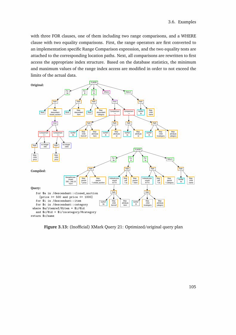
3.6. Examples
with three FOR clauses, one of them including two range comparisons, and a WHERE
clause with two equality comparisons. First, the range operators are first converted to
an implementation specific Range Comparison expression, and the two equality tests are
attached to the corresponding location paths. Next, all comparisons are rewritten to first
access the appropriate index structure. Based on the database statistics, the minimum
and maximum values of the range index access are modified in order to not exceed the
limits of the actual data.
Original:FLWOR
For
$a
For
$i
For
$cWhere Return
Path
Root
Step
descendant
closed_auction
And
Comparison
>=
Comparison
<=
Pathxs:integer
500
Step
child
price
Pathxs:integer
1000
Step
child
price
Path
Root
Step
descendant
item
Path
Root
Step
descendant
category
And
Comparison
=
Comparison
=
Path Path
VarRef
$a
Step
child
itemref
Step
attribute
item
VarRef
$i
Step
attribute
id
Path Path
VarRef
$c
Step
attribute
id
VarRef
$i
Step
child
incategory
Step
attribute
category
Path
VarRef
$c
Step
child
name
Compiled:
FLWOR
For
$a
For
$i
For
$cReturn
Path
RangeAccess
xmark
500 - 540.16
TEXT
Step
parent
*:price
Step
parent
*:closed_auction
Path
IndexAccess
xmark
ATTV
Step
self
*:id
Step
parent
*:item
Path
VarRef
$a
Step
child
itemref
Step
attribute
item
Path
IndexAccess
xmark
ATTV
Step
self
*:id
Step
parent
*:category
Path
VarRef
$i
Step
child
incategory
Step
attribute
category
Path
VarRef
$c
Step
child
name
Query:
for $a in /descendant::closed_auction
[price >= 500 and price <= 1000]
for $i in /descendant::item
for $c in /descendant::category
where $a/itemref/@item = $i/@id
and $c/@id = $i/incategory/@category
return $c/name
Figure 3.13: (Inofficial) XMark Query 21: Optimized/original query plan
105


4 Performance
If one parses the database publications, it seems groundbreaking how many “most effi-
cient” and “best” algorithms and techniques have been designed and implemented over
the last 30 years. The same observation accounts for newer performance results on XML
and XQuery, let alone the advertisements of commercial products. Summarizing, it is no
secret that everyone wants to be Number One, and, at the same time, it is well-known
that each scientific approach and code project excels in different areas. Accordingly, we
do know that we are Number One as well, and we could easily enough limit our per-
formance tests to a “most relevant” subset of queries to prove this claim. –Instead, we
want to point out that we have not come across any XQuery processor or database that
will beat all others, but there are surely some that focus on performance, while others
put more efforts into compliance or a rich feature list. Hence, this observation is meant
as an introductory warning, and to avoid that the presented performance results are
interpreted as the only relevant dimensions.
The performance of BASEX, our native XML database and XQuery processor that em-
braces all the techniques listed in the previous two chapters, is central to this chapter.
First of all, we will benchmark the performance of our storage unit and measure the
time needed to build new database instances and index structures. The results will be
compared with some other Open Source XML databases. Second, we will focus on its
query capabilities, and compare BASEX with additional XQuery processors. Finally, we
will present some statistics on very large database instances that have been built with
our system.
ID CPU RAM Hard disk OS BitsDual Intel Dual Core T7300 2.0 GHz 2 GB 80 GB Windows XP SP3 32Xeon Intel Xeon 2.33 GHz 32 GB 450 GB Linux 2.6.27 (Suse 10.2) 64AMD AMD Opteron 2.2 GHz 16 GB 400 GB Linux 2.6.13 (Suse 10.0) 64
Table 4.1: Hardware architectures used for testing
All tests in this section have been performed with Version 6.3 of BASEX. Three different
hardware architectures have been used for testing, which are shown in Table 4.1, and
which will from now on be addressed by their IDs Xeon, Dual, and AMD.
107

4.1. Storage
4.1 Storage
sec. 1MB 11MB 111MB 1GB 11GB 55GB� Main 0.071 0.57 4.96 50.8 508 5151� Text 0.012 0.14 1.95 22.9 241 2152� Attr. 0.003 0.04 0.60 10.0 132 1214� Trie 0.092 0.86 8.60 88.2 982 8363� Fuzzy 0.109 1.16 11.89 169.4 1981 15364
sec. 1M 11M 111M 1G 11G� Xeon 0.06 0.75 7.7 89 917� Dual 0.09 0.98 12.6 186 4099
Figure 4.1: Database creation of XMark instances with BASEX. Left: single times fordatabase and index creation, right: total time on different architectures
Figure 4.1 demonstrates the performance results for building databases from six XMark
instances ([SWK+02], see also 4.2.2). The left diagram was performed on the Xeonmachine with 32GB RAM. It lists times for creating the database and the four index
structures. Text and attribute indexing is very fast, whereas the full-text indexes, which
are optional and interchangeable, take approximately the same time as is needed for
building the database, as all text nodes need to be tokenized and normalized. The right
diagram compares build times measured on the two test architectures with a different
amount of RAM; this time, the results include the creation of the text and attribute
indexes, which are activated by default. It can be observed that more RAM speeds up
the creation of large databases. The memory consumption for creating the database
table is low for all instances, as all data is directly written to disk: instead, it is the index
creation process that takes up a lot of memory. The existing index builders have been
optimized to dynamically adapt to the available memory (see 2.6.3.3 for details). As a
result, also the 1GB and 11GB document instances can be successfully built with 2GB
RAM. 32GB RAM is needed, however, to build indexes for the 55GB instance, as the
intermediate data structures, which are created by the index builder, are too large to fit
into main memory.
Obviously, the time for building index structures is strongly dependent on the input data.
If a document contains many attributes, the costs for building the attribute index might
equal or surpass the text index. Figure 4.2 shows the numerically sorted timing results
108

4.1. Storage
sec. Factbook Shakespeare Nasa DDI Treebank Wikipedia MedLineDesc DBLP� Main 0.112 0.58 1.98 5.84 8.69 9.42 23.27 141.63� Text 0.012 0.28 0.40 0.64 4.88 0.12 4.35 62.92� Attribute 0.045 0.01 0.08 0.23 0.21 0.01 0.76 62.85� Trie 0.021 0.60 1.37 0.85 12.52 13.72 5.35 134.17� Fuzzy 0.019 0.77 1.82 1.13 10.08 18.47 6.68 145.57Size (MB) 1.7 7.5 23 75 82 99 260 694
Figure 4.2: Database creation of various smaller XML instances (Sources: Table 4.5)
for some smaller documents. Attribute indexing is comparatively time consuming for
the Factbook, while the Shakespeare and Treebank is predominated by text nodes. The
Wikipedia instance has just a few, but very long text nodes; consequently, most time is
spent for creating the full-text indexes.
sec. 1MB 11MB 111MB 1GB 11GB� BASEX 0.06 0.75 7.7 89 917� MONET 0.20 2.14 21.0 199 –� QIZX 0.68 4.44 42.7 – –� EXIST 0.90 6.24 65.7 702 –
MB 1MB 11MB 111MB 1GB 11GB� BASEX 1.3 13 133 1332 13325� MONET 2.6 26 262 2600 –� QIZX 1.1 9 99 – –� EXIST 2.1 18 181 1865 –
Figure 4.3: XMark documents: build times and database sizes
In Figure 4.3, BASEX is compared with some other Open Source XML engines. Com-
mercial systems have been tested as well, but were omitted in the results due to legal
restrictions. The first chart depicts the times that are needed to build XMark database
instances, using the engines’ default configurations, and the second chart summarizes
the database size on disk. All engines have been sorted by their processing speed:
• BASEX is clearly the fastest database builder, processing an average of 12 MB/sec.
109

4.1. Storage
for both creating the database and the text and attributes indexes. Moreover, it
was the only system that allowed us to create a database instance for the 11GB
instance. The complete database size is around 120% of the original document
size. The throughput rate is reduced to appr. 5.8 MB/sec. if full-text indexing is
included.
• Next comes MONETDB 4.38.5 with a throughput rate of 5.2 MB/sec. for building
the plain database. The resulting database is 260% of the original size. The largest
document we managed to shred with the latest version was 1 GB; earlier versions
of MONETDB, however, are known to have supported instances of up to 11 GB (see
e.g. [GHK+06]).
• QIZX 4.0 is placed third, parsing 2.3 MB/sec. The resulting database includes
all index structures and is only appr. 90% of the input size. Only three XMark
instances could have been built, as the free version of the software is limited to
documents of less than 1 GB.
• EXIST 1.4.0 comes last with 1.6 MB/sec. and a database size of 160% of the orig-
inal input size.
The unrivaled build performance of BASEX can be attributed to the flat table represen-
tation, which is an ideal candidate for sequential storage, and the compactification of
the table attributes, which reduces the amount of data to be written. As a result, most
of the build time is spent for parsing the XML input document and reading the data
from disk. Next, as XML attributes are inlined in the main table, the organization of
additional data structures is reduced. The inlining of integers contributes to a smaller
database size. Presumably, BASEX yields better results than MONETDB as all storage
patterns have been optimized for XML from the beginning; for example, the values of
the size property (which specify the number of descendants of a node and thus cannot
be written in the first run) are cached and sequentially stored in a second run. This is
faster than writing each value at the corresponding position once it has been evaluated
(see 2.5.1 for a reminder). Next, MONETDB is column-based, storing each attribute sep-
arately, whereas BASEX holds all values in one compactified tuple, which is comparable
to a single attribute.
Figure 4.4 opposes the bulk and incremental creation of database items. In BASEX, XML
sources can be specified as initial database input via the CREATE DB statement (Query
3). Alternatively, documents and collections can be added in a second step with the ADD
statement (Query 1 and 2). Obviously, Query 3 is performed fastest, as all documents
110

4.2. Querying
Number of documents 100 200 400 800 1600 3200 6400 12800Input size (MB) 1.8 3.8 4.6 9 18 37 75 151� 1: CREATE DB nyt; single ADD commands 0.19 0.4 0.92 2.78 8.56 28.97 99.47 421.32� 2: CREATE DB nyt; ADD /path/to/nyt 0.10 0.18 0.36 0.81 1.54 3.08 6.40 14.87� 3: CREATE DB nyt /path/to/nyt 0.10 0.17 0.34 0.77 1.48 2.70 5.13 10.32
Figure 4.4: Bulk vs. incremental database creation (NEWYORKTIMES documents)
are added in a single run. In Query 2, all documents are added to the empty database
in a second run, which nearly takes the same time, as the ADD statement triggers one
single commit. Accordingly, Query 1 performs worst of all, as all documents are inserted
one after another, leading to a repeated update of all database meta information. The
insertion time grows quadratically as internal meta data of the database is updated after
each single ADD operation.
4.2 Querying
In the following, BASEX will be compared with some more Open Source XQuery pro-
cessors. Table 4.2 lists all implementations in question, along with their version, pro-
gramming language, and the command line call that was used for testing. Due to limited
space, the project names will often be exchanged with the IDs, shown in the first column:
ID Project Version Lang. Command line callBA BASEX 6.3 Java java -cp basex-6.3.jar org.basex.BaseX query.xq
SA SAXON-HE 9.2.0.7 Java java -cp saxon9he.jar net.sf.saxon.Query query.xq
QI QIZX 4.0 Java java -cp resolver.jar;qizx.jar com.qizx.apps.QizxCLI query.xq
ZO ZORBA 1.4 C++ zorba.exe -f -q query.xq
MX MXQUERY 0.6 Java java -jar mxquery.jar -f query.xq
BC BASEX-C 6.3 Java java -cp basex-6.3.jar org.basex.BaseXClient query.xq
MO MONETDB 4.38.5 C++ mclient.exe -lx query.xq
EX EXIST 1.4.0 Java curl http://localhost:8080/exist/rest/db -X post -T query.xml
Table 4.2: Compared XQuery processors (standalone, client-/server architecture)
BASEX was tested both in the standalone and the client/server version (termed BASEX-
C). Similar to EXIST and MONETDB, which are both based on a server architecture,
client calls will usually be executed faster, as they benefit from shorter startup times and
runtime optimizations of the server instance. The POST method of the REST interface
111

4.2. Querying
was used to communicate with EXIST, for which the respective query was wrapped into
an XML fragment. All query results are serialized to temporary files.
Most processors offer numerous options to tweak specific queries. We decided to run all
implementations with the default settings, as a fair optimization would require expert
knowledge on each single project. Moreover, we believe that most users will start off
with the default setup before going any further. Next, some implementations (includ-
ing BASEX) generate optional timing output for each processing step, such as parsing,
compilation, evaluation, or serialization. This information was ignored, and the total
runtime was measured instead, as the analyzed projects embrace a too heterogeneous
architecture to be reasonably compared in more depth:
• If an implementation processes queries in an iterative manner, the evaluation and
serialization phase usually fall together, as the query will not be evaluated before
the first result item is output.
• Some processors opt to completely evaluate simple queries in the compilationphase, whereas others will interpret the complete query, or compile parts of it
just-in-time, i.e., in the evaluation phase.
• Last but not least, not all processors offer enough timing information to allow fair
comparisons, or the output timing results differ too much from the total processing
time.
The total runtime of the listed query processors is influenced by additional aspects: Some
overhead is generated for initializing the program code, which sometimes exceeds the
time for evaluating the actual query. This is particularly the case for Java programs,
which depend on the initialization of the Virtual Machine, and which perform much
faster after a longer runtime (as can be observed in the client version of BASEX). Finally,
some additional time is needed for launching and terminating the code and measuring
the performance.
sec. BASEX SAXON QIZX ZORBA MXQUERY BASEX-C MONETDB EXIST
min 0.252 0.562 0.308 0.143 0.253 0.202 0.057 0.049med 0.263 0.562 0.312 0.148 0.261 0.211 0.062 0.055max 0.270 0.624 0.375 0.157 0.270 0.217 0.065 0.068
Table 4.3: Usual runtimes for evaluating an empty sequence (15 runs)
All tests in this section were performed on the Dual system. The Linux time command
was used to measure the elapsed real time between program invocation and termination.
To get rid of the constant overhead for running the processors, the median of several runs
112

4.2. Querying
for evaluating an empty sequence () was measured (see Table 4.3), and was subtracted
from the median of the actual performance result. The median was preferred over other
values, such as the minimum value or the arithmetic mean, in order to suppress the
influence of outliers, which are more common on command line than in tighter test
settings. All tests were run 15 times. Consequently, most final results benefit from
caching behavior of the operating system (the performed cold cache tests turned out to
be too irreproducible to be further pursued in this work). A timeout of 5 minutes was
used in all tests.
4.2.1 XQuery
sec. BASEX SAXON QIZX ZORBA MXQUERY BASEX-C MONETDB EXIST
� Q1 0.002 0.05 0.03 0.003 2.19 0.001 0.10 0.65� Q2 0.002 0.05 0.03 0.004 DNF 0.001 DNF DNF� Q3 0.05 0.10 0.10 2.56 8.31 0.002 0.13 0.68� Q4 0.05 0.11 31.61 DNF DNF 0.002 DNF DNF� Q5 0.15 0.16 0.41 1.45 14.72 0.06 0.04 2.29� Q6 0.15 0.16 21.78 1.45 DNF 0.06 0.04 125.93� Q7 0.20 0.66 0.86 3.26 DNF 0.10 0.45 5.91
ID Query� Q1 (1 to 1000000)[1]
� Q2 (1 to 1000000000)[1]
� Q3 (1 to 1000000)[last()]
� Q4 (1 to 1000000000)[last()]
� Q5 (1 to 1000000)[. = 1]
� Q6 for $a in 1 to 50 let $b := (1 to 1000000)[. = 1] where $a = $b return $a
� Q7 let $a := 1000000
for $a in remove(reverse(subsequence((1 to $s), 2, $s - 1)), 1)
where $a = $s - 1 return $p
Figure 4.5: Basic XQuery expressions: comparison of different processors.DNF: did not finish within 5 min.
First, we will have a look at some basic XQuery expressions, which do not depend on
XML resources. The seven queries presented in Figure 4.5 have been chosen to demon-
strate the positive effects of performing static query optimizations, using the iterative
concept, and accessing items via offsets. As was announced in the last paragraph, the
time for evaluating an empty sequence was subtracted from the performance results. All
queries return a single integer. This way, side effects were minimized, which are caused
by the serialization of the results.
113

4.2. Querying
• Query Q1 and Q2 return the first value of a range of integers. 4 of the 7 engines
evaluated both queries in the same amount of time. This reveals two things: First,
the queries are evaluated in an iterative manner, as no time is spent for material-
izing the range expression. Second, processing is terminated after the first item,
respectively, the relevant item is directly requested. In contrast, the other 3 en-
gines either failed due to a lack of main memory, or did not terminate in the given
time frame.
• In Query Q3 and Q4, the last item of a range expression is returned. 2 engines
(BASEX and SAXON) needed the same time for both queries, which indicates that
the last item was directly requested. In QIZX, which also managed to return the
results in the given time, the query was iteratively processed, leading to a longer
execution time for the second query.
• One million integers are iterated by the filter expression in Query Q5, and the
first item (i.e., the item that matches the general comparison with the integer 1) is
chosen as result. MONETDB performs best here, most probably due to its simplified
type system and column-based processing, whereas most other implementations
create temporary objects for the integers. However, an error is raised by MONETDB
if an item of another type is added to the iterated sequence.
• Query Q6 includes the filter expression from Query Q5 in the inner LET clause.
This expression is evaluated 50 times by QIZX, MXQUERY, and EXIST. The timing
of the other 4 engines shows that the LET clause is only computed once; this
indicates that the result is either cached at runtime, or the LET clause is moved
out of the FLWOR expression, as done in BASEX.
• The FOR clause in Query Q7 specifies three sequence functions, which are wrapped
around a range expression, specified by the outer LET clause. This time, BASEX
managed to outpace the other engines: the evaluation time is nearly the same as
for Query Q5 and Q6, as the iterative processing and the direct access to values
returned by the subsequence() function ensures that no values need to be cached
(see 3.4.1).
As a follow-up, we have tested some advanced XQuery expressions, which are presented
in Figure 4.6, along with the tabular and visual results. The first three queries contain
recursive functions, while the fourth makes intensive use of sequence offsets. This time,
not all implementations managed to parse or evaluate the selected queries; MONETDB
even failed to compile any of them. The results indicate that 3 of the 7 processors
114

4.2. Querying
evaluated all four queries and did not exceed the given time frame. BASEX and SAXON
yielded the best average runtime among the tested implementations; the client version
of BASEX (which should only be compared to EXIST) delivered much better results for
all queries.
sec. BASEX SAXON QIZX ZORBA MXQUERY BASEX-C MONETDB EXIST
� Hanoi 0.004 0.12 0.007 0.008 0.10 0.001 ERR 0.002� Fibonacci 0.06 0.25 0.06 3.78 4.83 0.01 ERR 0.20� Tour 0.12 0.31 0.12 1.04 ERR 0.01 ERR ERR� Unicode 1 0.94 148.03 14.84 DNF 0.50 ERR DNF
ID Query� Hanoi Computes the Tower of Hanoi problem (n = 60):
declare function local:hanoi($n) {
if($n = 1) then (1) else (2 * local:hanoi($n - 1) + 1)
}; local:hanoi(60)
� Fibonacci Calculates the Fibonacci number (n = 20):declare function local:fib($n) {
if($n < 2) then ($n) else (local:fib($n - 1) + local:fib($n - 2))
}; local:fib(20)
� Tour Performs a Knight’s Tour on a chessboard. Author: Michael Kay, Source (11 kb):http://dev.w3.org/2006/xquery-test-suite/TestSuiteStagingArea/Queries/
XQuery/Expressions/PathExpr/Steps/Axes/Axes089.xq
� Unicode Returns a formatted list of all Unicode characters. Source (1.5 kb):http://dev.w3.org/2006/xquery-test-suite/TestSuiteStagingArea/Queries/XQuery/
Expressions/Construct/DirectConElem/DirectConElemContent/Constr-cont-document-3.xq
Figure 4.6: Advanced XQuery expressions: comparison of different processors.ERR: could not be evaluated, DNF: did not finish within 5 min.
• The first query represents a simple recursive function. It computes the Tower ofHanoi problem for a given number n. As the number of recursive calls is linear,
this query is evaluated quickly by most implementations.
• The second function for computing the Fibonacci number contains two function
calls to itself and, hence, causes exponential costs. The Java implementations,
headed by BASEX and QIZX, yielded the best results.
• Several recursive user functions are specified by the third query, computing a solu-
tion for the Knight’s Tour problem. Due to its complexity, 3 of the 7 engines failed
to return a solution, while the others delivered competitive times. Again, BASEX
and QIZX win the race (however, the commercial version of SAXON, which has not
115
4.2. Querying
been tested in this scope, is known to yield good results on this query).
• The last query outputs a formatted list of all Unicode characters. All valid code-
points are defined in a sequence, which is accessed via offsets. The performance
results indicate that SAXON, and possibly ZORBA, offer similar optimizations to BA-
SEX, which directly accesses the addressed sequence items (as has been described
in detail in 3.3.3.1).
4.2.2 XMark
XMark is the de facto reference XQuery benchmark in scientific publications [SWK+02].
Some of the queries and their BASEX expression trees have already been demonstrated
in 3.6.2. First, we will analyze the time needed for building main-memory instances of
XMark document instances. Next, we will compare the query times and demonstrate the
scalability of BASEX. Last, based on the benchmark, we will sketch how the performance
of our query architecture has improved version by version.
4.2.2.1 Main Memory Processing
XMLGEN is used to create XML documents of arbitrary size, which then serve as input
for the XMark queries1. In the first test, we measured the time and footprint for pro-
cessing a 111MB document in main memory. To guarantee that the document is actually
opened, and to minimize the overhead for query processing, the doc() function was
used, followed by a child step on comment nodes (another attempt to wrap doc() with
a count() function did not suffice, as the query was pre-evaluated by some processors
in constant time).
Figure 4.7 shows the times needed for evaluating the query (minus the usual overhead
for an empty sequence), and the occupied memory. Both charts are numerically sorted,
placing the best results first. For Java implementations, the available memory has been
limited by setting the -Xmx flag. The memory consumption for the other engines was
approximated over several runs and document instances of different sizes. As the results
show, QIZX offers the fastest document builder, followed by the server-based BASEX
and EXIST engines. The standalone version of BASEX is comparatively slow, as the same
1Source: http://www.xml-benchmark.org
116

4.2. Querying
representation is used for disk-based database instances and document instances in main
memory (see 2.5.3).
Name Time Mem� BASEX 8.14 218� SAXON 6.02 455� QIZX 4.25 255
Name Time Mem� ZORBA 14.63 650� MXQUERY 16.87 1044
Name Time Mem� BASEX-C 5.69 218� MONETDB 24.36 560� EXIST 5.91 737
Figure 4.7: Opening a 111MB XMark document in main memory
In compensation, the identical storage structure pays off in terms of memory footprint,
which is much lower than with most other implementations: except for QIZX, all pro-
cessors need at least twice the space of BASEX, and four to ten times the memory of the
original document. Next, some more memory is saved as all texts and attribute values
of the document are automatically indexed while parsing; the resulting indexes are also
used for query processing. Last but not least, all texts in BASEX are internally stored
in UTF8 byte arrays, which take less space than Java’s UTF16 string representation for
ASCII texts.
sec. Q0 Q8 Q12 Q15 Q15-Q0� BASEX 1 1.14 4.32 1.01 0.007� SAXON 0.82 4.39 1.80 0.88 0.062� QIZX 0.48 0.69 0.69 0.51 0.038� ZORBA 1.43 12.63 6.09 1.45 0.014
sec. Q0 Q8 Q12 Q15 Q15-Q0� MXQUERY 2.02 DNF 136.71 2.27 0.250� BASEX-C 0.56 0.60 2.59 0.56 0.003� MONETDB 2.16 2.32 2.38 2.27 0.106� EXIST 0.62 46.88 92.73 0.69 0.075
Figure 4.8: Processing four queries on an 11MB XMark instance.DNF: did not finish within 5 min.
Next, four XMark queries were run on a smaller document instance. Figure 4.8 illus-
trates that a slow build process can be counterbalanced by fast query processing: while
MONETDB needs longest for parsing the input, it shows very good performance for the
join-based queries Q8 and Q12. BASEX is particularly good at optimizing and evalu-
ating Q8, whereas it is outrun by other processors in Q12 and Q15. Due to its quick
build time and join optimizations, QIXZ yielded good results for all four queries. Finally,
117

4.2. Querying
the last column of the table, which contains the arithmetic difference between Q15 and
Q0, shows a completely different picture: BASEX and ZORBA are very fast in processing
simple child axes, after the document itself has been completely processed.
4.2.2.2 Database Processing
In this section, we will focus on the comparison of database engines. Accordingly, the
tests will be limited to query processors that create a persistent representation of XML
documents, and are backed by a client-/server architecture, namely BASEX, EXIST, and
MONETDB. Just like in all prior tests, the processing time for an evaluating empty se-
quence was subtracted from the final results.
sec. 1 2 3 4 5 6 7 8 9 10 11 12 13 14 15 16 17 18 19 20� BD .00 .13 .25 .14 .06 .00 .00 2.69 3.75 3.56 DNF DNF .13 .44 .06 .06 .12 .13 .37 .25� BM .00 .06 .10 .11 .05 .00 .00 .25 .31 1.87 DNF DNF .12 .31 .05 .06 .08 .08 .24 .13� EX .24 .71 1.94 DNF .32 .26 .11 DNF DNF DNF DNF DNF .19 1.01 .17 .99 .90 .34 2.02 1.40� MO .07 .12 .33 .47 .08 .03 .05 .36 .46 2.44 .97 .56 .19 .59 .10 .12 .17 .08 .33 .28
Figure 4.9: Processing all XMark queries on a 111MB XMark instance.DNF: did not finish within 5 min.
Figure 4.9 presents the time measurements for all 20 XMark queries, which are listed
in full in Section 4.2.2.3. The 111MB document was chosen as input, as it was the
largest instance that could be processed by all processors on the Dual test system with
2GB RAM (see Figure 4.3). MONETDB processes all database instances in main memory,
while EXIST is disk-oriented. BASEX was tested both in its disk-based and main memory
operating mode. The two modes, which will be abbreviated as BASEX-D and BASEX-
M, use a similar internal representation of XML documents (see 2.5.3 for a reminder).
As expected, the main memory mode of BASEX yielded better results for all queries,
although the differences are sometimes marginal. This can be attributed to the caching
behavior of the operating system, which enables quick access to all database blocks that
have been touched at least once, and fit into main memory. The results will now be
analyzed in detail:
• Query Q1 contains a predicate with an equality comparison, which is rewritten by
BASEX to an index access operator, followed by the inverted location path. As the
118
4.2. Querying
index returns a single result, the whole query was evaluated in less than 5 ms,
while MONETDB and EXIST needed 70 and 240 ms.
• Positional predicates are specified in Q2 and Q3, and the resulting items are wrapped
into new element nodes. BASEX-M offered the best performance, followed by
BASEX-D and MONETDB.
• In Query Q4, nodes are filtered by their document order. Again, node comparisons
are implemented most efficiently by BASEX, while EXIST failed to evaluate the
query in the given time frame.
• A numerical comparison is defined in Q5, which was performed comparatively fast
by all processors, especially by BASEX and MONETDB.
• Query Q6 and Q7 contain count() functions, which return the number of nodes
found for specific location paths. Both queries were evaluated in constant time
by BASEX: the traversal of the document is avoided, and the path summary is
requested instead (see Figure 3.11). The results of EXIST and MONETDB indicate
that a complete traversal of all descendants has been avoided here as well.
• Equi-joins on attribute values are specified in Q8 and Q9. The attribute index is
utilized in BASEX to avoid quadratic costs, as has been demonstrated in the query
plans in Figure 3.12. This time, BASEX-D is about ten times slower than BASEX-M,
as the index requests lead to numerous random disk accesses, which are evaluated
much faster by the main memory index structures. MONETDB applies loop liftingfor evaluating the nested loops [BGvK+05] – which is an excellent alternative as
long as enough main memory is available to the processor. EXIST was too slow
to evaluate any of the five join queries (Q8-Q12)within in the maximum allowed
time.
• Query Q10 specifies another equi-join for comparing attribute values with the re-
sults of a distinct-values() function. A large output is generated, which con-
tains numerous new elements. BASEX and MONETDB evaluated this query in a
similar time: again, BASEX-M was slightly faster than MONETDB.
• Some more theta-joins are performed in Q11 and Q12. This time, MONETDB was
the only processor to return results in the specified time frame by loop lifting the
join, whereas BASEX offers no optimizations for joins other than equality tests.
• All engines needed about the same time for evaluating Query Q13, which specifies
a FLWOR expression with a simple location path and an element constructor. While
119
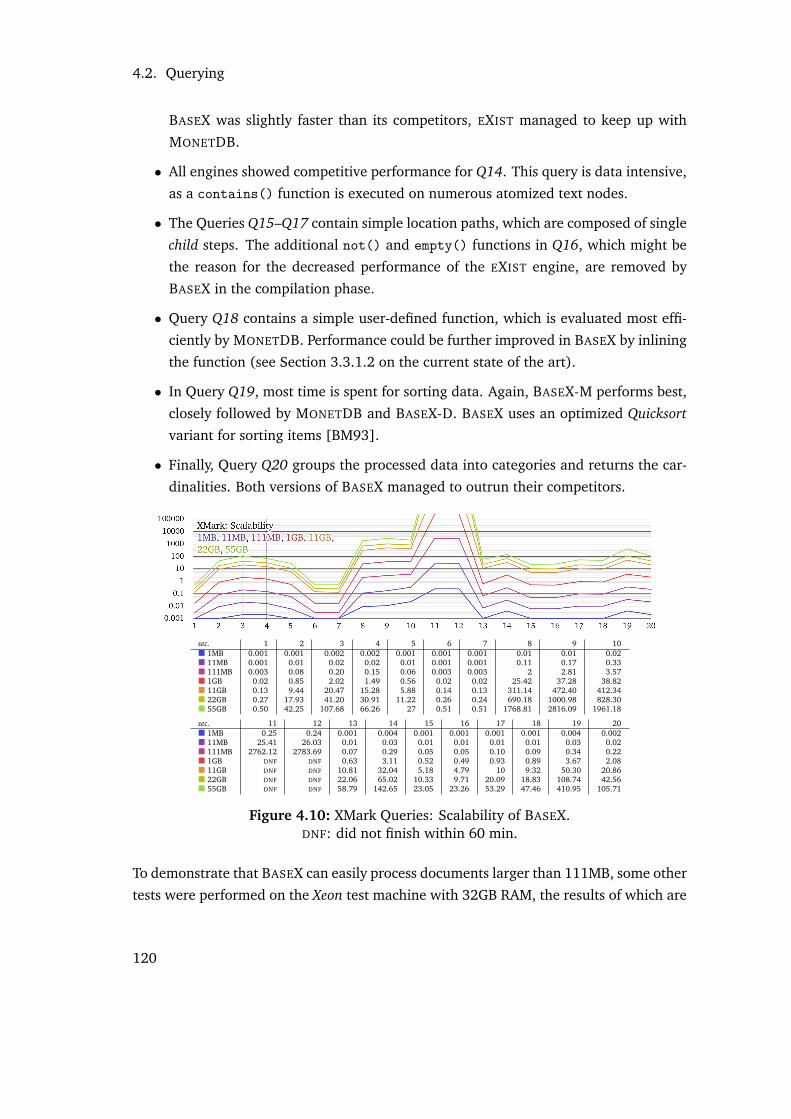
4.2. Querying
BASEX was slightly faster than its competitors, EXIST managed to keep up with
MONETDB.
• All engines showed competitive performance for Q14. This query is data intensive,
as a contains() function is executed on numerous atomized text nodes.
• The Queries Q15–Q17 contain simple location paths, which are composed of single
child steps. The additional not() and empty() functions in Q16, which might be
the reason for the decreased performance of the EXIST engine, are removed by
BASEX in the compilation phase.
• Query Q18 contains a simple user-defined function, which is evaluated most effi-
ciently by MONETDB. Performance could be further improved in BASEX by inlining
the function (see Section 3.3.1.2 on the current state of the art).
• In Query Q19, most time is spent for sorting data. Again, BASEX-M performs best,
closely followed by MONETDB and BASEX-D. BASEX uses an optimized Quicksortvariant for sorting items [BM93].
• Finally, Query Q20 groups the processed data into categories and returns the car-
dinalities. Both versions of BASEX managed to outrun their competitors.
sec. 1 2 3 4 5 6 7 8 9 10� 1MB 0.001 0.001 0.002 0.002 0.001 0.001 0.001 0.01 0.01 0.02� 11MB 0.001 0.01 0.02 0.02 0.01 0.001 0.001 0.11 0.17 0.33� 111MB 0.003 0.08 0.20 0.15 0.06 0.003 0.003 2 2.81 3.57� 1GB 0.02 0.85 2.02 1.49 0.56 0.02 0.02 25.42 37.28 38.82� 11GB 0.13 9.44 20.47 15.28 5.88 0.14 0.13 311.14 472.40 412.34� 22GB 0.27 17.93 41.20 30.91 11.22 0.26 0.24 690.18 1000.98 828.30� 55GB 0.50 42.25 107.68 66.26 27 0.51 0.51 1768.81 2816.09 1961.18
sec. 11 12 13 14 15 16 17 18 19 20� 1MB 0.25 0.24 0.001 0.004 0.001 0.001 0.001 0.001 0.004 0.002� 11MB 25.41 26.03 0.01 0.03 0.01 0.01 0.01 0.01 0.03 0.02� 111MB 2762.12 2783.69 0.07 0.29 0.05 0.05 0.10 0.09 0.34 0.22� 1GB DNF DNF 0.63 3.11 0.52 0.49 0.93 0.89 3.67 2.08� 11GB DNF DNF 10.81 32.04 5.18 4.79 10 9.32 50.30 20.86� 22GB DNF DNF 22.06 65.02 10.33 9.71 20.09 18.83 108.74 42.56� 55GB DNF DNF 58.79 142.65 23.05 23.26 53.29 47.46 410.95 105.71
Figure 4.10: XMark Queries: Scalability of BASEX.DNF: did not finish within 60 min.
To demonstrate that BASEX can easily process documents larger than 111MB, some other
tests were performed on the Xeon test machine with 32GB RAM, the results of which are
120

4.2. Querying
shown in Figure 4.10. The XMark queries were run on seven XMark instances, ranging
from 1MB to 55GB. The test conditions were slightly modified: The timeout was set to
60 minutes. The total runtime for testing a query was limited to 60 minutes as well, i.e.,
some queries were executed less than 15 times. Except for some queries on the 55GB
instances that generate some additional overhead, such as Q8, Q9, or Q19, the system
proved excellent scalability. Note that the good scalability is due to the large amount of
RAM. BASEX is the only Open Source database architecture known to us, however, that
allows it to perform XMark queries on instances larger than 11GB.
The query processor of BASEX has undergone several iterations before it has reached its
present performance. While many optimizations have been too diversified to be briefly
summarized, some of them have been presented in detail in Chapter 2 and 3, and will be
highlighted again by analyzing the performance of different versions of BASEX in Figure
4.11:
sec. 1 2 3 4 5 6 7 8 9 10� 4.0 .45 .56 .65 .33 .10 .61 1.33 DNF DNF DNF� 5.0 .04 .23 .35 .21 .10 .42 .002 DNF DNF DNF� 6.0 .001 .09 .20 .14 .06 .001 .002 DNF DNF DNF� 6.3 .001 .09 .20 .13 .06 .001 .001 2.63 3.66 3.59sec. 11 12 13 14 15 16 17 18 19 20� 4.0 DNF DNF .15 .97 .12 .11 .19 .56 8.87 .44� 5.0 DNF DNF .19 .97 .07 .06 .16 .25 .73 .31� 6.0 DNF DNF .07 .44 .05 .04 .09 .09 .35 .21� 6.3 DNF DNF .06 .40 .04 .04 .09 .09 .36 .22
Figure 4.11: XMark Queries: Version history of BASEX.DNF: did not finish within 5 min.
• The first optimizations were carried out on the storage backend: attributes (see
2.4.2.1) and numerical values (see 2.4.2.4) were inlined in the database table.
The changes were done before Version 4.0, which was the first to fully support
XQuery.
• Along with numerous other tweaks, iterative query evaluation was introduced with
Version 5.0. As the diagram indicates, the performance was increased from 50%
(Q15) up to 250% (Q2). The iterative traversal of location paths leads to a single
scanning of the database table; before, it was scanned multiple times for each axis
step. Next, the sort algorithm was improved to speed up the ORDER BY clause in
Q19, and the statistics of the name indexes were taken advantage of to speed up
the count() function of Q7.
• With Version 6.0, the index rewritings of location paths were generalized and ex-
tended to FLWOR expressions. As a result, Q1 is now evaluated via the attribute
index. Q6 was optimized by accessing statistics from the path summary and pre-
121

4.2. Querying
evaluating the count() function on arbitrary paths with child steps. A general
speedup for all location paths was achieved by reducing the number of temporary
objects and reusing existing node instances, as described in 3.4.2.3.
• Advanced rewritings of FLWOR expressions were realized in the latest version (see
Section 3.3.1.6). Q8-Q10 and numerous other queries are now rewritten to take
advantage of available content and full-text indexes.
sec. 1 2 3 4 5 6 7� ExpDB .001 .23 .08 .10 .06 .06 .24� 6.3 .001 .04 .12 .12 .04 .001 .001
sec. 8 9 10 11 12 13 14� ExpDB .69 1.03 7.90 .66 .33 .39 .66� 6.3 .27 .36 2.16 DNF DNF .06 .25
sec. 15 16 17 18 19 20� ExpDB .07 .07 .18 .11 .35 .25� 6.3 .04 .04 .08 .05 .26 .16
Figure 4.12: XMark Queries: Comparing BASEX 6.3 with results in [GHK+06].DNF: did not finish within 5 min.
This section is concluded with another review of a prototype of BASEX, which has been
compared with MONETDB in 2006 [GHK+06]. The XQuery expressions had been sim-
ulated with Java and XPath 1.0. At that time, we were confident that a future XQuery
implementation would yield comparable results. Figure 4.12 demonstrates that the as-
sumption was not only realistic, but was even exceeded. All tests were performed on
the AMD architecture, which was also used for the published results. For most queries,
the latest version of BASEX yields much better results than the former XPath implemen-
tation. Most time was saved for queries using the child step, as the original pre/parent
encoding was replaced by the pre/dist/size representation. Next, the switch to the iter-
ative processing model has been another important improvement, which is reflected by
nearly all queries.
4.2.2.3 XMark Queries
In the following, all 20 XMark queries have been reprinted2. We have added two Queries
Q0 and Q21, which have additionally been used for testing.
Q0 Open document and return non-existing child comment nodes.
2Source: http://www.ins.cwi.nl/projects/xmark/Assets/xmlquery.txt
122

4.2. Querying
doc("xmark.xml")/comment()
Q1 Return the name of the person with ID ‘person0’.let $auction := doc("xmark.xml") return
for $b in $auction/site/people/person[@id = "person0"]
return $b/name/text()
Q2 Return the initial increases of all open auctions.let $auction := doc("xmark.xml") return
for $b in $auction/site/open_auctions/open_auction
return <increase>{ $b/bidder[1]/increase/text() }</increase>
Q3 Return the IDs of all open auctions whose current increase is at least twice as high
as the initial increase.let $auction := doc("xmark.xml") return
for $b in $auction/site/open_auctions/open_auction
where zero-or-one($b/bidder[1]/increase/text()) * 2 <=
$b/bidder[last()]/increase/text()
return <increase first="{$b/bidder[1]/increase/text()}"
last="{$b/bidder[last()]/increase/text()}"/>
Q4 List the reserves of those open auctions where a certain person issued a bid before
another person.let $auction := doc("xmark.xml") return
for $b in $auction/site/open_auctions/open_auction
where some $pr1 in $b/bidder/personref[@person = "person20"],
$pr2 in $b/bidder/personref[@person = "person51"]
satisfies $pr1 << $pr2
return <history>{$b/reserve/text()}</history>
Q5 How many sold items cost more than 40?let $auction := doc("xmark.xml") return
count(for $i in $auction/site/closed_auctions/closed_auction
where $i/price/text() >= 40
return $i/price)
Q6 How many items are listed on all continents?let $auction := doc("xmark.xml") return
for $b in $auction//site/regions
return count($b//item)
Q7 How many pieces of prose are in our database?let $auction := doc("xmark.xml") return
for $p in $auction/site
return count($p//description) + count($p//annotation) + count($p//emailaddress)
Q8 List the names of persons and the number of items they bought.let $auction := doc("xmark.xml") return
for $p in $auction/site/people/person
123

4.2. Querying
let $a := for $t in $auction/site/closed_auctions/closed_auction
where $t/buyer/@person = $p/@id
return $t
return <item person="{ $p/name/text() }">{ count($a) }</item>
Q9 List the names of persons and the names of the items they bought in Europe.let $auction := doc("xmark.xml") return
let $ca := $auction/site/closed_auctions/closed_auction return
let $ei := $auction/site/regions/europe/item
for $p in $auction/site/people/person
let $a := for $t in $ca
where $p/@id = $t/buyer/@person
return let $n := for $t2 in $ei
where $t/itemref/@item = $t2/@id
return $t2
return <item>{ $n/name/text() }</item>
return <person name="{ $p/name/text() }">{ $a }</person>
Q10 List all persons according to their interest; use French markup in the result.let $auction := doc("xmark.xml") return
for $i in distinct-values($auction/site/people/person/profile/interest/@category)
let $p := for $t in $auction/site/people/person
where $t/profile/interest/@category = $i
return
<personne>
<statistiques>
<sexe>{$t/profile/gender/text()}</sexe>
<age>{$t/profile/age/text()}</age>
<education>{$t/profile/education/text()}</education>
<revenu>{fn:data($t/profile/@income)}</revenu>
</statistiques>
<coordonnees>
<nom>{$t/name/text()}</nom>
<rue>{$t/address/street/text()}</rue>
<ville>{$t/address/city/text()}</ville>
<pays>{$t/address/country/text()}</pays>
<reseau>
<courrier>{$t/emailaddress/text()}</courrier>
<pagePerso>{$t/homepage/text()}</pagePerso>
</reseau>
</coordonnees>
<cartePaiement>{$t/creditcard/text()}</cartePaiement>
</personne>
return <categorie>{ <id>{ $i }</id>, $p }</categorie>
Q11 For each person, list the number of items currently on sale whose price does not
exceed 0.02% of the person’s income.let $auction := doc("xmark.xml") return
for $p in $auction/site/people/person
let $l := for $i in $auction/site/open_auctions/open_auction/initial
where $p/profile/@income > 5000 * exactly-one($i/text())
return $i
124

4.2. Querying
return <items name="{ $p/name/text() }">{ count($l) }</items>
Q12 For each richer-than-average person, list the number of items currently on sale
whose price does not exceed 0.02% of the person’s income.let $auction := doc("xmark.xml") return
for $p in $auction/site/people/person
let $l := for $i in $auction/site/open_auctions/open_auction/initial
where $p/profile/@income > 5000 * exactly-one($i/text())
return $i
where $p/profile/@income > 50000
return <items person="{ $p/profile/@income }">{ count($l) }</items>
Q13 List the names of items registered in Australia along with their descriptions.let $auction := doc("xmark.xml") return
for $i in $auction/site/regions/australia/item
return <item name="{ $i/name/text() }">{ $i/description }</item>
Q14 Return the names of all items whose description contains the word ‘gold’.let $auction := doc("xmark.xml") return
for $i in $auction/site//item
where contains(string(exactly-one($i/description)), "gold")
return $i/name/text()
Q15 Print the keywords in emphasis in annotations of closed auctions.let $auction := doc("xmark.xml") return
for $a in $auction/site/closed_auctions/closed_auction/annotation/description/
parlist/listitem/parlist/listitem/text/emph/keyword/text()
return <text>{ $a }</text>
Q16 Return the IDs of those auctions that have one or more keywords in emphasis.let $auction := doc("xmark.xml") return
for $a in $auction/site/closed_auctions/closed_auction
where not(empty($a/annotation/description/parlist/listitem/parlist/listitem/text/
emph/keyword/text()))
return <person id="{ $a/seller/@person }"/>
Q17 Which persons don’t have a homepage?let $auction := doc("xmark.xml") return
for $p in $auction/site/people/person
where empty($p/homepage/text())
return <person name="{ $p/name/text() }"/>
Q18 Convert the currency of the reserve of all open auctions to another currency.declare namespace local = "http://www.foobar.org";
declare function local:convert($v as xs:decimal?) as xs:decimal? {
2.20371 * $v (: convert Dfl to Euro :)
};
let $auction := doc("xmark.xml") return
for $i in $auction/site/open_auctions/open_auction
return local:convert(zero-or-one($i/reserve))
125

4.2. Querying
Q19 Give an alphabetically ordered list of all items along with their location.let $auction := doc("xmark.xml") return
for $b in $auction/site/regions//item
let $k := $b/name/text()
order by zero-or-one($b/location) ascending empty greatest
return <item name="{ $k }">{ $b/location/text() }</item>
Q20 Group customers by their income and output the cardinality of each group.let $auction := doc("xmark.xml") return
<result>
<preferred>{
count($auction/site/people/person/profile[@income >= 100000])
}</preferred>
<standard>{
count($auction/site/people/person/
profile[@income < 100000 and @income >= 30000])
}</standard>
<challenge>{
count($auction/site/people/person/profile[@income < 30000])
}</challenge>
<na>{
count(for $p in $auction/site/people/person
where empty($p/profile/@income)
return $p)
}</na>
</result>
Q21 Return the category names of closed auctions in a certain price range.let $auction := doc("xmark.xml") return
for $a in $auction/descendant::closed_auction[price >= 500 and price <= 1000]
for $i in $auction/descendant::item
for $c in $auction/descendant::category
where $a/itemref/@item = $i/@id and $c/@id = $i/incategory/@category
return $c/name
4.2.3 XQuery Full Text
BASEX was the first query processor to support the XQuery Full Text Recommendation
(see 3.1.3), and, at the time of writing, it is still the only freely available implementation
that works on large XML instances. This section presents some performance results on a
complete XML dump of the English Wikipedia:
• Source: dumps.wikimedia.org/enwiki/latest/enwiki-latest-pages-articles.xml.bz2
• Accessed: 7 Jul 2010
• Document size: 25.4 GB
• XML nodes: 198.5 million
• Total database size: 45.4 GB (Full-text index: 20.0 GB)
126

4.2. Querying
sec. Q1 Q2 Q3 Q4 Q5 Q6 Q7� xquery .001 .001 .004 .004 .001 .001 .004� querying .004 .004 .02 .01 .001 .001 .02� queries .03 .03 .12 .12 .002 .002 .02� query .27 .27 1.56 1.38 .02 .02 .05� text 1.43 1.43 8.16 7.47 .29 .29 .31� name 6.04 6.04 49.8 47.6 1.87 1.87 1.94
Bytes Q1/2 Q3/4 Q5 Q6 Q7� xquery 571 19 K 165 1 K 19 K� querying 309 94 K 161 1 K 94 K� queries 3 K 699 K 161 1 K 136 K� query 20 K 8 M 161 1 K 94 K� text 235 K 51 M 163 1 K 131 K� name 1 M 329 M 163 1 K 129 K
ID Queryprolog declare default element namespace "http://www.mediawiki.org/xml/export-0.4/";
declare variable $term := ".....";
Q1 doc(’wiki’)//title[text() contains text { $term }]
Q2 let $doc := doc(’wiki’)
for $title in $doc//title
where $title/text() contains text { $term }
return $title
Q3 doc(’wiki’)//page[.//text contains text { $term }]/title
Q4 doc(’wiki’)//page[revision/text contains text { $term }]/title
Q5 (doc(’wiki’)//page[revision/text contains text { $term }]/title)[1]
Q6 (doc(’wiki’)//page[revision/text contains text { $term }]/title)[position() <= 10]
Q7 (doc(’wiki’)//page[revision/text contains text { $term }]/title)[position() <= 1000]
Figure 4.13: English Wikipedia: Processing times andresult sizes of seven full-text queries and six search terms
• Applied full-text index: Fuzzy Index
• Distinct full-text tokens: 42.9 million
• Index options: case/diacritics insensitive, no stemming/stopwords, default scoring
The client-/server-architecture of BASEX was used for all tests. The query results were
written to a temporary file, and the mean of the total processing time of 5 runs, as
returned by the following command call, was adopted for the figures:
java -cp basex-6.3.jar org.basex.BaseXClient -r5 -otmp -v query.xq
Figure 4.13 summarizes the results of the first test run, which demonstrates the scala-
bility of the XQuery Full Text implementation. Each query is introduced with the prolog,
shown in the table. Six different search terms were assigned to the $term variable, which
served as input for the full-text expression of the queries Q1-Q7 (totaling in 42 different
queries):
• Q1 and Q2 return all titles that contain the specified search term. Both queries
return the same results, as they are compiled and rewritten to the same internal,
127

4.2. Querying
index-based query plan. The FLWOR rewriting takes fractions of milliseconds;
hence, it is not reflected in the result times.
• In Q3 and Q4, the same text nodes are addressed by the full-text expression. Both
queries return the titles of all pages that contain the specified term in the full-text.
Due to the descendant step in the predicate, Q3 is supposed to take slightly longer
than Q4.
• Q5-Q7 return the first 1, 10, and 1000 results of Q4.
The search terms were selected by their number of occurrences: the term xquery occurs
in only 144 distinct text nodes, whereas the term name is placed 34th on the list of
most frequent terms in the Wikipedia corpus, occurring in 2,65 million nodes and 10,54
million times in total3. This means that there are appr. 18,400 times more text nodes
containing name than xquery. This difference is clearly reflected in the query results:
while all queries for the term xquery are processed in less than 5 milliseconds, including
the time for compiling the query and serializing the result, the output of 2,4 million
titles, the articles of which contain the term name, takes about 50 seconds and produces
329 MiB of data. As can be seen in Q5-Q7, much time can be saved by limiting the
number of results: the proportional difference for returning 1 or 1000 results is less
than 10% of the the total processing time for queries with large result sets.
ID sec. MB Queryprolog — — declare default element namespace
"http://www.mediawiki.org/xml/export-0.4/";
� Q1 .022 131 K //page[.//text contains text "Bu~nuel" ftor "Tanguy"]/title
� Q2 .010 19 K //page[.//text contains text "Yves" ftand "Tanguy"]/title
� Q3 .010 12 K //page[.//text contains text ("Yves" ftand "Tanguy")
distance at most 3 words]/title
� Q4 .084 14 K //page[.//text contains text ("Yves" ftand "Tanguy") same sentence]/title
� Q5 .006 12 K //page[.//text contains text "Yves Tanguy"]/title
� Q6 .009 4 K for $page score $s in //page[.//text contains text "Yves Tanguy"]
let $title := $page/title/text()
let $score := round($s * 100)
order by $s descending
return <hit xmlns="" s="{ $score }%">{ $title }</hit> }
� Q7 5.16 10 K //page[.//text contains text "ives tangui" using fuzzy]/title
Figure 4.14: English Wikipedia: Processing times andresult sizes of seven advanced full-text queries
3The BASEX command INFO INDEX FULLTEXT returns statistics on the full-text index structure.
128

4.2. Querying
Figure 4.14 shows the timings and result sizes of some more advanced XQuery Full Text
expressions:
• Q1 and Q2 demonstrate the logical connectives ftand and ftor, which combine the
results of two search tokens.
• Q3 and Q4 specify positional filters, namely a distance and a scope selection, to
further restrict the results returned by the ftand operator.
• Q5 performs a phrase search, which is comparable to a full-text query using ftand,
a distance and an ordered selection.
• Q6 calculates the score values of a location path with a full-text expression and
a phrase as search token. All scores are sorted in a descending manner and em-
bedded in new element fragments, along with the title elements of the original
document.
• Q7 demonstrates the BASEX specific fuzzy match option, which finds results that
are equal or similar to the specified tokens.
As the performance results indicate, all expressions were rewritten to access the full-text
index, and were evaluated in an iterative manner. Except for Q4 and Q7, all queries are
evaluated and serialized in a few milliseconds. For Query Q4, additional time is needed
for computing the sentence positions of all tokens, as this information is not stored in
the full-text index. The fuzzy option in Q7 leads to a large number of intermediate
results for the two single search terms, which are eventually combined to a small result
set. – Last but not least, the first 12 results of Q6 are printed in Table 4.4 and, for fun,
compared with the results of a Google query to indicate that the default scoring yields
good results:
BASEX, Q6 (first 12 of 90 results) site:en.wikipedia.org "Yves Tanguy"
<hit s="38%">Yves Tanguy</hit>
<hit s="35%">File:Reply to Red.jpg</hit>
<hit s="35%">File:Multiplication of the Arcs.jpg</hit>
<hit s="35%">File:Promontory Palace.jpg</hit>
<hit s="34%">File:Mama, Papa is Wounded!.jpg</hit>
<hit s="33%">File:Indefinite Divisibility.jpg</hit>
<hit s="30%">Kay Sage</hit>
<hit s="28%">Portal:Visual arts/Selected picture</hit>
<hit s="26%">Tanguay</hit>
<hit s="25%">Musick to Play in the Dark Vol. 1</hit>
<hit s="24%">Biomorph</hit>
<hit s="24%">Surrealism</hit>
1. Yves Tanguy
2. File:Indefinite Divisibility.jpg
3. Tanguy4. Kay Sage
5. File:Multiplication of the Arcs.jpg
6. Surrealism7. Bodley Gallery
8. Andre Breton
9. File:Reply to Red.jpg
10. Tanguy (film)
11. File:Promontory Palace.jpg
12. Yves (given name)
Table 4.4: Wikipedia: Ranking results of Query Q6, compared with a Google query
129

4.3. Statistics
4.3 Statistics
While many developers of scientific XML database prototypes and vendors of commercial
systems claim that they can “large” or “huge” XML documents, it is difficult to find
information on the factual limits of the presented architectures. It can be observed,
instead, that most publications on XML processing limit performance tests to documents
or collections of less than a Gigabyte, down to some Megabytes.
For this section, we first assembled the largest XML documents and collections that we
could locate online and offline. While many of the documents are freely available, some
of them have only been made available for testing purposes. Next, we approached the
theoretical limits of our storage architecture, which have been elaborated in Section
2.4.1. We hope that the resulting survey, shown in Table 4.5, might be helpful for other
XML developers as well. It offers the following information, specified in columns:
• file size represents the size of the original XML sources,
• db size is the size of the resulting database, excluding optional index structures,
• #nodes lists the number of unique XML nodes of a document,
• #atr reflects the maximum number of attribute nodes of a single element node,
• #eln and #atn represent the number of unique tag and attribute names,
• #uri indicates the number of distinct namespace URIs,
• height shows the tree height, and
• #docs contains the number of documents stored in the database.
The largest document we could get our hands – which was too large to be processed
by BASEX – was the complete, zipped dump of the Wikipedia Encyclopedia4, occupying
more than 3 TiB in a single file. References to all documents and collections (or the
homepages of its suppliers) that have been used for creating the survey are listed in
Table 4.6.
4XML dump of the Wikipedia, containing all pages with complete edit history:http://download.wikimedia.org/enwiki/latest/pages-meta-history.xml.7z
130

4.3. Statistics
INSTANCES file size db size #nodes #atr #eln #atn #uri height #docsRUWIKIHIST 421 GiB 416 GiB 324,848,508 3 21 6 2 6 1ZHWIKIHIST 126 GiB 120 GiB 179,199,662 3 21 6 2 6 1ENWIKTIONARY 79 GiB 75 GiB 134,380,393 3 21 6 2 6 1XMARK 55 GiB 64 GiB 1,615,071,348 2 74 9 0 13 1ENWIKIMETA 54 GiB 52 GiB 401,456,348 3 21 6 2 6 1MEDLINE 38 GiB 36 GiB 1,623,764,254 2 84 6 0 9 379IPROCLASS 36 GiB 37 GiB 1,631,218,984 3 245 4 2 9 1INEX209 31 GiB 34 GiB 1,336,110,639 15 28,034 451 1 37 2,666,500COPHIR 29 GiB 31 GiB 1,104,623,376 10 42 42 0 8 10,000,000ENWIKIPEDIA 26 GiB 25 GiB 198,546,747 3 24 21 2 6 1XMARK 22 GiB 26 GiB 645,997,965 2 74 9 0 13 1INTERPRO 14 GiB 19 GiB 860,304,235 5 7 15 0 4 1GENOME1 13 GiB 13 GiB 432,628,105 12 26 101 2 6 1NEWYORKTIMES 12 GiB 13 GiB 280,407,005 5 41 33 0 6 1,855,659TREMBL 11 GiB 14 GiB 589,650,535 8 47 30 2 7 1XMARK 11 GiB 13 GiB 323,083,409 2 74 9 0 13 1INTACT 7973 MiB 6717 MiB 297,478,392 7 64 22 2 14 25,624FREEBASE 7366 MiB 10 GiB 443,627,994 8 61 283 1 93 1SDMX 6356 MiB 8028 MiB 395,871,872 2 22 6 3 7 1OPENSTREETMAP 5312 MiB 5171 MiB 6,910,669 3 19 5 2 6 1SWISSPROT 4604 MiB 5422 MiB 241,274,406 8 70 39 2 7 1EURLEX 4815 MiB 5532 MiB 167,328,039 23 186 46 1 12 1WIKICORPUS 4492 MiB 4432 MiB 157,948,561 12 1,257 2,687 2 50 659,338ENWIKIRDF 3679 MiB 3537 MiB 98,433,194 1 11 2 11 4 1COPHIR 2695 MiB 2882 MiB 101,638,857 10 42 42 0 8 1,000,000MESH 2091 MiB 2410 MiB 104,845,819 3 6 5 2 5 1FREEDB 1723 MiB 2462 MiB 102,901,519 2 7 3 0 4 1XMARK 1134 MiB 1303 MiB 32,298,989 2 74 9 0 13 1DEEPFS 810 MiB 850 MiB 44,821,506 4 3 6 0 24 1LIBRARYUKN 760 MiB 918 MiB 46,401,941 3 23 3 0 5 1TWITTER 736 MiB 767 MiB 15,309,015 0 8 0 0 3 1,177,495ORGANIZATIONS 733 MiB 724 MiB 33,112,392 3 38 9 0 7 1,019,132DBLP 694 MiB 944 MiB 36,878,181 4 35 6 0 7 1FEEDS 692 MiB 604 MiB 5,933,713 0 8 0 0 3 444,014MEDLINESUPP 477 MiB 407 MiB 21,602,141 5 55 7 0 9 1AIRBASE 449 MiB 273 MiB 14,512,851 1 111 5 0 11 38MEDLINEDESC 260 MiB 195 MiB 10,401,847 5 66 8 0 9 1ZDNET 130 MiB 133 MiB 3,060,186 21 40 90 0 13 95,663JMNEDICT 124 MiB 171 MiB 8,592,666 0 10 0 0 5 1XMARK 111 MiB 130 MiB 3,221,926 2 74 9 0 13 1FRESHMEAT 105 MiB 86 MiB 3,832,028 1 58 1 0 6 1DEEPFS 83 MiB 93 MiB 4,842,638 4 3 6 0 21 1TREEBANK 82 MiB 92 MiB 3,829,513 1 250 1 0 37 1DBLP2 80 MiB 102 MiB 4,044,649 4 35 6 0 6 170,843DDI 76 MiB 39 MiB 2,070,157 7 104 16 21 11 3ALFRED 75 MiB 68 MiB 3,784,285 0 60 0 0 6 1UNIVERSITY 56 MiB 66 MiB 3,468,606 1 28 4 0 5 6MEDIAUKN 38 MiB 45 MiB 1,619,443 3 21 3 0 5 1HCIBIB2 32 MiB 33 MiB 617,023 1 39 1 0 4 26,390NASA 24 MiB 25 MiB 845,805 2 61 8 1 9 1MOVIEDB 16 MiB 19 MiB 868,980 6 7 8 0 4 1KANJIDIC2 13 MiB 18 MiB 917,833 3 27 10 0 6 1XMARK 11 MiB 13 MiB 324,274 2 74 9 0 13 1SHAKESPEARE 7711 KiB 9854 KiB 327,170 0 59 0 0 9 1TREEOFLIFE 5425 KiB 7106 KiB 363,560 7 4 7 0 243 1THESAURUS 4288 KiB 4088 KiB 201,798 7 33 9 0 7 1MUSICXML 3155 KiB 2942 KiB 171,400 8 179 56 0 8 17BIBDBPUB 2292 KiB 2359 KiB 80,178 1 54 1 0 4 3,465FACTBOOK 1743 KiB 1560 KiB 77,315 16 23 32 0 6 1XMARK 1134 KiB 1334 KiB 33,056 2 74 9 0 13 1
Table 4.5: Statistics on selected XML documents and collections
131
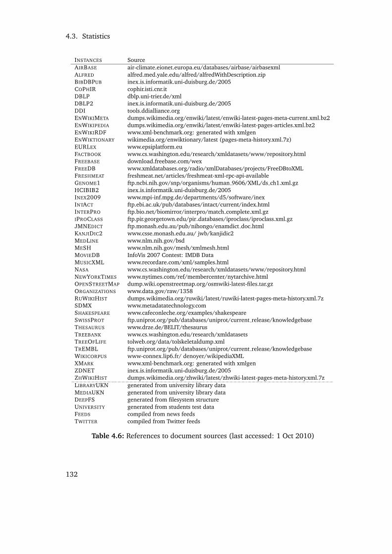
4.3. Statistics
INSTANCES SourceAIRBASE air-climate.eionet.europa.eu/databases/airbase/airbasexmlALFRED alfred.med.yale.edu/alfred/alfredWithDescription.zipBIBDBPUB inex.is.informatik.uni-duisburg.de/2005COPHIR cophir.isti.cnr.itDBLP dblp.uni-trier.de/xmlDBLP2 inex.is.informatik.uni-duisburg.de/2005DDI tools.ddialliance.orgENWIKIMETA dumps.wikimedia.org/enwiki/latest/enwiki-latest-pages-meta-current.xml.bz2ENWIKIPEDIA dumps.wikimedia.org/enwiki/latest/enwiki-latest-pages-articles.xml.bz2ENWIKIRDF www.xml-benchmark.org: generated with xmlgenENWIKTIONARY wikimedia.org/enwiktionary/latest (pages-meta-history.xml.7z)EURLEX www.epsiplatform.euFACTBOOK www.cs.washington.edu/research/xmldatasets/www/repository.htmlFREEBASE download.freebase.com/wexFREEDB www.xmldatabases.org/radio/xmlDatabases/projects/FreeDBtoXMLFRESHMEAT freshmeat.net/articles/freshmeat-xml-rpc-api-availableGENOME1 ftp.ncbi.nih.gov/snp/organisms/human 9606/XML/ds ch1.xml.gzHCIBIB2 inex.is.informatik.uni-duisburg.de/2005INEX2009 www.mpi-inf.mpg.de/departments/d5/software/inexINTACT ftp.ebi.ac.uk/pub/databases/intact/current/index.htmlINTERPRO ftp.bio.net/biomirror/interpro/match complete.xml.gzIPROCLASS ftp.pir.georgetown.edu/pir databases/iproclass/iproclass.xml.gzJMNEDICT ftp.monash.edu.au/pub/nihongo/enamdict doc.htmlKANJIDIC2 www.csse.monash.edu.au/ jwb/kanjidic2MEDLINE www.nlm.nih.gov/bsdMESH www.nlm.nih.gov/mesh/xmlmesh.htmlMOVIEDB InfoVis 2007 Contest: IMDB DataMUSICXML www.recordare.com/xml/samples.htmlNASA www.cs.washington.edu/research/xmldatasets/www/repository.htmlNEWYORKTIMES www.nytimes.com/ref/membercenter/nytarchive.htmlOPENSTREETMAP dump.wiki.openstreetmap.org/osmwiki-latest-files.tar.gzORGANIZATIONS www.data.gov/raw/1358RUWIKIHIST dumps.wikimedia.org/ruwiki/latest/ruwiki-latest-pages-meta-history.xml.7zSDMX www.metadatatechnology.comSHAKESPEARE www.cafeconleche.org/examples/shakespeareSWISSPROT ftp.uniprot.org/pub/databases/uniprot/current release/knowledgebaseTHESAURUS www.drze.de/BELIT/thesaurusTREEBANK www.cs.washington.edu/research/xmldatasetsTREEOFLIFE tolweb.org/data/tolskeletaldump.xmlTREMBL ftp.uniprot.org/pub/databases/uniprot/current release/knowledgebaseWIKICORPUS www-connex.lip6.fr/ denoyer/wikipediaXMLXMARK www.xml-benchmark.org: generated with xmlgenZDNET inex.is.informatik.uni-duisburg.de/2005ZHWIKIHIST dumps.wikimedia.org/zhwiki/latest/zhwiki-latest-pages-meta-history.xml.7zLIBRARYUKN generated from university library dataMEDIAUKN generated from university library dataDEEPFS generated from filesystem structureUNIVERSITY generated from students test dataFEEDS compiled from news feedsTWITTER compiled from Twitter feeds
Table 4.6: References to document sources (last accessed: 1 Oct 2010)
132

5 Conclusion
XML is here to stay – and so are techniques for storing and querying XML. In this thesis,
we hope to have shown that a database architecture needs to rely on both theoretical and
practical aspects to cover the demands of real-life applications and workloads. While this
may sound hackneyed, we have frequently come across counter examples, which either
focused on theoretical, albeit artificial scenarios, or which lacked a solid theoretical
background to be extensible enough for advanced use cases.
As a final conclusion, we have summarized the major contributions of this thesis:
• Section 2.4: We have presented Pre/Dist/Size as a powerful encoding for mapping
XML data to flat tables: the size property facilitates quick access to descendants
and following siblings of an XML node, and the dist property serves as direct,
update-invariant parent reference.
• Section 2.4.1.2: Using our architecture, we have collected statistical data of a
wide range of large-scale, real-life XML documents and collections. While the re-
sulting information was primarily evaluated to find a good tradeoff between a
minimum database size and maximum input document size, we also believe it rep-
resents one of the most comprehensive surveys on large XML instances that has
been published so far.
• Section 2.4.2: The proposed encoding is represented in a single compactified,
fixed-size tuple of 16 bytes. Static and redundant information were dropped, and
numerical document contents were inlined in the tuple. Next, attribute nodes were
inlined as well, i.e., stored in the same way as other XML nodes. This way, both
memory is saved and queries are accelerated.
• Section 2.6: In contrast to other data structures, our storage can be easily ex-
tended by various structural and content-based index structures, which provide a
base for accelerating many queries by orders of magnitudes.
• Section 3.3.1: In the Querying chapter, a thorough insight is given how classical
and XML-specific optimizations can be applied to arbitrary XQuery processors.
133

• Section 3.3.2: We were the first, to the best of our knowledge, to describe how lo-
cation paths with equality tests or full-text expressions as predicates can be rewrit-
ten for accessing index structures of an underlying database. This optimization,
which is comparatively straightforward in relational databases, requires that many
preconditions are met in the context of XPath/XQuery.
• Section 3.4.1: We have shown how an adaptive evaluation approach can be real-
ized to benefit from both the iterative and atomic processing paradigm.
• Section 3.4.2: Based on our Pre/Dist/Size encoding, the traversal of location paths
and all XPath axes was illustrated.
• Section 3.5: A detailed summary describes what optimizations exist for the most
important XQuery expressions. We hope that other implementors of XQuery might
benefit from this summary, too.
• Finally, Chapter 4 demonstrates that the chosen architecture yields excellent per-
formance results, both regarding efficiency and scalability.
In short, we believe that the proposed storage and query architecture represents a pow-
erful yet light-weight framework for both processing very large XML instances and eval-
uating queries with impressive performance. The Open Source database system BASEX
represents an elaborate proof of concept for the ideas discussed in this work.
134

Bibliography
Bibliography
[ABC+99] Vidur Apparao, Steve Byrne, Mike Champion, Scott Isaacs, Ian Jacobs, Ar-
naud Le Hors, Gavin Nicol, Jonathan Robie, Robert Sutor, Chris Wilson, and
Lauren Wood. Document Object Model Level 1. http://www.w3.org/DOM,
October 1999.
[ABF+09] Cezar Andrei, Matthias Brantner, Daniela Florescu, David Graf, Don-
ald Kossmann, and Markos Zacharioudakis. Extending XQuery with
Collections, Indexes, and Integrity Constraints, Working Draft, 2009.
http://www.flworfound.org/pubs/xqddf.pdf, 2009.
[Abi97] Serge Abiteboul. Querying Semi-Structured Data. In ICDT, volume 1186 of
Lecture Notes in Computer Science, pages 1–18. Springer, 1997.
[AMS92] Jun-Ichi Aoe, Katsushi Morimoto, and Takashi Sato. An Efficient Implemen-
tation of Trie Structures. Softw., Pract. Exper., 22(9):695–721, 1992.
[AOV+99] Malcolm P. Atkinson, Maria E. Orlowska, Patrick Valduriez, Stanley B.
Zdonik, and Michael L. Brodie, editors. VLDB’99, Proceedings of 25th In-ternational Conference on Very Large Data Bases, September 7-10, 1999, Ed-inburgh, Scotland, UK. Morgan Kaufmann, 1999.
[AQM+97] Serge Abiteboul, Dallan Quass, Jason McHugh, Jennifer Widom, and
Janet L. Wiener. The Lorel Query Language for Semistructured Data. Int. J.on Digital Libraries, 1(1):68–88, 1997.
[AS08] Ramez Alkhatib and Marc H. Scholl. CXQU: A compact XML storage for
efficient query and update processing. In ICDIM, pages 605–612. IEEE,
2008.
[AS09] Ramez Alkhatib and Marc H. Scholl. Compacting XML Structures Using
a Dynamic Labeling Scheme. In BNCOD, volume 5588 of Lecture Notes inComputer Science, pages 158–170. Springer, 2009.
135

Bibliography
[AYBB+09] Sihem Amer-Yahia, Chavdar Botev, Stephen Buxton, Pat Case, Jochen Do-
erre, et al. XQuery and XPath Full Text 1.0. W3C Candidate Recommenda-
tion. http://www.w3.org/TR/xpath-full-text-10, July 2009.
[BBB00] Ron Bourret, Christof Bornhovd, and Alejandro P. Buchmann. A Generic
Load/Extract Utility for Data Transfer between XML Documents and Rela-
tional Databases. In WECWIS, pages 134–143, 2000.
[BCF+07] Scott Boag, Don Chamberlin, Mary F. Fernandez, Daniela Florescu,
Jonathan Robie, and Jerome Simeon. XQuery 1.0: An XML Query Lan-
guage. W3C Recommendation. http://www.w3.org/TR/xquery, January
2007.
[BGvK+05] Peter A. Boncz, Torsten Grust, Maurice van Keulen, Stefan Manegold, Jan
Rittinger, and Jens Teubner. Pathfinder: XQuery - The Relational Way. In
VLDB, pages 1322–1325. ACM, 2005.
[Bib99] Die Deutsche Bibliothek. MAB2: Maschinelles Austauschformat fur Biblio-theken. Die Deutsche Bibliothek, Leipzig/Frankfurt am Main, second edi-
tion, 1999.
[BIRP02] Philip A. Bernstein, Yannis E. Ioannidis, Raghu Ramakrishnan, and Dimitris
Papadias, editors. VLDB 2002, Proceedings of 28th International Conferenceon Very Large Data Bases, August 20-23, 2002, Hong Kong, China. Morgan
Kaufmann, 2002.
[BK89] Elisa Bertino and Won Kim. Indexing Techniques for Queries on Nested
Objects. IEEE Trans. Knowl. Data Eng., 1(2):196–214, 1989.
[BKT+07] Scott Boag, Michael Kay, Joanne Tong, Norman Walsh, and Henry Zon-
garo. XSLT 2.0 and XQuery 1.0 Serialization. http://www.w3.org/TR/xslt-
xquery-serialization, January 2007.
[BM72] Rudolf Bayer and Edward M. McCreight. Organization and Maintenance of
Large Ordered Indices. Acta Inf., 1:173–189, 1972.
[BM93] Jon Louis Bentley and M. Douglas McIlroy. Engineering a Sort Function.
Softw., Pract. Exper., 23(11):1249–1265, 1993.
[BMR05] Peter A. Boncz, Stefan Manegold, and Jan Rittinger. Updating the Pre/Post
Plane in MonetDB/XQuery. In XIME-P, 2005.
136

Bibliography
[Boa05] Scott Boag. Building a Tokenizer for XPath or XQuery. http://www.w3.org/
TR/xquery-xpath-parsing, April 2005.
[Bot04] Per Bothner. Compiling XQuery to Java Bytecodes. In XIME-P, pages 31–36,
2004.
[BPSM+08] Tim Bray, Jean Paoli, C. M. Sperberg-McQueen, Eve Maler, et al. Extensible
Markup Language (XML) 1.0 (Fifth Edition). http://www.w3.org/TR/xml,
November 2008.
[BSAY04] Chavdar Botev, Jayavel Shanmugasundaram, and Sihem Amer-Yahia. A
TeXQuery-Based XML Full-Text Search Engine. In Weikum et al. [WKD04],
pages 943–944.
[Bun97] Peter Buneman. Semistructured Data. In PODS, pages 117–121. ACM Press,
1997.
[CB74] Donald D. Chamberlin and Raymond F. Boyce. SEQUEL: A Structured En-
glish Query Language. In SIGMOD Workshop, Vol. 1, pages 249–264. ACM,
1974.
[CD99] James Clark and Steven J. DeRose. XML Path Language (XPath) Version 1.0.
W3C Recommendation. http://www.w3.org/TR/xpath, November 1999.
[CD07] James Clark and Steven J. DeRose. XML Path Language (XPath) Version 2.0.
W3C Recommendation. http://www.w3.org/TR/xpath20, January 2007.
[CDF+09] Don Chamberlin, Michael Dyck, Daniela Florescu, Jim Melton,
Jonathan Robie, and Jerome Simeon. XQuery Update Facility.
http://www.w3.org/TR/xqupdate, June 2009.
[CEF+08] Don Chamberlin, Daniel Engovatov, Dana Florescu, Giorgio Ghelli, Jim
Melton, Jerome Simeon, and John Snelson. XQuery Scripting Extension
1.0. http://www.w3.org/TR/xquery-sx-10, April 2008.
[CKM02] Edith Cohen, Haim Kaplan, and Tova Milo. Labeling Dynamic XML Trees.
In PODS, pages 271–281. ACM, 2002.
[Cla99] James Clark. XSL Transformations (XSLT) Version 1.0. http://www.w3.org/
TR/xslt, November 1999.
137

Bibliography
[CMS02] Chin-Wan Chung, Jun-Ki Min, and Kyuseok Shim. APEX: an adaptive path
index for XML data. In Franklin et al. [FMA02], pages 121–132.
[CMV05] Barbara Catania, Anna Maddalena, and Athena Vakali. XML Document In-
dexes: A Classification. IEEE Internet Computing, 9(5):64–71, 2005.
[Cow08] John Cowan. TagSoup. http://ccil.org/˜cowan/XML/tagsoup, 2008.
[CRF00] Donald D. Chamberlin, Jonathan Robie, and Daniela Florescu. Quilt: An
XML Query Language for Heterogeneous Data Sources. In WebDB (SelectedPapers), volume 1997 of Lecture Notes in Computer Science, pages 1–25.
Springer, 2000.
[Cro06] Douglas Crockford. JSON: The Fat-Free Alternative to XML. In XML, 2006.
[Dam64] Fred Damerau. A technique for computer detection and correction of
spelling errors. Commun. ACM, 7(3):171–176, 1964.
[DFF+98] Alin Deutsch, Mary F. Fernandez, Daniela Florescu, Alon Y. Levy, and Dan
Suciu. XML-QL. In QL, 1998.
[DFF+99] Alin Deutsch, Mary F. Fernandez, Daniela Florescu, Alon Y. Levy, and Dan
Suciu. A Query Language for XML. Computer Networks, 31(11-16):1155–
1169, 1999.
[DFF+07] Denise Draper, Peter Fankhauser, Mary F. Fernandez, Ashok Malhotra,
Kristoffer Rose, Michael Rys, Jerome Simeon, and Philip Wadler. XQuery
1.0 and XPath 2.0 Formal Semantics. http://www.w3.org/TR/xquery-
semantics, January 2007.
[DFS99] Alin Deutsch, Mary F. Fernandez, and Dan Suciu. Storing Semistructured
Data with STORED. In SIGMOD Conference, pages 431–442. ACM Press,
1999.
[Die82] Paul F. Dietz. Maintaining Order in a Linked List. In STOC, pages 122–127.
ACM, 1982.
[ECM06] ECMA. ECMA-376: Office Open XML File Formats. ECMA (European Associ-
ation for Standardizing Information and Communication Systems), 2006.
[EH00] Richard Edwards and Sian Hope. Persistent DOM: An Architecture for XML
Repositories in Relational Databases. In IDEAL, volume 1983 of LectureNotes in Computer Science, pages 416–421. Springer, 2000.
138
Bibliography
[FG89] Johann Christoph Freytag and Nathan Goodman. On the Translation of
Relational Queries into Iterative Programs. ACM Trans. Database Syst.,14(1):1–27, 1989.
[FHK+02] Thorsten Fiebig, Sven Helmer, Carl-Christian Kanne, Guido Moerkotte, Julia
Neumann, Robert Schiele, and Till Westmann. Anatomy of a native XML
base management system. VLDB J., 11(4):292–314, 2002.
[FHK+03] Daniela Florescu, Chris Hillery, Donald Kossmann, Paul Lucas, Fabio Ric-
cardi, Till Westmann, Michael J. Carey, Arvind Sundararajan, and Geetika
Agrawal. The BEA/XQRL Streaming XQuery Processor. In Freytag et al.
[FLA+03], pages 997–1008.
[FHK+04] Daniela Florescu, Chris Hillery, Donald Kossmann, Paul Lucas, Fabio Ric-
cardi, Till Westmann, Michael J. Carey, and Arvind Sundararajan. The BEA
streaming XQuery processor. VLDB J., 13(3):294–315, 2004.
[FK99] Daniela Florescu and Donald Kossmann. Storing and Querying XML Data
using an RDMBS. IEEE Data Eng. Bull., 22(3):27–34, 1999.
[FLA+03] Johann Christoph Freytag, Peter C. Lockemann, Serge Abiteboul, Michael J.
Carey, Patricia G. Selinger, and Andreas Heuer, editors. VLDB 2003, Proceed-ings of 29th International Conference on Very Large Data Bases, September9-12, 2003, Berlin, Germany. Morgan Kaufmann, 2003.
[FMA02] Michael J. Franklin, Bongki Moon, and Anastassia Ailamaki, editors. Pro-ceedings of the 2002 ACM SIGMOD International Conference on Managementof Data, Madison, Wisconsin, June 3-6, 2002. ACM, 2002.
[FMM+07] Mary Fernandez, Ashok Malhotra, Jonathan Marsh, Marton Nagy,
and Norman Walsh. XQuery 1.0 and XPath 2.0 Data Model.
http://www.w3.org/TR/xpath-datamodel, January 2007.
[Fre60] Edward Fredkin. Trie Memory. j-CACM, 3(9):490–499, 1960.
[FRSV05] Achille Fokoue, Kristoffer Høgsbro Rose, Jerome Simeon, and Lionel Villard.
Compiling XSLT 2.0 into XQuery 1.0. In WWW, pages 682–691. ACM, 2005.
[Gat09] Sebastian Gath. Verarbeitung und Visualisierung von XML-Full-Text Daten.
Master’s thesis, University of Konstanz, Germany, May 2009.
139
Bibliography
[GC07] Gang Gou and Rada Chirkova. Efficiently Querying Large XML Data Repos-
itories: A Survey. IEEE Trans. Knowl. Data Eng., 19(10):1381–1403, 2007.
[GCCM98] Roy Goldman, Sudarshan Chawathe, Arturo Crespo, and Jason McHugh.
A Standard Textual Interchange Format for the Object Exchange Model
(OEM). Technical Report CS-TN-98-64, Stanford University, Stanford, CA,
1998.
[GGHS09a] Christian Grun, Sebastian Gath, Alexander Holupirek, and Marc H. Scholl.
INEX Efficiency Track meets XQuery Full Text in BaseX. In Pre-Proceedingsof the 8th INEX Workshop, pages 192–197, 2009.
[GGHS09b] Christian Grun, Sebastian Gath, Alexander Holupirek, and Marc H. Scholl.
XQuery Full Text Implementation in BaseX. In XSym, volume 5679 of Lec-ture Notes in Computer Science, pages 114–128. Springer, 2009.
[GGJ+05] Christian Grun, Jens Gerken, Hans-Christian Jetter, Werner A. Konig, and
Harald Reiterer. MedioVis – A User-Centred Library Metadata Browser. In
ECDL, volume 3652 of Lecture Notes in Computer Science, pages 174–185.
Springer, 2005.
[GHK+06] Christian Grun, Alexander Holupirek, Marc Kramis, Marc H. Scholl, and
Marcel Waldvogel. Pushing XPath Accelerator to its Limits. In ExpDB. ACM,
2006.
[GHS07] Christian Grun, Alexander Holupirek, and Marc H. Scholl. Visually Explor-
ing and Querying XML with BaseX. In BTW, volume 103 of LNI, pages
629–632. GI, 2007.
[GK02] Maxim Grinev and Sergei D. Kuznetsov. Towards an Exhaustive Set of
Rewriting Rules for XQuery Optimization: BizQuery Experience. In ADBIS,
volume 2435 of Lecture Notes in Computer Science, pages 340–345. Springer,
2002.
[GL04] Maxim Grinev and Dmitry Lizorkin. XQuery Function Inlining for Optimiz-
ing XQuery Queries. In ADBIS, volume 3255 of Lecture Notes in ComputerScience. Springer, 2004.
[GMR+07] Torsten Grust, Manuel Mayr, Jan Rittinger, Sherif Sakr, and Jens Teubner. A
SQL: 1999 Code Generator for the Pathfinder XQuery Compiler. In SIGMODConference, pages 1162–1164. ACM, 2007.
140

Bibliography
[Gra93] Goetz Graefe. Query Evaluation Techniques for Large Databases. ACM Com-put. Surv., 25(2):73–170, 1993.
[Gru02] Torsten Grust. Accelerating XPath location steps. In Franklin et al. [FMA02],
pages 109–120.
[Gru06] Christian Grun. Pushing XML Main Memory Databases to their Limits. In
Grundlagen von Datenbanken, pages 60–64. Institute of Computer Science,
Martin-Luther-University, 2006.
[Gru10] Christian Grun. BaseX – The XML Database for Processing, Querying and
Visualizing large XML data. http://basex.org, October 2010.
[GSBS03] Lin Guo, Feng Shao, Chavdar Botev, and Jayavel Shanmugasundaram.
XRANK: Ranked Keyword Search over XML Documents. In SIGMOD Confer-ence, pages 16–27. ACM, 2003.
[GT04] Torsten Grust and Jens Teubner. Relational Algebra: Mother Tongue –
XQuery: Fluent. In TDM, CTIT Workshop Proceedings Series, pages 9–
16. Centre for Telematics and Information Technology (CTIT), University of
Twente, Enschede, The Netherlands, 2004.
[GVK04] Torsten Grust, Roel Vercammen, and Maurice Van Keulen. Supporting Po-
sitional Predicates in Efficient XPath Axis Evaluation for DOM Data Struc-
tures. Technical Report TR 2004-05, University of Antwerp, 2004.
[GvKT03] Torsten Grust, Maurice van Keulen, and Jens Teubner. Staircase Join: Teach
a Relational DBMS to Watch its (Axis) Steps. In Freytag et al. [FLA+03],
pages 524–525.
[GW89] Goetz Graefe and Karen Ward. Dynamic Query Evaluation Plans. In SIG-MOD Conference, pages 358–366. ACM Press, 1989.
[GW97] Roy Goldman and Jennifer Widom. DataGuides: Enabling Query Formula-
tion and Optimization in Semistructured Databases. In VLDB, pages 436–
445. Morgan Kaufmann, 1997.
[Hau09] Jorg Hauser. Entwicklung effizienter Treemap-Visualisierungen im XML-
Kontext. Bachelor’s Thesis, University of Konstanz, Germany, November
2009.
141

Bibliography
[HGS09] Alexander Holupirek, Christian Grun, and Marc H. Scholl. BaseX & DeepFS
– Joint Storage for Filesystem and Database. In EDBT, volume 360 of ACMInternational Conference Proceeding Series, pages 1108–1111. ACM, 2009.
[HHMW07] Theo Harder, Michael Peter Haustein, Christian Mathis, and Markus Wag-
ner. Node labeling schemes for dynamic XML documents reconsidered. DataKnowl. Eng., 60(1):126–149, 2007.
[HM99] Gerald Huck and Ingo Macherius. GMD-IPSI XQL Engine. http://xml.
darmstadt.gmd.de/xql, 1999.
[HMV05] Jan Hidders, Philippe Michiels, and Roel Vercammen. Optimizing Sort-
ing and Duplicate Elimination in XQuery Path Expressions. Bulletin of theEATCS, 86:199–223, 2005.
[Ioa96] Yannis E. Ioannidis. Query Optimization. ACM Comput. Surv., 28(1):121–
123, 1996.
[JAKC+02] H. V. Jagadish, Shurug Al-Khalifa, Adriane Chapman, Laks V. S. Laksh-
manan, Andrew Nierman, Stelios Paparizos, Jignesh M. Patel, Divesh Sri-
vastava, Nuwee Wiwatwattana, Yuqing Wu, and Cong Yu. TIMBER: A native
XML database. VLDB J., 11(4):274–291, 2002.
[Joh84] Thomas Johnsson. Efficient compilation of lazy evaluation. In SIGPLANSymposium on Compiler Construction, pages 58–69. ACM, 1984.
[Kay04] Michael Kay. XSLT 2.0. Programmer’s Reference. Wiley Publishing, 2004.
[Kay08] Michael Kay. Ten Reasons Why Saxon XQuery is Fast. IEEE Data Eng. Bull.,31(4):65–74, 2008.
[Kir10] Lukas Kircher. Extending a native XML database with XQuery Update. Bach-
elor’s Thesis, University of Konstanz, Germany, October 2010.
[KKN03] Rajasekar Krishnamurthy, Raghav Kaushik, and Jeffrey F. Naughton. XML-
SQL Query Translation Literature: The State of the Art and Open Problems.
In XSym, volume 2824 of Lecture Notes in Computer Science, pages 1–18.
Springer, 2003.
[KM00] Carl-Christian Kanne and Guido Moerkotte. Efficient Storage of XML Data.
In ICDE, pages 198–218. IEEE Computer Society, 2000.
142

Bibliography
[Knu68] Donald E. Knuth. The Art of Computer Programming, Volume I: FundamentalAlgorithms. Addison-Wesley, 1968.
[Knu73] Donald E. Knuth. The Art of Computer Programming, Volume III: Sorting andSearching. Addison-Wesley, 1973.
[Lev66] Vladimir I. Levenshtein. Binary codes capable of correcting deletions, inser-
tions, and reversals. Soviet Physics Doklady, 10:707–710, 1966.
[Lew51] Kurt Lewin. Field theory in social science: Selected theoretical papers. Harper,
1951.
[LM01] Quanzhong Li and Bongki Moon. Indexing and Querying XML Data for
Regular Path Expressions. In VLDB, pages 361–370. Morgan Kaufmann,
2001.
[LM03] Andreas Laux and Lars Martin. XUpdate – XML Update Language Working
Draft. http://xmldb-org.sourceforge.net/xupdate/xupdate-wd.html, 2003.
[MAG+97] Jason McHugh, Serge Abiteboul, Roy Goldman, Dallan Quass, and Jennifer
Widom. Lore: A Database Management System for Semistructured Data.
SIGMOD Record, 26(3):54–66, 1997.
[MB04] David Megginson and David Brownell. SAX – Simple API for XML.
http://www.saxproject.org, 2004.
[Mei02] Wolfgang Meier. eXist: An Open Source Native XML Database. In Web, Web-Services, and Database Systems, volume 2593 of Lecture Notes in ComputerScience, pages 169–183. Springer, 2002.
[MMW07] Ashok Malhotra, Jim Melton, and Norman Walsh. XQuery 1.0 and XPath
2.0 Functions and Operators. http://www.w3.org/TR/xpath-functions, Jan-
uary 2007.
[Mor68] Donald R. Morrison. PATRICIA - Practical Algorithm To Retrieve Information
Coded in Alphanumeric. J. ACM, 15(4):514–534, 1968.
[MW99] Jason McHugh and Jennifer Widom. Query Optimization for XML. In Atkin-
son et al. [AOV+99], pages 315–326.
[MWA+98] Jason McHugh, Jennifer Widom, Serge Abiteboul, Qingshan Luo, and
Anand Rajaraman. Indexing semistructured data. Technical Report, Stan-
ford University, Stanford, CA, 1998.
143
Bibliography
[OMFB02] Dan Olteanu, Holger Meuss, Tim Furche, and Francois Bry. XPath: Looking
Forward. In EDBT Workshops, volume 2490 of Lecture Notes in ComputerScience, pages 109–127. Springer, 2002.
[OOP+04] Patrick E. O’Neil, Elizabeth J. O’Neil, Shankar Pal, Istvan Cseri, Gideon
Schaller, and Nigel Westbury. ORDPATHs: Insert-Friendly XML Node La-
bels. In Weikum et al. [WKD04], pages 903–908.
[PGMW95] Yannis Papakonstantinou, Hector Garcia-Molina, and Jennifer Widom. Ob-
ject Exchange Across Heterogeneous Information Sources. In ICDE, pages
251–260. IEEE Computer Society, 1995.
[PMC02] Chang-Won Park, Jun-Ki Min, and Chin-Wan Chung. Structural Function
Inlining Technique for Structurally Recursive XML Queries. In Bernstein
et al. [BIRP02], pages 83–94.
[RLS98] Jonathan Robie, Joe Lapp, and David Schach. XML Query Language (XQL).
In QL, 1998.
[RM01] Flavio Rizzolo and Alberto O. Mendelzon. Indexing XML Data with ToXin.
In WebDB, pages 49–54, 2001.
[Rod03] Henning Rode. Methods and Cost Models for XPath Query Processing in
Main Memory Databases. Master’s thesis, University of Konstanz, Germany,
October 2003.
[SCCS09] Haw Su-Cheng and Lee Chien-Sing. Node Labeling Schemes in XML Query
Optimization: A Survey and Trends. IETE Technical Review, 26(2):88–100,
2009.
[SHS04] Gargi M. Sur, Joachim Hammer, and Jerome Simeon. An XQuery-Based
Language for Processing Updates in XML. In PLAN-X, number NS-03-4 in
BRICS Notes Series, Venice, Italy, 2004.
[STZ+99] Jayavel Shanmugasundaram, Kristin Tufte, Chun Zhang, Gang He, David J.
DeWitt, and Jeffrey F. Naughton. Relational Databases for Querying XML
Documents: Limitations and Opportunities. In Atkinson et al. [AOV+99],
pages 302–314.
[SWK+02] Albrecht Schmidt, Florian Waas, Martin L. Kersten, Michael J. Carey, Ioana
Manolescu, and Ralph Busse. XMark: A Benchmark for XML Data Manage-
ment. In Bernstein et al. [BIRP02], pages 974–985.
144

Bibliography
[TIHW01] Igor Tatarinov, Zachary G. Ives, Alon Y. Halevy, and Daniel S. Weld. Updat-
ing XML. In SIGMOD Conference, pages 413–424, 2001.
[TS04] Andrew Trotman and Borkur Sigurbjornsson. Narrowed Extended XPath I
(NEXI). In INEX, volume 3493 of Lecture Notes in Computer Science, pages
16–40. Springer, 2004.
[TVB+02] Igor Tatarinov, Stratis Viglas, Kevin S. Beyer, Jayavel Shanmugasundaram,
Eugene J. Shekita, and Chun Zhang. Storing and Querying Ordered XML
Using a Relational Database System. In Franklin et al. [FMA02], pages
204–215.
[TW02] Anja Theobald and Gerhard Weikum. The XXL search engine: Ranked
Retrieval of XML data using Indexes and Ontologies. In Franklin et al.
[FMA02], page 615.
[Ukk85] Esko Ukkonen. Algorithms for Approximate String Matching. Informationand Control, 64(1-3):100–118, 1985.
[Vee09] Rolf Veen. OGDL – Ordered Graph Data Language. http://www.ogdl.org,
2009.
[vZAW99] Roelof van Zwol, Peter M. G. Apers, and Annita N. Wilschut. Modelling and
Querying Semistructured Data with MOA. In In proceedings of Workshop onQuery Processing for Semistructured Data and Non-standard Data Formats,1999.
[Wei09] Rob Weir. OpenDocument Format: The Standard for Office Documents.
IEEE Internet Computing, 13(2):83–87, 2009.
[Wei10] Andreas Weiler. Client-/Server-Architektur in XML Datenbanken. Master’s
thesis, University of Konstanz, Germany, September 2010.
[WG09] G. N. Wikramanayake and J. S. Goonetillake. Managing Very Large
Databases and Data Warehousing. Sri Lankan Journal on Librarianship andInformation Management, 2(1):22–29, 2009.
[Wir77] Niklaus Wirth. What Can We Do about the Unnecessary Diversity of Nota-
tion for Syntactic Definitions. CACM, 20(11):822–823, 1977.
145

Bibliography
[WK06] Utz Westermann and Wolfgang Klas. PTDOM: a Schema-Aware XML
Database System for MPEG-7 Media Descriptions. Softw., Pract. Exper.,36(8):785–834, 2006.
[WKD04] Gerhard Weikum, Arnd Christian Konig, and Stefan Deßloch, editors. Pro-ceedings of the ACM SIGMOD International Conference on Management ofData, Paris, France, June 13-18, 2004. ACM, 2004.
[WMB99] Ian H. Witten, Alistair Moffat, and Timothy C. Bell. Managing Gigabytes:Compressing and Indexing Documents and Images, Second Edition. Morgan
Kaufmann, 1999.
146

List of Figures
List of Figures
2.1 Preorder, postorder, and inorder traversal . . . . . . . . . . . . . . . . . . 8
2.2 XML document, tree with pre/post values, pre/post plane . . . . . . . . . 9
2.3 Bitwise distribution of node properties in BASEX 6.0. Note: the ns bit is
located to the right of the uri property . . . . . . . . . . . . . . . . . . . . . . 22
2.4 Directory of logical pages: a) initial state for a page size of 4096 bytes, b)
deletion of 100 nodes, and c) insertion of 100 nodes . . . . . . . . . . . . 24
2.5 Main structure of a database instance . . . . . . . . . . . . . . . . . . . . . 25
2.6 Class diagram for building a database with a SAX parser . . . . . . . . . . 26
2.7 Class diagram: extended architecture for database construction . . . . . . 30
2.8 XML document, tree representation, path summary incl. cardinalities . . . 34
2.9 Trie representation of the XML sample document . . . . . . . . . . . . . . 41
3.1 Class diagram with expression types . . . . . . . . . . . . . . . . . . . . . 52
3.2 Query with a function declaration, variables, arithmetic expressions, and
a conditional branch . . . . . . . . . . . . . . . . . . . . . . . . . . . . . . 58
3.3 Type hierarchy of the XML Data Model [FMM+07] . . . . . . . . . . . . . 59
3.4 XML document, tree representation, summary, and path expressions . . . . 60
3.5 FLWOR expression: original and optimized query . . . . . . . . . . . . . . 64
3.6 pre/post planes; descendant step for the three A elements: a) conven-
tional, b) with Pruning, c) with Partitioning, d) with Skipping . . . . . . . 84
3.7 Class diagram: location path expressions . . . . . . . . . . . . . . . . . . . 86
3.8 Query 1 & 2: Path expressions with equality comparison . . . . . . . . . . 100
3.9 Query 3: FLWOR expression with equality comparison . . . . . . . . . . . 101
3.10 XMark Query 1: Original and optimized query plan . . . . . . . . . . . . . 102
3.11 XMark Query 7: Original query plan . . . . . . . . . . . . . . . . . . . . . 103
3.12 XMark Query 9: Optimized/original query plan (top/bottom) . . . . . . . 104
3.13 (Inofficial) XMark Query 21: Optimized/original query plan . . . . . . . . 105
147

List of Figures
4.1 Database creation of XMark instances with BASEX. Left: single times for
database and index creation, right: total time on different architectures . . 108
4.2 Database creation of various smaller XML instances (Sources: Table 4.5) . 109
4.3 XMark documents: build times and database sizes . . . . . . . . . . . . . . 109
4.4 Bulk vs. incremental database creation (NEWYORKTIMES documents) . . . 111
4.5 Basic XQuery expressions: comparison of different processors. DNF: did
not finish within 5 min. . . . . . . . . . . . . . . . . . . . . . . . . . . . . 113
4.6 Advanced XQuery expressions: comparison of different processors. ERR:
could not be evaluated, DNF: did not finish within 5 min. . . . . . . . . . . 115
4.7 Opening a 111MB XMark document in main memory . . . . . . . . . . . 117
4.8 Processing four queries on an 11MB XMark instance. DNF: did not finish
within 5 min. . . . . . . . . . . . . . . . . . . . . . . . . . . . . . . . . . . 117
4.9 Processing all XMark queries on a 111MB XMark instance. DNF: did not
finish within 5 min. . . . . . . . . . . . . . . . . . . . . . . . . . . . . . . . 118
4.10 XMark Queries: Scalability of BASEX. DNF: did not finish within 60 min. . 120
4.11 XMark Queries: Version history of BASEX. DNF: did not finish within 5 min.121
4.12 XMark Queries: Comparing BASEX 6.3 with results in [GHK+06]. DNF:
did not finish within 5 min. . . . . . . . . . . . . . . . . . . . . . . . . . . 122
4.13 English Wikipedia: Processing times and result sizes of seven full-text
queries and six search terms . . . . . . . . . . . . . . . . . . . . . . . . . . 127
4.14 English Wikipedia: Processing times and result sizes of seven advanced
full-text queries . . . . . . . . . . . . . . . . . . . . . . . . . . . . . . . . . 128
148

List of Tables
List of Tables
2.1 Summary of node properties (X: fixed size, +: variable size) . . . . . . . 13
2.2 Summary of normalized node properties. +/–: large/small address space,
c: constant value . . . . . . . . . . . . . . . . . . . . . . . . . . . . . . . . 17
2.3 Value ranges for XML documents and collections. See Table 4.5 for a
complete survey . . . . . . . . . . . . . . . . . . . . . . . . . . . . . . . . . 18
2.4 Bits needed to allocate value ranges . . . . . . . . . . . . . . . . . . . . . 20
2.5 Concrete bit ranges for all node kinds . . . . . . . . . . . . . . . . . . . . . 21
2.6 Compression of numeric values. b represents a bit, B represents a byte . . 36
2.7 Fuzzy Index instance, sorted by token length and lexicographical order . . 39
2.8 Trie Index instance, tabular representation . . . . . . . . . . . . . . . . . . 40
3.1 Comparison between SQL and XQL (taken from [RLS98]) . . . . . . . . . 44
4.1 Hardware architectures used for testing . . . . . . . . . . . . . . . . . . . 107
4.2 Compared XQuery processors (standalone, client-/server architecture) . . 111
4.3 Usual runtimes for evaluating an empty sequence (15 runs) . . . . . . . . 112
4.4 Wikipedia: Ranking results of Query Q6, compared with a Google query . 129
4.5 Statistics on selected XML documents and collections . . . . . . . . . . . . 131
4.6 References to document sources (last accessed: 1 Oct 2010) . . . . . . . . 132
149