Embed Size (px)
Citation preview

University of RichmondUR Scholarship Repository
Master's Theses Student Research
5-2001
Storm-related suspended particulate matter in LittleWestham CreekJohn R. Jordan
Follow this and additional works at: http://scholarship.richmond.edu/masters-theses
This Thesis is brought to you for free and open access by the Student Research at UR Scholarship Repository. It has been accepted for inclusion inMaster's Theses by an authorized administrator of UR Scholarship Repository. For more information, please [email protected].
Recommended CitationJordan, John R., "Storm-related suspended particulate matter in Little Westham Creek" (2001). Master's Theses. Paper 639.

STORM·RELATED SUSPENDED PARTICULATE MATIER IN LITTLE WESTIIAM CREEK
JOHN R JORDAN, JR.
MAs1ER OF SCIENCE
UNIVERSITY OF RICHMOND
2001
ADVISOR: JOHN W. BISHOP
Abstract
Properties of a watershed regulate the amount of suspended particulate matter
(SPM) in a stream. The present study examined relationships between stonn-related
SPM and impervious area and tree cover in the suburban watershed of Little Westham
Creek, Richmond, Virginia during Summer and early Fall, 1999. SPM concentration,
SPM discharge, and turbidity due .to clay, silt and sand, and the areas of impervious
surface and tree stand cover in the watershed were measured at three sites. SPM
concentration, SPM discharge, and turbidity due to clay were greater upstream than
downstream. The percentages of watershed area covered by impervious surfaces and tree
stands also were greater upstream than downstream. SPM was most likely associated
with impervious area, not tree cover.

I certify that I have read this thesis and find that, in scope and quality, it satisfies the requirements for the degree of Master of Science.
Thesis committee:
Debra L. Wohl
Peter Smallwood
Other examining faculty members:
ii

STORM-RELATED SUSPENDED PARTICULATE MATTER IN LIT1LE WESTIIAM CREEK
By
JOHN R. JORDAN, JR.
B.S., Randolph-Macon College, 1998
A Thesis
Submitted to the Graduate Faculty
of the University of Richmond
in Candidacy
for the degree of
MAsTER OF SCIENCE
IN BIOLOGY
May,2001
Richmond, Virginia

2
Acknowledgements
I thank Dr. John Bishop for being my advisor, providing me with ideas, and
meeting with me for countless hours to help analyze data and properly present this thesis
in an effective manner. I also thank Drs. Charles Gowan, Debra L. Wohl, and Peter
Smallwood for serving on my committee. I appreciate all of their assistance and helpful
suggestions provided throughout the course of this study. Drs. Kingsley, Niedziela and
Radice provided thesis guidance during graduate seminar courses. Dr. J. Van Bowen, Jr.
gave statistical advice and Dr. Charles Gowan assisted with statistical analysis.
Tamara Keeler of the Virginia Dept. of Conservation and Recreation gave
suggestions on erosion and sediment control, and Paul Herman and Jeanne Gregory of the
Virginia Dept of Environmental Quality and Gary Speiran of the United States
Geological Survey counseled me about water sampling. Dr. Michael Fenster of
Randolph-Macon College provided guidance on water sampling and SPM settling. I give
special thanks to MD. "Mal" Lafoon, Jr., Jeff Perry, and Keith White, P.E. of the County
of Henrico Dept. of Public Works for advice on stream erosion and for their offer of
sampling equipment for the study. I express my gratitude to Dr. Charles Gowan of
Randolph-Macon College for loaning me equipment for water discharge measurements.
I thank Allyson Ladley for considerable help with lab analysis, Jedd Hillegass for
help especially with GIS, and Laina Baumann, Aaron Aunins, Chris Neilson, and Andrew
Jordan for their assistance. The University of Richmond Graduate School provided grant
funding necessary for this project.

3
Introduction
Genera/background
Watershed properties such as slope (Whipple et al. 1981, Rosgen 1994),land use
characteristics (Klein 1979, Whipple et al. 1981, Lenat & Crawford 1994), and soil type
(Renard et a/. 1997) regulate the amount of stonn-related suspended particulate matter
(SPM) carried by a stream. SPM in a stream is material, organic or inorganic, that is
lifted up anywhere in a watershed and remains in suspension in the water column.
Increased amounts of SPM can have negative environmental implications to the
aquatic environment such as scouring, phosphorus loading, and sedimentation (Home &
Goldman 1994 ). Scouring of streambeds destroys habitat for benthi~ invertebrates.
Phosphorus loading can cause algal blooms. Sedimentation caused by the settling of
SPM clogs the gills of some organisms and blocks sunlight from submerged vegetation.
SPM in general can be added to water from either increased surface runoff outside
the stream or from increased water discharge in the stream. Increased surface runoff can
directly add SPM from anywhere in the watershed when surfaces are exposed, or it can
indirectly add SPM by increasing water discharge. Increased water discharge in the
stream can add SPM from bank-cutting erosion, bed scouring, and resuspending
previously deposited sediment.
Quantities of SPM can follow trends along the length of a stream. Headwaters of
a stream have steep slopes, dense canopy cover, and low discharge (Leopold 1964,
Rosgen 1994 ). Steep slopes increase SPM by scouring (Rosgen 1994 ). Dense riparian
vegetation filters SPM (Minore & Weatherly 1994), and lower discharge decreases SPM

4
(Leopold 1964). As one looks downstream from the headwaters, riparian vegetation
decreases and more light is available to the stream (Minore & Weatherly 1994). This
light allows production of autotrophic biomass, increasing organic SPM (Solo-Gabriele et
al. 1997). Width, depth and discharge also increase downstream (Leopold 1964 ).
Discharge is directly proportional to SPM in the stream (Leopold 1994, Warren &
Zimmerman 1994, Jago & Mahamod 1999). Downstream areas have gentler slopes, less
dense canopy, and increased discharge (Leopold 1964, Rosgen 1994). Gentler slopes
produce less SPM from stream scouring than steeper ones (Rosgen 1994 ). Less dense
canopy (Karr & Schlosser 1978) and increased discharge (Leopold 1994) can cause
increased SPM. According to the river continuum concept, organic SPM follows a
gradient with course particulate matter near the headwaters and fine particulate matter
farther downstream (Vannote et al. 1980).
SPM-related variations in a stream's watershed can also exhibit a heterogeneous
distribution. Riparian vegetation can be found in patches (Elliot et a/. 1997), and
vegetation outside riparian zones, such as woodlots on banktops, can be patchy and
remove SPM from surface runoff (Karr & Schlosser 1978). Trees from woodlots also
decrease SPM by providing overhead cover from raindrops directly striking erodible soils
(Marsh 1991 ). Benthic macroinvertebrates require spatial heterogeneity of in-stream
vegetation (Kaenel eta/. 1998). Local geomorphology such as substrate type can be
independent of location along the stream gradient (Huryn & Wallace 1987). The amount
of SPM produced in that case would be dependent on features of the substrate, not the
location along the gradient.

s
Land use
Variations in land use characteristics in a watershed such as earth-disturbing
activities, slope, bank stability, impervious surfaces, and vegetative cover can affect SPM
in a stream. Agriculture and urban development remove vegetative cover and disturb soil,
contributing SPM to nearby streams (Lenat & Crawford 1994, Lamberti & Berg 1995).
Longer, steeper side slopes tend to increase the erosion potential of surface runoff
velocity. Increasing surface runoff can increase SPM if not filtered by vegetated buffers
(Karr & Schlosser 1978). Steeper slopes within the stream channel can cause scouring
and stream channelization (Whipple 1981, Rosgen 1994). Stream channelization inputs
SPM to streams with bank-cutting erosion (Karr & Schlosser 1978, Trimble 1997).
Impervious area also affects SPM yield to a stream. Surfaces impervious to water drain
quickly (Simmons & Reynolds 1982). When much of the watershed is impervious,
surface runoff water is increased (Klein 1979). Increased velocity and volume of surface
runoff provides energy necessary for eroding particles from exposed surfaces and
carrying SPM. Once the surface runoff reaches the stream, it is translated to increased
water discharge. The increase of water discharge provides energy to additionally
increase SPM with the resuspension of sediment previously deposited in the channel
(Cardenas eta/. 1995).

6
Suburban watersheds
Suburbanization of a watershed includes removal of vegetation followed by
development of impervious surface areas such as roads, parking lots, and roofs. Tree
cover decreases banktop surface runoff water in the immediate area. Based on many
long-term studies of forestry practices, Karr & Schlosser ( 1978) found that riparian
vegetation such as trees directly filter SPM out of surface runoff water. Impervious areas
dramatically increase the amount of surface runoff during storms (Tourbier &
Westmacott 1977, Klein 1979). When this increased runoff reaches bare earth, it has
energy to erode soil and increase SPM. As stated earlier, once increased surface runoff
reaches a stream it is translated to increased stream water discharge, also with energy to
increase SPM.
Environmental Implications to Westhampton Lake
During storm events, high turbidity has been found in Westhampton Lake at the
University of Richmond, Virginia and its feeder stream (Bishop 1982), and this poses a
serious sediment problem in the lake (Bishop 1998). Sedimentation in Westhampton
Lake is so severe that in 1994 it was recommended that the lake be dredged every two
years for the next ten at a total cost of$155,000 (App.1).
Westhampton Lake acts like a stormwater detention basin. It decreases the
velocity of influent water, causing SPM to settle out. The northeast comer of the lake
exemplifies this settling process where an accumulation of sediment is evident from Little
Westham Creek (L WC), the major tributary of the lake.
7
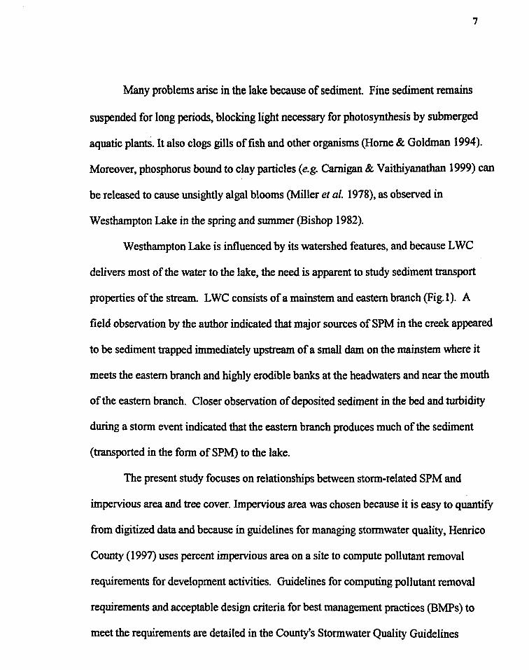
Many problems arise in the lake because of sediment. Fine sediment remains
suspended for long periods, blocking light necessary for photosynthesis by submerged
aquatic plants. It also clogs gills of fish and other organisms (Home & Goldman 1994 ).
Moreover, phosphorus bound to clay particles (e.g. Carnigan & Vaithiyanathan 1999) can
be released to cause unsightly algal blooms (Miller et a/. 1978), as observed in
Westhampton Lake in the spring and summer (Bishop 1982).
Westhampton Lake is influenced by its watershed features, and because LWC
delivers most of the water to the lake, the need is apparent to study sediment transport
properties of the stream. L WC consists of a mainstem and eastern branch (Fig. I). A
field observation by the author indicated that major sources of SPM in the creek appeared
to be sediment trapped immediately upstream of a small dam on the mainstem where it
meets the eastern branch and highly erodible banks at the headwaters and near the mouth
of the eastern branch. Closer observation of deposited sediment in the bed and turbidity
during a storm event indicated that the eastern branch produces much of the sediment
(transported in the form of SPM) to the lake.
The present study focuses on relationships between storm-related SPM and
impervious area and tree cover. Impervious area was chosen because it is easy to quantify
from digitized data and because in guidelines for managing stormwater quality, Henrico
County (1997) uses percent impervious area on a site to compute pollutant removal
requirements for development activities. Guidelines for computing pollutant removal
requirements and acceptable design criteria for best management practices (BMPs) to
meet the requirements are detailed in the County's Stormwater Quality Guidelines
8
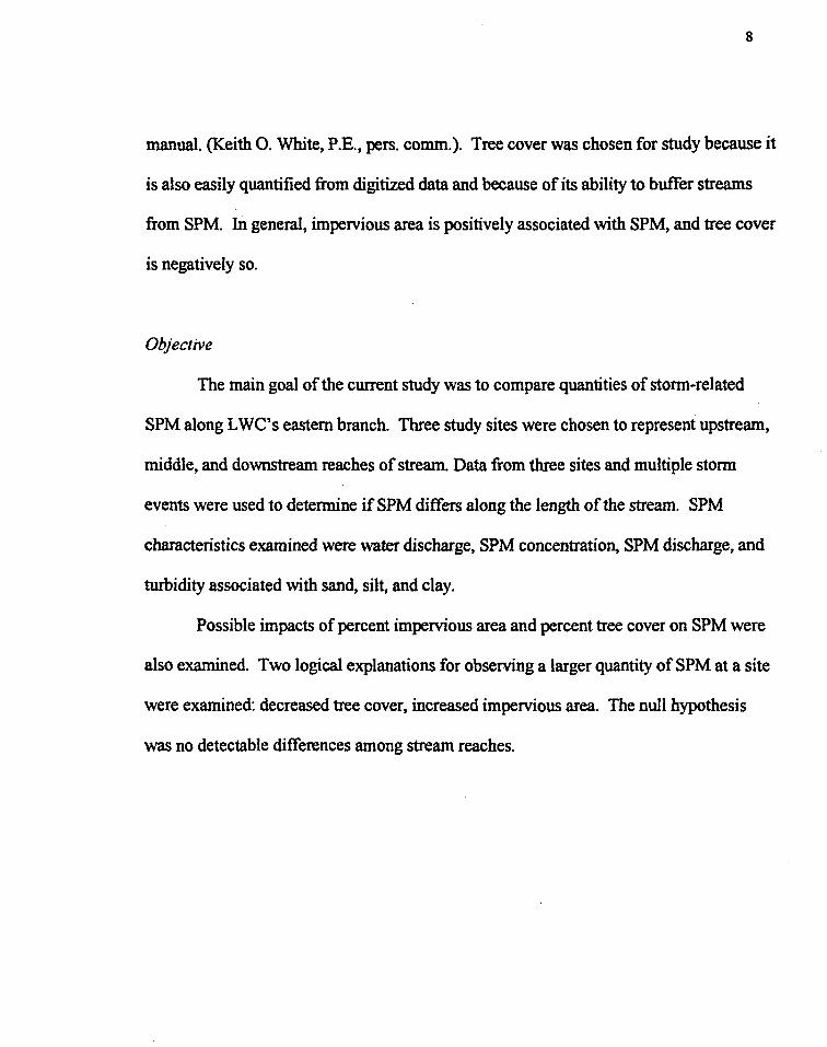
manual. (Keith 0. White, P.E., pers. comm.). Tree cover was chosen for study because it
is also easily quantified from digitized data and because of its ability to buffer streams
from SPM. In general, impervious area is positively associated with SPM, and tree cover
is negatively so.
Objective
The main goal of the current study was to compare quantities of storm-related
SPM along LWC's eastern branch. Three study sites were chosen to represent upstream,
middle, and downstream reaches of stream. Data from three sites and multiple stonn
events were used to determine if SPM differs along the length of the stream. SPM
characteristics examined were water discharge, SPM concentration, SPM discharge, and
turbidity associated with sand, silt, and clay.
Possible impacts of percent impervious area and percent tree cover on SPM were
also examined. Two logical explanations for observing a larger quantity of SPM at a site
were examined: decreased tree cover, increased impervious area. The null hypothesis
was no detectable differences among stream reaches.

9
Materials and Methods
Field
Study Sites
Three sampling sites were chosen on the eastern branch of Little Westham Creek
(Fig.l ). Site A was near the headwaters, Site B at about midpoint of the stream, and Site
C at the lower portion before it merges with the mainstem and enters the lake. Site A was
chosen because of its proximity to the highly erodable headwaters. Site B was chosen
because of its presence in a predominately forested area below Site A. Site C was chosen
because it was adjacent to residential lawns with few trees below Site B.
Watershed area, stream length, impervious area, and area covered by stands of
trees were determined using Arc View GIS 3.2 and digital data provided by Henrico
County with accuracy± 0.61 m (Frauenfelder 1999). Watershed area above each site
was determined by tabulating the area of a polygon bounded by the topographic
watershed boundary. Stream length was determined as the distance of each site from the
headwaters. Impervious area and tree cover were determined with data digitized from
aerial photographs (Frauenfelder 1999). Impervious area was defined as the area in each
watershed covered by digitized roads, building footprints, and parking lots. Tree cover
was considered as the area in each watershed covered by stands of trees.
Stream water samples and measurements of stream stage were taken during storm
events with significant rainfall between June 17 and September 16, 1999. Grab samples
of stream water were taken to characterize particle size distributions and concentration of
SPM. Stream stage was monitored to provide an estimate of water discharge.

10
Stream water samples
Water samples were collected using methods similar to those of Clesceri et a/.
(1998). The modification was that the plastic bottles were not wide-mouthed, and water
was stored in Whirlpaks (125 ml, Nasco) rather than plastic bottles. Grab samples were
collected using a plastic, 250 ml bottle facing upstream with the center of the 2 em
diameter mouth at a fixed position 3 em from the streambed in the center of the current.
After filling most of the bottle, it was shaken for a few seconds to homogenize the
sample. About 100 ml was poured into a Whirlpak and kept refrigerated until laboratory
analysis. Time and stream water stage were recorded for each sample.
Measuring water discharge
A water stage-discharge relationship was established by monitoring the water
discharge at 4-7 different flow stages as the water level dropped. An empirical
relationship between stage and discharge was developed to allow monitoring of water
discharge by measuring stream stage. Water discharges estimates for each site had the
general form:
Q=10 log10
(ST-SZF)B+A eq. (1)
where: Q was the predicted water discharge (m3 s"\ ST was the field measured stream
stage depth (em), SZF was the stage at zero flow (em), B was the slope and A was the
intercept. Actual measurements of stage were adjusted by subtracting the stage at zero

11
flow before predicting water discharge. Values ofSZF, A and B were estimated using
Microsoft Excel's Solver program to minimize the sum of squares of predicted discharge.
Water discharge (m3 s"1) was measured using methods ofRantz (1982). Time and
stage (em) were recorded at beginning and end of the discharge measurement to make
sure that flow Was steady while measurements were taken. If flow was not steady, mean
flow during the measurement was used for the estimate. Cloth measuring tape fastened
to stakes was stretched across a level weir to form a transect across each site (App. 2).
Distance was measured (facing upstream) from the left bank water's edge and to the right
bank water's edge. Intermediate measures were taken at 0.2-m intervals, dividing the
stream into subsections.
At each vertical substation along the transect, water depth (em) and mean velocity
(m s"1) were recorded. Depth was measured using a USGS top-setting wading rod, and
velocity using a flowmeter at six-tenths depth from the surface (Marsh-McBimey Flow
Mate). The flowmeter was factory calibmted with precision to the nearest 0.01 m s"1 with
accumcy at ± 2 % of actual flow. Measuring the velocity at six-tenths depth gave mean
velocity of the water column (Leopold et al. 1964, Gordon eta/. 1993).
Water discharge for each substation along the transect was calculated using the
following geneml form:
Q=dwv eq. (2)
where: Q was water discharge (m3 s"1) of the subsection, d was stream water depth (m) of
the subsection, w was subsection width (m), and v was mean velocity (m s"1 ).

12
Summing the discharges of all subsections of the transect yielded total water discharge of
the stream site at the measured stage of flow.
During a non-storm event, a bucket-filling method was used to estimate discharge
at a very low stage. Buckets of a known volume (7 1) were arranged to catch water as it
came over the transect weir. The given volume (m3) divided by the time (s) it took to fill
yielded an estimate of discharge (m3 s"1) into each bucket. Summing discharges from all
the buckets along the transect gave an estimate of total discharge for the stream site over
the weir at that stage.
Rainfall
A rain gauge (5" Taylor) was placed at each study site where rain could fall
directly into the gauge unobstructed by trees. The number of inches of water in the gauge
was recorded± 0.05 in each time a water sample was taken until rainfall had stopped.
Total accumulations per storm were compared to data from the internet (Accuweather).
The author's observations of rain pattern and rainfall duration also were noted.
Laboratory
Dry weight
Within 1-5 days of collection, water samples were analyzed for total suspended
solids (TSS) according to a modification of methods by Clesceri et al. (1998). The
modification was that before drying in an oven SPM was settled using centrifugation and
drawing off most of the water (see below) instead of glass-filtering. (Glass-filtering was

13
omitted because it was thought to remove some smaller particles with significant
turbidity such as fine clays. Centrifugation was necessary because the original design
used settling volume as a measure ofSPM.) Total dissolved solids left in the tubes
before drying in the oven were assumed negligible to the total dry weight.
Refrigerated stream water samples were warmed to room temperature. Whirlpaks
were shaken to homogenize the sample and 15 ml of sample water were poured into a
graduated centrifuge tube. The water sample remaining in each Whirlpak after TSS
analysis was frozen for later analysis.
Water in the centrifuge tubes was allowed to settle for 10 min so most of the TSS
settled out (Clesceri eta/. 1998). Tubes were centrifuged for 5-10 min at 2500 rpm. Most
of the water was then drawn off using a pipette without disturbing the settled matter.
Tubes were dried on a rack in an oven at 130° C. After only dry SPM was left, the dry
weight (g) using a digital balance was recorded with precision to the nearest 0.001 g and
accuracy± 0.003 g due to air currents. Weight of a centrifuge tube containing SPM was
compared to a recent measure of the same tube when empty to determine SPM dry
weight.
Empty centrifuge tube weight was recorded three times during the four months of
TSS analysis to ensure accuracy. Differences in weights of the empty tubes were within
the detection limits of the balance, and represented approximately 10 % of the maximum
dry weight of SPM encountered.
Because of the small quantities of SPM in the tubes, instrumental error yielded a
negative value for dry weight in 2.7% of the samples. Values with a negative dry weight

14
were set to 0.000 g. Complete dryness was checked approximately once for each set of
samples by comparing measured dry weights to dry weights after cooling and
desiccating.
Turbidity
Within a few months of collection, samples were analyzed for turbidity. Frozen
stream water samples were thawed to room temperature. Turbidity (NTU) was measured
using a LaMotte 2020 Turbidimeter after shaking to homogenize and after diluting the
sample to a readable level when necessary.
Measurements according to settling were taken at 0, 1, and 10 minutes to
separately account for turbidity due to sand, silt, and clay. The heaviest particle, sand
settled after 1 min, silt settled after 10 min, and the lightest particle, clay was the only
particle remaining suspended after 10 min. Fifteen samples (10%) were lost because of
Whirlpaks leaking and were not included in this analysis.
Data analysis
Data were nonnalized to properly characterize each site during each stonn. For
graphical analysis, actual routine grab sample times were nonnalized for duration of time
for each stonn by setting the first sample time equal to 0 min. Each stream property was
nonnalized by the site's watershed area to discount the effect oflarger watersheds having
more SPM due to their larger relative size and not their land use (Cuthbert & Kalf 1993).

IS
For statistical analysis, data from Storm 4 were omitted because measurements
did not capture both the rising and falling limbs of the discharge versus time plot
(hydrograph). For the remai~g storms, water discharge, SPM concentration, SPM
discharge, total turbidity, turbidity associated with sand, silt, and clay at each site were
plotted versus duration. Area under the curve was estimated to give each variable's
storm-wise yield to each site during sampling. Areas were estimated by summing for the
entire range: the difference of two consecutive x-values multiplied by mean y-values
between the two data points.
Means and standard deviations of each stream property were calculated. Using
each storm as a block, si~es were ranked and tested using a non-parametric Friedman's
ANOVA method for randomized blocks (storms) to detect if there were differences
among sites. If the null hypothesis of no differences among sites was rejected, a non
parametric equlivalent ofTukey's honestly-significant difference test (HSD) was used to
determine which sites were significantly different. Levels of significance were set at
p<O.OS for all statistical tests.
To estimate water discharge based on routine stream water stage ~easures, a
calibration curve, or rating curve (Leopold et al. 1964) was plotted using data from the
water discharge study. Water stage measurements were adjusted by SZF, the stage at
which zero water would flow over the weir. Microsoft Excel's Solver program was used
to determine the SZF, slope, and intercept of each site's least squares regression line by
minimizing the sum of squared deviations (predicted discharge minus observed
discharge).

16
Inserting field stream water stage measurements into the equation for the
calibration curve converted field measures to water discharges. Only 9 % of the staff
gauge measurements were outside the range of those used to develop the calibration
curve.
Water discharge per watershed area (m3 sec"1 km"2) at each site was plotted versus
time during each storm to produce a hydrograph. All storms were also compared in one
plot for Site C to show variation among storms in water discharge. Means ± standard
deviations and statistically significant differences of water discharge per stonn (water
yield hereafter) at each site were calculated and recorded.
SPM concentration per watershed area (kg m·3 km"2) at each site was plotted
versus time for each stonn at each site to graphically visualize the concentration of SPM
at each site as the storm progressed. SPM concentrations were calculated as dry weight
per 15 ml sample. The concentration ofSPM in each sample at each site was plotted
versus time for each stonn. All storms were also compared in one plot for Site C to show
variation among storms in SPM concentration. Means± standard deviations and
statistically significant differences of SPM concentration per storm at each site were
calculated and recorded.
SPM discharge per watershed area (kg min"1 km"2) at each site was calculated for
each sample at each site by multiplying water discharge by SPM concentration at each
sample time in the entire cross section of water. SPM discharge gave an approximation
of the flux of SPM going through a site at each sampling time during a storm. All storms
were also compared in one plot of Site C to show variations among storms in SPM

17
discharge. Means ± standard deviations and statistically significant differences of SPM
discharge per storm (SPM yield hereafter) at each site were calculated and recorded·
SPM discharge was plotted versus water discharge to compare relationships at the
three sites. A log-log relationship was used to normalize the data. Sites were compared
using linear regression. Because there were not visual differences in lines, data were
pooled for an overall correlation using a regression test. Linear regression provided a
correlation coefficient and a p-value for statistical significance of the trend line.

18
Results
Values for drainage area, stream length, total impervious area, and total area of
tree cover were smallest at Site A and largest at Site C (Table 1). Values for Site C were
approximately twice those of Site A for drainage area, stream length, and impervious
area. The percent impervious surface area and tree cover were greatest at Site A and least
at Site C.
Rainfall patterns were similar at the three sites (Table 2). The amount of rain
during a specific stonn was similar at each site. Mean rainfall ranged from 1.6 (Stonn 4)
to 14.1 em (Stonn 5) among stonns. Trends were the same when comparing the author's
observed values to those collected from Accuweather, although absolute values differed.
Rain patterns ranged from a light drizzle in Stonn 1, to thunderstonns in Stonns 2 and 3,
and a hurricane in Stonn 5. Unpublished ~ta from smaller stonns and baseline data did
not yield any turbidity or dry weight, and were not included in the study.
Stream water stage-discharge relationships were developed for each site (Fig. 2).
Values of~ were~ 0.96 at each site, indicating excellent fits (Table 3).
Sites were similar with respect to water discharge per watershed area (Fig. 3).
Following a unimodal response, discharge generally increased to a peak then decreased
over time. Measurements of water discharge started at and returned to base flow levels
for Stonns 1, 2 and 3, and started above base flow and returned to base flow levels for
Storms 4 and 5. The first value for Stonn 4 at Site B is probably an erroneous reading of
the staff gauge. (The staff gauge measurement was believed to have been accidentally
read 10 em higher than observed because it is much higher than measures observed at the

19
same site during the hurricane.) The system responded quickly to storm surges, returning
to pre-storm levels within about an hour for all storms other than Storm 5 (Fig 3). Values
of mean water yield were similar among sites (Table 4 ). Differences among storms
produced large values for standard deviations. Sites were ranked for each storm
separately in order to eliminate these storm effects. Differences in water yield were not
statistically significant among sites (Table 5).
Temporal patterns in SPM concentrations per watershed area followed a general
unimodal trend for Storms 1 and 3 (Fig. 4). Storm 2 was clearly bimodal. The peak at
Site C lagged behind the other two sites in Storms 1 and 3. Storms 1-3 show SPM
concentrations per watershed area starting at base levels and returning to base levels by
the end of the sampling duration. See the last plot in Fig. 4 for a comparison of trends
among storms. Mean SPM concentrations per watershed area per storm were greatest at
Site A and smallest at Site C (Table 4). Differences in mean-ranked SPM concentration
per storm between Sites A and C were statistically significant (Table 5).
Temporal patterns in SPM discharge per watershed area followed a unimodal
trend for Storms 1 and 3 (Fig. 5). Storm 2 was bimodal. The peak at Site C lagged
behind the other two sites in Storms 2 and 4. Storms 2-4 show measures starting at base
levels and returning to base levels by the end of the sampling duration. The first value for
Storm 4 at Site B is a visual outlier. See the last plot in Fig. 5 for a comparison of trends
among storms. Mean SPM yield per watershed area was greatest at Site A and smallest at
Site C (Table 4 ). Differences in mean-ranked SPM yield between Sites A and C were
statistically significant (Table 5).

20
SPM discharge and water discharge were positively related (Fig. 6). Visual
observations indicated similarities at each site. So, data were pooled to establish an
overall correlation coefficient. There was a positive correlation of the log SPM discharge
versus log water discharge plot with statistical significance (r= 0.94, n=I36, p<0.05). Eq.
3 describes the regression line
SPM = 0.011Qt.64 eq. (3)
where: SPM = SPM discharge (kg h"1), Q =water discharge (m3 h"\ and the numerical
values were least squares estimates of intercept and slope.
Mean total turbidities did not differ among sites {Tables 4&5). The three sites also
did not differ with respect to turbidity associated with sand and silt (Tables 4&5), but
turbidity associated with clay differed among sites (Table 4). Site A had more turbidity
associated with clay than did Site C (Table 5).
21
Discussion
Findings
The null hypothesis that all sites were the same with regard to water discharge,
SPM concentration, SPM discharge, total turbidity, and turbidity associated with sand,
silt and clay was rejected. Significant differences were found between the uppermost and
lowermost sites. Thus, comparisons discussed hereafter only involve Sites A and C. Site
A had greater SPM concentration, SPM discharge, and turbidity associated with clay than
did Site C.
LWC responded quickly to storm events. Solo-Gabriele eta/. (1997) observed
similar "quick storm flow" responses to an urban stream near Boston, Massachusetts.
These flashy responses to rainfall events were attributed to storm-sewer flows, direct
precipitation into the stream, and direct runoff into the channel. Slower responses were
attributed from runoff higher in the watershed that takes time to reach the stream.
In suburban areas, vegetation is removed which exposes soil. The removal of
trees is associated with an increase in surface runoff (Karr & Schlosser 1978) and SPM
(Klein 1979). Trees slow down runoff to a stream, physically intercepting runoff and
SPM (Gordon eta/. 1993). The slowing of runoff to a stream further reduces SPM by
reducing inputs from bank-cutting erosion (Trimble 1997), bed scouring (Whipple 1981),
and resuspension of sediment (Cardenas eta/. 1995). Trees also help cover soil from
direct rainfall and help stabilize erodible banks (Gordon et al. 1993). Thus, one would
expect areas in this watershed with higher percent tree cover to have decreased water
discharges and SPM.

22
After trees are removed more impervious areas are developed. Increased
impervious area along banktops directly shields soil from being picked up as SPM.
However, in LWC's watershed, less than 30% of the watershed is impervious. Because
the entire watershed is not impervious, shielding effects are masked by other SPM
contributing processes. Impervious areas increase surface runoff. The increased surface
runoff has energy to erode pervious surfaces, increasing SPM. Not only does this directly
add SPM to a stream, but it also increases water discharge, gaining energy to scour
stream beds, resuspend sediment, and cut stream banks. Thus, one would expect areas in
this watershed with greater percent impervious surfaces(~ 30 %) to have increased water
discharges and SPM.
In summary, one would expect impervious surfaces and trees to have opposite
effects on SPM. Impervious surfaces would increase SPM and tree cover would decrease
SPM.
Hypotheses
Based on assumptions about associations between SPM and land use, one can
predict relationships between Sites A and C. The author proposes three hypotheses to
explain relationships between SPM and land use. The first hypothesis (Hl) assumes
either that impervious area and tree cover have no effect on stream properties or that their
effects cancel each other, so stream properties do not differ at Sites A and C. The second
(H2) assumes that stream properties are associated with impervious area. Site A, with a
greater percentage of impervious area would have yielded more water (Simmons &

23
Reynolds 1982) and more SPM (Klein 1979). The last hypothesis (H3) assumes stream
properties are associated with tree cover. Knowing tree cover removal increases SPM
(Karr & Schlosser 1978), it is assumed presence of tree cover would decrease in SPM.
Thus Site A, with a greater percentage of tree cover would yield less water and less SPM.
Predictions of SPM associated properties based on the previous three hypotheses
can help explain SPM contributing processes in LWC (Table 6). Because any detectable
differences reject the null hypothesis, more weight needs to be given to differences when
shown. So, when differences were observed, a hypothesis with many predictions
matching field observations would best explain SPM yield to the stream.
Significant differences in SPM concentration, SPM discharge, and turbidity
associated with clay among the upper and lower study sites were evident, so H1 can be
rejected. Hubbard eta/. (1990) suggested that compared to non-forested areas, areas with
riparian buffer zones decreased runoff and SPM concentrations per unit area. This was
not the case in the current study. Site A bad both more tree cover and greater water
discharge per watershed area, so H3 can be rejected because its predictions were never
supported with observations.
In all three cases when differences between sites were observed, predictions ofH2
matched the observed relationships. SPM might be delivered to the stream due to SPM
contributing properties in Site A's watershed. Site A had a greater mean water yield per
watershed area, which may have allowed more SPM to be carried (Leopold 1994, Jago &
Mahamod 1999). Also, the runoff water added downstream of Site A may have been

24
relatively void of SPM. This clean water may have diluted the samples at Site C. The
effects of impervious area may have exceeded effects of trees.
Another study ofLWC showed possible erosion "hot spots" upstream of Site A
(Hillegass. unpub. MS.). Perhaps the buffering of SPM by trees was negligible compared
to SPM additions within the stream. Perhaps most SPM was added due to stream
channelization, scouring, and resuspension of sediment. Very steep, erodible banks
upstream of Site A were observed before the study, as well as evidence of bedload
transport throughout the length of the stream (personal observation). Stream channel
erosion has been shown to be a major sediment source in urbanizing watersheds (Trimble
1997). Another study ofLWC showed evidence of stream banks caving in during storms
(Aunins, unpub. MS.). Resuspension of particulate matter could also have been an SPM
producing factor (Cardenas eta/. 1995).
The inability to distinguish differences in total turbidity and turbidity associated
with sand and silt may also indicate that the type of SPM in the stream at Site A was not
different from Site C. Similar characteristics of turbidity would be expected between
sites if the consistency of the SPM were the same. This further supports the idea that
SPM was all from one main source upstream of Site A, and it remained the main source
between Sites A and B.
Limitations
The lack of large differences among sites in impervious area and tree cover may
have led to difficulty in detecting relationships between watershed and SPM. Vandalism,

25
grab sampling, complications in measuring water discharge, and low sample size may
have also limited the ability to detect differences in SPM among sites (App.3).
Conclusion
The waterihed of Site A tended to produce more stonn-related SPM to the stream
per watershed area than did the other sites. Thus, I conclude that the primary source of
SPM in Little Westham Creek was upstream of Site A. A personal observation of steep,
undercut banks and sediment in the bed indicated that the stream banks near the
headwaters and just upstream of Site A were highly erodible. If there were no other
significant sources of SPM to the stream, then one would expect SPM concentrations to
be diluted as water moves downstream from the headwaters. The author proposes that
the major source of SPM was upstream of Site A, within a reach starting at the
headwaters and extending approximately 500 meters downstream.
To alleviate the sediment loading in Westhampton Lake, it needs to be detennined
which branch ofLWC produces the most SPM to the lake. If the eastern branch produces
most of the SPM to the lake, and with careful control and more detailed information on
watershed properties, perhaps it can be shown that most of the sediment loading the
upper extents of Westhampton Lake comes from the highly erodible banks near the
headwaters. Restoration in this portion of stream might help resolve the sedimentation
problem in the lake.

26
Recommendations
The current study provides information to Henrico County Public Works
(specifically to Jeff Perry & Keith White) to help rank LWC among other streams in the
new stream restoration program. IfLWC is ranked high priority in need ofrestoratio~
perhaps Henrico County can restore water quality to the stream.
Water quality is low for the eastern branch of L WC. This study indicates the
loading of SPM in the watershed of the upper 500 m of stream. Also during the study,
there were no observations of fish or benthic invertebrates within the study reach.
Minnows were observed in the mainstem during occasional visits (personal observation).
Based on a small study in Spring 2000, benthic macroinvertebrate life approximately 10
m downstream of Site A in the eastern branch ofLWC appears to be severely impaired as
compared to a site of equal elevation in the mainstem (Jordan & Scott, unpub. MS.).
Residents in the study area informed the author of mysterious nighttime stream
flushes filling the stream banks a couple of times per year during non-storm periods.
Suspected sources of those flushes are either the water tanks at Triangle Shopping Center
or the parking lot at Village Shopping Center. Both sites are connected to the headwaters
area and have potential to produce large amounts of water to the stream. Visual
observation of scouring below a stormwater pipe just below the water tanks indicates
excessive discharge from the tanks. To stop this problem, water needs to be released in
lower volume and over a longer duration of time. The author suggests construction of a
discharge retention pond in the vicinity of the water tanks. This would not only prevent

27
stream channelization, sediment resuspension, and bank erosion by slowing the velocity
and volume of water, but it would also serve as a BMP to remove chlorine and other
toxins before entering the stream. A stormwater retention pond could serve as a BMP
downstream of Village Shopping Center, further helping water quality in the stream with
the removal of pollutants and slower release of storm water.
Along the first 500 m of stream, the banks are being severely eroded. One way to
fix that problem would be to lay back the slope of the banks and vegetate them. The
laying ofriprap, gravel, or some biological alternative with root mats in the stream itself
would prevent bed scouring and promote in-stream settling of SPM. The addition of
riffie-pool complexes might allow more settling and provide habitat necessary for benthic
macroinvertebrate life. Hopefully by minimizing SPM loading of the eastern branch
within 500 m of the headwaters will restore water quality to the stream and help resolve
the sedimentation problems of Westhampton Lake.

28
Literature cited
Aunins, A. 1999. Erosion analysis of Little Westham Creek. Unpublished B.S. Thesis, University of Richmond, Richmond, Virginia.
Bishop, J. W. 1982. Models relating lake properties and stonns. Pp. 81-102. In V.P. Singh (ed.) International Symposium on Rainfall-Runoff Modeling. Mississippi State University, Proceedings, vol. 3. Water Resources Publications, Littleton, Colorado. 1982.
Bishop, J. W. 1998. Westhampton lake report. Unpublished report. University of Richmond, Richmond, Virginia.
Cardenas, M., Gailani, J., Ziegler, C.K., and Lick, W. 1995. Sediment transport in the Lower Saginaw River. Marine and Freshwater Research. 46: 337-347.
Carnigan, R. and Vaithiyanathan, P. 1999. Phosphorus availability in the Parana floodplain lakes {Argentina): Influence of pH and phosphate buffering by fluvial sediments. Limnology and Oceanography. 44: 1540-1548.
Clesceri, L. S., Greenberg, A. E., and Eaton, A. D. 1998. Standard methods for the examination of water and wastewater. American Public Health Association. Washington.
County of Henrico. 1997. Guidelines for Stonnwater Quality. Department of Public Works, County of Henrico, Virginia. June 1, 1997.
Cuthbert, I.A. and Kalff, J. Empirical models for estimating the concentrations and exports of metals in rural rivers and streams. Water, Air, and Soil Pollution. 71: 205-230.
Elliot, A. G., W. A. Hubert, and S.H. Anderson. 1997. Habitat associations and effects of urbanization on macroinvertebrates of a small, high-plains stream. Journal of Freshwater Ecology. 12: 61-73.
Frauenfelder, A. 1999. Digitized data and aerial photographs accessible with GIS. Department of Planning, Henrico County, Virginia.
Gordon, N.D., McMahon, T.A., and Finlayson, B.L. 1993. Stream Hydrology. Wiley: Chichester.
Gowan, C. Randolph-Macon College in Ashland, VA. Personal communication regarding non-parametric Friedman-type test and Tukey-type test. Sept. 15,2000.
Hillegass, J. 2000. The implementation of Arc View GIS as a predictive model to determine erosion trouble areas along Little Westham Creek. Unpublished B.S. Thesis, University of Richmond, Richmond, Virginia.
Home, A.J. and Goldman, C.R. 1994. Limnology. McGraw-Hill: New York. Huryn, A.D., and Wallace, J.B. 1987. Local geomorphology as a determinant of
macrofauna! production in a mountain stream. Ecology. 6: 1932-1942. Jago, C.F. and Mahamod, Y. 1999. A total load algorithm for sand transport by fast
steady currents. Esturarine Coastal and Shelf Science. 48: 93-99. Jordan, J.R., and Scott, T. 2000. Comparison of benthos abundance and diversity in
Little Westham Creek. Unpublished report.
29
Kaenel, B.R, C.D. Mattheai, and U. Uehlinger. 1998. Disturbance by aquatic plant management in streams: effects on benthic invertebrates. Regul. Rivers: Res. Mgmt. 14: 341-356.
Karr, J.R. and Schlosser, I.J. 1978. Water resources and the land water interface. Science. 201:229-234.
Klein, RD. 1979. Urbanization and stream quality impainnent Water Resource Bulletin. 15: 948-963.
Lamberti, G. and M.B. Berg. 1995. Invertebrates and other benthic features as indicators of environmental change in Juday Creek, Indiana. Nat. Areas Journal 15: 249-258.
Lenat, D.R. and J. K Crawford. 1994. Effects ofland use on water quality and aquatic biota of three North Carolina Piedmont streams. Hydrobiologia. 294: 185-199.
Leopold, L.B. 1994. A view of the river. Harvard University Press. Cambridge, Massachusetts.
Leopold, L.B., Wolman, M.G. and Miller, J.P. 1964. Fluvial processes in geomorphology. W.H. Freeman and Company. San Francisco.
Martin, G.R., Smoot, J.L., and White, KD. 1992. A comparison of surface-grab and cross sectionally integrated stream-water-quality sampling methods. Water Environment Research. 64: 866-876.
Marsh, W. M. 1991. Landscape planning environmental applications. John Wiley and Sons, Inc. New York.
Miller, W.E., Greene, J.C., and Shiroyama, T. 1978. The Selenastrum capricomutum printz algal assay bottle test. U.S. Environmental Protection Agency. Office of Research and Development. EPA-600/9-78-0 18.
Minore, D. and Weatherly, H. G. 1994. Riparian trees, shrubs, and forest regeneration in the coastal mountains of Oregon. New Forests. 8: 249-263.·
Rantz, S. E. 1982. Measurement and Computation of Stream Flow: Volume 1. Measurement of stage and discharge. Geological Survey-Water-Supply Paper 2175. United States Government Printing Office: Washington.
Renard, K.G., Foster, G.R., Weesies, G.A., McCool, D.K, and Yoder, D.C. 1997. Predicting Soil Erosion by Water: A Guide to Conservation Planning with the Revised Universal Soil Loss Equation (RUSLE). U.S. Department of Agriculture, Agriculture Handbook No. 703, 404 pp.
Renfrow, M. Westhampton Lake- Erosion Control. Letter from Neil Bromilow, 3 June 1994.
Rosgen, D.L. 1994. A classification of natural rivers. Catena. 22: 169-199. Simmons, D.L. and Reynolds, R.J. 1982. Effects of urbanization on base flow of
selected Southshore streams, Long Island, New York. Water Resources Bulletin. 18: 797-805.
Sokal, R.R. and Rohlf, F.J. 1981. Biometry. W.H. Freeman and Company. San Francisco.
Solo-Gabriele, H.M and Perkins, F.E. 1997. Streamflow and suspended transport in an urban environment. Journal ofHydraulic Engineering. 123: 807-11.

30
Tourbier, J. and Westmacott, R 1977. Lakes and ponds. The Urban Land Institute. Washington.
Trimble, S.W. 1997. Contribution of stream channel erosion to sediment yield from an urbanizing watershed. Science. 278:1442-1444.
Vannote, R.L., Minshall, G.W., Cummins, K.W., Sedell, J.R, and Cushing, C.E. 1980. The river continuum concept. Can. J. Fish. Aquat. Sci. 37: 130-137.
Wallace, J.B., Cuffuey, T.F., Webster, J.R, Lu~ G.J., Chung, K., and Goldowitz, B.S. 1~91. Export of fine organic particles from headwater streams: Effects of season, extreme discharges, and invertebrate manipulation. Limnology and Oceanography. 36: 670-682.
Warren, L.A. and Zimmerman, A.P. 1994. Suspended particulate grain size 'dynamics and their implications for trace metal sorption in the Don River. Aquatic Sciences. 56: 348-362.
Whipple, W., DiLouie, J., and Pytlar, T. 1981. Erosion potential of streams in urbanizing areas. Water Resources Bulletin 17: 36-45.
White, K.O. Henrico County Public Works. Personal communication regarding stormwater quality guidelines for Henrico County. August 17, 2000.
Zar, J.H. 1999. Biostatistical Analysis. Prentice Hall: Upper Saddle River, New Jersey.

Table l. Properties of nested watersheds associated with study sites along Little Westham Creek
31
Site Watershed Stream Impervious o/o Impervious Tree o/o Tree Area Length Area 1 Area 1 Covered Covered
Area2 Area2
(km2) (m) (km2) (%) (km2) (%)
A 0.241 555 0.071 30 0.060 25 B 0.307 744 0.082 27 0.072 24 c 0.605 1331 0.160 26 0.096 16
l. Impervious area was estimated with digitized data of area covered by roads, building footprints, and parking lots. 2. Tree cover was estimated with digitized data of area covered by stands of trees, mostly forested areas.

32
Table 2. Rainfall for each stonn. Values are depths of rain (em) that accumulated in rain gauges during the stonns.
Date
06/17/1999
06/29/1999
06/30/1999 07/28/1999 09/16/1999
Storm1
1
2
3 4 5
Rain gauge depth (em} A B C
2.0 2.0 1.3
3.3 3.1 3.0
Mean 1.8
3.1
4.1 3.9 3.8 3.9 1.6 1.6 1.6 1.6
n/a2 15.2 13.0 14.1
Accuweather Type of Duration (em) Rainfall (h)
0.2
2.1
3.5 0.4
12.3
light Drizzle Severe
T-Storm T-Storm
Drizzle Hurricane
(Floyd)
1
4
1 3
60
1. Stonn 4 was characterized in graphical figures, but omitted from statistical analysis. 2. nfa means data were not available. 3. Data from http://www.accuweather.com/adcbinlclimo local?nav=home#moremaps . All other measures observed by the author.

33
Table 3. Values for estimating water discharge based on stage of water measured in the field
Site # Samples SZF A 7 0.1 8 4 -7.5 c ~ -1.5
Slope 1.5 3.0 2.3
Intercept r2 Mean % Error -2.4 0.96 0.82 -4.7 0.99 1.02 -3.3 1.00 0.71

34
Table 4. Stream properties at each site. Values represent accumulations throughout stonns. Values: mean ± standard deviation in 103
, and in parentheses, number of observations.
Site Stream Properties A B c
Water Discharge (m3 km-2) 8 ± 10 (4) 6 ± 9 (4) 6.± 8 (4) SPM Concentration 0.7 ± 0.7 (4) 0.4 ± 0.4 (4) 0.2 ± 0.2 (4) (kg min m·3 km-2)
SPM Discharge (kg km-2)
Turbidity (NTU min km-2)
9 ± 12 (4) 6 ± 8 (4) 5 ± 6 (4)
Total 357 ± 386 (4) 336 ± 308 (4) 150 ± 122 (4) Sand 97 ± 106 (4) 94 ± 72 (4) 42 ± 32 (4) Silt 132 ± 146 (4) 130 ± 128 (4) 58± 47 (4) Clay 128 ± 134 (4) 112±112(4) 50± 47 (4)

35
Table 5. Mean ranks of sites for stream properties. Sites were ranked for each storm separately. Sites arranged left to right in order of low to high mean ranks from -Friedman's test. Sites not connected by an underline were statistically different.
Mean rank Property 1 2 3
Water discharge CB A
SPM concentration c 8 A
SPM discharge c 8 A
Turbidity Total c BA
Sand c A 8 Silt c BA
Clay c B A

36
Table 6. Relationships of stream properties at Site A compared to Site C according to 1) no net effect of impervious area or tree cover on SPM, 2) SPM associated with % impervious area, 3) SPM associated with % tree cover. More weight given to differences when observed. Asterisks indicate where the prediction matches the observed relationship.
Relation to watershed Stream Property per
Area 1 2 3 Observed
Water discharge A=C* A>C A<C A=C SPM concentration A=C A>C* A<C A>C SPM discharge A=C A>C* A<C A>C Turbidity
Total A=C* A>C A<C A=C Sand A=C* A>C A<C A=C Silt A=C* A>C A<C A=C Clay A=C A>C* A<C A>C

0.5 0
Westhampton Lake
1
Waterbodies c=J Roads ,'', ,' Streams
I .,
if1111 A watershed
37
Fig.1 a. Watershed of Site A along the eastern branch of Little Westham Creek.

0.5 0 0.5
Waterbodies CJ Roads ,'', ,'Streams
I .,
I a B watershed
38
1 1.5 Kilometers
Fig.1 b. Watershed of Site 8 along the eastern branch of Little Westham Creek.
0.5 0 0.5
Waterbodies D Roads ,'', ,' Streams
I ., 111 C watershed
39
1 1.5 Kilometers
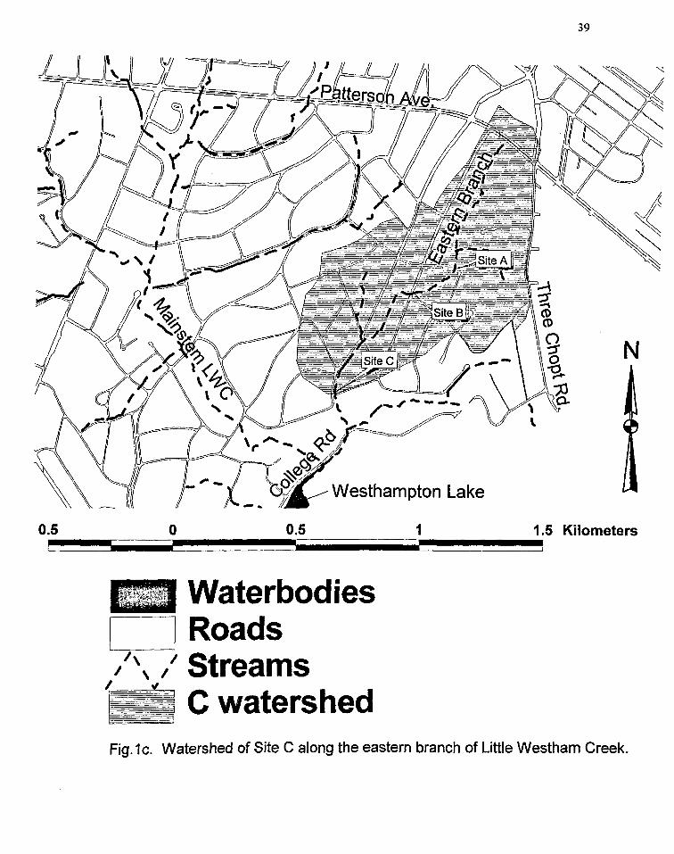
Fig.1c. Watershed of Site C along the eastern branch of Little Westham Creek.

Composite Discharge Calibration Curves
I• Site A • Site 8 A Site C I (I) 0.0 .--------------,A--, ~ -0.5 •••
= ~-~ --1.0 •• 41- .,.. ·- 1/) 1 5 c c:;:;-.
~< J ,s E -2.0 cu-3: -2.5 ~ -3.0 A
..J -3.5 ..L--------------0.0 0.5 1.0 1.5
Log Adjusted Stage (em)
Fig 2. Log water discharge (m3 s"1) versus log adjusted stage (em). Stage has been
adjusted to account for the actual stage where there is zero flow over the weir.
40

Storm 1 0.35
.... Cll ~0.30 a.< ~ E0.25 ,_.¥
~ !!0.20 -+-Site A UC'? -a-sm. a iS §_0.15 -6-Si1DC
; «J0.10 1ii~ == ct 0.05
0.00 0 50 100 150
Duration (min)
Storm3 0.6
.... &N'0.5
< cuE e'.:.t: 0.4 I'll .. -+-Si1DA .:::..!!! ~ r o.3 -G-Si!eB
i5 ..§. 02 -6-Si!eC
.... «J .2!cu ~ < 0.1
0 0 25 50 75 100
Dl.l'ation (min)
StormS 2.5
... Cl)--
a.~2.0 CD E e'.:.: ~!? 1.5 -+-Site A UC"J -G-Si!eB 111< i5 .§.1.0 -.-sm.c .... .., .SCI) IG '-05 :;:ct•
0.0
0 100 200 300 400 500 Dl.l'ation (min)
41
Storm2 3.0
.... [N'2.5
< ~~2.0 IG "
' -+-saeA
.:::~ -Sit9B ~ r 1.5 -lr-Si!eC ·- E ': -;1.0
~ .! ~ ~ ct 0.5 ~
0.0 0 50 100 150 200
Dl.l'ation (min)
Storm4 6~------------------~
0 25 50 Dtrcrtion (min)
-+-Site A
--a-Si!eB
--6--Si!eC
75
All Storms at Site C
-+-Storm1 -a--Storm2
-.-storm3 ~Stonn4
-a--stom5
0 50 100 150 200 250 Duration (min)
Fig.3. Water discharge per watershed area for each stonn (m3 sec·1 km-2). The last plot
summarizes water discharge from all the storms at Site C.

42
Storm 1 Storm2 2.8 14
2.4 12 I'IS- I'll-e! ~ 2.0 e ~ 10 c:te -+-SitoA c:t E
-+-Silo A ; ~ 1.6 '-.X 8 Qj • Q.M -§-SilaS C.M -SiteS c; e 1.2 -.-s;toc • < 6
-..-sitec u E c:-. c:-. 8~0.8 0 01 4
0~ 0.4 2
0.0 0
0 50 100 150 0 50 100 150 200 DlKation (min) Dtration (min)
Storm3 Storm4 12 18
16 10
I'IS- I'IS -14 e~ cuN
c:te 8 .t i: 12 ... _x -+-Site A :u ~ 10 -+-Site A 8.~ 6 -G-SiteS Q.M
8 -D-SiteB • < • < g.§ 4 --ir-SitoC u E --ir-SitoC c-. 6 001 001 0~ o=. 4
2 2·
0 0
0 25 50 75 100 0 25 50 75 Dilation (min) Dt.l"ation (min)
Storm5 All Storms at Site C 8 3.5 7 3.0
I'IS -s I'IS-e~ e~2.s --.-storm1 c:t E 5 -+-Site A c:te -§-Storm2 '-.X ; ~2.0 8.~4 --f!-SiteS Q.M -.-storm3 • < -A-SiteC u e1.5 -*-Storm4 g.E3 c::-001 8 ~1.0 0:.2
0.5
0.0
100 200 300 400 500 0 50 100 150 200 250 DlKation (min) OU'ation (min)
Fig.4. SPM concentrations per watershed area (kg m·3 km.2) for each storm. The last plot summarizes SPM concentrations from all the storms at Site C.

Storm 1 12
~ <'410 o.< e11 E 8 tl).¥: ... « tl1 s:: ...,._S~eA .ce6 -D-SiteB u_ .!!tD
-..-sitec c=.4 ::!EtiJ a..e 2 (/)<(
0 0 50 100 150
Duration (min)
Storm3 60
:p N"50 o.< &~40 .....
-+-Site A t11 .E '5 ~30 -D-SileB .!!CI
-..-s~ec c ::.20
=== 3i ~ 10
0 25 50 75 100 Duration (min)
StormS 250
... -~~200 e11 E E»~150 -+-Site A til_
'5,§ -D-S~eB
.!! tD100 -+-SiteC o=.
=== a..e 50 (/)<(
0 0 100 200 300 400 500
Duration (min)
400.
... -8.~ 320 e11 E ~ 'l' 240 tl1 c .s::-u,§ .!! ~160 c._. :Et11 a. e 80 (/)<(
0
:p N"250 Q,<
&~200 ... « 111 c
.s:: e 1so Me, 0 ::.100 :E tl1
a..eso (/)<(
t 0
0
43
Storm 2
~
-+-Site A
'/ -II-Si1aB
_,._SileC
l .b..,_. 50 100 150 200
Duration (min)
Storm4
-+-Site A
-11--SiteB
-.-sitae
25 50 75 Duration (min)
All Storms at Site C
-+-St>nn1
--t:I-St>nn2
-6-St>nn3 ->t-St>nn4
---Stlm!S
0 ~~hmrti~B-----=1 0 50 100 150 200 250
Duration (min)
Fig.5. SPM discharges per watershed area (kg min"1 km-2) for each storm. The last plot
summarizes SPM discharge from all the storms at Site C.

SPM Discharge vs Water Discharge I• Site A m Site 8 • Site C I
. 4.5 -...----------------..
:c 4.0 c, .X: 3.5 -& 3.0 -cu .c 2.5 (,) II)
i5 2.0
~ 1.5 en C) 1.0 0
..J 0.5
0.0 +-----r----,--------,-----l 0.0 1.0 2.0 3.0 4.0
Log Water Discharge (m"3/h)
Fig.6. SPM discharge (kg h-1) as a function of water discharge (m3 h-1
) for each site.
44
45
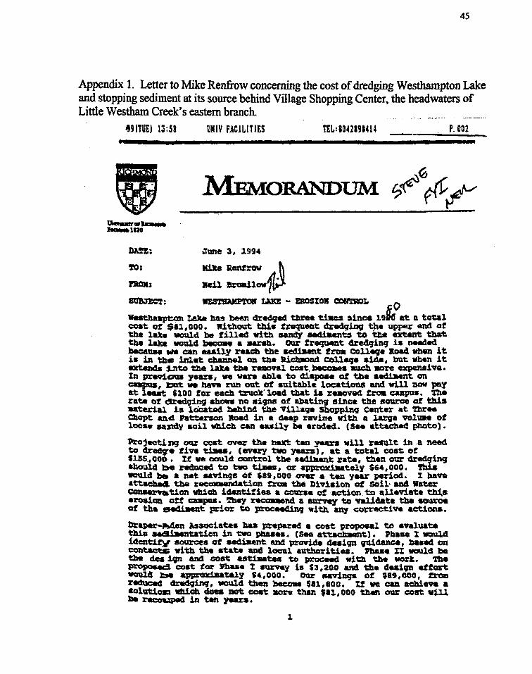
Appendix 1. Letter to Mike Renfrow concerning the cost of dredging Westhampton Lake and stopping sediment at its source behind Village Shopping Center, the headwaters of Little Westham Creek's eastern branch.
491TUE) 13:58 UMlV FACJLITIES TEl.: 1042191414
DA!Z; Jane 3, 1994
'1'0: X1ke Renfrow A.~ t'llCK; Jleil kaii.Uov?P 8UB."JEC'r: 'ftS'1'JWQIT()l U.U - EROStOJI COR'lWlt. O WMt.buptcxn taJca has been c!redqed three tiJies since 19~ at a to1:al <:oat ot $11,ooo. Without this .traqueat drecSqinO ~ upper end or the lab W01ald be fill~ with Andy Mdiacnts to tba extent tbat t!w lake WO\Jl.Cl ~ a JNJ:ah. Otu: frequ.nt 41'e4qinq ia needed bec:auae ..,. can eaaUy raac:b the ~unt fnra College Boa4 when it is in tb• inlet chamMa1 on the JlictuloDd c:oll~• aide, =t when it extends .t.nto the lalc.e the :raoval coat.~ ww::.h JIOI'e cxpenai va. 1A prftiOWI yean, ve van able to dispose of the aedilwnt em caapu, l:l&1t we bave run out ot aui table locatioca and will lJOV pay at leut $100 for each ~·load. tbat 1a raovad t:ca cupus. Thll rat. ot Clredging ahawa no aigna of ~tinq since the aow:ce of this 111lterial J.s l.oCa.to4 beh1n4 the ViUaga Sboppinq Center at '!bree Cbopt an.S Patterson Jtoad in a daep ravi.Da with a J.ar;a volUM ot loose aamy aoU Wich can easily t. eroded. ( saa attacbad pb.oto) •
l'J:ojecti:ng oq: cost ovw the MXt tan yean vUl result in a need to 4r~• tin t1Ms, (every tva years), at a total coat of S15S,ooo. U ve OCI\lld ecntrol tbe aadillent: rate, then our dredqinq *bould 'btl ndw:ed to two ti118S, or app:t'QXiMtely $64, ooo. 'lhia WCNl4 be a ut .avinqs Of $It ,ooo ewe a ten year period.. :t bavo attrhd tba r8COIIII8ndation ~ the Divi•ion of SOil· aft4 Water Couana.tion whiah idct.ifiaa a c:aana of action to alleviate t:b:f.s erosion cf.f CBJipu&. 'lhq HC1311encl a survey to val.ic!ate the ~ of the eediaat prior to procee41nq with any ~va a.ctiona.
!)~;ape-Men Anociatn has ~•P&Hd a coat proposal to evaluate t!Ua MaSMl''t&tion in~ pbaaes. (Sea a~). l'baae 1110\ll.d !dea~ aaurcea of •edbe.nt and provide dai9D guidanCe, lased em contacts witb the state and local &Utbarit.ies. l'baH n WIO'lld be tlle des i;n aDd coat uti.JDatea to proceed. with the work. '1'be proJIOMC1 cost t.or lJhaa4 t ~Y is $3,200 and th• daai;n effort 'lfOUl.S :be appraxiaataly ~4,000. ou- aavinqs of $89,000, rrc. reduced d.rlld9inCJ, 1IIOQlcS then becoM $11, aoo. If ve CIJ1 achieve a aolutiaa W1ich doea DOt coat aon than $11.,000 theft oa: cost viU • nco.:aped in t8n :years.
1
P.002

~ ·UQ - l:ROSZOV C:OH'l'ROL .TUlle 3. ' 1994
l rec:cmmenC! tbat "• pursue the ~ollotdnc;~ course ot action~
46
o Au1:.horize Draper-Aden tc proceed with PllaS• I which will ident:iry th4t source and quantitiq i)f aedilwnt cODling' into the lake for a cost ot $3,200.
o Prasent ~ia inforu.tian to Ben%'ico county Public: Works officials wit:b =• intention that they would ccmstnct. the erosion control :tacill ~·•, blt va woUld donate the funds to do 1 t. 1'hls ia DaCIUJIU'l' since we do not have ccnt:zac:btal statu. ~ the nvine beb]nd tbe Village Sboppinq Om~ whc:e thi• work lleecls to be dane.
o 'ftda desicp~ an4 survey should })a aCCQJ~Plished in the next 12 aonths, td.th t1mc:ling .beinq initiat.d in tbe .8'U:ZIIIlU of 1995. '!'his will redw:e the cost of tlle next ac::hedul.ed dre&Jinc;.
JIFB:jej

47
Appendix 2. Theoretical cross-section of a stream transect for measuring water discharge from Gordon et al. (1993). Mean velocity was measured at 0.6D from the water surface, standard for smaller streams. Only the mean velocity was measured at each vertical because time was limited by quickly diminishing flows. Verticals were evenly spaced at 0.2 m when possible.
Figure 5.18. Definition of terms used in computing discharge from current meter measurements (sec text). Note variable &-pacing of verticals

Appendix 3. Limitations of the study and ideas for future study.
Limitations
48
Only one stream was studied, but a control stream could have better shown effects
of similar landscape properties. A study stream with greater differences in impervious
area and tree cover may have shown better relationships between those watershed
properties and SPM. Because differences were so small among sites (Table 1), statistical
power may have been low. Sites with greater differences among sites in percent
impervious area and percent tree cover may have provided higher statistical power.
Also, sites were not truly independent. Water and SPM passed through Site A
and continued in the stream past Sites B and C. The statistical tests used assume
independent samples. When studying nested sites along a stream, even though sites have
different watershed properties, they are not exclusive of each other. This is a major
assumption in the current study.
Vandalism may have caused problems with detecting differences in SPM among
sites. This study was done in a residential area, prone to vandalism and intermittent creek
modification. One rain gauge was stolen, some were filled up when it did not rain, and
some were emptied when it had rained. Children were suspected to have been tampering
with rain gauges. This would have misrepresented the relationships of rainfall per stonn
and SPM per storm. A small dam had been built within two. meters upstream of Site A
before two of the storms. These dams could have impeded flow at low flows, and added
extra SPM at higher flows, because they washed out at high flows. A study with a
control in an area with limited access to the watershed could have prohibited unwanted

49
interference. Also, storm-sewer water and groundwater were not taken into consideration
in this analysis. Therefore, the sources of water in the study may not have all been from
within the dniinage area drawn from a topographical map. Water from unidentified
sources may have had watershed properties not counted for in this study, causing poor
relationships between watershed properties and SPM characteristics.
Water discharge sampling error may have caused difficulty in detecting
differences in SPM Water discharge estimates were sometimes greater than 25 % in
error. Staff gauges were not in deep, broad pools because there were not any such pools
nearby and out of site from potential vandals. The stream was narrow, so the number of
sampling points along a transect were limited. Optimally there should be at least 20
sampling points along a transect at a v-notch weir (Rantz 1982, Clesceri et a/. 1998).
Instead, weirs already present in the stream were chosen. These weirs were not v
notched, and were not completely even along the bottom. Also, rocks and other obstacles
were sometimes on the weir or directly upstream which may have impeded flow. Error in
discharge measures may have yielded falsely high or low water discharges and therefore
SPM discharges.
Grab sampling stream water may have caused difficulty in detecting differences
in SPM among sites. Martinet a/ (1992) found that surface grab samples underestimated
concentrations ofSPM as compared to flow-weighted comP<>site samples (independent of
stream velocity upon sampler intake). Using grab samples may have underestimated SPM
concentrations. This effect may have been magnified because samples were taken with a
small mouth bottle rather than a wide mouth bottle. Grab samples for this study were

so
taken near the bottom of flow because depths were less than 5 em at base flow. Because
sand is the heaviest constituent of SPM able to fit in the sample bottle, it is found closest
to the stream bed Lighter particles may have been homogeneously distributed in the
water column. This may have made the samples falsely heavy for TSS, overestimating
SPM concentration. Also, stream samples were taken in series rather than at the same
time for all sites. The water samples were taken approximately every ten minutes at each
site. Because LWC responded quickly to stonn events, more frequent sampling may
have been needed. This could have better distinguished curves of the hydro graphs and
sedigraphs, providing better estimates of stonn-wise yields. Additionally, SPM analysis
should have been done within a few days of the stonn (Clesceri eta/. 1998). Due to a
turbidity meter breaking, turbidity measures had to be taken on previously frozen
samples. Freezing the samples may have caused particles to bind that were not originally
bound together. This may have caused errors in turbidity estimates, making it difficult to
detect differences among sites.
Low sample size may also have caused difficulty in detecting differences in SPM
among sites. A study of rainstonns in every season over a few years would have been
preferred. There could have been seasonal effects on SPM. Fine particulate organic
matter can be more prevalent in SPM estimates in summer (Wallace et a/. 1991 ). This
may have yielded higher SPM measures as compared to storms in other seasons. Also,
with a larger number of samples there could have been more replicates for statistical
analysis. With year-round sampling, perhaps storms could be separated by rainfall
intensity and duration. There were a small number of samples in the study ( 5 storms) due

51
to the drought in the Richmond area in summer 1999. The lack of replication and
separation of storms made it necessmy to use non-parametric statistical tests, which
generally have lower statistical power than normal-theory tests. Differences among sites
in water yield, total turbidity, and turbidity associated with sand and silt may have been
detected had more powerful tests been appropriate.
Future study
This study provides good baseline data for further analysis. Future studies may
include control streams with less accessibility by the public and with more detectable
differences in watershed properties. The goal of the current study was to compare storm
related SPM at three sites along one stream. If one wanted to determine whether tree
cover and impervious area had effects on storm-related SPM, a study with a different
design would be necessmy. For instance, one stream could consist of completely forested
area, another with mostly impervious area, and another with tree cover removed and no
impervious area. Those conditions might better determine effects of tree cover and
impervious area on storm-related SPM in a stream. In addition, studying many streams in
a similar area of similar size, flow, and climatic conditions and varying tree cover and
impervious area would give the experiment replication necessary to significantly
determine effects of tree cover and impervious area on SPM.
Attention should also be taken to stormwater pipe inputs and their sources. Sites
might be chosen farther apart so that the effects of varying watershed properties could be
magnified. Watershed properties such as slope and soil erodibility might be taken into

52
consideration. Water samples might be taken synchronously and more frequently within
a storm. More storms should be measure<L and sampled for as long as a year or more.
Staff gauges might be located in deeper, broader pools, and water discharges could be
calibrated with more detail. Site-specific turbidity could be calibrated, and possibly used
as a measure of SPM concentration to reduce time-intensive lab analysis .

53
Appendix 4. Raw data for stream properties.
1 t1 8IDnn T T '"*' I T ...
• :Mil em c llll l'll NT\J NT\1 NT\1 X ... lnOl • 2 0&'171111111 A 1346 4 24 1 • 8 .4 ... 1
~ 0 11.f>87 1 11.686 2 Ga'l711llllll A ,_ 4 2f 2 I II ... 4.6 I 0.01 11.734 2 11.732 2 Ga'l7/lllllll A ,.15 5 2f 3 2 115 15 30 I 0.01 om 11 ... 7 a 11.843 2 11111'17/lllllll A 1427 7 24 4 4 2110 180 15 1 0,02 0.08 11.1154 4
,__ 2 OIVI7/IIlllll A 1440 • 24 5 3 140 110 45 1 0.111 om 11.714 • 11.'1110 2 OIVI711Illlll A 1453 5 2f • 1 110 • 11 1 0.01 0.01 11.127 24 11.125 2 OIVI711Illlll A 1104 4 2f 7 2 45 34 17 I 0 0.01 11.1153 7 11.8150 2 OIVI7/IIlllll A 151a 4 2f a 4 20 11 ... 1 0 G.01 11.712 I 11.711 2 OIVI7/IIlllll A 1531 3.5 2f 8 3 11 12 ... 1 0 0 11.124 I 11.821
~ Ga'I71111P A ::: 4 24 ~ : :~ =~ :-! 1 ~ 0:' ::.113 10 1:~~ OIVI711M "' 4 24 1 1.137 2 OIVI71111P 8 1341 a.ti 23.1 1 3 • u 4.1 1 0 0 11.1114 1 ll.saf 2 OIVI71111P B 1351 4 24 2 2 .., 7.4 4.7 1 0 0 11.733 2 11.732 2 OIVI71111P B 1410 4 LOST 3 LOST LOST LOST LOST 1 0 0.111 11.145 3 11.143 2 08117/lllllll B 1424 5 2f 4 4 110 130 15 I 0.05 D. I 11.153 4 11.145 2 01!117/lllllll 8 1438 5 24 5 I 180 130 10 1 0.01 0.1 11.714 5 11.710 2 0&'17/IIIP B 14110 4 24 I 3 liD 71 33 1 0.01 om 11.714 • 11.712 2 08117/lllllll 8 1101 4 24.6 7 2 II 40 20 1 0.01 0.01 11.1151 7 11.8150 2 01117/IIIP I 1513 3.5 24.2 I 4 110 32 17 1 0 0.01 11.711 • 11.711 2 01117/lllllll 8 1527 3.5 2U I 3 11 11 ... I 0 0.01 11.122 I 11.821
~ ::~~= : ::: 3.6 24.5 10 2 :~ ~~ 1.3 I : : ::~ :~ ::~~ 3.5 24.5 II I ... I 2 0611711111 c 133S 4 23.8 I I 4.1 4.5 u I 0 0 11.833 12 11.1131 2 01!11711111 c 1354 5 24 2 4 IU ... 3.1 1 0 0 11.743 13 11.743 2 01!117/lllllll c 1407 5 23.5 3 3 1.5 5 3.7 1 0 0 11.715 14 11.711 2 01!117/lllllll c 141t 5 23.8 • 2 15 13 1.3 1 0 0 11.101 15 11.101 2 0111711111 c 1432 11.5 24 5 I 21 Ul II I 0 0.03 11.714 II II.TB2 2 0&'171111!111 c 1441 • 24 • 4 220 170 70 I O.D2 0.1 11.733 17 !1.727 2 0111711111 c 1~ 7 24 7 3 270 110 10 1 0.01 o.oe 12.D23 11 12.011 2 0111711111 c 11101 • 24 • 2 115 1115 45 1 0.111 om 11.107 18 11.103 2 01117/lllllll c 1123 I 23 • I 45 32 II 1 0.01 om 11.171 20 11.1171
~ 0&'1711111 g :: : ~= 10 : ~ .:: u 1 : :: :~cs ~ 1::
0111711& 11 4.5 .I IMT 3 -- A 11152 I 24 I 3 50 25 • 1 0.111 0.011 11.7113 • 11.711 3 Ol!l2!lillll A 2000 IS 24 2 4 210 140 10 I om 0.10 11.8311 24 11.827 3 -- A 2011 3D 23.5 3 4 330 220 !10 5 0.10 0.17 11.1153 7 11.1104 3 -- A 2022 21 24 4 3 310 180 100 a 0.08 0.15 11.757 • 11.714 3 -- "' 2034 15 24 5 1 170 120 5I a 0.011 0.12 11.11151 • 11.825 3 -- A 2050 • LOST • LOST LOST LOST LOST LOST 0.05 0.10 11.131 10 11.1111
3 -- A 2107 4 24 7 4 4110 400 2110 I 0.01 0.011 11.747 II 11.'140
3 -- A 2121 3 24 I 3 eoo 400 240 I G.01 0.117 11.1143 12 ll.aa8 3 -- A 2130 2 LOST ' LOST LOST LOST LOST LOST 0.01 O.D2 11.e81 I 11.518
3 Ol!l2!lillll A 2151 1.6 24.5 10 1 .. 10 50 I 0.01 0.01 11.730 2 11.734
3 Ol!l2!lillll A 2205 10 LOST f1 LOST LOST LOST LOST LOST 11.011 0.13 11.170 3 II ....
3 -- A 221a 7.6 LOST 12 LOST LOST LOST LOST LOST om 0.10 11.162 4 11.841
3 Ol!l2!lillll A 2232 5 LOST 13 LOST LOST LOST LOST LOST 0.02 0.01 II.TIT a 11.711
3 == !,= ~~ ~ 14 4 ~ .~ .~ 1 :: :: 11.828 2_,4 !!:! 3 15 OST LOS'\' "·""" 3 -- 1851 2 24 1 2 25 1.2 u 5 0.0:: 0.015 11.143 23 11.142
3 -- 2004 • LOST 2 LOST LOST LOST LOST LOST O.ot 0.17 11.750 2 11.734
3 Ol!l2!lillll 2015 25 24 3 I 220 110 100 5 o.oa 0.11 11.1110 3 11.845
3 -- 2026 20 24 4 3 2110 110 70 e 0.05 0.14 11.N4 4 11.841
3 -- ZXl8 11 LOST 5 LOST LOST LOST LOST LOST 0.05 0.12 11.710 5 11.711
3 -- 2054 7 LOST e LOST LOST LOST LOST LOST om 0.10 11.140 24 11.827
3 -- 2110 4.5 2f 7 2 110 120 5I 5 0.01 o.oa 11.1110 7 11.1104
3 Ol!l2!lillll 2125 3 24 a I 10 40 22 e 0.01 0.01 11.711 I 11.714
3 -- 2142 3 24 I 4 40 23 12 e 0.111 O.D2 11.127 I 11.&21
3 -- 2151 2.5 24 10 3 110 10 40 1 0.01 O.D2 lUll 10 11.815
3 -- 2208 • I.OST II LOST LOST LOST LOST LOST 0.02 0.01 11.748 II 11.740
3 -- 2222 ... 24 12 2 140 115 40 & o.03 o.oa 11.153 12 11.1131
3 -- 2230 5 LOST 13 LOST LOST LOST LOST LOST 0.01 o.oa 11.7110 13 II.Tf7
~ == I= 3~ J!r 14 l..ds-r ~ ,:., .~ 5 11.01 ~: ~~~ :: :~~ 15 LOST 0.01
3 -- 111151 5 25 I I 45 21 8.3 5 0.03 0.10 11.7111 18 11.71115
3 -- c 2001 20 24 2 2 55 fl • 5 o.03 0.12 II.T.Ja 17 11.721
3 -- c 2011 30 21 3 1 370 270 liD e om 0.15 12.044 18 12.022
3 -- c 2030 23 25 4 2 110 100 37 5 0.07 0.14 11.823 II 11.108
3 -- c 2043 18 25 5 3 180 155 15 • 0.111 0.11 11.8112 20 11.812
3 -- c 20151 10 25.5 • 2 450 310 1!10 e 0.05 0.18 11.813 22 11.110
3 -- c 2114 I 24 7 I 120 II 24 6 0.01 0.08 11.1135 21 11.828
3 -- c 2130 ... 25 • 1 330 2110 120 e 0.01 O.D3 11 ... 7 23 11.142
3 -- c 2147 a 25 • 2 40 24 14 e 0.01 om 11.730 2 11.734
3 -- c 21118 4.5 25 10 3 75 10 25 3 0.01 om 11.111515 3 , .... 3 -- c .2214 5.5 25 11 I 50 17 e a 0.01 om 11.1150 4 11.841
3 -- c 2227 11.5 21 12 2 3110 2110 110 e 0.03 o.oe 11.714 5 11.711
3 -- c 2241 7.1l 24 13 I II u u 11.6 o.oe 0.12 11.151 2f 11.127
3 == ~ I= :~ ~5 :; 3 110 10 :! 5 0.01. :: ::~ 7 :::~ 3 I 150 100 s 0.01 I
4 01!13011811 A 1.221 I 14 I 2 5.7 2.5 u 5 0.00 0.01 11.143 23 11.142
4 -- A 1231 • 22 2 3 210 230 110 5 0.01 0.18 11.m 2 11.734
4 01!130118tt A 1244 10 20 3 I 10 45 If 5 0.10 0.12 11.1187 3 II ....
4 -- A 1251 ... 23 4 2 310 270 130 1 0.04 o.oa 11.651 4 11.141
4 -- A 1301 5 11.0 e 2 22 14 7.3 5 0.01 o.os 11.715 & 11.711
4 - A 1320 3.6 21 e 3 e.e 7 4.1 a 0.01 O.D2 11.827 2f 11.127
4 -- A 1332 125 ~ ~ 3 ~ ~ : ,
~~ ::: ::~ ~ 11.1104
4 -- A 1344 I I I .7U
4 01!1301111!111 8 1223 3 24 I 3 55 31 11 I 0.01 0.01 11.825 I 11.125
4 -- 8 1234 • 24 2 1 320 230 10 5 o.oe 0.17 11.148 10 II .Ill
4 -- II 1247 • 24 3 2 210 170 75 e 0.04 0.11 11.714 11 11.740
4 - II 1300 • 24 4 1 110 110 50 a om o.oe 11.1145 12 11.1131
4 -- 8 1312 ... 24 5 3 70 110 21 a 0.01 o.OII 11.7110 13 11.747
4 -- II 1323 3.5 24 e 130 110 II 1 0.01 0.04 11.724 14 11.723
4 == I 13311 3 2f ! ~ 110 55 : : 0.111 0.01 :~.aos 15 :::: 4 I 1348 2.5 24 5I 40 0.0 0.01 1.78!i 1e
4 -- c 1227 5.5 25 I 2 TO 28 u 1 0.01 O.D2 11 ... 1 23 , ... 2
4 -- c 1231 • 25 2 3 25 8.1 4.4 5 O.DI o.os 11.730 2 11.734

54
4 !lll30tlllllll c 1238 I& 24 3 a 1211 «< 12 a 0.011 0.11 11.11157 3 II .INS 4 !i11301'1111111 c 12!51 12 2S 4 3 320 1110 TO a o.oc 0.15 11.11R! 4 11.8CII 4 !lll30tlllllll c 13015 • 24.5 s I 70 46 14 a om 0.10 u.m 8 11.711! 4 !lll30tlllllll c 131a a 2S • 2 leo 100 «< a O.o2 0.1111 11.831 24 11.127 4 0513011111111 c 1327 7 2!5.5 7 3 eo 33 IS a 0.01 0.011 11.11157 7 11.1154
: == ,g 1340 :a ~ : ~ 'IS eo ~ : ~.~ ~: !!~ : !!!·~ 13SB " 12 I 0712111111111 A 2DOC 13 23 I 1 1110 86 33 a 0.01 o.08 ~~~ 23 11.842 07121111111111 A 2D01 211 LOST 2 LOST LOST LOST ~OSI" LOST 0-10 0.11 11.7110 2 11.734 07121111111111 A 21118 211 22.1 3 3 2SO 1eo 110 a 0.07 0.10 11.11111 3 11.1MS 0712111111111 A 2D2S 12 LOST 4 LOST LOSI" LOST LOST LOST 0-011 0.11 11.173 4 , .... 07l2Bflllllll A 2D3B 7 23 a 2 1«1 1211 sa s 0.01 0.08 11.n• a II.TBI
::::: ::=: ~ = ~ 2 = :: :: & ~.~ o.08 :::: z: ::: 4 1 O.OC 07121111- 8 2010 32 23 1 4 aeo 2SO 120 s 0.07 0.18 11.708 I 11.714 0712111111111 8 21121 14 23 2 I BOO 340 1110 6 o.oc 0.10 11.147 • 11.12& 07121111111111 I 2030 I 23 3 2 3110 210 ISS a o.08 0.10 11.1136 10 11.1116 0712111111111 8 2041 a 23.6 4 3 140 110 M 6 o.oc o.08 11.753 11 11.740
a :::::: == ! ~~ 6 4 _: M : : ~ ~: '!:! :~ ::·~ • 1 M 07121111& c 2013 2S 2S I 4 180 75 2i 6 0.011 0.13 11.806 16 11.78& 07121111 ... c Zl24 211 20 2 2 1110 130 eo & 0.07 0.13 II.TSB 17 11.721 07121111111111 c 21134 14 2S 3 3 130 110 31 s 0.05 0.11 I:Z.OC3 I& 12.1122 07121111 ... c 21144 • 24.5 4 I 110 130 70 & O.o5 0.011 11.12& II 11.1106 0712111111811 ,C 2054 a ~.5 5 3 100 110 : : 0.03 o.oe !!::! ~ 11.182
• tr1121111W!I c 21'"' 4.5 •. 5 • .... 86 70 0.01 0.07 11.928 7 Oflfltltll99 A 814 2S 22 I 3 400 21110 140 6 0.07 O.DII 11.711 2 11.734 7 Clltl'l&'t ... A m 21 22 2 4 130 115 00 a 0.07 0.08 11.865 3 11.141 7 Ollflllll11811 A 1011 25 22 3 2 110 as 34 6 0.05 0.08 II.M7 4 II.BCII 7 Olltlf!l18111 A 1118 , 22 4 I 110 eo «< & o.oc 0.07 ll.na 5 ,11.751 7 01111611- A 1123 II 22 a 3 140 115 46 5 o.oc 0.1111 11.181 23 11.14:! 7 011111S118111 A 1343 10 22.a a 4 115 M 32 a o.oc 0.015 11.1183 20 11.11110 7 01111111111811 A 1431 B 22.6 7 3 00 «< II a 0.02 0.04 11.861 7 11.184 7 011111S11tll9 A 1510 7 23 a I 70 55 23 a 0.02 0.05 11.722 a 11.716 7 0111111119811 A 1MO : ::: • l 46 : 21 6 0.01 ~-: 11.830 ! 11.12& 7 Oflfiiiii!IIO A 1832 10 " 7 5 0.01 1.1111 1.915 7 Oflflllllllfill 8 117 21 23 I I 2DO 120 M a 0.03 0.10 11.757 II 11.7«1 1 011111111- 8 830 23 23.5 2 2 1110 130 eo 5 0.02 0.10 11.710 13 11.746 7 011111111 ... 8 1016 22 24 3 3 100 eo " a 0.03 0.11 11.734 14 11.123 7 OIIMIItlllllll 8 1003 ,. 23 • I 1110 110 115 a 0.01 0.10 11.&20 15 11.1103 7 011111111- 8 1127 16 24 5 2 110 70 31 & 0.02 0.011 11.787 " 11.7SB 7 01111111111111 II 1347 10 23.5 • 3 120 eo 37 a o.oc 0.1111 "-7311 17 11.721 1 011111S1111811 8 1436 • 24 7 I 70 M as 6 0.01 0.07 12.032 " 12.1122 1 011111111- B 1514 7 24 • 2 75 00 17 a 0.01 0.08 11.112 18 11.808 7 011111111 ... B ::: : Z:;,& I 3 r~ 100 : I :~ ~-: ::= ~ ::~ 7 llll/1111111119 B 10 1 1110 I 1 -~~~~- c 821 211 23 I I 460 370 1110 5 0.01 0.1111 11.851 23 ll.ll42
7 Oflfllltl ... c 134 2i 23 2 2 100 1100 340 6 0.01 0.08 11.747 2 11.734 7 OWIIIIIS1119 c 1021 24 23 3 3 400 320 ITO & 0.02 0.1111 ~~- 3 11.141 7 Olllllltlllfill c - 20 23 4 I 460 300 120 5 0.03 0.08 liMO 4 II.NI
7 011111111!1119 c 1131 211 23 6 4 460 300 I«< 6 0.02 0.07 11.n1 5 11.751 7 011111111 ... c 1351 14 23 • 2 2110 210 110 a 0.01 0.07 1U31 24 11.828 7 Oflflllllllll9 c 1440 11 23 7 3 370 210 I«< I 0.01 O.G4 11.11511 7 11.184 7 01111111111119 c 1011 8 23 • , 200 2SO 130 a 0.01 0.04 11.7211 a "·"' 7 011111S1111119 c ~~ a ~ • 4 170 I«< 10 a 0.01 o.oz 11.830 • 11.826
1 09111S111189 c 1$43 a 10 2 110 1!1 00 I 0.00 0.01 1UI8 10 lUIIe
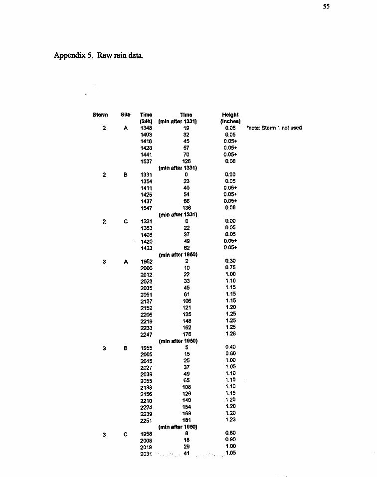
ss
Appendix 5. Raw rain data.
Storm Site nme nme Height (24h) (min after 1331) (Inches)
2 A 1348 19 0.05 *note: Storm 1 not used 1403 32 0.05 1416 45 0.05+ 1428 57 0.05+ 1441 70 0.05+ 1537 126 0.08
(min after 1331) 2 B 1331 0 0.00
1354 23 0.05 1411 40 0.05+ 1425 54 0.05+ 1437 66 0.05+ 1547 136 0.08
(min after 1331) 2 c 1331 0 0.00
1353 22 0.05 1408 37 0.05 1420 49 0.05+ 1433 62 0.05+
(min after 19!50) 3 A 1952 2 0.30
2000 10 0.75 2012 22 1.00 2023 33 1.10 2035 45 1.15 2051 61 1.15 2137 106 1.15 2152 121 1.20 2206 135 1.25 2219 148 1.25 2233 162 1.25
2247 176 1.28 (min after 19!50)
3 B 1955 5 0.40
2005 15 0.80
2015 25 1.00 2027 37 1.05
2039 49 1.10 2055 65 1.10
2138 108 1.10
2156 126 1.15
2210 140 1.20
2224 154 1.20
2239 169 1.20
2251 181 1.23 (min after 19!50)
3 c 1958 8 0.60
2008 18 0.90
2019 29 1.00
2031 41 .1.05

56
2044 54 1.05 2100 70 1.05 2145 115 1.08 2200 130 1.15 2213 143 1.15 2228 158 1.18 2242 172 1.18 2256 186 1.18
(min after 1220) 4 A 1221 1 1.50
1232 12 1.58 1245 25 1.58 1257 37 1.60 1345 85 1.60 1400 100 1.60
(min after 1220) 4 B 1224 4 1.50
1235 15 1.53 1248 28 1.53 1301 41 1.53 1350 90 1.53
(min after 1220) 4 c 1228 8 1.48
1239 19 1.48 1252 32 1.48 1305 45 1.48 1355 95 1.49
(min after 1720) 5 A 1729 9 0.02
1747 27 0.02 1814 54 0.02 1834 74 0.02 1846 86 0.05 1858 98 0.05 1911 111 0.05
(min after 1720) 5 B 1733 13 0.02
1752 32 0.02 1818 58 0.02 1838 78 0.05 1851 91 0.05 1902 102 0.05 1916 116 0.05
(min after 1720) 5 c 1737 17 0.02
1755 35 0.02 1821 61 0.02 1842 82 0.05 1854 94 0.05 1906 106 0.05 1918 118 0.05
(min after 2000)
6 A 2005 5 0.55 2019 19 0.60 2059 59 0.63
(min after 2000)
6 B 2011 11 0.60 2021 21 0.60 2102 62 0.63
(min after 2000)
6 c 2014 14 0.60 2024 24 0.60 2106 66 0.63

57
(min after 0830) 7 A 835 4.75
915 0.30 emptied 927 0.35 1011 0.62 1116 0.85 1123 0.85 1343 0.15 kids suspected to have dumped gauge 1431 0.15 1510 0.15 1550 0.15 1632 0.15
(min after 0830) 7 B 840 4.75
918 0.30 emJXjed 931 0.38 1016 0.62 1053 0.75 1127 0.85 1347 1.25 1435 1.25 didn, read carefully enough? 1514 1.23 1554 1.23 1636 1.23
(min after 0830) 7 c 830 4.00
922 0.33 emptied
935 0.40 1021 0.60 1046 0.66 1131 0.80 1351 1.10 1440 1.10 1518 1.10 1559 1.10 1643 1.10

58
Appendix 6. Weights of centrifuge tubes measured three times during TSS analysis. Mean difference was approximately± 0.003 g, within the detection limits of the balance .
. :- :i:-:~ ... -::-: ;.;. ·-:·· · .. : :. -~ >: . ' .. ·-:·.· .. -·· . --~-:::~;;~~ -~\-~:~:-__ --:~~~~:.::~+--~~-~--:~- ~-<~~~~::..;..: ... _ {_-:~:-.:---;~.-----'---"•··'·-"-'-··
....... ··· .
.•• __ ...J,.._,,-_ ..;. .. o -· -::·-~' '. \L':,
_ :: _r ____ : __ .:.n~:71L .. h·,-_~ 111.1', . .1/..?/S: .. :. ... :. ___ c .. 2'l.~----~'o.:_. o.""-~- .. ' -·------- 9.. . ; .. H.J~f:•" ___ _:. 'il~~zs. /.1:"'!3.~= .. ~~~- ~-c C)LS.· ... ll .. ~ ..... · ... __ . --•
.. · •. -•• _.:.:~. • .. :... ;~~;:••· _: J:~!~~ ~~t~f·•.:ya~:~:i~=::=~~-~-:·.•'• .. ·_ .... ~ .. ; ...... ~.:rz. .. _·_ -~:.:tl~':sr;;.: :~ JL-{g~o _,t/. ... <b. :7: ..... 4 'P_jh<:1"A(M;f:...IP.Qr
. ~--· .:/3_ : ___ ;:]1.'-7~3 .... ll~T~.1.~_/(~'lrt.£;' ........... .-.... :. :.: ... ' ........... : .. . . .. . . ., .· 1/. 7.Z] ..
. , .. ~ ....... :.JY ... : ___ f}/1l'L .... -.~·-·· .. · .. J/.723., .. -~-- -- .· --- --··: ............ .
·.. .. .. : ;!· -~::_·_ ~:~r .. _ j t~~ -;gz ::;- ~- ..... __ . _ ... . . ... . c •
....... >Fl . :1r;i7.~.7-.:~--------·Jt !f'h.>":. !/i .. 2J.1£.. -- ..... . ' ·. f . . . I ; . i . 11. Olt. J ~ C) '.1.:. . . ~-~~~,;! :: . -}~.:{~L .~::· -J~-.~~t4~~~~~· _- •..•... ·•·~ ~.- ... ·.. . . .. . :-
.• -~~~:_ ~ ~····· ·.!1!'~ • _u;.s~~~f '•5i~T··. . . •. -•. · .... =····- ~:- -~~~ .•.•. ~ . . : -· .·.-.: - ··- : .... ~ - ·-··..: ~

59
Appendix 7. Relationship of SPM concentration to total turbidity.
SPM Concentration vs Total Turbidity
- I• Sfte A 11 Sfte 8 • Site C I ~ 3500 -§, 3000 y = 0.9362x + 132.48 • 1'.3 -s::: 2500 • 0 1'.1 ;:: 2000 ~ e •• • - •• s::: 1500 •'•· • •• 13 Cl) • u 1000 c • s::: ... ,. . Ill 0 0 500
M~ :E • c. 0 en 0 500 1000 1500 2000 2500 3000
Total Turbidity (NTU)
SPM concentration and total turbidity were positively related. The relationship of sediment concentration to total turbidity was visually similar among all three sites. Data were pooled to establish an overall correlation coefficient. There was a positive correlation of SPM concentration versus total turbidity plot with statistical significance (r= 0.78, n=136, p<O.OS). Eq. 4 describes the regression line
y = 0.9362x + 132.48 eq. (4) - j .. '
where: Y was SPM concentration, and x was total turbidity.

60
Appendix 8. Total turbidity (NTU) versus duration (min) at each site for each storm.
300
~ 250 :I 1-
~200 ~
~ 150 :::1
!: 100 J9 0 1-
50
0 0
Stonn 1
50 100 Duration (min)
Storm 3
25 50 75 Duration (min)
Stonn 5
-.-site A
--SIIeB
_._SitBC
150
_._Site A
-e-siteB
_._SiteC
100
2500 .....------------,
s 2000
~ ~ 1500 :2 .a ~ 1000 ;;
-.-s~eA
--~eB
....,_SiteC
~ 500 IT"''tjt;i;:~!.;::?"'<;:...
0 100 200 300 400 500 Duration (min)
Storm 2 2500
s 2000 1-~ ~ 1500 ....,._Site A .., i3 --SiteB :; 1000 _,._SiteC 1-
~ 1- 500
0 0 50 100 150 200
Duration (min)
Storm 4 3000 ..---------------,
s 2500 1-
~2000 ~ :g 1500 s !: 1000 ~ 1- 500
-.-sHeA --SiteS
-.-Sitec
25 50 75 Duration (min)

61
Appendix 9. Sediment types as a fraction of total turbidity at each site for each storm. The thickness of each shaded area indicated percent contribution to the total turbidity attributed to sand, silt, and clay.
storm 2B Selimort T)pes SID!m 411 Sedlmont Typ ..
~ ·~,_-------, ===:rl ~ ~0 Jr~(~ f 'WI II I fw ~~~ .... ~ .. ~~-~
-("*'1
Slomi4C Sadlmont Types
~ ·=~ cCioyllllU)
f :: c&a~l - ..... (HI\J)
.. Ill<
.. ~ .,. . "' Drur.liontmfn,
Storm 8A Sediment Types 51Dnn7A Sedlmont'!'ypea
~ ·-s .... DO.,fll\l) .... DSIIf<TU)
f ~ l~--~) l ·=~~DO.,fll\l) f - D .. fll\1)
~ ·--CIIN) () ~ ol- .,.
~ <>~~ ·P-1' Ol.ndon Cmlnt
_..,_, Storm Ill SedlmontTypos Stonn 711 S.dlmont Typos
~ ·-~ = 1r .. (~) f <~~~< cs.t~~~NJ - ..... ~, .,.
l ·=~;::;;Jt'~~ f - DSilfll\l) ~ ._,~,
.. (> ~ ~ ~ ~ " 4- ~ .. .,p ~ Dt.nll on tmln)
Dw-.dot~ pnln)
SIDnn SC Sediment Typos S1Dnn 7C Sadl-nt Typos
~ ·-~ = 11:0.,(1<1\1) f ..,. DSiltfflV) ""' ..... (1<1\1) Ill<
"i'-911'<1' .. ' ........ (ln ..
~ ·::~ f
.... DO.,fll\l)
- ~~SII~) ~ ..... (HI\J)
"\ i} -~ 4' ,p'>
Durwlontlnlnl
62
Appendix 10. Critique and appropriateness of statistical tests used.
In order to detect differences among sites, data were ranked according to storm in
an attempt to eliminate the large variation among storms. Because storms ranged from
small drizzles to a hurricane, there was much variation among storms that were likely to
have masked differences among sites. The variables of interest, or treatments, were sites,
not storms. Thus, storms were blocked to eliminate their effect on the comparison of
sites. The specific statistical test used was Friedman's non-parametric ANOVA for
randomized blocks without replication. This test ranks each variate (Site) within each
block (Storm) (Zar 1999). For instance, the storm-wise SPM yield was ranked among
sites during a particular storm, assigning the site with the lowest value of SPM yield a 1
and the highest value a 3. This was done for every stollil, and the sum of the squares of
the rank sums at each site were used to compute a statisticr, and compared to critical
value of chi square for statistical significance (Zar 1999).
In the current study, it was only of interest whether there were differences among
sites. Specific absolute values were not as important as the relative trends of the sites.
Most of the assumptions of an ANOVA were avoided by using non-parametric statistics
(Sokal & Rohlf 1981 ). Two assumptions that still held were sampling at the site was
random according to the total distribution of possible samples representative of that site
wtder that specific condition. and sampling was independent. Samples were indeed
random. For instance, a sampling occasion at Site A had an equal chance of having a
high, low, or intermediate value on the distribution of possible sample values
representing that site (Gowan, pers. comm.). In other words, it was random as to how

63
representative was that specific sample of Site A during that particular stonn. Samples
were also independent of each other. Whether a sample taken at Site A was on the high
or low end of the distribution of possible samples taken at the site on that occasion did
not affect the location on the sampling distribution at Site B (Gowan, pers. comm.).
If Friedman's test found significant differences, a non-parametric equivalent of
Tukey's test of honestly significant differences (HSD) was used with ranked data to
detennine specifically which sites were different. Multiple comparisons in general
compare differences among means between all possible pairs (Sokal & Rohlf 1981 ). In
the case of the test used, it is conservative in the fact that it has low power to detect
differences (Gowan, pers. comm. ). In the current study, the assumption was made of
preference for Type II error over Type I. The null hypothesis was only rejected when
there were definite differences, and there was error by failing to reject the null hypothesis
when it was actually false (Sokal & Rohlf 1981 ). In other words, the multiple
comparisons test used in the current study fails to detect differences when they may
actually exist. Thus, when differences were found, they were probably real differences.
The multiple ·comparisons test in the current study tests for significance by
comparing the calculated q statistic, q, to the critical value for three variates (sites) with
a=0.05 (Zar 1999). The q statistic is calculated for each pair using the following
equation:
q = (Rs-Ra) SE1 eq. (4)
where: q is the pair-wise q statistic, R8 is the larger rank sum of the pair, R8 is the
smaller rank sum of the pair, and SE is the standard error.
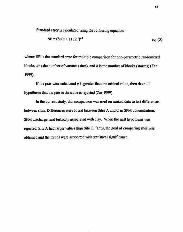
64
Standard error is calculated using the following equation:
SE = (ha(a + 1) 12"1)0·5 eq. (5)
where: SE is the standard error for multiple comparison for non-parametric randomized
blocks, a is the number of variates (sites), and b is the number of blocks (storms) (Zar
1999).
If the pair-wise calculated q is greater than the critical value, then the null
hypothesis that the pair is the same is rejected (Zar 1999).
In the current study, this comparison was used on ranked data to test differences
between sites. Differences were found between Sites A and C in SPM concentration,
SPM discharge, and turbidity a.Ssociated with clay. When the null hypothesis was
rejected, Site A had larger values than Site C. Thus, the goal of comparing sites was
obtained and the trends were supported with statistical significance.

65
Brief Autobiography
John R Jordan. Jr., son of John and Brenda Jordan was born on June 25, 1976 in
Richmond, Virginia He grew up in Chesterfield County, Virginia and attended
Midlothian High School in Midlothian, Virginia After graduating in 1994 he continued
his education at Randolph-Macon College. He graduated in May, 1998 with a Bachelor
of Science degree in Biology and Environmental Studies. He enrolled in graduate school
at University ofRichmond in Fall1998. This thesis completes his work for the Master of
Science degree in Biology. He is currently employed as an environmental scientist at
Jordan Consulting Engineers in Richmond, Virginia