Embed Size (px)
Citation preview

IESE Business School-University of Navarra - 1
STRATEGIC COMPLEMENTARITY, FRAGILITY, AND REGULATION
Xavier Vives
IESE Business School – University of Navarra Av. Pearson, 21 – 08034 Barcelona, Spain. Phone: (+34) 93 253 42 00 Fax: (+34) 93 253 43 43 Camino del Cerro del Águila, 3 (Ctra. de Castilla, km 5,180) – 28023 Madrid, Spain. Phone: (+34) 91 357 08 09 Fax: (+34) 91 357 29 13 Copyright © 2011 IESE Business School.
Working Paper WP-928-E Rev. June 2014

IESE Business School-University of Navarra
The Public-Private Sector Research Center is a Research Center based at IESE Business School. Its mission is to develop research that analyses the relationships between the private and public sectors primarily in the following areas: regulation and competition, innovation, regional economy and industrial politics and health economics.
Research results are disseminated through publications, conferences and colloquia. These activities are aimed to foster cooperation between the private sector and public administrations, as well as the exchange of ideas and initiatives.
The sponsors of the Public-Private Sector Research Center are the following:
� Ajuntament de Barcelona � Departament d’ Economia i Coneixement de la Generalitat de Catalunya � Departament d’ Empresa i Ocupació de la Generalitat de Catalunya � Diputació de Barcelona � Fundació AGBAR � Institut Català de les Empreses Culturals (ICEC) � PricewaterhouseCoopers � Sanofi � FGC
The contents of this publication reflect the conclusions and findings of the individual authors, and not the opinions of the Center's sponsors.

1
Strategic Complementarity, Fragility, and Regulation
Xavier Vives*
IESE Business School
Revised June 2014
ABSTRACT
Fragility is affected by how the balance sheet composition of financial intermediaries, the precision of information signals, and market stress parameters all influence the extent of strategic complementarity among investors’ strategies. A solvency and a liquidity ratio are required to control the likelihood of insolvency and illiquidity. The solvency requirement must be strengthened in the face of increased competition, whereas the liquidity requirement must be strengthened under more conservative fund managers and higher penalties for fire sales. Greater disclosure may aggravate fragility and require an increase in the liquidity ratio, so regulators should establish prudential and disclosure policies in tandem.
Keywords: crises, illiquidity risk, insolvency risk, prudential policy, leverage ratio, liquidity ratio, disclosure, transparency, opaqueness, panic, run, derivatives market, shadow banking, sovereign debt.
JEL codes: G21, G28
* An earlier version of this paper was circulated under the title “Stress, Crises, and Policy”. I am grateful to Elena Carletti, Gabriella Chiesa, Falco Fecht, Todd Keister, Arvind Krishnamurthy, Frédéric Malherbe, Jean-Charles Rochet, Philipp Schnabl, Anatoli Segura, Javier Suarez, Wolf Wagner, and to participants at the following conferences: 2010 ESMFM at Gerzensee, 2010 FIRS, 2011 Banca d'Italia-CEPR, 2011 EFA and EEA, 2011 CAREFIN, 2012 CESifo-Bundesbank, 2013 Barcelona GSE Summer Forum, 2013 DFG/MPI at Bonn, 2013 EBC at Tilburg, and 2014 IESE-CEPR-ERC Banking Conference, as well at seminars at the New York Fed, Northwestern Finance, the University of Oslo, IIES (Stockholm University), and EIEF for helpful comments, and to Rodrigo Escudero and Jorge Paz for able research assistance. The research leading to these results has received funding from the European Research Council under the European Advanced Grants scheme, Grant Agreement no. 230254 as well as from project ECO2011-29533 of the Spanish Ministry of Education and Science at the PPSRC of IESE.

2
Introduction
In a crisis situation—and the recent financial crisis is a good example—things seem to go
wrong at the same time, and an adverse shock is magnified by the actions and reactions of
investors.1 In particular, liquidity evaporates when short-term investors rush to exit, after which a
solvency problem may arise. The financial system’s fragility has been attributed to the increased
reliance, by investment banks and commercial banks both, on market funding. The demise of
Northern Rock in 2007, of Bear Stearns and Lehman Brothers in 2008, and of IKB and Hypo
Real State in Germany are all cases in point: each institution’s short-term leverage was revealed
as a crucial weakness of its balance sheet.2 In this context it has proved difficult to disentangle
liquidity risk from solvency risk. The debate has revolved around the opaqueness of financial
products, the impact of public news (as provided by, e.g., the ABX index on residential
mortgage–backed securities, public statements about the health of banks,3 and stigma associated
with known borrowing from the discount window),4 and the influence of derivative markets on
stability. A disclosure requirement such as the FAS rule 157, a mark to market accounting
legislation implemented in 2007, has been credited with aggravating the consequences of the bust
of the real state bubble since it forced banks to disclose large losses on their portfolios of
mortgage-based securities.5 The crisis has put regulatory reform in the agenda. Policy makers and
regulators are struggling with how to reform capital requirements, introduce liquidity
requirements, and improve disclosure requirements.6
1 See Brunnermeier (2009) and Krishnamurthy (2009). 2 In June 2007, wholesale funds represented about 26% of liabilities in Northern Rock (Shin 2009); before the
crisis, short-term financing represented a high percentage of Lehman Brothers’ total liabilities (Adrian and Shin 2010). Washington Mutual suffered the withdrawal of $16.5 billion worth of large deposits just in the two weeks before its collapse (according to the Office of Thrift Supervision). See also the evidence in Ivashina and Scharfstein (2010).
3 Such was the case for the run on IndyMac Bancorp in June 2008, which followed shortly after public release of letters by Senator Schumer of the Banking Committee.
4 See Armantier et al. (2011). 5 See the testimony of former FDIC chairman W. Isaac before the Subcommittee on Capital Markets, Insurance,
and Government-Sponsored Enterprises, U.S. House of Representatives Committee on Financial Services of March 12, 2009.
6 See, for example, Financial Services Authority (2009) and Bank for International Settlements (BIS; 2009). The Dodd-Frank Act of 2010 introduced a leverage limitation for financial holding companies larger than a certain size. The BIS proposed two new liquidity ratios: a liquidity coverage ratio to cover short-term cash outflows with highly liquid assets; and a net stable funding ratio to cover required stable funding with available stable funds. Bear Stearns was regulated by the SEC and was subject to a liquidity requirement—one, however, that proved ineffective in the crisis.

3
Lack of attention to liquidity issues is believed to be part of why policy responses were
inadequate during the Great Depression. Friedman and Schwartz (1963) argue that many bank
failures arose out of panics—that is, because of liquidity rather than solvency problems. This
explanation is consistent with the “self-fulfilling” view of crises described by Bryant (1980) and
Diamond and Dybvig (1983), although that view of crisis has been disputed by Gorton (1985,
1988) and others.7 During the Great Recession triggered by the subprime mortgage crisis in 2007,
liquidity issues have received a great deal of attention. For example, it has been claimed that the
sovereign debt crisis in the euro area is driven by a self-fulfilling panic.8 Yet clearly the euro area
also has important solvency problems. In general, the evidence points to issues of solvency and
liquidity being intertwined in any crisis.9 A corollary to these observations is that regulations
should address both solvency and liquidity concerns.
This paper presents a general framework for studying crises as well as an initial
exploration of how regulations addressing solvency, liquidity, and transparency should be related.
The key novel ingredient is showing how the degree of strategic complementarity of investors’
actions is the crucial parameter not only for characterizing equilibrium and fragility (where the
latter is understood as equilibrium sensitivity to small changes in parameters, including the
possibility of discrete jumps within a changing equilibrium set) but also for policy analysis. More
specifically, the paper relates information structure, balance sheet, and market parameters to the
degree of strategic complementarity of investors’ actions and fragility. Main findings are that (i)
better public information increases liquidity problems when fundamentals are weak; (ii) liquidity
requirements should be tightened in the presence of higher disclosure levels, if assets are opaque
and investors conservative; and (iii) solvency requirements must be strengthened in the face of
increased competition.
7 Gorton (1988) disputes the view that crises are panic driven with a study of crises in the US National Banking
Era; he concludes that the crises were predictable (see also Schotter and Yorulmazer 2009). The “information” view of crises has been developed by, among others, Chari and Jagannathan (1988), Jacklin and Bhattacharya (1988), and Allen and Gale (1998). Postlewaite and Vives (1987) present a model with incomplete information about the liquidity shocks suffered by depositors that features a unique Bayesian equilibrium in which there is a positive probability of bank runs. In that model, there is no uncertainty about the fundamental value of the banks’ assets and there are no solvency problems.
8 See De Grauwe and Ji (2013). 9 Calomiris and Mason (2003) also dispute the analysis of Friedman and Schwartz (1963); the latter authors
conclude that some episodes of 1930s US banking crises can be explained by deteriorating fundamentals whereas others can be explained by the domination of a panic component (as in January and February of 1933). Starr and Yilmaz (2007) claim that both fundamentals and elements of panic figure into the dynamics of bank runs in Turkey.

4
In the model considered here, investors must decide whether to keep an investment or run
(sell it or withdraw). The investment may be in a currency, a bank, or short-term debt. A financial
intermediary will be our leading example. The model is based on the theory of games with
strategic complementarities and incomplete information; an example are the “global games” of
Carlsson and van Damme (1993) and Morris and Shin (1998).10 I provide a general framework
that bridges the panics and fundamentals views of crises, characterizes illiquidity and insolvency
risk, and nests among others, the models of Morris and Shin (1998, 2004), Rochet and Vives
(2004), and Bebchuk and Goldstein (2011). This paper delivers predictions under both unique
and multiple equilibria; describes how a regulator should set solvency and liquidity requirements
in conjunction with requirements concerning degree of transparency, thereby reducing the
likelihood of both insolvency and illiquidity; and applies the model to interpret the 2007 run on
structured investment vehicles (SIVs). The model can also be applied to sovereign debt crises and
currency attacks.
I shall characterize how the degree of strategic complementarity depends on the balance
sheet composition of a financial intermediary, parameters of the information structure of
investors (i.e, the precision of public and private information), and the level of stress indicators in
the market. Strategic complementarity increases with a weaker balance sheet (higher leverage),
with greater competitive pressure for funding, and with higher fire-sale penalties for early asset
liquidation. All those parameter changes make the resistance level that must be overcome by the
mass of running investors in order for a run to succeed less sensitive to the fundamentals. This
diminished sensitivity of the resistance threshold induces an investor to react more strongly to
changes in the strategy of other investors. Furthermore, strategic complementarity also increases
when public information is more precise and when private information is less precise (when it is
worse than public information). These information factors render an investor less uncertain about
the behavior of others, which in turn leads that investor to react more strongly to any change in
the decision rules of other investors.
A weaker balance sheet or an increase in stress indicators makes a crisis more likely, and
there is a range of fundamentals that indicate coordination failure from the viewpoint of the
10 See Vives (2005) for a general overview. The importance of strategic complementarities in macro models is
highlighted by Cooper and John (1988). Liu and Mello (2011) apply the global games methodology to study the behavior of hedge funds in the crisis.

5
institution under attack (i.e., when it is solvent but illiquid). A key observation is that the effect of
bad news—say, a public signal about weak fundamentals—is magnified when strategic
complementarity is high. This means that the public signals coming from, for instance, a
derivatives market could be destabilizing, and the more so the more precise they are since they
generate a larger range of illiquidity. These results are consistent with the 2007 run on SIVs
(structured investment vehicles) and ABCP (asset-backed commercial paper) conduits featuring a
high level of strategic complementarity among investors given that leverage was high and the
crisis heightened fire-sale penalties. The results are also consistent with the potential destabilizing
effect of FAS rule 157, making banks’ balance sheets more transparent at a time of stress, as well
as with the practice of clearinghouses in the US National Banking Era (1863-1913) of suspending
the requirement for banks to publish their financial statements during a panic situation.11
The policy message that follows from the analysis presented here is that a regulator must
pay attention to the balance sheet composition of financial intermediaries—in particular, the
regulator should manage the ratio of liquid assets to unsecured short-term debt as well as the
short-term leverage ratio (ratio of unsecured short-term debt to equity or, more generally, stable
funds). Those two ratios can be used to control the probability of insolvency or illiquidity, and
they are partially substitutable. The reason why they are not perfectly substitutable is that a
solvency ratio is more effective in controlling the probability of insolvency while a liquidity ratio
is more effective in controlling the probability of illiquidity. The liquidity requirement is needed
when fire-sale penalties are high and investors are conservative, the regulator is not willing to
allow a large probability of illiquidity, and the precision of public information high enough
relative to the precision of private information. This paper establishes that, in a more competitive
environment (i.e, with higher returns offered on short-term debt), the solvency requirement
should be strengthened. This means that financial liberalization should not proceed without
increased solvency requirements, in contrast with the practice contributing to such banking crises
as the US S&Ls in the 1980s. The expectation of turbulent environments, high fire-sale penalties,
and conservative investors calls for the liquidity requirement to be strengthened but for the
solvency requirement to be relaxed. Finally, when potent public signals are anticipated (e.g.,
introduction of a derivatives market such as the ABX index, or a new disclosure requirement
such as the FAS rule 157), illiquidity may increase; then a strengthened liquidity requirement
11 See Gorton (2010).

6
might be necessary, especially when assets are opaque. These results have implications also for
the design of prudential policy with respect to sovereign debt.
The paper proceeds as follows. Section 1 sets up a framework of analysis with the basic
model; this section also characterizes the equilibrium and discusses its links to both strategic
complementarity and its comparative statics properties. The model is specialized to a bank run, a
leading example that illustrates the results. Section 2 deals with regulation of a financial
intermediary, and Section 3 extends the model for application to the 2007 run on SIVs. Section 4
covers connections in the literature as well as empirical issues. Section 5 considers other
applications, including a sovereign debt run, and Section 6 offers some concluding remarks. The
Appendix gives proofs of all the propositions.
1. A stylized crisis model: The link between strategic complementarity and fragility
This section presents a general framework for analysis, including the game played by
investors. Also presented are characterizations of the equilibrium and its comparative static
properties.
1.1. The investors’ game
Consider the following binary action game among a continuum of investors with unit
mass. The action set of player (investor) i is � �0,1 , where 1iy � is interpreted as “acting” and
0iy � as “not acting”. Possible actions include attacking a currency, refusing to roll over debt,
participating in a run on a bank or SIV, and declining to renew a certificate of deposit in the
interbank market.
Let � �1 1, ;iy y� � � � and � �0 0, ;iy y� � � � denote, respectively, the payoffs to
acting and not acting; here y is the fraction of investors acting and is the state of the world.
The differential payoff to acting is 1 0 0B� � � � if � �y h � and is 1 0 0C� � � if
� �y h , where � �h is the resistance function—that is, the critical fraction (of investors)
above which it pays to act. These relationships are summarized in the following matrix.
� �y h � � �y h �
1 0� � 0B � 0C

7
It pays to act if enough investors act and so resistance is overcome (i.e., if � �y h � ). Let
p be the probability that enough investors act. Then there is a critical success probability p of
the collective action such that an agent is indifferent between acting and not acting:
� � � �1 0pB p C� � . This probability is ( )C / B C� � � , � �0,1� � , the ratio of the cost C of
acting to B + C, the incremental benefit of acting with success versus acting with failure. An
investor will act if his assessed probability of successful mass action exceeds � . We shall assume
that � �h � is strictly increasing, is smooth on � �, ��
, crosses 0 at � �(with lim 0)h �� ���
,
and crosses 1 at � � .12
The investors’ game is one of strategic complementarities because the differential payoff
to acting 1 0 � � is increasing in the mass of players acting y .13 Suppose that , the state of the
world, is known; in other words, we have a game of complete information among investors. It
follows from the stated payoffs that if �
then acting is a dominant strategy but if � � then
not acting is a dominant strategy. For �, ���
�� there are multiple equilibria, including one in
which all investors act and one in which no investors act. The threshold �
can therefore be
understood as an institution’s “solvency” threshold (when �
, the institution is overrun even
if no investor attacks). Similarly, � is the “supersolvency” threshold (when � � , the institution
resists even if all investors attack).
Since this is a game of strategic complementarities, there is both a largest and a smallest
equilibrium—that is, we have extremal equilibria. The largest equilibrium is a “run” equilibrium
in which only “supersolvent” institutions survive: 1iy � for all i if � , and 0iy � for all i if
� � . The smallest equilibrium is a “no-run” equilibrium where only “solvent” institutions fail:
1iy � for all i if �
, and 0iy � for all i if ��
.14
From now on I consider an incomplete information version of the game where investors
have a Gaussian prior on the state of the world � �1,N � � � and investor i observes a private
12 Note that this allows the function � �h � to be discontinuous at �
� with � � 0h �
� and � � 0h � for
�
. 13 In a game of strategic complementarities, the marginal return of a player’s action is increasing in the level of
the rivals’ actions. As a result, best replies are monotonically increasing; see Vives (2005). 14 Note that both equilibria are (weakly) decreasing in ; the reason is that 1 0� � is decreasing in .

8
signal i is �� � (with Gaussian noise that is independent and identically distributed,
� �10,i N �� � � ).15 It is worth noting that the prior mean � of can be understood as a public
signal of precision � ; under this interpretation, � can be negative.
The model encompasses several crisis situations studied in the literature: currency attacks
(Morris and Shin 1998), loan foreclosures (Morris and Shin 2004), credit freezes (Bebchuk and
Goldstein 2011), and bank runs (Rochet and Vives 2004). I next present the bank run model,
which will underpin the policy exercise described in Section 2. Other applications of the model
framework are examined in Section 5.
1.2. The bank run model
Consider a bank run model that fits into the general framework already introduced (based
on Rochet and Vives 2004). Traditional bank runs resulted from massive withdrawals of deposits
by individual depositors. Modern bank runs result from the nonrenewal of short-term credit in the
interbank market; examples include the case of Northern Rock, the 2007 run on SIVs, and the
2008 run by short-term creditors on Bear Stearns and on Lehman Brothers.
Consider a market with three dates: 0 1 2t , ,� . At date 0t � , the bank has its own funds
E (including such stable resources as equity, long-term debt, and even insured deposits) as well
as uninsured short-term debt (e.g., uninsured wholesale deposits and certificates of deposit, CDs)
in amount 0 1D � . These funds are used as cash reserves M and also to finance risky investment
I. So at 0t � , the balance sheet constraint is 0E D I M� � � . The returns I on these assets are
collected at date 2t � ; if the bank can meet its obligations, then the short-term debt is repaid at
face value D and the bank’s equity holders receive any residual amounts. Investors are also
entitled to the face value D if they withdraw in the interim period 1t � . Let m M D� be the
liquidity ratio, D E�� the short-term leverage ratio, and 0d D D� the return on short-term
debt.16
15 The incomplete information game is referred to in the literature (e.g, Carlsson and van Damme 1993) as a
“global game”. 16 The distinction of stable funds within liabilities is made also in a BIS (2009) document that addresses liquidity
risk. In fact, the two liquidity ratios proposed by BIS are equivalent in our simple formulation: the BIS short-term funds ratio would correspond to m and the BIS net stable funds ratio to E I . Note also that leverage
� �D D E� equals � �11 1 � � and is monotonic in � .

9
Fund managers (recall that we view them as being on a continuum) make investment
decisions about whether or not to extend short-term debt to the bank. At 1t � each fund
manager, after observing a private signal regarding the future realization of , decides whether to
cancel ( 1iy � ) or to renew ( 0iy � ) her position. The claims on the bank at 1t � are yD , since
y is the mass of “acting” fund managers. If yD M� then the bank can meet its payments only
by selling some of its assets17 in a secondary market. The value of bank assets that are sold early
reflects a fire-sale penalty 0� � (i.e., retrieving only � �1 �� for each unit invested).18
A fund manager is rewarded for making the right decision (viz., withdrawing if and only
if the bank fails). The cost of canceling the investment is C , and the benefit from getting the
money back or canceling when the bank fails is B B C� � . The payoffs define (as in Section
1.1) the critical probability of failure � �C B C� � � , above which a fund manager does not
renew credit. What is crucial is that investors and fund managers both adopt, for whatever reason,
a behavioral rule of this type: Cancel the investment if and only if the likelihood of bank failure
exceeds some threshold � . This rule is followed also by investors who expect a fixed return
when withdrawing but expect nothing if they do not withdraw and the bank subsequently fails,
and there is a (small) cost to withdrawing. Larger values of � are associated with less
conservative investors, from which it follows that risk management rules may influence � .19
Suppose that all fund managers renew credit to the bank (i.e., 0y � ). Then there are no
fire sales at 1t � and the bank fails at 2t � if and only if M I D� or � �D M I � �
.
Hence �
can be viewed as the bank’s solvency threshold because, below that level, the bank fails
even if all fund managers renew credit.20 Given the balance sheet constraint, we have
17 Or borrowing against collateral in the repo market. 18 The parameter � could be related to the Libor–OIS spread (a measure of the difference between interbank rates
and the rates paid on overnight index swaps, instruments that are not exposed to the default risk of intermediaries), which increased substantially both in August 2007 (start of the crisis) and September 2008 (collapse of Lehman Brothers). In the case of secured collateral, � captures the haircut required. Haircuts on asset-backed securities rose dramatically after the collapse of Lehman Brothers (see e.g. Gorton and Metrick 2010).
19 According to Krishnamurthy’s (2010) review of debt markets during the crisis, investor conservatism is an important determinant of short-term lending behavior.
20 The solvency threshold is related to what the FDIC calls (as part of its CAMELS assessment) the “Net Non-core Funding Dependence Ratio”, which is computed as noncore liabilities less short-term investments divided by long-term assets.

10
� � � �1 11 m d m � � ��
.21 Suppose now that, at 1t � , the bank must liquidate some (but not
all) assets, � � 11M I yD M � � � � � . In this case, the bank will fail at 2t � if and only if
� � � � � �1 1I yD M y D � � (or, equivalently, if and only if
� �� �1y I M D D � �� � � ).22 Under the balance sheet constraint, we derive an equivalent
inequality that identifies bank failure for ��
:
� � � �1 1d my h m
�
� � � �
��
;
for �
we have � � 0h (see Figure 1). Note that, for � �1 � � � ���
, the bank does not
fail even if fund managers do not renew credit (i.e., 1y � ) because � � 1h �� . Therefore, � is
the “supersolvency” threshold. We have that � � 0h m � ��
and that h is decreasing in � and in
d . If 1 11 0d � then, since � � � �1 1sign sign 1m d � � � ��
, it follows that h is
increasing in m.23
21 Note that 1 1 0d m I D � � �� for a positive risky investment. 22 If � � 11M I yD �
� � then the bank fails at 1t � . It is worth noting that, whereas the US liquidity requirements of broker-dealers are based on unsecured funding, the demise of Bear Stearns followed from its failure to renew secured funding. See the US Securities and Exchange Commission’s report on its oversight of Bear Stearns “and related entities” (SEC 2008).
23 We have � �1 1 0h m � � � � � � � because 1 �
is implied by 1 11 0d � and then
� �1 1 � � � ��
.

11
Figure 1. The resistance function in the bank runs model: � � � � � �1 1 1h m d m � � � � �
� if
��
, and � � 0h if �
. Above the bold line � �y h � for ��
and the bank fails.
For the balance sheet of a financial intermediary, it is normally the case that 1 11 0d � . Indeed, the ratio of (uninsured) short-term debt to stable funds (equity, long-
term debt, and insured deposits), D E�� , is below 1 for commercial banks. Although � is above
1 for investment and wholesale banks, typically 1 0 9d . � (given interest rates not exceeding
10%) and so we would need 1 0 1. � or 10�� to have 1 11 0d �� .24 For a typical SIV,
� < 1.25
An alternative interpretation of the bank model would be to consider the aggregate
banking sector of a country and treat as a macroeconomic fundamental, where all investors are
outside the banking sector. In this interpretation the ratios are the aggregate ratios, we abstract
from any externalities among banks, and a crisis is a crisis of the banking sector.
24 See Figure A in the Appendix for data on some US banks. 25 According to the April 2008 Global Financial Stability Report of the International Monetary Fund (IMF), the
typical funding profile of an SIV in October 2007 was 27% in asset-backed commercial paper and the rest in medium-term notes and capital notes. That profile would translate into a value of � = 0.34.

12
1.3. Equilibrium and strategic complementarity
In this section we return to the general model and study equilibria of the investors’ game
as well as the factors affecting strategic complementarity. We seek a symmetric equilibrium in
threshold strategies under which an investor will run (or act) if and only if he receives a signal
whose value is below a certain threshold.
In order to gain some intuition of the game’s structure, let us think in terms of the best
reply of a player � �r � to the (common) signal threshold s used by the other players. An
equilibrium then is a signal threshold s� such that � �s r s� �� . This signal threshold will imply a
critical world state �,* ���
�� , below which the “acting mass” is successful.
The best reply can be computed in two steps. Given a signal threshold s at which other
investors run, the investor computes the failure threshold such that the institution fails if and
only if ˆ : � � � �Pr ˆ ˆˆs s | h � if ��
and ��
otherwise. This yields the failure
threshold curve � �Fˆ s � , which is increasing in s . On this curve, whenever �
�, the
fraction of acting players, � �Pr ˆˆy s s |� , equals the critical fraction above which it pays to
act, � �ˆh . Now, given a failure threshold , the investor can compute the signal threshold s
below which it is optimal to run: � �Pr ˆ ˆ| s � � . That expression yields the signal threshold
curve � �Tˆs s � , which is linear with slope � � � �� � �� and increasing in , and on which the
expected payoff from acting or not acting is the same (see Figure 2 and Claim 1 in the Appendix).

13
Figure 2: Equilibrium characterization in the bank run model. Parameters: 0 5.� � ,
0 1m .� , 1 0 2. �� , 1 0 9d . � , 1� � , 0 9. ��
, 1 8. �� , 0 5.� � , 0 05.�� � , 1 3.� � .
The best-response function is the composition of the two thresholds: � � � �� �T Fˆ ˆr s s s� ,
� � � � � �1Fˆ ˆr s s � �
� � �
� � � � � � �� � �
� �� � ,
and it is is increasing. Indeed, the game is one of strategic complementarities; a higher threshold
s by others induces a player to use a higher threshold, too (see Figure 3). Equilibria are fixed
points of this best response or, equivalently, are given by the intersection points of the two curves
in space of failure and signal thresholds: � �Fˆ s � and � �T
ˆs s � .

14
Figure 3: Possible best responses of a player to the threshold strategy s used by rivals for an intermediate range of � . The lower (resp., middle, upper) plot corresponds to high (resp., intermediate, low) values of
1h .
The following proposition provides the equilibrium characterization and generalizes the
results in the literature. Let 1h denote the smallest slope of � �h � on � �, ��
.
Proposition 1.
(i) An equilibrium is characterized by two thresholds � �,s � � , where s� is the signal
threshold below which an investor acts and �, � ���
�� is the state-of-the-world critical
threshold, below which the acting mass is successful. The probability of a crisis conditional
on s s�� is � .
(ii) There is a critical � � � �0 0,1h ��
such that:
� if � � � �0h h �� �
then at the smallest equilibrium � ��
;
� if � � � �0h h � �
then � ��
for any equilibrium.
(iii) The equilibrium is unique if � � 1 2h �� � �� .
The proof of this proposition is given in the Appendix, and it exploits the game’s
monotonicity properties (i.e., the game is monotone supermodular). In this type of game there are
extremal (largest and smallest) equilibria and they are in threshold strategies. Any other

15
equilibrium is bound by the largest and smallest equilibria. The uniqueness condition
1 2h �� � �� implies that � � � � 1Fˆ ˆr' s ' s �
�
� � ��
� � . In this case the largest and the
smallest equilibrium coincide at the unique equilibrium. It is worth noting that r' is increasing
in � because � �F ˆ' s is independent of � ; hence strategic complementarity increases with
better public information. This relation ensures that � �r � crosses the 45° line only once and that
the equilibrium is unique. A sufficient condition for the existence of multiple equilibria (a
necessary condition for regular equilibria when ( ) 1ˆr' s � ) is that ( ) 1r' s � for ( )r s s� .
In sum: a necessary condition for multiple equilibria is that strategic complementarity be
strong enough; a sufficient condition is that strategic complementarity be strong enough at
relevant points (candidate equilibria). So if strategic complementarity is always moderate (case
� � 1r' � � ) then there is a unique equilibrium, but when it is not moderate there may be multiple
equilibria (see Figure 3). If 1h (the smallest slope of � �h � ) is large enough, then there is a unique
equilibrium. In the linear case, for an intermediate range of � we find that reducing 1h yields
multiple equilibria (generically, three); if 1h is reduced further then we return to a unique
equilibrium, since in that case strategic complementarity is strong but in an irrelevant range (see
Figure 3). Furthermore, if � � 1 2h �� � �� then there is always a range of � in which there
are three equilibria.26
The extent of strategic complementarity among the players’ actions depends on the slope
of the best response. The maximal value of that slope is given by 1 2h
r ' �
� �
� �
� ��
�
�� , which is
increasing in 11h . The degree of strategic complementarity will be higher whenever h is less
sensitive to (larger 11h ), the prior is more precise (larger � ), and/or the signals are imprecise
(low �� when � � � ). When 11h is large, a change in fundamentals has little effect on the
critical threshold � �h . The implication is that a change in the strategy threshold s used by
26 Indeed, changes in � move vertically the best reply, and with � � 1 2h �� � �� , there is a range with
multiple equilibria. This happens, for example, around 0 5.� � when � � 10h � , 1�� , 5��� , 5� , while the equilibrium is unique with 0 1.� � and 0 9.� � .

16
other investors leads to a larger optimal reaction owing to the greater induced change in the
conditional probability that the acting investors succeed.
Furthermore, r ' is indeed increasing in � ; with respect to �� , r ' is first decreasing (in
particular when � � � with r ' � as 0��� ) and then increasing (with 1r ' � as � �� ).
When noise in the signals is large (small �� ), a player is relatively certain about the behavior of
others and so strategic complementarity is increased. In the limit case of �� � (or with a
diffuse prior 0� � ), investors face maximal strategic uncertainty; in this case, the distribution
of the proportion of acting players y is uniformly distributed over ! "0,1 conditional on is s�� .
Yet at any of the multiple equilibria with complete information when � �, ��
� , investors face
no strategic uncertainty. For example, in the equilibrium where everyone acts, an investor has a
point belief that all other investors will act.
In short, strategic complementarity increases with less sensitivity of the resistance function to
fundamentals, with more precise public information, and with less precise private information
(when it is worse than public information).
In the bank run case, � �1 1 11h d m� � � � ; therefore, strategic complementarity among
investors is increasing in short-term leverage � , in the face value of short-term debt d , in the
fire-sale penalty � , and in the liquidity ratio m . All these factors make the resistance function
less sensitive to . Thus we see that the strength of strategic complementarity, as measured by
the maximal slope of the best response r ' , is affected by information parameters ( � and �� ), by
balance sheet structure ( � and m ), and by market stress parameters ( d and � ).
1.4. Coordination failure, illiquidity risk, and insolvency risk
At equilibrium with threshold � , there is a crisis when � . In the range �, ���� there
is coordination failure from the point of view of investors, because if all of them were to act (say,
in the case of the currency peg) then they would succeed. In the range ! �, ��
there is
coordination failure from the point of view of the institution attacked. Recall that with our bank
run model the bank is solvent but illiquid in the range ! �, ��
; that is, the bank would be spared

17
any problems if investors renewed their short-term debt, but in this range they do not and so the
bank is illiquid. We can compare these concepts graphically as follows:
The risk of illiquidity is given by � �Pr �� �
and the risk of insolvency by
� � � �� �Pr � � � � � �
, where � denotes the standard Normal cumulative distribution.
Hence � �Pr �
is the probability that the bank is insolvent when there is no coordination
failure from the bank’s perspective. The overall probability of a crisis is
� � � �� �Pr � � �� � � . Note that � � � � � �Pr Pr Pr � �� � � �
. A
crisis occurs for low values of the fundamentals. In contrast, in the complete information model
there are multiple self-fulfilling equilibria in the range � �, ��
.
1.5. Comparative statics
We shall develop the comparative statics properties of both unique and multiple
equilibria. The comparative statics results that follow hold when the equilibrium is unique and
also when there are multiple equilibria for the extremal (largest and smallest) equilibria.
Furthermore, the results hold for any equilibrium—even the unstable, intermediate one, if out-of-
equilibrium adjustment is adaptive. With best-reply dynamics at any stage after the parameter
perturbation from equilibrium, a new state of the world is drawn independently and a player
responds to the strategy threshold used by other players at the previous stage. Then a parameter
change that monotonically alters the best reply will induce a monotone adjustment process with
an unambiguous prediction. For instance, if we are at the higher equilibrium of the middle plot in
Figure 3, then an increase in 1h may induce a movement to the lower plot, in which case the best-
reply dynamics would settle at the unique (and lower) equilibrium.27 The results are stated
formally in Proposition 2. Observe that, contrary to most of the literature, the comparative statics
27 See Echenique (2002) and Vives (2005).
Insolvency Illiquidity Supersolvency
� * �

18
results presented here are not restricted to parameter configurations that determine a unique
equilibrium.
In the applications it is useful to parameterize the resistance function � �;h # , where the
parameter # represents an index of vulnerability or stress (with 0h #� � ). A larger #
signifies more vulnerability or a more stressful environment for the institution under attack, since
then there is a lower threshold for the attack to be successful. In the bank run model, for instance,
� �; 0h m # � ��
and we can identify the parameter # with � , d , � , or 1m when
1 11 0d � , since h is decreasing in all these variables.
Proposition 2 (Comparative statics). Let � � 0;h h # �
. At extremal equilibria or under
adaptive dynamics, the following statements hold.
(i) The thresholds � and s� and the probability of crisis � �Pr � are all decreasing in
� (i.e., with less conservative investors) and in the expected value of the state of the
world � ; they are increasing in the stress indicator # .
(ii) The release of a public signal � has a multiplier effect on equilibrium thresholds (i.e.,
beyond its impact on an investor’s best response), which is enhanced when � is higher.
(iii) Let 1 2/� . If � is low enough (weak fundamentals with � ��
is sufficient), then a
more precise public signal increases � , the probability � �Pr � , and the range
! �, ��
whereas a more precise private signal reduces them. If � is high enough
(strong fundamentals with � � � �1 2 1/ �� � � � � � �� is sufficient), then the results
are reversed.
Remark 1. It is immediate from part (i) of the proposition that the range ! �, ��
is decreasing
in both � and � .
Remark 2. The region of potential multiplicity � � 1 2h �� � �� is enlarged with an
increase in payoff complementarity (decrease in 1h ) and/or an increase in the precision of the
public signal in relation to the private one, �� � .
Remark 3. The conditions for the comparative statics results in Proposition 2(iii) are
sufficient but by no means necessary. When the equilibrium is unique it can be checked that part

19
(iii) can be strengthened as follows: There are thresholds ˆ� and �� with ˆ � � � such that (a)
� increases with � if and only if ˆ � � and (b) � increases with �� if and only if � �� �
(see proof in Appendix).28
Let us now apply the results of the proposition to illustrating the comparative static results in
the bank run model. First of all, in this model 0h is given by a liquidity ratio � �0,1m� . This
critical ratio m depends on the parameters of the model and in particular it increases with � .
When m m� there is always an equilibrium in which only insolvent banks fail, � ��
. For
m m , there is always a range of illiquidity, with � ��
at any equilibrium. When
1 11 0d � , the comparative statics of � , d , � , and 1m follow from those of # in
Proposition 2(i). The following statements are then immediate (see Claim 2 in the Appendix):
� The probability of insolvency � �Pr �
is decreasing in the liquidity ratio m and in
the expected return on the bank’s assets � , increasing in the short-term leverage ratio
� and the face value of debt d , and independent of the fire-sale penalty � and the
critical withdrawal probability � .
� At extremal equilibria or under adaptive dynamics, the probability of failure
� �Pr � , the critical � , and the range of illiquidity � �
are all decreasing in
m , � , and � but increasing in � , � , and d . The probability of illiquidity
� �Pr �� �
is decreasing in � and increasing in � and � .
The equilibrium is unique if 12 h �� �� � where � �1 11h d m I D� � � � �� . In the
limit case where �� � the equilibrium is unique and allows for a closed-form solution. Then it
is easy to see that
� �� �1 max 1 ,01
s mm� �� � $ %� � � & '( )�
and 1m �� .29 Indeed, when 1m � , both � and � �
are decreasing in � and in m
(provided 1 11 0d � ) and increasing in � , � , and d .
28 See Metz (2002) for a closely related result. 29 In this case, * and *s are independent of � and � .

20
Table 1 summarizes the results. Note that the qualitative comparative statics of the
probability of failure and of the range of illiquidity are identical.
Table 1. Comparative Statics of Solvency and Liquidity Risk for m m
The likelihood of failure rises with an increase in balance sheet stress (lower m whenever 1 11 0d � or higher � ) or market stress (higher d ; the return of deposits, which can be
interpreted as an increase in competitive pressure; higher � , the fire-sale penalty for early
liquidation; or lower� , more conservative investors). The probability of failure is also increasing
in bad fundamentals (lower � ). The prior mean � can be interpreted as a public signal.
According to Proposition 2, the release of such a public signal has a multiplier effect on the
equilibrium (and the more so the more precise it is). We turn to those effects now.
Part (iii) of Proposition 2 indicates that releasing more public information need not be
beneficial, as when fundamentals are weak ( � low enough). In this case the public signal is a
coordinating device for investors to act (attack), since each one knows that others will weight the
public signal heavily. This effect is reinforced when the public signal is more precise—and also
� �Pr � ���
(Insolvency) � �*Pr � �� (Failure) �
�
(Range of illiquidity)
m (Liquidity ratio) � � � � � �
� (Strength of
fundamentals) � � � � � �
� (Leverage ratio) � �� � �� � ��
d (Cost of funds) � �� � �� � ��
� (Fire-sale penalty) � �0
� �� � �� 1�
(Investor
conservatism) � �0
� �� � ��

21
with less precise private information, since then the public signal’s value is enhanced (note that
strategic complementarity is maximized for high � and low �� ).30 The opposite occurs when
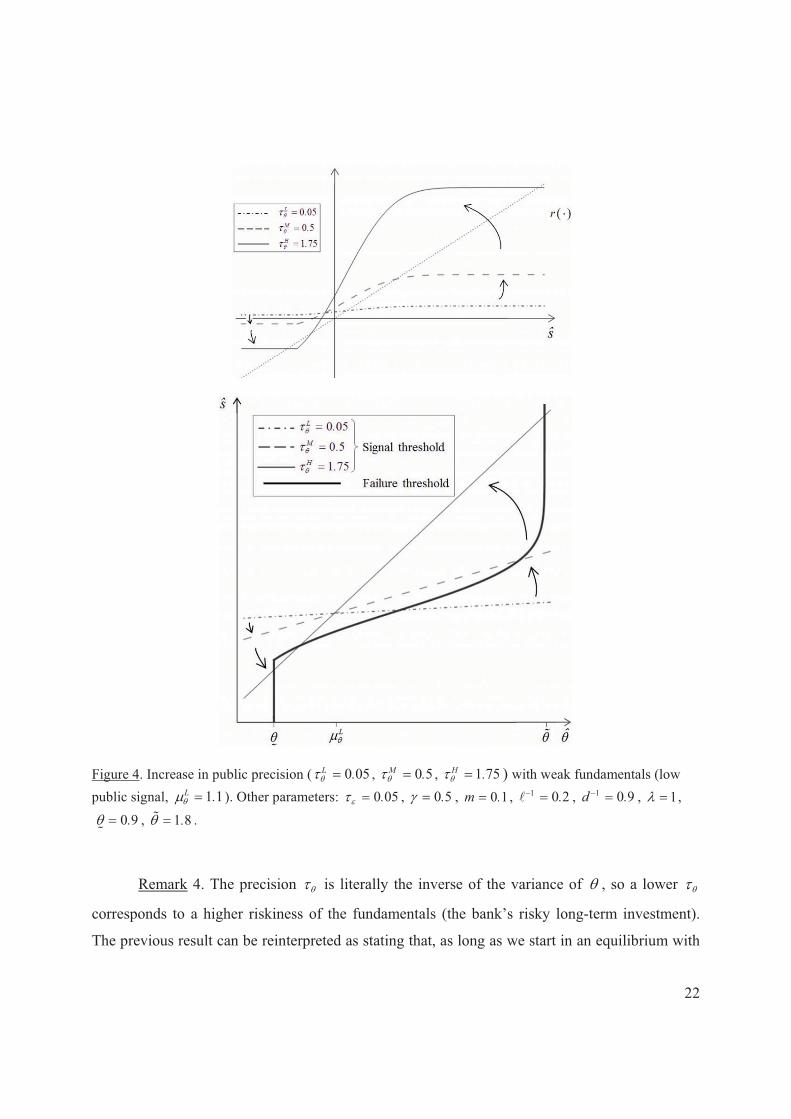
fundamentals are sound. Figure 4 illustrates how an increase in public precision raises strategic
complementarity and helps investors coordinate on a run when fundamentals are weak (although
the bank expects to remain solvent provided � ��
). We see how increasing � from 0 05L .� � ,
corresponding to the flat best response in Figure 4’s top panel, moves the equilibrium threshold
toward the “run” equilibrium (i.e., moves � toward � ) and generates more illiquidity. This is
true even when increasing � causes multiple equilibria to appear, among them a “no-run”
equilibrium (the smallest one; see Figure 4’s top panel, where the intersection of the 45º line with
the flat part of the best response marks an equilibrium with * ��
when 1 75L .� � ). Indeed,
when starting from 0 05L .� � , as � increases we would move—according to best-reply
dynamics—to the largest (not the smallest) equilibrium; this yields an unambiguous comparative
statics result.
30 If � is low then fund managers would tend to withdraw but if private signals are very precise then they will not
pay much attention to the public signal and will moderate their actions.
22
Figure 4. Increase in public precision ( 0 05L .� � , 0 5M .� � , 1 75H .� � ) with weak fundamentals (low public signal, 1 1L .� � ). Other parameters: 0 05.�� � , 0 5.� � , 0 1m .� , 1 0 2. �� , 1 0 9d . � , 1� � ,
0 9. ��
, 1 8. �� .
Remark 4. The precision � is literally the inverse of the variance of , so a lower �
corresponds to a higher riskiness of the fundamentals (the bank’s risky long-term investment).
The previous result can be reinterpreted as stating that, as long as we start in an equilibrium with

23
Low precision of public information ( 0.05L� � ) High precision of public information ( 0.5H
� � )
*� , an increase in the riskiness of the assets 1
� (a mean-preserving spread) will reduce
illiquidity risk. That is, starting in the “run” equilibrium 1 75H .� � , by reducing � we move to
safer equilibria.31
Figure 5 illustrates how the effect of bad news (when the public signal goes from H�
to L H � � ) differs markedly when public precision is low versus high. In the latter case (right
panel), strategic complementarity is high and the best response has a slope close to 1 since � is
high, and the impact is dramatic; when � is low (left panel), the effect is relatively small
because the best response curve is flatter.
Figure 5. The effect of bad news (from 1 4H .� � to 1 1L .� � ). Other parameters: 0 05.�� � , 0 5.� � ,
0 1m .� , 1 0 2. �� , 1 0 9d . � , 1� � , 0 9. ��
, 1 8. �� , 0 05L .� � , 0 5H .� � .
31 In a dynamic model related to the debt run model of He and Xiong (2012), Cheng and Milbradt (2012) find
that—during a freeze—a bank that increases its portfolio risk may thereby increase the confidence of creditors.

24
Let us turn now to regulation in the bank runs model and to controlling the likelihood of
crises.
2. Liquidity and solvency regulation of financial intermediaries
Two common objectives of regulators are to control the probabilities of insolvency and
illiquidity (see e.g. Freixas and Rochet 2008). The potential for insolvency is typically controlled
by reducing the incentives for investors to take risks on banks with limited liability. The potential
for illiquidity is reduced by alleviating fragility and addressing the coordination and contagion
problems associated with bank financing. In other words, the first objective is the prudential
requirement that sets a lower bound on solvency and the second objective is to prevent a solvent
institution from failing. The liquidity concern can be addressed by the central bank’s “lender of
last resort” facility and by liquidity regulation.32 In this paper it is assumed that the regulator’s
objectives include the control of both insolvency and illiquidity and that its instruments are
leverage and liquidity requirements.
So suppose that the regulator wants to bound the maximum probability of insolvency at
the level q and that of failure at the level p , thus bounding the probability of illiquidity. That is,
q is the highest probability of insolvency � �Pr �
allowed by the regulator and p is the
highest allowed probability of failure � �Pr � . This approach can be rationalized by
presuming the regulator has a loss function, with appropriate weights on the likelihood of
insolvency and illiquidity, that is minimized subject to an efficiency constraint (in terms of the
expected value of bank assets). It is noteworthy that the strategic behavior of investors does not
affect the determination of the solvency threshold �
; in fact, �
depends only on balance sheet
parameters and the cost of funds. However, the behavior of investors is crucial in determining the
equilibrium failure threshold � (even though � turns out to be a function also of the model’s
balance sheet, market, and information parameters).
The analysis in the paper builds on the connection between balance sheet parameters,
market stress parameters, and information parameters with the degree of strategic
32 Rochet and Vives (2004) study the central bank’s lender of last resort (LOLR) facility. A central bank with
perfect information on the focal bank’s fundamentals could provide the appropriate liquidity—at the possible cost of fostering moral hazard. Yet a central bank with only imperfect information will certainly make errors, which reinforces the role of liquidity requirements. Repullo (2005) shows how the existence of a LOLR induces banks to hold lower levels of liquid assets.
25
complementarity of the actions of investors and the probabilities of insolvency and failure. The
degree of strategic complementarity is quantified by the (maximal) slope of the best response
function of an investor to the signal threshold used by other investors r ' (as explained in Section
1.3) and is the key determinant of fragility (understood as equilibrium sensitivity to small
changes in parameters). Balance sheet parameters, such as m and � affect r ' through the slope
of the resistance function h (i.e. 1h ). The probability of failure depends directly on the critical
threshold �which is affected by the function h . Increasing m (whenever 1 11 0d � ) or 1�
relaxes the resistance function h and consequently decreases � . The end result is that the
likelihood of insolvency and of bank failure can be altered by the application of liquidity and
leverage ratios and that we can ascertain how those move with the deep parameters of the model.
For the sake of simplicity, let us restrict our attention to the parameter range in which there is a
unique equilibrium.33
A regulator that wants to eliminate illiquidity must set p q� . Yet that approach often
proves too costly (in terms of forgone returns) owing to the reduced level of investment in the
risky asset, so the regulator will set p q� and thus allow some solvent but illiquid banks to fail.
The regulator wants to ensure � �Pr q ��
and � �Pr p � � where * is the
critical threshold at the unique equilibrium. The goal is accomplished by fulfilling two
constraints:
� �1�q q � �� � �� �
(constraint S)
and
� �1�* *p p � �� � � (constraint L).
Note that if p q� then *p q ��
. It can be shown that the boundaries of both constraints
are linear in the space 1( , )m � and, as long as 0 1q �
,34 downward sloping with constraint L
having a larger slope (in absolute value) than constraint S. We have
33 Recall that a sufficient condition for the equilibrium to be unique is that 1 12 d m ��� �� � � � ;
therefore, for ��� � small a wide range of combinations of � �1m, � will fulfill the inequality. In
particular, if �� � the inequality will always hold. 34 Suppose, for instance, that 0 05q .� and 1 2.� � . Then � �1 1 65q .� � , and (0.19, 68) is the range of �
required to ensure that 0 1q �
.

26
� � � �� �1 11 1 1q qd m � �� �
for constraint S (solvency) and
1 11 1 1* *p p
k d m� �
� �$ %� & '( )
�
for constraint L (liquidity), where � �0 1k ,� . The constant k is the maximal critical fraction of
investors that may not renew credit in order for � �Pr p � � (i.e., � �*pk h � ). It is increasing
in p , decreasing in � , ambiguously related to �� � , and independent of the model’s other
parameters (see Claim 3 in the Appendix). Also, when p q� is required and *q ��
has been
induced, k is precisely the liquidity ratio m that would eliminate the illiquidity region. If
1*p qk� � �
then � � 11 ( ) 0*p qk� � ��
and so L intersects S from above, as shown in
Figure 6.
t follows from constraint S and 0 1q �
that 1 11 0d � for 1m . From Section
1.5 (and Claim 2 in the Appendix), both �
and * are decreasing in m (since 1 11 0d � )
and in 1� . Therefore, the regulator can make sure that � �Pr q ��
and
� �Pr p � � inducing a choice of 1( , )m � in the upper contour of the constraints S and L.
Figure 6 depicts the upper contour set, for ratios of leverage and liquidity, with respect to which
the probabilities of insolvency and overall crisis are bound by q and p , respectively.

27
Figure 6: Solvency constraint S and liquidity constraint L used to reduce the likelihood of insolvency and crisis with (respectively) a short-term leverage ratio ( D E�� ) and a liquidity ratio ( m M D� ). The upper contour sets consist of the leverage and liquidity ratios for which the probabilities of insolvency and overall crisis are bound, respectively, by q and p.
The regulator can set an upper bound q on the maximum allowed likelihood of insolvency
and an upper bound p on the maximum allowed likelihood of a crisis (and therefore of illiquidity)
by the appropriate choice of the ratios of liquidity m and leverage � . Thus a regulator must
propose a region of 1( , )m � space in which the bank ratios must lie. This region is the upper
contour of the constraints S and L, which is limited by a kinked downward-sloping schedule that
reflects the (partial) substitutability between 1and m � (Figure 6). The kink arises because, even
though both solvency and liquidity ratios can be used to reduce the likelihood of insolvency or
crisis, the solvency (resp., liquidity) ratio is naturally more effective at curtailing insolvency
(resp., illiquidity). That is, the slope of the S constraint is smaller, in absolute value, than the
slope of the L constraint.
It is assumed that both constraints are binding. This is reasonable when the constraints are
downward sloping. That is, unregulated banks would chose liquidity and solvency ratios 1( , )m � below the appropriate levels. For the case of constraint L this means, for example, that
the level of p is not so large so that for any equilibrium and combination of ratios 1( , )m � ,

28
* *p � , making L non-binding.35 When faced with the upper-contour constraint set, the bank
will choose the least-cost combination � �1,m � , which will necessarily lie on the frontier of one
of the constraints. Given the kink in the constraint set, however, often there will be no loss of
efficiency if the regulator sets minimum levels for � �1,m � . The reason is that the constrained
optimization of the financial intermediary will lead to the kink in the constrained set for ample
price ranges of liquidity and capital. The minimal � �1,ˆm � ratios are given by the intersection of
the boundaries of the solvency and liquidity constraints.
The regulator’s problem can be seen in another, equivalent, way. Given that the solvency
constraint S is binding at the set level q� it is easy to see that the resistance function h is
increasing in m (with 1� adjusting accordingly to fulfill S).36 Along S, therefore, increasing
m will reduce * and the regulator can choose m to fulfill * *p � .
When � � 1*p qk� � �
, the L constraint lies below the S constraint (and the absolute
value of its slope is greater); then typically 0m � . The inequality will tend to be satisfied when
the fire-sale premium � is low or investors are not too conservative (� large, since k is
decreasing in � ). For example, if 0� � then there is no fire-sale penalty and so in equilibrium
there is no illiquidity, � ��
. In this case it is clear that the liquidity requirement serves no
purpose; since insolvency can be controlled with the solvency requirement, the constraints L and
S collapse into one.
When � � 1*p qk� � �
, the liquidity requirement is necessary and
� � � �� �� � 111 1 1 1 0*p qm k � � ��
. This is so when fire sales penalties are significant
(� high), investors conservative (� low), and the regulator not willing to allow a large
probability of illiquidity ( p not much larger than q , since 1*p q ��
as p q� ). The liquidity
requirement is also necessary when the precision of public information � is high enough relative
35 For example, for �� � and � �1m, � fulfilling the constraint S, the largest possible equilibrium is
� �� �1 1q* � �� ��
for 0m � . For � �� �1 1q p* � � � �
� constraint L is non-binding.
36 We have that along S, � � � � � �1 q qh m m �� � � �
and, therefore, � �1 1 0qh m � � � � � � ��
because � �1 q � ��
.

29
to the precision of private information �� and investors are more conservative than the regulator
(1 2 p �� � , since in this case as �� � � , 1k � and 1m � ).37
Proposition 3 summarizes the main conclusions of our analysis and gives the formal
statement.
Proposition 3.
(i) The solvency constraint S and the liquidity constraint L, which are both linear and
acting on the ratios 1� and m , must be satisfied in order to control for the likelihood
(respectively) of insolvency at level q and of a crisis at level p .
(ii) Let 0 1q �
, then constraint S and constraint L are both downward sloping and
constraint L always has a larger slope (in absolute value) than constraint S.
Furthermore,
� �1
1max 1 1 1 1 , 0*p
qm k
�
* +$ $ % %, ,� - .& & ' '( ( ) ), ,/ 0�
and
� � � �� �1 11 1 11 1q qˆ ˆd m d � � �
� �,
where the constant � �0,1k � is increasing in p , 1� , and, whenever 1 2 p �� � and ��
is small, in �� � . When �� � we have 1k �� .
(iii) If p q� then m k� . If p q� and � � 1*p qk� � �
, then 0ˆk m� � and the
comparative statics of the regulatory ratios is given in Table 2.
37 However, if p � then as � � , we have that 0k � and � � 1*
p q ��
, and therefore 0m � .

30
Table 2. Comparative Statics of Regulatory Ratios When p q� and � � 1*p qk� ��
� 1� d � �
(Fire-sale penalty)
(Investor conservatism)
(Cost of funds)
(Strength of fundamentals)
(Precision of public information)
m (Liquidity ratio) � �� � �� 0 � �� � �*�
1ˆ � (Solvency ratio)
� � � � � �� � � � � *
* Provided 1 2p and either �� � or �� is small and p �� .
The minimal regulatory ratios m and 1ˆ � move in opposite directions in response to
parameter changes: the liquidity requirement m must be increased, and the solvency requirement 1ˆ � decreased, with increased fire-sale penalty � , with more conservative fund managers 1� ,
with better fundamentals � , and (provided either �� � or �� is small and p �� ) with more
precise public information � . More funding pressure on intermediaries (a higher d ) calls for an
increased 1ˆ � and a constant m . An explanation of the comparative statics results using the
movements of the regulatory constraints when parameters change follows.
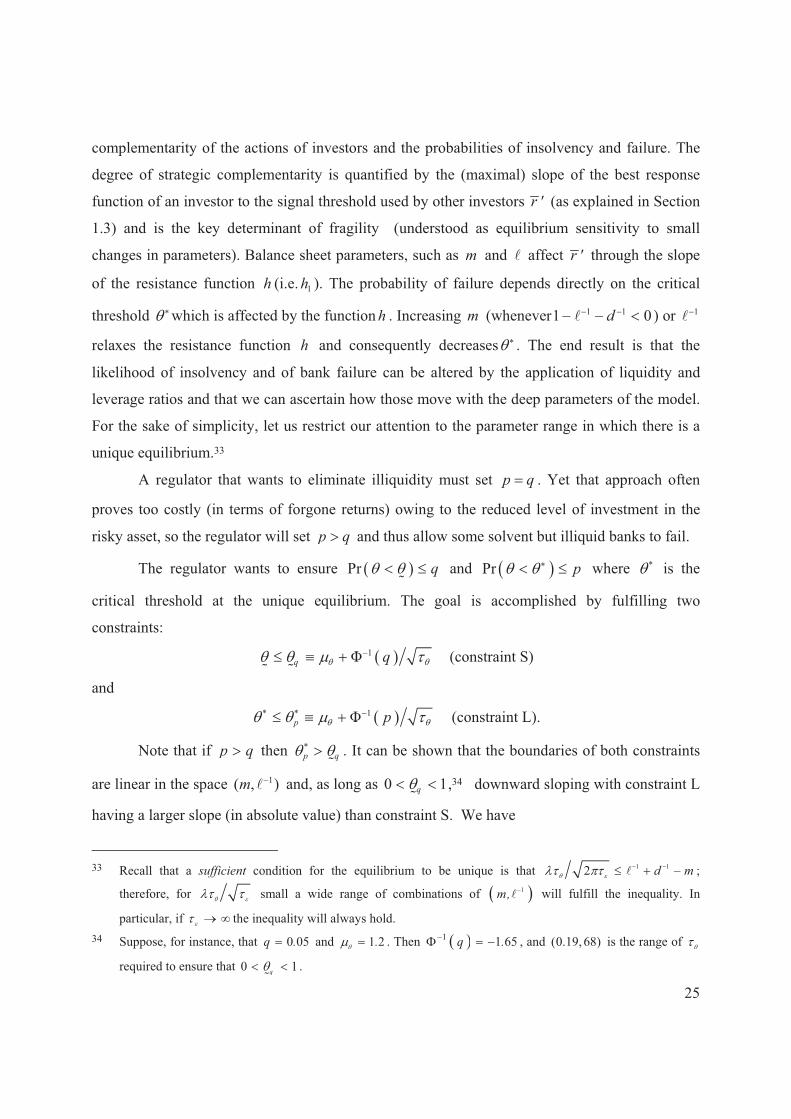
A higher return d on short-term debt will increase the solvency requirement but leave the
liquidity requirement unaffected. This is because both constraints are tightened in a vertical way
when d increases (see Figure 7(a)). Therefore, liberalized policies that increase competition
should be combined with increased solvency requirements. Those requirements were not (or were
only partially) increased in several liberalization episodes that lead to subsequent crises,
including the US Savings & Loans crisis in the 1980s, the 1990s crisis in the Nordic countries,
and the banking liberalization in Spain that began in the late 1970s. Proposition 3 implies that, for
a cross section of banks, intermediaries with higher funding costs (higher d) should have a higher
solvency requirement and the same liquidity requirement.
31
Figure 7(a). Effects of an increase in the cost of funds.
Figure 7(b). Effects of an increase in the fire-sale penalty.

32
Figure 7(c). Effects of an increase in the strength of fundamentals (good news) or in the precision of public information (transparency) under certain conditions.
A larger fire-sale penalty � and more conservative investment managers (lower � ) will
raise the liquidity requirement and lower the solvency requirement. The reason is that increases in
� and 1� have no effect on the solvency constraint but do tighten the liquidity constraint; see
Figure 7(b) for the effect of an increase in� (an increase in 1� has a similar effect) . So in an
environment where � is high and � is low, the liquidity requirement should be strengthened but
the solvency requirement can be relaxed.
An increase in return prospects � calls for a higher liquidity requirement and a lower
solvency requirement. Although both constraints are more relaxed when � increases, if p q�
then *p q �
is decreasing in � and so constraint L is relaxed relatively less than is constraint S;
hence m increases with � (indeed, m is decreasing in *p q �
) and 1ˆ � decreases with � (since
k is independent of � ). The same is true for an increase in � whenever �� is small enough and
p �� (or when �� � , in which case 1k �� ); see Figure 7(c). In general, if � increases
then a sufficient condition for L to be relaxed less than S (if at all) is that k be increasing in � ,
which it is when �� is small enough and p �� . This sufficient condition requires that the
regulator be more conservative than investors ( p �� ) and that investors be poorly informed (low
�� ). Then 0m �� � � and 1 0ˆ�� � � . If p �� then k is decreasing in � . In this case it is

33
typical for m to exhibit a hump-shaped pattern: increasing for low values of � and then slowly
decreasing for large values of � . Then we may have 0m �� � for a range of � values, in
which case increasing � leads to a reduction in both regulatory ratios.38
These results suggest that the regulator should set disclosure and prudential policies in
tandem, since prudential requirements depend on the precision � of the public signal. When
1 2p , for example, if either �� � or �� is small enough and p �� (conservative investors),
then m increases with � and 1ˆ � decreases with � . Requiring more disclosure must therefore
be accompanied by a higher liquidity requirement and a lower solvency requirement. As we will
see in Section 3, the existence of a derivatives market may entail the availability of a precise
public signal; this should be taken into account by prudential regulation.
It is noteworthy that our policy prescription of relaxing solvency requirements when
return prospects are higher (i.e., higher � ) does not contradict the BIS macroprudential
recommendation that capital requirements should be tightened in good times. The results of our
static model should be understood to hold on average during the cycle. For example, if the
regulator expects that a strong public signal will be available in the future (owing to disclosure or
the presence of a derivatives market) then it should tighten the liquidity requirement when the
conditions are fulfilled (i.e., when either �� � or �� is small enough and p �� ) while taking
into account the average value of parameters in the cycle (or perhaps the worst-case scenario in
terms of return prospects when assessing the probabilities of failure and illiquidity).
Remark 5. If parameters are such that multiple equilibria may appear then the analysis is
more complex. We know that given that the solvency constraint S is binding at the set level q�,
increasing m will reduce the largest equilibrium * . However, if the required threshold *p is low
enough then it may be that the liquidity ratio to induce * *p � , instead of m as given in
Proposition 3, is given by a higher level of m . Let m be the liquidity ratio that makes the failure
threshold just tangent to the signal threshold (see Figure 8). We have that m m� where
for m m� we have that *q ��
at the smallest equilibrium. Then for m m� there is a unique
38 For example, 0m �� � for 8 4.� � when 0 2p .� , 0 29.� � , 0 1q .� , 1� � , 5�� � , 1 0 9d . � , and
1 25.� � .

34
equilibrium at *q ��
. Increasing m increases strategic complementarity and, although it always
decreases the largest equilibrium * , it may induce multiple equilibria. Even though with m m�
the smallest equilibrium is always *q ��
, other equilibria may appear for intermediate values of
m .
Figure 8. Effect of an increase in the liquidity ratio along the solvency constraint S ( 0 01m .� , 0 1307m m .� 1 , 0 6749m m .� 1 with corresponding values of 1� , respectively and approximately, of
0 55. , 0 49. , 0 25. ). Let � �1q q � � ���
. For 0 01m .� there is a unique (and high) equilibrium; for m m� there are three equilibria with the smallest one with *
q ��
; and for m m� the equilibrium *q ��
is the unique one. Other parameters: 0 1.�� � , 2 5.� � , 1 5.� � , 0 1q .� , 0 69q . �
�, 0 15.� � ,
1 0 9d . � , 0 25.� � .
Let us explore briefly what happens in the extreme case of the regulator allowing leverage
so high that 1 11 0d �� . For banks with intense investment banking or wholesale activity
we have 11 0 �� because D E�� is usually greater than 1; therefore, 1 11 0d �� is
possible. If leverage is high enough and if 1 11 0d �� , then 1 ��
and 0m� � ��
and so
increasing liquid reserves makes insolvency more probable. The reason is that, if more liquid
reserves M are retained, then fewer are available for investment in the risky asset,
1I E M� � . The effect is to lower the solvency threshold for low equity. Suppose, for
example, that the bank has no equity ( 0E � and so 1 0 �� ); in this case, the solvency threshold

35
would be � � � �11 m d m � �
. Furthermore, if 1 11 0d �� then 0* m� � � if either �
or � is small. Now increasing the liquidity ratio leads not only to a greater likelihood of
insolvency and crisis but also to a higher range of illiquidity � �
. For instance, let �� �
with 1m � ; then � �11
1 mm
� � �
$ %� �& '( )�
and 0* m� � � for � �1 1 11 1d � � � �� ,
and � �
increases with m if � is small ( 1 11 d � �� ). Increasing the liquidity ratio may
actually increase the range of illiquidity. This occurs because keeping more cash reserves drains
resources for investment and hence reduces the liquidation value of investments during the
interim period, which may be needed to meet debt obligations.
Suppose the regulator allows that 1q ��
(and assume that
� �� � � �1 11 11 0*p qk d d� � � �
�). Then the solvency constraint is upward sloping, since
� � 1 1 0q
�, and the liquidity constraint will also be upward sloping if 1*
p �� � . If the
liquidity constraint is downward sloping then the bank’s choices when faced with the constraints
are � � � � � �� �11 1, 0, 1 *pm k d� � � � and � � � �1 1, ,ˆˆm m �� � . If both constraints are upward
sloping then the first equality is chosen. If � �� � � �1 11 *p qk� �
� then
� �� �11 1( , ) 0, qm d � ��
, since the intercept of the L constraint is below that of the S
constraint. This case could arise if the fire-sale penalty � is so low that the risk of illiquidity is
extremely small and thus the only concern is solvency.
The findings can be summarized as follows. When the regulator’s upper bound q for the
probability of insolvency is close enough to 1 2 (so that, e.g., � �1� 1q q � �� � ��
for
1� � since � �1� 1 2 0 � ), it may be optimal—to control the likelihood of insolvency and
illiquidity—to induce the intermediary to keep no liquid reserves and simply impose a leverage
limit (while allowing enough leverage that 1 11 0d �� ). It is somewhat surprising that,
when the regulator allows for a high chance of insolvency, it may propose no liquidity
requirement but a solvency requirement that helps meet the liquidity constraint needed to control
for the overall probability of crisis: � � � � � �� �11 1, 0, 1 *pm k d� � � � .

36
3. An interpretation of the 2007 run on structured investment vehicles
A slowdown in housing prices combined with a tightening of monetary policy led to
increasing doubts about subprime mortgages; these doubts were reflected in 2007’s sharp decline
in ABX, the asset-based securities index. This index had been launched in January 2006 to track
the evolution of residential mortgage–backed securities (RMBS).39 The decline in the ABX index
during 2007 seems to have played a major role in unfolding the crisis and especially in the run on
SIV and ABCP conduits. Indeed, at year-end 2006 the subindexes for triple-B securities began,
after trading at par, to move downward; these subindexes then dropped dramatically in 2007 (see
Figure 9).40 A similar phenomenon was evident with CMBX, a synthetic ABX-like index based
on a set of 25 commercial mortgage–backed securities (CMBS).
Figure 9: Prices of the 2006:1, 2006:2, 2007:1, and 2007:2 vintages of the ABX index for the BBB� tranche. Source: Gorton (2008).
39 The index is a credit derivative based on an equally weighted index of 20 RMBS tranches; there are also
subindexes of tranches with different ratings and for different vintages of mortgages. The ABX index filled two important functions: providing information about the aggregate market valuation of subprime risk; and serving as an instrument to cover positions in asset-based securities—for example, by shorting the index itself (Gorton 2008, 2010). In fact, trading in the ABX indexes by Paulson & Co. and Goldman Sachs delivered two of the largest payouts in the history of financial markets. See Stanton and Wallace (2011), who argue that the ABX index is an imperfect measure of subprime security values.
40 The index starts trading at par. The only exception is the 2007:2 index, which opened significantly below par.

37
The ABX (and CMBX) indexes were highly visible and had a strong influence on
markets. These indexes evolved in response to a sequence, from January to August 2007, of bad
news on subprime mortgages—bankruptcies of and earnings warnings from originators,
downgrading of ratings for RMBS bonds and collateralized debt obligations (CDOs), and large
losses for hedge funds. The accumulated bad news reflected in the ABX indexes culminated in
the panic of August 2007, when BNP Paribas froze a fund because liquidity had evaporated
completely in some segments of the US securitized market. A spike in the overnight spread in
ABCP and in the Libor–OIS spread followed, and the outstanding ABCP plummeted. The runs
began on ABCP conduits and on SIVs that held some percentage of securities backed by
subprime mortgages. These vehicles were funded with short-maturity paper, and the run
manifested as investors not rolling over that paper.41 Such investment vehicles may not have had
a high proportion of their assets directly contaminated by subprime mortgages, but their indirect
exposure was substantial. As short-term financing dried up, bank sponsors intervened and
absorbed many of these vehicles onto their balance sheets.42
Consider the following time line in the basic banking model. At time 0t � , mortgage
loans are awarded and securitized. At 0t � , an SIV is formed; it holds I loans and M reserves
financed by equity E (or stable funds) and short-term debt (CDs) 0D . At 1 2t � , a public signal
P about is released. At 1t � each fund manager, having received a private signal about ,
decides whether to cancel ( 1iy � ) or renew ( 0iy � ) her CD. At 2t � , the returns I on the
RMBS assets are collected; if the bank can meet its obligations then the CDs are repaid at their
face value D and the SIV’s equity holders receive the residual (if any).
41 At the end of 2007, ABCP liabilities amounted to little more than a fourth of the typical SIV’s total yet to
nearly all of the typical conduit’s total (see April’s report by the IMF (2008)). 42 See Acharya and Schnabl (2010) and Covitz et al. (2013) for evidence on runs in the ABCP market. It is
important to distinguish between conduits that were motivated by regulatory arbitrage (and were fully insured by large commercial banks) and conduits that were motivated to transfer risk by off–balance sheet considerations. There is little scope for strategic complementarities among investors in the first case but substantial scope in the second. There was a corresponding larger decline in ABCP conduits of the second type, relative to those of the first type, starting in August 2007. See Acharya, Schnabl, and Suarez (2013).
0t � SIV formed with I RMBS
1 2t � Public signal P released
2t � Return � on RMBS unit realized
1t � Fund managers receive private signals and decide on CD renewal

38
The public signal P could be the value of the ABX index or the price quoted by a
derivatives market with a package of RMBS as an underlying asset (such as the ABX index
itself). Denote by � the precision (accuracy) in P’s estimation of . Consider a scenario where
neither the SIV nor fund managers in the short-term debt market participate in the derivatives
market. Introduction of the ABX index implies a discrete increase in the precision � of the public
signal,43 which increases strategic complementarity. A high level of noise in the signals will also
tend to increase complementarity. Recall that, when �� is already low, a still lower �� increases
strategic complementarity (since the maximal slope of � �r � tends to infinity as �� approaches
zero). In this case, �� � will tend to be large and so multiple equilibria may appear
(Proposition 1). Signals from SIV investors are likely to be imprecise ( �� low) given the
opaqueness of structured subprime products and their distance from loan origination (as when the
German Landesbank invested in US structured subprime products).44
When bad news strikes (i.e., when � �E P� � declines), the probability of a crisis
occurring increases and we may move, as in the right panel of Figure 5, from a relatively safe
equilibrium to a “run” equilibrium (with � close to � ). Observe that the effect of bad news
would be small if the precision � of public signals were low (left panel of the figure). However,
strategic complementarity was high not only because � was high but also because short-term
leverage � was high and, in the crisis situation, the cost of funds d and the fire-sale penalty �
also increased (all these factors tend to increase 11h and thus strategic complementarity). In fact,
the fire-sale penalty increased dramatically: the market became practically illiquid, and SIVs had
to be reabsorbed by parent banking institutions. Thus the impact of bad news was even more
dramatic owing to it being combined with the increased precision of public signals (Proposition
2).
The model of Section 2 still applies, so both solvency requirements and liquidity
requirements will be necessary for “shadow” banks such as SIVs. In particular: Proposition 3 and
Table 2 together show the necessity of a liquidity requirement when the fire-sale premium is high 43 The precision � of public signals in the derivatives market is positively affected by the precision of the private
signals of sophisticated traders in that market. For related models, see Angeletos and Werning (2006), Tarashev (2007), and Vives (2008, Sec. 4.4).
44 See Pagano and Volpin (2012) for a model in which issuers of structured bonds choose opaque ratings in order to enhance the liquidity of their primary market—though at the cost of diminishing (perhaps drastically) the liquidity of the secondary market.

39
and investors are conservative and furthermore when �� is low, p� , then a higher precision of
the public signal should lead to an increased liquidity requirement. In other words, the
introduction of a strong public signal—such as that provided by a derivatives market—should be
met with tightened liquidity obligations.45
4. Connections to the literature; empirical implications and evidence
Previous literature has obtained results related to those presented here, and a growing
body of evidence is consistent with these results. We shall discuss both topics in turn.
4.1. Connections to the literature
Insolvency risk and illiquidity risk. Morris and Shin (2009) also study how insolvency
risk and illiquidity risk vary with the balance sheet composition of a financial institution in a
model where uncertainty about future fundamentals interacts with uncertainty about present
strategies. In that model, there would be no illiquidity risk in the absence of future insolvency
risk (i.e. ex post uncertainty) since the authors assume that the partial liquidation of assets has no
long-run effect. Morris and Shin demonstrate that illiquidity risk is (i) decreasing in the ratio of
cash plus interim realizable assets to short-term liabilities, (ii) increasing in the “outside option
ratio” (opportunity cost of the funds of short-term debt holders), and (iii) increasing in the ex post
variance of the asset portfolio (“fundamental risk ratio”). Both the particular results and the broad
message of that paper are consistent with ours: regulation must focus on the balance sheet
composition of any financial intermediary. Liu and Mello (2011) explain how the fragile capital
structure of hedge funds, which is due to a coordination problem in redemptions, limits their
arbitrage capabilities. The authors show that this fragility induces hedge funds to invest relatively
more in cash assets and to use relatively more leverage ex ante. These predictions are borne out
by our model, as when a regulator seeks to reduce the likelihood of insolvency or illiquidity since
a decrease in stable funds ( E ) leads to more cash holdings ( M ).
Competitive pressure and fragility. The links between fragility and the pressure of
competition have been analyzed in several papers. Chang and Velasco (2001), in a model of
financial crisis in emerging markets that follows the Diamond and Dybvig (1983) tradition, find
45 If parameters are such that multiple equilibria may appear then the liquidity ratio may need to be tightened to the point where the illiquidity region vanishes (see Remark 5).

40
that financial liberalization increases the expected welfare of depositors but may also increase
fragility. Matutes and Vives (1996) present a model that combines the banking model of
Diamond (1984) with a differentiated duopolistic structure à la Hotelling. These authors find that
an increase in rivalry increases the probability of failure in an interior equilibrium of the
depositor’s game in which banks have positive market shares. Cordella and Yeyati (1998) report
that disclosing a bank’s risk exposure (by parties beyond the bank manager’s control) may
increase fragility by increasing the deposit rates demanded by investors. Goldstein and Pauzner
(2005) also show, in a model of the global games type, how increasing the deposit rate increases
the probability of a run of depositors. In the model presented here, increasing the deposit rate
increases the likelihood of both insolvency and illiquidity.
Negative feedback loops. In the bank crisis model, the fire-sale penalty is related to
adverse selection. Vives (2010) establishes that the asset fire-sale penalty is increasing in the
noise component of the bidders’ signals and in the amount auctioned and also that it is decreasing
in the number of bidders. In a crisis scenario it is plausible to expect noisier signals, an increased
amount auctioned, and fewer bidders. As a result, a bank that tries to sell more assets (because it
is in distress) will face a larger discount, which in turn will induce more sales (to honor the
previous commitments) and still further discounts. In the extreme, the market may collapse
because adverse selection is so severe in relation to the number of bidders. A similar dynamic
may prevail with the face value of debt, since a distressed bank that needs refinancing will be
offered worse terms (than other banks would be) and this further aggravates the distressed bank’s
fragility.46
Liquidity regulation. Liquidity requirements may have the unintended consequences of
aggravating adverse selection and drying up markets for liquidity (Malherbe 2014). The reason is
that, when intermediaries hoard liquidity, their selling behavior is interpreted as wanting to
unload “lemon” assets. Perotti and Suárez (2011) explore how liquidity requirements and
Pigouvian taxes can help internalize the systemic externality induced by short-term funding of
intermediaries. In our model, the regulator implicitly minimizes a loss function that includes a
cost for illiquidity stemming from systemic (macroprudential) causes. The interbank market may
46 See Brunnermeier and Pedersen (2009) for a model of a liquidity spiral that combines market and funding
liquidity; see Bernardo and Welch (2004) for a model in which the fear of having to liquidate assets after a crisis may contribute to the frenzy by incentivating sales in the middle of the run. See also Eisenbach (2010) for a feedback model of short-term debt and rollover risk with endogenous fire-sale penalties.

41
be a source of coinsurance for liquidity risk. Battacharya and Gale (1987) show how banks, when
subject to shocks which are private information, have an incentive to underinvest in liquid assets
since they can free-ride on the liquidity pool in the interbank market. Acharya, Shin and
Yorulmazer (2010) show how liquidity support to failed banks, or unconditional support to
survivors, induces banks to hold less liquidity. Calomiris, Heider and Hoerova (2013) show how
the group of banks participating in the interbank market will impose cash requirements to prevent
free riding.
Large players and market power. Market power may facilitate liquidity provision in the
interbank market; liquidity is a public good, so sound banks may have an incentive to provide a
troubled bank with liquidity in order to avoid contagion (Allen and Gale 2004; Sáez and Shi
2004). Market power can also impede the provision of liqudity, as when banks with surplus funds
strategically underprovide lending in order to induce fire sales of the bank-specific assets of
needy intermediaries (Acharya, Gale, and Yorulmazer 2011).47
Strategic complementarity and the “many to fail” problem. The literature has also found
strategic complementarities in the decisions of individual banks that, with other banks, force the
central bank to bail them out collectively. Farhi and Tirole (2012) show how the private leverage
choices of financial intermediaries display strategic complementarities through the response of
monetary policy, which makes it optimal for banks to adopt a risky balance sheet. Acharya and
Yorulmazer (2007) identify the regulator’s ex post incentives to bail out failed banks when many
are failing. Hence banks, especially small ones, are induced to “herd” their investment policies
and thereby increase the risk of collective failure.
4.2. Empirical implications and evidence
The model yields a rich array of empirical implications. To start with, this model is
consistent with the notion that crises are driven both by fundamentals and by panic components.
It also predicts a multiplier effect of public information that is increasing in the accuracy of that
information. Table 1 provides testable predictions that link the probability of an intermediary’s
failure or insolvency with the strength of fundamentals ( � ), balance sheet ratios ( m and � ), and
market stress parameters (� , � , and d). We find that the strength of strategic complementarities
47 See Corsetti et al. (2004, 2006) for other effects of the presence of large players.

42
among investors, with its associated multiplier effect on comparative statics, increases with � , � ,
and d.
There is evidence that banking crises are driven by both solvency and liquidity issues.
Gorton (1988), in his study of crises during the US National Banking Era (1865–1914),
concluded that panics were triggered when the “fundamentals” (a leading indicator of recession)
reached a certain level. Calomiris and Mason (2003) argue that some episodes of US banking
crises in the 1930s can be explained by deteriorating fundamentals but that other episodes (e.g.,
the crises in January and February of 1933) are open to being interpreted as cases of the panic
component dominating. Starr and Yilmaz (2007) study bank runs in Turkey and conclude that
both fundamentals and panic elements are needed to account for the dynamics of those crises. In
an experimental study, Schotter and Yorulmazer (2009) find that the severity of bank runs
depends on fundamentals (i.e., the state of the economy).
Identifying and estimating strategic complementarities is difficult because the strategic
aspect must be disentangled from investor responses to common shocks. Chen et al. (2010)
identify strategic complementarities in mutual fund investment by relying on the fact that illiquid
funds (in our model, those with a higher fire-sale penalty� ) result in greater strategic
complementarities among investors than do liquid funds; the reason is that redemptions impose
higher costs on illiquid funds. Hertzberg et al. (2011) use a natural experiment with a credit
registry expansion in Argentina to identify complementarities.
Consistently with Proposition 2(i), there is experimental evidence that bank runs occur
less frequently when banks face less stress (in our model, a lower # ) in the sense of a larger
amount of withdrawals being required to induce insolvency (Madies 2006; Garratt and Keister
2009). There is also evidence of public information’s multiplier effect, Proposition 2(ii), from the
credit registry expansion in Argentina (Hertzberg et al. 2011) and from the so-called discount
window stigma (Armantier et al. 2011; Acharya and Merrouche 2012). The latter refers to the
reluctance of banks to borrow from the discount window because of fear that the bad news will
become publicly known. Armantier et al. (2011) report that, during the crisis, many banks
borrowed from the Term Auction Facility (where the borrowing bank is just one of many) at
higher rates than those available at the discount window; they also show that this rate spread was
increasing in the stress that affected the interbank market. The spread indicates how much a bank
is willing to pay to avoid the public release of a bad signal, and it is consistent with the positive

43
association (in the interbank market) between a higher publicity multiplier and a higher fire-sale
penalty � .
In accordance with these results, specializing Proposition 2 to the bank run model
indicates that—among the 72 largest commercial banks in OECD countries—those that relied
less on wholesale funding, and had higher capital cushions and liquidity ratios, fared better
during the crisis in terms of enduring smaller declines in equity value and being less subject to
government intervention; see Ratnovski and Huang (2009). Berger and Bouwman (2013) also
find that capital improves the performance of banks during crisis periods. Finally, Fahlenbrach et
al. (2012) document that banks with more short-term funding performed worse not only in the
2007 crisis but also in the 1998 crisis (when Russia defaulted on its debt).
5. Other applications
This section details three more illustrations of our approach: a sovereign debt crisis, a
currency attack, and a credit market freeze.
Sovereign debt crisis. The bank run model of Section 1.2 can be reinterpreted as a
sovereign debt run. So at 0t � , the country has some local resources E as well as external
(public and private) short-term debt 0D . The resources are invested in entrepreneurial projects I
and foreign cash reserves M (understood to be in a strong currency). As before, investors in
short-term debt can withdraw during the interim period at 1t � and receive the face value D .
The public signal now can be interpreted as a credit rating. Under this interpretation,
m M D� is the reserves liquidity ratio, D E�� is the short-term external leverage ratio, and
0d D D� is the risk premium on short-term debt. The regions of insolvency and illiquidity
identified in Section 1.4 still apply.
0t � Invest I D0: short-term external debt M: safe reserves
1/2t � Public signal P released
2t � Return � realized
1t �Fund managers receive private signals & decide on debt rollover

44
We can derive some prudential policy recommendations from these regulatory results.
Namely, if the international regulator’s objective is to reduce the risk of country insolvency and
illiquidity, then constraints must be placed on short-term external leverage and the ratio of
reserves. The solvency requirement should be higher for countries with a higher risk premium;
however, if fire-sale penalties (say, on real estate assets) are higher then the liquidity requirement
should be raised and the solvency requirement lowered. Of course, if both the risk premium and
the fire-sale penalty are relatively high then probably both requirements should be raised.
Prudential constraints must be adjusted in the presence of sovereign credit ratings with
strengthened reserve requirements—provided that fire-sale penalties are high and that foreign
investors are both conservative and not well informed.
Currency attacks. A streamlined version of the currency attacks model of Morris and Shin
(1998) fits our general model. Here denotes central bank reserves, and 0 � means that those
reserves are depleted. Each speculator has one unit of resources to attack the currency ( 1iy � ) at
a cost C . Let � � 1;h # # � , where 0# � is the mass of attackers and 1# is the proportion of
central bank reserves that are uncommitted; then the attack succeeds if 1y # � . Alternatively,
# could be interpreted as the wealth available to a fixed mass of speculators. See Figure 10(a). In
the event of depreciation, the capital gain is fixed and equal to B B C� � . We find that
( )C / B C� � � is likely to be small.
Figure 10(a). The resistance function � � 1;h # # � in the model of currency crises.

45
In the range �, ���� , if currency speculators coordinated their attack then they would
succeed; in fact, however, the currency holds. From Proposition 2(i) we have immediately that
the likelihood of a currency crisis is decreasing in � , the relative cost of the attack, and in � , the
expected value of the central bank reserves. Also, the probability of illiquidity � �Pr �� �
is
increasing in # whereas the probability of insolvency � �Pr �
is unaffected by # .48
Credit market freezes. Consider Bebchuk and Goldstein’s (2011) model of self-fulfilling
freezes in credit markets, which is a variation of the loan foreclosure model proposed by Morris
and Shin (2004).49 The bank’s action is to foreclose on a loan made previously to a firm. In this
case, denotes the fundamentals of the firms and y denotes the proportion of banks that do not
renew credit to firms. Firms with good projects—those in which banks prefer to invest—exhibit
returns above the risk-free rate only if � � 1 y # #� ��
, where � � 1 # #� ��
with 0 �� .
Firms with bad projects return nothing, and banks can distinguish good projects from bad ones.
Here the parameter # is interpreted as the inverse of the product of the mass of banks and a
“complementarity” parameter that captures the performance of firms. We have that
� � � �� � � �; 1h # # # # � � ���
(see Figure 10(b)). Observe that in this case an increase
in stress, 0h # � � � � , is associated with reduced strategic complementarity, 1 0h #� � � .
The parameter 1 � equals the ratio of the gross risk-free return to the gross return of good
projects. The authors use their model to assess government responses in the present financial
crisis. The comparative static results in Proposition 2 apply in this scenario as well. For example,
an increase in the precision of a public signal about bad fundamentals (low � ) will likewise
increase the range of fundamentals within which a panic credit freeze may occur. An increase in
48 If � � 1;h # # � then it is always the case that 0 � ��
� and � �Pr ��
� increases with # (since
� increases with # ). 49 The loan foreclosure model is formally equivalent to the currency attacks model. Here is the firm’s ability
to meet short-term claims (and 0 � signifies no such ability). The action is to foreclose on a loan. In this case we have � � 1;h # # � , where 0# � is the mass of creditors (and 1# is the proportion of the firm’s liquid
resources that are not committed) and so the project fails if 1y # � . The face value of the loan is L , and the
value of collateral (at interim liquidation) is K L . If we put B K� and C L K� , then 1 K L� � .

46
the mass of banks increases strategic complementarity and thus also increases the impact of
public signals.50
Figure 10(b). The resistance function � � � �� �;h # # #��
in the model of credit market freezes.
6. Concluding remarks
This paper presents a stylized model of a financial crisis that characterizes solvency and
liquidity risk and highlights how extensive strategic complementarity among investors’ actions
can increase system fragility (understood as high sensitivity of equilibrium to small changes in
parameters and the possibility of discrete jumps in the presence of multiple equilibria). Strategic
complementarity increases with short-term leverage, greater competition for funds, higher fire-
sale penalties, and public information that is more precise. If the asset side of a financial
intermediary is relatively opaque, then a strong public signal (say, from a derivatives market) will
increase both strategic complementarity and fragility. The analysis also characterizes how the
probability of failure or crisis depends on balance sheet structure (leverage and liquidity), market
stress parameters (extent of competition, fire-sale penalty for early liquidation of investments),
and the informativeness of public and private signals.
50 Gala and Volpin (2012) demonstrate how public information may reduce welfare since by correlating the
investment decisions of agents and exacerbating the negative externality that one borrower imposes on others in the presence of credit rationing.
47
The main general policy conclusion on regulatory reform is that a piecemeal approach
will not work. As it seeks to reduce the likelihood of insolvency or illiquidity, a regulator should
pay attention to the balance sheet composition of financial intermediaries and to the prevailing
level of disclosure. The regulator will need the option of imposing a leverage limitation and also
(if fire-sale penalties are high and investors are conservative) the option of imposing a liquidity
requirement. The solvency and liquidity requirements are partial substitutes, and both must be set
while accounting for the level of transparency. So in an environment characterized by low market
liquidity and conservative investors, the liquidity requirement should be tightened and the
solvency requirement relaxed; note that prudential constraints may require modification under
higher levels of disclosure (e.g., with stricter liquidity requirements and relaxed solvency
requirements). Competition policy and prudential regulation are not independent: in a more
competitive environment, leverage limits should be strengthened.51
The analysis presented here has several important limitations which have to be taken into
account when considering policy prescriptions. First, both the intermediary’s balance sheet and
the regulator’s objectives are exogenous. Each could be endogenized—for example, by
introducing a moral hazard problem on the part of the intermediary which would rationalize the
short-term debt structure and indicate an optimal closure policy for the regulator.52 Second, the
analysis is basically static even though the aim is to capture dynamic phenomena.53 Third, the
investors are symmetric.54 Finally, the analysis focuses on a single institution or a consolidated
banking sector and takes market parameters (e.g., the fire-sale penalty) as given. This approach is
therefore unable to account for either externalities among banks or contagion effects.55 These
issues are left for further research.
51 This theme is developed in Vives (2011) from a policy perspective. 52 For related approaches to the issue, see Calomiris and Kahn (1991), Diamond and Rajan (2000), Gale and
Vives (2002), and Rochet and Vives (2004). 53 See, for example, the dynamic analysis of panic debt runs in He and Xiong (2012) and in Cheng and Milbradt
(2012). 54 Sákovics and Steiner (2012) study a global game in which players are ex ante asymmetric. 55 See Acharya and Yorulmazer (2007) and Farhi and Tirole (2012).

48
Appendix
Figure A: Short-term leverage ratio of US banks, D E�� = (Deposits (Uninsured) + (Short Term Debt + Other Liabilities) / (Equity + Long Term Debt + Deposits (Insured)). Source: Veronesi and Zingales (2010); data for Goldman Sachs and Morgan Stanley as of August 31, 2008.56
Claim 1: Characterization of the best reply. The best reply is given by
� � � � � �1Fˆ ˆr s s . � �
� � �
� � � � � � �� � �
� �� � The maximal value of the slope is
1 2r '
h�
�� �
� �
� �� ��
, which is increasing in 11h and in � and is first decreasing and then
increasing in �� ( � � � � � �� �1sign sign 1 2 2 1lr ' h� � � � �� � � �� � � ). If � � 1 2h �� � ��
then � � � � 1Fˆ ˆr' s ' s �
�
� � ��
� � .
56 Only State Street Corp. would end up exceeding 10�� (with 14.77�� , which would yield 1 11 0d �� if the interest rate were 7.26%). For Lehman Brothers, 3.76�� at the end of 2007 (this
figure derived from Adrian and Shin 2010).

49
Proof: From the equality � �� � � �� s h�� � in the range � �, ��
we can solve for s
as a function of ; thus we obtain � � � � � �� �11 �Fs h�� � � with derivative
� � � �� �� �� � 111 1 � 0Fs' h' h�� 2
� � � , where 2 is the density of the standard normal
distribution. The threshold � �Fˆ s � is obtained as the inverse of � �Fs � whenever � �ˆ , � �
�
and ��
otherwise. Since 2 is bounded above by 1 2� and since 1h is the smallest slope of
� �h � , it follows that Fs' is bounded below: 11 2Fs' / h�� �� � . Hence
� � � � 111 2F ˆ' s / h� � �
� � with strict inequality except possibly when � � 1 2h � , because
then � �1� 1 2 0 � and 2 attains its maximum: � �0 1 2�2 � .
At the critical signal threshold s , for a given failure threshold the expected payoffs for
acting and for not acting should be the same:
� �� � � �� �! "
� � � �ˆ1, , ; 0, , ; |
ˆ ˆˆ ˆPr | Pr | ( ) 0
E y s y s s s
s B s C
� �
�
� � � �
or
� �Pr � sˆ ˆˆ| s � �
�
� � � � � �� �
�$ $ % % � � �& & ' '�( ( ) ),
where ( ) 1C / B C� � � . It follows that the signal threshold curve is given by
� � � �1T
ˆ ˆs � �
� � �
� � � � � � �� � �
� �� � ,
and
� � � �� � � � � �1T F Fˆ ˆ ˆr s s s s . � �
� � �
� � � � � � �� � �
� �� � �
Therefore, the maximal value of the slope is
1 2r '
h�
�� �
� �
� �� ��
,
which is increasing in 11h and in � and, with respect to �� , is first decreasing and then
increasing. Note that 1r ' � if and only if � � 1 2h� �� � � . We have that r ' � as 0���

50
and 1r ' � as � �� . It is easily checked that
� � � � � �� �1sign sign 1 2 2 1lr ' h� � � � �� � � �� � � ; in particular, 0r ' ��� � for � � � .�
Proof of Proposition 1: (i) The game is “monotone supermodular” (i.e., a game of
strategic complementarities with a monotone information structure) because � �, ;iy y� has
increasing differences in � �� �, ,iy y —that is, the differential payoff to act ( 1 0� � ) is
increasing in the aggregate action and in the negative of the state of the world ( , )y —and
signals are affiliated. This means that extremal equilibria exist, are symmetric (because the game
is symmetric), and are in monotone (decreasing) strategies in type (Van Zandt and Vives 2007).
Since there are only two possible actions, the strategies at an extremal equilibrium must be of the
threshold form: 1iy � if and only if i ˆs s , where s is the threshold. It follows also that the
extremal equilibrium thresholds, denoted s and s , bound the set of strategies that result from the
iterated elimination of strictly dominated strategies. In sum, the extremal equilibria are in
thresholds strategies and those bound any other possible equilibrium. If s s� then the game is
“dominance solvable” and the equilibrium is unique. Such an equilibrium is characterized by two
thresholds: s� denotes the signal threshold to act; and � denotes the state-of-the-world critical
threshold, below which the acting mass is successful and an acting player receives payoff
0B C � . In equilibrium, the fraction of acting players
� � � � � �� �, Pr | �y s s s s� � � � � � � �� � must be no larger than the critical fraction
above which it pays to act, � �*h . Note that �, � ���
�� because lim ( ) 0h � �
�, � �h � is
strictly increasing on � �, ��
, and � � 1h �� . Furthermore, at the critical signal threshold, the
expected payoffs for acting and for not acting should be the same:
� �Pr � s| s � �
�
� � � � � �� �
�� � � �$ $ % % � � �& & ' '�( ( ) )
,
where ( ) 1C / B C� � � .
(ii) Consider an equilibrium � �s ,� � . We show that if � �� � � �� s h�� � �� �
then � ��
.
This will be so if � � � �F Ts s �� �
(see, for example, lower panel of Figure 4), where
� � � �� �1�Fs h � �� �� � �
and � � � �1Ts . � �
� � �
� � � � � � � �� � �
� ��
� � It is

51
immediate then that � � � �F Ts s �� �
if � � � �0h h �� �
, where
� � � � � �10 � 1 � 0h
��
� � � ���
$ %� � �& '( )� �
.
For � � � �0h h � �
we have that � ��
at any equilibrium; in that case,
� �� � � �� s h�� � � � � and � ��
(here � � � �F Ts s � �
). In summary, there is a critical
� � � �0 0,1h ��
such that for � � � �0h h � �
we have � ��
and for � � � �0h h �� �
there is
always one equilibrium with � ��
.
(iii) From Claim 1 we have that if � � 1 2h �� � �� then � � 1ˆr' s � and the equilibrium is
unique. In this case, the game is dominance solvable because s s� . Furthermore, it should be
clear that the critical thresholds * and s� move together.
Let � � � �0h h � �
. Then we can combine
� �� � � �� s h�� � � � � (1)
and
� s � �
�
� � �� � �� �
�� �$ $ % %� �& & ' '�( ( ) )
(2)
to obtain
� � � � � �� � � �1 1� � 0* * *h � �3 � � � � � � � � � (3)
by substituting the value of *s from (1) into (2). Equation (3) may have multiple solutions in * .
As � � we have that � �� �1� h � � and 3 � ; as ��
we have that
� � � �h h ��
and � � 03 3 � ��
whenever � � 0h h �
. Hence there is at least one solution
�, � ���
�� . That solution will be unique if 0'3 ; if � � 0'3 � for a potential solution
� � 03 � then there will be multiple solutions (three when � �h � is linear or two when there is a
such that � � 03 � and � � 0'3 � ). As � tends to 0 (resp., 1) we have that � �1� � tends to
(resp., � ), s� tends to +� (resp., ��), and * tends to � (resp., �
). These claims follow
from equation (2) and because �, � ���
�� . There is indeed a unique solution if
1 2h �� � �� . (We have that � � � � � �� �� �1�' h' h �3 � � 2 � and '3 is bounded

52
above: 1 2' h �3 � ��� with strict inequality except possibly when � � 1 2h � . Therefore, if
1 2h �� � �� then 0'3 � .) �
Proof of Proposition 2: If � � 0h h �
, then � is determined by
� � � � � �� � � �1 1� � 0* * *h � �3 � � � � � � � � � .
We obtain the results by looking at how changes in the parameters affect � �3 � . When
1 2h �� � �� , we have that 0'3 and there is a unique equilibrium. The usual comparative
static analysis applies. When 1 2h �� � �� there may be multiple equilibria, in which case
our results will apply to the extremal ones. With adaptive dynamics the results apply in general.
(i) The result for * follows because 3 is decreasing in both � and � and is increasing in #
(since 0h #� � ). The threshold s� moves with * .57 The result for � �Pr � is immediate
for � and # , and also for � given that increases in � shift the distribution of rightward.
(ii) Suppose the equilibrium is unique. The equilibrium signal threshold is determined by
� �; 0r s s�� � � . From this it follows that, for a marginal change in � ,
1rds r
d r '
�� �
� � � �� �
�
whenever 0 1r4 . In consequence, an increase in � will have a larger effect on the
equilibrium threshold s� than does the direct impact on a player’s best response
r � � �� � � � . The same is true for discrete changes—even with multiple equilibria, provided
we restrict our attention to extremal equilibria or allow for adaptive dynamics. The multiplier
effect is greatest when r' is close to 1 at equilibrium (i.e., when strategic complementarities are
strong) and we approach the region of multiple equilibria (and this happens when � is large
because r' is increasing in � ).
57 The result for � follows also from a general argument in monotone supermodular games. We know that
extremal equilibria of monotone supermodular games are increasing in the posteriors of the players (Van Zandt and Vives 2007). A sufficient statistic for the posterior of a player under normality is the conditional expectation ! " � � � �E | s s � � � � � � �� � � , which is increasing in � . Thus it follows that extremal
equilibrium thresholds � �, s � � are increasing in � .

53
(iii) First consider changes in � . We have the equality
� � � �1 2 1� 2/* �3 � � � � � � � � � and therefore 03 �� � � when ��
�, since
* �� �
� and � �1 0�� for 1 2/� . Note that, for *
�� , if � increases then
� � � �� �Pr � � �� � � also increases. Consider now changes in �� . With our current
assumptions and using the equality � � 0*3 � in �3 �� � , we obtain
� � � �� �1 2 1� 2/*� � �3 � � � � � � � � � � � and 0�3 �� � . The results follow.
If � � � �1 2 1/ �� � � � � � �� then *
� and the results are reversed because * � ��
(since � �1 0�� , we have � � � �1 1 2� � � � � ). �
Proof of Remark 3: Let � �* � be the unique equilibrium. We have that ˆ� is the unique
solution in � to � �� �* , 0 3 � � �� � � or to � � � � � �1 2 1� 2/* � � � � � � � � � and that
�� is the unique solution in � to � �� �* , 0� 3 � � �� � � or to
� � � � � �1 2 1�/* � � � � � � � � � . The solutions are unique since � �*
� is decreasing in � .
This implies also that ˆ � � � since � �1� 0� because 1 2� . It follows that there are
thresholds ˆ� and �� with ˆ � � � such that (a) * increases with � if and only if ˆ � � and
(b) * increases with �� if and only if � �� � �
Claim 2: Comparative static results in the bank run model. There is a liquidity ratio
� �0,1m� such that when m m� there is always an equilibrium in which � ��
. For m m ,
� ��
at any equilibrium and if 1 11 0d � ,
� � �Pr �
is decreasing in m and in � , increasing in � and d , and independent of �
and � .
� At extremal equilibria or under adaptive dynamics,
o � �Pr � , the critical � , and � �
are all decreasing in m , � , and � but
increasing in � , � , and d ;
o � �Pr �� �
is decreasing in � and increasing in � and � .

54
Proof: From the proof of Proposition 1 it follows that the critical ratio m satisfies
� � � �1� 1 �m
��
� � � ���
$ %� �& '
( )�, where � � � �1 11 m d m � � �
�. Note that the
right-hand side is decreasing in m if 0m� � �
, which obtains according to our prevailing
assumption 1 11 0d � . We have also that 0d� � ��
, 0� � ���
, and �
is independent of
� and � . Note also that m depends on the parameters of the model and in particular it increases
with � since 0� � ���
. Moreover, 0h m� � � (under the maintained assumption), 1 0h � � �� ,
and 1 0h d � � � . The other results follow from Proposition 2 and Remark 1 or by direct
inspection of the equilibrium condition � � 03 � . �
Proof of Proposition 3: (i) Given that � � � �� �Pr � � � � � �
, the solvency
constraint S (namely, � �Pr q ��
) holds if and only if � �1�q q � �� � �� �
, where
� � � �1 11 m d m � � ��
. Constraint S then follows immediately yielding
� � � �� �1 11 1 1q qd m � �� �
. Note that S is independent of � and � . Let * be the critical
threshold at the unique equilibrium; � � � �� �Pr � � �� � � and, therefore,
� �Pr p � � if and only if � �1�* *p p � �� � � . Suppose that the constraint is
binding. The constraint L follows from this inequality once (a) we note that
� � � �1 1 1* * *
p pd m mh h m � �
� � � �
� at the boundary * *p � and (b) we trade off 1�
and m in a linear way to keep � �*ph constant at level k . Then constraint L is linear:
1 11 1 1* *p p
k d m� �
� �$ %� & '( )
� ; here, since � � 0*p3 � , we obtain
� � � � � � � � � �1 1 1� 1 � � � 1 �* *p pk h p
� � ��
� � � � � � �� � ��
$ % $ %� � � � �& ' & '
( ) ( )
because � �1�*p p � � � . Note that 1k �� when �� � �
Claim 3: We have that � �0,1k � is increasing in p , is decreasing in� , and has an
ambiguous dependence on �� � :
1. If 1 2 p �� � and if �� is small, then k is increasing in �� � ,and 1k � as �� � � .

55
2. If 1 2 p�� � then k is decreasing in �� � and if, furthermore, p� � then 0k �
as �� � � .
Proof: The comparative statics with respect to p and � follow immediately from the
expression for k and the monotonicity of � �� � . Implication (1) follows because the expression
� �� � � � � �1 2 1 2
1 1sgn sgn � 1 �/ /k p
� � �
� � �� � � �
* +� $ % $ %� �- .& ' & '� ( ) ( )/ 0
is positive when 1 2 p �� � (which implies that � � � �1 1� > � 0p� � ) and �� is small,
since 1 2 1 2
1 1/ /
�
� �
� � �� � �
$ % $ %� � �& ' & '( ) ( )
.
Furthermore then 1k � as �� � � from the expression for k since
� � � �1 1� < � 0p� . Implication (2) follows also from the expressions for � �� �sgn k
�� ��
�
and k . �
(ii) Let 0 1q �
. Then constraint S and constraint L are both downward sloping and constraint
L always has a larger slope (in absolute value) than constraint S. This is because, in that case,
� � � �1 11 1 0q qd � �� �
and � � � � � �1 11 1*p q� � � �
� since � �1 *
q p� � ��
given that
� �! �, 1 � � �� �
� . Furthermore, if � � 1*p qk /� � �
then � � 11 ( ) 0*p qk� � ��
, and so L
intersects S from above (as in Figure 6).
Constraints S and L both become tighter when d increases. Constraint L becomes tighter
if � increases (since 0k m � for interior solutions for m ) or if � decreases (since k is
decreasing in � ). Both constraints are more relaxed with higher � : S is looser because 1m
and q� is increasing in � ; and L is looser because 0k �� � � , 1m , 0k m � , and *
p is
increasing in � . If p q� , then *p q �
is decreasing in � and so constraint L is relaxed less
than is constraint S . A higher � increases both q� and *
p provided that 1 2 p� , since then
� � � �1 1� � 0q p . The implication is that increases in � relax S but may have an
ambiguous impact on L (when k is increasing in � ; if k decreases with � then L is also
relaxed).

56
The minimal � �1ˆˆ ,m � ratios are given by the intersection of the boundaries of the
solvency constraint
� � � �� �1 11 1 1q qd m � �� �
and the liquidity constraint
1 11 1 1* *p p
k d m� �
� �$ %� & '( )
� ;
note that � � � �1 11 1 0* *p p
q qk� �
� �
� �� �
if 1*p
q
k
� $ %� & '( )�
. For positive solutions we obtain
� �� �1
1 111 1 1
*p q
* *p q p q
k km� � �
� � �
� �� �
and
� � � �� �1 11 1 1q qˆ ˆd m � �
� �.
It follows that
� �1*
1ˆ max 1 1 1 1 ,0p
qm k
�
* +$ $ % %, ,� - .& & ' '
( ( ) ), ,/ 0�.
(iii) Observe that, if p q� then m k� , and for p q� , if � � 1*p qk� � �
then 0ˆk m� � . The
comparative statics of the regulatory ratios given in Table 2 then follow: 0m �� � � , 0m �� � ,
0m d� � � , 1 0ˆ �� � � , 1 0ˆ �� � �� , and 1 0ˆ d� � �� . We have also that 0m �� � � (since
k is independent of � ), � � 0*p q �� � �
(for p q� ), and m is decreasing in *p q �
.
Correspondingly, and since 1 0m � , from � � 1 0q �� � �
and 0m �� � � we obtain that
1 0ˆ�� � � . The same results hold for increasing � ( 0m �� � � and 1 0ˆ
�� � � ) as
�� � (in which case 1k �� ), since � � 0*p q �� � �
and � � 1 0q �� � �
when
1 2q . The same logic applies when p �� and �� is small; then k increases with � and
0m �� � � . Hence it follows that 1 0ˆ�� � � because
� �� � � � � �1 11 1 1 0q qˆ ˆ ˆm m � � � � � � � � � � � �
� �
since � � 1 0q �� � �
for 1 2 q� . �
57
References
Acharya, V., D. Gale, and T. Yorulmazer. 2010, Rollover risk and market freezes. Journal of
Finance 66:1177-209.
Acharya, V., and O. Merrouche. 2012. Precautionary hoarding of liquidity and interbank markets:
Evidence from the subprime crisis. Review of Finance 17:107-60.
Acharya, V., and P. Schnabl. 2010. Do global banks spread global imbalances? Asset-Backed
Commercial Paper during the Financial Crisis of 2007-09. IMF Economic Review 58:37-73.
Acharya, V., P. Schnabl, and G. Suarez. 2013. Securitization without risk transfer. Journal of
Financial Economics 107:515-36.
Acharya, V., H.S. Shin, and T. Yorulmazer. 2011. Crisis resolution and bank liquidity. Review of
Financial Studies 24:2166-205.
Acharya, V., and T. Yorulmazer. 2007. Too many to fail – An analysis of time-inconsistency in
bank closure policies. Journal of Financial Intermediation 16:1-31.
Adrian, T., and H. S. Shin. 2010. The changing nature of financial intermediation and the
financial crisis of 2007-09. Staff Report no. 439, Federal Reserve Bank of New York.
Allen, F., and D. Gale. 1998. Optimal financial crisis. Journal of Finance 53:1245-84.
Allen, F., and D. Gale. 2004. Competition and financial stability. Journal of Money, Credit and
Banking 36:453-80.
Angeletos, G., and I. Werning. 2006. Crises and prices: Information aggregation, multiplicity,
and volatility. American Economic Review 96:1720-36.
Armantier, O., E. Ghysels, A. Sarkar, and J. Shrader. 2011. Stigma in financial markets. FRB of
New York Staff Report No. 483.
Bank for International Settlements. 2009. Strengthening the resilience of the banking sector.
Basel, Bank for International Settlements.
Bhattacharya, S., and D. Gale. 1987. Preference shocks, liquidity, and central bank policy. In W.
Barnett and K. Singleton (eds.), New approaches to monetary economics. New York,
Cambridge University Press.

58
Bebchuk, L., and I. Goldstein. 2011. Self-fulfilling credit market freezes. Review of Financial
Studies 24:3519-55.
Berger, A., and C. Bouwman. 2013. How does capital affect bank performance during financial
crises? Journal of Financial Economics 109:146-76.
Bernardo, A., and I. Welch. 2004. Liquidity and financial market runs. Quarterly Journal of
Economics 119:135-58.
Brunnermeier, M. 2009. Deciphering the liquidity and credit crunch 2007-2008. Journal of
Economic Perspectives 23:77-100.
Brunnermeier, M., and L. Pedersen. 2009. Market liquidity and funding liquidity. Review of
Financial Studies 22:2201-38.
Bryant, J. 1980. A model of reserves, bank runs, and deposit insurance? Journal of Banking &
Finance 4:335-44.
Calomiris, C., F. Heider, and M. Hoerova. 2013. A theory of bank liquidity requirements.
Manuscript.
Calomiris, C., and C.M. Kahn. 1991. The role of demandable debt in structuring optimal banking
arrangements. American Economic Review 81:497-503.
Calomiris, C., and J. Mason. 2003. Fundamentals, panics, and bank distress during the
depression. American Economic Review 93:1615-47.
Carlsson, H., and E. van Damme. 1993. Global games equilibrium selection. Econometrica 61:
989-1018.
Chang, R., and A. Velasco. 2001. A model of financial crises in emerging markets, Quarterly
Journal of Economics 116:489-517.
Chari, V. and R. Jagannathan. 1988. Banking panics, information, and rational expectations
equilibrium. Journal of Finance 43:749-61.
Chen, Q., I. Goldstein, and W. Jiang. 2010. Payoff complementarities and financial fragility:
evidence from mutual fund outflows. Journal of Financial Economics 97:239-62.

59
Cheng, I-H., and K. Milbradt. 2012. The hazards of debt: rollover freezes, incentives, and
bailouts. Review of Financial Studies 25:1070-110.
Cooper, R., and A. John. 1988. Coordination failures in Keynesian models. Quarterly Journal of
Economics 103:441-63.
Cordella, T., and E. Yeyati. 1998. Public disclosure and bank failures. IMF Staff papers, 45:110-
31.
Corsetti, G., A. Dasgupta, S. Morris, and H. Shin. 2004. Does one Soros make a difference? A
theory of currency crises with large and small traders. Review of Economic Studies 71:87–
113.
Corsetti, G., B. Guimaraes, and N. Roubini. 2006. International lending of last resort and moral
hazard: A model of IMF’s catalytic finance. Journal of Monetary Economics 53:441-71.
Covitz, D. M., N. Liang, and G. A. Suarez. 2013. The evolution of a financial crisis: collapse of
the asset-backed commercial paper market. Journal of Finance 68:815-48.
De Grauwe, P., and Y. Ji. 2013. Self-fulfilling crises in the eurozone: an empirical test. Journal of
International Money and Finance 34:15-36.
Diamond, D. 1984. Financial intermediation and delegated monitoring. Review of Economic
Studies 51:393-414.
Diamond, D., and P. Dybvig. 1983. Bank runs, deposit insurance, and liquidity. Journal of
Political Economy 91:401-19.
Diamond, D., and R. Rajan. 2000. A theory of bank capital. Journal of Finance 55:2431-65.
Echenique, F. 2002. Comparative statics by adaptive dynamics and the correspondence principle.
Econometrica 70:833-44.
Eisenbach, T. 2010. Rollover risk: optimal but inefficient. Manuscript.
Fahlenbrach, R., R. Prilmeier, and R. Stulz. 2012. This time is the same: using bank performance
in 1998 to explain bank performance during the recent financial crisis. Journal of Finance
67:2139-85.

60
Farhi, E., and J. and Tirole. 2012. Collective moral hazard, maturity mismatch and systemic
bailouts. American Economic Review, 102:60-93.
Financial Services Authority. 2009. The Turner review. A regulatory response to the global
banking crisis. London, Financial Services Authority, pp. 126.
Freixas, X., and J.-C. Rochet. 2008. Microeconomics of banking, second edition. Cambridge,
MIT Press.
Friedman, M., and A. Schwartz. 1963. A monetary history of the United States 1867-1960.
Princeton, Princeton University Press.
Gala, V., and P. Volpin. 2012. Public information and inefficient investment. Manuscript.
Gale, D., and X. Vives. 2002. Dollarization, bailouts, and the stability of the banking system.
Quarterly Journal of Economics 117:467-502.
Garratt, R., and T. Keister. 2009. Bank runs as coordination failures: an experimental study.
Journal of Economic Behavior & Organization 71:300-17.
Goldstein, I., and A. Pauzner. 2005. Demand deposit contracts and the probability of bank runs.
Journal of Finance 60:1293-328.
Gorton, G. 1985. Bank supervision of convertibility. Journal of Monetary Economics 15:177-93.
Gorton, G. 1988. Banking panics and business cycles. Oxford Economic Papers 40:751-81.
Gorton, G. 2008. The Panic of 2007. in Maintaining stability in a changing financial system.
Proceedings of the 2008 Jackson Hole Conference, Federal Reserve Bank of Kansas City.
Gorton, G. 2010. Slapped by the invisible hand: the panic of 2007. Oxford, Oxford University
Press.
Gorton, G., and A. Metrick. 2010. Haircuts. Federal Reserve Bank of St. Louis Review 92:507-19.
He, Z., and W. Xiong. 2012. Dynamic debt runs. Review of Financial Studies 25:1799-843.
Hertzberg, A., J.M. Liberti, and D. Paravisini. 2011. Public information and coordination:
evidence from a credit registry expansion. Journal of Finance 66:379-412.
International Monetary Fund. 2008. Global financial stability report.

61
Ivashina, V., and D. Scharfstein. 2010. Bank lending during the financial crisis of 2008. Journal
of Financial Economics 97: 319-38.
Jacklin. C., and S. Bhattacharya. 1988. Distinguishing panics and information-based bank runs:
welfare and policy implications. Journal of Political Economy 96:568-92.
Krishnamurthy, A. 2009. Amplification mechanisms in liquidity crises. American Economic
Journals: Macroeconomics 2:1-33.
Krishnamurthy, A. 2010. How debt markets have malfunctioned in the crisis. Journal of
Economic Perspectives 24:3-28.
Liu, X., and A. Mello. 2011. The fragile capital structure of hedge funds and the limits to
arbitrage. Journal of Financial Economics 102:491–506.
Madies, P. 2006. An experimental exploration of self-fulfilling banking panics: their occurrence,
persistence, and prevention. Journal of Business 79:1831-66.
Malherbe, F. 2014. Self-fulfilling liquidity dry-ups. Journal of Finance 69:947-70.
Matutes, C., and X. Vives. 1996. Competition for deposits, fragility, and insurance. Journal of
Financial Intermediation 5:184-216.
Metz, C. 2002. Private and public information in self-fulfilling currency crises. Journal of
Economics 76:65-85.
Morris, S., and H.S. Shin. 1998. Unique equilibrium in a model of self-fulfilling currency attacks.
American Economic Review 88:587–97.
Morris, S., and H.S. Shin. 2004. Coordination risk and the price of debt. European Economic
Review 48:133-53.
Morris, S., and H.S. Shin. 2009. Illiquidity component of credit risk. Manuscript.
Pagano, M., and P. Volpin. 2012. Securitization, transparency and liquidity. Review of Financial
Studies, 25:2417-53.
Perotti, E., and J. Suarez. 2011. A Pigovian approach to liquidity regulation. International
Journal of Central Banking 7:3-41.

62
Postlewaite, A., and X. Vives. 1987. Bank runs as an equilibrium phenomenon, Journal of
Political Economy 95:487-91.
Ratnovski, L., and R. Huang. 2009. Why are Canadian banks more resilient? IMF WP/09/52.
Repullo, R. 2005. Liquidity, risk taking, and the lender of last resort. International Journal of
Central Banking 1:47-80.
Rochet, J.C., and X. Vives. 2004. Coordination failures and the lender of last resort: was Bagehot
right after all?. Journal of the European Economic Association 2:1116–47.
Sáez, L., and X. Shi. 2004. Liquidity pools, risk sharing, and financial contagion. Journal of
Financial Services Research 25:5-23.
Sákovics, J., and J. Steiner. 2012. Who matters in coordination games. American Economic
Review, 102:3439-61.
Schotter, A., and T. Yorulmazer. 2009. On the dynamics and severity of bank runs: an
experimental study. Journal of Financial Intermediation 18:217-41.
SEC. 2008. SEC’s Oversight of Bear Stearns and related entities: broker-dealer risk assessment
program. SEC Office of the Inspector General Report 446-B.
Shin, H.S. 2009. Reflections on Northern Rock: The bank run that heralded the global financial
crisis. Journal of Economic Perspectives 23:101-19.
Stanton, R., and N. Wallace. 2011. The bear’s lair: indexed credit default swaps and the subprime
mortgage crisis. Review of Financial Studies 24:3250-80.
Starr, M., and R. Yilmaz. 2007. Bank runs in emerging-market economies: evidence from
turkey’s special finance houses. Southern Economic Journal 73:1112-32.
Tarashev, N. 2007. speculative attacks and the information role of the interest rate. Journal of the
European Economic Association 5:1-36.
Van Zandt, T., and X. Vives. 2007. Monotone equilibria in Bayesian games of strategic
complementarities. Journal of Economic Theory 134:339-60.
Veronesi, P. and L. Zingales. 2010. Paulson’s gift. Journal of Financial Economics 97:339-68.

63
Vives, X., 2005. Complementarities and games: New developments. Journal of Economic
Literature 43:437-79.
Vives, X., 2008. Information and learning in markets, Princeton: Princeton U. Press.
Vives, X. 2010. Asset auctions, information, and liquidity. Journal of the European Economic
Association 8:467-77.
Vives, X. 2011. Competition and stability in banking. in Monetary Policy under Financial
Turbulence, L. Céspedes, R. Chang and R. Saravia (eds.), Santiago de Chile: Central Bank
of Chile.