Embed Size (px)
Citation preview
POLITECNICO DI MILANO Facoltá di Ingegneria dei Sistemi
POLO REGIONALE DI COMO
Master of Science in Management, Economics and Industrial Engineering
Strategic Distribution Network Design (DND): model and case studies in the Consumer
Electronics Industry
Supervisor: Prof. Alessandro PEREGO
Co – Supervisor: Prof. Riccardo MANGIARACINA
Master graduate thesis by:
Alejandro CASTRO Id number: 734376 Yamel MATARROLLO Id number: 736267
Academic Year 2009/2010

2
INDEX of Contents
Executive summary .......................................................................................................... 12
Chapter 1. Objectives of the research ............................................................................... 22
Chapter 2. Definition of the Distribution Network Problem .............................................. 23
2.1 Historical Perspective of Logistics ..................................................................... 23
2.2 Importance of Logistics ..................................................................................... 23
2.3 Factors influencing the logistic process .............................................................. 25
2.4 Description of the Network choices.................................................................... 27
Number of echelons ................................................................................................. 29
Number of warehouse in each echelon...................................................................... 32
Location of warehouses ............................................................................................ 33
Types of warehouses ................................................................................................ 35
2.5 Objective of the network design ............................................................................. 35
2.6 Consumer Electronics Industry ............................................................................... 36
Chapter 3. General Methodology for the Development of the Model ................................ 40
3.1 Procedure for the literature analysis (chapter 4) ...................................................... 41
3.2 Procedure for the interviews (chapter 5) ................................................................. 43
3.3 Procedure to Identify Distribution Problems (chapter 5) ......................................... 45
3.4 Procedure to make the clusters (chapter 6) .............................................................. 47
3.5 Criteria for the definition of the criticality intervals (chapter 7) .............................. 48
3.6 Procedure for the correlation analysis (chapter 8) ................................................... 52
3.7 Synthetic representation of the firm cases (chapter 8) ............................................. 52
Chapter 4. Identification of the main drivers that describe a distribution problem ............. 55
3
4.1 Description of the Drivers presented by “Archini and Bannó” ................................ 55
Product Drivers ........................................................................................................ 55
Service Drivers ......................................................................................................... 56
Demand Drivers ....................................................................................................... 57
Supply Drivers ......................................................................................................... 57
4.2 Classification of the papers by distribution network decisions and drivers .......... 58
4.3 Analysis of the collected information ................................................................. 62
Chapter 5. Company cases ............................................................................................... 74
Hewlett Packard ........................................................................................................... 74
5.1 Context Data of HP ............................................................................................ 74
5.2 Commercial Organization of HP ......................................................................... 75
5.3 Actual Distribution Network of HP ..................................................................... 76
5.4 Distribution Problems of HP ............................................................................... 81
SONY .......................................................................................................................... 82
5.1 Data Context of Sony ......................................................................................... 82
5.2 Commercial Organization of Sony ...................................................................... 82
5.3 Actual Distribution Network of Sony .................................................................. 83
5.4 Distribution Problems of Sony ............................................................................ 89
SAMSUNG .................................................................................................................. 92
5.1 Data Context of Samsung ................................................................................... 92
5.2 Commercial Organization of Samsung................................................................ 93
5.3 Actual Distribution Network of Samsung ........................................................... 94
5.4 Distribution Problems of Samsung.................................................................... 100

4
Chapter 6. Clusters of distribution problems based on the network strategic choice ........ 103
6.1 Projection elements .............................................................................................. 103
6.2 Identification of clusters ....................................................................................... 103
Number of levels and typology for each level ......................................................... 103
Characterization of nodes for the 1 level network with transit points ...................... 105
Characterization of nodes for the 1 level network with central warehouse .............. 106
Characterization of nodes for the 2 level network with central warehouse and TP... 107
Chapter 7. Relationship between distribution problems, drivers and logistic costs .......... 110
Product drivers: .......................................................................................................... 110
Service drivers: .......................................................................................................... 120
Demand drivers: ......................................................................................................... 127
Supply drivers: ........................................................................................................... 136
Distribution Problems expressed with Criticalities...................................................... 141
Chapter 8. Correlation Analysis ..................................................................................... 143
8.1 Correlation between drivers .................................................................................. 144
8.2 Correlations between Drivers and Macrodrivers ................................................... 145
8.3 Correlation between Macrodrivers, Market and Firm ............................................ 147
8.4 Synthetic representation of the firm cases ............................................................. 149
Chapter 9. Analysis of the solutions ............................................................................... 166
8.2 Analysis of the level and typology of network ...................................................... 166
Firm drivers ........................................................................................................... 168
Market drivers ........................................................................................................ 170
8.3 Analysis of the other strategic decisions ............................................................... 174

5
Chapter 10. Normative model ........................................................................................ 175
10.1 Description of the steps ...................................................................................... 175
Company analysis and data collection .................................................................... 175
Identification of the distribution problems and allocation of data for each distribution
problem .................................................................................................................. 176
Driver criticality analysis of the distribution problem ............................................. 177
Individualization of the adequate network typology ................................................ 185
Characterization of the network .............................................................................. 186
Conclusions ................................................................................................................... 187
Bibliography .................................................................................................................. 188
Appendix 1: Questionnaire ............................................................................................. 191

6
INDEX of Figures
Figure 1 Impact of Logistics costs over ROA ................................................................... 24
Figure 2 Scheme of Direct Shipment configuration .......................................................... 29
Figure 3 Scheme of the 1-echelon configuration ............................................................... 30
Figure 4 Scheme of the 2-echelon configuration ............................................................... 30
Figure 5 Scheme of the 1-echelon + transit point configuration ........................................ 31
Figure 6 Scheme of the Mixed configuration .................................................................... 31
Figure 7 Scheme of the 3-echelon configuration ............................................................... 31
Figure 8 Logistics cost distribution .................................................................................. 33
Figure 9 Flowchart for the development of the Distribution Network Design Model ........ 41
Figure 10 Distribution problem matrix of Dornier et all.................................................... 46
Figure 11 Diagram for the definition of Distribution Problems ......................................... 47
Figure 12 Diagram for the definition of the Criticality Intervals ....................................... 48
Figure 13 HP Distribution Network .................................................................................. 78
Figure 14 Location of HP facilities ................................................................................... 79
Figure 15 Sony Businesses ............................................................................................... 83
Figure 16 Sony Distribution Network ............................................................................... 86
Figure 17 Location of Sony facilities ................................................................................ 87
Figure 18 Location of Sony facilities ................................................................................ 87
Figure 19 Samsung Distribution Netowrk ........................................................................ 96
Figure 20 Location of Samsung facilities ......................................................................... 97
Figure 21 Location of Samsung facilities ......................................................................... 97
Figure 22 Location of CW.............................................................................................. 107
7
Figure 23 Location of TP for SO2, SO3, SO5 and SO6 .................................................. 108
Figure 24 Location of TP for SA3, SA4 and SA9 ........................................................... 109
Figure 25 Graphical representation of the distribution problem ...................................... 184
Figure 26 Proposed aggregated matrix Market-Firm and network levels. ........................ 185

INDEX of Graphs
Graph 1 Frequency of each cluster of drivers ................................................................... 62
Graph 2 Drivers frequency for the decision: “Number of echelons” ................................. 64
Graph 3 Drivers frequency ............................................................................................... 64
Graph 4. Drivers frequency for the decision “Warehouse Location” ................................. 65
Graph 5 Drivers frequency for the decision “Warehouse typology” .................................. 65
Graph 6 Total Drivers frequency ...................................................................................... 66
Graph 7 Macro drivers frequency ..................................................................................... 67
Graph 8 Relation between the variety of products, distribution problem and network
applied ........................................................................................................................... 112
Graph 9 Scale of Criticality of the driver “Variety” ........................................................ 113
Graph 10 Relation between the value of the products, distribution problem and network
applied ........................................................................................................................... 114
Graph 11 Scale of Criticality of the driver “Value” ........................................................ 115
Graph 12 Relation between the density of the products, distribution problem and network
applied ........................................................................................................................... 116
Graph 13 Scale of Criticality of the driver “Density” ...................................................... 117
Graph 14 Relation between the Risk of Obsolescence, distribution problem and network
applied ........................................................................................................................... 118
Graph 15 Scale of Criticality of the driver “Risk of Obsolescence” ................................ 118
Graph 16 Relation between the Contribution Margin, distribution problem and network
applied ........................................................................................................................... 120
Graph 17 Scale of Criticality of the driver “Contribution Margin”.................................. 120
Graph 18 Relation between the Cycle Time, distribution problem and network applied. . 122
Graph 19 Scale of Criticality of the driver “Cycle Time” ............................................... 123

9
Graph 20 Relation between the Order Completeness, distribution problem and network
applied ........................................................................................................................... 124
Graph 21 Scale of Criticality of the driver “Order Completeness” .................................. 125
Graph 22 Relation between the Order Dimension, distribution problem and network applied
...................................................................................................................................... 128
Graph 23 Scale of Criticality of the driver “Order Dimension” ....................................... 129
Graph 24 Relation between the Number of Clients, distribution problem and network
applied ........................................................................................................................... 130
Graph 25 Scale of Criticality of the driver “Number of Clients” ..................................... 131
Graph 26 Relation between the Frequency of Delivery, distribution problem and network
applied ........................................................................................................................... 132
Graph 27 Scale of Criticality of the driver “Frequency of Delivery” ............................... 132
Graph 28 Relation between the Seasonality, distribution problem and network applied .. 134
Graph 29 Scale of Criticality of the driver “Seasonality” ................................................ 134
Graph 30 Relation between the Predictability of Demand, distribution problem and network
applied ........................................................................................................................... 136
Graph 31 Scale of Criticality of the driver “Predictability of Demand” ........................... 136
Graph 32 Relation between the Distance from plant to client, distribution problem and
network applied ............................................................................................................. 137
Graph 33 Scale of Criticality of the driver “Distance from plant to client”...................... 138
Graph 34 Relation between the Number of Plants, distribution problem and network
applied ........................................................................................................................... 139
Graph 35 Scale of Criticality of the driver “Number of Plants” ...................................... 139
Graph 36 Relation between the Level of Specialization, distribution problem and network
applied ........................................................................................................................... 141
Graph 37 Scale of Criticality of the driver “Level of Specialization” .............................. 141
Graph 38 Market – Firm Matrix obtained ....................................................................... 167

10
Graph 39 Product – Supply Matrix Obtained .................................................................. 168
Graph 40 Market – Product Matrix obtained .................................................................. 169
Graph 41 Market – Supply Matrix Obtained ................................................................... 170
Graph 42 Service Demand Matrix Obtained ................................................................... 170
Graph 43 Demand – Firm Matrix Obtained .................................................................... 171
Graph 44 Number of Customers – Firm Matrix Obtained ............................................... 171
Graph 45 Dimension of the Order – Firm Matrix Obtained............................................. 172
Graph 46 Service – Firm Matrix Obtained ...................................................................... 173
Graph 47 Cycle Time – Firm Matrix Obtained ............................................................... 173
Graph 48 Number and location of Warehouses and Transit Points.................................. 174

INDEX of Tables
Table 1 Papers reference .................................................................................................. 59
Table 2 References related to the Product Drivers ............................................................ 60
Table 3 References related to the Service Drivers ............................................................. 60
Table 4 References related to the Demand Drivers ........................................................... 61
Table 5 References related to the Supply Drivers ............................................................. 61
Table 6 Frequency of each cluster of drivers .................................................................... 62
Table 7 Occurrence of each type of decision .................................................................... 63
Table 8 Selected drivers from the literature analysis ......................................................... 68
Table 9 Summary of HP drivers ....................................................................................... 77
Table 10 Summary of HP distribution problem ................................................................ 81
Table 11 Summary of Sony drivers .................................................................................. 85
Table 12 Summary of Sony distribution problems ............................................................ 91
Table 13 Summary of Samsung drivers ............................................................................ 95
Table 14 Summary of Samsung distribution problems .................................................... 102
Table 15 Distribution Problems and Network Solutions ................................................. 103
Table 16 Characterization of TP at first level ................................................................. 106
Table 17 Characterization of CW at the first level .......................................................... 106
Table 18 Characterization of the CW and TP of the 2 level network ............................... 108
Table 19 Drivers table: Punctual values.......................................................................... 176
Table 20 Drivers table: Criticalities ................................................................................ 182
Table 21 Weights proposed for the drivers ..................................................................... 183
Table 22 Weights proposed for the Macrodrivers ........................................................... 183

Abstract
This thesis has its foundations on the Logistics area, focusing specifically on the
part related to the Distribution Network Design (DND). In order to have an efficient
network, in terms of total logistics costs and service performance, designers need to match
the drivers that influence the network with the type of solution that best delivers the
company’s products.
The objective of this work was to develop a model that describes a framework for
the strategic phase of the distribution networks design process. It is intended to work for
companies in the Consumer Electronics industry which operate, or plan to operate, in Italy.
First, a description of different network solutions and the factors influencing them is
presented, and then an analysis of how these factors affect the logistics costs was followed.
Successful companies in the field were interviewed in order to understand how the own
company’s drivers were related with the type of distribution network solution they adopted.
Once all this information was collected and analyzed, it was established the network
solutions according to the different distribution problems a company in the sector may
have.
The normative model proposed consists on a list of drivers which are grouped in
macrodrivers (Product, Service, Demand, Supply) that characterize the distribution
problems presented by the firm. The information required by it is easy to be found and the
units of measure must be converted to a unique scale of criticalities from 1 to 5.
Using the provided table of weights or levels of importance of each driver, there are
calculated the values of “Market” and “Firm” associated to each distribution problem,
which will be lastly positioned in a graphical representation with clusters corresponding to
the distribution network types proposed. Finally, based on the previous decision, the
number and location of the warehouses or transit points is also suggested.
The qualitative tool presented as the result of this thesis is applicable to the
consumer electronics industry in Italy, easy to follow by distribution network designers,
understandable to decision makers, and easy to adapt to changing requirements.

12
Executive summary
Reasons to develop the model
Existing models
The principal reason to develop this model was that there are no models in the
literature trying to assess in a qualitative way the best distribution network solution
according to a range of different factors affecting the network.
The different models and methods present in the literature that try to asses this
objective, are quantitative tools very complex, not applicable to different scenarios, and not
understandable to decision makers.
Impact on Company Performance
Distribution and Logistics have a variety of impacts on an organization´s financial
performance. For companies, from 10 to 35 percent of gross sales are logistics cost,
depending on business, geography and weight/value.
Since distribution cannot be avoided because it is essential for service level, the way
in which it does not affect that much companies’ performance, apart from understanding
the implicated costs and how to reduce them, is to have an efficient distribution network
that allows the delivery of products at the right place and time. The logistics decisions
should also be made in order to decrease the level of inventories and the reduction of fixed
capital.
There are many types of inventory held by companies including, raw materials,
components, WIP (work-in-progress) and finished goods. The key logistics functions
impact significantly on the stock level of all of these. This impact can occur with respect to
stock allocation, inventory control, stock-holding policies, order and reorder quantities and
integrated systems, among others.
There are many assets to be found in logistics operations: warehouses, depots,
means of transportation, and material handling equipment. The number, size and extent of
their usage are fundamental for an effective logistics planning.
Objective
The objective of this thesis is to present a Distribution Network Design Model
useful for the Consumer Electronic industry in Italy, developed from the improvement and
expansion of an existing model (Archini & Bannó, 2003), that provides the guide lines for

13
selecting the most appropriate distribution network configuration for a certain distribution
problem. The distribution problem is considered as the input for the model and it consists in
a combination of different factors or drivers, internal or external to the firm. The aim of the
model is to identify the distribution network that better satisfies the service level required
by the customer at the lowest possible cost.
The model to be developed focuses only on the main strategic decisions, because
these constitute the preliminary phase of the distribution network design and are the ones
that define its performance and efficiency.
The decisions selected are:
• Definition of the number of echelons of the distribution network
• Definition of the number of warehouses for each echelon
• Definition of the warehouse location
• Definition of the warehouse typology
The distribution network design has as objective the identification of the network
structure that allows the minimization of total costs while maintaining a predefined service
level. The costs that need to be considered during the network design are the ones that are
affected by its configuration, which are: transportation costs, inventory costs, handling
costs and order management costs.
The result of the work is intended to be a qualitative tool easy to use, applicable to
actual cases, understandable to decision makers, easy to adapt to changing requirements
and valid for a wide range of distribution problems.
Methodology
The sequence of steps used for the development of the different stages of the
Distribution Network Design Model proposed by this work is presented in the following
flow chart with a short explanation of each step.

14
Procedure for the literature analysis
The drivers taken into account by most authors in the past years were considered as
a starting point to identify the founding set of drivers for a new model. The main sources of
information considered to carry out the analysis were research papers. A total amount of 30
papers were analyzed and classified according to the distribution network choice that was
intended to solve and the main drivers considered by each author as relevant.
In order to make a better analysis, the drivers mentioned in the papers were
classified in four categories of macrodrivers: product, service, demand, and supply. Once
identified the different drivers, different correlations between the drivers and the
distribution network decisions (number of echelons, number of warehouses, warehouse
location and typology of warehouse) were obtained taking in consideration the frequency of
appearance of the driver among all the papers to make one decision. It was assumed that
the frequency of appearance is directly proportional to the importance of that driver during

15
the distribution network design. With this it was possible to obtain a list of drivers that must
be taken in consideration.
Procedure for the interviews
A questionnaire was developed as a tool that could be used to obtain from
companies operating in the consumer electronics industry, the characteristics of the four
macrodrivers previously defined (product, service, demand and supply) and the distribution
networks actually implemented by them.
The tool developed included the following main sections:
1) Data Context
2) Commercial Organization
3) Characterization of the actual Distribution Network
4) Flow Characterization
5) Managerial Logic
The 3 companies interviewed were: Hewlett-Packard, Sony and Samsung. These
companies were considered to be a representative sample of the consumer electronics
industry because the distribution problems presented in each one were diverse, as well as
the network solution adopted.
Procedure to Identify Distribution Problems
The criteria proposed for the definition of distribution problems in the scope of each
analyzed firm case, is composed by two principal steps.
1. First the flow diagrams have to be studied, in order to identify groups of
products and clients characterized by a specific management.
2. Subsequently, the values of the drivers are analyzed for each individual
group.
Procedure to make the clusters
The generation of the clusters was based on the number of levels and typology of
the facilities at each level. Then, each group was characterized by specifying the number of
nodes for each level, location and allocation of them, area covered by each one, area of the
facility, types of clients served and variety of products managed.

16
Criteria for the definition of the criticality intervals
In order to get the synthetic representation of each distribution problem of the
company cases, it is needed for the projection a scale of reference, composed by 5 intervals
in order to find the criticality of each driver. The intervals have a growing scale of values
from 1 to 5.
Using the scales of criticalities, all the drivers values were converted into a unique
unit of measure. After this operation, it was possible to calculate the criticality values of
each macrodriver (Product, Service, Demand and Supply), which were considered as the
average of the drivers that compose each one.
Finally, with the objective of representing the distribution problems in a more
aggregated way it was decided to define two new dimensions: Market, which is the
combination of Service and Demand drivers, and Firm, which is the combination of
Product and Supply Drivers. Therefore it is possible to obtain representative values by
calculating the simple averages of the discussed pairs of macrodrivers. It is assumed, until
this point, that the drivers pertaining to a macrodriver, and the macrodrivers that conform a
group, have the same weight within it, which means that no differentiation of importance of
the drivers and macrodrivers was considered.
Procedure for the correlation analysis
For the purposes of this thesis, the correlation analysis was done with the objective
of identifying the relation between the drivers and between drivers and their correspondent
macrodriver. It was used as input data the chart of distribution problems expressed with the
drivers criticalities. Using the formula “CORRELATE” of a Microsoft Excel worksheet it
was possible to obtain the Correlation Factors between all the drivers and macrodrivers.
With the analysis of the result´s chart it was possible to determine whether or not different
weights or level of importance of each driver within the macrodrivers should be assigned.
Results
Drivers Selected from the Literature Analysis
From the literature analysis (chapter 4), based on the frequency of appearance on the
papers, 16 of a total amount of 28 drivers turn up to be significant for the distribution
network design process, which are presented in the following table.

17
SELECTED DRIVERS MACRODRIVER
1 Variety [SKUs]
Product drivers
2 Value [€/Kg]
3 Density [Kg/m3]
4 Risk of obsolescence [days]
5 Contribution Margin:
6 Cycle Time [days]
Service drivers 7 Completeness [IFR]
8 Returnability [%]
9 Dimension of the order [%FTL]
Demand drivers
10 Number of customers
11 Frequency of delivery [Deliveries per week]
12 Seasonality
13 Predictability of demand [%]
14 Distance from plant to client
Supply Drivers 15 Number of plants
16 Level of specialization
Distribution Networks obtained
From the interviews done to the three companies, punctual values for each driver
were obtained and it was possible to identify 16 distribution problems which adopted four
different types of network solutions (presented in chapter 5):
Company HP Sony Samsung
Distribution
Problem
HP1 SO1 SO2 SO3 SA1 SA2 SA3 SA4 SA5
SO4 SO5 SO6 SA6 SA7 SA8 SA9
Drivers Criticalities
In order to characterize each distribution problem using the list of drivers presented
before, a scale of criticalities was done based on the impact of each driver over the logistics
costs (analysis presented in chapter 7). The following graph corresponds to the general
representation of the criticalities of the drivers, which was done for each one with the

18
adequate values. On the upper part there are the punctual values of the driver obtained from
the interviews and on the lower one, the correspondent value of criticality.
After the analysis done on this step, the drivers Returnability and Predictability of
Demand were not considered for the future calculus of the macrodriver´s criticality because
the values obtained did not present considerable differences that could be associated with
one distribution network adopted or another.
Correlation Analysis
Using as input data a table with the characterization of the distribution problems
with their respective driver´s criticalities, it was done a Correlation Analysis between
drivers, and between the drivers and their correspondent macrodriver (Product, Service,
Demand and Supply) with the objective of determining if the assumption of equal level of
importance of the drivers within each macrodriver was correct or not.
As a result, it was obtained that not all the drivers influence in the same proportions
their correspondent macrodriver, and for this reason different weights were assigned to
each one of them.
It is possible to observe that for the macrodrivers that conform the “Firm” (Product
and Supply), the drivers Value, Risk of Obsolescence and Distance from plant to client are
Product
Variety 0.15
Value 0.45
Density 0.1
Risk of obsolescence 0.25
Contribution Margin 0.05
Service Cycle Time 0.8
Completeness 0.2
Demand
Dimensions of the order 0.4
Number of customers 0.4
Frequency of delivery 0.15
Seasonality 0.05
Supply
Distance from plant to client 0.5
Number of plants 0.25
Level of specialization 0.25
PUNCTUAL VALUE
CRITICALITY OF REFERENCE
FOR THE PROJECTION

19
the most important ones, while for the “Market” (Service and Demand) the Cycle Time,
Dimension of the Order and Number of Customers, are the drivers that impact in a higher
proportion their correspondent macrodriver.
The correlation analysis between the macrodrivers and their correspondent group
(Market and Firm) was also done with the same objective as the previous case: assigning
weights.
It can be observed that the Product and the Demand resulted to be the most
important macrodrivers for the model to be proposed.
Analysis of the level and typology of network
The average values of “Market” and “Firm” obtained for each distribution problem,
calculated with their correspondent weights, were used to place each distribution problem
on a graphic representation as follows.
It can be observed that distribution problems with relatively similar characteristics
of the Market and Firm adopted the same type of distribution networks forming clusters on
the graph. Distribution networks of 2 levels with CW and TP are located in the upper part,
1 level of CW networks are situated in the center, and direct delivery and 1 level network
with TP are placed in the lower-right corner. Further graphic representations of the impact
of each macrodriver and the most relevant drivers were also done (chapter 9).
FIRM MARKET
Product weight 0.65 Service weight 0.35
Supply weight 0.35 Demand weight 0.65
SO2 SO5
0.0
0.5
1.0
1.5
2.0
2.5
3.0
3.5
4.0
4.5
5.0
0.0 0.5 1.0 1.5 2.0 2.5 3.0 3.5 4.0 4.5 5.0
Mar
ket
Firm
Direct delivery
1 Level (TP)
1 Level (CW)
2 Level (CW+TP)

20
Normative Model
The Distribution Network Design (DND) model proposed by this thesis work
presents the following 5 steps:
1. Company analysis and collection of data
2. Identification of the distribution problems and allocation of data for each
distribution problem
3. Driver criticality analysis of the distribution problem
4. Individualization of the adequate network typology
5. Characterization of the network
The first step has the objective of obtain a complete and detailed vision of the
logistic requirements and processes of each company. The tool used for this is the
questionnaire (Appendix 1), specifically until the section 3.1 for the case of designing a
new distribution network, and the complete set of questions for the re-design of an existing
one, in order to compare the actual with the proposed by the model.
The second and third steps are very important because it is where the different
distribution problems of each company are identified, by making a detailed analysis of the
drivers and macrodrivers. The punctual values obtained in the second step will be then
allocated within their correspondent scale of criticalities on the step 3, in order to have a
unique and comparable unit of measure of the drivers. The scales of criticalities are
different for each driver and are presented in the chapter 10.
Then, for the individualization of the adequate network typology, a previous
calculus must be done. Using as input data the table of characterization of the distribution
networks with the driver´s criticalities obtained in the previous step, and the table of
driver´s weights presented before on the correlation analysis, it is possible to calculate the
average criticality of the macrodrivers (Product, Service, Demand and Supply) and the
group of macrodrivers (Market and Firm) by applying the corresponding formula.
max
max
*
j
cWj
C
j
jj
i
∑=
with: =iC Macrodriver criticality i;
=jc driver criticality j, with j = [1, …, jmax];
Wj = Weight of each driver

21
i = {product, service, demand, supply}
j = {variety, value, density, …., many products sources} = {all the drivers}
2
** ClWlCpWpCF
+=
2
** CdWdCsWsCM
+=
CF = firm criticality =CM market criticality
=Cp product criticality =Cs service criticality
=Cl supply criticality =Cd demand criticality
W(p, l, s, d) = Weights (product, supply, service, demand)
The results of the Market and Firm criticalities that characterize a particular distribution problem, must be placed on the following graph to obtain the most adequate distribution network for it.
The last step consists in the characterization of the distribution network proposed by
the model using the following suggestions:
• Networks with 1 level of CW should have one CW at National level. • Networks with 1 level of TP should have at least 2 TPs at European level. • Networks with 2 levels should have one CW at National level and at least 1TP
every 1.5 Italian region.
0.0
0.5
1.0
1.5
2.0
2.5
3.0
3.5
4.0
4.5
5.0
0.0 0.5 1.0 1.5 2.0 2.5 3.0 3.5 4.0 4.5 5.0
Mar
ket
Firm
2 levels network with CW and TP
1 level network with CW
1 level network with TP
DirectDelivery

22
Chapter 1. Objectives of the research
The objective of this thesis is to present a Distribution Network Design Model
useful for the Consumer Electronic industry in Italy, developed from the improvement and
expansion of an existing model (Archini & Bannó, 2003), that provides the guide lines for
selecting, during the strategic decisions phase, the most appropriate distribution network
configuration for a certain distribution problem. The distribution problem is considered as
the input for the model and it consists in a combination of different factors or drivers,
internal or external to the firm. The aim of the model is to identify the distribution network
that better satisfies the service level required by the customer at the lowest possible cost.
The model focuses only on the main strategic decisions: number of echelons,
number of warehouses per echelon, location and typology, because these constitute the
preliminary phase of the distribution network design and are the ones that define its
network performance and efficiency.
Once all these 4 choices have been set, subsequent operational decisions have to be
made, for example: product optimization, vehicle routing, warehouse layout, automation
level, transportation mode, inventory management, etc. These operational decisions are not
considered in this work because are another topic beyond the limits of this study.
The result of the work is intended to be a qualitative tool easy to use, applicable to
actual cases, understandable to decision makers, easy to adapt to changing requirements
and valid for a wide range of distribution problems.

23
Chapter 2. Definition of the Distribution Network Problem
2.1 Historical Perspective of Logistics
The operations in the distribution and logistics fields have existed since the
beginning of civilization and have been fundamental to the manufacturing, storage and
movement of goods and products. However, it is only relatively recently, their recognition
as vital functions within the business and economic environments. The role of logistics has
changed and now it plays a major part in the success of many different operations and
organizations.
The concept of logistics has evolved through several stages of development. From
being an unplanned and unformulated process in the 50s, to being related just to the
physical distribution of finished products during the 60s – 70s, then passing to an integrated
perspective of production activities and distribution in the 90s, and nowadays it is
considered as a part of the supply chain, which is a broader concept that includes the
suppliers and customers of the company (Rushton, Croucher, & Baker, 2006).
2.2 Importance of Logistics
Logistics follows the Dual Nature of Value Theory: “Create value to the customers
and suppliers of the firm and value for the firm´s stakeholders”. It is generally recognized
that business creates four types of value in products and services, which are: form,
possession, time and place. Manufacturing creates form value as raw materials are
converted to finished goods. Possession value is often considered the responsibility of
marketing, engineering and finance, where the values is created by helping customers
acquire the product through such mechanisms as advertising, technical support and term of
sale. While value in logistics, is primarily expressed in terms of time and place. Products
and services have no value unless they are in the possession of the customer when (time)
and where (place) they wish to consume them, and by doing so, the economic value for the
firm is generated. (Ronald Ballou, 2004).
Distribution and Logistics can have also a variety of different impacts on an
organization´s financial performance. This particularly applies when the whole of a
business is considered. Traditionally seen as an operational necessity that cannot be
avoided, taking into consideration that, for companies, from 10 to 35 percent of gross sales
are logistics cost, depending on business, geography and weight/value ratio a good logistics
operation, it can also offer opportunities for providing financial performance. (Nansi)

24
For many companies, a key measure of success is the Return on Assets (ROA): the
ratio between the operating income and the capital employed, as it can be observed in the
following graph.
Figure 1 Impact of Logistics costs over ROA
In order to improve the business performance, the operating income should increase,
and the capital employed decrease. Income can be enhanced through increased sales, and
sales benefits from the provision of high and consistent service levels (On time deliveries,
customer relationships, after-sales services), or by minimizing costs through efficient
logistics operations (reduction in transport, storage and inventory holding costs, as well as
maximizing labor efficiency).
On the other hand, the amount of capital employed can also be affected by the
different logistics components. The working capital can be divided in inventories and cash
and receivables. There are many types of inventory held by companies, including raw
materials, components, WIP (work-in-progress) and finished goods. The key logistics
functions impact very significantly on the stock level of all of these. This impact can occur
with respect to stock allocation, inventory control, stock-holding policies, order and reorder
quantities and integrated systems, among others. Cash and receivables are influenced by
cash-to-cash and order cycle times. The logistics decisions should be made in order to
decrease the level of inventories and to obtain faster payments.
Capital employed can also be decreased by reducing the fixed capital. There are
many assets to be found in logistics operations: warehouses, depots, means of
transportation, and material handling equipment. The number, size and extent of their usage
are fundamental for an effective logistics planning.
Based on the model presented above it can be said that the main trade-off for
logistics is between the expected customer service level and the costs that the company
incurs in order to achieve it.

25
2.3 Factors influencing the logistic process
In recent years there have been very significant developments in the structure,
organization and operations of logistics, notably in the interpretation of logistics within a
broader supply chain. Major changes have included the increase in customer service
expectations, the concept of compressing time within the supply chain, the globalization of
industries, in terms of global brands and global markets, and the integration of
organizational structures.
It is possible to view these different influences at various points along the supply
chain and the factors can be clustered in 5 main categories: (Rushton, Croucher, & Baker,
2006)
The External Environment
One area of significant change in recent years has been the increase in the number
of companies operating in the global marketplace. In the past, although companies may
have a presence across a wide geographic area, this was supported on a local or regional
basis through local or regional sourcing, manufacturing, storage and distribution.
Nowadays, companies are truly global, with a structure and policy that represent a global
business: global branding, global sourcing, global production, centralization of inventories
and centralization of information, but with the ability to provide for local or regional
requirements.
To service global markets, logistics networks become, necessarily, far more
expansive and more complex, particularly for those companies that want to achieve a global
strategy but providing a just-in-time service, fact that adds more importance to the design
of the distribution network. The major logistics implications of globalization are:
• Extended supply lead times
• Extended and unreliable transit times
• Multiple break-bulk and consolidation options
• Multiple freight mode and cost options
• Production postponement with local added value
One key influence that has become increasingly important in recent years has been
the development of a number of different economic unions (European Union, ASEAN,
NAFTA, etc). Although the reason for the formation of these unions may be political,
experience has shown that there have been significant economic changes, most of these
beneficial ones. Within the European Union, for example, there have been significant
advances in: transport deregulation, the harmonization of legislation across different
countries, the reduction of tariff barriers, the elimination of cross-border customs

26
requirements and tax harmonization. These changes had led many companies to reassess
their entire logistics strategy and move away from national approach to embrace a new
cross-border/international structure.
Another external factor affecting logistics is the rise in importance of “green” or
environmental issues has had a particular impact in Europe. This has occurred through an
increasing public awareness, but also as a result of the activity and pressure of international
organizations. The consequences for logistics are important, including:
• The banning of road freight movements at certain times and days of the week
• The attempted promotion of rail over road transport
• The recycling of packaging
• Modifications on the product characteristics
• The outsource of reverse logistics flows
• Manufacturing and Supply
With respect to the manufacturing and supply processes, there have been many
important developments which have resulted from both technological and organizational
changes, like for example:
• New manufacturing technology: which can accommodate more complex production
requirements and more product variations
• New supplier relationships: with the emphasis on single sourcing and lean supply,
thus enabling suppliers and buyers to work more closely together.
• Focused factories: with a concentration on fewer sources but necessitating longer
transport journeys.
• Global sourcing: emphasizing the move away from local or national sourcing.
• Postponement: where the final configuration of a product is delayed to enable
reduced stock-holding of finished goods in the supply chain.
Some impacts of the factors mentioned above include the shortening of product life
cycles, the wider product range expected by customers and provided by companies, and the
increase in demand for time sensitive products, especially for the food and the consumer
electronics industries. These may all add logistic problems with respect to the impact on
stock levels and in particular the speed of delivery required.
Distribution
Related with distribution, fewer changes have been observed. Most of them are
technology-based and are mainly focused in the operational context, like for example, new
vehicles systems, stockless depots operating cross-docking arrangements, paperless

27
information systems (implementations of RFID technology) and interactive routing and
scheduling for road transport operations.
Retailing
In Europe as a whole there have been several trends in the retail sector that have had
and will continue to have impact on logistics and supply chain development. In general,
there have been a growth in multiple stores and a decline in independents ones. Multiple
stores refer to those “one-stop” superstores and hypermarkets mainly located out of towns.
Some of the changes observed in this field are the followings:
• The maximization of retail selling space, at the expense of retail stockrooms
• The reduction in DC stock-holding due to cost saving policies
• The reduction in the number of stock-holding DCs
• Just-in-time philosophies and concepts
Vendor Managed Inventory (VMI) policies: which tries to reduce or eliminate stocks in
retail stores in favor of continuous flow of products needing more responsive delivery
systems and more accurate and timely information.
The Consumer
As it was mentioned before, the customer service is considered as one of the key
topics for the distribution network design and operation, and companies should take into
consideration for decision making some evidences that their behavior is changing, for
example, the fact that brand image is becoming less strong, and the dominant differentiator
is changing to the availability.
Another important change in consumer´s behavior during the recent years is the
non-store shopping or home shopping phenomenon that has been relatively common in the
USA and Europe, and takes advantage of the access of clients to computers and internet in
order to offer them electronic catalogues and direct selling services.
2.4 Description of the Network choices
The reasons why warehouses are required vary in importance depending on the
nature of a company’s business. The main reasons are:
- To hold inventory that is produced in lean manufacturing
- To hold inventory and decouple demand requirements from production capabilities,
helping to smooth the flow of products in the supply chain and assists in operational
efficiency, enabling an agile response to customer demands.
- To hold inventory to enable large seasonal demands

28
- To hold inventory to help provide good customer service
- To enable cost trade-offs with the transport system by allowing full vehicle loads to
be used.
- To facilitate order assembly
For the best possible customer service, a warehouse would have to be right next to
the customer and would have to hold adequate stocks of all goods the customer might
require; this would be an expensive, unmanageable and inefficient solution. The opposite
alternative, which is the cheapest solution, would be to have just one warehouse and to send
out a large truck to each customer whenever his orders are sufficient to fill the transport
vehicle. The optimal solution lies somewhere between the two extremes (Lovell, Saw, &
Stimson, 2005).
It is possible to classify distribution networks on the basis of choices that have to be
made during the distribution network design or redesign:
• Number of echelons: direct shipment, 1-echelon, 2-echelon, 1 echelon + transit
point, 3-echelon, mixed network. Some authors referred to this classification in
different words, but basically are the same, for example:
o (Payne & J. Peters, 2004):
§ Dispersed stock model. Finished goods stock held in more than one
European distribution center
§ Central stock model: finished goods stock held in only one European
distribution center.
§ Finished to order: no finished goods held in stock anywhere.
o (Eero & Holmström, 2009): transit point is the same as country buffer.
o (Chopra, 2003):
§ Manufacturer storage with direct shipping.
§ Manufacturer storage with direct shipping and in-transit merge.
§ Distributor storage with package carrier delivery.
§ Distributor storage with last mile delivery.
§ Manufacturer/distributor storage with costumer pickup.
§ Retail storage with customer pickup.
• Number of warehouses in each echelon: narrow distribution networks or wide
distribution networks
• Location of warehouses
• Typology of warehouses in each echelon: central warehouse, regional warehouse,
transit points, etc.

29
These choices have been considered, by many authors in the field, as the most
important and strategic ones when designing a distribution network. Others might be
considered as operational decisions, like for example the routing of vehicles, transportation
mode, layout of the warehouse, among others, which are required for the subsequent
refining of the design.
Next, the previous choices or decisions that have to be made are explained in detail.
Number of echelons
• Direct shipment: goods are delivered from the suppliers straight to the customers
Figure 2 Scheme of Direct Shipment configuration
This type of situation is present when some conditions are present: the dimension of
the expedition is big enough to guarantee low transportation tariff, the region considered is
small enough to guarantee an adequate service level.
• 1-echelon: the central warehouse (one or many) fulfill all the assignments of the
logistic channel. These warehouses provide the following functions:
• Product mixing: if suppliers only focus on a small part of the product range
• Reduction of the order cycle time: warehouses are nearer the market than the plants
• Optimization of transports: from plants to delivery points, thanks to the reduction in
the number of arcs and the ensuing increase in the trucks utilization
• Centralization of safety stocks
The disadvantages respect to the direct shipment option could be an increment of
handling costs due to additional activities of control movement and increase in maintenance
costs due to a greater level of inventories.
30
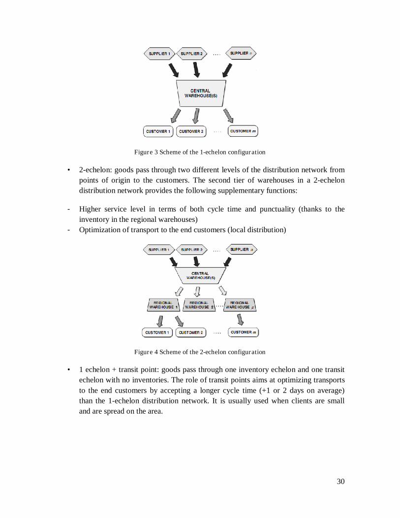
Figure 3 Scheme of the 1-echelon configuration
• 2-echelon: goods pass through two different levels of the distribution network from
points of origin to the customers. The second tier of warehouses in a 2-echelon
distribution network provides the following supplementary functions:
- Higher service level in terms of both cycle time and punctuality (thanks to the
inventory in the regional warehouses)
- Optimization of transport to the end customers (local distribution)
Figure 4 Scheme of the 2-echelon configuration
• 1 echelon + transit point: goods pass through one inventory echelon and one transit
echelon with no inventories. The role of transit points aims at optimizing transports
to the end customers by accepting a longer cycle time (+1 or 2 days on average)
than the 1-echelon distribution network. It is usually used when clients are small
and are spread on the area.

31
Figure 5 Scheme of the 1-echelon + transit point configuration
• Mixed network: this network allows direct shipment as well as deliveries through 1
or 2 echelons. Give the flexibility that allows the management of more than one
distribution problem at the same time.
Figure 6 Scheme of the Mixed configuration
• 3-echelon: goods pass through three different levels of the distribution network
from points of origin to the customers. It is composed of central warehouse,
regional warehouse and transit point.
Figure 7 Scheme of the 3-echelon configuration

32
Number of warehouse in each echelon
Assuming the number of echelons has been set, the number of warehouses has to be
determined in order to minimize the overall distribution cost for a given service level. In
order to determine the number of warehouses, several factors have to be taken into account,
for instance, costs trade-offs. The relationship of these costs will vary under different
circumstances (industry, product type, volume throughput, regional location, age of
building, handling system, etc).
The understanding and control of the trade-offs that exist between these different
costs is a key element of supply chain management and design.
First, we describe the 5 cost components.
1. Stocks cost:
• Maintenance cost:
§ Storage cost (employment and conditioned space facilities ,
goods insurance)
§ Borrowing costs on capital equipment
§ Inventories depreciation
§ Inventories obsolescence
• Order costs:
§ Management of stocking systems (stock control,
communication, update activities).
2. Inbound transport cost or Primary cost:
Cost due to the transport from establishments of the distribution network to the
nodes (compressive tariff of the extra, administrative costs, no legal responsibility
on the carrier)
3. Outbound transport cost or Secondary cost:
Cost due to the transport from the nodes of the distribution network to the clients
(compressive tariff of the extra, administrative costs, no legal responsibility on the
carrier)
4. Handling cost:
Movement of materials and packaging in the nodes of the distribution network
(unload merchandise, control, put into stock, picking, order consolidation, loading
to transport vehicle)
5. Order management cost:
Order transmission, insertion, formal and credit verification, availability, scheduling
deliveries, order confirmation)
The effect of different number of warehouses in a given distribution network can be
seen by developing the economies of scale argument. If a distribution network is changed

33
from one site to two sites, then the overall warehouse/storage costs will increase. The
inbound and outbound transports are also affected by the number of warehouses in the
distribution network, because the cost of delivery is essentially dependent on the distance
that has to be travelled.
With an increasing level of decentralization (increased number of warehouses) the
warehouse costs increase and the primary transport costs increase. In contrast, with
increasing decentralization, the secondary transport (or local delivery) costs decrease. The
total cost is assessed and this will usually lead to preferred level of centralization. In some
cases, there can be a certain amount of uncertainty as to where the optimum lies (Lovell,
Saw, & Stimson, 2005).
Cycle stocks and in transit stocks will not vary with an increase in the number of
warehouses. Instead safety stocks will increase with the number of warehouses because the
more the demand is split in the system warehouses, the more safety stocks.
Handling costs of course increase by incrementing the number of warehouses,
although is subject to economies of scale.
The next graph summarizes the costs explained before. It is obtained by adding
together the individual cost curves of the key distribution elements that correspond to each
number of sites. It can be seen from the graph that the least expensive overall logistics cost
occurs at the minimum point in the graph.
Figure 8 Logistics cost distribution
Location of warehouses
Locating fixed facilities throughout the supply chain network is an important
decision problem that gives form, structure and shape to the entire supply chain system.

34
Optimizing the location of facilities within an existing network frequently can save between
5 to 15 percent of logistics costs (Ballou 1995).
Many logistics modeling techniques used in logistics concentrate on the detailed
representation of specific parts of the logistics operation, for example: product
optimization, warehouse location and vehicle routing. Suitable techniques do not exist to
consider simultaneously all the possible alternatives. The problem of considering all
products, made at many plants, shipped via all modes, to all the customers, via all
warehouses is simple not possible. If the techniques did exist, solutions would require
uneconomic runtimes on high capacity computers.
Linear programming is a mathematical technique that finds the minimum cost or
maximum revenue solution to a distribution network problem. Under any given demand
scenario the technique is able to identify the optimum solution for the sourcing of products.
A typical sourcing model equation operates under the following constrains (Rushton,
Croucher, & Baker, 2006):
• The availability of each plant for production
• The customer demand should be met
• The least-cost solution is required
The objective of a typical sourcing model equation is to minimize the following,
given the run rate of each product at each plant:
• Raw material cost
• Material handling cost
• Production variable cost
• Logistics cost from plant to client
The output of the linear programming study is the optimized major product flows
from point of origin to final destination. The next stage is to take these flows and to
develop the most cost-effective logistics solution in terms of the most appropriate number,
type, and locations of warehouses. Cost trade-off analysis can be used as the basis for
planning and reasoning the planning of distribution systems. The models trying to address
this (Ballou, 1995) are:
• Mathematical programming or exact methods which includes, multiple center of
gravity, linear programming, integer programming and mixed integer programming
• Heuristics methods which use exact methods with heuristic procedures to guide the
solution process
• Simulation

35
Types of warehouses
(Rushton, Croucher, & Baker, 2006):
• Finished goods warehouses: hold inventories from factories
• Distribution centers, which might be central, regional, national or local: all of
these will hold stock to a greater or lesser extent
• Trans-shipment sites or stockless, transit or cross-docking DCs-by and large:
these do not hold stock, but act as intermediate points in the distribution
operation for the transfer of goods and picked orders to customers.
• Seasonal stock holding sites
• Overflow sites
In order to solve the previous problems it is important to understand what a
distribution problem is, which main factors characterize it and how it influences or affects
the flow of goods. Next section gives a broad definition of distribution problem and the
next chapter individualizes the drivers.
2.5 Objective of the network design
The distribution network design has two main objectives:
a) Identify the network structure that allows the minimization of total costs while
maintaining a predefined service level.
b) Identify the network structure that better manages the trade-off between the cost
minimization and revenue maximization derived from the increase of the service
level, guaranteeing the profit maximization.
Usually the first option is the one considered because it is simpler than the second
one. The profit maximization objective requires estimating the potential gains resulting
from the improvement of the service provided.
It is important when designing the distribution network to understand which are the
costs that impact the most and the main trade-offs between them, in order to find the most
efficient distribution solution.
Identification of the most relevant costs
The costs that need to be considered during the network design are the ones that are
affected by the network configuration, these are: transportation costs, inventory costs,
handling costs and order management costs (Chopra, 2003).
Transportation costs

36
Primary transportation costs: transportation from suppliers to the central warehouses and
from central warehouses to the regional warehouses or transit points.
Secondary transportation costs: transportation from the distribution network nodes to the
end customers.
Inventory costs
These costs refer to the four types of stocks that can be found within the logistic
system: cycle stock, safety stocks, in-transit stocks and work in progress-stock. It is
possible to group the main elements that compose the inventory costs in two categories:
Maintenance costs
• Storage Costs: generated by the used and equipped space and the insurance costs paid
for the goods stored.
• Cost of Capital
• Goods depreciation
• Goods obsolescence
Order costs
Cost of the storage system management: generated by the revision of the stock,
warehouse accountancy, communication and updating activities.
Handling costs
Costs generated by the handling activities in the warehouses and transit points of the
distribution network, which include: loading/unloading activities, picking, order
consolidation, etc.
Order management costs
These include all the costs related to personnel and information systems required for
the process of the orders (data entry, credit verification, goods availability control, delivery
scheduling, order confirmation, etc.).
2.6 Consumer Electronics Industry
This thesis will adapt the model of (Archini & Bannó, 2003) to the consumer
electronics sector; thus changes in the structure of the model will be required, for example:
change of relevant drivers and change of network solutions. It is the purpose of this thesis
to understand in a greater depth the mechanics of distribution networks in this industry, to
propose better changes and redesign approaches in order to save costs.

37
First an insight of the industry is presented, in order to understand better the basics.
Consumer electronics industry includes electronic equipment for everyday use. For
example: personal computers, telephones, televisions, cameras, mp3 players, calculators,
GPS, DVD’s and camcorders. This industry is largely dominated by Japanese and Korean
companies, such as Sony, Toshiba, Panasonic, Samsung, and LG.
Every year the Consumer Electronics Association, which is a sector of the
Electronic Industries Alliance (EIA), makes a worldwide exhibition, where manufactures
present their new products and consumers can see and try the most recent innovations.
Delivering innovative new products quickly and at competitive prices requires an
efficient and effective supply chain (Hammel, Keuttner, & Phelps, 2002).
Consumer Electronics market
According to the Consumer Electronics Unlimited the European market as a whole
in 2009 contracted by five percent. The members of Europe's biggest buying group have so
far been affected by the recession to widely differing degrees. While 2009 turnover growth
in Germany, France and Italy was actually slightly higher than the previous year's, Spain,
the United Kingdom and some East European members, for example, suffered marked
setbacks. Not all European countries are affected equally and simultaneously by the
consequences of the economic crisis. The reasons for this are the significant differences in
local market structures and consumer preferences. Despite this, intense competition persists
in the European market for consumer electronics and household appliances while pressure
on prices and margins is strong.
Eurostat has an interesting publication where compares price levels in consumer
electronics using purchasing power parities. It concludes that price levels in EU countries
lie very close together at the exception of Iceland which is far away from the average. Italy
is slightly above the average (Borchert, 2008).
e-commerce
Nowadays the Internet has become a very important resource to sell consumer
electronics equipment. The Internet is already the world's largest shopping mall, and is in a
position to grow considerably over the foreseeable future (McQuitty & Peterson, 2000).
With the Internet consumers can get great deals in less than 10 minutes of searching and
comparing prices; it eliminates the need of going physically from one store to another. It
has been stated that shoppers visit first the retailer and then buy through the Internet; this is
because they want to see first physically the product and then benefit from the Internet
purchase.

38
The electronics market is different from the markets of books, music and movies,
due to the after sales service. The success of the firms in the e-commerce market depends
on the efficiency of their distribution networks (Jay, Ozment, & Sink, 2007). This new
approach is characterized by small order size, increased daily order volumes, small parcel
shipments and same day shipments.
Environment
A very important issue to take into account is the environmental waste that is
generated every year by electronic equipment. Since 2003 there is an EU legislation that
restricts the use of hazardous substances in electrical and electronic equipment and
promotes the collection and recycling of such equipment. It also provides schemes where
consumers can return their used e-waste to the manufacturer free of charge.
Despite such rules on collection and recycling only one third of electrical and
electronic waste in the European Union is reported as separately collected and appropriately
treated. A part of the other two thirds is potentially still going to landfills and to sub-
standard treatment sites in or outside the European Union.
Network redesign examples
It has been realized that by redesigning the distribution network of this type of
industry, companies can save a lot in costs. For instance, the reengineering of HP’s CD-RW
Supply Chain and the design of a supply chain for innovative products of Nokia has lead to
a significant costs reduction.
HP
Hewlett Packard was one of the pioneers of the re-writable CD-RW industry.
Initially this product was targeted to business users but then the consumer market exploded
with the digital revolution and the Internet, so revenues were doubling annually. On the
other hand, the industry experienced accelerated product life cycles and the average selling
price continued to drop 50% per year, due to competition.
Due to the previous facts, HP was forced to create a new business model that could
deliver consistent profits in a market with significant price drops. The previous supply
chain model was slow (126 days Cycle Time), expensive, unresponsive and with increasing
inventory-driven costs.
After the implementation of the new supply chain, the results were savings from
$50m a year, realizing total investment in less than a month. One world wide- distribution
center in Asia, (instead of 3 regional locations) and 90% reduction in supply chain cycle
time (from 126 days to 8 days).

39
Nokia
Many businesses deal with the problem of designing supply chains for diverse
customer’s needs; this is the case of Nokia. Nokia’s networks division wrestled with a
challenging problem: how to deliver its mainstay product, the base station that is the back
bone of mobile communications, from a few days for some customers to a couple of weeks
for others, and do so at an acceptable cost (Eero & Holmström, 2009).
Nokia understood that in order to support sales growth of its innovative products, its
supply chain should be responsiveness, which is able to fill orders quickly, instead of
efficient, which Fisher recommends for functional products. At a first try, Nokia configured
a supply chain with country warehouses of finished products located close to the customers
in order to fulfill orders in a matter of days. This configuration did not work, because it
gave rise to inventory increasing costs (100 days of inventory), obsolescence and they
realized that often a needed product configuration was not available at a specific location.
After analyzing what went wrong, the company determined that its customers fell
into 3 categories and each needed a different supply chain. Three different supply chains
were implemented and an inventory reduction of 40-45 days of supply was achieved and
satisfaction improved significantly.

40
Chapter 3. General Methodology for the Development of the Model
In the previous chapter it was explained the characteristics and importance of the
distribution networks and the different possible configurations that can be obtained during
the design phase by combining the number of echelons, the number of warehouses in each
echelon, the location of the warehouses and their type. Also, it was described the different
types of costs that are involved in the logistic activities which demonstrate the high level of
complexity of the problem.
In this chapter, it is presented the methodology used for the development of the
different stages of the Distribution Network Design Model proposed by this work, starting
with the proper identification of the main factors or drivers that affect the first stages of the
distribution network design, data that was collected from the literature. Followed by the
identification and analysis of different distribution problems presented within firms
pertaining to the consumer electronics industry in Italy, for which some interviews were
done, and finally the identification of correlations between the distribution problems
observed and the distribution networks adopted by those companies in order to satisfy the
requirements of the clients in terms of service and at the same time reducing the total costs.
It has been decided to analyze Italian companies because as described in the section
2.3 there have been important changes in Europe during the last years that led to
reconfigurations of the distribution networks (Hammel, Keuttner, & Phelps, 2002).
The following flow chart presents the sequence of steps described above.
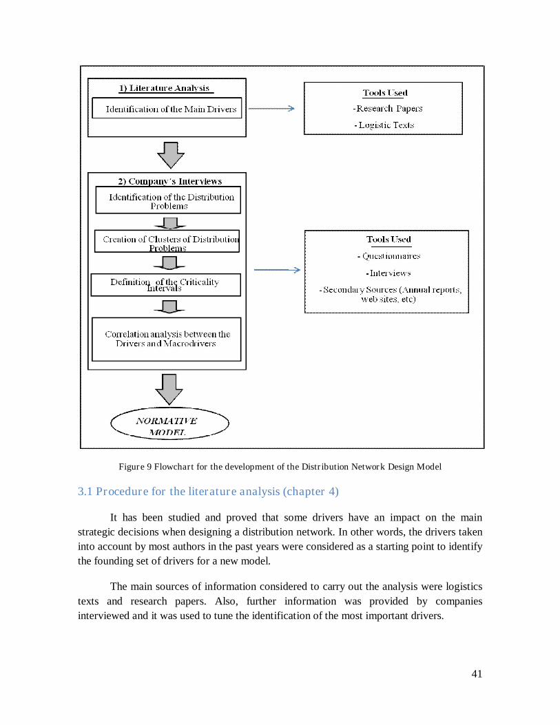
41
Figure 9 Flowchart for the development of the Distribution Network Design Model
3.1 Procedure for the literature analysis (chapter 4)
It has been studied and proved that some drivers have an impact on the main
strategic decisions when designing a distribution network. In other words, the drivers taken
into account by most authors in the past years were considered as a starting point to identify
the founding set of drivers for a new model.
The main sources of information considered to carry out the analysis were logistics
texts and research papers. Also, further information was provided by companies
interviewed and it was used to tune the identification of the most important drivers.
42
Several methodologies which are related to the distribution network design problem
have been presented by different authors. From those, it was possible to identify two types
of approaches: the “complete” ones that try to solve both strategic (structure of the network,
types of warehouses, etc) and operational issues (flow management, delivery policies, etc);
and other methods that are focused in a part of the problem, like for example the location
and allocation of the warehouses. For the purposes of this thesis, it has been decided to
consider only the researches of the first group, because they present the problem as a
combination of different factors.
In the case of the research papers, a total amount of 30 papers were analyzed and
classified according to the distribution network choice that was intended to solve and the
main drivers considered by each author as relevant in order to achieve an optimal solution.
Among the papers found, different distribution network choices were tackled but for
the driver analysis only four of those were considered since they are the relevant ones
according to the objective of the current thesis. The network choices selected, as it was
mentioned in the section 2.4, were:
• Definition of the number of echelons of the distribution network
• Definition of the number of warehouses for each echelon
• Definition of the warehouse location
• Definition of the warehouse typology
It can be distinguished two types of papers, the ones that face the problem using a
quantitative approach and the ones that are qualitative oriented.
• Quantitative papers: quantitative research refers to the systematic empirical
investigation of quantitative properties or variables, and their relationships. The
objective of quantitative research is to develop and employ mathematical models,
theories and/or hypotheses pertaining to a phenomenon. The analysis in the
quantitative research proceeds by using statistics, tables, or charts. In the case of
logistics, this type of papers usually intends to solve a specific problem of the
network configuration, for example the warehouse location.
• Qualitative papers: qualitative research involves gathering information that is not
based on empirical data accumulation. The focus is on the expert opinion of people
who are knowledgeable about the explored question and can give insights about the
area. It relies more on the authentic opinion of fewer subjects, and is hardly
presented in the form of numerical data. In-depth analysis can be carried out on the
base of this type of research. On the other hand, to some extend it suffers from
subjectivity and bias. For logistics, this second category of papers aims at solving

43
the problem from a wider perspective and not focusing only in one part of the
distribution network configuration (W.L & Neuman, 1997).
Both types were considered for the main drivers’ identification since ultimately all
the papers intent to solve the same problem despite the fact that the methods used are
different. To carry out their analysis with a methodological approach, a table was designed
and all the information considered relevant was registered. Its purpose was to have a
synthesized view of the main problems that were discussed in the papers and the main
drivers that were taken into account in order to solve those problems.
In order to make a better analysis, the drivers mentioned in the papers were
classified in four categories that are called macrodrivers, or group of drivers that have a
direct impact on a specific element of the distribution network. These macrodrivers
influence directly the logistics costs, but mostly the physical distribution, reason why they
can guide the designer to the best network. The macrodrivers are:
- Product Drivers: characteristics of the product
- Service Drivers: characteristics of the service provided to the customer and the
process performance
- Demand Drivers: spatial and temporal characteristics of the demand
- Supply Drivers: characteristics of the supply chain
Once identified the different drivers, different correlations between the drivers and
the distribution network decisions (number of echelons, number of warehouses, warehouse
location and typology of warehouse) were obtained taking in consideration the frequency of
appearance of the driver among all the papers to make one decision.
At the end, it was assumed that the frequency of appearance of the drivers in the
papers analyzed, and that are used to take one distribution network decision, is directly
proportional to the importance of that driver during the distribution network design. With
this it was possible to obtain a list of drivers that must be taken in consideration during the
design or re-design of a distribution network.
3.2 Procedure for the interviews (chapter 5)
Once having identified and analyzed the main drivers that must be taken in
consideration for the distribution network design, the next step was to develop a tool that
could be delivered to several companies operating in the consumer electronics industry in
Italy in order to obtain from them the characteristics of the four macrodrivers previously
defined (product, service, demand and supply) and the distribution networks actually
implemented by them.

44
The tool developed was a Questionnaire which includes the following main sections
(Appendix 1):
1) Data Context: Corresponds to general data of the interview (Name of the
company, Date, Interviewee) and general data of the company (Sector, Market
Share, Business units to consider)
2) Commercial Organization: which is referred to the type of clients of the
company,
3) Characterization of the actual Distribution Network:
a. Drivers for the design of the distribution network: the different drivers
obtained during the literature analysis were grouped in macrodrivers
(product, service, supply and demand) and presented in the questionnaire
with their respective units of measure.
b. Characterization of the Supply chain: includes a chart with the number,
location and characteristics of each node of the actual distribution
network.
c. Actual Distribution Network: includes a graphic representation of the
different distribution network types where it can be selected the used
one, and also an European map were it can be placed the different plants,
warehouses and transit points that conforms the distribution network of
the company
4) Flow Characterization: corresponds to a graph were it can be placed the
different flows that the company´s products follow from the plants the final
clients. It is asked to present also the percentage of each flow.
5) Managerial Logic: corresponds to the inventory policy used by the company, the
kind of transportation implemented and the strategic decision of give in
outsource or not some of the logistics activities.
For the implementation of the questionnaire, different companies of the consumer
electronics industry were contacted. Some prerequisites were established in advance in
order to obtain a representative, coherent with the objectives of this thesis and uniform
sample for the analysis, which were:
- Products manufactured: Personal computers, digital imaging, televisions, mobile
phone, sound and peripherals, and white goods.
- Multinational firms operating in Italy
- Interviewee: Logistic or Operations Manager
Three companies of the industry which satisfied the requirements mentioned above
accepted to be interviewed: Hewlett-Packard, Sony and Samsung. Although the limited
number of them, it was considered to be a representative sample of the consumer
electronics industry because the distribution problems presented in each one were diverse,

45
as well as the distribution network adopted. A wide range of problems and solutions was
obtained with the sample used.
Due to the availability of time of the Managers interviewed, a personal interview
was not possible, but a phone call appointment was fixed with each of them with duration
of approximately one hour. During the phone interview, several questions were asked and
the questionnaire was used as a supporting tool; it was not directly filled by the
interviewees.
3.3 Procedure to Identify Distribution Problems (chapter 5)
The information collected during the interviews was used to fill the questionnaires
in order to have in the form of charts, graphs and maps all the information given by the
managers in charge of the logistics of their company.
For each company case it was possible to identify at least one distribution problem,
or groups of products and clients characterized by specific values of the drivers that project
the network, and that justify a specific flow management. The individuation and description
of these problems is very important to understand the factors that affect and influence the
strategic decisions of the network design.
In “Global operations and logistics text and cases” (Dornier, Fender, & Kouvelis)
distribution problems are defined as “logistic families”, stressing that identifying diverse
families within an organization demonstrates a mature level in the flow management. These
approach permits to implement distribution processes differentiated according to the
regrouping characteristics, rather than only one for all the products and clients. For each
family a logistics route has to be established with the objective of minimizing total costs
guarantying the service level requested by the clients. The authors propose characterization
criteria:
• The cycle time, conditioned strongly by the choice of transportation and the
allocation of inventories in the system, and the
• Order dimension
A firm should in this way characterize its distribution problems only on the base of
4 groups that derive on the combination of cycle time (high/low) and the dimension of the
order (high/low). The adopted matrix for the definition is the following:

46
Figure 10 Distribution problem matrix of Dornier et all.
To describe the distribution problems based only in these two drivers, is not
complete, because there are other drivers that impact considerably over the firm strategic
choice: for example the high value of the product pushes over the centralization of the
stocks in order to reduce the costs related to the financial charges, the security and its
inventories.
In this point of the chapter it is explained the criteria followed by this model and
applied to the firm cases in order to define completely the distribution problems.
Adopted procedure
The criteria proposed for the definition of distribution problems in the scope of each
analyzed firm case, is composed by two principal steps.
First the flow diagrams has to be studied, presented in the paragraph 5.3 of each
firm case in the chapter 5, in order to identify groups of products and clients characterized
by a specific management of flow.
Subsequently, the values of the drivers are analyzed for each individual group, in
order to provide a complete description.
It is important to underline that, once the groups of products and clients with a
determined logistic route are identified, it corresponds always to precise values of service,
demand and supply, while the product drivers are not valuable in a univocal way.
This is because inside one logistic family individualized it can be found a wide
range of codes, each with specific characteristics. For example a firm can adopt one
distribution network for 5000 products belonging to diverse sectors and characterized by
different properties. To describe this problem in terms of product drivers, it was therefore
calculated the average of all the products distributed with one unique network.
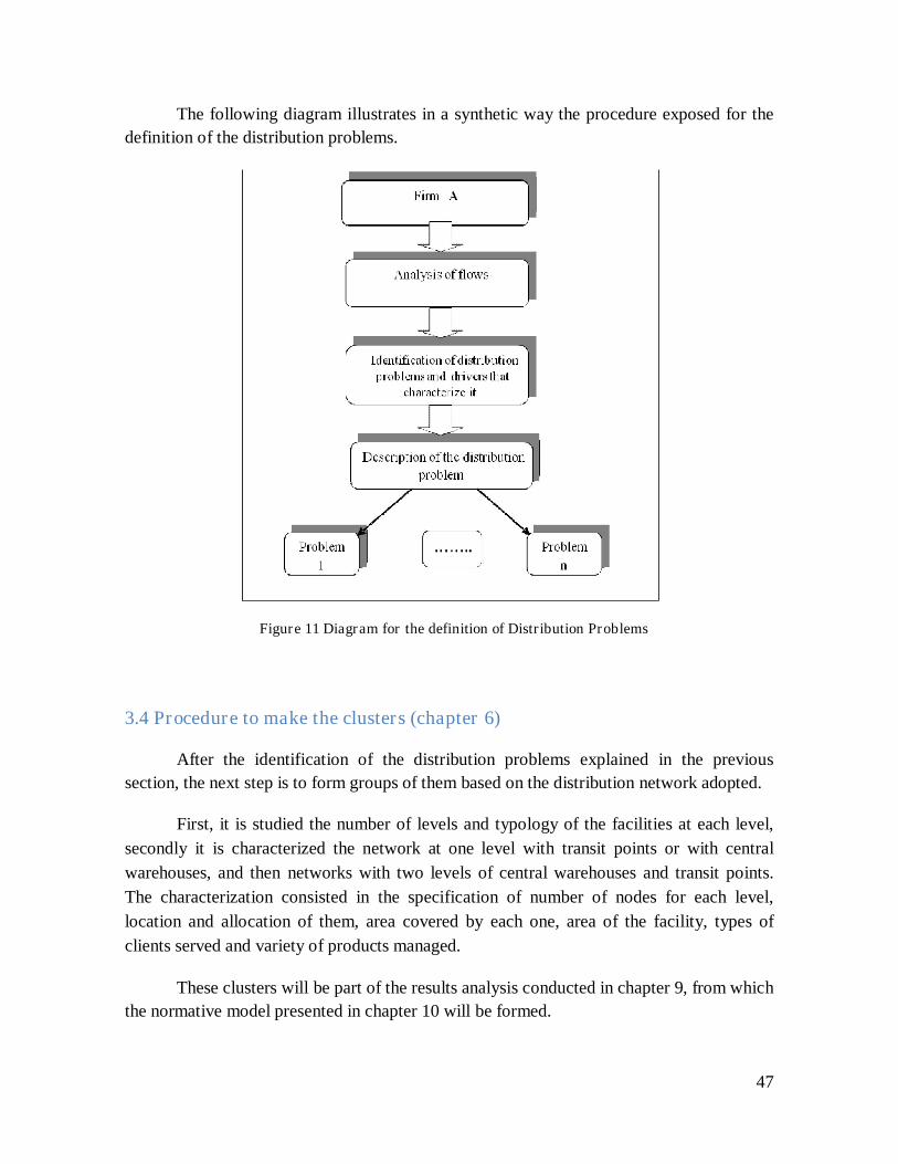
47
The following diagram illustrates in a synthetic way the procedure exposed for the
definition of the distribution problems.
3.4 Procedure to make the clusters (chapter 6)
After the identification of the distribution problems explained in the previous
section, the next step is to form groups of them based on the distribution network adopted.
First, it is studied the number of levels and typology of the facilities at each level,
secondly it is characterized the network at one level with transit points or with central
warehouses, and then networks with two levels of central warehouses and transit points.
The characterization consisted in the specification of number of nodes for each level,
location and allocation of them, area covered by each one, area of the facility, types of
clients served and variety of products managed.
These clusters will be part of the results analysis conducted in chapter 9, from which
the normative model presented in chapter 10 will be formed.
Figure 11 Diagram for the definition of Distribution Problems

48
3.5 Criteria for the definition of the criticality intervals (chapter 7)
In order to get the synthetic representation of each distribution problem of the
company cases, it is needed for the projection a reference scale, composed by 5 intervals in
order to find the criticality of each driver. The intervals have a growing criticality value
from 1 to 5.
The objectives of this operation are two:
• Obtain an absolute reference system that permits the confrontation between drivers with
different units of measure.
• Put in evidence the different intensities with which the value of a driver can influence
the costs, or identify the criticality that the particular driver has in the company case.
The 5 intervals are:
• 1: low criticality
• 2: medium low criticality
• 3: medium criticality
• 4: medium high criticality
• 5: high criticality
The criteria proposed for the definition of the intervals has the following steps:
1) Associate to each distribution problem, the characteristic color of the network solution.
2) Trace the axes of the driver to the growing criticality
3) Place the distribution problems over the axes basing on the punctual value
4) Subdivide the axes in intervals from 1 to 5
Figure 12 Diagram for the definition of the Criticality Intervals

49
1. Each driver is represented with different colors depending on the cluster that it belongs
to. In particular the colors are the following:
2. Trace the axes of the driver to the growing criticality
3. Each distribution problem is represented with its particular color over the axes basing
on the punctual value. For the representation, refer to the tables defined in chapter 5.
4. The identification of different zones of criticality for each driver is done analyzing the
distribution of the colors of the different distribution problems over the axes:
• The intervals of high and low criticality are characterized of specific colors that
identify network solutions well defined. For example, considering the following
figure that examines a generic driver: at a higher level of criticality the degree of
centralization augments. In this case the interval definition of high criticality (5)
is at the extreme right characterized by distribution problems with direct
delivery; the interval of low criticality (1) would be instead the one at the
extreme left characterized by decentralized solutions.
• The zones of criticality medium low or medium high are identified instead of
one or two colors representing solutions of gradual passing of one strategic
choice (centralization) to the opposite (decentralization). Considering the
preceding example, a medium high criticality (4) it’s characterized of networks
of one level with CW, one level with TP or networks of two levels with CW and
TP. Similarly will be indicated the medium low criticality (2) characterized by
Yellow: direct delivery from plantsGreen: 1 level of CWsBlue: 1 level of TPsRed: 2 levels, CWs and TPs
PB1 PB2 PB3 PB4 PB7 PB8 PB9 PB10 PB11 PB13 PB15 ........ PB(i) PB(i+1) PB(i+2) PB(n)
PB5 PB6 PB12 PB14 PB16 PB(i+3)
1
5
Low Criticality
High Criticality

50
distribution problems with networks of two levels with CW and TP or 1 level
with TP.
• The medium criticality (3) is characterized by the presence of all or almost all
the colors meaning that in this interval can be found almost every network
solution and therefore the driver has no particular influence in determining the
solution.
PB1 PB2 PB3 PB4 PB7 PB8 PB9 PB10 PB11 PB13 PB15 ........ PB(i) PB(i+1) PB(i+2) PB(n)
PB5 PB6 PB12 PB14 PB16 PB(i+3)
1 5 2 4 3
Medium
Criticality
PB1 PB2 PB3 PB4 PB7 PB8 PB9 PB10 PB11 PB13 PB15 ........ PB(i) PB(i+1) PB(i+2) PB(n)
PB5 PB6 PB12 PB14 PB16 PB(i+3)
1 5
Medium-
Low
Criticality
Medium-
High
Criticality
2 4

51
It is opportune to emphasize that the preceding example is an ideal case, because in
reality in the different zones could appear exceptions. Hence, never is a single driver which
determines the network choice, but rather the combination of more factors. The objective is
to get for each driver the reasonable intervals that are comparable between them and
characterized by the presence of distribution problems that fall on it.
Using the scales of criticalities, the conversion of all the driver´s values of the
distribution problems obtained during the interviews to a unique unit of measure was done.
After this operation, it was possible to calculate the criticality values of each macrodriver
(Product, Service, Demand and Supply), which were considered as the average of the
drivers that compose each macrodriver.
max
max
j
c
C
j
jj
i
∑=
with: =jc driver criticality j, with j = [1, …, jmax];
=iC Macrodriver criticality i;
i = {product, service, demand, supply}
j = {variety, value, density, …., level of specialization} = {all the drivers}
Finally, with the objective of represent the distribution problems in a more
aggregated way it has been decided to define two new dimensions: Market, which is the
combination of Service and Demand drivers, and Firm, which is the combination of
Product and Supply Drivers. The decision on grouping the data in this form derives from 2
hypotheses.
In the first place, it is considered that product and supply drivers are strongly
conditioned to the internal decisions of the firm, while demand and service is determined
by the market, or by exogenous elements of the firm. In reality, the limits between internal
and external decisions are not so clear. The characteristics inherent to the product, for
example, are not completely attributable to the firm’s will, but are in part determined from
the market needs; analog considerations can be made to the service level.
The other hypothesis is based on the fact that product and supply drivers influence
more over maintenance and handling costs, while the drivers of service and demand
influence more on transport costs.

52
Therefore it is possible to obtain representative values by calculating the averages of
the discussed pairs of macrodrivers.
2
ClCpCF
+=
2
CdCsCM
+=
CF = firm criticality; =CM market criticality;
=Cp product criticality; =Cs service criticality; =Cl supply criticality; =Cd demand criticality.
In the way that are expressed the formulas above, it is assumed that the drivers
pertaining to a macrodriver, and the macrodrivers that conform a group, has the same
weight within it, which means that no differentiation of importance of the drivers and
macrodrivers is considered. A further analysis of Correlations was done in order to prove if
this assumption was correct, or if the formulas needed to be adjusted by assigning levels of
importance to each element.
3.6 Procedure for the correlation analysis (chapter 8)
The correlation analysis is a statistical method that defines the variation in one
variable by the variation in another, without establishing a cause-and-effect relationship.
The coefficient of correlation is a measure of the strength of the relationship between the
variables; that is, how well changes in one variable can be predicted by changes in another
variable (Business Glossary, 2010).
For the purposes of this thesis, the correlation analysis was done with the objective
of identify the relation between the drivers and between drivers and their correspondent
macrodriver. It was used as input data the chart of distribution problems expressed with the
drivers criticalities (Tables 19 and 20). Using the formula “CORRELATE” of a Microsoft
Excel worksheet it was possible to obtain a symmetric and diagonal chart of Correlation
Factors between all the drivers and macrodrivers.
With the analysis of the result´s chart it was possible to determine whether or not
different weights or level of importance of each driver within the macrodrivers should be
assigned.
3.7 Synthetic representation of the firm cases (chapter 8)
With the objective of representing in a synthetic way the company cases, it was
opportune to build a form that permits to underline on one side the characteristics of the
identified distribution problem within each company case and on the other side the solution
of the correspondent network.

53
All data is reported in a structured and precise way. The form, in fact, is a document
that permits to observe the most significant information to deal with the analysis of
correlation between the complexity of the distribution problem and the spatial network.
Next, it is reported the structure of the form.
The sheet is divided in 3 major sections; which contain significant data for the
development of the research.
COMPANY NAME
General data
Distribution problem
Synthetic representation of data
Punctual values and criticality of
drivers
Legend: Na= not available
Criticalities of drivers and
macrodrivers
Solution of the network
- Decision on the number and typology of the levels
- Characterization (decision on the number, location and allocation) of the nodes
Supply
Service
Product
Demand

54
General data
First, general data, in order to identify and characterize the company context in test:
- Sector
- Categories of products
- Turnover
Synthetic representation of the data
Initially the distribution problem is represented graphically, in a way to immediately
provide the information of which are the more relevant drivers. Aggregation was carried
out using two broken lines to connect the values of product and supply and service and
demand. The two areas generated, colored different, provide immediately the idea of which
ones are the more critical drivers for each distribution problem considered. Green area
indicates market and yellow area indicates firm.
Afterwards, a summary table of the drivers is reported, completed with data
obtained during the meeting with the company. In the adjacent column to the punctual
values are the respective criticalities. The average is next reported, for each macrodriver,
following the table just described.
Solution of the network
Based on the solution adopted by the firm, it is first reported the graphical
representation of the network that describes the levels, then follows a representation that
characterized, in terms of number, location and allocation of the nodes of the network.
Followed by a short description.

55
Chapter 4. Identification of the main drivers that describe a distribution
problem
In this chapter is carried out the literature analysis in order to identify the main drivers
that describe a distribution problem and that will conduct the core of the analysis of the
company cases. First are described the total amount of drivers presented in the work of “Archini
and Bannò” in order to understand better what each one means and how they are measured. The
drivers are grouped in macrodrivers: Product, Supply, Demand and Service. Then, the literature
analysis was carried out by analyzing 30 papers. Graphs and tables are shown in order to
understand better which the most important drivers are and which most of them authors have
considered in their investigations.
4.1 Description of the Drivers presented by “Archini and Bannó”
Product Drivers
Density (kg/m3)
The density of a product is defined as its mass per unit volume.
Value (€/kg)
It’s the ratio between the price of the product and its weight.
Risk of Obsolescence (days)
Every product has a specific life cycle, time that can be measured in days, weeks,
months, etc. The risk of obsolescence can be considered either as perishability (time
from the date of production to the date of expiration), for example for fresh goods or it
can be seen as the period of time that a product can be offered to a market which is
determined by changes in the customer’s needs or due to the launch of a new version of
the product, for example for consumer electronics goods.
Variety (number of products)
Amount of different product codes that a company has. It is measured according to the
number of codes commercialized by the company during a year.
Substitutability (qualitative)
In the case that the product is out of stock the company could supply another product to
satisfy the same customer need.

56
Product complexity (qualitative)
Level of technology and innovation involved in developing the product, also includes
the level of services involved in supporting the product from production through
distribution and after sales support.
Contribution margin (%)
Contribution margin equals price minus variable cost divided by price and is expressed
as a percentage.
Service Drivers
Cycle Time (days)
Number of days it takes to deliver an order from the moment it was placed by the
customer.
Accuracy (%)
Represents the capacity of the firm to fulfill orders in the exact way as it was placed by
the customer. It can be calculated by dividing the number of correct orders delivered by
the total number of orders placed.
Completeness (item fill rate)
It is the probability of having a product in stock when a customer’s order arrives.
Tracking (qualitative)
Capacity of the firm to provide relatively accurate information about the state of the
order in progress.
Returnability (qualitative)
Ease with which a customer can return unsatisfactory merchandise and the ability of
the network to handle such returns.
Customer experience (qualitative)
Ease with which the customer can place and receive the order.

57
Demand Drivers
Number of Customers
Total number of customers the company has.
Spatial density (number of customers/km2)
The quantity delivered on each shipment is directly related with the amount of Point of
Sales (or customers) that a company has by square kilometer.
Dimension of the order (typology)
The dimension of the order can be classified from the point of view of the quantity, in
different levels: single product, packages, boxes, pallets, truck loads.
Frequency of delivery (deliveries/week client)
Corresponds to the amount of deliveries for unit of time (days, weeks, months)
Seasonality (qualitative)
Any predictable change or pattern in a time series that recurs or repeats over a specific
period of time can be said to be seasonal.
Predictability of demand (%)
Average margin of error in the demand forecast at the time production is committed.
Supply Drivers
Number of Plants
Total number of plants the company has.
Exclusivity of production in a plant
It is the exclusivity of realization of a product in one plant.
Distance from plant to client (km)
The location of customers and the location of the plants have to be known in order to
calculate the distance.
Level of specialization
Plants producing only one family of products

58
4.2 Classification of the papers by distribution network decisions and drivers
The first table details the paper reference number, author and year, and the second one
specifies the reference number of the paper that considers a driver relevant for each decision.
In the following tables are listed the four distribution network decisions and their
relation with the drivers according to each author.

59
Table 1 Papers reference
Reference
numberTitle Authors Journal Year
1 What is the right supply chain for your products? T. Payne and M. J. Peters Journal of Logistics Management 2004
2 Assessing International Allocation Strategies B.t Vos and E. van den Berg International Journal of Logistics Management 1996
3 How to design the right supply chain for your customers E. Eloranta and J. Holmström Supply Chain Management: an international journal 2009
4 Designing a Distribution Network in a SC S. Chopra Transportation Research Part E 2003
5Reformulating a Logistics Strategy: A concern for the Past, Present and
Future. R. Ballou International Journal of Physical Distribution 1993
6 Distribution/Logistics Network Planning D. Ratliff Georgia Tech
7 Product value-density: managing diversity through supply chain segmentationA. Lovell, R. Saw and J. Stimson
The Internationl Journal of Logistics Management 2005
8Distribution Network Design an Integrated Planning support framewor Mourtis and Evers International Journal of Physical Distribution & Logistics 1995
9 Logistics Network Design: Modeling and Info considerations R. Ballou International Journal of Logistics Management 1995
10Location/allocation and routing decisions in in supply chain network design S. H. Lashine, M. Fattouh and A. Issa
Journal of Modelling in Management2008
11 Distribution network design: New problems and related models D. Ambrosino, M.G. Scutell European Journal of Operational Research 2005
12International Logistics: A diagnostic Method for the Allocation of Production
and Distribution FacilitiesVan de Ven and Ribbers International Journal of Logistics Management
1993
13Achieving agility in SC through simultaneous design of and design for SC
H.Sharifi, H.S. Ismail and I. ReidJournal of Manufacturing Technology Management 2006
14 A taxonomy for selecting global supply chain strategies M. Christopher International Journal of Logistics Management 2006
15Distribution system Design with two level routing considerations
Jenn-Rong Lin and Hsien-Ching LeiDepartment of Transportation and Navigation Science, National
Taiwan Ocean University 2009
16 Linking Products with Supply Chains: Testing Fisher's Model E. Selldin and J. Olhager Supply Chain Management: An international Journal 2007
17 Distribution network design under uncertain demand I. Ferretti, S. Zanoni, and L. Zavanella Universita degli Studi di Brescia 2009
18 An integrated model for logistics network design J.F. Cordeau and F. Pasin HEC Montreal 2006
19 De Novo Programming Model for Optimal DND R. Thomas A Proposal for the Faculty of Research Grant 2002
20 Column generation: Application in distribution network design T. Chung-Piaw (NUS) 2002
21 What is the right supply chain for your products? (1997) M. Fisher Harvard Business Review 1997
22 Optimization models for the dynamic facility location and allocation problem R. Manzini and E. Gebennini International Journal of Production Research2006
23Transportation, facility location and inventory issues in distribution network
design - An investigationV. Jayaraman International Journal of Operations & Production Management
1998
24Inventory, transportation, service quality and the location of distribution
centersL. K. Nozick and M. A. Turnquist European Journal of Opeartions Research
2000
25 On assessing the sensitivity to uncertainty in distribution network design C.S. Lalwani, S.M. Disney and M.M. NaimInternational Journal of Physical Distribution & Logistics
Management 2006
26 Evaluating logistics network configurations for a global supply chain A. Creazza; F. Dallari; M. Melacini Supply Chain Management: An international Journal 2007
27Strategic design and operational management optimization of a multi stage
physical distribution systemR. Manzini and F. Bindi Transportation Research Part E
2008
28 Supply Chain design in the food industry J. van der Vorst, S. van Dijk and A. Beulens International Journal of Logistics Management 2001
29 Analytic hierarchy process to assess and optimize distribution network M. J. Sharma, I. Moon and H. Bae Applied mathematics and Computation2008
30 Central Distribution in Europe J. Ashayeri and J. Rongen International Journal of Logistics Management 1997
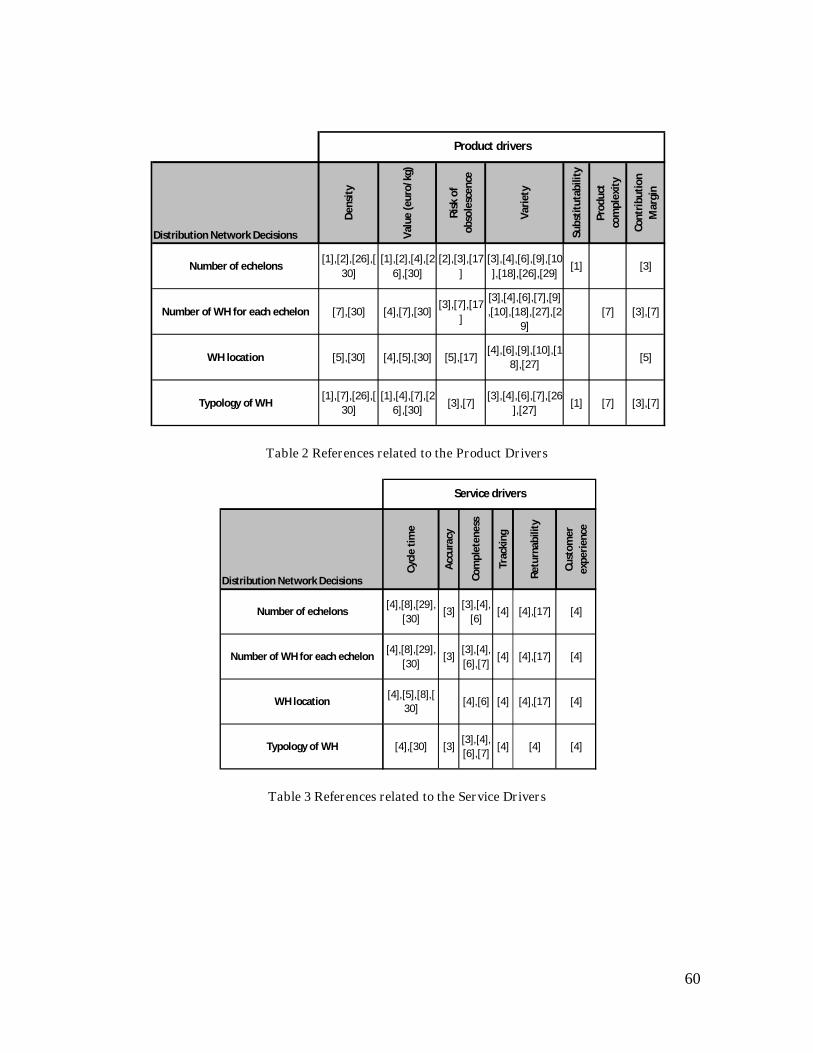
60
Table 2 References related to the Product Drivers
Table 3 References related to the Service Drivers
Distribution Network Decisions
De
nsi
ty
Val
ue
(e
uro
/kg)
Ris
k o
f
ob
sole
sce
nce
Var
iety
Sub
stit
uta
bili
ty
Pro
du
ct
com
ple
xity
Co
ntr
ibu
tio
n
Mar
gin
Number of echelons[1],[2],[26],[
30]
[1],[2],[4],[2
6],[30]
[2],[3],[17
]
[3],[4],[6],[9],[10
],[18],[26],[29][1] [3]
Number of WH for each echelon [7],[30] [4],[7],[30][3],[7],[17
]
[3],[4],[6],[7],[9]
,[10],[18],[27],[2
9]
[7] [3],[7]
WH location [5],[30] [4],[5],[30] [5],[17][4],[6],[9],[10],[1
8],[27][5]
Typology of WH[1],[7],[26],[
30]
[1],[4],[7],[2
6],[30][3],[7]
[3],[4],[6],[7],[26
],[27][1] [7] [3],[7]
Product drivers
Distribution Network Decisions
Cyc
le t
ime
Acc
ura
cy
Co
mp
lete
ne
ss
Tra
ckin
g
Re
turn
abili
ty
Cu
sto
me
r
exp
eri
en
ce
Number of echelons[4],[8],[29],
[30][3]
[3],[4],
[6][4] [4],[17] [4]
Number of WH for each echelon[4],[8],[29],
[30][3]
[3],[4],
[6],[7][4] [4],[17] [4]
WH location[4],[5],[8],[
30][4],[6] [4] [4],[17] [4]
Typology of WH [4],[30] [3][3],[4],
[6],[7][4] [4] [4]
Service drivers
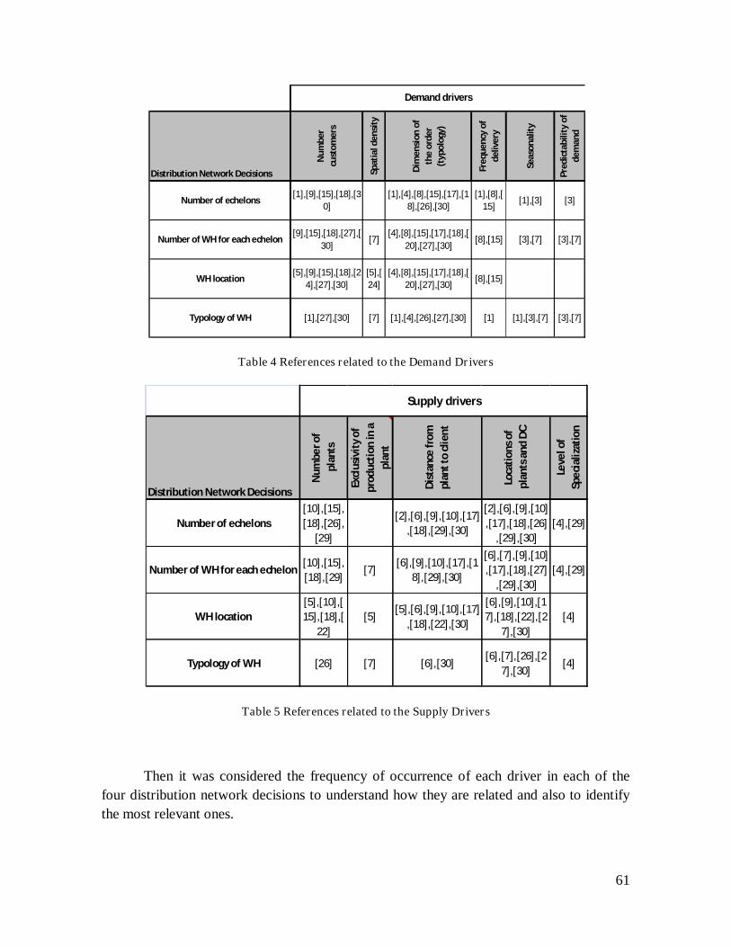
61
Table 4 References related to the Demand Drivers
Table 5 References related to the Supply Drivers
Then it was considered the frequency of occurrence of each driver in each of the
four distribution network decisions to understand how they are related and also to identify
the most relevant ones.
Distribution Network Decisions
Nu
mb
er
cust
om
ers
Spat
ial d
en
sity
Dim
en
sio
n o
f
the
ord
er
(ty
po
logy
)
Fre
qu
en
cy o
f
de
live
ry
Sea
son
alit
y
Pre
dic
tab
ility
of
de
ma
nd
Number of echelons[1],[9],[15],[18],[3
0]
[1],[4],[8],[15],[17],[1
8],[26],[30]
[1],[8],[
15][1],[3] [3]
Number of WH for each echelon[9],[15],[18],[27],[
30][7]
[4],[8],[15],[17],[18],[
20],[27],[30][8],[15] [3],[7] [3],[7]
WH location[5],[9],[15],[18],[2
4],[27],[30]
[5],[
24]
[4],[8],[15],[17],[18],[
20],[27],[30][8],[15]
Typology of WH [1],[27],[30] [7] [1],[4],[26],[27],[30] [1] [1],[3],[7] [3],[7]
Demand drivers
Distribution Network Decisions
Nu
mb
er
of
pla
nts
Excl
usi
vity
of
pro
du
ctio
n in
a
pla
nt
Dis
tan
ce f
rom
pla
nt
to c
lie
nt
Loca
tio
ns
of
pla
nts
an
d D
C
Leve
l of
Spe
cial
izat
ion
Number of echelons
[10],[15],
[18],[26],
[29]
[2],[6],[9],[10],[17]
,[18],[29],[30]
[2],[6],[9],[10]
,[17],[18],[26]
,[29],[30]
[4],[29]
Number of WH for each echelon[10],[15],
[18],[29][7]
[6],[9],[10],[17],[1
8],[29],[30]
[6],[7],[9],[10]
,[17],[18],[27]
,[29],[30]
[4],[29]
WH location
[5],[10],[
15],[18],[
22]
[5][5],[6],[9],[10],[17]
,[18],[22],[30]
[6],[9],[10],[1
7],[18],[22],[2
7],[30]
[4]
Typology of WH [26] [7] [6],[30][6],[7],[26],[2
7],[30][4]
Supply drivers

62
Macrodrivers frequency
0
10
20
30
40
50
60
70
80
90
Product Drivers Demand Drivers Supply Drivers Service Drivers
Drivers
Fre
qu
en
cy
4.3 Analysis of the collected information
On the previously shown tables are represented the connections between drivers and
decisions of the distribution network design problem. By considering these relationships
and their frequencies of occurrence the importance of the drivers can be weighted. The first
step is to consider the most aggregated level which is the macro groups of drivers
identified: Product, Service, Demand and Supply. In order to create a model that evaluates
all the tradeoffs existent when a decision is made, these four clusters should be carefully
considered.
The analysis of the collected data (Table 6) indicates that the Service cluster has
been less considered in the papers analyzed, while the Supply and Product drivers are the
ones in which the most effort has been placed. This conclusion is coherent with the fact that
most of the papers found are focused in the quantitative optimization of the system and
Service Level variables are much more difficult to translate into a variable in a
mathematical model.
Table 6 Frequency of each cluster of drivers
When focusing in the decisions for the distribution design problem the results
indicate that the previous authors focused more in determining the ideal number of
echelons and warehouses for the structure while giving less importance to which type of
warehouse suited best the network.
Driver Frequency Incidence (%)
Supply Drivers 56 22%
Product Drivers 77 31%
Demand Drivers 73 29%
Service Drivers 45 18%
Total 251
Graph 1 Frequency of each cluster of drivers

63
Table 7 Occurrence of each type of decision
The second level of analysis consists in finding which are the drivers that represent
better each decision of the distribution design problem and then choosing a balanced set of
drivers. This can be achieved through the graphical representation of the amount of times
that each driver was considered to model the decisions.
It could be argued that the frequency analysis leads to unfounded conclusions, since
it considers the amount of times and not the focus and deepness applied to the research in
each paper.
Since the objective is to determine what is considered by logistic experts as key
indicators for the distribution design problem, it is the frequency of occurrence rather than
other aspects that has to be studied in order to identify the starting group of drivers for the
model.
In the following graphs are represented the choices for distribution network design
against the amount of times that each driver was considered to explain them:
Decision Frequency Incidence (%)
Number of echelons 69 27%
Number of WH for each echelon 69 27%
WH location 59 24%
Typology of WH 54 22%
Total 251

64
Graph 2 Drivers frequency for the decision: “Number of echelons”
Graph 3 Drivers frequency
0123456789
10
Lo
cati
ons
of p
lants
an
d D
C
Vari
ety
Dim
en
sio
n o
f th
e o
rder (t
ypolo
gy)
Dis
tan
ce
fro
m p
lant t
o c
lient
Valu
e (e
uro
/kg)
Num
ber c
usto
mers
Num
ber
of p
lan
ts
Den
sity
Cycle
tim
e
Ris
k o
f obsole
scence
Co
mp
lete
ness
Fre
quen
cy o
f deliv
ery
Retu
rnability
Seas
on
alit
y
Level o
f Sp
ecia
lizatio
n
Subs
titu
tabil
ity
Co
ntr
ibution M
arg
in
Ac
cura
cy
Tra
ckin
g
Custo
mer experience
Pre
dic
tabili
ty o
f dem
and
Pro
duct c
om
ple
xity
Sp
atial d
ensity
Exc
lusiv
ity o
f pro
duct
ion in
a p
lant
Sto
rag
e c
hara
cteri
stic
s
Pun
ctu
ality
Custo
miz
ati
on
Den
sity o
f clie
nts
vis
ited p
er w
eek
Fre
qu
en
cy
Drivers
Number of echelons - Drivers frequency
0
1
2
3
4
5
6
7
8
9
10
Vari
ety
Lo
catio
ns o
f pla
nts
an
d D
C
Dim
en
sio
n o
f the
ord
er (t
ypo
logy)
Dis
tance fr
om
pla
nt t
o c
lient
Nu
mb
er c
ust
om
ers
Cyc
le ti
me
Co
mp
lete
ne
ss
Nu
mb
er of pla
nts
Valu
e (e
uro
/kg
)
Ris
k o
f ob
sole
sce
nce
De
nsi
ty
Con
trib
utio
n M
arg
in
Re
turn
abili
ty
Fre
qu
ency
of de
livery
Se
aso
na
lity
Pre
dic
tab
ility
of d
em
an
d
Level o
f Sp
eci
aliz
atio
n
Pro
du
ct c
om
ple
xity
Accu
racy
Tra
cki
ng
Cust
om
er e
xpe
rie
nce
Sp
atia
l de
nsi
ty
Excl
usi
vity
of p
rodu
ctio
n in
a p
lant
Su
bstit
uta
bility
Sto
rage
ch
ara
cte
ristic
s
Pu
nctu
ality
Cu
sto
miz
atio
n
De
nsi
ty o
f clien
ts v
isite
d p
er
we
ek
Fre
qu
en
cy
Drivers
Number of Warehouses for each echelon - Drivers frequency
Supply Drivers
Demand Drivers
Product Drivers
Service Drivers

65
Graph 4. Driver’s frequency for the decision “Warehouse Location”
Graph 5 Drivers frequency for the decision “Warehouse typology”
0
1
2
3
4
5
6
7
8
9
Dim
en
sio
n o
f th
e o
rder (t
ypolo
gy)
Dis
tan
ce
fro
m p
lant t
o c
lient
Lo
cations o
f pla
nts
an
d D
C
Num
ber custo
mers
Vari
ety
Num
ber o
f pla
nts
Cycle
tim
e
Valu
e (e
uro
/kg
)
De
nsity
Ris
k o
f obs
ole
scence
Co
mp
lete
ness
Retu
rnability
Sp
ati
al d
ensity
Fre
quen
cy o
f deliv
ery
Co
ntr
ibuti
on M
arg
in
Tra
ckin
g
Custo
mer experie
nce
Exclu
siv
ity o
f pro
duct
ion in
a p
lant
Level o
f Sp
ecia
lizatio
n
Substitu
tability
Pro
duct c
om
ple
xity
Accura
cy
Seaso
nalit
y
Pre
dic
tabili
ty o
f de
mand
Sto
rag
e c
hara
cteristic
s
Pun
ctu
ality
Cus
tom
ization
Den
sity o
f clie
nts
vis
ited p
er w
eek
Fre
qu
en
cy
Drivers
Warehouse location - Drivers frequency
Supply Drivers
Demand Drivers
Product Drivers
Service Drivers
0
1
2
3
4
5
6
7
Vari
ety
Valu
e (euro
/kg)
Dim
en
sio
n o
f th
e o
rder (t
ypolo
gy)
Lo
cati
ons o
f pla
nts
an
d D
C
Den
sit
y
Co
mp
lete
ness
Nu
mber
cus
tom
ers
Seaso
nalit
y
Ris
k o
f obsole
scence
Co
ntr
ibution M
arg
in
Cyc
le ti
me
Pre
dic
tabili
ty o
f dem
and
Dis
tan
ce
fro
m p
lant t
o c
lient
Substi
tuta
bility
Pro
duc
t com
ple
xity
Accura
cy
Tra
ckin
g
Re
turn
ability
Custo
mer experience
Sp
ati
al d
ensity
Fre
quen
cy o
f deliv
ery
Nu
mber
of p
lan
ts
Ex
clu
siv
ity o
f pro
ductio
n in
a p
lant
Lev
el o
f Sp
ecia
lizatio
n
Sto
rag
e c
hara
cteris
tics
Pun
ctu
ali
ty
Custo
miz
ation
Den
sity
of c
lients
vis
ited p
er w
eek
Fre
qu
en
cy
Drivers
Warehouse typology - Drivers frequency

66
Graph 6 Total Drivers frequency
From the graphics some interesting conclusions can be extracted:
- Even though the most frequently used drivers can be found in the first three clusters
(Supply, Demand, and Product) there is not a predominant one, which indicates that
for the distribution network design decision a global approach has to be taken.
- Service drivers appear to be less used for modeling decisions, not only due to a
smaller global number of references but also because in all cases the services
drivers are found in a second or third level of importance.
This is a key point to improve since Service Drivers play a strategic role in
distribution network design despite the fact that their impact is difficult to include in
a mathematical model.
- There are eight drivers that have high frequencies for all the four decisions, these
are:
o Variety
o Dimension of the order
o Distance from plant to client
o Number of customers
o Cycle time
0
5
10
15
20
25
30
35
Lo
cati
ons o
f pla
nts
an
d D
C
Vari
ety
Dim
en
sio
n o
f th
e o
rder (t
ypolo
gy)
Dis
tan
ce
fro
m p
lant
to c
lient
Num
ber cus
tom
ers
Valu
e (euro
/kg)
Num
ber o
f pla
nts
Cycle
tim
e
Co
mp
lete
ness
Den
sity
Ris
k o
f obsole
scence
Fre
quen
cy o
f deliv
ery
Retu
rnability
Seaso
nalit
y
Co
ntr
ibution M
arg
in
Level o
f Sp
ecia
lizatio
n
Pre
dic
tabili
ty o
f dem
and
Tra
ckin
g
Custo
mer experience
Sp
acia
l densi
ty
Acc
ura
cy
Exclu
siv
ity o
f pro
duct
ion in
a p
lant
Substitu
tability
Pro
duct c
om
ple
xity
Sto
rag
e c
hara
cteristic
s
Pun
ctu
ality
Custo
miz
ation
Den
sity o
f clie
nts
vis
ited p
er w
eek
Fre
qu
en
cy
Drivers
Drivers frequency

67
o Value
o Completeness
o Density
According to the literature analyzed and the findings previously mentioned it is
clear that the eight drivers highlighted are the cornerstones of every model considered and
therefore they should be the base of the future model. The model will have to be completed
with other drivers that deal with more specific parts of the problem.
The rest of the drivers needed were found by studying cluster by cluster,
considering those drivers that presented at least five or more references, and that the use the
authors gave them was coherent with the focus of this thesis, the complete list can be seen
in the following graphic:
Graph 7 Macro drivers frequency
As the driver of “location of plants and DC” cannot be measured it was considered
the same as the driver called “distance from plant to client” since both refer to the same
problem.
Analyzing the results from a global perspective, only 16 of the 28 drivers turn up to
be significant for the distribution network design process.
0
2
4
6
8
10
12
14
16
18
20
22
24
26
28
30
32
34
Vari
ety
Valu
e (
euro
/kg)
Den
sit
y
Ris
k o
f obsole
scence
Co
ntr
ibution M
arg
in
Subs
titu
tability
Pro
duc
t com
ple
xity
Sto
rag
e c
hara
cteris
tics
Cy
cle
tim
e
Co
mp
lete
ness
Retu
rnab
ility
Tra
ckin
g
Cus
tom
er experi
ence
Ac
cura
cy
Pun
ctu
ali
ty
Cus
tom
iza
tion
Dim
en
sio
n o
f th
e o
rder (t
ypolo
gy)
Num
ber
custo
mers
Fre
quen
cy o
f deliv
ery
Seas
on
alit
y
Pre
dic
tabili
ty o
f dem
and
Sp
acia
l densi
ty
Den
sit
y o
f clie
nts
vis
ited p
er w
eek
Lo
cati
ons o
f pla
nts
an
d D
C
Dis
tan
ce
fro
m p
lant t
o c
lient
Num
ber o
f pla
nts
Level o
f Sp
ecia
lizatio
n
Ex
clu
siv
ity o
f pro
ductio
n in
a p
lant
Fre
qu
en
cy
Drivers
Macro drivers frquency
Supply Drivers
Demand Drivers
Product Drivers
Service Drivers

68
SELECTED DRIVERS MACRODRIVERS
1 Variety
Product drivers
2 Value
3 Density
4 Risk of obsolescence
5 Contribution Margin
6 Cycle Time
Service drivers 7 Completeness
8 Returnability
9 Dimension of the Order
Demand drivers
10 Number of customers
11 Frequency of delivery
12 Seasonality
13 Predictability of demand
14 Number of plants
Supply Drivers 15 Distance from plant to client
16 Level of specialization
Table 8 Selected drivers from the literature analysis
It is important to highlight that at this point only three Service drivers have been
included due to the already discussed fact that the literature analyzed consisted in a higher
proportion of quantitative methods rather than qualitative.
Nevertheless, it is considered that Service drivers play a key role in the design of the
distribution network and that this fact will be reflected during the case studies and
interviews process.
For the Product Drivers group, the relevant drivers are:
- Variety
Several authors point out this driver as an important element for the network design.
Its main impact is related to the number of echelons decision and the typology of the
warehouse (Chopra, 2003). The effect over these two decisions has to do with the fact that a
wide range of products implies a higher level of stocks and then a higher maintenance cost.
- Value
This driver is highlighted as a key determinant of the level of centralization since as
its value increases the cost of holding inventory also increases (Lovell, Saw, & Stimson,

69
2005), causing the need of inventory centralization and also faster transport modes to
reduce the level of stock in transit.
Geographic proximity to major markets is often an important consideration for
products with a low value density, since the share of transportation costs in total costs will
become too high with increasing distances (van den Berg & Vos, 1996). It is often essential
for low-value products to have an inexpensive distribution system. Low values to weight
ratio products, for example ore or sand, incur relatively high transport unit costs compared
with high value to weight products, such as computer equipment.
- Density
Different authors have pointed out product density as one of the determinants for the
design problem. The main reason is that products of low density offer poor utilization of the
storage and transportation system (Ballou, 1993). The impact of product density is related
to number of echelons since in case density is either very high or very low it is relatively
easy to achieve transport saturation (weight or volume) with fewer orders. A low
volume/high weight product, such as sheet steel, books, etc) will fully utilize the weight-
constrained capacity of a transport vehicle; also will best utilize the handling cost
component of storage. A high volume to weight ratio, tends to be less efficient for
distribution, for example paper tissues; these products use a lot of space and are costly for
both transportation and storage.
- Risk of obsolescence
Even though this driver is not among the group of the most mentioned drivers (the
first nine), the risk of obsolescence it is considered an important factor for the design since
this product characteristic may affect the number of echelons within the network and also
the typology of the warehouses. Products with a short shelf life tend to have low levels of
inventories and require faster transportation modes (Lovell, Saw, & Stimson, 2005).
- Contribution Margin
High profit margin products increase the cost of shortages, instead low profit margin
products force to minimize the physical costs: costs of production, transportation and
inventory storage. These two types of costs determine the decision about where in the chain
to position inventory (Fisher, 1997).

70
For the Service Drivers group, the relevant drivers are:
- Cycle time
As mentioned in the glossary the cycle time is the number of days it takes to deliver
an order from the moment it was placed by the customer, firms that target customers who
can tolerate a large cycle time require few locations that may be far from the customer and
can focus on increasing the capacity of each location. On the other hand, firms that target
customers that value short cycle times need to locate close to them. These firms must have
many facilities, with each location having a low capacity. Thus, a decrease in customer’s
desired response time increases the number of facilities required in the network (Chopra,
2003).
- Completeness
An increase in the required completeness (item fill rate) will lead to additional
inventory holding at the decoupling point in the network. This increase in inventories will
translate in additional costs that have to be weighed against the increase in profits. This
trade-off is an important relationship in selecting the most appropriate supply chain for a
given situation. Diversity between products or customers in terms of completeness can,
therefore, influence the most appropriate supply chain selection (Lovell, Saw, & Stimson,
2005).
- Returnability
For some type of products the possibility to return them becomes very important,
for example, for electronic goods with parts that have to be disposed through specific
processes or in the case of defective products.
By implementing returnability to their products the company becomes responsible
of the recollection of all non usable products and their recycling either to re use them or to
sell as raw material to other companies
Even though Returnability could be associated with other clusters, it’s included here
because customers are every day more concerned about the impact disposed products have

71
on the environment and therefore this type of measures are perceived by them as an
additional services.
From a logistics point of view returnability is the capability of the network to handle
returns depends on the number of levels of the network. In the case of direct shipments
reverse supply chain will be expensive and difficult to implement (Chopra, 2003).
For the Demand Drivers group, the relevant drivers are:
- Dimension of the order
If the dimension of the order is such that it can saturate the transport unit, the direct
delivery from a central warehouse or factory will be mandatory. The inclusion of
intermediate levels on this case will produce an increase of handling and inventory costs
without a reduction in transport costs.
For smaller order sizes a second echelon will be required to allow the firm to reach
the clients with transport mediums with high saturation. This way the local delivery costs
will be optimized. The most critical scenario is represented by very small orders with high
density of clients; in this case a three echelon network must be applied (Archini & Bannó,
2003).
- Number of customers
The higher the number of customers the higher the logistics costs, since it implies a
higher number of deliveries causing an increase in the transportation costs, also in the
handling and order management costs (Archini & Bannó, 2003).
From another perspective this driver may be used to try to assess the risk of
obsolescence, the fewer customers the higher the risk due to customer turnover (Payne & J.
Peters, 2004).
- Frequency of delivery
The frequency of delivery affects the different logistics costs mainly due to the fact
that higher frequencies would imply higher levels of stock causing an increase in the cost of

72
maintenance. Besides in order to be able to deliver the products more frequently to the
customer is reasonable to think that the product should be closer to the client, causing also
an increase in the stocks.
It is important to point out that usually the volume of the order is lower for high
levels of frequency of delivery, impacting also in the handling and transportation costs
(Archini & Bannó, 2003).
- Seasonality
Seasonality affects stocking costs by increasing its levels in the seasons it occurs,
also increases the information requirements and the need of flexibility in order to cope with
the demand variations in those periods. If seasonality increases or the product has a high
seasonality there is a tendency of moving towards customers to ensure short delivery times
in periods of maximum requests.
- Predictability of the demand
The effect of demand predictability on supply chain design (which includes
inventory levels and locations) are widely discussed in the supply chain literature (Lovell,
Saw, & Stimson, 2005) (Fisher, 1997).
The predictability of the demand has an impact on inventory holding policies in
relation to the level of inventory centralization within a supply chain. The higher the level
of unpredictability the more centralized should be the inventories (Lovell, Saw, & Stimson,
2005).
For the Supply Drivers group, the relevant drivers are:
- Distance from plant to client
The distance from plant to client affects total logistic costs since with the increase of
distance there is a direct increase of transport costs being one of the drivers that define
fares. Network design models that use mathematical methods are prone to include this
driver due to its impact over the transportation cost (Lashine, Fattouh, & Issa, 2008) (Pasin
& Cordeau, 2006).
73
Also the cost of maintenance of inventories varies since with distance increments
the stocks tend to grow due to decentralization. Moreover safety stocks depend on lead
times which depend on the distance to the client.
- Number of plants
The number of plants has an effect over the location of warehouses and the level of
centralization of the warehouses (Lin & Lei, 2009). A large number of plants imply a larger
number of links between the manufacturing point and the warehouses or the customer in
case of direct distribution. This has a major impact over the transportation costs since
finished goods are delivered from production plants to a set of DC’s with trucks of larger
capacity (first level of transportation).
From another perspective in the case that the number of plants can be defined (for
Greenfield problems) it’s important to consider that when the fixed costs are high, the
volume is critical and large plants can produce products at significantly lower prices
(Lovell, Saw, & Stimson, 2005).
- Level of Specialization
As the level of specialization of the plants in a supply chain decrease, the inventory
and resulting inventory costs raise due to decentralization and loss of economies of scale,
on the other hand if the level of specialization increase, total transportation cost will also
rise by increasing the distances from plant to clients or warehouses.
Facility costs decrease as their number is reduced because consolidation allows the
firm to exploit economies of scale (Chopra, 2003).

74
Chapter 5. Company cases
Hewlett Packard
HP is a technology company that operates in more than 170 countries around the
world. HP explores how technology and services can help people and companies address
their problems and challenges, and realize their possibilities, aspirations and dreams. HP
applies new thinking and ideas to create more simple, valuable and trusted experiences with
technology, continuously improving the way our customers live and work.
No other company offers as complete a technology product portfolio as HP,
provides infrastructure and business offerings that span from handheld devices to some of
the world's most powerful supercomputer installations. HP offers consumers a wide range
of products and services from digital photography to digital entertainment and from
computing to home printing. This comprehensive portfolio helps match the right products,
services and solutions to the customers' specific needs.
5.1 Context Data of HP
General data of the interview
Date of the interview: 15 June 2010
Name of the company: Hewlett Packard
Address: Headquarters in Palo Alto, California. USA
Italy Central Office: Via G. di Vittorio, 9. Cernusco sul Naviglio, Milano.
Web Site: www.hp.com
Interviewee: Luciano Cesaroni, Operations Manager for the indirect channel for Europe
Company general data
Member of a Group: HP
Sector: Electronics
Multinational: Yes
Net revenues (2009): $114,552 million dollars

75
Market Share: worldwide leader in personal computers
N° Employees: approximately 304,000 worldwide
Business Unit to consider: The Personal Systems Group and The Imaging and Printing
Group.
5.2 Commercial Organization of HP
Organization of the commercial function
HP is a leading global provider of products, technologies, software, solutions and
services to individual consumers, small and medium-sized businesses (‘‘SMBs’’) and large
enterprises, their offerings span:
• multi-vendor customer services, including infrastructure technology and business
process outsourcing, technology support and maintenance, application development
and support services and consulting and integration services;
• Enterprise information technology infrastructure, including enterprise storage and
server technology, networking products and resources, and software that optimize
business technology investments;
• Personal computing and other access devices; and
• Imaging and printing-related products and services
HP has 3 business units, the Personal Systems Group (PSG), the Imaging and Printing
Group (IPG) and the Enterprise Business. Their customers are organized by consumer and
commercial customer groups, and distribution is organized by direct and indirect channel.
The direct clients usually correspond to the Enterprise Businesses while the indirect clients
refer to Wholesalers and Retailers.
Types of clients
The clients in Europe can be divided in:
• Indirect channel clients: are around 400 and 32 of those are located in Italy
o 5 big distributors that distribute to 1,000 Authorized resellers
o Retailers: Many, for example, Mediaworld, Saturn, etc.

76
• Direct channel clients: Particular B2B cases
o Consultancy
o Projects
There are no direct deliveries from plants, because all the deliveries to the clients
are managed through the European transit points, usually with loads of full truck.
5.3 Actual Distribution Network of HP
Drivers for the Design of Distribution Network
Product Characteristics
• Variety: HP has 20,000 product codes commercialized in Europe, taking into
consideration all the configurations a product may have to satisfy specific markets,
for example: batteries, keyboards, etc. For Italy, a quantity of 4,000 codes is
commercialized.
• Value (€/Kg): considering the wide range of products that HP has, an average value
of 1,000 €/Kg can be estimated.
• Density (Kg/m3): Including Notebooks, Desktops and Printers, the average density
is 7,6 Kg/m3
• Risk of obsolescence: the obsolescence of HP consumer products is of 3 months and
that of the commercial products 6-9 months.
• Contribution Margin: considering the return on equity 10-12%
Service Characteristics
• Cycle Time: it takes 15 days to deliver an order from the moment it is received.
• Completeness (item fill rate): the company has 100% of service level in their orders
due to the very well known market and predictability of demand.
• Returnability: the return flow is not very important since it consists of only 1% of
the total flows.
Demand Characteristics
• Dimension of the order (typology): usually the deliveries are of full truck load
(FTL) since the majority of customers are big and make big purchase orders. Orders
of more than one FTL might be also present. The value is presented as percentage of
FTL from 0 to 1.
• Number of customers: 400 in Europe, from which 32 are in Italy.
• Frequency of delivery: 1 FTL/ customer/ day; thus 5 times per week.

77
• Seasonality: sales increase in the last quarter of the year, but as is only this period it
can be said that the level is low-medium.
• Predictability of demand: it must be high (around 95%) in order to satisfy the
service level and follow a zero inventory policy.
Supply Characteristics
• Distance from plant to client: since there are many plants located all over the world,
we can consider 6,000 km in average.
• Number of plants: 50 located all over the world, from which 17 supplies Italy
• Level of specialization: although manufacturing plants are very dynamic and
flexible in changing product configurations, one product can be manufactured in
more than one plant in order to supply different markets; so the level of
specialization is medium.
Macrodriver Driver Value
Product
Variety [SKUs] 20,000 (Europe);
4,000 (Italy)
Value [€/Kg] 1,000
Density [Kg/m3] 7,6
Risk of obsolescence [days] 120 Contribution Margin [%] 10-12
Service
Cycle Time [days] 15
Completeness [%] 100 Returnability [%] 1
Demand
Dimension of the order [%FTL] 1
Number of customers 400 (Europe) 32 (Italy)
Frequency of delivery [Deliveries
per week] 5
Seasonality Low – Medium
Predictability of demand [%] 95
Supply
Distance from plant to client [Km] 6,000 Number of plants 50 (17 supplies Italy)
Level of specialization Medium
Table 9 Summary of HP drivers
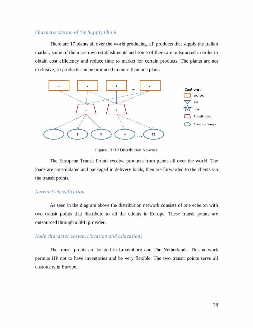
78
Characterization of the Supply Chain
There are 17 plants all over the world producing HP products that supply the Italian
market, some of them are own establishments and some of them are outsourced in order to
obtain cost efficiency and reduce time to market for certain products. The plants are not
exclusive, so products can be produced in more than one plant.
Figure 13 HP Distribution Network
The European Transit Points receive products from plants all over the world. The
loads are consolidated and packaged in delivery loads, then are forwarded to the clients via
the transit points.
Network classification
As seen in the diagram above the distribution network consists of one echelon with
two transit points that distribute to all the clients in Europe. These transit points are
outsourced through a 3PL provider.
Node characterization: (location and allocation)
The transit points are located in Luxemburg and The Netherlands. This network
permits HP not to have inventories and be very flexible. The two transit points serve all
customers in Europe.

79
Figure 14 Location of HP facilities
Activities, resources and capacity of each typology
Transit Point: cross docking activities, in order to assemble orders to be delivered to the
customers.
Flow Characteristics
Principal active flows:

80
F1: from plants to Transit Points, 100% of the volumes.
F2: from Transit Points to customers all over Europe, 100% of the volumes.
Managerial logic
Stocks
• Safety Stocks: no safety stocks due to the zero inventory policy
• Service Level: (K utilized): With the logistic strategy implemented by HP, they
have been able to reach 100% of service level.
• Logic of the material flow planning: The logic that HP uses is Assembly to Order.
The order is placed electronically by the customer and is received by the
establishment in charge of the production. It takes around 15 days to produce and
deliver the order.
Transport
• Organization of primary transport
The primary transport from Plants to European transit points is done mainly by air
because short cycle times are needed to satisfy the service level. The transit time for this
operation is around 8 days.
• Organization of secondary transport
The secondary transport from transit points to the customers is done by road, using
full truck loads.
Outsourcing
• Activities in outsourcing: the logic of HP regarding outsourcing is that each one has
to do what it does best, so HP contracts the best 3PL providers to do the
transportation and forwarding.
• Companies that handle the outsourced activities: the 3PL providers are different
from each country in Europe, depending on the covering capacity. For example:
CEVA, DHL and DMM.
Reverse Logistics
Reverse logistics constitutes 1% of the volumes, it is not really important for the
logistics activity but instead it is important for the customer service.

81
5.4 Distribution Problems of HP
It can be observed only one distribution problem.
• HP1: All HP products follow the same flow, come from plants from all over the
world and stop in a transit point in Europe to be assembled in orders and forwarded
to clients in Italy. Despite there is a wide range of products, they all follow the same
logistics path.
HP1
Macrodriver Driver Value
Product
Variety [SKUs] 4,000
Value [€/Kg] 1,000
Density [Kg/m3] 7,6
Risk of obsolescence [days] 120
Contribution Margin [%] 10-12
Service
Cycle Time [days] 15
Completeness [%] 100
Returnability [%] 1
Demand
Dimension of the order [%FTL] 1
Number of customers 32 in Italy
Frequency of delivery [Deliveries
per week] 5
Seasonality Low Medium
Predictability of demand [%] 95
Supply
Distance from plant to client
[Km] 6,000
Number of plants 17
Level of specialization Medium
Table 10 Summary of HP distribution problem

82
SONY
Sony is a leading manufacturer of audio, video, communications, and information
technology products for the consumer and professional markets. Its motion picture,
television, computer entertainment, music and online businesses make Sony one of the
most comprehensive entertainment and technology companies in the world. It is a company
with 1,006 consolidated subsidiaries worldwide.
5.1 Data Context of Sony
General data of the interview
Date of the interview: 29 June 2010
Name of the company: Sony
Address: Minato, Tokyo, Japan
Italy Central Office: Via Galileo Galilei, 40. Cinisello Balsamo – Milano.
Web Site: www.sony.com
Interviewee: Claudio Mirelli and Salvatore Paparelli: Logistics Directors of Sony Italy
Company general data
Member of a Group: Sony
Sector: Electronics
Multinational: Yes
Net revenues (2009): ¥7,214.0 billion
N° Employees: approximately 167,000 worldwide
Business Unit to consider: Sony Electronics that include IT and consumer electronics
5.2 Commercial Organization of Sony
Organization of the commercial function
Sony has 8 Business Units, from music and motion pictures to 3D Televisions. The
business units of consumer electronics constitute the bigger part of total sales, which are:

83
- The Consumer Products & Devices Group (40.5%)
- The Networked Products & Services Group (21.0%)
Figure 15 Sony Businesses
Types of clients
There are 1600 clients in Italy, from which 32 are big clients and the rest small
retailers or specialized stores; and a total of 2700 Delivery Points.
Depending on the volume DHL can deliver directly to the client, without passing
through the Transit points. If the volume is big enough to saturate the truck then it is
delivered directly from the central warehouse; instead if the volume is not big, the order is
delivered through transit points using a percentage of the truck load or using DHL express
if the order is of some boxes, serving mainly to small clients.
5.3 Actual Distribution Network of Sony
Drivers for the Design of Distribution Network
Product Characteristics
• Variety: between all the products managed by Sony from headphones to televisions,
there are 1,200 SKUs. Europe supplies 33% and Asia 66%.

84
• Value (€/Kg): a range of 55 €/Kg for televisions to 800 €/Kg for photo cameras.
• Density (Kg/m3): a range of 160 Kg/m3 for photo cameras to 643 Kg/m3 for home
theaters.
• Risk of obsolescence: it is medium for all the range of products varying from 180 to
240 days
• Contribution Margin: since it is not possible to calculate this for each type of
product, a range from 10 to 14% is considered.
Level of Service
• Cycle Time (order-delivery): 2 days to the north of Italy and 3 - 4 working days to
the south.
• Completeness (item fill rate): they have been able to reach 100% due to the backlog
management policy.
• Returnability: the return flow is not very important since it consists of only 1% of
the total flows.
Demand Characteristics
• Dimension of the order (typology): for direct deliveries to big customers the
dimension of the order is FTL; for customers ordering less volume the transport
managed by DHL is shared with Samsung so the dimension of the order is LFTL;
for small customers ordering small quantities of products, DHL express provides
the service, so the dimension of the order is some boxes.
• Number of customers: 1,600 invoicing points and 2,700 delivery points in Italy
• Frequency of delivery: 1 - 3 times per week
• Seasonality: for audio-video and informatics products the seasonality is well known
and is strong in some periods of the year, so the seasonality can be said to be
medium. For specialized products there is not a strong peak of sales so it can be said
that is low -medium.
• Predictability of demand: based on the stock levels that Sony manages, it can be
estimated an approximate percentage of predictability of the demand. Taking in
consideration that 85% of the flow of products come from plants located in Europe
reducing the transport times from plan to warehouse, Sony still manage high levels
of inventory: 12 days for Televisions and 1 month for the rest of the products. This
fact indicates that the predictability of the demand is not 100% but a 90% might be
adequate.
Supply drivers
• Distance from plant to client: for plants located in Europe 1,000 km and for plants
located in the Far East 9,000 km in average.

85
• Number of plants: 5 in Europe (Poland, Spain, Turkey, Slovakia, and Austria) and
around 7 in Asia that supplies Italy.
• Level of specialization: there is high specialization of the plants located in Europe
and medium for those located in Asia.
Macrodriver Driver Value
Product
Variety [SKUs] 1200
Value [€/Kg] 55 – 800
Density [Kg/m3] 160 – 643
Risk of obsolescence [days] 180 – 240
Contribution Margin: 10 - 14%
Service
Cycle Time [days] 2 – 4
Completeness [IFR] 100%
Returnability [%] 1
Demand
Dimension of the order
[%FTL] From 0,2 to 1
Number of customers 2,700 delivery points
Frequency of delivery [Deliveries per week]
1 – 3
Seasonality Low Medium - Medium
Predictability of demand [%] 90
Supply
Distance from plant to client 1,000 km - 9,000 km
Number of plants 5 in Europe and 7 in Asia
Level of specialization Medium – High
Table 11 Summary of Sony drivers
Characterization of the Supply Chain
The manufacturing plants that supply the European market are located in: Poland,
Turkey, Barcelona, Slovakia, Austria and 7 more located in the Far East. The European
plants are highly specialized, each one focuses on a type of product; while plants in Asia
produce very sophisticated products that can be produced in very few locations.

86
Figure 16 Sony Distribution Network
Network classification
As seen in the diagram above the distribution network consists of two echelons. The
first level consists of Central Warehouses, 1 in The Netherlands and the other one in Italy;
located in Liscate, Milano. Sony Logistics Europe B.V. (SLE) in Tilburg, The Netherlands
is the European Distribution Centre (EDC) of Sony Europe. It stores all product ranges of
Sony Electronics, which are shipped in by truck, sea and air freight from plants in Europe,
Japan and Asia. SLE, which has a ‘footprint’ of about 80,000 m2, distributes directly to
local Sony warehouses across Europe, Middle East and Africa.
The second level consists on regional transit points, which in the case of Italy are
13, one for each major region. The Warehouses and Transit Points are managed by DHL.
Node characterization: (location and allocation)
The Warehouse in The Netherlands stocks products coming from the different
plants around the world and provides these products to the rest of Europe. In addition, the
central warehouse in Italy stocks products coming from the European plants.

87
Figure 17 Location of Sony facilities
Figure 18 Location of Sony facilities
RW
sources
CW
Transit Point
Captions:

88
Activities, resources and capacity of each typology
The Central Warehouse located in Liscate has 80.000 m2 and is mainly dedicated to
picking activities, while in the transit points the orders are assembled using cross docking
and are delivered to the clients located within a circular area in order to increase the OFR.
Flow Characteristics
Principal active flows:
F1: products produced outside Europe are delivered to the CW in The Netherlands, which
corresponds to the 15%, and then are forwarded to the CW in Italy.
F2: products produced in European plants are delivered to the CW in Italy. This flow
represents 85%.
F3: 70% of the products from CW in Italy to regional transit points.
F4: 28.5% of the 70% that uses transit points are delivered to small customers. This flow is
managed by DHL express.
F5: 30% of products from CW in Italy to big customers managed directly by DHL without
stopping at the transit points, depending on the volume ordered.
F6: 71.5% of the 70% of products that uses transit points are delivered to big clients which
orders are of more than half truck load.
SMALL CUSTOMERS
PLANTS IN EUROPE
TRANSIT POINTS
BIG CUSTOMERS
F1 15%
F4 28,5%
PLANTS IN ASIA
CW IN NETHERLAND CW IN LISCATE
F2 85%
F3 70%
F1
F5 30%
F6 71,5%

89
Managerial logic
Stocks
• Safety Stocks: the stocks vary upon the type of product. For the central warehouse
in Italy (Liscate), TV stocks correspond to 12 days, while for the rest of products is
approximately 1 month.
• Service Level: they have been able to reach 100% thanks to the backlog
management policy.
Transport
• Organization of primary transport:
From plants in Europe, the primary transport consists of road. From plants in Asia,
consists in air.
• Organization of secondary transport:
The secondary transport to clients or to transit points is done by road using FTL or
LFTL depending on the client.
Outsourcing
• Activities in outsourcing: Warehouses, transit points and transportation are managed
in outsourcing.
• Companies that handle the outsourced activities: Sony which shares the service of
transit points and transportation with Samsung using DHL as 3PL, in order to
saturate the mean of transport.
Reverse Logistics
The management of returned products is not a relevant factor for the distribution
network, but it is considered as an internal organization problem at which Sony is making
great efforts to understand the causes by implementing a prevention program.
5.4 Distribution Problems of Sony
There are 6 distribution problems. The first 3 distribution problems are
characterized by the same supply and product drivers, but different demand and service
requested by customers; representing 85% of the total flow of goods. The last 3 problems
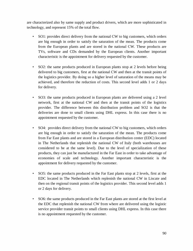
90
are characterized also by same supply and product drivers, which are more sophisticated in
technology, and represent 15% of the total flow.
• SO1: provides direct delivery from the national CW to big customers, which orders
are big enough in order to satisfy the saturation of the mean. The products come
from the European plants and are stored in the national CW. These products are
TVs, software and CDs demanded by the European clients. Another important
characteristic is the appointment for delivery requested by the customer.
• SO2: the same products produced in European plants stop at 2 levels before being
delivered to big customers, first at the national CW and then at the transit points of
the logistics provider. By doing so a higher level of saturation of the means may be
achieved, and therefore the reduction of costs. This second level adds 1 or 2 days
for delivery.
• SO3: the same products produced in European plants are delivered using a 2 level
network, first at the national CW and then at the transit points of the logistics
provider. The difference between this distribution problem and SO2 is that the
deliveries are done to small clients using DHL express. In this case there is no
appointment requested by the customer.
• SO4: provides direct delivery from the national CW to big customers, which orders
are big enough in order to satisfy the saturation of the mean. The products come
from Far East plants and are stored in a European distribution center (EDC) located
in The Netherlands that replenish the national CW of Italy (both warehouses are
considered to be at the same level). Due to the level of specialization of these
products, they can just be manufactured in the Far East in order to take advantage of
economies of scale and technology. Another important characteristic is the
appointment for delivery requested by the customer.
• SO5: the same products produced in the Far East plants stop at 2 levels, first at the
EDC located in The Netherlands which replenish the national CW in Liscate and
then on the regional transit points of the logistics provider. This second level adds 1
or 2 days for delivery.
• SO6: the same products produced in the Far East plants are stored at the first level at
the EDC that replenish the national CW from where are delivered using the logistic
service provider transit points to small clients using DHL express. In this case there
is no appointment requested by the customer.

91
MACRODRIVER DRIVER VALUE
SO1 SO2 SO3 SO4 SO5 SO6
PRODUCT
Variety [SKUs] 400 400 400 800 800 800
Value [€/Kg] 55 55 55 800 800 800
Density [Kg/m3] 160 160 160 643 643 643
Risk of obsolescence [days] 180 180 180 240 240 240
Contribution Margin: 10 10 10 14 14 14
SERVICE
Cycle Time [days] 3 4 2 3 4 2
Completeness [IFR] 100 100 100 100 100 100
Returnability [%] 1 1 1 1 1 1
DEMAND
Dimension of the order [%FTL] 1 0.6 0.2 1 0.6 0.2
Number of customers 32 32 2668 32 32 2668
Frequency of delivery [Deliveries per week] 3 2 1 3 2 1
Seasonality M M M LM LM LM
Predictability of demand [%] 90 90 90 90 90 90
SUPPLY
Distance from plant to client 1000 1000 1000 9000 9000 9000
Number of plants 5 5 5 7 7 7
Level of specialization H H H M M M
Table 12 Summary of Sony distribution problems

92
SAMSUNG
Samsung is comprised of companies that are setting new standards in a wide range
of business, from electronics to financial services, from chemicals and heavy industries to
trade and services. They share a commitment to creating innovative, high quality products
and services that are relied on every day by millions of people and businesses around the
world.
5.1 Data Context of Samsung
General data of the interview
Date of the interview: 30 June 2010
Name of the company: Samsung
Address: headquartered in Samsung Town, Seoul, South Korea
Italy Central Office: Via C.Donat Cattin, 5. Cernusco sul Naviglio – Milano.
Web Site: www.samsung.com
Interviewee: Danielle Farinella, Logistics Director
Company general data
Member of a Group: Samsung
Sector: Consumer electronics and home appliances
Multinational: Yes
Net revenues (2009): 138,994 (billions of KRW)
Market Share:
- LCD Monitor: 16.1%
- Hard disk drive: 9.5%
- Television set: 23%
- Printers: 16.4%
- Mobile phones: 23%
- Digital camera: 9.1%
N° Employees: approximately 164,000 worldwide

93
Business Unit to consider:
- Audio and Video
- Home Appliances
- Informatics
- Mobile
- Networking
5.2 Commercial Organization of Samsung
Organization of the commercial function
Samsung has 5 family products:
1. Audio and video: includes TVs, blue ray, Home Theaters and digital imaging
(cameras and videos)
2. Home appliances: microwaves, washing machines, air conditioners
3. Informatics products: monitors, notebooks
4. Mobile phones
5. Networking: fix telephony, fixed and satellite decoders
Generally, clients buy only from one product family which is stored in one specific
warehouse, so there is no order consolidation, Merge in Transit or Cross Docking activities
are required to assemble one order.
Types of clients:
There are 400 clients in Italy that corresponds to 1,200 delivery points, which can be
regrouped in:
• Mobile operators’ clients provided in direct way.
• Specialized clients
• Non specialized clients
• Distributors
Direct clients: (Clients with direct shipment)
Direct deliveries from plant located in the Far East to customers in Italy are
basically for the customized mobile phones that are delivered to the mobile operators. This
flow represents 30% of the total Mobile flow. Also the decoders for satellite television are
delivered directly to the customers, for example Sky.

94
5.3 Actual Distribution Network of Samsung
Drivers for the Design of Distribution Network
Product Characteristics
• Variety: there are 1,000 products from all the families which can be distributed in:
400 codes for audio video, 100 codes for home appliances, 150 codes for air
conditioners, 50 for mobile phones and 300 for informatics products.
• Value (€/Kg): range of 13 €/Kg for home appliances to 1,000 €/Kg for mobile
phones.
• Density (Kg/m3): range of 110 Kg/m3 for home appliances to 1,200 Kg/m3 for
mobile phones.
• Risk of obsolescence: from 3 months for mobile phones to 1 year for home
appliances and air conditioners.
• Contribution Margin: varies depending on the type of product from 14% for audio-
video to 30% for mobile phones.
Level of Service
• Cycle Time (order-delivery): 3-5 working days when appointments are not
requested.
• Completeness (item fill rate): difficult to supply 100% because the orders are
usually multiproduct within the same product family, so a 95% of completeness is
considered. The only case with 100% corresponds to mobile phones that are
delivered directly from the plants to the customers.
• Returnability: since the return flow is not very important it corresponds to only 1%
of the total flows.
Demand Characteristics
• Dimension of the order (typology): 65% of the orders go directly from the
warehouse to the client without passing through the transit point. From that 65%,
40% of the orders are 0,6FTL and the remaining 60% are of 0,4FTL or 0,2FTL. The
35% left, uses transit points and the average dimension of the order is 0,4FTL.
• Number of customers: 400 in Italy which correspond to 1200 delivery points.
• Frequency of delivery: depending on the product it goes from twice a week to once
a month.
• Seasonality: is considered as low for home appliances, medium for audio-video and
high for mobile phones.

95
• Predictability of demand: 95 %, it should be high because only the products that
have a high probability of being sold are delivered to the warehouses.
Supply drivers
• Distance from plant to client: 1,000 km for the plants located in Europe and 9,000
km for the plants in the Far East.
• Number of plants: 10 plants that provide the Italian market.
• Level of specialization: there is high specialization of the plants that supply the
warehouses in Italy.
Macrodriver Driver Value
Product
Variety [SKUs] 1,000
Value [€/Kg] 13 – 1,000
Density [Kg/m3] 110 – 1,200
Risk of obsolescence [days] 90 – 365
Contribution Margin: 14% - 30%
Service
Cycle Time [days] 3 – 5
Completeness [IFR] 95% - 100%
Returnability [%] 1
Demand
Dimension of the order
[%FTL] 0,2 – 0,6
Number of customers 1,200 delivery points
Frequency of delivery [Deliveries per week]
0,25 – 2
Seasonality From Low to High
Predictability of demand
[%] 95
Supply
Distance from plant to client 1,000 - 9,000
Number of plants 10
Level of specialization High
Table 13 Summary of Samsung drivers
Characterization of the Supply Chain
The 3 plants in Europe, located in Hungary and Slovakia, produce products for the
Audio-video and Informatics business units, while the plants in the Far East produce
mobile phones, home appliances and air conditioners. The plants are highly specialized and
the warehouses manage only one family of products because the training of personnel, the
security of products and the flow management are different.

96
Figure 19 Samsung Distribution Network
Network classification
The network is of 2 levels; the first one consists of 4 CW in Italy, which are
replenished by 10 plants located in Europe and the rest of the world. Each warehouse is
managed by 3PLs providers. The second level consists of transit points of the 3PLs,
distributed in the following way:
• DHL: 20 TP
• CEVA: 20 TP
• TNT Global express: 150 TP
Node characterization: (location and allocation)
The 4 CWs in Italy are located near Milan; instead the transit points are located in
each region. Each warehouse is specialized in stocking one or two kinds of products:
• Piacenza: storages home appliances, managed by DHL
• Melzo: storages audio video and informatics products, managed also by DHL
• Zingonia: storages mobile phones, managed by Bertola Central Docks.
• Arluno: storages air conditioning systems, managed by CEVA

97
Figure 20 Location of Samsung facilities
Figure 21 Location of Samsung facilities
sources
CW
RW
Transit point
Clients in Europe
Captions:
Clients in Europe
RW
sources
CW
Transit Point
Captions:

98
Activities, resources and capacity of each typology
The 4 Central Warehouses are used for storage activities and have the following
dimensions:
- Piacenza: 12.000 m2
- Melzo: 20.000 m2
- Zingonia and Arluno: the dimensions vary upon the time.
The Transit Points are designated for sorting and re-palletization activities.
Flow Characteristics
Principal active flows:
F1: Mobiles produced in the Far East are delivered directly to the mobile operators, this
flow corresponds 30% of all the mobiles delivered in Europe and corresponds 6% of the
total outbound flow.
F2: House appliances produced in Asia are delivered in the Piacenza Warehouse
corresponding 6% of the total inbound flow.
F3: Products from the audio-video and informatics family are produced in Europe and
delivered in the Melzo Warehouse, representing 40% and 30% respectively.
F4: The rest of the mobile phones that are not delivered directly to the mobile operators are
delivered to the Zingonia Warehouse, representing 70% of all the mobiles delivered in
Europe and 14% of the total outbound flow.
F5: Air conditioners are produced in Asia and delivered to the Arluno Warehouse. This
flow represents 4%.
F6: 60% of the products in the Piacenza warehouse are delivered to the clients without
stopping in the transit points.
F7: 40% of the products in the Piacenza warehouse stop in one of the 20 DHL transit
points, before final delivery.
F8: 40% of the products in the Melzo warehouse stop in one of the 20 DHL transit points,
before final delivery.
F9: products delivered to final customers from the DHL transit points

99
F10: 60% of the products in the Melzo warehouse are delivered to the clients without
stopping in the transit points.
F11: 40% of the products in the Zingonia warehouse stop in one of the 150 TNT transit
points and then these same products are delivered to final customers.
F12: 60% of the products in the Zingonia warehouse are delivered to the clients without
stopping in the transit points.
F13: 40% of the products in the Arluno warehouse stop in one of the 20 CEVA transit
points and then these same products are delivered to final customers.
F12: 60% of the products in the Arluno warehouse are delivered to the clients without
stopping in the transit points.
PLANTS IN EUROPE
20 DHL TP
CUSTOMERS
F16%
F11
PLANTS IN ASIA
CW Piacenza CW Melzo
F26%
F7
CW Zingonia CW Arluno
20 CEVA TP150 TNT TP
F660%
F940%
F1140%
F1340%
F8
F1060%
F1260%
F1460%
F13
F370%
F414%
F54%

100
Managerial logic
Stocks
• Safety Stocks: the stocks vary based on the type of product:
o 1 week of stock for Mobile and Audio – Video products
o 3 – 4 weeks for Home appliances
• Service Level: difficult to reach 100% due to multi product orders of one family.
Transport
• Organization of primary transport
- Products manufactured in Europe (Audio – Video and Informatics) use Air and
Road transportation
- Products manufactured in the Far East (Mobile and Home Appliances) arrive by
Air and Ship.
• Organization of secondary transport
The secondary transportation is mainly done by road.
Outsourcing
• Activities in outsourcing: Warehouses, transit points and transportation are managed
by 3PLs
• Companies that handle the outsourced activities: DHL, CEVA, Bertola Central
Docks.
5.4 Distribution Problems of Samsung
Due to the wide range of products Samsung provides, the distribution problems
have different product and supply drivers. It has to be underlined that each family of
products has its own warehouse, this because each family of products requires different
maintenance, personnel and also different channel for distribution.
• SA1: characterized by direct delivery of customized mobile phones and television
decoders from Far East plants to mobile operators or TV providers.
101
• SA2: consist of one level of CW located in Piacenza that stores products from the
home appliance family, produced in the Far East plants and are forwarded directly
to clients which request a specific appointment for delivery.
• SA3: consist of two levels, the first is the CW located in Piacenza that stores home
appliance products and the second level consists of 20 DHL transit points that
manage this type of products.
• SA4: consist of one level of CW located in Melzo that stores products from the
audio-video and informatics families produced in European plants and are
forwarded directly to clients which request a specific appointment for delivery.
• SA5: consist of two levels, the first is the CW located in Melzo that stores products
from the audio-video and informatics families produced in European plants and the
second level consists of 20 DHL transit points that manage this type of products.
• SA6: represented by mobile phones, which are not delivered directly to mobile
operators, but instead stop at one level of CW located in Zingonia and then are
forwarded directly to clients that request a specific appointment for delivery.
• SA7: represented by mobile phones, which are not delivered directly to mobile
operators, but instead stop at one level of CW located in Zingonia and then at a
second level of 150 TNT transit points that manage this type of products.
• SA8: characterized by air conditioners produced in the Far East plants, stop at one
level of CW located in Arluno and then delivered directly to clients that request a
specific appointment for delivery.
• SA9: characterized by air conditioners produced in the Far East plants, stop at one
level of CW located in Arluno and then at a second level of 20 CEVA transit points
that manage this type of products and then forwarded to clients.

102
MACRODRIVER DRIVER VALUE
SA1 SA2 SA3 SA4 SA5 SA6 SA7 SA8 SA9
PRODUCT
Variety [SKUs] 50 100 100 700 700 50 50 150 150
Value [€/Kg] 1000 13 13 370 370 1000 1000 90 90
Density [Kg/m3] 1200 110 110 170 170 1200 1200 170 170
Risk of obsolescence [days] 90 365 365 180 180 90 90 365 365
Contribution Margin: 30 24 24 14 14 30 30 14 14
SERVICE
Cycle Time [days] 5 3 5 3 5 3 5 3 5
Completeness [IFR] 100 95 95 95 95 95 95 95 95
Returnability [%] 1 1 1 1 1 1 1 1 1
DEMAND
Dimension of the order [%FTL] 0.4 0.6 0.4 0.6 0.4 0.4 0.2 0.6 0,4
Number of customers 5 35 1160 32 1163 32 1163 35 1160
Frequency of delivery [Deliveries per
week] 0.25 0.5 1 2 2 1 1 0.5 1
Seasonality H L L M M H H L L
Predictability of demand [%] 95 95 95 95 95 95 95 95 95
SUPPLY
Distance from plant to client 9000 9000 9000 1000 1000 9000 9000 9000 9000
Number of plants 4 3 3 3 3 4 4 3 3
Level of specialization H H H H H H H H H
Table 14 Summary of Samsung distribution problems

103
Chapter 6. Clusters of distribution problems based on the network
strategic choice
6.1 Projection elements
It has been said in chapter 2, that there are several types of solutions based in the
choice of the distribution network. In this chapter, there are identified and grouped all the
possible choices based in the strategic decision that has been chosen to consider in the path
of experimental analysis.
6.2 Identification of clusters
Number of levels and typology for each level
From the study of company cases, the proposed network solutions are: direct
delivery, one level of CW, one level of transit points, and two levels composed of CW and
transit points. Next, it has been compiled a table that reports all the possible solutions.
Distribution
Problem
Number and typology of levels of the distribution network
solution
HP1 Network of 1 level: transit points
SO1 Network of 1 level: central warehouse
SO2 Network of 2 levels: central warehouse and transit points
SO3 Network of 2 levels: central warehouse and transit points
SO4 Network of 1 level: central warehouse
SO5 Network of 2 levels: central warehouse and transit points
SO6 Network of 2 levels: central warehouse and transit points
SA1 Direct delivery from manufacturing plants
SA2 Network of 1 level: central warehouse
SA3 Network of 2 levels: central warehouse and transit points
SA4 Network of 1 level: central warehouse
SA5 Network of 2 levels: central warehouse and transit points
SA6 Network of 1 level: central warehouse
SA7 Network of 2 levels: central warehouse and transit points
SA8 Network of 1 level: central warehouse
SA9 Network of 2 levels: central warehouse and transit points
Table 15 Distribution Problems and Network Solutions

104
From the aggregated analysis of all the adopted possible solutions, emerged the next 4
clusters:
1. Direct delivery from manufacturing plants
Distribution problems belonging here: SA1
2. 1 level of transit points
Distribution problems belonging here: HP1
3. 1 level of central warehouse
Distribution problems belonging here: SO1, SO4, SA2, SA4, SA6, SA8

105
4. 2 levels of central warehouse and transit points
Distribution problems belonging here: SO2, SO3, SO6, SO5, SA3, SA4,
SA7, SA9
Characterization of nodes for the 1 level network with transit points
In the definition of the structure, as well as the decision of the number and type of level
already analyzed, contribute in fact other choices that in this work are characterized as
follows:
• Number of nodes at first level
• Average area served by nodes
• Location of nodes over the European surface
• Allocation of clients to the nodes
• Surface of the WH
• Variety of products for each WH

106
The HP1 distribution problem is the only one that implements this type of network.
It consists of two transit points located in Luxemburg and The Netherlands that are used to
satisfy the demand of clients from all over Europe and manage the complete variety of
products of the company.
DP Nodes Area served Location Allocation Surface Variety
HP1 2 10,180,000 km2
Luxemburg
and
Netherlands
All Europe Unknown Full mix
Table 16 Characterization of TP at first level
Characterization of nodes for the 1 level network with central warehouse
In the following table, it is presented the details for the distribution problems having
one level of CW.
DP Nodes Area
served Location Allocation Surface Variety
SO1 1 301,338 km2 Liscate
Big italian
customers 80,000 m2 Full mix
SO4 1 301,338 km2 Liscate Big Italian
Clients 80,000 m2 Full mix
SA2 1 301,338 km2 Piacenza Big Italian
Clients 12,000 m2
Home
appliances
SA4 1 301,338 km2 Melzo Big Italian
Clients 20,000 m2
Audio, video
and
informatics
SA6 1 301,338 km2 Zingonia Big Italian
Clients Variable
Mobile
phones
SA8 1 301,338 km2 Arluno Big Italian
Clients Variable
Air
conditioners
Table 17 Characterization of CW at the first level
As seen from the table above, all these distribution problems serve the national
territory of Italy. The difference relies on the Company, for example Sony has one WH
which stores all products, while Samsung has specialized warehouses that store only one
family of products, each.

107
Figure 22 Location of CW
Characterization of nodes for the 2 level network with central warehouse and
TP
The strategic decisions of the network to take into account, like in the preceding
analysis, are number, location and allocation for each level and variety of products
available in the CW. In order to group the alternatives of network proposed by the
companies in solution clusters, are resumed in the next table for each distribution problem.
DP 1° level: Central Warehouse 2° level: Transit Points
Number Variety Location Allocation Number Location Allocation
SO2 1 Full mix Liscate Big italian
customers 13 DHL
Principal
Italian
regions
1 TP for each
1.5 Italian
region
SO3 1 Full mix Liscate Small
italian
customers 13 DHL
Principal
Italian
regions
1 TP for each
1.5 Italian
region
SO5 1 Full mix Liscate Big italian
customers 13 DHL
Principal
Italian
regions
1 TP for each
1.5 Italian
region

108
SO6 1 Full mix Liscate Small
Italian
Clients 13 DHL
Principal
Italian
regions
1 TP for each
1.5 Italian
region
SA3 1 Home
appliance Piacenza
Big italian
customers 20 DHL
Italian
regions
1 TP for
every Italian
region
SA4 1 Audio-video
and
informatic Melzo
Big italian
customers 20 DHL
Italian
regions
1 TP for
every Italian
region
SA7 1 Mobile Zingonia Small
italian
customers
150
TNT
Principal
Italian
cities
7.5 transit
points for
each Italian
region
SA9 1 Air
conditioners Arluno
Big italian
customers 20
CEVA Italian
regions
1 TP for
every Italian
region
Table 18 Characterization of the CW and TP of the 2 level networks
With the information above it can obtain the following groups:
• Central Warehouse with one transit point every 1.5 Italian region: SO2, SO3, SO5
and SO6
Figure 23 Location of TP for SO2, SO3, SO5 and SO6

109
• Central Warehouse with one transit point every Italian region: SA3, SA4 and SA9
Figure 24 Location of TP for SA3, SA4 and SA9
• Central Warehouse with 7.5 transit points for each Italian region: SA7
Due to the complexity of this network, it is not possible to illustrate it.

110
Chapter 7. Relationship between distribution problems, drivers and
logistic costs
Among the sixteen drivers selected in chapter 4, there are three new drivers that
were added, and others that were removed from the work presented by “Archini and
Bannò” after carrying out the literature analysis. The objective of the following analysis is
to understand the impact of all these drivers over the logistic cost in order to see if each
driver is critical for the different network choices. Each driver has a different impact over
the network design process; this impact will be described by the criticality of the driver
which will depend on the effects of the driver over the logistic costs.
After understanding the costs, the criticalities of the drivers will be defined, which
consent to relate the factors characterized by different units of measure. The procedure
followed to identify the intervals of reference is described in paragraph 3.5. And it was
used the following legend:
Company HP Sony Samsung
Distribution
Problem
HP1 SO1 SO2 SO3 SA1 SA2 SA3 SA4 SA5
SO4 SO5 SO6 SA6 SA7 SA8 SA9
Product drivers:
Variety
An increase in the variety of the products offered cause an increase in the total
logistics costs due to the following reasons:

111
Transportation costs: a greater variety of products increases the transportation cost, both
primary and secondary. Primary transport increases because different products could
require different transport typologies creating the risk of not saturation of the transport
means, while secondary transport increases because client orders may be of just few
products and therefore there are more deliveries. However, by increasing the range of
products, customers could make larger orders, making it easier the saturation of the
transport mean, thus increasing the cost of primary transportation, but decreasing
substantially the secondary transport, having as a result the reduction of the total cost of
transport.
Inventory costs: with a great variety of products, the inventory costs tend to increase
because it leads to an increase in the average level of stock and the level of safety stocks for
the different products, having greater space occupancy and increasing the insurance costs.
Handling costs: these costs tend to increase because a greater variety could require, for an
average volume order, a greater number of picking operations. Furthermore, since the
product codes are large numbers, it would increase the risk of errors and might therefore
need a control system and the allocation of more resources.
Cost of lost sale: this cost might be reduced because, in the presence of a greater variety of
products, the needs of the clients could be satisfied with a substitutive product of the same
company.
For the analysis of the distribution problems, the variety of products was measured
in Number of Product Codes. Theoretically, it can be said that with a great variety of
products, the criticality of the driver raises and the distribution network implemented
should be centralized in order to avoid duplication and increase of the levels of stock.
From the graph below it can be observed that different values of variety were
obtained, from 50 to 4000 SKUs, but it was not possible to correlate a specific variety with
a type of distribution network implemented with the exception of the distribution problem
HP1.

112
Graph 8 Relation between the variety of products, distribution problem and network
applied
For the case of HP1, which is the distribution problem with more number of
products, the solution adopted was a network of 1 level conformed by transit points. This
design is coherent with the reasoning above because of the complete elimination of stocks,
and therefore the reduction of logistics costs. While, for the rest of the variety values
obtained, different distribution networks were applied no matter the number of SKUs. This
behavior is because for the same type of products, like for example the distribution
problems SA1, SA6 and SA7 which corresponds to mobile phones that are delivered
directly, with one level of warehouses, or with 2 level network of warehouses and transit
points, respectively, the distribution network adopted is based on other drivers, like number
of clients or cycle time, and not on the number of products.
As a conclusion, it can be said that for extremely high variety of products, the
implementation of a network that eliminates the products on inventory is recommended in
order to reduce total logistics costs, while for lower variety different distribution networks
might be applied.
The following graph presents the scale of criticality of the driver “Variety” were it
can be observed in one axis the conclusion mentioned above.
50 100 150
400 400
700800 800
4000
50 100 150
400
700800
500
500
1000
1500
2000
2500
3000
3500
4000
SA7 SA6 SA1 SA2 SA3 SA8 SA9 SO1 SO2 SO3 SA4 SA5 SO6 SO4 SO5 HP1
Nu
mb
er o
f P
rod
uct
Co
des
Direct Delivery
2 levels: CW and TP
1 TP
1 CW
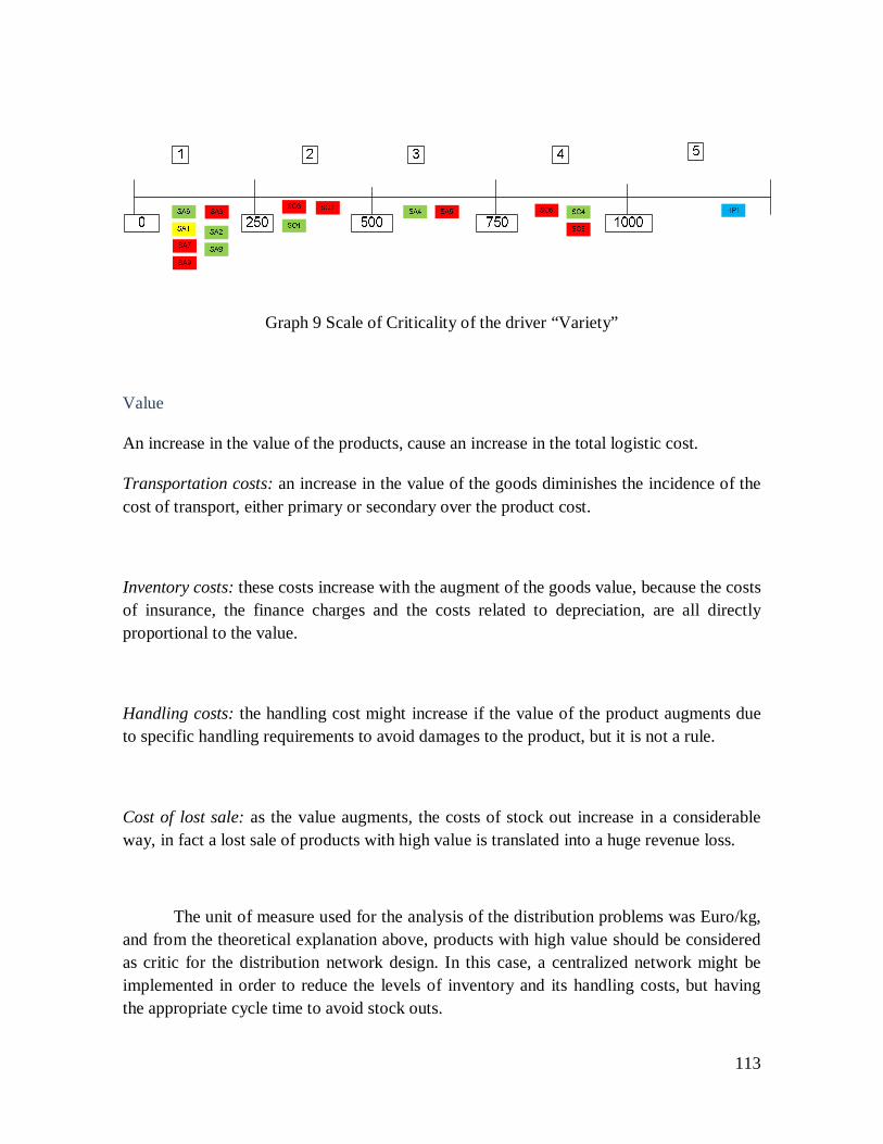
113
Graph 9 Scale of Criticality of the driver “Variety”
Value
An increase in the value of the products, cause an increase in the total logistic cost.
Transportation costs: an increase in the value of the goods diminishes the incidence of the
cost of transport, either primary or secondary over the product cost.
Inventory costs: these costs increase with the augment of the goods value, because the costs
of insurance, the finance charges and the costs related to depreciation, are all directly
proportional to the value.
Handling costs: the handling cost might increase if the value of the product augments due
to specific handling requirements to avoid damages to the product, but it is not a rule.
Cost of lost sale: as the value augments, the costs of stock out increase in a considerable
way, in fact a lost sale of products with high value is translated into a huge revenue loss.
The unit of measure used for the analysis of the distribution problems was Euro/kg,
and from the theoretical explanation above, products with high value should be considered
as critic for the distribution network design. In this case, a centralized network might be
implemented in order to reduce the levels of inventory and its handling costs, but having
the appropriate cycle time to avoid stock outs.

114
From the analysis of the distribution problems, it was not possible to observe a clear
pattern of relation between this driver and the distribution network implemented. For
example, products with high value like mobile phones (SA1, SA6 and SA7) are distributed
with three different networks going from centralized (direct delivery) to decentralized (2
level network of warehouses and transit points). The implementation of one network or
another might be based on other drivers, and not on the value of the product.
In the case of HP1, the value presented is an average from the complete variety of
products and, as it was established by the company, all the products are delivered through a
network with one transit point. With this policy, the company eliminates the inventory
costs, and therefore reduce the total logistics costs.
In the case of products with lower values, a similar behavior as the high value ones
was observed, were different network layouts are used for one particular relation Euro/Kg.
As a conclusion of this analysis it can be said that the driver “Value” itself is not
determinant for the distribution network design.
Graph 10 Relation between the value of the products, distribution problem and network
applied
The scale of criticalities of the driver “Value” is presented below:
13 55 5590
370
800 800
10001000
1355
90
370
800
1000 1000
0
100
200
300
400
500
600
700
800
900
1000
1100
SA3 SA2 SO3 SO1 SO2 SA8 SA9 SA5 SA4 SO6 SO4 SO5 SA7 SA1 HP1 SA6
Val
ue
[Eu
ro/k
g]
Direct Delivery
2 levels: CW and TP
1 TP
1 CW

115
Graph 11 Scale of Criticality of the driver “Value”
Density
A decrease in the density, generate an increase in the total logistic costs.
Transportation costs: a high density of the products favors the saturation of the
transportation mean, allowing in this way the reduction of secondary transportation costs.
Using a primary transportation delivery policy is cheaper than a combined one, and
therefore with an increase in density, a reduction in cost of transport is achieved. In
addition, high density products are less voluminous, so it takes less space in the transport
mean and allows weight saturation instead of volume. In this way, the cost is distributed in
a greater number of pieces.
Inventory costs: an augment in density can favor the reduction of storage costs. The saving
is mainly due to the reduction of space needed to store the goods
Handling costs: with a decrease in the density of the products, the number of delivery trips
required to meet demand increases, thus requiring more loading and unloading activities
that increase the cost of handling.
Cost of lost sale: this cost does not vary with a variation in density.

116
For the analysis of the distribution problems, the density was measured in Kg/m3,
and different values were obtained, from 7,6 to 1200. The graph below presents the average
values of density for each distribution problem, as well as the distribution network adopted.
Graph 12 Relation between the density of the products, distribution problem and network
applied
In theory, products having low value of density should be distributed with a
centralized network in order to facilitate primary transport policies and reduce the amount
of space required for inventories. From the analysis of the distribution problems this
behavior was obtained just for the distribution problem HP1 which has a density value of
7,6 kg/m3 and uses a distribution network of 1 level of transit points which eliminates the
stocks and therefore just need space for in-transit goods.
For the rest of the distribution problems, a clear pattern was not observed because
for the same value of density, different distribution networks were adopted. For example,
products with relatively low density (170 kg/m3) are distributed using two different types of
networks: 1 level of central warehouses and 2 levels of central warehouses and transit
points. The same performance was observed for medium and high density values.
With these results it may be assumed that the driver “Density” has not an important
role during the design phase of the distribution network. It is possible that its impact will be
higher for operational decisions such as warehouse management or transport routing.
110
160 160 170 170
643 643
1200
7.6
110
160 170 170
643
1200 1200
0
100
200
300
400
500
600
700
800
900
1000
1100
1200
HP1 SA3 SA2 SO1 SO3 SO2 SA8 SA4 SA5 SA9 SO6 SO4 SO5 SA7 SA6 SA1
Den
sity
[K
g/m
3]
Direct Delivery
2 levels: CW and TP
1 TP
1 CW

117
The scale of criticality of the driver “Density” is presented below:
Graph 13 Scale of Criticality of the driver “Density”
Risk of obsolescence
A high risk of obsolescence of the products implies an increase in the total logistic cost.
Transportation costs: with a high risk of obsolescence there is an augment in both primary
and secondary transportation costs. The products with this characteristic need presumably a
high efficiency and reduced cycle time of transport, both involving an increase of costs.
Inventory costs: with a presence of products highly risky there is a tendency to decrease the
stocks, and with this all the associated costs. However a high risk of obsolescence causes in
the products a constant depreciation that is translated in high costs of system management.
Handling costs: this cost is not affected by an increment in the risk of obsolescence.
Cost of lost sale: when the risk is high this cost tends to increase because once the product
is expired it is not marketable anymore, but rather the disposal has to be managed.
Theoretically, products with high risk of obsolescence (measured in Days) should
be distributed with a centralized network in order to reduce the cycle times and the levels of
stock. In the case of the consumer electronic industry, the gap of time between the
expiration date and the delivery cycle time is big enough to allow longer distribution
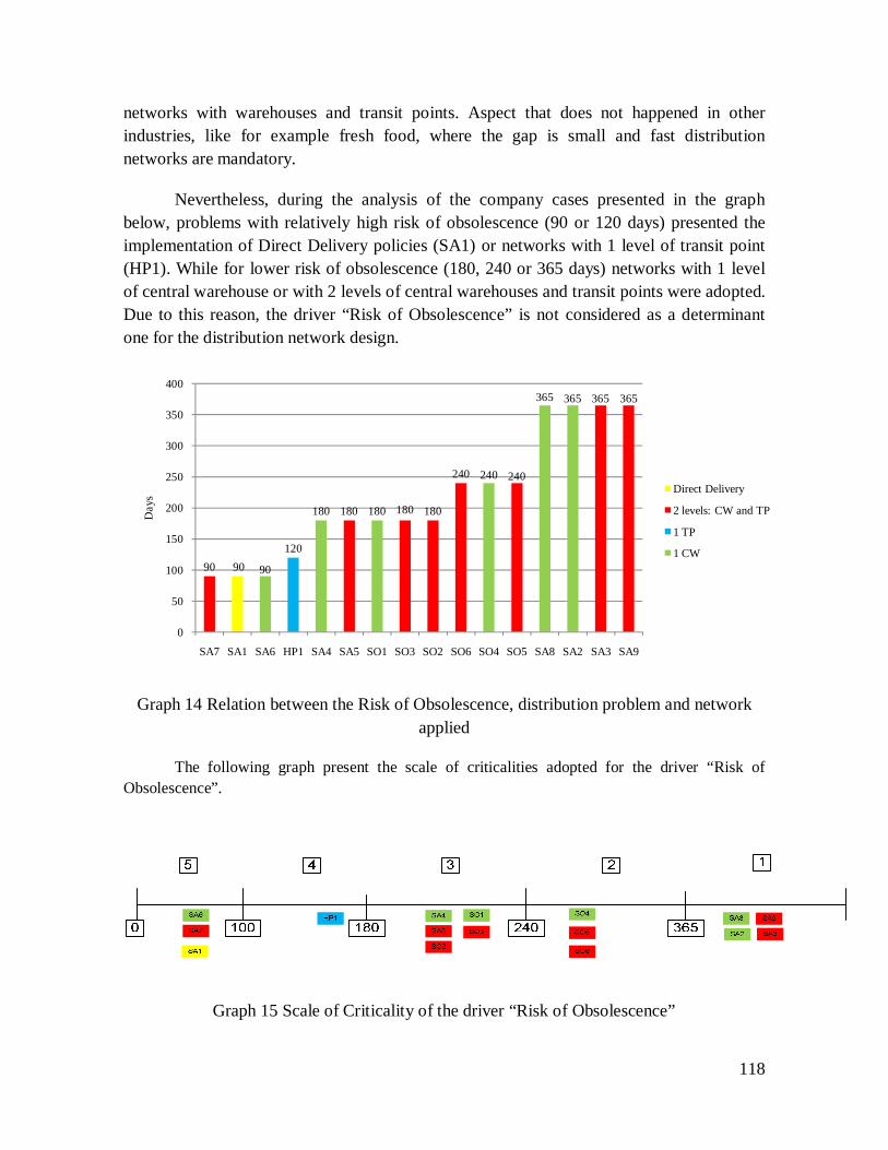
118
networks with warehouses and transit points. Aspect that does not happened in other
industries, like for example fresh food, where the gap is small and fast distribution
networks are mandatory.
Nevertheless, during the analysis of the company cases presented in the graph
below, problems with relatively high risk of obsolescence (90 or 120 days) presented the
implementation of Direct Delivery policies (SA1) or networks with 1 level of transit point
(HP1). While for lower risk of obsolescence (180, 240 or 365 days) networks with 1 level
of central warehouse or with 2 levels of central warehouses and transit points were adopted.
Due to this reason, the driver “Risk of Obsolescence” is not considered as a determinant
one for the distribution network design.
Graph 14 Relation between the Risk of Obsolescence, distribution problem and network
applied
The following graph present the scale of criticalities adopted for the driver “Risk of
Obsolescence”.
Graph 15 Scale of Criticality of the driver “Risk of Obsolescence”
90
180 180 180
240 240
365 365
120
90
180 180
240
365 365
90
0
50
100
150
200
250
300
350
400
SA7 SA1 SA6 HP1 SA4 SA5 SO1 SO3 SO2 SO6 SO4 SO5 SA8 SA2 SA3 SA9
Day
s
Direct Delivery
2 levels: CW and TP
1 TP
1 CW

119
Contribution Margin
Transportation costs: the augment of the contribution margin of the product diminish the
incidence of the transport cost over the product cost.
Inventory costs:
Maintenance of Stock: products with low contribution margin force to reduce the storage
and maintenance costs.
Order cost: there is no evident relation.
Handling costs: products with low contribution margin force to reduce the handling costs.
Cost of lost sale: the costs of lost sale increase considerably when the product has a high
contribution margin since a sale that cannot be done represents an important lost in terms of
profits. This is the cost that has the greater impact over the total logistic cost.
The contribution margin is a relation between the production costs and the price of
the product sold and is expressed in percentage. Theoretically, products with high
contribution margin allow to be distributed with networks using primary and secondary
transport policies (1 or 2 levels), while ensuring the presence of the product on the shelf on
time, in order to avoid considerable losses.
For the analysis of the company case studies, the contribution margin was calculated
as the average of the contribution margins of the products pertaining to one distribution
problem. It was not possible to associate a value of the contribution margin with a specific
distribution network solution, as it is presented in the following graph. For example, the
network of 2 levels with central warehouses and transit points was used by all the values
except 12% (SO2, SO3, SO5, SO6, SA5, SA9, SA3 and SA7), and a similar behavior is
present for networks of 1 level with central warehouses.
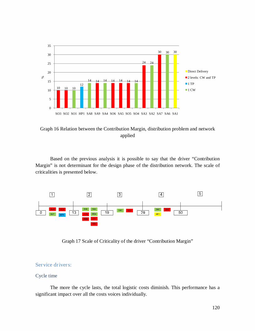
120
Graph 16 Relation between the Contribution Margin, distribution problem and network
applied
Based on the previous analysis it is possible to say that the driver “Contribution
Margin” is not determinant for the design phase of the distribution network. The scale of
criticalities is presented below.
Graph 17 Scale of Criticality of the driver “Contribution Margin”
Service drivers:
Cycle time
The more the cycle lasts, the total logistic costs diminish. This performance has a
significant impact over all the costs voices individually.
10 10
14 14 14 14
24
30
1210
14 14 14
24
30 30
0
5
10
15
20
25
30
35
SO3 SO2 SO1 HP1 SA8 SA9 SA4 SO6 SA5 SO5 SO4 SA3 SA2 SA7 SA6 SA1
%
Direct Delivery
2 levels: CW and TP
1 TP
1 CW
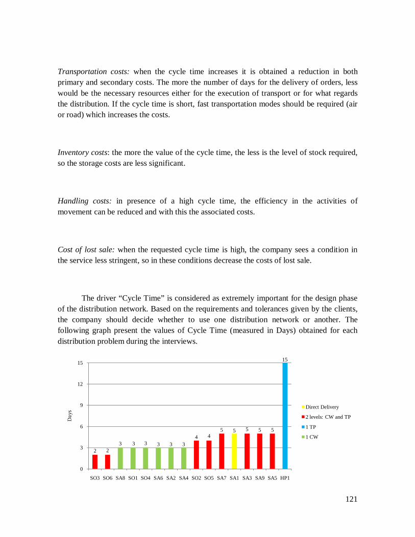
121
Transportation costs: when the cycle time increases it is obtained a reduction in both
primary and secondary costs. The more the number of days for the delivery of orders, less
would be the necessary resources either for the execution of transport or for what regards
the distribution. If the cycle time is short, fast transportation modes should be required (air
or road) which increases the costs.
Inventory costs: the more the value of the cycle time, the less is the level of stock required,
so the storage costs are less significant.
Handling costs: in presence of a high cycle time, the efficiency in the activities of
movement can be reduced and with this the associated costs.
Cost of lost sale: when the requested cycle time is high, the company sees a condition in
the service less stringent, so in these conditions decrease the costs of lost sale.
The driver “Cycle Time” is considered as extremely important for the design phase
of the distribution network. Based on the requirements and tolerances given by the clients,
the company should decide whether to use one distribution network or another. The
following graph present the values of Cycle Time (measured in Days) obtained for each
distribution problem during the interviews.
2 2
3 3 3 3 3 3
15
4 45 5 5 55
0
3
6
9
12
15
SO3 SO6 SA8 SO1 SO4 SA6 SA2 SA4 SO2 SO5 SA7 SA1 SA3 SA9 SA5 HP1
Day
s
Direct Delivery
2 levels: CW and TP
1 TP
1 CW

122
Graph 18 Relation between the Cycle Time, distribution problem and network applied.
From the analysis of the company cases, a clear pattern was obtained due to the fact
that each distribution network adopted provides a specific cycle time, except for the
distribution problems SO3 and SO6 which are a particular case. This two problems
corresponds to TVs and Peripherals, respectively, that are stored in one central warehouse
located in the north of Italy and pass through the transit points of the logistics service
provider, in this case DHL express, to be delivered to small clients which orders are also
small (some boxes). Due to the size of the orders, and probably the low mix of them, the
company is able to provide a cycle time of 2 days.
The distribution problems SO1, SO4, SA2, SA4, SA6 and SA8 corresponds to
products that are stored in a central warehouse in the north of Italy and are delivered to big
clients with order dimensions of more than half truck load, which accept 3 days of cycle
time. The difference of one day between the previous 2 distribution problems and this 5, is
mainly due to the dimension of the orders and the transport mean used.
Next, the rest of distribution networks with 2 levels of central warehouses and
transit points add 1 or 2 days to the cycle time with respect to the previous network, due to
the activities of cross docking developed in the transit point. The distribution problems SO2
and SO5 correspond to similar products delivered in SO1 and SO4, but due to the
dimension of the order (0,6 FTL) and probably because of the mix of products required, are
delivered with one more day.
The distribution problems SA3, SA5, SA7 and SA9 correspond to similar products
of SA2, SA4, SA6 and SA8, respectively, but which order dimensions are smaller than a
full truck load and require cross docking activities in the transit point, adding 2 more days
to the cycle time.
In the case of the distribution problem SA1, although it is direct delivery and should
have a small cycle time, the value obtained for this solution is equal to 5 days. The reason is
because products distributed with this network are mobile phones and TV decoders that are
produced in facilities located in the Far East and are delivered directly to few clients in Italy
(mobile and television service providers) using a combined transportation mode (air and
road) due to the high risk of obsolescence of this products.
The highest cycle time was obtained for the distribution problem HP1 which uses a
network of 1 level of Transit Points. The reason is because this company adopted a policy
of Zero stock and uses a particular dynamic of the flow of products; the order from a client
in Italy (mainly big clients) is placed directly in the facilities located in the Far East, the
production starts and takes 8 days approximately to be completed, then the product is
delivered to a transit point located in the Netherlands with the objective of assemble the

123
order and once it has been consolidated it is delivered using full truck loads, giving a total
cycle time of 15 days.
The scale of criticalities of the driver “Cycle Time” is presented below, and it is
possible to observe clearly the intervals of impact on the logistic costs.
Graph 19 Scale of Criticality of the driver “Cycle Time”
Completeness
While this performance increases, decreases the total logistic cost.
Transportation costs: if the completeness is reduced, the level of saturation of the
transportation mean should not be the optimal one increasing the costs. Also, incurring in a
situation of stock out, if the client accepts the late delivery of the rest of the order, the use
of "ad hoc" means should be necessary, increasing also the transportation costs.
Inventory costs: the relation in this case is evident; in order to satisfy a complete order from
a client, the average levels of stock should be increased and therefore, the costs will also
augments.
Handling costs: if an incomplete order can be supplied in a later date, the handling costs are
not affected by the level of completeness. If not, with a decrease in the level of
completeness, the handling cost will also diminished, but having as an impact the
reduction of the service level offered by the firm.
Cost of lost sale: the cost of lost sale decrease with an increase in the completeness.

124
From the analysis of the company cases, it was possible to observe that the level of
completeness is not directly related with the type of distribution network adopted by the
company. It is more an internal decision or goal of the firm rather than an effect of the
distribution network as it can be observed in the following graph.
Graph 20 Relation between the Order Completeness, distribution problem and network
applied
In the case of Samsung, the distribution problem SA1 reached 100% of
completeness due to the fact that the orders are placed to the plants and are directly
delivered to the clients once the order is complete; the completeness of the order depends
on the production capacity of the facility. A similar behavior is observed in the distribution
problem HP1.
For the rest of the distribution problems of Samsung, it is observed that no matter
which distribution network is used (1 or 2 levels), the percentage of completeness of the
order is 95%. This result might be caused by other factors like the forecast of demand and
the level of stocks implemented by the firm.
95 95 95 95
100 100 100 100 100
95 95 95 95
100 100 100
92
94
96
98
100
SA2 SA3 SA4 SA5 SA6 SA7 SA8 SA9 SO1 SO3 SO4 SO6 SO2 SO5 HP1 SA1
%
1 CW
1 TP
2 levels: CW and TP
Direct Delivery

125
In the case of Sony, the operational decisions of warehouse management and
production capacity have given as a result the achievement of 100% of orders complete.
As a conclusion it can be said that the driver “Completeness” is not determinant for
the design phase of the distribution network. The scale of criticalities is presented below.
Graph 21 Scale of Criticality of the driver “Order Completeness”
Returnability
The Returnability or Reverse logistics is the process of planning, implementing, and
controlling the efficient, cost effective flow of finished goods and related information from
the point of consumption to the point of origin for the purpose of recapturing value or
proper disposal. Also includes processing returned merchandise due to damage, seasonal
inventory, restock, salvage, recalls, excess inventory, recycling programs, hazardous
material programs, obsolete equipment disposition, and asset recovery. (Rogers & Tibben-
Lembke, 1998)
The impact on the total logistic costs, can be divided in:
Transportation Costs: managing returns implies an increase in the use of planes, trains or
trucks to transport the goods from the customer to the return center or directly to the
manufacturing plant, and therefore the costs rise significantly. When managing returned
products, the trade-off between the saturation level of the used means in order to reduce
costs and the customer service level is presented.
Handling Costs: products following a reverse flow may stop at different stages of the
distribution network or the production process for example, central return centers, quality
inspection, refurbishment and repackaging areas, or in the case the product cannot be

126
reused, the disposal of it. All this steps consumes time and resources that increase the
overall handling costs.
Inventory Costs: Reverse logistics can increase inventory costs in two ways. The first one is
related to the stock of finished goods that the company should have in order to replace the
product to the customer when it is returned by warranty, which should be considered as a
part of the safety stock. The second corresponds to the stock of the returned products based
on the route to follow: repair and sell it, sell it as is, recycle or disposal.
Cost of lost sale: companies adopt a reverse logistics process as a post-sale service to
increase customer service level, but also it can be implemented to be seen by customers as
an environmental responsible firm. The cost of lost sale associated to the reverse logistics
can be defined as the difference in demand produced by the implementation or not of the
reverse logistic service.
Distribution networks might be design to manage the flow of materials from the
plant to the clients, but also in the opposite direction. The reverse logistics is mainly used
by companies to cope with warranty claims or to receive obsolete devices from customers
as a part of a marketing promotion and improve their market image in terms of
environmental sustainability.
Although the reverse logistics is an area at which, from the perspective of the
customers, most of the companies of the consumer electronic industry are paying attention,
the reality obtained from the interviews is that distribution networks actually implemented
do not manage in a considerable proportion this type of flow, in fact, a value of just 1% of
the total flow of goods was obtained for all the distribution problems analyzed.
There are two possible reasons for this percentage of reverse logistics within the
firms. The first one is that production facilities are improving their efficiency and quality,
making warranty claims less frequent. The second one is that in many cases as the price of
the goods are becoming every day smaller, for example for printers and consumables, it is
cheaper for the company to discard the equipment with the failure and give the customer a
new one, rather than send it back to the production facility or to an intermediate phase to
repair it.
Theoretically, as the percentage of products returned increase, the criticality of this
driver also rise because a more complex network is required. But due to the value obtained
from the companies of the consumer electronic industry interviewed, the driver

127
“Returnability” is not considered as a determinant one for the design of the distribution
network, and will not be included in the model proposed by this thesis.
Demand drivers:
Dimension of the order (typology)
With an augment in the dimension of the order, decreases the total logistic cost.
Transportation costs: this cost tends to suffer a strong decrease with increasing order size,
because there is a greater probability of saturation of the transportation mean and of
optimization of the secondary transport, consequently reducing the total transportation cost.
Inventory costs: tend to augment because, due to the increase in order size, should be more
stocks in order to guarantee the deliveries.
Handling costs: with an increase in the dimension of the order, more handling activities
should be done, therefore there is an increase in these costs.
Cost of lost sale: due to an augment of the dimension of the order, could be a greater
probability of not being able to fully meet the demands of customers, so there is the
possibility of increased costs of not selling.
For the analysis of the distribution problems, it was considered the order dimension
as a percentage of Full truck Load. For example if the order dimension is of only some
boxes then it corresponds to 20% of FTL, if it is of pallets then 60% of FTL. According to
the costs relationship with this driver, a distribution problem is going to be more critical
when the order dimension is low, so no saturation of the mean could be achieved.
The next graph shows that by having a bigger order dimension (0,6 and 1 FTL) the
stocks tend to be more concentrated in one level of Warehouse or having stocks in transit.
In contrast, if the order dimension of a distribution problem has a saturation of the mean of
less than half (0,2 and 0,4 FTL), then it is more critical and the best option is to have a

128
network structure of two levels, in order to saturate the transport mean with products from
other companies managed by the same 3PL.
Graph 22 Relation between the Order Dimension, distribution problem and network applied
It can be confirmed by this graph the rule just explained. SO1 and SO4 are
distribution problems which orders are of 1 FTL because customers attended are big
enough to place them. Then, the distribution problems with 0,6FTL mainly implemented
networks of 1 level of central warehouses, but also networks of 2 levels. The reason might
be a corporate decision because Samsung adopted 1 level, while Sony 2 levels.
For the left side of the graph, because of the lower dimensions of the orders, the
distribution network mainly adopted consists of 2 levels of central warehouses and transit
points. Exceptions of the rule are also presented, for example SA1 which products are
mobile phones that are delivered directly to mobile operators. SA1 has an order dimension
of less than half full truck load because as the products are small it is difficult to saturate
the mean.
From the analysis presented above, it can be concluded that the order dimension is
an important driver to consider during the design of distribution networks, but some
exceptions might be present due to the type of product.
Next it is shown the scale of criticalities of this driver.
0.2 0.2
0.4
0.6 0.6 0.6
1 11
0.2
0.4 0.4 0.4
0.6 0.6
0.4
0
0.2
0.4
0.6
0.8
1
SA7 SO3 SO6 SA6 SA1 SA9 SA3 SA5 SA8 SO2 SA4 SA2 SO5 HP1 SO1 SO4
% o
f F
TL Direct Delivery
2 levels: CW and TP
1 TP
1 CW

129
Graph 23 Scale of Criticality of the driver “Order Dimension”
Number of customers
With an augment in the number of clients, there is an increase in total logistic cost.
Transportation costs: at the same managed flow, a greater number of clients imply a high
number of deliveries, which then leads to a significant increase in the cost of transport.
Inventory costs: by having a large number of customers more inventories are needed to
satisfy the demand, and therefore this cost will increase.
Handling costs: as in the case of transport, the operations of moving are directly connected
with the number of clients to serve, more these are numerous, more the handling costs are
high.
Cost of lost sale: with a high number of customers, the probability of having stock out
increase if the production capacity and the level of inventories are not enough to satisfy the
demand, having as a consequence an increase in the cost of lost sale.
According to the costs relation with this driver a distribution problem is going to be
more critical, if there are many customers being served. Theoretically a distribution
problem with a number of customers high enough to be considered critical should belong to
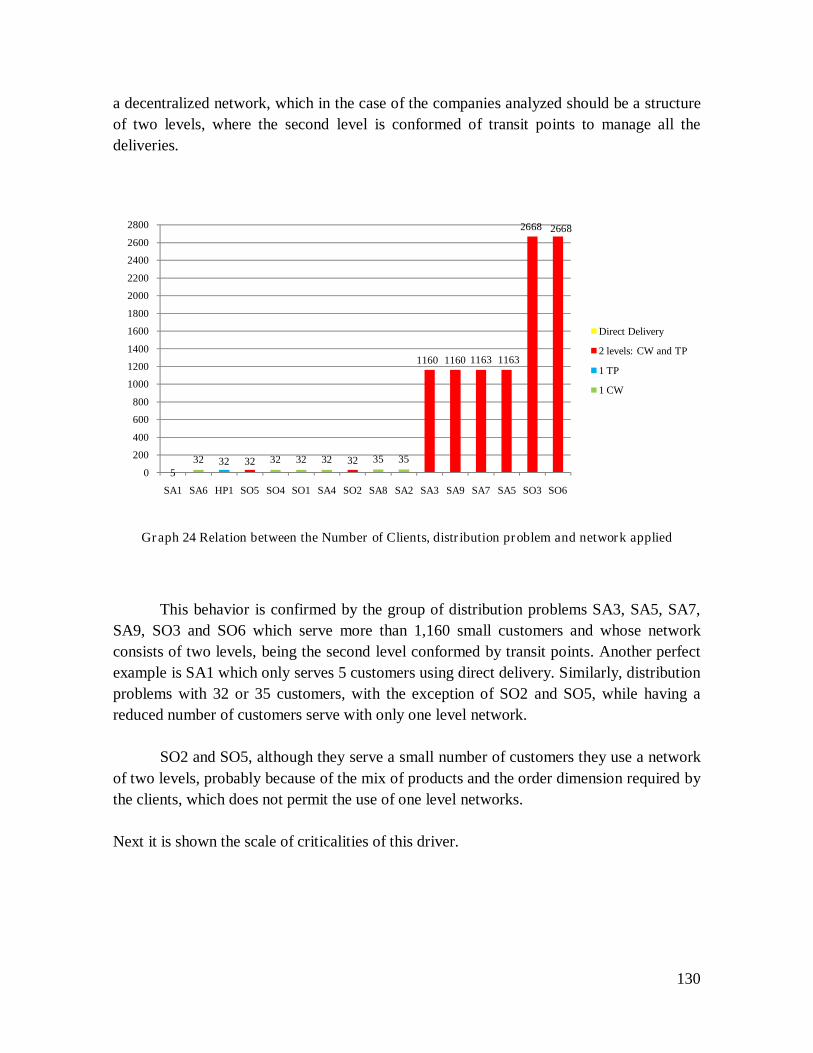
130
a decentralized network, which in the case of the companies analyzed should be a structure
of two levels, where the second level is conformed of transit points to manage all the
deliveries.
Graph 24 Relation between the Number of Clients, distribution problem and network applied
This behavior is confirmed by the group of distribution problems SA3, SA5, SA7,
SA9, SO3 and SO6 which serve more than 1,160 small customers and whose network
consists of two levels, being the second level conformed by transit points. Another perfect
example is SA1 which only serves 5 customers using direct delivery. Similarly, distribution
problems with 32 or 35 customers, with the exception of SO2 and SO5, while having a
reduced number of customers serve with only one level network.
SO2 and SO5, although they serve a small number of customers they use a network
of two levels, probably because of the mix of products and the order dimension required by
the clients, which does not permit the use of one level networks.
Next it is shown the scale of criticalities of this driver.
32 32 32 32 35 35
2668 2668
32 32 32
1160 1160 1163 1163
50
200
400
600
800
1000
1200
1400
1600
1800
2000
2200
2400
2600
2800
SA1 SA6 HP1 SO5 SO4 SO1 SA4 SO2 SA8 SA2 SA3 SA9 SA7 SA5 SO3 SO6
Direct Delivery
2 levels: CW and TP
1 TP
1 CW

131
Graph 25 Scale of Criticality of the driver “Number of Clients”
Frequency of delivery
An increase in the frequency of deliveries augments the total logistic cost.
Transportation costs: having to visit the same spot many times, the cost of transport
augments, and in particular the cost of secondary transport that constitutes in this case the
more relevant one.
Inventory costs: for high values of frequency it is necessary to have higher stocks and
therefore adequate safety stocks; in this way all the inventory costs are affected. In addition
can be satisfy a high frequency of delivery, presumably only if stocks are close to the
customer, this means that decentralization leads to an increase in the average stock and with
it an increase in all the costs of reference.
Handling costs: more the frequency is high, more would be the costs to sustain the
movements, because in the case of high values of this driver often correspond to low values
for ordered volumes; so would be necessary to make many operations of loading, unloading
and picking, for reduced volumes. In any case also at same volume of order, in presence of
a high frequency, make more visits and therefore more operations of handling.
Cost of lost sale: there is no relation.

132
The frequency of delivery is measured in times per week, for example, if a
distribution problem delivers once every two weeks then the frequency is 0.5 times per
week.
According to the costs relation with this driver, a distribution problem is going to be
more critical, meaning logistics costs are higher, if the frequency of delivery is high.
Theoretically a distribution problem with high frequency of delivery should be
decentralized, but unfortunately in the cases studied this is not confirmed; there is no clear
relation between the driver and the distribution network implemented.
Graph 26 Relation between the Frequency of Delivery, distribution problem and network applied
Next it is shown the scale of criticalities of this driver.
Graph 27 Scale of Criticality of the driver “Frequency of Delivery”
0.5 0.5
1 1 1
2
3 3
5
1 1 1
2 2 2
0.25
0
1
2
3
4
5
SA1 SA8 SA2 SA7 SA9 SA6 SA3 SO3 SO6 SA4 SA5 SO2 SO5 SO1 SO4 HP1
Tim
es p
er w
eek
Direct Delivery
2 levels: CW and TP
1 TP
1 CW

133
Seasonality
When this driver grows, the total logistic cost augments.
Transportation costs: in the presence of seasonality, it is necessary to provide excess
capacity to cover the peaks of request, this result in increased transport costs as more
resources are used.
Inventory costs: to guard against increases in these phenomena of uneven demand, the
company may decide to increase their stocks of products, with a consequent increase in
costs related to them.
Handling costs: with the same explanation of the transportation, the handling costs increase
when the driver is higher.
Cost of lost sale: it is possible that, in presence of high irregularities of the demand, the
company can less easily satisfy the upcoming requests, thus involving an increase in cost of
lost sale.
For the means of this study seasonality is measured by the times in a year the sales have
a peak and the length of time, so being:
• Low: it may be seasonality but it is well known and controlled. For example
products as home appliances which have a peak in sales from June to August, it
only happens one time in a year and lasts a few months.
• Low- Medium: seasonality is concentrated in the last third of the year, for example
audio-video and informatics products.
• Medium: peaks in sale occur two times per year. For example TVs which are sold
mostly at the end of the year but also while big events and promotions.
• Medium-High: peaks occur two times per year but the duration is longer.

134
• High: peaks occur more than two times per year. For example mobile phones which
are sold mostly at the end of the year, but also during important dates such as
mother’s day, father’s day, etc.
According to the costs relation with this driver a distribution problem is going to be
more critical, meaning logistics costs are higher, if the seasonality is high. Theoretically a
distribution problem with high seasonality should be centralized in order to cope with the
impact, but unfortunately in the cases studied this is not confirmed; as shown in the graph
below there is no clear relation between the driver of seasonality and the distribution
network implemented.
Graph 28 Relation between the Seasonality, distribution problem and network applied
Next it is shown the scale of criticalities of this driver.
1. Low seasonality
2. Low medium seasonality
3. Medium seasonality
4. Medium high seasonality
5. High seasonality
Graph 29 Scale of Criticality of the driver “Seasonality”
SA1SA3 SA5
SA7SA9 SO2
SO3
SO5
SO6
HP1SA2
SA4
SA6
SA8
SO1
SO4
0
1
2
3
4
5
6
L LM M H

135
Predictability of Demand
The predictability of the demand corresponds to the ability of the firm to forecast
the demands of their products in an accurate way. This driver can have a significant impact
on the logistics costs, which can be divided in:
Transportation Costs: If the demand cannot be predicted in a correct way, additional
unexpected deliveries of products must be done in order to avoid stock out, and exist a
great probability that the level of saturation of the means of transportation for these
circumstances will not be the optimal one, increasing the transportation costs of the firm.
Inventory Costs: when a high level of uncertainty of the future demand is presented,
inventory levels tend to increase in order to cope with unexpected increases in demand,
inventories that are known as safety stocks, and as a consequence the inventory costs
increase.
Handling Costs: low predictability of demand will force firms to deal with unexpected
deliveries of products, increasing therefore the handling costs.
Cost of lost sale: when the forecast process cannot be done properly, the probability of
stock out increases, having as a consequence a decrease in the service level and an increase
in the cost of lost sale.
Predictability of demand is measured as percentage of accuracy of the prediction
with the actual demand.
According to the costs relation with this driver a distribution problem is going to be
more critical, meaning logistics costs are higher, if the predictability of demand is low. In
the cases studied, as shown in the graph below, all the distribution problems have high
predictability of demand; therefore there is no critical difference to understand the behavior
of this driver with the network structure and will not be considered for the model proposed.

136
Graph 30 Relation between the Predictability of Demand, distribution problem and network applied
Next it is shown the scale of criticalities of this driver.
Graph 31 Scale of Criticality of the driver “Predictability of Demand”
Supply drivers:
Distance from plant to client:
When the distance is large, the total logistic cost is high.
Transportation costs: by having a large distance to travel, there is a direct increase in the
transport costs.
90 90 90 9095 95 95 95
90 9095 95 95 9595 95
0
25
50
75
100
SO2 SO3 SO1 SO4 SO6 SO5 SA7 SA2 HP1 SA3 SA9 SA4 SA8 SA5 SA1 SA6
%
Direct Delivery
1 TP
2 levels: CW and TP
1 CW

137
Inventory costs: these costs tend to increase, because due to the greater distance can be used
the decentralization of stocks in intermediate levels. In addition the safety stocks are
function of the lead time, which is as well function of the distance to reach the client.
Handling costs: the larger the distance, higher the handling costs, because may be required
the presence of distributive structures, weather there is capacity to stock or not like regional
warehouses or transit points.
Cost of lost sale: there is no direct relation.
The distance is measured in kilometers. For the sake of this study, plants located in
the Far East were given a distance of 9,000 km and plants located in Europe 1,000 km.
According to the costs relation with this driver a distribution problem is going to be
more critical, meaning logistics costs are higher, if the distance traveled to reach the client
is large. Theoretically by having a large distance to travel, the best option is
decentralization in order to have stocks nearer the client. In the cases studied, as shown in
the graph below most of the distribution problems have large distance from plant to client,
due to the fact that the majority of plants are located in the Far East. There is no critical
difference between centralized and decentralized distribution problems.
Graph 32 Relation between the Distance from plant to client, distribution problem and network
applied
1000 1000 1000
9000 9000 9000 9000 9000
6000
1000 1000
9000 9000 9000 9000 9000
0
1000
2000
3000
4000
5000
6000
7000
8000
9000
SA5 SO3 SA4 SO2 SO1 HP1 SA7 SA2 SA3 SA6 SA9 SO4 SA8 SO5 SA1 SO6
Km
Direct Delivery
2 levels: CW and TP
1 TP
1 CW

138
Next it is shown the scale of criticalities of this driver.
Graph 33 Scale of Criticality of the driver “Distance from plant to client”
Number of plants:
When there are many plants, the total logistic cost increase.
Transportation costs: the relation is with primary cost. It is evident that the transport costs
are conditioned to the number of travels and from the distance to cover in each trip. If the
plants, even if are high in number, are located close to each other, the average distance to
get to the client does not change, while probably changes the number of travels if products
from different plants cannot be picked by the same mean.
Inventory costs: there is no relation between this driver and the total costs.
Handling costs: by modifying the number of plants, the total flow of goods inside the
warehouses or transit points does not vary; therefore the costs of handling do not vary. The
only effect can be seen in the reduction of fixed times if it can benefit from economies of
scale on aggregate flows obtained from a limited number of establishments.
Cost of lost sale: there is no direct relation.

139
The plants considered are the plants that supply the Italian market for each
distribution problem. In the cases studied, as shown in the graph below, there is no critical
difference between the distribution problems and the network structures they follow.
Graph 34 Relation between the Number of Plants, distribution problem and network applied
Next it is shown the scale of criticalities of this driver.
Graph 35 Scale of Criticality of the driver “Number of Plants”
3 3 3
4
5 5
7 7
17
3 3 3
4
5
7
4
0
2
4
6
8
10
12
14
16
18
SA3 SA4 SA2 SA5 SA9 SA8 SA7 SA6 SA1 SO2 SO3 SO1 SO4 SO5 SO6 HP1
Nu
mb
er o
f P
lan
ts
Direct Delivery
2 levels: CW and TP
1 TP
1 CW

140
Level of specialization
The level of Specialization corresponds to the strategic decision of the firm of
producing one product in more than one plant or just in one facility. Having a low level of
specialization, the company can obtain an increase in the service level provided by bringing
the production closer to its customers, but at the same time it could loss economies of scale.
This driver directly affects the distribution network design process as it impacts the overall
company costs, or more specifically the following costs:
Transport Costs: As the level of specialization is low, or in other words the number of
product sources increase, the distance between the plants and the warehouses or clients will
be reduced, and therefore the costs of transportation will be also reduced.
Handling Costs: by increasing the number of product sources, more deliveries must be
done from the plants to the warehouses or directly to the clients, increasing the handling
cost of the firm.
Inventory Costs: having a low level of specialization, inventories of products are distributed
among the plants incurring in duplication of them and losing economies of scale
opportunities.
Costs of lost sale: if the level of specialization is low, the probability of stock out at the
point of sale decreases because different plants can satisfy customers’ orders. In the case of
having specialized plants, if a failure or disruption of the production occurs, customer needs
could not be satisfied by other plants and therefore the cost of lost sales will be elevated.
According to the costs relation with this driver a distribution problem is going to be
more critical, meaning logistics costs are higher, if the level of specialization of the plants
is high, mainly because of the higher distance between plants and clients and also due to the
higher risk of stock out. In the cases studied, the level of specialization is mostly high,
meaning that the driver is critical, but as different distribution networks are applied for the
same level of specialization, this driver is not considered as a determinant driver for the
distribution network design.
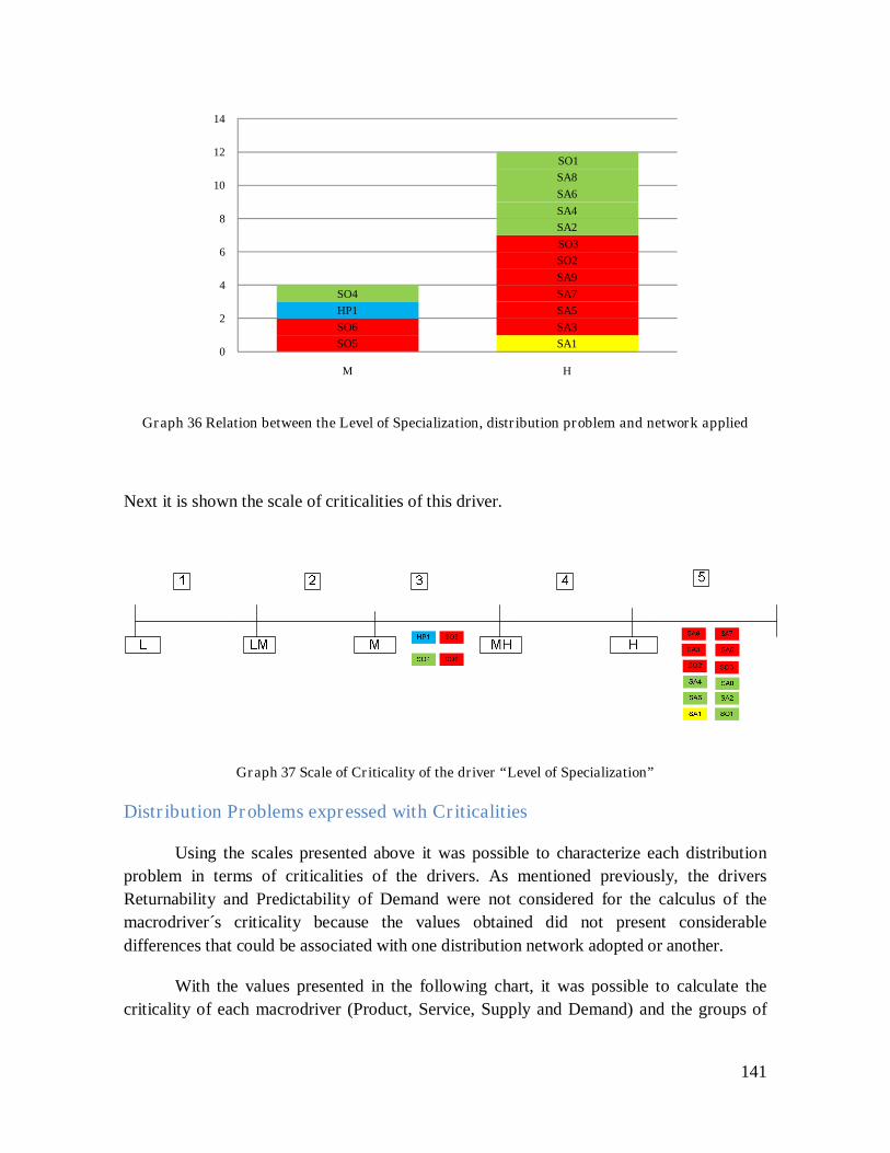
141
Graph 36 Relation between the Level of Specialization, distribution problem and network applied
Next it is shown the scale of criticalities of this driver.
Graph 37 Scale of Criticality of the driver “Level of Specialization”
Distribution Problems expressed with Criticalities
Using the scales presented above it was possible to characterize each distribution
problem in terms of criticalities of the drivers. As mentioned previously, the drivers
Returnability and Predictability of Demand were not considered for the calculus of the
macrodriver´s criticality because the values obtained did not present considerable
differences that could be associated with one distribution network adopted or another.
With the values presented in the following chart, it was possible to calculate the
criticality of each macrodriver (Product, Service, Supply and Demand) and the groups of
SA1
SA3
SA5
SA7
SA9
SO2
SO3
SO5
SO6
HP1
SA2
SA4
SA6
SA8
SO1
SO4
0
2
4
6
8
10
12
14
M H

142
macrodrivers (Market and Firm) for all the distribution problems using the formula
presented in 3.5.
MacroDriver Driver HP1 SO1 SO2 SO3 SO4 SO5 SO6 SA1 SA2 SA3 SA4 SA5 SA6 SA7 SA8 SA9
PRODUCT
Variety 5 2 2 2 4 4 4 1 1 1 3 3 1 1 1 1
Value 5 1 1 1 4 4 4 5 1 1 3 3 5 5 2 2
Density 5 3 3 3 2 2 2 1 4 4 3 3 1 1 3 3
Risk of obsolescence
4 3 3 3 2 2 2 5 1 1 3 3 5 5 1 1
Contribution Margin
1 1 1 1 2 2 2 4 3 3 2 2 4 4 2 2
SERVICE Cycle Time 1 4 3 5 4 3 5 2 4 2 4 2 4 2 4 2
Completeness 1 1 1 1 1 1 1 1 2 2 2 2 2 2 2 2
DEMAND
Dimension of the order
1 1 3 5 1 3 5 4 3 4 3 4 4 5 3 4
Number of customers
1 1 1 5 1 1 5 1 1 4 1 4 1 4 1 4
Frequency of delivery
5 4 3 2 4 3 2 1 1 2 3 3 2 2 1 2
Seasonality 2 3 3 3 2 2 2 5 1 1 3 3 5 5 1 1
SUPPLY
Distance from plant to
client 4 3 3 3 5 5 5 5 5 5 3 3 5 5 5 5
Number of plants
4 3 3 3 4 4 4 2 1 1 1 1 2 2 1 1
Level of specialization
3 5 5 5 3 3 3 5 5 5 5 5 5 5 5 5
Table 19 Distribution Problems expressed with criticalities
Distribution Problems
Product Service Demand Supply MARKET FIRM
HP1 4,0 1,0 2,3 3,7 1,6 3,8
SO1 2,0 2,0 2,0 3,7 2,0 2,8
SO2 2,0 1,7 2,2 3,7 1,9 2,9
SO3 2,0 2,3 3,2 3,7 2,8 2,8
SO4 2,8 2,0 1,8 4,0 1,9 3,4
SO5 2,8 1,7 2,0 4,0 1,8 3,4
SO6 2,8 2,3 3,0 4,0 2,7 3,4
SA1 3,2 1,3 2,4 4,0 1,9 3,6
SA2 2,0 2,3 1,4 3,7 1,9 2,9
SA3 2,0 1,7 2,4 3,7 2,0 2,8
SA4 2,8 2,3 2,2 3,0 2,3 2,9
SA5 2,8 1,7 3,0 3,0 2,3 2,9
SA6 3,2 2,3 2,6 4,0 2,5 3,6
SA7 3,2 1,7 3,4 4,0 2,5 3,6
SA8 1,8 2,3 1,4 3,7 1,9 2,7
SA9 1,8 1,7 2,4 3,7 2,0 2,7
Table 20 Macrodriver´s Criticality of the Distribution Problems

143
Chapter 8. Correlation Analysis
As it has been mentioned and demonstrated in the previous chapters, distribution
networks are designed based on the characteristics of the distribution problem they try to
solve, which are represented by a group of drivers related to the Product, Service, Demand
and Supply.
For the development of the Distribution Network Design model, it is important to
confirm that the list of drivers considered until this point are all necessary and contribute in
an specific proportion to the definition of the distribution problem. For this purpose, a
Correlation analysis was done taking as input data the tables of criticalities presented above
(19 and 20), and obtaining as a result the diagonal and symmetric table that continues.
Table 21 Correlation Analysis between drivers and macrodrivers
Var
iety
Val
ue
Den
sity
Ris
k o
f obso
lesc
ence
Contr
ibuti
on
Mar
gin
Cycl
e T
ime
Co
mp
lete
nes
s
Dim
ensi
on
of
the
ord
er
Num
ber
of
cust
om
ers
Fre
qu
ency
of
del
iver
y
Sea
sonal
ity
Dis
tan
ce f
rom
p
lant
to c
lien
t
Num
ber
of
pla
nts
Lev
el o
f sp
ecia
liza
tion
Pro
du
ct
Ser
vic
e
Dem
and
Su
pply
Mar
ket
Fir
m
Variety 1 0,4 0,2 0,0 -0,5 0,0 -0,6 -0,4 -0,1 0,7 -0,2 -0,2 0,7 -0,9 0,5 -0,2 0,0 -0,1 -0,1 0,4
Value --- 1 -0,5 0,6 0,5 -0,3 -0,1 0,0 -0,1 0,2 0,5 0,4 0,3 -0,5 0,9 -0,3 0,3 0,4 0,0 0,9
Density --- -- 1 -0,5 -0,6 -0,2 0,1 -0,4 0,0 0,3 -0,7 -0,3 -0,1 0,0 -0,2 -0,2 -0,4 -0,5 -0,4 -0,4
Risk of obsolescence
--- -- -- 1 0,3 -0,2 -0,2 0,1 -0,1 0,2 0,9 -0,2 0,2 0,1 0,7 -0,3 0,5 0,2 0,3 0,7
Contribution Margin
--- --- --- --- 1 -0,2 0,5 0,5 0,0 -0,6 0,5 0,6 -0,4 0,3 0,3 0,0 0,2 0,4 0,2 0,4
Cycle Time --- --- --- --- --- 1 -0,2 0,1 0,0 -0,2 -0,1 -0,1 0,2 0,0 -0,4 0,9 -0,1 0,1 0,5 -0,3
Completeness --- --- --- --- --- --- 1 0,3 0,2 -0,4 -0,1 0,2 -0,9 0,6 -0,2 0,3 0,0 -0,4 0,2 -0,3
Dimension of the order
--- --- --- --- --- --- --- 1 0,7 -0,7 0,3 0,2 -0,3 0,4 -0,1 0,2 0,7 0,1 0,7 -0,1
Number of customers
--- --- --- --- --- --- --- --- 1 -0,2 -0,1 0,0 -0,1 0,1 -0,2 0,1 0,8 -0,1 0,7 -0,2
Frequency of delivery
--- --- --- --- --- --- --- --- --- 1 0,0 -0,5 0,6 -0,5 0,4 -0,4 0,0 -0,2 -0,3 0,3
Seasonality --- --- --- --- --- --- --- --- --- --- 1 -0,2 0,1 0,3 0,5 -0,1 0,5 0,2 0,4 0,5
Distance from plant to client
--- --- --- --- --- --- --- --- --- --- --- 1 0,0 -0,3 0,1 0,0 -0,2 0,7 -0,2 0,4
Number of plants
--- --- --- --- --- --- --- --- --- --- --- --- 1 -0,8 0,4 -0,2 0,1 0,5 0,0 0,5
Level of specialization
--- --- --- --- --- --- --- --- --- --- --- --- --- 1 -0,5 0,2 0,1 -0,4 0,2 -0,6
Product --- --- --- --- --- --- --- --- --- --- --- --- --- --- 1 -0,5 0,3 0,2 0,0 0,9
Service --- --- --- --- --- --- --- --- --- --- --- --- --- --- --- 1 -0,1 -0,1 0,5 -0,4
Demand --- --- --- --- --- --- --- --- --- --- --- --- --- --- --- --- 1 0,0 0,8 0,3
Supply --- --- --- --- --- --- --- --- --- --- --- --- --- --- --- --- --- 1 0,0 0,6
Market --- --- --- --- --- --- --- --- --- --- --- --- --- --- --- --- --- --- 1 0,0
Firm --- --- --- --- --- --- --- --- --- --- --- --- --- --- --- --- --- --- --- 1

144
The correlation factors range from -1 to 1, meaning that for those variables that are
inversely correlated (when one raises the other one decreases) negative values will be
obtained, and for directly correlated variables (if one increase the other one will do it as
well) the result will be a positive value. The 0 is obtained when no correlation is presented.
For the purposes of this analysis, values of -0.7 or lower, and 0.7 or higher will be
considered as relevant.
From this table it is possible to identify different areas or groups of correlation
factors. First, the correlation factors between all the drivers located in the center of the
table; then the importance of each driver within its macrodriver located in the black box on
the right, and finally, the correlation between the macrodrivers and the groups of
macrodrivers (Market and Firm) located at the bottom right side of the table.
8.1 Correlation between drivers
Within this area there are presented all the correlation factors between drivers
without distinction of the macrodriver at which they pertain. Theoretically, the values
observed should be near the No Correlation value (0) in order to demonstrate that the
drivers considered are independent and necessary for the model to be proposed.
This behavior was observed in the majority of the cases, indicating that the total
amount of drivers selected were the appropriate ones to define in a complete manner the
distribution problems, without redundancy or duplication of data.
Some exceptions or pair of drivers with high correlation factor were obtained
(highlighted in green), but complete correlations where not present. These cases are listed
and explained below:
- Variety – Number of Plants: it was obtained a correlation factor of 0.7 which
indicates that a high criticality on the variety (high number of product codes) is
obtained mainly when the criticality of the number of plants is also high (many
plants). This correlation also depends on the level of specialization of the plants
as it will be see it in the next correlation.
- Variety – Level of Specialization: a correlation factor of -0.9 was obtained,
meaning that a high criticality on the variety (high number of product codes)
corresponds to a low criticality on the level of specialization (products are
manufactured in more than one plant). Both correlations are reasonable, but does
not justify the elimination of the driver Variety for two reasons: first, the data
obtained for the level of specialization is allocated in just two values of
criticalities (3 and 5) where different types of distribution networks are present,
which means that this driver is not determinant for the design. And second,

145
because the driver variety pertains to a different macrodriver, meaning that it
represents another aspect of the distribution problem.
- Number of Plants – Level of Specialization: as it might be expected after the
explanation above, the correlation factor of these two drivers should be also
considerable. In fact, a value of -0.8 was obtained, indicating that a high number
of plants (high criticality) tend to a low level of specialization of them. Although
the correlation factor is high, it is not considered to eliminate one of them, as
some exceptions were present and it is a field which is continuously changing
within firms and should be traced.
- Dimension of the order – Number of Customers: a correlation factor of 0.7
was obtained, indicating that a high criticality in the dimension of the order
(small quantities) are distributed generally to high number of customers. From
the interviews it was obtained that small clients, which orders are mainly of 0,2
or 0,4 FTL, are more than big clients, but as there are some cases were big
clients order small quantities, none of the two drivers should be discard.
- Dimension of the Order – Frequency of Delivery: a negative correlation of -
0,7 was obtained for this pair of drivers, meaning that when the criticality of the
dimension of the order is high (small quantities), the frequency of delivery is
reduced. As it was presented in the correlation before, small customers are the
ones which orders generally are small, and because of lack of stock space or
because of the amount of sales per week, the frequency of delivery is also
reduced. In this case, some exceptions are also present, reason why none of the
two drivers should be discard.
Other exceptions were the correlation factors of Risk of Obsolescence – Seasonality
(0.9) and Completeness – Number of Plants (-0.9). In the first case, the relation between the
two drivers is mainly due to the type of products, for example, mobile phones which have a
high risk of obsolescence, also have high seasonality because of marketing promotions.
Although the high correlation factor, none of the drivers is discard because they pertain to
different macrodrivers and therefore analyze different aspects of the distribution problem.
In the second case, the completeness of the order is considered to be a corporate decision
rather than a result of the distribution network implemented and, as it will be presented, this
driver does not have an important impact for the model, but it is not eliminated because it is
one of the KPIs commonly used by firms.
8.2 Correlations between Drivers and Macrodrivers
The objective of this part of the analysis is to understand the impact or relation of
each driver with respect to their correspondent macrodriver. Based on the correlation factor
obtained and the interpretation of the importance of each driver with respect to the logistics
costs done in chapter 7, each driver will be assigned with a specific weight for the calculus

146
of the average of the macrodriver. Drivers with high correlation factor (positive or
negative) will represent a greater proportion of the macrodriver, and the sum of the weights
of the drivers pertaining to one macrodriver must be equal to 1.
From the total amount of drivers analyzed, six were highlighted in yellow as having
an important correlation with their macrodriver. Starting from the Product, it can be
observed that the driver Value presented a correlation factor of 0.9, indicating an almost
perfect correlation, which is an expected result taking in consideration the industry object
of the analysis. The second driver corresponds to the Risk of Obsolescence with 0.7, which
although it was not considered as an important factor for the distribution network design
presents a relatively high correlation. The driver Variety, occupies the third place probably
due to the fact that the complete range of products might be delivered using different types
of distribution networks.
For the macrodriver Service, the Cycle Time presented a correlation factor of 0.9
which is extremely high compared with the Completeness (0.3). This result was expected
because as it was mentioned in the chapter 7, the Cycle Time is an intrinsic characteristic of
the distribution network implemented and must be taken in consideration for its design.
In the case of the macrodriver Demand, the Dimension of the Order and the Number
of Customers were the drivers that presented more correlation, 0.7 and 0.8 respectively. As
well as the Cycle Time, these drivers were mentioned in the chapter 7 as important for the
distribution network design.
Then, for the macrodriver Supply the driver that obtained a higher correlation factor
was the Distance from Plant to Clients with 0.7, while the Number of Plants and the Level
of Specialization presented 0.5 and -0.4, respectively. Taking into consideration that most
of the consumer electronics production plants are located in Asia in order to take advantage
of economies of scale, it is appropriate for this driver to be the most important within this
cluster.
Finally, using the previous results it is possible to demonstrate that the formula for
the calculation of the macrodrivers criticality presented in the chapter 3, that assumed equal
weights for the drivers within each macrodriver, was not the optimal one. In the next table
there are presented the corresponding weights of each driver that must be used.

147
Table 22 Driver´s weights
8.3 Correlation between Macrodrivers, Market and Firm
The last part of the correlation analysis table presents the correlation factors
between the macrodrivers (Product, Service, Demand and Supply) with the two groups of
macrodrivers (Market and Firm). The objective of this part is similar to the previous one,
assign weights to the macrodivers based on their level of relation with the Market and the
Firm, which will be used for the calculus of the average criticality.
The two macrodrivers that presented correlation with the Market were Service and
Demand with 0.5 and 0.8, respectively. This result is coherent with what it was presented
during the analysis of each macrodriver because for the Service just the Cycle Time
presented an important correlation, while for the Demand two drivers, Dimension of the
Order and Number of Clients, were highly correlated.
In the case of the Firm, the Product obtained 0.9 as correlation factor while the
Supply 0.6. As it was mentioned before, two drivers pertaining to the Product macrodriver,
Value and the Risk of Obsolescence, were highly correlated, while just the Distance from
plant to client presented a high correlation with the macrodriver Supply, making the results
for the Firm coherent.
The next table presents the weights for each macrodriver that must be used for the
calculus of the Market and Firm criticalities.
Product
Variety 0.15
Value 0.45
Density 0.1
Risk of obsolescence 0.25
Contribution Margin 0.05
Service Cycle Time 0.8
Completeness 0.2
Demand
Dimensions of the order 0.4
Number of customers 0.4
Frequency of delivery 0.15
Seasonality 0.05
Supply
Distance from plant to client 0.5
Number of plants 0.25
Level of specialization 0.25

148
Table 23 Macrodriver´s Weights
Then, using the data presented in the table 19, corresponding to the representation of
the distribution problems in terms of driver´s criticalities, and the weights of the drivers and
macrodrivers presented above, it was possible to calculate the correct values of each
macrodriver, Market and Firm for all the distribution problems, using the following
formulas:
max
max
*
j
cWj
C
j
jj
i
∑=
with: =iC Macrodriver criticality i;
=jc driver criticality j, with j = [1, …, jmax];
Wj = Weight of each driver
i = {product, service, demand, supply}
j = {variety, value, density, …., many products sources} = {all the drivers}
and: 2
** ClWlCpWpCF
+=
2
** CdWdCsWsCM
+=
CF = firm criticality =CM market criticality
=Cp product criticality =Cs service criticality
=Cl supply criticality =Cd demand criticality
W(p, l, s, d) = Weights (product, supply, service, demand)
FIRM MARKET
Product weight 0.65 Service weight 0.35
Supply weight 0.35 Demand weight 0.65

149
Table 24 Weighted Macrodriver´s Criticality of the Distribution Problems
8.4 Synthetic representation of the firm cases
At this point, it is important to represent in a synthetic way each distribution
problem to obtain a global perspective of all the characteristics. Thanks to the calculated
average, four indicative values were obtained (product, service, demand, and supply). In
order to point out the elements of higher criticality that characterize the problem, a
graphical representation is necessary. The solution adopted is based on the graphics where
each category of data (each macrodriver), has a specific axis that branches off the center
point and where the criticalities values are placed for each distribution problem. The
procedure for the design of the synthetic representations was detailed in section 3.7.
Distribution Problems
Product Service Demand Supply MARKET FIRM
HP1 4,6 1,0 1,7 3,8 1,4 4,3
SO1 1,9 3,4 1,6 3,5 2,2 2,4
SO2 1,9 2,6 2,2 3,5 2,3 2,4
SO3 1,9 4,2 4,5 3,5 4,4 2,4
SO4 3,2 3,4 1,5 4,3 2,2 3,6
SO5 3,2 2,6 2,2 4,3 2,3 3,6
SO6 3,2 4,2 4,4 4,3 4,3 3,6
SA1 4,0 1,8 2,2 4,3 2,1 4,1
SA2 1,4 3,6 1,8 4,0 2,4 2,3
SA3 1,4 2,0 3,6 4,0 3,0 2,3
SA4 3,0 3,6 2,1 3,0 2,6 3,0
SA5 3,0 2,0 3,7 3,0 3,1 3,0
SA6 4,0 3,6 2,4 4,3 2,8 4,1
SA7 4,0 2,0 4,0 4,3 3,3 4,1
SA8 1,7 3,6 1,8 4,0 2,4 2,5
SA9 1,7 2,0 3,6 4,0 3,0 2,5

150
Hewlett Packard Net revenues (2009): $114,552 million dollars Market Share: worldwide leader in personal computers N° Employees: approximately 304,000 worldwide Business Unit to consider: The Personal Systems Group and The Imaging and Printing Group.
HP1
Personal computers, monitors, printers and professional products
Synthetic representation of data
Punctual values and criticality
Criticalities
Product: 4.6 Demand: 1.7
Supply: 3.8 Service: 1
Firm: 4.3 Market: 1.4
Solution of the network
- 1 level of network structure with 2 Transit Points
- One transit point in Luxemburg and the other in The
Netherlands
4,6
3,8
1,7
1,0
PRODUCT
Firm criticality
SUPPLY
DEMAND
Market criticality
SERVICE
HP1
VALUE CRITICALITY
HP1 HP1
Variety [SKUs] 4000 5
Value [€/Kg] 1000 5
Density [Kg/m3] 7,6 5
Risk of obsolescence
[days]120 4
Contribution Margin: 12 1
Cycle Time [days] 15 1
Completeness [IFR] 100 1
Dimension of the order
[%FTL]1 1
Number of customers 32 1
Frequency of delivery
[Deliveries per week]5 5
Seasonality LM 2
Distance from plant to
client6000 4
Number of plants 17 4
Level of specialization M 3
DRIVERMACRODRIVER
PRODUCT
SERVICE
DEMAND
SUPPLY

151
Sony Net revenues (2009): ¥7,214.0 billion N° Employees: approximately 167,000 worldwide Business Unit to consider: Sony Electronics that include IT and consumer electronics
SO1
Televisions
Synthetic representation of data
Punctual values and criticality
Criticalities
Product: 1.9 Demand: 1.6 Supply: 3.5 Service: 3.4 Firm: 2.4 Market: 2.2
Solution of the network
- 1 level Network of 1 Central Warehouse
- Located in Milano
1.9
3.5
1.6
3.4
PRODUCT
Firm criticality
SUPPLY
DEMAND
Market criticality
SERVICE
SO1
VALUE C R ITIC IT Y
SO1 SO1
Variety 400 2
Value [Euro/Kg] 55 1
Density [kg/m3] 160 3
Risk of obsolescence 180 3
Contribution Margin 10 1
Cycle time 3 4
Completeness 100 1
Dimensions of the order (typology) 1 1
Number of customers 32 1
Ferequency of delivery 3 4
Seasonality M 3
Distance from plant to client 1000 3
Number of plants 5 3
Level of Specialization H 5
DEMAND
SUPPLY
SERVICE
MACRODRIVER DRIVER
PRODUCT

152
Sony Net revenues (2009): ¥7,214.0 billion N° Employees: approximately 167,000 worldwide Business Unit to consider: Sony Electronics that include IT and consumer electronics
SO2
Televisions
Synthetic representation of data
Punctual values and criticality
Criticalities
Product: 1.9 Demand: 2.6 Supply: 3.5 Service: 2.2 Firm: 2.9 Market: 2.3
Solution of the network
- 2 level Network of 1 Central Warehouse at the first level and 13 Transit Points
Central Warehouse located in Milano and Transit Points for each 1.5 Italian region.
1.9
3.5
2.2
2.6
PRODUCT
Firm criticality
SUPPLY
DEMAND
Market criticality
SERVICE
SO2
VALUE C R ITIC ITY
SO2 SO2
Variety 400 2
Value [Euro/Kg] 55 1
Density [kg/m3] 160 3
Risk of obsolescence 180 3
Contribution Margin 10 1
Cycle time 4 3
Completeness 100 1
Dimensions of the order (typology) 0.6 3
Number of customers 32 1
Ferequency of delivery 2 3
Seasonality M 3
Distance from plant to client 1000 3
Number of plants 5 3
Level of Specialization H 5
DEMAND
SUPPLY
SERVICE
MACRODRIVER DRIVER
PRODUCT

153
Sony Net revenues (2009): ¥7,214.0 billion N° Employees: approximately 167,000 worldwide Business Unit to consider: Sony Electronics that include IT and consumer electronics
SO3
Televisions
Synthetic representation of data
Punctual values and criticality
Criticalities
Product: 1.9 Demand: 4.5 Supply: 3.5 Service: 4.2 Firm: 2.4 Market: 4.4
Solution of the network
- 1 level Network of 1 Central Warehouse
- Central Warehouse located in Milano
1.9
3.5
4.5
4.2
PRODUCT
Firm criticality
SUPPLY
DEMAND
Market criticality
SERVICE
SO3
VALUE C R ITIC ITY
SO3 SO3
Variety 400 2
Value [Euro/Kg] 55 1
Density [kg/m3] 160 3
Risk of obsolescence 180 3
Contribution Margin 10 1
Cycle time 2 5
Completeness 100 1
Dimensions of the order (typology) 0.2 5
Number of customers 2668 5
Ferequency of delivery 1 2
Seasonality M 3
Distance from plant to client 1000 3
Number of plants 5 3
Level of Specialization H 5
DEMAND
SUPPLY
SERVICE
MACRODRIVER DRIVER
PRODUCT

154
Sony Net revenues (2009): ¥7,214.0 billion N° Employees: approximately 167,000 worldwide Business Unit to consider: Sony Electronics that include IT and consumer electronics
SO4
Notebooks, Peripherals, Audio, Digital Imaging
Synthetic representation of data
Punctual values and criticality
Criticalities
Product: 3.2 Demand: 1.5 Supply: 4.3 Service: 3.4 Firm: 3.6 Market: 2.2
Solution of the network
- 1 level Network of 1 Central Warehouse
- Central Warehouse located in Milano
3.2
4.3
1.5
3.4
PRODUCT
Firm criticality
SUPPLY
DEMAND
Market criticality
SERVICE
SO4
VALUE C R ITIC ITY
SO4 SO4
Variety 800 4
Value [Euro/Kg] 800 4
Density [kg/m3] 643 2
Risk of obsolescence 240 2
Contribution Margin 14 2
Cycle time 3 4
Completeness 100 1
Dimensions of the order (typology) 1 1
Number of customers 32 1
Ferequency of delivery 3 4
Seasonality LM 2
Distance from plant to client 9000 5
Number of plants 7 4
Level of Specialization M 3
DEMAND
SUPPLY
SERVICE
MACRODRIVER DRIVER
PRODUCT

155
Sony Net revenues (2009): ¥7,214.0 billion N° Employees: approximately 167,000 worldwide Business Unit to consider: Sony Electronics that include IT and consumer electronics
SO5
Notebooks, Peripherals, Audio, Digital Imaging
Synthetic representation of data
Punctual values and criticality
Criticalities
Product: 3.2 Demand: 2.2 Supply: 4.3 Service: 2.6 Firm: 3.6 Market: 2.3
Solution of the network
- 2 level Network of 1 Central Warehouse at first level and 13 Transit Point at second level.
- Central Warehouse located in Milano and transit
points every 1.5 italian regions
3.2
4.3
2.2
2.6
PRODUCT
Firm criticality
SUPPLY
DEMAND
Market criticality
SERVICE
SO5
VALUE C R IT IC ITY
SO5 SO5
Variety 800 4
Value [Euro/Kg] 800 4
Density [kg/m3] 643 2
Risk of obsolescence 240 2
Contribution Margin 14 2
Cycle time 4 3
Completeness 100 1
Dimensions of the order (typology) 0.6 3
Number of customers 32 1
Ferequency of delivery 2 3
Seasonality LM 2
Distance from plant to client 9000 5
Number of plants 7 4
Level of Specialization M 3
DEMAND
SUPPLY
SERVICE
MACRODRIVER DRIVER
PRODUCT

156
Sony Net revenues (2009): ¥7,214.0 billion N° Employees: approximately 167,000 worldwide Business Unit to consider: Sony Electronics that include IT and consumer electronics
SO6
Notebooks, Peripherals, Audio, Digital Imaging
Synthetic representation of data
Punctual values and criticality
Criticalities
Product: 3.2 Demand: 4.4 Supply: 4.3 Service: 4.2 Firm: 3.6 Market: 4.3
Solution of the network
- 1 level Network of 1 Central Warehouse
- Central Warehouse located in Milano
3.2
4.3
4.4
4.2
PRODUCT
Firm criticality
SUPPLY
DEMAND
Market criticality
SERVICE
SO6
VALUE CR ITICITY
SO6 SO6
Variety 800 4
Value [Euro/Kg] 800 4
Density [kg/m3] 643 2
Risk of obsolescence 240 2
Contribution Margin 14 2
Cycle time 2 5
Completeness 100 1
Dimensions of the order (typology) 0.2 5
Number of customers 2668 5
Ferequency of delivery 1 2
Seasonality LM 2
Distance from plant to client 9000 5
Number of plants 7 4
Level of Specialization M 3
MACRODRIVER DRIVER
PRODUCT
SERVICE
DEMAND
SUPPLY

157
Samsung - Net revenues (2009): 138,994 (billions of KRW) - Market Share: LCD Monitor: 16.1%, Hard disk drive: 9.5%, Television set: 23%, Printers: 16.4%, Mobile
phones: 23%, Digital camera: 9.1% - N° Employees: approximately 164,000 worldwide - Business Unit to consider: Audio and Video, Home Appliances, Informatics, Mobile, Networking
SA1
Mobile phones and television decoders
Synthetic representation of data
Punctual values and criticality
Criticalities
Product: 4 Demand: 2.2 Supply: 4.3 Service: 1.8 Firm: 4.1 Market: 2.1
Solution of the network
- Direct delivery to mobile operators
4.0
4.3
2.2
1.8
PRODUCT
Firm criticality
SUPPLY
DEMAND
Market criticality
SERVICE
SA1
VALUE C R ITIC IT Y
SA1 SA1
Variety 50 1
Value [Euro/Kg] 1000 5
Dens ity [kg/m3] 1200 1
Risk of obsolescence 90 5
Contribution Margin 30 4
Cycle time 5 2
Completeness 100 1
Returnability 1 1
Dimensions of the order (typology) 0.4 4
Number of customers 5 1
Ferequency of delivery 0.25 1
Seasonality H 5
Predictability of demand 95 1
Distance from plant to client 9000 5
Number of plants 4 2
Level of Specialization H 5
SUPPLY
PRODUCT
SERVICE
DEMAND
MACRODRIVER DRIVER

158
Samsung - Net revenues (2009): 138,994 (billions of KRW) - Market Share: LCD Monitor: 16.1%, Hard disk drive: 9.5%, Television set: 23%, Printers: 16.4%, Mobile
phones: 23%, Digital camera: 9.1% - N° Employees: approximately 164,000 worldwide - Business Unit to consider: Audio and Video, Home Appliances, Informatics, Mobile, Networking
SA2
Home Appliances
Synthetic representation of data
Punctual values and criticality
Criticalities
Product: 1.4 Demand: 1.8 Supply: 4 Service: 3.6 Firm: 2.3 Market: 2.4
Solution of the network
- 1 level network composed of one Central Warehouse
- Located in Milano
1.4
4.0
1.8
3.6
PRODUCT
Firm criticality
SUPPLY
DEMAND
Market criticality
SERVICE
SA2
VALUE C R ITIC ITY
SA2 SA2
Variety 100 1
Value [Euro/Kg] 13 1
Dens ity [kg/m3] 110 4
Risk of obsolescence 365 1
Contribution Margin 24 3
Cycle time 3 4
Completeness 95 2
Returnability 1 1
Dimensions of the order (typology) 0.6 3
Number of cus tomers 35 1
Ferequency of delivery 0.5 1
Seasonality L 1
Predictability of demand 95 1
Dis tance from plant to client 9000 5
Number of plants 3 1
Level of Specialization H 5
SUPPLY
PRODUCT
SERVICE
DEMAND
MACRODRIVER DRIVER

159
Samsung - Net revenues (2009): 138,994 (billions of KRW) - Market Share: LCD Monitor: 16.1%, Hard disk drive: 9.5%, Television set: 23%, Printers: 16.4%, Mobile
phones: 23%, Digital camera: 9.1% - N° Employees: approximately 164,000 worldwide - Business Unit to consider: Audio and Video, Home Appliances, Informatics, Mobile, Networking
SA3
Home Appliances
Synthetic representation of data
Punctual values and criticality
Criticalities
Product: 1.4 Demand: 3.6 Supply: 4.0 Service: 2.0 Firm: 2.3 Market: 3
Solution of the network
- 2 level network composed of one Central Warehouse at first level and 20 transit points.
- Central Warehouse located in Milano and transit
points every Italian region.
1.4
4.0
3.6
2.0
PRODUCT
Firm criticality
SUPPLY
DEMAND
Market criticality
SERVICE
SA3
VALUE C R ITIC ITY
SA3 SA3
Variety 100 1
Value [Euro/Kg] 13 1
Density [kg/m3] 110 4
Risk of obsolescence 365 1
Contribution Margin 24 3
Cycle time 5 2
Completeness 95 2
Returnability 1 1
Dimens ions of the order (typology) 0.4 4
Number of customers 1160 4
Ferequency of delivery 1 2
Seasonality L 1
Predictability of demand 95 1
Distance from plant to client 9000 5
Number of plants 3 1
Level of Specialization H 5
MACRODRIVER DRIVER
PRODUCT
SERVICE
DEMAND
SUPPLY

160
Samsung - Net revenues (2009): 138,994 (billions of KRW) - Market Share: LCD Monitor: 16.1%, Hard disk drive: 9.5%, Television set: 23%, Printers: 16.4%, Mobile
phones: 23%, Digital camera: 9.1% - N° Employees: approximately 164,000 worldwide - Business Unit to consider: Audio and Video, Home Appliances, Informatics, Mobile, Networking
SA4
Audio, Video and Informatics products
Synthetic representation of data
Punctual values and criticality
Criticalities
Product: 3.0 Demand: 2.1 Supply: 3.0 Service: 3.6 Firm: 3.0 Market: 2.6
Solution of the network
- 1 level network composed of one Central Warehouse
- Located in Milano
3.0
3.0
2.1
3.6
PRODUCT
Firm criticality
SUPPLY
DEMAND
Market
criticality
SERVICE
SA4
VALUE C R ITIC ITY
SA4 SA4
Variety 700 3
Value [Euro/Kg] 370 3
Density [kg/m3] 170 3
Risk of obsolescence 180 3
Contribution Margin 14 2
Cycle time 3 4
Completeness 95 2
Returnability 1 1
Dimensions of the order (typology) 0.6 3
Number of customers 32 1
Ferequency of delivery 2 3
Seasonality M 3
Predictability of demand 95 1
Distance from plant to client 1000 3
Number of plants 3 1
Level of Specialization H 5
SUPPLY
PRODUCT
SERVICE
DEMAND
MACRODRIVER DRIVER

161
Samsung - Net revenues (2009): 138,994 (billions of KRW) - Market Share: LCD Monitor: 16.1%, Hard disk drive: 9.5%, Television set: 23%, Printers: 16.4%, Mobile
phones: 23%, Digital camera: 9.1% - N° Employees: approximately 164,000 worldwide - Business Unit to consider: Audio and Video, Home Appliances, Informatics, Mobile, Networking
SA5
Audio, Video and Informatics products
Synthetic representation of data
Punctual values and criticality
Criticalities
Product: 3.0 Demand: 3.7 Supply: 3.0 Service: 2.0 Firm: 3.0 Market: 3.1
Solution of the network
- 2 level network composed of one Central Warehouse at first level and 20 transit points.
- Central Warehouse located in Milano and transit
points every Italian region.
3.0
3.0
3.7
2.0
PRODUCT
Firm criticality
SUPPLY
DEMAND
Market criticality
SERVICE
SA5
VALUE C R IT IC IT Y
SA5 SA5
Variety 700 3
Value [Euro/Kg] 370 3
Density [kg/m3] 170 3
Risk of obsolescence 180 3
Contribution Margin 14 2
Cycle time 5 2
Completeness 95 2
Returnability 1 1
Dimensions of the order (typology) 0.4 4
Number of customers 1163 4
Ferequency of delivery 2 3
Seasonality M 3
Predictability of demand 95 1
Distance from plant to client 1000 3
Number of plants 3 1
Level of Specialization H 5
MACRODRIVER DRIVER
PRODUCT
SERVICE
DEMAND
SUPPLY

162
Samsung - Net revenues (2009): 138,994 (billions of KRW) - Market Share: LCD Monitor: 16.1%, Hard disk drive: 9.5%, Television set: 23%, Printers: 16.4%, Mobile
phones: 23%, Digital camera: 9.1% - N° Employees: approximately 164,000 worldwide - Business Unit to consider: Audio and Video, Home Appliances, Informatics, Mobile, Networking
SA6
Mobile phones
Synthetic representation of data
Punctual values and criticality
Criticalities
Product: 4.0 Demand: 3.6 Supply: 4.3 Service: 2.4 Firm: 4.1 Market: 2.8
Solution of the network
- 1 level network composed of one Central Warehouse
- Located in Milano
4.0
4.3
2.4
3.6
PRODUCT
Firm criticality
SUPPLY
DEMAND
Market criticality
SERVICE
SA6
VALUE C R IT IC ITY
SA6 SA6
Variety 50 1
Value [Euro/Kg] 1000 5
Density [kg/m3] 1200 1
Risk of obsolescence 90 5
Contribution Margin 30 4
Cycle time 3 4
Completeness 95 2
Returnability 1 1
Dimensions of the order (typology) 0.4 4
Number of customers 32 1
Ferequency of delivery 1 2
Seasonality H 5
Predictability of demand 95 1
Distance from plant to client 9000 5
Number of plants 4 2
Level of Specialization H 5
MACRODRIVER DRIVER
PRODUCT
SERVICE
DEMAND
SUPPLY

163
Samsung - Net revenues (2009): 138,994 (billions of KRW) - Market Share: LCD Monitor: 16.1%, Hard disk drive: 9.5%, Television set: 23%, Printers: 16.4%, Mobile
phones: 23%, Digital camera: 9.1% - N° Employees: approximately 164,000 worldwide - Business Unit to consider: Audio and Video, Home Appliances, Informatics, Mobile, Networking
SA7
Mobile phones
Synthetic representation of data
Punctual values and criticality
Criticalities
Product: 4.0 Demand: 4.0 Supply: 4.3 Service: 2.0 Firm: 4.1 Market: 3.3
Solution of the network
- 2 level network composed of one Central Warehouse at first level and 150 transit points at the second level
- Central Warehouse located in Milano and 7.5 transit
points every region.
4.0
4.3
4.0
2.0
PRODUCT
Firm criticality
SUPPLY
DEMAND
Market criticality
SERVICE
SA7
VALUE C R IT IC IT Y
SA7 SA7
Variety 50 1
Value [Euro/Kg] 1000 5
Density [kg/m3] 1200 1
Risk of obsolescence 90 5
Contribution Margin 30 4
Cycle time 5 2
Completeness 95 2
Returnability 1 1
Dimensions of the order (typology) 0.2 5
Number of customers 1163 4
Ferequency of delivery 1 2
Seasonality H 5
Predictability of demand 95 1
Distance from plant to client 9000 5
Number of plants 4 2
Level of Specialization H 5
SUPPLY
PRODUCT
SERVICE
DEMAND
MACRODRIVER DRIVER

164
Samsung - Net revenues (2009): 138,994 (billions of KRW) - Market Share: LCD Monitor: 16.1%, Hard disk drive: 9.5%, Television set: 23%, Printers: 16.4%, Mobile
phones: 23%, Digital camera: 9.1% - N° Employees: approximately 164,000 worldwide - Business Unit to consider: Audio and Video, Home Appliances, Informatics, Mobile, Networking
SA8
Air conditioning systems
Synthetic representation of data
Punctual values and criticality
Criticalities
Product: 1.7 Demand: 1.8 Supply: 4 Service: 3.6 Firm: 4.1 Market: 2.4
Solution of the network
- 1 level network composed of one Central Warehouse
- Located in Milano
1.7
4.0
1.8
3.6
PRODUCT
Firm criticality
SUPPLY
DEMAND
Market criticality
SERVICE
SA8
VALUE CR ITIC ITY
SA8 SA8
Variety 150 1
Value [Euro/Kg] 90 2
Density [kg/m3] 170 3
Risk of obsolescence 365 1
Contribution Margin 14 2
Cycle time 3 4
Completeness 95 2
Returnability 1 1
Dimensions of the order (typology) 0.6 3
Number of customers 35 1
Ferequency of delivery 0.5 1
Seasonality L 1
Predictability of demand 95 1
Distance from plant to client 9000 5
Number of plants 3 1
Level of Specialization H 5
SUPPLY
PRODUCT
SERVICE
DEMAND
MACRODRIVER DRIVER

165
Samsung - Net revenues (2009): 138,994 (billions of KRW) - Market Share: LCD Monitor: 16.1%, Hard disk drive: 9.5%, Television set: 23%, Printers: 16.4%, Mobile
phones: 23%, Digital camera: 9.1% - N° Employees: approximately 164,000 worldwide - Business Unit to consider: Audio and Video, Home Appliances, Informatics, Mobile, Networking
SA9
Air conditioning systems
Synthetic representation of data
Punctual values and criticality
Criticalities
Product: 1.7 Demand: 3.6 Supply: 4 Service: 2.0 Firm: 2.5 Market: 3.0
Solution of the network
- 2 level network composed of one Central Warehouse at first level and 20 transit points at the second level
- Central Warehouse located in Milano and 1 transit
points every region.
1.7
4.0
3.6
2.0
PRODUCT
Firm criticality
SUPPLY
DEMAND
Market criticality
SERVICE
SA9
VALUE C R ITIC ITY
SA9 SA9
Variety 150 1
Value [Euro/Kg] 90 2
Density [kg/m3] 170 3
Risk of obsolescence 365 1
Contribution Margin 14 2
Cycle time 5 2
Completeness 95 2
Returnability 1 1
Dimensions of the order (typology) 0.4 4
Number of customers 1160 4
Ferequency of delivery 1 2
Seasonality L 1
Predictability of demand 95 1
Dis tance from plant to client 9000 5
Number of plants 3 1
Level of Specialization H 5
MACRODRIVER DRIVER
PRODUCT
SERVICE
DEMAND
SUPPLY

166
Chapter 9. Analysis of the solutions
Once identified the solution clusters in which each distribution problem can lay, and
once characterized the associated drivers, an empirical relation has to be found that shows
the possible strategic network choices. The adopted model to obtain the relation is based on
the theoretic considerations of the empirical analysis of the interviewed companies
pertaining to the consumer electronic industry in Italy.
As will be shown later, the points in the graphs lead to the individuation of zones
strongly characterized by drivers to which correspond specific network solutions; the
exceptions are only a few and characterized by specific reasons outside the projection
drivers. Each time a new distribution problem is introduced, its point lays always in the
zone that is characterized by the adopted network solution. Thus there is a continuous
confirmation of the validation of the method that in every moment is supported by theoretic
justifications related to logistics costs.
Through this chapter will be analyzed the 4 choices related to the network structure,
from the number and characterization of the levels to the choice of the number, location and
allocation of the nodes for each level. As explained in chapter 8, each distribution problem
is in fact characterized by different values of the four macrodrivers (product, service,
demand and supply), each will influence over the multiple network choices. It is important
to remark that the calculation of these drivers has to be done using the weights assigned in
chapter 8, otherwise the results will not lead to the optimized network solution.
The instrument of analysis consists on a correlation matrix that confronts over the 2
axes every macrodriver considered. First it is studied the strategic choice of number and
typology of levels; in the matrix, there are illustrated the main zones of membership of the
solutions under consideration. After that, the adopted choice has to be characterized by
number, location and allocation of the nodes for each level.
The summary of drivers used in the following analysis were presented in the table 24.
8.2 Analysis of the level and typology of network
As explained before this is the first choice that has to be analyzed for the design of
the distribution network. The clusters identified in this case are ordered according to the
level of decentralization.

167
• Direct delivery
• 1 level network with Transit Points
• 1 level network with Central Warehouse
• 2 level network with Central Warehouse and Transit Points
In the graph Market-Firm (Graph 38) are easily identified the clusters just
mentioned. The lines delimiting the clusters are continuous, while the dotted lines are
projections; this means that through the companies interviewed all the distribution
problems behave in a “similar” way and that is why are concentrated in one area and not
spread through all the scale. Although, it is expected that similar cases belonging to the
same type of industry will lay similarly as this examples, some projections were done in the
case the distribution problem in question do not behaves the same.
It can be observed a slope line dividing the two big clusters. In the upper part of the
line there are clustered all the distribution problems with 2 level network formed by central
warehouse and transit points (red dots), below are the distribution problems with 1 level
network formed by Central Warehouse (green dots).
In the bottom-right corner there are the direct delivery (yellow dot) and the 1 level
network with transit point (blue dot). As for each case there is only one distribution
problem it is difficult to assess the behavior of these types of solutions, however it was
established a specific area for each of them.
Graph 38 Market – Firm Matrix obtained
SO2 SO5
0.0
0.5
1.0
1.5
2.0
2.5
3.0
3.5
4.0
4.5
5.0
0.0 0.5 1.0 1.5 2.0 2.5 3.0 3.5 4.0 4.5 5.0
Mar
ket
Firm
Direct delivery
1 Level (TP)
1 Level (CW)
2 Level (CW+TP)

168
• The 2 level networks with central warehouse and transit points are characterized by
market levels from 3 and up, while the firm levels are spread through all the scale.
This behavior is true by understanding that these distribution problems are the most
decentralized, thus they have critical demand and service characteristics, as will be
shown later in this chapter.
• The 1 level networks with CW have market levels from 2.2 to 2.8, also in this case
the firm levels are spread though the scale. Market levels are lower than the
previous case because the demand and service drivers are not so critical. As for the
exceptions, only two red dots were observed in the green area, which are SO2 and
SO5. These two distribution problems have similar characteristics as the 1 level
networks, but they have 2 level networks because of the fact that Sony shares 3PL
with Samsung in order to saturate the transportation mean.
• The direct delivery network has market value of 2 and firm level of 4.05 and the 1
level networks with transit point is characterized by market level of 1.4 and firm
level of 4.27. This behavior is logic while the two cases are the most centralized and
have practically no stocks, thus market levels should be low and firm levels high.
Firm drivers
Graph 39 Product – Supply Matrix Obtained
SA2
SA4
SA6
SA8
SO1
SO4
HP1
SA3
SA5
SA7
SA9SO2SO3
SO5SO6
SA1
1
1.5
2
2.5
3
3.5
4
4.5
5
3 3.5 3.75 4 4.25
Pro
du
ct
Supply

169
From this graph, it can be understand that the Product component of the Firm
macrodriver is more important than the Supply driver because it is more spread over the
scale and also the points are overlapped due to the fact that the supply characteristics are
the same for some of the distribution problems. The weighted average of these two drivers
(0.65* Product criticality + 0.35* Supply criticality) gives as result the Firm macrodriver,
which is a little constrained due to the Supply component.
Analysis Market-Product
The graph 40 does not show a new report just that the product driver goes from 1.4
to 4.6. This is because, the characteristics of the products managed by each distribution
problem are different, but not until the level that the criticality of the product driver is
spread over the entire scale. It is observed that this scale is wider than the Firm scale of the
previous Market-Firm graph.
Graph 40 Market – Product Matrix obtained
Analysis Market-Supply
The matrix Market-Supply shows that the supply driver is concentrated on
criticalities from 3 to 4.3; this means that the majority of the distribution problems have
0.0
0.5
1.0
1.5
2.0
2.5
3.0
3.5
4.0
4.5
5.0
0.0 0.5 1.0 1.5 2.0 2.5 3.0 3.5 4.0 4.5 5.0
Mar
ket
Product
Direct delivery
1 Level (TP)
1 Level (CW)
2 Level (CW+TP)

170
similar supply characteristics, for example the number of plants which most of them are
located on the Far East.
Graph 41 Market – Supply Matrix Obtained
Market drivers
From the graph 42, it can be understand that both service and demand are important
drivers for the Market macrodriver, since both have very noticeable differences for each
cluster. The weighted average of these two drivers (0.65* Demand criticality + 0.35*
Service criticality) gives as result the Market macrodriver, which is a little constrained due
to the Supply component. It is also observed that the two exceptions of the Market - Firm
graph, SO2 and SO5, are due to the demand criticality and not to the service criticality.
Graph 42 Service Demand Matrix Obtained
0.0
0.5
1.0
1.5
2.0
2.5
3.0
3.5
4.0
4.5
5.0
0.0 0.5 1.0 1.5 2.0 2.5 3.0 3.5 4.0 4.5 5.0
Mar
ket
Supply
Direct delivery
1 Level (TP)
1 Level (CW)
2 Level (CW+TP)
SA2
SA4
SA6
SA8SO1SO4
HP1
SA3
SA5 SA7SA9
SO2
SO3
SO5
SO6
SA1
1
1.5
2
2.5
3
3.5
4
4.5
5
1.5 1.55 1.65 1.8 2.1 2.15 2.2 2.35 3.55 3.7 3.95 4.4 4.45
Serv
ice
demand
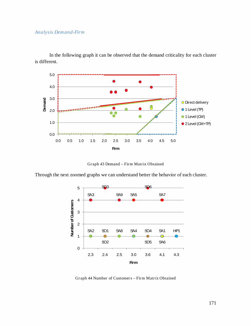
171
Analysis Demand-Firm
In the following graph it can be observed that the demand criticality for each cluster
is different.
Graph 43 Demand – Firm Matrix Obtained
Through the next zoomed graphs we can understand better the behavior of each cluster.
Graph 44 Number of Customers – Firm Matrix Obtained
0.0
1.0
2.0
3.0
4.0
5.0
0.0 0.5 1.0 1.5 2.0 2.5 3.0 3.5 4.0 4.5 5.0
De
man
d
Firm
Direct delivery
1 Level (TP)
1 Level (CW)
2 Level (CW+TP)
HP1SA1SA2
SA3
SA4
SA5
SA6
SA7
SA8
SA9
SO1
SO2
SO3
SO4
SO5
SO6
0
1
2
3
4
5
2.3 2.4 2.5 3.0 3.6 4.1 4.3
Nu
mb
er
of
Cu
sto
me
rs
Firm

172
Graph 45 Dimension of the Order – Firm Matrix Obtained
• The 2 level networks are characterized by high demand criticality, for example they have high number of customers (graph 44) and small order dimension (graph 45). Remembering that small order dimension means high driver criticality.
• The 1 level networks are characterized by small demand criticality, because they have smaller number of customers and higher order dimension than the previous group. The 2 exceptions as explained before are SO2 and SO5.
• The direct delivery network has demand criticality of 2.2 while the 1 level networks with transit points has demand criticality of 1.65.
Analysis Service-Firm
From the next graph it can be observed the clusters according to the service criticality.
HP1
SA1
SA2
SA3
SA4
SA5
SA6
SA7
SA8
SA9
SO1
SO2
SO3
SO4
SO5
SO6
1
2
3
4
5
2.3 2.4 2.5 3.0 3.6 4.1 4.3
Dim
en
sio
n o
f th
e o
rde
r
Firm

173
Graph 46 Service – Firm Matrix Obtained
• The 2 level networks are characterized by low service criticality, for example they
have higher cycle time (graph 47). Remembering that high cycle time means lower
driver criticality. This is theoretically true because by having 1 level of TP adds one
or two days more.
• The 1 level networks are characterized by high service criticality, because they have
shorter cycle time. The 2 exceptions in this case are SO3 and SO6 which are
distribution problems with the shortest cycle time because they use DHL express,
but as they use the DHL transit points they are considered in the red cluster instead
of the green cluster.
• The direct delivery network has service criticality of 1.8 while the 1 level networks
with transit points has service criticality of 1.
Graph 47 Cycle Time – Firm Matrix Obtained
SO3 SO6
0.0
1.0
2.0
3.0
4.0
5.0
0.0 0.5 1.0 1.5 2.0 2.5 3.0 3.5 4.0 4.5 5.0
serv
ice
Firm
1 Level (TP)
1 Level (TP)
1 Level (CW)
2 Level (CW+TP)
HP1
SA1
SA2
SA3
SA4
SA5
SA6
SA7
SA8
SA9
SO1
SO2
SO3
SO4
SO5
SO6
1
2
3
4
5
2.3 2.4 2.5 3.0 3.6 4.1 4.3
Cyc
le t
ime
Firm

174
8.3 Analysis of the other strategic decisions
The other strategic decisions considered for this model cannot be analyzed since the
data gathered only contains few solutions. However it can be concluded for this type of
industry, as shown in the graph 48, the following:
• When having one level network of CW the number and location should be 1 CW for
national territory
• When having two level network with CW and TP the number and location of the
CW should be 1 for national territory and the number of transit points should be at
least one for each main region.
• When having one level network of TP the number and location should be from the
information obtained 2 for European territory, but it cannot be considered as a
precise rule.
Graph 48 Number and location of Warehouses and Transit Points
1 1 1 1 1 1 1 1 1 1 1 1 1 1
20 20 20
13 13 13 13
2
0
3
6
9
12
15
18
21
24
HP1 SA2 SA4 SA6 SA8 SO1 SO4 SA3 SA5 SA7 SA9 SO2 SO3 SO5 SO6 SA1
1 echelon 2 echelon direct delivery
Number and location of WH and TP
Number of National CW
Number of Regional TP
Number of European TP

175
Chapter 10. Normative model
In this section it is described in detail the methodology to apply for designing the
distribution network, which was previously developed by Archini and Bannò, (2003), but
re-arranged in this Thesis project in order to meet requirements for the consumer
electronics industry.
The procedure is simple and the necessary data is easy to be found. In particular it has 5
steps:
6. Company analysis and collection of data
7. Identification of the distribution problems and allocation of data for each
distribution problem
8. Driver criticality analysis of the distribution problem
9. Individualization of the adequate network typology
10. Characterization of the network
The first 3 steps analyze the company reality, identifying the most important
distribution problems and giving a synthetic representation in order to express the principal
characteristics of each distribution problem.
The step 4 has the objective of determining the network typology, meaning the
number and types of levels that minimize the relevant logistics costs, defined in paragraph
2.5, and respecting the service level defined by the company. The solution could be:
- Direct delivery
- 1 level network with transit point
- 1 level network with central warehouse
- 2 level network with central warehouse and transit points
10.1 Description of the steps
Company analysis and data collection
The first step has the objective of obtain a complete and detailed vision of the
logistic requirements and processes of each company. The tool used for this is the
questionnaire (Appendix 1), specifically until the section 3.1 for the case of designing a

176
new distribution network, and the complete set of questions for the re-design of an existing
one, in order to compare the actual with the proposed by the model.
Identification of the distribution problems and allocation of data for each
distribution problem
This step is very important because it is where the different distribution problems of
each company are identified. By distribution problem is meant, a group of products and
clients characterized by similar driver values that justify a specific flow management. It is
very important to single out and describe these distribution problems in order to understand
the factors that mostly affect the strategic decisions and the network planning.
From the detailed analysis of the drivers and macrodrivers (product, supply, service
and demand), it is possible to construct the distribution problems, while in the case of
redesign, the analysis of the flow diagrams permits to see the distribution problems already
existent and then validate or modify them. The values collected in the previous phases have
to be grouped according to the identified distribution problems (DP1, DP2,…, DPN)
Macrodriver Driver Value
DP1 DP2 DP3
Product
Variety (SKUs)
Value (euro/kg)
Density (kg/m3)
Risk of obsolescence (days)
Contribution Margin (%)
Service Cycle Time (days)
Completeness (%)
Demand
Dimension of the order (%FTL)
Number of customers
Frequency of delivery (deliveries per week)
Seasonality (L - LM - M - MH - H)
Supply
Distance from plant to client (km)
Number of plants
Level of Specialization (Low, Medium or High)
Table 19 Drivers table: Punctual values

177
Driver criticality analysis of the distribution problem
In order to detect immediately the relevance of each driver, once known the
punctual values, it is proposed a scale of projection composed of 5 reference intervals that
identify the criticality of each driver. The objective of the scale is to obtain an absolute
reference system that allows the comparison of drivers with different unit of measurement
and to make visible the impact that different drivers’ values have over the costs.
The five intervals are:
1: low criticality
2: medium low criticality
3: medium criticality
4: medium high criticality
5: high criticality
The identification of these criticalities is through the use of axes divided into
discrete intervals as was mentioned before. On the axes are placed the exact values
identified in the previous step (step 2) and according to the interval where the value is
placed, a critical evaluation between 1 to 5 is given to each driver.
Here is an explanation of the axes to identify the critical value of each driver.
Now, each driver with its axes of criticality:
PUNCTUAL VALUE
CRITICALITY OF REFERENCE
FOR THE PROJECTION

178
PRODUCT:
Variety (number of products):
Value (Euro/Kg):
Density (Kg/m3):

179
Risk of obsolescence(days):
Contribution Margin:
SERVICE:
Cycle time (days):
Completeness (item fill rate):

180
DEMAND:
Dimension of the order:
Number of customers:
Frequency of delivery (deliveries/week client):
Seasonality (qualitativo):

181
SUPPLY:
Distance from plant to client (Km):
Number of plants:
Level of Specialization:

182
The values, between 1 and 5, indicating the criticality of the specific drivers for
each distribution problem, should be reported in the next table.
Macrodriver Driver Criticality
DP1 DP2 DP3
Product
Variety
Value
Density
Risk of obsolescence
Contribution Margin
Service Cycle Time
Completeness
Demand
Dimension of the order
Number of customers
Frequency of delivery
Seasonality
Supply
Distance from plant to client
Number of plants
Level of Specialization
Table 20 Drivers table: Criticalities
At this point, for each distribution problem it is necessary to express synthetically
the criticalities of each macrodriver. This can be done by calculating the weighted average
of the drivers that compose each macrodriver by utilizing the following weights in the next
formulas.

183
Table 21 Weights proposed for the drivers
max
max
*
j
cWj
C
j
jj
i
∑=
with: =iC Macrodriver criticality i;
=jc driver criticality j, with j = [1, …, jmax];
Wj = Weight of each driver
i = {product, service, demand, supply}
j = {variety, value, density, …., many products sources} = {all the drivers}
Table 22 Weights proposed for the Macrodrivers
2
** ClWlCpWpCF
+=
2
** CdWdCsWsCM
+=
CF = firm criticality =CM market criticality
Product
Variety 0.15
Value 0.45
Density 0.1
Risk of obsolescence 0.25
Contribution Margin 0.05
Service Cycle Time 0.8
Completeness 0.2
Demand
Dimensions of the order 0.4
Number of customers 0.4
Frequency of delivery 0.15
Seasonality 0.05
Supply
Distance from plant to client 0.5
Number of plants 0.25
Level of specialization 0.25

184
=Cp product criticality =Cs service criticality
=Cl supply criticality =Cd demand criticality
W(p, l, s, d) = Weights (product, supply, service, demand)
In order understand better the previous results; a synthetic graph can be represented
for each distribution problem. For example in the next figure, aggregation was carried out
using two broken lines to connect the values of product and supply and service and
demand.
The two areas generated, colored different, provide immediately the idea of which
ones are the more critical drivers for each distribution problem considered.
The bigger the colored area is, the higher the criticality of the macrodriver for that
distribution problem: green area indicates market and yellow area indicates firm.
Supply
Service
Product
Demand
Firm criticality
Market criticality
Figure 25 Graphical representation of the distribution problem

185
Individualization of the adequate network typology
This step consists in position the distribution problem, synthesized as in step 3, in
the aggregated matrix market-firm of Figure 26. According to the area to which the
distribution problem belongs it is possible to obtain information about the most appropriate
level of centralization/decentralization of the distribution network. Different zones are
identified:
§ Yellow zone: direct delivery;
§ Green zone: 1 level network of central warehouse
§ Blue zone: 1 level network of transit points
§ Red zone: 2 level network with central warehouse at first level and transit points at
second level
Figure 26 Proposed aggregated matrix Market-Firm and network levels.
0.0
0.5
1.0
1.5
2.0
2.5
3.0
3.5
4.0
4.5
5.0
0.0 0.5 1.0 1.5 2.0 2.5 3.0 3.5 4.0 4.5 5.0
Mar
ket
Firm
2 levels network with CW and TP
1 level network with CW
1 level network with TP
DirectDelivery

186
Characterization of the network
• Networks with 1 level of CW should have one CW at National level.
• Networks with 1 level of TP should have at least 2 TP at European level.
• Networks with 2 levels should have one CW at National level and at least 1TP
every 1.5 Italian region.

187
Conclusions
• From the literature analysis and the interviews realized, it can be said that nowadays
firms are paying more attention to the design of their Distribution Networks as it has
been proved its important impact over the financial performance.
• Not all the drivers mentioned on the papers analyzed resulted to be useful for the design
of distribution networks in the consumer electronics industry.
• The list of drivers that were considered as important for the distribution network design
were:
o Product Macrodriver: Variety, Value, Density, Risk of Obsolescence and
Contribution Margin.
o Service Macrodriver: Cycle Time and Completeness
o Demand Macrodriver: Dimension of the order, Number of customers,
Frequency of delivery and Seasonality.
o Supply Macrodriver: Distance from plant to client, Number of plants and Level
of specialization.
• The allocation of specific weights for each driver applied on the model proposed by this
work, correspond to an improvement on the procedure with respect to the base model
used.
• The Distribution Network Design model presented as the result of this thesis is
applicable to the consumer electronics industry in Italy, easy to follow by distribution
network designers, understandable to decision makers, and easy to adapt to changing
requirements.
• The proposed aggregated matrix Market – Firm presents well defined areas for
networks with 1 level of CW (green) and 2 levels of CW and TPs (red), while for the
network with 1 level of TPs (Blue) and the Direct Delivery decision (yellow), the
information obtained was not enough to present this cases as a rule.

188
Bibliography
Ambrosino, D., & Scutell, M. (2005). Distribution Network Design: Modelling and Info
considerations. European Journal of Operational Research .
Archini, G., & Bannó, M. (2003). Modelli di evoluzione dell'assetto dei sistemi logistico
produttivi di aziende multinazionali operanti du base europea.
Ashayeri, J., & Rongen, J. (1997). Central Distribution in Europe. International Journal of
Logistics Management .
Ballou, R. (2004). Business Logistics/ Supply Chain Management.
Ballou, R. (1995). Logistics Network Design: Modeling and Info considerations.
International Journal of Logistics Management .
Ballou, R. (1993). Reformulating a Logistics Strategy: A concern for the Past, Present and
Future. International Journal of Physical Distribution .
Borchert, E. (2008). Consumer Electronics and Household appliances- comparative price
levels in 37 European countries for 2997.
Business Glossary. (2010). Obtenido de http://www.allbusiness.com/glossaries/correlation-
analysis/4964988-1.html.
Chopra, S. (2003). Designing a Distribution Network in a Supply Chain. Transportation
Research Part E .
Christopher, M. (2006). A taxonomy for selecting global supply chain strategies.
International Journal of Logistics Management .
Chung-Plaw, T. (2002). Column generation: Application in distribution network design.
Creazza, A., Dallari, F., & Melacini, M. (2007). Evaluating logistics network
configurations for a global supply chain. Supply Chain Management: an International
Journal .
den Ven, V., & Ribbers. (1993). International Logistics: A diagnostic method for the
allocation of production and distribution facilities. International Journal of Logistics
Management .
Dornier, Fender, & Kouvelis. (s.f.). Global operations and logistics text and cases.

189
Eero, E., & Holmström, J. (2009). How to design the right supply chain for your customers.
Supply Chain Management: an international journal .
Eleonatra, E., & Holmström, J. (2009). How to design the right supply chain for your
customers. Supply chain Management an International Journal .
Ferretti, I., Zanoni, S., & Zavanella, L. (2009). Distribution network design under uncertain
demand. Universitá degli studi di Brescia .
Fisher, M. (1997). What is the right supply chain for your products? Harvard Business
Review .
Hammel, T., Keuttner, D., & Phelps, T. (2002). The re-engineering of Hewlett Packard's
CD-RW supply chain . Supply Chain Management: An International Journal .
Jay, J.-K., Ozment, J., & Sink, H. (2007). Logistics capability, logistics outsourcing and
firm performance in an e-commerce market. International Journal of Physical Distribution
and Logistics Management .
Jayaraman, V. (1998). Transportation, facility location and inventory issues in distribution
network design. International journal of operations & production management .
Lalwani, C., & Naim, M. (2006). On assessing the sensitivity to uncertainty in distribution
network design. International Journal of Physical Distribution and Logistics .
Lashine, S., Fattouh, M., & Issa, A. (2008). Location/allocation and routing decisions in in
supply chain network design. Journal of Modelling in Management .
Lin, J.-R., & Lei, H.-C. (2009). Distribution system Design with two level routing
considerations. Department of Transportation and Navigation Science, National Taiwan
Ocean University.
Lovell, A., Saw, R., & Stimson, J. (2005). Product value-density: managing diversity
through supply chain segmentation. The Internationl Journal of Logistics Management .
Manzani, R., & Gebennini, E. (2006). Optimization models for the dynamic facility
location and allocation problem. International journal of production research .
Manzini, R., & Bindi, F. (2008). Strategic design and operational management optimization
of a multistage physical distribution system. Transportation Research part E .
McQuitty, S., & Peterson, R. T. (2000). Selling home entertainment on the Internet: an
overview of a dynamic marketplace.

190
Mourtis, & Evers. (1995). Distribution Network Design an Integrated Planning Support
Framework. International Journal of Physical Distribution & Logistics .
Nansi, P. (s.f.). What is logistics? What does it mean to projects? Project Monitor .
Nozick, L., & Turnquist, M. (2000). Inventory, transportation, service quality and location
of distribution centers. European Jorunal of Operations research .
Pasin, F., & Cordeau, J.-F. (2006). An integrated model for logistics network design. HEC
Montreal.
Payne, T., & J. Peters, M. (2004). What is the right supply chain for your products? .
Journal of Logistics Management .
Ratliff, D. (1993). Distribution/Logistics Network Planning. Georgia Tech .
Rogers, D. S., & Tibben-Lembke, R. S. (1998). Going Backwards: Reverse logistics trends
and practices. Univeristy of Nevada .
Rushton, A., Croucher, P., & Baker, P. (2006). The Handbook of Logistics and Distribution
Mangement. Kogan Page.
Selldin, E., & Olhager, J. (2007). Linking products with supply chains: testing fisher's
model. Supply Chain Management: an international journal .
Sharifi, H., Ismail, H., & Reld, I. (2006). Achieving agility in Supply chains through
simultaneous design of and design for supply chains. Journal of Manufacturing Technology
Management .
Sharma, M., Moon, I., & Bae, H. (2008). Analytic hierarchy process to assess and optimiza
distribution netowrk. Applied mathematics and computation .
Thomas, R. (2002). De Novo Programming Model for optimal DND. A Proposal for the
Faculty of research Grant .
van den Berg, E., & Vos, B. (1996). Assessing International Allocation Strategies.
International Journal of Logistics Management .
van der Vorst, J., van Dijk, S., & Beulens, A. (2001). Supply chain design in the food
industry. International journal of Logistics Management .
W.L, N., & Neuman, W. (1997). Social Research Methods: Qualitative and Quantitative
Approaches. Allyn and Bacon .

191
Appendix 1: Questionnaire
Research of Distribution Network of the Consumer Electronic Industry in Italy
1. Data Context
1.1 General data of the interview
Date:____________________________________________________________________
Name of the company:_____________________________________________________
Address:________________________________________________________________
Web Site :________________________________________________________________
Interviewee:
I. Name:____________________________________________________________
Function: ___________________________________________________________
II. Name:____________________________________________________________
Function:____________________________________________________________
1.2 Company general data
Member of a Group:_________________________________________________________
Sector:___________________________________________________________________
Multinational: (Yes/No) Type:_________________________________________________
Dimensions: Total Sales: ____________Market Share: _________N° Employees:_______
Business Unit to consider: ____________________________________________________
2. Commercial Organization
2.1 Organization of the commercial function
_________________________________________________________________________
_________________________________________________________________________
_________________________________________________________________________
_________________________________________________________________________

192
2.2 Types of clients:
2.2.1 Distributors:___________________________________________________
2.2.2. Retailers:_____________________________________________________
2.2.3 Final consumer:________________________________________________
2.2.4 Wholesalers:___________________________________________________
Direct clients: (Clients with direct shipment)
_________________________________________________________________________
3. Characterization of the actual Distribution Network
3.1 Drivers for the design of the Distribution Network
Product Drivers:
Variety (SKUs):_____________________________________________________
Value (€/Kg): _______________________________________________________
Density (Kg/m3): ____________________________________________________
Risk of obsolescence (Days):___________________________________________
Contribution Margin (%):______________________________________________
Service Drivers:
Cycle Time (days order-delivery):________________________________________
Completeness (item fill rate):___________________________________________
Returnability:________________________________________________________
Demand Drivers:
Dimension of the order (%FTL): ________________________________________
Number of customers: _________________________________________________
Frequency of delivery (per week):________________________________________
Seasonality :_________________________________________________________
Predictability of demand:_______________________________________________

193
Supply drivers
Distance from plant to client (Km):_______________________________________
Number of plants: ____________________________________________________
Level of Specialization:________________________________________________
Other Drivers: _______________________________________________________
3.2 Characterization of the Supply Chain
Number, Localization and characteristics of each node.
Own Establishments
_________________________________________________________________________
_________________________________________________________________________
Supplier Establishments
_________________________________________________________________________
_________________________________________________________________________
# Plants Location Own establishment? Products Exclusivity of
products
Average
distance from
plant to client
1
2
3
4
…..

194
3.3 Actual Distribution Network
According to the model above, please specify how is the actual distribution network of
the firm, clarifying the number of echelons, plants, warehouses, transit points and the
flows. Also specify what is outsourced.

195
Network classification
Direct delivery:________________________________________________________
1- Echelon: __________________________________________________________
2- Echelon: __________________________________________________________
3- Echelon: __________________________________________________________
4- mixed network : ____________________________________________________
Node characterization: (location and allocation)
• Types of nodes
Central WH: ______________________________________________________________
Regional WH: _____________________________________________________________
Transit Point:______________________________________________________________

196
• Activities, resources and capacity of each typology
Central WH
_________________________________________________________________________
_________________________________________________________________________
Regional WH
_________________________________________________________________________
_________________________________________________________________________
Transit Point
_________________________________________________________________________
_________________________________________________________________________
4. Flows Characterization
From the scheme above, identify the type/s of flow/s used, the percentage and type
of products that follows that route, the location of the points of origin and destination and
the typical quantity per delivery for each type of flow used (FTL, LFTL, Pallets, etc)
(Primary or Secondary Transportation). Indicate the nodes and/or arcs that are outsourced.

197
_________________________________________________________________________
_________________________________________________________________________
_________________________________________________________________________
_________________________________________________________________________
5. Managerial logic
5.1 Stocks
Safety Stocks
Service Level: (K utilized) and decisions about centralization/decentralization
_________________________________________________________________________
_________________________________________________________________________
_________________________________________________________________________
Logic of the material flow planning: Indicate the anticipation period used to forecast the
demand and how the safety stocks are estimated.
_________________________________________________________________________
_________________________________________________________________________
_________________________________________________________________________
5.2 Transport
Organization of primary transport
_________________________________________________________________________
_________________________________________________________________________
_________________________________________________________________________
Organization of secondary transport
_________________________________________________________________________
_________________________________________________________________________
_________________________________________________________________________

198
5.3 Outsourcing
Activities in outsourcing
_________________________________________________________________________
_________________________________________________________________________
_________________________________________________________________________
Companies that handle the outsourced activities (with which terms and conditions)
_________________________________________________________________________
_________________________________________________________________________
_________________________________________________________________________
Why to outsource? Which drivers to consider?
_________________________________________________________________________
_________________________________________________________________________
_________________________________________________________________________
5.4 Reverse Logistics
5.4.1 Indicate if Reverse Logistics is used. Amount of returned products as a percentage
of products sold. Which distribution network is used.
_________________________________________________________________________
_________________________________________________________________________
_________________________________________________________________________