Strategic Investment in Renewable Energy Sourcesflora.insead.edu/fichiersti_wp/inseadwp2012/2012-59.pdf · Renewable (or \green") sources of energy, such as wind and solar power,

$Page 1: Strategic Investment in Renewable Energy Sourcesflora.insead.edu/fichiersti_wp/inseadwp2012/2012-59.pdf · Renewable (or \green") sources of energy, such as wind and solar power,$
Strategic Investment in Renewable

Energy Sources

_______________

Sam AFLAKI

Serguei NETESSINE

2012/59/TOM

(Revised version of 2011/05/DS/TOM)

Strategic Investment in Renewable Energy Sources

Sam Aflaki*

Serguei Netessine**

Revised version of 2011/05/DS/TOM

June 1, 2012

* Assistant Professor Operations Management & Information Technology at HEC Paris, 1, rue

de la Libération 78351 Jouy en Josas cedex. Email : [email protected]

** The Timken Chaired Professor of Global Technology and Innovation, Professor of

Technology and Operations Management, Research Director of the INSEAD-Wharton

Alliance at INSEAD Boulevard de Constance 77305 Fontainebleau, France.

E-mail: [email protected]

A Working Paper is the author’s intellectual property. It is intended as a means to promote research to

interested readers. Its content should not be copied or hosted on any server without written permission

from [email protected]

Find more INSEAD papers at http://www.insead.edu/facultyresearch/research/search_papers.cfm

Strategic Investment in Renewable Energy Sources

Sam AflakiHEC Paris, Operations Management and Information Technology Area. [email protected]

Serguei NetessineINSEAD, Technology and Operations Management Area. [email protected]

June 1, 2012

We analyze incentives for investing in renewable electricity generating capacity by modeling the trade-off

between renewable (e.g. wind) and nonrenewable (e.g. natural gas) technology. Renewable technology has

higher investment cost and yields only an intermittent supply of electricity; nonrenewable technology is

reliable and has lower investment cost but entails both fuel expenditures and carbon emission costs. With

reference to existing electricity markets, we model several interrelated contexts—the vertically integrated

electricity supplier, market competition, and partial market competition with long-term fixed-price contracts

for renewable electricity—and examine the effect of carbon taxes on the cost and share of wind capacity

in an energy portfolio. We find that the intermittency of renewable technologies drives the effectiveness of

carbon pricing mechanisms, which suggests that increasing emissions prices could unexpectedly discourage

investment in renewables. We also show that market liberalization may have a negative effect on investment

in renewable capacity while increasing the overall system’s cost and emissions. Fixed-price contracts with

renewable generators can mitigate these detrimental effects, but not without possibly creating other prob-

lems. Actions to reduce the intermittency of renewable sources may be more effective than carbon taxes

alone at promoting investment in renewable generation capacity.

Key words : Electricity Generation, Renewables, Intermittency, Capacity Planning and Investment,

Incentives and Contracting

1. Introduction

Renewable (or “green”) sources of energy, such as wind and solar power, will play a key role in

the future energy landscape. By providing emission-free and sustainable energy, these sources are

important alternatives to fossil fuels. The worldwide increase in capacity installations for renew-

ables has been accelerating; in the last decade, wind capacity installations have increased tenfold.

The United States has the highest level of installations with 25 gigawatts (GW), followed by Ger-

many (24 GW), Spain (17 GW), China (12 GW), and India (9 GW). A critical aspect of renewable

technologies is their intermittency–that is, the supply of electricity from these sources is uncertain.

For instance, wind blows neither continuously nor in concert with demand, and electricity gener-

ation from solar panels is volatile because of their sensitivity to weather conditions, air pollution,

1

Aflaki & Netessine: Investment in Renewables2

and other determinants of solar radiation intensity. Although some of this variability in supply is

natural and can be planned for (e.g., the lack of generation from solar panels at night), there is still

significant uncertainty associated with the outputs of renewable technologies. A main goal of this

paper is to investigate the effect of generation intermittency on investment in renewable capacity.

Investment in renewable energy capacity is hampered not only by intermittency but also by the

high costs involved. A variety of strategies have been adopted to incentivize investment in renew-

ables. These include renewable portfolio standards, minimum prices for energy from renewable

energy injected into the grid (a.k.a. renewable feed-in tariffs), and multiyear subsidies and invest-

ment credits in some jurisdictions as direct incentives for new renewable capacity.1 In addition to

these direct incentives for renewable investment are indirect incentives based on increasing the price

of fossil-fuel electricity generation (gas-fired, coal, etc.) by penalizing firms for the environmental

damage these technologies cause. The most significant of these penalties is referred to generically

as carbon pricing.2 This paper aims to understand the relationship between supply intermittency

and the effectiveness of carbon pricing strategies.

Besides the introduction of renewables, electricity markets have undergone another important

change in the last two decades: market liberalization. In the past, electric utilities were vertically

integrated; this means that the functions of generating, transmitting, retailing, and distributing

electricity were all performed by a single utility company. The logic of this approach was based on

operational constraints associated with balancing the generation, transmission, and distribution

of electricity. That balancing also contributed to the economics of electricity generation because

it reduced retailing costs (Michaels 2007). The first step toward the liberalization of electricity

markets was “vertical unbundling” of the industry’s generators and retailers. Such restructuring

was motivated by the desire to create competition among generators, thereby reducing retail prices,

and to prevent incumbent utilities from exercising the market power deriving from their historically

dominant position. Market liberalization has rendered electricity a commodity that can be traded in

wholesale electricity markets. These markets are typically organized through a national or regional

pool, with an independent system operator (ISO) responsible for assuring stability and control of

the interconnecting transmission network. The pool (or spot) prices in these markets are determined

by a complex set of bidding and dispatching rules that vary widely across countries and regions.

Yet all these markets share a common characteristic: significant volatility of spot prices. The reason

is that, with some minor exceptions, electricity cannot be economically stored and so supply and

1 See Bushnell (2010) for a critical review of various incentives for renewable energy investments.

2 Proposals for pricing the carbon emissions from fossil-fuel electricity plants include a carbon tax or a “cap andtrade” system of credits. For a discussion of various forms of carbon pricing in the context of technology planning,see Drake et al. (2010).


demand must be continually balanced. The need to achieve this balance in a decentralized fashion

through competitive electrical power markets implies that a pool price reflecting the marginal

cost of the last unit dispatched will vary considerably over time, driven as it is by economic and

technical uncertainties in supply and demand as well as by uncertain exogenous variables such as

weather conditions.

Motivated by the two developments just described, in this paper we study the effect of market

liberalization on investment in renewable electricity generation capacity. In particular, we highlight

the role that supply intermittency plays in determining the competitiveness of renewables in a

liberalized market. We propose a stylized economic model based on the key features of electricity

markets. This model features two electricity generators (e.g., wind and gas) that make capacity

investment decisions given the pricing mechanism established by the electricity retailer. Shortfalls

in supply are procured from backup generators. The model captures uncertainty in both the supply

of and the demand for electricity, and we use it to answer several broad questions. How does

intermittency affect capacity investment in renewables? Is the intermittency-driven comparative

disadvantage of renewables simply a cost issue? How will taxing emissions from fossil-fuel generation

change the share of green technologies in energy portfolios and in total emissions?

Within this framework, we study how carbon taxing would affect investment in renewable and

nonrenewable electricity generation capacities. We find that increasing the carbon price has two

counteracting effects on investments in renewables. On the one hand, it improves the cost com-

petitiveness of renewables relative to non-renewable technologies—a result of the former’s lower

greenhouse gas (GHG) emissions. On the other hand, renewables require backup generation, which

typically comes from generators using fossil fuels; thus an increase in the carbon price leads to an

increase in the cost of reserves to cover intermittency. How these counterforces affect the technology

share of renewables in the overall generation portfolio depends on the carbon price and also on the

emission intensity of backup generation technologies. Often it is the older, more emission-intensive

technologies that are used as backup. So in stark contrast to intuition, increasing the carbon price

may actually reduce the overall proportion of renewable generation. This effect is present in the

vertically integrated setting and also in the liberalized setting. However, in the liberalized market

the negative effect of intermittency is amplified by the marginal cost pricing typical of such mar-

kets (i.e., the price of electricity is equal to the marginal cost of the unit last dispatched). This

finding offers additional and novel support for the hypothesis that market liberalization leads to

underinvestment in renewable electric generation capacity (Joskow 2006).

In order to counter these disincentives to invest in renewables in the liberalized market, public

policy experts suggest long-term fixed-price contracts with generators so that investment in new

generating capacity will be protected from the risk of volatile spot prices (Borenstein 2002). For


instance, long-term contracts involving wind developers, electricity suppliers, and large customers

are used in the United States and Europe to promote investment in renewable capacity. Such

fixed-price contracts with renewable generators are typically benchmarked on feed-in tariffs, often

with regulatory guarantees, that specify long-term prices based on generation costs rather than

spot prices. We therefore consider an extension of our basic model in which the price of nongreen

electricity is determined in the spot market but the retailer sets a fixed price for green electricity

ex ante. Using numerical experiments with real-world data, we find that fixed-price contracts are

effective at stimulating investment in renewables in a liberalized market. However, overreliance on

carbon-intensive backup generation may significantly lessen the environmental benefits of using

renewables relative to the vertically integrated case.

This paper makes three principal contributions. First, we study the effect of supply intermittency

of renewables on the capacity investment decision, proposing a way (other than average cost)

to capture this intermittency cost. Second, we demonstrate how incentives arising from vertical

unbundling of the electricity supply’s organizational structure affect capacity investments, total cost

and emissions, and the share of renewables in the energy capacity portfolio. Third, we obtain the

surprising result that increasing the price of carbon can adversely affect investments in renewables

owing to the interdependence of renewable and backup capacity, since the latter is almost always

a carbon-intensive form. Our analysis leads to new insights about the relative merits of different

structures for the electricity market and about the impact of carbon pricing on the promotion

of renewable energy sources. Throughout, we use numerical analysis based on real-world data to

support our analytical results.

The rest of the paper is structured as follows. In Section 2 we review the related literature

and position our paper. Section 3 lays out the foundations of our model. In Section 4 we study a

vertically integrated electricity supplier and examine the effect of intermittency on decisions about

capacity decisions. In Section 5 we analyze market competition, and Section 6 considers fixed-price

contracts for green electricity. Section 7 concludes.

2. Literature Review

Our paper belongs to the growing literature on sustainable operations (Kleindorfer et al. 2005), a

field of considerable interest to operations researchers who tackle the sustainability challenges that

various organizations face in their daily decisions. Given the ever-increasing relevance of sustain-

ability issues to businesses, this literature spans a wide variety of operational issues; these include

green process design (Sosa 2011), closed-loop supply chains (Savaskan et al. 2004), and optimal

incentive strategies for adoption of green products (Avci et al. 2012; Lobel and Perakis 2011). Our

paper considers another general operational problem—namely, adoption of green technology while


accommodating the new necessities induced by the “carbon economy”. Along these lines, Islegen

and Reichelstein (2011) characterize the break-even carbon emission price that induces adoption

of technology to capture and store carbon, an undertaking that is costly but does significantly

reduce the firm’s emission intensity. Closer to our model is Drake et al. (2010). Though in a context

other than electricity generation, their decision maker also faces a trade-off between investing in a

“clean” versus a “dirty” technology when emission costs are a possibility. These authors suggest,

as we do, that increasing carbon prices might have an adverse effect on investment in the clean

technology. Yet unlike our model, theirs does not consider supply intermittency; also, the adverse

effect they identify is “carbon leakage” (i.e., increasing dirty production in unregulated regions).

Within the sustainable operations literature, most of the papers that consider the intermittency

of renewable energy sources do so from the standpoint of short-term decisions made after the renew-

able capacity is already in place (see e.g. Zhou et al. 2011). Kim and Powell (2011) characterize the

economic value of storage when the renewable owner commits output capacity in the advance elec-

tricity market. Wu and Kapuscinski (2012) suggest curtailing the intermittent generation—that is,

reducing renewables output through technical methods—in order to balance the system. The effect

of intermittency on long-term capacity decisions has been explored in various different contexts.

For example, Tomlin and Wang (2005) consider a dual-sourcing problem in which the retailer can

meet demand by ordering either from a cheap but unreliable supplier or from a more expensive

but reliable supplier. At least two important features distinguish our paper from these. First, only

we consider incentive issues arising from emission regulation. Second, although these papers focus

(as we do) on unreliability and capacity investment, they typically consider only the vertically

integrated (monopolistic) setting. Conversely, several other papers study incentives for capacity

investment in a vertically unbundled setting but do not consider supply intermittency.3 Similarly

to these papers (e.g., Taylor and Plambeck 2007), this paper considers fixed-price contracts under

which a retailer4 announces a fixed price for (renewable) electricity and the generator/supplier

chooses capacity based on the announced price. Our paper emerges from the interfaces of the afore-

mentioned literatures by addressing both supply intermittency and the incentive issues associated

with vertical unbundling in the context of integrating renewable energy sources into electricity

markets.

Capacity choice and peak-load pricing in electricity markets received significant attention from

economists in 1970s and 1980s (for a review, see Crew et al. 1995). Given the characteristics of the

3 Perhaps an exception is Deo and Corbett (2009), who study yield uncertainty in the vaccine market.

4 We use the term “retailer” to denote the economic entity with the ultimate responsibility for interacting with theend buyer or customer in the electricity supply chain. Depending on the context, this retailer could be a “supplier”, anindependent broker or wholesale power intermediary, a distribution company, or (in the case of vertical integration)the division of an industrial company that is responsible for installing its own self-generation.


electricity markets at that time, these studies focused on monopolistic settings. For instance, Crew

and Kleindorfer (1976) model joint determination of capacity and prices when demand is uncertain

and there are several technologies (with different cost structures) available. Chao (1983) extends

this analysis by considering uncertain supply in a monopolistic setting. Vertical unbundling of

the electricity supply chain and introducing competition to the market for generation have drawn

fresh attention to this field. Liberalized electricity markets have been the subject of a fast-growing

stream of research (for a detailed review, see Ventosa et al. 2005). Models of liberalized markets

can be separated into short-term pricing/dispatching models and longer-term investment models.

Elmaghraby (1997) studies optimal auction mechanisms for achieving efficiency in electricity mar-

kets when firms have already made their investment decisions (other examples include Borenstein

et al. 2000; Green and Newbery 1992). Longer-term investment incentives are examined in papers,

such as Von der Fehr and Harbord (1997) and Castro-Rodriguez et al. (2009), that consider capac-

ity investment decisions—often in the context of Cournot competition. The main finding reported

by these papers is that, consistently with the broader Cournot literature, decentralization (vertical

unbundling) leads to underinvestment in capacity, which in turn leads to higher electricity prices.

Economic research on renewable energy sources has examined the theory of efficient integration

of renewables into grid operations as well as the empirical evidence regarding cost competitiveness.

A key finding of this literature (e.g., Owen 2004) is that renewables are competitive and efficient

when the pricing of traditional sources of energy, such as fossil fuels, accurately reflects environ-

mental externalities. The issue of intermittency—along with its cost and reliability implications for

electricity generation—has been addressed primarily in empirical studies that are region specific

(e.g., Butler and Neuhoff 2008; Kennedy 2005; Neuhoff et al. 2007). A few of the papers in this field

(e.g., Ambec and Crampes 2010; Garcia and Alzate 2010) address the issue of intermittency. Much

as in our model, both of these papers consider the optimal investment in two types of technolo-

gies with different cost structures: an intermittent renewable technology and a reliable fossil-fuel

technology. They, too, characterize and compare the optimal capacity investments under vertical

integration and competition. Unlike our paper, however, these two consider neither demand uncer-

tainty nor the incentive issues that arise from fixed-price contracting between the generator and

retailer of electricity.

3. Model Setup

This section introduces our basic model and assumptions. We consider an electricity retailer,

indexed by R, that is responsible for meeting the random market demand. Demand is represented

by a random variable D with positive support, distribution function F (·), and density f(·). Two

types of electricity generation technologies are available. For expositional purposes we refer to these


technology types as wind (W ) and gas (G), although these should be viewed as also representing

other technology types—for example, photovoltaic and coal—that are, respectively, of renewable

(green) and nonrenewable type.

Decision and Generation Parameters. The firm must decide, for each technology, how much

to invest in the development of energy capacity. This decision determines not only the long-term

limits on electricity production but also the carbon intensity of that production from the resulting

electricity generation portfolio. We denote by ki the decision with respect to capacity investment for

each technology type i∈ {W,G}. We denote by αi > 0 the fixed investment and maintenance costs

of each unit of capacity, and we represent the unit variable cost (including fuel cost but excluding

emission cost) by ui. We assume that each unit of electricity generation that uses gas capacity

results in one unit of GHG emissions, and a will denote the associated “unit emission allowance

price”. Hence, the total unit variable cost for gas technology is UG = uG + a. We assume that

uW = 0; that is, the fuel and operational costs of the wind generator are negligible. We also assume

that wind technology is emission free, so that its total unit cost is UW = uW = 0. This cost structure

is consistent with existing technologies: investment costs for green technologies are significantly

higher than for efficient fossil-fuel technologies (e.g., combined heat and power gas turbines), and

the latter’s variable generation costs—especially when emission costs are included—are significantly

higher (Tarjanne and Kivisto 2008). The data that we use for numerical experiments confirms this

relationship.

We further assume that the wind technology is intermittent. That is, the production from the

available capacity is uncertain and so, from capacity kW , an actual production amount of only

vWkW < kW is obtainable. The random variable vW ∈ [0,1] represents the uncertainty factor in

the availability of wind capacity, which we assume (for tractability reasons) to have a two-point

distribution: v = [1, q; 0,1− q]. In other words, the capacity is available with probability q and is

unavailable with probability 1− q. This assumption captures the presence/absence of wind (for

wind capacity) or sun (for solar panels) but is only a rough approximation of reality in that

both wind and sun have continuously varying strengths. Nonetheless, this assumption serves the

purposes of capturing intermittency (in its simplest form) while allowing for tractable solutions. We

remark that a similar assumption is made by Tomlin and Wang (2005) and Ambec and Crampes

(2010) and that our conclusions are not altered if instead we assume a continuous distribution for

supply. To unify presentation of the problem, we abuse notation slightly and set vG = 1 as the gas

capacity’s availability factor.


Model Factor Onshore Wind CCGTAvailability factor E{vi} 0.25–0.4 0.87–0.97Capital and fixed O&M costa αi 28–40 14–28Variable cost ui 0 40–50Direct unit emission costb a 0 10Total cost αi/E{vi}+ui + a 80–114 70–84a Per installed unit. b Assuming an average carbon price of $20/tonne.

Table 1 Real data for electricity generating costs ($/MWh) for wind versus conventional combined cycle gas

turbine (CCGT) generation. Source: US Department of Energy (EIA 2010).

Data. Table 1 presents the US Department of Energy’s 2011 estimates of unit costs for new

generation capacity using onshore wind and “combined cycle” gas turbines. Note that these fixed

costs are adjusted to account for the availability factors. Each megawatt-hour (MWh) of electricity

generated by a combined cycle gas unit has a (CO2-equivalent) emission footprint of about 0.5

(metric) tonnes. Emission prices in the European spot market have historically been volatile, and

the current spot price is about $20. Within our model framework, then, a= 10.5 These data are

fully consistent with our assumptions about generation costs and availability factors of the two

technologies under consideration, and we shall use them in all of our numerical experiments.

Supply Function. Because the variable cost of wind is negligible (zero, in our model), it is

always dispatched to the grid first. When the total demand exceeds the amount of production

by wind technology (D > vKW ), the firm uses gas capacity to generate the additional amount

required—up to the available capacity. But when demand exceeds the production capacity of both

technologies combined (D > vWkW +kG), the firm must accommodate the extra demand by drawing

on an external backup source; this source has infinite capacity, but using it entails a per-unit fuel

and operational cost of c. We assume that this backup technology also entails GHG emissions with

per-unit intensity e, so the total unit generation cost from the backup technology is C = c+ae. We

also assume that backup generation is at the upper end of the dispatch merit order in operating

cost; that is, C >max{UG+αG, αW/q}.6 Backup capacity should be a fast-reacting generation unit.

Typically the less efficient but more flexible technologies (e.g., open-cycle gas turbine) are used for

backup generation. These units have higher operating cost and emission intensity, since efficiency

losses are incurred when using older generation units, as well as lower load factors resulting from

less-frequent usage (Kaffine et al. 2011).7 Inhaber (2011) provides a comprehensive overview of the

5 Throughout the paper, we will refer to a, the “emission cost per unit of electricity generation”, simply as the“emission price”; it is approximately equal to half the carbon spot price.

6 We assume that the price of backup generation is fixed. In reality, the amount of installed backup capacity (andhence backup prices) could well be variable in the long run. Although it would be interesting to consider such dynamicsin the problem, doing so is beyond the scope of this paper.

7 An exception is hydro power, which is both fast-reacting and emission free. However the supply of this energy sourceis limited in many countries.


!"#$%&'(()*%

+),-./"-".*%0,12#$%

3#4,5.1,#.%0,-"5"6#%

789%:,2/5%

;,#,/2<6#%=,/"6$%

>"1,%

?2@% ?A@%

Figure 1 (a) The supply function. (b) The decision timeline.

efficiency loss associated with wind intermittency in various countries; the results of that research

justify our assumption and, moreover, imply that e > 1.8 Although this inequality is not required

for our theoretical results, we will use it in our numerical experiments.

Figure 1(a) plots the short-run supply function for our model world with two technologies and

backup. This graph is the standard merit-order dispatch function, which is the basis for ISO pool

dispatch operations and for efficiency analysis in the economics literature on electricity generation

(see e.g. Hogan 1995).

Timeline. We present the timeline of events in Figure 1(b). The decision about capacities is

made before realization of demand and of the wind capacity availability factor vW ∈ [0,1]. There is

usually a gap of 1–5 years between an investment decision and actual operation in the market. Once

a energy project is on line, demand and supply are realized in real time over a longer operational

period. Our model captures these temporal variations by considering one-shot random variables

in supply and demand. Hence the expectation operator (E) over the random variables captures

expectations over a representative period (e.g., a typical month) during the operational time period,

with units of demand and cost all normalized so that they correspond to the length of the chosen

representative period.9

4. The Vertically Integrated Retailer

For almost a century, the electricity sector resembled a natural monopoly. All four primary elements

of electricity supply—generation, transmission, distribution, and retailing—were organized as a

vertically integrated firm that was owned either privately or by the state and with price and entry

8 This by no means implies that using intermittent wind energy leads to higher emissions. Yet it does mean that,because of intermittency, introducing 1 MWh of emission-free wind energy need not lead to eliminating the emissionsassociated with 1 MWh generated by fossil fuels.

9 This “representative period” model is standard in both the operations and economics literature. Of course, thedefinitions of demand, capacity, and variable costs must be consistent with the length of the representative periodchosen; (for a review, see Crew et al. 1995).


regulations identical to natural monopolies. In this section we consider a firm that is vertically

integrated and thus not only owns the generation capacity but is also responsible for meeting

demand. Within this framework, we first consider the case where only one of the technologies

is available for generating electricity. In addition to its theoretical importance for comparing the

advantages of two different technology types, this section explains the factors underlying capacity

choice for each technology. That understanding will be needed when we analyze the case where

both types of technology are available.

4.1. Single Technology

When only one technology i ∈ {W,G} is available, the optimization problem of the vertically

integrated firm can be formulated as

minki

Πi(ki) =ED{Uimin(D, viki) +C(D− ki)+}+αiki. (1)

Thus, the firm chooses capacity ki to minimize expected operating costs (the first term in (1)) plus

expected backup generation costs (the second term) plus total investment cost (the third term).

Observe that the emission cost is included in the operating and backup costs.

We define the critical ratio Ai = αiE{vi}(C−Ui)

so that AW = αWqC

and AG = αGC−UG

. Intuitively, this

is the ratio of the “overage cost”: the unit cost of overinvesting in capacity divided by the sum of

overage cost and underage cost (i.e., the cost of underinvesting in a unit of capacity). In other words,

one extra unit of capacity bears one unit of investment cost αi, but if capacity is not developed

and demand exceeds capacity then the expected unit cost for such underinvestment is E{vi}(C −

Ui). Note that our assumption C >max{UG + αG,

αWq

}implies that Ai < 1. Let F (·) = 1− F (·)

represent the survival function for the random variable D. Recall that the distribution function F

has increasing failure rate (IFR) if the fraction φ(x) = f(x)/F (x) is increasing;10 decreasing failure

rate (DFR) is defined analogously. Most distributions that are used for practical purposes have IFR;

these include the uniform, exponential, normal, truncated normal, and lognormal distributions.

There are fewer well-known distributions, such as the Pareto distribution, that have DFR (see

Barlow et al. 1996). We next state the solution of the vertically integrated problem with one

technology type, where the superscript VI denotes vertically integrated.

Proposition 1. Suppose that demand distribution has IFR. Then the following statements hold.

(a) The unique optimal vertically integrated capacity in the single-technology setting kVIi for tech-

nology i∈ {W,G} solves F (ki) =Ai. (b) kVIG ≥ kVI

W if and only if AG ≤AW . (c) kVIW is increasing in

a, and kVIG is increasing in a if and only if e > 1.

10 We use the terms “increasing” and “decreasing” in their weak sense.


10 20 30 40 50 60 7030

40

50

60

70

80

90

100

Emission Price ($)

Tota

lAverageUnit

Cost

(a)

10 20 30 40 50 60 700

0.5

1

1.5

2

Emission Price ($)

Critica

lRatio(A

i)

(b)

Wind

Gas Wind

Gas

Figure 2 (a) Total generating cost and (b) critical ratio of the two technologies as a function of the emission

price a; here αW = 12, q= 0.25, αG = 13, uG = 40, and e= 2.2.

The solution is essentially equivalent to the well-known newsvendor solution in the operations

literature (Cachon and Terwiesch 2006): the probability of meeting the demand via the backup

capacity (“rationing demand” in the newsvendor context) is the ratio of overage costs to overage

plus underage costs. It follows that, as Ai increases, the optimal capacity for technology i decreases.

Hence we can view Ai as a cost: the higher is Ai, the less attractive is the focal technology. As

a consequence, part (b) of the proposition states that the technology with the lower critical ratio

will have the higher capacity.

We remark that this critical ratio approach to technology investment decisions is different from

simply using total average cost. The total average unit generating cost is αW/q for the wind

technology and αG +UG for the gas technology. Yet comparing these two total average unit costs

is not equivalent to comparing the respective values of Ai. As is evident from Figure 2 (which is

based on the real data in Table 1), the total average generating cost of the gas technology is higher

than that of wind technology when the emission price is high (a > 57, which is equivalent to a

carbon spot price of about $30). At about a= 25, however, the gas technology’s critical ratio falls

below that of wind technology—implying that, for emission prices near this value, the gas capacity

exceeds the wind capacity even though the former technology has higher generating cost. Looking

at the critical ratio rather than the total average cost has the advantage of taking into account the

effect of intermittency. The total average cost of the wind technology is independent of the price

a of carbon emissions and of how emission intensive the backup technology is (as reflected in the

parameter e); in contrast, the wind technology’s critical ratio depends on these factors. Finally,

the magnitude of backup cost c affects the total average costs of neither technology, whereas the

same cannot be said for their respective critical ratios.

According to part (c) of Proposition 1, the amount of wind capacity is always increasing in

the price of carbon allowance a. This relation does not always hold for natural gas technology.


Indeed, we should expect gas-based capacity to be decreasing in the carbon price when the backup

technology is less emission intensive or when its price is independent of the carbon price. If e > 1—

that is, if the backup technology is more emission intensive than the gas technology (as is usually

the case in practice)—then gas capacity is also increasing in the carbon price.

4.2. Two Technologies

When both technologies are available, the firm’s objective is to minimize the expected production

and capacity costs subject to meeting all the demand and while dispatching the wind technology

first:

minkW ,kG

Π(kW , kG) =EDEvW{UW min(kW , D) +UGmin(kG, D− vkW )+ +C(D− vkW − kG)+

}−αWkW −αGkG. (2)

Proposition 2 characterizes the solution to the vertically integrated problem formulated in (2). The

index VI denotes vertically integrated.

Proposition 2. (a) The optimal capacities for each technology, kVIW and kVI

G , are unique and

jointly solve the following first-order conditions:

qF (kW + kG) + (1− q)F (kG) =AG(1− UG

C

)F (kW + kG) +

UGCF (kW ) =AW ;

(3)

furthermore, the two types of technologies are strategic substitutes. (b) If AW Q AG and q R 1−

UG/C, then kVIW R kVI

G . (c) The optimal capacity kVIW (resp., kVI

G ) is increasing (resp., decreasing)

in q and uG. (d) The optimal capacity for each technology kVIi , i∈ {W,G}, is decreasing in its own

unit investment cost αi and increasing in the other technology’s unit investment cost α−i.

The first observation we make is that the set of equations (3) that characterizes the optimal

solution with two technologies resembles the solution to the single-technology case. Essentially, the

left-hand side of each equation is a convex combination of the probability of rationing demand

when both capacities are available and when only one of the capacities is available. In particular:

when AW → 1 it is straightforward to verify that kVIW = 0; when AG→ 1 we have kVI

G = 0, which

reduces (3) to the solution in the single-technology case F (ki) =Ai.

In part (b) of the proposition we can see that, similarly to the single-technology case, the critical

ratio Ai plays a role in determining the economic attractiveness of the technology. When AW <AG

and q is high (q ≥ 1−UG/C), the optimal wind capacity is higher than the optimal gas capacity.

Parts (c) and (d) state intuitive comparative statics results. Keeping all else constant, as wind


technology becomes more reliable (i.e., as q increases) the firm invests more in this technology.

Also, when the variable cost of gas generation increases, the firm has more incentive to invest in

wind generation. An increase in the unit investment cost of each technology i leads to a decrease in

its capacity at the optimum, and—because the two capacity types are substitutes—the result is an

increase in the other capacity type. The following proposition provides (somewhat less intuitive)

comparative statics results regarding the cost of backup generation and the carbon price.

Proposition 3. (a) The optimal capacity for gas-based generation kVIG is increasing in the unit

backup price c. If the distribution function of the electricity demand has IFR, then the optimal

capacity for wind is decreasing in c; otherwise, it is increasing in c. The total optimal capacity

kVIW + kVI

G is increasing in c. (b) If e≤ 1 (i.e., if backup emission intensity is lower than gas), then

kVIW /k

VIG is strictly increasing in the unit price of the carbon allowance a. This relation does not

necessarily hold when e > 1.

It is interesting that monotonicity of the optimal capacities in the cost of backup generation does

not depend on the marginal production and capacity costs of wind and gas. Rather, it depends

on the structure of the demand distribution and, in particular, on its failure rate. Proposition 3

states that—regardless of the relative magnitude of production costs for wind and gas—increased

backup cost always leads to higher gas capacity and, if we assume an increasing failure rate, to

a decrease in wind capacity. This is a direct consequence of wind’s intermittency and its primacy

in the dispatch order. In fact, if the wind technology is not intermittent (q= 1), then the amount

of wind capacity does not change as c increases whereas gas capacity is increasing in c (see the

proof of Proposition 3 in the Appendix). An increase in c leads to higher cost of underage for wind.

There is, however, a second effect: since an increase in c leads to more gas capacity, the probability

of having “low” underage (when demand does not exceed the capacity of wind plus gas) increases.

Which effect dominates depends on the failure rate of demand distribution: when the failure rate is

increasing there is more likely to be demand in the region between wind and wind + gas; hence the

probability of “low” underage increases rapidly while the probability of “high” underage decreases.

As a result, the optimal wind capacity decreases.

Another counterintuitive result is related to part (b). We fully expect that, when the emission

price increases, the share of wind technology also increases. However, it turns out that this is true

only when e < 1. It would be reasonable to suppose that, when the carbon price a increases, it leads

to a similar comparative statics effect as in the single-technology case when e > 1: if the backup

technology is more carbon intensive than the gas technology, then an increase in the carbon price

a leads to higher capacity investment in both technologies—although wind capacity might grow

more rapidly because of the lower emissions involved. Moreover, if there are two technologies then


16 22 28 34 400

20

40

60

80

Emiss ion Price ($)

IndividualCapacities

(a)

16 22 28 34 4020

40

60

80

100

120

Emiss ion Price ($)

Tota

lAvailable

Capacity

(b)

16 22 28 34 400.4

0.5

0.6

0.7

0.8

0.9

Emiss ion Price ($)

WindCapacityShare

(c)

16 22 28 34 40120

130

140

150

160

170

180

190

Emiss ion Price ($)

Tota

lEmissions

(d)

Wind

Gas

Figure 3 (a) Individual capacities, (b) total available capacity qkVIW + kVI

G , (c) share of wind capacity

kVIW /(kVI

G + kVIW ), and (d) total emissions as functions of the price of emission allowance in the vertically

integrated case; here D∼ logN(100,50), αW = 28, q= 0.35, αG = 23, uG = 45, c= 45, and e= 2.2.

the substitution effect also comes into play; that is, as gas technology becomes more expensive,

one would expect that the investment in wind would further increase (because it substitutes for

gas). Yet as illustrated in Figure 3, this is not what happens. The numbers that underly this

figure (and all the other figures) are consistent with the real-world data provided in Section 3.

We observe that, as the carbon price increases, investment in gas capacity increases significantly

while the wind capacity barely changes and even decreases for a certain range of carbon prices.

The reason is that, when e > 1, the cost of intermittency for wind increases as a increases because

the backup technology becomes more expensive. Hence wind technology becomes less attractive

relative to gas. Moreover, when e > 1, an increase in the price of carbon allowance a also leads

to an increase in the optimal gas capacity. Because the two capacities are substitutes, this has an

adverse effect on optimal wind capacity and explains the corresponding decrease in its share of

electricity production. A higher carbon price naturally leads to less total emissions, as shown in

Figure 3(d), but this reduction reflects a substitution of emission-intensive backup for gas and not,

as one might expect, an increase in wind capacity. This dynamic may also explain the decreasing

marginal benefit from increasing carbon price. Thus, even in the vertically integrated scenario,

higher carbon prices may be ineffective at stimulating investment in renewable energy sources.


5. Market Competition

In this section we consider a liberalized market in which two firms are competing through their

capacity decisions. We model this situation as a noncooperative game, with each firm’s capacity

decision affecting the other firm’s profit via the market price. We shall first elaborate on the

market pricing mechanism and then present our capacity game. We also explore how moving from

a vertically integrated setting to a game setting changes the decisions for each capacity type.

5.1. Marginal Cost Pricing

In a competitive electricity market, power generators typically submit their supply offers to the

market (grid or pool) administrator and retailers (representing their end-use electricity customers)

submit their demand bids. The independent system operator then sorts the supply offers from the

lowest to the highest before scheduling dispatch based on the merit order—subject to transmission

(and other physical) constraints. The efficient dispatch algorithms used in this process, in combi-

nation with the bidding rules, imply that the spot price of electricity under typical conditions and

in a perfectly competitive market is determined by the marginal cost of the last unit of energy

dispatched (Joskow 2006). Hence, the spot price is determined by the realized random demand and

supply.

Because we focus on long-term capacity decisions and not on the market’s structure, it is beyond

the scope of this paper to model details of the dynamic competitive bidding process. Instead

we present a stylized model of such a process that captures the essential features of the bidding

outcomes. In our model, if the total demand is less than the available wind capacity, then the

electricity price is equal to the marginal cost of wind electricity generation (in our case, zero). If

realized demand is more than the available wind capacity but still less than the total capacity of

wind plus gas, then the spot price is equal to the marginal cost UG of gas electricity generation.

Finally, if demand exceeds the total available capacity then the price jumps to C. Each generator

earns positive margin only when the realized demand exceeds its own capacity in the dispatch

order. The expected margin is used to cover the investment cost of each technology. Given this

background, the spot price ps in our competition model can be formalized as follows:

ps =

0 if D≤ vWkW ,UG if vWkW < D≤ vWkW + kG,

C if vWkW + kG < D.

(4)

Two assumptions should be noted in this price model. First, we assume that the electricity

demand is perfectly inelastic and therefore unaffected by the price level. This assumption is fairly

realistic, according to results reported in empirical studies of electricity markets; for example, “on

a typical US network, 98+% of peak demand is effectively price inelastic in the time frame that


system operates” (Joskow 2006). Second, we focus on competition in electricity generation and not

on competition in electricity retailing. Although competition in the spot electricity markets is now

widespread, the scope of retail competition is more restricted and thus its results are less certain

(Defeuilley 2009). This is why, in the price model (4), it is only the demand of the single retailer

D that determines the price. Yet, the model remains valid if there is extra demand D0 with little

variability in the market that is served by other retailers, affecting the spot price. Indeed one can

view D0 as a constant demand that is met by base-load technologies (e.g., nuclear or coal) and D

as the shoulder and peak demand (i.e., in addition to the base load) that is met by a single retailer.

5.2. The Capacity Game

Under market competition, the wind generator chooses capacity to maximize its own profit:

maxkW

EDEvW {psmin(D, vkW )}−αWkW ; (5)

the analogous gas generator’s problem is

maxkG

EDEvW {psmin(D− vkW , kG)+}−αGkG. (6)

Proposition 4 characterizes the Nash equilibrium (NE) of the capacity game.

Proposition 4. Assume that D has an IFR distribution. (a) The Nash equilibrium capacity

levels (kNEW , kNE

G ) exist, are unique, and are found from the following set of simultaneous equations:

qF (kW + kG)(1− kGφ(kW + kG)) + (1− q)F (kG)(1− kGφ(kG)) =AG,(1− UG

C

)F (kW + kG)(1− kWφ(kW + kG)) +

UGCF (kW )(1− kWφ(kW )) =AW .

(7)

(b) kNEW R kNE

G if AW QAG and qR 1−UG/C. (c) The total installed capacity under competition is

less than under the vertically integrated case; furthermore, if e > 1 then the total emission under

competition is higher than in the vertically integrated case.

Existence and uniqueness of the pure strategy Nash equilibrium is guaranteed if the demand

distribution has increasing failure rate. A comparison between the system of equations (7) that

characterizes our solution to the capacity game and the system of equations (3) that characterizes

our solution to the vertically integrated case reveals that they follow the same structure—except

that, with competition, the hazard rate of the demand distribution enters the picture. Similarly to

the vertically integrated case, part (b) of the proposition confirms the importance of the critical

ratio in assessing the relative merits of each technology. So under competition as well, investment

will be higher for the technology with lower critical ratio, not with lower total average cost.

Part (c) of Proposition 4 states that the total installed capacity under the vertically integrated

case is higher than under competition. As a consequence, the greater expense of a backup option


allows us to conclude that the total cost of the system is higher under competition (as are total

emissions if e > 1).

The explanation for this observed effect lies in the market pricing mechanism. Recall that both

wind and gas suppliers are paid the highest price only when they run out of capacity. For instance,

if demand never exceeds wind capacity then the wind supplier always receives zero payment (its

marginal cost). This pricing mechanism creates a direct incentive for both suppliers to invest in

less capacity and to increase thereby the likelihood of demand exceeding it.

This result is consistent with several recent studies in electricity markets showing that, under

competition, new capacity investments can decline and the system’s total cost can increase. For

instance, Michaels (2004) reviews a large body of research on the economics of vertical unbundling

and concludes (in the US context) that “it remains unclear why restructuring acquired a critical

mass of support as quickly as it did in most states. Many may have been blinded to its potential

costs by an understandable dissatisfaction with regulation.”11 Although our stylized model does

not capture all elements of market competition for electricity, our findings on inefficient investment

under competition and on marginal cost pool operations are in line with real-world practices and

with more detailed models of electricity markets.

Which technology is hurt more by the move to competition? An analytical response to this

question is complicated by the interaction between capacities and their impact on the spot price.

However, we can address this question numerically using real-world data; see Figure 4. When

we compare panels (a) and (c) of this figure, it seems clear that under competition the wind

technology’s portfolio share is lower (resp., higher) when it has a lower (resp., higher) capacity.

So it is interesting that, when wind has higher capacity than gas (because of a low emission price

and hence a low critical ratio), it is hurt more under competition than under vertical integration.

The intuition behind this is that the incentive of each generator to underinvest in the competition

scenario depends not only on its unit total cost but also on the market price. A higher carbon price

increases the unit cost of gas-generated electricity, which under competition creates a disincentive

for the gas generator to invest. Similarly, the intermittency of wind generation creates a disincentive

for the wind generator to invest under competition. The reason is that, by (4), the spot price

11 Market liberalization and regulation go hand in hand, of course, but regulation that is inappropriate or rigid canlead to trouble. The most famous example of this was the California electricity crisis in 2001. The electricity marketin California opened in April 2000. By June 2000, the spot price for electricity was twice as high as in any monthsince the market opened—even as regulated retail prices remained fixed. By March 2001, the spread became sowide that the state’s largest utility declared bankruptcy. California was forced to take over guarantees for powerpurchases by the state’s three major distribution companies, spending $1 billion each month during the spring of2001 to meet electricity demand. Beyond these regulatory problems of market values vastly exceeding end-user prices,other factors contributing to the California crisis included the format of the state’s wholesale auctions, the manner inwhich generating capacity was priced, and local sources of market power among transmission-constrained generators(Borenstein 2002).


16 22 28 34 400

20

40

60

80

Emiss ion Price ($)


(a)

16 22 28 34 4020

40

60

80

100

120

Emiss ion Price ($)

Tota

lAvailable

Capacity (b)

16 22 28 34 400.4

0.5

0.6

0.7

0.8

0.9

Emiss ion Price ($)

WindCapacityShare

(c)

16 22 28 34 40120

140

160

180

200

Emiss ion Price ($)

Tota

lEmissions

(d)

VI

NE

VI

NE

NE

VI

Wind VI

Wind NE

Gas VI

Gas NE

Figure 4 (a) Individual capacities, (b) total available capacity qkNEW + kNE


kNEW /(kNE

G + kNEW ), and (d) total emissions as a function of the emission price under vertical integration

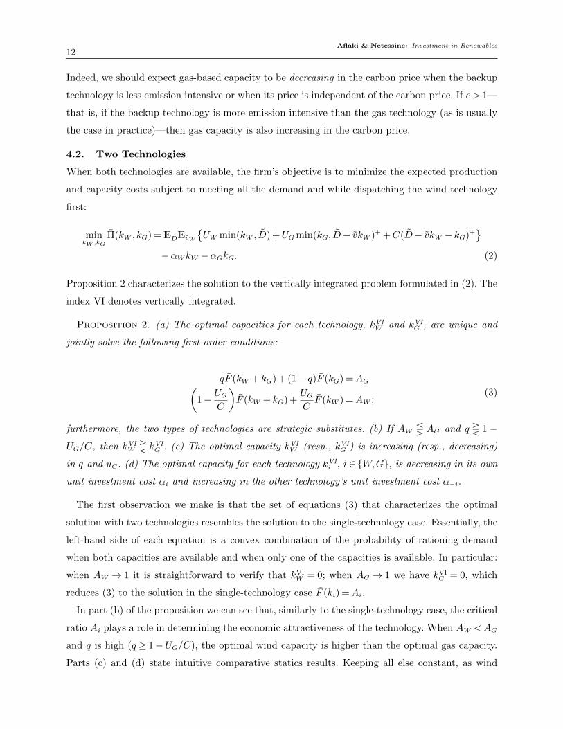
(VI) and a competitive Nash equilibrium (NE); here the data are as in Figure 3.

of electricity is decreasing in the availability of wind capacity; this puts wind at a significant

competitive disadvantage, since the price is lowest when wind is available and is highest when

wind is not available. Thus we observe in Figure 4(c) that, for a ≤ 18 (which spans the current

carbon price of a≈ 10), the share of wind capacity is lower under competition than under vertical

integration; in other words, the spot-price disadvantage of wind dominates. This disadvantage

fades as carbon prices rise and the gas generator significantly benefits from underinvestment in the

competition setting, which enables the share of wind capacity to exceed its share under vertical

integration.

Finally, we note with reference to panels (b) and (d) of Figure 4 that the increase in total capacity

and decrease in total emissions following a higher carbon price occurs more rapidly under vertical

integration than under competition. In other words, increasing the carbon price is less effective

at reducing carbon emissions under competition. This result is due mainly to underinvestment

incentives stemming from vertical unbundling and its effect on the spot price. In the competitive

scenario, higher carbon prices lead to generators benefitting more from underinvestment. This is

because the backup technology is more carbon intensive and its total cost is rapidly increasing in

the carbon price. Hence generators whose capacity is exceeded will benefit more when the carbon


price is high, which in that case incentivizes them to underinvest.

This section has demonstrated the adverse effect of market competition on capacity investment

in electricity generation technologies. A common solution that is proposed in related studies is

long-term capacity contracts to ensure sufficient capacity investments. This subject is discussed in

the next section.

6. Fixed Price Contracts

Here we consider a partially liberalized market in which the retailer signs a long-term fixed-price

(FP) contract with the electricity generator. Given the volatility of spot prices, bilateral forward

contracts between retailers and generators play a significant role in almost all electricity markets

today.12 The time horizon of the forward contracts can range from a single day to 15–20 years.

Short-term forward contracts are typically signed a day ahead and specify the committed capacity

and the agreed-upon price. In the United States, long-term forward contracts have been advocated

as a means to promote investment in renewable generation capacity and to “spur the growth of

renewable generation” (Wilson et al. 2005). In a number of states (including Massachusetts, Rhode

Island, New Jersey, and Delaware), the legal instruments are already in place to sign long-term

power purchase agreements with fixed prices and with contracting horizons of 10–25 years. Germany

and Spain, the two European countries with highest installed capacity for renewable energy, have

used long-term FP contracts to promote renewable energy investments. As before, we start with a

single-technology benchmark to understand the basic effects of fixed-price contracts and only then

address the case of two technologies, where FP forward contracts are signed to promote investment

in renewable capacity.

6.1. Benchmark Case: One Technology

For an announced fixed price pi, the generator’s problem is choosing ki (i ∈ {W,G}) to maximize

its expected profit:

maxki

Πi(ki, pi) =EviED{(pi−Ui)min(D, viki)}−αiki. (8)

The retailer seeks to minimize the total cost of the system by choosing pi, given that the supplier

solves (8):

minpi

ΠR(ki) =EviED{pimin(D, viki) +C(D− viki)+}

s.t. ki = arg maxki

Πi(ki, pi).(9)

12 Such a bilateral arrangement takes one of two possible forms Borenstein (2002). In an electricity pool, or marketbased bilateral contracts, all generators sell to a pool run by an independent system operator and all retailers buyfrom that pool. In this case, the system operator manages the physical feasibility of electricity flow in the network.An alternative to this arrangement is buyers and sellers making their own arrangements for electricity purchase andthen informing the system operator about those arrangements. The system operator steps in only if some physicalinfeasibility might otherwise occur—as when a part of the transmission grid is overloaded. In that case the operatorsets grid usage charges to balance the network.


Let εi = (kVIi − kFP

i )/kVI represent the inefficiency that arises from contracting.

Proposition 5. Suppose the distribution of demand has IFR. (a) There exist unique prices p∗i

(i∈ {W,G}) and capacities kFPi (i∈ {G,B}) that solve (9) and are characterized as follows:

p∗i =Ui +Ai

F (kFPi )

, where kFPi solves

L(k,Ai) =Aiφ(k)

(∫ k0xf(x)dx

F (k)+ k

)+Ai− F (k) = 0.

(10)

(b) kFPG ≥ kFP

W if and only if AG ≤ AW . (c) kFPW is increasing in a, and kFP

G is increasing in a if

and only if e > 1. (d) Regardless of the technology type, firms always underinvest in the fixed-price

contract setting at the optimal solution (10). Moreover, εW ≥ εG if and only if AW ≥AG.

This proposition states that the optimal fixed price for a long-term contract between generator

and retailer is calculated as the total unit variable cost of generating electricity with technology

i plus a markup that is a function of i’s critical ratio. That markup need not be increasing in

the critical ratio Ai, since the optimal capacity kFPi is decreasing in Ai and so the numerator and

denominator of the markup fraction Ai/F (kFPi ) move in the same direction.

Much as in the settings of vertical integration and competition, in this contract setting the driver

of technology advantage is the critical ratio Ai. The reason is that the backup cost is reflected in

the contract price, which determines the capacity decisions made by the generators. As a result,

all of the comparative static results described previously for Ai still apply. In particular, part (c)

of Proposition 5 states that the optimal wind capacity is always increasing in the carbon price but

that gas capacity is increasing in the carbon price only when it emits less carbon than the backup

technology (although, as mentioned before, this is usually the case). Section 6.2 shows that—

because of the substitution effect—this result may not hold when there is simultaneous investment

in two technologies.

Finally, Proposition 5 states that the vertical separation of retailer and generator in the setting

of a fixed-price contract leads to an inefficiency in the form of underinvestment in capacity, εi ≥ 0.

Moreover, that inefficiency is greater for the technology with the higher critical ratio (and thus

the lower capacity investment) because this technology can be more efficiently substituted for the

backup generation. In the next section we show that this is not the case when both technologies

are present because one of them will have a comparative advantage.

6.2. Partial Market Competition with Long-Term Fixed-Price Contracts for theWind Generator

We now consider the case where the retailer enters into a long-term fixed-price contract with

the wind generator but the price for the gas generator is still determined through a spot-market


mechanism similar to the one described in Section 5. Based on the contracted fixed price, the wind

generator decides what level of wind capacity to install. This decision, in turn, affects the spot

price by shifting the demand curve and thereby influencing the gas generator’s decision regarding

what level of capacity to install. Thus the level of installed capacity for gas technology does depend

(albeit indirectly) on the fixed price set by the retailer for the wind technology, so in this sense

the two suppliers compete in the market. The retailer’s objective is to choose the price for wind

electricity such that its own total cost is minimized:

minpW

EviED{pW min(D, vkW ) + psmin(D− vkW , kG)+}. (11)

The wind generator decides on the amount of capacity to install based on the retailer’s announced

price for wind electricity,

maxkW

ΠW (kW ) =EviED{pW min(D, vkW )}−αWkW , (12)

and the gas generator’s problem is formulated as

maxkG

ΠG(kG) =EviED{(ps−UG)min(D− vkW , kG)+}−αGkG. (13)

The complexity of the relation between contracted capacity and the gas generator’s problem pre-

cludes our establishing analytically the concavity of the retailer’s objective function. The first-order

conditions are characterized in the Appendix and are, indeed, similar to those for Proposition 5.

We use these conditions to obtain the optimal solutions in Figure 5, which illustrates the solution

in the FP case as well as in the cases of vertical integration and market competition, as before

using the real data. In line with the results from Section 6.1, we observe that fixed-price contracts

decrease investment for both technologies relative to the vertically integrated case. Also, as one

would expect, FP contracts increase the installed wind capacity and decrease the gas capacity

relative to the case of market competition. This is because the wind generator now has the clear

advantage of no uncertainty in prices. Somewhat surprisingly, however, there is little difference

in gas capacity investment between the FP and NE cases. Hence we observe more total installed

capacity in the contracting than in the market competition case, where most of the increased

generation capacity now comes from wind.

Although the overall increase in wind capacity under a regime of fixed-price contracts is good

news, there is no free lunch: the increase in wind and total capacity is such that emissions in this

setting remain higher than under vertical integration. The reason is that the installed gas capacity

in this case is insufficient to provide backup for the intermittent wind capacity, forcing the retailer

to employ the emission-intensive backup option. In short, fixed-price contracts are successful at

promoting renewables but fail to abate emissions relative to the case of market competition. Of

course, these statements hold only for relatively high shares of renewable electricity generation

capacity.


16 22 28 34 400

20

40

60

80

Emiss ion Price ($)


(a)

16 22 28 34 4020

40

60

80

100

120

Emiss ion Price ($)

Tota

lAvailable

Capacity (b)

16 22 28 34 400.4

0.5

0.6

0.7

0.8

0.9

Emiss ion Price ($)

WindCapacityShare

(c)

16 22 28 34 40120

140

160

180

200

Emiss ion Price ($)

Tota

lEmissions

(d)

VI

NE

FP VI

FP

NE

NE

FP

VI

Wind VI

Wind NE

Gas VI

Gas NE

Gas FP

Wind FP

Figure 5 (a) Individual capacities, (b) total available capacity qkFPW + kFP


kFPW /(kFP

G + kFPW ), and (d) total emissions as a function of the emission price under vertical integration

(VI), a competitive Nash equilibrium (NE), and a partially liberalized market with fixed-price contracts

(FP); here the data are as in Figure 3.

7. Conclusions

In this paper we study the effect of two recent developments in the electricity markets: liberalization

and the introduction of renewables. Using a novel approach in this context, we analyze how the

intermittency of renewables links these two changes in the electricity industry. In particular, we

demonstrate direct relationships among cost structure, intermittency, and capacity investments;

in so doing, we establish an important yet largely overlooked link between the intermittency of

renewable energy sources and the effectiveness of renewable-promoting policies such as carbon

pricing. We demonstrate that, even though renewables become more cost competitive on average

as the carbon price increases, higher carbon prices may actually decrease the share of renewable

capacity in the overall generation portfolio—in both the vertically integrated and the (partially)

liberalized market. Thus, although increasing the price of carbon emissions does lead to lower

total emissions, this policy is not a good way to promote investment in renewables. Moreover,

we show that market liberalization may not promote efficient investment in generation capacity.

Liberalization also leads to an increase in total emissions from the generation portfolio, and for

a reasonable range of carbon prices it leads to a lower share of renewables than in the vertically


integrated case. The root cause of this effect is the interaction between intermittency and market

pricing.

We further show that long-term electricity contracts, which offer fixed feed-in tariffs to the owners

of renewable generation capacity, do ameliorate some disadvantages of the liberalized markets.

Namely, they lead to a significant increase in renewable capacity investment while not appreciably

affecting nonrenewable capacities. Thus long-term contracts with renewable generators increase the

total installed capacity and reduce emissions relative to the market competition case. We conclude

that long-term fixed-price contracts are a good means of compensating for the disadvantages of

market liberalization from the viewpoints of total cost and greenness both. However, these contracts

could also lead to dramatic overinvestment in renewables and underinvestment in gas generation

(relative to the vertically integrated case) for high enough carbon prices. The likely result would be

an overreliance on the backup (coal-fired) generators; besides being detrimental to the environment,

this could also lead to grid-balancing issues if the need arises for significant backup generation.

Overall, our analysis indicates that the intermittency of renewable energy sources is a problematic

feature that handicaps investment decisions in these technologies. Although raising carbon taxes is

meant to improve the attractiveness of renewables, we show that this is probably not an effective

policy. A more effective approach to increasing capacity investment in renewables would be to

reduce intermittency. There are various options to achieve this goal. The first option is storage,

for which various (relatively new technologies) are available.13 These technologies include pumped-

storage hydropower, which stores electricity in the form of potential energy, and pumped heat

electricity storage, which uses argon gas to store power in the form of heat. There are many recent

papers that consider the problem of optimal storage policies while taking installed generation

capacity as fixed (for a comprehensive review, see Faghih et al. 2012). Other options besides storage

include the “curtailing” of intermittent generation (as described in Wu and Kapuscinski 2012) and

the pooling of multiple generation units (possibly with different technologies) whose supply is not

perfectly correlated. This latter approach may be possible only for large generators with enough

resources to invest in multiple wind farms in different geographical regions. So even though there

are no economies of scale in wind electricity generation, clearly there are statistical economies

of scale in terms of reduced intermittency. Our analysis is a first step toward further research

on an integrated framework that will combine these solutions with an explanation of how long-

run capacity decisions are affected by the cost structure of renewables. Our results suggest the

possibility of additional value to these solutions if generation capacity decisions are taken into

account.

13 See an Economist article on this topic at http://www.economist.com/node/21548495.


In this paper we have refrained from modeling multiple generating firms each with multiple

technologies, which would have allowed a more realistic presentation. Extending our model along

such lines would require modeling a complex bidding process that involves many firms and several

technologies—an analytically challenging task. Another limitation of this study is that we focused

on just two technology types, although other electricity generation technologies may have strongly

different features. For instance, nuclear and large-scale coal generators have no intermittency prob-

lems, but neither do they have any flexibility in adjusting output. Future research may consider

these and other extensions of the long-term capacity investment problem.

References

Ambec, S., C. Crampes. 2010. Electricity Production with Intermittent Sources. TSE Working Papers .

Avci, B., K. Girotra, S. Netessine. 2012. Electric vehicles with a battery switching station: Adoption and

environmental impact .

Barlow, R.E., F. Proschan, L.C. Hunter. 1996. Mathematical theory of reliability , vol. 17. Society for

Industrial Mathematics.

Borenstein, S. 2002. The trouble with electricity markets: understanding California’s restructuring disaster.

The Journal of Economic Perspectives 16(1) 191–211.

Borenstein, S., J. Bushnell, S. Stoft. 2000. The competitive effects of transmission capacity in a deregulated

electricity industry. The Rand Journal of Economics 31(2) 294–325.

Bushnell, J. 2010. Building blocks: Investment in renewable and non-renewable technologies. Harnessing

Renewable Energy in Electric Power Systems: Theory, Practice, Policy 159.

Butler, L., K. Neuhoff. 2008. Comparison of feed-in tariff, quota and auction mechanisms to support wind

power development. Renewable Energy 33(8) 1854–1867.

Cachon, G., C. Terwiesch. 2006. Matching supply with demand: An introduction to operations management .

McGraw-Hill.

Castro-Rodriguez, F., P.L. Marın, G. Siotis. 2009. Capacity choices in liberalised electricity markets. Energy

Policy 37(7) 2574–2581.

Chao, H. 1983. Peak load pricing and capacity planning with demand and supply uncertainty. The Bell

Journal of Economics 14(1) 179–190.

Crew, M.A., C.S. Fernando, P.R. Kleindorfer. 1995. The theory of peak-load pricing: a survey. Journal of

Regulatory Economics 8(3) 215–248.

Crew, M.A., P.R. Kleindorfer. 1976. Peak load pricing with a diverse technology. The Bell Journal of

Economics 7(1) 207–231.

Defeuilley, C. 2009. ScienceDirect.com - Energy Policy - Retail competition in electricity markets. Energy

Policy .


Deo, S., C.J. Corbett. 2009. Cournot competition under yield uncertainty: The case of the US influenza

vaccine market. Manufacturing & Service Operations Management 11(4) 563–576.

Drake, D., P.R. Kleindorfer, L. N. Van Wassenhove. 2010. Technology choice and emissions flexibility in a

carbon economy. INSEAD working paper.

EIA, US. 2010. Annual energy outlook 2011. Energy Information Administration .

Elmaghraby, W. 1997. Multi-unit auctions with dependent valuations: issues of efficiency in electricity

auctions. Univerisity of California Energy Institute, Power Working Paper 53.

Faghih, A., M. Roozbehani, M. A. Dahleh. 2012. On the economic value and price-responsiveness of ramp-

constrained storage Working paper available at http://web.mit.edu/mardavij/www/.

Garcia, A., J.M. Alzate. 2010. Regulatory design and incentives for renewable energy. Working paper.

Green, R.J., D.M. Newbery. 1992. Competition in the British electricity spot market. Journal of political

economy 100(5) 929–953.

Hogan, W. 1995. A Competitive Electricity Market Model. Harvard Electricity Policy Group, Draft .

Inhaber, H. 2011. Why wind power does not deliver the expected emissions reductions. Renewable and

Sustainable Energy Reviews 15(6) 2557–2562.

Islegen, O., S. Reichelstein. 2011. Carbon capture by fossil fuel power plants: An economic analysis. Man-

agement Science 57(1) 21.

Joskow, P.L. 2006. Competitive electricity markets and investment in new generating capacity MIT, Center

for Energy and Environmental Policy Research.

Kaffine, D.T., B.J. McBee, J. Lieskovsky. 2011. Emissions savings from wind power generation: Evidence

from texas, california, and the upper midwest.

Kennedy, S. 2005. Wind power planning: assessing long-term costs and benefits. Energy Policy 33(13)

1661–1675.

Kim, J.H., W.B. Powell. 2011. Optimal energy commitments with storage and intermittent supply. Operations

Research-Baltimore 59(6) 1347.

Kleindorfer, P.R., K. Singhal, L.N. Wassenhove. 2005. Sustainable operations management. Production and

Operations Management 14(4) 482–492.

Lobel, R., G. Perakis. 2011. Consumer rebates for green technology adoption.

Michaels, R. J. 2004. Vertical Integration: The Economics that Electricity Forgot. The Electricity Journal

17(10) 11–23.

Michaels, R. J. 2007. Vertical integration and the restructuring of the U.S. electricity industry. Cato Institute

Policy Analysis Series. Available at http://ssrn.com/abstract=975682.

Neuhoff, K., J. Cust, K. Keats. 2007. Implications of intermittency and transmission constraints for renew-

ables deployment. Cambridge Working Papers in Economics .


Owen, A.D. 2004. Environmental externalities, market distortions and the economics of renewable energy

technologies. The Energy Journal 25(3) 127–156.

Savaskan, R.C., S. Bhattacharya, L.N. Van Wassenhove. 2004. Closed-loop supply chain models with product

remanufacturing. Management science 239–252.

Sosa, M.E. 2011. Design for environment. K.T. Ulrich, S.D. Eppinger, eds., Product design and development .

McGraw-Hill.

Tarjanne, R., A. Kivisto. 2008. Comparison of electricity generation costs. Research report/Faculty of

Technology. Department of Energy and Environmental Technology .

Taylor, T.A., E.L. Plambeck. 2007. Simple relational contracts to motivate capacity investment: Price only

vs. price and quantity. Manufacturing & service operations management 9(1) 94.

Tomlin, B., Y. Wang. 2005. On the value of mix flexibility and dual sourcing in unreliable newsvendor

networks. Manufacturing & Service Operations Management 7(1) 37–57.

Ventosa, M., A. Baillo, A. Ramos, M. Rivier. 2005. Electricity market modeling trends. Energy policy 33(7)

897–913.

Vives, X. 2001. Oligopoly pricing: Old ideas and new tools. The MIT Press.

Von der Fehr, NH, DC Harbord. 1997. Capacity investment and competition in decentralised electricity

markets. Memorandum from Department of Economics University of Oslo.

Wilson, N.E., R.G. Newell, D. Burtraw, Resources for the Future. 2005. The Effect of Long-Term Generation

Contracts on Valuation of Electricity Generating Assets Under the Regional Greenhouse Gas Initiative.

Resources for the Future.

Wu, O., R. Kapuscinski. 2012. Curtailing intermittent generation in electrical systems. Operations Research-

Baltimore .

Zhou, Yangfang, Alan Andrew Scheller-Wolf, Nicola Secomandi, Stephen Smith. 2011. Managing Wind-based

Electricity Generation with Storage and Transmission Capacity. SSRN eLibrary .

Appendix: Proofs

Proof of Proposition 1. (a) Define

Π(k;α, q,u) =ED{q(umin(D, k) +C(D− k)+

)+ (1− q)CD

}+αk. (14)

It is straightforward to verify that ΠW (kW ) = Π(kW ;αW , q,0) and ΠG(kG) = Π(kG;αG,1,UG). So

solving problem (1) requires only that we characterize the solution to mink Π(k;α, q,u). Equa-

tion (14) can be equivalently written as

Π(k;α, q,u) = q

(u

(∫ k

0

xf(x)dx+

∫ ∞k

kf(x)dx

)+ c

∫ ∞k

(x− k)f(x)dx

)


+ (1− q)cE{D}+αk. (15)

We write the first-order condition (FOC) as

∂

∂kΠ(k;α, q,u) =−q(c−u)(F (k)) +α= 0 (16)

or, equivalently, F (k) = αq(c−u)

=A(α, q,u). The rest follows from the definition of AW and AG. For

c > u, we have ∂2

∂k2Π(k;α, q,u) = q(c−u)f(k)> 0 and so the FOC is sufficient.

(b) The result follows immediately from part (a) of Proposition 1 after considering that Ai > 0

and F (k) is decreasing.

(c) The result follows immediately from part (a) of Proposition 1 once we verify that AW is

always decreasing in a and that AW is decreasing in a if and only if e > 1.

Proof of Proposition 2. (a) We rewrite (2) as:

Π(kW , kG) = q

(∫ kW +kG

kW

UG(x− kW )f(x)dx

)+

∫ ∞kW +kG

(UGkG + c(x− kW − kG))f(x)dx

+ (1− q)∫ kG

0

UGxf(x)dx

+

∫ ∞kG

(UGkG +C(d− kG))f(x)dx+αWkW +αGkG. (17)

First we verify that Π(kW , kG) is jointly convex. Calculating the Hessian matrix yields

H =

∂2Π∂k2

W

∂2Π∂kW ∂kG

∂2Π∂kW ∂kG

∂2Π∂k2

G

, (18)

where

∂2Π

∂k2W

= q(UGf(kW ) + (C −UG)f(kW + kG)

)> 0,

∂2Π

∂k2G

= (C −UG)(qf(kW + kG) + (1− q)f(kG)

)> 0,

∂2Π

∂kW∂kG= q(C −UG)f(kW + kG)> 0,

and |H| = Cq((qUGf(kW ) + (1− q)Cf(kG)

)f(kW + kG) + UG(1− q)f(kW )f(kG)

)> 0. Therefore,

H is a positive definite matrix; this implies that Π(kW , kG) is jointly convex in its arguments and

hence that the FOCs are sufficient. Writing the FOCs with respect to kW and kG, we obtain

−q(UG

∫ kW +kG

kW

f(x)dx+C

∫ ∞kW +kG

f(x)dx

)+αW = 0, (19)


−(C −UG)

(q

∫ ∞kW +kG

f(x)dx+ (1− q)∫ ∞kG

f(x)dx

)+αG = 0; (20)

after some simplification and substitution, this yields the system of equations identified in Propo-

sition 2.

Furthermore, Π(kW , kG) is supermodular in its arguments (see Vives 2001, Thm. 2.3):

∂2Π

∂kW∂kG= q(C −UG)f(kW + kG)> 0, (21)

so the technologies are substitutes.

(b) If AW ≤AG and q≥ 1− UGC

, then

qF (kVIW + kVI

G ) + (1− q)F (kVIW )

≤(

1− UGC

)F (kVI

W + kVIG ) +

UGCF (kVI

W )

(because q≥ 1− UG

Cand F (kVI

W + kVIG )≤ F (kVI

W )

)≤ qF (kVI

W + kG) + (1− q)F (kVIG ) ( because AW ≤AG)

=⇒ F (kVIW )≤ F (kVI

G ) =⇒ kNEW ≥ kNE

G .

The converse case is proved analogously.

Parts (c) and (d) of the proposition are similarly obtained by using monotone comparative statics

to verify that Π(kW , kG; q,uG, αW , αG) has increasing (or decreasing) differences in the following

parameters:

∂2

∂kW∂qΠ(kW , kG; q,UG, αW , αG) = −

∫ kW +kG

kW

UGf(x)dx−∫ ∞kW +kG

Cf(x)dx≤ 0,

∂2

∂kW∂uGΠ(kW , kG; q,UG, αW , αG) = −q

∫ kW +kG

kW

f(x)dx≤ 0,

∂2

∂kW∂αWΠ(kW , kG; q,UG, αW , αG) = 1> 0,

∂2

∂kW∂αGΠ(kW , kG; q,UG, αW , αG) = 0,

∂2

∂kG∂qΠ(kW , kG; q,UG, αW , αG) = (C −U2)

(∫ ∞kG

f(x)dx−∫ ∞kW +kG

f(x)dx

)≥ 0,

∂2

∂kG∂uGΠ(kW , kG; q,UG, αW , αG) = q

∫ ∞kW +kG

f(x)dx+ (1− q)∫ ∞kG

f(x)dx≥ 0,

∂2

∂kG∂αWΠ(kW , kG; q,UG, αW , αG) = 0,

∂2

∂kG∂αGΠ(kW , kG; q,UG, αW , αG) = 1> 0.

Proof of Proposition 3. (a) The general rule for implicit derivatives implies that(∂kVI

W∂c∂kVI

W∂c

)=H−1 ·

(∂2Π

∂kW ∂c∂2Π∂kG∂c

), (22)


where H−1 is the inverse of the Hessian matrix defined in the proof of Proposition 2. We calculate

the partial derivatives and obtain

∂2Π

∂kW∂c= −q

∫ M

kW +kG

f(d)dd,

∂2Π

∂kG∂c= −

(q

∫ M

kW +kG

f(d)dd+ (1− q)∫ M

kG

f(d)dd

).

Substituting these values into (22) and then applying Cramer’s rule, we obtain(∂kVI

W∂c∂kVI

G∂c

)=

1

|H|

((C −UG)q(1− q)

(− f(kW + kG)F (kG) + F (kW + kG)f(kG)

)q(qF (kW + kG)UGf(kW ) + (1− q)F (kG)

(uGf(kW ) + (C −UG)f(kW + kG)

))) ,(23)

where |H|> 0 is the determinant of the Hessian matrix. We observe in (23) that∂kVI

G∂c≥ 0 and that

if F has IFR then f(kG)

F (kG)≤ f(kW +kG)

F (kW +kG), which implies that

∂kVIW∂c≤ 0. Furthermore,

∂kVIW

∂c+∂kVI

G

∂c=

q

|H|((quGf(kW ) + (1− q)Cf(kG))F (kW + kG) + (1− q)F (kG)uGf(kW )

)≥ 0. (24)

(b) We show that if e≤ 1 then kVIW is increasing in a and kVI

G is decreasing in a. Much as in the

proof of Proposition 2, we obtain the desired result by first using monotone comparative statics to

calculate the cross partial derivatives of Π(kW , kG;a) with respect to (kW , a) and (kG, a) and then

using that capacities are substitutes. If e≤ 1 then

∂2

∂kW∂a= −q

(∫ ∞kW +kG

f(x)dx+ e

∫ ∞kW +kG

f(x)dx

)≤ 0 and (25)

∂2

∂kG∂a= (1− e)

(q

∫ ∞kW +kG

f(x)dx+ (1− q)∫ ∞kG

f(x)dx

)≥ 0. (26)

The second part of the proposition is proved by the existence of the counterexample provided in

the text.

Proof of Proposition 4. (a) We rewrite the wind generator’s profit in (5) as

ΠW (kW , kG) = q

(UGkW

∫ kW +kG

kW

f(x)dx+CkW

∫ ∞kW +kG

f(x)dx

)−αWkW (27)

and rewrite the gas generator’s problem in (6) as

ΠG(kW , kG) = qkG(C −UG)

∫ ∞kW +kG

f(x)dx+ (1− q)kG(C −UG)

∫ ∞kG

f(x)dx−αGkG. (28)

Now taking the derivatives of ΠW (kW , kG) with respect to kW and of ΠG(kW , kG) with respect to

kG, we find that the Nash equilibrium of the capacity game solves the following system of equations:

qUG

∫ kW +kG

kW

f(x)dx+ qC

∫ ∞kW +kG

f(x)dx− qkW (C −UG)f(kW + kG)− qUGkWf(kW )−αW = 0,


(C −UG)

(q

∫ ∞kW +kG

f(x)dx+ (1− q)∫ ∞kG

f(x)dx− qkGf(kW + kG)− kG(1− q)f(kG)

)−αG = 0.

If we replace f(·) with φ(·)F (·) then, after some simplification, we obtain that the NE of the

capacity game solves the system of equations specified in Proposition 4. Observe that if the demand

distribution has IFR—that is, if φ(x) is increasing—then the left-hand side of each FOC just

displayed is strictly decreasing in both arguments. Hence ΠW (kW , kG) is strictly concave in kW

and ΠG(kW , kG) is strictly concave in kG, which implies that the FOCs are sufficient and the NE

is unique.

(b) The proof of this part of Proposition 4 is analogous to the proof of Proposition 2(b).

(c) Recall that the optimal capacities for the vertically integrated case solve the system of

equations in Proposition 2. Suppose that the total capacity under competition is higher than the

first-best case—that is, let kNEW +kNE

G >kVIW +kVI

G . Then we should have either kVIG <kNE

G or kVIW <kNE

W

(or both). In the first case, kVIG <kNE

G , we have

AG = qF (kNEW + kNE

G )(1− kNEG φ(kNE

W + kNEG )) + (1− q)F (kNE

G )(1− kNEG φ(kNE

G ))

< qF (kNEW + kNE

G ) + (1− q)F (kNEG )

< qF (kNEW + kNE

G ) + (1− q)F (kNEG ) =AG,

which is a contradiction. The other two cases also lead to a contradiction in a similar fashion. We

therefore conclude that the inequality kNEW + kNE

G >kVIW + kVI

G can never hold.

It is now straightforward to verify that if e > 1 then the total emissions of the system is higher

under competition.

Proof of Proposition 5. (a) The objective function in (8) for the wind technology may be

written as

ΠW (kW , pW ) = pW q

(∫ kW

0

xf(x)dx+

∫ ∞kW

kWf(x)dx

)− kWαW (29)

and that for gas technology as

ΠG(kG, pG) = (pG−UG)

(∫ kG

0

xf(x)dx+

∫ ∞kG

kGf(x)dx

)− kGαG. (30)

We shall prove the case for wind technology; the case for gas technology proceeds along analogous

lines. Writing the FOC for problem (30) with respect to kW , we obtain

∂ΠW (kW , pW )

∂kW= pW q

(∫ ∞kW

f(x)dx

)−αW = pW q(F (kW ))−αW = 0. (31)

We note that ∂2

∂k2W

ΠW (kW , pW ) =−pW qf(kW )< 0, so the FOC is sufficient. The retailer’s problem

(9) is then written as

minpW

q

(pW

∫ kW

0

xf(x)dx+ c

∫ ∞kW

(x− kW )f(x)dx

)s.t. kW solves (31).

(32)


Because there is a one-to-one relationship between k∗ and p∗ in (31), problem (32) can be trans-

formed so that the decision variable is kW . Toward this end, we first solve (31) for pW to obtain

pW = αWq(F (kW ))

. Substituting this into (32) yields the following transformation of the retailer’s prob-

lem:

minkW

q

(αW

q(F (kW ))

∫ kW

0

xf(x)dx+ c

∫ ∞kW

(x− kW )f(x)dx

). (33)

Writing the FOC for problem (33) and then simplifying, we find that that k∗ solves LW (k,AW ) = 0.

It is straightforward to verify that if the demand distribution has IFR then L(k,Ai) is increasing

in k because∫ k

0xf(x)dx and F (k) are both strictly increasing in k. This state is equivalent to the

objective function in (32) being strictly convex in k; hence the FOC is sufficient and the solution

to problem (32) is unique.

(b,c) These results follow simply by verifying that L(k,Ai) is increasing in k and Ai; and that

AW is decreasing in a and AG is decreasing in a if and only if e > 1.

(d) By Proposition 1, kVIi solves Ai− F (k) = 0; by part (a) of Proposition 5, k∗i solves L(k,Ai) =

l(Ai, k) +Ai − F (k) = 0, where l(Ai, k)> 0 is the first term in L(k,Ai) defined in (10). The first

part of the result (underinvestment) follows from considering that both Ai− F (k) and L(k,Ai) are

increasing and that L(k,Ai)≥Ai− F (k). As for the second part, because l(Ai, k) is increasing in

Ai, we conclude that kVIi − k∗i is increasing in Ai. This, along with the fact that kVI

i is decreasing

in Ai implies that εi is increasing in Ai.

Characterization of the First-Order Conditions in Section 6.2. The following proposition

states the necessary conditions for the interior capacity solutions.

Proposition 6. The interior optimal capacities for wind and gas under a fixed-price contract

for the wind generator (i.e., kFPW and kFPG ) solve the following first-order conditions:

qF (kW + kG)(1− kGφ(kW + kG)) + (1− q)F (kG)(1− kGφ(kG)) =AG,(1− UG

C

)F (kW + kG)(1 + kGf(kW + kG)) +

UGCF (kW ) =AW

(1 +φ(kW )

(kW +

∫ kW0

xf(x)dx

F (kW )

)).

Proof. The proof is analogous to that of Proposition 5 and is therefore omitted.


Documents

Strategic Investment in Renewable Energy Sourcesflora.insead.edu/fichiersti_wp/inseadwp2012/2012-59.pdf · Renewable (or \green") sources of energy, such as wind and solar power,