Strategies for Cohort Sampling Under the Cox Proportional Hazards Model, Application to an AIDS Clinical Trial

Lifetime Data Analysis, 5, 149–172 (1999)c© 1999 Kluwer Academic Publishers, Boston. Manufactured in The Netherlands.

Strategies for Cohort SamplingUnder the Cox Proportional Hazards Model,Application to an AIDS Clinical Trial

SOYEON KIM [email protected] DE GRUTTOLA [email protected] of Biostatistics, Harvard School of Public Health, 677 Huntington Ave., Boston, MA 02115

Received March 17, 1998; Revised November 24, 1998; December 2, 1998

Abstract. In some studies that relate covariates to times of failure it is not feasible to observe all covariates forall subjects. For example, some covariates may be too costly in terms of time, money, or effect on the subject torecord for all subjects. This paper considers the relative efficiencies of several designs for sampling a portion ofthe cohort on which the costly covariates will be observed. Such designs typically measure all covariates for eachfailure and control for covariates of lesser interest. Control subjects are sampled either from “risk sets” at times ofobserved failures or from the entire cohort. A new design in which the sampling probability for each individualdepends on the amount of information that the individual can contribute to estimated coefficients is shown to besuperior to other sampling designs under certain conditions. Primary focus of our designs is on time-invariantcovariates, but some methods easily generalize to the time-varying setting. Data from a study conducted by theAIDS Clinical Trials Group are used to illustrate the new sampling procedure and to explore the relative efficiencyof several sampling schemes.

Keywords: case-cohort sampling, missing covariates, proportional hazards regression, risk set sampling, surrogatemarkers

1. Introduction

This article reports on ways to design and analyze cohort studies that relate covariates totime of failure, when only partial covariate information is obtained on study subjects. Ourprimary focus is on settings where some covariates are measured on all subjects, but othersare available on only a sample of subjects. This situation can arise because cost of measuringcertain covariates may be high or because new techniques for covariate measurement maybecome available after study inception. In the settings we consider, the main objectiveis to estimate parameters associated with the partially-observed covariates; but there mayalso be interest in the remaining covariates and in the survival distribution. By samplingwithin well-defined cohorts, it is often possible to limit the number of subjects for whomcovariate information is collected without much loss of information for estimating covariateeffects. When the study endpoint is rare, investigators typically select a sample for covariatemeasurement that includes all cases (subjects with endpoints) and a subset of the remainingsubjects. As first suggested by Mantel (1973) methods for sampling within well definedcohorts can be categorized into two broad classes: those that sample controls from “risksets” at times of observed failures and those that sample controls from the entire cohort. Arisk set refers to the set of all subjects at risk at the time of an observed failure. We consider

150 KIM AND DE GRUTTOLA

a variety of sampling strategies of both classes and propose a new one; we also proposenew methods of analysis for both established and novel study designs.

Our work was motivated by reconsidering the design and analysis of a retrospectivestudy based on stored blood specimens obtained in a clinical trial conducted by the AIDSClinical Trials Group (ACTG). The parent clinical trial, ACTG 019 (Volberdinget al.,1990), was a randomized double-blind, placebo-controlled prospective trial of two doses ofzidovudine (ZDV) in subjects with asymptomatic HIV-1 disease and CD4+ T-lymphocytecount less than 500 cells/mm3. This study demonstrated the effect of both doses of ZDVin reducing the risk of progression to clinical AIDS, the study endpoint. After completionof the study, investigators were interested in determining whether serum immunologicalmarkers, measurable in stored blood specimens, might convey important information aboutdisease progression. Because the study was large (1338 subjects) and the event rate low,the investigators (Jacobsonet al., 1995) could not assay all specimens, but instead assayedonly those from a selected sample of the cohort. Selecting a sample reduced the cost of thestudy by about 80% compared to the cost of assaying specimens from all subjects.

In this report, we use two different data sets from ACTG 019 for two different purposes.The first data set includes only covariates measured on all study subjects in the parent study.These data allow us to evaluate the performance of a wide variety of different samplingdesigns and analytical methods, in addition to the approach actually taken by Jacobsonet al.(1995). From these analyses, we are able to make recommendations about the best possibleapproaches for conducting such a retrospective study. The second data set is restrictedto the subjects sampled in the retrospective study of serum immunological markers, andincludes the new covariate information on these subjects. The use of new analytic methodsfor reanalysis of these data improves the efficiency of estimation compared to standardmethods, and also permits estimation of quantities related to absolute risk of developingan endpoint. In addition to the analyses of ACTG 019, we also perform a Monte Carlosimulation study in which distributions of all quantities are fully specified to resemble thesetting of ACTG 019.

Section 2.1 reviews risk-set study designs; Section 2.2 reviews estimation procedures forthe simple and stratified designs, and develops the conditions required for consistency andasymptotic normality of these procedures. Section 2.3 discusses existing estimation proce-dures for matched risk-set designs and proposes a new approach, weighted Cox regression.Theoretical justification of this estimator is also provided in Section 2.3 because standardconditions required for its asymptotic properties are not met. Section 3.1 reviews existingcase-cohort designs and also proposes a new study design to improve the efficiency of esti-mation of parameters corresponding to partially measured covariate. Section 3.2 discussesestimation procedures, and, once again, proposes the use of weighted Cox regression forestimation. Section 4 investigates small sample properties of estimators through simulationstudies. Section 5 applies methods to data from ACTG 019. Section 6 provides a discus-sion of practical advantages and disadvantages to different approaches, as well as of use theexisting software.

Throughout this article we assume the Cox proportional hazards model (Cox, 1972) anduse the following notation. For a cohort ofn individuals, the observed data for thei thsubject is(Xi , δi ,Zi ), whereXi is the min(Ti ,Ui ), Ti is the failure time,Ui is the censoring

STRATEGIES FOR COHORT SAMPLING 151

time,δi is the failure indicator, andZi is the vector of time-invariant covariates. The hazardat timet for an individual with covariate vectorZ is given byλ(t | Z) ≡ λ0(t)exp(β′Z),whereβ is a vector of regression coefficients. Under independent censoring, estimation isperformed using the Cox partial likelihood,

Lcox =n∏

i=1

(exp(β′Zi )∑

j∈R(Xi )exp(β′Zj )

)δi

, (1)

whereR(t) is the risk set at timet . Properties of estimates arising from the partial likelihoodare well established (Andersen and Gill, 1982; Tsiatis, 1981).

2. Risk-Set Sampling Strategies

2.1. Study Designs

Designs based on risk set sampling arise naturally from the Cox partial likelihood; the sim-ple design samples all failures, andm− 1 controls from all subjects at risk at each failuretime. Introduced by Thomas (1977), this design has also been discussed by several authors:Oakes (1981); Prentice (1986); Lubin and Gail (1984); Robins, Gail, and Lubin (1986);and Robins, Prentice, and Blevins (1989). To control for the effects of a certain covariate,we can sample within strata of that covariate, and thereby improve efficiency of estimationof regression parameters for the sampled covariates of greater interest. When stratifica-tion covariates take on discrete values, exact matches on covariate values between casesand controls are possible. For continuous stratification covariates, we obtain approximatematches by sampling from within predefined strata. There is a trade-off between closenessof the match, and ensuring available matches for each failure.

Because the choice of strata is often arbitrary, alternatives that permit closer matching,like caliper and nearest neighbor caliper matching, may be preferable. Caliper matchingdesigns include all failures, and, for each failure time, a random sample ofm− 1 controlsfrom subjects at risk whose covariate values lie within a specified distancec of the failure’scovariate value. Nearest neighbor caliper matching is similar, except the matches are thenearest m− 1 individuals among those at risk, within a certain distancec of the failure.Cochran and Rubin (1973) review work on different matching techniques when comparingtwo populations, adjusting for confounders under a linear regression model; other papersof interest include those of Carpenter (1977) and Raynor (1983).

2.2. Estimation: Simple and Stratified Designs

For simple risk-set sampling designs, estimation of regression parameters can be based ona partial likelihood similar to that of the full cohort analysis (1), except that the comparisonrisk set for a failure is composed only of the sampled risk setincludingthe failure. We denotethis sampled risk setR(Xi ), which replacesR(Xi ) in (1). For stratified sampling, estimationis based on the product of such terms over theQ strata with the comparison group being the


sampled risk set. The partial likelihood, which yields consistent and asymptotically normalresults, is given by

Lsrs =Q∏

q=1

nq∏i=1

(exp(β′Zqi )∑

j∈Rq(Xqi )exp(β′Zq j )

)δqi

, (2)

whereRq(t) is the sampled risk set at time in stratumq; andZqi , the covariate value for thei th subject in stratumq.

For the simple designs, asymptotic properties of parameter estimates have been shown byGoldstein and Langholz (1992). For the stratified design, the asymptotic properties of theestimation procedure can be obtained as a special case of the theory presented by Borganetal. (1995). The parameters corresponding to the stratification covariate are only estimablewhen there are a variety of covariate values in some of the strata – a situation guaranteed byabsolute continuity of the matching variable. Even when this condition is met, efficiency ofestimation for this parameter may be low. When estimating parameters corresponding to thestratification variable is not of interest, fine stratification, essentially matching, is desirable.In this setting, the matching covariate should be excluded from the partial likelihood (2).With the omission of the matching covariate, we designate this a “pseudo” likelihood, andthe associated score, a “pseudo” score.

Consistency and asymptotic normality of the non-matched regression coefficients requiresconditions similar to those of of Andersen and Gill (1982), with one addition. The newcondition requires that the matching covariate be absolutely continuous and that the stratumlength (the range of covariate values in a stratum) converge to zero at rateOp(n−ψ), 1/2<ψ < 1, asn→∞. We developed these conditions and proved the asymptotic properties bycomparing the pseudo score and information, suitably normalized, to the partial likelihoodscore, and information with the value ofβ1, corresponding to the matching covariate,fixed at its true value. Since this partial likelihood provides consistent and asymptoticallynormal estimates of the remaining Cox regression coefficients, we need only show that thenormalized pseudo score and information converge to the same quantities. The quantityψ

must be less than one to ensure that the number of individuals in each strata approachesinfinity as the sample size becomes infinite, and greater than 1/2 to ensure that the differencein the two normalized scores approaches zero.

Borgan and Langholz (1993) proposed a method for estimating the baseline cumulativehazard for the simple risk-set sample design. For designs with fine stratification, where thematching covariate is omitted from the model, the baseline hazard is not estimable withoutan outside estimate of the parameter associated with the matching covariate. If we do havean estimate of this parameter, baseline cumulative hazard can be estimated by a weightedaverage of theQ estimates of the baseline cumulative hazard:

3srs0 (t) =

Q∑q=1

nq∑i=1

wq(t)∫ t

01/

∑j∈Rq(u)

(nq(u)/m

)exp

(β′Zq j

)d Nqi (u),

whereq specifies stratum,Nqi (u) is the counting process associated with failure for in-dividual i in stratumq at timeu, nq(u) is the number of individuals at risk at timeu in


stratumq, m is the number sampled at the time of failure (including the failure),Rq(u) isthe sampled risk set at timeu, and where the weightswq(t) sum to 1. A natural choicefor weights are values proportional to the inverse of the variance. Borganet al. (1995)proposed a similar estimator wheren(u) the number at risk in all strata at timeu replacesnq(u), and we do not weight bywq(t). For a fixed number of strata, proving consistencyand asymptotic normality of these estimators is a straightforward extension of the approachof Goldstein and Langholz (1992).

2.3. Estimation: Matched Designs

For the caliper or nearest neighbor designs, it seems natural to base estimation on a partiallikelihood, which has the following form:

n∏i=1

(exp(β′Zi )wi (Xi )∑

j∈R(Xi )exp(β′Zj )wj (Xi )

)δi

. (3)

The weight,wj (t), for the j th individual is proportional to the probability thatR(t) issampled whenj is the failure at timet . In risk set sampling, whether simple or stratifiedby a discrete-valued covariate, we use weightswi (t) = wj (t) = w(t); hence the weightsfactor out of the likelihood. The partial likelihood approach is more problematic for caliper-matched sampling, however, because these designs can have an appreciable number of zeroweights, eliminating the contribution of controls to estimation. When weights associatedwith all controls are zero, the entire risk set, including the failure, does not contribute tothe likelihood. Controls receive zero weights in the caliper match partial likelihood when,conditional on the caliper size, there is information provided by the covariate values aboutwho is the failure among the sampled risk set. Similarly, nearest neighbor controls canreceive zero weights because individuals are not always mutually nearest neighbors.

As an alternative to using the partial likelihoods for these sampling designs, we con-sider a pseudo likelihood that is identical to the partial likelihood for the simple risk-setsample design, but omits the matching covariate, i.e., expression (1) with the sampled riskset Ri (Xi ) replacingR(Xi ), and the covariate vectorZi excluding the matching covariate.This approach is justified by the fact that the estimates retain the usual maximum likeli-hood properties of consistency and asymptotic normality of the estimates, provided that thematching covariate is absolutely continuous. The proof, provided in the appendix, hingeson the fact that asn → ∞, we can approximate the relevant quantities, i.e., the suitablynormalized pseudo score and information, by quantities that correspond to exact matching.Using this analysis method, we cannot estimate the parameters corresponding to the match-ing covariates; and, consequently, we cannot estimate the baseline hazard without furtherassumptions.

In addition to these approaches, we propose the use of an estimator that makes moreefficient use of the data. In this approach, estimates of the sampling probabilities serveas weights in a Cox regression. In addition to gains in efficiency, this approach makes itpossible to estimate the baseline cumulative hazard, thus allowing us to fully characterizethe failure time distribution. In order to discuss weighted Cox regression, we introduce


some additional notation. We letIni be an indicator for subjecti being sampled (either asa case or control) and partitionZi into two components(Zi 1,Zi 2) whereZi 1 is the vectorof covariates that are observed with probability 1, i.e., the matching covariates andZi 2 isobserved only whenIni = 1. β1 andβ2 are the Cox regression parameters corresponding toZi 1 andZi 2 respectively. We represent the probability that thei th individual is sampled givenhis fully observed information byπni ≡ P(Ini = 1 | (Xi , δi ,Zi 1)). Then in the subscriptfor R andπ indicate that both are functions of the sample size. DefiningYi (t) as the at riskprocess for thei th subject, and lettingS(k)w (β,u) = n−1∑n

j=1π−1j In j Yj (u)exp(β′Zj )Z

⊗kj

for k = 0,1, and 2, andZw(β,u) = S(1)w (β,u)/S(0)w (β,u), the estimating equation is

given by:

Uw(β) =n∑

i=1

∫ τ

0

{Zi − Zw(β,u)

}d Ni (u), (4)

which is a weighted version of the usual Cox score. The variance of the estimator can beestimated using a weighted version of the robust variance of Lin and Wei (1989).

The weighted Cox estimator is included in the class of estimators proposed by Robinsetal. (1994). In an unpublished report, Pughet al. (1994) show consistency and asymptoticnormality of the resulting estimate under the condition that data are missing at random andthat the probability of observing the data for a subject depends only on data,(Xi , δi ,Zi 1), forthat subject. Since data yielded by the caliper-matched design meet only the first condition,we must provide additional theoretical justification. In the caliper-matched design, theprobability of being sampled for individuali depends on the covariate values for others inthe cohort:πni = P(Ini = 1 | (Xi , δi ,Zi 1), i = 1, ...,n). We were able to extend theconditions for consistency and asymptotic normality, however, by showing that asymptoticindependence is sufficient to guarantee these properties. The proof requires that:

|P(In j = 1, Ink = 1 | Xj , δj ,Zj 1, Xk, δk,Zk1)

− P(In j = 1 | Xj , δj ,Zj 1)P(Ink = 1 | Xk, δk,Zk1)| → 0,

with rateop(1). In fact, this condition can be further relaxed; asymptotic properties requireonly that the sum of the differences (4) overj and k 6= j approach 0 at rateop(n−2)

(details of the proof are available from the authors.) It seems intuitive that the matchedrisk set sampling schemes yield data that are asymptotically independent under regularityconditions on covariate and hazard functions. As the number of subjects (and the numberof failures) with a covariate value “near” that of a given subject becomes infinite, thedependence of the probability of selecting any given control on the probability of selectingall failures and controls becomes small. When the proportion of failures also gets small asn→∞, the probabilities in (4) get small as does their difference. Finally, the dependenceof the sampling probability for each individual on all data other than(Xi , δi ,Zi 1) becomesvanishingly small. Although we do not have a formal proof, simulation results in Section 4support the accuracy of this claim.

Estimation of sampling probabilities,πni , can be achieved with a variety of techniquesthat make assumptions about the relationship between these probabilities and fully observedinformation, including(Xi , δi ,Zi 1), and any additional relevant information. Unlike the


stratified approach, this approach permits estimation ofβ1 as well asβ2. Using the sameweights, we can estimate the baseline hazard by weighting the Breslow estimator as follows:

3pr0 (t) =

∫ t

0

n∑i=1

[n∑

j=1

π−1nj In j Yj (u)exp(β

′Zj )

]−1

d Ni (u).

Provided that the model for estimating the weights is correct, the weighted estimators ofmodel parameters and baseline hazard are asymptotically unbiased.

3. Case-Cohort Type Sampling

3.1. Study Designs

In the case-cohort design introduced by Prentice (1986), the sample consists of a sub-cohort of individuals randomly selected from the cohort plus all failures outside that cohort.As with the risk-set designs, the efficiency of case-cohort sampling can be improved bymatching on variables of lesser interest. This can be achieved by frequency matching, i.e.,by forming strata based on the matching covariate information. For example, if there arenk failures andNk controls in stratumk and we wantm− 1 controls per failure, then wesample from the controls with probability min[(m− 1)nk/Nk,1]. The expected (althoughnot the exact) number of controls per failure will bem− 1.

The approach described above works well if there is only one matching variable anda reasonable number of failures in each stratum. When these conditions are not met, wepropose an “efficient case-cohort design” as an alternative. This design samples the controlsbased on the estimated probability of failure using any reasonable parametric model. Toillustrate, letW contain information that is always observed, including(X, δ,Z1), and anyother information that predicts whether failure occurs during the study time frame; and letW∗ be any function ofW. For a logistic model, we can obtain the maximum likelihoodestimate ofα from the model:

logit (P(δ = 1 |W)) = α′W∗. (5)

We then sample from among the controls according to the estimated probability of fail-ure: πi = exp(α′W∗)/(1+ exp(α′W∗)). These are the true probabilities that subjects arecompletely observed; therefore, the distribution of covariates will be similar for controlsand failures.

3.2. Estimation

For the simple case-cohort design, Self and Prentice (1988) showed consistency and asymp-totic normality of an estimator based on a pseudo likelihood. The latter resembles the fullsample Cox partial likelihood, except that the controls for each failure (R(Xi ) in (1)) con-sist only of those at risk in the random sub-cohort at the time of the failure. Kalbfleischand Lawless (1988) suggested using a pseudo score where the cases are all weighted by a


factor 1 and the remaining sample is weighted by 1/p, and wherep is the probability thatan individual is in the random sample. This procedure is a special case of the weightedCox regression proposed by Robinset al.(1994), and the score equation (3) can be used forestimation. Lin and Ying (1993) also discuss the case-cohort design and provide a simplervariance estimate than Self and Prentice (1988); they also show how to supplement thesub-cohort as the number at risk diminishes.

For the efficient case-cohort design, where the the probability of being sampled dependson covariate values, weighted Cox regression can also be used for estimation. The weightsfor the Cox estimation equation (4) are the inverse of sampling probabilities. Providedthat the probability of selection depends only an individual’s fully observed data and esti-mated parameters from a logistic or other model, conditions for consistency and asymptoticnormality are met. This method allows estimation of the Cox regression parameters formatching covariates as well as the covariates of primary interest. Even if model (5) isincorrect, the estimation method should produce consistent and asymptotically unbiasedestimates. If sampling prospectively, we can use a sampling scheme based on data fromoutside studies. As long as theπi ’s are bounded away from 0, the weighted Cox regressionestimating equation will provide consistent and asymptotically normal results.

For any of these designs, we can estimate the baseline cumulative hazard by a weightedversion of the Breslow estimator as described in Section 2.2. This method of estimating thebaseline cumulative hazard uses the failures as part of the comparison risk set at each timepoint they are at risk. An alternative proposed by Self and Prentice (1988) differs from thisestimator in that the failures are included as part of the comparison risk set only when theyare in the selected sub-cohort. Inclusion of the failures can lead to a gain in efficiency; thisis demonstrated for one setting in Section 4.

4. Comparison of Sampling Methods

Before applying our methods to data from ACTG 019, we compare the finite sample prop-erties of our estimators by performing a simulation study. A sample size of 1000 wasselected to resemble ACTG 019, a phase III clinical trial. Two covariates,Z1 andZ2, weregenerated using a bivariate normal distribution with mean equal to(0,0)′, both variancesequal to 1, and correlation equal to .5. Failure times were generated according to an expo-nential distribution with hazardλ(t | Z1, Z2) = λ0 exp(β1Z1 + β2Z2). The first covariateis observed for the entire cohort; and the second, only for the failures and selected controls.The Cox regression parametersβ1 andβ2 were set to 1 and.5 respectively, andλ0, to .1.The baseline hazard was chosen so that the overall failure rate is similar to that seen inclinical trials of subjects in early disease. Times of entry into the study were generated bya uniform(0,1) distribution, hence time of censoring is also uniform(0,1). With theseparameters, the average number of failures was approximately 91.

To create the data sets corresponding to the simple and stratified risk-set study designs,we sampled one control per failure from subjects at risk at each failure time. Based onZ1,the cohort was stratified into three, five, and ten strata, chosen to divide the failures intogroups of approximately equal proportions. Because the sampling was done independentlyat each failure time, some individuals were sampled more than once. Caliper matched


samples were based on a caliper size,c, of .25, (one quarter of a standard deviation); andnearest neighbor samples, on a caliper of size of .50. Failures were occasionally discardedbecause there were no corresponding controls within the failure’s stratum or caliper. Forthe case-cohort designs, we sampled from the full study cohort to obtain approximately onecontrol per failure. The “efficient” case-cohort was sampled according to probabilities ofobserving a failure that were estimated from a logistic regression model; covariates for thatmodel includedZ1, entry time, and their interaction.

We compare the results of the different methods of sampling and estimation appliedto 1000 replicated data sets. To analyze the risk-set samples, we used both stratified Coxregression (SCR), with each pair making up a stratum, and weighted Cox regression (WCR).SCR is performed by maximizing (3) withwi (Xi ) = 1; WCR is performed by solving (4).For the latter, sampling probabilities were estimated from logistic regression models withcovariates that includedZ1, time of entry, and their interaction. The case-cohort sampleswere analyzed both by the method of Self and Prentice (1988) and by WCR. Table 1 showsaverages of the following quantities: number of observations per sample, Cox regressioncoefficient estimates, and variance estimates. Table 1 also provides the sample variance,the empirical coverage of nominal 95% confidence intervals, the empirical estimate ofefficiency, and a measure of precision of hazard estimation. The efficiency is defined as theratio of sample sizes needed to maintain constant power comparing the sampling method tothe full cohort; this comparison is based on the empirical variances. The hazard precisionis the area between the estimated and true baseline cumulative hazard for the samplingmethod compared to that obtained from the full cohort.

From Table 1, it appears that the greatest increases in efficiency over the full cohortanalysis arose from the use of WCR in the caliper-matched designs or in the proposedefficient case-cohort design. The simple risk set sampling scheme had only modest increasesin efficiency; and the Self and Prentice case-cohort analysis was less efficient than wouldbe a purely random sample in this setting. Stratification onZ1 improved the efficiencyof estimatingβ2, but caused a progressive decrease in the efficiency of estimatingβ1, asindicated by the increasing in the variance of this estimate as the number of strata increased.When the strata cut points were deliberately chosen poorly (not shown), the variance ofβ2 did not necessarily decrease because an increasing number of failures did not havematches, and hence did not contribute to estimation. Caliper and nearest neighbor calipermatched samples analyzed by SCR produced estimates ofβ2 with variance similar to thatof stratified sampling with high number of strata. Analyses of these samples by WCR, notonly permitted estimation ofβ1, but was also more efficient in estimatingβ2.

For the case-cohort design, WCR produced better estimates of the parameters than theSelf and Prentice (1988) estimator, in terms of both bias and variance. Among all of theapproaches the only serious bias arose in the Self and Prentice (1988) estimator; this biasis a small sample phenomenon, and the high empirical variance results from a few outlyingestimates. The Prentice estimator (1986), which differs by a single term in the denominatorfor each risk set, had smaller bias in small samples (not shown). With the efficient case-cohort sample, we were able to achieve the lowest variance (and highest efficiency) inestimates ofβ2 of all sampling methods, and a low variance for estimates ofβ1 as well. Infact, there was less than a twofold increase in these variances compared to those based onthe entire cohort, although we required only about one-fifth the number of samples.


Tab

le1

.Sim

ulat

ion

resu

ltsw

hen(β

1,β

2)

=(1

,.5).

Avg

β1

β2

Haz

Sam

plin

gE

stim

atio

nS

amp

Avg

Avg

Sam

pE

mp

Effi

cA

vgA

vgS

amp

Em

pE

ffic

Pre

ci-

Met

hod

Met

hod∗

Siz

eE

stVa

rVa

rC

ovg

Est

Est

Var

Var

Cov

gE

stsi

on

Ful

lCoh

ort

CR

1000

1.01

0.01

70.

017

94.4

1.0

0.50

0.01

60.

015

95.4

1.0

1.0

Sim

ple

SC

R17

21.

070.

089

0.09

096

.01.

10.

520.

070

0.07

695

.61.

21.

3

RS

trat

ified

I3

Str

ata

SC

R16

11.

070.

202

0.23

195

.00.

50.

520.

045

0.04

496

.42.

21.

7S

5S

trat

aS

CR

159

1.09

0.37

70.

423

94.6

0.3

0.51

0.04

20.

042

96.0

2.3

2.1

K10

Str

ata

SC

R15

81.

151.

062

1.12

696

.50.

10.

520.

041

0.04

195

.72.

43.

1

SC

alip

erS

CR

158

——

——

—0.

510.

039

0.03

796

.72.

6—

EC

alip

erW

CR

-LR

158

1.01

0.03

40.

025

97.7

4.3

0.52

0.03

10.

034

94.3

2.9

1.1

TN

ear

Nei

ghbo

rS

CR

159

——

——

—0.

510.

038

0.03

796

.22.

6—

Nea

rN

eigh

bor

WC

R-L

R15

91.

000.

034

0.02

598

.14.

20.

520.

031

0.03

393

.93.

01.

0

C OC

ase-

Coh

ort

SP

182

1.18

0.08

40.

180

87.0

0.5

0.58

0.06

90.

123

91.3

0.7

5.3

HC

ase-

Coh

ort

WC

R18

21.

060.

042

0.05

387

.51.

70.

520.

042

0.05

191

.51.

61.

2O R

Effi

cien

tCas

e-C

ohor

tW

CR

173

0.99

0.03

10.

032

93.6

3.0

0.52

0.02

80.

027

95.1

3.3

1.3

T Not

e:∗

Est

imat

ion

met

hods

are

asfo

llow

s:C

R:

Cox

regr

essi

onS

CR

:st

ratifi

edC

oxre

gres

sion

with

each

case

and

mat

ched

cont

rolc

ompo

sing

ast

ratu

mW

CR

-LR

:w

eigh

ted

Cox

regr

essi

on—

wei

ghts

estim

ated

usin

glo

gist

icre

gres

sion

SP

:S

elfa

ndP

rent

ice

estim

ator

WC

R:

wei

ghte

dC

oxre

gres

sion

—w

eigh

tsar

eth

ein

vers

esa

mpl

ing

prob

abili

ty


The cumulative baseline hazard was fairly well estimated for all sampling schemes exceptstratified sampling and case-cohort sampling using the Self and Prentice (1988) estimator.As expected, precision of hazard estimation decreased as we increased the number of stratafor stratified matching due to the decreased precision ofβ1 estimation. Hazard estimationbased on the simple case-cohort design using the Self and Prentice (1988) estimator appearsto be biased due to bias in the regression coefficient estimates. The use of WCR in thissetting improves the estimation of hazard. The hazard estimates obtained from caliper andnearest neighbor caliper matched sampling methods analyzed with WCR were excellentand very close to those from the full cohort.

5. Example: Application to Study ACTG 019

We use the methods discussed above to develop efficient designs for evaluating new diseasemarkers (covariates) in ACTG 019. We first perform a simulation study based on repeatedsampling from the ACTG 019 cohort, and then apply appropriate methods to investigate anew covariate measured only on a sampled cohort from this study. Our first investigationconcerns the effect on AIDS-free survival of the response in CD4+ T-lymphocyte countat week 8 (which is the change from baseline to week 8), controlling for baseline CD4+

count. The CD4+ T-lymphocyte is the immune cell whose decline is associated with riskof clinical AIDS. Only those subjects with CD4+ T-lymphocyte count (hereafter, CD4+

count) measures at baseline and week eight are included, resulting in a “full” cohort of 977subjects with 98 failures. We obtained 1000 samples, taking approximately two controlsper failure. Sampling strategies included risk set sampling, caliper matching, case-cohortsampling, and efficient case-cohort sampling. In caliper matched sampling, the matchingcovariate isZ1, and the sampled covariate isZ2. We omit nearest neighbor caliper matchingfrom the study because sampling is nearly deterministic given the data (ties allow for a smallamount of variability). For several of the risk set sampling schemes, we selected controlsonly from subjects at risk who were not observed to fail at a later time; the purpose was toinvestigate the properties of designs comparable to the one used by Jacobsonet al. (1995).

Our analyses were based on the model:λ(t |Z1, Z2) = λ0(t)exp(β1Z1 + β2Z2), whereZ1 is the baseline CD4+ count andZ2 is the CD4+ count response at week 8 (all onthe loge scale). Table 2 provides the average sample sizes, the average Cox regressioncoefficient estimates, and the average of their estimated variances. The sample sizes are allfairly similar, although sampling schemes that did not allow future failures to be controlshad slightly larger sample sizes due to this restriction. Because the data arose from anactual clinical study, we do not know the true model and cannot assess bias or compareempirical variances to variance estimates. However, results of a Cox regression on the fulldata controls can be used as a benchmark. The results are similar to the pure simulationsreported in the previous section. The matched sampling and efficient case-cohort samplingdesigns provide the Cox regression parameter estimates with lowest variance as comparedto the other designs. In addition, only data from these designs analyzed by WCR producedestimates ofβ1 similar to the estimates from the full cohort. Of course, for matched samples,SCR cannot be used to estimateβ1. To check whether differences between sampled cohortsand the full cohort might be due to one type of model misspecification we added quadratic


Table 2.Sampling simulation using ACTG 019 data, model with baseline CD4+ count and CD4+ count responseat week 8.

Avg β1(C D4 ct bs)† β2(1C D4 ct wk 8)‡

Sampling Estimation Sample Avg Avg Avg AvgMethod∗ Method∗ Size Estimate Var Estimate Var

Full Cohort CR 977 −1.13 0.031 −0.55 0.029

Simple SCR 262 −1.36 0.105 −0.57 0.071Simple∗∗ SCR 271 −1.45 0.111 −0.59 0.073

StratifiedR 3 Strata SCR 262 −1.35 0.105 −0.57 0.071I 5 Strata SCR 262 −1.37 0.106 −0.59 0.072S 10 Strata SCR 261 −1.36 0.105 −0.57 0.071K Stratified∗∗

3 Strata SCR 271 −1.43 0.109 −0.58 0.073S 5 Strata SCR 271 −1.44 0.109 −0.59 0.073E 10 Strata SCR 271 −1.44 0.110 −0.58 0.073T

Caliper SCR 255 — — −0.51 0.057Caliper WCR-LR 255 −1.15 0.057 −0.63 0.055Caliper∗∗ SCR 265 — — −0.51 0.057Caliper∗∗ WCR-LR 265 −1.16 0.055 −0.63 0.053

CO Case-Cohort SP 260 −1.26 0.091 −0.65 0.080H Case-Cohort WCR 260 −1.23 0.079 −0.60 0.067OR Efficient Case-Cohort WCR 259 −1.15 0.047 −0.58 0.055T

Note:∗ Sampling and estimation methods are defined as in Table 1.∗∗ Future cases were not allowed to be controls.† β1(C D4 ct bs) corresponds to baseline CD4+ count.‡ β2(1C D4 ct wk 8) corresponds to CD4+ count response at week 8.All covariates were loge transformed.

terms in the covariates to the model, but results did not change substantially. As expected,the stratified risk set sampling schemes had poor estimates ofβ1. Excluding future failuresas controls had little effect on parameter or variance estimates, except that the poorlyestimatedβ1 from stratified samples moved even further from the full cohort estimates.

Our second investigation re-analyzes the data from the nearest-neighbor caliper matchedsample of Jacobsonet al.(1995). In this study, controls were sampled only from members ofthe risk set who were never observed to fail. Our analyses are based on the following model:λ(t | Z1, Z2, Z3, Z4) = λ0(t)exp(β1Z1+β2Z2+β3Z3+β4Z4), whereZ1 is CD4+ countat baseline,Z2 is change in CD4+ from baseline to week 8, count,Z3 is β2-microglobulinat baseline, andZ4 is the change inβ2-microglobulin from baseline to week 8. The goal of


Table 3.Modeling the effect ofβ2-microglobulin, adjusted for CD4+ count in ACTG 019.

Stratified WeightedCox Regression Cox Regression∗

Covariate Coef Std Error Coef Std Error

CD4 Baseline† — — −1.10 .341CD4 to Week 8† −.52 .41 −.90 .46β2-Microglobulin Baseline‡ 1.38 .34 1.13 .181β2-Microglobulin to Week 8‡ 1.43 .44 1.13 .32

Note:∗ Model was stratified by entry time.† loge transformed.‡× 1000.

our analyses is to compare SCR (used by Jacobsonet al., 1995) to WCR, and to estimatethe absolute risk of failure for different categories of subjects. In order to use WCR, wemust estimate the probability of having complete covariate information; we obtained suchestimates using logistic regression separately for cases and for controls. The probabilityhaving complete information in this situation is the product of the probability that an indi-vidual is sampled for evaluation ofβ2- microglobulin, and the probability that the selectedsubject has complete data. This product reflects the fact that missing observations resultpartly from design and partly due to happenstance. Modeling the missingness mechanismcan be done in stages (i.e., first the sampling mechanisms, and then the missingness bychance) or together in one step. In this example, we took the former approach. Of the 98cases, 79 had complete covariate data, of the 879 possible controls, 177 were sampled andof those, 141 had complete information.

Table 3 shows the Cox parameter estimates using both SCR and the WCR. When analyzingwith SCR, we omitted baseline CD4+ count from the model. The WCR parameter estimateβ2 (corresponding to the change in CD4+ count) is somewhat larger than the correspondingSCR estimate, and has lower estimated variance. Differences might be expected becausethe models differed (baseline CD4+ count was included only in the WCR), because baselineCD4+ count is highly correlated with CD4+ response at week 8, and because matching wasin some cases poor.

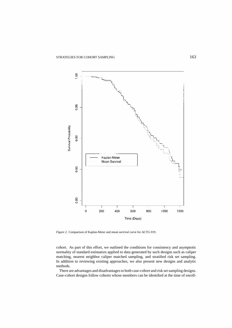
Because the WCR approach provides estimates of the effect of CD4+ count at baseline,we can also estimate the baseline hazard and survival curves for any given set of covariatevalues. Figure 1 shows the estimated survival curves for subjects with median values ofbaseline CD4+ count andβ2-microglobulin, and different values of change from baselineto week 8 for those measurements. In the figure, quantiles are defined in terms of positiveeffect on survival (i.e., the 25% percentile ofβ2-microglobulin is one-quarter of the wayfrom the worst, or highest, to the best value). These curves show a surprising result that theβ2-microglobulin response to therapy seems to explain at least as much of the variability intime to clinical event as does the CD4 response. The analysis method used by Jacobsonet al.(1995) precluded the estimation of survival curves such as these. To validate our methods,we compute the mean estimated survival curve, averaging over observed covariates, and


Figure 1. Kaplan-Meier survival curve and survival curve estimates for various percentiles of CD4+ count andβ2-microglobulin response at week 8 for ACTG 019.

compare it to the Kaplan-Meier curve in Figure 2. Their close agreement suggest that themodels are appropriate.

6. Discussion

This paper provides a review of methods for sampling from cohorts to determine the addi-tional predictive value of a covariate, after controlling for covariates available on the entire


Figure 2. Comparison of Kaplan-Meier and mean survival curve for ACTG 019.

cohort. As part of this effort, we outlined the conditions for consistency and asymptoticnormality of standard estimators applied to data generated by such designs such as calipermatching, nearest neighbor caliper matched sampling, and stratified risk set sampling.In addition to reviewing existing approaches, we also present new designs and analyticmethods.

There are advantages and disadvantages to both case-cohort and risk set sampling designs.Case-cohort designs follow cohorts whose members can be identified at the time of enroll-


ment into studies and may therefore be logistically simpler than the risk set based designs.In prospective case-cohort studies, individualized sampling probabilities must be based onresults of prior studies. Case-cohort designs also allow for estimation of survival curveswithout any additional modeling assumptions. On the other hand, for our study settings,matched risk set sampling is the most efficient method of estimation for the covariate ofprimary interest. For simple or stratified risk set sampling with a small number of strata,survival curve estimation can be done without additional assumptions. Matched risk setdesigns do have the important disadvantage that the probability of being sampled must beestimated to get survival curves and other quantities of potential interest. Estimation ofthese probabilities requires additional assumptions and can lead to bias in survival esti-mates. When appropriate models for estimating sampling probabilities exist, this designoffers great freedom in sampling strategies; for example one can sample as controls, sub-jects who never fail as opposed to subjects who are at risk at failure times. An advantageof the risk set sampling designs is that they arise naturally out of the Cox partial likelihoodand are therefore especially useful for analyzing data with time-varying covariates. If onlycurrent values are needed, these values can be ascertained at the time of failure for the caseand of selection for the control. With the case-cohort type designs, samples need to betaken at each failure time for every member of the selected sub-cohort.

Methods that use weighting can be sensitive to the extreme weight values. For example,when the matching covariate is a strong predictor, it will cause subjects whose covari-ate values predict low risk to be sampled infrequently and therefore have large associatedweights. For this reason, flexible regression models, which reduce the influence of outlyingobservations in weight estimation, seem to be the best approach. Although methods of cal-culating weights based on histograms or kernel densities do not require model assumptions,estimates based on such weights tend not to be robust, in part because of the tails of thecovariate distributions cannot be well estimated. An advantage to weighted estimators isthat they provide the ability to correct for missingness due to happenstance, although thisrequires an appropriate model for missingness.

For evaluating the proportional hazards assumption or covariate transformation, the usualdiagnostics should be applicable. Residuals can be obtained from fitting any of the abovemodels, and they should have similar properties. Methods of analysis when the proportionalhazards model does not hold have not been discussed. Risk set sampling methods resultin data that do not naturally lend themselves to analysis under other models, such as theaccelerated failure time or proportional odds models. On the other hand, we should be ableto weight the appropriate estimating equations for case-cohort data, just as we did for theCox score. Robustness and model misspecification issues also warrant additional study.

Because most current Cox regression software allow for the use of strata, offsets, andweights, all the methods discussed here can be fit using standard software. All Cox regres-sion parameters used here were estimated using S-plus software (StatSci Division Mathsoft,Inc., Seattle, WA).


Appendix

Large Sample Properties of Estimates Using the Conditional Logistic Likelihood forNearest Neighbor Caliper Matched Sampling Designs

We show that the pseudo likelihoodLm =∏n

i=1

{exp(β

′2Zi 2)∑

j∈R(Xi )exp(β

′2Zj 2)

}δi

provides consistent

and asymptotically normal estimates ofβ2. The proof uses notation and ideas from Gold-stein and Langholz (1992). Settingηi j (0) = 0, specifyηi j (t) =

∑k≥1 I { j ∈ Rk,i }I {Tk−1 <

t ≤ Tk}, whereTk are the ordered collection of event times forYi and Ni processes andRk,i is selected according to nearest neighbor caliper matching. Soηi j (t) is one during theintervalTk−1 < t ≤ Tk when individuali fails at timeTk and individualj is sampled as timeTk and zero otherwise. Note thatηi j (t) andRk,i specify the same sampling process. Define

E(β2, t) =∑n

i=1Yi (t)Zi 2 exp(β

′Zi )∑n

i=1Yi (t)exp(β

′Zi )

, Ei (β2, t) =∑n

j=1ηi j (t)Yj (t)Zj 2 exp(β

′2Zj 2)∑n

j=1ηi j (t)Yj (t)exp(β

′2Zj 2)

, andDi (β2, t) =∑n

j=1ηi j (t)Yj (t)Z

⊗2j 2 exp(β

′2Zj 2)∑n


′2Zj 2)

−(∑n


′2Zj 2)∑n


′2Zj 2)

)⊗2

. Let (Ä, F, P) be the probabil-

ity space that supports copies of a counting processN(t), a covariate processZ and anobservation processY(t). Proofs require regularity conditions described in detail by Gold-stein and Langholz (1992), which we briefly summarize:λo bounded away from 0 and∞;boundedZ; a positive definite conditional covariance matrix forZ given Y(t) = 1; leftcontinuity of processY(t) with only finitely many jumps on any bounded interval; inde-pendent and identically distributed processes(Z,Y(t)). Fix a timet and writeY(t) = Y.Let Gt = G, whereGt is a right continuous, nondecreasing family of subσ -algebras ofF(Fleming and Harrington, 1991). We require a new condition:

Condition 1. Z1 is absolutely continuous andfZ2|Z1=Zi 1,Y=1(z2)− fZ2|Z1=Zj 1,Y=1(z2)→ 0asZi 1− Zj 1→ 0 for all j ∈ Ri , whereRi is the sampled risk set wheni is the failure andZ2 6= g(Z1,Y) for any functiong(·).

After subjecti ’s failure time or change in risk status, we select as potential controls,m−1individuals withY(t) = 1 andZ1 values closest toZ1i within a fixed distancec. Absolutecontinuity of Z1 assures that there will be more thanm− 1 such individuals. AssumingCondition 1, there are no ties; conditional onG sampling is completely determined.

LEMMA 1 Let Ri be the m smallest values of|Zj 1 − Zi 1|, including the ith individualamong those at risk, and let P= {Ri , i = 1, . . . ,n}. With T ∈ P andρ ∈ {1, 2}, define

w(T) ={∑

j∈TZj 2 exp(β

′2Zj 2)∑

j∈Texp(β

′2Zj 2)

}⊗ρor w(T) =

∑j∈T

Z⊗ρj 2 exp(β′2Zj 2)∑

j∈Texp(β

′2Zj 2)

withw(∅) = 0. Ai is either

exp(β′0Zi ) or Zi 2 exp(β′0Zi ) whenρ = 1 and Ai = exp(β′0Zi ) whenρ = 2. Define

Sn = n−1n∑

i=1

w(Ri )Yi A′i . (A.1)


Under the conditions of Goldstein and Langholz (1992) and Condition 1, Sn →P q, where

q = E[

1m

∑i∈U Aiw(U )′

∣∣∣YU = 1], Zi 1 = ZU for i ∈ U, U = { j : Zj 2 ∼ fZ2|Z1=ZU ,Y=1

}and|U | = m.

Proof: Considerρ = 1,w(T) =∑

j∈TZj 2 exp(β

′2Zj 2)∑

j∈Texp(β

′2Zj 2)

, Ai = exp(β′0Zi ), andSn = n−1∑ni=1

w(Ri )Yi A′i . The other cases are similar.Let Sn,m be themth component ofSn. Conditional onG, Sn,m is the average ofn inde-

pendent random variables for allm. Letting Zm,max = max|Zm| andZmax be the vector ofZm,max values, we havew(T) bounded byZmax so

Var[Sn,m|G

] ≤ n−1n∑

i=1

E[Yi exp(2|β0|′Zmax)Z

2m,max | G

]which has limit zero asn→∞ since each summand is bounded. E[Sn|G] is the same asSn, because sampling is deterministic givenG.

Let Qn = n−1∑ni=1 Yi exp(β′0Zi )

∑j∈U Zj 2 exp(β

′2Zj 2)∑

j∈U exp(β′2Zj 2)

, where {Zj 2 ∼ fZ2|Z1=ZU ,Y=1 for

j ∈ U }. E[Sn|G] − Qn| is given by

n−1

∣∣∣∣∣ n∑i=1

Yi exp(β′0Zi )

[∑j∈Ri

Zj 2 exp(β′2Zj 2)∑j∈Ri

exp(β′2Zj 2)−∑

j∈U Zj 2 exp(β′2Zj 2)∑j∈U exp(β′2Zj 2)

]∣∣∣∣∣≤ n−1K

∣∣∣∣∣ n∑i=1

[∑j∈Ri

Zj 2 exp(β′2Zj 2)

][∑j∈U

exp(β′2Zj 2)

]

−[∑

j∈Ri

exp(β′2Zj 2)

][∑j∈U

Zj 2 exp(β′2Zj 2)

]∣∣∣∣∣,whereK = max

{[∑j∈Ri

exp(β′2Zj 2)] [∑

j∈U exp(β′2Zj 2)]/[Yi exp(β′0Zi )

]}−1which is

finite because covariates are bounded. Asn→ ∞, the components ofRi andU becomeidentically distributed, and the difference approaches zero. Thus var(Qn) hasO(n) finiteterms multiplied byn−2 and hence Var[Qn] → 0. SoQn converges to

E[Qn] = E

[Yi exp(β′0Zi )

∑j∈U Zj 2 exp(β′2Zj 2)∑


]

= E

[1

m

∑i∈U

Yi exp(β′0Zi )

∑j∈U Zj 2 exp(β′2Zj 2)∑


]= q.

COROLLARY 1 If β = β0, w(T) ={∑

j∈TZj 2 exp(β

′2Zj 2)∑

j∈Texp(β

′2Zj 2)

}, and Ai = exp(β′0Zi ), then

Sn →P E[Yj Zj 2 exp(β′0Zj )

].


Proof: We can rewriteQn

n−1n∑

i=1

∑j∈U

Zj 2 exp(β01Zi 1+ β′02Zj 2)Yi exp(β′02Zi 2)∑j∈U exp(β′02Zj 2)

= n−1n∑

i=1

∑j∈U

Zj 2 exp(β′0Zj )Yi exp(β′02Zi 2)∑j∈U exp(β′02Zj 2)

= n−1n∑

i=1

1

m

∑j∈U

Zj 2 exp(β′0Zj )

+ n−1n∑

i=1

∑j∈U

Zj 2 exp(β′0Zj )

[Yi exp(β′02Zi 2)∑j∈U exp(β′02Zj 2)

− 1

m

]. (A.2)

The first equality holds becauseZ j 1= ZU for all j ∈ U . Also,

n−1n∑

i=1

1

m

∑j∈U

Zj 2 exp(β′0Zj ) →P E

[1

m

∑j∈U

Zj 2 exp(β′0Zj )

]= E

[Yj Zj 2 exp(β′0Zj )

].

The second term in (A.2) can be written

n−1n∑

i=1

∑j∈U

Zj 2 exp(β′0Zj )

[Yi exp(β′02Zi 2)−m−1∑

j∈U exp(β′02Zj 2)∑j∈U exp(β′02Zj 2)

]

≤ K n−1∑ni=1

[Yi exp(β′02Zi 2)− 1

m

∑j∈U exp(β′02Zj 2)

]→P 0,

whereK = maxZ2 exp(β′0Z2)/exp(β′02Z2) <∞.

Consistency ofβ2:. Following Goldstein and Langholz (1992), we define the log likelihoodprocess by

C(β2, t) =n∑

i=1

∫ τ

0

[β′2Zi 2− log

{n∑

j=1

ηi j (s)Yj (s)exp(β′2Zj 2)

}]d Ni (s)

and the score process by

U(β2, t) =n∑

i=1

∫ t

0

[Zi 2− Ei (β2, t)

]d Ni (s). (A.3)

THEOREM1 Given sampling by nearest neighbor caliper matching, the regularity condi-tions of Goldstein and Langholz (1992) and Condition 1,β02→P β02.


Proof:. Let

X(β2, t) = n−1(C(β2, t)− C(β02, t))

= n−1n∑

i=1

∫ t

0

[(β2− β02)

′Zi 2

− log

{ ∑nj=1 ηi j (s)Yj (s)exp(β′2Zj 2)∑nj=1 ηi j (s)Yj (s)exp(β′02Zj 2)

}]d Ni (s)

and

A(β2, t) = n−1n∑

i=1

∫ t

0

[(β2− β02)

′Zi 2

− log

{ ∑nj=1 ηi j (s)Yj (s)exp(β′2Zj 2)∑nj=1 ηi j (s)Yj (s)exp(β′02Zj 2)

}]× Yi (s)exp(β′0Zi )λ0(s)ds.

X(β2, ·)− A(β2, ·) is a local square integrable martingale with quadratic variation

n−2n∑

i=1

∫ t

0

[(β2− β02)

′Zi 2− log

{∑nj=1 ηi j (s)Yj (s)exp(β′2Zj 2)∑nj=1 ηi j (s)Yj (s)exp(β′2Zj 2)

}]⊗2

× Yi (s)exp(β′0Zi )λ0(s)ds,

which converges to0 asn→∞ since the covariates are bounded. It follows thatX(β2, τ )

converges to the same limit asA(β2, τ ) by Lenglart’s inequality as in Andersen and Gill(1982).

∂A(β2, τ )

∂β2= n−1

n∑i=1

∫ τ

0

{Zi 2−

∑nj=1 ηi j (s)Yj (s)Zj 2 exp(β′2Zj 2)∑n

j=1 ηi j (s)Yj (s)exp(β′2Zj 2)

}× Yi (s)exp(β′0Zi )λ0(s)ds

=∫ τ

0

{n−1

n∑i=1

Zi 2 Yi (s)exp(β′0Zi )

− n−1n∑

i=1

∑nj=1 ηi j (s)Yj (s)Zj 2 exp(β′2Zj 2)∑n

j=1 ηi j (s)Yj (s)exp(β′2Zj 2)

Yi (s)exp(β′0Zi )

}λ0(s)ds,

which approaches zero atβ = β0 using Corollary 1. Also

∂2A(β2, τ )

∂β22

= −∫ τ

0n−1

n∑i=1

Di (β2, s)Yi (s) exp(β′0Zi )λ0(s)ds,


which is minus a non-negative definite matrix for everyβ2, sinceDi (β2, s) is the covariancematrix for a random variableZ with distribution

P(Z = Zj 2) = ηi j (t)Yj (s)exp(β′2Zj 2)∑nj=1 ηi j (t)Yj (s)exp(β′2Zj 2)

andYi (s)exp(β′0Zi )λ0(s) is non-negative. AssumingZ2|Z1,Y = 1 has a non-trivial dis-tribution, the second derivative converges to a negative definite matrix with probability 1.Soβ02→P β02 as in Andersen and Gill.

Asymptotic Normality ofβ02:. Definenn(β2, t) to be

nE

[∫ t

0

{∑j∈U Z⊗2

j 2 exp(β′2Zj 2)∑j∈U exp(β′2Zj 2)

−(∑

j∈U Zj 2 exp(β′2Zj 2)∑j∈U exp(β′2Zj 2)

)⊗2}

× 1

m

∑i∈U

exp(β′0Zi )λ0(s)ds∣∣∣YU = 1

],

andnn = nn(β02, τ ).

THEOREM2 Under nearest neighbor caliper matching and the regularity conditions ofGoldstein and Langholz (1992) and Condition 1, n1/2(β02− β02)⇒ N(0,−1

nn ).

Proof:. Taylor’s argument implies thatU(β02, τ )− U(β02, τ ) = −I (β∗2, τ )(β02− β02),

whereI (β2, t) =∑n

i=1

∫ τ0 Di (β2, t)d Ni (s), andβ∗2 is on the line segment betweenβ2

andβ02. BecauseU(β02, τ ) = 0, n−1/2U(β02, τ ) = n−1I (β∗2, τ )n1/2(β02 − β02). We

need only show thatn−1/2U(β02, τ )⇒ N(0,nn) and thatn−1I (β∗2, τ ) →P nn, with nn

positive definite. Write the normalized score process (A.3) as

n−1/2n∑

i=1

∫ t

0

[Zi 2− E(β2, s)

]d Ni (s)+n−1/2

n∑i=1

∫ t

0

[E(β2, s)− Ei (β2, s)

]d Ni (s)

= n−1/2n∑

i=1

∫ t

0

[Zi 2− E(β2, s)

]d Mi (s)

+ n−1/2n∑

i=1

∫ t

0

[E(β2, s)− Ei (β2, s)

]d Mi (s)

+ n−1/2n∑

i=1

∫ t

0

[E(β2, s)− Ei (β2, s)

]Yi (s)exp(β′0Zi )λ0(s)ds

= n−1/2n∑

i=1

∫ t

0

[Zi 2− Ei (β2, s)

]d Mi (s)

+ n−1/2n∑

i=1

∫ t

0

[E(β2, s)− Ei (β2, s)

]Yi (s)exp(β′0Zi )λ0(s)ds, (A.4)


where the first term of (A.4) has mean0 and quadratic variation

n−1n∑

i=1

∫ t

0

[Zi 2− Ei (β2, s)

]⊗2Yi (s)exp(β′0Zi )λ0(s)ds, (A.5)

Using Lemma 1, it is straightforward to show that (A.5) converges in probability tonn.The second term of (A.4) goes to zero using the arguments of Goldstein and Langholz(1992, pg 1917). Sinceβ02 is consistent, it suffices to show thatn−1I (β∗2, τ ) →P nn foranyβ∗2 →P β02. We have

n−1I (β02, t) = n−1n∑

i=1

∫ t

0Di (β02, s)d Mi (s)

+ n−1n∑

i=1

∫ t

0Di (β02, s)Yi (s)exp(β′0Zi )λ0(s)ds.

The first term is a local square integrable martingale with quadratic variation that convergesin probability to zero. Factoringλ0(s) out of the integrand of the second term,

n−1∑ni=1 Di (β02, s)Yi (s)exp(β′0Zi )

= n−1∑ni=1

∑n

j=1ηi j (t)Yj (t)Z

⊗2j 2 exp(β

′02Zj 2)∑n


′02Zj 2)

Yi (s)exp(β′0Zi )

− n−1∑ni=1

(∑n


′02Zj 2)∑n


′02Zj 2)

)⊗2

Yi (s)exp(β′0Zi ) (A.6)

Applying Lemma 1, the first term on the right converges to

E

[1

m

∑j∈U Z⊗2

j 2 exp(β′02Zj 2)∑j∈U exp(β′02Zj 2)

∑j∈U

exp(β′0Zj )

∣∣∣YU = 1

],

and the second term converges to

E

1

m

{∑j∈U Zj 2 exp(β′02Zj 2)∑


}⊗2∑j∈U

exp(β′0Zj )

∣∣∣YU = 1

.Hencen−1∑n

i=1

∫ τ0 Di (β02, s)d Ni (s) →P nn, which is positive definite.

Acknowledgments

Research supported by grants from the National Institutes of Health NIAID 1-R29-AI28905and NIAID 1-R01-A128076. The authors are grateful to Bryan Langholz for helpful com-ments.


References

P. K. Andersen and R. D. Gill, “Cox’s regression model for counting processes: A large sample study,”The Annalsof Statisticsvol. 10 pp. 1100–1120, 1982.

Ø. Borgan, L. Goldstein and B. Langholz, “Methods for the analysis of sampled cohort data in the Cox proportionalhazards model,”The Annals of Statisticsvol. 5 pp. 1749–1778, 1995.

Ø. Borgan and B. Langholz, “Nonparametric estimation of relative mortality from nested case-control studies,”Biometricsvol. 49 pp. 593–602, 1993.

R. G. Carpenter, “Matching when covariables are normally distributed,”Biometrikavol. 64 pp. 299–307, 1977.

W. G. Cochran and D. B. Rubin, “Controlling bias in observational studies: A review,”Sankhya-Series Avol. 35pp. 417–446, 1973.

D. R. Cox, “Regression models and life-tables (with discussion),”Journal of the Royal Statistical Society, SeriesB vol. 34 pp. 187–220, 1972.

T. R. Fleming and D. P. Harrington,Counting Processes and Survival Analysis, John Wiley & Sons, Inc.: NewYork, NY, 1991.

L. Goldstein and B. Langholz, “Asymptotic theory for nested case-control sampling in the Cox regression model,”The Annals of Statisticsvol. 20 pp. 1903–1928, 1992.

M. A. Jacobson, V. De Gruttola, M. Reddy, J. M. Arduino, S. Strickland, R. C. Reichman, J. A. Barlett, J. P. Phair,M. S. Hirsch, A. C. Collier, R. Soeiro and P. A. Volberding, “The predictive value of changes in serologic andcell markers of HIV activity for subsequent clinical outcome in patients with asymptomatic HIV disease treatedwith Zidovudine,”AIDSvol. 9 pp. 727–734, 1995.

J. D. Kalbfleisch and J. F. Lawless, “Likelihood analysis of multi-state models for disease incidence and mortality,”Statistics in Medicinevol. 7 pp. 149–160, 1988.

D. Y. Lin and L. J. Wei, “The robust inference for the Cox proportional hazards model,”Journal of the AmericanStatistical Associationvol. 84 pp. 1074–1078, 1989.

D. Y. Lin and Z. Ying, “Cox regression with incomplete covariate measurements,”Journal of the AmericanStatistical Associationvol. 88 pp. 1341–1349, 1993.

J. H. Lubin and M. H. Gail, “Biased selection of controls for case-control analyses of cohort studies,”Biometricsvol. 40 pp. 63–75, 1984.

N. Mantel, “Synthetic retrospective studies and related topics,”Biometricsvol. 29 pp. 479–486, 1973.

D. Oakes, “Survival times: Aspects of partial likelihood (with discussions),”International Statistical Reviewvol. 49 pp. 235–264, 1981.

R. L. Prentice, “On the design of synthetic case-control studies,”Biometricsvol. 42 pp. 301–310, 1986.

R. L. Prentice, “A case-cohort design for epidemiologic cohort studies and disease prevention trials,”Biometrikavol. 73 pp. 1–11, 1986.

M. Pugh, J. Robins, S. Lipsitz and D. Harrington, “Inference in the Cox proportional hazards model with missingcovariate data,”Technical Report, Harvard School of Public Health, Department of Biostatistics, 1994.

W. J. Raynor, Jr, “Caliper pair-matching on a continuous variable in case-control studies,”Communications inStatistics, Part A—Theory and Methodsvol. 12 pp. 1499–1509, 1983.

J. M. Robins, M. H. Gail and J. H. Lubin, “More on biased selection of controls for case-control cnalyses of cohortstudies,”Biometricsvol. 42 pp. 293–299, 1986.

J. M. Robins, R. L. Prentice and D. Blevins, “Designs for synthetic case-control studies in open cohorts,”Biometricsvol. 45 pp. 1103–1116, 1989.

J. Robins, A. Rotnitzky and L. P. Zhao, “Estimation of regression coefficients when some regressors are not alwaysobserved,”Journal of the American Statistical Associationvol. 89 pp. 846–866, 1994.

S. G. Self and R. L.Prentice, “Asymptotic distribution theory and efficiency results for case-cohort studies,”TheAnnals of Statisticsvol. 16 pp. 64–81, 1988.


D. C. Thomas, In appendix to F. D. K. Liddell, J. C. McDonald and D. C. Thomas, “Methods of cohort analysis:Appraisal by application to asbestos mining,”Journal of the Royal Statistical Society, Series Avol. 140 pp. 469–491, 1977.

A. Tsiatis, “A large sample study of Cox’s regression model,”The Annals of Statisticsvol. 9 pp. 93–108, 1981.

P. A. Volberding, S. W. Lagakos, M. A. Koch, C. Pettinelli, M. W. Myers, D. K. Booth, H. H. Balfour, R. C. Re-ichman, J. A. Bartlett, M. S. Hirsch, R. L. Murphy, W. D. Hardy, R. Soeiro, M. A. Fischl, J. G. Bartlett,T. C. Merigan, N. E. Hyslop, D. D. Richman, F. T. Valentine, L. Corey and The AIDS Clinical Trials Groupof the National Institute of Allergy and Infectious Diseases, “Zidovudine in asymptomatic human immunodefi-ciency virus infection, a controlled trial in persons with fewer than 500 CD4-positive cells per cubic millimeter,”The New England Journal of Medicinevol. 322 pp. 941–949, 1990.

Documents

Strategies for Cohort Sampling Under the Cox Proportional Hazards Model, Application to an AIDS Clinical Trial