Embed Size (px)
Citation preview

Strategies for Reliability Enhancement of Electrical
Distribution Systems
A Thesis submitted to Gujarat Technological University
for the Award of
Doctor of Philosophy
in
Electrical Engineering
By
Kela Kalpesh Bansidhar
Enrollment No. : 139997109005
under supervision of
Dr. Bhavik N. Suthar (Supervisor)
Dr. L D Arya (Co-supervisor)
GUJARAT TECHNOLOGICAL UNIVERSITY
AHMEDABAD
December 2018

iii
© Kela Kalpesh Bansidhar

iv
DECLARATION
I declare that the thesis entitled “Strategies for Reliability Enhancement of Electrical
Distribution Systems” submitted by me for the degree of Doctor of Philosophy, is the record
of research work carried out by me during the period from October 2013 to August 2018 under
the supervision of Dr. Bhavik N. Suthar, Professor & Head - Electrical Engineering
Department, Government Engineering College, Bhuj, and Dr. L D Arya , Sr. Professor-
Electrical Engineering Department, Medi-Caps University,Indore and this has not formed the
basis for the award of any degree, diploma, associateship , fellowship, titles in this or any other
University or other institution of higher learning.
I further declare that the material obtained from other sources has been duly acknowledged in
the thesis. I shall be solely responsible for any plagiarism or other irregularities, if noticed in the
thesis.
Signature of the Research Scholar: _____________________ Date:
Name of Research Scholar: Kela Kalpesh Bansidhar
Place: Ahmedabad.

v
CERTIFICATE
I certify that the work incorporated in the thesis titled as Strategies for Reliability
Enhancement of Electrical Distribution Systems submitted by Mr. Kela Kalpesh Bansidhar
was carried out by the candidate under our supervision/guidance. To the best of our knowledge:
(i) the candidate has not submitted the same research work to any other institution for any
degree/diploma, Associateship, Fellowship or other similar titles (ii) the thesis submitted is a
record of original research work done by the Research Scholar during the period of study under
our supervision, and (iii) the thesis represents independent research work on the part of the
Research Scholar.
Signature of Supervisor: Date:
Name of Supervisor: Dr. Bhavik N. Suthar
Place: Ahmedabad.
Name of Co-Supervisor: Dr. L D Arya Date:
Place: Indore

vi
Course-work Completion Certificate
This is to certify that Mr. Kela Kalpesh Bansidhar enrolment no 139997109005 is a PhD
scholar enrolled for PhD program in the branch Electrical of Gujarat Technological
University, Ahmedabad.
1 (Please tick the relevant option(s))
He/She has been exempted from the course-work (successfully completed during
M.Phil Course)
He/She has been exempted from Research Methodology Course only (successfully
completed during M.Phil Course)
He/She has successfully completed the PhD course work for the partial requirement
for the award of PhD Degree. His/ Her performance in the course work is as follows-
Grade Obtained in Research Methodology
(PH001)
Grade Obtained in Self Study Course (Core Subject)
(PH002)
BB AB
Supervisor’s Sign
Name of Supervisor: Dr. Bhavik N. Suthar
Co- Supervisor’s Sign
Name of Co-Supervisor: Dr. L D Arya
vii
Originality Report Certificate
It is certified that PhD Thesis titled Strategies for Reliability Enhancement of Electrical
Distribution Systems submitted by Mr. Kela Kalpesh Bansidhar has been examined by me. I
undertake the following:
a. Thesis has significant new work / knowledge as compared already published or are under
consideration to be published elsewhere. No sentence, equation, diagram, table, paragraph or
section has been copied verbatim from previous work unless it is placed under quotation marks
and duly referenced.
b. The work presented is original and own work of the author (i.e. there is no plagiarism). No ideas,
processes, results or words of others have been presented as Author own work.
c. There is no fabrication of data or results which have been compiled / analyzed.
d. There is no falsification by manipulating research materials, equipment or processes, or changing
or omitting data or results such that the research is not accurately represented in the research
record.
e. The thesis has been checked using https://turnitin.com (copy of originality report attached) and
found within limits as per GTU Plagiarism Policy and instructions issued from time to time (i.e.
permitted similarity index <=25%).
Signature of Research Scholar: …………….. Date:
Name of Research Scholar: Kela Kalpesh Bansidhar
Place: Ahmedabad
Signature of Supervisor: …………….. Date:
Name of Supervisor: Dr. Bhavik N Suthar
Place: Ahmedabad
Signature of Supervisor: …………….. Date:
Name of Co-Supervisor: Dr. L D Arya
Place: Indore

viii


ix
Ph. D. THESIS Non-Exclusive License to
GUJARAT TECHNOLOGICAL UNIVERSITY
In consideration of being a Ph. D. Research Scholar at GTU and in the interests of the facilitation
of research at GTU and elsewhere, I, Kela Kalpesh Bansidhar having Enrollment No.
139997109005 hereby grant a non-exclusive, royalty free and perpetual license to GTU on the
following terms:
a) GTU is permitted to archive, reproduce and distribute my thesis, in whole or in part, and/or my
abstract, in whole or in part ( referred to collectively as the “Work”) anywhere in the world, for
non-commercial purposes, in all forms of media;
b) GTU is permitted to authorize, sub-lease, sub-contract or procure any of the acts mentioned in
paragraph (a);
c) GTU is authorized to submit the Work at any National / International Library, under the authority
of their “Thesis Non-Exclusive License”;
d) The Universal Copyright Notice (©) shall appear on all copies made under the authority of this
license;
e) I undertake to submit my thesis, through my University, to any Library and Archives. Any
abstract submitted with the thesis will be considered to form part of the thesis.
f) I represent that my thesis is my original work, does not infringe any rights of others, including
privacy rights, and that I have the right to make the grant conferred by this non-exclusive license.
g) If third party copyrighted material was included in my thesis for which, under the terms of the
Copyright Act, written permission from the copyright owners is required, I have obtained such
permission from the copyright owners to do the acts mentioned in paragraph (a) above for the
full term of copyright protection.

x
h) I retain copyright ownership and moral rights in my thesis, and may deal with the copyright in
my thesis, in any way consistent with rights granted by me to my University in this non-exclusive
license.
i) I further promise to inform any person to whom I may hereafter assign or license my copyright
in my thesis of the rights granted by me to my University in this non- exclusive license.
j) I am aware of and agree to accept the conditions and regulations of PhD including all policy
matters related to authorship and plagiarism.
Signature of Research Scholar: Date:
Name of Research Scholar: Kela Kalpesh Bansidhar
Place: Ahmedabad
Signature of Supervisor: ………………... Date:
Name of Supervisor: Dr. Bhavik N. Suthar
Place: Ahmedabad
Seal:
Signature of Co-Supervisor: ………………... Date:
Name of Supervisor: Dr. L D Arya
Place:
Seal:

xi
(The panel must give justifications for rejecting the research work)
Thesis Approval Form
The viva-voce of the Ph.D. Thesis submitted by Shri Kela Kalpesh Bansidhar (Enrollment No.
139997109005) entitled Strategies for Reliability Enhancement of Electrical Distribution
Systems was conducted on …………………….., (day and date) at Gujarat Technological
University.
(Please tick any one of the following option)
The performance of the candidate was satisfactory. We recommend that he be awarded the PhD
degree.
Any further modifications in research work recommended by the panel after 3 months from the
date of first viva-voce upon request of the Supervisor or request of Independent Research Scholar
after which viva-voce can be re-conducted by the same panel again.
The performance of the candidate was unsatisfactory. We recommend that he should not be
awarded the Ph.D. degree.
--------------------------------------------------
Name and Signature of Supervisor with Seal
---------------------------------------------------
Name and Signature of Co-Supervisor
---------------------------------------------------
External Examiner -1 Name and Signature
--------------------------------------------------
External Examiner -2 Name and Signature
--------------------------------------------------
External Examiner -3 Name and Signature
(briefly specify the modifications suggested by the panel)

xii
Abstract
Different strategies to enhance reliability of electrical distribution system have been
proposed in this thesis. Reliability of distribution system has been improved considering
specified budget allocation. The primary and customer and energy based reliability indices
have been optimized subject to constraint of budget allocation. A balance between the utility
cost and cost incurred to the customers due to interruptions have been found maintaining the
required targets of reliability of the system. The optimum value of reliability with least
combined costs have been evaluated. Further, distributed generators (DGs) have been added
at certain load points. Optimum values of customer interruption costs, system maintenance
costs and additional costs on DGs have been found achieving the required enhancement in
reliability of the system. Proper locations of DGs keep significance in the enhancement of
reliability. Proper placements of DGs have been found in this thesis and then reliability of
the system has been optimized considering the above mentioned cost values. A cost-benefit
analysis has been made to verify the possibility of its execution. In the process of optimizing
reliability the additional costs have to be spent by any utility which can be justified by
rendering reward to it by the regulating authority. Optimized values of rewards have been
obtained considering customer interruption costs and costs on maintenance of the system.
This has been done attaining required reliability targets.Voltage sag at different load points
due to occurrence of symmetrical and unsymmetrical faults in the system may lead to
momentary or sustained interruption affecting the reliability of the system. The study of
power quality confined to voltage sag has been incorporated in the enhancement of
reliability. The developed algorithms have been applied on sample radial distribution system,
sample meshed distribution system and Roy Billinton Test System-Bus 2.The solutions to
these different strategies for reliability enhancement have been done by applying soft
computing techniques like Flower pollination, Teaching learning based optimization and
Differential evolution. Comparison has been made between the optimized results obtained
by them.

xiii
Acknowledgment
With due respect, I would like to express my sincere gratitude towards Dr. Bhavik N Suthar,
Professor and Head , Electrical Department, Government Engineering College, Bhuj ,who
has been supervising me for my PhD thesis . It would not have been possible for me to opt
for this study had he not provided me the platform to embark upon. His continuous support,
motivation and positive approach has made my journey possible to reach to its destination. I
foresee the same cooperation in my future pursuit.
I have deep sense of respect and gratitude for a learned teacher Dr. L D Arya, Senior
Professor, Electrical Department, Medi-Caps University, Indore, who has been my co-
supervisor for my PhD work. He had been the ‘GURU’ of Professor Suthar as well as mine
during our respective tenure of post-graduation studies at S.G.S.I.T.S., Indore. He got me
introduced to a topic of reliability and its applications to power system during my post-
graduate studies and opened the doors for further studies by continuously inspiring me for
the same. I obsequiously owe to him, whatever meager I have achieved. Besides his
tremendous knowledge in his field, I have felt a human touch in him for the students. I expect
the same warmth and cooperation from him for the years to come.
I am highly thankful to my DPC members Dr. Sanjay R. Joshi, Principal, Government
Engineering College, Valsad and Dr. M C Chudasama , Professor and Head , Electrical
Department , L D College of Engineering ,Ahmedabad for their valuable suggestions and all
possible help.
I am very thankful to my institute and department for their kind support. I am thankful to
GTU V.C., Registrar, Controller of Examination and Ph.D. section for their kind support. I
extend my sincere gratitude to all those people who have helped me in achieving my
objective. I am also indebted to my colleagues who have helped me directly or indirectly
during my research work.

xiv
I am especially thankful to Dr. Rajesh Arya, a young researcher in the same area and son of
Dr. L D Arya, who has continuously helped me in abridging the gap due to physical distance
between me and my co-supervisor.
I would like to thank my whole family for their affection, prayer and continuous support
throughout my study.
I bow down to Almighty for giving me strength paving a right path for me.
Kalpesh B Kela

xv
Table of Contents
Abstract xii
Acknowledgement xiii
Table of contents xv
List of Abbreviations xviii
List of Symbols xix
List of Figures xxi
List of Tables xxiii
1 Introduction 1
1.1 General 1
1.1.2 Need of Reliability Evaluation of Distribution system 4
1.2 State of the Art 5
1.3 Motivation & Objectives 12
1.4 Outline of the thesis 14
2 Application of Metaheuristic Optimization Methods for Reliability
Enhancement of Electrical Distribution Systems based on AHP
16
2.1 Introduction 16
2.2 Indices Evaluation for Radial Distribution System 16
2.2.1 Basic Indices 16
2.3 Indices Evaluation for Meshed Distribution System 17
2.3.1 Approximate Relations for Evaluating Indices for Series and
Parallel configuration
18
2.4 Customer oriented and energy oriented indices 19
2.5 Problem Formulation 20
2.6 Analytic Hierarchical Process (AHP) 23
2.7 Solution Methodology using FP algorithm 24
2.8 Results and Discussions 27
2.8.1 Case-1 27
2.8.2 Case-2 27
2.8.3 Case-3 28
2.9 Conclusions 38

xvi
3 A Value Based Reliability Optimization of Electrical Distribution 39
Systems considering Expenditures on Maintenance and Customer
Interruptions
3.1 Introduction 39
3.2 Problem Formulation 40
3.3 Solution Methodology using FP algorithm 42
3.4 Results and Discussions 45
3.4.1 Distribution systems: Descriptions 45
3.5 Conclusions 60
4 Cost Benefit Analysis for Active Distribution Systems in Reliability 61
Enhancement
4.1 Introduction 61
4.2 Problem Formulation 62
4.2.1 Deciding locations of DGs 62
4.2.2 Connecting DGs as stand by units in the system 63
4.3 Cost-benefit analysis 66
4.4 Solution methodology 67
4.4.1 Finding the locations of DGs 67
4.4.2 Finding the optimized solution by FP 68
4.4.3 Doing cost-benefit analysis 69
4.5 Results and discussions 72
4.5.1 Distribution systems : Descriptions 72
4.6 Conclusions 86
5 Optimal Parameter Setting in Distribution System Reliability 87
Enhancement with Reward and Penalty
5.1 Introduction 87
5.2 Reward / Penalty Scheme (RPS) 88
5.2.1 Socio-economical perspectives of RPS 88
5.3 Problem formulation 89
5.4 Solution Methodology 94
5.5 Results and Discussions 97
5.5.1 Distribution systems: Descriptions 97
5.6 Conclusions 112

xvii
6 Reliability Performance Optimization of Radial Distribution System
Enhancing Power Quality Considering Voltage Sag
113
6.1 Introduction 113
6.2 Power Quality and Reliability Indices 115
6.3 Methodology for enhancing Reliability accounting Voltage Sag 115
6.3.1 Method to find out number of Voltage Sags and Interruptions 115
6.3.2 Problem Formulation for Optimization 116
6.4 Solution Methodology 119
6.5 Results and discussions 123
6.6 Conclusions 128
7 Conclusions and Guidelines for Future Work 129
7.1 General 129
7.2 Summary of important conclusions 130
7.3 Scope for further work 131
References 133
List of papers published/communicated 145
Appendix-A 146
Appendix-B 149
Appendix-C 153
Appendix-D 157
Appendix-E 159
Appendix-F 161

xviii
List of Abbreviations
AHP : Analytic hierarchical process
SAIFI : System average interruption frequency index
SAIDI : System average interruption duration index
CAIDI : Customer average interruption duration index
AENS : Average energy not supplied
EENS : Expected energy not supplied
CBUDGET : Cost of budget
CIC : Customer interruption cost
FP : Flower pollination
TLBO : Teaching learning based optimization
DE : Differential evolution
RBTS-2 : Roy Billinton Test System –Bus 2
DG : Distributed generation
CPV : Cumulative present value
RPS : Reward penalty scheme
PQ : Power quality
SARFI : System average RMS frequency index

xix
List of Symbols
λk, rk : failure rate and average repair time of kth distributor
segment respectively
Li : average load connected at ith load point
λsys,i : system failure rate at ith load point
Usys,i : system annual outage duration at ith load point
Ni : number of customers at load point i
Nc : total number of distributor segments
w1, w2, w3 and w4 : relative weightage given to the normalized values of
SAIFI, SAIDI , CAIDI and AENS
F : objective function
Cpk
: interruption cost of different distributor segments
(Rs./kW)
Rs. : Indian currency rupees
λk,min and rk,min : reachable minimum values of failure rate and repair time
of kth distributor segment
λk,max and rk,max : maximum allowable failure rate and repair time of kth
distributor segment
SAIFIt , SAIDIt ,
CAIDIt and AENSt
: target values of the respective indices
αK, βK : cost coefficients corresponding to failure rates and
repair time respectively
ADCOST : additional cost spent on DGs to purchase energy
EENSO : expected energy not supplied /year when DGs are not
connected
EENSD : expected energy not supplied/year when DGs are
connected
λdg : Failure rate of DG
rdg : average outage duration of DG
λsw : failure rate of the switch transferring load to the DG
s : switching time or service restoration time with DG

xx
X0 ij : jth parameter of Xi vector
Xj,min and Xj,max : lower and upper bounds on variable Xj
X(k) best
: the current best solution found among all solutions at the
current generation in FP
L : L´evy flight distribution step in FP
X(k) i
: solution vector at kth generation
X(k+1) i
: updated vector at kth generation
rand : random digit in the range [0,1]
R : reliability level of utility considering all customer and
energy based reliability indices
Ropt : socio-economical optimal reliability level
CRP : cost of reward/penalty to the utility
Cnetwork : total reliability cost of the network
Cutility total
: total reliability cost of utility
Csociety total
: total reliability cost of society
Nsag : total number of short duration of voltage deviation by all
possible fault events
NT : represents number of customers served from the section
of the system to be assessed
𝜆𝑘_𝑓𝑎𝑢𝑙𝑡 : fault rate of the 𝑘𝑡ℎ distributor segment
𝑁𝑖𝑛𝑡 : total number of annual interruptions per annum
SARFIt : target value of the index
𝛾𝑘 : cost coefficients corresponding to fault rates for re-
modified radial distribution system with DGs
λk_fault,max : Maximum allowable fault rate
λk_fault,min : reachable minimum values of fault rate

xxi
List of Figures
Fig. No. Title of the Figure Page No.
Fig.1.1 Hierarchical levels for reliability evaluation 2
Fig.2.1. Flow chart for solving the formulated problem in section 2.5 by
AHP & FP
26
Fig.3.1 Flow chart for solution of the problem formulated in section
3.2 by FP
44
Fig.3.2 Variation of Objective function (F) over number of generations
for sample radial system
54
Fig.3.3 Frequency distribution of the minimum values of objective
function (F) using FP for sample radial system
54
Fig.3.4 Frequency distribution of the minimum values of objective
function (F) using TLBO for sample radial system
55
Fig.3.5 Frequency distribution of the minimum values of objective
function (F) using DE for sample radial system
55
Fig.3.6 Variation of Objective function (F) over number of generations
for sample meshed system
56
Fig.3.7 Frequency distribution of the minimum values of objective
function (F) using FP for sample meshed system
56
Fig.3.8 Frequency distribution of the minimum values of objective
function (F) using TLBO for sample meshed system
57
Fig.3.9 Frequency distribution of the minimum values of objective
function (F) using DE for sample meshed system
57
Fig.3.10 Variation of Objective function (F) over number of generations
for RBTS-2
58
Fig.3.11 Frequency distribution of the minimum values of objective
function (F) using FP for RBTS-2
58
Fig.3.12 Frequency distribution of the minimum values of objective
function (F) using TLBO for RBTS-2
59
Fig.3.13 Frequency distribution of the minimum values of objective
function (F) using DE for RBTS-2
59
Fig.4.1 Flow chart for finding out the locations of DGs 70
Fig.4.2 Flow chart for enhancing reliability of distribution system
incorporating DGs by FP
71
Fig.5.1 The cost versus reliability depicting socio-economically
optimal reliability level
93
Fig.5.2 Different designs of RPS 93
Fig.5.3 Flow chart for the solution of the problem formulated in section
5.3 by FP
96

xxii
Fig.5.4 Impact of an optimal continuous RPS on different parameter
costs for sample radial distribution system
109
Fig.5.5 Impact of an optimal continuous RPS on different parameter
costs for sample meshed distribution system
110
Fig.5.6 Impact of an optimal continuous RPS on different parameter
costs for RBTS-2
111
Fig.6.1 Flow chart for the solution of the problem formulated in section
6.3.2 by FP
121
Fig.6.2 Re-modified Radial Distribution System with DG 122
Fig.A.1 Sample radial distribution system 146
Fig.A.2 Modified radial distribution system with DG 147
Fig.B.1 Sample Meshed Distribution System 149
Fig.B.2 Reliability logic diagram of the meshed distribution system 150
Fig.B.3 Modified Meshed Distribution System with DG 151
Fig.C.1 RBTS-2 153
Fig.C.2 Modified RBTS-2 with DG 154

xxiii
List of Tables
Table No. Title of the Table Page No.
Table 2.1 AHP Matrix 29
Table 2.2 Weightage Coefficients 29
Table 2.3 Control Parameters for FP, TLBO and DE for sample radial
network, meshed network and RBTS-2
29
Table 2.4 Optimized values of failure rates and repair times as obtained
by FP, TLBO and DE and corresponding cost incurred for
radial network
30
Table 2.5 Current and optimized reliability indices and corresponding
value of objective function for radial distribution system
30
Table 2.6 Statistical analysis of sample values of objective function for
radial network
31
Table 2.7 Sections involved in each block of Figure B.2 32
Table 2.8 Optimized values of failure rates and repair times as obtained
by FP, TLBO and DE and corresponding cost incurred for
meshed network
33
Table 2.9 Current and optimized reliability indices and corresponding
value of objective function for meshed distribution system
34
Table 2.10 Statistical analysis of sample values of objective function for
meshed network
35
Table 2.11 Optimized values of failure rates and repair times for RBTS-2
as obtained by FP, TLBO and DE
36
Table 2.12 Current and optimized reliability indices for RBTS-2 36
Table 2.13 Statistical analysis of sample values of objective function for
RBTS-2
37
Table 3.1 Interruption costs at load points for sample radial distribution
system
48
Table 3.2 Control Parameters for FP, TLBO and DE for sample radial
network, meshed network and RBTS-2
48
Table 3.3 Optimized values of failure rates and repair times as obtained
by FP, TLBO and DE for sample radial distribution system
48
Table 3.4 Current and optimized values of Objective function (F)
obtained by FP, TLBO and DE for radial distribution system
49
Table 3.5 Current and optimized reliability indices for radial distribution
system
49
Table 3.6 Interruption cost at load points for sample meshed network 49

xxiv
Table 3.7 Optimized values of failure rates and repair times as obtained
by FP, TLBO and DE and corresponding cost incurred for
meshed network
50
Table 3.8 Current and optimized values of Objective function (F)
obtained by FP, TLBO and DE for meshed distribution system
51
Table 3.9 Current and optimized reliability indices for meshed
distribution system
51
Table 3.10 Optimized values of failure rates and repair times for RBTS-2
as obtained by FP, TLBO and DE
52
Table 3.11 Current and optimized values of Objective function (F)
obtained by FP, TLBO and DE for RBTS-2
53
Table 3.12 Current and optimized reliability indices for RBTS-2 53
Table 4.1 Interruption costs at load points for sample radial distribution
system
75
Table 4.2 The parameter values without DG and with DG connected at
different load points of sample radial distribution system
75
Table 4.3 Ranking of the load points with reference to reliability
improvement from maximum to minimum for sample radial
distribution system
76
Table 4.4 Reliability with more than one generators connected
according to the load point ranking for sample radial
distribution system
76
Table 4.5 Control Parameters for FP, TLBO and DE for sample radial
distribution system, sample meshed distribution system and
RBTS-2
76
Table 4.6 Optimized values of failure rates and repair times for radial
system as obtained by FP, TLBO and DE
77
Table 4.7 Current and optimized values of Objective function (F)
obtained by FP, TLBO and DE for sample radial distribution
system
77
Table 4.8 Current and optimized reliability indices for sample radial
distribution system
77
Table 4.9 Cost-Benefit Analysis for sample radial distribution system 78
Table 4.10 Interruption cost at load points for sample meshed network 78
Table 4.11 The parameter values without DG and with DG connected at
different load points of meshed distribution system
78
Table 4.12 Ranking of the load points with reference to reliability
improvement from maximum to minimum for sample meshed
distribution system
79

xxv
Table 4.13 Reliability with more than one generators connected
according to the load point ranking for sample meshed
distribution system
79
Table 4.14 Optimized values of failure rates and repair times for the
sample meshed distribution system as obtained by FP, TLBO
and DE
80
Table 4.15 Current and optimized values of Objective function (F)
obtained by FP, TLBO and DE for sample meshed
distribution system
80
Table 4.16 Current and optimized reliability indices for sample meshed
distribution system
81
Table 4.17 Cost-Benefit Analysis for sample meshed distribution system 81
Table 4.18 The parameter values without DG and with DG connected at
different load points of RBTS-2
82
Table 4.19 Ranking of the load points with reference to reliability
improvement from maximum to minimum for RBTS-2
83
Table 4.20 Reliability with more than one generators connected
according to the load point ranking for RBTS-2
83
Table 4.21 Optimized values of failure rates and repair times for RBTS-2
as obtained by FP, TLBO and DE
84
Table 4.22 Current and optimized values of Objective function (F)
obtained by FP, TLBO and DE for RBTS-2
85
Table 4.23 Current and optimized reliability indices for RBTS-2 85
Table 4.24 Cost-Benefit Analysis for RBTS-2 85
Table 5.1 Interruption costs at load points for sample radial distribution
system
100
Table 5.2 Optimized values of overall reliability R and other parameters
for sample radial distribution system
100
Table 5.3 Current and optimized values of Objective function (F)
obtained by FP for sample radial distribution system
101
Table 5.4 Current and optimized reliability indices for sample radial
distribution system
101
Table 5.5 Optimal cost of network, utility and society considering the
impact of continuous RPS on utility for sample radial
distribution system
102
Table 5.6 Optimized values of failure rates and repair times for sample
radial distribution system as obtained by FP
102
Table 5.7 Interruption costs at load points for sample meshed
distribution system
103
Table 5.8 Optimized values of overall reliability R and other parameters
for sample meshed distribution system
103

xxvi
Table 5.9 Current and optimized values of Objective function (F)
obtained by FP for sample meshed distribution system
103
Table 5.10 Current and optimized reliability indices for sample meshed
distribution system
104
Table 5.11 Optimal cost of network, utility and society considering the
impact of continuous RPS on utility for sample meshed
distribution system
104
Table 5.12 Optimized values of failure rates and repair times for sample
meshed distribution system as obtained by FP
105
Table 5.13 Optimized values of overall reliability R and other parameters
for RBTS-2
105
Table 5.14 Current and optimized values of Objective function (F)
obtained by FP for RBTS-2
106
Table 5.15 Current and optimized reliability indices for RBTS-2 106
Table 5.16 Optimal cost of network, utility and society considering the
impact of continuous RPS on utility
107
Table 5.17 Optimized values of failure rates and repair times for RBTS-2
as obtained by FP
108
Table 6.1 System data for Sample Radial Distribution System 124
Table 6.2 Interruption costs at load points for sample radial distribution
system
124
Table 6.3 Weighting factors for different Voltage Sag Magnitude and
corresponding values of customer interruption cost (CIC)
124
Table 6.4 Cost coefficients αk, βk and 𝛾𝑘 for Radial Distribution System 124
Table 6.5 Control Parameters for FP, TLBO and DE 125
Table 6.6 Component reactance data 125
Table 6.7 Percentage of fault occurrence according to fault type 125
Table 6.8 Optimized values of failure rates for sample radial system as
obtained by DE, TLBO and FP
125
Table 6.9 Optimized values of fault rates for sample radial system as
obtained by DE, TLBO and FP
126
Table 6.10 Optimized values of repair times for sample radial system as
obtained by DE, TLBO and FP
126
Table 6.11 Current and optimized reliability and power quality indices
for sample radial system obtained by FP, TLBO and DE
126
Table 6.12 Current and optimized values of objective function (F) as
given by DE, TLBO and FP
127
Table A.1 Maximum allowable and minimum reachable values of failure
rates and repair times for sample radial distribution system
148

xxvii
Table A.2 Average load and number of customers at load points for
radial network
148
Table A.3 Cost coefficients 𝛼𝐾 and 𝛽𝐾 for radial network 148
Table B.1 Maximum allowable and minimum reachable values of failure
rates and repair times for sample meshed distribution system
152
Table B.2 Average load and number of customers at load points for
meshed network
152
Table B.3 Cost coefficients 𝛼𝐾 and 𝛽𝐾 for meshed network 152
Table C.1 Failure rates and average repair time of different components
of RBTS-2
154
Table C.2 Maximum allowable and minimum reachable values of failure
rates and repair times for RBTS-2
155
Table C.3 Cost coefficients 𝛼𝐾 and 𝛽𝐾 for RBTS-2 156
Table C.4 Customer data for RBTS-2 156

CHAPTER 1
Introduction
1.1 General:
Electric power systems are extremely complex due to physical size, widely dispersed
geography, national and international interconnections, and many other reasons. The
function of an electric power system is to satisfy the load requirement of the system with
proper maintenance of continuity and quality of service. The ability of the system to provide
electricity adequately is usually termed as reliability. The concept of power system reliability
is quite broad and contains various aspects of its ability to satisfy the requirements of
customers. Earlier prior to 1945, deterministic criteria were used for solving reliability
design problems [1, 2].
As the the primary emphasis has been on providing a reliable and economic supply of
electrical energy to customers, spare or redundant capacities in generation and network
facilities have been inbuilt in order to ensure adequate and acceptable continuity of supply
in the event of failures and forced outages of plant, and the removal of facilities for regular
scheduled maintenance. Along with redundancy, it has to be ensured that the supply should
be as economic as possible [3]. The probability of discontinuity of supply to consumers may
be reduced by increased investment during planning phase. Economic and reliability
constraints are competitive and may lead to difficult optimization problems at both the
planning and operating phases.
As system behavior is stochastic in nature, it is logical to consider the assessment of such
systems based on techniques that respond to this behavior (i.e., probabilistic techniques) [1,
2]. But, it is a fact that most of the present planning, design, and operational criteria are
based on deterministic techniques. However, use of probabilistic approach can be justified
in a way that more objective assessment in to the decision making process can be made by
it.
Power system reliability indices can be calculated using two main approaches which are
analytical and simulation. Analytical techniques represent the system by a mathematical
model and evaluate the reliability indices from this model using direct numerical solutions.
1

Introduction
As frequent assumptions are required to simplify the problem and to produce analytical
model, it sometimes loses some or much of its significance. When complex operating
systems are to be modeled it is utilized. In such situations, simulation techniques are
important. They estimate the reliability indices by simulating the actual process and random
behavior of the system therefore treating the problem as a series of real experiments,
theoretically taking into account virtually all aspects and contingencies inherent in the
planning, design, and operation of a power system.
Due to its large size and complexity, power system cannot be analyzed completely as a single
entity. But this problem can be solved by dividing it in to appropriate subsystems and then
analyzed them separately. Electric power system may be divided into functional zones of (i)
generation (ii) transmission and (iii) distribution. These zones have been combined to give
three hierarchical levels for reliability assignment as shown in Fig-1.1 [4]. The concept of
hierarchical levels (HL) has been developed in order to establish a consistent means of
identifying and grouping these functional zones.
The first level [HL I] relates to generation facility, the second level [HL II] involves
generation and transmission facilities and third level [HL III] refers to the complete system
including distribution network.
Generation
facilities
Transmission
facilities
Distribution
facilities
Hierarchical level I
HL I
Hierarchical level II
HL II
Fig-1.1 Hierarchical levels for reliability evaluation
Hierarchical level III
HL III
2

General
The first level [HL I] relates to generation facility, the second level [HL II] involves
generation and transmission facilities and third level [HL III] refers to the complete system
including distribution network.
The HL structure implies that all generation delivers energy through the transmission system.
Whereas now a days significant role is played by an increasingly amount of individually
small scale generation embedded or distributed within distribution system also. This affects
voltage profile and improves reliability and security of power system. The economical
operation of conventional generation may be affected by this. An optimum co-ordination are
required to be established between distributed generations (DG) and centrally located
conventional generators. Reliability of combined generation as well as transmission system
[HL II] in a single problem formulation have been evaluated by many researchers.
Evaluation of combined reliability of generation, transmission and distribution system using
in a single problem formulation [HLIII] is impractical. Reliability studies of distribution
systems are usually done separately since (i) distribution networks are connected to
transmission system through one supply point and load point indices evaluated may be used
to evaluate reliability indices if needed and (ii) 80% interruptions or unavailability of supply
are observed at distribution side[1,2].
The outages occurring in the system not only impact the revenue economy of the system but
also affects the customers in terms of interruption costs at their ends. In order to reduce the
frequency and duration of these events it becomes necessary to increase investment either in
the better design, operation or both of the system. In other words, reliability of the system is
required to be improved considering costs in mind as reliability and economics play a major
role in decision making. Thus, economics is an extremely important issue/constraint for
deciding threshold values of reliability indices. Acceptable reliability goals can be achieved
by enhanced investments. In order to perform cost-benefit analysis of any objective,
reliability and economics both must be considered together. Reliability improvement is an
important issue to be focussed upon not only while designing and planning phase but also
during operation phase also. During operational phase of a system reliability is improved by
preventive maintenance. It can be executed by trained personnel of the specific area. By
replacing components of the system at specific intervals, it can be improved further. Various
incentive schemes are provided by power companies to the field workers to reduce failure
rates and average repair times of the components. This in turn enhances the reliability
indices. Cost keeps a significant consideration in operational reliability optimization of
3

Introduction
power network. By associating cost values to the ‘reliabilities’ of the system components it
is possible to obtain optimum values of various parameters which provides desired values of
reliability with minimum cost functions. A relation between cost of improvement and
reliability may be obtained. From actual data cost function can be formulated. Past
experience is of great significance for having a reliability growth program wherein the cost
associated with each stage of improvement is quantified. Thus complete consideration of
reliability economics includes two aspects known as ‘reliability cost’ and ‘reliability worth’.
Reliability cost is the amount spent in achieving certain level of reliability. Reliability worth
is the monetary benefits or gain derived by the supplier and customers from that investment.
It is the cost associated with the outages at various levels. Reliability optimization can be
done keeping balance between the two at minimum value of cost function. Reliability worth
assessment is an important function of reliability studies at all levels [5,6,7].
1.1.2 Need of Reliability Evaluation of Distribution system:
Distribution systems are the final link between generation sides and end users. But over the
past few decades, they have been paid considerably less attention in terms of reliability
modeling and evaluation than the generation side since the later are individually very capital
intensive and inadequacy in supply may cause a widespread catastrophic impact both on
the society and environment. Consequently great emphasis have been given on them to
ensure adequacy in supply and meeting the requirements of this part of power system. As a
distribution system is relatively cheap and its outages have more or less localized impact, it
has been paid less attention in regards to the quantitative assessment of the adequacy of
various alternative designs and reinforcements. Contrarily, analysis from various utilities
regarding customer failure statistics shows that almost 80% of the interruptions are
contributed by distribution systems[2]. Most of such system are radial and the system is
exposed to adverse environmental conditions. Hence distribution systems are prone to have
higher frequency of failure and lengthy outage durations.
Distribution systems are currently exploring use of distributed generation (DG) that are
integrated within distribution network. DGs of various capacities may be installed at utility
locations throughout the distribution system to meet various needs e.g. loss reduction, power
quality improvement, transmission and distribution expansion deferral, transformer bank
relief etc. These may serve as standby power and thus useful for reliability improvement of
distribution systems [8]. Due to the presence of DGs, the distribution system has become a
mini composite system requiring analysis similar to [HL II]. The DGs are frequently
4

State of the Art
disconnected from the supply but still connected with the consumers. At that point, it is
important to make a decision that whether they must be continued supplying load from
reliability point of view or must be tripped from safety point of view. From reliability
consideration point of view, DGs are classified as (i) which can not operate without main
source of supply and (ii) which can be operated independently. Certain DGs like
photovoltaic produce real power only. Synchronous condenser type DGs provide only
reactive power. DGs like wind power provide real power but consumes reactive power from
the supply source [9]. Research efforts have been made to reduce unsupplied energy to the
consumers via distribution network. The methodologies used so far regarding reliability
enhancement of distribution systems are (i) reduction in section lengths by adding new
substations (ii) automatic reconfiguration of network to provide alternate paths (iii) using
insulated overhead lines or underground cables (iv) intensifying fault avoidance and
corrective repair methods [10,11,12,13,14].
The purpose of investigation is to develop computationally efficient algorithms for reliability
optimization of distribution systems. In the proposed work different strategies have been
adopted to enhance reliability of distribution systems. Enormous literature is available in this
area. The next section briefly discusses regarding literature survey concerned with this
thesis.
1.2 State of the Art
Considerable change is occurring in the structure and operation of electric power system
throughout the world. It is required to study these changes, the forces creating them and the
possible reliability issues associated with them. This thesis proposes the enhancement of
reliability of a radial and meshed distribution systems by different strategies and the
methodology to be adopted in optimizing it. In reliability evaluation, various methods have
been presented so far in the literature [15,16,17,18]. In its early stage, a methodology known
as gradient projection method was developed for evaluating optimal reliability indices for
distribution system [19]. Reliability issues in the prevailing electric power utility
environment considering the uncertainties associated with deregulation, wheeling and
transmission access and disintegration of the distribution systems have been discussed by
Billinton et al. [20] .
Pinheiro et al.[21] probed into the new IEEE Reliability Test System(RTS-96). A set of
investigations about the bulk reliability performance evaluation of (RTS-96) are presented in
the paper. Several bulk reliability system indices representing a hierarchical level two (HL-
5

Introduction
II) assessment of the new system are provided. This test system permits comparative and
benchmark studies to be performed on new and existing reliability evaluation techniques. It
was developed by modifying and updating the original IEEE RTS (referred to as RTS-79)
to reflect changes in evaluation methodologies and to overcome perceived deficiencies [22].
In [23], an algorithm was developed by the researchers to obtain an optimal solution by
considering a nonlinear objective function with both linear and nonlinear constraints for a
large scale radial distribution system. In [13], an evolutionary algorithm was presented to
reliably design a distribution system using modified genetic algorithm for optimization.
Wang et al.[24] proposed an algorithm for assessing reliability indices of general
distribution system which presents a practical reliability assessment algorithm for
distribution systems of general network configurations. This algorithm is an extension of the
analytical simulation approach for radial distribution systems. Amjady et al.[25] published
paper on optimal reliable operation of hydrothermal power systems with random unit
outages in which, a new model for long term operation of hydrothermal power systems is
introduced and a method for obtaining an optimal solution is also developed. The objective
has been to minimize the total cost of the system as well as the expected interruption cost of
energy (EIC) during a given planning horizon. In [26], a composite reliability evaluation
model for different types of distribution systems was presented describing a set of composite
distribution system reliability evaluation models that can be applied to a non-radial type
system. The developed models reflect the effect of distribution substations, primary
distribution systems, and the interaction between them. Pedro et al. [27] presented a paper
in which a matured evolutionary –based application is used to search for the optimum trade
off between individual quality of service (QoS) and system reliability. Tradeoff results are
presented to compare the traditional with the modern regulation designs and also illustrated
that system optimum reliability must be decreased in order to improve individual quality at
constant investment. Reducing the overall cost and improving the reliability are two primary
but conflicting objectives for composite power system. Scheduling of appropriate preventive
maintenance requires optimization among multiple objectives. Yang and Chang [28]
developed an integrated methodology to achieve the mentioned objectives. A decomposed
approach for reliability design of a radial distribution system using PSO was presented in
[29]. A technique determining optimal interval for major maintenance activities in
distribution systems was given in [30]. In [31], authors proposed reliability enhancement of
distribution systems using sensitivity analysis. The paper describes a two stage methodology
for reliability enhancement using sensitivity analysis. The same authors developed a
6

State of the Art
technique for improving reliability indices of a radial distribution system in which a method
for optimum determination of failure rate and repair time for each component of a radial
distribution system is proposed. Here objective function is selected as to minimize the
increased cost which is a function of change in failure rate and repair time [32].Outages in
overhead distribution systems caused by different factors significantly impact their
reliability. A paper proposing a methodology for year-end analysis of animal-caused outages
in the past year has been presented by Gui et al. [33]. Vladimiro et al. [34] presented an
application of evolutionary particle swarm optimization (EPSO) based methods to evaluate
power system reliability. Here the results obtained with EPSO are compared to traditional
Monte Carlo simulation (MCS) and with other population based (PB) methods. Arya et al.
[35] proposed an algorithm for modifying failure rate and repair time of a distributor segment
considering the outage due to overloading and repair time omission, here termed as repair
tolerance time. This methodology has been implemented on a meshed distribution network.
The same authors have described a method for reliability optimization of radial distribution
systems by applying differential evolution. Penalty cost functions have been constructed.
They are functions of failure rates and repair times. Constraints on customer and energy
based indices have been considered. [36]. For overhead distribution systems, the reliability
of covered overhead line could considerably be improved using various alternative methods.
Li et al. [37] has applied the Monte Carlo simulation (MCS) to obtain reliability and safety
indices for a distribution system.
Arya et al. [38] have described a methodology for reliability assessment of electrical
distribution system accounting random repair time omission for each section. R. Arya et al.
[39] have described an algorithm for optimum modifications for failure rate and repair time
for a radial electrical distribution system. Coordinated aggregation based particle swarm
optimization (CAPSO) has been used for optimization. The same authors [40] have
described an analytical methodology for reliability evaluation and enhancement of
distribution system having distributed generation (DG). In this paper, standby mode of
operation of DG has been considered for this purpose. In [41], authors used Monte Carlo
simulation (MCS) along with PSO for reliability planning of power network in terms of
forced outage rate (FOR) allocation. In [42], authors used PSO for multi objective planning
and redundancy allocation. Distribution reliability indices neglecting random interruption
duration have been found in [43]. The algorithm is based on smooth boot strapping
technique along with Monte Carlo simulation (MCS). In [44], authors presented an efficient
Genetic Algorithms (GAs) based method to improve the reliability and power quality of
7

Introduction
distribution systems using network reconfiguration. Reliability centred maintenance
optimization for distribution systems has been presented in [45]. Bakkiyaraj et al. [46] have
given optimal reliability enhancement model by applying population based natural
computational optimization algorithms. Hashemi-Dezaki et al. [47] have proposed a novel
approach of internal loops (ILs) to optimize electrical distribution system reliability. Li Duan
et al. [48] have presented a method for the reconfiguration of distribution network for loss
reduction and reliability improvement by enhanced genetic algorithm. Yssaad et al. [49]
have presented a new rational reliability centred maintenance optimization method for power
distribution system.
As the electricity selling market has started becoming competitive, it is a challenging task
for any utility to provide qualitative service to the customers keeping the cost on its operation
and maintenance such as to provide low cost services to them. The optimum value of system
reliability with least combined cost thus found may lead towards value based reliability
planning of distribution systems [50]. Cossi et al. [51] gave a formulation regarding planning
of primary distribution networks considering the reliability costs obtained by calculating the
non-supplied energy due to the repairing and switching operations. Kahrobaee and
Asgarpoor [52] have determined the optimum standby electricity storage capacity in a smart
grid based on reliability indices such as Expected Interruption Cost (EIC) using particle
swarm optimization. Beni et al. [53] presented a practical method to estimate customer
damage function (CDF) which describes relationship between interruption duration and its
customer economic losses due to interruptions. Nelson and Lankutis [54] presented a method
to quantify the costs associated with interruptions of service to customers of electric utilities.
Schellenberg et al. [55] developed an Interruption Cost Estimate (ICE) calculator, a tool
designed for electric reliability planners at utilities, government organizations or other
entities that are interested in estimating interruption costs and/or the benefits associated with
reliability improvements. Tsao et al. [56] presented a value based reliability assessment
considering different topologies for planning a new distribution system based on comparison
of the distribution system reliability cost/worth analysis for different planning topologies.
Sonvane and Kushare [57] have increased reliability of distribution system by placing
capacitors in proper way. An optimized balance between the costs of reliability and capacitor
bank has been found in this paper. Narimani et al. [58] have presented an algorithm to
reconfigure distribution feeder considering reliability, loss and operational cost by applying
Enhanced Gravitational Search Algorithm (EGSA). Bakkiyaraj and Kumarappan [59] have
given optimal reliability enhancement model of electrical distribution system based on the
8

State of the Art
trade-off between the investments required for improving reliability and reduction in the
costs of power interruptions applying natural computational algorithms. The optimal
locations of distributed static series compensator (DSSC) to enhance the power system
reliability by reducing expected damage cost (EDC) have been found by Ghamsari et al.
[60]. An algorithm for reliability optimization of power distribution systems considering cost
minimization has been given by Banerjee et al.[61]. Ghosh and Kumar [62] have given a
methodology for feeder reconfiguration considering overall system cost and reliability
incorporating both primary and secondary power distribution systems. Küfeoğlu and
Lehtonen [63] have given a review summarizing the academic work done in the fields of
worth of electric power reliability and customer interruption costs assessment techniques
from the year 1990 to 2015. Lei Sun et al.[64] presented a smart substation allocation
model to determine the optimal number and allocation of smart substations in a given
distribution system with the upgrade costs of substations and the interruption costs of
customers taken into account considering reliability criterion.
Distributed generations (DGs) are becoming the best alternatives for power distribution
companies to increase reliability of distribution systems. DGs enhance performance of the
systems by improving reliability, voltage profile and reducing losses of the system. In recent
years, many researchers have worked to enhance reliability of distribution systems
employing DG. Yousefian and Monsef [65] have proposed a method to determine best
locations of DGs based on reliability indices using sequential Monte Carlo simulation. In
[66] authors have assessed the impact of conventional and renewable distributed generation
(DG) on the reliability of distribution system. An integrated Markov model which
incorporates the DG adequacy in terms of transition, DG mechanical failure and starting and
switching probability have been used for the DG reliability assessment. Awad et al.[67] have
proposed a methodology for allocating dispatchable distributed generation units in
distribution systems to improve system reliability economically. An optimized balance has
been obtained between the cost on installation and operation of DGs and the amount to be
paid worth of reliability by the customers in the research. Kumar et al.[68] have presented
optimal placement and sizing of multiple distributed generators to achieve higher system
reliability in large-scale primary distribution networks using a random search algorithm
known as cat swarm optimization. Abbasi and Hosseini [69] have studied the effect of
distribution network reconfiguration, size and allocation of DGs in the presence of storage
system on the reliability improvement of the system. Bagheri et al. [70] have proposed
9

Introduction
distribution network expansion planning incorporating DGs in an integrated way considering
reliability also as one of the aspects. Battu et al. [71] have given solution for optimal
locations of DGs in the distribution system for reliability improvement considering total cost
of of power consumed by the system. Arya [72] has presented a methodology for evaluating
customer and energy oriented reliability indices for distribution systems in the presence of
distributed generations, considering the effect of omission of random tolerable interruption
durations at load points. It has been done using Bootstrapping technique. In [73] authors
have found optimum value of primary reliability indices with and without DGs incorporated
in the distribution system. This has been done with differential search algorithm. Kansal et
al. [74] have found optimal allocations of DGs in distribution system considering
maximization of profit. In [75] authors have made DG scheduling maximizing reliability of
the system. A cost-benefit analysis is made here considering various costs involved in the
calculations.
Due to introduction of restructuring in power systems, service quality regulation has become
very important in distribution system. A reward and penalty scheme (RPS) regulates and
ensures the service reliability. It is a financial tool implemented by regulator to maintain
service reliability. A reward and penalty scheme (RPS) penalizes the distribution company
for poor reliability and rewards it for better one in performance based regulation (PBR). In
performance based regulations incentives are decided for strong efficiency (in terms of
profit) by the companies. In RPS financial incentives are created for distribution companies
to maintain or change their quality level. The regulator tries to maintain socioeconomically
optimum reliability level which minimizes the total reliability cost for society with RPS [76].
The concept of using reliability indices in RPS was discussed in [77].In [78] different
reward- penalty models using real system reliability data from Tehran Regional Electrical
Company had been applied presenting their applications and properties. An approach for
improving service reliability of distribution system with RPS integrated with clustering
analysis was presented in [79]. Here the utilities are categorized and the performance of
utilities in one cluster has been compared with the other members of same cluster. The effect
of system reliability improvement on the financial risk due to RPS has been mentioned in
[80]. In [81] main requirements for designing and implementing of an effective RPS have
been investigated. Here different types of RPS have been described comprehensively. In [82]
an algorithm is presented to obtain the parameters of RPS for each electric company by using
data envelopment analysis (DEA) and fuzzy c-means clustering (FCM) based on system
10
State of the Art
average interruption duration index. In [83] a method was proposed to not only motivate the
utilities to improve their service reliability but equalize the total rewards paid and total
penalties received by the regulators. In [84] a method for designing procedure for
reward/penalty scheme based on the concept of Yardstick theory has been proposed.
A modern electric power system must be designed such as to supply acceptable levels of
electrical energy to customers. Voltage sags are simple power quality disturbance events
which may cause considerable economic losses because industrial processes rely on
electronic power-control devices. Thus, the power supplied to utilities must be reliable
having good quality. In [85] authors have discussed impact of distributed generation on
reliability and power quality indices. Voltage sag mitigation and reliability improvement by
the network reconfiguration of utility power system has been discussed in [86]. An analytical
method for evaluating the voltage sag performance of a distribution network has been
discussed in [87]. The report [88] describes the relation between distributed generation and
power quality. The direct impact of increased wind power penetration on power quality and
reliability of distribution network has been focussed here. The authors in [89] have applied
an evolutionary-based approach for multi-objective reconfiguration in electrical power
distribution networks for improving power quality indicators like power system’s losses and
reliability indices. Here the micro genetic algorithm (mGA) is used to handle the
reconfiguration problem as a multi-objective optimization problem. In [90], a method for
improving bus voltage magnitude during voltage sag by applying network reconfiguration
to the exposed weak area in distribution systems is presented. In [91] authors have addressed
to enhance power quality issues such as harmonics and voltage sags while mitigating power
losses by applying network reconfiguration . It has been solved using a complicated
combinatorial optimization where best switching options are optimized. Based on the failure
modes and effects analysis framework (FMEA), the paper [92] has presented a non-
sequential Monte Carlo method (FMEA-NSMC) for distribution system reliability
assessment considering sustained interruptions, momentary interruptions and voltage sags.
In the paper [93], an optimization method is proposed to find the optimal and simultaneous
place and capacity of the DG units to reduce losses and to improve voltage profile of IEEE
30 bus test system calculated with and without DG placement. A Genetic Algorithms based
method has been presented in [94] to improve reliability and power quality of distribution
systems using network reconfiguration. Various power quality and reliability objectives such
as feeder power loss, system’s node voltage deviation, system’s average interruption
11
Introduction
frequency index, average interruption unavailability index and energy not supplied are
considered in a single objective function. Reliability and power quality have been improved
in [95] by minimizing the number of voltage sags (Nsag) propagated and other reliability
indices such as the average system interruption frequency index, sustained average
interruption frequency index, and momentary average interruption frequency index
employing optimum network reconfiguration. In [93] a new method using particle swarm
optimization has been proposed to considerably reduce the total power loss in the system
and improved voltage profiles of the buses and reliability indices. It has been done by
employing optimum location, size and number of distributed generations. The paper [96] has
presented a review of the main power quality (PQ) problems with their associated causes
and solutions with codes and standards. D-STATCOM has been used in [97] for voltage sag
and swell mitigation in renewable energy based distributed generation systems. In [98] it has
been shown to identify the power quality issues and the impact of DG or other non-linear
loads on LV distribution networks aiming to develop an equipment able to remove or
mitigate all electromagnetic disturbances considering the characteristics and sensitivity of
end use equipment within customer facilities.
1.3 Motivation & Objectives
It has been observed from literature survey that limited work has been done on the
development of quantitative technique for distribution system reliability evaluation and
enhancement. As distribution system being final link between transmission network and
ultimate customers, it is one of the most important parts of the power system. Due to less
cost and localized effect of outages on it compared to transmission network, it has been given
less importance. But the statistical data in technical reports show that more than 80% of all
customer interruptions occur due to failure/outage in distribution systems only. This requires
the distribution system to be adequately reliable and the need to evaluate its reliability.
Several other aspects are also considered which show the need to evaluate the reliability of
distribution systems. A given reinforcements scheme may be relatively inexpensive but large
sums of money are expanded collectively on such system. It is also necessary to ensure
balance in the reliability of generation, transmission and distribution. Another important
point of consideration is to select an option for reliability improvement among the number
of alternatives available. To achieve this, various methodologies have been developed by
researchers for reliability evaluation of distribution system.
12

Motivation & Objectives
In view of the above mentioned work done by various researchers in the evaluation and
enhancement of distribution system reliability so far, this thesis too covers the work in the
same line. In this thesis, reliability enhancement is done on a sample radial [31] and mesh
distribution [13] network and Roy Billinton Test System (RBTS-2) [99]. The motivation in
the present work is to develop computationally efficient algorithm for reliability
optimization using soft computing techniques [100,101,102]. Literature survey reveals
deficiency in the following aspect of reliability studies of distribution systems.
(i) Limited research efforts have been made in the area of distribution system
reliability enhancement.
(ii) Inclusion of DG for reliability enhancement. Location of DGs from reliability
point of view. The effects of DG need to be incorporated in optimization
algorithm.
(iii) Inclusion of reward/penalty studies in an optimization algorithm.
(iv) Effect of voltage sag on reliability studies and its inclusion in an optimization
algorithm.
The objectives of the proposed research work in this thesis are as follows.
I. Defining different methodologies by which reliability of electrical distribution
systems can be enhanced.
II. Improvement in reliability indices below their target values considering the budget
allocated to achieve the same by developing an algorithm embedding metaheuristic
optimization techniques.
III. Developing an algorithm to enhance reliability of the distribution system by
achieving proper balance between the cost incurred on customers due to interruptions
and the utility cost to achieve the desired reliability targets.
IV. Enhancing reliability by placing DGs at various locations. Deciding locations of DGs
from the point of view of enhancing reliability optimally by developing
methodologies for both the tasks.
V. Incorporating reward/penalty imposed to the utility for achieving reliability targets
below/above certain target values. Deciding the optimum value of reward/penalty
corresponding to achieving the desired reliability targets.
13

Introduction
VI. Assessment and enhancement of reliability of distribution system considering power
quality (PQ) disturbance events, such as voltage sags for different kind of faults in
the system.
In all the objectives mentioned above, optimized values of primary as well as customer and
energy oriented reliability indices [103] are to be found so as to set targets for distribution
companies for achieving them.
1.4. Outline of the thesis
The thesis includes the work done organised in the following way.
Chapter - 1 presents a critical survey of the past works concerning power system reliability
and clearly spells out the motivations and objectives of the research work carried out in this
thesis.
Chapter – 2 describes a computationally efficient algorithm for reliability optimization of
sample radial distribution system, meshed distribution system and RBTS-2 modifying the
values of the two decision variables (failure rate and repair time) of different section of the
distribution systems. Here optimization has been done considering the constraint of allocated
budget to enhance reliability. As customer and energy based reliability indices are in terms
of primary indices, they too are optimized. The optimization has been done by flower
pollination (FP) [101], teaching learning based optimization (TLBO) [102] and differential
evolution (DE) [103]. The developed algorithm has been implemented on a sample radial
distribution network, sample mesh distribution network and Roy Billinton Test System-Bus-
2 (RBTS_2) and the results thus obtained by the three methods have been compared.
Chapter – 3 presents a proposed methodology which shows enhancement of reliability by
optimizing total reliability cost of electrical distribution systems. The total reliability cost
consists of cost incurred by utility and customers both. An objective function in terms of
failure rates and repair times i.e. primary reliability indices has been formulated which
depicts both these costs . Hence, optimization of the objective function will give a balance
between these costs with optimized values of primary reliability indices. This optimization
has been done considering the constraints of achieving customer and energy based reliability
indices below threshold/target values. The methodology has been applied on a sample radial
network, sample mesh network and Roy Billinton Test System- Bus 2 (RBTS-2).
14

Outline of the thesis
Chapter – 4 provides the development of an algorithm for reliability optimization of
electrical distribution system accounting the effect of distributed generation (DG) connected
at load points. Here, an algorithm finding out proper locations for connecting DGs from
reliability point of view has been presented. A cost function which accounts cost of failure
rate and repair time modification and customer interruption cost along with additional cost
of expected energy supplied by DG has been constructed. The effect of DG on reliability
and parameter modifications have been obtained by implementing the developed algorithm
on the three sample systems as before and results have been obtained using FP,TLBO and
DE strategies.
Chapter – 5 represents the development of algorithm for reliability optimization of electrical
distribution system incorporating reward/penalty scheme (RPS). Here the cost function
formulated includes cost of reward/penalty. Optimized values of reward/penalty have been
found for the set value of target reliability indices. Optimized values of maintenance cost,
customer interruption cost and additional cost required to be spent by DGs to achieve the
reliability targets have been found by the computational methods in consideration and this
algorithm has been applied on all the systems as considered so far.
Chapter – 6 depicts the algorithm for reliability enhancement considering effect of power
quality disturbance such as voltage sag . For different kinds of fault, the voltage sag
occurring at different load points and substantially its effect on reliability of system has been
considered and optimized values of reliability indices and power quality index have been
found considering the constraints imposed. It has been implemented on the distribution
systems under consideration.
Chapter – 7 highlights the main conclusions and significant contributions of this thesis and
presents scope for future work in the area of distribution system reliability evaluation and
optimization. The methodologies developed in the contributory chapters 2-6 have been
implemented on sample radial and meshed distribution networks and Roy Billinton Test
System -Bus-2 (RBTS-2). The vital findings, contribution of the thesis and future scope are
described in this chapter.
15

CHAPTER 2
Application of Metaheuristic Optimization
Methods for Reliability Enhancement of Electrical
Distribution Systems based on AHP
2.1. Introduction
As the distribution systems proves to be final link between transmission network and end
customers, they are supposed to render continuous and quality electric service to their
customers at a reasonable rate with economical use of available facilities and options. It is
required to intensify fault prevention and corrective maintenance measures for maintaining
reliable services to the customers. Additional budget is required for the same. In fact by
doing so, failure rate and repair time of the sections are modified. Generally fault tolerant
measures should be included during planning stage only. Later on such additional measures
may not be always justified as they require extra expenditures to fulfil them. In this chapter,
the objective has been to achieve desired reliability goals after having modified the failure
rates and repair times of the distributor sections. Here, this modification has been done by
providing rational weightage to the customer and energy oriented reliability indices.
Regarding the evaluation and enhancement of distribution reliability, various aspects have
been presented so far by researchers [103].
This chapter deals with developing an algorithm to enhance the reliability indices of
distribution system using an analytic hierarchical process (AHP) [104]. The AHP method
has proven to be effective in solving multi-criteria problems, involving many kinds of
aspects. In view of this a multi-objective function has been proposed to achieve the motives
of this chapter giving proper weightage to all the terms in the function.
2.2 Indices Evaluation for Radial Distribution System [103]
2.2.1 Basic Indices: A radial distribution system consists of a set of series components,
including lines, cables, disconnects (or isolators), busbars, etc. A customer connected to any
load point of such a
16

Indices Evaluation for Meshed Distribution System
system requires all components between itself and the supply point to be operating.
Consequently the principle of series systems can be applied directly to these systems. The
three basic reliability indices i.e. average failure rate, 𝜆𝑠𝑦𝑠 , average outage time, 𝑟𝑠𝑦𝑠 , and
average annual outage time, U𝑠𝑦𝑠 are given by
𝜆𝑠𝑦𝑠,𝑖 = ∑ 𝜆𝑘 (2.1)
U𝑠𝑦𝑠,𝑖 = ∑ 𝜆𝑘𝑟𝑘 (2.2)
𝑟𝑠𝑦𝑠 =𝑈𝑠𝑦𝑠
𝜆𝑠𝑦𝑠=
∑ 𝜆𝑘𝑟𝑘
∑ 𝜆𝑘 (2.3)
Where,
𝜆𝑠𝑦𝑠 System failure rate.
𝜆𝑘 Failure rate of 𝑘𝑡ℎ section.
𝑟𝑘 Average repair time of 𝑘𝑡ℎ section.
U𝑠𝑦𝑠 Unavailability of series system (hrs/year).
𝑟𝑠𝑦𝑠 Average interruption duration of the series system.
𝜆𝑠𝑦𝑠 , 𝑟𝑠𝑦𝑠 and U𝑠𝑦𝑠 are the basic indices required to evaluate for a distribution system
reliability.
2.3 Indices Evaluation for Meshed Distribution System [103]
The basic techniques used to evaluate the reliability of distribution systems (sec 2.2) have
been applied to simple radial networks for long. Though these basic techniques have been
used in practice for some considerable time, they are restricted in their application because
they cannot directly be used for systems containing parallel circuits or meshed networks. In
recent years distribution reliability evaluation techniques have been enhanced and developed
rapidly [103] and now comprehensive evaluation is also possible. These techniques are very
useful in complete analysis of parallel and meshed networks and can be used for all failure
as well as repair modes known to the system planner or operator. The network being analysed
17

Application of Metaheuristic Optimization Methods for Reliability Enhancement of Electrical
Distribution Systems based on AHP
is divided into groups, and the indices evaluated for a group is used as an input to the next
level and so on until the customer load points have been reached. The basic indices
commonly used to represent distribution system reliability are system failure rate and
interruption duration at the load point.
2.3.1 Approximate Relations for Evaluation of Indices for Series and Parallel
configuration
A distribution system being radial or mesh, can be solved as explained here. A radial network
can be solved by applying series law of reliability (sec. 2.2). For a meshed system, the
network is sequentially reduced by combining gradually series and parallel components.
Approximate relations used to evaluate three reliability indices are as follows.
System failure rate (𝜆ser)
𝜆ser = ∑ 𝜆𝑘 / year (2.4)
Average interruption duration per year (𝑈ser)
𝑈𝑠𝑒𝑟 = ∑ 𝜆𝑘𝑟𝑘 h/year (2.5)
Average interruption duration (𝑟ser)
𝑟𝑠𝑒𝑟 = 𝑈ser 𝜆ser ⁄ h (2.6)
𝜆𝑘, 𝑟𝑘 are failure rate and average repair time of 𝑘𝑡ℎ distributor segment respectively, where
𝑘 ∈ 𝑠, 𝑠 being the set of distributor segments connected in series.
If two components are in parallel having 𝜆𝑖 and 𝜆𝑗 as failure rates and 𝑟𝑖 and 𝑟𝑗 are repair
times, then the three basic reliability indices are given as follows
𝜆𝑝𝑎𝑟𝑎 =𝜆𝑖𝜆𝑗(𝑟𝑖+𝑟𝑗)
8760 /year (2.7)
𝑟𝑝𝑎𝑟𝑎 =𝑟𝑖𝑟𝑗
𝑟𝑖+𝑟𝑗 h (2.8)
𝑈𝑝𝑎𝑟𝑎 = 𝜆𝑝𝑎𝑟𝑎𝑟𝑝𝑎𝑟𝑎 h/year (2.9)
In evaluating these relations, it is assumed that repair rate is much greater than failure rate.
18

Customer oriented and energy oriented indices
2.4 Customer oriented and energy oriented indices:
The three primary indices are fundamentally important but they do not always give a
complete representation of the system behaviour and response as they do not consider
number of customers and average load at load points. In order to exhibit the severity or
significance of an outage, additional reliability indices are frequently evaluated. The
additional indices that are most commonly used are defined as [103]:
(a) Customer-orientated indices:
(i) System average interruption frequency index, SAIFI
SAIFI =total number of customer interruptions
total number of customers served=
∑ 𝜆𝑠𝑦𝑠,𝑖 𝑁𝑖
∑ 𝑁𝑖 (2.10)
(ii) System average interruption duration index, SAIDI
SAIDI =sum of customer interruption durations
total number of customers =
∑ 𝑈𝑠𝑦𝑠,𝑖𝑁𝑖
∑ 𝑁𝑖 (2.11)
(iii) Customer average interruption duration index, CAIDI
CAIDI =sum of customer interruption durations
total number of customer interruptions=
∑ 𝑈𝑠𝑦𝑠,𝑖𝑁𝑖
∑ 𝜆𝑠𝑦𝑠,𝑖 𝑁𝑖 (2.12)
(b) Energy –oriented indices:
(i) Expected energy not supplied index, (EENS)
EENS = ∑ Li Usys,i (2.13)
(ii) Average energy not supplied, AENS or average system curtailment index,
(ASCI)
AENS =total energy not supplied
total number of customers served=
∑ 𝐿𝑖𝑈𝑠𝑦𝑠,𝑖
∑ 𝑁𝑖 (2.14)
19

Application of Metaheuristic Optimization Methods for Reliability Enhancement of Electrical
Distribution Systems based on AHP
Where,
𝑖 Load point,
𝜆𝑠𝑦𝑠,𝑖 Average failure rate of load point 𝑖 ,
U𝑠𝑦𝑠,𝑖 Average annual interruption duration,
N𝑖 Number of customers connected to load point ,
L𝑖 Average load connected to load point ,
Where,
𝜆𝑝𝑎𝑟𝑎 Failure rate of parallel combinations
𝑟𝑝𝑎𝑟𝑎 Average interruption duration of parallel combination
𝑈𝑝𝑎𝑟𝑎 Average interruption duration per year of the parallel combination
2.5 Problem Formulation
This sections depicts a method for enhancing reliability of radial distribution system. Here,
to achieve this, optimal values of failure rates and repair times of the distributor segments
are found. These are the primary reliability indices and they measure the adequacy of the
system undoubtedly. Though these indices are of fundamental importance, they may not
always give the total performance of the system. As severity of the outages are given by
customer and energy based indices mentioned in section 2.4, they are frequently used to
depict the characterization of distribution system.
Various associated cost are represented implicitly by these indices and they may be reduced
by proper selection of the desired values of these indices. Cost associated to system failure
is represented by SAIFI considering relative weightage of customers also connected to the
load points. In the same way, SAIDI shows the system interruption duration which is the
product of system failure rate and average annual outage (𝜆𝑠𝑦𝑠𝑟𝑠𝑦𝑠) of the system. CAIDI
represents satisfaction of the customers for the overall system. Cost of energy not supplied
to consumer is depicted implicitly by AENS and hence is an indicator of not only customer
satisfaction but also represents loss of revenue to the utility. Hence, these indices are very
20
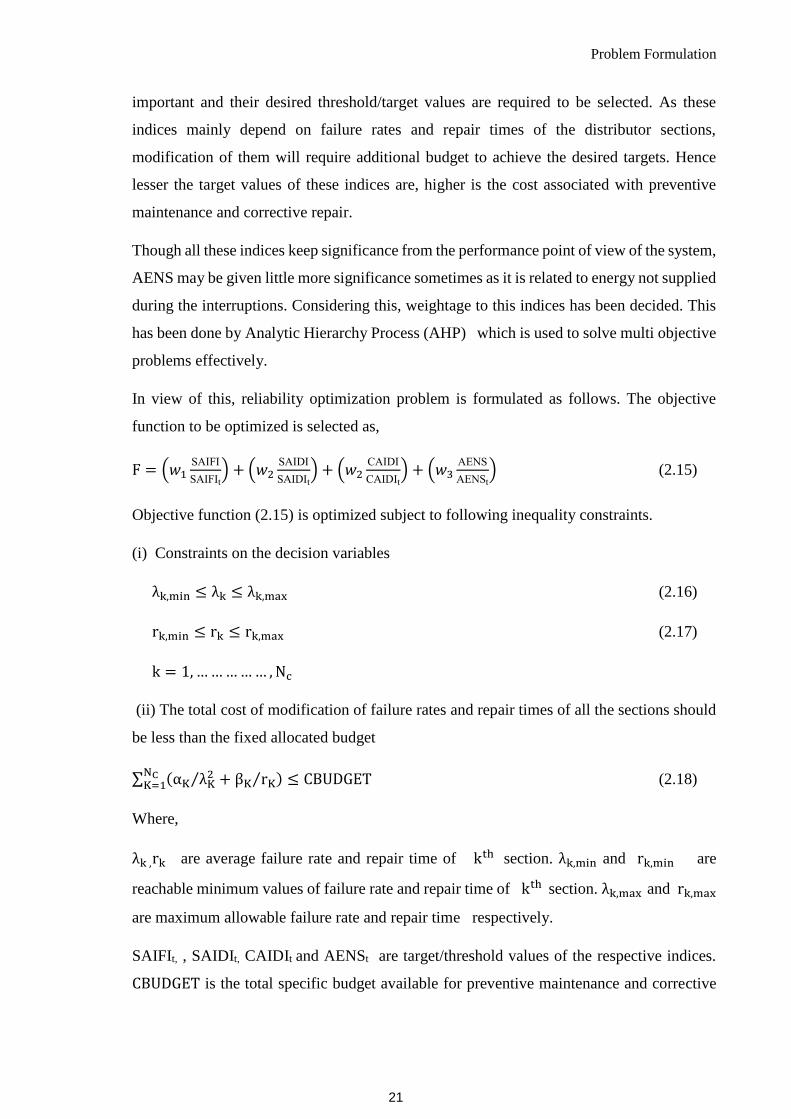
Problem Formulation
important and their desired threshold/target values are required to be selected. As these
indices mainly depend on failure rates and repair times of the distributor sections,
modification of them will require additional budget to achieve the desired targets. Hence
lesser the target values of these indices are, higher is the cost associated with preventive
maintenance and corrective repair.
Though all these indices keep significance from the performance point of view of the system,
AENS may be given little more significance sometimes as it is related to energy not supplied
during the interruptions. Considering this, weightage to this indices has been decided. This
has been done by Analytic Hierarchy Process (AHP) which is used to solve multi objective
problems effectively.
In view of this, reliability optimization problem is formulated as follows. The objective
function to be optimized is selected as,
F = (𝑤1SAIFI
SAIFIt) + (𝑤2
SAIDI
SAIDIt) + (𝑤2
CAIDI
CAIDIt) + (𝑤3
AENS
AENSt) (2.15)
Objective function (2.15) is optimized subject to following inequality constraints.
(i) Constraints on the decision variables
λk,min ≤ λk ≤ λk,max (2.16)
rk,min ≤ rk ≤ rk,max (2.17)
k = 1, … … … … … , Nc
(ii) The total cost of modification of failure rates and repair times of all the sections should
be less than the fixed allocated budget
∑ (αK λK2⁄ + βK rK⁄ )NC
K=1 ≤ CBUDGET (2.18)
Where,
λk ,rk are average failure rate and repair time of kth section. λk,min and rk,min are
reachable minimum values of failure rate and repair time of kth section. λk,max and rk,max
are maximum allowable failure rate and repair time respectively.
SAIFIt, , SAIDIt, CAIDIt and AENSt are target/threshold values of the respective indices.
CBUDGET is the total specific budget available for preventive maintenance and corrective
21

Application of Metaheuristic Optimization Methods for Reliability Enhancement of Electrical
Distribution Systems based on AHP
repair. αK, βK are cost coefficients. w1, w2, w3 and w4 are the relative weightage given to
the normalized values of SAIFI, SAIDI , CAIDI and AENS in the objective function (2.15).
The objective function of equation (2.15) is minimized subject to constraints (2.16), (2.17)
and (2.18) obtaining optimal values of failure rate and repair time for each section of the
distribution systems. The overall failure rate is contributed by various failure modes. Some
may have constant failure rates while some modes of failure contribute to increasing failure
rate. Such types require preventive maintenance and repairing or replacement of
subcomponent in time so as to have overall failure rate practically constant. In this chapter,
optimization has been carried out considering overall failure rate which is combination of
failure rates due to various modes of failure.
By failure rate optimization, targets can be assigned to the crew involved in maintenance
activities: preventive maintenance and repair and persons involved in managerial work.
Thus, by doing so ultimately failure rates can be reduced reaching to their root causes. The
modes responsible for higher failure rates should be given more weightage in regards to
preventive maintenance efforts. In the same way, targets may be set to reduce corrective
repair time. The objective function is the sum of the normalized weighted values of SAIFI,
SAIDI , CAIDI and AENS. The weightage are decided by AHP which is explained in the
later section. Constraints (2.16) and (2.17) impose bounds on the decision variables. Lower
bounds represent minimum reachable value of the decision variables decided with respect to
reliability growth testing model [105]. Similarly reliability monitoring mode give upper
bounds on these decision variables. With the change in the values of decision variables, cost
varies. Cost required to achieve lesser values of decision variables will be higher and vice
versa. A cost curve can be plotted and a cost function can be decided based on past data.
Based on Duane’s growth model [105], the typical cost functions have been selected for each
component in this chapter. Inequality constraints on total cost of repair time and failure rate
has been considered and given as relation (2.18).
The formulated problem is proposed to be solved using flower pollination (FP) [100]
,teaching learning based optimization (TLBO)[101] and differential evolution optimization
algorithms[102] for the sample radial and meshed networks and Roy Billinton Test
System,Bus-2 (RBTS-2). Thus for each section of the distribution systems under
consideration, optimal values of repair time and failure rates are obtained considering budget
allocated for them.
22

Analytic Hierarchical Process (AHP)
2.6 Analytic Hierarchical Process (AHP)
The AHP method has proved to be effective in solving multi-objective problem [104]. It is
used as the decision making technique because of its efficiency in handling quantitative and
qualitative criteria for solution of a problem.
The AHP divides a complex decision problem in to a hierarchical structure. A pairwise
comparison is made to decide relative weightage for different individual options/alternatives
/objectives. Pairwise comparisons are usually quantified by the linear scale or the nine-point
intensity scale proposed by Saaty [104]. By doing pairwise comparison, each linguistic term
is transformed in to numerical intensity values like {9,8,7,6,5,4,3,2,1,1/2,1/3,1/4,1/5,
1/6,1/7,1/8,1/9}. A judgement matrix is formed based on this as follows.
𝑀 = [
𝑎11 𝑎12 ⋯ 𝑎1𝑛
𝑎21 𝑎22 ⋯ 𝑎2𝑛
⋮ ⋮ ⋱ ⋮𝑎𝑛1 𝑎𝑛2 ⋯ 𝑎𝑛𝑛
] (2.19)
Where, 𝑎𝑖𝑗 ∈ {9,8,7,6,5,4,3,2,1, 1 2⁄ , 1 3⁄ , 1 4⁄ , 1 5⁄ , 1 6⁄ , 1 7⁄ , 1 8⁄ , 1 9⁄ } and 𝑎𝑖𝑖 =
1,
where 1 ≤ 𝑖, 𝑗 ≤ 𝑛 . 𝑎𝑖𝑗 shows pairwise judgement representation. Here, 𝑎𝑖𝑗 =1
𝑎𝑖𝑗 .
If M is perfectly consistent, then the principal eigenvalue 𝐷𝑚𝑎𝑥 is equal to number of
comparisons n.
That is 𝑀𝑤 = 𝑛𝑤.
Where, 𝑤 = (𝑤1, 𝑤2, … . , 𝑤𝑛)𝑇 is the principal eigenvector corresponding to 𝐷𝑚𝑎𝑥.
The effectiveness of the judgement matrix M and consistency of the results are checked by
an index called consistency ratio (CR) as follows [106].
𝐶𝑅 =(
𝐷𝑚𝑎𝑥−𝑛
𝑛−1)
𝑅𝐼 (2.20)
Where, 𝐷𝑚𝑎𝑥 is the largest eigenvalue of matrix M and RI is the random index. Here RI=0.58
for n=3 [104].
The AHP algorithm:
The steps of the AHP algorithm are as follows.
23

Application of Metaheuristic Optimization Methods for Reliability Enhancement of Electrical
Distribution Systems based on AHP
1. Set up the hierarchical model by comparing the different objectives to be evaluated.
2. Construct a judgement matrix M. It reflects the user’s knowledge about the relative
importance of each objective. For the objective function used in this chapter, the
matrix formed is as shown in Table 2.1
3. Calculate the maximum eigenvalue and corresponding eigenvector for the
judgement matrix M. By normalizing the eigenvector the vector containing the
weightage of different objectives is found as shown in Table 2.2.
4. Find consistency ratio CR by relation (2.20).
5. A consistency ratio of 0.10 or less is considered acceptable.
The nominal weightage coefficients have been obtained using AHP and are as shown in
Table 2.2. However, if satisfactory adequate indices in terms of the threshold values are not
obtained, these have to be judiciously varied so as to get all indices within threshold limit.
Due to normalization, these additional variation in weighting factor has not been required as
all the indices found are within threshold limit.
2.7 Solution Methodology using FP algorithm
The overview of Flower pollination algorithm has been presented in Appendix D. The
method of solving the formulated problem mentioned in section 2.5 by FP is as follows.
Step 1. Data input 𝜆𝑘,𝑚𝑎𝑥,𝑟𝑘,𝑚𝑎𝑥 , 𝜆𝑘,𝑚𝑖𝑛, 𝑟𝑘,𝑚𝑖𝑛 and SAIFIt, SAIDIt, CAIDIt and AENSt .
Step 2. Initialization: Generate a population of size ‘M’ (flowers) for failure rate λ and repair
time r each by relation (D.3), where each vector of respective population consists of failure
rate and repair time of each component respectively. These values are obtained by sampling
uniformly between lower and upper limits as given by relation (2.16) and (2.17).
Step 3. Evaluate 𝜆𝑠𝑦𝑠,𝑖 , 𝑟𝑠𝑦𝑠,𝑖 and 𝑈𝑠𝑦𝑠,𝑖 at each load point.
Step 4. Evaluate SAIFI, SAIDI, CAIDI and AENS as mentioned in the relations (2.10),
(2.11), (2.12) and (2.14) respectively for vectors of the population.
Step 5. Calculate value of objective function 𝐹 for all vectors in the population i.e.𝐹(𝑋𝑖(𝑘)
),
𝑖 = 1, … … … … … , ′𝑀′ as given by relation (2.15).
Step 6. Evaluate inequality constraints from the relations (2.16), (2.17) and (2.18] for each
vector of the population. Vectors satisfying these constraints will be feasible otherwise not
24

Solution Methodology using FP algorithm
feasible vectors. From among the feasible vectors, based on the value of objective function,
identify the best solution vector 𝑋𝑏𝑒𝑠𝑡(𝑘)
.
Step 7. Set generation counter 𝑘 = 1 .
Step 8. Select target vector, 𝑖 = 1 .
Step 9. Find the updated value of the vector by relation (D.4).
Step 10. Compare the fitness of the updated vectors with that of the initial vectors and retain
the best ones using relation (D.9).
Step 11.Repeat from Step 3.to Step 6. for the updated vector.
Step 12. Increase target vector 𝑖 = 𝑖 + 1. If 𝑖 ≤ 𝑀, repeat from Step 9 otherwise increase
generation count 𝑘 = 𝑘 + 1 .
Step 13. Repeat from step 8 if the desired optimum value is not found or 𝑘 ≤ 𝑘𝑚𝑎𝑥 .
In the same way, the same problem can be solved by TLBO and DE. The overview of both
the optimization methods have been presented in the Appendix E and Appendix F
respectively. Fig. 2.1 shows the flow chart for solving the formulated problem by FP.
25

Application of Metaheuristic Optimization Methods for Reliability Enhancement of Electrical
Distribution Systems based on AHP
END
START
Evaluate SAIFI, SAIDI, CAIDI and AENS
Set generation counter k=1
Evaluate the constraints for each updated solution
Print solution
generation = k+1
NO YESIs solution
converged?
Calculate value of objective function F for all vectors in
the population and Identify the ( ) &best bestkX F
If any updated solution violates the
inequality constraints , then set the values
of the vectors to ( )kiX
Select target vector, i=1 and find updated value of
each vector by D.4
Compare the fitness of the updated vectors with that of
the initial vectors and retain the best ones by D.9
( 1)kiX
( )kiX
Calculate value of objective function F for all vectors in the
population and identify ( )best
kX
Generate a population of size ‘M’ for failure rate λ and
repair time r each between lower and upper limits . , 0 00 0 0 0 0 0, , , X , , .,
1 2 1 2i
TS X X X X X X
M iDi i
Data input,
SAIFIt, SAIDIt, CAIDIt and AENSt
,max ,min ,max ,mink k k kr r
Decide values of w1, w2, w3, & w4 by AHP
Fig. 2.1 Flow chart for solving the formulated problem in section 2.5 by AHP & FP
26
Results and Discussions
2.8 Results and Discussions
The developed methodology has been implemented on the sample radial, mesh and Roy
Billinton test systems and results are described as and results are described as case-1, case-
2 case-3.
2.8.1. Case-1
In this case the developed algorithm has been implemented on a sample radial distribution
system [29] as shown in Fig.A.1. The system consists of seven load points LP-2 to LP-8
labelled in the diagram. Table-A.1 gives maximum allowable values (𝜆𝑘,𝑚𝑎𝑥 , 𝑟𝑘,𝑚𝑎𝑥) and
minimum reachable values (𝜆𝑘,𝑚𝑖𝑛, 𝑟𝑘,𝑚𝑖𝑛) of failure rates and repair times respectively.
Table- A.2 depicts average load and number of customers at load points. Table A.3 gives
cost coefficients for each segment of the distributor. The total budget CBUDGET has been
given Rs. 95000 as required in relation (2.18). Table 2.4 depicts optimized values of failure
rates and repair times as obtained by all the techniques. Table 2.5 shows the current and
optimized values of all reliability indices and objective function obtained by all methods.
Table 2.6 gives statistical analysis of samples of objective function. For the analysis, thirty
random sample values of the objective function were taken for all the methods with various
values of self-generated different initial populations. Student-t distribution has been used to
evaluate confidence interval of mean value of minimized objective function with confidence
coefficient γ=0.95
2.8.2 Case-2
The developed algorithm in this case has been implemented on a sample meshed distribution
system [13] as shown in Fig.B.1 for reliability optimization. The system consists of four load
points LP-T1 to LP-T4 labelled in the diagram. Table B.1 shows maximum allowable values
(𝜆𝑘,𝑚𝑎𝑥, 𝑟𝑘,𝑚𝑎𝑥) and minimum reachable values (𝜆𝑘,𝑚𝑖𝑛 , 𝑟𝑘,𝑚𝑖𝑛) of failure rates and repair
times of each section of Fig.B.1 respectively. Table B.2 depicts average load and number of
customers at load points. Table B.3 gives cost coefficients for each segment of the
distributor. The total budget CBUDGET is Rs. 4x10⁶ as required in relation (2.18). Fig. B.2
is a reliability logic diagram of the meshed distribution system of Fig.B.1 to evaluate
reliability indices at load points LP-T1 to LP-T4. In Fig. B.2, there are three different paths
(A, C, D), (A, B, D) and (A, E) to reach LP-T from the source. The sections included in
blocks A, B, C, D and E to reach each load point from the source is shown in Table 2.7. In
27

Application of Metaheuristic Optimization Methods for Reliability Enhancement of Electrical
Distribution Systems based on AHP
each block sections are in series. The network is solved sequentially up to load point by
applying series and parallel laws of reliability as mentioned in section 2.3 and hence average
failure rate, 𝜆𝑠𝑦𝑠 , average outage time, 𝑟𝑠𝑦𝑠, and average annual outage time, 𝑈𝑠𝑦𝑠 for all
load points are found. The customer and energy oriented reliability indices for the load points
are calculated from relations 2.10-2.14. Optimized values of failure rates and repair times
as obtained by all the techniques are given in Table 2.8. The current and optimized values of
all reliability indices and objective function obtained by all the methods are given in Table
2.9. Statistical analysis done by taking thirty random sample values of minimized objective
function F is shown in Table 2.10. It has been done with the same procedure as mentioned
in section 2.8.1.
2.8.3 Case-3
The developed algorithm in this case has been implemented on RBTS-2 [99] as shown in
Fig.C.1 for reliability optimization. The total budget CBUDGET has been given Rs. 5.6
x106 as required in relation (2.18). Table-C.1 gives failure rates and average repair time of
different components of RBTS-2. Table C.2 shows maximum allowable values
(𝜆𝑘,𝑚𝑎𝑥, 𝑟𝑘,𝑚𝑎𝑥) and minimum reachable values (𝜆𝑘,𝑚𝑖𝑛 , 𝑟𝑘,𝑚𝑖𝑛) of failure rates and repair
times of each section of Fig.C.1 respectively. Table C.3 gives cost coefficients for each
segment of RBTS-2. The customer data of RBTS-2 is shown in Table C.4. All these data of
RBTS-2 have been taken from [99, 72]. Table 2.11 gives optimized values of failure rates
and repair times as obtained by all the techniques. Table 2.12 shows the current and
optimized values of all reliability indices and objective function obtained by all the methods.
Table 2.13 depicts statistical analysis for this system as done in the previous two cases.
Table 2.3 gives control parameters for FP, TLBO and DE techniques for all the sample
distribution systems in consideration.
28

Results and Discussions
Table 2.1 AHP Matrix
SAIFI SAIDI CAIDI AENS
SAIFI 1 1/5 1/5 1/5
SAIDI 5 1 1 1
CAIDI 5 5 1 1
AENS 5 1 1 1
Table 2.2 Weightage Coefficients
𝒘𝟏 𝒘𝟐 𝒘𝟑 𝒘𝟒
0.0625
0.313
0.313
0.313
Table 2.3 Control Parameters for FP, TLBO and DE for sample radial network, meshed network and
RBTS-2
Sr No. Parameters Values of parameters
1 Population size(FP,TLBO,DE) 20
2 Max generation specified(kmax) (FP,TLBO,DE) 1000
3 Updated step size (∝) (FP) 0.01
4 Distribution factor (𝛽) (FP) 1.5
5 Switch probability (FP) 0.8
6 Step size (F) (DE) 0.8
7 Cross over rate (Cr) (DE) 0.7
29

Application of Metaheuristic Optimization Methods for Reliability Enhancement of Electrical
Distribution Systems based on AHP
Table 2.4 Optimized values of failure rates and repair times as obtained by FP, TLBO and DE and
corresponding cost incurred for radial network
Variables Magnitudes as obtained
by FP
Magnitudes as obtained by
TLBO
Magnitudes as obtained
by DE
𝜆1 /year 0.200000 0.200000 0.223634
𝜆2 /year 0.050000 0.050000 0.067726
𝜆3 /year 0.100001 0.100216 0.123634
𝜆4 /year 0.100000 0.100000 0.147268
𝜆5 /year 0.150000 0.150001 0.155909
𝜆6 /year 0.056906 0.057048 0.055909
𝜆7 /year 0.100000 0.100000 0.055909
r 1(h) 6.000000 6.000000 6.032479
r 2(h) 6.001086 6.000000 6.024359
r 3(h) 4.000000 4.000008 4.064958
r 4(h) 8.000000 8.000001 8.097437
r 5(h) 7.000000 7.000003 7.064958
r 6(h) 8.000000 6.000000 6.01624
r 7(h) 6.001575 6.000005 6.048719
Cost
incurred(Rs.)
94970.51732
94801.278113
94927.3867
Table 2.5 Current and optimized reliability indices and corresponding value of objective function for
radial distribution system
Sr.
No.
Index Current
Values
Optimized values Threshold
values
FP TLBO DE
1 SAIFI(interruptions/customer) 0.7200 0.299572
0.299636
0.345223
0.5000
2 SAIDI(h/customer) 8.4500 1.876613
1.842774
2.149817
4.0000
3 CAIDI(h/customer
interruption)
11.7361 6.604517
7.047034
6.430872
8.0000
4 AENS(kW/customer) 26.4100 5.699442
5.660151
6.630001
10.000
Objective function (F) 7.6597 2.463806
2.506860
2.694759
30

Results and Discussions
Table 2.6 Statistical analysis of sample values of objective function for radial network
Optimization
method
Sample
Mean (
F)
Sample
Variance
(σF2)
Sample
Standard
deviation
(σ)
Sample
Median(F)
Min(F) Max(F) Coefficient
of
variation(cv)
Frequency of
convergence(f)
CONFγ(γ=0.95) Length of
confidence
interval of
(F)
FP 2.532549
0.001082
0.006005
2.533971
2.463806
2.587286
0.002371
0.566667
(2.520267, 2.544830)
0.024563
TLBO 2.563355
0.001547
0.007183
2.567007
2.506860
2.627623
0.002802
0.631353
(2.548665,2.578045)
0.029379
DE 2.800179
0.0057612
0.0138579
2.7773987
2.694759
2.985234
0.0049489
0.533333
(2.7718399,2.8285188)
0.0566788
31

Application of Metaheuristic Optimization Methods for Reliability Enhancement of Electrical
Distribution Systems based on AHP
Table 2.7 Sections involved in each block of Figure B.2
Load point Blocks Sections involved
For LP-T1 A 1,18
B 9,10,11
C 2,3,4,5,6,7,8
D 17
E 12,13,14,15,16
For LP-T2 A 1,15
B 9,10,11
C 2,3,4,5,6,7,8
D 16,17,18
E 12,13,14
For LP-T3 A 1,5
B 9,10,11
C 12,13,14,15,16,17,18
D 6,7,8
E 2,3,4
For LP-T4 A 1,7
B 9,10,11
C 12,13,14,15,16,17,18
D 8
E 2,3,4,5,6
32

Results and Discussions
Table 2.8 Optimized values of failure rates and repair times as obtained by FP, TLBO and DE and
corresponding cost incurred for meshed network
Variables Magnitudes as obtained
by FP
Magnitudes as obtained
by TLBO
Magnitudes as obtained
by DE
𝜆1 /year 0.254201 0.294427 0.328754
𝜆2 /year 0.12957058 0.097152 0.115491
𝜆3 /year 0.10514493 0.057423 0.071714
𝜆4 /year 0.10870638 0.071586 0.073280
𝜆5 /year 0.08330304 0.093439 0.112782
𝜆6 /year 0.01588112 0.011389 0.011394
𝜆7 /year 0.09485342 0.111542 0.119163
𝜆8 /year 0.17224346 0.098350 0.115610
𝜆9 /year 0.00542577 0.006182 0.006170
𝜆10 /year 0.06710431 0.042832 0.038513
𝜆11 /year 0.18062197 0.113593 0.132740
𝜆12 /year 0.12280254 0.128550 0.132740
𝜆13 /year 0.10964525 0.061832 0.071714
𝜆14 /year 0.06829886 0.062165 0.073280
𝜆15 /year 0.08172781 0.075800 0.094018
𝜆16 /year 0.0173002 0.011878 0.011394
𝜆17 /year 0.09122349 0.101662 0.115610
𝜆18 /year 0.13022653 0.090152 0.112782
r 1(h) 3.5449659 3.355670 3.358106
r 2(h) 3.2074669 3.137684 3.070081
r 3(h) 17.368277 10.815550 10.765800
r 4(h) 2.8455409 2.149450 2.133019
r 5(h) 3.9297324 3.614628 3.409275
r 6(h) 13.378692 9.331444 9.263219
r 7(h) 3.9665742 3.569844 3.409275
r 8(h) 3.7539499 3.901679 3.770399
r 9(h) 6.4000603 8.516112 6.428649
r 10(h) 24.350023 20.227300 18.587450
r 11(h) 2.0124065 2.562779 2.022167
r 12(h) 5.124369 2.113666 2.022167
r 13(h) 20.427964 15.600660 10.765750
r 14(h) 2.2620942 2.172341 2.133019
r 15(h) 6.403899 6.612923 6.365820
r 16(h) 13.28581 11.048240 9.263219
r 17(h) 4.6775905 4.968170 4.370771
r 18(h) 4.9195583 3.423207 3.409275
Cost
incurred(Rs.)
3976795
3956863
3989327.645
33

Application of Metaheuristic Optimization Methods for Reliability Enhancement of Electrical
Distribution Systems based on AHP
Table 2.9 Current and optimized reliability indices and corresponding value of objective function for
meshed distribution system
Sr.
No.
Index Current
Values
Optimized values Threshold
values
FP TLBO DE
1 SAIFI(interruptions/customer) 0.689895
0.355732
0.389773
0.440188
0.5000
2 SAIDI(h/customer) 4.854797
1.379787
1.369254
1.537291
3.0000
3 CAIDI(h/customer
interruption)
7.037003
3.878721
3.512954
3.492352
5.0000
4 AENS(kW/customer) 20.533869
5.786142
5.794515
6.496036
9.000
Objective function (F) 5.526503
2.119866
2.14043
2.350846
34

Results and Discussions
Table 2.10 Statistical analysis of sample values of objective function for meshed network
Optimization
method
Sample
Mean
( F)
Sample
Variance
(σF2)
Sample
Standard
deviation
(σ)
Sample
Median(F)
Min(F) Max(F) Coefficient
of
variation(cv)
Frequency of
convergence(f)
CONFγ(γ=0.95) Length of
confidence
interval of
(F)
FP 2.199801
0.002880
0.009798432
2.218620
2.123239
2.309730
0.004454
0.6
(2.179764 ,2.219839)
0.040075
TLBO 2.160977
0.001688
0.007502166
2.140666
2.140430
2.287644
0.003471
0.7
(2.145634,2.176318)
0.0306838
DE 2.451934
0.0172337
0.0239678
2.403646
2.350846
2.962969
0.009775
0.733333
(2.402920,2.500948) 0.0980285
35

Application of Metaheuristic Optimization Methods for Reliability Enhancement of Electrical
Distribution Systems based on AHP
Table 2.11 Optimized values of failure rates and repair times for RBTS-2 as obtained by FP, TLBO
and DE
Failure rates (/Year) Repair times (in hrs)
Distributor
segment
By FP
By TLBO
By DE
By FP
By TLBO
By DE
1 0.036650 0.036650 0.036650 2.252263 2.252347 2.252313
2 0.011270 0.011319 0.012878 4.504504 4.504504 4.504516
3 0.039090 0.039090 0.039094 4.504504 4.504694 4.504504
4 0.036090 0.036090 0.036094 2.252252 2.252252 2.252252
5 0.011270 0.011270 0.012122 4.504504 4.504892 4.508222
6 0.013873 0.015279 0.011953 4.504504 4.504504 4.504504
7 0.036650 0.036650 0.036697 2.252314 2.252252 2.254525
8 0.011278 0.011279 0.011281 4.504509 4.518765 4.504509
9 0.013770 0.011278 0.012859 4.504504 4.514888 4.504504
10 0.029323 0.029323 0.029429 2.252252 2.252326 2.252252
11 0.011278 0.011278 0.011279 4.504505 4.511500 4.504504
12 0.036650 0.036650 0.037005 2.252250 2.252300 2.252250
13 0.039097 0.039097 0.039136 2.252250 2.252250 2.252250
14 0.029324 0.029323 0.029371 2.252250 2.252250 2.252360
15 0.039097 0.039434 0.039119 2.252251 2.252250 2.252250
16 0.036650 0.036650 0.036650 2.252250 2.252250 2.252250
17 0.011278 0.011278 0.011361 4.504500 4.513518 4.504500
18 0.039099 0.039097 0.039216 2.252250 2.252250 2.252253
19 0.011278 0.011278 0.011371 4.504500 4.504500 4.504757
20 0.011278 0.011278 0.011340 4.504502 4.504501 4.504500
21 0.029323 0.029323 0.029530 2.252251 2.252250 2.252255
22 0.011278 0.011608 0.021116 4.504651 4.504540 4.504585
23 0.014813 0.016704 0.011423 4.504500 4.504500 4.523343
24 0.036650 0.036650 0.036650 2.252250 2.252250 2.252250
25 0.011278 0.011282 0.011278 4.504530 4.504500 4.524141
26 0.039097 0.039097 0.039099 2.252250 2.252263 2.252250
27 0.015025 0.011278 0.011285 4.504500 4.504504 4.504500
28 0.011278 0.011278 0.012235 4.504500 4.504500 4.504549
29 0.036650 0.036650 0.036650 2.252250 2.252609 2.252250
30 0.011282 0.011278 0.011474 4.504511 4.504500 4.504923
31 0.011278 0.011296 0.011279 4.504500 4.505667 4.504500
32 0.036650 0.036650 0.036682 2.252250 2.252250 2.252250
33 0.011279 0.014680 0.011279 4.504516 4.504500 4.504500
34 0.029323 0.029323 0.029332 2.252250 2.252250 2.252250
35 0.011414 0.012563 0.012546 4.504540 4.504500 4.504500
36 0.011279 0.012101 0.011316 4.504500 4.504500 4.504500
Table 2.12 Current and optimized reliability indices for RBTS-2
Sr.
No. Index
Current
Values
Optimized Values Threshold
Values
FP TLBO DE
1 SAIFI(interruptions/customer) 0.0986 0.074149
0.074132
0.074576
0.085
2 SAIDI(h/customer) 0.5882 0.199349
0.19929
0.201212
0.35
3 CAIDI(h/customer
interruption)
5.9666 2.688509
2.688172
2.697489
3.50 4 AENS(kW/customer) 4.6641 1.594604
1.60041
1.604065
2.5
Objective function (F) 6.3108 2.772857
2.774727
2.789118
Cost incurred (Rupees) 5597472
5594369
5588765
36
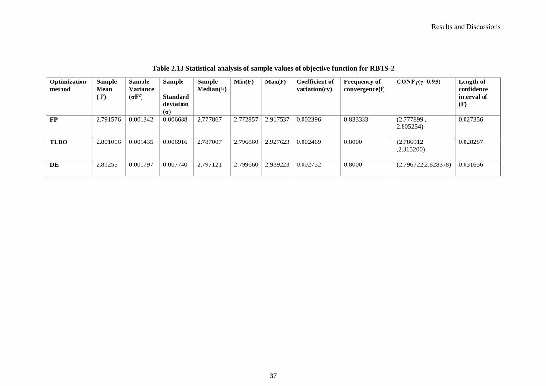
Results and Discussions
Table 2.13 Statistical analysis of sample values of objective function for RBTS-2
Optimization
method
Sample
Mean
( F)
Sample
Variance
(σF2)
Sample
Standard
deviation
(σ)
Sample
Median(F)
Min(F) Max(F) Coefficient of
variation(cv)
Frequency of
convergence(f)
CONFγ(γ=0.95) Length of
confidence
interval of
(F)
FP 2.791576
0.001342
0.006688
2.777867
2.772857
2.917537
0.002396 0.833333
(2.777899 ,
2.805254)
0.027356
TLBO 2.801056
0.001435
0.006916
2.787007
2.796860
2.927623
0.002469
0.8000
(2.786912
,2.815200)
0.028287
DE 2.81255
0.001797
0.007740
2.797121
2.799660
2.939223
0.002752
0.8000
(2.796722,2.828378)
0.031656
37

Application of Metaheuristic Optimization Methods for Reliability Enhancement of Electrical
Distribution Systems based on AHP
2.9 Conclusions
The algorithm in this chapter is used to find out optimum values of customer oriented and
energy based reliability indices while specified budget is allocated to achieve the same. Here,
in the objective function different weightage has been given to all the indices. The weighting
factors are found by AHP. As all the indices are normalized with respect their respective
threshold values, the optimized values found have been within the threshold limit. This
algorithm is applied to sample radial distribution system, sample meshed distribution system
and RBTS-2 in this chapter. The optimum values are found by FP, TLBO and DE
optimization algorithms. It has been authenticated by making comparison of the values found
by all the optimization methods.
38

CHAPTER 3
A Value Based Reliability Optimization of
Electrical Distribution Systems considering
Expenditures on Maintenance and Customer
Interruptions
3.1 Introduction
It has been observed that the customers look for value-added service from their utilities.
Failures in identifying customer needs may lead to drastic fall in the business of utilities as
the electricity selling market has started becoming competitive. It is a challenging task for
any utility to provide qualitative service to the customers keeping the cost on its operation
and maintenance such as to provide low cost services to them. In this chapter a balance
between the utility cost and cost incurred to the customers due to interruptions have been
found maintaining the required targets of reliability of the system. The optimum value of
system reliability with least combined cost thus found may lead towards value based
reliability planning of distribution systems [50].
In this chapter, a methodology is proposed which shows enhancement of reliability by
optimizing total reliability cost of electrical distribution systems. The total reliability cost
consists of cost incurred by utility and customers both.
In this chapter, interruptions costs at the customer end have been focused and also tried for
their reduction. This chapter aims at reducing the total reliability cost of system by reducing
customer interruptions and hence consequently enhancing the reliability of distribution
systems.
This chapter has been organized as follows. In section 3.2, the problem to be solved has been
formulated. Section 3.3 gives solution methodology for the problem by FP. Section 3.4 is
regarding discussion of the results obtained in this chapter. Section 3.5 leads to the
conclusions evaluated.
39

A Value Based Reliability Optimization of Electrical Distribution Systems considering
Expenditures on Maintenance and Customer Interruptions
3.2 Problem Formulation
Distribution system reliability should be based on proper balance between cost to the utility
and benefits received by the customers. If the customer interruptions are less, the benefits in
terms of profit to the customers and customer satisfaction are more. Thus to design a
reliability planning rationally so as to maintain proper service continuity requires
incorporating the utility costs and the costs incurred by the customers associated with service
interruptions in the analysis.
In view of this, the objective function is designed as follows.
𝐹 = ∑ 𝛼𝑘 𝜆𝑘2⁄𝑁𝑐
𝑘=1 + ∑ 𝛽𝑘 𝑟𝑘⁄𝑁𝑐𝑘=1 + ∑ 𝐶𝐼𝐶
𝑁𝑐𝑘=1 (3.1)
where, 𝐶𝐼𝐶 = 𝜆𝑘 × 𝑟𝑘 × 𝐿𝑖 × 𝐶𝑝𝑘 (3.2)
In the relation (3.1), 𝜆𝑘 is the failure rate of 𝑘𝑡ℎ section ; 𝑟𝑘 is the average repair time of
𝑘𝑡ℎ section ; 𝛼𝑘 and 𝛽𝑘 are the cost coefficients ; 𝐶𝐼𝐶 is customer interruption cost at
various load points ; 𝐿𝑖 is the average connected load at load point 𝑖 ; 𝐶𝑝𝑘 is the cost of
interruption in rupees per kilowatt for an outage duration of 𝑟𝑘 associated with 𝑘𝑡ℎ section
; 𝑁𝑐 is the total number sections of the distribution system.
The objective function consists of three terms. The first two terms are related to modification
costs related to maintenance activities. The first term shows cost of modification of failure
rates of each section. The failure rates can be reduced by investing in maintenance activities
on regular basis. The second term is related to cost of modifications in average repair time.
Lesser the values of these terms are; more are the costs or investments associated with
preventive maintenance and corrective repair required by utility to achieve them [111]. Both
these terms are based on Duane’s reliability growth model [105]. The third part of the
relation (3.1); i.e. cost of interruption depicts the costs incurred at the customers end in terms
of loss at the time of power fail. When a utility is engaged in supplying power to industrial
and commercial facilities, the high costs associated with power outages of course keep more
significance. The total cost of interruptions for any load point 𝑖 can be determined by adding
the cost of all section outages. The total cost of customer interruptions for all customers can
then be evaluated. The value of service which is equivalent to the cost of reliability, depicted
40

Problem Formulation
in terms of cost of customer interruptions can be derived by doing actual surveys of
customers regarding their expectations in regard to the level of reliability of supply. By
defining specific values in rupees for specific level of service reliability a balance in
distribution reliability can be established. The customer cost at a single customer load point
depends entirely on the cost characteristics of the customers at that load point. The customer
cost associated to any load point due to any interruption is the combination of the costs of
all type of customers affected due to that distribution outage [50]. Objective function (3.1)
is minimized based on the following customer and energy based constraints [103].
(i) Constraints on the decision variables
𝜆𝑘,𝑚𝑖𝑛 ≤ 𝜆𝑘 ≤ 𝜆𝑘,𝑚𝑎𝑥 (3.3)
𝑟𝑘,𝑚𝑖𝑛 ≤ 𝑟𝑘 ≤ 𝑟𝑘,𝑚𝑎𝑥 (3.4)
𝑘 = 1, … … … … … , 𝑁𝑐
where,
λk,min and rk,min are minimum reachable values of failure rate and repair time of 𝑘𝑡ℎ
section. λk,max and rk,max are maximum allowable failure rate and repair time
respectively.
(ii) Inequality constraints on the system average interruption frequency index SAIFI
SAIFI ≤ SAIFIt (3.5)
(iii) Inequality constraints on the system average interruption duration index (SAIDI)
SAIDI ≤ SAIDIt (3.6)
(iv) Inequality constraints on the customer average interruption duration index (CAIDI)
CAIDI ≤ CAIDIt (3.7)
(v) Inequality constraints on the average energy not supplied index (AENS)
AENS ≤ AENSt (3.8)
41
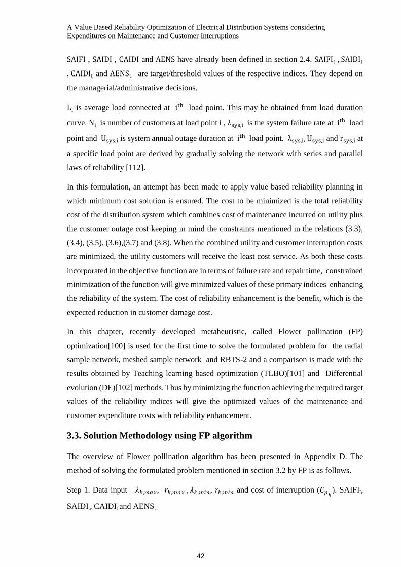
A Value Based Reliability Optimization of Electrical Distribution Systems considering
Expenditures on Maintenance and Customer Interruptions
SAIFI , SAIDI , CAIDI and AENS have already been defined in section 2.4. SAIFIt , SAIDIt
, CAIDIt and AENSt are target/threshold values of the respective indices. They depend on
the managerial/administrative decisions.
Li is average load connected at ith load point. This may be obtained from load duration
curve. Ni is number of customers at load point i , λsys,i is the system failure rate at ith load
point and Usys,i is system annual outage duration at ith load point. λsys,i, Usys,i and rsys,i at
a specific load point are derived by gradually solving the network with series and parallel
laws of reliability [112].
In this formulation, an attempt has been made to apply value based reliability planning in
which minimum cost solution is ensured. The cost to be minimized is the total reliability
cost of the distribution system which combines cost of maintenance incurred on utility plus
the customer outage cost keeping in mind the constraints mentioned in the relations (3.3),
(3.4), (3.5), (3.6),(3.7) and (3.8). When the combined utility and customer interruption costs
are minimized, the utility customers will receive the least cost service. As both these costs
incorporated in the objective function are in terms of failure rate and repair time, constrained
minimization of the function will give minimized values of these primary indices enhancing
the reliability of the system. The cost of reliability enhancement is the benefit, which is the
expected reduction in customer damage cost.
In this chapter, recently developed metaheuristic, called Flower pollination (FP)
optimization[100] is used for the first time to solve the formulated problem for the radial
sample network, meshed sample network and RBTS-2 and a comparison is made with the
results obtained by Teaching learning based optimization (TLBO)[101] and Differential
evolution (DE)[102] methods. Thus by minimizing the function achieving the required target
values of the reliability indices will give the optimized values of the maintenance and
customer expenditure costs with reliability enhancement.
3.3. Solution Methodology using FP algorithm
The overview of Flower pollination algorithm has been presented in Appendix D. The
method of solving the formulated problem mentioned in section 3.2 by FP is as follows.
Step 1. Data input 𝜆𝑘,𝑚𝑎𝑥, 𝑟𝑘,𝑚𝑎𝑥 , 𝜆𝑘,𝑚𝑖𝑛, 𝑟𝑘,𝑚𝑖𝑛 and cost of interruption (𝐶𝑝𝑘). SAIFIt,
SAIDIt, CAIDIt and AENSt .
42

Solution Methodology using FP algorithm
Step 2. Initialization: Generate a population of size ‘M’ (flowers) for failure rate λ and repair
time r each by relation (D.3), where each vector of respective population consists of failure
rate and repair time of each component respectively. These values are obtained by sampling
uniformly between lower and upper limits as given by relation (3.3) and (3.4).
Step 3. Evaluate 𝜆𝑠𝑦𝑠,𝑖 , 𝑟𝑠𝑦𝑠,𝑖 and 𝑈𝑠𝑦𝑠,𝑖 at each load point.
Step 4. Evaluate SAIFI, SAIDI, CAIDI and AENS as mentioned in the relations (2.10),
(2.11), (2.12) and (2.14) respectively for vectors of the population.
Step 5. Calculate value of objective function 𝐹 for all vectors in the population i.e.𝐹(𝑋𝑖(𝑘)
),
𝑖 = 1, … … … … … , ′𝑀′ as given by relation (3.1) and (3.2).
Step 6. Evaluate inequality constraints from the relations (3.5), (3.6), (3.7) and (3.8) for each
vector of the population. Vectors satisfying these constraints will be feasible otherwise not
feasible vectors. From among the feasible vectors, based on the value of objective function,
identify the best solution vector 𝑋𝑏𝑒𝑠𝑡(𝑘)
.
Step 7. Set generation counter 𝑘 = 1 .
Step 8. Select target vector, 𝑖 = 1 .
Step 9. Find the updated value of the vector by relation (D.4).
Step 10. Compare the fitness of the updated vectors with that of the initial vectors and retain
the best ones using relation (D.9).
Step 11.Repeat from Step 3.to Step 6. for the updated vector.
Step 12. Increase target vector 𝑖 = 𝑖 + 1. If 𝑖 ≤ 𝑀, repeat from Step 9 otherwise increase
generation count 𝑘 = 𝑘 + 1 .
Step 13. Repeat from step 8 if the desired optimum value is not found or 𝑘 ≤ 𝑘𝑚𝑎𝑥 .
In the same way, the same problem can be solved by TLBO and DE. The overview of both
the optimization methods have been presented in the Appendix E and Appendix F
respectively. Fig. 3.1 shows the flow chart for solving the formulated problem by FP.
43
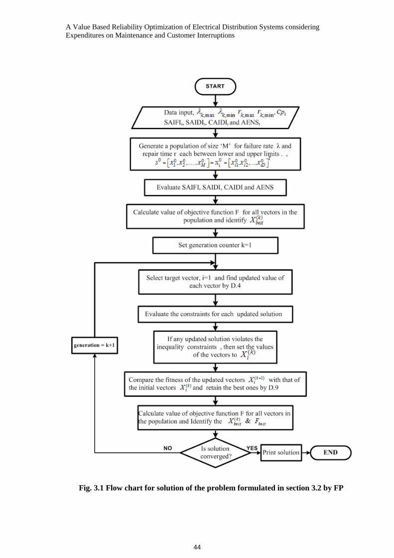
A Value Based Reliability Optimization of Electrical Distribution Systems considering
Expenditures on Maintenance and Customer Interruptions
Fig. 3.1 Flow chart for solution of the problem formulated in section 3.2 by FP
44

Results and Discussions
3.4. Results and Discussions
The developed algorithm in this chapter has been implemented on three distribution systems
as follows. The problem has been solved by FP algorithm and comparison has been made
with the results obtained by TLBO and DE. The algorithms used have been coded in
MATLAB-13.
3.4.1 Distribution systems: Descriptions
(A) Sample radial distribution system [29]:
The radial system consists of seven load points LP-2 to LP-8 labelled in Fig. A.1. The data
regarding the maximum allowable and minimum reachable values of failure rates and repair
times, average load and number of customers at load points and cost coefficients for each
segment of radial distributor have been taken from [111] .They are shown as Table A.1
,Table A.2 and Table A.3 in Appendix. Table 3.1 gives interruption cost (𝐶𝑝𝑘) at different
load points for the sample radial distribution system. The customer and energy based
reliability indices for the load points are calculated from relations (2.10), (2.11), (2.12) and
(2.14) using laws of reliability [103]. Table 3.3 gives optimized values of failure rates and
repair times of different sections of radial distribution system. Table 3.4 gives the optimized
values of objective function (F) which shows the total expenditure costs of the sample radial
distribution system due to maintenance activity and customer interruptions. Table 3.5 shows
the current and optimized values of customer and energy based reliability indices obtained
by all the methods. Fig.3.2 shows convergence plots of objective function (F) for all the
methods for specified number of generations for the sample radial distribution
system.Fig.3.3 , Fig. 3.4 and Fig.3.5 show frequency distribution plots for minimum values
of (F) obtained by FP ,TLBO and DE respectively for sample radial distribution system.
These histograms have been plotted from the 40 random values of minimum (F) obtained by
the respective optimization method.
(B) Sample meshed distribution system [13]
The developed algorithm in this case has been implemented on a sample meshed distribution
system [13] as shown in Fig.B.1. The system consists of four load points LP-T1 to LP-T4
labelled in the diagram. Table B.1 shows maximum allowable values (𝜆𝑘,𝑚𝑎𝑥 , 𝑟𝑘,𝑚𝑎𝑥) and
minimum reachable values (𝜆𝑘,𝑚𝑖𝑛 , 𝑟𝑘,𝑚𝑖𝑛) of failure rates and repair times of each section
of Fig.2.2 respectively. Table B.2 depicts average load and number of customers at load
45

A Value Based Reliability Optimization of Electrical Distribution Systems considering
Expenditures on Maintenance and Customer Interruptions
points. Table B.3 gives cost coefficients for each segment of the distributor. Table 3.6 gives
interruption cost (𝐶𝑝𝑘) at different load points for the sample meshed distribution system.
Table 3.7 gives optimized values of failure rates and repair times of different sections of
meshed distribution system. Fig. B.2 is a reliability logic diagram of the meshed distribution
system of Fig.B.1 to evaluate reliability indices at load points LP-T1 to LP-T4. The
procedure for the same has already been explained in section 2.8.2. Table 3.8 gives the
optimized values of objective function (F) which shows the total expenditure costs of the
sample meshed distribution system due to maintenance activity and customer interruptions.
Table 3.9 shows the current and optimized values of customer and energy based reliability
indices obtained by all the methods. Fig.3.10 shows convergence plots of objective function
(F) for all the methods for specified number of generations for the sample meshed
distribution system. Fig. 3.11 , Fig. 3.12 and Fig.3.13 show frequency distribution plots for
minimum values of (F) obtained by FP ,TLBO and DE respectively for sample meshed
distribution system. These histograms have been plotted from the 40 random values of
minimum (F) obtained by the respective optimization method.
(B) Roy Billinton Test System-Bus 2 (RBTS-2) [99]:
Another test system which has been used in this chapter is Roy Billinton Test System-Bus 2
as shown in Fig.C.1. Table C.1 represents failure rates and average repair times of different
components of RBTS-2. Table C.2 gives maximum allowable (𝜆𝑘,𝑚𝑎𝑥 /year) and minimum
reachable (λk,min/year) failure rates, maximum allowable (𝑟𝑘,𝑚𝑎𝑥 (h)) and minimum
reachable (rk,min (h)) average repair times. Table C.3 gives cost coefficients 𝛼𝐾 and 𝛽𝐾
for failure rates and repair times respectively of the different sections of RBTS-2. Table C.4
represents sector wise customer data. Table-(C.1-C.4) are shown in the Appendix. Table
3.10 gives optimized values of failure rates and repair times for different sections of RBTS-
2 by the three optimization methods in consideration. Table 3.11 gives the optimized values
of maintenance cost, customer interruption cost and objective function (F) for RBTS-2.
Table 3.12 shows the current and optimized values of customer and energy based reliability
indices. The convergence of minimum value of objective function (F) over the number of
generations for all the optimization methods are shown in Fig. 3.10. The frequency
distribution plots of minimum values of (F) due to FP, TLBO and DE are shown in Fig. 3.11,
Fig.3.12 and Fig. 3.13 respectively.
46

Results and Discussions
Table 3.2 gives control parameters for all the three optimization methods; FP, TLBO and
DE applied in this chapter for all the distribution test systems in consideration.
47

A Value Based Reliability Optimization of Electrical Distribution Systems considering
Expenditures on Maintenance and Customer Interruptions
Table 3.1 Interruption costs at load points for sample radial distribution system
Distributor Load points(LP) #2 #3 #4 #5 #6 #7 #8
Interruption Cost(𝑪𝒑𝒌)(Rs./kW) 15 13 17 20 20 12 14
Table 3.2 Control Parameters for FP, TLBO and DE for sample radial network, meshed network and
RBTS-2
Sr No. Parameters Values of parameters
1 Population size(FP,TLBO,DE) 20
2 Max generation specified(kmax) (FP,TLBO,DE) 1000
3 Updated step size (∝) (FP) 0.01
4 Distribution factor (𝛽) (FP) 1.5
5 Switch probability (FP) 0.8
6 Step size (F) (DE) 0.8
7 Cross over rate (Cr) (DE) 0.7
Table 3.3 Optimized values of failure rates and repair times as obtained by FP, TLBO and DE for
sample radial distribution system
Variables Magnitudes as obtained
by FP
Magnitudes as obtained by
TLBO
Magnitudes as obtained by
DE
𝜆1 /year 0.200001 0.200000 0.200005
𝜆2 /year 0.099307 0.099573 0.130767
𝜆3 /year 0.121371 0.120466 0.163934
𝜆4 /year 0.100000 0.100012 0.100068
𝜆5 /year 0.150000 0.150000 0.151810
𝜆6 /year 0.100000 0.100000 0.100000
𝜆7 /year 0.100000 0.099999 0.100000
r 1(h) 7.053993 6.023147 6.000011
r 2(h) 7.468035 6.000003 6.029284
r 3(h) 6.979073 11.981230 4.000000
r 4(h) 8.099595 19.999997 8.000005
r 5(h) 15.000000 14.999999 7.002543
r 6(h) 7.999764 6.000118 6.000013
r 7(h) 6.000052 12.000000 8.125879
48

Results and Discussions
Table 3.4 Current and optimized values of Objective function (F) obtained by FP, TLBO and DE for
radial distribution system
Sr.
No.
Current Values (Rs.)
(In Rupees)
Optimized Values(Rs.) (In Rupees)
FP TLBO DE
1 Maintenance cost
(∑ 𝛼𝑘 𝜆𝑘2⁄𝑁𝑐
𝑘=1 + ∑ 𝛽𝑘 𝑟𝑘⁄𝑁𝑐𝑘=1 )
133640 38650.264 38271.185 37124.837
2 Customer interruption cost
(∑ 𝐶𝐼𝐶𝑁𝑐𝑘=1 )
450920 103543.623 103905.846 105818.215
3 Objective function (F) 584560 142193.888
142177.032
142943.053
Table 3.5 Current and optimized reliability indices for radial distribution system
Table 3.6 Interruption cost at load points for sample meshed network
Load point(LP) LP-T1 LP-T2 LP-T3 LP-T4
Interruption Cost(𝐶𝑝𝑘)(Rs./kW) 45 39 51 68
Sr.
No.
Index Current
Values
Optimized Values Threshold
Values
FP TLBO DE
1 SAIFI(interruptions/customer) 0.7200 0.355884 0.356937 0.363519 0.5000
2 SAIDI(h/customer) 8.4500 2.167820 2.174372 2.226317 4.0000
3 CAIDI(h/customer
interruption)
11.7361 6.096659 6.095436 6.124353 8.0000
4 AENS(kW/customer) 26.4100 6.437391 6.457199 6.596871 10.000
49

A Value Based Reliability Optimization of Electrical Distribution Systems considering
Expenditures on Maintenance and Customer Interruptions
Table 3.7 Optimized values of failure rates and repair times as obtained by FP, TLBO and DE for
meshed network
Variables Magnitudes as obtained
by FP
Magnitudes as obtained by
TLBO
Magnitudes as obtained by
DE
𝜆1 /year 0.2553 0.2546 0.2542
𝜆2 /year 0.1770 0.1774 0.1776
𝜆3 /year 0.1100 0.1102 0.1100
𝜆4 /year 0.1135 0.1104 0.0823
𝜆5 /year 0.1409 0.1846 0.1847
𝜆6 /year 0.0188 0.0216 0.0270
𝜆7 /year 0.0977 0.0939 0.1845
𝜆8 /year 0.1780 0.1780 0.1760
𝜆9 /year 0.0130 0.0105 0.0099
𝜆10 /year 0.0690 0.0690 0.0690
𝜆11 /year 0.2052 0.2139 0.2054
𝜆12 /year 0.2052 0.2053 0.2053
𝜆13 /year 0.1100 0.1100 0.1105
𝜆14 /year 0.1135 0.1135 0.1137
𝜆15 /year 0.0779 0.0916 0.1065
𝜆16 /year 0.0183 0.0225 0.0248
𝜆17 /year 0.1780 0.1780 0.1844
𝜆18 /year 0.1846 0.1846 0.0894
r 1(h) 3.3497 3.3551 3.3967
r 2(h) 3.0703 3.0966 3.9018
r 3(h) 13.0590 10.7526 22.7541
r 4(h) 3.4867 2.2564 2.6154
r 5(h) 3.3992 3.4063 3.4441
r 6(h) 13.0687 9.2661 13.4836
r 7(h) 3.3962 3.8256 3.3967
r 8(h) 3.7523 5.1322 4.5333
r 9(h) 9.8108 11.8247 7.3207
r 10(h) 18.5600 23.9913 19.0307
r 11(h) 5.2414 5.2366 2.0130
r 12(h) 2.0328 2.0825 2.1480
r 13(h) 10.7323 11.1655 11.3504
r 14(h) 2.2283 2.1229 5.6074
r 15(h) 10.7150 6.7947 6.3526
r 16(h) 10.0676 10.5634 9.3792
r 17(h) 9.7627 4.4298 4.3556
r 18(h) 3.3940 3.4074 3.4348
50

Results and Discussions
Table 3.8 Current and optimized values of Objective function (F) obtained by FP, TLBO and DE for
meshed distribution system
Sr.
No.
Current Values (Rs.)
(In Rupees)
Optimized Values(Rs.) (In
Rupees)
FP TLBO DE
1 Maintenance cost
(∑ 𝛼𝑘 𝜆𝑘2⁄𝑁𝑐
𝑘=1 + ∑ 𝛽𝑘 𝑟𝑘⁄𝑁𝑐𝑘=1 )
5990100 1140410
1288345 1293725
2 Customer interruption cost
(∑ 𝐶𝐼𝐶𝑁𝑐𝑘=1 )
1345365 376491.4 379059.6
394511.2
3 Objective function (F) 7335465 1516901 1667404 1688237
Table 3.9 Current and optimized reliability indices for meshed distribution system
Sr.
No.
Index Current
Values
Optimized Values Threshold
Values
FP TLBO DE
1 SAIFI(interruptions/customer) 0.689895499
0.382709
0.390077
0.394655
0.5000
2 SAIDI(h/customer) 4.85479713 1.397391 1.388927 1.403352 3.0000
3 CAIDI(h/customer
interruption)
7.03700363 3.651317 3.560645 3.555901 5.0000
4 AENS(kW/customer) 20.53386959 5.863466 5.856543 5.983471 9.000
51

A Value Based Reliability Optimization of Electrical Distribution Systems considering
Expenditures on Maintenance and Customer Interruptions
Table 3.10 Optimized values of failure rates and repair times for RBTS-2 as obtained by FP, TLBO
and DE
Failure rates (/year) Repair times (in hours)
Distributor
segment
By FP
By TLBO
By DE By FP
By TLBO By DE
1 0.04067 0.03980 0.04180 2.34895 2.40811 2.41678
2 0.01423 0.01404 0.01372 4.56710 4.61473 4.61094
3 0.04768 0.04806 0.04774 4.50648 4.50465 4.50655
4 0.04068 0.04077 0.04077 2.32691 2.33253 2.33265
5 0.01312 0.01312 0.01300 5.05549 4.74732 4.99724
6 0.01491 0.01494 0.01493 5.20528 5.10142 5.16181
7 0.03883 0.03902 0.03903 2.26240 2.26318 2.26357
8 0.01401 0.01307 0.01308 4.64416 4.71025 4.74558
9 0.01490 0.01487 0.01489 4.55736 4.56210 4.55732
10 0.03533 0.03467 0.03492 2.25480 2.25600 2.25568
11 0.01296 0.01305 0.01305 4.54916 4.54507 4.54465
12 0.03894 0.03876 0.03928 2.25404 2.25462 2.25448
13 0.04250 0.04555 0.04533 2.34997 2.31891 2.32369
14 0.03458 0.03420 0.03487 2.35791 2.36782 2.35036
15 0.04488 0.04565 0.04571 2.34296 2.38577 2.38756
16 0.04311 0.04312 0.04316 2.39287 2.26125 2.39336
17 0.01361 0.01427 0.01353 4.68361 4.63416 4.71301
18 0.04621 0.04628 0.04595 2.38859 2.36988 2.40849
19 0.01373 0.01435 0.01386 4.59464 4.53633 4.59258
20 0.01496 0.01496 0.01495 6.18585 6.30544 6.31555
21 0.03000 0.02998 0.03001 2.35188 2.34865 2.34762
22 0.01499 0.01491 0.01488 4.93747 4.56683 4.57449
23 0.01436 0.01411 0.01409 4.50663 4.51735 4.51706
24 0.04383 0.04531 0.04522 2.41031 2.42249 2.42519
25 0.01258 0.01268 0.01281 4.66017 4.60806 4.77149
26 0.04531 0.04487 0.04502 2.29775 2.30302 2.30232
27 0.01355 0.01354 0.01352 4.59393 4.57949 4.56971
28 0.01406 0.01433 0.01381 4.60544 4.67907 4.73198
29 0.04202 0.04234 0.04223 2.25610 2.25654 2.25627
30 0.01329 0.01347 0.01322 4.66126 4.63142 4.64577
31 0.01497 0.01497 0.01497 4.51927 4.52424 4.51887
32 0.04344 0.04259 0.04257 2.32004 2.32091 2.32403
33 0.01386 0.01366 0.01374 4.65211 4.72676 4.70384
34 0.03364 0.03388 0.03381 2.25934 2.25996 2.25982
35 0.01371 0.01359 0.01353 4.61507 4.64740 4.62705
36 0.01331 0.01347 0.01340 4.52793 4.52579 4.52585
52

Results and Discussions
Table 3.11 Current and optimized values of Objective function (F) obtained by FP, TLBO and DE for
RBTS-2
Sr.
No.
Current Values
(Rs.) (In
Rupees)
Optimized Values(Rs.) (In Rupees)
FP TLBO DE
1 Maintenance cost
(∑ 𝛼𝑘 𝜆𝑘2⁄𝑁𝑐
𝑘=1 ∑ 𝛽𝑘 𝑟𝑘⁄𝑁𝑐𝑘=1 )
232680 277346.7 277639.6 281772.4
2 Customer interruption cost
(∑ 𝐶𝐼𝐶𝑁𝑐𝑘=1 )
828680 327034.3 328533.5 331767.3
3 Objective function (F) 1061360 604381 606173.1 613539.8
Table 3.12 Current and optimized reliability indices for RBTS-2
Sr.
No.
Index Current
Values
Optimized Values Threshold
Values
FP TLBO DE
1 SAIFI(interruptions/customer) 0.098578 0.086459 0.086329 0.086686 0.085
2 SAIDI(h/customer) 0.58817 0.244802 0.243527 0.246796 0.510
3 CAIDI(h/customer
interruption)
5.9665 2.838637 2.829866 2.847023 5.700
4 AENS(kW/customer) 4.6640 1.889124 1.882015 1.904028 3.750
53
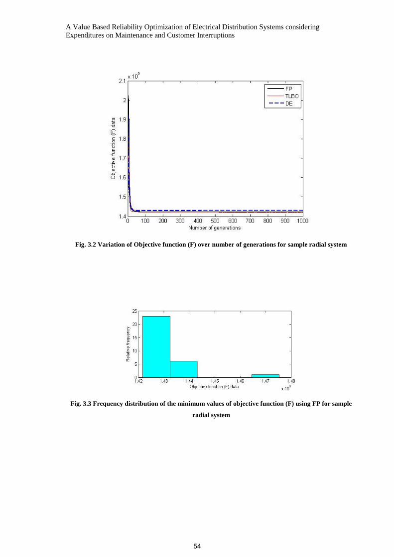
A Value Based Reliability Optimization of Electrical Distribution Systems considering
Expenditures on Maintenance and Customer Interruptions
Fig. 3.2 Variation of Objective function (F) over number of generations for sample radial system
Fig. 3.3 Frequency distribution of the minimum values of objective function (F) using FP for sample
radial system
54

Results and Discussions
Fig.3.4 Frequency distribution of the minimum values of objective function (F) using TLBO for sample
radial system
Fig. 3.5 Frequency distribution of the minimum values of objective function (F) using DE for sample
radial system
55

A Value Based Reliability Optimization of Electrical Distribution Systems considering
Expenditures on Maintenance and Customer Interruptions
Fig. 3.6 Variation of Objective function (F) over number of generations for sample meshed system
Fig.3.7. Frequency distribution of the minimum values of objective function (F) using FP for sample meshed
system
56

Results and Discussions
Fig.3.8 Frequency distribution of the minimum values of objective function (F) using TLBO for sample
meshed system
Fig.3.9 Frequency distribution of the minimum values of objective function (F) using DE for sample
meshed system
57

A Value Based Reliability Optimization of Electrical Distribution Systems considering
Expenditures on Maintenance and Customer Interruptions
Fig. 3.10 Variation of Objective function (F) over number of generations for RBTS-2
Fig.3.11 Frequency distribution of the minimum values of objective function (F) using FP for RBTS-2
58

Results and Discussions
Fig.3.12 Frequency distribution of the minimum values of objective function (F) using TLBO for
RBTS-2
Fig.3.13 Frequency distribution of the minimum values of objective function (F) using DE for RBTS-2
59
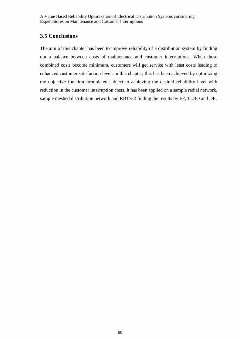
A Value Based Reliability Optimization of Electrical Distribution Systems considering
Expenditures on Maintenance and Customer Interruptions
3.5 Conclusions
The aim of this chapter has been to improve reliability of a distribution system by finding
out a balance between costs of maintenance and customer interruptions. When these
combined costs become minimum, customers will get service with least costs leading to
enhanced customer satisfaction level. In this chapter, this has been achieved by optimizing
the objective function formulated subject to achieving the desired reliability level with
reduction in the customer interruption costs. It has been applied on a sample radial network,
sample meshed distribution network and RBTS-2 finding the results by FP, TLBO and DE.
60

CHAPTER 4
Cost Benefit Analysis for Active Distribution
Systems in Reliability Enhancement
4.1 Introduction
Active distribution system consists of infrastructure of power delivery and active resources
say combining passive infrastructure with active. The active distribution system is developed
to create an energy efficient, high power quality and reliable network. Distributed
generations (DGs) are becoming the best alternatives for power distribution companies to
increase reliability of distribution systems. DGs enhance performance of the systems by
improving reliability, voltage profile and reducing losses of the system. The use of small
capacity DGs at customer ends is also increasing due to many reasons like reducing
resources of fossil fuels, growing demands, pollution problems etc.
By modifying failure rates and repair times of different sections of distribution system
reliability of the system may be improved. By incorporating DGs at customer ends the
additional cost to achieve this can be reduced. On the other end, cost of energy purchased
from DGs may be high. The interruption time in the reliability indices can be reduced to
momentary interruption if the switch over time of DGs are less.
The impact of DGs in distribution system on reliability and other parameters highly depends
on proper locations and size of DGs. Reliability of the distribution system has been improved
by DGs at predefined locations [40]. In many literatures the locations of DGs have been
found minimizing the loss. But for certain loads reliability may keep more worth than the
loss and voltage profile. Various costs related to investment, maintenance, operations etc.
are also involved with the incorporation of DGs in the distribution system. Hence costs and
benefits to the customers and the utilities due to installation of DGs must be calculated.
In line to the above discussions, this chapter aims at improving reliability of distribution
system by modifying the failure rates and repair times of different sections thereof while
61

Cost Benefit Analysis for Active Distribution Systems in Reliability Enhancement
DGs are incorporated in it. This has been done by optimizing an objective function
formulated here. But this optimization has been done after having found proper locations of
DGs from the reliability improvement aspects and not with any presumed locations. Of
course, cost-benefit analysis has been performed for justification.
The rest of the chapter has been arranged this way. Section 4.2 describes the mathematical
formulation of the problem. Section 4.3 gives briefs about cost-benefit analysis. Section 4.4
represents steps to solve the problem. Section 4.5 is regarding results and its interpretation.
Conclusion is drawn in section 4.6.
4.2 Problem Formulation
The aim of this article is to improve reliability of distribution system by reducing failure
rates and repair times of different sections of the system defining proper locations of DGs.
In this regard, two objective functions have been considered as follows.
4.2.1 Deciding locations of DGs
As the main criterion for deciding location of DGs is improvement in reliability, the
objective function considered is as below.
J =SAIFI
SAIFIt+
SAIDI
SAIDIt+
CAIDI
CAIDIt+
AENS
AENSt (4.1)
Here, the objective function in (4.1) is the sum of the normalized values of customer and
energy based reliability indices i.e. SAIFI, SAIDI, CAIDI and AENS. The normalization is
with respect to respective target/threshold values of the indices. Hence all the indices will be
given equal weightage in the procedure.
First the value of J is found connecting DG at load point 1. The value of J here represents
overall reliability of the system. Gradually DGs are connected individually at all the
remaining load points one by one and value of J is found. Improvement in reliability of the
system is found at all the load points as DG is connected at those load points. The
improvement in reliability at all load points in terms of J is arranged in descending order and
ranked accordingly. Now, first two numbers from the ranking are taken, DGs are connected
at those load points and value of J is found. Then first three numbers of ranking are taken
and the same procedure is followed. This procedure may be continued till the desired value
of reliability is achieved. It is explained in detail in section 4.4.1.
62

Problem Formulation
After having found the locations of DGs, optimized values of reliability indices are found as
follows.
4.2.2 Connecting DGs as stand by units in the system
The DGs may be owned by the distribution company itself or it may encourage large
customers to own their DGs. The DGs owned and controlled by customer/or any other
agency may prove to be highly significant in improving reliability of the system. Due to
incorporation of DGs, the outage time reduces and the expense spent in the improvement of
failure rates and repair time is reduced. The interruption cost at the customer ends can also
be reduced. On the other hand, the cost of energy borrowed through DG may be high due to
its higher per unit rates [40]. In view of this, the objective function is formulated as follows.
F = ∑ αk λk2⁄Nc
k=1 + ∑ βk rk⁄Nck=1 + ∑ CIC
Nck=1 + ADCOST(EENSO − EENSD) (4.2)
where, CIC = λk × rk × Li × Cpk (4.3)
In the relations (4.2) and (4.3), λk is the failure rate of kth section;rk is the average repair
time of kth section; αk and βk are the cost coefficients; CIC is customer interruption cost
at various load points; Li is the average connected load at load point i ; Cpk is the cost of
interruption in rupees per kilowatt for an outage duration of rk associated with kth section
; Nc is the total number sections of the distribution system. EENSO is the expected energy
not supplied without DG and EENSD is the expected energy not supplied when DGs are
connected. ADCOST is the additional cost per kWH to be paid to the DG owner. It is assumed
to be Rs.2/kWH.
The objective function consists of four terms. The first two terms are related to modification
costs related to maintenance activities, i.e. cost for modifying failure rates and average repair
times of each section of the distribution system respectively. Lesser are the values of these
terms; more are the costs or investments associated with preventive maintenance and
corrective repair required by utility to achieve them [111]. Both these terms are based on
Duane’s reliability growth model [105]. The third part of the relation (4.2); i.e. cost of
interruption depicts the costs incurred at the customers end in terms of loss at the time of
power fail. When a utility is engaged in supplying power to industrial and commercial
facilities, the high costs associated with power outages of course keep more significance.
The total cost of interruptions for any load point i can be determined by adding the cost of
63

Cost Benefit Analysis for Active Distribution Systems in Reliability Enhancement
all section outages. The total cost of customer interruptions for all customers can then be
evaluated. The customer cost at a single customer load point depends entirely on the cost
characteristics of the customers at that load point. The customer cost associated to any load
point due to any interruption is the combination of the costs of all type of customers affected
due to that distribution outage [50]. For modified radial distribution system (Fig.A.2), for
modified meshed distribution system (Fig.B.3) and modified RBTS-2 (Fig.C.2) it is as
shown in the Table 4.1, Table 4.10 and Table C.4 respectively. The fourth part depicts the
additional cost to be given to the DG owners for the energy purchased from them. It is
multiplication of energy provided by DGs and additional charge (ADCOST) in Rs. /kWH.
Thus the objective function provides balance between the cost spent on DGs and the cost of
maintenance plus customer interruptions. As the expense on DGs increases, the other two
costs are supposed to decrease. This is achieved by minimizing the objective function as
formulated in relation (4.2).
Expected energy not supplied (EENS) is calculated as below.
EENS = ∑ LiUsys,i (4.4)
Where Li average load is connected at ith load point and Usys,i is system annual outage
duration at ith load point. Without DG in the system Usys,i can be calculated as shown in
relation (2.2).
With DG present in the system as a standby unit, load may be transferred to DG in case of
any disruption of supply to the load points from the source. In this case failure rate and
switching time of the switch transferring the load to DG should be considered. The reliability
model of this can be represented by considering the transfer switch in series with the parallel
combination of the system and DG. The equivalent failure rate and repair time when DG is
connected as a stand by unit at a load point is given by following approximate formulas [40].
λeq = λsλdg(rs + rdg) + λsw (4.5)
req =λs.λdg.rs.rdg+λsw.s
λs.λdg(rs+rdg)+λsw (4.6)
Ueq = λeqreq (4.7)
Where λeq is the equivalent failure rate , req the equivalent interruption duration , λs
represents total failure rate up to load point from the source , rs represents average
64

Problem Formulation
interruption duration from the source up to the load point , λdg the failure rate of DG , rdg
the average outage duration of DG ,λsw the failure rate of the switch transferring load to the
DG and s is the switching time or service restoration time with DG. Ueq is the equivalent
annual outage duration of load points when DGs are connected in the system.
The objective function (4.2) is optimized subject to fulfilling the following constraints.
(i) Constraints on the decision variables
λk,min ≤ λk ≤ λk,max and rk,min ≤ rk ≤ rk,max , k = 1, … … … … … , Nc (4.8)
Inequality constraints on the customer oriented and energy based indices
SAIFI ≤ SAIFIt (4.9)
SAIDI ≤ SAIDIt (4.10)
CAIDI ≤ CAIDIt (4.11)
AENS ≤ AENSt (4.12)
where,
λk,max and rk,max are maximum allowable failure rate and repair time respectively. λk,min
and rk,minare minimum reachable values of failure rate and repair time of 𝑘𝑡ℎ section which
are achieved in optimization process. These lower bound values are obtained by failure and
repair data analysis along with the associated costs and it is done through reliability growth
model [105].
SAIFIt ,SAIDIt , CAIDIt and AENSt are target/threshold values of the respective indices. They
depend on the managerial/administrative decisions.
The formulated problem is solved by flower pollination (FP) optimization method [100].
The same has been verified by other two optimization methods named teaching learning
optimization (TLBO) [101] and differential evolution (DE) [102]. The method in this paper
has been applied on a sample radial distribution network, sample meshed distribution
network and Roy Billinton Test System Bus-2 (RBTS-2). The optimized values obtained
after having solved the problem may be given as target values to the crew to enhance the
reliability of the system.
65

Cost Benefit Analysis for Active Distribution Systems in Reliability Enhancement
4.3 Cost-benefit analysis
Over a long run, whether the fixed and variable amount spent on DGs embedded in the
distribution system would yield in benefit or not, can be found by doing cost benefit analysis.
It justifies the installation of specific numbers of DGs at the locations found in this paper.
The cumulative present value (CPV) method [113, 114] has been applied to evaluate the
total costs and benefits when specific number of DGs is connected at specific locations for
the economic life cycle considered. The method of the time value of money or the CPV
method is based on the premise that an investor prefers to receive a payment of a fixed
amount of money today rather than an equal amount in the future. This method converts all
costs and benefits of the plan during the lifecycle to the first year of operation. The following
equations depict the concept.
Benefit = CICDGO − CICDG − ADCOSTDG − CostMDG − DGI − DGM (4.13)
where,
CICDGO = CICDGO × CPV1
CICDGO= Customer interruption cost when DGs are not connected (4.14)
CICDG = CIC × CPV1
CICDG= Customer interruption cost when DGs are connected (4.15)
ADCOSTDG = ADCOST × CPV1
ADCOSTDG = Additional cost required on the operation of DGs in Rs./kWh (4.16)
CostMDG = CostMDG × CPV2
CostMDG = cost of maintenance required to achieve the desired reliability in the system.
(4.17)
DGI = ∑ DGIi × CPV2
n
i=1
DGI = Installation cost of all the DGs connected (4.18)
DGM = ∑ DGMi × CPV2
n
i=1
66

Solution Methodology
DGM = Maintenance cost of all the DGs connected in the system (4.19)
CPV1 =(1−PV1
EL)
(1−PV1) (4.20)
PV1 =(1+Iinf)×(1+LG)
(1+Iint) (4.21)
CPV2 =(1−PV2
EL)
(1−PV2) (4.22)
PV2 =(1+Iinf)
(1+Iint) (4.23)
EL is the economic lifecycle of equipments . LG is load growth rate. Iinf and Iint stand for
inflation rate and interest rate respectively.
4.4 Solution Methodology
The steps to solve the whole problem are described as follows.
4.4.1 Finding the locations of DGs
Step 1. Data input λk , rk, , λdg , rdg , λsw , s , Cpk , N , La , SAIFIt , SAIDIt , CAIDIt
and AENSt .
Step 2. Evaluate load point indices (failure rate and repair time).
Step 3. Evaluate SAIFI, SAIDI, CAIDI, AENS, EENS, ADCOST and CIC for the system.
Step 4. Calculate value of objective function given by relation (4.1) for the system.
Step 5. Connect DG at load point 1 only and calculate the values of all the indices and
objective function given by relation (4.1).
Step 6. Now connect DG at next load point only and calculate all the indices and J as in
(4.1).In the same way , connect DG at all load points one by one and calculate the values of
all indices and J as in (4.1).
Step 7. Find out the improvement in reliability at all the load points due to DG from the
values of J in (4.1).
67

Cost Benefit Analysis for Active Distribution Systems in Reliability Enhancement
Step 8. Arrange the improvement in reliability at load points (in terms of J as in (4.1)) in
descending order and rank them accordingly.
Step 9.Take first two numbers from ranking and connect DGs at those load points. Calculate
all the indices and value of J for DGs connected at these load points.
Step 10. Take first three numbers from ranking. Connect DGs at these load points and
calculate all the indices and J for the system.
Step 11. Increase the number from the ranking in this way and connect DGs at the respective
load points finding out all the indices and J .
Step 12. Continue till the desired value of reliability is achieved.
4.4.2 Finding the optimized solution by FP
The overview of Flower pollination algorithm has been presented in Appendix D. The
method of solving the formulated problem mentioned in section 4.2 by FP is as follows.
Step 1. Data input λk,max, rk,max , λk,min, rk,min and cost of interruption (Cpk ). SAIFIt ,
SAIDIt , CAIDIt and AENSt .
Step 2. Initialization: Generate a population of size ‘M’ (flowers) for failure rate λ and repair
time r each by relation (D.3), where each vector of respective population consists of failure
rate and repair time of each component respectively. These values are obtained by sampling
uniformly between lower and upper limits as given by relation (4.8).
Step 3. Evaluate λsys,i , rsys,i and Usys,i at each load point.
Step 4. Evaluate SAIFI, SAIDI, CAIDI and AENS as mentioned in the relations (2.10),
(2.11), (2.12) and (2.14) respectively for vectors of the population.
Step 5. Calculate value of objective function F for all vectors in the population i.e.F (Xi(k)
),
i = 1, … … … … … , ′M′ as given by relation (4.2) and (4.3).
Step 6. Evaluate inequality constraints from the relations (4.9), (4.10), (4.11) and (4.12) for
each vector of the population. Vectors satisfying these constraints will be feasible otherwise
not feasible vectors. From among the feasible vectors, based on the value of objective
function, identify the best solution vector Xbest(k)
.
Step 7. Set generation counter k = 1 .
68

Solution Methodology
Step 8. Select target vector, i = 1 .
Step 9. Find the updated value of the vector by relation (D.4).
Step 10. Compare the fitness of the updated vectors with that of the initial vectors and retain
the best ones using relation (D.9).
Step 11.Repeat from Step 3.to Step 6.for the updated vector.
Step 12. Increase target vector i = i + 1. If i ≤ M, repeat from Step 9 otherwise increase
generation count k = k + 1 .
Step 13. Repeat from step 8 if the desired optimum value is not found or k ≤ kmax .
In the same way, the same problem can be solved by TLBO and DE. The overview of both
the optimization methods have been presented in the Appendix E and Appendix F
respectively. Fig. 4.1 shows the flow chart to find out locations of DGs from reliability point
of view. Fig 4.2 shows the flow chart for solving the formulated problem by FP.
4.4.3 Doing cost-benefit analysis
Step 1.Do cost- benefit analysis with the relations (4.13)-(4.23) for certain planning
periods i.e. 5 years, 10 years and 15 years and make decisions accordingly.
69

Cost Benefit Analysis for Active Distribution Systems in Reliability Enhancement
START
Evaluate SAIFI, SAIDI, CAIDI,AENS, EENS, ADCOST, CIC for the system
Connect DG at Load point 1 only and calculate the values of all the indices and objective function J
Take first two number from raking and connect DGs at those load points.
Calculate all the indicies and value of J for DGs connected at these load points
,
,, , ,Data input ,
, , , , , &,k t t t ti i
swk k dg dg
SAIFI SAIDI AIDIS Cp N L C AENS
r r
Evaluate load point indices (Failure rate and Repair time)
Increase the number from the ranking in this way and connect DGs at the respective load points
finidng out all the indices and J
Continue till the desired value of reliability is achieved
Take first three number from raking and connect DGs at these load points. Calculate all the indicies and
value of J for DGs connected at these load points
Now Connect DG at next load point only and calculate the values of all the indices and
objective function J, In the same way, connect DG at all load points one by one and
calculate the values of all indices and objective function J
Find out the improvement in reliability at all the load points due to DG from the values of J
Arrange the improvement in reliability at load points (in terms of J) in descending order and
rank them accordingly
Calculate value of objective function
t t t t
SAIFI SAIDI CAIDI AENSfor the system
SAIFI SAIDI CAIDI AENSJ
END
Fig. 4.1 Flow chart for finding out the locations of DGs
70

Solution Methodology
Fig. 4.2 Flow chart for enhancing reliability of distribution system incorporating DGs by FP
71

Cost Benefit Analysis for Active Distribution Systems in Reliability Enhancement
4.5 Results and discussions
The developed methodology in this paper has been implemented on a sample radial
distribution system, sample meshed distribution system and RBTS-2. The problem has been
solved by FP algorithm and comparison has been made with the results obtained by TLBO
and DE. The algorithms used have been coded in MATLAB-13.
4.5.1 Distribution systems: Descriptions
(A) Sample radial distribution system [29]:
The radial system is shown in Fig. A.2. It has been modified with DGs being connected at
its different load points. The data regarding the current and minimum reachable values of
failure rates and repair times, average load and number of customers at load points and cost
coefficients for each segment of radial distributor have been taken from [111]. They have
been represented in Table A.1-Table A.3 in Appendix. Table 4.1 gives interruption cost
(𝐶𝑝𝑘) at different load points for the sample radial distribution system. Table 4.2 gives the
values of customer and energy based reliability indices, customer interruption cost,
additional cost expended on DG and the value of J as given by relation (4.1) when single
DG is connected to different load points of the distribution system one by one. The values
of J found in Table 4.2 are ranked according to improvement in reliability of the distribution
system in descending order as shown in Table 4.3. Reliability with more than one DGs
connected at different load points is found as per ranking as shown in Table 4.4. From Table
4.4 the locations of DGs are found. In this chapter, DGs are connected at load points 5, 6
and 7 and the objective function F in relation (4.2) has been optimized by FP, TLBO and
DE. Table 4.6 gives the optimized values of failure rates and repair times obtained by the
three methods. Table 4.7 gives the optimized values of maintenance cost, customer
interruption cost, additional expense made in purchasing energy from the generators
connected and objective function (F) for sample radial distribution system obtained by all
the three methods. Table 4.8 shows the optimized values of customer and energy based
reliability indices obtained by all the three methods. The cost benefit analysis has been made
according to the section 4.3 in Table 4.9.
(B) Sample meshed distribution system [13,107]
This test system used in this chapter is as shown in Fig.B3. It is a modified system with DGs
being connected at its different load points to solve the problem formulated in this chapter.
72

Results and discussions
The data regarding failure rates and average repair times of different components of meshed
system have been taken from [13,107]. Table B.1 gives maximum allowable (λk,max/year)
and minimum reachable (λk,min/year) failure rates, and maximum allowable (rk,max (h))
and minimum reachable (rk,min (h)) average repair times. Table B.3 gives cost coefficients
for different distributor segments corresponding to failure rate and repair time. Table 4.10
gives interruption cost (𝐶𝑝𝑘) at different load points for the sample meshed distribution
system. Table 4.11 gives the values of customer and energy based reliability indices,
customer interruption cost, additional cost expended on DG and the value of J as given by
relation (4.1) when single DG is connected to different load points of the distribution system
one by one. The values of J found in Table 4.11 are ranked according to improvement in
reliability of the distribution system in descending order as shown in Table 4.12. Reliability
with more than one DGs connected at different load points is found as per ranking as shown
in Table 4.13. From Table 4.13, the locations of DGs are found. In this chapter, DGs are
connected at load points 1 and 4 for the meshed system and the objective function F in
relation (4.2) has been optimized by FP, TLBO and DE. Table 4.14 gives the optimized
values of failure rates and repair times obtained by the three methods. Table 4.15 gives the
optimized values of maintenance cost, customer interruption cost, and additional expense
made in purchasing energy from the generators connected and objective function (F) for
sample meshed distribution system obtained by all the three methods. Table 4.16 shows the
optimized values of customer and energy based reliability indices obtained by all the three
methods. The cost benefit analysis has been made according to the section 4.3 in Table 4.17.
(C) Roy Billinton Test System-Bus 2 (RBTS-2) [99]:
Another test system which has been used in this chapter is Roy Billinton Test System-Bus 2
as shown in Fig.C.2. It is a modified system with DGs being connected at its different load
points as per the requirement of the problem formulated in this chapter. The data regarding
failure rates and average repair times of different components of RBTS-2 have been taken
from [99, 72]. Table C.2 gives maximum allowable (λk,max/year) and minimum reachable
(λk,min/year) failure rates, maximum allowable (rk,max (h)) and minimum reachable
(rk,min (h)) average repair times. Cost coefficients 𝛼𝐾 and 𝛽𝐾 for failure rates and repair
times respectively of the different sections of RBTS-2 are shown in Table C.3. Table C.4
represents sector wise customer data. The results which have been found for the sample
radial and meshed distribution system, have also been found for RBTS-2 in the same way.
73

Cost Benefit Analysis for Active Distribution Systems in Reliability Enhancement
They have been shown in from Table 4.18 to Table 4.24. The locations of DGs found for
RBTS-2 are 2, 3, 11, 12 and 18. The optimized values of the objective function (F) has been
found at these locations for RBTS-2.
Table 4.5 gives control parameters for the three optimization methods; FP, TLBO and DE
applied in this chapter for all the distribution test systems. Here, the DGs to be connected
are taken as standby units. The failure rate and average down time of DG taken in this chapter
are 0.5 failures/year and 13.25 hrs. respectively for all the three systems. Failure rate and
service restoration time of the changeover switch of DG are 0.1 failures/year and 0.25 hrs.
respectively for all the systems. Installation and maintenance cost of the DGs connected in
the system have been taken as Rs. 25/kW and Rs. 5.94/kW respectively for all systems. The
inflation rate, interest rate and load growth rate have been taken as 5%, 10% and 5 %
respectively. The calculations have been made for economical life cycle plans of 5 years, 10
years and 15 years by all the three optimization methods and comparison has been made in
all the case studies.
74

Results and discussions
Table 4.1 Interruption costs at load points for sample radial distribution system
Distributor Load points(LP) #2 #3 #4 #5 #6 #7 #8
Interruption Cost(𝑪𝒑𝒌)(Rs./kW) 15 13 17 20 20 12 14
Table 4.2 The parameter values without DG and with DG connected at different load points of sample radial distribution system
Parameters Without DG With DG (Load point locations)
LP2 LP3 LP4 LP5 LP6 LP7 LP8
1 SAIFI(interruptions/customer) 0.72 0.7403 0.7054 0.6805 0.6607 0.6608 0.6710 0.7053
2 SAIDI(h/customer) 8.45 7.8015 7.6949 7.5885 6.4682 6.8313 6.9937 8.0993
3 CAIDI(h/customer interruption) 11.7361 10.5388 10.9086 11.1510 9.7895 10.3388 10.4230 11.4839
4 AENS(kWh/customer) 26.4100 23.1676 22.8860 22.9640 19.8039 21.5540 25.2449 25.3580
5 EENS (kWh) 26410 23168 22886 22964 19803 21554 25245 25358
6 Additional cost incurred on DG ( Rs.) ------- 6484.9 7048.1 6891.9 13212 9711.9 2330.1 2104
7 CIC (Rs) 450920 402280 405110 392340 318800 353800 436940 436190
8 J (Objective function) 7.6605 7.0650 6.9867 6.9485 6.1426 6.4771 6.9177 7.4067
75

Cost Benefit Analysis for Active Distribution Systems in Reliability Enhancement
Table 4.3 Ranking of the load points with reference to reliability improvement from maximum to
minimum for sample radial distribution system
Sr.
No.
Ranking of the load
points according to
reliability
improvement when
connected with DG
Increase in
reliability in
(%)
(In terms of
J)
1 LP5 28.8483
2 LP6 20.1377
3 LP7 12.1372
4 LP4 11.9957
5 LP3 11.6366
6 LP2 9.1929
7 LP8 3.6577
Table 4.4 Reliability with more than one generators connected according to the load point ranking for
sample radial distribution system
Table 4.5 Control Parameters for FP, TLBO and DE for sample radial distribution system, sample
meshed distribution system and RBTS-2.
Sr No. Parameters Values of parameters
1 Population size(FP,TLBO,DE) 30
2 Max generation specified(kmax) (FP,TLBO,DE) 1000
3 Updated step size (∝) (FP) 0.01
4 Distribution factor (𝛽) (FP) 1.5
5 Switch probability (FP) 0.8
6 Step size (F) (DE) 0.8
7 Cross over rate (Cr) (DE) 0.7
Parameters Without DG With DG
LP(5,6) LP(5,6,7)
1 SAIFI(interruptions/customer) 0.72 0.601474 0.552457
2 SAIDI(h/customer) 8.45 4.849518 3.393176
3 CAIDI(h/customer interruption) 11.7361 8.062717 6.141971
4 AENS(kWh/customer) 26.4100 14.94795 13.78287
5 EENS (kWh) 26410 14947.95 13782.87
6 Additional cost incurred on DG ( Rs.) -------- 22924.11 25254.26
7 CIC (Rs.) 450920 221678.9 207698
8 J (Objective function) 7.6605 4.917963 4.099242
76
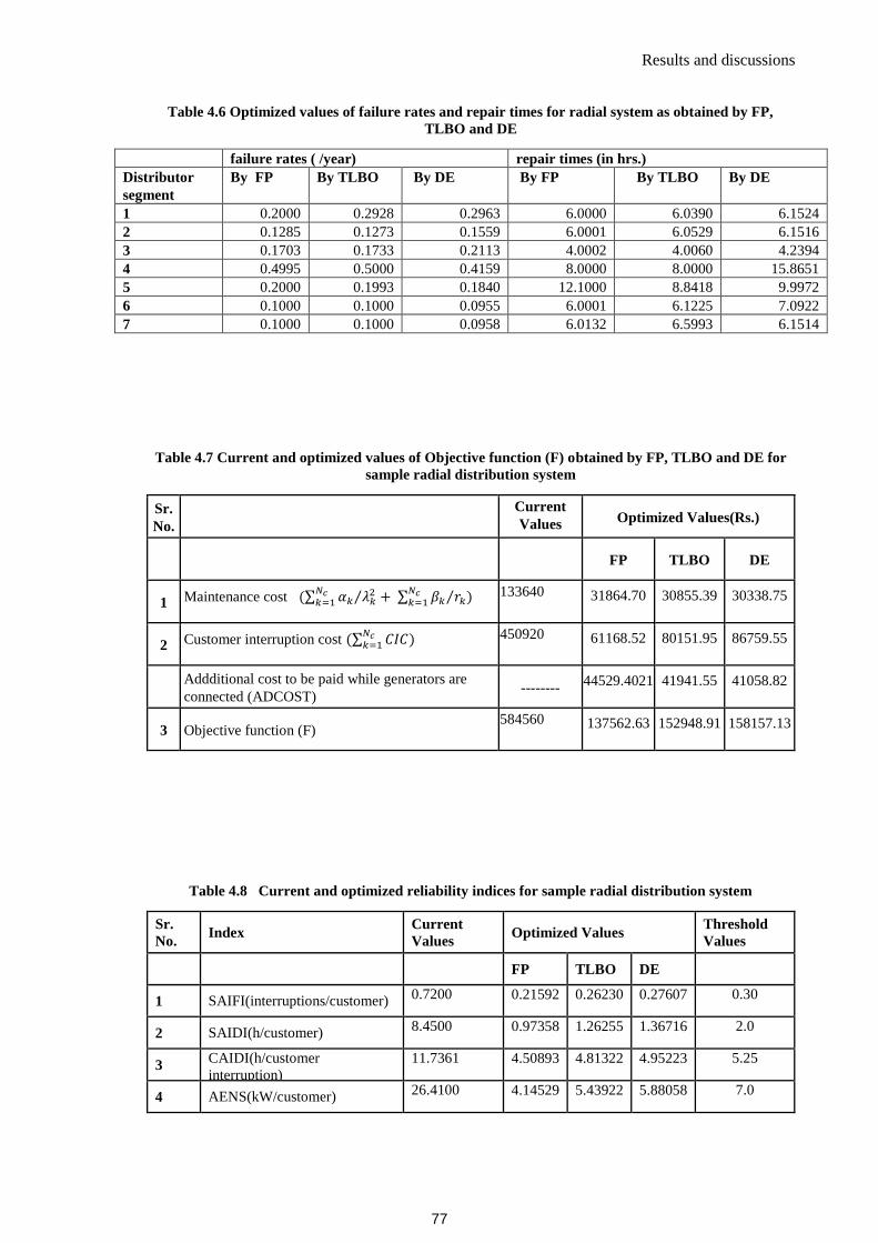
Results and discussions
Table 4.6 Optimized values of failure rates and repair times for radial system as obtained by FP,
TLBO and DE
failure rates ( /year) repair times (in hrs.)
Distributor
segment
By FP
By TLBO
By DE
By FP
By TLBO By DE
1 0.2000 0.2928 0.2963 6.0000 6.0390 6.1524
2 0.1285 0.1273 0.1559 6.0001 6.0529 6.1516
3 0.1703 0.1733 0.2113 4.0002 4.0060 4.2394
4 0.4995 0.5000 0.4159 8.0000 8.0000 15.8651
5 0.2000 0.1993 0.1840 12.1000 8.8418 9.9972
6 0.1000 0.1000 0.0955 6.0001 6.1225 7.0922
7 0.1000 0.1000 0.0958 6.0132 6.5993 6.1514
Table 4.7 Current and optimized values of Objective function (F) obtained by FP, TLBO and DE for
sample radial distribution system
Sr.
No.
Current
Values
(Rs.)
Optimized Values(Rs.)
FP TLBO DE
1 Maintenance cost (∑ 𝛼𝑘 𝜆𝑘2⁄𝑁𝑐
𝑘=1 + ∑ 𝛽𝑘 𝑟𝑘⁄𝑁𝑐𝑘=1 ) 133640 31864.70 30855.39 30338.75
2 Customer interruption cost (∑ 𝐶𝐼𝐶𝑁𝑐𝑘=1 ) 450920 61168.52 80151.95 86759.55
Addditional cost to be paid while generators are
connected (ADCOST) --------
44529.4021 41941.55 41058.82
3 Objective function (F) 584560 137562.63 152948.91 158157.13
Table 4.8 Current and optimized reliability indices for sample radial distribution system
Sr.
No. Index
Current
Values Optimized Values
Threshold
Values
FP TLBO DE
1 SAIFI(interruptions/customer) 0.7200 0.21592 0.26230 0.27607 0.30
2 SAIDI(h/customer) 8.4500 0.97358 1.26255 1.36716 2.0
3 CAIDI(h/customer
interruption)
11.7361 4.50893 4.81322 4.95223 5.25
4 AENS(kW/customer) 26.4100 4.14529 5.43922 5.88058 7.0
77

Cost Benefit Analysis for Active Distribution Systems in Reliability Enhancement
Table 4.9 Cost-Benefit Analysis for sample radial distribution system
Sr. No Economic
lifecycle
planning
( In Years)
Benefit in Rs.
Optimization Methods
FP TLBO DE
1 5 1496660 1481797 1392532
2 10 3062288 3047702 2960448
3 15 4687144 4448412 4366869
Table 4.10 Interruption cost at load points for sample meshed network
Load point(LP) LP-T1 LP-T2 LP-T3 LP-T4
Interruption Cost(𝐶𝑝𝑖)(Rs./kW) 45 39 51 68
Table 4.11 The parameter values without DG and with DG connected at different load points of
meshed distribution system
SAIFI SAIDI CAIDI AENS EENS Additional
cost
incurred
on DG
(Rs.)
CIC
(Rs.)
J ((
Without
DG
0.689895 4.854797 7.037003 20.533869 26694 ________ 1345365 8.614597
With
DG
( At
Load
points)
LP1 0.506889 3.376967 6.662140 14.992007 19489 14408 1021166 6.665947
LP2 0.580880 3.906521 6.725177 16.740767 21762 9862 1153055 7.345548
LP3 0.598379 4.115833 6.878297 16.839053 21890 9606 1100399 7.545763
LP4 0.484016 3.192271 6.595373 13.144866 17088 19211 769023 6.288435
78

Results and discussions
Table 4.12 Ranking of the load points with reference to reliability improvement from maximum to
minimum for sample meshed distribution system
Sr.
No.
Ranking of
the load
points
according to
reliability
improvement
when
connected
with DG
Increase
in
reliability
in (%)
(In terms
of J)
1 LP4 36.991095
2 LP1 29.232890
3 LP2 16.818020
4 LP3 14.164684
Table 4.13 Reliability with more than one generators connected according to the load point ranking for
sample meshed distribution system
DGs
connected
atLoad points
SAIFI SAIDI CAIDI AENS EENS Additional
cost
incurred
on DG
(Rs.)
CIC
(Rs.)
J
4,1 0.301010 1.714441 5.695621 7.603005 9883 33620 444824 4.189817
4,1,2 0.191995 0.766166 3.990551 3.809902 4952 43482 252514 2.522699
79

Cost Benefit Analysis for Active Distribution Systems in Reliability Enhancement
Table 4.14 Optimized values of failure rates and repair times for the sample meshed distribution
system as obtained by FP, TLBO and DE
failure rates ( /year) repair times (in hrs.)
Distributor
segment
By FP
By TLBO
By DE
By FP
By TLBO By DE
1 0.2543 0.2586 0.5108 3.3638 6.4239 3.3488
2 0.1777 0.1732 0.1789 3.0692 4.0616 3.1863
3 0.1100 0.1102 0.1102 13.6459 14.1663 15.2239
4 0.1136 0.1135 0.1135 5.2832 5.5838 5.5767
5 0.0845 0.1836 0.0936 3.8810 3.3947 3.6861
6 0.0271 0.0284 0.0216 12.8049 11.4817 9.8042
7 0.1847 0.1846 0.1895 8.3979 8.8077 5.0402
8 0.1720 0.1784 0.1782 7.6295 5.7566 4.3617
9 0.0125 0.0124 0.0107 15.2188 6.5967 6.6022
10 0.0691 0.0693 0.0690 20.5688 20.0002 23.2368
11 0.2052 0.2091 0.2056 2.7692 5.2598 4.5500
12 0.2562 0.2008 0.2060 2.0162 4.8160 4.5732
13 0.1075 0.1100 0.1163 18.0929 24.5014 12.8537
14 0.1136 0.1135 0.1135 6.1741 2.1240 5.1153
15 0.0683 0.0903 0.1569 10.7236 6.8451 6.4803
16 0.0269 0.0275 0.0215 13.5553 9.3975 11.3589
17 0.1779 0.1780 0.1331 9.7524 13.8321 6.8392
18 0.1853 0.1846 0.1847 4.2503 8.5663 3.7627
Table 4.15 Current and optimized values of Objective function (F) obtained by FP, TLBO and DE for
sample meshed distribution system
Sr.
No.
Current
Values (Rs.) Optimized Values(Rs.)
FP TLBO DE
1
Maintenance cost
(∑ 𝛼𝑘 𝜆𝑘2⁄𝑁𝑐
𝑘=1 + ∑ 𝛽𝑘 𝑟𝑘⁄𝑁𝑐𝑘=1 ) 5990100 924368.54 907796.36 1267214.73
2 Customer interruption cost (∑ 𝐶𝐼𝐶𝑁𝑐𝑘=1 ) 1345365 127239.70 210511.40 216164.70
Addditional cost to be paid while
generators are connected (ADCOST) --------
47659.68
44068.38 43636.45184
3 Objective function (F) 7335465 1099267.92 1162376.15 1527016.89
80

Results and discussions
Table 4.16 Current and optimized reliability indices for sample meshed distribution system
Sr.
No. Index
Current
Values Optimized Values
Threshold
Values
FP TLBO DE
1 SAIFI(interruptions/customer) 0.689895 0.179817 0.200842 0.287110 0.30
2 SAIDI(h/customer) 4.854797 0.504747 0.807696 0.858059 2.00
3 CAIDI(h/customer
interruption) 7.037003 2.807004 4.021537 2.988605 3.5
4 AENS(kW/customer) 20.533869 2.203200 3.584467 3.750595 6.00
Table 4.17 Cost-Benefit Analysis for sample meshed distribution system
Sr. No Economic
lifecycle
planning
( In Years)
Benefit in Rs.
Optimization Methods
FP TLBO DE
1 5 1164232 839678 -827526
2 10 3374027 2704648 -289509
3 15 6427093 5395824 1344290
81

Cost Benefit Analysis for Active Distribution Systems in Reliability Enhancement
Table 4.18 The parameter values without DG and with DG connected at different load points of RBTS-2
SAIFI SAIDI CAIDI AENS EENS Additional
cost
incurred
on DG
(Rs.)
CIC
(Rs.)
J
Without
DG
0.0986 0.5882 5.9666 4.6641 8899 ________ 828680 5.663
With
DG
( At
Load
points)
LP1 0.102576 0.550374 5.365523 4.567758 8715.282 367.4939 824578.4 5.432647
LP2 0.098509 0.509682 5.173954 4.464089 8517.482 763.0945 820168.4 5.201177
LP3 0.097299 0.523979 5.385271 4.500513 8586.979 624.0997 821717.9 5.287815
LP4 0.098572 0.58787 5.963838 4.491036 8568.898 660.2624 820756.8 5.603837
LP5 0.098547 0.587742 5.964087 4.418784 8431.039 935.9788 817450.3 5.579199
LP6 0.098262 0.583842 5.941668 4.467319 8523.645 750.7674 756231.6 5.576713
LP7 0.098058 0.582821 5.943626 4.420955 8435.182 927.6935 739159.6 5.55682
LP8 0.098578 0.587938 5.96418 4.426446 8445.66 906.738 714689 5.582629
LP9 0.098558 0.587836 5.96438 4.273329 8153.512 1491.034 641237.1 5.531147
LP10 0.102575 0.550371 5.365532 4.567749 8715.265 367.5265 827564.2 5.432628
LP11 0.096857 0.521774 5.387035 4.494895 8576.26 645.5377 826723.9 5.27574
LP12 0.096939 0.524936 5.415099 4.521772 8627.541 542.9756 827033.9 5.300572
LP13 0.09855 0.587757 5.964058 4.427286 8447.262 903.5328 817839.4 5.582098
LP14 0.09855 0.587757 5.964058 4.427286 8447.262 903.5328 817839.4 5.582098
LP15 0.098037 0.582715 5.943829 4.416179 8426.07 945.9166 863237.8 5.554772
LP16 0.098752 0.58629 5.937007 4.578467 8735.715 326.6273 795406.9 5.624409
LP17 0.102045 0.550469 5.394395 4.579221 8737.154 323.7495 825945.5 5.437743
LP18 0.096939 0.524936 5.415099 4.521772 8627.541 542.9756 825282.9 5.300572
LP19 0.096939 0.524936 5.415099 4.521772 8627.541 542.9756 826898.8 5.300572
LP20 0.098545 0.587732 5.964108 4.412835 8419.689 958.6804 815427.1 5.57717
LP21 0.098524 0.587629 5.964307 4.355028 8309.393 1179.271 812781.6 5.557458
LP22 0.098037 0.582715 5.943829 4.416179 8426.07 945.9166 735650.2 5.554772
82

Results and discussions
Table 4.19 Ranking of the load points with reference to reliability improvement from maximum to
minimum for RBTS-2
Table 4.20 Reliability with more than one generators connected according to the load point ranking for
RBTS-2
DGs
connected
atLoad points
SAIFI SAIDI CAIDI AENS EENS Additional
cost
incurred
on DG
(Rs.)
CIC (Rs.) J
2,11 0.09678 0.44328 4.579908 4.294923 8194.713 1408.63 818217.3 4.810259
2,3,11 0.09550 0.379084 3.969128 4.131375 7882.663 2032.73 811260.1 4.427674
2,3,11,12 0.093869 0.315844 3.364737 3.989085 7611.175 2575.70 809619 4.051987
2,3,11,12,18 0.09223 0.252604 2.738863 3.846796 7339.687 3118.68 807977.9 3.670929
2,3,11,12,18,19 0.09059 0.18936 2.09033 3.70450 7068.1994 3661.658 806336.717 3.28420
Sr.
No.
Ranking of
the load
points
according to
reliability
improvement
when
connected
with DG
Increase
in
reliability
in (%)
(In terms
of J)
Sr.
No.
Ranking of
the load
points
according to
reliability
improvement
when
connected
with DG
Increase
in
reliability
in (%)
(In terms
of J)
1 LP2 8.879202 12 LP22 1.948386
2 LP11 7.340399 13 LP7 1.9108
3 LP3 7.095283 14 LP21 1.899099
4 LP12 6.837517 15 LP6 1.547274
5 LP18 6.837517 16 LP20 1.53895
6 LP19 6.837517 17 LP5 1.502031
7 LP10 4.24052 18 LP13 1.449311
8 LP1 4.24017 19 LP14 1.449311
9 LP17 4.14248 20 LP8 1.439657
10 LP9 2.383825 21 LP4 1.055767
11 LP15 1.948386 22 LP16 0.686126
83

Cost Benefit Analysis for Active Distribution Systems in Reliability Enhancement
Table 4.21 Optimized values of failure rates and repair times for RBTS-2 as obtained by FP,
TLBO and DE
failure rates ( /year) repair times (in hrs.)
Distributor
segment
By FP
By TLBO
By DE
By FP
By TLBO
By DE
1 0.0367 0.0367 0.0398 2.2523 2.2523 2.2523
2 0.0150 0.0150 0.0149 4.5045 4.5045 4.5045
3 0.0391 0.0520 0.0474 4.5088 4.5045 4.5045
4 0.0361 0.0361 0.0361 2.2526 2.2523 2.2523
5 0.0150 0.0150 0.0148 9.9978 10.0000 10.0000
6 0.0150 0.0150 0.0149 4.5136 4.5045 4.5045
7 0.0367 0.0367 0.0372 2.2528 2.2523 2.2523
8 0.0150 0.0150 0.0147 4.5160 4.5045 4.5045
9 0.0150 0.0150 0.0148 4.5053 4.5045 4.5045
10 0.0390 0.0293 0.0297 2.2524 2.2523 2.2523
11 0.0150 0.0150 0.0150 4.5050 4.5045 4.5045
12 0.0367 0.0367 0.0367 2.2525 2.2523 2.2523
13 0.0391 0.0391 0.0391 2.2579 2.2523 2.2523
14 0.0390 0.0293 0.0293 2.2553 2.2523 2.2523
15 0.0391 0.0391 0.0397 2.2530 2.2523 2.2523
16 0.0367 0.0367 0.0371 2.2681 2.2523 2.2523
17 0.0150 0.0150 0.0150 9.9870 4.5045 4.5045
18 0.0391 0.0391 0.0394 2.2625 2.2523 2.2523
19 0.0150 0.0150 0.0142 4.5100 4.5045 4.5045
20 0.0150 0.0150 0.0150 4.5050 4.5045 4.5045
22 0.0293 0.0293 0.0316 2.2525 2.2523 2.2523
23 0.0150 0.0150 0.0145 4.5083 4.5045 4.5045
24 0.0150 0.0150 0.0144 4.5049 4.5045 4.5045
25 0.0487 0.0367 0.0374 2.2561 2.2523 2.2523
26 0.0150 0.0150 0.0149 4.5068 4.5045 4.5045
27 0.0392 0.0391 0.0400 2.2529 2.2523 2.2523
28 0.0150 0.0150 0.0146 4.5058 4.5045 4.5045
29 0.0150 0.0150 0.0141 9.9824 4.5045 4.5045
30 0.0487 0.0367 0.0368 2.2534 2.2523 2.2523
31 0.0150 0.0150 0.0150 4.5054 4.5045 4.5045
32 0.0150 0.0150 0.0149 4.5383 4.5045 4.5045
33 0.0367 0.0367 0.0417 2.2529 2.2523 2.2523
34 0.0150 0.0150 0.0150 9.9800 4.5045 4.5045
35 0.0293 0.0306 0.0295 2.2529 2.2523 2.2523
36 0.0150 0.0150 0.0149 9.9384 4.5045 4.5045
84

Results and discussions
Table 4.22 Current and optimized values of Objective function (F) obtained by FP, TLBO
and DE for RBTS-2
Sr.
No.
Current
Values (Rs.) Optimized Values(Rs.)
FP TLBO DE
1
Maintenance cost
(∑ 𝛼𝑘 𝜆𝑘2⁄𝑁𝑐
𝑘=1 + ∑ 𝛽𝑘 𝑟𝑘⁄𝑁𝑐𝑘=1 )
232680
254692.6 254620.043 253861.34
2 Customer interruption cost (∑ 𝐶𝐼𝐶
𝑁𝑐𝑘=1 ) 828680 284052.8 284985.027 285949.06
Addditional cost to be paid while generators
are connected(ADCOST) --------
12398.98 12262.9861 12237.510
3 Objective function (F) 1061360 551144.3 551868.056
552047.91
Table 4.23 Current and optimized reliability indices for RBTS-2
Sr.
No. Index
Current
Values Optimized Values
Threshold
Values
FP TLBO DE
1 SAIFI(interruptions/customer) 0.0986 0.079722 0.080853 0.080867 0.086
2 SAIDI(h/customer) 0.5882 0.111135 0.132302 0.174741 0.4
3 CAIDI(h/customer interruption) 5.9666 1.301081 1.586033 2.163416 4.0
4 AENS(kW/customer) 4.6641 1.414852 1.560067 1.688404 2.2
Table 4.24 Cost-Benefit Analysis for RBTS-2
Sr. No Economic
lifecycle
planning
( In Years)
Benefit in Rs.
Optimization Methods
FP TLBO DE
1 5 1128600 1173100 972060
2 10 2658400 2540400 2280500
3 15 4438500 4137300 3895700
85

Cost Benefit Analysis for Active Distribution Systems in Reliability Enhancement
4.6 Conclusions
In this chapter, reliability of distribution systems (a sample radial distribution system, a
sample meshed system and RBTS-2) have been enhanced with DGs connected at different
load points of the systems. The locations of DGs have been found with a methodology
considering improvement in reliability as the chief motive. With these locations thus found,
the objective function formulated in this paper has been optimized by three optimization
methods say FP, TLBO and DE. To justify the installation of DGs in a long run, the cost-
benefit analysis has been made. It has been shown that for specific locations of DGs in the
distribution system, reliability enhancement is better. Of course, additional amount has to be
spent on the energy purchased from DGs but that too has been justified for specific period
of life cycle of DGs by doing cost-benefit analysis.
86

CHAPTER 5
Optimal Parameter Setting in Distribution System
Reliability Enhancement with Reward and Penalty
5.1 Introduction
The distribution companies are transiting gradually from the conventional cost based (cost
of service or rate of return) regulation to performance based regulation (PBR) in many
countries of the world for efficiency improvement. In performance based regulations
incentives are decided for strong efficiency (in terms of profit) by the companies. This may
lead to deterioration of quality services to customers [115].
In order to reach out such conditions, many performance based regulations are embedded
with quality regulations adopting direct or indirect quality controls [116]. In indirect quality
control, customers are provided information regarding quality of performance of distribution
companies while in direct control, the performance is evaluated in terms of financial
incentives provided by the regulators for maintaining adequate service quality [117]. The
quality of services rendered by distribution companies are defined in three ways; reliability
of services /continuity of supply, voltage quality and commercial quality [115].This paper
focuses on service reliability regulations. Service reliability has been regulated by different
mechanisms introduced by regulators. The reward and penalty scheme (RPS), which is a
direct quality control, is an effective and highly accepted mechanism for regulatory purpose
in distribution systems. The regulator uses this tool to regulate service reliability index like
SAIFI, SAIDI and AENS. Reward or penalty to the distribution company is decided
depending on the achievement of these indices below their target levels.
In RPS financial incentives are created for distribution companies to maintain or change
their quality level. The regulator tries to maintain socioeconomically optimum reliability
level which minimizes the total reliability cost for society with RPS [117].
This chapter focuses on enhancing the reliability of distribution system incorporating
reward/penalty imposed on distribution systems by the regulator. Here the optimized values
of reward /penalty have been found achieving the target values of reliability indices. By
87

Optimal Parameter Setting in Distribution System Reliability Enhancement with Reward and Penalty
finding optimum values of reward/penalty it is possible to limit financial risk of distribution
companies and unnecessary tariff changes for the customers.
The chapter is arranged as follows. The RPS theory is depicted in section 5.2. In Section 5.3
the problem formulated in this chapter has been described. Section 5.4 is regarding the
solution methodology of the problem by FP. In section 5.5 results obtained for the three
distribution systems i.e. sample radial, sample mesh and RBTS-2 are discussed. Conclusions
are drawn in section 5.6.
5.2. Reward / Penalty Scheme (RPS)
In RPS regulator uses system quality indicators to measure the reliability of the system.
Target levels of these indicators are imposed on the utilities by the regulators. Success or
failure in achieving them decides the reward or penalty for the utility. The higher the
reliability level, higher will be the profit of utility. Thus the market-like conditions are tried
to be replicated by regulator. The quality indicators commonly used are system average
interruption frequency index (SAIFI) and system average interruption duration index
(SAIDI) from reliability point of view. Both are customer based indices. Energy based
reliability index (EENS) can also be integrated with these indices.
5.2.1 Socio-economical perspectives of RPS
With RPS the regulator tries to achieve socio-economically optimum reliability level [115].
The socio-economical reliability relates to the customer interruption costs and network costs.
For poor reliability customer interruption costs are high. Higher reliability of the system
reduces interruption costs to the customers but it requires higher expenditures on capital and
maintenance activities which is ultimately paid by the customers in terms of tariffs.
Somewhere in between is the socioeconomic optimal reliability level which is the sum of
customer interruption costs and network costs, minimizing the total reliability cost for
society [118]. The cost versus reliability depicting socio-economically optimal reliability
level is shown in Fig.5.1.The optimal reliability Ropt is achieved when the rate of increase
of network costs equals the rate of decrease of customer interruption costs.
∂Cnetwork
∂R|
R=Ropt
= − ∂CIC
∂R|
R=Ropt
(5.1)
The utility’s optimum may or may not be the socio-economical optimum as the utility tries
to set the optimum at its minimum cost. In optimum RPS incentives are given to achieve the
88

Reward / Penalty Scheme (RPS)
socio-economical reliability by including the customer interruption costs in their own cost
functions [119]. In actual the socio-economical reliability level is not known to the regulator,
instead a target value is set for the quality indicator which measures reliability. The increase
or decrease in customer interruption costs due to deviation of reliability from this target value
is adjusted by the utility in terms of either reward or penalty. It is the financial risk CRP(cost
of reward/penalty) borne by the utility when it succeeds or fails in achieving the target
reliability level, which is reflected in either profit or loss of the utility. Here CRP < 0 stands
for reward to the utility and CRP > 0 as penalty to the utility. Thus the ultimate aim here
is to bring the minimum of total reliability cost curve of the utility, which includes the impact
of RPS, to the socio-economical reliability level Ropt .
The various RPS schemes are as shown in Fig. 5.2 [120]. This paper focuses on continuous
scheme where rewards/penalties increase with the deviation from the set target level.
5.3 Problem formulation
In context to the discussions made in the previous sections, the problem is formulated as
follows.
The adjustment of utility’s cost curve such that its minimum occurs at the same reliability
level Ropt as society, leads to defining the optimum values of reward and penalty CRP .
With impact of RPS, at the socio-economically optimal reliability level Ropt, the total
reliability cost for society is minimized.
∂Ctotalsociety
∂R|
R=Ropt
= ∂(Cnetwork+CIC)
∂R|
R=Ropt
= 0 (5.2)
For an optimal RPS following must also be satisfied.
∂Ctotalsociety
∂R|
R=Ropt
= ∂(Cnetwork+CRP)
∂R|
R=Ropt
= 0 (5.3)
From (8) and (9), an optimal RPS must fulfill
∂CRP
∂R|
R=Ropt
= ∂CIC
∂R|
R=Ropt
(5.4)
89

Optimal Parameter Setting in Distribution System Reliability Enhancement with Reward and Penalty
In [120] it is shown that for an optimal RPS (5.4) can be written as below.
∂CRP
∂R=
∂CIC
∂R , ∀ R (5.5)
CRP = CIC − K , ∀ R (5.6)
K is an arbitrary constant.
The derivative ∂CRP ∂R⁄ is the monetary value per unit system quality indicator for
reliability and is known as incentive rate. For this paper it is a slope for continuous type RPS.
As per (5.6), optimal reward/penalty at specific reliability level is a function of customer
interruption costs CIC at that reliability level. Thus it depends on the ability of regulator to
measure and reconstruct CIC to get optimal reward/penalty [120].
For the continuous RPS scheme in Fig.5.2 the slope (incentive rate) is constant. Hence, the
relation between system reliability and customer interruption costs is liner for (5.5) to be
satisfied. As long as (5.5) is satisfied, socio-economically optimal reliability level is
achieved at any value of K in (5.6). The value of K is responsible for the transaction between
the utility and customers. If value of K is set to zero, all the customer interruption costs will
be transferred to the utility. Hence, the utility will operate on society’s total reliability cost.
In this case, a profit maximizing utility may likely to incur loss as the allowed revenue only
covers the utility’s total reliability cost for the target value set. Hence, setting the value of K
in continuous RPS corresponds to setting of target level for system quality indicator for
reliability.
K = CIC (R = Rtarget ) (5.7)
Relation (5.6) must be zero for (5.7). From this it can be depicted that irrespective of the
target level set, optimum reliability level is achieved by the profit maximizing utility if
incentive rate is set on the basis of customer interruption costs.
With the objective of enhancing reliability with finding out optimum values of
reward/penalty, the objective function is defined as follows.
F = ∑ αk λk2⁄Nc
k=1 + ∑ βk rk⁄Nck=1 + ∑ CIC
Nck=1 + ADCOST(EENSO − EENSD) + ∑ CRP
Nck=1
(5.8)
90

Problem formulation
where, CIC = λk × rk × Li × Cpk (5.9)
The objective function consists of five terms. The first two terms are related to modification
costs related to maintenance activities, i.e. cost for modifying failure rates and average repair
times of each section of the distribution system respectively. Lesser are the values of these
terms; more are the costs or investments associated with preventive maintenance and
corrective repair required by utility to achieve them [111]. Both these terms are based on
Duane’s reliability growth model [105]. The third part of the relation (5.8); i.e. cost of
interruption depicts the costs incurred at the customers end in terms of loss at the time of
power fail. When a utility is engaged in supplying power to industrial and commercial
facilities, the high costs associated with power outages of course keep more significance.
The total cost of interruptions for any load point i can be determined by adding the cost of
all section outages. The total cost of customer interruptions for all customers can then be
evaluated. The fourth part depicts the additional cost to be given to the DG owners for the
energy purchased from them. It is multiplication of energy provided by DGs and additional
charge (ADCOST) in Rs. /kWH. In this chapter, the DGs considered are working as standby
units. The reliability model followed here is as per [40]. The fifth part is related to cost of
reward/penalty which has already been depicted in detail. Thus the objective function
provides balance between the cost spent on DGs, the cost of maintenance, customer
interruption costs and cost of reward/penalty. This is achieved by minimizing the objective
function as formulated in relation (5.8).
The objective function (5.8) is optimized subject to fulfilling the following constraints.
(i) Constraints on the decision variables
λk,min ≤ λk ≤ λk,max and rk,min ≤ rk ≤ rk,max , k = 1, … … … … … , Nc (5.10)
(ii) Inequality constraints on the customer and energy based indices
SAIFI ≤ SAIFIt (5.11)
SAIDI ≤ SAIDIt (5.12)
CAIDI ≤ CAIDIt (5.13)
AENS ≤ AENSt (5.14)
91

Optimal Parameter Setting in Distribution System Reliability Enhancement with Reward and Penalty
As all these indices are interdependent, in this chapter, the reliability level(R)
has been defined considering the impact of all the customer and energy based reliability
indices as shown below.
R =SAIFI
SAIFIt+
SAIDI
SAIDIt+
CAIDI
CAIDIt+
AENS
AENSt . (5.15)
Here R is the sum of the normalized values of customer and energy oriented reliability
indices i.e. SAIFI, SAIDI, CAIDI and AENS. The normalization is with respect to respective
threshold/target values of the indices. Hence all the indices will be given equal weightage in
the procedure. The customer and energy oriented indices have already been represented in
section 2.4.
λk,max and rk,max are maximum allowable failure rate and repair time of kth section
respectively. λk,min and rk,min are minimum reachable values of failure rate and repair
time of kth section which are achieved in optimization process. These lower bound values
are obtained by failure and repair data analysis along with the associated costs and it is done
through reliability growth model [105]. Nc stands for total number of sections in the
distribution systems in consideration.
SAIFIt , SAIDIt , CAIDIt and AENSt are target/threshold values of the respective indices.
They depend on the managerial/administrative decisions.
The formulated problem is solved by flower pollination optimization method (FP) [100].
The method in this chapter has been applied on a sample radial distribution system, sample
meshed distribution system and RBTS-2. The optimized values obtained after having solved
the problem may be given as target values to the crew with setting up optimum
reward/penalty values to the utilities and their reliability being enhanced.
92

Problem formulation
Fig. 5.1 The cost versus reliability depicting socio-economically optimal reliability level
Fig. 5.2 Different designs of RPS
93

Optimal Parameter Setting in Distribution System Reliability Enhancement with Reward and Penalty
5.4 Solution Methodology
The overview of Flower pollination algorithm has been presented in Appendix D. The
method of solving the formulated problem mentioned in section 5.3 by FP is as follows.
Step 1. Data input λk,max, rk,max , λk,min, rk,min , λdg , rdg , λsw , cost of interruption ( Cpk
) , Ni, Li, SAIFIt , SAIDIt , CAIDIt and AENSt .
Step 2. Find value K at target values of indices.
Step 3. Initialization: Generate a population of size ‘M’ (flowers) for failure rate λ and repair
time r each by relation (D.3), where each vector of respective population consists of failure
rate and repair time of each component respectively. These values are obtained by sampling
uniformly between lower and upper limits as given by relation (5.10).
Step 4. Evaluate λsys,i , rsys,i and Usys,i at each load point.
Step 5. Evaluate SAIFI, SAIDI, CAIDI and AENS as mentioned in the relations (2.10),
(2.11), (2.12) and (2.14) respectively for vectors of the population.
Step 6. Calculate value of objective function F for all vectors in the population i.e.F (Xi(k)
),
i = 1, … … … … … , ′M′ as given by relation (5.8) and (5.9).
Step 7. Calculate value of overall reliability R for all vectors in the population by relation
(5.15).
Step 8. Evaluate inequality constraints from the relations (5.1), (5.12), (5.13) and (5.14) for
each vector of the population. Vectors satisfying these constraints will be feasible otherwise
not feasible vectors. From among the feasible vectors, based on the value of objective
function, identify the best solution vector Xbest(k)
.
Step 9. Set generation counter k = 1 .
Step 10. Select target vector, i = 1 .
Step 11. Find the updated value of the vector by relation (D.4).
Step 12. Compare the fitness of the updated vectors with that of the initial vectors and retain
the best ones using relation (D.9).
Step 13.Repeat from Step 4.to Step 8. for the updated vector.
94

Solution Methodology
Step 13. Increase target vector i = i + 1. If i ≤ M, repeat from Step 11 otherwise increase
generation count k = k + 1 .
Step 14. Repeat from step 11 if the desired optimum value is not found or k ≤ kmax .
In the same way, the same problem can be solved by TLBO and DE. The overview of both
the optimization methods have been presented in the Appendix E and Appendix F
respectively. Fig 5.3 shows the flow chart for solving the formulated problem by FP.
95

Optimal Parameter Setting in Distribution System Reliability Enhancement with Reward and Penalty
END
START
Evaluate SAIFI, SAIDI, CAIDI, AENS, EENS, ADCOST,CIC
Set generation counter k=1
Evaluate the constraints for each updated solution
Print solution
generation = k+1
NO
YES
Is solution
converged?
Find value of K at the target values of indices
Generate a population of size ‘M’ for failure rate λ and repair time r each between lower and upper limits
0 00 0 0 0 0 0, , , X , , .,
1 2 1 2i
TS X X X X X XM i i iD
Calculate the optimum values of SAIFI, SAIDI, CAIDI, AENS, overall reliability R & CRP
Calculate value of objective function F for all vectors in the
population and Identify the( )
&best best
kX F
Select target vector, i=1 and find updated value of each vector by D.4
Calculate value of objective function F for all vectors in the population and identify ( )best
kX
If any updated solution violates the inequality constraints , then set the values of the vectors to ( )kiX
Compare the fitness of the updated vectors with that of the initial vectors and retain the best ones by D.9 ( 1)k
iX
( )kiX
,
,,max ,min ,max ,minData input , , , , ,
, , , , , ,,k t t t ti i
swk k k k dg
dgSAIFI SAIDI AIDIS Cp N L C AENS
r r
r
Fig.5.3 Flow chart for the solution of the problem formulated in section 5.3 by FP
96
Results and Discussions
5.5. Results and Discussions
The developed methodology in this paper has been implemented on a sample radial
distribution system, sample meshed system and RBTS-2. The problem has been solved by
FP algorithm. The algorithms used have been coded in MATLAB-13.
5.5.1 Distribution systems: Descriptions
(A) Sample radial distribution system [29]:
The radial system is as shown in Fig. A.2. It is a modified system with DGs.The data
regarding the maximum allowable and minimum reachable values of failure rates and repair
times, average load and number of customers at load points and cost coefficients for each
segment of radial distributor have been taken from [111]. The basic data have been shown
in Table (A.1-A.2). Table A.3 gives cost coefficients corresponding to failure rates and
repair times for all the sections of the system. Table 5.1 shows interruption cost (Cpk) at
different load points for the sample radial distribution system. Optimized values of
maintenance cost and additional cost spent on DGs corresponding to different level of
reliability achieved around a target reliability level are shown in Table 5.2. In this chapter,
DGs are connected at load points 5, 6 and 7 for sample radial system. Table 5.3 represents
optimized values of maintenance cost, additional cost spent on DGs for purchasing energy,
customer interruption cost, cost of reward/penalty and objective function (F) for specific
values of reliability indices (SAIFI= 0.202724, SAIDI=0.90335, CAIDI=4.456051 and
AENS= 3.855498). Table 5.4 shows the extent of enhancement of these reliability indices
compared to their respective threshold values. Table 5.5 shows optimal costs of network,
utility and society considering the impact of continuous RPS on utility (considering SAIFIt =
0.254709 , SAIDIt = 1.220574, CAIDIt = 4.792019, AENSt = 5.273897 ) . Optimized
values of reward/penalties and customer interruption costs for different reliability level are
shown here. Table 5.6 represents the optimized values of failure rates and repair times
different sections of the sample radial distribution system.
(B) Sample meshed distribution system [13,107]:
This test system used in this chapter is as shown in Fig.B.3. It is a modified system with
DGs.The data regarding failure rates and average repair times of different components of
meshed system have been taken from [13,107]. Table B.1 gives maximum allowable
(λk,max/year) and minimum reachable (λk,min/year) failure rates, and maximum allowable
97
Optimal Parameter Setting in Distribution System Reliability Enhancement with Reward and Penalty
(rk,max (h)) and minimum reachable (rk,min (h)) average repair times. Table B.3 gives cost
coefficients for different distributor segments corresponding to failure rate and repair time.
Table 5.7 gives interruption cost (𝐶𝑝𝑘) at different load points for the sample meshed
distribution system. Optimized values of maintenance cost and additional cost spent on DGs
corresponding to different level of reliability achieved around a target reliability level are
shown in Table 5.8. In this chapter, DGs are connected at load points 1 and 4 for sample
meshed system. Table 5.9 represents optimized values of maintenance cost, additional cost
spent on DGs for purchasing energy, customer interruption cost, cost of reward/penalty and
objective function (F) for specific values of reliability indices (SAIFI= 0.19547226,
SAIDI=0.494002204, CAIDI=2.527223971 and AENS= 2.205591604). Table 5.10 shows
the extent of enhancement of these reliability indices compared to their respective threshold
values. Table 5.11 shows optimal costs of network, utility and society considering the impact
of continuous RPS on utility (considering SAIFIt = 0.249358965 , SAIDIt =
0.889319751, CAIDIt = 3.566423809, AENSt = 3.916585348) . Optimized values of
reward/penalties and customer interruption costs for different reliability level are shown
here. Table 5.12 represents the optimized values of failure rates and repair times different
sections of the sample meshed distribution system.
(C) Roy Billinton Test System-Bus 2 (RBTS-2) [99]:
Another test system which has been used in this chapter is Roy Billinton Test System-Bus 2
as shown in Fig.C.2.It is a modified system as per the requirement of the problem formulated
in this chapter. The data regarding failure rates and average repair times of different
components of RBTS-2 have been taken from [99,72]. Table C.2 gives maximum allowable
(λk,max/year) and minimum reachable (λk,min/year) failure rates, maximum allowable
(rk,max (h)) and minimum reachable (rk,min (h)) average repair times. Table C.3 gives cost
coefficients 𝛼𝐾 and 𝛽𝐾 for failure rates and repair times respectively of the different sections
of RBTS-2. Table C.4 represents sector wise customer data. Table 5.13 represents optimized
values of maintenance cost and additional cost spent on DGs corresponding to different
levels of reliability achieved around a target reliability level. The locations of DGs for
RBTS-2 are 2, 3, 11, 12 and 18 in this chapter. Table 5.14 represents optimized values of
maintenance cost, additional cost spent on DGs for purchasing energy, customer interruption
cost, cost of reward/penalty and objective function (F) for specific values of reliability
indices (For SAIFI= 0.080462, SAIDI=0.177953, CAIDI=2.2301 and AENS= 1.667670).
98

Results and Discussions
Table 5.15 shows the extent of enhancement of these reliability indices compared to their
respective threshold values. Table 5.16 shows optimal costs of network, utility and society
considering the impact of continuous RPS on the utility (consideringSAIFIt =
0.084746 , SAIDIt = 0.198559, CAIDIt = 2.435000, AENSt = 1.806670 ). Optimized
values of reward/penalties and customer interruption costs for different reliability level are
shown here. Table 5.17 represents the optimized values of failure rates and repair times
different sections of RBTS-2.
In Table 5.5, Table 5.11 and Table 5.16, the Cnetwork has been taken considering the cost of
maintenance and ADCOST.
The optimization method applied to solve the problem to all the three systems is FP. The
control parameters taken for both system are as follows. Population size is 30, max
generation specified (kmax) is 1000, updated step size (∝) is 0.01, distribution factor (β) is
1.5 and switch probability is 0.8.
Here, the DGs to be connected are taken as standby units. The failure rate and average down
time of DG taken in this chapter are 0.5 failures/year and 13.25 hrs. respectively for all the
systems. Failure rate and service restoration time of the changeover switch of DG are 0.1
failures/year and 0.25 hrs. respectively for all the systems.
Fig.5.4, Fig. 5.5 and Fig.5.6 represent impact of an optimal continuous RPS on the different
parameter costs for sample radial distribution system, sample meshed distribution system
and RBTS-2 respectively. Here, the optimal costs of network, utility, society, and
reward/penalty and customer interruptions for different optimal reliability levels are shown
graphically.
99

Optimal Parameter Setting in Distribution System Reliability Enhancement with Reward and Penalty
Table 5.1 Interruption costs at load points for sample radial distribution system
Distributor Load points(LP) #2 #3 #4 #5 #6 #7 #8
Interruption Cost(𝑪𝒑𝒌)(Rs./kW) 15 13 17 20 20 12 14
Table 5.2 Optimized values of overall reliability R and other parameters (considering SAIFIt =
0.254709 , SAIDIt = 1.220574, CAIDIt = 4.792019, AENSt = 5.273897 ) for sample radial distribution
system
Sr
No.
Maintenance
cost
ADCOST SAIFI SAIDI CAIDI AENS F R
1 30798.39 38806.75 0.320538 1.619708 5.048653 7.006626 199316.9 4.967553
2 31088.81 39388.04 0.3047 1.559464 5.291998 6.71598 191991.9 4.851686
3 34642.64 39807.21 0.269647 1.514092 5.617732 6.506395 189364.8 4.705128
4 39700.64 40692.63 0.242534 1.412223 5.867464 6.063685 182582.8 4.483391
5 32354.31 40831.04 0.274817 1.392263 5.027384 5.994482 173244.2 4.405355
6 37848.65 41100.75 0.218936 1.356924 6.046232 5.859623 174261.9 4.34405
7 37186.95 41578.9 0.269569 1.304547 4.842746 5.620551 167572.9 4.203453
8 30215.71 42034.58 0.257399 1.263473 4.9094 5.392708 154712.9 4.092729
9 46374.53 42020.28 0.242871 1.249995 5.212499 5.399858 170648.4 4.089254
10 39862.73 42238.59 0.219782 1.232748 5.588844 5.290704 161503.6 4.042314
11 41401.91 42367.68 0.24085 1.211027 5.025977 5.226161 160760.2 3.977537
12 39646.99 42580.06 0.251573 1.188188 4.724997 5.119969 155999.1 3.917981
13 38078.5 42874.51 0.238869 1.15296 4.829063 4.972743 150194.6 3.833043
14 32888.81 43207.45 0.223323 1.123043 5.044864 4.806275 140974.1 3.760967
15 39575.15 44440.8 0.212177 0.990427 4.667917 4.189601 130539.7 3.412966
16 53422.76 44498.82 0.19987 0.973452 4.871609 4.160588 143375.1 3.387744
17 36498.06 44911.49 0.204953 0.929797 4.536846 3.954257 120890.9 3.262954
18 38130.06 45109 0.202724 0.90335 4.456051 3.855498 119720.4 3.196949
19 52484.85 45352.6 0.195331 0.872065 4.471005 3.7337 130673.9 3.122317
100
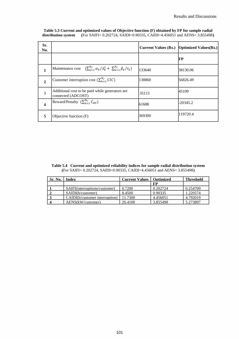
Results and Discussions
Table 5.3 Current and optimized values of Objective function (F) obtained by FP for sample radial
distribution system (For SAIFI= 0.202724, SAIDI=0.90335, CAIDI=4.456051 and AENS= 3.855498)
Sr.
No. Current Values (Rs.) Optimized Values(Rs.)
FP
1 Maintenance cost (∑ 𝛼𝑘 𝜆𝑘
2⁄𝑁𝑐𝑘=1 + ∑ 𝛽𝑘 𝑟𝑘⁄𝑁𝑐
𝑘=1 ) 133640 38130.06
2 Customer interruption cost (∑ 𝐶𝐼𝐶
𝑁𝑐𝑘=1 ) 138860 56826.49
3 Additional cost to be paid while generators are
connected (ADCOST) 35115
45109
4 Reward/Penalty (∑ 𝐶𝑅𝑃
𝑁𝑐𝑘=1 )
61688 -20345.2
5 Objective function (F) 369300 119720.4
Table 5.4 Current and optimized reliability indices for sample radial distribution system
(For SAIFI= 0.202724, SAIDI=0.90335, CAIDI=4.456051 and AENS= 3.855498)
Sr. No. Index Current Values Optimized
Values
Threshold
Values FP
1 SAIFI(interruptions/customer) 0.7200 0.202724 0.254709
2 SAIDI(h/customer) 8.4500 0.90335 1.220574
3 CAIDI(h/customer interruption) 11.7300 4.456051 4.792019
4 AENS(kW/customer) 26.4100 3.855498 5.273897
101

Optimal Parameter Setting in Distribution System Reliability Enhancement with Reward and Penalty
Table 5.5 Optimal cost of network, utility and society considering the impact of continuous RPS on
utility (considering SAIFIt = 0.254709 , SAIDIt = 1.220574, CAIDIt = 4.792019, AENSt = 5.273897 )
for sample radial distribution system
Sr No. 𝐂𝐈𝐂 𝐂𝐑𝐏 𝐂𝐧𝐞𝐭𝐰𝐨𝐫𝐤 𝐂𝐭𝐨𝐭𝐚𝐥𝐮𝐭𝐢𝐥𝐢𝐭𝐲
= 𝐂𝐧𝐞𝐭𝐰𝐨𝐫𝐤 + 𝐂𝐑𝐏 𝐂𝐭𝐨𝐭𝐚𝐥𝐬𝐨𝐜𝐢𝐞𝐭𝐲
= 𝐂𝐧𝐞𝐭𝐰𝐨𝐫𝐤 + 𝐂𝐈𝐂 𝐑
1 103441.8 26270.06 69605.13335 95875.18925 173046.8856 4.967553
2 99343.39 22171.69 70476.84515 92648.53864 169820.235 4.851686
3 96043.32 18871.63 74449.85414 93321.4801 170493.1764 4.705128
4 89680.61 12508.91 80393.27286 92902.18687 170073.8832 4.483391
5 88615.27 11443.57 73185.34189 84628.91224 161800.6086 4.405355
6 86242.08 9070.388 78949.40583 88019.7936 165191.4899 4.34405
7 82989.39 5817.695 78765.84991 84583.54517 161755.2415 4.203453
8 79817.16 2645.463 72250.29019 74895.75305 152067.4494 4.092729
9 79712.62 2540.923 88394.81422 90935.73745 168107.4338 4.089254
10 78287.01 1115.312 82101.32533 83216.63688 160388.3332 4.042314
11 77081.16 -90.5391 83769.59327 83679.0542 160850.7505 3.977537
12 75471.86 -1699.83 82227.05043 80527.21763 157698.914 3.917981
13 73206.65 -3965.04 80953.01612 76987.97267 154159.669 3.833043
14 71024.76 -6146.94 76096.26314 69949.32787 147121.0242 3.760967
15 61847.71 -15324 84015.94759 68691.95883 145863.6552 3.412966
16 61312.61 -15859.1 97921.58514 82062.50064 159234.197 3.387744
17 58326.53 -18845.2 81409.5417 62564.37401 139736.0703 3.262954
18 56826.49 -20345.2 83239.0693 62893.86578 140065.5621 3.196949
19 55004.06 -22167.6 97837.4538 75669.81549 152841.5118 3.122317
Table 5.6 Optimized values of failure rates and repair times for sample radial distribution system as
obtained by FP (For SAIFI= 0.202724, SAIDI=0.90335, CAIDI=4.456051 and AENS= 3.855498)
failure rates
( /year)
repair
times
(in hrs.)
Distributor
segment
By FP
By FP
1 0.20000 6.00003
2 0.09858 6.00000
3 0.12815 4.03472
4 0.46368 10.18818
5 0.18284 10.30196
6 0.10000 6.00032
7 0.09985 6.00679
102

Results and Discussions
Table 5.7 Interruption costs at load points for sample meshed distribution system
Distributor Load points(LP) #1 #2 #3 #4
Interruption Cost(𝐶𝑝𝑘)(Rs./kW) 45 39 51 60
Table 5.8 Optimized values of overall reliability R and other parameters (considering SAIFIt =
0.249358965 , SAIDIt = 0.889319751, CAIDIt = 3.566423809, AENSt = 3.916585348 ) for sample
meshed distribution system
Sr No. Maintenance cost ADCOST SAIFI SAIDI CAIDI AENS F R
1 1772970 37320.29124 0.282981 1.397184 4.937379 6.179888 2303808 5.668187
2 1924724 40923.01712 0.270251 1.086869 4.021705 4.794224 2296061 4.657657
3 1870741 41722.00093 0.300166 1.015511 3.383167 4.486923 2208300 4.439884
4 1924738 42201.83822 0.210338 0.975149 4.636094 4.30237 2240457 4.338456
5 1935662 42854.25257 0.300693 0.919314 3.057319 4.051441 2222278 4.131274
6 1659570 42857.35179 0.29623 0.921081 3.10934 4.050249 1944790 4.129647
7 1084723 43101.72096 0.299282 0.897566 2.999068 3.956261 1360670 4.060523
8 1887726 44695.43922 0.229252 0.761488 3.321624 3.343293 2092366 3.560608
9 1602372 45247.38113 0.208406 0.715315 3.432316 3.131007 1781738 3.401927
10 1505257 45783.45383 0.220983 0.665849 3.013124 2.924825 1662949 3.226559
11 1498295 46496.78823 0.206862 0.607311 2.93582 2.650466 1622590 3.012382
12 1477021 47014.27825 0.199655 0.566487 2.837325 2.451431 1576096 2.859139
13 1329648 47449.09315 0.197876 0.513538 2.59526 2.284195 1419132 2.681891
14 1444479 47653.46183 0.195472 0.494002 2.527224 2.205592 1526139 2.61114
15 1369748 48248.09819 0.179971 0.448075 2.489708 1.976885 1421817 2.428417
16 1734180 48295.00614 0.180722 0.445403 2.464572 1.958844 1783284 2.416772
17 1572818 48345.19558 0.17999 0.44048 2.44725 1.93954 1620084 2.398512
18 1074699 48349.229 0.179806 0.440314 2.448832 1.937989 1121699 2.397637
19 1094404 48360.21741 0.179664 0.439299 2.445114 1.933763 1140925 2.393804
Table 5.9 Current and optimized values of Objective function (F) obtained by FP for sample meshed
distribution system (For SAIFI= 0.19547226, SAIDI=0.494002204, CAIDI=2.527223971 and AENS=
2.205591604)
Sr.
No. Current Values (Rs.) Optimized Values(Rs.)
FP
1 Maintenance cost (∑ 𝛼𝑘 𝜆𝑘
2⁄𝑁𝑐𝑘=1 + ∑ 𝛽𝑘 𝑟𝑘⁄𝑁𝑐
𝑘=1 ) 5990100 1444479.383
2 Customer interruption cost (∑ 𝐶𝐼𝐶
𝑁𝑐𝑘=1 ) 1345365 130892.7156
3 Additional cost to be paid while generators are
connected(ADCOST) 33620
47653.46183
4 Reward/Penalty (∑ 𝐶𝑅𝑃
𝑁𝑐𝑘=1 )
217044 -96886.4521
5 Objective function (F) 6685591 1526139.108
103

Optimal Parameter Setting in Distribution System Reliability Enhancement with Reward and Penalty
Table 5.10 Current and optimized reliability indices for sample meshed distribution system
(For SAIFI= 0.19547226, SAIDI=0.494002204, CAIDI=2.527223971 and AENS= 2.205591604)
Sr. No. Index Current Values Optimized
Values
Threshold
Values FP
1 SAIFI(interruptions/customer) 0.689895 0.195472269 0.24935896
2 SAIDI(h/customer) 4.854797 0.494002204 0.88931975
3 CAIDI(h/customer interruption) 7.037003 2.527223971 3.5664238
4 AENS(kW/customer) 20.533869 2.205591604 3.9165853
Table 5.11 Optimal cost of network, utility and society considering the impact of continuous RPS on
utility (considering SAIFIt = 0.249358965 , SAIDIt = 0.889319751, CAIDIt = 3.566423809, AENSt =
3.916585348 ) for sample meshed distribution system
Sr No. 𝐂𝐈𝐂 𝐂𝐑𝐏 𝐂𝐧𝐞𝐭𝐰𝐨𝐫𝐤
𝐂𝐭𝐨𝐭𝐚𝐥𝐮𝐭𝐢𝐥𝐢𝐭𝐲
= 𝐂𝐧𝐞𝐭𝐰𝐨𝐫𝐤 +
𝐂𝐑𝐏 𝐂𝐭𝐨𝐭𝐚𝐥
𝐬𝐨𝐜𝐢𝐞𝐭𝐲= 𝐂𝐧𝐞𝐭𝐰𝐨𝐫𝐤 + 𝐂𝐈𝐂
𝐑
1 360648.3967 132869.22 1810290 1943159.299 2170938.467 5.668187
2 279096.5508 51317.383 1965647 2016964.664 2244743.832 4.657657
3 261808.1469 34028.979 1912463 1946491.996 2174271.164 4.439884
4 250648.3983 22869.23 1966940 1989808.898 2217588.066 4.338456
5 235770.7489 7991.5811 1978516 1986507.742 2214286.91 4.131274
6 235070.5675 7291.3997 1702428 1709719.103 1937498.271 4.129647
7 230311.9049 2532.7371 1127825 1130357.894 1358137.062 4.060523
8 193861.7708 -33917.396 1932421 1898503.919 2126283.087 3.560608
9 180948.9067 -46830.261 1647619 1600789.14 1828568.308 3.401927
10 169843.8596 -57935.30 1551041 1493105.584 1720884.752 3.226559
11 152788.4079 -74990.759 1544792 1469801.421 1697580.588 3.012382
12 139919.9301 -87859.237 1524035 1436175.635 1663954.802 2.859139
13 134907.07 -92872.097 1377097 1284225.256 1512004.424 2.681891
14 130892.7156 -96886.45 1492133 1395246.393 1623025.56 2.61114
15 115799.9339 -111979.23 1417997 1306017.356 1533796.524 2.428417
16 114293.8314 -113485.33 1782475 1668989.726 1896768.894 2.416772
17 113349.8037 -114429.36 1621164 1506734.197 1734513.365 2.398512
18 113215.3972 -114563.77 1123048 1008484.012 1236263.18 2.397637
19 112969.6452 -114809.52 1142765 1027955.191 1255734.359 2.393804
104

Results and Discussions
Table 5.12 Optimized values of failure rates and repair times for sample meshed distribution system as
obtained by FP (For SAIFI= 0.19547226, SAIDI=0.494002204, CAIDI=2.527223971 and
AENS= 2.205591604)
failure rates
( /year)
repair
times
(in hrs.)
Distributor
segment
By FP
By FP
1 0.2542 3.3531
2 0.1776 3.0817
3 0.1100 21.7324
4 0.1146 3.8403
5 0.1846 3.3945
6 0.0190 10.1910
7 0.1846 3.5109
8 0.1780 4.5522
9 0.0105 7.1412
10 0.0802 27.5656
11 0.2053 5.2349
12 0.2052 2.1985
13 0.1140 12.7190
14 0.1176 3.3301
15 0.0699 6.3538
16 0.0176 13.5615
17 0.1781 9.6232
18 0.1849 8.3621
Table 5.13 Optimized values of overall reliability R and other parameters (considering SAIFIt =
0.084746 , SAIDIt = 0.198559, CAIDIt = 2.435000, AENSt = 1.806670) for RBTS-2
Sr. No. Maintenance
cost
ADCOST SAIFI SAIDI CAIDI AENS F R
1 292425.5 10128 0.086 0.225 2.623 2.01 667137.2 3.132
2 290868.1 10385 0.085 0.223 2.66 1.943 656514 3.094 3 295194.8 10630 0.082 0.226 2.757 1.878 658002 3.06
4 264349.6 10650 0.086 0.204 2.417 1.873 617472.5 2.964 5 275661.7 10687 0.086 0.198 2.286 1.864 623918.5 2.916
6 281435.6 10933.7 0.0829 0.203 2.322 1.798 620153.9 2.871
7 266436.7 11206 0.081 0.19 2.383 1.728 574835.8 2.8 8 266249.7 11252 0.083 0.187 2.253 1.715 574703.2 2.775
9 270691.6 11340 0.083 0.176 2.156 1.692 576717.2 2.712 10 283167 11400 0.083 0.178 2.14 1.677 585878.1 2.707
11 295181.6 11375 0.082 0.175 2.156 1.683 597618.4 2.698
12 306348.7 11434 0.08 0.178 2.23 1.668 604785.9 2.696
13 268835.9 11471 0.084 0.172 2.115 1.658 560790.9 2.691
14 287743.7 11574 0.083 0.17 2.056 1.631 585959.7 2.645 15 275668.9 11618 0.082 0.166 2.074 1.62 571269.7 2.623
16 271853.2 11595 0.08 0.166 2.121 1.626 562966.3 2.619 17 275059.6 11605 0.081 0.166 2.091 1.623 568568 2.616
18 287907.5 11526 0.08 0.166 2.063 1.644 578949.5 2.614
105

Optimal Parameter Setting in Distribution System Reliability Enhancement with Reward and Penalty
Table 5.14 Current and optimized values of Objective function (F) obtained by FP for RBTS-2
(For SAIFI= 0.080462, SAIDI=0.177953, CAIDI=2.2301 and AENS= 1.667670)
Sr.
No. Current Values (Rs.) Optimized Values(Rs.)
FP
1 Maintenance cost (∑ 𝛼𝑘 𝜆𝑘
2⁄𝑁𝑐𝑘=1 + ∑ 𝛽𝑘 𝑟𝑘⁄𝑁𝑐
𝑘=1 ) 232680 306348.71
2 Customer interruption cost (∑ 𝐶𝐼𝐶
𝑁𝑐𝑘=1 ) 807980 302267.59
3 Additional cost to be paid while generators are
connected(ADCOST) 3118
11434.22
4 Reward/Penalty (∑ 𝐶𝑅𝑃
𝑁𝑐𝑘=1 )
490450 -15264.67
5 Objective function (F) 1534228 604785.85
Table 5.15 Current and optimized reliability indices for RBTS-2
(For SAIFI= 0.080462, SAIDI=0.177953, CAIDI=2.2301 and AENS= 1.667670)
Sr. No. Index Current Values Optimized
Values
Threshold
Values
FP
1 SAIFI(interruptions/customer) 0.0986 0.080462 0.084746
2 SAIDI(h/customer) 0.5882 0.177953 0.198559
3 CAIDI(h/customer interruption) 5.9666 2.2301 2.435000
4 AENS(kW/customer) 4.6641 1.667670 1.806670
106
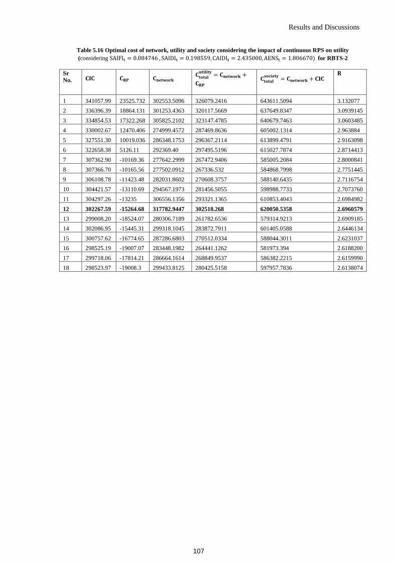
Results and Discussions
Table 5.16 Optimal cost of network, utility and society considering the impact of continuous RPS on utility
(considering SAIFIt = 0.084746 , SAIDIt = 0.198559, CAIDIt = 2.435000, AENSt = 1.806670) for RBTS-2
Sr
No. 𝐂𝐈𝐂 𝐂𝐑𝐏 𝐂𝐧𝐞𝐭𝐰𝐨𝐫𝐤 𝐂𝐭𝐨𝐭𝐚𝐥
𝐮𝐭𝐢𝐥𝐢𝐭𝐲= 𝐂𝐧𝐞𝐭𝐰𝐨𝐫𝐤 +
𝐂𝐑𝐏 𝐂𝐭𝐨𝐭𝐚𝐥
𝐬𝐨𝐜𝐢𝐞𝐭𝐲= 𝐂𝐧𝐞𝐭𝐰𝐨𝐫𝐤 + 𝐂𝐈𝐂
𝐑
1 341057.99 23525.732 302553.5096 326079.2416 643611.5094 3.132077
2 336396.39 18864.131 301253.4363 320117.5669 637649.8347 3.0939145
3 334854.53 17322.268 305825.2102 323147.4785 640679.7463 3.0603485
4 330002.67 12470.406 274999.4572 287469.8636 605002.1314 2.963884
5 327551.30 10019.036 286348.1753 296367.2114 613899.4791 2.9163098
6 322658.38 5126.11 292369.40 297495.5196 615027.7874 2.8714413
7 307362.90 -10169.36 277642.2999 267472.9406 585005.2084 2.8000841
8 307366.70 -10165.56 277502.0912 267336.532 584868.7998 2.7751445
9 306108.78 -11423.48 282031.8602 270608.3757 588140.6435 2.7116754
10 304421.57 -13110.69 294567.1973 281456.5055 598988.7733 2.7073760
11 304297.26 -13235 306556.1356 293321.1365 610853.4043 2.6984982
12 302267.59 -15264.68 317782.9447 302518.268 620050.5358 2.6960579
13 299008.20 -18524.07 280306.7189 261782.6536 579314.9213 2.6909185
14 302086.95 -15445.31 299318.1045 283872.7911 601405.0588 2.6446134
15 300757.62 -16774.65 287286.6803 270512.0334 588044.3011 2.6231037
16 298525.19 -19007.07 283448.1982 264441.1262 581973.394 2.6188200
17 299718.06 -17814.21 286664.1614 268849.9537 586382.2215 2.6159990
18 298523.97 -19008.3 299433.8125 280425.5158 597957.7836 2.6138074
107

Optimal Parameter Setting in Distribution System Reliability Enhancement with Reward and Penalty
Table 5.17 Optimized values of failure rates and repair times for RBTS-2 as obtained by FP
(For SAIFI= 0.080462, SAIDI=0.177953, CAIDI=2.2301 and AENS= 1.667670)
failure rates
( /year)
repair
times
(in hrs.)
Distributor
segment
By FP
By FP
1 0.03679 2.25225
2 0.01497 4.50497
3 0.03910 4.60288
4 0.03609 2.25237
5 0.01127 4.96719
6 0.01500 9.34639
7 0.03665 2.25229
8 0.01237 9.43417
9 0.01500 4.50613
10 0.03899 2.25525
11 0.01128 4.50491
12 0.03665 2.27395
13 0.03943 2.44635
14 0.03102 2.25353
15 0.03911 2.25225
16 0.04238 2.25229
17 0.01499 9.97048
18 0.03910 2.27024
19 0.01500 9.97133
20 0.01485 9.98236
21 0.02934 2.75800
22 0.01260 5.03652
23 0.01136 5.11156
24 0.04780 2.25635
25 0.01500 4.50450
26 0.03910 2.31682
27 0.01481 4.52148
28 0.01128 9.85532
29 0.03665 2.25238
30 0.01500 9.53818
31 0.01500 9.99991
32 0.04875 2.25870
33 0.01283 4.50450
34 0.02996 2.25408
35 0.01153 5.59178
36 0.01128 4.50450
108

Results and Discussions
Fig. 5.4 Impact of an optimal continuous RPS on different parameter costs for sample radial distribution system
-50000
0
50000
100000
150000
200000
4.9
68
4.8
52
4.7
05
4.4
83
4.4
05
4.3
44
4.2
03
4.0
93
4.0
89
4.0
42
3.9
78
3.9
18
3.8
33
3.7
61
3.4
13
3.3
88
3.2
63
3.1
97
3.1
22
Op
tim
um
An
nu
al C
ost
Optimum Reliability
CRP
CIC
Cnetwork
Ctotal_utility= Cnetwork + CRP
Ctotal_society= Cnetwork + CIC
R
109

Optimal Parameter Setting in Distribution System Reliability Enhancement with Reward and Penalty
Fig. 5.5 Impact of an optimal continuous RPS on different parameter costs for sample meshed distribution system
-500000
0
500000
1000000
1500000
2000000
2500000
Op
tim
um
An
nu
al C
ost
Optimum Reliability
CRP
CIC
Cnetwork
Ctotal_utility= Cnetwork + CRP
Ctotal_society= Cnetwork +CIC
110

Results and Discussions
Fig. 5.6 Impact of an optimal continuous RPS on different parameter costs for RBTS-2
-100000
0
100000
200000
300000
400000
500000
600000
700000
3.1
32
3.0
94
3.0
60
2.9
64
2.9
16
2.8
71
2.8
00
2.7
75
2.7
12
2.7
07
2.6
98
2.6
96
2.6
91
2.6
45
2.6
23
2.6
19
2.6
16
2.6
14
Op
tim
um
An
nu
al C
ost
Optimum Reliability
CRP
CIC
Cnetwork
Ctotal_utility= Cnetwork + CRP
Ctotal_society= Cnetwork + CIC
R
111

Optimal Parameter Setting in Distribution System Reliability Enhancement with Reward and Penalty
5.6 Conclusions
In this chapter, reliability of distribution system has been enhanced incorporating
reward/penalty to the utilities by the regulator. The optimum values of reward/penalties have
been found considering the target values of customer and energy based reliability indices. It
is clear from the results obtained that when all these indices are below their target values,
utility is rewarded otherwise penalized. The objective function formulated has been
optimized by FP. Along with optimized values of all reliability indices, optimized values of
other terms in the objective function like maintenance cost, customer interruptions and
additional cost required to achieve this reliability level have also been obtained. The
algorithm developed has been implemented on the three test distribution systems in
consideration.
112

CHAPTER 6
Reliability Performance Optimization of Radial
Distribution System Enhancing Power Quality
Considering Voltage Sag
6.1 Introduction
For long time the main concern of consumers of electricity was the continuity of the supply,
i.e. the reliability. Nowadays consumers want not only reliability, but quality too. Any
distribution system is supposed to supply ideally an uninterrupted flow of power with smooth
sinusoidal voltage at its rated magnitude level and frequency to its customers [121]. As the
distribution company practically consists of numerous nonlinear loads, the quality and purity
of power supply is considerably affected. Besides these loads, some systems events like
capacitor switching, motor starting and various faults which do occur frequently, too affect
the power quality problems [122]. The three most significant power quality problems
concerned to most of the customers are voltage sags, momentary interruptions and sustained
interruptions. Different customers are affected differently. Residential customers generally
suffer sustained interruptions and momentary interruptions whereas for commercial and
industrial customers sag and momentary interruptions are main problems. These three power
quality problems are caused due to faults in the utility power system and mostly in the
distribution system. Of course, faults can never be eliminated but their impact on the
customers can be minimized. Among many problems related to power quality, these three
are the most common [123]. Generally industrial processes rely on electronic power control
devices so, simple power quality problems like voltage sag may affect economically in a
considerable way. Thus power supplied must be reliable and of good quality. Power quality
can be defined in a simple and concise way as: “It is a set of electrical boundaries that allows
a piece of equipment to function in its intended manner without significant loss of
performance or life expectancy” [124].
During one or more outages customers are no more supplied with electricity, are known as
interruptions. Interruptions may be long or short and are both power quality events. During
113
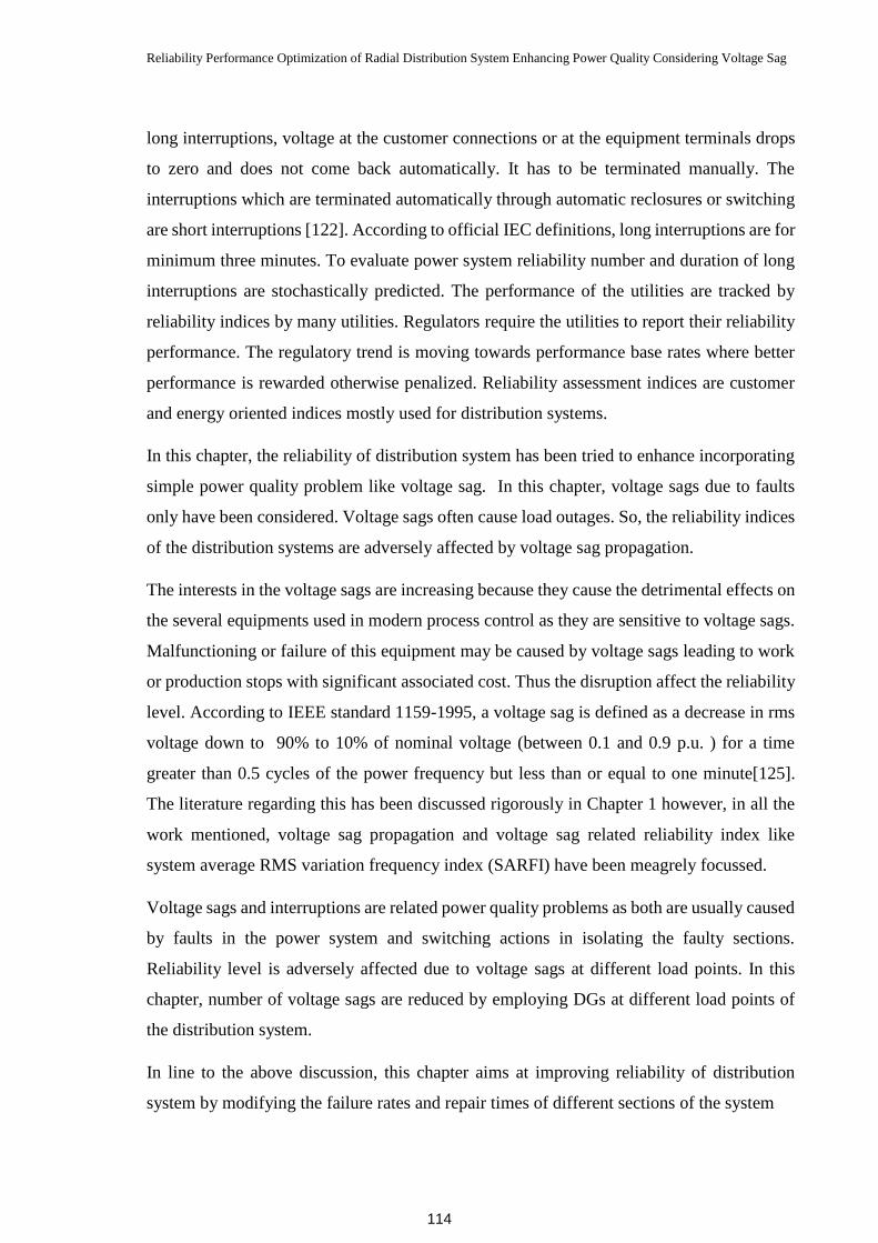
Reliability Performance Optimization of Radial Distribution System Enhancing Power Quality Considering Voltage Sag
long interruptions, voltage at the customer connections or at the equipment terminals drops
to zero and does not come back automatically. It has to be terminated manually. The
interruptions which are terminated automatically through automatic reclosures or switching
are short interruptions [122]. According to official IEC definitions, long interruptions are for
minimum three minutes. To evaluate power system reliability number and duration of long
interruptions are stochastically predicted. The performance of the utilities are tracked by
reliability indices by many utilities. Regulators require the utilities to report their reliability
performance. The regulatory trend is moving towards performance base rates where better
performance is rewarded otherwise penalized. Reliability assessment indices are customer
and energy oriented indices mostly used for distribution systems.
In this chapter, the reliability of distribution system has been tried to enhance incorporating
simple power quality problem like voltage sag. In this chapter, voltage sags due to faults
only have been considered. Voltage sags often cause load outages. So, the reliability indices
of the distribution systems are adversely affected by voltage sag propagation.
The interests in the voltage sags are increasing because they cause the detrimental effects on
the several equipments used in modern process control as they are sensitive to voltage sags.
Malfunctioning or failure of this equipment may be caused by voltage sags leading to work
or production stops with significant associated cost. Thus the disruption affect the reliability
level. According to IEEE standard 1159-1995, a voltage sag is defined as a decrease in rms
voltage down to 90% to 10% of nominal voltage (between 0.1 and 0.9 p.u. ) for a time
greater than 0.5 cycles of the power frequency but less than or equal to one minute[125].
The literature regarding this has been discussed rigorously in Chapter 1 however, in all the
work mentioned, voltage sag propagation and voltage sag related reliability index like
system average RMS variation frequency index (SARFI) have been meagrely focussed.
Voltage sags and interruptions are related power quality problems as both are usually caused
by faults in the power system and switching actions in isolating the faulty sections.
Reliability level is adversely affected due to voltage sags at different load points. In this
chapter, number of voltage sags are reduced by employing DGs at different load points of
the distribution system.
In line to the above discussion, this chapter aims at improving reliability of distribution
system by modifying the failure rates and repair times of different sections of the system
114
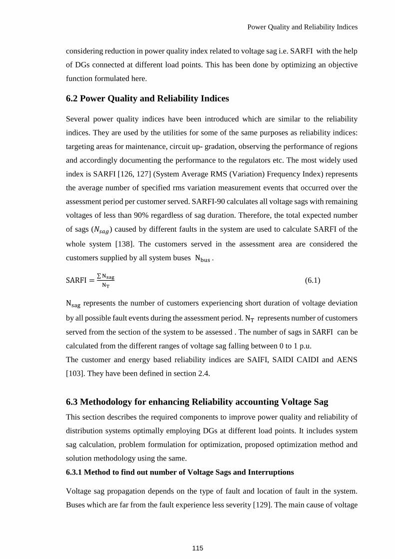
Power Quality and Reliability Indices
considering reduction in power quality index related to voltage sag i.e. SARFI with the help
of DGs connected at different load points. This has been done by optimizing an objective
function formulated here.
6.2 Power Quality and Reliability Indices
Several power quality indices have been introduced which are similar to the reliability
indices. They are used by the utilities for some of the same purposes as reliability indices:
targeting areas for maintenance, circuit up- gradation, observing the performance of regions
and accordingly documenting the performance to the regulators etc. The most widely used
index is SARFI [126, 127] (System Average RMS (Variation) Frequency Index) represents
the average number of specified rms variation measurement events that occurred over the
assessment period per customer served. SARFI-90 calculates all voltage sags with remaining
voltages of less than 90% regardless of sag duration. Therefore, the total expected number
of sags (𝑁𝑠𝑎𝑔) caused by different faults in the system are used to calculate SARFI of the
whole system [138]. The customers served in the assessment area are considered the
customers supplied by all system buses Nbus .
SARFI =∑ Nsag
NT (6.1)
Nsag represents the number of customers experiencing short duration of voltage deviation
by all possible fault events during the assessment period. NT represents number of customers
served from the section of the system to be assessed . The number of sags in SARFI can be
calculated from the different ranges of voltage sag falling between 0 to 1 p.u.
The customer and energy based reliability indices are SAIFI, SAIDI CAIDI and AENS
[103]. They have been defined in section 2.4.
6.3 Methodology for enhancing Reliability accounting Voltage Sag
This section describes the required components to improve power quality and reliability of
distribution systems optimally employing DGs at different load points. It includes system
sag calculation, problem formulation for optimization, proposed optimization method and
solution methodology using the same.
6.3.1 Method to find out number of Voltage Sags and Interruptions
Voltage sag propagation depends on the type of fault and location of fault in the system.
Buses which are far from the fault experience less severity [129]. The main cause of voltage
115

Reliability Performance Optimization of Radial Distribution System Enhancing Power Quality Considering Voltage Sag
sags are line faults. All the symmetrical and unsymmetrical faults can be calculated by fault
analysis. The system branches inducing great sag exposure can be determined by fault
analysis
Total number of estimated line faults per year can be determined as follows.
𝑓𝑡𝑜𝑡𝑎𝑙 = ∑ ∑ 𝐿𝑘𝜆𝑘_𝑓𝑎𝑢𝑙𝑡𝑁𝐿𝑘=1
4𝑝=1 (6.2)
Where, 𝑝 is the types of faults like line to ground (LG), line-to-line-to-ground (LLG), line-
to-line (LL) and three phase (LLL) faults. 𝐿𝑘 is the length of the 𝑘𝑡ℎ distributor segment .
𝑁𝐿 represents total number of distributor segments up to the fault point. 𝜆𝑘_𝑓𝑎𝑢𝑙𝑡 is the fault
rate of the 𝑘𝑡ℎ distributor segment. In this work, different kinds of faults are considered at
a specific load points and the values of sag are found. 𝑁𝑠𝑎𝑔 per year can be found from the
magnitudes of voltage sags as below.
𝑁𝑠𝑎𝑔 = ∑ ∑ { 1 𝑖𝑓 0.1 𝑝. 𝑢. < 𝑉𝑖 < 0.9 𝑝. 𝑢.
0 𝑜𝑡ℎ𝑒𝑟𝑤𝑖𝑠𝑒 𝑡𝑜𝑡𝑎𝑙𝑓=1
𝑁𝑏𝑢𝑠𝑖=1 (6.3)
When the value of voltage sag due to any fault at any load point is less than 0.1 p.u., it will
lead to sustained interruption. The total number of annual interruptions per annum (𝑁𝑖𝑛𝑡)
can be obtained as below.
𝑁𝑖𝑛𝑡 = ∑ ∑ { 1 𝑖𝑓 𝑉𝑖 < 0.1 𝑝. 𝑢.
0 𝑜𝑡ℎ𝑒𝑟𝑤𝑖𝑠𝑒 𝑡𝑜𝑡𝑎𝑙𝑓=1
𝑁𝑏𝑢𝑠𝑖=1 (6.4)
From relation (6.3), power quality index SARFI can be determined using relation (6.1). The
interruptions obtained from relation (6.4) are used along with the interruptions due to failures
of different distributor segments due to ageing, environmental reasons, accidents etc. to find
out customer and energy based reliability indices.
As different magnitudes of voltage sags have different impact from the viewpoint of
customer interruption costs, they have been given weighting factors for the purpose of
economic analysis. Table 6.3 depicts the same.
6.3.2 Problem Formulation for Optimization
With the objective of enhancing reliability of radial distribution system considering voltage
sags, the objective function is defined as follows.
116

Methodology for enhancing Reliability accounting Voltage Sag
F = ∑ (αk λk_failure2⁄Nc
k=1 + (γk λk_fault2⁄ ) + ∑ βk rk⁄Nc
k=1 + ∑ CICNck=1 + ADCOST(EENSO −
EENSD) + ∑ 𝐶𝑅𝑃Nck=1 (6.5)
where,
CIC = λk × rk × Li × Cpk (6.6)
CIC = CIC1 + CIC2 + CIC3 + CIC4 (6.7)
λk = λk_failure + λk_fault (Sustained interruptions) (6.8)
λk_fault = fault rate of kthdistributor segment (6.9)
In the objective function (6.5), first three terms depict the cost related to maintenance. First
two terms are amount spent to reduce failure rates and fault rates of each section of the
distribution system. The third term relates to the cost required to modify repair time for the
distributor segment. Lesser are the values of these terms; more are the costs or investments
associated with preventive maintenance and corrective repair required by utility to achieve
them [111]. These terms are related to Duane’s reliability growth model [105]. The fourth
part is related to interruption cost at the customers end. The momentary and sustained
interruptions affect economically if load is sensitive for the interruptions. On this basis, the
segmental interruption costs to the customers are as shown in Table 6.3. The total cost of
interruptions for any load point i can be determined by adding the cost of all section outages.
The total cost of customer interruptions for all customers can then be evaluated. The fifth
term is related to the additional cost of energy provided by the DGs connected at different
load points. It is multiplication of energy provided by DGs and additional charge (ADCOST)
in Rs. /kWH. In this chapter, the DGs considered are working as standby units. The reliability
model followed here is as per [40]. Here , the standby DGs are connected in combination
with uninterrupted emergency power supplies (UPS) which supply power in case of
occurrence of failure or fault for a very short period of time until DGs at those load points
are connected to supply power. The sixth term is related to the cost of reward/penalty to the
utility. If reliability of the utility is below the set target value, it is rewarded otherwise
penalized. Thus the objective function provides balance between the cost spent on DGs, the
cost of maintenance, customer interruption costs and cost of reward/penalty. This objective
function not only tries to improve reliability of the system by reducing failure rates and repair
times of the distribution system but also tries to reduce fault rates of various sections of the
117
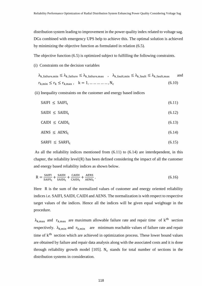
Reliability Performance Optimization of Radial Distribution System Enhancing Power Quality Considering Voltage Sag
distribution system leading to improvement in the power quality index related to voltage sag.
DGs combined with emergency UPS help to achieve this. The optimal solution is achieved
by minimizing the objective function as formulated in relation (6.5).
The objective function (6.5) is optimized subject to fulfilling the following constraints.
(i) Constraints on the decision variables
λk_failure,min ≤ λk_failure ≤ λk_failure,max , λk_fault,min ≤ λk_fault ≤ λk_fault,max and
rk,min ≤ rk ≤ rk,max , k = 1, … … … … … , Nc (6.10)
(ii) Inequality constraints on the customer and energy based indices
SAIFI ≤ SAIFIt (6.11)
SAIDI ≤ SAIDIt (6.12)
CAIDI ≤ CAIDIt (6.13)
AENS ≤ AENSt (6.14)
SARFI ≤ SARFIt (6.15)
As all the reliability indices mentioned from (6.11) to (6.14) are interdependent, in this
chapter, the reliability level(R) has been defined considering the impact of all the customer
and energy based reliability indices as shown below.
R =SAIFI
SAIFIt+
SAIDI
SAIDIt+
CAIDI
CAIDIt+
AENS
AENSt . (6.16)
Here R is the sum of the normalized values of customer and energy oriented reliability
indices i.e. SAIFI, SAIDI, CAIDI and AENS. The normalization is with respect to respective
target values of the indices. Hence all the indices will be given equal weightage in the
procedure.
λk,max and rk,max are maximum allowable failure rate and repair time of kth section
respectively. λk,min and rk,min are minimum reachable values of failure rate and repair
time of kth section which are achieved in optimization process. These lower bound values
are obtained by failure and repair data analysis along with the associated costs and it is done
through reliability growth model [105]. Nc stands for total number of sections in the
distribution systems in consideration.
118

Solution Methodology
SAIFIt , SAIDIt , CAIDIt , AENSt and SARFIt are target/threshold values of the respective
indices. They depend on the managerial/administrative decisions.
The formulated problem is solved by flower pollination optimization method (FP) [100].
The method in this chapter has been applied on a sample radial distribution system. The
optimized values obtained after having solved the problem may be given as target values to
the crew for the enhancement of reliability and power quality of the distribution system.
6.4. Solution Methodology
The overview of Flower pollination algorithm has been presented in Appendix D. The
method of solving the formulated problem mentioned in section 6.3.2 by FP is as follows.
Step 1. Data input λk_failure,max , λk_failure,min , λk_fault,max , λk_fault,min , rk,max , rk,min ,
λdg , rdg , λsw , cost of interruption ( Cpk ) , Ni, Li, SAIFIt , SAIDIt , CAIDIt , AENSt and
SARFIt .
Step 2. Find value K at target values of indices.
Step 3. Initialization: Generate a population of size ‘M’ (flowers) for failure rate (λ_failure)
and fault rate (λ_fault) and repair time r each by relation (D.3), where each vector of
respective population consists of failure rate and repair time of each component respectively.
These values are obtained by sampling uniformly between lower and upper limits as given
by relation (6.10).
Step 4. Evaluate λsys,i , rsys,i and Usys,i and 𝑁𝑠𝑎𝑔 at each load point.
Step 5. Evaluate SARFI, SAIFI, SAIDI, CAIDI and AENS as mentioned in the relations
(6.1), (2.10), (2.11), (2.12) and (2.14) respectively for vectors of the population.
Step 6. Calculate value of objective function F for all vectors in the population i.e.F (Xi(k)
),
i = 1, … … … … … , ′M′ as given by relation (6.5) - (6.9).
Step 7. Calculate value of overall reliability R for all vectors in the population by relation
(6.16).
Step 8. Evaluate inequality constraints from the relations (6.11)-(6.15) for each vector of the
population. Vectors satisfying these constraints will be feasible otherwise not feasible
119

Reliability Performance Optimization of Radial Distribution System Enhancing Power Quality Considering Voltage Sag
vectors. From among the feasible vectors, based on the value of objective function, identify
the best solution vector Xbest(k)
.
Step 9. Set generation counter k = 1 .
Step 10. Select target vector, i = 1 .
Step 11. Find the updated value of the vector by relation (D.4).
Step 12. Compare the fitness of the updated vectors with that of the initial vectors and retain
the best ones using relation (D.9).
Step 13.Repeat from Step 4.to Step 8. for the updated vector.
Step 13. Increase target vector i = i + 1. If i ≤ M, repeat from Step 11 otherwise increase
generation count k = k + 1 .
Step 14. Repeat from step 11 if the desired optimum value is not found or k ≤ kmax .
In the same way, the same problem can be solved by TLBO and DE. The overview of both
the optimization methods have been presented in the Appendix E and Appendix F
respectively. Fig 6.1 shows the flow chart for solving the formulated problem by FP.
120

Solution Methodology
END
START
Evaluate SAIFI, SAIDI, CAIDI, AENS, EENS, SARFI, ADCOST, CIC
Set generation counter k=1
Evaluate the constraints for each updated solution
Print solution
generation = k+1
NO
YES
Is solution
converged?
Find value of K at the target values of indices
Generate a population of size ‘M’ for failure rate λ and repair time r each between lower and upper limits
0 00 0 0 0 0 0, , , X , , .,
1 2 1 2i
TS X X X X X XM i i iD
Calculate the optimum values of SAIFI, SAIDI, CAIDI, AENS, SARFI, overall reliability R & CRP
Calculate value of objective function F for all vectors in the
population and Identify the( )
&best best
kX F
Select target vector, i=1 and find updated value of each vector by D.4
Calculate value of objective function F for all vectors in the population and identify ( )best
kX
If any updated solution violates the inequality constraints , then set the values of the vectors to ( )kiX
Compare the fitness of the updated vectors with that of the initial vectors and retain the best ones by D.9 ( 1)k
iX
( )kiX
,
,max ,min ,max ,min _ ,max
_ ,min
Data input , , , , , , ,
, , , , , , , ,,k t t t t ti i
swk k k k dg k fault
k fault dgSAIFI SAIDI AIDI SARFIS Cp N L C AENS
r r
r
Fig. 6.1 Flow chart for the solution of the problem formulated in section 6.3.2 by FP
121

Reliability Performance Optimization of Radial Distribution System Enhancing Power Quality Considering Voltage Sag
Fig. 6.2 Re-modified Radial Distribution System with DG
122

Results and discussions
6.5 Results and discussions
The developed methodology in this chapter has been implemented on a sample radial
distribution system. The problem has been solved by FP algorithm and comparison has been
made with the results obtained by TLBO and DE. The algorithms used have been coded in
MATLAB-13.
Sample radial distribution system [29]:
The radial system is as shown in Fig. 6.2. The system has been re-modified in terms of
locations of DGs for the problem formulated in this chapter to show the effectiveness of the
methodology. The data regarding the current and minimum reachable values of failure rates
and repair times, average load and number of customers at load points and cost coefficients
for each segment of radial distributor have been taken from [111]. Table 6.1 shows the
failure rates, fault rates and repair times related data for the different sections of the sample
radial distribution system. Table 6.2 depicts the interruption cost at various load points of
the system. On the basis of sustained and momentary interruptions, the total contribution to
the cost of customer interruptions is decided according to the weightage considered as shown
in Table 6.3 for the different ranges of the voltage sag values. Table A.2. gives average load
and number of customers at different load points. Table 6.4 represents cost coefficients for
failure rates, fault rates and repair times of different segments. Table 6.5 gives control
parameters for the three optimization methods, FP, TLBO and DE used in this work. Table
6.6 gives component reactance related data. Percentage of occurrence of different kind of
faults are according to Table 6.7. Optimized values of failure rates, fault rates and repair
times of different distributor segments are given in (Table 6.8-Table 6.10) respectively.
Optimized values of reliability and power quality indices as given by FP.TLBO and DE are
given in Table 6.11. Table 6.12 gives optimized value of objective function and all the cost
components thereof as obtained by FP, TLBO and DE. In this work, DGs are connected at
load points 3, 6 and 7 in the sample radial distribution system so as to show the effectiveness
of the methodology.
Here, the DGs to be connected are taken as standby units. The failure rate and average down
time of DG taken in this chapter are 0.5 failures/year and 13.25 hrs. respectively. Failure rate
and service restoration time of the changeover switch of DG are 0.1 failures/year and 0.25
hrs. respectively.
123

Reliability Performance Optimization of Radial Distribution System Enhancing Power Quality Considering Voltage Sag
Table 6.1 System data for Sample Radial Distribution System
Distributor segment #1 #2 #3 #4 #5 #6 #7
𝜆𝑘_𝑓𝑎𝑖𝑙𝑢𝑟𝑒0 /𝑦𝑒𝑎𝑟 0.4 0.2 0.3 0.5 0.2 0.1 0.1
𝜆𝑘_𝑓𝑎𝑢𝑙𝑡0 /𝑦𝑒𝑎𝑟 4.5 2.25 3.3 5.6 2.25 1.1 1.1
Average repair time 𝑟𝑘0 (ℎ) 10 9 12 20 15 8 12
λk_failure,min/year 0.2 0.05 0.1 0.1 0.15 0.05 0.05
λk_fault,min/year 2.25 0.56 1.1 1.12 1.68 0.55 0.55
𝑟𝑘,𝑚𝑖𝑛(ℎ) 6 6 4 8 7 6 6
Length (km) 0.83 2.08 3.03 1.73 2.98 2.78 3.63
Table 6.2 Interruption costs at load points for sample radial distribution system
Distributor Load points (LP) #2 #3 #4 #5 #6 #7 #8
Interruption Cost (Rs./kW) 15 13 17 20 20 12 14
Table 6.3 Weighting factors for different Voltage Sag Magnitude and corresponding values of
customer interruption cost (CIC)
Category of event Weighting for economic
analysis
Corresponding CIC
Interruption 1.0 CIC1
Sag with minimum voltage below 50 % 0.8 CIC2
Sag with minimum voltage between 50% and
70%
0.4 CIC3
Sag with minimum voltage between 70% and
90%
0.1 CIC4
Table 6.4 Cost coefficients αk, βk and 𝜸𝒌 for Radial Distribution System
Distributor segment #1 #2 #3 #4 #5 #6 #7
αk Rs. 240 300 180 120 240 285 300
βk
Rs. 400 360 200 200 320 240 220
𝛾𝑘 Rs. 1500 2000 1250 900 1500 1850 2000
124
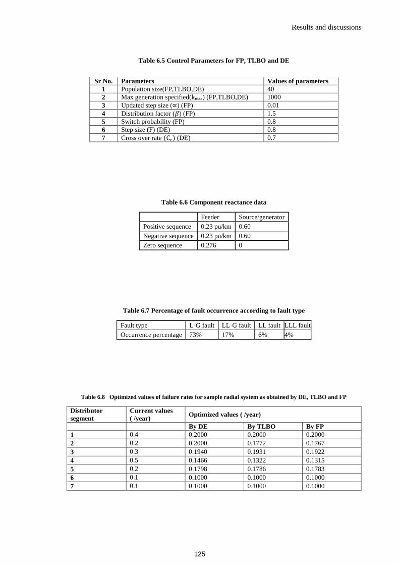
Results and discussions
Table 6.5 Control Parameters for FP, TLBO and DE
Sr No. Parameters Values of parameters
1 Population size(FP,TLBO,DE) 40
2 Max generation specified(kmax) (FP,TLBO,DE) 1000
3 Updated step size (∝) (FP) 0.01
4 Distribution factor (𝛽) (FP) 1.5
5 Switch probability (FP) 0.8
6 Step size (F) (DE) 0.8
7 Cross over rate (Cr) (DE) 0.7
Table 6.6 Component reactance data
Feeder Source/generator
Positive sequence 0.23 pu/km 0.60
Negative sequence 0.23 pu/km 0.60
Zero sequence 0.276 0
Table 6.7 Percentage of fault occurrence according to fault type
Fault type L-G fault LL-G fault LL fault LLL fault
Occurrence percentage 73% 17% 6% 4%
Table 6.8 Optimized values of failure rates for sample radial system as obtained by DE, TLBO and FP
Distributor
segment
Current values
( /year) Optimized values ( /year)
By DE By TLBO By FP
1 0.4 0.2000 0.2000 0.2000
2 0.2 0.2000 0.1772 0.1767
3 0.3 0.1940 0.1931 0.1922
4 0.5 0.1466 0.1322 0.1315
5 0.2 0.1798 0.1786 0.1783
6 0.1 0.1000 0.1000 0.1000
7 0.1 0.1000 0.1000 0.1000
125

Reliability Performance Optimization of Radial Distribution System Enhancing Power Quality Considering Voltage Sag
Table 6.9 Optimized values of fault rates for sample radial system as obtained by DE, TLBO and FP
Distributor
segment
Current values
( /year) Optimized values ( /year)
By DE By TLBO By FP
1 4.5 2.2500 2.2500 2.2500
2 2.25 0.7607 0.7524 0.7523
3 3.3 1.1000 1.1000 1.1000
4 5.6 3.5579 1.1200 1.1200
5 2.25 1.6875 1.6875 1.6875
6 1.1 1.1000 1.1000 1.1000
7 1.1 1.0999 1.1000 1.1000
Table 6.10 Optimized values of repair times for sample radial system as obtained by DE, TLBO and FP
Distributor
segment
Current values
(in hrs) Optimized values (in hrs)
By DE By TLBO By FP
1 10 6.0000 6.0000 6.0000
2 9 6.0040 6.0000 6.0000
3 12 4.0000 4.0000 4.0000
4 20 8.0000 8.0000 8.0000
5 15 7.0025 7.0000 7.0000
6 8 6.0000 6.0000 6.0000
7 12 6.0000 6.0000 6.0000
Table 6.11 Current and optimized reliability and power quality indices for sample radial system
obtained by FP, TLBO and DE
Sr. No. Index Current
Values Optimized Values
FP TLBO DE
1 SAIFI(interruptions/customer) 0.3205 0.176946 0.177221 0.182307
2 SAIDI(h/customer) 3.2030 1.066906 1.068554 1.102044
3 CAIDI(h/customer interruption) 9.9929 6.029546 6.029495 6.044994
4 AENS(kW/customer) 12.1076 3.982938 3.988557 4.103098
5 SARFI 0.0156 0.007096 0.007096 0.007962
6 Overall Reliability (R) 6.6095 2.871777 2.874789 2.936356
126

Results and discussions
Table 6.12 Current and optimized values of objective function (F) as given by DE, TLBO and FP
Sr.
No.
Current
Values (Rs.) Optimized Values(Rs.)
FP TLBO DE
1 Maintenance cost (∑ 𝛼𝑘 𝜆𝑘
2⁄𝑁𝑐𝑘=1 + ∑ 𝛽𝑘 𝑟𝑘⁄𝑁𝑐
𝑘=1 ) 422610 103091.7 102884.8 98675.96
2 Customer interruption cost (∑ 𝐶𝐼𝐶
𝑁𝑐𝑘=1 ) 1893550 384043.5 384150.3 406212.3
Addditional cost to be paid while generators are
connected(ADCOST) 20185
44854.12 44842.89 44613.8
Reward /Penalty (∑ 𝐶𝑅𝑃Nck=1 ) 113360
-24398.5 -24297.1 -22299.8
3 Objective function (F) 2035500 507590.8 507580.9
527202.3
127

Reliability Performance Optimization of Radial Distribution System Enhancing Power Quality Considering Voltage Sag
6.6 Conclusions
In this chapter, reliability of a sample radial distribution system has been enhanced
incorporating power quality problem like voltage sag. Voltage sags often cause load outages.
So, the reliability indices of the distribution systems are adversely affected by voltage sag
propagation. The objective function which has been optimized is in terms of failure rate,
fault rate and repair time. As the customer and energy based indices and power quality index
based on voltage sag depend on these primary indices, optimized values of these indices
have been found for radial distribution system. It has been found that with the specific
locations of DGs as shown in the sample radial distribution system (Fig. 6.1), the reliability
indices as well as power quality index for voltage sag have been enhanced optimally.
Optimized values of maintenance cost, customer interruption cost, additional energy spent
on DGs and value of reward have also been found.
128

CHAPTER 7
Conclusions and Guidelines for Future Work
7.1 General
Power system reliability evaluation and its optimization are of significant importance for
planning, operation and control. For the solution of this, there has been a continuous interest
and subsequent efforts to develop more sophisticated, robust and computationally efficient
models and methodologies. Reliability evaluation is the performance of the system whereas
optimization results help in giving targets to the field crew members and planners to reduce
failure rates and repair times to further enhance reliability
Following aspects were observed from the state of art in the domain of power system
reliability;
(i) As compared to distribution system reliability studies, large number of
methodologies have been developed for the reliability evaluation of generation
system and composite power system.
(ii) In distribution system reliability optimization mostly classical and evolutionary
algorithms e.g. GA have been used. Latest and computationally efficient
metaheuristic optimization methods have not been focused much
(iii) In most of the work related to distribution reliability, work is based on primary
reliability indices i.e. failure rate, average repair time and average
interruption/outage duration per year. In practice these indices may not
represent the actual performance of the system in terms of reliability. Reliability
indices based on customer and energy must be considered to have a realistic
picture of the performance of distribution system.
(iv) Effects of distributed generation (DG) is very important from reliability point
of view. The locations of DGs too keep importance in enhancing reliability of
distribution system. These have not been considered effectively so far.
(v) Reward /Penalty scheme affects reliability of distribution system. The optimized
values of reward/penalties with reference to specific target values of customer
and energy based reliability indices have not been focused yet.
129

Conclusions and Guidelines for Future Work
(vi) Optimizing reliability of distribution system incorporating optimization of
power quality index representing voltage sag has not been focused much.
In view of the above, work carried out in this thesis was to focus on distribution system
reliability evaluation and optimization accounting the above mentioned uncovered areas.
The aim of this chapter is to highlight the important contribution made in this thesis and to
mention the further scope in the very significant area of reliability assessment and
enhancement of distribution system.
7.2 Summary of important conclusions
In chapter 2, a computationally efficient algorithm is developed to enhance the reliability of
distribution system. The objective function to be optimized consists of all the customer and
energy based reliability indices. Here each index has been given weightage by Analytical
Hierarchical Process (AHP). Further, each index is normalized with reference to their
respective target/threshold value. Every index has been given weightage in regards to its
contributory importance in the overall reliability of the system. Optimum values of customer
oriented and energy based reliability indices are found while specified budget is allocated to
achieve the same. Here optimized values of reliability indices for the allocated budget have
been found. More is the budget better is reliability and vice versa. This algorithm is applied
to sample radial distribution network, sample meshed system and RBTS-2 in this thesis. The
optimum values are found by flower Pollination (FP) optimization algorithm, teaching
learning based optimization (TLBO) and differential evolution (DE). It has been
authenticated by making comparison of the values found.
In chapter 3, the aim has been to improve reliability of a distribution system by finding out
a balance between costs of maintenance and customer interruptions. When these combined
costs become minimum, customers will get service with least costs leading to enhanced
customer satisfaction level. In this chapter, this has been achieved by optimizing the
objective function formulated subject to achieving the desired reliability level with reduction
in the customer interruption costs. It has been applied on a sample radial network, sample
meshed network and RBTS-2 finding the results by FP, TLBO and DE.
130

Scope for further work
In chapter 4, reliability of distribution systems (a sample radial distribution system, sample
meshed system and RBTS-2) have been enhanced with DGs connected at different load
points. The locations of DGs have been found with a methodology considering improvement
in reliability as the chief motive. With these locations thus found, the objective function
formulated in this chapter has been optimized by three optimization methods say FP, TLBO
and DE. To justify the installation of DGs in a long run, the cost-benefit analysis has been
made. Here, DGs are operating on standby mode. Enhanced values of reliability indices and
reduced customer interruption cost than those obtained in the previous chapter have been
achieved by spending additional amounts on a generator.
In chapter 5, reliability of distribution system has been enhanced incorporating
reward/penalty to the utilities by the regulator. The optimum values of reward/penalties have
been found considering the target values of customer and energy based reliability indices. It
is clear from the results obtained that when all these indices are below their target values,
utility is rewarded otherwise penalized. The objective function formulated has been
optimized by FP. Along with optimized values of all reliability indices, optimized values of
other terms in the objective function like maintenance cost, customer interruptions and
additional cost required to achieve this reliability level have also been obtained. The
algorithm has been applied on all the three test systems considered here.
In chapter 6, reliability of a sample radial distribution system has been enhanced
incorporating simple power quality problem like voltage sag. Voltage sags often cause load
outages. So, the reliability indices of the distribution systems are adversely affected by
voltage sag propagation. The objective function to be optimized is in terms of failure rate,
fault rate and repair time. As the customer and energy based indices and power quality index
based on voltage sag depend on these, optimized values of these indices have been found for
radial distribution system. Optimized values of maintenance cost, customer interruption cost,
additional energy spent on DGs and value of reward have also been found.
7.3 Scope for further work
As a consequences of investigation made in reliability assessment and optimal reliability
performance evaluation of distribution systems, following suggestions are made for future
research.
(i) In reliability performance optimization of distribution system, decision variables
taken are for all the sections of distribution system. They may be reduced. In view
131

Conclusions and Guidelines for Future Work
of this a line outage ranking algorithm may be developed and selected sections
which are more valuable for reliable supply view point may be considered in
reliability optimization. For meshed distribution system, this may prove to be an
important study.
(ii) In this thesis, reliability optimization of distribution system has been done.
Reliability optimization algorithm of a distribution network accounting network
reconfiguration can be developed along with network limitations resulting in loss
minimization.
(iii) Reliability enhancement of distribution system incorporating DGs have been
done in the thesis. Here, the location of DGs are found by ranking algorithm
considering reliability enhancement as a chief motive. Locations of DGs may be
found by any binary optimization including capacity of them.
(iv) Reliability improvement may be obtained using fault tolerant measures. An
algorithm may be developed to this extent.
(v) Algorithm may be developed for reliability assessment of electrical distribution
systems accounting voltage stability constraints.
(vi) Algorithm may be developed including load and capacity models. In fact basic
reliability indices may be evaluated using Monte Carlo simulation.
132

References
1. W. J. Lyman, 'Fundamental consideration in preparing master system plan’,
Electrical World, 101(24) (1933): 788-92.
2. Dean, S. M. "Considerations involved in making system investments for improved
service reliability." EEI Bulletin 6.1 (1938): 491-596.
3. Billinton, Roy, and Ronald N. Allan. "Power-system reliability in
perspective." Electronics and Power 30.3 (1984) : 231-236.
4. Allan, Ronald, and Roy Billinton. "Probabilistic assessment of power
systems." Proceedings of the IEEE 88.2 (2000): 140-162.
5. Shipley, R. Bruce, Alton D. Patton, and J. S. Denison. "Power reliability cost vs
worth." IEEE transactions on Power Apparatus and Systems 5 (1972): 2204-2212.
6. Billinton, Roy. "Evaluation of reliability worth in an electric power
system." Reliability Engineering & System Safety 46.1 (1994): 15-23.
7. Goel, L., X. Liang, and Y. Ou. "Monte Carlo simulation-based customer service
reliability assessment." Electric power systems research 49.3 (1999): 185-194.
8. Hegazy, Y. G., M. M. A. Salama, and A. Y. Chikhani. "Adequacy assessment of
distributed generation systems using Monte Carlo simulation." IEEE Transactions
on Power Systems 18.1 (2003): 48-52.
9. Ermiş, M., et al. "Various induction generator schemes for wind-electricity
generation." Electric Power Systems Research 23.1 (1992): 71-83.
10. Levitin, Gregory, Shmuel Mazal-Tov, and David Elmakis. "Optimal sectionalizer
allocation in electric distribution systems by genetic algorithm." Electric Power
Systems Research 31.2 (1994): 97-102.
11. Levitin, Gregory, Shmuel Mazal-Tov, and David Elmakis. "Genetic algorithm for
optimal sectionalizing in radial distribution systems with alternative
supply." Electric Power Systems Research 35.3 (1995): 149-155.
12. Levitin, Gregory, Shmuel Mazal-Tov, and David Elmakis. "Optimal insulation in
radial distribution networks." Electric Power Systems Research 37.2 (1996): 97-103.
13. Su, Ching-Tzong, and Guor-Rurng Lii. "Reliability design of distribution systems
using modified genetic algorithms." Electric Power Systems Research 60.3 (2002):
201-206.
133

References
14. Chang, Wei-Fu, and Yu-Chi Wu. "Optimal reliability design in an electrical
distribution system via a polynomial-time algorithm." International journal of
electrical power & energy systems 25.8 (2003): 659-666.
15. Billinton, R., T. K. P. Medicherla, and M. S. Sachdev. "Common-cause outages in
multiple circuit transmission lines." IEEE Transactions on Reliability 27.2 (1978):
128-131.
16. Allan, R. N., E. N. Dialynas, and I. R. Homer. "Modelling and evaluating the
reliability of distribution systems." IEEE Transactions on Power Apparatus and
systems 6 (1979): 2181-2189.
17. Allan, R. N., E. N. Dialynas, and I. R. Homer. "Modeling Common -Mode Failures
In The Reliability Evaluation Of Power-System Networks." IEEE Transactions On
Power Apparatus And Systems. Vol. 98. No. 4. 345 E 47th ST, New York, NY 10017-
2394: IEEE-Inst Electrical Electronics Engineers Inc, 1979.
18. Billinton, R., and Y. Kumar. "Transmission line reliability models including
common mode and adverse weather effects." IEEE Transactions on Power
Apparatus and Systems8 (1981): 3899-3910.
19. Sallam, Abdelhay A., Mohamed Desouky, and Hussien Desouky. "Evaluation of
optimal-reliability indices for electrical distribution systems." IEEE transactions on
reliability 39.3 (1990): 259-264.
20. Billinton, R., et al. "Reliability issues in today's electric power utility
environment." IEEE Transactions on Power Systems 12.4 (1997): 1708-1714.
21. Pinheiro, J. M. S., et al. "Probing the new IEEE reliability test system (RTS-96): HL-
II assessment." IEEE Transactions on Power Systems 13.1 (1998): 171-176.
22. Force, RTS Task. "The IEEE reliability test system-1996." IEEE Trans. Power
Syst 14.3 (1999): 1010-1020.
23. Bhowmik, S., S. K. Goswami, and P. K. Bhattacherjee. "A new power distribution
system planning through reliability evaluation technique." Electric Power Systems
Research 54.3 (2000): 169-179.
24. Wang, Zhuding, Farrokh Shokooh, and Jun Qiu. "An efficient algorithm for
assessing reliability indexes of general distribution systems." IEEE Transactions on
Power Systems17.3 (2002): 608-614.
134

References
25 Amjady, Nima, Davood Farrokhzad, and Mohammad Modarres. "Optimal reliable
operation of hydrothermal power systems with random unit outages." IEEE
Transactions on Power Systems 18.1 (2003): 279-287.
26. Tsao, Teng-Fa, and Hong-Chan Chang. "Composite reliability evaluation model for
different types of distribution systems." IEEE Transactions on power systems 18.2
(2003): 924-930.
27. Carvalho, Pedro MS, and Luìs AFM Ferreira. "Distribution quality of service and
reliability optimal design: individual standards and regulation effectiveness." IEEE
Transactions on Power Systems 20.4 (2005): 2086-2092.
28. Yang, F., and C. S. Chang. "Multiobjective evolutionary optimization of
maintenance schedules and extents for composite power systems." IEEE
Transactions on Power Systems 24.4 (2009): 1694-1702.
29. Arya, R., S. C. Choube, and L. D. Arya. "A decomposed approach for optimum
failure rate and repair time allocation for radial distribution systems." Journal of The
Institution of Engineers (India) 89.June (2008): 3-7.
30. Louit, Darko, Rodrigo Pascual, and Dragan Banjevic. "Optimal interval for major
maintenance actions in electricity distribution networks." International Journal of
Electrical Power & Energy Systems 31.7-8 (2009): 396-401.
31. Arya, R., S. C. Choube, and L. D. Arya. "Reliability enhancement of distribution
system using sensitivity analysis." J. Inst. Eng 90 (2009): 46-50.
32. Arya, R., S. C. Choube, and L. D. Arya. "A technique for improving Reliability
indices of a radial distribution system." J. Inst. Eng.(India), pt. EL 90 (2009): 12-17.
33. Gui, Min, Anil Pahwa, and Sanjoy Das. "Analysis of animal-related outages in
overhead distribution systems with wavelet decomposition and immune systems-
based neural networks." IEEE transactions on power systems 24.4 (2009): 1765-
1771.
34. Miranda, Vladimiro, et al. "Improving power system reliability calculation
efficiency with EPSO variants." IEEE Transactions on Power Systems 24.4 (2009):
1772-1779.
35. Arya, L. D., S. C. Choube, and Rajesh Arya. "Probabilistic reliability indices
evaluation of electrical distribution system accounting outage due to overloading and
repair time omission." International Journal of Electrical Power & Energy
Systems 33.2 (2011): 296-302.
135

References
36. Arya, L. D., S. C. Choube, and Rajesh Arya. "Differential evolution applied for
reliability optimization of radial distribution systems." International Journal of
Electrical Power & Energy Systems 33.2 (2011): 271-277.
37. Li, Ming-Bin, Ching-Tzong Su, and Chih-Lung Shen. "The impact of covered
overhead conductors on distribution reliability and safety." International journal of
electrical power & energy systems 32.4 (2010): 281-289.
38. Arya, L. D., et al. "Evaluation of reliability indices accounting omission of random
repair time for distribution systems using Monte Carlo simulation." International
Journal of Electrical Power & Energy Systems 42.1 (2012): 533-541.
39. Arya, Rajesh, et al. "Reliability enhancement of a radial distribution system using
coordinated aggregation based particle swarm optimization considering customer
and energy based indices." Applied soft computing 12.11 (2012): 3325-3331.
39. Arya, Rajesh, S. C. Choube, and L. D. Arya. "Reliability evaluation and
enhancement of distribution systems in the presence of distributed generation based
on standby mode." International Journal of Electrical Power & Energy Systems43.1
(2012): 607-616.
40. Bakkiyaraj, R. Ashok, and N. Kumarappan. "Optimal reliability planning for a
composite electric power system based on Monte Carlo simulation using particle
swarm optimization." International Journal of Electrical Power & Energy
Systems 47 (2013): 109-116.
41. Khalili-Damghani, Kaveh, Amir-Reza Abtahi, and Madjid Tavana. "A new multi-
objective particle swarm optimization method for solving reliability redundancy
allocation problems." Reliability Engineering & System Safety 111 (2013): 58-75.
42. Arya, Rajesh, et al. "A smooth bootstrapping based technique for evaluating
distribution system reliability indices neglecting random interruption
duration." International Journal of Electrical Power & Energy Systems 51 (2013):
307-310.
43. Gupta, Nikhil, Anil Swarnkar, and K. R. Niazi. "Distribution network
reconfiguration for power quality and reliability improvement using Genetic
Algorithms." International Journal of Electrical Power & Energy Systems 54
(2014): 664-671.
136

References
44. Yssaad, B., M. Khiat, and A. Chaker. "Reliability centered maintenance optimization
for power distribution systems." International Journal of Electrical Power & Energy
Systems 55 (2014): 108-115.
45. Bakkiyaraj, R. Ashok, and N. Kumarappan. "Application of natural computational
algorithms in optimal enhancement of reliability parameters for electrical
distribution system." Advances in Engineering and Technology (ICAET), 2014
International Conference on. IEEE, 2014.:1-6
46. Hashemi-Dezaki, H., H. Askarian-Abyaneh, and H. Haeri-Khiavi. "Reliability
optimization of electrical distribution systems using internal loops to minimize
energy not-supplied (ENS)." Journal of applied research and technology 13.3
(2015): 416-424.
47. Hashemi-Dezaki, H., H. Askarian-Abyaneh, and H. Haeri-Khiavi. "Reliability
optimization of electrical distribution systems using internal loops to minimize
energy not-supplied (ENS)." Journal of applied research and technology 13.3
(2015): 416-424.
48. Duan, Dong-Li, et al. "Reconfiguration of distribution network for loss reduction
and reliability improvement based on an enhanced genetic algorithm." International
Journal of Electrical Power & Energy Systems 64 (2015): 88-95.
49. Yssaad, B., and A. Abene. "Rational reliability centered maintenance optimization
for power distribution systems." International Journal of Electrical Power & Energy
Systems 73 (2015): 350-360.
50. Chowdhury, Ali, and Don Koval. Power distribution system reliability: practical
methods and applications. Vol. 48. John Wiley & Sons, 2011.
51. Cossi, A. M., et al. "Primary power distribution systems planning taking into account
reliability, operation and expansion costs." IET generation, transmission &
distribution6.3 (2012): 274-284.
52. Kahrobaee, Salman, and Sohrab Asgarpoor. "Reliability-driven optimum standby
electric storage allocation for power distribution systems." Technologies for
Sustainability (SusTech), 2013 1st IEEE Conference on. IEEE, 2013.:44-48
53. Beni, Sadegh Amani, M-R. Haghifam, and Rahmatullah Hammamian. "Estimation
of customers damage function by questionnaire method." 22nd International
Conference and Exhibition on Electricity Distribution (CIRED 2013), Stockholm,
2013, pp. 1-4.doi: 10.1049/cp.2013.1078
137

References
54. Nelson, John P., and J. David Lankutis. "Accurate evaluation of cost for power
reliability issues for electric utility customers." Rural Electric Power Conference
(REPC), 2014 IEEE. IEEE, 2014.: C2-1 - C2-11
55. Schellenberg, Josh A., Michael J. Sullivan, and Joe H. Eto. "Incorporating customer
interruption costs into reliability planning." Rural Electric Power Conference
(REPC), 2014 iEEE. IEEE, 2014.: C1-1-C1-5. doi: 10.1109/REPCon.2014.6842206
56. Tsao, Teng-Fa, and Hsiang-Bin Cheng. "Value-based distribution systems reliability
assessment considering different topologies." Machine Learning and Cybernetics
(ICMLC), 2014 International Conference on. Vol. 2. IEEE, 2014.:621:626
57. Sonwane, Pravin Machhindra, and Bansidhar Eknath Kushare. "Optimal capacitor
placement and sizing for enhancement of distribution system reliability and power
quality using PSO." Convergence of Technology (I2CT), 2014 International
Conference for. IEEE, 2014.:1-7
58. Narimani, Mohammad Rasoul, et al. "Enhanced gravitational search algorithm for
multi-objective distribution feeder reconfiguration considering reliability, loss and
operational cost." IET Generation, Transmission & Distribution 8.1 (2014): 55-69.
59. Bakkiyaraj, R. Ashok, and N. Kumarappan. "Application of natural computational
algorithms in optimal enhancement of reliability parameters for electrical
distribution system." Advances in Engineering and Technology (ICAET), 2014
International Conference on. IEEE, 2014.:1-6
60. Dorostkar-Ghamsari, Mohammadreza, et al. "Optimal distributed static series
compensator placement for enhancing power system loadability and reliability." IET
Generation, Transmission & Distribution 9.11 (2015): 1043-1050.
61. Banerjee, Avishek, et al. "A fuzzy hybrid approach for reliability optimization
problem in power distribution systems." Electrical and Power Engineering (EPE),
2016 International Conference and Exposition on. IEEE, 2016.:809-814
62. Ghosh, Ayan, and Deepak Kumar. "Optimal merging of primary and secondary
power distribution systems considering overall system cost and reliability." Power
Electronics, Intelligent Control and Energy Systems (ICPEICES), IEEE
International Conference on. IEEE, 2016.: 1-6
63. Küfeoğlu, Sinan, and Matti Lehtonen. "A review on the theory of electric power
reliability worth and customer interruption costs assessment techniques." European
138

References
Energy Market (EEM), 2016 13th International Conference on the. IEEE, 2016.: 1-
6
64. Sun, Lei, et al. "Optimal Allocation of Smart Substations in a Distribution System
Considering Interruption Costs of Customers." IEEE Transactions on Smart Grid 99
(2016).: 1-1
65. Yousefian, R., and H. Monsef. "DG-allocation based on reliability indices by means
of Monte Carlo simulation and AHP." Environment and Electrical Engineering
(EEEIC), 2011 10th International Conference on. IEEE, 2011.: 1-4
66. Al-Muhaini, Mohammad, and Gerald T. Heydt. "Evaluating future power
distribution system reliability including distributed generation." IEEE transactions
on power delivery 28.4 (2013): 2264-2272.
67. Awad, Ahmed SA, Tarek HM El-Fouly, and Magdy MA Salama. "Optimal
distributed generation allocation and load shedding for improving distribution
system reliability." Electric Power Components and Systems 42.6 (2014): 576-584.
68. Kumar, Deepak, et al. "Reliability-constrained based optimal placement and sizing
of multiple distributed generators in power distribution network using cat swarm
optimization." Electric Power Components and Systems 42.2 (2014): 149-164.
69. Abbasi, Fazel, and Seyed Mehdi Hosseini. "Optimal DG allocation and sizing in
presence of storage systems considering network configuration effects in distribution
systems." IET Generation, Transmission & Distribution 10.3 (2016): 617-624.
70. Bagheri, A., H. Monsef, and H. Lesani. "Integrated distribution network expansion
planning incorporating distributed generation considering uncertainties, reliability,
and operational conditions." International Journal of Electrical Power & Energy
Systems 73 (2015): 56-70.
71. Battu, Neelakanteshwar Rao, A. R. Abhyankar, and Nilanjan Senroy. "DG planning
with amalgamation of economic and reliability considerations." International
Journal of Electrical Power & Energy Systems 73 (2015): 273-282.
72. Arya, Rajesh. "Determination of customer perceived reliability indices for active
distribution systems including omission of tolerable interruption durations
employing bootstrapping." IET Generation, Transmission & Distribution 10.15
(2016): 3795-3802.
139

References
73. Ray, Saheli, Aniruddha Bhattacharya, and Subhadeep Bhattacharjee. "Differential
search algorithm for reliability enhancement of radial distribution system." Electric
Power Components and Systems 44.1 (2016): 29-42.
74. Kansal, Satish, Barjeev Tyagi, and Vishal Kumar. "Cost–benefit analysis for optimal
distributed generation placement in distribution systems." International Journal of
Ambient Energy38.1 (2017): 45-54.
75. Rahiminejad, Abolfazl, et al. "Simultaneous distributed generation placement,
capacitor placement, and reconfiguration using a modified teaching-learning-based
optimization algorithm." Electric Power Components and Systems 44.14 (2016):
1631-1644.
76. Alvehag, Karin, and Kehinde Awodele. "Impact of reward and penalty scheme on
the incentives for distribution system reliability." IEEE Transactions on Power
Systems 29.1 (2014): 386-394.
77. Billinton, Roy, and Zhaoming Pan. "Historic performance-based distribution system
risk assessment." IEEE transactions on power delivery 19.4 (2004): 1759-1765.
78. Fotuhi, M., et al. "Reliability assessment of utilities using an enhanced reward-
penalty model in performance based regulation system." Power System Technology,
. PowerCon 2006. International Conference on. IEEE, 2006.: 1-6
79. Mohammadnezhad-Shourkaei, H., M. Fotuhi-Firuzabad, and R. Billinton.
"Integration of clustering analysis and reward/penalty mechanisms for regulating
service reliability in distribution systems." IET generation, transmission &
distribution 5.11 (2011): 1192-1200.
80. Billinton, Roy, and Zhaoming Pan. "Incorporating reliability index probability
distributions in performance based regulation." Electrical and Computer
Engineering, 2002. IEEE CCECE 2002. Canadian Conference on. Vol. 1. IEEE.:
12-17
81. Mohammadnezhad-Shourkaei, H., and M. Fotuhi-Firuzabad. "Principal
requirements of designing the reward-penalty schemes for reliability improvement
in distribution systems." Proc. 21st Int. Conf. Electricity Distribution (CIRED2011).
2011.
82. Simab, Mohsen, et al. "Designing reward and penalty scheme in performance-based
regulation for electric distribution companies." IET generation, transmission &
distribution 6.9 (2012): 893-901.
140

References
83. Mohammadnezhad-Shourkaei, H., and M. Fotuhi-Firuzabad. "Impact of penalty–
reward mechanism on the performance of electric distribution systems and regulator
budget." IET generation, transmission & distribution 4.7 (2010): 770-779.
84. Jooshaki, M., et al. "A new reward-penalty mechanism for distribution companies
based on concept of competition." Innovative Smart Grid Technologies Conference
Europe (ISGT-Europe), 2014 IEEE PES. IEEE, 2014.:1-5
85. McDermott, Thomas E., and Roger C. Dugan. "Distributed generation impact on
reliability and power quality indices." Rural Electric Power Conference, 2002. 2002
IEEE. IEEE, 2002.: D3-1
86. Chen, S. L., et al. "Mitigation of voltage sags by network reconfiguration of a utility
power system." Transmission and Distribution Conference and Exhibition 2002:
Asia Pacific. IEEE/PES. Vol. 3. IEEE, 2002.:2067-2072
87. Wang, J., S. Chen, and T. T. Lie. "System voltage sag performance
estimation." IEEE transactions on power delivery 20.2 (2005): 1738-1747.
88. Yang, Yongtao, and Math HJ Bollen. Power quality and reliability in distribution
networks with increased levels of distributed generation. Elforsk, 2008.
89. Mendoza, J. E., et al. "Microgenetic multiobjective reconfiguration algorithm
considering power losses and reliability indices for medium voltage distribution
network." IET Generation, Transmission & Distribution 3.9 (2009): 825-840.
90. Salman, Nesrallh, Azah Mohamed, and Hussain Shareef. "Voltage sag mitigation in
distribution systems by using genetically optimized switching actions." Power
Engineering and Optimization Conference (PEOCO), 2011 5th International. IEEE,
2011.:329-334
91. Jazebi, Saeed, and Behrooz Vahidi. "Reconfiguration of distribution networks to
mitigate utilities power quality disturbances." Electric Power Systems Research 91
(2012): 9-17.
92. Tao, Shun, et al. "Power quality & reliability assessment of distribution system
considering voltage interruptions and sags." Harmonics and Quality of Power
(ICHQP), 2012 IEEE 15th International Conference on. IEEE, 2012.:751-757
93. Mishra, Ankita, and Arti Bhandakkar. "Power quality improvement of distribution
system by optimal location and size of DGs using particle swarm optimization." Int.
J. Sci. Res. Eng. Technol 3 (2014): 72-78.
141

References
94. Gupta, Nikhil, Anil Swarnkar, and K. R. Niazi. "Distribution network
reconfiguration for power quality and reliability improvement using Genetic
Algorithms." International Journal of Electrical Power & Energy Systems 54
(2014): 664-671.
95. Shareef, H., et al. "Power quality and reliability enhancement in distribution systems
via optimum network reconfiguration by using quantum firefly
algorithm." International Journal of Electrical Power & Energy Systems 58 (2014):
160-169.
96. Balasubramaniam, P. M., and S. U. Prabha. "Power quality issues, solutions and
standards: A technology review." J. Appl. Sci. Eng. 18.4 (2015): 371-380.
97. Hamoud, Faris, Mamadou Lamine Doumbia, and Ahmed Chériti. "Voltage sag and
swell mitigation using D-STATCOM in renewable energy based distributed
generation systems." Ecological Vehicles and Renewable Energies (EVER), 2017
Twelfth International Conference on. IEEE, 2017.:1-6
98. Chindris, M., A. Cziker, and Anca Miron. "UPQC—The best solution to improve
power quality in low voltage weak distribution networks." Modern Power Systems
(MPS), 2017 International Conference on. IEEE, 2017.:1-8
99. Allan, Ronald N., et al. "A reliability test system for educational purposes-basic
distribution system data and results." IEEE Transactions on Power systems 6.2
(1991): 813-820.
100. Yang, Xin-She. "Flower pollination algorithm for global
optimization." International conference on unconventional computing and natural
computation. Springer, Berlin, Heidelberg, 2012.:240:249
101. Rao, R. Venkata, Vimal J. Savsani, and D. P. Vakharia. "Teaching–learning-based
optimization: an optimization method for continuous non-linear large scale
problems." Information sciences 183.1 (2012): 1-15.
102. Price, Kenneth, Rainer M. Storn, and Jouni A. Lampinen. Differential evolution: a
practical approach to global optimization. Springer Science & Business Media,
2006.
103. R. Billinton and R.N. Allan, ‘Reliability evaluation of power system’ Springer
International Edition, 1996.
142

References
104. Saaty, T. "The Analytic Hierarchy Process: Planning, Priority Setting, Resource
Allocation. The Analytic Hierarchy Process Series, vol. I.", New York: McGraw-
Hill (1990).
105. Ebeling, Charles E. An introduction to reliability and maintainability engineering.
Tata McGraw-Hill Education, 2004.
106. Saaty, Thomas L., and Liem T. Tran. "On the invalidity of fuzzifying numerical
judgments in the Analytic Hierarchy Process." Mathematical and Computer
Modelling 46.7-8 (2007): 962-975.
107. Arya, L. D., and Kela K. B.. "Reliability performance optimization of meshed
electrical distribution system considering customer and energy based reliability
indices." Journal of The Institution of Engineers (India): Series B 94.4 (2013): 237-
246.
108. Pavlyukevich, Ilya. "Lévy flights, non-local search and simulated
annealing." Journal of Computational Physics 226.2 (2007): 1830-1844.
109. Yang, Xin-She. Nature-inspired metaheuristic algorithms. Luniver press, 2010.
110. Tvrdík, Josef. "Adaptation in differential evolution: A numerical
comparison." Applied Soft Computing 9.3 (2009): 1149-1155.
111. Kela, K. B., and Arya L.D. "Reliability optimization of radial distribution systems
employing differential evolution and bare bones particle swarm
optimization." Journal of The Institution of Engineers (India): Series B 95.3 (2014):
231-239.
112. Billinton, Roy, and Ronald Norman Allan. Reliability evaluation of engineering
systems. New York: Plenum press, 1992.
113. Kellison, Stephen G. "The theory of interest." New York: McGraw-Hill/Irwin, 3rd
ed., Chap. 1, 2008.:4-12
114. Raoofat, Mahdi, and Ahmad Reza Malekpour. "Optimal allocation of distributed
generations and remote controllable switches to improve the network performance
considering operation strategy of distributed generations." Electric Power
Components and Systems 39.16 (2011): 1809-1827.
115. Fumagalli, Elena, Luca Schiavo, and Florence Delestre. Service quality regulation
in electricity distribution and retail. Springer Science & Business Media, 2007.
116. CEER, 5th CEER benchmarking report on the quality of electricity supply, Council
of European Energy Regulators, Tech. Rep, Brussels, Belgium, 2011.
143

References
117. Alvehag, Karin, and Kehinde Awodele. "Impact of reward and penalty scheme on
the incentives for distribution system reliability." IEEE Transactions on Power
Systems 29.1 (2014): 386-394.
118. Billinton, R., and Li, W. Reliability Assessment of Electrical Power Systems using
Monte Carlo Methods. New York, NY, USA: Plenum, 1994.
119. Sappington, David EM. "Regulating service quality: A survey." Journal of
regulatory economics 27.2 (2005): 123-154.
120. Ajodhia, Virendra Shailesh. "Regulating beyond price." Integrated Price-Quality
Regulation for Electricity Distribution Networks (2005). Ph.D. dissertation, Delft
Univ., Delft, The Netherlands, 2005. [Online]. Available: http://www. leonardo-
energy.org/regulating-beyond price.
121. De Almeida, A., L. Moreira, and J. Delgado. "Power quality problems and new
solutions." International conference on renewable energies and power quality. Vol.
3. 2003.
122. Bollen, Math HJ, and Math HJ Bollen. Understanding power quality problems:
voltage sags and interruptions. Vol. 445. New York: IEEE press, 2000.
123. Short, Thomas Allen. Distribution reliability and power quality. Crc Press, 2005.
124. Sankaran, C. Power quality. CRC press, 2001.
125. Smith, J. Charles, G. Hensley, and L. Ray. "IEEE recommended practice for
monitoring electric power quality." IEEE Std (1995): 1159-1995.
126. McGranaghan, M., D. Brooks, and D. Mueller. "EPRI reliability benchmarking
application guide for Utility/Customer PQ indices: Guide for utilizing the EPRI
reliability benchmarking, methodology power quality indices and customer specific
indices as service quality benchmarks." EPRI. USA (1999).
127. Sabin, D. Daniel, Thomas E. Grebe, and A. Sundaram. "RMS voltage variation
statistical analysis for a survey of distribution system power quality
performance." Power Engineering Society 1999 Winter Meeting, IEEE. Vol. 2.
IEEE, 1999.:1235-1240
128. Brooks, Daniel L., et al. "Indices for assessing utility distribution system RMS
variation performance." IEEE transactions on power delivery 13.1 (1998): 254-259.
129. Heising, C. "IEEE recommended practice for the design of reliable industrial and
commercial power systems." IEEE Inc., New York (2007).
144

List of papers published/communicated
(1) K. B. Kela, B. N. Suthar, and L. D. Arya, ‘Application of Metaheuristic Optimization
Methods for Reliability Enhancement of Meshed Distribution System based on
AHP,” International Journal of Advance Engineering and Research Development.,
vol.5, no. 1, pp 309-316, ISSN : 2348-4470.
(2) K. B. Kela, B. N. Suthar, and L. D. Arya, “Reliability Enhancement of RBTS-2 by
Jaya Optimization Algorithm,”International Journal of Emerging Technology and
Advanced Engineering, vol. 8, no. 2, pp. 71–76, 2018., ISSN : 2250-2459
(3) K. B. Kela, B. N. Suthar, and L. D. Arya, “Cost Benefit Analysis for Active
Distribution Systems in Reliability Enhancement” communicated to Electric Power
Components and Systems.
(4) K. B. Kela, B. N. Suthar, and L. D. Arya, “A Value Based Reliability Optimization
of Electrical Distribution Systems considering Expenditures on Maintenance and
Customer Interruptions” communicated to Indonesian Journal of Electrical
Engineering and Computer Science.
(5) K. B. Kela, B. N. Suthar, and L. D. Arya, “Optimal Parameter Setting in Distribution
System Reliability Enhancement with Reward and Penalty” communicated to Journal
of Electrical Systems and Information Technology, Elsevier.
145

APPENDIX-A
A.1 Radial Distribution System [29]
Fig.-A.1 Sample radial distribution system
146
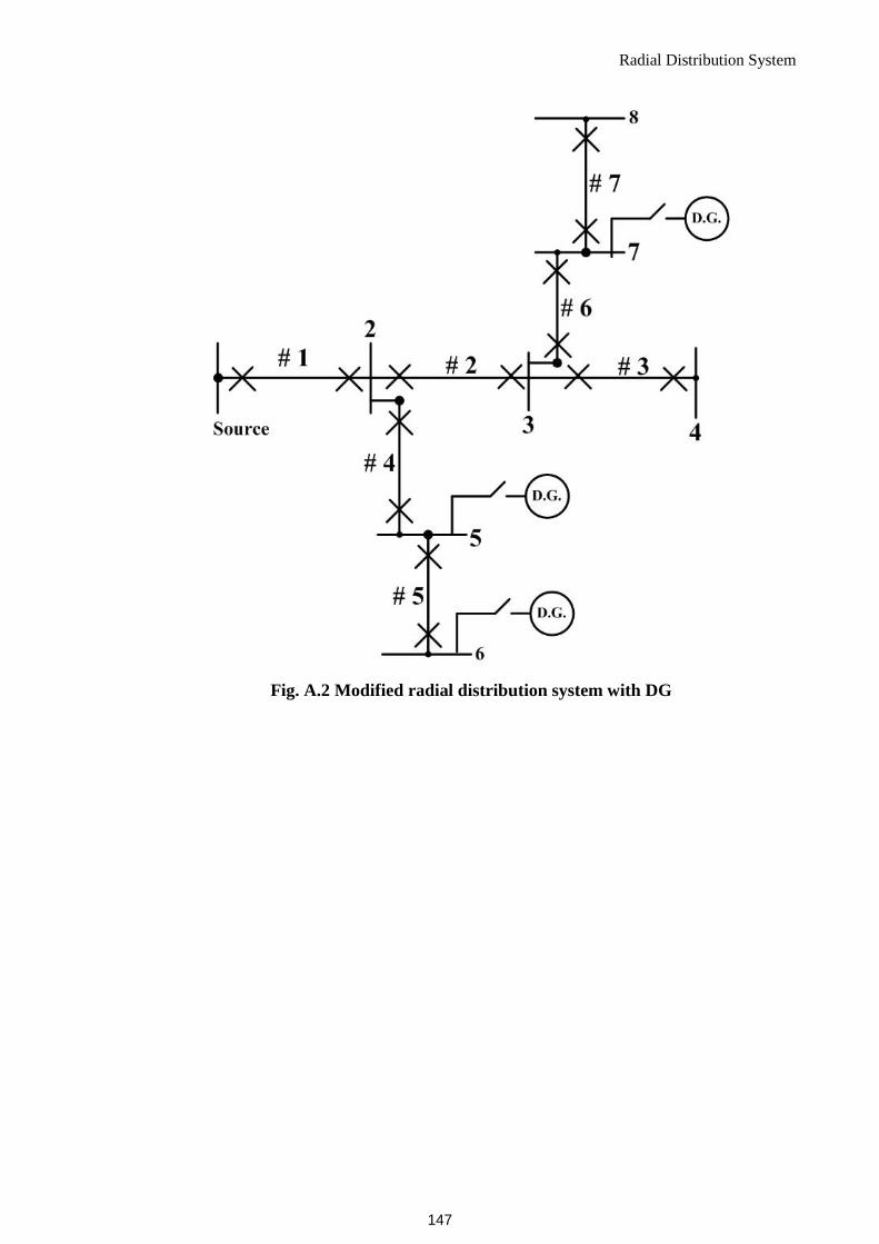
Radial Distribution System
Fig. A.2 Modified radial distribution system with DG
147

APPENDIX-A
Table A.1 Maximum allowable and minimum reachable values of failure rates and repair times for
sample radial distribution system
Distributor segment #1 #2 #3 #4 #5 #6 #7
𝜆𝑘,𝑚𝑎𝑥 /year (failure rate) 0.4 0.2 0.3 0.5 0.2 0.1 0.1
𝑟𝑘,𝑚𝑎𝑥 (h) (repair time) 10 9 12 20 15 8 12
𝜆𝑘,𝑚𝑖𝑛/year (failure rate) 0.2 0.05 0.1 0.1 0.15 0.05 0.05
𝑟𝑘,𝑚𝑖𝑛 (h) (repair time) 6 6 4 8 7 6 6
Table A.2 Average load and number of customers at load points for radial network
Load
point(LP)
2 3 4 5 6 7 8
Average load
Li(kW)
1000 700 400 500 300 200 150
Number of
customers,Ni
200 150 100 150 100 250 50
Table A.3 Cost coefficients 𝜶𝑲 and 𝜷𝑲 for radial network
Distributor segment #1 #2 #3 #4 #5 #6 #7
𝛼𝐾 Rs. 80 100 60 40 80 95 100
𝛽𝐾 Rs. 100 90 50 50 80 60 55
148

APPENDIX-B
B.1 Meshed Distribution System [13]
Fig. B.1 Sample Meshed Distribution System
149

APPENDIX-B
Fig B.2 Reliability logic diagram of the meshed distribution system
150
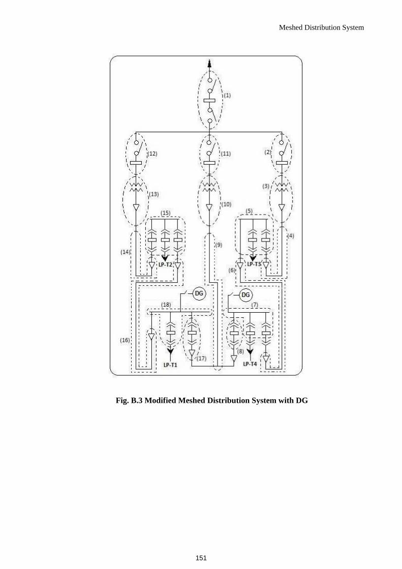
Meshed Distribution System
Fig. B.3 Modified Meshed Distribution System with DG
151

APPENDIX-B
Table B.1 Maximum allowable and minimum reachable values of failure rates and repair times for
sample meshed distribution system
Distributor
segment
𝜆𝑘,𝑚𝑎𝑥 /year
(failure rate)
𝑟𝑘,𝑚𝑎𝑥(h)
(repair time)
𝜆𝑘,𝑚𝑖𝑛/year
(failure rate)
𝑟𝑘,𝑚𝑖𝑛 (h)
repair time
1 0.510402 6.423706 0.254201 3.348734
2 0.177600 4.061540 0.090000 3.067050
3 0.110000 21.732271 0.056000 10.732271
4 0.113525 5.565712 0.056762 2.122525
5 0.184607 8.397691 0.083303 3.394025
6 0.017640 13.555102 0.008830 9.250098
7 0.184607 8.397691 0.092304 3.394025
8 0.178010 9.752112 0.090000 3.752112
9 0.008460 15.800000 0.005230 6.400000
10 0.069000 27.565217 0.026000 18.560000
11 0.205200 5.234919 0.103000 2.012345
12 0.205200 5.234919 0.103000 2.012345
13 0.110000 21.732210 0.056000 10.732221
14 0.113525 5.565712 0.056762 2.122525
15 0.156600 10.714943 0.068333 6.352524
16 0.017640 13.555102 0.008830 9.250098
17 0.178010 9.752120 0.090000 4.354320
18 0.184607 8.397691 0.083303 3.394025
Table B.2 Average load and number of customers at load points for meshed network
Load point(LP) LP-T1 LP-T2 LP-T3 LP-T4
Average load Li(kW) 1500 1000 1000 2000
Number of customers, Ni 400 250 200 450
Table B.3 Cost coefficients 𝜶𝑲 and 𝜷𝑲 for meshed network
Distributor
segment
1 2 3 4 5 6 7 8 9 10 11 12 13 14 15 16 17 18
𝛼𝐾 Rs 80 100 60 40 80 95 100 80 95 75 85 65 45 50 75 80 80 90
𝛽𝐾 Rs 100 90 50 50 80 60 55 100 50 55 70 80 75 90 40 60 85 100
152

APPENDIX-C
C.1 Roy Billinton Test System Bus-2 (RBTS-2) [99]
Fig. C.1 RBTS-2
153

APPENDIX-C
Fig. C.2 Modified RBTS-2 with DG
Table C.1 Failure rates and average repair time of different components of RBTS-2
Sr.
No.
Transformers / Feeder sections Failure
rate(failures/year) λ
Repair/
replacement time
(hr) r
1 Transformer 1-22 (except 8,9 ) 0.01500 10
2 Feeder sections (0.6 km)
2,6,10,14,17,21,25,28,30,34
0.06500 5
3 Feeder sections (0.75 km)
1,4,7,9,12,16,19,22,24,27,29,32,35
0.06500 5
4 Feeder sections (0.80 km)
3,5,8,11,13,15,18,20,23,26,31,33,36
0.06500 5
154

Roy Billinton Test System Bus-2
Table C.2 Maximum allowable and minimum reachable values of failure rates and repair times for
RBTS-2
Distributor
segment
𝜆𝑘,𝑚𝑎𝑥/
year (failure
rate)
λk,min/year
(failure rate)
rk,max (h)
(repair time)
rk,min (h)
(repair
time)
#1 0.048750 0.036650 5.000 2.252252
#2 0.015000 0.011270 10.000 4.504504
#3 0.052000 0.039090 10.000 4.504504
#4 0.048000 0.036090 5.000 2.252252
#5 0.015000 0.011270 10.000 4.504504
#6 0.015000 0.011270 10.000 4.504504
#7 0.048750 0.036650 5.000 2.252252
#8 0.015000 0.011278 10.000 4.504504
#9 0.015000 0.011278 10.000 4.504504
#10 0.039000 0.029323 5.000 2.252252
#11 0.015000 0.011278 10.000 4.504504
#12 0.048750 0.036650 5.000 2.252250
#13 0.052000 0.039097 5.000 2.252250
#14 0.039000 0.029323 5.000 2.252250
#15 0.052000 0.039097 5.000 2.252250
#16 0.048750 0.036650 5.000 2.252250
#17 0.015000 0.011278 10.000 4.504500
#18 0.052000 0.039097 5.000 2.252250
#19 0.015000 0.011278 10.000 4.504500
#20 0.015000 0.011278 10.000 4.504500
#21 0.039000 0.029323 5.000 2.252250
#22 0.015000 0.011278 10.000 4.504500
#23 0.015000 0.011278 10.000 4.504500
#24 0.048750 0.036650 5.000 2.252250
#25 0.015000 0.011278 10.000 4.504500
#26 0.052000 0.039097 5.000 2.252250
#27 0.015000 0.011278 10.000 4.504500
#28 0.015000 0.011278 10.000 4.504500
#29 0.048750 0.036650 5.000 2.252250
#30 0.015000 0.011278 10.000 4.504500
#31 0.015000 0.011278 10.000 4.504500
#32 0.048750 0.036650 5.000 2.252250
#33 0.015000 0.011278 10.000 4.504500
#34 0.039000 0.029323 5.000 2.252250
#35 0.015000 0.011278 10.000 4.504500
#36 0.015000 0.011278 10.000 4.504500
155
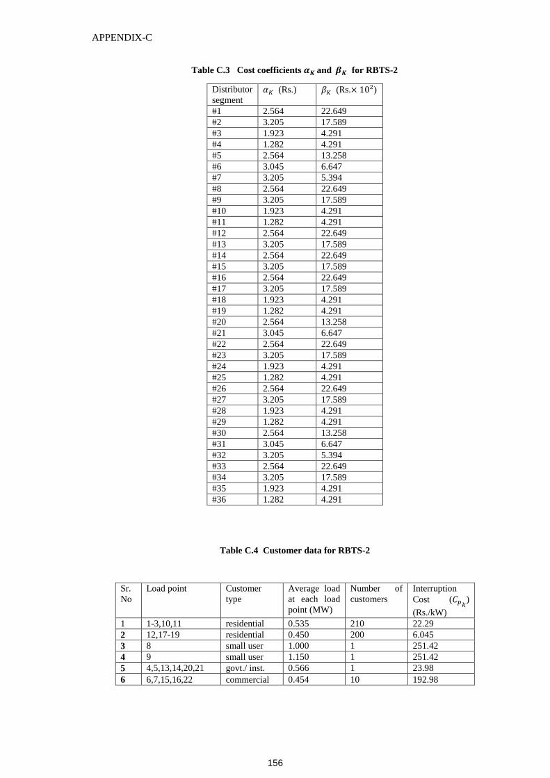
APPENDIX-C
Table C.3 Cost coefficients 𝜶𝑲 and 𝜷𝑲 for RBTS-2
Distributor
segment 𝛼𝐾 (Rs.) 𝛽𝐾 (Rs.× 102)
#1 2.564 22.649
#2 3.205 17.589
#3 1.923 4.291
#4 1.282 4.291
#5 2.564 13.258
#6 3.045 6.647
#7 3.205 5.394
#8 2.564 22.649
#9 3.205 17.589
#10 1.923 4.291
#11 1.282 4.291
#12 2.564 22.649
#13 3.205 17.589
#14 2.564 22.649
#15 3.205 17.589
#16 2.564 22.649
#17 3.205 17.589
#18 1.923 4.291
#19 1.282 4.291
#20 2.564 13.258
#21 3.045 6.647
#22 2.564 22.649
#23 3.205 17.589
#24 1.923 4.291
#25 1.282 4.291
#26 2.564 22.649
#27 3.205 17.589
#28 1.923 4.291
#29 1.282 4.291
#30 2.564 13.258
#31 3.045 6.647
#32 3.205 5.394
#33 2.564 22.649
#34 3.205 17.589
#35 1.923 4.291
#36 1.282 4.291
Table C.4 Customer data for RBTS-2
Sr.
No
Load point Customer
type
Average load
at each load
point (MW)
Number of
customers
Interruption
Cost (𝐶𝑝𝑘)
(Rs./kW)
1 1-3,10,11 residential 0.535 210 22.29
2 12,17-19 residential 0.450 200 6.045
3 8 small user 1.000 1 251.42
4 9 small user 1.150 1 251.42
5 4,5,13,14,20,21 govt./ inst. 0.566 1 23.98
6 6,7,15,16,22 commercial 0.454 10 192.98
156

APPENDIX-D
An Overview of Flower Pollination Algorithm (FP):
The Flower Pollination (FP) algorithm was developed by Xin-She Yang [100] in 2012 and
is inspired by the flow pollination process of flowering plants. The certain rules defining the
process in brief are: (a) Biotic and cross-pollination are global pollination process and
pollen-carrying pollinators travel in a way which obeys Levy flights. (b) A-biotic and self-
pollination are local pollination. (c) Pollinators such as insects can develop flower reliability,
which is equivalent to a reproduction probability and it is proportional to the similarity of
two flowers implicated. (d) A switch probability 𝑝 ∈ [0,1] controls local pollination and
global pollination.
Local pollination do have a significant fraction 𝑝 in the overall pollination activities due to
the physical proximity and other factors such as wind.
Following are the notations used for describing the FP.
𝑀 : population of flowers /pollen gametes
𝐷 : number of variables
𝑘𝑚𝑎𝑥 : maximum number of allowable generations
𝑝 : switch probability ∈ [0,1]
Step-(a) Initialization: An initial population of size ‘𝑀’ is generated as follows.
S0 = [𝑋1
0, 𝑋20, … … , 𝑋𝑀
0 ] (D.1)
Xi0 = [𝑋𝑖1
0 , 𝑋𝑖20 , … . , 𝑋𝑖𝐷
0 ]T (D.2)
𝑋𝑖𝑗0
i.e. 𝑗𝑡ℎ parameter of 𝑋𝑖 vector is obtained from uniform distribution as follows.
𝑋𝑖𝑗0 = 𝑋𝑗,𝑚𝑖𝑛 + (𝑋𝑗,𝑚𝑎𝑥 − 𝑋𝑗,𝑚𝑖𝑛)𝑟𝑎𝑛𝑑𝑗 (D.3)
𝑋𝑗,𝑚𝑖𝑛 and 𝑋𝑗,𝑚𝑎𝑥 are lower and upper bounds on variable 𝑋𝑗. 𝑟𝑎𝑛𝑑𝑗 is a random digit in the
range [0,1].
157

APPENDIX-D
Step-(b) Updating vectors by global and local pollination
𝑋𝑖(𝑘+1)
= {𝑋𝑖
𝑘+ ∝ × 𝐿 (𝑋𝑏𝑒𝑠𝑡(𝑘)
− 𝑋𝑖𝑘), 𝑖𝑓 𝑟𝑎𝑛𝑑 < 𝑝
𝑋𝑖(𝑘)
+∈ (𝑋𝑗(𝑘)
− 𝑋𝑘(𝑘)
) 𝑜𝑡ℎ𝑒𝑟𝑤𝑖𝑠𝑒. 𝑤ℎ𝑒𝑟𝑒, 𝑋𝑗(𝑘)
≠ 𝑋𝑘(𝑘)
(D.4)
𝑋𝑏𝑒𝑠𝑡(𝑘)
is the current best solution found among all solutions at the current
generation/iteration. ∈ is drawn from uniform distribution [0,1] .
∝ > 0 is a scaling factor to control the step size. The parameter 𝐿 is the strength of the
pollination, which essentially is a step size. Since insects may move over a long distance
with various distance steps, a L´evy flight can be used to represent this characteristic
efficiently [108,109].
Lévy distribution:
𝐿 = 𝑣 ×𝜎𝑥(𝛽)
𝜎𝑦(𝛽) (D.5)
𝑣 =𝑟𝑎𝑛𝑑𝑥
|𝑟𝑎𝑛𝑑𝑦|1
𝛽⁄ (D.6)
Where 𝑟𝑎𝑛𝑑𝑥 and 𝑟𝑎𝑛𝑑𝑦 are two normally distributed stochastic variables with standard
deviation 𝜎𝑥(𝛽) and 𝜎𝑦(𝛽) given by:
𝜎𝑥(𝛽) = [⎾(1+𝛽)× (
𝜋𝛽
2)
⎾ (1+𝛽
2)× 2
(𝛽−1
2)]
1𝛽⁄
(D.7)
𝜎𝑦(𝛽) = 1 (D.8)
Where 𝛽 is the distribution factor (0.3 ≤ 𝛽 ≤ 1.99) and Γ (.) is the gamma distribution
function.
Step-(c) Comparing the fitness of the updated vectors with the initial vectors
𝑋𝑖(𝑘+1)
= {𝑋𝑖
𝑘+1, 𝑖𝑓 𝑓(𝑋𝑖𝑘+1) < 𝑓(𝑋𝑖
(𝑘))
𝑋𝑖(𝑘)
𝑜𝑡ℎ𝑒𝑟𝑤𝑖𝑠𝑒 (D.9)
The current best solution 𝑋𝑏𝑒𝑠𝑡(𝑘)
and its fitness is then found.This process is executed for all
target vector index 𝑖 and a new population is created till the optimal solution is obtained or
the pre-specified generations (𝑘𝑚𝑎𝑥) have been executed.
158

APPENDIX-E
Teaching Learning Based Optimization (TLBO): An Overview
Teaching-learning-based- optimization (TLBO) algorithm is also one of the most recently
developed metaheuristicalgorithms [101]. Similar to most other evolutionary optimization
methods, TLBO is a population-based algorithm inspired by learning process in a classroom.
A group of learners constitute the population in TLBO. In any optimization algorithms there
are D numbers of different design variables. The different design variables in TLBO are
analogous to different subjects offered to learners and the learners’ result is analogous to the
‘fitness’, as in other population-based optimization techniques. The searching process
consists of two phases, i.e. Teacher Phase and Learner Phase. In teacher phase, learners first
get knowledge from a teacher and then from classmates in learner phase through interaction
between them. In the entire population, the best solution is considered as the teacher
(𝑋𝑇𝑒𝑎𝑐ℎ𝑒𝑟).
The fundamental steps are explained below.
Following are the notations used for describing the TLBO.
𝑀 : number of learners in class i.e. “ class size ”
𝐷 : number of courses offered to the learners
𝑘𝑚𝑎𝑥 : maximum number of allowable generations
Step-(a) Initialization: an initial population of size ‘𝑀’ is generated as follows
S0 = [𝑋1
0, 𝑋20, … … , 𝑋𝑀
0 ] (E.1)
Xi0 = [𝑋𝑖1
0 , 𝑋𝑖20 , … . , 𝑋𝑖𝐷
0 ]T (E.2)
𝑋𝑖𝑗0 i.e. 𝑗𝑡ℎ parameter of 𝑋𝑖 vector is obtained from uniform distribution as follows.
𝑋𝑖𝑗0 = 𝑋𝑗,𝑚𝑖𝑛 + (𝑋𝑗,𝑚𝑎𝑥 − 𝑋𝑗,𝑚𝑖𝑛)𝑟𝑎𝑛𝑑𝑗 (E.3)
𝑋𝑗,𝑚𝑖𝑛and𝑋𝑗,𝑚𝑎𝑥 are lower and upper bounds on variable 𝑋𝑗. 𝑟𝑎𝑛𝑑𝑗 is a random digit in the
range [0,1].
159

APPENDIX-E
Step-(b) Teacher phase:
The mean parameter 𝑋𝑀𝑒𝑎𝑛𝑘 of each subject of the learners in the class at generation 𝑘 is
given as 𝑋𝑀𝑒𝑎𝑛𝑘 = [𝑋1
𝑘, 𝑋2𝑘 , … . , 𝑋𝐷
𝑘]T.
The learner with the minimum objective function value is considered as the teacher
𝑋𝑇𝑒𝑎𝑐ℎ𝑒𝑟(𝑘)
for respective generation. In order to maintain stochastic features of the search,
two randomly-generated parameters 𝑟𝑎𝑛𝑑and 𝑇𝐹 are applied in update formula for the
solution 𝑋𝑖 as:
𝑋𝑁𝑒𝑤𝑘 = 𝑋𝑖
𝑘 + 𝑟𝑎𝑛𝑑 × (𝑋𝑇𝑒𝑎𝑐ℎ𝑒𝑟(𝑘)
− 𝑇𝐹 𝑋𝑀𝑒𝑎𝑛𝑘 ) (E.4)
𝑇𝐹is the teaching factor which decides the value of mean to be changed. Value of 𝑇𝐹 can
be either 1 or 2. The value of 𝑇𝐹 is decided randomly with equal probability as,
𝑇𝐹 = 𝑟𝑜𝑢𝑛𝑑 [1 + 𝑟𝑎𝑛𝑑(0,1){2 − 1}] (E.5)
If 𝑋𝑁𝑒𝑤𝑘 is found to be a superior learner than 𝑋𝑖
𝑘 in generation 𝑘 , than it replaces inferior
learner 𝑋𝑖𝑘 in the matrix.
Step-(c) Learner phase:
In this phase the interaction of learners with one another takes place. The process of mutual
interaction tends to increase the knowledge of the learner. The random interaction among
learners improves his or her knowledge. For a given learner 𝑋𝑖𝑘 , another learner 𝑋𝑟
𝑘is
randomly selected 𝑖 ≠ 𝑟 . The 𝑖𝑡ℎ parameter of the matrix 𝑋𝑁𝑒𝑤,𝑖𝑘 in the learner phase is
given as
𝑋𝑁𝑒𝑤,𝑖𝑘 = {
𝑋𝑖𝑘 + 𝑟𝑎𝑛𝑑 × (𝑋𝑖
𝑘 − 𝑋𝑟𝑘), 𝑖𝑓 𝑓(𝑋𝑖
𝑘) < 𝑓(𝑋𝑟𝑘)
𝑋𝑖𝑘 + 𝑟𝑎𝑛𝑑 × (𝑋𝑟
𝑘 − 𝑋𝑖𝑘) 𝑜𝑡ℎ𝑒𝑟𝑤𝑖𝑠𝑒
(E.6)
This process is executed for all target vector index 𝑖 and a new population is created till the
optimal solution is obtained. The procedure is terminated if a maximum number of
generations (𝑘𝑚𝑎𝑥) have been executed or no improvement in objective function is noticed
in a pre-specified generations.
160

APPENDIX-F
Differential Evolution (DE): An overview
Differential evolution (DE) developed by Storn and Price is a very simple population based,
stochastic function minimizer and has been found very powerful to solve various nature of
engineering problems[102,110]. DE attacks the optimization problem by sampling the
objective function at multiple randomly chosen initial points. Pre-set parameter bounds
define the region from which ‘M’ vectors in this initial population are chosen. DE generates
new solution points in ‘D’ dimensional space that are perturbations of existing points. It
perturbs vectors with the scaled difference of two randomly selected population vectors. To
produce a mutated vector, DE adds the scaled, random vector difference to a third selected
population vector (called as based vector). Further DE also employs a uniform cross over to
produce trial vector from target vector and mutated vector.
The three fundamental steps are explained below.
Step-(a) Initialization: An initial population of size ‘M’ is generated as follows
S0 = [X1
0, X20, … … , XM
0 ] (F.1)
Xi0 = [Xi1
0 , Xi20 , … . , XiD
0 ]T (F.2)
X0 ij i.e. jth parameter of Xi vector is obtained from uniform distribution as follows.
Xij0 = Xj,min + (Xj,max − Xj,min)randj (F.3)
Xj,min and Xj,max are lower and upper bounds on variable Xj. randj is a random digit in the
range [0,1].
Step-(b) Mutation: DE mutates and recombines the population to produce a population of
‘M’ trial vectors. Differential mutation adds a scaled, randomly sampled, vector difference
to a third vector as follows.
V__𝑖(k)
= Xbase(k)
+ σ(Xp(k)
− Xq(k)
) (F.4)
σ is known as scale factor usually lies in the range [0,1]. Xp(k)
and Xq(k)
are two randomly
selected vectors (p≠ q). Xbase(k)
is known as base vector. V__𝑖(k)
is a mutant vector. The base
161

APPENDIX-F
vector index ‘base’ may be determined in variety of ways. This may be a randomly chosen
vector (base≠ p≠ q).
Step (c) Crossover: DE employs a uniform cross over strategy. Crossover generates trial
vectors tij(k)
as follows
tij(k)
= {vij
(k), if (randj ≤ Cr or j = jrand
Xij(k)
otherwise (F.5)
Cr is crossover probability lies in the range [0, 1]. Cr is user defined value which controls the
number of parameter values which are copied from the mutant. If the random number randj
is less than or equal to Cr, the trial parameter is adopted from the mutant V__𝑖(k)
. Further, the
trial parameter with randomly chosen index, jrand is taken from the mutant to ensure that trial
vector does not duplicate target vector Xi(k)
. Otherwise the parameter is adopted from the
target vector Xi(k)
.
Step-(d) Selection: Objective function is evaluated for target vector and trial vector, trial
vector is selected if it provides better value of the function than target vector as follows.
Xi(k+1)
= {ti
(k), if f(ti
(k)) < f(Xi
(k))
Xi(k)
otherwise (F.6)
The process of mutation, crossover and selection is executed for all target vector index i and
a new population is created till the optimal solution is obtained. The procedure is terminated
if a maximum number of generations (kmax) have been executed or no improvement in
objective function is noticed in a pre-specified generations. Various benchmark versions of
DE that differ in the new generation methods largely are available [102]. In this paper
DE/best/1/bin has been selected. The first term after DE i.e. ‘best’ specifies the way base
vector is chosen. In this selected scheme, the base vector is the current best so far vector. ‘1’
after the best denotes that one vector difference contributes to the differential. Last term ‘bin’
denotes binomial distribution that results because of uniform crossover. Number of
parameters denoted by mutant vector closely follows binomial distribution. It is to be noted
that best, target and difference vector indices are all different.
162