Jumal Mekanikal, JiIid II, 2000

STREAMLIKE FUNCTION FORMULATION OFENTRY FLOW

Amer Nordin Darns

Faculty of Mechanical EngineeringUniversiti Teknologi Malaysia

ABSTRACT

A numerical study offluid flow in a rectangular duct is presented.

The flow ofthe working fluid is assumed to be steady and laminar.

It is also assumed that the flow field is rotational. The flow

analysis is carried out in three dimensional space using Cartesian

coordinate. The problem formulation results in a non-linear type

partial differential equation for the through flow velocity, which is

solved numerically using marching technique. The other

formulation is an elliptic type partial differential equation, for

which the streamlike function is solved using successive over

relaxation method. The results obtained are investigated to

determine the velocity distribution across a constant duct cross

section and the development ofthroughflow velocity in the duct.

1.0 INTRODUCTION

1.1 General

The development of a parabolic Poiseuille profile downstream of entry flow into

plane channel is one of the standard problems in laminar flow theory. It has also

73

Jumal Mekanikal, Jilid II. 2000

attracted more alternative than is warranted by its intrinsic practical importance.

This is because it exemplifies certain features of viscous flow.

The importance of this study on entry flow of a viscous fluid is mainly to

investigate the velocity distribution in the entrance region. Most approximate

analysis of the problem involve some forms of Prandtl's boundary layer

approximation and the exact solution of the Navier Stokes equation which is to

illustrate certain qualitative aspects 'of viscous flow. The boundary concept as

introduced by Prandtl [1] and the resulting approximations only involve the

boundary layer for two dimensional flow. By two dimensional boundary layer

flow it means that, a boundary layer which is formed over plane surface, infinite

in lateral extent, where the projections of the streamlines of the outer flow on this

surface (that is the geometrical surface) are straight lines perpendicular to the

leading edge. In three dimensional flow, calculations will constitute a complex

mathematical problem. This is due to the fact that three velocity and vorticity

components are involved. The partial differential equations governing the fluid

motion are complicated and it is hardly surprising that their analytical solution

becomes difficult or even impossible unless considerable simplifications are

made. In an attempt to overcome these difficulties and thereby extend the range

of possible solutions, a finite difference technique is used. The primary reason

for this development is, of course, the advent of electronic digital computers

featuring both high speed and high capacity.

1.2 Previous Work in Entry Flow

Historically, a numerical solution of an entrance flow in a rectangular duct has

been the subject of extensive research. In 1942, Langhaar [l] has postulated a

linearization of the Navier Stokes equation of fluid motion which enables him to

solve the laminar flow problem for an incompressible fluid in a circular pipe.

Mohanty and Asthana [2] have divided the entrance region into two parts, the

inlet region and the filled region. Their objective is to re-examine analytically

the flow in the pipe entrance region and to verify salient results by experiments.

74

Jumal Mekanikal, Ji/id II, 2000

The result which they obtained shows that, the experimental result agrees well

with the analytical one.

Han [3] employed Langhaar's linearization assumption to solve the

development of flow problem in a rectangular duct. Sparrow, Lin and Lungren

[4] devised an approximate technique for two dimensional entrance flow which

was the basis for a recent solution by Wigninton and Dalton [5] for entrance flow

in a rectangular duct. Rubin, Khosla and Saari [6] studied the entrance region in

two parts. In the first part, the entry region is evaluated by a boundary

layer/potential core analysis and in the second part, a numerical solution is

obtained for the viscous flow equation which is derived earlier in the first part.

They solved a two stream functions, velocity and vorticity systems which are

independent of the Reynolds number, with a combined Alternating Direction

Implicit Method (ADI) with a point relaxation numerical procedure. The results

of axial flow behavior in the first and second parts seem to agree fairly well with

the experimental data.

Many recent investigations have centered on the numerical solution of the

finite different equation. Hornbeck's [7] finite difference analysis for a circular

pipe yielded velocity distributions somewhat different from those of Langhaar

but agree very well with regard to the entrance length and the pressure

distributions. Experimental investigation of the flow development in a

rectangular duct by Sparrow, Hixon and Shavit [8], and Beavers, Sparrow and

Magnuson [9] indicate that Han's solution underestimates the entrance length

over the estimates of the entrance pressure drop.

2.0 METHOD OF ANALYSIS

2.1 Exact Numerical Method

Laminar incompressible flow in a straight two dimensional axisymmetric

rectangular channel have also been investigated by a variety of analytical and

75

Jurnal Mekanikal, Jilid II. 2000

numerical techniques. These are typified by the linear boundary layer (Oseen)

approximation [3] for evaluating the axial velocity and pressure distribution

downstream of an initial entry region. There are more exact numerical analysis

using boundary layer [10,11] or Navier Stokes equation [12,13,14] and finally a

boundary layer/potential core expansion method [15,16,17] that gives a better

models of flow in entry region. Basically, the governing equations used in this

analysis include:

Continuity equation:

Y'.v =0

Momentum equation:

DV 1 2­-=-Y'p+vY'Vt» p

(1)

(2)

2.2 Stream Function Method of Analysis

This method of analysis is only applicable for two dimensional flow system. The

introduction of stream function in two dimensional flow system will allow a

relatively simple mathematical solution. The mathematical solution is those of a

complex variable is given in [18,19]. In order to solve the boundary layer

equation, as in the of steady flow, it is much easier to introduce a stream function

that satisfies the continuity equation. By introducing this function into the Navier

Stokes equation, we will obtain a partial differential equation of the third order.

This method of analysis can be understood better from the recent study of entry

flow problem [6]. Thus , in general , the governing equations involved are:

Continuity equation:

\l.V =0

Vorticity equation:

\lxV = Q

76

(3)

(4)

Jumal Mekanikal, Jilid II, 2000

Momentum equation:

DV 1 2­-=-V'p+vV'VDt P

A defined stream function : u =- 0\jJOy

v = 8\jJax

2.3 Streamlike Function Method of Solution

(5)

(6)

From the previous method of analysis, it is seen that several problems were

encountered. The direct method which solved the momentum equation together

with the continuity equation constitutes a large system. They are computationally

inefficient and suffer from round-off error accumulation. The second method

which utilised the vorticity definition besides momentum and continuity

equations finally evolve a Poisson type of equation. This requires a considerable

programming effort and also limited to two dimensional flow problems.

The streamlike function method of analysis first proposed and used by

Abdallah and Hamed [20] seems an advantage. It has successfully been used by

Darns [21] in his channel flow problem. However, the fluid model is assumed

inviscid. Basically in this method, the governing equations involve are :

Continuity equation:

V'.v=o

Momentum equation:

DV I 2­-=-V'p+vV'VDt P

Vorticity equation:

V'xV =0

(7)

(8)

(9)

77

Jurna/ Mekanikal, Ji/id II, 2000

A defined streamlike function :

w= O\vOy

v=_O\v -J au dyaz ax

3.0 MATHEMATICAL FORMULATION

(10)

3.1 Governing Equation

Assuming steady laminar flow of an incompressible viscous fluid with rotational

flow field and constant physical properties, the flow in the entrance region of the

rectangular duct may be described by the following equations:

Continuity equation :

Y'.v=o

Momentum equation:

DV I 2­-=-Y'p+vY'VDt P

(11)

(12)

where V is the velocity vector, P is the total pressure divided by the density and

o is the vorticity vector which is defined as the curl of V

Y'xV =0 (13)

By substituting equation (13) and assuming steady state, the momentum

equation becomes :

(14)

78

Jumal Mekanikal, Jilid IL 2000

The Cartesian coordinate system is used in this analysis to simplify the

boundary conditions. Referring to Figure I and 2, the x-axis is taken along the

duct primary direction while y and z axes are taken in the cross sectional.plane.

Equation (11), (12) and (13) are written in this coordinate as,

Continuity equation,

au Ov Ow-+-+-=0ax By az

Vorticity equation,

x-component,

Ow Ov~=--­

By azy-component,

au Ow11=--­az ax

z-component,

Ov aus=--­ax By

Equation (14) then becomes,

x-component,

(15)

(16a)

(16b)

(16c)

79

Jumal Mekanikal , Jilid II, 2000

y-component

Or] Or] Or] av av av (a 21] a21] a21]Ju-+V-+w--~--1]--s-=v -+-+- (17b)aX y az ax 0' az ax2 0'2 az2 .

z-component

uas + v as + was _~ aw -1] aw -s aw =v(a2s+.a2s+ a2sJ(17c)

ax y az ax 0' az ax2 0'2 az2

where u, v and ware the velocity components in the x, y and z direction

respectively and ~, 1] and (are the vorticity components in the x, y, and z

direction respectively.

3.2 Simplification of the Governing Equation

An order of magnitude analysis which is valid only for the average values of each

term of the flow field, may be applied to equation (17) . Representative distances

in the axial direction are taken to be in the order of the development length

(entrance length) z, while the distances in the transverse direction yare taken in

the order of the duct half width "a", and the direction z are taken in the order of

the duct half breadth "b", The basic assumption underlying this simplifying

approximation is that the entrance length is much greater than the half width and

the half breadth of the duct, that is,

Y»a,

Z»b

From simplicity, we assume the following orders of magnitude:

x =O(Z)y =O(a)z =O(b)u =O(UJ

v=o(a~ o)

80

Jurnal Mekanikal, Jilid II, 2000

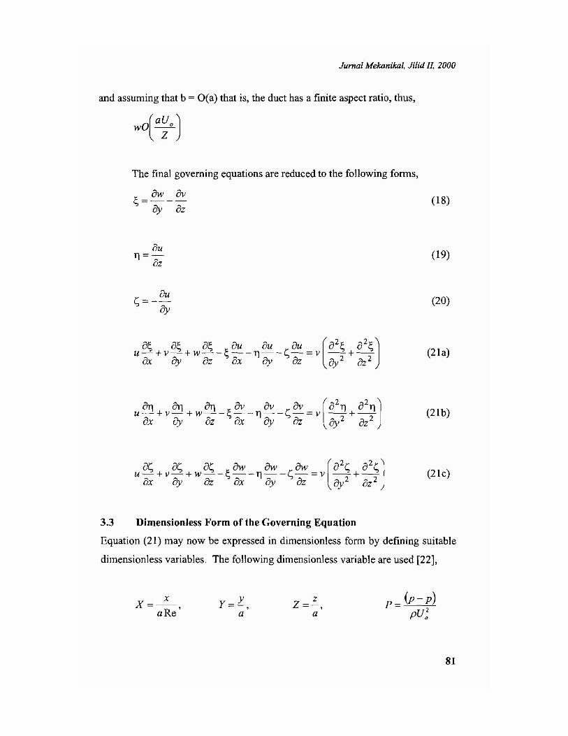
and assuming that b = O(a) that is, the duct has a finite aspect ratio, thus,

The final governing equations are reduced to the following forms,

~ = Ow _ 8v (18)By oz

ou11 =- (19)oz

C;, = - ou (20)By

uo~ + v o~ + w o~ _~ ou -11 ou _C;, ou = v (02~ + 02~J (21a)ox By oz ox By OZ 0'2 Oz2

u 0(, + v 0(, + W oC;, _~ Ow -11 Ow -C;, Ow = v (02C;, + 02C;,J (2Ic)ox 0' oz ox 0' OZ 0'2 Oz2

3.3 Dimensionless Form of the Governing Equation

Equation (21) may now be expressed in dimensionless form by defining suitable

dimensionless variables. The following dimensionless variable are used [22],

x=_x_aRe'

y=Y ,a

z=3- ,a

81

Jumal Mekanikal, Jilid II. 2000

u=~U'

a

v= vReU'

a

w= wReU 'a

Re = paU a

f-L

Using the above variables, the following expressions are than obtained:

au u, auax = aRe ax'

8v u, avax = aRe ax'

Ow Uo awax = aRe ax'

au u, er8y ;:= aRe aY'

Ow u, aw8y = aRe aY'

au uoau-=--8z a az

au u, av-=----az aRe ez

Ow Uo aw-=----az aRe ez

On applying the above expressions to equations (15), (18) and (21), one

obtains the following:

~ = aw _av (23)ay ez

au11 = az (24)

t;, =- au (25)ay

x~ + v a~ +w a~ _~ au -11 au _t;, au = v [a2~ + a2~ J (26a)ax ay ez ax ay ez ay2 az2

82

Jurnal Mekanikal, Jilid II, 2000

uOr] + V Or] + w Or] _~~_" av -S av =v [a 2

" + a2"J (26b)

ax ay az ax ay az ay2 az2

u as +v 8S+w as _~ 8w _"aw _saw =v[a2s + a

2sJ (26c)ax 8y az ax ay az ay2 ez?

3.4 Derivation of the Streamlike Function Formulation

Equations (22) through (26) do not represent a form entirely suited to finite

difference computation. There exists a dimensionless streamlike function.

Abdallah and Hamed [20] define a streamlike function If! which identically

satisfies the continuity equation and having the source term. According to this

definition, the cross flow velocity components Wand V are related through the

following expressions:

From definition,

w=£7\vay

using continuity equation

av aw au-=----ay az ax

substituting equation (27) into the above equation,

av a2\11 au-=-----ay ayaz ax

integrating with respect to Y, one obtains,

£7\v auV=---J-dYez ax

(27)

(28)

83

Jumal Mekanikal, Jilid 1J, 2000

Substituting equations (27) and (28) into equation ( 23)

~ = aw _avay az

~ =~(a\jlJ - ~(- 0\jI - Jau dYJay ay az az ax

or

~ = a2\j1 + a2

\j1 +~J au dYay2 az2 az ax (29)

(30)

equation (30) is first solved for the streamJike function If. Then equations (27)

and (28) are used to get the cross flow velocities V and W.

3.5 Derivation of Through Flow Velocity Equation

Equation (26) is used in the derivation of the through flow velocity equation .

Eliminating the kinematic viscosity term from these equations , two equitions are

obtained. Substituting equation (26b) into equation (26a), the following equation

is obtained,

(31)

84

Jurnal Mekanikal, Jilid Il, 2000

substituting equation (26c) into equation (26a), the following equation is

obtained,

(32)

Equation (31) and (32) are used to solved separately the through flow velocity U.

3.6 Boundary Condition

Referring to Figure 1 and 2, the following boundary conditions are obtained:

At all walls,

(y == a, Z == b) :

At the entrance :

U==v==w==o

U(O,O,O)==UQ

'1'(0,0,0) == °

(33)

(34)

(35)

4.0 METHOD OF SOLUTION

The approach used in the solution of the governing equations is similar to that of

those developed by Abdallah and Hamed [23] and Darns [21] for the secondary

flow constant area duct. The basic idea behind the mathematical solution is to

manipulate the governing equations in order to arrive at a certain first order

parabolic type partial differential equations for the through flow velocity. The

two equations used for solving the through flow velocity are given by equations

(31) and (32). The through flow velocity is then solved by using marching

technique [22].

85

Jurnal Mekanikal, Jilid II. 2000

The streamlike function formulation which is given by equation (30) is in

the form of an elliptic type partial differential equation. The terms on the right

hand side of equation (30) are considered as the source term. This equation is

solved for the streamlike function If by using successive over relaxation method

[24]. For this study, a relaxation factor equal to 1.73 is used. If convergence is

not reached after 100 iterations, the program is stop. The cross flow velocity W

and V are computed by using equation (27) and (28). Finally the vorticity

components ~ ,." and , are determined by using equation (23), (24) and (25).

The iterative procedure can be summarized as follows:

1. All variables are initialized at the entrance

2. Calculate U(2.J,K) from equation (31) or (32) using marching technique.

3. Calculate 1f{J, K) from equation (30) using successive over relaxation.

4. Calculate W(2,J,K) and V(2.J,K) from equation (27) and (28).

5. Calculate ~(2,J,K), .,,(2,J,K) and '(2,J,K) from equation (23), (24) and

(25).

6. Return to step 2

This procedure continues until the flow becomes fully developed. The reader

is requested to refer to Figure 11.

4.1 Finite Difference Form of Governing Equation

4.1.1 System ofGrid Point

In obtaining the finite difference approximation to the solution of any partial

differential equation, it is first necessary to establish a system of grid points in the

region occupied by the independent variables. The present problem lends itself to

the automatic adoption of grid points located at the intersection of a series of

equally spaced horizontal and vertical lines. Such a scheme, known as

rectangular grid, is shown in Figure 3. The indexes 1, J and K indicate positions

86

Jumal Mekanikal , Ji/id II, 2000

in the X, Y and Z directions respectively . The axial mesh spacing is ~, while

the transverse mesh spacing are 11Y == IIMZI and I1Z == Q1M31. MZ and M3 are

integers showing the number of mesh spaces in Y and Z directions respectively

and Q which is the aspect ratio of the channel is equal to b/a.

4.1.2 Finite Differencefrom ofthe Stream like Function

Equation (30) is used to solve for the streamlike function. This is solved by using

successive over relaxation technique which is the standard method used to solve

elliptic type partial differential equation. The finite difference form of this

equation is,

IjI(J ,Kf = ORF·(IjI(J, K + 1)+ 1jI(j,K --:1)+ 1jI(J+ 1,K )+IjI(J -1,K)+ (DZ)· XN(J,K))

4+ (l-ORF)·IjI(J,K)

(36)

where,

ORF == over relaxation factor

'I/(J,K)* == new value of streamlike function

XN(J,K) == source term

4.2 Finite Difference from of the Cross Flow Velocity

The cross flow velocities are calculated by using equation (Z7) and (Z8). Their

finite difference forms are as follows:

W(Z J K) == (vr(J + I,K)- 'I/(J -1)) (37), , (Z *DY)

V(Z,J,K) =VI(Z,J,K)- VZ(Z,J,K) (38)

where,

VI(Z J K)= -('I/(J,K +l)-'l/(J,K -1)), , (Z*DZ)

87

Jumal Mekanikal, Jilid IL 2000

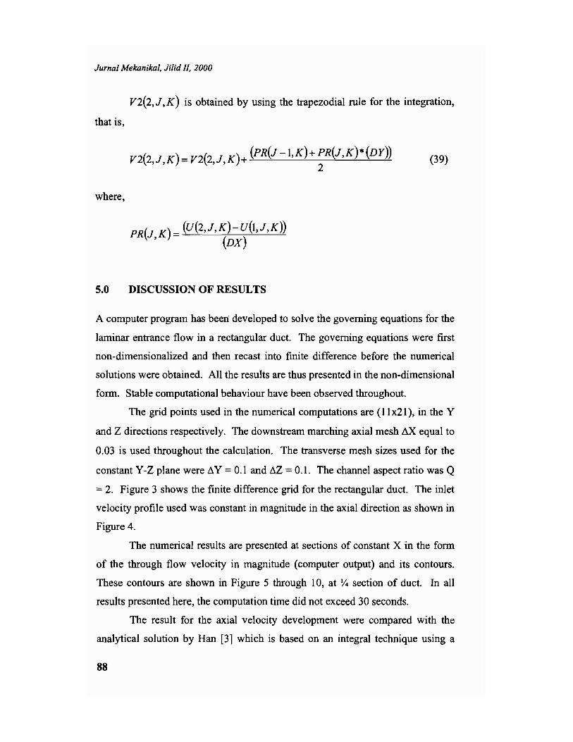
V2(2,J,K) is obtained by using the trapezodial rule for the integration,

that is,

V2(2,J,K)=V2(2,J,K)+ (PR(J -1,K)+ ~R(J,K)*(DY)) (39)

where,

PR(J K) = (U(2,J,K)- U(I,J,K)), (DX)

5.0 DISCUSSION OF RESULTS

A computer program has been: developed to solve the governing equations for the

laminar entrance flow in a rectangular duct. The governing equations were first

non-dimensionalized and then recast into finite difference before the numerical

solutions were obtained. All the results are thus presented in the non-dimensional

form. Stable computational behaviour have been observed throughout.

The grid points used in the numerical computations are (11x21), in the Y

and Z directions respectively. The downstream marching axial mesh LlX equal to

0.03 is used throughout the calculation. The transverse mesh sizes used for the

constant Y-Z plane were /),Y = 0.1 and /),Z = 0.1. The channel aspect ratio was Q

= 2. Figure 3 shows the finite difference grid for the rectangular duct. The inlet

velocity profile used was constant in magnitude in the axial direction as shown in

Figure 4.

The numerical results are presented at sections of constant X in the form

of the through flow velocity in magnitude (computer output) and its contours.

These contours are shown in Figure 5 through 10, at Y4 section of duct. In all

results presented here, the computation time did not exceed 30 seconds.

The result for the axial velocity development were compared with the

analytical solution by Han [31 which is based on an integral technique using a

88

Juma/ Mekanikal, Jilid II, 2000

linearized form of the axial momentum equation and the experimental data by

Goldstein and Kreid [25] using a Laser Doppler flowmeter. Carlson and

Hornbeck numerical solution [11] are also included in the comparison. At the

duct center line in Figure 5, the numerical solution for axial velocity development

are in good agreement with the solutions obtained by [3], [11] and [25]. The

numerical results for X less than 0.08 agrees very well with [3] and [11].

However, after X = 0.2, the numerical solutions were closer to experimental data.

The entrance length L is defined as the dimensionless axial position at

which the center line velocity reaches 99 percent of its fully developed value

[II] . The numerical solution yielded L = 0.3. Carlson and Hornbeck's numerical

solutions yielded L = 0.278 for the first model and L = 0.266 for the second

model. Han's analytical value was L = 0.301 while the experimental value found

by Goldstein and Kreid was L = 0.36. These large discrepancies, as mentioned

by Goldstein and Kreid, are highly sensitive to very small variation in the center

line velocity as the fully developed value is approached and even these large

variation is of relatively little significance. Table I shows the comparisons for

the entrance length.

Figures 6, 7 and 8 show the axial velocity contours for different X planes

taken at 2 = 0.0, 2 = 0.5 and 2 = 0.75 respectively. the axial velocity profile at

Z = 0.00 assembles the center line velocity. At X = 0.33, the axial velocity has

reached its fully developed value. It can be observed from these figures that the

fluid flow actually characterized the Poiseuille flow which is parabolic. It can

also be observed that the effect of vorticity is more significant on the flow

especially nearer to the wall (2 = 0.75).

Figure 9 and 10 illustrate the axial velocity profile at constant of X = 0.12

and X =0.3. It can be observed from these figures that the maximum value of the

through flow velocity is initially closer to the wall. However, the velocity

contours move downward and towards the center of the duct as the flow moved

further downstream. It appear therefore that the progressive change in the

89

Jurnal Mekanikal, Jilid II, 2000

velocity contours are due to the effect of denser circulation occurs which starts at

the wall and moves towards the center of the duct.

6.0 CONCLUSION

Numerical results have been presented for the laminar entrance flow in a

rectangular channel. The adequacy of the results obtained for the entrance length

is shown by comparing the solution of this simpler model to that of a more exact

model. The choice of equation (31) and (32) at least and qualitatively verifies the

entrance flow solution.

From the solutions obtained, it can be concluded that the formulation of

the streamlike function is possible for the entry flow problem at least in

rectangular duct. Finally, the present study centers only for the velocity

distribution in a rectangular duct. It may be suggested that the present study can

be also applied to the study of the pressure distribution in a rectangular duct

which is more of engineering interest especially in turbomachines.

REFERENCES

1. Langhaar, R.L., 1942, Steady Flow in the Transition Length of a Straight

Tube,1. of Applied Mechanics, Vol. 9, TRANS. ASME, Vol.64, pp. 55-58.

2. Mohanty, A.K. and Asthana, S.B.L, 1978, Laminar Flow in the Entrance

Region ofa Smooth Pipe, 1. Fluid Mechanics, Vo1.90, prt 3, pp. 433-447.

3. Han, L.S., 1960, Hydrodynamic Entrance Length for Incompressible Flow in

Rectangular Ducts, J. of Applied Mechanics, Vol. 27, TRANS, ASME, Vol.

82, Series E, pp. 403-409.

4. Sparrow, E.M., Lin, S.H., and Lundgren, T.S., 1964, Flow Development in

the Hydrodynamic Entrance Region of Tubes and Ducts, Physics of Fluid,

Vol. 7, pp. 338-347.

90

Jurnal Mekanikal, Jilid IL 2000

5. Wigninton, C.L. and Dalton, C., 1970, Incompressible Laminar Flow in the

Entrance Region ofa Rectangular Duct, J of Applied Mechanics, Vol. 37,

TRANS. ASME, Vol. 92, pp. 854-856.

6. Rubin, S.G., Khosla, P.K., and Saari, S., 1977, Laminar Flow in Rectangular

Channels, 1. of Computers and Fluid, Vol. 5, pp. 151-173.

7. Hornbeck, R.W., 1964, Laminar Flow in the Entrance Region of a Pipe,

Applied Scientific Research, Section A, Vol. 13, pp. 224-232.

8. Sparrow, E.M., Hixon, C.W; and Shavit, G., Oct. 1964, Experiments on

Laminar Flow Development in Rectangular Ducts, J. of Basic Engineering,

TRANS, ASME, Series D, Vol. 89, No.1 (AFEOAR).

9. Beavers, G.S., Sparrow, E.M., and Magnuson, R.A., 1970, Experiments on

Hydrodynamically Developing Flow in Rectangular Ducts ofArbitrary Ratio,

International Journal ofHeat and Mass Transfer, Vol. 13, pp. 689-702.

10. Brilley, R., 1972, A Numerical Method for Predicting Three Dimensional

Viscous Flow in Ducts, United Aircraft Research Laboratories Report

LII0888-1.

11. Carlson, G.A. and Hornbeck, R.W., 1973, A Numerical Solution for Laminar

Entrance Flow in a Square Ducts, 1. of Applied Mechanics, Vol. 40,

TRANS, ASME, pp. 26-30.

12. Hiroshi Morihara and Chang, R.A, 1973, Numerical Solution of the Viscous

Flow in the Entrance Region ofParallel Plates, J. of Computer Physics, Vol.

11, pp. 550-572.

13. Wang, Y.L. and Longwell, P.A, 1964, Laminar Flow in the Inlet Section of

Parallel Plates, AICHE Journal, Vol. 10, pp. 323-329.

14. Me Donald, J.W., Denny, V.W. and Mills, AF., 1972, Numerical Solution of

the Navier Stokes Equations in Inlet, J. of Applied Mechanics, Vol. 39,

TRANS, pp. 873-878.

15. Wilson, S.D.R, 1971, Entry Flow in Channel, Part 2, J. of Fluid Mechanics,

Vol. 46, No.4, pp. 787-799.

91

Jurnal Mekanikal, Jilid IL 2000

16. Milton Van Dyke, 1970, Entry Flow in a channel, J. of Fluid Mechanics,

Vol. 44, No.4, pp. 813-823.

17. Kapila, A.K., Ludford, G.S.S., and Olunloyo, V.O.S., 1973, Entry Flow in a

Channel, Part 3, Inlet in a Uniform Stream, J. of Fluid Mechanics, Vol. 57,

No.4, pp. 769-784.

18. Churchill, RV., 1948, Complex Variables and Applications, Mc Graw-Hill,

New York.

19. Mickley, H.S., Sherwood, T.K, and Reed, C.R, 1957, Applied Mathematics

in Chemical Engineering, Me Graw-Hill, New York.

20. Abdallah, S. and Hamed, A., 1979, Streamlike Function: A New Concept in

Flow Problems Formulation, J. of Aircraft, Vol. 16, No. 12, pp. 801-802.

21. Darns, A.N., August 1980, A Study of Secondary Flow in a Curved

Rectangular Variable Area Duct, For the Degree of Master of Science

(M.E.), University of Cincinnati.

22. Hornbeck, RW., 1973, Numerical Marching Techniquefor Fluid Flows with

Hear Transfer, NASA SP - 297.

23. Abdallah, S. and Hamed, A., 1980, An Inviscid Solution for the Secondary

Flow in Curved Ducts, AIM Paper no. 80-1116.

24. James, M.L., Smith, G.M. and Wolford, le., Applied Numerical Methodfor

Digital Computation with FORTRAN and CSMP, IEP - A Dun-Donnelly

Publisher, New York.

25. Goldstein, RJ. and Kreid, D.K., 1967, Measurement of Laminar Flow

Development in Square Duct Using a Laser-Doppler Flow Meter, 1. of

Applied Mechanics, Vol. 34, TRANS. ASME, Vol. 89, pp. 813-818.

26. Wilkes, J.O., 1963, The Finite Difference Computation of Natural

Convention in an Enclosed Rectangular Cavity, Ph. D. Thesis, University of

Michigan.

27. Roache, P.l, Computational Fluid Dynamics, Albuquerque, New York, New

Mexico.

92

Jumal Mekanikal, Ji/id IL 2000

Table 1 Entrance Length, L

Investigation Dimensionless entrance length, L

Carlson and Harbeck (4) :First model .... . .................. . 0.278Second model . .... ...... ... ... . . .. 0.266

Han (5) ............................... ...... . 0.301Goldstein and Kreid (6)

(experimental) ...... .............. . 0.360Present solution ........ ................... . 0.300

Y,V

Do-----+-~~-t----.. x u,

z,w

Figure 1 Rectangular channel in Cartesian coordinate

Y,v

a

~----.-~ -. x, u

Entrance Length I ~

Figure 2 Physical model of entrance region in X-V plane

93

Jurnal Mekanikal, Jilid II, 2000

y

J=M2

./).y

J=l

K= 1 K=M3 Z

Figure 3 Finite difference grid for rectangular channel cross section (for constantvalue of I)

94

40

40

Figure 4 Inlet velocity profile

40

40

40

40

40

Jurnal Mekanikal, Jilid II. 2000

2.0

1.8

y

1.6

1.4

1.2

Present Solution

2nd Mod.el, Re=2000

1st M:>del

+ Han

o Goldstein & Kreid(experimental)

1.0a .0 4 • 0 B . 12 • 16 . 20 .24 .28 .32

Dimensionless axial distance, X

Figure 5 Axial velocity development at duct center line

1.0

axialdi stance, X

.03

0.80.60.40.2

1.0y

0.8

0.6

0.4

0.2

0.0

0

Dimensionless axial velocity, U(x,y,O)

Figure 6 Axial velocity profiles on center plane Z = 0

95

Jurnal Mekanikal, Jilid II, 2000

1.0r--~;:::-----~y

0.8

0.6

0.4

Dimensionless axial

x

0.2 -

0.0 L-_..L-_..L-_....l.-_...l.-_---'--_---'--_---J..._---J..._---l._.....

o 0.2 0.4 O. 0.6 0.8 1.0Dimensionless axial velocity, U(x,y,O.S)

Figure 7 Axial velocity profiles on the plane Z = 0.5

1.00.80.60.40.2

1~~=:=;====--__-.:.·031.0

y0.8

0.6

0.4

0.2

0.00

Dimensionless axial velocity. U(x,y,O.7S)

Figure 8 Axial velocity profiles on the plane Z = 0.75

96

Jurna / Mekan ikal, Ji/id II, 2000

2.01.61.20.80.4

Di mens ion les s ~ial ¥ eloci t y1--- ----------- U(0.12 .v , z)

1.0

Y

0.8

0.6

0.4

0.2

0.00

Figure 9 Axial velocity profiles on Y - Z plane at X = 0.12

1.0

y

0.8

0.6

0.4

0.2

0.00 0.4 0.8 1.2 1.6 2.0

Figure 10 Axial velocity profiles on Y - Z plan e at X = 0.3

97