Embed Size (px)
Citation preview

Strength and fracture energy of adhesives for
the automotive industry
AUTHOR:
CARLOS M. S. CANTO - 080504114
SUPERVISOR:
PROFESSOR LUCAS F. M. DA SILVA
Departamento de Engenharia Mecânica
FACULDADE DE ENGENHARIA DA UNIVERSIDADE DO PORTO
Oporto, Portugal, July of 2013


REPORT DEVELOPED AS A RESULT OF THE WORK DONE FOR THE MASTER
THESIS IN MECHANICAL ENGINEERING.
Strength and fracture energy of adhesives for
the automotive industry
AUTHOR:
CARLOS M. S. CANTO - 080504114
SUPERVISOR:
PROFESSOR LUCAS F. M. DA SILVA
Departamento de Engenharia Mecânica
FACULDADE DE ENGENHARIA DA UNIVERSIDADE DO PORTO
Oporto, Portugal, July of 2013

The present dissertation presents the work done for the
acquisition of the master degree in mechanical engineering. It
has been developed in conjunction with laboratory of adhesive
and laboratory of technological trials from the department of
mechanical engineering of FEUP.
Carlos Maurício Sousa Canto
FACULDADE DE ENGENHARIA DA UNIVERSIDADE DO PORTO
Departamento de Engenharia Mecânica
Rua Dr. Roberto Frias
4200 – 465 Porto
Portugal


“It is not in the stars to hold our destiny but in ourselves.”
William Shakespeare


Strength and fracture energy of adhesives for the automotive industry i
Abstract
Adhesives used in automotive industry must be cheap and have good mechanical
properties when bonding metal parts or composites and although there are
disadvantages some adhesive bonds are stronger than the materials being bonded
together. In some cases it may be the only solution to efficiently bond two surfaces
together (ex: carbon fibber and all composites in general) and could be the solution for
building lighter and more efficient cars. Nowadays, design is initiated using computer
aided simulation and in order to predict the mechanical behaviour of adhesives bonds
with a finite element analysis (FEA) a full characterization of the adhesive is necessary.
In this study two different adhesives were characterized: a high elongation and high
toughness epoxy adhesive, and a toughened epoxy adhesive. Failure strength tests were
conducted using both structural adhesives. Tensile bulk tests were performed using long
dogbone specimens to characterize the adhesives at room temperature. In addition, a
study of size dependence of the bulk specimen was also carried out.
Secondly, numerical models of double cantilever beam (DCB) specimens using
cohesive zone models were developed using Abaqus®. This was used to develop an
optimized smaller DCB specimen that allows a reliable characterization of adhesive
fracture toughness. Afterwards fracture strength tests were used to characterize a
toughened epoxy adhesive loaded in mode I and validate the numerical results.
Lastly, a drop weight impact test was conducted to characterize the mechanical
behaviour of a high elongation and high ductility adhesive with low yield strength steel
adherends.


Strength and fracture energy of adhesives for the automotive industry ii
Resumo
Os adesivos usados na indústria automóvel têm de ser economicamente competitivos e
ter boas propriedades mecânicas quando ligam metais ou compósitos. As ligações
adesivas são por vezes tão eficientes que acabam por ser mais resistentes que os
substratos a ligar. Em outros casos, as ligações adesivas são mesmo a única forma eficaz
de fazer ligações, (e.g. fibra de carbono e os compósitos em geral) e podem ser a
solução para construir carros mais leves. Hoje em dia o design é auxiliado por
ferramentas numéricas de simulação, ajudando a prever o comportamento das juntas
adesivas. Para tal é preciso caracterizar o adesivo a usar no modelo de elementos finitos.
Nesta tese foi feita a caracterização de dois adesivos diferentes. O primeiro, com grande
elongação e grande tenacidade e o segundo, um epóxido estrutural. A caracterização á
tracção foi feita com provetes maciços longos de adesivos num estado unidireccional de
tensão. Também foi feito um estudo de factores de escala nos provetes sendo para tal
construídos provetes de pequenas dimensões. Todos os provetes foram testados à
temperatura ambiente.
Numa segunda etapa, foi usado o modelo coesivo do Abaqus® para fazer um estudo
numérico dos provetes DCB. O objectivo foi desenvolver um provete DCB de reduzidas
dimensões que permitisse uma caracterização fiel da tenacidade em modo I do adesivo.
Em seguida, foram realizados ensaios experimentais para caracterizar os adesivos e
validar os resultados numéricos obtidos.
Por fim, foi feito um ensaio de impacto para caracterizar a resposta do adesivo com
grande elongação e avaliar se seria uma boa solução a usar nas chapas dos automóveis
utilitários.


Strength and fracture energy of adhesives for the automotive industry iii
Acknowledgements
I would like to thank Professor Lucas da Silva for the guidance and advice both
important for the completion of this thesis. Furthermore, I am very grateful to him for
giving me the opportunity to work under his supervision.
I want also to acknowledge Professor Raul Campilho and Doctor Mariana Banea for the
many hours that we spent discussing some of the results, the advice and experience
shared.
When doing the experimental work Engineer Ricardo Carbas was always available both
as a teacher and a friend and my gratitude goes to him.
All the personnel in the Adhesives group of FEUP, specially Marcelo, for the help and
company in the long hours spent studying adhesives and developing this thesis.
The company NAGASE CHEMTEX® (Osaka, Japan) for the information provided,
supplying of the epoxy adhesive XNR6852 and sponsoring the present work.
Also I would like to acknowledge the mechanical workshop of FEUP for helping in the
production of the specimens.
And lastly, all my family and friends for the support and care that were of the most
importance to persevere and accomplish this final step in my master degree.


Strength and fracture energy of adhesives for the automotive industry iv
Contents
1. INTRODUCTION .................................................................................................. 1
1.1 Background and motivation ............................................................................................................. 1
1.2 Problem definition ............................................................................................................................ 1
1.3 Objectives .......................................................................................................................................... 1
1.4 Research methodology ...................................................................................................................... 1
1.5 Outline of thesis ................................................................................................................................. 2
2. LITERATURE REVIEW ...................................................................................... 5
2.1 Adhesive properties .......................................................................................................................... 6
2.1.1 General properties ..................................................................................................................... 7
2.1.2 Temperature related properties .................................................................................................. 8
2.1.3 Viscoelasticity ......................................................................................................................... 10
2.2 Analysis of adhesive joints .............................................................................................................. 11
2.2.1 Analytical approach ................................................................................................................. 11
2.2.2 Numerical approach ................................................................................................................ 13
2.3 Test methods .................................................................................................................................... 17
2.3.1 Tensile tests ............................................................................................................................. 17
2.3.2 Fracture strength tests (Mode I) .............................................................................................. 18
2.3.3 Impact tests .............................................................................................................................. 23
3. FAILURE STRENGTH TESTS ......................................................................... 27
3.1 Bulk tensile test ............................................................................................................................... 27
3.1.1 Adhesives ................................................................................................................................ 27
3.1.2 Tensile strength test ................................................................................................................. 27
3.1.3 Optimization of the bulk tensile test specimen ........................................................................ 30
4. FRACTURE TESTS ............................................................................................ 37
4.1 Numerical analysis of the DCB tests.............................................................................................. 37

Contents v
4.1.1 Numerical modelling ............................................................................................................... 37
4.1.2 Numerical results and discussion ............................................................................................ 40
4.2 Experimental DCB tests ................................................................................................................. 57
4.2.1 Experimental procedure .......................................................................................................... 57
4.2.2 Experimental results and discussion of DCB tests .................................................................. 59
5. IMPACT TESTS .................................................................................................. 65
5.1 Experimental procedure ................................................................................................................. 65
5.1.1 Adhesive .................................................................................................................................. 65
5.1.2 Substrates ................................................................................................................................ 65
5.1.3 Specimen manufacture ............................................................................................................ 65
5.1.4 Test procedure ......................................................................................................................... 66
5.2 Experimental results and discussion ............................................................................................. 66
6. CONCLUSIONS ................................................................................................... 69
7. FUTURE WORK .................................................................................................. 71
REFERENCES ............................................................................................................. 73
APPENDED PAPERS .................................................................................................. 75

Strength and fracture energy of adhesives for the automotive industry vi
List of publications
1. D. F. S. Saldanha, C. Canto, L. F. M. da Silva, R. J. C. Carbas, F. J. P. Chaves, K.
Nomura, T.Ueda, Mechanical characterization of a high elongation and high toughness
epoxy adhesive, International Journal of Adhesion and Adhesives, accepted for
publication.


Strength and fracture energy of adhesives for the automotive industry vii
List of tables
Table 1 – Comparative values of stiffness and strength of common structural materials.* ............................................ 7 Table 2 – General properties of the most common structural adhesives. ** .................................................................. 9 Table 3 - Results of bulk tensile tests ........................................................................................................................... 30 Table 4 – Comparison of the stress intensity factor between the three cases studied (see Figure 32). ......................... 36 Table 5 - The adhesive properties used for the simulations ......................................................................................... 37 Table 6 – Compilation of the fracture toughness calculated using the CCM, CBT and CBBM. .................................. 53 Table 7 - Summary of the fracture toughness calculated using the CCM, CBT and CBBM. ....................................... 56 Table 8 - Mechanical properties of the steel used for the substrates of the DCB specimens. ....................................... 57 Table 9 – Values of the fracture toughness of adhesive SikaPower 4720 using the normal specimen. ........................ 59 Table 10 – Mechanical properties of the substrates in SLJ .......................................................................................... 65 Table 11 - Energy (J) and failure load (N) values obtained from the quasi-static and impact test. .............................. 67


Strength and fracture energy of adhesives for the automotive industry viii
List of figures
Figure 1 - Comparison of two stress distribution caused by tension on a sheet part, a) traditional riveted assembly and
stress distribution, b) stress distribution on adhesive bonded sheets. [1] ....................................................................... 5 Figure 2 - Schematic models of viscoelastic behaviour, a) Maxwell model, b) Voigt model. ..................................... 10 Figure 3 – Deformations in loaded single-lap joints with rigid adherends. [8] ............................................................ 11 Figure 4 – Deformation in loaded single-lap joints with elastic adherends. [8] ........................................................... 12 Figure 5 – Typical stress distribution using Volkersen’s model for SLJ. ..................................................................... 12 Figure 6 - Typical shear stress and peel stress distribution using Goland and Reissner´s model for SLJ. ................... 12 Figure 7 - Examples of singularities in single lap joints and its contribution to the strain and stress results. [3] ......... 13 Figure 8 – The three modes of loading that can be applied to a crack. ......................................................................... 14 Figure 9 - A comparative representation of the fracture toughness of different materials as a function of density
(CesEdupack® (Cambridge, UK)). ............................................................................................................................... 15 Figure 10 (continues)- CZM laws with triangular, exponential and trapezoidal shapes. [10] ...................................... 16 Figure 11 – Butt joint geometry with the load direction (dimensions in mm) (ASTM D 2095) .................................. 18 Figure 12 –Fracture bulk specimens, a) compact tension (CT), b) single-edge notched bending (SENB) [1] ............ 19 Figure 13 – Mode I double cantilever beam (DCB) adhesive-joint specimen. ............................................................. 20 Figure 36 - Schematic representation of the FPZ and crack equivalent concept. ......................................................... 21 Figure 14 – Mode I tapered double cantilever beam (TDCB) test specimen. ............................................................... 22 Figure 15 - Instrumented impact pendulum test. [12] .................................................................................................. 24 Figure 16 - ASTM block impact test (ASTM D950-78) [12] ....................................................................................... 24 Figure 17 - ISO 11343 wedge impact peel test specimen. [1] ...................................................................................... 25 Figure 18 - Exploded view of the mold to produce plate specimens under hydrostatic pressure. ................................ 28 Figure 19 - Dimensions of the bulk tensile specimen used in accordance with standard BS 2782 (dimensions in mm).
..................................................................................................................................................................................... 28 Figure 20 - Stress-strain curve with, Pliogrip 7400/7410 (PU), AV 119 (toughened epoxy), XNR6852 and SikaPower
4720 ............................................................................................................................................................................. 29 Figure 21 - True Stress-True strain curve with, Pliogrip 7400/7410 (PU), AV 119 (toughened epoxy), XNR6852 and
SikaPower 4720. .......................................................................................................................................................... 29 Figure 22 – Bulk tensile specimens after test, a) XNR 6852 and b) SikaPower 4720 .................................................. 30 Figure 23 – Short tensile specimen according to EN ISO 527-2 (dimensions in mm) ................................................. 31 Figure 24 – Short specimen with transition radius of 25 (dimensions in mm) ............................................................. 31 Figure 25 – Short specimen with a 54 radius in the transition area (dimensions in mm) ............................................. 31 Figure 26 – Comparison of stress and strain curves between the EN ISO 527-2 short specimen and long dogbone
specimen using XNR 6852. .......................................................................................................................................... 32 Figure 27 – Ductile fracture of the short specimen (EN ISO 527-2 standard) in the necking part of the specimen using
XNR 6852 .................................................................................................................................................................... 33 Figure 28 - Comparison of stress and strain curve between the short specimen (25 radius) and long dogbone specimen
using adhesive XNR 6852. ........................................................................................................................................... 33 Figure 29 - Ductile fracture of short specimen (25 radius) in the necking part of the specimen using XNR 6852. ..... 33 Figure 30 - Comparison of stress and strain curve between the short specimen (54 radius) and long dogbone specimen
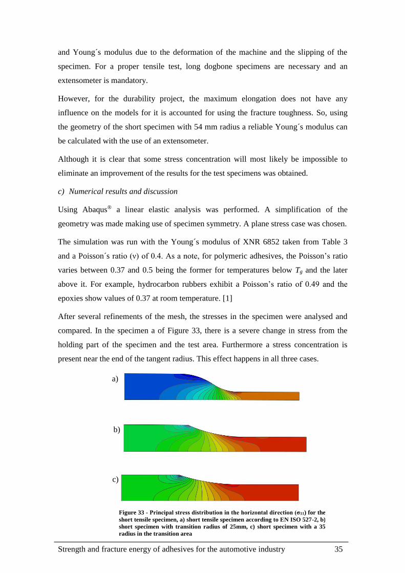
using SikaPower 4720. ................................................................................................................................................. 34 Figure 31 – Fragile fracture of the short specimen (54 radius) using SikaPower 4720. ............................................... 34 Figure 32 - Principal stress distribution in the horizontal direction (σ11) for the short tensile specimen, a) short tensile
specimen according to EN ISO 527-2, b) short specimen with transition radius of 25mm, c) short specimen with a 35
radius in the transition area .......................................................................................................................................... 35 Figure 33 - Geometry of the DCB specimen (dimensions in mm). .............................................................................. 37 Figure 34 – Modelled DCB specimen with the finite element mesh, a) cohesive zone (red), b) view of the all
specimen, c) boundary conditions. ............................................................................................................................... 38 Figure 35 - Traction separation law with linear softening available in Abaqus® ......................................................... 39 Figure 37 – Numerical P-δ of three different initial cracks. ......................................................................................... 40 Figure 38 – P-a curve for the three different initial crack lengths. ............................................................................... 40

List of figures ix
Figure 39 – Numerical R-curves of the three different initial cracks lengths, a) CCM method, b) CBT method, c)
CBBM method. ............................................................................................................................................................ 41 Figure 40 - Summary of the numerical fracture toughness as a function of initial crack length. ................................. 42 Figure 41 - Numerical P-δ of three different specimen length. .................................................................................... 43 Figure 42 – P-a curve for the three different specimen length. .................................................................................... 43 Figure 43 – Numerical R-curves of the three different specimen lengths, a) CCM method, b) CBT method, c) CBBM
method. ........................................................................................................................................................................ 44 Figure 44 - Summary of the fracture toughness as a function of specimen length. ...................................................... 45 Figure 45 – Numerical P-δ curve for three different widths. ........................................................................................ 46 Figure 46 – Numerical P-a curve with three different widths. ..................................................................................... 46 Figure 47 – Comparison of the numerical fracture toughness in the plateau region of the R-curve for three different
widths and three different methods: CCM, CBT and CBBM. ...................................................................................... 47 Figure 48 – Numerical P-δ curve of three different thicknesses. ................................................................................. 48 Figure 49 – Numerical P-a curve of three different substrates thicknesses. ................................................................. 48 Figure 50 – Numerical R-cures of the three different substrate thicknesses using: a) CCM method, b) CBT method, c)
CBBM method. ............................................................................................................................................................ 49 Figure 51 – Comparison of the numerical fracture toughness in the plateau region of the R-curve for three different
substrate thicknesses and three different methods: CCM, CBT and CBBM ................................................................ 50 Figure 52 – P-δ curve of two DCB specimens with different materials for adherends. ................................................ 51 Figure 53 - P-a curve for the two different materials. .................................................................................................. 51 Figure 54 – von Mises stresses during the DCB test simulation, a) to d) frames of the test from the beginning to the
end and e) an amplification of the critical part of the specimen. .................................................................................. 52 Figure 55 (continues) - Numerical R-curves of the two different materials, a) CCM method, b) CBT method, c)
CBBM method. ............................................................................................................................................................ 52 Figure 56 – Geometry of the small DCB specimen; final specimen (dimensions in mm) ............................................ 54 Figure 57 - Numerical P-δ of a normal and a small DCB specimen............................................................................. 54 Figure 58 – P-a curve for the normal and a small DCB specimen. .............................................................................. 54 Figure 59 – Numerical R-curves for the normal and small DCB specimen, a) CCM method, b) CBT method, c)
CBBM method. ............................................................................................................................................................ 55 Figure 60 - von Mises stresses during the final DCB test simulation. .......................................................................... 56 Figure 61 - Geometry of the DCB specimens tested, a) small specimen, b) normal specimen. ................................... 58 Figure 62 - Schematic representation of the mold used to cure the DCB specimens with the respective legend. ........ 58 Figure 63 – Example of the P-δ obtained, specimen 4. ................................................................................................ 59 Figure 64 – Example of an R-curve obtained, specimen 4. .......................................................................................... 59 Figure 65 - Comparison of three R-curves using the CBBM method for different velocities. ..................................... 60 Figure 66 – Comparison of the fracture toughness of SikaPower 4720 with different displacement rates................... 60 Figure 67 – Example of the failure mode of DCB specimens with SikaPower 4720 using three different displacement
rates, a) 0.2mm/min, b) 0.5mm/min and c) 2 mm/min. ................................................................................................ 61 Figure 68 – P-δ curve for the short and normal DCB specimens tested with SIKA® 4720. ......................................... 61 Figure 69 – R-curve of the small specimen and normal specimen using the CBBM method. ..................................... 62 Figure 70 - Two examples of the cohesive fracture surface of the specimens tested, a) small specimen and b) normal
specimen. ..................................................................................................................................................................... 63 Figure 71 – Geometry of the SLJ used for the impact tests (dimensions in mm). ........................................................ 65 Figure 72 - Schematic mold for SLJ specimens. .......................................................................................................... 66 Figure 73 - Comparison of SLJ with mild steel adherends under two different strain rates. ........................................ 67 Figure 74 – Failure mode of the SLJ tested .................................................................................................................. 67

Strength and fracture energy of adhesives for the automotive industry x
List of acronyms
CT Compact tension
DCB Double cantilever beam
DMA Dynamic mechanical analysis
ENF End notched flexure
EVA Ethylene-vinyl acetate
FEA Finite element analysis
FPZ Fracture process zone
PU Polyurethane
SENB Single-edge notched bending
SLJ Single lap joint
CCM Compliance calibration method
CBT Compliance beam theory
CBBM Compliance-Based beam method


Strength and fracture energy of adhesives for the automotive industry xi
List of symbols
δ Displacement
ε Strain
η Dumping constant
σ Normal stress
τ Shear stress
a Crack length
a0 Initial crack length
aeq Equivalent Crack length
b Substrate width
C Compliance
E Young´s modulus
Ef Corrected flexure modulus
G Shear modulus
GI Fracture toughness in mode I
GIC Critical fracture toughness in mode I
GII Fracture toughness in mode II
GIIC Critical fracture toughness in mode II
h Substrate thickness
k Rigidity
KI Stress intensity factor
KIC Critical stress intensity factor
l Overlap length
m Geometric factor
P Applied load
Tg Glass transition temperature
Y Correction coefficient
Δ Correction for the crack tip rotation
ν Poisson´s ratio

Strength and fracture energy of adhesives for the automotive industry 1
1. Introduction
1.1 Background and motivation
Adhesive bonding is increasingly being used in structural applications such as in rail
vehicle or automotive industry. However, design in terms of durability still needs a lot
of research. It is at the moment difficult to predict the failure load after exposure to load
under static or dynamic conditions, temperature and humidity over a long period of
time. With the rapid increase in numerical computing power there have been attempts to
formalize the different environmental contributions in order to provide a procedure to
predict assembly durability, based on an initial identification of diffusion coefficients
and mechanical parameters.
Adhesive joints can be designed with the help of analytical method or numerical tools.
For complex predictions that include various factors such as the effect of temperature
and humidity, only the numerical methods can be used.
1.2 Problem definition
Cohesive zone elements have been developed to simulate the static damage but also
damage due to fatigue and more recently due to the environment. However, the
adhesive behaviour also depends on temperature and strain rate. For a complete
modelling, the cohesive element should also include these effects.
1.3 Objectives
The objective of this thesis was to lay the foundations for a project to develop a
cohesive element that includes the effect of temperature, humidity, time (viscoelastic
behaviour of the adhesive) and fatigue. In order to accomplish it a complete mechanical
characterization of the adhesives used has to be done and optimization of the resources
studied.
1.4 Research methodology
In order to achieve the aim of this thesis, the following work was done:
Introduction 2
• An overview of some advantages and good practices was done. This was followed by
a study of the most used adhesives and their common characteristics in order to grasp
the huge variety of structural adhesives available.
• Failure strength tests were carried out using bulk specimens to determine the tensile
adhesive properties. Also, small dogbone specimens were produced to validate the
geometry to be used in the durability project.
• Numerical simulations using cohesive zone models, in which the failure behaviour is
expressed by a bilinear traction separation law, were developed using Abaqus®. This
was done to find an optimum small specimen that would enable a quicker aging
process.
• DCB tests were done to characterize the fracture toughness of a toughened epoxy
adhesive and validate the results of the numerical simulation.
• Impact test is an important feature when designing an adhesive joint for the
automotive industry. From previous studies it was concluded that adhesive joints
behaviour is changes at high strain rates so to investigate it a drop weight impact test
was conducted.
1.5 Outline of thesis
The second chapter of this thesis consists of a literature review on adhesives. Some
general properties were compiled as well as an overview of the most used adhesives.
The third chapter is a summary of the Failure strength tests conducted using two
structural epoxy adhesives, XNR 6852 , supplied by NAGASE CHEMTEX® (Osaka,
Japan), and SikaPower 4720, supplied by SIKA® (Portugal, Vila Nova de Gaia). Tensile
bulk tests were performed using long dogbone to characterize the adhesive and compare
with other available solution. In addition a study of size dependence of the bulk
specimen was also carried out.
The forth chapter begins with a numerical study of the double cantilever beam (DCB)
test. This was done to develop an optimized smaller DCB specimen that would allow a
reliable characterization of adhesive fracture toughness. This was done using Abaqus®´s
cohesive zone models. Afterwards fracture strength tests, DCB tests, were used to
characterize an adhesive bond solicited in mode I and validate the numerical findings. In

Strength and fracture energy of adhesives for the automotive industry 3
this case toughened epoxy SikaPower 4720 was used and its fracture toughness studied
as a function of geometry.
Lastly, in the fifth chapter an impact test was conducted to characterize the mechanical
behaviour of the high elongation and high ductility adhesive XNR6852, with low yield
strength steel adherends.

Strength and fracture energy of adhesives for the automotive industry 5
2. Literature review
An adhesive is defined as a substance that binds two surfaces together and resists
separation. Usually there are many terms to refer to it, some common ones are: glue,
cement, mucilage, mastic or paste.
In order to understand adhesives and adhesion there can be two different approaches. A
practical approach, concerned with the mechanical properties resulting from the
adhesion, and a theoretical approach, evaluating the reasons behind the molecular
bonding of the surfaces. As a result, to accurately understand and predict the adhesives
joint properties different areas are investigated such as: physics, chemistry and
mechanics. This thesis focuses on the mechanical properties.
The use of adhesive bonded joints has increased in recent years. The reason is the many
advantages that a well-constructed adhesive joint bring to the structural integrity when
compared to the traditional mechanical fasteners. Some of the advantages are:
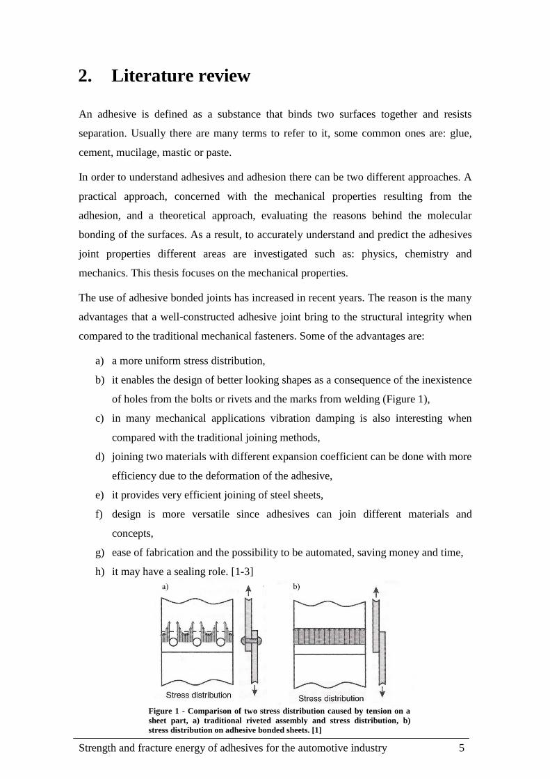
a) a more uniform stress distribution,
b) it enables the design of better looking shapes as a consequence of the inexistence
of holes from the bolts or rivets and the marks from welding (Figure 1),
c) in many mechanical applications vibration damping is also interesting when
compared with the traditional joining methods,
d) joining two materials with different expansion coefficient can be done with more
efficiency due to the deformation of the adhesive,
e) it provides very efficient joining of steel sheets,
f) design is more versatile since adhesives can join different materials and
concepts,
g) ease of fabrication and the possibility to be automated, saving money and time,
h) it may have a sealing role. [1-3]
Figure 1 - Comparison of two stress distribution caused by tension on a
sheet part, a) traditional riveted assembly and stress distribution, b)
stress distribution on adhesive bonded sheets. [1]

Literature review 6
On the other hand, some disadvantages are:
a) the service temperature is limited,
b) requires in most cases a surface preparation,
c) due to a huge variety of adhesives available selecting a suitable one requires
some experience,
d) adhesive bonding is weak when loaded in tension. The two main cases to be
avoided are cleavage and peel stresses,
e) avoiding localized stresses on the adhesive is not always possible and can cause
rupture of the adhesive,
f) in consequence of its polymeric nature heat and humidity are very harmful,
g) the joint cannot be built instantly and usually needs a holding mechanism,
h) needs curing at high temperatures in most cases,
i) although there has been improvements in the quality control of adhesive joints it
is still a very hard task to accomplish.[1-3]
The adhesives industry is very diverse with multiple applications in areas such as:
aeronautical, aerospace, automotive, shoe, furniture and others. With many applications
and a market share already well-established the future for adhesives looks promising.
According to a study from Ceresana®, 2012, on adhesive markets, it is concluded that it
is expanding with growth rates of about 2.9% for the next 8 years. This evolution is
predicted as a result of the rapid increase in the demand of consumer goods in the Asia-
Pacific region.
2.1 Adhesive properties
Adhesives are polymeric by nature and are formed by large molecules, polymers, with
small groups of atoms, monomers. The diversity of viable combinations for monomers
is great and, as a consequence, the number of polymeric compounds that result are vast.
On top of it, there are also mixed adhesives, resulting from a combination of several
polymeric compounds. As a consequence the classification of adhesive is accomplished
in different ways. Among the most common are:
a) Polymer base; natural or synthetic.
b) Chemical composition; thermoplastic, thermoset or rubber.
c) Physical forms; one or multiple components, films, tape, powder.

Strength and fracture energy of adhesives for the automotive industry 7
d) Chemical families; epoxy, polyamides and others.
e) Function; structural or non-structural. [1, 4]
2.1.1 General properties
In this thesis there is a particular interest in structural adhesives and their mechanical
properties. A structural adhesive is an adhesive that transfer loads between adherends
and usually have a shear strength higher than 5 MPa. Typically, structural adhesives are
cross-linked/thermosetting polymers even though some thermoplastics are used. [7]
The strength of properly made adhesive joints is directly related to the strength of the
adhesive. It has also been proved that failure is unlikely to occur at the interface and
only in cases of poor surface preparation it is likely to take place. [5] Furthermore, since
in most cases the adherends (ex. metals and carbon fibber) have a higher rigidity than
the adhesive, the displacement will be mainly due to strain in the adhesive. Some
common strength properties are presented in Table 1.
The choice of the adhesive for a particular application is not unique. Usually there are a
variety of adhesives suitable and surface pre-treatments that can be applied to improve
the joint performance. Also, the surface type can condition the adhesive selection for the
task. For example, in the case of thermoplastic substrates, some adhesives may have a
detrimental effect producing effects such as crazing, swelling, dissolutions or may be
simply incompatible. On the other hand, some adhesives such as epoxies are versatile
and will bond to different substrates.[6]
Table 1 – Comparative values of stiffness and strength of common structural materials.*
*Information compiled from several text books and databases, illustrative only.
Literature review 8
When selecting adhesives, some key factors to consider in the fabrication process are:
joint performance (load, operating environment, durability), substrates type, adhesive
form, costs, aesthetics, manufacturing process, application, health requirements and pre-
treatments. Finally testing and validation is recommended to ensure the process
quality.[1]
Since the diversity of adhesives available is extensive, an accurate choice is hard and
will require experience. An overview of the most used structural adhesives is presented
in Table 2 with a compilation of several general properties.
2.1.2 Temperature related properties
a) Glass transition temperature
The glass transition temperature, Tg, is the most important temperature in polymers and
is a property of the amorphous part. It marks a transition from a glass-like structure to a
rubber-like state. It is not a phase transition but a change in the derivative of the
fundamental quantities with respect to temperature.
Although in some polymer (linear and very regular) the transition is masked, this is not
the case for amorphous polymers where above Tg the long coiled molecular chains can
rearrange and extend. This behaviour is mostly unwanted in rigid structures because the
viscoelastic nature of the polymer will result in fast stress relaxation, low modulus and
strength. In conclusion, the structural adhesives are expected to work below their Tg.[1,
5]
b) Decomposition temperature
Using adhesives above this temperature will completely destroy the joint and only for a
short time there will be relevant mechanical properties. This is important for military
projectiles for it relies on the char strength for a short period of time.[5]
c) Melting temperature
Opposed to the glass transition the melting temperature is not very important for
adhesives because crystalline melting does not take place in amorphous polymers.
Although of little importance, some adhesives do exhibit cristallinity such as: ethylene-
vinyl acetate (EVA) and polyamides hot melts; polyvinylalcohol, polychloroprene and
starch. [1]

Strength and fracture energy of adhesives for the automotive industry 9
Table 2 – General properties of the most common structural adhesives. **
**Information compiled from several text books and databases, illustrative only.

Literature review 10
d) Thermal expansion
The thermal expansion coefficient of the adhesive is much higher than that of typical
metallic substrates, which can lead to damaging interfacial stresses. The expansion can
be reduced by the addition of mineral fillers.[1]
2.1.3 Viscoelasticity
In the elastic domain of metals an imposed stress will generate an extension
proportional to it. However, in polymers the tensile behaviour is strongly influenced by
time and the instantaneous response will be a small fraction of the total deformation.
Figure 2 shows two different models to describe viscoelasticity. The Maxwell model
(Figure 2 - a) is described by:
𝑑휀
𝑑𝑡=
1
𝜂𝑆 +
1
𝑘
𝑑𝜎
𝑑𝑡 (1)
In Equation 1, σ represents stress, ε the strain, η and k are constants relating to the
dashpot viscosity and the rigidity of the spring respectively. According to Equation 1 if
the deformation is constant (dε/dt = 0) the stress will decay to zero, commonly known
as stress relaxation.
The Voigt model (Figure 2 - b) is described by:
𝜎 = 𝜂𝑑휀
𝑑𝑡+ 𝑘휀 (2)
In this model the deformation and its recovery is subjected to a time dependency, and
this constant is commonly known as retardation time.
Figure 2 - Schematic models of viscoelastic
behaviour, a) Maxwell model, b) Voigt model.

Strength and fracture energy of adhesives for the automotive industry 11
If the stress is applied during a period of time much smaller than the relaxation and
retardation times the behaviour is determined by the spring. Typically, for polymers
below the glass transition temperature, the relaxation time is infinitely long making the
response elastic but time dependent. If the temperature is raised, the viscous component
becomes increasingly important, especially above the Tg.[1, 5-7]
2.2 Analysis of adhesive joints
For complex geometries, a finite element analysis (FEA) is preferable however, for a
fast and easy answer a closed-form analysis is usually used.[1, 3, 8]
2.2.1 Analytical approach
In the literature, most attention is given to single lap joint (SLJ) specimens for it is an
efficient geometry to characterize an adhesive joint. For this geometry, generally, failure
takes place in the adhesive and the stress distribution in that region was subjected to
extensive study from many researchers.
For the analysis, some simplifying assumptions are made: substrates deformation due to
tension and bending only and adhesive stresses restricted to peel and shear are assumed
to be constant across the adhesive layer. However, the stresses in the adhesive are not
uniform because of differential straining and the eccentricity of the loading path.[2, 8, 9]
a) Linear elastic analysis
A common and simple analysis is to consider undeformable substrates with a constant
shear stress state in the adhesive layer (Figure 3). The adhesive shear stress is given by
Equation 3 where P is the remote load applied, b is specimen width and l is overlap
length. [8, 9]
Figure 3 – Deformations in loaded single-lap joints with rigid adherends. [8]

Literature review 12
𝜏 =𝑃
𝑏 ∙ 𝑙 (3)
b) Volkersen´s analysis
The Volkersen’s analysis introduces a differential shear stress in the adhesive as a
consequence of substrate deformation (Figure 4). It considers that the SLJ has no
bending moment and therefore substrates are in pure tension. The adhesive is in pure
shear.[8, 9]
Substrates deformation is maximum near the adhesive overlap (point A) and minimum
in the opposite end (point B). The reduction of strain along the overlap causes a non-
uniform shear stress distribution in the adhesive (Figure 5).
The Volkersen´s model does not take into account the effects of the adherend bending
and shear deformation, both important aspects for a correct analysis of adhesive joint
Figure 4 – Deformation in loaded single-lap joints with elastic adherends. [8]
Figure 5 – Typical stress distribution using
Volkersen’s model for SLJ.
Figure 6 - Typical shear stress and peel
stress distribution using Goland and
Reissner´s model for SLJ.

Strength and fracture energy of adhesives for the automotive industry 13
stress distribution. This is particularly important in adherends with low shear and
transverse modulus.[3, 8, 9]
c) Goland and Reissner analysis
In this analysis a more sophisticated approach is done introducing the aspect of
adherend bending and with it peel stresses in the adhesive layer. Figure 6 is an example
of the adhesive shear and peel stress in a SLJ. [10]
In summary, the classical analysis of Volkersen and Goland and Reissner were a big
step forward in adhesive modelling and failure prediction. Nevertheless there are some
limitations to these models. Firstly, variation of stresses along bondline thickness is not
taken into account. Secondly, the peak shear stresses at the overlap ends are inaccurate
as a correct representation should take into account the zero shear stress at the end of the
overlap. Also, the complex stress field of the substrates is neglected to most extend.
In order to improve these models, more work has been done and more complex models
have been put forward increasing the accuracy of the stress distributions.[8, 9]
2.2.2 Numerical approach
a) Continuum mechanics approach
In continuum mechanics, one of the approaches is the strength of materials which
accounts for the maximum stress and strain. It is among the most used. However it is
sometimes inappropriate due to singularities inherent to the bonded joint and in such
cases the refinement of the mesh will increase greatly the values obtained from the
simulation for the strain and stress. Some common singularities are presented in Figure
7.[3]
b) Fracture mechanics approach
In the continuum mechanics approach, materials are considered to have no defects, in
contrast with fracture mechanics analysis where a defect has to exist. The fracture
mechanics approach studies the defects to predict if they will cause a catastrophic
Figure 7 - Examples of singularities in single lap joints and its contribution to the strain and stress results. [3]

Literature review 14
failure of the structure or if they can withstand the stresses throughout the service life of
the component. In this analysis there are two types of criteria, stress intensity factor and
energetic concepts. [11]
It´s a relatively recent field of study and current research is being done to introduce time
dependent effects such as viscoelasticity. These effects are important when traditional
fracture mechanics are insufficient to accurately predict failure. In this case new
computer aided technologies are emerging. [11]
In the traditional approach to the design of structures there are two variables, applied
stress and strength of the material but with the introduction of the failure criteria of
fracture mechanics this has changed. Following the fracture mechanics approach one
takes into account the stress, the flaw size and the fracture toughness of the material.
The combinations of these three factors can be done with the energy criterion or the
stress-intensity one.[5, 11]
There are three modes of loading that produce a singularity at the crack tip (Figure 8).
Energy criterion
The energy approach states that fracture will occur when the energy available for the
crack growth is sufficient to overcome the resistance of the material. The material
resistance can take into account the surface energy, plastic work, or other energy
dissipation associated with the propagation of the crack.[11]
The present version of the approach was developed by Irwin which is defined as the rate
of change in potential energy with the crack area for a linear elastic material. At the
moment of fracture GI = GIC (critical energy release rate which is a measure of fracture
Figure 8 – The three modes of loading that can be applied to a crack.

Strength and fracture energy of adhesives for the automotive industry 15
toughness). As an example of the method, for a crack of length 2a in an infinite plate
subject to a remote tensile stress, the energy release rate is given by:
GI =πσ2a
E (4)
Where E is Young’s modulus, σ is the remotely applied stress, and a is the half-crack
length.[11]
Since a well-designed adhesive joint will fail cohesively, it is reasonable to assume that
the fracture toughness is, to some extent, dependent on the adhesive bulk toughness.
The fracture toughness is an important aspect of design and has a great variation as a
consequence of temperature, geometry and material. Most adhesives are polymers with
intermediate fracture toughness and, in most cases, are one order of magnitude lower
than the metal and alloys (Figure 9).
Stress intensity approach
According to this criterion one assumes the material will fail locally at a critical
combination of stress and strain commonly known as the critical intensity factor, KIC.
For a situation similar to the energy approach presented above, infinite long plate
subject to a remote tensile stress:
Figure 9 - A comparative representation of the fracture toughness of different materials as a function of
density (CesEdupack® (Cambridge, UK)).
Literature review 16
KI = 𝑌𝜎√𝜋𝑎 (5)
Where Y is a correction coefficient to account for structure geometry. In this case KI is a
measure of the local stress and KIC is a measure of the material resistance. The critical
stress intensity factor, KIC, is assumed a size-independent material property and can be
related to GIC. In the case of plane stress it is calculated through the expression
bellow.[11]
GI =K𝐼
2
E (6)
For plane strain:
GI =K𝐼
2(1 − ν2)
E (7)
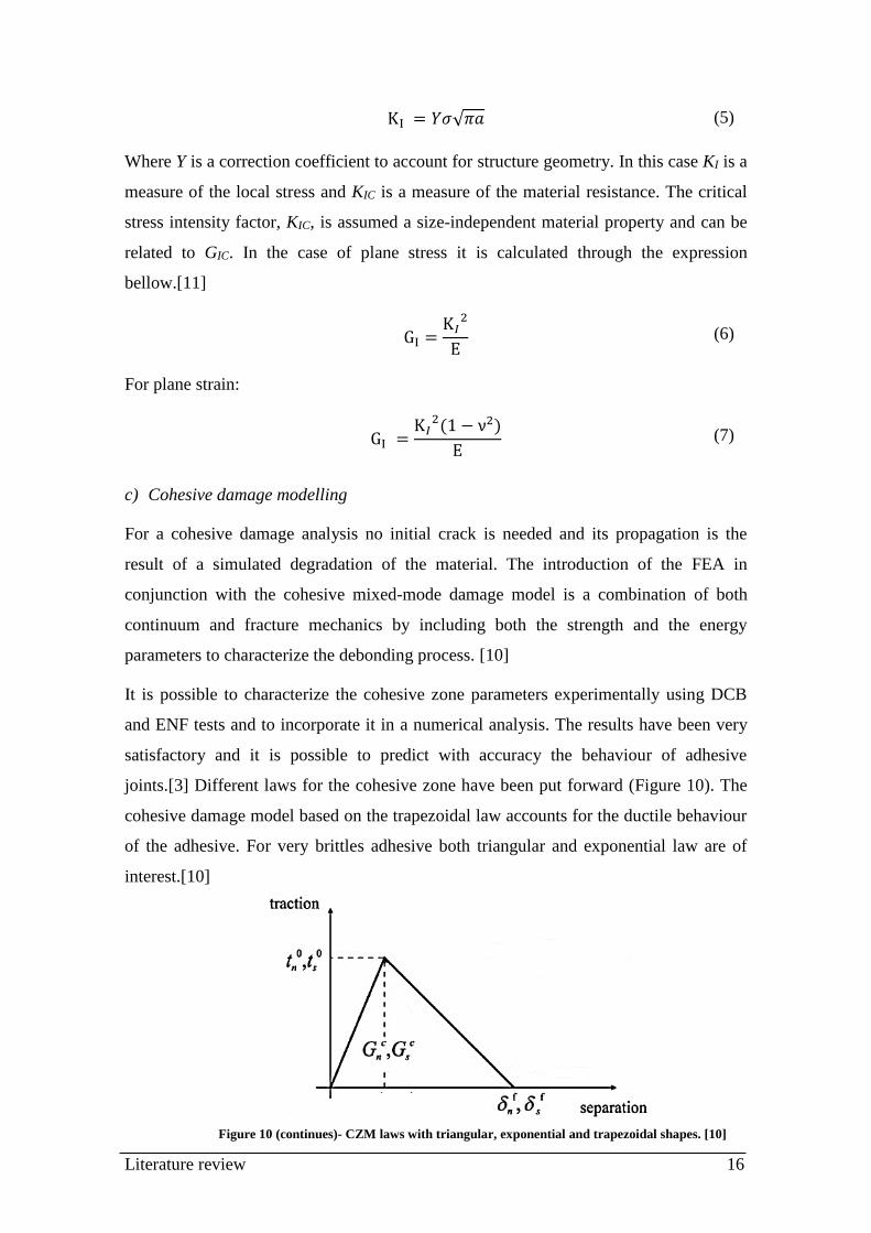
c) Cohesive damage modelling
For a cohesive damage analysis no initial crack is needed and its propagation is the
result of a simulated degradation of the material. The introduction of the FEA in
conjunction with the cohesive mixed-mode damage model is a combination of both
continuum and fracture mechanics by including both the strength and the energy
parameters to characterize the debonding process. [10]
It is possible to characterize the cohesive zone parameters experimentally using DCB
and ENF tests and to incorporate it in a numerical analysis. The results have been very
satisfactory and it is possible to predict with accuracy the behaviour of adhesive
joints.[3] Different laws for the cohesive zone have been put forward (Figure 10). The
cohesive damage model based on the trapezoidal law accounts for the ductile behaviour
of the adhesive. For very brittles adhesive both triangular and exponential law are of
interest.[10]
Figure 10 (continues)- CZM laws with triangular, exponential and trapezoidal shapes. [10]

Strength and fracture energy of adhesives for the automotive industry 17
2.3 Test methods
2.3.1 Tensile tests
a) Bulk specimens
A common test to determine the strength of the adhesive is the tensile test similar to
those for plastic materials. The properties are intrinsic to the material and are obtained
under a uniform and uniaxial state of stress. Using this method one can obtain the
Young´s modulus, the yield and tensile strength, and elongation at break.
It is usual to obtain the specimens through pouring or injection. The first is suited to
one-part adhesives that are liquid. The second gives better results when the adhesive is
viscous.[1]
b) Axially loaded butt joints
The tensile properties can also be measured using a thin layer of adhesive between two
steel substrates. Many standards exist for this test and round (Figure 11) and square
Figure 10 (continued)

Literature review 18
geometry can be employed. Alignment and adhesive thickness can be controlled using
the mold present in ASTM D 2095. [1]
The tensile strength of the adhesive is calculated dividing the load to failure by the
initial cross sectional area of the specimen. Also, the adhesive displacement can be
measured with an extensometer but a correction has to be made. The influence of the
substrates has to be taken into account in order to accurately calculate the adhesive
displacement. [1, 12]
The stress strain curve is not representative of the intrinsic adhesive behaviour and
cannot be correlated with the bulk tensile test. Also, despite the use of precise apparatus
and specially designed extensometer, the reproducibility of this test is low. [1, 12]
2.3.2 Fracture strength tests (Mode I)
a) Fracture tests on bulk specimens test
There are several international standards for the determination of the experimental
fracture toughness of the bulk specimen, e.g.: ASTM D5045-99 (2007) and ISO
13586:2000. The dimensions for the bulk specimens presented in Figure 12 are chosen
to ensure a case of plane strain. For most epoxies the dimensions chosen for SENB are:
6.4 mm thick, 12.7 mm wide, and 75 mm long specimen and it is important to introduce
a sharp crack in the specimens in order to have an accurate result of the fracture
toughness. This effect is usually accomplished tapping on a sharp razor blade,
previously immersed in liquid nitrogen, or by fatigue cracking. [1]
Figure 11 – Butt joint geometry with the load
direction (dimensions in mm) (ASTM D 2095)

Strength and fracture energy of adhesives for the automotive industry 19
To test SENB specimens a three-point bending fixture is used. Once positioned, the
machine records the load and displacement using a constant speed (10 mm/min). Very
strict restrictions for the validation of the test exist specially on linearity of the load –
displacement diagram.
Using these methods if the amount of plastic deformation is significant an elastic-plastic
fracture approach is more appropriate, e.g.: J-integral.[1, 12]
b) Double cantilever beam (DCB) test
The specimen geometry is presented in Figure 13 and the loading is done vertically
introducing a mode I fracture in the adhesive layer of the DCB specimen.
Two different standards exist, ASTM D3433 and ISO 25217. The first determines the
fracture toughness through several loadings of the specimen. This is done in order to
induce crack propagation and measure the peak load required, also the load for crack
arrest is recorded and the final crack length measured. Both load values are used to
measure the fracture toughness.
In standard ISO 25217 the specimen is loaded with a constant cross head displacement
up to crack propagation starts. Usually the crack increases slightly, 2-5 mm, and at this
point the machine is reset. This pre-crack is not part of the test but a prerequisite.
Subsequently the specimen is reloaded again and the resistance to crack initiation and
steady-state propagation are calculated.
Figure 12 –Fracture bulk specimens, a) compact tension (CT),
b) single-edge notched bending (SENB) [1]

Literature review 20
Several methods exist to measure the fracture toughness of the DCB test specimens.
Compliance Calibration Method (CCM)
This technique is based on Irwin proposed energy approach defined as energy release
rate. The Equation 8 derives from Irwin-Kies theory where GIC, represents the energy
available for an increment of crack extension. [11]
𝐺𝐼𝐶 =𝑃2
2𝑏
𝑑𝐶
𝑑𝑎 (8)
In the above equation P is the load, b represents the width of the specimen on the
transversal direction, C is the compliance and a is the crack length.
The partial derivative of the compliance as a function of crack length is obtained from
experimental observation of the crack length and the Equation 9.
C =δ
P (9)
The values are fitted into a cubic polynomial approximation being the compliance, C, a
function of crack length, a.
Finally, the cubic polynomial fitting of compliance as a function of crack length is
derived and used in the initial equation of Irwin- Kies, Equation 8.
Corrected Beam Theory (CBT)
As a complement, another model was employed. This second model, corrected beam
theory (CBT), is an improvement of the CCM and also derives from Irwin-Kies
equation. Often, the loading line displacement deviates from the one assumed in the
CCM because of the deformation around the crack tip. In this case, the fracture
toughness is calculated through:
Figure 13 – Mode I double cantilever beam (DCB) adhesive-
joint specimen.

Strength and fracture energy of adhesives for the automotive industry 21
𝐺𝐼𝐶 =3𝑃𝛿
2𝑏(𝑎 + |Δ|) (10)
where Δ is a correction for crack tip rotation and deflection, proposed by Wang and
Williams [22], and is calculated using the Equation 11.
Δ = ℎ√1
13𝑘(
𝐸𝑥
𝐺𝑥𝑦) (3 − 2 (
𝛤
1 + 𝛤)
2
) (11)
where 𝐸𝑥 and 𝐺𝑥𝑦 is the longitudinal normal and shear modulus of the substrate, ℎ is the
substrate’s thickness and k is the shear stress distribution constant for correcting the
deflection caused by shear force (derived as 0.85 for the DCB specimen).
𝛤 =√𝐸𝑥𝐸𝑦
𝑘𝐺𝑥𝑦 (12)
Finally, 𝐸𝑦 is the Young´s modulus of the substrates on thickness the direction.[23]
Compliance-Based Beam Method (CBBM)
Although in other methods crack length measurement is necessary, here, by using the
crack equivalent concept (Figure 14) this measurement is irrelevant depending only on
the specimen’s compliance during the test. [24]
The equation to calculate 𝐺𝐼𝐶 is [15, 25]:
𝐺𝐼𝐶 =6𝑃2
𝑏2ℎ(
2𝑎𝑒𝑞2
ℎ2𝐸𝑓+
1
5𝐺𝑥𝑦) (13)
where aeq is an equivalent crack length obtained from the experimental compliance and
accounting for the fracture process zone (FPZ) at the crack tip, Ef is a corrected flexural
modulus to account for all phenomena affecting the P-δ curve, such as stress
concentrations at the crack tip and stiffness variability between specimens, and G is the
shear modulus of the adherends. [26]
Figure 14 - Schematic representation of the FPZ and crack
equivalent concept.

Literature review 22
𝐸𝑓 can be obtained using:
𝐸𝑓 = (𝐶0 −12(𝑎0 + |Δ|)
5𝑏ℎ𝐺𝑥𝑦 )
−18(𝑎0 + |Δ|)3
𝑏ℎ3 (14)
The crack equivalent concept is:
𝑎𝑒𝑞 =1
6𝛼𝐴 −
2𝛽
𝐴 (15)
where the coefficients are:
𝛼 =8
𝑏ℎ3𝐸𝑓 ; β =
12
5𝑏ℎ𝐺𝑥𝑦 ; 𝛾 = −𝐶 (16)
𝐴 = ((1 − 108𝛾 + 12√3(4𝛽3 + 27𝛾2𝛼)
𝛼 ) 𝛼2)
1/3
(17)
Effect of adhesive layer
If the bondline thickness is too low for full development of a plastic zone the fracture
toughness will change. As a recommendation, the thickness should be between 0.1 mm
and 1 mm. This is also applicable in the case of TDCB. [1, 12]
c) Tapered double cantilever beam (TDCB) test
This method was developed to enable long term measurements of adhesive damage
propagation without the need to measure the crack length. The height of the beam
changes along the adhesive layer to ensure a constant change of compliance as a
function of crack length (Figure 15).[1]
The manufacturing of these specimens is more expensive and complex, requiring a
CNC machine to account for the non-linear height profile.
Figure 15 – Mode I tapered double cantilever beam (TDCB) test
specimen.

Strength and fracture energy of adhesives for the automotive industry 23
Values of 𝐺𝐼𝐶 can be determined using a simple beam theory, Equation 18.
𝐺𝐼𝐶 =4𝑃2𝑚
𝐸𝑠𝑏2 (18)
Where P is the load, 𝐸𝑠 the substrate elastic modulus, 𝑏 the substrate width, and 𝑚 the
geometry factor defined previously.
Or using a more complex but accurate method, corrected beam theory. This method
formulation is presented below.
𝐺𝐼𝐶 =4𝑃2𝑚
𝐸𝑠𝑏2∙ (1 + 0.43 (
3
𝑚𝑎)
13
) (19)
2.3.3 Impact tests
The impact is an important feature when designing an adhesive joint for the automotive
industry due to the passenger safety regulations and manufacturer quality standards. As
a result the behaviour of adhesive joints in high strain rates is a major consideration in
order to know how the strength of the joint reduces varies.
a) Instrumented pendulum impact test
An instrumented pendulum was developed by Harris and Adams to impact a single lap
joint or a solid adhesive specimen. The fixture is presented in Figure 16 showing the
specimen clapped to the machine’s piezoelectric force transducer that in turn is
connected to the frame. The other end is free although there is a journal bearing block to
guide the specimen during the test. [12]
The strength of the joint is calculated with the load cell and the energy is measured from
the pendulum swing after impact. The movement of the end clamp can be instrumented
to record the acceleration and thus monitor the position recording the specimen’s
behaviour.
The energy absorbed by the adhesive rupture is small compared to the energy required
to deform the metallic substrates. On the other hand, a low ductility adhesive can have
high lap shear strength when using high yield strength substrates and fail with low load
loads with ductile substrates.

Literature review 24
b) Block impact test
This test applies a condition of impact loading, mainly shear, on the test rig similar to
that of the Izod resilience measurement (Figure 17). The specimen is fabricated using
two blocks, a larger block that will be attached to the base and a smaller block on top of
the adhesive layer. This smaller block will be struck during the test by a pendulum in a
direction parallel to the bonded surface.
In the case of misalignment, the distribution of the shear and peel stresses is strongly
influenced. Also, the elastic energy of the steel block may not be negligible in some
cases. For these reasons this method is not suitable for the measurement of the energy
absorption of the adhesive and can only be used for comparative studies.
Figure 17 - ASTM block impact test (ASTM D950-78) [12]
Figure 16 - Instrumented impact pendulum test. [12]
Strength and fracture energy of adhesives for the automotive industry 25
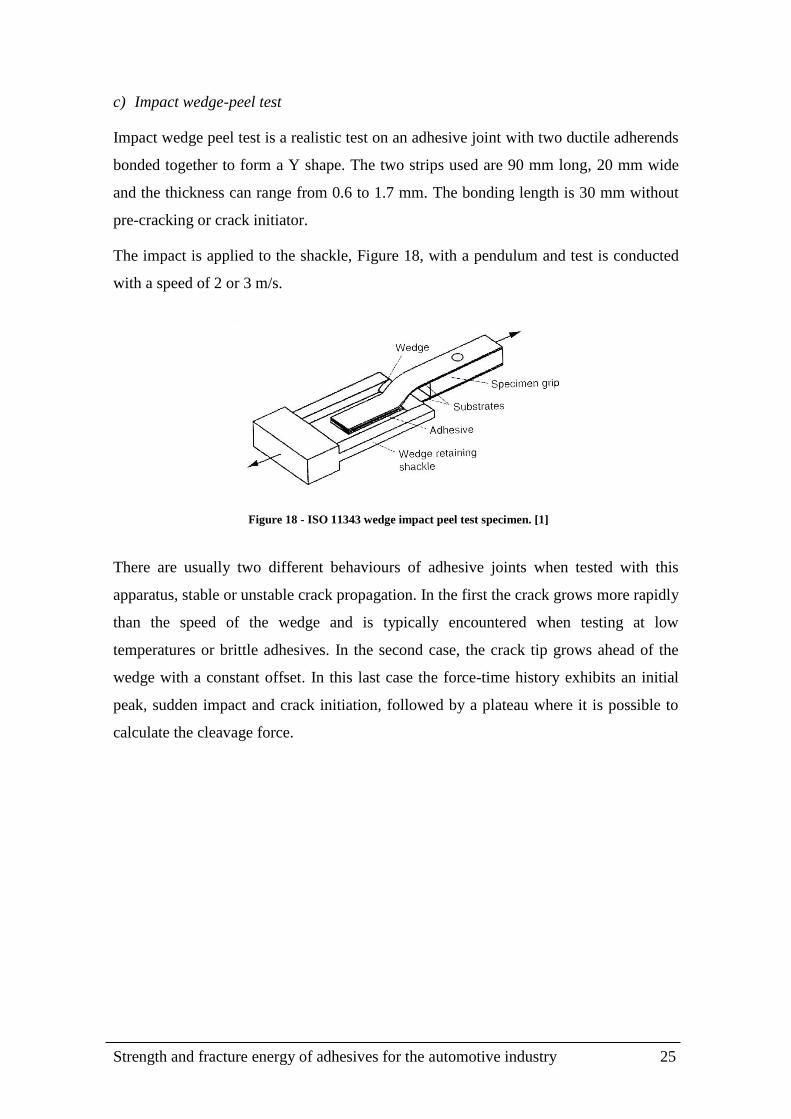
c) Impact wedge-peel test
Impact wedge peel test is a realistic test on an adhesive joint with two ductile adherends
bonded together to form a Y shape. The two strips used are 90 mm long, 20 mm wide
and the thickness can range from 0.6 to 1.7 mm. The bonding length is 30 mm without
pre-cracking or crack initiator.
The impact is applied to the shackle, Figure 18, with a pendulum and test is conducted
with a speed of 2 or 3 m/s.
There are usually two different behaviours of adhesive joints when tested with this
apparatus, stable or unstable crack propagation. In the first the crack grows more rapidly
than the speed of the wedge and is typically encountered when testing at low
temperatures or brittle adhesives. In the second case, the crack tip grows ahead of the
wedge with a constant offset. In this last case the force-time history exhibits an initial
peak, sudden impact and crack initiation, followed by a plateau where it is possible to
calculate the cleavage force.
Figure 18 - ISO 11343 wedge impact peel test specimen. [1]


Strength and fracture energy of adhesives for the automotive industry 27
3. Failure strength tests
3.1 Bulk tensile test
3.1.1 Adhesives
The epoxy adhesive XNR6852 was used, supplied by NAGASE CHEMTEX® (Osaka,
Japan). This adhesive is a one-part system that cures at 150 ºC for 3 h. This adhesive
has a linear structure, which allows greater freedom of movement to the chains, unlike
the network structure of a conventional epoxy adhesive. Along with the development of
this adhesive, NAGASE CHEMTEX® has produced others with the same technique.
The epoxy resin of XNR6852, when pure, is a conventional thermosetting resin due to
generating cross-linking during polymerization. A technological advance in the epoxy
adhesive has been done and a no cross-linking polymer has been produced through the
introduction of phenols. Thus, the reaction process is changed and in this new process
the epoxy resin and phenol are polymerized linearly by a consecutive reaction getting a
no cross-linking polymer. As a consequence, this polymer has some features of
thermoplastic polymers due to the resulting linear structure [18].
Also, the epoxy adhesive SikaPower 4720 was used, supplied by SIKA® (Portugal, Vila
Nova de Gaia). This adhesive is a two-part system that cures at room temperature for 24
hours.
3.1.2 Tensile strength test
a) Experimental procedure
Specimen manufacture
The bulk tensile specimens were produced by curing the adhesive between steel plates
of a mold (Figure 19) with a silicone rubber frame according to the French standard NF
T 76-142. A silicone rubber frame was used to avoid the adhesive from flowing out.
The dimensions of the adhesive plate after cure were defined from the internal
dimensions of the silicone rubber frame. Then, dogbone specimens were machined from
the bulk sheet plates (Figure 20).

Failure strength tests 28
Test procedure
The bulk tensile test was performed in an INSTRON® model 3367 universal test
machine (Norwood, Massachusetts, USA) with a capacity of 30 kN, at room
temperature and constant displacement rate of 1 mm/min. An extensometer to record the
displacement was also used. Loads and displacements were recorded up to failure. Four
specimens of each were tested.
b) Experimental results and discussion
Figure 21 and Figure 22 present a comparison of a tensile curve between toughened
epoxy; AV 119 from Hunstman® [19], a polyurethane (PU); Pliogrip 7400/7410 from
Ashland Specialty Chemicals® [20], and the studied adhesives; XNR 6852 and
SikaPower 4720. The values of tensile strength determined in this test for XNR 6852
correspond to the values expected for a conventional epoxy adhesive (Table 3). In
Figure 19 - Exploded view of the mold to produce plate specimens under hydrostatic
pressure.
Figure 20 - Dimensions of the bulk tensile specimen used in accordance
with standard BS 2782 (dimensions in mm).

Strength and fracture energy of adhesives for the automotive industry 29
contrast the two part epoxy, SikaPower 4720, has a low tensile strength more typical of
polyurethane or a natural rubber. On top of it, the maximum strain is small and is far
from the 100% strain of XNR 6852. In conclusion, XNR 6852, has a maximum strain
much higher than a conventional toughened epoxy adhesive and a higher strength than a
polyurethane adhesive.
The stress-strain curves of polymeric materials are not linear in tension and have usually
low rigidity in the elastic domain. Despite the evident non-linear behaviour, the
Figure 21 - Stress-strain curve with, Pliogrip 7400/7410 (PU), AV 119 (toughened
epoxy), XNR6852 and SikaPower 4720
Figure 22 - True Stress-True strain curve with, Pliogrip 7400/7410 (PU), AV 119
(toughened epoxy), XNR6852 and SikaPower 4720.

Failure strength tests 30
Young´s modulus is used to describe most adhesive as it is simple to determine. It is
worth mentioning that the shear modulus is relatively linear.[5]
The Young’s modulus obtained for XNR 6852 is approximately half of a typical
toughened epoxy (Table 3) and it is a consequence of the addition of the phenols. This
property can have some advantages to the vibration damping [21] because of its smaller
rigidity. On the other hand, SikaPower 4720 has a normal Young’s modulus for a
toughened epoxy.
Table 3 - Results of bulk tensile tests
Before fracturing, adhesive XNR 6852 deforms in a ductile manner (Figure 23, a)
suffering a reduction of area and acquiring an opaque colour, behaviour typical of
thermoplastic polymers. This behaviour is an improvement in the properties of epoxy
adhesives demonstrating an increased ductility of the material. As for the SikaPower
4720, it has a very fragile behaviour with little deformation (Figure 23, b).
3.1.3 Optimization of the bulk tensile test specimen
a) Experimental procedure
Specimen manufacture
In order to increase productivity of specimens for the durability project that follows a
reduction of specimen size is required. The reason is the many hours that take to cure
the adhesive and the low number of long dogbone specimens produced with a single
a)
b)
Figure 23 – Bulk tensile specimens after test, a) XNR 6852 and b) SikaPower 4720

Strength and fracture energy of adhesives for the automotive industry 31
bulk plate. To produce the short specimens the same manufacturing process as for the
long dogbone was employed.
A first attempt was made with standard EN ISO 572-2, short specimen, represented in
Figure 24. This geometry is suited for ductile adhesive such as polyurethanes.
The geometry in Figure 25 is not in accordance with any standard and was developed
with the purpose of eliminating, as far as possible, the concentration of stress. In order
to do so, a less abrupt transition was used with higher (double) radius.
A further improvement of the previous geometry with an increased radius and increased
cross section area was developed. Figure 26 shows the geometry of this specimen.
In all cases, the specimen thickness was 2 mm.
Figure 24 – Short tensile specimen according to EN ISO 527-2 (dimensions in mm)
Figure 25 – Short specimen with transition radius of 25 (dimensions in mm)
Figure 26 – Short specimen with a 54 radius in the transition area (dimensions in mm)

Failure strength tests 32
The introduction of the smaller specimens boosted productivity. On top of that, a steel
plate in the middle of the mold introducing a second layer of adhesive increased
productivity by a factor of two and also will save many hours of work.
Test procedure
The bulk tensile test was performed in an INSTRON® model 3367 universal test
machine (Norwood, Massachusetts, USA) with a capacity of 30kN at room temperature
and constant displacement rate of 1mm/min. When testing the first and second geometry
no extensometer was used because the specimen was very fragile and would fail due to
the sharp edges of the apparatus. Three specimens were tested.
b) Experimental results and discussion
The stress-strain curve of short specimen (EN ISO 527-2 standard) using XNR 6852 is
presented in Figure 27. Due to the concentration of stress in the necking area the
maximum stress to failure decreased for the short specimen. It is also worth mentioning
that although no extensometer was used the Young´s modulus is approximately the
same.
Although the specimens with geometry of Figure 24 tested with XNR 6852 had a
ductile behaviour (Figure 28) it did not have the same magnitude of elongation as
previously with the long specimens. On top of it, it was also very susceptible to
machining imperfections and inclusions.
Figure 27 – Comparison of stress and strain curves between the EN ISO 527-2 short specimen and
long dogbone specimen using XNR 6852.

Strength and fracture energy of adhesives for the automotive industry 33
The results of the short specimen (25 mm radius) with adhesive XNR 6852 are
presented in Figure 29. The maximum stress of this short specimen is similar to the long
dogbone tested previously. On the other hand, the elongation was much smaller in all
cases tested and is the consequence of small flaws in cross sectional area causing
sudden failure.
The second geometry tested was also very susceptible to imperfections and as a result
failed sooner than the long counterpart.
In summary, for the ductile adhesive XNR 6852, the stress concentration is not
influencing the results and the values necessary for a finite element analysis can be
Figure 28 – Ductile fracture of the short specimen (EN ISO 527-2 standard) in the
necking part of the specimen using XNR 6852
Figure 29 - Comparison of stress and strain curve between the short specimen (25
radius) and long dogbone specimen using adhesive XNR 6852.
Figure 30 - Ductile fracture of short specimen (25 radius) in the necking part of the
specimen using XNR 6852.

Failure strength tests 34
acquired with the second geometry presented above (Young´s modulus, Tensile
strength). However, for a fragile adhesive as SikaPower 4720 the stress concentration
can still be relevant.
The stress and strain curves for the SikaPower 4720 are presented in Figure 31. In all
cases the tensile strength was only slightly lower than the long dogbone specimens, with
a mean of 24.32 MPa ± .12 opposed to 24.96 MPa ± 0.24. In contrast, the maximum
elongation was higher in almost all tests.
The adhesive SikaPower 4720 tested with the geometry presented in Figure 26
experienced a brittle fracture (Figure 32).
In summary, the adhesive is a soft material and with the avoidance of the extensometer
for small specimens it is granted that there is no damaging of the adhesive being tested.
On the other hand, there is a loss of precision and a non-reliable maximum elongation
Figure 31 - Comparison of stress and strain curve between the short specimen (54 radius) and long dogbone
specimen using SikaPower 4720.
Figure 32 – Fragile fracture of the short specimen (54 radius) using
SikaPower 4720.
Strength and fracture energy of adhesives for the automotive industry 35
and Young´s modulus due to the deformation of the machine and the slipping of the
specimen. For a proper tensile test, long dogbone specimens are necessary and an
extensometer is mandatory.
However, for the durability project, the maximum elongation does not have any
influence on the models for it is accounted for using the fracture toughness. So, using
the geometry of the short specimen with 54 mm radius a reliable Young´s modulus can
be calculated with the use of an extensometer.
Although it is clear that some stress concentration will most likely be impossible to
eliminate an improvement of the results for the test specimens was obtained.
c) Numerical results and discussion
Using Abaqus® a linear elastic analysis was performed. A simplification of the
geometry was made making use of specimen symmetry. A plane stress case was chosen.
The simulation was run with the Young´s modulus of XNR 6852 taken from Table 3
and a Poisson´s ratio (ν) of 0.4. As a note, for polymeric adhesives, the Poisson’s ratio
varies between 0.37 and 0.5 being the former for temperatures below Tg and the later
above it. For example, hydrocarbon rubbers exhibit a Poisson’s ratio of 0.49 and the
epoxies show values of 0.37 at room temperature. [1]
After several refinements of the mesh, the stresses in the specimen were analysed and
compared. In the specimen a of Figure 33, there is a severe change in stress from the
holding part of the specimen and the test area. Furthermore a stress concentration is
present near the end of the tangent radius. This effect happens in all three cases.
a)
b)
Figure 33 - Principal stress distribution in the horizontal direction (σ11) for the
short tensile specimen, a) short tensile specimen according to EN ISO 527-2, b)
short specimen with transition radius of 25mm, c) short specimen with a 35
radius in the transition area
c)

Failure strength tests 36
The stress concentration factor was calculated using Equation 20 and the results are
presented in Table 4.
K =σmax
𝜎11 (20)
The specimen c of Figure 33 has the lower stress concentration of the three. In the
numerical analysis only the linear elastic phenomenon was studied and as a result one
has to assume that in the plastic region stress concentration can be ignored if in the
presence of a ductile adhesive.
Table 4 – Comparison of the stress intensity factor
between the three cases studied (see Figure 33).

Strength and fracture energy of adhesives for the automotive industry 37
4. Fracture tests
4.1 Numerical analysis of the DCB tests
For the durability project a reduced DCB specimen is to be used in order to decrease the
diffusion time. Furthermore, the normal DCB specimen is longer than the small
chamber used to test at high temperature. Because the toughness results will change due
to a different geometry, a study of the influence of these properties was done using a
numerical analysis.
4.1.1 Numerical modelling
The numerical analysis was performed in Abaqus® to study the influence of different
geometries in the fracture toughness. This was done using two dimensional models and
comparing the results to a standard model with the geometry of the specimens
commonly tested in laboratory (Figure 34).
Firstly, in Abaqus®, a part was created with the dimensions of the specimen.
Afterwards, several partitions were made to improve the mesh construction.
The second step was to introduce the properties of the materials (Table 5) in the
database and appoint sections. Subsequently, an assembly model was created.
Figure 34 - Geometry of the DCB specimen (dimensions in mm).
Table 5 - The adhesive properties used for the simulations

Fracture tests 38
The shear modulus was calculated with Equation 14 using a Poisson’s ratio (ν) of 0.4. It
is only valid for simple stress fields with no shear.
𝐺𝑥𝑦 =𝐸
2(1 + 𝜈) (21)
A general/static analysis was chosen in the step module library. Also, an output field for
the degradation of the adhesive was programed in order to evaluate the adhesive
condition. No interactions were input in the program.
The boundary conditions are presented in Figure 35, c).
The specimen arms were modelled with plane-strain 4-node quadrilateral solid (CPE4R:
A 4-node bilinear plane strain quadrilateral, reduced integration, hourglass control). In
order to have a square cohesive finite element with a 0.2 mm edge, the seed edges
function was used. The mesh was constructed taking advantage of the automatic
capabilities of Abaqus®.
a) Cohesive zone model
The experimental values of toughness and strength present in Table 5 were used to
configure the triangular CZM model presented below.
Figure 35 – Modelled DCB specimen with the finite element mesh, a) cohesive zone
(red), b) view of the all specimen, c) boundary conditions.
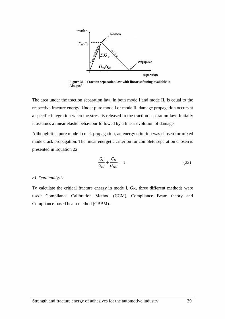
Strength and fracture energy of adhesives for the automotive industry 39
The area under the traction separation law, in both mode I and mode II, is equal to the
respective fracture energy. Under pure mode I or mode II, damage propagation occurs at
a specific integration when the stress is released in the traction-separation law. Initially
it assumes a linear elastic behaviour followed by a linear evolution of damage.
Although it is pure mode I crack propagation, an energy criterion was chosen for mixed
mode crack propagation. The linear energetic criterion for complete separation chosen is
presented in Equation 22.
𝐺𝐼
𝐺𝐼𝐶+
𝐺𝐼𝐼
𝐺𝐼𝐼𝐶= 1 (22)
b) Data analysis
To calculate the critical fracture energy in mode I, GIC, three different methods were
used: Compliance Calibration Method (CCM), Compliance Beam theory and
Compliance-based beam method (CBBM).
Figure 36 - Traction separation law with linear softening available in
Abaqus®

Fracture tests 40
4.1.2 Numerical results and discussion
a) Initial crack length
Three initial crack lengths were studied to investigate the effect on the toughness
measurement. The three initial cracks used in Abaqus® were: 20 mm, 56 mm and 120
mm. The P-δ curve presented below shows a high rigidity for the specimen with a short
crack, a softer linear loading for the intermediate and a further decrease in compliance
for the bigger crack. Also the maximum load for each crack decreased accordingly to
the crack length. All the graphs coincide once the crack length is the same.
To complement the P-δ curve Figure 38 shows the variation of the applied load with the
crack length. Again, for the same crack length the applied load coincides.
Figure 37 – Numerical P-δ of three different initial cracks.
Figure 38 – P-a curve for the three different initial crack lengths.

Strength and fracture energy of adhesives for the automotive industry 41
a)
b)
c)
Figure 39 – Numerical R-curves of the three different initial cracks lengths, a)
CCM method, b) CBT method, c) CBBM method.
The R-curves calculated from the numerical data acquired are presented below.
The CCM and the CBT have a peak in the initial toughness (Figure 39). This peak is
higher in the CCM method but rapidly tends to the exact value. In contrast the CBT has
a smaller peak but a smaller slope until the exact value. Lastly the CBBM is highly

Fracture tests 42
influenced by the initial crack length and, in the plateau region, the value of fracture
toughness does not converge.
The fracture toughness was calculated using the plateau region of the R-curve and the
results are compiled in Figure 40. From all the methods used the CBBM is the most
affected by the initial crack length with an increased toughness. Although CBT has a
similar behaviour, it is more consistent and is not affected to the same extend as CBBM
method. The accurate method was CCM giving precise results in all three tests with
different initial crack lengths.
Figure 40 - Summary of the numerical fracture toughness as a function of initial
crack length.

Strength and fracture energy of adhesives for the automotive industry 43
b) Specimen length
A crucial parameter is the length of the specimen because the chamber has a limitation
of 120 mm from the loading line. As a result, three specimen lengths were used, 290
mm, 240 mm and 200 mm. The P-δ curve of the simulation is presented below.
To complement the previous graph, the force versus crack length is presented in Figure
42.
Figure 41 - Numerical P-δ of three different specimen length.
Figure 42 – P-a curve for the three different specimen length.
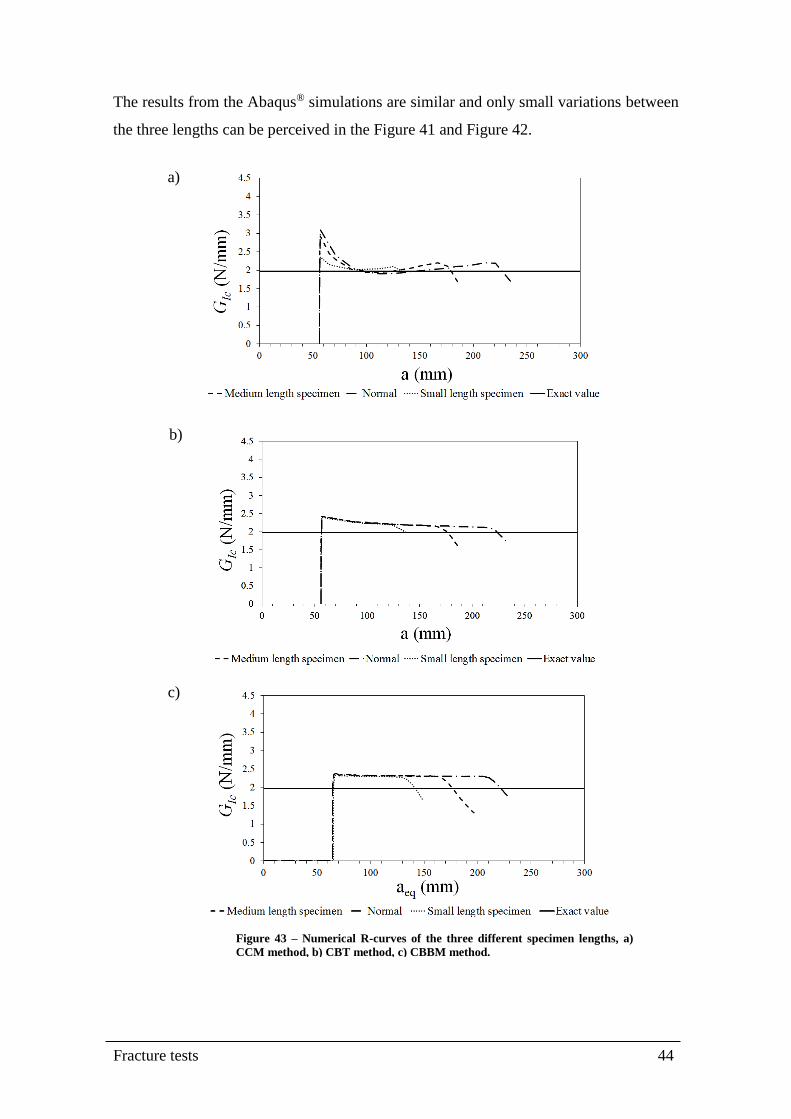
Fracture tests 44
a)
b)
c)
Figure 43 – Numerical R-curves of the three different specimen lengths, a)
CCM method, b) CBT method, c) CBBM method.
The results from the Abaqus® simulations are similar and only small variations between
the three lengths can be perceived in the Figure 41 and Figure 42.

Strength and fracture energy of adhesives for the automotive industry 45
The results from the CCM method are the only that have a shape with a big deviation
from the normal specimen. In the two other methods the difference in the shapes of the
R-curves is only due to the breaking of the specimen.
The fracture toughness is in this case almost constant and it can be assumed that there is
little influence of this parameter. In conclusion, if it is guaranteed enough length for a
stable propagation then the fracture toughness in the plateau region is not influenced by
the length of the specimen.
Figure 44 - Summary of the fracture toughness as a function of specimen length.
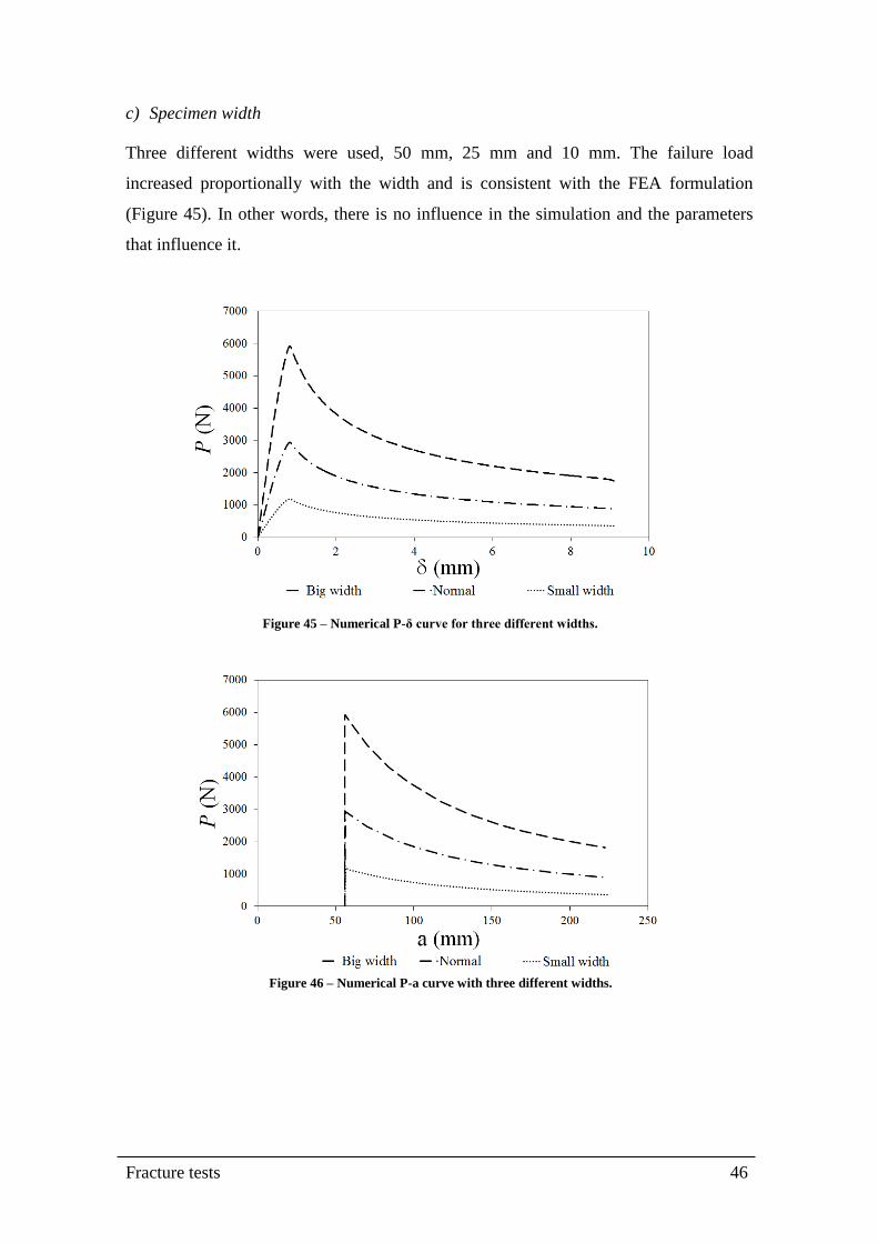
Fracture tests 46
c) Specimen width
Three different widths were used, 50 mm, 25 mm and 10 mm. The failure load
increased proportionally with the width and is consistent with the FEA formulation
(Figure 45). In other words, there is no influence in the simulation and the parameters
that influence it.
Figure 45 – Numerical P-δ curve for three different widths.
Figure 46 – Numerical P-a curve with three different widths.

Strength and fracture energy of adhesives for the automotive industry 47
In all methods the shape of the R-curves was identical as was the fracture toughness in
the plateau region (Figure 47).
The decrease of the width has little influence on the numerical results. However,
diffusion in the bondline of the DCB specimen can take up to two years and a reduction
of the section can decrease greatly the period of the durability study.
Figure 47 – Comparison of the numerical fracture toughness in the plateau region of the
R-curve for three different widths and three different methods: CCM, CBT and CBBM.

Fracture tests 48
d) Substrates thickness
Three substrates thickness were studied, 15 mm, 12.7 mm and 9 mm.
Increasing the thickness of the substrates can improve the adhesive´s maximum load
(Figure 48 and Figure 49). This is the result of the deformation in cohesive zone model
being smaller and the fracture process zone being bigger.
Figure 48 – Numerical P-δ curve of three different thicknesses.
Figure 49 – Numerical P-a curve of three different substrates thicknesses.

Strength and fracture energy of adhesives for the automotive industry 49
a)
b)
c)
Figure 50 – Numerical R-cures of the three different substrate thicknesses
using: a) CCM method, b) CBT method, c) CBBM method.
The CCM method has a deviation in the initial crack toughness opposed to the CBT.
This is a result of the correction of the deformation around the crack tip introduced by
the later. The CBBM method is also corrected and the initial fracture toughness is
similar in all cases. However the 𝑎𝑒𝑞 presents a different initial crack length in all tests

Fracture tests 50
because it accounts for the fracture process zone (FPZ). The stiffer the substrates the
bigger the initial FPZ and the bigger is the initial crack length (equivalent).
There is a consistent decrease in toughness in the plateau region for the CBT method.
For the other two methods used the values are similar.
Figure 51 – Comparison of the numerical fracture toughness in the plateau region of the
R-curve for three different substrate thicknesses and three different methods: CCM,
CBT and CBBM

Strength and fracture energy of adhesives for the automotive industry 51
e) Different materials
Two normal DCB specimens with different materials, steel and aluminium, were tested.
The linear elastic properties of aluminium were used for the substrates, Young´s
modulus of 80 GPa and 0.33 for the Poisson´s ratio.
The initial linear loading of the aluminium specimen is less rigid and the final
displacement, in the loading line, is higher in accordance with its lower Young´s
modulus. Also failure and crack propagation occurs at lower loads (Figure 52 and
Figure 53) as a consequence of a smaller FPZ.
Figure 52 – P-δ curve of two DCB specimens with different materials for adherends.
Figure 53 - P-a curve for the two different materials.

Fracture tests 52
a)
The stresses were analysed using the von Mises criteria to evaluate if a normal
aluminium specimen would deform plastically.
The stress of 160 MPa in the adherends near the adhesive layer would cause
deformation of a low strength aluminium substrate. Although some aluminium alloys
and heat treatments can provide such strength it is easier to use hard steel for the small
DCB prototype.
The shape of the R-curves, in Figure 55, for the CCM method is very similar with an
almost perfect overlap.
Figure 54 – von Mises stresses during the DCB test simulation, a) to d) frames of the test from the
beginning to the end and e) an amplification of the critical part of the specimen.
Figure 55 (continues) - Numerical R-curves of the two different materials,
a) CCM method, b) CBT method, c) CBBM method.

Strength and fracture energy of adhesives for the automotive industry 53
b)
c)
Also in Figure 55 the CBT and CBBM have contradicting results. For the CBT the
fracture toughness in the R-curve is always higher for the steel simulation and in
contrast the CBBM gives opposite results. Experimental results have confirmed an
increase in toughness for softer substrates but this phenomenon is not taken into account
in the numerical simulation. [27]
Both fracture toughness in the plateau region were similar in the CCM method (Table
6). For the other two methods there is a higher deviation.
Table 6 – Compilation of the fracture toughness calculated using the CCM, CBT and CBBM.
Figure 55 (continued)

Fracture tests 54
f) Final specimen
After the evaluation of different parameters a final specimen was designed. The small
specimen geometry is presented in Figure 56 and a similar finite element analysis as the
previously presented was conducted.
Both P-δ curves shown below have a similar shape and although there is a smaller
initial crack in the short specimen the force up to failure is reduced due to the smaller
width.
Figure 57 - Numerical P-δ of a normal and a small DCB specimen.
Figure 58 – P-a curve for the normal and a small DCB specimen.
Figure 56 – Geometry of the small DCB specimen; final specimen (dimensions in mm)

Strength and fracture energy of adhesives for the automotive industry 55
a)
b)
c)
Figure 59 – Numerical R-curves for the normal and small DCB specimen, a)
CCM method, b) CBT method, c) CBBM method.
From the three models used to calculate fracture toughness only the CBT and CBBM
worked and gave reasonable R-curves (Figure 43).

Fracture tests 56
The shape of the CCM method presented in Figure 59, a), does not have either a plateau
or the shape that would be expected for stable damage propagation in the adhesive. In
contrast, the two other methods accurately calculated the fracture toughness of the
adhesive (Table 7).
The stresses in the specimen were studied. The tensions in the final specimen are equal
to the normal DCB specimen and as a result the same steel can be used effectively. The
distribution of tension in the final specimen is presented below.
The final specimen has the required dimensions of less than 120 mm from the loading
line to the wall and will fit in the chamber to be used in the subsequent durability
project.
Figure 60 - von Mises stresses during the final DCB test simulation.
Table 7 - Summary of the fracture toughness calculated using the CCM, CBT and CBBM.

Strength and fracture energy of adhesives for the automotive industry 57
4.2 Experimental DCB tests
4.2.1 Experimental procedure
a) Adhesive
The epoxy adhesive SikaPower 4720 was used, supplied by SIKA® (Portugal, Vila
Nova de Gaia). This adhesive is a two-part system that cures at room temperature for 24
hours. It has a tensile strength of 25 MPa and an elongation at break of 4%.
b) Substrates
In the DCB tests, a high tensile strength steel (DIN 40 CrMnMo 7) was used to avoid
plastic deformation of the substrates. The general properties of the steels used are
presented in Table 8.
c) Specimen manufacture
The geometry of the normal and final DCB test specimens of the numerical study of this
thesis were used and are given again in Figure 61 for convenience. In order to prepare
the specimens, firstly the surface of the substrates was grit blasted and degreased with
acetone prior to the application of adhesive. To guarantee the adhesive bondline
thickness, spacers were inserted between the adherends on both ends. On one end, two
steel plates and a razor blade of 0.1 mm was inserted to introduce a pre-crack and
guarantee cohesive failure propagation from the beginning of the test. On the other end,
one steel plate was inserted to guarantee a bondline thickness of 0.2mm. Adhesive was
applied in both adherends before assembly and were set in a mold for correct alignment
while curing (Figure 62). Lastly, the joints were left under 2 MPa pressure for 24h at
room temperature in a hydraulic hot plates press. After curing the spacers were removed
along with any excess adhesive. The bondline thickness was controlled using an optic
microscope.
Table 8 - Mechanical properties of the steel used for the substrates of the DCB specimens.

Fracture tests 58
d) Test procedure
The specimen were tested according to standard ASTM D3433 in a INSTRON® model
3367 universal test machine (Norwood, Massachusetts, USA) with a capacity of 30 kN,
at room temperature and constant displacement rate of 0.2, 0.5 and 2 mm/min. The
specimen was loaded to measure the behaviour of the adhesive to fracture in mode I.
Pictures were recorded during the testing with 5 s intervals using a 10 MPixel digital
camera. These images allowed the measurement of the crack length during its growth.
Loads and displacements were recorded up to failure. Four specimens were tested for
each geometry.
a)
b)
Figure 61 - Geometry of the DCB specimens tested, a) small specimen, b) normal specimen.
Figure 62 - Schematic representation of the mold used to cure the DCB specimens with the respective legend.

Strength and fracture energy of adhesives for the automotive industry 59
4.2.2 Experimental results and discussion of DCB tests
a) Characterization of fracture toughness
Four normal DCB tests were conducted with a displacement rate of 0.5 mm/min to
characterize the adhesive toughness in mode I. One typical P-δ curve obtained with this
method is presented in Figure 63.
For each normal specimen an R-curve was calculated similar to the curve shown in
Figure 64.
The final value of 1.53 N/mm (value determined using the average of the techniques
showed in Table 9) is much higher than conventional toughened epoxy adhesives (0.3-
0.6 N/mm) and comparable to that of a polyurethane adhesive (1.2-2.9 N/mm). [28]
Table 9 – Values of the fracture toughness of adhesive SikaPower 4720 using the normal specimen.
Figure 64 – Example of an R-curve obtained, specimen 4.
Figure 63 – Example of the P-δ obtained, specimen 4.

Fracture tests 60
1.50
1.75
2.00
0.2 mm/min 0.5 mm/min 2 mm/min
GIc
(N/m
m)
Test displacement rate (mm/min)
b) Displacement rate
Three displacement rates were compared, 0.2, 0.5 and 2 mm/min to study the effect of
strain rate on the fracture toughness (Figure 65).
For the two lowest displacement rates, 0.2 and 0.5 mm/min, the values of fracture
toughness were almost the same (Figure 64). On the other hand the displacement rate of
2 mm/min had an increase in toughness which can be a result of the adhesive’s
viscoelastic behaviour.
The rupture was cohesive in all tests and a picture of the facture surface is presented in
Figure 67. As a note, the fracture surface of the DCB specimens with 2 mm/min
displacement had less rugosity than the specimens tested with slower velocities and is
further proof that viscoelastic behaviour has to be taken into account.
Figure 65 - Comparison of three R-curves using the CBBM method for
different velocities.
Figure 66 – Comparison of the fracture toughness of SikaPower 4720
with different displacement rates.

Strength and fracture energy of adhesives for the automotive industry 61
c) Comparison of two different DCB specimens
The initial rigidity of the specimens is not the same for all the cases (Figure 68). A part
of the reason is the variation of the initial crack length for the normal and short DCB
specimens. The normal specimens have a mean value of 46.35 mm (45 idealized) and a
standard deviation of 0.68 for the initial crack length. There was a better result for the
short specimen of 19.93 mm (20mm idealized) of crack length with a standard deviation
of 0.18 mm.
Figure 68 – P-δ curve for the short and normal DCB specimens tested with SIKA® 4720.
Figure 67 – Example of the failure mode of DCB specimens with SikaPower 4720
using three different displacement rates, a) 0.2mm/min, b) 0.5mm/min and c) 2
mm/min.

Fracture tests 62
Throughout the work done with the normal and small specimens it is clearly much
easier to control the manufacturing process for the small specimens, ex. bondline
thickness and the initial crack length.
Only the CBBM method was used in the analysis of the small DCB specimens. The first
reason was due to the better results in the numerical study and on top of it a technical
difficulty. The initial crack of the small DCB specimen was obstructed by the machines
holding mechanism making it impossible to monitor the beginning of the failure
propagation.
The initial fracture toughness is very high for the small specimen (Figure 69). Since it
was a toughened adhesive the initial crack introduced by the blade may not have been
sufficient to introduce a high enough stress concentration factor. Also the concept of
linear elastic fracture mechanics implies that plasticity should be limited to a small
region ahead of the crack tip and a long enough crack should exist. Most likely neither
verify in the testing of the small specimen.
There was a stable propagation in all small specimens. [11]
Figure 69 – R-curve of the small specimen and normal specimen using the CBBM method.

Strength and fracture energy of adhesives for the automotive industry 63
The rupture was cohesive in all tests and a picture of the facture surface is presented in
Figure 70.
Figure 70 - Two examples of the cohesive fracture surface of the specimens tested, a) small specimen and b)
normal specimen.


Strength and fracture energy of adhesives for the automotive industry 65
5. Impact tests
5.1 Experimental procedure
5.1.1 Adhesive
The epoxy adhesive XNR6852 was used, supplied by NAGASE CHEMTEX® (Osaka,
Japan).
5.1.2 Substrates
A ductile steel (DIN St33), used in car body shells, was used in order to study the effect
of adherend yielding on the joint strength. The properties of the steel can be found in
Table 10.
5.1.3 Specimen manufacture
The geometry for the SLJ test specimen is given in Figure 71. By attaching two steel
plates at the end of the SLJ specimen with mild steel there is improved grip during the
test. The joint surfaces were grit blasted and degreased with acetone prior to the
application of adhesive. After the surface preparation an overlap of 50 mm was
constructed. The thickness of the adhesive bond line was 0.2 mm. All the joints were
manufactured without a fillet.
Table 10 – Mechanical properties of the substrates in SLJ
Figure 71 – Geometry of the SLJ used for the impact tests (dimensions in mm).

Impact tests 66
A mold with spacers for correct alignment of the substrates was used to produce the SLJ
specimens (Figure 72). The substrates were bonded and the joints left under 2 MPa
pressure for 3 h at 150 ºC in a hydraulic hot plates press, being removed from the mold
along with any excess adhesive at the end of the curing process.
This geometry was chosen because it is usually used and will therefore enable
comparison with other academic work. Furthermore it is representative of a structural
part.
5.1.4 Test procedure
The tests were conducted in Rosand® Intrumented Falling weight impact tester, type 5
H.V. (Stourbridge, West Midlands, U.K.). The machine was calibrated to give an
energy at impact of 300 J loading the specimen in tension. The energy was dissipated in
the specimen from a falling mass of 29.83 kg with a velocity approximately equal to
4.47 m/s.
5.2 Experimental results and discussion
Due to the high strain rate the steel adherends had a different behaviour when
comparing with the quasi static test, deforming less and absorbing less energy (Table 11
and Figure 73). As a result of the strain rate dependence of the steel, the failure load was
increased but the adhesive experienced a similar damage as in the case of static loading.
Figure 72 - Schematic mold for SLJ specimens.

Strength and fracture energy of adhesives for the automotive industry 67
0
2000
4000
6000
8000
10000
12000
14000
0 10 20 30 40 50
Fo
rce
(N)
Displacement (mm)
Impact test Static test
For application where impact energy absorption is important well-constructed adhesive
joints with a high elongation epoxy such as the studied is interesting for it has a high
damage tolerance, high elongation and high strength.
The rupture was in all cases in the steel adherends (Figure 74). Under high strain rate
the same failure mode as in the quasi-static tests was obtained and again a case of plane
stress was observed in the steel adherend.
Figure 73 - Comparison of SLJ with mild steel adherends under two different strain rates.
Table 11 - Energy (J) and failure load (N) values obtained from the quasi-static and
impact test.
Figure 74 – Failure mode of the SLJ tested


Strength and fracture energy of adhesives for the automotive industry 69
6. Conclusions
A characterization of two adhesives was done. The adhesive XNR 6852 has:
• High tensile strength (approximately 60 MPa), typical of an epoxy adhesive.
• High elongation (approximately 100%), typical of a polyurethane adhesive.
• Can withstand deformation and damage without a brittle behavior for both
impact and quasi-static cases.
• High toughness (GIC = 1.97 N/mm and GIIC = 12.5 ±1.1), typical of a
polyurethane adhesive.
The adhesive SikaPower 4720 has:
• Low tensile strength (approximately 25 MPa) for an epoxy adhesive.
• Normal elongation and Young´s modulus (approximately 4% and 2000 MPa
respectively) for an epoxy adhesive.
• High toughness (GIC = 1,31 N/mm).
From the numerical study of fracture toughness in mode I using a DCB geometry it was
concluded that:
• The smaller the crack length the higher the fracture toughness.
• Specimen length, width and substrate thickness do not have much influence on
the fracture toughness
A small DCB specimen was put forward and:
• Numerical results suggested that a good and similar result for fracture toughness
would be achieved using CBBM and CBT method but experimental results have
proved otherwise for CBBM. A small DCB specimen increases the toughness
because GIC formulation is heavily dependent on the initial crack length and
specimen compliance.


Strength and fracture energy of adhesives for the automotive industry 71
7. Future work
Study the small bulk specimens with other adhesives and compare with the results from
the long dogbone.
Improve the results for the short DCB specimen studying other parameters.
Validate the numerical findings of the DCB simulations.
Using bulk specimens developed to study the water aging process of the both,
NAGASE CHEMPTEX® XNR 6852 and SikaPower® 4720.


Strength and fracture energy of adhesives for the automotive industry 73
References
[1] da Silva L.F.M., Öchsner A., Adams R.D., Handbook of Adhesion Technology, 1
ed., Springer, Berlin, 2011.
[2] Kinloch A.J., Adhesion and Adhesives, Science and Technology., 1 ed., Chapman
and Hall, Great Britain, 1987.
[3] Banea M.D., Da Silva L.F.M., Adhesively bonded joints in composite materials: An
overview, Proceedings of the Institution of Mechanical Engineers, Part L: Journal of
Materials: Design and Applications, 223 (2009) 1-18.
[4] Hartshorn S.R., Structural Adhesives, Chemistry and Technology., Hartshorn, 1986.
[5] Adams R.D., Wake W.C., Structural Adhesive Joints in Enginering, ELSEVIER
APPLIED SCIENCE PUBLISHERS LTD, 1984.
[6] Adams R.D., Adhesive bonding, Science, technology and applications, Woodhead
Publishing Limited, 2000.
[7] Lees W.A., Adhesives in Engineering Design, Springer-Verlag, The Design
Council, 1984.
[8] da Silva L.F.M., das Neves P.J.C., Adams R.D., Spelt J.K., Analytical models of
adhesively bonded joints—Part I: Literature survey, International Journal of Adhesion
and Adhesives, 29 (2009) 319-30.
[9] da Silva L.F.M., das Neves P.J.C., Adams R.D., Wang A., Spelt J.K., Analytical
models of adhesively bonded joints—Part II: Comparative study, International Journal
of Adhesion and Adhesives, 29 (2009) 331-41.
[10] da Silva L.F.M., Öchsner A., Modeling of Adhesive Bonded Joints, Springer, 2008.
[11] Kanninen M.F., Popelar C.H., Advanced Fracture Mechanics, Oxford University
Press, 1985.
[12] da Silva L.F.M., Dillard D.A., Blackman B.R.K., Adams R.D., Testing Adhesive
Joints, Best practices., WILEI-VCH, 2012.
[13] Kanninen M.F., Popelar C.H., Advanced Fracture Mechanics, Oxford University
Press.
[14] Robinson P., Das S., Mode I DCB testing of composite laminates reinforced with
z-direction pins: a simple model for the investigation of data reduction strategies,
Engineering Fracture Mechanics, 71 (2004) 345-64.
[15] de Moura M.F.S.F., Gonçalves J.P.M., Chousal J.A.G., Campilho R.D.S.G.,
"Cohesive and continuum mixed-mode damage models applied to the simulation of the
mechanical behaviour of bonded joints, International Journal of Adhesion and
Adhesives, 2008.
[16] de Moura M.F.S.F., Gonçalves J.P.M., Chousal J.A.G., Campilho R.D.S.G.,
Cohesive and continuum mixed-mode damage models applied to the simulation of the
mechanical behaviour of bonded joints, International Journal of Adhesion and
Adhesives, 28 (2008) 419-26.
[17] Banea M.D., Silva L.F.M.d., Campilho R.D.S.G., Effect of Temperature on Tensile
Strength and Mode I Fracture Toughness of a High Temperature Epoxy Adhesive,
Journal of Adhesion Science and Technology, 26 (2012) 939-53.
[18] Tsujimura T.Y., High toughness composites based on insitupolymerizable
thermoplastic epoxy-resin, 29th International Conference and Forum -SAMPE Europe
SEICO 08, Paris, 2008.
[19] Karachalios E.F., Adams R.D., da Silva L.F.M., Single lap joints loaded in tension
with high strength steel adherends, International Journal of Adhesion and Adhesives, 43
(2013) 81-95.
References 74
[20] Gordon K., Quasi-static strength and fatigue life of hybrid (bonded/bolted)
composite single-lap joints, Composite Structures, 72 (2006) 119-29.
[21] Banea M.D., da Silva L.F.M., Static and fatigue behaviour of room temperature
vulcanising silicone adhesives for high temperature aerospace applications. Statisches
Verhalten und Dauerfestigkeitsanalyse von vulkanisierten Silikonklebstoffen für
Luftfahrtanwendungen bei hohen Temperaturen, Materialwissenschaft und
Werkstofftechnik, 41 (2010) 325-35.
[22] Wang Y., Williams J.G., Corrections for mode II fracture toughness specimens of
composites materials, Composites Science and Technology, 43 (1992) 251-6.
[23] Yoshihara H., Kawamura T., Mode I fracture toughness estimation of wood by
DCB test, Composites Part A: Applied Science and Manufacturing, 37 (2006) 2105-13.
[24] de Moura M.F.S.F., Campilho R.D.S.G., Gonçalves J.P.M., Crack equivalent
concept applied to the fracture characterization of bonded joints under pure mode I
loading, Composites Science and Technology, 68 (2008) 2224-30.
[25] de Moura M.F.S.F., Campilho R.D.S.G., Gonçalves J.P.M., Crack equivalent
concept applied to the fracture characterization of bonded joints under pure mode I
loading, Composites Science and Technology, 2008.
[26] Banea M.D., L. F. M. Silva, and R. D. S. G. Campilho, Effect of temperature on
tensile strength and mode I fracture toughness of a high temperature epoxy adhesive,
Journal of adhesivion science and technology, 2011.
[27] Yan C., Mai Y.-W., Yuan Q., Ye L., Sun J., Effects of substrate materials on
fracture toughness measurement in adhesive joints, International Journal of Mechanical
Sciences, 43 (2001) 2091-102.
[28] da Silva L.F.M., Carbas R.J.C., Critchlow G.W., Figueiredo M.A.V., Brown K.,
Effect of material, geometry, surface treatment and environment on the shear strength of
single lap joints, International Journal of Adhesion and Adhesives, 29 (2009) 621-32.

Strength and fracture energy of adhesives for the automotive industry 75
Appended papers