Strengthening the Reporting of Observational Studies in ... · Strengthening the Reporting of Observational Studies in Epidemiology (STROBE) ... of Observational Studies in Epidemiology

STROBE INITIATIVE

Strengthening the Reporting of Observational Studies inEpidemiology (STROBE)Explanation and Elaboration

Jan P. Vandenbroucke,* Erik von Elm,†‡ Douglas G. Altman,§ Peter C. Gøtzsche,¶Cynthia D. Mulrow,� Stuart J. Pocock,** Charles Poole,†† James J. Schlesselman,‡‡

and Matthias Egger,†§§ for the STROBE Initiative

Abstract: Much medical research is observational. The reporting ofobservational studies is often of insufficient quality. Poor reportinghampers the assessment of the strengths and weaknesses of a studyand the generalizability of its results. Taking into account empiricalevidence and theoretical considerations, a group of methodologists,researchers, and editors developed the Strengthening the Reportingof Observational Studies in Epidemiology (STROBE) recommen-dations to improve the quality of reporting of observational studies.

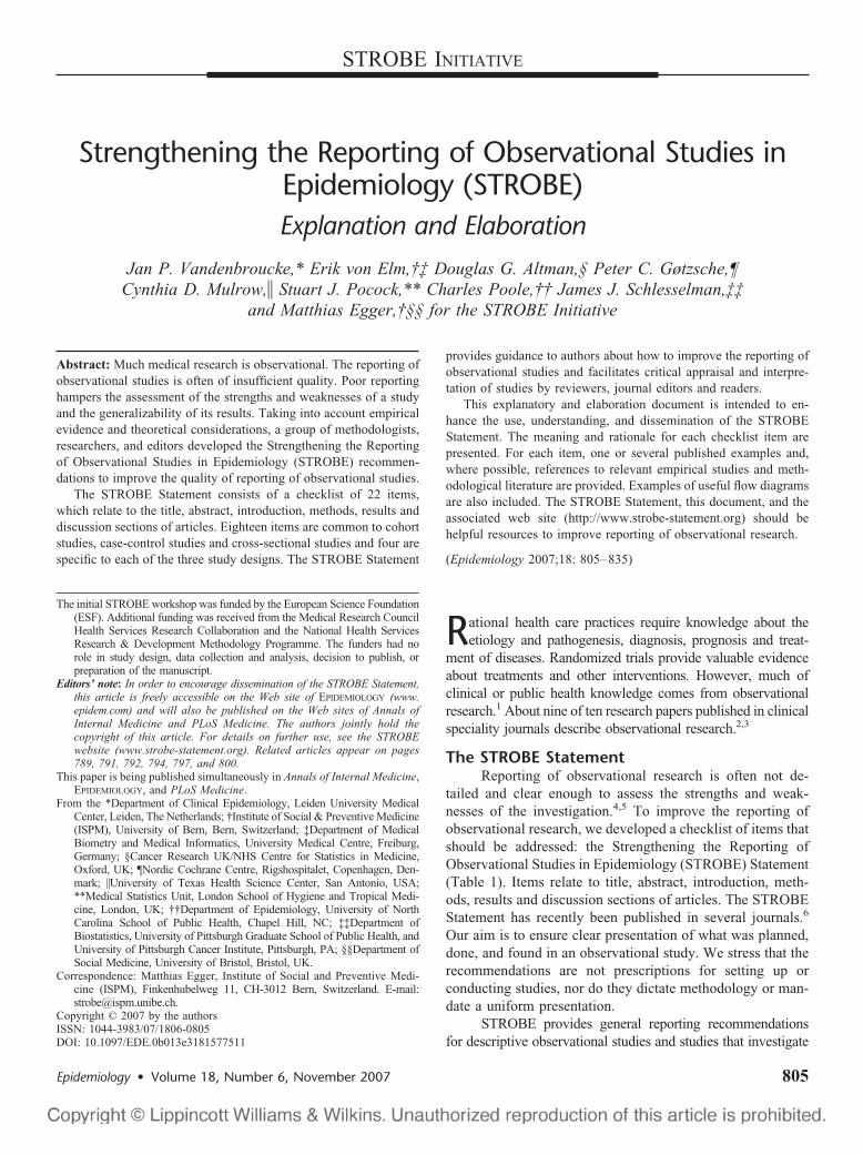
The STROBE Statement consists of a checklist of 22 items,which relate to the title, abstract, introduction, methods, results anddiscussion sections of articles. Eighteen items are common to cohortstudies, case-control studies and cross-sectional studies and four arespecific to each of the three study designs. The STROBE Statement

provides guidance to authors about how to improve the reporting ofobservational studies and facilitates critical appraisal and interpre-tation of studies by reviewers, journal editors and readers.

This explanatory and elaboration document is intended to en-hance the use, understanding, and dissemination of the STROBEStatement. The meaning and rationale for each checklist item arepresented. For each item, one or several published examples and,where possible, references to relevant empirical studies and meth-odological literature are provided. Examples of useful flow diagramsare also included. The STROBE Statement, this document, and theassociated web site (http://www.strobe-statement.org) should behelpful resources to improve reporting of observational research.

(Epidemiology 2007;18: 805–835)

Rational health care practices require knowledge about theetiology and pathogenesis, diagnosis, prognosis and treat-

ment of diseases. Randomized trials provide valuable evidenceabout treatments and other interventions. However, much ofclinical or public health knowledge comes from observationalresearch.1 About nine of ten research papers published in clinicalspeciality journals describe observational research.2,3

The STROBE StatementReporting of observational research is often not de-

tailed and clear enough to assess the strengths and weak-nesses of the investigation.4,5 To improve the reporting ofobservational research, we developed a checklist of items thatshould be addressed: the Strengthening the Reporting ofObservational Studies in Epidemiology (STROBE) Statement(Table 1). Items relate to title, abstract, introduction, meth-ods, results and discussion sections of articles. The STROBEStatement has recently been published in several journals.6

Our aim is to ensure clear presentation of what was planned,done, and found in an observational study. We stress that therecommendations are not prescriptions for setting up orconducting studies, nor do they dictate methodology or man-date a uniform presentation.

STROBE provides general reporting recommendationsfor descriptive observational studies and studies that investigate

The initial STROBE workshop was funded by the European Science Foundation(ESF). Additional funding was received from the Medical Research CouncilHealth Services Research Collaboration and the National Health ServicesResearch & Development Methodology Programme. The funders had norole in study design, data collection and analysis, decision to publish, orpreparation of the manuscript.

Editors’ note: In order to encourage dissemination of the STROBE Statement,this article is freely accessible on the Web site of EPIDEMIOLOGY (www.epidem.com) and will also be published on the Web sites of Annals ofInternal Medicine and PLoS Medicine. The authors jointly hold thecopyright of this article. For details on further use, see the STROBEwebsite (www.strobe-statement.org). Related articles appear on pages789, 791, 792, 794, 797, and 800.

This paper is being published simultaneously in Annals of Internal Medicine,EPIDEMIOLOGY, and PLoS Medicine.

From the *Department of Clinical Epidemiology, Leiden University MedicalCenter, Leiden, The Netherlands; †Institute of Social & Preventive Medicine(ISPM), University of Bern, Bern, Switzerland; ‡Department of MedicalBiometry and Medical Informatics, University Medical Centre, Freiburg,Germany; §Cancer Research UK/NHS Centre for Statistics in Medicine,Oxford, UK; ¶Nordic Cochrane Centre, Rigshospitalet, Copenhagen, Den-mark; �University of Texas Health Science Center, San Antonio, USA;**Medical Statistics Unit, London School of Hygiene and Tropical Medi-cine, London, UK; ††Department of Epidemiology, University of NorthCarolina School of Public Health, Chapel Hill, NC; ‡‡Department ofBiostatistics, University of Pittsburgh Graduate School of Public Health, andUniversity of Pittsburgh Cancer Institute, Pittsburgh, PA; §§Department ofSocial Medicine, University of Bristol, Bristol, UK.

Correspondence: Matthias Egger, Institute of Social and Preventive Medi-cine (ISPM), Finkenhubelweg 11, CH-3012 Bern, Switzerland. E-mail:[email protected].

Copyright © 2007 by the authorsISSN: 1044-3983/07/1806-0805DOI: 10.1097/EDE.0b013e3181577511

Epidemiology • Volume 18, Number 6, November 2007 805

associations between exposures and health outcomes. STROBEaddresses the three main types of observational studies: cohort,case-control and cross-sectional studies. Authors use diverse

terminology to describe these study designs. For instance, ‘fol-low-up study’ and ‘longitudinal study’ are used as synonyms for‘cohort study’, and ‘prevalence study’ as synonymous with

TABLE 1. The STROBE statement—Checklist of Items That Should be Addressed in Reports of Observational Studies

ItemNumber Recommendation

TITLE andABSTRACT

1 (a) Indicate the study’s design with a commonly used term in the title or the abstract(b) Provide in the abstract an informative and balanced summary of what was done and what was found

INTRODUCTIONBackground/rationale

2 Explain the scientific background and rationale for the investigation being reported

Objectives 3 State specific objectives, including any prespecified hypothesesMETHODS

Study design 4 Present key elements of study design early in the paperSetting 5 Describe the setting, locations, and relevant dates, including periods of recruitment, exposure, follow-up, and data collectionParticipants 6 (a) Cohort study—Give the eligibility criteria, and the sources and methods of selection of participants. Describe methods of

follow-upCase-control study—Give the eligibility criteria, and the sources and methods of case ascertainment and control selection. Givethe rationale for the choice of cases and controlsCross-sectional study—Give the eligibility criteria, and the sources and methods of selection of participants

(b) Cohort study—For matched studies, give matching criteria and number of exposed and unexposedCase-control study—For matched studies, give matching criteria and the number of controls per case

Variables 7 Clearly define all outcomes, exposures, predictors, potential confounders, and effect modifiers. Give diagnostic criteria, if applicableData sources/measurement

8* For each variable of interest, give sources of data and details of methods of assessment (measurement). Describe comparability ofassessment methods if there is more than one group

Bias 9 Describe any efforts to address potential sources of biasStudy size 10 Explain how the study size was arrived atQuantitativevariables

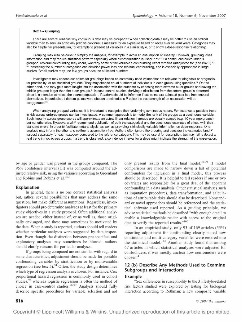
11 Explain how quantitative variables were handled in the analyses. If applicable, describe which groupings were chosen, and why

Statisticalmethods

12 (a) Describe all statistical methods, including those used to control for confounding(b) Describe any methods used to examine subgroups and interactions(c) Explain how missing data were addressed(d) Cohort study—If applicable, explain how loss to follow-up was addressed

Case-control study—If applicable, explain how matching of cases and controls was addressedCross-sectional study—If applicable, describe analytical methods taking account of sampling strategy

(e) Describe any sensitivity analysesRESULTS

Participants 13* (a) Report the numbers of individuals at each stage of the study—eg, numbers potentially eligible, examined for eligibility,confirmed eligible, included in the study, completing follow-up, and analyzed

(b) Give reasons for non-participation at each stage(c) Consider use of a flow diagram

Descriptive data 14* (a) Give characteristics of study participants (eg, demographic, clinical, social) and information on exposures and potentialconfounders

(b) Indicate the number of participants with missing data for each variable of interest(c) Cohort study—Summarize follow-up time (eg, average and total amount)

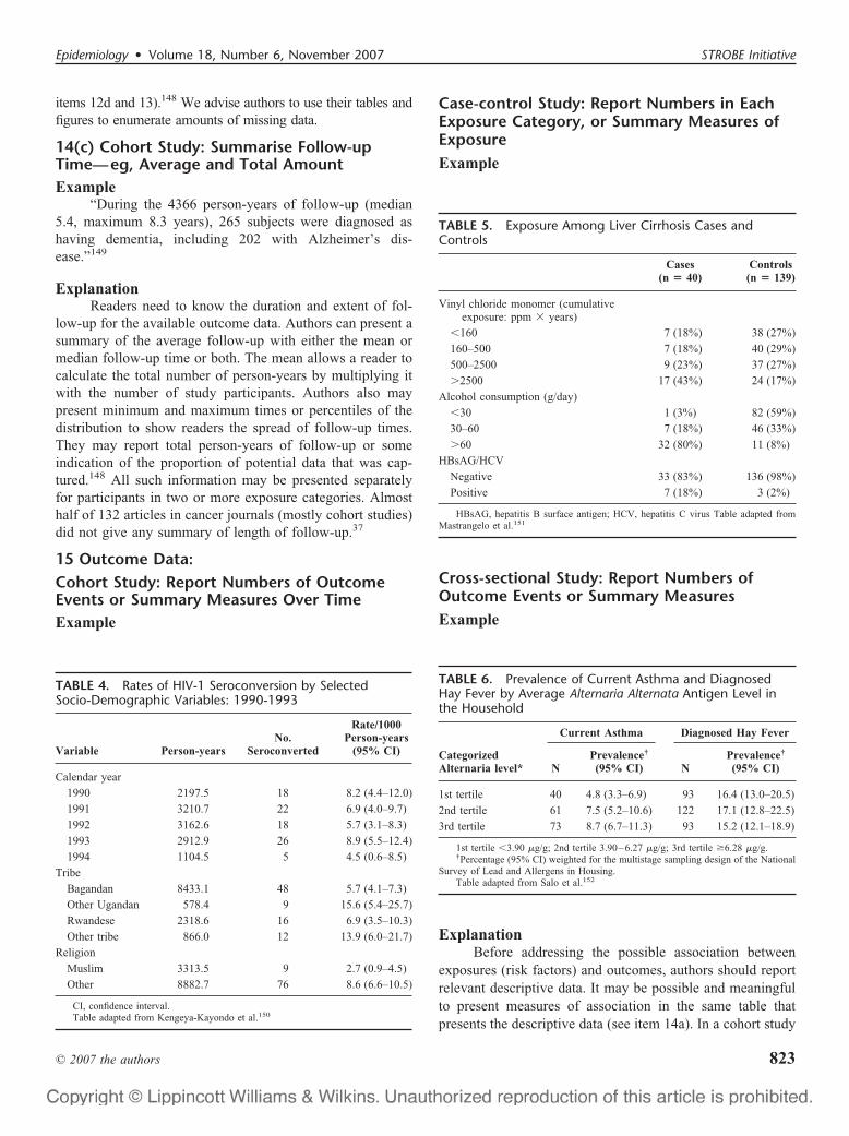
Outcome data 15* Cohort study—Report numbers of outcome events or summary measures over timeCase-control study—Report numbers in each exposure category, or summary measures of exposureCross-sectional study—Report numbers of outcome events or summary measures

Main results 16 (a) Give unadjusted estimates and, if applicable, confounder-adjusted estimates and their precision (eg 95% confidence intervals).Make clear which confounders were adjusted for and why they were included

(b) Report category boundaries when continuous variables were categorised(c) If relevant, consider translating estimates of relative risk into absolute risk for a meaningful time period

Other analyses 17 Report other analyses done—eg, analyses of subgroups and interactions, and sensitivity analysesKey results 18 Summarise key results with reference to study objectivesLimitations 19 Discuss limitations of the study, taking into account sources of potential bias or imprecision. Discuss both direction and magnitude

of any potential biasInterpretation 20 Give a cautious overall interpretation of results considering objectives, limitations, multiplicity of analyses, results from similar

studies, and other relevant evidenceGeneralizability 21 Discuss the generalizability (external validity) of the study results

OTHERINFORMATIONFunding 22 Give the source of funding and the role of the funders for the present study and, if applicable, for the original study on which the

present article is based

*Give such information separately for cases and controls in case-control studies, and, if applicable, for exposed and unexposed groups in cohort and cross-sectional studies.Separate versions of the checklist for cohort, case-control and cross-sectional studies are available on the STROBE website at www.strobe-statement.org.

Vandenbroucke et al Epidemiology • Volume 18, Number 6, November 2007

© 2007 the authors806

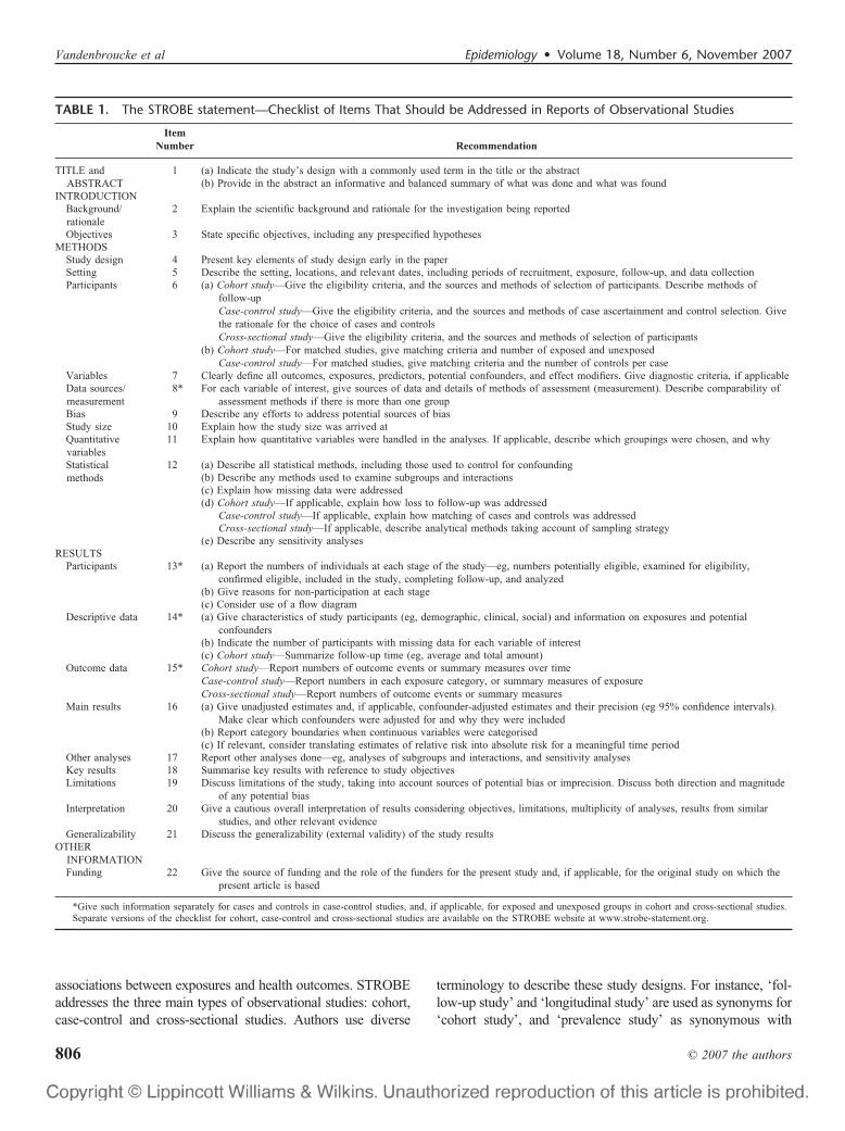
‘cross-sectional study’. We chose the present terminology be-cause it is in common use. Unfortunately, terminology is oftenused incorrectly7 or imprecisely.8 In box 1 we describe thehallmarks of the three study designs.

The Scope of Observational ResearchObservational studies serve a wide range of purposes:

from reporting a first hint of a potential cause of a disease, toverifying the magnitude of previously reported associations.Ideas for studies may arise from clinical observations or frombiologic insight. Ideas may also arise from informal looks atdata that lead to further explorations. Like a clinician who hasseen thousands of patients, and notes one that strikes herattention, the researcher may note something special in thedata. Adjusting for multiple looks at the data may not bepossible or desirable,9 but further studies to confirm or refuteinitial observations are often needed.10 Existing data may beused to examine new ideas about potential causal factors, andmay be sufficient for rejection or confirmation. In otherinstances, studies follow that are specifically designed toovercome potential problems with previous reports. The latterstudies will gather new data and will be planned for that

purpose, in contrast to analyses of existing data. This leads todiverse viewpoints, eg, on the merits of looking at subgroupsor the importance of a predetermined sample size. STROBEtries to accommodate these diverse uses of observational re-search—from discovery to refutation or confirmation. Wherenecessary we will indicate in what circumstances specific rec-ommendations apply.

How to Use This PaperThis paper is linked to the shorter STROBE paper that

introduced the items of the checklist in several journals,6 andforms an integral part of the STROBE Statement. Our inten-tion is to explain how to report research well, not howresearch should be done. We offer a detailed explanation foreach checklist item. Each explanation is preceded by anexample of what we consider transparent reporting. This doesnot mean that the study from which the example was takenwas uniformly well reported or well done; nor does it meanthat its findings were reliable, in the sense that they were laterconfirmed by others: it only means that this particular itemwas well reported in that study. In addition to explanations

Epidemiology • Volume 18, Number 6, November 2007 STROBE Initiative

© 2007 the authors 807

and examples we included boxes with supplementary infor-mation. These are intended for readers who want to refreshtheir memories about some theoretical points, or be quicklyinformed about technical background details. A full under-standing of these points may require studying the textbooksor methodological papers that are cited.

STROBE recommendations do not specifically addresstopics such as genetic linkage studies, infectious diseasemodeling or case reports and case series.11,12 As many of thekey elements in STROBE apply to these designs, authors whoreport such studies may nevertheless find our recommenda-tions useful. For authors of observational studies that specif-ically address diagnostic tests, tumor markers and geneticassociations, STARD,13 REMARK,14 and STREGA15 rec-ommendations may be particularly useful.

The Items in the STROBE ChecklistWe now discuss and explain the 22 items in the

STROBE checklist (Table 1), and give published examplesfor each item. Some examples have been edited by removingcitations or spelling out abbreviations. Eighteen items applyto all three study designs whereas four are design-specific.Starred items (for example item 8*) indicate that the infor-mation should be given separately for cases and controls incase-control studies, or exposed and unexposed groups incohort and cross-sectional studies. We advise authors toaddress all items somewhere in their paper, but we do notprescribe a precise location or order. For instance, we discussthe reporting of results under a number of separate items,while recognizing that authors might address several itemswithin a single section of text or in a table.

TITLE AND ABSTRACT

1(a) Indicate the Study’s Design with aCommonly Used Term in the Title or theAbstractExample

“Leukemia incidence among workers in the shoe andboot manufacturing industry: a case-control study.”18

ExplanationReaders should be able to easily identify the design that

was used from the title or abstract. An explicit, commonlyused term for the study design also helps ensure correctindexing of articles in electronic databases.19,20

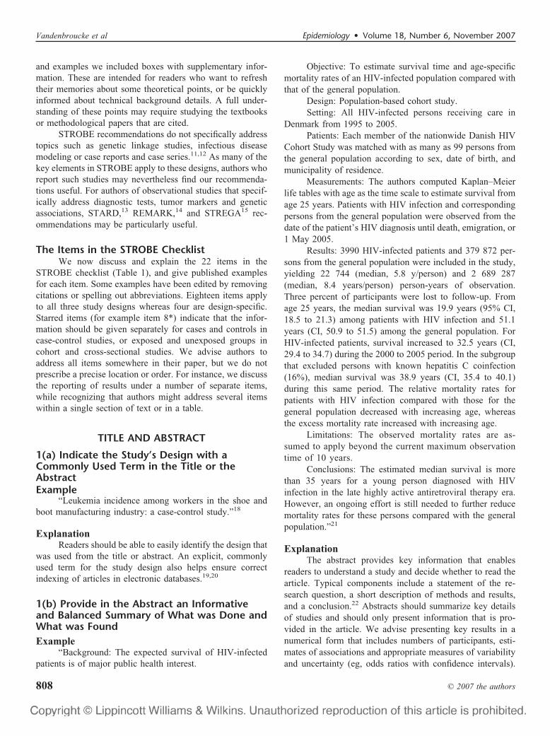
1(b) Provide in the Abstract an Informativeand Balanced Summary of What was Done andWhat was FoundExample

“Background: The expected survival of HIV-infectedpatients is of major public health interest.

Objective: To estimate survival time and age-specificmortality rates of an HIV-infected population compared withthat of the general population.

Design: Population-based cohort study.Setting: All HIV-infected persons receiving care in

Denmark from 1995 to 2005.Patients: Each member of the nationwide Danish HIV

Cohort Study was matched with as many as 99 persons fromthe general population according to sex, date of birth, andmunicipality of residence.

Measurements: The authors computed Kaplan–Meierlife tables with age as the time scale to estimate survival fromage 25 years. Patients with HIV infection and correspondingpersons from the general population were observed from thedate of the patient’s HIV diagnosis until death, emigration, or1 May 2005.

Results: 3990 HIV-infected patients and 379 872 per-sons from the general population were included in the study,yielding 22 744 (median, 5.8 y/person) and 2 689 287(median, 8.4 years/person) person-years of observation.Three percent of participants were lost to follow-up. Fromage 25 years, the median survival was 19.9 years (95% CI,18.5 to 21.3) among patients with HIV infection and 51.1years (CI, 50.9 to 51.5) among the general population. ForHIV-infected patients, survival increased to 32.5 years (CI,29.4 to 34.7) during the 2000 to 2005 period. In the subgroupthat excluded persons with known hepatitis C coinfection(16%), median survival was 38.9 years (CI, 35.4 to 40.1)during this same period. The relative mortality rates forpatients with HIV infection compared with those for thegeneral population decreased with increasing age, whereasthe excess mortality rate increased with increasing age.

Limitations: The observed mortality rates are as-sumed to apply beyond the current maximum observationtime of 10 years.

Conclusions: The estimated median survival is morethan 35 years for a young person diagnosed with HIVinfection in the late highly active antiretroviral therapy era.However, an ongoing effort is still needed to further reducemortality rates for these persons compared with the generalpopulation.”21

ExplanationThe abstract provides key information that enables

readers to understand a study and decide whether to read thearticle. Typical components include a statement of the re-search question, a short description of methods and results,and a conclusion.22 Abstracts should summarize key detailsof studies and should only present information that is pro-vided in the article. We advise presenting key results in anumerical form that includes numbers of participants, esti-mates of associations and appropriate measures of variabilityand uncertainty (eg, odds ratios with confidence intervals).



We regard it insufficient to state only that an exposure is oris not significantly associated with an outcome.

A series of headings pertaining to the background, design,conduct, and analysis of a study may help readers acquire theessential information rapidly.23 Many journals require suchstructured abstracts, which tend to be of higher quality and morereadily informative than unstructured summaries.24,25

INTRODUCTIONThe Introduction section should describe why the study

was done and what questions and hypotheses it addresses. Itshould allow others to understand the study’s context andjudge its potential contribution to current knowledge.

2 Background/Rationale: Explain the ScientificBackground and Rationale for theInvestigation Being ReportedExample

“Concerns about the rising prevalence of obesity inchildren and adolescents have focused on the well docu-mented associations between childhood obesity and increasedcardiovascular risk and mortality in adulthood. Childhoodobesity has considerable social and psychological conse-quences within childhood and adolescence, yet little is knownabout social, socioeconomic, and psychological consequences inadult life. A recent systematic review found no longitudinalstudies on the outcomes of childhood obesity other than physicalhealth outcomes and only 2 longitudinal studies of the socio-economic effects of obesity in adolescence. Gortmaker et alfound that US women who had been obese in late adolescencein 1981 were less likely to be married and had lower incomesseven years later than women who had not been overweight,while men who had been overweight were less likely to bemarried. Sargent et al found that UK women, but not men, whohad been obese at 16 years in 1974 earned 7.4% less than theirnonobese peers at age 23. (. . .) We used longitudinal data fromthe 1970 British birth cohort to examine the adult socioeco-nomic, educational, social, and psychological outcomes of child-hood obesity.”26

ExplanationThe scientific background of the study provides impor-

tant context for readers. It sets the stage for the study anddescribes its focus. It gives an overview of what is known ona topic and what gaps in current knowledge are addressed bythe study. Background material should note recent pertinentstudies and any systematic reviews of pertinent studies.

3 Objectives: State Specific Objectives,Including Any Prespecified HypothesesExample

“Our primary objectives were to 1) determine the prev-alence of domestic violence among female patients present-ing to four community-based, primary care, adult medicine

practices that serve patients of diverse socioeconomic back-ground and 2) identify demographic and clinical differencesbetween currently abused patients and patients not currentlybeing abused.”27

ExplanationObjectives are the detailed aims of the study. Well

crafted objectives specify populations, exposures and out-comes, and parameters that will be estimated. They may beformulated as specific hypotheses or as questions that thestudy was designed to address. In some situations objectivesmay be less specific, for example, in early discovery phases.Regardless, the report should clearly reflect the investigators’intentions. For example, if important subgroups or additionalanalyses were not the original aim of the study but aroseduring data analysis, they should be described accordingly(see also items 4, 17 and 20).

METHODSThe Methods section should describe what was planned

and what was done in sufficient detail to allow others tounderstand the essential aspects of the study, to judgewhether the methods were adequate to provide reliable andvalid answers, and to assess whether any deviations from theoriginal plan were reasonable.

4 Study Design: Present Key Elements of StudyDesign Early in the PaperExample

“We used a case-crossover design, a variation of acase-control design that is appropriate when a brief exposure(driver’s phone use) causes a transient rise in the risk of a rareoutcome (a crash). We compared a driver’s use of a mobilephone at the estimated time of a crash with the same driver’suse during another suitable time period. Because drivers aretheir own controls, the design controls for characteristics ofthe driver that may affect the risk of a crash but do not changeover a short period of time. As it is important that risks duringcontrol periods and crash trips are similar, we comparedphone activity during the hazard interval (time immediatelybefore the crash) with phone activity during control intervals(equivalent times during which participants were driving butdid not crash) in the previous week.”28

ExplanationWe advise presenting key elements of study design

early in the methods section (or at the end of the introduction)so that readers can understand the basics of the study. Forexample, authors should indicate that the study was a cohortstudy, which followed people over a particular time period,and describe the group of persons that comprised the cohortand their exposure status. Similarly, if the investigation useda case-control design, the cases and controls and their sourcepopulation should be described. If the study was a cross-



sectional survey, the population and the point in time atwhich the cross-section was taken should be mentioned.When a study is a variant of the three main study types, thereis an additional need for clarity. For instance, for a case-crossover study, one of the variants of the case-control design,a succinct description of the principles was given in the exampleabove.28

We recommend that authors refrain from simply callinga study ‘prospective’ or ‘retrospective’ because these termsare ill defined.29 One usage sees cohort and prospective assynonymous and reserves the word retrospective for case-control studies.30 A second usage distinguishes prospectiveand retrospective cohort studies according to the timing ofdata collection relative to when the idea for the study wasdeveloped.31 A third usage distinguishes prospective andretrospective case-control studies depending on whether thedata about the exposure of interest existed when cases wereselected.32 Some advise against using these terms,33 or adopt-ing the alternatives ‘concurrent’ and ‘historical’ for describ-ing cohort studies.34 In STROBE, we do not use the wordsprospective and retrospective, nor alternatives such as con-current and historical. We recommend that, whenever authorsuse these words, they define what they mean. Most impor-tantly, we recommend that authors describe exactly how andwhen data collection took place.

The first part of the methods section might also be theplace to mention whether the report is one of several from astudy. If a new report is in line with the original aims of thestudy, this is usually indicated by referring to an earlierpublication and by briefly restating the salient features of thestudy. However, the aims of a study may also evolve overtime. Researchers often use data for purposes for which theywere not originally intended, including, for example, officialvital statistics that were collected primarily for administrativepurposes, items in questionnaires that originally were onlyincluded for completeness, or blood samples that were col-lected for another purpose. For example, the Physicians’Health Study, a randomized controlled trial of aspirin andcarotene, was later used to demonstrate that a point mutationin the factor V gene was associated with an increased risk ofvenous thrombosis but not of myocardial infarction orstroke.35 The secondary use of existing data is a creative partof observational research and does not necessarily makeresults less credible or less important. However, briefly re-stating the original aims might help readers understand thecontext of the research and possible limitations in the data.

5 Setting: Describe the Setting, Locations, andRelevant Dates, Including Periods ofRecruitment, Exposure, Follow-up, and DataCollectionExample

“The Pasitos Cohort Study recruited pregnant womenfrom Women, Infant and Child clinics in Socorro and San

Elizario, El Paso County, Texas and maternal-child clinics ofthe Mexican Social Security Institute in Ciudad Juarez, Mex-ico from April 1998 to October 2000. At baseline, prior to thebirth of the enrolled cohort children, staff interviewed moth-ers regarding the household environment. In this ongoingcohort study, we target follow-up exams at 6-month intervalsbeginning at age 6 months.”36

ExplanationReaders need information on setting and locations to

assess the context and generalizability of a study’s results.Exposures such as environmental factors and therapies canchange over time. Also, study methods may evolve over time.Knowing when a study took place and over what periodparticipants were recruited and followed up places the studyin historical context and is important for the interpretation ofresults.

Information about setting includes recruitment sites orsources (eg, electoral roll, outpatient clinic, cancer registry, ortertiary care centre). Information about location may refer tothe countries, towns, hospitals or practices where the inves-tigation took place. We advise stating dates rather than onlydescribing the length of time periods. There may be differentsets of dates for exposure, disease occurrence, recruitment,beginning and end of follow-up, and data collection. Of note,nearly 80% of 132 reports in oncology journals that usedsurvival analysis included the starting and ending dates foraccrual of patients, but only 24% also reported the date onwhich follow-up ended.37

6 Participants:6(a) Cohort Study: Give the Eligibility Criteria,and the Sources and Methods of Selection ofParticipants. Describe Methods of Follow-upExample

“Participants in the Iowa Women’s Health Study were arandom sample of all women ages 55 to 69 years derived fromthe state of Iowa automobile driver’s license list in 1985, whichrepresented approximately 94% of Iowa women in that agegroup. (. . .) Follow-up questionnaires were mailed in October1987 and August 1989 to assess vital status and address changes.(. . .) Incident cancers, except for nonmelanoma skin cancers,were ascertained by the State Health Registry of Iowa (. . .). TheIowa Women’s Health Study cohort was matched to the registrywith combinations of first, last, and maiden names, zip code,birthdate, and social security number.”38

6(a) Case-Control Study: Give the EligibilityCriteria, and the Sources and Methods of CaseAscertainment and Control Selection. Give TheRationale for the Choice of Cases and ControlsExample

“Cutaneous melanoma cases diagnosed in 1999 and2000 were ascertained through the Iowa Cancer Registry



(. . .). Controls, also identified through the Iowa CancerRegistry, were colorectal cancer patients diagnosed duringthe same time. Colorectal cancer controls were selectedbecause they are common and have a relatively long survival,and because arsenic exposure has not been conclusivelylinked to the incidence of colorectal cancer.”39

6 (a) Cross-Sectional Study: Give the EligibilityCriteria, and the Sources and Methods ofSelection of ParticipantsExample

“We retrospectively identified patients with a principaldiagnosis of myocardial infarction (code 410) according tothe International Classification of Diseases, 9th Revision,Clinical Modification, from codes designating discharge di-agnoses, excluding the codes with a fifth digit of 2, whichdesignates a subsequent episode of care (. . .). A randomsample of the entire Medicare cohort with myocardial infarc-tion from February 1994 to July 1995 was selected (. . .). Tobe eligible, patients had to present to the hospital after at least30 minutes but less than 12 hours of chest pain and had tohave ST-segment elevation of at least 1 mm on two contig-uous leads on the initial electrocardiogram.”40

ExplanationDetailed descriptions of the study participants help

readers understand the applicability of the results. Investiga-tors usually restrict a study population by defining clinical,demographic and other characteristics of eligible participants.Typical eligibility criteria relate to age, gender, diagnosis andcomorbid conditions. Despite their importance, eligibilitycriteria often are not reported adequately. In a survey ofobservational stroke research, 17 of 49 reports (35%) did notspecify eligibility criteria.5

Eligibility criteria may be presented as inclusion andexclusion criteria, although this distinction is not alwaysnecessary or useful. Regardless, we advise authors to reportall eligibility criteria and also to describe the group fromwhich the study population was selected (eg, the generalpopulation of a region or country), and the method of recruit-ment (eg, referral or self-selection through advertisements).

Knowing details about follow-up procedures, includingwhether procedures minimized nonresponse and loss to fol-low-up and whether the procedures were similar for allparticipants, informs judgments about the validity of results.For example, in a study that used IgM antibodies to detectacute infections, readers needed to know the interval betweenblood tests for IgM antibodies so that they could judgewhether some infections likely were missed because theinterval between blood tests was too long.41 In other studieswhere follow-up procedures differed between exposed andunexposed groups, readers might recognize substantial biasdue to unequal ascertainment of events or differences innonresponse or loss to follow-up.42 Accordingly, we advise

that researchers describe the methods used for followingparticipants and whether those methods were the same for allparticipants, and that they describe the completeness of as-certainment of variables (see also item 14).

In case-control studies, the choice of cases and controlsis crucial to interpreting the results, and the method of theirselection has major implications for study validity. In general,controls should reflect the population from which the casesarose. Various methods are used to sample controls, all withadvantages and disadvantages: for cases that arise from ageneral population, population roster sampling, random digitdialling, neighborhood or friend controls are used. Neighbor-hood or friend controls may present intrinsic matching onexposure.17 Controls with other diseases may have advan-tages over population-based controls, in particular for hospi-tal-based cases, because they better reflect the catchmentpopulation of a hospital, have greater comparability of recalland ease of recruitment. However, they can present problemsif the exposure of interest affects the risk of developing orbeing hospitalized for the control condition(s).43,44 To rem-edy this problem often a mixture of the best defensiblecontrol diseases is used.45

6(b) Cohort Study: For Matched Studies, GiveMatching Criteria and Number of Exposed andUnexposedExample

“For each patient who initially received a statin, weused propensity-based matching to identify one control whodid not receive a statin according to the following protocol.First, propensity scores were calculated for each patient in theentire cohort on the basis of an extensive list of factors poten-tially related to the use of statins or the risk of sepsis. Second,each statin user was matched to a smaller pool of nonstatin-usersby sex, age (plus or minus 1 year), and index date (plus or minus3 months). Third, we selected the control with the closestpropensity score (within 0.2 SD) to each statin user in a 1:1fashion and discarded the remaining controls.”46

6(b) Case-Control Study: For Matched Studies,Give Matching Criteria and the Number ofControls Per CaseExample

“We aimed to select five controls for every case fromamong individuals in the study population who had no diagnosisof autism or other pervasive developmental disorders (PDD)recorded in their general practice record and who were alive andregistered with a participating practice on the date of the PDDdiagnosis in the case. Controls were individually matched tocases by year of birth (up to 1 year older or younger), sex, andgeneral practice. For each of 300 cases, five controls could beidentified who met all the matching criteria. For the remaining994, one or more controls was excluded . . .”47



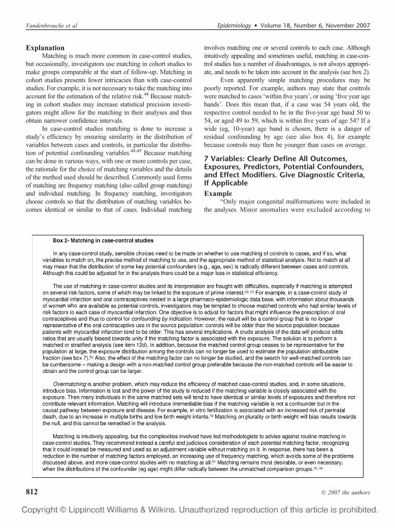
ExplanationMatching is much more common in case-control studies,

but occasionally, investigators use matching in cohort studies tomake groups comparable at the start of follow-up. Matching incohort studies presents fewer intricacies than with case-controlstudies. For example, it is not necessary to take the matching intoaccount for the estimation of the relative risk.48 Because match-ing in cohort studies may increase statistical precision investi-gators might allow for the matching in their analyses and thusobtain narrower confidence intervals.

In case-control studies matching is done to increase astudy’s efficiency by ensuring similarity in the distribution ofvariables between cases and controls, in particular the distribu-tion of potential confounding variables.48,49 Because matchingcan be done in various ways, with one or more controls per case,the rationale for the choice of matching variables and the detailsof the method used should be described. Commonly used formsof matching are frequency matching (also called group matching)and individual matching. In frequency matching, investigatorschoose controls so that the distribution of matching variables be-comes identical or similar to that of cases. Individual matching

involves matching one or several controls to each case. Althoughintuitively appealing and sometimes useful, matching in case-con-trol studies has a number of disadvantages, is not always appropri-ate, and needs to be taken into account in the analysis (see box 2).

Even apparently simple matching procedures may bepoorly reported. For example, authors may state that controlswere matched to cases ‘within five years’, or using ‘five year agebands’. Does this mean that, if a case was 54 years old, therespective control needed to be in the five-year age band 50 to54, or aged 49 to 59, which is within five years of age 54? If awide (eg, 10-year) age band is chosen, there is a danger ofresidual confounding by age (see also box 4), for examplebecause controls may then be younger than cases on average.

7 Variables: Clearly Define All Outcomes,Exposures, Predictors, Potential Confounders,and Effect Modifiers. Give Diagnostic Criteria,If ApplicableExample

“Only major congenital malformations were included inthe analyses. Minor anomalies were excluded according to



the exclusion list of European Registration of CongenitalAnomalies (EUROCAT). If a child had more than onemajor congenital malformation of one organ system, thosemalformations were treated as one outcome in the analysesby organ system (. . .). In the statistical analyses, factorsconsidered potential confounders were maternal age atdelivery and number of previous parities. Factors consid-ered potential effect modifiers were maternal age at reim-bursement for antiepileptic medication and maternal age atdelivery.”55

ExplanationAuthors should define all variables considered for and

included in the analysis, including outcomes, exposures,predictors, potential confounders and potential effect modi-fiers. Disease outcomes require adequately detailed descrip-tion of the diagnostic criteria. This applies to criteria for casesin a case-control study, disease events during follow-up in acohort study and prevalent disease in a cross-sectional study.Clear definitions and steps taken to adhere to them areparticularly important for any disease condition of primaryinterest in the study.

For some studies, ‘determinant’ or ‘predictor’ may beappropriate terms for exposure variables and outcomes maybe called ‘endpoints’. In multivariable models, authors some-times use ‘dependent variable’ for an outcome and ‘indepen-dent variable’ or ‘explanatory variable’ for exposure andconfounding variables. The latter is not precise as it does notdistinguish exposures from confounders.

If many variables have been measured and included inexploratory analyses in an early discovery phase, considerproviding a list with details on each variable in an appendix,additional table or separate publication. Of note, the Interna-tional Journal of Epidemiology recently launched a newsection with ‘cohort profiles’, that includes detailed informa-tion on what was measured at different points in time inparticular studies.56,57 Finally, we advise that authors declareall ‘candidate variables’ considered for statistical analysis,rather than selectively reporting only those included in thefinal models (see also item 16a).58,59

8 Data Sources/Measurement: For Each Variableof Interest Give Sources of Data and Details ofMethods of Assessment (Measurement).Describe Comparability of Assessment MethodsIf There is More Than One GroupExample 1

“Total caffeine intake was calculated primarily using USDepartment of Agriculture food composition sources. In thesecalculations, it was assumed that the content of caffeine was 137mg per cup of coffee, 47 mg per cup of tea, 46 mg per can orbottle of cola beverage, and 7 mg per serving of chocolatecandy. This method of measuring (caffeine) intake was shown tobe valid in both the NHS I cohort and a similar cohort study of

male health professionals (. . .). Self-reported diagnosis of hy-pertension was found to be reliable in the NHS I cohort.”60

Example 2“Cases and controls were always analyzed together in

the same batch and laboratory personnel were unable todistinguish among cases and controls.”61

ExplanationThe way in which exposures, confounders and out-

comes were measured affects the reliability and validity of astudy. Measurement error and misclassification of exposuresor outcomes can make it more difficult to detect cause-effectrelationships, or may produce spurious relationships. Error inmeasurement of potential confounders can increase the risk ofresidual confounding.62,63 It is helpful, therefore, if authorsreport the findings of any studies of the validity or reliabilityof assessments or measurements, including details of thereference standard that was used. Rather than simply citingvalidation studies (as in the first example), we advise thatauthors give the estimated validity or reliability, which canthen be used for measurement error adjustment or sensitivityanalyses (see items 12e and 17).

In addition, it is important to know if groups beingcompared differed with respect to the way in which the datawere collected. This may be important for laboratory exam-inations (as in the second example) and other situations. Forinstance, if an interviewer first questions all the cases andthen the controls, or vice versa, bias is possible because of thelearning curve; solutions such as randomizing the order ofinterviewing may avoid this problem. Information bias mayalso arise if the compared groups are not given the samediagnostic tests or if one group receives more tests of thesame kind than another (see also item 9).

9 Bias: Describe Any Efforts to AddressPotential Sources of BiasExample 1

“In most case-control studies of suicide, the controlgroup comprises living individuals but we decided to have acontrol group of people who had died of other causes (. . .).With a control group of deceased individuals, the sources ofinformation used to assess risk factors are informants whohave recently experienced the death of a family member orclose associate - and are therefore more comparable to thesources of information in the suicide group than if livingcontrols were used.”64

Example 2“Detection bias could influence the association be-

tween Type 2 diabetes mellitus (T2DM) and primaryopen-angle glaucoma (POAG) if women with T2DM wereunder closer ophthalmic surveillance than women withoutthis condition. We compared the mean number of eye



examinations reported by women with and without diabe-tes. We also recalculated the relative risk for POAG withadditional control for covariates associated with morecareful ocular surveillance (a self-report of cataract, mac-ular degeneration, number of eye examinations, and num-ber of physical examinations).”65

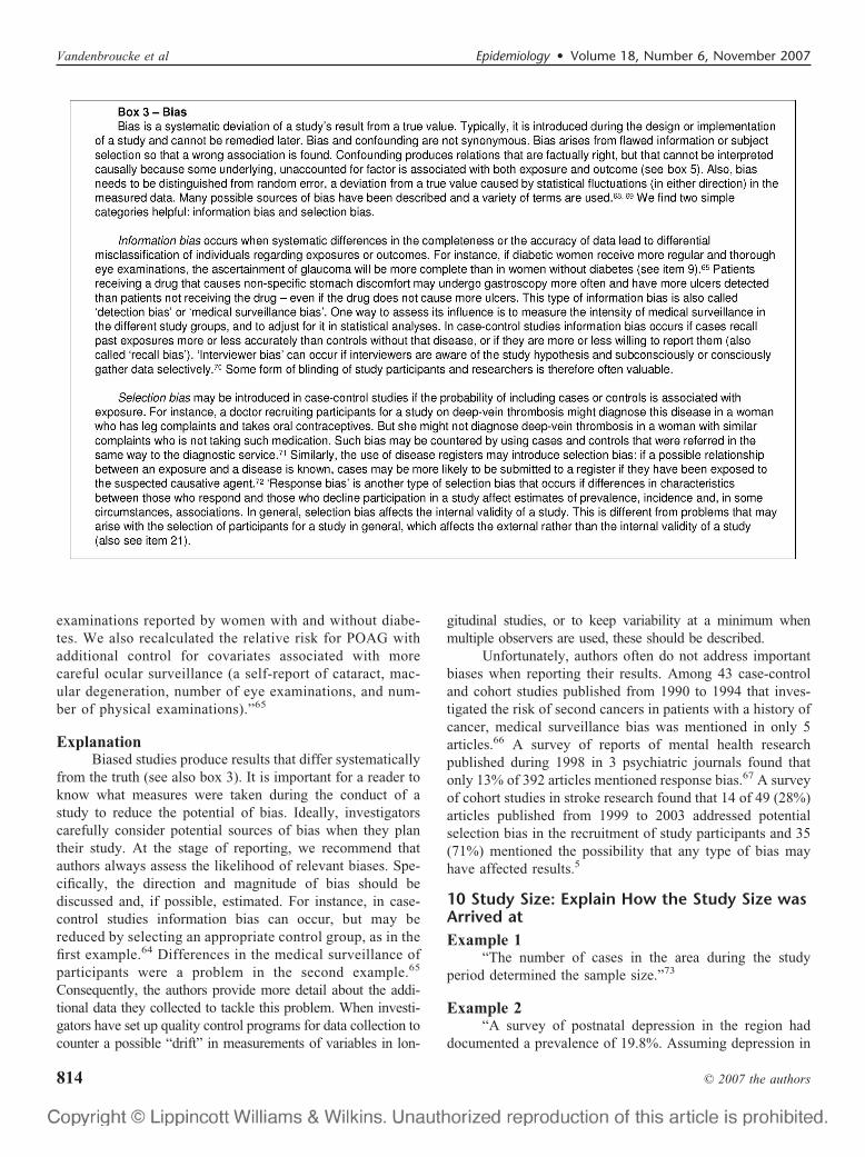
ExplanationBiased studies produce results that differ systematically

from the truth (see also box 3). It is important for a reader toknow what measures were taken during the conduct of astudy to reduce the potential of bias. Ideally, investigatorscarefully consider potential sources of bias when they plantheir study. At the stage of reporting, we recommend thatauthors always assess the likelihood of relevant biases. Spe-cifically, the direction and magnitude of bias should bediscussed and, if possible, estimated. For instance, in case-control studies information bias can occur, but may bereduced by selecting an appropriate control group, as in thefirst example.64 Differences in the medical surveillance ofparticipants were a problem in the second example.65

Consequently, the authors provide more detail about the addi-tional data they collected to tackle this problem. When investi-gators have set up quality control programs for data collection tocounter a possible “drift” in measurements of variables in lon-

gitudinal studies, or to keep variability at a minimum whenmultiple observers are used, these should be described.

Unfortunately, authors often do not address importantbiases when reporting their results. Among 43 case-controland cohort studies published from 1990 to 1994 that inves-tigated the risk of second cancers in patients with a history ofcancer, medical surveillance bias was mentioned in only 5articles.66 A survey of reports of mental health researchpublished during 1998 in 3 psychiatric journals found thatonly 13% of 392 articles mentioned response bias.67 A surveyof cohort studies in stroke research found that 14 of 49 (28%)articles published from 1999 to 2003 addressed potentialselection bias in the recruitment of study participants and 35(71%) mentioned the possibility that any type of bias mayhave affected results.5

10 Study Size: Explain How the Study Size wasArrived atExample 1

“The number of cases in the area during the studyperiod determined the sample size.”73

Example 2“A survey of postnatal depression in the region had

documented a prevalence of 19.8%. Assuming depression in



mothers with normal weight children to be 20% and an oddsratio of 3 for depression in mothers with a malnourished childwe needed 72 case-control sets (one case to one control) withan 80% power and 5% significance.”74

ExplanationA study should be large enough to obtain a point

estimate with a sufficiently narrow confidence interval tomeaningfully answer a research question. Large samplesare needed to distinguish a small association from noassociation. Small studies often provide valuable informa-tion, but wide confidence intervals may indicate that theycontribute less to current knowledge in comparison withstudies providing estimates with narrower confidence in-tervals. Also, small studies that show ‘interesting’ or‘statistically significant’ associations are published morefrequently than small studies that do not have ‘significant’findings. While these studies may provide an early signalin the context of discovery, readers should be informed oftheir potential weaknesses.

The importance of sample size determination in obser-vational studies depends on the context. If an analysis isperformed on data that were already available for otherpurposes, the main question is whether the analysis of thedata will produce results with sufficient statistical precision tocontribute substantially to the literature, and sample sizeconsiderations will be informal. Formal, a priori calculationof sample size may be useful when planning a new study.75,76

Such calculations are associated with more uncertainty thanimplied by the single number that is generally produced. Forexample, estimates of the rate of the event of interest or otherassumptions central to calculations are commonly imprecise,if not guesswork.77 The precision obtained in the final anal-ysis can often not be determined beforehand because it willbe reduced by inclusion of confounding variables in multi-variable analyses,78 the degree of precision with which keyvariables can be measured,79 and the exclusion of someindividuals.

Few epidemiological studies explain or report deliber-ations about sample size.4,5 We encourage investigators toreport pertinent formal sample size calculations if they weredone. In other situations they should indicate the consider-ations that determined the study size (eg, a fixed availablesample, as in the first example above). If the observationalstudy was stopped early when statistical significance wasachieved, readers should be told. Do not bother readers withpost hoc justifications for study size or retrospective powercalculations.77 From the point of view of the reader, confi-dence intervals indicate the statistical precision that wasultimately obtained. It should be realized that confidenceintervals reflect statistical uncertainty only, and not all uncer-tainty that may be present in a study (see item 20).

11 Quantitative Variables: Explain HowQuantitative Variables were Handled in theAnalyses. If Applicable, Describe WhichGroupings Were Chosen, and WhyExample

“Patients with a Glasgow Coma Scale (GCS) less than8 are considered to be seriously injured. A GCS of 9 or moreindicates less serious brain injury. We examined the associ-ation of GCS in these two categories with the occurrence ofdeath within 12 months from injury.”80

ExplanationInvestigators make choices regarding how to collect

and analyse quantitative data about exposures, effect modi-fiers and confounders. For example, they may group a con-tinuous exposure variable to create a new categorical variable(see box 4). Grouping choices may have important conse-quences for later analyses.81,82 We advise that authors explainwhy and how they grouped quantitative data, including thenumber of categories, the cut-points, and category mean ormedian values. Whenever data are reported in tabular form,the counts of cases, controls, persons at risk, person-time atrisk, etc. should be given for each category. Tables should notconsist solely of effect-measure estimates or results of modelfitting.

Investigators might model an exposure as continuous inorder to retain all the information. In making this choice, oneneeds to consider the nature of the relationship of the expo-sure to the outcome. As it may be wrong to assume a linearrelation automatically, possible departures from linearityshould be investigated. Authors could mention alternativemodels they explored during analyses (eg, using log trans-formation, quadratic terms or spline functions). Several meth-ods exist for fitting a nonlinear relation between the exposureand outcome.82–84 Also, it may be informative to present bothcontinuous and grouped analyses for a quantitative exposureof prime interest.

In a recent survey, two thirds of epidemiological pub-lications studied quantitative exposure variables.4 In 42 of 50articles (84%) exposures were grouped into several orderedcategories, but often without any stated rationale for thechoices made. Fifteen articles used linear associations tomodel continuous exposure but only 2 reported checking forlinearity. In another survey, of the psychological literature,dichotomization was justified in only 22 of 110 articles(20%).85

12 Statistical Methods:12 (a) Describe all statistical methods, including those

used to control for confounding.

Example“The adjusted relative risk was calculated using the

Mantel-Haenszel technique, when evaluating if confounding



by age or gender was present in the groups compared. The95% confidence interval (CI) was computed around the ad-justed relative risk, using the variance according to Greenlandand Robins and Robins et al.”93

ExplanationIn general, there is no one correct statistical analysis

but, rather, several possibilities that may address the samequestion, but make different assumptions. Regardless, inves-tigators should pre-determine analyses at least for the primarystudy objectives in a study protocol. Often additional analy-ses are needed, either instead of, or as well as, those origi-nally envisaged, and these may sometimes be motivated bythe data. When a study is reported, authors should tell readerswhether particular analyses were suggested by data inspec-tion. Even though the distinction between pre-specified andexploratory analyses may sometimes be blurred, authorsshould clarify reasons for particular analyses.

If groups being compared are not similar with regard tosome characteristics, adjustment should be made for possibleconfounding variables by stratification or by multivariableregression (see box 5).94 Often, the study design determineswhich type of regression analysis is chosen. For instance, Coxproportional hazard regression is commonly used in cohortstudies,95 whereas logistic regression is often the method ofchoice in case-control studies.96,97 Analysts should fullydescribe specific procedures for variable selection and not

only present results from the final model.98,99 If modelcomparisons are made to narrow down a list of potentialconfounders for inclusion in a final model, this processshould be described. It is helpful to tell readers if one or twocovariates are responsible for a great deal of the apparentconfounding in a data analysis. Other statistical analyses suchas imputation procedures, data transformation, and calcula-tions of attributable risks should also be described. Nonstand-ard or novel approaches should be referenced and the statis-tical software used reported. As a guiding principle, weadvise statistical methods be described “with enough detail toenable a knowledgeable reader with access to the originaldata to verify the reported results.”100

In an empirical study, only 93 of 169 articles (55%)reporting adjustment for confounding clearly stated howcontinuous and multi-category variables were entered intothe statistical model.101 Another study found that among67 articles in which statistical analyses were adjusted forconfounders, it was mostly unclear how confounders werechosen.4

12 (b) Describe Any Methods Used to ExamineSubgroups and InteractionsExample

“Sex differences in susceptibility to the 3 lifestyle-relatedrisk factors studied were explored by testing for biologicalinteraction according to Rothman: a new composite variable



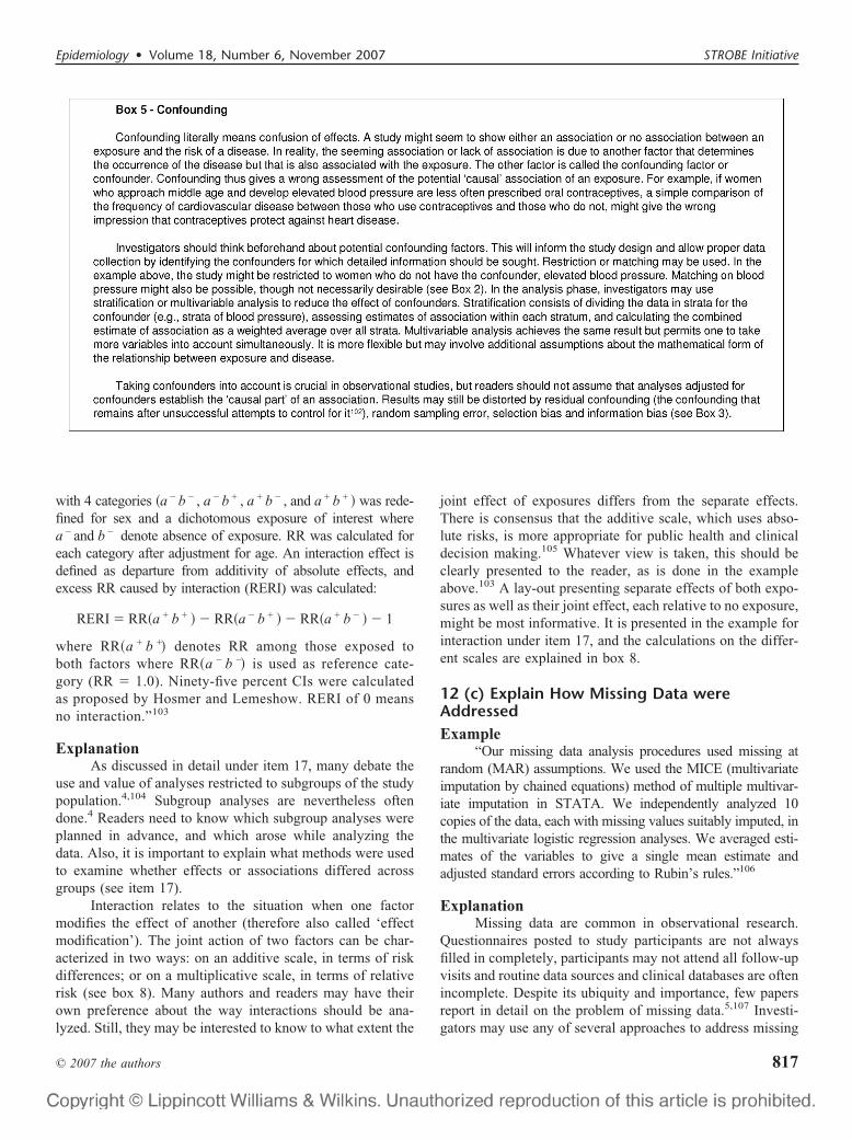
with 4 categories �a � b � , a � b � , a � b � , and a � b � � was rede-fined for sex and a dichotomous exposure of interest wherea � and b � denote absence of exposure. RR was calculated foreach category after adjustment for age. An interaction effect isdefined as departure from additivity of absolute effects, andexcess RR caused by interaction (RERI) was calculated:

RERI � RR�a � b � � � RR�a � b � � � RR�a � b � � � 1

where RR�a � b �� denotes RR among those exposed toboth factors where RR�a � b �� is used as reference cate-gory (RR � 1.0). Ninety-five percent CIs were calculatedas proposed by Hosmer and Lemeshow. RERI of 0 meansno interaction.”103

ExplanationAs discussed in detail under item 17, many debate the

use and value of analyses restricted to subgroups of the studypopulation.4,104 Subgroup analyses are nevertheless oftendone.4 Readers need to know which subgroup analyses wereplanned in advance, and which arose while analyzing thedata. Also, it is important to explain what methods were usedto examine whether effects or associations differed acrossgroups (see item 17).

Interaction relates to the situation when one factormodifies the effect of another (therefore also called ‘effectmodification’). The joint action of two factors can be char-acterized in two ways: on an additive scale, in terms of riskdifferences; or on a multiplicative scale, in terms of relativerisk (see box 8). Many authors and readers may have theirown preference about the way interactions should be ana-lyzed. Still, they may be interested to know to what extent the

joint effect of exposures differs from the separate effects.There is consensus that the additive scale, which uses abso-lute risks, is more appropriate for public health and clinicaldecision making.105 Whatever view is taken, this should beclearly presented to the reader, as is done in the exampleabove.103 A lay-out presenting separate effects of both expo-sures as well as their joint effect, each relative to no exposure,might be most informative. It is presented in the example forinteraction under item 17, and the calculations on the differ-ent scales are explained in box 8.

12 (c) Explain How Missing Data wereAddressedExample

“Our missing data analysis procedures used missing atrandom (MAR) assumptions. We used the MICE (multivariateimputation by chained equations) method of multiple multivar-iate imputation in STATA. We independently analyzed 10copies of the data, each with missing values suitably imputed, inthe multivariate logistic regression analyses. We averaged esti-mates of the variables to give a single mean estimate andadjusted standard errors according to Rubin’s rules.”106

ExplanationMissing data are common in observational research.

Questionnaires posted to study participants are not alwaysfilled in completely, participants may not attend all follow-upvisits and routine data sources and clinical databases are oftenincomplete. Despite its ubiquity and importance, few papersreport in detail on the problem of missing data.5,107 Investi-gators may use any of several approaches to address missing



data. We describe some strengths and limitations of variousapproaches in box 6. We advise that authors report thenumber of missing values for each variable of interest (ex-posures, outcomes, confounders) and for each step in theanalysis. Authors should give reasons for missing values ifpossible, and indicate how many individuals were excludedbecause of missing data when describing the flow of partic-ipants through the study (see also item 13). For analyses thataccount for missing data, authors should describe the natureof the analysis (eg, multiple imputation) and the assumptionsthat were made (eg, missing at random, see box 6).

12 (d) Cohort Study: If Applicable, DescribeHow Loss to Follow-up was AddressedExample

“In treatment programs with active follow-up, thoselost to follow-up and those followed-up at 1 year hadsimilar baseline CD4 cell counts (median 115 cells per �Land 123 cells per �L), whereas patients lost to follow-up inprograms with no active follow-up procedures had consid-erably lower CD4 cell counts than those followed-up(median 64 cells per �L and 123 cells per �L). (. . .)Treatment programs with passive follow-up were excludedfrom subsequent analyses.”116

ExplanationCohort studies are analyzed using life table methods or

other approaches that are based on the person-time of fol-

low-up and time to developing the disease of interest. Amongindividuals who remain free of the disease at the end of theirobservation period, the amount of follow-up time is assumedto be unrelated to the probability of developing the outcome.This will be the case if follow-up ends on a fixed date or at aparticular age. Loss to follow-up occurs when participantswithdraw from a study before that date. This may hamper thevalidity of a study if loss to follow-up occurs selectively inexposed individuals, or in persons at high risk of developingthe disease (�informative censoring’). In the example above,patients lost to follow-up in treatment programs with noactive follow-up had fewer CD4 helper cells than thoseremaining under observation and were therefore at higher riskof dying.116

It is important to distinguish persons who reach theend of the study from those lost to follow-up. Unfortu-nately, statistical software usually does not distinguishbetween the two situations: in both cases follow-up time isautomatically truncated (‘censored’) at the end of theobservation period. Investigators therefore need to decide,ideally at the stage of planning the study, how they willdeal with loss to follow-up. When few patients are lost,investigators may either exclude individuals with incom-plete follow-up, or treat them as if they withdrew alive ateither the date of loss to follow-up or the end of the study.We advise authors to report how many patients were lost tofollow-up and what censoring strategies they used.



12 (d) Case-control Study: If Applicable,Explain How Matching of Cases and Controlswas AddressedExample

“We used McNemar’s test, paired t test, and conditionallogistic regression analysis to compare dementia patients withtheir matched controls for cardiovascular risk factors, theoccurrence of spontaneous cerebral emboli, carotid disease,and venous to arterial circulation shunt.”117

ExplanationIn individually matched case-control studies a crude

analysis of the odds ratio, ignoring the matching, usuallyleads to an estimation that is biased towards unity (see box 2).A matched analysis is therefore often necessary. This canintuitively be understood as a stratified analysis: each case isseen as one stratum with his or her set of matched controls.The analysis rests on considering whether the case is moreoften exposed than the controls, despite having made themalike regarding the matching variables. Investigators can dosuch a stratified analysis using the Mantel-Haenszel methodon a ‘matched’ 2 by 2 table. In its simplest form the odds ratiobecomes the ratio of pairs that are discordant for the exposurevariable. If matching was done for variables like age and sexthat are universal attributes, the analysis needs not retain theindividual, person-to-person matching: a simple analysis incategories of age and sex is sufficient.50 For other matchingvariables, such as neighborhood, sibship, or friendship, how-ever, each matched set should be considered its own stratum.

In individually matched studies, the most widely usedmethod of analysis is conditional logistic regression, in whicheach case and their controls are considered together. The con-ditional method is necessary when the number of controls variesamong cases, and when, in addition to the matching variables,other variables need to be adjusted for. To allow readers to judgewhether the matched design was appropriately taken into ac-count in the analysis, we recommend that authors describe indetail what statistical methods were used to analyse the data. Iftaking the matching into account does have little effect on theestimates, authors may choose to present an unmatched analysis.

12 (d) Cross-sectional Study: If Applicable,Describe Analytical Methods Taking Account ofSampling StrategyExample

“The standard errors (SE) were calculated using theTaylor expansion method to estimate the sampling errors ofestimators based on the complex sample design. (. . .) Theoverall design effect for diastolic blood pressure was found tobe 1.9 for men and 1.8 for women and, for systolic bloodpressure, it was 1.9 for men and 2.0 for women.”118

ExplanationMost cross-sectional studies use a pre-specified sam-

pling strategy to select participants from a source population.

Sampling may be more complex than taking a simple randomsample, however. It may include several stages and clusteringof participants (eg, in districts or villages). Proportionate strati-fication may ensure that subgroups with a specific characteristicare correctly represented. Disproportionate stratification may beuseful to over-sample a subgroup of particular interest.

An estimate of association derived from a complexsample may be more or less precise than that derived from asimple random sample. Measures of precision such as stan-dard error or confidence interval should be corrected usingthe design effect, a ratio measure that describes how muchprecision is gained or lost if a more complex samplingstrategy is used instead of simple random sampling.119 Mostcomplex sampling techniques lead to a decrease of precision,resulting in a design effect greater than 1.

We advise that authors clearly state the method used toadjust for complex sampling strategies so that readers mayunderstand how the chosen sampling method influenced theprecision of the obtained estimates. For instance, with clus-tered sampling, the implicit trade-off between easier datacollection and loss of precision is transparent if the designeffect is reported. In the example, the calculated designeffects of 1.9 for men indicates that the actual sample sizewould need to be 1.9 times greater than with simple randomsampling for the resulting estimates to have equal precision.

12 (e) Describe any Sensitivity AnalysesExample

“Because we had a relatively higher proportion of‘missing’ dead patients with insufficient data (38/148 �25.7%) as compared to live patients (15/437 � 3.4%) (. . .),it is possible that this might have biased the results. We have,therefore, carried out a sensitivity analysis. We have assumedthat the proportion of women using oral contraceptives in thestudy group applies to the whole (19.1% for dead, and 11.4%for live patients), and then applied two extreme scenarios:either all the exposed missing patients used second generationpills or they all used third-generation pills.”120

ExplanationSensitivity analyses are useful to investigate whether or

not the main results are consistent with those obtained withalternative analysis strategies or assumptions.121 Issues thatmay be examined include the criteria for inclusion in analy-ses, the definitions of exposures or outcomes,122 which con-founding variables merit adjustment, the handling of missingdata,120,123 possible selection bias or bias from inaccurate orinconsistent measurement of exposure, disease and othervariables, and specific analysis choices, such as the treatmentof quantitative variables (see item 11). Sophisticated methodsare increasingly used to simultaneously model the influenceof several biases or assumptions.124–126

In 1959 Cornfield et al famously showed that a relativerisk of 9 for cigarette smoking and lung cancer was extremely



unlikely to be due to any conceivable confounder, since theconfounder would need to be at least nine times as prevalentin smokers as in non-smokers.127 This analysis did not ruleout the possibility that such a factor was present, but it dididentify the prevalence such a factor would need to have. Thesame approach was recently used to identify plausible con-founding factors that could explain the association betweenchildhood leukemia and living near electric power lines.128

More generally, sensitivity analyses can be used to identifythe degree of confounding, selection bias, or information biasrequired to distort an association. One important, perhapsunder recognized, use of sensitivity analysis is when a studyshows little or no association between an exposure and anoutcome and it is plausible that confounding or other biasestoward the null are present.

RESULTSThe Results section should give a factual account of

what was found, from the recruitment of study participants,the description of the study population to the main results andancillary analyses. It should be free of interpretations anddiscursive text reflecting the authors’ views and opinions.

13 Participants:13(a) Report the Numbers of Individuals atEach Stage of the Study—eg, NumbersPotentially Eligible, Examined for Eligibility,Confirmed Eligible, Included in the Study,Completing Follow-up, and AnalyzedExample

“Of the 105 freestanding bars and taverns sampled, 13establishments were no longer in business and 9 were locatedin restaurants, leaving 83 eligible businesses. In 22 cases, theowner could not be reached by telephone despite 6 or moreattempts. The owners of 36 bars declined study participation.(. . .) The 25 participating bars and taverns employed 124bartenders, with 67 bartenders working at least 1 weeklydaytime shift. Fifty-four of the daytime bartenders (81%)completed baseline interviews and spirometry; 53 of thesesubjects (98%) completed follow-up.”129

ExplanationDetailed information on the process of recruiting study

participants is important for several reasons. Those includedin a study often differ in relevant ways from the targetpopulation to which results are applied. This may result inestimates of prevalence or incidence that do not reflect theexperience of the target population. For example, people whoagreed to participate in a postal survey of sexual behaviourattended church less often, had less conservative sexualattitudes and earlier age at first sexual intercourse, and weremore likely to smoke cigarettes and drink alcohol than peoplewho refused.130 These differences suggest that postal surveysmay overestimate sexual liberalism and activity in the popu-lation. Such response bias (see box 3) can distort exposure-

disease associations if associations differ between those eli-gible for the study and those included in the study. As anotherexample, the association between young maternal age andleukemia in offspring, which has been observed in somecase-control studies,131,132 was explained by differential par-ticipation of young women in case and control groups. Youngwomen with healthy children were less likely to participatethan those with unhealthy children.133 Although low partici-pation does not necessarily compromise the validity of astudy, transparent information on participation and reasonsfor nonparticipation is essential. Also, as there are no univer-sally agreed definitions for participation, response or fol-low-up rates, readers need to understand how authors calcu-lated such proportions.134

Ideally, investigators should give an account of the num-bers of individuals considered at each stage of recruiting studyparticipants, from the choice of a target population to theinclusion of participants’ data in the analysis. Depending on thetype of study, this may include the number of individualsconsidered to be potentially eligible, the number assessed foreligibility, the number found to be eligible, the number includedin the study, the number examined, the number followed up andthe number included in the analysis. Information on differentsampling units may be required, if sampling of study participantsis carried out in two or more stages as in the example above(multistage sampling). In case-control studies, we advise thatauthors describe the flow of participants separately for case andcontrol groups.135 Controls can sometimes be selected fromseveral sources, including, for example, hospitalized patientsand community dwellers. In this case, we recommend a separateaccount of the numbers of participants for each type of controlgroup. Olson and colleagues proposed useful reporting guide-lines for controls recruited through random-digit dialling andother methods.136

A recent survey of epidemiological studies published in10 general epidemiology, public health and medical journalsfound that some information regarding participation wasprovided in 47 of 107 case-control studies (59%), 49 of 154cohort studies (32%), and 51 of 86 cross-sectional studies(59%).137 Incomplete or absent reporting of participation andnonparticipation in epidemiological studies was also docu-mented in two other surveys of the literature.4,5 Finally, thereis evidence that participation in epidemiological studies mayhave declined in recent decades,137,138 which underscores theneed for transparent reporting.139

13(b) Give Reasons for Non-participation atEach StageExample

“The main reasons for nonparticipation were the par-ticipant was too ill or had died before interview (cases 30%,controls �1%), nonresponse (cases 2%, controls 21%), re-fusal (cases 10%, controls 29%), and other reasons (refusal



by consultant or general practitioner, non-English speaking,mental impairment) (cases 7%, controls 5%).”140

ExplanationExplaining the reasons why people no longer partici-

pated in a study or why they were excluded from statisticalanalyses helps readers judge whether the study populationwas representative of the target population and whether biaswas possibly introduced. For example, in a cross-sectionalhealth survey, non-participation due to reasons unlikely to berelated to health status (for example, the letter of invitation was

not delivered because of an incorrect address) will affectthe precision of estimates but will probably not introducebias. Conversely, if many individuals opt out of the surveybecause of illness, or perceived good health, results mayunderestimate or overestimate the prevalence of ill healthin the population.

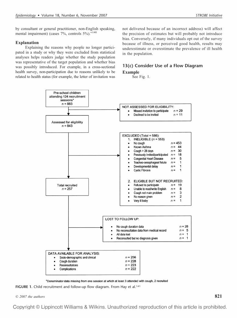
13(c) Consider Use of a Flow DiagramExample

See Fig. 1.

FIGURE 1. Child recruitment and follow-up flow diagram. From Hay et al.141



ExplanationAn informative and well-structured flow diagram can

readily and transparently convey information that might oth-erwise require a lengthy description,142 as in the exampleabove. The diagram may usefully include the main results,such as the number of events for the primary outcome. Whilewe recommend the use of a flow diagram, particularly forcomplex observational studies, we do not propose a specificformat for the diagram.

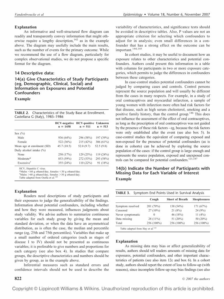
14 Descriptive data:14(a) Give Characteristics of Study Participants(eg, Demographic, Clinical, Social) andInformation on Exposures and PotentialConfoundersExample

ExplanationReaders need descriptions of study participants and

their exposures to judge the generalizability of the findings.Information about potential confounders, including whetherand how they were measured, influences judgments aboutstudy validity. We advise authors to summarize continuousvariables for each study group by giving the mean andstandard deviation, or when the data have an asymmetricaldistribution, as is often the case, the median and percentilerange (eg, 25th and 75th percentiles). Variables that make upa small number of ordered categories (such as stages ofdisease I to IV) should not be presented as continuousvariables; it is preferable to give numbers and proportions foreach category (see also box 4). In studies that comparegroups, the descriptive characteristics and numbers should begiven by group, as in the example above.

Inferential measures such as standard errors andconfidence intervals should not be used to describe the

variability of characteristics, and significance tests shouldbe avoided in descriptive tables. Also, P values are not anappropriate criterion for selecting which confounders toadjust for in analysis; even small differences in a con-founder that has a strong effect on the outcome can beimportant.144,145

In cohort studies, it may be useful to document how anexposure relates to other characteristics and potential con-founders. Authors could present this information in a tablewith columns for participants in two or more exposure cate-gories, which permits to judge the differences in confoundersbetween these categories.

In case-control studies potential confounders cannot bejudged by comparing cases and controls. Control personsrepresent the source population and will usually be differentfrom the cases in many respects. For example, in a study oforal contraceptives and myocardial infarction, a sample ofyoung women with infarction more often had risk factors forthat disease, such as high serum cholesterol, smoking and apositive family history, than the control group.146 This doesnot influence the assessment of the effect of oral contraceptives,as long as the prescription of oral contraceptives was not guidedby the presence of these risk factors - eg, because the risk factorswere only established after the event (see also box 5). Incase-control studies the equivalent of comparing exposed andnon-exposed for the presence of potential confounders (as isdone in cohorts) can be achieved by exploring the sourcepopulation of the cases: if the control group is large enough andrepresents the source population, exposed and unexposed con-trols can be compared for potential confounders.121,147

14(b) Indicate the Number of Participants withMissing Data for Each Variable of InterestExample

ExplanationAs missing data may bias or affect generalizability of

results, authors should tell readers amounts of missing data forexposures, potential confounders, and other important charac-teristics of patients (see also item 12c and box 6). In a cohortstudy, authors should report the extent of loss to follow-up (withreasons), since incomplete follow-up may bias findings (see also

TABLE 2. Characteristics of the Study Base at Enrollment.Castellana G (Italy), 1985–1986

HCV-negativen � 1458

HCV-positiven � 511

Unknownn � 513

Sex (%)

Male 936 (64%) 296 (58%) 197 (39%)

Female 522 (36%) 215 (42%) 306 (61%)

Mean age at enrolment (SD) 45.7 (10.5) 52.0 (9.7) 52.5 (9.8)

Daily alcohol intake (%)

None 250 (17%) 129 (25%) 119 (24%)

Moderate* 853 (59%) 272 (53%) 293 (58%)

Excessive† 355 (24%) 110 (22%) 91 (18%)

HCV, Hepatitis C virus.*Males �60 g ethanol/day, females �30 g ethanol/day.†Males �60 g ethanol/day, females �30 g ethanol/day.Table adapted from Osella et al.143

TABLE 3. Symptom End Points Used in Survival Analysis

Cough Short of Breath Sleeplessness

Symptom resolved 201 (79%) 138 (54%) 171 (67%)

Censored 27 (10%) 21 (8%) 24 (9%)

Never symptomatic 0 46 (18%) 11 (4%)

Data missing 28 (11%) 51 (20%) 50 (20%)

Total 256 (100%) 256 (100%) 256 (100%)

Table adapted from Hay et al.141



items 12d and 13).148 We advise authors to use their tables andfigures to enumerate amounts of missing data.

14(c) Cohort Study: Summarise Follow-upTime—eg, Average and Total AmountExample

“During the 4366 person-years of follow-up (median5.4, maximum 8.3 years), 265 subjects were diagnosed ashaving dementia, including 202 with Alzheimer’s dis-ease.”149

ExplanationReaders need to know the duration and extent of fol-

low-up for the available outcome data. Authors can present asummary of the average follow-up with either the mean ormedian follow-up time or both. The mean allows a reader tocalculate the total number of person-years by multiplying itwith the number of study participants. Authors also maypresent minimum and maximum times or percentiles of thedistribution to show readers the spread of follow-up times.They may report total person-years of follow-up or someindication of the proportion of potential data that was cap-tured.148 All such information may be presented separatelyfor participants in two or more exposure categories. Almosthalf of 132 articles in cancer journals (mostly cohort studies)did not give any summary of length of follow-up.37

15 Outcome Data:Cohort Study: Report Numbers of OutcomeEvents or Summary Measures Over TimeExample

Case-control Study: Report Numbers in EachExposure Category, or Summary Measures ofExposureExample

Cross-sectional Study: Report Numbers ofOutcome Events or Summary MeasuresExample

ExplanationBefore addressing the possible association between

exposures (risk factors) and outcomes, authors should reportrelevant descriptive data. It may be possible and meaningfulto present measures of association in the same table thatpresents the descriptive data (see item 14a). In a cohort study

TABLE 4. Rates of HIV-1 Seroconversion by SelectedSocio-Demographic Variables: 1990-1993

Variable Person-yearsNo.

Seroconverted

Rate/1000Person-years

(95% CI)

Calendar year

1990 2197.5 18 8.2 (4.4–12.0)

1991 3210.7 22 6.9 (4.0–9.7)

1992 3162.6 18 5.7 (3.1–8.3)

1993 2912.9 26 8.9 (5.5–12.4)

1994 1104.5 5 4.5 (0.6–8.5)

Tribe

Bagandan 8433.1 48 5.7 (4.1–7.3)

Other Ugandan 578.4 9 15.6 (5.4–25.7)

Rwandese 2318.6 16 6.9 (3.5–10.3)

Other tribe 866.0 12 13.9 (6.0–21.7)

Religion

Muslim 3313.5 9 2.7 (0.9–4.5)

Other 8882.7 76 8.6 (6.6–10.5)

CI, confidence interval.Table adapted from Kengeya-Kayondo et al.150

TABLE 5. Exposure Among Liver Cirrhosis Cases andControls

Cases(n � 40)

Controls(n � 139)

Vinyl chloride monomer (cumulativeexposure: ppm � years)

�160 7 (18%) 38 (27%)

160–500 7 (18%) 40 (29%)

500–2500 9 (23%) 37 (27%)

�2500 17 (43%) 24 (17%)

Alcohol consumption (g/day)

�30 1 (3%) 82 (59%)

30–60 7 (18%) 46 (33%)

�60 32 (80%) 11 (8%)

HBsAG/HCV

Negative 33 (83%) 136 (98%)

Positive 7 (18%) 3 (2%)

HBsAG, hepatitis B surface antigen; HCV, hepatitis C virus Table adapted fromMastrangelo et al.151

TABLE 6. Prevalence of Current Asthma and DiagnosedHay Fever by Average Alternaria Alternata Antigen Level inthe Household

CategorizedAlternaria level*

Current Asthma Diagnosed Hay Fever

NPrevalence†

(95% CI) NPrevalence†

(95% CI)

1st tertile 40 4.8 (3.3–6.9) 93 16.4 (13.0–20.5)

2nd tertile 61 7.5 (5.2–10.6) 122 17.1 (12.8–22.5)

3rd tertile 73 8.7 (6.7–11.3) 93 15.2 (12.1–18.9)

1st tertile �3.90 �g/g; 2nd tertile 3.90–6.27 �g/g; 3rd tertile �6.28 �g/g.†Percentage (95% CI) weighted for the multistage sampling design of the National

Survey of Lead and Allergens in Housing.Table adapted from Salo et al.152



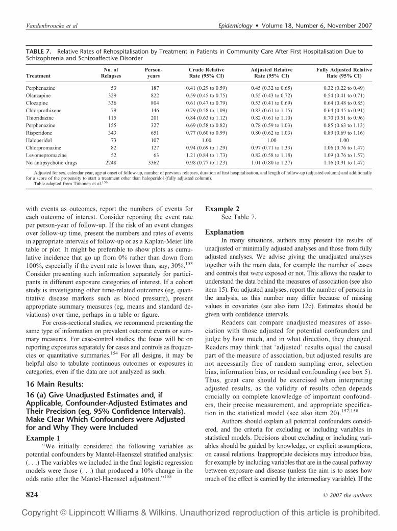
with events as outcomes, report the numbers of events foreach outcome of interest. Consider reporting the event rateper person-year of follow-up. If the risk of an event changesover follow-up time, present the numbers and rates of eventsin appropriate intervals of follow-up or as a Kaplan-Meier lifetable or plot. It might be preferable to show plots as cumu-lative incidence that go up from 0% rather than down from100%, especially if the event rate is lower than, say, 30%.153

Consider presenting such information separately for partici-pants in different exposure categories of interest. If a cohortstudy is investigating other time-related outcomes (eg, quan-titative disease markers such as blood pressure), presentappropriate summary measures (eg, means and standard de-viations) over time, perhaps in a table or figure.

For cross-sectional studies, we recommend presenting thesame type of information on prevalent outcome events or sum-mary measures. For case-control studies, the focus will be onreporting exposures separately for cases and controls as frequen-cies or quantitative summaries.154 For all designs, it may behelpful also to tabulate continuous outcomes or exposures incategories, even if the data are not analyzed as such.

16 Main Results:16 (a) Give Unadjusted Estimates and, ifApplicable, Confounder-Adjusted Estimates andTheir Precision (eg, 95% Confidence Intervals).Make Clear Which Confounders were Adjustedfor and Why They were IncludedExample 1

“We initially considered the following variables aspotential confounders by Mantel-Haenszel stratified analysis:(. . .) The variables we included in the final logistic regressionmodels were those (. . .) that produced a 10% change in theodds ratio after the Mantel-Haenszel adjustment.”155

Example 2See Table 7.

ExplanationIn many situations, authors may present the results of

unadjusted or minimally adjusted analyses and those from fullyadjusted analyses. We advise giving the unadjusted analysestogether with the main data, for example the number of casesand controls that were exposed or not. This allows the reader tounderstand the data behind the measures of association (see alsoitem 15). For adjusted analyses, report the number of persons inthe analysis, as this number may differ because of missingvalues in covariates (see also item 12c). Estimates should begiven with confidence intervals.

Readers can compare unadjusted measures of asso-ciation with those adjusted for potential confounders andjudge by how much, and in what direction, they changed.Readers may think that ‘adjusted’ results equal the causalpart of the measure of association, but adjusted results arenot necessarily free of random sampling error, selectionbias, information bias, or residual confounding (see box 5).Thus, great care should be exercised when interpretingadjusted results, as the validity of results often dependscrucially on complete knowledge of important confound-ers, their precise measurement, and appropriate specifica-tion in the statistical model (see also item 20).157,158

Authors should explain all potential confounders consid-ered, and the criteria for excluding or including variables instatistical models. Decisions about excluding or including vari-ables should be guided by knowledge, or explicit assumptions,on causal relations. Inappropriate decisions may introduce bias,for example by including variables that are in the causal pathwaybetween exposure and disease (unless the aim is to asses howmuch of the effect is carried by the intermediary variable). If the

TABLE 7. Relative Rates of Rehospitalisation by Treatment in Patients in Community Care After First Hospitalisation Due toSchizophrenia and Schizoaffective Disorder

TreatmentNo. of

RelapsesPerson-years

Crude RelativeRate (95% CI)

Adjusted RelativeRate (95% CI)

Fully Adjusted RelativeRate (95% CI)

Perphenazine 53 187 0.41 (0.29 to 0.59) 0.45 (0.32 to 0.65) 0.32 (0.22 to 0.49)

Olanzapine 329 822 0.59 (0.45 to 0.75) 0.55 (0.43 to 0.72) 0.54 (0.41 to 0.71)

Clozapine 336 804 0.61 (0.47 to 0.79) 0.53 (0.41 to 0.69) 0.64 (0.48 to 0.85)

Chlorprothixene 79 146 0.79 (0.58 to 1.09) 0.83 (0.61 to 1.15) 0.64 (0.45 to 0.91)

Thioridazine 115 201 0.84 (0.63 to 1.12) 0.82 (0.61 to 1.10) 0.70 (0.51 to 0.96)

Perphenazine 155 327 0.69 (0.58 to 0.82) 0.78 (0.59 to 1.03) 0.85 (0.63 to 1.13)

Risperidone 343 651 0.77 (0.60 to 0.99) 0.80 (0.62 to 1.03) 0.89 (0.69 to 1.16)

Haloperidol 73 107 1.00 1.00 1.00

Chlorpromazine 82 127 0.94 (0.69 to 1.29) 0.97 (0.71 to 1.33) 1.06 (0.76 to 1.47)

Levomepromazine 52 63 1.21 (0.84 to 1.73) 0.82 (0.58 to 1.18) 1.09 (0.76 to 1.57)

No antipsychotic drugs 2248 3362 0.98 (0.77 to 1.23) 1.01 (0.80 to 1.27) 1.16 (0.91 to 1.47)

Adjusted for sex, calendar year, age at onset of follow-up, number of previous relapses, duration of first hospitalisation, and length of follow-up (adjusted column) and additionallyfor a score of the propensity to start a treatment other than haloperidol (fully adjusted column).

Table adapted from Tiihonen et al.156



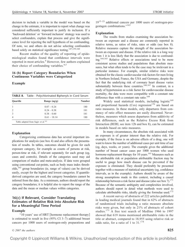
decision to include a variable in the model was based on thechange in the estimate, it is important to report what change wasconsidered sufficiently important to justify its inclusion. If a‘backward deletion’ or ‘forward inclusion’ strategy was used toselect confounders, explain that process and give the signifi-cance level for rejecting the null hypothesis of no confounding.Of note, we and others do not advise selecting confoundersbased solely on statistical significance testing.147,159,160

Recent studies of the quality of reporting of epide-miological studies found that confidence intervals werereported in most articles.4 However, few authors explainedtheir choice of confounding variables.4,5

16 (b) Report Category Boundaries WhenContinuous Variables were Categorized

Example

ExplanationCategorizing continuous data has several important im-

plications for analysis (see box 4) and also affects the presenta-tion of results. In tables, outcomes should be given for eachexposure category, for example as counts of persons at risk,person-time at risk, if relevant separately for each group (eg,cases and controls). Details of the categories used may aidcomparison of studies and meta-analysis. If data were groupedusing conventional cut-points, such as body mass index thresh-olds,162 group boundaries (ie, range of values) can be derivedeasily, except for the highest and lowest categories. If quantile-derived categories are used, the category boundaries cannot beinferred from the data. As a minimum, authors should report thecategory boundaries; it is helpful also to report the range of thedata and the mean or median values within categories.

16(c) If Relevant, Consider TranslatingEstimates of Relative Risk into Absolute Riskfor a Meaningful Time PeriodExample

“10 years’ use of HRT �hormone replacement therapyis estimated to result in five (95% CI 3–7) additional breastcancers per 1000 users of oestrogen-only preparations and

1915–23 additional cancers per 1000 users of oestrogen-pro-gestagen combinations.”163

ExplanationThe results from studies examining the association be-

tween an exposure and a disease are commonly reported inrelative terms, as ratios of risks, rates or odds (see box 8).Relative measures capture the strength of the association be-tween an exposure and disease. If the relative risk is a long wayfrom 1 it is less likely that the association is due to confound-ing.164,165 Relative effects or associations tend to be moreconsistent across studies and populations than absolute mea-sures, but what often tends to be the case may be irrelevant in aparticular instance. For example, similar relative risks wereobtained for the classic cardiovascular risk factors for men livingin Northern Ireland, France, the USA and Germany, despite thefact that the underlying risk of coronary heart disease variessubstantially between these countries.166,167 In contrast, in astudy of hypertension as a risk factor for cardiovascular diseasemortality, the data were more compatible with a constant ratedifference than with a constant rate ratio.168

Widely used statistical models, including logistic169

and proportional hazards (Cox) regression170 are based onratio measures. In these models, only departures from con-stancy of ratio effect measures are easily discerned. Never-theless, measures which assess departures from additivity ofrisk differences, such as the Relative Excess Risk fromInteraction (RERI, see item 12b and box 8), can be estimatedin models based on ratio measures.

In many circumstances, the absolute risk associated withan exposure is of greater interest than the relative risk. Forexample, if the focus is on adverse effects of a drug, one willwant to know the number of additional cases per unit time of use(eg, days, weeks, or years). The example gives the additionalnumber of breast cancer cases per 1000 women who usedhormone-replacement therapy for 10 years.163 Measures such asthe attributable risk or population attributable fraction may beuseful to gauge how much disease can be prevented if theexposure is eliminated. They should preferably be presentedtogether with a measure of statistical uncertainty (eg, confidenceintervals, as in the example). Authors should be aware of thestrong assumptions made in this context, including a causalrelationship between a risk factor and disease (also see box 7).171

Because of the semantic ambiguity and complexities involved,authors should report in detail what methods were used tocalculate attributable risks, ideally giving the formulae used.172

A recent survey of abstracts of 222 articles publishedin leading medical journals found that in 62% of abstractsof randomized trials including a ratio measure absoluterisks were given, but only in 21% of abstracts of cohortstudies.173 A free text search of Medline 1966 to 1997showed that 619 items mentioned attributable risks in thetitle or abstract, compared to 18,955 using relative risk orodds ratio, for a ratio of 1 to 31.174

TABLE 8. Table - Polychlorinated Biphenyls in Cord Serum

Quartile Range (ng/g) Number

1 0.07 – 0.24 180

2 0.24 – 0.38 181

3 0.38 – 0.60 181

4 0.61 – 18.14 180

Table adapted from Sagiv et al.161



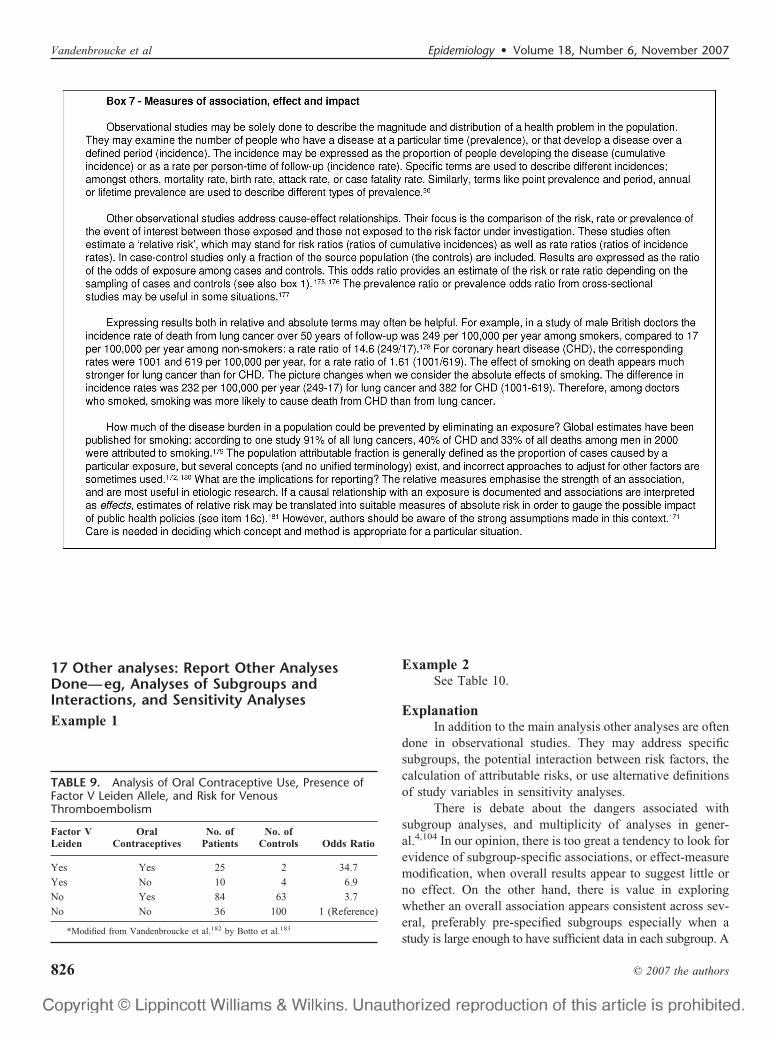
17 Other analyses: Report Other AnalysesDone—eg, Analyses of Subgroups andInteractions, and Sensitivity AnalysesExample 1

Example 2See Table 10.

ExplanationIn addition to the main analysis other analyses are often

done in observational studies. They may address specificsubgroups, the potential interaction between risk factors, thecalculation of attributable risks, or use alternative definitionsof study variables in sensitivity analyses.

There is debate about the dangers associated withsubgroup analyses, and multiplicity of analyses in gener-al.4,104 In our opinion, there is too great a tendency to look forevidence of subgroup-specific associations, or effect-measuremodification, when overall results appear to suggest little orno effect. On the other hand, there is value in exploringwhether an overall association appears consistent across sev-eral, preferably pre-specified subgroups especially when astudy is large enough to have sufficient data in each subgroup. A

TABLE 9. Analysis of Oral Contraceptive Use, Presence ofFactor V Leiden Allele, and Risk for VenousThromboembolism

Factor VLeiden

OralContraceptives

No. ofPatients

No. ofControls Odds Ratio

Yes Yes 25 2 34.7

Yes No 10 4 6.9

No Yes 84 63 3.7

No No 36 100 1 (Reference)

*Modified from Vandenbroucke et al.182 by Botto et al.183



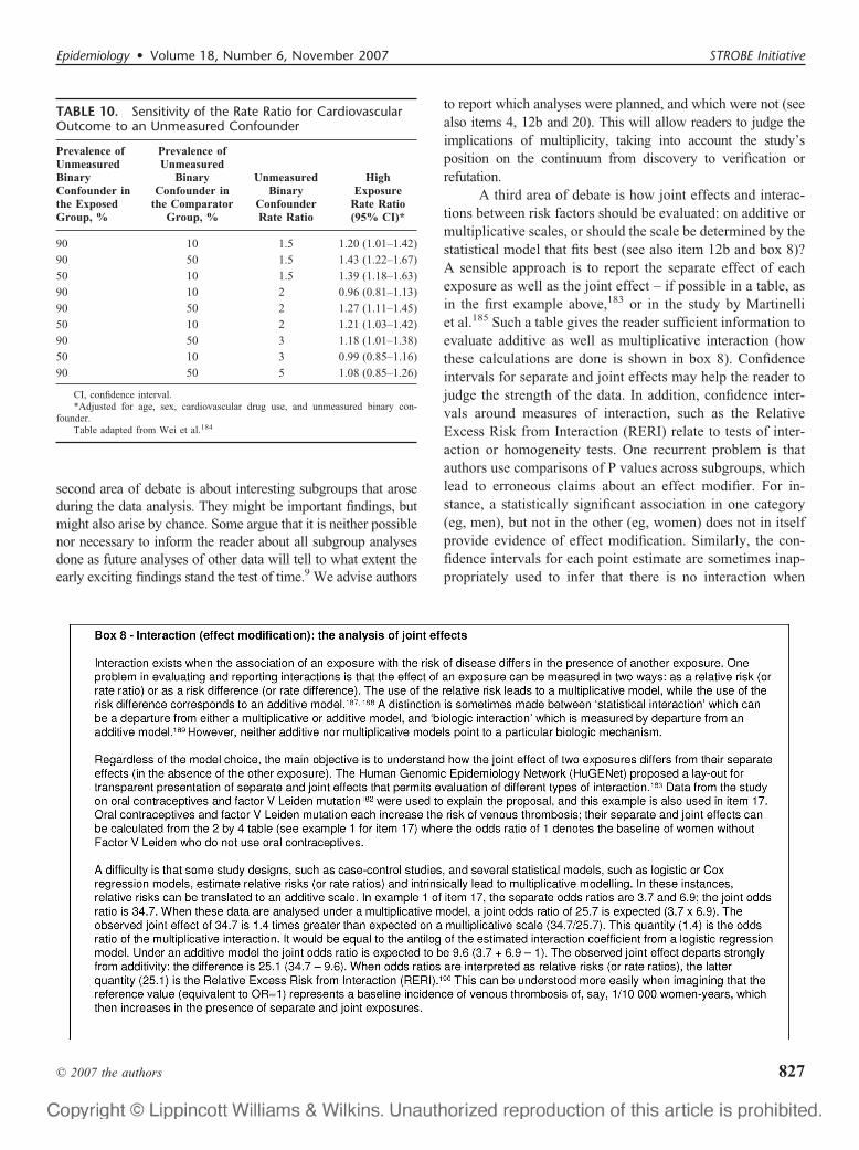
second area of debate is about interesting subgroups that aroseduring the data analysis. They might be important findings, butmight also arise by chance. Some argue that it is neither possiblenor necessary to inform the reader about all subgroup analysesdone as future analyses of other data will tell to what extent theearly exciting findings stand the test of time.9 We advise authors

to report which analyses were planned, and which were not (seealso items 4, 12b and 20). This will allow readers to judge theimplications of multiplicity, taking into account the study’sposition on the continuum from discovery to verification orrefutation.

A third area of debate is how joint effects and interac-tions between risk factors should be evaluated: on additive ormultiplicative scales, or should the scale be determined by thestatistical model that fits best (see also item 12b and box 8)?A sensible approach is to report the separate effect of eachexposure as well as the joint effect – if possible in a table, asin the first example above,183 or in the study by Martinelliet al.185 Such a table gives the reader sufficient information toevaluate additive as well as multiplicative interaction (howthese calculations are done is shown in box 8). Confidenceintervals for separate and joint effects may help the reader tojudge the strength of the data. In addition, confidence inter-vals around measures of interaction, such as the RelativeExcess Risk from Interaction (RERI) relate to tests of inter-action or homogeneity tests. One recurrent problem is thatauthors use comparisons of P values across subgroups, whichlead to erroneous claims about an effect modifier. For in-stance, a statistically significant association in one category(eg, men), but not in the other (eg, women) does not in itselfprovide evidence of effect modification. Similarly, the con-fidence intervals for each point estimate are sometimes inap-propriately used to infer that there is no interaction when

TABLE 10. Sensitivity of the Rate Ratio for CardiovascularOutcome to an Unmeasured Confounder

Prevalence ofUnmeasuredBinaryConfounder inthe ExposedGroup, %

Prevalence ofUnmeasured

BinaryConfounder in

the ComparatorGroup, %

UnmeasuredBinary

ConfounderRate Ratio

HighExposure

Rate Ratio(95% CI)*

90 10 1.5 1.20 (1.01–1.42)

90 50 1.5 1.43 (1.22–1.67)

50 10 1.5 1.39 (1.18–1.63)

90 10 2 0.96 (0.81–1.13)

90 50 2 1.27 (1.11–1.45)

50 10 2 1.21 (1.03–1.42)

90 50 3 1.18 (1.01–1.38)

50 10 3 0.99 (0.85–1.16)

90 50 5 1.08 (0.85–1.26)

CI, confidence interval.*Adjusted for age, sex, cardiovascular drug use, and unmeasured binary con-

founder.Table adapted from Wei et al.184



intervals overlap. A more valid inference is achieved bydirectly evaluating whether the magnitude of an associationdiffers across subgroups.

Sensitivity analyses are helpful to investigate the influenceof choices made in the statistical analysis, or to investigate therobustness of the findings to missing data or possible biases (seealso item 12b). Judgement is needed regarding the level ofreporting of such analyses. If many sensitivity analyses wereperformed, it may be impractical to present detailed findings forthem all. It may sometimes be sufficient to report that sensitivityanalyses were carried out and that they were consistent with themain results presented. Detailed presentation is more appropriateif the issue investigated is of major concern, or if effect estimatesvary considerably.59,186

Pocock and colleagues found that 43 out of 73 articlesreporting observational studies contained subgroup analyses. Themajority claimed differences across groups but only eight arti-cles reported a formal evaluation of interaction (see item 12b).4

DISCUSSIONThe discussion section addresses the central issues of

validity and meaning of the study.191 Surveys have found thatdiscussion sections are often dominated by incomplete orbiased assessments of the study’s results and their implica-tions, and rhetoric supporting the authors’ findings.192,193

Structuring the discussion may help authors avoid unwar-ranted speculation and over-interpretation of results whileguiding readers through the text.194,195 For example, Annalsof Internal Medicine196 recommends that authors structurethe discussion section by presenting the following: 1) a briefsynopsis of the key findings; 2) consideration of possiblemechanisms and explanations; 3) comparison with relevantfindings from other published studies; 4) limitations of thestudy; and 5) a brief section that summarizes the implicationsof the work for practice and research. Others have madesimilar suggestions.191,194 The section on research recom-mendations and the section on limitations of the study shouldbe closely linked to each other. Investigators should suggestways in which subsequent research can improve on theirstudies rather than blandly stating ‘more research is need-ed’.197,198 We recommend that authors structure their discus-sion sections, perhaps also using suitable subheadings.

18 Key Results: Summarise Key Results withReference to Study ObjectivesExample

“We hypothesized that ethnic minority status would beassociated with higher levels of cardiovascular disease (CVD)risk factors, but that the associations would be explained sub-stantially by socioeconomic status (SES). Our hypothesis wasnot confirmed. After adjustment for age and SES, highly signif-icant differences in body mass index, blood pressure, diabetes,and physical inactivity remained between white women andboth black and Mexican American women. In addition, we

found large differences in CVD risk factors by SES, a findingthat illustrates the high-risk status of both ethnic minoritywomen as well as white women with low SES.”199

ExplanationIt is good practice to begin the discussion with a short

summary of the main findings of the study. The short sum-mary reminds readers of the main findings and may help themassess whether the subsequent interpretation and implicationsoffered by the authors are supported by the findings.

19 Limitations: Discuss Limitations of theStudy, Taking into Account Sources ofPotential Bias or Imprecision. Discuss BothDirection and Magnitude of Any Potential BiasExample

“Since the prevalence of counseling increases withincreasing levels of obesity, our estimates may overestimatethe true prevalence. Telephone surveys also may overesti-mate the true prevalence of counseling. Although personswithout telephones have similar levels of overweight aspersons with telephones, persons without telephones tend tobe less educated, a factor associated with lower levels ofcounseling in our study. Also, of concern is the potential biascaused by those who refused to participate as well as thosewho refused to respond to questions about weight. Further-more, because data were collected cross-sectionally, we can-not infer that counseling preceded a patient’s attempt to loseweight.”200

ExplanationThe identification and discussion of the limitations of a

study are an essential part of scientific reporting. It is impor-tant not only to identify the sources of bias and confoundingthat could have affected results, but also to discuss therelative importance of different biases, including the likelydirection and magnitude of any potential bias (see also box 3,item 9).

Authors should also discuss any imprecision of theresults. Imprecision may arise in connection with severalaspects of a study, including the study size (item 10) and themeasurement of exposures, confounders and outcomes (item8). The inability to precisely measure true values of anexposure tends to result in bias towards unity: the lessprecisely a risk factor is measured, the greater the bias. Thiseffect has been described as ‘attenuation’,201,202 or morerecently as ‘regression dilution bias’.203 However, whencorrelated risk factors are measured with different degrees ofimprecision, the adjusted relative risk associated with themcan be biased towards or away from unity.204–206

When discussing limitations, authors may compare thestudy being presented with other studies in the literature interms of validity, generalizability and precision. In this ap-proach, each study can be viewed as contribution to the



literature, not as a stand-alone basis for inference and ac-tion.207 Surprisingly, the discussion of important limitationsof a study is sometimes omitted from published reports. Asurvey of authors who had published original research articlesin The Lancet found that important weaknesses of the studywere reported by the investigators in the survey question-naires, but not in the published article.192

20 Interpretation: Give a Cautious OverallInterpretation Considering Objectives,Limitations, Multiplicity of Analyses, Resultsfrom Similar Studies, and Other RelevantEvidenceExample

“Any explanation for an association between deathfrom myocardial infarction and use of second generation oralcontraceptives must be conjectural. There is no publishedevidence to suggest a direct biologic mechanism, and thereare no other epidemiologic studies with relevant results. (. . .)The increase in absolute risk is very small and probablyapplies predominantly to smokers. Due to the lack of corrob-orative evidence, and because the analysis is based on rela-tively small numbers, more evidence on the subject is needed.We would not recommend any change in prescribing practiceon the strength of these results.”120

ExplanationThe heart of the discussion section is the interpreta-

tion of a study’s results. Over-interpretation is commonand human: even when we try hard to give an objectiveassessment, reviewers often rightly point out that we wenttoo far in some respects. When interpreting results, authorsshould consider the nature of the study on the discovery toverification continuum and potential sources of bias, in-cluding loss to follow-up and non-participation (see alsoitems 9, 12 and 19). Due consideration should be given toconfounding (item 16a), the results of relevant sensitivityanalyses, and to the issue of multiplicity and subgroupanalyses (item 17). Authors should also consider residualconfounding due to unmeasured variables or imprecisemeasurement of confounders. For example, socioeconomicstatus (SES) is associated with many health outcomes andoften differs between groups being compared. Variablesused to measure SES (income, education, or occupation)are surrogates for other undefined and unmeasured expo-sures, and the true confounder will by definition be mea-sured with error.208 Authors should address the real rangeof uncertainty in estimates, which is larger than the statis-tical uncertainty reflected in confidence intervals. Thelatter do not take into account other uncertainties that arisefrom a study’s design, implementation, and methods ofmeasurement.209

To guide thinking and conclusions about causality,some may find criteria proposed by Bradford Hill in 1965helpful.164 How strong is the association with the exposure?Did it precede the onset of disease? Is the association con-sistently observed in different studies and settings? Is theresupporting evidence from experimental studies, includinglaboratory and animal studies? How specific is the exposure’sputative effect, and is there a dose-response relationship? Isthe association biologically plausible? These criteria shouldnot, however, be applied mechanically. For example, somehave argued that relative risks below 2 or 3 should beignored.210,211 This is a reversal of the point by Cornfield etal about the strength of large relative risks (see item 12b).127

Although a causal effect is more likely with a relative risk of9, it does not follow that one below 3 is necessarily spurious.For instance, the small increase in the risk of childhoodleukemia after intrauterine irradiation is credible because itconcerns an adverse effect of a medical procedure for whichno alternative explanations are obvious.212 Moreover, thecarcinogenic effects of radiation are well established. Thedoubling in the risk of ovarian cancer associated with eating2 to 4 eggs per week is not immediately credible, sincedietary habits are associated with a large number of lifestylefactors as well as SES.213 In contrast, the credibility of muchdebated epidemiologic findings of a difference in thrombosisrisk between different types of oral contraceptives wasgreatly enhanced by the differences in coagulation found in arandomized cross-over trial.214 A discussion of the existingexternal evidence, from different types of studies, shouldalways be included, but may be particularly important forstudies reporting small increases in risk. Further, authorsshould put their results in context with similar studies andexplain how the new study affects the existing body ofevidence, ideally by referring to a systematic review.

21 Generalizability: Discuss theGeneralizability (External Validity) of theStudy ResultsExample

“How applicable are our estimates to other HIV-1-infected patients? This is an important question because theaccuracy of prognostic models tends to be lower when ap-plied to data other than those used to develop them. Weaddressed this issue by penalising model complexity, and bychoosing models that generalized best to cohorts omittedfrom the estimation procedure. Our database included pa-tients from many countries from Europe and North America,who were treated in different settings. The range of patientswas broad: men and women, from teenagers to elderly peoplewere included, and the major exposure categories were wellrepresented. The severity of immunodeficiency at baselineranged from not measureable to very severe, and viral loadfrom undetectable to extremely high.”215



ExplanationGeneralizability, also called external validity or ap-

plicability, is the extent to which the results of a study canbe applied to other circumstances.216 There is no externalvalidity per se; the term is meaningful only with regard toclearly specified conditions.217 Can results be applied to anindividual, groups or populations that differ from thoseenrolled in the study with regard to age, sex, ethnicity,severity of disease, and co-morbid conditions? Are thenature and level of exposures comparable, and the defini-tions of outcomes relevant to another setting or popula-tion? Are data that were collected in longitudinal studiesmany years ago still relevant today? Are results fromhealth services research in one country applicable to healthsystems in other countries?

The question of whether the results of a study haveexternal validity is often a matter of judgment that depends onthe study setting, the characteristics of the participants, theexposures examined, and the outcomes assessed. Thus, it iscrucial that authors provide readers with adequate informa-tion about the setting and locations, eligibility criteria, theexposures and how they were measured, the definition ofoutcomes, and the period of recruitment and follow-up. Thedegree of nonparticipation and the proportion of unex-posed participants in whom the outcome develops are alsorelevant. Knowledge of the absolute risk and prevalence ofthe exposure, which will often vary across populations, arehelpful when applying results to other settings and popu-lations (see box 7).

OTHER INFORMATION

22 Funding: Give the Source of Funding andthe Role of the Funders for the Present Studyand, if Applicable, for the Original Study onWhich the Present Article is BasedExplanation

Some journals require authors to disclose the presence orabsence of financial and other conflicts of interest.100,218 Severalinvestigations show strong associations between the source offunding and the conclusions of research articles.219–222 Theconclusions in randomized trials recommended the experimentaldrug as the drug of choice much more often (odds ratio 5.3) ifthe trial was funded by for-profit organisations, even afteradjustment for the effect size.223 Other studies document theinfluence of the tobacco and telecommunication industries onthe research they funded.224–227 There are also examples ofundue influence when the sponsor is governmental or a non-profit organization.

Authors or funders may have conflicts of interest thatinfluence any of the following: the design of the study228;choice of exposures,228,229 outcomes,230 statistical meth-ods,231 and selective publication of outcomes230 and stud-ies.232 Consequently, the role of the funders should be de-

scribed in detail: in what part of the study they took directresponsibility (eg, design, data collection, analysis, draftingof the manuscript, decision to publish).100 Other sources ofundue influence include employers (eg, university adminis-trators for academic researchers and government supervisors,especially political appointees, for government researchers),advisory committees, litigants, and special interest groups.

Concluding RemarksThe STROBE Statement aims to provide helpful rec-

ommendations for reporting observational studies in epide-miology. Good reporting reveals the strengths and weak-nesses of a study and facilitates sound interpretation andapplication of study results. The STROBE Statement mayalso aid in planning observational studies, and guide peerreviewers and editors in their evaluation of manuscripts.

We wrote this explanatory article to discuss the impor-tance of transparent and complete reporting of observationalstudies, to explain the rationale behind the different itemsincluded in the checklist, and to give examples from pub-lished articles of what we consider good reporting. We hopethat the material presented here will assist authors and editorsin using STROBE.

We stress that STROBE and other recommendations onthe reporting of research13,233,234 should be seen as evolvingdocuments that require continual assessment, refinement,and, if necessary, change.235,236 For example, the CONSORTStatement for the reporting of parallel-group randomizedtrials was first developed in the mid 1990s.237 Since thenmembers of the group have met regularly to review the needto revise the recommendations; a revised version appeared in2001233 and a further version is in development. Similarly,the principles presented in this article and the STROBEchecklist are open to change as new evidence and criticalcomments accumulate. The STROBE web site (http://www.strobe-statement.org) provides a forum for discussion andsuggestions for improvements of the checklist, this explana-tory document and information about the good reporting ofepidemiological studies.

Several journals ask authors to follow the STROBEStatement in their instructions to authors (see web site forcurrent list). We invite other journals to adopt the STROBEStatement and contact us through our web site to let us know.The journals publishing the STROBE recommendations pro-vide open access. The STROBE Statement is thereforewidely accessible to the biomedical community.

ACKNOWLEDGMENTSWe are grateful to Gerd Antes, Kay Dickersin, Shah

Ebrahim and Richard Lilford for supporting the STROBEInitiative. We are grateful to the following institutions thathave hosted working meetings: Institute of Social and Pre-ventive Medicine (ISPM), University of Bern, Switzerland;Department of Social Medicine, University of Bristol, UK;



London School of Hygiene & Tropical Medicine, London,UK; Nordic Cochrane Centre, Copenhagen, Denmark; andCentre for Statistics in Medicine, Oxford, UK. We are grate-ful to 4 anonymous reviewers who provided helpful commentson a previous draft of this paper.

The following persons have contributed to the content andelaboration of the STROBE Statement: Douglas G. Altman,Maria Blettner, Paolo Boffetta, Hermann Brenner, GenevieveChene, Cyrus Cooper, George Davey-Smith, Erik von Elm,Matthias Egger, France Gagnon, Peter C. Gøtzsche, PhilipGreenland, Sander Greenland, Claire Infante-Rivard, John Io-annidis, Astrid James, Giselle Jones, Bruno Ledergerber, JulianLittle, Margaret May, David Moher, Hooman Momen, AlfredoMorabia, Hal Morgenstern, Cynthia D. Mulrow, Fred Paccaud,Stuart J. Pocock, Charles Poole, Martin Roosli, DietrichRothenbacher, Kenneth Rothman, Caroline Sabin, Willi Sauer-brei, Lale Say, James J. Schlesselman, Jonathan Sterne, HollySyddall, Jan P. Vandenbroucke, Ian White, Susan Wieland,Hywel Williams, Guang Yong Zou.

REFERENCES1. Glasziou P, Vandenbroucke JP, Chalmers I. Assessing the quality of

research. BMJ. 2004;328:39–41.2. Funai EF, Rosenbush EJ, Lee MJ, Del Priore G. Distribution of study

designs in four major US journals of obstetrics and gynecology.Gynecol Obstet Invest. 2001;51:8–11.

3. Scales CD Jr, Norris RD, Peterson BL, Preminger GM, Dahm P.Clinical research and statistical methods in the urology literature.J Urol. 2005;174:1374–9.

4. Pocock SJ, Collier TJ, Dandreo KJ, et al. Issues in the reporting ofepidemiological studies: a survey of recent practice. BMJ. 2004;329:883.

5. Tooth L, Ware R, Bain C, Purdie DM, Dobson A. Quality of reportingof observational longitudinal research. American Journal of Epidemi-ology. 2005;161:280–8.

6. von Elm E, Altman D, Egger M, Pocock S, Gøtzsche PC,Vandenbroucke JP. The Strengthening the Reporting of ObservationalStudies in Epidemiology (STROBE) Statement: guidelines for report-ing observational studies. Epidemiology. 2007;18:800–804.

7. Mihailovic A, Bell CM, Urbach DR. Users’ guide to the surgicalliterature. Case-control studies in surgical journals. Can J Surg. 2005;48:148–51.

8. Rushton L. Reporting of occupational and environmental research: useand misuse of statistical and epidemiological methods. Occup EnvironMed. 2000;57:1–9.

9. Rothman KJ. No adjustments are needed for multiple comparisons.Epidemiology. 1990;1:43–6.

10. Moonesinghe R, Khoury MJ, Janssens AC. Most published researchfindings are false-but a little replication goes a long way. PLoSMedicine. 2007;4:e28.

11. Jenicek M. Clinical Case Reporting. Evidence-Based Medicine. Ox-ford: Butterworth-Heinemann; 1999; p. 117.

12. Vandenbroucke JP. In defense of case reports and case series. Annalsof Internal Medicine. 2001;134:330–4.

13. Bossuyt PM, Reitsma JB, Bruns DE, et al. Towards complete andaccurate reporting of studies of diagnostic accuracy: The STARDInitiative. Annals of Internal Medicine. 2003;138:40–4.

14. McShane LM, Altman DG, Sauerbrei W, Taube SE, Gion M, ClarkGM. REporting recommendations for tumour MARKer prognosticstudies (REMARK). Br J Cancer. 2005;93:387–91.

15. Ioannidis JP, Gwinn M, Little J, et al. A road map for efficient andreliable human genome epidemiology. Nat Genet. 2006;38:3–5.

16. Rodrigues L, Kirkwood BR. Case-control designs in the study ofcommon diseases: updates on the demise of the rare disease assumptionand the choice of sampling scheme for controls. International Journalof Epidemiology. 1990;19:205–13.

17. Rothman KJ, Greenland S. Case-Control Studies. In: Rothman KJ,Greenland S, editors. Modern epidemiology. 2nd ed: Lippincott Raven;1998. p. 93–114.

18. Forand SP. Leukaemia incidence among workers in the shoe and bootmanufacturing industry: a case-control study. Environ Health. 2004;3:7

19. Benson K, Hartz AJ. A comparison of observational studies andrandomized, controlled trials. The New England Journal of Medicine.2000;342:1878–86.

20. Gøtzsche PC, Harden A. Searching for non-randomised studies. Draftchapter 3. Cochrane Non-Randomised Studies Methods Group, 26 July2002 (http://www.cochrane.dk/nrsmg).

21. Lohse N, Hansen AB, Pedersen G, et al. Survival of persons with andwithout HIV infection in Denmark, 1995–2005. Annals of InternalMedicine. 2007;146:87–95.

22. American Journal of Epidemiology. Instructions to authors. Avai-lable from: http://www.oxfordjournals.org/our_journals/aje/for_authors/general.html.

23. Haynes RB, Mulrow CD, Huth EJ, Altman DG, Gardner MJ. Moreinformative abstracts revisited. Annals of Internal Medicine. 1990;113:69–76.

24. Taddio A, Pain T, Fassos FF, Boon H, Ilersich AL, Einarson TR.Quality of nonstructured and structured abstracts of original researcharticles in the British Medical Journal, the Canadian Medical Associ-ation Journal and the Journal of the American Medical Association.Canadian Medical Association Journal. 1994;150:1611–5.

25. Hartley J, Sydes M. Which layout do you prefer? An analysis ofreaders’ preferences for different typographic layouts of structuredabstracts. Journal of Information Science. 1996;22:27–37.

26. Viner RM, Cole TJ. Adult socioeconomic, educational, social, andpsychological outcomes of childhood obesity: a national birth cohortstudy. BMJ. 2005;330:1354.

27. McCauley J, Kern DE, Kolodner K, et al. The “battering syndrome”:prevalence and clinical characteristics of domestic violence in primarycare internal medicine practices. Annals of Internal Medicine. 1995;123:737–46.

28. McEvoy SP, Stevenson MR, McCartt AT, et al. Role of mobile phonesin motor vehicle crashes resulting in hospital attendance: a case-crossover study. BMJ. 2005;331:428.

29. Vandenbroucke JP. Prospective or retrospective: what’s in a name?BMJ. 1991;302:249–50.

30. Last JM. A Dictionary of Epidemiology. 4th ed. New York: OxfordUniversity Press; 2000.

31. Miettinen OS. Theoretical Epidemiology: principles of occurrenceresearch in medicine. New York: Wiley; 1985.

32. Rothman KJ, Greenland S. Types of Epidemiologic Studies. In: Roth-man KJ, Greenland S, editors. Modern Epidemiology. 2nd ed: Lippin-cott Raven; 1998. p. 74–5.

33. MacMahon B, Trichopoulos D. Epidemiology, principles and methods.2nd ed. Boston: Little, Brown and Co.; 1996. p. 81.

34. Lilienfeld AM. Foundations of Epidemiology. New York: OxfordUniversity Press; 1976.

35. Ridker PM, Hennekens CH, Lindpaintner K, Stampfer MJ, EisenbergPR, Miletich JP. Mutation in the gene coding for coagulation factor Vand the risk of myocardial infarction, stroke, and venous thrombosis inapparently healthy men. The New England Journal of Medicine. 1995;332:912–7.

36. Goodman KJ, O’Rourke K, Day RS, et al. Dynamics of Helicobacterpylori infection in a US-Mexico cohort during the first two years of life.International Journal of Epidemiology. 2005;34:1348–55.

37. Altman DG, De Stavola BL, Love SB, Stepniewska KA. Review ofsurvival analyses published in cancer journals. Br J Cancer. 1995;72:511–8.

38. Cerhan JR, Wallace RB, Folsom AR, Potter JD, Munger RG, PrineasRJ. Transfusion history and cancer risk in older women. Annals ofInternal Medicine. 1993;119:8–15.

39. Beane Freeman LE, Dennis LK, Lynch CF, Thorne PS, Just CL.Toenail arsenic content and cutaneous melanoma in Iowa. AmericanJournal of Epidemiology. 2004;160:679–87.

40. Canto JG, Allison JJ, Kiefe CI, et al. Relation of race and sex to the use ofreperfusion therapy in Medicare beneficiaries with acute myocardial in-farction. The New England Journal of Medicine. 2000;342:1094–100.



41. Metzkor-Cotter E, Kletter Y, Avidor B, et al. Long-term serologicalanalysis and clinical follow-up of patients with cat scratch disease. ClinInfect Dis. 2003;37:1149–54.

42. Johnson ES. Bias on withdrawing lost subjects from the analysis at thetime of loss, in cohort mortality studies, and in follow-up methods.J Occup Med. 1990;32:250–4.

43. Berkson J. Limitations of the application of fourfold table analysis tohospital data. Biometrics Bulletin 1946;2:53.

44. Feinstein AR, Walter SD, Horwitz RI. An analysis of Berkson’s bias incase-control studies. J Chronic Dis. 1986;39:495–504.

45. Jick H, Vessey MP. Case-control studies in the evaluation of drug-induced illness. American Journal of Epidemiology. 1978;107:1–7.

46. Hackam DG, Mamdani M, Li P, Redelmeier DA. Statins and sepsis inpatients with cardiovascular disease: a population-based cohort analy-sis. Lancet. 2006;367:413–8.

47. Smeeth L, Cook C, Fombonne E, et al. MMR vaccination and perva-sive developmental disorders: a case-control study. Lancet. 2004;364:963–9.

48. Costanza MC. Matching. Prev Med. 1995;24:425–33.49. Sturmer T, Brenner H. Flexible matching strategies to increase power

and efficiency to detect and estimate gene-environment interactions incase-control studies. American Journal of Epidemiology. 2002;155:593–602.

50. Rothman KJ, Greenland S. Matching. In: Rothman KJ, Greenland S,editors. Modern Epidemiology. 2nd ed: Lippincott Raven; 1998. p.147–61.

51. Szklo MF, Nieto J. Epidemiology, Beyond the Basics. Sudbury, MA:Jones and Bartlett; 2000. p. 40–51.

52. Cole P, MacMahon B. Attributable risk percent in case-control studies.Br J Prev Soc Med. 1971;25:242–4.

53. Gissler M, Hemminki E. The danger of overmatching in studies of theperinatal mortality and birthweight of infants born after assisted con-ception. Eur J Obstet Gynecol Reprod Biol. 1996;69:73–5.

54. Gefeller O, Pfahlberg A, Brenner H, Windeler J. An empirical inves-tigation on matching in published case-control studies. Eur J Epide-miol. 1998;14:321–5.

55. Artama M, Ritvanen A, Gissler M, Isojarvi J, Auvinen A. Congenitalstructural anomalies in offspring of women with epilepsy–a population-based cohort study in Finland. International Journal of Epidemiology.2006;35:280–7.

56. Ebrahim S. Cohorts, infants and children. International Journal ofEpidemiology. 2004;33:1165–66.

57. Walker M, Whincup PH, Shaper AG. The British Regional Heart Study1975–2004. International Journal of Epidemiology. 2004;33:1185–92.

58. Wieland S, Dickersin K. Selective exposure reporting and Medlineindexing limited the search sensitivity for observational studies of theadverse effects of oral contraceptives. J Clin Epidemiol. 2005;58:560–7.

59. Anderson HR, Atkinson RW, Peacock JL, Sweeting MJ, Marston L.Ambient particulate matter and health effects: publication bias instudies of short-term associations. Epidemiology. 2005;16:155–63.

60. Winkelmayer WC, Stampfer MJ, Willett WC, Curhan GC. Habitualcaffeine intake and the risk of hypertension in women. JAMA. 2005;294:2330–5.

61. Lukanova A, Soderberg S, Kaaks R, Jellum E, Stattin P. Serumadiponectin is not associated with risk of colorectal cancer. CancerEpidemiol Biomarkers Prev. 2006;15:401–2.

62. Becher H. The concept of residual confounding in regression modelsand some applications. Stat Med. 1992;11:1747–58.

63. Brenner H, Blettner M. Controlling for continuous confounders inepidemiologic research. Epidemiology. 1997;8:429–34.

64. Phillips MR, Yang G, Zhang Y, Wang L, Ji H, Zhou M. Risk factorsfor suicide in China: a national case-control psychological autopsystudy. Lancet. 2002;360:1728–36.

65. Pasquale LR, Kang JH, Manson JE, Willett WC, Rosner BA,Hankinson SE. Prospective study of type 2 diabetes mellitus and risk ofprimary open-angle glaucoma in women. Ophthalmology. 2006;113:1081–6.

66. Craig SL, Feinstein AR. Antecedent therapy versus detection bias ascauses of neoplastic multimorbidity. Am J Clin Oncol. 1999;22:51–6.

67. Rogler LH, Mroczek DK, Fellows M, Loftus ST. The neglect of

response bias in mental health research. J Nerv Ment Dis. 2001;189:182–7.

68. Murphy EA. The logic of medicine. Baltimore: Johns Hopkins Uni-versity Press; 1976.

69. Sackett DL. Bias in analytic research. J Chronic Dis. 1979;32:51–63.70. Johannes CB, Crawford SL, McKinlay JB. Interviewer effects in a

cohort study. Results from the Massachusetts Women’s Health Study.American Journal of Epidemiology. 1997;146:429–38.

71. Bloemenkamp KW, Rosendaal FR, Buller HR, Helmerhorst FM, CollyLP, Vandenbroucke JP. Risk of venous thrombosis with use of currentlow-dose oral contraceptives is not explained by diagnostic suspicionand referral bias. Arch Intern Med. 1999;159:65–70.

72. Feinstein AR. Clinical epidemiology: the architecture of clinical re-search. Philadelphia: W.B. Saunders Company; 1985.

73. Yadon ZE, Rodrigues LC, Davies CR, Quigley MA. Indoor andperidomestic transmission of American cutaneous leishmaniasis innorthwestern Argentina: a retrospective case-control study. The Amer-ican Journal of Tropical Medicine and Hygiene. 2003;68:519–26.

74. Anoop S, Saravanan B, Joseph A, Cherian A, Jacob KS. Maternaldepression and low maternal intelligence as risk factors for malnutri-tion in children: a community based case-control study from SouthIndia. Arch Dis Child. 2004;89:325–9.

75. Carlin JB, Doyle LW. Sample size. J Paediatr Child Health. 2002;38:300–4.

76. Rigby AS, Vail A. Statistical methods in epidemiology. II: A common-sense approach to sample size estimation. Disabil Rehabil. 1998;20:405–10.

77. Schulz KF, Grimes DA. Sample size calculations in randomised trials:mandatory and mystical. Lancet. 2005;365:1348–53.

78. Drescher K, Timm J, Jockel KH. The design of case-control studies: theeffect of confounding on sample size requirements. Stat Med. 1990;9:765–76.

79. Devine OJ, Smith JM. Estimating sample size for epidemiologicstudies: the impact of ignoring exposure measurement uncertainty. StatMed. 1998;17:1375–89.

80. Linn S, Levi L, Grunau PD, Zaidise I, Zarka S. Effect measuremodification and confounding of severe head injury mortality by ageand multiple organ injury severity. Annals of epidemiology. 2007;17:142–7.

81. Altman DG, Lausen B, Sauerbrei W, Schumacher M. Dangers of using“optimal” cutpoints in the evaluation of prognostic factors. J NatlCancer Inst. 1994;86:829–35.

82. Royston P, Altman DG, Sauerbrei W. Dichotomizing continuous pre-dictors in multiple regression: a bad idea. Stat Med. 2006;25:127–41.

83. Greenland S. Avoiding power loss associated with categorization andordinal scores in dose-response and trend analysis. Epidemiology.1995;6:450–4.

84. Royston P, Ambler G, Sauerbrei W. The use of fractional polynomialsto model continuous risk variables in epidemiology. InternationalJournal of Epidemiology. 1999;28:964–74.

85. MacCallum RC, Zhang S, Preacher KJ, Rucker DD. On the practice ofdichotomization of quantitative variables. Psychol Methods. 2002;7:19–40.

86. Altman DG. Categorizing continuous variables. In: Armitage P, ColtonT, editors. Encyclopedia of biostatistics. 2nd ed. Chichester: JohnWiley; 2005. p. 708–11.

87. Cohen J. The cost of dichotomization. Applied Psychological Measure-ment. 1983;7:249–53.

88. Zhao LP, Kolonel LN. Efficiency loss from categorizing quantitativeexposures into qualitative exposures in case-control studies. AmericanJournal of Epidemiology. 1992;136:464–74.

89. Cochran WG. The effectiveness of adjustment by subclassificationin removing bias in observational studies. Biometrics. 1968;24:295–313.

90. Clayton D, Hills M. Models for dose-response (Chapter 25). StatisticalModels in Epidemiology. Oxford: Oxford University Press; 1993. p.249–60.

91. Cox DR. Note on grouping. J Am Stat Assoc. 1957;52:543–7.92. Il’yasova D, Hertz-Picciotto I, Peters U, Berlin JA, Poole C. Choice of

exposure scores for categorical regression in meta-analysis: a casestudy of a common problem. Cancer Causes Control. 2005;16:383–8.



93. Berglund A, Alfredsson L, Cassidy JD, Jensen I, Nygren A. Theassociation between exposure to a rear-end collision and future neck orshoulder pain: a cohort study. J Clin Epidemiol. 2000;53:1089–94.

94. Slama R, Werwatz A. Controlling for continuous confounding factors:non- and semiparametric approaches. Rev Epidemiol Sante Publique2005;53(Spec No 2):2S65–80.

95. Greenland S. Introduction to regression modelling (Chapter 21). In:Rothman KJ, Greenland S, editors. Modern epidemiology. 2nd ed:Lippincott Raven; 1998. p. 401–32.

96. Thompson WD. Statistical analysis of case-control studies. EpidemiolRev. 1994;16:33–50.

97. Schlesselman JJ. Logistic regression for case-control studies (Chapter8. 2). Case-control studies Design, conduct, analysis. New York,Oxford: Oxford University Press; 1982. p. 235–41.

98. Clayton D, Hills M. Choice and interpretation of models (Chapter 27).Statistical Models in Epidemiology. Oxford: Oxford University Press;1993. p. 271–81.

99. Altman DG, Gore SM, Gardner MJ, Pocock SJ. Statistical guidelinesfor contributors to medical journals. Br Med J. 1983;286:1489–93.

100. International Committee of Medical Journal Editors (ICMJE).Uniformrequirements for manuscripts submitted to biomedical journals. Elec-tronic version updated February 2006, available at http://www.icmje.org. The New England Journal of Medicine 1997;336:309–15.

101. Mullner M, Matthews H, Altman DG. Reporting on statistical methodsto adjust for confounding: a cross-sectional survey. AnnInternMed.2002;136:122–6.

102. Olsen J, Basso O. Re: Residual confounding. American Journal ofEpidemiology. 1999;149:290.

103. Hallan S, de Mutsert R, Carlsen S, Dekker FW, Aasarod K, Holmen J.Obesity, smoking, and physical inactivity as risk factors for CKD: aremen more vulnerable? Am J Kidney Dis. 2006;47:396–405.

104. Gotzsche PC. Believability of relative risks and odds ratios in abstracts:cross sectional study. BMJ. 2006;333:231–4.

105. Szklo MF, Nieto J. Communicating Results of Epidemiologic Studies(Chapter 9). Epidemiology, Beyond the Basics. Sudbury, MA: Jonesand Bartlett; 2000. p. 408–30.

106. Chandola T, Brunner E, Marmot M. Chronic stress at work and themetabolic syndrome: prospective study. BMJ. 2006;332:521–5.

107. Vach W, Blettner M. Biased estimation of the odds ratio in case-controlstudies due to the use of ad hoc methods of correcting for missingvalues for confounding variables. American Journal of Epidemiology.1991;134:895–907.

108. Little RJ, Rubin DB. A taxonomy of missing-data methods (Chapter 1.4.) (need to check). Statistical Analysis with Missing Data. New York:Wiley; 2002. p. 19–23.

109. Ware JH. Interpreting incomplete data in studies of diet and weightloss. The New England Journal of Medicine. 2003;348:2136–7.

110. Rubin DB. Inference and missing data. Biometrika. 1976;63:581–92.111. Schafer JL. Analysis of Incomplete Multivariate Data. London: Chap-

man & Hall; 1997.112. Lipsitz SR, Ibrahim JG, Chen MH, Peterson H. Non-ignorable missing

covariates in generalized linear models. Stat Med. 1999;18:2435–48.113. Rotnitzky A, Robins J. Analysis of semi-parametric regression models

with non-ignorable non-response. Stat Med. 1997;16:81–102.114. Rubin DB. Multiple Imputation for Nonresponse in Surveys. New

York: John Wiley; 1987.115. Barnard J, Meng XL. Applications of multiple imputation in medical

studies: from AIDS to NHANES. Stat Methods Med Res. 1999;8:17–36.116. Braitstein P, Brinkhof MW, Dabis F, et al. Mortality of HIV-1-infected

patients in the first year of antiretroviral therapy: comparison betweenlow-income and high-income countries. Lancet. 2006;367:817–24.

117. Purandare N, Burns A, Daly KJ, et al. Cerebral emboli as a potentialcause of Alzheimer’s disease and vascular dementia: case-controlstudy. BMJ. 2006;332:1119–24.

118. Steyn K, Gaziano TA, Bradshaw D, Laubscher R, Fourie J.Hypertension in South African adults: results from the Demographicand Health Survey, 1998. J Hypertens. 2001;19:1717–25.

119. Lohr SL. Design Effects (Chapter 7.5). Sampling: Design and Analysis.Pacific Grove: Duxbury Press.; 1999.

120. Dunn NR, Arscott A, Thorogood M. The relationship between use oforal contraceptives and myocardial infarction in young women with

fatal outcome, compared to those who survive: results from the MICAcase-control study. Contraception. 2001;63:65–9.

121. Rothman KJ, Greenland S. Basic Methods for Sensitivity Analysis andExternal Adjustment. In: Rothman KJ, Greenland S, editors. Modernepidemiology. 2nd ed: Lippincott Raven; 1998. p. 343–57.

122. Custer B, Longstreth WT, Jr., Phillips LE, Koepsell TD, Van Belle G.Hormonal exposures and the risk of intracranial meningioma in wom-en: a population-based case-control study. BMC Cancer. 2006;6:152.

123. Wakefield MA, Chaloupka FJ, Kaufman NJ, Orleans CT, Barker DC,Ruel EE. Effect of restrictions on smoking at home, at school, and inpublic places on teenage smoking: cross sectional study. BMJ. 2000;321:333–7.

124. Greenland S. The impact of prior distributions for uncontrolled con-founding and response bias: a case study of the relation of wire codesand magnetic fields to childhood leukemia. Journal of the AmericanStatistical Association. 2003;98:47–54.

125. Lash TL, Fink AK. Semi-automated sensitivity analysis to assesssystematic errors in observational data. Epidemiology. 2003;14:451–8.

126. Phillips CV. Quantifying and reporting uncertainty from systematicerrors. Epidemiology. 2003;14:459–66.

127. Cornfield J, Haenszel W, Hammond EC, Lilienfeld AM, Shimkin MB,Wynder EL. Smoking and lung cancer: recent evidence and a discus-sion of some questions. J Natl Cancer Inst. 1959;22:173–203.

128. Langholz B. Factors that explain the power line configuration wiringcode-childhood leukemia association: what would they look like?Bioelectromagnetics 2001;Suppl 5:S19–31.

129. Eisner MD, Smith AK, Blanc PD. Bartenders’ respiratory healthafter establishment of smoke-free bars and taverns. JAMA. 1998;280:1909 –14.

130. Dunne MP, Martin NG, Bailey JM, et al. Participation bias in asexuality survey: psychological and behavioural characteristics of re-sponders and non-responders. International Journal of Epidemiology.1997;26:844–54.

131. Schuz J, Kaatsch P, Kaletsch U, Meinert R, Michaelis J. Association ofchildhood cancer with factors related to pregnancy and birth. Interna-tional Journal of Epidemiology. 1999;28:631–9.

132. Cnattingius S, Zack M, Ekbom A, Gunnarskog J, Linet M, Adami HO.Prenatal and neonatal risk factors for childhood myeloid leukemia.Cancer Epidemiol Biomarkers Prev. 1995;4:441–5.

133. Schuz J. Non-response bias as a likely cause of the association betweenyoung maternal age at the time of delivery and the risk of cancer in theoffspring. Paediatr Perinat Epidemiol. 2003;17:106–12.

134. Slattery ML, Edwards SL, Caan BJ, Kerber RA, Potter JD. Responserates among control subjects in case-control studies. Annals of epide-miology. 1995;5:245–9.

135. Schulz KF, Grimes DA. Case-control studies: research in reverse.Lancet. 2002;359:431–4.

136. Olson SH, Voigt LF, Begg CB, Weiss NS. Reporting participation incase-control studies. Epidemiology. 2002;13:123–6.

137. Morton LM, Cahill J, Hartge P. Reporting participation in epidemio-logic studies: a survey of practice. American Journal of Epidemiology.2006;163:197–203.

138. Olson SH. Reported participation in case-control studies: changes overtime. American Journal of Epidemiology. 2001;154:574–81.

139. Sandler DP. On revealing what we’d rather hide: the problem ofdescribing study participation. Epidemiology. 2002;13:117

140. Hepworth SJ, Schoemaker MJ, Muir KR, Swerdlow AJ, van TongerenMJ, McKinney PA. Mobile phone use and risk of glioma in adults:case-control study. BMJ. 2006;332:883–7.

141. Hay AD, Wilson A, Fahey T, Peters TJ. The duration of acute cough inpre-school children presenting to primary care: a prospective cohortstudy. Fam Pract. 2003;20:696–705.

142. Egger M, Juni P, Bartlett C. Value of flow diagrams in reports ofrandomized controlled trials. JAMA. 2001;285:1996–9.

143. Osella AR, Misciagna G, Guerra VM, et al. Hepatitis C virus (HCV)infection and liver-related mortality: a population-based cohort study insouthern Italy. The Association for the Study of Liver Disease inPuglia. International Journal of Epidemiology. 2000;29:922–7.

144. Dales LG, Ury HK. An improper use of statistical significance testingin studying covariables. International Journal of Epidemiology. 1978;7:373–5.



145. Maldonado G, Greenland S. Simulation study of confounder-selectionstrategies. American Journal of Epidemiology. 1993;138:923–36.

146. Tanis BC, van den Bosch MA, Kemmeren JM, et al. Oral contracep-tives and the risk of myocardial infarction. The New England Journalof Medicine. 2001;345:1787–93.

147. Rothman KJ, Greenland S. Precision and Validity in EpidemiologicStudies. In: Rothman KJ, Greenland S, editors. Modern epidemiology.2nd ed: Lippincott Raven; 1998. p. 120–5.

148. Clark TG, Altman DG, De Stavola BL. Quantification of the complete-ness of follow-up. Lancet. 2002;359:1309–10.

149. Qiu C, Fratiglioni L, Karp A, Winblad B, Bellander T. Occupationalexposure to electromagnetic fields and risk of Alzheimer’s disease.Epidemiology. 2004;15:687–94.

150. Kengeya-Kayondo JF, Kamali A, Nunn AJ, Ruberantwari A, WagnerHU, Mulder DW. Incidence of HIV-1 infection in adults and socio-demographic characteristics of seroconverters in a rural population inUganda: 1990–1994. International Journal of Epidemiology. 1996;25:1077–82.

151. Mastrangelo G, Fedeli U, Fadda E, et al. Increased risk of hepatocel-lular carcinoma and liver cirrhosis in vinyl chloride workers: synergis-tic effect of occupational exposure with alcohol intake. Environmentalhealth perspectives. 2004;112:1188–92.

152. Salo PM, Arbes SJJr. , Sever M, et al. Exposure to Alternaria alternatain US homes is associated with asthma symptoms. The Journal ofallergy and clinical immunology. 2006;118:892–8.

153. Pocock SJ, Clayton TC, Altman DG. Survival plots of time-to-eventoutcomes in clinical trials: good practice and pitfalls. Lancet. 2002;359:1686–9.

154. Sasieni P. A note on the presentation of matched case-control data. StatMed. 1992;11:617–20.

155. Lee GM, Neutra RR, Hristova L, Yost M, Hiatt RA. A nested case-control study of residential and personal magnetic field measures andmiscarriages. Epidemiology. 2002;13:21–31.

156. Tiihonen J, Walhbeck K, Lonnqvist J, et al. Effectiveness of antipsy-chotic treatments in a nationwide cohort of patients in community careafter first hospitalisation due to schizophrenia and schizoaffectivedisorder: observational follow-up study. BMJ. 2006;333:224.

157. Christenfeld NJ, Sloan RP, Carroll D, Greenland S. Risk factors,confounding, and the illusion of statistical control. Psychosom Med.2004;66:868–75.

158. Smith GD, Phillips A. Declaring independence: why we should becautious. �published erratum appears in J Epidemiol CommunityHealth 1991 Mar;45(1):88. J Epidemiol Community Health. 1990;44:257–8.

159. Greenland S, Neutra R. Control of confounding in the assessment ofmedical technology. International Journal of Epidemiology. 1980;9:361–7.

160. Robins JM. Data, design, and background knowledge in etiologicinference. Epidemiology. 2001;12:313–20.

161. Sagiv SK, Tolbert PE, Altshul LM, Korrick SA. Organochlorineexposures during pregnancy and infant size at birth. Epidemiology.2007;18:120–9.

162. World Health Organization. Body Mass Index (BMI). Accessed at:http://www.euro.who.int/nutrition/20030507_1.

163. Beral V. Breast cancer and hormone-replacement therapy in the MillionWomen Study. Lancet. 2003;362:419–27.

164. Hill AB. The Environment and Disease: Association or Causation?Proc R Soc Med. 1965;58:295–300.

165. Vineis P. Causality in epidemiology. Soz Praventivmed. 2003;48:80–7.166. Empana JP, Ducimetiere P, Arveiler D, et al. Are the Framingham

and PROCAM coronary heart disease risk functions applicable todifferent European populations? The PRIME Study. Eur Heart J.2003;24:1903–11.

167. Tunstall-Pedoe H, Kuulasmaa K, Mahonen M, Tolonen H, RuokokoskiE, Amouyel P. Contribution of trends in survival and coronary-eventrates to changes in coronary heart disease mortality: 10-year resultsfrom 37 WHO MONICA project populations. Monitoring trends anddeterminants in cardiovascular disease. Lancet. 1999;353:1547–57.

168. Cambien F, Chretien JM, Ducimetiere P, Guize L, Richard JL. Is therelationship between blood pressure and cardiovascular risk dependenton body mass index? American Journal of Epidemiology. 1985;122:

434–42.169. Hosmer DW, Taber S, Lemeshow S. The importance of assessing the

fit of logistic regression models: a case study. American journal ofpublic health. 1991;81:1630–5.

170. Tibshirani R. A plain man’s guide to the proportional hazards model.Clin Invest Med. 1982;5:63–8.

171. Rockhill B, Newman B, Weinberg C. Use and misuse of populationattributable fractions. American journal of public health. 1998;88:15–9.

172. Uter W, Pfahlberg A. The application of methods to quantify attribut-able risk in medical practice. Stat Methods Med Res. 2001;10:231–7.

173. Schwartz LM, Woloshin S, Dvorin EL, Welch HG. Ratio measures inleading medical journals: structured review of accessibility of under-lying absolute risks. BMJ. 2006;333:1428

174. Nakayama T, Zaman MM, Tanaka H. Reporting of attributable andrelative risks, 1966–97. Lancet. 1998;351:1179.

175. Cornfield J. A method of estimating comparative rates from clinicaldata; applications to cancer of the lung, breast, and cervix. J NatlCancer Inst. 1951;11:1269–75.

176. Pearce N. What does the odds ratio estimate in a case-control study?International Journal of Epidemiology. 1993;22:1189–92.

177. Rothman KJ, Greenland S. Measures of Disease Frequency. In: Roth-man KJ, Greenland S, editors. Modern epidemiology. 2nd ed: Lippin-cott Raven; 1998. p. 44–5.

178. Doll R, Hill AB. The mortality of doctors in relation to their smokinghabits: a preliminary report. 1954. BMJ. 328:1529–33, 2004; discus-sion 33.

179. Ezzati M, Lopez AD. Estimates of global mortality attributable tosmoking in 2000. Lancet. 2003;362:847–52.

180. Greenland S. Applications of Stratified Analysis Methods. In: RothmanKJ, Greenland S, editors. Modern Epidemiology. 2nd ed: LippincottRaven; 1998. p. 295–7.

181. Rose G. Sick individuals and sick populations. International Journal ofEpidemiology. 2001;30:427–32 discussion 33-4.

182. Vandenbroucke JP, Koster T, Briet E, Reitsma PH, Bertina RM,Rosendaal FR. Increased risk of venous thrombosis in oral-contracep-tive users who are carriers of factor V Leiden mutation. Lancet.1994;344:1453–7.

183. Botto LD, Khoury MJ. Commentary: facing the challenge of gene-environment interaction: the two-by-four table and beyond. AmericanJournal of Epidemiology. 2001;153:1016–20.

184. Wei L, MacDonald TM, Walker BR. Taking glucocorticoids by pre-scription is associated with subsequent cardiovascular disease. Annalsof Internal Medicine. 2004;141:764–70.

185. Martinelli I, Taioli E, Battaglioli T, et al. Risk of venous thromboem-bolism after air travel: interaction with thrombophilia and oral contra-ceptives. Arch Intern Med. 2003;163:2771–4.

186. Kyzas PA, Loizou KT, Ioannidis JP. Selective reporting biases incancer prognostic factor studies. J Natl Cancer Inst. 2005;97:1043–55.

187. Rothman KJ, Greenland S, Walker AM. Concepts of interaction.American Journal of Epidemiology. 1980;112:467–70.

188. Saracci R. Interaction and synergism. American Journal of Epidemi-ology. 1980;112:465–6.

189. Rothman KJ. Epidemiology. An introduction. Oxford: Oxford Univer-sity Press; 2002. p. 168–80.

190. Rothman KJ. Interactions Between Causes. Modern epidemiology.Boston: Little Brown,; 1986. p. 311–26.

191. Hess DR. How to write an effective discussion. Respir Care. 2004;49:1238–41.

192. Horton R. The hidden research paper. JAMA. 2002;287:2775–8.193. Horton R. The rhetoric of research. BMJ. 1995;310:985–7.194. Docherty M, Smith R. The case for structuring the discussion of

scientific papers. BMJ. 1999;318:1224–5.195. Perneger TV, Hudelson PM. Writing a research article: advice to

beginners. Int J Qual Health Care. 2004;16:191–2.196. Annals of Internal Medicine. Information for authors. �cited; Available from:

http://www.annals.org/shared/author_info.shtml#manuscriptpreparation197. Maldonado G, Poole C. More research is needed. Annals of epidemi-

ology. 1999;9:17–8.198. Phillips CV. The economics of ‘more research is needed’. International

Journal of Epidemiology. 2001;30:771–6.199. Winkleby MA, Kraemer HC, Ahn DK, Varady AN. Ethnic and socio-



economic differences in cardiovascular disease risk factors: findings forwomen from the Third National Health and Nutrition ExaminationSurvey, 1988–1994. JAMA. 1998;280:356–62.

200. Galuska DA, Will JC, Serdula MK, Ford ES. Are health care profes-sionals advising obese patients to lose weight? JAMA. 1999;282:1576–8.

201. Spearman C. The proof and measurement of association between twothings. Am J Psychol. 1904;15:72–101.

202. Fuller WA, Hidiroglou MA. Regression estimates after correcting forattenuation. J Am Stat Assoc. 1978;73:99–104.

203. MacMahon S, Peto R, Cutler J, et al. Blood pressure, stroke, andcoronary heart disease. Part 1, Prolonged differences in blood pressure:prospective observational studies corrected for the regression dilutionbias. Lancet. 1990;335:765–74.

204. Phillips AN, Smith GD. How independent are “independent” effects?Relative risk estimation when correlated exposures are measured im-precisely. J Clin Epidemiol. 1991;44:1223–31.

205. Phillips AN, Smith GD. Bias in relative odds estimation owing toimprecise measurement of correlated exposures. Stat Med. 1992;11:953–61.

206. Greenland S. The effect of misclassification in the presence of covari-ates. American Journal of Epidemiology. 1980;112:564–9.

207. Poole C, Peters U, Il’yasova D, Arab L. Commentary: This studyfailed? International Journal of Epidemiology. 2003;32:534–5.

208. Kaufman JS, Cooper RS, McGee DL. Socioeconomic status and healthin blacks and whites: the problem of residual confounding and theresiliency of race. Epidemiology. 1997;8:621–8.

209. Greenland S. Randomization, statistics, and causal inference. Epidemi-ology. 1990;1:421–9.

210. Taubes G. Epidemiology faces its limits. Science. 1995;269:164–9.211. Temple R. Meta-analysis and epidemiologic studies in drug develop-

ment and postmarketing surveillance. JAMA. 1999;281:841–4.212. Greenberg RS, Shuster JLJr. Epidemiology of cancer in children.

Epidemiol Rev. 1985;7:22–48.213. Kushi LH, Mink PJ, Folsom AR, et al. Prospective study of diet and

ovarian cancer. American Journal of Epidemiology. 1999;149:21–31.214. Kemmeren JM, Algra A, Meijers JC, et al. Effect of second- and

third-generation oral contraceptives on the protein C system in theabsence or presence of the factor VLeiden mutation: a randomized trial.Blood. 2004;103:927–33.

215. Egger M, May M, Chene G, et al. Prognosis of HIV-1-infected patientsstarting highly active antiretroviral therapy: a collaborative analysis ofprospective studies. Lancet. 2002;360:119–29.

216. Campbell DT. Factors relevant to the validity of experiments in socialsettings. Psychol Bull. 1957;54:297–312.

217. Justice AC, Covinsky KE, Berlin JA. Assessing the generalizability ofprognostic information. Annals of Internal Medicine. 1999;130:515–24.

218. Krimsky S, Rothenberg LS. Conflict of interest policies in science andmedical journals: editorial practices and author disclosures. Sci EngEthics 2001;7:205–18.

219. Bekelman JE, Li Y, Gross CP. Scope and impact of financial conflictsof interest in biomedical research: a systematic review. JAMA. 2003;289:454–65.

220. Davidson RA. Source of funding and outcome of clinical trials. J GenIntern Med. 1986;1:155–8.

221. Stelfox HT, Chua G, O’Rourke K, Detsky AS. Conflict of interest in

the debate over calcium-channel antagonists. The New England Journalof Medicine. 1998;338:101–6.

222. Lexchin J, Bero LA, Djulbegovic B, Clark O. Pharmaceutical industrysponsorship and research outcome and quality: systematic review.BMJ. 2003;326:1167–70.

223. Als-Nielsen B, Chen W, Gluud C, Kjaergard LL. Association offunding and conclusions in randomized drug trials: a reflection oftreatment effect or adverse events? JAMA. 2003;290:921–8.

224. Barnes DE, Bero LA. Industry-funded research and conflict of interest:an analysis of research sponsored by the tobacco industry through theCenter for Indoor Air Research. J Health Polit Policy Law. 1996;21:515–42.

225. Barnes DE, Bero LA. Why review articles on the health effects of passivesmoking reach different conclusions. JAMA. 1998;279:1566–70.

226. Glantz SA, Barnes DE, Bero L, Hanauer P, Slade J. Looking througha keyhole at the tobacco industry. The Brown and Williamson docu-ments. JAMA. 1995;274:219–24.

227. Huss A, Egger M, Hug K, Huwiler-Muntener K, Roosli M. Source offunding and results of studies of health effects of mobile phone use:systematic review of experimental studies. Environmental health per-spectives. 2007;115:1–4.

228. Safer DJ. Design and reporting modifications in industry-sponsoredcomparative psychopharmacology trials. J Nerv Ment Dis. 2002;190:583–92.

229. Aspinall RL, Goodman NW. Denial of effective treatment and poorquality of clinical information in placebo controlled trials of ondanse-tron for postoperative nausea and vomiting: a review of publishedtrials. BMJ. 1995;311:844–6.

230. Chan AW, Hrobjartsson A, Haahr MT, Gotzsche PC, Altman DG.Empirical evidence for selective reporting of outcomes in randomizedtrials: comparison of protocols to published articles. JAMA. 2004;291:2457–65.

231. Melander H, Ahlqvist-Rastad J, Meijer G, Beermann B. Evidenceb(i)ased medicine–selective reporting from studies sponsored by phar-maceutical industry: review of studies in new drug applications. BMJ.2003;326:1171–3.

232. Scherer RW, Langenberg P, von Elm E. Full publication of resultsinitially presented in abstracts. Cochrane Database of Systematic Re-views. 2007;2. No. MR000005.

233. Moher D, Schulz KF, Altman DG. The CONSORT statement: revisedrecommendations for improving the quality of reports of parallel-grouprandomised trials. Lancet. 2001;357:1191–4.

234. Stroup DF, Berlin JA, Morton SC, et al. Meta-analysis of observationalstudies in epidemiology: a proposal for reporting. Meta-analysis OfObservational Studies in Epidemiology (MOOSE) group. JAMA. 2000;283:2008–12.

235. Altman DG, Schulz KF, Moher D, et al. The revised CONSORTstatement for reporting randomized trials: explanation and elaboration.Annals of Internal Medicine. 2001;134:663–94.

236. Moher D. CONSORT: an evolving tool to help improve the quality ofreports of randomized controlled trials. Consolidated Standards ofReporting Trials. JAMA. 1998;279:1489–91.

237. Begg C, Cho M, Eastwood S, et al. Improving the quality of reportingof randomized controlled trials. The CONSORT statement. JAMA.1996;276:637–9.



Documents

Strengthening the Reporting of Observational Studies in ... · Strengthening the Reporting of Observational Studies in Epidemiology (STROBE) ... of Observational Studies in Epidemiology