OTH 354

STRESS CONCENTRATIONFACTORS FOR SIMPLE TUBULAR

JOINTS

Assessment of Existing andDevelopment of New Parametric

Formulae

Prepared by

Lloyd’s Register of Shipping

71 Fenchurch Street

London

EC3M 4BS

HSE BOOKS

Health and Safety Executive - Offshore Technology Report

© Crown copyright 1997Applications for reproduction should be made in writing to:

Copyright Unit, Her Majesty's Stationery Office,St Clements House, 2-16 Colegate, Norwich NR3 1BQ

First published 1997

ISBN 0-7176-1418-2

All rights reserved. No part of this publicationmay be reproduced, stored in a retrieval system,or transmitted in any form or by any means(electronic, mechanical, photocopying,recording, or otherwise) without the priorwritten permission of the copyright owner.

This report is published by the Health and Safety Executive aspart of a series of reports of work which has been supported byfunds provided by the Executive. Neither the Executive, or thecontractors concerned assume any liability for the report nor dothey necessarily reflect the views or policy of the Executive.

Results, including detailed evaluation and, where relevant,recommendations stemming from their research projects arepublished in the OTH/OTI series of reports.

CONTENTS

35TABLES

32REFERENCES

31ACKNOWLEDGEMENTS

31CONCLUSIONS6.0

29Beta = 1.0 joints5.628Data used in SCF assessment5.528Assessment of parametric equations5.427Assessment of parametric equations5.326Criteria for assessment of parametic equations5.223Assessment database5.123ASSESSMENT OF SIMPLE JOINT SCF EQUATIONS5.0

21Lloyd’s Register equations (1991)4.620Hellier, Connolly and Dover equations (1990)4.519Efthymiou/Durkin equations (1985 and 1998)4.419UEG equations (1985)4.318Wordsworth/Smedley equations (1978 and 1981)4.217Kuang equations (1975 and 1977)4.117SIMPLE JOINT SCF EQUATIONS4.0

15Factors applied to the SCF database3.214Criteria for the acceptance of SCF data3.114DATABASE3.0

12Short chord effects at the saddle2.6.212Supported chord effects at the crown under axial load2.6.111Chord length and chord end effects2.610Weld fillet profile2.5.39Weld cut-back at the saddle locations on ß = 1 joints2.5.27The inclusion of a weld fillet2.5.17The influence of a weld fillet2.56Extrapolation procedure2.44Measurement of stress and strains2.33Strain gauge locations and stress sampling positions2.23Methods of modelling tubular joints2.13REVIEW OF EXPERIMENTAL TECHNIQUES2.0

1INTRODUCTION1.0

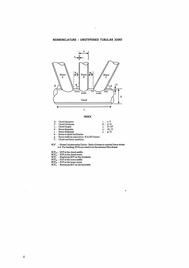
vNOMENCLATURE

ivEXECUTIVE SUMMARY

PAGE

1

101Extrapolation proceduresAPPENDIX C

70Simple joint SCF assessment databaseAPPENDIX B

49Parametric equations used in this studyAPPENDIX A

2

EXECUTIVE SUMMARY

This report covers the development of a new set of SCF parametric formulae forsimple tubular joints, ie the Lloyd’s Register equations, the work being largelyfunded by the HSE. Additionally, the report covers as assessment of the commonlyused SCF equations for simple tubular joints including the new LR equations. Thislatter work was carried out under the auspices of the HSE Review Panel for FatigueGuidance (RPFG).

In the development of the LR equations, a comprehensive database of measuredSCFs for full-scale steel joints and acrylic models was created. The joint acceptancecriteria for this database was agreed with representatives from the Industry. Fromthis database the new LR equations, which are given in Appendix A, were developed.

For the assessment of SCF parametric formulae for simple tubular joints thedatabase above was refined. The finalised database, which is given in Appendix B,was used to assess the existing commonly used parametric formulae and the newLR equations. The assessment criteria which was agreed with the RPFG is given inSection 5.2 and the equations assessed are given in Appendix A.1

3

1 See footnote to Section 1.0 Introduction

4

1. INTRODUCTION

In the 1970s with the increasing development of the hot-spot stress S-N approach tonodal joint fatigue life estimation, it became clear that the determination of reliablestress concentration factors (SCFs) for tubular joints was fundamental to thisconcept. The first parametric SCF equations covering simple tubular joints werederived by Toprac and Beale in 1967 (1) using a limited steel joint database. Theprohibitive cost of testing scaled steel models led Reber (2), Visser (3) and Kuang etal (4,5) to use finite element (FE) analyses based on analytical models of cylindricalshells. Subsequent equations by Wordsworth and Smedley (6,7) using acrylic modelspecimens and by Efthymiou and Durkin (8,9) employing 3-D shell FE analyses,have made considerable advances both in the accuracy of parametric equations and inthe range of joints covered.

Over this period, differences arose between the experimental procedures used toderive stress concentration factors for simple tubular joints. These differences led toinconsistencies both in the measured SCFs themselves, and also in theSCF parametric formulae based on these measured SCF values. Theseinconsistencies in SCF derivation are reflected in the hot-spot S-N curves used toestimate fatigue lives for simple tubular joints.

In the Lloyd’s Register (LR) group-sponsored project ‘SCFs for tubular complexjoints’, parametric expressions have been derived to calculate the relief obtained byadding ring-stiffeners into a simple unstiffened tubular joint. Similar expressionsalso exist which give the relief obtained by grouting tubular joints. In both cases arelief factor is applied to the unreinforced joint SCF, further highlighting the need foraccurate simple joint SCF equations.

In the UKOSRP II project, reported in 1987 (10), a limited programme of workinvestigated anomalies between the existing simple joint parametric SCF equations.However, many of the anomalies highlighted in the UKOSRP II project remainunresolved. A test programme on unstiffened tubular joints performed byLloyd’s Register (11), has further emphasised inconsistencies between test resultsand the more commonly used parametric equations.

Despite considerable differences that exist between parametric SCF formulae, thecurrent offshore installations guidance document (12), accepts the use of parametricequations to determine hot-spot stresses in tubular joints. While current guidancemerely states that ‘the appropriate SCF’ should be used, it is the intention of futureguidance (13) to give more specific directions on which parametric SCFs may beemployed in fatigue design, and the procedures that should be considered prior toperforming either experimental tests, FE analysis, or in deriving parametricequations.

In this report, 2 studies, largely funded by the HSE, are presented. In the first studya comprehensive database of steel and acrylic simple joint SCFs was created, titledthe LR SCF derivation database and described in Section 3. The acceptance criteriafor this database was agreed with representatives of the Industry. From this databasea new set of SCF formulae for simple joints (ie the LR equations) has been derived.These new equations are given in Appendix A. In the second study the databaseabove was refined under the auspices of the Review Panel for Fatigue Guidance. Thefinalised database, titled the SCF assessment database and given in Appendix B, was

5

used to assess existing simple joint SCF parametric formulae including the newLR equations. The equations assessed are given in Appendix A and the assessmentcriteria in Section 5.22

6

2 In the SCF assessment, 5 sets of parametric equations were considered. However,in the new HSE fatigue guidance only 2 sets are considered for recommendation.Therefore, only these 2 sets, ie the new LR and Eftymiou equations, are given inAppendix A.

2. REVIEW OF EXPERIMENTAL TECHNIQUES

The HSE fatigue guidance background document (14), highlights 5 factors thatinfluence the development of fatigue failure in welded tubular joints, and hencedetermine the joint fatigue life. The first of these factors describes the overallgeometry of the tubular joint and the detailed geometry of its welds. For this factor,the ‘hot-spot’ is described as the region where fatigue cracking is likely to initiate dueto a stress concentration. The definition of the hot-spot stress varies considerablyfrom a very general philosophy to a detailed description of its formulation, dependingupon the source quoted. During early UKOSRP studies the HSE sought aclarification in the definition of the hot-spot stress and its calculation, thus enablingthe derivation of the ‘T’ S-N curve. In this project the HSE definition of hot-spotstress and design guidance has been adopted, although alternative approaches arediscussed and assessed.

The definition of hot-spot stress (14), as the region where fatigue cracking is mostlikely to initiate due to a stress concentration, proposed linear extrapolation of themaximum principal stresses, outside the region of weld toe influence, to the weld toe.However, differences in the definition of hot-spot stress and between the type ofexperimental technique employed has led to considerable variation in measuredstresses between nominally identical joints.

For most simple joint geometries and loadings the hot-spot will be located at eitherthe saddle or crown. However, studies of the measured stress around the brace/chordperiphery indicate that under IPB and axial load the hot-spot stress may be located atan interim position for some geometrics.

2.1 METHODS OF MODELLING TUBULAR JOINTS

In the UKOSRP I project an assessment of the performance of different modellingtechniques was performed (15). This assessment concluded that differences observedbetween SCFs measured on steel models, acrylic models and photoelastic models orderived using a finite element analysis method, gave very similar results oncedifferences in the local joint geometry and the experimental procedure were taken intoaccount.

In previous studies, acrylic models and FE results have been utilised to developparametric formulae which are verified against results from steel models. In thisstudy the limited range of geometrics for steel joints led to the consideration ofalternative methods into the database against which parametric methods would bebenchmarked. This decision is discussed in detail in Section 3.

2.2 STRAIN GAUGE LOCATIONS AND STRESS SAMPLINGPOSITIONS

Due to the rapid increase and variation in stress around the region of the weld toeresulting from the local weld geometry, it is recommended that strain gauges shouldbe located outside this notch region. The maximum extent of this local notch regionis defined as 0.2ª rt (and not less than 4 mm), where r and t are the brace outsideradius and thickness respectively. The dependence upon ªrt has been derived from

7

studies of the bending stress in tubes (16), and this parameter has been empiricallymodified following detailed analyses of large scale tubular joint intersections in theUKOSRP and ECSC projects.

The ECSC recommendations for the extent of the notch region to 0.2ª rt have beenadopted by the HSE as the suggested location for the gauges nearest to the weld toeor brace/chord intersection. However more recent work on photoelastic joints (17)suggests that for some K joint configurations this notch region extends beyond0.2ªrt, giving a maximum error in the order of 10% - 12%.

A second set of gauges, enabling linear extrapolation to the weld toe, are locatedaccording to the location around the brace/chord intersection:

0.65ª(rt)=braceside0.44ª(rtRT) =chord crown5°arc=chord saddle

(It should be noted that this definition does not give guidance as to the gauge locationon the chordside between the saddle and the crown locations). Where non-linearextrapolation is required a third gauge set is placed equidistant from the secondgauge set (eg braceside = 1.10ªrt).

An alternative approach developed by Gurney (18), recommended a minimum straingauge distance of 0.4T, from the weld toe, where T is the chord thickness. Gurney’srecommendation results from FE analyses of simple fillet welded joints in plates,which indicate that the region of the notch stress is a function of the thickness of theplate upon which stresses are being measured.

In comparing the variation in SCF between the ECSC and the Gurney recommendedgauge locations, Swensson et al (19) tested 3 X joints (ß = 0.35, 0.67 and 1.00).These tests showed that on average the SCF derived by the Gurney method exceedsthe ECSC method by 7.6%, with the least difference between the methods occurringwhen ß = 0.67. This result corresponds with the findings of another analysis byWardenier (20), which states that the hot-spot stress will be ‘nearly the same’ forjoints with ß = 0.6 irrespective of the method used, although for joints withpronounced 3-dimensional effects, eg ß = 1.0, Gurney’s method describes the notchregion better than the ECSC method.

8

2.3 MEASUREMENT OF STRESSES AND STRAINS

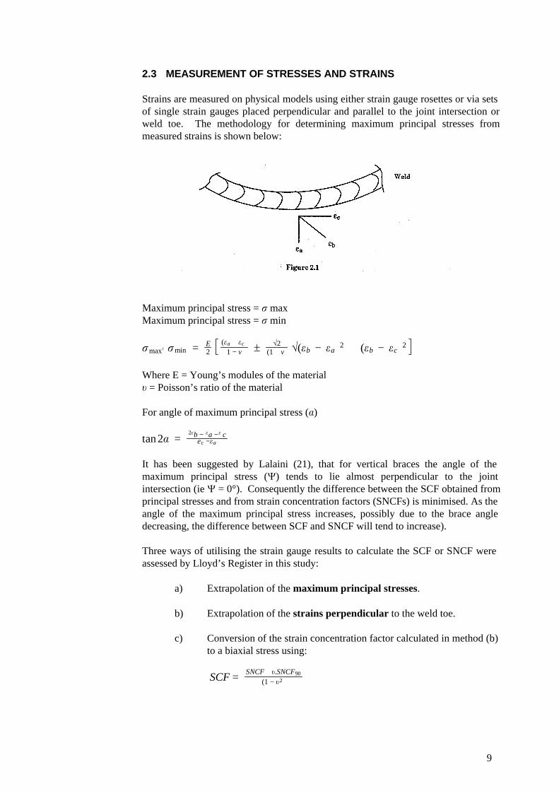
Strains are measured on physical models using either strain gauge rosettes or via setsof single strain gauges placed perpendicular and parallel to the joint intersection orweld toe. The methodology for determining maximum principal stresses frommeasured strains is shown below:

Maximum principal stress = r maxMaximum principal stress = r min

rmax∏ rmin = E2

(ea + ec)1 − v ! ª2

(1 + v) ª(eb − ea)2 + (eb − ec)2

Where E = Young’s modules of the materialu = Poisson’s ratio of the material

For angle of maximum principal stress (a)

tan 2a =2eb − ea −e c

ec −ea

It has been suggested by Lalaini (21), that for vertical braces the angle of themaximum principal stress (Y) tends to lie almost perpendicular to the jointintersection (ie Y = 0°). Consequently the difference between the SCF obtained fromprincipal stresses and from strain concentration factors (SNCFs) is minimised. As theangle of the maximum principal stress increases, possibly due to the brace angledecreasing, the difference between SCF and SNCF will tend to increase).

Three ways of utilising the strain gauge results to calculate the SCF or SNCF wereassessed by Lloyd’s Register in this study:

a) Extrapolation of the maximum principal stresses.

b) Extrapolation of the strains perpendicular to the weld toe.

c) Conversion of the strain concentration factor calculated in method (b)to a biaxial stress using:

SCF = SNCF + u.SNCF90

(1 − u2)

9

[where u is the Poisson’s ratio of the model material (u = 0.30 steel, u = 0.36 acrylic)and SNCF90 is the strain concentration factor from the nearest parallel gauge to theweld toe or joint intersection].

In this study, it was found that for 90° joints, the maximum principalstress (method (a)) was approximately 20% - 25% larger than the perpendicularstrain (method (b)) for acrylic models, while for steel models the difference wasnearer to 15%. This can be accounted for by the different Poisson’s ratio for the2 materials. Furthermore, for both steel and acrylic 90° joint specimens, it wasconfirmed that the angle of the maximum principal stress varied by less than 10%from the perpendicular to the joint intersection.

These results correspond well with the UEG design guide (22) which recommends anoverall factor of 1.20, while examination of a K joint by Lalani (21) suggest a lowerfactor of 1.16.

For both steel and acrylic joints with inclined braces, the angle of the maximumprincipal stress increased as the brace angle decreased. However, far moresignificant differences occur between the maximum principal stress and theperpendicular strain on steel joints (30% - 50%) than on similar acrylic modelspecimens (23% - 30%) despite the aforementioned difference in the Poisson’s ratio.This inconsistency between the limited number of steel and acrylic joint specimensreviewed requires investigation in future testing programmes.

For all joint configurations, the SCF derived from maximum principalstress (method (a)) is consistently 2% - 3% larger than the SCF derived from biaxialstress (method (c)).

2.4 EXTRAPOLATION PROCEDURE

The HSE recommendations regarding extrapolation technique requires linearextrapolation to be adopted for 90°T and X joints (ß<1), while for inclined Y andK joints it is stated that in some cases there may be a non-linear geometric stressdistribution. However, the hot-spot stress S-N approach for simple tubular joints iscurrently based on linear extrapolation, irrespective of the joint configuration.

The HSE does not give a method for extrapolating stresses, however, theextrapolation procedures adopted by Lloyd’s Register in conjunction with acrylicmodel testing are given in Appendix C.

Lloyd’s Register have reviewed 67 simple acrylic T/Y, X and K joints that employedboth linear and non-linear extrapolation of maximum principal stresses to thebrace/chord intersection (23). Linear extrapolation was performed through the2 rosettes nearest to the brace/chord junction, while non-linear extrapolation,employing a quadratic fit or Lagrange polynomial, utilised these 2 rosettes and athird rosette positioned on equal distance from the second rosette.

It was concluded that non-linear extrapolation exceeds linear extrapolation on thechordside for all loadcases by less than 5% irrespective of brace angle. On thebraceside, particularly at the brace crown under IPB, larger differences of around10% can be found, although the degree of brace inclination does not appear to be asignificant factor, see Table 2.1. However, it should be noted that to give a realistic

10

assessment of the differences between linear and non-linear extrapolation, jointswhere ß = 1 or where the measured SCF was less than 1.5 were excluded. Forß = 1 joints (particularly ß = 1 X joints) where the stresses tend to be relativelysmall, SCFs using non-linear extrapolation could be twice those using linearextrapolation (eg SCF = 0.41 linear, and SCF = 0.76 non-linear).

Table 2.1Increase in SCF using non-linear extrapolation

7%3%0%2%8%1%-1%4%22K12%5%6%3%6%6%5%3%9X

---2%2%--1%-4%6Y10%4%5%2%6%6%0%4%20T

BraceCrown

ChordCrown

BraceSaddle

ChordSaddle

BraceCrown

BraceSaddle

ChordCrown

ChordSaddle

IPBOPBAxial LoadNo ofjoints

Jointconfig

2.5 THE INFLUENCE OF A WELD FILLET

Acrylic model tests and some FE analyses do not include a weld fillet on the tubularjoint intersection, and therefore require some modification to their measured hot-spotstress if they are to be compared to steel joint test results. The addition of a weldfillet to a tubular connection results in a reduced SCF which is measured at the weldtoe rather than at the joint intersection.

It is important to note that the extrapolation of stresses on a model with no weld filletshould not be foreshortened to where the weld toe would be in an attempt to reflectthe influence of the weld.

2.5.1 The inclusion of a weld fillet

Employing acrylic model T and 90° X joints, Smedley (24) produced a weld filletcorrection factor based on the chordside weld fillet leg length.

SCF Weld toe = SCF No weld

3„ 1 + XT

(where x is the weld fillet leg length on the chordside)

While being specifically designed for the chordside stress on 90° joints, Smedley alsoconsidered this expression to be acceptable for 90° joints on the braceside. However,for inclined braces it was considered that this factor was not applicable.

Alternatively, Marshall (25) proposed a design equation, based on FE analysis ofK joints.

SCF Brace weld toe = 1.0 + [SCF Brace mid−surface − 1.0] x exp − 0.5T+t„rt

This equation, applied to the braceside mid-section stress, uses an exponential decayfunction to approximate the SCF at the braceside weld toe, and is generally used inconjunction with the Kuang parametric equations (5).

11

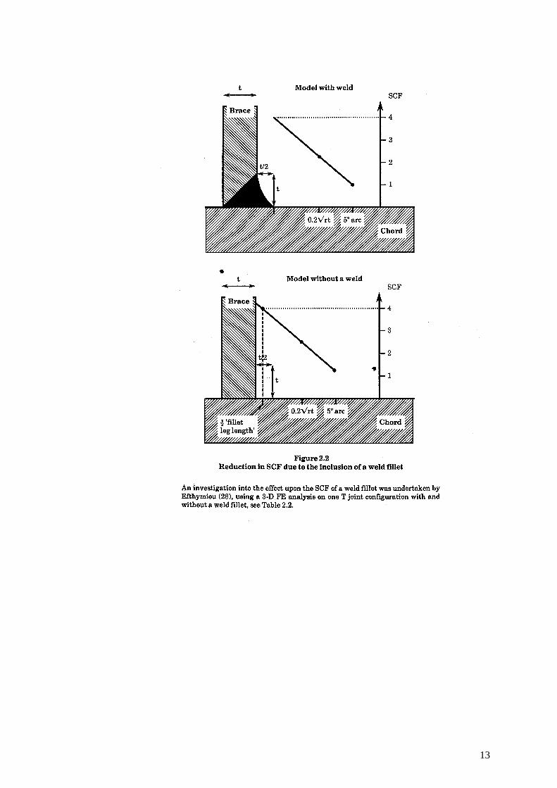
A more recent approach (26), suggested that for a specimen with no weld fillet, theextrapolation to the brace/chord intersection should be foreshortened by half thestandard fillet leg length to simulate the inclusion of a weld fillet, see Figure 2.2.Further work by Lloyd’s Register using this approach on joints with ß<1, showed aconsistent stress reduction factor of 0.95 on the chordside and 0.88 on the braceside,when a weld fillet leg length = t/2 on the chordside and = t on the braceside wasdescribed in accordance with API recommendations for controlled weld profiles (27).It should be noted that for many of the steel test specimens, particularly those ofsmall scale, the weld leg length on the braceside exceeded the brace thickness (t).

12

13

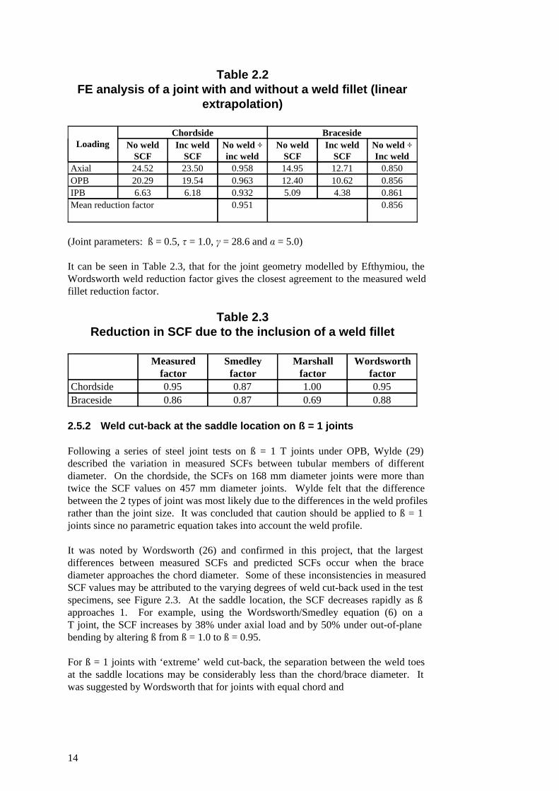
Table 2.2FE analysis of a joint with and without a weld fillet (linear

extrapolation)

0.8560.951Mean reduction factor0.8614.385.090.9326.186.63IPB0.85610.6212.400.96319.5420.29OPB0.85012.7114.950.95823.5024.52Axial

No weld ÷Inc weld

Inc weldSCF

No weldSCF

No weld ÷inc weld

Inc weldSCF

No weldSCF

BracesideChordsideLoading

(Joint parameters: ß = 0.5, t = 1.0, c = 28.6 and a = 5.0)

It can be seen in Table 2.3, that for the joint geometry modelled by Efthymiou, theWordsworth weld reduction factor gives the closest agreement to the measured weldfillet reduction factor.

Table 2.3Reduction in SCF due to the inclusion of a weld fillet

0.880.690.870.86Braceside0.951.000.870.95Chordside

Wordsworthfactor

Marshallfactor

Smedleyfactor

Measuredfactor

2.5.2 Weld cut-back at the saddle location on ß = 1 joints

Following a series of steel joint tests on ß = 1 T joints under OPB, Wylde (29)described the variation in measured SCFs between tubular members of differentdiameter. On the chordside, the SCFs on 168 mm diameter joints were more thantwice the SCF values on 457 mm diameter joints. Wylde felt that the differencebetween the 2 types of joint was most likely due to the differences in the weld profilesrather than the joint size. It was concluded that caution should be applied to ß = 1joints since no parametric equation takes into account the weld profile.

It was noted by Wordsworth (26) and confirmed in this project, that the largestdifferences between measured SCFs and predicted SCFs occur when the bracediameter approaches the chord diameter. Some of these inconsistencies in measuredSCF values may be attributed to the varying degrees of weld cut-back used in the testspecimens, see Figure 2.3. At the saddle location, the SCF decreases rapidly as ßapproaches 1. For example, using the Wordsworth/Smedley equation (6) on aT joint, the SCF increases by 38% under axial load and by 50% under out-of-planebending by altering ß from ß = 1.0 to ß = 0.95.

For ß = 1 joints with ‘extreme’ weld cut-back, the separation between the weld toesat the saddle locations may be considerably less than the chord/brace diameter. Itwas suggested by Wordsworth that for joints with equal chord and

14

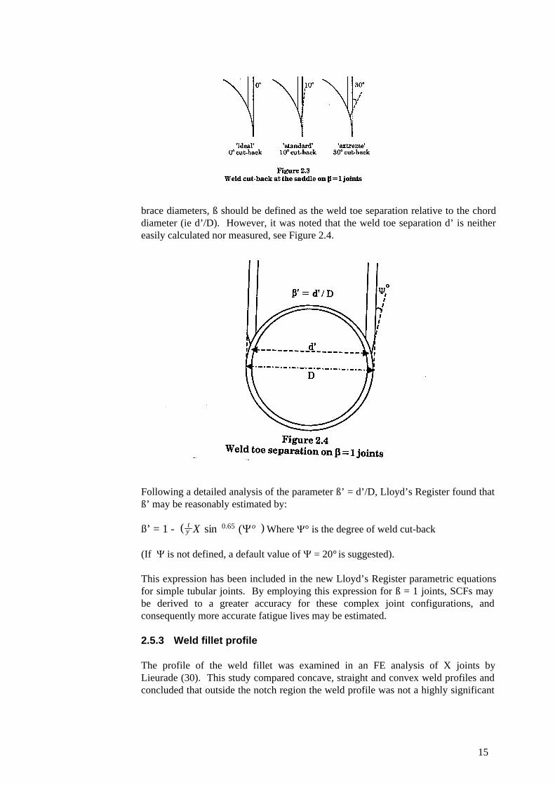
brace diameters, ß should be defined as the weld toe separation relative to the chorddiameter (ie d’/D). However, it was noted that the weld toe separation d’ is neithereasily calculated nor measured, see Figure 2.4.

Following a detailed analysis of the parameter ß’ = d’/D, Lloyd’s Register found thatß’ may be reasonably estimated by:

Where Y° is the degree of weld cut-back¾’ = 1 - ( ty X sin 0.65 (Yo))

(If Y is not defined, a default value of Y = 20° is suggested).

This expression has been included in the new Lloyd’s Register parametric equationsfor simple tubular joints. By employing this expression for ß = 1 joints, SCFs maybe derived to a greater accuracy for these complex joint configurations, andconsequently more accurate fatigue lives may be estimated.

2.5.3 Weld fillet profile

The profile of the weld fillet was examined in an FE analysis of X joints byLieurade (30). This study compared concave, straight and convex weld profiles andconcluded that outside the notch region the weld profile was not a highly significant

15

factor, although a concave weld will always give the lowest stress. Since most jointsare generally modelled to a concave weld profile there will be negligible influence onthe hot-spot stress due to marginal differences in weld profile.

2.6 CHORD LENGTH AND CHORD END EFFECTS

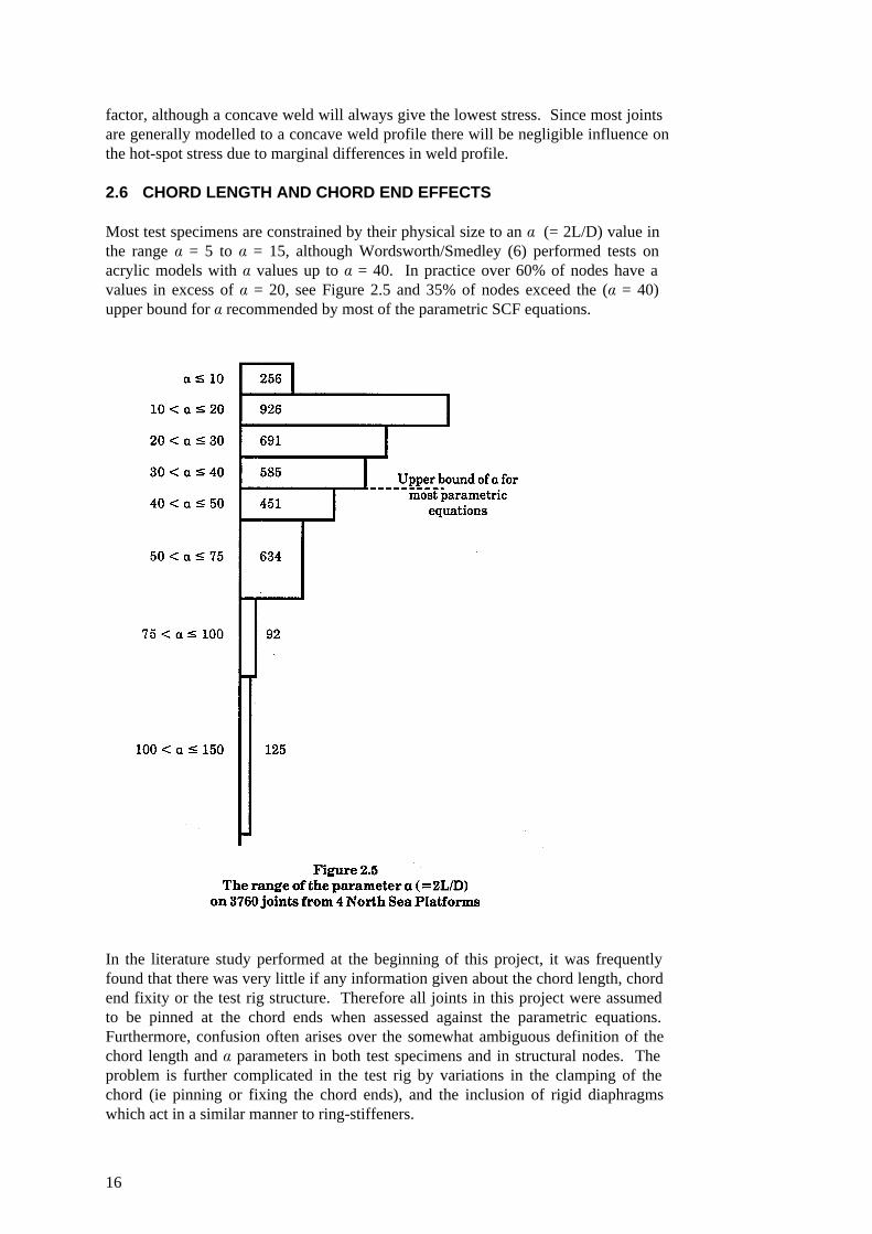
Most test specimens are constrained by their physical size to an a (= 2L/D) value inthe range a = 5 to a = 15, although Wordsworth/Smedley (6) performed tests onacrylic models with a values up to a = 40. In practice over 60% of nodes have avalues in excess of a = 20, see Figure 2.5 and 35% of nodes exceed the (a = 40)upper bound for a recommended by most of the parametric SCF equations.

In the literature study performed at the beginning of this project, it was frequentlyfound that there was very little if any information given about the chord length, chordend fixity or the test rig structure. Therefore all joints in this project were assumedto be pinned at the chord ends when assessed against the parametric equations.Furthermore, confusion often arises over the somewhat ambiguous definition of thechord length and a parameters in both test specimens and in structural nodes. Theproblem is further complicated in the test rig by variations in the clamping of thechord (ie pinning or fixing the chord ends), and the inclusion of rigid diaphragmswhich act in a similar manner to ring-stiffeners.

16

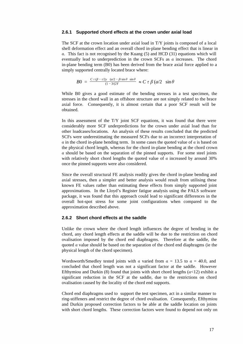
2.6.1 Supported chord effects at the crown under axial load

The SCF at the crown location under axial load in T/Y joints is composed of a localshell deformation effect and an overall chord in-plane bending effect that is linear ina. This fact is not recognised by the Kuang (5) and HCD (31) equations which willeventually lead to underprediction in the crown SCFs as a increases. The chordin-plane bending term (B0) has been derived from the brace axial force applied to asimply supported centrally located brace where:

B0 =C t (b − t/2y)) (a/2 − b/ sin h) sin h

(1 − 3/(2Y)) l C t b (a/2) sinh

While B0 gives a good estimate of the bending stresses in a test specimen, thestresses in the chord wall in an offshore structure are not simply related to the braceaxial force. Consequently, it is almost certain that a poor SCF result will beobtained.

In this assessment of the T/Y joint SCF equations, it was found that there wereconsiderably more SCF underpredictions for the crown under axial load than forother loadcases/locations. An analysis of these results concluded that the predictedSCFs were underestimating the measured SCFs due to an incorrect interpretation ofa in the chord in-plane bending term. In some cases the quoted value of a is based onthe physical chord length, whereas for the chord in-plane bending at the chord crowna should be based on the separation of the pinned supports. For some steel jointswith relatively short chord lengths the quoted value of a increased by around 30%once the pinned supports were also considered.

Since the overall structural FE analysis readily gives the chord in-plane bending andaxial stresses, then a simpler and better analysis would result from utilising theseknown FE values rather than estimating these effects from simply supported jointapproximations. In the Lloyd’s Register fatigue analysis using the PALS softwarepackage, it was found that this approach could lead to significant differences in theoverall hot-spot stress for some joint configurations when compared to theapproximation described above.

2.6.2 Short chord effects at the saddle

Unlike the crown where the chord length influences the degree of bending in thechord, any chord length effects at the saddle will be due to the restriction on chordovalisation imposed by the chord end diaphragms. Therefore at the saddle, thequoted a value should be based on the separation of the chord end diaphragms (ie thephysical length of the chord specimen).

Wordsworth/Smedley tested joints with a varied from a = 13.5 to a = 40.0, andconcluded that chord length was not a significant factor at the saddle. HoweverEfthymiou and Durkin (8) found that joints with short chord lengths (a<12) exhibit asignificant reduction in the SCF at the saddle, due to the restrictions on chordovalisation caused by the locality of the chord end supports.

Chord end diaphragms used to support the test specimen, act in a similar manner toring-stiffeners and restrict the degree of chord ovalisation. Consequently, Efthymiouand Durkin proposed correction factors to be able at the saddle location on jointswith short chord lengths. These correction factors were found to depend not only on

17

a, but also on ß and c. So that for a T joint under axial load with a relatively thinchord wall and a = 5, the short chord correction factor can halve the saddle SCFcompared to a similar node with a = 10.

Most steel joint test specimens are constrained to having a values in the range a = 5to a = 10, with the larger diameter joints tending to have the smaller a values.Therefore, nearly all the SCFs derived from steel joint test results are influenced bythe locality of the end restraint, and as a consequence the SCFs measured on testspecimens may be significantly less than those observed on more realistic joints. Itshould be emphasised that this is a chord end ovalisation effect rather than a chordsupport effect. Therefore, for most X joints where the joint is supported by thebrace ends and no chord end diaphragms are fitted, chord length effects are far lesspronounced.

As steel joint test specimens are used as a benchmark for testing the validity ofparametric equations, it is important that end effects are taken into account prior toany assessment. In future, it is recommended that consideration should be given toshort chord effects before any physical model or FE analyses are performed, whetherfor static strength, SCF or fatigue endurance.

3. DATABASE

This section describes the Lloyd’s Register SCF derivation database. This databaseof steel and acrylic joint SCFs was created for the development of a new set ofparametric equations for simple tubular joints. The work was largely funded by theHSE.

At the outset of the project lengthy discussion took place with both the HSE and withmany representatives from the oil industry regarding the composition of thisdatabase. It was felt that steel data alone was insufficient to enable a new set ofparametric equations for simple joints to be developed, particularly for X, K andKT joints. It was considered that acrylic models gave a good representation of thestress distribution observed in equivalent steel joints, and that acrylic joints should beincluded in the database provided allowance was made for differences inexperimental techniques. This conclusion was supported by assessments ofexperimental techniques performed in the UKOSRP I project (15).

With regard to FE results, it was felt that published data was of variable quality andoften the analysis methodology was insufficiently documented. Therefore, it wasdecided to exclude SCFs derived by FE analysis from the database, while acceptingthat FE analysis, particularly using 3-D shell elements, generally gives goodcorrelation to similar steel joint configurations. The database of photoelastic modeltests was considered too small to be validated independently.

3.1 CRITERIA FOR THE ACCEPTANCE OF SCF DATA

The initial objective of this project was to gather measured SCF data relating tosimple tubular joints. To meet this objective, a literature search was undertaken tolocate experimental data relevant to this project. In association with SCF resultsfrom work performed in-house, this literature search has provided a substantialdatabase for this project.

18

(i) The following data items are included:

a) Source of the SCF data - title of paper, authors, where the data hasbeen located, the date of publication and any confidentialityrestrictions.

b) Experimental details - specimen material, extrapolation type, locationof the nearest gauge, stress/strain measurement, weld fillet inclusionand chord end fixity.

c) Number and configuration of the joints tested.

d) Geometric and parametric details of the joint - (D, T, L, d, t, h, t, b,c, a).

e) Applied loadcases - (axial, OPB, IPB - single, balanced,unbalanced).

f) The measured SCFs and their location on the joint - (chordside orbraceside - saddle, crown or an interim location).

g) Repetitions - where several configurations were tested with the samejoint parameters, the results of each test were included. However, thedanger of bias in the analysis was noted.

h) Several saddle results - where 2 or 4 individual SCFs are quoted forone joint, the maximum SCF result was taken.

i) Tension/compression - where a joint is axially loaded in both tensionand compression, the average of the 2 results was taken.

Verifying the accuracy of the data involved locating the source paper or experimentalreports where possible and comparing the given results to a second publication. Thisexercise was time consuming and not always feasible, however the necessity of thiscross-checking procedure was proved with several inconsistencies in SCF resultsoccurring between published papers.

(i) Single-plane, non-overlapped, unstiffened and ungrouted tubular joints, witha chord diameter m150 mm and the strain gauge nearest to the brace/chordintersection being outside the notch region, were recorded on the database.

The chord length quoted in most papers was the physical length of the test specimen,and this was the value recorded in the database. However, it would have beendesirable to record 2 ‘chord length’ values if these had been quoted. The separationbetween the chord end diaphragms is required to derive ovalisation effects, and theseparation between the chord end supports is required to calculate the degree of chordbending in the test specimen.

Only joints with parameters typical of those noted in practice were included, and thefollowing subset of data was felt to be typical of offshore platforms: t[1.05, c[40,SCFsm1.5, b[1.0 (only b = 1 joints at the saddle where the degree of weld cut-back isrecorded).

19

(ii) The initial analysis of the SCF data involves the standardisation of themeasured SCFs to conform with the HSE recommended method, this has beenachieved by the use of a number of correction factors covering differences in theexperimental derivation of the hot-spot stress, see section 3.2.

3.2 FACTORS APPLIED TO THE SCF DATABASE

w Strain gauge locations: the nearest strain gauge to the weld toe or to thebrace/chord intersection must be in excess of a distance of 0.18„rt from theweld toe or the brace/chord intersection. This is based on a 10% reduction inthe recommended value of 0.2„rt, since some papers appear to round straingauge location to the nearest mm. This small allowance did not result in asignificant increase in the extrapolated SCF value.

w Maximum principal stress or biaxial stress derived from strain concentrationfactors: it is considered that no factor is required to differentiate betweenSCFs derived from either biaxial stress or maximum principal stress.

w Stress and strain measurement: the recommended factors for convertingperpendicular strain (SNCFs) to maximum principal stress (SCFs) are:

SCF = SNCF X 1.15 for T joints (steel joints).SCF = SNCF X 1.23 for T joints (acrylic joints).

For inclined braces larger differences between SNCFs and SCFs would beexpected, however there is insufficient data on strain concentration factorsfrom inclined braces to derive an estimate of this difference. These factorswere applied to all braces despite these limitations.

w Extrapolation procedure: the recommended factor for converting non-linearSCFs to linear SCFs is:

Linear = non-linear X 0.95 (including b= 1 joints).

This factor is less than the 10% difference proposed by UEG (22), but wouldappear to give a better estimate of the difference between linear andnon-linear stress since this value is based on a database of 57 joints analysedin the LR project (23).

w The absence of a weld fillet: weld fillet correction factors of 0.95 on thechordside and of 0.86 on the braceside have been adopted, these values arebased on the only measured weld fillet comparison available (ie theKSEPL joint) (28).

w Weld cut-back at the saddle location on b = 1 joints: following a detailedanalysis of the parameter b = d’D, Lloyd’s Register found that b’ may bereasonably estimated by:

Where Y° is the degree of weld cut-backb ∏ = 1 − ( tc X sin0.65(Yo))

(If Y is not defined, a default value of Y = 20° is suggested).

20

This expression has been included in the new Lloyd’s Register parametricequations for simple tubular joints, listed in Appendix A.

w It should be noted that many steel joints in particular, have a values based onthe separation of pinned end supports rather than chord end diaphragmseparation. This gives a more accurate assessment of the SCF at the crownwhich is dependent upon the level of bending in the chord, while thereduction in SCF due to the restriction on chord ovalisation noted at thesaddle on joints with short chord lengths tended to be underestimated.

Chord length effects due to the restriction of ovalisation caused by thediaphragms at the chord ends leads to considerable reduction in SCFs at thesaddle for short chord lengths. This problem is described by Efthymiou (8)who published short chord correction factors to be used in accordance withthe Efthymiou SCF equations when a (=2L/D) <12. A substantial numberof steel T joints were tested with a values in the range a = 4.3 to 12.0. Toeliminate these joints from the database would have had a substantial effecton the number of steel joints that could be considered.

4. SIMPLE JOINT SCF EQUATIONS

The parametric equation gives the designer the most convenient way of estimating thehot-spot stress in simple tubular joints, however at the present time no equations arerecommended by the HSE. Even between the more commonly used parametricequations, there are significant differences in the way the hot-spot stress is defined,calculated, and in their recommended ranges of applicability. It should be noted thatsome of the comments made here are based on the assessment covered in Section 5.0.

4.1 KUANG EQUATIONS (1975 AND 1977)

The Kuang equations (5), cover T/Y, K and KT joint configurations and utilise amodified thin-shell finite element program specifically designed to analyse tubularconnections. The tubular connections were modelled without a weld fillet, andstresses were measured at the mid-section of the member wall. Therefore the stressescalculated using the Kuang finite element models are considerably different from theHSE definition of hot-spot stress. The Kuang equations are based on a mean fit tothe database of FE joints examined, and do not indicate the location of the hot-spotaround the periphery, but are merely expressed as chordside or braceside.

With regard to the Kuang equations, the following points were noted:

(i) Of the equations reviewed, the Kuang equations have the mostrestricted validity range, and consequently cover the fewest joints in thedatabase. The Kuang equations were not designed to cover joints with b>0.8and do not cover X joints or the unbalanced OPB loadcase for K andKT joint configurations.

(ii) For T/Y joints under axial load, no account is given to the beambending effect, and consequently underpredictions at the crown for higha values may be anticipated.

21

(iii) No account is given to chord length effects at the saddle, due to thechord end restraints. Therefore, given that the database of FE joints utilisedby Kuang had generally short chord lengths, there is a possibility ofunderestimation of SCFs for more realistic chord length (a) values.

(iv) The performance of the Kuang equations for T/Y joints for b valuesabove 0.5 is generally poor, although there can be considerable variation inthe degree of underprediction depending upon the loadcase considered. Forexample, the Kuang equation gives a very poor fit to chordside SCFs underOPB underpredicting 70% of joints in this database, yet gives a reasonablygood fit to the braceside SCFs under OPB.

(v) For K joints, the Kuang equations are generally conservative for allvalues of b. Non-symmetric K joint configurations exhibit the largestdifference between the measured SCFs and the predicted SCFs, since theKuang K joint equations were specifically designed for joints with symmetricbraces.

(vi) For KT joints under balanced axial load, the Kuang equations showgood agreement with the measured SCF values on the chordside. However,on the braceside, the Kuang KT joint SCF equations differs considerablyfrom the corresponding equation for a K joint, with the predicted SCFs forthe KT joints in this database up to 4 times larger than the measuredSCF values.

The Kuang equations are still widely used in the fatigue design of offshore tubularjoints.

4.2 WORDSWORTH/SMEDLEY EQUATIONS (1978 AND 1981)

The Wordsworth/Smedley (W/S) equations were derived using acrylic model testresults on tubular joints modelled without a weld fillet. The equations covering T/Yand X joint configurations were published by Wordsworth/Smedley in 1978 (6), andthe K and KT joint configurations were covered by Wordsworth in 1981 (7).Generally, the HSE recommendations for the derivation of the hot-spot stress werefollowed, using maximum principal stresses from outside the (0.2 „rt) ‘notch’ zone.However, some areas of uncertainty do exist. The first surrounds the extrapolationtechnique adopted, which appears to be generally linear except where the stressdistribution was found to be particularly non-linear and therefore open to error. Thesecond concerns the number of sets of strain gauges adopted around the brace/chordintersection. The Wordsworth parametric equations specifically cover the saddle andcrown, but it is unclear whether interim sets of gauges were adopted, particularlyunder IPB where for some configurations the hot-spot stress occurs between thesaddle and crown.

For the W/S and Wordsworth equations, the following points were noted:

(i) On the braceside, for all loadcases and measuring locations, the W/Sand Wordsworth equations estimate the SCF using a simple factor applied tothe chordside SCF. Consequently, the predicted SCFs on the braceside tendto be rather conservative relative to the measured braceside

22

SCFs. However, it should be noted that the braceside SCF on a simpletubular joint rarely exceeds the chordside SCF. The Wordsworth equationsgenerally give a good estimate of the measured chordside SCFs.

(ii) For joint configurations with equal chord and bracediameters (ie b = 1 joints), a b value of b = 0.98 was taken at the saddlelocation as recommended by Wordsworth to simulate the weld cut-backfound at the saddle in typical steel b = joints.

(iii) The Wordsworth equations for K and KT joints utilise carry-overfunctions applied to the T joint expressions. Therefore the influence ofadding further braces to a simple T joint can clearly be determined.

(iv) Under axial loading and OPB at the saddle location, the Wordsworthequations tend to underpredict measured SCFs on joints with b = 0.8 andhigh c, and joints with b = 1.0 where there is a significant degree of weldcut-back.

(v) The W/S and Wordsworth equations are only valid for chord radiusto thickness ratios R/Tm12. A significant number of tubular joints aredesigned with relatively thick chords, to avoid the use of ring-stiffeners.Consequently, R/T ratios in the range 8 [R/T< 12 are not uncommon inpractice, and by using the W/S and Wordsworth equations a conservativeassumption of R/T = 12 must be made in determining the SCF.

4.3 UEG EQUATIONS (1985)

The UEG equations proposed in 1985 (22), are based on the W/S and Wordsworthequations with a modification factor applied to configurations with high b(b>0.6) orhigh c (c>20) values.

The following points may be made with regard to the UEG equations:

(i) All the comments for the W/S equations hold true for theUEG equations except for the weld-cut back simulation at b = 1, which isaccounted for in the Q’b term.

(ii) The factors „Q’b and Q’c are both applied under axial load and OPBwhile only „Q’c is applied under IPB where:

for cm20Q’c = 480/c(40 - 0.833c)for c<20Q’c = 1.0

for b>0.6Q’b = 0.3/b(1 - 0.833b)for b [0.6Q’b = 1.0

These modification factors based on comparisons of predicted and measuredresults from both static and fatigue studies, apply to all joint configurationsand are designed to give a characteristic set of equations (ie underpredicting5% of the measured data).

23

4.4 EFTHYMIOU/DURKIN EQUATIONS (1985 AND 1988)

In 1985, Efthymiou and Durkin (8) published a series of parametric equationscovering T/Y and gap/overlap K joints. Over 150 configurations were analysed viathe PMBSHELL finite element program using 3-dimensional shell elements, and theresults were checked against the SATE finite element program for one T joint and2 K joint configurations. The hot-spot SCFs were based on maximum principalstresses linearly extrapolated to the modelled weld toe, in accordance with theHSE recommendations, with some consideration being given to boundaryconditions (ie short chords and chord end fixity).

In 1988, Efthymiou (9) published a comprehensive set of simple joint parametricequations covering T/Y, X, K and KT simple joint configurations. These equationswere designed using influence functions to describe K, KT and multi-planar joints interms of simple T braces with carry-over effects from the additional loaded braces.

With respect to the Efthymiou/Durkin equations, the following points may be noted:

(i) It has been shown by Efthymiou that the saddle SCF is reduced injoints with short chord lengths, due to the restriction in chord ovalisationcaused by either the presence of chord end diaphragms or by the rigidity ofthe chord end fixing onto the test rig. Therefore, the measured saddle SCFson joints with short chords may be less than for the equivalent joint with amore realistic chord length. Factors have been included in the Efthymiouparametric equations to cover short chords.

(ii) The T/Y joint equation for the saddle under axial load includes ashort chord correction factor for either fixed or pinned ends. The short chordeffect at the saddle is due to the presence of chord end diaphragms, therefore,it is unclear why the chord end fixity should be a factor. The equation for Xjoints at the brace crown under axial load does not equal the correspondingT/Y joint equation excluding chord bending terms, as would be expected.

(iii) The Efthymiou equations give a comprehensive coverage of all theparametric variations and are designed to be mean fit equations. Due to thegreater correlation with steel models by the Efthymiou FE models, and thefewer conservative assumptions made, these equations tend to be nearest to amean fit and consequently more underpredictions are frequently observed.

(iv) Under unbalanced OPB, the Efthymiou equations give a good fit tosymmetric K joints or the outer braces in KT joints, but consistently appearto underestimate the SCF in the branch with hmax in non-symmetric K joints.

4.5 HELLIER, CONNOLLY AND DOVER EQUATIONS (1990)

The Hellier, Connolly and Dover (HCD) equations (31) were published in 1990 andwere primarily developed to improve fracture mechanics estimates of remaining lifefor a joint rather than for tubular joint design. Consequently, the overall programmeincluded not only hot-spot stress estimates, but modelling of the stress distributionaround the brace/chord intersection and the proportions of bending to axial stressthrough the member thickness. The SCF equations themselves cover T/Y jointconfigurations alone, and have a range of applicability for the b parameter limited to

24

b [ 0.8. Therefore, these expressions are currently limited in their application,however, further work is intended for b = 1 joints and for X and K jointconfigurations.

A thin-shell finite element method was developed using the PAFEC package, and in asimilar manner to the work by Kuang weld fillets were not modelled. It has beennoted in previous numerical modelling of tubular joints using the PAFEC semi-loofFE package (32) that poor results were obtained for large brace relative to chorddiameters, and hence an upper recommended limit of b = 0.8 was proposed. In thisstudy for b values near to b = 0.8, the HCD and Kuang equations often gave similarpredictions, which differed from the other equations reviewed. Therefore, furthercorrelation studies between the PAFEC FE package and physical specimens wouldbe beneficial for large b ratios.

In a similar manner to the Kuang equations, the HCD equations were initially derivedusing the simple form:

SCF = a1 aa2 ba3 ca4 ta5 ha6

where variables a1 to a6 are determined using a regression analysis method. Theexpressions were then refined by the addition of further terms.

With regard to the HCD equations, the following points were noted:

(i) For T/Y joints, at the chord crown under axial load, the linearoverall beam bending effect has not been accounted for in the expressions.The chord length (a) effect was deemed to have little effect for a valuesgreater than 13.1, consequently this upper bound test parameter wasremoved, so that these expressions are applicable for all a values exceedinga = 6.21. Furthermore, the majority of specimens modelled were influencedby chord end constraints, but again no account of this effect was taken. Thefailure to consider chord length effects must have an influence on theestimation of SCFs for joints with more realistic chord lengths.

(ii) With the exception of the b range, these expressions givecomprehensive coverage of realistic geometries observed on offshorestructures, and it is particularly worth noting that the chord radius tothickness ratio (c) was studied to as low as c = 7.6

(iii) The derived expressions estimate the SCF at both the saddle andcrown locations and also the maximum SCF around the brace/chordintersection. In addition, these expressions give the angle around thebrace/chord intersection of the maximum SCF. These expressions give acomprehensive description of the stress distribution around the periphery, forall loadcases, on both the chordside and braceside. However, someanomalies are associated with these expressions. The position of the hot-spotstress may be identified as being at the saddle or crown, but the hot-spotSCF equation (eg chordside) may not give the same result as thesaddle/crown equations. Cases were observed, where the hot-spot SCF (atthe saddle) exceeds the saddle equation SCF by up to 20%, and in othercases the saddle equation SCF was larger than the hot-spot (saddle) SCF.

25

For symmetric 90º T joints the 2 crown positions would yield the same SCF,however the 0º and 180º expressions for IPB do not give the same SCF.

4.6 LLOYD’S REGISTER EQUATIONS (1991)

The Lloyd’s Register (LR) equations were developed as part of the “SCFs for simpletubular joints” project which was largely funded by the HSE, in 1991. An initialreview of the performance of existing SCF equations with regard to the LR SCFdatabase highlighted a number of anomalies in the goodness of fit of all theseexpressions. Therefore the HSE suggested that a consistent set of SCF equationsshould be developed.

The LR equations (33) were developed as mean fit equations to the LR SCFderivation database, described in Section 3, by minimising the percentage differencebetween the measured SCF values and the estimated SCF values. The objective ofthese equations was to employ influence functions wherever possible, so that theexpression for one brace on a K joint would be that for an equivalent Y joint withfactors to describe the stiffening effect of the additional brace and loading given themagnitude of the load applied to this additional brace. Furthermore, considerationwas to be given to b = 1 joints where particular problems had been identified due tothe degree of cut-back of the weld at the saddle location. Short chord effects werealso considered to be of particular significance, however it became clear that for thedata available to LR derivation of short chord correction factors could not beachieved. Therefore, the Efthymiou short chord correction factors were used, inaccordance with the LR SCF equations, without any independent verification beingpossible.

The design factor to be applied to these mean fit expressions was also a matter forsome debate. No safety factor is suggested for SCF equations in the HSE guidancenotes (12), and consequently some SCF equations are designed to be a mean fit to theassociated experimental dataset, while some are designed to be a characteristic fit.Overall, it was felt that SCF equations that are currently used in offshore tubularjoint design have an appropriate level of safety. This rather subjective view of thereliability of SCF prediction led LR to multiply the mean fit equation, by onestandard deviation of this mean fit to the LR database. This led to a design equationthat underestimated around 15% to 20% of results.

The LR SCF derivation database is almost identical to the SCF assessment databasethat was used in this project to assess SCF formulae. It includes both steel andacrylic joint data, and has the same parametric and geometric limitations. Therefore,comparisons between the SCF assessment database and the LR equations should beconsidered in the knowledge that the equations themselves were largely developedfrom the dataset against which they are being compared.

With regard to the LR equations, the following points should be noted:

(i) These equations generally give the SCF at the saddle and crownlocations (except for IPB), and may underestimate a larger SCF if locatedbetween these locations. This is most likely to be the case for K/KT jointsunder axial load, although it was considered that the differences would besmall.

26

(ii) The LR equations use the Efthymiou short chord correction factors,which have not been independently verified.

(iii) The LR equations are limited to c ratios greater than c = 12, while asignificant number of tubular joints are designed with c values below thislimitation.

(iv) Short chord length effects, chord bending effects and the weldinfluence have been considered in deriving these equations.

(v) The form of the equations, while being more complex for ‘handcalculations’, gives a more logical influence function format, which largelyremoves the problem of joint classification.

5. ASSESSMENT OF SIMPLE JOINT SCF EQUATIONS

Throughout the duration and subsequent to the completion of this project, aconsiderable amount of discussion has centred on defining the characteristics of a‘good’ or ‘poor’ SCF parametric equation.

While it is clear that an equation is superior if it exhibits less scatter with respect totest data for all combinations of parametric values, acceptable levels ofunderprediction have not been defined. Unlike the current tubular joint S-N fatiguedesign curve where a 2.5% probability of failure is predicted, no specific probabilitylevel is currently defined for SCF equations. It was found that the parametricequations generally underpredict around 0% - 40% of measured SCF resultsdepending upon the equation/joint configuration/loadcase/measuring locationconsidered.

The equations derived by Kuang, W/S, UEG and HCD are based on either acrylicmodel test results or on the results of thin shell FE analyses. In both these methodsof analysis, no weld fillets were described and consequently the test resultsthemselves tend to be conservative. Therefore, since equations have been produced,generally by some form of least squares curve fit to these data points, the equationsthemselves do tend to be conservative relative to steel joint test results.

The Efthymiou equations on the other hand, were based on a least square fit toFE results using 3-D shell elements including a realistic weld fillet. Consequently,the Efthymiou equations frequently give the closest agreement with steel joint testresults in terms of scatter, but are generally less conservative than other parametricequations.

The HSE Review Panel for Fatigue Guidance (RPFG) considered that the newfatigue guidance should give recommendations regarding the applicability of SCFs.The panel was seeking to give a clear definition of the requirements of an acceptableparametric equation for simple tubular T/Y, X and K joints (13). This definitiontakes into account the scatter of the equation with respect to measured SCF results,the number of SCF underpredictions and to a lesser extent the number of significantSCF overpredictions.

The LR SCF derivation database described in Section 3 was refined and used toassess the applicability of the more commonly used SCF parametric equations forsimple joints. From this assessment a series of matrices for each joint type and

27

loading case was produced. There was insufficient data to produce a matrix forKT joints.

5.1 ASSESSMENT DATABASE

The decision to compare parametric equations with a combined database of steel andacrylic joints led to a great deal of debate over the validity of this approach. Withregard to the measurement of SCFs, steel data was known to be limited in geometricrange, applied loadcases and in location of strain gauges. Additionally, the steel datawas potentially biased due to the short chord lengths of the specimens and theproportionally large welds modelled. The short chord length and large weld filleteffects would both tend to reduce the measured SCFs, thus leading to possibleunderestimation of tubular joint stresses in practice. Furthermore, some anomalieshad been noted in the design SCF equations when compared to acrylic model testresults which would not be noted if only steel joint data was considered. However,acrylic joints are not steel joints, they merely represent steel models. Acrylic modelsdo not include weld fillets and consequently, approximations had to be made torepresent the effect of the weld fillet.

It was agreed that the ideal position would be to use acrylic models/finite elementanalyses to identify the areas of potential underestimation, and model these joints insteel. However, it was clear that a substantial number of steel models would berequired given the combinations of joint configuration, loadcase and measuringpositions to be assessed. It was felt to be more important to highlight potentiallyunsafe SCF design equations given the aforementioned limitations, than removeacrylic models from the assessment of parametric equations. Comparisons of thesteel and acrylic model subsets within the database were performed to assesspotential differences between the modelling techniques.

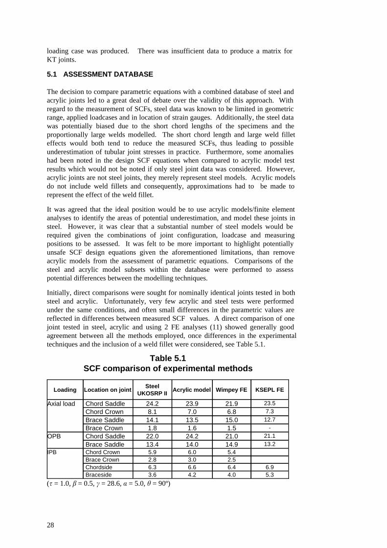
Initially, direct comparisons were sought for nominally identical joints tested in bothsteel and acrylic. Unfortunately, very few acrylic and steel tests were performedunder the same conditions, and often small differences in the parametric values arereflected in differences between measured SCF values. A direct comparison of onejoint tested in steel, acrylic and using 2 FE analyses (11) showed generally goodagreement between all the methods employed, once differences in the experimentaltechniques and the inclusion of a weld fillet were considered, see Table 5.1.

Table 5.1SCF comparison of experimental methods

5.34.04.23.6Braceside6.96.46.66.3Chordside

2.53.02.8Brace Crown5.46.05.9Chord CrownIPB

13.214.914.013.4Brace Saddle21.121.024.222.0Chord SaddleOPB

-1.51.61.8Brace Crown12.715.013.514.1Brace Saddle7.36.87.08.1Chord Crown

23.521.923.924.2Chord SaddleAxial load

KSEPL FEWimpey FEAcrylic modelSteel

UKOSRP IILocation on jointLoading

(t = 1.0, b = 0.5, c = 28.6, a = 5.0, h = 90º)

28

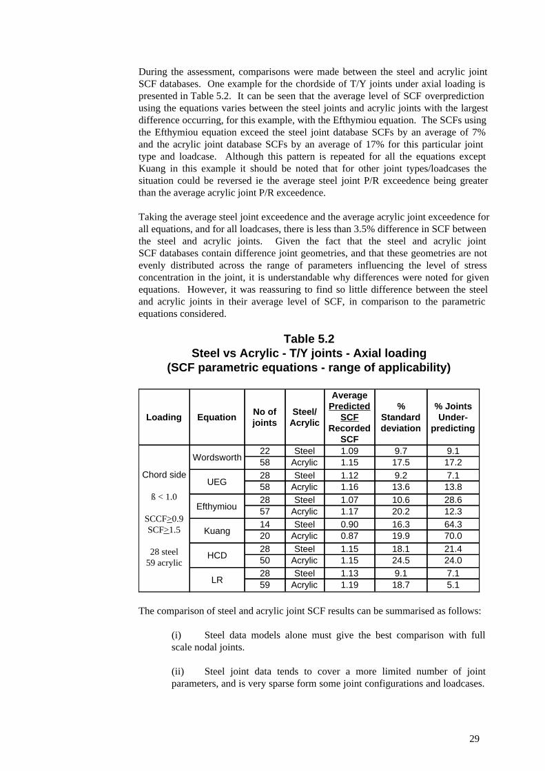
During the assessment, comparisons were made between the steel and acrylic jointSCF databases. One example for the chordside of T/Y joints under axial loading ispresented in Table 5.2. It can be seen that the average level of SCF overpredictionusing the equations varies between the steel joints and acrylic joints with the largestdifference occurring, for this example, with the Efthymiou equation. The SCFs usingthe Efthymiou equation exceed the steel joint database SCFs by an average of 7%and the acrylic joint database SCFs by an average of 17% for this particular jointtype and loadcase. Although this pattern is repeated for all the equations exceptKuang in this example it should be noted that for other joint types/loadcases thesituation could be reversed ie the average steel joint P/R exceedence being greaterthan the average acrylic joint P/R exceedence.

Taking the average steel joint exceedence and the average acrylic joint exceedence forall equations, and for all loadcases, there is less than 3.5% difference in SCF betweenthe steel and acrylic joints. Given the fact that the steel and acrylic jointSCF databases contain difference joint geometries, and that these geometries are notevenly distributed across the range of parameters influencing the level of stressconcentration in the joint, it is understandable why differences were noted for givenequations. However, it was reassuring to find so little difference between the steeland acrylic joints in their average level of SCF, in comparison to the parametricequations considered.

Table 5.2Steel vs Acrylic - T/Y joints - Axial loading

(SCF parametric equations - range of applicability)

5.118.71.19Acrylic597.19.11.13Steel28

LR

24.024.51.15Acrylic5021.418.11.15Steel28

HCD

70.019.90.87Acrylic2064.316.30.90Steel14

Kuang

12.320.21.17Acrylic5728.610.61.07Steel28

Efthymiou

13.813.61.16Acrylic587.19.21.12Steel28

UEG

17.217.51.15Acrylic589.19.71.09Steel22

Wordsworth

Chord side

ß < 1.0

SCCF>0.9SCF>1.5

28 steel59 acrylic

% JointsUnder-

predicting

%Standarddeviation

AveragePredicted

SCFRecorded

SCF

Steel/Acrylic

No ofjointsEquationLoading

The comparison of steel and acrylic joint SCF results can be summarised as follows:

(i) Steel data models alone must give the best comparison with fullscale nodal joints.

(ii) Steel joint data tends to cover a more limited number of jointparameters, and is very sparse form some joint configurations and loadcases.

29

In addition, steel data has intended to be based on joints with relatively shortchord lengths and is more prone to the effects of the end diaphragms.

(iii) Acrylic data generally gives good coverage of parametric ranges formost joint configurations. However, factors have to be employed to accountfor the lack of a weld fillet.

(iv) Acrylic joints gives correlation with steel joints in the few caseswhere identical specimens have been tested. Global comparisons of theacrylic database and steel databases do show differences in the percentage ofjoints underpredicting, which on average balance out. These differences aregenerally explained by different joint configurations held in the databases,however, some differences have not yet been fully understood and explained.

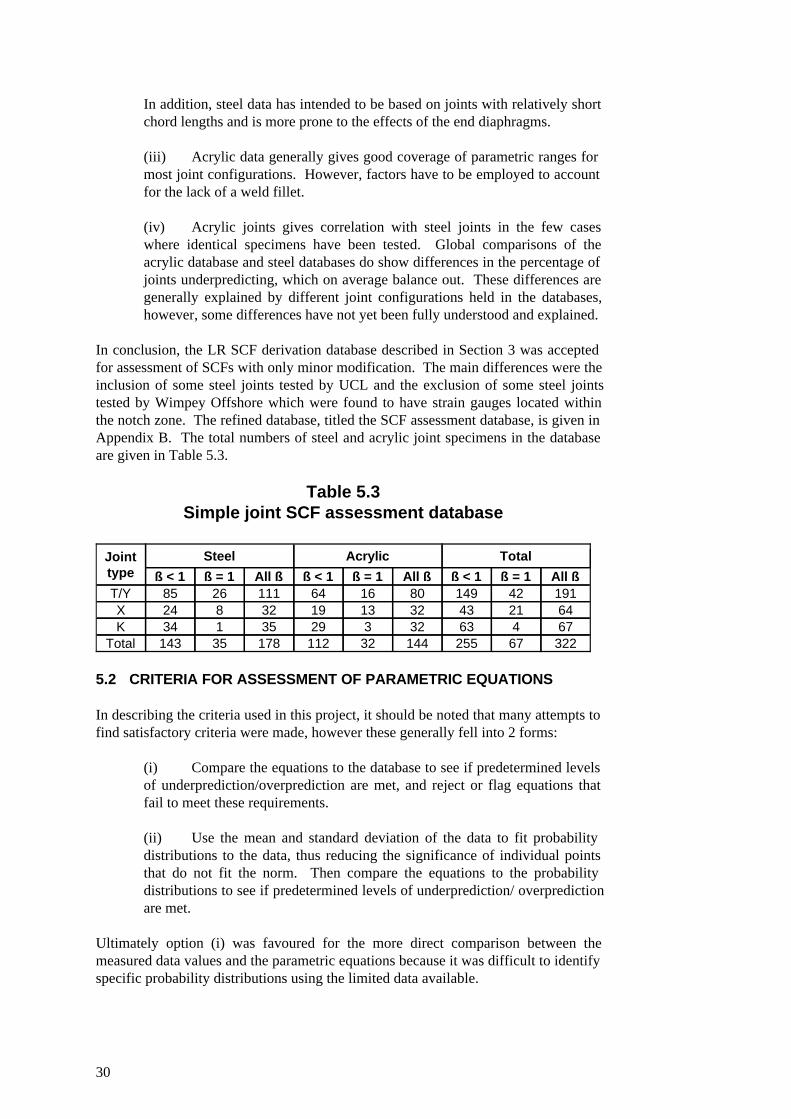
In conclusion, the LR SCF derivation database described in Section 3 was acceptedfor assessment of SCFs with only minor modification. The main differences were theinclusion of some steel joints tested by UCL and the exclusion of some steel jointstested by Wimpey Offshore which were found to have strain gauges located withinthe notch zone. The refined database, titled the SCF assessment database, is given inAppendix B. The total numbers of steel and acrylic joint specimens in the databaseare given in Table 5.3.

Table 5.3Simple joint SCF assessment database

322672551443211217835143Total674633232935134K64214332131932824X191421498016641112685T/YAll ßß = 1ß < 1All ßß = 1ß < 1All ßß = 1ß < 1

TotalAcrylicSteelJointtype

5.2 CRITERIA FOR ASSESSMENT OF PARAMETRIC EQUATIONS

In describing the criteria used in this project, it should be noted that many attempts tofind satisfactory criteria were made, however these generally fell into 2 forms:

(i) Compare the equations to the database to see if predetermined levelsof underprediction/overprediction are met, and reject or flag equations thatfail to meet these requirements.

(ii) Use the mean and standard deviation of the data to fit probabilitydistributions to the data, thus reducing the significance of individual pointsthat do not fit the norm. Then compare the equations to the probabilitydistributions to see if predetermined levels of underprediction/ overpredictionare met.

Ultimately option (i) was favoured for the more direct comparison between themeasured data values and the parametric equations because it was difficult to identifyspecific probability distributions using the limited data available.

30

For determining the performance of an SCF equation against an SCF database, thefollowing aspects were felt to be the most significant:

(i) The percentage of joints underpredicted by a given equation, ie % ofjoints where P/R < 1 where P = predicted SCF and R = recorded SCF.

(ii) The percentage of joints that are significantly underpredicted by agiven equation (for this purpose percentage of joints where P/R < 0.8 waschosen as a guideline).

(iii) The percentage of joints that are significantly overpredicted by agiven equation (for this purpose percentage of joints where P/R > 1.5 waschosen as a guideline). It was felt that it would be useful to know when anequation was generally overconservative, however an equation should not beconsidered unacceptable because it is overconservative.

(iv) Steel joints should be given priority where sufficient data exists.

After considerable investigation the following criteria were felt to give the bestguideline and have been employed in this study:

� If the number of steel joint SCFs in the database [ 20 then assess thesteel database alone.If the number of steel joint SCFs in the database < 20, and thenumber of pooled joint SCFs (steel joints and acrylic joints) m 15then assess the pooled database.If the number of pooled joint SCFs in the database < 15, then theequation cannot be assessed.

� For the given dataset, if percentage SCFs underpredicting [ 25%(%P/R < 1.0 [ 25%) and if percentage SCFs considerablyunderpredicting [ 5% (%P/R < 0.8 [ 5%) then the equation meetsthe acceptance criteria used in this study. If, in addition, thepercentage SCFs considerably overpredicting m 50%) (%P/R > 1.5m 50%), then note that the equation is generally conservative.

� If the acceptance criteria as used in this study is nearlymet (ie 25% < [%P/R < 1.0] [ 30% and/or 5% < {%P/R < 0.8] [7.5%) then the equation is regarded as borderline and engineeringjudgement has been used.

It is obvious that the values taken in this assessment are subjective, however, thesevalues do meet the objectives of the project, and generally support the equations thatare currently in use while identifying some significant anomalies in the parametricequations which should be avoided.

31

5.3 ASSESSMENT OF PARAMETRIC EQUATIONS

In assessing the parametric equations the following methodology was adopted:

(i) To assess the effect of chord length on saddle SCFs for axial loadingand OPB a considerable amount of work was performed. It was concludedthat no single a cut-off value could account for the effect of the chord enddiaphragms. Consequently, the short chord correction factors proposed byEfthymiou were employed. If an SCF were influenced by more than 10%due to the end conditions (ie SCCF < 0.9) then the SCF was excluded fromthe assessment.

(ii) All joints were assumed to be pinned at the chord ends.

(iii) Initially, b = 1 joints were excluded from analyses at the saddlelocations, since b = 1 joints generally give very variable results primarily dueto the degree of weld cut-back employed.

(iv) Only joints that have all parameters inside the equation’srecommended range of applicability were included in the analysis. Thisaction had the effect of considerably reducing the number of joints available,particularly for the Kuang equations.

(v) Joints with SCFs less than 1.5 were excluded from the assessment.

(vi) The variable P/R (= Predicted SCF/Recorded SCF) was analysedand found to be approximately lognormally distributed. The mean P/Rvalue, the standard deviation of the variable P/R, % P/R < 0.8, %P/R < 1.0and the %P/R > 1.5 are assessed for each combination ofconfiguration/loadcase/measuring position/equation.

5.4 PERFORMANCE OF PARAMETRIC EQUATIONS

In Tables 1 - 22 the performance of each equation is described for jointgeometries (T/Y, X and K), loadcases (axial, OPB and IPB) and measuringpositions (chord saddle, chord crown, brace saddle and brace crown). It should benoted that the HCD equations only cover T/Y joints and the Kuang equations T/Yand K joints. For the acceptance criteria used, the Efthymiou and new LR equationsare the most consistent giving the best performance overall.

5.5 DATA USED IN SCF ASSESSMENT

Stress concentration factor matrices for T/Y, X and K joints have been produced inthis project, see Tables 5.4 to 5.6. There was insufficient data available to produce amatrix for KT joints.

32

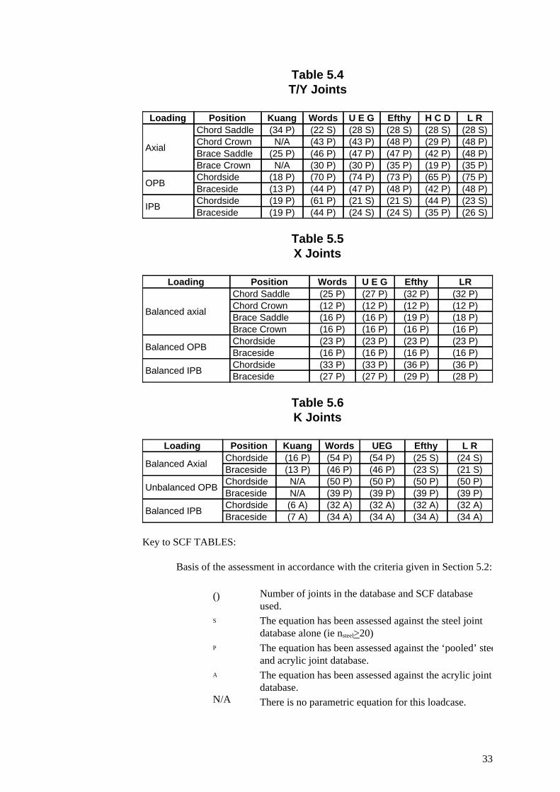
Table 5.4T/Y Joints

(26 S)(35 P)(24 S)(24 S)(44 P)(19 P)Braceside(23 S)(44 P)(21 S)(21 S)(61 P)(19 P)Chordside

IPB

(48 P)(42 P)(48 P)(47 P)(44 P)(13 P)Braceside(75 P)(65 P)(73 P)(74 P)(70 P)(18 P)Chordside

OPB

(35 P)(19 P)(35 P)(30 P)(30 P)N/ABrace Crown(48 P)(42 P)(47 P)(47 P)(46 P)(25 P)Brace Saddle(48 P)(29 P)(48 P)(43 P)(43 P)N/AChord Crown(28 S)(28 S)(28 S)(28 S)(22 S)(34 P)Chord Saddle

Axial

L RH C DEfthyU E GWordsKuangPositionLoading

Table 5.5X Joints

(28 P)(29 P)(27 P)(27 P)Braceside(36 P)(36 P)(33 P)(33 P)Chordside

Balanced IPB

(16 P)(16 P)(16 P)(16 P)Braceside(23 P)(23 P)(23 P)(23 P)Chordside

Balanced OPB

(16 P)(16 P)(16 P)(16 P)Brace Crown(18 P)(19 P)(16 P)(16 P)Brace Saddle(12 P)(12 P)(12 P)(12 P)Chord Crown(32 P)(32 P)(27 P)(25 P)Chord Saddle

Balanced axial

LREfthyU E GWordsPositionLoading

Table 5.6K Joints

(34 A)(34 A)(34 A)(34 A)(7 A)Braceside(32 A)(32 A)(32 A)(32 A)(6 A)Chordside

Balanced IPB

(39 P)(39 P)(39 P)(39 P)N/ABraceside(50 P)(50 P)(50 P)(50 P)N/AChordside

Unbalanced OPB

(21 S)(23 S)(46 P)(46 P)(13 P)Braceside(24 S)(25 S)(54 P)(54 P)(16 P)Chordside

Balanced Axial

L REfthyUEGWordsKuangPositionLoading

Key to SCF TABLES:

Basis of the assessment in accordance with the criteria given in Section 5.2:

There is no parametric equation for this loadcase.N/A

The equation has been assessed against the acrylic jointdatabase.

A

The equation has been assessed against the ‘pooled’ steeland acrylic joint database.

P

The equation has been assessed against the steel jointdatabase alone (ie nsteel>20)

S

Number of joints in the database and SCF databaseused.

()

33

5.6 BETA = 1.0 JOINTS

Joints with equal brace and chord diameters (ie b = 1.0) were excluded from the mainassessment at the saddle location. For b = 1.0 acrylic models the factors applied withrespect to extrapolation, conversion from SNCF to SCF and weld fillet effects werevery different from those for b ! 1.0 joints. The factors were also very inconsistentwithin the b = 1.0 dataset itself.

At the saddle location for b = 1.0 joints the SCF is very significantly influenced bythe degree of cut-back, see paragraph 2.5.2. In the JISSP study for b = 1.0 X jointsthere were significant differences in quoted SCFs resulting from linear and non-linearextrapolation.

However, b = 1.0 joints have been analysed separately to account for the widevariation in the degree of cut-back at the saddle. A number of b modification factorshave been derived which should be used in conjunction with equations which meet theacceptance criteria, used in this study, at the saddle location.

For T/Y joints the b modification factors are given in Table 23 and for X joints inTable 24. These factors should be applied to those equations which meet the criteriain Tables 1 to 22 for b = 1.0 joints. These factors have been selected to ensure thatthe equations accepted for the b = 1.0 range can be applied to b = 1.0 joints to meetthe criteria used in this study. No modification factors can be derived for the K jointsbecause of the lack of suitable data (less than 10 joints of this type).

6. CONCLUSIONS

In this report, 2 studies largely funded by the HSE, have been described. The firststudy led to the creation of a comprehensive database of steel and acrylic joint SCFstitled the Lloyd’s Register SCF derivation database and described in Section 3.0.

From this database a new set of SCF parametric equations was derived from simpletubular nodal joints. These equations are referred to as the new LR equations andwere derived as a mean fit to the database. A one standard deviation safety factorwas included to give the design equations, see Appendix A.

In the second study the database was refined and used to assess existing simple jointSCF parametric forumulae including the new LR equations. The finalised database,titled the SCF assessment database and given in Appendix B, contains 191 T/Y,64 X and 67 K joints. The database was screened and for the assessment all jointsfailing to meet the specified criteria were excluded.

In the assessment of existing SCF parametric equations, the objective was to produceSCF matrices giving recommendations regarding the use of the equations for newHSE fatigue guidance. The assessment criteria was agreed by the Review Panel forFatigue Guidance and the performance of the equations is presented in Tables 1 to22.

In determining which SCF equations should be used, the allowable equations shouldbe treated with caution for 2 reasons. Firstly, the designer may feel, with somejustification, that since a number of SCF equations are acceptable for a givenloadcase, the minimum SCF from these acceptable equations could be taken.

34

Secondly, ‘mixing’ equations to give one allowable set of equations may lead toproblems if in future the influence function approach is adopted rather than thecurrent rather vague joint classification approach. The influence function approachrelies on an understanding of the effect of the presence and loading of individualbraces and the change in SCF that results.

ACKNOWLEDGEMENTS

The authors wish to thank their colleagues at Lloyd’s Register, Dr J Sharp of theHSE and N Nichols of MaTSU for their valuable contributions during this project,and to the HSE for providing the major funding for the work described in this report.

REFERENCES

(1) TOPRAC A A and BEALE L AAnalysis of in-plane, T, Y and K welded tubular connectionsWelding Research Council 125, 1967

(2) REBER J BUltimate strength design of tubular jointsOTC 1664, Houston, Taxas, 1972

(3) VISSER WOn the structural design of tubular joints”OTC 2117, Houston (1974)

(4) KUANG J G, POTVIN A B and LEICK R DStress concentration in tubular jointsOTC 2205, Houston, Texas, 1975

(5) KUANG J G, POTVIN A B, LEICK R D and KAHLICK J LStress concentration in tubular jointsSociety of Petroleum Engineers Journal, August 1977

(6) WORDSWORTH A C and SMEDLEY G PStress concentrations at unstiffened tubular jointsEuropean Offshore Steels Research Seminar, November 1978

(7) WORDSWORTH A CStress concentration factors at K and KT tubular jointsFatigue in Offshore Structural Steels Conference, ICE, February 1981

(8) EFTHYMIOU M and DURKIN SStress concentrations in T/Y and gap/overlap K jointsBehaviour of Offshore Steel Structures, Delft, 1985

(9) EFTHYMIOU MDevelopment of SCF formulae and generalised influence functions for use infatigue analysisOffshore Tubular Joints, Surrey 1988

(10) DEPARTMENT OF ENERGY

35

United Kingdom Offshore Research Project - Phase II (UKOSRP II) SummaryReportHMSO, OTH-87-265, 1987

(11) SMEDLEY P A and FISHER P JA review of stress concentration factors for tubular complex jointsIntegrity of Offshore Structures-4, Glasgow 1990

(12) DEPARTMENT OF ENERGYOffshore installations: Guidance on design, construction and certification”, 4thEdition, HMSO, 1990

(13) REYNOLDS A and SHARP JThe fatigue performance of tubular joints - an overview of recent work to reviseDepartment of Energy GuidanceIntegrity of Offshore Structures - 4, Glasgow, 1990

(14) DEPARTMENT OF ENERGYBackground to new fatigue design guidance for steel welded joints in offshorestructuresHMSO 1984

(15) DEPARTMENT OF ENERGYUnited Kingdom Offshore Research Project - Phase I (UKOSRP I) - Final ReportHMSO OTH-88-282

(16) CLAYTON A M and IRVINE N MStress analysis method for tubular connectionsEuropean Offshore Steels Research Seminar, November 1978

(17) ELLIOTT K S and FESSLER HStress at weld toes in non-overlapped tubular jointsFatigue and crack growth in offshore structures, IMechE, London 1986

(18) GURNEY T RFatigue of welded structures2nd Ed, Cambridge University Press, 1979, pp 176 - 189

(19) SWENSSON K D, HOADLEY P W, YURA J A and SANDERS D HStress concentration factors in Double-Tee jointsPhil M Ferguson Structural Engineering Laboratory Report 86 - 1, 1986

(20) WARDENIER JHollow section jointsDelft University Press, 1982

(21) LALANI M, TEBBETT I E and CHOO B SImproved fatigue life estimation of tubular jointsOffshore Technology Conference (OTC 5306), Houston, May 1986

36

(22) UNDERWATER ENGINEERING GROUPDesign guidance on tubular joints in steel offshore structuresUR33, April 1985

(23) DEPARTMENT OF ENERGYInvestigation into the differences between the measured hot-spot stress whenderived by either linear or non-linear extrapolation techniquesPrepared by Lloyd’s Register for the Den, February 1988, Rev 2

(24) SMEDLEY G PPeak strains at tubular jointsI Mech E, September 1977

(25) MARSHALL P WA review of stress concentration factors in tubular jointsCE-32 report, Shell Oil Co, Houston, Texas

(26) WORDSWORTH A CAspects of stress concentration factors at tubular jointsSteels in Marine Structures (SIMS) Conference, 1987

(27) API RECOMMENDED PRACTICE 2A (RP 2A)Recommended practice for planning, designing and constructing fixed offshoreplatformsNineteenth edition, August 1 1991

(28) EFTHYMIOU MFinite element analysis for Task 4A of Lloyd’s project - Stress concentration factorsin tubular complex jointsShell report RKER.84.151 sponsored by LRS August 1984

(29) WYLDE J GFatigue tests on welded tubular T-joints with equal brace and chord diametersOffshore Technology Conference (OTC 4527), Houston, May 1983

(30) LIEURADE H-P, GERALD J P and PUTOT C JFatigue life prediction of tubular nodesOffshore Technology Conference (OTC 3699), Houston, May 1980

(31) HELLIER A K, CONNOLLY M P and DOVER W DStress concentration factors for tubular Y - and T - jointsInt J Fatigue 12 No 1 (1990) pp 13 - 23

(32) WIMPEY OFFSHORELloyd’s Register of Shipping - Stress concentration factors for tubular complex joints- Finite element analysis in tasks 4A and 4B - Interim report 1Report No WOL 215/84A, September 1984

(33) SMEDLEY P A and FISHER P JStress concentration factors for simple tubular jointsThe First International Offshore and Polar Engineering Conference, (ISOPE),Edinburgh, UK, 1991

37

TABLES

38

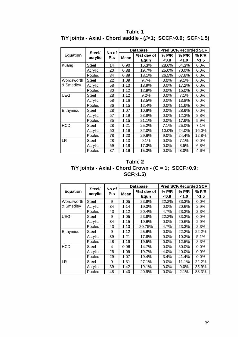
Table 1T/Y joints - Axial - Chord saddle - (b<1; SCCFm0.9; SCFm1.5)

4.6%8.0%0.0%15.3%1.1687Pooled6.8%8.5%0.0%17.3%1.1859Acrylic0.0%7.1%0.0%9.1%1.1328SteelLR12.8%24.4%9.0%29.6%1.2078Pooled16.0%24.0%10.0%32.0%1.1950Acrylic7.1%25.0%7.1%25.2%1.2128SteelHCD5.9%17.6%0.0%21.1%1.1585Pooled8.8%12.3%0.0%23.8%1.1957Acrylic0.0%28.6%0.0%10.6%1.0728SteelEfthymiou0.0%11.6%0.0%12.4%1.1586Pooled0.0%13.8%0.0%13.5%1.1658Acrylic0.0%7.1%0.0%9.2%1.1228SteelUEG0.0%15.0%0.0%12.9%1.1280Pooled0.0%17.2%0.0%13.9%1.1358Acrylic0.0%9.1%0.0%9.7%1.0922SteelWordsworth

& Smedley

0.0%67.6%26.5%18.1%0.8934Pooled0.0%70.0%25.0%19.7%0.8820Acrylic0.0%64.3%28.6%16.3%0.9014SteelKuang

% P/R>1.5

% P/R<1.0

% P/R<0.8

%st dev ofEqunMean

Pred SCF/Recorded SCFDatabaseNo ofPts

Steel/acrylicEquation

Table 2T/Y joints - Axial - Chord Crown - (C = 1; SCCFm0.9;

SCFm1.5)

33.3%2.1%0.0%20.9%1.4048Pooled35.9%0.0%0.0%19.1%1.4239Acrylic22.2%11.1%0.0%27.1%1.319SteelLR0.0%41.4%3.4%19.4%1.0729Pooled0.0%40.0%4.0%19.7%1.0925Acrylic0.0%50.0%0.0%14.7%0.964SteelHCD8.3%12.5%0.0%19.5%1.1948Pooled5.1%10.3%0.0%17.8%1.2139Acrylic22.2%22.2%0.0%25.6%1.129SteelEfthymiou2.3%23.3%4.7%20.75%1.1343Pooled2.9%20.6%0.0%19.6%1.1534Acrylic0.0%33.3%22.2%23.8%1.059SteelUEG2.3%23.3%4.7%20.4%1.1243Pooled2.9%20.6%0.0%19.3%1.1434Acrylic0.0%33.3%22.2%23.8%1.059SteelWordsworth

& Smedley

% P/R>1.5

% P/R<1.0

% P/R<0.8

%st dev ofEqunMean

Pred SCF/Recorded SCFDatabaseNo ofPts

Steel/acrylicEquation

39

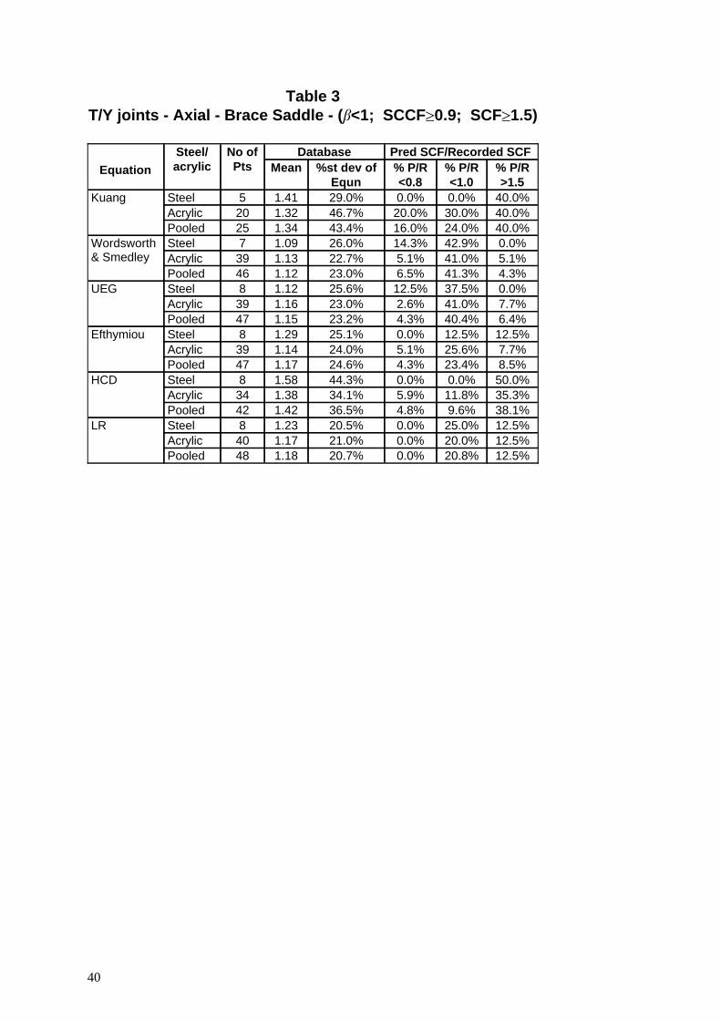
Table 3T/Y joints - Axial - Brace Saddle - (b<1; SCCFm0.9; SCFm1.5)

12.5%20.8%0.0%20.7%1.1848Pooled12.5%20.0%0.0%21.0%1.1740Acrylic12.5%25.0%0.0%20.5%1.238SteelLR38.1%9.6%4.8%36.5%1.4242Pooled35.3%11.8%5.9%34.1%1.3834Acrylic50.0%0.0%0.0%44.3%1.588SteelHCD8.5%23.4%4.3%24.6%1.1747Pooled7.7%25.6%5.1%24.0%1.1439Acrylic12.5%12.5%0.0%25.1%1.298SteelEfthymiou6.4%40.4%4.3%23.2%1.1547Pooled7.7%41.0%2.6%23.0%1.1639Acrylic0.0%37.5%12.5%25.6%1.128SteelUEG4.3%41.3%6.5%23.0%1.1246Pooled5.1%41.0%5.1%22.7%1.1339Acrylic0.0%42.9%14.3%26.0%1.097SteelWordsworth

& Smedley

40.0%24.0%16.0%43.4%1.3425Pooled40.0%30.0%20.0%46.7%1.3220Acrylic40.0%0.0%0.0%29.0%1.415SteelKuang

% P/R>1.5

% P/R<1.0

% P/R<0.8

%st dev ofEqun

MeanPred SCF/Recorded SCFDatabaseNo of

PtsSteel/acrylicEquation

40

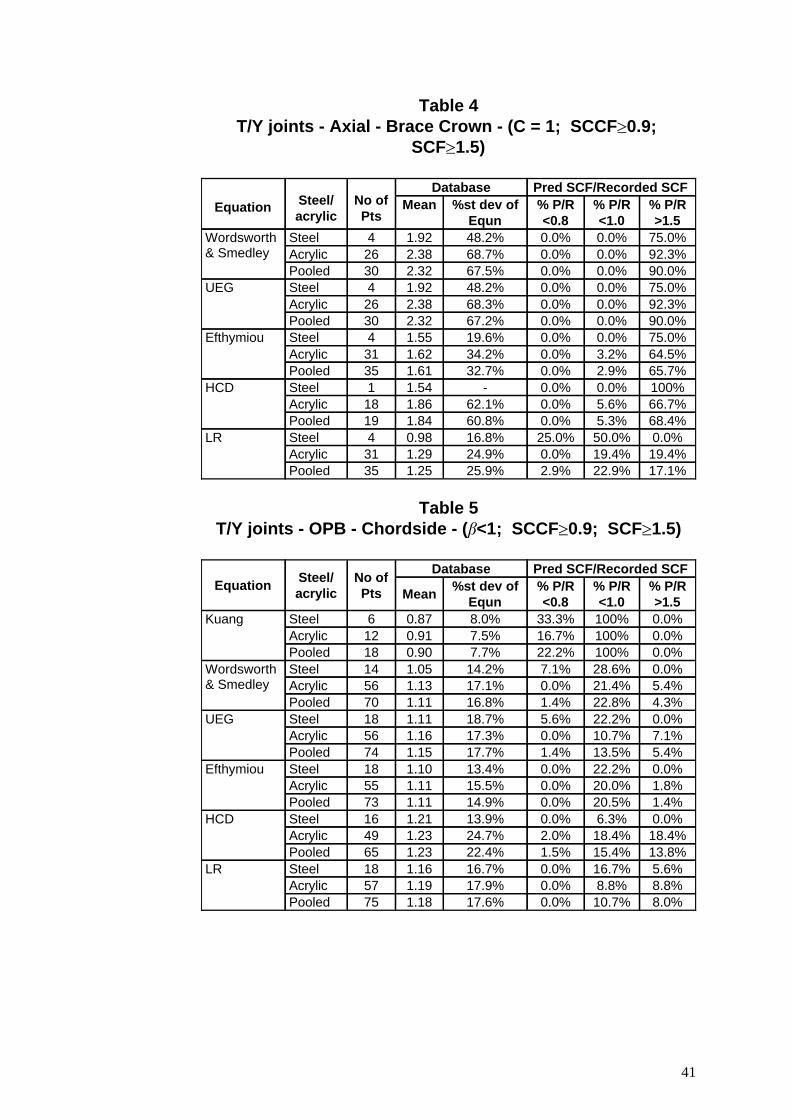
Table 4T/Y joints - Axial - Brace Crown - (C = 1; SCCFm0.9;

SCFm1.5)

17.1%22.9%2.9%25.9%1.2535Pooled19.4%19.4%0.0%24.9%1.2931Acrylic0.0%50.0%25.0%16.8%0.984SteelLR68.4%5.3%0.0%60.8%1.8419Pooled66.7%5.6%0.0%62.1%1.8618Acrylic100%0.0%0.0%-1.541SteelHCD65.7%2.9%0.0%32.7%1.6135Pooled64.5%3.2%0.0%34.2%1.6231Acrylic75.0%0.0%0.0%19.6%1.554SteelEfthymiou90.0%0.0%0.0%67.2%2.3230Pooled92.3%0.0%0.0%68.3%2.3826Acrylic75.0%0.0%0.0%48.2%1.924SteelUEG90.0%0.0%0.0%67.5%2.3230Pooled92.3%0.0%0.0%68.7%2.3826Acrylic75.0%0.0%0.0%48.2%1.924SteelWordsworth

& Smedley

% P/R>1.5

% P/R<1.0

% P/R<0.8

%st dev ofEqun

MeanPred SCF/Recorded SCFDatabase

No ofPts

Steel/acrylic

Equation

Table 5T/Y joints - OPB - Chordside - (b<1; SCCFm0.9; SCFm1.5)

8.0%10.7%0.0%17.6%1.1875Pooled8.8%8.8%0.0%17.9%1.1957Acrylic5.6%16.7%0.0%16.7%1.1618SteelLR13.8%15.4%1.5%22.4%1.2365Pooled18.4%18.4%2.0%24.7%1.2349Acrylic0.0%6.3%0.0%13.9%1.2116SteelHCD1.4%20.5%0.0%14.9%1.1173Pooled1.8%20.0%0.0%15.5%1.1155Acrylic0.0%22.2%0.0%13.4%1.1018SteelEfthymiou5.4%13.5%1.4%17.7%1.1574Pooled7.1%10.7%0.0%17.3%1.1656Acrylic0.0%22.2%5.6%18.7%1.1118SteelUEG4.3%22.8%1.4%16.8%1.1170Pooled5.4%21.4%0.0%17.1%1.1356Acrylic0.0%28.6%7.1%14.2%1.0514SteelWordsworth

& Smedley

0.0%100%22.2%7.7%0.9018Pooled0.0%100%16.7%7.5%0.9112Acrylic0.0%100%33.3%8.0%0.876SteelKuang

% P/R>1.5

% P/R<1.0

% P/R<0.8

%st dev ofEqunMean

Pred SCF/Recorded SCFDatabaseNo ofPts

Steel/acrylicEquation

41

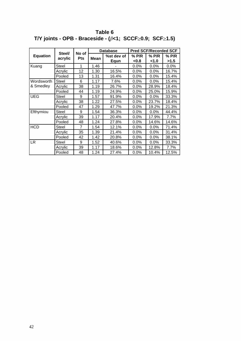
Table 6T/Y joints - OPB - Braceside - (b<1; SCCFm0.9; SCFm1.5)

12.5%10.4%0.0%27.4%1.2448Pooled7.7%12.8%0.0%18.6%1.1739Acrylic33.3%0.0%0.0%40.6%1.529SteelLR38.1%0.0%0.0%20.8%1.4242Pooled31.4%0.0%0.0%21.4%1.3935Acrylic71.4%0.0%0.0%12.1%1.547SteelHCD14.6%14.6%0.0%27.8%1.2448Pooled7.7%17.9%0.0%20.4%1.1739Acrylic44.4%0.0%0.0%36.3%1.549SteelEfthymiou21.3%19.2%0.0%47.7%1.2947Pooled18.4%23.7%0.0%27.5%1.2238Acrylic33.3%0.0%0.0%91.9%1.579SteelUEG15.9%25.0%0.0%24.9%1.1944Pooled18.4%28.9%0.0%26.7%1.1938Acrylic15.4%0.0%0.0%7.6%1.176SteelWordsworth

& Smedley

15.4%0.0%0.0%16.4%1.3113Pooled16.7%0.0%0.0%16.5%1.3012Acrylic0.0%0.0%0.0%-1.461SteelKuang

% P/R>1.5

% P/R<1.0

% P/R<0.8

%st dev ofEqunMean

Pred SCF/Recorded SCFDatabaseNo ofPts

Steel/acrylicEquation

42

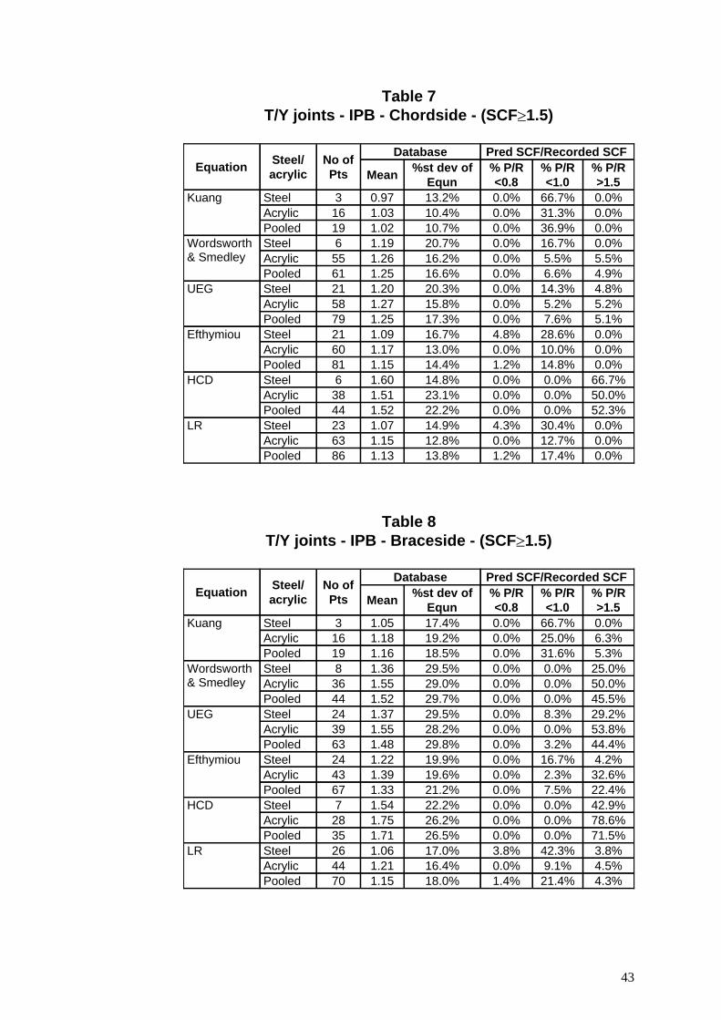
Table 7T/Y joints - IPB - Chordside - (SCFm1.5)

0.0%17.4%1.2%13.8%1.1386Pooled0.0%12.7%0.0%12.8%1.1563Acrylic0.0%30.4%4.3%14.9%1.0723SteelLR52.3%0.0%0.0%22.2%1.5244Pooled50.0%0.0%0.0%23.1%1.5138Acrylic66.7%0.0%0.0%14.8%1.606SteelHCD0.0%14.8%1.2%14.4%1.1581Pooled0.0%10.0%0.0%13.0%1.1760Acrylic0.0%28.6%4.8%16.7%1.0921SteelEfthymiou5.1%7.6%0.0%17.3%1.2579Pooled5.2%5.2%0.0%15.8%1.2758Acrylic4.8%14.3%0.0%20.3%1.2021SteelUEG4.9%6.6%0.0%16.6%1.2561Pooled5.5%5.5%0.0%16.2%1.2655Acrylic0.0%16.7%0.0%20.7%1.196SteelWordsworth

& Smedley

0.0%36.9%0.0%10.7%1.0219Pooled0.0%31.3%0.0%10.4%1.0316Acrylic0.0%66.7%0.0%13.2%0.973SteelKuang

% P/R>1.5

% P/R<1.0

% P/R<0.8

%st dev ofEqunMean

Pred SCF/Recorded SCFDatabaseNo ofPts

Steel/acrylicEquation

Table 8T/Y joints - IPB - Braceside - (SCFm1.5)

4.3%21.4%1.4%18.0%1.1570Pooled4.5%9.1%0.0%16.4%1.2144Acrylic3.8%42.3%3.8%17.0%1.0626SteelLR71.5%0.0%0.0%26.5%1.7135Pooled78.6%0.0%0.0%26.2%1.7528Acrylic42.9%0.0%0.0%22.2%1.547SteelHCD22.4%7.5%0.0%21.2%1.3367Pooled32.6%2.3%0.0%19.6%1.3943Acrylic4.2%16.7%0.0%19.9%1.2224SteelEfthymiou44.4%3.2%0.0%29.8%1.4863Pooled53.8%0.0%0.0%28.2%1.5539Acrylic29.2%8.3%0.0%29.5%1.3724SteelUEG45.5%0.0%0.0%29.7%1.5244Pooled50.0%0.0%0.0%29.0%1.5536Acrylic25.0%0.0%0.0%29.5%1.368SteelWordsworth

& Smedley

5.3%31.6%0.0%18.5%1.1619Pooled6.3%25.0%0.0%19.2%1.1816Acrylic0.0%66.7%0.0%17.4%1.053SteelKuang

% P/R>1.5

% P/R<1.0

% P/R<0.8

%st dev ofEqunMean

Pred SCF/Recorded SCFDatabaseNo ofPts

Steel/acrylicEquation

43

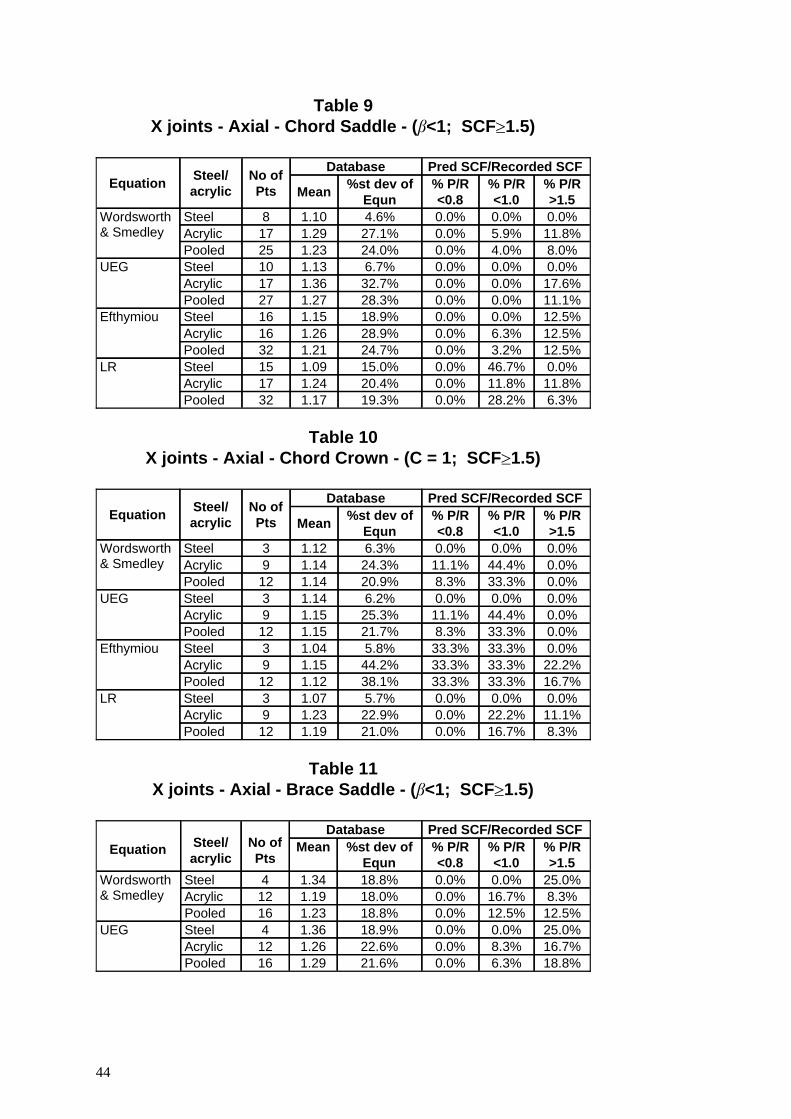
Table 9X joints - Axial - Chord Saddle - (b<1; SCFm1.5)

6.3%28.2%0.0%19.3%1.1732Pooled11.8%11.8%0.0%20.4%1.2417Acrylic0.0%46.7%0.0%15.0%1.0915SteelLR12.5%3.2%0.0%24.7%1.2132Pooled12.5%6.3%0.0%28.9%1.2616Acrylic12.5%0.0%0.0%18.9%1.1516SteelEfthymiou11.1%0.0%0.0%28.3%1.2727Pooled17.6%0.0%0.0%32.7%1.3617Acrylic0.0%0.0%0.0%6.7%1.1310SteelUEG8.0%4.0%0.0%24.0%1.2325Pooled11.8%5.9%0.0%27.1%1.2917Acrylic0.0%0.0%0.0%4.6%1.108SteelWordsworth

& Smedley

% P/R>1.5

% P/R<1.0

% P/R<0.8

%st dev ofEqunMean

Pred SCF/Recorded SCFDatabaseNo ofPts

Steel/acrylicEquation

Table 10X joints - Axial - Chord Crown - (C = 1; SCFm1.5)

8.3%16.7%0.0%21.0%1.1912Pooled11.1%22.2%0.0%22.9%1.239Acrylic0.0%0.0%0.0%5.7%1.073SteelLR16.7%33.3%33.3%38.1%1.1212Pooled22.2%33.3%33.3%44.2%1.159Acrylic0.0%33.3%33.3%5.8%1.043SteelEfthymiou0.0%33.3%8.3%21.7%1.1512Pooled0.0%44.4%11.1%25.3%1.159Acrylic0.0%0.0%0.0%6.2%1.143SteelUEG0.0%33.3%8.3%20.9%1.1412Pooled0.0%44.4%11.1%24.3%1.149Acrylic0.0%0.0%0.0%6.3%1.123SteelWordsworth

& Smedley

% P/R>1.5

% P/R<1.0

% P/R<0.8

%st dev ofEqunMean

Pred SCF/Recorded SCFDatabaseNo ofPts

Steel/acrylicEquation

Table 11X joints - Axial - Brace Saddle - (b<1; SCFm1.5)

18.8%6.3%0.0%21.6%1.2916Pooled16.7%8.3%0.0%22.6%1.2612Acrylic25.0%0.0%0.0%18.9%1.364SteelUEG12.5%12.5%0.0%18.8%1.2316Pooled8.3%16.7%0.0%18.0%1.1912Acrylic25.0%0.0%0.0%18.8%1.344SteelWordsworth

& Smedley

% P/R>1.5

% P/R<1.0

% P/R<0.8

%st dev ofEqun

MeanPred SCF/Recorded SCFDatabase

No ofPts

Steel/acrylic

Equation

44

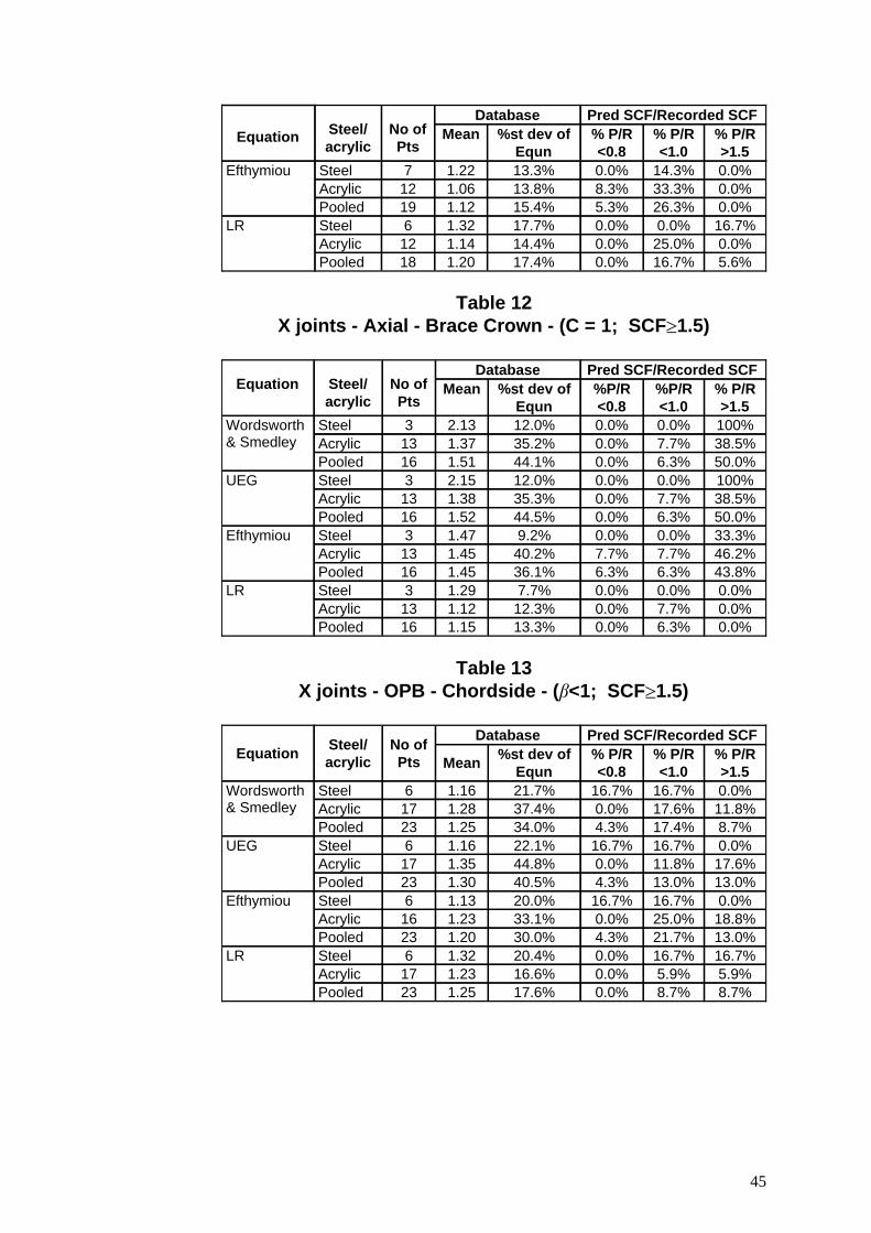
5.6%16.7%0.0%17.4%1.2018Pooled0.0%25.0%0.0%14.4%1.1412Acrylic16.7%0.0%0.0%17.7%1.326SteelLR0.0%26.3%5.3%15.4%1.1219Pooled0.0%33.3%8.3%13.8%1.0612Acrylic0.0%14.3%0.0%13.3%1.227SteelEfthymiou

% P/R>1.5

% P/R<1.0

% P/R<0.8

%st dev ofEqun

MeanPred SCF/Recorded SCFDatabase

No ofPts

Steel/acrylic

Equation

Table 12X joints - Axial - Brace Crown - (C = 1; SCFm1.5)

0.0%6.3%0.0%13.3%1.1516Pooled0.0%7.7%0.0%12.3%1.1213Acrylic0.0%0.0%0.0%7.7%1.293SteelLR43.8%6.3%6.3%36.1%1.4516Pooled46.2%7.7%7.7%40.2%1.4513Acrylic33.3%0.0%0.0%9.2%1.473SteelEfthymiou50.0%6.3%0.0%44.5%1.5216Pooled38.5%7.7%0.0%35.3%1.3813Acrylic100%0.0%0.0%12.0%2.153SteelUEG50.0%6.3%0.0%44.1%1.5116Pooled38.5%7.7%0.0%35.2%1.3713Acrylic100%0.0%0.0%12.0%2.133SteelWordsworth

& Smedley

% P/R>1.5

%P/R<1.0

%P/R<0.8

%st dev ofEqun

MeanPred SCF/Recorded SCFDatabase

No ofPts

Steel/acrylic

Equation

Table 13X joints - OPB - Chordside - (b<1; SCFm1.5)

8.7%8.7%0.0%17.6%1.2523Pooled5.9%5.9%0.0%16.6%1.2317Acrylic16.7%16.7%0.0%20.4%1.326SteelLR13.0%21.7%4.3%30.0%1.2023Pooled18.8%25.0%0.0%33.1%1.2316Acrylic0.0%16.7%16.7%20.0%1.136SteelEfthymiou13.0%13.0%4.3%40.5%1.3023Pooled17.6%11.8%0.0%44.8%1.3517Acrylic0.0%16.7%16.7%22.1%1.166SteelUEG8.7%17.4%4.3%34.0%1.2523Pooled11.8%17.6%0.0%37.4%1.2817Acrylic0.0%16.7%16.7%21.7%1.166SteelWordsworth

& Smedley

% P/R>1.5

% P/R<1.0

% P/R<0.8

%st dev ofEqunMean

Pred SCF/Recorded SCFDatabaseNo ofPts

Steel/acrylicEquation

45

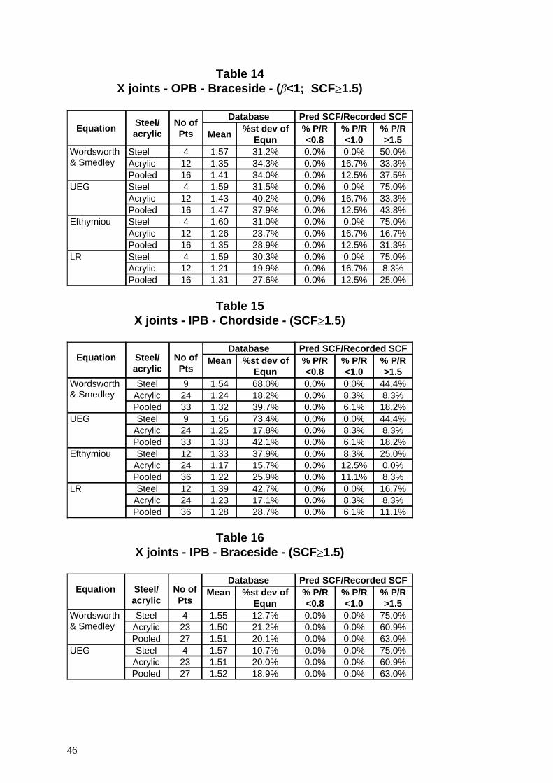
Table 14X joints - OPB - Braceside - (b<1; SCFm1.5)

25.0%12.5%0.0%27.6%1.3116Pooled8.3%16.7%0.0%19.9%1.2112Acrylic75.0%0.0%0.0%30.3%1.594SteelLR31.3%12.5%0.0%28.9%1.3516Pooled16.7%16.7%0.0%23.7%1.2612Acrylic75.0%0.0%0.0%31.0%1.604SteelEfthymiou43.8%12.5%0.0%37.9%1.4716Pooled33.3%16.7%0.0%40.2%1.4312Acrylic75.0%0.0%0.0%31.5%1.594SteelUEG37.5%12.5%0.0%34.0%1.4116Pooled33.3%16.7%0.0%34.3%1.3512Acrylic50.0%0.0%0.0%31.2%1.574SteelWordsworth

& Smedley

% P/R>1.5

% P/R<1.0

% P/R<0.8

%st dev ofEqunMean

Pred SCF/Recorded SCFDatabaseNo ofPts

Steel/acrylicEquation

Table 15X joints - IPB - Chordside - (SCFm1.5)

11.1%6.1%0.0%28.7%1.2836Pooled8.3%8.3%0.0%17.1%1.2324Acrylic16.7%0.0%0.0%42.7%1.3912SteelLR8.3%11.1%0.0%25.9%1.2236Pooled0.0%12.5%0.0%15.7%1.1724Acrylic25.0%8.3%0.0%37.9%1.3312SteelEfthymiou18.2%6.1%0.0%42.1%1.3333Pooled8.3%8.3%0.0%17.8%1.2524Acrylic44.4%0.0%0.0%73.4%1.569SteelUEG18.2%6.1%0.0%39.7%1.3233Pooled8.3%8.3%0.0%18.2%1.2424Acrylic44.4%0.0%0.0%68.0%1.549SteelWordsworth

& Smedley

% P/R>1.5

% P/R<1.0

% P/R<0.8

%st dev ofEqun

MeanPred SCF/Recorded SCFDatabase

No ofPts

Steel/acrylic

Equation

Table 16X joints - IPB - Braceside - (SCFm1.5)

63.0%0.0%0.0%18.9%1.5227Pooled60.9%0.0%0.0%20.0%1.5123Acrylic75.0%0.0%0.0%10.7%1.574SteelUEG63.0%0.0%0.0%20.1%1.5127Pooled60.9%0.0%0.0%21.2%1.5023Acrylic75.0%0.0%0.0%12.7%1.554SteelWordsworth

& Smedley

% P/R>1.5

% P/R<1.0

% P/R<0.8

%st dev ofEqun

MeanPred SCF/Recorded SCFDatabase

No ofPts

Steel/acrylic

Equation

46

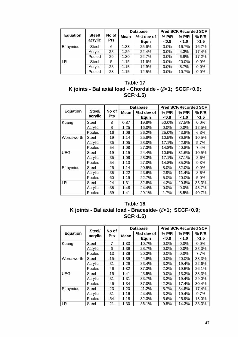
0.0%10.7%0.0%12.5%1.1528Pooled0.0%8.7%0.0%12.9%1.1523Acrylic0.0%20.0%0.0%11.6%1.155SteelLR17.2%6.9%0.0%22.7%1.3029Pooled17.4%4.3%0.0%22.4%1.2923Acrylic16.7%16.7%0.0%25.6%1.336SteelEfthymiou

% P/R>1.5

% P/R<1.0

% P/R<0.8

%st dev ofEqun

MeanPred SCF/Recorded SCFDatabase

No ofPts

Steel/acrylic

Equation

Table 17K joints - Bal axial load - Chordside - (b<1; SCCF[0.9;

SCFm1.5)

40.7%8.5%1.7%29.1%1.4159Pooled45.7%0.0%0.0%24.4%1.4835Acrylic33.3%20.8%4.2%32.8%1.3124SteelLR5.0%20.0%5.0%22.7%1.1960Pooled8.6%11.4%2.9%23.6%1.2235Acrylic0.0%32.0%8.0%20.9%1.1425SteelEfthymiou9.3%35.2%14.8%27.0%1.1054Pooled8.6%37.1%17.1%28.3%1.0835Acrylic10.5%31.6%10.5%24.4%1.1519SteelUEG7.4%40.8%14.8%27.3%1.0854Pooled5.7%42.9%17.1%28.0%1.0535Acrylic10.5%36.8%10.5%25.8%1.1419SteelWordsworth 6.3%43.8%25.0%26.2%1.0616Pooled12.5%0.0%0.0%16.0%1.258Acrylic0.0%87.5%50.0%19.8%0.878SteelKuang

% P/R>1.5

% P/R<1.0

% P/R<0.8

%st dev ofEqun

MeanPred SCF/Recorded SCFDatabase

No ofPts

Steel/acrylic

Equation

Table 18K joints - Bal axial load - Braceside- (b<1; SCCF[0.9;

SCFm1.5)

33.3%14.3%9.5%36.1%1.3021SteelLR13.0%25.9%5.6%32.3%1.1854Pooled9.7%19.4%3.2%24.4%1.1631Acrylic17.4%34.8%8.7%41.2%1.2023SteelEfthymiou30.4%17.4%2.2%37.0%1.3446Pooled29.0%19.4%3.2%33.7%1.3131Acrylic33.3%13.3%0.0%43.5%1.4115SteelUEG26.1%19.6%2.2%37.3%1.3246Pooled22.6%19.4%3.2%33.4%1.2931Acrylic33.3%20.0%0.0%44.8%1.3915SteelWordsworth 7.7%0.0%0.0%20.3%1.3613Pooled33.3%0.0%0.0%28.7%1.396Acrylic0.0%0.0%0.0%10.7%1.337SteelKuang

% P/R>1.5

% P/R<1.0

% P/R<0.8

%st dev ofEqunMean

Pred SCF/Recorded SCFDatabaseNo ofPts

Steel/acrylicEquation

47

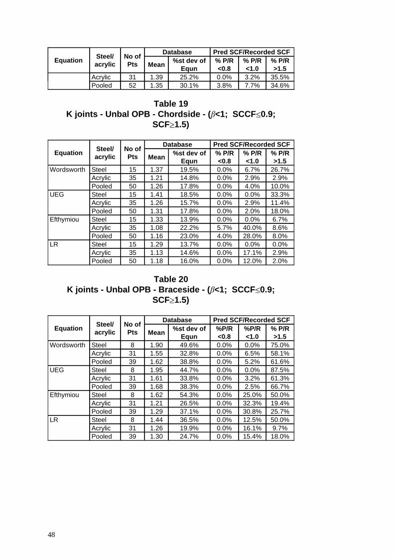
34.6%7.7%3.8%30.1%1.3552Pooled35.5%3.2%0.0%25.2%1.3931Acrylic

% P/R>1.5

% P/R<1.0

% P/R<0.8

%st dev ofEqunMean

Pred SCF/Recorded SCFDatabaseNo ofPts

Steel/acrylicEquation

Table 19K joints - Unbal OPB - Chordside - (b<1; SCCF[0.9;

SCFm1.5)

2.0%12.0%0.0%16.0%1.1850Pooled2.9%17.1%0.0%14.6%1.1335Acrylic0.0%0.0%0.0%13.7%1.2915SteelLR8.0%28.0%4.0%23.0%1.1650Pooled8.6%40.0%5.7%22.2%1.0835Acrylic6.7%0.0%0.0%13.9%1.3315SteelEfthymiou18.0%2.0%0.0%17.8%1.3150Pooled11.4%2.9%0.0%15.7%1.2635Acrylic33.3%0.0%0.0%18.5%1.4115SteelUEG10.0%4.0%0.0%17.8%1.2650Pooled2.9%2.9%0.0%14.8%1.2135Acrylic26.7%6.7%0.0%19.5%1.3715SteelWordsworth

% P/R>1.5

% P/R<1.0

% P/R<0.8

%st dev ofEqunMean

Pred SCF/Recorded SCFDatabaseNo ofPts

Steel/acrylicEquation

Table 20K joints - Unbal OPB - Braceside - (b<1; SCCF[0.9;

SCFm1.5)

18.0%15.4%0.0%24.7%1.3039Pooled9.7%16.1%0.0%19.9%1.2631Acrylic50.0%12.5%0.0%36.5%1.448SteelLR25.7%30.8%0.0%37.1%1.2939Pooled19.4%32.3%0.0%26.5%1.2131Acrylic50.0%25.0%0.0%54.3%1.628SteelEfthymiou66.7%2.5%0.0%38.3%1.6839Pooled61.3%3.2%0.0%33.8%1.6131Acrylic87.5%0.0%0.0%44.7%1.958SteelUEG61.6%5.2%0.0%38.8%1.6239Pooled58.1%6.5%0.0%32.8%1.5531Acrylic75.0%0.0%0.0%49.6%1.908SteelWordsworth

% P/R>1.5

%P/R<1.0

%P/R<0.8

%st dev ofEqunMean

Pred SCF/Recorded SCFDatabaseNo ofPts

Steel/acrylicEquation

48

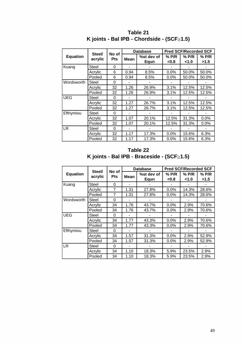
Table 21K joints - Bal IPB - Chordside - (SCFm1.5)

6.3%15.6%0.0%17.3%1.1732Pooled6.3%15.6%0.0%17.3%1.1732Acrylic

-----0SteelLR0.0%31.3%12.5%20.1%1.0732Pooled0.0%31.3%12.5%20.1%1.0732Acrylic

-----0SteelEfthymiou12.5%12.5%3.1%26.7%1.2732Pooled12.5%12.5%3.1%26.7%1.2732Acrylic

-----0SteelUEG12.5%12.5%3.1%26.9%1.2632Pooled12.5%12.5%3.1%26.9%1.2632Acrylic

-----0SteelWordsworth50.0%50.0%0.0%8.5%0.946Pooled50.0%50.0%0.0%8.5%0.946Acrylic

-----0SteelKuang

% P/R>1.5

% P/R<1.0

% P/R<0.8

%st dev ofEqunMean

Pred SCF/Recorded SCFDatabaseNo ofPts

Steel/acrylicEquation

Table 22K joints - Bal IPB - Braceside - (SCFm1.5)

2.9%23.5%5.9%18.3%1.1034Pooled2.9%23.5%5.9%18.3%1.1034Acrylic

-----0SteelLR52.9%2.9%0.0%31.3%1.5734Pooled52.9%2.9%0.0%31.3%1.5734Acrylic

-----0SteelEfthymiou70.6%2.9%0.0%43.3%1.7734Pooled70.6%2.9%0.0%43.3%1.7734Acrylic

-----0SteelUEG70.6%2.9%0.0%43.7%1.7634Pooled70.6%2.9%0.0%43.7%1.7634Acrylic

-----0SteelWordsworth28.6%14.3%0.0%27.8%1.317Pooled28.6%14.3%0.0%27.8%1.317Acrylic

-----0SteelKuang

% P/R>1.5

% P/R<1.0

% P/R<0.8

%st dev ofEqunMean

Pred SCF/Recorded SCFDatabaseNo ofPts

Steel/acrylicEquation

49

Table 23T/Y joints b = 1.0

0.960.980.960.98Braceside (26)0.990.980.980.94Chordside (25)OPB0.950.980.970.98Braceside (16)0.940.980.970.94Chordside (9)Axial

LR Beta*mod

UEG Betamod

EfthymiouBeta mod

Wordsworth/SmedleyBeta mod

Location Nojoints (P)Loading

*Note: for LR the Beta mod value quoted is that to be used in the LR equationie b = bmod - ( t

c sin0.65(Y))

Where: Y is the degree of cut-back at saddle, default value = 20º if cutback notknown

t = thickness of bracethickness of chord

c = diameter of chord2 X thickness of chord

Table 24X joints b = 1.0

0.990.980.960.98Braceside (11)0.990.981.00.98Chordside (13)Balanced

OPB

0.990.980.980.98Braceside (16)0.990.981.00.98Chordside (16)Balanced

Axial

LR Beta*mod

UEG Betamod

EfthymiouBeta mod

Wordsworth/SmedleyBeta mod

Location Nojoints (P)Loading

*Note: for LR the Beta mod value quoted is that to be used in the LR equationie b = bmod - ( t

c sin0.65(Y))

Where: Y is the degree of cut-back at saddle, default value = 20º if cutback notknown

t = thickness of bracethickness of chord

c = diameter of chord2 X thickness of chord

50

APPENDIX APARAMETRIC EQUATIONS USED IN THIS STUDY

51

INDEX

Efthymiou Equations for KT JointsA2.4Efthymiou Equations for K JointsA2.3Efthymiou Equations for X JointsA2.2Efthymiou Equations for T/Y JointsA2.1

EFTHYMIOU PARAMETRIC EQUATIONSA2

Parametric Equation ExpressionsA1.7Lloyd’s Register KT Joint EquationsA1.6Lloyd’s Register K Joint EquationsA1.5Lloyd’s Register Equations for X JointsA1.4Lloyd’s Reigster Equations for T/Y JointsA1.3Derived Parametric Equations and Measured SCF ValuesA1.2Derivation of Equations and Safety FactorsA1.1

LLOYD’S REGISTER PARAMETRIC EQUATIONSA1

52

A1. LLOYD’S REGISTER PARAMETRIC EQUATIONS

A1.1 Derivation of Equations and Safety Factors

These equations have been derived from the Lloyd’s Register (LR) simple jointSCF database using a least squares minimisation procedure. The quoted equationsgive an approximately mean fit to the database, however characteristic equations canbe derived by applying an appropriate safety factor.

Beside each equation is the percentage standard deviation of the least squares fit tothe database (r%), which can be utilised to calculate the required safety factor. Ithas been found that the LR equations are lognormally distributed about the mean fitline. Therefore, the design curve weighting may be calculated to give a estimateddegree of joint underpredictions.

SCF (design) = SCF (mean)† X (1 + nr/100)Where g = Chosen design curve weighting

† Exclude the chord in place bending term, B0 X B1 and add in expressionunfactored.

53

A1.2 Derived Parametric Equations and Measured SCF Values

The SCF database was standardised to DEn fatigue recommendations prior to curvefitting (ie to results derived from linear extrapolation of maximum principal stressesoutside the 0.2„(rt) notch zone to the weld toe). Measured SCF results that do notmeet this standard should be factored as follows:

to convert perpendicular strains to principal stress (acrylicmodels)

X 1.23

to convert perpendicular strain to principal stress (steel models)X 1.15

to simulate a weld fillet on the bracesideX 0.86

to simulate a weld fillet on the chordsideX 0.95

to convert from non-linear extrapolation of stessesX 0.95

54

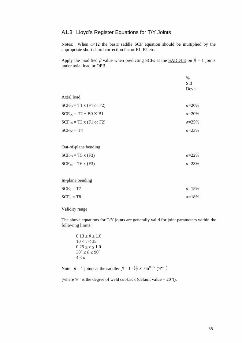
A1.3 Lloyd’s Register Equations for T/Y Joints

Notes: When a<12 the basic saddle SCF equation should be multiplied by theappropriate short chord correction factor F1, F2 etc.

Apply the modified b value when predicting SCFs at the SADDLE on b = 1 jointsunder axial load or OPB.

r=18%SCFB = T8

r=15%SCFC = T7

In-plane bending

r=28%SCFBS = T6 x (F3)

r=22%SCFCS = T5 x (F3)

Out-of-plane bending

r=23%SCFBC = T4

r=25%SCFBS = T3 x (F1 or F2)

r=20%SCFCC = T2 + B0 X B1

r=20%SCFCS = T1 x (F1 or F2)

Axial load

%StdDevn

Validity range

The above equations for T/Y joints are generally valid for joint parameters within thefollowing limits:

0.13 [ b [ 1.010 [ c [ 350.25 [ t [ 1.030° [ h [ 90°4 [ a

Note: b = 1 joints at the saddle: b = 1 - ( tc x sin0.65 (Y)))

(where Y° is the degree of weld cut-back (default value = 20°)).

55

A1.4 Lloyd’s Register Equations for X Joints

Notes: When a<12 the basic saddle SCF equation should be multiplied by theappropriate short chord correction factor F1, F2 etc.

Apply the modified b value when predicting SCFs at the SADDLE on b = 1 jointsunder axial load or OPB.

r=12%SCFB = X8

r=23%SCFC = X7

Balanced in-plane bending

r=20%SCFBS = X6 x (F3)

r=22%SCFCS = X5 x (F3)

Balanced out-of-plane bending

r=13%SCFBC = X4

r=19%SCFBS = X3 x (F1 or F2)

r=33%SCFCC = X2

r=22%SCFCS = X1 x (F1 or F2)

Balanced axial load

%StdDevn

Validity range

The above equations are generally valid for joint parameters within the followinglimits:

0.13 [ b [ 1.010 [ c [ 350.25 [ t [ 1.030° [ h [ 90°4 [ a

Note: b = 1 joints at the saddle: b = 1 - ( tc x sin0.65 (Y)))

(where Y° is the degree of weld cut-back (default value = 20°)).

56

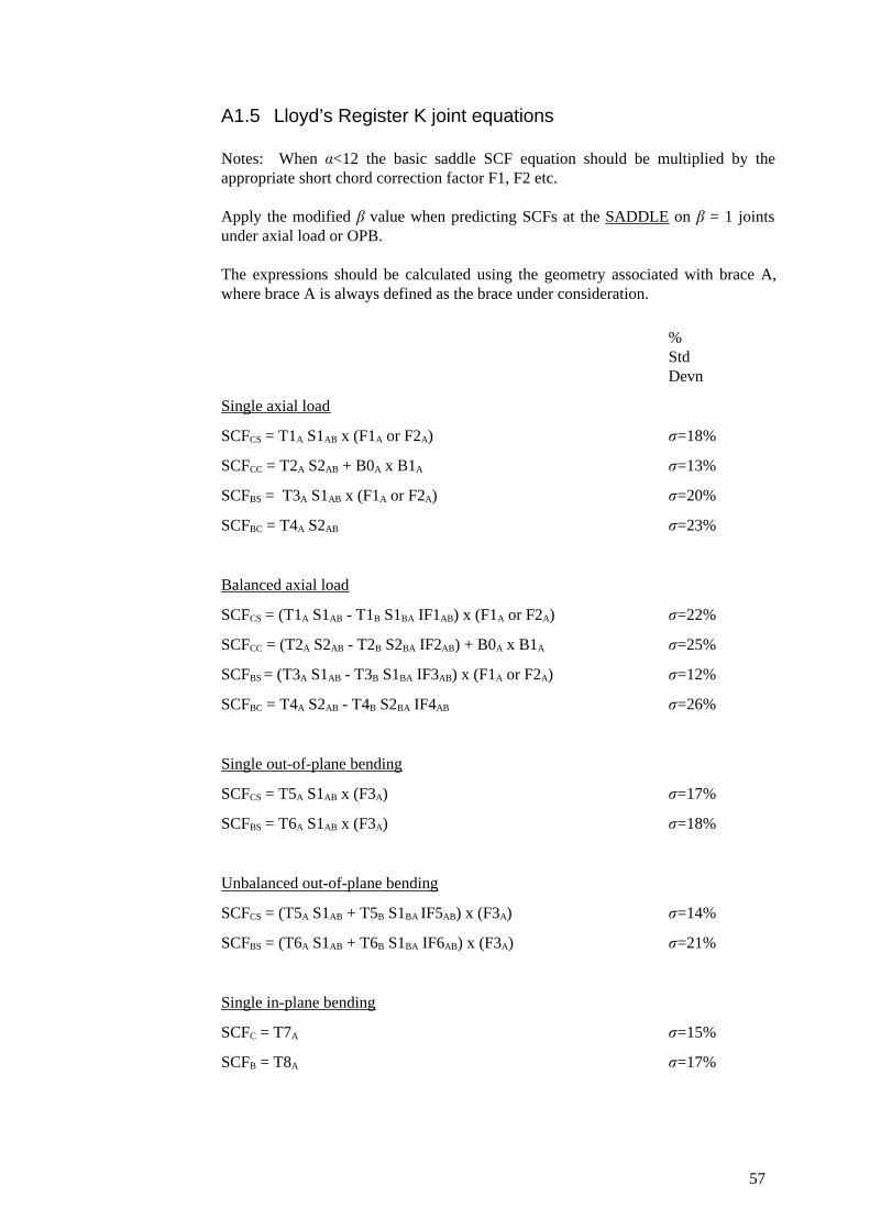
A1.5 Lloyd’s Register K joint equations

Notes: When a<12 the basic saddle SCF equation should be multiplied by theappropriate short chord correction factor F1, F2 etc.

Apply the modified b value when predicting SCFs at the SADDLE on b = 1 jointsunder axial load or OPB.

The expressions should be calculated using the geometry associated with brace A,where brace A is always defined as the brace under consideration.

r=17%SCFB = T8A

r=15%SCFC = T7A

Single in-plane bending

r=21%SCFBS = (T6A S1AB + T6B S1BA IF6AB) x (F3A)

r=14%SCFCS = (T5A S1AB + T5B S1BA IF5AB) x (F3A)

Unbalanced out-of-plane bending

r=18%SCFBS = T6A S1AB x (F3A)

r=17%SCFCS = T5A S1AB x (F3A)

Single out-of-plane bending

r=26%SCFBC = T4A S2AB - T4B S2BA IF4AB

r=12%SCFBS = (T3A S1AB - T3B S1BA IF3AB) x (F1A or F2A)

r=25%SCFCC = (T2A S2AB - T2B S2BA IF2AB) + B0A x B1A

r=22%SCFCS = (T1A S1AB - T1B S1BA IF1AB) x (F1A or F2A)

Balanced axial load

r=23%SCFBC = T4A S2AB

r=20%SCFBS = T3A S1AB x (F1A or F2A)

r=13%SCFCC = T2A S2AB + B0A x B1A

r=18%SCFCS = T1A S1AB x (F1A or F2A)

Single axial load

%StdDevn

57

r=16%SCFB = T8A + T8B IF8AB

r=15%SCFC = T7A + T7B IF7AB

Balanced in-plane bending

Validity range

The above equations are generally valid for joint parameters within the followinglimits:

0.13 [ b [ 1.010 [ c [ 350.25 [ t [ 1.030° [ h [ 90°4 [ a0 < ζ < 1.0

Note: b = 1 joints at the saddle: b = 1 - ( tc x sin0.65 (Y)))

(where Y° is the degree of weld cut-back (default value = 20°)).

58

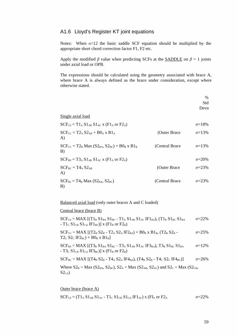
A1.6 Lloyd’s Register KT joint equations

Notes: When a<12 the basic saddle SCF equation should be multiplied by theappropriate short chord correction factor F1, F2 etc.

Apply the modified b value when predicting SCFs at the SADDLE on b = 1 jointsunder axial load or OPB.

The expressions should be calculated using the geometry associated with brace A,where brace A is always defined as the brace under consideration, except whereotherwise stated.

r=22%SCFCS = (T1A S1AB S1AC - T1C S1CB S1CA IF1AC) x (FIA or F2A

Outer brace (brace A)

Where S2B = Max (S2BA, S2BC), S2A = Max (S2AB, S2AC) and S2C = Max (S2CB,S2CA)

r=26%SCFBC = MAX [(T4B S2B - T4A S2A IF4BA), (T4B S2B - T4C S2C IF4BC)]

r=12%SCFBS = MAX [(T3B S1BA S1BC - T3A S1AB S1AC IF3BA), T3B S1BC S1BA

- T3C S1CB S1CA IF3BC)] x (F1B or F2B)

r=25%SCFCC = MAX [(T2B S2B - T2A S2A IF2BA) + B0B x B1B, (T2B S2B -T2C S2C IF2BC) + B0B x B1B]

r=22%SCFCS = MAX [(T1B S1BA S1BC - T1A S1AB S1AC IF1BA), (T1B S1BC S1BA

- T1C S1CB S1CA IF1BC)] x (F1B or F2B)

Central brace (brace B)

Balanced axial load (only outer braces A and C loaded)

r=23%SCFBC = T4B Max (S2BA, S2BC) (Central BraceB)

r=23%SCFBC = T4A S2AB (Outer BraceA)

r=20%SCFBS = T3A S1AB S1AC x (F1A or F2A)

r=13%SCFCC = T2B Max (S2BA, S2BC) + B0B x B1B (Central BraceB)

r=13%SCFCC = T2A S2AB + B0A x B1A (Outer BraceA)

r=18%SCFCS = T1A S1AB S1AC x (F1A or F2A)

Single axial load

%Std

Devn

59

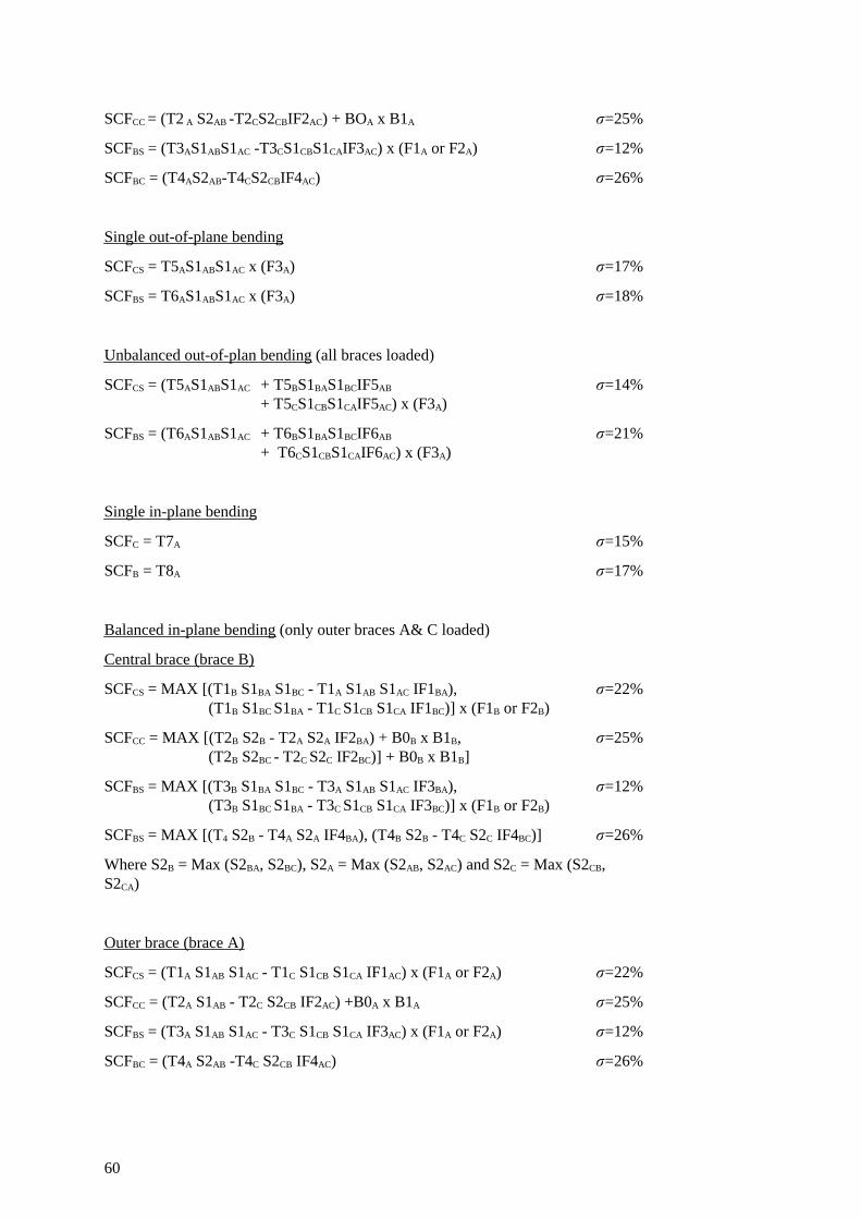
r=26%SCFBC = (T4A S2AB -T4C S2CB IF4AC)

r=12%SCFBS = (T3A S1AB S1AC - T3C S1CB S1CA IF3AC) x (F1A or F2A)

r=25%SCFCC = (T2A S1AB - T2C S2CB IF2AC) +B0A x B1A

r=22%SCFCS = (T1A S1AB S1AC - T1C S1CB S1CA IF1AC) x (F1A or F2A)

Outer brace (brace A)

Where S2B = Max (S2BA, S2BC), S2A = Max (S2AB, S2AC) and S2C = Max (S2CB,S2CA)

r=26%SCFBS = MAX [(T4 S2B - T4A S2A IF4BA), (T4B S2B - T4C S2C IF4BC)]

r=12%SCFBS = MAX [(T3B S1BA S1BC - T3A S1AB S1AC IF3BA),(T3B S1BC S1BA - T3C S1CB S1CA IF3BC)] x (F1B or F2B)

r=25%SCFCC = MAX [(T2B S2B - T2A S2A IF2BA) + B0B x B1B,(T2B S2BC - T2C S2C IF2BC)] + B0B x B1B]

r=22%SCFCS = MAX [(T1B S1BA S1BC - T1A S1AB S1AC IF1BA),(T1B S1BC S1BA - T1C S1CB S1CA IF1BC)] x (F1B or F2B)

Central brace (brace B)

Balanced in-plane bending (only outer braces A& C loaded)

r=17%SCFB = T8A

r=15%SCFC = T7A

Single in-plane bending

r=21%SCFBS = (T6AS1ABS1AC + T6BS1BAS1BCIF6AB

+ T6CS1CBS1CAIF6AC) x (F3A)

r=14%SCFCS = (T5AS1ABS1AC + T5BS1BAS1BCIF5AB

+ T5CS1CBS1CAIF5AC) x (F3A)

Unbalanced out-of-plan bending (all braces loaded)

r=18%SCFBS = T6AS1ABS1AC x (F3A)

r=17%SCFCS = T5AS1ABS1AC x (F3A)

Single out-of-plane bending

r=26%SCFBC = (T4AS2AB-T4CS2CBIF4AC)

r=12%SCFBS = (T3AS1ABS1AC -T3CS1CBS1CAIF3AC) x (F1A or F2A)

r=25%SCFCC = (T2 A S2AB -T2CS2CBIF2AC) + BOA x B1A

60

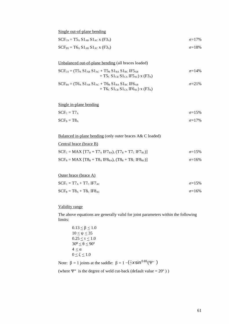
(where Ψº is the degree of weld cut-back (default value = 20º))

Note: β = 1 joints at the saddle: β = 1 − ( tc xsin0.65(Y)))

0.13 < β < 1.010 < ψ < 350.25 < τ < 1.030º < θ < 90º4 < α0 < ζ < 1.0

The above equations are generally valid for joint parameters within the followinglimits:

Validity range

r=16%SCFB = T8A + T8C IF8AC

r=15%SCFC = T7A + T7C IF7AC

Outer brace (brace A)

r=16%SCFB = MAX [T8B + T8A IF8BA), (T8B + T8C IF8BC)]

r=15%SCFC = MAX [T7B + T7A IF7BA), (T7B + T7C IF7BC)]

Central brace (brace B)

Balanced in-plane bending (only outer braces A& C loaded)

r=17%SCFB = T8A

r=15%SCFC = T7A

Single in-plane bending

r=21%SCFBS = (T6A S1AB S1AC + T6B S1BA S1BC IF6AB

+ T6C S1CB S1CA IF6AC) x (F3A)

r=14%SCFCS = (T5A S1AB S1AC + T5B S1BA S1BC IF5AB

+ T5C S1CB S1CA IF5AC) x (F3A)

Unbalanced out-of-plane bending (all braces loaded)

r=18%SCFBS = T6A S1AB S1AC x (F3A)

r=17%SCFCS = T5A S1AB S1AC x (F3A)

Single out-of-plane bending

61

A1.7 Parametric Equations Expressions

A1.7.1 T Factors - T joint factors

Note: Apply the modified β value when predicting SCFs at the SADDLE on β = 1joints under axial load or OPB

Axial load

T1 = τ γ1.2 β (2.12-2β) sin2 θ

T2 = τ γ0.2 (3.5-2.4β) sin0.3 θ

T3 = 1 + τ0.6 γ1.3 β (0.76-0.7β) sin2.2 Θ

T4 = 2.6β0.65 γ(0.3-0.5β)

Out-of-plane bending

T5 = τ γ β (1.4-β5) sin1.7 Θ

T6 = 1 + τ0.6 γ1.3 β(0.27-0.2β5) sin1.7 Θ

In-plane bending

T7 = 1.22τ0.8 βγ(1-0.68β) sin(1-β3) Θ

T8 = 1 + τ0.2 γβ(0.26-0.21β) sin1.5 Θ

A1.7.2 X Factors = X joint factors

Note: Apply the modified β value when predicting SCFs at the SADDLE on β = 1joints under axial load or OPB

Axial load

X1 = τβγ1.3 (1.46-1.4β2) sin2 Θ

X2 = (0.36 + 1.9 τγ0.5 exp(-β1.5 γ0.5)) (sin Θ + 3cos 2Θ)

X3 = 1 + 0.6 x X1

X4 = (1.3 + 0.06 τγ exp (-β2 γ0.5)) sin-1 Θ

Out-of-plane bending

X5 = τβγ1.3 (0.63-0.6β3) sin2 Θ

X6 = 1 + τβγ1.5 (0.19-0.185β3) sin7(1-β2) Θ

In-plane bending

62

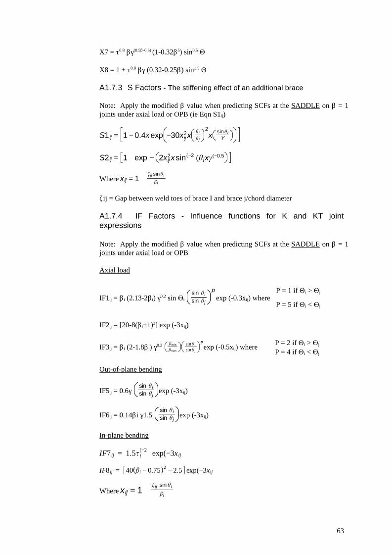
X7 = τ0.8 βγ(0.5β-0.5) (1-0.32β5) sin0.5 Θ

X8 = 1 + τ0.8 βγ (0.32-0.25β) sin1.5 Θ

A1.7.3 S Factors - The stiffening effect of an additional brace

Note: Apply the modified β value when predicting SCFs at the SADDLE on β = 1joints under axial load or OPB (ie Eqn S1ij)

S1 ij = 1 − 0.4xexp −30xij2x

b i

b j

2x sinh i

Y

S2 ij = 1 + exp − 2xij2xsin(−2)(h jxc(−0.5

Where xij = 1 +fij sinh i

b i

ζij = Gap between weld toes of brace I and brace j/chord diameter

A1.7.4 IF Factors - Influence functions for K and KT jointexpressions

Note: Apply the modified β value when predicting SCFs at the SADDLE on β = 1joints under axial load or OPB

Axial load

P = 5 if Θi < Θj

P = 1 if Θi > Θj

IF1ij = βi (2.13-2βi) γ0.2 sin Θi exp (-0.3xij) wheresin h isin h j

p

IF2ij = [20-8(βi+1)2] exp (-3xij)

P = 4 if Θi < Θj

P = 2 if Θi > ΘjIF3ij = βi (2-1.8βi) γ0.2 exp (-0.5xij) wherebmin

bmax

sin h i

sin h j

p

Out-of-plane bending

IF5ij = 0.6γ exp (-3xij)sin h isin h j

IF6ij = 0.14βi γ1.5 exp (-3xij)sin h isin h j

In-plane bending

IF7 ij = 1.5t i(−2) exp(−3x ij)

IF8 ij = 40(b i − 0.75)2 − 2.5 exp(−3xij)

Where x ij = 1 +f ij sin h i

b i

63

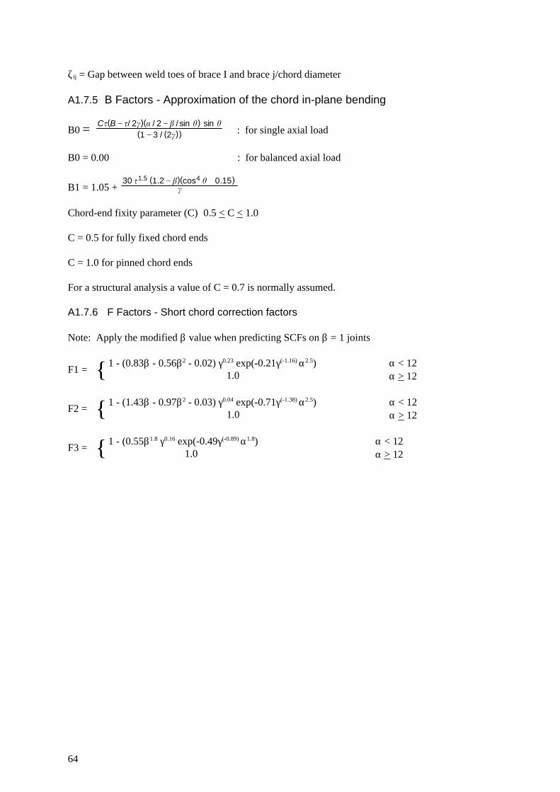
ζij = Gap between weld toes of brace I and brace j/chord diameter

A1.7.5 B Factors - Approximation of the chord in-plane bending

B0 : for single axial load= Ct(B − t/ 2c)(a / 2 − b / sin h) sin h(1 − 3 / (2c))

B0 = 0.00 : for balanced axial load

B1 = 1.05 + 30 t1.5 (1.2 − b)(cos4 h + 0.15)

c

Chord-end fixity parameter (C) 0.5 < C < 1.0

C = 0.5 for fully fixed chord ends

C = 1.0 for pinned chord ends

For a structural analysis a value of C = 0.7 is normally assumed.

A1.7.6 F Factors - Short chord correction factors

Note: Apply the modified β value when predicting SCFs on β = 1 joints

α > 121.0α < 121 - (0.83β - 0.56β2 - 0.02) γ0.23 exp(-0.21γ(-1.16) α2.5){F1 =

α > 121.0α < 121 - (1.43β - 0.97β2 - 0.03) γ0.04 exp(-0.71γ(-1.38) α2.5){F2 =

α > 121.0α < 121 - (0.55β1.8 γ0.16 exp(-0.49γ(-0.89) α1.8){F3 =

64

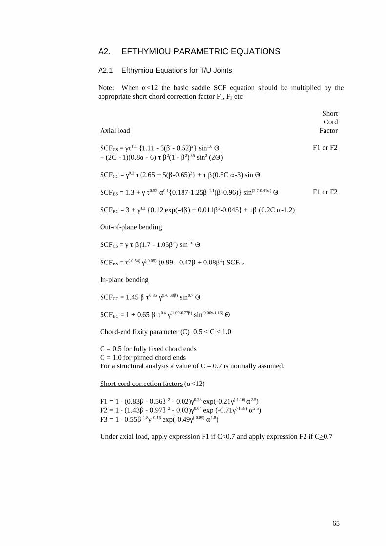
A2. EFTHYMIOU PARAMETRIC EQUATIONS

A2.1 Efthymiou Equations for T/U Joints

Note: When α<12 the basic saddle SCF equation should be multiplied by theappropriate short chord correction factor F1, F2 etc

Under axial load, apply expression F1 if C<0.7 and apply expression F2 if C>0.7

F3 = 1 - 0.55β 1.8γ 0.16 exp(-0.49γ(-0.89) α1.8)F2 = 1 - (1.43β - 0.97β 2 - 0.03)γ0.04 exp (-0.71γ(-1.38) α2.5)F1 = 1 - (0.83β - 0.56β 2 - 0.02)γ0.23 exp(-0.21γ(-1.16) α2.5)

Short cord correction factors (α<12)

For a structural analysis a value of C = 0.7 is normally assumed.C = 1.0 for pinned chord endsC = 0.5 for fully fixed chord ends

Chord-end fixity parameter (C) 0.5 < C < 1.0

SCFBC = 1 + 0.65 β τ0.4 γ(1.09-0.77β) sin(0.06γ-1.16) Θ

SCFCC = 1.45 β τ0.85 γ(1-0.68β) sin0.7 Θ

In-plane bending

SCFBS = τ(-0.54) γ(-0.05) (0.99 - 0.47β + 0.08β4) SCFCS

SCFCS = γ τ β(1.7 - 1.05β3) sin1.6 Θ

Out-of-plane bending

SCFBC = 3 + γ1.2 {0.12 exp(-4β) + 0.011β2-0.045} + τβ (0.2C α-1.2)

F1 or F2SCFBS = 1.3 + γ τ0.52 α0.1{0.187-1.25β 1.1(β-0.96)} sin(2.7-0.01α) Θ

SCFCC = γ0.2 τ{2.65 + 5(β-0.65)2} + τ β(0.5C α-3) sin Θ

F1 or F2SCFCS = γτ1.1 {1.11 - 3(β - 0.52)2} sin1.6 Θ+ (2C - 1)(0.8α - 6) τ β2(1 - β2)0.5 sin2 (2Θ)

ShortCord

FactorAxial load

65

Validity range

The above equations for T/Y joints are generally valid for joint parameters within thefollowing limits:

0.2 < β < 1.08 < γ < 320.2 < τ < 1.020° < Θ < 90°4 < α < 40

66

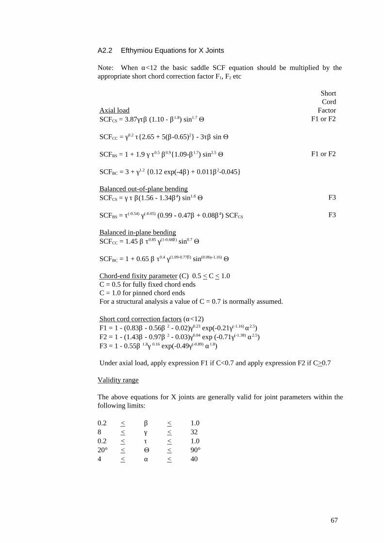
A2.2 Efthymiou Equations for X Joints

Note: When α<12 the basic saddle SCF equation should be multiplied by theappropriate short chord correction factor F1, F2 etc

Under axial load, apply expression F1 if C<0.7 and apply expression F2 if C>0.7

F3 = 1 - 0.55β 1.8γ 0.16 exp(-0.49γ(-0.89) α1.8)F2 = 1 - (1.43β - 0.97β 2 - 0.03)γ0.04 exp (-0.71γ(-1.38) α2.5)F1 = 1 - (0.83β - 0.56β 2 - 0.02)γ0.23 exp(-0.21γ(-1.16) α2.5)Short cord correction factors (α<12)

For a structural analysis a value of C = 0.7 is normally assumed.C = 1.0 for pinned chord endsC = 0.5 for fully fixed chord endsChord-end fixity parameter (C) 0.5 < C < 1.0

SCFBC = 1 + 0.65 β τ0.4 γ(1.09-0.77β) sin(0.06γ-1.16) Θ

SCFCC = 1.45 β τ0.85 γ(1-0.68β) sin0.7 ΘBalanced in-plane bending

F3SCFBS = τ(-0.54) γ(-0.05) (0.99 - 0.47β + 0.08β4) SCFCS

F3SCFCS = γ τ β(1.56 - 1.34β4) sin1.6 ΘBalanced out-of-plane bending

SCFBC = 3 + γ1.2 {0.12 exp(-4β) + 0.011β2-0.045}

F1 or F2SCFBS = 1 + 1.9 γ τ0.5 β0.9{1.09-β1.7) sin2.5 Θ

SCFCC = γ0.2 τ{2.65 + 5(β-0.65)2} - 3τβ sin Θ

F1 or F2SCFCS = 3.87γτβ (1.10 - β1.8) sin1.7 Θ

ShortCord

FactorAxial load

Validity range

The above equations for X joints are generally valid for joint parameters within thefollowing limits:

0.2 < β < 1.08 < γ < 320.2 < τ < 1.020° < Θ < 90°4 < α < 40

67

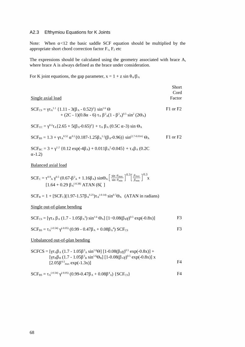
A2.3 Efthymiou Equations for K Joints

Note: When α<12 the basic saddle SCF equation should be multiplied by theappropriate short chord correction factor F1, F2 etc

The expressions should be calculated using the geometry associated with brace A,where brace A is always defined as the brace under consideration.

For K joint equations, the gap parameter, x = 1 + z sin θA/βA

F4SCFBS = τA(-0.54) γ(-0.05) (0.99-0.47βA + 0.08β4

A) {SCFCS}

F4

SCFCS = [γτAβA (1.7 - 1.05β3A sin1.6Θ] [1-0.08(βBγ)0.5 exp(-0.8x)] +

[γτΒβB (1.7 - 1.05β3B sin1.6ΘB] [1-0.08(βΑγ)0.5 exp(-0.8x)] x

[2.05β0.5max exp(-1.3x)]

Unbalanced out-of-plan bending

F3SCFBS = τA(-0.54) γ(-0.05) (0.99 - 0.47βΑ + 0.08βA

4) SCFCS

F3SCFCS = [γτΑ βA (1.7 - 1.05βA3) sin1.6 ΘΑ] [1−0.08(βBγ)0.5 exp(-0.8x)]

Single out-of-plane bending

SCFB = 1 + [SCFC](1.97-1.57βA0.25)τA

(-0.14) sin0.7ΘA (ATAN in radians)

SCFC = τ0.9A γ0.5 (0.67-β2

A + 1.16βA) sinΘA xsin hmaxsin hmin

0.3 bmax

bmin

0.3

[1.64 + 0.29 βΑ(-0.38) ATAN (8ζ)]

Balanced axial load

SCFBC = 3 + γ1.2 {0.12 exp(-4βΑ) + 0.011βA2-0.045} + τΑβΑ (0.2C

α-1.2)

F1 or F2SCFBS = 1.3 + γτA0.52 α0.1{0.187-1.25βA

1.1(βA-0.96)} sin(2.7-0.01α) ΘΑ

SCFCC = γ0.2τA{2.65 + 5(βA-0.65)2} + τΑ βA (0.5C α-3) sin ΘΑ

F1 or F2SCFCS = γτA1.1 {1.11 - 3(βA - 0.52)2} sin1.6 Θ

+ (2C - 1)(0.8α - 6) τΑ β2A(1 - β2

A)0.5 sin2 (2ΘΑ)

ShortCord

FactorSingle axial load

68

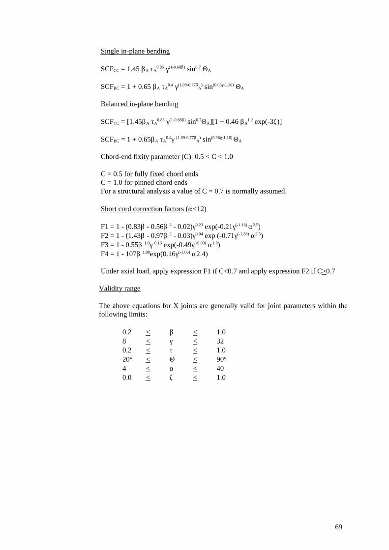
Under axial load, apply expression F1 if C<0.7 and apply expression F2 if C>0.7

F4 = 1 - 107β 1.88exp(0.16γ(-1.06) α2.4)F3 = 1 - 0.55β 1.8γ 0.16 exp(-0.49γ(-0.89) α1.8)F2 = 1 - (1.43β - 0.97β 2 - 0.03)γ0.04 exp (-0.71γ(-1.38) α2.5)F1 = 1 - (0.83β - 0.56β 2 - 0.02)γ0.23 exp(-0.21γ(-1.16) α2.5)

Short cord correction factors (α<12)

For a structural analysis a value of C = 0.7 is normally assumed.C = 1.0 for pinned chord endsC = 0.5 for fully fixed chord ends

Chord-end fixity parameter (C) 0.5 < C < 1.0

SCFBC = 1 + 0.65βA τA0.4γ (1.09-0.77β

A) sin(0.06g-1.16) ΘA

SCFCC = [1.45βA τA0.85 γ(1-0.68β) sin0.7ΘA][1 + 0.46 βA

1.2 exp(-3ζ)]

Balanced in-plane bending

SCFBC = 1 + 0.65 βA τA0.4 γ(1.09-0.77β

Α) sin(0.06γ-1.16) ΘA

SCFCC = 1.45 βA τA0.85 γ(1-0.68β) sin0.7 ΘA

Single in-plane bending

Validity range

The above equations for X joints are generally valid for joint parameters within thefollowing limits:

0.2 < β < 1.08 < γ < 320.2 < τ < 1.020° < Θ < 90°4 < α < 400.0 < ζ < 1.0

69

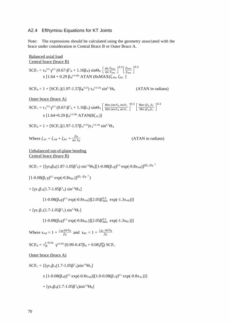
A2.4 Efthymiou Equations for KT Joints

Note: The expressions should be calculated using the geometry associated with thebrace under consideration ie Central Brace B or Outer Brace A.

+ [γτBβB(1.7-1.05β3B)sin1.6ΘB]

x [1-0.08(βBγ)0.5 exp(-0.8xAB)][1.0-0.08(βCγ)0.5 exp(-0.8xAC)]}

SCFC = {[γτAβA(1.7-1.05β3A)sin1.6ΘA]

Outer brace (brace A)

SCFB = γ(-0.05) (0.99-0.47βB + 0.08 ) SCFCtB(−0.54) bB

4

Where xAB = 1 + and xBC = 1 + fAB sinhB

bB

fBC sin hBbB

[1-0.08(βBγ)0.5 exp(-0.8xBC)][2.05β exp(-1.3xBC)]]max0.5

+ [γτCβC(1.7-1.05β3C) sin1.6ΘC]

[1-0.08(βBγ)0.5 exp(-0.8xAB)][2.05β exp(-1.3xAB)]]max0.5

+ [γτAβA(1.7-1.05β3A) sin1.6ΘA]

[1-0.08(βCγ)0.5 exp(-0.8xBC)] }(bC /bB)2

SCFC = {[γτBβB(1.87-1.05β3B) sin1.6ΘB][1-0.08(βAγ)0.5 exp(-0.8xAB)](bA /bB)2

Central brace (brace B)Unbalanced out-of-plane bending

Where ζAC = ζAB + ζBC + (ATAN in radians)bB

sin hB

SCFB = 1 + [SCFC](1.97-1.57βA0.25)τA

(-0.14) sin0.7ΘA

x [1.64+0.29 βB(-0.38) ATAN(8ζAC)]

SCFC = τA0.9 γ0.5 (0.67-β2

A + 1.16βA) sinΘA Max (sin hA, sinhC

Min (sin hA, sin hC

0.3 Max (bA, bC

Min (bA,bC

0.3Outer brace (brace A)

SCFB = 1 + [SCFC](1.97-1.57βΒ0.25) τB

(-0.14) sin0.7ΘB (ATAN in radians)

SCFC = τB0.9 γ0.5 (0.67-β2

B + 1.16βB) sinΘB sin hmaxsin hmin

0.3 bmax

bmin

0.3

x [1.64 + 0.29 βB(-0.38) ATAN (8xMAX(ζAB, ζBC)]

Central brace (brace B)Balanced axial load

70

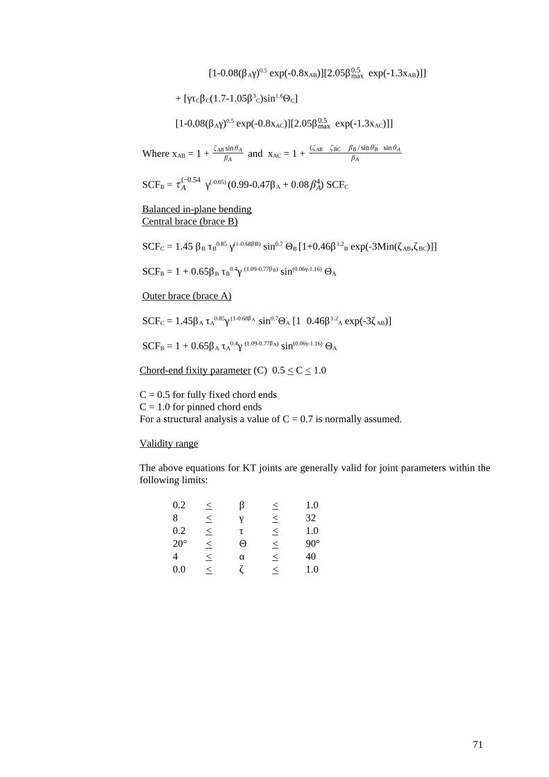
SCFB = 1 + 0.65βA τA0.4γ (1.09-0.77βA) sin(0.06γ-1.16) ΘA

SCFC = 1.45βA τA0.85γ (1-0.68βA) sin0.7ΘA [1+0.46β1.2

A exp(-3ζAB)]

Outer brace (brace A)

SCFB = 1 + 0.65βB τB0.4γ (1.09-0.77βB) sin(0.06γ-1.16) ΘA

SCFC = 1.45 βB τB0.85 γ(1-0.68βB) sin0.7 ΘB [1+0.46β1.2

B exp(-3Min(ζAB,ζBC)]]

Central brace (brace B)Balanced in-plane bending

SCFB = γ(-0.05) (0.99-0.47βA + 0.08 ) SCFCtA(−0.54) bA

4

Where xAB = 1 + and xAC = 1 + fAB sinhA

bA

(fAB + fBC + bB / sinhB) sin hA

bA

[1-0.08(βAγ)0.5 exp(-0.8xAC)][2.05β exp(-1.3xAC)]]max0.5

+ [γτCβC(1.7-1.05β3C)sin1.6ΘC]

[1-0.08(βAγ)0.5 exp(-0.8xAB)][2.05β exp(-1.3xAB)]]max0.5

Chord-end fixity parameter (C) 0.5 < C < 1.0

C = 0.5 for fully fixed chord endsC = 1.0 for pinned chord endsFor a structural analysis a value of C = 0.7 is normally assumed.

Validity range

The above equations for KT joints are generally valid for joint parameters within thefollowing limits:

0.2 < β < 1.08 < γ < 320.2 < τ < 1.020° < Θ < 90°4 < α < 400.0 < ζ < 1.0

71

APPENDIX B

SIMPLE JOINT SCH ASSESSMENT DATABASE

72

INDEX

APPENDIX B REFERENCES

K Joint Geometries and SCFsTables B3.1 - B3.6X Joint Geometries and SCFsTables B2.1 - B2.5T/Y Joint Geometries and SCFsTables B1.1 - B1.15

73

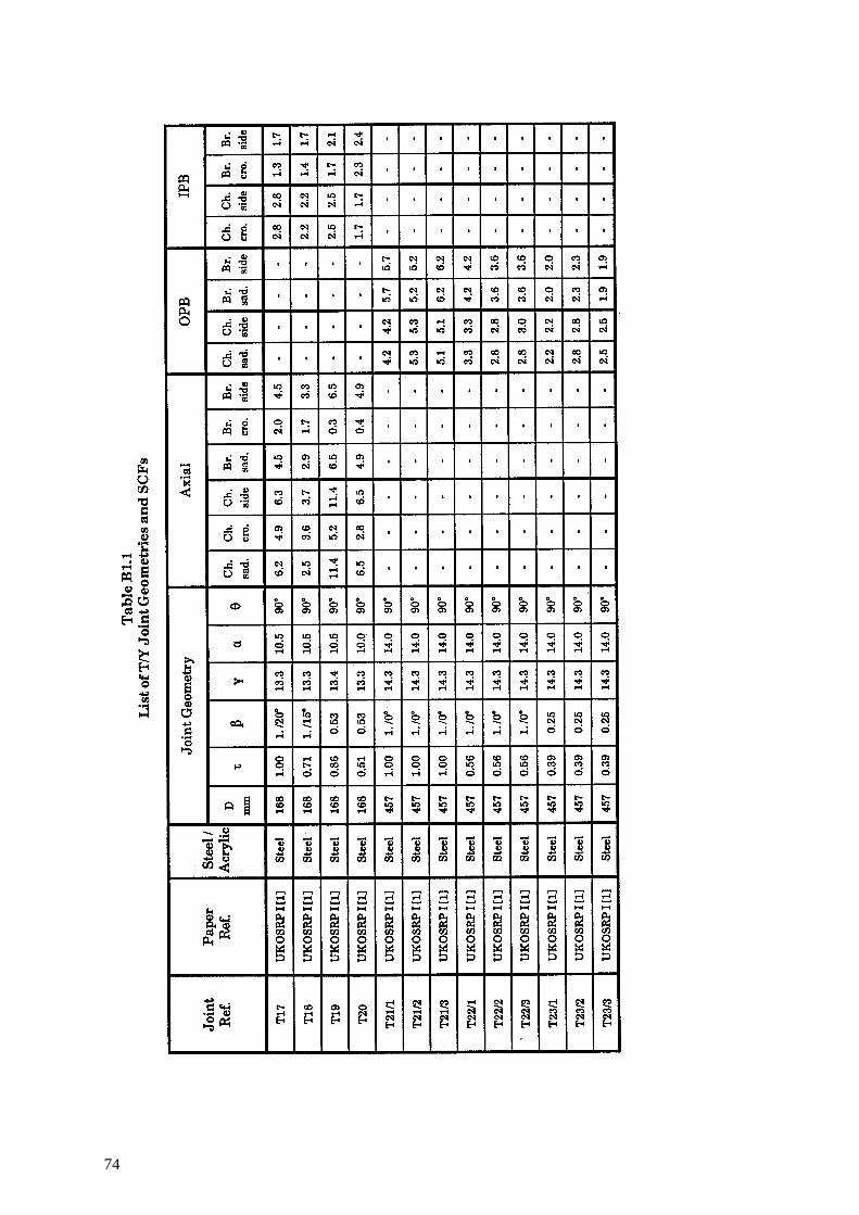
74

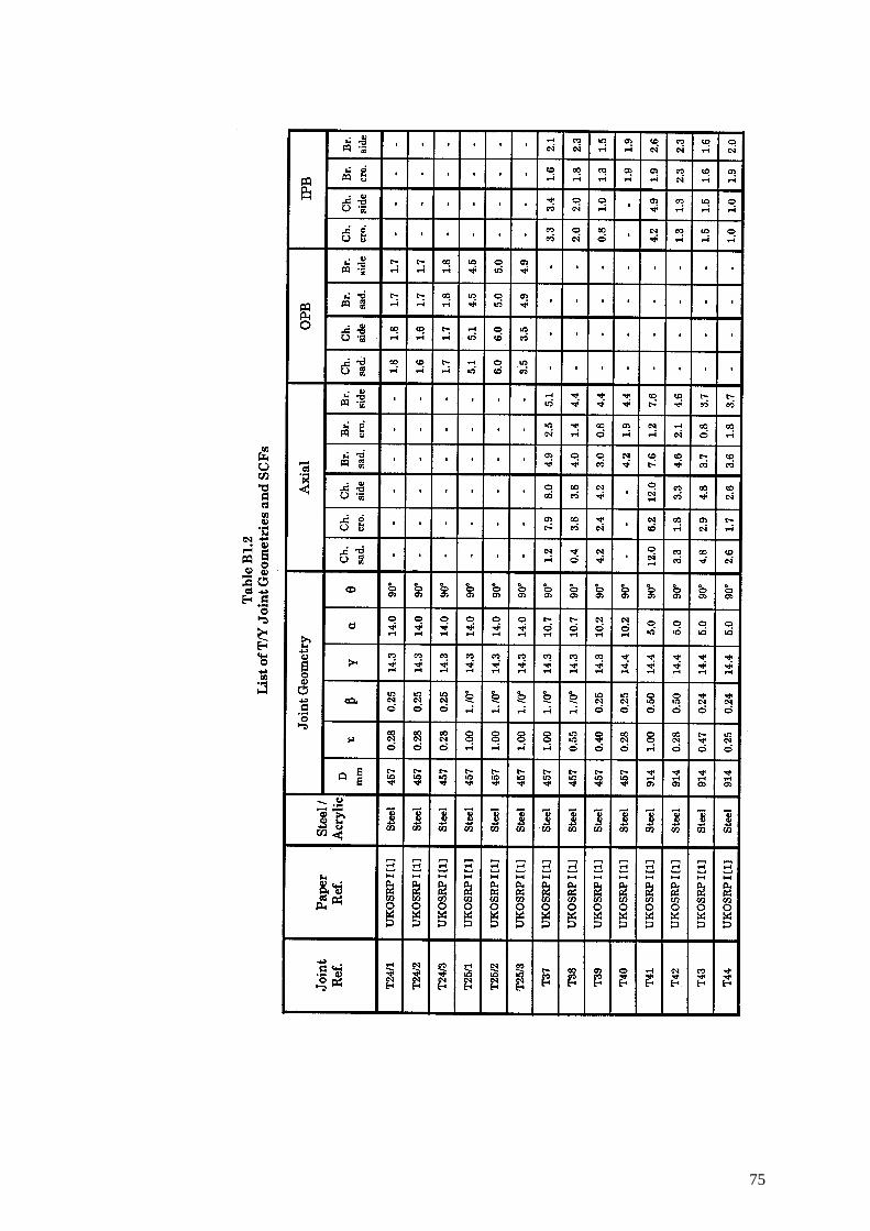
75

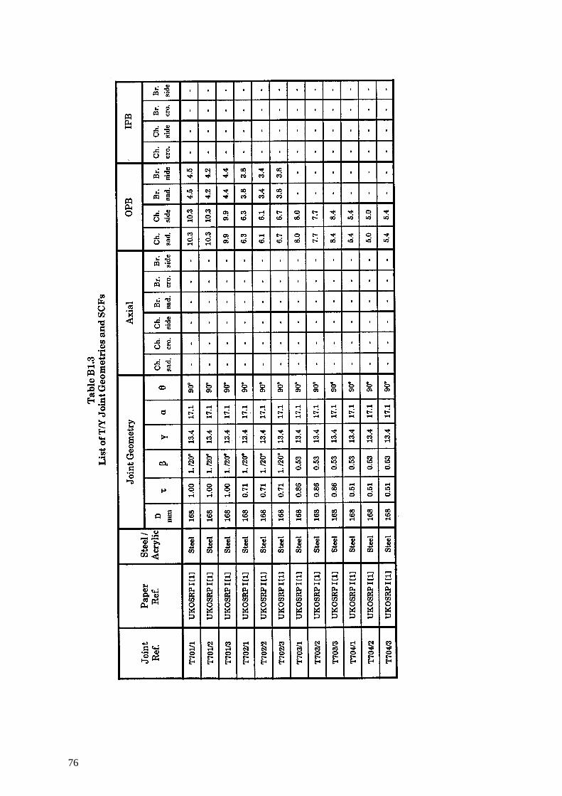
76

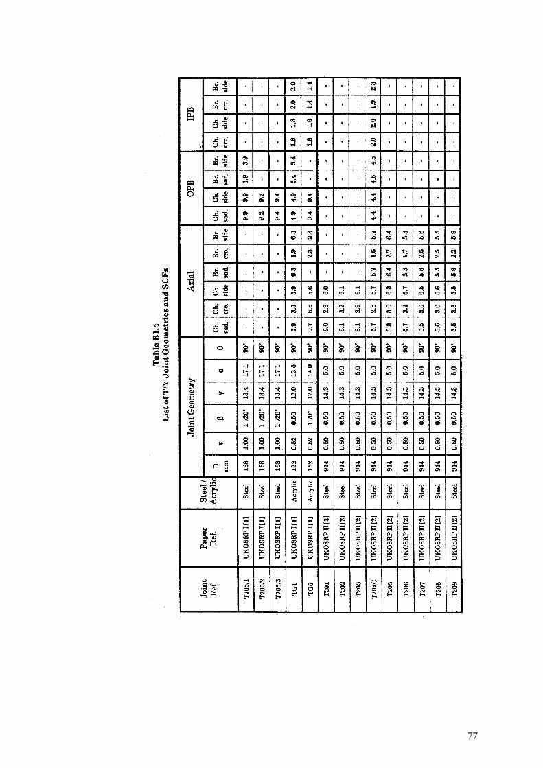
77

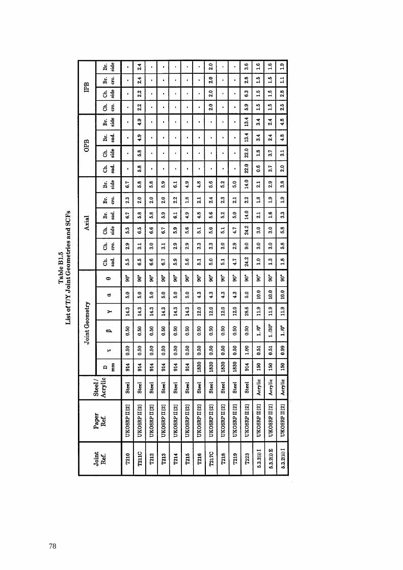
78

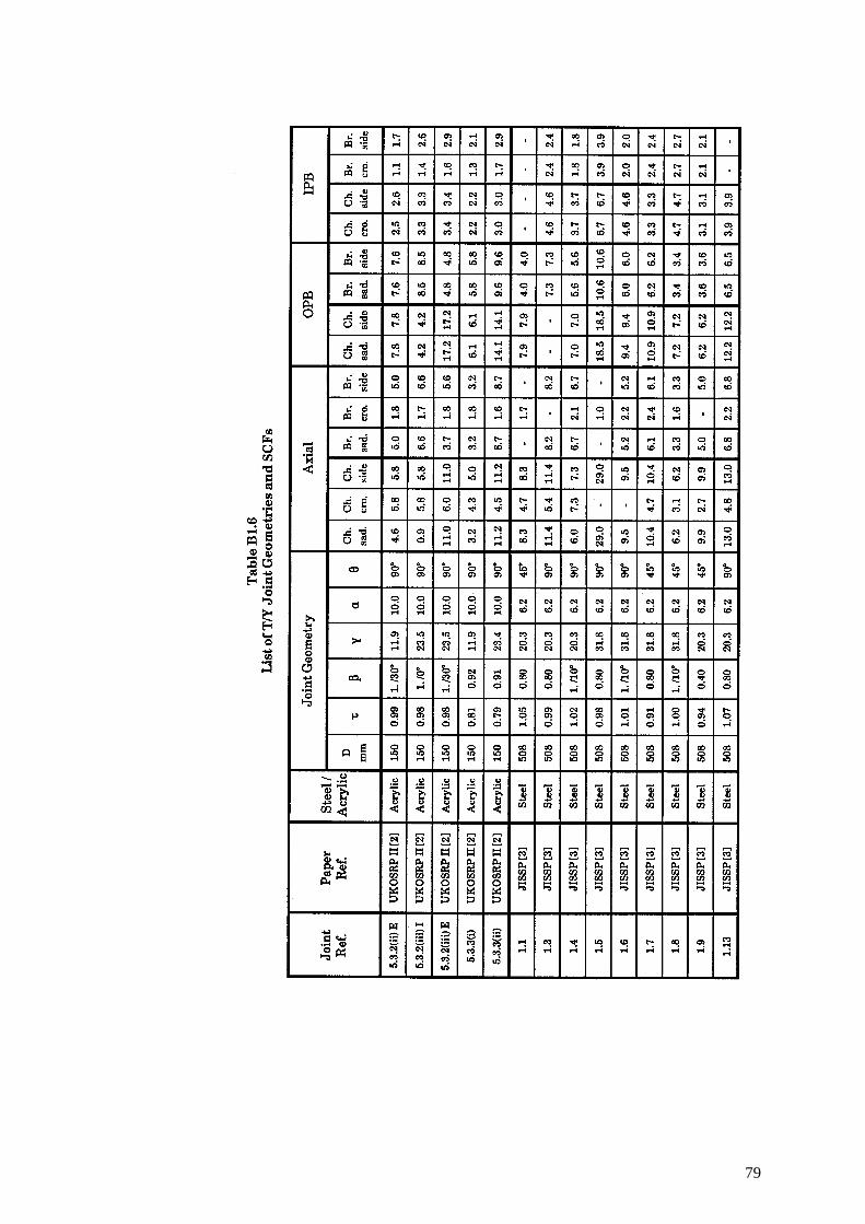
79

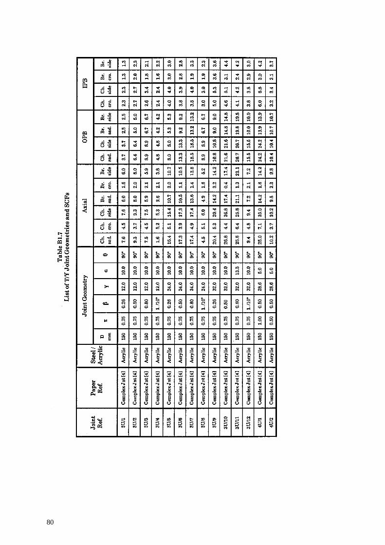
80

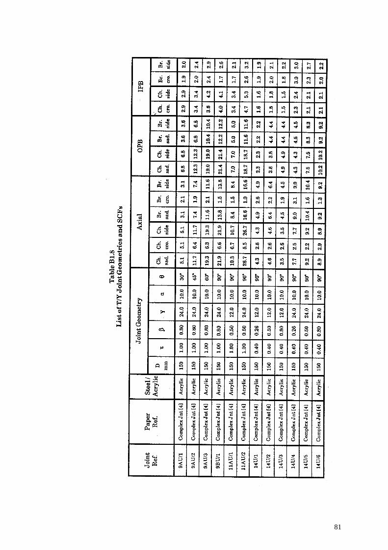
81

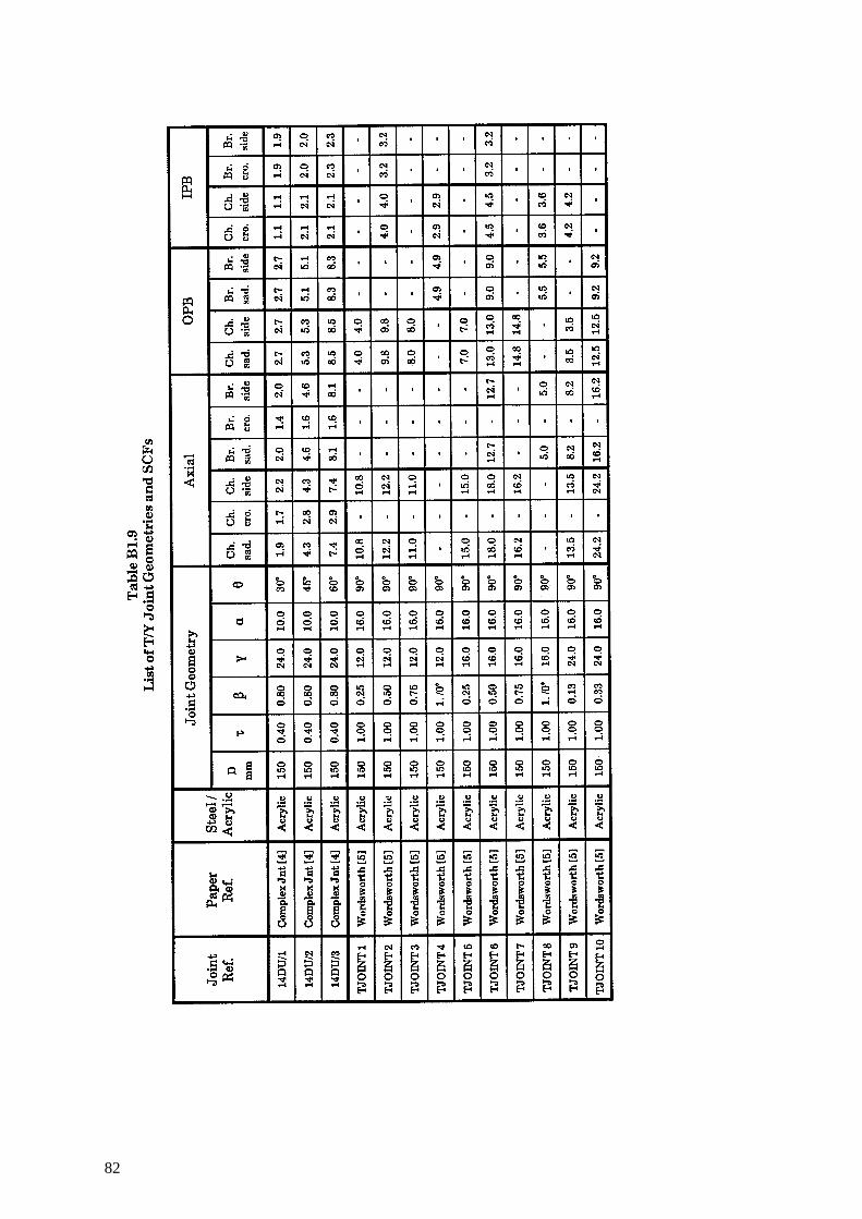
82

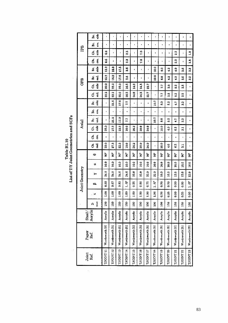
83

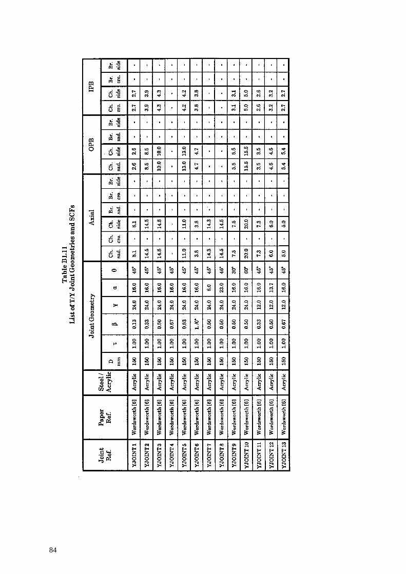
84

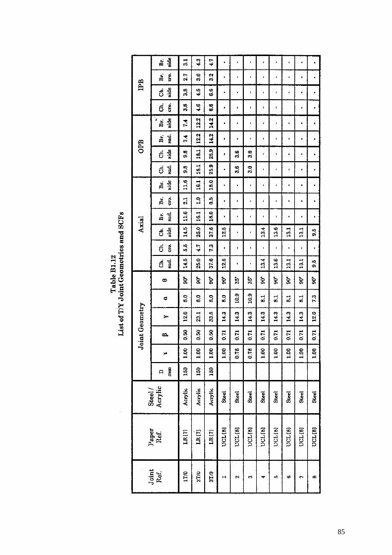
85

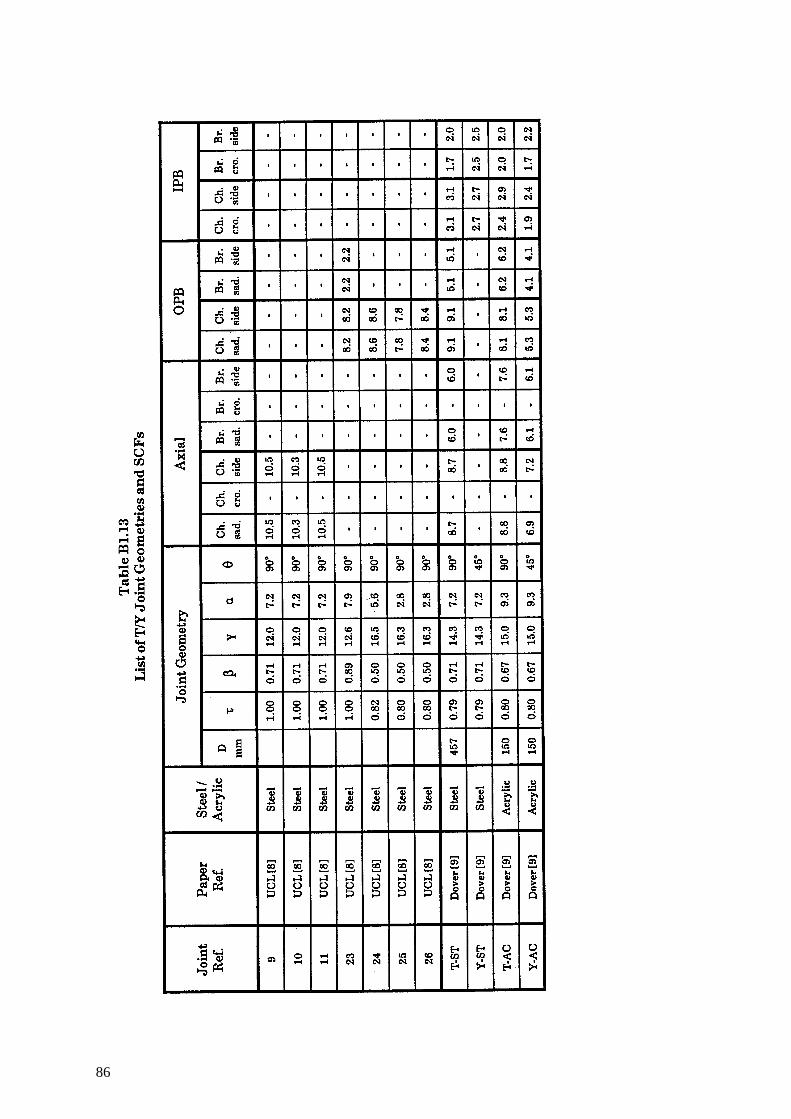
86

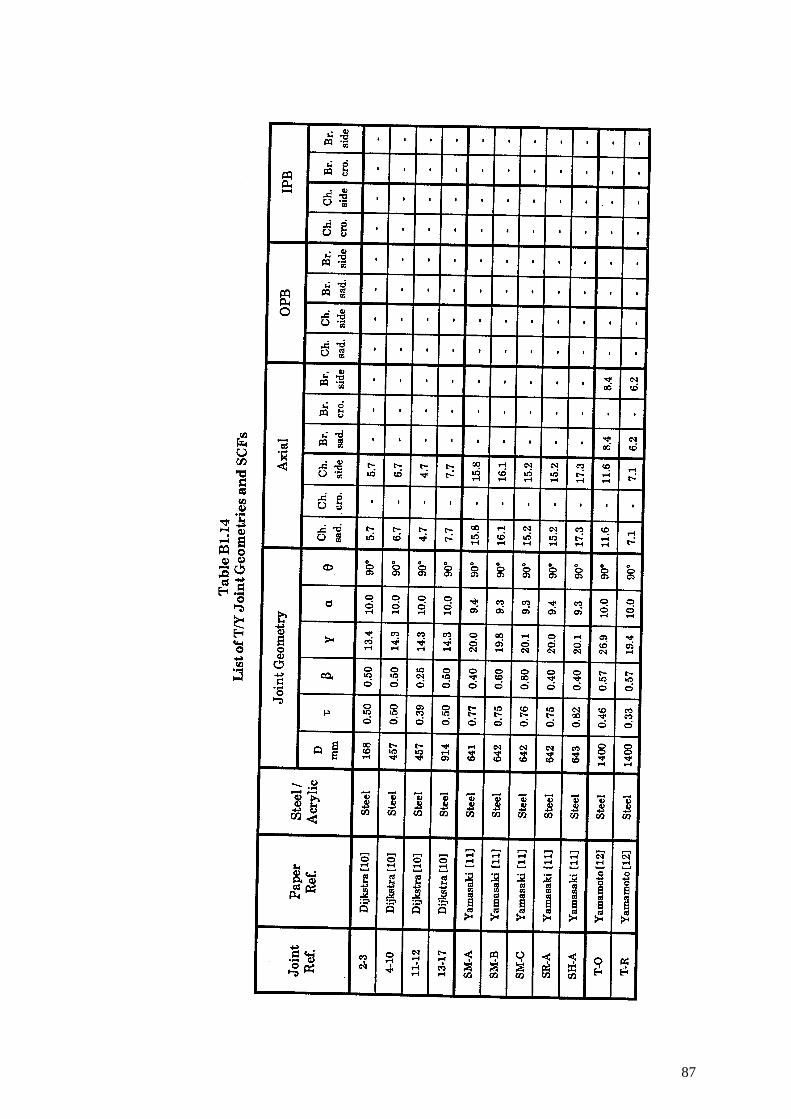
87

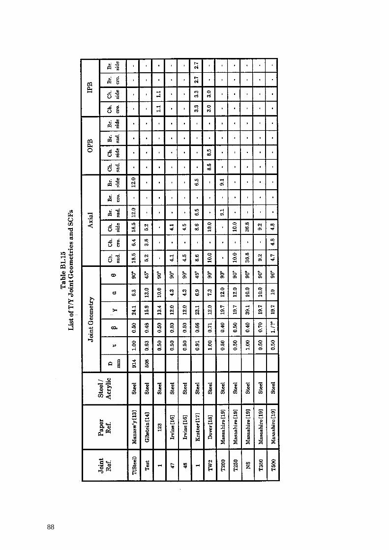
88

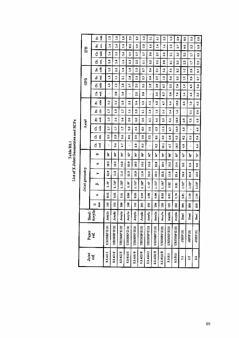
89

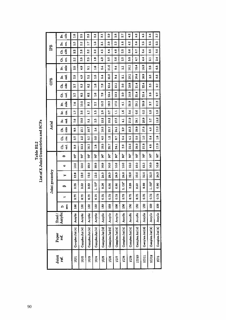
90

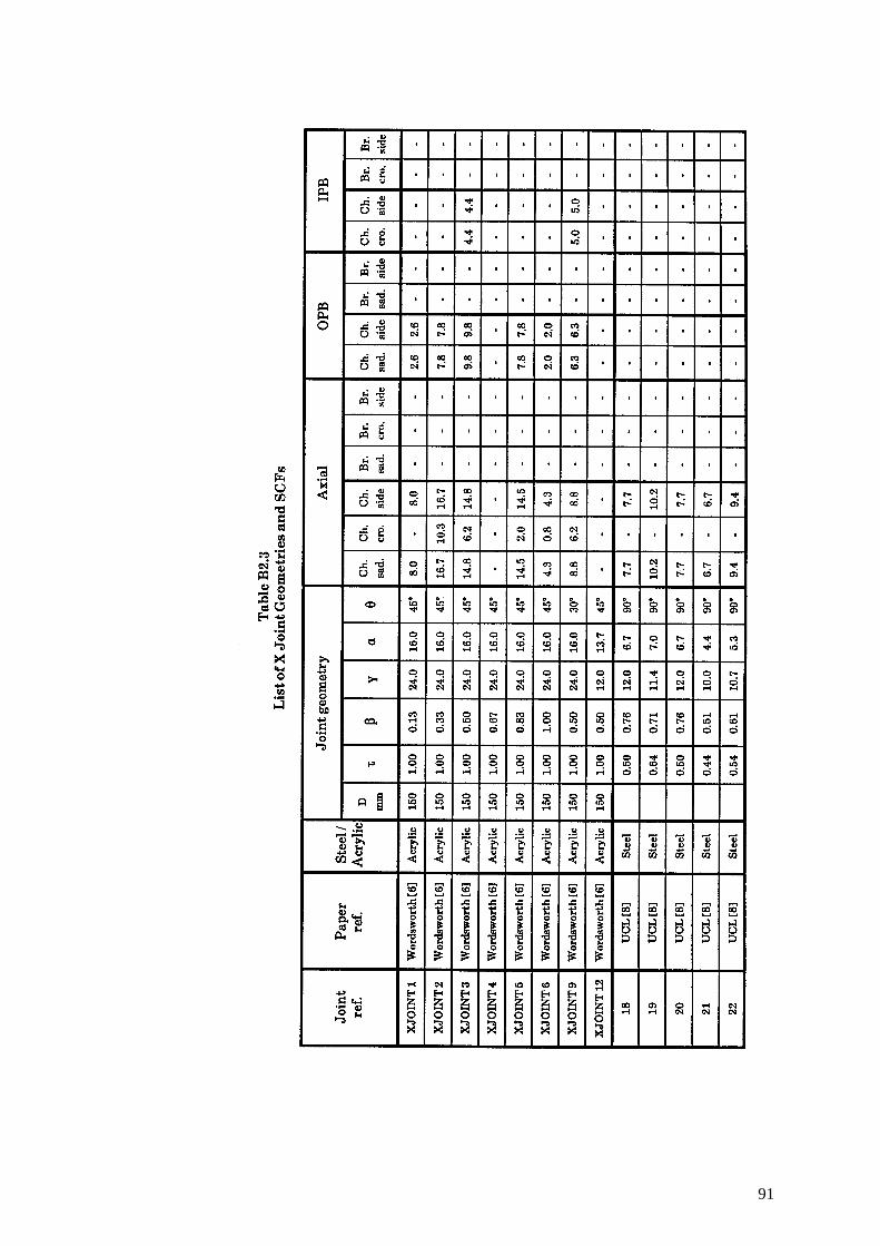
91

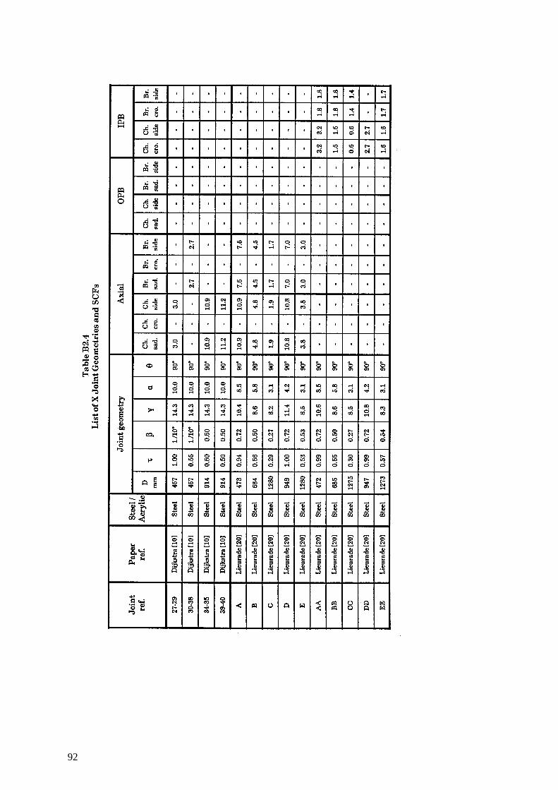
92

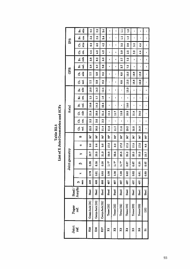
93

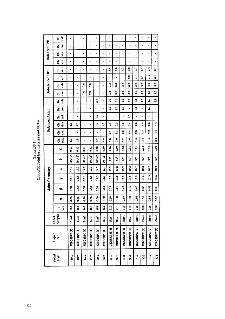
94

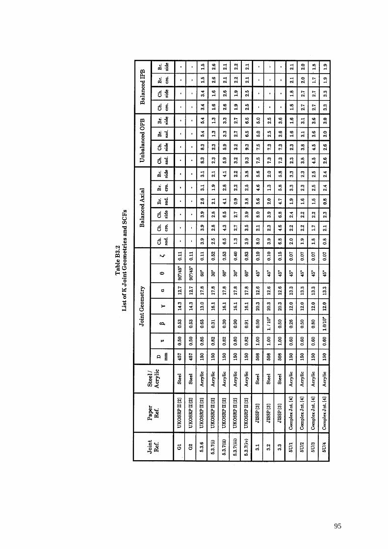
95

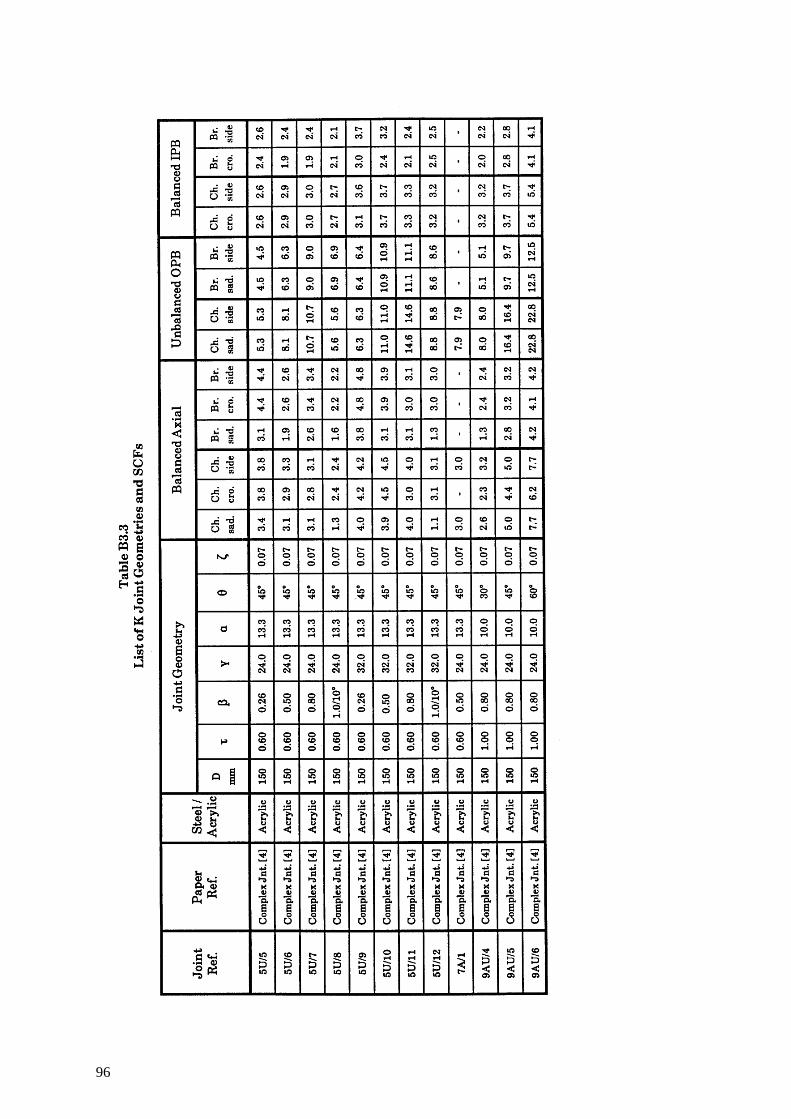
96

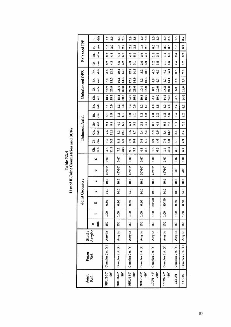
97

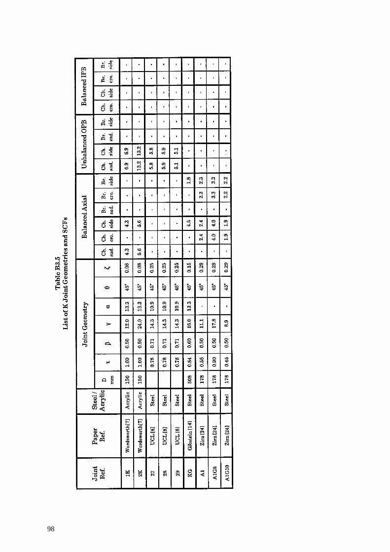
98

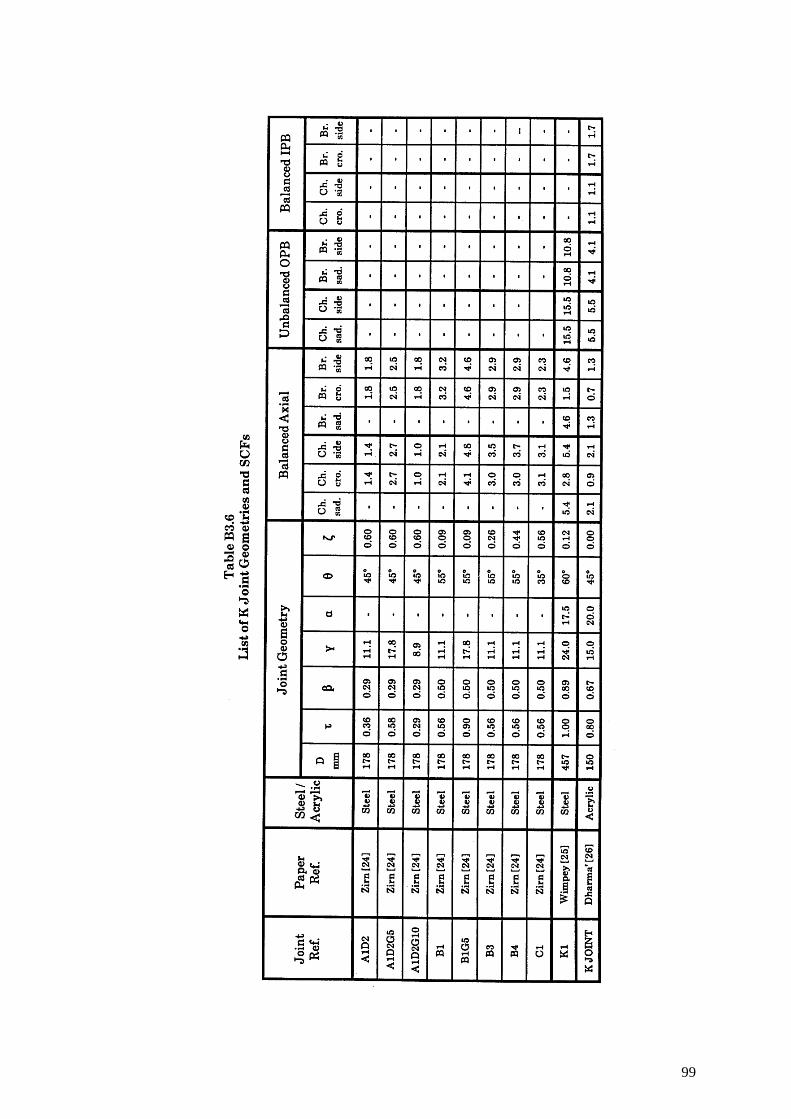
99

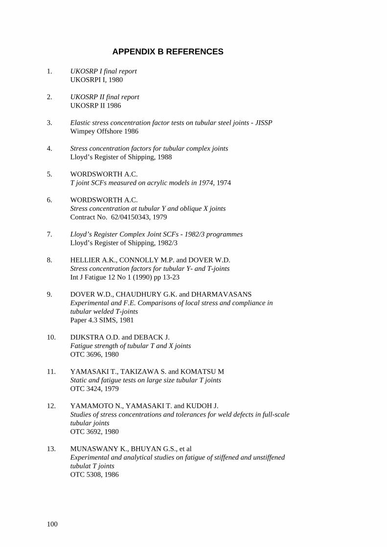
APPENDIX B REFERENCES

1. UKOSRP I final reportUKOSRPI I, 1980

2. UKOSRP II final reportUKOSRP II 1986

3. Elastic stress concentration factor tests on tubular steel joints - JISSPWimpey Offshore 1986

4. Stress concentration factors for tubular complex jointsLloyd’s Register of Shipping, 1988

5. WORDSWORTH A.C.T joint SCFs measured on acrylic models in 1974, 1974

6. WORDSWORTH A.C.Stress concentration at tubular Y and oblique X jointsContract No. 62/04150343, 1979

7. Lloyd’s Register Complex Joint SCFs - 1982/3 programmesLloyd’s Register of Shipping, 1982/3

8. HELLIER A.K., CONNOLLY M.P. and DOVER W.D.Stress concentration factors for tubular Y- and T-jointsInt J Fatigue 12 No 1 (1990) pp 13-23

9. DOVER W.D., CHAUDHURY G.K. and DHARMAVASANSExperimental and F.E. Comparisons of local stress and compliance intubular welded T-jointsPaper 4.3 SIMS, 1981

10. DIJKSTRA O.D. and DEBACK J.Fatigue strength of tubular T and X jointsOTC 3696, 1980

11. YAMASAKI T., TAKIZAWA S. and KOMATSU MStatic and fatigue tests on large size tubular T jointsOTC 3424, 1979

12. YAMAMOTO N., YAMASAKI T. and KUDOH J.Studies of stress concentrations and tolerances for weld defects in full-scaletubular jointsOTC 3692, 1980

13. MUNASWANY K., BHUYAN G.S., et alExperimental and analytical studies on fatigue of stiffened and unstiffenedtubulat T jointsOTC 5308, 1986

100

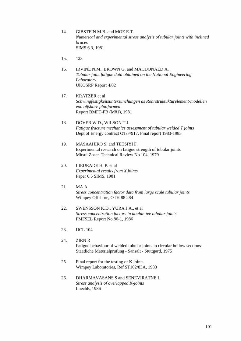
14. GIBSTEIN M.B. and MOE E.T.Numerical and experimental stress analysis of tubular joints with inclinedbracesSIMS 6.3, 1981

15. 123

16. IRVINE N.M., BROWN G. and MACDONALD A.Tubular joint fatigue data obtained on the National EngineeringLaboratoryUKOSRP Report 4/02

17. KRATZER et alSchwingfestigkeitsuntersunchungen as Rohrstruktukturelement-modellenvon offshore plattformenReport BMFT-FB (M81), 1981

18. DOVER W.D., WILSON T.J.Fatigue fracture mechanics assessment of tubular welded T jointsDept of Energy contract OT/F/917, Final report 1983-1985

19. MASAAHIRO S. and TETSIYI F.Experimental research on fatigue strength of tubular jointsMitsui Zosen Technical Review No 104, 1979

20. LIEURADE H, P. et alExperimental results from X jointsPaper 6.5 SIMS, 1981

21. MA A.Stress concentration factor data from large scale tubular jointsWimpey Offshore, OTH 88 284

22. SWENSSON K.D., YURA J.A., et alStress concentration factors in double-tee tubular jointsPMFSEL Report No 86-1, 1986

23. UCL 104

24. ZIRN RFatigue behaviour of welded tubular joints in circular hollow sectionsStaatliche Materialprufung - Sansalt - Stuttgard, 1975

25. Final report for the testing of K jointsWimpey Laboratories, Ref ST102/83A, 1983

26. DHARMAVASANS S and SENEVIRATNE LStress analysis of overlapped K-jointsImechE, 1986

101

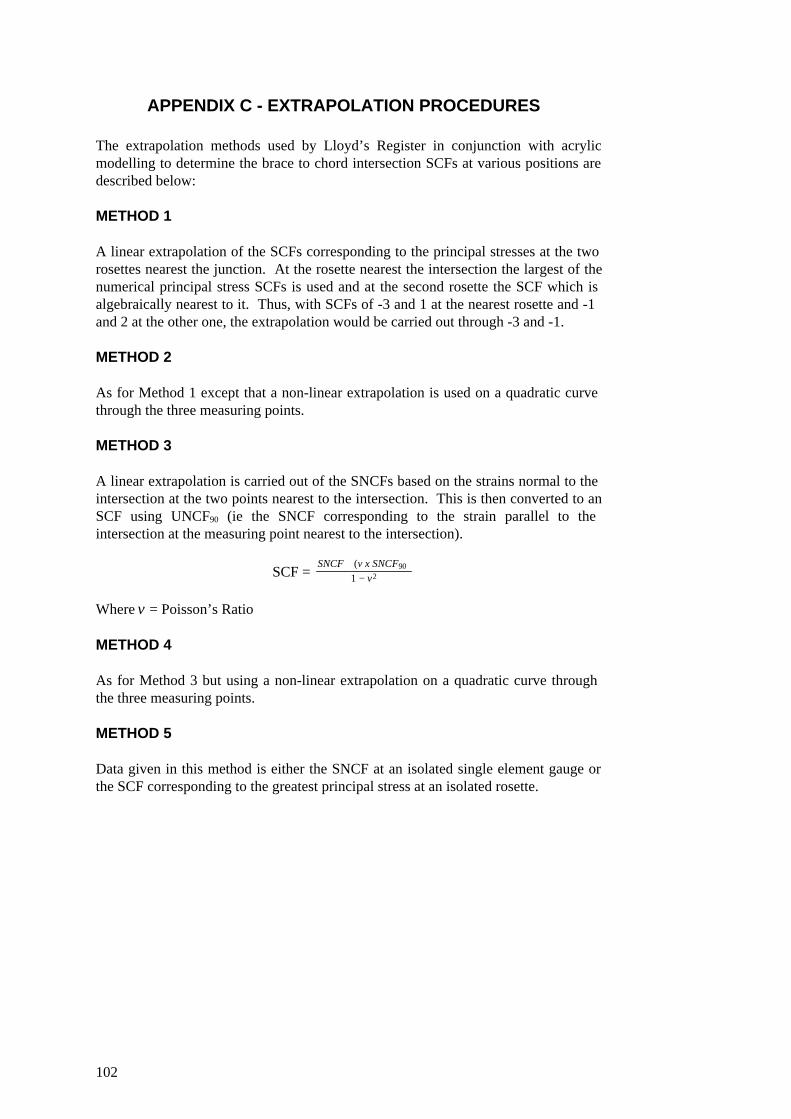
APPENDIX C - EXTRAPOLATION PROCEDURES

The extrapolation methods used by Lloyd’s Register in conjunction with acrylicmodelling to determine the brace to chord intersection SCFs at various positions aredescribed below:

METHOD 1

A linear extrapolation of the SCFs corresponding to the principal stresses at the tworosettes nearest the junction. At the rosette nearest the intersection the largest of thenumerical principal stress SCFs is used and at the second rosette the SCF which isalgebraically nearest to it. Thus, with SCFs of -3 and 1 at the nearest rosette and -1and 2 at the other one, the extrapolation would be carried out through -3 and -1.

METHOD 2

As for Method 1 except that a non-linear extrapolation is used on a quadratic curvethrough the three measuring points.

METHOD 3

A linear extrapolation is carried out of the SNCFs based on the strains normal to theintersection at the two points nearest to the intersection. This is then converted to anSCF using UNCF90 (ie the SNCF corresponding to the strain parallel to theintersection at the measuring point nearest to the intersection).

SCF = SNCF + (v x SNCF90)

1 − v2

Where = Poisson’s Ratiov

METHOD 4

As for Method 3 but using a non-linear extrapolation on a quadratic curve throughthe three measuring points.

METHOD 5

Data given in this method is either the SNCF at an isolated single element gauge orthe SCF corresponding to the greatest principal stress at an isolated rosette.

102

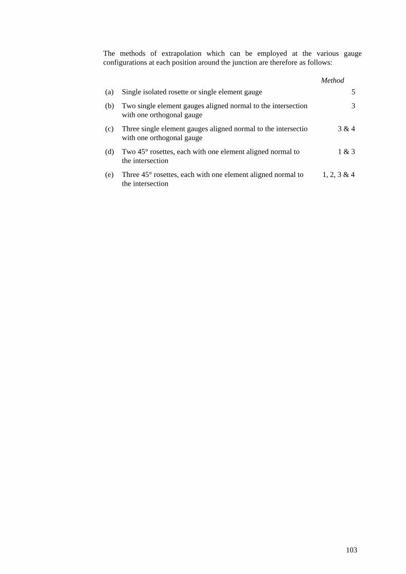
The methods of extrapolation which can be employed at the various gaugeconfigurations at each position around the junction are therefore as follows:

1, 2, 3 & 4Three 45° rosettes, each with one element aligned normal tothe intersection

(e)

1 & 3Two 45° rosettes, each with one element aligned normal tothe intersection

(d)

3 & 4Three single element gauges aligned normal to the intersectionwith one orthogonal gauge

(c)

3Two single element gauges aligned normal to the intersectionwith one orthogonal gauge

(b)

5Single isolated rosette or single element gauge(a)

Method

103