Embed Size (px)
Citation preview
MODELING METHODOLOGY
DECEMBER 2015
Stress Testing a Securities Portfolio with Spread Risk and Loss Recognition
Abstract
This paper introduces a framework for stress testing portfolios of credit risk sensitive securities. Specifically, the framework uses a macroeconomic scenario to project stressed expected losses (EL) on the securities by accounting for credit quality changes, recovery risk effects, fluctuations in market price of risk, and interest rates paths. The calculations are carried out analytically over multiple periods.
An important consideration of the framework is that the stressed EL are determined in-line with how institutions recognize accounting losses. For securities in a trading book and loans held-for-sale or measured through fair value option, any change in fair values is recognized as a gain/loss in the income statement (Mark-to-Market accounting). For securities in investment portfolio (Available-for-Sale or Held-to-Maturity), the framework realizes losses when an Other-than-Temporary-Impairment (OTTI) event occurs. If an OTTI occurs, the losses are bifurcated into a credit component, which is recognized in earnings and a non-credit component contributing towards Other Comprehensive Income (OCI). The framework allows for various ways to define OTTI threshold, including definitions based on agency ratings.
In addition to the analytic treatments, we also discuss the empirical estimation of various model components, present a validation analysis, and illustrate how this bottom-up approach to stress testing makes it possible to explain patterns in stressed EL using credit and market risk drivers.
Authors Jay Harvey Sunny Kanugo Vishal Mangla Libor Pospisil Yashan Wang Ian Ward Kevin Yang
Acknowledgements
We are extremely grateful to Amnon Levy, Nihil Patel, and Christopher Crossen for their help.
Contact Us Americas +1.212.553.1658 [email protected]
Europe +44.20.7772.5454 [email protected]
Asia (Excluding Japan) +85 2 2916 1121 [email protected]
Japan +81 3 5408 4100 [email protected]
2 DECEMBER 2015 STRESS TESTING A SECURITY PORTFOLIO WITH SPREAD RISK AND LOSS RECOGNITION
Table of Contents
1. Introduction 3
2.Modeling Framework for Stress Testing a Securities Portfolio 7 2.1 Framework Overview 7 2.2 Loss Recognition Rules 9 2.3 Macroeconomic Scenarios 11 2.4 Stressing Credit Qualities, Recoveries, and Market Price of Risk 12 2.5 Instrument Valuation 16 2.6 Loss Calculation 17 2.7 International Portfolios 19
3.Estimating Parameters for Spread Risk and Loss Recognition 21 3.1 Credit Risk Factors and Macroeconomic Variables 21 3.2 Market Price of Risk 24 3.3 Rating-implied PD 27
4.Understanding Projected Losses 30 4.1 Instrument-Level Losses 32 4.2 Portfolio Level Losses 36
5.Backtesting of Losses on a Securities Portfolio 40 5.1 Backtesting of Mark-to-Market Losses 40 5.2 Backtesting of Default Losses 42
6.Summary 45
Appendix 46
References 51
3 DECEMBER 2015 STRESS TESTING A SECURITY PORTFOLIO WITH SPREAD RISK AND LOSS RECOGNITION
1. Introduction
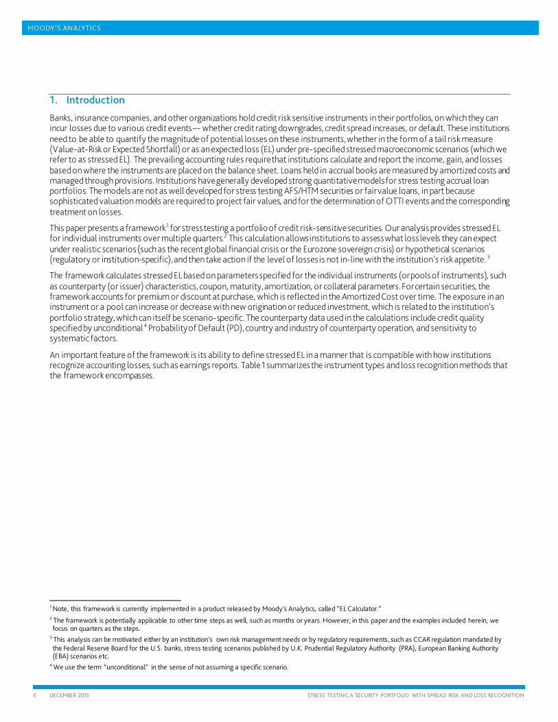
Banks, insurance companies, and other organizations hold credit risk sensitive instruments in their portfolios, on which they can incur losses due to various credit events –- whether credit rating downgrades, credit spread increases, or default. These institutions need to be able to quantify the magnitude of potential losses on these instruments, whether in the form of a tail risk measure (Value-at-Risk or Expected Shortfall) or as an expected loss (EL) under pre-specified stressed macroeconomic scenarios (which we refer to as stressed EL). The prevailing accounting rules require that institutions calculate and report the income, gain, and losses based on where the instruments are placed on the balance sheet. Loans held in accrual books are measured by amortized costs and managed through provisions. Institutions have generally developed strong quantitative models for stress testing accrual loan portfolios. The models are not as well developed for stress testing AFS/HTM securities or fair value loans, in part because sophisticated valuation models are required to project fair values, and for the determination of OTTI events and the corresponding treatment on losses.
This paper presents a framework1 for stress testing a portfolio of credit risk-sensitive securities. Our analysis provides stressed EL for individual instruments over multiple quarters.2 This calculation allows institutions to assess what loss levels they can expect under realistic scenarios (such as the recent global financial crisis or the Eurozone sovereign crisis) or hypothetical scenarios (regulatory or institution-specific), and then take action if the level of losses is not in-line with the institution’s risk appetite. 3
The framework calculates stressed EL based on parameters specified for the individual instruments (or pools of instruments), such as counterparty (or issuer) characteristics, coupon, maturity, amortization, or collateral parameters. For certain securities, the framework accounts for premium or discount at purchase, which is reflected in the Amortized Cost over time. The exposure in an instrument or a pool can increase or decrease with new origination or reduced investment, which is related to the institution’s portfolio strategy, which can itself be scenario-specific. The counterparty data used in the calculations include credit quality specified by unconditional4 Probability of Default (PD), country and industry of counterparty operation, and sensitivity to systematic factors.
An important feature of the framework is its ability to define stressed EL in a manner that is compatible with how institutions recognize accounting losses, such as earnings reports. Table 1 summarizes the instrument types and loss recognition methods that the framework encompasses.
1 Note, this framework is currently implemented in a product released by Moody’s Analytics, called “EL Calculator.” 2 The framework is potentially applicable to other time steps as well, such as months or years. However, in this paper and the examples included herein, we focus on quarters as the steps.
3 This analysis can be motivated either by an institution’s own risk management needs or by regulatory requirements, such as CCAR regulation mandated by the Federal Reserve Board for the U.S. banks, stress testing scenarios published by U.K. Prudential Regulatory Authority (PRA), European Banking Authority (EBA) scenarios etc.
4 We use the term “unconditional” in the sense of not assuming a specific scenario.
4 DECEMBER 2015 STRESS TESTING A SECURITY PORTFOLIO WITH SPREAD RISK AND LOSS RECOGNITION
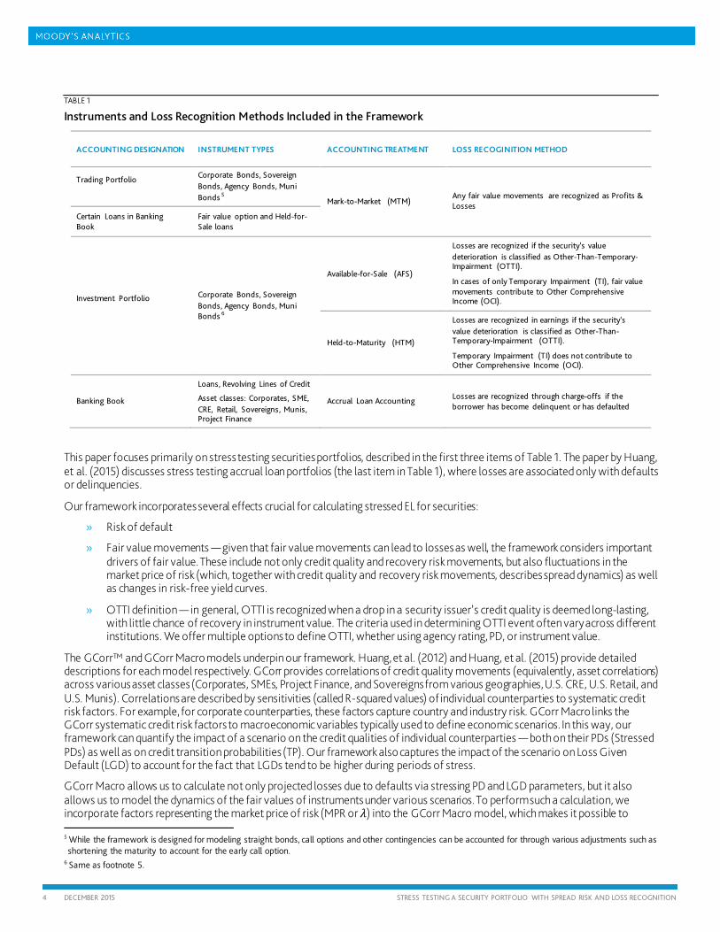
TABLE 1
Instruments and Loss Recognition Methods Included in the Framework
ACCOUNTING DESIGNATION INSTRUMENT TYPES ACCOUNTING TREATMENT LOSS RECOGINITION METHOD
Trading Portfolio
Corporate Bonds, Sovereign Bonds, Agency Bonds, Muni Bonds 5 Mark-to-Market (MTM)
Any fair value movements are recognized as Profits & Losses
Certain Loans in Banking Book
Fair value option and Held-for-Sale loans
Investment Portfolio
Corporate Bonds, Sovereign Bonds, Agency Bonds, Muni Bonds 6
Available-for-Sale (AFS)
Losses are recognized if the security’s value deterioration is classified as Other-Than-Temporary-Impairment (OTTI).
In cases of only Temporary Impairment (TI), fair value movements contribute to Other Comprehensive Income (OCI).
Held-to-Maturity (HTM)
Losses are recognized in earnings if the security’s value deterioration is classified as Other-Than-Temporary-Impairment (OTTI).
Temporary Impairment (TI) does not contribute to Other Comprehensive Income (OCI).
Banking Book
Loans, Revolving Lines of Credit
Asset classes: Corporates, SME, CRE, Retail, Sovereigns, Munis, Project Finance
Accrual Loan Accounting Losses are recognized through charge-offs if the borrower has become delinquent or has defaulted
This paper focuses primarily on stress testing securities portfolios, described in the first three items of Table 1. The paper by Huang, et al. (2015) discusses stress testing accrual loan portfolios (the last item in Table 1), where losses are associated only with defaults or delinquencies.
Our framework incorporates several effects crucial for calculating stressed EL for securities:
» Risk of default
» Fair value movements — given that fair value movements can lead to losses as well, the framework considers important drivers of fair value. These include not only credit quality and recovery risk movements, but also fluctuations in the market price of risk (which, together with credit quality and recovery risk movements, describes spread dynamics) as well as changes in risk-free yield curves.
» OTTI definition — in general, OTTI is recognized when a drop in a security issuer’s credit quality is deemed long-lasting, with little chance of recovery in instrument value. The criteria used in determining OTTI event often vary across different institutions. We offer multiple options to define OTTI, whether using agency rating, PD, or instrument value.
The GCorr™ and GCorr Macro models underpin our framework. Huang, et al. (2012) and Huang, et al. (2015) provide detailed descriptions for each model respectively. GCorr provides correlations of credit quality movements (equivalently, asset correlations) across various asset classes (Corporates, SMEs, Project Finance, and Sovereigns from various geographies, U.S. CRE, U.S. Retail, and U.S. Munis). Correlations are described by sensitivities (called R-squared values) of individual counterparties to systematic credit risk factors. For example, for corporate counterparties, these factors capture country and industry risk. GCorr Macro links the GCorr systematic credit risk factors to macroeconomic variables typically used to define economic scenarios. In this way, our framework can quantify the impact of a scenario on the credit qualities of individual counterparties — both on their PDs (Stressed PDs) as well as on credit transition probabilities (TP). Our framework also captures the impact of the scenario on Loss Given Default (LGD) to account for the fact that LGDs tend to be higher during periods of stress.
GCorr Macro allows us to calculate not only projected losses due to defaults via stressing PD and LGD parameters, but it also allows us to model the dynamics of the fair values of instruments under various scenarios. To perform such a calculation, we incorporate factors representing the market price of risk (MPR or 𝜆𝜆) into the GCorr Macro model, which makes it possible to
5 While the framework is designed for modeling straight bonds, call options and other contingencies can be accounted for through various adjustments such as shortening the maturity to account for the early call option.
6 Same as footnote 5.
5 DECEMBER 2015 STRESS TESTING A SECURITY PORTFOLIO WITH SPREAD RISK AND LOSS RECOGNITION
project a path of 𝜆𝜆 under a given economic scenario. Another important variable impacting a fair value is the risk-free yield curve. We take the projected curve directly from the given economic scenario.
The macroeconomic variables included in GCorr Macro relevant for stressing credit quality and the market price of risk include various economic indicators, such as GDP and Unemployment Rate, and financial market indicators such as stock market index, VIX, and a corporate spread Index. The 2014 version of GCorr Macro 20147 covers 77 macroeconomic variables, which cover various types of indicators across many countries, both developed and emerging. Thus, the model has the flexibility to perform stress testing on a range of asset classes from a range of geographies. A small set of macroeconomic variables relevant for a given portfolio can be determined using a variable selection procedure.
Our framework projects fair values in the following way. At the end of each quarter, we build a grid of credit states, each associated with a certain PD and LGD level. Combined with the projected 𝜆𝜆 and the projected risk-free yield curve, we can associate each credit state with the instrument’s price. Using GCorr Macro, which links movements in credit qualities to macroeconomic variables, we can calculate the transition probability of a counterparty migrating from its initial credit state to a credit state at the end of the given quarter under the given scenario.
An important step in calculating stressed EL is translating the fair value of an instrument in each credit state into a loss. For Accrual Loss Accounting, non-default credit states do not imply any loss. In the case of MTM method, any movement in fair value is recognized as profit or loss. For an AFS or HTM security, we must decide whether a given credit state represents OTTI event and, thus, whether a loss should be recognized in income statement. Once the loss at each credit state is determined, we obtain stressed EL values by taking expectation of losses across various future credit states, weighted by the stressed transition probabilities.
Our framework provides three approaches to deciding whether OTTI has occurred:
» The first approach classifies OTTI as credit states associated with a lower agency rating than a pre-specified threshold. For insurance companies such a threshold could be Baa3 (lowest investment grade rating), which means that an OTTI loss is recognized if the security’s issuer is downgraded to a speculative grade. In the case of banks, this threshold could be Caa — the level specified by the Federal Reserve CCAR regulation.8
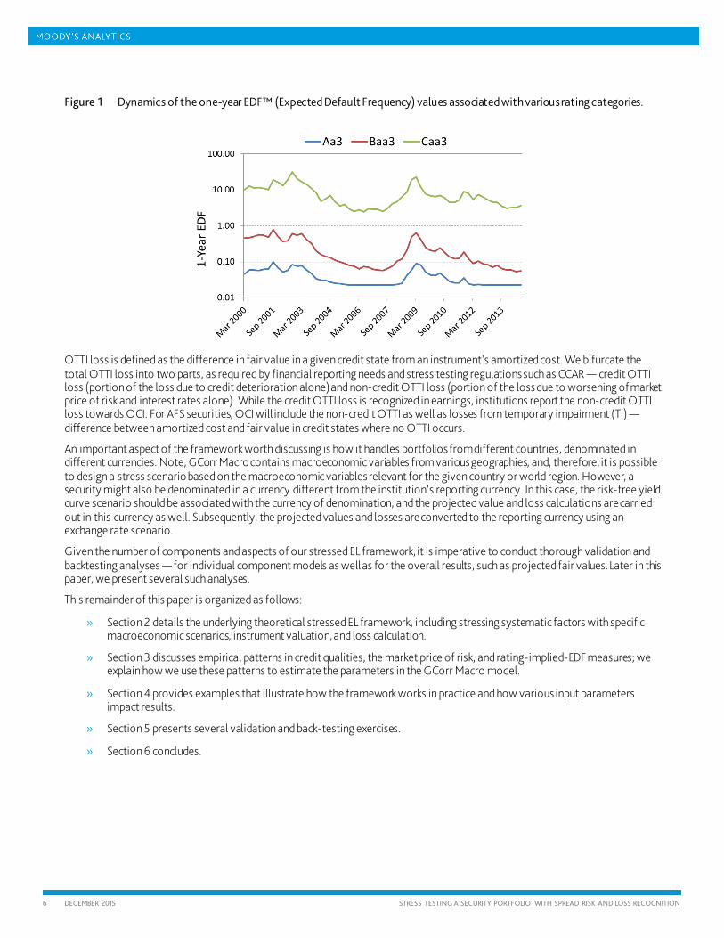
• Credit states are, however, defined by PDs in the framework, and, therefore, we must introduce a link between PD level and rating in order to assign ratings to credit states. As Figure 1 suggests, such a link is dynamic, meaning that a PD level associated with a given rating varies with the economic environment. Thus, we introduce a new factor into the GCorr Macro model, which represents movements in rating-specific PD and is correlated with macroeconomic variables. As a result, we can project rating-specific PD over time under a given economic scenario and, thus, determine which credit states should be classified as OTTI under that scenario.
» The second approach to defining OTTI is to specify the threshold not in terms of agency rating, but in terms of PD level, which can be readily used to identify credit states with PD level higher than this threshold. For example, all credit states with one-year PD higher than 5% may be considered OTTI states.
» Third, a credit state is considered OTTI if the fair value in that credit state is below the amortized cost by a certain threshold, for example 20%.
Our framework allows institutions to specify the threshold in each of the approaches above, based on their individual needs and practices.
7 We are referring to the GCorr Macro 2014 model. 8 See DFAST (2015)
6 DECEMBER 2015 STRESS TESTING A SECURITY PORTFOLIO WITH SPREAD RISK AND LOSS RECOGNITION
Figure 1 Dynamics of the one-year EDF™ (Expected Default Frequency) values associated with various rating categories.
OTTI loss is defined as the difference in fair value in a given credit state from an instrument’s amortized cost. We bifurcate the total OTTI loss into two parts, as required by financial reporting needs and stress testing regulations such as CCAR — credit OTTI loss (portion of the loss due to credit deterioration alone) and non-credit OTTI loss (portion of the loss due to worsening of market price of risk and interest rates alone). While the credit OTTI loss is recognized in earnings, institutions report the non-credit OTTI loss towards OCI. For AFS securities, OCI will include the non-credit OTTI as well as losses from temporary impairment (TI) — difference between amortized cost and fair value in credit states where no OTTI occurs.
An important aspect of the framework worth discussing is how it handles portfolios from different countries, denominated in different currencies. Note, GCorr Macro contains macroeconomic variables from various geographies, and, therefore, it is possible to design a stress scenario based on the macroeconomic variables relevant for the given country or world region. However, a security might also be denominated in a currency different from the institution’s reporting currency. In this case, the risk-free yield curve scenario should be associated with the currency of denomination, and the projected value and loss calculations are carried out in this currency as well. Subsequently, the projected values and losses are converted to the reporting currency using an exchange rate scenario.
Given the number of components and aspects of our stressed EL framework, it is imperative to conduct thorough validation and backtesting analyses — for individual component models as well as for the overall results, such as projected fair values. Later in this paper, we present several such analyses.
This remainder of this paper is organized as follows:
» Section 2 details the underlying theoretical stressed EL framework, including stressing systematic factors with specific macroeconomic scenarios, instrument valuation, and loss calculation.
» Section 3 discusses empirical patterns in credit qualities, the market price of risk, and rating-implied-EDF measures; we explain how we use these patterns to estimate the parameters in the GCorr Macro model.
» Section 4 provides examples that illustrate how the framework works in practice and how various input parameters impact results.
» Section 5 presents several validation and back-testing exercises.
» Section 6 concludes.
7 DECEMBER 2015 STRESS TESTING A SECURITY PORTFOLIO WITH SPREAD RISK AND LOSS RECOGNITION
2. Modeling Framework for Stress Testing a Securities Portfolio
This section describes the main building blocks of our stressed EL framework. We first preview the flow of calculations and then discuss how our framework allocates losses to different accounting categories according to the loss recognition rules. We then discuss in more details the macroeconomic scenario definition, GCorr Macro model, instrument valuation, and loss calculation. We also touch upon how the framework handles instruments denominated in currencies other than the reporting currency.
2.1 Framework Overview
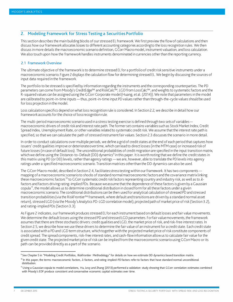
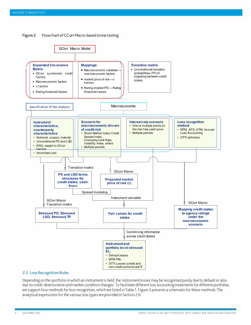
The ultimate objective of the framework is to determine stressed EL for a portfolio of credit risk sensitive instruments under a macroeconomic scenario. Figure 2 displays the calculation flow for determining stressed EL. We begin by discussing the sources of input data required in the framework.
The portfolio to be stressed is specified by information regarding the instruments and the corresponding counterparties. The PD parameters can come from Moody’s CreditEdge™ and RiskCalc™, LGD from LossCalc™, and weights to systematic factors and the R-squared values can be assigned using the GCorr Corporate model (Huang, et al. (2014)). We note that parameters in the model are calibrated to point-in-time inputs — thus, point-in-time input PD values rather than through-the-cycle values should be used for loss projection in the model.
Loss calculation specifics depend on what loss recognition rule is considered. In Section 2.2, we describe in detail how our framework accounts for the choice of loss recognition rule.
The multi-period macroeconomic scenario used in a stress testing exercise is defined through two sets of variables — macroeconomic drivers of credit risk and interest rate path. The former set contains variables such as Stock Market Index, Credit Spread Index, Unemployment Rate, or other variables related to systematic credit risk. We assume that the interest rate path is specified, so that we can calculate the path of stressed instrument fair values. Section 2.3 discusses the scenario in more detail.
In order to conduct calculations over multiple periods, we define a grid of credit states at the end of each period that captures how issuers’ credit qualities improve or deteriorate over time, which can lead to direct losses (in the MTM case) or increased risk of future losses (in case of default loss). The unconditional probabilities of credit migration are specified in the input transition matrix, which we define using the Distance-to-Default (DD) dynamics9 in this paper. It is worth noting that we define the credit states in this matrix using PD (or DD) levels, rather than agency ratings — we are, however, able to translate the PD levels into agency ratings under a specified macroeconomic scenario. Transition matrices other than the DD dynamics can also be used.
The GCorr Macro model, described in Section 2.4, facilitates stress testing within our framework. It has two components —mapping of a macroeconomic scenario to shocks of standard normal macroeconomic factors and the covariance matrix linking these macroeconomic factors 10 to GCorr systematic credit risk factors representing country and industry risk, as well as to 𝜆𝜆-factors and factors driving rating-implied PDs. Because we assume that the dependence of these factors is given by a Gaussian copula11, the model allows us to determine conditional distribution in closed form for all these factors under a given macroeconomic scenario. The conditional distributions can be then used for analytical calculation of stressed PD and stressed transition probabilities (via the RiskFrontier™ framework, where default and transitions are driven by a standard normal asset return), stressed LGD (via the Moody’s Analytics PD-LGD correlation model), projected path of market price of risk (Section 3.2), and rating-implied PDs (Section 3.3).
As Figure 2 indicates, our framework produces stressed EL for each instrument based on default losses and fair value movements. We determine the default losses using the stressed PD and stressed LGD parameters. For fair value movements, the framework assumes that there are three stochastic drivers: credit qualities and LGD, the market price of risk, and risk-free interest rates. In Section 2.5, we describe how we use these drivers to determine the fair value of an instrument for a credit state. Each credit state is associated with a PD and LGD term structure, which together with the projected market price of risk constitute components of credit spread. The spread components, risk-free interest rates, and cash-flow information allow us to calculate fair value for the given credit state. The projected market price of risk can be implied from the macroeconomic scenario using GCorr Macro or its path can be provided directly as a part of the scenario.
9 See Chapter 5 in “Modeling Credit Portfolios, RiskFrontier Methodology” for details on how we estimate DD dynamics based transition matrix. 10 In this paper, the terms macroeconomic factors, 𝜆𝜆-factors, and rating-implied-PD factors refer to factors that have standard normal unconditional distribution.
11 Using a Gaussian copula to model correlations, Hu, Levy and Zhang (2013) performed a validation study showing that GCorr correlation estimates combined with Moody’s EDF produce consistent and conservative economic capital estimates over time.

8 DECEMBER 2015 STRESS TESTING A SECURITY PORTFOLIO WITH SPREAD RISK AND LOSS RECOGNITION
» Depending on the loss recognition method, the framework converts the fair value to the corresponding loss in each credit state. For example, if OTTI is defined as a downgrade below a certain rating, we can use the projected rating-implied PD values to identify which credit states are associated with this downgrade and, hence, lead to an OTTI loss.
» Using stressed transition probabilities, we combine losses across credit states to determine the stressed EL for each period, as detailed in Section 2.6. As this overview and Figure 2 show, our framework can be considered a bottom-up approach for determining stressed EL, which allows us to conduct analyses to understand the contributions of individual components to patterns in the stressed EL — credit qualities, LGD, market price of risk, risk-free interest rates, or rating-specific PD.
9 DECEMBER 2015 STRESS TESTING A SECURITY PORTFOLIO WITH SPREAD RISK AND LOSS RECOGNITION
Figure 2 Flowchart of GCorr Macro-based stress testing.
2.2 Loss Recognition Rules
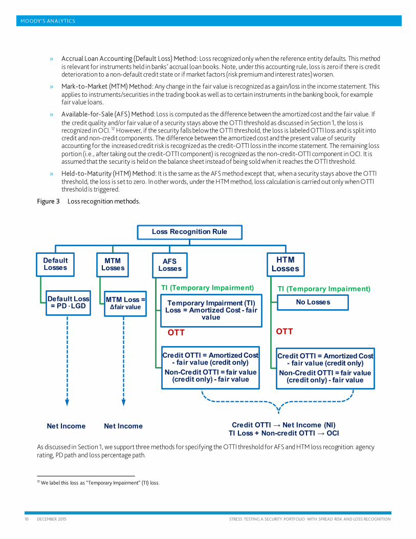
Depending on the portfolio in which an instrument is held, the instrument losses may be recognized purely due to default or also due to credit deterioration and market condition changes. To facilitate different loss accounting treatments for different portfolios, we support four methods for loss recognition, which we listed in Table 1. Figure 3 presents a schematic for these methods. The analytical expressions for the various loss types are provided in Section 2.6.
GCorr Macro
Combining information across credit states
Stressed PD, Stressed LGD, Stressed TP
GCorr Macro Transition matrix
Projected market price of risk (λ)
PD and LGD terms structures for
credit states, cash-flows
Expanded Cov ariance Matrix • GCorr sy stematic credit
f actors • Macroeconomic factors • 𝜆𝜆 f actors
• Rating threshold factors
Mappings
• Macroeconomic variables ↔ macroeconomic factors
• market price of risk ↔λ f actors
• Rating-implied-PD ↔ Rating threshold f actors
GCorr Macro Model
Instrument characteristics, counterparty characteristics • Notional, coupon, maturity • Unconditional PD and LGD • RSQ, weight to GCorr
f actors • Amortized cost
Interest rate scenario • One or multiple points on
the risk-f ree yield curve • Multiple periods
Loss recognition method • MTM, AFS, HTM, Accrual
Loan Accounting • OTTI def inition
Specification of the Analysis Macroeconomic
Scenario for macroeconomic driv ers of credit risk • Stock Market Index, Credit
Spread Index, Unemployment Rate, Volatility Index, others
• Multiple periods
Transition matrix • Unconditional transition
probabilities (TP) of migrating between credit states.
Fair v alues for credit states
Mapping credit states to agency ratings
under the macroeconomic
scenario
Instrument and portfolio lev el stressed EL: • Def ault losses • MTM P&L • OTTI Losses (credit and
non-credit portions) and TI
GCorr Macro Transition matrix
Spread modeling
Instrument valuation
10 DECEMBER 2015 STRESS TESTING A SECURITY PORTFOLIO WITH SPREAD RISK AND LOSS RECOGNITION
» Accrual Loan Accounting (Default Loss) Method: Loss recognized only when the reference entity defaults. This method is relevant for instruments held in banks’ accrual loan books. Note, under this accounting rule, loss is zero if there is credit deterioration to a non-default credit state or if market factors (risk premium and interest rates) worsen.
» Mark-to-Market (MTM) Method: Any change in the fair value is recognized as a gain/loss in the income statement. This applies to instruments/securities in the trading book as well as to certain instruments in the banking book, for example fair value loans.
» Available-for-Sale (AFS) Method: Loss is computed as the difference between the amortized cost and the fair value. If the credit quality and/or fair value of a security stays above the OTTI threshold as discussed in Section 1, the loss is recognized in OCI. 12 However, if the security falls below the OTTI threshold, the loss is labeled OTTI loss and is split into credit and non-credit components. The difference between the amortized cost and the present value of security accounting for the increased credit risk is recognized as the credit-OTTI loss in the income statement. The remaining loss portion (i.e., after taking out the credit-OTTI component) is recognized as the non-credit-OTTI component in OCI. It is assumed that the security is held on the balance sheet instead of being sold when it reaches the OTTI threshold.
» Held-to-Maturity (HTM) Method: It is the same as the AFS method except that, when a security stays above the OTTI threshold, the loss is set to zero. In other words, under the HTM method, loss calculation is carried out only when OTTI threshold is triggered.
Figure 3 Loss recognition methods.
As discussed in Section 1, we support three methods for specifying the OTTI threshold for AFS and HTM loss recognition: agency rating, PD path and loss percentage path.
12 We label this loss as “Temporary Impairment” (TI) loss.
Loss Recognition Rule
Default Losses
Default Loss = PD ·LGD
MTM Losses
MTM Loss = Δfair value
AFS Losses
Temporary Impairment (TI) Loss = Amortized Cost - fair
value
Credit OTTI = Amortized Cost - fair value (credit only)
Non-Credit OTTI = fair value (credit only) - fair value
HTM Losses
No Losses
Credit OTTI = Amortized Cost - fair value (credit only)
Non-Credit OTTI = fair value (credit only) - fair value
Net Income Credit OTTI → Net Income (NI) TI Loss + Non-credit OTTI → OCI
Net Income
TI (Temporary Impairment)
OTT
TI (Temporary Impairment)
OTT
11 DECEMBER 2015 STRESS TESTING A SECURITY PORTFOLIO WITH SPREAD RISK AND LOSS RECOGNITION
2.3 Macroeconomic Scenarios
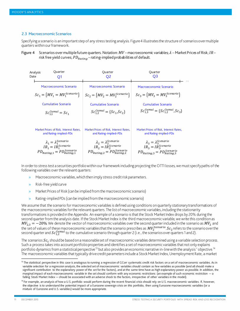
Specifying a scenario is an important step of any stress testing analysis. Figure 4 illustrates the structure of scenarios over multiple quarters within our framework.
Figure 4 Scenarios over multiple future quarters. Notation: 𝑀𝑀𝑀𝑀 – macroeconomic variables; 𝜆𝜆 – Market Prices of Risk; 𝐼𝐼𝐼𝐼 – risk free yield curves; 𝑃𝑃𝑃𝑃𝑅𝑅𝑅𝑅𝑅𝑅𝑅𝑅𝑅𝑅𝑅𝑅 – rating-implied probabilities of default.
In order to stress test a securities portfolio within our framework including projecting the OTTI losses, we must specify paths of the following variables over the relevant quarters:
» Macroeconomic variables, which then imply stress credit risk parameters.
» Risk-free yield curve
» Market Prices of Risk (can be implied from the macroeconomic scenario)
» Rating-implied PDs (can be implied from the macroeconomic scenario)
We assume that the scenario for macroeconomic variables is defined using conditions on quarterly stationary transformations of the macroeconomic variables for the relevant quarters. The list of macroeconomic variables, including the stationarity transformations is provided in the Appendix. An example of a scenario is that the Stock Market Index drops by 20% during the second quarter from the analysis date. If the Stock Market Index is the third macroeconomic variable, we write this condition as 𝑀𝑀𝑀𝑀2,3 = −20%. We denote the vector of macroeconomic variables over the second quarter included in the scenario as 𝑀𝑀𝑀𝑀2 and the set of values of these macroeconomic variables that the scenario prescribes as 𝑀𝑀𝑀𝑀2𝑆𝑆𝑆𝑆𝑆𝑆𝑅𝑅𝑅𝑅𝑆𝑆𝑅𝑅𝑆𝑆. 𝑆𝑆𝑐𝑐2 refers to the scenario over the second quarter and 𝑆𝑆𝑐𝑐1,2
𝐶𝐶𝐶𝐶𝐶𝐶𝐶𝐶𝐶𝐶 to the cumulative scenario through quarter 2 (i.e., the scenarios over quarters 1 and 2).
The scenarios 𝑆𝑆𝑐𝑐𝑅𝑅 should be based on a reasonable set of macroeconomic variables determined using a variable selection process. Such a process takes into account portfolio properties and identifies a set of macroeconomic variables that not only explains portfolio dynamics from a statistical perspective13 but also provides an economic narrative in-line with the analysis ‘ objective.14 The macroeconomic variables that typically drive credit parameters include a Stock Market Index, Unemployment Rate, a market
13 The statistical perspective in this case is analogous to running a regression of GCorr systematic credit risk factors on a set of macroeconomic variables. As in variable selection for a regression analysis, the selected set of macroeconomic variables should contain as few variables as possible (and all should make a significant contribution to the explanatory power of the set for the factors), and at the same time have as high explanatory power as possible. In addition, the marginal impact of each macroeconomic variable in the set should conform with any economic restrictions (an example of such economic restriction — a falling Stock Market Index — should be associated with an adverse shock to the factors, irrespective of other variables in the model).
14 For example, an analysis of how a U.S. portfolio would perform during the recent financial crisis should rely on U.S. macroeconomic variables. If, however, the objective is to understand the potential impact of a Eurozone sovereign crisis on this portfolio, then using Eurozone macroeconomic variables (or a mixture of Eurozone and U.S. variables) would be more appropriate.
𝜆𝜆1 = 𝜆𝜆1𝑆𝑆𝑆𝑆𝑆𝑆𝑅𝑅𝑅𝑅𝑆𝑆𝑅𝑅𝑆𝑆 𝐼𝐼𝐼𝐼1 = 𝐼𝐼𝐼𝐼1𝑆𝑆𝑆𝑆𝑆𝑆𝑅𝑅𝑅𝑅𝑆𝑆𝑅𝑅𝑆𝑆
𝑃𝑃𝑃𝑃𝑅𝑅𝑅𝑅𝑅𝑅𝑅𝑅𝑅𝑅𝑅𝑅,1 = 𝑃𝑃𝑃𝑃𝑅𝑅𝑅𝑅𝑅𝑅𝑅𝑅𝑅𝑅𝑅𝑅,1𝑆𝑆𝑆𝑆𝑆𝑆𝑅𝑅𝑅𝑅𝑆𝑆𝑅𝑅𝑆𝑆
Quarter Analysis Date
Q1
Q2
Q3
𝑆𝑆𝑐𝑐1 = �𝑀𝑀𝑀𝑀1 = 𝑀𝑀𝑀𝑀1𝑆𝑆𝑆𝑆𝑆𝑆𝑅𝑅𝑅𝑅𝑆𝑆𝑅𝑅𝑆𝑆�
Macroeconomic Scenario
𝑆𝑆𝑐𝑐2 = �𝑀𝑀𝑀𝑀2 = 𝑀𝑀𝑀𝑀2𝑆𝑆𝑆𝑆𝑆𝑆𝑅𝑅𝑅𝑅𝑆𝑆𝑅𝑅𝑆𝑆� 𝑆𝑆𝑐𝑐3 = �𝑀𝑀𝑀𝑀3 = 𝑀𝑀𝑀𝑀3𝑆𝑆𝑆𝑆𝑆𝑆𝑅𝑅𝑅𝑅𝑆𝑆𝑅𝑅𝑆𝑆�
Cumulative Scenario 𝑆𝑆𝑐𝑐1,1
𝐶𝐶𝐶𝐶𝐶𝐶𝐶𝐶𝐶𝐶 = 𝑆𝑆𝑐𝑐1
…
Quarter
Quarter
Macroeconomic Scenario
Macroeconomic Scenario
Market Prices of Risk, Interest Rates, and Rating-implied-PDs
𝑆𝑆𝑐𝑐1,3𝐶𝐶𝐶𝐶𝐶𝐶𝐶𝐶𝐶𝐶 = {𝑆𝑆𝑐𝑐1,2
𝐶𝐶𝐶𝐶𝐶𝐶𝐶𝐶𝐶𝐶 ,𝑆𝑆𝑐𝑐3}
Cumulative Scenario 𝑆𝑆𝑐𝑐1,2
𝐶𝐶𝐶𝐶𝐶𝐶𝐶𝐶𝐶𝐶 = {𝑆𝑆𝑐𝑐1,𝑆𝑆𝑐𝑐2}
Market Prices of Risk, Interest Rates, and Rating-implied-PDs
𝜆𝜆2 = 𝜆𝜆2𝑆𝑆𝑆𝑆𝑆𝑆𝑅𝑅𝑅𝑅𝑆𝑆𝑅𝑅𝑆𝑆 𝐼𝐼𝐼𝐼2 = 𝐼𝐼𝐼𝐼2𝑆𝑆𝑆𝑆𝑆𝑆𝑅𝑅𝑅𝑅𝑆𝑆𝑅𝑅𝑆𝑆
𝑃𝑃𝑃𝑃𝑅𝑅𝑅𝑅𝑅𝑅𝑅𝑅𝑅𝑅𝑅𝑅,2 = 𝑃𝑃𝑃𝑃𝑅𝑅𝑅𝑅𝑅𝑅𝑅𝑅𝑅𝑅𝑅𝑅,2𝑆𝑆𝑆𝑆𝑆𝑆𝑅𝑅𝑅𝑅𝑆𝑆𝑅𝑅𝑆𝑆
Cumulative Scenario
Market Prices of Risk, Interest Rates, and Rating-implied-PDs
𝜆𝜆3 = 𝜆𝜆3𝑆𝑆𝑆𝑆𝑆𝑆𝑅𝑅𝑅𝑅𝑆𝑆𝑅𝑅𝑆𝑆 𝐼𝐼𝐼𝐼3 = 𝐼𝐼𝐼𝐼3𝑆𝑆𝑆𝑆𝑆𝑆𝑅𝑅𝑅𝑅𝑆𝑆𝑅𝑅𝑆𝑆
𝑃𝑃𝑃𝑃𝑅𝑅𝑅𝑅𝑅𝑅𝑅𝑅𝑅𝑅𝑅𝑅,3 = 𝑃𝑃𝑃𝑃𝑅𝑅𝑅𝑅𝑅𝑅𝑅𝑅𝑅𝑅𝑅𝑅,3𝑆𝑆𝑆𝑆𝑆𝑆𝑅𝑅𝑅𝑅𝑆𝑆𝑅𝑅𝑆𝑆
12 DECEMBER 2015 STRESS TESTING A SECURITY PORTFOLIO WITH SPREAD RISK AND LOSS RECOGNITION
volatility index (VIX), a corporate bond credit spread index (e.g. BBB spread), and potentially other variables, such as GDP. We make further comments and provide references for variable selection in Section 2.4.
» A path of risk-free yield curves must be explicitly specified through one or several points on the yield curve15 — in other words, it is not determined from within the model.
» Market prices of risk and rating-implied PDs for various agency ratings can be specified directly as a part of the scenario, or we can imply them from the macroeconomic scenarios 𝑆𝑆𝑐𝑐1,𝑅𝑅
𝐶𝐶𝐶𝐶𝐶𝐶𝐶𝐶𝐶𝐶 as explained in Section 2.4.
2.4 Stressing Credit Qualities, Recoveries, and Market Price of Risk GCorr is a multi-factor model used to estimate correlations among credit quality changes (asset returns) of obligors in a credit portfolio.16 A borrower’s credit quality is affected by a systematic factor and an idiosyncratic factor. The systematic factor represents the state of the economy and summarizes all the relevant systematic risks that affect the borrower’s credit quality. GCorr defines the systematic factor as a weighted combination of 245 correlated geographical and sector risk factors where the weights can be unique to each borrower.17 The sensitivity of a borrower’s credit quality to the systematic factor is given by the asset R-squared value. The idiosyncratic factor represents the borrower-specific risk. Thus, two borrowers with the same weights to the 245 factors are exposed to the same systematic shock but different borrower-specific, idiosyncratic factors.
In GCorr, we represent a change in a borrower’s credit quality using asset return:
𝑟𝑟𝑅𝑅 = �𝐼𝐼𝑆𝑆𝑅𝑅𝑅𝑅ϕ𝐶𝐶𝑅𝑅,𝑅𝑅 +�1−𝐼𝐼𝑆𝑆𝑅𝑅𝑅𝑅ε𝑅𝑅 (1)
where 𝑟𝑟𝑅𝑅 is the asset return of borrower 𝑖𝑖 and ϕ𝐶𝐶𝑅𝑅,𝑅𝑅 is the systematic credit risk factor of borrower 𝑖𝑖 (CR–credit risk). The systematic factor can be represented as a linear combination of geographical and sector risk factors, based on the borrower’s type, location, and business. The factor ε𝑅𝑅 can be interpreted as the idiosyncratic (borrower specific) factor. Parameter 𝐼𝐼𝑆𝑆𝑅𝑅𝑅𝑅 is the asset R-squared value of borrower 𝑖𝑖.
The systematic factor is assumed to be independent of the idiosyncratic factor and both are modeled using a standard normal distribution. Two borrowers correlate with one another when both are exposed to correlated systematic factors.
The GCorr Macro model expands the GCorr model for credit risk by linking GCorr systematic credit risk factors to macroeconomic variables. These macroeconomic variables can include standard indicators of economic activity (e.g., GDP, Unemployment Rate), financial market variables (e.g., Stock Market Index, Interest Rates), price indexes (e.g., House Price Index, Oil Price) and others. In addition, the variables can represent various geographies. By linking the systematic credit risk factors to macroeconomic variables, GCorr Macro allows for various types of credit portfolio analyses, such as stress testing, reverse stress testing, and risk integration. 18
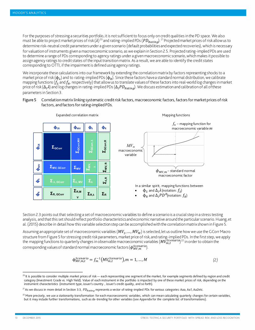
Figure 5 presents the GCorr Macro structure. As the figure shows, GCorr Macro captures the relationship between GCorr systematic credit risk factors ϕ𝐶𝐶𝑅𝑅 and macroeconomic variables 𝑀𝑀𝑀𝑀 in two steps:
1. The GCorr systematic factors ϕ𝐶𝐶𝑅𝑅 and standard normal macroeconomic factors ϕ𝑀𝑀𝑀𝑀 are linked by a Gaussian copula model with a correlation matrix. 19
2. Mapping functions 𝑓𝑓 transform values of the standard normal macroeconomic factors 𝜙𝜙𝑀𝑀𝑀𝑀 to the corresponding values of observable macroeconomic variables 𝑀𝑀𝑀𝑀 (or more precisely, their stationary versions).
We emphasize that the GCorr Macro model does not change the loadings of borrowers’ asset returns to systematic and idiosyncratic GCorr credit risk factors. Borrower asset returns are only linked to macroeconomic variables through their loadings to the existing GCorr factors via the covariance matrix.
15 Any intermediate points on the par yield curve needed for the calculation are determined by interpolation and extrapolation from the points specified in the scenario. The spot curve is obtained from the par curve by bootstrapping 16 GCorr includes correlation estimates across a variety of asset classes: listed corporates (GCorr Corporate), private firms, small and medium-size enterprises (GCorr SME), U.S. commercial real estate (GCorr CRE), U.S. retail (GCorr Retail) and sovereigns (including GCorr Emerging Markets).
17 The set of 245 factors consists of three asset class related subsets: 110 corporate factors (49 country factors and 61 industry factors), 78 U.S. commercial real estate factors (73 MSA factors and 5 property type factors), and 57 U.S. retail factors (51 state factors and 6 product type factors).
18 For more details and examples of GCorr Macro uses, see “Applications of GCorr Macro: Risk Integration, Stress Testing, and Reverse Stress Testing” (Pospisil et al. 2013).
19 In practice, we link the 245 geographical and sector factors to macroeconomic variables and then the correlation matrix presented in Figure 5 is implied by that link. Further details on these steps can be found in the paper by Huang, et al. (2015).
13 DECEMBER 2015 STRESS TESTING A SECURITY PORTFOLIO WITH SPREAD RISK AND LOSS RECOGNITION
For the purposes of stressing a securities portfolio, it is not sufficient to focus only on credit qualities in the PD space. We also must be able to project market prices of risk (𝜆𝜆)20 and rating-implied PDs (𝑃𝑃𝑃𝑃𝑅𝑅𝑅𝑅𝑅𝑅𝑅𝑅𝑅𝑅𝑅𝑅). 21 Projected market prices of risk allow us to determine risk-neutral credit parameters under a given scenario (default probabilities and expected recoveries), which is necessary for valuation of instruments given a macroeconomic scenario, as we explain in Section 2.5. Projected rating-implied PDs are used to determine a range of PDs corresponding to agency ratings under a given macroeconomic scenario, which makes it possible to assign agency ratings to credit states of the input transition matrix. As a result, we are able to identify the credit states corresponding to OTTI, if the impairment is defined using agency ratings.
We incorporate these calculations into our framework by extending the correlation matrix by factors representing shocks to a market price of risk (ϕ𝜆𝜆) and to rating-implied PDs (ϕ𝑅𝑅). Since these factors have a standard normal distribution, we calibrate mapping functions (𝑓𝑓𝜆𝜆 and 𝑓𝑓𝑅𝑅, respectively) that allow us to translate values of these factors into real-world log changes in market price of risk (Δ𝐶𝐶𝜆𝜆) and log changes in rating-implied PDs (Δ𝐶𝐶𝑃𝑃𝑃𝑃𝑅𝑅𝑅𝑅𝑅𝑅𝑅𝑅𝑅𝑅𝑅𝑅). We discuss estimation and calibration of all of these parameters in Section 3.
Figure 5 Correlation matrix linking systematic credit risk factors, macroeconomic factors, factors for market prices of risk factors, and factors for rating-implied PDs.
Section 2.3 points out that selecting a set of macroeconomic variables to define a scenario is a crucial step in a stress testing analysis, and that this set should reflect portfolio characteristics and economic narrative around the particular scenario. Huang, et al. (2015) describe in detail how this variable selection step can be accomplished with the correlation matrix shown in Figure 5.
Assuming an appropriate set of macroeconomic variables (𝑀𝑀𝑀𝑀1,…,𝑀𝑀𝑀𝑀𝑀𝑀) is selected, let us outline how we use the GCorr Macro structure from Figure 5 for stressing credit risk parameters, market price of risk, and rating-implied PDs. In the first step, we apply the mapping functions to quarterly changes in observable macroeconomic variables (𝑀𝑀𝑀𝑀𝐶𝐶 ,𝑅𝑅
𝑆𝑆𝑆𝑆𝑆𝑆𝑅𝑅𝑅𝑅𝑆𝑆𝑅𝑅𝑆𝑆)22 in order to obtain the corresponding values of standard normal macroeconomic factors (𝜙𝜙𝑀𝑀𝑀𝑀,𝐶𝐶
𝑆𝑆𝑆𝑆𝑆𝑆𝑅𝑅𝑅𝑅𝑆𝑆𝑅𝑅𝑆𝑆).
ϕ𝑀𝑀𝑀𝑀,𝐶𝐶,𝑅𝑅𝑆𝑆𝑆𝑆𝑆𝑆𝑅𝑅𝑅𝑅𝑆𝑆𝑅𝑅𝑆𝑆 = 𝑓𝑓𝐶𝐶−1�𝑀𝑀𝑀𝑀𝐶𝐶 ,𝑅𝑅
𝑆𝑆𝑆𝑆𝑆𝑆𝑅𝑅𝑅𝑅𝑆𝑆𝑅𝑅𝑆𝑆�,𝑚𝑚 = 1, …,𝑀𝑀 (2)
20 It is possible to consider multiple market prices of risk — each representing one segment of the market, for example segments defined by region and credit category (Investment Grade vs. High Yield). Value of each instrument in the portfolio is impacted by one of these market prices of risk, depending on the instrument characteristics (instrument type, issuer’s country , issuer’s credit quality, and so forth).
21 As we discuss in more detail in Section 3.3, 𝑃𝑃𝑃𝑃𝑅𝑅𝑅𝑅𝑅𝑅𝑅𝑅𝑅𝑅𝑅𝑅 represents a vector of rating-implied PDs for various categories: Aaa, Aa1, Aa2etc. 22 More precisely, we use a stationarity transformation for each macroeconomic variables, which can mean calculating quarterly changes for certain variables, but it may include further transformations, such as de-trending for other variables (see Appendix for the complete list of transformations).
ΣGCorr
ΣMV ΣMV, GCorr
Σ λ, GCorr
Σ MV,
λ
Σλ, MV Σλ
ΣR, GCorr ΣR,M
V ΣR,λ
Σ MV,
R
Σ λ,R
ΣR
φCR
φCR
φ
MV
φMV φλ
φλ
φR
φR
Σ GC
orr,
λ
ΣG
Cor
r,MV
Σ GC
orr,R
Mapping functions
𝜙𝜙𝑀𝑀𝑀𝑀,𝐶𝐶 – standard normal macroeconomic factor
MVm macroeconomic
variable
fm – mapping function for macroeconomic variable m
Expanded correlation matrix
In a similar spirit, mapping functions between • ϕ𝜆𝜆 and Δ𝐶𝐶𝜆𝜆 (notation: 𝑓𝑓𝜆𝜆) • ϕ𝑅𝑅 and Δ𝐶𝐶𝑃𝑃𝑃𝑃𝑅𝑅(notation: 𝑓𝑓𝑅𝑅)
14 DECEMBER 2015 STRESS TESTING A SECURITY PORTFOLIO WITH SPREAD RISK AND LOSS RECOGNITION
For example, if a scenario prescribes a Stock Market Index drop by 25% over a quarter, the mapping function may imply that this value corresponds to a -2.1 shock in the standard normal space.
Thus, we have a scenario for the macroeconomic factors for a given quarter: ϕ𝑀𝑀𝑀𝑀,𝑅𝑅𝑆𝑆𝑆𝑆𝑆𝑆𝑅𝑅𝑅𝑅𝑆𝑆𝑅𝑅𝑆𝑆 = (𝜙𝜙𝑀𝑀𝑀𝑀,1,𝑅𝑅
𝑆𝑆𝑆𝑆𝑆𝑆𝑅𝑅𝑅𝑅𝑆𝑆𝑅𝑅𝑆𝑆,…𝜙𝜙𝑀𝑀𝑀𝑀,𝑀𝑀,𝑅𝑅𝑆𝑆𝑆𝑆𝑆𝑆𝑅𝑅𝑅𝑅𝑆𝑆𝑅𝑅𝑆𝑆). Using the
Gaussian copula assumption and the matrix from Figure 5, we can determine the conditional distribution of the systematic credit risk factors, the factors for market price of risk, and the factors for rating-implied PDs. Formula (3) shows these conditional distributions for individual factors:23
ϕ𝐶𝐶𝑅𝑅,𝑅𝑅�𝑆𝑆𝑐𝑐𝑅𝑅 ~ 𝑁𝑁�𝛴𝛴𝐺𝐺𝐶𝐶𝑆𝑆𝑆𝑆𝑆𝑆,𝑀𝑀𝑀𝑀 × 𝛴𝛴𝑀𝑀𝑀𝑀−1 ×ϕ𝑀𝑀𝑀𝑀,𝑅𝑅𝑆𝑆𝑆𝑆𝑆𝑆𝑅𝑅𝑅𝑅𝑆𝑆𝑅𝑅𝑆𝑆, 1 −𝛴𝛴𝐺𝐺𝐶𝐶𝑆𝑆𝑆𝑆𝑆𝑆,𝑀𝑀𝑀𝑀 ×𝛴𝛴𝑀𝑀𝑀𝑀−1 × 𝛴𝛴𝑀𝑀𝑀𝑀,𝐺𝐺𝐶𝐶𝑆𝑆𝑆𝑆𝑆𝑆�
ϕ𝜆𝜆,𝑅𝑅�𝑆𝑆𝑐𝑐𝑅𝑅 ~ 𝑁𝑁�𝛴𝛴𝜆𝜆,𝑀𝑀𝑀𝑀 × 𝛴𝛴𝑀𝑀𝑀𝑀−1 ×ϕ𝑀𝑀𝑀𝑀,𝑅𝑅𝑆𝑆𝑆𝑆𝑆𝑆𝑅𝑅𝑅𝑅𝑆𝑆𝑅𝑅𝑆𝑆, 1 −𝛴𝛴𝜆𝜆 ,𝑀𝑀𝑀𝑀 ×𝛴𝛴𝑀𝑀𝑀𝑀−1 × 𝛴𝛴𝑀𝑀𝑀𝑀,𝜆𝜆�
ϕ𝑅𝑅,𝑅𝑅�𝑆𝑆𝑐𝑐𝑅𝑅 ~ 𝑁𝑁�𝛴𝛴𝑅𝑅,𝑀𝑀𝑀𝑀 × 𝛴𝛴𝑀𝑀𝑀𝑀−1 ×ϕ𝑀𝑀𝑀𝑀,𝑅𝑅𝑆𝑆𝑆𝑆𝑆𝑆𝑅𝑅𝑅𝑅𝑆𝑆𝑅𝑅𝑆𝑆, 1 −𝛴𝛴𝑅𝑅,𝑀𝑀𝑀𝑀 × 𝛴𝛴𝑀𝑀𝑀𝑀−1 ×𝛴𝛴𝑀𝑀𝑀𝑀,𝑅𝑅�
(3)
Equation (3) highlights the fact that the means of the stressed distributions are linear functions of the scenario values of the standard normal macroeconomic factors ϕ𝑀𝑀𝑀𝑀,𝑅𝑅
𝑆𝑆𝑆𝑆𝑆𝑆𝑅𝑅𝑅𝑅𝑆𝑆𝑅𝑅𝑆𝑆 with coefficients 𝛽𝛽. Note, the macroeconomic factor values under the scenario impact only the mean, not the variance. The expression for variance in Equation (3) can be summarized as 1 −𝜌𝜌2, where 𝜌𝜌2 has the same role as the R-squared coefficient in a regression (in this case the regression of the systematic credit risk factor on the macroeconomic variables selected for the scenario). We label 𝜌𝜌2 as the pseudo-regression R-squared. Thus, the variance of the stressed distribution is directly related to the explanatory power of the selected macroeconomic variables — in the extreme case, when the macroeconomic variables completely explain the systematic factor, the variance is zero (and 𝜌𝜌 = 1). Similar interpretation applies to the conditional distributions of the factors for market price of risk and rating-implied PDs.
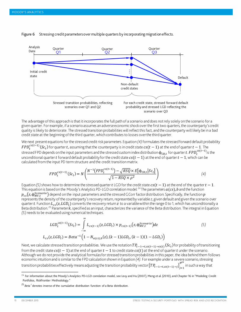
The stressed distributions of the systematic credit risk factors (custom index) from Equation (3) imply stressed values of credit risk parameters — PDs, LGDs, and transition probabilities (TPs). Importantly, we need to carry out these calculations over multiple quarters, which Figure 6 illustrates. For example, when calculating stressed expected loss for the third quarter after the analysis date, we determine the stressed PD and LGD for the third quarter for each non-default credit state in which the counterparty resides at the beginning of that quarter. As shown in Figure 6 the stressed PD and LGD depend on the stressed distribution of the systematic credit risk factors for the third quarter, given by the scenario over the third quarter. In addition, we compute stressed transition probabilities that the counterparty will migrate from an initial credit state, known on the analysis date, to a credit state at the beginning of the third quarter. These stressed transition probabilities account for the scenarios over the first and second quarters. Based on information available on the analysis date, we can calculate the stressed expected loss for the third quarter by combining the third quarter stressed credit risk parameters and stressed transition probabilities between the analysis date and the third quarter.
23 In Equation (3) the notation 𝛴𝛴…𝑀𝑀𝑀𝑀 refers only to the portion of the matrix in Figure 5 which represents the macroeconomic variables selected for the scenario. In other words, the rows and columns of the matrix corresponding to the macroeconomic variables not included in the scenario are omitted from 𝛴𝛴…𝑀𝑀𝑀𝑀.
𝐸𝐸�ϕ𝐶𝐶𝑅𝑅,𝑅𝑅�𝑆𝑆𝑐𝑐𝑅𝑅�= 𝛽𝛽𝑇𝑇 ×ϕ𝑀𝑀𝑀𝑀,𝑅𝑅𝑆𝑆𝑆𝑆𝑆𝑆𝑅𝑅𝑅𝑅𝑆𝑆𝑅𝑅𝑆𝑆 1 −𝜌𝜌2
15 DECEMBER 2015 STRESS TESTING A SECURITY PORTFOLIO WITH SPREAD RISK AND LOSS RECOGNITION
Figure 6 Stressing credit parameters over multiple quarters by incorporating migration effects.
The advantage of this approach is that it incorporates the full path of a scenario and does not rely solely on the scenario for a given quarter. For example, if a scenario assumes an adverse economic shock over the first two quarters, the counterparty’s credit quality is likely to deteriorate. The stressed transition probabilities will reflect this fact, and the counterparty will likely be in a bad credit state at the beginning of the third quarter, which contributes to losses over the third quarter.
We next present equations for the stressed credit risk parameters. Equation (4) formulates the stressed forward default probability 𝐹𝐹𝑃𝑃𝑃𝑃𝑅𝑅
𝑆𝑆𝑐𝑐(𝑅𝑅−1) (𝑆𝑆𝑐𝑐𝑅𝑅) for quarter 𝑡𝑡, assuming that the counterparty is in credit state 𝑐𝑐𝑐𝑐(𝑡𝑡 − 1) at the end of quarter 𝑡𝑡 − 1. The stressed FPD depends on the input parameters and the stressed custom index distribution ϕ𝐶𝐶𝑅𝑅,𝑅𝑅 for quarter 𝑡𝑡. 𝐹𝐹𝑃𝑃𝑃𝑃𝑅𝑅
𝑆𝑆𝑐𝑐(𝑅𝑅−1)is the unconditional quarter 𝑡𝑡 forward default probability for the credit state 𝑐𝑐𝑐𝑐(𝑡𝑡 − 1) at the end of quarter 𝑡𝑡 − 1, which can be calculated from the input PD term structure and the credit transition matrix.
𝐹𝐹𝑃𝑃𝑃𝑃𝑅𝑅𝑆𝑆𝑐𝑐(𝑅𝑅−1) (𝑆𝑆𝑐𝑐𝑅𝑅) = 𝑁𝑁�
𝑁𝑁−1�𝐹𝐹𝑃𝑃𝑃𝑃𝑅𝑅𝑆𝑆𝑐𝑐(𝑅𝑅−1)�−�𝐼𝐼𝑆𝑆𝑅𝑅× 𝐸𝐸�ϕ𝐶𝐶𝑅𝑅,𝑅𝑅�𝑆𝑆𝑐𝑐𝑅𝑅�
�1−𝐼𝐼𝑆𝑆𝑅𝑅× 𝜌𝜌2� (4)
Equation (5) shows how to determine the stressed quarter 𝑡𝑡 LGD for the credit state 𝑐𝑐𝑐𝑐(𝑡𝑡 − 1) at the end of the quarter 𝑡𝑡 − 1. This equation is based on the Moody’s Analytics PD-LGD correlation model. 24 The parameters 𝑎𝑎(𝑐𝑐𝑐𝑐),𝑏𝑏 and the function 𝑝𝑝𝑆𝑆𝑐𝑐�𝑧𝑧,ϕ𝑀𝑀𝑀𝑀,𝑅𝑅
𝑆𝑆𝑆𝑆𝑆𝑆𝑅𝑅𝑅𝑅𝑆𝑆𝑅𝑅𝑆𝑆� depend on the input parameters and the stressed GCorr factor distribution. Specifically, the function 𝑝𝑝 represents the density of the counterparty’s recovery return, represented by variable z, given default and given the scenario over quarter 𝑡𝑡. Function 𝐿𝐿𝑆𝑆𝑐𝑐(𝑧𝑧,𝐿𝐿𝐿𝐿𝑃𝑃𝑅𝑅) converts the recovery return 𝑧𝑧 to a variable within the range 0 to 1, which has unconditionally a Beta distribution. 25 Parameter 𝑘𝑘, specified as an input, characterizes the variance of the Beta distribution. The integral in Equation (5) needs to be evaluated using numerical techniques.
𝐿𝐿𝐿𝐿𝑃𝑃𝑅𝑅𝑆𝑆𝑐𝑐(𝑅𝑅−1)(𝑆𝑆𝑐𝑐𝑅𝑅) = � 𝐿𝐿𝑆𝑆𝑐𝑐(𝑅𝑅−1)(𝑧𝑧,𝐿𝐿𝐿𝐿𝑃𝑃𝑅𝑅) × 𝑝𝑝𝑆𝑆𝑐𝑐(𝑅𝑅−1)�𝑧𝑧,ϕ𝑀𝑀𝑀𝑀,𝑅𝑅
𝑆𝑆𝑆𝑆𝑆𝑆𝑅𝑅𝑅𝑅𝑆𝑆𝑅𝑅𝑆𝑆�𝑑𝑑𝑧𝑧∞
−∞
𝐿𝐿𝑆𝑆𝑐𝑐(𝑧𝑧,𝐿𝐿𝐿𝐿𝑃𝑃𝑅𝑅) = 𝐵𝐵𝐵𝐵𝑡𝑡𝑎𝑎−1�1 −𝑁𝑁𝑅𝑅(𝑆𝑆𝑐𝑐),𝑏𝑏(𝑧𝑧),(𝑘𝑘 − 1)𝐿𝐿𝐿𝐿𝑃𝑃𝑅𝑅 , (𝑘𝑘 − 1)(1 −𝐿𝐿𝐿𝐿𝑃𝑃𝑅𝑅)�
(5)
Next, we calculate stressed transition probabilities. We use the notation 𝑇𝑇𝑃𝑃𝑅𝑅−1→𝑅𝑅,𝑆𝑆𝑐𝑐(𝑅𝑅−1)→𝑆𝑆𝑐𝑐(𝑅𝑅) (𝑆𝑆𝑐𝑐𝑅𝑅) for probability of transitioning from the credit state 𝑐𝑐𝑐𝑐(𝑡𝑡 − 1) at the end of quarter 𝑡𝑡 − 1 to credit state 𝑐𝑐𝑐𝑐(𝑡𝑡) at the end of quarter 𝑡𝑡 under the scenario. Although we do not provide the analytical formulas for stressed transition probabilities in this paper, the idea behind them follows economic intuition and is similar to the FPD calculation shown in Equation (4). For example under a severe scenario, stressing transition probabilities effectively means adjusting the transition probability vector �𝑇𝑇𝑃𝑃𝑅𝑅−1→𝑅𝑅,𝑆𝑆𝑐𝑐(𝑅𝑅−1)→𝑗𝑗�𝑗𝑗=1
𝑁𝑁𝑐𝑐𝑐𝑐 in such a way that
24 For information about the Moody’s Analytics PD-LGD correlation model, see Levy and Hu (2007), Meng et al. (2010), and Chapter 16 in “Modeling Credit Portfolios, RiskFrontier Methodology.”
25 Beta-1 denotes inverse of the cumulative distribution function of a Beta distribution.
Analysis Date
Quarter
Quarter
Quarter Q1
Q2
Q3
…
Non-default credit states
Initial credit state
Default
Stressed transition probabilities, reflecting scenarios over Q1 and Q2
For each credit state, stressed forward default probability and stressed LGD reflecting the
scenario over Q3
16 DECEMBER 2015 STRESS TESTING A SECURITY PORTFOLIO WITH SPREAD RISK AND LOSS RECOGNITION
probabilities of migrating to better credit quality states become lower while probabilities of migrating to worse credit quality states become higher. Here, credit state 1 corresponds to the default credit state, and 𝑁𝑁𝑆𝑆𝑐𝑐 corresponds to the highest credit state. Equation (6) provides an iterative procedure for calculating cumulative stressed transition probabilities. We denote the initial credit state by 𝑐𝑐𝑐𝑐(0).
𝑇𝑇𝑃𝑃0→𝑅𝑅,𝑆𝑆𝑐𝑐(0)→𝑆𝑆𝑐𝑐(𝑅𝑅)𝐶𝐶𝐶𝐶𝐶𝐶𝐶𝐶𝐶𝐶 �𝑆𝑆𝑐𝑐1,𝑅𝑅
𝐶𝐶𝐶𝐶𝐶𝐶𝐶𝐶𝐶𝐶�= � 𝑇𝑇𝑃𝑃0→𝑅𝑅−1, 𝑆𝑆𝑐𝑐(0)→𝑆𝑆𝑐𝑐(𝑅𝑅−1)𝐶𝐶𝐶𝐶𝐶𝐶𝐶𝐶𝐶𝐶 �𝑆𝑆𝑐𝑐1,𝑅𝑅−1
𝐶𝐶𝐶𝐶𝐶𝐶𝐶𝐶𝐶𝐶�𝑆𝑆𝑐𝑐(𝑅𝑅−1)
× 𝑇𝑇𝑃𝑃𝑅𝑅−1→𝑅𝑅,𝑆𝑆𝑐𝑐(𝑅𝑅−1)→𝑆𝑆𝑐𝑐(𝑅𝑅)(𝑆𝑆𝑐𝑐𝑅𝑅) (6)
Market Price of Risk
Let us now turn to projecting market price of risk. Our objective is to determine conditional expected value of 𝜆𝜆 as of the end of quarter 𝑡𝑡, while accounting for the macroeconomic scenario up to the end of that quarter: 𝐸𝐸�𝜆𝜆𝑅𝑅|𝑆𝑆𝑐𝑐1,𝑅𝑅
𝐶𝐶𝐶𝐶𝐶𝐶𝐶𝐶𝐶𝐶�. The initial value of the market price of risk is known as of the analysis date: 𝜆𝜆0. Assume that we have the projections up to the end of quarter 𝑡𝑡 − 1, 𝐸𝐸�𝜆𝜆𝑅𝑅−1|𝑆𝑆𝑐𝑐1,𝑡𝑡−1
𝐶𝐶𝐶𝐶𝑚𝑚𝐶𝐶𝐶𝐶�. Equation (3) expresses the stressed distribution of the quarterly shock to 𝜆𝜆 in the standard normal space. We can apply the transformation 𝑓𝑓𝜆𝜆 to express this distribution in terms of log-changes in 𝜆𝜆 and combine the result with the quarter 𝑡𝑡 − 1 projection to obtain the projection for quarter 𝑡𝑡, 𝐸𝐸�𝜆𝜆𝑅𝑅|𝑆𝑆𝑐𝑐1,𝑡𝑡
𝐶𝐶𝐶𝐶𝑚𝑚𝐶𝐶𝐶𝐶�.
As discussed earlier, the scenario values of the market price of risk, 𝜆𝜆𝑅𝑅𝑆𝑆𝑆𝑆𝑆𝑆𝑅𝑅𝑅𝑅𝑆𝑆𝑅𝑅𝑆𝑆, can be defined in two ways: either directly by stating an assumption about their path or by implying them from the scenario path of macroeconomic variables, in which case, we set 𝜆𝜆𝑅𝑅𝑆𝑆𝑆𝑆𝑆𝑆𝑅𝑅𝑅𝑅𝑆𝑆𝑅𝑅𝑆𝑆 = 𝐸𝐸�𝜆𝜆𝑅𝑅|𝑆𝑆𝑐𝑐1,𝑡𝑡
𝐶𝐶𝐶𝐶𝑚𝑚𝐶𝐶𝐶𝐶�. 26
The stressed credit risk parameters and scenario values of the market price of risk are used for projecting fair values of instruments and for calculation of default losses, which we describe in Section 2.5 and Section 2.6.
Rating-implied PD
For OTTI calculation, we must translate the conditional distribution of the rating-implied PD factor ϕ𝑅𝑅,𝑅𝑅 into conditional rating-implied PD: 𝐸𝐸�𝑃𝑃𝑃𝑃𝑅𝑅𝑅𝑅𝑅𝑅𝑅𝑅𝑅𝑅𝑅𝑅,𝑅𝑅�𝑆𝑆𝑐𝑐1,𝑅𝑅
𝐶𝐶𝐶𝐶𝐶𝐶𝐶𝐶𝐶𝐶�. The approach is similar to projecting the market price of risk — we use the conditional distribution of the factor from Equation (3), which can be converted to distribution of log-changes in the rating-implied PDs using the mapping function 𝑓𝑓𝑅𝑅.
We carry out this calculation in an iterative way, with the initial values representing the rating-implied PDs as of the analysis date: 𝑃𝑃𝑃𝑃𝑅𝑅𝑅𝑅𝑅𝑅𝑅𝑅𝑅𝑅𝑅𝑅,0. The projected rating-implied PD, 𝑃𝑃𝑃𝑃𝑅𝑅𝑅𝑅𝑅𝑅𝑅𝑅𝑅𝑅𝑅𝑅,𝑅𝑅
𝑆𝑆𝑆𝑆𝑆𝑆𝑅𝑅𝑅𝑅𝑆𝑆𝑅𝑅𝑆𝑆, can be either implied by the macroeconomic scenario, in which case 𝑃𝑃𝑃𝑃𝑅𝑅𝑅𝑅𝑅𝑅𝑅𝑅𝑅𝑅𝑅𝑅,𝑅𝑅
𝑆𝑆𝑆𝑆𝑆𝑆𝑅𝑅𝑅𝑅𝑆𝑆𝑅𝑅𝑆𝑆 =𝐸𝐸�𝑃𝑃𝑃𝑃𝑅𝑅𝑅𝑅𝑅𝑅𝑅𝑅𝑅𝑅𝑅𝑅,𝑅𝑅�𝑆𝑆𝑐𝑐1,𝑅𝑅𝐶𝐶𝐶𝐶𝐶𝐶𝐶𝐶𝐶𝐶�, 27 or specified directly. Having the 𝑃𝑃𝑃𝑃𝑅𝑅𝑅𝑅𝑅𝑅𝑅𝑅𝑅𝑅𝑅𝑅,𝑅𝑅
𝑆𝑆𝑆𝑆𝑆𝑆𝑅𝑅𝑅𝑅𝑆𝑆𝑅𝑅𝑆𝑆 for a given rating allows us to identify the credit states (defined by PD or DD levels), which correspond to OTTI.
2.5 Instrument Valuation
The fair or market value of an instrument in a quarter in a scenario depends on the credit quality of the reference entity and the market factors — risk premium and interest rates — in that quarter. To model evolution of credit quality, we employ a lattice consisting of a set of discrete credit states at each quarter in the scenario and a matrix of quarterly transition probabilities. The dynamics of market risk premium are modeled by linking market price of risk with macroeconomic variables using GCorr Macro as described in Section 3.2. The interest rate curve is assumed to be supplied as a part of the scenario. Once we know the fair value of an instrument, the loss calculation is straighforward.
This subsection describes valuation of credit instruments with no embedded optionality. We use a risk-neutral valuation framework to calculate fair value 𝑀𝑀𝑅𝑅
𝑆𝑆𝑐𝑐(𝑅𝑅)�𝑆𝑆𝑐𝑐1,𝑅𝑅𝐶𝐶𝐶𝐶𝐶𝐶𝐶𝐶𝐶𝐶� at credit state 𝑐𝑐𝑐𝑐(𝑡𝑡) at the end of quarter 𝑡𝑡 under the scenario 𝑆𝑆𝑐𝑐1,𝑅𝑅
𝐶𝐶𝐶𝐶𝐶𝐶𝐶𝐶𝐶𝐶. The calculation proceeds in several steps. First, we obtain the PD and LGD term-structures specific to each non-default credit state. Next, the physical PD and LGD are transformed to their risk-neutral values by using the stressed value of market price of risk. Finally, at the end of each quarter 𝑡𝑡 in the scenario, we calculate the present value of the future cashflows by discounting at the stressed risk-free rate.
26 From a theoretical perspective, we are adding a new scenario condition for valuation of instruments: 𝜆𝜆𝑅𝑅𝑆𝑆𝑆𝑆𝑆𝑆𝑅𝑅𝑅𝑅𝑆𝑆𝑅𝑅𝑆𝑆 = 𝐸𝐸�𝜆𝜆𝑅𝑅|𝑆𝑆𝑐𝑐1,𝑅𝑅𝐶𝐶𝐶𝐶𝐶𝐶𝐶𝐶𝐶𝐶�. Note, without such a
condition, the instrument valuation described in Section 2.5 would need to account for the entire distribution of the market price of risk under the macroeconomic scenario: 𝜆𝜆𝑅𝑅|𝑆𝑆𝑐𝑐1,𝑅𝑅
𝐶𝐶𝐶𝐶𝐶𝐶𝐶𝐶𝐶𝐶 27 As for the market price of risk, we are adding a new scenario condition for loss calculation: 𝑃𝑃𝑃𝑃𝑅𝑅𝑅𝑅𝑅𝑅𝑅𝑅𝑅𝑅𝑅𝑅,𝑅𝑅
𝑆𝑆𝑆𝑆𝑆𝑆𝑅𝑅𝑅𝑅𝑆𝑆𝑅𝑅𝑆𝑆 = 𝐸𝐸�𝑃𝑃𝑃𝑃𝑅𝑅𝑅𝑅𝑅𝑅𝑅𝑅𝑅𝑅𝑅𝑅,𝑅𝑅�𝑆𝑆𝑐𝑐1,𝑅𝑅𝐶𝐶𝐶𝐶𝐶𝐶𝐶𝐶𝐶𝐶�. Note that without such
condition , the loss calculation in Section 2.6 would need to account for the entire distribution of the rating-implied-PD under the macroeconomic scenario: 𝑃𝑃𝑃𝑃𝑅𝑅𝑅𝑅𝑅𝑅𝑅𝑅𝑅𝑅𝑅𝑅,𝑅𝑅�𝑆𝑆𝑐𝑐1,𝑅𝑅
𝐶𝐶𝐶𝐶𝐶𝐶𝐶𝐶𝐶𝐶.
17 DECEMBER 2015 STRESS TESTING A SECURITY PORTFOLIO WITH SPREAD RISK AND LOSS RECOGNITION
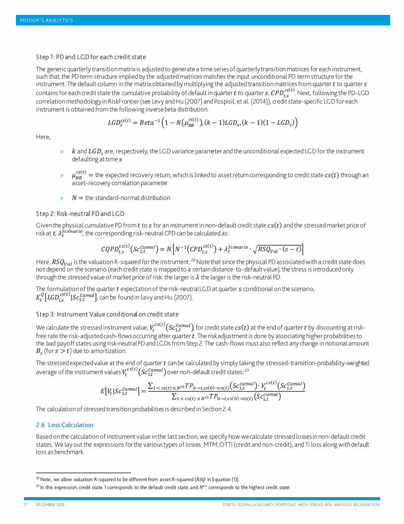
Step 1: PD and LGD for each credit state
The generic quarterly transition matrix is adjusted to generate a time series of quarterly transition matrices for each instrument, such that the PD term structure implied by the adjusted matrices matches the input unconditional PD term structure for the instrument. The default column in the matrix obtained by multiplying the adjusted transition matrices from quarter 𝑡𝑡 to quarter 𝑐𝑐 contains for each credit state the cumulative probability of default in quarter 𝑡𝑡 to quarter 𝑐𝑐: 𝐶𝐶𝑃𝑃𝑃𝑃𝑅𝑅,𝑐𝑐
𝑆𝑆𝑐𝑐(𝑅𝑅). Next, following the PD-LGD
correlation methodology in RiskFrontier (see Levy and Hu (2007) and Pospisil, et al. (2014)), credit state-specific LGD for each instrument is obtained from the following inverse beta distribution.
𝐿𝐿𝐿𝐿𝑃𝑃𝑐𝑐𝑆𝑆𝑐𝑐(𝑅𝑅) = 𝐵𝐵𝐵𝐵𝑡𝑡𝑎𝑎−1�1 −𝑁𝑁�𝜇𝜇𝑅𝑅𝑅𝑅
𝑆𝑆𝑐𝑐(𝑅𝑅)�, (𝑘𝑘 − 1)𝐿𝐿𝐿𝐿𝑃𝑃𝑐𝑐, (𝑘𝑘 − 1)(1 −𝐿𝐿𝐿𝐿𝑃𝑃𝑐𝑐)�
Here,
» 𝑘𝑘 and 𝐿𝐿𝐿𝐿𝑃𝑃𝑐𝑐 are, respectively, the LGD variance parameter and the unconditional expected LGD for the instrument defaulting at time 𝑐𝑐
» 𝜇𝜇𝑅𝑅𝑅𝑅𝑆𝑆𝑐𝑐(𝑅𝑅) = the expected recovery return, which is linked to asset return corresponding to credit state 𝑐𝑐𝑐𝑐(𝑡𝑡) through an
asset-recovery correlation parameter
» 𝑁𝑁= the standard-normal distribution
Step 2: Risk-neutral PD and LGD
Given the physical cumulative PD from 𝑡𝑡 to 𝑐𝑐 for an instrument in non-default credit state 𝑐𝑐𝑐𝑐(𝑡𝑡) and the stressed market price of risk at 𝑡𝑡, 𝜆𝜆𝑅𝑅𝑆𝑆𝑆𝑆𝑆𝑆𝑅𝑅𝑅𝑅𝑆𝑆𝑅𝑅𝑆𝑆, the corresponding risk-neutral CPD can be calculated as:
𝐶𝐶𝑅𝑅𝑃𝑃𝑃𝑃𝑅𝑅,𝑐𝑐𝑆𝑆𝑐𝑐(𝑅𝑅)�𝑆𝑆𝑐𝑐1,𝑅𝑅
𝐶𝐶𝐶𝐶𝐶𝐶𝐶𝐶𝐶𝐶�= 𝑁𝑁�𝑁𝑁−1�𝐶𝐶𝑃𝑃𝑃𝑃𝑅𝑅,𝑐𝑐𝑆𝑆𝑐𝑐(𝑅𝑅)�+ 𝜆𝜆𝑅𝑅𝑆𝑆𝑆𝑆𝑆𝑆𝑅𝑅𝑅𝑅𝑆𝑆𝑅𝑅𝑆𝑆 ∙ �𝐼𝐼𝑆𝑆𝑅𝑅𝑀𝑀𝑅𝑅𝐶𝐶 ∙ (𝑐𝑐 − 𝑡𝑡)�
Here, 𝐼𝐼𝑆𝑆𝑅𝑅𝑀𝑀𝑅𝑅𝐶𝐶 is the valuation R-squared for the instrument. 28 Note that since the physical PD associated with a credit state does not depend on the scenario (each credit state is mapped to a certain distance-to-default value), the stress is introduced only through the stressed value of market price of risk: the larger is 𝜆𝜆 the larger is the risk-neutral PD.
The formulation of the quarter 𝑡𝑡 expectation of the risk-neutral LGD at quarter 𝑐𝑐 conditional on the scenario, 𝐸𝐸𝑅𝑅𝑄𝑄�𝐿𝐿𝐿𝐿𝑃𝑃𝑅𝑅,𝑐𝑐
𝑆𝑆𝑐𝑐(𝑅𝑅)|𝑆𝑆𝑐𝑐1,𝑅𝑅𝐶𝐶𝐶𝐶𝐶𝐶𝐶𝐶𝐶𝐶�, can be found in Levy and Hu (2007).
Step 3: Instrument Value conditional on credit state
We calculate the stressed instrument value, 𝑀𝑀𝑅𝑅𝑆𝑆𝑐𝑐(𝑅𝑅)�𝑆𝑆𝑐𝑐1,𝑅𝑅
𝐶𝐶𝐶𝐶𝐶𝐶𝐶𝐶𝐶𝐶�, for credit state 𝑐𝑐𝑐𝑐(𝑡𝑡) at the end of quarter 𝑡𝑡 by discounting at risk-free rate the risk-adjusted cash-flows occurring after quarter 𝑡𝑡. The risk adjustment is done by associating higher probabilities to the bad payoff states using risk-neutral PD and LGDs from Step 2. The cash-flows must also reflect any change in notional amount 𝐵𝐵𝑐𝑐 (for 𝑐𝑐 > 𝑡𝑡) due to amortization.
The stressed expected value at the end of quarter 𝑡𝑡 can be calculated by simply taking the stressed-transition-probability-weighted average of the instrument values 𝑀𝑀𝑅𝑅
𝑆𝑆𝑐𝑐(𝑅𝑅)�𝑆𝑆𝑐𝑐1,𝑅𝑅𝐶𝐶𝐶𝐶𝐶𝐶𝐶𝐶𝐶𝐶� over non-default credit states: 29
𝐸𝐸�𝑀𝑀𝑅𝑅|𝑆𝑆𝑐𝑐1,𝑅𝑅𝐶𝐶𝐶𝐶𝐶𝐶𝐶𝐶𝐶𝐶�=
∑ 𝑇𝑇𝑃𝑃0→𝑅𝑅,𝑆𝑆𝑐𝑐(0)→𝑆𝑆𝑐𝑐(𝑅𝑅)�𝑆𝑆𝑐𝑐1,𝑅𝑅𝑆𝑆𝐶𝐶𝐶𝐶𝐶𝐶𝐶𝐶�∙ 𝑀𝑀𝑅𝑅
𝑆𝑆𝑐𝑐(𝑅𝑅)�𝑆𝑆𝑐𝑐1,𝑅𝑅𝐶𝐶𝐶𝐶𝐶𝐶𝐶𝐶𝐶𝐶�1 < 𝑆𝑆𝑐𝑐(𝑅𝑅) ≤ 𝑁𝑁𝑐𝑐𝑐𝑐
∑ 𝑇𝑇𝑃𝑃0→𝑅𝑅,𝑆𝑆𝑐𝑐(0)→𝑆𝑆𝑐𝑐(𝑅𝑅)�𝑆𝑆𝑐𝑐1,𝑅𝑅𝑆𝑆𝐶𝐶𝐶𝐶𝐶𝐶𝐶𝐶�1 < 𝑆𝑆𝑐𝑐(𝑅𝑅) ≤ 𝑁𝑁𝑐𝑐𝑐𝑐
The calculation of stressed transition probabilities is described in Section 2.4.
2.6 Loss Calculation
Based on the calculation of instrument value in the last section, we specify how we calculate stressed losses in non-default credit states. We lay out the expressions for the various types of losses: MTM, OTTI (credit and non-credit), and TI loss along with default loss as benchmark.
28 Note, we allow valuation R-squared to be different from asset R-squared (𝐼𝐼𝑆𝑆𝑅𝑅 in Equation (1)). 29 In this expression, credit state 1 corresponds to the default credit state, and 𝑁𝑁𝑆𝑆𝑐𝑐 corresponds to the highest credit state.
18 DECEMBER 2015 STRESS TESTING A SECURITY PORTFOLIO WITH SPREAD RISK AND LOSS RECOGNITION
Default Loss
Default loss in quarter 𝑡𝑡 is simply the stressed-transition-probability-weighted sum of the expected default loss in quarter 𝑡𝑡 for each credit state at the end of quarter 𝑡𝑡 − 1:
𝐸𝐸�𝐿𝐿𝐿𝐿𝑐𝑐𝑐𝑐𝐷𝐷𝑆𝑆𝐷𝐷𝑅𝑅𝐶𝐶𝐶𝐶𝑅𝑅,𝑅𝑅�𝑆𝑆𝑐𝑐1,𝑅𝑅𝑆𝑆𝐶𝐶𝐶𝐶𝐶𝐶𝐶𝐶� = 𝐵𝐵𝑅𝑅−1 ∙ � 𝑇𝑇𝑃𝑃0→𝑅𝑅−1,𝑆𝑆𝑐𝑐(0)→𝑆𝑆𝑐𝑐(𝑅𝑅−1)�𝑆𝑆𝑐𝑐1,𝑅𝑅−1
𝑆𝑆𝐶𝐶𝐶𝐶𝐶𝐶𝐶𝐶�∙ 𝐿𝐿𝐿𝐿𝑐𝑐𝑐𝑐𝐷𝐷𝑆𝑆𝐷𝐷𝑅𝑅𝐶𝐶𝐶𝐶𝑅𝑅,𝑅𝑅𝑆𝑆𝑐𝑐(𝑅𝑅−1) (𝑆𝑆𝑐𝑐𝑅𝑅)
1 < 𝑆𝑆𝑐𝑐(𝑅𝑅−1)≤ 𝑁𝑁𝑐𝑐𝑐𝑐
𝐿𝐿𝐿𝐿𝑐𝑐𝑐𝑐𝐷𝐷𝑆𝑆𝐷𝐷𝑅𝑅𝐶𝐶𝐶𝐶𝑅𝑅,𝑅𝑅𝑆𝑆𝑐𝑐(𝑅𝑅−1) (𝑆𝑆𝑐𝑐𝑅𝑅) = 𝐹𝐹𝑃𝑃𝑃𝑃𝑅𝑅
𝑆𝑆𝑐𝑐(𝑅𝑅−1)(𝑆𝑆𝑐𝑐𝑅𝑅) ∙ 𝐿𝐿𝐿𝐿𝑃𝑃𝑅𝑅𝑆𝑆𝑐𝑐(𝑅𝑅−1)(𝑆𝑆𝑐𝑐𝑅𝑅)
Here, the 𝐵𝐵𝑅𝑅−1 represents the notional at the beginning of quarter 𝑡𝑡.
Mark-to-Market (MTM) Loss
Given the fair/market value of an instrument at time 0, the fair value at non-default credit state 𝑐𝑐𝑐𝑐(𝑡𝑡) at time 𝑡𝑡, and the balance trajectory 𝐵𝐵𝑅𝑅, the cumulative MTM loss for credit state 𝑐𝑐𝑐𝑐(𝑡𝑡) at the end of quarter 𝑡𝑡 is:
𝐿𝐿𝐿𝐿𝑐𝑐𝑐𝑐𝑀𝑀𝑇𝑇𝑀𝑀,𝑅𝑅𝑆𝑆𝑐𝑐(𝑅𝑅) �𝑆𝑆𝑐𝑐1,𝑅𝑅
𝐶𝐶𝐶𝐶𝐶𝐶𝐶𝐶𝐶𝐶�= �𝑀𝑀0 −𝑀𝑀𝑅𝑅𝑆𝑆𝑐𝑐(𝑅𝑅)�𝑆𝑆𝑐𝑐1,𝑅𝑅
𝐶𝐶𝐶𝐶𝐶𝐶𝐶𝐶𝐶𝐶��+ (𝐵𝐵𝑅𝑅 −𝐵𝐵0)
The cumulative expected MTM loss from the analysis date to the end of quarter 𝑡𝑡 is simply the transition-probabilities weighted sum of the credit-state specific losses.
𝐸𝐸�𝐿𝐿𝐿𝐿𝑐𝑐𝑐𝑐𝑀𝑀𝑇𝑇𝑀𝑀,𝑅𝑅𝑆𝑆𝐶𝐶𝐶𝐶𝐶𝐶𝐶𝐶�𝑆𝑆𝑐𝑐1,𝑅𝑅
𝑆𝑆𝐶𝐶𝐶𝐶𝐶𝐶𝐶𝐶� = � 𝑇𝑇𝑃𝑃0→𝑅𝑅,𝑆𝑆𝑐𝑐(0)→𝑆𝑆𝑐𝑐(𝑅𝑅) ∙ 𝐿𝐿𝐿𝐿𝑐𝑐𝑐𝑐𝑀𝑀𝑇𝑇𝑀𝑀,𝑅𝑅𝑆𝑆𝑐𝑐(𝑅𝑅) �𝑆𝑆𝑐𝑐1,𝑅𝑅
𝐶𝐶𝐶𝐶𝐶𝐶𝐶𝐶𝐶𝐶�1 < 𝑆𝑆𝑐𝑐(𝑅𝑅) ≤ 𝑁𝑁𝑐𝑐𝑐𝑐
The quarterly expected MTM loss for quarter 𝑡𝑡 > 1 is the first difference of the cumulative loss.
𝐸𝐸�𝐿𝐿𝐿𝐿𝑐𝑐𝑐𝑐𝑀𝑀𝑇𝑇𝑀𝑀,𝑅𝑅�𝑆𝑆𝑐𝑐1,𝑅𝑅𝑆𝑆𝐶𝐶𝐶𝐶𝐶𝐶𝐶𝐶� = 𝐸𝐸�𝐿𝐿𝐿𝐿𝑐𝑐𝑐𝑐𝑀𝑀𝑇𝑇𝑀𝑀,𝑅𝑅
𝑆𝑆𝐶𝐶𝐶𝐶𝐶𝐶𝐶𝐶�𝑆𝑆𝑐𝑐1,𝑅𝑅𝑆𝑆𝐶𝐶𝐶𝐶𝐶𝐶𝐶𝐶� −𝐸𝐸�𝐿𝐿𝐿𝐿𝑐𝑐𝑐𝑐𝑀𝑀𝑇𝑇𝑀𝑀,𝑅𝑅−1
𝑆𝑆𝐶𝐶𝐶𝐶𝐶𝐶𝐶𝐶 �𝑆𝑆𝑐𝑐1,𝑅𝑅−1𝑆𝑆𝐶𝐶𝐶𝐶𝐶𝐶𝐶𝐶�
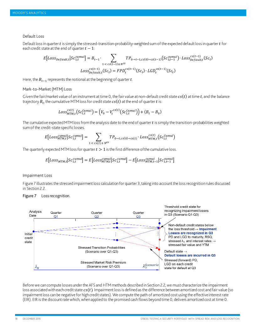
Impairment Loss
Figure 7 illustrates the stressed impairment loss calculation for quarter 3, taking into account the loss recognition rules discussed in Section 2.2.
Figure 7 Loss recognition.
Before we can compute losses under the AFS and HTM methods described in Section 2.2, we must characterize the impairment loss associated with each credit state 𝑐𝑐𝑐𝑐(𝑡𝑡). Impairment loss is defined as the difference between amortized cost and fair value (so impairment loss can be negative for high credit states). We compute the path of amortized cost using the effective interest rate (EIR). EIR is the discount rate which, when applied to the promised cash flows beyond time 0, delivers amortized cost at time 0.
19 DECEMBER 2015 STRESS TESTING A SECURITY PORTFOLIO WITH SPREAD RISK AND LOSS RECOGNITION
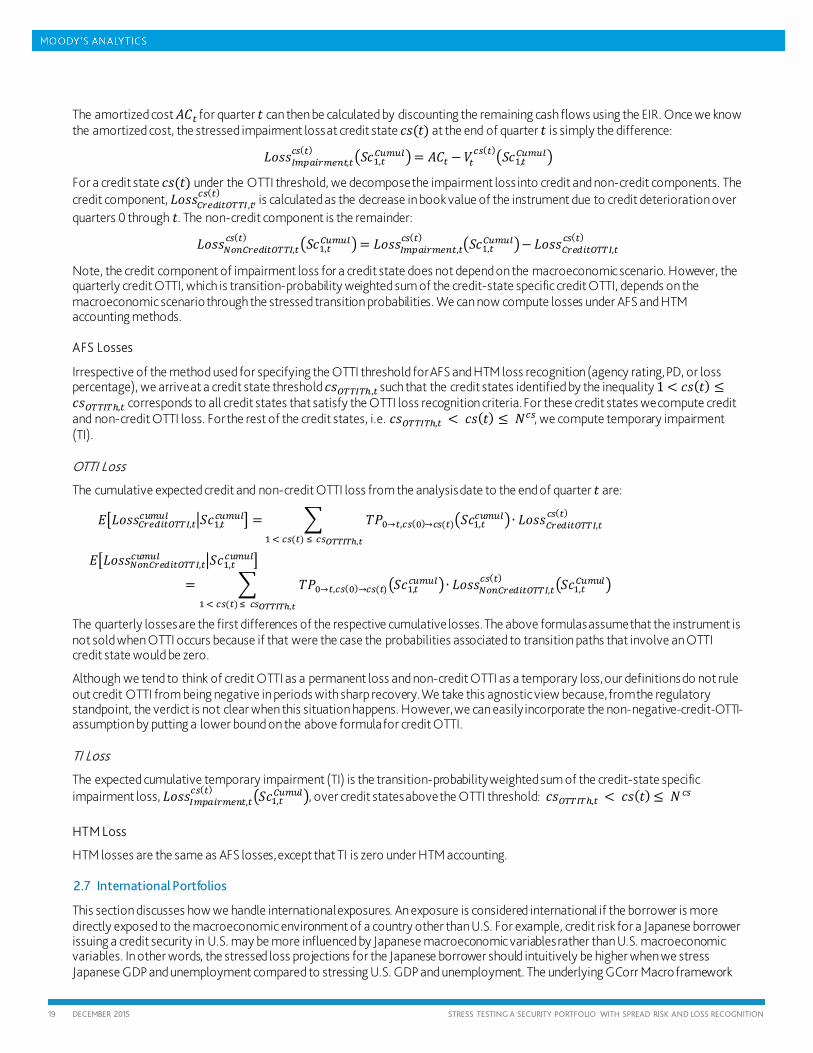
The amortized cost 𝐴𝐴𝐶𝐶𝑅𝑅 for quarter 𝑡𝑡 can then be calculated by discounting the remaining cash flows using the EIR. Once we know the amortized cost, the stressed impairment loss at credit state 𝑐𝑐𝑐𝑐(𝑡𝑡) at the end of quarter 𝑡𝑡 is simply the difference:
𝐿𝐿𝐿𝐿𝑐𝑐𝑐𝑐𝐼𝐼𝐶𝐶𝐼𝐼𝑅𝑅𝑅𝑅𝑆𝑆𝐶𝐶𝑆𝑆𝑅𝑅𝑅𝑅,𝑅𝑅𝑆𝑆𝑐𝑐(𝑅𝑅) �𝑆𝑆𝑐𝑐1,𝑅𝑅
𝐶𝐶𝐶𝐶𝐶𝐶𝐶𝐶𝐶𝐶�= 𝐴𝐴𝐶𝐶𝑅𝑅 −𝑀𝑀𝑅𝑅𝑆𝑆𝑐𝑐(𝑅𝑅)�𝑆𝑆𝑐𝑐1,𝑅𝑅
𝐶𝐶𝐶𝐶𝐶𝐶𝐶𝐶𝐶𝐶�
For a credit state 𝑐𝑐𝑐𝑐(𝑡𝑡) under the OTTI threshold, we decompose the impairment loss into credit and non-credit components. The credit component, 𝐿𝐿𝐿𝐿𝑐𝑐𝑐𝑐𝐶𝐶𝑆𝑆𝑆𝑆𝐶𝐶𝑅𝑅𝑅𝑅𝐶𝐶𝑇𝑇𝑇𝑇𝐼𝐼,𝑅𝑅
𝑆𝑆𝑐𝑐(𝑅𝑅), is calculated as the decrease in book value of the instrument due to credit deterioration over
quarters 0 through 𝑡𝑡. The non-credit component is the remainder:
𝐿𝐿𝐿𝐿𝑐𝑐𝑐𝑐𝑁𝑁𝑆𝑆𝑅𝑅𝐶𝐶𝑆𝑆𝑆𝑆𝐶𝐶𝑅𝑅𝑅𝑅𝐶𝐶𝑇𝑇𝑇𝑇𝐼𝐼,𝑅𝑅𝑆𝑆𝑐𝑐(𝑅𝑅) �𝑆𝑆𝑐𝑐1,𝑅𝑅
𝐶𝐶𝐶𝐶𝐶𝐶𝐶𝐶𝐶𝐶�= 𝐿𝐿𝐿𝐿𝑐𝑐𝑐𝑐𝐼𝐼𝐶𝐶𝐼𝐼𝑅𝑅𝑅𝑅𝑆𝑆𝐶𝐶𝑆𝑆𝑅𝑅𝑅𝑅,𝑅𝑅𝑆𝑆𝑐𝑐(𝑅𝑅) �𝑆𝑆𝑐𝑐1,𝑅𝑅
𝐶𝐶𝐶𝐶𝐶𝐶𝐶𝐶𝐶𝐶�− 𝐿𝐿𝐿𝐿𝑐𝑐𝑐𝑐𝐶𝐶𝑆𝑆𝑆𝑆𝐶𝐶𝑅𝑅𝑅𝑅𝐶𝐶𝑇𝑇𝑇𝑇𝐼𝐼,𝑅𝑅𝑆𝑆𝑐𝑐(𝑅𝑅)
Note, the credit component of impairment loss for a credit state does not depend on the macroeconomic scenario. However, the quarterly credit OTTI, which is transition-probability weighted sum of the credit-state specific credit OTTI, depends on the macroeconomic scenario through the stressed transition probabilities. We can now compute losses under AFS and HTM accounting methods.
AFS Losses
Irrespective of the method used for specifying the OTTI threshold for AFS and HTM loss recognition (agency rating, PD, or loss percentage), we arrive at a credit state threshold 𝑐𝑐𝑐𝑐𝐶𝐶𝑇𝑇𝑇𝑇𝐼𝐼𝑇𝑇ℎ,𝑅𝑅 such that the credit states identified by the inequality 1 < 𝑐𝑐𝑐𝑐(𝑡𝑡) ≤𝑐𝑐𝑐𝑐𝐶𝐶𝑇𝑇𝑇𝑇𝐼𝐼𝑇𝑇ℎ,𝑅𝑅 corresponds to all credit states that satisfy the OTTI loss recognition criteria. For these credit states we compute credit and non-credit OTTI loss. For the rest of the credit states, i.e. 𝑐𝑐𝑐𝑐𝐶𝐶𝑇𝑇𝑇𝑇𝐼𝐼𝑇𝑇ℎ,𝑅𝑅 < 𝑐𝑐𝑐𝑐(𝑡𝑡) ≤ 𝑁𝑁𝑆𝑆𝑐𝑐, we compute temporary impairment (TI).
OTTI Loss
The cumulative expected credit and non-credit OTTI loss from the analysis date to the end of quarter 𝑡𝑡 are:
𝐸𝐸�𝐿𝐿𝐿𝐿𝑐𝑐𝑐𝑐𝐶𝐶𝑆𝑆𝑆𝑆𝐶𝐶𝑅𝑅𝑅𝑅𝐶𝐶𝑇𝑇𝑇𝑇𝐼𝐼,𝑅𝑅𝑆𝑆𝐶𝐶𝐶𝐶𝐶𝐶𝐶𝐶 �𝑆𝑆𝑐𝑐1,𝑅𝑅𝑆𝑆𝐶𝐶𝐶𝐶𝐶𝐶𝐶𝐶� = � 𝑇𝑇𝑃𝑃0→𝑅𝑅,𝑆𝑆𝑐𝑐(0)→𝑆𝑆𝑐𝑐(𝑅𝑅)�𝑆𝑆𝑐𝑐1,𝑅𝑅
𝑆𝑆𝐶𝐶𝐶𝐶𝐶𝐶𝐶𝐶�∙ 𝐿𝐿𝐿𝐿𝑐𝑐𝑐𝑐𝐶𝐶𝑆𝑆𝑆𝑆𝐶𝐶𝑅𝑅𝑅𝑅𝐶𝐶𝑇𝑇𝑇𝑇𝐼𝐼,𝑅𝑅𝑆𝑆𝑐𝑐(𝑅𝑅)
1 < 𝑆𝑆𝑐𝑐(𝑅𝑅) ≤ 𝑆𝑆𝑐𝑐𝑂𝑂𝑂𝑂𝑂𝑂𝑂𝑂𝑂𝑂ℎ,𝑡𝑡
𝐸𝐸�𝐿𝐿𝐿𝐿𝑐𝑐𝑐𝑐𝑁𝑁𝑆𝑆𝑅𝑅𝐶𝐶𝑆𝑆𝑆𝑆𝐶𝐶𝑅𝑅𝑅𝑅𝐶𝐶𝑇𝑇𝑇𝑇𝐼𝐼,𝑅𝑅𝑆𝑆𝐶𝐶𝐶𝐶𝐶𝐶𝐶𝐶 �𝑆𝑆𝑐𝑐1,𝑅𝑅𝑆𝑆𝐶𝐶𝐶𝐶𝐶𝐶𝐶𝐶�
= � 𝑇𝑇𝑃𝑃0→𝑅𝑅,𝑆𝑆𝑐𝑐(0)→𝑆𝑆𝑐𝑐(𝑅𝑅)�𝑆𝑆𝑐𝑐1,𝑅𝑅𝑆𝑆𝐶𝐶𝐶𝐶𝐶𝐶𝐶𝐶�∙ 𝐿𝐿𝐿𝐿𝑐𝑐𝑐𝑐𝑁𝑁𝑆𝑆𝑅𝑅𝐶𝐶𝑆𝑆𝑆𝑆𝐶𝐶𝑅𝑅𝑅𝑅𝐶𝐶𝑇𝑇𝑇𝑇𝐼𝐼,𝑅𝑅
𝑆𝑆𝑐𝑐(𝑅𝑅) �𝑆𝑆𝑐𝑐1,𝑅𝑅𝐶𝐶𝐶𝐶𝐶𝐶𝐶𝐶𝐶𝐶�
1 < 𝑆𝑆𝑐𝑐(𝑅𝑅) ≤ 𝑆𝑆𝑐𝑐𝑂𝑂𝑂𝑂𝑂𝑂𝑂𝑂𝑂𝑂ℎ,𝑡𝑡
The quarterly losses are the first differences of the respective cumulative losses. The above formulas assume that the instrument is not sold when OTTI occurs because if that were the case the probabilities associated to transition paths that involve an OTTI credit state would be zero.
Although we tend to think of credit OTTI as a permanent loss and non-credit OTTI as a temporary loss, our definitions do not rule out credit OTTI from being negative in periods with sharp recovery. We take this agnostic view because, from the regulatory standpoint, the verdict is not clear when this situation happens. However, we can easily incorporate the non-negative-credit-OTTI-assumption by putting a lower bound on the above formula for credit OTTI.
TI Loss
The expected cumulative temporary impairment (TI) is the transition-probability weighted sum of the credit-state specific impairment loss, 𝐿𝐿𝐿𝐿𝑐𝑐𝑐𝑐𝐼𝐼𝐶𝐶𝐼𝐼𝑅𝑅𝑅𝑅𝑆𝑆𝐶𝐶𝑆𝑆𝑅𝑅𝑅𝑅,𝑅𝑅
𝑆𝑆𝑐𝑐(𝑅𝑅) �𝑆𝑆𝑐𝑐1,𝑅𝑅𝐶𝐶𝐶𝐶𝐶𝐶𝐶𝐶𝐶𝐶�, over credit states above the OTTI threshold: 𝑐𝑐𝑐𝑐𝐶𝐶𝑇𝑇𝑇𝑇𝐼𝐼𝑇𝑇ℎ,𝑅𝑅 < 𝑐𝑐𝑐𝑐(𝑡𝑡)≤ 𝑁𝑁𝑆𝑆𝑐𝑐
HTM Loss
HTM losses are the same as AFS losses, except that TI is zero under HTM accounting.
2.7 International Portfolios
This section discusses how we handle international exposures. An exposure is considered international if the borrower is more directly exposed to the macroeconomic environment of a country other than U.S. For example, credit risk for a Japanese borrower issuing a credit security in U.S. may be more influenced by Japanese macroeconomic variables rather than U.S. macroeconomic variables. In other words, the stressed loss projections for the Japanese borrower should intuitively be higher when we stress Japanese GDP and unemployment compared to stressing U.S. GDP and unemployment. The underlying GCorr Macro framework

20 DECEMBER 2015 STRESS TESTING A SECURITY PORTFOLIO WITH SPREAD RISK AND LOSS RECOGNITION
allows us to capture this effect by providing a view on the correlation between a country’s credit risk factor and another (or the same) country’s macroeconomic variables. All we need to do is to specify an exposure’s loadings to the various country factors and choose the macroeconomic variables to stress.
Another way an exposure is considered international is if the currency of denomination is not USD — e.g. a U.S. borrower issuing a credit security in Euro. In this case, although the U.S. credit risk factors would suffice to capture credit migration, the Euro interest rates and the USD/Euro forex rate (we always assume that the reporting currency is USD) are more relevant for non-credit component of the valuation risk. In order to capture this effect, the framework allows for specifying the scenario path of Euro yield curve (which can be obtained from Moody’s ECCA for example), which is used to project losses in Euro. The Euro losses are then converted to USD losses by applying the stressed scenario path for the Euro/USD forex rate (for example from CCAR).
Finally, we may have a combination of the above two cases: for example, a Japanese borrower issuing a security in Euro denomination. To project stressed losses more accurately using our framework, we want to ensure that the Japanese country factor has relatively higher weight in the instrument parameterization, and so we include the following in the scenario: (i) one or more Japanese macroeconomic variables, (ii) the stressed Euro yield curve, and (iii) the stressed Euro/USD forex rate.
21 DECEMBER 2015 STRESS TESTING A SECURITY PORTFOLIO WITH SPREAD RISK AND LOSS RECOGNITION
3. Estimating Parameters for Spread Risk and Loss Recognition
This section describes how we estimate parameters for the various components of the framework introduced in Section 2.4. In order to model spread-risk under various scenarios, we must estimate relationships between systematic credit factors and macroeconomic variables, as well as between factors representing shocks to market prices of risk and macroeconomic variables. For loss recognition, we need to estimate relationships between the rating-implied PDs and macroeconomic variables. In addition to correlations, the other set of parameters required for calculations within the framework are the mapping functions, also defined in Section 2.4.
3.1 Credit Risk Factors and Macroeconomic Variables
We provide an overview of the data and estimation methods that allow us to link GCorr systematic credit risk factors, ϕ𝐶𝐶𝑅𝑅 , to macroeconomic variables, 𝑀𝑀𝑀𝑀, and thus determine stressed PD, LGD, and transition probabilities. Note, the data and methods are identical to those described in a considerable detail in the paper by Huang, et al. (2015).
Macroeconomic Data
We use quarterly macroeconomic time series, spanning 1970–2014 (or shorter if data availability is limited). For the variables available at a higher than quarterly frequency, we select the last observation for a quarter. This choice makes the data consistent with the credit risk factor time series, which can be interpreted as returns between end-of-quarter time points. The choice of quarterly frequency is based mainly on empirical analysis.30 Moreover, quarterly data makes it possible to align calculations within our framework with macroeconomic scenarios based on quarterly projections, such as the Fed’s CCAR, UK’s PRA, Moody’s Analytics ECCA forecasts, and internal scenarios developed by many financial institutions.
For estimation purposes, we transform the macroeconomic time series into stationary time series.
Estimating Correlations of Systematic Credit Risk Factors and Macroeconomic Variables
For credit risk data, we use time series of systematic credit risk factors from GCorr Corporate, available as weekly returns 1999Q3– 2014Q1, and we convert them to quarterly return series. In addition to the GCorr data, we also utilize other sources of credit risk data — such as delinquency rate-implied factors and CDS-implied factors — to ensure robustness of the estimated parameters.
Our objective is to estimate the correlations between macroeconomic factors and the credit risk factors, as well as across credit macroeconomic factors — all of these correlations are represented by blocks Σ𝐺𝐺𝐶𝐶𝑆𝑆𝑆𝑆𝑆𝑆,𝑀𝑀𝑀𝑀 and Σ𝑀𝑀𝑀𝑀 in the matrix in Figure 5. We focus on period the period 1999–2014 for the estimation, because it reflects relationships among variables over the recent period, especially the effects of the financial crisis of 2008–2009. Such an approach makes the model applicable to typical stress testing exercises, such as CCAR, based on scenarios that, to some degree, mimic the financial crisis episode. Figure 8 illustrates time series dynamics of the U.S. Unemployment Rate and U.S. credit risk factors. These dynamics are the basis for estimating the correlations.
30 For certain macroeconomic variables, it might make sense to use a higher frequency for estimation. For many variables, however, the higher frequency correlation estimates tend to be noisy. In the end, we chose quarterly frequency as the appropriate balance between removing noise from data and still having enough observations to estimate parameters.
22 DECEMBER 2015 STRESS TESTING A SECURITY PORTFOLIO WITH SPREAD RISK AND LOSS RECOGNITION
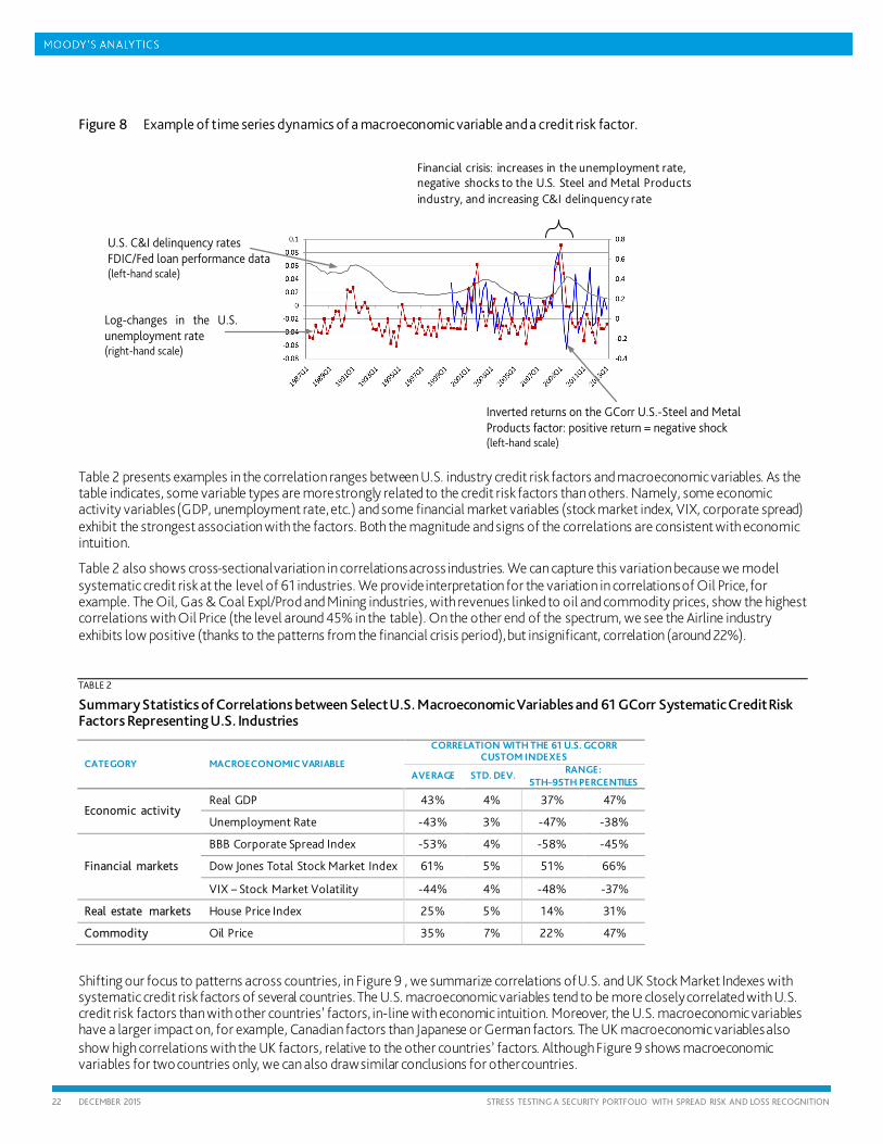
Figure 8 Example of time series dynamics of a macroeconomic variable and a credit risk factor.
Table 2 presents examples in the correlation ranges between U.S. industry credit risk factors and macroeconomic variables. As the table indicates, some variable types are more strongly related to the credit risk factors than others. Namely, some economic activity variables (GDP, unemployment rate, etc.) and some financial market variables (stock market index, VIX, corporate spread) exhibit the strongest association with the factors. Both the magnitude and signs of the correlations are consistent with economic intuition.
Table 2 also shows cross-sectional variation in correlations across industries. We can capture this variation because we model systematic credit risk at the level of 61 industries. We provide interpretation for the variation in correlations of Oil Price, for example. The Oil, Gas & Coal Expl/Prod and Mining industries, with revenues linked to oil and commodity prices, show the highest correlations with Oil Price (the level around 45% in the table). On the other end of the spectrum, we see the Airline industry exhibits low positive (thanks to the patterns from the financial crisis period), but insignificant, correlation (around 22%).
TABLE 2
Summary Statistics of Correlations between Select U.S. Macroeconomic Variables and 61 GCorr Systematic Credit Risk Factors Representing U.S. Industries
CATEGORY MACROECONOMIC VARIABLE
CORRELATION WITH THE 61 U.S. GCORR CUSTOM INDEXES
AVERAGE STD. DEV. RANGE: 5TH–95TH PERCENTILES
Economic activity Real GDP 43% 4% 37% 47%
Unemployment Rate -43% 3% -47% -38%
Financial markets
BBB Corporate Spread Index -53% 4% -58% -45%
Dow Jones Total Stock Market Index 61% 5% 51% 66%
VIX – Stock Market Volatility -44% 4% -48% -37%
Real estate markets House Price Index 25% 5% 14% 31%
Commodity Oil Price 35% 7% 22% 47%
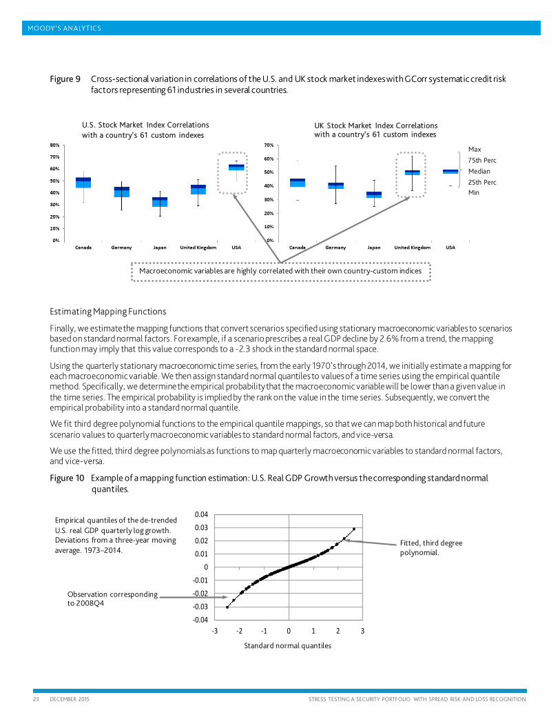
Shifting our focus to patterns across countries, in Figure 9 , we summarize correlations of U.S. and UK Stock Market Indexes with systematic credit risk factors of several countries. The U.S. macroeconomic variables tend to be more closely correlated with U.S. credit risk factors than with other countries’ factors, in-line with economic intuition. Moreover, the U.S. macroeconomic variables have a larger impact on, for example, Canadian factors than Japanese or German factors. The UK macroeconomic variables also show high correlations with the UK factors, relative to the other countries’ factors. Although Figure 9 shows macroeconomic variables for two countries only, we can also draw similar conclusions for other countries.
Log-changes in the U.S. unemployment rate (right-hand scale)
U.S. C&I delinquency rates FDIC/Fed loan performance data (left-hand scale)
Inverted returns on the GCorr U.S.-Steel and Metal Products factor: positive return = negative shock (left-hand scale)
Financial crisis: increases in the unemployment rate, negative shocks to the U.S. Steel and Metal Products industry, and increasing C&I delinquency rate
23 DECEMBER 2015 STRESS TESTING A SECURITY PORTFOLIO WITH SPREAD RISK AND LOSS RECOGNITION
Figure 9 Cross-sectional variation in correlations of the U.S. and UK stock market indexes with GCorr systematic credit risk factors representing 61 industries in several countries.
Estimating Mapping Functions
Finally, we estimate the mapping functions that convert scenarios specified using stationary macroeconomic variables to scenarios based on standard normal factors. For example, if a scenario prescribes a real GDP decline by 2.6% from a trend, the mapping function may imply that this value corresponds to a -2.3 shock in the standard normal space.
Using the quarterly stationary macroeconomic time series, from the early 1970’s through 2014, we initially estimate a mapping for each macroeconomic variable. We then assign standard normal quantiles to values of a time series using the empirical quantile method. Specifically, we determine the empirical probability that the macroeconomic variable will be lower than a given value in the time series. The empirical probability is implied by the rank on the value in the time series. Subsequently, we convert the empirical probability into a standard normal quantile.
We fit third degree polynomial functions to the empirical quantile mappings, so that we can map both historical and future scenario values to quarterly macroeconomic variables to standard normal factors, and vice-versa.
We use the fitted, third degree polynomials as functions to map quarterly macroeconomic variables to standard normal factors, and vice-versa.
Figure 10 Example of a mapping function estimation: U.S. Real GDP Growth versus the corresponding standard normal quantiles.
-0.04-0.03-0.02-0.01
00.010.020.030.04
-3 -2 -1 0 1 2 3
UK Stock Market Index Correlations with a country’s 61 custom indexes
U.S. Stock Market Index Correlations with a country’s 61 custom indexes
Macroeconomic variables are highly correlated with their own country-custom indices
Max
75th Perc
Median
25th Perc Min
Standard normal quantiles
Empirical quantiles of the de-trended U.S. real GDP quarterly log growth. Deviations from a three-year moving average. 1973–2014.
Observation corresponding to 2008Q4
Fitted, third degree polynomial.
24 DECEMBER 2015 STRESS TESTING A SECURITY PORTFOLIO WITH SPREAD RISK AND LOSS RECOGNITION
For the mapping estimation, we use the early 1970s through 2014 period, or the longest possible period for variables with limited data. We conduct exercises to examine the impact of this choice on the estimated mappings and losses projected by GCorr Macro. We find that the period we ultimately select is the most suitable, because it provides more observations in the tail to fit a polynomial than a shorter period allows. Moreover, the selected period leads to the satisfactory validation results discussed in Section 5.2.
3.2 Market Price of Risk
A market price of risk reflects the risk appetite of market participants – it is an important driver of the risk premium that the participants require to hold a risky asset, and in this way the market price of risk level impacts market values of instruments. During an economic downturn, we typically observe an increase in the market prices of risk as investors demand a higher return for a certain level of risk because they have become more risk averse.
In our framework, we use 𝜆𝜆 to denote the market price of credit risk. From a theoretical stand point, there is a link between this market price of risk and a credit spread in Merton’s credit risk framework.31 Namely, a spread over a time horizon 𝑇𝑇 can be expressed as follows:32
𝑆𝑆𝑇𝑇 = −1𝑇𝑇∙ 𝐶𝐶𝐿𝐿𝑙𝑙 �1−𝐿𝐿𝐿𝐿𝑃𝑃 ∙ 𝑁𝑁�𝑁𝑁−1(𝐶𝐶𝑃𝑃𝑃𝑃𝑇𝑇) + 𝜆𝜆 ∙ �𝐼𝐼𝑆𝑆𝑅𝑅𝑀𝑀𝑅𝑅𝐶𝐶 ∙ 𝑇𝑇��
(7)
Moody’s Analytics uses the above formula to estimate time series of market prices of risk from certain samples of market spreads. One sample considered for estimation is a set of high quality North American bonds issued by large corporates.33 Other samples are spreads from the CDS market, segmented in such a way that market prices of risk can be estimated by regions and credit qualities (investment grade versus high yield).34 In this paper, we focus on the North American bond-implied market price of risk. The same methodology, however, can be applied to other market prices of risk as well.
One point worth noting in relation to estimating market price of risk from market spreads: it is typically not possible to isolate purely the credit risk component of the spreads. Even though the estimation described above narrows the sample to the most liquid bonds, there will still be some liquidity and other effects in the spreads. Thus, even if the credit risk effects dominate in the market price of risk dynamics, in practice, it still, to some degree, captures prices of other risks as well.
Estimating Correlations of the Market Price of Risk with Other Factors
In the first step of the analysis, we must estimate relationships between the market price of risk and other factors from GCorr Macro. Specifically, we need to estimate blocks Σ𝐺𝐺𝐶𝐶𝑆𝑆𝑆𝑆𝑆𝑆,𝜆𝜆 and Σ𝑀𝑀𝑀𝑀,𝜆𝜆 from the matrix in Figure 5. In Figure 11, we present the time series of the market price of risk from the North American bond market and highlight that, around the financial crisis period, its time series patterns align with the financial markets’ and the broader economy’s dynamics. If markets experience turmoil, or the economy is hit by a recession, we see an increase in the market price of risk.
31 See Agrawal, Arora, and Bohn (2004). 32 𝐶𝐶𝑃𝑃𝑃𝑃𝑇𝑇 denotes a physical cumulative default probability over horizon 𝑇𝑇. 33 See Section 6.3 in Chen, et al. (2015) 34 See Dwyer, et al. (2010).
Risk-neutral cumulative default probability 𝐶𝐶𝑅𝑅𝑃𝑃𝑃𝑃𝑇𝑇
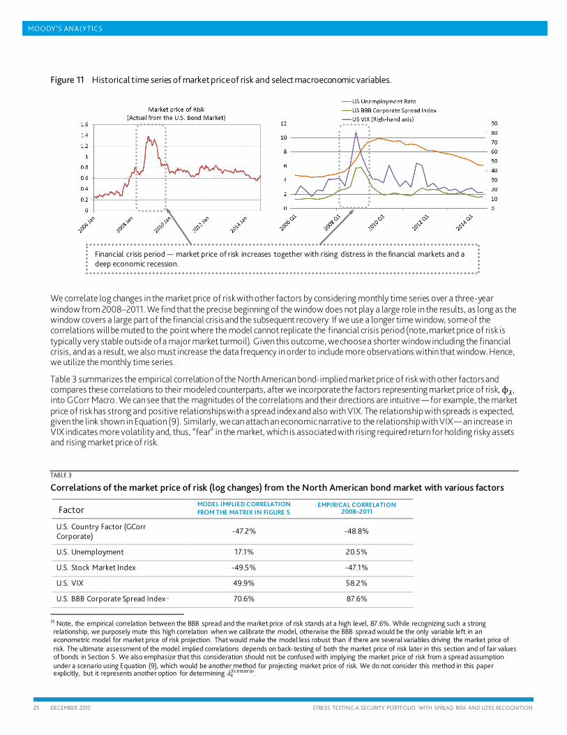
25 DECEMBER 2015 STRESS TESTING A SECURITY PORTFOLIO WITH SPREAD RISK AND LOSS RECOGNITION
Figure 11 Historical time series of market price of risk and select macroeconomic variables.
We correlate log changes in the market price of risk with other factors by considering monthly time series over a three-year window from 2008–2011. We find that the precise beginning of the window does not play a large role in the results, as long as the window covers a large part of the financial crisis and the subsequent recovery. If we use a longer time window, some of the correlations will be muted to the point where the model cannot replicate the financial crisis period (note, market price of risk is typically very stable outside of a major market turmoil). Given this outcome, we choose a shorter window including the financial crisis, and as a result, we also must increase the data frequency in order to include more observations within that window. Hence, we utilize the monthly time series.
Table 3 summarizes the empirical correlation of the North American bond-implied market price of risk with other factors and compares these correlations to their modeled counterparts, after we incorporate the factors representing market price of risk, ϕ𝜆𝜆, into GCorr Macro. We can see that the magnitudes of the correlations and their directions are intuitive — for example, the market price of risk has strong and positive relationships with a spread index and also with VIX. The relationship with spreads is expected, given the link shown in Equation (9). Similarly, we can attach an economic narrative to the relationship with VIX — an increase in VIX indicates more volatility and, thus, “fear” in the market, which is associated with rising required return for holding risky assets and rising market price of risk.
TABLE 3
Correlations of the market price of risk (log changes) from the North American bond market with various factors
Factor MODEL IMPLIED CORRELATION FROM THE MATRIX IN FIGURE 5
EMPIRICAL CORRELATION 2008–2011
U.S. Country Factor (GCorr Corporate)
-47.2% -48.8%
U.S. Unemployment 17.1% 20.5%
U.S. Stock Market Index -49.5% -47.1%
U.S. VIX 49.9% 58.2%
U.S. BBB Corporate Spread Index 3 5 70.6% 87.6%
35 Note, the empirical correlation between the BBB spread and the market price of risk stands at a high level, 87.6%. While recognizing such a strong relationship, we purposely mute this high correlation when we calibrate the model, otherwise the BBB spread would be the only variable left in an econometric model for market price of risk projection. That would make the model less robust than if there are several variables driving the market price of risk. The ultimate assessment of the model implied correlations depends on back-testing of both the market price of risk later in this section and of fair values of bonds in Section 5. We also emphasize that this consideration should not be confused with implying the market price of risk from a spread assumption under a scenario using Equation (9), which would be another method for projecting market price of risk. We do not consider this method in this paper explicitly, but it represents another option for determining 𝜆𝜆𝑅𝑅𝑆𝑆𝑆𝑆𝑆𝑆𝑅𝑅𝑅𝑅𝑆𝑆𝑅𝑅𝑆𝑆.
Financial crisis period — market price of risk increases together with rising distress in the financial markets and a deep economic recession.
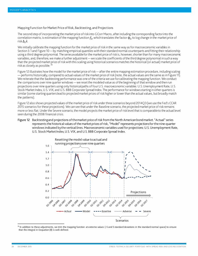
26 DECEMBER 2015 STRESS TESTING A SECURITY PORTFOLIO WITH SPREAD RISK AND LOSS RECOGNITION
Mapping Function for Market Price of Risk, Backtesting, and Projections
The second step of incorporating the market price of risk into GCorr Macro, after including the corresponding factor into the correlation matrix, is estimation of the mapping function 𝑓𝑓𝜆𝜆, which translates the factor ϕ𝜆𝜆 to log change in the market price of risk Δ𝐶𝐶𝜆𝜆.
We initially calibrate the mapping function for the market price of risk in the same way as for macroeconomic variables in Section 3.1 and Figure 10 — by matching empirical quantiles with their standard normal counterparts and fitting their relationship using a third degree polynomial. The series available for the market price of risk is, however, shorter than for many macroeconomic variables, and, therefore, we make a further adjustment — we scale the coefficients of the third degree polynomial in such a way that the projected market price of risk with this scaling using historical scenarios matches the historical (or actual) market price of risk as closely as possible. 36
Figure 12 illustrates how the model for the market price of risk — after the entire mapping estimation procedure, including scaling — performs historically, compared to actual values of the market price of risk (note, the actual values are the same as in Figure 11). We reiterate that the backtesting performance was one of the criteria we use for calibrating the mapping function. We conduct the comparisons over nine quarter windows — we reset the modeled value as of the beginning of that window and then run projections over nine quarters using only historical paths of four U.S. macroeconomic variables: U.S. Unemployment Rate, U.S. Stock Market Index, U.S. VIX, and U.S. BBB Corporate Spread Index. The performance for windows starting in other quarters is similar (some starting quarters lead to projected market prices of risk higher or lower than the actual values, but broadly match the patterns).
Figure 12 also shows projected values of the market price of risk under three scenarios beyond 2014Q3 (we use the Fed’s CCAR 2015 scenarios for these projections). We can see that under the Baseline scenario, the projected market price of risk remains more or less flat. Under the Severe scenario, the model projects the market price of risk level that is comparable to the actual level seen during the 2008 financial crisis.
Figure 12 Backtesting and projections of the market price of risk from the North American bond market. “Actual” series represents the historical values of the market prices of risk, “Model” represents projections for the nine-quarter windows indicated by the vertical lines. Macroeconomic variables used for projections: U.S. Unemployment Rate, U.S. Stock Market Index, U.S. VIX, and U.S. BBB Corporate Spread Index.
36 In addition to these adjustments, we trim the mapping function at extreme values (-5 and 5 standard deviations in the standard normal space) to ensure that the integral in Eequation (8) is well-defined.
Projections
Scenarios
Resetting the model value to actual and running projections over nine quarters
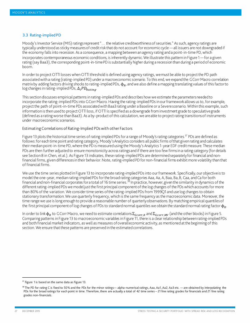
27 DECEMBER 2015 STRESS TESTING A SECURITY PORTFOLIO WITH SPREAD RISK AND LOSS RECOGNITION
3.3 Rating-implied PD
Moody’s Investor Service (MIS) ratings represent “… the relative creditworthiness of securities.” As such, agency ratings are typically understood as sticky measures of credit risk that do not account for economic cycle — all issuers are not downgraded if the economy falls into recession. As a consequence, a mapping between an agency rating and a point-in-time PD, which incorporates contemporaneous economic conditions, is inherently dynamic. We illustrate this pattern in Figure 1 — for a given rating (say Baa3), the corresponding point-in-time PD is substantially higher during a recession than during a period of economic boom.
In order to project OTTI losses when OTTI threshold is defined using agency ratings, we must be able to project the PD path associated with a rating (rating-implied PD) under a macroeconomic scenario. To this end, we expand the GCorr Macro correlation matrix by adding factors driving shocks to rating-implied PDs, ϕ𝑅𝑅, and we also define a mapping translating values of this factor to log changes in rating-implied PDs, Δ𝐶𝐶𝑃𝑃𝑃𝑃𝑅𝑅𝑅𝑅𝑅𝑅𝑅𝑅𝑅𝑅𝑅𝑅.
This section discusses empirical patterns in rating-implied PDs and describes how we estimate the parameters needed to incorporate the rating-implied PDs into GCorr Macro. Having the rating-implied PDs in our framework allows us to, for example, project the path of point-in-time PDs associated with Baa3 rating under a Baseline or a Severe scenario. Within this example, such information is then used to project OTTI loss, if OTTI is specified as a downgrade from investment grade to speculative grade (defined as a rating worse than Baa3). As a by-product of this calculation, we are able to project rating transitions of instruments under macroeconomic scenarios.
Estimating Correlations of Rating-Implied PDs with other Factors
Figure 13 plots the historical time series of rating-implied PDs for a range of Moody’s rating categories.37 PDs are defined as follows: for each time point and rating category, Moody’s Analytics considers all public firms of that given rating and calculates their median point-in-time PD, where the PD is measured using the Moody’s Analytics 1-year EDF credit measure. These median PDs are then further adjusted to ensure monotonicity across ratings and if there are too few firms in a rating category (for details see Section 8 in Chen, et al.). As Figure 13 indicates, these rating-implied PDs are determined separately for financial and non-financial firms, given differences in their behavior. Note, rating-implied PD for non-financial firms exhibit more volatility than that of financial firms.
We use the time series plotted in Figure 13 to incorporate rating-implied PDs into our framework. Specifically, our objective is to model the one-year, median rating-implied PDs for the broad rating categories Aaa, Aa, A, Baa, Ba, B, Caa, and Ca for both financial and non-financial corporates for a total of 16 time series.38 In practice, however, given the similarity in dynamics of the different rating-implied PDs we model just the first principal component of the log changes of the PDs which accounts for more than 80% of the variation. We consider time series of the rating-implied PDs from 1999Q1 and use log changes to obtain stationary transformation. We use quarterly frequency, which is the same frequency as the macroeconomic data. Moreover, the time range we use is long enough to provide a reasonable number of quarterly observations. By matching empirical quantiles of the first principal component of log changes of PDs to standard normal quantiles we obtain the standard normal rating factor ϕ𝑅𝑅.
In order to link ϕ𝑅𝑅 to GCorr Macro, we need to estimate correlations Σ𝐺𝐺𝑆𝑆𝑆𝑆𝑆𝑆𝑆𝑆,𝑅𝑅 and Σ𝐺𝐺𝑆𝑆𝑆𝑆𝑆𝑆𝑆𝑆,𝑀𝑀𝑀𝑀 (and the other blocks) in Figure 5. Comparing patterns in Figure 13 to macroeconomic variables in Figure 11, there is a clear relationship between rating-implied PDs and both financial market indicators, as well as measures of overall economic activity, as mentioned at the beginning of this section. We ensure that these patterns are preserved in the estimated correlations.
37 Figure 1 is based on the same data as Figure 13. 38 The PD for rating C is fixed to 50% and the PDs for the minor ratings— alpha-numerical ratings, Aaa, Aa1, Aa2, Aa3 etc. — are obtained by interpolating the PDs for the broad ratings for each point in time. Therefore, there are actually a total of 42 time series – 21 fine rating grades for financials and 21 fine rating grades non-financials.
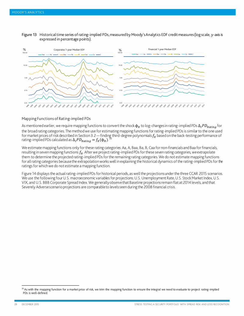
28 DECEMBER 2015 STRESS TESTING A SECURITY PORTFOLIO WITH SPREAD RISK AND LOSS RECOGNITION
Figure 13 Historical time series of rating-implied PDs, measured by Moody’s Analytics EDF credit measures (log scale, y-axis is expressed in percentage points).
Mapping Functions of Rating-implied PDs
As mentioned earlier, we require mapping functions to convert the shock ϕ𝑅𝑅 to log-changes in rating-implied PDs Δ𝐶𝐶𝑃𝑃𝑃𝑃𝑅𝑅𝑅𝑅𝑅𝑅𝑅𝑅𝑅𝑅𝑅𝑅 for the broad rating categories. The method we use for estimating mapping functions for rating-implied PDs is similar to the one used for market prices of risk described in Section 3.2 — finding third-degree polynomials 𝑓𝑓𝑅𝑅 based on the back-testing performance of rating-implied PDs calculated as Δ𝐶𝐶𝑃𝑃𝑃𝑃𝑅𝑅𝑅𝑅𝑅𝑅𝑅𝑅𝑅𝑅𝑅𝑅 = 𝑓𝑓𝑅𝑅(ϕ𝑅𝑅). 39
We estimate mapping functions only for these rating categories: Aa, A, Baa, Ba, B, Caa for non-financials and Baa for financials, resulting in seven mapping functions 𝑓𝑓𝑅𝑅. After we project rating-implied PDs for these seven rating categories, we extrapolate them to determine the projected rating-implied PDs for the remaining rating categories. We do not estimate mapping functions for all rating categories because the extrapolation works well in explaining the historical dynamics of the rating-implied PDs for the ratings for which we do not estimate a mapping function.
Figure 14 displays the actual rating-implied PDs for historical periods, as well the projections under the three CCAR 2015 scenarios. We use the following four U.S. macroeconomic variables for projections: U.S. Unemployment Rate, U.S. Stock Market Index, U.S. VIX, and U.S. BBB Corporate Spread Index. We generally observe that Baseline projections remain flat at 2014 levels, and that Severely Adverse scenario projections are comparable to levels seen during the 2008 financial crisis.
39 As with the mapping function for a market price of risk, we trim the mapping function to ensure the integral we need to evaluate to project rating-implied PDs is well-defined.
0.01
0.10
1.00
10.00
100.00
Corporates 1-year Median EDF
Aaa Aa A Baa Ba B Caa Ca C
0.01
0.10
1.00
10.00
100.00
Financial 1-year Median EDF
Aaa Aa A Baa Ba B Caa Ca C
% %
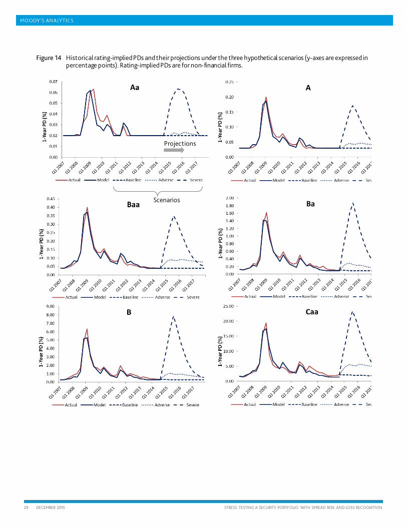
29 DECEMBER 2015 STRESS TESTING A SECURITY PORTFOLIO WITH SPREAD RISK AND LOSS RECOGNITION
Figure 14 Historical rating-implied PDs and their projections under the three hypothetical scenarios (y-axes are expressed in percentage points). Rating-implied PDs are for non-financial firms.
Scenarios
Projections
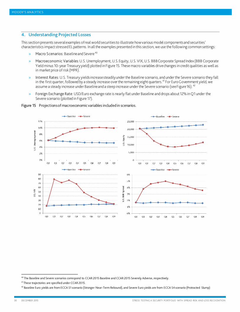
30 DECEMBER 2015 STRESS TESTING A SECURITY PORTFOLIO WITH SPREAD RISK AND LOSS RECOGNITION
4. Understanding Projected Losses
This section presents several examples of real world securities to illustrate how various model components and securities’ characteristics impact stressed EL patterns. In all the examples presented in this section, we use the following common settings:
» Macro Scenarios: Baseline and Severe40
» Macroeconomic Variables: U.S. Unemployment, U.S. Equity, U.S. VIX, U.S. BBB Corporate Spread Index (BBB Corporate Yield minus 10-year Treasury yield) plotted in Figure 15. These macro variables drive changes in credit qualities as well as in market price of risk (MPR).
» Interest Rates: U.S. Treasury yields increase steadily under the Baseline scenario, and under the Severe scenario they fall in the first quarter, followed by a steady increase over the remaining eight quarters.41 For Euro Government yield, we assume a steady increase under Baseline and a steep increase under the Severe scenario (see Figure 16). 42
» Foreign Exchange Rate: USD/Euro exchange rate is nearly flat under Baseline and drops about 12% in Q1 under the Severe scenario (plotted in Figure 17).
Figure 15 Projections of macroeconomic variables included in scenarios.
40 The Baseline and Severe scenarios correspond to CCAR 2015 Baseline and CCAR 2015 Severely Adverse, respectively. 41 These trajectories are specified under CCAR 2015. 42 Baseline Euro yields are from ECCA S1 scenario (Stronger Near-Term Rebound), and Severe Euro yields are from ECCA S4 scenario (Protracted Slump)
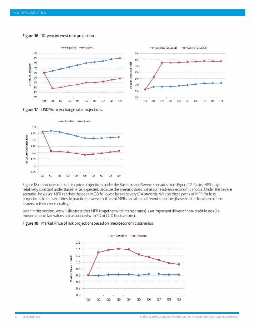
31 DECEMBER 2015 STRESS TESTING A SECURITY PORTFOLIO WITH SPREAD RISK AND LOSS RECOGNITION
Figure 16 10-year interest rate projections.
Figure 17 USD/Euro exchange rate projections.
Figure 18 reproduces market risk price projections under the Baseline and Severe scenarios from Figure 12. Note, MPR stays relatively constant under Baseline, as expected, because the scenario does not assume adverse economic shocks. Under the Severe scenario, however, MPR reaches the peak in Q3 followed by a recovery Q4 onwards. We use these paths of MPR for loss projections for all securities. In practice, however, different MPRs can affect different securities (based on the locations of the issuers or their credit quality).
Later in this section, we will illustrate that MPR (together with interest rates) is an important driver of non-credit losses (i.e. movements in fair values not associated with PD or LGD fluctuations).
Figure 18 Market Price of risk projections based on macroeconomic scenarios.
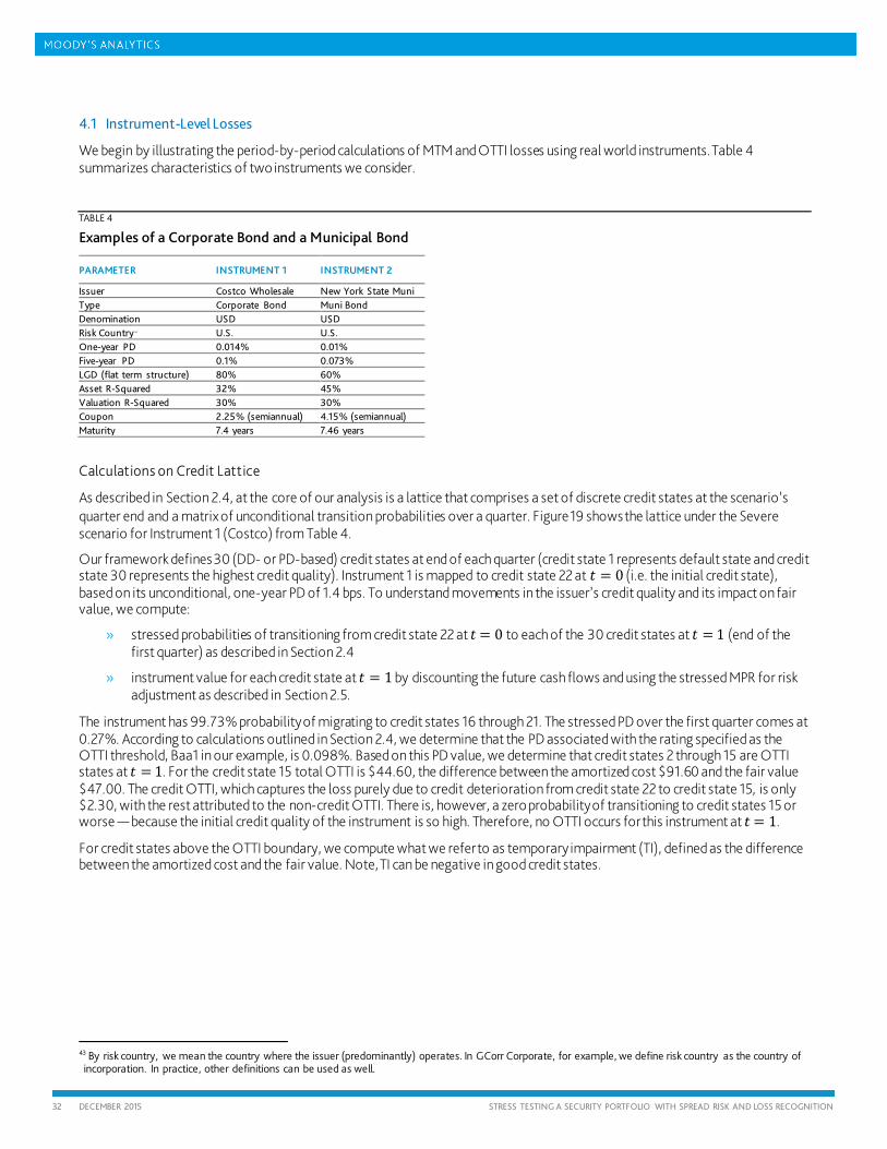
32 DECEMBER 2015 STRESS TESTING A SECURITY PORTFOLIO WITH SPREAD RISK AND LOSS RECOGNITION
4.1 Instrument-Level Losses
We begin by illustrating the period-by-period calculations of MTM and OTTI losses using real world instruments. Table 4 summarizes characteristics of two instruments we consider.
TABLE 4
Examples of a Corporate Bond and a Municipal Bond
PARAMETER INSTRUMENT 1 INSTRUMENT 2
Issuer Costco Wholesale New York State Muni Type Corporate Bond Muni Bond Denomination USD USD Risk Country 43 U.S. U.S. One-year PD 0.014% 0.01% Five-year PD 0.1% 0.073% LGD (flat term structure) 80% 60% Asset R-Squared 32% 45% Valuation R-Squared 30% 30% Coupon 2.25% (semiannual) 4.15% (semiannual) Maturity 7.4 years 7.46 years
Calculations on Credit Lattice
As described in Section 2.4, at the core of our analysis is a lattice that comprises a set of discrete credit states at the scenario’s quarter end and a matrix of unconditional transition probabilities over a quarter. Figure 19 shows the lattice under the Severe scenario for Instrument 1 (Costco) from Table 4.
Our framework defines 30 (DD- or PD-based) credit states at end of each quarter (credit state 1 represents default state and credit state 30 represents the highest credit quality). Instrument 1 is mapped to credit state 22 at 𝑡𝑡 = 0 (i.e. the initial credit state), based on its unconditional, one-year PD of 1.4 bps. To understand movements in the issuer’s credit quality and its impact on fair value, we compute:
» stressed probabilities of transitioning from credit state 22 at 𝑡𝑡 = 0 to each of the 30 credit states at 𝑡𝑡 = 1 (end of the first quarter) as described in Section 2.4
» instrument value for each credit state at 𝑡𝑡 = 1 by discounting the future cash flows and using the stressed MPR for risk adjustment as described in Section 2.5.
The instrument has 99.73% probability of migrating to credit states 16 through 21. The stressed PD over the first quarter comes at 0.27%. According to calculations outlined in Section 2.4, we determine that the PD associated with the rating specified as the OTTI threshold, Baa1 in our example, is 0.098%. Based on this PD value, we determine that credit states 2 through 15 are OTTI states at 𝑡𝑡 = 1. For the credit state 15 total OTTI is $44.60, the difference between the amortized cost $91.60 and the fair value $47.00. The credit OTTI, which captures the loss purely due to credit deterioration from credit state 22 to credit state 15, is only $2.30, with the rest attributed to the non-credit OTTI. There is, however, a zero probability of transitioning to credit states 15 or worse — because the initial credit quality of the instrument is so high. Therefore, no OTTI occurs for this instrument at 𝑡𝑡 = 1.
For credit states above the OTTI boundary, we compute what we refer to as temporary impairment (TI), defined as the difference between the amortized cost and the fair value. Note, TI can be negative in good credit states.
43 By risk country, we mean the country where the issuer (predominantly) operates. In GCorr Corporate, for example, we define risk country as the country of incorporation. In practice, other definitions can be used as well.
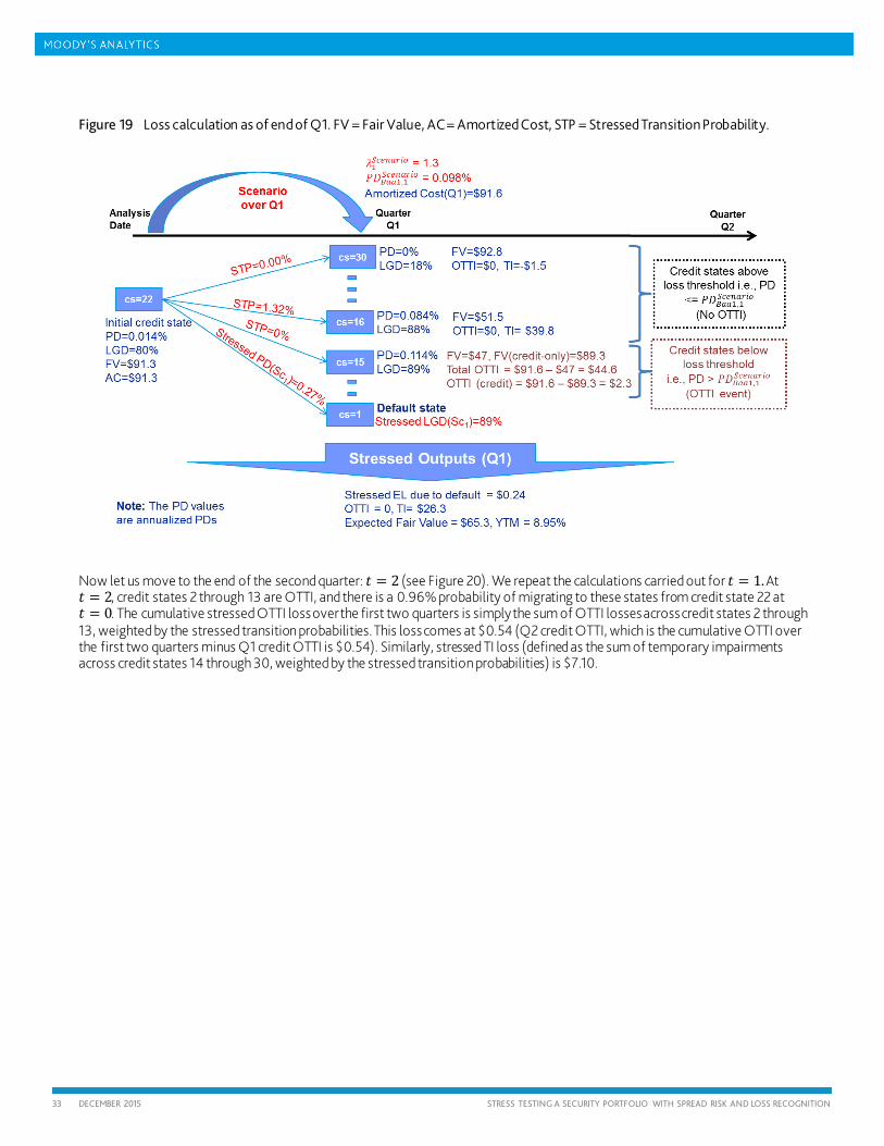
33 DECEMBER 2015 STRESS TESTING A SECURITY PORTFOLIO WITH SPREAD RISK AND LOSS RECOGNITION
Figure 19 Loss calculation as of end of Q1. FV = Fair Value, AC = Amortized Cost, STP = Stressed Transition Probability.
Now let us move to the end of the second quarter: 𝑡𝑡 = 2 (see Figure 20). We repeat the calculations carried out for 𝑡𝑡 = 1. At 𝑡𝑡 = 2, credit states 2 through 13 are OTTI, and there is a 0.96% probability of migrating to these states from credit state 22 at 𝑡𝑡 = 0. The cumulative stressed OTTI loss over the first two quarters is simply the sum of OTTI losses across credit states 2 through 13, weighted by the stressed transition probabilities. This loss comes at $0.54 (Q2 credit OTTI, which is the cumulative OTTI over the first two quarters minus Q1 credit OTTI is $0.54). Similarly, stressed TI loss (defined as the sum of temporary impairments across credit states 14 through 30, weighted by the stressed transition probabilities) is $7.10.
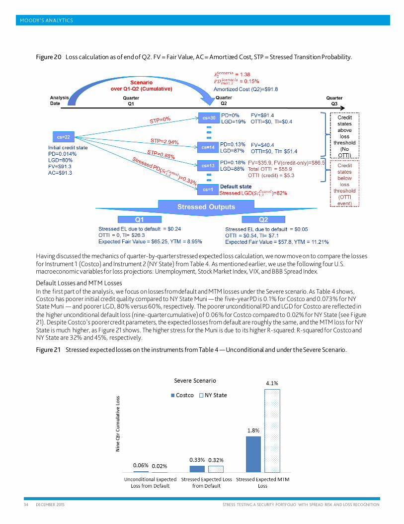
34 DECEMBER 2015 STRESS TESTING A SECURITY PORTFOLIO WITH SPREAD RISK AND LOSS RECOGNITION
Figure 20 Loss calculation as of end of Q2. FV = Fair Value, AC = Amortized Cost, STP = Stressed Transition Probability.
Having discussed the mechanics of quarter-by-quarter stressed expected loss calculation, we now move on to compare the losses for Instrument 1 (Costco) and Instrument 2 (NY State) from Table 4. As mentioned earlier, we use the following four U.S. macroeconomic variables for loss projections: Unemployment, Stock Market Index, VIX, and BBB Spread Index.
Default Losses and MTM Losses In the first part of the analysis, we focus on losses from default and MTM losses under the Severe scenario. As Table 4 shows, Costco has poorer initial credit quality compared to NY State Muni — the five-year PD is 0.1% for Costco and 0.073% for NY State Muni — and poorer LGD, 80% versus 60%, respectively. The poorer unconditional PD and LGD for Costco are reflected in the higher unconditional default loss (nine-quarter cumulative) of 0.06% for Costco compared to 0.02% for NY State (see Figure 21). Despite Costco’s poorer credit parameters, the expected losses from default are roughly the same, and the MTM loss for NY State is much higher, as Figure 21 shows. The higher stress for the Muni is due to its higher R-squared: R-squared for Costco and NY State are 32% and 45%, respectively.
Figure 21 Stressed expected losses on the instruments from Table 4 — Unconditional and under the Severe Scenario.
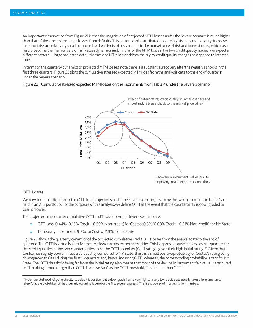
35 DECEMBER 2015 STRESS TESTING A SECURITY PORTFOLIO WITH SPREAD RISK AND LOSS RECOGNITION
An important observation from Figure 21 is that the magnitude of projected MTM losses under the Severe scenario is much higher than that of the stressed expected losses from defaults. This pattern can be attributed to very high issuer credit quality; increases in default risk are relatively small compared to the effects of movements in the market price of risk and interest rates, which, as a result, become the main drivers of fair values dynamics and, in turn, of the MTM losses. For low credit quality issuers, we expect a different pattern — large projected default losses and MTM losses driven mainly by credit quality changes as opposed to interest rates.
In terms of the quarterly dynamics of projected MTM losses, note there is a substantial recovery after the negative shocks in the first three quarters . Figure 22 plots the cumulative stressed expected MTM loss from the analysis date to the end of quarter 𝑡𝑡 under the Severe scenario.
Figure 22 Cumulative stressed expected MTM losses on the instruments from Table 4 under the Severe Scenario.
OTTI Losses
We now turn our attention to the OTTI loss projections under the Severe scenario, assuming the two instruments in Table 4 are held in an AFS portfolio. For the purposes of this analysis, we define OTTI as the event that the counterparty is downgraded to Caa1 or lower.
The projected nine-quarter cumulative OTTI and TI loss under the Severe scenario are:
» OTTI Loss: 0.44% (0.15% Credit + 0.29% Non-credit) for Costco; 0.3% (0.09% Credit + 0.21% Non-credit) for NY State
» Temporary Impairment: 9.9% for Costco; 2.3% for NY State
Figure 23 shows the quarterly dynamics of the projected cumulative credit OTTI losses from the analysis date to the end of quarter 𝑡𝑡. The OTTI is virtually zero for the first few quarters for both securities. This happens because it takes several quarters for the credit qualities of the two counterparties to hit the OTTI boundary (Caa1 rating), given their high initial rating. 44 Given that Costco has slightly poorer initial credit quality compared to NY State, there is a small positive probability of Costco’s rating being downgraded to Caa1 during the first six quarters and, hence, incurring OTTI, whereas, the corresponding probability is zero for NY State. The OTTI threshold being far from the initial rating also means that most of the decline in instrument fair value is attributed to TI, making it much larger than OTTI. If we use Baa1 as the OTTI threshold, TI is smaller than OTTI.
44 Note, the likelihood of going directly to default is positive, but a downgrade from a very high to a very low credit state usually takes a long time, and, therefore, the probability of that scenario occurring is zero for the first several quarters. This is a property of most transition matrixes.
Effect of deteriorating credit quality in initial quarters and importantly adverse shock to the market price of risk
Recovery in instrument values due to improving macroeconomic conditions
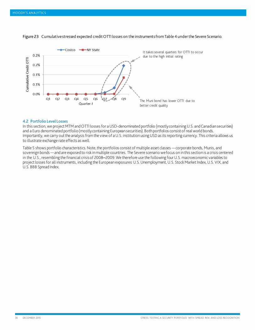
36 DECEMBER 2015 STRESS TESTING A SECURITY PORTFOLIO WITH SPREAD RISK AND LOSS RECOGNITION
Figure 23 Cumulative stressed expected credit OTTI losses on the instruments from Table 4 under the Severe Scenario.
4.2 Portfolio Level Losses In this section, we project MTM and OTTI losses for a USD-denominated portfolio (mostly containing U.S. and Canadian securities) and a Euro denominated portfolio (mostly containing European securities). Both portfolios consist of real world bonds. Importantly, we carry out the analysis from the view of a U.S. institution using USD as its reporting currency. This criteria allows us to illustrate exchange rate effects as well.
Table 5 shows portfolio characteristics. Note, the portfolios consist of multiple asset classes — corporate bonds, Munis, and sovereign bonds — and are exposed to risk in multiple countries. The Severe scenario we focus on in this section is a crisis centered in the U.S., resembling the financial crisis of 2008–2009. We therefore use the following four U.S. macroeconomic variables to project losses for all instruments, including the European exposures: U.S. Unemployment, U.S. Stock Market Index, U.S. VIX, and U.S. BBB Spread Index.
It takes several quarters for OTTI to occur due to the high initial rating
The Muni bond has lower OTTI due to better credit quality
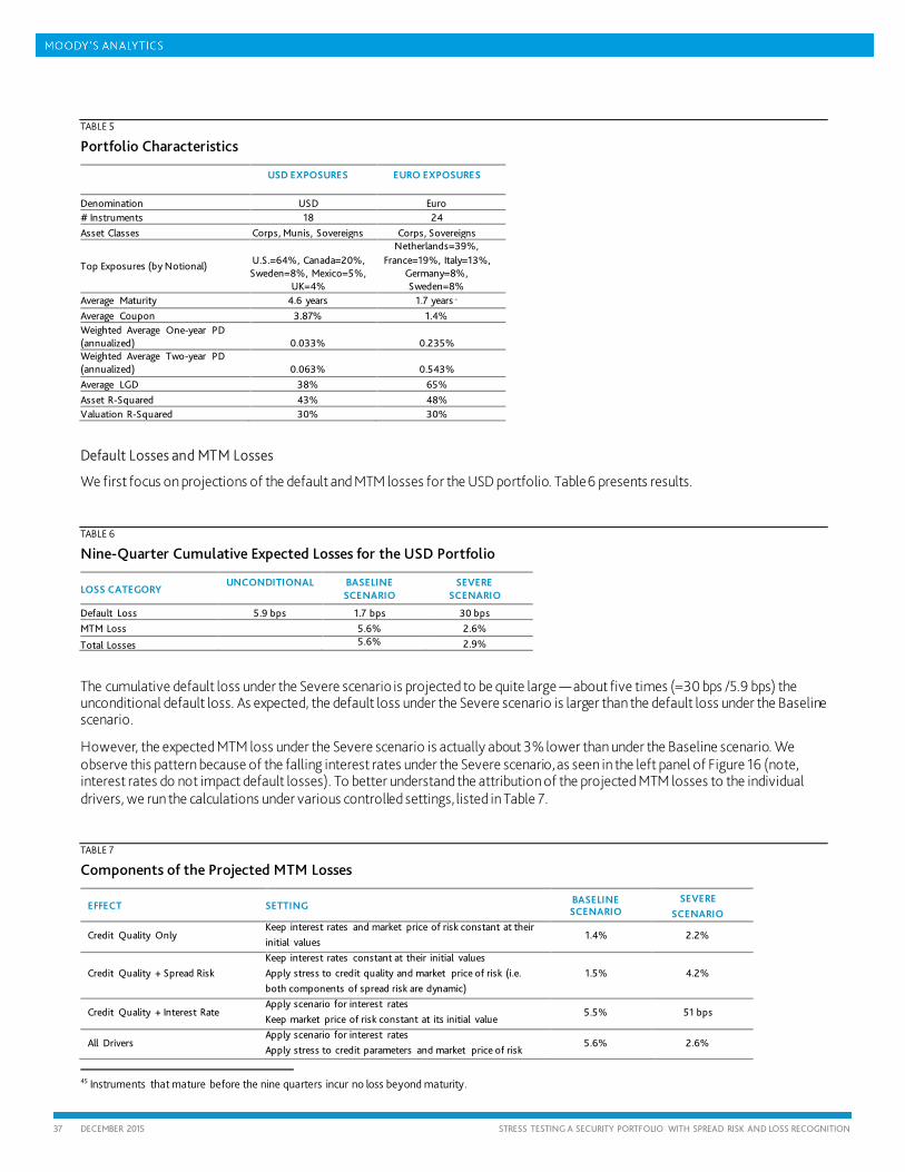
37 DECEMBER 2015 STRESS TESTING A SECURITY PORTFOLIO WITH SPREAD RISK AND LOSS RECOGNITION
TABLE 5
Portfolio Characteristics
USD EXPOSURES EURO EXPOSURES
Denomination USD Euro # Instruments 18 24 Asset Classes Corps, Munis, Sovereigns Corps, Sovereigns
Top Exposures (by Notional) U.S.=64%, Canada=20%, Sweden=8%, Mexico=5%,
UK=4%
Netherlands=39%, France=19%, Italy=13%,
Germany=8%, Sweden=8%
Average Maturity 4.6 years 1.7 years 45 Average Coupon 3.87% 1.4% Weighted Average One-year PD (annualized) 0.033% 0.235% Weighted Average Two-year PD (annualized) 0.063% 0.543% Average LGD 38% 65% Asset R-Squared 43% 48% Valuation R-Squared 30% 30%
Default Losses and MTM Losses
We first focus on projections of the default and MTM losses for the USD portfolio. Table 6 presents results.
TABLE 6
Nine-Quarter Cumulative Expected Losses for the USD Portfolio
LOSS CATEGORY UNCONDITIONAL
BASELINE
SCENARIO SEVERE
SCENARIO
Default Loss 5.9 bps 1.7 bps 30 bps MTM Loss 5.6% 2.6%
Total Losses 5.6% 2.9%
The cumulative default loss under the Severe scenario is projected to be quite large — about five times (=30 bps /5.9 bps) the unconditional default loss. As expected, the default loss under the Severe scenario is larger than the default loss under the Baseline scenario.
However, the expected MTM loss under the Severe scenario is actually about 3% lower than under the Baseline scenario. We observe this pattern because of the falling interest rates under the Severe scenario, as seen in the left panel of Figure 16 (note, interest rates do not impact default losses). To better understand the attribution of the projected MTM losses to the individual drivers, we run the calculations under various controlled settings, listed in Table 7.
TABLE 7
Components of the Projected MTM Losses
EFFECT SETTING BASELINE SCENARIO
SEVERE SCENARIO
Credit Quality Only Keep interest rates and market price of risk constant at their initial values
1.4% 2.2%
Credit Quality + Spread Risk Keep interest rates constant at their initial values Apply stress to credit quality and market price of risk (i.e. both components of spread risk are dynamic)
1.5% 4.2%
Credit Quality + Interest Rate Apply scenario for interest rates Keep market price of risk constant at its initial value
5.5% 51 bps
All Drivers Apply scenario for interest rates Apply stress to credit parameters and market price of risk
5.6% 2.6%
45 Instruments that mature before the nine quarters incur no loss beyond maturity.
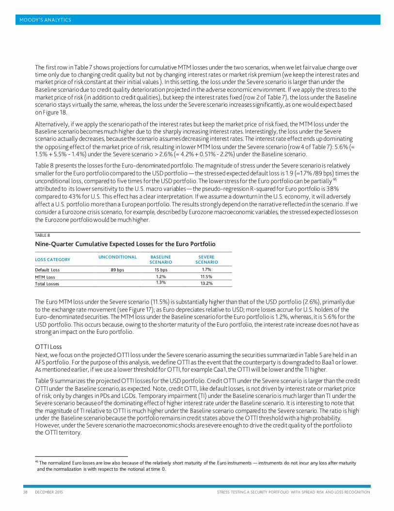
38 DECEMBER 2015 STRESS TESTING A SECURITY PORTFOLIO WITH SPREAD RISK AND LOSS RECOGNITION
The first row in Table 7 shows projections for cumulative MTM losses under the two scenarios, when we let fair value change over time only due to changing credit quality but not by changing interest rates or market risk premium (we keep the interest rates and market price of risk constant at their initial values ). In this setting, the loss under the Severe scenario is larger than under the Baseline scenario due to credit quality deterioration projected in the adverse economic environment. If we apply the stress to the market price of risk (in addition to credit qualities), but keep the interest rates fixed (row 2 of Table 7), the loss under the Baseline scenario stays virtually the same, whereas, the loss under the Severe scenario increases significantly, as one would expect based on Figure 18.
Alternatively, if we apply the scenario path of the interest rates but keep the market price of risk fixed, the MTM loss under the Baseline scenario becomes much higher due to the sharply increasing interest rates. Interestingly, the loss under the Severe scenario actually decreases, because the scenario assumes decreasing interest rates. The interest rate effect ends up dominating the opposing effect of the market price of risk, resulting in lower MTM loss under the Severe scenario (row 4 of Table 7): 5.6% (≈ 1.5% + 5.5% - 1.4%) under the Severe scenario > 2.6% (≈ 4.2% + 0.51% - 2.2%) under the Baseline scenario.
Table 8 presents the losses for the Euro-denominated portfolio. The magnitude of stress under the Severe scenario is relatively smaller for the Euro portfolio compared to the USD portfolio — the stressed expected default loss is 1.9 (=1.7% /89 bps) times the unconditional loss, compared to five times for the USD portfolio. The lower stress for the Euro portfolio can be partially46 attributed to its lower sensitivity to the U.S. macro variables — the pseudo-regression R-squared for Euro portfolio is 38% compared to 43% for U.S. This effect has a clear interpretation. If we assume a downturn in the U.S. economy, it will adversely affect a U.S. portfolio more than a European portfolio. The results strongly depend on the narrative reflected in the scenario. If we consider a Eurozone crisis scenario, for example, described by Eurozone macroeconomic variables, the stressed expected losses on the Eurozone portfolio would be much higher. TABLE 8
Nine-Quarter Cumulative Expected Losses for the Euro Portfolio
LOSS CATEGORY UNCONDITIONAL
BASELINE SCENARIO
SEVERE SCENARIO
Default Loss 89 bps 15 bps 1.7%
MTM Loss 1.2% 11.5%
Total Losses 1.3% 13.2%
The Euro MTM loss under the Severe scenario (11.5%) is substantially higher than that of the USD portfolio (2.6%), primarily due to the exchange rate movement (see Figure 17); as Euro depreciates relative to USD; more losses accrue for U.S. holders of the Euro-denominated securities. The MTM loss under the Baseline scenario for the Euro portfolio is 1.2%, whereas, it is 5.6% for the USD portfolio. This occurs because, owing to the shorter maturity of the Euro portfolio, the interest rate increase does not have as strong an impact on the Euro portfolio.
OTTI Loss Next, we focus on the projected OTTI loss under the Severe scenario assuming the securities summarized in Table 5 are held in an AFS portfolio. For the purpose of this analysis, we define OTTI as the event that the counterparty is downgraded to Baa1 or lower. As mentioned earlier, if we use a lower threshold for OTTI, for example Caa1, the OTTI will be lower and the TI higher.
Table 9 summarizes the projected OTTI losses for the USD portfolio. Credit OTTI under the Severe scenario is larger than the credit OTTI under the Baseline scenario, as expected. Note, credit OTTI, like default losses, is not driven by interest rate or market price of risk; only by changes in PDs and LGDs. Temporary impairment (TI) under the Baseline scenario is much larger than TI under the Severe scenario because of the dominating effect of higher interest rate under the Baseline scenario. It is interesting to note that the magnitude of TI relative to OTTI is much higher under the Baseline scenario compared to the Severe scenario. The ratio is high under the Baseline scenario because the portfolio remains in credit states above the OTTI threshold with a high probability. However, under the Severe scenario the macroeconomic shocks are severe enough to drive the credit quality of the portfolio to the OTTI territory.
46 The normalized Euro losses are low also because of the relatively short maturity of the Euro instruments — instruments do not incur any loss after maturity and the normalization is with respect to the notional at time 0.
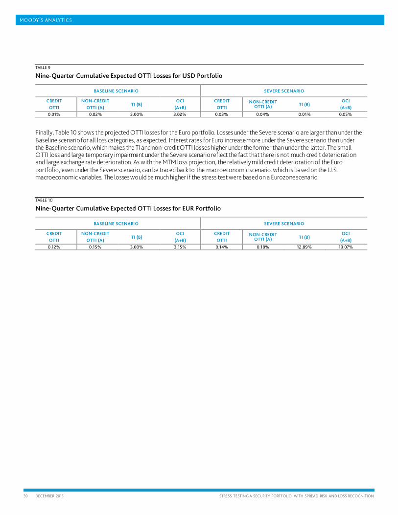
39 DECEMBER 2015 STRESS TESTING A SECURITY PORTFOLIO WITH SPREAD RISK AND LOSS RECOGNITION
TABLE 9
Nine-Quarter Cumulative Expected OTTI Losses for USD Portfolio
BASELINE SCENARIO SEVERE SCENARIO
CREDIT OTTI
NON-CREDIT OTTI (A)
TI (B) OCI
(A+B) CREDIT
OTTI NON-CREDIT
OTTI (A) TI (B) OCI
(A+B) 0.01% 0.02% 3.00% 3.02% 0.03% 0.04% 0.01% 0.05%
Finally, Table 10 shows the projected OTTI losses for the Euro portfolio. Losses under the Severe scenario are larger than under the Baseline scenario for all loss categories, as expected. Interest rates for Euro increase more under the Severe scenario than under the Baseline scenario, which makes the TI and non-credit OTTI losses higher under the former than under the latter. The small OTTI loss and large temporary impairment under the Severe scenario reflect the fact that there is not much credit deterioration and large exchange rate deterioration. As with the MTM loss projection, the relatively mild credit deterioration of the Euro portfolio, even under the Severe scenario, can be traced back to the macroeconomic scenario, which is based on the U.S. macroeconomic variables. The losses would be much higher if the stress test were based on a Eurozone scenario.
TABLE 10
Nine-Quarter Cumulative Expected OTTI Losses for EUR Portfolio
BASELINE SCENARIO SEVERE SCENARIO
CREDIT OTTI
NON-CREDIT OTTI (A)
TI (B) OCI
(A+B) CREDIT
OTTI NON-CREDIT
OTTI (A) TI (B) OCI
(A+B) 0.12% 0.15% 3.00% 3.15% 0.14% 0.18% 12.89% 13.07%
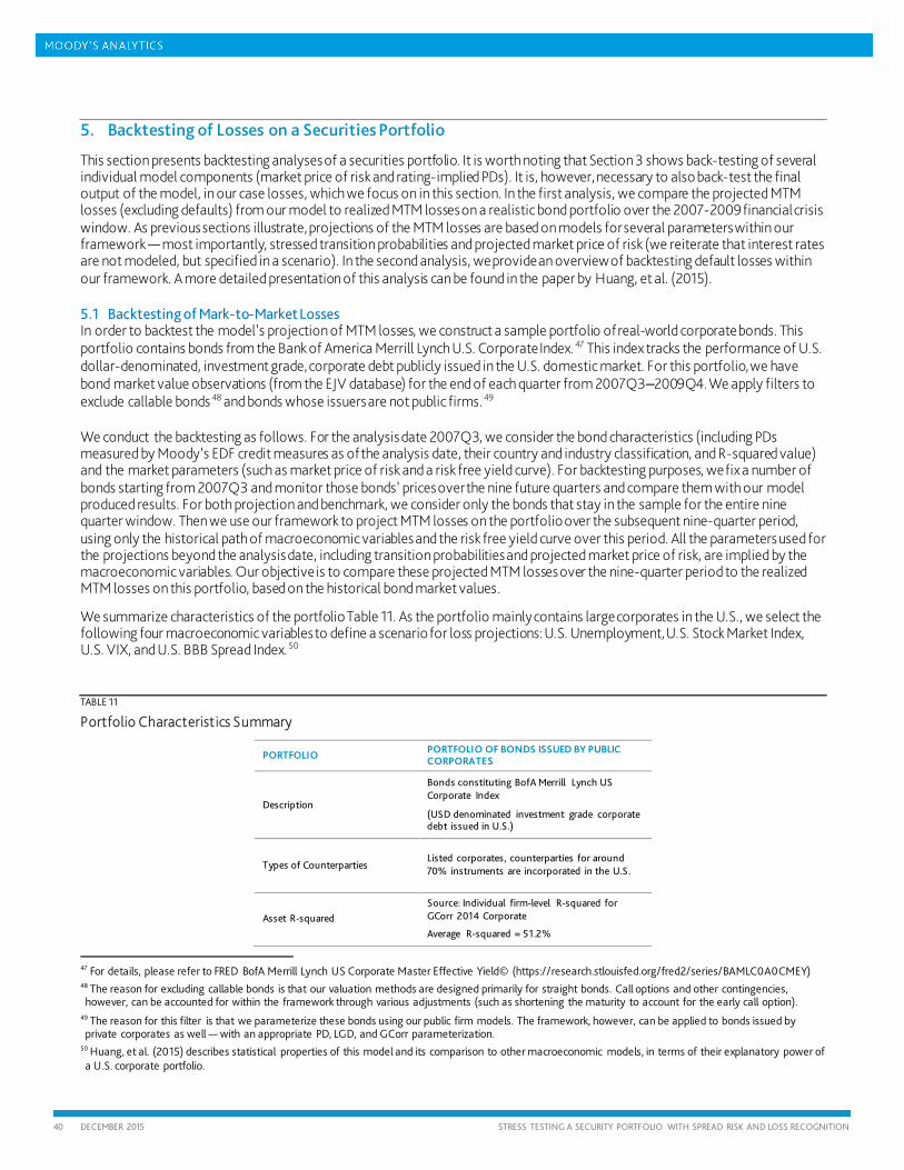
40 DECEMBER 2015 STRESS TESTING A SECURITY PORTFOLIO WITH SPREAD RISK AND LOSS RECOGNITION
5. Backtesting of Losses on a Securities Portfolio
This section presents backtesting analyses of a securities portfolio. It is worth noting that Section 3 shows back-testing of several individual model components (market price of risk and rating-implied PDs). It is, however, necessary to also back-test the final output of the model, in our case losses, which we focus on in this section. In the first analysis, we compare the projected MTM losses (excluding defaults) from our model to realized MTM losses on a realistic bond portfolio over the 2007-2009 financial crisis window. As previous sections illustrate, projections of the MTM losses are based on models for several parameters within our framework — most importantly, stressed transition probabilities and projected market price of risk (we reiterate that interest rates are not modeled, but specified in a scenario). In the second analysis, we provide an overview of backtesting default losses within our framework. A more detailed presentation of this analysis can be found in the paper by Huang, et al. (2015).
5.1 Backtesting of Mark-to-Market Losses In order to backtest the model’s projection of MTM losses, we construct a sample portfolio of real-world corporate bonds. This portfolio contains bonds from the Bank of America Merrill Lynch U.S. Corporate Index. 47 This index tracks the performance of U.S. dollar-denominated, investment grade, corporate debt publicly issued in the U.S. domestic market. For this portfolio, we have bond market value observations (from the EJV database) for the end of each quarter from 2007Q3–2009Q4. We apply filters to exclude callable bonds 48 and bonds whose issuers are not public firms. 49 We conduct the backtesting as follows. For the analysis date 2007Q3, we consider the bond characteristics (including PDs measured by Moody’s EDF credit measures as of the analysis date, their country and industry classification, and R-squared value) and the market parameters (such as market price of risk and a risk free yield curve). For backtesting purposes, we fix a number of bonds starting from 2007Q3 and monitor those bonds’ prices over the nine future quarters and compare them with our model produced results. For both projection and benchmark, we consider only the bonds that stay in the sample for the entire nine quarter window. Then we use our framework to project MTM losses on the portfolio over the subsequent nine-quarter period, using only the historical path of macroeconomic variables and the risk free yield curve over this period. All the parameters used for the projections beyond the analysis date, including transition probabilities and projected market price of risk, are implied by the macroeconomic variables. Our objective is to compare these projected MTM losses over the nine-quarter period to the realized MTM losses on this portfolio, based on the historical bond market values.
We summarize characteristics of the portfolio Table 11. As the portfolio mainly contains large corporates in the U.S., we select the following four macroeconomic variables to define a scenario for loss projections: U.S. Unemployment, U.S. Stock Market Index, U.S. VIX, and U.S. BBB Spread Index. 50
TABLE 11
Portfolio Characteristics Summary
PORTFOLIO PORTFOLIO OF BONDS ISSUED BY PUBLIC CORPORATES
Description
Bonds constituting BofA Merrill Lynch US Corporate Index
(USD denominated investment grade corporate debt issued in U.S.)
Types of Counterparties Listed corporates, counterparties for around 70% instruments are incorporated in the U.S.
Asset R-squared Source: Individual firm-level R-squared for GCorr 2014 Corporate
Average R-squared = 51.2%
47 For details, please refer to FRED BofA Merrill Lynch US Corporate Master Effective Yield© (https://research.stlouisfed.org/fred2/series/BAMLC0A0CMEY) 48 The reason for excluding callable bonds is that our valuation methods are designed primarily for straight bonds. Call options and other contingencies, however, can be accounted for within the framework through various adjustments (such as shortening the maturity to account for the early call option).
49 The reason for this filter is that we parameterize these bonds using our public firm models. The framework, however, can be applied to bonds issued by private corporates as well — with an appropriate PD, LGD, and GCorr parameterization.
50 Huang, et al. (2015) describes statistical properties of this model and its comparison to other macroeconomic models, in terms of their explanatory power of a U.S. corporate portfolio.
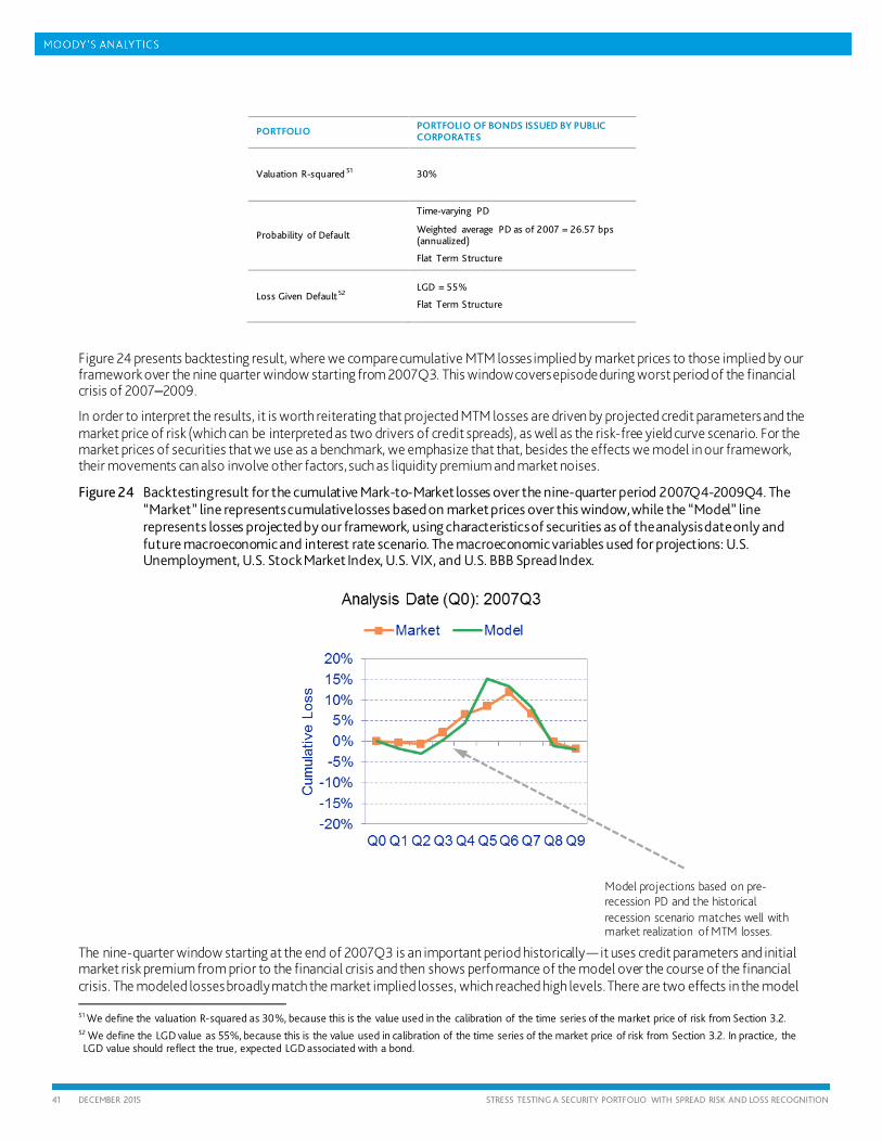
41 DECEMBER 2015 STRESS TESTING A SECURITY PORTFOLIO WITH SPREAD RISK AND LOSS RECOGNITION
PORTFOLIO PORTFOLIO OF BONDS ISSUED BY PUBLIC CORPORATES
Valuation R-squared 51 30%
Probability of Default
Time-varying PD
Weighted average PD as of 2007 = 26.57 bps (annualized)
Flat Term Structure
Loss Given Default52 LGD = 55%
Flat Term Structure
Figure 24 presents backtesting result, where we compare cumulative MTM losses implied by market prices to those implied by our framework over the nine quarter window starting from 2007Q3. This window covers episode during worst period of the financial crisis of 2007–2009.
In order to interpret the results, it is worth reiterating that projected MTM losses are driven by projected credit parameters and the market price of risk (which can be interpreted as two drivers of credit spreads), as well as the risk-free yield curve scenario. For the market prices of securities that we use as a benchmark, we emphasize that that, besides the effects we model in our framework, their movements can also involve other factors, such as liquidity premium and market noises.
Figure 24 Backtesting result for the cumulative Mark-to-Market losses over the nine-quarter period 2007Q4-2009Q4. The “Market” line represents cumulative losses based on market prices over this window, while the “Model” line represents losses projected by our framework, using characteristics of securities as of the analysis date only and future macroeconomic and interest rate scenario. The macroeconomic variables used for projections: U.S. Unemployment, U.S. Stock Market Index, U.S. VIX, and U.S. BBB Spread Index.
The nine-quarter window starting at the end of 2007Q3 is an important period historically — it uses credit parameters and initial market risk premium from prior to the financial crisis and then shows performance of the model over the course of the financial crisis. The modeled losses broadly match the market implied losses, which reached high levels. There are two effects in the model
51 We define the valuation R-squared as 30%, because this is the value used in the calibration of the time series of the market price of risk from Section 3.2. 52 We define the LGD value as 55%, because this is the value used in calibration of the time series of the market price of risk from Section 3.2. In practice, the LGD value should reflect the true, expected LGD associated with a bond.
Model projections based on pre-recession PD and the historical recession scenario matches well with market realization of MTM losses.
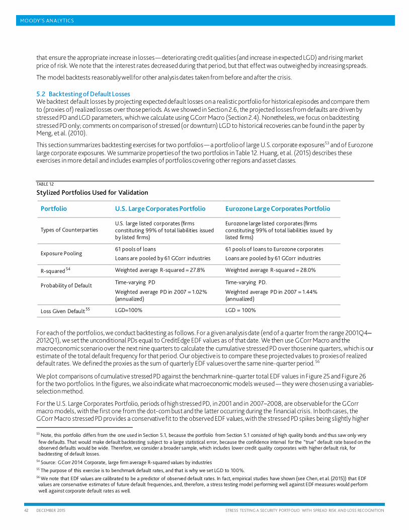
42 DECEMBER 2015 STRESS TESTING A SECURITY PORTFOLIO WITH SPREAD RISK AND LOSS RECOGNITION
that ensure the appropriate increase in losses — deteriorating credit qualities (and increase in expected LGD) and rising market price of risk. We note that the interest rates decreased during that period, but that effect was outweighed by increasing spreads.
The model backtests reasonably well for other analysis dates taken from before and after the crisis.
5.2 Backtesting of Default Losses We backtest default losses by projecting expected default losses on a realistic portfolio for historical episodes and compare them to (proxies of) realized losses over those periods. As we showed in Section 2.6, the projected losses from defaults are driven by stressed PD and LGD parameters, which we calculate using GCorr Macro (Section 2.4). Nonetheless, we focus on backtesting stressed PD only; comments on comparison of stressed (or downturn) LGD to historical recoveries can be found in the paper by Meng, et al. (2010).
This section summarizes backtesting exercises for two portfolios — a portfolio of large U.S. corporate exposures53 and of Eurozone large corporate exposures. We summarize properties of the two portfolios in Table 12. Huang, et al. (2015) describes these exercises in more detail and includes examples of portfolios covering other regions and asset classes.
TABLE 12
Stylized Portfolios Used for Validation
Portfolio U.S. Large Corporates Portfolio Eurozone Large Corporates Portfolio
Types of Counterparties U.S. large listed corporates (firms constituting 99% of total liabilities issued by listed firms)
Eurozone large listed corporates (firms constituting 99% of total liabilities issued by listed firms)
Exposure Pooling 61 pools of loans
Loans are pooled by 61 GCorr industries
61 pools of loans to Eurozone corporates
Loans are pooled by 61 GCorr industries
R-squared 54 Weighted average R-squared = 27.8% Weighted average R-squared = 28.0%
Probability of Default
Time-varying PD
Weighted average PD in 2007 = 1.02% (annualized)
Time-varying PD.
Weighted average PD in 2007 = 1.44% (annualized)
Loss Given Default 55 LGD=100% LGD = 100%
For each of the portfolios, we conduct backtesting as follows. For a given analysis date (end of a quarter from the range 2001Q4–2012Q1), we set the unconditional PDs equal to CreditEdge EDF values as of that date. We then use GCorr Macro and the macroeconomic scenario over the next nine quarters to calculate the cumulative stressed PD over those nine quarters, which is our estimate of the total default frequency for that period. Our objective is to compare these projected values to proxies of realized default rates. We defined the proxies as the sum of quarterly EDF values over the same nine-quarter period. 56
We plot comparisons of cumulative stressed PD against the benchmark nine-quarter total EDF values in Figure 25 and Figure 26 for the two portfolios. In the figures, we also indicate what macroeconomic models we used — they were chosen using a variables- selection method.
For the U.S. Large Corporates Portfolio, periods of high stressed PD, in 2001 and in 2007–2008, are observable for the GCorr macro models, with the first one from the dot-com bust and the latter occurring during the financial crisis. In both cases, the GCorr Macro stressed PD provides a conservative fit to the observed EDF values, with the stressed PD spikes being slightly higher
53 Note, this portfolio differs from the one used in Section 5.1, because the portfolio from Section 5.1 consisted of high quality bonds and thus saw only very few defaults. That would make default backtesting subject to a large statistical error, because the confidence interval for the “true” default rate based on the observed defaults would be wide. Therefore, we consider a broader sample, which includes lower credit quality corporates with higher default risk, for backtesting of default losses.
54 Source: GCorr 2014 Corporate, large firm average R-squared values by industries 55 The purpose of this exercise is to benchmark default rates, and that is why we set LGD to 100%. 56 We note that EDF values are calibrated to be a predictor of observed default rates. In fact, empirical studies have shown (see Chen, et al. (2015)) that EDF values are conservative estimates of future default frequencies, and, therefore, a stress testing model performing well against EDF measures would perform well against corporate default rates as well.
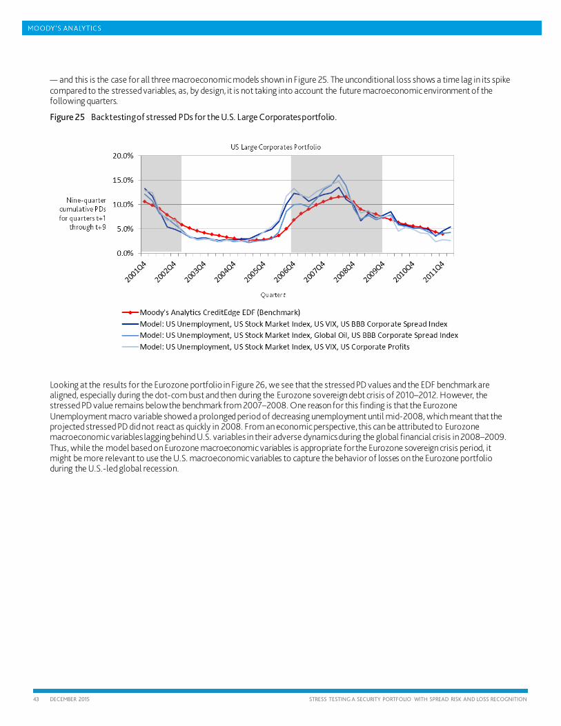
43 DECEMBER 2015 STRESS TESTING A SECURITY PORTFOLIO WITH SPREAD RISK AND LOSS RECOGNITION
— and this is the case for all three macroeconomic models shown in Figure 25. The unconditional loss shows a time lag in its spike compared to the stressed variables, as, by design, it is not taking into account the future macroeconomic environment of the following quarters.
Figure 25 Backtesting of stressed PDs for the U.S. Large Corporates portfolio.
Looking at the results for the Eurozone portfolio in Figure 26, we see that the stressed PD values and the EDF benchmark are aligned, especially during the dot-com bust and then during the Eurozone sovereign debt crisis of 2010–2012. However, the stressed PD value remains below the benchmark from 2007–2008. One reason for this finding is that the Eurozone Unemployment macro variable showed a prolonged period of decreasing unemployment until mid-2008, which meant that the projected stressed PD did not react as quickly in 2008. From an economic perspective, this can be attributed to Eurozone macroeconomic variables lagging behind U.S. variables in their adverse dynamics during the global financial crisis in 2008–2009. Thus, while the model based on Eurozone macroeconomic variables is appropriate for the Eurozone sovereign crisis period, it might be more relevant to use the U.S. macroeconomic variables to capture the behavior of losses on the Eurozone portfolio during the U.S.-led global recession.
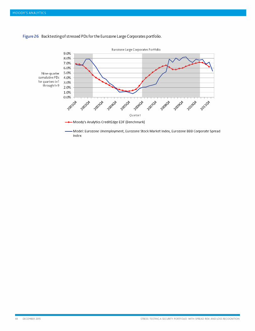
44 DECEMBER 2015 STRESS TESTING A SECURITY PORTFOLIO WITH SPREAD RISK AND LOSS RECOGNITION
Figure 26 Backtesting of stressed PDs for the Eurozone Large Corporates portfolio.
45 DECEMBER 2015 STRESS TESTING A SECURITY PORTFOLIO WITH SPREAD RISK AND LOSS RECOGNITION
6. Summary
This paper introduces a framework for stress testing a portfolio of credit risk-sensitive securities. Given a macroeconomic and interest rate scenario, the framework projects stressed expected losses on the portfolio for multiple future periods. An important feature of such calculations is a loss recognition rule — it is necessary to align the loss calculation with how institutions recognize accounting losses. The framework distinguishes whether the portfolio contains instruments in a trading book and fair value loans 57 (in this case, losses are recognized according to the Mark-to-Market method) or for investment (in this case, losses are recognized depending on whether the securities are Held-to-Maturity or Available-for-Sale). For trading portfolios, loss correspond to fluctuations in fair value of the instrument, while for investment portfolios, losses are recognized in earnings only in the cases of OTTI. We consider several potential definitions of OTTI in our framework, one of which is directly linked to agency ratings – in line with how many institutions interpret OTTI in their regular accounting and financial reporting. Crucially, we bifurcate the total OTTI losses into components associated with credit quality deterioration and with market parameters movements.
We built the framework from the bottom-up — modeling dynamics of credit qualities for individual issuers projecting losses on individual bonds and then aggregating them to the portfolio level. The calculations take various instrument and issuer characteristics as inputs, including point-in-time PD as of the analysis date and sensitivity of issuer’s credit quality to systematic shocks (which can be obtained from the GCorr model). We use the GCorr Macro model to link credit qualities to macroeconomic variables, which allows us to project stressed PDs, stressed LGDs, and stressed Transition Probabilities. For many securities with a high credit quality, the main drivers of fair values are, however, the market price of risk and the risk-free yield curve. We therefore model the market price of risk in relation to the macroeconomic variables, if it is not specified in the macroeconomic scenario, and we utilize the paths of risk-free rates that as defined by the scenario. Our framework measures credit qualities in terms of PDs, and we, therefore, also incorporate a model linking PDs to agency ratings (rating-implied PD) under a specific scenario into our framework.
Additionally, we validate various components of our framework — stressed PDs, the model for market risk premium, and the model for rating-implied PD. We also validate overall model outputs: projected losses from defaults and projected Mark-to-Market losses. We focus, in terms of estimating certain parameters as well as validation, on the periods before, during, and after the financial crisis (for some estimation and analyses, we consider a period from the late 1990’s through 2014, dominated by the financial crisis). Thus, scenarios representing recent economic episodes are the most relevant to which our framework can be applied. Using the framework for other scenarios is possible, but one must consider whether the calculation requires re-calibration of some parameters and additional validation analyses.
While this paper addresses using our framework for vanilla corporate bonds, the calculations are applicable — with appropriate parameterization — to other asset classes as well (even if the calculations are approximate in some cases): callable corporate bonds, sovereign bonds, municipal bonds, agency bonds etc. By bringing in a scenario for a foreign exchange rate, the framework can also project losses on instruments denominated in a currency different from the reporting currency. Moody’s Analytics Structured Analytics and ValuationTM (SAV) can calculate OTTI under stress scenarios for structured securities.
57 Loans held-for-sale and loans held for investment with fair value option.
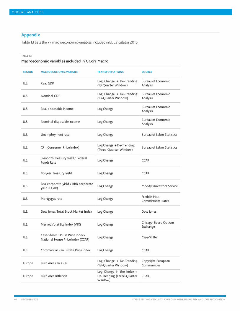
46 DECEMBER 2015 STRESS TESTING A SECURITY PORTFOLIO WITH SPREAD RISK AND LOSS RECOGNITION
Appendix
Table 13 lists the 77 macroeconomic variables included in EL Calculator 2015.
TABLE 13
Macroeconomic variables included in GCorr Macro
REGION MACROECONOMIC VARIABLE TRANSFORMATIONS SOURCE
U.S. Real GDP Log Change + De-Trending (13 Quarter Window)
Bureau of Economic Analysis
U.S. Nominal GDP Log Change + De-Trending (13-Quarter Window)
Bureau of Economic Analysis
U.S. Real disposable income Log Change Bureau of Economic Analysis
U.S. Nominal disposable income Log Change Bureau of Economic Analysis
U.S. Unemployment rate Log Change Bureau of Labor Statistics
U.S. CPI (Consumer Price Index) Log Change + De-Trending (Three-Quarter Window)
Bureau of Labor Statistics
U.S. 3-month Treasury yield / Federal Funds Rate
Log Change CCAR
U.S. 10-year Treasury yield Log Change CCAR
U.S. Baa corporate yield / BBB corporate yield (CCAR) Log Change Moody's Investors Service
U.S. Mortgages rate Log Change Freddie Mac Commitment Rates
U.S. Dow Jones Total Stock Market Index Log Change Dow Jones
U.S. Market Volatility Index (VIX) Log Change Chicago Board Options Exchange
U.S. Case-Shiller House Price Index / National House Price Index (CCAR)
Log Change Case-Shiller
U.S. Commercial Real Estate Price Index Log Change CCAR
Europe Euro Area real GDP Log Change + De-Trending (13-Quarter Window)
Copyright European Communities
Europe Euro Area Inflation Log Change in the Index + De-Trending (Three-Quarter Window)
CCAR
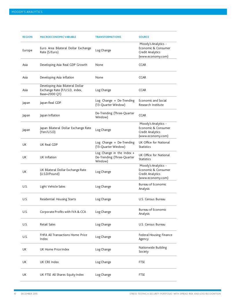
47 DECEMBER 2015 STRESS TESTING A SECURITY PORTFOLIO WITH SPREAD RISK AND LOSS RECOGNITION
REGION MACROECONOMIC VARIABLE TRANSFORMATIONS SOURCE
Europe Euro Area Bilateral Dollar Exchange Rate ($/Euro) Log Change
Moody’s Analytics - Economic & Consumer Credit Analytics (www.economy.com)
Asia Developing Asia Real GDP Growth None CCAR
Asia Developing Asia inflation None CCAR
Asia Developing Asia Bilateral Dollar Exchange Rate (F/U.S.D, index, Base=2000 Q1)
Log Change CCAR
Japan Japan Real GDP Log Change + De-Trending (13-Quarter Window)
Economic and Social Research Institute
Japan Japan Inflation De-Trending (Three-Quarter Window) CCAR
Japan Japan Bilateral Dollar Exchange Rate (Yen/U.S.D)
Log Change
Moody’s Analytics - Economic & Consumer Credit Analytics (www.economy.com)
UK UK Real GDP Log Change + De-Trending (13-Quarter Window)
UK Office for National Statistics
UK UK Inflation Log Change in the Index + De-Trending (Three-Quarter Window)
UK Office for National Statistics
UK UK Bilateral Dollar Exchange Rate (U.S.D/Pound)
Log Change
Moody’s Analytics - Economic & Consumer Credit Analytics (www.economy.com)
U.S. Light Vehicle Sales Log Change Bureau of Economic Analysis
U.S. Residential Housing Starts Log Change U.S. Census Bureau
U.S. Corporate Profits with IVA & CCA Log Change Bureau of Economic Analysis
U.S. Retail Sales Log Change U.S. Census Bureau
U.S. FHFA All Transactions Home Price Index
Log Change Federal Housing Finance Agency
UK UK Home Price Index Log Change Nationwide Building Society
UK UK CRE Index Log Change FTSE
UK UK FTSE All Shares Equity Index Log Change FTSE
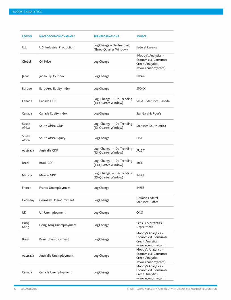
48 DECEMBER 2015 STRESS TESTING A SECURITY PORTFOLIO WITH SPREAD RISK AND LOSS RECOGNITION
REGION MACROECONOMIC VARIABLE TRANSFORMATIONS SOURCE
U.S. U.S. Industrial Production Log Change + De-Trending (Three-Quarter Window)
Federal Reserve
Global Oil Price Log Change
Moody’s Analytics - Economic & Consumer Credit Analytics (www.economy.com)
Japan Japan Equity Index Log Change Nikkei
Europe Euro Area Equity Index Log Change STOXX
Canada Canada GDP Log Change + De-Trending (13-Quarter Window) STCA - Statistics Canada
Canada Canada Equity Index Log Change Standard & Poor's
South Africa South Africa GDP
Log Change + De-Trending (13-Quarter Window) Statistics South Africa
South Africa
South Africa Equity Log Change FTSE
Australia Australia GDP Log Change + De-Trending (13-Quarter Window)
AU.S.T
Brazil Brazil GDP Log Change + De-Trending (13-Quarter Window)
IBGE
Mexico Mexico GDP Log Change + De-Trending (13-Quarter Window)
INEGI
France France Unemployment Log Change INSEE
Germany Germany Unemployment Log Change German Federal Statistical Office
UK UK Unemployment Log Change ONS
Hong Kong Hong Kong Unemployment Log Change
Census & Statistics Department
Brazil Brazil Unemployment Log Change
Moody’s Analytics - Economic & Consumer Credit Analytics (www.economy.com)
Australia Australia Unemployment Log Change
Moody’s Analytics - Economic & Consumer Credit Analytics (www.economy.com)
Canada Canada Unemployment Log Change
Moody’s Analytics - Economic & Consumer Credit Analytics (www.economy.com)
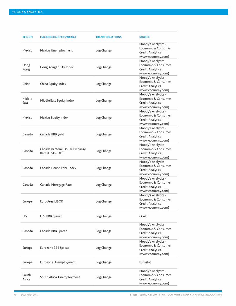
49 DECEMBER 2015 STRESS TESTING A SECURITY PORTFOLIO WITH SPREAD RISK AND LOSS RECOGNITION
REGION MACROECONOMIC VARIABLE TRANSFORMATIONS SOURCE
Mexico Mexico Unemployment Log Change
Moody’s Analytics - Economic & Consumer Credit Analytics (www.economy.com)
Hong Kong
Hong Kong Equity Index Log Change
Moody’s Analytics - Economic & Consumer Credit Analytics (www.economy.com)
China China Equity Index Log Change
Moody’s Analytics - Economic & Consumer Credit Analytics (www.economy.com)
Middle East
Middle East Equity Index Log Change
Moody’s Analytics - Economic & Consumer Credit Analytics (www.economy.com)
Mexico Mexico Equity Index Log Change
Moody’s Analytics - Economic & Consumer Credit Analytics (www.economy.com)
Canada Canada BBB yield Log Change
Moody’s Analytics - Economic & Consumer Credit Analytics (www.economy.com)
Canada Canada Bilateral Dollar Exchange Rate (U.S.D/CAD)
Log Change
Moody’s Analytics - Economic & Consumer Credit Analytics (www.economy.com)
Canada Canada House Price Index Log Change
Moody’s Analytics - Economic & Consumer Credit Analytics (www.economy.com)
Canada Canada Mortgage Rate Log Change
Moody’s Analytics - Economic & Consumer Credit Analytics (www.economy.com)
Europe Euro Area LIBOR Log Change
Moody’s Analytics - Economic & Consumer Credit Analytics (www.economy.com)
U.S. U.S. BBB Spread Log Change CCAR
Canada Canada BBB Spread Log Change
Moody’s Analytics - Economic & Consumer Credit Analytics (www.economy.com)
Europe Eurozone BBB Spread Log Change
Moody’s Analytics - Economic & Consumer Credit Analytics (www.economy.com)
Europe Eurozone Unemployment Log Change Eurostat
South Africa
South Africa Unemployment Log Change
Moody’s Analytics - Economic & Consumer Credit Analytics (www.economy.com)
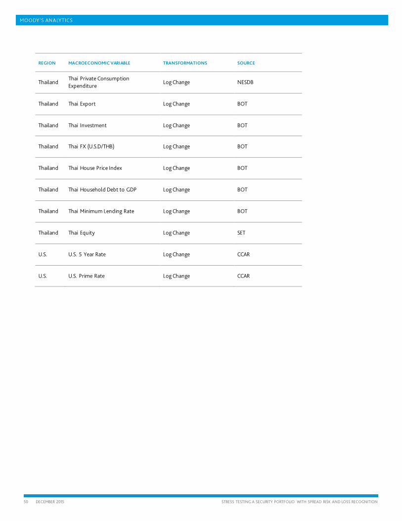
50 DECEMBER 2015 STRESS TESTING A SECURITY PORTFOLIO WITH SPREAD RISK AND LOSS RECOGNITION
REGION MACROECONOMIC VARIABLE TRANSFORMATIONS SOURCE
Thailand Thai Private Consumption Expenditure
Log Change NESDB
Thailand Thai Export Log Change BOT
Thailand Thai Investment Log Change BOT
Thailand Thai FX (U.S.D/THB) Log Change BOT
Thailand Thai House Price Index Log Change BOT
Thailand Thai Household Debt to GDP Log Change BOT
Thailand Thai Minimum Lending Rate Log Change BOT
Thailand Thai Equity Log Change SET
U.S. U.S. 5 Year Rate Log Change CCAR
U.S. U.S. Prime Rate Log Change CCAR
51 DECEMBER 2015 STRESS TESTING A SECURITY PORTFOLIO WITH SPREAD RISK AND LOSS RECOGNITION
References
Agrawal, Deepak, Navneet Arora, and Jeffrey Bohn, “Parsimony In Practice: An EDF-Based Model Of Credit Spreads.” Moody’s Analytics White Paper, April 2004.
Chen, Nan, Houman Dehghan, Min Ding, Jian Du, James Edwards, Danielle Ferry, Pooya Nazeran, Sue Zhang, Douglas Dwyer, Jing Zhang, “EDF9: Introduction and Overview.” Moody’s Analytics White Paper, February 2015.
DFAST, “Dodd-Frank Act Stress Test 2015: Supervisory Stress Test Methodology and Results.” Board of Governors of the Federal Reserve System, March 2015.
Dwyer, Douglas, Zan Li, Shisheng Qu, Heather Russell, Jing Zhang, “CDS-implied EDFTM Credit Measures and Fair-value Spreads. ” Moody’s Analytics White Paper, March 2010.
Huang, Jimmy, Mariano Lanfranconi, Nihil Patel, Libor Pospisil, “Modeling Credit Correlations: An Overview of the Moody’s Analytics GCorr Model.” Moody’s Analytics White Paper, December 2012.
Huang, Jimmy, Marc Mitrovic, Olcay Ozkanoglu, Nihil Patel, and Libor Pospisil, “Understanding GCorr® 2014 Corporate.” Moody’s Analytics White Paper, December 2014.
Huang, Jimmy, Mariano Lanfranconi, Albert Lee, Amnon Levy, Marc Mitrovic, Olcay Ozkanoglu, Nihil Patel, Libor Pospisil, and Kevin Yang, “Using GCorr® Macro for Multi-Period Stress Testing of Credit Portfolios.” Moody’s Analytics White Paper, January 2015.
Meng, Qiang, Amnon Levy, Andrew Kaplin, Yashan Wang, and Zhenya Hu, “Implications of PD-LGD Correlation in a Portfolio Setting.” Moody’s Analytics White Paper, February 2010.
Moody’s Analytics, 2015, “Modeling Credit Portfolios, RiskFrontier Methodology,” Fifth Edition.
Pospisil, Libor, Nihil Patel, Amnon Levy, and Qiang Meng, “Parameterizing the RiskFrontier™ PD-LGD Correlation Model.” Moody’s Analytics White Paper, February 2014.
52 DECEMBER 2015 STRESS TESTING A SECURITY PORTFOLIO WITH SPREAD RISK AND LOSS RECOGNITION
© Copyright 2016 Moody’s Corporation, Moody’s Investors Service, Inc., Moody’s Analytics, Inc. and/or their licensors and affiliates (collectively, “MOODY’S”). All rights reserved.
CREDIT RATINGS ISSUED BY MOODY'S INVESTORS SERVICE, INC. (“MIS”) AND ITS AFFILIATES ARE MOODY’S CURRENT OPINIONS OF THE RELATIVE FUTURE CREDIT RISK OF ENTITIES, CREDIT COMMITMENTS, OR DEBT OR DEBT-LIKE SECURITIES, AND CREDIT RATINGS AND RESEARCH PUBLICATIONS PUBLISHED BY MOODY’S (“MOODY’S PUBLICATIONS”) MAY INCLUDE MOODY’S CURRENT OPINIONS OF THE RELATIVE FUTURE CREDIT RISK OF ENTITIES, CREDIT COMMITMENTS, OR DEBT OR DEBT-LIKE SECURITIES. MOODY’S DEFINES CREDIT RISK AS THE RISK THAT AN ENTITY MAY NOT MEET ITS CONTRACTUAL, FINANCIAL OBLIGATIONS AS THEY COME DUE AND ANY ESTIMATED FINANCIAL LOSS IN THE EVENT OF DEFAULT. CREDIT RATINGS DO NOT ADDRESS ANY OTHER RISK, INCLUDING BUT NOT LIMITED TO: LIQUIDITY RISK, MARKET VALUE RISK, OR PRICE VOLATILITY. CREDIT RATINGS AND MOODY’S OPINIONS INCLUDED IN MOODY’S PUBLICATIONS ARE NOT STATEMENTS OF CURRENT OR HISTORICAL FACT. MOODY’S PUBLICATIONS MAY ALSO INCLUDE QUANTITATIVE MODEL-BASED ESTIMATES OF CREDIT RISK AND RELATED OPINIONS OR COMMENTARY PUBLISHED BY MOODY’S ANALYTICS, INC. CREDIT RATINGS AND MOODY’S PUBLICATIONS DO NOT CONSTITUTE OR PROVIDE INVESTMENT OR FINANCIAL ADVICE, AND CREDIT RATINGS AND MOODY’S PUBLICATIONS ARE NOT AND DO NOT PROVIDE RECOMMENDATIONS TO PURCHASE, SELL, OR HOLD PARTICULAR SECURITIES. NEITHER CREDIT RATINGS NOR MOODY’S PUBLICATIONS COMMENT ON THE SUITABILITY OF AN INVESTMENT FOR ANY PARTICULAR INVESTOR. MOODY’S ISSUES ITS CREDIT RATINGS AND PUBLISHES MOODY’S PUBLICATIONS WITH THE EXPECTATION AND UNDERSTANDING THAT EACH INVESTOR WILL, WITH DUE CARE, MAKE ITS OWN STUDY AND EVALUATION OF EACH SECURITY THAT IS UNDER CONSIDERATION FOR PURCHASE, HOLDING, OR SALE.
MOODY’S CREDIT RATINGS AND MOODY’S PUBLICATIONS ARE NOT INTENDED FOR USE BY RETAIL INVESTORS AND IT WOULD BE RECKLESS FOR RETAIL INVESTORS TO CONSIDER MOODY’S CREDIT RATINGS OR MOODY’S PUBLICATIONS IN MAKING ANY INVESTMENT DECISION. IF IN DOUBT YOU SHOULD CONTACT YOUR FINANCIAL OR OTHER PROFESSIONAL ADVISER.
ALL INFORMATION CONTAINED HEREIN IS PROTECTED BY LAW, INCLUDING BUT NOT LIMITED TO, COPYRIGHT LAW, AND NONE OF SUCH INFORMATION MAY BE COPIED OR OTHERWISE REPRODUCED, REPACKAGED, FURTHER TRANSMITTED, TRANSFERRED, DISSEMINATED, REDISTRIBUTED OR RESOLD, OR STORED FOR SUBSEQUENT USE FOR ANY SUCH PURPOSE, IN WHOLE OR IN PART, IN ANY FORM OR MANNER OR BY ANY MEANS WHATSOEVER, BY ANY PERSON WITHOUT MOODY’S PRIOR WRITTEN CONSENT.
All information contained herein is obtained by MOODY’S from sources believed by it to be accurate and reliable. Because of the possibility of human or mechanical error as well as other factors, however, all information contained herein is provided “AS IS” without warranty of any kind. MOODY'S adopts all necessary measures so that the information it uses in assigning a credit rating is of sufficient quality and from sources MOODY'S considers to be reliable including, when appropriate, independent third-party sources. However, MOODY’S is not an auditor and cannot in every instance independently verify or validate information received in the rating process or in preparing the Moody’s Publications.
To the extent permitted by law, MOODY’S and its directors, officers, employees, agents, representatives, licensors and suppliers disclaim liability to any person or entity for any indirect, special, consequential, or incidental losses or damages whatsoever arising from or in connection with the information contained herein or the use of or inability to use any such information, even if MOODY’S or any of its directors, officers, employees, agents, representatives, licensors or suppliers is advised in advance of the possibility of such losses or damages, including but not limited to: (a) any loss of present or prospective profits or (b) any loss or damage arising where the relevant financial instrument is not the subject of a particular credit rating assigned by MOODY’S.
To the extent permitted by law, MOODY’S and its directors, officers, employees, agents, representatives, licensors and suppliers disclaim liability for any direct or compensatory losses or damages caused to any person or entity, including but not limited to by any negligence (but excluding fraud, willful misconduct or any other type of liability that, for the avoidance of doubt, by law cannot be excluded) on the part of, or any contingency within or beyond the control of, MOODY’S or any of its directors, officers, employees, agents, representatives, licensors or suppliers, arising from or in connection with the information contained herein or the use of or inability to use any such information.
NO WARRANTY, EXPRESS OR IMPLIED, AS TO THE ACCURACY, TIMELINESS, COMPLETENESS, MERCHANTABILITY OR FITNESS FOR ANY PARTICULAR PURPOSE OF ANY SUCH RATING OR OTHER OPINION OR INFORMATION IS GIVEN OR MADE BY MOODY’S IN ANY FORM OR MANNER WHATSOEVER.
MIS, a wholly-owned credit rating agency subsidiary of Moody’s Corporation (“MCO”), hereby discloses that most issuers of debt securities (including corporate and municipal bonds, debentures, notes and commercial paper) and preferred stock rated by MIS have, prior to assignment of any rating, agreed to pay to MIS for appraisal and rating services rendered by it fees ranging from $1,500 to approximately $2,500,000. MCO and MIS also maintain policies and procedures to address the independence of MIS’s ratings and rating processes. Information regarding certain affiliations that may exist between directors of MCO and rated entities, and between entities who hold ratings from MIS and have also publicly reported to the SEC an ownership interest in MCO of more than 5%, is posted annually at www.moodys.com under the heading “Shareholder Relations — Corporate Governance — Director and Shareholder Affiliation Policy.”
For Australia only: Any publication into Australia of this document is pursuant to the Australian Financial Services License of MOODY’S affiliate, Moody’s Investors Service Pty Limited ABN 61 003 399 657AFSL 336969 and/or Moody’s Analytics Australia Pty Ltd ABN 94 105 136 972 AFSL 383569 (as applicable). This document is intended to be provided only to “wholesale clients” within the meaning of section 761G of the Corporations Act 2001. By continuing to access this document from within Australia, you represent to MOODY’S that you are, or are accessing the document as a representative of, a “wholesale client” and that neither you nor the entity you represent will directly or indirectly disseminate this document or its contents to “retail clients” within the meaning of section 761G of the Corporations Act 2001. MOODY’S credit rating is an opinion as to the creditworthiness of a debt obligation of the issuer, not on the equity securities of the issuer or any form of security that is available to retail clients. It would be dangerous for “retail clients” to make any investment decision based on MOODY’S credit rating. If in doubt you should contact your financial or other professional adviser.