strong-lensing systems

MNRAS 000, 000–000 (2017) Preprint 9 September 2020 Compiled using MNRAS LATEX style file v3.0

Testing dark energy models with a new sample ofstrong-lensing systems

Mario H. Amante1?, Juan Magana2,3,4 †, V. Motta4‡, Miguel A. Garcıa-Aspeitia1,5§ andTomas Verdugo6¶1 Unidad Academica de Fısica, Universidad Autonoma de Zacatecas,

Calzada Solidaridad esquina con Paseo a la Bufa S/N C.P. 98060,Zacatecas, Mexico.2Instituto de Astrofısica, Pontificia Universidad Catolica de Chile, Av. Vicuna Mackenna, 4860, Santiago, Chile.3Centro de Astro-Ingenierıa, Pontificia Universidad Catolica de Chile, Av. Vicuna Mackenna, 4860, Santiago, Chile.4Instituto de Fısica y Astronomıa, Facultad de Ciencias,

Universidad de Valparaıso, Avda. Gran Bretana 1111, Valparaıso, Chile.5Consejo Nacional de Ciencia y Tecnologıa, Av. Insurgentes Sur 1582.

Colonia Credito Constructor, Del. Benito Juarez C.P. 03940, Ciudad de Mexico, Mexico.6Instituto de Astronomıa, Universidad Nacional Autonoma de Mexico, Apartado postal 106, C.P. 22800, Ensenada, B.C., Mexico

Accepted YYYYMMDD. Received YYYYMMDD; in original form YYYYMMDD

ABSTRACTInspired by a new compilation of strong lensing systems, which consist of 204 pointsin the redshift range 0.0625 < zl < 0.958 for the lens and 0.196 < zs < 3.595 for thesource, we constrain three models that generate a late cosmic acceleration: the ω-colddark matter model, the Chevallier-Polarski-Linder and the Jassal-Bagla-Padmanabhanparametrizations. Our compilation contains only those systems with early type galax-ies acting as lenses, with spectroscopically measured stellar velocity dispersions, esti-mated Einstein radius, and both the lens and source redshifts. We assume an axiallysymmetric mass distribution in the lens equation, using a correction to alleviate differ-ences between the measured velocity dispersion (σ) and the dark matter halo velocitydispersion (σDM ) as well as other systematic errors that may affect the measurements.We have considered different sub-samples to constrain the cosmological parameters ofeach model. Additionally, we generate a mock data of SLS to asses the impact of thechosen mass profile on the accuracy of Einstein radius estimation. Our results showthat cosmological constraints are very sensitive to the selected data: some cases showconvergence problems in the estimation of cosmological parameters (e.g. systems withobserved distance ratio Dobs < 0.5), others show high values for the chi-square func-tion (e.g. systems with a lens equation Dobs > 1 or high velocity dispersion σ > 276km s−1). However, we obtained a fiduciary sample with 143 systems which improvesthe constraints on each tested cosmological model.

Key words: gravitational lensing: strong, dark energy, cosmology: observations,cosmology: theory, cosmological parameters.

1 INTRODUCTION

Contrasting cosmological models with modern observationsis fundamental to understand the nature of the ∼ 96% of ourUniverse (Planck Collaboration et al. 2016; Aghanim et al.2018a) known as the dark sector, which refers to ∼ 26% ofthe total content in dark matter (DM) the one responsible

? E-mail:[email protected]† E-mail:[email protected]‡ E-mail: [email protected]§ E-mail:[email protected]¶ E-mail:[email protected]

for the formation of large-scale structure, and ∼ 69% in darkenergy (DE), the possible cause for the current acceleratedexpansion (Schmidt et al. 1998; Perlmutter et al. 1999; Riesset al. 1998). In the most accepted paradigm, DM is a non-relativistic matter in the decoupling epoch (i.e. cold), andthe traditional way to treat the DE nature is through theaddition of an effective cosmological constant (CC) in theenergy-momentum tensor of the Einstein field equations.The CC origin is related to the quantum vacuum fluctu-ations, but this hypothesis is plagued by severe patholo-gies due to its inability to renormalize the energy density ofquantum vacuum, obtaining a discrepancy of ∼ 120 orders

c© 2017 The Authors

arX

iv:1

906.

0410

7v2

[as

tro-

ph.C

O]

8 S

ep 2

020

2 H. Amante, Magana, Motta, Garcıa-Aspeitia, Verdugo

of magnitude between the theoretical estimations and thecosmological observations (Zeldovich 1968; Weinberg 1989).The CC also has the coincidence problem, i.e. why the Uni-verse transition, from a decelerated to an accelerated phase,is produced at late times.

The CC theoretical problems have led the community topropose a variety of ideas to reproduce the late cosmic accel-eration. Some of them postulate the existence of DE, for ex-ample, quintessence (Ratra & Peebles 1988; Wetterich 1988),phantom (Chiba et al. 2000; Caldwell 2002) fields, Chap-lygin gas (Chaplygin 1904; Kamenshchik et al. 2001; Bilicet al. 2002; Hernandez-Almada et al. 2018), w(z) parame-terizations for dynamical DE (Chevallier & Polarski 2001;Linder 2003; Jassal et al. 2005), interacting dark energy(Caldera-Cabral et al. 2009), etc (for a thorough review of allthese alternatives see Copeland et al. 2006; Li et al. 2011).Other models modify the Einsteinian gravity to resemblethe DE like brane models (Garcıa-Aspeitia & Matos 2011;Garcıa-Aspeitia et al. 2018a; Garcıa-Aspeitia et al. 2018b),f(R) models (Buchdahl 1970; Starobinsky 1980; Sotiriou &Faraoni 2010), scalar-tensor theories (Brans & Dicke 1961;Galiautdinov & Kopeikin 2016; Langlois et al. 2018), Uni-modular gravity (Perez & Sudarsky 2017; Garcıa-Aspeitiaet al. 2019), among others.

On the other hand, observational data are used to testthese models. Among the most frequently used are the cos-mic microwave background radiation (CMB, Planck Collab-oration et al. 2016; Aghanim et al. 2018a), baryonic acous-tic oscillations (BAO, Eisenstein et al. 2005; Blake et al.2012; Alam et al. 2017; Bautista et al. 2017), type Ia Super-novae (SNe Ia, Scolnic et al. 2018) and observational Hub-ble data (OHD, Jimenez & Loeb 2002; Moresco et al. 2016;Magana et al. 2018). Consistency in the cosmological pa-rameters among different techniques, rather than more ac-curate measurements, is desirable to better understand thenature of DE. In the last years, several efforts have beenmade by the community to include gravitational lens sys-tems in the study of the Universe’s evolution. Some of thepioneers are Futamase & Yoshida (2001); Biesiada (2006),who used only one strong-lens system to study some of themost popular cosmological models. Grillo et al. (2008) intro-duced a methodology to estimate cosmological parametersusing Strong Lensing Systems (SLS) (see also Jullo et al.2010; Magana et al. 2015, 2018). They apply the relationbetween the Einstein radius and the central stellar velocitydispersion assuming an isothermal profile for the total den-sity distribution of the lens (elliptical) galaxy. Their simula-tions found that the method is accurate enough to obtain in-formation about the underlying cosmology. They concludedthat the stellar velocity dispersion and velocity dispersionof the isothermal lens model are very similar in the w colddark matter (wCDM) model. Biesiada et al. (2010) usedthe same procedure comparing a distance ratio, Dobs, con-structed from SLS observations such as the Einstein radiusand spectroscopic velocity dispersion of the lens galaxy, witha theoretical counterpart, Dth. By using a sample contain-ing 20 SLS, they demonstrated that this technique is usefulto provide insights into DE. Cao et al. (2012) updated thesample to 80 systems and proposed a modification that takesinto account deviations from sphericity, i.e. from the singu-lar isothermal sphere (SIS). Later on, Cao et al. (2015) con-sidered lens profile deviations due to the redshift evolution

of elliptical galaxies by using spherically symmetric power-law mass distributions for the lenses and also increased thecompilation up to 118 points. They also explore the conse-quences of using aperture-corrected velocity dispersions onthe parameter estimations. Some authors have pointed outthe need for a sufficiently large sample to test DE modelswith higher precision (Yennapureddy & Melia 2018). Forinstance, Melia et al. (2015) have emphasized that a sam-ple of ∼ 200 SLS can discern the Rh = ct model from thestandard one. Qi et al. (2018) simulated strong lensing datato constrain the curvature of the Universe and found that,by increasing the sample (16000 lenses) and combining withcompact radio quasars, it could be constrained with an accu-racy of ∼ 10−3. Recently, Leaf & Melia (2018) have revisitedthis cosmological tool with the largest sample of SLS (158)until now, including 40 new systems presented by Shu et al.(2017). The authors proposed a new approach to improvethis technique by introducing in the observational distanceratio error (δDobs), a parameter σx to take into account theSIE scatter and any other source of errors in the measure-ments. In their analysis, they excluded 29 SLS that are out-side the region 0 < Dobs < 1, and the system SL2SJ085019-034710 (Sonnenfeld et al. 2013b) which seems to be an ex-treme outlier for their models. Their results show that aσx = 12.2% provides more statistically significative cosmo-logical constraints. Finally, Chen et al. (2018) used 157 SLSto analyze the ΛCDM model. They considered a lens massdistribution ρ(r) = ρ0r

−γ and three possibilities for the γparameter: a constant value, a dependence with the lensredshift (zl), and a dependence with both the surface massdensity and the lens redshift. They concluded that althoughΩ0m, used as the only free parameter in ΛCDM scenario,is very sensitive to the lens mass model, it provides weakconstraints which are also in tension with Planck measure-ments.

In this work we compile a new sample of 204 stronggravitational lens systems, which have been measured bydifferent surveys: Sloan Lens ACS survey (SLACS Boltonet al. 2006); BOSS Emission-Line Lens Survey (BELLSBrownstein et al. 2012a); CfA-Arizona Space TelescopeLEns Survey (CASTLES Munoz et al. 1998); Lenses Struc-ture and Dynamics survey (LSD Treu & Koopmans 2004);CFHT Strong Lensing Legacy Survey (SL2S Cabanac et al.2007); Strong-lensing Insights into Dark Energy Survey(STRIDES Treu et al. 2018). We have added 47 systemsto the last compilation Chen et al. (2018) with the aimto constrain the parameters for the w cold dark matter(ωCDM) model, the Chevallier-Polarski-Linder (CPL) andJassal-Bagla-Padmanabhan (JBP) parameterizations of theDE equation of state.

The paper is organized as follows. In Sec. 2 we showthe data for the strong lensing cosmological observations. InSec. 3 we present the Friedmann equations for the modelsand parametrizations mentioned previously. In section 4 weintroduce the criteria to assess the goodness-of-fit for eachcase. In section 5 our results are shown and finally in section6 we present the conclusions and perspectives.

MNRAS 000, 000–000 (2017)

Dark energy with new SL systems 3

2 STRONG LENSING AS A COSMOLOGICALTEST

2.1 Methodology

Strong lensing systems have been used over the years toconstrain cosmological parameters and supply an alterna-tive way to understand the nature of dark energy (Biesiada2006; Biesiada et al. 2010; Cao et al. 2012; Cao et al. 2015;Jullo et al. 2010; Magana et al. 2015, 2018). In this paperwe gather new data from SLS, making a catalog with 204systems. This compilation allow us to analyze cosmologicalmodels with more precision and compare with other astro-physical tools as standard candles or standard rulers (Scol-nic et al. 2018; Blake et al. 2012; Alam et al. 2017; Bautistaet al. 2017). When a galaxy acts as a lens, the separationamong the multiple-images depends on the deflector massand the angular diameter distances to the lens and to thesource. When a lens is described by a Singular IsothermalSphere (SIS), the Einstein radius is defined as (Schneideret al. 1992)

θE = 4πσ2SISDlsc2Ds

, (1)

where σSIS is the velocity dispersion of the lensing galaxy,c is the speed of light, Ds is the angular diameter distanceto the source, and Dls the angular diameter distance be-tween the lens and the source. The enclosed projected massinside the Einstein radius (θE) is independent of the massprofile (Schneider et al. 1992), generally estimated using anisothermal-ellipsoid mass distribution (SIE). Furthermore,it has been demostrated that the lensing mass distributionof early-type galaxies is very close to isothermal (Kochanek1995; Munoz et al. 2001; Rusin et al. 2002; Treu & Koop-mans 2002; Koopmans & Treu 2003a; Rusin et al. 2003b;Grillo et al. 2008).

Since the angular diameter distance D, in terms of red-shift z is defined as

D(z) =c

H0(1 + z)

∫ z

0

dz′

E(z′), (2)

being H0 the Hubble constant, then the Einstein radius de-pends on the cosmological model through the dimensionlessFriedmann equation E(z). By defining a theoretical distanceratio Dth ≡ Dls/Ds, we obtain

Dth (zl, zs; Θ) =

∫ zszl

dz′

E(z′,Θ)∫ zs0

dz′E(z′,Θ)

, (3)

where Θ is the free parameter vector for any underlyingcosmology, zl and zs are the redshifts to the lens and sourcerespectively. On the other hand, its observable counterpartcan be computed as

Dobs =c2θE4πσ2

, (4)

where σ is the measured velocity dispersion of the lens darkmatter halo. Therefore, the compilation of SLS with theirmeasurements for σ and θE can be used to estimate cos-mological parameters (Grillo et al. 2008) by minimizing thefollowing chi-square function,

χ2

SL(Θ) =

NSL∑i=1

[Dth (zl, zs; Θ)−Dobs(θE , σ

2)]2

(δDobs)2, (5)

where the sum is over all the (NSL) lens systems and δDobs

is the uncertainty of each Dobs measurement which can becomputed employing the standard way of error propagationas

δDobs = Dobs

√(δθEθE

)2

+ 4

(δσ

σ

)2

, (6)

being δθE and δσ the error reported for the Einstein radiusand velocity dispersion respectively.

One of the advantages of this method is its indepen-dence of the Hubble constant H0, as it is eliminated in theratio of two angular diameter distances (see Eq. 1). Hence,the tension ofH0 between some of the most reliable measure-ments (Riess et al. 2016; Aghanim et al. 2018b; Riess et al.2019) is not a problem for this method since it is not necce-sary to assume any H0 initial value. Some disadvantages are:its dependency on the lens model fitted to the data to obtainthe Einstein radius (e.g. Cao et al. 2015), the spectroscop-ically measured stellar velocity dispersion (σ) that mightnot be the same as the dark matter halo velocity dispersionσDM , and any other systematic error that could change theseparation between images or the observed σ. Consequently,we take into account these uncertainties by introducing theparameter f into the relation σDM = fσ, thus Eq. (1) is

Dobs =c2θE

4πσ2f2. (7)

Ofek et al. (2003) estimate that those systematics might af-fect the image separation ∆θ up to ∼ 20% (since ∆θ ∝ σ2),and thus assume the constraints (0.8)1/2 < f < (1.2)1/2.Moreover, Treu et al. (2006) claim that, for systems withvelocity dispersion between 200− 300km s−1, there is a re-lation between the measurement of σspec from spectroscopyand those estimated from the lens model

< fSIE >=σspecσSIE

≈ 1.010± 0.017, (8)

where σSIE is the velocity dispersion obtained from a singu-lar isothermal ellipsoid, and it is also consistent with Ofeket al. (2003) results. Notice that Treu et al. (2006) relationcannot be used in our case because: a) σ for several objectsfall outside the interval of validity, and b) it was obtained as-suming a ΛCDM model, and thus it could introduce anothersource of bias in our estimations. Therefore, hereafter we useOfek et al. (2003) estimation for f . We also investigate therepercussions of assuming f as an independent parameterfor each SLS to estimate cosmological parameters (see Ap-pendix B). In addition, we analyze a mock catalog of 788SLS to asess the impact on the Einstein radius estimationwhen using an isothermal profile instead of a more complexmodel (7) (see Appendix C).

On the other hand, for some SLS we obtain incorrectDobs > 1 values (i.e. Dls > Ds, see Table A2). Leaf & Melia(2018) point out that these values are theoretically unphys-ical, thus they should be either disregarded or corrected byintroducing an extra source of error (e.g. δDobs). However,as the source of such behavior is unknown, we chooseto keep these observed systems throughout our analysis(without introducing the suggested δDobs error) and,instead, offer the parameter estimations with and withoutthose systems for comparison. In the following section we

MNRAS 000, 000–000 (2017)


present the data that will be used in the chi-square function(Eq. 5) to test DE models.

2.2 Data

In this section we describe our new compilation of SLS. Toconstruct Dobs we have choosen only systems with spec-troscopically data well measured from different surveys.We have considered 19 SLS from the CASTLES, 107 fromSLACS, 38 from BELLS, 4 from LSD, 35 from SL2S andone system from the DES survey. The final list has a to-tal of 204 systems, being the largest sample of SLS todate. We use spectroscopy to select those lenses with lentic-ular (S0) or elliptical (E) morphologies which have beenmodeled assuming a SIS (∼ 3%) or SIE (∼ 97%) lensmodel. Many systems have not been taken into accountdue to several issues. For instance, the system PG1115+080(Tonry 1998) from the CASTLES survey has been discardedbecause the lens mass model is steeper than isothermal.In addition, the system MGJ0751+2716 (Spingola et al.2018) was also discarded because the main lens belongsto a group of galaxies. From the SLACS survey (Boltonet al. 2008; Auger et al. 2009), we remove the systemsSDSSJ1251-0208, SDSSJ1432+6317, SDSSJ1032+5322 andSDSSJ0955+0101 since the lens galaxies are late-type. Thesame reason is applied to the systems SDSSJ1611+1705 andSDSSJ1637+1439 from the BELLS survey (Shu et al. 2016).We have also discarded the systems SDSSJ2347−0005 andSDSSJ0935−0003 from the SLACS survey and the systemSDSSJ111040.42+364924.4 from the BELLS survey becausethey have large measured velocity dispersions (∼ 400km s−1

or bigger values), suggesting the lens might be part of agroup of galaxies or that there is substructure in the line-ofsight. For those systems without reported velocity dispersionerror, we assumed the average error of the measurements inthe survey subsample as follows. For the 9 systems fromCASTLES we consider the average error on σ for this sur-vey, i.e. a 14 %. In the case of the system DES J2146-0047(Agnello et al. 2015), we have assumed a 10% error on σ,which is the average error of the entire sample. The LSDsurvey (Koopmans & Treu 2003b; Treu & Koopmans 2004)reports σ corrected by circular aperture using the expressionobtained by Jorgensen et al. (1995a,b). A close inspectionof the σspec values, with and without aperture correction,presented by Cao et al. (2015) show the difference is smallerthan reported error. Thus, we decided to use the observedvalues (σ) and the reported error for the sample without theapperture correction. On the other hand, in those systemsin which the Einstein radius error was not reported, we fol-lowed Cao et al. (2015) and assumed an error of δθE = 0.05,which is the average value of the systems with reported er-rors in this sample.

Our final sample (FS) is presented in Table A1, havinga total of 204 data points whose lens and source redshifts arein the ranges 0.0625 < zl < 0.958 and 0.196 < zs < 3.595,respectively. All the systems for which we assumed a velocitydispersion error are marked in the sample.

In addition, we have constructed the following subsam-ples to test the impact on the parameter estimation for thedifferent DE models. We divide the sample into different re-gions according to the observed value for the distance ratio

Dobs, because there are systems that do not fall in a phys-ical region. We also split the sample into different regionsaccording to the redshift of the lens galaxy to check for anysignificant changes in the estimation of cosmological param-eters associated to the deflector position. Finally, followingChen et al. (2018), we also separate the systems in distinctsub-samples according to the measured velocity dispersion.We name the sub-samples as follows:

• SS1: 172 data points with Dobs 6 1• SS2: 29 data points with Dobs < 0.5• SS3: 143 data points in 0.5 6 Dobs 6 1• SS4: 32 data points with Dobs > 1• SS5: 64 data points with σ < 210 km s−1

• SS6: 53 data points in 210 km s−1 6 σ < 243 km s−1

• SS7: 49 data points in 243 km s−16 σ 6 276 km s−1

• SS8: 38 data points with σ > 276 km s−1

• SS9: 52 data points with Dobs 6 1 and zl < 0.2• SS10: 48 data points with Dobs 6 1 and 0.2 6 zl 6 0.4• SS11: 72 data points with Dobs 6 1 and zl > 0.4

3 COSMOLOGICAL MODELS

Hereafter we consider the following models with flat geome-try that contain dark and baryonic matter and dark energy,neglecting the density parameter of radiation because itscontribution at low redshifts is of the order of ∼ 10−5.

• The ωCDM cosmology.- This model is the simplest ex-tension to the CC. The dark energy has a constant EoS butit deviates from w0 = −1, and should satisfy ω0 < −1/3 toobtain an accelerated Universe. The equation E(z) can bewritten as:

E(z)2ω = Ωm0(1 + z)3 + (1− Ωm0)(1 + z)3(1+ω0), (9)

where Ωm0 is the matter density parameter at z = 0 andthe deceleration parameter reads

q(z)ω =1

2E(z)2ω

[3Ωm0(1 + z)3

+3(1 + ω0)(1− Ωm0)(1 + z)3(1+ω0)]− 1. (10)

• The CPL parametrization.- An approach to study dy-namical DE models is through a parametrization of its equa-tion of state. One of the most popular is proposed by Cheval-lier & Polarski (2001); Linder (2003), and reads as

ω(z) = ω0 + ω1z

(1 + z), (11)

where ω0 is the EoS at redshift z = 0 and ω1 = dw/dz|z=0.The dimensionless E(z) for the CPL parametrization is

E(z)2CPL = Ωm0(1 + z)3 +

(1− Ωm0)(1 + z)3(1+ω0+ω1) exp

(−3ω1z

1 + z

), (12)

the q(z) is written in the form

q(z)CPL =1

2E(z)2CPL

[3Ωm0(1 + z)3

+3(1− Ωm0)(1 + w0 + w1)(1 + z)3(1+ω0+ω1) ×

exp

(−3ω1z

1 + z

)− 3w1(1− Ωm0)(1 + z)3(1+ω0+ω1)−1 ×

exp

(−3ω1z

1 + z

)]− 1. (13)

MNRAS 000, 000–000 (2017)


Table 1. ∆AIC and ∆BIC criteria.

∆AIC Empirical support for model i

0 - 2 Substantial4 - 7 Considerably less

> 10 Essentially none

∆BIC Evidence against model i

0 - 2 Not worth more than a bare mention

2 - 6 Positive

6 - 10 Strong> 10 Very strong

• The JBP parametrization.- Jassal et al. (2005) proposedthe following ansatz to parametrize the dark energy EoS

ω(z) = ω0 + ω1z

(1 + z)2, (14)

where ω0 is the EoS at redshift z = 0 and ω1 = dw/dz|z=0.The dimensionless E(z) for the JBP parametrization is

E(z)2JBP = Ωm0(1 + z)3 +

(1− Ωm0)(1 + z)3(1+ω0) exp

(3ω1z

2

2(1 + z)2

), (15)

the deceleration parameter reads

q(z)JBP =1

2E(z)2JBP

[3Ωm0(1 + z)3

3(1− Ωm0)(1 + ω1)(1 + z)3(1+ω1) ×

exp

(3ω1z

2

2(1 + z)2

)+ 3ω1(1− Ωm0)z(1 + z)3(1+ω1)−2 ×

exp

(3ω1z

2

2(1 + z)2

)]− 1. (16)

Therefore, it may be possible to reconstruct the q(z) byconstraining the parameters for each model and determinewhether the Universe experiments an accelerated phase atlate times.

4 MODEL SELECTION

To compare among the different DE models, we usethe Akaike information criterion (AIC, Akaike 1974) andBayesian information criterion (BIC, Schwarz 1978) definedas:

AIC = χ2min + 2k, (17)

BIC = χ2min + k lnN, (18)

where χ2min is the chi-square obtained from the best fit of

the parameters, k is the number of parameters and N thenumber of data points used in the fit. A model with smallerAIC and BIC is more favored. Notice that the AIC (BIC)absolute value is irrelevant, the important quantity is therelative value of AIC (BIC) for the model i with respectto the minimum AICmin (BICmin) among all the models.Table 1 shows the ∆AIC = AICi − AICmin and ∆BIC =BICi −BICmin criteria. (see Shi et al. 2012, and referencestherein for further details).

In addition, to measure the quality of our cosmologicalconstraints we use the FOM estimator

FoM =1√

det Cov(f1, f2, f3, ...), (19)

where Cov(f1, f2, f3, ...) is the covariance matrix of the cos-mological parameters fi (Wang 2008). This indicator is ageneralization of those proposed by Albrecht et al. (2006),and larger values imply stronger constraints on the cosmo-logical parameters since they correspond to a smaller errorellipse.

5 RESULTS

In the parameter estimation we have considered the Gaus-

sian likelihood L(Θ) ∝ e−χ2SL(Θ)/2, where the χ2

SL(Θ) isgiven by Eq. (5). The free parameters Θ for each model wereestimated through a MCMC Bayesian statistical analysis.We used the Affine Invariant Markov chain Monte Carlo(MCMC) Ensemble sampler from the emcee (Foreman-Mackey et al. 2013) Python module. We considered 1000(burn-in-phase) steps to approach the region of the meanvalue, 5000 MCMC steps and 1000 walkers initialized closeto the region of maximum probability according to otherastrophysical observations. We check the convergence of thechains using the Gelman-Rubin test proposed by Gelman& Rubin (1992), stopping the burn-in-phase if all theparameters are less than 1.07.

In each model, we have considered thirteen tests in theBayesian analysis. The first test was performed employingthe FS using the SIS approach given by Eq. 4; the secondtest was done using the SS1 sample; and the third test wascarried out on the FS sample adding a new parameter (f)that takes into account unknown systematics as was previ-ously mentioned in equation (7). We also performed testswith the SLS data binned in Dobs: the samples SS2, SS3and SS4. In addition, we estimated the model parameterswith the SLS data binned in σ using: the SS5 sample; theSS6 sample; the SS7 sample; and the SS8 sample. Finally, weconstrained the model parameters with the SLS data binnedin the lens redshift (zl) for: the SS9 sample, the SS10 sample,and the SS11 sample. These tests were carried out assuminga gaussian prior for Ω0m = 0.3111±0.0056, according to themost recent observations from Planck 2018 (Aghanim et al.2018a). We also assume the following priors: −4 < ω0 < 1,−5 < ω1 < 5 and (0.8)2 < f < (1.2)2. Table 2 providesthe mean values for the free parameters of each model us-ing the different cases mentioned above. The error propa-gation was performed through a Monte Carlo approach at1σ confidence level. We also present the values for χ2

min andχ2red = χ2

min/(N − k), where N and k are the number ofdata points and parameters used in each scenario (see sec-tion 4). Table 3 gives the AIC, BIC, and FOM values foreach cosmological model using the results of the FS, FS+f,SS3 analysis.

5.1 The ωCDM constraints

For the ωCDM model, we considered two free parametersΩ0m and ω0, aditionally we consider an extra parameter fonly in one case (FS). As we mentioned earlier, a Gaussianprior on Ω0m is assumed, hence our attention is focused onthe ω0 parameter. We found consistency for the constraintsobtained in the first three tests (see figure 1, upper-left andlower panels), i.e. the ω0 value is not affected whether a

MNRAS 000, 000–000 (2017)


new extra parameter f is considered or the systems withDobs > 1 are excluded. However, the χ2

min and χ2red val-

ues reflect the goodness of the constraints: improvementwhen we exclude the systems in the region of Dobs > 1,and without significant change when we consider the correc-tive parameter f , in agreement with previous studies (f ∼ 1;f = 1.010±0.017 for Cao et al. 2012; Treu et al. 2006, respec-tively). However, when different sub-samples are considered(see figure 1, upper-right and middle panels) ω0 seems tohave different values, the majority pointing to an Universewith a phantom DE, and two cases (SS2 and SS8) where ω0

is positive, which does not satisfies the accelerated conditionω0 < −1/3, yielding an unphysical q(z) (see Figure 2, upperpanel). In the following, we discuss in further detail somekey results obtained from the sub-samples.

The SS2 was done using systems in the region ofDobs < 0.5, this sub-sample consist of 29 points, eight ofthem have the peculiarity that their theoretical lens equa-tion Eq. (3) provides Dth < 0.5 only when ω0 becomespositive. However, three of these systems (MG0751+2716,SL2SJ085019−034710, and SL2SJ02325−040823) never en-ter the aforementioned region. These are consequences ofthe functional form for Dth, which gives the same result fordifferent values of ω0. As a repercussion, cosmological pa-rameters show convergence problems with the MCMC, e.g.notice that the Ωm0-ω0 posterior distribution presents dou-ble contours (see figure 1, upper-right panel).

The SS8 considers systems with velocity dispersions forthe lens galaxies in the region of σ > 276km s−1. This casegives larger χ2

red values than previous tests, indicating anUniverse without an acceleration stage within 3σ error. TheDobs > 1 (SS4) region presents the highest χ2

red value forthe ωCDM model. These issues indicate that some systemswithin this regions could have some uncertainties affectingthe measured quantities θE and σ. Appendix A2 shows dif-ferent kinds of systematics affecting the measurements forthe Dobs > 1 region.

Finally, we examined three different regions accordingto the lens galaxy redshift, excluding those systems withDobs > 1. We found that: 0.2 6 zl 6 0.4 presents the worstconstraints, although with similar values to those obtainedusing the complete sample; zl < 0.2 and zl > 0.4 show thesecond and third best constraints (see χ2

red values in table2). In general, we obtain a good fit to the data and theworst results (higher χ2

red) are those corresponding to thesub-samples: Dobs > 1 (SS4), σ < 210km s−1 (SS5) andσ > 276km s−1 (SS8). The best χ2

red value is obtained usingSS3, i.e when 0.5 < Dobs < 1.

For most of the tests, the estimated values for theω0 constraints deviate from the concordance ΛCDM model(ω0 = 1) towards the phantom region. When the com-plete sample is used, our ω0 bounds (∼ −2.5) are incon-sistent with ω0 = −0.978 ± 0.059, ω0 = −1.56 ± 0.54 andω0 = −1.026 ± 0.041, obtained by Abbott et al. (2019);Aghanim et al. (2018b); Scolnic et al. (2018) respectively.However, our best ω0 = −1.653+0.264

−0.322 constraint obtained

for 0.5 6 Dobs < 1 (SS3) is consistent with the aforemen-tioned values and those obtained by Cao et al. (2012) (ω0 =−1.15+0.34

−0.35) using the same method (46 SLS) with a correc-tive parameter f , and Cao et al. (2015) (ω0 = −1.48+0.54

−0.94)assuming a generalization of the mass distribution (118SLS). To judge the quality of our constraints we also cal-

culate the FOM (Eq. 19) for each test. The strongest con-straints (i.e highest FOM) are obtained when 0.5 6 Dobs < 1(see table 3). On the other hand, the Dobs < 0.5 region pro-vides the least reliable constraints, as expected from theconvergence problems and the double confidence contours(see Figure 1 for details).

We present the reconstruction of the ωCDM deceler-ation parameter in figure 2 (upper panel) using the con-straints obtained in each test. Notice that both SS2 andSS8 constraints exhibit unphysical values, i.e. they do notprovide an acceleration stage and their q(z) are in disagree-ment with the standard theoretical prediction at high red-shifts (q(z) → 0.5). The constraints obtained from othersamples provide an accelerated phase at late times. How-ever, only SS11 yields a q0 = q(z = 0) value in agreementwith the standard model (q0ΛCDM ∼ −0.5), while the re-maining sample values are in tension with the standard one.

5.2 The CPL constraints

Notice that despite the CPL parametrization for the DEEoS (Eq. 11) adds an extra free parameter compared tothe ωCDM one, the range of values for χ2

min and χ2red

are roughly similar. The ω0 constraints estimated with theFS (with and without f) and the SS1 are very similar(∼ −2.3,−2.7), a straightforward comparison among ω1

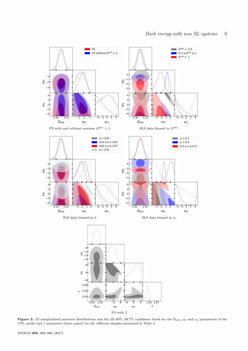
values is not possible because the bounds are different foreach scenario (see figure 3, upper-left and lower panels), butshowing consistency at 1σ of confidence level. When sub-samples are considered (SS2 to SS11, figure 3, upper-rightand middle panels), ω0 is positive only for the region zl > 0.4(see middle-right panel), and adopts negative values for theother sub-samples. The ω1 parameter is very sensitive toall cases having different mean values in each test, howevermost being consistent at 1σ of confidence level.

When a new parameter f , (FS) is added, no substantialimprovements on χ2

red value is shown. The result for thecorrective parameter f is consistent with the ones obtainedby Cao et al. (2012); Treu et al. (2006). Once again, the ω0

and ω1 constraints seem to get worse in the region Dobs <0.5 (SS2), showing convergence problems reflected in doublecontours in the correlation of the cosmological parameters(see figure 3, upper-right panel). Notice that χ2

red valueshigher than the one obtained for the entire sample (table 2)are achieved only in the regions: Dobs > 1 (SS4), σ < 210 kms−1 (SS5) and σ > 276 km s−1 (SS8). On the other hand, thesmallest χ2

red value is reached in the region of 0.5 < Dobs < 1(SS3), suggesting a better model fitting.

When the complete sample is used, the ω0 and ω1 con-straints are not consistent with the observations of Scolnicet al. (2018); Aghanim et al. (2018b) (ω0 = −1.009± 0.159,ω1 = −0.129 ± 0.755 and ω0 = −0.961 ± 0.077, ω1 =−0.28± 0.29, respectively) but show consistency at 1σ withthose obtained by Cao et al. (2012) (ω0 = −0.024±2.42ω1 =−6.35 ± 9.75) using 46 SLS. In spite of this, some sub-samples are consistent with the works of Scolnic et al. (2018);Aghanim et al. (2018b), showing different behaviors for theDE (phantom and quintessence regime). The ω0 parameteradopt a positive value in the region zl > 0.4, a similar valueis reported in the work of Cao et al. (2012) using a sam-ple with 80 SLS. For all the tests, the FOM estimator givestight constraints in the 0.2 6 zl 6 0.4 region (SS10), and

MNRAS 000, 000–000 (2017)


0.30 0.32

m0

3

2

1

0

3 2 1

0

FSFS without Dobs > 1

FS with and without systems Dobs > 1.

0.30 0.32m0

3

2

1

0

0

3 2 1 00

Dobs < 0.50.5 Dobs 1Dobs > 1

SLS data binned in Dobs.

0.30 0.32m0

3

2

1

0

0

3 2 1 00

< 210210 < 243243 276

> 276

SLS data binned in σ.

0.30 0.32

m0

3

2

1

0

3 2 1

0

zl > 0.4zl < 0.20.2 zl 0.4

SLS data binned in zl.

0.30 0.32m0

1.021.041.06

f

3210

0

3 2 1 00

1.01 1.04f

FS with f .

Figure 1. 1D marginalized posterior distributions and the 2D 68%, 99.7% confidence levels for the Ωm0 and ω0 parameters of the ωCDM

model and f parameter (lower panel) for the different samples presented in Table 2.

MNRAS 000, 000–000 (2017)


FSFS(f)SS1SS2SS3

SS4SS5SS6SS7SS8

SS9SS10SS11

0.0 0.5 1.0 1.5 2.0-1.0

-0.5

0.0

0.5

1.0

1.5

z

q(z)

FSFS(f)SS1SS2SS3SS4SS5SS6

SS7SS8SS9SS10SS11

0.0 0.5 1.0 1.5 2.0

-1.5

-1.0

-0.5

0.0

0.5

1.0

1.5

z

q(z)

FSFS(f)SS1SS2SS3SS4SS5SS6

SS7SS8SS9SS10SS11

0.0 0.5 1.0 1.5 2.0

-1.5

-1.0

-0.5

0.0

0.5

1.0

1.5

z

q(z)

Figure 2. Reconstruction of the q(z) parameter, using data con-

straints for ωCDM (upper panel), CPL (middle panel) and JBP(lower panel) models. In the JBP case (lower panel), notice that

SS2 it is outside the range shown in the figure, in this case SS2does not predicts an accelerated universe and therefore it is not

inside of the labels. Remarking SS3 as the best sample for our

analysis.

poor constraints in the region 243km s−1 < σ 6 276km s−1

(SS7).We reconstruct the q(z) function for CPL model using

the constraints obtained for each test (see figure 2, middlepanel). Notice that SS2, SS8 and SS10 yield constraints thatresult in unphysical behaviours for q(z). On the contrary,those provided by SS3, SS5 and SS11 source an acceleration-deceleration stage which is characteristic of models wherethe DE EoS is parametrized, i.e. a slowing down of cosmicacceleration (Cardenas & Rivera 2012; Cardenas et al. 2013;Magana et al. 2014; Wang et al. 2016; Zhang & Xia 2018).

Although SS11 constraints produce an acceleration phase inthe Universe, it does not ocurrs at z = 0.

5.3 The JBP constraints

The free parameters of the JBP parametrization are Ω0m,ω0 and ω1. It is worth to notice that the range of values forχ2min and χ2

red are similar to those obtained for the ωCDMand CPL models. For the FS (with and without f) and SS1,although the ω0 constraints differ slightly, they locate onthe phantom regime (see Table 2, figure 4 upper-left andlower panels). The ω1 parameter has remarkable changes inits value for each case being consistent at 1σ. The correctiveparameter f does not introduce significant improvements inthe χ2

red value, and it is consistent with the values reportedin Cao et al. (2012); Treu et al. (2006). When different sub-samples are used (e.g. SS2 to SS11), the cosmological pa-rameter constraints are sensitive to the selected data (seefigure 4, upper-right and middle panels). The ω0 parameterprefers negative values leading to an accelerated expansionstage in all the scenarios excluding the Dobs < 0.5 region(SS2). The ω1 parameter also adopt distinct values in allthe cases. Like for wCDM and CPL models, we obtain largeχ2red values for the regions: Dobs > 1 (SS4), σ < 210 km

s−1 (SS5) and σ > 276 km s−1 (SS8). Similarly, the bestvalue for χ2

red is also achieved in the region 0.5 < Dobs < 1(SS3). The Dobs < 0.5 (SS2) region presents convergenceproblems as well, showing double contours in all the free pa-rameters and being incompatible with an accelerated Uni-verse. For the first three tests, the JBP constraints are in-consistent with those obtained by Wang et al. (2016) (ω0 =−0.648 ± 0.252, ω1 = −3.419 ± 2.290) and Magana et al.(2017), (ω0 = −0.80 ± 0.45, ω1 = −3.78 ± 3.73). However,the constraint obtained for ω0 in the region 0.5 6 Dobs 6 1is consistent with those estimated by Magana et al. (2017)and Wang et al. (2016), although ω1 is only consistent withthe value obtained by Magana et al. (2017). The FOM es-timator gives tight constraints in the 0.5 6 Dobs < 1 (SS3)region and weak ones in Dobs < 0.5 (SS2) and 0.2 6 zl 6 0.4(SS10) regions.

The figure 2 shows the reconstruction of the decelera-tion parameter for the JBP model using the constraints de-rived from each test. It is noticeable the q(z) behavior show-ing a slowing down of the cosmic acceleration at late timesfor the SS3 and SS11. This behavior is in agreement withthose found by several authors for these parametrizations(see for example Magana et al. 2014; Wang et al. 2016). No-tice also that SS2 and SS8 present a non standard behavior,i.e. they never cross the acceleration region. The remainingcases are in good agreement with the standard knowledge.

5.4 The impact of the f parameter

The mean values of the f parameter obtained with differentmodels (1.021+0.012

−0.006, 1.021+0.008−0.006, and 1.021+0.011

−0.006 for ωCDM,CPL, and JBP respectively) are consistent with each otherand also in agreement with those reported by Treu et al.(2006), and Cao et al. (2012). This indicates that the pos-sible systematic errors affecting the image separation pro-duced by the lens for our sample is estimated at most at5 % when the value of f is considered equal for all SLS.

MNRAS 000, 000–000 (2017)


0.30 0.32

m0

42024

1

3

2

1

0

3 2 1

0

4 2 0 2 4

1



0.30 0.32

m0

42024

1

3210

0

3 2 1 0

0

4 2 0 2 4

1



0.30 0.32

m0

42024

1

3210

0

3 2 1 0

0

4 2 0 2 4

1

< 210210 < 243243 276

> 276


0.30 0.32

m0

42024

1

3210

0

3 2 1 0

0

4 2 0 2 4

1

zl < 0.2zl > 0.40.2 zl 0.4


0.30 0.32m0

1.02

1.05

1.08

f

4

0

4

1

3210

0

2 00

4 0 41

1.03 1.07f

FS with f .

Figure 3. 1D marginalized posterior distributions and the 2D 68%, 99.7% confidence levels for the Ωm0, ω0 and ω1 parameters of the

CPL model and f parameter (lower panel) for the different samples presented in Table 2.

MNRAS 000, 000–000 (2017)


0.30 0.32

m0

42024

1

3

2

1

0

3 2 1

0

4 2 0 2 4

1



0.30 0.32

m0

42024

1

3210

0

3 2 1 0

0

4 2 0 2 4

1



0.30 0.32

m0

42024

1

3210

0

3 2 1 0

0

4 2 0 2 4

1

< 210210 < 243243 276

> 276


0.30 0.32

m0

42024

1

3210

0

3 2 1 0

0

4 2 0 2 4

1

zl < 0.20.2 zl 0.4zl > 0.4


0.30 0.32m0

1.02

1.05

1.08

f

4

0

4

1

3210

0

2 00

4 0 41

1.03 1.07f

FS with f .

Figure 4. 1D marginalized posterior distributions and the 2D 68%, 99.7% confidence levels for the Ωm0, ω0 and ω1 parameters of the

JBP model and f parameter (lower panel) for the different samples presented in Table 2.

MNRAS 000, 000–000 (2017)


On the other hand, if we assume f as an independent freeparameter in each SLS, the value of f becomes larger forsome measured systems. However, if we restrict the analysisto the region between 0.5 6 Dobs 6 1 (i.e., sample SS3) thescatter decreases (see Appendix B for details).

The deviation on the value of f could be related tothe fact that some systems are not properly described byan isothermal model as found by Ritondale et al. (2018)for the BELLS gallery in almost all cases at the 2σ level.These deviations are also found by Barnabe et al. (2011),and by Vegetti et al. (2014) for the SLACS survey employingmore sophisticated modelling. In this sense, in Appendix Cwe studied the effect of assuming a SIE (or a SIS) actingas a lens when the mass distribution follows a power-law.Although the scatter in f is even greater, with some sys-tems outside the range proposed by Ofek et al. (2003), noneof the mock systems shows a nonphysical value for Dobs. Itis important to note that in most previous studies the lensmodels are close to isothermal. Thus, in this work we are us-ing Eq.(4) as a first approximation, and Eq. (7) to take intoaccount all the above mentioned irregularities (see for exam-ple Cao et al. 2012). Except those systematics that producesunphysically values on the observational lens equation.

5.5 The restricted sample SS3 as a fiduciarysample

Table 2 shows that there are four regions showing non-physical behaviours for the EoS of the dark energy (i.e.it does not satisfy ω0 < −1/3) or higher values for theχ2min function with respect to the FS, we label these sub-

samples as unreliable (marked with a letter U in the table)since they have similar aspects among the cosmological mod-els presented in this work being the following regions: SS2(Dobs < 0.5) wich present convergence problems in the es-timation of cosmological parameters and a non-acceleratingUniverse at z = 0 for the ωCDM and JBP models, SS4(Dobs > 1) showing a non physical value for the lens equa-tion and the highest χ2

min value for all the models, SS5(σ < 210 km s−1) and SS8 (σ > 276 km s−1) showing higherχ2min values than those obtained for the FS and also showing

a non-accelerating Universe in SS8 for the ωCDM model.It is worth to notice that the region SS11 (Dobs 6 1 andzl > 0.4) also presents a non-accelerating Universe at z = 0for the CPL model, however is consistent with an acceleratedone at 1σ of confidence level and do not show an increas-ing χ2

min function in comparisson with the FS, hence wedo not discard this region from the following. Even thoughcosmological parameters has different mean values for theremaining samples, most are consistent at 1 σ of confidencelevel for all the models.

However, to constrain cosmological parameters, we rec-ommend the use of the restricted sample (SS3), which showsthe best constraints and a lower dispersion in the value ofthe corrective parameter f , when is considered as an inde-pendent parameter in each SLS (see appendix B). The SS3constraints for the different models, also shows consistencywith CMB (Aghanim et al. 2018b) and SNe Ia (Scolnic et al.2018) measurements. Therefore, we favour the SS3 sampleas the fiduciary sample.

5.6 Comparing cosmological models

In this section, we discuss the comparison among cosmo-logical models for only three samples: FS, FS+f and SS3.We add to the present discussion the FS, FS+f samples,because they are the complete samples (besides, as we ap-preciate in Table 2, χ2

red values are very similar among thethree models in them). Nevertheless, we highlight the resultsfor the fiduciary SS3 sample.

In Table 3 we present the model selection’s criteria, forthe constraints obtained from the FS sample (with and with-out the f parameter), and the SS3 sample. To discern amongmodels (in any sample), it is necesary to compare the dif-ferent criterias; the favored model is obtained trhough thecompromise between the AIC, BIC and FOM estimators.When we perform the model comparison using the FS con-straints, the ωCDM model produce the lowest AIC and BICvalues. By measuring the relative differences ∆AIC = AICi- AICmin, and ∆BIC = BICi - BICmin (where the subindexi refers to the different models and AICmin (BICmin) is thelowest AIC (BIC) value) there is substantial support for thethree models (∆AIC< 2 or ∼ 2). However, exists positive ev-idence against the CPL and JBP models (4.2 < ∆BIC< 4.8respectively). By looking the FOM criteria, the higest valuesis obtained from the ωCDM model. Therefore, all estimatorssuggest that ωCDM is the favored model from the FS con-straints. Similarly, the AIC, BIC, and FOM values from theFS+f constraints suggest the same, the ωCDM model is theprefered one.

As mentioned before, we strongly suggest the use ofSS3 sample to estimate cosmological parameters. In partic-ular, for the constraints obtained for sample SS3, the low-est AIC and BIC values are obtained from the CPL model.Indeed, the relative difference ∆AIC with respect to thismodel (∼ 3.1 and 6.2 for JBP and ωCDM model respec-tively) point out to a considerably less support for the thesemodels. Moreover, the ∆BIC ∼ 3.1 and ∼ 3.2 for the JBPand ωCDM model respectively, suggest a positive evidenceagainst both models. By analyzing the FOM criteria, thehighest value is obtained for the CPL model, i.e. it pro-duce the strongest constraints. Thus, all the criteria suggestthat the CPL is the favored model from the fiduciary SS3sample. However, it is important to mention that does notexist enough evidence to rule out the ωCDM model. There-fore, when the SLS data are used as cosmological test inthe range 0.5 6 Dobs 6 1, a dynamical dark energy with aCPL parameterization is favored to explain the late cosmicacceleration.

6 CONCLUSIONS AND OUTLOOKS

In this paper we study three dark energy models: the ωCDMmodel with a DE constant equation of state, and the CPLand the JBP parametrizations where DE evolves with time.To constrain the cosmological parameters of the three mod-els we used a new compilation of strong gravitational lenssystems (SLS) with a total of 204 objects, the largest sam-ple to date (details of all systems can be found in AppendixA1). We test the models using different cases. First con-sidering all the systems using the Dobs estimated from theobserved Einstein ring radius and velocity dispersion, sec-ondly excluding those systems with a Dobs > 1 (unphysical)

MNRAS 000, 000–000 (2017)


Table 2. Mean values for the ωCDM, CPL and JBP parameters (Ωm0, w0, w1) and the f corrective parameter derived from different

test employing the SLS data. We labeled some subsamples as U, wich present weak constraints for all the models and unreliable resultsfor the bayesian analysis.

Data set: data point number χ2min χ2

red Ωm0 w0 w1 f

ωCDM model

FS (all systems: 204) 570.359 2.824 0.309+0.006−0.006 −2.478+0.479

−0.587 — —

SS1 (Dobs 6 1: 172) 409.759 2.396 0.311+0.006−0.006 −2.593+0.794

−0.860 — —

FS (all systems with f : 204) 559.619 2.784 0.311+0.006−0.006 −2.013+1.229

−1.167 — 1.021+0.012−0.006

SS2 (Dobs < 0.5 : 29)U 52.943 1.961 0.312+0.006−0.006 0.572+0.174

−4.403 — —

SS3 (0.5 6 Dobs 6 1: 143) 263.795 1.871 0.308+0.006−0.006 −1.653+0.264

−0.322 — —

SS4 (Dobs > 1 : 32)U 383.875 2.258 0.311+0.006−0.006 −2.336+0.684

−0.894 — —

SS5 (σ < 210 km s−1 : 64)U 201.766 3.254 0.309+0.006−0.006 −2.100+0.416

−0.525 — —

SS6 (210 km s−1 6 σ < 243 km s−1: 53) 118.092 2.316 0.309+0.006−0.006 −2.633+0.550

−0.641 — —

SS7 (243 km s−16 σ 6 276 km s−1: 49) 107.252 2.282 0.311+0.006−0.006 −1.854+0.672

−0.958 — —

SS8 (σ > 276 km s−1 : 38)U 109.457 3.040 0.311+0.006−0.006 0.148+0.122

−0.134 — —

SS9 (Dobs 6 1 and zl < 0.2: 52) 110.663 2.213 0.311+0.006−0.006 −3.134+0.807

−0.603 — —

SS10 (Dobs 6 1 and 0.2 6 zl 6 0.4: 48) 112.860 2.453 0.312+0.006−0.006 −3.558+0.701

−0.327 — —

SS11 (Dobs 6 1 and zl > 0.4: 72) 149.099 2.129 0.311+0.006−0.006 −1.163+0.318

−0.446 — —

CPL model

FS (all systems: 204) 569.317 2.832 0.309+0.006−0.006 −2.224+0.612

−0.707 −2.548+2.882−1.765 –

SS1 (Dobs 6 1: 172) 409.780 2.410 0.311+0.006−0.006 −2.768+0.833

−0.764 0.163+2.914−3.270 –


−0.984 1.045+2.338−3.219 1.021+0.008

−0.006

SS2 (Dobs < 0.5 : 29)U 46.235 1.778 0.311+0.006−0.006 −0.505+0.456

−0.342 3.585+0.989−1.535 —

SS3 (0.5 6 Dobs 6 1: 143) 255.552 1.825 0.308+0.006−0.006 −0.735+0.319

−0.395 −4.202+1.208−0.592 —

SS4 (Dobs > 1 : 32)U 384.067 2.273 0.311+0.006−0.006 −2.530+0.823

−0.832 −0.056+2.871−3.077 —

SS5 (σ < 210 km s−1 : 64)U 196.854 3.227 0.309+0.006−0.006 −1.292+0.500

−0.641 −3.912+1.767−0.813 —

SS6 (210 km s−1 6 σ < 243 km s−1: 53) 116.000 2.320 0.309+0.006−0.006 −2.205+0.668

−0.789 −3.159+2.728−1.369 —

SS7 (243 km s−16 σ 6 276 km s−1: 49) 107.363 2.334 0.311+0.006−0.006 −1.856+0.889

−1.062 −1.208+3.130−2.580 —

SS8 (σ > 276 km s−1 : 38)U 108.338 3.095 0.311+0.006−0.006 −0.423+0.494

−0.552 1.692+1.558−1.438 —

SS9 (Dobs 6 1 and zl < 0.2: 52) 110.539 2.256 0.311+0.006−0.006 −3.107+0.857

−0.624 −1.148+3.690−2.743 —

SS10 (Dobs 6 1 and 0.2 6 zl 6 0.4: 48) 101.321 2.252 0.311+0.006−0.006 −1.377+0.244

−0.284 4.551+0.336−0.781 —

SS11 (Dobs 6 1 and zl > 0.4: 72) 144.466 2.094 0.311+0.006−0.006 0.049+0.536

−0.711 −3.672+1.567−0.925 —

JBP model

FS (all systems: 204) 569.624 2.834 0.309+0.006−0.006 −2.312+0.592

−0.671 −2.220+3.368−2.022 –

SS1 (Dobs 6 1: 172) 409.750 2.410 0.311+0.006−0.006 −2.671+0.801

−0.811 0.201+3.209−3.408 –


−1.097 1.367+2.544−3.659 1.021+0.011

−0.006

SS2 (Dobs < 0.5 : 29)U 50.465 1.941 0.311+0.006−0.006 −0.055+0.421

−0.396 3.105+1.400−3.034 —

SS3 (0.5 6 Dobs 6 1: 143) 258.744 1.848 0.308+0.006−0.006 −1.047+0.324

−0.413 −3.921+1.705−0.805 —

SS4 (Dobs > 1 : 32)U 383.931 2.272 0.311+0.006−0.006 −2.433+0.754

−0.851 0.125+3.203−3.335 —

SS5 (σ < 210 km s−1 : 64)U 198.932 3.261 0.309+0.006−0.006 −1.617+0.502

−0.645 −3.419+2.520−1.181 —

SS6 (210 km s−1 6 σ < 243 km s−1: 53) 116.777 2.336 0.309+0.006−0.006 −2.370+0.648

−0.742 −2.682+3.262−1.718 —

SS7 (243 km s−16 σ 6 276 km s−1: 49) 107.317 2.333 0.311+0.006−0.006 −1.869+0.821

−0.985 −0.752+3.553−2.941 —

SS8 (σ > 276 km s−1 : 38)U 108.660 3.105 0.311+0.006−0.006 −0.271+0.558

−0.404 2.122+1.997−2.838 —

SS9 (Dobs 6 1 and zl < 0.2: 52) 110.569 2.257 0.311+0.006−0.006 −3.112+0.846

−0.619 −1.012+3.686−2.823 —

SS10 (Dobs 6 1 and 0.2 6 zl 6 0.4: 48) 112.833 2.507 0.311+0.006−0.006 −3.529+0.803

−0.349 −0.663+3.849−3.098 —

SS11 (Dobs 6 1 and zl > 0.4: 72) 147.010 2.131 0.311+0.006−0.006 −0.589+0.510

−0.696 −3.182+2.633−1.341 —

Table 3. AIC, BIC and FOM values for the ωCDM, CPL and JBP models derived from different test employing the SLS data.

Data set ωCDM CPL JBP

AIC BIC FOM AIC BIC FOM AIC BIC FOM

FS 204 574.359 580.995 343.671 575.317 585.271 143.0289 575.624 585.578 130.268

FS with f 204 565.619 575.573 18716.678 567.26 580.532 10122.341 567.147 580.419 7941.123

SS3 (143) 267.795 273.720 584.736 261.552 270.441 586.979 264.744 273.632 338.777

MNRAS 000, 000–000 (2017)


value, and finally using the entire sample with a new freeparameter f that take into account systematics that mightaffect the observables. In addition, to assess the impact ofsome observables, we estimated the cosmological parametersusing sub-samples of the SLS according to three differentscenarios, considering distinct regions on the observationalvalue of the lens equation (Dobs), the velocity dispersion (σ)and the redshift interval probed by the lens galaxy (zl). Wefound weak constraints for some regions.

The f parameter is consistent among the three models(within 5% error), having similar values to those reportedby Treu et al. (2006); Cao et al. (2012). Assuming f as anindependent free parameter in each SLS, the cosmologicalconstraints are consistent with those estimated assuming fequal for all the SLS. However, the scatter (in comparissonwith the Ofek estimations) of the value of f seems to belarger for some measured systems. To study this deviation,we analyze a mock catalog of 788 SLS, that mimics the dis-tribution of the observational data compiled in this work.When the Einstein radius of the simulated sample is com-pared with the one obtained from a SIE fitting, we foundthat the error is less than 10% for most of the objects (seeAppendix C). Considering that the majority of the data inour SLS compilation comes from models assuming SIEs, thissupports the range of the parameter used in our paper. How-ever, when a power-law mass distribution for the mock cata-logue is assumed, the scatter of the Einstein radius increases(35% or less).

We found that some of the sub-samples consideredin this work provide values for the cosmological parame-ters that are inconsistent with other observations (SNe Ia,CMB). Nevertheless, improvements on the constraints for allthe models are reflected in the χ2

red value when we excludethe systems in the region of Dobs > 1. This unphysical re-gion (also found by Leaf & Melia 2018) seems to be relatedto those systems with different kind of uncertainties (e.g.not fully confirmed lenses, multiple arcs, uncertain redshifts,complex lens substructure, see A2). Thus, as a byproductof our analysis, results with Dobs > 1 point towards thosesystems with untrustworthy observed parameters or thosewhich depart from our isothermal spherical mass distribu-tion hypothesis (e.g. external shear and/or lens substruc-ture). Most of the SLS considered in the present work havebeen modeled assuming a SIE lens model. Thus, the valueof f obtained from the mock data deviates from the rangeproposed by Ofek et al. (2003) for some systems and a widerinterval should be used.

Regarding the velocity dispersion, some of the selectedregions provide weaker constraints (larger values in the χ2

red

function): σ < 210 km s−1 and σ > 276 km s−1. Chen et al.(2018) also found weak constraints for the lens mass modelparameters assuming different regions on the velocity disper-sion. This could be due to an observational bias measuringthe velocity dispersion σ, that can be related to a small θE ,or not measuring the entire lens mass, or the lens galaxy hasclose companions.

We found that eight systems in the Dobs < 0.5 regioncan not be modeled properly by the theoretical lens equa-tion, obtaining double confidence contours for the cosmo-logical parameters. Finally, the lowest χ2

red value for eachmodel is achieved in the 0.5 6 Dobs 6 1 region, with val-ues for the cosmological parameters (−1.653 6 ω0 6 −0.735

and −4.202 6 ω1 6 −3.921) in agreement with those ex-pected from other astrophysical observations (see for in-stance (Magana et al. 2014; Betoule et al. 2014; Aghanimet al. 2018b)). Therefore, we favour the SS3 sample as thefiduciary sample to constrain DE cosmological parameters.The model selection criteria show that the CPL model is pre-ferred from this sample constraints, i.e. these data point outtowards a dynamical dark energy behavior consistent withthe three different criteria presented in table 3, obtainingω0 = −0.735+0.319

−0.395 and ω1 = −4.202+1.208−0.592 for this region.

The estimation of the cosmological parameters presentedin this paper, employing the strong lensing features oflens galaxies, provides constraints which are consistent withother cosmological probes (Magana et al. 2014; Betoule et al.2014; Scolnic et al. 2018; Magana et al. 2017; Aghanim et al.2018b). Nevertheless, a further analysis should be done, inparticular to consider systematic biases, that help us to moretightly estimate cosmological parameters and improve ourmethod.

ACKNOWLEDGMENTS

We thank the anonymous referee for thoughtful remarksand suggestions. Authors acknowledges the enlighteningconversations and valuable feedback with Karina Rojasand Mario Rodriguez. M.H.A. acknowledges support fromCONACYT PhD fellow, Consejo Zacatecano de Ciencia,Tecnologıa e Innovacion (COZCYT) and Centro de As-trofısica de Valparaıso (CAV). M.H.A. thanks the staff ofthe Instituto de Fısica y Astronomıa of the Universidadde Valparaıso where part of this work was done. J.M. ac-knowledges support from CONICYT project Basal AFB-170002 and CONICYT/FONDECYT 3160674. T.V. ac-knowledges support from PROGRAMA UNAM-DGAPA-PAPIIT IA102517. M.A.G.-A. acknowledges support fromCONACYT research fellow, Sistema Nacional de Investi-gadores (SNI), COZCYT and Instituto Avanzado de Cos-mologıa (IAC) collaborations. V.M. acknowledges supportfrom Centro de Astrofısica de Valparaıso (CAV) and CON-ICYT REDES (190147).

DATA AVAILABILITY

The data underlying this article were accessed from the ref-erences presented in Table A1.

REFERENCES

Abbott T. M. C., et al., 2019, Astrophys. J., 872, L30

Aghanim N., et al., 2018a

Aghanim N., et al., 2018b

Agnello A., et al., 2015, MNRAS, 454, 1260

Akaike H., 1974, IEEE Transactions on Automatic Control, 19,

716

Alam S., et al., 2017, MNRAS, 470, 2617

Albrecht A., et al., 2006, ArXiv Astrophysics e-prints,

Auger M. W., Treu T., Bolton A. S., Gavazzi R., KoopmansL. V. E., Marshall P. J., Bundy K., Moustakas L. A., 2009,ApJ, 705, 1099

Barnabe M., Czoske O., Koopmans L. V. E., Treu T., BoltonA. S., 2011, Mon. Not. Roy. Astron. Soc., 415, 2215

MNRAS 000, 000–000 (2017)


Bautista J. E., et al., 2017, A&A, 603, A12

Betoule M., et al., 2014, Astronomy & Astrophysics, 568, A22

Biesiada M., 2006, Phys. Rev., D73, 023006

Biesiada M., Piorkowska A., Malec B., 2010, MNRAS, 406, 1055

Bilic N., Tupper G. B., Viollier R. D., 2002, Phys. Lett., B535,17

Blake C., et al., 2012, MNRAS, 425, 405

Bolton A. S., Burles S., Koopmans L. V. E., Treu T., Moustakas

L. A., 2006, ApJ, 638, 703

Bolton A. S., Burles S., Koopmans L. V. E., Treu T., Gavazzi R.,Moustakas L. A., Wayth R., Schlegel D. J., 2008, Astrophys.

J., 682, 964

Brans C., Dicke R. H., 1961, Phys. Rev., 124, 925

Brownstein J. R., et al., 2012a, ApJ, 744, 41

Brownstein J. R., et al., 2012b, The Astrophysical Journal, 744,41

Buchdahl H. A., 1970, Monthly Notices of the Royal AstronomicalSociety, 150, 1

Cabanac R. A., et al., 2007, A&A, 461, 813

Caldera-Cabral G., Maartens R., Urena-Lopez L. A., 2009, Phys.Rev. D, 79, 063518

Caldwell R. R., 2002, Phys. Lett., B545, 23

Cao S., Pan Y., Biesiada M., Godlowski W., Zhu Z.-H., 2012,

J. Cosmology Astropart. Phys., 3, 016

Cao S., Biesiada M., Gavazzi R., Pirkowska A., Zhu Z.-H., 2015,Astrophys. J., 806, 185

Cardenas V. H., Rivera M., 2012, Physics Letters B, 710, 251

Cardenas V. H., Bernal C., Bonilla A., 2013, MNRAS, 433, 3534

Chaplygin S., 1904, Sci. Mem. Mosc. Univ. Math. Phys, 21

Chen Y., Li R., Shu Y., 2018

Chevallier M., Polarski D., 2001, Int. J. Mod. Phys., D10, 213

Chiba T., Okabe T., Yamaguchi M., 2000, Phys. Rev., D62,023511

Copeland E. J., Sami M., Tsujikawa S., 2006, Int. J. Mod. Phys.,

D15, 1753

Eisenstein D. J., et al., 2005, ApJ, 633, 560

Foreman-Mackey D., Hogg D. W., Lang D., Goodman J., 2013,Publ. Astron. Soc. Pac., 125, 306

Futamase T., Yoshida S., 2001, Prog. Theor. Phys., 105, 887

Galiautdinov A., Kopeikin S. M., 2016, Phys. Rev., D94, 044015

Garcıa-Aspeitia M. A., Matos T., 2011, Gen. Rel. Grav., 43, 315

Garcıa-Aspeitia M. A., Magana J., Hernandez-Almada A., MottaV., 2018a, International Journal of Modern Physics D, 27,

1850006

Garcıa-Aspeitia M. A., Hernandez-Almada A., Magana J.,

Amante M. H., Motta V., Martınez-Robles C., 2018b, Phys.

Rev., D97, 101301

Garcıa-Aspeitia M. A., Martınez-Robles C., Hernandez-Almada

A., Magana J., Motta V., 2019, Phys. Rev., D99, 123525

Gelman A., Rubin D. B., 1992, Statist. Sci., 7, 457

Grillo C., Lombardi M., Bertin G., 2008, A&A, 477, 397

Hernandez-Almada A., Magana J., Garcia-Aspeitia M. A., MottaV., 2018

Hewett P. C., Irwin M. J., Foltz C. B., Harding M. E., CorriganR. T., Webster R. L., Dinshaw N., 1994, AJ, 108, 1534

Inada N., et al., 2003, AJ, 126, 666

Inada N., et al., 2005, AJ, 130, 1967

Jassal H. K., Bagla J. S., Padmanabhan T., 2005, Mon. Not. Roy.

Astron. Soc., 356, L11

Jimenez R., Loeb A., 2002, Astrophys. J., 573, 37

Jorgensen I., Franx M., Kjaergaard P., 1995a, MNRAS, 273, 1097

Jorgensen I., Franx M., Kjaergaard P., 1995b, MNRAS, 276, 1341

Jullo E., Natarajan P., Kneib J. P., D’Aloisio A., Limousin M.,

Richard J., Schimd C., 2010, Science, 329, 924

Kamenshchik A. Yu., Moschella U., Pasquier V., 2001, Phys.

Lett., B511, 265

Keeton C. R., 2011, GRAVLENS: Computational Methods forGravitational Lensing (ascl:1102.003)

Kochanek C. S., 1995, ApJ, 445, 559

Koopmans L. V. E., Treu T., 2003a, ApJ, 583, 606

Koopmans L. V. E., Treu T., 2003b, Astrophys. J., 583, 606

Lacy M., Gregg M., Becker R. H., White R. L., Glikman E.,Helfand D., Winn J. N., 2002, AJ, 123, 2925

Langlois D., Saito R., Yamauchi D., Noui K., 2018, Phys. Rev.,

D97, 061501

Leaf K., Melia F., 2018, Mon. Not. Roy. Astron. Soc., 478, 5104

Lehar J., Cooke A. J., Lawrence C. R., Silber A. D., Langston

G. I., 1996, AJ, 111, 1812

Leier D., Ferreras I., Saha P., Falco E. E., 2011, ApJ, 740, 97

Li M., Li X.-D., Wang S., Wang Y., 2011, Communications in

Theoretical Physics, 56, 525

Linder E. V., 2003, Phys. Rev., D68, 083503

Magana J., Cardenas V. H., Motta V., 2014, J. Cosmology As-

tropart. Phys., 10, 017

Magana J., Motta V., Cardenas V. H., Verdugo T., Jullo E., 2015,ApJ, 813, 69

Magana J., Motta V., Cardenas V. H., Foex G., 2017, Mon. Not.

Roy. Astron. Soc., 469, 47

Magana J., Acebron A., Motta V., Verdugo T., Jullo E., Limousin

M., 2018, ApJ, 865, 122

Magana J., Amante M. H., Garcia-Aspeitia M. A., Motta V.,2018, Mon. Not. Roy. Astron. Soc., 476, 1036

Melia F., Wei J.-J., Wu X.-F., 2015, Astron. J., 149, 2

Moresco M., et al., 2016, Journal of Cosmology and Astro-ParticlePhysics, 2016, 014

Morgan N. D., Becker R. H., Gregg M. D., Schechter P. L., White

R. L., 2001, Astron. J., 121, 611

Morgan N. D., Kochanek C. S., Pevunova O., Schechter P. L.,2005, AJ, 129, 2531

Munoz J. A., Falco E. E., Kochanek C. S., Lehar J., McLeod

B. A., Impey C. D., Rix H.-W., Peng C. Y., 1998, Ap&SS,263, 51

Munoz J. A., Kochanek C. S., Keeton C. R., 2001, ApJ, 558, 657

Ofek E. O., Rix H.-W., Maoz D., 2003, Mon. Not. Roy. Astron.Soc., 343, 639

Ofek E. O., Maoz D., Rix H.-W., Kochanek C. S., Falco E. E.,

2006, ApJ, 641, 70

Perez A., Sudarsky D., 2017

Perlmutter S., Aldering G., Goldhaber G., Knop R. A., Nugent

P., others Project T. S. C., 1999, The Astrophysical Journal,517, 565

Pindor B., et al., 2004, AJ, 127, 1318

Planck Collaboration et al., 2016, A&A, 594, A13

Qi J.-Z., Cao S., Zhang S., Biesiada M., Wu Y., Zhu Z.-H., 2018,preprint, (arXiv:1803.01990)

Ratra B., Peebles P. J. E., 1988, Phys. Rev. D, 37, 3406

Riess A. G., Filippenko A. V., Challis P., Clocchiatti A., DiercksA., et al., 1998, The Astronomical Journal, 116, 1009

Riess A. G., et al., 2016, Astrophys. J., 826, 56

Riess A. G., Casertano S., Yuan W., Macri L. M., Scolnic D.,2019, arXiv e-prints,

Ritondale E., Auger M. W., Vegetti S., McKean J. P., 2018,

Monthly Notices of the Royal Astronomical Society, 482, 4744

Rusin D., Norbury M., Biggs A. D., Marlow D. R., Jackson N. J.,Browne I. W. A., Wilkinson P. N., Myers S. T., 2002, MNRAS,

330, 205

Rusin D., et al., 2003a, ApJ, 587, 143

Rusin D., Kochanek C. S., Keeton C. R., 2003b, ApJ, 595, 29

Schmidt B. P., Suntzeff N. B., Phillips M. M., Schommer R. A.,

Clocchiatti A., et al., 1998, The Astrophysical Journal, 507,46

Schneider P., Ehlers J., Falco E. E., 1992, Gravitational Lenses,

doi:10.1007/978-3-662-03758-4.

Schwarz G., 1978, Annals of Statistics, 6, 461

Scolnic D. M., et al., 2018, Astrophys. J., 859, 101

MNRAS 000, 000–000 (2017)


Shi K., Huang Y., Lu T., 2012, Mon. Not. Roy. Astron. Soc., 426,

2452

Shu Y., et al., 2016, The Astrophysical Journal, 833, 264

Shu Y., et al., 2017, ApJ, 851, 48

Sonnenfeld A., Gavazzi R., Suyu S. H., Treu T., Marshall P. J.,2013a, Astrophys. J., 777, 97

Sonnenfeld A., Treu T., Gavazzi R., Suyu S. H., Marshall P. J.,

Auger M. W., Nipoti C., 2013b, Astrophys. J., 777, 98

Sonnenfeld A., Treu T., Marshall P. J., Suyu S. H., Gavazzi R.,

Auger M., Nipoti C., 2015, Astrophys. J., 800, 94

Sotiriou T. P., Faraoni V., 2010, Rev. Mod. Phys., 82, 451

Spingola C., McKean J. P., Auger M. W., Fassnacht C. D., Koop-

mans L. V. E., Lagattuta D. J., Vegetti S., 2018, MNRAS,478, 4816

Starobinsky A., 1980, Physics Letters B, 91, 99

Tonry J. L., 1998, AJ, 115, 1

Treu T., Koopmans L., 2002, Astrophys. J., 575, 87

Treu T., Koopmans L. V. E., 2004, ApJ, 611, 739

Treu T., Koopmans L. V., Bolton A. S., Burles S., Moustakas

L. A., 2006, ApJ, 640, 662

Treu T., et al., 2018, MNRAS, 481, 1041

Turner E. L., Ostriker J. P., Gott J. R. I., 1984, ApJ, 284, 1

Vegetti S., Koopmans L. V. E., Auger M. W., Treu T., BoltonA. S., 2014, Mon. Not. Roy. Astron. Soc., 442, 2017

Wang Y., 2008, Phys. Rev. D, 77, 123525

Wang S., Hu Y., Li M., Li N., 2016, ApJ, 821, 60

Weinberg S., 1989, Reviews of Modern Physics, 61

Wetterich C., 1988, Nuclear Physics B, 302, 668

Yennapureddy M. K., Melia F., 2018, Eur. Phys. J., C78, 258

Zeldovich Y. B., 1968, Soviet Physics Uspekhi, 11

Zhang M.-J., Xia J.-Q., 2018, Nuclear Physics B, 929, 438

APPENDIX A: STRONG-LENSING SYSTEMSCOMPILATION

• In Table A1 presents the compilation of SLS with 204points.• Table A2 shows the 32 systems with Dobs > 1. Many of

these systems appear flagged, which means that such objectsare: not confirmed lenses, or have complex source structureswith multiple arcs and counter-arcs, or the foreground lensis clearly composed of two distinct components, have uncer-tain redshift measurements, or the arcs (rings) are embebedin the light of the foreground lens. We refer the interestedreader to the references presented in Table A1. We suggestthat these systems with Dobs > 1, shoul not be used incosmological parameter estimation (see also Leaf & Melia2018).

APPENDIX B: THE EFFECT OF F AS ANINDIVIDUAL AND FREE PARAMETER FOREACH SLS MEASUREMENT

In the third test (FS with f) presented in Table 2, we es-timated cosmological parameters under the hypothesis thatall the measurements has the same value for the f param-eter in Eq. (7). This corrective parameter, has been intro-duced to explain unknown systematics that can be producedby some of the assumptions mentioned in section 2. How-ever, each SLS has been study under different circumstancesand employing different telescopes and instruments. There-fore, the unknown systematics should not be the same, i.e

the value for the corrective parameter f must be differentin each case. To quantify this, we carried out an optimiza-tion for the parameters considering f as an individual andfree parameter for each SLS. We performed the optimiza-tion for the ωCDM model through the differential evolutionmethod from scipy python package. We assume the samepriors for the ω (−4 < ω < 1) and Ωm0 (gaussian prior ofΩ0m = 0.3111 ± 0.0056) parameters, nevertheless, to assessthe impact of the possible systematic errors, we considera bigger interval for the f parameter within the followingrange 0.6 < f < 1.5.

Figure B1 shows the histogram of the values obtainedfor the f parameter when the complete and SS3 sample(0.5 6 Dobs 6 1) are considered. For the complete sample,this result show that many systems are outside of the regionproposed by Treu et al. (2006), and Ofek et al. (2003). Inparticular nine systems have extreme f values, eight withf = 1.5 and one at f = 0.6. Which suggests that somemeasured systems have larger systematic errors. However,when we use the SS3 sample, only one system take a valueof f = 1.5 and the remain systems that are beyond the men-tioned region are considerably less. This result indicates thatthe corrective parameter f decreases when the SS3 sample isconsidered, and it is consistent with the results obtained forthe three cosmological models, obtaining the lowest valuesfor χ2

red (see table 2). Nevertheless, the two samples havesimilar f mean values, obtaining f = 1.10 and f = 1.09for the complete and SS3 sample respectively. Following thesame procedure, we optimize the cosmological parametersfor the CPL, and JBP models along with f (as individualfree parameter in each SLS). Obtaining the same behavioras in the ωCDM scenario for both samples. Therefore, un-der the assumption that each SLS has its own associatedf , we do not expect significant differences in the cosmo-logical constraints. Indeed, in Figures B2-B4 we show thehistograms of the cosmological parameter best fits when ftakes different values in each data point on the FS sample.To compare with the MCMC analysis of section 5, we fit aGaussian kernel to these histograms and calculate the meanvalues and their uncertainties. We obtain for the wCDMmodel w0 = −1.62+1.31

−1.28. This result is consistent with thevalue reported in Table 2 (FS+f) within ∼ 1.02σ. For theoptimization in the CPL model, we obtain the constraintsw0 = −1.99+1.80

−1.25 and w1 = −0.10+2.91−3.50, which are also con-

sistent with the MCMC results within ∼ 0.83σ, and ∼ 0.32σrespectively. Similarly, for the JBP model, the individualoptimization gives w0 = −2.07+1.69

−1.03, and w1 = −0.53+3.82−3.40.

These values are in agrement within ∼ 0.58σ, and ∼ 0.43σ,with the values reported in Table 2.

APPENDIX C: MOCK DATA WITHSTRONG-LENSING SYSTEMS

In this section, we use a mock data set of SLS to estimatethe effect on the f parameter when we use the θE valuesreported in the literature.

To simulate our data we procede as follow: mimickingthe same distribution of zs of our SLS sample (within therange 0.196 < zs < 3.595), we generate an aleatory sampleof 1000 sources. Then, for each source we calculate the mostprobably redshift of the lens, zl, following the work of Turner

MNRAS 000, 000–000 (2017)


Table A1. Compilation of 204 strong-lensing measurements. Here, the ∗ indicates that the uncertainties were estimated.

System Name Survey zl zs θE(′′) σ0 (Km s−1) Reference

SDSSJ0819+4534 SLACS 0.194 0.446 0.85 225 ±15 Auger et al. (2009)SDSSJ0959+4416 SLACS 0.237 0.531 0.96 244 ±19 Bolton et al. (2008)

SDSSJ1029+0420 SLACS 0.104 0.615 1.01 210 ±11 Bolton et al. (2008)

SDSSJ1103+5322 SLACS 0.158 0.735 1.02 196 ±12 Bolton et al. (2008)SDSSJ1306+0600 SLACS 0.173 0.472 1.32 237 ±17 Auger et al. (2009)

SDSSJ1313+4615 SLACS 0.185 0.514 1.37 221 ±17 Auger et al. (2009)SDSSJ1318-0313 SLACS 0.240 1.300 1.58 213 ±18 Auger et al. (2009)

SDSSJ1420+6019 SLACS 0.063 0.535 1.04 205 ±10 Bolton et al. (2008)

SDSSJ1443+0304 SLACS 0.134 0.419 0.81 209 ±11 Bolton et al. (2008)SDSSJ1614+4522 SLACS 0.178 0.811 0.84 182 ±13 Bolton et al. (2008)

SDSSJ1644+2625 SLACS 0.137 0.610 1.27 229 ±12 Auger et al. (2009)

SDSSJ1719+2939 SLACS 0.181 0.578 1.28 286 ±15 Auger et al. (2009)HE0047-1756 CASTLES 0.408 1.670 0.80 190 ±27∗ Ofek et al. (2006)

HE0230-2130 CASTLES 0.522 2.162 0.87 240 ±34∗ Ofek et al. (2006)

J0246-0825 CASTLES 0.723 1.686 0.53 265 ±37∗ Inada et al. (2005)HE0435-1223 CASTLES 0.454 1.689 1.22 257 ±36∗ Morgan et al. (2005)

SDSSJ092455.87+021924.9 CASTLES 0.393 1.523 0.88 230 ±32∗ Inada et al. (2003)LBQS1009-0252 CASTLES 0.871 2.739 0.77 245 ±34∗ Hewett et al. (1994)J1004+1229 CASTLES 0.950 2.640 0.83 240 ±34∗ Lacy et al. (2002)

SDSSJ115517.35+634622.0 CASTLES 0.176 2.888 0.76 190 ±27∗ Pindor et al. (2004)FBQ1633+3134 CASTLES 0.684 1.518 0.35 160 ±22∗ Morgan et al. (2001)

MG1654+1346 CASTLES 0.254 1.740 1.05 200+120−80 Rusin et al. (2003a)

DES J2146-0047 DES 0.799 2.38 0.68 215 ±21∗ Agnello et al. (2015)

SDSSJ0151+0049 BELLS 0.517 1.364 0.68 219 ±39 Brownstein et al. (2012b)

SDSSJ0747+5055 BELLS 0.438 0.898 0.75 328 ±60 Brownstein et al. (2012b)SDSSJ0747+4448 BELLS 0.437 0.897 0.61 281 ±52 Brownstein et al. (2012b)


SDSSJ0830+5116 BELLS 0.53 1.332 1.14 268 ±36 Brownstein et al. (2012b)SDSSJ0944−0147 BELLS 0.539 1.179 0.72 204 ±34 Brownstein et al. (2012b)

SDSSJ1159−0007 BELLS 0.579 1.346 0.68 165 ±41 Brownstein et al. (2012b)


SDSSJ1234−0241 BELLS 0.49 1.016 0.53 122 ±31 Brownstein et al. (2012b)

SDSSJ1318−0104 BELLS 0.659 1.396 0.68 177 ±27 Brownstein et al. (2012b)SDSSJ1337+3620 BELLS 0.564 1.182 1.39 225 ±35 Brownstein et al. (2012b)

SDSSJ1349+3612 BELLS 0.44 0.893 0.75 178 ±18 Brownstein et al. (2012b)SDSSJ1352+3216 BELLS 0.463 1.034 1.82 161 ±21 Brownstein et al. (2012b)SDSSJ1522+2910 BELLS 0.555 1.311 0.74 166 ±27 Brownstein et al. (2012b)



SDSSJ1601+2138 BELLS 0.544 1.446 0.86 207 ±36 Brownstein et al. (2012b)SDSSJ1631+1854 BELLS 0.408 1.086 1.63 272 ±14 Brownstein et al. (2012b)SDSSJ2122+0409 BELLS 0.626 1.452 1.58 324 ±56 Brownstein et al. (2012b)


SDSSJ0008-0004 SLACS 0.44 1.192 1.16 193 ±36 Auger et al. (2009)SDSSJ0029-0055 SLACS 0.227 0.931 0.96 229 ±18 Auger et al. (2009)

SDSSJ0037-0942 SLACS 0.196 0.632 1.53 279 ±10 Auger et al. (2009)SDSSJ0044+0113 SLACS 0.12 0.196 0.79 266 ±13 Auger et al. (2009)SDSSJ0109+1500 SLACS 0.294 0.525 0.69 251 ±19 Auger et al. (2009)

SDSSJ0157-0056 SLACS 0.513 0.924 0.79 295 ±47 Auger et al. (2009)

SDSSJ0216-0813 SLACS 0.332 0.524 1.16 333 ±23 Auger et al. (2009)SDSSJ0252+0039 SLACS 0.28 0.982 1.04 164 ±12 Auger et al. (2009)SDSSJ0330-0020 SLACS 0.351 1.071 1.1 212 ±21 Auger et al. (2009)

SDSSJ0405-0455 SLACS 0.075 0.81 0.8 160 ±7 Auger et al. (2009)SDSSJ0728+3835 SLACS 0.206 0.688 1.25 214 ±11 Auger et al. (2009)

SDSSJ0737+3216 SLACS 0.322 0.581 1 338 ±16 Auger et al. (2009)

SDSSJ0808+4706 SLACS 0.219 1.025 1.23 236 ±11 Auger et al. (2009)SDSSJ0822+2652 SLACS 0.241 0.594 1.17 259 ±15 Auger et al. (2009)SDSSJ0841+3824 SLACS 0.116 0.657 1.41 225 ±8 Auger et al. (2009)SDSSJ0903+4116 SLACS 0.43 1.065 1.29 223 ±27 Auger et al. (2009)SDSSJ0912+0029 SLACS 0.164 0.324 1.63 326 ±12 Auger et al. (2009)

MNRAS 000, 000–000 (2017)


Table A1 – continued


SDSSJ0936+0913 SLACS 0.19 0.588 1.09 243 ±11 Auger et al. (2009)SDSSJ0946+1006 SLACS 0.222 0.608 1.38 263 ±21 Auger et al. (2009)








SDSSJ1143-0144 SLACS 0.106 0.402 1.68 269 ±5 Auger et al. (2009)SDSSJ1153+4612 SLACS 0.18 0.875 1.05 269 ±15 Auger et al. (2009)




SDSSJ1330-0148 SLACS 0.081 0.712 0.87 185 ±9 Auger et al. (2009)



SDSSJ1430+4105 SLACS 0.285 0.575 1.52 322 ±32 Auger et al. (2009)SDSSJ1436-0000 SLACS 0.285 0.805 1.12 281 ±19 Auger et al. (2009)

SDSSJ1451-0239 SLACS 0.125 0.52 1.04 223 ±14 Auger et al. (2009)SDSSJ1525+3327 SLACS 0.358 0.717 1.31 264 ±26 Auger et al. (2009)SDSSJ1531-0105 SLACS 0.16 0.744 1.71 279 ±12 Auger et al. (2009)

SDSSJ1538+5817 SLACS 0.143 0.531 1 189 ±12 Auger et al. (2009)SDSSJ1621+3931 SLACS 0.245 0.602 1.29 236 ±20 Auger et al. (2009)SDSSJ1627-0053 SLACS 0.208 0.524 1.23 290 ±14 Auger et al. (2009)

SDSSJ1630+4520 SLACS 0.248 0.793 1.78 276 ±16 Auger et al. (2009)SDSSJ1636+4707 SLACS 0.228 0.674 1.09 231 ±15 Auger et al. (2009)SDSSJ2238-0754 SLACS 0.137 0.713 1.27 198 ±11 Auger et al. (2009)

SDSSJ2300+0022 SLACS 0.228 0.464 1.24 279 ±17 Auger et al. (2009)SDSSJ2303+1422 SLACS 0.155 0.517 1.62 255 ±16 Auger et al. (2009)SDSSJ2321-0939 SLACS 0.082 0.532 1.6 249 ±8 Auger et al. (2009)

SDSSJ2341+0000 SLACS 0.186 0.807 1.44 207 ±13 Auger et al. (2009)Q0047-2808 LSD 0.485 3.595 1.34 ±0.01 229 ±15 Koopmans & Treu (2003b)

CFRS03-1077 LSD 0.938 2.941 1.24 ±0.06 251 ±19 Treu & Koopmans (2004)HST14176+5226 LSD 0.81 3.399 1.41 ±0.08 224 ±15 Treu & Koopmans (2004)

HST15433 LSD 0.497 2.092 0.36 ±0.04 116 ±10 Treu & Koopmans (2004)SL2SJ021247−055552 SL2S 0.75 2.74 1.27 ±0.04 273 ±22 Sonnenfeld et al. (2013b)SL2SJ021325−074355 SL2S 0.717 3.48 2.39 ±0.07 293 ±34 Sonnenfeld et al. (2013b)

SL2SJ021411−040502 SL2S 0.609 1.88 1.41 ±0.04 287 ±47 Sonnenfeld et al. (2013b)

SL2SJ021737−051329 SL2S 0.646 1.847 1.27 ±0.04 239 ±27 Sonnenfeld et al. (2013b)SL2SJ021902−082934 SL2S 0.389 2.15 1.30 ±0.04 289 ±23 Sonnenfeld et al. (2013b)SL2SJ022346−053418 SL2S 0.499 1.44 1.22 ±0.11 288 ±28 Sonnenfeld et al. (2013b)

SL2SJ022511−045433 SL2S 0.238 1.199 1.76 ±0.05 234 ±21 Sonnenfeld et al. (2013b)SL2SJ022610−042011 SL2S 0.494 1.232 1.19 ±0.04 263 ±24 Sonnenfeld et al. (2013b)


SL2SJ084909−041226 SL2S 0.722 1.54 1.10 ±0.03 320 ±24 Sonnenfeld et al. (2013b)SL2SJ084959−025142 SL2S 0.274 2.09 1.16 ±0.04 276 ±35 Sonnenfeld et al. (2013b)SL2SJ085019−034710 SL2S 0.337 3.25 0.93 ±0.03 290 ±24 Sonnenfeld et al. (2013b)SL2SJ085540−014730 SL2S 0.365 3.39 1.03 ±0.04 222 ±25 Sonnenfeld et al. (2013b)


SL2SJ095921+020638 SL2S 0.552 3.35 0.74 ±0.02 188 ±22 Sonnenfeld et al. (2013b)SL2SJ135949+553550 SL2S 0.783 2.77 1.14 ±0.03 228 ±29 Sonnenfeld et al. (2013b)SL2SJ140454+520024 SL2S 0.456 1.59 2.55 ±0.08 342 ±20 Sonnenfeld et al. (2013b)SL2SJ140546+524311 SL2S 0.526 3.01 1.51 ±0.05 284 ±21 Sonnenfeld et al. (2013b)

SL2SJ140650+522619 SL2S 0.716 1.47 0.94 ±0.03 253 ±19 Sonnenfeld et al. (2013b)SL2SJ141137+565119 SL2S 0.322 1.42 0.93 ±0.03 214 ±23 Sonnenfeld et al. (2013b)


MNRAS 000, 000–000 (2017)





SL2SJ221326−000946 SL2S 0.338 3.45 1.07 ±0.03 165 ±20 Sonnenfeld et al. (2013b)

SL2SJ221929−001743 SL2S 0.289 1.02 0.52 ±0.13 189 ±20 Sonnenfeld et al. (2013b)SL2SJ222012+010606 SL2S 0.232 1.07 2.16 ±0.07 127 ±15 Sonnenfeld et al. (2013b)

SL2SJ222148+011542 SL2S 0.325 2.35 1.40 ±0.05 222 ±23 Sonnenfeld et al. (2013b)

SL2SJ222217+001202 SL2S 0.436 1.36 1.44 ±0.15 221 ±22 Sonnenfeld et al. (2013b)SDSSJ002927.38+254401.7 BELLS 0.5869 2.4504 1.34 241 ±45 Shu et al. (2016)

SDSSJ020121.39+322829.6 BELLS 0.3957 2.8209 1.70 256 ±20 Shu et al. (2016)

SDSSJ023740.63−064112.9 BELLS 0.4859 2.2491 0.65 290 ±89 Shu et al. (2016)SDSSJ074249.68+334148.9 BELLS 0.4936 2.3633 1.22 218 ±28 Shu et al. (2016)


SDSSJ085621.59+201040.5 BELLS 0.5074 2.2335 0.98 334 ±54 Shu et al. (2016)SDSSJ091807.86+451856.7 BELLS 0.5238 2.3440 0.77 119 ±61 Shu et al. (2016)





SDSSJ222825.76+120503.9 BELLS 0.5305 2.8324 1.28 255 ±50 Shu et al. (2016)SDSSJ234248.68−012032.5 BELLS 0.5270 2.2649 1.11 274 ±43 Shu et al. (2016)

SL2SJ020457-110309 SL2S 0.609 1.89 0.54 ±0.07 250 ±30 Sonnenfeld et al. (2015)

SL2SJ020524-093023 SL2S 0.557 1.33 0.76 ±0.09 276 ±37 Sonnenfeld et al. (2015)SL2SJ021801-080247 SL2S 0.884 2.06 1.00 ±0.03 246 ±48 Sonnenfeld et al. (2015, 2013a)

SL2SJ023307-043838 SL2S 0.671 1.87 1.77 ±0.06 204 ±21 Sonnenfeld et al. (2015)SDSSJ0143−1006 SLACS 0.2210 1.1046 1.23 203 ±17 Shu et al. (2017)SDSSJ0159−0006 SLACS 0.1584 0.7477 0.92 216 ±18 Shu et al. (2017)

SDSSJ0324+0045 SLACS 0.3210 0.9199 0.55 183 ±19 Shu et al. (2017)SDSSJ0324−0110 SLACS 0.4456 0.6239 0.63 310 ±38 Shu et al. (2017)SDSSJ0753+3416 SLACS 0.1371 0.9628 1.23 208 ±12 Shu et al. (2017)

SDSSJ0754+1927 SLACS 0.1534 0.7401 1.04 193 ±16 Shu et al. (2017)SDSSJ0757+1956 SLACS 0.1206 0.8326 1.62 206 ±11 Shu et al. (2017)SDSSJ0826+5630 SLACS 0.1318 1.2907 1.01 163 ±8 Shu et al. (2017)


SDSSJ0955+3014 SLACS 0.3214 0.4671 0.54 271 ±33 Shu et al. (2017)SDSSJ0956+5539 SLACS 0.1959 0.8483 1.17 188 ±11 Shu et al. (2017)



SDSSJ1051+4439 SLACS 0.1634 0.5380 0.99 216 ±16 Shu et al. (2017)




SDSSJ1213+2930 SLACS 0.0906 0.5954 1.35 232 ±7 Shu et al. (2017)SDSSJ1301+0834 SLACS 0.0902 0.5331 1.00 178 ±8 Shu et al. (2017)SDSSJ1330+1750 SLACS 0.2074 0.3717 1.01 250 ±12 Shu et al. (2017)SDSSJ1403+3309 SLACS 0.0625 0.7720 1.02 190 ±6 Shu et al. (2017)


SDSSJ1541+3642 SLACS 0.1406 0.7389 1.17 194 ±11 Shu et al. (2017)SDSSJ1543+2202 SLACS 0.2681 0.3966 0.78 285 ±16 Shu et al. (2017)SDSSJ1550+2020 SLACS 0.1351 0.3501 1.01 243 ±9 Shu et al. (2017)SDSSJ1553+3004 SLACS 0.1604 0.5663 0.84 194 ±15 Shu et al. (2017)


SDSSJ2309−0039 SLACS 0.2905 1.0048 1.14 184 ±13 Shu et al. (2017)

MNRAS 000, 000–000 (2017)



system name survey zl zs θE(′′) σ0 (Km s−1) reference

SDSSJ2324+0105 SLACS 0.1899 0.2775 0.59 245 ±15 Shu et al. (2017)

Q0142-100 CASTLES 0.491 2.719 1.12 246+17−47 Rusin et al. (2003a) Leier et al. (2011)

MG0414+0534 CASTLES 0.958 2.639 1.19 247+10−13 Rusin et al. (2003a) Leier et al. (2011)

B0712+472 CASTLES 0.406 1.339 0.71 164±7 Rusin et al. (2003a) Leier et al. (2011)

HS0818+1227 CASTLES 0.390 3.115 1.42 246+17−42 Rusin et al. (2003a) Leier et al. (2011)

B1030+074 CASTLES 0.599 1.535 0.78 257+10−18 Rusin et al. (2003a) Leier et al. (2011)

HE1104-1805 CASTLES 0.729 2.303 1.595 303+11−10 Rusin et al. (2003a) Leier et al. (2011)

B1608+656 CASTLES 0.630 1.394 1.135 267+6−15 Rusin et al. (2003a) Leier et al. (2011)

HE2149-2745 CASTLES 0.603 2.033 0.85 191+7−9 Rusin et al. (2003a) Leier et al. (2011)

MG1549+3047 CASTLES 0.111 1.170 1.15 227±18 Rusin et al. (2003a) Lehar et al. (1996)

System Name Dobs θE(′′) Flag

SDSSJ1318-0313 1.207548476671243 1.58

SDSSJ0801+4727 1.7690928325399644 0.49 †SDSSJ1234−0241 1.234704134938535 0.53 †SDSSJ1352+3216 2.4345927827771154 1.82 †SDSSJ0008-0004 1.079816763956848 1.16 †SDSSJ0252+0039 1.3407639908720494 1.04 †SDSSJ0405-0455 1.0835693599307283 0.8 †SDSSJ1100+5329 1.5071867558989571 1.52SDSSJ1218+0830 1.0483021267443504 1.45SDSSJ2238-0754 1.123259330363861 1.27 †SDSSJ2341+0000 1.1652751780813544 1.44 †SL2SJ022511−045433 1.1145194380761674 1.76SL2SJ090407−005952 1.4495478313743804 1.40SL2SJ220329+020518 1.4903288161448882 1.95 †SL2SJ221326−000946 1.362770060019399 1.07 †SL2SJ222012+010606 4.643580764983071 2.16 †SL2SJ222217+001202 1.022314778682008 1.44 †SDSSJ091807.86+451856.7 1.8853999737796163 0.77 †SL2SJ023307-043838 1.4747541461571618 1.77SDSSJ0143−1006 1.0349508604157698 1.23

SDSSJ0757+1956 1.323692987529667 1.62 †SDSSJ0826+5630 1.318113655499309 1.01 †SDSSJ0851+0505 1.0303196656712754 0.91 †SDSSJ0956+5539 1.147828113281079 1.17 †SDSSJ1048+1313 1.0760178574880814 1.18SDSSJ1056+4141 1.0128377643232576 0.72 †SDSSJ1142+2509 1.0835264989141573 0.79 †SDSSJ1301+0834 1.094376326151474 1.0 †SDSSJ1430+6104 1.0701919604254106 1.0 †SDSSJ1433+2835 1.0028649501362656 1.53 †SDSSJ1541+3642 1.0779263693220975 1.17 †SDSSJ2309−0039 1.1675511061635446 1.14

Table A2. 32 gravitational lens systems with Dobs > 1.

et al. (1984). Since not all the obtained zl were physicallypossible, the final sample was reduced to 788 lenses. Later,we randomly associate to each one of the 788 lenses, theirparameters, i. e., velocity dispersion (98 < σ < 342), ellip-ticity (0.5 < ε < 0.9), position angle (0 < θ < 180), andexternal shear (0.< γ < 0.2). In addition, following the sameprocedure, we have simulated SLS assuming an isothermaland ellipitical power-law mass distribution, with a slope αbetween 1.6 < α < 2.6 obtaining ∼ 788 systems. We consid-ered the definition for the Einstein radius following the workof Vegetti et al. (2014) for both approaches. Finally, thesemock SLS were fitted using the GRAVLENS code (Keeton2011) using a SIE model, and assuming a ΛCDM Cosmology(Λ= 0.73, Ωm = 0.27, h = 0.7). Figure C1 shows the his-tograms of the relative error between the simulated Einstein

radius (from the SIE and SIE+α lens models, and assuminga SIS SIS+α) and the fitted SIE Einstein radius. In addition,we overplot the cumulative distribution function (CDF) forall the cases. The comparison (through the relative error)between the simulated SIE θE , and the fitted one, gives asa result that approximately the 80% of the sample have anerror less than the 10%. However, comparing the simulatedSIE+α θE and the fitted SIE θE , gives an error of ∼ 35%or less for the majority of the data (80%) On the otherhand, when we compare the simulated θE (assuming a SIS)with the θE obtained from the fit, we obtain that approx-imately the 80% of the objects have an error less than the25%. Moreover, when the SIS+α θE is compared with thefitted SIE, the error increases to 45% or less for the 80% ofthe objects. We can interprate these results as follows. If we

MNRAS 000, 000–000 (2017)


Figure B1. Probability density function (PDF) histogram of the

best fit values of f for the complete sample (top panel) and the

SS3 sample 0.5 < Dobs < 1 (bottom panel) for the ωCDM model,assuming f as an individual and free parameter for each SLS.

4 3 2 1 0 10

0.00

0.05

0.10

0.15

0.20

0.25

0.30

PDF

CDMG-FitFS

Figure B2. Histogram of the best fit values of ω0 for the FS

sample (ωCDM model). The continuous line represents a Gaus-

sian kernel fit. The mean value is indicated with a vertical solidline, and with dashed vertical lines the 1σ values.

4 3 2 1 0 10

0.00

0.05

0.10

0.15

0.20

0.25

PDF

CPLG-FitFS

4 2 0 2 41

0.00

0.02

0.04

0.06

0.08

0.10PD

F

CPLG-FitFS

Figure B3. Histogram of the best fit values of ω0 (top panel) and

ω1 (bottom panel) of the FS in the CPL model. The continuous

line represents a Gaussian kernel fit. The mean value is indicatedwith a vertical solid line, and with dashed vertical lines the 1σ

values.

adopt a simple SIS θE to characterize a lens, we could havea worse estimate of the lens mass, i.e. we will have a biggerscatter on the value of the velocity dispersion of the lens.This scatter could be inherited to the corrective parameterf used in Eq. (7). Moreover, assuming a power-law massdistribution with a SIS or SIE lens model, the lens mass cannot be modeled accurately enough obtaining a worst esti-mate on the value of the velocity dispersion. These resultscan be related to the values obtained for the f parameterconsidered as an independent free parameter for each sys-tem (see appendix B), in wich some systems are outside therange proposed by Ofek et al. (2003). This problem couldbe addressed by both including an external shear parameterin complex systems (i.e. quadruply lensed quasars, systemswith lensed arcs) and by estimating cosmological parametersand lens modelling simultaneously. Even though some sim-ulated systems present a bigger scatter with respect to thefitted SIE θE , neither of these systems shows a nonphysicalvalue for the observational lens equation.

This paper has been typeset from a TEX/LATEX file prepared by

the author.

MNRAS 000, 000–000 (2017)


4 3 2 1 0 10

0.00

0.05

0.10

0.15

0.20

0.25

0.30

PDF

JBPG-FitFS

4 2 0 2 41

0.00

0.02

0.04

0.06

0.08

0.10

0.12

PDF

JBPG-FitFS

Figure B4. Histogram of the best fit values of ω0 (top panel) and

ω1 (bottom panel) of the FS for the JBP model. The continuous

line represents a Gaussian kernel fit. The mean value is indicatedwith a vertical solid line, and with dashed vertical lines the 1σ

values.

Figure C1. Relative error’s histograms. Top panel.- Calculated

using the simulated θE asuming a SIE and SIE+α, (black and

gray colors respectively), and the θE from a SIE model fitting.Bottom panel.- Calculated using the simulated θE (asuming a SIS

and SIS+α, blue and green colors respectively) and the θE from

a SIE model fitting. The dotted line in both panels shows thecumulative distribution function (CDF).

MNRAS 000, 000–000 (2017)

Documents

strong-lensing systems