Strongly Deterministic Population Dynamics in Closed Microbial Communities

Zak Frentz,1,* Seppe Kuehn,1,2 and Stanislas Leibler1,31Laboratory of Living Matter and the Center for Studies in Physics and Biology,The Rockefeller University, 1230 York Avenue, New York, New York 10065, USA

2Department of Physics, Center for the Physics of Living Cells, University of Illinois at Urbana-Champaign,1110 West Green Street, Urbana, Illinois 61801, USA

3The Simons Center for Systems Biology and School of Natural Sciences, Institute for Advanced Study,Einstein Drive, Princeton, New Jersey 08540, USA

(Received 15 May 2015; published 26 October 2015)

Biological systems are influenced by random processes at all scales, including molecular, demographic,and behavioral fluctuations, as well as by their interactions with a fluctuating environment. We previouslyestablished microbial closed ecosystems (CES) as model systems for studying the role of random eventsand the emergent statistical laws governing population dynamics. Here, we present long-term measure-ments of population dynamics using replicate digital holographic microscopes that maintain CES underprecisely controlled external conditions while automatically measuring abundances of three microbialspecies via single-cell imaging. With this system, we measure spatiotemporal population dynamics in morethan 60 replicate CES over periods of months. In contrast to previous studies, we observe stronglydeterministic population dynamics in replicate systems. Furthermore, we show that previously discoveredstatistical structure in abundance fluctuations across replicate CES is driven by variation in externalconditions, such as illumination. In particular, we confirm the existence of stable ecomodes governing thecorrelations in population abundances of three species. The observation of strongly deterministic dynamics,together with stable structure of correlations in response to external perturbations, points towards apossibility of simple macroscopic laws governing microbial systems despite numerous stochastic eventspresent on microscopic levels.

DOI: 10.1103/PhysRevX.5.041014 Subject Areas: Biological Physics, Statistical Physics

I. INTRODUCTION

Random processes pervade biological phenomena at allscales, from molecular interactions in cells [1,2] to inter-actions between organisms in ecosystems [3,4]. Thesestochastic processes can dramatically alter system dynam-ics, leading some to argue that historical contingency is anessential part of long-term biological dynamics and thatnarrative is the appropriate framework to describe biologi-cal systems [5]. Dependence on random processes isparticularly relevant for ecological dynamics, whichinclude all scales of interactions. When studying ecologyin natural conditions, one rarely knows every interactingspecies, nor can one monitor precisely the chemical andphysical environment. In these conditions, populationdynamics measurements typically consist of a single,unique, time series [6,7]; thus, it is impossible to separaterandom fluctuations from trends [8]. In this case, each

change in species abundance is a unique event, whoseorigins one can only speculate about. In fact, any organismthat is part of a complex ecosystem can be subject torandom interactions with other individuals of the same or ofdifferent species [3,4]. It can also interact with a stochas-tically varying physical environment, characterized bytime-dependent chemical and physical parameters, suchas temperature, pressure, chemical potential, or illuminance[9,10]. In light of such pervasive stochastic processes,acting on a variety of temporal and spatial scales, the searchfor general principles underlying ecological dynamicsshould follow the example of other fields in biology, suchas genetics, and move into the laboratory, where controlledexperiments, performed on replicate systems, can bringvaluable insights [11,12].

A. Closed ecosystems

In order to assess the role of stochastic events inecosystems on relatively long time scales, we recentlyused closed microbial ecosystems composed of threespecies: the photosynthetic green alga (denoted asspecies A) Chlamydomonas reinhardtii, the bacterium(B) Escherichia coli, and the ciliate (C) Tetrahymenathermophila [13]. Closed ecosystems (CES) [14–16] are

*zfrentz@rockefeller.edu

Published by the American Physical Society under the terms ofthe Creative Commons Attribution 3.0 License. Further distri-bution of this work must maintain attribution to the author(s) andthe published article’s title, journal citation, and DOI.

PHYSICAL REVIEW X 5, 041014 (2015)

2160-3308=15=5(4)=041014(18) 041014-1 Published by the American Physical Society

sealed to material exchange but open to heat exchangeand incident light. As model systems, CES are ideal forstudying population dynamics since they permit the long-term maintenance of microbial communities under con-trolled external conditions. Replicate CES can be createdwith low variation in initial conditions (nutrients, speciesabundances), permitting the study of population dynamicsin ensembles of replicate ecosystems. Quantitative, non-invasive methods for measuring population dynamics weredeveloped for characterizing these systems: light-sheetfluorescence microscopy in previous work [13] and, inthe present study, digital in-line holographic (DIH) micros-copy [17]. Measuring population dynamics in replicateCES permits us to explicitly quantify the role of stochasticevents and deterministic processes in system dynamics.Under constant illumination, these closed ecosystems

sustain their three species for years. The detailed ecologicalinteractions in this system are not well known. However,each of the three species is well characterized biologically.The green alga C. reinhardtii is widely distributed in soiland water, is phototactic, and presumably acts as a primaryproducer in our CES by fixing carbon through photosyn-thesis [18]. T. thermophila, a single-celled eukaryote thatis common in freshwater ponds, commonly consumesbacteria but can also grow axenically [19]. The bacteriumE. coli, which is commonly found in mammalian guts andsoil [20], acts to some extent as a decomposer in our CES,metabolizing nutrients that are not utilized by the otherspecies. To our knowledge, these three organisms are notcommonly found in the same wild populations nor are theyisolated from hundreds of other interacting species. OurCES are therefore purely synthetic, and we should notexpect that any specific preadaptation between thesespecies has taken place naturally. In ideal laboratoryconditions, these organisms’ doubling times are as shortas 6 h, 20 min, and 2 h for A, B, and C, respectively.However, the doubling time of each species in our CES,which varies over time, is not known.As demonstrated in a recent study of diatoms interacting

with bacteria [21], it is likely that many chemical inter-actions arise between the three species in our CES. Theseinteractions obscure the simple producer, consumer,decomposer classification described above. In fact, ourCES exhibited a wide range of complex phenomena [13].In the presence of gravity and thermal convection, eachCES quickly became an ensemble of local ecologicalniches. For example, at the bottom of the containers, weobserved large clumps of algae living among debris anddense colonies of nonmotile bacteria. Phenotypic trans-formations occurred spontaneously in many CES includingfilamentous E. coli and, most strikingly, the appearance ofunusually large T. thermophila (with ≈10-fold biggervolume) capable of ingesting algae [22]. In addition tothese phenotypic changes, random processes taking placewithin each CES included swimming, taxis, predation,

genetic variation, cell division, and death, which are allimportant sources of biological complexity.

B. Correlation matrix and ecomodes

Rather than attempt to characterize all of the processestaking place in a CES, a previous study using manyreplicate ecosystems characterized the structure of thevariation in the abundance dynamics in time and acrossreplicate CES. In Fig. 1(c), we reproduce, for comparison,the data obtained in Ref. [13]—we plot the geometricmean abundances for all three species ðs ¼ A;B; CÞ,μs ¼ expðhlogNsðtÞiÞ. Here, NsðtÞ are defined as numbersof individuals in 1 mL, rather than densities, and h·i denotesan average across 24 replicate ecosystems.The shaded regions in Fig. 1(c) define the geometric

standard deviations, σsðtÞ ¼ expðσ½logNsðtÞ�Þ, where thestandard deviation is computed across replicate ecosystemsat each point in time t. The fluctuations across replicates, asmeasured through σsðtÞ, increased monotonically in time.We defined the correlation matrix,

Cs;s0 ðtÞ ¼Cov½logNsðtÞ; logNs0 ðtÞ�σ½logNsðtÞ�σ½logNs0 ðtÞ�

; ð1Þ

where the covariance is computed across replicates.Remarkably, after the first 21 days, the fluctuations ofabundances maintained a stable correlation structure intime as quantified by the eigensystem of CðtÞ. Theeigenvectors of this matrix were dubbed “ecomodes”;the ecomode corresponding to the largest eigenvaluedominated the fluctuations and reflected positively corre-lated fluctuations between all three species (see Ref. [13],Fig. 4A). Thus, despite the apparent complexity present inCES, measurements of replicate systems revealed a simplestructure in the fluctuations of abundances.The observation of structured, increasing fluctuations

across replicate ecosystems raises an important question:Are these fluctuations driven by processes intrinsic to theecosystem (e.g., phenotypic switching, mutation, demo-graphic fluctuations), or are they a consequence of uncon-trolled variation in external conditions across replicateecosystems (e.g., illumination, temperature)? In otherwords, do the intrinsic dynamics follow a strongly deter-ministic trajectory? Or, do stochastic processes, known tobe present in the system, drive the variation observed inFig. 1(c)?

C. Digital in-line holographic microscopeswith well-controlled external conditions

In order to address this question, we built a newinstrument consisting of ten DIH microscopes [17].Hermetically sealed 2-mL cuvettes, each containing1.6 mL of medium and organisms, were positionedhorizontally inside the microscopes, and holograms were

ZAK FRENTZ, SEPPE KUEHN, AND STANISLAS LEIBLER PHYS. REV. X 5, 041014 (2015)

041014-2

acquired at 400-s intervals [Fig. 1(a)]. Each hologramwas reconstructed computationally [17], yielding three-dimensional micrographs of the ≈5 mm3 imaging volumewith sufficient resolution and sensitivity to distinguishspecies morphologically [Fig. 1(b) and Appendix B].The holographic microscopes allowed us to measureabundances of all three species with temporal resolutionof a few minutes, over periods of months. Each microscopeprovided precise control over temperature and illuminance(20 mK and 2.5% variation across replicates, respectively),making the control of external conditions an order ofmagnitude more precise than the experiments shown inFig. 1(c). Using ten dedicated microscopes, we were able togather a large amount of data for different illuminationlevels (totaling 9.7 microscope years of data).

II. RESULTS

A. Population dynamics

Figure 1(d) shows the geometric mean dynamics and thegeometric standard deviation for ten replicate CES usingthis instrument under conditions similar but not identical(see Appendix A 2) to those shown in Fig. 1(c). It isimmediately clear that the observed dynamics are verydifferent from those measured previously [Fig. 1(c)], inwhich fluctuations were over threefold for algae and overfivefold for bacteria and ciliates by the end. Under carefullycontrolled external conditions in our holographic micro-scopes, fluctuations across replicates no longer increasedover the course of the experiment but instead remainedsmall, on the order of 1.5-fold for algae, 1.9-fold for

FIG. 1. Closed ecosystem population dynamics by digital holography. (a) Imaging schematic: A red laser beam diverges from a focusat the surface of a gradient-index (GRIN) lens (cylinder on lower right) and illuminates a region within the cuvette containing themicrobial ecosystem, forming an interference pattern or hologram, which is recorded by a camera sensor (rectangle, left). Arrows aboveand below the cuvette indicate the direction of homogeneous white illumination provided by LEDs. (b) A single plane, near the wall ofthe cuvette facing the camera sensor, is reconstructed computationally from the hologram in (a). Hundreds of such planes form a 3Dimage of the observed volume. Gray scale represents intensity. The scale bar is 200 μm. Many T. thermophila and some C. reinhardtiiare visible. E. coli are not readily distinguished by eye in this image (see Appendix B). Inset: Magnified images of, from left to right,C. reinhardtii, E. coli, and T. thermophila at the same magnification and contrast. The scale bar is 10 μm. (c) Population dynamics fromprevious work [13], measured by fluorescence microscopy, in 24 replicate ecosystems. The curve indicates the geometric meanabundance across replicates, and the shaded region includes 1 geometric standard deviation above and below the geometric mean.Vertical black dashes along the bottom indicate measurement times. Green (A—algae, right axis): C. reinhardtii; red (B—bacteria):E. coli; blue (C—ciliates): T. thermophila. (d) Population dynamics measured by digital holography, in 10 replicate ecosystems withI ¼ I0 (1200 lx) constant illumination. Species abundances were measured every 400 s. A gap occurred between 1.1 and 2.3 days, whenabundances were too high to measure. The horizontal dashes on the right indicate the offset applied to zero counts to avoid divergence oflog transforms. The individual time series used to calculate these statistics are shown in Fig. 2(b). (e) Geometric mean and standarddeviation for 10 replicates in I ¼ 0.25I0 illumination [see individual time series in Fig. 2(a)]. Note that for (c–e) the vertical axis on theleft of panel (c) applies to NB and NC for all three panels, while the vertical axis on the right of panel (e) applies to NA in all three panels.

STRONGLY DETERMINISTIC POPULATION DYNAMICS IN … PHYS. REV. X 5, 041014 (2015)

041014-3

FIG. 2. Population time series and phase portraits at low and high illuminations. (a) Time series of population dynamics for 10 replicateecosystems at I ¼ 0.25I0 illuminance.Green (A—algae, right axis):C. reinhardtii; red (B—bacteria):E. coli; blue (C—ciliate):T. thermophila.(b) Time series for 10 replicates at I ¼ I0, as in (a). (c) Population dynamics are plotted as trajectories in the space of one species abundanceversus another, for two illumination conditions: left column, I ¼ 0.25I0 [low illumination, 10 replicates, Figs. 1(e) and 2(a)]; right column,I ¼ I0 [high illumination, 10 replicates, Figs. 1(d) and 2(b)]; top row, E. coli vs C. reinhardtii; center row, T. thermophila vs C. reinhardtii;bottom row, E. coli vs T. thermophila. Gray curve, geometric mean trajectory over replicates; white region, 68% confidence interval oflogarithmic abundance over replicates; blue curve, trajectory for a single replicate; red ellipse, 95% confidence interval for initial inoculationabundance; numbered points, timing along trajectory inweeks, starting at the beginning ofweek 1. The typical time between inoculation and thefirst labeled point was 20 h.

ZAK FRENTZ, SEPPE KUEHN, AND STANISLAS LEIBLER PHYS. REV. X 5, 041014 (2015)

041014-4

bacteria, and 1.1-fold for ciliates (these values likelyoverestimate the intrinsic variations since they also includevariations due to differences among positions of the imagedvolume within the replicates—see Appendix A 6). Thus,based on the time series in Fig. 1(d), it appears that intrinsicpopulation dynamics in CES were strongly deterministic.This implies that the increasing temporal fluctuationsbetween replicate systems that we observed previously[Fig. 1(c)] were not driven by intrinsic dynamics but ratherby extrinsic variations in temperature and illumination.The illuminance for the CES in Fig. 1(d), I0 ¼ 1200 lx,

was constant in time and chosen to approximately matchthat of our past experiments [Fig. 1(c)]. To explore whetherthe fluctuations around the mean dynamics always stayedsmall, we performed another experiment, measuring pop-ulation dynamics in ten replicate CES with one-quarter theilluminance (I ¼ 0.25I0). The resulting time series areshown in Fig. 1(e), where we can observe both a qualitativechange in the geometric means and a substantial increase inthe geometric standard deviations relative to the dynamicsobserved at I0. Comparing Figs. 1(d) and 1(e) seems tosuggest that reducing the illumination might qualitativelyalter the role of random events in the dynamics of thesystem. In order to scrutinize this observation, we examinethe individual time series for all ten replicate ecosystemsin the 0.25I0 illumination condition [Fig. 2(a)]. It appearsthat the structure of the dynamics in this condition is verysimilar across replicates, but there exists variability in thetiming of various features characterizing those dynamics.For example, a rapid and nearly 100-fold increase in the T.

thermophila abundance is observed in 7 out of 10 repli-cates, occurring between 29 and 41 days after the start ofthe experiment. This variability in the timing of strongchanges in the abundances leads to large values of thegeometric standard deviations compared to the onesobserved at I ¼ I0, where individual time series do notexhibit comparable temporal features and are very similarto each other [Fig. 2(b)].To further quantify this similarity, we construct phase

portraits [Fig. 2(c)], i.e., NsðtÞ plotted against one another,for I¼ 0.25I0 and I¼ I0, and quantify the variability acrossreplicate ecosystems in this space (see Appendix B 5). Wefind that the replicate-to-replicate variations in the phasespace of abundances are similar and small in both illumi-nation conditions [Fig. 2(c), white regions]. Remarkably, inthe lower illumination condition (I ¼ 0.25I0), where vari-ability across replicates in time series was large [Fig. 1(e)],replicate CES follow very similar trajectories in the phaseportraits.Interestingly, in the I ¼ 0.25I0 condition, we find that

the timing of the above-mentioned rapid increase in NCðtÞis strongly correlated with the time of the phenotypicswitching between small and large cells of T. thermophilathat took place in the CES approximately three weeks prior(Fig. 3). We measured this correlation by defining twoquantities: τp, the time since the beginning of the experi-ment when the peak in NCðtÞ is observed, and τm, the time(after an initial decline) when 10% of the T. thermophilapopulation is classified as large using a statistical model(Appendix B 6, Fig. 11). We find that τm is approximately

FIG. 3. Morphological dynamics at low illumination. (a) An example of morphological dynamics from a single replicate at lowillumination (I ¼ 0.25I0). Upper panel: NCðtÞ. Lower panel: The fraction of cells at each time point that are classified as large (π2, seeAppendix B 6). The times τp and τm are defined as shown by the arrows (see text for details). (b) Scatter plot of τp versus τm as defined in(a) for 7 CES in the I ¼ 0.25I0 condition. τp can only be defined for seven of ten replicates in which the peak inNCðtÞwas observed. Forthe remaining three replicates, the large values of τm (not shown) suggest that the peak in NCðtÞ would have occurred at times after dataacquisition terminated. Error bars in τm were computed by varying the threshold applied to π2 by �25%. The correlation coefficientbetween τm and τp is 0.90 (p ¼ 0.006).

STRONGLY DETERMINISTIC POPULATION DYNAMICS IN … PHYS. REV. X 5, 041014 (2015)

041014-5

20 days shorter than τp, and the two quantities are stronglycorrelated [Fig. 3(b)]. In this sense, the apparently stochas-tic dynamics in each CES are strongly deterministic whenconditioned on the timing of the reappearance of the largeciliates, which is variable across replicates.

B. Spatial distributions

We find that low variability across replicate CES extendsto the spatial distributions of organisms as well. In Fig. 4,we show these distributions, in the I ¼ I0 illuminationcondition, for all three species. We observe an asymmetricdistribution of algae, potentially driven by a phototactic

response to asymmetry in the illumination due to the gasbubble present in each CES. Bacteria exhibit spatialstructure consistent with the pattern of thermal convectionthat is known to be present in each cuvette (while thetemperature is constant in time, gradients have not beensuppressed). For the ciliates, roughly half of the populationis observed in close proximity to the cuvette walls, wherecells move along the boundary. We observe time depend-ence in all of these spatial structures. A full analysis of thisrich set of spatiotemporal data lies beyond the scope of thispaper. However, our data already reveal a surprising result:Despite the many stochastic processes taking place in eachCES, replicate-to-replicate variation in the time-averaged

FIG. 4. Spatial distributions of microbes in the imaging volume. Using data from the ten replicates in the I ¼ I0 illumination condition

[Figs. 1(d) and 2(b)], the time-averaged spatial density gðiÞs ðx; y; zÞ of each species s and replicate i was calculated as described inAppendix B 4. The mean hgsðx; y; zÞi and coefficient of variation, σ½gsðx; y; zÞ�=hgsðx; y; zÞi, of the time-averaged spatial density werecalculated over replicates. These three-dimensional statistics of spatial density were sliced along five planes of constant y, as shown bythe transparent red slices in the central schematic view of the monitored volume [see Fig. 1(a)], and plotted as heat maps within eachslice (left panel, normalized mean; right panel, coefficient of variation). Within each panel, species are sorted by column [left column,C. reinhardtii (A); center column, E. coli (B); right column, T. thermophila (C)]. The normalized mean γshgsðx; y; zÞi is shown, whereγ−1s ¼ maxx;y;zhgsðx; y; zÞi.

ZAK FRENTZ, SEPPE KUEHN, AND STANISLAS LEIBLER PHYS. REV. X 5, 041014 (2015)

041014-6

spatial distributions of microbes is very low (Fig. 4, rightpanel); indeed, the coefficient of variation is less than 10%for algae and ciliates, and less than 30% for bacteria. Weobserve similar variability for the I ¼ 0.25I0 condition(Appendix B 4, Fig. 10).

C. Variation of external conditions excitesfluctuations along ecomodes

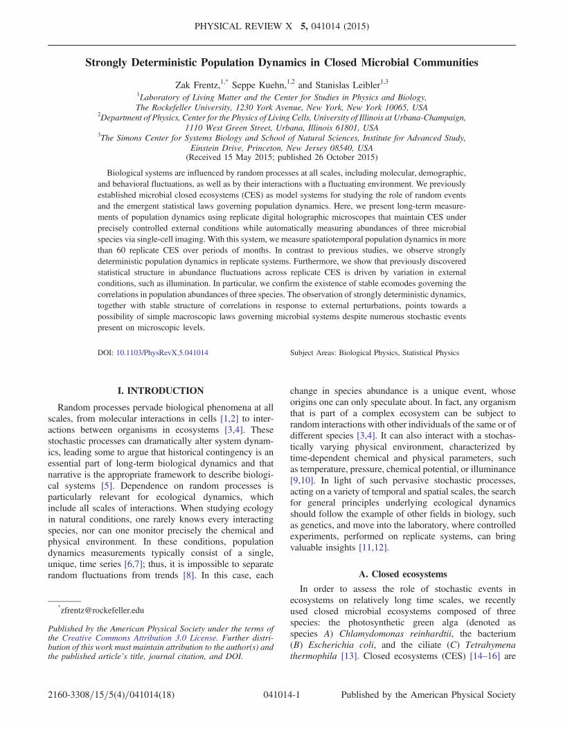
From the analysis of time series of abundances, mor-phological variation, and spatial distributions, we thusconclude that CES maintained under tight environmentalcontrol exhibit strongly deterministic dynamics. It istempting to presume that the fluctuations observed inprevious experiments [Fig. 1(c)] were driven by variationsin extrinsic parameters between replicate CES. This explan-ation assumes that the nature of the interactions inside theCES, leading to the intrinsic dynamics observed here, wasnot substantially modified in the new experiments. To testthis assumption, we studied the nature of correlationsbetween the abundances of the three species and comparedthem with the ecomodes observed in the previous studies.Fluctuations across replicates within a single illuminationcondition were typically small and were not stably corre-lated (Fig. 12). Therefore, to test whether we could excitefluctuations along ecomodes by varying the extrinsicparameters of our CES, we measured population dynamicsfor 45 days in 8 to 10 CES in each of 7 illuminationconditions ranging from 0.2I0 to I0. Figure 5(a) depicts thedynamics of the geometric mean and standard deviationacross all 63 replicates and 7 conditions. It is clear

that varying the illuminance by a factor of 5 inducessubstantial variation across replicate ecosystems [compareto Fig. 1(d)]. We compute the eigensystem of the corre-lation matrix CðtÞ, also calculated over 63 replicates and 7conditions, and the results are shown in Fig. 5(b).Remarkably, the ecomodes in Fig. 5(b) are nearly identicalto those we found in the previous experiments. Forinstance, the ecomode corresponding to the largest eigen-value of CðtÞ (L) is identical to that from the previousexperiments, and it corresponds to the abundances of allthree microbial species fluctuating coherently about themean. The ranking of the two lower modes is reversed incomparison with the previous experiments [13], but theircomposition is unchanged. This result strongly supportsour hypothesis that the intrinsic dynamics in both experi-ments are very similar, and it supports the claim that thefluctuations across replicates observed previously, and thestructure of these fluctuations, were driven by variation inillumination and possibly other extrinsic variables such astemperature.

III. DISCUSSION

We are thus facing a rather astonishing situation: Onmicroscopic scales, we observe many stochastic processestaking place in each CES. However, on more macroscopicscales, replicate-to-replicate variations in the measuredabundances remain small over periods of months.Strongly deterministic dynamics have been observed pre-viously in response to what one could call a “strongperturbation.” For instance, a drastic change of the

FIG. 5. Structure of fluctuations across ecosystems in a range of conditions. (a) Population dynamics, as in Fig. 1(d), for 63 replicateecosystems maintained at 7 illumination conditions between I ¼ 0.2I0 and I ¼ I0. The geometric mean (bold curves) and standarddeviation (shaded regions) are computed across all 63 replicates and 7 illumination conditions. Data before 9 days are missing in someconditions because of overly high cell abundance. (b) Dynamics of the correlation matrix: The correlation matrix CðtÞ of logarithmicabundances of the three species was calculated for the data shown in (a). The eigenvalues of CðtÞ were sorted by size and are plotted astime series in the top panel: L (large, black line);M (medium, cyan line); S (small, magenta line). The composition of the correspondingeigenvectors is plotted in the bottom three panels. Green: C. reinhardtii (A), red: E. coli (B), blue: T. thermophila (C).

STRONGLY DETERMINISTIC POPULATION DYNAMICS IN … PHYS. REV. X 5, 041014 (2015)

041014-7

environment (e.g., large increase of temperature, salinity, orantibiotic concentration) or of the internal composition ofan organism (e.g., deletion of a crucial gene) can induce aquasideterministic change of phenotypes or of speciesabundances [23]. The CES in our experiments are not,however, subject to such strong perturbations, and weobserve long-term strongly deterministic dynamics, ratherthan rapid transformations.From the point of view of biology, this situation is

reminiscent of the developmental dynamics of a singleorganism, which can be buffered against perturbations andappear quasideterministic, or subject to “canalization” [24](also called homeorhesis [25]). In developmental canali-zation [24], the dynamics and the outcomes are observed tobe highly reproducible despite many sources of noise. Theanalogy of highly deterministic population dynamicsobserved here with developmental canalization cannot,however, be directly applied. Our closed ecosystems werecreated with three laboratory strains of microbes, whichhave lived in isolation for many years in the laboratory, andoriginated from complex ecosystems with a multitude ofcomponents. It is, therefore, difficult to argue that naturalselection evolved buffering mechanisms [26] to reducevariation in the population dynamics exhibited by ourparticular synthetic ecosystems.Under selection, microbial populations can undergo

rapid genetic change [27,28]. The extent of genetic diver-sification in our ecosystems has not been determined.However, the strongly deterministic dynamics that weobserve are unlikely to be wholly due to selection, for atleast three reasons. First, the population size is small, atleast in the bulk—less than 1 × 105 for algae, less than1 × 106 for bacteria, and less than 1 × 104 for ciliates.Second, the number of generations during the experiment islikely small. Since our DIH microscopes image an opensubvolume within each cuvette [Fig. 1(a)], the abundanceswe measure arise from division and death as well asmigration; thus, we cannot directly resolve the numberof divisions. However, in the I ¼ I0 condition, over the first2 to 3 days, all three species experience rapid growth fromtheir initial abundances [Fig. 1(d)]. From the maximumabundance reached during this period of growth, we canestimate the number of generations that occur for eachspecies, assuming that birth dominates migration duringthis period. We find that the number of generations is atleast 3 for algae, at least 7 for bacteria, and at least 5 forciliates. We can place a loose upper bound on the number ofgenerations that occurred during the entire experiment bycalculating how many generations would transpire if thegrowth rate inferred early in the experiment were main-tained for the full 90 days. From this, we approximate themaximum number of generations to be 160, 230, and 70 foralgae, bacteria, and ciliates, respectively. However, giventhat nutrients are not supplied during the experiment, weexpect the actual number of generations to be well below

this estimate. For comparison, similarly sized populationsof yeast propagated under rapid growth had very fewdetectable mutations after 100 generations [27]. Third, thedeterministic nature of the dynamics we observe is difficultto reconcile with the random generation of genetic vari-ability through mutation.From a more general point of view, the observation of

deterministic effective dynamics in the presence of noiseis reminiscent of equilibrium thermodynamics and hydro-dynamics. In both cases, stochastic phenomena takingplace on the microscopic level contribute to often-deterministic collective behavior on the macroscopic level,described by simple laws, which use coarse-grained statevariables, such as densities or fluxes. The results of ourexperiments are a strong indicator that complex stochasticphenomena taking place on the microscopic level in a CEScould also be coarse grained on more macroscopic scales,where the relevant degrees of freedom are few. What arethe collective variables best suited to describe our CES? Atpresent, we cannot provide a definitive answer to thisquestion. However, two points are worth noticing: (i) Thetrajectories of abundances are strongly deterministic and donot significantly self-intersect, suggesting that the dynam-ics can be usefully coarse grained to this level; (ii) the firstecomode dominates the externally driven fluctuations,suggesting further dimensional reduction of the space ofcollective variables. Of course, our CES are much morecomplex than systems described by thermodynamics orhydrodynamics. In view of many levels of organization,with interdependent components, we cannot invoke simplestatistical laws, e.g., the law of large numbers, in order todirectly explain the observed strongly deterministic dynam-ics. The dynamics in thermodynamic or hydrodynamicsystems is often driven by temporal or spatial gradients inphysical quantities, such as temperature, pressure, orgravitational potential. At present, we do not know whatquantities drive dynamics in our CES, or what the appro-priate state variables for ecosystems are. However, based onour results, it seems that the view that contingency alwaysdominates long-term biological dynamics, imposing ahistorical narrative as the appropriate method of study[5], might be too pessimistic.We propose that coarse-grained regularities, such as the

strongly deterministic dynamics and the stable ecomodesobserved in this study, might originate in general bio-chemical [29] and physical constraints, common to many, ifnot all, microbial ecosystems. They can be explored furtherby systematically measuring the effects of additionalperturbations on population dynamics. Such an approachwould be facilitated by the strongly deterministic nature ofthe dynamics around which one would apply perturbations.Experiments may include both external perturbations, suchas time-dependent modulations of temperature or illumi-nation, and internal perturbations, such as modifications ofspecies composition, genomes, gene expression profiles, or

ZAK FRENTZ, SEPPE KUEHN, AND STANISLAS LEIBLER PHYS. REV. X 5, 041014 (2015)

041014-8

epigenetic markers. In view of the simplicity and low costof the apparatus used here [17], such systematic studiescould, in principle, be performed in hundreds of replicatesystems in a wide range of conditions. Beyond explainingthe behavior of these particular CES, it is our hope thatthese studies will establish the basis for a more general,quantitative theory of ecological dynamics.

IV. MATERIALS AND METHODS

A. Media and strains

Three species (“ABC”) microbial communities [13] wereconstructed using the alga Chlamydomonas reinhardtii(A: strain UTEX 2244, mating type +), the bacteriumEscherichia coli [B: strain MG1655 Δ flu Δ fimA HK022att::(cat PλR dTomato) hsdR], and the ciliate Tetrahymenathermophila (C: CU428 mating type VI, Cornell UniversityCulture Collection).For each experiment, each species was grown axenically

as follows. Algae were grown in Sager-Granick medium[30] with Hutner’s trace elements (purchased from [31])substituted for the standard trace elements. Cells werethawed from a frozen stock and diluted into Sager-Granickmedia and maintained at 200 rpm shaking, 25 °C, and7500 lx in an incubator. Cultures were grown 7 to 9 daysprior to initiating ecosystems resulting in densities of≈1 × 106 cells=mL. Bacteria were grown from glycerolfrozen stocks in the same media used to construct thecommunity, at 30 °C with 200 rpm shaking resulting indensities of ≈1 × 107 cells=mL. Ciliates were grown inSPP rich media at room temperature without shakingfor approximately 2 days, resulting in densities of1 × 105 cells=mL. Cultures were initiated from a singlelong-term soybean stock that was replenished every6 months [32]. ABC ecosystems were constructed using1=2x Taub #36 supplemented with 0.03% w/v proteosepeptone No. 3 (BD) [33] and a Tris-acetate pH buffer(20 mM Tris, 3 mM acetate).

B. Initiating closed ABC ecosystems

To initiate replicate ecosystems, an axenic culture ofeach of the three species was grown. Each culture waswashed twice in the media used to construct the commu-nity. For A and C, the densities of the washed cultures weremeasured by flow cytometry (BD Biosciences LSR II)using Spherotech AccuCount Fluorescent Particles(Spherotech, ACFP-50-5). For B, culture density afterwashing was measured by optical density. Three specieswere then combined into a single culture at densities of5000 cells=mL, 500 cells=mL, and 500 cells=mL for A, B,and C, respectively. Replicate ecosystems were initiated ina biosafety cabinet by pipetting 1.6 mL of this mixture intosterile and clean quartz cuvettes (StarnaCell, 23-Q-5).Cuvettes were sealed with a sterile, greased (ApiezonM) teflon stopper and epoxy designed to form a hermetic

seal with glass (Epoxy Technology, 905-T). The epoxy wascured for ≈20 h upright, without shaking, in an incubator at25 °C with 7500 lx illumination.Prior to initiating ecosystems, quartz cuvettes were

cleaned thoroughly by scrubbing with a detergent(StarnaCell, CellClean), rinsing with deionized (DI) water,sonicating with a mixture of acetone and isopropyl alcohol(IPA), and soaking for 2 h with 50% nitric acid. Finally,cuvettes were rinsed with DI water and IPA, driedunder pressurized nitrogen gas, and capped with teflonstoppers. Cuvettes were sterilized by UV light from atransilluminator.For each of the seven illumination conditions, we

performed two independent experiments measuringdynamics in 3 to 6 replicate ecosystems. For each experi-ment, the entire initiation protocol described here wasperformed independently.To test for contamination, we plated axenic cultures

used to initiate the communities on four nutrient conditions(Luria-Burtani Broth, Nutrient Broth, Yeast-Peptone-Dextrose, and Thioglycollate broth) and terminated anyexperiment in which contamination was detected. In theexperiments presented here, no contamination was detectedby this method.

C. Ecosystem external conditions

As described previously [17], each microscope inde-pendently controls the temperature (temporal-fluctuationstandard deviation 3 mK, standard deviation across repli-cates 20 mK) and illumination (standard deviation 2.5%)for each ecosystem. Illumination is supplied symmetricallyfrom above and below for each ecosystem by two 1-Wlight-emitting diodes (LEDs, Lumileds, nominal colortemperature 3000 K). For all experiments presented here,the temperature was held constant at 25 °C. The illuminancewas constant in time and symmetric from above and below,but this level of illuminance was varied between experi-ments. Illuminance is measured as a fraction of themaximum calibrated output of the LEDs (I0 is the maxi-mum output). The maximum output was estimated, using acalibrated photodetector, to be 1200 lx (I0).

ACKNOWLEDGMENTS

We thank the following authors for discussions, com-ments, and suggestions: B. Chazelle, J-P. Eckmann, D.Hekstra, D. Huse, J. Lebowitz, A. Libchaber, L. Peliti, T.Tlusty, and L-S. Young, as well as current and formermembers of our laboratory. For technical assistance, wethank J. Chuang, D. Jordan, S. Mazel, and Y. Liu. We thankthe following for distribution of genetic constructs andstrains: the laboratories of C. D. Allis, the Yale Coli GeneticStock Center, the National BioResource Project (NIG,Japan), and the Culture Collection of Algae (UT Austin).This research has been partly supported by grants from the

STRONGLY DETERMINISTIC POPULATION DYNAMICS IN … PHYS. REV. X 5, 041014 (2015)

041014-9

Simons Foundation to S. L. through Rockefeller University(Grant No. 345430) and the Institute for Advanced Study(Grant No. 345801). S. K. acknowledges funding from theHelen Hay Whitney Foundation.Z. F. and S. K. contributed equally to this work.

APPENDIX A: ADDITIONALEXPERIMENTAL METHODS

1. Seal quality

To test the quality of the teflon stopper-grease-epoxyseal, each cuvette was weighed before and after eachexperiment. Any reduction in mass was attributed to waterevaporation. Changes in mass of <1 mg over the durationof the experiment were below the resolution of the balanceused. The mean evaporation rate was 0.098 mgd−1.

2. Differences in conditionsfrom previous experiments

The experiments presented here differed from the mea-surements of Hekstra and Leibler [13] in two importantways. First, we modified the medium by adding a Tris-acetate pH buffer. This increased pH buffering capacity andresulted in less dramatic changes in pH over the course ofthe experiment than were observed previously (see below).Second, the incubators used by Hekstra and Leibler forstorage of CES during the experiment subjected thosesystems to ≈30% variation in the level of illuminationacross replicates and greater thermal fluctuations overtime (s:d: ≈ 50 mK).We performed an experiment to test whether the pH

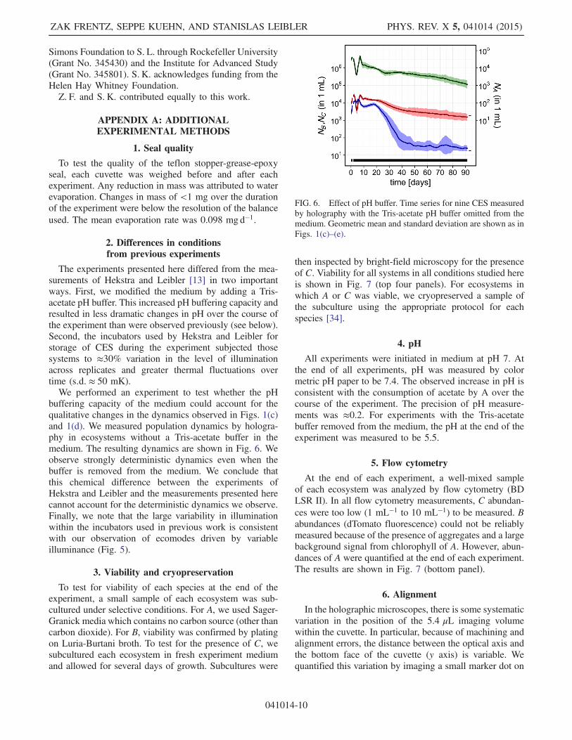
buffering capacity of the medium could account for thequalitative changes in the dynamics observed in Figs. 1(c)and 1(d). We measured population dynamics by hologra-phy in ecosystems without a Tris-acetate buffer in themedium. The resulting dynamics are shown in Fig. 6. Weobserve strongly deterministic dynamics even when thebuffer is removed from the medium. We conclude thatthis chemical difference between the experiments ofHekstra and Leibler and the measurements presented herecannot account for the deterministic dynamics we observe.Finally, we note that the large variability in illuminationwithin the incubators used in previous work is consistentwith our observation of ecomodes driven by variableilluminance (Fig. 5).

3. Viability and cryopreservation

To test for viability of each species at the end of theexperiment, a small sample of each ecosystem was sub-cultured under selective conditions. For A, we used Sager-Granick media which contains no carbon source (other thancarbon dioxide). For B, viability was confirmed by platingon Luria-Burtani broth. To test for the presence of C, wesubcultured each ecosystem in fresh experiment mediumand allowed for several days of growth. Subcultures were

then inspected by bright-field microscopy for the presenceof C. Viability for all systems in all conditions studied hereis shown in Fig. 7 (top four panels). For ecosystems inwhich A or C was viable, we cryopreserved a sample ofthe subculture using the appropriate protocol for eachspecies [34].

4. pH

All experiments were initiated in medium at pH 7. Atthe end of all experiments, pH was measured by colormetric pH paper to be 7.4. The observed increase in pH isconsistent with the consumption of acetate by A over thecourse of the experiment. The precision of pH measure-ments was ≈0.2. For experiments with the Tris-acetatebuffer removed from the medium, the pH at the end of theexperiment was measured to be 5.5.

5. Flow cytometry

At the end of each experiment, a well-mixed sampleof each ecosystem was analyzed by flow cytometry (BDLSR II). In all flow cytometry measurements, C abundan-ces were too low (1 mL−1 to 10 mL−1) to be measured. Babundances (dTomato fluorescence) could not be reliablymeasured because of the presence of aggregates and a largebackground signal from chlorophyll of A. However, abun-dances of A were quantified at the end of each experiment.The results are shown in Fig. 7 (bottom panel).

6. Alignment

In the holographic microscopes, there is some systematicvariation in the position of the 5.4 μL imaging volumewithin the cuvette. In particular, because of machining andalignment errors, the distance between the optical axis andthe bottom face of the cuvette (y axis) is variable. Wequantified this variation by imaging a small marker dot on

FIG. 6. Effect of pH buffer. Time series for nine CES measuredby holography with the Tris-acetate pH buffer omitted from themedium. Geometric mean and standard deviation are shown as inFigs. 1(c)–(e).

ZAK FRENTZ, SEPPE KUEHN, AND STANISLAS LEIBLER PHYS. REV. X 5, 041014 (2015)

041014-10

the back face of each cuvette prior to removing it from themicroscope at the end of the experiment. The position ofthe dot was then measured on a separate bright-fieldmicroscope with a large field of view. For the 48 ecosys-tems in which this measurement was performed, we foundthe distance to be 2560 μm �430 μm.Because of the significant spatial heterogeneity we

observed in the ecosystems, we investigated whether thevariability in abundance over replicates could be explainedby their vertical positions. Vertical positions were onlymeasured for the six replicates from one repetition of theI ¼ I0 condition. For these replicates, we found that therelative abundance residuals ðNi

sðtÞ − hNsðtÞiÞ=hNsðtÞi forreplicate i and species s stabilized after day 27. Wecomputed the time averages of these quantities from day27 to day 92 for each of the six replicates in this data set andregressed them on the vertical position of the imaged regionwithin that replicate, yi. For both algae and bacteria (ciliateswere not considered because of low abundance), the relativeabundance residual and vertical position were negativelycorrelated [ρA¼−0.86ðp¼0.014Þ, ρB¼−0.71ðp¼0.06Þ].

After adjusting for the influence of the vertical position onthe abundances, the remaining fluctuations are significantlysmaller (σA ¼ 1.26 and σB ¼ 1.6), suggesting that bettercontrol of the cuvette position should result in the meas-urement of even less variability across replicates.

APPENDIX B: DATA ANALYSIS

1. Iterative signal removal

The reconstruction of each hologram results in a three-dimensional array of complex amplitudes from within thesample. For our purposes, the phase information is notused, and only the squared modulus, or intensity, is ofinterest. The focal plane of each object is identifiedautomatically [17].A major difficulty for automated computer analysis is

the low intensity of E. coli relative to C. reinhardtii andT. thermophila. The signal-to-noise ratio for the majority ofbacterial cells is sufficient to separate them from thebackground; however, out-of-focus light from the brighterspecies complicates segmentation. This out-of-focus lightcan have significant spatial extent and can exhibit localizedregions of intensity above the background. These discretebright spots do not come into focus and can be distin-guished from in-focus objects in three dimensions.However, applying global segmentation results in manyfalse objects. An example of this effect is shown in Fig. 8.To solve this problem, we exploit the computational

nature of digital holography by removing the signal frombright objects before analyzing dimmer objects. By per-forming an initial segmentation at a high intensity thresh-old, all bright objects are identified, the focal plane of eachbright object is determined, and the morphology is ana-lyzed in that plane. The signal from the object can then beremoved from all focal planes by setting all complexamplitudes within the object to zero. The result is propa-gated back to the hologram plane by inverting thereconstruction procedure, resulting in a hologram that isequivalent to the original with the signal from the brightobject removed (Fig. 8). All objects above the intensitythreshold are analyzed and removed, and then a secondround of segmentation, analysis, and removal is performedat a lower intensity threshold. By using many thresholds,artifacts associated with objects having intensities near thethreshold intensity can be avoided. In our implementation,18 rounds of signal subtraction are used.

2. Species classification

The image analysis of each blob measures the spatiallocation, spatial moments of the two-dimensional intensitydistribution in the focal plane, and statistics describing thenumber of voxels exceeding various intensity thresholds.A training set of 8967 manually classified objects was usedto train a support vector machine [35] to classify objectsinto four classes (algae, bacteria, ciliates, and background).

FIG. 7. Final viability and total algal density. Top four panels:Viability of each species, measured as described above, as afunction of illumination. Green, red, and blue symbols show thefraction of systems with A, B, and C viable, respectively. Blacksquares show the fraction of replicates where all three species areviable. The two experiments in each illumination condition arerepresented by circle and square symbols. Bottom panel: Densityof C. reinhardtii, as measured by flow cytometry, from a well-mixed sample of each replicate, at the end of each experiment as afunction of illumination condition. A single point is plotted foreach replicate with symbols denoting different experimentswithin each illumination condition.

STRONGLY DETERMINISTIC POPULATION DYNAMICS IN … PHYS. REV. X 5, 041014 (2015)

041014-11

A test set of 1825 manually classified objects was used toestimate the classification error rate—the results are tabu-lated in Table I; there were no detection errors for thetest set.

3. Count statistics

Cells leave and enter the imaged region by a combinationof swimming and convective flow. Our goal is to filter thenoise due to sampling in order to infer an underlyingabundance. We can roughly estimate the residence times ofeach species using measurements of the convective flowand diffusion coefficients for typical swimming behaviors;in each case, the estimated residence time is less than oneminute, so we expect little correlation in sampling noise formeasurements separated by 400 s.

We assume that the counts of each species are atemporally uncorrelated Poisson-distributed random varia-ble AðtÞ, whose rate fluctuates in time. This rate isinterpreted as a spatial density integrated over the imagingregion, from which Poisson-distributed random counts aredrawn because of discrete cells entering and leaving theregion. The rate is unitless and corresponds to the expectedvalue for the counts as a function of time. It is estimatedindependently for each species in each replicate. In ourexperiments, the underlying rate varies over time by at least3 orders of magnitude, so the variance due to countingnoise also varies by several orders of magnitude. In thiscase, it is clear that a stationary filter is inappropriate,and we specify a probabilistic model for the counts andunderlying rate which has superior performance. Thequantity of interest is the conditional probability of theunderlying logarithmic rate given the counts:

L ¼ PðWjfAðtiÞgÞ; ðB1Þ

where W represents the logarithm of the rate over the timeinterval of the experiment, ½0; tm�, and ti is the time ofmeasurement i, i ¼ 1; 2;…; m. Applying Bayes’ rule gives

FIG. 8. Signal subtraction detail. (a) Focal plane of reconstructed T. thermophila, to the upper left. (b) Same T. thermophila from (a),290 μm out of focus. An E. coli, indicated by a red arrow, is barely visible, to the right—see (f) and (h) for better visibility at highcontrast. (c) Focal plane from (a), after the signal from the T. thermophila has been subtracted. (d) Focal plane from (b), after signalsubtraction, showing unperturbed E. coli. (e)–(h) Duplicate panels (a)–(d) at high contrast. The scale bar is 20 μm. (i) Intensity profileacross the horizontal coordinate in (b) and (f), through the E. coli cell, before subtraction. The large high-intensity region around 70 μmis the out-of-focus T. thermophila, while the peak at 140 μm is the in-focus E. coli cell. (j) Intensity profile through the same row ofpixels as in (i), after signal subtraction—see (d) and (h).

TABLE I. Classification table.

Manual classification

Algae Bacteria Ciliates Background

SVMclassification

Algae 812 19 0 0Bacteria 3 618 1 0Ciliates 2 0 282 0Background 0 1 0 87

ZAK FRENTZ, SEPPE KUEHN, AND STANISLAS LEIBLER PHYS. REV. X 5, 041014 (2015)

041014-12

L ¼ PðfAðtiÞgjWÞPðWÞ=PðAÞ; ðB2Þ

where PðAÞ does not depend on W and so does not affectthe estimation of W. From our assumption that AðtÞ isPoisson and temporally uncorrelated,

PðfAðtiÞgjWÞ ¼Ymi¼1

PðAðtiÞ ¼ aijWðtiÞ ¼ wiÞ

¼Ymi¼1

e−ewi ewiai

ai!: ðB3Þ

Previous work suggested that the fluctuations of WðtÞacross replicates can be well described as a random walk[13]. To derive an expression for PðWÞ for our filterwithout imposing additional structure, we assume thatWðtÞ itself is a random walk, with Gaussian increments.Define Δti ¼ tiþ1 − ti, and let γ be a parameter thatdetermines the increment variance:

PðWÞ ¼ PðWðt1Þ ¼ w1ÞYm−1

i¼1

PðWiþ1 ¼ wiþ1jWi ¼ wiÞ

¼ PðWðt1Þ ¼ w1ÞYm−1

i¼1

ð2πγΔtiÞ−1=2

× expð−ðwiþ1 − wiÞ2=2γΔtiÞ: ðB4Þ

We can now write the portion of the log likelihood thatdepends on W:

logðLPðAÞÞ ¼ logPðWðt1Þ ¼ w1Þ

þXm−1

i¼1

�− 1

2log 2πγΔti − ðwiþ1 − wiÞ2

2γΔti− ewi

þ aiwi − logðai!Þ�

− ewm þ amwm − logðam!Þ: ðB5Þ

This expression is maximized over wi by gradientascent, using a moving average of the logarithm ofmeasured counts as starting values. The parameter γwas chosen by testing the distribution of ai against aPoisson distribution with rate ewi . The optimal valuewas γ ¼ 2.56 × 10−2= day. The distribution of the initiallogarithmic rate was assumed to be Gaussian, with meanequal to the average of the logarithm of the first fewmeasurements:

PðWðt1Þ¼w1Þ¼ð2πσ20Þ−1=2exp½−ðw1−μ0Þ2=2σ20�; ðB6Þ

where μ0 ¼ 1n

Pni¼1 log ai, σ0 ¼ μ−1=20 and n ¼ 5.

We found that this filter performed very well. Thedistributions of counts were indistinguishable fromPoisson with the inferred rate, and the autocorrelation ofthe residuals δi ¼ log ai − wi decayed very quickly(Fig. 9), justifying the assumption of independence ofconsecutive measurements.

4. Spatial density estimation

The analysis of our experiments yields a list of identifiedorganisms, with a location in space, which we denote as

rðiÞj;s ¼ ðxj; yj; zjÞ, where i denotes the experimental repli-cate, s denotes the species, and j indexes the individualorganisms of species s in replicate i. The simplest

FIG. 9. Autocorrelation of count-smoothing residuals. The autocorrelation function of the residual from the count-smoothingprocedure, δi ¼ log ai − wi, was calculated for one of the replicates and each species, with lag measured in time points (400 s). The blueline shows the 95% confidence interval. The rapid decay observed here was typical for all replicates.

STRONGLY DETERMINISTIC POPULATION DYNAMICS IN … PHYS. REV. X 5, 041014 (2015)

041014-13

characterization of spatial structure is the time-averagedspatial density:

PrðrðiÞs ∈ VÞ ¼ZVgðiÞs ðx; y; zÞ dx dy dz; ðB7Þ

where V is a region in space.We estimated the spatial density gðiÞs ðx; y; zÞ for each

replicate and species via kernel density estimation [36],using cross validation to choose bandwidths. The optimalbandwidths in x, y, and z were 82 μm, 68 μm, 204 μm foralgae; 88 μm, 72 μm, 225 μm for bacteria; and 107 μm,88 μm, 246 μm for ciliates.Our data are sharply truncated in space, by optical

constraints in x and y, and by the cuvette walls in z. Toreduce bias in the estimate due to truncations, wesupplemented the bounded data set with its reflectionsacross the boundaries [37]. The cuvette wall positions

were determined manually by finding a region near eachz extremum where the density of blobs fell close to zero.We estimated the precision of this procedure to be�5 μm. The wall locations varied by a small amount,which was accounted for by linearly transforming thedata from each replicate along the z axis to coincide witha standard reference.The confidence interval of the estimate can be calculated

by bootstrapping [38]. We calculated 95% confidenceintervals with at least 70% coverage, denoted bðiÞs , and

considered the ratio bðiÞs =gðiÞs , averaged over space, toindicate the precision of the spatial density estimates.Typical values over space and replicates were 6% foralgae, 10% for bacteria, and 8% for ciliates.Spatial distributions for all three species are shown in

Fig. 4 for the I ¼ I0 condition and Fig. 10 for the I ¼0.25I0 condition. We note that the apparently large σ½g�=hgifor E. coli and T. thermophila in the I ¼ 0.25I0 condition is

FIG. 10. I ¼ 0.25I0 spatial distributions of microbes in imaging volume. γhgi and σ½g�=hgi are defined in the caption to Fig. 4 for theI ¼ I0 condition.

ZAK FRENTZ, SEPPE KUEHN, AND STANISLAS LEIBLER PHYS. REV. X 5, 041014 (2015)

041014-14

due to statistical variation in hgi arising from low abun-dances rather than variation across replicates.

5. Phase portrait statistics

To quantify the stereotypical nature of the trajectories inthe I ¼ 0.25I0 and I ¼ I0 illumination conditions, weapplied a temporal alignment to the time series of loga-rithmic densities. We denote the smoothed logarithmic

abundance of species s and replicate i by uðiÞs ðtÞ ¼wðiÞs ðtÞ − logðVðiÞ=1 mLÞ, where VðiÞ is the volume of

the imaged region for replicate i, in units of mL. Note

that the abundance NðiÞs ðtÞ ¼ expðuðiÞs ðtÞÞ. The goal is to

find nondecreasing functions τij and τ0ij such that theintegrated squared difference upon alignment is minimized:

τij; τ0ij ¼ argminτ;τ0∈T

Z1

0

Xs

ðuðiÞs ðτðlÞÞ − uðjÞs ðτ0ðlÞÞÞ2dl; ðB8Þ

whereT is the space of nondecreasing functions from [0,1]to ½0; T�, T is the experiment duration, and l parametrizesthe alignment functions. The functions τ and τ0 can becalculated on a discrete grid by dynamic programming.Statistics over the aligned trajectories are calculated as

follows. First, one of the replicates is chosen as thereference trajectory—this replicate is denoted with the

index i0. Aligned versions of each replicate are defined

as ~uðjÞs ðtÞ ¼ uðjÞs ðτ0i0jðτ−1i0jðtÞÞÞ and statistics of aligned

trajectories can be calculated for ~uðjÞðtÞ over replicates j.The mean of ~uðjÞs ðtÞ over replicates is calculated

and transformed to represent effective populationabundance:

~μsðtÞ ¼ exp

�1

n

Xnj¼1

~uðjÞs ðtÞ�: ðB9Þ

In Fig. 2(c), the mean aligned densities ~μsðtÞ in theI ¼ I0 and I ¼ 0.25I0 illumination conditions are plottedas gray curves, and the covariance matrix for these samedata sets is used to compute the 68% confidence interval,plotted as white ellipses. For the I ¼ 0.25I0 data set, it wasnecessary to adjust the temporal range of alignmentdetermined by T for three replicates that did not exhibitthe rapid increase in T. thermophila abundance aroundday 28–42.

6. Morphological dynamics

As discussed above, analysis of the reconstructionsyields blobs classified as one of the three microbial speciesas well as each blob’s morphological properties. Themorphological dynamics are most significant for species

FIG. 11. Gaussian mixture model fit for one replicate in the I ¼ 0.25I0 condition. The upper panel shows the means of the two modes(μ1 and μ2), the second panel shows the weights of these modes in the mixture distribution (π1 and π2, respectively), the third panelshows a histogram of the raw data, and the fourth panel shows the inferred probability density at each time point. In both the third andfourth panels, each column (time point) is normalized independently. The bottom panel plots the classification with large cells in red andsmall cells in black; note that there is no overlap between these classes.

STRONGLY DETERMINISTIC POPULATION DYNAMICS IN … PHYS. REV. X 5, 041014 (2015)

041014-15

C, so we focus our characterization of the morphologicaldynamics on this species only.In particular, we consider the lateral size of each blob,

denoted Sij for individual j in replicate i, measured in μm.The distribution of lateral size over time and replicates isapproximately log-normal, so we consider the logarithm:λij ¼ logðSij=1 μmÞ. Each logarithmic size is associatedwith the time of measurement, tij, and so we write λiðtÞ toindicate time dependence.We found that distributions of λiðtÞ in many temporal

windows were bimodal, with a strongly time-dependent structure (Fig. 11). We therefore parametrizedthe time-dependent distribution of logarithmic size using aGaussian mixture model (GMM) with two modes. Thesedistributions are estimated independently for each replicate,so we suppress the replicate index i:

PðλðtÞjΘðtÞÞ ¼ π1ðtÞϕ1ðλðtÞ; θ1ðtÞÞþ π2ðtÞϕ2ðλðtÞ; θ2ðtÞÞ; ðB10Þ

where ϕmðλ; θmÞ is Gaussian with θm ¼ fμm; σ2mg andΘ ¼ fπ1; π2; θ1; θ2g. We regularize the model for smooth-ness between time points by maximizing the followingobjective function:

OðΘðtiÞ;Θðti−1Þ; λðtiÞÞ

¼ lðΘðtiÞ; λðtiÞÞ − η1X2m¼1

ðμmðtiÞ − μmðti−1ÞÞ2

− η2ðπ1ðtiÞ − π1ðti−1ÞÞ2; ðB11Þ

where

lðΘðtiÞ; λðtiÞÞ ¼ log

�Yk

PðλðtiÞ ¼ λkjΘðtiÞÞ�

ðB12Þ

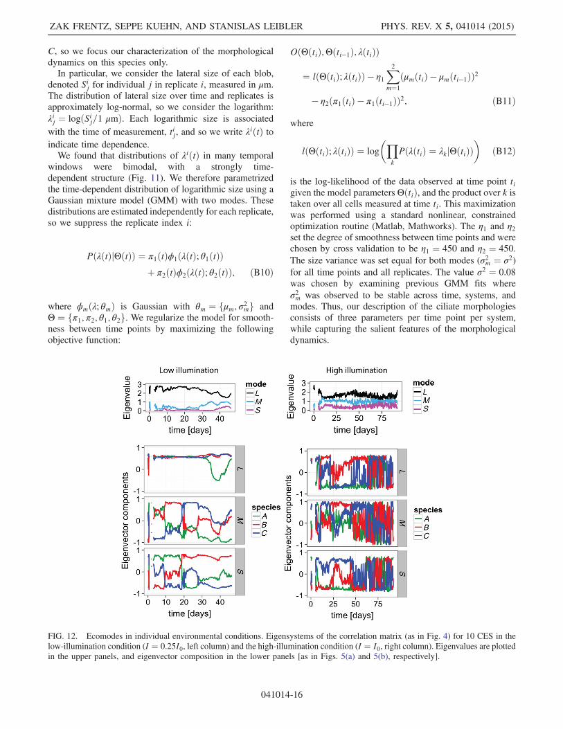
is the log-likelihood of the data observed at time point tigiven the model parameters ΘðtiÞ, and the product over k istaken over all cells measured at time ti. This maximizationwas performed using a standard nonlinear, constrainedoptimization routine (Matlab, Mathworks). The η1 and η2set the degree of smoothness between time points and werechosen by cross validation to be η1 ¼ 450 and η2 ¼ 450.The size variance was set equal for both modes (σ2m ¼ σ2)for all time points and all replicates. The value σ2 ¼ 0.08was chosen by examining previous GMM fits whereσ2m was observed to be stable across time, systems, andmodes. Thus, our description of the ciliate morphologiesconsists of three parameters per time point per system,while capturing the salient features of the morphologicaldynamics.

FIG. 12. Ecomodes in individual environmental conditions. Eigensystems of the correlation matrix (as in Fig. 4) for 10 CES in thelow-illumination condition (I ¼ 0.25I0, left column) and the high-illumination condition (I ¼ I0, right column). Eigenvalues are plottedin the upper panels, and eigenvector composition in the lower panels [as in Figs. 5(a) and 5(b), respectively].

ZAK FRENTZ, SEPPE KUEHN, AND STANISLAS LEIBLER PHYS. REV. X 5, 041014 (2015)

041014-16

Θðti−1Þ is not always available because of gaps in thedata, which vary in duration from a single acquisition tomany days. For small gaps in the data, we wish to maintainthe smoothness between nearby time points, while forlarge gaps, the smoothness penalty, determined by η1 andη2, should be much smaller to permit large changes inthe model parameters. Therefore, when Θðti−1Þ is notavailable because of missing data, we maximizeOðΘðtiÞ;Θðti−kÞ; λðtiÞÞ, where ti−k is the most recent timepoint with available data, and we use modified regulari-zation parameters η01 ¼ η1=k, η02 ¼ η2=k.

7. Ecomodes

We computed the eigensystem of the correlation matrixCðtÞ for ecosystems in a single illumination condition,either high (I ¼ I0) or low (I ¼ 0.25I0), and the results areshown in Fig. 12. We find that in the high-illuminationcondition, the correlation matrix is dominated by noise. Inthe low-illumination condition, the largest ecomode has asimilar structure to that computed across illuminationconditions, but this breaks down after about 30 days.The M and S ecomodes in the I ¼ 0.25I0 condition differqualitatively from those we computed across all illumina-tion conditions (see Fig. 5).

[1] M. Delbrück, Statistical Fluctuations in AutocatalyticReactions, J. Chem. Phys. 8, 120 (1940).

[2] M. B. Elowitz, A. J. Levine, E. D. Siggia, and P. S. Swain,Stochastic Gene Expression in a Single Cell, Science 297,1183 (2002).

[3] M. Lieb, The Establishment of Lysogenicity in Escherichiacoli, J. Bacteriol. 65, 642 (1953).

[4] J. Sheng, E. Malkiel, J. Katz, J. Adolf, R. Belas, and A. R.Place, Digital Holographic Microscopy Reveals Prey-Induced Changes in Swimming Behavior of PredatoryDinoflagellates, Proc. Natl. Acad. Sci. U.S.A. 104, 17512(2007).

[5] S. J. Gould, Wonderful Life: The Burgess Shale and theNature of History (WW Norton & Company, NY, 1990).

[6] J. Esper, U. Büntgen, D. C. Frank, D. Nievergelt, andA. Liebhold, 1200 Years of Regular Outbreaks in AlpineInsects, Proc. R. Soc. B 274, 671 (2007).

[7] M. Dornelas, N. J. Gotelli, B. McGill, H. Shimadzu,F. Moyes, C. Sievers, and A. E. Magurran, AssemblageTime Series Reveal Biodiversity Change but Not SystematicLoss, Science 344, 296 (2014).

[8] D. R. Hekstra, S. Cocco, R. Monasson, and S. Leibler,Trend and Fluctuations: Analysis and Design of PopulationDynamics Measurements in Replicate Ecosystems, Phys.Rev. E 88, 062714 (2013).

[9] L. W. Alvarez, W. Alvarez, F. Asaro, and H. V. Michel,Extraterrestrial Cause for the Cretaceous-TertiaryExtinction, Science 208, 1095 (1980).

[10] A. M. Michalak, E. J. Anderson, D. Beletsky, S. Boland,N. S. Bosch, T. B. Bridgeman, J. D. Chaffin, K. Cho, R.Confesor, I. Daloğlu et al., Record-Setting Algal Bloom in

Lake Erie Caused by Agricultural and MeteorologicalTrends Consistent with Expected Future Conditions, Proc.Natl. Acad. Sci. U.S.A. 110, 6448 (2013).

[11] S. E. Luria and M. Delbrück, Mutations of Bacteria fromVirus Sensitivity to Virus Resistance, Genetics 28, 491(1943).

[12] A. H. Sturtevant, H. J. Muller, and C. B. Bridges, TheMechanism of Mendelian Heredity (Holt, NY, 1922).

[13] D. R. Hekstra and S. Leibler, Contingency and StatisticalLaws in Replicate Microbial Closed Ecosystems, Cell 149,1164 (2012).

[14] Z. Kawabata, K. Matsui, K. Okazaki, M. Nasu, N. Nakano,and T. Sugai, Synthesis of a Species-Defined Microcosmwith Protozoa, J. Protozoo. Res. 5, 23 (1995).

[15] F. B. Taub and A. K. McLaskey, Oxygen Dynamics ofAquatic Closed Ecological Systems: Comparing the Wholeto a Subsystem, Ecol. Model. 293, 49 (2014).

[16] E. A. Kearns and C. E. Folsome,Measurement of BiologicalActivity in Materially Closed Microbial Ecosystems,BioSystems 14, 205 (1981).

[17] Z. Frentz, S. Kuehn, D. Hekstra, and S. Leibler, MicrobialPopulation Dynamics by Digital In-Line HolographicMicroscopy, Rev. Sci. Instrum. 81, 084301 (2010).

[18] The Chlamydomonas Sourcebook, Vol. 1, edited byE. H. Harris, D. B. Stern, and G. Witman (Academic Press,Waltham, MA, 2009).

[19] Tetrahymena thermophila, Methods in Cell Biology,Vol. 109, edited by K. Collins (Academic Press, Waltham,MA, 2012).

[20] M. A. Savageau, Escherichia coli Habitats, Cell Types, andMolecular Mechanisms of Gene Control, Am. Nat. 122, 732(1983).

[21] S. A. Amin, L. R. Hmelo, H. M. van Tol, B. P. Durham, L. T.Carlson, K. R. Heal, R. L. Morales, C. T. Berthiaume, M. S.Parker, B. Djunaedi et al., Interaction and Signallingbetween a Cosmopolitan Phytoplankton and AssociatedBacteria, Nature (London) 522, 98 (2015).

[22] A. Sano, M. Watanabe, and T. Nakajima, AdaptiveCharacteristics of a Ciliate Tetrahymena thermophila inEndosymbiotic Association with a Green Alga Chlorellavulgaris Derived in a Long-Term Microcosm Culture,Symbiosis 47, 151 (2009).

[23] Q. Zhang, G. Lambert, D. Liao, H. Kim, K. Robin, C-k.Tung, N. Pourmand, and R. H. Austin, Acceleration ofEmergence of Bacterial Antibiotic Resistance in ConnectedMicroenvironments, Science 333, 1764 (2011).

[24] C. H. Waddington, Canalization of Development and theInheritance of Acquired Characters, Nature (London) 150,563 (1942).

[25] C. H. Waddington, The Strategy of the Genes (Allen &Unwin, Australia, 1957).

[26] S. L. Rutherford and S. Lindquist, Hsp90 as a Capacitorfor Morphological Evolution, Nature (London) 396, 336(1998).

[27] G. I. Lang, D. P. Rice, M. J. Hickman, E. Sodergren, G. M.Weinstock, D. Botstein, and M.M. Desai, Pervasive GeneticHitchhiking and Clonal Interference in Forty Evolving YeastPopulations, Nature (London) 500, 571 (2013).

[28] M.M. Zambrano, D. A. Siegele, M. Almirón, A. Tormo,and R. Kolter, Microbial Competition: Escherichia coli

STRONGLY DETERMINISTIC POPULATION DYNAMICS IN … PHYS. REV. X 5, 041014 (2015)

041014-17

Mutants that Take Over Stationary Phase Cultures, Science259, 1757 (1993).

[29] M. Scott, C.W.Gunderson, E. M.Mateescu, Z. Zhang, and T.Hwa, Interdependence of Cell Growth and Gene Expression:Origins and Consequences, Science 330, 1099 (2010).

[30] http://www.chlamy.org/SG.html.[31] http://www.chlamy.org.[32] M. T. Sweet and C. D. Allis, Long-Term Storage of

Unfrozen Tetrahymena Cultures in Soybean Medium,CSH Protocols, doi: 10.1101/pdb.prot4470 (2006).

[33] F. B. Taub and A. M. Dollar, The Nutritional Inadequacyof Chlorella and Chlamydomonas as Food for Daphniapulex, Limnol. Oceanogr. 13, 607 (1968).

[34] D. Cassidy-Hanley, H. R. Smith, and P. J. Bruns, ASimple, Efficient Technique for Freezing Tetrahymenathermophila, J. Euk. Microbiol. 42, 510 (1995).

[35] V. N. Vapnik, The Nature of Statistical LearningTheory (Springer Science & Business Media, Berlin,2013).

[36] L. Wasserman, All of Nonparametric Statistics (SpringerScience & Business Media, Berlin, 2006).

[37] M. G. Albers, Master’s thesis, Swiss Federal Institute ofTechnology Zurich (2012).

[38] P. Hall and J. Horowitz, A Simple Bootstrap Methodfor Constructing Nonparametric Confidence Bands forFunctions, Ann. Stat. 41, 1892 (2013).

ZAK FRENTZ, SEPPE KUEHN, AND STANISLAS LEIBLER PHYS. REV. X 5, 041014 (2015)

041014-18