Embed Size (px)
Citation preview
University of Central Florida University of Central Florida
STARS STARS
Electronic Theses and Dissertations, 2004-2019
2009
Structural Analysis And Active Vibration Control Of Tetraform Structural Analysis And Active Vibration Control Of Tetraform
Space Frame For Use In Micro-scale Machining Space Frame For Use In Micro-scale Machining
Kevin Knipe University of Central Florida
Part of the Mechanical Engineering Commons
Find similar works at: https://stars.library.ucf.edu/etd
University of Central Florida Libraries http://library.ucf.edu
This Masters Thesis (Open Access) is brought to you for free and open access by STARS. It has been accepted for
inclusion in Electronic Theses and Dissertations, 2004-2019 by an authorized administrator of STARS. For more
information, please contact [email protected].
STARS Citation STARS Citation Knipe, Kevin, "Structural Analysis And Active Vibration Control Of Tetraform Space Frame For Use In Micro-scale Machining" (2009). Electronic Theses and Dissertations, 2004-2019. 4100. https://stars.library.ucf.edu/etd/4100
STRUCTURAL ANALYSIS AND ACTIVE VIBRATION CONTROL OF
TETRAFORM SPACE FRAME FOR USE IN MICRO-SCALE MACHINING
by
KEVIN KNIPE
B.S. The Ohio State University, 2007
A thesis submitted in partial fulfillment of the requirements
for the degree of Master of Science
in the department of Mechanical, Materials, and Aerospace Engineering
in the College of Engineering and Computer Science
at the University of Central Florida
Orlando, Florida
Fall Term
2009
ii
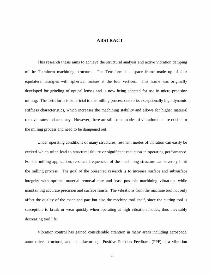
ABSTRACT
This research thesis aims to achieve the structural analysis and active vibration damping
of the Tetraform machining structure. The Tetraform is a space frame made up of four
equilateral triangles with spherical masses at the four vertices. This frame was originally
developed for grinding of optical lenses and is now being adapted for use in micro-precision
milling. The Tetraform is beneficial to the milling process due to its exceptionally high dynamic
stiffness characteristics, which increases the machining stability and allows for higher material
removal rates and accuracy. However, there are still some modes of vibration that are critical to
the milling process and need to be dampened out.
Under operating conditions of many structures, resonant modes of vibration can easily be
excited which often lead to structural failure or significant reduction in operating performance.
For the milling application, resonant frequencies of the machining structure can severely limit
the milling process. The goal of the presented research is to increase surface and subsurface
integrity with optimal material removal rate and least possible machining vibration, while
maintaining accurate precision and surface finish. The vibrations from the machine tool not only
affect the quality of the machined part but also the machine tool itself, since the cutting tool is
susceptible to break or wear quickly when operating at high vibration modes, thus inevitably
decreasing tool life.
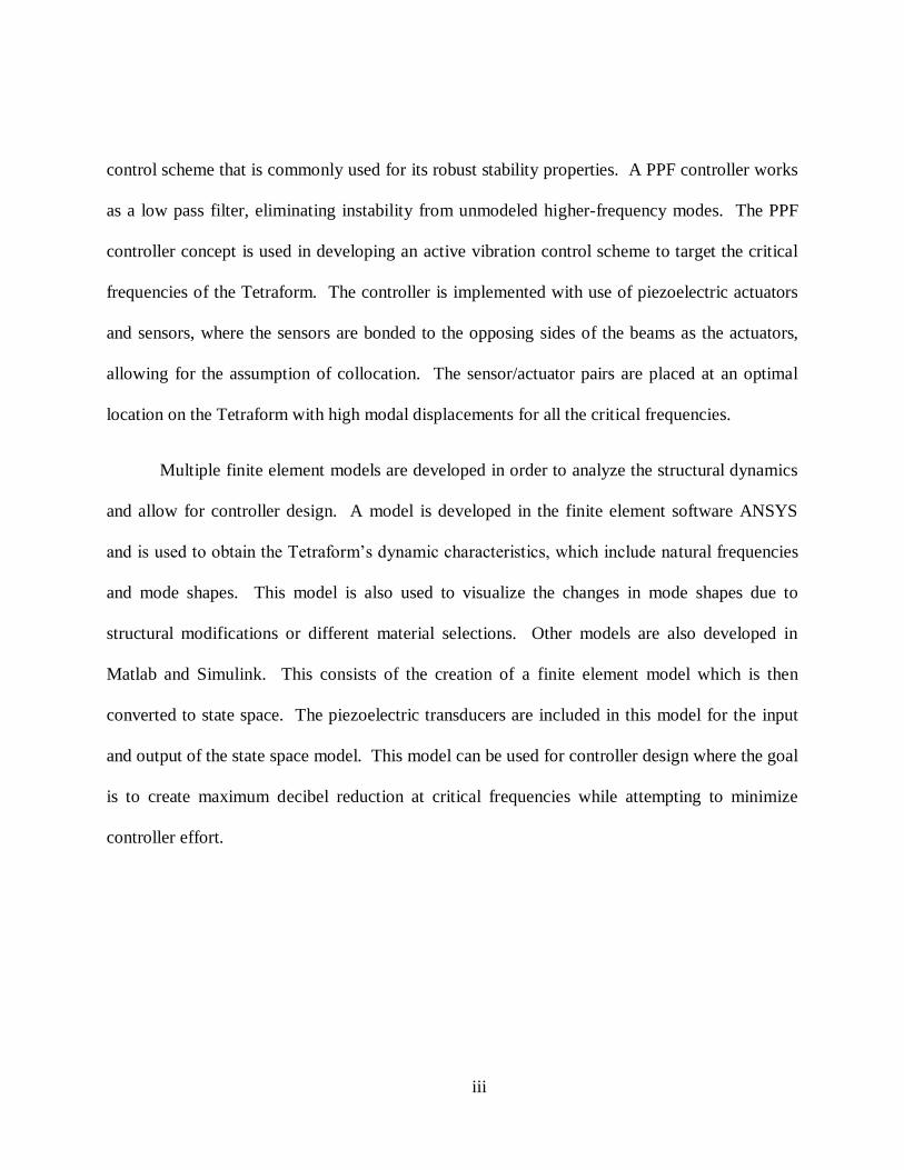
Vibration control has gained considerable attention in many areas including aerospace,
automotive, structural, and manufacturing. Positive Position Feedback (PPF) is a vibration
iii
control scheme that is commonly used for its robust stability properties. A PPF controller works
as a low pass filter, eliminating instability from unmodeled higher-frequency modes. The PPF
controller concept is used in developing an active vibration control scheme to target the critical
frequencies of the Tetraform. The controller is implemented with use of piezoelectric actuators
and sensors, where the sensors are bonded to the opposing sides of the beams as the actuators,
allowing for the assumption of collocation. The sensor/actuator pairs are placed at an optimal
location on the Tetraform with high modal displacements for all the critical frequencies.
Multiple finite element models are developed in order to analyze the structural dynamics
and allow for controller design. A model is developed in the finite element software ANSYS
and is used to obtain the Tetraform’s dynamic characteristics, which include natural frequencies
and mode shapes. This model is also used to visualize the changes in mode shapes due to
structural modifications or different material selections. Other models are also developed in
Matlab and Simulink. This consists of the creation of a finite element model which is then
converted to state space. The piezoelectric transducers are included in this model for the input
and output of the state space model. This model can be used for controller design where the goal
is to create maximum decibel reduction at critical frequencies while attempting to minimize
controller effort.

iv
ACKNOWLEDGMENTS
First, I would like to express my greatest appreciation to my advisor, Dr. Chengying Xu.
I am very thankful for the amazing opportunity she had granted me with being able to work with
her on this exciting project. I am also thankful for the time, effort, and guidance that she has
invested into me and my research studies.
Next, I would like to thank Dr. David Nicholson for his guidance with the finite element
model development of the Tetraform and Mr. Alex Pettit for his assistance with obtaining the
experimental frequency responses through the impact hammer method. Their help was essential
to the development of this project.
Also, I would like to thank my committee members, as a whole, for taking time out of
their very busy schedules to help me through the thesis process. Additionally, I would like to
thank my fellow lab members for always being there to help.
Finally, but certainly not least, I would like to thank my parents. They have always been
there to support me in any way throughout my college career. Without them, none of my
education would have been possible.
v
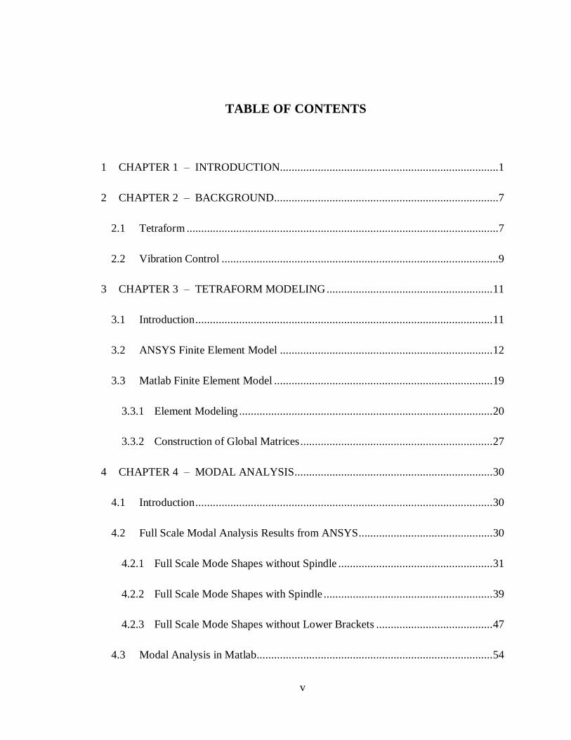
TABLE OF CONTENTS
1 CHAPTER 1 – INTRODUCTION ...........................................................................1
2 CHAPTER 2 – BACKGROUND.............................................................................7
2.1 Tetraform ...........................................................................................................7
2.2 Vibration Control ...............................................................................................9
3 CHAPTER 3 – TETRAFORM MODELING ......................................................... 11
3.1 Introduction ...................................................................................................... 11
3.2 ANSYS Finite Element Model ......................................................................... 12
3.3 Matlab Finite Element Model ........................................................................... 19
3.3.1 Element Modeling ....................................................................................... 20
3.3.2 Construction of Global Matrices .................................................................. 27
4 CHAPTER 4 – MODAL ANALYSIS .................................................................... 30
4.1 Introduction ...................................................................................................... 30
4.2 Full Scale Modal Analysis Results from ANSYS.............................................. 30
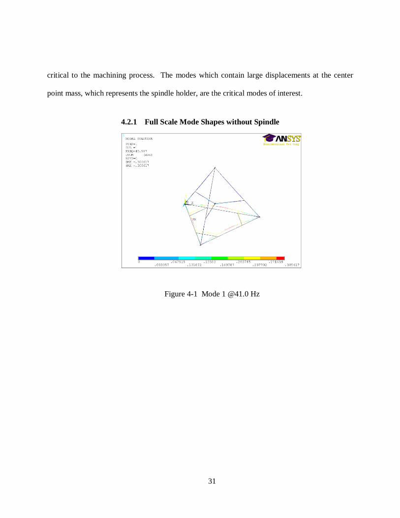
4.2.1 Full Scale Mode Shapes without Spindle ..................................................... 31
4.2.2 Full Scale Mode Shapes with Spindle .......................................................... 39
4.2.3 Full Scale Mode Shapes without Lower Brackets ........................................ 47
4.3 Modal Analysis in Matlab................................................................................. 54
vi
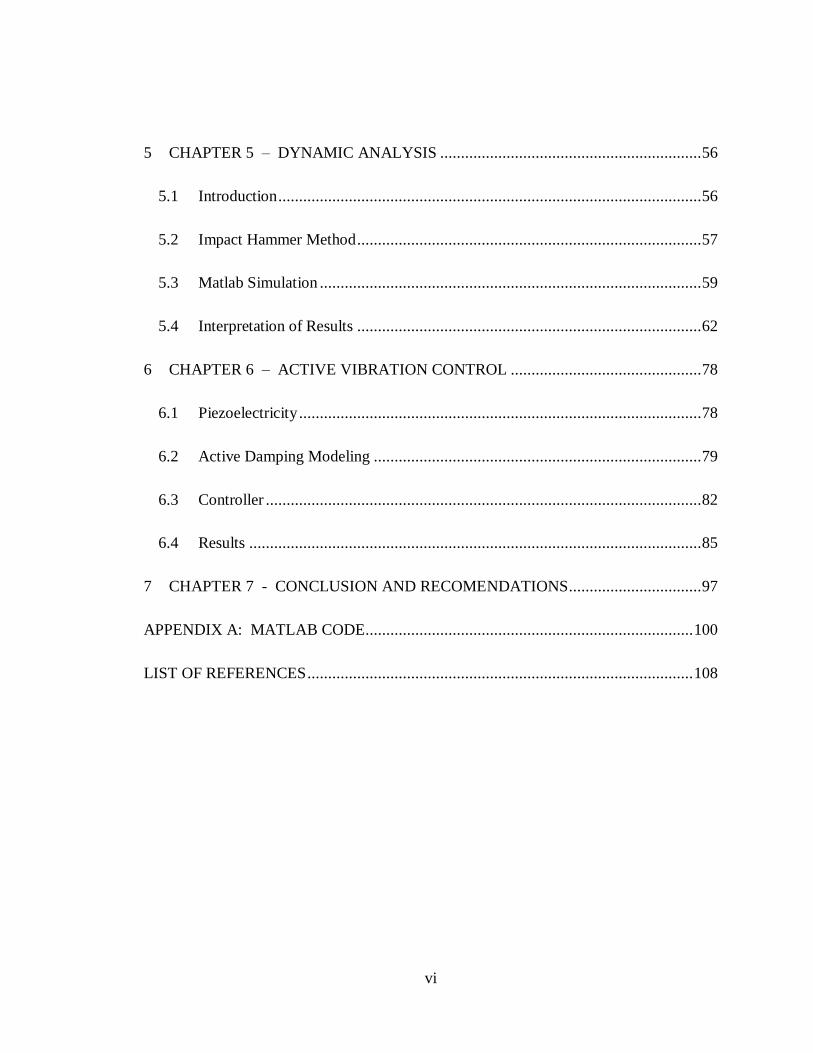
5 CHAPTER 5 – DYNAMIC ANALYSIS ............................................................... 56
5.1 Introduction ...................................................................................................... 56
5.2 Impact Hammer Method ................................................................................... 57
5.3 Matlab Simulation ............................................................................................ 59
5.4 Interpretation of Results ................................................................................... 62
6 CHAPTER 6 – ACTIVE VIBRATION CONTROL .............................................. 78
6.1 Piezoelectricity ................................................................................................. 78
6.2 Active Damping Modeling ............................................................................... 79
6.3 Controller ......................................................................................................... 82
6.4 Results ............................................................................................................. 85
7 CHAPTER 7 - CONCLUSION AND RECOMENDATIONS................................ 97
APPENDIX A: MATLAB CODE............................................................................... 100
LIST OF REFERENCES ............................................................................................. 108
vii
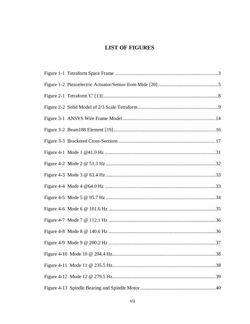
LIST OF FIGURES
Figure 1-1 Tetraform Space Frame .................................................................................3
Figure 1-2 Piezoelectric Actuator/Sensor from Mide [20] ...............................................5
Figure 2-1 Tetraform 'C' [13] ..........................................................................................8
Figure 2-2 Solid Model of 2/3 Scale Tetraform ...............................................................9
Figure 3-1 ANSYS Wire Frame Model ......................................................................... 14
Figure 3-2 Beam188 Element [19] ................................................................................ 16
Figure 3-3 Bracketed Cross-Sections ............................................................................ 17
Figure 4-1 Mode 1 @41.0 Hz ....................................................................................... 31
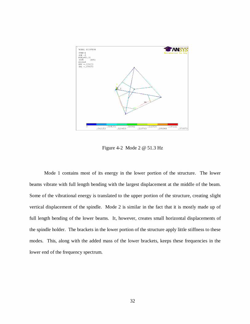
Figure 4-2 Mode 2 @ 51.3 Hz ...................................................................................... 32
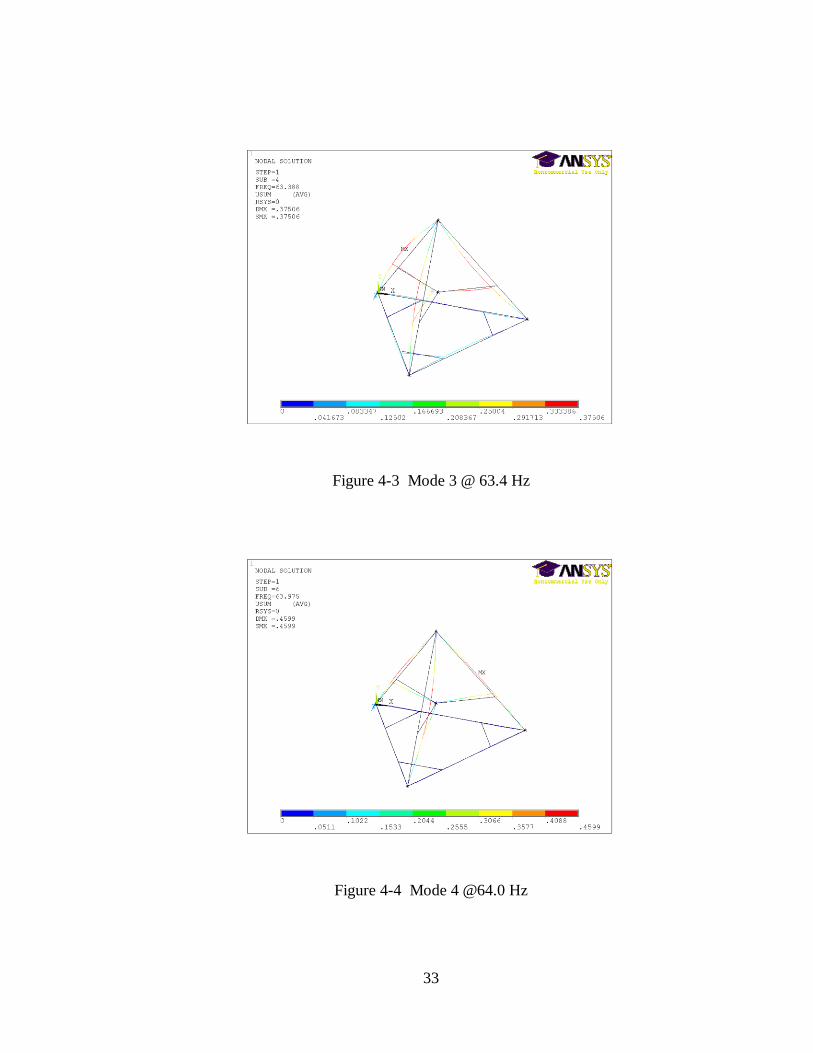
Figure 4-3 Mode 3 @ 63.4 Hz ...................................................................................... 33
Figure 4-4 Mode 4 @64.0 Hz ....................................................................................... 33
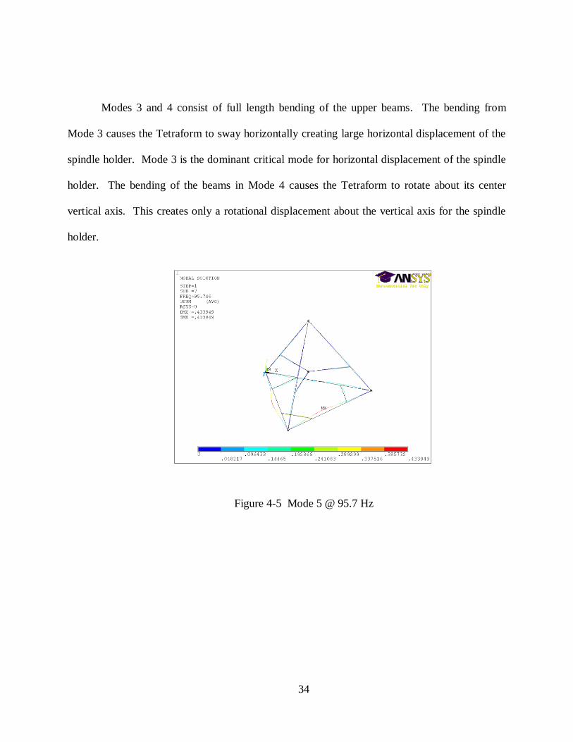
Figure 4-5 Mode 5 @ 95.7 Hz ...................................................................................... 34
Figure 4-6 Mode 6 @ 101.6 Hz .................................................................................... 35
Figure 4-7 Mode 7 @ 112.1 Hz .................................................................................... 36
Figure 4-8 Mode 8 @ 140.6 Hz .................................................................................... 36
Figure 4-9 Mode 9 @ 200.2 Hz .................................................................................... 37
Figure 4-10 Mode 10 @ 204.4 Hz ................................................................................. 38
Figure 4-11 Mode 11 @ 235.5 Hz ................................................................................. 38
Figure 4-12 Mode 12 @ 279.5 Hz ................................................................................. 39
Figure 4-13 Spindle Bearing and Spindle Motor ........................................................... 40
viii
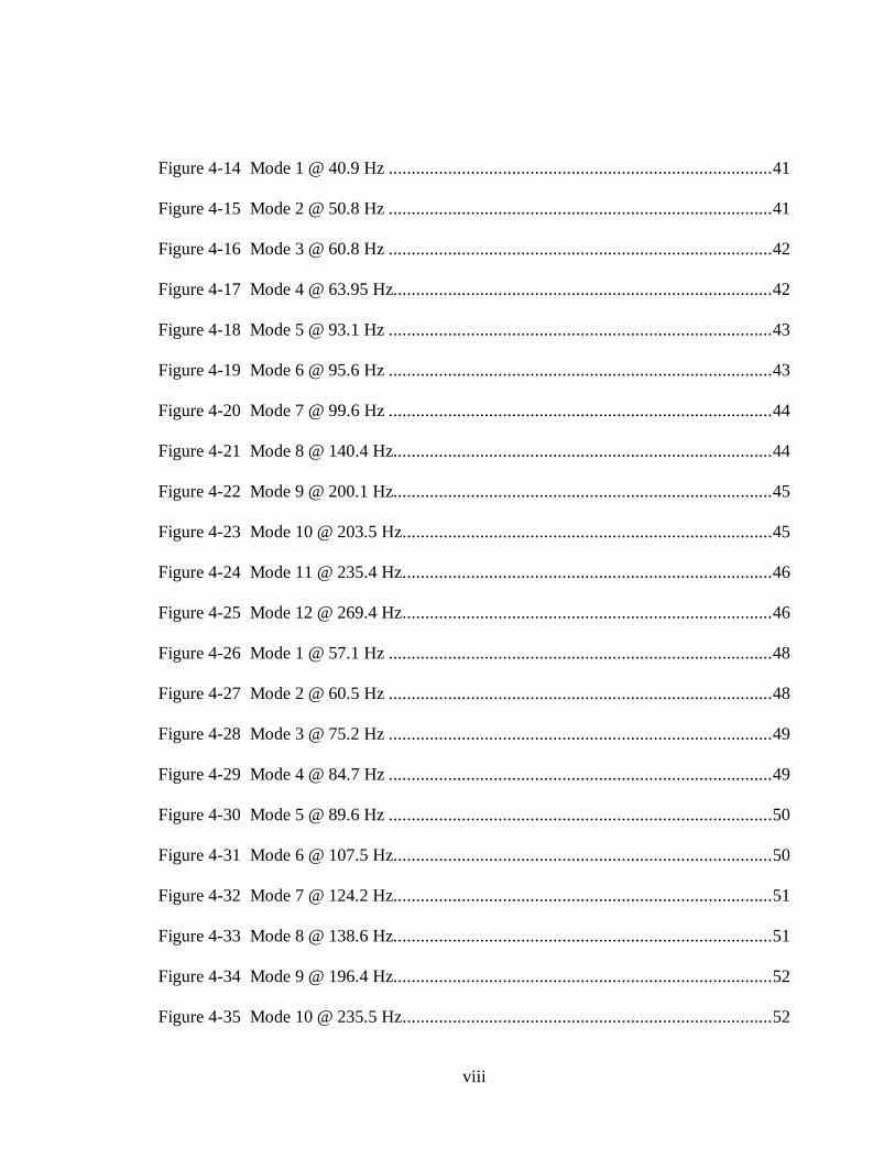
Figure 4-14 Mode 1 @ 40.9 Hz .................................................................................... 41
Figure 4-15 Mode 2 @ 50.8 Hz .................................................................................... 41
Figure 4-16 Mode 3 @ 60.8 Hz .................................................................................... 42
Figure 4-17 Mode 4 @ 63.95 Hz................................................................................... 42
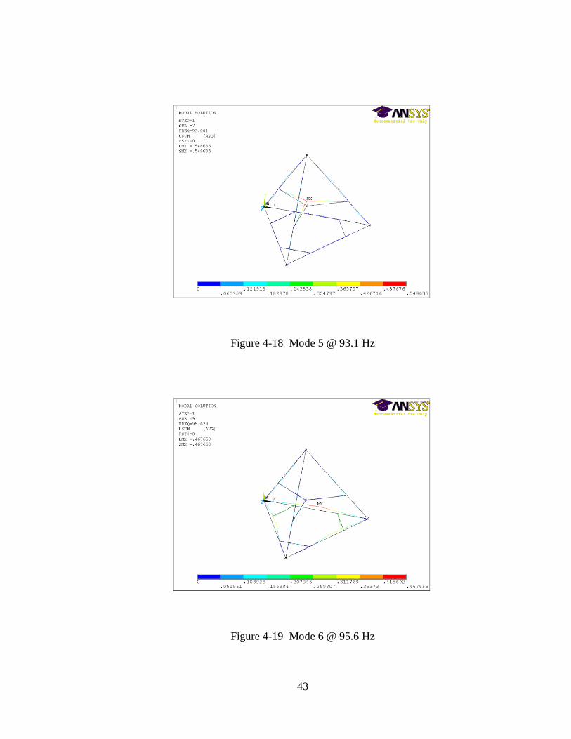
Figure 4-18 Mode 5 @ 93.1 Hz .................................................................................... 43
Figure 4-19 Mode 6 @ 95.6 Hz .................................................................................... 43
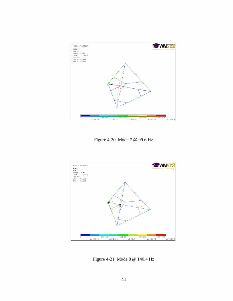
Figure 4-20 Mode 7 @ 99.6 Hz .................................................................................... 44
Figure 4-21 Mode 8 @ 140.4 Hz................................................................................... 44
Figure 4-22 Mode 9 @ 200.1 Hz................................................................................... 45
Figure 4-23 Mode 10 @ 203.5 Hz ................................................................................. 45
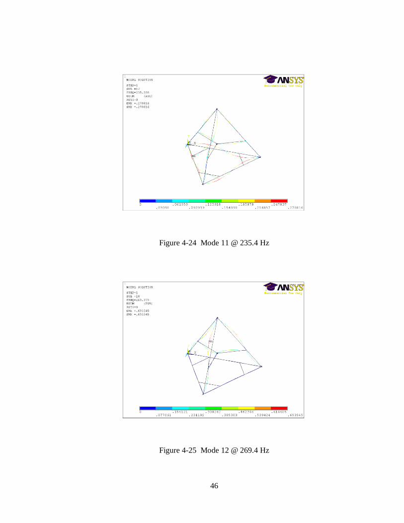
Figure 4-24 Mode 11 @ 235.4 Hz ................................................................................. 46
Figure 4-25 Mode 12 @ 269.4 Hz ................................................................................. 46
Figure 4-26 Mode 1 @ 57.1 Hz .................................................................................... 48
Figure 4-27 Mode 2 @ 60.5 Hz .................................................................................... 48
Figure 4-28 Mode 3 @ 75.2 Hz .................................................................................... 49
Figure 4-29 Mode 4 @ 84.7 Hz .................................................................................... 49
Figure 4-30 Mode 5 @ 89.6 Hz .................................................................................... 50
Figure 4-31 Mode 6 @ 107.5 Hz................................................................................... 50
Figure 4-32 Mode 7 @ 124.2 Hz................................................................................... 51
Figure 4-33 Mode 8 @ 138.6 Hz................................................................................... 51
Figure 4-34 Mode 9 @ 196.4 Hz................................................................................... 52
Figure 4-35 Mode 10 @ 235.5 Hz ................................................................................. 52
ix
Figure 4-36 Mode 11 @ 264.0 Hz ................................................................................. 53
Figure 4-37 Mode 12 @ 278.5 Hz ................................................................................. 53
Figure 5-1 PCB Impact Hammer................................................................................... 58
Figure 5-2 Accelerometer Locations ............................................................................. 63
Figure 5-3 Accelerometer 1 Response to Vertical Input at Spindle ................................ 64
Figure 5-4 Accelerometer 2 Response to Vertical Input at Spindle ................................ 64
Figure 5-5 Accelerometer 3 Response to Vertical Input at Spindle ................................ 65
Figure 5-6 Translational Force Responses of Spindle .................................................... 67
Figure 5-7 Torque Responses of Spindle ....................................................................... 68
Figure 5-8 Z axis Spindle Response to Torque Inputs at Spindle ................................... 70
Figure 5-9 X Axis Spindle Response to Torque Inputs at Spindle ................................. 70
Figure 5-10 Y Axis Spindle Response to Torque Inputs at Spindle................................ 71
Figure 5-11 Disturbance Locations ............................................................................... 72
Figure 5-12 Response of Spindle to Perpendicular Force at Point 1 ............................... 72
Figure 5-13 Response of Spindle to Perpendicular Force at Point 2 ............................... 73
Figure 5-14 Response of Spindle to Perpendicular Force at Point 3 ............................... 73
Figure 5-15 Response of Spindle to Vertical Force at Point 4 ........................................ 74
Figure 5-16 Actuator Test Locations ............................................................................. 75
Figure 5-17 Spindle X-Axis Response to Actuators ...................................................... 76
Figure 5-18 Spindle Y-Axis Response to Actuators ...................................................... 76
Figure 5-19 Spindle Z-Axis Response to Actuators ....................................................... 77
Figure 6-1 Mide pa16n Transducer Performance [20] ................................................... 80
x
Figure 6-2 Bode Plot of PPF Filter ................................................................................ 83
Figure 6-3 Positive Position Feedback Controller ......................................................... 84
Figure 6-4 Root Locus Plot for Actuator Location 1...................................................... 86
Figure 6-5 Vertical Spindle Frequency Response for Actuator Location 1 .................... 87
Figure 6-6 Vertical Spindle Impulse Response for Actuator Location 1 ........................ 88
Figure 6-7 Horizontal Spindle Frequency Response for Actuator Location 1 ................ 89
Figure 6-8 Horizontal Spindle Impulse Response for Actuator Location 1 .................... 89
Figure 6-9 Root Locus Plot for Actuator Location 3...................................................... 91
Figure 6-10 Vertical Spindle Frequency Response for Actuator Location 3................... 92
Figure 6-11 Vertical Spindle Impulse Response for Actuator Location 3 ...................... 92
Figure 6-12 Horizontal Spindle Frequency Response for Actuator Location 3 .............. 93
Figure 6-13 Horizontal Spindle Impulse Response for Actuator Location 3 .................. 94
Figure 6-14 Horizontal Frequency Response of Spindle with Additional PPF ............... 95
Figure 6-15 Horizontal Impulse Response of Spindle with Additional PPF ................... 96
xi
LIST OF TABLES
Table 3-1 Point Mass Inertia Values ............................................................................. 15
Table 3-2 Bracketed Beam Cross-Section 1 Properties .................................................. 17
Table 3-3 Bracketed Beam Cross-Section 2 Properties .................................................. 17
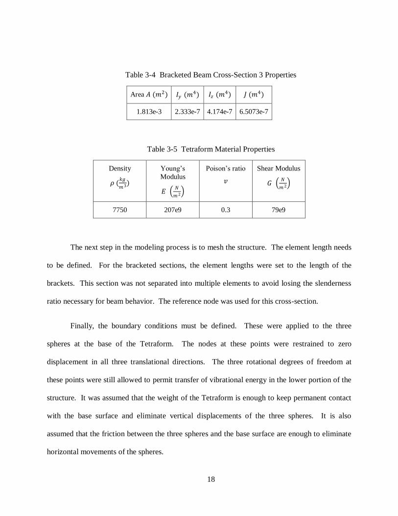
Table 3-4 Bracketed Beam Cross-Section 3 Properties .................................................. 18
Table 3-5 Tetraform Material Properties ....................................................................... 18
Table 4-1 Full Scale Tetraform Natural Frequencies without Spindle ............................ 47
Table 4-2 Full Scale Tetraform Natural Frequencies without Spindle ............................ 55
Table 5-1 Tetraform Natural Frequencies with Spindle Added ...................................... 66
Table 6-1 Piezoelectric Material Properties ................................................................... 79
1
1 CHAPTER 1 – INTRODUCTION
There are two main goals of this research. They are to analyze the Tetraform space frame
and to develop a method of vibration control of the Tetraform intended to optimize the
machining process. The Tetraform is a tetrahedral frame used to hold a high speed spindle for
micro-scale milling. It is essential to the machining process to have minimal vibrations in the
structure holding the spindle. The Tetraform prototypes were analyzed to determine how
susceptible the structure is to vibration. An active vibration control scheme was then designed to
dampen out natural frequencies that are critical to the machining process.
Structural vibration is very critical to machining performance. When machining on the
micro/nano scale, it is desirable to operate at a high material removal rate to increase economic
efficiency. The goal of present research is to increase surface and subsurface integrity with
satisfactory material removal rate by decreasing the vibrations of the tool holding structure. This
helps to prevent fatigue cracking and increase part life. Structural vibrations play an important
role in the ability to machine at a very high material removal rate while maintaining high
precision and surface finish. The vibrations felt by the machine tool not only affect the quality of
the machined part but also the machine tool itself, since the cutting tool is susceptible to pitting
and wear when operating at high speeds, thus inevitably decreasing tool life.
While the Tetraform displays favorable dynamic stiffness compared to the more
commonly used machining structures [4][5], there is still a need to dampen out certain modes of
2
vibration. For this, an active vibration control scheme was developed to target such frequencies.
The Tetraform is converted to a smart-structure by implementing piezoelectric sensors/actuators.
The positions of the sensors/actuators are chosen to effectively dampen out the modes of
vibration that are most critical to the machining process, i.e., induces the largest displacement to
the spindle holder. The actuators and sensors will be collocated to best obtain a displacement
signal for the controller. Positive Position Feedback is then used to control the input signal to the
actuators.
With the increasing demand for micro-scale devices, the need for improved accuracy and
precision in machining processes goes up continuously. This has driven research in the
development of a machine tool structure that contains the dynamic stiffness properties to
machine with nano-scale accuracy and precision. One way to achieve this goal is the Tetraform,
which was originally designed by Kevin Lindsey [1] at the UK’s National Physical Laboratory.
In his research he developed the Tetraform 1 for grinding of optical lenses with ultra smooth
surfaces.
The Tetraform consists of four equilateral triangles connected by spherical masses at the
vertices, which is ideal for a machining structure due to how vibration waves propagate through
the structure. The vibrations travel through the closed loops of the space frame creating high
dynamic stiffness with the companion of high static stiffness [2].
In this study, the Tetraform is adopted for use in micro-machining by Dr. Mark Jackson
[3], where the frame has been scaled down significantly and a spindle holder in the center of the
structure was added in. The modified Tetraform is used to hold a high speed spindle while the
3
work piece is moved with three linear position stages for two horizontal degrees of freedom and
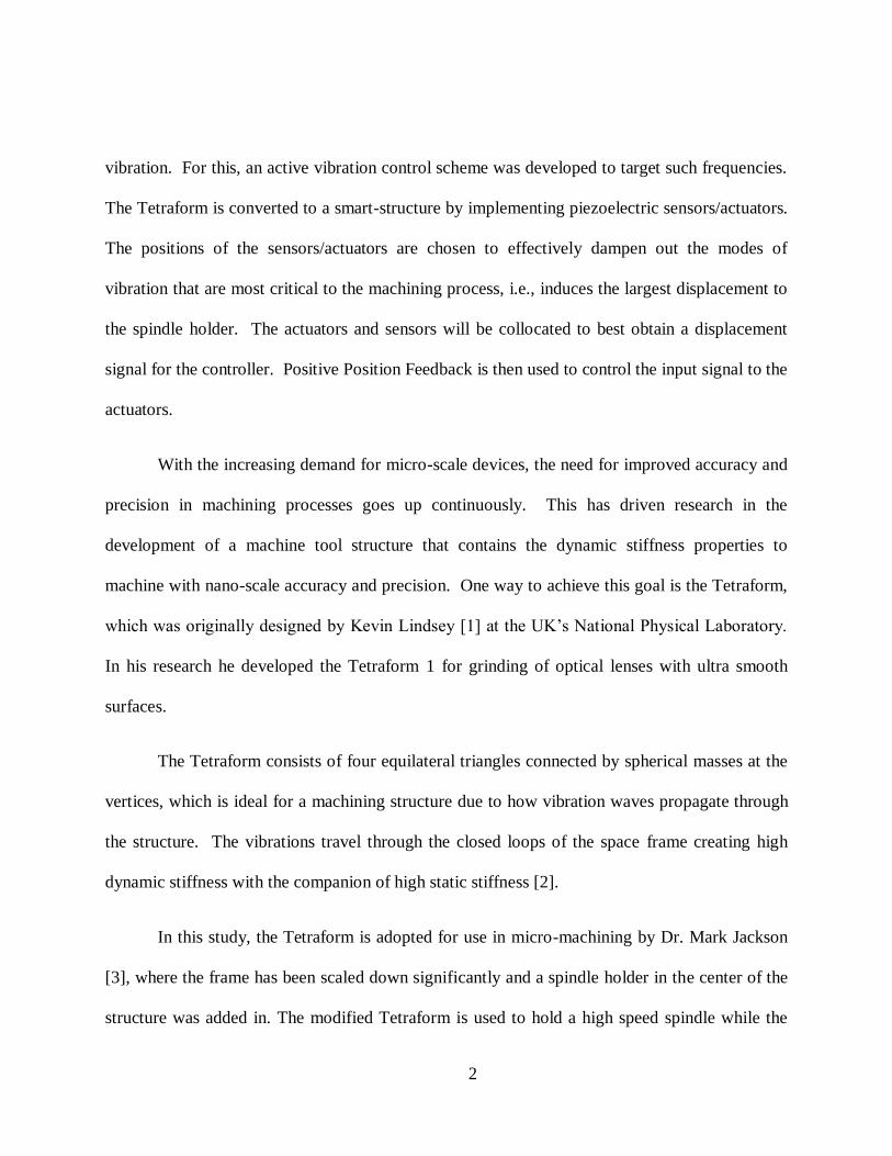
a vertical degree of freedom. The complete setup is shown in Figure 1.
Figure 1-1 Tetraform Space Frame
The structural dynamics of the Tetraform were thoroughly analyzed to compare structural
modifications and to help develop and simulate active vibration control schemes. Modal analysis
consists of obtaining mode shapes, natural frequencies, and damping values. The mode shapes
show the displaced structure for each natural frequency. This gives insight into where areas of
high vibration energy occur in the structure for different natural frequencies. The ultimate goal
is to minimize modes with high energy influence on the spindle position, which create mal
effects on the machining process. The Finite Element Analysis (FEA) software, ANSYS, was
used to calculate and display the modal responses of the Tetraform. This software is an effective
way of displaying the mode shapes along with visualizing the effects of structural modifications.
4
Dynamic responses of the Tetraform were also studied. Frequency response functions
(FRFs) created experimentally and from simulation models show the responses of different
points on the Tetraform to a dynamic input at a particular point on the Tetraform. The dynamic
relationships between the spindle location and other points on the structure are of most
importance. Input forces from machining can trigger certain modes of vibration when there is a
strong dynamic relationship between theses two points along with the inverse affect of outer
disturbance inputs creating a large dynamic response of the spindle location. Structural
modifications can be conducted to strategically reduce the dynamic response between different
points on the Tetraform. Dynamic analysis is also useful for the application of active vibration
control. Locations of actuator-sensor pairs are critical to the effectiveness of the vibration
control scheme. It is desirable to place the actuators at a point the high influence on the dynamic
response of the spindle location while minimizing the dynamic response of the sensors to inputs
from modes that do not significantly affect the spindle. FRFs obtained experimentally are also
used to verify the simulation models created in Matlab and ANSYS.
Active vibration control via piezoelectric transducer patches is used to dampen out the
critical modes which have high influence on the spindle location. Piezoelectric materials
generate an electric potential from an applied mechanical stress. They also exhibit the inverse
effect of expanding when subjected to an applied voltage. The development of ceramics that
possess very strong mechanical electrical coupling properties is one of the driving factors behind
the emergence of active vibration control as a more viable solution to vibration than passive
control techniques.
5
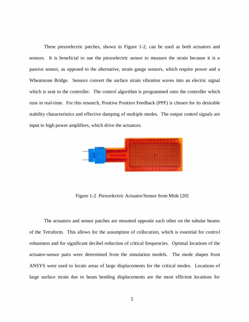
These piezoelectric patches, shown in Figure 1-2, can be used as both actuators and
sensors. It is beneficial to use the piezoelectric sensor to measure the strain because it is a
passive sensor, as opposed to the alternative, strain gauge sensors, which require power and a
Wheatstone Bridge. Sensors convert the surface strain vibration waves into an electric signal
which is sent to the controller. The control algorithm is programmed onto the controller which
runs in real-time. For this research, Positive Position Feedback (PPF) is chosen for its desirable
stability characteristics and effective damping of multiple modes. The output control signals are
input to high power amplifiers, which drive the actuators.
Figure 1-2 Piezoelectric Actuator/Sensor from Mide [20]
The actuators and sensor patches are mounted opposite each other on the tubular beams
of the Tetraform. This allows for the assumption of collocation, which is essential for control
robustness and for significant decibel reduction of critical frequencies. Optimal locations of the
actuator-sensor pairs were determined from the simulation models. The mode shapes from
ANSYS were used to locate areas of large displacements for the critical modes. Locations of
large surface strain due to beam bending displacements are the most efficient locations for
6
mounting the actuators. FRFs were setup to display the dynamic relationships between the
surface strain at possible mounting locations and the spindle point.
Simulations, using the Matlab FEA model, were conducted to design multiple PPF
controllers and test their controllability over the targeted modes. The FEA model was converted
to state space to allow for output and input matrices. Piezoelectric sensor and actuator equations
were derived and input into these output and input matrices. Three piezoelectric actuator-sensor
pairs were positioned at symmetric locations on the Tetraform. Different locations were tested
for their controllability and required control effort. In order to dampen out modes of the
Tetraform, root locus was used to tune second order PPF filters to optimal damping and
stability. The effectiveness of the controllers are displayed by decibel reduction of the critical
frequencies in the bode plots.
7
2 CHAPTER 2 – BACKGROUND
2.1 Tetraform
The first prototype of the Tetraform was the Tetraform 1, created by Lindsey [1] for
grinding glass and quartz to optical quality at high material removal rates. With the Tetraform 1,
10 μm cuts were able to produce 5nm Ra surface finish. This model consisted of steel tubular
members that were 600 mm long with an outside diameter of 131 mm. The Tetraform concept
has inherently desirable dynamic characteristics. Internal damping was included for the
Tetraform to further increase it’s resistance to vibration. Pistons were inserted into the inner
diameter of the tubular members with viscous damping material in the gaps for damping. The
legs were attached to the spheres with pin joints that could be tightened or loosened to change
the magnitude of the resonant frequencies. By loosening the joints, frictional damping by the pin
joints became effective [1]. This along with the internal damping and dynamic stiffness
properties of the frame made the Tetraform 1 highly resistant to vibration across a wide range of
frequencies.
The Tetraform 1 was limited to one degree of freedom for grinding. The z-axis was on
the inner portion of the structure, attached under the top sphere. It was clear that development of
multi-axis machines with high stiffness were possible using the Tetraform concept. The
Tetraform ‘C’ [13] was created adding in the two horizontal degrees of freedom. It was also
determined that the pin jointed Tetraform frame had sufficient damping properties and the
hydraulic damping was omitted for the Tetraform ‘C’ [14].
8
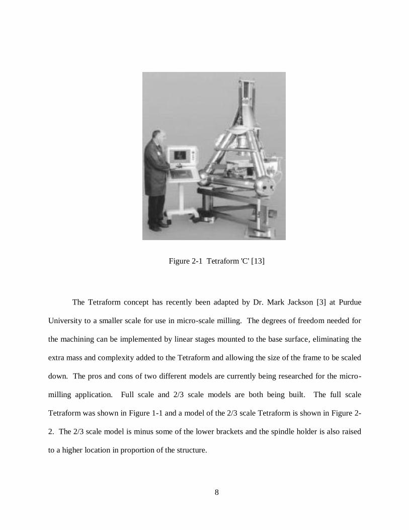
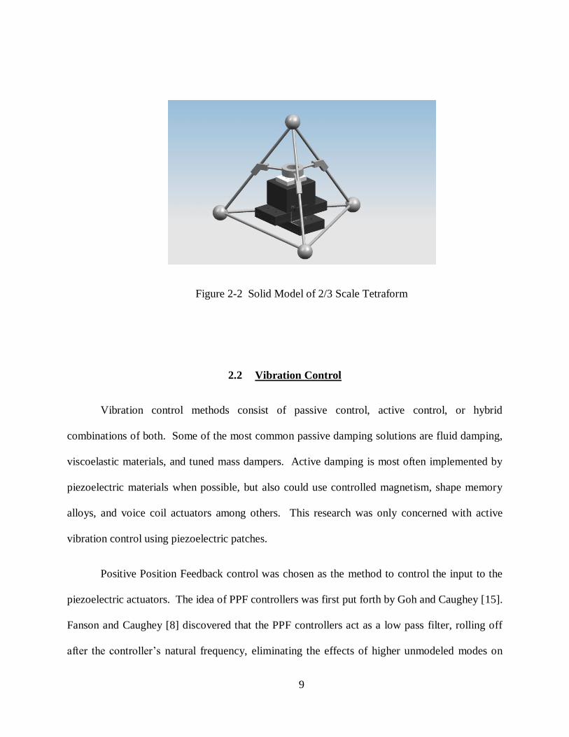
Figure 2-1 Tetraform 'C' [13]
The Tetraform concept has recently been adapted by Dr. Mark Jackson [3] at Purdue
University to a smaller scale for use in micro-scale milling. The degrees of freedom needed for
the machining can be implemented by linear stages mounted to the base surface, eliminating the
extra mass and complexity added to the Tetraform and allowing the size of the frame to be scaled
down. The pros and cons of two different models are currently being researched for the micro-
milling application. Full scale and 2/3 scale models are both being built. The full scale
Tetraform was shown in Figure 1-1 and a model of the 2/3 scale Tetraform is shown in Figure 2-
2. The 2/3 scale model is minus some of the lower brackets and the spindle holder is also raised
to a higher location in proportion of the structure.
9
Figure 2-2 Solid Model of 2/3 Scale Tetraform
2.2 Vibration Control
Vibration control methods consist of passive control, active control, or hybrid
combinations of both. Some of the most common passive damping solutions are fluid damping,
viscoelastic materials, and tuned mass dampers. Active damping is most often implemented by
piezoelectric materials when possible, but also could use controlled magnetism, shape memory
alloys, and voice coil actuators among others. This research was only concerned with active
vibration control using piezoelectric patches.
Positive Position Feedback control was chosen as the method to control the input to the
piezoelectric actuators. The idea of PPF controllers was first put forth by Goh and Caughey [15].
Fanson and Caughey [8] discovered that the PPF controllers act as a low pass filter, rolling off
after the controller’s natural frequency, eliminating the effects of higher unmodeled modes on
10
the controller’s output. Therefore, the controlled system will not become destabilized due to the
unmodeled modes. Although PPF control guarantees robustness against the spillover of higher
modes, it does not guarantee absolute stability. Conditions for the controller constants to
guarantee stability can be derived by requiring the closed loop stiffness matrix to be positive
definite [16]. Poh and Baz [17] modified the PPF concept to a controller which they named
Modal Positive Position Feedback (MPPF). They used first order filters to obtain similar
damping results as PPF filters. However, using first order filters allows lower modes to have
higher influence on the control signal than the targeted mode, causing spillover effects from
lower modes [16].
11
3 CHAPTER 3 – TETRAFORM MODELING
3.1 Introduction
Different models of the Tetraform were created using Finite Element Analysis (FEA).
FEA is the process of breaking a complex object under analysis into smaller simpler elements in
order to derive a series of equations to accurately describe it. Discretizing the object into
elements allows the ability to approximate values at connecting points, or nodes. The elements
that connect the different nodes use interpolation functions to approximate the relationship
between the values at those nodes. In the case of structural analysis, the values being
approximated are the physical displacements. Reducing the size and therefore increasing the
quantity of the elements will reduce the errors produced from using approximation functions.
However, it should be noted that the size need only be reduced so much as the error will
converge to zero. Further reduction is unnecessary and could even induce calculation error.
Different types of elements can be used to approximate displacements of a structure. The
basic structural elements include solid, shell, plate, beam, link, and point elements. Solid
elements, which are most commonly tetrahedral and brick elements, are used to mesh volumes.
These are usually used when other elements are not feasible due to a large quantity of required
nodes and hence a longer computing time. Shell and plate elements are surface elements with
thickness used to mesh curved or flat surfaces and can allow for bending and membrane
displacements. Beam elements are used for objects whose length is larger than its other two
dimensions. It’s most dominant displacement is beam bending but beam elements may also
12
include axial and torsional displacements. Link elements are line elements that act as a spring
with either axial or torsional displacements. And finally point elements are used to represent
mass or inertia at one node. There are many types of these elements as there are varying theories
and combinations of the different elements.
The derived element equations are in matrix form which contains mass and stiffness
matrices. All of the element matrices are combined to create global mass and stiffness matrices
to represent the entire structure. Both are symmetric n x n matrices where n is the total number
of degrees of freedom for the entire structure. The constructed global mass and stiffness
matrices are then used in a second order differential equation to describe the dynamics of the
structure.
The derived FEA models of the Tetraform can then be used for modal analysis, dynamic
analysis, and controller design simulations. The models were created both manually in Matlab
and also in the FEA software ANSYS. The model in ANSYS was used in the modal analysis to
display the mode shapes. Both were used to compare structural changes and different scales of
the Tetraform. The Matlab model was used to create a state space model to be controlled for
vibration control simulations.
3.2 ANSYS Finite Element Model
FEA software is a very powerful tool in the design and simulation process. In addition to
the numerical solver, the modeling and results may be monitored visually. This has cut the time
down significantly of today’s design processes by eliminating the need for excessive
13
prototyping. Static stresses and dynamic characteristics can now be analyzed without the
creation of entirely new prototypes. This software allows for quick and easy implementation of
structural changes. Addition of structural members and changes to existing members can be
done with ease while being able to visualize the resulting changes in stress and dynamic
characteristics.
For this research, ANSYS 11.0 was used. When using this software, and most other FEA
software, there are three steps in the analysis process. These are preprocessing, solution, and
postprocessing. For the preprocessing, the model is created, meshed and the boundary
conditions and input forces are applied. The solution involves defining and setting up the solver.
Postprocessing is where listing and displaying of the results takes place. ANSYS combines all
three into a graphical user interface environment.
Preprocessing is the first step in the analysis process. This involves the creation of the
structural geometry in ANSYS. Beam elements were chosen to model the Tetraform. It is well
suited for this due to its slender tubular frame without any solid volumes consisting of any
significant stresses. It was assumed that the solid spheres at four outer joints and the spindle
holder could be accurately represented as point masses since the internal displacements of the
volumes are negligible compared to the bending of the tubular frame. It was also assumed that
the bracketed sections could be modeled as thick beam sections.
Depending on the complexity of the object under analysis, it is often created in modeling
software and imported into the Finite Element Software. Since the beam elements that were used
are line elements, the structure was modeled in ANSYS directly as a simple wire frame.
14
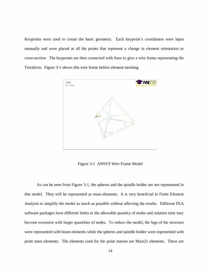
Keypoints were used to create the basic geometry. Each keypoint’s coordinates were input
manually and were placed at all the points that represent a change in element orientation or
cross-section. The keypoints are then connected with lines to give a wire frame representing the
Tetraform. Figure 3-1 shows this wire frame before element meshing.
Figure 3-1 ANSYS Wire Frame Model
As can be seen from Figure 3-1, the spheres and the spindle holder are not represented in
this model. They will be represented as mass elements. It is very beneficial in Finite Element
Analysis to simplify the model as much as possible without affecting the results. Different FEA
software packages have different limits to the allowable quantity of nodes and solution time may
become excessive with larger quantities of nodes. To reduce the model, the legs of the structure
were represented with beam elements while the spheres and spindle holder were represented with
point mass elements. The elements used for the point masses are Mass21 elements. These are
15
purely inertial elements and do not affect the stiffness of the structure. This means that the input
for these elements will consist of linear inertia terms, 𝑚𝑥 ,𝑚𝑦 , and 𝑚𝑧 , and rotational inertia
terms, 𝐼𝑥𝑥 , 𝐼𝑦𝑦 , and 𝐼𝑧𝑧 . The three linear inertia terms are the same and are equal to the mass of
the element. The rotational inertia terms, or mass moments of inertia, were found by solving
(3.1) for each axis. The inertia terms for the sphere and spindle holder are listed in Table 3-1
where 𝑧 is the vertical axis and 𝑥 and 𝑦 are the horizontal axis.
𝐼 = 𝑟2𝑑𝑚 (3.1)
Table 3-1 Point Mass Inertia Values
𝑚
(𝑘𝑔)
𝐼𝑥𝑥
(𝑘𝑔 −𝑚2)
𝐼𝑦𝑦
(𝑘𝑔 −𝑚2)
𝐼𝑧𝑧
(𝑘𝑔 −𝑚2)
Spheres 2.6 2.153e-3 2.153e-3 2.153e-3
Spindle Holder 1.7 1.485e-3 1.485e-3 2.225e-3
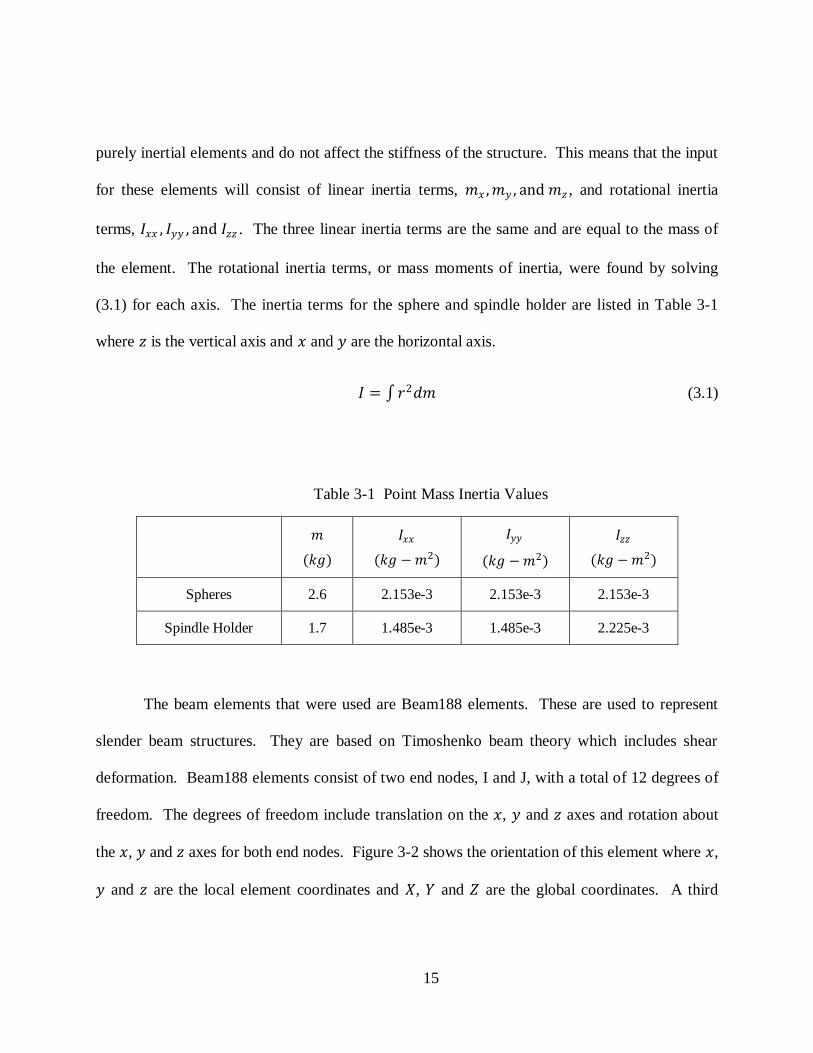
The beam elements that were used are Beam188 elements. These are used to represent
slender beam structures. They are based on Timoshenko beam theory which includes shear
deformation. Beam188 elements consist of two end nodes, I and J, with a total of 12 degrees of
freedom. The degrees of freedom include translation on the 𝑥, 𝑦 and 𝑧 axes and rotation about
the 𝑥, 𝑦 and 𝑧 axes for both end nodes. Figure 3-2 shows the orientation of this element where 𝑥,
𝑦 and 𝑧 are the local element coordinates and 𝑋, 𝑌 and 𝑍 are the global coordinates. A third
16
orientation node, J, is also included when the 𝑧 direction needs to be specified. This is the case
when the cross-section is not circular. This node is input to define the IJK plane.
Figure 3-2 Beam188 Element [19]
Other input data for the beam elements include material properties and cross-sectional
data. For this structure, there are four different beam cross-sections that need to be defined. The
first is the tubular beam section and the other three are the different bracketed sections. ANSYS
has options for common cross-sections where only dimensions need to be input. For uncommon
cross-sections, the area moments of inertia, polar moment of inertia, and area must be input. A
tubular cross-section is a common cross-section in ANSYS so the outer and inner radii are the
only required input. The inner and outer radii of the legs are 𝑅𝑖 = # and 𝑅𝑜 = # respectively.
The area, area moments of inertia, and polar moment of inertia are then calculated by ANSYS.
For the bracketed sections, the area moments inertia, 𝐼𝑦 and 𝐼𝑧 , were calculated from the
moment of a rectangular cross-section minus the moment of the circular area inside the tubular
17
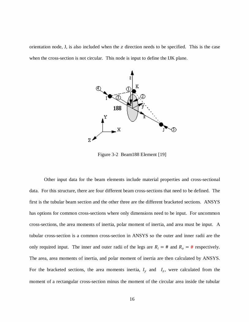
beam. The polar moment of inertia 𝐽 is the summation of 𝐼𝑦 and 𝐼𝑧 . The three bracketed cross-
sections are labeled in Figure 3-3 while the calculated moments of inertia are listed in Tables 3-2
to 3-4. The Tetraform is made of steel and the material properties are listed in Table 3-5.
Figure 3-3 Bracketed Cross-Sections
Table 3-2 Bracketed Beam Cross-Section 1 Properties
Area 𝐴 (𝑚2) 𝐼𝑦 (𝑚4) 𝐼𝑧 (𝑚4) 𝐽 (𝑚4)
1.799e-3 2.502e-7 3.788e-7 6.289e-7
Table 3-3 Bracketed Beam Cross-Section 2 Properties
Area 𝐴 (𝑚2) 𝐼𝑦 (𝑚4) 𝐼𝑧 (𝑚4) 𝐽 (𝑚4)
1.17e-3 2.191e-7 3.624e-7 5.816e-7
Bracket 2
Bracket 1
Bracket 3
18
Table 3-4 Bracketed Beam Cross-Section 3 Properties
Area 𝐴 (𝑚2) 𝐼𝑦 (𝑚4) 𝐼𝑧 (𝑚4) 𝐽 (𝑚4)
1.813e-3 2.333e-7 4.174e-7 6.5073e-7
Table 3-5 Tetraform Material Properties
Density
𝜌 (𝑘𝑔
𝑚3)
Young’s
Modulus
𝐸 𝑁
𝑚2
Poison’s ratio
𝑣
Shear Modulus
𝐺 𝑁
𝑚2
7750 207e9 0.3 79e9
The next step in the modeling process is to mesh the structure. The element length needs
to be defined. For the bracketed sections, the element lengths were set to the length of the
brackets. This section was not separated into multiple elements to avoid losing the slenderness
ratio necessary for beam behavior. The reference node was used for this cross-section.
Finally, the boundary conditions must be defined. These were applied to the three
spheres at the base of the Tetraform. The nodes at these points were restrained to zero
displacement in all three translational directions. The three rotational degrees of freedom at
these points were still allowed to permit transfer of vibrational energy in the lower portion of the
structure. It was assumed that the weight of the Tetraform is enough to keep permanent contact
with the base surface and eliminate vertical displacements of the three spheres. It is also
assumed that the friction between the three spheres and the base surface are enough to eliminate
horizontal movements of the spheres.
19
3.3 Matlab Finite Element Model
A derived Finite Element model was also created by manually coding the model in
Matlab. This mathematical model serves several purposes. This FEA model was used to verify
the ANSYS model by comparison of the calculated natural frequencies. It can be used to quickly
implement small structural changes. Some changes are easier and quicker to change in code as
opposed to making the changes in the ANSYS model. It was also used, along with the addition
of the piezoelectric coupled equations, to develop a state space model that could be used for
simulating the active vibration control of the Tetraform. This state space model has an input of
voltage to the three piezoelectric actuators and an output of voltage from the three piezoelectric
sensors. The state space model was also used to calculate the FRFs in Matlab.
The same modeling techniques used in ANSYS were used here. The frame legs were
represented as Timoshenko beam elements and the spheres and spindle holder were represented
as point mass elements. The same boundary conditions were applied to the three base spheres.
The elements lengths were different from those of the ANSYS model. As the input data needed
to be set up for each element individually, the element lengths were made larger to give fewer
elements. Also, the element lengths in the area of the mounted piezoelectric sensors and
actuators were setup based on optimal placement of these transducers for vibration control.
Using the element interpolation functions that approximate the displacement values
across the element, equations of motion were developed to approximate the displacement values
at the connecting nodes. The resulting element mass and stiffness matrices are input into the
differential equation to describe the nodal displacements. The differential equation is of the form
20
shown in (3.2). 𝑀𝑒 is the element mass matrix, 𝐾𝑒 is the element stiffness matrix, 𝑓𝑒 is the
nodal force vector, and 𝑟 is the nodal displacement vector.
𝑀𝑒 𝑟 + 𝐾𝑒 𝑟 = 𝑓𝑒 (3.2)
The process of finite element analysis is to ultimately obtain global mass and stiffness
matrices to represent the entire system. First, the mass and stiffness matrices are derived for
each element in local coordinates (x,y,z). The mass and stiffness matrices are then converted to
the global coordinate system (X,Y,Z). Finally, all the element matrices are input into the global
mass and stiffness matrices that represent the entire structure. These can be used in a differential
equation similar to that of (3.2).
3.3.1 Element Modeling
The element equations used for the legs were not restricted to beam theory. They also
include axial and torsional displacements. The dynamic equation matrices for bending, axial and
torsional movements are derived independently and superimposed into the final element
matrices. These equations can be uncoupled and still represent an accurate assumption as long as
large deformations do not occur. Each beam element contains twelve degrees of freedom. These
include translational displacements, 𝑢,𝑣, and 𝑤, in the 𝑥,𝑦 and 𝑧 directions for both nodes i and
j and rotational displacements, 휃𝑥 ,휃𝑦 , and 휃𝑧 , about the 𝑥, 𝑦 and 𝑧 axis for both nodes i and j.
The beam element displacement vector is represented as 𝑟𝑇 = 𝑢𝑖 , 𝑣𝑖 , 𝑤𝑖 , 휃𝑥𝑖 , 휃𝑦𝑖 , 휃𝑧𝑖 , 𝑢𝑗 ,
𝑣𝑗 , 𝑤𝑗 , 휃𝑥𝑗 , 휃𝑦𝑗 , 휃𝑧𝑗 .
21
The beam or bending equations were developed for transverse displacements, 𝑣 and 𝑤.
However, the derivation will just be shown for the transverse displacement 𝑤, or bending about
the 𝑦 axis. As in the ANSYS analysis, Timoshenko beam theory is used for the beam elements.
Timoshenko beam theory differs from classical beam theory in that it includes bending shear and
rotational inertia. The equations of motion for the Timoshenko beam elements for bending about
the 𝑦 axis will be of the form
𝑀𝑏
𝑤 𝑖휃 𝑦𝑖𝑤 𝑗
휃 𝑦𝑗
+ 𝐾𝑏
𝑤𝑖
휃𝑦𝑖𝑤𝑗휃𝑦𝑗
=
𝑄𝑧𝑖𝑀𝑦𝑖
𝑄𝑧𝑗𝑀𝑦𝑗
(3.3)
where 𝑀𝑏 is the Timoshenko beam mass matrix, 𝐾𝑏 is the Timoshenko beam stiffness
matrix, 𝑄𝑧 is the nodal shear force, and 𝑀𝑦 is the nodal bending moment about the 𝑦 axis.
Hamilton’s Principle will be used to derive the Timoshenko equations of motion. This
principle is the variational equation listed in (3.4). The strain energy, 𝑈, kinetic energy, 𝑇, and
work due to external forces, 𝑊, are derived and input into this equation to obtain the
Timoshenko beam equations. The axial and transverse displacements used to derive these terms
are approximated by (3.5) and (3.6) respectively. 휃 𝑥, 𝑡 is the cross-section rotation about the
𝑦 axis and 𝛽(𝑥) is the slope due to shear.
𝛿𝑈 − 𝛿𝑇 − 𝛿𝑊 𝑑𝑡 = 0 (3.4)
𝑢 𝑥,𝑦, 𝑧, 𝑡 = 𝑧휃 𝑥, 𝑡 = 𝑧 𝜕𝑤
𝜕𝑥− 𝛽(𝑥) (3.5)
𝑤 𝑥, 𝑦, 𝑧, 𝑡 = 𝑤(𝑥, 𝑡) (3.6)
22
As can be seen from the axial displacement, 𝑢 𝑥,𝑦, 𝑧, 𝑡 , the total slope, 휃 𝑥, 𝑡 , of the
cross-section is determined by the slope from bending, 𝜕𝑤
𝜕𝑥, and the slope from shear, 𝛽(𝑥). This
is one of the aspects that differentiate Timoshenko beam elements from Euler-Bernoulli beam
elements. The latter does not account for shear and assumes that the beam cross-section remains
perpendicular to the neutral axis. These displacements are then used to obtain the energy
variation terms for Hamilton’s Principle equation. The strain energy, 𝑈, and kinetic energy, 𝑇,
are shown in Eqs. (3.7) and (3.8) respectively. The strain energy accounts for both linear and
shear strain. These are then converted to matrix form and are given in Eqs. (3.9) and (3.10).
𝑈 =1
2𝐸𝐼𝑦
𝜕휃𝑦
𝜕𝑥
2
+1
2𝐾𝐺𝐴
𝜕𝑤
𝜕𝑥+ 휃𝑦
2
(3.7)
𝑇 =1
2𝜌𝐴
𝜕𝑤
𝜕𝑡
2
+1
2𝜌𝐼𝑦
𝜕휃𝑦
𝜕𝑡
2
(3.8)
𝑈 =1
2
𝜕휃𝑦
𝜕𝑥𝜕𝑤
𝜕𝑥+ 휃𝑦
𝑇
𝐸𝐼𝑦 0
0 𝐾𝐺𝐴
𝜕휃𝑦
𝜕𝑥𝜕𝑤
𝜕𝑥+ 휃𝑦
𝐿𝑒
0𝑑𝑥 (3.9)
𝑇 =1
2
𝜕𝑤
𝜕𝑡𝜕휃𝑦
𝜕𝑡
𝑇
𝜌𝐴 00 𝜌𝐼𝑦
𝜕𝑤
𝜕𝑡𝜕휃𝑦
𝜕𝑡
𝑑𝑥𝐿𝑒
0 (3.10)
Here, 𝑤 is the transverse displacement in the z direction, 휃𝑦 is the rotation of the beam
cross-section about y axis, 𝐿𝑒 is the length of the element, 𝐴 is the cross-sectional area, 𝐸 is the
23
Modulus of Elasticity, 𝐼𝑦 is the bending moment about the y axis, 𝐾 is the shear coefficient and
is most often given the value of 9
10 [18], and 𝐺 is the shear modulus.
The work done by external forces 𝑊 is also given as
𝑊 = 𝑤휃𝑦 𝑇
𝑄𝑀 𝑑𝑥
𝐿𝑒
0 (3.11)
where 𝑄 is the shear force and 𝑀 is the bending moment.
Equations (3.9), (3.10) and (3.11) are then substituted into (3.4). The resulting equations
of motion are the Timoshenko beam equations and are given in (3.12) and (3.13).
𝜕 𝐾𝐺𝐴 𝜕𝑤
𝜕𝑥+휃𝑦
𝜕𝑥+ 𝑄 = 𝜌𝐴
𝜕2𝑤
𝜕𝑡2 (3.12)
𝜕 𝐸𝐼 𝜕휃𝑦
𝜕𝑥
𝜕𝑥−𝐾𝐺𝐴
𝜕𝑤
𝜕𝑥+ 휃𝑦 + 𝑀 = 𝜌𝐼𝑦
𝜕2휃𝑦
𝜕𝑡2 (3.13)
From this, it can be seen that a quadratic interpolation function for 𝑤 must be used. The
interpolation function for 휃𝑦 can be obtained from taking the spatial derivative of 𝑤. Both of
these equations for displacements are then used along with the boundary conditions listed in
(3.16) and (3.17) to calculate the shape functions. The shape functions for transverse
displacement, rotations and accelerations are 𝑁𝑤 , 𝑁휃 and 𝑁𝑎 respectively where 𝑁휃 =
𝑁𝑤 ′ and 𝑁𝑎 = 𝑁𝑤 ′′. (. )′ denotes the spatial derivative in the 𝑥 direction.
𝑤 = 𝑎1 + 𝑎2𝑥 + 𝑎3𝑥2 + 𝑎4𝑥
3 (3.14)
휃𝑦 = 𝑤′ = 𝑎2 + 2𝑎3𝑥 + 3𝑎4𝑥2 (3.15)
24
𝑤 0 = 𝑤𝑖 ,휃𝑦 0 = −휃𝑖 (3.16)
𝑤 𝐿𝑒 = 𝑤𝑗 ,휃𝑦 = −휃𝑗 (3.17)
𝑤 𝑥, 𝑡 = 𝑁𝑤 𝑇 𝜑 (3.18)
𝑤 𝑥, 𝑡 = 𝑁𝑤 𝑇 𝜑 (3.19)
𝑤 ′ 𝑥, 𝑡 = 𝑁휃 𝑇 𝜑 (3.20)
𝑤′′ 𝑥, 𝑡 = 𝑁𝑎 𝑇 𝜑 (3.21)
Finally, these shape functions along with the Timoshenko beam equations listed in (3.12)
and (3.13) are used to obtain expressions for the stiffness matrix 𝐾𝑏 and the mass matrix 𝑀𝑏
listed in (3.22) and (3.23). Solving these expressions gives the matrices listed in (3.24) and
(3.25). The first term in the mass matrix is the translational inertia and the second term is the
rotational inertia.
𝐾𝑏 =
𝜕
𝜕𝑥 𝑁휃
𝑁휃 +𝜕
𝜕𝑥 𝑁𝑤
𝑇
𝐸𝐼𝑦 0
0 𝐾𝐺𝐴
𝜕
𝜕𝑥 𝑁휃
𝑁휃 +𝜕
𝜕𝑥 𝑁𝑤
𝑑𝑥𝐿𝑒
0 (3.22)
𝑀𝑏 = 𝑁𝑤𝑁휃
𝑇
𝜌𝐴 00 𝜌𝐼𝑦
𝐿𝑒
0 𝑁𝑤𝑁휃
𝑑𝑥 (3.23)
𝐾𝑏 =𝐸𝐼𝑦
(1+𝜎)𝐿𝑒3
12 6𝐿𝑒 −12 6𝐿𝑒6𝐿𝑒 4 + 𝜎 𝐿𝑒
2 −6𝐿𝑒 (2 − 𝜎)𝐿𝑒2
−12 −6𝐿𝑒 12 −6𝐿𝑒6𝐿𝑒 (2 − 𝜎)𝐿𝑒
2 −6𝐿𝑒 (4 + 𝜎)𝐿𝑒2
(3.24)
25
𝑀𝑏 =
𝜌𝐴
210 1+𝜎 2
70𝜎2 + 147𝜎 + 78
35𝜎2+77𝜎+44 𝐿𝑒
4 35𝜎2 + 63𝜎 + 27 −
35𝜎2+63𝜎+26 𝐿𝑒
4
35𝜎2+77𝜎+44 𝐿𝑒
4
7𝜎2+14𝜎+8 𝐿𝑒2
4
35𝜎2+63𝜎+26 𝐿𝑒
4 −
7𝜎2+14𝜎+6 𝐿𝑒2
4
35𝜎2 + 63𝜎 + 27 35𝜎2+63𝜎+26 𝐿𝑒
4 70𝜎2 + 147𝜎 + 78 −
35𝜎2+77𝜎+44 𝐿𝑒
4
− 35𝜎2+63𝜎+26 𝐿𝑒
4 −
7𝜎2+14𝜎+6 𝐿𝑒2
4 −
35𝜎2 +77𝜎+44 𝐿𝑒
4
7𝜎2+14𝜎+8 𝐿𝑒2
4
+
𝜌𝐼𝑦
30 1+𝜎 2𝐿𝑒
36 −(15𝜎 − 3)𝐿𝑒 −36 −(15𝜎 − 3)𝐿𝑒−(15𝜎 − 3)𝐿𝑒 10𝜎2 + 5𝜎 + 4 𝐿𝑒
2 (15𝜎 − 3)𝐿𝑒 5𝜎2 − 5𝜎 − 1 𝐿𝑒2
−36 (15𝜎 − 3)𝐿𝑒 36 (15𝜎 − 3)𝐿𝑒−(15𝜎 − 3)𝐿𝑒 5𝜎2 − 5𝜎 − 1 𝐿𝑒
2 (15𝜎 − 3)𝐿𝑒 10𝜎2 + 5𝜎 + 4 𝐿𝑒2
(3.25)
where 𝜎 =12
𝐿𝑒2
𝐸𝐼𝑦
𝐾𝐴𝐺 .
The axial and torsional equations use classical element stiffness and mass matrices. The
axial equations of motion will be in the form of (3.26). The torsional equations of motion will be
in the form of (3.27).
𝑀𝑎 𝑢 𝑖𝑢 𝑗 + 𝐾𝑎
𝑢𝑖𝑢𝑗 =
𝐹𝑥𝑖𝐹𝑥𝑗
(3.26)
𝑀𝑡 휃 𝑥𝑖휃 𝑥𝑗
+ 𝐾𝑡 휃𝑥𝑖휃𝑥𝑗
= 𝑀𝑥𝑖
𝑀𝑥𝑗 (3.27)
The axial stiffness, 𝐾𝑎 , and mass, 𝑀𝑎 , matrices are given in (3.28) and (3.29) and the
torsional stiffness, 𝐾𝑡 , and mass, 𝑀𝑡 , matrices are listed in (3.30) and (3.31).
26
𝐾𝑎 =
𝐴𝐸
𝐿𝑒−
𝐴𝐸
𝐿𝑒
−𝐴𝐸
𝐿𝑒
𝐴𝐸
𝐿𝑒
(3.28)
𝑀𝑎 =
𝜌𝐴𝐿𝑒
3
𝜌𝐴𝐿𝑒
6𝜌𝐴𝐿𝑒
6
𝜌𝐴𝐿𝑒
3
(3.29)
𝐾𝑡 =
𝐺𝐽
𝐿𝑒−
𝐺𝐽
𝐿𝑒
−𝐺𝐽
𝐿𝑒
𝐺𝐽
𝐿𝑒
(3.30)
𝑀𝑡 =
𝜌𝐽 𝐿𝑒
3
𝜌𝐽 𝐿𝑒
6𝜌𝐽 𝐿𝑒
6
𝜌𝐽 𝐿𝑒
3
(3.31)
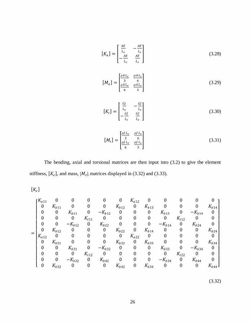
The bending, axial and torsional matrices are then input into (3.2) to give the element
stiffness, 𝐾𝑒 , and mass, 𝑀𝑒 , matrices displayed in (3.32) and (3.33).
𝐾𝑒
=
𝐾𝑎11 0 0 0 0 0 𝐾𝑎12 0 0 0 0 0
0 𝐾𝑏11 0 0 0 𝐾𝑏12 0 𝐾𝑏13 0 0 0 𝐾𝑏14
0 0 𝐾𝑏11 0 −𝐾𝑏12 0 0 0 𝐾𝑏13 0 −𝐾𝑏14 00 0 0 𝐾𝑡11 0 0 0 0 0 𝐾𝑡12 0 00 0 −𝐾𝑏12 0 𝐾𝑏22 0 0 0 −𝐾𝑏14 0 𝐾𝑏24 00 𝐾𝑏12 0 0 0 𝐾𝑏22 0 𝐾𝑏14 0 0 0 𝐾𝑏24
𝐾𝑎12 0 0 0 0 0 𝐾𝑎22 0 0 0 0 00 𝐾𝑏31 0 0 0 𝐾𝑏32 0 𝐾𝑏33 0 0 0 𝐾𝑏34
0 0 𝐾𝑏31 0 −𝐾𝑏32 0 0 0 𝐾𝑏33 0 −𝐾𝑏34 00 0 0 𝐾𝑡12 0 0 0 0 0 𝐾𝑡22 0 00 0 −𝐾𝑏32 0 𝐾𝑏42 0 0 0 −𝐾𝑏34 0 𝐾𝑏44 00 𝐾𝑏32 0 0 0 𝐾𝑏42 0 𝐾𝑏34 0 0 0 𝐾𝑏44
(3.32)
27
𝑀𝑒
=
𝑀𝑎11 0 0 0 0 0 𝑀𝑎12 0 0 0 0 0
0 𝑀𝑏11 0 0 0 𝑀𝑏12 0 𝑀𝑏13 0 0 0 𝑀𝑏14
0 0 𝑀𝑏11 0 −𝑀𝑏12 0 0 0 𝑀𝑏13 0 −𝑀𝑏14 00 0 0 𝑀𝑡11 0 0 0 0 0 𝑀𝑡12 0 00 0 −𝑀𝑏12 0 𝑀𝑏22 0 0 0 −𝑀𝑏14 0 𝑀𝑏24 00 𝑀𝑏12 0 0 0 𝑀𝑏22 0 𝑀𝑏14 0 0 0 𝑀𝑏24
𝑀𝑎12 0 0 0 0 0 𝑀𝑎22 0 0 0 0 00 𝑀𝑏31 0 0 0 𝑀𝑏32 0 𝑀𝑏33 0 0 0 𝑀𝑏34
0 0 𝑀𝑏31 0 −𝑀𝑏32 0 0 0 𝑀𝑏33 0 −𝑀𝑏34 00 0 0 𝑀𝑡12 0 0 0 0 0 𝑀𝑡22 0 00 0 −𝑀𝑏32 0 𝑀𝑏42 0 0 0 −𝑀𝑏34 0 𝑀𝑏44 00 𝑀𝑏32 0 0 0 𝑀𝑏42 0 𝑀𝑏34 0 0 0 𝑀𝑏44
(3.33)
3.3.2 Construction of Global Matrices
Once these element matrices are calculated, they need to be converted from local to
global coordinates. This is done by computing a transformation matrix, 𝑇 . Matrix 𝑇𝑒 is made
by inputting the angles between the local and global axes. This matrix is then input into 𝑇 .
There are four 𝑇𝑒 terms in this matrix because there are six degrees of freedom per node or
twelve per element. The element stiffness and mass matrices are then converted using Eqs.
(3.36) and (3.37) where 𝐾𝑒′ is the element stiffness matrix in global coordinates and 𝑀𝑒′ is
the element mass matrix in global coordinates.
.

28
𝑇𝑒 =
cos( 𝑥,𝑋 ) cos( 𝑥,𝑌 ) cos( 𝑥,𝑍 )
cos( 𝑦,𝑋 ) cos( 𝑦,𝑌 ) cos( 𝑦,𝑍 )
cos( 𝑧,𝑋 ) cos( 𝑧,𝑌 ) cos( 𝑧,𝑍 )
(3.34)
𝑇 =
𝑇𝑒 0 0 00 𝑇𝑒 0 00 0 𝑇𝑒 00 0 0 𝑇𝑒
(3.35)
𝐾𝑒′ = 𝑇 𝑇 𝐾𝑒 𝑇 (3.36)
𝑀𝑒′ = 𝑇 𝑇 𝑀𝑒 𝑇 (3.37)
Now that the element matrices are in the global coordinates, the global matrices can be
constructed. Each matrix can be broken up to the form of (3.38), where i and j are the node
numbers for that particular element. Therefore, each quadrant of the matrix can be input into the
global matrix at a place that corresponds to the global node numbers for the element.
𝐾𝑒′ = 𝐾𝑖𝑖 𝐾𝑖𝑗
𝐾𝑖𝑗𝑇 𝐾𝑗𝑗
(3.38)
The last step in creation of the model is to add the mass elements. These include four
spheres and the spindle holder. Since these are point masses, the inertia terms will lie on the
diagonal of the mass matrix. These point masses will have no affect on the stiffness matrix. The
terms in the matrices will be the same as those calculated for the ANSYS method. These point
mass matrices will be input to the global matrix where the diagonal terms correspond to that
particular node. Here, m is the mass of the object and 𝐼𝑥𝑥 , 𝐼𝑦𝑦 , and 𝐼𝑧𝑧 are the mass moments of
inertia.
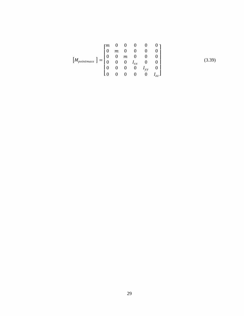
29
𝑀𝑝𝑜𝑖𝑛𝑡𝑚𝑎𝑠𝑠 =
𝑚 0 0 0 0 00 𝑚 0 0 0 00 0 𝑚 0 0 00 0 0 𝐼𝑥𝑥 0 00 0 0 0 𝐼𝑦𝑦 0
0 0 0 0 0 𝐼𝑧𝑧
(3.39)
30
4 CHAPTER 4 – MODAL ANALYSIS
4.1 Introduction
Modal analysis was conducted on the different Tetraform prototypes. This was done
using both the ANSYS and Matlab models. The modal analysis results are the natural
frequencies and the mode shapes. The mode shapes are the structural displacements at a
particular natural frequency and are used to analyze where the areas of high energy are on the
Tetraform for that natural frequency. It is not desirable to have modes with high vibrational
energy at the point of the spindle holder. The frequencies that fall into this category are
considered critical frequencies. The mode shapes for the critical frequencies can be used to
identify all of the areas of high surface strain that could be used to attach the piezoelectric
sensors and actuators. The mode shapes and frequencies for different Tetraforms are also
compared to see the advantages of the different models.
4.2 Full Scale Modal Analysis Results from ANSYS
The first modal analysis results are from the full scale Tetraform. This is the Tetraform
model to which active vibration will be applied to. The modal analysis method used in ANSYS
was Block Lanczos. The first results obtained were for the full scale Tetraform without the
spindle motor and bearing attached to the spindle holder. This additional mass and inertia is
added for the second set of results. The mode shapes and frequencies for the first 12 modes are
displayed in Figures 4-1 to 4-12. These mode shapes are used to analyze which modes are
31
critical to the machining process. The modes which contain large displacements at the center
point mass, which represents the spindle holder, are the critical modes of interest.
4.2.1 Full Scale Mode Shapes without Spindle
Figure 4-1 Mode 1 @41.0 Hz
32
Figure 4-2 Mode 2 @ 51.3 Hz
Mode 1 contains most of its energy in the lower portion of the structure. The lower
beams vibrate with full length bending with the largest displacement at the middle of the beam.
Some of the vibrational energy is translated to the upper portion of the structure, creating slight
vertical displacement of the spindle. Mode 2 is similar in the fact that it is mostly made up of
full length bending of the lower beams. It, however, creates small horizontal displacements of
the spindle holder. The brackets in the lower portion of the structure apply little stiffness to these
modes. This, along with the added mass of the lower brackets, keeps these frequencies in the
lower end of the frequency spectrum.
33
Figure 4-3 Mode 3 @ 63.4 Hz
Figure 4-4 Mode 4 @64.0 Hz
34
Modes 3 and 4 consist of full length bending of the upper beams. The bending from
Mode 3 causes the Tetraform to sway horizontally creating large horizontal displacement of the
spindle holder. Mode 3 is the dominant critical mode for horizontal displacement of the spindle
holder. The bending of the beams in Mode 4 causes the Tetraform to rotate about its center
vertical axis. This creates only a rotational displacement about the vertical axis for the spindle
holder.
Figure 4-5 Mode 5 @ 95.7 Hz
35
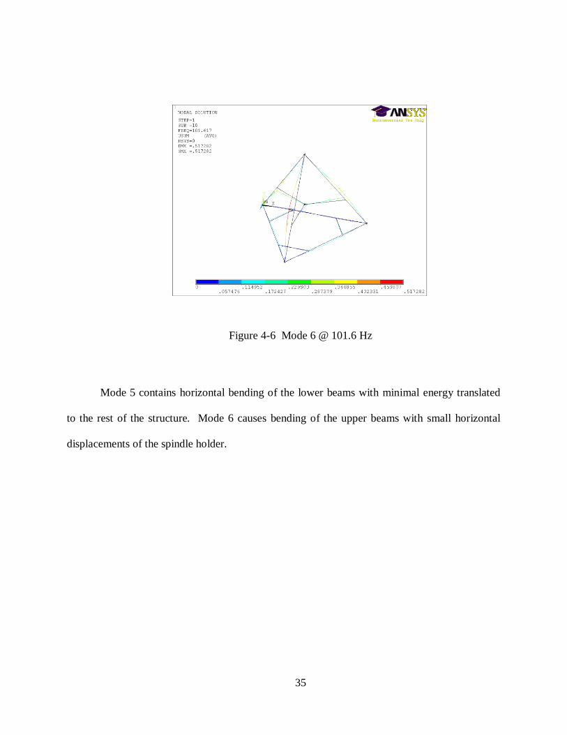
Figure 4-6 Mode 6 @ 101.6 Hz
Mode 5 contains horizontal bending of the lower beams with minimal energy translated
to the rest of the structure. Mode 6 causes bending of the upper beams with small horizontal
displacements of the spindle holder.
36
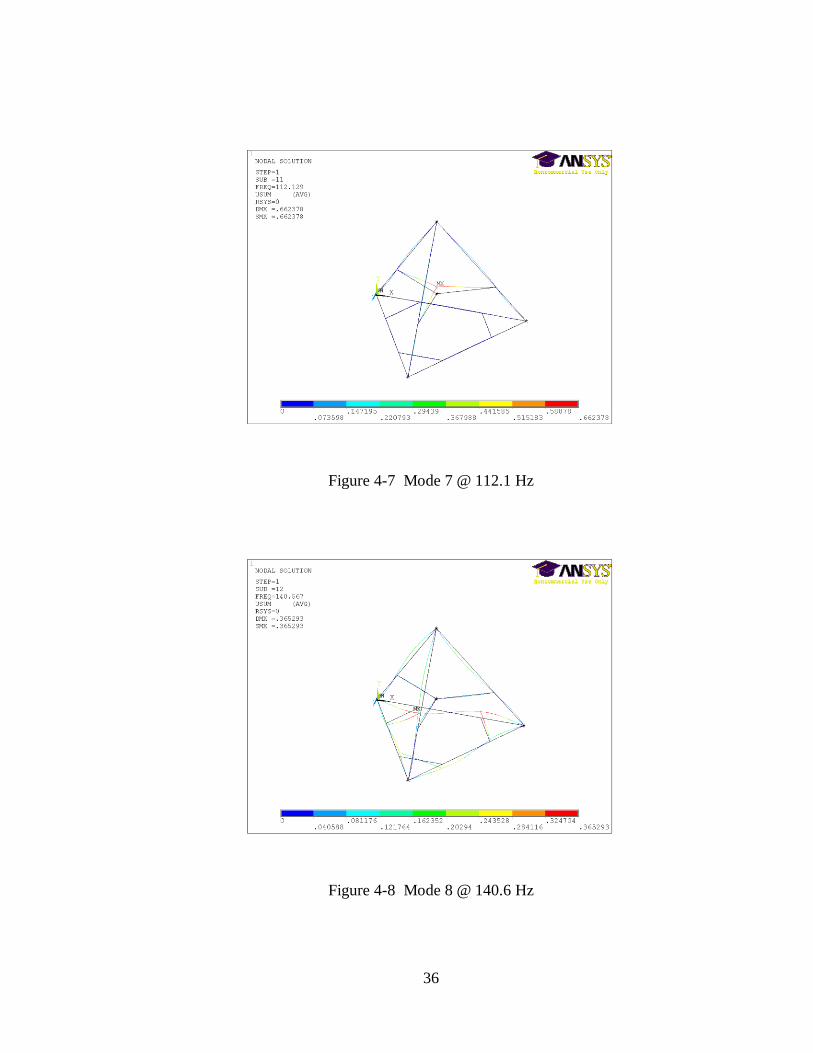
Figure 4-7 Mode 7 @ 112.1 Hz
Figure 4-8 Mode 8 @ 140.6 Hz
37
Mode 7 contains bending of the inner beams which attach the spindle holder, creating
large vertical displacements of the spindle holder. This mode is the dominant critical mode for
vertical displacement of the spindle holder. This mode is also highly sensitive to the addition of
mass and inertia of different spindles attached to the holder. Mode 8 consists of energy
throughout most of the structure but does not affect the inner beams attaching the spindle holder.
Figure 4-9 Mode 9 @ 200.2 Hz
38
Figure 4-10 Mode 10 @ 204.4 Hz
Figure 4-11 Mode 11 @ 235.5 Hz
39
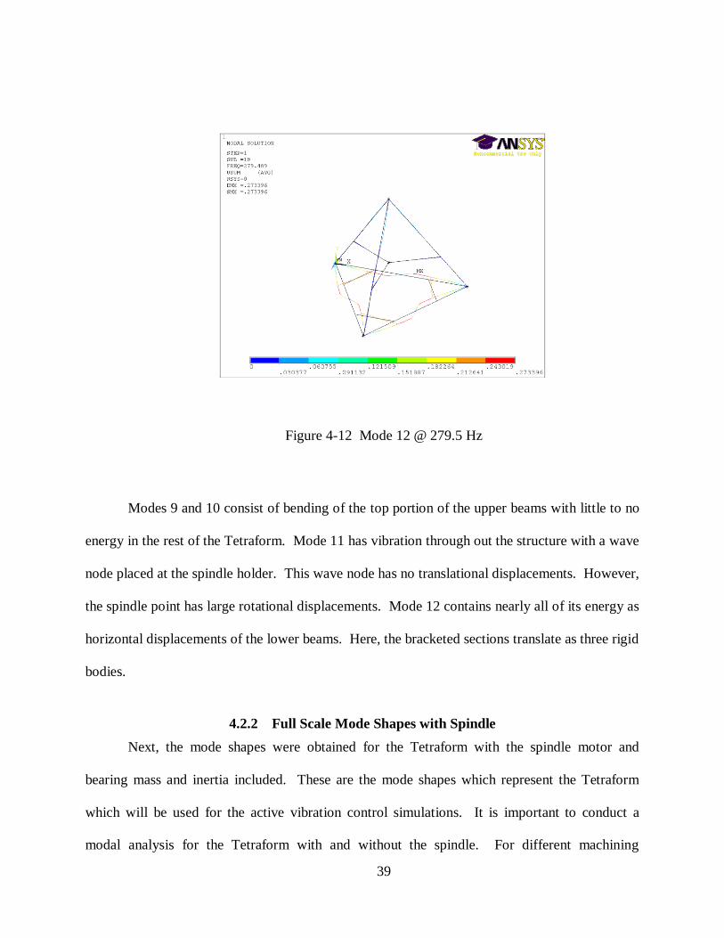
Figure 4-12 Mode 12 @ 279.5 Hz
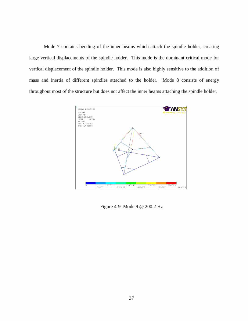
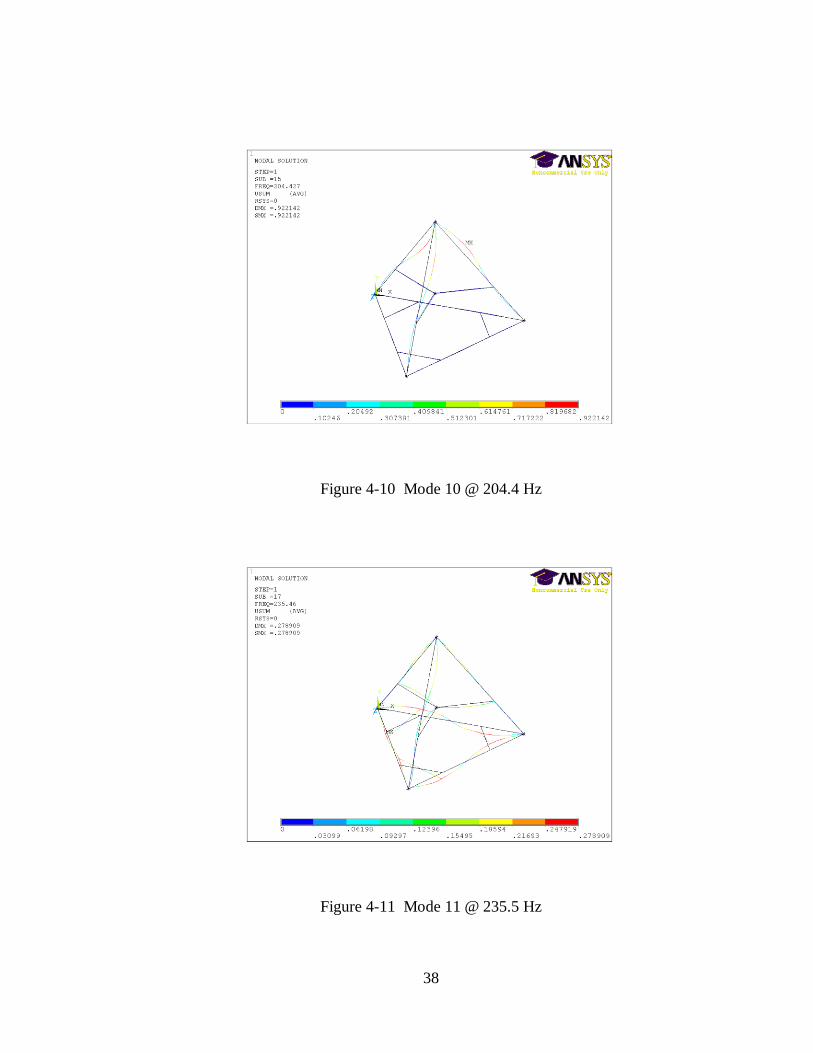
Modes 9 and 10 consist of bending of the top portion of the upper beams with little to no
energy in the rest of the Tetraform. Mode 11 has vibration through out the structure with a wave
node placed at the spindle holder. This wave node has no translational displacements. However,
the spindle point has large rotational displacements. Mode 12 contains nearly all of its energy as
horizontal displacements of the lower beams. Here, the bracketed sections translate as three rigid
bodies.
4.2.2 Full Scale Mode Shapes with Spindle
Next, the mode shapes were obtained for the Tetraform with the spindle motor and
bearing mass and inertia included. These are the mode shapes which represent the Tetraform
which will be used for the active vibration control simulations. It is important to conduct a
modal analysis for the Tetraform with and without the spindle. For different machining
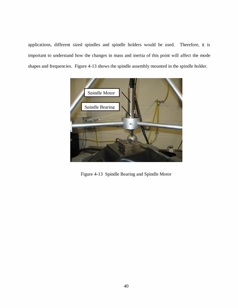
40
applications, different sized spindles and spindle holders would be used. Therefore, it is
important to understand how the changes in mass and inertia of this point will affect the mode
shapes and frequencies. Figure 4-13 shows the spindle assembly mounted in the spindle holder.
Figure 4-13 Spindle Bearing and Spindle Motor
Spindle Motor
Spindle Bearing
41
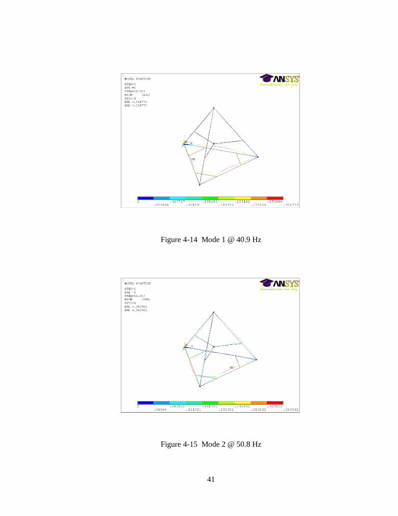
Figure 4-14 Mode 1 @ 40.9 Hz
Figure 4-15 Mode 2 @ 50.8 Hz
42
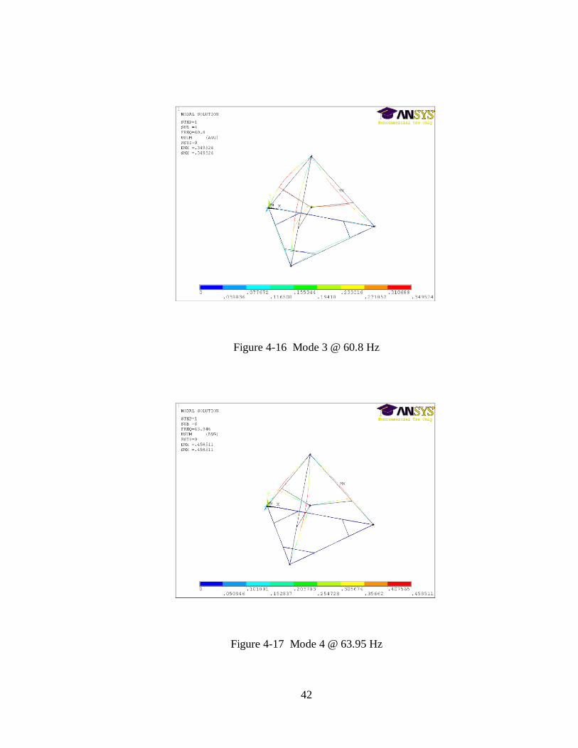
Figure 4-16 Mode 3 @ 60.8 Hz
Figure 4-17 Mode 4 @ 63.95 Hz
43
Figure 4-18 Mode 5 @ 93.1 Hz
Figure 4-19 Mode 6 @ 95.6 Hz
44
Figure 4-20 Mode 7 @ 99.6 Hz
Figure 4-21 Mode 8 @ 140.4 Hz

45
Figure 4-22 Mode 9 @ 200.1 Hz
Figure 4-23 Mode 10 @ 203.5 Hz
46
Figure 4-24 Mode 11 @ 235.4 Hz
Figure 4-25 Mode 12 @ 269.4 Hz
47
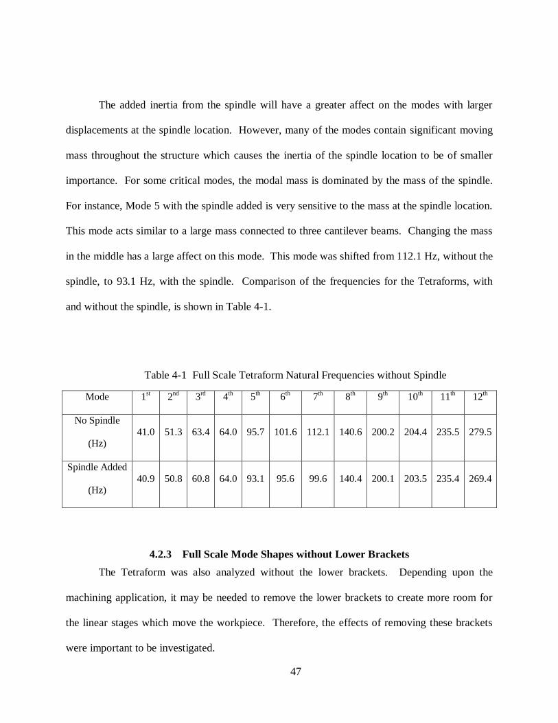
The added inertia from the spindle will have a greater affect on the modes with larger
displacements at the spindle location. However, many of the modes contain significant moving
mass throughout the structure which causes the inertia of the spindle location to be of smaller
importance. For some critical modes, the modal mass is dominated by the mass of the spindle.
For instance, Mode 5 with the spindle added is very sensitive to the mass at the spindle location.
This mode acts similar to a large mass connected to three cantilever beams. Changing the mass
in the middle has a large affect on this mode. This mode was shifted from 112.1 Hz, without the
spindle, to 93.1 Hz, with the spindle. Comparison of the frequencies for the Tetraforms, with
and without the spindle, is shown in Table 4-1.
Table 4-1 Full Scale Tetraform Natural Frequencies without Spindle
Mode 1st 2
nd 3
rd 4
th 5
th 6
th 7
th 8
th 9
th 10
th 11
th 12
th
No Spindle
(Hz) 41.0 51.3 63.4 64.0 95.7 101.6 112.1 140.6 200.2 204.4 235.5 279.5
Spindle Added
(Hz) 40.9 50.8 60.8 64.0 93.1 95.6 99.6 140.4 200.1 203.5 235.4 269.4
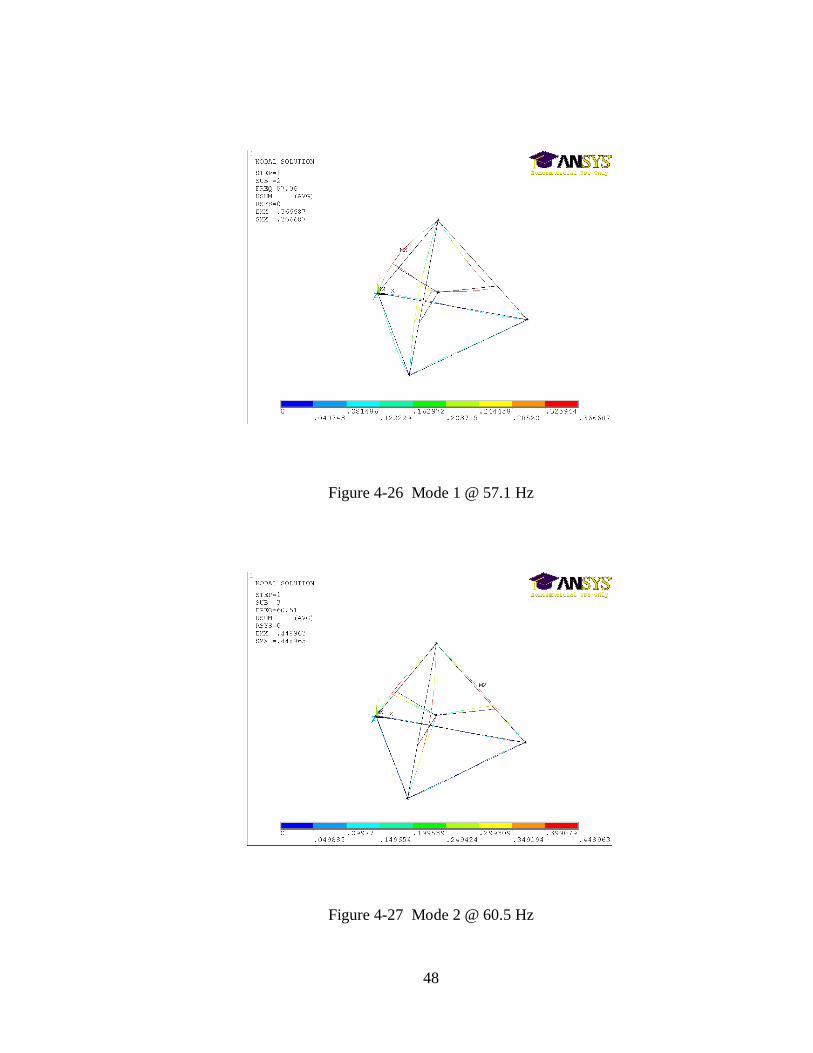
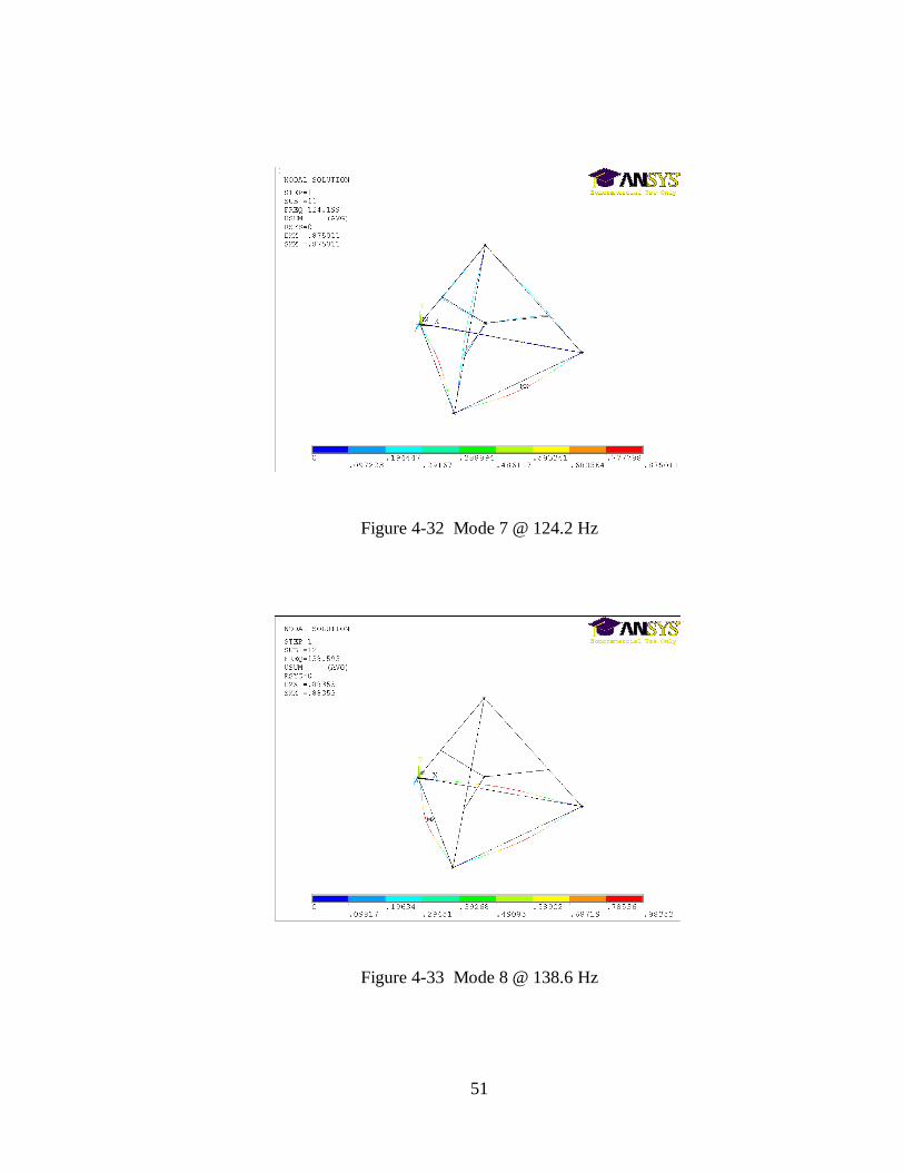
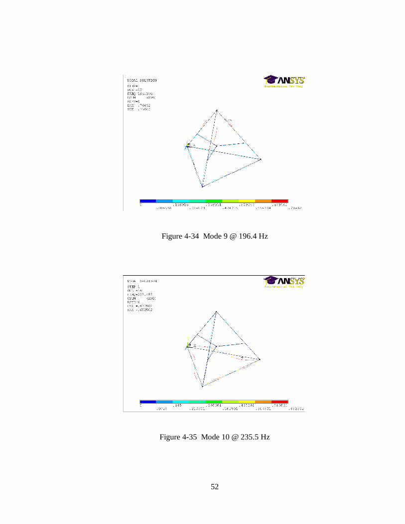
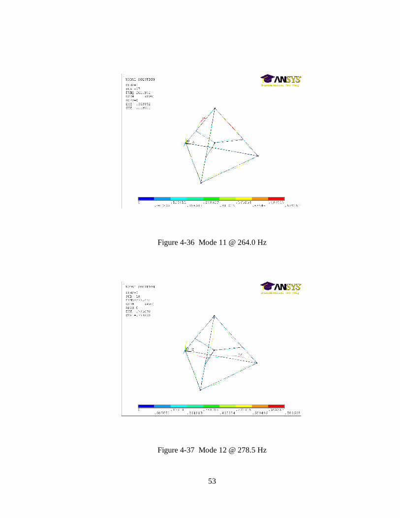
4.2.3 Full Scale Mode Shapes without Lower Brackets
The Tetraform was also analyzed without the lower brackets. Depending upon the
machining application, it may be needed to remove the lower brackets to create more room for
the linear stages which move the workpiece. Therefore, the effects of removing these brackets
were important to be investigated.
48
Figure 4-26 Mode 1 @ 57.1 Hz
Figure 4-27 Mode 2 @ 60.5 Hz

49
Figure 4-28 Mode 3 @ 75.2 Hz
Figure 4-29 Mode 4 @ 84.7 Hz

50
Figure 4-30 Mode 5 @ 89.6 Hz
Figure 4-31 Mode 6 @ 107.5 Hz
51
Figure 4-32 Mode 7 @ 124.2 Hz
Figure 4-33 Mode 8 @ 138.6 Hz
52
Figure 4-34 Mode 9 @ 196.4 Hz
Figure 4-35 Mode 10 @ 235.5 Hz
53
Figure 4-36 Mode 11 @ 264.0 Hz
Figure 4-37 Mode 12 @ 278.5 Hz
54
Modes 4 and 6 both contain vertical displacement of the spindle holder. They both also
have a large amount of energy in the lower beams. For Mode 4, the lower beams displace
downward when the spindle moves upward. This mode is similar to Mode 5 of the Tetraform
with the brackets and spindle. When removing the lower brackets, more of the energy is
transferred to the lower portion of the Tetraform for this mode. For Mode 5, the lower beams
and the spindle both displace in the same vertical direction. This mode is similar to Mode 1 of
the Tetraform with the brackets and spindle. Removing the brackets for this mode creates more
modal energy at the spindle location.
4.3 Modal Analysis in Matlab
Using the model that was created in Chapter 3 in Matlab, the natural frequencies, ωn , can
be calculated and checked with the ANSYS results. The structural equation of motion can be put
into the form of (4.1). 𝐼 is an identity matrix and 𝜑 is the eigenvector. 𝐾 − 𝜔𝑛2 𝐼 𝑀
is referred to as the dynamic stiffness matrix.
𝐾 − 𝜔𝑛2 𝐼 𝑀 𝜑 = 𝐹 (4.1)
Taking the determinant of the dynamic stiffness matrix and setting it equal to zero yields
a polynomial of 𝜔𝑛2 which are the eigenvalues of the system. The eigenvectors of the system are
the relative nodal displacement vectors for their corresponding natural frequencies, or the mode
shapes. The mode shapes will not be plotted in Matlab. However, they will be needed for
converting the model to modal coordinates in the next chapter.
55
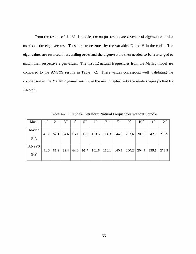
From the results of the Matlab code, the output results are a vector of eigenvalues and a
matrix of the eigenvectors. These are represented by the variables D and V in the code. The
eigenvalues are resorted in ascending order and the eigenvectors then needed to be rearranged to
match their respective eigenvalues. The first 12 natural frequencies from the Matlab model are
compared to the ANSYS results in Table 4-2. These values correspond well, validating the
comparison of the Matlab dynamic results, in the next chapter, with the mode shapes plotted by
ANSYS.
Table 4-2 Full Scale Tetraform Natural Frequencies without Spindle
Mode 1st 2
nd 3
rd 4
th 5
th 6
th 7
th 8
th 9
th 10
th 11
th 12
th
Matlab
(Hz) 41.7 52.1 64.6 65.1 98.5 103.5 114.3 144.0 203.6 208.5 242.3 293.9
ANSYS
(Hz) 41.0 51.3 63.4 64.0 95.7 101.6 112.1 140.6 200.2 204.4 235.5 279.5

56
5 CHAPTER 5 – DYNAMIC ANALYSIS
5.1 Introduction
Dynamic analysis of the Tetraform is important to realize how different points on the
structure respond to force inputs at different areas. FRFs were plotted to show the dynamic
response between these points. They consist of a magnitude response and a phase response.
The magnitude plot shows the amplitude of the output vs. the frequency of the input where the
amplitude is in decibels (dB) and the frequency is on the log scale in either radians/s or Hz. The
phase plot shows the phase shift between the input force and the output response plotted vs.
frequency on the log scale. These plots are also referred to as Bode plots. When carried out
experimentally, the input force must be measured in order to compute the relationship between
the input amplitude and phase to that of the output amplitude and phase.
The force inputs of interest are disturbance forces, machining forces, and actuator forces.
Therefore, the FRFs were setup to display responses to these inputs. The relationship between
responses of the spindle holder from machining forces were plotted to show which modes are
easily triggered by machining. Similarly, the relationship between input disturbance forces at
various points throughout the structure to the response of the spindle is important to show how
easily the different critical modes can be triggered by external disturbances. These FRFs are also
needed to determine the placement of the actuator to have the highest influence over the critical
modes. Location of the actuators can be fine tuned by this method to find optimal placement for
the vibration controller. Since the sensors and actuators are collocated, this location also allows
57
the sensor to receive the strongest response from the critical modes. It is also desirable for the
sensor to have little response from non-critical modes.
Dynamic responses were conducted both experimentally and by simulation.
Experimentally, the FRFs were obtained using the impact hammer method. This method uses an
impact hammer to apply a measured impulse input while an accelerometer measures the dynamic
response at the output point. Similar responses were also plotted by simulation to compare and
validate the mathematical model. The simulation model was then used for structural analysis
and design purposes due to the ease at which the inputs and outputs may be changed in
simulation.
5.2 Impact Hammer Method
Experimental FRFs are most often obtained by one of two methods. The first method
uses a force input of varying frequency to excite the structure while measuring the dynamic
response with an accelerometer. A common device used to apply the force input for this method
is a shaker. A shaker either mounts the test object on top of it or applies the input force to a
point by way of an armature. Forcing frequency is then varied to measure the amplitude and
phase of the response for a range of frequencies.
The alternative method is that of the impact hammer method. A hammer is used to apply
an input that acts as an impulse. An impulse is a force input of constant amplitude and infinitely
small duration. Ideally, this input triggers the entire frequency. In actuality, the hammer force
input cannot be of infinitely small duration. Interchangeable hammer tips may be used to obtain
58
responses from different ranges of the frequency spectrum. The harder tips create shorter time of
impacts and are used to trigger higher frequencies.
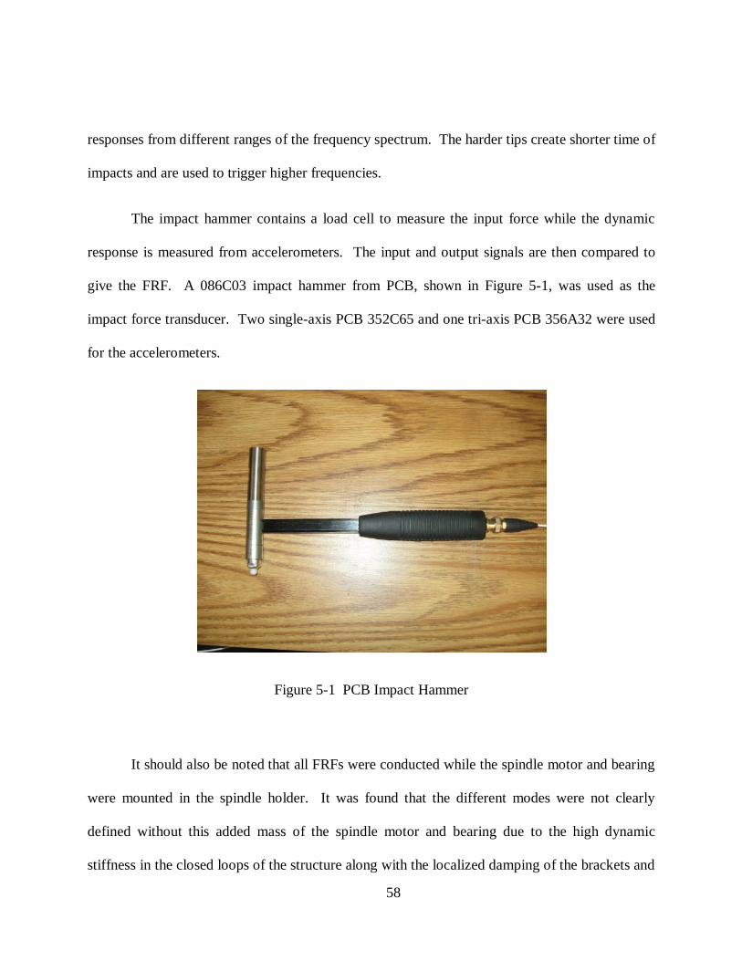
The impact hammer contains a load cell to measure the input force while the dynamic
response is measured from accelerometers. The input and output signals are then compared to
give the FRF. A 086C03 impact hammer from PCB, shown in Figure 5-1, was used as the
impact force transducer. Two single-axis PCB 352C65 and one tri-axis PCB 356A32 were used
for the accelerometers.
Figure 5-1 PCB Impact Hammer
It should also be noted that all FRFs were conducted while the spindle motor and bearing
were mounted in the spindle holder. It was found that the different modes were not clearly
defined without this added mass of the spindle motor and bearing due to the high dynamic
stiffness in the closed loops of the structure along with the localized damping of the brackets and
59
joints. The addition of the mass and inertia of the spindle motor and bearing will also more
accurately represent the Tetraform under machining conditions.
Multiple impact hammer responses were conducted on the full scale Tetraform. These
were used to verify the FEA simulation models and to obtain damping values. Damping must be
added to the FEA models in order to accurately simulate any type of forced response. The
comparison of these results with the FEA model results are shown at the end of the chapter.
5.3 Matlab Simulation
The FEA model must be converted to a form that will give the displacement response to a
force input. Therefore, the model must be reduced in size, damping must be added, and then
must be converted over to state space. The FEA model that was created in Matlab, (5.1), must be
converted into a form that will give the displacement response to force inputs. Therefore, it was
required that the model be reduced in size, damping to be added, and the model to be converted
to state space.
𝑀 𝑟 + 𝐾 𝑟 = 𝑓 (5.1)
This model contains 101 nodes with six degrees of freedom at each node. The size of this
model creates much difficulty in computation during simulation. By using the method of
decoupling the model into modal coordinates, we can reduce the size of the model significantly.
This is done by using the eigenvectors that were solved from the model described in (5.1) to
manipulate the mass and stiffness matrices into decoupled equations of motion in modal
60
coordinates. An eigenvector matrix 𝛷 was constructed from the eigenvectors 𝜑𝑖 where 𝑖 = 1:𝑛
and 𝑛 is the number of degrees of freedom. These were sorted in ascending order where 𝜑1 is the
eigenvector of the first mode.
𝛷 = 𝜑1𝜑
2… . . 𝜑
𝑛 (5.2)
Using this modal matrix, the dynamic equation is converted from structural coordinates,
𝑟 , to modal coordinates, 𝑞 . Equation (5.3) shows the conversion between the two
coordinates. By plugging this into (5.1) and multiplying through by 𝛷 𝑇 results in (5.4).
𝑟 = 𝛷 𝑞 (5.3)
𝛷 𝑇 𝑀 𝛷 𝑞 + 𝛷 𝑇 𝐾 𝛷 𝑞 = 𝛷 𝑇 𝑓 (5.4)
Due to orthogonality of the eigenvectors, the mass and stiffness matrices are diagonalized
into the modal mass and stiffness matrices shown in Eqs. (5.5) and (5.6). Here, 𝑚𝑖 and 𝑘𝑖 are
the modal mass and stiffness values for the 𝑖𝑡 mode.
𝛷 𝑇 𝑀 𝛷 = 𝑀′ =
𝑚1 0 … … 00 𝑚2 0 … 0: 0 𝑚3 0 0: : 0 … 00 0 … 0 𝑚𝑛
(5.5)
𝛷 𝑇 𝐾 𝛷 = 𝐾′ =
𝑘1 0 … … 00 𝑘2 0 … 0: 0 𝑘3 0 0: : 0 … 00 0 … 0 𝑘𝑛
(5.6)

61
Equation (5.7) is the new dynamic equation in modal coordinates. This shows the
response is the superposition of 𝑛 uncoupled modal equations. The number of eigenvectors, 𝑛,
may then be limited to the highest mode of interest. With 101 nodes and six degrees of freedom
at each, there are 606 eigenvectors before removing nine through boundary conditions. As a
majority of the higher modes are dampened out and nonexistent in reality, the number of
included modes can be greatly reduced.
𝑀′ 𝑞 + 𝐾′ 𝑞 = 𝑓′ (5.7)
Once the model in modal coordinates is reduced, damping may be included. The
damping matrix is determined by Rayleigh’s damping coefficients, 𝛼 and 𝛽, and is given in
(5.8). These coefficients are determined from experimental results. For this simulation,
damping will be given the values 𝛼 = 2 and 𝛽 = 3𝑒 − 5. The equation of motion with damping
is now (5.9).
𝐷 = 𝛼 𝑀′ + 𝛽 𝐾′ (5.8)
𝑀′ 𝑞 + 𝐷 𝑞 + 𝐾′ 𝑞 = 𝑓′ (5.9)
Converting the equation of motion to state space form gives an output vector of
displacements, 𝑦 , to an input vector, 𝑢 . The size of the input and output vectors depends on
the number of inputs and outputs of the system. For frequency responses, only one of each is
required, making these terms scalar. The second order differential equations from (5.9) will be
separated into first order equations by defining the state vector, 𝜉 , in (5.10).
62
𝜉 = 𝑞
𝑞 (5.10)
Redefining the system in terms of the state vector gives Eqs. (5.11) through (5.14) where
𝑓 is the force input vector and 𝐶 is the output matrix. These are defined based on the input
and output locations on the Tetraform. For these simulations, the feed through matrix, 𝐷 , is set
to zero. The sensor responses used the piezoelectric sensor equations that are defined in Chapter
6.
𝜉 = 𝐴 𝜉 + 𝐵 𝑢 (5.11)
𝑦 = 𝐶 Φ 𝜉 + 𝐷 𝑢 (5.12)
𝐴 = 0 𝐼
− 𝑀′ −1 𝐾′ − 𝑀′ −1 𝐷 (5.13)
𝐵 = 0
− 𝑀′ −1 Φ 𝑇 𝑓 (5.14)
5.4 Interpretation of Results
Since the impact hammer method used accelerometers for the response, the FRFs reflect
the relationship between acceleration outputs to a force inputs. The previously made FEA model
was set up to output displacement. Just for the purpose of comparison to the experimental plots,
the state space model was converted to acceleration output. This was done by multiplying the
output by the transfer function 𝑠2. All the FRFs that were not compared to experimental results
were kept as position responses.
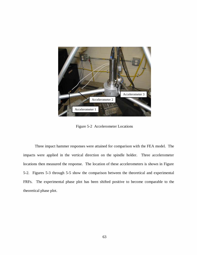
63
Figure 5-2 Accelerometer Locations
Three impact hammer responses were attained for comparison with the FEA model. The
impacts were applied in the vertical direction on the spindle holder. Three accelerometer
locations then measured the response. The location of these accelerometers is shown in Figure
5-2. Figures 5-3 through 5-5 show the comparison between the theoretical and experimental
FRFs. The experimental phase plot has been shifted positive to become comparable to the
theoretical phase plot.
Accelerometer 1
Accelerometer 2
Accelerometer 3
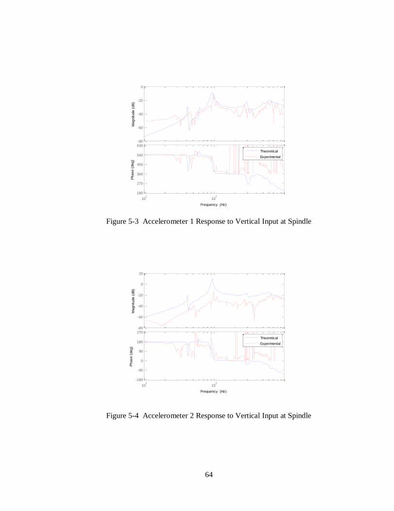
64
Figure 5-3 Accelerometer 1 Response to Vertical Input at Spindle
Figure 5-4 Accelerometer 2 Response to Vertical Input at Spindle
-80
-60
-40
-20
0
Magnitu
de (
dB
)
101
102
180
270
360
450
540
630
Phase (
deg)
Frequency (Hz)
Theoretical
Experimental
-80
-60
-40
-20
0
20
Magnitu
de (
dB
)
101
102
-180
-90
0
90
180
270
Phase (
deg)
Frequency (Hz)
Theoretical
Experimental
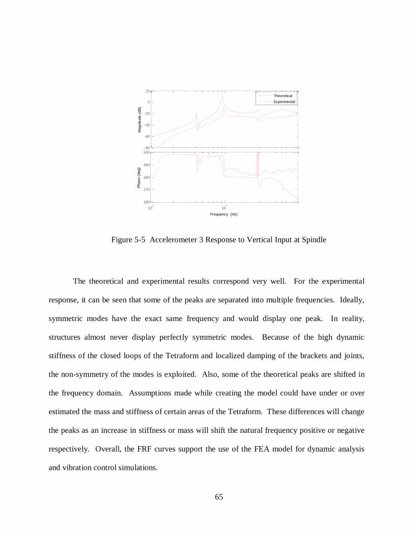
65
Figure 5-5 Accelerometer 3 Response to Vertical Input at Spindle
The theoretical and experimental results correspond very well. For the experimental
response, it can be seen that some of the peaks are separated into multiple frequencies. Ideally,
symmetric modes have the exact same frequency and would display one peak. In reality,
structures almost never display perfectly symmetric modes. Because of the high dynamic
stiffness of the closed loops of the Tetraform and localized damping of the brackets and joints,
the non-symmetry of the modes is exploited. Also, some of the theoretical peaks are shifted in
the frequency domain. Assumptions made while creating the model could have under or over
estimated the mass and stiffness of certain areas of the Tetraform. These differences will change
the peaks as an increase in stiffness or mass will shift the natural frequency positive or negative
respectively. Overall, the FRF curves support the use of the FEA model for dynamic analysis
and vibration control simulations.
-80
-60
-40
-20
0
20
Magnitu
de (
dB
)
101
102
180
270
360
450
540
Phase (
deg)
Frequency (Hz)
Theoretical
Experimental
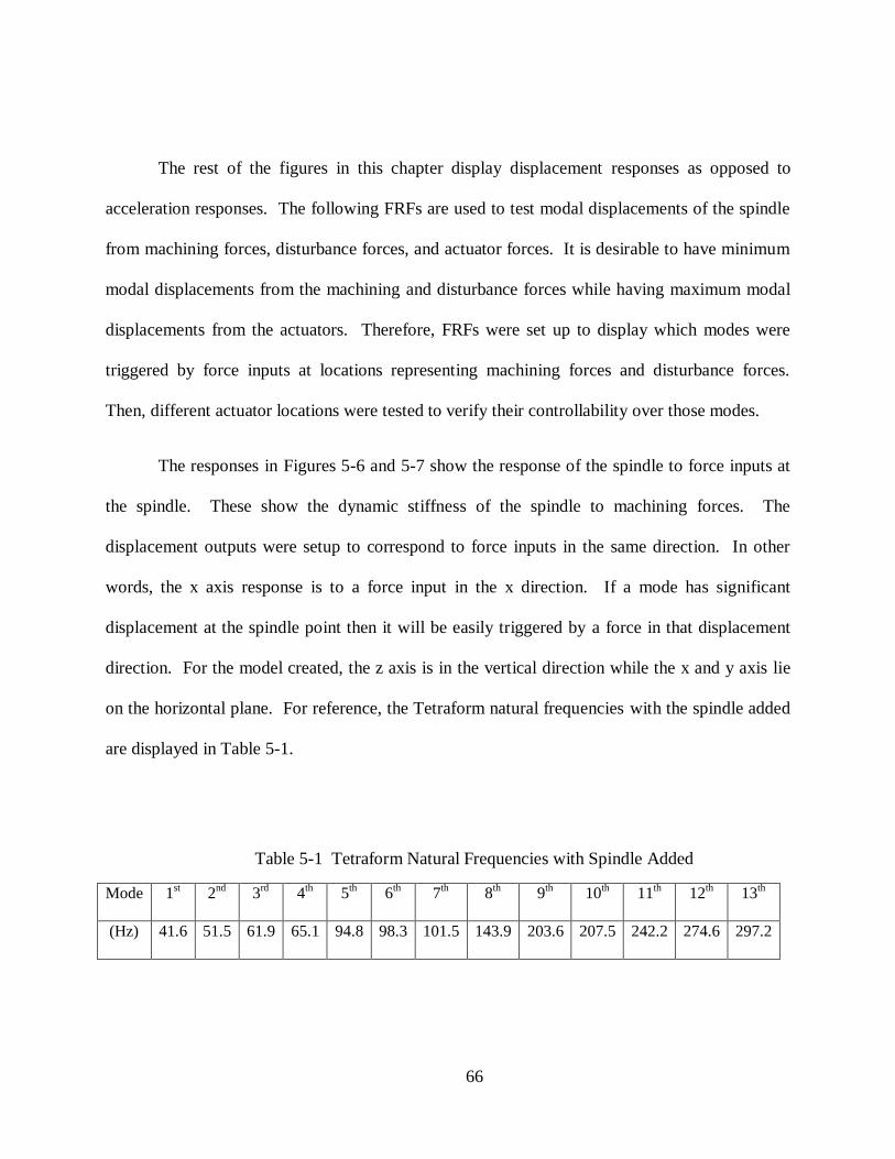
66
The rest of the figures in this chapter display displacement responses as opposed to
acceleration responses. The following FRFs are used to test modal displacements of the spindle
from machining forces, disturbance forces, and actuator forces. It is desirable to have minimum
modal displacements from the machining and disturbance forces while having maximum modal
displacements from the actuators. Therefore, FRFs were set up to display which modes were
triggered by force inputs at locations representing machining forces and disturbance forces.
Then, different actuator locations were tested to verify their controllability over those modes.
The responses in Figures 5-6 and 5-7 show the response of the spindle to force inputs at
the spindle. These show the dynamic stiffness of the spindle to machining forces. The
displacement outputs were setup to correspond to force inputs in the same direction. In other
words, the x axis response is to a force input in the x direction. If a mode has significant
displacement at the spindle point then it will be easily triggered by a force in that displacement
direction. For the model created, the z axis is in the vertical direction while the x and y axis lie
on the horizontal plane. For reference, the Tetraform natural frequencies with the spindle added
are displayed in Table 5-1.
Table 5-1 Tetraform Natural Frequencies with Spindle Added
Mode 1st 2
nd 3
rd 4
th 5
th 6
th 7
th 8
th 9
th 10
th 11
th 12
th 13
th
(Hz) 41.6 51.5 61.9 65.1 94.8 98.3 101.5 143.9 203.6 207.5 242.2 274.6 297.2
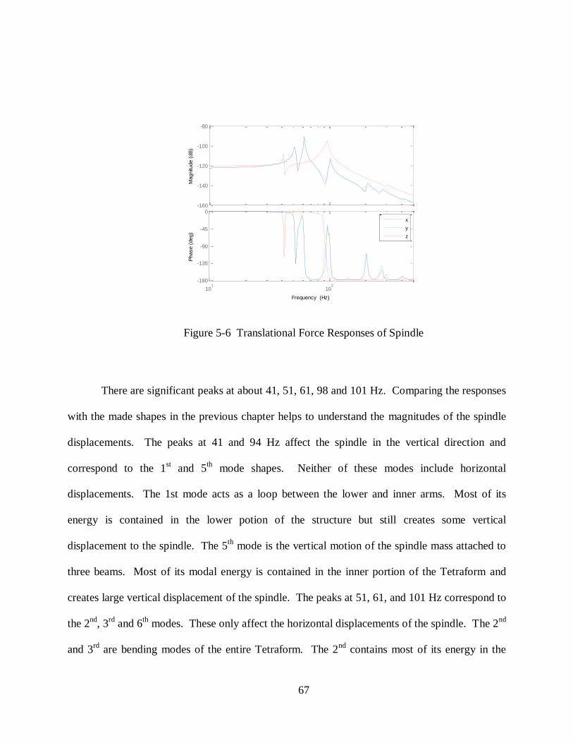
67
Figure 5-6 Translational Force Responses of Spindle
There are significant peaks at about 41, 51, 61, 98 and 101 Hz. Comparing the responses
with the made shapes in the previous chapter helps to understand the magnitudes of the spindle
displacements. The peaks at 41 and 94 Hz affect the spindle in the vertical direction and
correspond to the 1st and 5
th mode shapes. Neither of these modes include horizontal
displacements. The 1st mode acts as a loop between the lower and inner arms. Most of its
energy is contained in the lower potion of the structure but still creates some vertical
displacement to the spindle. The 5th
mode is the vertical motion of the spindle mass attached to
three beams. Most of its modal energy is contained in the inner portion of the Tetraform and
creates large vertical displacement of the spindle. The peaks at 51, 61, and 101 Hz correspond to
the 2nd
, 3rd
and 6th
modes. These only affect the horizontal displacements of the spindle. The 2nd
and 3rd
are bending modes of the entire Tetraform. The 2nd
contains most of its energy in the
-160
-140
-120
-100
-80
Magnitu
de (
dB
)
101
102
-180
-135
-90
-45
0
Phase (
deg)
Frequency (Hz)
x
y
z
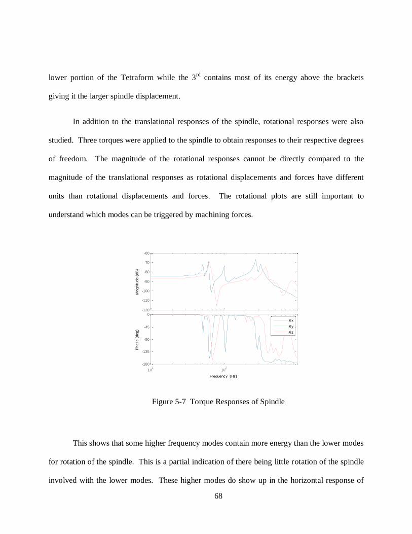
68
lower portion of the Tetraform while the 3rd
contains most of its energy above the brackets
giving it the larger spindle displacement.
In addition to the translational responses of the spindle, rotational responses were also
studied. Three torques were applied to the spindle to obtain responses to their respective degrees
of freedom. The magnitude of the rotational responses cannot be directly compared to the
magnitude of the translational responses as rotational displacements and forces have different
units than rotational displacements and forces. The rotational plots are still important to
understand which modes can be triggered by machining forces.
Figure 5-7 Torque Responses of Spindle
This shows that some higher frequency modes contain more energy than the lower modes
for rotation of the spindle. This is a partial indication of there being little rotation of the spindle
involved with the lower modes. These higher modes do show up in the horizontal response of
-120
-110
-100
-90
-80
-70
-60
Magnitu
de (
dB
)
101
102
-180
-135
-90
-45
0
Phase (
deg)
Frequency (Hz)
x
y
z
69
Figure 5-6 but contain much less modal energy than the lower modes for the spindle location.
However, these higher modes are still of importance.
The translational responses of the spindle to applied torques at the spindle were plotted in
Figures 5-8 through 5-10 to show the coupling between the translational and the rotational
degrees of freedom. For these plots, the three torque inputs were applied at the spindle while the
output is a single degree of freedom at the spindle. This could have been done inversely by
applying one torque and measuring the output in different degrees of freedom for the spindle.
These FRFs would be interchangeable. This comes from Maxwell’s Theorem of Reciprocity
which is applicable to linear structures. When looking at the force-displacement relationship
between two points on the structure, the displacement of point 1 from a unit force on point 2 is
equal to the displacement of point 2 from a unit force on point 1. This means that the FRF will
be equal in both directions between the two points. This property is true because of the
symmetry of the mass and stiffness matrices for linear structures.
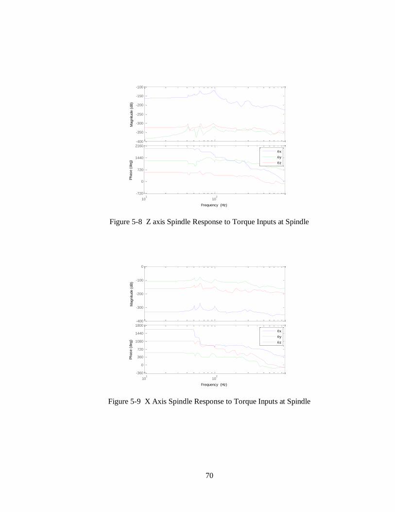
70
Figure 5-8 Z axis Spindle Response to Torque Inputs at Spindle
Figure 5-9 X Axis Spindle Response to Torque Inputs at Spindle
-400
-350
-300
-250
-200
-150
-100
Magnitu
de (
dB
)
101
102
-720
0
720
1440
2160
Phase (
deg)
Frequency (Hz)
x
y
z
-400
-300
-200
-100
0
Magnitu
de (
dB
)
101
102
-360
0
360
720
1080
1440
1800
Phase (
deg)
Frequency (Hz)
x
y
z
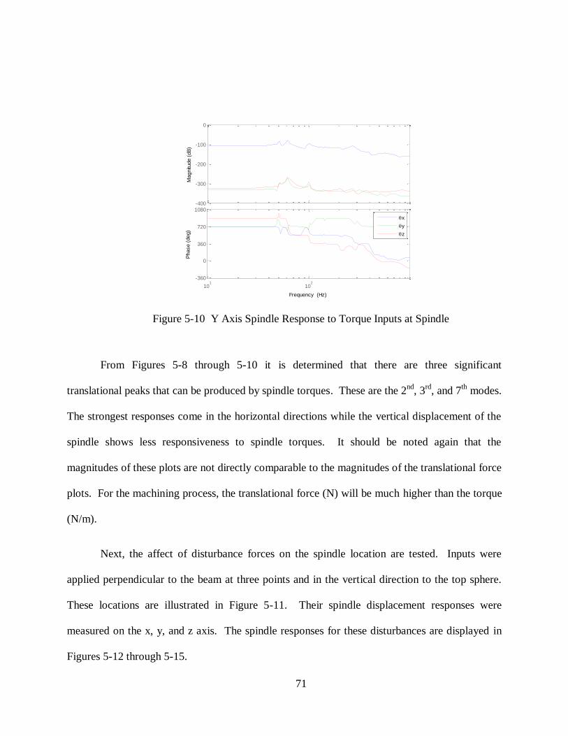
71
Figure 5-10 Y Axis Spindle Response to Torque Inputs at Spindle
From Figures 5-8 through 5-10 it is determined that there are three significant
translational peaks that can be produced by spindle torques. These are the 2nd
, 3rd
, and 7th modes.
The strongest responses come in the horizontal directions while the vertical displacement of the
spindle shows less responsiveness to spindle torques. It should be noted again that the
magnitudes of these plots are not directly comparable to the magnitudes of the translational force
plots. For the machining process, the translational force (N) will be much higher than the torque
(N/m).
Next, the affect of disturbance forces on the spindle location are tested. Inputs were
applied perpendicular to the beam at three points and in the vertical direction to the top sphere.
These locations are illustrated in Figure 5-11. Their spindle displacement responses were
measured on the x, y, and z axis. The spindle responses for these disturbances are displayed in
Figures 5-12 through 5-15.
-400
-300
-200
-100
0
Magnitu
de (
dB
)
101
102
-360
0
360
720
1080
Phase (
deg)
Frequency (Hz)
x
y
z
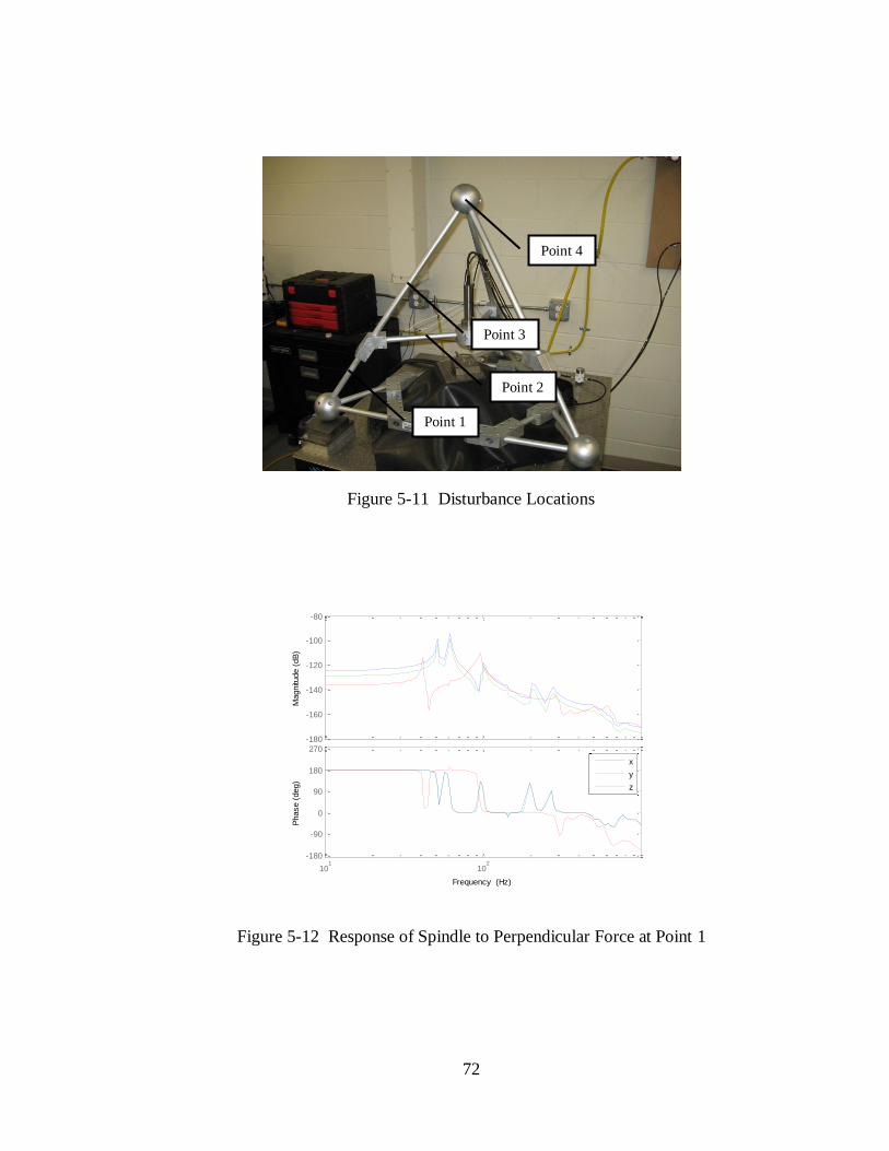
72
Figure 5-11 Disturbance Locations
Figure 5-12 Response of Spindle to Perpendicular Force at Point 1
-180
-160
-140
-120
-100
-80
Magnitu
de (
dB
)
101
102
-180
-90
0
90
180
270
Phase (
deg)
Frequency (Hz)
x
y
z
Point 1
Point 2
Point 3
Point 4
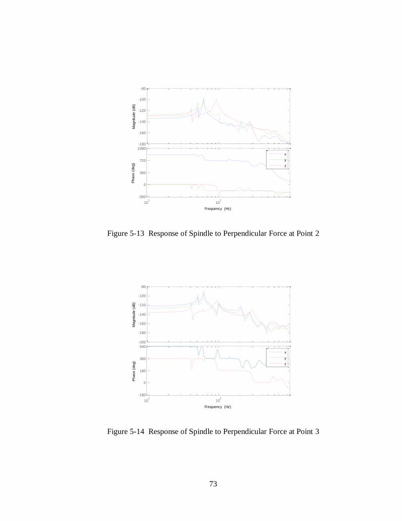
73
Figure 5-13 Response of Spindle to Perpendicular Force at Point 2
Figure 5-14 Response of Spindle to Perpendicular Force at Point 3
-180
-160
-140
-120
-100
-80
Magnitu
de (
dB
)
101
102
-360
0
360
720
1080
Phase (
deg)
Frequency (Hz)
x
y
z
-200
-180
-160
-140
-120
-100
-80
Magnitu
de (
dB
)
101
102
-180
0
180
360
540
Phase (
deg)
Frequency (Hz)
x
y
z
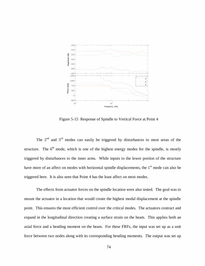
74
Figure 5-15 Response of Spindle to Vertical Force at Point 4
The 2nd
and 3rd
modes can easily be triggered by disturbances to most areas of the
structure. The 6th mode, which is one of the highest energy modes for the spindle, is mostly
triggered by disturbances to the inner arms. While inputs to the lower portion of the structure
have more of an affect on modes with horizontal spindle displacements, the 1st mode can also be
triggered here. It is also seen that Point 4 has the least affect on most modes.
The effects from actuator forces on the spindle location were also tested. The goal was to
mount the actuator in a location that would create the highest modal displacement at the spindle
point. This ensures the most efficient control over the critical modes. The actuators contract and
expand in the longitudinal direction creating a surface strain on the beam. This applies both an
axial force and a bending moment on the beam. For these FRFs, the input was set up as a unit
force between two nodes along with its corresponding bending moments. The output was set up
-400
-350
-300
-250
-200
-150
-100
Magnitu
de (
dB
)
101
102
-360
0
360
720
1080
1440
Phase (
deg)
Frequency (Hz)
x
y
z
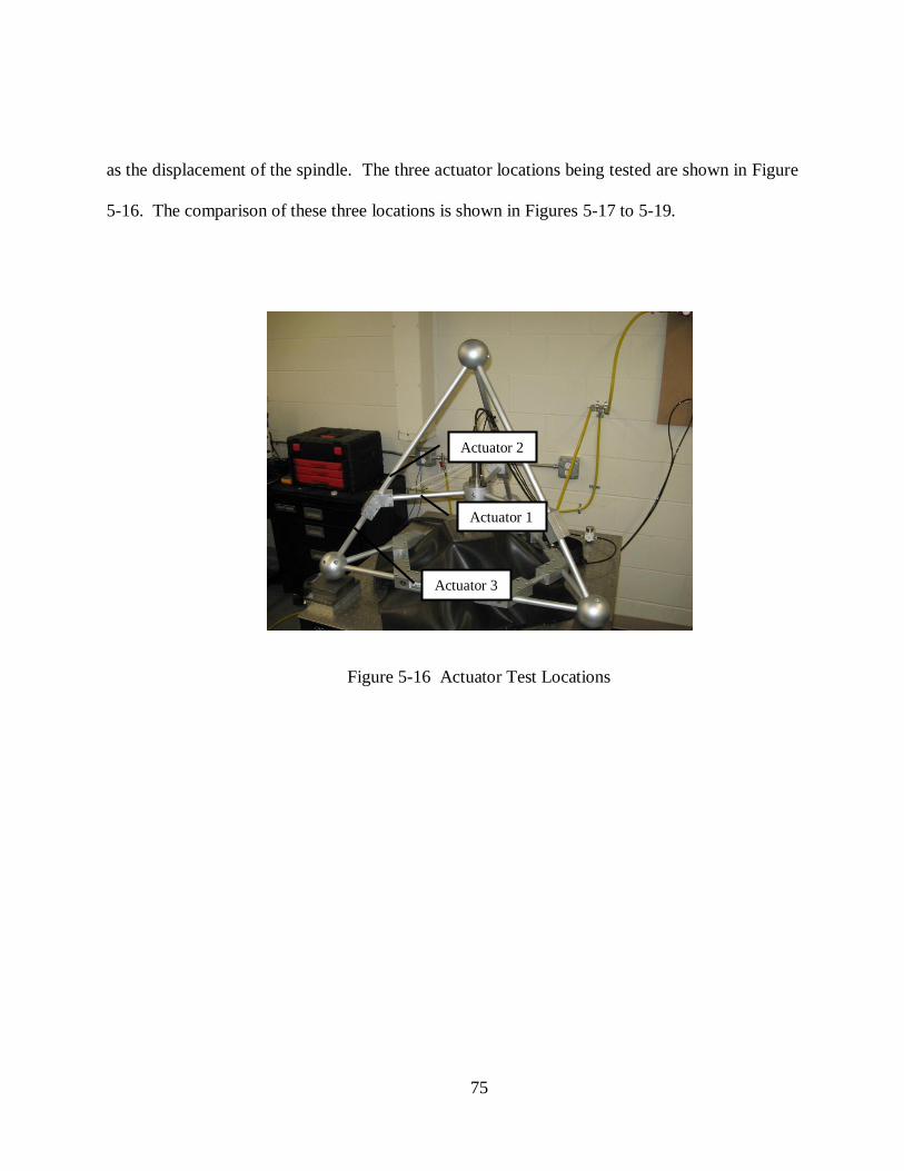
75
as the displacement of the spindle. The three actuator locations being tested are shown in Figure
5-16. The comparison of these three locations is shown in Figures 5-17 to 5-19.
Figure 5-16 Actuator Test Locations
Actuator 1
Actuator 2
Actuator 3
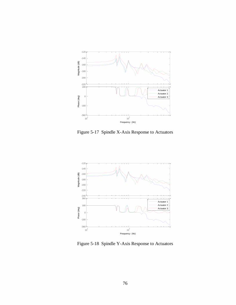
76
Figure 5-17 Spindle X-Axis Response to Actuators
Figure 5-18 Spindle Y-Axis Response to Actuators
-220
-200
-180
-160
-140
-120
Magnitu
de (
dB
)
101
102
-360
-180
0
180
Phase (
deg)
Frequency (Hz)
Actuator 1
Actuator 2
Actuator 3
-240
-220
-200
-180
-160
-140
-120
Magnitu
de (
dB
)
101
102
-360
-180
0
180
360
Phase (
deg)
Frequency (Hz)
Actuator 1
Actuator 2
Actuator 3
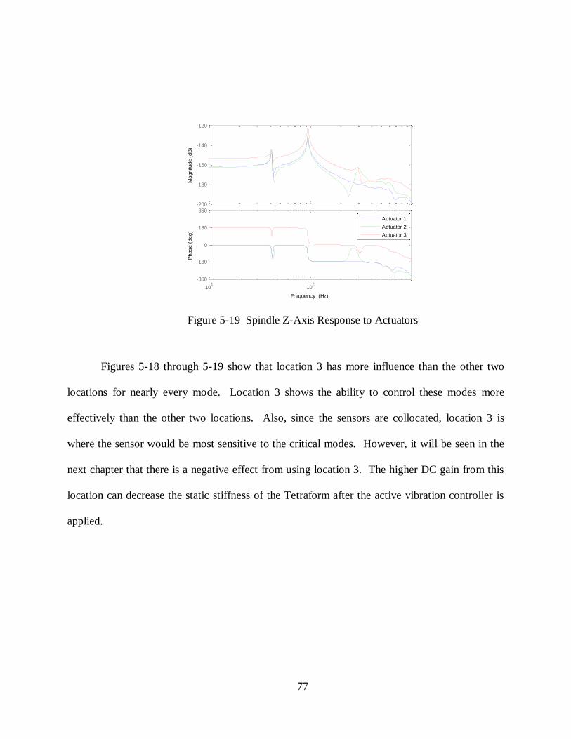
77
Figure 5-19 Spindle Z-Axis Response to Actuators
Figures 5-18 through 5-19 show that location 3 has more influence than the other two
locations for nearly every mode. Location 3 shows the ability to control these modes more
effectively than the other two locations. Also, since the sensors are collocated, location 3 is
where the sensor would be most sensitive to the critical modes. However, it will be seen in the
next chapter that there is a negative effect from using location 3. The higher DC gain from this
location can decrease the static stiffness of the Tetraform after the active vibration controller is
applied.
-200
-180
-160
-140
-120
Magnitu
de (
dB
)
101
102
-360
-180
0
180
360
Phase (
deg)
Frequency (Hz)
Actuator 1
Actuator 2
Actuator 3
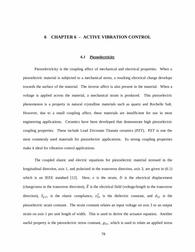
78
6 CHAPTER 6 – ACTIVE VIBRATION CONTROL
6.1 Piezoelectricity
Piezoelectricity is the coupling affect of mechanical and electrical properties. When a
piezoelectric material is subjected to a mechanical stress, a resulting electrical charge develops
towards the surface of the material. The inverse affect is also present in the material. When a
voltage is applied across the material, a mechanical strain is produced. This piezoelectric
phenomenon is a property in natural crystalline materials such as quartz and Rochelle Salt.
However, due to a small coupling affect, these materials are insufficient for use in most
engineering applications. Ceramics have been developed that demonstrate high piezoelectric
coupling properties. These include Lead Zirconate Titanate ceramics (PZT). PZT is one the
most commonly used materials for piezoelectric applications. Its strong coupling properties
make it ideal for vibration control applications.
The coupled elastic and electric equations for piezoelectric material stressed in the
longitudinal direction, axis 1, and polarized in the transverse direction, axis 3, are given in (6.1)
which is an IEEE standard [12]. Here, 𝜖 is the strain, 𝐷 is the electrical displacement
(charge/area in the transverse direction), 𝐸 is the electrical field (voltage/length in the transverse
direction), 𝑆𝑝11 is the elastic compliance, 휀33𝑇 is the dielectric constant, and 𝑑31 is the
piezoelectric strain constant. The strain constant relates an input voltage on axis 3 to an output
strain on axis 1 per unit length of width. This is used to derive the actuator equation. Another
useful property is the piezoelectric stress constant, 𝑔31 , which is used to relate an applied stress
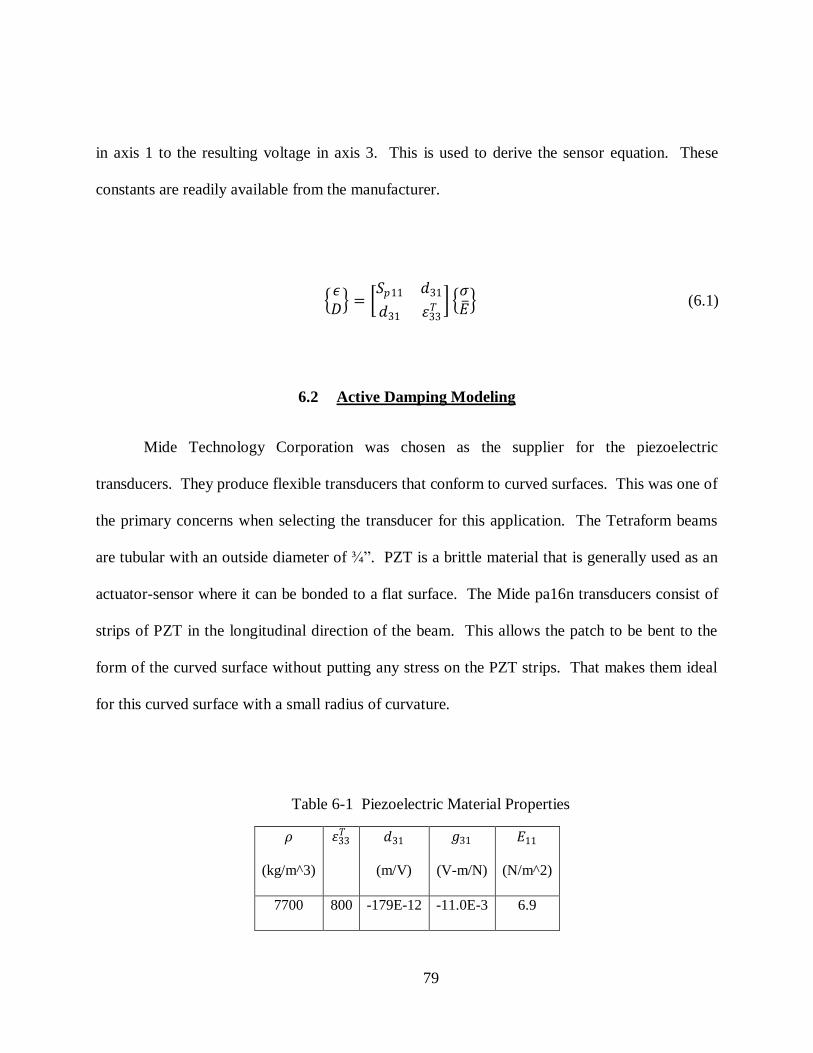
79
in axis 1 to the resulting voltage in axis 3. This is used to derive the sensor equation. These
constants are readily available from the manufacturer.
𝜖𝐷 =
𝑆𝑝11 𝑑31
𝑑31 휀33𝑇
𝜎𝐸 (6.1)
6.2 Active Damping Modeling
Mide Technology Corporation was chosen as the supplier for the piezoelectric
transducers. They produce flexible transducers that conform to curved surfaces. This was one of
the primary concerns when selecting the transducer for this application. The Tetraform beams
are tubular with an outside diameter of ¾”. PZT is a brittle material that is generally used as an
actuator-sensor where it can be bonded to a flat surface. The Mide pa16n transducers consist of
strips of PZT in the longitudinal direction of the beam. This allows the patch to be bent to the
form of the curved surface without putting any stress on the PZT strips. That makes them ideal
for this curved surface with a small radius of curvature.
Table 6-1 Piezoelectric Material Properties
𝜌
(kg/m^3)
휀33𝑇
𝑑31
(m/V)
𝑔31
(V-m/N)
𝐸11
(N/m^2)
7700 800 -179E-12 -11.0E-3 6.9
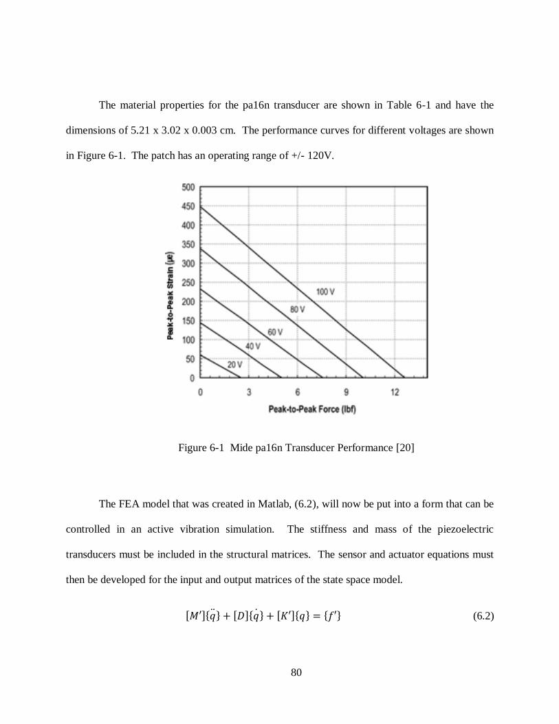
80
The material properties for the pa16n transducer are shown in Table 6-1 and have the
dimensions of 5.21 x 3.02 x 0.003 cm. The performance curves for different voltages are shown
in Figure 6-1. The patch has an operating range of +/- 120V.
Figure 6-1 Mide pa16n Transducer Performance [20]
The FEA model that was created in Matlab, (6.2), will now be put into a form that can be
controlled in an active vibration simulation. The stiffness and mass of the piezoelectric
transducers must be included in the structural matrices. The sensor and actuator equations must
then be developed for the input and output matrices of the state space model.
𝑀′ 𝑞 + 𝐷 𝑞 + 𝐾′ 𝑞 = 𝑓′ (6.2)
81
The sensors and actuators patches were modeled as beams to include in the structural
mass and stiffness matrices. These were modeled in a similar manner as the frame beams but
with the moments of inertia calculated about the tubular beam’s axes. The smart structure finite
element model was converted to state space, therefore the actuator and sensor equations needed
to be developed in input and output vector format [6, 7]. Using (6.1), the actuator force vector
𝑓𝑎 is shown in (6.3) and (6.4) where 𝑢(𝑡) is the input voltage, 𝐸𝑝 is the piezoelectric Young’s
Modulus, 𝑟 is the radius of the axial force created by the patch, and 𝑏 is the width of the contact
area between the patch and beam. Equation (6.4) shows that this vector represents the actuator
axial force, 𝐹𝑎𝑥 , and the actuator bending moment, 𝑀𝑎𝑦 . These forces are applied at the end
nodes of the piezoelectric elements. The sensor voltage vector, 𝜙, is given in (6.5) where 𝑡 is the
patch thickness. The stress in the sensor equation is created from both bending and axial forces
and is evaluated at the end nodes of the piezoelectric elements.
𝑓𝑎 = 𝑢(𝑡)𝐸𝑝𝑑31𝑏 −1 𝑟 1 −𝑟 𝑇 (6.3)
𝑓𝑎 = −𝐹𝑎𝑥 𝑀𝑎𝑦 𝐹𝑎𝑥 −𝑀𝑎𝑦 𝑇 (6.4)
𝜙 = −𝑡
𝐿𝑒𝑔31𝐸𝑝 [𝑟휃𝑦−𝑢]𝑛𝑜𝑑𝑒𝑗
𝑛𝑜𝑑𝑒 𝑖 (6.5)
The input matrix, 𝐵 , is given in (6.6) where 𝑓𝑎 is the matrix made up of the actuator
input vectors. The output matrix, 𝐶 , is given in (6.7) where 𝜙 is a matrix made up of the
sensor output vectors.
82
𝐵 = 0
− 𝑀 −1 Φ 𝑇 𝑓𝑎 (6.6)
𝐶 = 𝜙 0 (6.7)
6.3 Controller
A positive position feedback controller will be used in targeting the critical modes. One
common task in vibration control is overcoming spillover, which is the affect of out of
bandwidth modes on the controller. This can destabilize the controller [9]. The PPF controller
was chosen for its ability to minimize the effect of the out of bandwidth modes [8]. The
dynamics of the controller resemble that of a mass-spring-damper system being applied to the
structure, which the response naturally rolls off after a certain frequency, making it invulnerable
to higher frequencies. Shown in Figure 6-2 is the bode plot of a PPF filter.
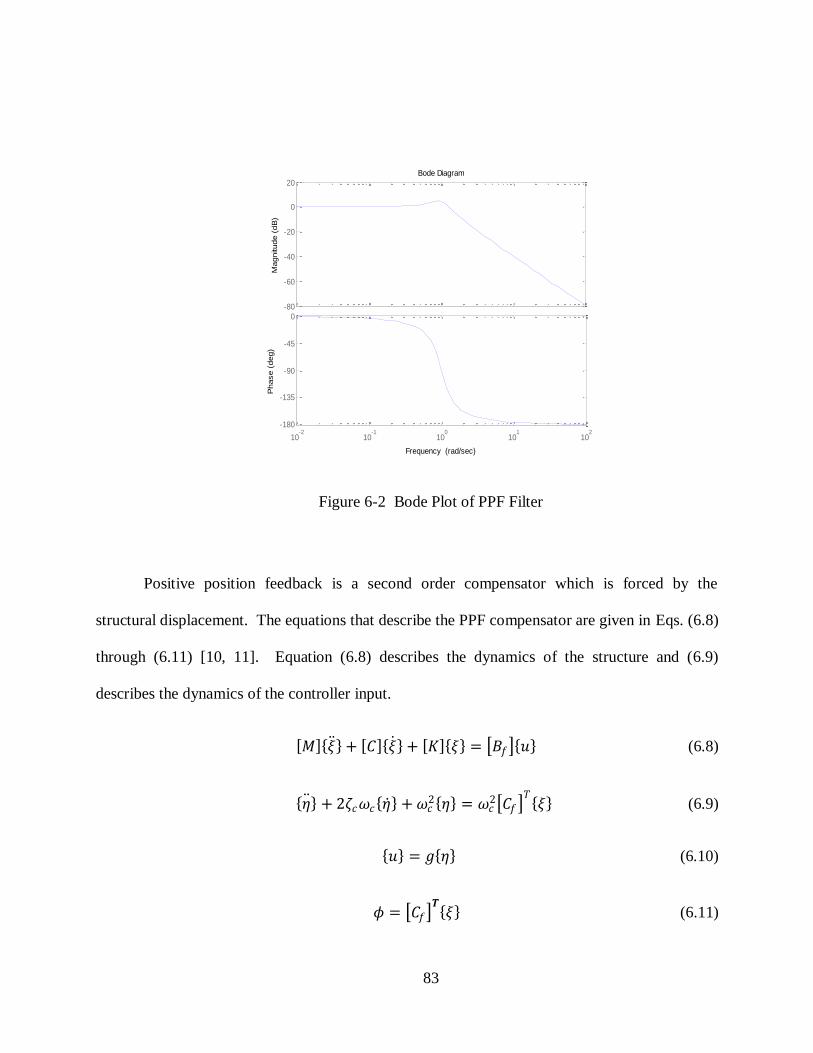
83
Figure 6-2 Bode Plot of PPF Filter
Positive position feedback is a second order compensator which is forced by the
structural displacement. The equations that describe the PPF compensator are given in Eqs. (6.8)
through (6.11) [10, 11]. Equation (6.8) describes the dynamics of the structure and (6.9)
describes the dynamics of the controller input.
𝑀 𝜉 + 𝐶 𝜉 + 𝐾 𝜉 = 𝐵𝑓 𝑢 (6.8)
휂 + 2휁𝑐𝜔𝑐 휂 + 𝜔𝑐2 휂 = 𝜔𝑐
2 𝐶𝑓 𝑇 𝜉 (6.9)
𝑢 = 𝑔 휂 (6.10)
𝜙 = 𝐶𝑓 𝑻 𝜉 (6.11)
-80
-60
-40
-20
0
20
Magnitude (
dB
)
10-2
10-1
100
101
102
-180
-135
-90
-45
0
Phase (
deg)
Bode Diagram
Frequency (rad/sec)
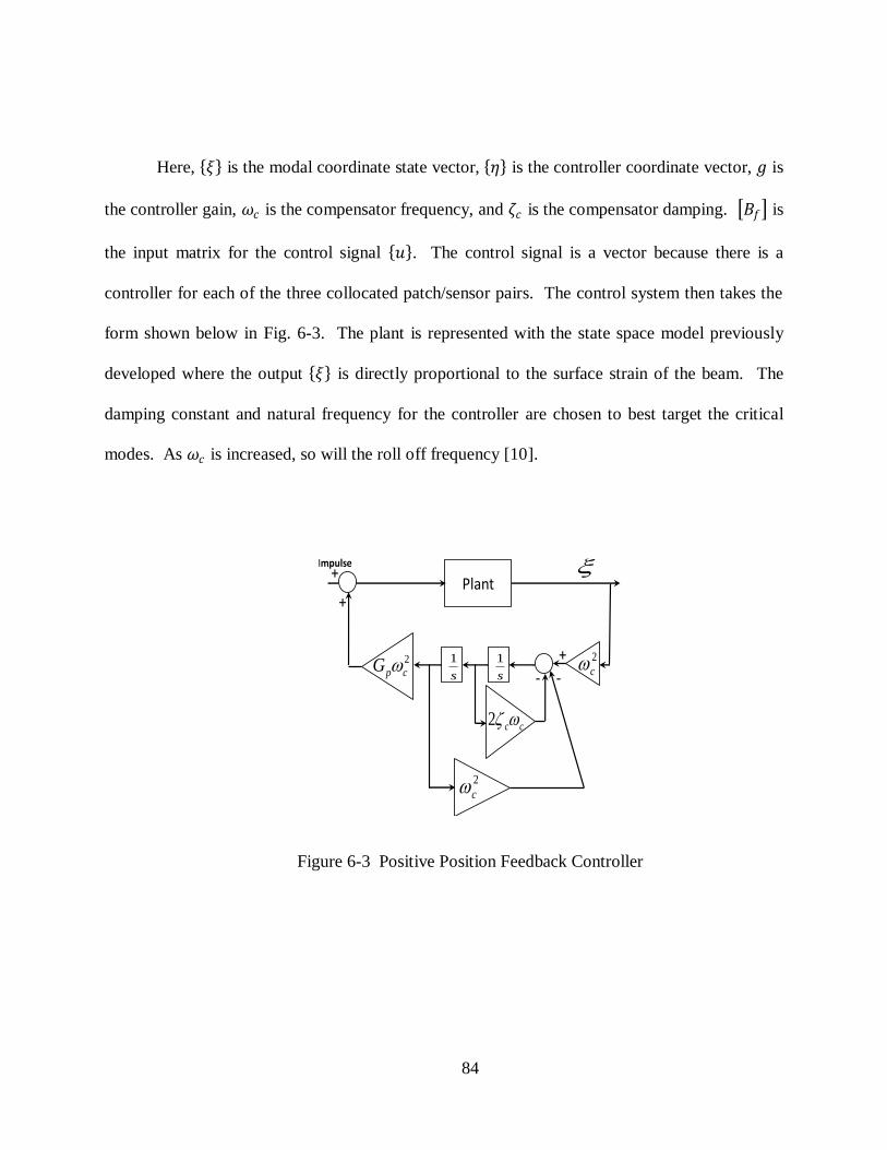
84
Here, 𝜉 is the modal coordinate state vector, 휂 is the controller coordinate vector, 𝑔 is
the controller gain, 𝜔𝑐 is the compensator frequency, and 휁𝑐 is the compensator damping. 𝐵𝑓 is
the input matrix for the control signal 𝑢 . The control signal is a vector because there is a
controller for each of the three collocated patch/sensor pairs. The control system then takes the
form shown below in Fig. 6-3. The plant is represented with the state space model previously
developed where the output 𝜉 is directly proportional to the surface strain of the beam. The
damping constant and natural frequency for the controller are chosen to best target the critical
modes. As 𝜔𝑐 is increased, so will the roll off frequency [10].
Plant+
-
Impulse
s
1
s
12
cpG
cc2
2
c
2
c-
+
+
Figure 6-3 Positive Position Feedback Controller
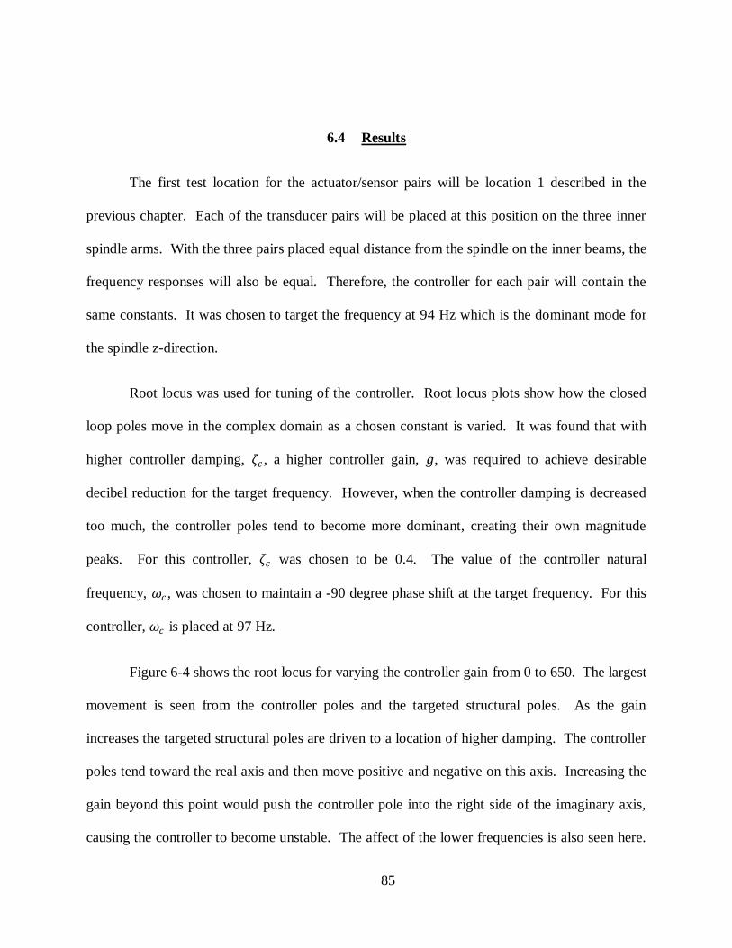
85
6.4 Results
The first test location for the actuator/sensor pairs will be location 1 described in the
previous chapter. Each of the transducer pairs will be placed at this position on the three inner
spindle arms. With the three pairs placed equal distance from the spindle on the inner beams, the
frequency responses will also be equal. Therefore, the controller for each pair will contain the
same constants. It was chosen to target the frequency at 94 Hz which is the dominant mode for
the spindle z-direction.
Root locus was used for tuning of the controller. Root locus plots show how the closed
loop poles move in the complex domain as a chosen constant is varied. It was found that with
higher controller damping, 휁𝑐 , a higher controller gain, 𝑔, was required to achieve desirable
decibel reduction for the target frequency. However, when the controller damping is decreased
too much, the controller poles tend to become more dominant, creating their own magnitude
peaks. For this controller, 휁𝑐 was chosen to be 0.4. The value of the controller natural
frequency, 𝜔𝑐 , was chosen to maintain a -90 degree phase shift at the target frequency. For this
controller, 𝜔𝑐 is placed at 97 Hz.
Figure 6-4 shows the root locus for varying the controller gain from 0 to 650. The largest
movement is seen from the controller poles and the targeted structural poles. As the gain
increases the targeted structural poles are driven to a location of higher damping. The controller
poles tend toward the real axis and then move positive and negative on this axis. Increasing the
gain beyond this point would push the controller pole into the right side of the imaginary axis,
causing the controller to become unstable. The affect of the lower frequencies is also seen here.
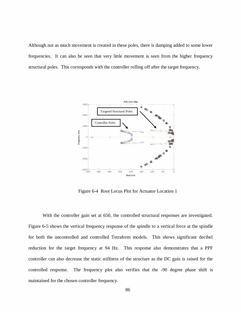
86
Although not as much movement is created in these poles, there is damping added to some lower
frequencies. It can also be seen that very little movement is seen from the higher frequency
structural poles. This corresponds with the controller rolling off after the target frequency.
Figure 6-4 Root Locus Plot for Actuator Location 1
With the controller gain set at 650, the controlled structural responses are investigated.
Figure 6-5 shows the vertical frequency response of the spindle to a vertical force at the spindle
for both the uncontrolled and controlled Tetraform models. This shows significant decibel
reduction for the target frequency at 94 Hz. This response also demonstrates that a PPF
controller can also decrease the static stiffness of the structure as the DC gain is raised for the
controlled response. The frequency plot also verifies that the -90 degree phase shift is
maintained for the chosen controller frequency.
Pole-Zero Map
Real Axis
Imagin
ary
Axis
-400 -350 -300 -250 -200 -150 -100 -50 0-3000
-2000
-1000
0
1000
2000
3000
Controller Poles
Targeted Structural Poles
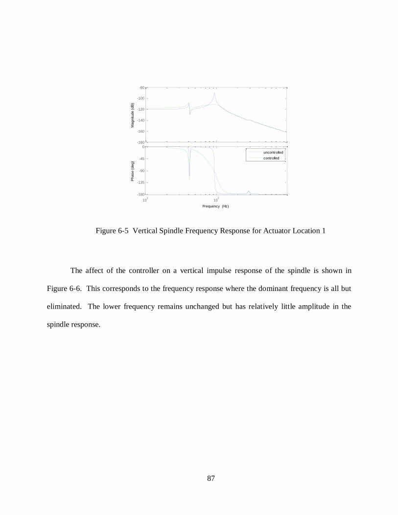
87
Figure 6-5 Vertical Spindle Frequency Response for Actuator Location 1
The affect of the controller on a vertical impulse response of the spindle is shown in
Figure 6-6. This corresponds to the frequency response where the dominant frequency is all but
eliminated. The lower frequency remains unchanged but has relatively little amplitude in the
spindle response.
-180
-160
-140
-120
-100
-80
Magnitu
de (
dB
)
101
102
-180
-135
-90
-45
0
Phase (
deg)
Frequency (Hz)
uncontrolled
controlled
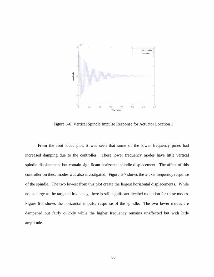
88
Figure 6-6 Vertical Spindle Impulse Response for Actuator Location 1
From the root locus plot, it was seen that some of the lower frequency poles had
increased damping due to the controller. These lower frequency modes have little vertical
spindle displacement but contain significant horizontal spindle displacement. The affect of this
controller on these modes was also investigated. Figure 6-7 shows the x-axis frequency response
of the spindle. The two lowest from this plot create the largest horizontal displacements. While
not as large as the targeted frequency, there is still significant decibel reduction for these modes.
Figure 6-8 shows the horizontal impulse response of the spindle. The two lower modes are
dampened out fairly quickly while the higher frequency remains unaffected but with little
amplitude.
0 0.1 0.2 0.3 0.4 0.5 0.6 0.7-6
-4
-2
0
2
4
6x 10
-4
Time (sec)
Am
plit
ude
Uncontrolled
Controlled
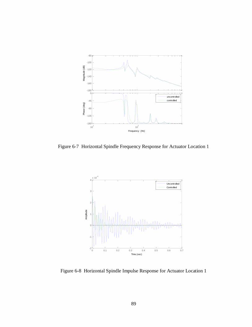
89
Figure 6-7 Horizontal Spindle Frequency Response for Actuator Location 1
Figure 6-8 Horizontal Spindle Impulse Response for Actuator Location 1
-180
-160
-140
-120
-100
-80
Magnitu
de (
dB
)
101
102
-180
-135
-90
-45
0
Phase (
deg)
Frequency (Hz)
uncontrolled
controlled
0 0.1 0.2 0.3 0.4 0.5 0.6 0.7-2
-1
0
1
2
3
4x 10
-4
Time (sec)
Am
plit
ude
Uncontrolled
Controlled
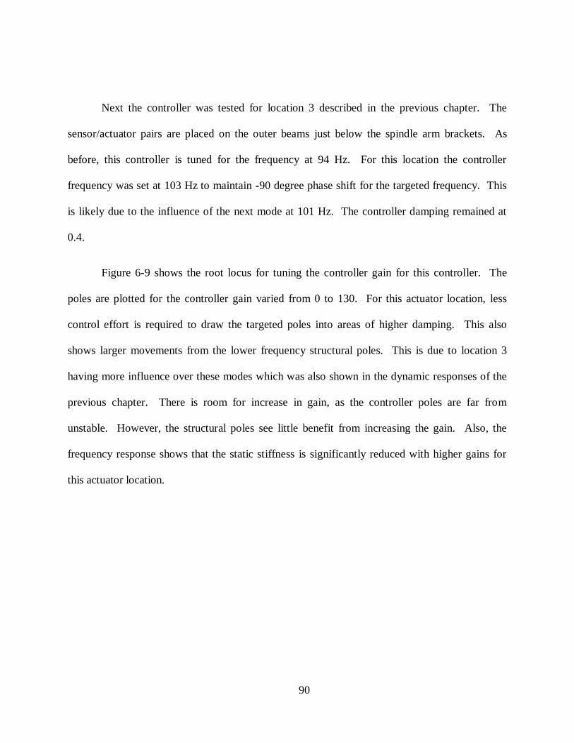
90
Next the controller was tested for location 3 described in the previous chapter. The
sensor/actuator pairs are placed on the outer beams just below the spindle arm brackets. As
before, this controller is tuned for the frequency at 94 Hz. For this location the controller
frequency was set at 103 Hz to maintain -90 degree phase shift for the targeted frequency. This
is likely due to the influence of the next mode at 101 Hz. The controller damping remained at
0.4.
Figure 6-9 shows the root locus for tuning the controller gain for this controller. The
poles are plotted for the controller gain varied from 0 to 130. For this actuator location, less
control effort is required to draw the targeted poles into areas of higher damping. This also
shows larger movements from the lower frequency structural poles. This is due to location 3
having more influence over these modes which was also shown in the dynamic responses of the
previous chapter. There is room for increase in gain, as the controller poles are far from
unstable. However, the structural poles see little benefit from increasing the gain. Also, the
frequency response shows that the static stiffness is significantly reduced with higher gains for
this actuator location.
91
Figure 6-9 Root Locus Plot for Actuator Location 3
The vertical spindle frequency response is displayed in Figure 6-10. Similar decibel
reduction is created for this controller as from the controller form location 1. This is, however,
realized with a much lower gain than the controller from location 1. Care must be taken when
tuning this controller as the static stiffness is easily decreased.
Pole-Zero Map
Real Axis
Imagin
ary
Axis
-300 -250 -200 -150 -100 -50 0-3000
-2000
-1000
0
1000
2000
3000
Targeted Structural Poles
Controller Poles
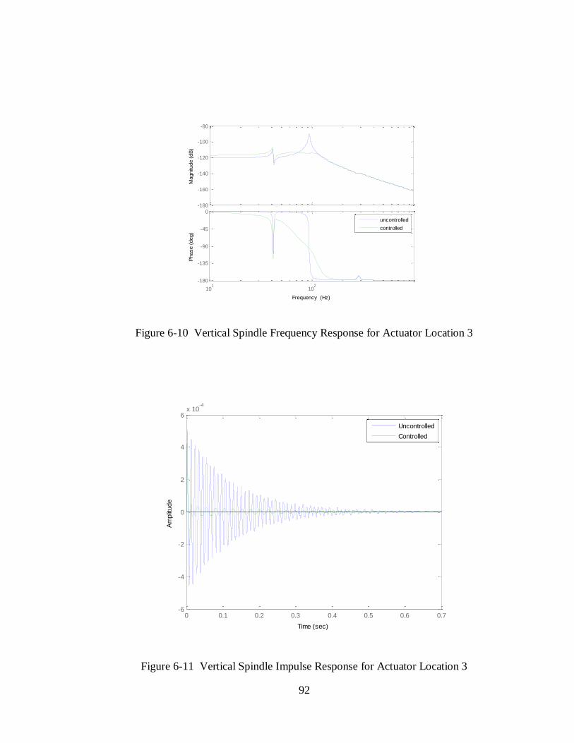
92
Figure 6-10 Vertical Spindle Frequency Response for Actuator Location 3
Figure 6-11 Vertical Spindle Impulse Response for Actuator Location 3
-180
-160
-140
-120
-100
-80
Magnitu
de (
dB
)
101
102
-180
-135
-90
-45
0
Phase (
deg)
Frequency (Hz)
uncontrolled
controlled
0 0.1 0.2 0.3 0.4 0.5 0.6 0.7-6
-4
-2
0
2
4
6x 10
-4
Time (sec)
Am
plit
ude
Uncontrolled
Controlled
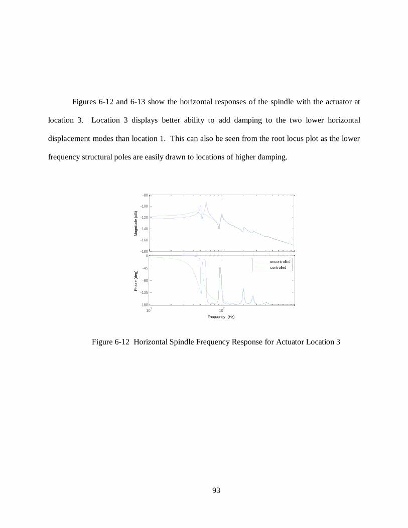
93
Figures 6-12 and 6-13 show the horizontal responses of the spindle with the actuator at
location 3. Location 3 displays better ability to add damping to the two lower horizontal
displacement modes than location 1. This can also be seen from the root locus plot as the lower
frequency structural poles are easily drawn to locations of higher damping.
Figure 6-12 Horizontal Spindle Frequency Response for Actuator Location 3
-180
-160
-140
-120
-100
-80
Magnitu
de (
dB
)
101
102
-180
-135
-90
-45
0
Phase (
deg)
Frequency (Hz)
uncontrolled
controlled
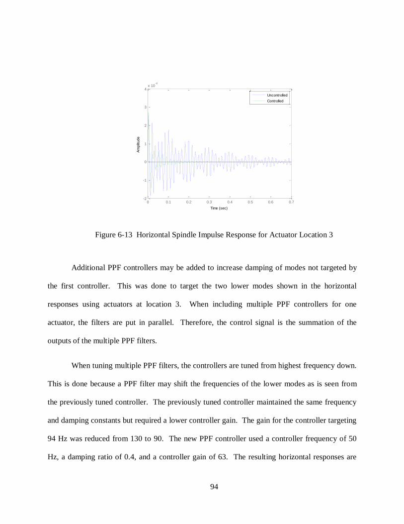
94
Figure 6-13 Horizontal Spindle Impulse Response for Actuator Location 3
Additional PPF controllers may be added to increase damping of modes not targeted by
the first controller. This was done to target the two lower modes shown in the horizontal
responses using actuators at location 3. When including multiple PPF controllers for one
actuator, the filters are put in parallel. Therefore, the control signal is the summation of the
outputs of the multiple PPF filters.
When tuning multiple PPF filters, the controllers are tuned from highest frequency down.
This is done because a PPF filter may shift the frequencies of the lower modes as is seen from
the previously tuned controller. The previously tuned controller maintained the same frequency
and damping constants but required a lower controller gain. The gain for the controller targeting
94 Hz was reduced from 130 to 90. The new PPF controller used a controller frequency of 50
Hz, a damping ratio of 0.4, and a controller gain of 63. The resulting horizontal responses are
0 0.1 0.2 0.3 0.4 0.5 0.6 0.7-2
-1
0
1
2
3
4x 10
-4
Time (sec)
Am
plit
ude
Uncontrolled
Controlled
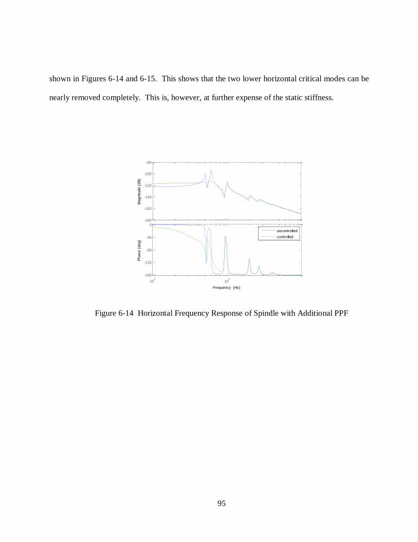
95
shown in Figures 6-14 and 6-15. This shows that the two lower horizontal critical modes can be
nearly removed completely. This is, however, at further expense of the static stiffness.
Figure 6-14 Horizontal Frequency Response of Spindle with Additional PPF
-180
-160
-140
-120
-100
-80
Magnitu
de (
dB
)
101
102
-180
-135
-90
-45
0
Phase (
deg)
Frequency (Hz)
uncontrolled
controlled

96
Figure 6-15 Horizontal Impulse Response of Spindle with Additional PPF
0 0.1 0.2 0.3 0.4 0.5 0.6 0.7-2
-1
0
1
2
3
4x 10
-4
Time (sec)
Am
plit
ude
Uncontrolled
Controlled
97
7 CHAPTER 7 - CONCLUSION AND RECOMENDATIONS
Finite Element Models of the Tetraform were created in both ANSYS and Matlab. The
ANSYS model was used to conduct the modal analysis on the Tetraform. The resulting mode
shapes were used to help determine which modes create displacements at the spindle location.
They are also used to study which areas of the Tetraform contain the most vibrational energy for
these modes. Both of FEA models can be used to study structural changes made to the
Tetraform. The mode shapes from ANSYS are helpful in showing the changes in the displaced
structure.
The Matlab model was converted to state space in order to plot frequency responses
between different points on the structure. This shows the modal displacements relative to each
other. These are insightful to how easily the modes are triggered by machining forces and
external disturbances. This was also used to test the controllability of different actuator locations
on the modes of interest. Finally, this state space model was used for active vibration control
simulations
Positive Position Feedback Controllers were chosen as the active vibration control
method and were designed to target the critical modes. The controllers were designed for
actuators placed at locations 1 and 3. Both could significantly reduce the decibels of the target
mode with the dominant vertical displacement of the spindle. Location 3 realized this decibel
reduction with a much lower control effort. However, this location was much more prone to
reducing the static stiffness of the Tetraform. Care must be taken when tuning PPF controller for
98
the Tetraform as reducing the static stiffness can be detrimental to the machining process. It was
found that location 3 was more effective at targeting the lower frequency modes which create
horizontal displacements to the spindle. Additional PPF controllers can be added to remove
these lower modes, but once again, at the expense of static stiffness. This was a very effective
way of adding damping to most critical modes. Therefore, this is very beneficial to the micro-
machining process.
Some structural changes may also benefit the full scale Tetraform. One such change can
stiffen the mode that contains significant vertical displacement of the spindle. The spindle
holder and arms may be raised to a higher to a higher location on the Tetraform. This will
shorten the spindle holder arms, stiffening this area of the mode shape. This will also transfer
more energy to the lower portion of the Tetraform. The bottom brackets may also be removed to
create more room for the linear position stages. This increases the transfer of more of the energy
from some modes to the lower region. This also reduces the moving mass in this area for some
modes, raising the frequency for these modes. It should be noted that these changes create a
stronger resemblance between the full scale and 2/3 scale Tetraforms.
It is recommended that some adjustments be made to the tuning method of the PPF
controllers. First, it should be converted over to optimal control. The controller should be tuned
optimally based on target mode decibel reduction, maximizing static stiffness, and minimizing
control effort. Also, the controller should be made adaptable. The structural poles change
significantly with different structural modifications and different spindles. A method of online
determination of the structural poles would be strongly recommended. It is also recommended to

99
include disturbance rejection control to supplement the vibration control to further stabilize the
machining process.

100
APPENDIX A: MATLAB CODE
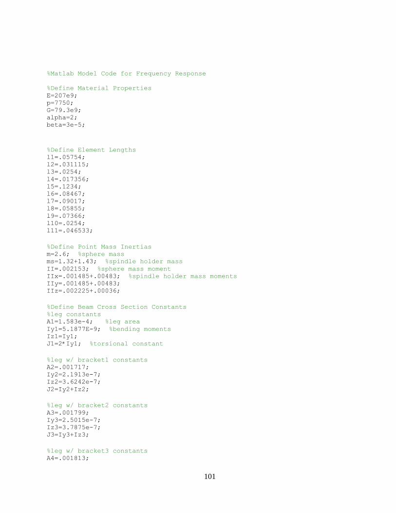
101
%Matlab Model Code for Frequency Response
%Define Material Properties E=207e9; p=7750; G=79.3e9; alpha=2; beta=3e-5;
%Define Element Lengths l1=.05754; l2=.031115; l3=.0254; l4=.017356; l5=.1234; l6=.08467; l7=.09017; l8=.05855; l9=.07366; l10=.0254; l11=.046533;
%Define Point Mass Inertias m=2.6; %sphere mass ms=1.32+1.43; %spindle holder mass II=.002153; %sphere mass moment IIx=.001485+.00483; %spindle holder mass moments IIy=.001485+.00483; IIz=.002225+.00036;
%Define Beam Cross Section Constants %leg constants A1=1.583e-4; %leg area Iy1=5.1877E-9; %bending moments Iz1=Iy1; J1=2*Iy1; %torsional constant
%leg w/ bracket1 constants A2=.001717; Iy2=2.1913e-7; Iz2=3.6242e-7; J2=Iy2+Iz2;
%leg w/ bracket2 constants A3=.001799; Iy3=2.5015e-7; Iz3=3.7875e-7; J3=Iy3+Iz3;
%leg w/ bracket3 constants A4=.001813;
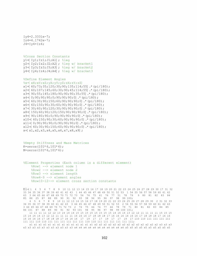
102
Iy4=2.3331e-7; Iz4=4.1742e-7; J4=Iy4+Iz4;
%Cross Section Constants y1=[Iy1;Iz1;J1;A1]; %leg y2=[Iy2;Iz2;J2;A2]; %leg w/ bracket1 y3=[Iy3;Iz3;J3;A3]; %leg w/ bracket2 y4=[Iy4;Iz4;J4;A4]; %leg w/ bracket3
%Define Element Angles %x=[xX;xY;xZ;yX;yY;yZ;zX;zY;zZ] x1=[60;73;35;120;30;90;135;114;55].*(pi/180); x2=[60;107;145;60;30;90;45;114;55].*(pi/180); x3=[90;55;145;180;90;90;90;35;55].*(pi/180); x4=[0;90;90;90;0;90;90;90;0].*(pi/180); x5=[60;30;90;150;60;90;90;90;0].*(pi/180); x6=[60;150;90;30;60;90;90;90;0].*(pi/180); x7=[30;60;90;120;30;90;90;90;0].*(pi/180); x8=[150;60;90;120;150;90;90;90;0].*(pi/180); x9=[90;180;90;0;90;90;90;90;0].*(pi/180); x10=[60;150;90;30;60;90;90;90;0].*(pi/180); x11=[0;90;90;90;0;90;90;90;0].*(pi/180); x12=[60;30;90;150;60;90;90;90;0].*(pi/180); x=[x1,x2,x3,x4,x5,x6,x7,x8,x9];
%Empty Stiffness and Mass Matrices K=zeros(101*6,101*6); M=zeros(101*6,101*6);
%Element Properties (Each column is a different element) %Row1 --> element node 1 %Row2 --> element node 2 %Row3 --> element length %Row4-9 --> element angles %Row10-12--> element cross section constants
El=[1 4 5 6 7 8 9 10 11 12 13 14 15 16 17 18 19 20 21 22 23 24 25 26 27 28 29 30 17 31 32 33 34 35 36 37 38 39 40 41 42 43 1 44 45 46 47 48 49 50 51 52 53 1 54 55 56 57 58 59 60 61 62
63 3 64 65 66 67 68 69 70 71 72 73 56 74 75 61 76 77 51 78 79 9 80 81 82 83 84
85 86 25 87 88 89 90 91 92 93 38 94 95 96 97 98 99 100;
4 5 6 7 8 9 10 11 12 13 14 15 16 17 18 19 20 21 22 23 24 25 26 27 28 29 30 2 31 32 33
34 35 36 37 38 39 40 41 42 43 3 44 45 46 47 48 49 50 51 52 53 2 54 55 56 57 58 59 60 61 62 63
3 64 65 66 67 68 69 70 71 72 73 2 74 75 46 76 77 66 78 79 71 80 81 82 83 84 85
86 101 87 88 89 90 91 92 93 101 94 95 96 97 98 99 100 101;
l1 l1 l1 l1 l2 l2 l3 l4 l4 l4 l5 l5 l5 l5 l5 l5 l5 l5 l4 l4 l4 l3 l2 l2 l1 l1 l1 l1 l5 l5 l5
l5 l4 l4 l4 l3 l2 l2 l1 l1 l1 l1 l6 l6 l6 l7 l8 l8 l8 l7 l6 l6 l6 l6 l6 l6 l7 l8 l8 l8 l7 l6 l6
l6 l6 l6 l6 l7 l8 l8 l8 l7 l6 l6 l6 l7 l9 l7 l7 l9 l7 l7 l9 l7 l10 l10 l11 l11 l11 l11
l11 l11 l10 l10 l11 l11 l11 l11 l11 l11 l10 l10 l11 l11 l11 l11 l11 l11;
x1 x1 x1 x1 x1 x1 x1 x1 x1 x1 x1 x1 x1 x1 x2 x2 x2 x2 x2 x2 x2 x2 x2 x2 x2 x2 x2 x2 x3 x3 x3
x3 x3 x3 x3 x3 x3 x3 x3 x3 x3 x3 x4 x4 x4 x4 x4 x4 x4 x4 x4 x4 x4 x5 x5 x5 x5 x5 x5 x5 x5 x5 x5
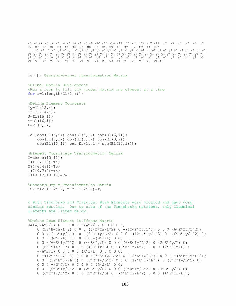
103
x5 x6 x6 x6 x6 x6 x6 x6 x6 x6 x6 x6 x10 x10 x10 x11 x11 x11 x12 x12 x12 x7 x7 x7 x7 x7 x7
x7 x7 x8 x8 x8 x8 x8 x8 x8 x8 x9 x9 x9 x9 x9 x9 x9 x9;
y1 y1 y1 y1 y2 y2 y1 y1 y1 y1 y1 y1 y1 y1 y1 y1 y1 y1 y1 y1 y1 y1 y2 y2 y1 y1 y1 y1 y1 y1 y1
y1 y1 y1 y1 y1 y2 y2 y1 y1 y1 y1 y1 y1 y1 y4 y1 y1 y1 y4 y1 y1 y1 y1 y1 y1 y4 y1 y1 y1 y4 y1 y1
y1 y1 y1 y1 y4 y1 y1 y1 y4 y1 y1 y1 y4 y1 y4 y4 y1 y4 y4 y1 y4 y3 y3 y1 y1 y1 y1
y1 y1 y3 y3 y1 y1 y1 y1 y1 y1 y3 y3 y1 y1 y1 y1 y1 y1];
Ts=[]; %Sensor/Output Transformation Matrix
%Global Matrix Development %Run a loop to fill the global matrix one element at a time for i=1:length(El(1,:));
%Define Element Constants Iy=El(13,i); Iz=El(14,i); J=El(15,i); A=El(16,i); L=El(3,i);
Te=[cos(El(4,i)) cos(El(5,i)) cos(El(6,i)); cos(El(7,i)) cos(El(8,i)) cos(El(9,i)); cos(El(10,i)) cos(El(11,i)) cos(El(12,i))];
%Element Coordinate Transformation Matrix T=zeros(12,12); T(1:3,1:3)=Te; T(4:6,4:6)=Te; T(7:9,7:9)=Te; T(10:12,10:12)=Te;
%Sensor/Output Transformation Matrix TS(i*12-11:i*12,i*12-11:i*12)=T;
% Both Timshenko and Classical Beam Elements were created and gave very
similar results. Due to size of the Timoshenko matrices, only Classical
Elements are listed below.
%Define Beam Element Stiffness Matrix Kel=[(A*E/L) 0 0 0 0 0 -(A*E/L) 0 0 0 0 0; 0 (12*E*Iz/L^3) 0 0 0 (6*E*Iz/L^2) 0 -(12*E*Iz/L^3) 0 0 0 (6*E*Iz/L^2); 0 0 (12*E*Iy/L^3) 0 -(6*E*Iy/L^2) 0 0 0 -(12*E*Iy/L^3) 0 -(6*E*Iy/L^2) 0; 0 0 0 (G*J/L) 0 0 0 0 0 -(G*J/L) 0 0; 0 0 -(6*E*Iy/L^2) 0 (4*E*Iy/L) 0 0 0 (6*E*Iy/L^2) 0 (2*E*Iy/L) 0; 0 (6*E*Iz/L^2) 0 0 0 (4*E*Iz/L) 0 -(6*E*Iz/L^2) 0 0 0 (2*E*Iz/L) ; -(A*E/L) 0 0 0 0 0 (A*E/L) 0 0 0 0 0; 0 -(12*E*Iz/L^3) 0 0 0 -(6*E*Iz/L^2) 0 (12*E*Iz/L^3) 0 0 0 -(6*E*Iz/L^2); 0 0 -(12*E*Iy/L^3) 0 (6*E*Iy/L^2) 0 0 0 (12*E*Iy/L^3) 0 (6*E*Iy/L^2) 0; 0 0 0 -(G*J/L) 0 0 0 0 0 (G*J/L) 0 0; 0 0 -(6*E*Iy/L^2) 0 (2*E*Iy/L) 0 0 0 (6*E*Iy/L^2) 0 (4*E*Iy/L) 0; 0 (6*E*Iz/L^2) 0 0 0 (2*E*Iz/L) 0 -(6*E*Iz/L^2) 0 0 0 (4*E*Iz/L)];
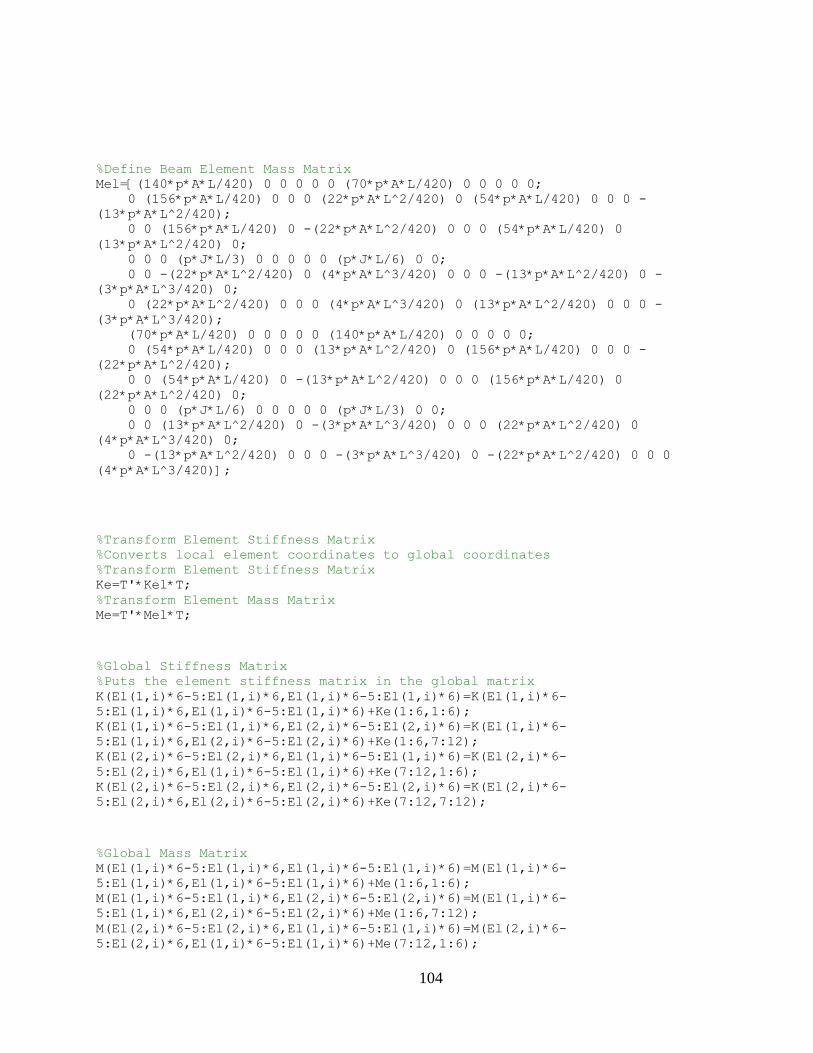
104
%Define Beam Element Mass Matrix Mel=[(140*p*A*L/420) 0 0 0 0 0 (70*p*A*L/420) 0 0 0 0 0; 0 (156*p*A*L/420) 0 0 0 (22*p*A*L^2/420) 0 (54*p*A*L/420) 0 0 0 -
(13*p*A*L^2/420); 0 0 (156*p*A*L/420) 0 -(22*p*A*L^2/420) 0 0 0 (54*p*A*L/420) 0
(13*p*A*L^2/420) 0; 0 0 0 (p*J*L/3) 0 0 0 0 0 (p*J*L/6) 0 0; 0 0 -(22*p*A*L^2/420) 0 (4*p*A*L^3/420) 0 0 0 -(13*p*A*L^2/420) 0 -
(3*p*A*L^3/420) 0; 0 (22*p*A*L^2/420) 0 0 0 (4*p*A*L^3/420) 0 (13*p*A*L^2/420) 0 0 0 -
(3*p*A*L^3/420); (70*p*A*L/420) 0 0 0 0 0 (140*p*A*L/420) 0 0 0 0 0; 0 (54*p*A*L/420) 0 0 0 (13*p*A*L^2/420) 0 (156*p*A*L/420) 0 0 0 -
(22*p*A*L^2/420); 0 0 (54*p*A*L/420) 0 -(13*p*A*L^2/420) 0 0 0 (156*p*A*L/420) 0
(22*p*A*L^2/420) 0; 0 0 0 (p*J*L/6) 0 0 0 0 0 (p*J*L/3) 0 0; 0 0 (13*p*A*L^2/420) 0 -(3*p*A*L^3/420) 0 0 0 (22*p*A*L^2/420) 0
(4*p*A*L^3/420) 0; 0 -(13*p*A*L^2/420) 0 0 0 -(3*p*A*L^3/420) 0 -(22*p*A*L^2/420) 0 0 0
(4*p*A*L^3/420)];
%Transform Element Stiffness Matrix %Converts local element coordinates to global coordinates %Transform Element Stiffness Matrix Ke=T'*Kel*T; %Transform Element Mass Matrix Me=T'*Mel*T;
%Global Stiffness Matrix %Puts the element stiffness matrix in the global matrix K(El(1,i)*6-5:El(1,i)*6,El(1,i)*6-5:El(1,i)*6)=K(El(1,i)*6-
5:El(1,i)*6,El(1,i)*6-5:El(1,i)*6)+Ke(1:6,1:6); K(El(1,i)*6-5:El(1,i)*6,El(2,i)*6-5:El(2,i)*6)=K(El(1,i)*6-
5:El(1,i)*6,El(2,i)*6-5:El(2,i)*6)+Ke(1:6,7:12); K(El(2,i)*6-5:El(2,i)*6,El(1,i)*6-5:El(1,i)*6)=K(El(2,i)*6-
5:El(2,i)*6,El(1,i)*6-5:El(1,i)*6)+Ke(7:12,1:6); K(El(2,i)*6-5:El(2,i)*6,El(2,i)*6-5:El(2,i)*6)=K(El(2,i)*6-
5:El(2,i)*6,El(2,i)*6-5:El(2,i)*6)+Ke(7:12,7:12);
%Global Mass Matrix M(El(1,i)*6-5:El(1,i)*6,El(1,i)*6-5:El(1,i)*6)=M(El(1,i)*6-
5:El(1,i)*6,El(1,i)*6-5:El(1,i)*6)+Me(1:6,1:6); M(El(1,i)*6-5:El(1,i)*6,El(2,i)*6-5:El(2,i)*6)=M(El(1,i)*6-
5:El(1,i)*6,El(2,i)*6-5:El(2,i)*6)+Me(1:6,7:12); M(El(2,i)*6-5:El(2,i)*6,El(1,i)*6-5:El(1,i)*6)=M(El(2,i)*6-
5:El(2,i)*6,El(1,i)*6-5:El(1,i)*6)+Me(7:12,1:6);
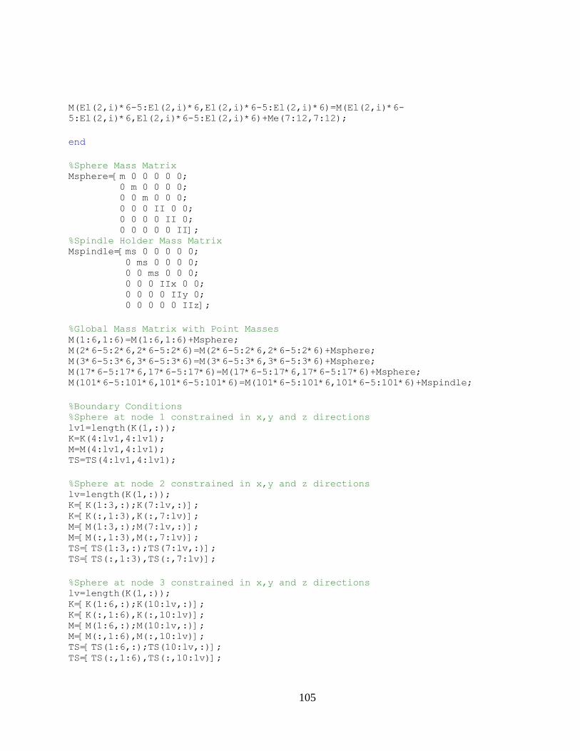
105
M(El(2,i)*6-5:El(2,i)*6,El(2,i)*6-5:El(2,i)*6)=M(El(2,i)*6-
5:El(2,i)*6,El(2,i)*6-5:El(2,i)*6)+Me(7:12,7:12);
end
%Sphere Mass Matrix Msphere=[m 0 0 0 0 0; 0 m 0 0 0 0; 0 0 m 0 0 0; 0 0 0 II 0 0; 0 0 0 0 II 0; 0 0 0 0 0 II]; %Spindle Holder Mass Matrix Mspindle=[ms 0 0 0 0 0; 0 ms 0 0 0 0; 0 0 ms 0 0 0; 0 0 0 IIx 0 0; 0 0 0 0 IIy 0; 0 0 0 0 0 IIz];
%Global Mass Matrix with Point Masses M(1:6,1:6)=M(1:6,1:6)+Msphere; M(2*6-5:2*6,2*6-5:2*6)=M(2*6-5:2*6,2*6-5:2*6)+Msphere; M(3*6-5:3*6,3*6-5:3*6)=M(3*6-5:3*6,3*6-5:3*6)+Msphere; M(17*6-5:17*6,17*6-5:17*6)=M(17*6-5:17*6,17*6-5:17*6)+Msphere; M(101*6-5:101*6,101*6-5:101*6)=M(101*6-5:101*6,101*6-5:101*6)+Mspindle;
%Boundary Conditions %Sphere at node 1 constrained in x,y and z directions lv1=length(K(1,:)); K=K(4:lv1,4:lv1); M=M(4:lv1,4:lv1); TS=TS(4:lv1,4:lv1);
%Sphere at node 2 constrained in x,y and z directions lv=length(K(1,:)); K=[K(1:3,:);K(7:lv,:)]; K=[K(:,1:3),K(:,7:lv)]; M=[M(1:3,:);M(7:lv,:)]; M=[M(:,1:3),M(:,7:lv)]; TS=[TS(1:3,:);TS(7:lv,:)]; TS=[TS(:,1:3),TS(:,7:lv)];
%Sphere at node 3 constrained in x,y and z directions lv=length(K(1,:)); K=[K(1:6,:);K(10:lv,:)]; K=[K(:,1:6),K(:,10:lv)]; M=[M(1:6,:);M(10:lv,:)]; M=[M(:,1:6),M(:,10:lv)]; TS=[TS(1:6,:);TS(10:lv,:)]; TS=[TS(:,1:6),TS(:,10:lv)];
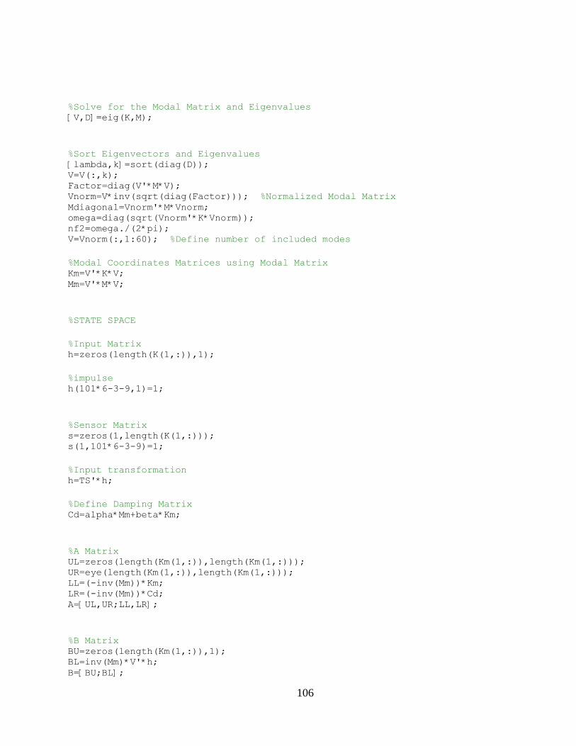
106
%Solve for the Modal Matrix and Eigenvalues [V,D]=eig(K,M);
%Sort Eigenvectors and Eigenvalues [lambda,k]=sort(diag(D)); V=V(:,k); Factor=diag(V'*M*V); Vnorm=V*inv(sqrt(diag(Factor))); %Normalized Modal Matrix Mdiagonal=Vnorm'*M*Vnorm; omega=diag(sqrt(Vnorm'*K*Vnorm)); nf2=omega./(2*pi); V=Vnorm(:,1:60); %Define number of included modes
%Modal Coordinates Matrices using Modal Matrix Km=V'*K*V; Mm=V'*M*V;
%STATE SPACE
%Input Matrix h=zeros(length(K(1,:)),1);
%impulse h(101*6-3-9,1)=1;
%Sensor Matrix s=zeros(1,length(K(1,:))); s(1,101*6-3-9)=1;
%Input transformation h=TS'*h;
%Define Damping Matrix Cd=alpha*Mm+beta*Km;
%A Matrix UL=zeros(length(Km(1,:)),length(Km(1,:))); UR=eye(length(Km(1,:)),length(Km(1,:))); LL=(-inv(Mm))*Km; LR=(-inv(Mm))*Cd; A=[UL,UR;LL,LR];
%B Matrix BU=zeros(length(Km(1,:)),1); BL=inv(Mm)*V'*h; B=[BU;BL];
107
%C Matrix CR=zeros(1,length(Km(1,:))); CL=s*TS*V; C=[CL,CR];
D=0;
G=ss(A,B,C,D);
w={10*2*pi,1000*2*pi}; h=bodeplot(G,w); % Change units to Hz and make phase plot invisible setoptions(h,'FreqUnits','Hz');
108
LIST OF REFERENCES
[1] Lindsey, K. (1991). Tetraform Grinding. SPIE., Commercial applications of precision
manufacturing at the sub-micron level, 1573, 129.
[2] Stephenson, D. J. et al. (2002). Ultra Precision Grinding using the Tetraform Concept.
Abrasives Magazine, 12-16.
[3] Jackson, M. J. & Hyde, L. J. & Robinson, G. M. & Ahmed, W. (2006). Dynamic
Response of a Tetrahedral Nanomachining Machine Tool Structure. International
Journal of Nanomanufacturing, 1 (1), 26-46.
[4] Hyde, L. J. (2003). Vibration Analysis of a Tetrahedral Structure, Tennessee
Technological University Master Thesis.
[5] Ma, L. (2008). Design and Development of a Micromachining Tool Structure, Purdue
University Master Thesis.
[6] Manjunath, T. C. Mathematical Modeling of SISO based Timoshenko Structures-A Case
Study. International Journal of Mathematics Sciences, 1 (1).
[7] Narayanan, S. & Balamurugan, V. (2003). Finite Element Modeling of Piezolaminated
Smart Structures for Active Vibration Control with Distributed Sensors and Actuators.
Journal of Sound and Vibration, 262, 529-562.
[8] Fanson, J. L. & Caughey, T. K. (1990), Positive position feedback-control for large space
structures. AIAA Journal, 28, 4, 717-724.
[9] Moheimani, S. O. & Fleming, A. J. (2006) Piezoelectric Transducers for Vibration
Control and Dampin., Springer-Verlag London Ltd.
[10] Inman, D. J. (2006). Vibration with Control. John Wiley & Sons, Ltd.
[11] Baillargeon, B. P. & Vel, S. S. (2005). Active Vibration Suppression of Sandwich Beams
using Piezoelectric Shear Actuators: Experiments and Numerical Simulations. Journal of
Intelligent Material Systems and Structures, 16, 517-530.
[12] IEEE Standard on Piezoelectricity. (1987). ANSI-IEEE Std, 176-187.
[13] Corbett, J., et al, 1999, An Ultra Precision Machine Tool Demonstrating a Novel
Vibration Resistant Structure Precision Engineering – Nanotechnology, Proceedings of
the 1st International euspen Conference, 1, 159-162, Shaker Verlag, Aachen.
109
[14] Slocum, S. & Wilson, S. A. & Corbett, J. & Whatmore, R. W. Ultra-Precision Grinding
of PZT Ceramics—Surface Integrity Control and Tooling Design. International Journal
of Machine Tools & Manufacture, 49, 998–1007.
[15] Goh, C. J. & Caughey, T. K. (1985). On the Stability Problem Caused by Finite Actuator
Dynamics in the Collocated Control of Large Space Structures. International Journal of
Control, 41, 787-802.
[16] Friswell, M. I. & Inman, D. J. (1999). The Relationship Between Positive Position
Feedback and Output Feedback Controllers. Smart Materials and Structures, 8, 285-291.
[17] Poh, S. & Baz, A. (1990). Active Control of a Flexible Structure Using a Modal Positive
Position Feedback Controller. Journal of Intelligent Material Systems and Structures, 1,
273-288.
[18] Rao, S. S. (2004). Mechanical Vibrations. Pearson Education, Ltd.
[19] SAS, Inc. (2007). ANSYS Element Reference, Release 11.0.
[20] Mide Technologies (October 2009). Mide Engineering Smart Technologies.
http://www.mide.com/