Embed Size (px)
Citation preview
Developed at Politecnico di Milano, Department of Aerospace Science and Technology, as part
of an international exchange.
Supervisor at Universitat Politècnica de València:
Prof. Vicent Giner Bosch
Supervisor at Politecnico di Milano:
Prof. Sergio Ricci
Universitat Politècnica de València
ESCUELA TÉCNICA SUPERIOR DE INGENIERÍA INDUSTRIAL
Master Universitario en Ingeniería Industrial
Author:
Laura Feria del Rosario
Academic Year 2020-2021
Structural Analysis and Optimization of a
Space Module

i
Abstract Designing light-weight aerospace structures without compromising structural integrity has
historically been a strong driving force behind the development of optimum design methods. The
main goal of this thesis work is to check the capability of the Finite Element solver OptiStruct
from HyperWorks suite, from Altair Engineering in order to optimize design of a curved panel
forming a space module.
This structure is a pressurized manned module designed by the company Thales Alenia Space. It
is in a habitable module devoted to be part of a space station, consisting of a single compartment
with two bulkhead-hatch systems which provide connection with other two modules, one of which
being an airlock. The design of the cylindrical panels of the module is object of study.
In particular, stiffening of this plate is analysed so that mechanical requirements derived from
design loads are fulfilled with the lightest design possible. For this purpose, OptiStruct
optimization options (free-size, topology, topography and free-shape) are investigated in order to
obtain the method providing the lightest feasible panel design.
Design loads include maximum expected accelerations and pressure during its whole life-time.
This means that primary structure of the module is designed to withstand loads during handling,
transportation, testing, launch, flight, on-orbit docking, berthing and on-orbit. Several constraints
are involved: normal modes and yielding and buckling failure modes. Uncertainties in the space
program (e.g., stability of the mass budget, well defined design) and the mathematical model used
to represent the structure are considered in the optimization by applying factors of safety provided
by European Space Agency standards.
Two approaches are followed to obtain the optimized panel design: optimization of the
unstiffened and reinforced panel.
In the first case, thickness results are compared with equivalent optimization process performed
in the same model in HyperSizer, another optimization tool. For this approach, the model used is
the space module model itself composed by cylinder panels. Free-size method is employed.
Differences in results show distinct capabilities of both tools used.
For the second approach, a stiffening panel optimization process is performed applying topology,
topography and free-shape methods. Output reinforcement designs have distinct characteristics
and shapes that are usable for an early design stage in order to define topology of stiffeners,
depending on designer’s priority.
ii
Acknowledgements I thank my thesis supervisors Prof. Sergio Ricci from the Aerospace Department of Engineering
at Politecnico di Milano and Prof. Vicent Giner Bosch from Universitat Poltècnica de València.
Their active support and help during this project were indeed crucial. Thanks to them this thesis
has become a priceless educational experience.
I am also grateful for my family and friends for supporting me and encouraging me along the
way, but especially in the hardest days.
In addition, I want to address thanks to Altair Engineering who has generously provided a full
software license and access for courses and tutorials in how to use the software (HyperMesh,
OptiStruct and HyperView). Altair Engineering has also assisted with technical support in the
best possible way.
iii
Content Abstract .......................................................................................................................................... i
Acknowledgements ....................................................................................................................... ii
List of figures ................................................................................................................................ v
List of tables ................................................................................................................................ vii
Acronyms ................................................................................................................................... viii
1 Introduction ........................................................................................................................... 1
1.1 Context and motivation ................................................................................................. 1
1.2 Objectives ...................................................................................................................... 1
1.3 Scope and limitations .................................................................................................... 1
1.4 Thesis outline ................................................................................................................ 2
2 Optimization process ............................................................................................................. 3
2.1 Structural optimization .................................................................................................. 3
2.2 Optimization problem ................................................................................................... 3
2.3 Types of optimization problems .................................................................................... 4
3 OptiStruct features................................................................................................................. 5
3.1 OptiStruct capabilities ................................................................................................... 5
3.2 Optimization process ..................................................................................................... 5
3.3 OptiStruct optimization types ........................................................................................ 6
3.4 Manufacturing constraints ........................................................................................... 10
3.5 Convergence ................................................................................................................ 11
3.6 OSSmooth ................................................................................................................... 11
4 Structure description ........................................................................................................... 12
4.1 Components ................................................................................................................. 12
4.2 Coordinate system ....................................................................................................... 16
4.3 Material ....................................................................................................................... 17
4.4 Finite element model ................................................................................................... 17
4.5 Constrains .................................................................................................................... 18
5 Mechanical requirements and failure modes ....................................................................... 19
5.1 Limit Loads ................................................................................................................. 19
5.2 Panel stability .............................................................................................................. 19
5.3 Primary modes ............................................................................................................ 19
5.4 Subcases ...................................................................................................................... 20
5.5 Design Limit Loads ..................................................................................................... 20
5.6 Failure modes .............................................................................................................. 21
6 Preliminary analyses ........................................................................................................... 24
iv
6.1 Analysis set up ............................................................................................................ 24
6.2 Results ......................................................................................................................... 25
7 Optimization of an unstiffened curved panel ...................................................................... 32
7.1 Optimization set up ..................................................................................................... 32
7.2 Results ......................................................................................................................... 33
7.3 Normal modes analysis ............................................................................................... 36
7.4 Comparison of optimization results with HyperSizer ................................................. 37
8 Optimization of a reinforced curved panel .......................................................................... 39
8.1 Optimization model ..................................................................................................... 39
8.2 Finite element model for the panel .............................................................................. 40
8.3 Free size optimization ................................................................................................. 41
8.4 Topology optimization ................................................................................................ 41
8.5 Topography optimization ............................................................................................ 45
8.6 Free-shape optimization .............................................................................................. 49
9 Conclusions ......................................................................................................................... 55
Appendix A. Finite element model of module ...................................................................... 57
References ................................................................................................................................... 61
v
List of figures Figure 2.1. Types of structural optimization problems [3] ............................................................ 4
Figure 3.1. HyperWorks workflow ............................................................................................... 5
Figure 3.2. Transition zone grids [4] ............................................................................................. 7
Figure 3.3. Bead parameters [4] .................................................................................................... 8
Figure 3.4. Buffer zone [4] ............................................................................................................ 9
Figure 3.5. Check boarding: (a) Design problem, (b) Checkerboards [7] ................................... 10
Figure 4.1. Lateral view of module’s primary structure [1] ........................................................ 13
Figure 4.2. Top view of module’s primary structure [1] ............................................................. 13
Figure 4.3.Bottom view of module’s primary structure [1] ........................................................ 14
Figure 4.4. Front view of module's primary structure [1] ........................................................... 15
Figure 4.5. Example of secondary masses allocation [1] ............................................................ 15
Figure 4.6. Schematic representation of secondary masses (in blue) between longerons (in red)
[1] ................................................................................................................................................ 16
Figure 4.7. Module's coordinate system [1] ................................................................................ 17
Figure 4.8. Lateral view of the FE model [1] .............................................................................. 18
Figure 4.9. Constrained nodes [1] ............................................................................................... 18
Figure 6.1. Module's area of study [1] ........................................................................................ 24
Figure 6.2. Maximum von Mises stresses [Pa] for quasi-static loads (subcase 8) ...................... 26
Figure 6.3. Maximum von Mises stresses [Pa] for pressure loads (subcase 9) ........................... 27
Figure 6.4. Buckling shape for subcase 2 with displacement contour (m) .................................. 28
Figure 6.5. Mode 1 (first lateral mode) deformed representation (x10) and mass normalized
displacement contour (m) ............................................................................................................ 29
Figure 6.6. Mode 2 (second lateral mode) deformed representation (x10) and mass normalized
displacement contour (m) ............................................................................................................ 30
Figure 6.7. Mode 4 (first longitudinal mode) deformed representation (x10) and mass normalized
displacement contour (m) ............................................................................................................ 31
Figure 7.1. Optimization model [1] ............................................................................................. 32
Figure 7.2. Buckling shape for subcase 2 after optimization with displacement contour (m) .... 34
Figure 7.3. Maximum von Mises stress [Pa] after optimization for pressure loads (subcase 9) . 35
Figure 8.1. Panel dimensions ...................................................................................................... 39
Figure 8.2. Panel finite element model ....................................................................................... 40
Figure 8.3. Panel connections ..................................................................................................... 41
Figure 8.4. Rib pattern definition for topology optimization [4] ................................................ 42
Figure 8.5. Topology ptimized panel. Element density values from 0 to1 ................................. 43
Figure 8.6. Buckling shapes for subcase 7 after topology optimization with displacement contour
(m) ............................................................................................................................................... 44
Figure 8.7. Envelope of maximum von Mises stress [Pa] for topology optimization (subcase 9)
..................................................................................................................................................... 44
Figure 8.8. Topography optimization shape changes [m] ........................................................... 47
Figure 8.9. Buckling shapes for subcase 7, case (B), along topography optimization with
displacement contour (m) ............................................................................................................ 48
Figure 8.10. Topography optimization stress results [Pa] ........................................................... 48
Figure 8.11. Linear manufacturing constraint example [4] ......................................................... 49
Figure 8.12. Free-shape optimization shape changes [m] ........................................................... 52
Figure 8.13. Buckling shapes for 4-layer model after free-shape optimization (subcase 7) ....... 53
Figure 8.14. Free-shape optimization stress results for 4-layer model [Pa] (subcase 9) ............. 53 Figure A.1. Lateral view of the FE model [1]……………………………………………………58

vi
Figure A.2. Top view of the FE model [1] .………………………………………………...……58
Figure A.3. Detailed view of longerons attachments and secondary masses connections [1]……59
Figure A.4. Detailed view of CBUSH elements (in white) [1]..…………………………………60
vii
List of tables Table 4.1. Aluminium 2219-T851 properties .............................................................................. 17
Table 5.1. Quasi-Static Limit Loads ........................................................................................... 19
Table 5.2. Subcases ..................................................................................................................... 20
Table 5.3. Factors of safety ......................................................................................................... 21
Table 6.1. Preliminary stress and buckling results ...................................................................... 25
Table 6.2. Modal preliminary analysis results ............................................................................ 28
Table 7.1. Buckling analysis results for optimized and baseline models .................................... 33
Table 7.2. Yield strength analysis results for optimized and baseline models ............................ 34
Table 7.3. Modal analysis results for optimized module ............................................................ 36
Table 7.4. Modal analysis difference results. Values refer to difference between optimized model
minus baseline results ................................................................................................................. 37
Table 7.5. Buckling analysis results obtained in [1] (Table 5.6) ................................................. 38
Table 7.6. Strength analysis results obtained in [1] .................................................................... 38
Table 8.1. Constraints for panel FE model .................................................................................. 41
Table 8.2. Stiffened (topology) vs unstiffened (free-size) panel optimization results ................ 43
Table 8.3. Cases of study for topography optimization .............................................................. 46
Table 8.4. Results for topography optimizations ........................................................................ 46
Table 8.5. Results for free-shape optimizations .......................................................................... 50
Table A.1. FE model summary..…………………………………………………………………57
viii
Acronyms
CAD Computer Aided Design
DLL Design Limit Loads
DOF Degree Of Freedom
FE Finite Element
FEA Finite Element Analysis
FEM Finite Element Method
FOS Factor Of Safety
FOSB Buckling Factor of Safety
FOSY Yield design Factor Of Safety
KDF Knock Down Factor
KM Model factor
KP Project factor
MOS Margin Of Safety
1. Introduction
1
1 Introduction
1.1 Context and motivation
In aerospace industry, there is a need of minimizing spacecraft structural weight in order to
increase launchers payload capabilities, as it is one of the major contributors to spacecraft dry
mass. Design of light-weight structures which does not compromise mechanical integrity, has
historically been a strong driving force behind the development of optimum design methods.
Especially, design of reinforced panels has been considerably researched. This interest is due to
the fact that launch vehicle stages, propellant tanks, pressurized modules, and many other
aerospace structures consist mostly of those.
However, majority of research is done in some typical stiffening designs, e.g., panels with an
orthogrid waffle internal reinforcement. In general, optimization tools are limited for the need of
input parameters that already constrain final optimized designs. An automated variation of
optimization input parameters is necessary to get this approach.
OptiStruct is a finite element solver which can conduct optimizations as well. It belongs to the
HyperWorks suite from Altair Engineering, and it is a powerful finite element optimization tool
because of its wide variety of optimization methods.
Therefore, OptiStruct is a good candidate for allowing structure designer not to restrict himself
for predefined stiffening shapes, but is it able to produce a reinforcement pattern without any
predefined limitation? In order to answer this ultimate question, optimization methods available
in OptiStruct must be studied.
1.2 Objectives
The main purpose of this thesis work is to determine OptiStruct capabilities for the optimization
of a curved panel used in a space module. However, it can be subdivided into two objectives. The
first goal is to compare optimization process and results for an unstiffened curved panel performed
by OptiStruct and HyperSizer. Optimization for the former solver is done as part of the present
thesis. Results for the latter software are obtained from another master thesis written by Virtudes
de Gregorio Roig for Politecnico di Milano [1].
The second objective is to determine whether OptiStruct is capable of generating an optimized
stiffened panel with minimum design parameter limitations that fulfils established structural
requirements. For this purpose, the different optimization methods included in OptiStruct are
studied.
1.3 Scope and limitations
The object of study is a curved panel of a space module. Finite element model is provided by
Thales Alenia Space. However, different models are used for both approaches made along this
work.
In order to compare OptiStruct optimization with results obtained in [1], the complete space
module model is used, so that finite element model is the same in both studies. Optimization is
performed in the unstiffened panel that forms the primary structure of the space module. This
study is part of a preliminary design phase. The resulting design can be used to perform a
preliminary mass estimation and assessment of the module structure primary frequencies as part
of the mission design.
1. Introduction
2
For the second approach, optimization with the different methods provided by OptiStruct is
applied to a single cylinder panel. Geometry is extracted from previous space module primary
structure. In this way, it is possible to simplify Finite Element Analysis (FEA) to investigate
OptiStruct capabilities. The obtained results will give an initial idea of where to locate and how
to define reinforcements in a curved panel. It is not part of a preliminary design mission phase.
From the curved panel, only stiffening strategies are studied, so areas close to the edges of the
curved panel will not be case of research as they are extremely conditioned by joining techniques
between adjacent components.
1.4 Thesis outline
The present thesis document is organized in 9 sections. The current section includes the context
and motivation of this thesis work as well as the scope and the objectives. Section 2 gives an
overview of how optimization is applied to structural designs. In section 3, a summary of
OptiStruct features and capabilities is developed. Section 4 is devoted to the description of the
structure which is object of study, including its geometry, material and principal information
related to finite element model. In section 5, design mechanical requirements, that structure object
of study must fulfils, are described and associated to specific failure modes to be prevented.
Section 6 presents preliminary structural analyses results. Section 7 is devoted to the optimization
formulation and results of the complete model. A comparison with preliminary results and those
obtained in [1] is done. In section 8, different OptiStruct optimization methods are evaluated for
optimizing a curved panel. Lastly, section 9 is devoted to the conclusion’s discussion.
The present thesis document has one appendix. In Appendix A structure finite element model is
thoroughly described.

2. IntroductionOptimization process
3
2 Optimization process
2.1 Structural optimization
The purpose of structural optimization is to obtain the optimal material distribution according to
some given demands of the structure. Typical objective functions are minimization of mass,
displacement or compliance (strain energy). Constraints are usually related to mass, volume, size
or failure.
Structural optimization is traditionally done manually using a 3-steps iterative-intuitive process
[2]:
A structural design is suggested.
The mechanical requirements to be fulfilled are evaluated. This step is nowadays
developed by means of computer-based methods like the Finite Element Method (FEM).
If requirements are met, the optimization process is finished. Otherwise, modifications
are made, a new improved design is proposed and steps 2 and 3 are repeated.
Results and number of iterations depend to a large extent on designer's knowledge, experience
and intuitive understanding of the problem. This is due to the fact that changes in design are made
in an intuitive way, often using trial and error. For this reason, optimization process can be very
time consuming and, finally, may result in a non-optimal design because some characteristics can
still be improved.
So as to improve timing and results, a mathematical design optimization method is implemented
so that steps 2 and 3 are automatically developed. OptiStruct is an optimization tool that can solve
this type of problem.
2.2 Optimization problem
For every optimization process there are 5 elements that must be defined.
• Design space, includes parts which are designable during optimization process. The
excluded parts are known as the non-design space.
• Design variables, are the system parameters that are varied to optimize performance.
• Responses, are the measurements of system performance, e.g., mass, volume, mass and
volume fraction, temperature, stress, displacement, buckling factor or frequency. They
can then be used either as an objective function or as a constraint.
• Objective function, represents the response function of the system to be optimized.
• Constraint functions, are the bounds on response functions of the system that must be
satisfied for the design to be feasible.
The typical formulation for an optimization problem is the following one
minimize 𝑓(𝑥) = 𝑓(𝑥1, 𝑥2, … , 𝑥𝑛) 𝑖 = 1, 2, … , 𝑛 (2.1)
subject to 𝑔𝑗(𝑥) ≤ 0 𝑗 = 1, 2, … , 𝑚 (2.2)
𝑥𝑖𝐿 ≤ 𝑥𝑛 ≤ 𝑥𝑖
𝑈 (2.3)
2. IntroductionOptimization process
4
where 𝑓(𝑥) is the objective function, and 𝑔𝑗(𝑥) are the constraint functions. A constraint can be
considered active if it is satisfied exactly (𝑔𝑗(𝑥) = 0); inactive if it is simply satisfied; and
violated. Finally, 𝑥𝑛 represents the design variables with their corresponding lower and upper
limits (𝑥𝑖𝐿 , 𝑥𝑖
𝑈).
2.3 Types of optimization problems
According to Christensen and Klarbring [2], there are three different types of structural
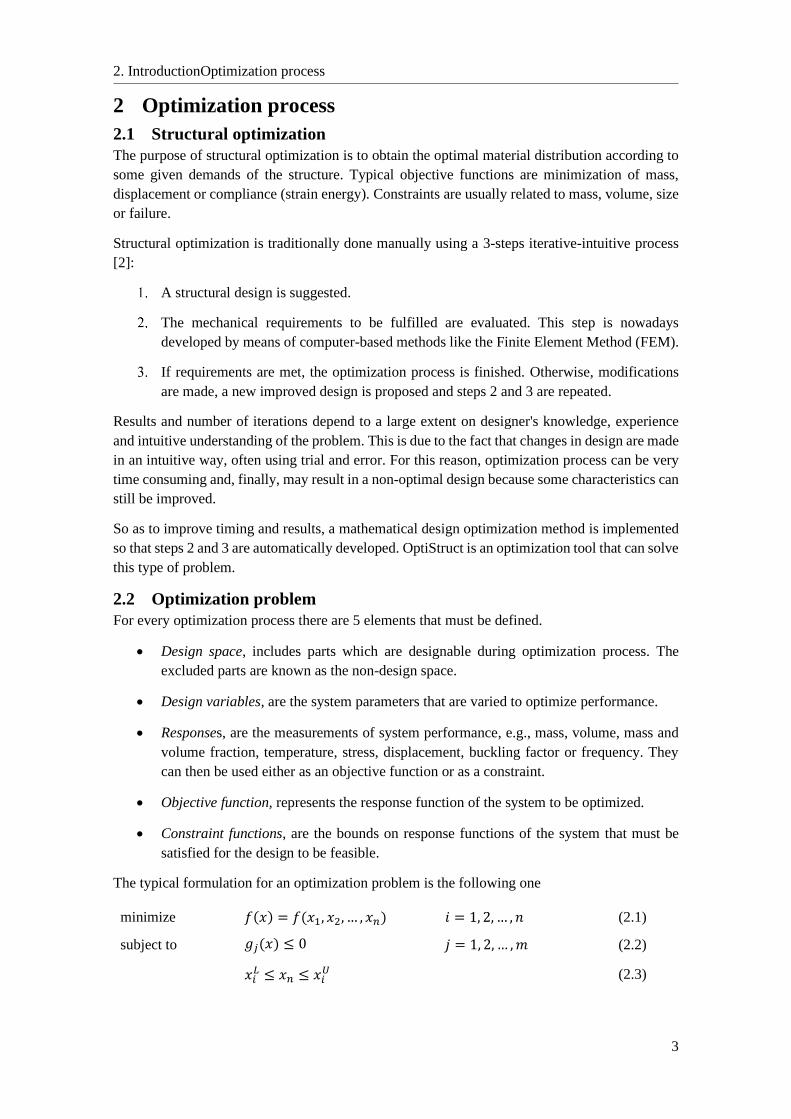
optimization problems: sizing, shape and topology.
• Sizing optimization is the simplest form of structural optimization. It is performed when
it is not necessary to remove materials, generate beads or change the shape of the
structure, which is known. The objective is to optimize the structure by adjusting sizes of
components, which are the design variables, e.g., cross-sectional areas of truss members,
or the thickness distribution of a sheet. See Figure 2.1.(a) for an example of size
optimization where shape is fixed and design variables correspond to diameter of rods.
• Shape optimization is developed by modifying the outer boundary of the structure.
However, connectivity of the structure is not changed: new boundaries are not formed,
e.g., new holes or split bodies will not appear. Shape variables are the design variables,
and those could be, for instance, thickness distribution along structural members,
diameter of holes or radii of fillets. A shape optimization problem is seen in Figure
2.1.(b).
A fundamental difference between shape vs. topology and size optimization is that instead
of having one or more design variables for each element, in this case, design variables
affect many elements.
• Topology optimization is the most general form of structural optimization. In this case,
the resulting shape or topology is not known, the number of holes, bodies, etc., are not
decided yet. The purpose is to find the optimum distribution of material and voids, a so
called 0-1 problem, where material either exists or not. To solve this problem, structure
is discretized by using FEM and dividing the design domain into discrete elements
(mesh). An example is shown in Figure 2.1c.
Figure 2.1. Types of structural optimization problems [3]
3. OptiStruct features
5
3 OptiStruct features
3.1 OptiStruct capabilities
OptiStruct is a solver which is capable of performing a range of finite element analyses; like static,
modal, buckling and thermal analyses. Several types of loads such as point forces, pressure,
gravitational loads, and thermal loads can be applied. In addition, many different types of
elements are supported including: three-dimensional solid elements, two-dimensional shell
elements and other elements such as beams, bars, springs and point masses.
Both, finite element analysis and optimizations, can be solved with OptiStruct. Moreover, there
are different types of optimizations available based on the subdivision established for structural
optimization in section 2.3.
• Free-size optimization, determines the optimal thickness distribution of shell elements.
• Size optimization, calculates the optimal design variables which affect the property of
interest.
• Free-shape optimization, determines the optimal shape of a structure.
• Shape optimization, determines the optimal shape of a structure based on pre-defined
boundaries created by the user.
• Topography optimization, finds the best reinforcement pattern of a shell structure.
• Topology optimization
More information about each optimization can be found in section 3.3 or in OptiStruct User’s
Guide [4].
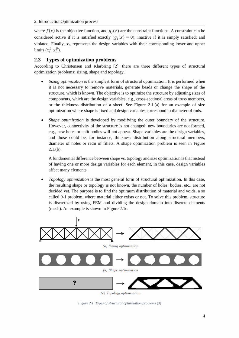
3.2 Optimization process
OptiStruct does not have any graphical interface. For this reason, HyperMesh and HyperView
were also used for this work. All of them are part of the software suite HyperWorks from Altair
Engineering. HyperMesh is the pre-processor, which is used to create the mesh from a CAD
model, set boundary conditions and set up the problem to be solved. Afterwards, HyperMesh
exports a file which defines the problem so that OptiStruct can solve it. Finally, results can be
reviewed in the HyperView post-processor. Figure 3.1 represents the workflow of HyperWorks.
All tools used for this work from HyperWorks suite correspond to 2021.1 version.
Figure 3.1. HyperWorks workflow
3. OptiStruct features
6
In general, the procedure for setting up an optimization problem to be solved in OptiStruct is
roughly the same independently of the optimization type. It is mainly developed in HyperMesh.
Steps to be followed are listed below.
Obtaining the Finite Element (FE) model. HyperMesh is capable of importing and
creating linked geometry and FE model. For checking HyperMesh capabilities, please
refer to [5].
Definition of design variables and their constraints.
Definition of responses that will be used as objective or constraints.
Formulation of optimization objective.
Set of constraints on responses. This step is not always necessary, it depends on each
optimization problem.
For steps from 2 to 5, there are different possibilities and limitations for each optimization type.
In the next section, some of them are mentioned, however in order to widen information,
OptiStruct User’s Guide [4] can be consulted.
3.3 OptiStruct optimization types
Free-size optimization
Free-size produces an optimized thickness distribution per element for a 2D structure. Several
manufacturing constraints can be set in order to, for example, have uniform thickness for a group
of elements.
Free-size stress constraints have some limitations that must be consulted in [4] previously, but for
the scope of this work it is possible to add stress constraints by using the stress-NORM
aggregation. The NORM method calculates the maximum value of a particular response of all the
grids/elements grouped approximately.
The buckling factor can be constrained only if shells have a base thickness not equal to zero.
Moreover, OptiStruct has the capability of performing free-size optimization simultaneously with
the other types of optimizations.
Free-size optimization is the process used in this work to obtain the optimized thickness for the
curved panels of the pressurized module.
Size (parameter) optimization
Some structural elements have properties depending on several parameters; like beams whose
area, moments of inertia, and torsional constants (properties) depend on the cross-section
geometry (parameters). Those parameters are the design variables. The objective of size
optimization is to adjust the design variables so that the property of interest is optimized.
These design variables can be set to take a continuous value, a discrete value or choose between
a set of predefined values.
Furthermore, OptiStruct has the capability of performing size optimization simultaneously with
the other types of optimizations.
Because of the scope of this work, sizing optimization will not be used. The only improvement
with respect to free-sizing is that discrete thickness variables can be imposed in order to find the
3. OptiStruct features
7
commercial panel model that better fits the requirements. However, as this work is part of a
preliminary design, this approach is not necessary.
Free-shape optimization
Free-shape optimization is an automated way to modify the structure shape based on set of nodes
that can move totally free on the boundary to find the optimal shape. The allowable movement of
the outer boundary is automatically determined, so it is not needed that user defines those
boundaries for the shape variables. It is sufficient to choose a set of nodes on the boundary.
During a classic free-shape optimization, the outer boundary of a structure is modified to meet
objectives and constraints. Depending on the element property, the design grids can move in one
of two ways:
For shell structures, grids move normal to the surface edge in the tangential plane.
For solid structures, grids move normal to the surface.
It is remarkable that the normal directions are modified with the change in shape of the structure;
i.e., design grids move along the updated normals for each iteration.
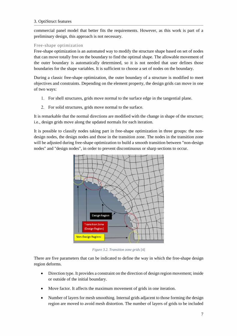
It is possible to classify nodes taking part in free-shape optimization in three groups: the non-
design nodes, the design nodes and those in the transition zone. The nodes in the transition zone
will be adjusted during free-shape optimization to build a smooth transition between "non-design
nodes" and "design nodes", in order to prevent discontinuous or sharp sections to occur.
Figure 3.2. Transition zone grids [4]
There are five parameters that can be indicated to define the way in which the free-shape design
region deforms.
• Direction type. It provides a constraint on the direction of design region movement; inside
or outside of the initial boundary.
• Move factor. It affects the maximum movement of grids in one iteration.
• Number of layers for mesh smoothing. Internal grids adjacent to those forming the design
region are moved to avoid mesh distortion. The number of layers of grids to be included
3. OptiStruct features
8
in the mesh smoothing buffer can be defined. A larger value will give a larger smoothing
buffer; nevertheless, it will result in a slower optimization.
• Maximum shrinkage and growth, which limit the total amount of deformation of the free-
shape design region.
Free-shape optimization will be used for checking OptiStruct capabilities in order to determine
optimum stiffeners shape and position for the curved panels of the module.
Shape
Shape optimization is able to modify the structure shape based on user-predefined shape variables
to find the optimal shape, on the contrary to free-shape process. Using finite element models, the
shape is defined by the grid point locations. Then, shape optimization modifies these locations to
update the shape.
To define design variables, firstly a shape is created by using a module in HyperMesh called
Hypermorph. Then, a design variable is easily defined from the shape, together with bounds on
maximum or minimum magnitude of the shape change.
Shape optimization will not be used in this work because user-predefined shapes are needed.
Therefore, shapes generated are already limited that could result in a non-optimized solution and
the objective of this work is to obtain different reinforcement patterns without any restriction in
order to check whether traditional stiffeners patterns are the optimized ones.
Topography optimization
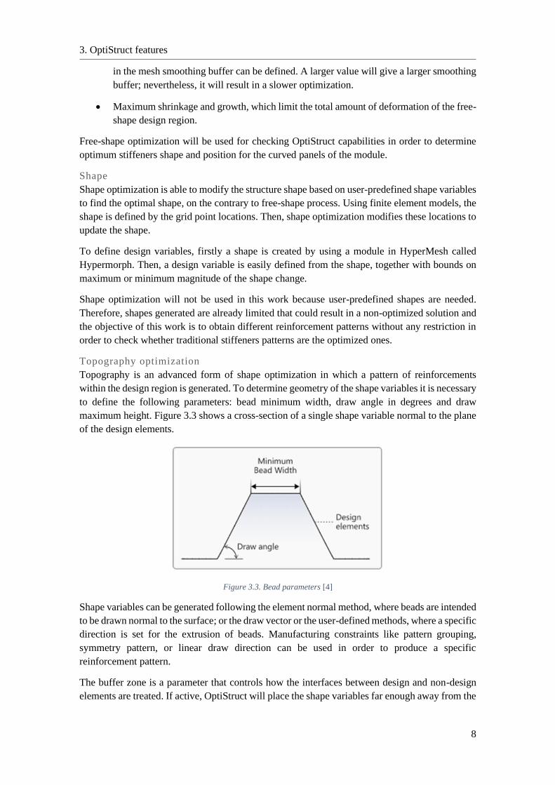
Topography is an advanced form of shape optimization in which a pattern of reinforcements
within the design region is generated. To determine geometry of the shape variables it is necessary
to define the following parameters: bead minimum width, draw angle in degrees and draw
maximum height. Figure 3.3 shows a cross-section of a single shape variable normal to the plane
of the design elements.
Figure 3.3. Bead parameters [4]
Shape variables can be generated following the element normal method, where beads are intended
to be drawn normal to the surface; or the draw vector or the user-defined methods, where a specific
direction is set for the extrusion of beads. Manufacturing constraints like pattern grouping,
symmetry pattern, or linear draw direction can be used in order to produce a specific
reinforcement pattern.
The buffer zone is a parameter that controls how the interfaces between design and non-design
elements are treated. If active, OptiStruct will place the shape variables far enough away from the
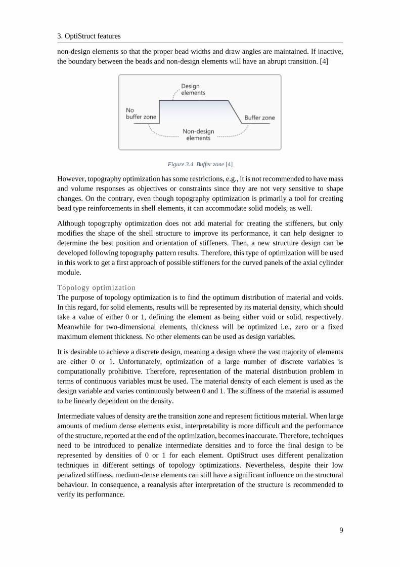
3. OptiStruct features
9
non-design elements so that the proper bead widths and draw angles are maintained. If inactive,
the boundary between the beads and non-design elements will have an abrupt transition. [4]
Figure 3.4. Buffer zone [4]
However, topography optimization has some restrictions, e.g., it is not recommended to have mass
and volume responses as objectives or constraints since they are not very sensitive to shape
changes. On the contrary, even though topography optimization is primarily a tool for creating
bead type reinforcements in shell elements, it can accommodate solid models, as well.
Although topography optimization does not add material for creating the stiffeners, but only
modifies the shape of the shell structure to improve its performance, it can help designer to
determine the best position and orientation of stiffeners. Then, a new structure design can be
developed following topography pattern results. Therefore, this type of optimization will be used
in this work to get a first approach of possible stiffeners for the curved panels of the axial cylinder
module.
Topology optimization
The purpose of topology optimization is to find the optimum distribution of material and voids.
In this regard, for solid elements, results will be represented by its material density, which should
take a value of either 0 or 1, defining the element as being either void or solid, respectively.
Meanwhile for two-dimensional elements, thickness will be optimized i.e., zero or a fixed
maximum element thickness. No other elements can be used as design variables.
It is desirable to achieve a discrete design, meaning a design where the vast majority of elements
are either 0 or 1. Unfortunately, optimization of a large number of discrete variables is
computationally prohibitive. Therefore, representation of the material distribution problem in
terms of continuous variables must be used. The material density of each element is used as the
design variable and varies continuously between 0 and 1. The stiffness of the material is assumed
to be linearly dependent on the density.
Intermediate values of density are the transition zone and represent fictitious material. When large
amounts of medium dense elements exist, interpretability is more difficult and the performance
of the structure, reported at the end of the optimization, becomes inaccurate. Therefore, techniques
need to be introduced to penalize intermediate densities and to force the final design to be
represented by densities of 0 or 1 for each element. OptiStruct uses different penalization
techniques in different settings of topology optimizations. Nevertheless, despite their low
penalized stiffness, medium-dense elements can still have a significant influence on the structural
behaviour. In consequence, a reanalysis after interpretation of the structure is recommended to
verify its performance.
3. OptiStruct features
10
The transition zone is acceptable in most cases. But it should be avoided to have large areas
containing mainly medium dense elements. For this reason, the amount of medium dense elements
is calculated. A ratio between the volume from elements with densities of at least 0.9 and that of
the entire design space is used. For a perfectly discrete model this value would be 1.0 but for
structures where a transition zone exists, this parameter should be 0.5 or higher. When values are
smaller than that at the end of the optimization, the topology should, at least, be interpreted with
caution
It is important to remark that different properties must be used for design and non-design
elements, where properties are defined using HyperMesh and describes an element by type,
material, etc.
As for the free-size, for topology optimization, stress constraints have some limitations that can
be consulted in [4], but for the scope of this work it is possible to add stress constraints by using
the stress-NORM aggregation.
Likewise, the buckling factor can be constrained for shell topology optimization problems with a
base thickness not equal to zero. Constraints on the buckling factor are not allowed in any other
cases.
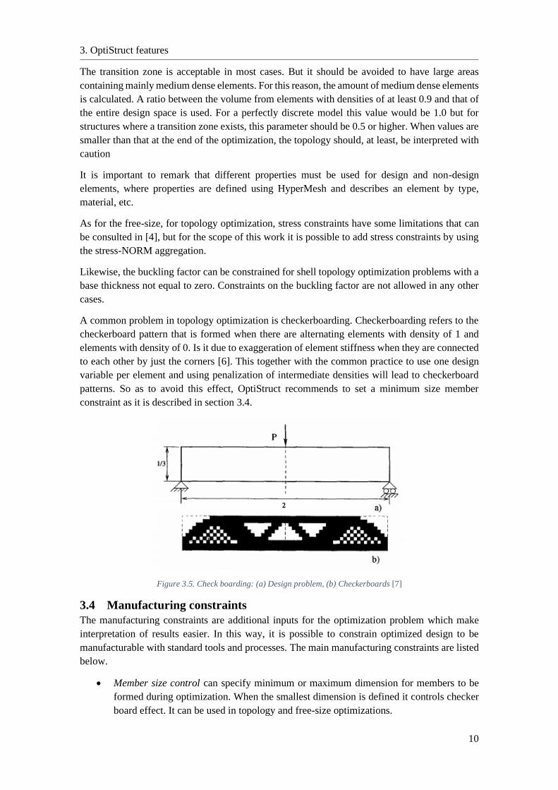
A common problem in topology optimization is checkerboarding. Checkerboarding refers to the
checkerboard pattern that is formed when there are alternating elements with density of 1 and
elements with density of 0. Is it due to exaggeration of element stiffness when they are connected
to each other by just the corners [6]. This together with the common practice to use one design
variable per element and using penalization of intermediate densities will lead to checkerboard
patterns. So as to avoid this effect, OptiStruct recommends to set a minimum size member
constraint as it is described in section 3.4.
Figure 3.5. Check boarding: (a) Design problem, (b) Checkerboards [7]
3.4 Manufacturing constraints
The manufacturing constraints are additional inputs for the optimization problem which make
interpretation of results easier. In this way, it is possible to constrain optimized design to be
manufacturable with standard tools and processes. The main manufacturing constraints are listed
below.
• Member size control can specify minimum or maximum dimension for members to be
formed during optimization. When the smallest dimension is defined it controls checker
board effect. It can be used in topology and free-size optimizations.
3. OptiStruct features
11
• Side constraints, in a similar way, allow the deformation space to be defined as a
coordinate range during free-shape optimization. These ranges may be with reference to
rectangular, cylindrical or spherical systems.
• Pattern grouping and pattern repetition can be applied to enforce a repeating pattern or
symmetrical design even if the loads applied on the structure are unsymmetrical or non-
repeating. Symmetry can be applied in 1, 2 or 3 planes or even cyclic symmetry
(rotational). They can be used in all optimization types.
• Draw direction constraints can be applied to obtain design suitable for casting or
machining operations. Constrained determined topology will allow the die to slide in a
given direction by preventing cavities formation. It can be used in topology and free-
shape optimizations.
• Extrusion constraint allows to define a constant cross-section design for solid models in
a specified direction, or along a curve. It can be used in topology and free-shape
optimizations.
• Grid constraints can be set for free-shape optimization to limit grid’s movement during
process (along a plane, a vector or totally fixed).
Several manufacturing constraints can be combined at the same optimization process.
3.5 Convergence
It must be pointed out that even when constraints are settled up, OptiStruct has some margin to
consider a feasible design. This means that slightly negative MOS can be obtained. In order to
reach convergence, satisfaction of only one of the two tests used by OptiStruct is required.
• Regular convergence. For two consecutive iterations, the change in the objective function
must be less than the objective tolerance and constraint violations must be less than 1%.
• Soft convergence. For two consecutive iterations, there is little or no change in the design
variables.
3.6 OSSmooth
OSSmooth is a semi-automated design interpretation tool embed in HyperMesh, which facilitates
recovery of a modified geometry resulted from a structural optimization for further use in the
design process and FEA reanalysis.
OSSmooth can be used in three different ways: OSSmooth for geometry, FEA topology
reanalysis, and FEA topography reanalysis.
OSSmooth (for geometry) is generally used to recover geometry by interpreting topology,
topography, and shape optimization results. Resulting shapes can be smoothed.
Meanwhile, OSSmooth for FEA topology and FEA topography reanalysis are used to generate
recovered geometry with boundary conditions for FEA reanalysis.
4. Structure description
12
4 Structure description The structure object of study is a habitable module designed to be part of a space station. It has
two bulkhead-hatches in order to connect it to two other modules, being one of them an airlock.
The primary structure of the module must fulfil the following mechanical requirements:
• Withstand loads during its whole life-time; i.e., testing, transportation, launch, on-orbit
docking and on-orbit accelerations.
• Withstand internal ambient pressure and depressurization for emergency flight cases.
• Guarantee pressure containment.
• Withstand loads induced by the crew and secondary masses.
• Provide structural stiffness in accordance with dynamic requirements.
4.1 Components
The following components conform the module’s primary structure:
• Axial cylinder,
• Top ring,
• Axial bulkhead,
• Axial hatch,
• Bottom ring,
• Access closure,
• Radial cylindrical segment,
• Radial ring,
• Airlock interface,
• Radial hatch,
• Longerons,
• Secondary masses.
In Figure 4.1, Figure 4.2, Figure 4.3, Figure 4.4, overall views of the module are provided. The
Computer Aided Design (CAD) is property of Thales Alenia Space, therefore to safeguard
confidentiality dimensions are not provided.
Axial cylinder
The axial cylinder corresponds to the habitable volume. Its baseline design consists of an
unstiffened panel. However, it is divided by internal longerons to improve stiffness. It has a
cylindrical shape to allow pressure loads to be smeared. The longerons are fastened to longitudinal
ribs along the axial cylinder. Connection to the radial cylindrical segment and to the top and
bottom rings is made by welding.
4. Structure description
13
Figure 4.1. Lateral view of module’s primary structure [1]
Top ring
The top ring connects the axial cylinder with the axial bulkhead. It is joined to the axial cylinder
by means of a circular weld and bolted to the axial bulkhead.
Axial bulkhead
The axial bulkhead accommodates the docking mechanisms to allow connection with another
module. It is bolted to the top ring.
Axial hatch
The axial hatch is mounted on the axial bulkhead. It permits crew, payload and equipment transfer
when opened and guarantees pressure containment when closed.
Figure 4.2. Top view of module’s primary structure [1]
4. Structure description
14
Bottom ring
The bottom ring connects the axial cylinder with the access closure. It is joined to the axial
cylinder by means of a circular weld and bolted to the access closure.
Access closure
The access closure is the bottom component of the module that encloses the habitable volume. It
is fastened to the bottom ring.
Radial cylindrical segment
The radial cylindrical segment is the connection between axial cylinder and the airlock interface.
It is welded to the axial cylinder and to the radial ring.
Radial ring
The radial ring connects the radial cylindrical segment with the airlock interface. It is joined to
the radial cylindrical segment by means of a circular weld and bolted to the airlock interface.
Figure 4.3.Bottom view of module’s primary structure [1]
Airlock interface
The airlock interface accommodates the docking mechanisms and serves as interface with the
airlock. It is bolted to the radial ring.
Radial hatch
The radial hatch is mounted on the airlock interface. It permits crew, payload and equipment
access to airlock when opened and guarantees pressure containment when closed.
4. Structure description
15
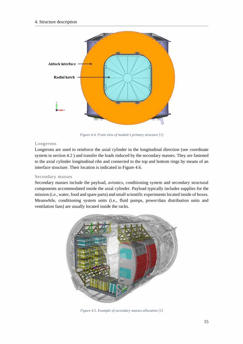
Figure 4.4. Front view of module's primary structure [1]
Longerons
Longerons are used to reinforce the axial cylinder in the longitudinal direction (see coordinate
system in section 4.2 ) and transfer the loads induced by the secondary masses. They are fastened
to the axial cylinder longitudinal ribs and connected to the top and bottom rings by means of an
interface structure. Their location is indicated in Figure 4.6.
Secondary masses
Secondary masses include the payload, avionics, conditioning system and secondary structural
components accommodated inside the axial cylinder. Payload typically includes supplies for the
mission (i.e., water, food and spare parts) and small scientific experiments located inside of boxes.
Meanwhile, conditioning system units (i.e., fluid pumps, power/data distribution units and
ventilation fans) are usually located inside the racks.
Figure 4.5. Example of secondary masses allocation [1]
4. Structure description
16
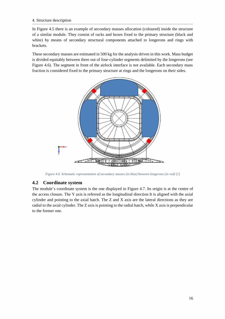
In Figure 4.5 there is an example of secondary masses allocation (coloured) inside the structure
of a similar module. They consist of racks and boxes fixed to the primary structure (black and
white) by means of secondary structural components attached to longerons and rings with
brackets.
These secondary masses are estimated in 500 kg for the analysis driven in this work. Mass budget
is divided equitably between three out of four-cylinder segments delimited by the longerons (see
Figure 4.6). The segment in front of the airlock interface is not available. Each secondary mass
fraction is considered fixed to the primary structure at rings and the longerons on their sides.
Figure 4.6. Schematic representation of secondary masses (in blue) between longerons (in red) [1]
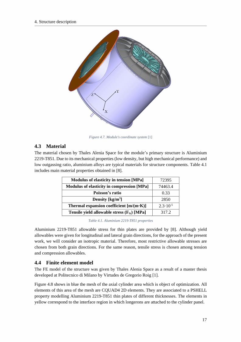
4.2 Coordinate system
The module’s coordinate system is the one displayed in Figure 4.7. Its origin is at the centre of
the access closure. The Y axis is referred as the longitudinal direction It is aligned with the axial
cylinder and pointing to the axial hatch. The Z and X axis are the lateral directions as they are
radial to the axial cylinder. The Z axis is pointing to the radial hatch, while X axis is perpendicular
to the former one.
4. Structure description
17
Figure 4.7. Module's coordinate system [1]
4.3 Material
The material chosen by Thales Alenia Space for the module’s primary structure is Aluminium
2219-T851. Due to its mechanical properties (low density, but high mechanical performance) and
low outgassing ratio, aluminium alloys are typical materials for structure components. Table 4.1
includes main material properties obtained in [8].
Modulus of elasticity in tension [MPa] 72395
Modulus of elasticity in compression [MPa] 74463.4
Poisson’s ratio 0.33
Density [kg/m3] 2850
Thermal expansion coefficient [m/(m·K)] 2.3·10-5
Tensile yield allowable stress (Fty) [MPa] 317.2
Table 4.1. Aluminium 2219-T851 properties
Aluminium 2219-T851 allowable stress for thin plates are provided by [8]. Although yield
allowables were given for longitudinal and lateral grain directions, for the approach of the present
work, we will consider an isotropic material. Therefore, most restrictive allowable stresses are
chosen from both grain directions. For the same reason, tensile stress is chosen among tension
and compression allowables.
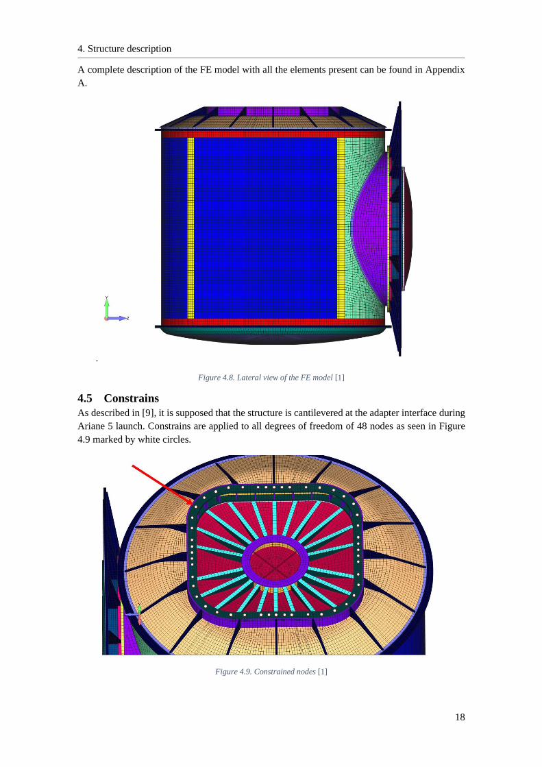
4.4 Finite element model
The FE model of the structure was given by Thales Alenia Space as a result of a master thesis
developed at Politecnico di Milano by Virtudes de Gregorio Roig [1].
Figure 4.8 shows in blue the mesh of the axial cylinder area which is object of optimization. All
elements of this area of the mesh are CQUAD4 2D elements. They are associated to a PSHELL
property modelling Aluminium 2219-T851 thin plates of different thicknesses. The elements in
yellow correspond to the interface region in which longerons are attached to the cylinder panel.
4. Structure description
18
A complete description of the FE model with all the elements present can be found in Appendix
A.
.
Figure 4.8. Lateral view of the FE model [1]
4.5 Constrains
As described in [9], it is supposed that the structure is cantilevered at the adapter interface during
Ariane 5 launch. Constrains are applied to all degrees of freedom of 48 nodes as seen in Figure
4.9 marked by white circles.
Figure 4.9. Constrained nodes [1]
5. Mechanical requirements and failure modes
19
5 Mechanical requirements and failure modes Along this section, mechanical requirements to be fulfilled by the structure are exposed. For the
scope of this work, failure modes to be checked are yield strength, axial cylinder global buckling
and resonance. The requirements definition is done in accordance with [10] standards.
5.1 Limit Loads
The Limit Loads are the maximum loads a structure is expected to experience with a given
probability, during the performance of specified missions in specified environments [10]. Even
though these loads could be static or dynamic, only static accelerations and operative maximum
pressure will be considered in the present work.
5.1.1 Quasi-Static Limit Loads
A quasi-static load is independent of time or it varies slowly, so that the dynamic response of the
structure is not significant. The Quasi-Static Limit Loads correspond to the most restrictive
combination of static and dynamic accelerations that can be encountered at any instant of the
mission (ground and flight operations) [9]. For this purpose, it was supposed that Ariane 5
launcher would be used. Nevertheless, this optimization study can be adapted to any launcher.
The Quasi-Static Limit Loads for a spacecraft launched on Ariane 5 provided by [9] are shown in
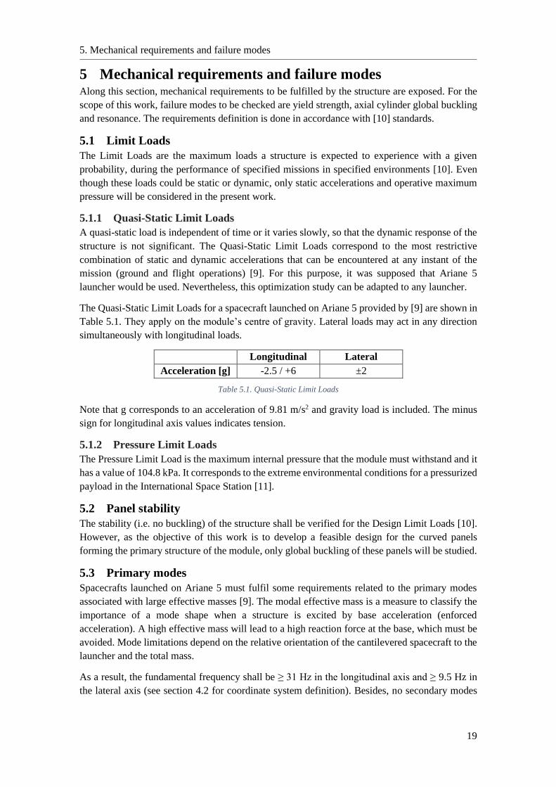
Table 5.1. They apply on the module’s centre of gravity. Lateral loads may act in any direction
simultaneously with longitudinal loads.
Longitudinal Lateral
Acceleration [g] -2.5 / +6 ±2
Table 5.1. Quasi-Static Limit Loads
Note that g corresponds to an acceleration of 9.81 m/s2 and gravity load is included. The minus
sign for longitudinal axis values indicates tension.
5.1.2 Pressure Limit Loads
The Pressure Limit Load is the maximum internal pressure that the module must withstand and it
has a value of 104.8 kPa. It corresponds to the extreme environmental conditions for a pressurized
payload in the International Space Station [11].
5.2 Panel stability
The stability (i.e. no buckling) of the structure shall be verified for the Design Limit Loads [10].
However, as the objective of this work is to develop a feasible design for the curved panels
forming the primary structure of the module, only global buckling of these panels will be studied.
5.3 Primary modes
Spacecrafts launched on Ariane 5 must fulfil some requirements related to the primary modes
associated with large effective masses [9]. The modal effective mass is a measure to classify the
importance of a mode shape when a structure is excited by base acceleration (enforced
acceleration). A high effective mass will lead to a high reaction force at the base, which must be
avoided. Mode limitations depend on the relative orientation of the cantilevered spacecraft to the
launcher and the total mass.
As a result, the fundamental frequency shall be ≥ 31 Hz in the longitudinal axis and ≥ 9.5 Hz in
the lateral axis (see section 4.2 for coordinate system definition). Besides, no secondary modes
5. Mechanical requirements and failure modes
20
should be lower than the first primary mode. For this work, total mass of the module is supposed
to be lower than 4500 kg.
5.4 Subcases
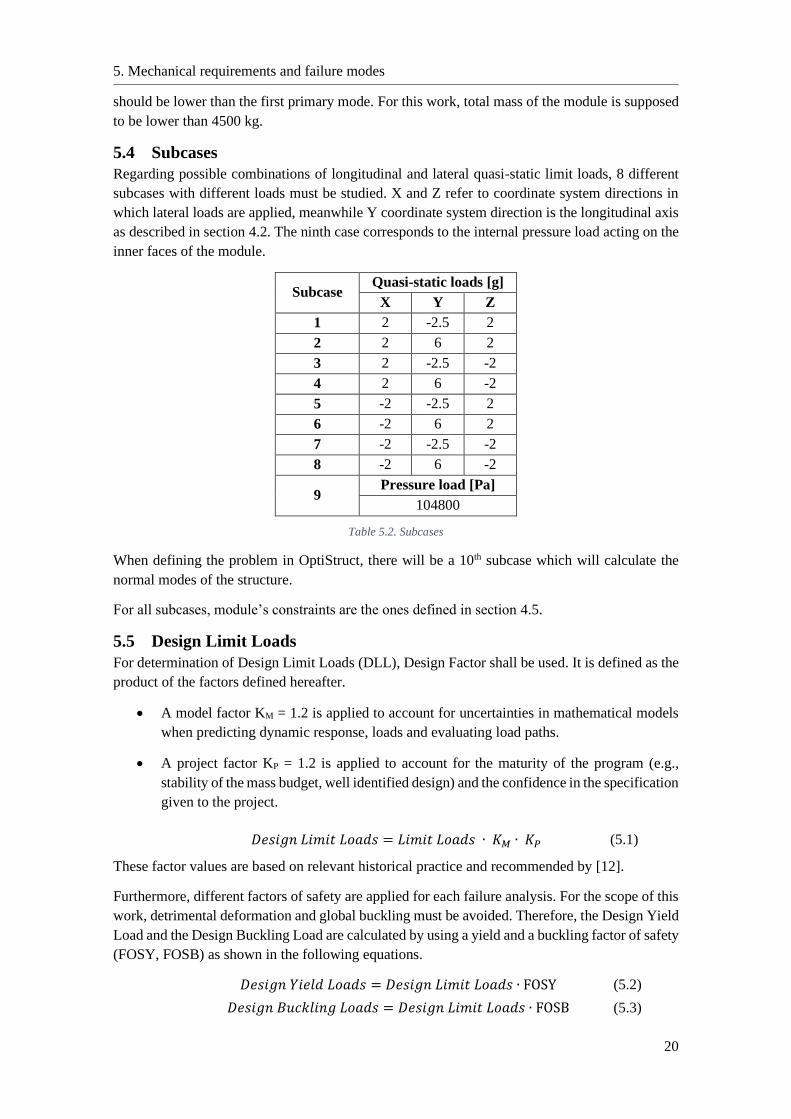
Regarding possible combinations of longitudinal and lateral quasi-static limit loads, 8 different
subcases with different loads must be studied. X and Z refer to coordinate system directions in
which lateral loads are applied, meanwhile Y coordinate system direction is the longitudinal axis
as described in section 4.2. The ninth case corresponds to the internal pressure load acting on the
inner faces of the module.
Subcase Quasi-static loads [g]
X Y Z
1 2 -2.5 2
2 2 6 2
3 2 -2.5 -2
4 2 6 -2
5 -2 -2.5 2
6 -2 6 2
7 -2 -2.5 -2
8 -2 6 -2
9 Pressure load [Pa]
104800
Table 5.2. Subcases
When defining the problem in OptiStruct, there will be a 10th subcase which will calculate the
normal modes of the structure.
For all subcases, module’s constraints are the ones defined in section 4.5.
5.5 Design Limit Loads
For determination of Design Limit Loads (DLL), Design Factor shall be used. It is defined as the
product of the factors defined hereafter.
• A model factor KM = 1.2 is applied to account for uncertainties in mathematical models
when predicting dynamic response, loads and evaluating load paths.
• A project factor KP = 1.2 is applied to account for the maturity of the program (e.g.,
stability of the mass budget, well identified design) and the confidence in the specification
given to the project.
𝐷𝑒𝑠𝑖𝑔𝑛 𝐿𝑖𝑚𝑖𝑡 𝐿𝑜𝑎𝑑𝑠 = 𝐿𝑖𝑚𝑖𝑡 𝐿𝑜𝑎𝑑𝑠 ∙ 𝐾𝑀 ∙ 𝐾𝑃 (5.1)
These factor values are based on relevant historical practice and recommended by [12].
Furthermore, different factors of safety are applied for each failure analysis. For the scope of this
work, detrimental deformation and global buckling must be avoided. Therefore, the Design Yield
Load and the Design Buckling Load are calculated by using a yield and a buckling factor of safety
(FOSY, FOSB) as shown in the following equations.
𝐷𝑒𝑠𝑖𝑔𝑛 𝑌𝑖𝑒𝑙𝑑 𝐿𝑜𝑎𝑑𝑠 = 𝐷𝑒𝑠𝑖𝑔𝑛 𝐿𝑖𝑚𝑖𝑡 𝐿𝑜𝑎𝑑𝑠 ∙ FOSY (5.2)
𝐷𝑒𝑠𝑖𝑔𝑛 𝐵𝑢𝑐𝑘𝑙𝑖𝑛𝑔 𝐿𝑜𝑎𝑑𝑠 = 𝐷𝑒𝑠𝑖𝑔𝑛 𝐿𝑖𝑚𝑖𝑡 𝐿𝑜𝑎𝑑𝑠 ∙ FOSB (5.3)
5. Mechanical requirements and failure modes
21
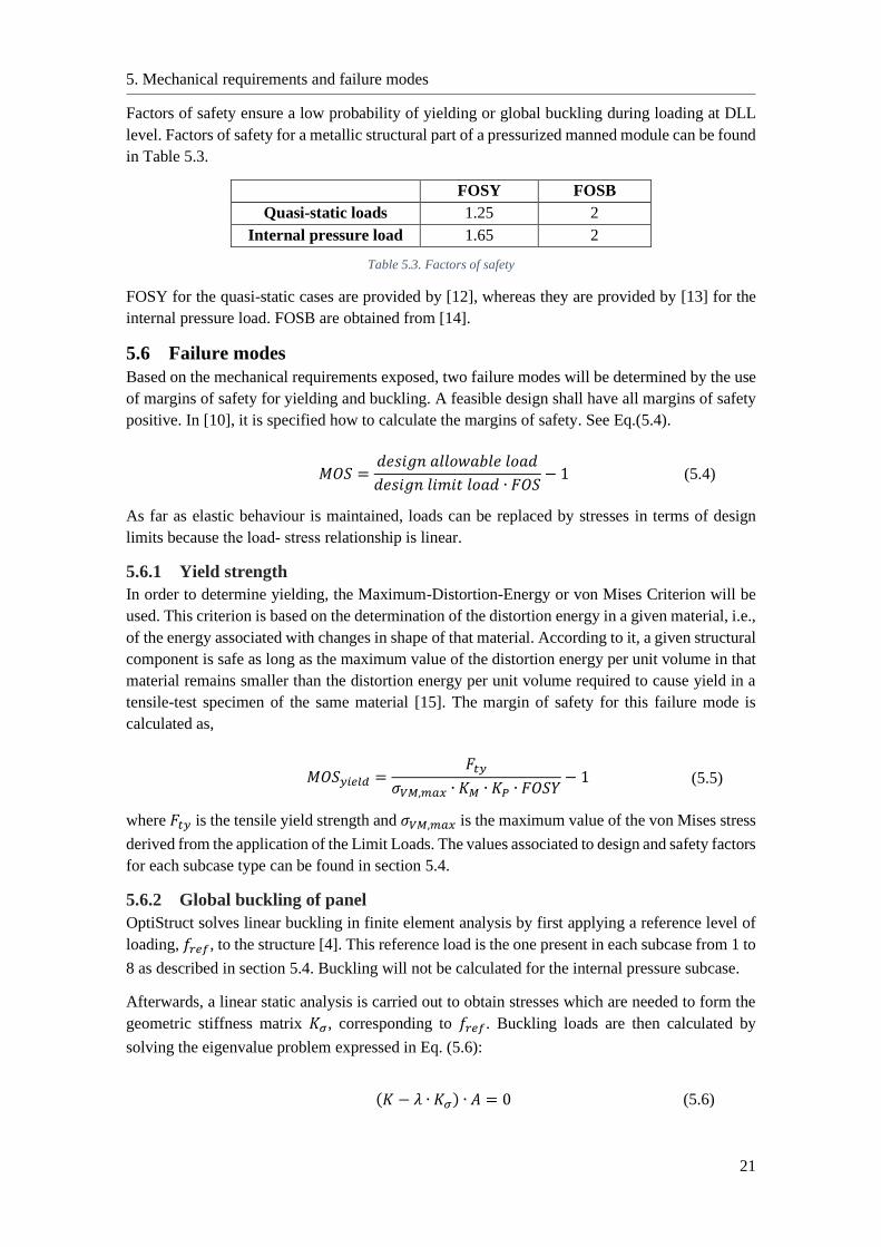
Factors of safety ensure a low probability of yielding or global buckling during loading at DLL
level. Factors of safety for a metallic structural part of a pressurized manned module can be found
in Table 5.3.
FOSY FOSB
Quasi-static loads 1.25 2
Internal pressure load 1.65 2
Table 5.3. Factors of safety
FOSY for the quasi-static cases are provided by [12], whereas they are provided by [13] for the
internal pressure load. FOSB are obtained from [14].
5.6 Failure modes
Based on the mechanical requirements exposed, two failure modes will be determined by the use
of margins of safety for yielding and buckling. A feasible design shall have all margins of safety
positive. In [10], it is specified how to calculate the margins of safety. See Eq.(5.4).
𝑀𝑂𝑆 =𝑑𝑒𝑠𝑖𝑔𝑛 𝑎𝑙𝑙𝑜𝑤𝑎𝑏𝑙𝑒 𝑙𝑜𝑎𝑑
𝑑𝑒𝑠𝑖𝑔𝑛 𝑙𝑖𝑚𝑖𝑡 𝑙𝑜𝑎𝑑 ∙ 𝐹𝑂𝑆− 1 (5.4)
As far as elastic behaviour is maintained, loads can be replaced by stresses in terms of design
limits because the load‐ stress relationship is linear.
5.6.1 Yield strength
In order to determine yielding, the Maximum-Distortion-Energy or von Mises Criterion will be
used. This criterion is based on the determination of the distortion energy in a given material, i.e.,
of the energy associated with changes in shape of that material. According to it, a given structural
component is safe as long as the maximum value of the distortion energy per unit volume in that
material remains smaller than the distortion energy per unit volume required to cause yield in a
tensile-test specimen of the same material [15]. The margin of safety for this failure mode is
calculated as,
𝑀𝑂𝑆𝑦𝑖𝑒𝑙𝑑 =𝐹𝑡𝑦
𝜎𝑉𝑀,𝑚𝑎𝑥 ∙ 𝐾𝑀 ∙ 𝐾𝑃 ∙ 𝐹𝑂𝑆𝑌− 1 (5.5)
where 𝐹𝑡𝑦 is the tensile yield strength and 𝜎𝑉𝑀,𝑚𝑎𝑥 is the maximum value of the von Mises stress
derived from the application of the Limit Loads. The values associated to design and safety factors
for each subcase type can be found in section 5.4.
5.6.2 Global buckling of panel
OptiStruct solves linear buckling in finite element analysis by first applying a reference level of
loading, 𝑓𝑟𝑒𝑓, to the structure [4]. This reference load is the one present in each subcase from 1 to
8 as described in section 5.4. Buckling will not be calculated for the internal pressure subcase.
Afterwards, a linear static analysis is carried out to obtain stresses which are needed to form the
geometric stiffness matrix 𝐾𝜎, corresponding to 𝑓𝑟𝑒𝑓. Buckling loads are then calculated by
solving the eigenvalue problem expressed in Eq. (5.6):
(𝐾 − 𝜆 ∙ 𝐾𝜎) ∙ 𝐴 = 0 (5.6)
5. Mechanical requirements and failure modes
22
where 𝐾, is the stiffness matrix of the structure and 𝜆, the eigenvalue, is the multiplier to the
reference load. The vector 𝐴 is the eigenvector corresponding to the eigenvalue.
In order to solve the eigenvalue problem, a matrix method called the Lanczos method is used,
where not all eigenvalues are required. Only a small number of the lowest eigenvalues are
normally calculated for buckling analysis.
The lowest eigenvalue 𝜆𝛼, also called the minimum buckling factor, is associated with buckling.
The critical or buckling load is:
𝑓𝛼 = 𝜆𝛼 ∙ 𝑓𝑟𝑒𝑓 (5.7)
A typical buckling constraint is a lower bound of 1.0 for the buckling factor, indicating that the
structure is not to buckle with the given static load (𝑓𝑟𝑒𝑓). OptiStruct recommends to constrain
the buckling factor for several of the lower modes, not just of the first mode. For the scope of this
work first 5 modes will be checked.
Knock down factor
Experience has shown that large discrepancies often occur between theoretic shell stability
analysis and its results from experiments. Empirical knock-down factors (KDF) are recommended
by buckling design guidelines, like [14] and [16]. They are intended to compensate those
differences mainly caused by geometrical imperfections, residual stresses and pre-buckling
deformations.
NASA SP-8007 [16] is a widely used reference for computing knock-down factors for cylindrical
thin walls, depending on the radius cylinder (𝑅) and wall thickness (𝑡) ratio. They are calculated
following Eq. (5.8)
𝛾 = 1 − 0.901𝛼 ∙ (1 − 𝑒−𝜙) (5.8)
where,
𝜙 =1
16∙ √
𝑅
𝑡 𝑓𝑜𝑟
𝑅
𝑡< 1500 (5.9)
If the knock-down factor is multiplied by the buckling load, then it is obtained a lower bound for
considered experimental data. That is the reason why this function is part of the Lower Bound
Design Philosophy [14].
Even though [14] considers [16] functions conservative, this method does not require knowledge
about pattern or even amplitude of imperfection, which are very costly to measure and introduce
in analyses. Besides, it must be considered that knock-down factors in [16] correspond to
complete cylinder panels, while the case of study is a cylinder covering only 79º of circumference.
However, as part of a preliminary design of the structure and to check OptiStruct capabilities,
method suggested in [16] is sufficient.
It possible to multiply that 1 by the knock down factor, which varies with thickness.
Finally, if knock-down factor is multiplied by the buckling load, according to Eq. (5.4), the margin
of safety is computed using the following equations:
5. Mechanical requirements and failure modes
23
𝑀𝑂𝑆𝑏𝑢𝑐𝑘 =𝛾 ∙ 𝑓𝛼
𝑓𝑟𝑒𝑓 ∙ 𝐾𝑀 ∙ 𝐾𝑃 ∙ 𝐹𝑂𝑆𝐵− 1 =
𝛾 ∙ 𝜆𝛼
𝐾𝑀 ∙ 𝐾𝑃 ∙ 𝐹𝑂𝑆𝐵− 1 (5.10)
5.6.3 Primary modes
As far as the fundamental frequencies of the panel/module are higher than the limits established
for longitudinal and lateral axis in section 5.3 taking into account the effective mass associated,
failure will be avoided
6. Preliminary analyses
24
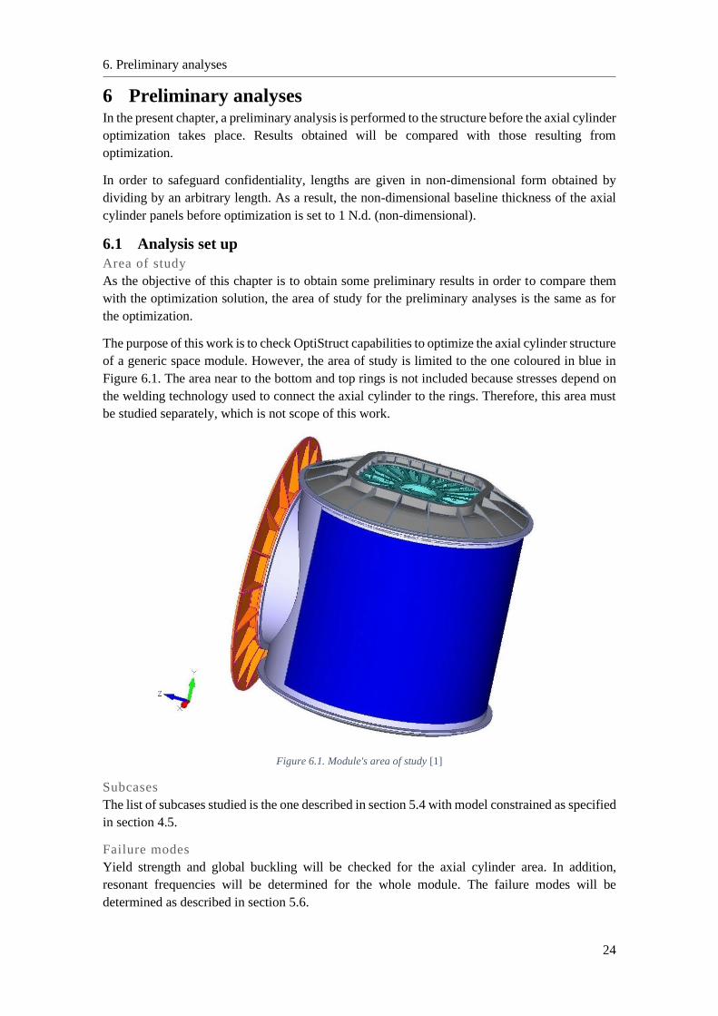
6 Preliminary analyses In the present chapter, a preliminary analysis is performed to the structure before the axial cylinder
optimization takes place. Results obtained will be compared with those resulting from
optimization.
In order to safeguard confidentiality, lengths are given in non-dimensional form obtained by
dividing by an arbitrary length. As a result, the non-dimensional baseline thickness of the axial
cylinder panels before optimization is set to 1 N.d. (non-dimensional).
6.1 Analysis set up
Area of study
As the objective of this chapter is to obtain some preliminary results in order to compare them
with the optimization solution, the area of study for the preliminary analyses is the same as for
the optimization.
The purpose of this work is to check OptiStruct capabilities to optimize the axial cylinder structure
of a generic space module. However, the area of study is limited to the one coloured in blue in
Figure 6.1. The area near to the bottom and top rings is not included because stresses depend on
the welding technology used to connect the axial cylinder to the rings. Therefore, this area must
be studied separately, which is not scope of this work.
Figure 6.1. Module's area of study [1]
Subcases
The list of subcases studied is the one described in section 5.4 with model constrained as specified
in section 4.5.
Failure modes
Yield strength and global buckling will be checked for the axial cylinder area. In addition,
resonant frequencies will be determined for the whole module. The failure modes will be
determined as described in section 5.6.
6. Preliminary analyses
25
It is recalled that FOSY has different values for quasi-static (subcases 1-8) and pressure loads
(subcase 9).
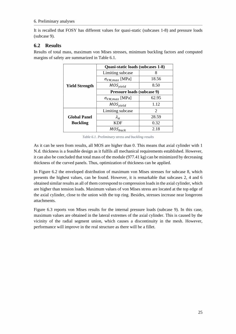
6.2 Results
Results of total mass, maximum von Mises stresses, minimum buckling factors and computed
margins of safety are summarized in Table 6.1.
Yield Strength
Quasi-static loads (subcases 1-8)
Limiting subcase 8
𝜎𝑉𝑀,𝑚𝑎𝑥 [MPa] 18.56
𝑀𝑂𝑆𝑦𝑖𝑒𝑙𝑑 8.50
Pressure loads (subcase 9)
𝜎𝑉𝑀,𝑚𝑎𝑥 [MPa] 62.95
𝑀𝑂𝑆𝑦𝑖𝑒𝑙𝑑 1.12
Global Panel
Buckling
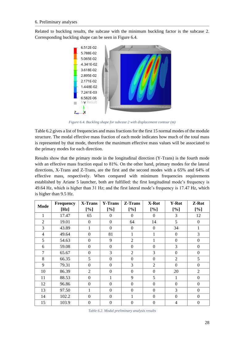
Limiting subcase 2
𝜆𝛼 28.59
KDF 0.32
𝑀𝑂𝑆𝑏𝑢𝑐𝑘 2.18
Table 6.1. Preliminary stress and buckling results
As it can be seen from results, all MOS are higher than 0. This means that axial cylinder with 1
N.d. thickness is a feasible design as it fulfils all mechanical requirements established. However,
it can also be concluded that total mass of the module (977.41 kg) can be minimized by decreasing
thickness of the curved panels. Thus, optimization of thickness can be applied.
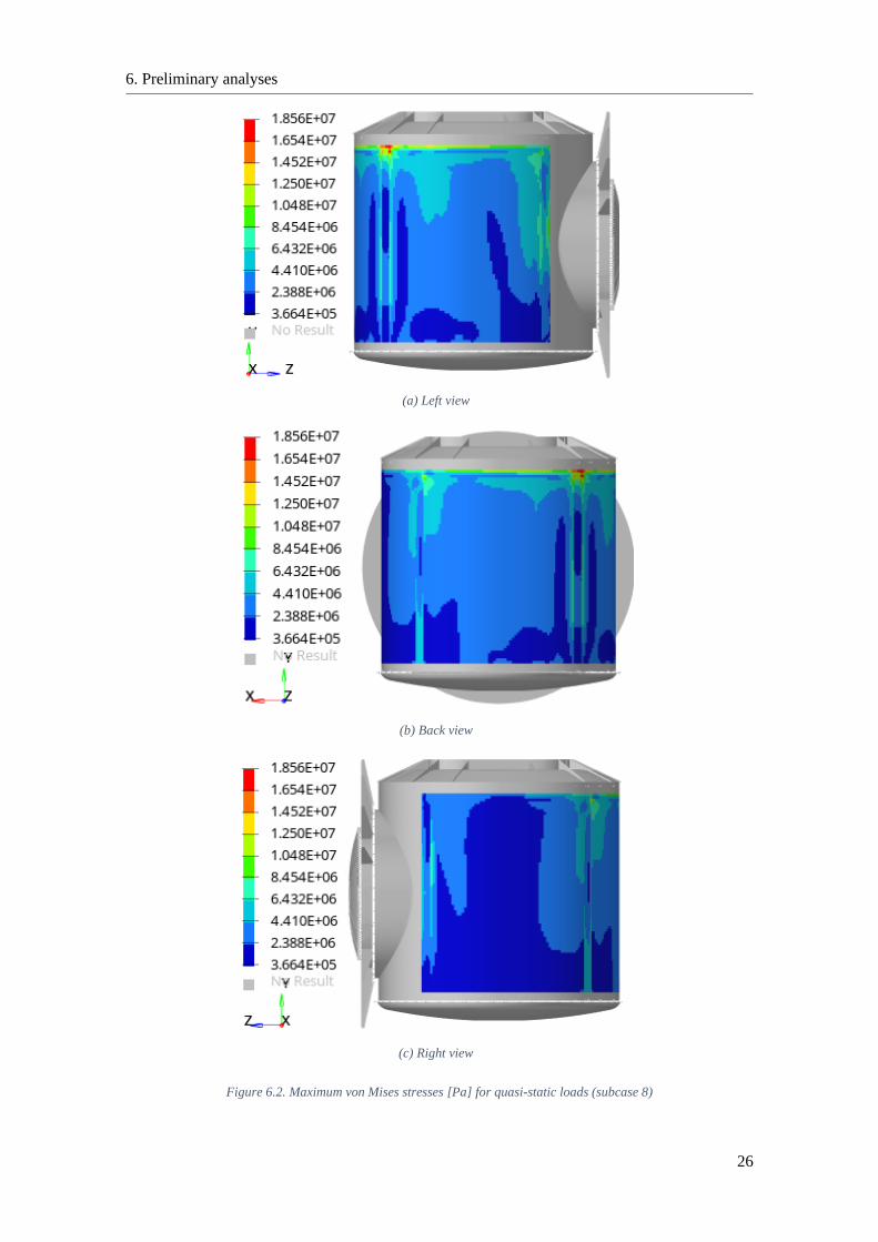
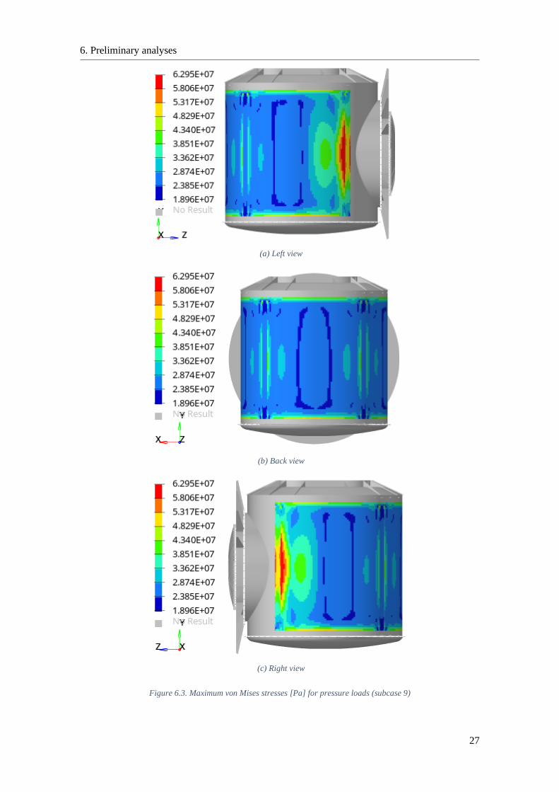
In Figure 6.2 the enveloped distribution of maximum von Mises stresses for subcase 8, which
presents the highest values, can be found. However, it is remarkable that subcases 2, 4 and 6
obtained similar results as all of them correspond to compression loads in the axial cylinder, which
are higher than tension loads. Maximum values of von Mises stress are located at the top edge of
the axial cylinder, close to the union with the top ring. Besides, stresses increase near longerons
attachments.
Figure 6.3 reports von Mises results for the internal pressure loads (subcase 9). In this case,
maximum values are obtained in the lateral extremes of the axial cylinder. This is caused by the
vicinity of the radial segment union, which causes a discontinuity in the mesh. However,
performance will improve in the real structure as there will be a fillet.
6. Preliminary analyses
26
(a) Left view
(b) Back view
(c) Right view
Figure 6.2. Maximum von Mises stresses [Pa] for quasi-static loads (subcase 8)
6. Preliminary analyses
27
(a) Left view
(b) Back view
(c) Right view
Figure 6.3. Maximum von Mises stresses [Pa] for pressure loads (subcase 9)
6. Preliminary analyses
28
Related to buckling results, the subcase with the minimum buckling factor is the subcase 2.
Corresponding buckling shape can be seen in Figure 6.4.
Figure 6.4. Buckling shape for subcase 2 with displacement contour (m)
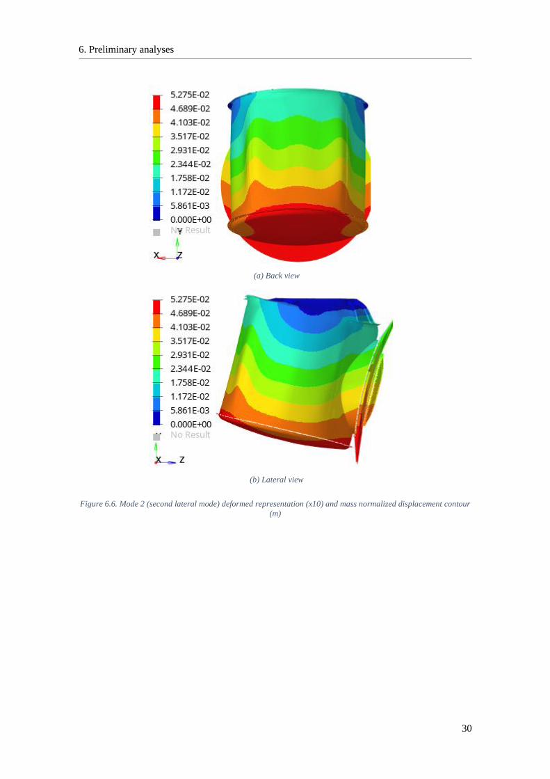
Table 6.2 gives a list of frequencies and mass fractions for the first 15 normal modes of the module
structure. The modal effective mass fraction of each mode indicates how much of the total mass
is represented by that mode, therefore the maximum effective mass values will be associated to
the primary modes for each direction.
Results show that the primary mode in the longitudinal direction (Y-Trans) is the fourth mode
with an effective mass fraction equal to 81%. On the other hand, primary modes for the lateral
directions, X-Trans and Z-Trans, are the first and the second modes with a 65% and 64% of
effective mass, respectively. When compared with minimum frequencies requirements
established by Ariane 5 launcher, both are fulfilled: the first longitudinal mode’s frequency is
49.64 Hz, which is higher than 31 Hz; and the first lateral mode’s frequency is 17.47 Hz, which
is higher than 9.5 Hz.
Mode Frequency
[Hz]
X-Trans
[%]
Y-Trans
[%]
Z-Trans
[%]
X-Rot
[%]
Y-Rot
[%]
Z-Rot
[%]
1 17.47 65 0 0 0 3 12
2 19.01 0 0 64 14 5 0
3 43.89 1 0 0 0 34 1
4 49.64 0 81 1 1 0 3
5 54.63 0 9 2 1 0 0
6 59.08 0 0 0 0 3 0
7 65.67 0 3 2 3 0 0
8 66.35 5 0 0 0 2 5
9 79.31 0 0 3 2 0 0
10 86.39 2 0 0 0 20 2
11 88.53 0 1 9 5 1 0
12 96.86 0 0 0 0 0 0
13 97.50 1 0 0 0 3 0
14 102.2 0 0 1 0 0 0
15 103.9 0 0 0 0 4 0
Table 6.2. Modal preliminary analysis results
6. Preliminary analyses
29
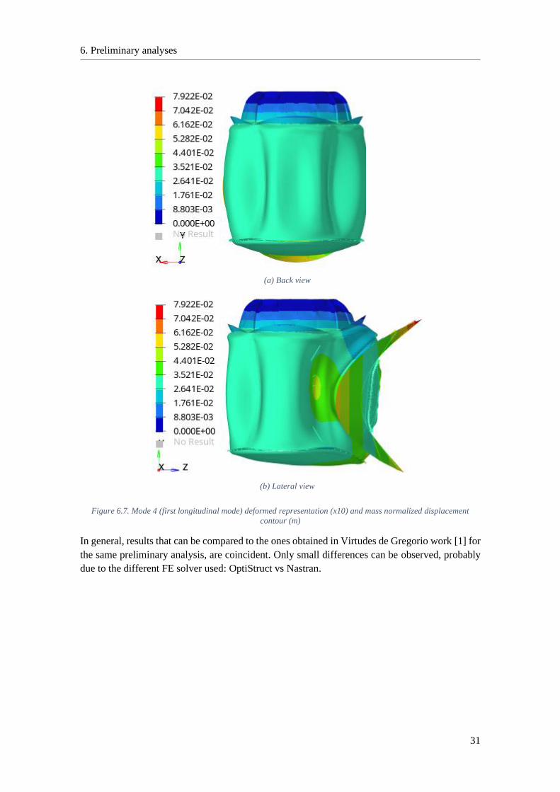
In Figure 6.5, Figure 6.6, Figure 6.7, modal shapes corresponding to the primary lateral and
longitudinal modes, respectively, are shown.
(a) Back view
(b) Lateral view
Figure 6.5. Mode 1 (first lateral mode) deformed representation (x10) and mass normalized displacement contour
(m)
6. Preliminary analyses
30
(a) Back view
(b) Lateral view
Figure 6.6. Mode 2 (second lateral mode) deformed representation (x10) and mass normalized displacement contour
(m)
6. Preliminary analyses
31
(a) Back view
(b) Lateral view
Figure 6.7. Mode 4 (first longitudinal mode) deformed representation (x10) and mass normalized displacement
contour (m)
In general, results that can be compared to the ones obtained in Virtudes de Gregorio work [1] for
the same preliminary analysis, are coincident. Only small differences can be observed, probably
due to the different FE solver used: OptiStruct vs Nastran.
7. Optimization of an unstiffened curved panel
32
7 Optimization of an unstiffened curved panel In the present chapter, optimization of the panel thickness for the curved panel of the axial
cylinder is developed and compared with results obtained in the preliminary analyses and in
Virtudes de Gregorio master thesis [1]. For this process, free-size optimization will be performed.
7.1 Optimization set up
Optimization model
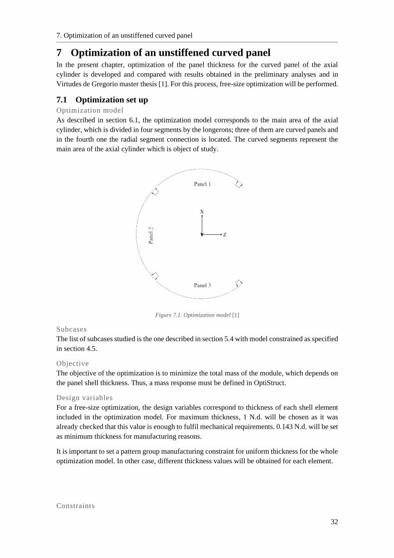
As described in section 6.1, the optimization model corresponds to the main area of the axial
cylinder, which is divided in four segments by the longerons; three of them are curved panels and
in the fourth one the radial segment connection is located. The curved segments represent the
main area of the axial cylinder which is object of study.
Figure 7.1. Optimization model [1]
Subcases
The list of subcases studied is the one described in section 5.4 with model constrained as specified
in section 4.5.
Objective
The objective of the optimization is to minimize the total mass of the module, which depends on
the panel shell thickness. Thus, a mass response must be defined in OptiStruct.
Design variables
For a free-size optimization, the design variables correspond to thickness of each shell element
included in the optimization model. For maximum thickness, 1 N.d. will be chosen as it was
already checked that this value is enough to fulfil mechanical requirements. 0.143 N.d. will be set
as minimum thickness for manufacturing reasons.
It is important to set a pattern group manufacturing constraint for uniform thickness for the whole
optimization model. In other case, different thickness values will be obtained for each element.
Constraints
7. Optimization of an unstiffened curved panel
33
In order to check yield strength and global buckling failure modes, two responses will be defined:
one for von Mises static stress and another one for buckling. To introduce maximum and
minimum constraints, it is necessary to calculate values for which each response will have at least
MOS = 0. It is recalled that FOSY has different values for quasi-static (subcases 1-8) and pressure
loads (subcase 9). Taking into account FOS, design factors and KDF, limit values for these
responses are:
• For von Mises constraint, upper boundaries are 176.22 MPa for subcases 1-8 and 133.50
MPa for subcase 9. If stresses go higher than these values, yielding will occur.
• For buckling constraint, lower boundary is 9.80. OptiStruct does not have the option to
update the KDF with each iteration, therefore an initial value is supposed (0.857 N.d.)
based on optimized thickness resulted for the same module obtained by Virtudes de
Gregorio [1], which corresponds to a KDF equal to 0.294.
If optimized thickness is not the same as the one obtained in [1], optimization will be
repeated with the updated KDF.
7.2 Results
After three iterations updating the KDF based on the thickness, the final optimized shell thickness
got 0.643 N.d. The final KDF used corresponds to previous iteration with a value of 0.256. This
iterative process stopped when values were differing less than 0.05 mm.
Optimized total mass corresponds to 955.57 kg. It means that 21.84 kg (2.23% of primary
structure mass) can be saved by minimizing panel thickness for the optimization area.
Each optimization process took around 51 minutes of computing time.
Buckling analyses
Buckling is the controlling failure mode, i.e., the one that gives lower MOS. The most critical
load cases correspond to the compression loads in the longitudinal axis which are larger than the
tension ones; the subcase 2 (2g X, 6g Y, 2g Z) and the subcase 6 (-2g X, 6g Y, 2g Z).
In Table 7.1 results for the buckling analysis are shown. As it was mentioned, buckling was the
controlling failure mode during optimization, therefore its MOS reaches zero; which is the limit
imposed for avoiding buckling taking into account FOS, KDF and design factors. When compared
with previous values obtained for the baseline model, it can be seen that the limiting subcase is
still the same, but MOS is reduced to the extreme.
Optimized model Baseline model
Limiting subcase 2 2
𝜆𝛼 11.25 28.59
KDF 0.256 0.32
𝑴𝑶𝑺𝒃𝒖𝒄𝒌 0 2.18
Table 7.1. Buckling analysis results for optimized and baseline models
See Figure 7.2 for the optimized buckling shape. In general, buckling shapes are similar to the
ones obtained in the preliminary analysis (Figure 6.4).
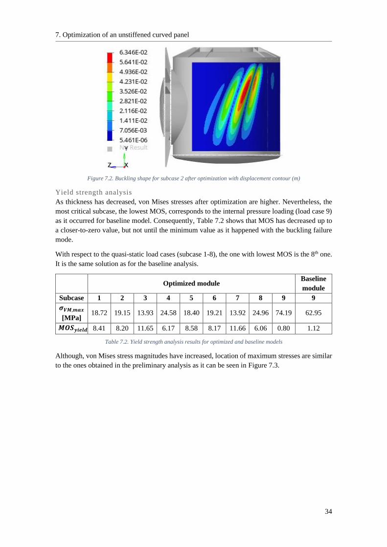
7. Optimization of an unstiffened curved panel
34
Figure 7.2. Buckling shape for subcase 2 after optimization with displacement contour (m)
Yield strength analysis
As thickness has decreased, von Mises stresses after optimization are higher. Nevertheless, the
most critical subcase, the lowest MOS, corresponds to the internal pressure loading (load case 9)
as it occurred for baseline model. Consequently, Table 7.2 shows that MOS has decreased up to
a closer-to-zero value, but not until the minimum value as it happened with the buckling failure
mode.
With respect to the quasi-static load cases (subcase 1-8), the one with lowest MOS is the 8th one.
It is the same solution as for the baseline analysis.
Optimized module Baseline
module
Subcase 1 2 3 4 5 6 7 8 9 9
𝝈𝑽𝑴,𝒎𝒂𝒙
[MPa] 18.72 19.15 13.93 24.58 18.40 19.21 13.92 24.96 74.19 62.95
𝑴𝑶𝑺𝒚𝒊𝒆𝒍𝒅 8.41 8.20 11.65 6.17 8.58 8.17 11.66 6.06 0.80 1.12
Table 7.2. Yield strength analysis results for optimized and baseline models
Although, von Mises stress magnitudes have increased, location of maximum stresses are similar
to the ones obtained in the preliminary analysis as it can be seen in Figure 7.3.
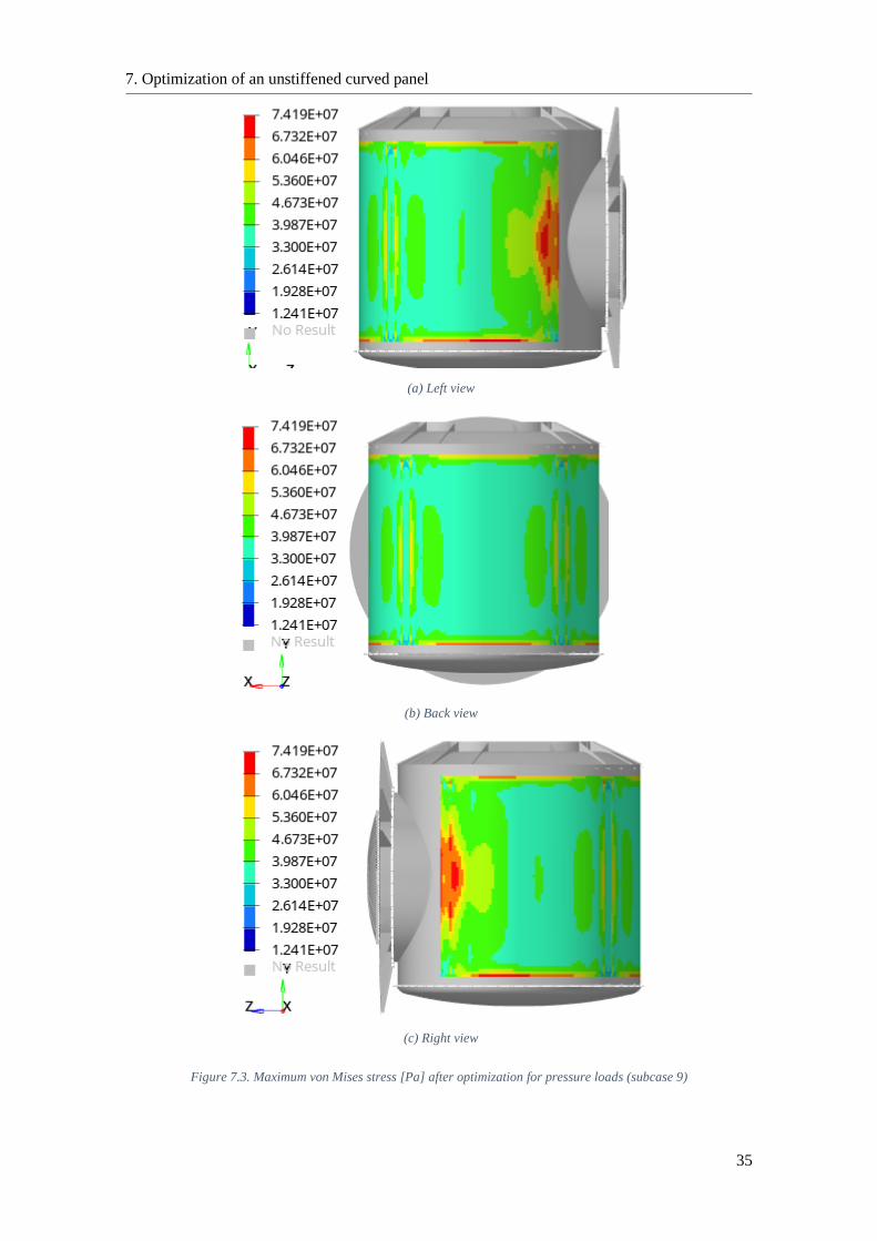
7. Optimization of an unstiffened curved panel
35
(a) Left view
(b) Back view
(c) Right view
Figure 7.3. Maximum von Mises stress [Pa] after optimization for pressure loads (subcase 9)
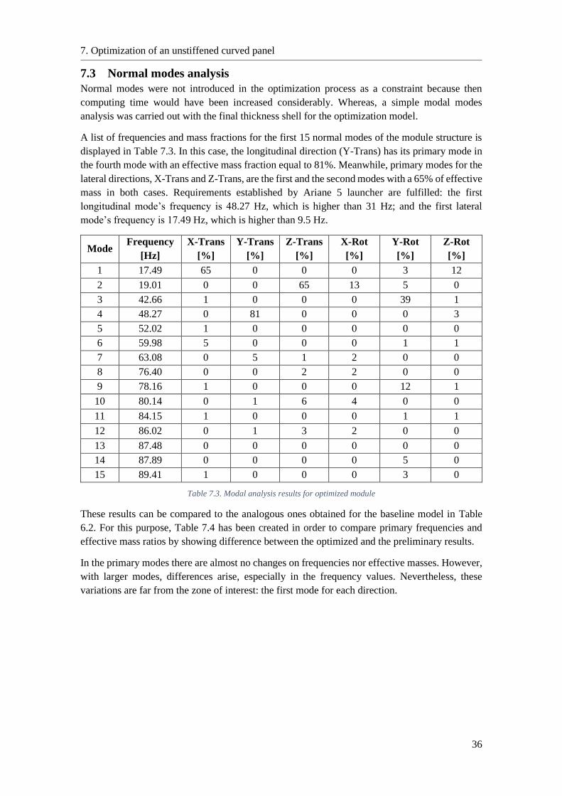
7. Optimization of an unstiffened curved panel
36
7.3 Normal modes analysis
Normal modes were not introduced in the optimization process as a constraint because then
computing time would have been increased considerably. Whereas, a simple modal modes
analysis was carried out with the final thickness shell for the optimization model.
A list of frequencies and mass fractions for the first 15 normal modes of the module structure is
displayed in Table 7.3. In this case, the longitudinal direction (Y-Trans) has its primary mode in
the fourth mode with an effective mass fraction equal to 81%. Meanwhile, primary modes for the
lateral directions, X-Trans and Z-Trans, are the first and the second modes with a 65% of effective
mass in both cases. Requirements established by Ariane 5 launcher are fulfilled: the first
longitudinal mode’s frequency is 48.27 Hz, which is higher than 31 Hz; and the first lateral
mode’s frequency is 17.49 Hz, which is higher than 9.5 Hz.
Mode Frequency
[Hz]
X-Trans
[%]
Y-Trans
[%]
Z-Trans
[%]
X-Rot
[%]
Y-Rot
[%]
Z-Rot
[%]
1 17.49 65 0 0 0 3 12
2 19.01 0 0 65 13 5 0
3 42.66 1 0 0 0 39 1
4 48.27 0 81 0 0 0 3
5 52.02 1 0 0 0 0 0
6 59.98 5 0 0 0 1 1
7 63.08 0 5 1 2 0 0
8 76.40 0 0 2 2 0 0
9 78.16 1 0 0 0 12 1
10 80.14 0 1 6 4 0 0
11 84.15 1 0 0 0 1 1
12 86.02 0 1 3 2 0 0
13 87.48 0 0 0 0 0 0
14 87.89 0 0 0 0 5 0
15 89.41 1 0 0 0 3 0
Table 7.3. Modal analysis results for optimized module
These results can be compared to the analogous ones obtained for the baseline model in Table
6.2. For this purpose, Table 7.4 has been created in order to compare primary frequencies and
effective mass ratios by showing difference between the optimized and the preliminary results.
In the primary modes there are almost no changes on frequencies nor effective masses. However,
with larger modes, differences arise, especially in the frequency values. Nevertheless, these
variations are far from the zone of interest: the first mode for each direction.
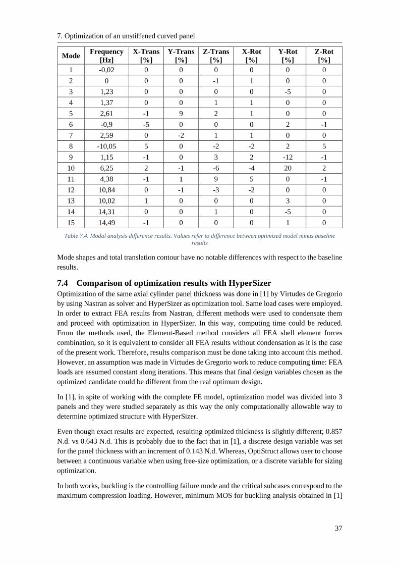
7. Optimization of an unstiffened curved panel
37
Mode Frequency
[Hz]
X-Trans
[%]
Y-Trans
[%]
Z-Trans
[%]
X-Rot
[%]
Y-Rot
[%]
Z-Rot
[%]
1 -0,02 0 0 0 0 0 0
2 0 0 0 -1 1 0 0
3 1,23 0 0 0 0 -5 0
4 1,37 0 0 1 1 0 0
5 2,61 -1 9 2 1 0 0
6 -0,9 -5 0 0 0 2 -1
7 2,59 0 -2 1 1 0 0
8 -10,05 5 0 -2 -2 2 5
9 1,15 -1 0 3 2 -12 -1
10 6,25 2 -1 -6 -4 20 2
11 4,38 -1 1 9 5 0 -1
12 10,84 0 -1 -3 -2 0 0
13 10,02 1 0 0 0 3 0
14 14,31 0 0 1 0 -5 0
15 14,49 -1 0 0 0 1 0
Table 7.4. Modal analysis difference results. Values refer to difference between optimized model minus baseline
results
Mode shapes and total translation contour have no notable differences with respect to the baseline
results.
7.4 Comparison of optimization results with HyperSizer
Optimization of the same axial cylinder panel thickness was done in [1] by Virtudes de Gregorio
by using Nastran as solver and HyperSizer as optimization tool. Same load cases were employed.
In order to extract FEA results from Nastran, different methods were used to condensate them
and proceed with optimization in HyperSizer. In this way, computing time could be reduced.
From the methods used, the Element-Based method considers all FEA shell element forces
combination, so it is equivalent to consider all FEA results without condensation as it is the case
of the present work. Therefore, results comparison must be done taking into account this method.
However, an assumption was made in Virtudes de Gregorio work to reduce computing time: FEA
loads are assumed constant along iterations. This means that final design variables chosen as the
optimized candidate could be different from the real optimum design.
In [1], in spite of working with the complete FE model, optimization model was divided into 3
panels and they were studied separately as this way the only computationally allowable way to
determine optimized structure with HyperSizer.
Even though exact results are expected, resulting optimized thickness is slightly different; 0.857
N.d. vs 0.643 N.d. This is probably due to the fact that in [1], a discrete design variable was set
for the panel thickness with an increment of 0.143 N.d. Whereas, OptiStruct allows user to choose
between a continuous variable when using free-size optimization, or a discrete variable for sizing
optimization.
In both works, buckling is the controlling failure mode and the critical subcases correspond to the
maximum compression loading. However, minimum MOS for buckling analysis obtained in [1]
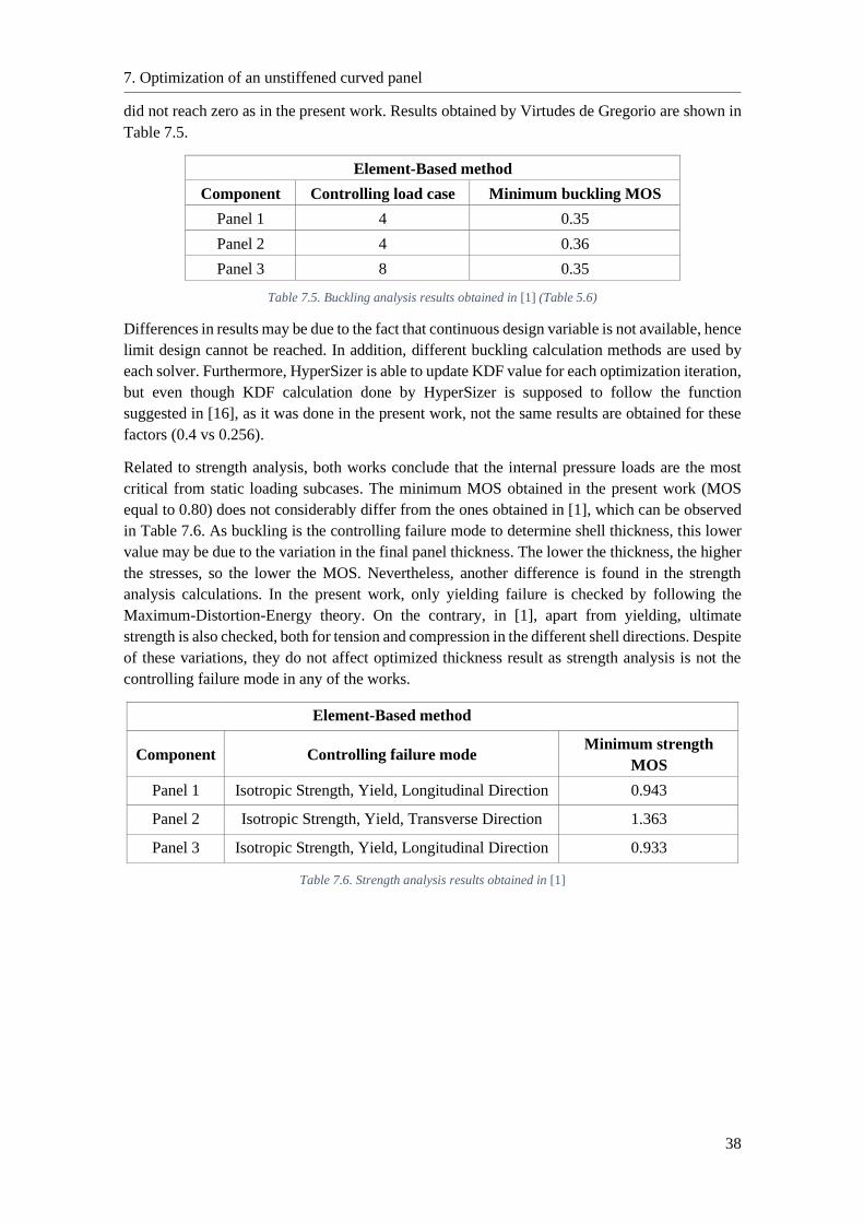
7. Optimization of an unstiffened curved panel
38
did not reach zero as in the present work. Results obtained by Virtudes de Gregorio are shown in
Table 7.5.
Element-Based method
Component Controlling load case Minimum buckling MOS
Panel 1 4 0.35
Panel 2 4 0.36
Panel 3 8 0.35
Table 7.5. Buckling analysis results obtained in [1] (Table 5.6)
Differences in results may be due to the fact that continuous design variable is not available, hence
limit design cannot be reached. In addition, different buckling calculation methods are used by
each solver. Furthermore, HyperSizer is able to update KDF value for each optimization iteration,
but even though KDF calculation done by HyperSizer is supposed to follow the function
suggested in [16], as it was done in the present work, not the same results are obtained for these
factors (0.4 vs 0.256).
Related to strength analysis, both works conclude that the internal pressure loads are the most
critical from static loading subcases. The minimum MOS obtained in the present work (MOS
equal to 0.80) does not considerably differ from the ones obtained in [1], which can be observed
in Table 7.6. As buckling is the controlling failure mode to determine shell thickness, this lower
value may be due to the variation in the final panel thickness. The lower the thickness, the higher
the stresses, so the lower the MOS. Nevertheless, another difference is found in the strength
analysis calculations. In the present work, only yielding failure is checked by following the
Maximum-Distortion-Energy theory. On the contrary, in [1], apart from yielding, ultimate
strength is also checked, both for tension and compression in the different shell directions. Despite
of these variations, they do not affect optimized thickness result as strength analysis is not the
controlling failure mode in any of the works.
Element-Based method
Component Controlling failure mode Minimum strength
MOS
Panel 1 Isotropic Strength, Yield, Longitudinal Direction 0.943
Panel 2 Isotropic Strength, Yield, Transverse Direction 1.363
Panel 3 Isotropic Strength, Yield, Longitudinal Direction 0.933
Table 7.6. Strength analysis results obtained in [1]
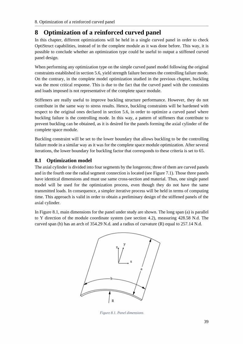
8. Optimization of a reinforced curved panel
39
8 Optimization of a reinforced curved panel In this chapter, different optimizations will be held in a single curved panel in order to check
OptiStruct capabilities, instead of in the complete module as it was done before. This way, it is
possible to conclude whether an optimization type could be useful to output a stiffened curved
panel design.
When performing any optimization type on the simple curved panel model following the original
constraints established in section 5.6, yield strength failure becomes the controlling failure mode.
On the contrary, in the complete model optimization studied in the previous chapter, buckling
was the most critical response. This is due to the fact that the curved panel with the constraints
and loads imposed is not representative of the complete space module.
Stiffeners are really useful to improve buckling structure performance. However, they do not
contribute in the same way to stress results. Hence, buckling constraints will be hardened with
respect to the original ones declared in section 5.6, in order to optimize a curved panel where
buckling failure is the controlling mode. In this way, a pattern of stiffeners that contribute to
prevent buckling can be obtained, as it is desired for the panels forming the axial cylinder of the
complete space module.
Buckling constraint will be set to the lower boundary that allows buckling to be the controlling
failure mode in a similar way as it was for the complete space module optimization. After several
iterations, the lower boundary for buckling factor that corresponds to these criteria is set to 65.
8.1 Optimization model
The axial cylinder is divided into four segments by the longerons; three of them are curved panels
and in the fourth one the radial segment connection is located (see Figure 7.1). Those three panels
have identical dimensions and must use same cross-section and material. Thus, one single panel
model will be used for the optimization process, even though they do not have the same
transmitted loads. In consequence, a simpler iterative process will be held in terms of computing
time. This approach is valid in order to obtain a preliminary design of the stiffened panels of the
axial cylinder.
In Figure 8.1, main dimensions for the panel under study are shown. The long span (a) is parallel
to Y direction of the module coordinate system (see section 4.2), measuring 428.58 N.d. The
curved span (b) has an arch of 354.29 N.d. and a radius of curvature (R) equal to 257.14 N.d.
Figure 8.1. Panel dimensions
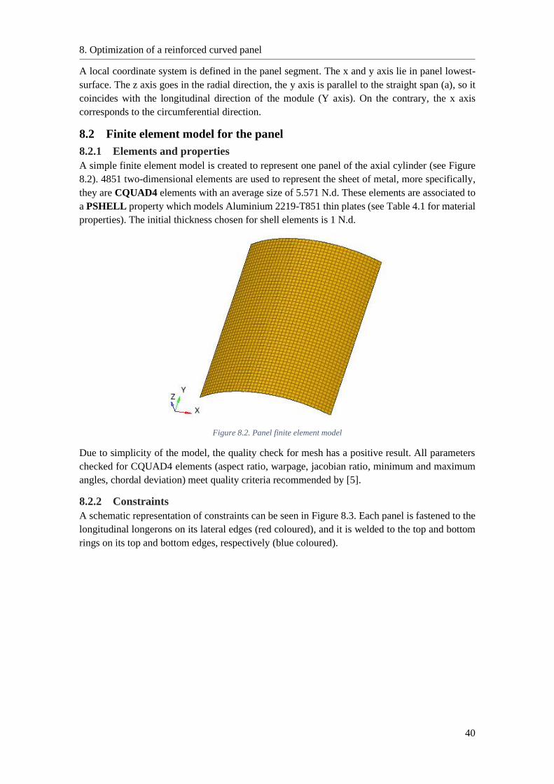
8. Optimization of a reinforced curved panel
40
A local coordinate system is defined in the panel segment. The x and y axis lie in panel lowest-
surface. The z axis goes in the radial direction, the y axis is parallel to the straight span (a), so it
coincides with the longitudinal direction of the module (Y axis). On the contrary, the x axis
corresponds to the circumferential direction.
8.2 Finite element model for the panel
8.2.1 Elements and properties
A simple finite element model is created to represent one panel of the axial cylinder (see Figure
8.2). 4851 two-dimensional elements are used to represent the sheet of metal, more specifically,
they are CQUAD4 elements with an average size of 5.571 N.d. These elements are associated to
a PSHELL property which models Aluminium 2219-T851 thin plates (see Table 4.1 for material
properties). The initial thickness chosen for shell elements is 1 N.d.
Figure 8.2. Panel finite element model
Due to simplicity of the model, the quality check for mesh has a positive result. All parameters
checked for CQUAD4 elements (aspect ratio, warpage, jacobian ratio, minimum and maximum
angles, chordal deviation) meet quality criteria recommended by [5].
8.2.2 Constraints
A schematic representation of constraints can be seen in Figure 8.3. Each panel is fastened to the
longitudinal longerons on its lateral edges (red coloured), and it is welded to the top and bottom
rings on its top and bottom edges, respectively (blue coloured).
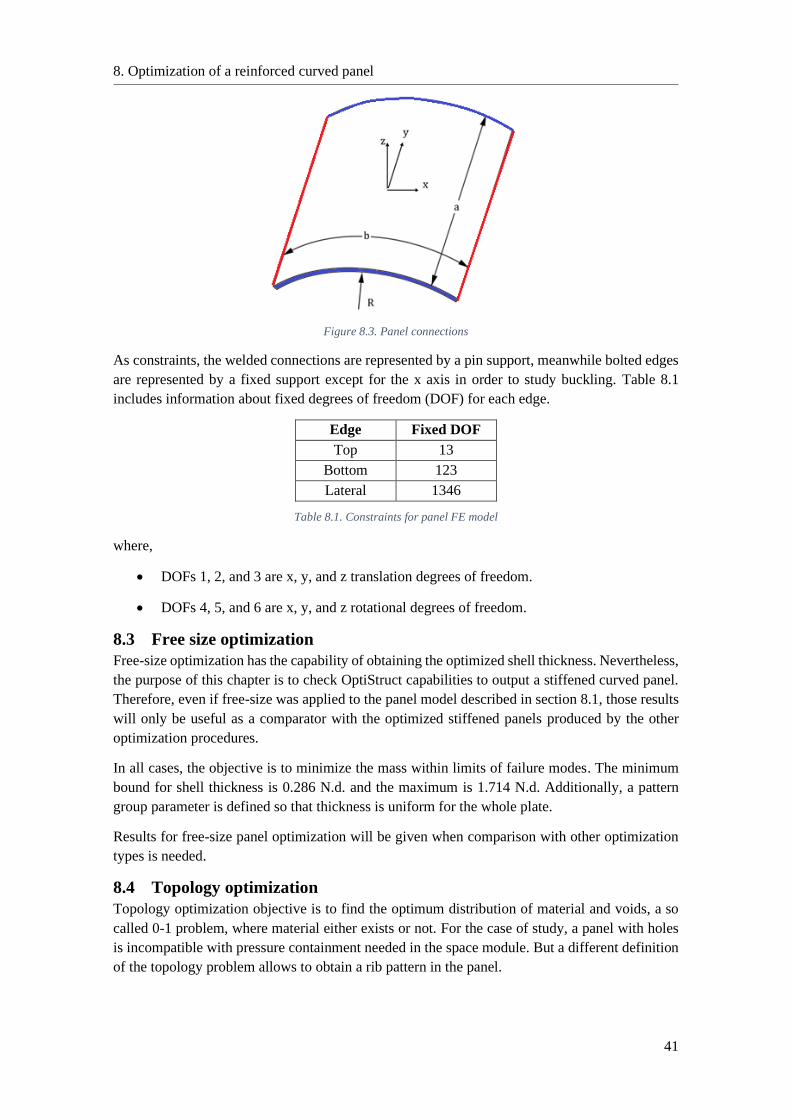
8. Optimization of a reinforced curved panel
41
Figure 8.3. Panel connections
As constraints, the welded connections are represented by a pin support, meanwhile bolted edges
are represented by a fixed support except for the x axis in order to study buckling. Table 8.1
includes information about fixed degrees of freedom (DOF) for each edge.
Edge Fixed DOF
Top 13
Bottom 123
Lateral 1346
Table 8.1. Constraints for panel FE model
where,
• DOFs 1, 2, and 3 are x, y, and z translation degrees of freedom.
• DOFs 4, 5, and 6 are x, y, and z rotational degrees of freedom.
8.3 Free size optimization
Free-size optimization has the capability of obtaining the optimized shell thickness. Nevertheless,
the purpose of this chapter is to check OptiStruct capabilities to output a stiffened curved panel.
Therefore, even if free-size was applied to the panel model described in section 8.1, those results
will only be useful as a comparator with the optimized stiffened panels produced by the other
optimization procedures.
In all cases, the objective is to minimize the mass within limits of failure modes. The minimum
bound for shell thickness is 0.286 N.d. and the maximum is 1.714 N.d. Additionally, a pattern
group parameter is defined so that thickness is uniform for the whole plate.
Results for free-size panel optimization will be given when comparison with other optimization
types is needed.
8.4 Topology optimization
Topology optimization objective is to find the optimum distribution of material and voids, a so
called 0-1 problem, where material either exists or not. For the case of study, a panel with holes
is incompatible with pressure containment needed in the space module. But a different definition
of the topology problem allows to obtain a rib pattern in the panel.
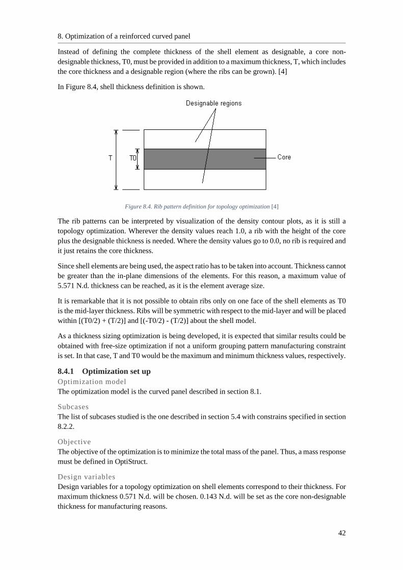
8. Optimization of a reinforced curved panel
42
Instead of defining the complete thickness of the shell element as designable, a core non-
designable thickness, T0, must be provided in addition to a maximum thickness, T, which includes
the core thickness and a designable region (where the ribs can be grown). [4]
In Figure 8.4, shell thickness definition is shown.
Figure 8.4. Rib pattern definition for topology optimization [4]
The rib patterns can be interpreted by visualization of the density contour plots, as it is still a
topology optimization. Wherever the density values reach 1.0, a rib with the height of the core
plus the designable thickness is needed. Where the density values go to 0.0, no rib is required and
it just retains the core thickness.
Since shell elements are being used, the aspect ratio has to be taken into account. Thickness cannot
be greater than the in-plane dimensions of the elements. For this reason, a maximum value of
5.571 N.d. thickness can be reached, as it is the element average size.
It is remarkable that it is not possible to obtain ribs only on one face of the shell elements as T0
is the mid-layer thickness. Ribs will be symmetric with respect to the mid-layer and will be placed
within [(T0/2) + (T/2)] and [(-T0/2) - (T/2)] about the shell model.
As a thickness sizing optimization is being developed, it is expected that similar results could be
obtained with free-size optimization if not a uniform grouping pattern manufacturing constraint
is set. In that case, T and T0 would be the maximum and minimum thickness values, respectively.
8.4.1 Optimization set up
Optimization model
The optimization model is the curved panel described in section 8.1.
Subcases
The list of subcases studied is the one described in section 5.4 with constrains specified in section
8.2.2.
Objective
The objective of the optimization is to minimize the total mass of the panel. Thus, a mass response
must be defined in OptiStruct.
Design variables
Design variables for a topology optimization on shell elements correspond to their thickness. For
maximum thickness 0.571 N.d. will be chosen. 0.143 N.d. will be set as the core non-designable
thickness for manufacturing reasons.
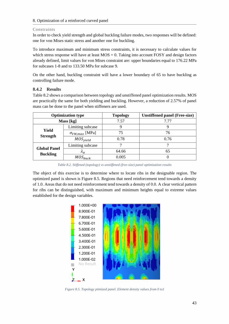
8. Optimization of a reinforced curved panel
43
Constraints
In order to check yield strength and global buckling failure modes, two responses will be defined:
one for von Mises static stress and another one for buckling.
To introduce maximum and minimum stress constraints, it is necessary to calculate values for
which stress response will have at least MOS = 0. Taking into account FOSY and design factors
already defined, limit values for von Mises constraint are: upper boundaries equal to 176.22 MPa
for subcases 1-8 and to 133.50 MPa for subcase 9.
On the other hand, buckling constraint will have a lower boundary of 65 to have buckling as
controlling failure mode.
8.4.2 Results
Table 8.2 shows a comparison between topology and unstiffened panel optimization results. MOS
are practically the same for both yielding and buckling. However, a reduction of 2.57% of panel
mass can be done to the panel when stiffeners are used.
Optimization type Topology Unstiffened panel (Free-size)
Mass [kg] 7.57 7.77
Yield
Strength
Limiting subcase 9 9
𝜎𝑉𝑀,𝑚𝑎𝑥 [MPa] 75 76
𝑀𝑂𝑆𝑦𝑖𝑒𝑙𝑑 0.78 0.76
Global Panel
Buckling
Limiting subcase 7 7
𝜆𝛼 64.66 65
𝑀𝑂𝑆𝑏𝑢𝑐𝑘 0.005 0
Table 8.2. Stiffened (topology) vs unstiffened (free-size) panel optimization results
The object of this exercise is to determine where to locate ribs in the designable region. The
optimized panel is shown is Figure 8.5. Regions that need reinforcement tend towards a density
of 1.0. Areas that do not need reinforcement tend towards a density of 0.0. A clear vertical pattern
for ribs can be distinguished, with maximum and minimum heights equal to extreme values
established for the design variables.
Figure 8.5. Topology ptimized panel. Element density values from 0 to1
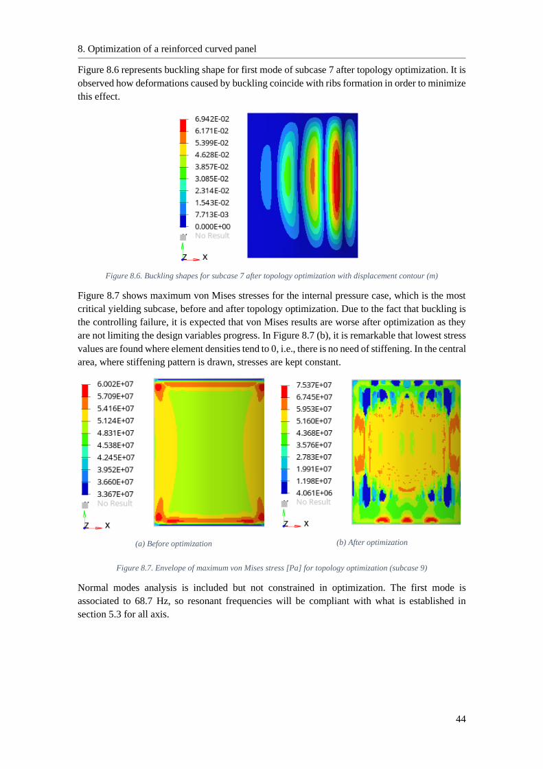
8. Optimization of a reinforced curved panel
44
Figure 8.6 represents buckling shape for first mode of subcase 7 after topology optimization. It is
observed how deformations caused by buckling coincide with ribs formation in order to minimize
this effect.
Figure 8.6. Buckling shapes for subcase 7 after topology optimization with displacement contour (m)
Figure 8.7 shows maximum von Mises stresses for the internal pressure case, which is the most
critical yielding subcase, before and after topology optimization. Due to the fact that buckling is
the controlling failure, it is expected that von Mises results are worse after optimization as they
are not limiting the design variables progress. In Figure 8.7 (b), it is remarkable that lowest stress
values are found where element densities tend to 0, i.e., there is no need of stiffening. In the central
area, where stiffening pattern is drawn, stresses are kept constant.
(a) Before optimization
(b) After optimization
Figure 8.7. Envelope of maximum von Mises stress [Pa] for topology optimization (subcase 9)
Normal modes analysis is included but not constrained in optimization. The first mode is
associated to 68.7 Hz, so resonant frequencies will be compliant with what is established in
section 5.3 for all axis.
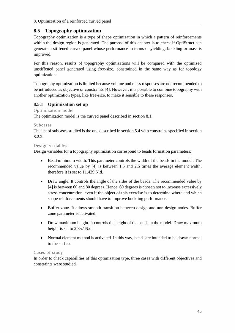
8. Optimization of a reinforced curved panel
45
8.5 Topography optimization
Topography optimization is a type of shape optimization in which a pattern of reinforcements
within the design region is generated. The purpose of this chapter is to check if OptiStruct can
generate a stiffened curved panel whose performance in terms of yielding, buckling or mass is
improved.
For this reason, results of topography optimizations will be compared with the optimized
unstiffened panel generated using free-size, constrained in the same way as for topology
optimization.
Topography optimization is limited because volume and mass responses are not recommended to
be introduced as objective or constraints [4]. However, it is possible to combine topography with
another optimization types, like free-size, to make it sensible to these responses.
8.5.1 Optimization set up
Optimization model
The optimization model is the curved panel described in section 8.1.
Subcases
The list of subcases studied is the one described in section 5.4 with constrains specified in section
8.2.2.
Design variables
Design variables for a topography optimization correspond to beads formation parameters:
• Bead minimum width. This parameter controls the width of the beads in the model. The
recommended value by [4] is between 1.5 and 2.5 times the average element width,
therefore it is set to 11.429 N.d.
• Draw angle. It controls the angle of the sides of the beads. The recommended value by
[4] is between 60 and 80 degrees. Hence, 60 degrees is chosen not to increase excessively
stress concentration, even if the object of this exercise is to determine where and which
shape reinforcements should have to improve buckling performance.
• Buffer zone. It allows smooth transition between design and non-design nodes. Buffer
zone parameter is activated.
• Draw maximum height. It controls the height of the beads in the model. Draw maximum
height is set to 2.857 N.d.
• Normal element method is activated. In this way, beads are intended to be drawn normal
to the surface
Cases of study
In order to check capabilities of this optimization type, three cases with different objectives and
constraints were studied.
8. Optimization of a reinforced curved panel
46
(A) (B) (C)
Optimization
type Topography Topography + free-size Topography + free-size
Objective Maximize minimum
buckling factor
Maximize minimum
buckling factor Minimize mass
Constraints Yielding constraint as
defined in section 5.6.1
Mass lower than the
one for the unstiffened
optimized panel
Yielding constraint as
defined in section 5.6.1.
Buckling factor > 65
Table 8.3. Cases of study for topography optimization
On the other hand, buckling constraint will have a lower boundary of 65 to have buckling as
controlling failure mode in a similar way as it was for the complete space module optimization.
8.5.2 Results
Results from all cases are shown in Table 8.4.
Optimization case Topography Unstiffened panel
(Free-size) (A) (B) (C)
Mass [kg] 27.64 7.76 8.63 7.76
Yield
Strength
Limiting subcase 9 9 9 9
𝜎𝑉𝑀,𝑚𝑎𝑥 [MPa] 131.91 573 121.30 76
𝑀𝑂𝑆𝑦𝑖𝑒𝑙𝑑 0.01 -0.77 0.10 1.76
Global
Panel
Buckling
Limiting subcase 7 7 7 7
𝜆𝛼 1569 248 73 65
𝑀𝑂𝑆𝑏𝑢𝑐𝑘 23.14 2.82 0.12 0
Table 8.4. Results for topography optimizations
Case (A) has the best buckling performance, however, that is not needed for the loads present as
it can be observed for the large MOS value. In addition, mass is increased more than 350% with
respect to the unstiffened panel, which already fulfils all mechanical requirements. Thus, the
unstiffened panel would be a clear better option rather than the panel solution obtained from case
(A).
For case (B), mass is constrained to the unstiffened panel value. Due to stiffeners produced,
buckling MOS is improved, but yield constraint is not fulfilled (𝑀𝑂𝑆𝑦𝑖𝑒𝑙𝑑<0). Nevertheless, stress
values should be taken only as a guide, because stiffeners produced with topography optimization
are changing shape of the metal sheet. They do not change its thickness to form ribs. Hence, if
stiffening must be done by the use of ribs, stresses will be completely different from the
topography reinforcements results. They will only help with pattern definition.
Case (C) have better buckling and yielding performances than the unstiffened panel, but an 11%
of extra mass is needed.
Figure 8.8 shows shape changes for the three different cases studied. It must be pointed out that
all reinforcements are automatically extruded to the inner face of the panel, in the same way as
typical waffle stiffeners are located for this kind of structure.
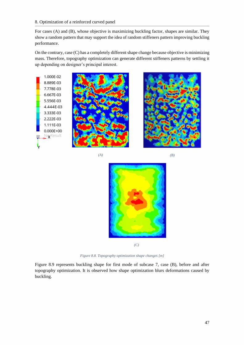
8. Optimization of a reinforced curved panel
47
For cases (A) and (B), whose objective is maximizing buckling factor, shapes are similar. They
show a random pattern that may support the idea of random stiffeners pattern improving buckling
performance.
On the contrary, case (C) has a completely different shape change because objective is minimizing
mass. Therefore, topography optimization can generate different stiffeners patterns by settling it
up depending on designer’s principal interest.
(A)
(B)
(C)
Figure 8.8. Topography optimization shape changes [m]
Figure 8.9 represents buckling shape for first mode of subcase 7, case (B), before and after
topography optimization. It is observed how shape optimization blurs deformations caused by
buckling.
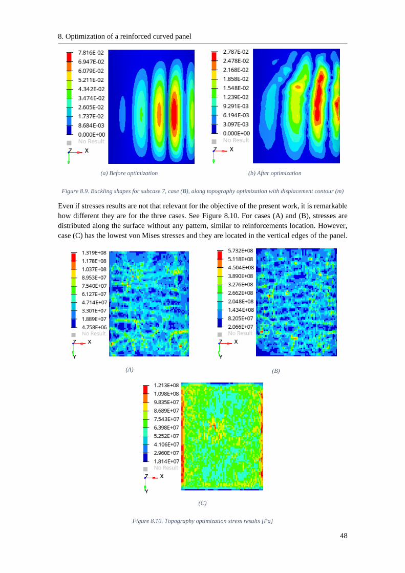
8. Optimization of a reinforced curved panel
48
(a) Before optimization
(b) After optimization
Figure 8.9. Buckling shapes for subcase 7, case (B), along topography optimization with displacement contour (m)
Even if stresses results are not that relevant for the objective of the present work, it is remarkable
how different they are for the three cases. See Figure 8.10. For cases (A) and (B), stresses are
distributed along the surface without any pattern, similar to reinforcements location. However,
case (C) has the lowest von Mises stresses and they are located in the vertical edges of the panel.
(A)
(B)
(C)
Figure 8.10. Topography optimization stress results [Pa]
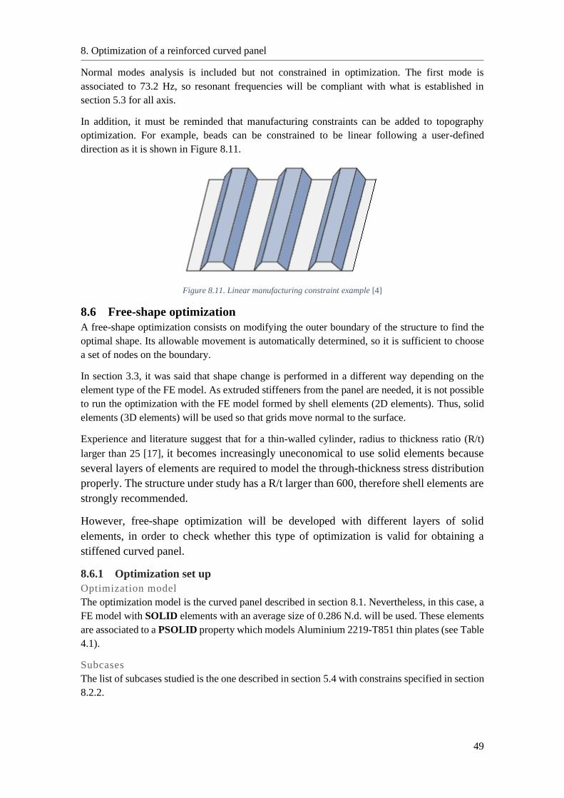
8. Optimization of a reinforced curved panel
49
Normal modes analysis is included but not constrained in optimization. The first mode is
associated to 73.2 Hz, so resonant frequencies will be compliant with what is established in
section 5.3 for all axis.
In addition, it must be reminded that manufacturing constraints can be added to topography
optimization. For example, beads can be constrained to be linear following a user-defined
direction as it is shown in Figure 8.11.
Figure 8.11. Linear manufacturing constraint example [4]
8.6 Free-shape optimization
A free-shape optimization consists on modifying the outer boundary of the structure to find the
optimal shape. Its allowable movement is automatically determined, so it is sufficient to choose
a set of nodes on the boundary.
In section 3.3, it was said that shape change is performed in a different way depending on the
element type of the FE model. As extruded stiffeners from the panel are needed, it is not possible
to run the optimization with the FE model formed by shell elements (2D elements). Thus, solid
elements (3D elements) will be used so that grids move normal to the surface.
Experience and literature suggest that for a thin-walled cylinder, radius to thickness ratio (R/t)
larger than 25 [17], it becomes increasingly uneconomical to use solid elements because
several layers of elements are required to model the through-thickness stress distribution
properly. The structure under study has a R/t larger than 600, therefore shell elements are
strongly recommended.
However, free-shape optimization will be developed with different layers of solid
elements, in order to check whether this type of optimization is valid for obtaining a
stiffened curved panel.
8.6.1 Optimization set up
Optimization model
The optimization model is the curved panel described in section 8.1. Nevertheless, in this case, a
FE model with SOLID elements with an average size of 0.286 N.d. will be used. These elements
are associated to a PSOLID property which models Aluminium 2219-T851 thin plates (see Table
4.1).
Subcases
The list of subcases studied is the one described in section 5.4 with constrains specified in section
8.2.2.
8. Optimization of a reinforced curved panel
50
Objective
The objective of the optimization is to minimize the total mass of the panel. Thus, a mass response
must be defined in OptiStruct.
Design variables
Shape variables are not needed as free-shape optimization automatically does it. However, it is
possible to constrain extrusion of reinforcements to go to the inner face of the panel, in the same
way as typical waffle stiffeners are located for this kind of structure.
Constraints
In order to check yield strength and global buckling failure modes, two responses will be defined:
one for von Mises static stress and another one for buckling.
To introduce maximum and minimum stress constraints, it is necessary to calculate values for
which stress response will have at least MOS = 0. Taking into account FOSY and design factors
already defined, limit values for von Mises constraint are: upper boundaries equal to 176.22 MPa
for subcases 1-8 and to 133.50 MPa for subcase 9. If stresses go higher than these values, yielding
will occur.
On the other hand, buckling constraint will have a lower boundary of 65 to have buckling as
controlling failure mode.
Cases of study
Three different models will be used with one, two and four layers of solid elements forming the
panel thickness.
8.6.2 Results
Table 8.5 includes results of the cases of study and the optimized unstiffened panel obtained from
free-size optimization in order to compare data.
Optimization case Free-shape Unstiffened panel
(Free-size) 1 layer 2 layers 4 layers
Mass [kg] 9.76 7.18 7.17 7.76
Computing time [min] 237 200 908 28
Yield
Strength
Limiting subcase 9 9 9 9
𝜎𝑉𝑀,𝑚𝑎𝑥 [MPa] 133.5 116 127 76
𝑀𝑂𝑆𝑦𝑖𝑒𝑙𝑑 0 0.15 0.05 1.76
Global
Panel
Buckling
Limiting subcase 7 7 7 7
𝜆𝛼 89 64.99 65 65
𝑀𝑂𝑆𝑏𝑢𝑐𝑘 0.37 ≈ 0 0 0
Table 8.5. Results for free-shape optimizations
Although optimizations have the same parameters, results are different for the three cases due to
the accuracy that extra element layers provide.
With only one layer of elements, yielding becomes the controlling failure mode (𝑀𝑂𝑆𝑦𝑖𝑒𝑙𝑑 equal
to 0), which is incoherent with constraints applied and results for the free-size optimization. It is
clear that stress distribution is not properly calculated as it was predicted in [17]. Thus,
this 1-element-layer model is not reliable.
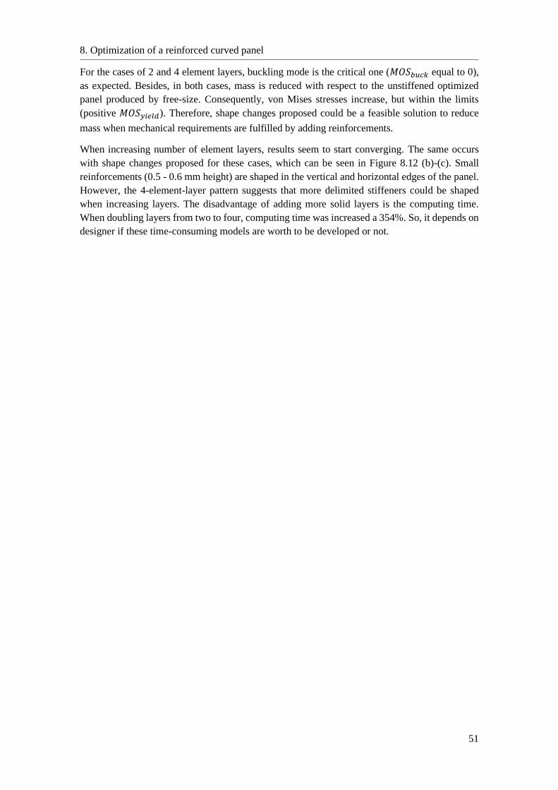
8. Optimization of a reinforced curved panel
51
For the cases of 2 and 4 element layers, buckling mode is the critical one (𝑀𝑂𝑆𝑏𝑢𝑐𝑘 equal to 0),
as expected. Besides, in both cases, mass is reduced with respect to the unstiffened optimized
panel produced by free-size. Consequently, von Mises stresses increase, but within the limits
(positive 𝑀𝑂𝑆𝑦𝑖𝑒𝑙𝑑). Therefore, shape changes proposed could be a feasible solution to reduce
mass when mechanical requirements are fulfilled by adding reinforcements.
When increasing number of element layers, results seem to start converging. The same occurs
with shape changes proposed for these cases, which can be seen in Figure 8.12 (b)-(c). Small
reinforcements (0.5 - 0.6 mm height) are shaped in the vertical and horizontal edges of the panel.
However, the 4-element-layer pattern suggests that more delimited stiffeners could be shaped
when increasing layers. The disadvantage of adding more solid layers is the computing time.
When doubling layers from two to four, computing time was increased a 354%. So, it depends on
designer if these time-consuming models are worth to be developed or not.
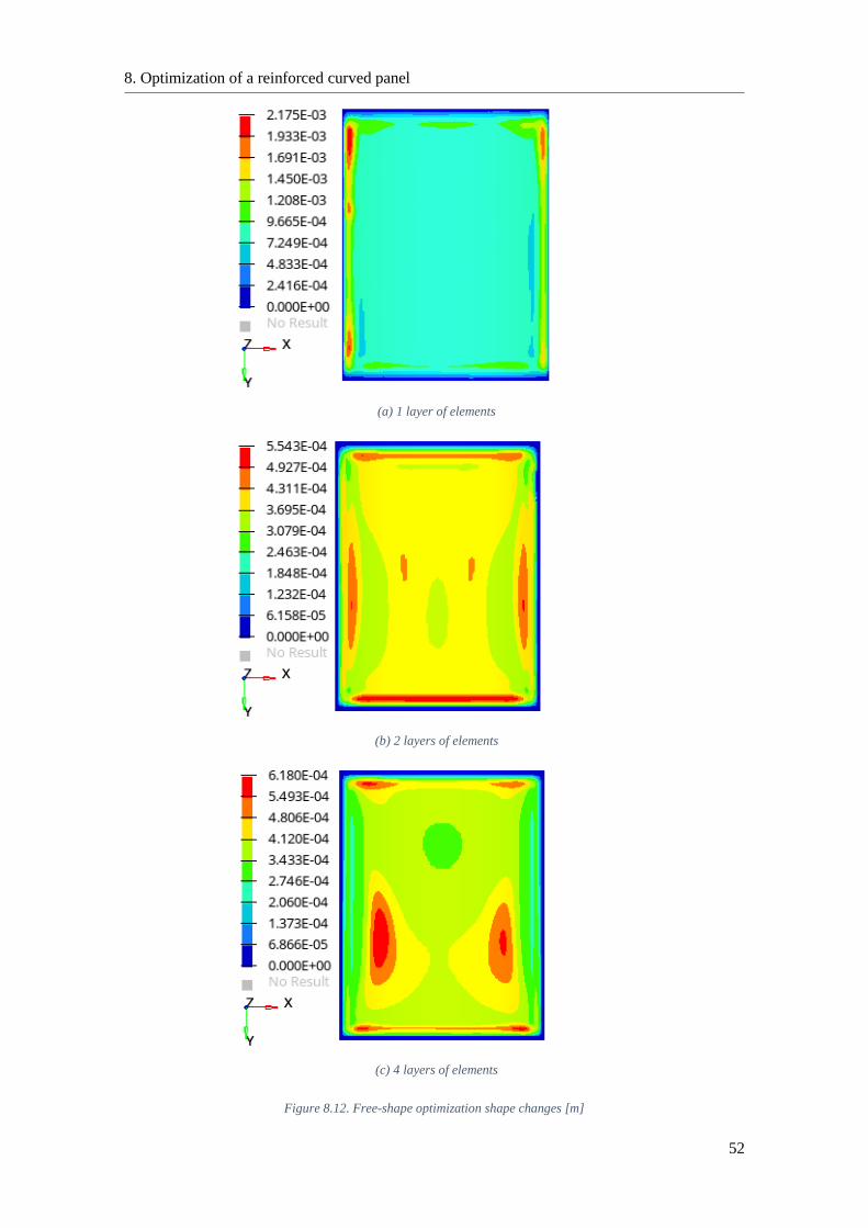
8. Optimization of a reinforced curved panel
52
(a) 1 layer of elements
(b) 2 layers of elements
(c) 4 layers of elements
Figure 8.12. Free-shape optimization shape changes [m]
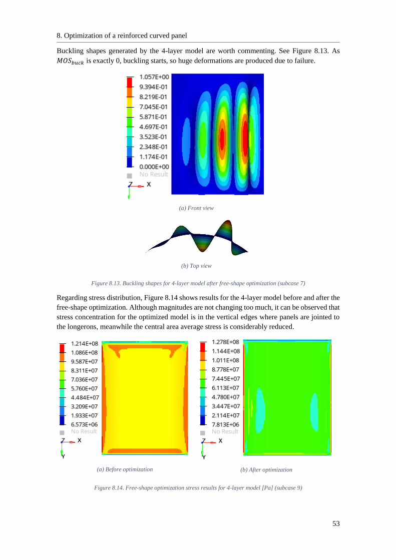
8. Optimization of a reinforced curved panel
53
Buckling shapes generated by the 4-layer model are worth commenting. See Figure 8.13. As
𝑀𝑂𝑆𝑏𝑢𝑐𝑘 is exactly 0, buckling starts, so huge deformations are produced due to failure.
(a) Front view
(b) Top view
Figure 8.13. Buckling shapes for 4-layer model after free-shape optimization (subcase 7)
Regarding stress distribution, Figure 8.14 shows results for the 4-layer model before and after the
free-shape optimization. Although magnitudes are not changing too much, it can be observed that
stress concentration for the optimized model is in the vertical edges where panels are jointed to
the longerons, meanwhile the central area average stress is considerably reduced.
(a) Before optimization
(b) After optimization
Figure 8.14. Free-shape optimization stress results for 4-layer model [Pa] (subcase 9)

8. Optimization of a reinforced curved panel
54
Normal modes analysis is included but not constrained in optimization. The first mode is
associated to 71.1 Hz, so resonant frequencies will be compliant with what is established in
section 5.3 for all axis.
In the same way as for topography, pattern manufacturing constraints can be added for free-shape
optimizations to produce specific shaped reinforcements. Another alternative could be to directly
create the shape variables using shape optimization.
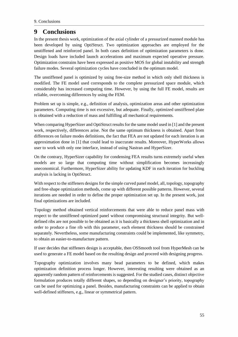
9. Conclusions
55
9 Conclusions In the present thesis work, optimization of the axial cylinder of a pressurized manned module has
been developed by using OptiStruct. Two optimization approaches are employed for the
unstiffened and reinforced panel. In both cases definition of optimization parameters is done.
Design loads have included launch accelerations and maximum expected operative pressure.
Optimization constrains have been expressed as positive MOS for global instability and strength
failure modes. Several optimization cycles have concluded in the optimum model.
The unstiffened panel is optimized by using free-size method in which only shell thickness is
modified. The FE model used corresponds to the complete pressurized space module, which
considerably has increased computing time. However, by using the full FE model, results are
reliable, overcoming differences by using the FEM.
Problem set up is simple, e.g., definition of analysis, optimization areas and other optimization
parameters. Computing time is not excessive, but adequate. Finally, optimized unstiffened plate
is obtained with a reduction of mass and fulfilling all mechanical requirements.
When comparing HyperSizer and OptiStruct results for the same model used in [1] and the present
work, respectively, differences arise. Not the same optimum thickness is obtained. Apart from
differences on failure modes definitions, the fact that FEA are not updated for each iteration is an
approximation done in [1] that could lead to inaccurate results. Moreover, HyperWorks allows
user to work with only one interface, instead of using Nastran and HyperSizer.
On the contrary, HyperSizer capability for condensing FEA results turns extremely useful when
models are so large that computing time without simplification becomes increasingly
uneconomical. Furthermore, HyperSizer ability for updating KDF in each iteration for buckling
analysis is lacking in OptiStruct.
With respect to the stiffeners designs for the simple curved panel model, all, topology, topography
and free-shape optimization methods, come up with different possible patterns. However, several
iterations are needed in order to define the proper optimization set up. In the present work, just
final optimizations are included.
Topology method obtained vertical reinforcements that were able to reduce panel mass with
respect to the unstiffened optimized panel without compromising structural integrity. But well-
defined ribs are not possible to be obtained as it is basically a thickness shell optimization and in
order to produce a fine rib with this parameter, each element thickness should be constrained
separately. Nevertheless, some manufacturing constraints could be implemented, like symmetry,
to obtain an easier-to-manufacture pattern.
If user decides that stiffeners design is acceptable, then OSSmooth tool from HyperMesh can be
used to generate a FE model based on the resulting design and proceed with designing progress.
Topography optimization involves many bead parameters to be defined, which makes
optimization definition process longer. However, interesting resulting were obtained as an
apparently random pattern of reinforcements is suggested. For the studied cases, distinct objective
formulation produces totally different shapes, so depending on designer’s priority, topography
can be used for optimizing a panel. Besides, manufacturing constraints can be applied to obtain
well-defined stiffeners, e.g., linear or symmetrical pattern.
9. Conclusions
56
A disadvantage is that reinforcements are simply changes of shape, they are not adding material,
so OSSmooth cannot be used to generate the optimized model in HyperMesh for a reanalysis.
Free-shape approach is able to produce a stiffeners pattern which is able to reduce panel mass
with respect to the unstiffened optimized panel without compromising mechanical integrity.
Despite this, this method requires high computing time because of the use of solid elements, which
are still not proven to be reliable in terms of stress performance.
However, if free-shape method is considered, manufacturing constraints can be added to obtain a
well-defined reinforcement shape, e.g., member size control, side constraints or some
symmetrical pattern. Then OSSmooth tool from HyperMesh can be used to generate a FE model
based on the output design and proceed.
In general, OptiStruct, and so HyperWorks suite, is a powerful optimization tool that allows
designer to work along the whole mission process. Firstly, it is possible to obtain optimized results
when there are no limitations for the output, like the research made for stiffening methods for
curved panels. This capability extremely increases designer possibilities. Secondly, a preliminary
design can be done by using free-size, free-shape or topology optimization, which still have wide
margin for modifications. Lastly, it is possible to add many constraints so that manufacturing
feasibilities are granted for the optimized detailed design.
Even though Altair Engineering provides users with guides, tutorials, forums and courses,
OptiStruct capabilities can be adapted to any optimization problem, from the simplest to the most
complicated and specific ones. Therefore, it is impossible to know in advance all possibilities for
a concrete structure design problem.
Moreover, working with a complete suite facilitates communication between programmes,
making sure that no information will be lost, and it makes easier for the user to work with the
different tools as interfaces and capabilities are similar and connected.
In conclusion, OptiStruct is a powerful optimization tool with limitless options for any kind of
structural problem. It can help design engineer at different mission states and provide him with
new shape designs that has never thought about.

Appendix A. Finite element model of module
57
Appendix A. Finite element model of module In this chapter the FE model of the module is described. The FE model was provided by Thales
Alenia Space as a result of a master thesis developed at Politecnico di Milano by Virtudes de
Gregorio Roig [1]. Checks for the FE model can be found in the mentioned work. For the scope
of this work, the FE model will be considered already checked.
A summary of elements and properties used is given in Table A.1. The terminology employed is
typically used in FEM. It is widely described in HyperMesh User’s Guide [5].
Type of element Number Characteristics
CBEAM 742 1D element. It supports tension, compression,
axial torsion and bending.
CBUSH 104 1D element. It can generate a link between not
coincident nodes and recover the resultant element
forces for bolts verification.
CONM2 3 0D element. It is a concentrated mass.
CQUAD4 75,694 2D element. It can model in-plane, bending, and
transverse shear behaviour.
CTRIA3 635 2D element. It can model in-plane, bending, and
transverse shear behaviour.
RBE2 789 1D element. It represents an idealized rigid
connection to transmit loads between interfaces.
RBE3 3 1D element. It is an interpolation element, but it is
not rigid. It does not add any stiffness between the
independent and dependent nodes, but loads are
transferred.
Total 77,970 -
Type of property Number -
PBEAML 1 -
PBUSH 1 -
PSHELL 26 -
Table A.1. FE model summary
Most of the structure geometry is represented using two-dimensional elements, CQUAD4 and
CTRIA3. From all the two-dimensional elements, 99% are CQUAD4, with average size equal to
20 mm. Meanwhile, CTRIA3 triangular elements are mainly used for mesh transitions or for
modelling portions of the structure when quadrilateral elements are impractical. Both, CQUAD4
and CTRIA3 elements, are associated to a PSHELL property modelling Aluminium 2219-T851
thin plates of different thicknesses.
Appendix A. Finite element model of module
58
Figure A.1. Lateral view of the FE model [1]
In general, CQUAD4 elements are more accurate than CTRIA3 elements, because the latter may
exhibit excessive stiffness, particularly for membrane strain. Nevertheless, quadrilateral elements
should be kept as nearly square as possible, and triangular elements should be kept as nearly
equilateral as possible. This is due to deterioration of accuracy when their aspect ratio increases
as described in [5].
Figure A.2. Top view of the FE model [1]
Appendix A. Finite element model of module
59
Regarding the element size, it has been selected according to Thales Alenia Space
recommendations for the type of analysis and dimensions. It is a compromise between accuracy
of the finite element analysis results and the solution computing time.
The hatches ribs are simplified and represented by CBEAM elements (coloured in light blue in
Figure A.2). They are associated to a PBEAML property used to define the L-cross-section shape.
Figure A.3. Detailed view of longerons attachments and secondary masses connections [1]
Figure A.3 shows a detailed view of the rigid elements (coloured in white) used to represent
connections between parts. The longerons and the axial cylinder ribs are fastened by using RBE2
rigid elements. In correspondence of the fasteners, the nodes at the ribs are defined as independent
and all 6 DOF of the nodes at the longerons are made dependent. The same type of elements is
used to model the interface structure that connects longerons to the top and bottom rings. In this
case, an independent grid point is used to represent the interface and all 6 DOF of a set of nodes
at the end of longerons and at rings in correspondence of the connection are defined as dependent.
RBE2 elements simplify the representation of the mentioned interfaces, which are complex to
model in detail. Therefore, results in the proximity of these links should not be trusted as an
artificial rigidity may be introduced in the model. For the final design, it is required to develop a
detailed model and a fine mesh to capture local effects, which is out of the scope of the present
work.
In addition, RBE2 elements are used to model the interface between the axial bulkhead and the
axial hatch and between the access closure and the radial hatch. These interfaces must secure the
pressure containment, hence the rigidity introduced by RBE2 elements is adequate.
Three CONM2 elements are used to model the secondary masses, which are described in section
4.1. The total mass budget is divided equally between those three elements, which are associated
to one panel each and are located at nodes in correspondence of the centre of gravity of the axial
cylinder segments (see Figure A.3). Brackets are used to connect them to the longerons of the
primary structure and they are represented by RB3 elements that transfer the secondary masses
inertial loads to the primary structure. The RB3 elements define the motion of the CONM2 nodes
(dependent) as the weighted average of the motions at the set of grid points representing brackets
(independent). Then, RBE2 are used to model the joints of brackets with longerons and rings. For
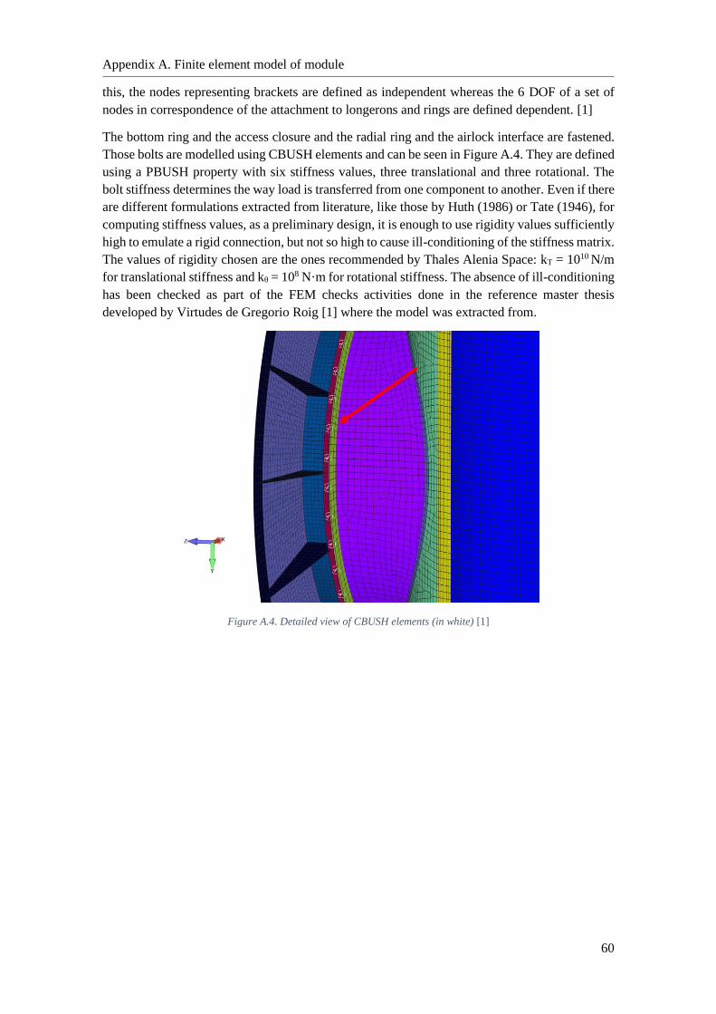
Appendix A. Finite element model of module
60
this, the nodes representing brackets are defined as independent whereas the 6 DOF of a set of
nodes in correspondence of the attachment to longerons and rings are defined dependent. [1]
The bottom ring and the access closure and the radial ring and the airlock interface are fastened.
Those bolts are modelled using CBUSH elements and can be seen in Figure A.4. They are defined
using a PBUSH property with six stiffness values, three translational and three rotational. The
bolt stiffness determines the way load is transferred from one component to another. Even if there
are different formulations extracted from literature, like those by Huth (1986) or Tate (1946), for
computing stiffness values, as a preliminary design, it is enough to use rigidity values sufficiently
high to emulate a rigid connection, but not so high to cause ill-conditioning of the stiffness matrix.
The values of rigidity chosen are the ones recommended by Thales Alenia Space: kT = 1010 N/m
for translational stiffness and kθ = 108 N·m for rotational stiffness. The absence of ill-conditioning
has been checked as part of the FEM checks activities done in the reference master thesis
developed by Virtudes de Gregorio Roig [1] where the model was extracted from.
Figure A.4. Detailed view of CBUSH elements (in white) [1]
61
References [1] V. De Gregorio Roig, “Structural Analysis and Optimization of a Pressurized Manned
Module,” Politecnico di Milano, 2020.
[2] P. W. Christensen and A. Klarbring, An introduction to structural optimization - Solid
Mechanics and its Applications, vol. 153. Linköping, Sweden: Springer Science +
Business Media B.V., 2009.
[3] A. Olason and D. Tidman, “Methodology for Topology and Shape Optimization in the
Design Process,” Chalmers University of Technology, 2010.
[4] Altair, “Altair OptiStruct 2021 User Guide,” 2021.
[5] Altair, “Altair HyperMesh 2021 User Guide,” 2021.
[6] M. Zhou, Y. K. Shyy, and H. L. Thomas, “Checkerboard and minimum member size
control in topology optimization,” Struct. Multidiscip. Optim., vol. 21, no. 2, pp. 152–158,
2001, doi: 10.1007/s001580050179.
[7] O. Sigmund and J. Petersson, “Numerical instabilities in topology optimization: A survey
on procedures dealing with checkerboards, mesh-dependencies and local minima,” Struct.
Optim., vol. 16, no. 1, pp. 68–75, 1998, doi: 10.1007/BF01214002.
[8] R. C. Rice, J. L. Jackson, J. Bakuckas, and S. Thompson, “Metallic Materials Properties
Development and Standardization (MMPDS),” U.S. Department of Transportation,
Federal Aviation Administration, 2003.
[9] Arianespace, Ariane 5 - User’s manual, no. 5, Rev. 3. Arianegroup, 2020.
[10] European Cooperation for Space Standarization, Space engineering: Structural general
requirements, ECSS‐E‐ST‐32C Rev. 1. Noordwijk, The Netherlands: ESA Requirements
and Standards Division, 2008.
[11] G. C. Nelson, Pressurized Payloads Interface Requirements Document: International
Space Station Program, Revision R. Houston, TX: NASA Johnson Space Center, 2015.
[12] European Cooperation for Space Standarization, Structural factors of safety for spaceflight
hardware, ECSS-E-ST-32-10C. Noordwijk, The Netherlands: ESA Requirements and
Standards Division, 2019.
[13] European Cooperation for Space Standarization, Space engineering: Structural design and
verification of pressurized hardware, ECSS-E-ST-32-02C Rev. 1. Noordwijk, The
Netherlands: ESA Requirements and Standards Division, 2008.
[14] European Cooperation for Space Standardization, Space engineering: buckling of
structures, ECSS‐E‐HB‐32‐24A. Noordwijk, The Netherlands: ESA Requirements and
Standards Division, 2010.
[15] J. E. R. Johnston, J. T. DeWolf, D. F. Mazurek, and F. P. Beer, Mechanics of materials,
6th ed. McGraw-Hill, 1981.
[16] V. I. Weingarten, P. Seide, and J. P. Petersson, “Bucking of Thin Walled Circular
Cylinders,” NASA Langley Research Center, NASA SP-8007, 1965.
[17] A. J. Sadowski and J. M. Rotter, “Solid or shell fi nite elements to model thick cylindrical
tubes and shells under global bending,” Int. J. Mech. Sci., vol. 74, pp. 143–153, 2013.