Structural Change and Competition in Seven U.S. Food Markets

Structural Change and Competition in Seven U.S. Food MarketsA. J. ReedJ. S. Clark

EconomicResearch Service

United StatesDepartment ofAgriculture

TechnicalBulletinNumber 1881

beef vealporkpoultryeggsdairyfresh fruitfresh vegtables

It’s Easy To Order Another Copy!

Just dial 1-800-999-6779. Toll free in the UnitedStates and Canada.

Ask for Structural Change and Competition in Seven U.S. FoodMarkets (TB-1881).

Charge to your VISA or MasterCard.

For additional information about ERS publications, databases, and other products, both paper and electronic, visit the ERS Home Page on the Internet athttp://www.econ.ag.gov/

The U.S. Department of Agriculture (USDA) prohibits discrimination in its programsand activities on the basis of race, color, national origin, sex, religion, age, disability,political beliefs, sexual orientation, or marital or family status. (Not all prohibitedbases apply to all programs.) Persons with disabilities who require alternativemeans for communication of program information (Braille, large print, audiotape,etc.) should contact USDA's TARGET Center at (202) 720-2600 (voice and TDD).

To file a complaint of discrimination, write USDA, Director, Office of Civil Rights,Room 326-W, Whitten Building, 14th and Independence Ave., SW, Washington, DC20250-9410, or call (202) 720-5964 (voice and TDD). USDA is an equal opportunityprovider and employer.

National Agricultural Library Cataloging Record:

Reed, A. J.Structural change and competition in seven U.S. food markets.

(Technical bulletin; no. 1881)1. Food industry and trade—Prices—United States.2. Farm produce—Prices—United States. I. Clark, J. S.II. United States. Dept. of Agriculture. Economic Research Service.1 Ag84Te no.1881

HD9004

Structural Change and Competition in Seven U.S. Food Markets.By A. J. Reedand J. S. Clark. Food and Rural Economics Division, Economic Research Service,U.S. Department of Agriculture. Technical Bulletin No. 1881.

Abstract

Recent trends in mergers and acquisitions in the U.S. food sector – food manufactur-ers, wholesalers, and retailers – raise concerns about market power. In the presence ofmarket power, farmers may receive lower than competitive farm prices, and con-sumers may pay higher than competitive retail prices. This study presents empiricaltests of market power at the national level for seven food categories: beef, pork, poul-try, eggs, dairy, fresh fruit, and fresh vegetables. At the national level, our tests pro-vide evidence of competitive conduct in both the sale of final food products and thepurchase of farm ingredients.

Keywords: Retail food and farm prices, market power, structural change, cointegration.

Acknowledgments

Much of this research was accomplished while Clark was affiliated with the U.S.Department of Agriculture, Economic Research Service, Food and Rural EconomicsDivision. The authors thank Mike Wohlgenant and Kuo Huang for helpful commentson earlier drafts of this report.

A.J. Reed is an economist at the U.S. Department Agriculture, Economic ResearchService; J.S. Clark is an associate professor of agricultural economics at the NovaScotia Agricultural College.

1800 M Street, NWWashington, DC 20036-5831 February 2000

ii ❖ Structural Change and Competition in Seven U.S. Food Markets/TB-1881 Economic Research Service/USDA

Contents

Summary . . . . . . . . . . . . . . . . . . . . . . . . . . . . . . . . . . . . . . . . . . . . . . . . . . . . . .iii

Introduction . . . . . . . . . . . . . . . . . . . . . . . . . . . . . . . . . . . . . . . . . . . . . . . . . . . . 1

The Economic Model . . . . . . . . . . . . . . . . . . . . . . . . . . . . . . . . . . . . . . . . . . . . . 2

Structural Change, Cointegration, and Market Clearing . . . . . . . . . . . . . . . . . . . .7

Further Empirical Results . . . . . . . . . . . . . . . . . . . . . . . . . . . . . . . . . . . . . . . . . .10Consumer Demand . . . . . . . . . . . . . . . . . . . . . . . . . . . . . . . . . . . . . . . . . . . . .10Tests of Competition and Constant Returns… . . . . . . . . . . . . . . . . . . . . . . . . .11Oligopsony Power . . . . . . . . . . . . . . . . . . . . . . . . . . . . . . . . . . . . . . . . . . . . . .11Longrun Industry Structure . . . . . . . . . . . . . . . . . . . . . . . . . . . . . . . . . . . . . . .12Input Substitution . . . . . . . . . . . . . . . . . . . . . . . . . . . . . . . . . . . . . . . . . . . . . . .14Full-Reduced-Form Price Responses . . . . . . . . . . . . . . . . . . . . . . . . . . . . . . . .15

Conclusions . . . . . . . . . . . . . . . . . . . . . . . . . . . . . . . . . . . . . . . . . . . . . . . . . . . .18

References . . . . . . . . . . . . . . . . . . . . . . . . . . . . . . . . . . . . . . . . . . . . . . . . . . . . .19

Appendix . . . . . . . . . . . . . . . . . . . . . . . . . . . . . . . . . . . . . . . . . . . . . . . . . . . . . .21

Summary

Recent trends in mergers and acquisitions in the U.S. food sector – food manufactur-ers, wholesalers, and retailers – raise concerns about market power. In the presence ofmarket power, farmers may receive lower than competitive farm prices, and consumersmay pay higher than competitive retail prices. This study presents empirical tests ofmarket power at the national level for seven food categories: beef, pork, poultry, eggs,dairy, fresh fruit, and fresh vegetables.

The procedures employed in this study account for three important features of foodmarkets. First, the procedures recognize that within a product category consumers pre-fer a variety of food items. Second, the procedures account for firm diversity by recog-nizing that different firms produce a variety of different products using different tech-nologies. Firm and technological diversity seem to be particularly relevant to foodindustries because mergers and acquisitions may be feasible only if firms and tech-nologies are diverse. Third, the procedures recognize that structural changes in foodmarkets may be unpredictable. Some of the most significant impacts on food marketsmay have been unpredictable. For example, it was probably difficult to predict trendsin consumer patterns following the entry of women into the labor force in the 1970’sand 1980’s. Unpredictability of consumer behavior poses considerable risk to foodproducers and can induce industrial reorganizations that spread this risk across stagesof food production. Failure to account for product diversity and uncertainty has beenshown to seriously affect tests of market power.

The empirical evidence presented in this bulletin is mostly consistent with competitiveconduct. At the national level, our tests provide evidence of competitive conduct inboth the sale of final food products and the purchase of farm ingredients. Also at thenational level, the tests suggest that food industries pay competitive prices for farmcommodities. The results do not rule out imperfectly competitive local markets, andthey cannot be used to address questions of relative market power between specificstages of food production. Nevertheless, the broad implications of these results may bethat it is the unpredictable nature of trends in consumer demand, and not imperfectcompetition, that may be responsible for observed trends in the industrialization andconcentration of the U.S. food sector.

Economic Research Service/USDA Structural Change and Competition in Seven U.S. Food Markets/TB-1881 ❖ iii

Economic Research Service/USDA Structural Change and Competition in Seven U.S. Food Markets/TB-1881 ❖ 1

This bulletin presents empirical analyses of marketstructure and competition for seven major U.S. foodmarkets: beef, pork, poultry, eggs, dairy, fresh fruit,and fresh vegetables. The analyses account for struc-tural change. Our work emerges from a theory firstdeveloped by Heiner in which consumer demand andinput supply mesh with the output supply and the inputdemands of nonidentical firms. While Chavas and Coxhave recently generalized this theory, Wohlgenant(1989) and Wohlgenant and Haidacher (WH) were thefirst to extend and apply it to food markets. This bul-letin builds on the work of WH by accounting forstructural change.

We appeal to the economic theory found in WH andWohlgenant (1989, 1996) to test for market power.However, the market data that we use to implement thetests appear to be driven by trends. In food markets,we hear about trends in technical change among firms(e.g., Clark and Youngblood), about trends in theindustrial reorganization of industries (e.g., Martinezand Reed, MacDonald and Ollinger), and about trendsin food consumption (Kinsey and Senauer). In thisstudy, we define structural change as trends in marketvariables and account for different types of trends intests of market power.

Unlike approaches that define structural change bychanges in a model’s parameters (e.g., Goodwin andBrester), our approach allows us to capture a key fea-ture of some types of structural change: its changingtrends are unpredictable. This view allows us todescribe and to test for unpredictably changing trendsin consumer and producer behavior. It allows us totest for market-clearing and to estimate longrun struc-tural relationships despite such unpredictability.Finally, it allows us to test for market power in mar-kets that may have undergone a series of permanentchanges over time.

Our work sheds light on policy concerns associatedwith trends in the industrialization of food industriesand in consumer behavior. Economic theory suggestssuch trends would be linked if markets clear (Engleand Granger). A cointegratedmodel links trendsacross variables and, in our case, provides a market-clearing representation. By failing to reject competi-tion with a cointegrated model, our results suggest thattrends in concentration and industrialization may beefficient solutions to unpredictable trends in consumerdemand for food (Paul).

Structural Change and Competition inSeven U.S. Food Markets

A.J. Reed and J.S. Clark

Introduction

Wohlgenant (1989) and WH introduced the agricultur-al economics profession to a market-clearing frame-work in which diverse firms demand farm and nonfarminputs to produce the product mix of a compositeindustry. By relaxing the restriction of identical pro-duction functions across firms, they account for anindustry’s heterogeneous food items. They note thateven if eachfirm produces its items in fixed-input pro-portions, because proportions vary across the diversefirms of a food industry, production of the entireindustry is variable proportions.1 The frameworkequips analysts with a tool for studying market rela-tionships that is more general than the models derivedfrom the traditional assumptions of fixed proportionsand identical firms.

Market models of diverse firms generalize competitivemarket relationships. In particular, they can be used toreconcile the conceptof competitive markets with theobservationthat: (1) increases in consumer food pricesare not fully passed through to farmers (Wohlgenant,1994); (2) nonfarm input prices and consumer foodprices may move in opposite directions; (3) consumersmay pay higher markups for higher priced products(George and King); and (4) competitive food industriesmay earn positive longrun rents (U.S. Department ofAgriculture, September 1996). Market models basedon fixed-proportions production must appeal to imper-fect competition to explain these observations(Wohlgenant, 1999).

Tests of market power using market-level data, then,depend on assumptions concerning the nature ofindustryproduction. Retail-to-farm price spreads thatexceed the marginal cost of transforming farm ingre-dients to final food products suggest market power,but the formulas used to compute spreads depend on

the industry production function.2 Studies based onfixed-proportions consistently reject the competitivemodel (e.g., Schroeter, Schroeter and Azzam, Azzam,Azzam and Park, and Koontz, Garcia, and Hudson),whereas WH and Wohlgenant (1989, 1996) just asconsistently fail to reject the competitive model forU.S. food industries.3

This section presents an overview of the theory used inour empirical analyses. We refer readers unfamiliarwith this theory to the cited studies of WH andWohlgenant (1989, 1996) for a discussion that is morecomplete than that presented in this section. Readersfamiliar with the theory can skip to the next section.

At the core of the WH model are a pair of quasi-reduced-form retail and farm price equations for eachmarket and a system of consumer-demand relation-ships linking the markets. Given a consumer demandschedule, the underlying structural model consists oftwo market-clearing conditions. The first states that thesum of food supply across the firms of the industryequals consumer demand for the industry output. Thesecond states that the sum of farm ingredient demandacross firms of the industry equals farm supply. Thecritical feature of the WH model is that an industry’sfirms are not restricted to possessing identical produc-tion functions. Within this general setup, WH assumethat each industry faces an infinitely elastic supply ofnonfarm inputs (exogenous nonfarm input prices), anda less-than-infinitely elastic supply of farm ingredients(endogenous farm prices). To simplify the model struc-ture and isolate analysis on retail and farm prices, WHassume the food industry for a particular market con-sists of all the firms that manufacture, wholesale, andretail the industry’s final food products.

2 Retail-to-farm price spread formulas used by ERS/USDA(Elitzak) are based on fixed-proportions production. Presumably,formulas based on variable-proportions would yield different mag-nitudes.

2 ❖ Structural Change and Competition in Seven U.S. Food Markets/TB-1881 Economic Research Service/USDA

1 Wohlgenant (1999) formally shows that if one analyzes a com-petitive industry producing a heterogeneous mix of final consumergoods that we treat as a single composite (e.g., beef ), the observa-tion that retail-to-farm price spreads widen with increases in con-sumer food prices (e.g., George and King) implies input substitu-tion. To explain this observation with a fixed-proportions basedmodel for this heterogeneous industry, one must rule outthe com-petitive model.

3 These results are predicted by the theoretical results presented inWohlgenant (1999).

The Economic Model

Based on this structure4 and on market clearing forfarm ingredients and food output, Wohlgenant (1989,1996) and WH derive the quasi-reduced-form

lnPrj = Arf(j) lnFj + Arw

(j) lnW + Arz(j) lnZj + erj

(1)lnPfj = Aff

(j) lnFj + Afw(j) lnW + Afz

(j) lnZj + efj

j = 1,...,J

in which lnPrj represents the natural logarithm (log) ofthe retail price in the jth market,lnPfj is the log of theprice of the farm ingredient used to produce output ofthe jth market,lnFj is the log of the supply of the farmingredient used to produce output of the jth market. Inthis study,lnFj captures changes in domestic supply,and excludes changes in net exports and changes inprivate and government stocks of farm commodities.lnW is a vector of logged nonfarm input prices, andlnZj is a consumer demand shifter to be defined below.erj and efj are model errors on the retail and farm priceequations.5 These two retail and farm price equationsare central to this bulletin.

In this framework, consumer demand defines the mar-ket, and the total consumer demand shift variable forthe jth market,lnZj represents the effect of all variablesthat affect demand except the own-retail price for theproduct. For this bulletin,lnZj is derived as follows.Let

ln(Qj /POP) = ejj lnPrj + ejy ln (Y/POP)

+Sk¹ j ejk lnPrk + uj

be a per capita consumer demand relationship for thejth product in which ln(Qj/POP) is the log of per capi-ta consumer demand for the output of the jth industry,lnPrj is the log of the own-retail price,ln(Y/POP)isthe log of per capita disposable income,lnPrk (k¹j) isthe kth retail price of a gross substitute or complement

to product category j, and uj is an error term. Hence,the ejj is the own-retail price elasticity of consumerdemand,ejk (k¹j) is a set of cross-price elasticities ofdemand, and ejy is the income elasticity of demand forthe jth good. Based on this relationship, the totaldemand shifter for the jth market is

(2) lnZj = ejy ln (Y/POP) +Sk¹ j ejk lnPrk + lnPOP

in which lnPOP is the log of population. lnZj does notcapture shifts in consumer demand caused by changesin the demand for food away from home, nor does itcapture shifts caused by changes in the composition ofthe population.

The equations 1 are “quasi” reduced because theyaccount for market-clearing in the jth market inde-pendent of market clearing in other markets.6 Theorysuggests four sets of expected signs on the quasi-reduced forms.

First, Heiner proves that for an industry of diversefirms, an increase (decrease) in the price of an inputdecreases (increases) an industry’s demand for theinput. While this result is standard for an isolated firmand for an industry comprised of identical firms,Heiner’s proof applies to an industry comprised offirms with different longrun average costs. Heiner’sproof does not describe the negative slope of the sumof competitive firms’ input demand schedules holdingoutput price constant. It describes instead the slope ofindustry input demand schedule as the sum of firms’supply moves along a downward-sloping consumerdemand schedule and, output price changes.7 Braulkeshowed that Heiner’s proof applies to longrun equilib-rium in which firms enter and exit the industry. Inequations 1,Aff

(j) is the own-price flexibility of an


4 A brief discussion of the relationship between the structuralmodel and the quasi-reduced form is provided in the Appendix.The reader is referred to Wohlgenant (1989) or Wohlgenant andHaidacher for a more complete discussion.

5 Constants and deterministic time trends are added to all of theempirical specifications below except the system of consumerdemand relationships (Appendix). Only a constant term was addedto the consumer demand system.

6 The quasi-reduced-form equations derive from Heiner’s seminalwork and the extensions of this work by Wohlgenant (1989) andWH. In the quasi-reduced-form representation, shifts in the mar-ket’s demand schedule are exogenous.

7 For any single firm, Heiner found that the simultaneous changein the output price caused by the change in input price may traceout a positively sloped input demand for the firm. He found thispositive relationship disappears when summing over all firms.

industry’s demand for farm ingredients, and theorysuggests Aff < 0.8

Second, the industry’s longrun quantity of food supplyincreases with its own-consumer food price. Heiner,Braulke, Panzar and Willig, and WH show that even ifall input prices are exogenous to a competitive indus-try (flat input supplies), firm diversity implies thatpositive shifts in consumer demand trace an upward-sloping longrun industry supply function. Theoryimplies Arz > 0.

Third, if firms are identical and farm ingredients arenormal factors of production, a decrease in the supplyof farm ingredients leads to a contraction of food sup-ply and to an increase in consumer food prices. A nor-mal factor of industryproduction is one in which theindustry uses more of the factor to produce more out-put, while an inferior factor is one in which the indus-try uses less of the input to produce more output. Thetheory of diverse firms extends the neoclassical resultthat an increase in farm prices leads to increases infood prices only if farm ingredients are normal factorsof industry food production. Since we expect that theaggregate farm ingredients specified here are normal,we expect Arf < 0.

Fourth, if farm ingredients are normal factors of indus-try production and firms are diverse, positive shifts inconsumer demand lead to longrun increases in farmprices. For that reason we expect Afz > 0.

The theory of diverse firms does not unambiguouslysign the response of consumer food prices to changesin nonfarm input prices. The reason is that a marketinginput may be an inferior factor of production.9 Anincrease in the price of an inferior factor raises a firm’saverage costs, but reducesits marginal costs. For acompetitive industry comprised of identical firms,higher longrun average costs drive firms from theindustry, reduce industry supply, and drive up con-

sumer prices. The results may be different if an indus-try’s firms are diverse.

Inframarginal firms are bestowed with firm-specificfixed assets that earn rent in the long run. Such firmsare bestowed with firm-specific entrepreneurial capaci-ty (Friedman) or location that provides them with acost advantage over marginal firms (Panzar andWillig). One could argue that the entrepreneurialcapacity of inframarginal pork-producing firms in theSoutheast United States exceeds that of marginal pro-ducers in the Midwest. The cost advantage of infra-marginal firms allows them to remain in the industryeven as the longrun average cost of other firms isabove market price. It follows that even in competitivemarkets, if the factor is inferior to inframarginal firms,an increase in its prices allows inframarginal firms toincrease their supply even in the long run. The increaseplaces downward pressure on output price. On theother hand, if the factor is inferior to marginal firms,their longrun average cost rises above output price.Marginal firms would exit the industry, thereby reduc-ing industry supply and placing upward pressure onthe market’s average price of output. A negative signon an element of Arw suggests the associated factor isinferior to industryproduction, and that the positivesupply response of inframarginal firms outweighsthe negative response of marginal firms10 (Panzarand Willig).

Theory provides a homogeneity condition. Since con-sumer demand is homogeneous of degree zero inretail (food) prices and income, and output supply andinput demand are homogeneous of degree zero infarm and nonfarm input prices, the market-clearingprice equations of (equations 1) are homogeneous ofdegree zero in farm and nonfarm input prices, retailprices, and income (e.g., WH, Wohlgenant [1989],Chavas and Cox).

The WH framework provides a test of the competitivemodel. The test is based on the notion that if a firm is


8 Correspondingly, the retail price equation of (1) is a Heiner-typeof industry-level output supply schedule.

9 The example given here would not hold for the special case ofonly two inputs (e.g., one farm and one non-farm input). In thistwo-input case both factors must be normal, and increases in theprice of either input raise the output price.

10 Because firm-level production functions are not identical, a fac-tor of production can be normal for some firms and inferior forothers (e.g., older versus modern plants). Hence, a factor is normal(inferior) for an industryif the industry uses more (less) of the fac-tor as it increases output. The weighted sums of individual firm-level elasticities determine whether a factor is normal or inferior(WH).

a price taker in both its purchase of inputs and itssales of output its profit function exists, and the sym-metric second derivatives of its profit function definereciprocal relationships between a firm’s output sup-ply and input demands. Wohlgenant and WH derive ananalogous symmetry condition for the group ofdiverse industry firms. Denoting Sf

(j)as the cost shareof farm ingredients for the jth industry, and to thecoefficients in equations 1, WH show that symmetryat the industrylevel implies

Arf(j) = -Sf

(j) Afz(j).

This condition states that if firms take farm and con-sumer prices as given, there exists a symmetricresponse of consumer and farm-level prices.

When studying retail and farm price relationships,analysts are often interested in the elasticity of trans-mission of farm prices to retail food prices. The elas-ticity of price transmission is the percent change in aretail food price induced by a 1-percent change in thefarm price (George and King). Estimates of this elas-ticity reduce to the farm share if the food industry iscompetitive and if industry production exhibits con-stant returns with respect to farm ingredients. Theassumption of fixed-proportions production (at theindustry level) imposes constant returns with respectto all inputs, and therefore ensures transmission elas-ticities equal to the farm share. The WH modelallows us to test whether the elasticity of price trans-mission equals the farm share within a variable-pro-portions framework.

Wohlgenant and WH show that in terms of the coeffi-cients of equations 1, the jth industry’s production dis-plays constant returns with respect to the farm input if

Arz(j) = -Arf

(j)

Afz(j) = -Aff

(j)

hold. Constant returns for an industry imply zeroindustry profits in the long run. If both the symmetryand the constant returns restrictions hold, the elasticityof price transmission equals the farm share.

The model provides refutable hypotheses concerningoligopsony power. Policymakers often express con-cern that food producers exert market power whenacquiring raw agricultural commodities from farmers.Some point out that captive supplies associated withnew marketing arrangements may have changed the

market structure so as to favor food producers andkeep farm prices below competitive levels (U.S.Department of Agriculture, February 1996). Otherscounter that such voluntary arrangements may reflectthe response to risk in a competitive market (Paul).The WH framework provides a test of the null thatfood producers acquire farm commodities competi-tively in national markets.

The test recognizes that if firms exert market power inacquiring farm commodities, a gap would existbetween the farm price and the industry’s demand forfarm ingredients. Shifters on the farm supply functionwould define this gap.

At the level of the firm, the arguments are as follows.Let Pfj = Pfj (Fj, Sj) denote the inverse supply functionfor farm commodities facing the jth food industry,where Sj denotes a vector of shifters to this supplyfunction. The first-order condition for profit maximiza-tion of a food-producing firm takes the form MVP =Pfj + lf (MPfj /MF), where MVP is the marginal valueproduct or firm-level demand for the farm commodity,and l is a market power parameter. l embodies thefirm’s conjecture about the effect its purchases of farmingredients will have on the market (Bresnahan, p.102-104). Note that the term (MPf /MF) in the aboverelationship is a function of Sj. When l ¹ 0, the marketlevel demand shifters,Sj, enter the firm’s optimizationrule and define a gap between the market’s farm priceand the value of the marginal product for a competitivefirm. Hence, when l ¹ 0, the marginal farm price – thefirm’s MVP – lies above the average farm price andfirms restrict their demand for farm commodities. If l= 0, price-taking firms recognize that their purchasesimpart no effect on the market, the farm price (or thevalue of the marginal product) equals the MVP as theindustry level demand shifters (Sj,) do not enter firms’optimization conditions.

For a group of nonidentical firms of an industry, thearguments are similar. By eliminating Fj from equa-tions 1, the two equations reduce to

(3) Prj = Bf(j) Pfj + Bw

(j) W + Bz(j) Zj + vr.

Equation 3 is an industry-level relationship similar tothe first-order conditions of a price-taking firm. Underthe null of no oligopsony power, the vector of supplyshifters,Sj, does not appear in equation 3. Under thealternative,Sj explains the gap and


(4) Prj = Bf(j) Pfj + Bw

(j) W + Bz(j) Zj + Bs

(j)¢ Sj + vr

suggests the industry exerts oligopsony power inacquiring farm inputs. Equations 3 and 4 suggest thatif industry j acquires farm commodities competitively,Bs

(j)¢ = 0.

This concludes the review of the theory used to inter-pret the empirical results presented in the remainderof this report. Before we present these empiricalresults, however, we review the way in which struc-tural change enters our empirical analyses.


In the previous section, the retail and farm price equa-tions of 1 derive from market-clearing conditions forconsumer food products and for farm ingredients (seeAppendix). However, questions concerning the specifi-cation of equations 1 arise if markets have undergonestructural change.

Regardless of the impact of structural change, marketclearing means that excess supply (demand) would beof short duration and would equal zero on average.Furthermore, the effects of unforeseen shocks to mar-ket clearing would die out over time. In time series jar-gon, excess supply (demand) would be stationary. It isstraightforward to show (using the market-clearingconditions shown in the Appendix) that the errorterms,erj and efj , of equations 1 may represent excesssupply (demand) variables for food and farm products.Stationary error terms imply market clearing, and mar-ket clearing would prevent the variables of equations 1from moving too far apart.

Associated with structural change are market trends.Evidence of trends or changes in trends of market vari-ables are often used as indicators of structural change.In time series jargon, variables that are characterizedor generated by trends are non-stationary. However,even if each of the variables of equations 1 displaystrends, the equations would still reflect market clearingif the excess supply variables or error terms are sta-tionary. If each of the time series variables used in amodel displays trends, and if model errors are station-ary, the model is cointegrated(Engle and Granger).Tests of cointegration are tests of whether the data sup-port the theory. In a cointegrated regression, somemechanism cancels or aligns the trends among thevariables, and in equations 1 the mechanism is marketclearing.

If the trends driving the non-stationary variables ofequations 1 are not linked, excess supply would notdie out, and the regression would be spurious(Grangerand Newbold, p. 202-214, Hamilton p. 557-562). If theprice equations of (1) are spurious, inter-temporalmovements in one set of variables of equations 1 donot explain inter-temporal movements in other vari-ables. A finding of a spurious regression would notsupport the theory.

In general, if market variables are driven by trends, thetrends can be deterministic, stochastic, or a combination

of both. A deterministic trend is a time trend defined inthe usual way. Trends in demographics or predictableincreases in real wages and productivity over the lastcentury may drive the deterministic portion of trends inmarket variables. Market variables generated by deter-ministic trends pose few problems for statistical infer-ence because with an infinite number of observations,such variables can be forecast from past observationswith an arbitrary degree of accuracy. The second type oftrend is a stochastictrend. Variables driven by stochas-tic trends are referred to as unit root or integratedseries. For example, trends in real wages tied to unpre-dictable changes in the direction of inflation, unpre-dictable changes in the direction of consumer demand,technology, or the continual process of industrial reor-ganization, may be generating stochastic trends in mar-ket variables.11 Unlike deterministic trends, stochastictrends change direction unpredictably. Integrated marketvariables pose special problems for statistical inferencebecause even in infinite samples, optimal forecasts ofthese variables do not converge, but are continuallyrevised as new observations become available.

More formally, the accuracy and reliability of forecastsof market variables depend on whether the variable isdriven by a deterministic or a stochastic trend. As theforecast horizon grows, the forecast of a series generat-ed by a deterministic trend converges to a time trend,and the mean squared error (MSE) of this forecast con-verges to the unconditional variance of the series(Hamilton, p. 438-42). Population, real wages, and realdisposable income may be accurately and reliably fore-cast. On the other hand, tastes and preferences, technol-ogy, and the continual reorganization of an industrymay be stochastic trends because changes in any ofthese may be impossible to predict. Unlike determinis-tically trending variables, the forecast of a unit rootvariable diverges with the length of the forecast hori-zon, and the MSE of the forecast increases withoutbound (Hamilton, p. 438-42).

Associated with each type of trend is a type of cointe-gration. A model constructed from deterministicallytrending variable series is deterministically cointe-gratedif the deterministic trends in the model’s vari-ables are linked. In practice, a regression model is


11 That is, a series that is stationary around a deterministic trend.

Structural Change, Cointegration, and Market Clearing

deterministically cointegrated if a time trend variableappended to the model is not statistically differentfrom zero. A model constructed from a set of sto-chastically trending series is stochastically cointe-gratedif the model errors are stationary. Just as mar-ket variables may reflect both a deterministic and astochastic trend, a model may be both deterministi-cally and stochastically cointegrated.

Using annual time series from 1958-97, we computedDickey-Fuller and Phillips-Perron t-tests for the loggedand deflated variables used in the seven sets of retailand farm price equations.12 Both sets of tests aredesigned to refute the hypothesis that, conditioned onan AR(1) representation, a single unit root net of anintercept (or drift) or net of a deterministic time trendgoverns the series. The tests differ in the way theyhandle serial correlation of the error terms of theAR(1) specification.13 Almost without exception, thetwo sets of tests suggest that both a stochastic and adeterministic trend drive most of the variable seriesused in equations 1.14

Given evidence of trends in the variables, the questionis whether these equations are stochastically and deter-ministically cointegrated. The specification of equa-tions 1 used throughout this report is as follows. The

deterministic regressors include an intercept and adeterministic time trend. The stochastic regressorsinclude a vector of (logged) nonfarm input prices (lnW), a (log) farm supply variable specific to market i(ln Qi), and the total demand shifters (ln Zi) for each ofthe consumer demand equations.15 The vector ln Wconsists of (logs of) wages, the price of packaging, theprice of transportation, and the price of energy. To sat-isfy homogeneity, all prices and income variables inequations 1 and 2 are deflated by the price of othernonfarm inputs (Elitzak). Hence, the tests for cointe-gration are based on a specification that includes sixstochastic regressors, a constant, and a deterministictime trend for each retail and farm price equation. Wecompute two sets of tests.16

The first is based on model residuals, and specificallytests the null hypothesis of a spurious regression.Again, a model is spurious (or not stochasticallycoin-tegrated) if the model errors follow a unit process.Engle and Granger (1987) suggest applying Dickey-Fuller tests to model residuals. Phillips and Ouliarisconfirm that the Dickey-Fuller and Phillips-Perron sta-tistics can be used to test for spurious regressions. Theyfind, however, that the critical values depend not on thenumber of observations, but on the number of stochas-tic regressors used in model specification, and whetherthe regression includes an intercept or a deterministictime trend.

Table 1 reports Dickey-Fuller and Phillips-Perron t-tests designed to refute the null that the equations 1 arespurious regressions. The statistics are based onOrdinary Least Squares (OLS) residuals. The Dickey-Fuller results presented in table 1 fail to reject the nullof a spurious regression for each of the 14 equations,while the Phillips-Perron results fail to reject the nullfor 8 of the 14 equations.


12 The sample series used to create the variables are discussed inthe Appendix. All price and income variables are deflated by theprice of other nonfarm inputs and logged prior to testing. The totaldemand shifters are computed directly from the estimates of thedouble-log level system of consumer demand equations. Prices andincome are also deflated by the price of other nonfarm inputs priorto estimation. The test results were computed using Shazam.

13 Dickey and Fuller control for the serial correlation in the errorterms by adding lags to the AR(1) representation. Phillips andPerron compute estimates of the covariogram of the errors of anAR(1) process. For a concise comparison between the tests werefer the reader to Hamilton (p. 504-518). The simulations present-ed in Phillips and Perron (1988) reveal that neither test is univer-sally more powerful than the other.

14 The Dickey-Fuller and Phillips-Perron results are available uponrequest. Some results conflict. For example, the results suggest thefarm prices for poultry and eggs may be stationary around a timetrend (-3.95 and -4.49) but are unit root non-stationary around anintercept. The results also suggest the farm supply for beef may bestationary around a constant but non-stationary around a timetrend. When unit root tests conflict, Holden and Perman spell out amulti-step procedure that may be useful in sorting out the results.

15 The seven-equation demand system was also found to be sto-chastically cointegrated, and seemingly unrelated canonical cointe-grating regression estimates with an intercept and no time trendand symmetry and homogeneity imposed are used to construct thedemand shift variables used in equations 1.

16 Because we found that a linear deterministic time trend variablewas invariably statistically different from zero, we reject the nullof deterministic cointegration for each price equation and includedit in the model specifications for each industry. Hence, our tests ofcointegration are tests specifically for stochastic cointegration.

The second set of tests is designed to examine the nullthat the regressions are stochastically cointegrated. Thetests are based on the observation by Park (1990) thatappending a set of integrated series to a stochasticallycointegrated model yields a spurious regression. If theadditional variables add no explanatory power to theregression, they are superfluous, and the originalmodel specification is cointegrated. The technicalproblem of testing whether the variables are superflu-ous is that, in general, the model error terms are corre-lated with the first differences of the model’s regres-sors. This correlation destroys the asymptotic normali-ty of parameter estimates, and hence destroys the relia-bility of the usual chi-square tests. Park (1990) derivesa transformation that accounts for this correlation, anduses it to transform each of the variables of a model.Chi-square tests based on the transformed regressionrepresent valid tests of the null that the additional vari-ables are superfluous, and the original model is sto-chastically cointegrated.

To employ the test, however, one is faced with choos-ing a set of integrated and potentially superfluous vari-ables to append to the model. Here, theory provides noclear guide. Hence, we follow Park’s suggestion byappending higher order polynomials of deterministictime trends to the retail and farm price equations.

Table 2 reports chi-square estimates associated withPark’s J1 test (1990) of the null that the coefficients ofthe polynomial time trend terms (T2, T3 & T4) arejointly zero (see table 2 for the specification of thepolynomial terms). The p-values (in parentheses) sug-gest that at the 0.05 level of rejection, all equations arestochastically cointegrated except the retail price equa-tion for poultry and the farm price equations for beef,poultry, and dairy.

The results in tables 1 and 2 provide somewhat mixedresults. The Dickey-Fuller tests (table 2) suggest eachof the 14 equations is spurious. The Phillips-Perrontests suggest that, at reasonable levels of rejection, 8 ofthe 14 price equations are cointegrated. Finally, Park’sJ1 test suggests that, at reasonable levels of rejection,10 of the 14 equations are cointegrated. In combina-tion, the Phillips-Perron and Park’s test results suggestthat only the retail price equation for poultry and thefarm price equation for beef and veal may be spurious.


Table 1 � Residual-based tests of spuriousregressions

Dickey-Fuller Phillips-Perron

Retail price equationsBeef and veal -3.61 (1) -5.73** (1)Pork -3.18 (3) -5.74** (3)Poultry -4.65 (0) -4.44 (1)Eggs -3.94 (4) -3.80 (1)Dairy -4.84 (1) -7.52** (1)Fresh fruit -4.20 (0) -4.12 (1)Fresh vegetables -4.22 (2) -4.55 (2)

Farm prices (ln Pf)Beef and veal -3.18 (0) -3.15 (1)Pork -3.41 (0) -3.49 (1)Poultry -3.41 (1) -5.21* 1)Eggs -3.15 (1) -4.99 (1)Dairy -3.72 (1) -6.00** (1)Fresh fruit -4.02 (0) -3.92 (1)Fresh vegetables -3.82 (1) -5.23* (1)

Values are t-tests associated with the coefficient of the lagged OLSresiduals in which the regression includes a constant and a timetrend. Values in parentheses indicate the number of lagged-first dif-ferences in the autoregression (Dickey-Fuller) or the number of lagsincluded in the error covariogram (Phillips-Perron).

*Reject the null of a spurious regression at (approximately) the 0.10level. The result is based on a critical value of approximately -5.2.which is -0.5 plus -4.7. -4.7 is the critical value computed by Phillipsand Ouliaris for a demeaned (constant) and detrended (one deter-ministic time trend) regression with five stochastic regressors(Phillips and Ouliaris, Table IIc). -0.5 is the increment associatedwith adding the sixth stochastic regressor (Ng).

**Reject the null of a spurious regression at (approximately) the0.05 level. The result is based on a critical value of approximately -5.5 which is -0.5 plus -5.0. -5.0 is the critical value associated witha demeaned and detrended regression with five stochastic regressorsand -0.5 is the increment associated with the sixth regressor (Ng).

Table 2 � Variable-addition tests of cointegration

Industry Retail price equations Farm price equations

Beef and veal 6.83 9.52(.08) (.02)

Pork 3.75 0.59(.29) (.90)

Poultry 18.23 27.27(.00) (.00)

Eggs 4.81 3.16(.19) (.37)

Dairy 7.72 16.90(.05) (.00)

Fresh fruit 1.28 6.83(.73) (.08)

Fresh vegetables 0.31 2.92(.96) (.40)

Entries are c2 with the restriction a1=a2=a3=0 in the general regres-sion P=Xbbbb + f(a,T) + e in which f(a,T) = 1T2 + a2T3 + a3T4 and in

which T = t/max(t) where P is either the logged and deflated retail orfarm price, X includes the intercept, the linear time trend, and thesix logged and deflated stochastic regressors. The values in paren-theses are p-values, and represent the size of the rejection regionassociated with the restriction. For example, values greater than0.05 fail to reject the null of stochastic cointegration at the 0.05 levelof rejection.

In the previous section, we argued that trends in mar-ket data reflect structural change, and found evidenceof both deterministic and stochastic trends in key vari-ables associated with seven U.S. markets. In addition,we found evidence that markets distribute these trendsacross consumers and food producers. Despite theclaim that food markets may have undergone asequence of permanent changes over time, we show inthis section that market-clearing provides mostly stablelongrun retail and farm price relationships.

The stochastic trends embedded in the variables ofequations 1 require us to deviate from textbook estima-tion procedures. As stated above, such procedures failto account for a non-zero correlation (at any lag)between the first difference of an explanatory variable(i.e., the fundamental error terms of the variables) anda cointegrated model’s stationary error terms. This cor-relation is present in all but the simplest class of coin-tegrated models. While it does not destroy the consis-tency of parameter estimates, the correlation doesdestroy the asymptotic normality of the estimates andrenders textbook formulas for the c2, F, and t testsinvalid for inference.

Park (1990, 1992) and Park and Ogaki transform vari-ables of cointegrated regressions based on this correla-tion. Their transformations reduce general, cointegrat-ed regressions to the simple (or canonical) class ofcointegrated regressions in which first differences ofexplanatory variables are not correlated with regres-sion errors. The procedure is to first transform the vari-ables of a cointegrated regression and then to applytextbook procedures to the transformed regressions.The canonical cointegrating regression (CCR) estima-tor applies OLS to a transformed single equation (Park1990). We used the CCR estimator in the previous sec-tion to compute Park’s variable addition test of the nullof cointegration (Park 1992). In this section we againuse the CCR estimator to compute a variable additiontest of oligopsony power. In addition, we apply theseemingly unrelated regression (SUR) estimator to atransformed, seven-equation consumer demand sys-tem, and to the cointegrated quasi-reduced-form retailand farm price equations (i.e., equations 1) for eachindustry. This two-step estimator, termed the seeming-ly unrelated canonical cointegrating regression estima-tor (SUCCR), provides us with unbiased estimates ofmarket structure and asymptotically-correct inferenceon tests of market power and constant returns in multi-

ple equation systems (Park and Ogaki). We refer inter-ested readers to Park, and to Park and Ogaki for detailson the transformations that we use to compute the esti-mates presented in this section.

Consumer Demand

Kinsey and Senauer argue that changing trends inconsumer behavior lead to a changing structure of thefood sector. Cointegrated, market-clearing relation-ships would reflect the transmission of trends fromconsumers. To capture trends in consumer demand,we specify and estimate a consumer demand systemfor the seven industries. In this section, we discussthe specification of the seven-equation consumerdemand system.

Appendix table 1 presents point estimates and t-valuesof the seven-equation system of composite per-capitademand. To construct the empirical consumer demandmodel, we used logged data on per-capita consumerdisappearance as proxies for the seven dependent percapita consumption variables, and deflated all pricesand income (explanatory variables) by the price ofother nonfarm inputs (to ensure homogeneity of themarket-clearing conditions). Based on Dickey-Fullerand Phillips-Perron tests, we could not refute the nullthat virtually all of the logged variables of the con-sumer demand system are unit root non-stationaryaround a deterministic trend. In addition, we foundevidence that the individual consumer demand equa-tions are cointegrated. Next, we imposed the symmetryand homogeneity restrictions (e.g., Deaton andMuellbauer, p. 43-46; Silberberg, p. 250-253) at themean of the sample, and report the restricted pointestimates in appendix table 1. The restricted estimateswere then used to construct the demand shifters,ln Zj,for each industry j (equation 2), and to compute fullreduced-form price responses reported below.17


Further Empirical Results

17 We are aware of the problem with incorporating the adding-upcondition on this double-log specification (Deaton and Muellbauer,p. 17), and are aware of the conceptual problem of using farm-level disappearance data as the dependent variable of the system(WH). Our purpose here is to compute only approximate values ofthe shifters on consumer demand.

Tests of Competition and Constant Returns

Table 3 reports the c2 and p-values associated withsymmetry, constant returns or zero profits for theindustry, and the joint restrictions of symmetry andconstant returns for the seven industries. Failure torefute symmetry suggests food firms take both outputand farm ingredient prices as given. Failure to rejectconstant returns for the industrysuggests that freeentry and exit of diverse firms result in zero longrunprofits. Failure to refute the joint hypotheses of sym-metry and constant returns suggests that, in the longrun, a 1-percent increase in the price of a farm com-modity results in an increase in the price of a compos-ite food category by a percentage equal to the costshare of the farm commodity used in producing thefood category.

The symmetry (only) and constant returns (only) testresults provide evidence of longrun competition. Inparticular, the symmetry test fails to refute (at the 0.05level) the longrun competitive model for the beef,dairy, eggs, fresh fruit, and fresh vegetable industries.The constant returns test fails to refute the longruncompetitive model for poultry, fresh fruit, and freshvegetables. It is worth repeating that this general find-ing of competitive markets takes into account themany permanent changes that may have occurred inthese markets over time.

Furthermore, our tests reject the joint restriction ofsymmetry and constant returns for all industries exceptfresh fruit and fresh vegetables. The results suggestthat estimates of elasticities of farm price transmissionto retail apply only to markets in which final productsundergo a minimal amount of food processing.

The general finding of competitive markets is consis-tent with WH and Wohlgenant’s (1989, 1994, 1996)findings. On the one hand, we expect our findings tobe similar because the model structures and data arevery much the same.18 On the other hand we expectdifferences because of the different estimation proce-dures. While our approach exploits deterministic andstochastic trends in market data, the cited worksremove stochastic trends through a first-differencetransformation prior to estimation. In comparing theprocedures using the same retail and farm price equa-tions, Reed and Clark find that one fails to reject para-metric restrictions more often using a first-differencespecification of an econometric model.19 The reason isif the explanatory variables are integrated, a first-dif-ference transformation removes the dominant, longruncomponent of the variance of the variables. Hence, ifthe variables are integrated, a first-difference filterwould inflate the variance of parameter estimates andcould reduce the likelihood of rejecting any parametricrestrictions. It is noteworthy that we reject both thesymmetry and the joint restriction of symmetry andconstant returns more often than the cited works.

Oligopsony Power

In a previous section, we reviewed the theory used totest for oligopsony power. If food firms exert oligop-sony power in acquiring farm ingredients, a gap wouldexist between the farm price and the value of the mar-ginal product of farm ingredients at the market level.Shifters on the farm supply associated with the jthmarket,Sj, would explain this gap. Recall from abovethat under the null hypothesis of food producers taking


Table 3 � Tests of symmetry and constant returns

Symmetry Constant Symmetry andonly returns only constant returns

Beef and veal 0.4773 87.9159 97.2574(.490) (0.00) (.000)

Pork 94.9740 34.3050 98.0828(.000) (0.00) (.000)

Poultry 26.1533 4.0383 39.4573(3E-7) (.133) (1E-8)

Eggs 0.0381 223.52 255.7759(.845) (0.00) (0.00)

Dairy 0.9081 48.6256 49.1519(.341) (0.00) (.000)

Fresh fruit 2.1428 4.7536 4.7871(.143) (.093) (.188)

Fresh vegetables 1.7731 0.8505 6.0862(.183) (.654) (.107)

Values are chi-square statistics. Values in parentheses are p-values,or the size of the rejection region necessary to reject the nullhypothesis.

18 We are aware that the model specifications for eight industriesin Wohlgenant (1989, 1994) include only a single nonfarm inputprice. The model specification for beef and pork (only) used in his1996 paper is similar to the specification used here, as it includesthe same four nonfarm input prices. Furthermore, our work uses adifferent deflator to impose homogeneity.

19 The study controls for differences in the data and model specifications.

farm prices as given, no gap exists and the retail-farmprice relationship is

(3¢) Prj = Bf(j) Pfj + Bw

(j) W + Bz(j) Zj + vr .

Under the alternative of oligopsony power, the retail-farm price relationship is

(4¢) Prj = Bf(j) Pfj + Bw

(j) W + Bz(j) Zj + Bs

(j)¢ Sj + vr .

A test of whether firms acquire farm commoditiescompetitively in national markets reduces to a test ofthe restriction Bs

(j)¢=0.

The usual chi-square tests of statistical significance ofthe Sj variables would be reliable only if the variablesof equation 3¢ and the Sj would be stationary. Becausewe found evidence that both sets of variables are inte-grated, we proceed as follows. Under the null hypothe-sis of price-taking, equation 3¢ is cointegrated and itserror terms are stationary, and the variables of equation3¢ are transformed to account for the correlationbetween first differences of explanatory variables andthe model error terms (Park 1990, 1992). Under thenull, the integrated (untransformed) Sj variables wouldbe independent of the stationary error terms of equa-tion 3¢, and Bs

(j)¢=0. Under the alternative of oligop-sony power, the error terms of equation 3¢ would beintegrated, and this price-taking relationship would bespurious. In this case, the integrated Sj variables andthe integrated error terms of equation 3 would not beindependent and in generalBs

(j)¢¹¹¹¹ 0. Rather than test-ing for the statistical significance of Sj, chi-square testsof Bs

(j)¢=0 represent a test of whether the price takingmodel is cointegrated or correctly specified against thealternative that the oligopsony power relationship iscorrectly specified (Park 1992).

Table 4 reports the chi-square and p-values computedfrom the transformed regressions. The results reportthe statistics associated with one integrated, industry-specific farm supply shifter (S1) and both integrated,industry-specific farm supply shifters (S1 & S2).

20 Theresults are based on a specification that includes a con-stant and a deterministic time trend. At reasonable lev-

els of rejection, we fail to reject the null that in nation-al markets, the seven food industries acquire farmingredients competitively.

Longrun Industry Structure

Table 5 presents SUCCR estimates of the parametersof equations 1 for the seven food markets. Althoughthey account for a negative own-price consumerresponse, they are conditioned on shifters of consumerdemand (i.e.,ln Z). Hence, the estimates would notaccount for particular shifts in consumer demandinduced by endogenous changes in relative retail pricesamong the seven composite markets. However, by con-trolling for such shifts, the ‘quasi’ reduced-form esti-mates of equations 1 provide information on industrystructure. Given evidence of permanent change andcointegration presented above, the results in table 5represent longrun estimates of industry structure.

Theory predicts a negatively sloped, longrun industrydemand for farm ingredients. In terms of equations 1,


Table 4 � Tests of competition in acquiring farmcommodities

S1 S1 & S2

Beef and veal 1.2377 1.3832 (.266) (.501)

Pork 0.0443 2.4686(.833) (.291)

Poultry 0.0538 0.2956(.816) (.862)

Eggs** 0.1994(.655)

Dairy 0.1294 0.2022(.719) (.904)

Fresh fruit 2.5509(.110)

Fresh vegetables 0.2176(.641)

Entries are c2 values and values in parentheses are significancelevels. The sets of supply shifters on farm supply are as follows(see Appendix for data series definitions): Beef: S1 is steers, S1 &

S2 are steers and corn price; Pork: S1 is hog inventories, S1 & S2

are hog inventories and corn price; Poultry: S1 is the price of soy-

bean meal, S1 & S2 are the price of soybean meal and corn price;

Eggs: S1 is laying flock; Dairy: S1 is cow numbers and S1 & S2 are

cow numbers and price of soybean meal; Fresh fruit: S1 is farm

wages; Fresh vegetables: S1 is farm wages.

**Sample interval is 1960-97.

20 The industry-specific shift variables on farm supply are definedin the appendix. For the test to be meaningful, the variables mustbe integrated. We could not refute the claim of integrated farmsupply shifters. Furthermore, because the null hypothesis is thatequation 3¢ (and not equation 4¢) is cointegrated, the Sj variablesare not transformed.

�� !"##"�❖ "$

��

��

��

��

� ��

�

��

��

��

��

��

%��&

'��&&

'��(&&

��&

��(&

�� %��&

�� )�&

��

��

��

��

��

��

��

��

��

��

��

��

��

��

*��)�

��

��

��

��

��

��

��

��

��

��

��

��

��

��

��

�� %��+�,

"�-""

.�/$0

"�-0/

"�-.-

-�#-#

-�0-1

2�.#/

"�-2/

"�"$.

"�-//

-�-1.

-�220

-�-$3

"�-31

+""�",

+"#�/,

+"$�1,

+2�/$,

+0�0.,

+0�"$,

+"0�/,

+0�3/,

+"/�0,

+#�"/,

+�$.,

+"�0",

+�.",

+/�#0,

4��+�

�,"�$0.

"�$00

-�-"$

.�.$1

!-�21"

"�..3

-�-03

.�-$0

-�"0.

"�03.

!-�3$-

"�/00

!-�""/

"�021

+"/�1,

+/�$#,

+�"30,

+"-�1,

+!.�33,

+2�#/,

+�$1,

+0�3",

+$�.1,

+"2�3,

+!/�",

+$�3.,

+!�3-,

+1�#1,

'��+�

�,-�221

-�$/2

-�""/

!-�-"$

-�---

-�--/

"�$3/

!-�-#-

-�-"-

!-�-"-

-�23"

!-�"-#

-�$-#

-�.$/

+1�.3,

+"�13,

+"�1$,

+!�-1,

+�--",

+�-"0,

+/�2#,

+!�.3,

+�.",

+!�-3,

+.�12,

+!�$2,

+.�.2,

+"�-#,

��+�

�,!-�1-#

!-�/$2

!-�".$

!-�03/

-�22"

!-�.1"

!-�311

!"�$1.

!-�.$/

!-�21#

-�..2

!-�-"/

-�"3"

!-�./"

+!0�00,

+!.�.0,

+!.�-/,

+!$�#2,

+.�3-,

+!"�-",

+!2�-$,

+!/�-$,

+!2�#.,

+!$�3",

+"�$1,

+�-2,

+"�/.,

+!�3#,

��(��+�

�,!-�"/0

!-�"0-

-�--3

!-�"--

!-�"$.

!-�"-"

!-�-."

-�"21

-�-$0

!-�"/.

!-�"$"

!-�..2

!-�.#.

!-�.//�

+!2�-3,

+!"�2#,

+�./,

+!�#2,

+!"�20,

+!�13,

+!�"/,�

+�3$,

+"�2$,

+!.�//,

+!"�$1,

+!"�$",

+!$�30,

+!.�-3,

��(�+��,

!"�221

!"�30-

!"�"#0

!.�"-0

!"�-/0

!-�#30

!-�1/#

!.�"./

!-�/"0

!"�/3$

!-�"2#

!-�3#2

!-�$0$

!"�$2.

+!"#�/,

+!#�0.,

+!..�2,

+!"0�.,

+!#�"0,

+!3�13,

+!0�3/,

+!."�3,

+!#�"/,

+!"/�$,

+!"�0",

+!$�0.,

+!/�#0,

+!0�31,

��

$�13-

!-�-31

-�./0

#�..$

0�$--

.�//"

!.-�$/1

#�$"0

!-�333

2�32"

-�/3$

2�$"#

.�3.2

$�."-

+3�#$,

+!�"",

+�12,

+#�23,

+1�1$,

+$�$#,

+!"$�/,

+"2�2,

+!"�.",

+#�23,

+!�/-,

+.�-0,

+$�..,

+.�//,

��

!-�--2

!-�-./

!-�---

!-�-"#

-�--1

!-�-.-

!-�-"1

!-�-.$

!-�--/

!-�-"#

-�-."

!-�-"0

-�-."

!-�-"#

+!2�2#,

+!"-�",

+!-�$$,

+!0�.0,

+"�-",

+!1�/3,

+!/�.#,

+!1�31,

+!1�0-,

+!"2�.,

+!2�$$,

+!2�$2,

+2�03,

+!0�-",

&��(��(��

��

&&��

��

theory predicts Aff < 0. The negative estimates of Afffor each of the seven markets are statistically differentfrom zero. The estimates describe downward sloping,industry-level demand schedules for farm ingredients.

The theory of diverse firms in a competitive marketpredicts that positive shifts in the consumer demandfunction trace an upward sloping, longrun industrysupply schedule. In terms of equations 1, theory pre-dicts Arz > 0. The estimates of Arz are positive for allseven markets, and except for fresh fruit and fresh veg-etables, they are statistically different from zero at rea-sonable levels of rejection.

The theory of competitive markets predicts that if farmingredients are normal factors of production, a contrac-tion in farm supply raises consumer food prices. Interms of equations 1, theory predicts Arf < 0. The esti-mates of Arf are negative for each of the seven indus-tries, and are statistically different from zero. Theoryalso predicts that if farm ingredients are normal,Afz >0. The estimates of Afz are positive for all seven mar-kets and are statistically different from zero. Negativeestimates of Arf and positive estimates of Afz suggestthe aggregate farm ingredients are normal factors ofindustry production.

The estimates presented in table 5 suggest some mar-keting factors are inferior to a number of industries.Negative signs on elements of Arw suggest the particu-lar factor is inferior and that the supply response ofinframarginal firms exceeds that of marginal firms. Forexample, the results suggest transportation is an inferi-or factor for the beef and pork industries. The esti-mates may indicate that for the U.S. pork industry,changes in vertical coordination have allowed theinframarginal firms in the Southeast United States toeconomize on the transportation of hogs. The estimatesalso suggest that labor is an inferior factor for the freshfruit and fresh vegetable industries.

The results presented in table 5 also point to somenonfarm inputs that appear to be normal across indus-tries. The positive signs on the Arw coefficients associ-ated with the price of packaging suggest that packag-ing is a normal factor for all seven industries. Thismay reflect the notion that consumers value the conve-nience associated with the packaging of food products,and suggests that consumers would be willing to paymore for packaging through higher food prices.Furthermore, labor appears to be a normal factor ofproduction for four of the seven industries.

Input Substitution

The variety of consumer products and diversity offirms within a composite industry (e.g., fresh fruits)provide evidence of variable-proportions at the marketlevel (e.g., WH, Wohlgenant [1999]). Refutation ofrestrictions implied by fixed-proportions analyses pro-vides additional evidence.

The diversity of a composite industry’s products sug-gests that production processes vary across firms. Meatproducts, for example, vary by the amount of process-ing. Manufacturers of processed meat products would,for example, utilize higher proportions of nonfarmingredients (e.g., packaging, energy) than manufactur-ers of fresh meat products. An increase in the price ofnonfarm inputs relative to farm inputs would, there-fore, raise longrun average and marginal costs formanufacturers of processed products more than formanufacturers of fresh products.21 In terms of meatindustry supply, the quantity of manufactured productswould fall relative to fresh products. In terms of inputdemand, the reduction in the supply of manufacturedproducts relative to fresh products means that the ratioof nonfarm inputs to farm inputs demanded by theindustry falls in response to an increase in the relativeprice of nonfarm inputs.

WH (p. 21) formally show that if firms are diverse, anindustry’s input price response can be decomposedinto a substitution and an output effect in precisely thesame manner as one could decompose the response ofa single firm with a variable proportions productiontechnology. Wohlgenant (1999) illustrates the pres-ence of input substitution directly for a compositeindustry producing heterogeneous final food products.All that is required is that production functions differacross firms. These results imply that even if eachfirm in an industry produces its specific product infixed-input proportions, if these proportions varyacross firms, variable-proportions relationships applyat the market level.

Test results presented in table 6 suggest that marketdata do not follow the predictions of fixed proportions.In particular, fixed proportions at the market levelimply that the own-price elasticity of an industry’s


21 The marginal costs could fall if nonfarm ingredients are inferiorfactors of industry production. The discussion here assumes theyare normal factors.

demand for farm ingredients equals the product of theown-price elasticity of consumer demand and theindustry’s cost share of farm ingredients (e.g., Georgeand King). Since Aff

(j) is the inverse of the industry j’ sdemand elasticity with respect to the jth farm price(from equations 1),ejj is the own-price elasticity ofconsumer demand for the jth consumer product, andSf

(j) is the industry’s cost share of farm ingredients, therestriction Aff

(j) = 1/(Sf(j)ejj ) would hold if an industry

produced its composite mix of products in fixed-fac-tor proportions. Based on the t-values reported intable 6, one can refute the null hypothesis of fixedproportions at the industry level for reasonable levelsof rejection.22

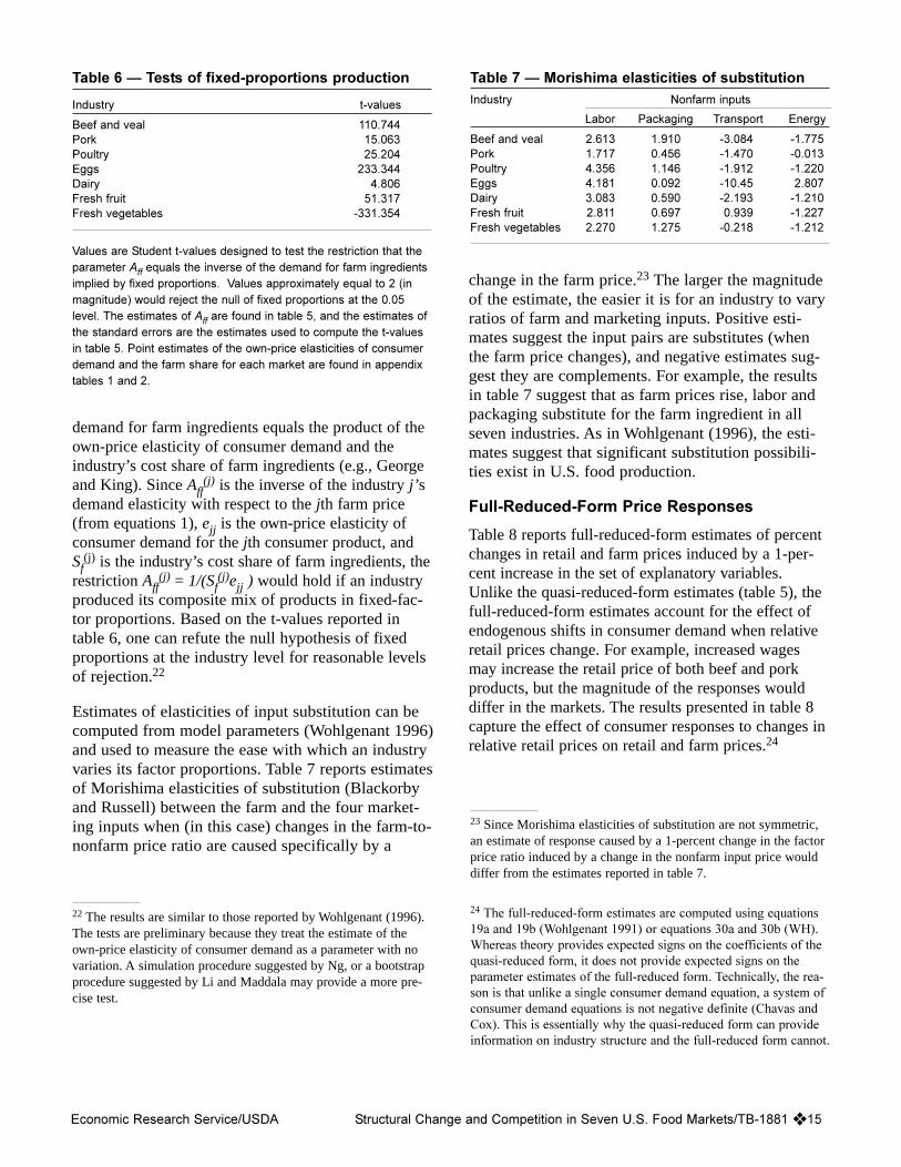
Estimates of elasticities of input substitution can becomputed from model parameters (Wohlgenant 1996)and used to measure the ease with which an industryvaries its factor proportions. Table 7 reports estimatesof Morishima elasticities of substitution (Blackorbyand Russell) between the farm and the four market-ing inputs when (in this case) changes in the farm-to-nonfarm price ratio are caused specifically by a

change in the farm price.23 The larger the magnitudeof the estimate, the easier it is for an industry to varyratios of farm and marketing inputs. Positive esti-mates suggest the input pairs are substitutes (whenthe farm price changes), and negative estimates sug-gest they are complements. For example, the resultsin table 7 suggest that as farm prices rise, labor andpackaging substitute for the farm ingredient in allseven industries. As in Wohlgenant (1996), the esti-mates suggest that significant substitution possibili-ties exist in U.S. food production.

Full-Reduced-Form Price Responses

Table 8 reports full-reduced-form estimates of percentchanges in retail and farm prices induced by a 1-per-cent increase in the set of explanatory variables.Unlike the quasi-reduced-form estimates (table 5), thefull-reduced-form estimates account for the effect ofendogenous shifts in consumer demand when relativeretail prices change. For example, increased wagesmay increase the retail price of both beef and porkproducts, but the magnitude of the responses woulddiffer in the markets. The results presented in table 8capture the effect of consumer responses to changes inrelative retail prices on retail and farm prices.24

Table 7 � Morishima elasticities of substitutionIndustry Nonfarm inputs

Labor Packaging Transport Energy

Beef and veal 2.613 1.910 -3.084 -1.775Pork 1.717 0.456 -1.470 -0.013Poultry 4.356 1.146 -1.912 -1.220Eggs 4.181 0.092 -10.45 2.807Dairy 3.083 0.590 -2.193 -1.210Fresh fruit 2.811 0.697 0.939 -1.227Fresh vegetables 2.270 1.275 -0.218 -1.212


Table 6 � Tests of fixed-proportions production

Industry t-values

Beef and veal 110.744Pork 15.063Poultry 25.204Eggs 233.344Dairy 4.806Fresh fruit 51.317Fresh vegetables -331.354

Values are Student t-values designed to test the restriction that theparameter Aff equals the inverse of the demand for farm ingredientsimplied by fixed proportions. Values approximately equal to 2 (inmagnitude) would reject the null of fixed proportions at the 0.05level. The estimates of Aff are found in table 5, and the estimates ofthe standard errors are the estimates used to compute the t-valuesin table 5. Point estimates of the own-price elasticities of consumerdemand and the farm share for each market are found in appendixtables 1 and 2.

22 The results are similar to those reported by Wohlgenant (1996).The tests are preliminary because they treat the estimate of theown-price elasticity of consumer demand as a parameter with novariation. A simulation procedure suggested by Ng, or a bootstrapprocedure suggested by Li and Maddala may provide a more pre-cise test.

23 Since Morishima elasticities of substitution are not symmetric,an estimate of response caused by a 1-percent change in the factorprice ratio induced by a change in the nonfarm input price woulddiffer from the estimates reported in table 7.

24 The full-reduced-form estimates are computed using equations19a and 19b (Wohlgenant 1991) or equations 30a and 30b (WH).Whereas theory provides expected signs on the coefficients of thequasi-reduced form, it does not provide expected signs on theparameter estimates of the full-reduced form. Technically, the rea-son is that unlike a single consumer demand equation, a system ofconsumer demand equations is not negative definite (Chavas andCox). This is essentially why the quasi-reduced form can provideinformation on industry structure and the full-reduced form cannot.

�� ❖ �� !�� "��#$

��%��&��

!'�� ( "�� &� ��

��)� *�� +�+,- ��./ ��00�� +�++0 +��0� �+��,�� +�+1- �+��,- +��1+�� +�+, ��--. ��1.�2 �� +�+1� +�0 . �+�0� 3�� +�+�� +�-�. +�-+/4�� +�� 1 �+��,� +�+-/3�� +�1. �+�+-/ +�--�� +�11, +��. �+�,/-! ��(�� +�1 1 �+�1,. �+�+--��( +�+0+ ��,+, ��-0,5��( +�+11 +��1 �+�0.+3��(��( �+�+�1 �+�--� +�-�.!��( +�+++ +�+�- �+�+�1��( +�++� +�+-/ �+�+-0��( �+�++1 �+�+�+ +�+0 %��( �+�-/0 ��,+� ��+1/

�� *� �� 3�� 3��(

!'�� ( "�� "�� "�� &� ��

��)� *�� +�/+/ ��//- ��+�� +�/,. +�/�� +�+- �+�/�0 �+��. �+�+.�� +��- �+�-,/ +�1+. +�+. +�+.- +�++0 +��,. +��-+ +�+�.�� +�-/. +�.01 �+�0/1 �+��, �+��00 �+�++ �+�/ �+�� . �+�+..�� +� �� 1��+ ��1.. �+��// �+�� +�++. ��+/- +�.- +��-02 �� +�+,- �+��+/ +�+�0 �+�11� �+�1+. �+�+�� +��+, +�01 +�+/�3�� 1�1., 0�/00 �-�,�� 1�/-� 1�0.� +��,+ +�./+ +� , +��114�� 1�1.1 -�� , ��-.1 ��0 � -�/1. �1��,- ��11+ +�0�� / �3�� +�0.1 +�/1� �+��1. +�, - +�--� +��,/ +��-, +��11 +�+�1�� 0+ �� .- +�/,- �+�.,+ ��0/+ +��-� +�� / �+�+,� +�/--! ��(�� +��/ �+�+�. �+�+, �+�+-. �+��,� +��+/ �+��/. �+��,� �+�+- ��( �1�+-/ �-�,01 ��,�� -1. ��1�� +�+� +�,// +�,�/ +�+�+5��( �+�0// ��,, +� /� ��0// �1�,// +�.++ +�� +��- +�+1-3��(��( +�+.� +�1,+ �+��,, +�+/. +�+/0 +�++, ��0. �+�. � �+��/-!��( �+�+,� �+�� +�+/+ �+�+,+ �+�+- �+�++1 �+�+,� �+�+-� �+�++0��( �+�+�0 �+��- +�+. �+�+.� �+�+ � �+�++0 �+��-- �+�� +�+�/��( +�+,1 +��+0 �+�+�- +�+-0 +�+-- +�++1 �+�+,� �+�+,+ �+�++�%��( +�+�- +��0/ �+�+.0 +�+�1 +�+0 +�++- �+�+� �+�+�+ �+�++.

!�� #��( ��

!'�� ( "�� "�� "�� &� ��

��)� *�� 1�,// +��+, �� /- ��,- ��+�0 +�+/ �+�+/, �+�0-0 +�,�+�� +�+0, +�+�- +�+,� +��- +��1. +�++. +�+�. +��- �+��.�� +�.�0 �+�11- �+��.1 �+�1�/ �+�1+1 �+�+�0 �+�+01 �+�-/, +�-11�� +� +� �+��.0 �+��+� +�1/+ +�10� +�+� +�� +�/.� �+�� 02 �� ,,. �+�-0- ��+.� �+�, 1 �+�,,. �+�+-- +�+-. +�1/ �+�1-.3�� /��1/ �� + 0�/�/ ��.0 �� 1, +��-, �+�+ , �+��+, +�01+4�� 1�101 1�0�/ �+�-�0 +�,.� 1�+.- ��0./ ��+/- +�0,/ ��1+3�� . +�+,1 �� 0� +�� +��-0 +�+-� +�,0/ �+�-0+ +� + �� 1�+�+ ��/ �+�-., �+�,� �+��-. +�11� +�-+/ +�0/� �+�1�.! ��(�� +��0. +��1 �+�1/� +�++� �+�� +�� +��-� �+�11� +�+.0��( ��/.. �+�,-. ��-�� +�-�, �+�1.1 �+�+1� +��+ +�/., �+�� -5��( �+�� + �+�� +�0�, �+�� 1 �+��/+ �+�+�1 +�+,� +�1.� �+�10�3��(��( �+�,+/ �+�+.. �+�-+ �+��,- �+��-, �+�+�+ �+�+1� �+�� / +��!��( �+�/-- �1��,- ��,�+ �+�+- �+�+-0 �+�++- +�++� +�+,- �+�+-/��( �+�-1� �+�+/ �+�1,- �+�00 ��-1 ��+/, +�++/ +�+0+ �+�+,-��( +�+ 1 +�+1+ +�+�1 +�+�� +�+�+ +�++� �+��0� ��++. +� 0 %��( +�+�- +�++- +�+�+ +�++0 +�++0 +�+++ �+�++/ �+�+0+ +�+,-

The effect of consumer substitution links the effects ofchanges in farm supply on retail and farm pricesacross the seven markets. For example, the first panelof table 8 suggests that increases in cattle supplydepress both retail and farm prices for pork. Hence,increased cattle supply will lower both cattle prices(farm-level price) and consumer-level beef prices.Because our estimates suggest that consumers treatbeef and pork as gross substitutes (appendix table 1),lower relative beef prices imply a reduction in con-sumer demand for pork. Because hogs are a normalfactor of production in pork supply, hog prices (farmlevel) also fall. In this particular example, it is impor-tant to recall that estimates presented in table 8exclude the effects of imports and exports of farmcommodities.25

The column labeled “spread” summarizes the relativeresponses of retail and farm prices associated with a1-percent increase in a particular explanatory vari-able. In particular, the estimates, computed in thisdouble-log specification as the difference between thepercent change in the retail and the percent change inthe farm price, represent Gardner’s response estimatesof retail-to-farm price spreads. A positive (negative)sign implies that the market’s retail price responseexceeds (is less than) the response of the market’sfarm price. Because the estimates account for theresponse of a market’s farm price and not the retailequivalentfarm price based on variable proportions,the “spread” estimates reported in table 8 representresponses of spreads computed under the assumptionof fixed-factor proportions.

Table 9 compares the own-price elasticities of con-sumer demand with the full-reduced form, own-priceelasticity of farm demand for farm ingredients for eachmarket. Fixed-proportions production implies that anindustry’s input demand would be less own-price elas-tic than the own-price elasticity of retail demand.However, the results in table 9 suggest that for four ofthe seven markets, the industry’s full-reduced-formdemand for farm ingredients is more own-price elasticthan consumer demand.26 Such results call into ques-tion the validity of market price analyses based onfixed proportions.


25 Attempts to interpret the results presented in this section are dif-ficult because standard errors and t-tests are not computed. Suchestimates might be computed using the methods suggested in foot-note 22.

26 The derived demand for farm ingredients reported in table 9 isas follows. If the full-reduced-form system (i.e., table 8) of farmprice equations is represented in matrix notation as Pf = bbbb1 F + bbbb2X, where F is the vector of farm supplies, and X is the vector of allother explanatory variables, the estimates in table 9 are bbbb1

-1. Theown-price elasticities of derived demand for farm ingredients(accounting for consumer substitution) are the diagonal elementsof bbbb1

-1.

Table 9 � Own-price elasticities of farm and con-sumer demand

Own-farm price elasticity Own-retail priceof industry demand elasticity of

Market for farm ingredients consumer demand

Beef and veal -0.402 -0.065Pork -0.514 -0.745Poultry -1.074 -0.607Eggs -0.472 -0.064Dairy -0.627 -0.974Fresh fruit -1.020 -0.208Fresh vegetables -0.753 0.054

This report demonstrates that structural change can beincorporated directly into a very general and powerfulset of market models. Early empirical findings of com-petitive U.S. food markets based on this general theorystood in sharp contrast to findings of market powerbased on the traditional and restrictive assumptions offixed-factor proportions. By accounting for structuralchange, we have shown that food market data closelysupport this general theory and result in further evi-dence of competitive U.S. food industries.

In this report, we equate trends in market variableswith structural change. We found that the most intrigu-ing type of trend is the type that changes directionunexpectedly. Unpredictable changes in trends fitKinsey and Senauer’s description of structural changein food consumption and Paul’s explanation of indus-try reorganization. Yet, it is precisely their unpre-dictability that poses obstacles to statistical inference.A main motivation of this report is to provide infer-ence on competition, and we have relied on recentadvances in econometrics to exploit such trends inmarket variables and test whether seven U.S. foodindustries operate competitively within an environmentof structural change.

Although market variables may be driven by unpre-dictable changes in trends, it is necessary that modelsconstructed from them do not. Our finding that retail-and farm-price relationships derived from this generaltheory are cointegrated supports the theory, as well asthe claim, that changing trends in food consumptionalter the structure of food industries. It also suggeststhat such models can be used to test for market powerdespite the many permanent changes in U.S. food mar-kets that may have occurred over time.

Our finding of mostly competitive U.S. food industriesoffers important explanations of why concentratedfood industries may be competitive. Paul argues thatunexpected downward trends in consumer demandmotivate firms to specialize and seek vertical arrange-ments that serve to spread the risk of downward trendsin revenues. Our finding of cointegrated retail- andfarm-price relationships suggests that competitiveindustries will reorganize to spread the risk of uncer-tain downward trends in consumer demand.


Conclusions

Azzam, A.M. “Testing the Competitiveness of FoodPrice Spreads.”J. Agr. Econ.43 (May 1992): 248-256.

__, and T. Park, “Testing for Switching Market Conduct.”Applied Econ. 25 (June 1993): 795-800.

Blackorby, C., and R.R. Russell. “Will the Real Elasticity ofSubstitution Please Stand Up? (A Comparison of theAllen/Uzawa and Morishima Elasticities).”Amer. Econ.Rev. 79 (September 1989): 882-888.

Braulke, M. “On the Comparative Statics of a CompetitiveIndustry.”Amer. Econ. Rev. 77 (June 1987): 479-485.

Bresnahan, T.F. “The Oligopoly Solution Concept IsIdentified.” Economics Letters. 10 (1982): 87-92.

Chavas, J.P., and T. Cox. “On Market EquilibriumAnalysis.”Amer. J. Agr. Econ. 79 (May 1997): 500-513.

Clark, J.S., and C.E. Youngblood. “Estimating DualityModel with Biased Technical Change: A Time SeriesApproach.”Amer. J. Agr. Econ. 74 (May 1992): 353-360.

Deaton, A., and J. Muellbauer. Economics and ConsumerBehavior. London: Cambridge University Press. 1980.

Dickey, D.A., and W.A. Fuller. “A Distribution of theEstimators for Autoregressive Time Series with a UnitRoot.” J. of the Am. Stat. Association74 (1979): 427-431.

Elitzak, H. Food Cost Review, 1996.U.S. Department ofAgriculture, Econ. Res. Serv., AER-761, December 1997.

Engle, R.F., and C.W.J. Granger. “Co-integration and ErrorCorrection: Representation, Estimation, and Testing,”Econometrica55 (March 1987): 251-276.

Friedman, M. Price Theory. New York: Aldine PublishingCo. 1976.

Fuller, W.A. Introduction to Statistical Time Series. NewYork: John Wiley and Sons. 1976.

Gardner, B.L. “The Farm-Retail Price Spread in aCompetitive Food Industry.”Amer. J. Agr. Econ. 57(August 1975): 399-409.

George, P.S., and G.A. King. “Consumer Demand for FoodCommodities in the United States With Projections for1980.” California Agr. Exp. Sta., Giannini FoundationMonograph No. 26, March 1971.

Goodwin, B.K., and G.W. Brester, “Structural Change inFactor Demand Relationships in the U.S. Food andKindred Products Industry.”J. Agr. Econ. 77 (February1995): 69-79.

Granger, C.W.J., and P. Newbold. Forecasting EconomicTime Series. New York: Academic Press. 1977.

Hamilton, J.D. Time Series Analysis. Princeton: PrincetonUniversity Press. 1994.

Heiner, R.A., “Theory of the Firm in ‘Short-Run’ IndustryEquilibrium.” Amer. Econ. Rev.72 (June 1982): 555-562.

Holden, D., and R. Perman. “Unit Roots and Cointegrationfor the Economist.”Cointegration for the AppliedEconomist, B. Bhaskara Rao, ed., New York: St. Martin’sPress, 1994.

Huang, K.S. “An Inverse Demand for U.S. CompositeFoods,”Amer. J. Agr. Econ.70 (November 1988): 902-909.

Kinsey, J. and B. Senauer. “Consumer Trends and ChangingFood Retailing Formats.”Amer. J. Agr. Econ. 78(December 1996):1187-1191.

Koontz, S.R., P. Garcia, and M.A. Hudson. “MeatpackerConduct in Fed Cattle Pricing: An Investigation ofOligopsony Power.”Amer. J. Agr. Econ. 75 (August1993): 527-548.

Li, H., and G.S. Maddala. “Bootstrapping CointegratedRegressions.”J. of Econometrics.80:2(1997): 297-318.

MacDonald, J.M., and M. Ollinger. “U.S. Meat SlaughterConsolidating Rapidly.”Food Review, May-August 1997,pp. 22-27.

Martinez, S.W., and A.J. Reed. From Farmers toConsumers, Vertical Coordination in the Food Industry.U.S. Department of Agriculture, Econ. Res. Serv., AIB-720, June 1996.

Martinez, S.W., K. Smith, and K. Zering. “Changing PorkBusiness Affects Pork Prices and Quality.”Food Review,May-August 1997, pp. 17-21.

Ng, S. “Testing for Homogeneity in Demand Systems Whenthe Regressors Are Nonstationary.”J. of AppliedEconometrics.10 (1995): 147-163.

Panzar, J.C., and R.D. Willig. “On the Comparative Statics


References

of a Competitive Industry With Inframarginal Firms.”Am.Econ. Rev., 68 (June 1978): 474-478.

Park, J.Y. 1990. “Testing for Cointegration Through VariableAddition.” Studies in Econometric Theory. Fromby andRhodes, eds., pp. 107-133. New York: JAI Press, 1990.

Park, J.Y. “Canonical Cointegrating Regressions.”Econometrica60 (January 1992):119-143.

Park, J.Y., and M. Ogaki. “Seemingly Unrelated CanonicalCointegrating Regressions.” Working Paper No. 280, TheRochester Center for Economic Research, Rochester,New York, 1991.

Paul, A.B. “The Role of Competitive Market Institutions.”Agr. Econ. Res. 26 (April 1974):41-48.

Phillips, P.C.B., and S.N. Durlauf. “Multiple Time SeriesWith Integrated Processes.”Rev. of Econ. Studies53(August 1986): 473-496.

Phillips, P.C.B., and S. Ouliaris. “Asymptotic Properties ofResidual-Based Tests for Cointegration.”Econometrica58 (January 1990): 165-193.

Phillips, P.C.B., and P. Perron. “Testing for Unit Roots inTime Series Regression.”Biometrica, 75 (1988): 335-346.

Reed, A.J., and J.S. Clark. “The Transmission of Trends inRetail Food and Farm Prices.”Amer. J. Agr. Econ. 80(Number 5, 1998): 1139-1143.

_____. Nonfarm Input Prices, Price Margins, andConsumer Food Prices. U.S. Department of Agriculture,Econ. Res. Serv., TB-1867, March 1998.

Schroeter, J.R. “Estimating the Degree of Market Power inthe Beef Packing Industry.”Rev. Econ. and Stat.70(February 1988): 158-162.

__, and A.M. Azzam. “Marketing Margins, Market Powerand Price Uncertainty.”Amer. J. Agr. Econ. 73 (November1991): 990-999.

Silberberg, E. The Structure of Economics: A MathematicalAnalysis. New York: McGraw-Hill. 1978.

U.S. Department of Agriculture, Econ. Res. Serv. FoodMarketing Review, 1994-95. AER-743, September 1996.

U.S. Department of Agriculture, Grain Inspection, Packersand Stockyards Administration. Concentration in the RedMeat Packing Industry. February 1996.

Wohlgenant, M.K. “Product Heterogeneity and theRelationship between Retail and Farm Prices:Econometric Implications.”European Review ofAgricultural Economics,26 (June 1999): 219-227.

Wohlgenant, M.K. “Retail to Farm Price Linkages in aComplete System of Demand Functions: Extension toDisaggregated Marketing Costs and Tests for MarketPower.” Unpublished report in cooperation with Econ.Res. Serv., 1996.

__. “Impact of Changes in Consumer Demand on Farm-level Demand for Food.”Policy Implications for U.S.Agriculture of Changes in Demand for Food, H. Jensenand J. Chalfant, eds., pp. 19-26. Ames: Iowa StateUniversity Press CARD, 1994.

__. “Demand for Farm Output in a Complete System ofDemand Functions.”Amer. J. Agr. Econ. 72 (May 1989):241-252.

__, and R.C. Haidacher. Retail to Farm Linkage for aComplete Demand System of Food Commodities. U.S.Department of Agriculture, Econ. Res. Serv., TB-1775,Dec. 1989.


Structure of the WH Model

Underpinning the pair of quasi-reduced-form retail andfarm price equations in the text equations 1 for eachmarket is a general market-clearing condition for finalindustry output and a general market-clearing condi-tion for farm ingredients. They are general because,within the same composite industry, firms’ farmdemand and firms’ output supply will vary acrossfirms. Within the same industry, one firm’s productionfunction may be different from other firms’ productionfunctions. Hence, the structure of this class of modelsprovides an analytical framework for price analyses ofmarket for which any one industry produces a varietyof different final products. The comparative staticresults developed by Heiner, and extended byWohlgenant (1989), do not depend on the restriction ofidentical firms. For a more detailed discussion of thisstructure, see WH or Wohlgenant (1989).

In the particular setup in the text, a food industry con-sists of all manufacturing, wholesaling, and retailingfirms associated with a composite final demand prod-uct (e.g., beef). Each industry faces a final, market-level consumer demand schedule for its products and amarket-level supply schedule for the farm ingredients.For tractability, firms in the same industry face thesame composite market prices for output and allinputs.

In this setup, if i denotes an index associated with afirm in the industry, market clearing for final consumergoods could be generally written as

Si Sri (Pr , Pf , W) = Dr (Pr, Z) (i)

where Sri is the supply of the ith firm, Pr the output

price, Pf the farm price, W a vector of non-farm inputprices, and Z is a consumer demand shifter. Condition(i) states that the sum of firm-level supply equals finalconsumer demand for the industry’s output. Marketclearing associated with farm ingredients is expressedas

Si Dfi (Pr , Pf , W ) = F (ii)

in which F is farm supply, and Dfi is the ith firm’s

demand for farm ingredients. Condition (ii ) states that the sum of firm-level demands for farm ingredi-ents equals the market-level supply of farm ingredi-ents. Equations i and ii represent a general form of

the structural model for each market examined in this study.

The structural parameters of equations i and ii definethe Ar and the Af of equations 1 in the text. The struc-tural parameters of equations i and ii are found bytotally differentiating equations i and ii and expressingthe results in terms of partial elasticities of supply anddemand. Totally differentiating equations i and ii andrearranging, gives

(err - e) d lnPr + erf d lnPf = ez d lnZ - erw d lnW

- efr d lnPr - eff d lnPf = efw d lnW - d ln F

where err , for example, is the weighted sum of theelasticities of firm supply, i.e.,err = Si err

i (Qri/Qr).

Wohlgenant and WH solve the two-equation systemfor d lnPr and d lnPf in terms of d lnZ, d lnW, and dlnF and reveal the precise way in which the structuralparameters define the coefficients of the quasi-reduced-form flexibilities (the A coefficients) in thetext. The relationship between the structural parame-ters and the response coefficients are spelled out in thecited articles, and define the comparative static resultsdiscussed in the text.

Data

To the greatest extent possible, we followed the direc-tions of Wohlgenant and Haidacher (WH) when con-structing the economic variables used in this study. Allof the variables of equations 1-4 in the text were con-structed from annual data from 1958 to 1997. All ofthe potentially superfluous farm supply shift variablesexcept the laying flock (for eggs) were also construct-ed from annual data from 1958 to 1997. The layingflock variable was constructed from 1960-97 data.

The retail prices are constructed from annual averageConsumer Price Index (CPI) data, U.S. City Average,Not Seasonally Adjusted. The particular series used toconstruct retail prices are:

Beef and veal Beef and Veal, CPI, U.S. CityAverage, Not Seasonally Adjusted

Pork Pork, CPI, U.S. City Average, NotSeasonally Adjusted

Poultry Poultry, CPI, U.S. City Average,Not Seasonally Adjusted


Appendix

Eggs Eggs, CPI, U.S. City Average, NotSeasonally Adjusted

Dairy Dairy and Related Products, CPI,U.S. City Average, Not SeasonallyAdjusted

Fresh fruit Fresh Fruits, CPI, U.S. CityAverage, Not Seasonally Adjusted

Fresh veg. Fresh Vegetables, CPI, U.S. CityAverage, Not Seasonally Adjusted

Nonfood All Items Less Food, CPI, U.S. CityAverage, Not Seasonally Adjusted

Beverages Non-Alcoholic Beverages andBeverage Material, CPI, U.S. CityAverage, Not Seasonally Adjusted

Sugar Sugar and Sweets, CPI, U.S. CityAverage, Not Seasonally Adjusted

Cereal Cereals and Bakery Products, U.S.City Average, Not SeasonallyAdjusted

Farm level prices are constructed from non-seasonallyadjusted annual Producer Price Index (PPI) data forfarm products. The series used to construct farm pricevariables are:

Beef and veal Slaughter Cattle, PPI, FarmProducts, Not Seasonally Adjusted

Pork Slaughter Hogs, PPI, FarmProducts, Not Seasonally Adjusted

Poultry Slaughter Poultry, PPI, FarmProducts, Not Seasonally Adjusted

Eggs Chicken Eggs, PPI, Farm Products,Not Seasonally Adjusted

Dairy Fluid Milk, PPI, Farm Products,Not Seasonally Adjusted

Fresh fruit Fresh Fruits and Melons, PPI, FarmProducts, Not Seasonally Adjusted

Fresh veg. Fresh Vegetables Except Potatoes,PPI, Farm Products, Not SeasonallyAdjusted

The raw farm prices for beef and veal and pork (Pf*)are adjusted (as in Wohlgenant and WH) to account forthe value of byproducts in the farm prices for slaughtercattle and slaughter hogs. We use the 1982 levels ofthe gross farm value (GFV) and the byproduct value(BPV), and hence the net farm value (NFV = GFV -BPV) for cattle and for hogs. These data are recordedby USDA/ERS. Using the 1982 values, data onbyproduct allowances (Pb) for cattle and hogs are usedto adjust the raw PPI farm price series. In general, thelog of the adjusted farm price,ln Pf is computed as

ln Pf = (GFV82/ NFV82) ln Pf* - (BPV82/ NFV82) ln Pb

In particular, the adjusted farm price formula for beefis

ln Pf = (155.5/141.1) ln Pf* - (14.4/ 141.1) ln Pb

and is

ln Pf = (94.3/87.0) ln Pf* - (7.3/87.0) ln Pb

for pork.

All CPI and PPI price series were obtained fromBureau of Labor Statistics (BLS) web sites, and theGFV, BPV and byproduct allowances were obtainedfrom ERS data sets with help from Lawrence Duewer.

The price of labor, packaging, transportation, energy,and other inputs from 1968-1997 were obtained direct-ly from published reports (Elitzak). The series wasextended back to 1958-1967 by overlapping the 1968-97 data set with a consistent and similar data set cover-ing the 1958-67 period. The data were provided byHoward Elitzak.

The series used to construct farm supply are computedas the product of per capita food disappearance multi-plied by U.S. Population, including armed services(July 1). The particular per capita disappearance dataseries used are:

Beef and veal Beef plus Veal, Food DisappearancePer Capita, Carcass Weight (lbs)

Pork Pork, Food Disappearance PerCapita, Carcass Weight (lbs)

Poultry Total Chicken Plus Turkey, FoodDisappearance Per Capita, CarcassWeight (lbs)


Eggs Eggs, Food Disappearance PerCapita, Farm Weight (lbs)

Dairy All Dairy Products, FoodDisappearance Commercial Salesplus USDA donations (lbs of milkequivalent, milkfat basis)

Fresh fruit Fresh Fruit (including melons),Food Disappearance Per Capita,Farm Weight (lbs)

Fresh veg. Commercially Produced FreshVegetables Excluding Potatoes andSweet Potatoes Minus Mushrooms,Commercial Disappearance PerCapita, Farm Weight (lbs)

The farm supply variables for beef and pork were con-verted from carcass weight to live weight by dividingthe disappearance values (in carcass weight) by theannual average ratio of the dressed to live weightunder federal inspection. The dressed and live weightdata are reported in Annual Livestock Slaughter, theAgricultural Statistics Board, NASS, USDA, and weremade available by Lawrence Duewer. The dependentvariables used in the estimation of the system of con-sumer demand relationships were constructed usingthe same food disappearance variables, except noadjustment was made to convert the beef and pork dis-appearance data to live weight.

The data to compute shifters on consumer demand(other than prices) are:

Population U.S. Population, including armedservices, July 1

Income Per Capita Personal DisposableIncome, Current Dollars, multipliedby Population

The data used to form nonfarm input prices were pro-vided by Howard Elitzak. They are:

Packaging Food Marketing Cost Index (1982 = 100), packaging component

Transportation Food Marketing Cost Index (1982 = 100), transportation component

Energy Food Marketing Cost Index, energycomponent

Other Food Marketing Cost Index, advertis-ing, communications, rent mainte-nance and repair, business services,supplies, property taxes, short-terminterest. This variable is used as thedeflator in this bulletin.

Data to construct the shifters on the farm supply usedto test for oligopsony power tests are:

Beef & veal S1: Steers, 1 year and older, January 1S2: Price of number 2 yellow corn,Chicago

Pork S1: U.S. hog inventory, all hogs and pigsS2: Price of number 2 yellow corn,Chicago

Poultry S1: Price of soybean meal, 48 percent,Decatur S2: Price of number 2 yellow corn,Chicago

Eggs S1: Laying flock, average annual permonth

Dairy S1: Cows and heifers on farms, 2 yearsand older, January 1S2: Price of soybean meal, 48 percent,Decatur

Fresh fruit S1: Average hourly wages paid toall hired farm workers

Fresh vegetablesS1: Average hourly wages paid toall hired farm workers



Appendix table 1 � System of consumer demand equations

Explanatory Per capita consumer demand equation for:variable Beef Pork Poultry Eggs Dairy Fresh fruit Fresh vegetables

Beef -0.065 0.574 -0.333 0.191 0.089 -0.621 -0.481price (-1.02) (15.3) (-3.20) (5.08) (2.37) (-6.5) (-7.3)

Pork 0.322 -0.745 -0.085 0.030 0.069 -0.083 -0.152price (15.0) (-20.0) (-1.2) (.91) (2.23) (-1.3) (-3.04)

Poultry -0.078 0.029 0.607 0.091 0.112 0.335 0.207price (-3.0) (-.95) (-6.0) (2.60) (3.36) (5.02) (3.70)

Egg 0.045 0.012 0.083 -0.064 0.030 -0.101 0.014price (4.70) (.79) (2.31) (-2.18) (1.50) (-2.90) (.37)

Dairy 0.053 0.085 0.303 0.084 -0.974 -0.140 -0.035price (1.87) (2.06) (3.01) (1.45) (-14.5) (-1.52) (-0.37)

Fresh fruit 0.148 -0.033 0.327 -0.089 -0.039 -0.208 0.135price (-6.51) (-1.24) (4.90) (-2.77) (-1.37) (-2.50) (2.63)

Fresh vegetable 0.093 -0.050 0.157 0.015 -0.004 0.113 0.054price (-7.22) (-2.89) (3.59) (.51) (-.17) (2.66) (.81)

Nonfood 0.210 0.139 -1.170 0.388 0.905 -0.008 -0.466price (1.93) (2.00) (-6.67) (5.5) (13.8) (-.052) (-4.08)

Beverage -0.163 0.164 0.093 0.012 0.110 0.202 0.057price (-3.74) (6.37) (1.36) (.47) (4.78) (3.12) (1.32)

Sugar 0.410 -0.367 -0.701 -0.195 -0.101 -0.455 -0.253price (4.51) (-6.50) (-4.48) (-3.3) (-1.9) (-3.0) (-2.53)

Cereal -0.668 0.353 0.967 -0.129 0.235 0.801 0.564price (-4.56) (3.57) (3.53) (-1.2) (2.51) (2.92) (3.19)

Income/ 0.175 -0.103 0.965 -0.335 -0.430 0.145 0.357pop. (5.33) (-3.23) (12.2) (-9.0) (-13.8) (2.10) (5.66)

Intercept 1.005 -0.321 6.291 2.797 5.406 5.010 5.344(14.0) (-4.51) (36.9) (34.3) (79.5) (33.0) (38.7)

Entries are elasticity estimates with symmetry and homogeneity imposed at the sample means. Values in parentheses are t-values. The shares of income used to impose the symmetry restriction at the point estimates are as follows: 0.316 (beef and veal), 0.0180 (pork), 0.008 (poultry), 0.0082 (eggs), 0.0241 (dairy), 0.0075 (fresh fruit), and 0.0062 (fresh vegetables).

Appendix table 2 � Factor shares for the seven industriesIndustry Labor Packaging Transport Energy Other Farm

Beef & veal 0.1892 0.0731 0.0430 0.0215 0.1032 0.5700

Pork 0.2904 0.1122 0.0660 0.0330 0.1584 0.3400

Poultry 0.2156 0.0833 0.0490 0.0245 0.1176 0.5100

Eggs 0.1628 0.0629 0.0370 0.0185 0.0888 0.6300

Dairy 0.2244 0.0867 0.0510 0.0255 0.1224 0.4900

Fresh fruit 0.2948 0.1139 0.0670 0.0335 0.1608 0.3300

Fresh vegetables 0.2904 0.1122 0.0660 0.0330 0.1584 0.3400

Estimates of Consumer Demand and Factor Shares

United States Department of AgricultureEconomic Research Service1800 M Street, NWWashington, DC 20036-5831

Documents

Structural Change and Competition in Seven U.S. Food Markets