Structural change and lag length in VAR modelspages.uoregon.edu/mthoma/Papers/Structural Change... · Structural change and lag length in ... agent’s use of learning equations can

Available online at www.sciencedirect.com

Journal of Macroeconomics 30 (2008) 965–976

www.elsevier.com/locate/jmacro

Structural change and lag length in VAR models

Mark Thoma *

Department of Economics, University of Oregon, Eugene, OR 97403-1285, United States

Received 15 November 2006; accepted 1 August 2007Available online 17 August 2007

Abstract

This paper investigates the relationship between changes in policy rules and changes in the esti-mated lag length in empirical models. The paper finds that there is a close association betweenchanges in the parameter on the output gap term in the monetary policy rule investigated hereand changes in estimated lag length for an associated VAR model.� 2007 Elsevier Inc. All rights reserved.

JEL classification: E52

Keywords: Lag length; Policy changes; Structural change

1. Introduction

To what extent do the dynamics of empirical macroeconomic models change whenthere is a change in monetary policy? This paper examines this question by looking atone aspect of macroeconomic dynamics, lag length in empirical models, and its relation-ship to changes in the parameters of a monetary policy rule for the federal funds rate.

Motivation for looking for changes in dynamics comes from the large literature onchanges in the monetary policy rule over time. Theoretical and empirical investigationsof shifts in monetary policy rules have a long history, but the recent literature is motivatedlargely by the Clarida et al. (2000) finding that policy changed from values consistent withindeterminacy in the 1970s to policy consistent with determinacy in the 1980s.

0164-0704/$ - see front matter � 2007 Elsevier Inc. All rights reserved.

doi:10.1016/j.jmacro.2007.08.001

* Tel.: +1 541 346 4673; fax: +1 541 346 1243.E-mail address: [email protected]

mailto:[email protected]

966 M. Thoma / Journal of Macroeconomics 30 (2008) 965–976

This generated considerable debate concerning whether policy prior to the 1980s actu-ally led to indeterminacy and whether structural breaks in policy parameters haveoccurred at all. Papers such as Clarida et al. (2000), Cogley and Sargent (2002), Boivinand Giannoni (2003) and Boivin (2004) support the idea that there have been importantshifts in monetary policy parameters. Some papers, such as Sims and Zha (2004), arguethat allowing for changes in the variance of structural disturbances over time can poten-tially overturn the result that there have been monetary policy shifts, but they also allowfor parameter shifts over time and find support for such changes.1 Thus, though work inthis area is still developing, strong empirical evidence for changes in the parameters of themonetary policy rule over time exists, and theoretical work shows that such changes canhave important effects on how variables in the model respond dynamically to shocks.2

There are several reasons to expect that a change in policy can affect estimated laglengths in empirical VAR models: (i) policy parameters consistent with indeterminacyfor some time periods, (ii) changes in policy that change the number of lags in the policyequation, (iii) agent’s use of learning equations can bring variable numbers of lagged val-ues into the solution causing estimated lag lengths to change, (iv) changes in the policyparameters causing structural breaks that, if unaccounted for in the econometric model,can cause changes in the estimated lags, and (v) changes in the parameters of the moneyrule causing changes in the degree of real rigidity and changes in the amount of persistencedisplayed in response to shocks. Finally, there are also reasons to think causality mightrun in the other direction, that is, that (vi) changes in the dynamic structure of the econ-omy can bring about an altered policy response.

2. Empirical model

To estimate the monetary policy reaction function described below, data are needed onthe federal funds rate, inflation, and the output gap. Quarterly data for the federal fundsrate, the inflation rate, and the log of GDP from 1960 through the second quarter of 2006are used in the estimation.3 To estimate the output gap, estimates of real potential outputfrom the Congressional Budget Office’s are used.

The next step is to use rolling regressions to obtain two data series, one containingchanges in the values of the policy parameters over time, and the other containing changesin the estimated optimal lag length according to likelihood ratio (LR) tests.4 To obtainchanges in the parameter values in the policy equation, the following regression, a Taylorrule augmented by interest rate smoothing, is estimated using rolling window regression

it ¼ b0 þ b1it�1 þ bppt þ b~y~yt þ wt ð1Þ

1 Sims and Zha (2004) discuss recent empirical work in this area and note that Bernanke and Mihov (1998)conclude there is little evidence for major shifts in policy regimes over time.

2 Several papers examine the role of lag structure in assessments of monetary policy and how the effects ofmonetary policy change over time. For example, Kim and McMillin (2003) show that lag structure is important inassessing monetary policy effects, and Swanson (1998) assesses how the relationship between money and outputchanges over time using rolling window regression. Lee (1997) uses rolling window regression combined withoptimal lag length selection to examine the dynamic relationship between money and income over bothsubsamples and lag specifications.

3 The data are obtained from the FRED II data set available on the St Louis Fed web site.4 The use of a rolling window and the optimal lag selection resemble the techniques used in Lee (1997).

M. Thoma / Journal of Macroeconomics 30 (2008) 965–976 967

In this equation, the right-hand side variables are inflation, the output gap, and lags of thefederal funds rate.5 The window is assumed to be 60 observations, i.e. 15 years. Theparameter values at each step are saved and indexed by the last observation in the windowof data used in the estimation. This gives a series of parameter values, one for each param-eter in Eq. (1).

The next step is to obtain changes in the estimated lag length for the associated VAR modelinvolving inflation, output, and the federal funds rate. To obtain the optimal lag length foreach sample period, again use rolling regressions on a VAR model containing the three vari-ables output (not the output gap since it is much more common for output to be used in VARmodels), inflation, and the federal funds rate.6 For each window of 60 observations, estimatethe lag length using the LR test, and save the result. The estimated lag lengths are indexed bythe last time period in the window. This gives a time-series of values for the optimal lag lengththat can be matched to the changes in the parameters of the Taylor rule.

3. Results

Fig. 1a–d plot the coefficients of the Taylor rule along with two standard deviation con-fidence bounds.

These parameters exhibit notable variation through time, but there is a theoretical rea-son for using a transformation of the estimated parameters. In theoretical models such asGertler, and Clarida et al. (1999) and in Honkapohja and Mitra (2003), the policy reactionfunction for the quarterly case is

it ¼ ð1� b1Þðb0 þ bppt þ b~y~ytÞ þ b1it�1 þ wt: ð2Þ

This is a standard Taylor rule augmented by a lagged interest rate term to capture interestrate smoothing. It is assumed that b1 6 1 and that bp P 1. In this specification, the federalfunds rate is increased when inflation or output rises above target with the strength of theresponse depending upon the values of the parameters of the policy rule.

The parameters estimated using Eq. (1) must be transformed to match those from Eq.(2).7 The transformations are

b̂�0 ¼ b̂0=ð1� b̂1Þ ð3Þb̂�p ¼ b̂p=ð1� b̂1Þ ð4Þb̂�y ¼ b̂y=ð1� b̂1Þ: ð5Þ

These parameters, along with the estimated lag lengths for comparison, are shown inFig. 2a–c.

The last graph (Fig. 2c) showing the relationship between the coefficient on the outputgap in the Taylor rule and the estimated lag lengths from a three variable output, inflation,

5 Other versions of the policy equations that use the lagged rather than current values of the right-hand sidevariables were also investigated.

6 This is a standard baseline model in the empirical monetary policy and income causality literature. Forexample, see the discussion on page 20 of the recent paper by Bernanke et al. (2004).

7 This simply corrects expected values for the AR(1) term on the right-hand side.

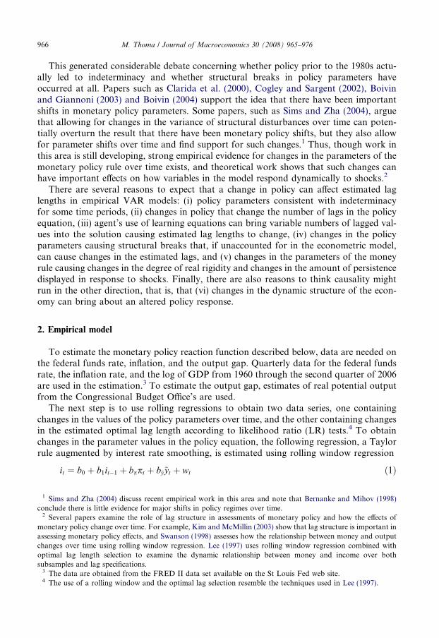
Fig. 1. (a) Taylor rule constant over time, (b) Taylor rule AR1 coefficient over time, (c) Taylor rule inflationcoefficient over time and (d) Taylor rule output coefficient over time.


and federal funds rate VAR shows the clearest association.8 If these two series aresmoothed with a rectangular window seven quarters wide to remove high frequency var-iation, the association is more evident as shown in Fig. 3.

There are several results to note from the figures. First, with respect to the coefficient onthe inflation term, theory implies that indeterminacy will arise if the coefficient is too small,and in many models, a coefficient value less than one defines too small. These results showthat the coefficient was below 1.0 in the late 1970, consistent with Clarida et al. (2000).After 1980, the value of the coefficient generally stays above 1.0, but not uniformly so.In particular, the coefficient dips into the indeterminacy range in the mid and late

8 If the level of output in the VAR model is replaced by the output gap so that the definition of output isidentical in the monetary policy rule and the VAR model, the results are very similar to those shown in the graph,i.e. the estimated lag lengths in the VAR model are very similar.

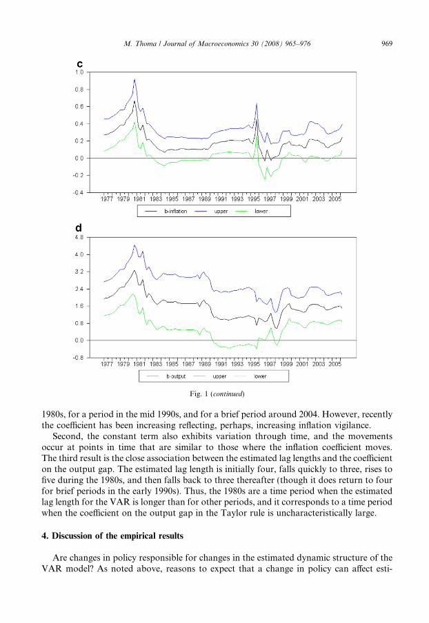
Fig. 1 (continued)


1980s, for a period in the mid 1990s, and for a brief period around 2004. However, recentlythe coefficient has been increasing reflecting, perhaps, increasing inflation vigilance.

Second, the constant term also exhibits variation through time, and the movementsoccur at points in time that are similar to those where the inflation coefficient moves.The third result is the close association between the estimated lag lengths and the coefficienton the output gap. The estimated lag length is initially four, falls quickly to three, rises tofive during the 1980s, and then falls back to three thereafter (though it does return to fourfor brief periods in the early 1990s). Thus, the 1980s are a time period when the estimatedlag length for the VAR is longer than for other periods, and it corresponds to a time periodwhen the coefficient on the output gap in the Taylor rule is uncharacteristically large.

4. Discussion of the empirical results

Are changes in policy responsible for changes in the estimated dynamic structure of theVAR model? As noted above, reasons to expect that a change in policy can affect esti-

Fig. 2. (a) Optimum lag lenght and the constant term, (b) optimum lag length and the inflation coefficient and (c)optimum lag lenght and the gap coefficient.


Fig. 3. Smoothed optimum lag length and smoothed gap coeffiecient.


mated lag lengths in empirical VAR models include: (i) policy parameters consistent withindeterminacy for some time periods, (ii) changes in policy that change the number of lagsin the policy equation, (iii) agent’s use of learning equations can bring variable numbers oflagged values into the solution causing estimated lag lengths to change, (iv) changes in thepolicy parameters causing structural breaks that, if unaccounted for in the econometricmodel, can cause changes in the estimated lags, and (v) changes in the parameters ofthe money rule causing changes in the degree of real rigidity and changes in the amountof persistence after shocks hit the economy. Finally, there are also reasons to think cau-sality runs in the other direction, that is, that (vi) changes in the dynamic structure ofthe economy can bring about an altered policy response.

Taking these in turn, the first reason lag lengths might vary with changes in policy isthat policy might be consistent with indeterminacy during some time periods. It can beshown that the solution under indeterminacy can contain more lags than the solutionfor parameter ranges with a determinate solution so that variation between these param-eter ranges can cause variation in both estimated and theoretical lag lengths. In addition,there may be multiple solutions with different persistence characteristics leading to differ-ent estimated lag lengths over time.9 However, since there is no clear association betweenchanges in the estimated lag lengths and the time periods when the inflation coefficient fallsbelow one in the figure above, it does not appear that indeterminacy is the source of theestimated variation in the estimated lag length.

The second reason is changes in the number of lags in the policy equation causingchanges in the persistence of output, inflation, and the interest rate in the estimatedVAR model. However, there is little evidence that the number of lags involved in the pol-icy equation has changed substantially. For example, one lag of the interest rate is suffi-cient to remove serial correlation in the policy equation throughout the sample.

The third reason that estimated lag lengths might vary with changes in policy param-eters arises in learning models. In learning models, parameter values are estimated by

9 The paper by Sims and Zha (2004) discusses this issue and argues that allowing for stochastic volatility andrelaxing very strong identifying restrictions overturns the Clarida et al. (2000) indeterminacy result.


economic agents using linear models and a particular window of data, i.e. a particulargain.10 These regressions bring lagged values of variables into the solutions. In modelssuch as Evans and Ramey (2003) the gain varies through time according to the frequencyof policy changes. For example, in the learning regressions, frequent changes in policyparameters can cause agents to place more weight on more recent data, and less weighton data that is more distant thus changing the gain. As the gain changes, the numberof lagged variables in the learning regressions changes which can bring about a changein estimated lag lengths. Again, however, this seems to be an unlikely explanation forthe results since the lag length changes appear to be associated with the magnitude ofthe parameter, not the frequency with which it changes.

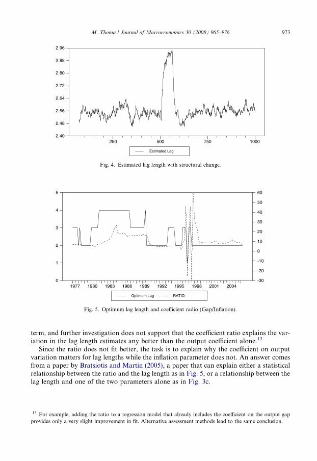
Fourth, changes in the policy parameters themselves may be responsible for changes inthe estimated number of lags. A simulation is used to examine this possibility. In the sim-ulation, artificial data are generated from an AR(3) with lag coefficients of .5, .25, and.125. The constant term captures the structural change imposed on the simulation andis equal to 1.0 for the first 500 observations, and 2.0 for the second 500 observations.11

The error term is drawn from a unit normal distribution.The graph in Fig. 4 shows the estimated lag length at each date determined by mimick-

ing the procedure above, i.e. by rolling a window of 60 observations through the data andestimating the lag length for each sample window. As is evident, in periods when bothparts of the sample are in the data set, the lag length estimates are affected by the breakin the constant value.12

The fifth explanation, like the fourth, involves changes in the coefficients of the moneyrule driving changes in the lag structure. This explanation relies on theoretical work byBratsiotis and Martin (2005) discussed below showing that changes in the parameters ofthe money rule can cause changes in the degree of real rigidity, and this in turn can causechanges in the degree of persistence and changes in the estimated lag lengths.

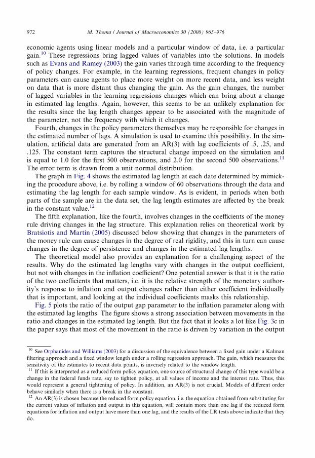
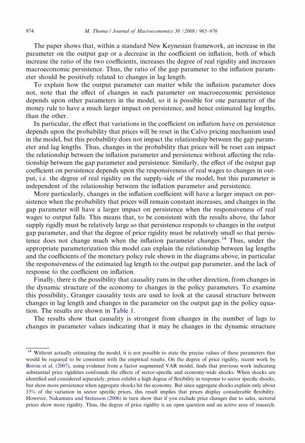
The theoretical model also provides an explanation for a challenging aspect of theresults. Why do the estimated lag lengths vary with changes in the output coefficient,but not with changes in the inflation coefficient? One potential answer is that it is the ratioof the two coefficients that matters, i.e. it is the relative strength of the monetary author-ity’s response to inflation and output changes rather than either coefficient individuallythat is important, and looking at the individual coefficients masks this relationship.

Fig. 5 plots the ratio of the output gap parameter to the inflation parameter along withthe estimated lag lengths. The figure shows a strong association between movements in theratio and changes in the estimated lag length. But the fact that it looks a lot like Fig. 3c inthe paper says that most of the movement in the ratio is driven by variation in the output

10 See Orphanides and Williams (2003) for a discussion of the equivalence between a fixed gain under a Kalmanfiltering approach and a fixed window length under a rolling regression approach. The gain, which measures thesensitivity of the estimates to recent data points, is inversely related to the window length.11 If this is interpreted as a reduced form policy equation, one source of structural change of this type would be a

change in the federal funds rate, say to tighten policy, at all values of income and the interest rate. Thus, thiswould represent a general tightening of policy. In addition, an AR(3) is not crucial. Models of different orderbehave similarly when there is a break in the constant.12 An AR(3) is chosen because the reduced form policy equation, i.e. the equation obtained from substituting for

the current values of inflation and output in this equation, will contain more than one lag if the reduced formequations for inflation and output have more than one lag, and the results of the LR tests above indicate that theydo.

Estimated Lag

250 500 750 10002.40

2.48

2.56

2.64

2.72

2.80

2.88

2.96

Fig. 4. Estimated lag length with structural change.

Optimum Lag RATIO

1977 1980 1983 1986 1989 1992 1995 1998 2001 20040

1

2

3

4

5

-30

-20

-10

0

10

20

30

40

50

60

Fig. 5. Optimum lag length and coefficient radio (Gap/Inflation).


term, and further investigation does not support that the coefficient ratio explains the var-iation in the lag length estimates any better than the output coefficient alone.13

Since the ratio does not fit better, the task is to explain why the coefficient on outputvariation matters for lag lengths while the inflation parameter does not. An answer comesfrom a paper by Bratsiotis and Martin (2005), a paper that can explain either a statisticalrelationship between the ratio and the lag length as in Fig. 5, or a relationship between thelag length and one of the two parameters alone as in Fig. 3c.

13 For example, adding the ratio to a regression model that already includes the coefficient on the output gapprovides only a very slight improvement in fit. Alternative assessment methods lead to the same conclusion.


The paper shows that, within a standard New Keynesian framework, an increase in theparameter on the output gap or a decrease in the coefficient on inflation, both of whichincrease the ratio of the two coefficients, increases the degree of real rigidity and increasesmacroeconomic persistence. Thus, the ratio of the gap parameter to the inflation param-eter should be positively related to changes in lag length.

To explain how the output parameter can matter while the inflation parameter doesnot, note that the effect of changes in each parameter on macroeconomic persistencedepends upon other parameters in the model, so it is possible for one parameter of themoney rule to have a much larger impact on persistence, and hence estimated lag lengths,than the other.

In particular, the effect that variations in the coefficient on inflation have on persistencedepends upon the probability that prices will be reset in the Calvo pricing mechanism usedin the model, but this probability does not impact the relationship between the gap param-eter and lag lengths. Thus, changes in the probability that prices will be reset can impactthe relationship between the inflation parameter and persistence without affecting the rela-tionship between the gap parameter and persistence. Similarly, the effect of the output gapcoefficient on persistence depends upon the responsiveness of real wages to changes in out-put, i.e. the degree of real rigidity on the supply-side of the model, but this parameter isindependent of the relationship between the inflation parameter and persistence.

More particularly, changes in the inflation coefficient will have a larger impact on per-sistence when the probability that prices will remain constant increases, and changes in thegap parameter will have a larger impact on persistence when the responsiveness of realwages to output falls. This means that, to be consistent with the results above, the laborsupply rigidly must be relatively large so that persistence responds to changes in the outputgap parameter, and that the degree of price rigidity must be relatively small so that persis-tence does not change much when the inflation parameter changes.14 Thus, under theappropriate parameterization this model can explain the relationship between lag lengthsand the coefficients of the monetary policy rule shown in the diagrams above, in particularthe responsiveness of the estimated lag length to the output gap parameter, and the lack ofresponse to the coefficient on inflation.

Finally, there is the possibility that causality runs in the other direction, from changes inthe dynamic structure of the economy to changes in the policy parameters. To examinethis possibility, Granger causality tests are used to look at the causal structure betweenchanges in lag length and changes in the parameter on the output gap in the policy equa-tion. The results are shown in Table 1.

The results show that causality is strongest from changes in the number of lags tochanges in parameter values indicating that it may be changes in the dynamic structure

14 Without actually estimating the model, it is not possible to state the precise values of these parameters thatwould be required to be consistent with the empirical results. On the degree of price rigidity, recent work byBoivin et al. (2007), using evidence from a factor augmented VAR model, finds that previous work indicatingsubstantial price rigidities confounds the effects of sector-specific and economy-wide shocks. When shocks areidentified and considered separately, prices exhibit a high degree of flexibility in response to sector specific shocks,but show more persistence when aggregate shocks hit the economy. But since aggregate shocks explain only about15% of the variation in sector specific prices, this result implies that prices display considerable flexibility.However, Nakamura and Steinsson (2006) in turn show that if you exclude price changes due to sales, sectoralprices show more rigidity. Thus, the degree of price rigidity is an open question and an active area of research.

Table 1Causality tests

Causality direction Test statistic

Lags! parameter 3.22(.03)

Parameter! lags 1.15(.32)

Note: F-statistics are shown with p-values in parentheses.


of the economy that is driving changes in the policy responses rather than changes in pol-icy changing the dynamics of the system.

5. Conclusion

This paper investigates the relationship between changes in the policy rule for the fed-eral funds rate and the estimated lag length in a typical VAR model involving output,inflation, and the federal funds rate. The paper finds an association between changes inthe estimated lag length of the VAR model and changes in the coefficient on the gap termin a Taylor rule.

After discussing several reasons why lag length changes might be associated withchanges in the policy rule, the paper finds that the two most likely explanations for theassociation between lag lengths and parameter values are the last two given above, onewhere structural change in the economy changes the dynamic structure, and this bringsabout a change in the policy response to deviations of output from its target value, andthe other where changes in the coefficient on the output gap in the monetary policy rulecause changes in the degree of real rigidity and the degree of persistence.

But whatever the reason for the change in the estimate lag lengths and the direction ofcausality, the main message is that the typical means of estimating structural change inempirical models where parameter values are allowed to change while holding the dynamicstructure constant may not fully capture the structural change. The results of this paperindicate that when allowing for changes in the structure of the economy in empirical inves-tigations, particularly changes in the parameters of the monetary policy rule, it may bebeneficial to allow for changes in the lag length of the empirical model as well.

References

Bernanke, Ben S., Mihov, I., 1998. Measuring monetary policy. The Quarterly Journal of Economics 113 (3),869–902. August.

Bernanke, Ben S., Boivin, J., Eliasz, P., Measuring the effects of monetary policy: A factor-augmented vectorautoregressive (FAVAR) approach. NBER WP 10220, Jan 2004, 1–47.

Boivin, J., 2004. Has U.S. monetary policy changed? evidence from drifting coefficients and real-time data.Discussion paper, Columbia University.

Boivin, J., Giannoni, M., 2003. Has monetary policy become more effective? Working Paper 9459, WorkingPaper 9459, National Bureau of Economic Research.

Boivin, J., Giannoni, M., Mihov, I., 2007. Sticky prices and monetary policy: Evidence from disaggregated U.S.data. NBER WP 12824 (January).

Bratsiotis, G.J., Martin, C., 2005. Output stabilization and real rigidity. The Manchester School 73, 6728.


Clarida, R., Gali, J., Gertler, M., 1999. The science of monetary policy: A new Keynesian perspective. Journal ofEconomic Literature 37 (4), 1661–1707, December.

Clarida, R., Gali, J., Gertler, M., 2000. Monetary policy rules and macroeconomic stability: Evidence and sometheory. The Quarterly Journal of Economics 115 (1), 147–180, February.

Cogley, T., Sargent, T.J., 2002. Drifts and volatilities: Monetary policies and outcomes in the post WWII U.S.Discussion paper, Arizona State University and New York University.

Evans, G.W., Ramey, G., 2003. Adaptive expectations, ‘‘Underparameterization and the Lucas Critique,’’Working Paper, 1–22.

Honkapohja, S., Mitra, K., 2003. Performance of inflation targeting based on constant interest rate projections.CFS Working Paper No. 2003/39 (October), 1–33.

Kim, K.-S., McMillin, W.D., 2003. Estimating the effects of monetary policy shocks: Does lag structure matter?Applied Economics 35 (13), 1515–1526, September.

Lee, J., 1997. Money, income and dynamic lag patterns. Southern Economic Journal 64 (1), 97–103.Nakamura, E., Steinsson, J., 2006. Five facts about prices: A reevaluation of menu cost models. Harvard

University, manuscript.Orphanides, A., Williams, J.C., 2003. Imperfect knowledge, inflation expectations, and monetary policy. CFS

Working Paper 2003/40 (July).Sims, C.A., Zha, T.A., 2004. Were there regime switches in U.S. monetary policy? FRB of Atlanta Working

Paper No. 2004-14, June.Swanson, N., 1998. Money and output viewed through a rolling window. Journal of Monetary Economics 41 (3),

455–474.

Documents

Structural change and lag length in VAR modelspages.uoregon.edu/mthoma/Papers/Structural Change... · Structural change and lag length in ... agent’s use of learning equations can