Embed Size (px)
Citation preview
STRUCTURAL DAMAGE DETECTION BY COMPARISON OF EXPERIMENTAL AND
THEORETICAL MODE SHAPES
A Thesis
presented to
the Faculty of California Polytechnic State University,
San Luis Obispo
In Partial Fulfillment
of the Requirements for the Degree
Master of Science in Architecture with a Specialization in Architectural Engineering
by
William George Rosenblatt
March 2016

ii
© 2016
William George Rosenblatt
ALL RIGHTS RESERVED
iii
COMMITTEE MEMBERSHIP
TITLE: Structural Damage Detection by Comparison of Experimental and Theoretical Mode Shapes
AUTHOR: William George Rosenblatt
DATE SUBMITTED: March 2016
COMMITTEE CHAIR: Peter Laursen, Ph.D.
Associate Professor of Architectural Engineering
COMMITTEE MEMBER: Cole McDaniel, Ph.D.
Professor of Architectural Engineering
COMMITTEE MEMBER: Graham Archer, Ph.D.
Professor of Architectural Engineering
iv
ABSTRACT
Structural Damage Detection by Comparison of Experimental and Theoretical Mode Shapes
William George Rosenblatt
Existing methods of evaluating the structural system of a building after a seismic event
consist of removing architectural elements such as drywall, cladding, insulation, and fireproofing.
This method is destructive and costly in terms of downtime and repairs. This research focuses
on removing the guesswork by using forced vibration testing (FVT) to experimentally determine
the health of a building. The experimental structure is a one-story, steel, bridge-like structure
with removable braces. An engaged brace represents a nominal and undamaged condition; a
dis-engaged brace represents a brace that has ruptured thus changing the stiffness of the
building. By testing a variety of brace configurations, a set of experimental data is collected that
represents potential damage to the building after an earthquake. Additionally, several unknown
parameters of the building’s substructure, lateral-force-resisting-system, and roof diaphragm are
determined through FVT.
A suite of computer models with different levels of damage are then developed. A
quantitative analysis procedure compares experimental results to the computer models. Models
that show high levels of correlation to experimental brace configurations identify the extent of
damage in the experimental structure. No testing or instrumentation of the building is necessary
before an earthquake to identify if, and where, damage has occurred.
Keywords: Structural damage detection, NDT, modal analysis, Modal Assurance Criterion, MAC,
Post Earthquake Assessment, Forced Vibration Testing, FVT, system identification, diaphragm
stiffness, substructure stiffness, soil stiffness
v
ACKNOWLEDGMENTS
I’d like to thank the Warren J. Baker and Robert D. Koob endowments that supported this
research. The equipment acquired from the grant allowed this research to happen. Other
students have been able to use this equipment for their research. Additionally, the same
equipment has integrated into the course curriculums for undergraduate and graduate classes.
vi
TABLE OF CONTENTS
Page
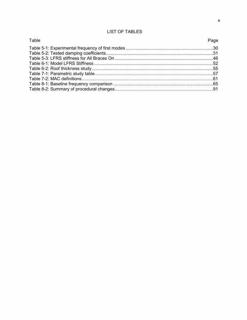
LIST OF TABLES ......................................................................................................................x
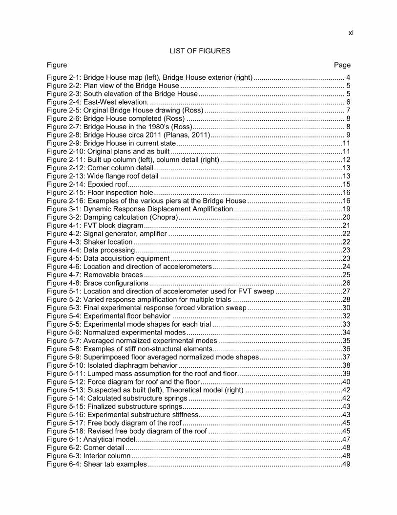
LIST OF FIGURES .................................................................................................................. xi
CHAPTER
1.0 Introduction ................................................................................................................... 1
1.1 Overview .................................................................................................................... 1
1.2 Purpose of Research ................................................................................................. 1
1.3 Scope and Topics ...................................................................................................... 1
1.4 Previous Research ..................................................................................................... 2
2.0 Experimental Structure .................................................................................................. 4
2.1 Overview and Building Description ............................................................................. 4
2.2 History ....................................................................................................................... 6
2.2.1 Original Structure, 1965 – 1968 Senior Project ................................................... 6
2.2.2 Pavilion and Caretaker, 1968 – 2000 .................................................................. 8
2.2.3 Vacancy, 2000 – 2011 ........................................................................................ 9
2.2.4 Structural Dynamic Field Laboratory, 2011 – Present Day .................................. 9
2.3 Building Survey ........................................................................................................ 11
2.3.1 Original Plans and Survey................................................................................. 11
2.3.2 Exterior Survey and Structural System.............................................................. 12
2.3.3 Roof System ..................................................................................................... 14
2.3.4 Floor System..................................................................................................... 15
2.3.5 Substructure ..................................................................................................... 16
3.0 Theory and Methodology ............................................................................................. 17
3.1 Overview .................................................................................................................. 17
3.2 Displacement Response Amplification Factor, Rd .................................................... 17
3.3 Damping .................................................................................................................. 20
4.0 Testing Procedure and Set-Up .................................................................................... 21
4.1 Overview .................................................................................................................. 21
4.2 Equipment ............................................................................................................... 21
4.2.1 Forced Vibration Equipment .............................................................................. 21
4.2.2 Data Acquisition ................................................................................................ 22
4.3 Testing Procedure.................................................................................................... 24
4.3.1 Ambient Vibration Testing ................................................................................. 24
4.3.2 Forced Vibration Testing ................................................................................... 24
4.3.3 Brace Configurations ........................................................................................ 25
vii
5.0 Testing Results and System Identification ................................................................... 27
5.1 System Identification ................................................................................................ 27
5.2 Ambient Vibration Test ............................................................................................. 27
5.3 Forced Vibration Sweep ........................................................................................... 27
5.3.1 Variation ........................................................................................................... 28
5.3.2 Final Forced Vibration Sweep ........................................................................... 29
5.4 Damping .................................................................................................................. 31
5.5 Mode Shapes ........................................................................................................... 31
5.5.1 Rigid Floor Verification ...................................................................................... 31
5.5.2 Raw Mode Shapes for Multiple Shaker Voltage Input ....................................... 32
5.5.3 Normalized Mode Shapes ................................................................................. 34
5.5.4 Average Normalized Mode Shapes ................................................................... 35
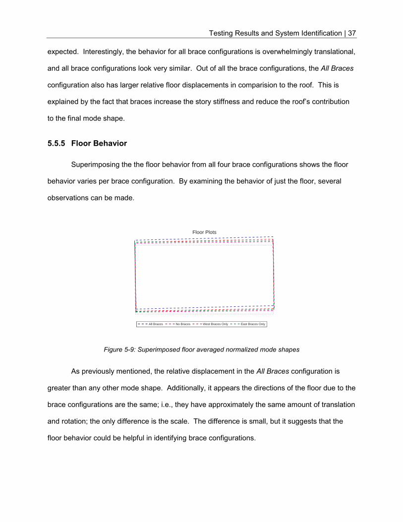
5.5.5 Floor Behavior .................................................................................................. 37
5.5.6 Roof Behavior ................................................................................................... 38
5.6 Substructure Stiffness .............................................................................................. 38
5.7 Lateral Force Resisting System Stiffness ................................................................. 44
6.0 Analytical Models ........................................................................................................ 47
6.1 Background.............................................................................................................. 47
6.2 Built-Up Sections ..................................................................................................... 47
6.3 Joints ....................................................................................................................... 49
6.4 Substructure Springs ............................................................................................... 49
6.5 Single Frame Model ................................................................................................. 51
6.6 Roof Properties ........................................................................................................ 52
7.0 Methods of Damage Detection .................................................................................... 56
7.1 Scope of Damage Detection .................................................................................... 56
7.2 Parametric Studies and Definitions .......................................................................... 56
7.3 Assessment Methods ............................................................................................... 57
7.3.1 Frequency Analysis........................................................................................... 57
7.3.2 Visual Inspection ............................................................................................... 58
7.3.3 Blind Visual Inspection ...................................................................................... 58
7.3.4 Modal Assurance Criterion (MAC) ..................................................................... 59
Mass Weighted Modal Assurance Criterion (MWMAC) .............................. 61
Application of MAC .................................................................................... 62
8.0 Damage Detection ....................................................................................................... 64
8.1 Baseline Model ........................................................................................................ 64
8.1.1 Overview ........................................................................................................... 64
8.1.2 Frequency Analysis........................................................................................... 64
8.1.3 Visual Inspection ............................................................................................... 65
8.1.4 Blind Visual Inspection ...................................................................................... 67
8.1.5 Modal Assurance Criterion ................................................................................ 68
viii
8.1.6 Conclusion ........................................................................................................ 70
8.2 Model Parametric Studies ........................................................................................ 71
8.2.1 Overview ........................................................................................................... 71
8.2.2 Early Model ....................................................................................................... 71
Overview .................................................................................................... 71
Visual Inspection ........................................................................................ 72
MAC Comparison ...................................................................................... 72
Early Model Conclusion ............................................................................. 74
8.2.3 Substructure - Rigid .......................................................................................... 74
Overview .................................................................................................... 74
Visual Inspection ........................................................................................ 74
Blind Visual Inspection ............................................................................... 75
MAC Comparison ...................................................................................... 76
Rigid Substructure Conclusion ................................................................... 77
8.2.4 Substructure Springs - Variable and Individual .................................................. 77
Overview .................................................................................................... 77
Visual Inspection ........................................................................................ 78
MAC Comparison ...................................................................................... 78
Variable Substructure Conclusion .............................................................. 79
8.2.5 Diaphragm Changes – Rigid ............................................................................. 79
Overview .................................................................................................... 79
Visual Inspection ........................................................................................ 79
Blind Visual Comparison ............................................................................ 80
MAC Comparison ...................................................................................... 81
8.2.6 Diaphragm Changes – Flexible ......................................................................... 81
Overview .................................................................................................... 81
Visual Inspection ........................................................................................ 82
MAC Comparison ...................................................................................... 82
Flexible Diaphragm Conclusion ................................................................. 84
8.2.7 Diaphragm Changes – Very Flexible ................................................................. 84
Overview .................................................................................................... 84
Visual Inspection ........................................................................................ 84
Blind Visual Inspection ............................................................................... 85
MAC Comparison ...................................................................................... 86
Very Flexible Diaphragm Conclusion ......................................................... 87
8.2.8 Modeling of Non-Structural ............................................................................... 87
Overview .................................................................................................... 87
Visual Inspection ........................................................................................ 88
MAC Comparison ...................................................................................... 88
Non-Structural Conclusion ......................................................................... 89
8.2.9 Conclusion to Parametric Studies ..................................................................... 90
8.3 Procedural Changes ................................................................................................ 91
8.3.1 Overview ........................................................................................................... 91
8.3.2 Nine DOF (7 Translational Roof, 1 Translational Floor, 1 Rotational Floor) ....... 92
Experimental Comparison .......................................................................... 92
Theoretical Comparison ............................................................................. 93
8.3.3 Five DOF (3 Translational Roof, 1 Translational Floor, 1 Rotational Floor) ....... 94
Experimental Comparison .......................................................................... 94
Theoretical Comparison ............................................................................. 95
8.3.4 Four DOF (2 Translational + 2 Rotational) ........................................................ 96
ix
Experimental Comparison .......................................................................... 96
Theoretical Comparison ............................................................................. 97
8.3.5 Conclusion of Procedural Changes ................................................................... 99
9.0 Conclusion ................................................................................................................ 100
9.1 System Identification .............................................................................................. 100
9.2 Damage Detection ................................................................................................. 100
9.2.1 Modal Assurance Criterion .............................................................................. 100
9.2.2 Model Accuracy .............................................................................................. 101
9.2.3 Data Collection ............................................................................................... 101
9.3 Suggestions for Future Research ........................................................................... 101
9.3.1 Bridge House .................................................................................................. 101
9.3.2 Suggestions for Application ............................................................................. 102
BIBLIOGRAPHY .................................................................................................................. 103
APPENDICES
A.1 Response Spectrum Analysis ..................................................................................... 105
Steady-State Response ................................................................................................ 105
Maximum Deformation .................................................................................................. 108
Displacement Response Amplification Factor, Rd ......................................................... 109
Phase Angle ................................................................................................................. 112
Damping ....................................................................................................................... 113
A.2 Raw Data ................................................................................................................... 115
x
LIST OF TABLES
Table Page
Table 5-1: Experimental frequency of first modes .....................................................................30
Table 5-2: Tested damping coefficients .....................................................................................31
Table 5-3: LFRS stiffness for All Braces On ..............................................................................46
Table 6-1: Model LFRS Stiffness ..............................................................................................52
Table 6-2: Roof thickness study ................................................................................................55
Table 7-1: Parametric study table..............................................................................................57
Table 7-2: MAC definitions ........................................................................................................61
Table 8-1: Baseline frequency comparison ...............................................................................65
Table 8-2: Summary of procedural changes ..............................................................................91
xi
LIST OF FIGURES
Figure Page
Figure 2-1: Bridge House map (left), Bridge House exterior (right) ............................................. 4
Figure 2-2: Plan view of the Bridge House ................................................................................. 5
Figure 2-3: South elevation of the Bridge House ........................................................................ 5
Figure 2-4: East-West elevation. ................................................................................................ 6
Figure 2-5: Original Bridge House drawing (Ross) ..................................................................... 7
Figure 2-6: Bridge House completed (Ross) .............................................................................. 8
Figure 2-7: Bridge House in the 1980’s (Ross) ........................................................................... 8
Figure 2-8: Bridge House circa 2011 (Planas, 2011) .................................................................. 9
Figure 2-9: Bridge House in current state ..................................................................................11
Figure 2-10: Original plans and as built .....................................................................................11
Figure 2-11: Built up column (left), column detail (right) ............................................................12
Figure 2-12: Corner column detail .............................................................................................13
Figure 2-13: Wide flange roof detail ..........................................................................................13
Figure 2-14: Epoxied roof ..........................................................................................................15
Figure 2-15: Floor inspection hole .............................................................................................16
Figure 2-16: Examples of the various piers at the Bridge House ...............................................16
Figure 3-1: Dynamic Response Displacement Amplification......................................................19
Figure 3-2: Damping calculation (Chopra) .................................................................................20
Figure 4-1: FVT block diagram ..................................................................................................21
Figure 4-2: Signal generator, amplifier ......................................................................................22
Figure 4-3: Shaker location .......................................................................................................22
Figure 4-4: Data processing ......................................................................................................23
Figure 4-5: Data acquisition equipment .....................................................................................23
Figure 4-6: Location and direction of accelerometers ................................................................24
Figure 4-7: Removable braces ..................................................................................................25
Figure 4-8: Brace configurations ...............................................................................................26
Figure 5-1: Location and direction of accelerometer used for FVT sweep .................................27
Figure 5-2: Varied response amplification for multiple trials ......................................................28
Figure 5-3: Final experimental response forced vibration sweep ...............................................30
Figure 5-4: Experimental floor behavior ....................................................................................32
Figure 5-5: Experimental mode shapes for each trial ................................................................33
Figure 5-6: Normalized experimental modes .............................................................................34
Figure 5-7: Averaged normalized experimental modes .............................................................35
Figure 5-8: Examples of stiff non-structural elements ................................................................36
Figure 5-9: Superimposed floor averaged normalized mode shapes .........................................37
Figure 5-10: Isolated diaphragm behavior .................................................................................38
Figure 5-11: Lumped mass assumption for the roof and floor ....................................................39
Figure 5-12: Force diagram for roof and the floor ......................................................................40
Figure 5-13: Suspected as built (left), Theoretical model (right) ................................................42
Figure 5-14: Calculated substructure springs ............................................................................42
Figure 5-15: Finalized substructure springs ...............................................................................43
Figure 5-16: Experimental substructure stiffness .......................................................................43
Figure 5-17: Free body diagram of the roof ...............................................................................45
Figure 5-18: Revised free body diagram of the roof ..................................................................45
Figure 6-1: Analytical model ......................................................................................................47
Figure 6-2: Corner detail ...........................................................................................................48
Figure 6-3: Interior column ........................................................................................................48
Figure 6-4: Shear tab examples ................................................................................................49
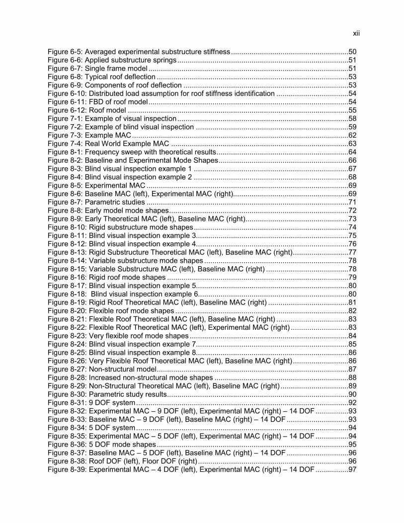
xii
Figure 6-5: Averaged experimental substructure stiffness .........................................................50
Figure 6-6: Applied substructure springs ...................................................................................51
Figure 6-7: Single frame model .................................................................................................51
Figure 6-8: Typical roof deflection .............................................................................................53
Figure 6-9: Components of roof deflection ................................................................................53
Figure 6-10: Distributed load assumption for roof stiffness identification ...................................54
Figure 6-11: FBD of roof model .................................................................................................54
Figure 6-12: Roof model ...........................................................................................................55
Figure 7-1: Example of visual inspection ...................................................................................58
Figure 7-2: Example of blind visual inspection ..........................................................................59
Figure 7-3: Example MAC .........................................................................................................62
Figure 7-4: Real World Example MAC ......................................................................................63
Figure 8-1: Frequency sweep with theoretical results ................................................................64
Figure 8-2: Baseline and Experimental Mode Shapes ...............................................................66
Figure 8-3: Blind visual inspection example 1 ...........................................................................67
Figure 8-4: Blind visual inspection example 2 ...........................................................................68
Figure 8-5: Experimental MAC ..................................................................................................69
Figure 8-6: Baseline MAC (left), Experimental MAC (right)........................................................69
Figure 8-7: Parametric studies ..................................................................................................71
Figure 8-8: Early model mode shapes .......................................................................................72
Figure 8-9: Early Theoretical MAC (left), Baseline MAC (right) ..................................................73
Figure 8-10: Rigid substructure mode shapes ...........................................................................74
Figure 8-11: Blind visual inspection example 3..........................................................................75
Figure 8-12: Blind visual inspection example 4..........................................................................76
Figure 8-13: Rigid Substructure Theoretical MAC (left), Baseline MAC (right) ...........................77
Figure 8-14: Variable substructure mode shapes ......................................................................78
Figure 8-15: Variable Substructure MAC (left), Baseline MAC (right) ........................................78
Figure 8-16: Rigid roof mode shapes ........................................................................................79
Figure 8-17: Blind visual inspection example 5..........................................................................80
Figure 8-18: Blind visual inspection example 6.........................................................................80
Figure 8-19: Rigid Roof Theoretical MAC (left), Baseline MAC (right) .......................................81
Figure 8-20: Flexible roof mode shapes ....................................................................................82
Figure 8-21: Flexible Roof Theoretical MAC (left), Baseline MAC (right) ...................................83
Figure 8-22: Flexible Roof Theoretical MAC (left), Experimental MAC (right) ............................83
Figure 8-23: Very flexible roof mode shapes .............................................................................84
Figure 8-24: Blind visual inspection example 7..........................................................................85
Figure 8-25: Blind visual inspection example 8..........................................................................86
Figure 8-26: Very Flexible Roof Theoretical MAC (left), Baseline MAC (right) ...........................86
Figure 8-27: Non-structural model .............................................................................................87
Figure 8-28: Increased non-structural mode shapes .................................................................88
Figure 8-29: Non-Structural Theoretical MAC (left), Baseline MAC (right) .................................89
Figure 8-30: Parametric study results ........................................................................................90
Figure 8-31: 9 DOF system .......................................................................................................92
Figure 8-32: Experimental MAC – 9 DOF (left), Experimental MAC (right) – 14 DOF ................93
Figure 8-33: Baseline MAC – 9 DOF (left), Baseline MAC (right) – 14 DOF ..............................93
Figure 8-34: 5 DOF system .......................................................................................................94
Figure 8-35: Experimental MAC – 5 DOF (left), Experimental MAC (right) – 14 DOF ................94
Figure 8-36: 5 DOF mode shapes .............................................................................................95
Figure 8-37: Baseline MAC – 5 DOF (left), Baseline MAC (right) – 14 DOF ..............................96
Figure 8-38: Roof DOF (left), Floor DOF (right) .........................................................................96
Figure 8-39: Experimental MAC – 4 DOF (left), Experimental MAC (right) – 14 DOF ................97

xiii
Figure 8-40: 4 DOF mode shapes .............................................................................................98
Figure 8-41: Baseline MAC – 4 DOF (left), Baseline MAC (right) – 14 DOF ..............................98
Figure A-1: Dynamic Response Displacement Amplification ................................................... 111
Figure A-2: Phase Angle ......................................................................................................... 113
Figure A-3: Damping calculation (Chopra) .............................................................................. 114
Introduction | 1
1.0 INTRODUCTION
1.1 Overview
The objective of this thesis is to use temporary instrumentation and system identification
through the use of forced vibration testing to identify the location of structural damage in a
building after a seismic, wind, or blast event. The proposed methods in this thesis need no
previous identification or knowledge of the building to identify if, and where, structural damage
has occurred.
1.2 Purpose of Research
Current investigative techniques after a lateral force event consist of destructive testing.
Drywall, ceiling tiles, fireproofing, insulation, and other like elements are required to be removed
in order to inspect steel members and connections. These methods are intrusive, they displace
tenants, and are costly, both in terms of repairs and lost revenues, especially in large buildings.
The methods used in this research will mitigate the need for guesswork when assessing
the structural robustness of a building. They has the potential to give the engineer an “x-ray”
look into the building to determine if, and where, further inspections are necessary. If
successful, the damaged detection system could expedite and minimize the destructive
inspections needed. This would lower costs for building owners and tenants by shortening the
turnaround time for the building to return to service.
1.3 Scope and Topics
The main focus of this research is system identification through forced vibration testing
and damage detection through comparison of experimental and theoretical mode shapes. To
help establish the results of this thesis, it will be broken down as linearly as possible. Much
work is needed to be done in order implement this system into a turn-key solution; it is the hope
Introduction | 2
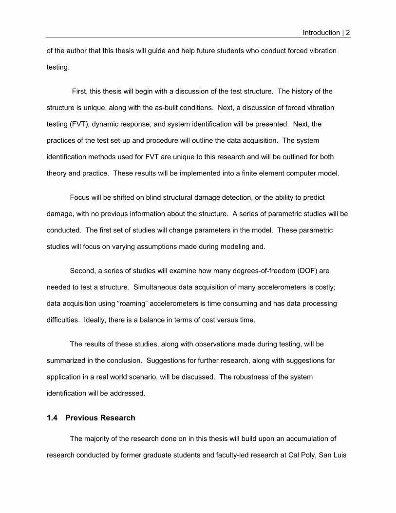
of the author that this thesis will guide and help future students who conduct forced vibration
testing.
First, this thesis will begin with a discussion of the test structure. The history of the
structure is unique, along with the as-built conditions. Next, a discussion of forced vibration
testing (FVT), dynamic response, and system identification will be presented. Next, the
practices of the test set-up and procedure will outline the data acquisition. The system
identification methods used for FVT are unique to this research and will be outlined for both
theory and practice. These results will be implemented into a finite element computer model.
Focus will be shifted on blind structural damage detection, or the ability to predict
damage, with no previous information about the structure. A series of parametric studies will be
conducted. The first set of studies will change parameters in the model. These parametric
studies will focus on varying assumptions made during modeling and.
Second, a series of studies will examine how many degrees-of-freedom (DOF) are
needed to test a structure. Simultaneous data acquisition of many accelerometers is costly;
data acquisition using “roaming” accelerometers is time consuming and has data processing
difficulties. Ideally, there is a balance in terms of cost versus time.
The results of these studies, along with observations made during testing, will be
summarized in the conclusion. Suggestions for further research, along with suggestions for
application in a real world scenario, will be discussed. The robustness of the system
identification will be addressed.
1.4 Previous Research
The majority of the research done on in this thesis will build upon an accumulation of
research conducted by former graduate students and faculty-led research at Cal Poly, San Luis
Introduction | 3
Obispo. Much of this research was conducted by professors Graham Archer, Ph.D. and Cole
McDaniel, Ph.D. (McDaniel, 2012). Archer and McDaniel have successfully used ultralow-force,
linear vibrating shakers to perform system identification on multiple low rise buildings. Archer
and McDaniel have refined testing results to a turn-key system for the majority of building types.
A paper titled Influence of Boundary Conditions on Building Behavior (Raney et. al., 2015)
successfully calculated the stiffness of boundary conditions through both forced vibration tests
and static loading tests. This research was used to show that system identification methods can
be expanded to calculate previously unknown parameters of a structure.
While many studies impacted the direction of this research, a few major studies were
used to help converge the ideas for this thesis. The first was a thesis called System
Identification Of A Bridge-Type Building Structure, (Ramos, 2013). Ramos performed dynamic
studies on the same structure used for this thesis. In addition, Ramos’ work outlined and
discovered many of the unique challenges particular to the test structure. Archer and Graham
expanded this research to have limited success using damage detection (Archer, 2014).
Additionally, the thesis titled Structural Damage Detection Utilizing Experimental Mode Shapes
(Gerbo, 2014) expanded on the idea that damage could precisely be identified by comparing
experimental mode shapes to theoretical mode shapes. Gerbo tested a two-story laboratory
structure with removable braces to simulate damage. Gerbo compared the experimental results
to a suite of finite element models to successfully detect the different brace configurations.
Experimental Structure | 4
2.0 EXPERIMENTAL STRUCTURE
The name of the structure used for the testing in this thesis is called the Bridge House.
The following section details the history, overview, and structural evaluation of the Bridge
House.
2.1 Overview and Building Description
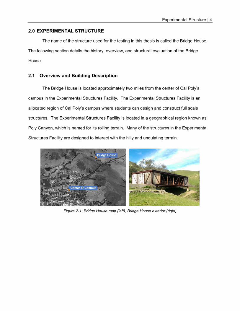
The Bridge House is located approximately two miles from the center of Cal Poly’s
campus in the Experimental Structures Facility. The Experimental Structures Facility is an
allocated region of Cal Poly’s campus where students can design and construct full scale
structures. The Experimental Structures Facility is located in a geographical region known as
Poly Canyon, which is named for its rolling terrain. Many of the structures in the Experimental
Structures Facility are designed to interact with the hilly and undulating terrain.
Figure 2-1: Bridge House map (left), Bridge House exterior (right)
Experimental Structure | 5
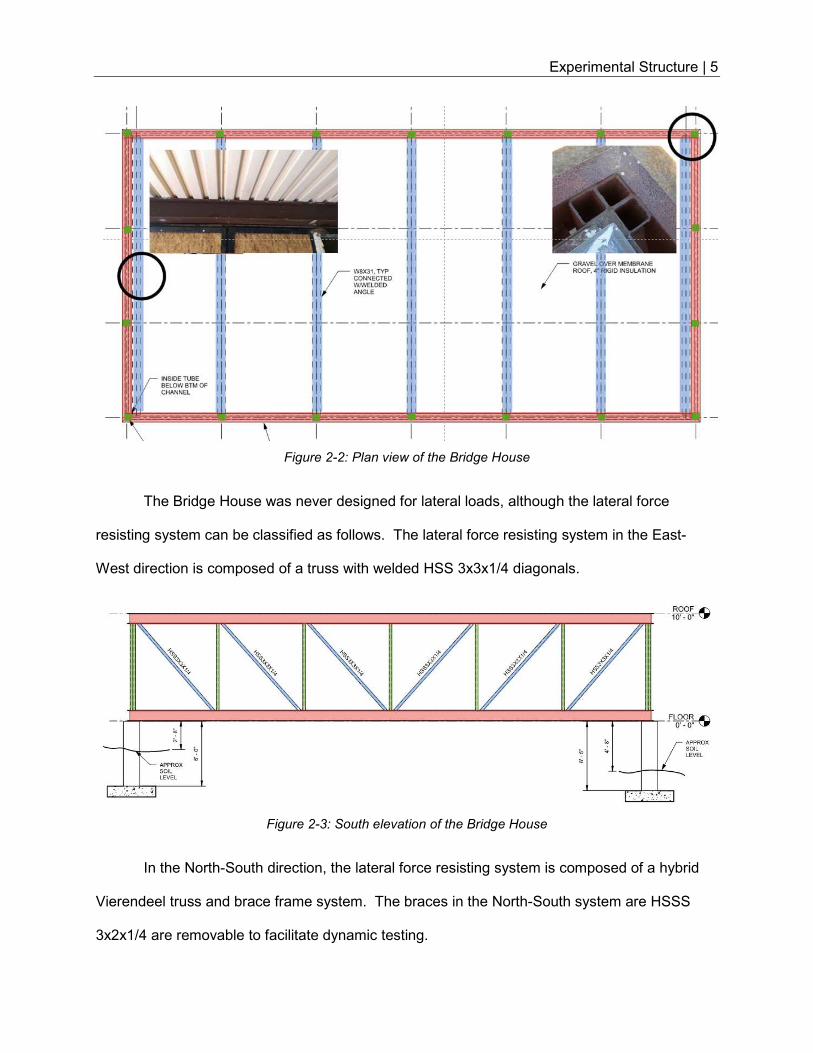
Figure 2-2: Plan view of the Bridge House
The Bridge House was never designed for lateral loads, although the lateral force
resisting system can be classified as follows. The lateral force resisting system in the East-
West direction is composed of a truss with welded HSS 3x3x1/4 diagonals.
Figure 2-3: South elevation of the Bridge House
In the North-South direction, the lateral force resisting system is composed of a hybrid
Vierendeel truss and brace frame system. The braces in the North-South system are HSSS
3x2x1/4 are removable to facilitate dynamic testing.
Experimental Structure | 6
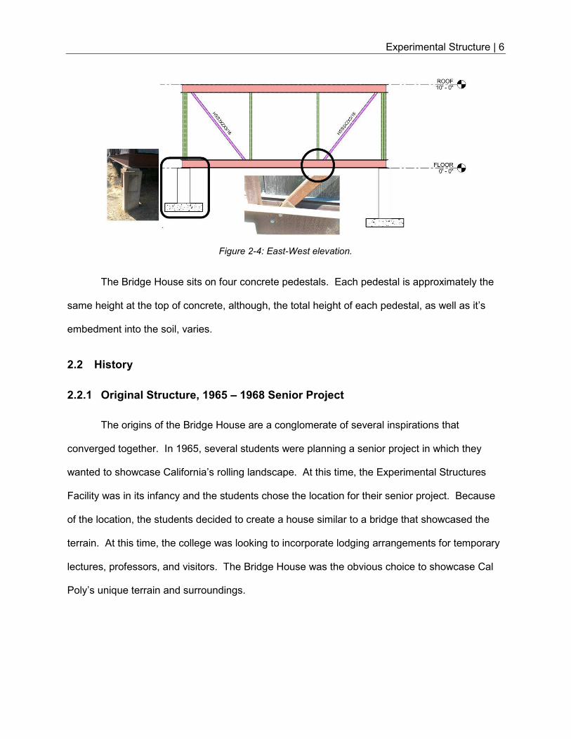
Figure 2-4: East-West elevation.
The Bridge House sits on four concrete pedestals. Each pedestal is approximately the
same height at the top of concrete, although, the total height of each pedestal, as well as it’s
embedment into the soil, varies.
2.2 History
2.2.1 Original Structure, 1965 – 1968 Senior Project
The origins of the Bridge House are a conglomerate of several inspirations that
converged together. In 1965, several students were planning a senior project in which they
wanted to showcase California’s rolling landscape. At this time, the Experimental Structures
Facility was in its infancy and the students chose the location for their senior project. Because
of the location, the students decided to create a house similar to a bridge that showcased the
terrain. At this time, the college was looking to incorporate lodging arrangements for temporary
lectures, professors, and visitors. The Bridge House was the obvious choice to showcase Cal
Poly’s unique terrain and surroundings.
Experimental Structure | 7
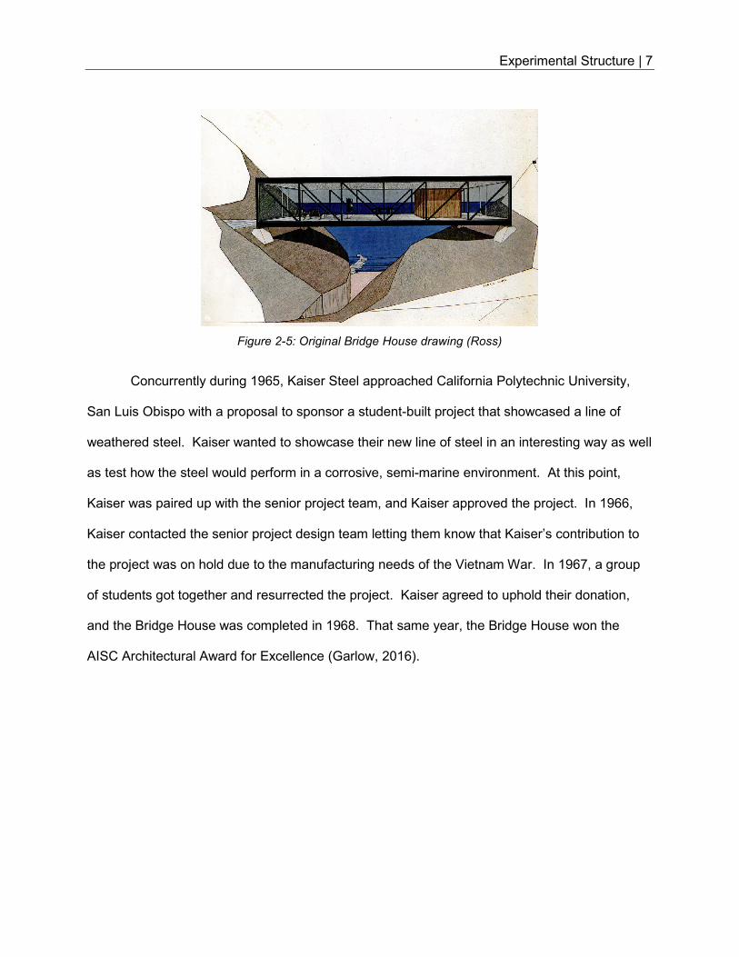
Concurrently during 1965, Kaiser Steel approached California Polytechnic University,
San Luis Obispo with a proposal to sponsor a student-built project that showcased a line of
weathered steel. Kaiser wanted to showcase their new line of steel in an interesting way as well
as test how the steel would perform in a corrosive, semi-marine environment. At this point,
Kaiser was paired up with the senior project team, and Kaiser approved the project. In 1966,
Kaiser contacted the senior project design team letting them know that Kaiser’s contribution to
the project was on hold due to the manufacturing needs of the Vietnam War. In 1967, a group
of students got together and resurrected the project. Kaiser agreed to uphold their donation,
and the Bridge House was completed in 1968. That same year, the Bridge House won the
AISC Architectural Award for Excellence (Garlow, 2016).
Figure 2-5: Original Bridge House drawing (Ross)
Experimental Structure | 8
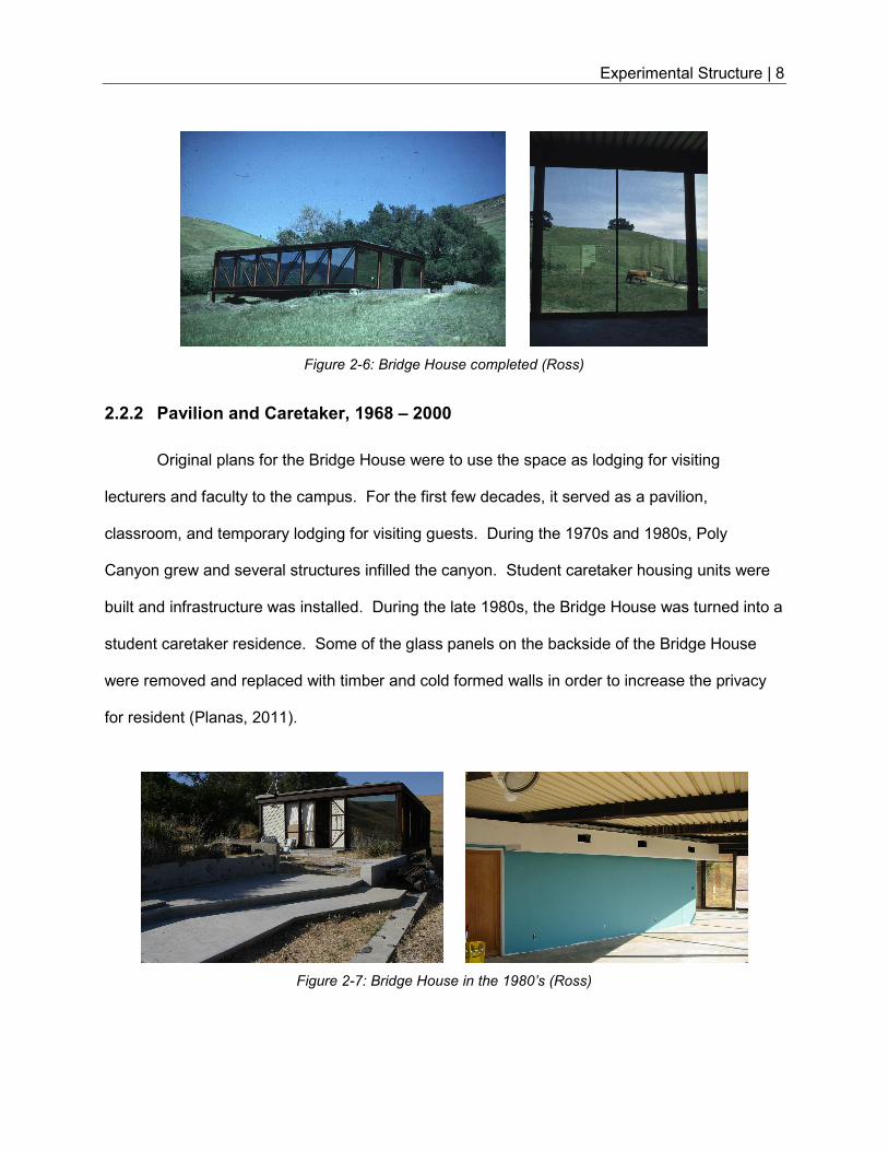
2.2.2 Pavilion and Caretaker, 1968 – 2000
Original plans for the Bridge House were to use the space as lodging for visiting
lecturers and faculty to the campus. For the first few decades, it served as a pavilion,
classroom, and temporary lodging for visiting guests. During the 1970s and 1980s, Poly
Canyon grew and several structures infilled the canyon. Student caretaker housing units were
built and infrastructure was installed. During the late 1980s, the Bridge House was turned into a
student caretaker residence. Some of the glass panels on the backside of the Bridge House
were removed and replaced with timber and cold formed walls in order to increase the privacy
for resident (Planas, 2011).
Figure 2-6: Bridge House completed (Ross)
Figure 2-7: Bridge House in the 1980’s (Ross)
Experimental Structure | 9
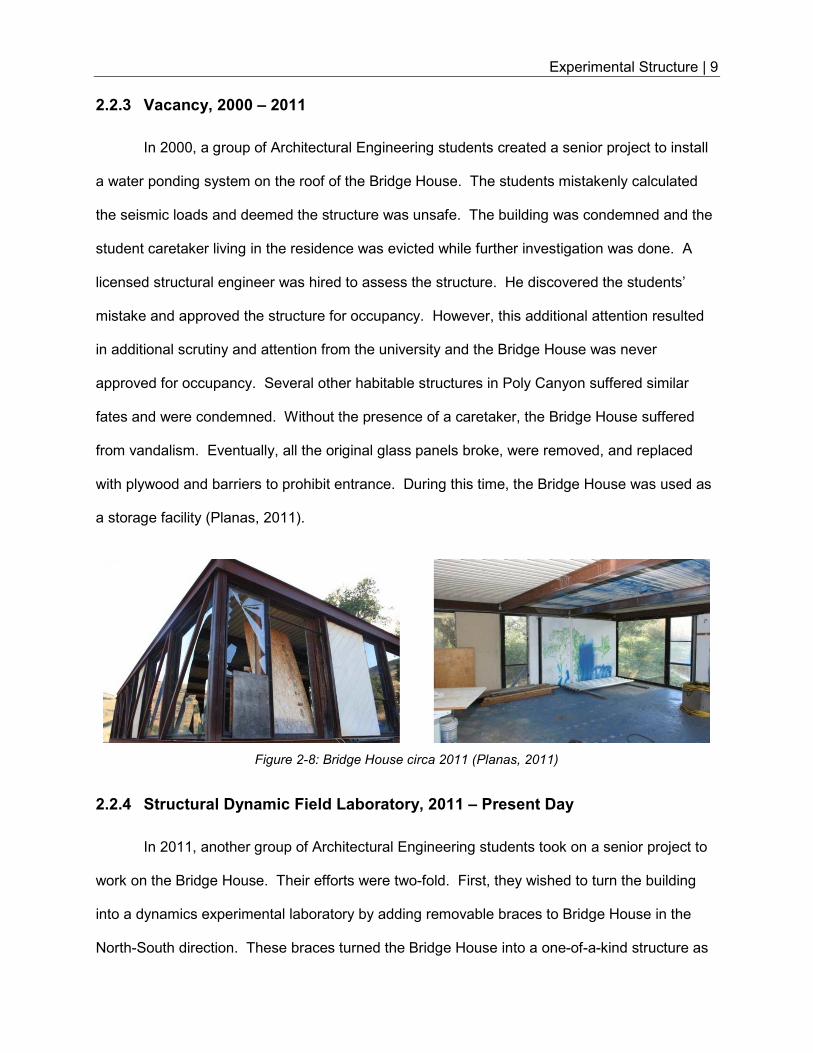
2.2.3 Vacancy, 2000 – 2011
In 2000, a group of Architectural Engineering students created a senior project to install
a water ponding system on the roof of the Bridge House. The students mistakenly calculated
the seismic loads and deemed the structure was unsafe. The building was condemned and the
student caretaker living in the residence was evicted while further investigation was done. A
licensed structural engineer was hired to assess the structure. He discovered the students’
mistake and approved the structure for occupancy. However, this additional attention resulted
in additional scrutiny and attention from the university and the Bridge House was never
approved for occupancy. Several other habitable structures in Poly Canyon suffered similar
fates and were condemned. Without the presence of a caretaker, the Bridge House suffered
from vandalism. Eventually, all the original glass panels broke, were removed, and replaced
with plywood and barriers to prohibit entrance. During this time, the Bridge House was used as
a storage facility (Planas, 2011).
2.2.4 Structural Dynamic Field Laboratory, 2011 – Present Day
In 2011, another group of Architectural Engineering students took on a senior project to
work on the Bridge House. Their efforts were two-fold. First, they wished to turn the building
into a dynamics experimental laboratory by adding removable braces to Bridge House in the
North-South direction. These braces turned the Bridge House into a one-of-a-kind structure as
Figure 2-8: Bridge House circa 2011 (Planas, 2011)
Experimental Structure | 10
it allowed students to change the building properties of the structure. The lateral stiffness of the
Bridge House became variable depending on the respective brace configuration. Second, they
aimed to restore and clean up the Bridge House to bring it up to acceptable conditions. They
gutted and cleaned the interior of the structure.
By 2013, all the exterior glass of the Bridge House had been broken. Plywood panels
were added to keep intruders out of the structure. Despite these panels, intruders continually
made it into the structure. Reinforced barriers made of an assortment of materials were added
to certain locations. Student and faculty research in the Bridge House was conducted during
this time. Irregularities in the roof diaphragm behavior lead researchers to believe that the
corrugated roof decking was never properly adhered to the roof wide flanges. In the spring of
2014, two students epoxied the wide flange roof beams and the corrugated desk at two foot
intervals. The goal of this modification was to force regular diaphragm behavior.
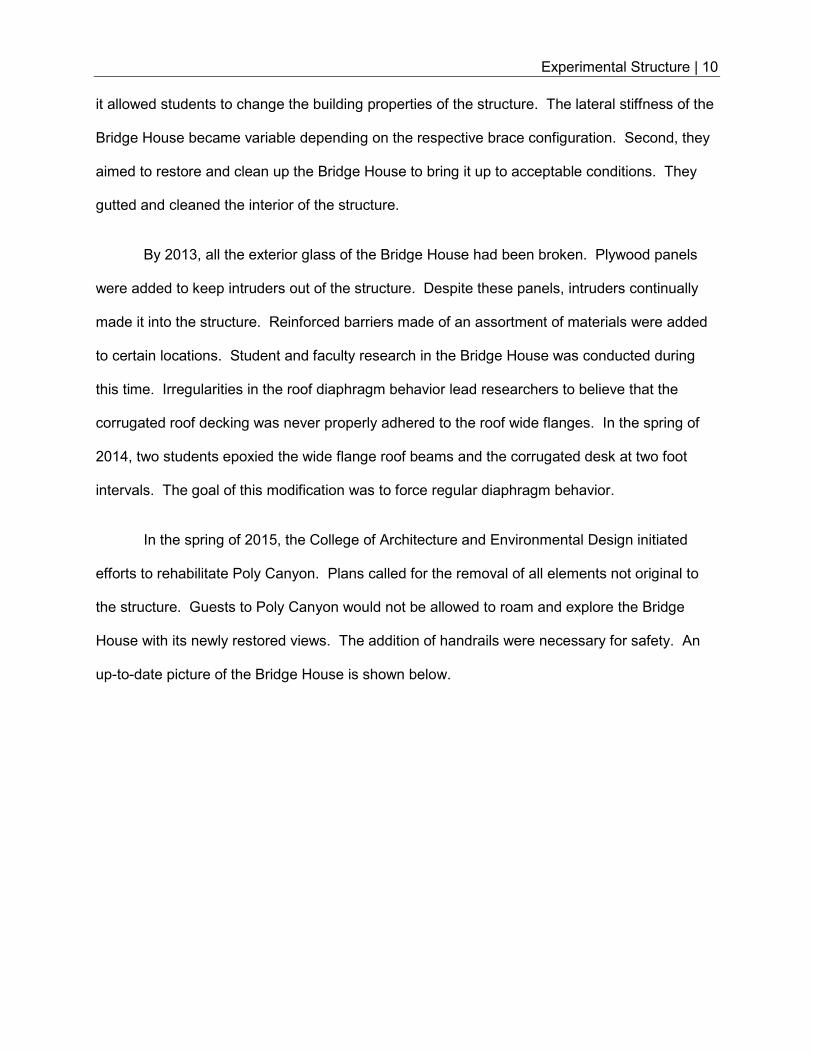
In the spring of 2015, the College of Architecture and Environmental Design initiated
efforts to rehabilitate Poly Canyon. Plans called for the removal of all elements not original to
the structure. Guests to Poly Canyon would not be allowed to roam and explore the Bridge
House with its newly restored views. The addition of handrails were necessary for safety. An
up-to-date picture of the Bridge House is shown below.
Experimental Structure | 11
Figure 2-9: Bridge House in current state
2.3 Building Survey
A building survey was necessary to grasp greater understanding of the characteristics,
the as-built conditions, and the modifications made to the Bridge House over the its history.
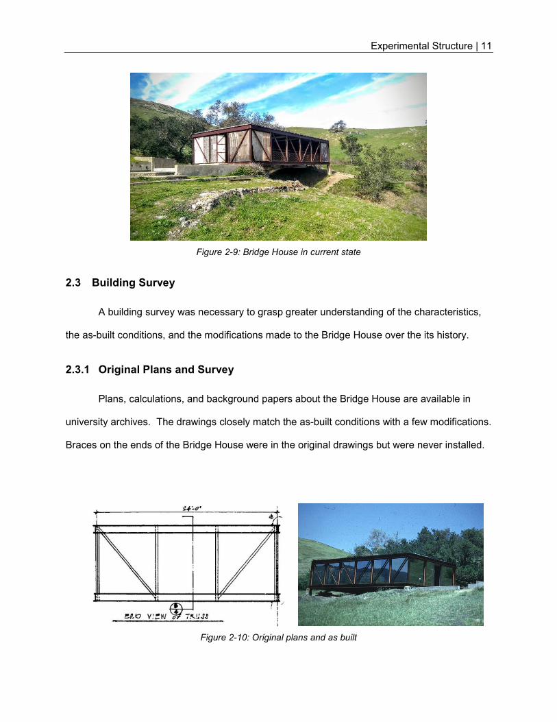
2.3.1 Original Plans and Survey
Plans, calculations, and background papers about the Bridge House are available in
university archives. The drawings closely match the as-built conditions with a few modifications.
Braces on the ends of the Bridge House were in the original drawings but were never installed.
Figure 2-10: Original plans and as built
Experimental Structure | 12
The other major structural change occurred at the interior beams. The drawn detail
showed a bolted shear tab. All as-built conditions were observed as welded shear tabs. At the
foundation, a bolted base plate design was shown in original plans. No bolts are observed,
therefore, it is assumed that embedded studs, j-bolts, or rebar was used instead. Additionally,
all non-structural steel (i.e. window mullions) were never included in the original plans. Other
differences were observed but were mainly small details regarding insulation, roofing, and
mullion details.
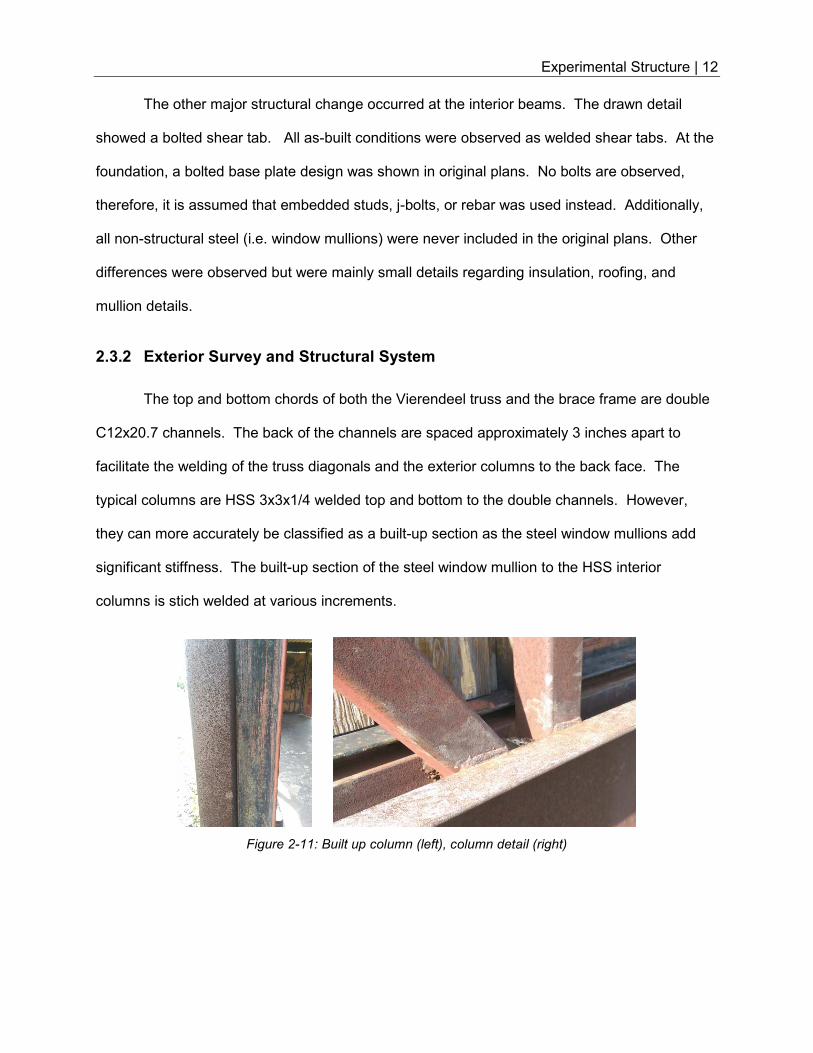
2.3.2 Exterior Survey and Structural System
The top and bottom chords of both the Vierendeel truss and the brace frame are double
C12x20.7 channels. The back of the channels are spaced approximately 3 inches apart to
facilitate the welding of the truss diagonals and the exterior columns to the back face. The
typical columns are HSS 3x3x1/4 welded top and bottom to the double channels. However,
they can more accurately be classified as a built-up section as the steel window mullions add
significant stiffness. The built-up section of the steel window mullion to the HSS interior
columns is stich welded at various increments.
Figure 2-11: Built up column (left), column detail (right)
Experimental Structure | 13
The corner columns are built-up sections composed of four HSS 3x3x1/4. The HSS
sections are butted together with no intermediate welds; the only connection of each built-up
member occurs at the end where they are abundantly welded.
Figure 2-12: Corner column detail
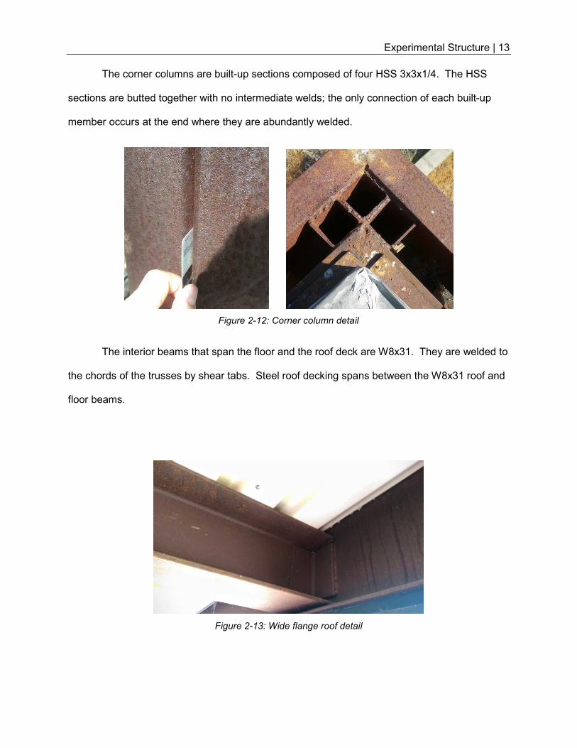
The interior beams that span the floor and the roof deck are W8x31. They are welded to
the chords of the trusses by shear tabs. Steel roof decking spans between the W8x31 roof and
floor beams.
Figure 2-13: Wide flange roof detail
Experimental Structure | 14
Unlike typical bridge structures, the Bridge House has no expansion or thermals gaps to
allow for expansion and contraction. Any stresses that are induced due to thermal effects are
not able to be released.
2.3.3 Roof System
Previous research identified the mass of the roof by saw cutting, removing, and weighing
a square foot of the roof section. The composition was determined to be a rigid insulation and
weatherproofing material with gravel topping. This section was determined to weigh fifteen
pounds-per-square foot. To determine the stiffness of the deck, the underside of the roof deck
was investigated. These results were compared to old catalogues and the deck was
determined to be Robertson Sec. 3 decking. The thickness of the deck was determined to be
18 gauge after a small inspection opening was made and the thickness was measured.
Roof deck seams that run parallel to the beams are visible every two feet. The length of
the panels is assumed to be eight feet long. This is consistent with product availability and
historic photos of the Bridge House; however, there is no evidence to suggest that the seams of
adjacent panels are connected or adhered together.
Additionally, it is unknown if, or how, the roof deck was originally connected to the rest of
the structural system. Typically, puddle welds would be used to attach the deck to the roof
beams. Burn marks on the underside would be evidence of welds. There are no burn marks or
any evidence to suggest that roof deck is adhered to the roof beams.
Lastly, it is believed that the roof deck is not properly adhered to the double channels
external beams that surround the roof. These double channels would act as chords and
collectors in a flexible roof system. An inspection camera was utilized to examine the boundary
conditions of the roof deck to the rest of the structure; no such connection was found.
Experimental Structure | 15
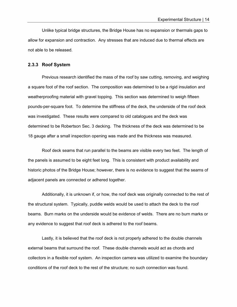
These issues were a concern for previous research done on the Bridge House (Ramos,
2013). Specifically, the researchers were concerned whether the steel deck was adhered to the
roof beams and a friction connection was the only way forces were transferred. To mitigate
these issues, the roof beams were epoxied to the roof beams at two foot intervals.
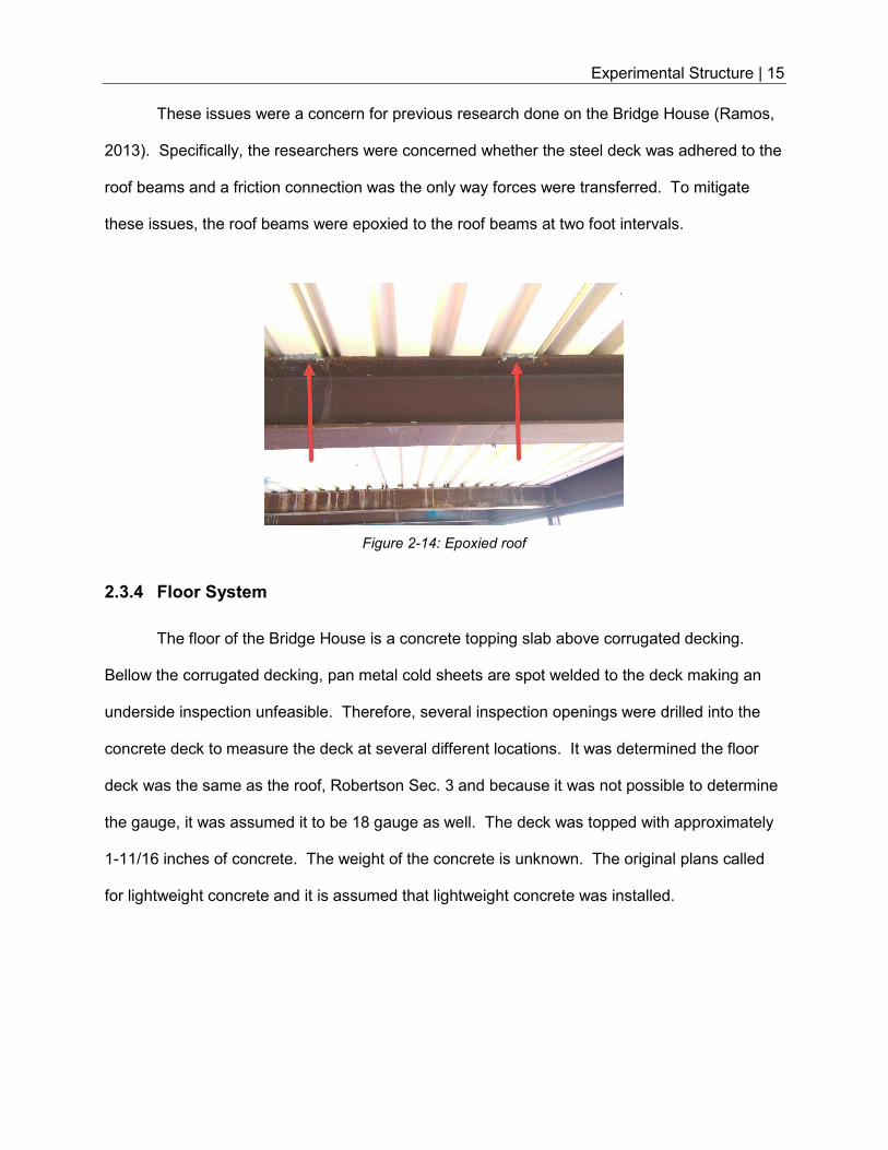
2.3.4 Floor System
The floor of the Bridge House is a concrete topping slab above corrugated decking.
Bellow the corrugated decking, pan metal cold sheets are spot welded to the deck making an
underside inspection unfeasible. Therefore, several inspection openings were drilled into the
concrete deck to measure the deck at several different locations. It was determined the floor
deck was the same as the roof, Robertson Sec. 3 and because it was not possible to determine
the gauge, it was assumed it to be 18 gauge as well. The deck was topped with approximately
1-11/16 inches of concrete. The weight of the concrete is unknown. The original plans called
for lightweight concrete and it is assumed that lightweight concrete was installed.
Figure 2-14: Epoxied roof
Experimental Structure | 16
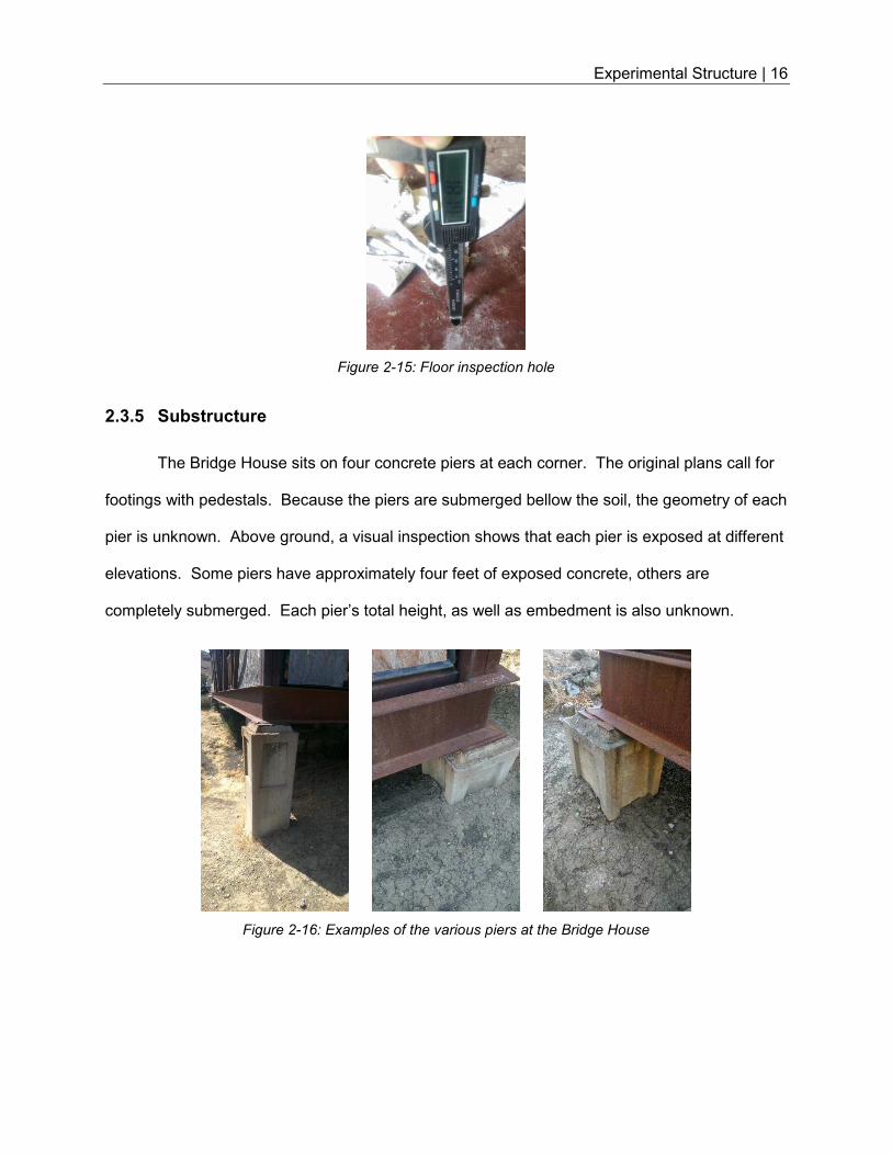
2.3.5 Substructure
The Bridge House sits on four concrete piers at each corner. The original plans call for
footings with pedestals. Because the piers are submerged bellow the soil, the geometry of each
pier is unknown. Above ground, a visual inspection shows that each pier is exposed at different
elevations. Some piers have approximately four feet of exposed concrete, others are
completely submerged. Each pier’s total height, as well as embedment is also unknown.
Figure 2-16: Examples of the various piers at the Bridge House
Figure 2-15: Floor inspection hole
Theory and Methodology | 17
3.0 THEORY AND METHODOLOGY
3.1 Overview
It is assumed that steady state response, modal analysis, the equation-of-motion, and a
system subjected to sinusoidal forces are previously well understood by the reader.
Discussions here are a summary of the importance of steady state response. Detailed
derivations and explanations are listed in Appendix 0. Traditionally, dynamic response would
also have transient homogenous behavior. This will be ignored as the contribution during
steady state is small and irrelevant. It will be shown in the following sections that the response
due to forced vibration at resonance is much larger than transient behavior.
The equations in this section are for a single-degree-of-freedom (SDOF) system.
Additional assumptions are needed for a multi-degree-of-freedom system (MDOF). In a
dynamic analysis, the response of the structure is made up of many equations-of-motion (EOM)
that are coupled together. A modal analysis decouples the EOM into independent and
orthogonal SDOF equations. If the system is first mode dominate, the dynamic properties can
be idealized as a SDOF system. When coupling the EOM back into a MDOF system, if the
contribution of higher modes is small, the system can be modeled as a SDOF system.
3.2 Displacement Response Amplification Factor, Rd
The displacement response amplification factor, Rd, is a ratio that compares the static
deformations to the dynamic deformations of similar systems. The displacement response
amplification factor is as follows:
�� = ������� Equation 3-1
Where ��� is the deformation due the applied force and ���� is the maximum
displacement of a structure when subjected to a sinusoidal force.
Theory and Methodology | 18
��� = � � Equation 3-2
���� = � � 1��1 −� ������� + �2� � ������
Equation 3-3
Substituting Equation 3-2 and Equation 3-3 into Equation 3-1 cancel outs � �� and yields
the following equation at steady state:
�� = 1��1 −� ������� + �2� � ������
Equation 3-4
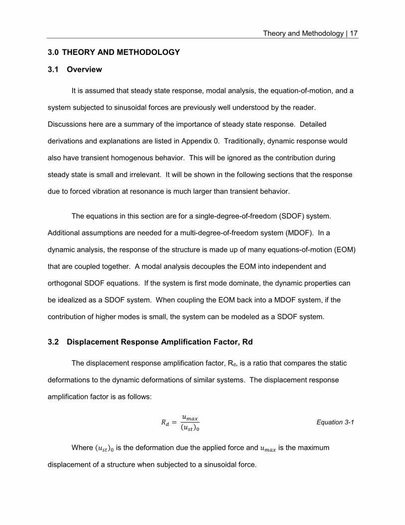
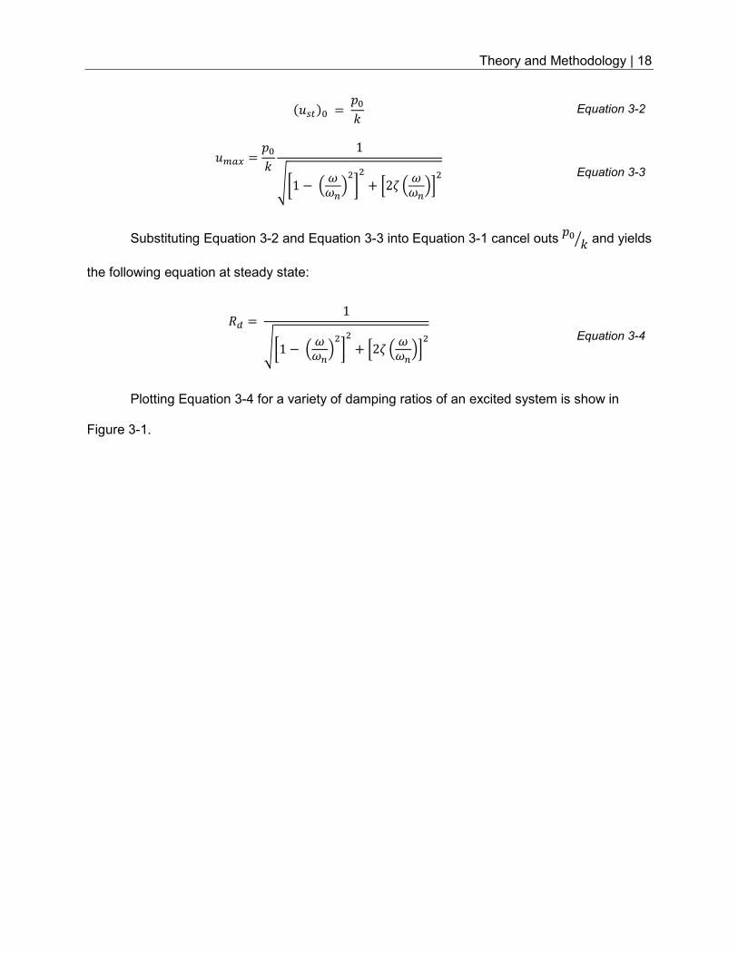
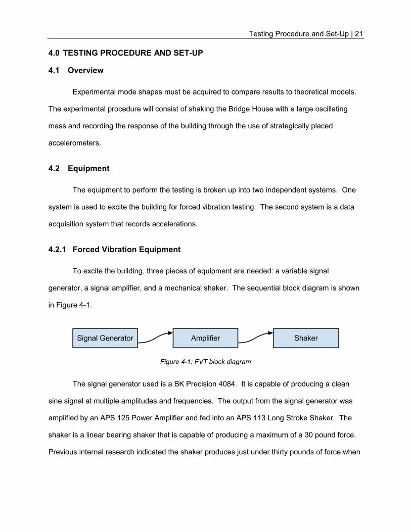
Plotting Equation 3-4 for a variety of damping ratios of an excited system is show in
Figure 3-1.
Theory and Methodology | 19
Figure 3-1: Dynamic Response Displacement Amplification
Increasing damping for a system will reduce the displacements. For low-dampened
systems, (when ζ is approximately less than 10 percent), the maximum displacements occur
when the system is excited at its natural frequency (when w/wn = 1). For systems with large
damping, the maximum displacements will not occur at w/wn = 1. For typical building systems,
zeta is well below 10 percent. Therefore, for the scope of this research, it shall always be
assumed that the maximum displacement occurs when w/wn = 1. By exciting a building at a
variety of frequencies, a response amplification plot as shown in Figure 3-1 can be composed.
The frequency-displacement response curve can be calculated experimentally by subjecting a
building to a sinusoidal dynamic force, waiting for steady state response, and measuring the
acceleration response. This is repeated for several frequencies until an experimental
frequency-acceleration response curve is built.
0 0.2 0.4 0.6 0.8 1 1.2 1.4 1.6 1.8 20
1
2
3
4
5
6
7
8
9
10
w/wn
Rd
Dynamic Response Amplification
ζ =0.01ζ =0.05ζ =0.10ζ =0.25ζ =0.50ζ =1.00
Theory and Methodology | 20
3.3 Damping
To experimentally calculate damping ratios, two methods can be utilized. One method
utilizes the transient response properties due to the decay of motion. This method typically
involves enforcing a displacement in the building, releasing the displacement, and recording the
decay of the vibrations. By recording the time history, damping can be calculated. Because of
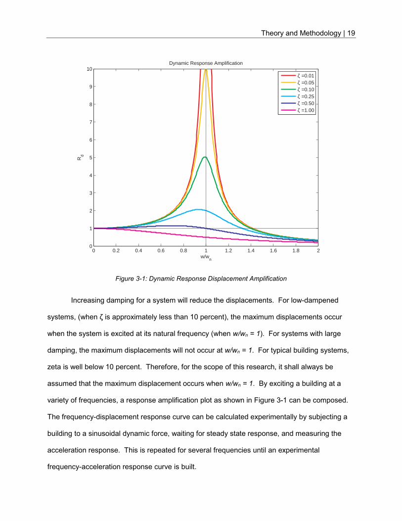
the size and terrain limitations of the Bridge House, this method cannot be utilized. A second
method called the Half-Power Bandwidth allows for the calculation of the damping from a
displacement response amplification curve.
Figure 3-2: Damping calculation (Chopra)
The half-power bandwidth method allows the calculation of the damping from the
displacement frequency response curve. Simplification and substitution yields the following:
� = ! − �2 � Equation 3-5
Where ! − � is defined as the bandwidth and � is the natural frequency. In lieu of
frequencies, periods may be used to calculate the damping ratio.
Testing Procedure and Set-Up | 21
4.0 TESTING PROCEDURE AND SET-UP
4.1 Overview
Experimental mode shapes must be acquired to compare results to theoretical models.
The experimental procedure will consist of shaking the Bridge House with a large oscillating
mass and recording the response of the building through the use of strategically placed
accelerometers.
4.2 Equipment
The equipment to perform the testing is broken up into two independent systems. One
system is used to excite the building for forced vibration testing. The second system is a data
acquisition system that records accelerations.
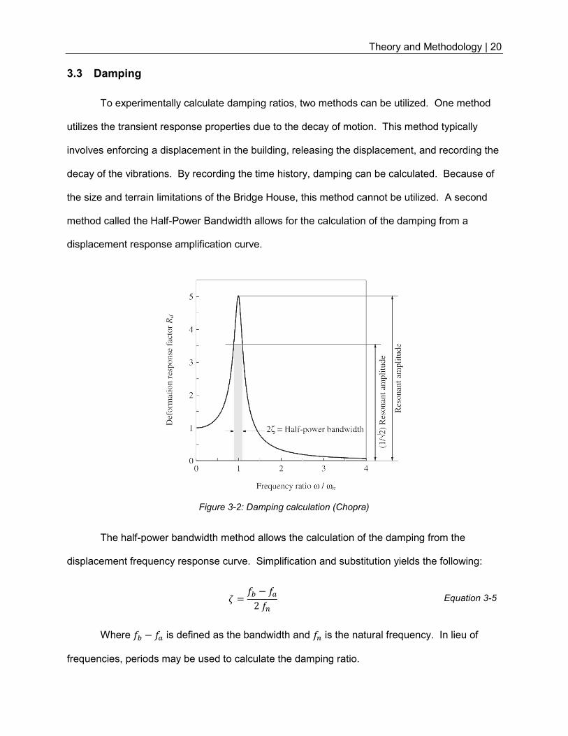
4.2.1 Forced Vibration Equipment
To excite the building, three pieces of equipment are needed: a variable signal
generator, a signal amplifier, and a mechanical shaker. The sequential block diagram is shown
in Figure 4-1.
Figure 4-1: FVT block diagram
The signal generator used is a BK Precision 4084. It is capable of producing a clean
sine signal at multiple amplitudes and frequencies. The output from the signal generator was
amplified by an APS 125 Power Amplifier and fed into an APS 113 Long Stroke Shaker. The
shaker is a linear bearing shaker that is capable of producing a maximum of a 30 pound force.
Previous internal research indicated the shaker produces just under thirty pounds of force when
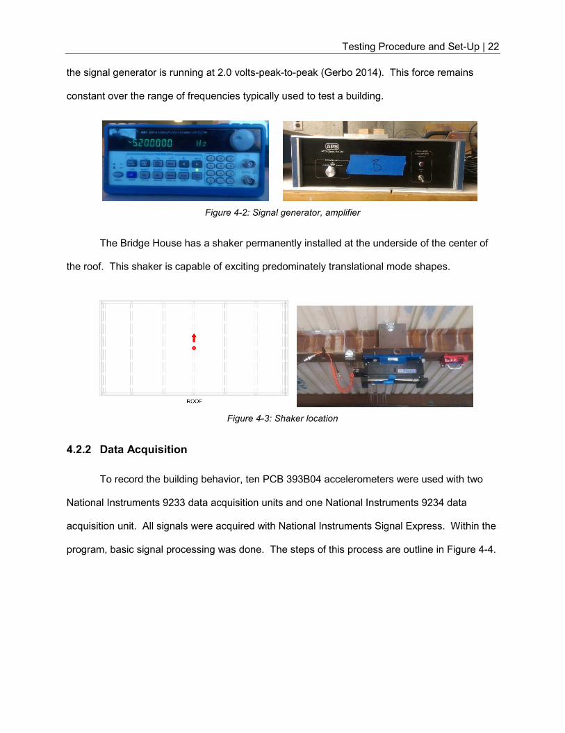
Testing Procedure and Set-Up | 22
the signal generator is running at 2.0 volts-peak-to-peak (Gerbo 2014). This force remains
constant over the range of frequencies typically used to test a building.
Figure 4-2: Signal generator, amplifier
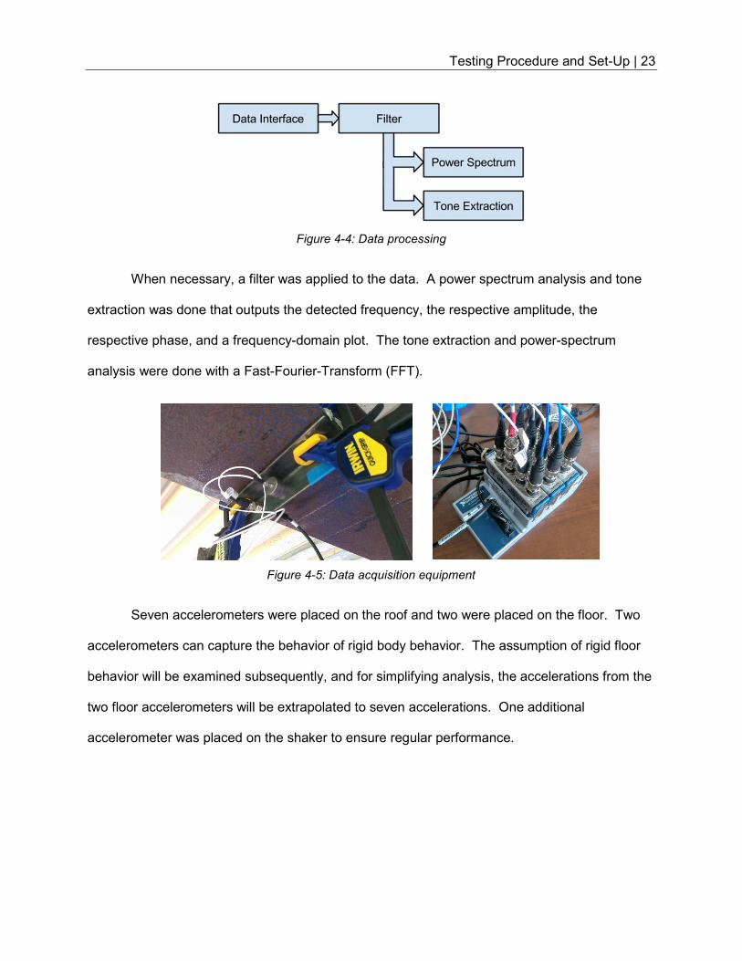
The Bridge House has a shaker permanently installed at the underside of the center of
the roof. This shaker is capable of exciting predominately translational mode shapes.
Figure 4-3: Shaker location
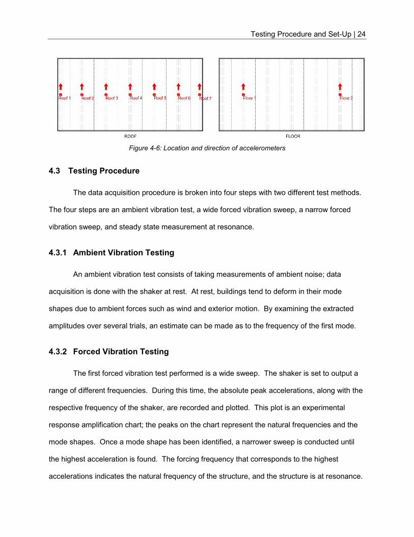
4.2.2 Data Acquisition
To record the building behavior, ten PCB 393B04 accelerometers were used with two
National Instruments 9233 data acquisition units and one National Instruments 9234 data
acquisition unit. All signals were acquired with National Instruments Signal Express. Within the
program, basic signal processing was done. The steps of this process are outline in Figure 4-4.
Testing Procedure and Set-Up | 23
Figure 4-4: Data processing
When necessary, a filter was applied to the data. A power spectrum analysis and tone
extraction was done that outputs the detected frequency, the respective amplitude, the
respective phase, and a frequency-domain plot. The tone extraction and power-spectrum
analysis were done with a Fast-Fourier-Transform (FFT).
Figure 4-5: Data acquisition equipment
Seven accelerometers were placed on the roof and two were placed on the floor. Two
accelerometers can capture the behavior of rigid body behavior. The assumption of rigid floor
behavior will be examined subsequently, and for simplifying analysis, the accelerations from the
two floor accelerometers will be extrapolated to seven accelerations. One additional
accelerometer was placed on the shaker to ensure regular performance.
Testing Procedure and Set-Up | 24
Figure 4-6: Location and direction of accelerometers
4.3 Testing Procedure
The data acquisition procedure is broken into four steps with two different test methods.
The four steps are an ambient vibration test, a wide forced vibration sweep, a narrow forced
vibration sweep, and steady state measurement at resonance.
4.3.1 Ambient Vibration Testing
An ambient vibration test consists of taking measurements of ambient noise; data
acquisition is done with the shaker at rest. At rest, buildings tend to deform in their mode
shapes due to ambient forces such as wind and exterior motion. By examining the extracted
amplitudes over several trials, an estimate can be made as to the frequency of the first mode.
4.3.2 Forced Vibration Testing
The first forced vibration test performed is a wide sweep. The shaker is set to output a
range of different frequencies. During this time, the absolute peak accelerations, along with the
respective frequency of the shaker, are recorded and plotted. This plot is an experimental
response amplification chart; the peaks on the chart represent the natural frequencies and the
mode shapes. Once a mode shape has been identified, a narrower sweep is conducted until
the highest acceleration is found. The forcing frequency that corresponds to the highest
accelerations indicates the natural frequency of the structure, and the structure is at resonance.
Testing Procedure and Set-Up | 25
At this point, the shaker frequency is fixed and acceleration readings are taken. These
acceleration readings correspond to the experimental mode shapes. These procedures were
repeated several times for different shaker amplitude and brace configurations. For the scope
of this thesis, only first mode from each brace configuration will be examined.
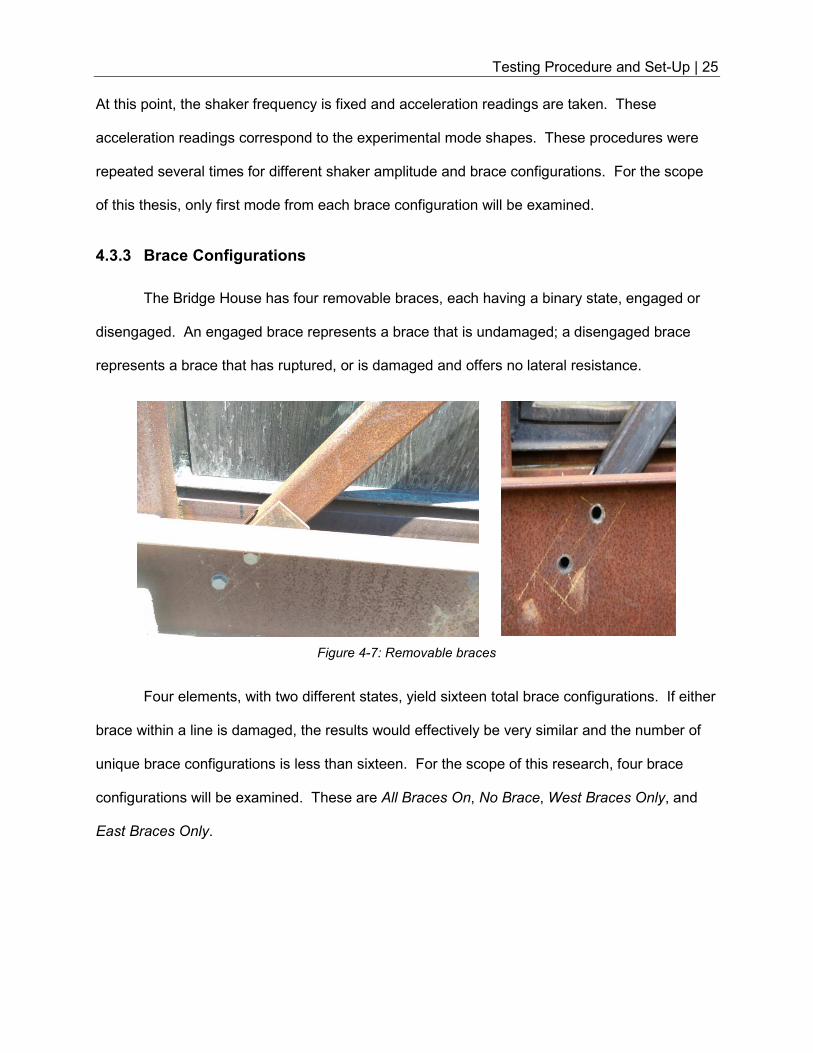
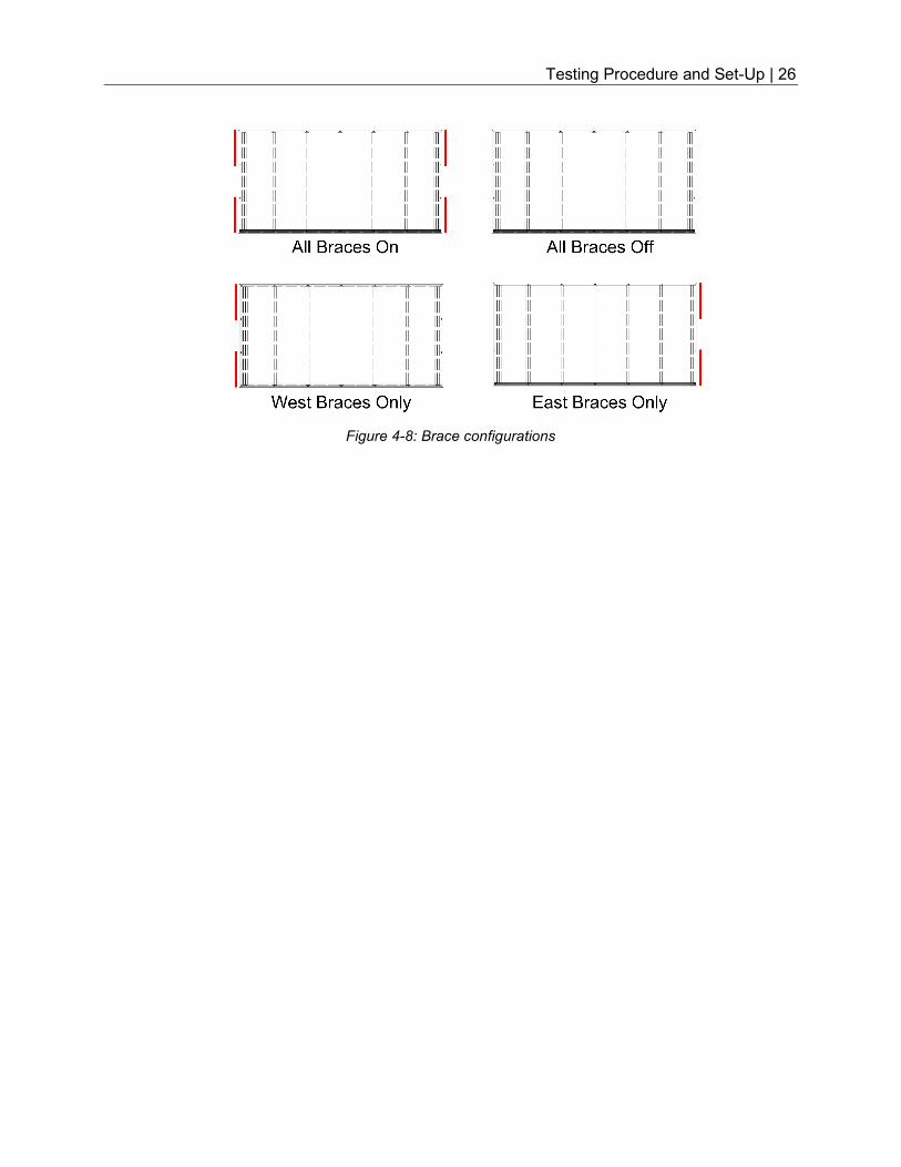
4.3.3 Brace Configurations
The Bridge House has four removable braces, each having a binary state, engaged or
disengaged. An engaged brace represents a brace that is undamaged; a disengaged brace
represents a brace that has ruptured, or is damaged and offers no lateral resistance.
Figure 4-7: Removable braces
Four elements, with two different states, yield sixteen total brace configurations. If either
brace within a line is damaged, the results would effectively be very similar and the number of
unique brace configurations is less than sixteen. For the scope of this research, four brace
configurations will be examined. These are All Braces On, No Brace, West Braces Only, and
East Braces Only.
Testing Procedure and Set-Up | 26
Figure 4-8: Brace configurations
Testing Results and System Identification | 27
5.0 TESTING RESULTS AND SYSTEM IDENTIFICATION
5.1 System Identification
System identification of a building consists of analyzing a structure to extract the
structural properties of the building. Typically, system identification by the use of forced
vibration testing consists of determining the frequency response spectrum, the mode shapes,
and the damping. Through the use of dynamic principals and equilibrium, the stiffness of the
braces, the roof diaphragm, and the substructure can also be determined.
5.2 Ambient Vibration Test
Ambient vibration tests were forgone for the Bridge House. Prior trial tests established
the approximate fundamental frequencies and eliminated the need to search for the range of
excited frequencies.
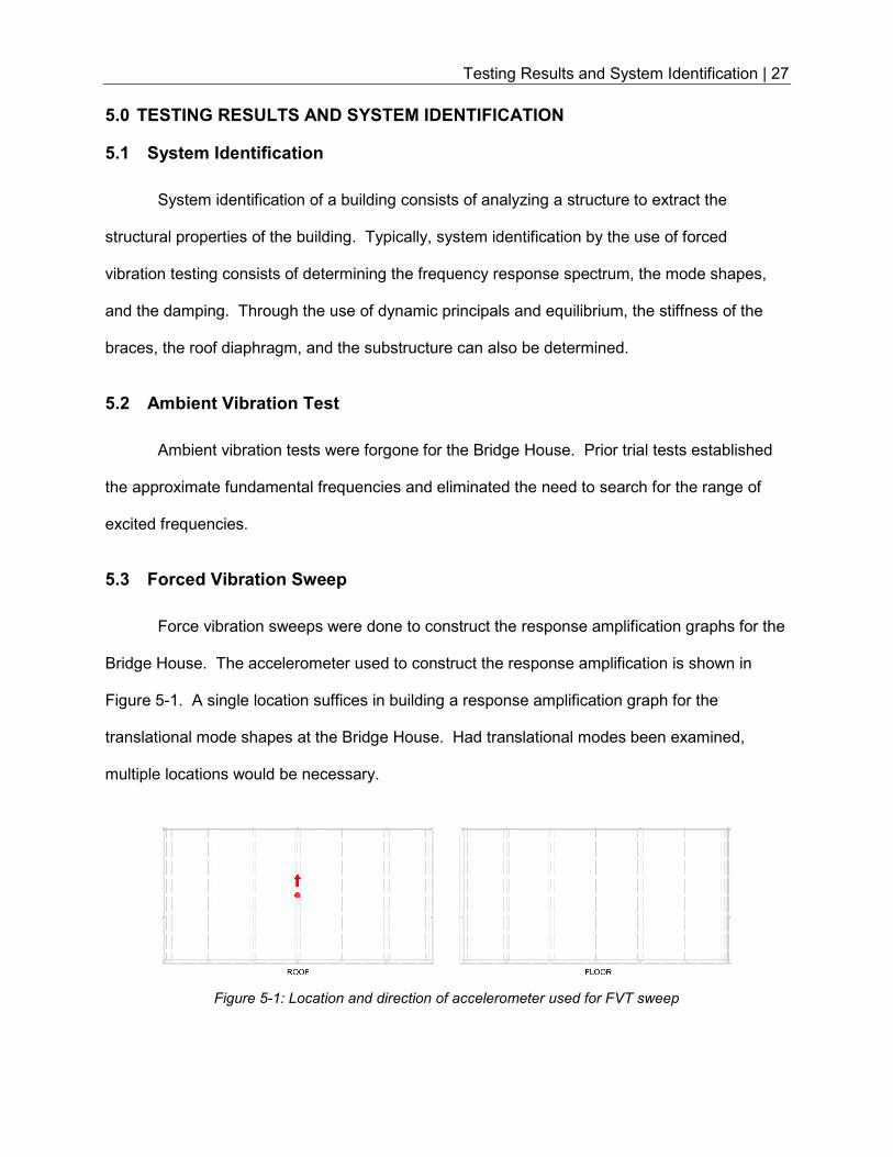
5.3 Forced Vibration Sweep
Force vibration sweeps were done to construct the response amplification graphs for the
Bridge House. The accelerometer used to construct the response amplification is shown in
Figure 5-1. A single location suffices in building a response amplification graph for the
translational mode shapes at the Bridge House. Had translational modes been examined,
multiple locations would be necessary.
Figure 5-1: Location and direction of accelerometer used for FVT sweep
Testing Results and System Identification | 28
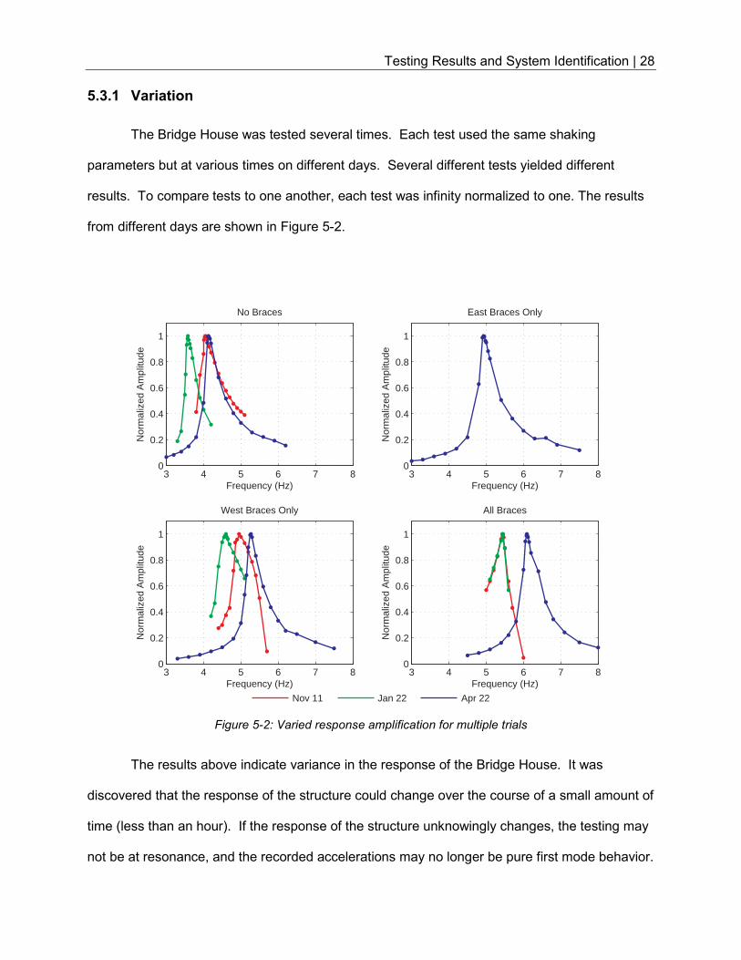
5.3.1 Variation
The Bridge House was tested several times. Each test used the same shaking
parameters but at various times on different days. Several different tests yielded different
results. To compare tests to one another, each test was infinity normalized to one. The results
from different days are shown in Figure 5-2.
Figure 5-2: Varied response amplification for multiple trials
The results above indicate variance in the response of the Bridge House. It was
discovered that the response of the structure could change over the course of a small amount of
time (less than an hour). If the response of the structure unknowingly changes, the testing may
not be at resonance, and the recorded accelerations may no longer be pure first mode behavior.
3 4 5 6 7 80
0.2
0.4
0.6
0.8
1
No Braces
Frequency (Hz)
Nor
mal
ized
Am
plitu
de
3 4 5 6 7 80
0.2
0.4
0.6
0.8
1
East Braces Only
Frequency (Hz)
Nor
mal
ized
Am
plitu
de
3 4 5 6 7 80
0.2
0.4
0.6
0.8
1
West Braces Only
Frequency (Hz)
Nor
mal
ized
Am
plitu
de
3 4 5 6 7 80
0.2
0.4
0.6
0.8
1
All Braces
Frequency (Hz)
Nor
mal
ized
Am
plitu
de
Nov 11 Jan 22 Apr 22
Testing Results and System Identification | 29
Typically, minor adjustments in the response amplification are ignored in forced vibration
testing; the deviations observed in the Bridge House were not minor. This discrepancy has
been well documented in the past (Ramos, 2013). It has been observed that the Bridge House
is susceptible to temperature effects as the structural system is exposed steel. Some parts of
the Bridge House are exposed to direct sunlight while others are subjected to complete shade.
A surface temperature gradient on the steel has been measured as large as 100 degrees
Fahrenheit.
To solve this problem, two changes to the procedure were made. First, more
accelerometers were acquired to expedite the testing and to facilitate concurrent data
acquisition. Second, all testing was done at night to eliminate environmental variables. These
changes allowed for repeatable and consistent results that were verified through multiple trials.
The results are shown in blue in Figure 5-2.
5.3.2 Final Forced Vibration Sweep
After procedural changes were made, a final forced vibration frequency sweep was
conducted. The final for each brace configuration are shown in Figure 5-3. It is important to
note that the amplitude has not been normalized for each brace configuration and the output of
the shaker is a fairly constant at 30 pounds. The maximum accelerations for each brace
configuration varies; the accelerations were recorded at the center of the Bridge House as
shown in Figure 5-1. For this reason, the magnitude of the final force vibration sweep should
not be regarded as significant.
Testing Results and System Identification | 30
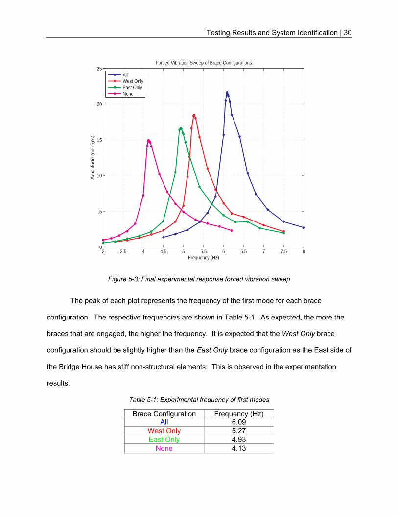
Figure 5-3: Final experimental response forced vibration sweep
The peak of each plot represents the frequency of the first mode for each brace
configuration. The respective frequencies are shown in Table 5-1. As expected, the more the
braces that are engaged, the higher the frequency. It is expected that the West Only brace
configuration should be slightly higher than the East Only brace configuration as the East side of
the Bridge House has stiff non-structural elements. This is observed in the experimentation
results.
Table 5-1: Experimental frequency of first modes
Brace Configuration Frequency (Hz)
All 6.09
West Only 5.27
East Only 4.93
None 4.13
3 3.5 4 4.5 5 5.5 6 6.5 7 7.5 80
5
10
15
20
25Forced Vibration Sweep of Brace Configurations
Frequency (Hz)
Am
plit
ud
e (
mill
i-g
’s)
AllWest OnlyEast OnlyNone
Testing Results and System Identification | 31
5.4 Damping
Using the half-power bandwidth method as shown in Figure 3-2, the experimental results
for the various brace configurations are shown below.
Table 5-2: Tested damping coefficients
Brace Configuration Damping
All 4.04
West Only 3.03
East Only 3.95
None 2.99
The values are all within expected damping values of a steel structure. These damping
values are also within the ten percent threshold discussed in section 3.2; the assumption that
max displacements and max accelerations occur when w/wn = 1 holds valid. There is an
increase in damping when less braces are engaged. This is expected as the external cladding
elements along the brace line are engaged, although it is difficult to show causation. These
cladding elements closely resemble damage; as damage increases in a building, the damping
increases as well.
5.5 Mode Shapes
5.5.1 Rigid Floor Verification
The as built condition of the Bridge House is not completely known. Verification of the
floor behavior is necessary. To verify the floor behavior, seven accelerometers were placed on
the floor and a forced vibration test at resonance was performed. Several trials yielded similar
results. The results of a typical trial are shown below in Figure 5-4.
Testing Results and System Identification | 32
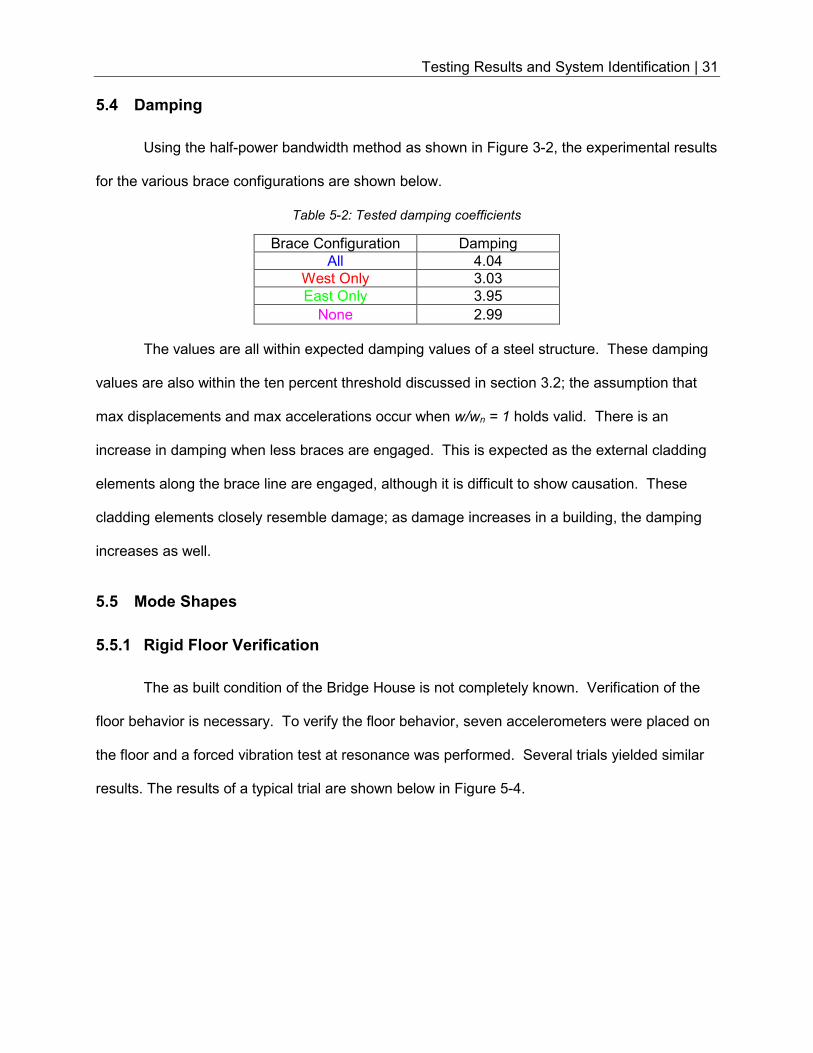
Figure 5-4: Experimental floor behavior
Testing shows linear results which indicates the floor behaves as a rigid body. Two
irregularities were spotted at 8 and 16 feet. The cause of these irregularities is unknown and
has little to no impact on the test results. In addition, this verification allows the testing to be
conducted with less degrees-of-freedom. Because the floor behaves as a rigid body, two
accelerometers can capture rotation and one direction of translational behavior. To achieve
additional degrees of freedom, the behavior of the two degrees-of-freedom can be extrapolated.
Having additional degrees of freedom eases analysis for several reasons. It allows for
increased precision when making a lumped mass assumption and easier calculations when
computing story drift.
5.5.2 Raw Mode Shapes for Multiple Shaker Voltage Input
After several pre-trail runs, a final data collection of experimental mode shapes was
collected. For every brace configuration, the shaker was set to four different peak-to-peak
voltages: 0.5 VPP, 1.0 VPP, 1.5 VPP, and 2.0 VPP.
Testing Results and System Identification | 33
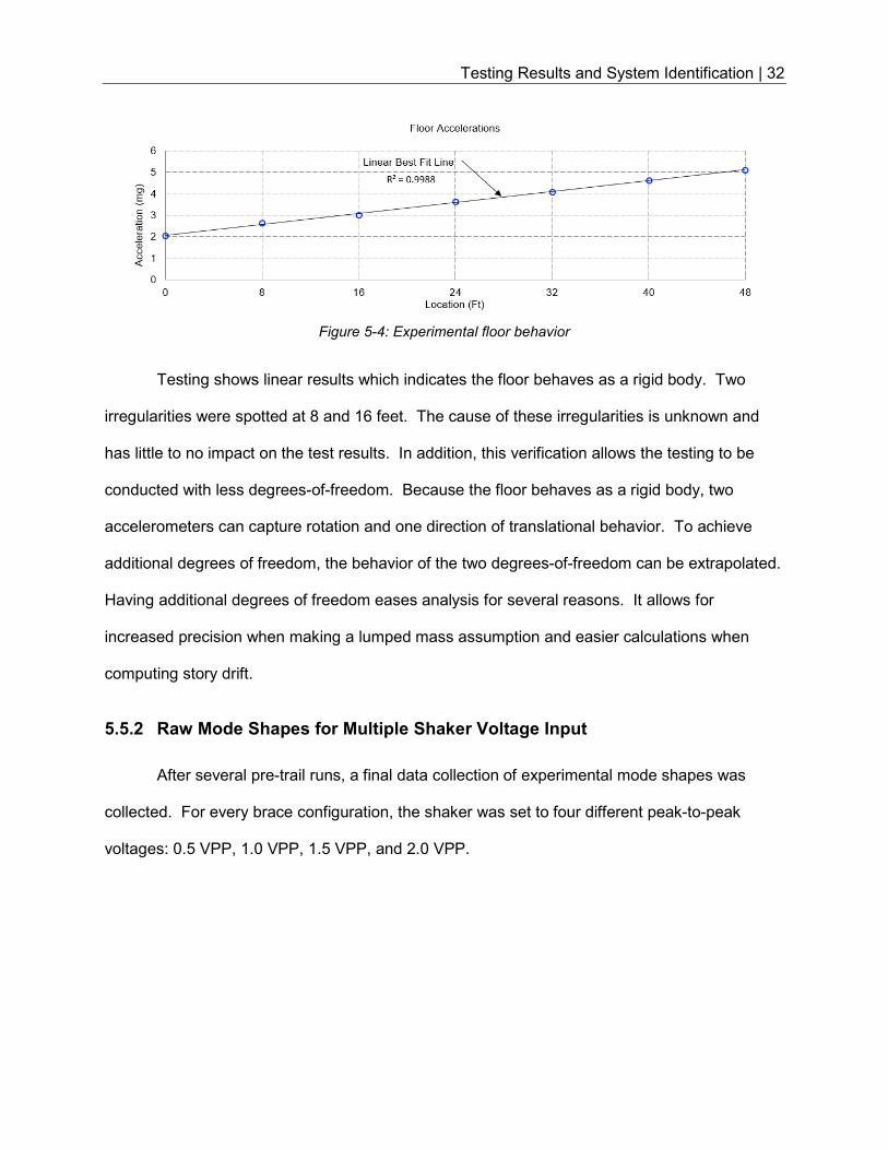
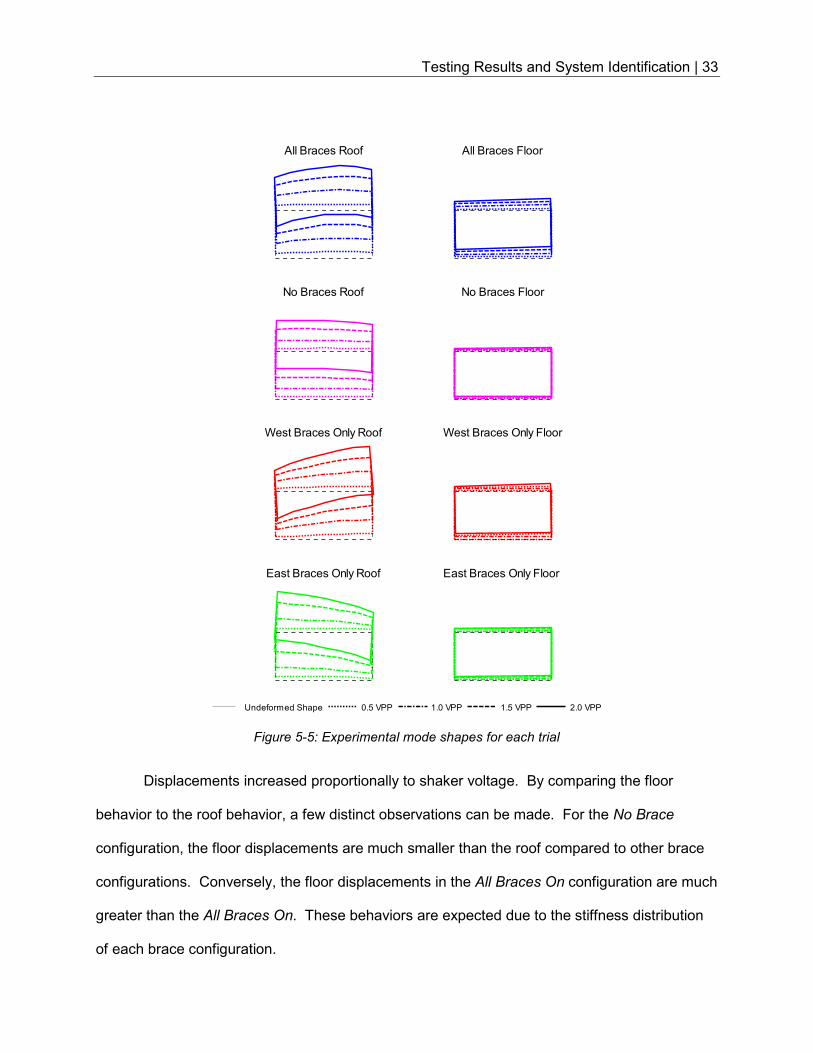
Figure 5-5: Experimental mode shapes for each trial
Displacements increased proportionally to shaker voltage. By comparing the floor
behavior to the roof behavior, a few distinct observations can be made. For the No Brace
configuration, the floor displacements are much smaller than the roof compared to other brace
configurations. Conversely, the floor displacements in the All Braces On configuration are much
greater than the All Braces On. These behaviors are expected due to the stiffness distribution
of each brace configuration.
All Braces Roof All Braces Floor
No Braces Roof No Braces Floor
West Braces Only Roof West Braces Only Floor
East Braces Only Roof East Braces Only Floor
Undeformed Shape 0.5 VPP 1.0 VPP 1.5 VPP 2.0 VPP
Testing Results and System Identification | 34
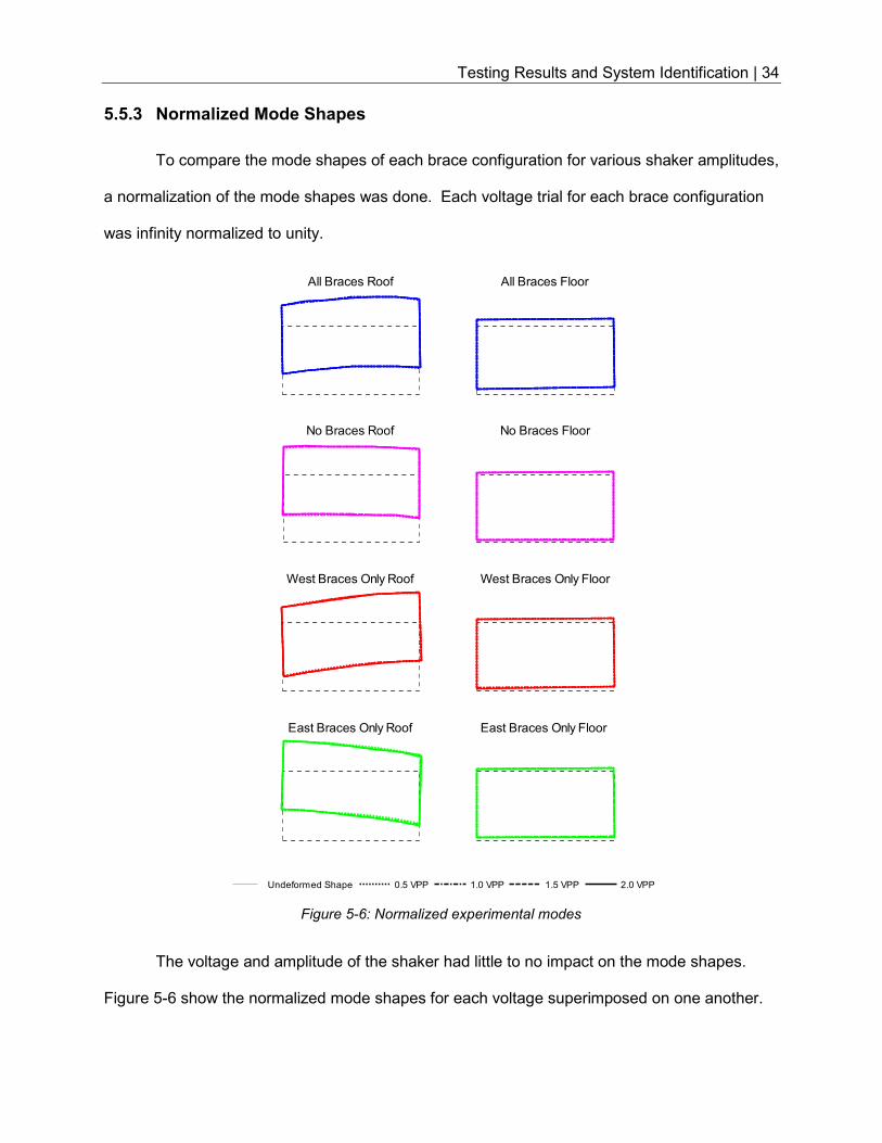
5.5.3 Normalized Mode Shapes
To compare the mode shapes of each brace configuration for various shaker amplitudes,
a normalization of the mode shapes was done. Each voltage trial for each brace configuration
was infinity normalized to unity.
Figure 5-6: Normalized experimental modes
The voltage and amplitude of the shaker had little to no impact on the mode shapes.
Figure 5-6 show the normalized mode shapes for each voltage superimposed on one another.
All Braces Roof All Braces Floor
No Braces Roof No Braces Floor
West Braces Only Roof West Braces Only Floor
East Braces Only Roof East Braces Only Floor
Undeformed Shape 0.5 VPP 1.0 VPP 1.5 VPP 2.0 VPP
Testing Results and System Identification | 35
If examined closely, slight variances are observable. In summary, the amplitude of the shaker,
and the corresponding force it outputs has no impact on the mode shapes for each brace
configuration.
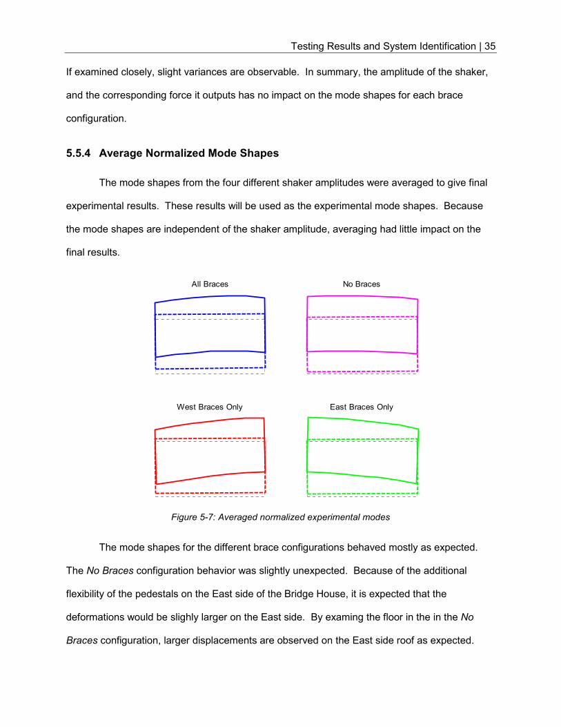
5.5.4 Average Normalized Mode Shapes
The mode shapes from the four different shaker amplitudes were averaged to give final
experimental results. These results will be used as the experimental mode shapes. Because
the mode shapes are independent of the shaker amplitude, averaging had little impact on the
final results.
Figure 5-7: Averaged normalized experimental modes
The mode shapes for the different brace configurations behaved mostly as expected.
The No Braces configuration behavior was slightly unexpected. Because of the additional
flexibility of the pedestals on the East side of the Bridge House, it is expected that the
deformations would be slighly larger on the East side. By examing the floor in the in the No
Braces configuration, larger displacements are observed on the East side roof as expected.
All Braces No Braces
West Braces Only East Braces Only
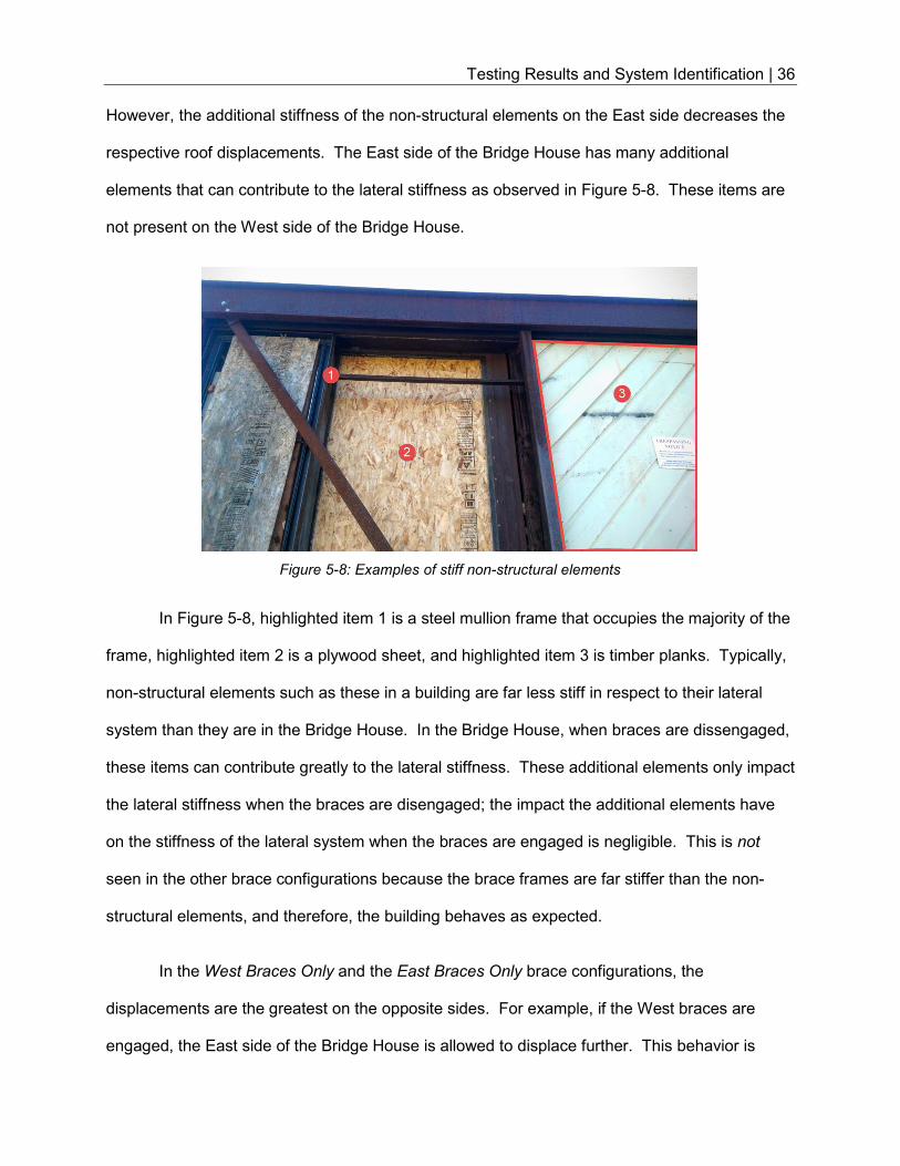
Testing Results and System Identification | 36
However, the additional stiffness of the non-structural elements on the East side decreases the
respective roof displacements. The East side of the Bridge House has many additional
elements that can contribute to the lateral stiffness as observed in Figure 5-8. These items are
not present on the West side of the Bridge House.
In Figure 5-8, highlighted item 1 is a steel mullion frame that occupies the majority of the
frame, highlighted item 2 is a plywood sheet, and highlighted item 3 is timber planks. Typically,
non-structural elements such as these in a building are far less stiff in respect to their lateral
system than they are in the Bridge House. In the Bridge House, when braces are dissengaged,
these items can contribute greatly to the lateral stiffness. These additional elements only impact
the lateral stiffness when the braces are disengaged; the impact the additional elements have
on the stiffness of the lateral system when the braces are engaged is negligible. This is not
seen in the other brace configurations because the brace frames are far stiffer than the non-
structural elements, and therefore, the building behaves as expected.
In the West Braces Only and the East Braces Only brace configurations, the
displacements are the greatest on the opposite sides. For example, if the West braces are
engaged, the East side of the Bridge House is allowed to displace further. This behavior is
Figure 5-8: Examples of stiff non-structural elements
Testing Results and System Identification | 37
expected. Interestingly, the behavior for all brace configurations is overwhelmingly translational,
and all brace configurations look very similar. Out of all the brace configurations, the All Braces
configuration also has larger relative floor displacements in comparision to the roof. This is
explained by the fact that braces increase the story stiffness and reduce the roof’s contribution
to the final mode shape.
5.5.5 Floor Behavior
Superimposing the the floor behavior from all four brace configurations shows the floor
behavior varies per brace configuration. By examining the behavior of just the floor, several
observations can be made.
Figure 5-9: Superimposed floor averaged normalized mode shapes
As previously mentioned, the relative displacement in the All Braces configuration is
greater than any other mode shape. Additionally, it appears the directions of the floor due to the
brace configurations are the same; i.e., they have approximately the same amount of translation
and rotation; the only difference is the scale. The difference is small, but it suggests that the
floor behavior could be helpful in identifying brace configurations.
Floor Plots
All Braces No Braces West Braces Only East Braces Only
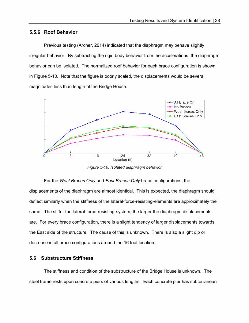
Testing Results and System Identification | 38
5.5.6 Roof Behavior
Previous testing (Archer, 2014) indicated that the diaphragm may behave slightly
irregular behavior. By subtracting the rigid body behavior from the accelerations, the diaphragm
behavior can be isolated. The normalized roof behavior for each brace configuration is shown
in Figure 5-10. Note that the figure is poorly scaled, the displacements would be several
magnitudes less than length of the Bridge House.
Figure 5-10: Isolated diaphragm behavior
For the West Braces Only and East Braces Only brace configurations, the
displacements of the diaphragm are almost identical. This is expected, the diaphragm should
deflect similarly when the stiffness of the lateral-force-resisting-elements are approximately the
same. The stiffer the lateral-force-resisting-system, the larger the diaphragm displacements
are. For every brace configuration, there is a slight tendency of larger displacements towards
the East side of the structure. The cause of this is unknown. There is also a slight dip or
decrease in all brace configurations around the 16 foot location.
5.6 Substructure Stiffness
The stiffness and condition of the substructure of the Bridge House is unknown. The
steel frame rests upon concrete piers of various lengths. Each concrete pier has subterranean
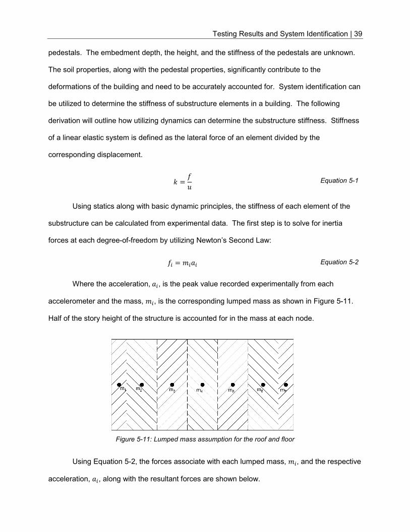
Testing Results and System Identification | 39
pedestals. The embedment depth, the height, and the stiffness of the pedestals are unknown.
The soil properties, along with the pedestal properties, significantly contribute to the
deformations of the building and need to be accurately accounted for. System identification can
be utilized to determine the stiffness of substructure elements in a building. The following
derivation will outline how utilizing dynamics can determine the substructure stiffness. Stiffness
of a linear elastic system is defined as the lateral force of an element divided by the
corresponding displacement.
� = � Equation 5-1
Using statics along with basic dynamic principles, the stiffness of each element of the
substructure can be calculated from experimental data. The first step is to solve for inertia
forces at each degree-of-freedom by utilizing Newton’s Second Law:
" = #"$" Equation 5-2
Where the acceleration,$", is the peak value recorded experimentally from each
accelerometer and the mass, #", is the corresponding lumped mass as shown in Figure 5-11.
Half of the story height of the structure is accounted for in the mass at each node.
Figure 5-11: Lumped mass assumption for the roof and floor
Using Equation 5-2, the forces associate with each lumped mass, #", and the respective
acceleration, $", along with the resultant forces are shown below.
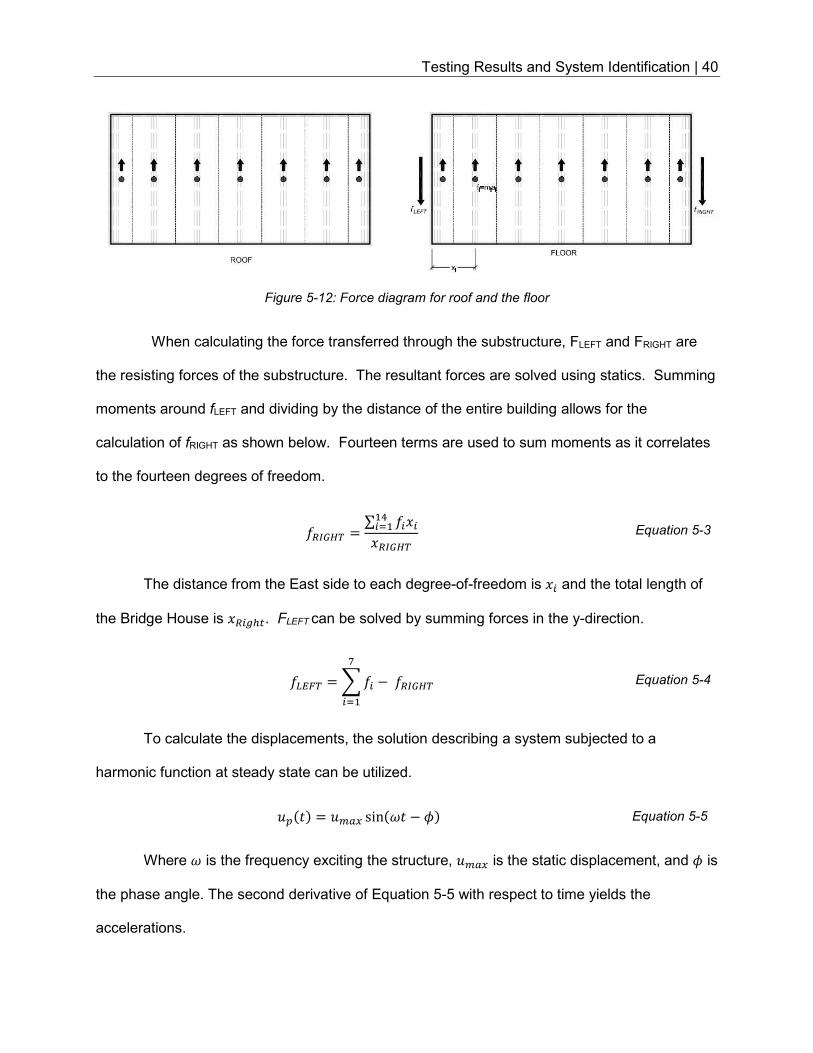
Testing Results and System Identification | 40
Figure 5-12: Force diagram for roof and the floor
When calculating the force transferred through the substructure, FLEFT and FRIGHT are
the resisting forces of the substructure. The resultant forces are solved using statics. Summing
moments around fLEFT and dividing by the distance of the entire building allows for the
calculation of fRIGHT as shown below. Fourteen terms are used to sum moments as it correlates
to the fourteen degrees of freedom.
%&'() = ∑ "+",-".,+%&'() Equation 5-3
The distance from the East side to each degree-of-freedom is +" and the total length of
the Bridge House is +%"/0�. FLEFT can be solved by summing forces in the y-direction.
123) = 4 "5"., − %&'() Equation 5-4
To calculate the displacements, the solution describing a system subjected to a
harmonic function at steady state can be utilized.
�67� = ���� sin�7 − ;� Equation 5-5
Where � is the frequency exciting the structure, ���� is the static displacement, and ; is
the phase angle. The second derivative of Equation 5-5 with respect to time yields the
accelerations.
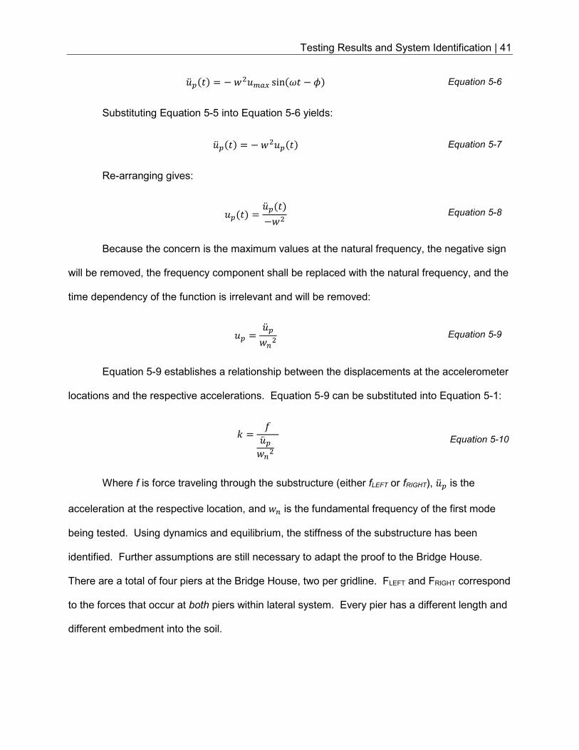
Testing Results and System Identification | 41
�<67� = −=����� sin�7 − ;� Equation 5-6
Substituting Equation 5-5 into Equation 5-6 yields:
�<67� = −=��67� Equation 5-7
Re-arranging gives:
�67� = �<67�−=� Equation 5-8
Because the concern is the maximum values at the natural frequency, the negative sign
will be removed, the frequency component shall be replaced with the natural frequency, and the
time dependency of the function is irrelevant and will be removed:
�6 = �<6=�� Equation 5-9
Equation 5-9 establishes a relationship between the displacements at the accelerometer
locations and the respective accelerations. Equation 5-9 can be substituted into Equation 5-1:
� = �<6=�� Equation 5-10
Where f is force traveling through the substructure (either fLEFT or fRIGHT), �<6 is the
acceleration at the respective location, and =� is the fundamental frequency of the first mode
being tested. Using dynamics and equilibrium, the stiffness of the substructure has been
identified. Further assumptions are still necessary to adapt the proof to the Bridge House.
There are a total of four piers at the Bridge House, two per gridline. FLEFT and FRIGHT correspond
to the forces that occur at both piers within lateral system. Every pier has a different length and
different embedment into the soil.
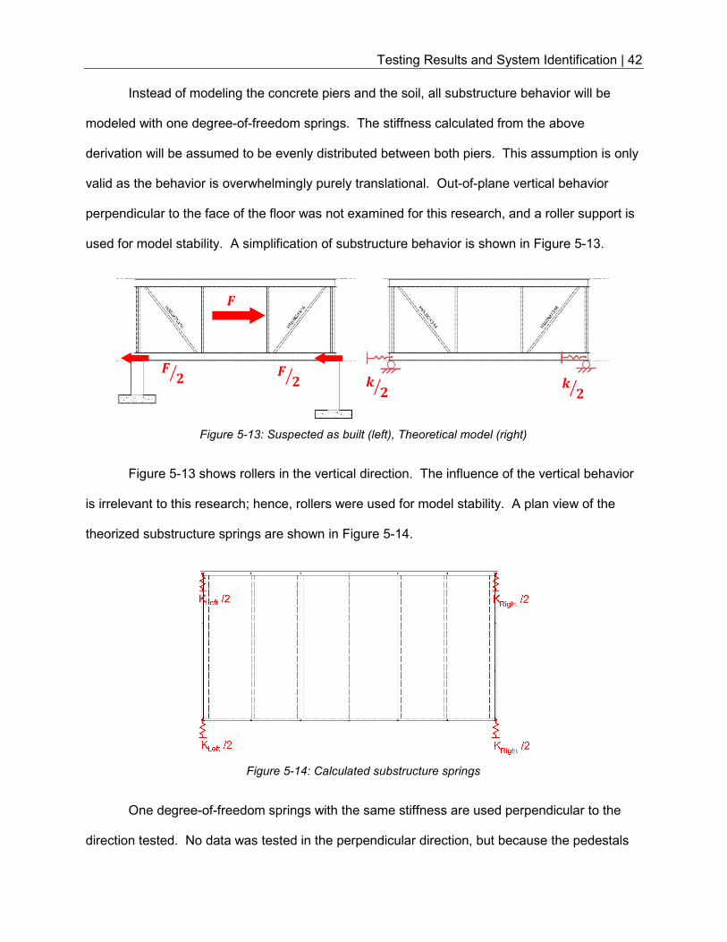
Testing Results and System Identification | 42
Instead of modeling the concrete piers and the soil, all substructure behavior will be
modeled with one degree-of-freedom springs. The stiffness calculated from the above
derivation will be assumed to be evenly distributed between both piers. This assumption is only
valid as the behavior is overwhelmingly purely translational. Out-of-plane vertical behavior
perpendicular to the face of the floor was not examined for this research, and a roller support is
used for model stability. A simplification of substructure behavior is shown in Figure 5-13.
Figure 5-13: Suspected as built (left), Theoretical model (right)
Figure 5-13 shows rollers in the vertical direction. The influence of the vertical behavior
is irrelevant to this research; hence, rollers were used for model stability. A plan view of the
theorized substructure springs are shown in Figure 5-14.
Figure 5-14: Calculated substructure springs
One degree-of-freedom springs with the same stiffness are used perpendicular to the
direction tested. No data was tested in the perpendicular direction, but because the pedestals
> ?� > ?�
@
@ ?� @ ?�
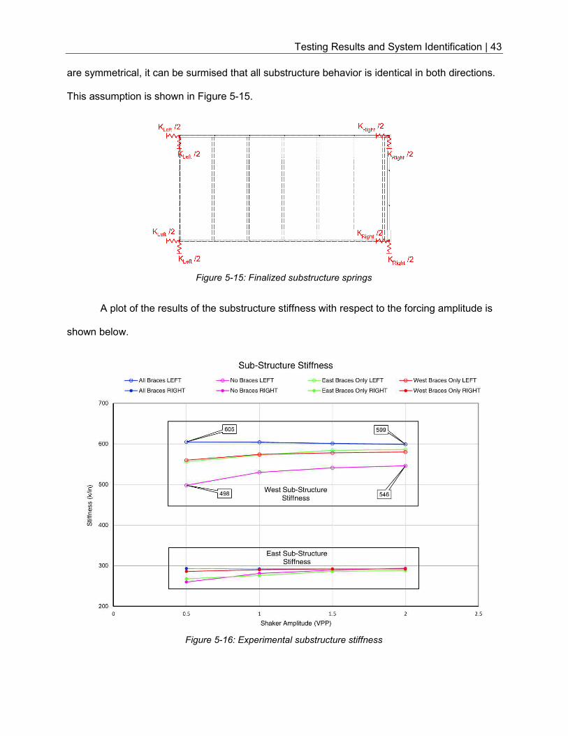
Testing Results and System Identification | 43
are symmetrical, it can be surmised that all substructure behavior is identical in both directions.
This assumption is shown in Figure 5-15.
Figure 5-15: Finalized substructure springs
A plot of the results of the substructure stiffness with respect to the forcing amplitude is
shown below.
Figure 5-16: Experimental substructure stiffness
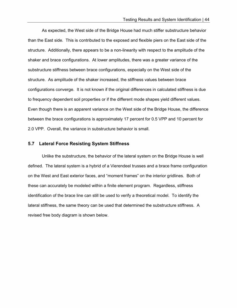
Testing Results and System Identification | 44
As expected, the West side of the Bridge House had much stiffer substructure behavior
than the East side. This is contributed to the exposed and flexible piers on the East side of the
structure. Additionally, there appears to be a non-linearity with respect to the amplitude of the
shaker and brace configurations. At lower amplitudes, there was a greater variance of the
substructure stiffness between brace configurations, especially on the West side of the
structure. As amplitude of the shaker increased, the stiffness values between brace
configurations converge. It is not known if the original differences in calculated stiffness is due
to frequency dependent soil properties or if the different mode shapes yield different values.
Even though there is an apparent variance on the West side of the Bridge House, the difference
between the brace configurations is approximately 17 percent for 0.5 VPP and 10 percent for
2.0 VPP. Overall, the variance in substructure behavior is small.
5.7 Lateral Force Resisting System Stiffness
Unlike the substructure, the behavior of the lateral system on the Bridge House is well
defined. The lateral system is a hybrid of a Vierendeel trusses and a brace frame configuration
on the West and East exterior faces, and “moment frames” on the interior gridlines. Both of
these can accurately be modeled within a finite element program. Regardless, stiffness
identification of the brace line can still be used to verify a theoretical model. To identify the
lateral stiffness, the same theory can be used that determined the substructure stiffness. A
revised free body diagram is shown below.
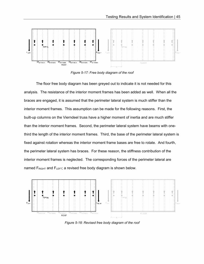
Testing Results and System Identification | 45
Figure 5-17: Free body diagram of the roof
The floor free body diagram has been greyed out to indicate it is not needed for this
analysis. The resistance of the interior moment frames has been added as well. When all the
braces are engaged, it is assumed that the perimeter lateral system is much stiffer than the
interior moment frames. This assumption can be made for the following reasons. First, the
built-up columns on the Vierndeel truss have a higher moment of inertia and are much stiffer
than the interior moment frames. Second, the perimeter lateral system have beams with one-
third the length of the interior moment frames. Third, the base of the perimeter lateral system is
fixed against rotation whereas the interior moment frame bases are free to rotate. And fourth,
the perimeter lateral system has braces. For these reason, the stiffness contribution of the
interior moment frames is neglected. The corresponding forces of the perimeter lateral are
named FRIGHT and FLEFT; a revised free body diagram is shown below.
Figure 5-18: Revised free body diagram of the roof
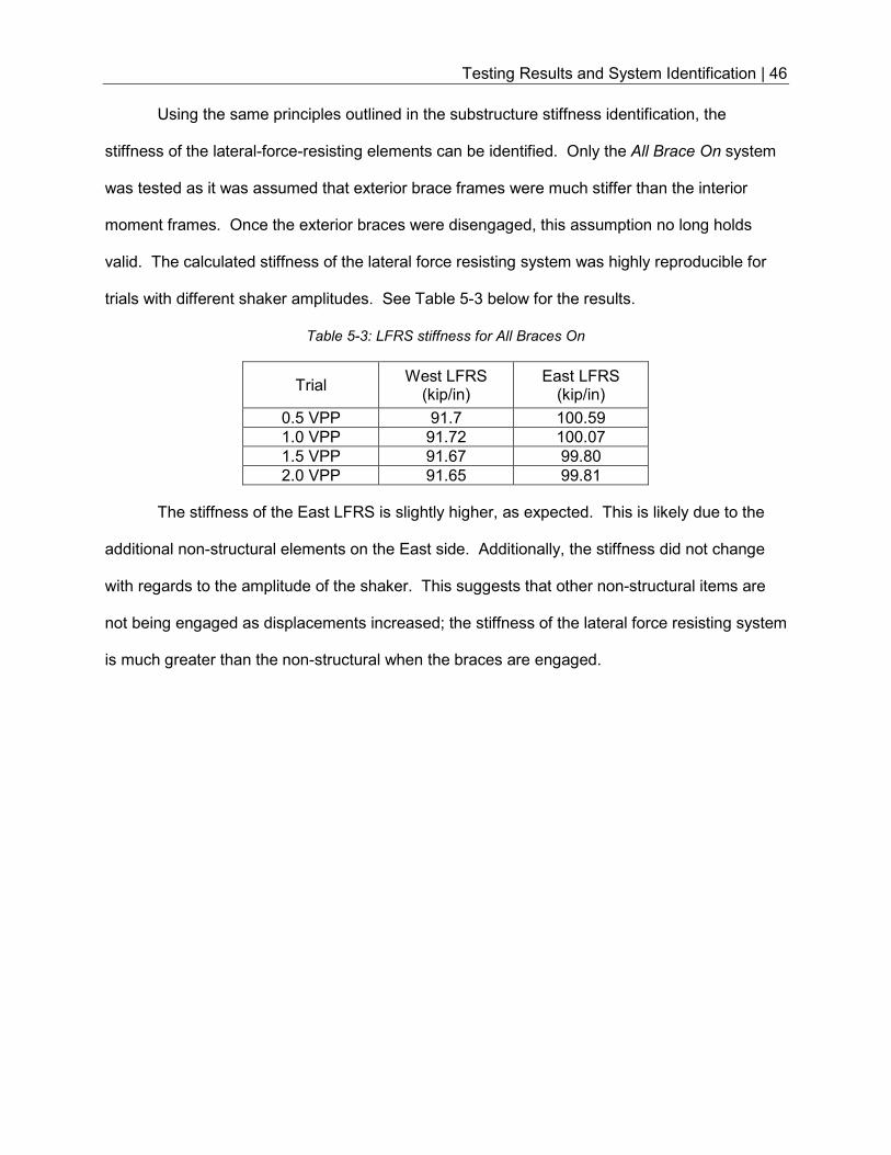
Testing Results and System Identification | 46
Using the same principles outlined in the substructure stiffness identification, the
stiffness of the lateral-force-resisting elements can be identified. Only the All Brace On system
was tested as it was assumed that exterior brace frames were much stiffer than the interior
moment frames. Once the exterior braces were disengaged, this assumption no long holds
valid. The calculated stiffness of the lateral force resisting system was highly reproducible for
trials with different shaker amplitudes. See Table 5-3 below for the results.
Table 5-3: LFRS stiffness for All Braces On
Trial West LFRS
(kip/in) East LFRS
(kip/in)
0.5 VPP 91.7 100.59
1.0 VPP 91.72 100.07
1.5 VPP 91.67 99.80
2.0 VPP 91.65 99.81
The stiffness of the East LFRS is slightly higher, as expected. This is likely due to the
additional non-structural elements on the East side. Additionally, the stiffness did not change
with regards to the amplitude of the shaker. This suggests that other non-structural items are
not being engaged as displacements increased; the stiffness of the lateral force resisting system
is much greater than the non-structural when the braces are engaged.
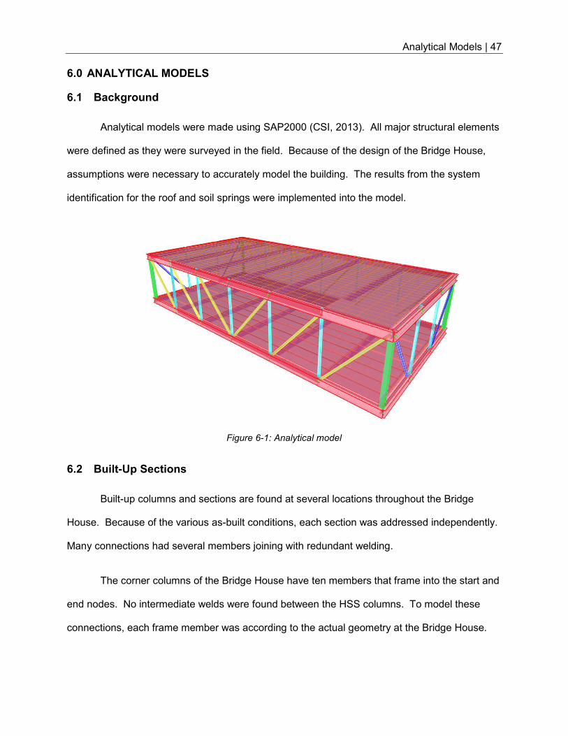
Analytical Models | 47
6.0 ANALYTICAL MODELS
6.1 Background
Analytical models were made using SAP2000 (CSI, 2013). All major structural elements
were defined as they were surveyed in the field. Because of the design of the Bridge House,
assumptions were necessary to accurately model the building. The results from the system
identification for the roof and soil springs were implemented into the model.
Figure 6-1: Analytical model
6.2 Built-Up Sections
Built-up columns and sections are found at several locations throughout the Bridge
House. Because of the various as-built conditions, each section was addressed independently.
Many connections had several members joining with redundant welding.
The corner columns of the Bridge House have ten members that frame into the start and
end nodes. No intermediate welds were found between the HSS columns. To model these
connections, each frame member was according to the actual geometry at the Bridge House.
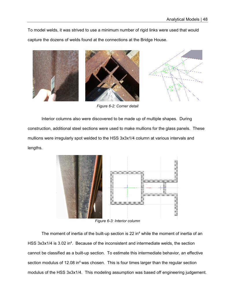
Analytical Models | 48
To model welds, it was strived to use a minimum number of rigid links were used that would
capture the dozens of welds found at the connections at the Bridge House.
Figure 6-2: Corner detail
Interior columns also were discovered to be made up of multiple shapes. During
construction, additional steel sections were used to make mullions for the glass panels. These
mullions were irregularly spot welded to the HSS 3x3x1/4 column at various intervals and
lengths.
Figure 6-3: Interior column
The moment of inertia of the built-up section is 22 in4 while the moment of inertia of an
HSS 3x3x1/4 is 3.02 in4. Because of the inconsistent and intermediate welds, the section
cannot be classified as a built-up section. To estimate this intermediate behavior, an effective
section modulus of 12.08 in4 was chosen. This is four times larger than the regular section
modulus of the HSS 3x3x1/4. This modeling assumption was based off engineering judgement.
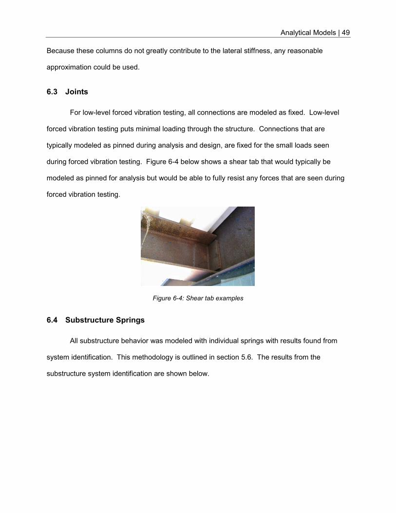
Analytical Models | 49
Because these columns do not greatly contribute to the lateral stiffness, any reasonable
approximation could be used.
6.3 Joints
For low-level forced vibration testing, all connections are modeled as fixed. Low-level
forced vibration testing puts minimal loading through the structure. Connections that are
typically modeled as pinned during analysis and design, are fixed for the small loads seen
during forced vibration testing. Figure 6-4 below shows a shear tab that would typically be
modeled as pinned for analysis but would be able to fully resist any forces that are seen during
forced vibration testing.
Figure 6-4: Shear tab examples
6.4 Substructure Springs
All substructure behavior was modeled with individual springs with results found from
system identification. This methodology is outlined in section 5.6. The results from the
substructure system identification are shown below.
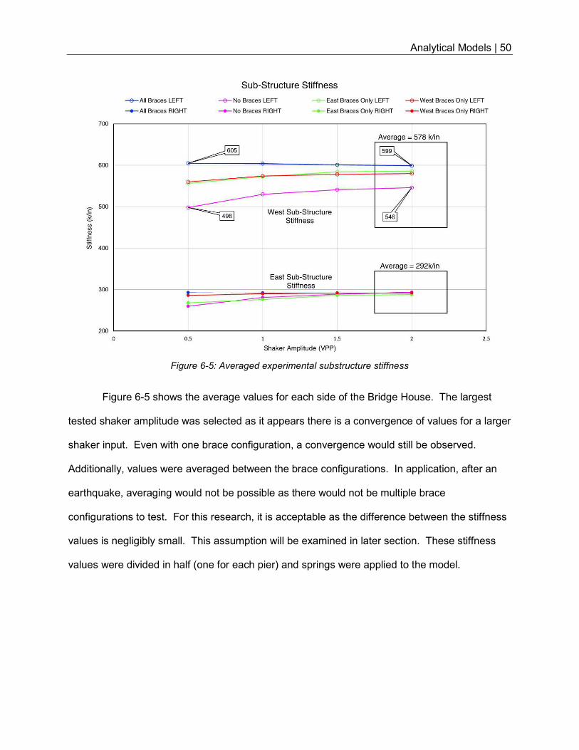
Analytical Models | 50
Figure 6-5: Averaged experimental substructure stiffness
Figure 6-5 shows the average values for each side of the Bridge House. The largest
tested shaker amplitude was selected as it appears there is a convergence of values for a larger
shaker input. Even with one brace configuration, a convergence would still be observed.
Additionally, values were averaged between the brace configurations. In application, after an
earthquake, averaging would not be possible as there would not be multiple brace
configurations to test. For this research, it is acceptable as the difference between the stiffness
values is negligibly small. This assumption will be examined in later section. These stiffness
values were divided in half (one for each pier) and springs were applied to the model.
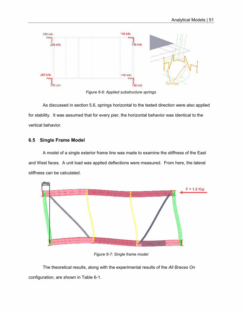
Analytical Models | 51
Figure 6-6: Applied substructure springs
As discussed in section 5.6, springs horizontal to the tested direction were also applied
for stability. It was assumed that for every pier, the horizontal behavior was identical to the
vertical behavior.
6.5 Single Frame Model
A model of a single exterior frame line was made to examine the stiffness of the East
and West faces. A unit load was applied deflections were measured. From here, the lateral
stiffness can be calculated.
Figure 6-7: Single frame model
The theoretical results, along with the experimental results of the All Braces On
configuration, are shown in Table 6-1.
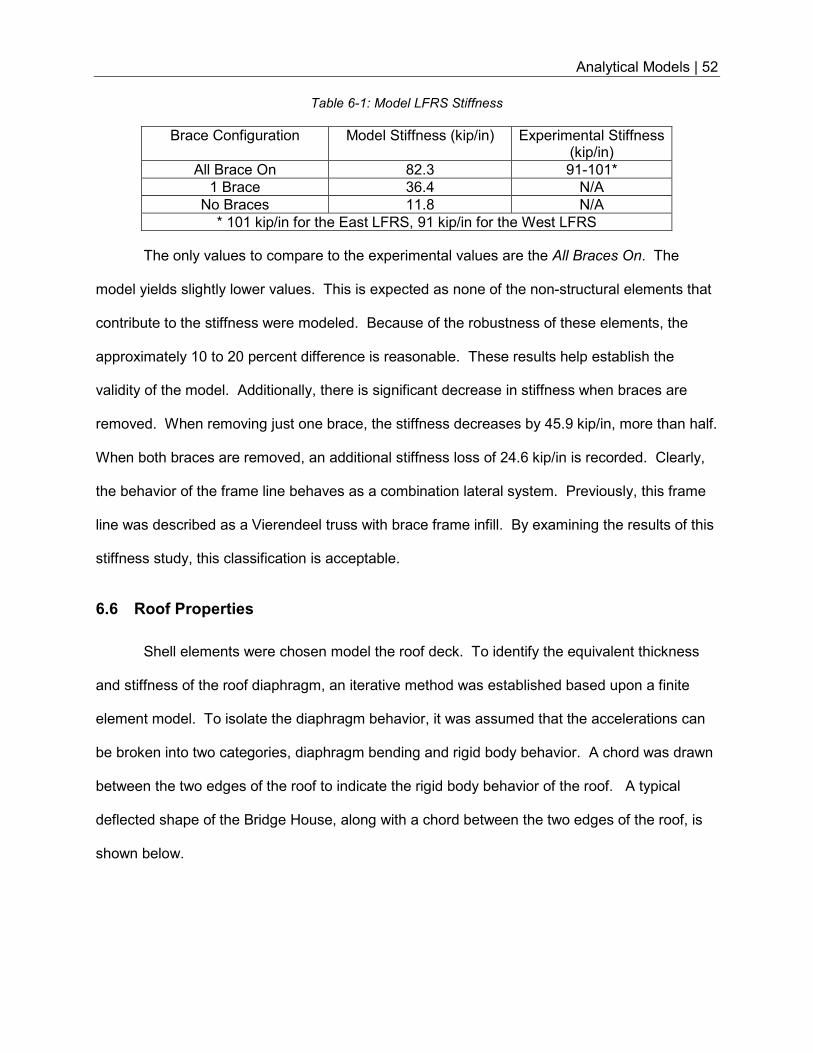
Analytical Models | 52
Table 6-1: Model LFRS Stiffness
Brace Configuration Model Stiffness (kip/in) Experimental Stiffness (kip/in)
All Brace On 82.3 91-101*
1 Brace 36.4 N/A
No Braces 11.8 N/A
* 101 kip/in for the East LFRS, 91 kip/in for the West LFRS
The only values to compare to the experimental values are the All Braces On. The
model yields slightly lower values. This is expected as none of the non-structural elements that
contribute to the stiffness were modeled. Because of the robustness of these elements, the
approximately 10 to 20 percent difference is reasonable. These results help establish the
validity of the model. Additionally, there is significant decrease in stiffness when braces are
removed. When removing just one brace, the stiffness decreases by 45.9 kip/in, more than half.
When both braces are removed, an additional stiffness loss of 24.6 kip/in is recorded. Clearly,
the behavior of the frame line behaves as a combination lateral system. Previously, this frame
line was described as a Vierendeel truss with brace frame infill. By examining the results of this
stiffness study, this classification is acceptable.
6.6 Roof Properties
Shell elements were chosen model the roof deck. To identify the equivalent thickness
and stiffness of the roof diaphragm, an iterative method was established based upon a finite
element model. To isolate the diaphragm behavior, it was assumed that the accelerations can
be broken into two categories, diaphragm bending and rigid body behavior. A chord was drawn
between the two edges of the roof to indicate the rigid body behavior of the roof. A typical
deflected shape of the Bridge House, along with a chord between the two edges of the roof, is
shown below.
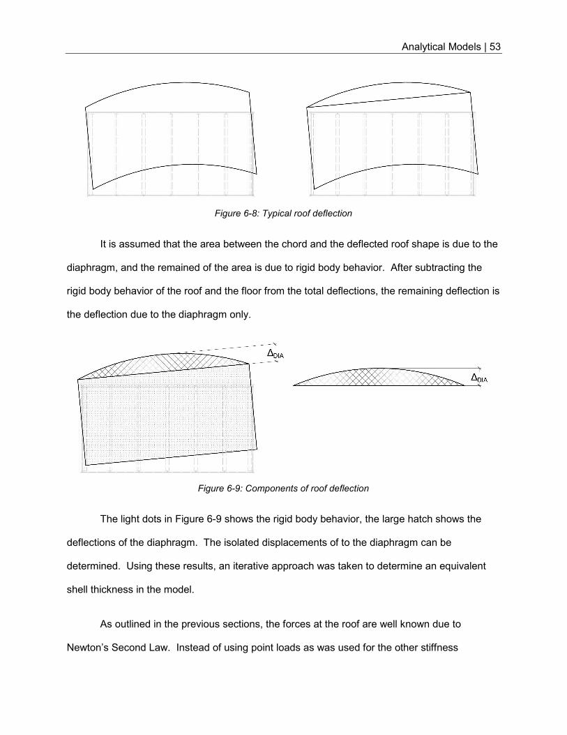
Analytical Models | 53
Figure 6-8: Typical roof deflection
It is assumed that the area between the chord and the deflected roof shape is due to the
diaphragm, and the remained of the area is due to rigid body behavior. After subtracting the
rigid body behavior of the roof and the floor from the total deflections, the remaining deflection is
the deflection due to the diaphragm only.
Figure 6-9: Components of roof deflection
The light dots in Figure 6-9 shows the rigid body behavior, the large hatch shows the
deflections of the diaphragm. The isolated displacements of to the diaphragm can be
determined. Using these results, an iterative approach was taken to determine an equivalent
shell thickness in the model.
As outlined in the previous sections, the forces at the roof are well known due to
Newton’s Second Law. Instead of using point loads as was used for the other stiffness
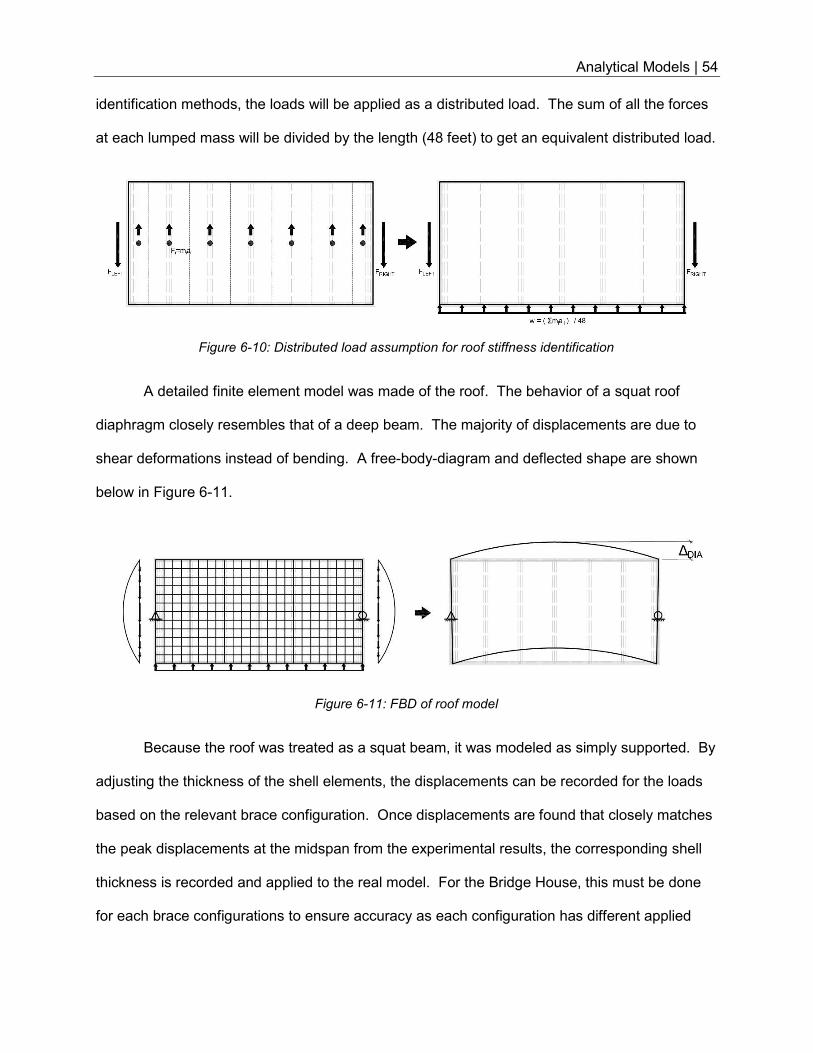
Analytical Models | 54
identification methods, the loads will be applied as a distributed load. The sum of all the forces
at each lumped mass will be divided by the length (48 feet) to get an equivalent distributed load.
Figure 6-10: Distributed load assumption for roof stiffness identification
A detailed finite element model was made of the roof. The behavior of a squat roof
diaphragm closely resembles that of a deep beam. The majority of displacements are due to
shear deformations instead of bending. A free-body-diagram and deflected shape are shown
below in Figure 6-11.
Figure 6-11: FBD of roof model
Because the roof was treated as a squat beam, it was modeled as simply supported. By
adjusting the thickness of the shell elements, the displacements can be recorded for the loads
based on the relevant brace configuration. Once displacements are found that closely matches
the peak displacements at the midspan from the experimental results, the corresponding shell
thickness is recorded and applied to the real model. For the Bridge House, this must be done
for each brace configurations to ensure accuracy as each configuration has different applied
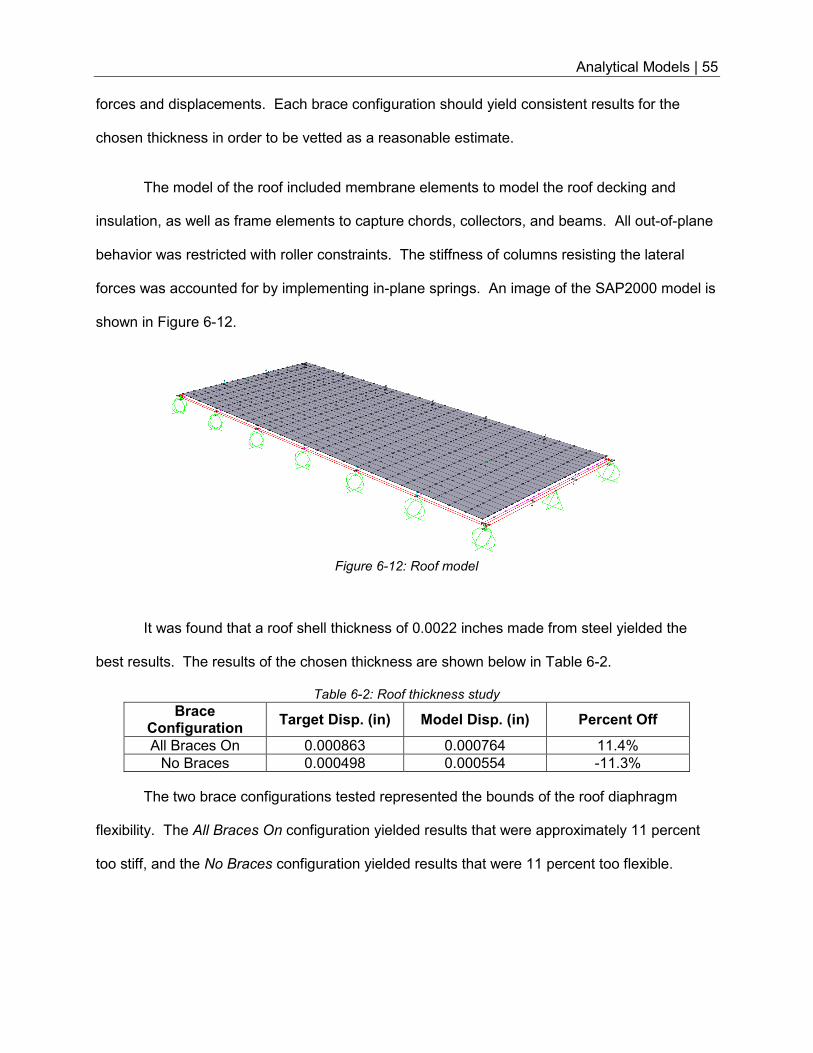
Analytical Models | 55
forces and displacements. Each brace configuration should yield consistent results for the
chosen thickness in order to be vetted as a reasonable estimate.
The model of the roof included membrane elements to model the roof decking and
insulation, as well as frame elements to capture chords, collectors, and beams. All out-of-plane
behavior was restricted with roller constraints. The stiffness of columns resisting the lateral
forces was accounted for by implementing in-plane springs. An image of the SAP2000 model is
shown in Figure 6-12.
Figure 6-12: Roof model
It was found that a roof shell thickness of 0.0022 inches made from steel yielded the
best results. The results of the chosen thickness are shown below in Table 6-2.
Table 6-2: Roof thickness study
Brace Configuration
Target Disp. (in) Model Disp. (in) Percent Off
All Braces On 0.000863 0.000764 11.4%
No Braces 0.000498 0.000554 -11.3%
The two brace configurations tested represented the bounds of the roof diaphragm
flexibility. The All Braces On configuration yielded results that were approximately 11 percent
too stiff, and the No Braces configuration yielded results that were 11 percent too flexible.
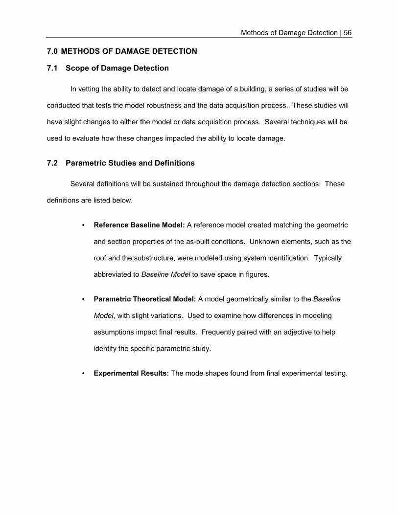
Methods of Damage Detection | 56
7.0 METHODS OF DAMAGE DETECTION
7.1 Scope of Damage Detection
In vetting the ability to detect and locate damage of a building, a series of studies will be
conducted that tests the model robustness and the data acquisition process. These studies will
have slight changes to either the model or data acquisition process. Several techniques will be
used to evaluate how these changes impacted the ability to locate damage.
7.2 Parametric Studies and Definitions
Several definitions will be sustained throughout the damage detection sections. These
definitions are listed below.
• Reference Baseline Model: A reference model created matching the geometric
and section properties of the as-built conditions. Unknown elements, such as the
roof and the substructure, were modeled using system identification. Typically
abbreviated to Baseline Model to save space in figures.
• Parametric Theoretical Model: A model geometrically similar to the Baseline
Model, with slight variations. Used to examine how differences in modeling
assumptions impact final results. Frequently paired with an adjective to help
identify the specific parametric study.
• Experimental Results: The mode shapes found from final experimental testing.
Methods of Damage Detection | 57
Three groups of studies will be done to investigate the damage detection. The studies
are outlined in Table 7-1.
Table 7-1: Parametric study table
Study Question Comparison
Baseline Is damage detection through
FVT possible? Reference Baseline Model vs
Experimental Results
Parametric Model Changes
How robust of a model is needed?
Parametric Theoretical Model vs Reference Baseline Model
Parametric Procedural Changes
How much data is needed? Reference Baseline Model vs
Experimental Results (Revised DOF)
The first study will compare experimental results to the Baseline Model. This will
establish if damage detection is possible using forced vibration testing. The second study will
compare the Baseline Model to the Theoretical Model to help understand the impact of model
accuracy. The third study will examine the consequences of changing the experimental
degrees-of-freedom in terms of damage detection. The changed degrees-of-freedom were
systematically chosen to replicate a scenario where a limited amount of accelerometers are
available. For each study, the mass matrix must be reformulated. System identification,
however, was not re-established with the new DOF.
7.3 Assessment Methods
7.3.1 Frequency Analysis
When applicable, frequency analysis will be examined. Previous research has shown
that comparing experimental natural frequencies to theoretical natural frequencies has
limitations (Archer, 2014). Regardless, theoretical frequencies must be reasonable and
approximate or else the validity of the model needs to be questioned. It will be shown that a
frequency analysis can be used as model verification to set upper and lower bounds.
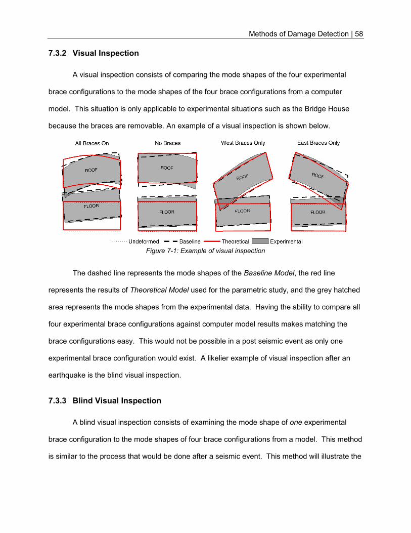
Methods of Damage Detection | 58
7.3.2 Visual Inspection
A visual inspection consists of comparing the mode shapes of the four experimental
brace configurations to the mode shapes of the four brace configurations from a computer
model. This situation is only applicable to experimental situations such as the Bridge House
because the braces are removable. An example of a visual inspection is shown below.
The dashed line represents the mode shapes of the Baseline Model, the red line
represents the results of Theoretical Model used for the parametric study, and the grey hatched
area represents the mode shapes from the experimental data. Having the ability to compare all
four experimental brace configurations against computer model results makes matching the
brace configurations easy. This would not be possible in a post seismic event as only one
experimental brace configuration would exist. A likelier example of visual inspection after an
earthquake is the blind visual inspection.
7.3.3 Blind Visual Inspection
A blind visual inspection consists of examining the mode shape of one experimental
brace configuration to the mode shapes of four brace configurations from a model. This method
is similar to the process that would be done after a seismic event. This method will illustrate the
Figure 7-1: Example of visual inspection
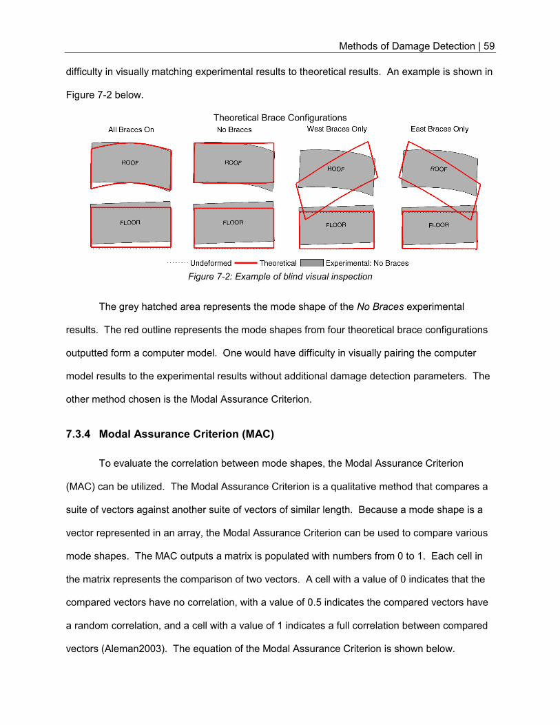
Methods of Damage Detection | 59
difficulty in visually matching experimental results to theoretical results. An example is shown in
Figure 7-2 below.
The grey hatched area represents the mode shape of the No Braces experimental
results. The red outline represents the mode shapes from four theoretical brace configurations
outputted form a computer model. One would have difficulty in visually pairing the computer
model results to the experimental results without additional damage detection parameters. The
other method chosen is the Modal Assurance Criterion.
7.3.4 Modal Assurance Criterion (MAC)
To evaluate the correlation between mode shapes, the Modal Assurance Criterion
(MAC) can be utilized. The Modal Assurance Criterion is a qualitative method that compares a
suite of vectors against another suite of vectors of similar length. Because a mode shape is a
vector represented in an array, the Modal Assurance Criterion can be used to compare various
mode shapes. The MAC outputs a matrix is populated with numbers from 0 to 1. Each cell in
the matrix represents the comparison of two vectors. A cell with a value of 0 indicates that the
compared vectors have no correlation, with a value of 0.5 indicates the compared vectors have
a random correlation, and a cell with a value of 1 indicates a full correlation between compared
vectors (Aleman2003). The equation of the Modal Assurance Criterion is shown below.
Theoretical Brace Configurations
Figure 7-2: Example of blind visual inspection
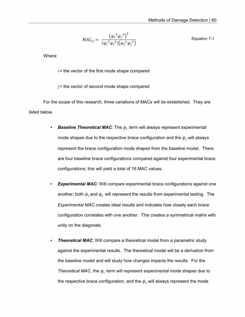
Methods of Damage Detection | 60
ABC"D = EF")FD)G�F")F")�EFD)F")G Equation 7-1
Where:
i = the vector of the first mode shape compared
j = the vector of second mode shape compared
For the scope of this research, three variations of MACs will be established. They are
listed below.
• Baseline Theoretical MAC: The ;" term will always represent experimental
mode shapes due to the respective brace configuration and the ;D will always
represent the brace configuration mode shapes from the baseline model. There
are four baseline brace configurations compared against four experimental brace
configurations; this will yield a total of 16 MAC values.
• Experimental MAC: Will compare experimental brace configurations against one
another; both ;" and ;D will represent the results from experimental testing. The
Experimental MAC creates ideal results and indicates how closely each brace
configuration correlates with one another. This creates a symmetrical matrix with
unity on the diagonals.
• Theoretical MAC: Will compare a theoretical model from a parametric study
against the experimental results. The theoretical model will be a derivation from
the baseline model and will study how changes impacts the results. For the
Theoretical MAC, the ;" term will represent experimental mode shapes due to
the respective brace configuration, and the ;D will always represent the mode
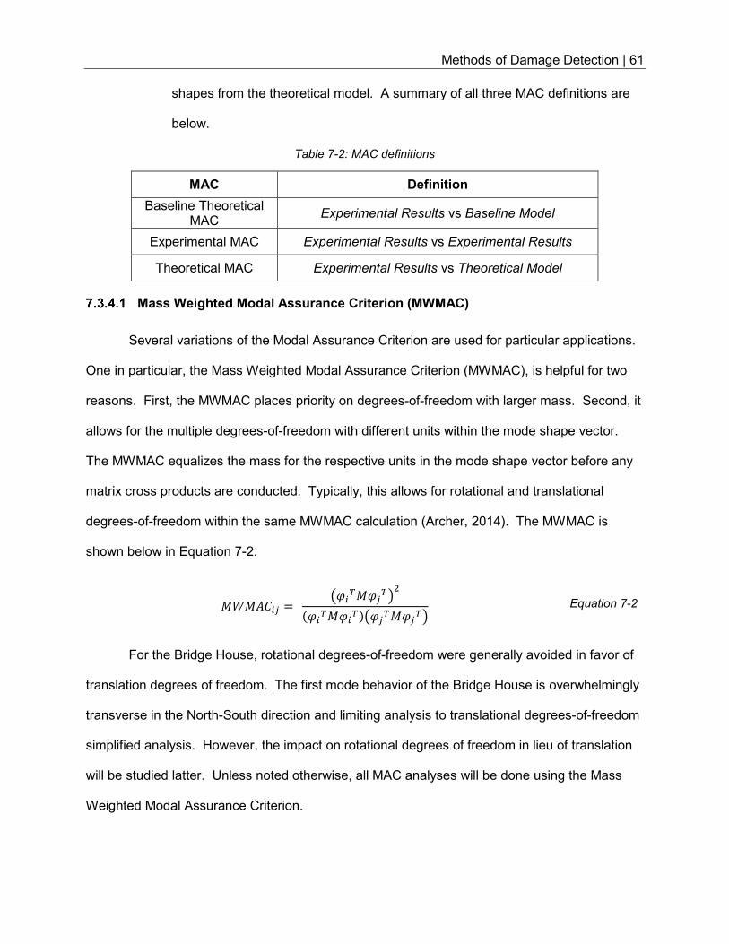
Methods of Damage Detection | 61
shapes from the theoretical model. A summary of all three MAC definitions are
below.
Table 7-2: MAC definitions
MAC Definition
Baseline Theoretical MAC
Experimental Results vs Baseline Model
Experimental MAC Experimental Results vs Experimental Results
Theoretical MAC Experimental Results vs Theoretical Model
Mass Weighted Modal Assurance Criterion (MWMAC)
Several variations of the Modal Assurance Criterion are used for particular applications.
One in particular, the Mass Weighted Modal Assurance Criterion (MWMAC), is helpful for two
reasons. First, the MWMAC places priority on degrees-of-freedom with larger mass. Second, it
allows for the multiple degrees-of-freedom with different units within the mode shape vector.
The MWMAC equalizes the mass for the respective units in the mode shape vector before any
matrix cross products are conducted. Typically, this allows for rotational and translational
degrees-of-freedom within the same MWMAC calculation (Archer, 2014). The MWMAC is
shown below in Equation 7-2.
AHABC"D = EF")AFD)G�F")AF")�EFD)AFD)G Equation 7-2
For the Bridge House, rotational degrees-of-freedom were generally avoided in favor of
translation degrees of freedom. The first mode behavior of the Bridge House is overwhelmingly
transverse in the North-South direction and limiting analysis to translational degrees-of-freedom
simplified analysis. However, the impact on rotational degrees of freedom in lieu of translation
will be studied latter. Unless noted otherwise, all MAC analyses will be done using the Mass
Weighted Modal Assurance Criterion.
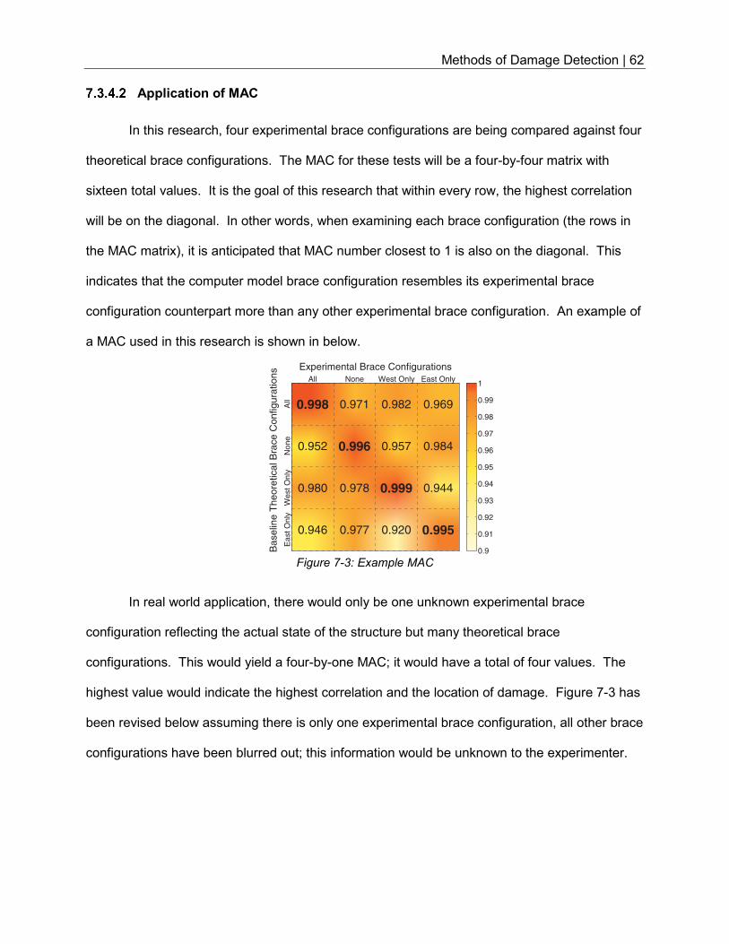
Methods of Damage Detection | 62
Application of MAC
In this research, four experimental brace configurations are being compared against four
theoretical brace configurations. The MAC for these tests will be a four-by-four matrix with
sixteen total values. It is the goal of this research that within every row, the highest correlation
will be on the diagonal. In other words, when examining each brace configuration (the rows in
the MAC matrix), it is anticipated that MAC number closest to 1 is also on the diagonal. This
indicates that the computer model brace configuration resembles its experimental brace
configuration counterpart more than any other experimental brace configuration. An example of
a MAC used in this research is shown in below.
In real world application, there would only be one unknown experimental brace
configuration reflecting the actual state of the structure but many theoretical brace
configurations. This would yield a four-by-one MAC; it would have a total of four values. The
highest value would indicate the highest correlation and the location of damage. Figure 7-3 has
been revised below assuming there is only one experimental brace configuration, all other brace
configurations have been blurred out; this information would be unknown to the experimenter.
Figure 7-3: Example MAC
Experimental Brace Configurations
All
None
West O
nly
East O
nly
Ba
se
line
Th
eo
retica
l B
race
Co
nfig
ura
tio
ns
0.998
0.952
0.980
0.946
0.971
0.996
0.978
0.977
0.982
0.957
0.999
0.920
0.969
0.984
0.944
0.995
All None West Only East Only
0.9
0.91
0.92
0.93
0.94
0.95
0.96
0.97
0.98
0.99
1
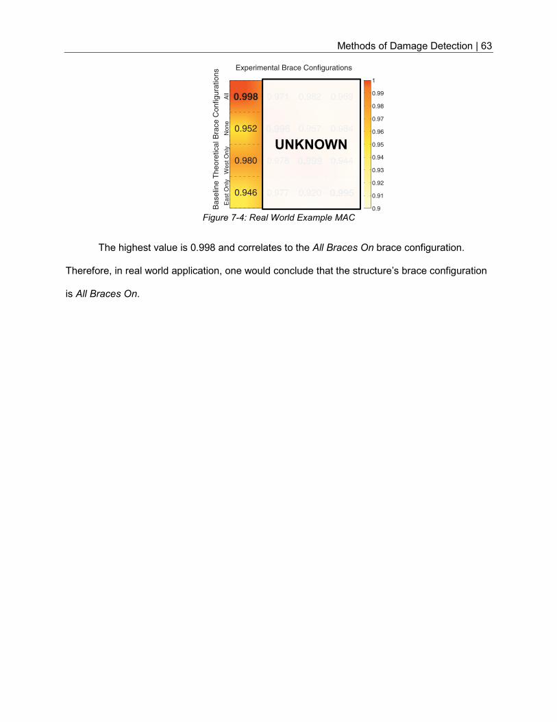
Methods of Damage Detection | 63
The highest value is 0.998 and correlates to the All Braces On brace configuration.
Therefore, in real world application, one would conclude that the structure’s brace configuration
is All Braces On.
Figure 7-4: Real World Example MAC
Experimental Brace Configurations
All
None
West
Only
East
Only
Ba
se
line
Th
eo
retica
l B
race
Co
nfig
ura
tio
ns
0.998
0.952
0.980
0.946
0.971
0.996
0.978
0.977
0.982
0.957
0.999
0.920
0.969
0.984
0.944
0.995
All None West Only East Only
0.9
0.91
0.92
0.93
0.94
0.95
0.96
0.97
0.98
0.99
1
UNKNOWN
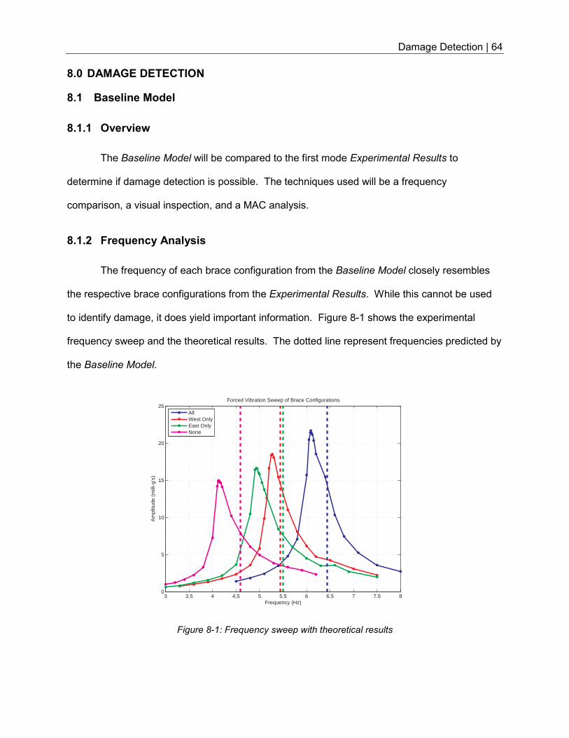
Damage Detection | 64
8.0 DAMAGE DETECTION
8.1 Baseline Model
8.1.1 Overview
The Baseline Model will be compared to the first mode Experimental Results to
determine if damage detection is possible. The techniques used will be a frequency
comparison, a visual inspection, and a MAC analysis.
8.1.2 Frequency Analysis
The frequency of each brace configuration from the Baseline Model closely resembles
the respective brace configurations from the Experimental Results. While this cannot be used
to identify damage, it does yield important information. Figure 8-1 shows the experimental
frequency sweep and the theoretical results. The dotted line represent frequencies predicted by
the Baseline Model.
Figure 8-1: Frequency sweep with theoretical results
3 3.5 4 4.5 5 5.5 6 6.5 7 7.5 80
5
10
15
20
25Forced Vibration Sweep of Brace Configurations
Frequency (Hz)
Am
plitu
de (
mill
i-g’s
)
AllWest OnlyEast OnlyNone
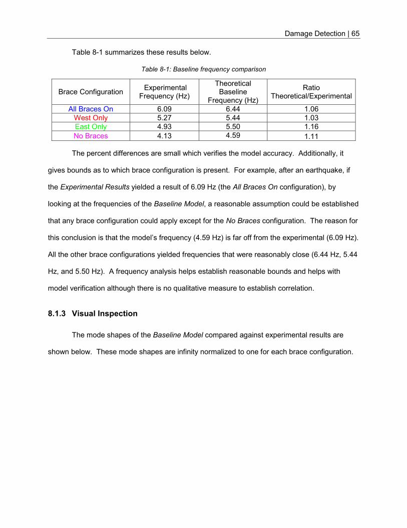
Damage Detection | 65
Table 8-1 summarizes these results below.
Table 8-1: Baseline frequency comparison
Brace Configuration Experimental
Frequency (Hz)
Theoretical Baseline
Frequency (Hz)
Ratio Theoretical/Experimental
All Braces On 6.09 6.44 1.06
West Only 5.27 5.44 1.03
East Only 4.93 5.50 1.16
No Braces 4.13 4.59 1.11
The percent differences are small which verifies the model accuracy. Additionally, it
gives bounds as to which brace configuration is present. For example, after an earthquake, if
the Experimental Results yielded a result of 6.09 Hz (the All Braces On configuration), by
looking at the frequencies of the Baseline Model, a reasonable assumption could be established
that any brace configuration could apply except for the No Braces configuration. The reason for
this conclusion is that the model’s frequency (4.59 Hz) is far off from the experimental (6.09 Hz).
All the other brace configurations yielded frequencies that were reasonably close (6.44 Hz, 5.44
Hz, and 5.50 Hz). A frequency analysis helps establish reasonable bounds and helps with
model verification although there is no qualitative measure to establish correlation.
8.1.3 Visual Inspection
The mode shapes of the Baseline Model compared against experimental results are
shown below. These mode shapes are infinity normalized to one for each brace configuration.
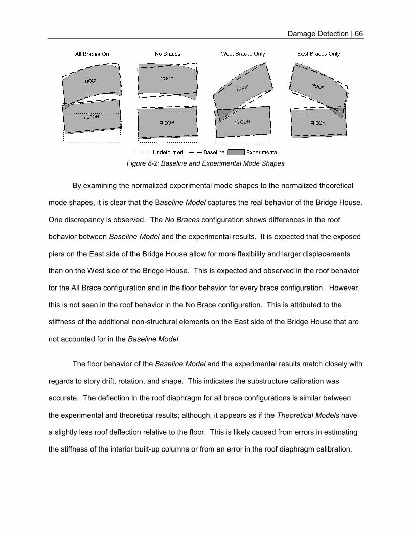
Damage Detection | 66
By examining the normalized experimental mode shapes to the normalized theoretical
mode shapes, it is clear that the Baseline Model captures the real behavior of the Bridge House.
One discrepancy is observed. The No Braces configuration shows differences in the roof
behavior between Baseline Model and the experimental results. It is expected that the exposed
piers on the East side of the Bridge House allow for more flexibility and larger displacements
than on the West side of the Bridge House. This is expected and observed in the roof behavior
for the All Brace configuration and in the floor behavior for every brace configuration. However,
this is not seen in the roof behavior in the No Brace configuration. This is attributed to the
stiffness of the additional non-structural elements on the East side of the Bridge House that are
not accounted for in the Baseline Model.
The floor behavior of the Baseline Model and the experimental results match closely with
regards to story drift, rotation, and shape. This indicates the substructure calibration was
accurate. The deflection in the roof diaphragm for all brace configurations is similar between
the experimental and theoretical results; although, it appears as if the Theoretical Models have
a slightly less roof deflection relative to the floor. This is likely caused from errors in estimating
the stiffness of the interior built-up columns or from an error in the roof diaphragm calibration.
Figure 8-2: Baseline and Experimental Mode Shapes
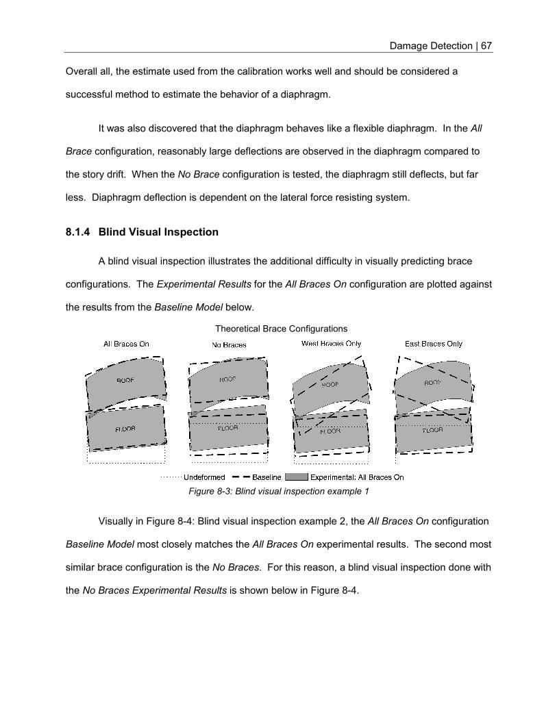
Damage Detection | 67
Overall all, the estimate used from the calibration works well and should be considered a
successful method to estimate the behavior of a diaphragm.
It was also discovered that the diaphragm behaves like a flexible diaphragm. In the All
Brace configuration, reasonably large deflections are observed in the diaphragm compared to
the story drift. When the No Brace configuration is tested, the diaphragm still deflects, but far
less. Diaphragm deflection is dependent on the lateral force resisting system.
8.1.4 Blind Visual Inspection
A blind visual inspection illustrates the additional difficulty in visually predicting brace
configurations. The Experimental Results for the All Braces On configuration are plotted against
the results from the Baseline Model below.
Visually in Figure 8-4: Blind visual inspection example 2, the All Braces On configuration
Baseline Model most closely matches the All Braces On experimental results. The second most
similar brace configuration is the No Braces. For this reason, a blind visual inspection done with
the No Braces Experimental Results is shown below in Figure 8-4.
Theoretical Brace Configurations
Figure 8-3: Blind visual inspection example 1
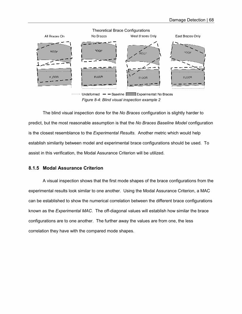
Damage Detection | 68
The blind visual inspection done for the No Braces configuration is slightly harder to
predict, but the most reasonable assumption is that the No Braces Baseline Model configuration
is the closest resemblance to the Experimental Results. Another metric which would help
establish similarity between model and experimental brace configurations should be used. To
assist in this verification, the Modal Assurance Criterion will be utilized.
8.1.5 Modal Assurance Criterion
A visual inspection shows that the first mode shapes of the brace configurations from the
experimental results look similar to one another. Using the Modal Assurance Criterion, a MAC
can be established to show the numerical correlation between the different brace configurations
known as the Experimental MAC. The off-diagonal values will establish how similar the brace
configurations are to one another. The further away the values are from one, the less
correlation they have with the compared mode shapes.
Theoretical Brace Configurations
Figure 8-4: Blind visual inspection example 2
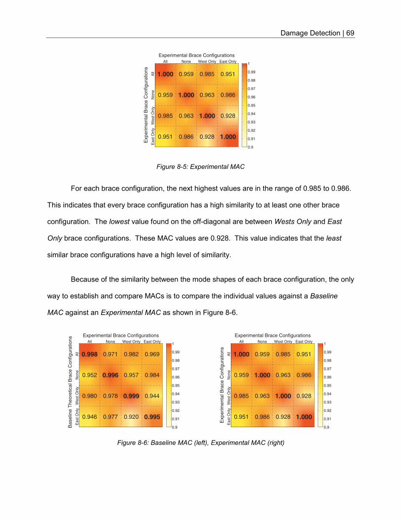
Damage Detection | 69
Figure 8-5: Experimental MAC
For each brace configuration, the next highest values are in the range of 0.985 to 0.986.
This indicates that every brace configuration has a high similarity to at least one other brace
configuration. The lowest value found on the off-diagonal are between Wests Only and East
Only brace configurations. These MAC values are 0.928. This value indicates that the least
similar brace configurations have a high level of similarity.
Because of the similarity between the mode shapes of each brace configuration, the only
way to establish and compare MACs is to compare the individual values against a Baseline
MAC against an Experimental MAC as shown in Figure 8-6.
Experimental Brace Configurations
All
None
West O
nly
East O
nly
Experim
enta
l B
race C
onfigura
tions
1.000
0.959
0.985
0.951
0.959
1.000
0.963
0.986
0.985
0.963
1.000
0.928
0.951
0.986
0.928
1.000
All None West Only East Only
0.9
0.91
0.92
0.93
0.94
0.95
0.96
0.97
0.98
0.99
1
Figure 8-6: Baseline MAC (left), Experimental MAC (right)
Experimental Brace Configurations
All
None
West O
nly
East O
nly
Baselin
e T
heore
tical B
race C
onfigura
tions
0.998
0.952
0.980
0.946
0.971
0.996
0.978
0.977
0.982
0.957
0.999
0.920
0.969
0.984
0.944
0.995
All None West Only East Only
0.9
0.91
0.92
0.93
0.94
0.95
0.96
0.97
0.98
0.99
1
Experimental Brace Configurations
All
None
West O
nly
East O
nly
Experim
enta
l B
race C
onfigura
tions
1.000
0.959
0.985
0.951
0.959
1.000
0.963
0.986
0.985
0.963
1.000
0.928
0.951
0.986
0.928
1.000
All None West Only East Only
0.9
0.91
0.92
0.93
0.94
0.95
0.96
0.97
0.98
0.99
1
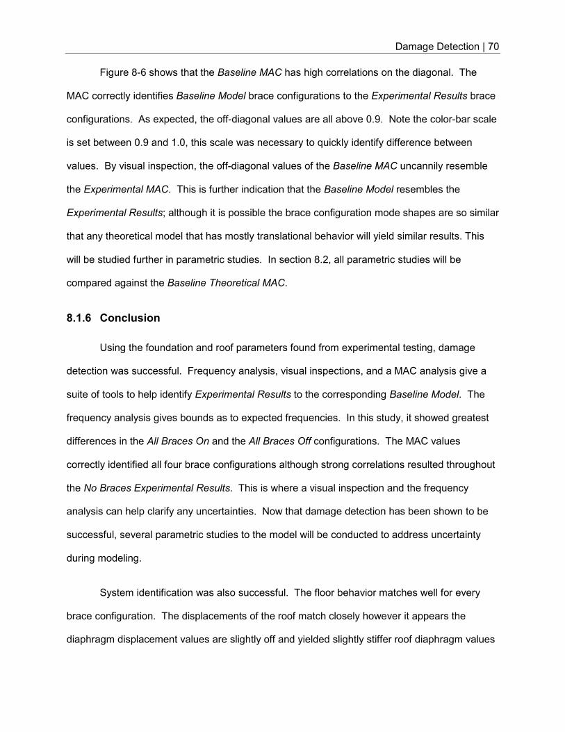
Damage Detection | 70
Figure 8-6 shows that the Baseline MAC has high correlations on the diagonal. The
MAC correctly identifies Baseline Model brace configurations to the Experimental Results brace
configurations. As expected, the off-diagonal values are all above 0.9. Note the color-bar scale
is set between 0.9 and 1.0, this scale was necessary to quickly identify difference between
values. By visual inspection, the off-diagonal values of the Baseline MAC uncannily resemble
the Experimental MAC. This is further indication that the Baseline Model resembles the
Experimental Results; although it is possible the brace configuration mode shapes are so similar
that any theoretical model that has mostly translational behavior will yield similar results. This
will be studied further in parametric studies. In section 8.2, all parametric studies will be
compared against the Baseline Theoretical MAC.
8.1.6 Conclusion
Using the foundation and roof parameters found from experimental testing, damage
detection was successful. Frequency analysis, visual inspections, and a MAC analysis give a
suite of tools to help identify Experimental Results to the corresponding Baseline Model. The
frequency analysis gives bounds as to expected frequencies. In this study, it showed greatest
differences in the All Braces On and the All Braces Off configurations. The MAC values
correctly identified all four brace configurations although strong correlations resulted throughout
the No Braces Experimental Results. This is where a visual inspection and the frequency
analysis can help clarify any uncertainties. Now that damage detection has been shown to be
successful, several parametric studies to the model will be conducted to address uncertainty
during modeling.
System identification was also successful. The floor behavior matches well for every
brace configuration. The displacements of the roof match closely however it appears the
diaphragm displacement values are slightly off and yielded slightly stiffer roof diaphragm values
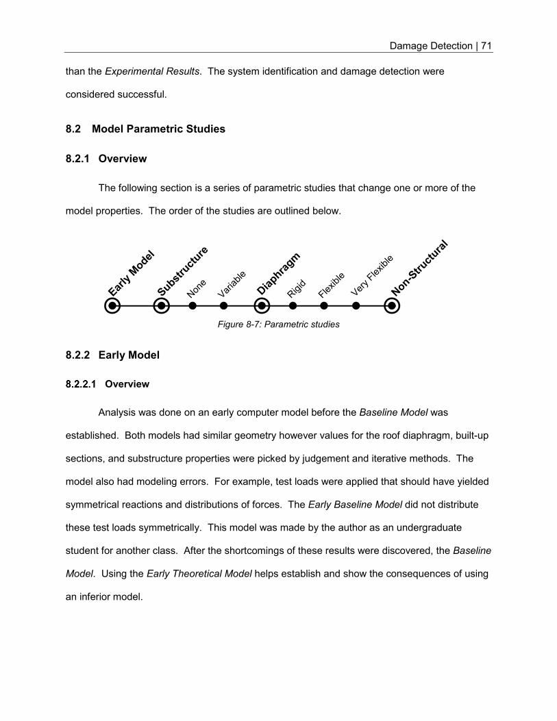
Damage Detection | 71
than the Experimental Results. The system identification and damage detection were
considered successful.
8.2 Model Parametric Studies
8.2.1 Overview
The following section is a series of parametric studies that change one or more of the
model properties. The order of the studies are outlined below.
8.2.2 Early Model
Overview
Analysis was done on an early computer model before the Baseline Model was
established. Both models had similar geometry however values for the roof diaphragm, built-up
sections, and substructure properties were picked by judgement and iterative methods. The
model also had modeling errors. For example, test loads were applied that should have yielded
symmetrical reactions and distributions of forces. The Early Baseline Model did not distribute
these test loads symmetrically. This model was made by the author as an undergraduate
student for another class. After the shortcomings of these results were discovered, the Baseline
Model. Using the Early Theoretical Model helps establish and show the consequences of using
an inferior model.
Figure 8-7: Parametric studies
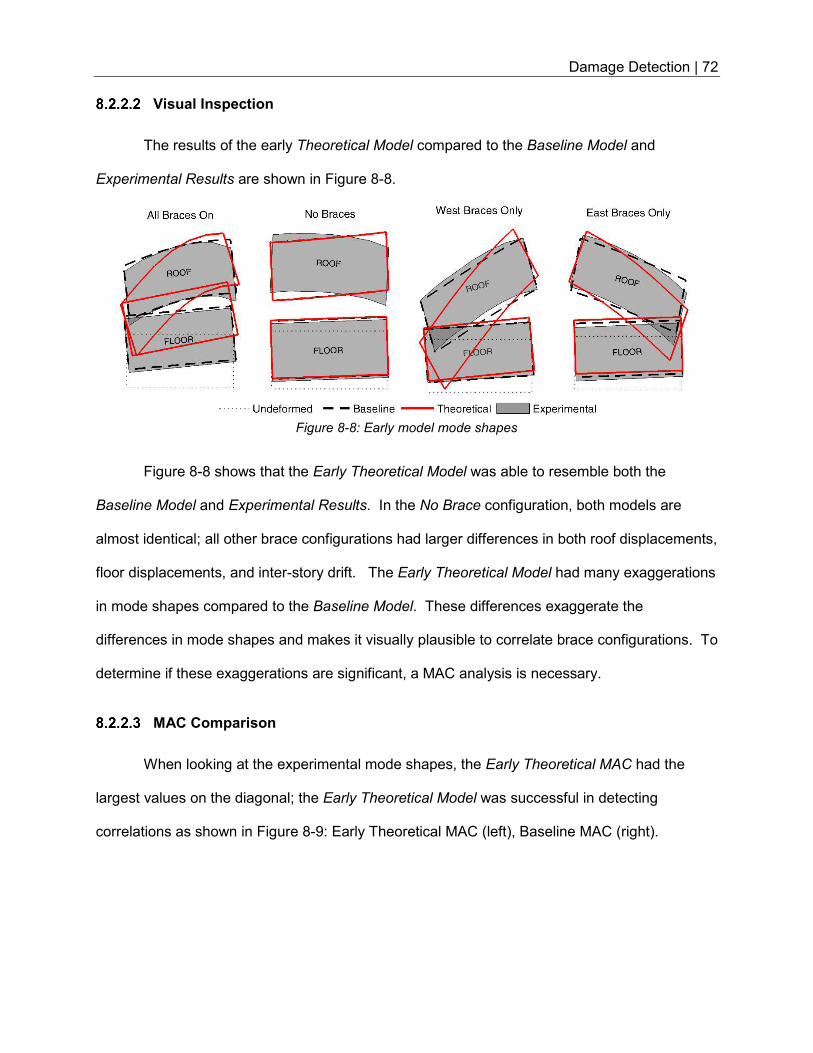
Damage Detection | 72
Visual Inspection
The results of the early Theoretical Model compared to the Baseline Model and
Experimental Results are shown in Figure 8-8.
Figure 8-8 shows that the Early Theoretical Model was able to resemble both the
Baseline Model and Experimental Results. In the No Brace configuration, both models are
almost identical; all other brace configurations had larger differences in both roof displacements,
floor displacements, and inter-story drift. The Early Theoretical Model had many exaggerations
in mode shapes compared to the Baseline Model. These differences exaggerate the
differences in mode shapes and makes it visually plausible to correlate brace configurations. To
determine if these exaggerations are significant, a MAC analysis is necessary.
MAC Comparison
When looking at the experimental mode shapes, the Early Theoretical MAC had the
largest values on the diagonal; the Early Theoretical Model was successful in detecting
correlations as shown in Figure 8-9: Early Theoretical MAC (left), Baseline MAC (right).
Figure 8-8: Early model mode shapes
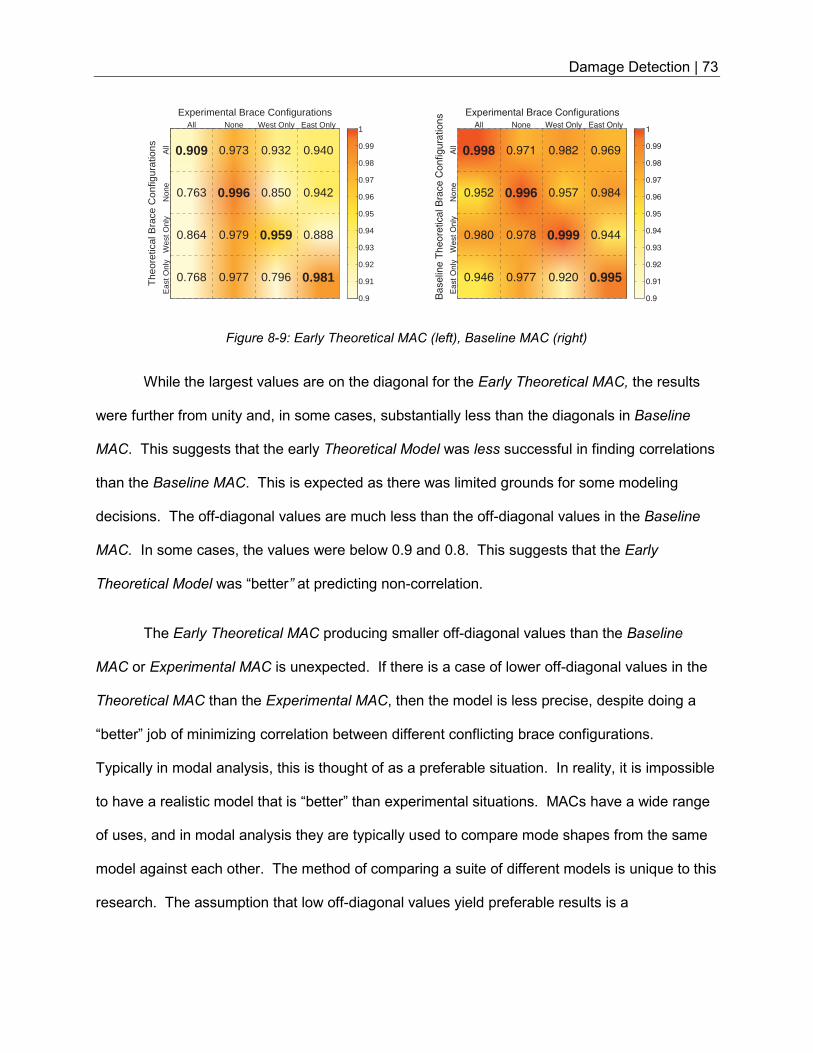
Damage Detection | 73
While the largest values are on the diagonal for the Early Theoretical MAC, the results
were further from unity and, in some cases, substantially less than the diagonals in Baseline
MAC. This suggests that the early Theoretical Model was less successful in finding correlations
than the Baseline MAC. This is expected as there was limited grounds for some modeling
decisions. The off-diagonal values are much less than the off-diagonal values in the Baseline
MAC. In some cases, the values were below 0.9 and 0.8. This suggests that the Early
Theoretical Model was “better” at predicting non-correlation.
The Early Theoretical MAC producing smaller off-diagonal values than the Baseline
MAC or Experimental MAC is unexpected. If there is a case of lower off-diagonal values in the
Theoretical MAC than the Experimental MAC, then the model is less precise, despite doing a
“better” job of minimizing correlation between different conflicting brace configurations.
Typically in modal analysis, this is thought of as a preferable situation. In reality, it is impossible
to have a realistic model that is “better” than experimental situations. MACs have a wide range
of uses, and in modal analysis they are typically used to compare mode shapes from the same
model against each other. The method of comparing a suite of different models is unique to this
research. The assumption that low off-diagonal values yield preferable results is a
Figure 8-9: Early Theoretical MAC (left), Baseline MAC (right)
Experimental Brace Configurations
All
Non
eW
est O
nly
Eas
t Onl
y
The
oret
ical
Bra
ce C
onfig
urat
ions 0.909
0.763
0.864
0.768
0.973
0.996
0.979
0.977
0.932
0.850
0.959
0.796
0.940
0.942
0.888
0.981
All None West Only East Only
0.9
0.91
0.92
0.93
0.94
0.95
0.96
0.97
0.98
0.99
1
Experimental Brace Configurations
All
None
West O
nly
East O
nly
Baselin
e T
heore
tical B
race C
onfigura
tions
0.998
0.952
0.980
0.946
0.971
0.996
0.978
0.977
0.982
0.957
0.999
0.920
0.969
0.984
0.944
0.995
All None West Only East Only
0.9
0.91
0.92
0.93
0.94
0.95
0.96
0.97
0.98
0.99
1
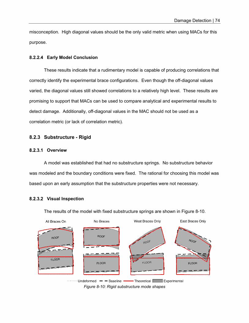
Damage Detection | 74
misconception. High diagonal values should be the only valid metric when using MACs for this
purpose.
Early Model Conclusion
These results indicate that a rudimentary model is capable of producing correlations that
correctly identify the experimental brace configurations. Even though the off-diagonal values
varied, the diagonal values still showed correlations to a relatively high level. These results are
promising to support that MACs can be used to compare analytical and experimental results to
detect damage. Additionally, off-diagonal values in the MAC should not be used as a
correlation metric (or lack of correlation metric).
8.2.3 Substructure - Rigid
Overview
A model was established that had no substructure springs. No substructure behavior
was modeled and the boundary conditions were fixed. The rational for choosing this model was
based upon an early assumption that the substructure properties were not necessary.
Visual Inspection
The results of the model with fixed substructure springs are shown in Figure 8-10.
Figure 8-10: Rigid substructure mode shapes
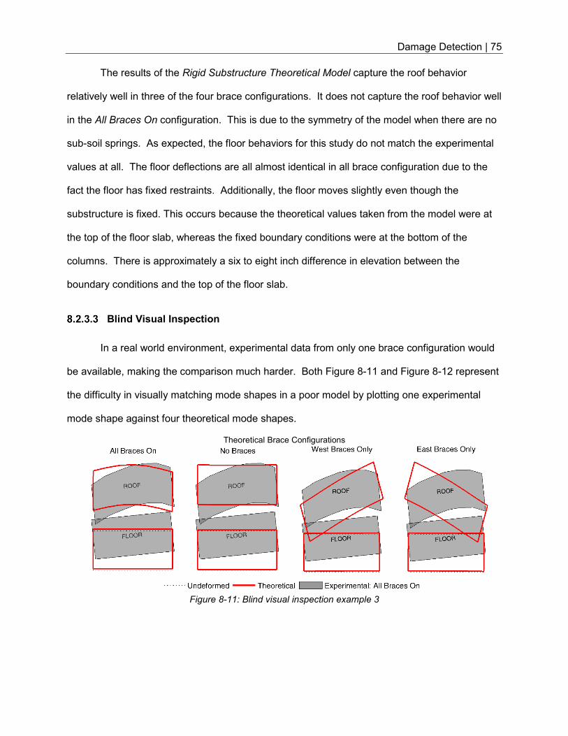
Damage Detection | 75
The results of the Rigid Substructure Theoretical Model capture the roof behavior
relatively well in three of the four brace configurations. It does not capture the roof behavior well
in the All Braces On configuration. This is due to the symmetry of the model when there are no
sub-soil springs. As expected, the floor behaviors for this study do not match the experimental
values at all. The floor deflections are all almost identical in all brace configuration due to the
fact the floor has fixed restraints. Additionally, the floor moves slightly even though the
substructure is fixed. This occurs because the theoretical values taken from the model were at
the top of the floor slab, whereas the fixed boundary conditions were at the bottom of the
columns. There is approximately a six to eight inch difference in elevation between the
boundary conditions and the top of the floor slab.
Blind Visual Inspection
In a real world environment, experimental data from only one brace configuration would
be available, making the comparison much harder. Both Figure 8-11 and Figure 8-12 represent
the difficulty in visually matching mode shapes in a poor model by plotting one experimental
mode shape against four theoretical mode shapes.
Theoretical Brace Configurations
Figure 8-11: Blind visual inspection example 3
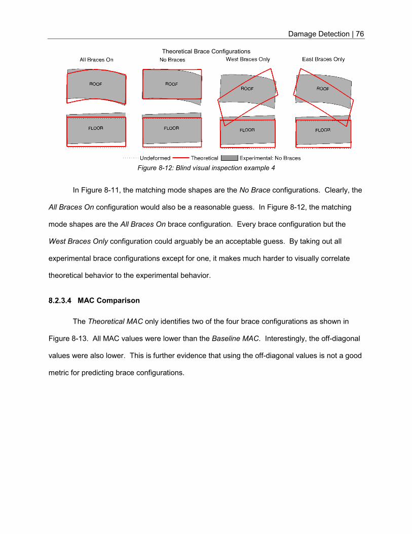
Damage Detection | 76
In Figure 8-11, the matching mode shapes are the No Brace configurations. Clearly, the
All Braces On configuration would also be a reasonable guess. In Figure 8-12, the matching
mode shapes are the All Braces On brace configuration. Every brace configuration but the
West Braces Only configuration could arguably be an acceptable guess. By taking out all
experimental brace configurations except for one, it makes much harder to visually correlate
theoretical behavior to the experimental behavior.
MAC Comparison
The Theoretical MAC only identifies two of the four brace configurations as shown in
Figure 8-13. All MAC values were lower than the Baseline MAC. Interestingly, the off-diagonal
values were also lower. This is further evidence that using the off-diagonal values is not a good
metric for predicting brace configurations.
Theoretical Brace Configurations
Figure 8-12: Blind visual inspection example 4
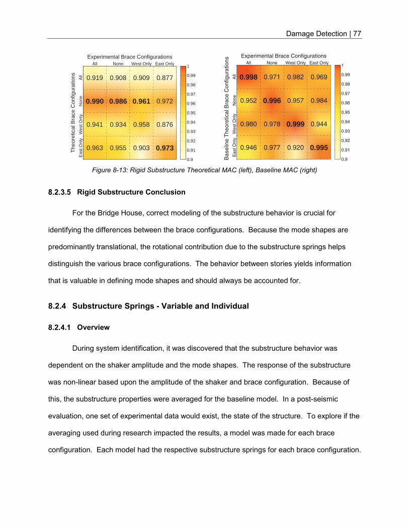
Damage Detection | 77
Rigid Substructure Conclusion
For the Bridge House, correct modeling of the substructure behavior is crucial for
identifying the differences between the brace configurations. Because the mode shapes are
predominantly translational, the rotational contribution due to the substructure springs helps
distinguish the various brace configurations. The behavior between stories yields information
that is valuable in defining mode shapes and should always be accounted for.
8.2.4 Substructure Springs - Variable and Individual
Overview
During system identification, it was discovered that the substructure behavior was
dependent on the shaker amplitude and the mode shapes. The response of the substructure
was non-linear based upon the amplitude of the shaker and brace configuration. Because of
this, the substructure properties were averaged for the baseline model. In a post-seismic
evaluation, one set of experimental data would exist, the state of the structure. To explore if the
averaging used during research impacted the results, a model was made for each brace
configuration. Each model had the respective substructure springs for each brace configuration.
Figure 8-13: Rigid Substructure Theoretical MAC (left), Baseline MAC (right)
Experimental Brace Configurations
All
Non
eW
est O
nly
Eas
t Onl
y
The
oret
ical
Bra
ce C
onfig
urat
ions 0.919
0.990
0.941
0.963
0.908
0.986
0.934
0.955
0.909
0.961
0.958
0.903
0.877
0.972
0.876
0.973
All None West Only East Only
0.9
0.91
0.92
0.93
0.94
0.95
0.96
0.97
0.98
0.99
1
Experimental Brace Configurations
All
None
West
Only
East
Only
Ba
se
line
Th
eo
retica
l B
race
Co
nfig
ura
tio
ns
0.998
0.952
0.980
0.946
0.971
0.996
0.978
0.977
0.982
0.957
0.999
0.920
0.969
0.984
0.944
0.995
All None West Only East Only
0.9
0.91
0.92
0.93
0.94
0.95
0.96
0.97
0.98
0.99
1
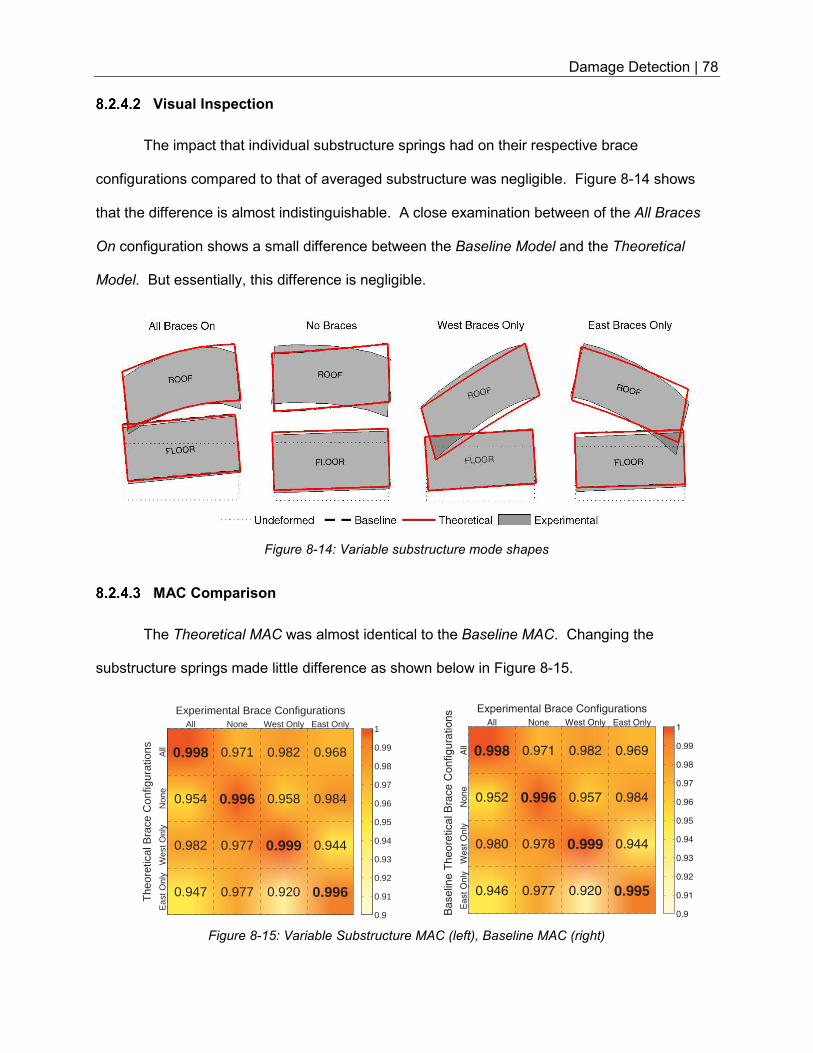
Damage Detection | 78
Visual Inspection
The impact that individual substructure springs had on their respective brace
configurations compared to that of averaged substructure was negligible. Figure 8-14 shows
that the difference is almost indistinguishable. A close examination between of the All Braces
On configuration shows a small difference between the Baseline Model and the Theoretical
Model. But essentially, this difference is negligible.
MAC Comparison
The Theoretical MAC was almost identical to the Baseline MAC. Changing the
substructure springs made little difference as shown below in Figure 8-15.
Figure 8-14: Variable substructure mode shapes
Figure 8-15: Variable Substructure MAC (left), Baseline MAC (right)
Experimental Brace Configurations
All
Non
eW
est O
nly
Eas
t Onl
y
The
oret
ical
Bra
ce C
onfig
urat
ions 0.998
0.954
0.982
0.947
0.971
0.996
0.977
0.977
0.982
0.958
0.999
0.920
0.968
0.984
0.944
0.996
All None West Only East Only
0.9
0.91
0.92
0.93
0.94
0.95
0.96
0.97
0.98
0.99
1
Experimental Brace Configurations
All
None
West O
nly
East O
nly
Ba
se
line
Th
eo
retica
l B
race
Co
nfig
ura
tio
ns
0.998
0.952
0.980
0.946
0.971
0.996
0.978
0.977
0.982
0.957
0.999
0.920
0.969
0.984
0.944
0.995
All None West Only East Only
0.9
0.91
0.92
0.93
0.94
0.95
0.96
0.97
0.98
0.99
1
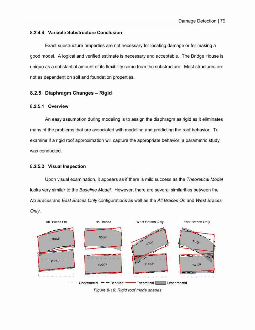
Damage Detection | 79
Variable Substructure Conclusion
Exact substructure properties are not necessary for locating damage or for making a
good model. A logical and verified estimate is necessary and acceptable. The Bridge House is
unique as a substantial amount of its flexibility come from the substructure. Most structures are
not as dependent on soil and foundation properties.
8.2.5 Diaphragm Changes – Rigid
Overview
An easy assumption during modeling is to assign the diaphragm as rigid as it eliminates
many of the problems that are associated with modeling and predicting the roof behavior. To
examine if a rigid roof approximation will capture the appropriate behavior, a parametric study
was conducted.
Visual Inspection
Upon visual examination, it appears as if there is mild success as the Theoretical Model
looks very similar to the Baseline Model. However, there are several similarities between the
No Braces and East Braces Only configurations as well as the All Braces On and West Braces
Only.
Figure 8-16: Rigid roof mode shapes
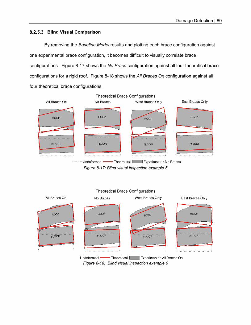
Damage Detection | 80
Blind Visual Comparison
By removing the Baseline Model results and plotting each brace configuration against
one experimental brace configuration, it becomes difficult to visually correlate brace
configurations. Figure 8-17 shows the No Brace configuration against all four theoretical brace
configurations for a rigid roof. Figure 8-18 shows the All Braces On configuration against all
four theoretical brace configurations.
Theoretical Brace Configurations
Figure 8-17: Blind visual inspection example 5
Theoretical Brace Configurations
Figure 8-18: Blind visual inspection example 6
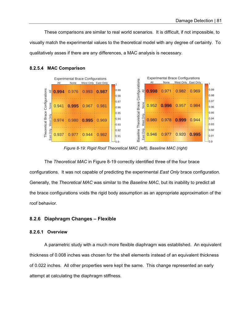
Damage Detection | 81
These comparisons are similar to real world scenarios. It is difficult, if not impossible, to
visually match the experimental values to the theoretical model with any degree of certainty. To
qualitatively asses if there are any differences, a MAC analysis is necessary.
MAC Comparison
The Theoretical MAC in Figure 8-19 correctly identified three of the four brace
configurations. It was not capable of predicting the experimental East Only brace configuration.
Generally, the Theoretical MAC was similar to the Baseline MAC, but its inability to predict all
the brace configurations voids the rigid body assumption as an appropriate approximation of the
roof behavior.
8.2.6 Diaphragm Changes – Flexible
Overview
A parametric study with a much more flexible diaphragm was established. An equivalent
thickness of 0.008 inches was chosen for the shell elements instead of an equivalent thickness
of 0.022 inches. All other properties were kept the same. This change represented an early
attempt at calculating the diaphragm stiffness.
Figure 8-19: Rigid Roof Theoretical MAC (left), Baseline MAC (right)
Experimental Brace Configurations
All
Non
eW
est O
nly
Eas
t Onl
y
The
oret
ical
Bra
ce C
onfig
urat
ions 0.994
0.941
0.974
0.937
0.976
0.995
0.980
0.977
0.993
0.967
0.995
0.944
0.987
0.981
0.969
0.982
All None West Only East Only
0.9
0.91
0.92
0.93
0.94
0.95
0.96
0.97
0.98
0.99
1
Experimental Brace Configurations
All
None
West O
nly
East O
nly
Ba
se
line
Th
eo
retica
l B
race
Co
nfig
ura
tio
ns
0.998
0.952
0.980
0.946
0.971
0.996
0.978
0.977
0.982
0.957
0.999
0.920
0.969
0.984
0.944
0.995
All None West Only East Only
0.9
0.91
0.92
0.93
0.94
0.95
0.96
0.97
0.98
0.99
1
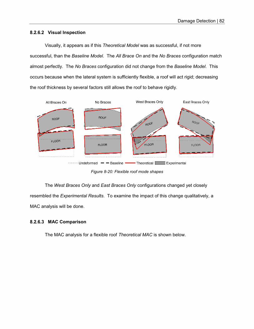
Damage Detection | 82
Visual Inspection
Visually, it appears as if this Theoretical Model was as successful, if not more
successful, than the Baseline Model. The All Brace On and the No Braces configuration match
almost perfectly. The No Braces configuration did not change from the Baseline Model. This
occurs because when the lateral system is sufficiently flexible, a roof will act rigid; decreasing
the roof thickness by several factors still allows the roof to behave rigidly.
The West Braces Only and East Braces Only configurations changed yet closely
resembled the Experimental Results. To examine the impact of this change qualitatively, a
MAC analysis will be done.
MAC Comparison
The MAC analysis for a flexible roof Theoretical MAC is shown below.
Figure 8-20: Flexible roof mode shapes
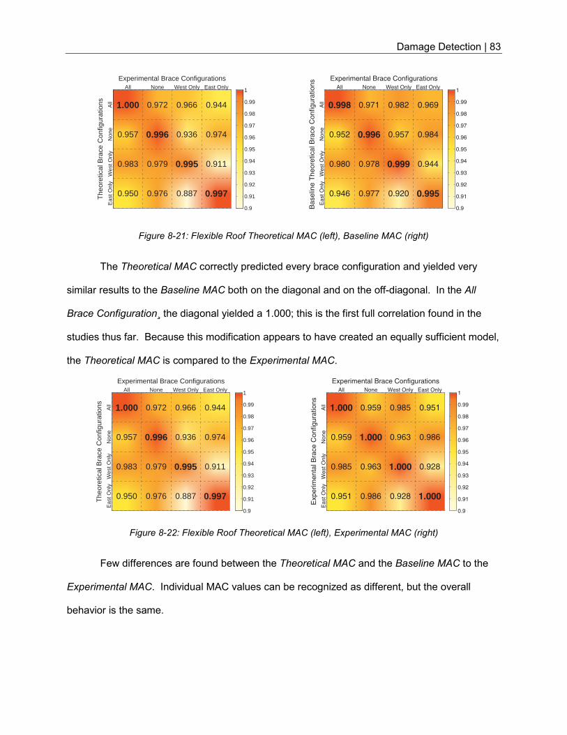
Damage Detection | 83
The Theoretical MAC correctly predicted every brace configuration and yielded very
similar results to the Baseline MAC both on the diagonal and on the off-diagonal. In the All
Brace Configuration¸ the diagonal yielded a 1.000; this is the first full correlation found in the
studies thus far. Because this modification appears to have created an equally sufficient model,
the Theoretical MAC is compared to the Experimental MAC.
Few differences are found between the Theoretical MAC and the Baseline MAC to the
Experimental MAC. Individual MAC values can be recognized as different, but the overall
behavior is the same.
Figure 8-21: Flexible Roof Theoretical MAC (left), Baseline MAC (right)
Figure 8-22: Flexible Roof Theoretical MAC (left), Experimental MAC (right)
Experimental Brace Configurations
All
Non
eW
est O
nly
Eas
t Onl
y
The
oret
ical
Bra
ce C
onfig
urat
ions 1.000
0.957
0.983
0.950
0.972
0.996
0.979
0.976
0.966
0.936
0.995
0.887
0.944
0.974
0.911
0.997
All None West Only East Only
0.9
0.91
0.92
0.93
0.94
0.95
0.96
0.97
0.98
0.99
1
Experimental Brace Configurations
All
None
West O
nly
East O
nly
Baselin
e T
heore
tical B
race C
onfigura
tions
0.998
0.952
0.980
0.946
0.971
0.996
0.978
0.977
0.982
0.957
0.999
0.920
0.969
0.984
0.944
0.995
All None West Only East Only
0.9
0.91
0.92
0.93
0.94
0.95
0.96
0.97
0.98
0.99
1
Experimental Brace Configurations
All
Non
eW
est O
nly
Eas
t Onl
y
The
oret
ical
Bra
ce C
onfig
urat
ions 1.000
0.957
0.983
0.950
0.972
0.996
0.979
0.976
0.966
0.936
0.995
0.887
0.944
0.974
0.911
0.997
All None West Only East Only
0.9
0.91
0.92
0.93
0.94
0.95
0.96
0.97
0.98
0.99
1
Experimental Brace Configurations
All
None
West O
nly
East O
nly
Experim
enta
l B
race C
onfigura
tions
1.000
0.959
0.985
0.951
0.959
1.000
0.963
0.986
0.985
0.963
1.000
0.928
0.951
0.986
0.928
1.000
All None West Only East Only
0.9
0.91
0.92
0.93
0.94
0.95
0.96
0.97
0.98
0.99
1
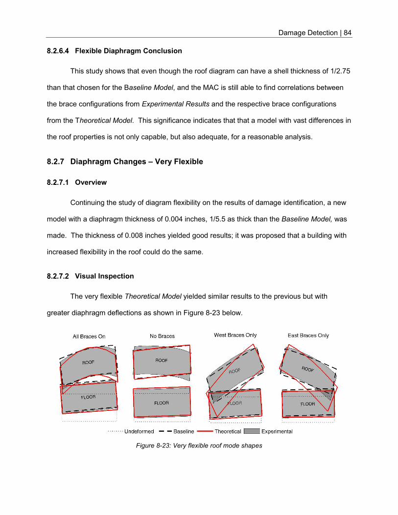
Damage Detection | 84
Flexible Diaphragm Conclusion
This study shows that even though the roof diagram can have a shell thickness of 1/2.75
than that chosen for the Baseline Model, and the MAC is still able to find correlations between
the brace configurations from Experimental Results and the respective brace configurations
from the Theoretical Model. This significance indicates that that a model with vast differences in
the roof properties is not only capable, but also adequate, for a reasonable analysis.
8.2.7 Diaphragm Changes – Very Flexible
Overview
Continuing the study of diagram flexibility on the results of damage identification, a new
model with a diaphragm thickness of 0.004 inches, 1/5.5 as thick than the Baseline Model, was
made. The thickness of 0.008 inches yielded good results; it was proposed that a building with
increased flexibility in the roof could do the same.
Visual Inspection
The very flexible Theoretical Model yielded similar results to the previous but with
greater diaphragm deflections as shown in Figure 8-23 below.
Figure 8-23: Very flexible roof mode shapes
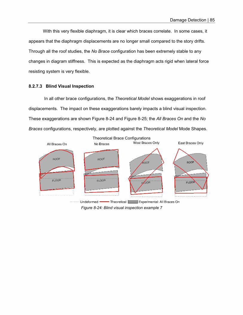
Damage Detection | 85
With this very flexible diaphragm, it is clear which braces correlate. In some cases, it
appears that the diaphragm displacements are no longer small compared to the story drifts.
Through all the roof studies, the No Brace configuration has been extremely stable to any
changes in diagram stiffness. This is expected as the diaphragm acts rigid when lateral force
resisting system is very flexible.
Blind Visual Inspection
In all other brace configurations, the Theoretical Model shows exaggerations in roof
displacements. The impact on these exaggerations barely impacts a blind visual inspection.
These exaggerations are shown Figure 8-24 and Figure 8-25; the All Braces On and the No
Braces configurations, respectively, are plotted against the Theoretical Model Mode Shapes.
Theoretical Brace Configurations
Figure 8-24: Blind visual inspection example 7
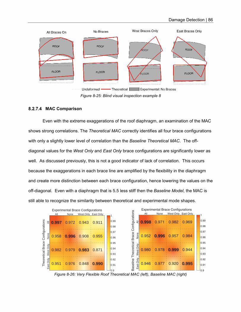
Damage Detection | 86
MAC Comparison
Even with the extreme exaggerations of the roof diaphragm, an examination of the MAC
shows strong correlations. The Theoretical MAC correctly identifies all four brace configurations
with only a slightly lower level of correlation than the Baseline Theoretical MAC. The off-
diagonal values for the West Only and East Only brace configurations are significantly lower as
well. As discussed previously, this is not a good indicator of lack of correlation. This occurs
because the exaggerations in each brace line are amplified by the flexibility in the diaphragm
and create more distinction between each brace configuration, hence lowering the values on the
off-diagonal. Even with a diaphragm that is 5.5 less stiff then the Baseline Model, the MAC is
still able to recognize the similarity between theoretical and experimental mode shapes.
Figure 8-25: Blind visual inspection example 8
Figure 8-26: Very Flexible Roof Theoretical MAC (left), Baseline MAC (right)
Experimental Brace Configurations
All
Non
eW
est O
nly
Eas
t Onl
y
The
oret
ical
Bra
ce C
onfig
urat
ions 0.997
0.958
0.982
0.951
0.972
0.996
0.979
0.976
0.943
0.908
0.983
0.848
0.911
0.955
0.871
0.990
All None West Only East Only
0.9
0.91
0.92
0.93
0.94
0.95
0.96
0.97
0.98
0.99
1
Experimental Brace Configurations
All
None
West O
nly
East O
nly
Ba
se
line
Th
eo
retica
l B
race
Co
nfig
ura
tio
ns
0.998
0.952
0.980
0.946
0.971
0.996
0.978
0.977
0.982
0.957
0.999
0.920
0.969
0.984
0.944
0.995
All None West Only East Only
0.9
0.91
0.92
0.93
0.94
0.95
0.96
0.97
0.98
0.99
1
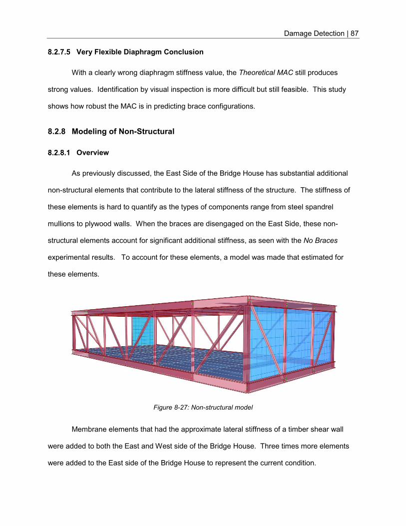
Damage Detection | 87
Very Flexible Diaphragm Conclusion
With a clearly wrong diaphragm stiffness value, the Theoretical MAC still produces
strong values. Identification by visual inspection is more difficult but still feasible. This study
shows how robust the MAC is in predicting brace configurations.
8.2.8 Modeling of Non-Structural
Overview
As previously discussed, the East Side of the Bridge House has substantial additional
non-structural elements that contribute to the lateral stiffness of the structure. The stiffness of
these elements is hard to quantify as the types of components range from steel spandrel
mullions to plywood walls. When the braces are disengaged on the East Side, these non-
structural elements account for significant additional stiffness, as seen with the No Braces
experimental results. To account for these elements, a model was made that estimated for
these elements.
Membrane elements that had the approximate lateral stiffness of a timber shear wall
were added to both the East and West side of the Bridge House. Three times more elements
were added to the East side of the Bridge House to represent the current condition.
Figure 8-27: Non-structural model
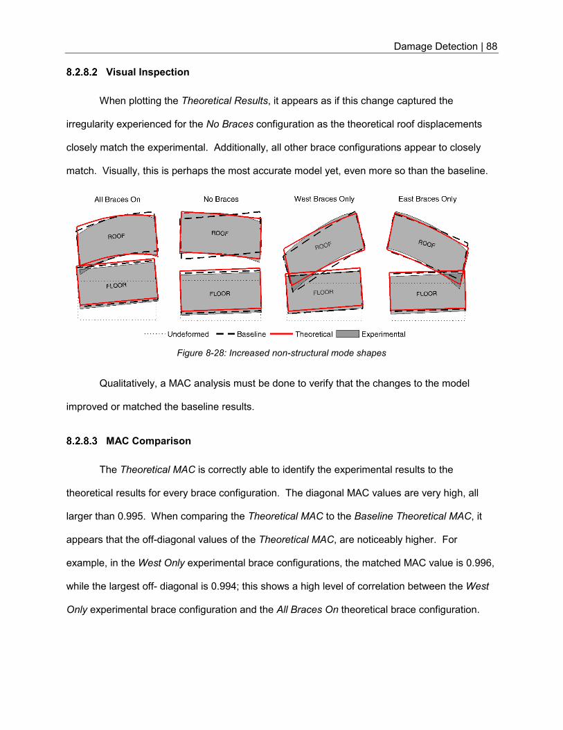
Damage Detection | 88
Visual Inspection
When plotting the Theoretical Results, it appears as if this change captured the
irregularity experienced for the No Braces configuration as the theoretical roof displacements
closely match the experimental. Additionally, all other brace configurations appear to closely
match. Visually, this is perhaps the most accurate model yet, even more so than the baseline.
Qualitatively, a MAC analysis must be done to verify that the changes to the model
improved or matched the baseline results.
MAC Comparison
The Theoretical MAC is correctly able to identify the experimental results to the
theoretical results for every brace configuration. The diagonal MAC values are very high, all
larger than 0.995. When comparing the Theoretical MAC to the Baseline Theoretical MAC, it
appears that the off-diagonal values of the Theoretical MAC, are noticeably higher. For
example, in the West Only experimental brace configurations, the matched MAC value is 0.996,
while the largest off- diagonal is 0.994; this shows a high level of correlation between the West
Only experimental brace configuration and the All Braces On theoretical brace configuration.
Figure 8-28: Increased non-structural mode shapes
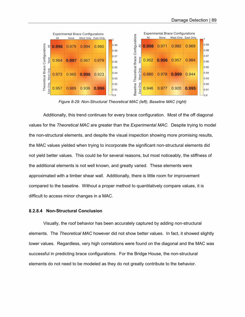
Damage Detection | 89
Additionally, this trend continues for every brace configuration. Most of the off diagonal
values for the Theoretical MAC are greater than the Experimental MAC. Despite trying to model
the non-structural elements, and despite the visual inspection showing more promising results,
the MAC values yielded when trying to incorporate the significant non-structural elements did
not yield better values. This could be for several reasons, but most noticeably, the stiffness of
the additional elements is not well known, and greatly varied. These elements were
approximated with a timber shear wall. Additionally, there is little room for improvement
compared to the baseline. Without a proper method to quantitatively compare values, it is
difficult to access minor changes in a MAC.
Non-Structural Conclusion
Visually, the roof behavior has been accurately captured by adding non-structural
elements. The Theoretical MAC however did not show better values. In fact, it showed slightly
lower values. Regardless, very high correlations were found on the diagonal and the MAC was
successful in predicting brace configurations. For the Bridge House, the non-structural
elements do not need to be modeled as they do not greatly contribute to the behavior.
Figure 8-29: Non-Structural Theoretical MAC (left), Baseline MAC (right)
Experimental Brace Configurations
All
Non
eW
est O
nly
Eas
t Onl
y
The
oret
ical
Bra
ce C
onfig
urat
ions 0.996
0.964
0.973
0.957
0.979
0.997
0.965
0.989
0.994
0.967
0.996
0.936
0.960
0.979
0.923
0.996
All None West Only East Only
0.9
0.91
0.92
0.93
0.94
0.95
0.96
0.97
0.98
0.99
1
Experimental Brace Configurations
All
None
West
Only
East
Only
Ba
se
line
Th
eo
retica
l B
race
Co
nfig
ura
tio
ns
0.998
0.952
0.980
0.946
0.971
0.996
0.978
0.977
0.982
0.957
0.999
0.920
0.969
0.984
0.944
0.995
All None West Only East Only
0.9
0.91
0.92
0.93
0.94
0.95
0.96
0.97
0.98
0.99
1
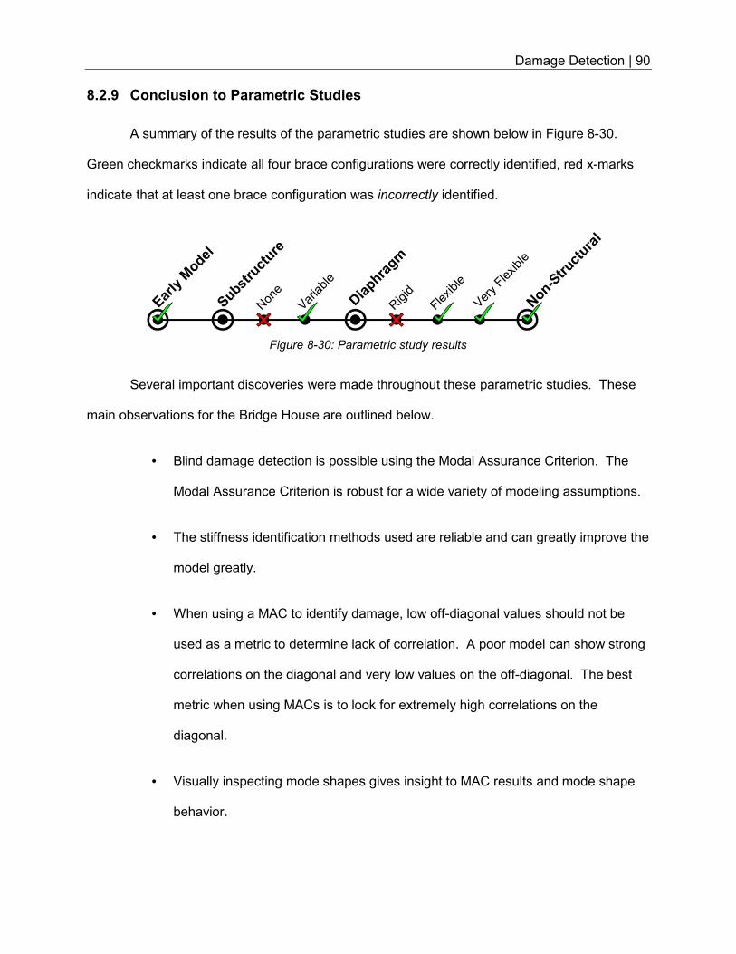
Damage Detection | 90
8.2.9 Conclusion to Parametric Studies
A summary of the results of the parametric studies are shown below in Figure 8-30.
Green checkmarks indicate all four brace configurations were correctly identified, red x-marks
indicate that at least one brace configuration was incorrectly identified.
Several important discoveries were made throughout these parametric studies. These
main observations for the Bridge House are outlined below.
• Blind damage detection is possible using the Modal Assurance Criterion. The
Modal Assurance Criterion is robust for a wide variety of modeling assumptions.
• The stiffness identification methods used are reliable and can greatly improve the
model greatly.
• When using a MAC to identify damage, low off-diagonal values should not be
used as a metric to determine lack of correlation. A poor model can show strong
correlations on the diagonal and very low values on the off-diagonal. The best
metric when using MACs is to look for extremely high correlations on the
diagonal.
• Visually inspecting mode shapes gives insight to MAC results and mode shape
behavior.
Figure 8-30: Parametric study results
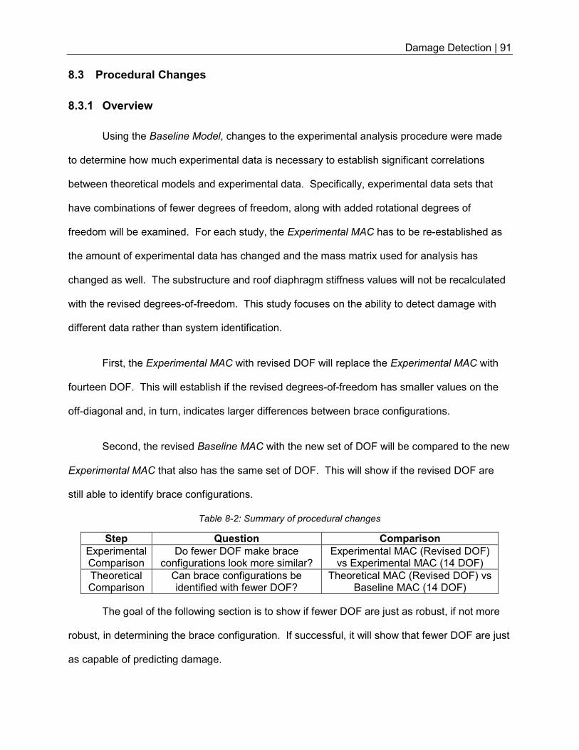
Damage Detection | 91
8.3 Procedural Changes
8.3.1 Overview
Using the Baseline Model, changes to the experimental analysis procedure were made
to determine how much experimental data is necessary to establish significant correlations
between theoretical models and experimental data. Specifically, experimental data sets that
have combinations of fewer degrees of freedom, along with added rotational degrees of
freedom will be examined. For each study, the Experimental MAC has to be re-established as
the amount of experimental data has changed and the mass matrix used for analysis has
changed as well. The substructure and roof diaphragm stiffness values will not be recalculated
with the revised degrees-of-freedom. This study focuses on the ability to detect damage with
different data rather than system identification.
First, the Experimental MAC with revised DOF will replace the Experimental MAC with
fourteen DOF. This will establish if the revised degrees-of-freedom has smaller values on the
off-diagonal and, in turn, indicates larger differences between brace configurations.
Second, the revised Baseline MAC with the new set of DOF will be compared to the new
Experimental MAC that also has the same set of DOF. This will show if the revised DOF are
still able to identify brace configurations.
Table 8-2: Summary of procedural changes
Step Question Comparison
Experimental Comparison
Do fewer DOF make brace configurations look more similar?
Experimental MAC (Revised DOF) vs Experimental MAC (14 DOF)
Theoretical Comparison
Can brace configurations be identified with fewer DOF?
Theoretical MAC (Revised DOF) vs Baseline MAC (14 DOF)
The goal of the following section is to show if fewer DOF are just as robust, if not more
robust, in determining the brace configuration. If successful, it will show that fewer DOF are just
as capable of predicting damage.
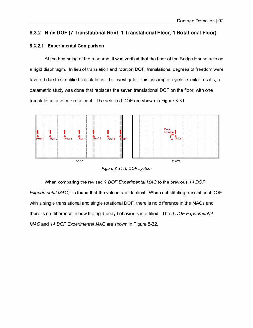
Damage Detection | 92
8.3.2 Nine DOF (7 Translational Roof, 1 Translational Floor, 1 Rotational Floor)
Experimental Comparison
At the beginning of the research, it was verified that the floor of the Bridge House acts as
a rigid diaphragm. In lieu of translation and rotation DOF, translational degrees of freedom were
favored due to simplified calculations. To investigate if this assumption yields similar results, a
parametric study was done that replaces the seven translational DOF on the floor, with one
translational and one rotational. The selected DOF are shown in Figure 8-31.
When comparing the revised 9 DOF Experimental MAC to the previous 14 DOF
Experimental MAC, it’s found that the values are identical. When substituting translational DOF
with a single translational and single rotational DOF, there is no difference in the MACs and
there is no difference in how the rigid-body behavior is identified. The 9 DOF Experimental
MAC and 14 DOF Experimental MAC are shown in Figure 8-32.
Figure 8-31: 9 DOF system
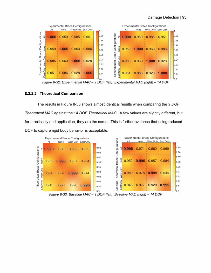
Damage Detection | 93
Theoretical Comparison
The results in Figure 8-33 shows almost identical results when comparing the 9 DOF
Theoretical MAC against the 14 DOF Theoretical MAC. A few values are slightly different, but
for practicality and application, they are the same. This is further evidence that using reduced
DOF to capture rigid body behavior is acceptable.
Figure 8-32: Experimental MAC – 9 DOF (left), Experimental MAC (right) – 14 DOF
Figure 8-33: Baseline MAC – 9 DOF (left), Baseline MAC (right) – 14 DOF
Experimental Brace Configurations
All
None
West O
nly
East O
nly
Exp
erim
en
tal B
race
Co
nfig
ura
tio
ns
1.000
0.959
0.985
0.951
0.959
1.000
0.963
0.986
0.985
0.963
1.000
0.928
0.951
0.986
0.928
1.000
All None West Only East Only
0.9
0.91
0.92
0.93
0.94
0.95
0.96
0.97
0.98
0.99
1
Experimental Brace Configurations
All
No
ne
We
st
On
lyE
ast
On
ly
Experim
enta
l B
race C
onfigura
tions
1.000
0.959
0.985
0.951
0.959
1.000
0.963
0.986
0.985
0.963
1.000
0.928
0.951
0.986
0.928
1.000
All None West Only East Only
0.9
0.91
0.92
0.93
0.94
0.95
0.96
0.97
0.98
0.99
1
Experimental Brace Configurations
All
Non
eW
est O
nly
Eas
t Onl
y
The
oret
ical
Bra
ce C
onfig
urat
ions 0.998
0.952
0.980
0.945
0.972
0.996
0.978
0.977
0.982
0.957
0.999
0.920
0.969
0.984
0.944
0.995
All None West Only East Only
0.9
0.91
0.92
0.93
0.94
0.95
0.96
0.97
0.98
0.99
1
Experimental Brace Configurations
All
None
West O
nly
East O
nly
Ba
se
line
Th
eo
retica
l B
race
Co
nfig
ura
tio
ns
0.998
0.952
0.980
0.946
0.971
0.996
0.978
0.977
0.982
0.957
0.999
0.920
0.969
0.984
0.944
0.995
All None West Only East Only
0.9
0.91
0.92
0.93
0.94
0.95
0.96
0.97
0.98
0.99
1
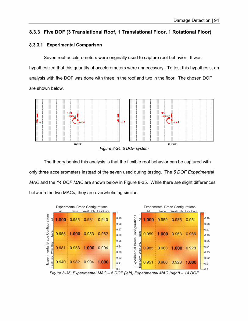
Damage Detection | 94
8.3.3 Five DOF (3 Translational Roof, 1 Translational Floor, 1 Rotational Floor)
Experimental Comparison
Seven roof accelerometers were originally used to capture roof behavior. It was
hypothesized that this quantity of accelerometers were unnecessary. To test this hypothesis, an
analysis with five DOF was done with three in the roof and two in the floor. The chosen DOF
are shown below.
The theory behind this analysis is that the flexible roof behavior can be captured with
only three accelerometers instead of the seven used during testing. The 5 DOF Experimental
MAC and the 14 DOF MAC are shown below in Figure 8-35. While there are slight differences
between the two MACs, they are overwhelming similar.
Figure 8-34: 5 DOF system
Figure 8-35: Experimental MAC – 5 DOF (left), Experimental MAC (right) – 14 DOF
Experimental Brace Configurations
All
None
West O
nly
East O
nly
Exp
erim
en
tal B
race
Co
nfig
ura
tio
ns
1.000
0.955
0.981
0.940
0.955
1.000
0.953
0.982
0.981
0.953
1.000
0.904
0.940
0.982
0.904
1.000
All None West Only East Only
0.9
0.91
0.92
0.93
0.94
0.95
0.96
0.97
0.98
0.99
1
Experimental Brace Configurations
All
No
ne
We
st
On
lyE
ast
On
ly
Experim
enta
l B
race C
onfigura
tions
1.000
0.959
0.985
0.951
0.959
1.000
0.963
0.986
0.985
0.963
1.000
0.928
0.951
0.986
0.928
1.000
All None West Only East Only
0.9
0.91
0.92
0.93
0.94
0.95
0.96
0.97
0.98
0.99
1
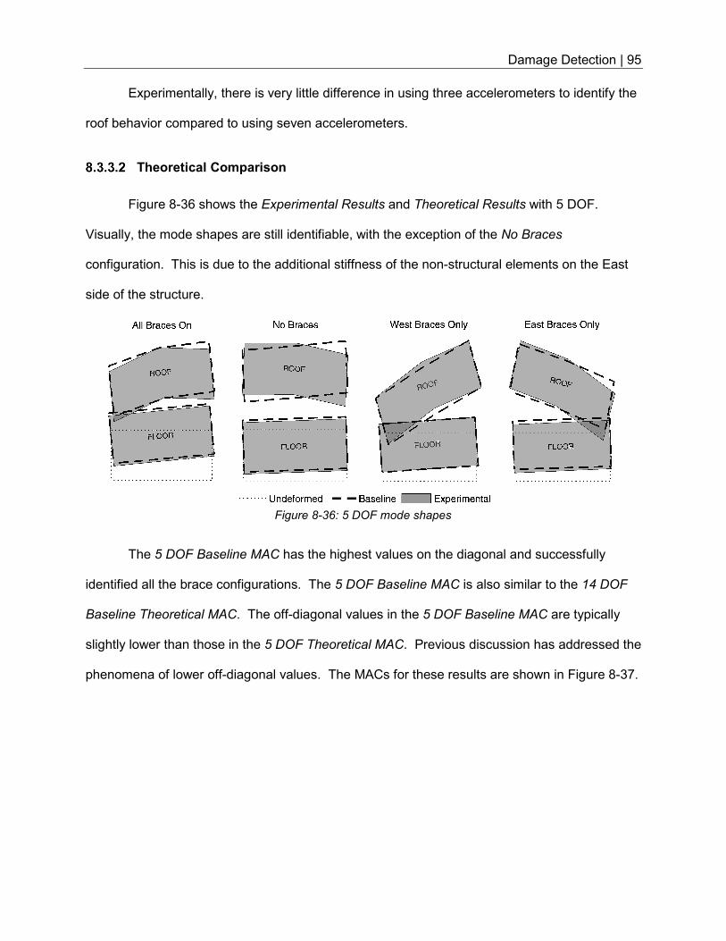
Damage Detection | 95
Experimentally, there is very little difference in using three accelerometers to identify the
roof behavior compared to using seven accelerometers.
Theoretical Comparison
Figure 8-36 shows the Experimental Results and Theoretical Results with 5 DOF.
Visually, the mode shapes are still identifiable, with the exception of the No Braces
configuration. This is due to the additional stiffness of the non-structural elements on the East
side of the structure.
The 5 DOF Baseline MAC has the highest values on the diagonal and successfully
identified all the brace configurations. The 5 DOF Baseline MAC is also similar to the 14 DOF
Baseline Theoretical MAC. The off-diagonal values in the 5 DOF Baseline MAC are typically
slightly lower than those in the 5 DOF Theoretical MAC. Previous discussion has addressed the
phenomena of lower off-diagonal values. The MACs for these results are shown in Figure 8-37.
Figure 8-36: 5 DOF mode shapes
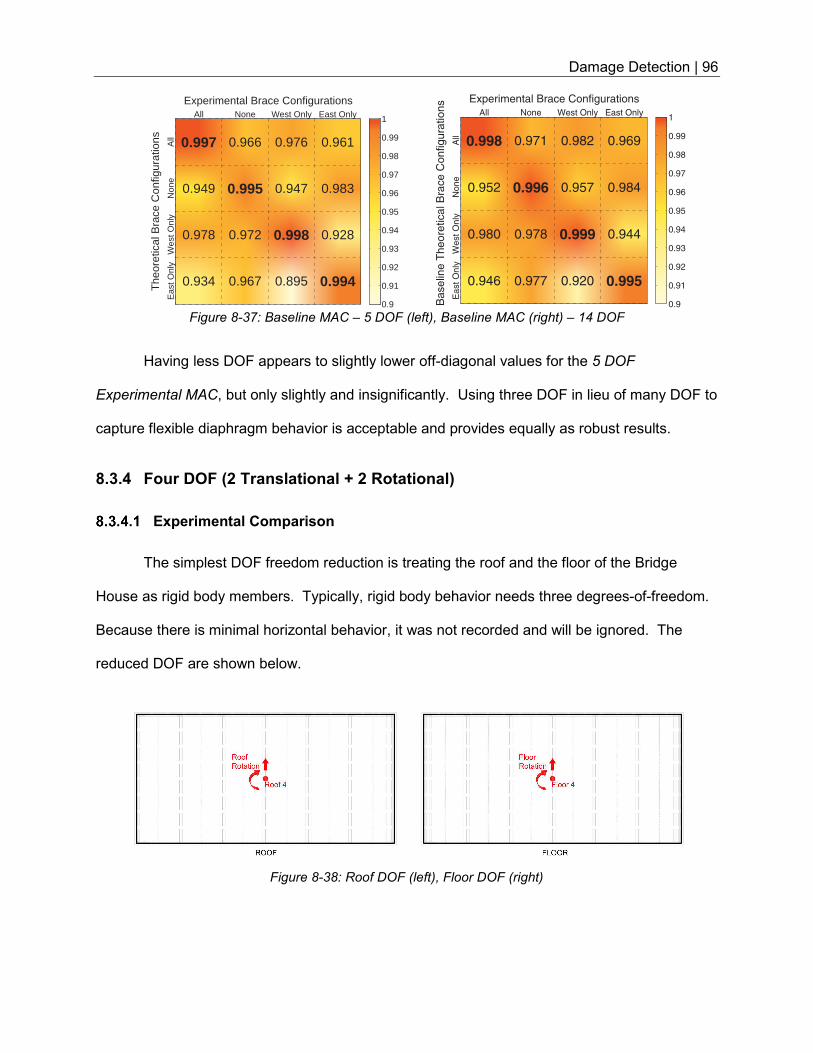
Damage Detection | 96
Having less DOF appears to slightly lower off-diagonal values for the 5 DOF
Experimental MAC, but only slightly and insignificantly. Using three DOF in lieu of many DOF to
capture flexible diaphragm behavior is acceptable and provides equally as robust results.
8.3.4 Four DOF (2 Translational + 2 Rotational)
Experimental Comparison
The simplest DOF freedom reduction is treating the roof and the floor of the Bridge
House as rigid body members. Typically, rigid body behavior needs three degrees-of-freedom.
Because there is minimal horizontal behavior, it was not recorded and will be ignored. The
reduced DOF are shown below.
Figure 8-37: Baseline MAC – 5 DOF (left), Baseline MAC (right) – 14 DOF
Figure 8-38: Roof DOF (left), Floor DOF (right)
Experimental Brace Configurations
All
Non
eW
est O
nly
Eas
t Onl
y
The
oret
ical
Bra
ce C
onfig
urat
ions 0.997
0.949
0.978
0.934
0.966
0.995
0.972
0.967
0.976
0.947
0.998
0.895
0.961
0.983
0.928
0.994
All None West Only East Only
0.9
0.91
0.92
0.93
0.94
0.95
0.96
0.97
0.98
0.99
1
Experimental Brace Configurations
All
None
West
Only
East
Only
Ba
se
line
Th
eo
retica
l B
race
Co
nfig
ura
tio
ns
0.998
0.952
0.980
0.946
0.971
0.996
0.978
0.977
0.982
0.957
0.999
0.920
0.969
0.984
0.944
0.995
All None West Only East Only
0.9
0.91
0.92
0.93
0.94
0.95
0.96
0.97
0.98
0.99
1
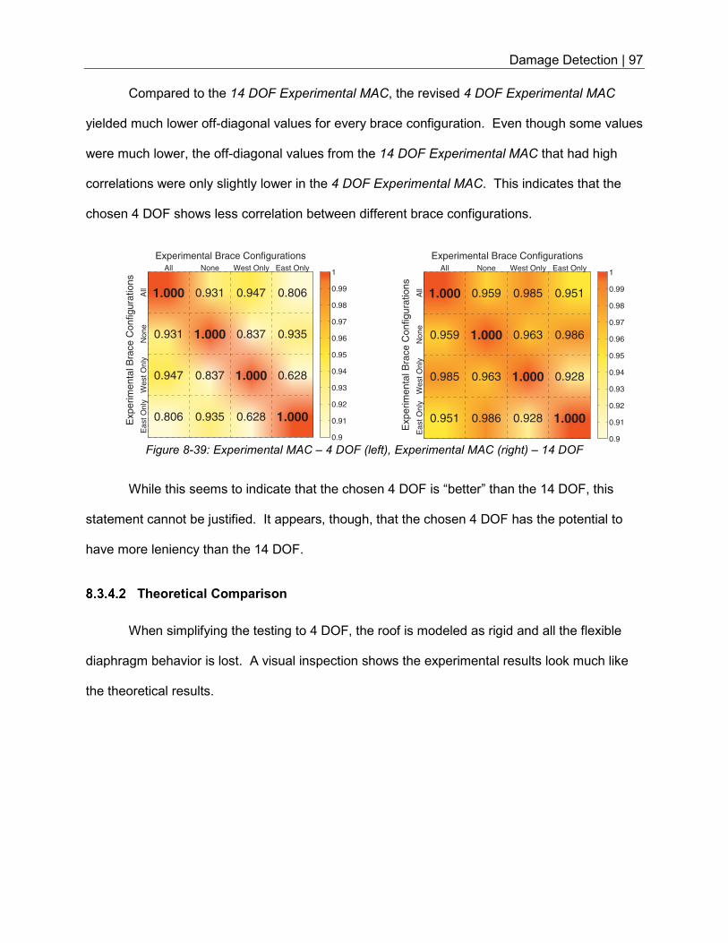
Damage Detection | 97
Compared to the 14 DOF Experimental MAC, the revised 4 DOF Experimental MAC
yielded much lower off-diagonal values for every brace configuration. Even though some values
were much lower, the off-diagonal values from the 14 DOF Experimental MAC that had high
correlations were only slightly lower in the 4 DOF Experimental MAC. This indicates that the
chosen 4 DOF shows less correlation between different brace configurations.
While this seems to indicate that the chosen 4 DOF is “better” than the 14 DOF, this
statement cannot be justified. It appears, though, that the chosen 4 DOF has the potential to
have more leniency than the 14 DOF.
Theoretical Comparison
When simplifying the testing to 4 DOF, the roof is modeled as rigid and all the flexible
diaphragm behavior is lost. A visual inspection shows the experimental results look much like
the theoretical results.
Figure 8-39: Experimental MAC – 4 DOF (left), Experimental MAC (right) – 14 DOF
Experimental Brace Configurations
All
No
ne
We
st O
nly
Ea
st
On
ly
Experim
enta
l B
race C
onfigura
tions
1.000
0.931
0.947
0.806
0.931
1.000
0.837
0.935
0.947
0.837
1.000
0.628
0.806
0.935
0.628
1.000
All None West Only East Only
0.9
0.91
0.92
0.93
0.94
0.95
0.96
0.97
0.98
0.99
1
Experimental Brace Configurations
All
No
ne
We
st
On
lyE
ast
On
ly
Experim
enta
l B
race C
onfigura
tions
1.000
0.959
0.985
0.951
0.959
1.000
0.963
0.986
0.985
0.963
1.000
0.928
0.951
0.986
0.928
1.000
All None West Only East Only
0.9
0.91
0.92
0.93
0.94
0.95
0.96
0.97
0.98
0.99
1
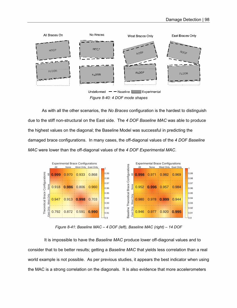
Damage Detection | 98
As with all the other scenarios, the No Braces configuration is the hardest to distinguish
due to the stiff non-structural on the East side. The 4 DOF Baseline MAC was able to produce
the highest values on the diagonal; the Baseline Model was successful in predicting the
damaged brace configurations. In many cases, the off-diagonal values of the 4 DOF Baseline
MAC were lower than the off-diagonal values of the 4 DOF Experimental MAC.
It is impossible to have the Baseline MAC produce lower off-diagonal values and to
consider that to be better results; getting a Baseline MAC that yields less correlation than a real
world example is not possible. As per previous studies, it appears the best indicator when using
the MAC is a strong correlation on the diagonals. It is also evidence that more accelerometers
Figure 8-40: 4 DOF mode shapes
Figure 8-41: Baseline MAC – 4 DOF (left), Baseline MAC (right) – 14 DOF
Experimental Brace Configurations
All
Non
eW
est O
nly
Eas
t Onl
y
The
oret
ical
Bra
ce C
onfig
urat
ions 0.999
0.918
0.947
0.792
0.970
0.986
0.913
0.872
0.933
0.806
0.998
0.591
0.868
0.960
0.703
0.990
All None West Only East Only
0.9
0.91
0.92
0.93
0.94
0.95
0.96
0.97
0.98
0.99
1
Experimental Brace Configurations
All
None
West O
nly
East O
nly
Baselin
e T
heore
tical B
race C
onfigura
tions
0.998
0.952
0.980
0.946
0.971
0.996
0.978
0.977
0.982
0.957
0.999
0.920
0.969
0.984
0.944
0.995
All None West Only East Only
0.9
0.91
0.92
0.93
0.94
0.95
0.96
0.97
0.98
0.99
1
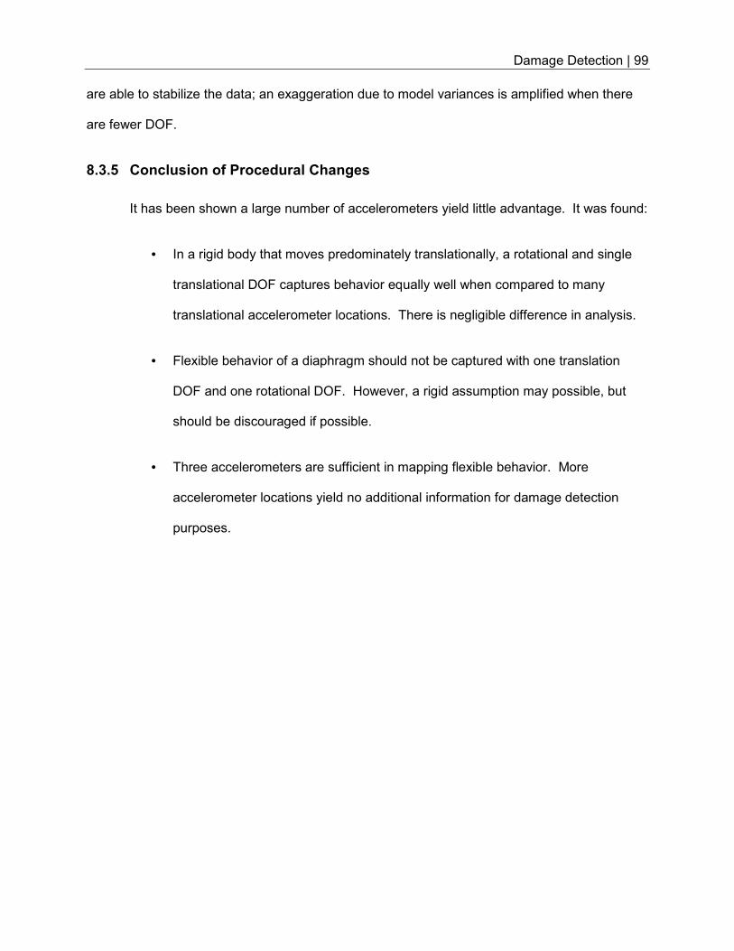
Damage Detection | 99
are able to stabilize the data; an exaggeration due to model variances is amplified when there
are fewer DOF.
8.3.5 Conclusion of Procedural Changes
It has been shown a large number of accelerometers yield little advantage. It was found:
• In a rigid body that moves predominately translationally, a rotational and single
translational DOF captures behavior equally well when compared to many
translational accelerometer locations. There is negligible difference in analysis.
• Flexible behavior of a diaphragm should not be captured with one translation
DOF and one rotational DOF. However, a rigid assumption may possible, but
should be discouraged if possible.
• Three accelerometers are sufficient in mapping flexible behavior. More
accelerometer locations yield no additional information for damage detection
purposes.
Conclusion | 100
9.0 CONCLUSION
9.1 System Identification
Using first mode experimental data, the system identification methods outlined in this
thesis to identify structure stiffness succeeded in capturing the behavior of the structure. The
methods developed in a lab environment (Raney et al., 2015) translated well for the
Experimental Dynamics Field Laboratory, most commonly referred to in this thesis as the Bridge
House. These results improved model accuracy. Variance was found in both the substructure
properties and the diaphragm stiffness. This variance was negligible and did not impact the
ability to correctly identify the brace configurations.
9.2 Damage Detection
9.2.1 Modal Assurance Criterion
The use of the Modal Assurance Criterion to detect damage was successful. The
Baseline Model results were used to accurately identify all four tested brace configurations to
the corresponding experimental brace configuration. The Experimental MAC indicated that
every experimental brace configuration at the Bridge House was similar to one another. Even
with these strong correlations, the Modal Assurance Criterion was successful.
Previously, the use of the Modal Assurance Criterion to detect structural damage relied
on two assumptions. The first assumption being that, in every column of the MAC, the highest
value should also be on the diagonal. The second assumption asserted that the better results
should yield a larger number on the diagonal and smaller numbers on the off-diagonals. This
research indicated that the last assumption is not valid. A model that clearly does not capture
the behavior of the Bridge House produced low off-diagonal values while still creating
reasonably high diagonal values. This assumption should be investigated in further research.
Conclusion | 101
For this research, the last assumption was revised to ignore low off-diagonal values as an
indicator of lack-of-correlation.
9.2.2 Model Accuracy
The parametric studies showed a wide variety of models are capable of correctly
predicting brace configurations. Specifically, the roof diaphragm stiffness could be modeled
with wide bounds and the MAC values displayed strong correlations between experimental
brace configurations and corresponding theoretical brace configurations. Likewise, an early,
undeveloped model was able to predict damage. This model had rough estimates of the
substructure and roof diaphragm behavior.
9.2.3 Data Collection
The quantity of DOF used for measurement in this research exceeded the minimum
amount needed for successful results. When representing a flexible diaphragm as a rigid body
with two DOF, the results were inconclusive. Flexible diaphragm behavior should be accounted
for with additional DOF. However, more than 3 DOF did not increase the accuracy on a flexible
diaphragm.
9.3 Suggestions for Future Research
9.3.1 Bridge House
For future research on the Bridge House, it is recommended that several studies be
conducted. First, it is suggested that higher modes be incorporated into the research.
Software, equipment, and time constraints prohibited the data acquisition of higher modes for
this research. Previous research (Gerbo, 2014) has indicated that including higher modes could
provide further validity for the use of the Modal Assurance Criterion to identify damage.
Conclusion | 102
It is also suggested that a refinement to the brace states be conducted. For this
research, four brace configurations were tested with binary states, either engaged or
disengaged. These states correlated to an intact brace, or a fully ruptured brace, respectively.
While braces do fully rupture and complete stiffness is lost, they are more likely to buckle,
partially rupture, or locally buckle. Each one of these scenarios would result in a stiffness
reduction. It is recommended that these scenarios be examined in order to create a scenario
more analogous to the real world.
Lastly, additional tools could be established to help with damage detection in the future.
For this research, mode shapes were normalized and magnitudes of the experimental
accelerations were disregarded. It is possible that additional information could be gained from
developing a method that accounts for the magnitude of the accelerations.
9.3.2 Suggestions for Application
The methods outlined in this research have the most practicality when they are
streamlined and applied to a large building. For a mobile system, solutions for the workflow
must be turnkey. System identification and data acquisition is not always a straight forward
procedure. The more that can be done to quickly and correctly identify the modes in the field,
the more advantageous this method becomes.
Additionally, there is potential for integration with existing building health monitoring
systems. A large earthquake can displace tenants for weeks or months at a time. Today, many
companies with large buildings or critical systems are retaining engineers in the case a seismic
event occurs. Building monitoring systems are increasing in popularity and having tools that
can accurately assess damaged locations is advantageous. The cost of having permanent
equipment installed has the potential to reduce revenue lost due to downtime.

BIBLIOGRAPHY | 103
BIBLIOGRAPHY
Archer G.C., McDaniel C.C. “An Experimental Study Of Damage Detection Using Removable
Braces.” 10th U.S. National Conference on Earthquake Engineering, Earthquake
Engineering Research Institute, 2014.
Allemang R. J. “The Modal Assurance Criterion (MAC): Twenty Years of Use and Abuse.”
Sound and Vibration, 2003.
Ross, Ben. Ben + Jo Photo | Bridge House. N.p., n.d. Web. 3 Feb. 2016.
<benandjophoto.com>.
Chopra, Anil K. Dynamics of Structures: Theory and Applications to Earthquake Engineering.
Boston: Prentice Hall, 2012. Print.
CSI Analysis Reference Manual. (2013). Berkeley, California: Computers & Structures Inc.
Davena, Ronald, et al. California Polytechnic State University, San Luis Obispo, 1966. San Luis
Obispo: Cal Poly SLO, 1966. Print.
Garlow, Robert. "Bridge House Inquiry." Message to the author. 24 Jan. 2016. E-mail.
Gerbo, Evan Jamison. "Structural Damage Detection Utilizing Experimental Mode Shapes."
Thesis. California Polytechnic University, San Luis Obispo, 2014. 31 July 2014. Web.
<digitalcommons.calpoly.edu/theses/1247>.
McDaniel, C., Archer, G. Classroom-Based Forced-Vibration Testing, 15th World Conference on
Earthquake Engineering (15th WCEE), Lisbon, Portugal, 2012.
Planas, Brian, et al. “Rehabilitation of the Bridge House”. California Polytechnic State University,
San Luis Obispo, 2011. San Luis Obispo: Cal Poly SLO, 2011. Print
BIBLIOGRAPHY | 104
Ramos, Pablo D., Jr. "System Identification Of A Bridge-type Building Structure." Thesis.
California Polytechnic University, San Luis Obispo, 2013. 18 June 2013. Web.
<digitalcommons.calpoly.edu/theses/944>.
Raney, Joshua, et al. "Influence of Boundary Conditions on Building Behavior". 2015 ASEE
Annual Conference and Exposition, Seattle, Washington, 2015, June. ASEE
Conferences, 2015. https://peer.asee.org/24296 Internet. 09 Feb, 2016.
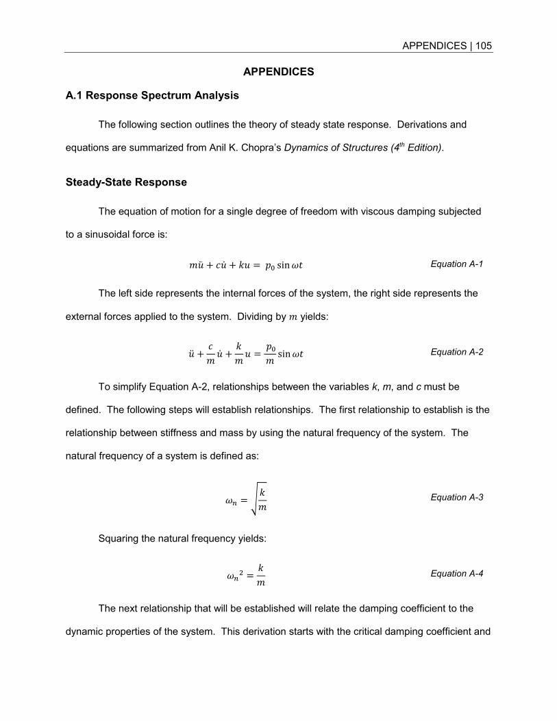
APPENDICES | 105
APPENDICES
A.1 Response Spectrum Analysis
The following section outlines the theory of steady state response. Derivations and
equations are summarized from Anil K. Chopra’s Dynamics of Structures (4th Edition).
Steady-State Response
The equation of motion for a single degree of freedom with viscous damping subjected
to a sinusoidal force is:
#�< + I�J + �� = � sin�7 Equation A-1
The left side represents the internal forces of the system, the right side represents the
external forces applied to the system. Dividing by # yields:
�< + I# �J + �#� = � # sin�7 Equation A-2
To simplify Equation A-2, relationships between the variables k, m, and c must be
defined. The following steps will establish relationships. The first relationship to establish is the
relationship between stiffness and mass by using the natural frequency of the system. The
natural frequency of a system is defined as:
�� = ��# Equation A-3
Squaring the natural frequency yields:
��� = �# Equation A-4
The next relationship that will be established will relate the damping coefficient to the
dynamic properties of the system. This derivation starts with the critical damping coefficient and
APPENDICES | 106
the damping ratio. The critical damping coefficient is the value where the system does not
oscillate beyond one cycle and is defined by:
IKL = 2#�� Equation A-5
The damping ratio, or the ratio of damping to the critical damping, is represented by
variable zeta:
� = IIKL Equation A-6
Substituting Equation A-5 into Equation A-6 yields:
� = I2#�� Equation A-7
Re-arranging Equation A-7 gives: I# = 2��� Equation A-8
The previously established relationships will be substituted into the equation of motion.
Substituting Equation A-4 and Equation A-8 into Equation A-2 yields:
�< + 2����J + ���� = � # sin�7 Equation A-9
In this form, Equation A-9 has a particular (or steady state) solution of:
�67� = C sin�7 + M cos�7 Equation A-10
The transient component of the solution to Equation A-9 is assumed to be negligible as
the impact of the steady state response damps out after a short period of time. The increase in
amplitude due to harmonic loading will be shown later. The first and second derivative of
Equation A-10 with respect to time are:
APPENDICES | 107
�J67� = �C cos�7 − �M sin�7 Equation A-11 �<67� = −��C sin�7 − ��M cos�7 Equation A-12
Substituting Equation A-11 and Equation A-12 into Equation A-9 yields:
P��� − ���C − 2���MQ sin�7 + P2����C + ��� − ���MQ cos�7 = 6R� sin�7 Equation A-13
Extracting the sine and cosine for Equation A-13 yields two algebraic equations:
S1 − T ���U�V C −T2� ���UM = � � Equation A-14
�2� WWX� C +�1 − � WWX��� M = 0 Equation A-15
Simultaneously solving Equation A-14 and Equation A-15 for coefficients C and D yields:
C = � � 1 −� ������1 −� ������� + �2� � ������ Equation A-16
M =� � −2� � �����1 −� ������� + �2� � ������ Equation A-17
Equation A-16 and Equation A-17 are the coefficients for Equation A-10. The outlined
proof is for steady state behavior. Traditionally, dynamic response would also have transient,
homogenous behavior. This will be ignored as its contribution during steady state is small and
irrelevant. It will be shown in the following sections that the response due to forced vibration is
much larger.
APPENDICES | 108
Maximum Deformation
The basis of system identification in modal testing relies on the ability to predict the
maximum displacements from experimental data. To calculate the maximum displacements,
the following formulation is used. The solution to Equation A-10 can be defined by the following
trigometric identity.
C sinZ + M cosZ = √C� +M� cosZ − tan^,M C⁄ �� Equation A-18
The right hand side of Equation A-8 can be simplified to the following terms: �67� = ���� sin�7 − ;� Equation A-19
Where ����is the maximum dynamic displacement due to a sine vibration:
���� = `C� + M� Equation A-20
And where ;, the phase lag:
; = tan^,M C⁄ �. Equation A-21
To solve for the maximum displacement, variables D and C from Equation A-16 and
Equation A-17 are substituted into Equation A-20:
���� = ab6Rc ,^� ddX�e�,^� ddX�e�ef��g� ddX�e�h� + b6Rc ^�g� ddX��,^� ddX�e�ef��g� ddX�e�h
� Equation A-22
Further simplification produces the following equations:
APPENDICES | 109
���� = � � ijk1−� ������1 −� ������� + �2� � ������lm
� + jk−2� � �����1 −� ������� + �2� � ������lm
�
���� = � � noooooooop �1 −� �������q�1 −� ������� + �2� � ������r� +
�2� � ������q�1 −� ������� + �2� � ������r�
���� = � � noooooooop �1 −� ������� + �2� � ������q�1 −� ������� + �2� � ������r�
���� = � � a 1�1 −� ������� + �2� � ������
���� = � � 1��1 −� ������� + �2� � ������
Equation A-23
It is important to note that the sine term from Equation A-19 has been disregarded as the
only property being examined is the maximum amplification; this occurs when the sine term
reaches its upper bound of one.
Displacement Response Amplification Factor, Rd
The displacement response amplification factor, Rd, is a ratio that compares the static
deformations to the dynamic deformations of similar systems. The displacement response
amplification factor is as follows:
APPENDICES | 110
�� = ������� Equation A-24
Where ��� the deformation due the applied force, and � is the amplitude of the
applied force.
��� = � � Equation A-25
Substituting Equation A-23 and Equation A-25 into Equation A-24 yields the following
equation at steady state:
�� =� � 1��1 −� ������� + �2� � ������� �
Equation A-26
Which simplifies to:
�� = 1��1 −� ������� + �2� � ������
Equation A-27
Plotting Equation A-27 for a variety of damping ratios of an excited system is show in
Figure A-1.
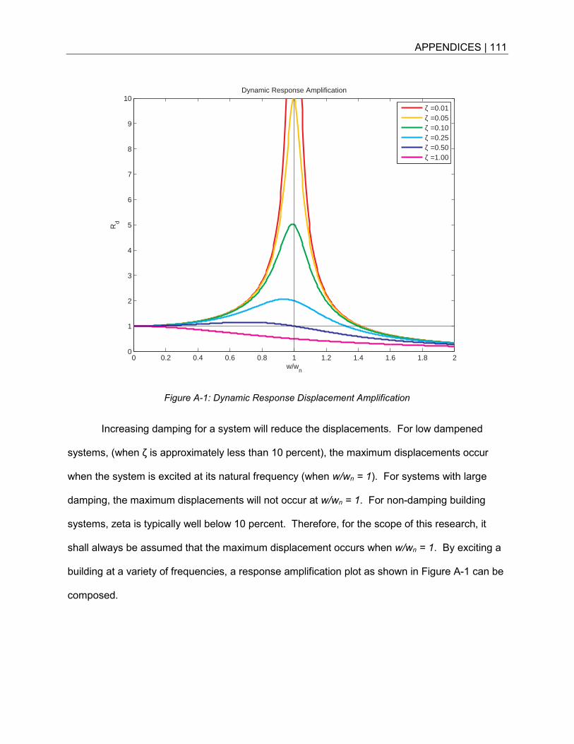
APPENDICES | 111
Figure A-1: Dynamic Response Displacement Amplification
Increasing damping for a system will reduce the displacements. For low dampened
systems, (when ζ is approximately less than 10 percent), the maximum displacements occur
when the system is excited at its natural frequency (when w/wn = 1). For systems with large
damping, the maximum displacements will not occur at w/wn = 1. For non-damping building
systems, zeta is typically well below 10 percent. Therefore, for the scope of this research, it
shall always be assumed that the maximum displacement occurs when w/wn = 1. By exciting a
building at a variety of frequencies, a response amplification plot as shown in Figure A-1 can be
composed.
0 0.2 0.4 0.6 0.8 1 1.2 1.4 1.6 1.8 20
1
2
3
4
5
6
7
8
9
10
w/wn
Rd
Dynamic Response Amplification
ζ =0.01ζ =0.05ζ =0.10ζ =0.25ζ =0.50ζ =1.00
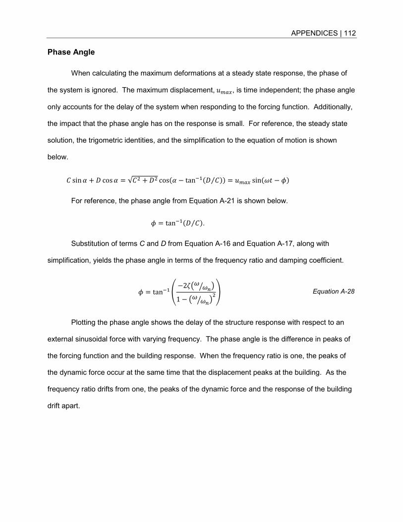
APPENDICES | 112
Phase Angle
When calculating the maximum deformations at a steady state response, the phase of
the system is ignored. The maximum displacement,����, is time independent; the phase angle
only accounts for the delay of the system when responding to the forcing function. Additionally,
the impact that the phase angle has on the response is small. For reference, the steady state
solution, the trigometric identities, and the simplification to the equation of motion is shown
below.
C sinZ + M cosZ = √C� +M� cosZ − tan^,M C⁄ �� = ���� sin�7 − ;�
For reference, the phase angle from Equation A-21 is shown below.
; = tan^,M C⁄ �.
Substitution of terms C and D from Equation A-16 and Equation A-17, along with
simplification, yields the phase angle in terms of the frequency ratio and damping coefficient.
; = tan^,b−2�E� ��� G1 − E� ��� G�h Equation A-28
Plotting the phase angle shows the delay of the structure response with respect to an
external sinusoidal force with varying frequency. The phase angle is the difference in peaks of
the forcing function and the building response. When the frequency ratio is one, the peaks of
the dynamic force occur at the same time that the displacement peaks at the building. As the
frequency ratio drifts from one, the peaks of the dynamic force and the response of the building
drift apart.
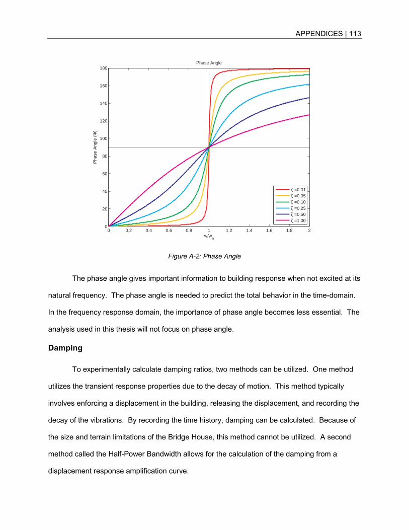
APPENDICES | 113
Figure A-2: Phase Angle
The phase angle gives important information to building response when not excited at its
natural frequency. The phase angle is needed to predict the total behavior in the time-domain.
In the frequency response domain, the importance of phase angle becomes less essential. The
analysis used in this thesis will not focus on phase angle.
Damping
To experimentally calculate damping ratios, two methods can be utilized. One method
utilizes the transient response properties due to the decay of motion. This method typically
involves enforcing a displacement in the building, releasing the displacement, and recording the
decay of the vibrations. By recording the time history, damping can be calculated. Because of
the size and terrain limitations of the Bridge House, this method cannot be utilized. A second
method called the Half-Power Bandwidth allows for the calculation of the damping from a
displacement response amplification curve.
0 0.2 0.4 0.6 0.8 1 1.2 1.4 1.6 1.8 20
20
40
60
80
100
120
140
160
180
w/wn
Pha
se A
ngle
(Φ
)
Phase Angle
ζ =0.01ζ =0.05ζ =0.10ζ =0.25ζ =0.50ζ =1.00
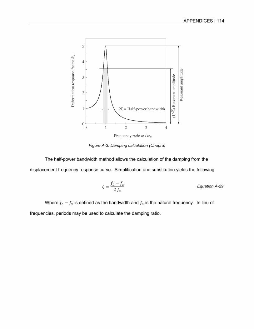
APPENDICES | 114
Figure A-3: Damping calculation (Chopra)
The half-power bandwidth method allows the calculation of the damping from the
displacement frequency response curve. Simplification and substitution yields the following
� = ! − �2 � Equation A-29
Where ! − � is defined as the bandwidth and � is the natural frequency. In lieu of
frequencies, periods may be used to calculate the damping ratio.
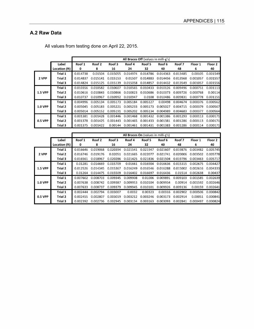
APPENDICES | 115
A.2 Raw Data
All values from testing done on April 22, 2015.
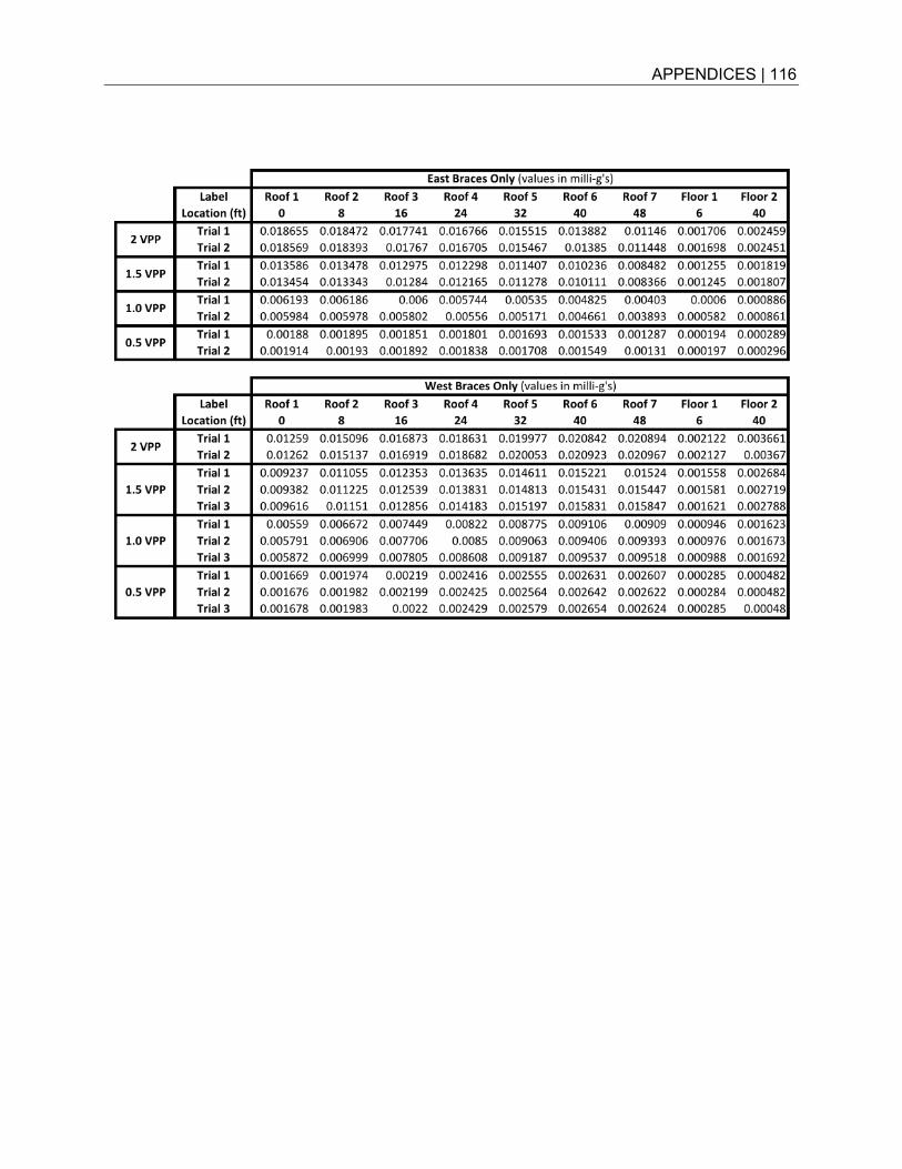
APPENDICES | 116