Embed Size (px)
Citation preview
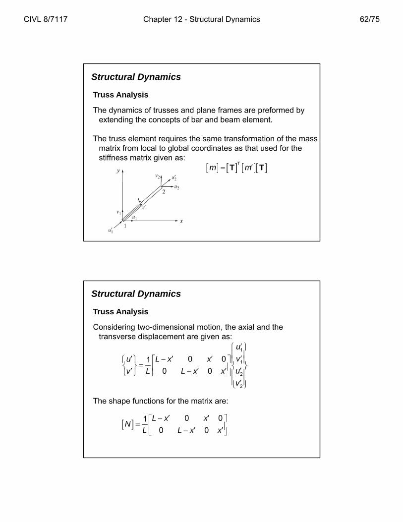
Structural Dynamics
Introduction
• To discuss the dynamics of a single-degree-of freedom spring-mass system. y
• To derive the finite element equations for the time-dependent stress analysis of the one-dimensional bar, including derivation of the lumped and consistent mass matrices.
• To introduce procedures for numerical integration in time, including the central difference method, Newmark's method,
d Wil ' th dand Wilson's method.
• To describe how to determine the natural frequencies of bars by the finite element method.
• To illustrate the finite element solution of a time-dependent bar problem.
Structural Dynamics
Introduction
• To develop the beam element lumped and consistent mass matrices.
• To illustrate the determination of natural frequencies for beams by the finite element method.
• To develop the mass matrices for truss, plane frame, plane stress, plane strain, axisymmetric, and solid elements.
• To report some results of structural dynamics problems solved p y pusing a computer program, including a fixed-fixed beam for natural frequencies, a bar, a fixed-fixed beam, a rigid frame, and a gantry crane-all subjected to time-dependent forcing functions.
CIVL 8/7117 Chapter 12 - Structural Dynamics 1/75
Structural Dynamics
Introduction
This chapter provides an elementary introduction to time-dependent problems. p p
We will introduce the basic concepts using the single-degree-of-freedom spring-mass system.
We will include discussion of the stress analysis of the one-dimensional bar, beam, truss, and plane frame.
Structural Dynamics
Introduction
We will provide the basic equations necessary for structural dynamic analysis and develop both the lumped- and the y y p pconsistent-mass matrices involved in the analyses of a bar, beam, truss, and plane frame.
We will describe the assembly of the global mass matrix for truss and plane frame analysis and then present numerical integration methods for handling the time derivative.
We will provide longhand solutions for the determination of the natural frequencies for bars and beams, and then illustrate the time-step integration process involved with the stress analysis of a bar subjected to a time dependent forcing function.
CIVL 8/7117 Chapter 12 - Structural Dynamics 2/75
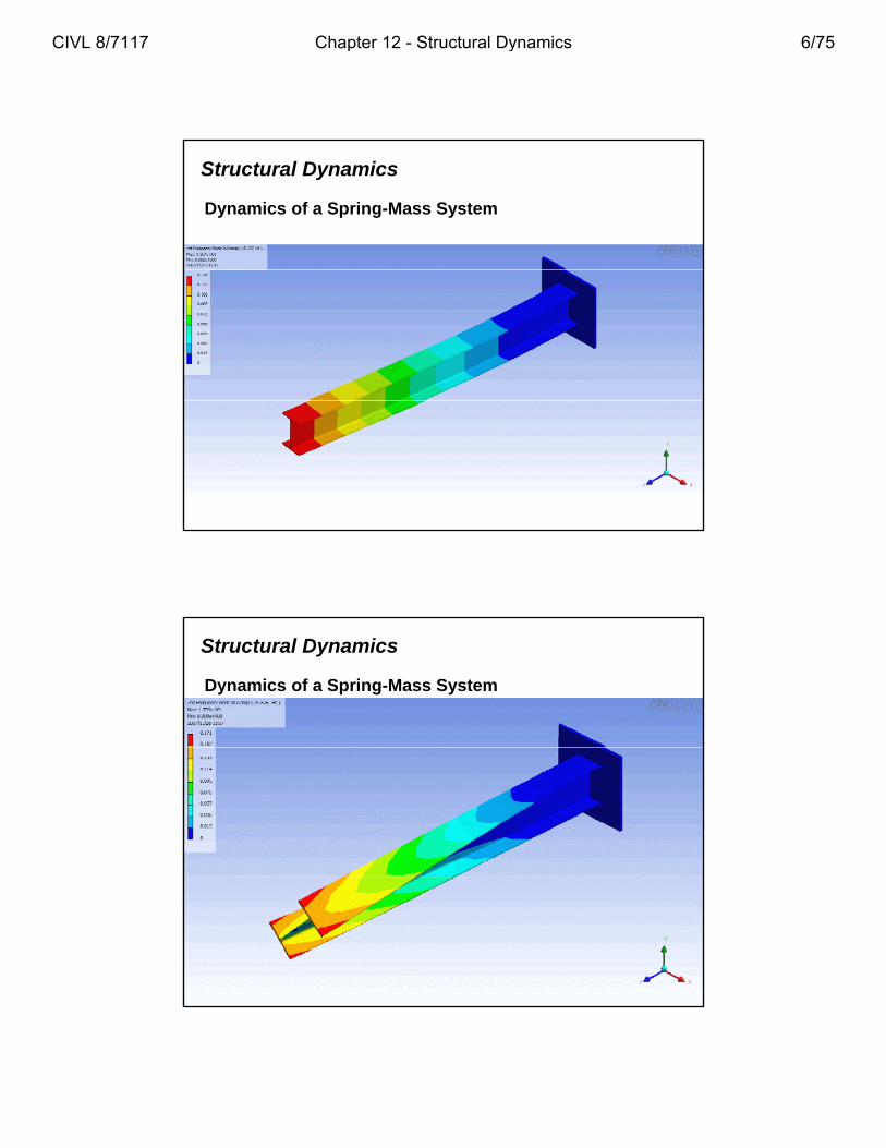
Structural Dynamics
Dynamics of a Spring-Mass System
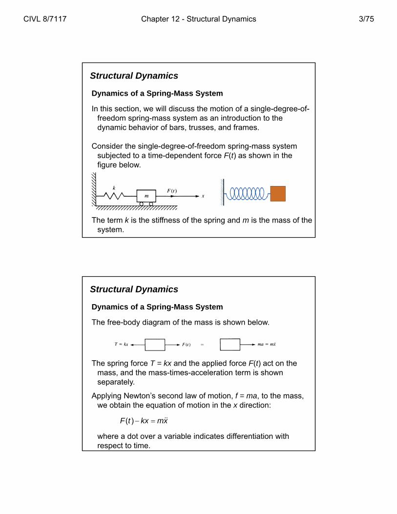
In this section, we will discuss the motion of a single-degree-of-freedom spring-mass system as an introduction to the p g ydynamic behavior of bars, trusses, and frames.
Consider the single-degree-of-freedom spring-mass system subjected to a time-dependent force F(t) as shown in the figure below.
The term k is the stiffness of the spring and m is the mass of the system.
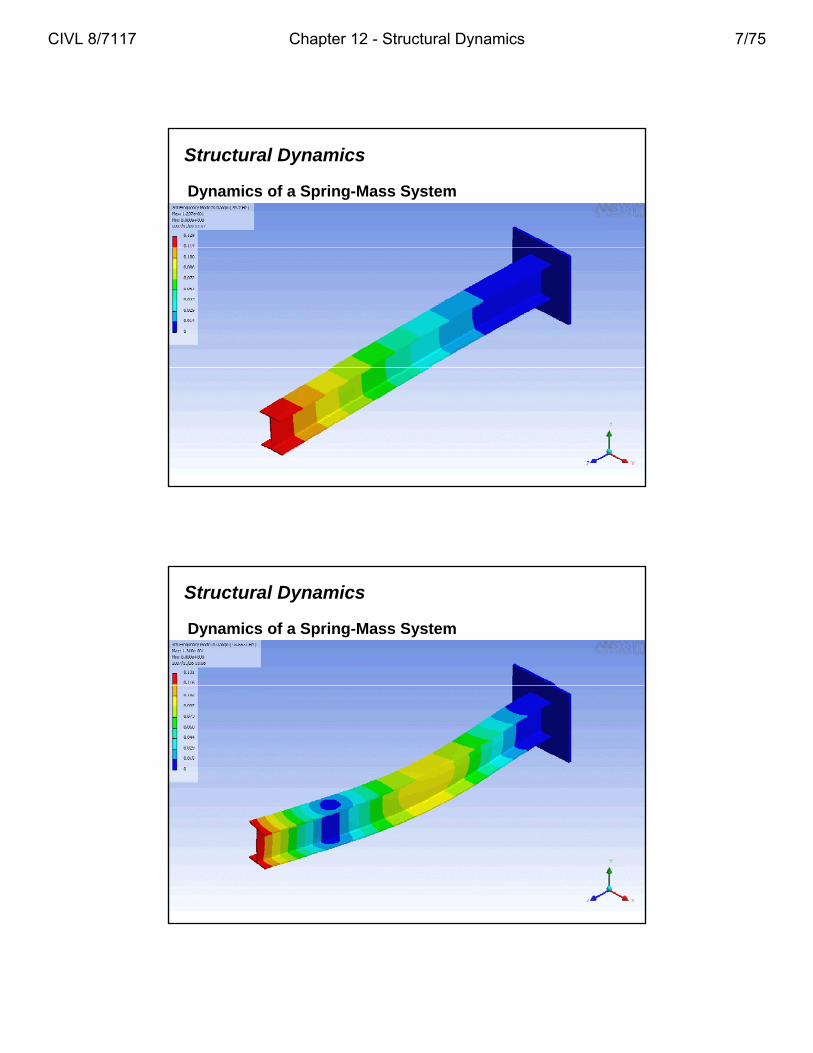
Structural Dynamics
Dynamics of a Spring-Mass System
The free-body diagram of the mass is shown below.
The spring force T = kx and the applied force F(t) act on the mass, and the mass-times-acceleration term is shown separately.
A l i N ’ d l f i f hApplying Newton’s second law of motion, f = ma, to the mass, we obtain the equation of motion in the x direction:
( )F t kx mx
where a dot over a variable indicates differentiation with respect to time.
CIVL 8/7117 Chapter 12 - Structural Dynamics 3/75
Structural Dynamics
Dynamics of a Spring-Mass System
The standard form of the equation is:
ff
( )mx kx F t
The above equation is a second-order linear differential equation whose solution for the displacement consists of a homogeneous solution and a particular solution.
The homogeneous solution is the solution obtained when the right-hand-side is set equal to zero.
A number of useful concepts regarding vibrations are available when considering the free vibration of a mass; that is when F(t) = 0.
Structural Dynamics
Dynamics of a Spring-Mass System
Let’s define the following term: 2 k
m
The equation of motion becomes: 2 0x x
where is called the natural circular frequency of the free vibration of the mass (radians per second).
Note that the natural frequency depends on the spring stiffness k and the mass m of the body.
CIVL 8/7117 Chapter 12 - Structural Dynamics 4/75
Structural Dynamics
Dynamics of a Spring-Mass System
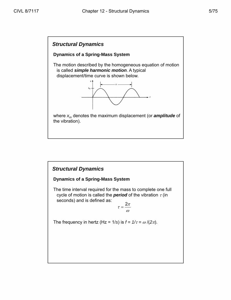
The motion described by the homogeneous equation of motion is called simple harmonic motion A typicalis called simple harmonic motion. A typical displacement/time curve is shown below.
where xm denotes the maximum displacement (or amplitude of the vibration).
Structural Dynamics
Dynamics of a Spring-Mass System
The time interval required for the mass to complete one full cycle of motion is called the period of the vibration (incycle of motion is called the period of the vibration (in seconds) and is defined as:
The frequency in hertz (Hz = 1/s) is f = 1/ = /(2).
2
CIVL 8/7117 Chapter 12 - Structural Dynamics 5/75
Structural Dynamics
Dynamics of a Spring-Mass System
Structural Dynamics
Dynamics of a Spring-Mass System
CIVL 8/7117 Chapter 12 - Structural Dynamics 6/75
Structural Dynamics
Dynamics of a Spring-Mass System
Structural Dynamics
Dynamics of a Spring-Mass System
CIVL 8/7117 Chapter 12 - Structural Dynamics 7/75
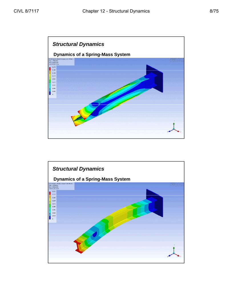
Structural Dynamics
Dynamics of a Spring-Mass System
Structural Dynamics
Dynamics of a Spring-Mass System
CIVL 8/7117 Chapter 12 - Structural Dynamics 8/75
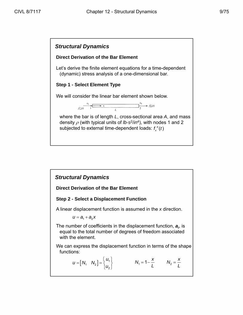
Structural Dynamics
Direct Derivation of the Bar Element
Let’s derive the finite element equations for a time-dependent (dynamic) stress analysis of a one-dimensional bar(dynamic) stress analysis of a one-dimensional bar.
Step 1 - Select Element Type
We will consider the linear bar element shown below.
where the bar is of length L, cross-sectional area A, and mass density (with typical units of lb-s2/in4), with nodes 1 and 2 subjected to external time-dependent loads: ( )e
xf t
Structural Dynamics
Direct Derivation of the Bar Element
Step 2 - Select a Displacement Function
A linear displacement function is assumed in the x direction.
The number of coefficients in the displacement function, ai, is equal to the total number of degrees of freedom associated with the element.
1 2u a a x
We can express the displacement function in terms of the shape functions:
1
1 22
uu N N
u 1 21
x xN N
L L
CIVL 8/7117 Chapter 12 - Structural Dynamics 9/75
Structural Dynamics
Direct Derivation of the Bar Element
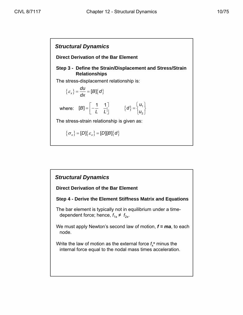
Step 3 - Define the Strain/Displacement and Stress/Strain RelationshipsRelationships
The stress-displacement relationship is:
[ ]x
duB d
dx
where: 11 1
[ ]u
B dL L
where: 2
[ ]uL L
[ ] [ ][ ]x xD D B d
The stress-strain relationship is given as:
Structural Dynamics
Direct Derivation of the Bar Element
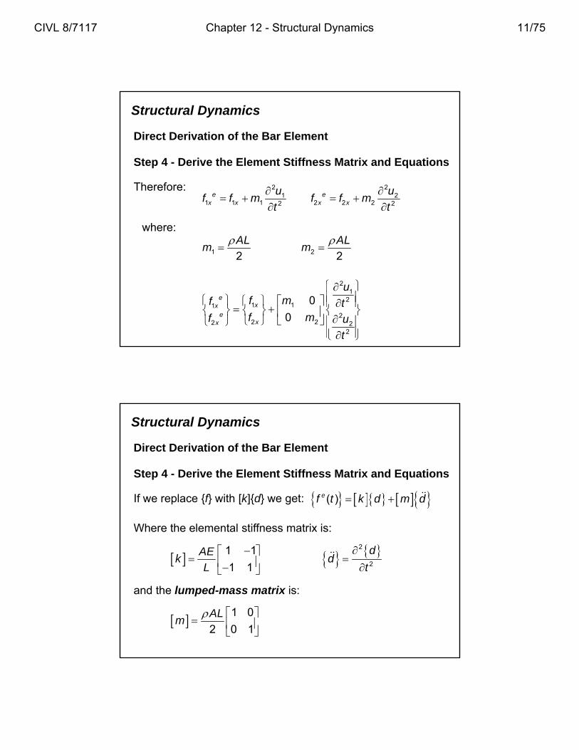
Step 4 - Derive the Element Stiffness Matrix and Equations
The bar element is typically not in equilibrium under a time-dependent force; hence, f1x ≠ f2x.
We must apply Newton’s second law of motion, f = ma, to each node.
Write the law of motion as the external force fxe minus the internal force equal to the nodal mass times acceleration.
CIVL 8/7117 Chapter 12 - Structural Dynamics 10/75
Structural Dynamics
Direct Derivation of the Bar Element
Step 4 - Derive the Element Stiffness Matrix and Equations
Therefore:
2 21 2
1 1 1 2 2 22 2e e
x x x x
u uf f m f f m
t t
where:
1 22 2
AL ALm m
21
21 11
22 22 2
2
0
0
exx
exx
uf mf tf mf u
t
Structural Dynamics
Direct Derivation of the Bar Element
Step 4 - Derive the Element Stiffness Matrix and Equations
If we replace {f} with [k]{d} we get: ( )ef t k d m d
Where the elemental stiffness matrix is:
2
2
1 1
1 1
dAEk d
L t
1 0
2 0 1
ALm
and the lumped-mass matrix is:
CIVL 8/7117 Chapter 12 - Structural Dynamics 11/75
Structural Dynamics
Direct Derivation of the Bar Element
Step 4 - Derive the Element Stiffness Matrix and Equations
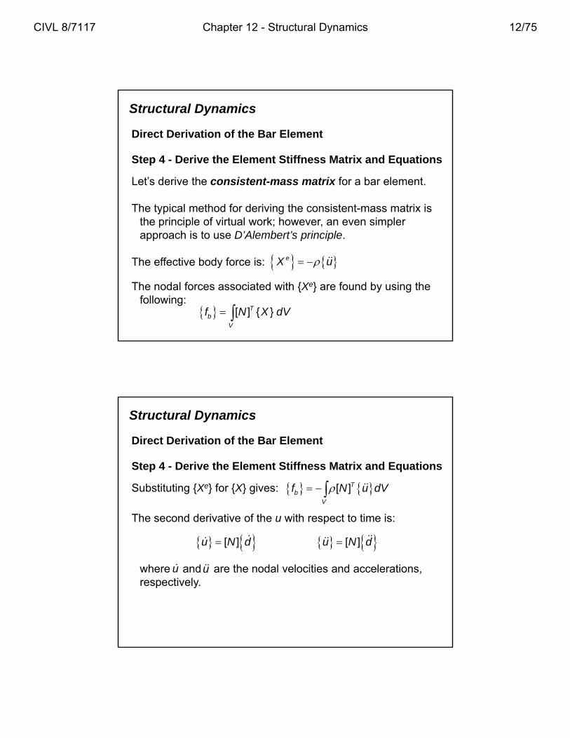
Let’s derive the consistent-mass matrix for a bar element.
The typical method for deriving the consistent-mass matrix is the principle of virtual work; however, an even simpler approach is to use D’Alembert’s principle.
eXThe effective body force is: eX u
The nodal forces associated with {Xe} are found by using the following:
[ ] { }Tb
V
f N X dV
Structural Dynamics
Direct Derivation of the Bar Element
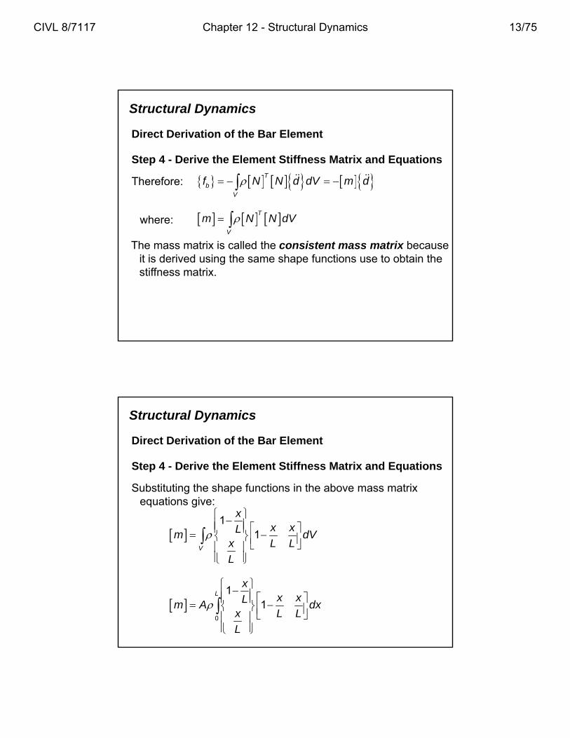
Step 4 - Derive the Element Stiffness Matrix and Equations
Substituting {Xe} for {X} gives: [ ]Tb
V
f N u dV
[ ] [ ]u N d u N d
The second derivative of the u with respect to time is:
where and are the nodal velocities and accelerations, respectively.
u u
CIVL 8/7117 Chapter 12 - Structural Dynamics 12/75
Structural Dynamics
Direct Derivation of the Bar Element
Step 4 - Derive the Element Stiffness Matrix and Equations
T T
b
V
f N N d dV m d
where:
The mass matrix is called the consistent mass matrix because it is derived using the same shape functions use to obtain the
Therefore:
T
V
m N N dV
it is derived using the same shape functions use to obtain the stiffness matrix.
Structural Dynamics
Direct Derivation of the Bar Element
Step 4 - Derive the Element Stiffness Matrix and Equations
Substituting the shape functions in the above mass matrix equations give:
1
1V
xx xLm dV
x L L
L
0
11
Lx
x xLm A dxx L L
L
CIVL 8/7117 Chapter 12 - Structural Dynamics 13/75
Structural Dynamics
Direct Derivation of the Bar Element
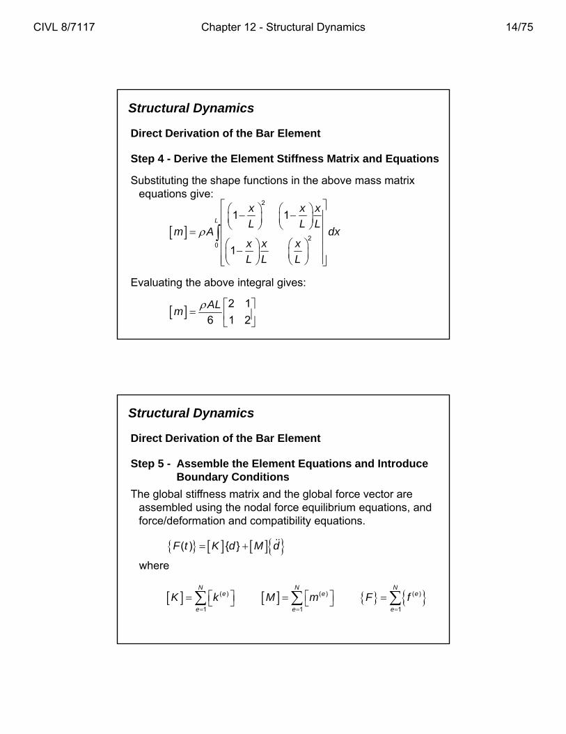
Step 4 - Derive the Element Stiffness Matrix and Equations
Substituting the shape functions in the above mass matrix equations give:
2
20
1 1
1
L
x x x
L L Lm A dx
x x x
L L L
L L L
2 1
6 1 2
ALm
Evaluating the above integral gives:
Structural Dynamics
Direct Derivation of the Bar Element
Step 5 - Assemble the Element Equations and Introduce Boundary ConditionsBoundary Conditions
The global stiffness matrix and the global force vector are assembled using the nodal force equilibrium equations, and force/deformation and compatibility equations.
( ) { }F t K d M d
( )
1
Ne
e
K k
where
( )
1
Ne
e
M m
( )
1
Ne
e
F f
CIVL 8/7117 Chapter 12 - Structural Dynamics 14/75
Structural Dynamics
Numerical Integration in Time
We now introduce procedures for the discretization of the equations of motion with respect to time.
These procedures will allow the nodal displacements to be determined at different time increments for a given dynamic system.
The general method used is called direct integration. There t l ifi ti f di t i t ti li it d i li itare two classifications of direct integration: explicit and implicit.
We will formulate the equations for two direct integration methods.
Structural Dynamics
Numerical Integration in Time
The first, and simplest, is an explicit method known as the central difference method.
The second more complicated but more versatile than the central difference method, is an implicit method known as the Newmark-Beta (or Newmark’s) method.
The versatility of Newmark’s method is evidenced by its d t ti i i ll il bl tadaptation in many commercially available computer
programs.
CIVL 8/7117 Chapter 12 - Structural Dynamics 15/75
Structural Dynamics
Central Difference Method
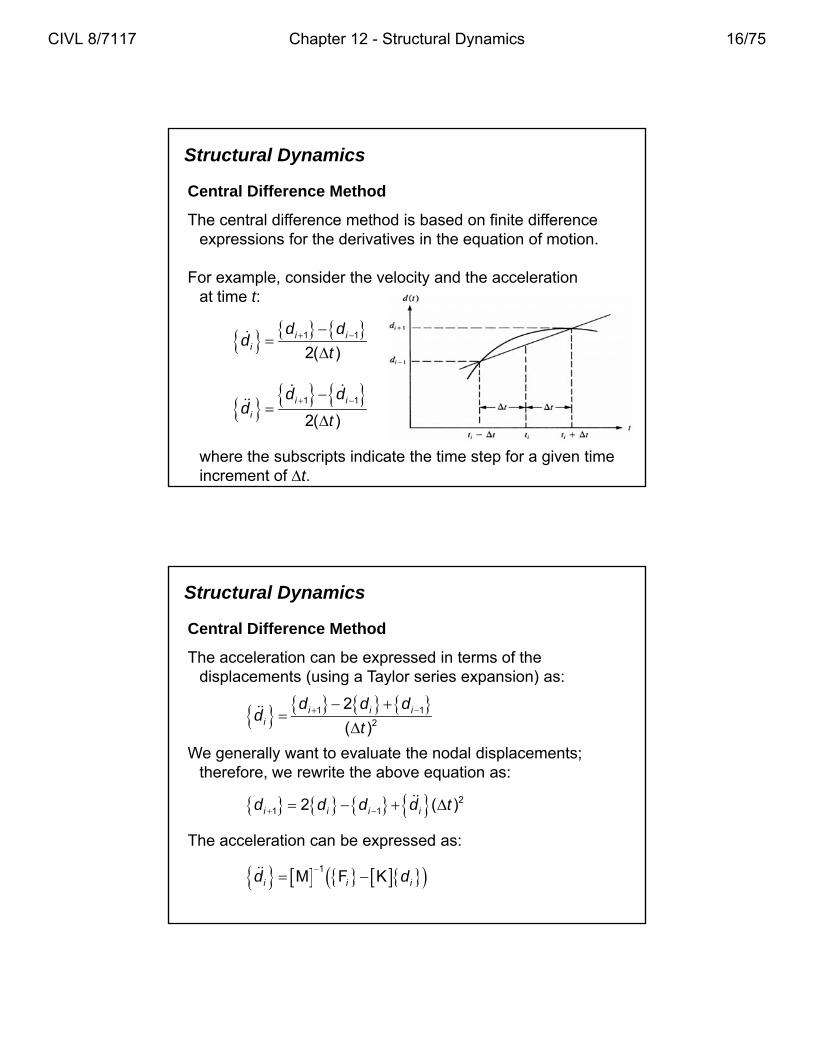
The central difference method is based on finite difference expressions for the derivatives in the equation of motion.
For example, consider the velocity and the acceleration at time t:
1 1
2( )i i
i
d dd
t
1 1
2( )
i i
i
d dd
t
where the subscripts indicate the time step for a given time increment of t.
Structural Dynamics
Central Difference Method
The acceleration can be expressed in terms of the displacements (using a Taylor series expansion) as:( g y )
1 12
2
( )i i i
i
d d dd
t
22 ( )d d d d t
We generally want to evaluate the nodal displacements; therefore, we rewrite the above equation as:
1 12 ( )i i i id d d d t
1M F Ki i id d
The acceleration can be expressed as:
CIVL 8/7117 Chapter 12 - Structural Dynamics 16/75
Structural Dynamics
Central Difference Method
To develop an expression of di+1, first multiply the nodal displacement equation by M and substitute the above equation
2
1 12i i i i id d d d t M M M F K
2 22d t t d d M F M K M
Combining terms in the above equations gives:
yfor into this equation. id
1 12i i i id t t d d M F M K M
To start the computation to determine we need the displacement at time step i -1.
1 1 1, , andi i id d d
Structural Dynamics
Central Difference Method
Using the central difference equations for the velocity and acceleration and solving for {di-1}:
2
1
( )( )
2i i i i
td d t d d
Procedure for solution:
g { i 1}
1. Given: 0 0, , and ( )id d F t 0 0
2. If the acceleration is not given, solve for 0d
1
0 0 0M F Kd d
CIVL 8/7117 Chapter 12 - Structural Dynamics 17/75
Structural Dynamics
Central Difference Method
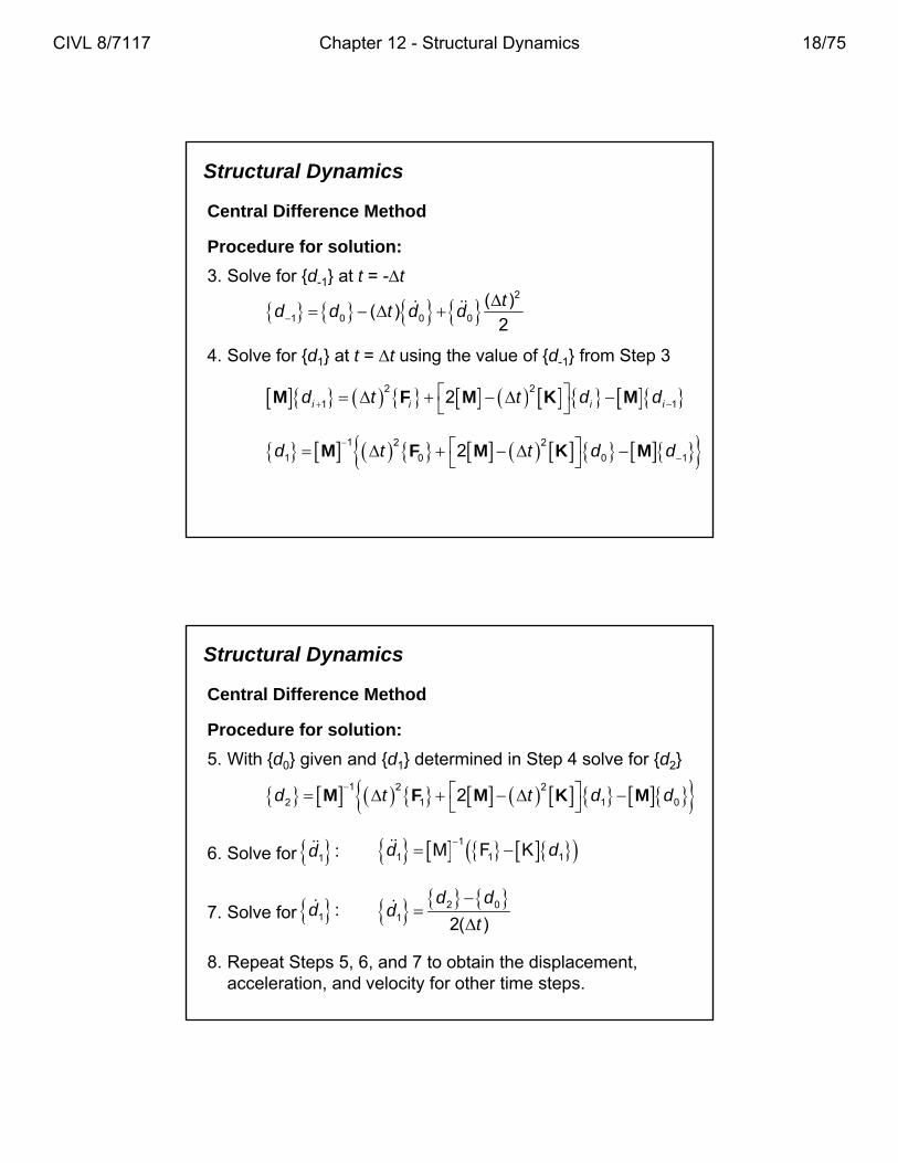
Procedure for solution:
3 Solve for {d } at t = t3. Solve for {d-1} at t = -t
4. Solve for {d1} at t = t using the value of {d-1} from Step 3
2
1 0 0 0
( )( )
2
td d t d d
2 2
1 12i i i id t t d d M F M K M 1 1i i i i
1 2 2
1 0 0 12d t t d d
M F M K M
Structural Dynamics
Central Difference Method
Procedure for solution:
5 With {d } given and {d } determined in Step 4 solve for {d }5. With {d0} given and {d1} determined in Step 4 solve for {d2}
1 2 2
2 1 1 02d t t d d M F M K M
6. Solve for 1 :d 1
1 1 1M F Kd d
7. Solve for 1 :d 2 0
1 2( )
d dd
t
8. Repeat Steps 5, 6, and 7 to obtain the displacement, acceleration, and velocity for other time steps.
CIVL 8/7117 Chapter 12 - Structural Dynamics 18/75
Structural Dynamics
Central Difference Method
Procedure for solution:
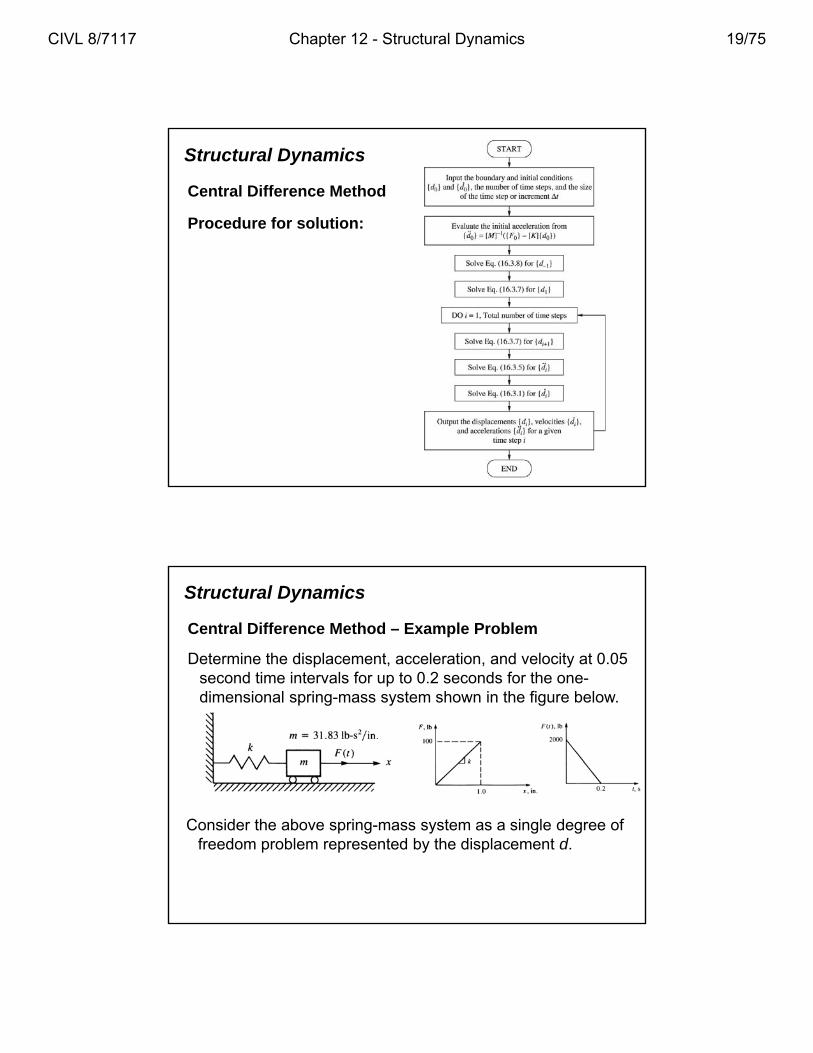
Structural Dynamics
Central Difference Method – Example Problem
Determine the displacement, acceleration, and velocity at 0.05 second time intervals for up to 0.2 seconds for the one-pdimensional spring-mass system shown in the figure below.
Consider the above spring-mass system as a single degree of freedom problem represented by the displacement d.
CIVL 8/7117 Chapter 12 - Structural Dynamics 19/75
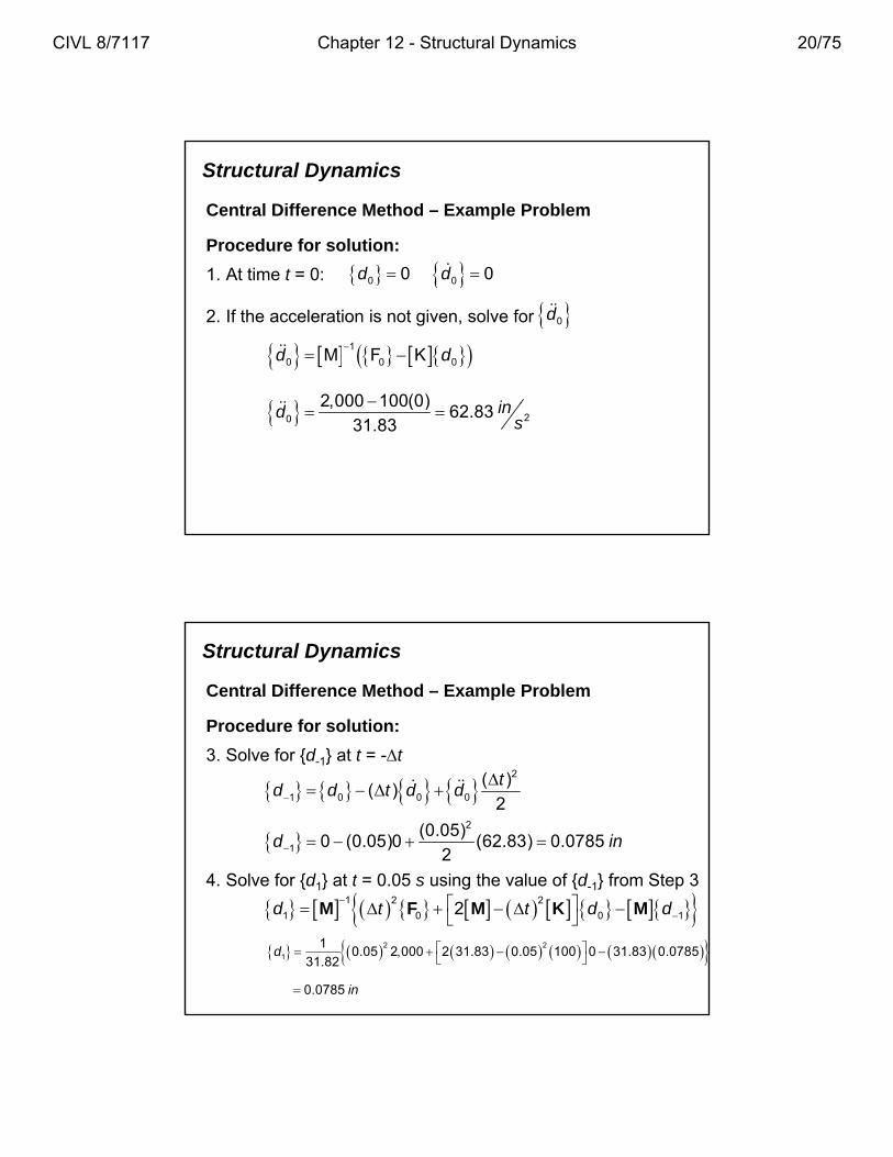
Structural Dynamics
Central Difference Method – Example Problem
Procedure for solution:
1 At time t = 0: 0 0d d1. At time t = 0: 0 00 0d d
2. If the acceleration is not given, solve for 0d
1
0 0 0M F Kd d
2 000 100(0) i 20
2,000 100(0)62.83
31.83ind
s
Structural Dynamics
Central Difference Method – Example Problem
Procedure for solution:
3 Solve for {d } at t = t3. Solve for {d-1} at t = -t
4. Solve for {d1} at t = 0.05 s using the value of {d 1} from Step 3
2
1 0 0 0
( )( )
2
td d t d d
2
1
(0.05)0 (0.05)0 (62.83) 0.0785
2d in
4. Solve for {d1} at t 0.05 s using the value of {d-1} from Step 3
1 2 2
1 0 0 12d t t d d
M F M K M
2 2
1
10.05 2,000 2 31.83 0.05 100 0 31.83 0.0785
31.82d
0.0785 in
CIVL 8/7117 Chapter 12 - Structural Dynamics 20/75
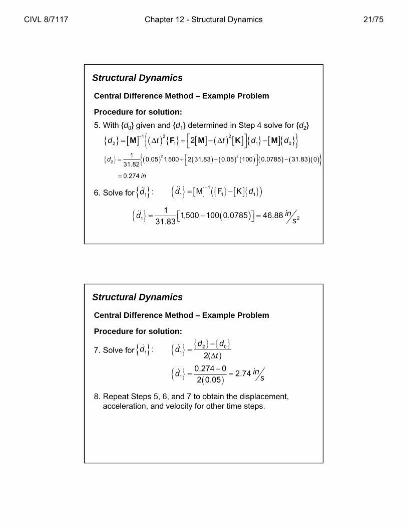
Structural Dynamics
Central Difference Method – Example Problem
Procedure for solution:
5 With {d } given and {d } determined in Step 4 solve for {d }5. With {d0} given and {d1} determined in Step 4 solve for {d2}
1 2 2
2 1 1 02d t t d d M F M K M
2 2
2
10.05 1,500 2 31.83 0.05 100 0.0785 31.83 0
31.82d
0.274 in
6. Solve for 1 :d 1
1 1 1M F Kd d
21
11,500 100 0.0785 46.88
31.83ind
s
Structural Dynamics
Central Difference Method – Example Problem
Procedure for solution:
d d7. Solve for 1 :d 2 0
1 2( )
d dd
t
8. Repeat Steps 5, 6, and 7 to obtain the displacement, l ti d l it f th ti t
1
0.274 02.74
2 0.05ind s
acceleration, and velocity for other time steps.
CIVL 8/7117 Chapter 12 - Structural Dynamics 21/75
Structural Dynamics
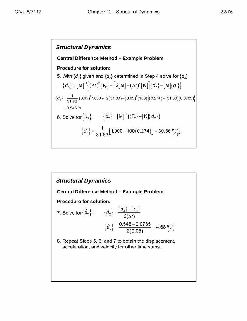
Central Difference Method – Example Problem
Procedure for solution:
5 With {d } given and {d } determined in Step 4 solve for {d }5. With {d1} given and {d2} determined in Step 4 solve for {d3}
1 2 2
3 2 2 12d t t d d M F M K M
2 2
3
10.05 1,000 2 31.83 0.05 100 0.274 31.83 0.0785
31.82d
0.546 in
6. Solve for 2 :d 1
2 2 2M F Kd d
22
11,000 100 0.274 30.56
31.83ind
s
Structural Dynamics
Central Difference Method – Example Problem
Procedure for solution:
d d7. Solve for 2 :d 3 1
2 2( )
d dd
t
8. Repeat Steps 5, 6, and 7 to obtain the displacement, l ti d l it f th ti t
2
0.546 0.07854.68
2 0.05ind s
acceleration, and velocity for other time steps.
CIVL 8/7117 Chapter 12 - Structural Dynamics 22/75
Structural Dynamics
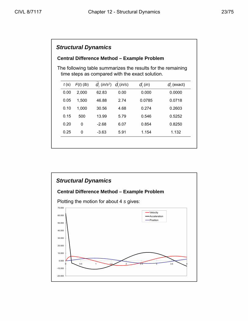
Central Difference Method – Example Problem
The following table summarizes the results for the remaining time steps as compared with the exact solution.time steps as compared with the exact solution.
t (s) F(t) (lb) (in/s2) (in/s) (in) (exact)
0.00 2,000 62.83 0.00 0.000 0.0000
0.05 1,500 46.88 2.74 0.0785 0.0718
0.10 1,000 30.56 4.68 0.274 0.2603
id id id id
0.15 500 13.99 5.79 0.546 0.5252
0.20 0 -2.68 6.07 0.854 0.8250
0.25 0 -3.63 5.91 1.154 1.132
Structural Dynamics
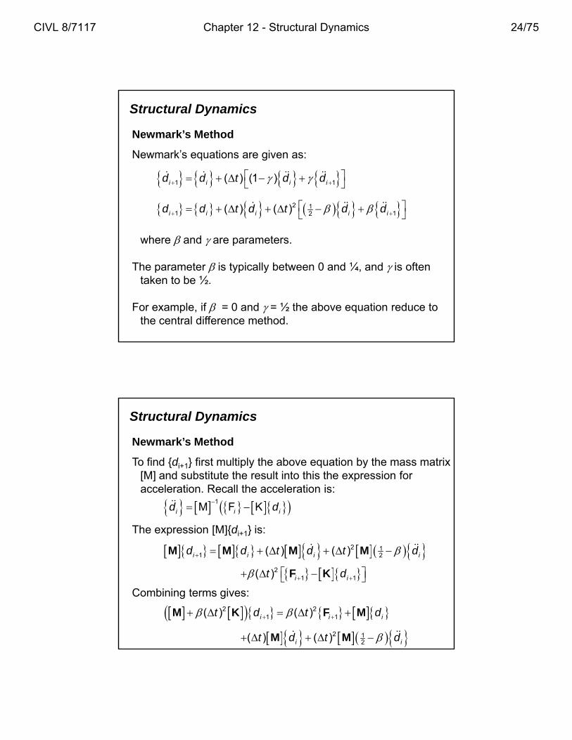
Central Difference Method – Example Problem
Plotting the motion for about 4 s gives:70.000
20 000
30.000
40.000
50.000
60.000Velocity
Acceleration
Position
-20.000
-10.000
0.000
10.000
20.000
0 0.5 1 1.5 2 2.5 3 3.5 4
CIVL 8/7117 Chapter 12 - Structural Dynamics 23/75
Structural Dynamics
Newmark’s Method
Newmark’s equations are given as:
( ) (1 )d d t d d 1 1( ) (1 )i i i id d t d d
2 11 12( ) ( )i i i i id d t d t d d
where and are parameters.
The parameter is typically between 0 and ¼, and is often taken to be ½.
For example, if = 0 and = ½ the above equation reduce to the central difference method.
Structural Dynamics
Newmark’s Method
To find {di+1} first multiply the above equation by the mass matrix [M] and substitute the result into this the expression for acceleration. Recall the acceleration is:
The expression [M]{di+1} is:
1M F Ki i id d
2 11 2( ) ( )i i i id d t d t dM M M M
2
1 1( ) i it d F K
Combining terms gives:
2 21 1( ) ( )i i it d t d M K F M
2 12( ) ( )i it d t dM M
CIVL 8/7117 Chapter 12 - Structural Dynamics 24/75
Structural Dynamics
Newmark’s Method
Dividing the above equation by (Δt)2 gives:
where:
1 1K' F'i id
where:
2
1'
( )tK K M
211 1 22
' ( ) ( )( )i i i i id t d t d
t
M
F F
The advantages of using Newmark’s method over the central difference method are that Newmark’s method can be made unconditionally stable (if = ¼ and = ½) and that larger time steps can be used with better results.
Structural Dynamics
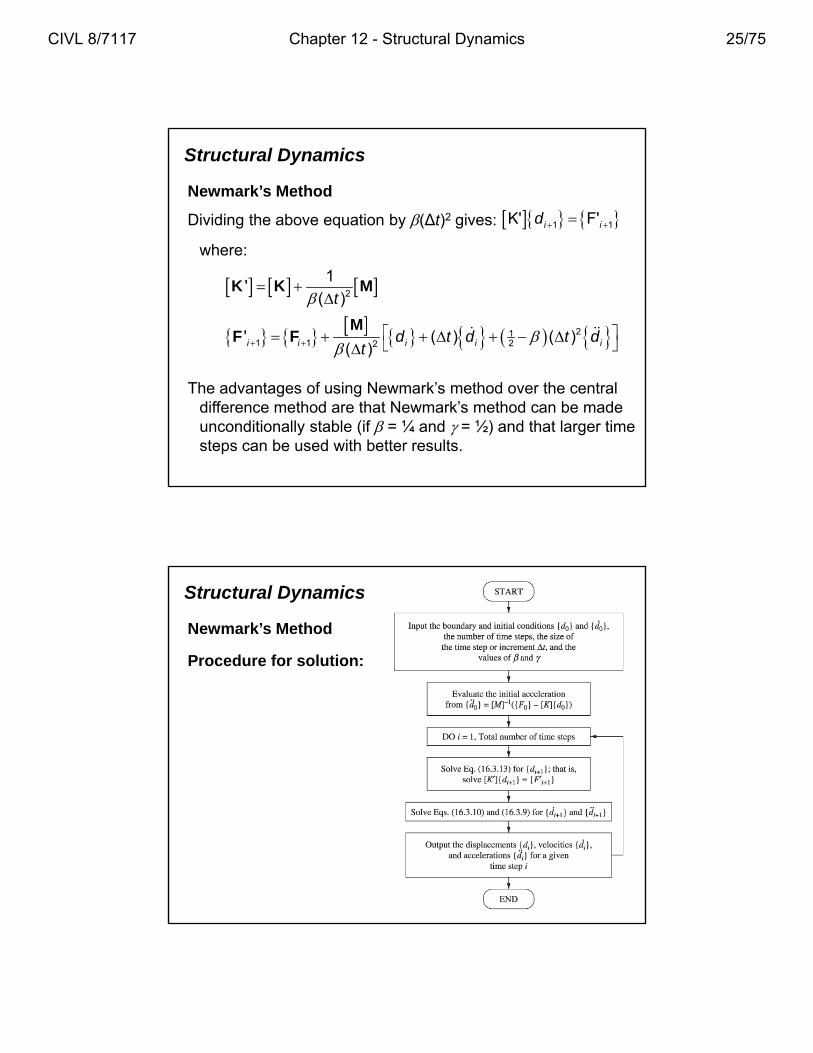
Newmark’s Method
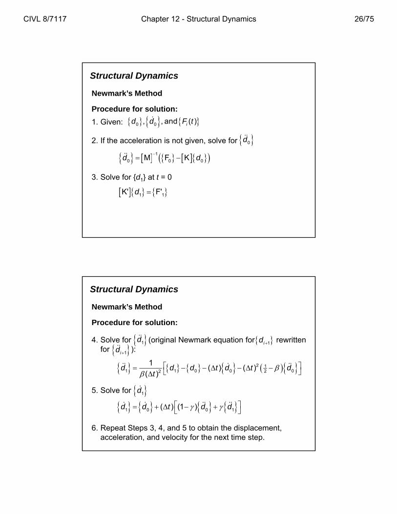
Procedure for solution:
CIVL 8/7117 Chapter 12 - Structural Dynamics 25/75
Structural Dynamics
Newmark’s Method
Procedure for solution:
1 Given: and ( )d d F t1. Given: 0 0, , and ( )id d F t
2. If the acceleration is not given, solve for 0d
1
0 0 0M F Kd d
3. Solve for {d1} at t = 03. Solve for {d1} at t 0
1 1K' F'd
Structural Dynamics
Newmark’s Method
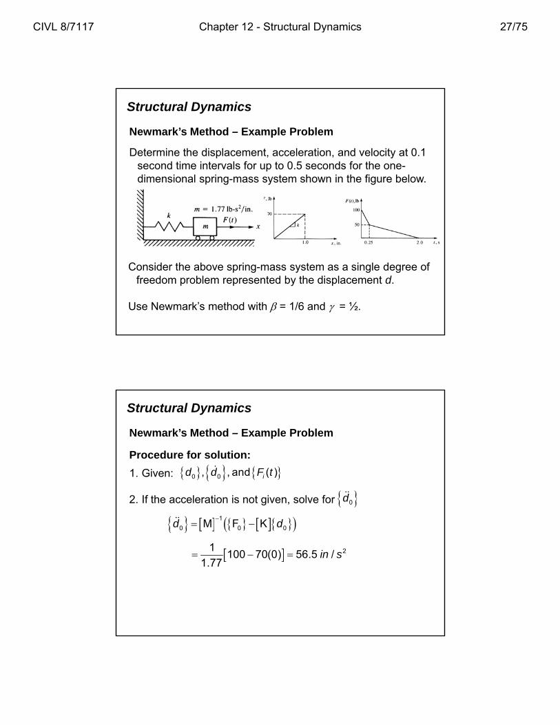
Procedure for solution:
2 11 1 0 0 022
1( ) ( )
( )d d d t d t d
t
4. Solve for (original Newmark equation for rewritten for ):
1d 1id
1id
5. Solve for 1d
1 0 0 1( ) (1 )d d t d d
5. Solve for 1d
6. Repeat Steps 3, 4, and 5 to obtain the displacement, acceleration, and velocity for the next time step.
CIVL 8/7117 Chapter 12 - Structural Dynamics 26/75
Structural Dynamics
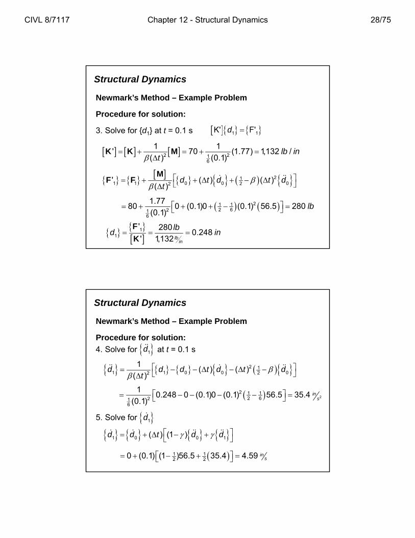
Newmark’s Method – Example Problem
Determine the displacement, acceleration, and velocity at 0.1 second time intervals for up to 0.5 seconds for the one-pdimensional spring-mass system shown in the figure below.
Consider the above spring-mass system as a single degree of freedom problem represented by the displacement d.
Use Newmark’s method with = 1/6 and = ½.
Structural Dynamics
Newmark’s Method – Example Problem
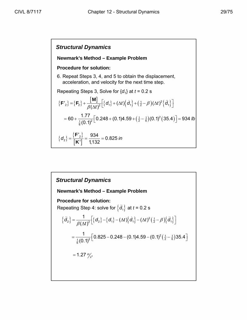
Procedure for solution:
1 Given: and ( )d d F t1. Given: 0 0, , and ( )id d F t
2. If the acceleration is not given, solve for 0d
1
0 0 0M F Kd d
21100 70(0) 56 5 /in s 100 70(0) 56.5 /
1.77in s
CIVL 8/7117 Chapter 12 - Structural Dynamics 27/75
Structural Dynamics
Newmark’s Method – Example Problem
Procedure for solution:
3. Solve for {d1} at t = 0.1 s 1 1K' F'd
2 216
1 1' 70 (1.77) 1,132 /
( ) (0.1)lb in
t
K K M
211 1 0 0 022' ( ) ( )
( )d t d t d
t
MF F
( )t
21 12 621
6
1.7780 0 (0.1)0 (0.1) 56.5 280
(0.1)lb
11
' 2800.248
' 1,132 lbin
lbd in
F
K
Structural Dynamics
Newmark’s Method – Example Problem
Procedure for solution:
4 Solve for at t = 0 1 s d4. Solve for at t = 0.1 s 1d
2 11 1 0 0 022
1( ) ( )
( )d d d t d t d
t
22 1 1
2 6216
10.248 0 (0.1)0 (0.1) 56.5 35.4
(0.1)in
s
1 0 0 1( ) (1 )d d t d d
5. Solve for 1d
1 12 20 (0.1) (1 )56.5 35.4 4.59 in
s
CIVL 8/7117 Chapter 12 - Structural Dynamics 28/75
Structural Dynamics
Newmark’s Method – Example Problem
Procedure for solution:
6 R t St 3 4 d 5 t bt i th di l t6. Repeat Steps 3, 4, and 5 to obtain the displacement, acceleration, and velocity for the next time step.
Repeating Steps 3, Solve for {d1} at t = 0.2 s
212 2 1 1 122' ( ) ( )
( )d t d t d
t
MF F
21 12 621
6
1.7760 0.248 (0.1)4.59 (0.1) 35.4 934
(0.1)lb
22
' 9340.825
' 1,132d in
F
K
Structural Dynamics
Newmark’s Method – Example Problem
Procedure for solution:
Repeating Step 4: solve for at t = 0 2 s dRepeating Step 4: solve for at t = 0.2 s 1d
2 12 2 1 1 122
1( ) ( )
( )d d d t d t d
t
2 1 12 621
6
10.825 0.248 (0.1)4.59 (0.1) 35.4
(0.1)
21.27 ins
CIVL 8/7117 Chapter 12 - Structural Dynamics 29/75
Structural Dynamics
Newmark’s Method – Example Problem
Procedure for solution:
2 1 1 2( ) (1 )d d t d d
5. Solve for 2d
1 12 24.59 (0.1) (1 )35.4 1.27 6.42 in
s
Structural Dynamics
Newmark’s Method – Example Problem
Procedure for solution:
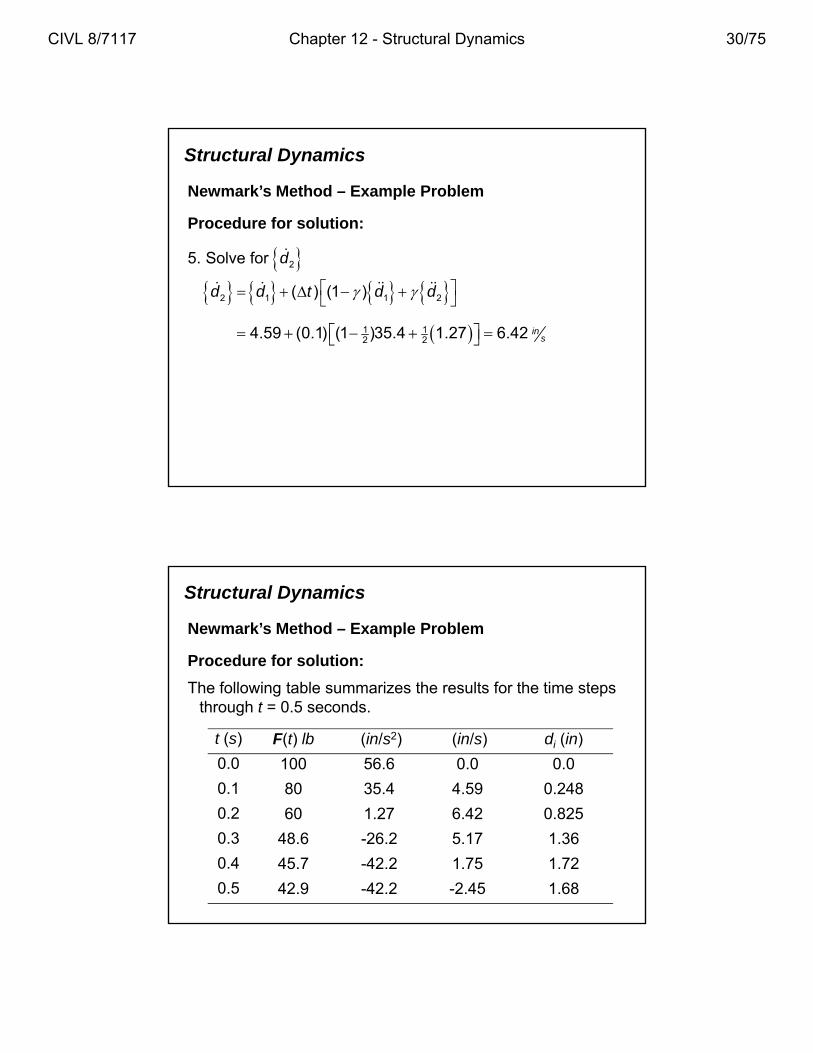
The following table summarizes the results for the time stepsThe following table summarizes the results for the time steps through t = 0.5 seconds.
t (s) F(t) lb (in/s2) (in/s) di (in)
0.0 100 56.6 0.0 0.0
0.1 80 35.4 4.59 0.248
0.2 60 1.27 6.42 0.825
0.3 48.6 -26.2 5.17 1.36
0.4 45.7 -42.2 1.75 1.72
0.5 42.9 -42.2 -2.45 1.68
CIVL 8/7117 Chapter 12 - Structural Dynamics 30/75
Structural Dynamics
Newmark’s Method – Example Problem
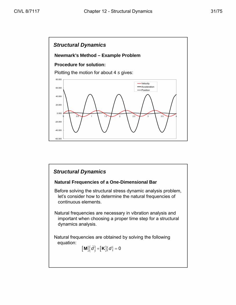
Procedure for solution:
Plotting the motion for about 4 s gives:Plotting the motion for about 4 s gives:
20.000
40.000
60.000
80.000
Velocity
Acceleration
Position
-60.000
-40.000
-20.000
0.000
0 0.5 1 1.5 2 2.5 3 3.5 4
Structural Dynamics
Natural Frequencies of a One-Dimensional Bar
Before solving the structural stress dynamic analysis problem, let’s consider how to determine the natural frequencies of qcontinuous elements.
Natural frequencies are necessary in vibration analysis and important when choosing a proper time step for a structural dynamics analysis.
Natural frequencies are obtained by solving the following equation:
0d d M K
CIVL 8/7117 Chapter 12 - Structural Dynamics 31/75
Structural Dynamics
Natural Frequencies of a One-Dimensional Bar
The standard solution for {d} is given as: ( ) ' i td t d e
where {d } is the part of the nodal displacement matrix called natural modes that is assumed to independent of time, i is the standard imaginary number, and is a natural frequency.
2' i td d e
Differentiating the above equation twice with respect to time gives: d d e
Substituting the above expressions for {d} and into the equation of motion gives:
d
2 ' ' 0i t i td e d e M K
Structural Dynamics
Natural Frequencies of a One-Dimensional Bar
Combining terms gives: 2 ' 0i te d K M
Since eit is not zero, then: 2 0 K M
The above equations are a set of linear homogeneous equations in terms of displacement mode {d }.
There exists a non trivial solution if and only if the determinant
2 0 K M
There exists a non-trivial solution if and only if the determinant of the coefficient matrix of is zero.
CIVL 8/7117 Chapter 12 - Structural Dynamics 32/75
Structural Dynamics
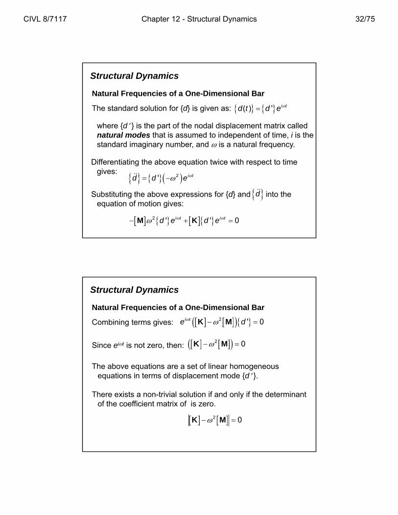
One-Dimensional Bar - Example Problem
Determine the first two natural frequencies for the bar shown in the figure below. g
Assume the bar has a length 2L, modulus of elasticity E, mass density , and cross-sectional area A.
Structural Dynamics
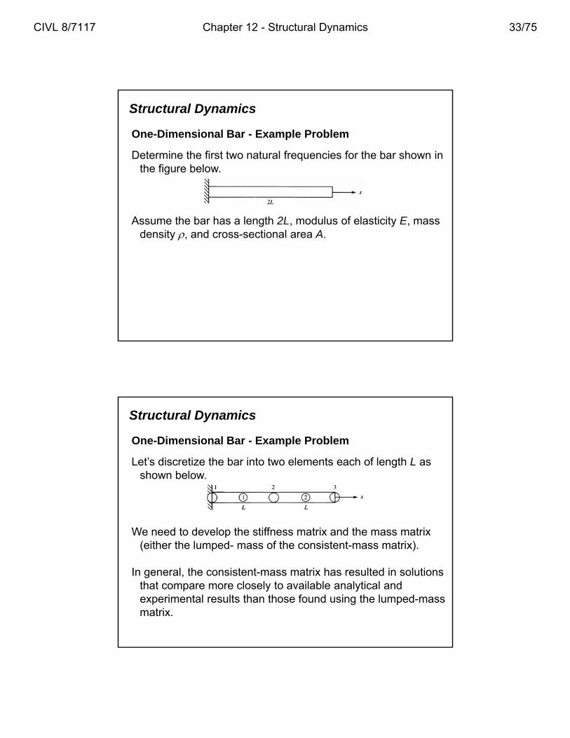
One-Dimensional Bar - Example Problem
Let’s discretize the bar into two elements each of length L as shown below.
We need to develop the stiffness matrix and the mass matrix (either the lumped- mass of the consistent-mass matrix).
In general, the consistent-mass matrix has resulted in solutions that compare more closely to available analytical and experimental results than those found using the lumped-mass matrix.
CIVL 8/7117 Chapter 12 - Structural Dynamics 33/75
Structural Dynamics
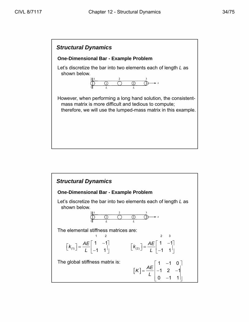
One-Dimensional Bar - Example Problem
Let’s discretize the bar into two elements each of length L as shown below.
However, when performing a long hand solution, the consistent-mass matrix is more difficult and tedious to compute; therefore, we will use the lumped-mass matrix in this example.p p
Structural Dynamics
One-Dimensional Bar - Example Problem
Let’s discretize the bar into two elements each of length L as shown below.
The elemental stiffness matrices are:1 2 2 3
1 1 1 1AE AEk k
(1) (2)1 1 1 1k k
L L
The global stiffness matrix is:
1 1 0
1 2 1
0 1 1
AEK
L
CIVL 8/7117 Chapter 12 - Structural Dynamics 34/75
Structural Dynamics
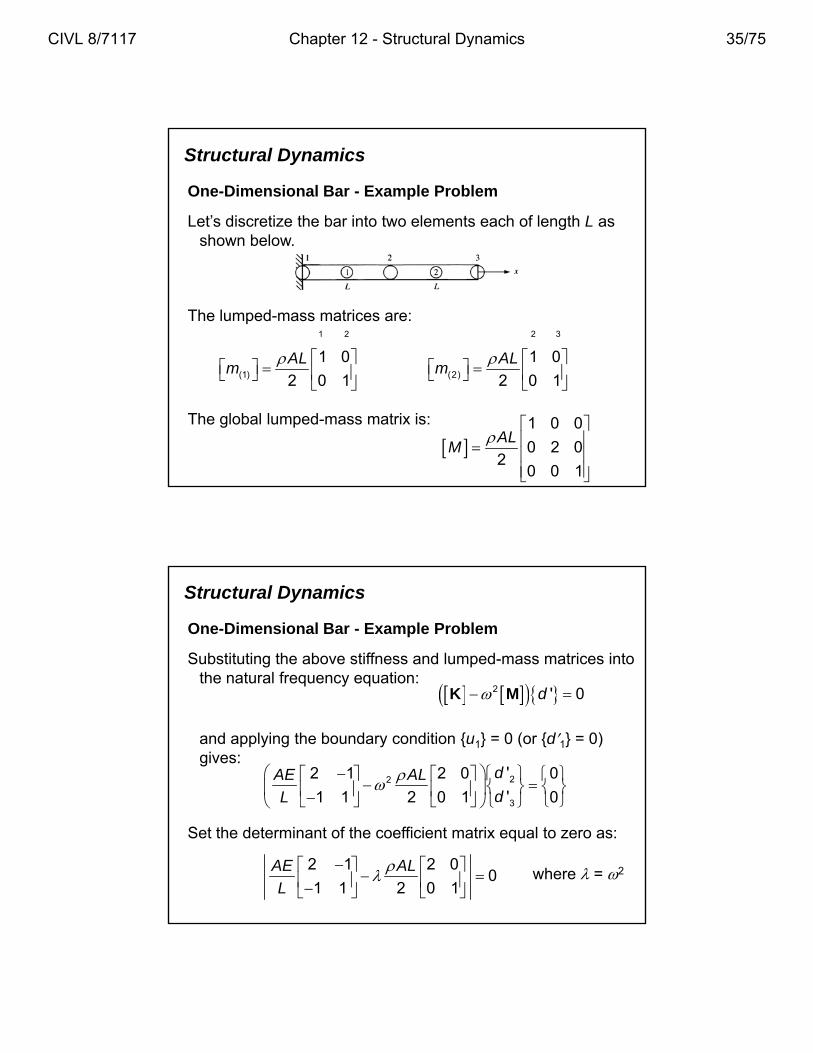
One-Dimensional Bar - Example Problem
Let’s discretize the bar into two elements each of length L as shown below.
The lumped-mass matrices are:1 2 2 3
1 0 1 0AL ALm m
(1) (2)2 0 1 2 0 1m m
The global lumped-mass matrix is:
1 0 0
0 2 02
0 0 1
ALM
Structural Dynamics
One-Dimensional Bar - Example Problem
Substituting the above stiffness and lumped-mass matrices into the natural frequency equation:
q y q
and applying the boundary condition {u1} = 0 (or {d1} = 0) gives:
2 ' 0d K M
22
3
'2 1 2 0 0
'1 1 2 0 1 0
dAE ALdL
3
Set the determinant of the coefficient matrix equal to zero as:
2 1 2 00
1 1 2 0 1
AE AL
L
where = 2
CIVL 8/7117 Chapter 12 - Structural Dynamics 35/75
Structural Dynamics
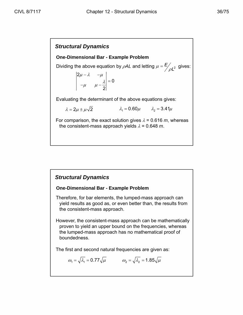
One-Dimensional Bar - Example Problem
2
Dividing the above equation by AL and letting gives:2E
L
20
2
Evaluating the determinant of the above equations gives:
2 2 1 20.60 3.41 2 2
For comparison, the exact solution gives = 0.616 m, whereas the consistent-mass approach yields = 0.648 m.
1 20.60 3.41
Structural Dynamics
One-Dimensional Bar - Example Problem
Therefore, for bar elements, the lumped-mass approach can yield results as good as, or even better than, the results fromyield results as good as, or even better than, the results from the consistent-mass approach.
However, the consistent-mass approach can be mathematically proven to yield an upper bound on the frequencies, whereas the lumped-mass approach has no mathematical proof of boundedness.
1 1 2 20.77 1.85
The first and second natural frequencies are given as:
CIVL 8/7117 Chapter 12 - Structural Dynamics 36/75
Structural Dynamics
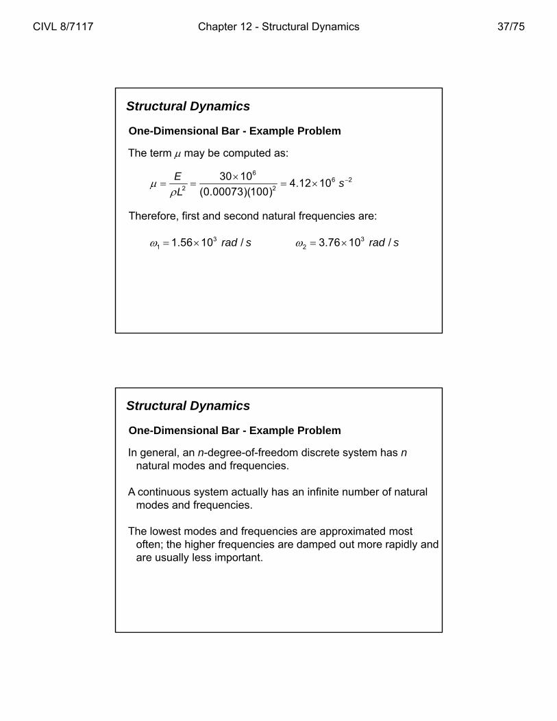
One-Dimensional Bar - Example Problem
The term may be computed as:
66 2
2 2
30 104.12 10
(0.00073)(100)
Es
L
Therefore, first and second natural frequencies are:
3 31 21.56 10 / 3.76 10 /rad s rad s
Structural Dynamics
One-Dimensional Bar - Example Problem
In general, an n-degree-of-freedom discrete system has nnatural modes and frequencies.natural modes and frequencies.
A continuous system actually has an infinite number of natural modes and frequencies.
The lowest modes and frequencies are approximated most often; the higher frequencies are damped out more rapidly and are usually less important.
CIVL 8/7117 Chapter 12 - Structural Dynamics 37/75
Structural Dynamics
One-Dimensional Bar - Example Problem
Substituting 1 into the following equation
22
3
'2 1 2 0 0
'1 1 2 0 1 0
dAE ALdL
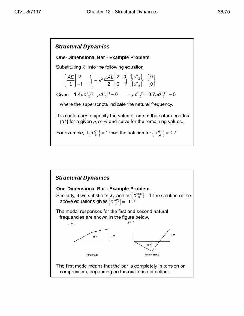
Gives: (1) (1) (1) (1)2 3 2 31.4 ' ' 0 ' 0.7 ' 0d d d d
where the superscripts indicate the natural frequency.
It is customary to specify the value of one of the natural modes {d } for a given i or i and solve for the remaining values.
For example, if than the solution for (1)3' 1d (1)
2' 0.7d
Structural Dynamics
One-Dimensional Bar - Example Problem
Similarly, if we substitute 2 and let the solution of the above equations gives
(2)3' 1d
(2)2' 0.7d
The modal responses for the first and second natural frequencies are shown in the figure below.
The first mode means that the bar is completely in tension or compression, depending on the excitation direction.
CIVL 8/7117 Chapter 12 - Structural Dynamics 38/75
Structural Dynamics
One-Dimensional Bar - Example Problem
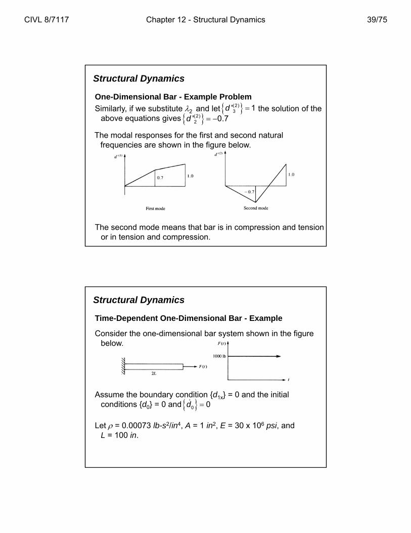
Similarly, if we substitute 2 and let the solution of the above equations gives
(2)3' 1d
(2)2' 0.7d
The modal responses for the first and second natural frequencies are shown in the figure below.
The second mode means that bar is in compression and tension or in tension and compression.
Structural Dynamics
Time-Dependent One-Dimensional Bar - Example
Consider the one-dimensional bar system shown in the figure below.
Assume the boundary condition {d1x} = 0 and the initial conditions {d0} = 0 and 0 0d { 0} 0
Let = 0.00073 lb-s2/in4, A = 1 in2, E = 30 x 106 psi, and L = 100 in.
CIVL 8/7117 Chapter 12 - Structural Dynamics 39/75
Structural Dynamics
Time-Dependent One-Dimensional Bar - Example
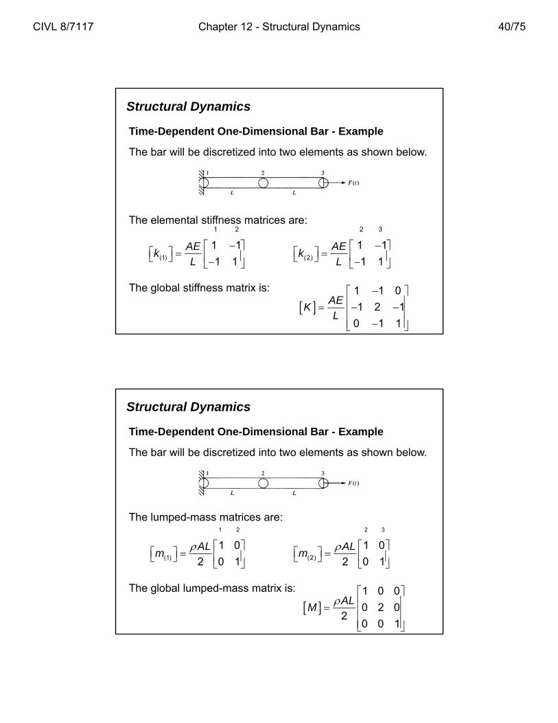
The bar will be discretized into two elements as shown below.
The elemental stiffness matrices are:1 2 2 3
1 1 1 1AE AEk k
(1) (2)1 1 1 1k k
L L
The global stiffness matrix is:
1 1 0
1 2 1
0 1 1
AEK
L
Structural Dynamics
Time-Dependent One-Dimensional Bar - Example
The bar will be discretized into two elements as shown below.
The lumped-mass matrices are:1 2 2 3
1 0 1 0AL ALm m
(1) (2)2 0 1 2 0 1m m
The global lumped-mass matrix is:
1 0 0
0 2 02
0 0 1
ALM
CIVL 8/7117 Chapter 12 - Structural Dynamics 40/75
Structural Dynamics
Time-Dependent One-Dimensional Bar - Example
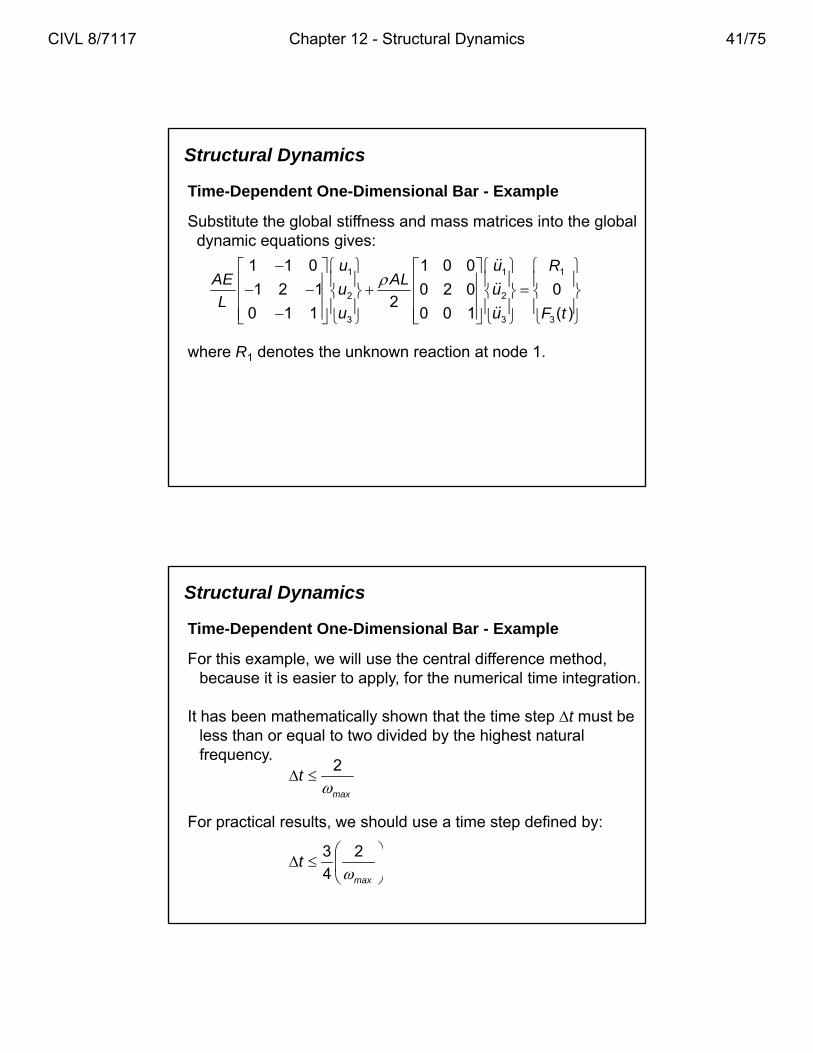
Substitute the global stiffness and mass matrices into the global dynamic equations gives:y q g
1 1 1
2 2
3 3 3
1 1 0 1 0 0
1 2 1 0 2 0 02
0 1 1 0 0 1 ( )
u u RAE AL
u uL
u u F t
where R1 denotes the unknown reaction at node 1.
Structural Dynamics
Time-Dependent One-Dimensional Bar - Example
For this example, we will use the central difference method, because it is easier to apply, for the numerical time integration.pp y, g
It has been mathematically shown that the time step t must be less than or equal to two divided by the highest natural frequency.
2
max
t
For practical results, we should use a time step defined by:
3 2
4 max
t
CIVL 8/7117 Chapter 12 - Structural Dynamics 41/75
Structural Dynamics
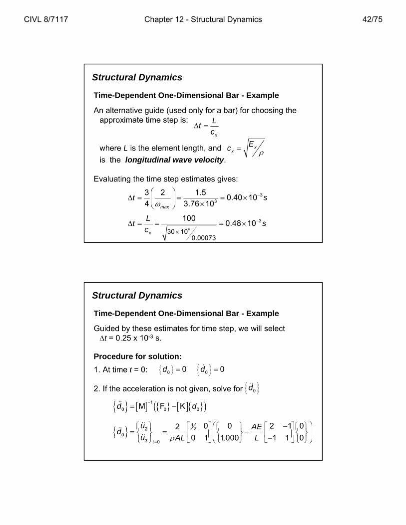
Time-Dependent One-Dimensional Bar - Example
An alternative guide (used only for a bar) for choosing the approximate time step is: L
tpp p
x
tc
where L is the element length, and xx
Ec is the longitudinal wave velocity.
Evaluating the time step estimates gives:
33
3 2 1.50.40 10
4 3.76 10max
t s
g g
6
3
30 100.00073
1000.48 10
x
Lt s
c
Structural Dynamics
Time-Dependent One-Dimensional Bar - Example
Guided by these estimates for time step, we will select t = 0.25 x 10⁻³ s.
Procedure for solution:
1. At time t = 0: 0 00 0d d
2. If the acceleration is not given, solve for 0d
1 1
0 0 0M F Kd d
1
220
3 0
0 0 2 1 02
0 1 1,000 1 1 0t
u AEd
u AL L
CIVL 8/7117 Chapter 12 - Structural Dynamics 42/75
Structural Dynamics
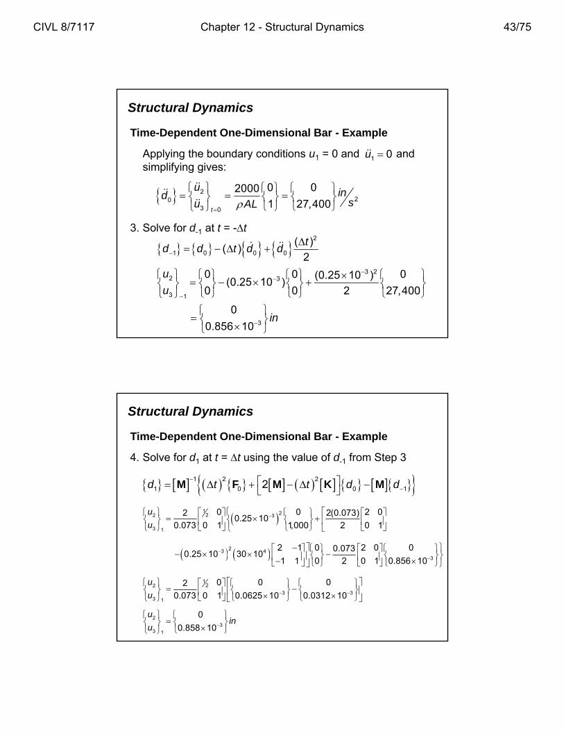
Time-Dependent One-Dimensional Bar - Example
Applying the boundary conditions u1 = 0 and and simplifying gives:
1 0u p y g g
3. Solve for d-1 at t = -t
2
1 0 0 0
( )( )
2
td d t d d
220
3 0
0 02000
1 27,400t
u indsu AL
1 0 0 0 23 2
2 3
3 1
0 0 0(0.25 10 )(0.25 10 )
0 0 2 27,400
u
u
3
0
0.856 10in
Structural Dynamics
Time-Dependent One-Dimensional Bar - Example
4. Solve for d1 at t = t using the value of d-1 from Step 3
1 2 2
1 0 0 12d t t d d
M F M K M
1 222 3
3 1
0 0 2 02 2(0.073)0.25 10
0.073 0 1 1,000 2 0 1
u
u
23 43
2 1 0 2 0 00.0730.25 10 30 10
1 1 0 2 0 1 0 856 10
31 1 0 2 0 1 0.856 10
122
3 33 1
0 0 02
0.073 0 1 0.0625 10 0.0312 10
u
u
2
33 1
0
0.858 10
uin
u
CIVL 8/7117 Chapter 12 - Structural Dynamics 43/75
Structural Dynamics
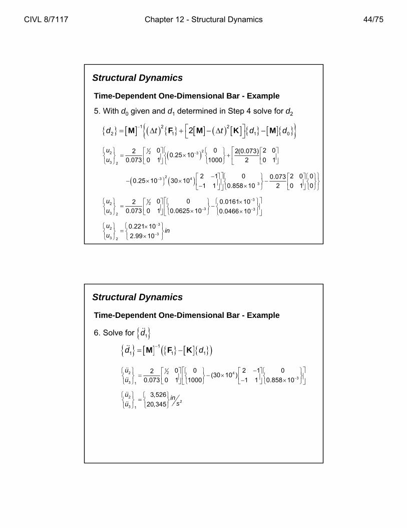
Time-Dependent One-Dimensional Bar - Example
5. With d0 given and d1 determined in Step 4 solve for d2
1 2 2
2 1 1 02d t t d d M F M K M
1 222 3
3 2
0 0 2 02 2(0.073)0.25 10
0.073 0 1 1000 2 0 1
u
u
23 43
2 1 0 2 0 00.0730.25 10 30 10
1 1 0 858 10 2 0 1 0
31 1 0.858 10 2 0 1 0
3122
3 33 2
0 0 0.0161 102
0.073 0 1 0.0625 10 0.0466 10
u
u
32
33 2
0.221 10
2.99 10
uin
u
Structural Dynamics
Time-Dependent One-Dimensional Bar - Example
6. Solve for 1d
1
1 1 1d d
M F K
122 4
33 1
0 0 2 1 02(30 10 )
0.073 0 1 1000 1 1 0.858 10
u
u
22
3,526
20 345
u insu
3 120,345 su
CIVL 8/7117 Chapter 12 - Structural Dynamics 44/75
Structural Dynamics
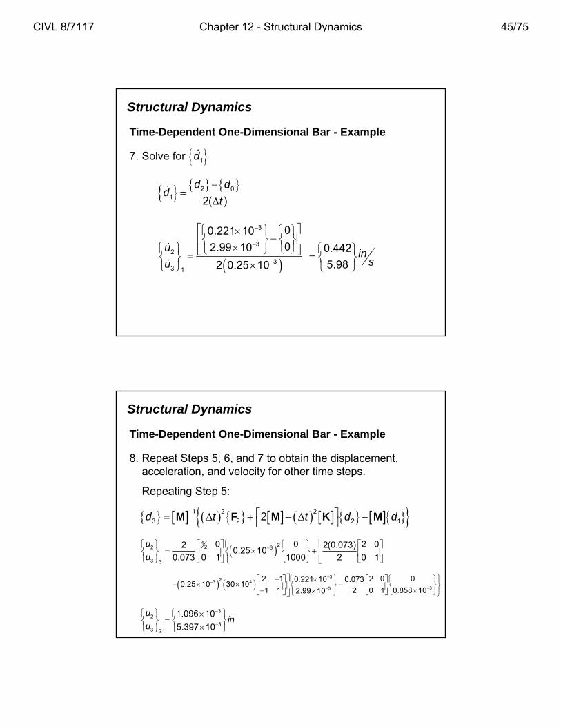
Time-Dependent One-Dimensional Bar - Example
7. Solve for 1d
2 01 2( )
d dd
t
3
32
00.221 10
02.99 10u
0.442 in
2
33 1 2 0.25 10u
5.98
ins
Structural Dynamics
Time-Dependent One-Dimensional Bar - Example
8. Repeat Steps 5, 6, and 7 to obtain the displacement, acceleration and velocity for other time stepsacceleration, and velocity for other time steps.
Repeating Step 5:
1 2 2
3 2 2 12d t t d d M F M K M
1 222 30 0 2 02 2(0.073)
0.25 100 073 0 1 1000 2 0 1
u
u
3 3
0.073 0 1 1000 2 0 1u
3
23 433
2 1 2 0 00.221 10 0.0730.25 10 30 10
1 1 2 0 1 0.858 102.99 10
32
33 2
1.096 10
5.397 10
uin
u
CIVL 8/7117 Chapter 12 - Structural Dynamics 45/75
Structural Dynamics
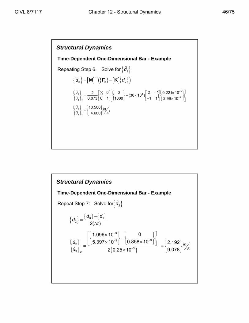
Time-Dependent One-Dimensional Bar - Example
Repeating Step 6. Solve for 2d
1
2 2 2d d
M F K
3122 4
33 2
0 0 2 1 0.221 102(30 10 )
0.073 0 1 1000 1 1 2.99 10
u
u
22
10,500
4 600
u insu
3 14,600 su
Structural Dynamics
Time-Dependent One-Dimensional Bar - Example
Repeat Step 7: Solve for 2d
3 12 2( )
d dd
t
3
332
01.096 10
0.858 105.397 10u
2.192 in 3
3 2 2 0.25 10u 9.078 s
CIVL 8/7117 Chapter 12 - Structural Dynamics 46/75
Structural Dynamics
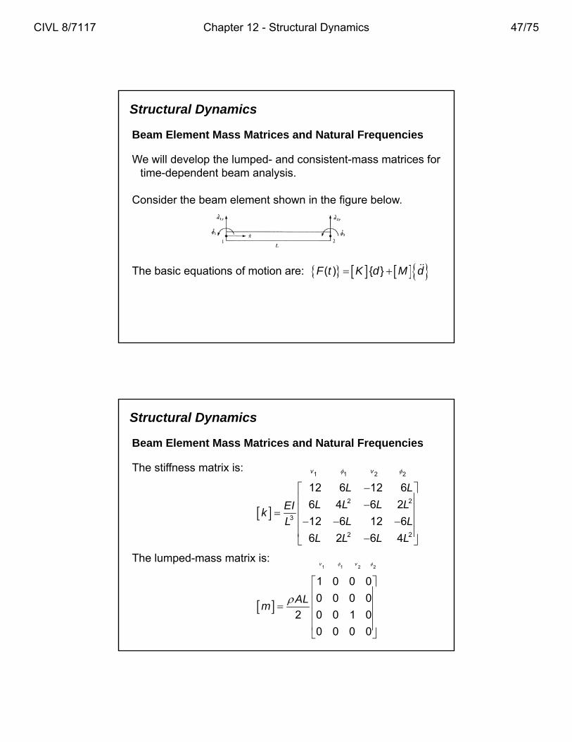
Beam Element Mass Matrices and Natural Frequencies
We will develop the lumped- and consistent-mass matrices for time-dependent beam analysistime dependent beam analysis.
Consider the beam element shown in the figure below.
( ) { }F t K d M d The basic equations of motion are:
Structural Dynamics
Beam Element Mass Matrices and Natural Frequencies
1 1 2 2v v The stiffness matrix is:
2 2
3
2 2
12 6 12 6
6 4 6 2
12 6 12 6
6 2 6 4
L L
L L L LEIk
L L L
L L L L
The lumped-mass matrix is:1 1 2 2
v v
1 1 2 2
1 0 0 0
0 0 0 0
2 0 0 1 0
0 0 0 0
ALm
CIVL 8/7117 Chapter 12 - Structural Dynamics 47/75
Structural Dynamics
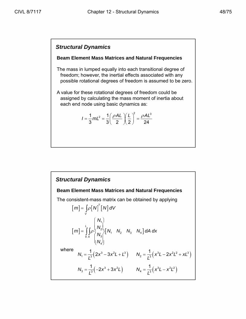
Beam Element Mass Matrices and Natural Frequencies
The mass in lumped equally into each transitional degree of freedom; however the inertial effects associated with anyfreedom; however, the inertial effects associated with any possible rotational degrees of freedom is assumed to be zero.
A value for these rotational degrees of freedom could be assigned by calculating the mass moment of inertia about each end node using basic dynamics as:
2 321 1
3 3 2 2 24
AL L ALI mL
Structural Dynamics
Beam Element Mass Matrices and Natural Frequencies
The consistent-mass matrix can be obtained by applying
T
m N N dV V
m N N dV
1
21 2 3 4
30
4
L
A
N
Nm N N N N dA dx
N
N
where 4
3 2 31 3
12 3N x x L L
L 3 2 2 3
2 3
12N x L x L xL
L
3 23 3
12 3N x x L
L 3 2 2
4 3
1N x L x L
L
CIVL 8/7117 Chapter 12 - Structural Dynamics 48/75
Structural Dynamics
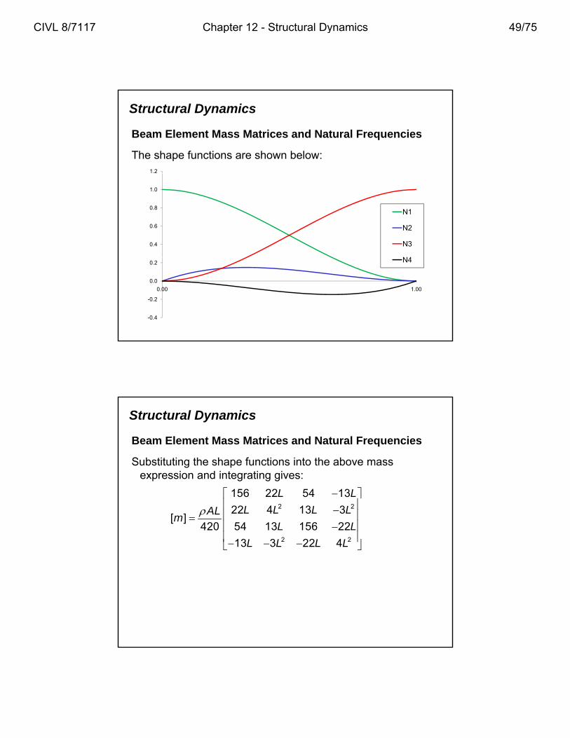
Beam Element Mass Matrices and Natural Frequencies
The shape functions are shown below:1.2
0.4
0.6
0.8
1.0
N1
N2
N3
N4
-0.4
-0.2
0.0
0.2
0.00 1.00
N4
Structural Dynamics
Beam Element Mass Matrices and Natural Frequencies
Substituting the shape functions into the above mass expression and integrating gives:p g g g
2 2
2 2
156 22 54 13
22 4 13 3[ ]
420 54 13 156 22
13 3 22 4
L L
L L L LALm
L L
L L L L
CIVL 8/7117 Chapter 12 - Structural Dynamics 49/75
Structural Dynamics
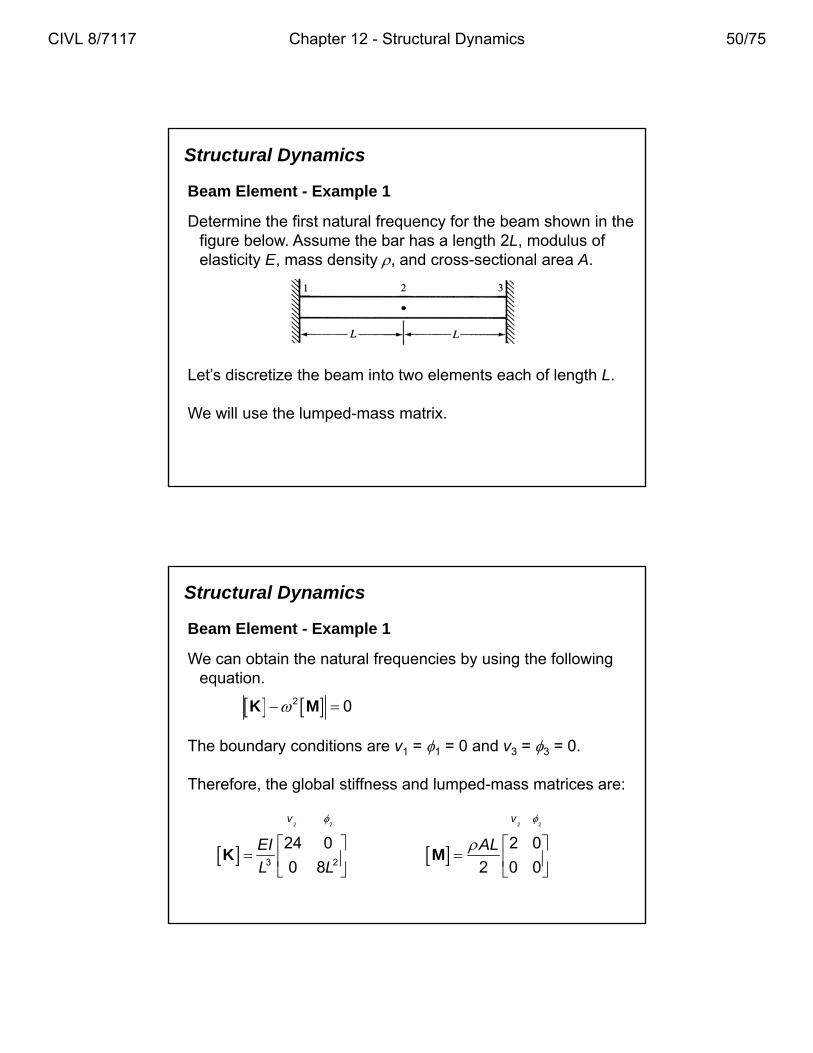
Beam Element - Example 1
Determine the first natural frequency for the beam shown in the figure below. Assume the bar has a length 2L, modulus of g g ,elasticity E, mass density , and cross-sectional area A.
Let’s discretize the beam into two elements each of length L.
We will use the lumped-mass matrix.
Structural Dynamics
Beam Element - Example 1
We can obtain the natural frequencies by using the following equation.q
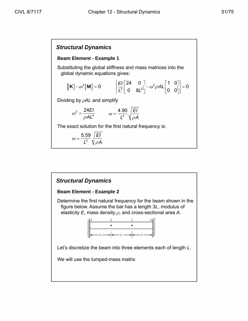
The boundary conditions are v1 = 1 = 0 and v3 = 3 = 0.
Therefore, the global stiffness and lumped-mass matrices are:
2 0 K M
2 2
3 2
24 0
0 8
v
EI
L L
K
2 2
2 0
2 0 0
v
AL
M
CIVL 8/7117 Chapter 12 - Structural Dynamics 50/75
Structural Dynamics
Beam Element - Example 1
Substituting the global stiffness and mass matrices into the global dynamic equations gives:g y q g
2 0 K M
23 2
24 0 1 00
0 8 0 0
EIAL
L L
2 24EI
Dividing by AL and simplify
4.90 EI24AL
2
4.90 EI
L A
The exact solution for the first natural frequency is:
2
5.59 EI
L A
Structural Dynamics
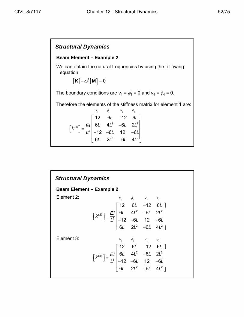
Beam Element - Example 2
Determine the first natural frequency for the beam shown in the figure below. Assume the bar has a length 3L, modulus of g g ,elasticity E, mass density , and cross-sectional area A.
Let’s discretize the beam into three elements each of length L.
We will use the lumped-mass matrix.
CIVL 8/7117 Chapter 12 - Structural Dynamics 51/75
Structural Dynamics
Beam Element – Example 2
We can obtain the natural frequencies by using the following equation.q
The boundary conditions are v1 = 1 = 0 and v4 = 4 = 0.
Therefore the elements of the stiffness matrix for element 1 are:
2 0 K M
v v
1 1 2 2
2 2(1)
3
2 2
12 6 12 6
6 4 6 2
12 6 12 6
6 2 6 4
v v
L L
L L L LEIk
L L L
L L L L
Structural Dynamics
Beam Element – Example 2
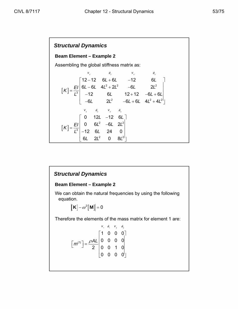
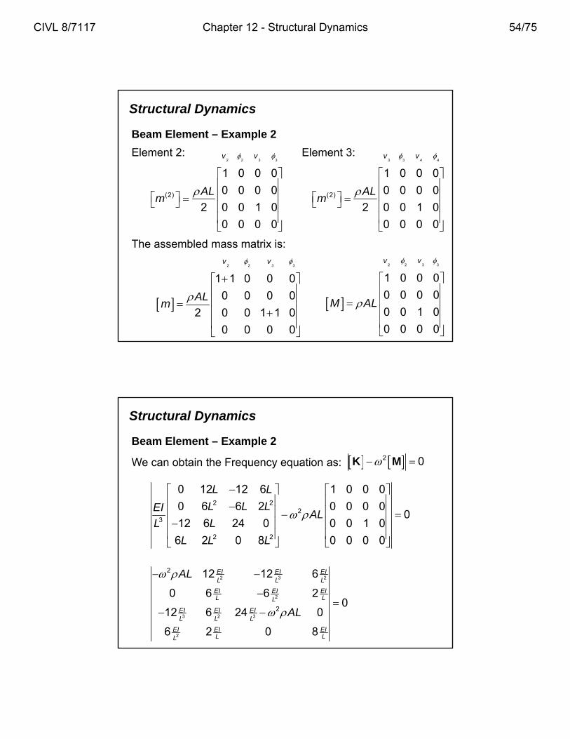
Element 2:
2 2 3 3
12 6 12 6
v v
L L
2 2(2)
3
2 2
12 6 12 6
6 4 6 2
12 6 12 6
6 2 6 4
L L
L L L LEIk
L L L
L L L L
Element 3:3 3 4 4
v v
2 2(3)
3
2 2
12 6 12 6
6 4 6 2
12 6 12 6
6 2 6 4
L L
L L L LEIk
L L L
L L L L
CIVL 8/7117 Chapter 12 - Structural Dynamics 52/75
Structural Dynamics
Beam Element – Example 2
Assembling the global stiffness matrix as:
v v
2 2 3 3
2 2 2
3
2 2 2
12 12 6 6 12 6
6 6 4 2 6 2
12 6 12 12 6 6
6 2 6 6 4 4
v v
L L L
L L L L L LEIK
L L L L
L L L L L L
2 2 3 3
2 2
3
2 2
0 12 12 6
0 6 6 2
12 6 24 0
6 2 0 8
v v
L L
L L LEIK
L L
L L L
Structural Dynamics
Beam Element – Example 2
We can obtain the natural frequencies by using the following equation.q
Therefore the elements of the mass matrix for element 1 are:
2 0 K M
1 1 2 2
1 0 0 0
v v
(1) 0 0 0 0
2 0 0 1 0
0 0 0 0
ALm
CIVL 8/7117 Chapter 12 - Structural Dynamics 53/75
Structural Dynamics
Beam Element – Example 2
Element 2:
2 2 3 3
1 0 0 0
v v Element 3:
3 3 4 4
1 0 0 0
v v
(2)
1 0 0 0
0 0 0 0
2 0 0 1 0
0 0 0 0
ALm
(2)
1 0 0 0
0 0 0 0
2 0 0 1 0
0 0 0 0
ALm
The assembled mass matrix is:
2 2 3 3
1 1 0 0 0
0 0 0 0
2 0 0 1 1 0
0 0 0 0
v v
ALm
2 2 3 3
1 0 0 0
0 0 0 0
0 0 1 0
0 0 0 0
v v
M AL
Structural Dynamics
Beam Element – Example 2
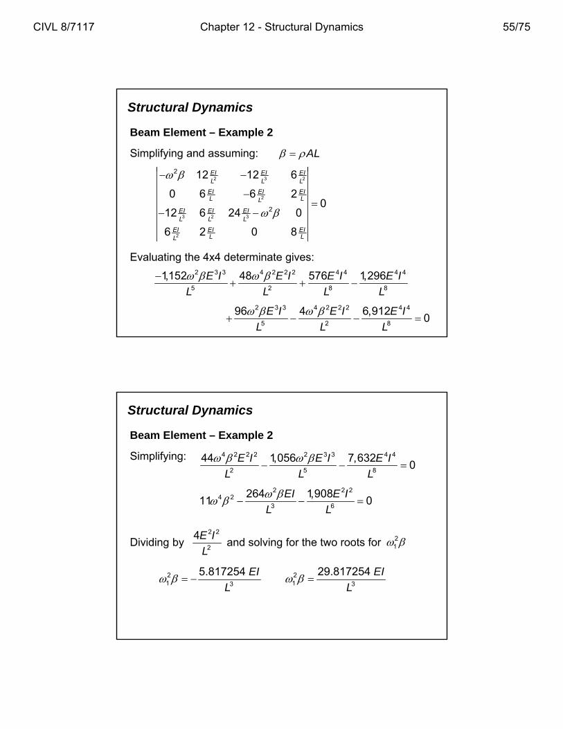
We can obtain the Frequency equation as: 2 0 K M
2 22
3
2 2
0 12 12 6 1 0 0 0
0 6 6 2 0 0 0 00
12 6 24 0 0 0 1 0
6 2 0 8 0 0 0 0
L L
L L LEIAL
L L
L L L
2 3 2
2
3 2 3
2
2
2
12 12 6
0 6 6 20
12 6 24 0
6 2 0 8
EI EI EIL L L
EI EI EIL LL
EI EI EIL L L
EI EI EIL LL
AL
AL
CIVL 8/7117 Chapter 12 - Structural Dynamics 54/75
Structural Dynamics
Beam Element – Example 2
Simplifying and assuming: AL 2 12 12 6EI EI EI
2 3 2
2
3 2 3
2
2
2
12 12 6
0 6 6 20
12 6 24 0
6 2 0 8
EI EI EIL L L
EI EI EIL LL
EI EI EIL L L
EI EI EIL LL
E l ti th 4 4 d t i t iEvaluating the 4x4 determinate gives:
2 3 3 4 2 2 2 4 4 4 4
5 2 8 8
1,152 48 576 1,296E I E I E I E I
L L L L
2 3 3 4 2 2 2 4 4
5 2 8
96 4 6,9120
E I E I E I
L L L
Structural Dynamics
Beam Element – Example 2
Simplifying:
4 2 2 2 2 3 3 4 4
2 5 8
44 1,056 7,6320
E I E I E I
L L L
L L L
2 2 2
4 23 6
264 1,90811 0
EI E I
L L
Dividing by and solving for the two roots for 2 2
2
4E I
L21
21 3
5.817254 EI
L 2
1 3
29.817254 EI
L
CIVL 8/7117 Chapter 12 - Structural Dynamics 55/75
Structural Dynamics
Beam Element – Example 2
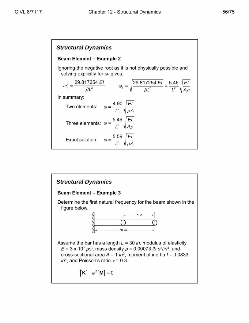
Ignoring the negative root as it is not physically possible and solving explicitly for 1 gives:g p y 1 g
1 3 2
29.817254 5.46EI EI
L L A
2
1 3
29.817254 EI
L
In summary:
Two elements: 2
4.90 EI
L A
Three elements:
Exact solution:
2
5.59 EI
L A
2
5.46 EI
L A
Structural Dynamics
Beam Element – Example 3
Determine the first natural frequency for the beam shown in the figure below. g
Assume the bar has a length L = 30 in, modulus of elasticity 7 2/ 4E = 3 x 10⁷ psi, mass density = 0.00073 lb-s2/in4, and
cross-sectional area A = 1 in2, moment of inertia I = 0.0833 in4, and Poisson’s ratio = 0.3.
2 0 K M
CIVL 8/7117 Chapter 12 - Structural Dynamics 56/75
Structural Dynamics
Beam Element – Example 3
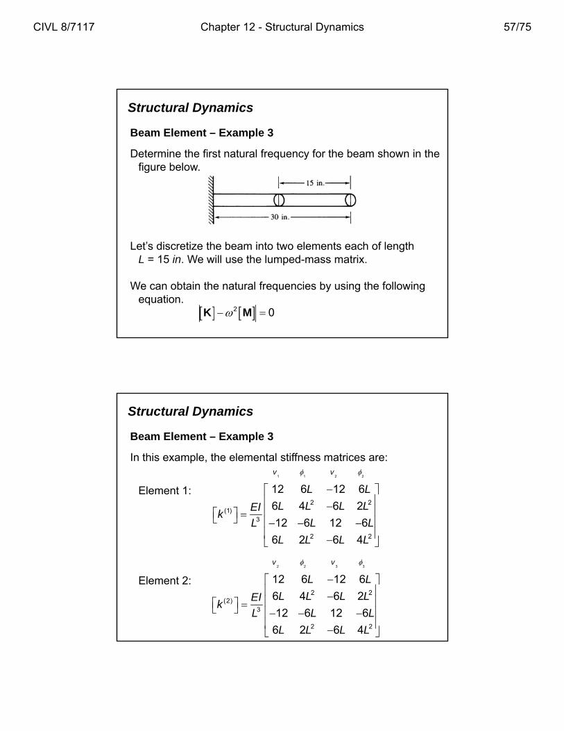
Determine the first natural frequency for the beam shown in the figure below. g
Let’s discretize the beam into two elements each of length L = 15 in. We will use the lumped-mass matrix.
We can obtain the natural frequencies by using the following equation.
2 0 K M
Structural Dynamics
Beam Element – Example 3
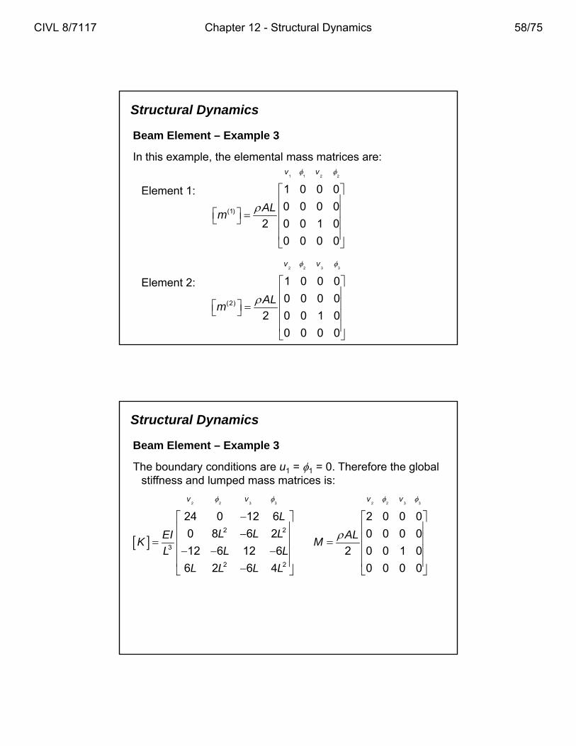
In this example, the elemental stiffness matrices are:
1 1 2 2v v
Element 1:
1 1 2 2
2 2(1)
3
2 2
12 6 12 6
6 4 6 2
12 6 12 6
6 2 6 4
L L
L L L LEIk
L L L
L L L L
Element 2:
2 2 3 3
2 2(2)
3
2 2
12 6 12 6
6 4 6 2
12 6 12 6
6 2 6 4
v v
L L
L L L LEIk
L L L
L L L L
CIVL 8/7117 Chapter 12 - Structural Dynamics 57/75
Structural Dynamics
Beam Element – Example 3
In this example, the elemental mass matrices are:
1 1 2 2v v
Element 1:
1 1 2 2
(1)
1 0 0 0
0 0 0 0
2 0 0 1 0
0 0 0 0
ALm
Element 2:
2 2 3 3
(2)
1 0 0 0
0 0 0 0
2 0 0 1 0
0 0 0 0
v v
ALm
Structural Dynamics
Beam Element – Example 3
The boundary conditions are u1 = 1 = 0. Therefore the global stiffness and lumped mass matrices is:p
2 2 3 3
2 2
3
2 2
24 0 12 6
0 8 6 2
12 6 12 6
6 2 6 4
v v
L
L L LEIK
L L L
L L L L
2 2 3 3
2 0 0 0
0 0 0 0
2 0 0 1 0
0 0 0 0
v v
ALM
6 2 6 4L L L L 0 0 0 0
CIVL 8/7117 Chapter 12 - Structural Dynamics 58/75
Structural Dynamics
Beam Element – Example 3
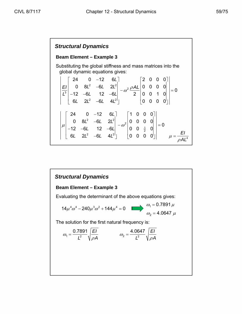
Substituting the global stiffness and mass matrices into the global dynamic equations gives:g y q g
2 22
3
2 2
24 0 12 6 2 0 0 0
0 8 6 2 0 0 0 00
12 6 12 6 2 0 0 1 0
6 2 6 4 0 0 0 0
L
L L LEI AL
L L L
L L L L
2 22
12
2 2
24 0 12 6 1 0 0 0
0 8 6 2 0 0 0 00
12 6 12 6 0 0 0
6 2 6 4 0 0 0 0
L
L L L
L L
L L L L
4
EI
AL
Structural Dynamics
Beam Element – Example 3
Evaluating the determinant of the above equations gives:
0 7891 4 4 3 2 414 240 144 0
1 22 2
0.7891 4.0647EI EI
L A L A
1 0.7891
2 4.0647
The solution for the first natural frequency is:
CIVL 8/7117 Chapter 12 - Structural Dynamics 59/75
Structural Dynamics
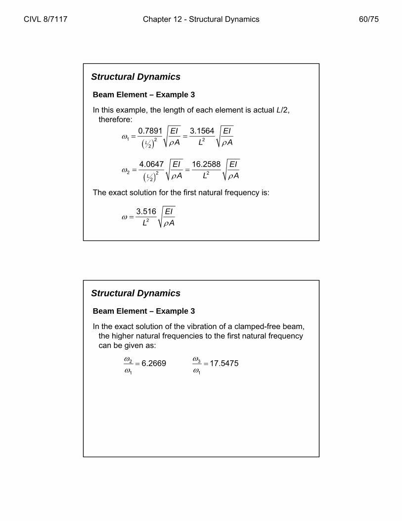
Beam Element – Example 3
In this example, the length of each element is actual L/2, therefore:
1 2 2
2
0.7891 3.1564L
EI EI
A L A
2 2 2
2
4.0647 16.2588L
EI EI
A L A
The exact solution for the first natural frequency is:
2
3.516 EI
L A
Structural Dynamics
Beam Element – Example 3
In the exact solution of the vibration of a clamped-free beam, the higher natural frequencies to the first natural frequency g q q ycan be given as:
32
1 1
6.2669 17.5475
CIVL 8/7117 Chapter 12 - Structural Dynamics 60/75
Structural Dynamics
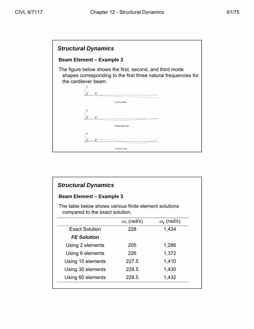
Beam Element – Example 3
The figure below shows the first, second, and third mode shapes corresponding to the first three natural frequencies for p p g qthe cantilever beam.
Structural Dynamics
Beam Element – Example 3
The table below shows various finite element solutions compared to the exact solution.p
1 (rad/s) 2 (rad/s)
Exact Solution 228 1,434
FE Solution
Using 2 elements 205 1,286
U i 6 l t 226 1 372Using 6 elements 226 1,372
Using 10 elements 227.5 1,410
Using 30 elements 228.5 1,430
Using 60 elements 228.5 1,432
CIVL 8/7117 Chapter 12 - Structural Dynamics 61/75
Structural Dynamics
Truss Analysis
The dynamics of trusses and plane frames are preformed by extending the concepts of bar and beam element. g p
The truss element requires the same transformation of the mass matrix from local to global coordinates as that used for the stiffness matrix given as:
T
m mT T
Structural Dynamics
Truss Analysis
Considering two-dimensional motion, the axial and the transverse displacement are given as:p g
1
1
2
2
0 01
0 0
u
vu L x x
uv L L x x
v
Th h f ti f th t iThe shape functions for the matrix are:
0 01
0 0
L x xN
L L x x
CIVL 8/7117 Chapter 12 - Structural Dynamics 62/75
Structural Dynamics
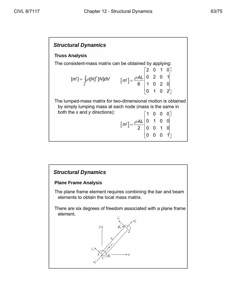
Truss Analysis
The consistent-mass matrix can be obtained by applying:
2 0 1 0
[ ] [ ] [ ]T
V
m N N dV
The lumped-mass matrix for two-dimensional motion is obtained by simply lumping mass at each node (mass is the same in
0 2 0 1
6 1 0 2 0
0 1 0 2
ALm
by simply lumping mass at each node (mass is the same in both the x and y directions):
1 0 0 0
0 1 0 0
2 0 0 1 0
0 0 0 1
ALm
Structural Dynamics
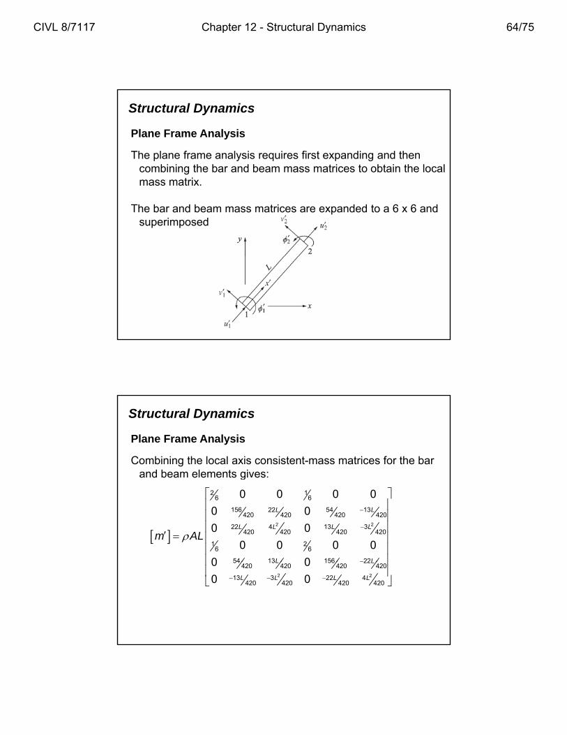
Plane Frame Analysis
The plane frame element requires combining the bar and beam elements to obtain the local mass matrix.
There are six degrees of freedom associated with a plane frame element.
CIVL 8/7117 Chapter 12 - Structural Dynamics 63/75
Structural Dynamics
Plane Frame Analysis
The plane frame analysis requires first expanding and then combining the bar and beam mass matrices to obtain the local gmass matrix.
The bar and beam mass matrices are expanded to a 6 x 6 and superimposed
Structural Dynamics
Plane Frame Analysis
Combining the local axis consistent-mass matrices for the bar and beam elements gives:g
22
2 16 6
156 54 1322420 420 420 420
13 322 4420 420 420 420
1 26 6
54 13 156 22
0 0 0 0
0 0
0 0
0 0 0 0
0 0
LL
L LL L
L L
m AL
2 2
54 13 156 22420 420 420 420
13 3 22 4420 420 420 420
0 0
0 0
L L
L L L L
CIVL 8/7117 Chapter 12 - Structural Dynamics 64/75
Structural Dynamics
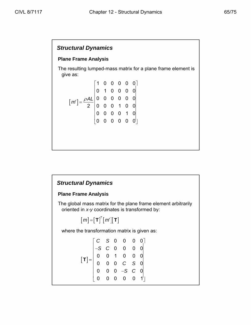
Plane Frame Analysis
The resulting lumped-mass matrix for a plane frame element is give as:g
1 0 0 0 0 0
0 1 0 0 0 0
0 0 0 0 0 0
2 0 0 0 1 0 0
0 0 0 0 1 0
ALm
0 0 0 0 1 0
0 0 0 0 0 0
Structural Dynamics
Plane Frame Analysis
The global mass matrix for the plane frame element arbitrarily oriented in x-y coordinates is transformed by:y y
0 0 0 0
0 0 0 0
C S
S C
T
m mT T
where the transformation matrix is given as:
0 0 0 0
0 0 1 0 0 0
0 0 0 0
0 0 0 0
0 0 0 0 0 1
S C
C S
S C
T
CIVL 8/7117 Chapter 12 - Structural Dynamics 65/75
Structural Dynamics
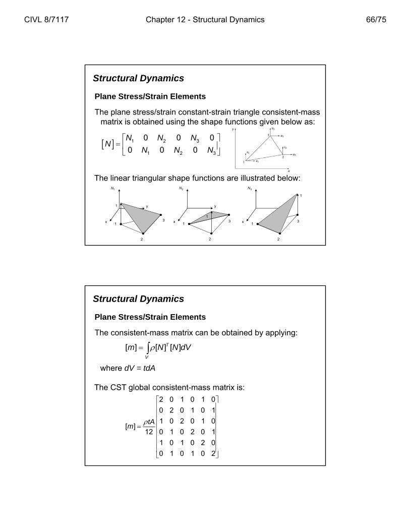
Plane Stress/Strain Elements
The plane stress/strain constant-strain triangle consistent-mass matrix is obtained using the shape functions given below as: g p g
1 2 3
1 2 3
0 0 0
0 0 0
N N NN
N N N
The linear triangular shape functions are illustrated below:
2
1
1
N1
y
x
2
13
1
N2
y
x
2
13
1
N3
y
x3
Structural Dynamics
Plane Stress/Strain Elements
The consistent-mass matrix can be obtained by applying:
[ ] [ ] [ ]TN N dV [ ] [ ] [ ]T
V
m N N dV
where dV = tdA
The CST global consistent-mass matrix is:
2 0 1 0 1 0
0 2 0 1 0 1
1 0 2 0 1 0[ ]
12 0 1 0 2 0 1
1 0 1 0 2 0
0 1 0 1 0 2
tAm
CIVL 8/7117 Chapter 12 - Structural Dynamics 66/75
Structural Dynamics
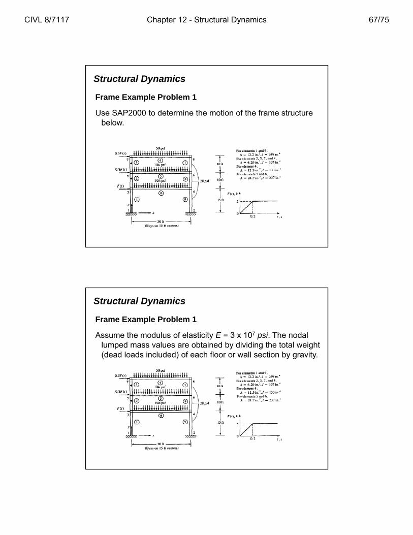
Frame Example Problem 1
Use SAP2000 to determine the motion of the frame structure below.
Structural Dynamics
Frame Example Problem 1
Assume the modulus of elasticity E = 3 x 10⁷ psi. The nodal lumped mass values are obtained by dividing the total weight p y g g(dead loads included) of each floor or wall section by gravity.
CIVL 8/7117 Chapter 12 - Structural Dynamics 67/75
Structural Dynamics
Frame Example Problem 1
For example, compute the total mass of the uniform vertical load on elements 4, 5, and 6:, ,
2
24
4
50 30 1558.28
386.04 ins
psf ft ftW lb sM ing
2
25
5
104 30 15121.23
386.04 ins
psf ft ftW lb sM ing
2
26
6
104 30 15121.23
386.04 ins
psf ft ftW lb sM ing
Structural Dynamics
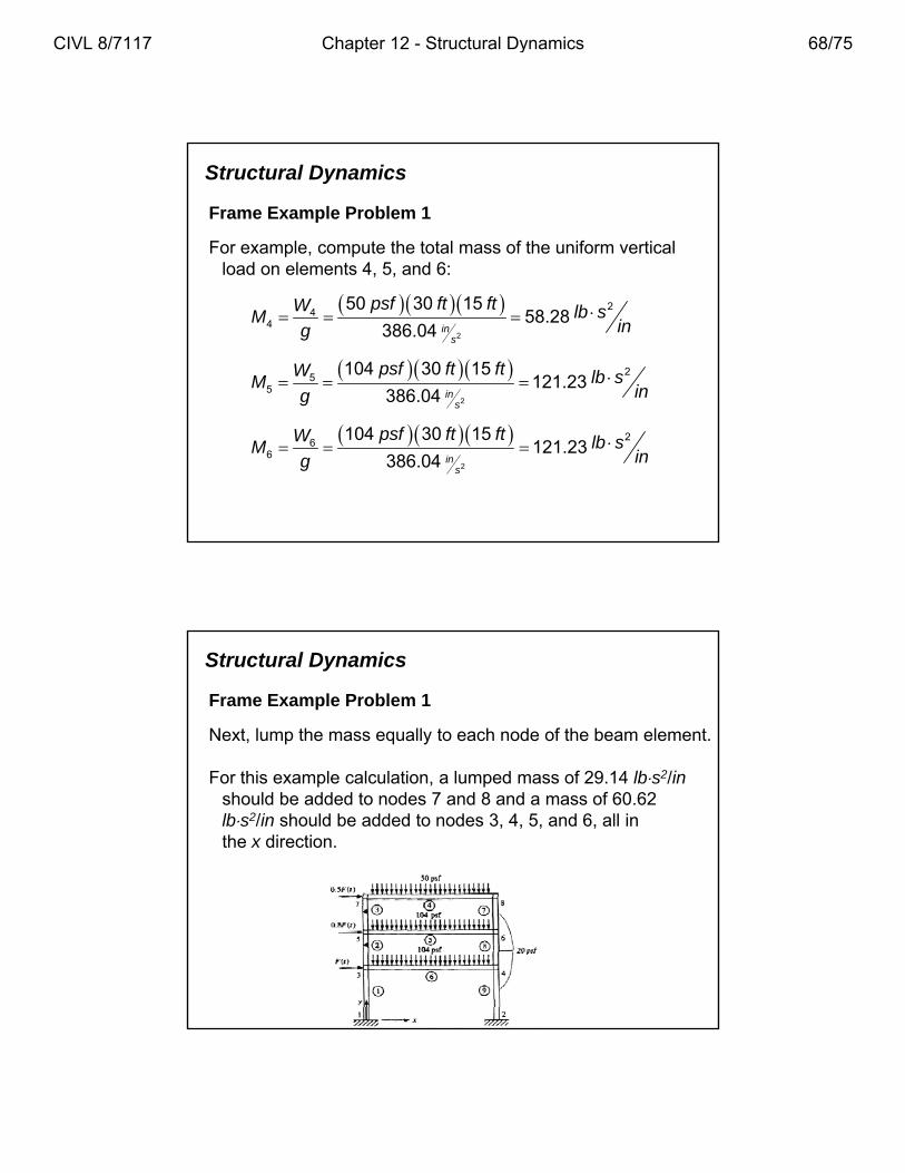
Frame Example Problem 1
Next, lump the mass equally to each node of the beam element.
For this example calculation, a lumped mass of 29.14 lbs2/inshould be added to nodes 7 and 8 and a mass of 60.62 lbs2/in should be added to nodes 3, 4, 5, and 6, all in the x direction.
CIVL 8/7117 Chapter 12 - Structural Dynamics 68/75
Structural Dynamics
Frame Example Problem 1
In an identical manner, masses for the dead loads for additional wall sections should be added to their respective nodes.
In this example, additional wall loads should be converted to mass added to the appropriate loads.
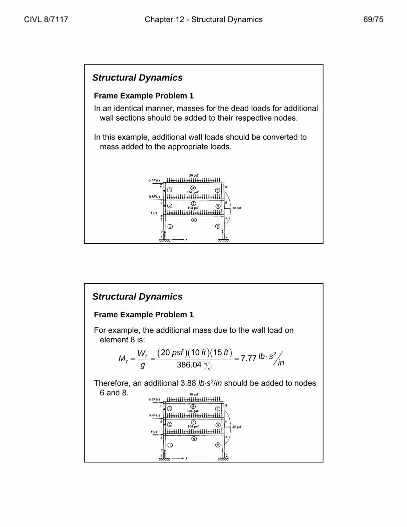
Structural Dynamics
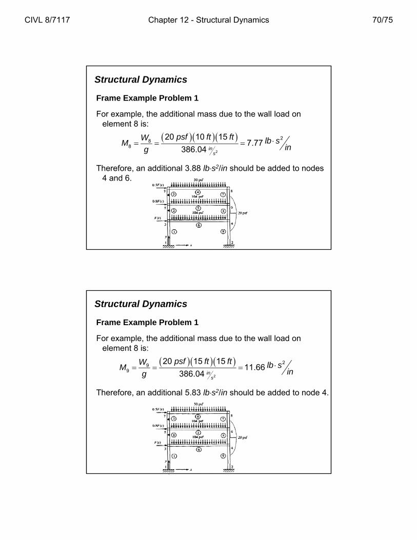
Frame Example Problem 1
For example, the additional mass due to the wall load on element 8 is:
2
27
7
20 10 157.77
386.04 ins
psf ft ftW lb sM ing
Therefore, an additional 3.88 lbs2/in should be added to nodes 6 and 8.
CIVL 8/7117 Chapter 12 - Structural Dynamics 69/75
Structural Dynamics
Frame Example Problem 1
For example, the additional mass due to the wall load on element 8 is:
2
28
8
20 10 157.77
386.04 ins
psf ft ftW lb sM ing
Therefore, an additional 3.88 lbs2/in should be added to nodes 4 and 6.
Structural Dynamics
Frame Example Problem 1
For example, the additional mass due to the wall load on element 8 is:
2
29
9
20 15 1511.66
386.04 ins
psf ft ftW lb sM ing
Therefore, an additional 5.83 lbs2/in should be added to node 4.
CIVL 8/7117 Chapter 12 - Structural Dynamics 70/75
Structural Dynamics
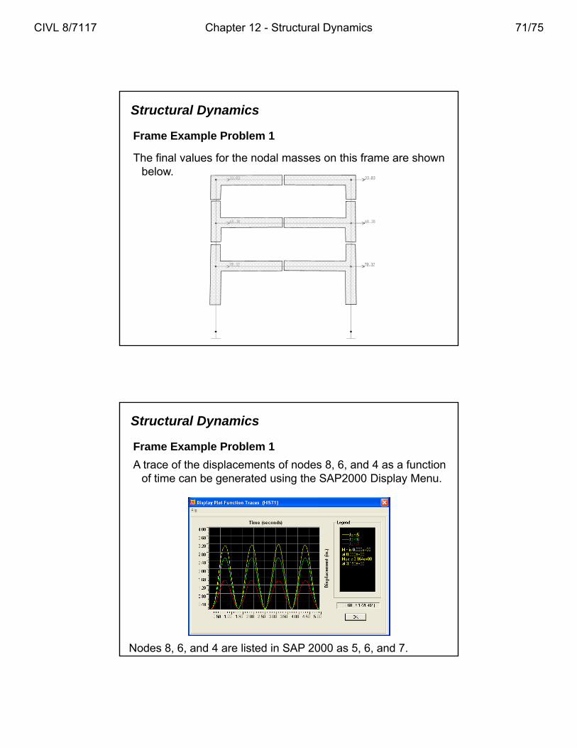
Frame Example Problem 1
The final values for the nodal masses on this frame are shown below.
Structural Dynamics
Frame Example Problem 1
A trace of the displacements of nodes 8, 6, and 4 as a function of time can be generated using the SAP2000 Display Menu.
Nodes 8, 6, and 4 are listed in SAP 2000 as 5, 6, and 7.
CIVL 8/7117 Chapter 12 - Structural Dynamics 71/75
Structural Dynamics
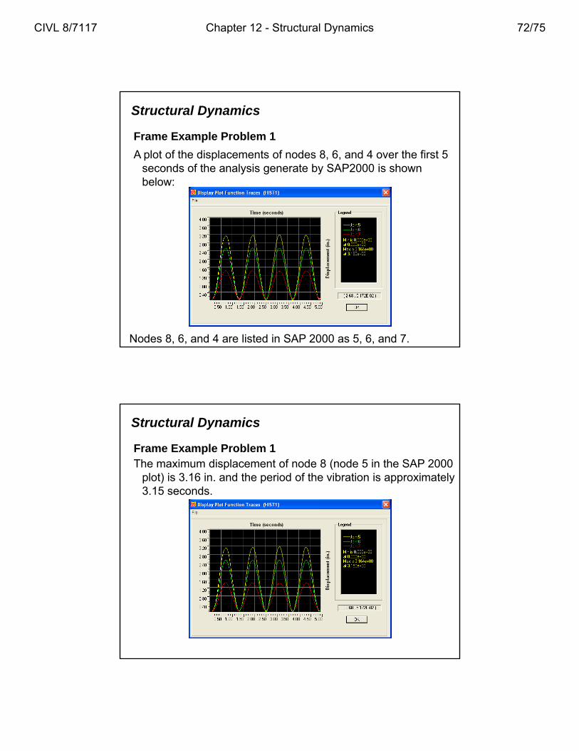
Frame Example Problem 1
A plot of the displacements of nodes 8, 6, and 4 over the first 5 seconds of the analysis generate by SAP2000 is shown below:
Nodes 8, 6, and 4 are listed in SAP 2000 as 5, 6, and 7.
Structural Dynamics
Frame Example Problem 1The maximum displacement of node 8 (node 5 in the SAP 2000
plot) is 3.16 in. and the period of the vibration is approximately 3 15 d3.15 seconds.
CIVL 8/7117 Chapter 12 - Structural Dynamics 72/75
Structural Dynamics
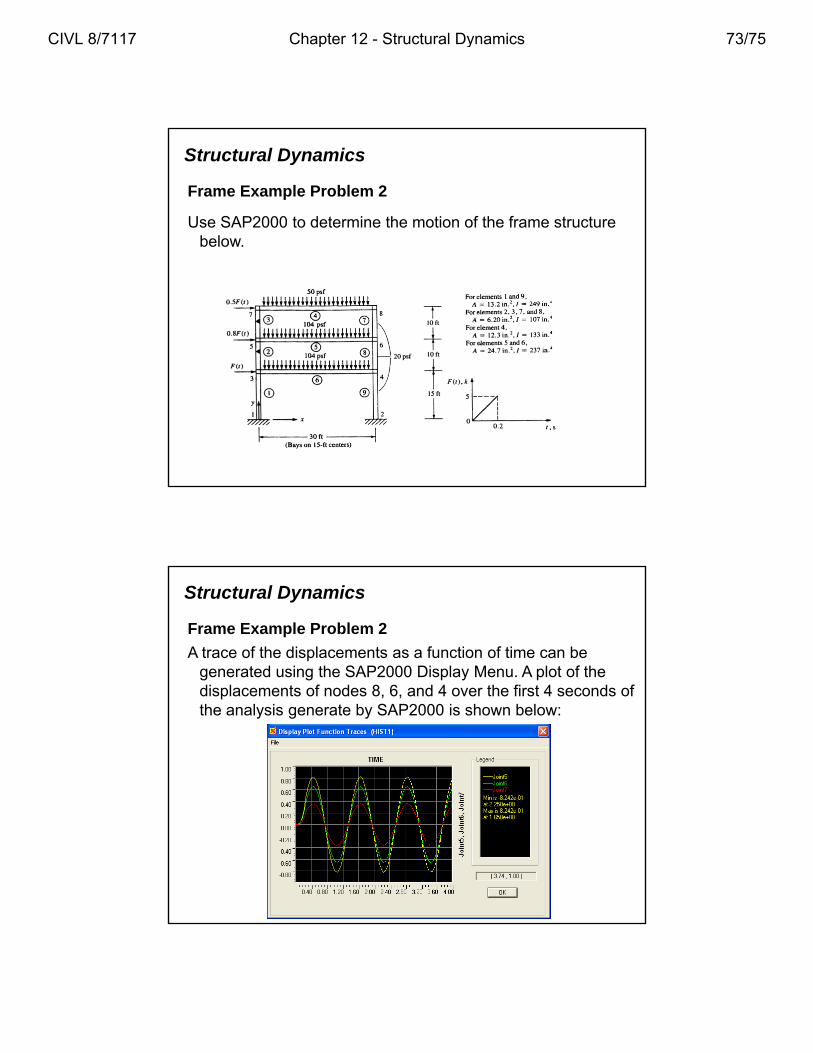
Frame Example Problem 2
Use SAP2000 to determine the motion of the frame structure below.
Structural Dynamics
Frame Example Problem 2
A trace of the displacements as a function of time can be generated using the SAP2000 Display Menu. A plot of the di l t f d 8 6 d 4 th fi t 4 d fdisplacements of nodes 8, 6, and 4 over the first 4 seconds of the analysis generate by SAP2000 is shown below:
CIVL 8/7117 Chapter 12 - Structural Dynamics 73/75
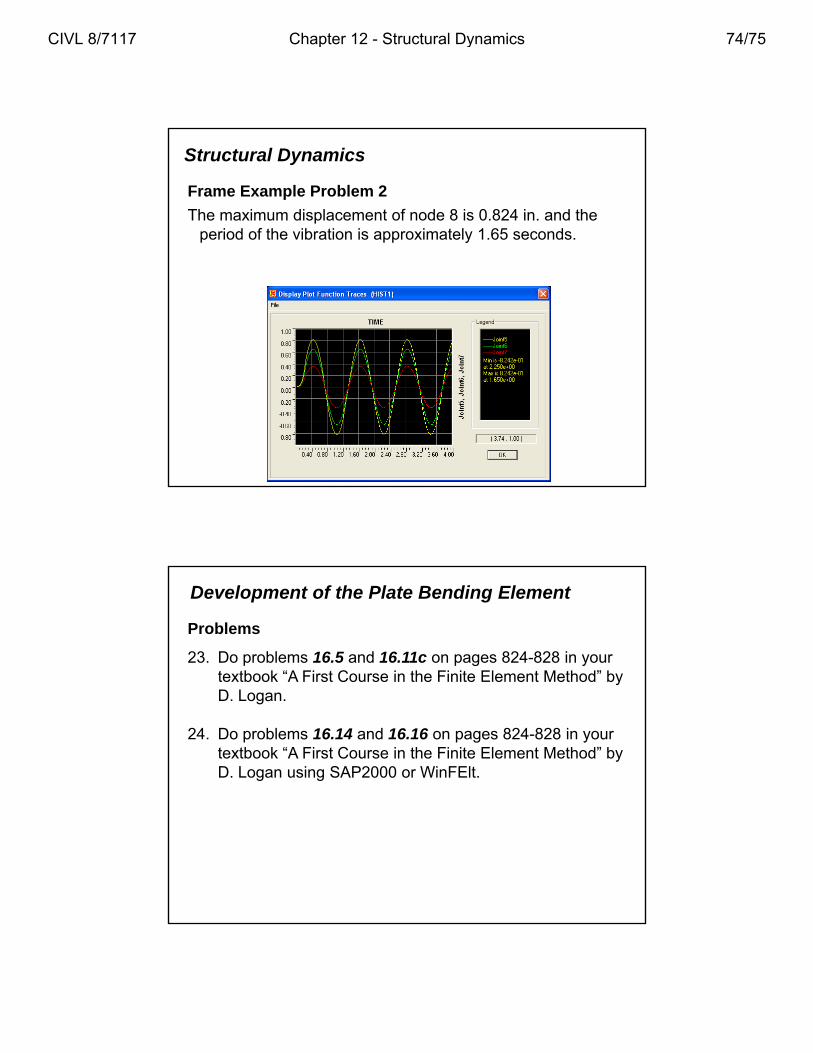
Structural Dynamics
Frame Example Problem 2
The maximum displacement of node 8 is 0.824 in. and the period of the vibration is approximately 1.65 seconds.
Development of the Plate Bending Element
Problems
23. Do problems 16.5 and 16.11c on pages 824-828 in your textbook “A First Course in the Finite Element Method” by yD. Logan.
24. Do problems 16.14 and 16.16 on pages 824-828 in your textbook “A First Course in the Finite Element Method” by D. Logan using SAP2000 or WinFElt.
CIVL 8/7117 Chapter 12 - Structural Dynamics 74/75

End of Chapter 16
CIVL 8/7117 Chapter 12 - Structural Dynamics 75/75