Embed Size (px)
DESCRIPTION
Study on soil-structure interaction
Citation preview
Structural Element Approaches for Soil-Structure Interaction
Master of Science Thesis in the Master’s Programme Structural Engineering and
Building Performance Design
CASELUNGHE ARON & ERIKSSON JONAS Department of Civil and Environmental Engineering Division of Structural Engineering and GeoEngineering
Concrete Structures and Geotechnical Engineering CHALMERS UNIVERSITY OF TECHNOLOGY Göteborg, Sweden 2012 Master’s Thesis 2012:62

MASTER’S THESIS 2012:62
Structural Element Approaches for Soil-Structure Interaction
Master of Science Thesis in the Master’s Programme Structural Engineering and
Building Performance Design
CASELUNGHE ARON & ERIKSSON JONAS
Department of Civil and Environmental Engineering Division of Structural Engineering and GeoEngineering
Concrete Structures and Geotechnical Engineering
CHALMERS UNIVERSITY OF TECHNOLOGY
Göteborg, Sweden 2012
Structural Element Approaches for Soil-Structure Interaction
Master of Science Thesis in the Master’s Programme Structural Engineering and
Building Performance Design
CASELUNGHE ARON & ERIKSSON JONAS
© Caselunghe Aron & Eriksson Jonas, 2012
Examensarbete / Institutionen för bygg- och miljöteknik, Chalmers tekniska högskola 2012:62
Department of Civil and Environmental Engineering
Division of Structural Engineering and GeoEngineering
Concrete Structures and Geotechnical Engineering
Chalmers University of Technology
SE-412 96 Göteborg
Sweden
Telephone: + 46 (0)31-772 1000
Cover: Visualized structural element model for soil-structure interaction. Adapted from (Teodoru, 2009).
Chalmers reproservice Göteborg, Sweden 2012


I
Structural Element Approaches for Soil-Structure Interaction
Master of Science Thesis in the Master’s Programme Structural Engineering and
Building Performance Design
CASELUNGHE ARON & ERIKSSON JONAS Department of Civil and Environmental Engineering Division of Structural Engineering and GeoEngineering
Concrete Structures and Geotechnical Engineering Chalmers University of Technology
ABSTRACT
The emphasis within this study regards structural element models for soil-structure
interaction (SSI). The methods are compared and calibrated against an elastic continuum modelled with solid elements, which in the study is used as the “correct” solution. Main interest is the influence on results of simplifications in the method often used today, with springs representing the subgrade (Winkler model). In the study this model is modified to better capture the soil’s behaviour.
In a Winkler model the springs act independently of each other, while the soil in reality is a continuous medium that also transfers shear stresses. To achieve a better behaviour in a structural element model, different kinds of interaction elements are included, which couple the springs.
The biggest shortcoming, identified in this thesis, for a Winkler model with uniform foundation stiffness is that the soil around the superstructure is not taken into account. This can result in major underestimation of the foundation’s stiffness towards the superstructure’s edges which normally, at the edges, leads to conservative sectional forces in the ground slab and unconservative ground pressure. It can also result in a convex settlement profile, where a concave would be more realistic.
Surrounding soil can be taken into account by increasing the foundation’s stiffness towards the superstructure’s edges, alternatively the different models described in the thesis can be implemented. The different models are applied in two simple cases, one representing a footing and the second a slab. The best correlation to the elastic continuum was achieved by applying an interaction element between the springs in a Winkler model that only transfers shear deformations. This shear layer model is also evaluated in 3D for a case study of “Malmö Konsert, Kongress och Hotell”.
A simple method, for practical use in 2D, to determine this shear layer model’s parameters is developed by the authors. Analyses indicate that the shear layer’s stiffness can be determined independently of the superstructure’s geometry. Therefore only the soil’s properties and depth is needed to determine the shear layer’s stiffness. A relation for homogenous and elastic soil is presented to determine the stiffness. The relation is based on 2D analysis and is not verified for 3D. Further study and verification is needed to make the method complete for practical use.
Key words: Winkler, elastic foundation, shear layer, multi-parameter model, MK-R, soil-structure interaction, static analysis, ground slab, subgrade, superstructure.
II
Strukturelementsmetoder för samverkan mellan överbyggnad och jord
Examensarbete inom Structural Engineering and Building Performance Design
CASELUNGHE ARON & ERIKSSON JONAS
Institutionen för bygg- och miljöteknik
Avdelningen för Konstruktionsteknik och Geologi och geoteknik
Betongbyggnad och Geoteknik
Chalmers tekniska högskola
SAMMANFATTNING
Denna studie inriktar sig på strukturelementsmodeller för samverkan mellan överbyggnad och jord. Metoderna jämförs och kalibreras gentemot ett elastiskt kontinuum, vilket i studien ses som den ”korrekta” lösningen. Fokus läggs på att förklara brister och redogöra för effekter av dem, för den idag vanligen använda fjäderbädden (Winkler-modell) som representerar jorden. Denna modell modifieras i studien för att bättre representera jordens beteende.
I en Winkler-modell är responsen för fjädrarna oberoende av varandra, medan jorden är ett sammanhängande kraftöverförande medium. För att efterlikna detta bättre i en fjäderbädd införs interaktionselement som kopplar fjädrarna.
Den mest betydande, observerade effekten av att fjädrarna inte är kopplade i en fjäderbädd, är att omkringliggande jord runt överbyggnaden försummas. Detta kan resultera i en stor underskattning av jordens styvhet längs överbyggnadens kanter, vilket vid kanterna normalt leder till konservativa snittkrafter i grundplattan och ett underskattat grundtryck. Det kan också medföra en konvex sättningsprofil för fall när snarare en konkav kan förväntas i verkligheten.
För att ta hänsyn till omliggande jord kan styvheten på fjädrarna längs överbyggnadens kanter ökas. Alternativt kan de modifierade fjäderbäddarna beskrivna i rapporten tillämpas. De olika modellerna har prövats för två olika enkla fall i 2D. Det ena för att representera ett pelarfundament och det andra en grundplatta. Bäst korrelation jämfört med det elastiska kontinuumet uppnådes genom att införa ett interaktionselement mellan fjädrarna i Winklers modell som endast överför skjuvning. Denna skjuvlagermodell har även i en 3D-analys utvärderats för det praktiska fallet Malmö Konsert, Kongress och Hotell.
En enkel metod, för praktiskt användande, har utvecklats av författarna och undersöks i en 2D-studie för att bestämma skuvlagermodellens parametrar. I studien indikeras att skjuvlagrets styvhet kan bestämmas oberoende av överbyggnadens geometri. Detta gör det möjligt att bestämma skjuvstyvheten enbart beroende på jordens geometri och materialparametrar. En relation för homogen och elastisk jord har tagits fram för att bestämma denna skjuvstyvhet. Relationen är framtagen i 2D-analys och är ej verifierad för 3D. Fortsatt studie och verifikation av metoden krävs för praktisk användning.
Nyckelord: Winkler, fjäderbädd, skjuvlager, MK-R, statisk analys, överbyggnad, jord.
CHALMERS Civil and Environmental Engineering, Master’s Thesis 2012:62 III
Contents
ABSTRACT I
SAMMANFATTNING II
CONTENTS III
PREFACE V
1 INTRODUCTION 1
1.1 Background 1
1.2 Purpose 1
1.3 Method 1
1.4 Limitations 2
2 SOIL-STRUCTURE INTERACTION MODELS 3
2.1 Elastic Continuum 3
2.2 Winkler Model 4
2.3 Multi-Parameter Models 6
2.4 Hybrid Model 8
3 PRE-STUDY: NUMERICAL ANALYSIS OF SSI FOR STIFF AND SLENDER SUPERSTRUCTURES IN 2D 10
3.1 Implementing of SSI-Methods in Software 10
3.1.1 Elastic Continuum 10
3.1.2 Winkler Model 11
3.1.3 Multi-Parameter Models 11
3.1.4 MK-R Model 12
3.2 SSI Analysis for Stiff Superstructure 12
3.3 SSI Analysis for Slender Superstructure 13
3.4 Further Analysis of Shear Beam Model 15
3.4.1 No Tension Interaction between Superstructure and Subgrade 15
3.4.2 Variation of Soil Depth for Stiff Superstructure 16
3.4.3 Variation of Soil Depth for Slender Superstructure 18
3.4.4 Parameter Determination in Practice 19
3.5 Further Study of Winkler Model 20
3.6 Further Study of MK-R Model 21
4 CASE STUDY OF KKH 22
4.1 Description of KKH 22
4.2 Implementation of Models in ABAQUS 24
4.2.1 Superstructure Model 24
4.2.2 Continuum Model 25
CHALMERS, Civil and Environmental Engineering, Master’s Thesis 2012:62 IV
4.2.3 Shear Layer Model 26
4.2.4 Winkler Model 28
4.3 Results from Case Study 28
4.3.1 Deformation for Winkler, Shear layer and Continuum model 29
4.3.2 Moment Distribution for Winkler, Shear layer and Continuum model32
4.3.3 Ground Pressure for Winkler, Shear layer and Continuum Model 33
4.3.4 Influence of Interior and Exterior Walls 34
5 DISCUSSION AND FURTHER STUDIES 38
6 CONCLUSIONS 40
APPENDIX
CHALMERS Civil and Environmental Engineering, Master’s Thesis 2012:62 V
Preface
The work behind the Master’s thesis has been carried out in collaboration between Skanska Teknik and Chalmers University of Technology. Both divisions of Structural Engineering and GeoEngineering at Chalmers have been involved under the supervision of associate professors Mario Plos and Claes Alén whom we want to thank for their great support and for always having taken the time for guidance.
Many thanks to our supervisor Camilla Lidgren at Skanska for having given us the opportunity and making this work possible as well as rewarding and Lars Johansson for helpful guidance within geotechnical matters. Thanks are also directed to Sven Junkers who provided us with all necessary contacts at Skanska and helped us finding the subject.
We want to direct special acknowledgement to Per Kettil, our mentor at Skanska, for the continuous guidance. His expertise and enthusiasm have been highly valuable for the execution of the work behind this master thesis.
We are also grateful to Strusoft for providing us with their software FEM-Design and education within the software.
Göteborg, June 2012
Aron Caselunghe & Jonas Erikssson
CHALMERS, Civil and Environmental Engineering, Master’s Thesis 2012:62 VI
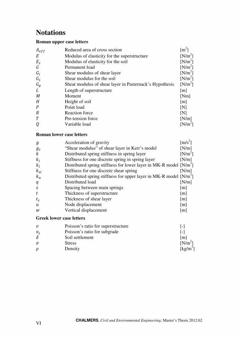
Notations
Roman upper case letters ���� Reduced area of cross section [m2] � Modulus of elasticity for the superstructure [N/m2] �� Modulus of elasticity for the soil [N/m2] � Permanent load [N/m2] �� Shear modulus of shear layer [N/m2] �� Shear modulus for the soil [N/m2] �� Shear modulus of shear layer in Pasternack’s Hypothesis [N/m2] Length of superstructure [m] Moment [Nm] � Height of soil [m] � Point load [N] Reaction force [N] � Pre-tension force [N/m] � Variable load [N/m2]
Roman lower case letters � Acceleration of gravity [m/s2] �� “Shear modulus” of shear layer in Kerr’s model [N/m] � Distributed spring stiffness in spring layer [N/m2] �� Stiffness for one discrete spring in spring layer [N/m] �� Distributed spring stiffness for lower layer in MK-R model [N/m3] ��� Stiffness for one discrete shear spring [N/m] �� Distributed spring stiffness for upper layer in MK-R model [N/m3] � Distributed load [N/m] � Spacing between main springs [m] � Thickness of superstructure [m] �� Thickness of shear layer [m] � Node displacement [m] � Vertical displacement [m]
Greek lower case letters � Poisson’s ratio for superstructure [-] �� Poisson’s ratio for subgrade [-] � Soil settlement [m] � Stress [N/m2] � Density [kg/m3]


CHALMERS, Civil and Environmental Engineering, Master’s Thesis 2012:62 1
1 Introduction
1.1 Background
Structural engineering and Geotechnics are closely connected subjects in analysis of civil engineering structures, often analysis in neither of the two subjects can be performed independently with accurate results. To get the superstructure’s real behaviour, the subgrade must be modelled sufficiently well. On the other hand, an advanced model of the is superstructure needed to get the correct response in the subgrade. To capture the right behaviours of both superstructure and subgrade in one model, it must include a good soil-structure interaction (SSI).
Structural engineers in practice often use software where the structure is modelled in detail, but the subgrade is represented with simple structural element models which sometimes poorly describe the behaviour of the soil. Geotechnical engineers instead use software with advanced soil model, but with a simple model of the structure. However, merging today’s most advanced commercial design software for the two disciplines, would result in demand for unrealistic large computation time. The user would in such a model also need great knowledge in both of the subjects. Therefore, there is a need for simplified methods in practice to model SSI. Consequently, it is of great interest how the simplifications influence the results.
In engineering practice there are different opinions how to model SSI. In design of the superstructure, some consider that it’s enough with structural element model of the subgrade. Others claim that the soil should be modelled more physically correct with a continuum model, to achieve a good enough SSI-analysis.
At Skanska the software FEM-Design, Strusoft (2012), is used for structural analysis and PLAXIS, PLAXIS (2012), for geotechnical analysis. At the company, a need for software which better handle SSI has been identified. A SBUF founded project is therefore started with the aim to improve analyses involving SSI, with the soil represented as a continuum approximated with solid elements. This thesis instead focuses on structural element SSI models.
1.2 Purpose
The purpose of this study is to describe and investigate different structural approaches and their accuracy to model SSI, with regard to the response in the superstructure’s ground slab. Main interest is the influence on results of simplifications in the method often used today, with springs representing the subgrade, compared to alternative approaches. The aim is to find a simple structural method suited for structural software as FEM-Design which handles SSI sufficiently well.
1.3 Method
A literature study is made to collect information about the subject. Of main interest in the study is information about different modelling-techniques and their advantages and disadvantages.
As a pre-study, some interesting approaches are modelled in 2D with the finite
element method (FEM) for simple SSI problems. The purpose is to study accuracy and point out characteristic effects of the approaches. The superstructure is modelled as a beam for two cases to capture influence of the superstructure’s geometry; one case with a stiff beam and the other with a slender.
CHALMERS, Civil and Environmental Engineering, Master’s Thesis 2012:62 2
Modelled approaches:
• Superstructure as a beam and subgrade with spring supports.
• Superstructure as a beam and subgrade with springs supports with interacting
elements for shear transfer.
• Superstructure as a beam and the ground as a continuum with solid elements.
Some approaches are compared in 3D as a case study for a part of “Malmö Koncert,
Kongress och Hotell” (KKH). Analyses from design work are provided by Skanska, which will be used for comparison. The purpose is to compare the approaches for a complex superstructure and highlight effects observed in the pre-study.
Deformation, sectional forces and ground pressure are compared for the different approaches.
The software which mainly is used is ABAQUS, Simulia (2012), and when possible also FEM-Design.
1.4 Limitations
Both structure and ground are modelled with simplifications to make the project possible to carry out within the limited time available. The ground and structure are limited to linear-elastic behaviour. Time dependence and nonlinear effects are accounted for when necessary, but by simplified methods.
CHALMERS, Civil and Environmental Engineering, Master’s Thesis 2012:62 3
2 Soil-Structure Interaction Models
Basically there are two types of derivation approaches used for models of SSI problems; structural and continuum approach. The structural approach has a rigid base from which subgrade and superstructure are built up with structural elements, such as flexural elements, springs, etc. The other alternative, continuum approach is based on three partially-differential equations (compatibility, constitutive and equilibrium) which are governing the behaviour for the subgrade as a continuum (Teodoru, 2009). When combining the two derivation approaches, the method is called a hybrid derivation approach.
The two approaches have advantages as well as disadvantages. A structural model is easy to implement in practice, since modelling and solving are simple in available commercial analysis software. However, estimation of material parameters for the structural elements representing the subgrade is a well-known problem. In contrast to the structural approach the soil parameters are straight forward to specify for an elastic continuum model, but implementing such models in existing commercial software is problematic. Nonetheless both methods require geotechnical evaluation of the soil’s parameters. (Horvath and Colasanti, 2011)
2.1 Elastic Continuum
In continuum mechanics, continuum is defined by a continuously distributed matter through the space. The simplest elastic continuum is described with the constitutive relation with linear elastic isotropic behaviour given by Hook’s law (Irgens, 2008), which is applied in the pre-study. Without failure criteria the elastic medium has infinite tension and compression capacity, which can be questioned for soil. Several constitutive relations exist, with different failure criteria in tension and compression, which better capture soil behavior, e.g. Mohr-Coulomb’s constitutive relation. For more information about constitutive relations suited for different soil conditions, see Kok et al. (2009).
The analytical solution for several loading cases has been developed for semi-infinite elastic continuum. The solution for point- and distributed load was given by Boussinesq, for derivation and solution see Timoshenko and Goodier (1970). However, subgrade with shallow soil depth is poorly described with semi-infinite space. A solution for a simplified continuum with finite height was developed by Reissner.
Reissner’s equation for an elastic medium representing soil, with height H, elasticity Es and shear modules Gs with a distributed load q and a vertical surface displacement w at any point is displayed in equation (2.1).
���, ! − �� ∗ �$12 ∗ �� ∇$���, ! = ��� ���, ! − �� ∗ �3 ∇$���, !�2.1! In Reissner’s equation the elastic medium is assumed to be weightless (Horvath and Colasanti, 2011). Horizontal normal and shear stresses are zero as well as the horizontal displacements at top and bottom of the medium. Due to these assumptions, Reissner’s differential equation should only be applied near the surface and is not suitable to study stresses inside the medium. (Teoduro, 2009)
A continuum can approximately be analysed with numerical methods. The numerical methods FEM and boundary element method (BEM) are suitable for SSI analysis.
CHALMERS, Civil and Environmental Engineering, Master’s Thesis 2012:62 4
FEM is preferable for non-linear soil properties, the method is well known and several commercial software are based on the method. In linear elastic analysis BEM can be advantageous, due to lower computation time compared to FEM. Further BEM is suitable to consider infinite and semi-infinite spaces (Bolteus, 1984). Application possibilities for the two methods in SSI-analysis are described in detail in (Bolteus, 1984).
2.2 Winkler Model
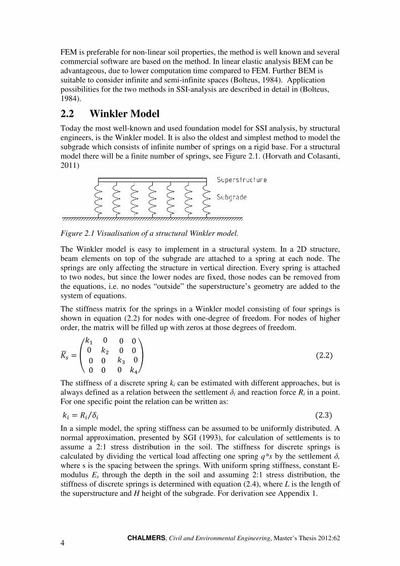
Today the most well-known and used foundation model for SSI analysis, by structural engineers, is the Winkler model. It is also the oldest and simplest method to model the subgrade which consists of infinite number of springs on a rigid base. For a structural model there will be a finite number of springs, see Figure 2.1. (Horvath and Colasanti, 2011)
Figure 2.1 Visualisation of a structural Winkler model.
The Winkler model is easy to implement in a structural system. In a 2D structure, beam elements on top of the subgrade are attached to a spring at each node. The springs are only affecting the structure in vertical direction. Every spring is attached to two nodes, but since the lower nodes are fixed, those nodes can be removed from the equations, i.e. no nodes “outside” the superstructure’s geometry are added to the system of equations.
The stiffness matrix for the springs in a Winkler model consisting of four springs is shown in equation (2.2) for nodes with one-degree of freedom. For nodes of higher order, the matrix will be filled up with zeros at those degrees of freedom.
,-� = .�/ 00 �$ 0 00 000 00 �1 00 �23�2.2! The stiffness of a discrete spring ki can be estimated with different approaches, but is always defined as a relation between the settlement δi and reaction force Ri in a point. For one specific point the relation can be written as:
�� = � ��⁄ �2.3! In a simple model, the spring stiffness can be assumed to be uniformly distributed. A normal approximation, presented by SGI (1993), for calculation of settlements is to assume a 2:1 stress distribution in the soil. The stiffness for discrete springs is calculated by dividing the vertical load affecting one spring q*s by the settlement δ, where s is the spacing between the springs. With uniform spring stiffness, constant E-modulus Es through the depth in the soil and assuming 2:1 stress distribution, the stiffness of discrete springs is determined with equation (2.4), where L is the length of the superstructure and H height of the subgrade. For derivation see Appendix 1.
CHALMERS, Civil and Environmental Engineering, Master’s Thesis 2012:62 5
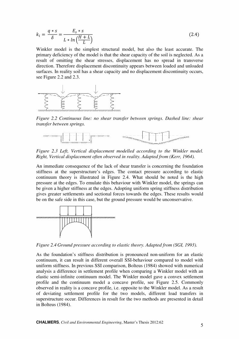
�� (� ∗ �� ( �� ∗ � ∗ 56 7� 8 9�2.4! Winkler model is the simplest structural model, but also the least accurate. The primary deficiency of the model is that the shear capacity of the soil is neglected. As a result of omitting the shear stresses, displacement has no spread in transverse direction. Therefore displacement discontinuity appears between loaded and unloaded surfaces. In reality soil has a shear capacity and no displacement discontinuity occurs, see Figure 2.2 and 2.3.
Figure 2.2 Continuous line: no shear transfer between springs. Dashed line: shear
transfer between springs.
Figure 2.3 Left, Vertical displacement modelled according to the Winkler model.
Right, Vertical displacement often observed in reality. Adapted from (Kerr, 1964).
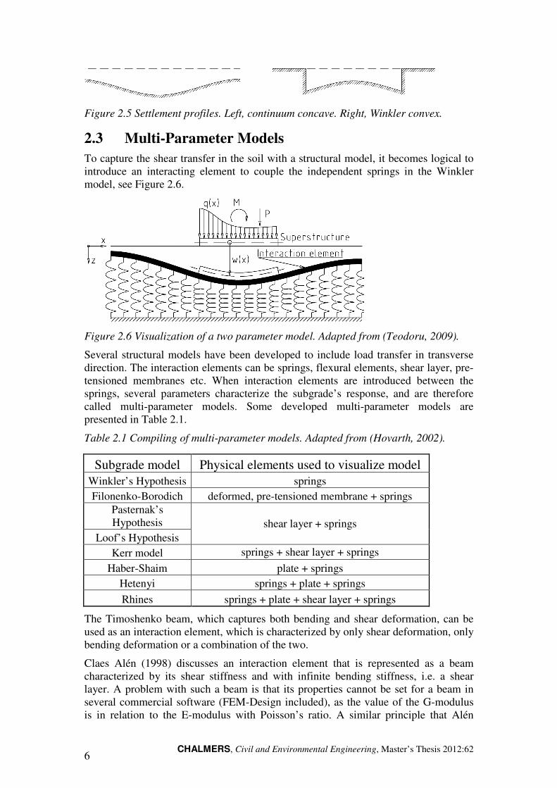
An immediate consequence of the lack of shear transfer is concerning the foundation stiffness at the superstructure’s edges. The contact pressure according to elastic continuum theory is illustrated in Figure 2.4. What should be noted is the high pressure at the edges. To emulate this behaviour with Winkler model, the springs can be given a higher stiffness at the edges. Adopting uniform spring stiffness distribution gives greater settlements and sectional forces towards the edges. These results would be on the safe side in this case, but the ground pressure would be unconservative.
Figure 2.4 Ground pressure according to elastic theory. Adapted from (SGI, 1993).
As the foundation’s stiffness distribution is pronounced non-uniform for an elastic continuum, it can result in different overall SSI-behaviour compared to model with uniform stiffness. In previous SSI comparison, Bolteus (1984) showed with numerical analysis a difference in settlement profile when comparing a Winkler model with an elastic semi-infinite continuum model. The Winkler model gave a convex settlement profile and the continuum model a concave profile, see Figure 2.5. Commonly observed in reality is a concave profile, i.e. opposite to the Winkler model. As a result of deviating settlement profile for the two models, different load transfers in superstructure occur. Differences in result for the two methods are presented in detail in Bolteus (1984).
CHALMERS, Civil and Environmental Engineering, Master’s Thesis 2012:62 6
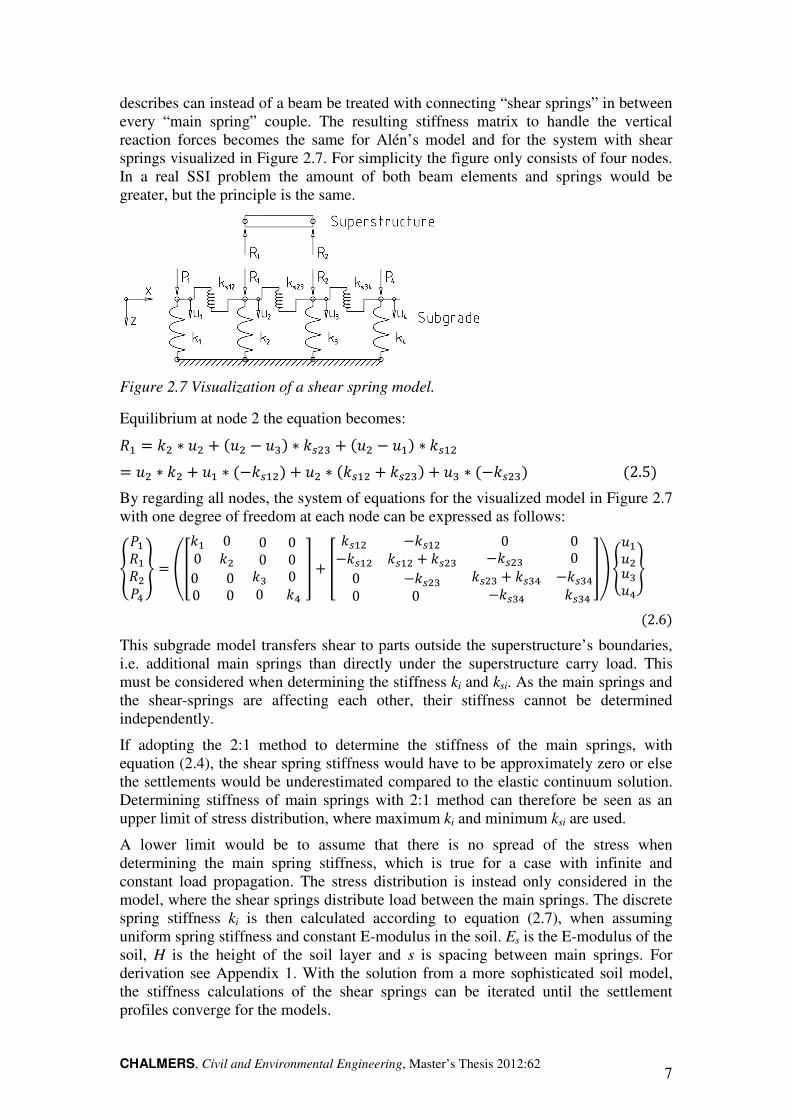
Figure 2.5 Settlement profiles. Left, continuum concave. Right, Winkler convex.
2.3 Multi-Parameter Models
To capture the shear transfer in the soil with a structural model, it becomes logical to introduce an interacting element to couple the independent springs in the Winkler model, see Figure 2.6.
Figure 2.6 Visualization of a two parameter model. Adapted from (Teodoru, 2009).
Several structural models have been developed to include load transfer in transverse direction. The interaction elements can be springs, flexural elements, shear layer, pre-tensioned membranes etc. When interaction elements are introduced between the springs, several parameters characterize the subgrade’s response, and are therefore called multi-parameter models. Some developed multi-parameter models are presented in Table 2.1.
Table 2.1 Compiling of multi-parameter models. Adapted from (Hovarth, 2002).
Subgrade model Physical elements used to visualize model
Winkler’s Hypothesis springs
Filonenko-Borodich deformed, pre-tensioned membrane + springs
Pasternak’s Hypothesis shear layer + springs
Loof’s Hypothesis
Kerr model springs + shear layer + springs
Haber-Shaim plate + springs
Hetenyi springs + plate + springs
Rhines springs + plate + shear layer + springs
The Timoshenko beam, which captures both bending and shear deformation, can be used as an interaction element, which is characterized by only shear deformation, only bending deformation or a combination of the two.
Claes Alén (1998) discusses an interaction element that is represented as a beam characterized by its shear stiffness and with infinite bending stiffness, i.e. a shear layer. A problem with such a beam is that its properties cannot be set for a beam in several commercial software (FEM-Design included), as the value of the G-modulus is in relation to the E-modulus with Poisson’s ratio. A similar principle that Alén
CHALMERS, Civil and Environmental Engineering, Master’s Thesis 2012:62 7
describes can instead of a beam be treated with connecting “shear springs” in between every “main spring” couple. The resulting stiffness matrix to handle the vertical reaction forces becomes the same for Alén’s model and for the system with shear springs visualized in Figure 2.7. For simplicity the figure only consists of four nodes. In a real SSI problem the amount of both beam elements and springs would be greater, but the principle is the same.
Figure 2.7 Visualization of a shear spring model.
Equilibrium at node 2 the equation becomes: / ( �$ ∗ �$ 8 ��$ " �1! ∗ ��$1 8 ��$ " �/! ∗ ��/$ ( �$ ∗ �$ 8 �/ ∗ �"��/$! 8 �$ ∗ ���/$ 8 ��$1! 8 �1 ∗ �"��$1!�2.5! By regarding all nodes, the system of equations for the visualized model in Figure 2.7 with one degree of freedom at each node can be expressed as follows:
<�/ / $�2= ( .>�/ 00 �$ 0 00 00 00 0 �1 00 �2 ? 8 > ��/$ "��/$"��/$ ��/$ 8 ��$1 0 0"��$1 00 "��$10 0 ��$1 8 ��12 "��12"��12 ��12 ?3@�/�$�1�2A �2.6! This subgrade model transfers shear to parts outside the superstructure’s boundaries, i.e. additional main springs than directly under the superstructure carry load. This must be considered when determining the stiffness ki and ksi. As the main springs and the shear-springs are affecting each other, their stiffness cannot be determined independently.
If adopting the 2:1 method to determine the stiffness of the main springs, with equation (2.4), the shear spring stiffness would have to be approximately zero or else the settlements would be underestimated compared to the elastic continuum solution. Determining stiffness of main springs with 2:1 method can therefore be seen as an upper limit of stress distribution, where maximum ki and minimum ksi are used.
A lower limit would be to assume that there is no spread of the stress when determining the main spring stiffness, which is true for a case with infinite and constant load propagation. The stress distribution is instead only considered in the model, where the shear springs distribute load between the main springs. The discrete spring stiffness ki is then calculated according to equation (2.7), when assuming uniform spring stiffness and constant E-modulus in the soil. Es is the E-modulus of the soil, H is the height of the soil layer and s is spacing between main springs. For derivation see Appendix 1. With the solution from a more sophisticated soil model, the stiffness calculations of the shear springs can be iterated until the settlement profiles converge for the models.
CHALMERS, Civil and Environmental Engineering, Master’s Thesis 2012:62 8
�� ( � ∗ �� ( ��� ∗ s�2.7! The same equation to determine spring stiffness is under simplified loading conditions suggested in Kerr (1964), where the differential equation for Pasternak’s Hypothesis is compared with Reissner’s differential equation (equation (2.1)).Corresponding shear modulus is suggested to be
�� (� ∗ ��3 ∗ �� �2.8! where H and Gs is the height and shear modulus of the soil, respectively, and ts is the thickness of the shear layer.
A compromise of the two approaches is to consider some of the stress spread in the settlement calculation and some in the model. It can be done by assuming a stress distribution in the settlement calculation, but smaller than 2:1, e.g. 12:1 distribution. Spring stiffness for discrete springs based on a 12:1 stress distribution and uniform E-modulus in the soil is determined with equation (2.9). Same assumptions and parameters used as in equation (2.4). For derivation see Appendix 1.
�� (� ∗ �� ( �� ∗ �6 ∗ ∗ 56 F� 6G 8 H�2.9!
Since more main springs than directly under the superstructure carry the load, stresses in the soil cannot be evaluated with the sectional forces in the structural elements representing the subgrade. Ground pressure should instead be determined by the reaction forces between superstructure and subgrade, as R1 and R2 in Figure 2.7.
2.4 Hybrid Model
As described in previous sections, there are pros and cons for both structural models and continuum model. The structural models are easy to model, but the simple ones have a lack of accuracy. The more complex models are improved, but the difficulty to estimate realistic parameters increases. The continuum model is more accurate for soil modelling and geotechnical engineers have relatively accurate methods to evaluate its parameters, but the model can be difficult to implement in today’s existing structural design software (Horvath and Colasanti, 2011).
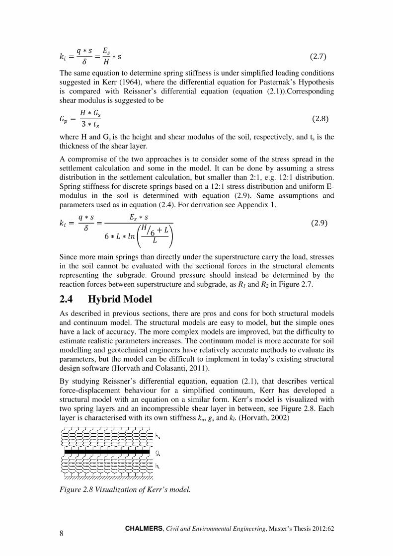
By studying Reissner’s differential equation, equation (2.1), that describes vertical force-displacement behaviour for a simplified continuum, Kerr has developed a structural model with an equation on a similar form. Kerr’s model is visualized with two spring layers and an incompressible shear layer in between, see Figure 2.8. Each layer is characterised with its own stiffness ku, gs and kl. (Horvath, 2002)
Figure 2.8 Visualization of Kerr’s model.
CHALMERS, Civil and Environmental Engineering, Master’s Thesis 2012:62 9
Kerr’s differential equation for the vertical force-displacement behaviour:
���, ! " ���� 8 �� '$���, ! ( �� ∗ ���� 8 �� ���, ! " �� ∗ ���� 8 �� '$���, !�2.10! Comparing equation (2.1) and (2.10) the relation between the parameters can be written as:
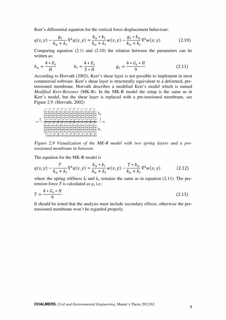
�� ( 4 ∗ ��� �� ( 4 ∗ ��3 ∗ � �� ( 4 ∗ �� ∗ �9 �2.11! According to Horvath (2002), Kerr’s shear layer is not possible to implement in most commercial software. Kerr’s shear layer is structurally equivalent to a deformed, pre-tensioned membrane. Horvath describes a modified Kerr’s model which is named Modified Kerr-Reissner (MK-R). In the MK-R model the setup is the same as in Kerr’s model, but the shear layer is replaced with a pre-tensioned membrane, see Figure 2.9. (Horvath, 2002)
Figure 2.9 Visualization of the MK-R model with two spring layers and a pre-
tensioned membrane in between.
The equation for the MK-R model is
���, ! " ��� 8 �� '$���, ! ( �� ∗ ���� 8 �� ���, ! " � ∗ ���� 8 �� '$���, !�2.12! where the spring stiffness kl and ku remains the same as in equation (2.11). The pre-tension force T is calculated as gs i.e.:
� ( 4 ∗ �� ∗ �9 �2.13! It should be noted that the analysis must include secondary effects, otherwise the pre-tensioned membrane won’t be regarded properly.
CHALMERS, Civil and Environmental Engineering, Master’s Thesis 2012:62 10
3 Pre-Study: Numerical Analysis of SSI for Stiff
and Slender Superstructures in 2D
FEM analyses is in this chapter presented for SSI-methods described in previous chapter for two extreme cases, one case with a stiff superstructure and the other with a slender superstructure. The first case represents a footing and the second a house slab, both on an elastic layer like sand.
3.1 Implementing of SSI-Methods in Software
In all methods the superstructure, i.e. the footing or the slab, is modelled as a linear Timoshenko beam with elastic isotropic material. All analyses are made in the software ABAQUS and when possible also in FEM-Design. In ABAQUS x-, y- and z-direction is defined respectively with 1-, 2-, and 3-direction. This convection is also used in this thesis. Important ABAQUS commands are presented in Appendix 4.
3.1.1 Elastic Continuum
For the elastic continuum analyses ABAQUS is used. No attempt to model in FEM-Design is made, since solid elements do not exist in the software. The result from the elastic continuum model is considered as the “corect” solution. The other SSI-methods are compared to how well they correspond to this solution.
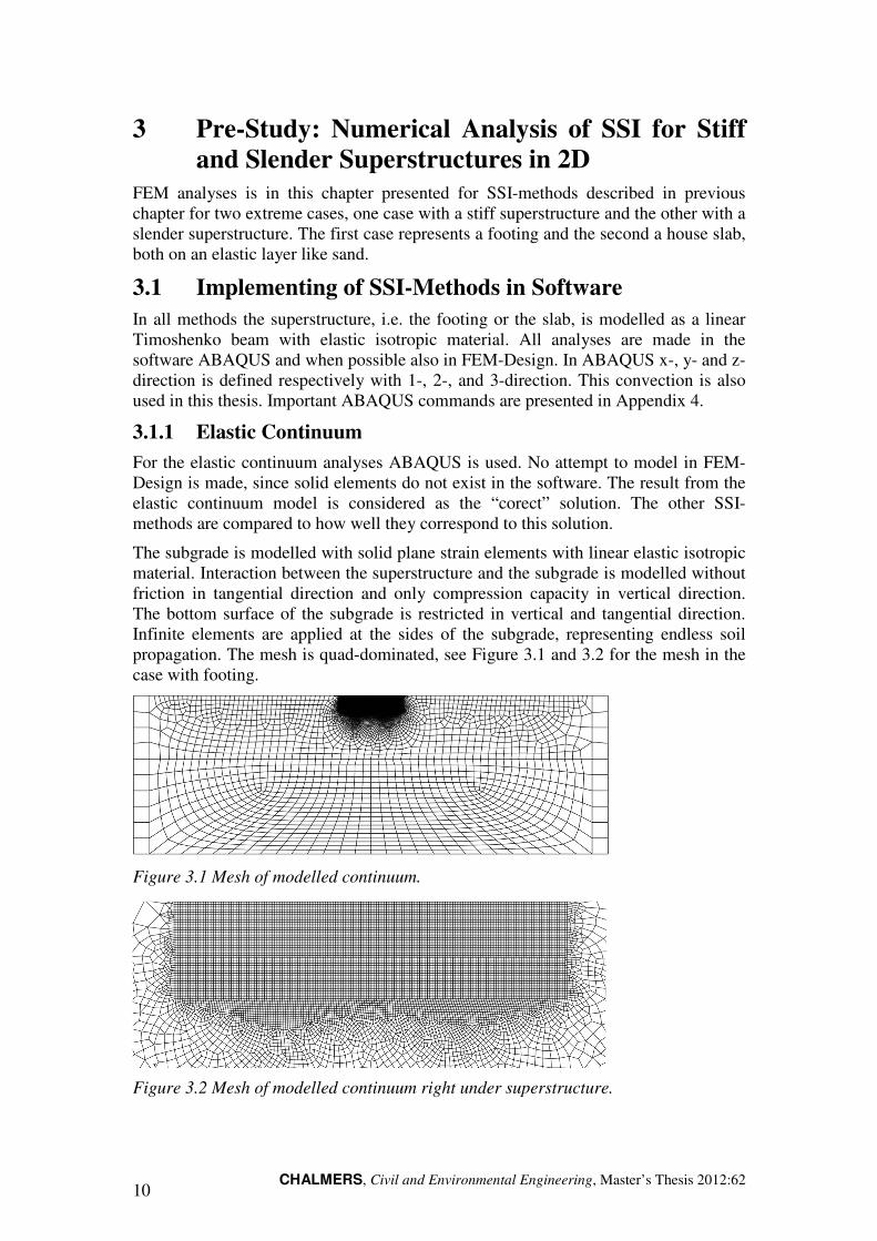
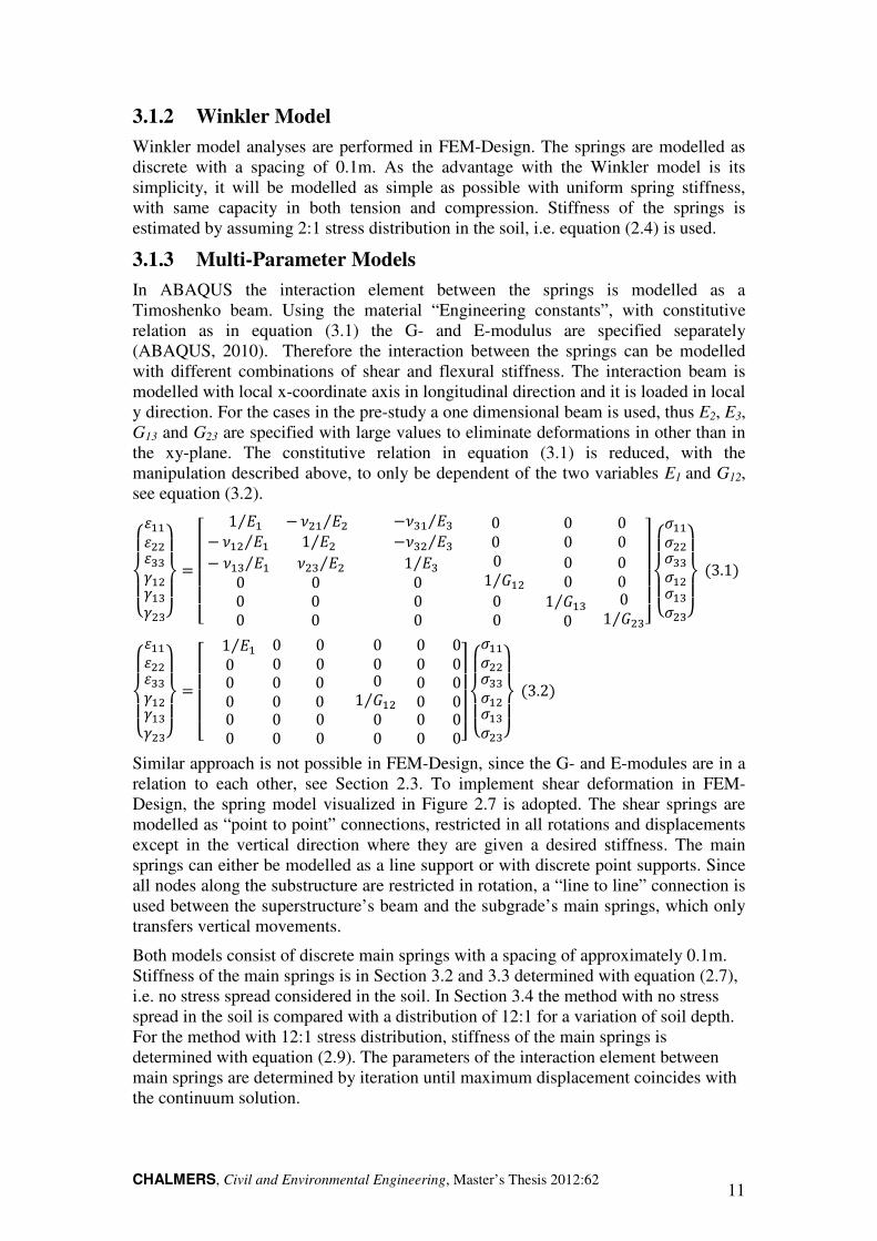
The subgrade is modelled with solid plane strain elements with linear elastic isotropic material. Interaction between the superstructure and the subgrade is modelled without friction in tangential direction and only compression capacity in vertical direction. The bottom surface of the subgrade is restricted in vertical and tangential direction. Infinite elements are applied at the sides of the subgrade, representing endless soil propagation. The mesh is quad-dominated, see Figure 3.1 and 3.2 for the mesh in the case with footing.
Figure 3.1 Mesh of modelled continuum.
Figure 3.2 Mesh of modelled continuum right under superstructure.
CHALMERS, Civil and Environmental Engineering, Master’s Thesis 2012:62 11
3.1.2 Winkler Model
Winkler model analyses are performed in FEM-Design. The springs are modelled as discrete with a spacing of 0.1m. As the advantage with the Winkler model is its simplicity, it will be modelled as simple as possible with uniform spring stiffness, with same capacity in both tension and compression. Stiffness of the springs is estimated by assuming 2:1 stress distribution in the soil, i.e. equation (2.4) is used.
3.1.3 Multi-Parameter Models
In ABAQUS the interaction element between the springs is modelled as a Timoshenko beam. Using the material “Engineering constants”, with constitutive relation as in equation (3.1) the G- and E-modulus are specified separately (ABAQUS, 2010). Therefore the interaction between the springs can be modelled with different combinations of shear and flexural stiffness. The interaction beam is modelled with local x-coordinate axis in longitudinal direction and it is loaded in local y direction. For the cases in the pre-study a one dimensional beam is used, thus E2, E3, G13 and G23 are specified with large values to eliminate deformations in other than in the xy-plane. The constitutive relation in equation (3.1) is reduced, with the manipulation described above, to only be dependent of the two variables E1 and G12, see equation (3.2).
JKLKMN//N$$N11O/$O/1O$1PKQ
KR (STTTTU1 �/⁄" V/$ �/⁄ "V$/ �$⁄1 �$⁄ "V1/ �1⁄"V1$ �1⁄ 00 00 00"V/1 �/⁄0 V$1 �$⁄0 1 �1⁄0 01 �/$⁄ 00 0000 00 00 00 1 �/1⁄0 01 �$1⁄ WXX
XXYJKLKM�//�$$�11�/$�/1�$1PKQ
KR�3.1!
JKLKMN//N$$N11O/$O/1O$1PKQ
KR (STTTTU1 �/⁄0 00 00 00 00 0000 00 00 01 �/$⁄ 00 0000 00 00 00 00 00WXX
XXYJKLKM�//�$$�11�/$�/1�$1PKQ
KR�3.2! Similar approach is not possible in FEM-Design, since the G- and E-modules are in a relation to each other, see Section 2.3. To implement shear deformation in FEM-Design, the spring model visualized in Figure 2.7 is adopted. The shear springs are modelled as “point to point” connections, restricted in all rotations and displacements except in the vertical direction where they are given a desired stiffness. The main springs can either be modelled as a line support or with discrete point supports. Since all nodes along the substructure are restricted in rotation, a “line to line” connection is used between the superstructure’s beam and the subgrade’s main springs, which only transfers vertical movements.
Both models consist of discrete main springs with a spacing of approximately 0.1m. Stiffness of the main springs is in Section 3.2 and 3.3 determined with equation (2.7), i.e. no stress spread considered in the soil. In Section 3.4 the method with no stress spread in the soil is compared with a distribution of 12:1 for a variation of soil depth. For the method with 12:1 stress distribution, stiffness of the main springs is determined with equation (2.9). The parameters of the interaction element between main springs are determined by iteration until maximum displacement coincides with the continuum solution.
CHALMERS, Civil and Environmental Engineering, Master’s Thesis 2012:62 12
3.1.4 MK-R Model
Analyses of the MK-R model are performed in ABAQUS. Bar elements with infinite tension stiffness and no compression stiffness are used as pre-tensioned members, instead of using a membrane as specified for 3D MK-R model. Pre-tension force and stiffness for upper and lower spring layers are calculated with equations (2.11) and (2.13). Also in this model, discrete springs are used with a spacing of approximately 0.1m. To use the MK-R model properly, second order effects need to be considered, which is done by the option “Include large deformations”.
3.2 SSI Analysis for Stiff Superstructure
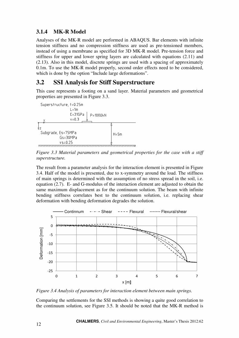
This case represents a footing on a sand layer. Material parameters and geometrical properties are presented in Figure 3.3.
Figure 3.3 Material parameters and geometrical properties for the case with a stiff
superstructure.
The result from a parameter analysis for the interaction element is presented in Figure 3.4. Half of the model is presented, due to x-symmetry around the load. The stiffness of main springs is determined with the assumption of no stress spread in the soil, i.e. equation (2.7). E- and G-modulus of the interaction element are adjusted to obtain the same maximum displacement as for the continuum solution. The beam with infinite bending stiffness correlates best to the continuum solution, i.e. replacing shear deformation with bending deformation degrades the solution.
Figure 3.4 Analysis of parameters for interaction element between main springs.
Comparing the settlements for the SSI methods is showing a quite good correlation to the continuum solution, see Figure 3.5. It should be noted that the MK-R method is
-25
-20
-15
-10
-5
0
5
0 1 2 3 4 5 6 7
Defo
rmation [m
m]
x [m]
Continnum Shear Flexural Flexural/shear
CHALMERS, Civil and Environmental Engineering, Master’s Thesis 2012:62 13
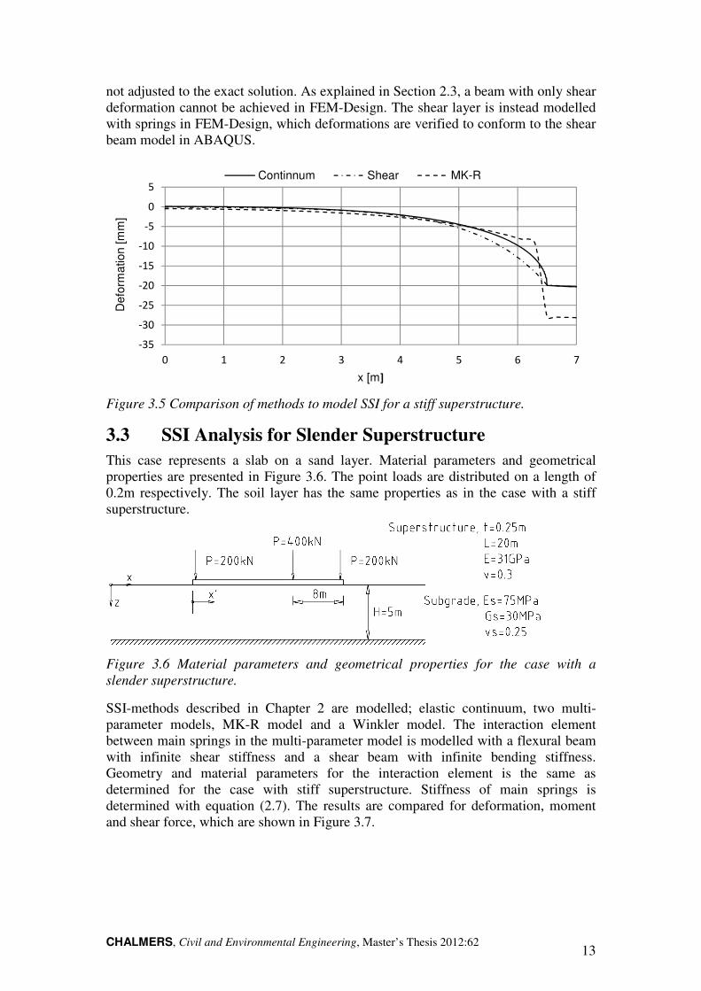
not adjusted to the exact solution. As explained in Section 2.3, a beam with only shear deformation cannot be achieved in FEM-Design. The shear layer is instead modelled with springs in FEM-Design, which deformations are verified to conform to the shear beam model in ABAQUS.
Figure 3.5 Comparison of methods to model SSI for a stiff superstructure.
3.3 SSI Analysis for Slender Superstructure
This case represents a slab on a sand layer. Material parameters and geometrical properties are presented in Figure 3.6. The point loads are distributed on a length of 0.2m respectively. The soil layer has the same properties as in the case with a stiff superstructure.
Figure 3.6 Material parameters and geometrical properties for the case with a
slender superstructure.
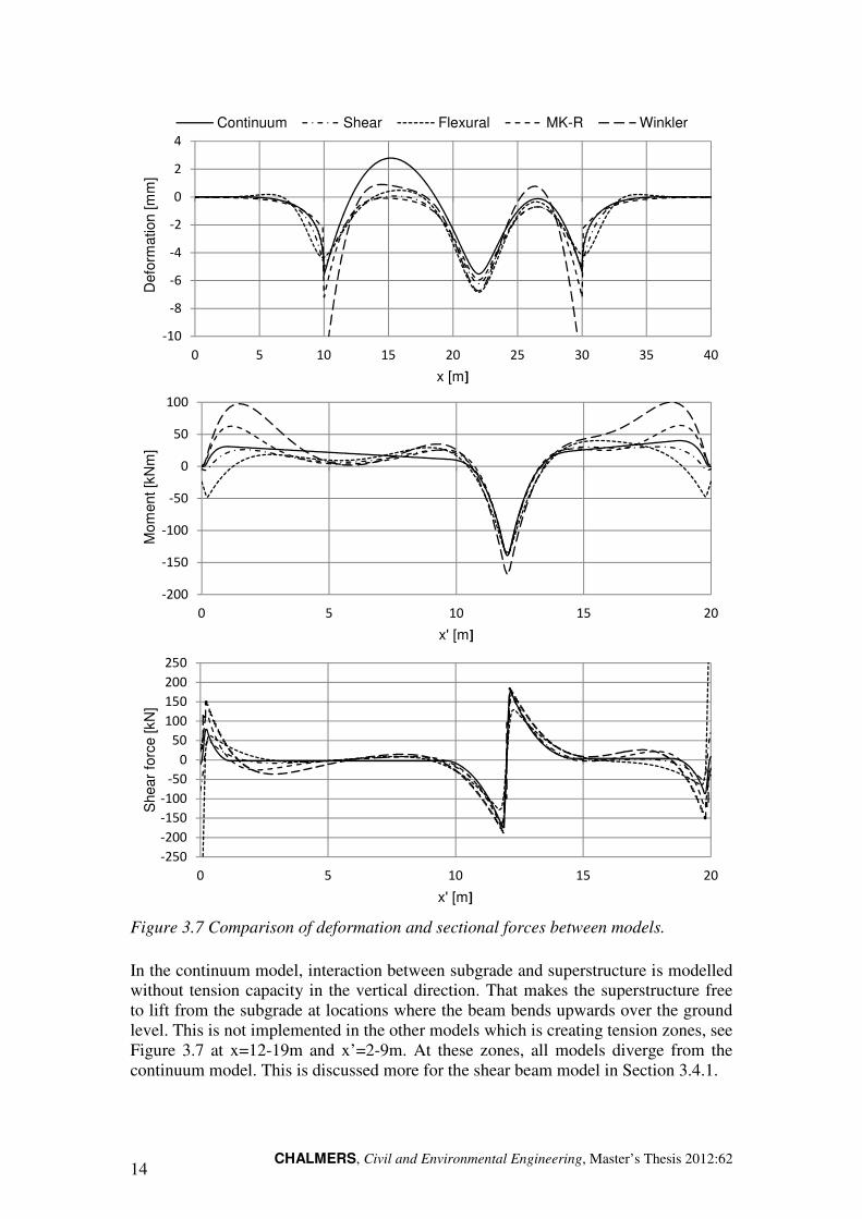
SSI-methods described in Chapter 2 are modelled; elastic continuum, two multi-parameter models, MK-R model and a Winkler model. The interaction element between main springs in the multi-parameter model is modelled with a flexural beam with infinite shear stiffness and a shear beam with infinite bending stiffness. Geometry and material parameters for the interaction element is the same as determined for the case with stiff superstructure. Stiffness of main springs is determined with equation (2.7). The results are compared for deformation, moment and shear force, which are shown in Figure 3.7.
-35
-30
-25
-20
-15
-10
-5
0
5
0 1 2 3 4 5 6 7
Defo
rmation [m
m]
x [m]
Continnum Shear MK-R
CHALMERS, Civil and Environmental Engineering, Master’s Thesis 2012:62 14
In the continuum model, interaction between subgrade and superstructure is modelled without tension capacity in the vertical direction. That makes the superstructure free to lift from the subgrade at locations where the beam bends upwards over the ground level. This is not implemented in the other models which is creating tension zones, see Figure 3.7 at x=12-19m and x’=2-9m. At these zones, all models diverge from the continuum model. This is discussed more for the shear beam model in Section 3.4.1.
-250
-200
-150
-100
-50
0
50
100
150
200
250
0 5 10 15 20
Shear
forc
e [kN
]
x' [m]
-200
-150
-100
-50
0
50
100
0 5 10 15 20
Mom
ent [k
Nm
]
x' [m]
-10
-8
-6
-4
-2
0
2
4
0 5 10 15 20 25 30 35 40
Defo
rmation [m
m]
x [m]
Continuum Shear Flexural MK-R Winkler
Figure 3.7 Comparison of deformation and sectional forces between models.
CHALMERS, Civil and Environmental Engineering, Master’s Thesis 2012:62 15
Least accurate of the models is the Winkler model, which is expected since the other models in some way are modifications on the Winkler model for improvements. The Winkler model is except from at the tension zones, giving more conservative results in the ground slab though. As expected, the Winkler model results in high moments towards the superstructure edges, see Section 2.2 for explanation. A modification that reduces this effect is to increase the stiffness in the springs close to the edges, which is investigated in Section 3.5.
The shear beam solution conforms well to the continuum solution. Smaller moment towards the edges indicates that the shear transfer is slightly overestimated, see Figure 3.7. Similar behaviour can also be observed in Figure 3.5, where the settlement is larger adjacent to the superstructure for the shear beam model.
As the same shear stiffness is used for the case with a stiff superstructure, it indicates that the shear stiffness can be determined independently of the superstructure’s geometry. Using bending deformation instead of shear deformations degrades the solution, as also shown for the case with stiff superstructure. The most significant difference is for this case noted at the edges where the moment for the flexural beam is negative.
The MK-R model is also conforming quite well to the continuum model. Higher moment at the edges can be observed, but not as high as with the Winkler model.
3.4 Further Analysis of Shear Beam Model
This section presents a further study of the shear beam model, where modifications on the model and the parameters are made to improve the results. More specifically, two topics will be regarded; influence on results of soil depth variation and influence of tension zones between the superstructure and the subgrade.
3.4.1 No Tension Interaction between Superstructure and
Subgrade
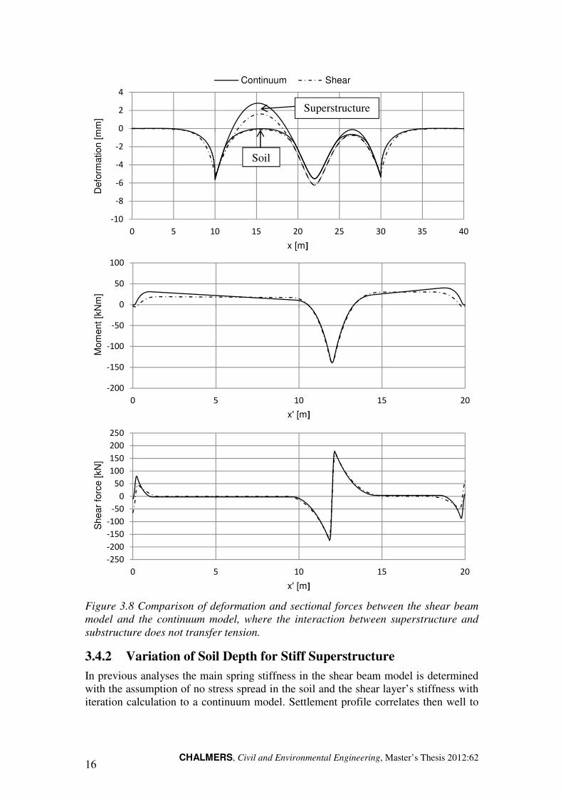
In the analysis described in Section 3.3, the shear beam diverges from the elastic continuum model in the tension zones, see Figure 3.7. This difference arises because the superstructure in the continuum solution is modelled with an interaction that only transfers compression in the interface zone between the superstructure and subgrade. By implementing the same interaction to the shear beam model, the results are improved, which are shown in Figure 3.8. In the deformation plot there are two curves displayed for each model since the superstructure and the substructure are separating where the superstructure is bending upwards.
CHALMERS, Civil and Environmental Engineering, Master’s Thesis 2012:62 16
Figure 3.8 Comparison of deformation and sectional forces between the shear beam
model and the continuum model, where the interaction between superstructure and
substructure does not transfer tension.
3.4.2 Variation of Soil Depth for Stiff Superstructure
In previous analyses the main spring stiffness in the shear beam model is determined with the assumption of no stress spread in the soil and the shear layer’s stiffness with iteration calculation to a continuum model. Settlement profile correlates then well to
-250
-200
-150
-100
-50
0
50
100
150
200
250
0 5 10 15 20
Shear
forc
e [kN
]
x' [m]
-200
-150
-100
-50
0
50
100
0 5 10 15 20
Mom
ent [k
Nm
]
x' [m]
-10
-8
-6
-4
-2
0
2
4
0 5 10 15 20 25 30 35 40
Defo
rmation [m
m]
x [m]
Continuum Shear
Superstructure
Soil
CHALMERS, Civil and Environmental Engineering, Master’s Thesis 2012:62 17
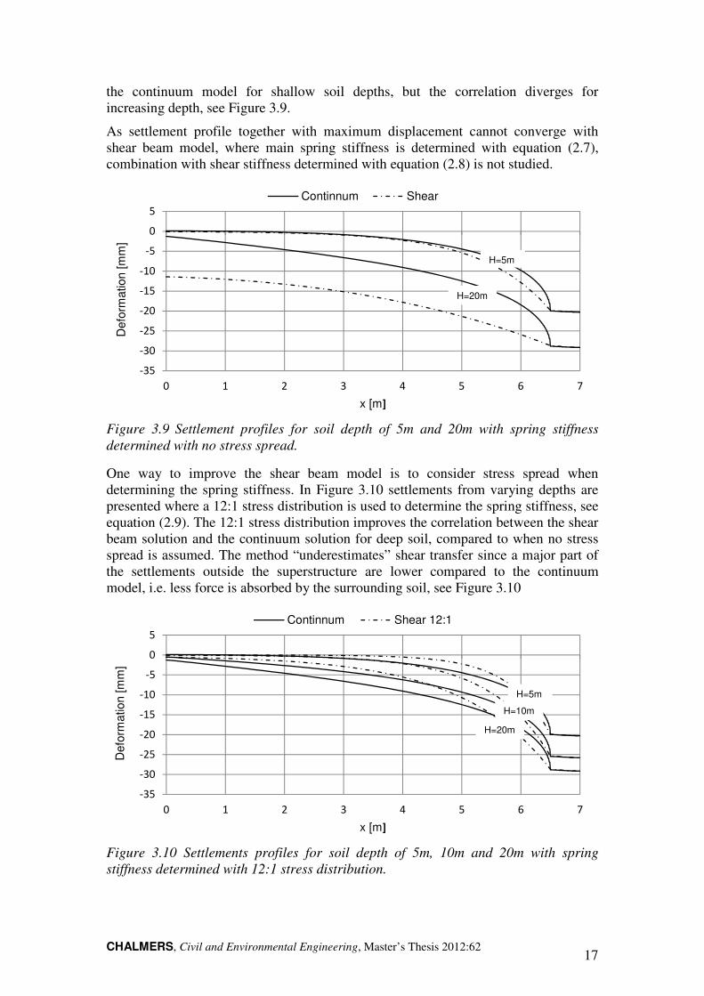
the continuum model for shallow soil depths, but the correlation diverges for increasing depth, see Figure 3.9.
As settlement profile together with maximum displacement cannot converge with shear beam model, where main spring stiffness is determined with equation (2.7), combination with shear stiffness determined with equation (2.8) is not studied.
Figure 3.9 Settlement profiles for soil depth of 5m and 20m with spring stiffness
determined with no stress spread.
One way to improve the shear beam model is to consider stress spread when determining the spring stiffness. In Figure 3.10 settlements from varying depths are presented where a 12:1 stress distribution is used to determine the spring stiffness, see equation (2.9). The 12:1 stress distribution improves the correlation between the shear beam solution and the continuum solution for deep soil, compared to when no stress spread is assumed. The method “underestimates” shear transfer since a major part of the settlements outside the superstructure are lower compared to the continuum model, i.e. less force is absorbed by the surrounding soil, see Figure 3.10
Figure 3.10 Settlements profiles for soil depth of 5m, 10m and 20m with spring
stiffness determined with 12:1 stress distribution.
-35
-30
-25
-20
-15
-10
-5
0
5
0 1 2 3 4 5 6 7
Defo
rmation [m
m]
x [m]
Continnum Shear
H=5m
H=20m
-35
-30
-25
-20
-15
-10
-5
0
5
0 1 2 3 4 5 6 7
Defo
rmation [m
m]
x [m]
Continnum Shear 12:1
H=5m
H=10m
H=20m
CHALMERS, Civil and Environmental Engineering, Master’s Thesis 2012:62 18
3.4.3 Variation of Soil Depth for Slender Superstructure
In this section the variation of soil depth for the case with a slender superstructure is considered. Same shear stiffness is used for the shear beam as for the case with stiff superstructure for respectively soil depth. Main spring stiffness is determined with a 12:1 stress distribution according to equation (2.9). Interaction between superstructure and subgrade is modelled without friction and only compression capacity in vertical direction. Results for the Winkler model are also presented to better illustrate the accuracy of the shear beam model’s results. Spring stiffness for the Winkler model is determined with 2:1 method, according to equation (2.4) and has the same behaviour in tension and compression.
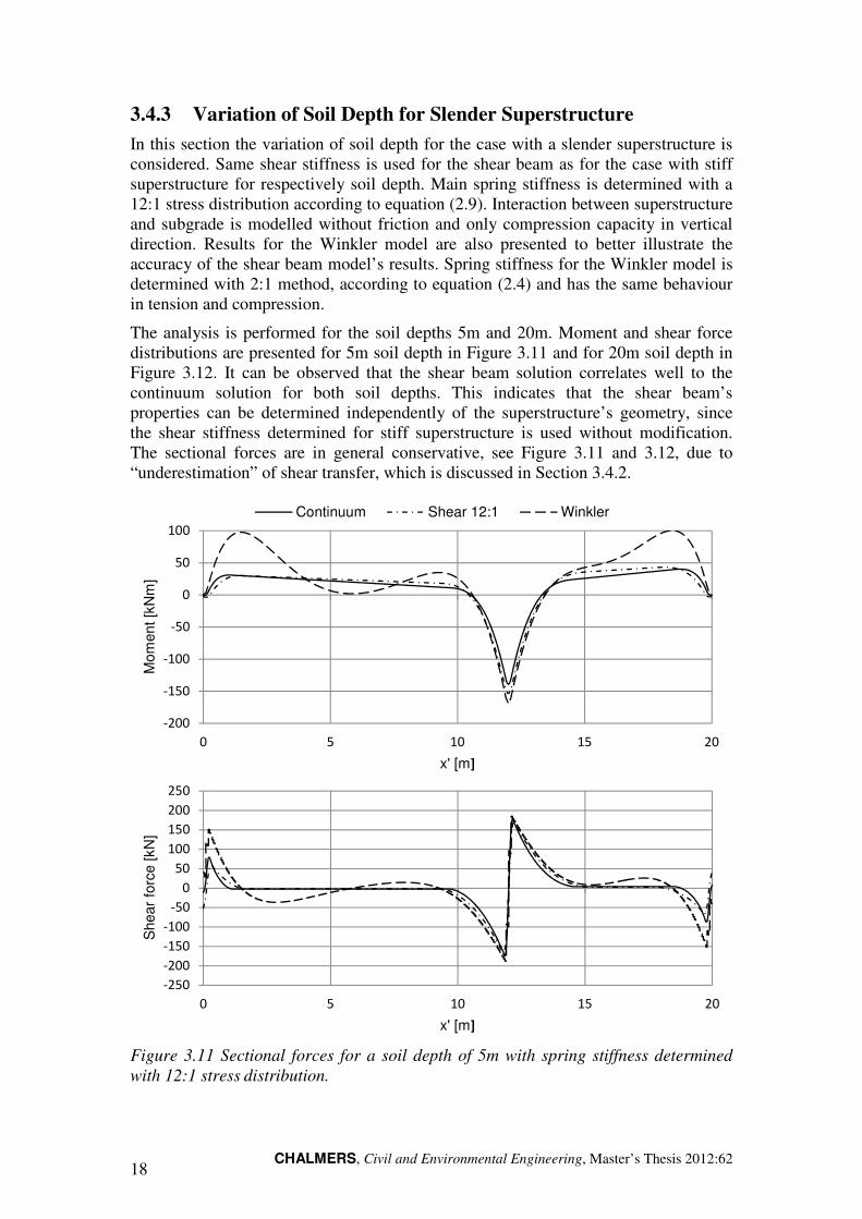
The analysis is performed for the soil depths 5m and 20m. Moment and shear force distributions are presented for 5m soil depth in Figure 3.11 and for 20m soil depth in Figure 3.12. It can be observed that the shear beam solution correlates well to the continuum solution for both soil depths. This indicates that the shear beam’s properties can be determined independently of the superstructure’s geometry, since the shear stiffness determined for stiff superstructure is used without modification. The sectional forces are in general conservative, see Figure 3.11 and 3.12, due to “underestimation” of shear transfer, which is discussed in Section 3.4.2.
Figure 3.11 Sectional forces for a soil depth of 5m with spring stiffness determined
with 12:1 stress distribution.
-250
-200
-150
-100
-50
0
50
100
150
200
250
0 5 10 15 20
Shear
forc
e [kN
]
x' [m]
-200
-150
-100
-50
0
50
100
0 5 10 15 20
Mom
ent [k
Nm
]
x' [m]
Continuum Shear 12:1 Winkler
CHALMERS, Civil and Environmental Engineering, Master’s Thesis 2012:62 19
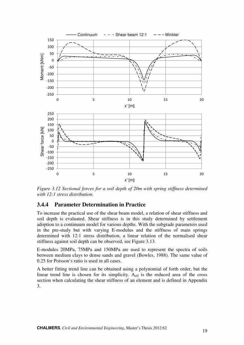
Figure 3.12 Sectional forces for a soil depth of 20m with spring stiffness determined
with 12:1 stress distribution.
3.4.4 Parameter Determination in Practice
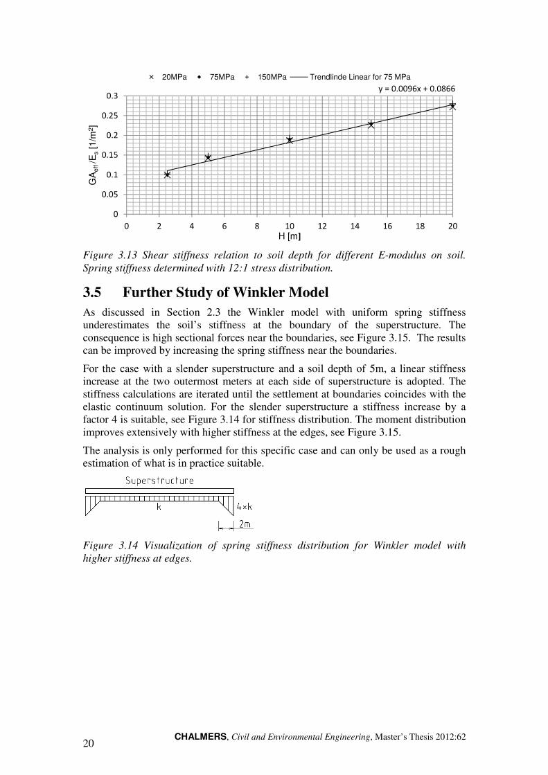
To increase the practical use of the shear beam model, a relation of shear stiffness and soil depth is evaluated. Shear stiffness is in this study determined by settlement adoption to a continuum model for various depths. With the subgrade parameters used in the pre-study but with varying E-modulus and the stiffness of main springs determined with 12:1 stress distribution, a linear relation of the normalised shear stiffness against soil depth can be observed, see Figure 3.13.
E-modules 20MPa, 75MPa and 150MPa are used to represent the spectra of soils between medium clays to dense sands and gravel (Bowles, 1988). The same value of 0.25 for Poisson’s ratio is used in all cases.
A better fitting trend line can be obtained using a polynomial of forth order, but the linear trend line is chosen for its simplicity. Aeff is the reduced area of the cross section when calculating the shear stiffness of an element and is defined in Appendix 3.
-250
-200
-150
-100
-50
0
50
100
150
200
250
0 5 10 15 20
Shear
forc
e [kN
]
x' [m]
-250
-200
-150
-100
-50
0
50
100
150
0 5 10 15 20
Mom
ent [k
Nm
]
x' [m]
Continuum Shear beam 12:1 Winkler
CHALMERS, Civil and Environmental Engineering, Master’s Thesis 2012:62 20
Figure 3.13 Shear stiffness relation to soil depth for different E-modulus on soil.
Spring stiffness determined with 12:1 stress distribution.
3.5 Further Study of Winkler Model
As discussed in Section 2.3 the Winkler model with uniform spring stiffness underestimates the soil’s stiffness at the boundary of the superstructure. The consequence is high sectional forces near the boundaries, see Figure 3.15. The results can be improved by increasing the spring stiffness near the boundaries.
For the case with a slender superstructure and a soil depth of 5m, a linear stiffness increase at the two outermost meters at each side of superstructure is adopted. The stiffness calculations are iterated until the settlement at boundaries coincides with the elastic continuum solution. For the slender superstructure a stiffness increase by a factor 4 is suitable, see Figure 3.14 for stiffness distribution. The moment distribution improves extensively with higher stiffness at the edges, see Figure 3.15.
The analysis is only performed for this specific case and can only be used as a rough estimation of what is in practice suitable.
Figure 3.14 Visualization of spring stiffness distribution for Winkler model with
higher stiffness at edges.
y = 0.0096x + 0.0866
0
0.05
0.1
0.15
0.2
0.25
0.3
0 2 4 6 8 10 12 14 16 18 20
GA
eff
/Es
[1/m
2]
H [m]
20MPa 75MPa 150MPa Trendlinde Linear for 75 MPa
CHALMERS, Civil and Environmental Engineering, Master’s Thesis 2012:62 21
Figure 3.15 Moment distribution for Winkler model with stiffer springs at the
superstructures edges.
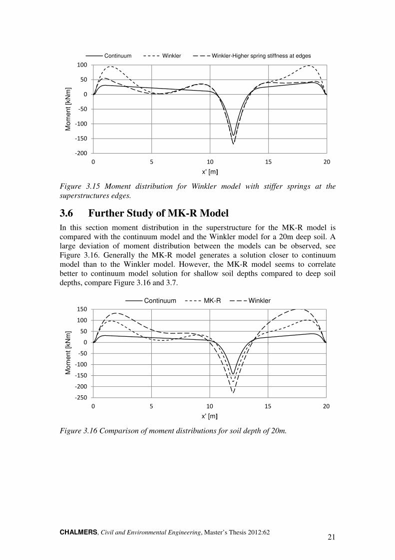
3.6 Further Study of MK-R Model
In this section moment distribution in the superstructure for the MK-R model is compared with the continuum model and the Winkler model for a 20m deep soil. A large deviation of moment distribution between the models can be observed, see Figure 3.16. Generally the MK-R model generates a solution closer to continuum model than to the Winkler model. However, the MK-R model seems to correlate better to continuum model solution for shallow soil depths compared to deep soil depths, compare Figure 3.16 and 3.7.
Figure 3.16 Comparison of moment distributions for soil depth of 20m.
-200
-150
-100
-50
0
50
100
0 5 10 15 20
Mom
ent [k
Nm
]
x' [m]
Continuum Winkler Winkler-Higher spring stiffness at edges
-250
-200
-150
-100
-50
0
50
100
150
0 5 10 15 20
Mom
ent [k
Nm
]
x' [m]
Continuum MK-R Winkler
CHALMERS, Civil and Environmental Engineering, Master’s Thesis 2012:62 22
4 Case Study of KKH
In the pre-study it is observed that a model with shear layer as interaction element extensively can improve 2D SSI-analysis compared with a Winkler model. In this chapter 3D models of “Malmö Kongress, Koncert och Hotell” (KKH) are compared.
KKH is currently the greatest project of “Skanska hus och bostad” in Skåne and it is one of their first greater projects that will be designed according to Eurocode. Since Skanska tries to design the construction on a raft without piles, the discussion about SSI is given a lot of attention.
As the soil is heavily over-consolidated, and therefore can be modelled with linear elastic behaviour the case is well suited for implementation of the different model-techniques discussed in this thesis.
The SSI-problem is modelled by the authors as with Winkler, shear layer and model. Skanska is providing with a contour plot over deformations from a continuum model which is modelled in the geotechnical analysis software PLAXIS. To regard the influence on the bending stiffness from the walls on basement floor level, the model with an interacting shear element is modelled with and without walls.
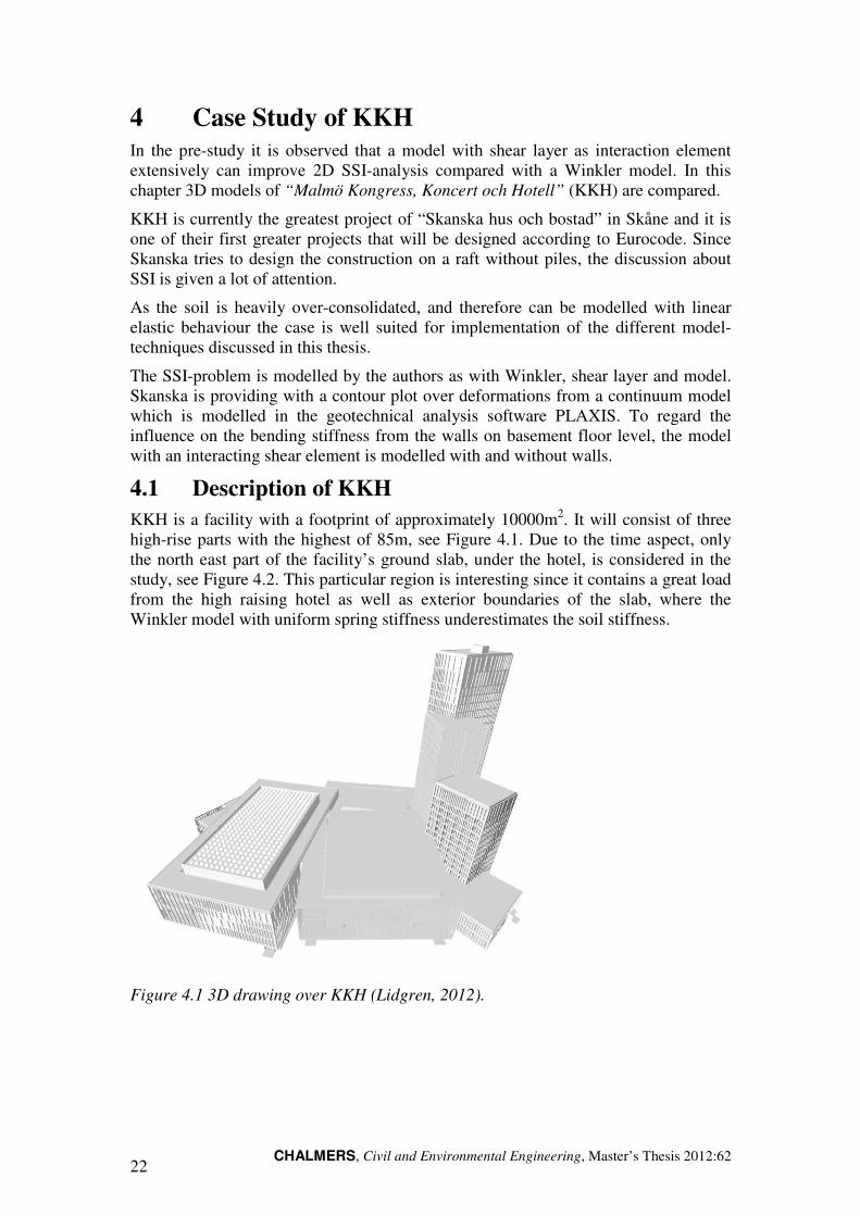
4.1 Description of KKH
KKH is a facility with a footprint of approximately 10000m2. It will consist of three high-rise parts with the highest of 85m, see Figure 4.1. Due to the time aspect, only the north east part of the facility’s ground slab, under the hotel, is considered in the study, see Figure 4.2. This particular region is interesting since it contains a great load from the high raising hotel as well as exterior boundaries of the slab, where the Winkler model with uniform spring stiffness underestimates the soil stiffness.
Figure 4.1 3D drawing over KKH (Lidgren, 2012).
CHALMERS, Civil and Environmental Engineering, Master’s Thesis 2012:62 23
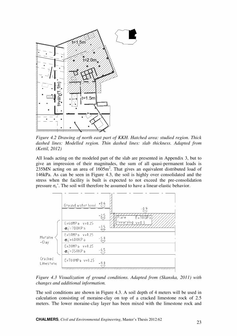
Figure 4.2 Drawing of north east part of KKH. Hatched area: studied region. Thick
dashed lines: Modelled region. Thin dashed lines: slab thickness. Adapted from
(Kettil, 2012)
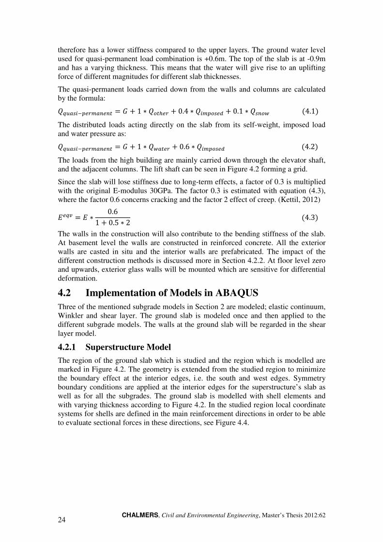
All loads acting on the modeled part of the slab are presented in Appendix 3, but to give an impression of their magnitudes, the sum of all quasi-permanent loads is 235MN acting on an area of 1605m2. That gives an equivalent distributed load of 146kPa. As can be seen in Figure 4.3, the soil is highly over consolidated and the stress when the facility is built is expected to not exceed the pre-consolidation pressure σc’. The soil will therefore be assumed to have a linear-elastic behavior.
Figure 4.3 Visualization of ground conditions. Adapted from (Skanska, 2011) with
changes and additional information.
The soil conditions are shown in Figure 4.3. A soil depth of 4 meters will be used in calculation consisting of moraine-clay on top of a cracked limestone rock of 2.5 meters. The lower moraine-clay layer has been mixed with the limestone rock and
CHALMERS, Civil and Environmental Engineering, Master’s Thesis 2012:62 24
therefore has a lower stiffness compared to the upper layers. The ground water level used for quasi-permanent load combination is +0.6m. The top of the slab is at -0.9m and has a varying thickness. This means that the water will give rise to an uplifting force of different magnitudes for different slab thicknesses.
The quasi-permanent loads carried down from the walls and columns are calculated by the formula: �Z�[��\��]^[_�_` = � + 1 ∗ �a`b�] + 0.4 ∗ ��^�a��c + 0.1 ∗ ��_ad(4.1) The distributed loads acting directly on the slab from its self-weight, imposed load and water pressure as:
�Z�[��\��]^[_�_` = � + 1 ∗ �d[`�] + 0.6 ∗ ��^�a��c(4.2) The loads from the high building are mainly carried down through the elevator shaft, and the adjacent columns. The lift shaft can be seen in Figure 4.2 forming a grid.
Since the slab will lose stiffness due to long-term effects, a factor of 0.3 is multiplied with the original E-modulus 30GPa. The factor 0.3 is estimated with equation (4.3), where the factor 0.6 concerns cracking and the factor 2 effect of creep. (Kettil, 2012)
��Ze = � ∗ 0.61 + 0.5 ∗ 2(4.3)
The walls in the construction will also contribute to the bending stiffness of the slab. At basement level the walls are constructed in reinforced concrete. All the exterior walls are casted in situ and the interior walls are prefabricated. The impact of the different construction methods is discussed more in Section 4.2.2. At floor level zero and upwards, exterior glass walls will be mounted which are sensitive for differential deformation.
4.2 Implementation of Models in ABAQUS
Three of the mentioned subgrade models in Section 2 are modeled; elastic continuum, Winkler and shear layer. The ground slab is modeled once and then applied to the different subgrade models. The walls at the ground slab will be regarded in the shear layer model.
4.2.1 Superstructure Model
The region of the ground slab which is studied and the region which is modelled are marked in Figure 4.2. The geometry is extended from the studied region to minimize the boundary effect at the interior edges, i.e. the south and west edges. Symmetry boundary conditions are applied at the interior edges for the superstructure’s slab as well as for all the subgrades. The ground slab is modelled with shell elements and with varying thickness according to Figure 4.2. In the studied region local coordinate systems for shells are defined in the main reinforcement directions in order to be able to evaluate sectional forces in these directions, see Figure 4.4.
CHALMERS, Civil and Environmental Engineering, Master’s Thesis 2012:62 25
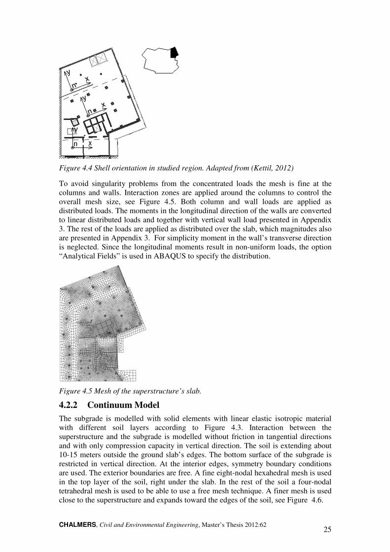
Figure 4.4 Shell orientation in studied region. Adapted from (Kettil, 2012)
To avoid singularity problems from the concentrated loads the mesh is fine at the columns and walls. Interaction zones are applied around the columns to control the overall mesh size, see Figure 4.5. Both column and wall loads are applied as distributed loads. The moments in the longitudinal direction of the walls are converted to linear distributed loads and together with vertical wall load presented in Appendix 3. The rest of the loads are applied as distributed over the slab, which magnitudes also are presented in Appendix 3. For simplicity moment in the wall’s transverse direction is neglected. Since the longitudinal moments result in non-uniform loads, the option “Analytical Fields” is used in ABAQUS to specify the distribution.
Figure 4.5 Mesh of the superstructure’s slab.
4.2.2 Continuum Model
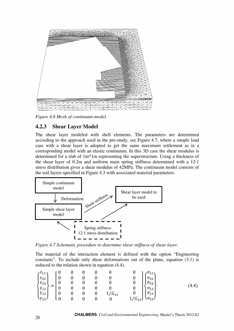
The subgrade is modelled with solid elements with linear elastic isotropic material with different soil layers according to Figure 4.3. Interaction between the superstructure and the subgrade is modelled without friction in tangential directions and with only compression capacity in vertical direction. The soil is extending about 10-15 meters outside the ground slab’s edges. The bottom surface of the subgrade is restricted in vertical direction. At the interior edges, symmetry boundary conditions are used. The exterior boundaries are free. A fine eight-nodal hexahedral mesh is used in the top layer of the soil, right under the slab. In the rest of the soil a four-nodal tetrahedral mesh is used to be able to use a free mesh technique. A finer mesh is used close to the superstructure and expands toward the edges of the soil, see Figure 4.6.
CHALMERS, Civil and Environmental Engineering, Master’s Thesis 2012:62 26
Figure 4.6 Mesh of continuum-model.
4.2.3 Shear Layer Model
The shear layer modeled with shell elements. The parameters are determined according to the approach used in the pre-study, see Figure 4.7, where a simple load case with a shear layer is adopted to get the same maximum settlement as in a corresponding model with an elastic continuum. In this 3D case the shear modulus is determined for a slab of 1m*1m representing the superstructure. Using a thickness of the shear layer of 0.2m and uniform main spring stiffness determined with a 12:1 stress distribution gives a shear modulus of 42MPa. The continuum model consists of the soil layers specified in Figure 4.3 with associated material parameters.
Figure 4.7 Schematic procedure to determine shear stiffness of shear layer.
The material of the interaction element is defined with the option “Engineering constants”. To include only shear deformations out of the plane, equation (3.1) is reduced to the relation shown in equation (4.4).
JKLKMN//N$$N11O/$O/1O$1PK
QKR =
STTTTU00 00 00 00 00 0000 00 00 00 00 0000 00 00 00 1 �/1⁄0 01 �$1⁄ WX
XXXY
JKLKM�//�$$�11�/$�/1�$1PK
QKR(4.4)
Shear layer model to
be used
Spring stiffness
12:1 stress distribution
Simple shear layer
model
Simple continuum
model
Deformation
CHALMERS, Civil and Environmental Engineering, Master’s Thesis 2012:62 27
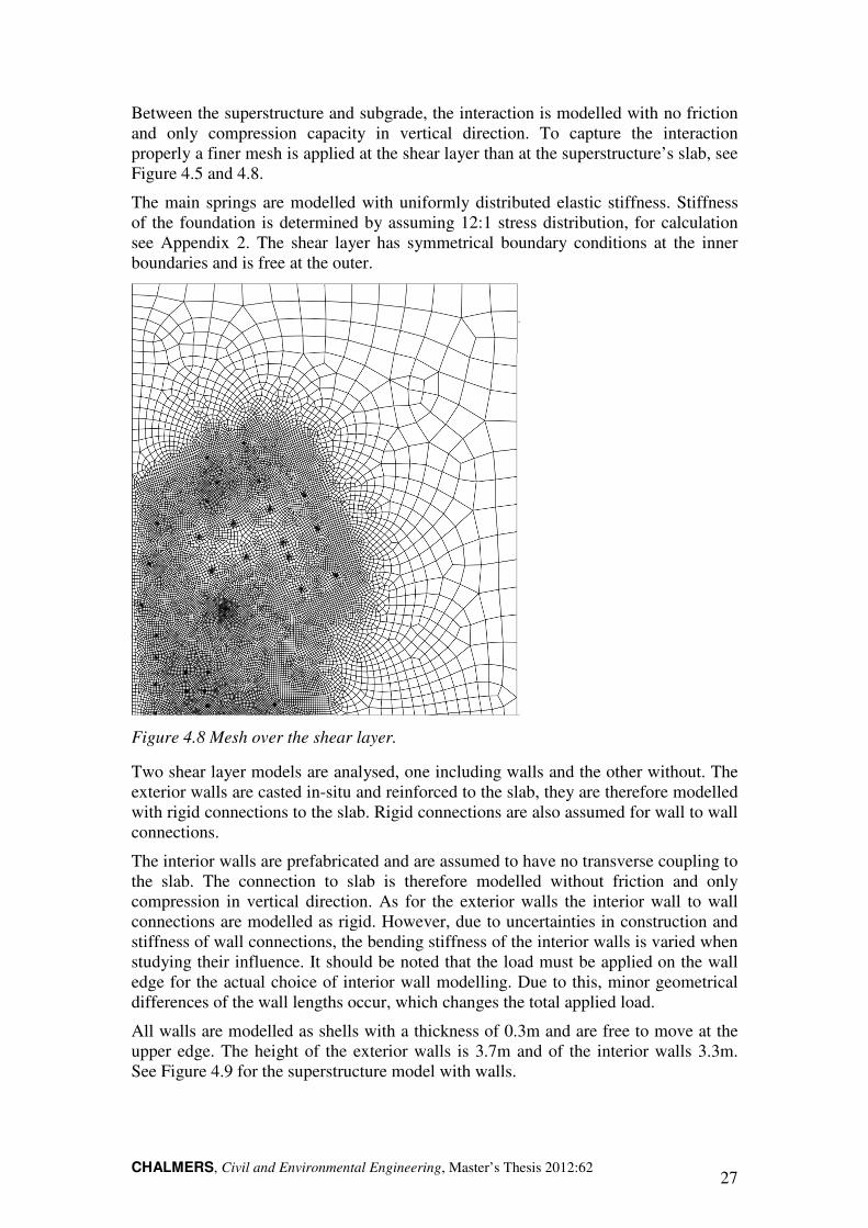
Between the superstructure and subgrade, the interaction is modelled with no friction and only compression capacity in vertical direction. To capture the interaction properly a finer mesh is applied at the shear layer than at the superstructure’s slab, see Figure 4.5 and 4.8.
The main springs are modelled with uniformly distributed elastic stiffness. Stiffness of the foundation is determined by assuming 12:1 stress distribution, for calculation see Appendix 2. The shear layer has symmetrical boundary conditions at the inner boundaries and is free at the outer.
Figure 4.8 Mesh over the shear layer.
Two shear layer models are analysed, one including walls and the other without. The exterior walls are casted in-situ and reinforced to the slab, they are therefore modelled with rigid connections to the slab. Rigid connections are also assumed for wall to wall connections.
The interior walls are prefabricated and are assumed to have no transverse coupling to the slab. The connection to slab is therefore modelled without friction and only compression in vertical direction. As for the exterior walls the interior wall to wall connections are modelled as rigid. However, due to uncertainties in construction and stiffness of wall connections, the bending stiffness of the interior walls is varied when studying their influence. It should be noted that the load must be applied on the wall edge for the actual choice of interior wall modelling. Due to this, minor geometrical differences of the wall lengths occur, which changes the total applied load.
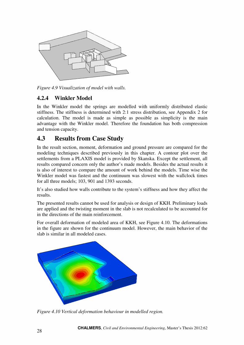
All walls are modelled as shells with a thickness of 0.3m and are free to move at the upper edge. The height of the exterior walls is 3.7m and of the interior walls 3.3m. See Figure 4.9 for the superstructure model with walls.
CHALMERS, Civil and Environmental Engineering, Master’s Thesis 2012:62 28
Figure 4.9 Visualization of model with walls.
4.2.4 Winkler Model
In the Winkler model the springs are modelled with uniformly distributed elastic stiffness. The stiffness is determined with 2:1 stress distribution, see Appendix 2 for calculation. The model is made as simple as possible as simplicity is the main advantage with the Winkler model. Therefore the foundation has both compression and tension capacity.
4.3 Results from Case Study
In the result section, moment, deformation and ground pressure are compared for the modeling techniques described previously in this chapter. A contour plot over the settlements from a PLAXIS model is provided by Skanska. Except the settlement, all results compared concern only the author’s made models. Besides the actual results it is also of interest to compare the amount of work behind the models. Time wise the Winkler model was fastest and the continuum was slowest with the wallclock times for all three models; 103, 901 and 1393 seconds.
It’s also studied how walls contribute to the system’s stiffness and how they affect the results.
The presented results cannot be used for analysis or design of KKH. Preliminary loads are applied and the twisting moment in the slab is not recalculated to be accounted for in the directions of the main reinforcement.
For overall deformation of modeled area of KKH, see Figure 4.10. The deformations in the figure are shown for the continuum model. However, the main behavior of the slab is similar in all modeled cases.
Figure 4.10 Vertical deformation behaviour in modelled region.
CHALMERS, Civil and Environmental Engineering, Master’s Thesis 2012:62 29
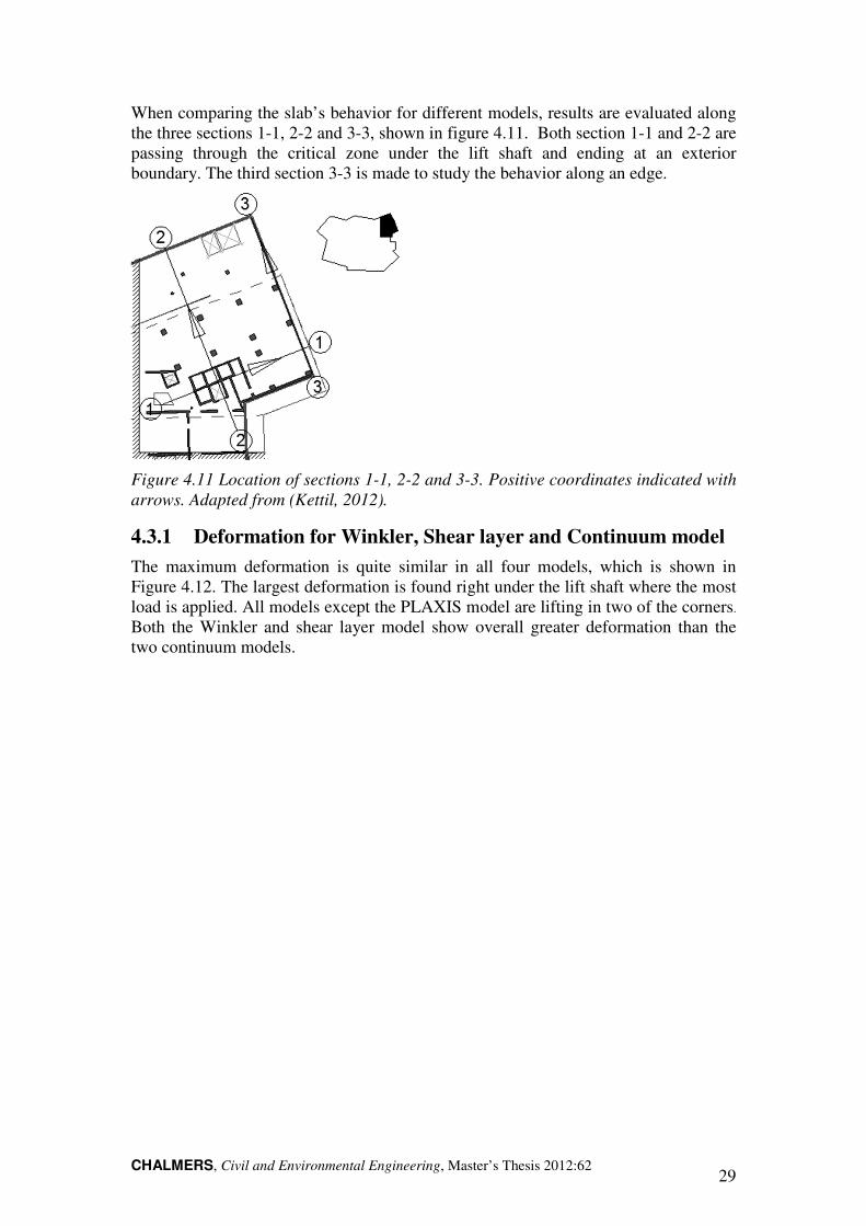
When comparing the slab’s behavior for different models, results are evaluated along the three sections 1-1, 2-2 and 3-3, shown in figure 4.11. Both section 1-1 and 2-2 are passing through the critical zone under the lift shaft and ending at an exterior boundary. The third section 3-3 is made to study the behavior along an edge.
Figure 4.11 Location of sections 1-1, 2-2 and 3-3. Positive coordinates indicated with
arrows. Adapted from (Kettil, 2012).
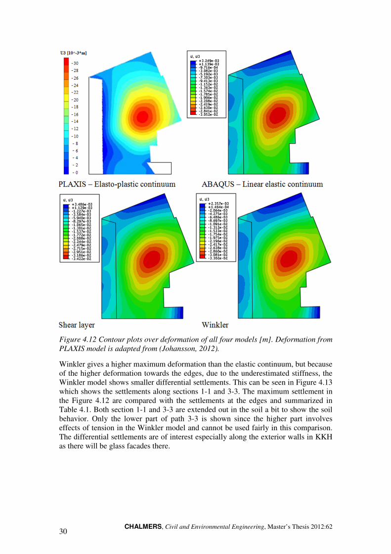
4.3.1 Deformation for Winkler, Shear layer and Continuum model
The maximum deformation is quite similar in all four models, which is shown in Figure 4.12. The largest deformation is found right under the lift shaft where the most load is applied. All models except the PLAXIS model are lifting in two of the corners.
Both the Winkler and shear layer model show overall greater deformation than the two continuum models.
CHALMERS, Civil and Environmental Engineering, Master’s Thesis 2012:62 30
Figure 4.12 Contour plots over deformation of all four models [m]. Deformation from
PLAXIS model is adapted from (Johansson, 2012).
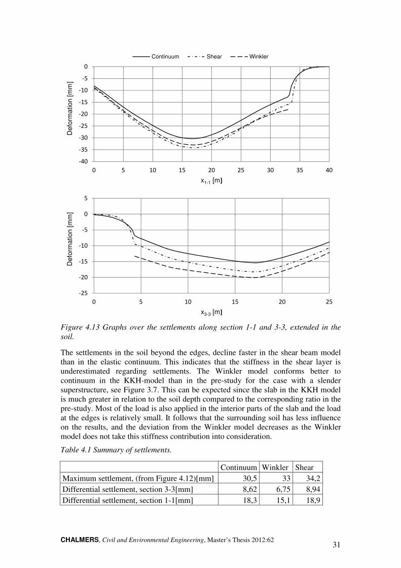
Winkler gives a higher maximum deformation than the elastic continuum, but because of the higher deformation towards the edges, due to the underestimated stiffness, the Winkler model shows smaller differential settlements. This can be seen in Figure 4.13 which shows the settlements along sections 1-1 and 3-3. The maximum settlement in the Figure 4.12 are compared with the settlements at the edges and summarized in Table 4.1. Both section 1-1 and 3-3 are extended out in the soil a bit to show the soil behavior. Only the lower part of path 3-3 is shown since the higher part involves effects of tension in the Winkler model and cannot be used fairly in this comparison. The differential settlements are of interest especially along the exterior walls in KKH as there will be glass facades there.
CHALMERS, Civil and Environmental Engineering, Master’s Thesis 2012:62 31
Figure 4.13 Graphs over the settlements along section 1-1 and 3-3, extended in the
soil.
The settlements in the soil beyond the edges, decline faster in the shear beam model than in the elastic continuum. This indicates that the stiffness in the shear layer is underestimated regarding settlements. The Winkler model conforms better to continuum in the KKH-model than in the pre-study for the case with a slender superstructure, see Figure 3.7. This can be expected since the slab in the KKH model is much greater in relation to the soil depth compared to the corresponding ratio in the pre-study. Most of the load is also applied in the interior parts of the slab and the load at the edges is relatively small. It follows that the surrounding soil has less influence on the results, and the deviation from the Winkler model decreases as the Winkler model does not take this stiffness contribution into consideration.
Table 4.1 Summary of settlements.
Continuum Winkler Shear
Maximum settlement, (from Figure 4.12)[mm] 30,5 33 34,2
Differential settlement, section 3-3[mm] 8,62 6,75 8,94
Differential settlement, section 1-1[mm] 18,3 15,1 18,9
-25
-20
-15
-10
-5
0
5
0 5 10 15 20 25
Defo
rmation [m
m]
x3-3 [m]
-40
-35
-30
-25
-20
-15
-10
-5
0
0 5 10 15 20 25 30 35 40
Defo
rmation [m
m]
x1-1 [m]
Continuum Shear Winkler
CHALMERS, Civil and Environmental Engineering, Master’s Thesis 2012:62 32
4.3.2 Moment Distribution for Winkler, Shear layer and
Continuum model
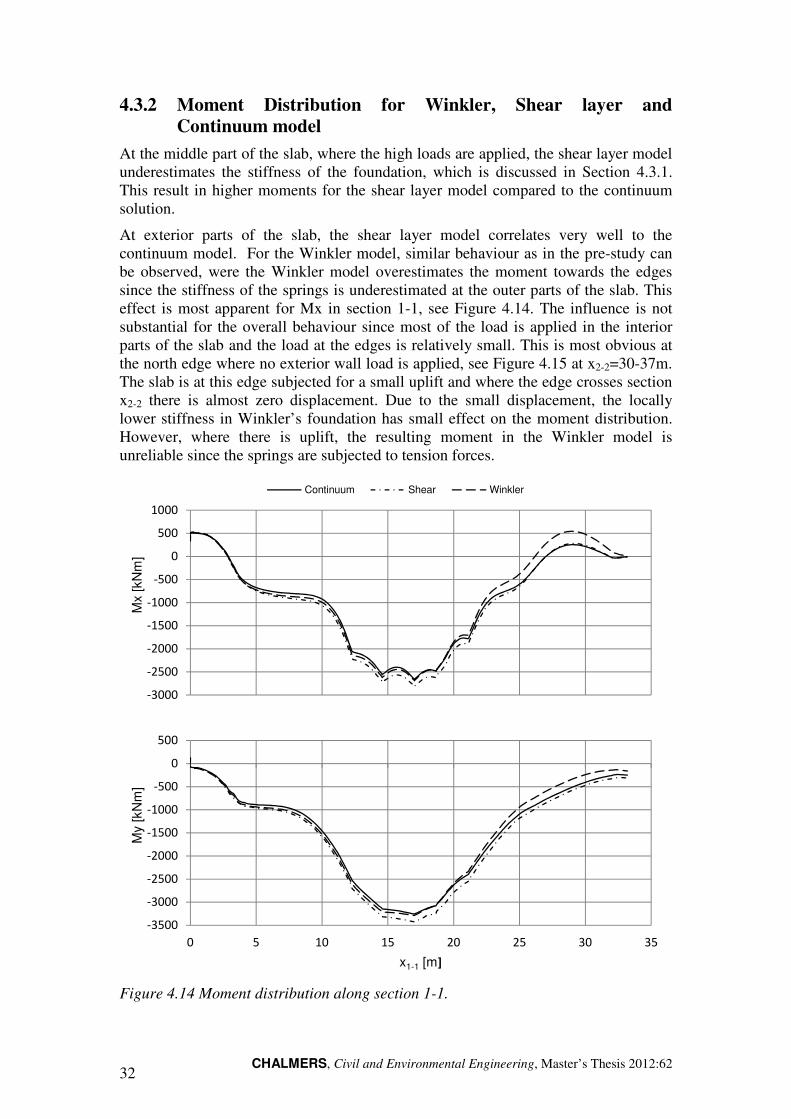
At the middle part of the slab, where the high loads are applied, the shear layer model underestimates the stiffness of the foundation, which is discussed in Section 4.3.1. This result in higher moments for the shear layer model compared to the continuum solution.
At exterior parts of the slab, the shear layer model correlates very well to the continuum model. For the Winkler model, similar behaviour as in the pre-study can be observed, were the Winkler model overestimates the moment towards the edges since the stiffness of the springs is underestimated at the outer parts of the slab. This effect is most apparent for Mx in section 1-1, see Figure 4.14. The influence is not substantial for the overall behaviour since most of the load is applied in the interior parts of the slab and the load at the edges is relatively small. This is most obvious at the north edge where no exterior wall load is applied, see Figure 4.15 at x2-2=30-37m. The slab is at this edge subjected for a small uplift and where the edge crosses section x2-2 there is almost zero displacement. Due to the small displacement, the locally lower stiffness in Winkler’s foundation has small effect on the moment distribution. However, where there is uplift, the resulting moment in the Winkler model is unreliable since the springs are subjected to tension forces.
Figure 4.14 Moment distribution along section 1-1.
-3000
-2500
-2000
-1500
-1000
-500
0
500
1000
Mx [kN
m]
Continuum Shear Winkler
-3500
-3000
-2500
-2000
-1500
-1000
-500
0
500
0 5 10 15 20 25 30 35
My
[kN
m]
x1-1 [m]
CHALMERS, Civil and Environmental Engineering, Master’s Thesis 2012:62 33
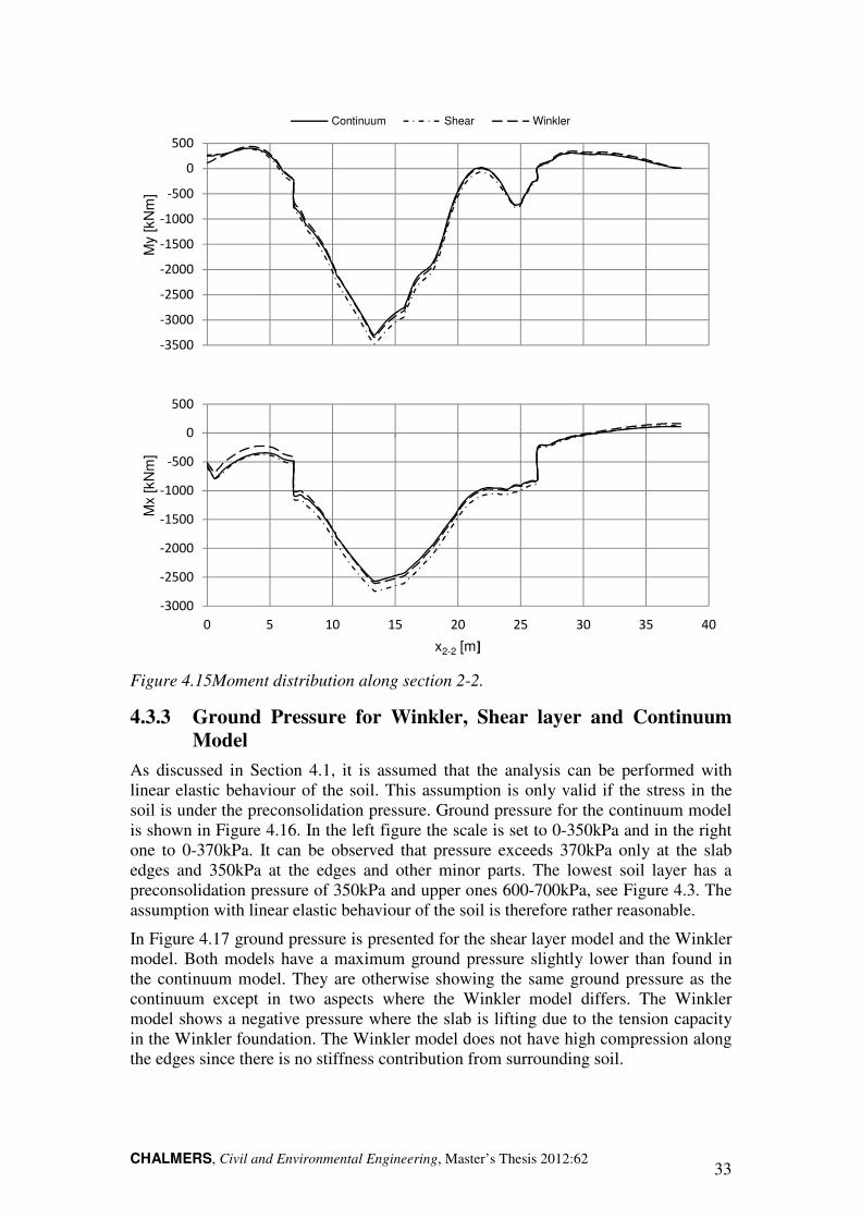
Figure 4.15Moment distribution along section 2-2.
4.3.3 Ground Pressure for Winkler, Shear layer and Continuum
Model
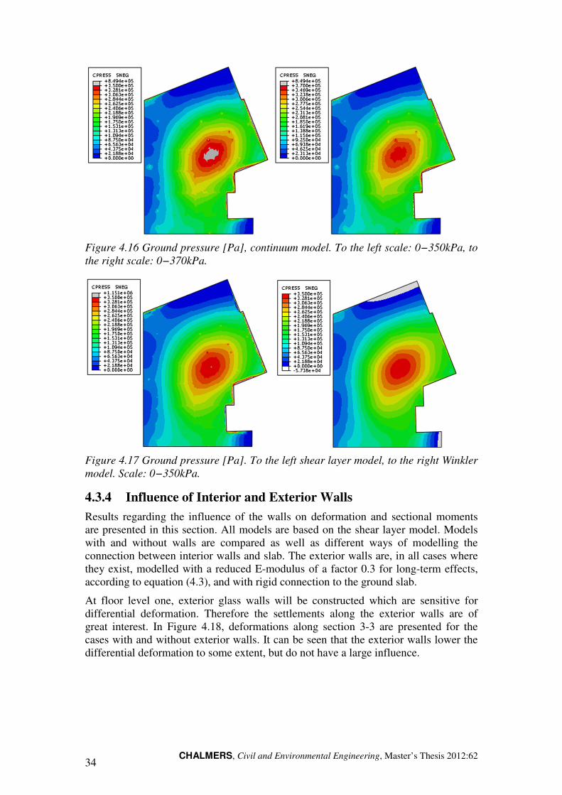
As discussed in Section 4.1, it is assumed that the analysis can be performed with linear elastic behaviour of the soil. This assumption is only valid if the stress in the soil is under the preconsolidation pressure. Ground pressure for the continuum model is shown in Figure 4.16. In the left figure the scale is set to 0-350kPa and in the right one to 0-370kPa. It can be observed that pressure exceeds 370kPa only at the slab edges and 350kPa at the edges and other minor parts. The lowest soil layer has a preconsolidation pressure of 350kPa and upper ones 600-700kPa, see Figure 4.3. The assumption with linear elastic behaviour of the soil is therefore rather reasonable.
In Figure 4.17 ground pressure is presented for the shear layer model and the Winkler model. Both models have a maximum ground pressure slightly lower than found in the continuum model. They are otherwise showing the same ground pressure as the continuum except in two aspects where the Winkler model differs. The Winkler model shows a negative pressure where the slab is lifting due to the tension capacity in the Winkler foundation. The Winkler model does not have high compression along the edges since there is no stiffness contribution from surrounding soil.
-3500
-3000
-2500
-2000
-1500
-1000
-500
0
500M
y [k
Nm
]
Continuum Shear Winkler
-3000
-2500
-2000
-1500
-1000
-500
0
500
0 5 10 15 20 25 30 35 40
Mx [kN
m]
x2-2 [m]
CHALMERS, Civil and Environmental Engineering, Master’s Thesis 2012:62 34
Figure 4.16 Ground pressure [Pa], continuum model. To the left scale: 0−350kPa, to
the right scale: 0−370kPa.
Figure 4.17 Ground pressure [Pa]. To the left shear layer model, to the right Winkler
model. Scale: 0−350kPa.
4.3.4 Influence of Interior and Exterior Walls
Results regarding the influence of the walls on deformation and sectional moments are presented in this section. All models are based on the shear layer model. Models with and without walls are compared as well as different ways of modelling the connection between interior walls and slab. The exterior walls are, in all cases where they exist, modelled with a reduced E-modulus of a factor 0.3 for long-term effects, according to equation (4.3), and with rigid connection to the ground slab.
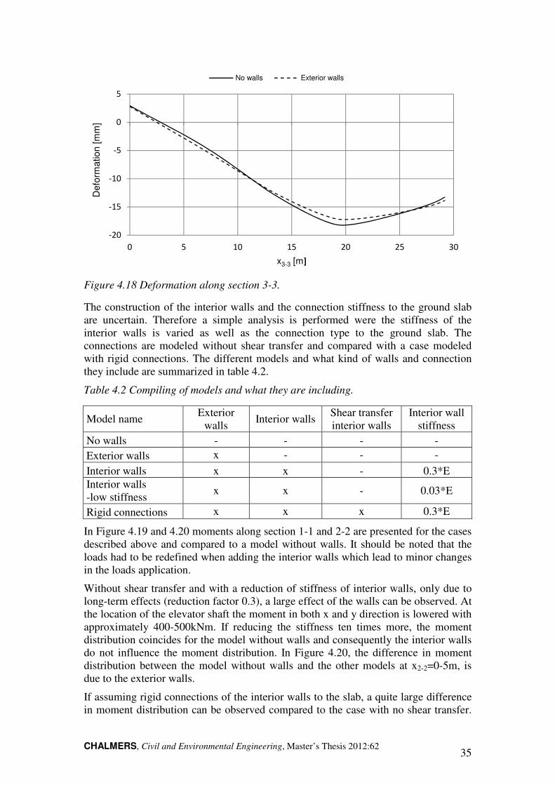
At floor level one, exterior glass walls will be constructed which are sensitive for differential deformation. Therefore the settlements along the exterior walls are of great interest. In Figure 4.18, deformations along section 3-3 are presented for the cases with and without exterior walls. It can be seen that the exterior walls lower the differential deformation to some extent, but do not have a large influence.
CHALMERS, Civil and Environmental Engineering, Master’s Thesis 2012:62 35
Figure 4.18 Deformation along section 3-3.
The construction of the interior walls and the connection stiffness to the ground slab are uncertain. Therefore a simple analysis is performed were the stiffness of the interior walls is varied as well as the connection type to the ground slab. The connections are modeled without shear transfer and compared with a case modeled with rigid connections. The different models and what kind of walls and connection they include are summarized in table 4.2.
Table 4.2 Compiling of models and what they are including.
Model name Exterior
walls Interior walls
Shear transfer interior walls
Interior wall stiffness
No walls - - - -
Exterior walls x - - -
Interior walls x x - 0.3*E
Interior walls -low stiffness
x x - 0.03*E
Rigid connections x x x 0.3*E
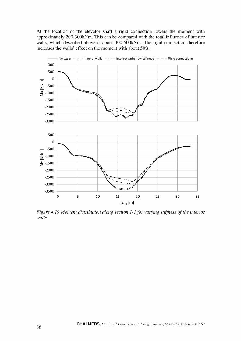
In Figure 4.19 and 4.20 moments along section 1-1 and 2-2 are presented for the cases described above and compared to a model without walls. It should be noted that the loads had to be redefined when adding the interior walls which lead to minor changes in the loads application.
Without shear transfer and with a reduction of stiffness of interior walls, only due to long-term effects (reduction factor 0.3), a large effect of the walls can be observed. At the location of the elevator shaft the moment in both x and y direction is lowered with approximately 400-500kNm. If reducing the stiffness ten times more, the moment distribution coincides for the model without walls and consequently the interior walls do not influence the moment distribution. In Figure 4.20, the difference in moment distribution between the model without walls and the other models at x2-2=0-5m, is due to the exterior walls.
If assuming rigid connections of the interior walls to the slab, a quite large difference in moment distribution can be observed compared to the case with no shear transfer.
-20
-15
-10
-5
0
5
0 5 10 15 20 25 30
Defo
rmation [m
m]
x3-3 [m]
No walls Exterior walls
CHALMERS, Civil and Environmental Engineering, Master’s Thesis 2012:62 36
At the location of the elevator shaft a rigid connection lowers the moment with approximately 200-300kNm. This can be compared with the total influence of interior walls, which described above is about 400-500kNm. The rigid connection therefore increases the walls’ effect on the moment with about 50%.
Figure 4.19 Moment distribution along section 1-1 for varying stiffness of the interior
walls.
-3000
-2500
-2000
-1500
-1000
-500
0
500
1000
Mx [kN
m]
No walls Interior walls Interiror walls -low stiffness Rigid connections
-3500
-3000
-2500
-2000
-1500
-1000
-500
0
500
0 5 10 15 20 25 30 35
My
[kN
m]
x1-1 [m]
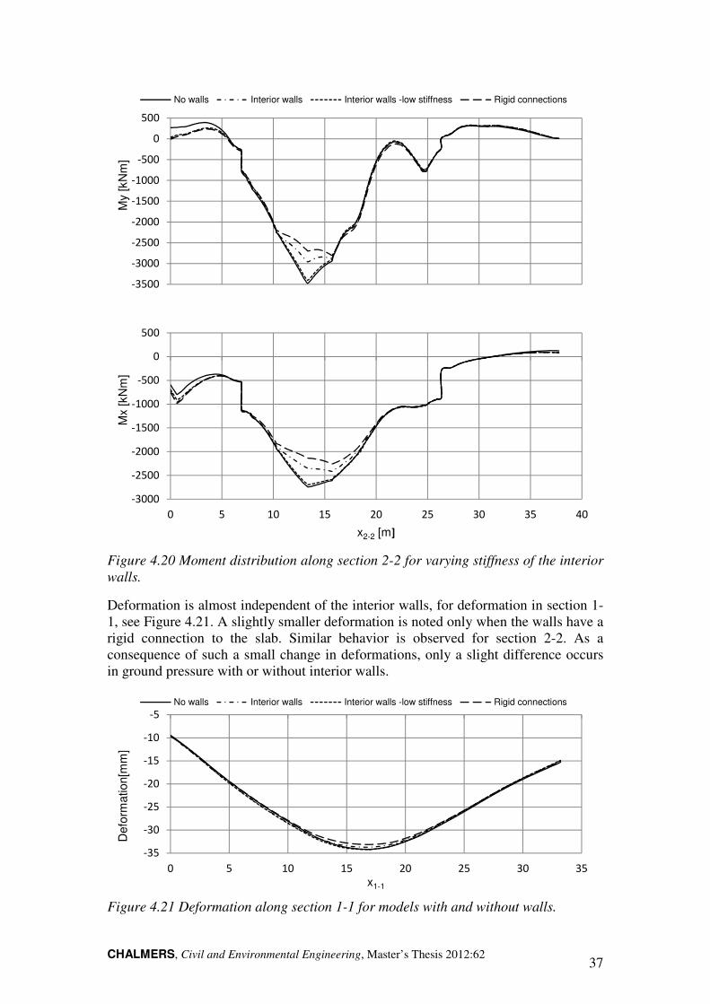
CHALMERS, Civil and Environmental Engineering, Master’s Thesis 2012:62 37
Figure 4.20 Moment distribution along section 2-2 for varying stiffness of the interior
walls.
Deformation is almost independent of the interior walls, for deformation in section 1-1, see Figure 4.21. A slightly smaller deformation is noted only when the walls have a rigid connection to the slab. Similar behavior is observed for section 2-2. As a consequence of such a small change in deformations, only a slight difference occurs in ground pressure with or without interior walls.
Figure 4.21 Deformation along section 1-1 for models with and without walls.
-35
-30
-25
-20
-15
-10
-5
0 5 10 15 20 25 30 35
Defo
rmation[m
m]
x1-1
No walls Interior walls Interior walls -low stiffness Rigid connections
-3500
-3000
-2500
-2000
-1500
-1000
-500
0
500M
y [k
Nm
]
No walls Interior walls Interior walls -low stiffness Rigid connections
-3000
-2500
-2000
-1500
-1000
-500
0
500
0 5 10 15 20 25 30 35 40
Mx [kN
m]
x2-2 [m]
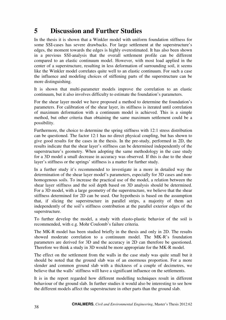
CHALMERS, Civil and Environmental Engineering, Master’s Thesis 2012:62 38
5 Discussion and Further Studies
In the thesis it is shown that a Winkler model with uniform foundation stiffness for some SSI-cases has severe drawbacks. For large settlement at the superstructure’s edges, the moment towards the edges is highly overestimated. It has also been shown in a previous SSI-analysis that the overall settlement profile can be different compared to an elastic continuum model. However, with most load applied in the center of a superstructure, resulting in less deformation of surrounding soil, it seems like the Winkler model correlates quite well to an elastic continuum. For such a case the influence and modeling choices of stiffening parts of the superstructure can be more distinguishing.
It is shown that multi-parameter models improve the correlation to an elastic continuum, but it also involves difficulty to estimate the foundation’s parameters.
For the shear layer model we have proposed a method to determine the foundation’s parameters. For calibration of the shear layer, its stiffness is iterated until correlation of maximum deformation with a continuum model is achieved. This is a simple method, but other criteria than obtaining the same maximum settlement could be a possibility.
Furthermore, the choice to determine the spring stiffness with 12:1 stress distribution can be questioned. The factor 12:1 has no direct physical coupling, but has shown to give good results for the cases in the thesis. In the pre-study, performed in 2D, the results indicate that the shear layer’s stiffness can be determined independently of the superstructure’s geometry. When adopting the same methodology in the case study for a 3D model a small decrease in accuracy was observed. If this is due to the shear layer’s stiffness or the springs’ stiffness is a matter for further study.
In a further study it’s recommended to investigate in a more in detailed way the determination of the shear layer model’s parameters, especially for 3D cases and non-homogenous soils. To increase the practical use of the model, a relation between the shear layer stiffness and the soil depth based on 3D analysis should be determined. For a 3D model, with a large geometry of the superstructure, we believe that the shear stiffness determined for 2D can be used. Our hypothesis is based on the assumption that, if slicing the superstructure in parallel strips, a majority of them act independently of the soil’s stiffness contribution at the parallel exterior edges of the superstructure.
To further develop the model, a study with elasto-plastic behavior of the soil is recommended, with e.g. Mohr Coulomb’s failure criteria.
The MK-R model has been studied briefly in the thesis and only in 2D. The results showed moderate correlation to a continuum model. The MK-R’s foundation parameters are derived for 3D and the accuracy in 2D can therefore be questioned. Therefore we think a study in 3D would be more appropriate for the MK-R model.
The effect on the settlement from the walls in the case study was quite small but it should be noted that the ground slab was of an enormous proportion. For a more slender and common ground slab with a thickness of a couple of decimetres, we believe that the walls’ stiffness will have a significant influence on the settlements.
It is in the report regarded how different modelling techniques result in different behaviour of the ground slab. In further studies it would also be interesting to see how the different models affect the superstructure in other parts than the ground slab.
CHALMERS, Civil and Environmental Engineering, Master’s Thesis 2012:62 39
Whether a structural subgrade model is good enough for SSI-analysis or if solid elements are needed, is according to the authors not a question with a definite answer. It is rather a question when the different approaches should be used.
In the thesis the shear layer model is shown to capture the SSI-behavior well in elastic analysis and a method to determine its parameters is suggested. For the shear layer models performed in ABAQUS, an interface layer between the superstructure and the shear layer has been used. As the shear layer and the superstructure both are structural elements it is in theory possible to couple them in mutual nodes and add their elements’ stiffness together straight forward. The continuum on the other hand must have some kind of interface layer between the soil, made of solid elements, and the ground slab, made of shell elements. This means that the computational time for the shear layer model could be as low as for the Winkler model while the continuum model’s computational time probably can’t be improved in the same manner.
Structural models are also easy to implement in structural analysis software and the models are simple to visualize. The Winkler model is well known and has been used for a long time by structural engineers. We therefore think the step to include an interaction element model is smaller for structural engineers than to introduce a different modeling-technique where solid elements are used. However, a continuum model is a better physical representation of the soil and with FEM, SSI-problems with complex soil conditions can be solved rather exactly.
It should be noted that the elastic continuum is still only modeled after an idealization of the soil. In reality the soil is non-homogenous and irregular. One could ask how large the deviation between the different models is compared to the deviation between the idealized model and the real soil.
CHALMERS, Civil and Environmental Engineering, Master’s Thesis 2012:62 40
6 Conclusions
The biggest shortcoming, identified in this thesis, for a Winkler model with uniform foundation stiffness is that no consideration is taken to the soil around the superstructure. This can result in major underestimation of the foundation’s stiffness towards the superstructure’s edges, which normally at the edges, leads to conservative sectional forces in the ground slab and unconservative ground pressure. It can also lead to a convex settlement profile, when a concave would be more realistic in reality for the specific case.
The Winkler model can be improved by introducing higher foundation stiffness towards the superstructure’s edges.
Tension zones between superstructure and subgrade should be observed, as it can give unconservative sectional forces.
The job time for the continuum model for KKH was 14 times the job time for the corresponding Winkler model.
Including interaction elements, which couple the foundation’s springs, improves the correlation to an elastic continuum compared to a Winkler model with uniform foundation stiffness. An interaction element characterized with only shear deformations is to prefer, since omitting bending deformations is shown to degrade the solution.
The 2D analysis indicates that the shear layer’s stiffness can be determined independently of the superstructure’s geometry.
A simple method, for practical use, to determine the shear layer model’s foundation properties is developed. Further study and verification is needed to make the method complete for practical use.
CHALMERS, Civil and Environmental Engineering, Master’s Thesis 2012:62 41
References
ABAQUS (2010): ABAQUS/CAE User’s Manual version 6.10.
Alén, C. (1998): On Probability in Geotechnics. Ph.D. Thesis. Department of Geotechnical Engineering, Chalmers University of Technology, Göteborg, Sweden, 242 pp.
Bolteus, L. (1984): Soil-Structure Interaction a Study Based on Numerical Methods. Ph.D. Thesis. Division of Structural Design, Chalmers University of Technology, Publication no. 84:3, Göteborg, Sweden, 1984, 165 pp.
Bowles, J. (1988): Foundation Analysis and Design. McGraw-Hill Inc., United States of America, 1004 pp.
Horvath, J. (2002): Soil-Structure Interaction Research Project - Basic SSI Concepts
and Applications Overview. Center for Geotechnology, Manhattan College, Publication no. CGT-2002-2, New York, U.S.A, 112 pp.
Horvath, J., Colasanti R. (2011): New Hybrid Subgrade Model for Soil-Structure
Interaction Analysis: Foundation and Geosynthetics Applications. ASCE, Proceedings of the Geo-Frontiers 2011 Conference, March 2011, 10 pp.
Irgens, F. (1980): Continuum Mechanics. Springer-Verlag, Berlin, 649 pp.
Johansson, L. (2012): Material from Skanska.
Kerr, A. (1964): Elastic and Viscoelastic Foundation Models. ASME Journal of
Applied Mechanics, No. 64__APM-40, September 1964, pp. 491-498.
Kettil, P. (2012): Material from Skanska.
Kok T., Bujang H., Noorzaei J., Moh´d J., Gue S. (2009): A Review of Basic Soil Constitutive - Models for Geotechnical Application. The Electronic Journal of
Geotechnical Engineering, Volume 14 J, 2009. pp.18.
Lidgren, C. (2012): Material from Skanska.
PLAXIS (2012): Products PLAXIS 3D 2011. PLAXIS, homepage: http://www.plaxis.nl/shop/113/info//PLAXIS+3D+2011/, available 2012-05-07.
Simulia (2012): ABAQUS Overview. Dassult Systemes, homepage: http://www.3ds.com/products/simulia/portfolio/abaqus/overview/, available 2012-05-07.
Skanska (2011): KKH Malmö Stad Nybyggnation av konsert, kongress och hotell
Projekterings PM Geoteknik. Skanska Sverige AB Teknik och Projektledning Geoteknik och Infra, Malmö, Sweden, 18pp.
Statens Geotekniska Institut (SGI) (1993): Plattgrundläggning. AB Svensk Byggtjänst och Statens Geotekniska Institut, Stockholm, Sweden, 282 pp.
Strusoft (2012): FEM-Design Overview. Structural Design Software in Europe AB, homepage: http://www.strusoft.com/index.php/en/products/fem-design, available 2012-05-07.
Teodoru, I.B (2009): Beams on elastic foundation – The simplified continuum approach. Bulletin of Polytechnic Institute of Jassy – CONSTRUCTIONS.
ARCHITECTURE Section, Vol. LV (LIX), No. 4, 2009. pp. 37-46.

CHALMERS, Civil and Environmental Engineering, Master’s Thesis 2012:62 42
Timoshenko S.P., Goodier J.N. (1970): Theory of Elasticity - Third Edition. McGraw-Hill Book Company, Singapore, 567 pp.
CHALMERS, Civil and Environmental Engineering, Master’s Thesis 2012:62
Appendix:
Structural Element Approaches for
Soil-Structure Interaction
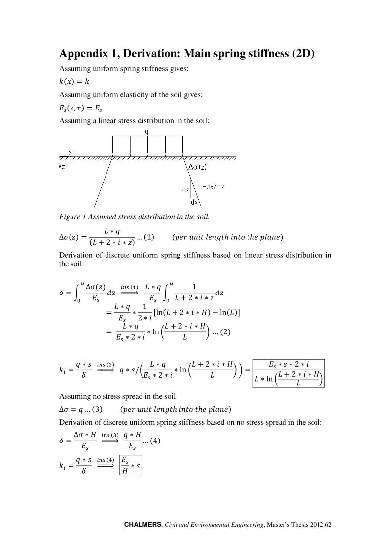
CHALMERS, Civil and Environmental Engineering, Master’s Thesis 2012:62
Appendix 1, Derivation: Main spring stiffness (2D)
Assuming uniform spring stiffness gives: ���! = � Assuming uniform elasticity of the soil gives: ���f, �! ( �� Assuming a linear stress distribution in the soil:
Figure 1 Assumed stress distribution in the soil.
∆��f! ( ∗ �� 8 2 ∗ h ∗ f!… �1!�jkl�6h�5k6��mh6�n�mkj5o6k! Derivation of discrete uniform spring stiffness based on linear stress distribution in the soil: � ( p ∆��f!�� qfr
s �_��/!tuuuv ∗ ��� p 1 8 2 ∗ h ∗ f qfrs( ∗ ��� ∗ 12 ∗ h wln� 8 2 ∗ h ∗ �! " ln�!z
( ∗ ��� ∗ 2 ∗ h ∗ ln { 8 2 ∗ h ∗ � | … �2!
�� ( � ∗ �� �_��$!tuuuv � ∗ � { ∗ ��� ∗ 2 ∗ h ∗ ln { 8 2 ∗ h ∗ � ||G ( �� ∗ � ∗ 2 ∗ h ∗ ln 7 8 2 ∗ h ∗ � 9
Assuming no stress spread in the soil: ∆� ( �… �3!�jkl�6h�5k6��mh6�n�mkj5o6k! Derivation of discrete uniform spring stiffness based on no stress spread in the soil:
� ( ∆� ∗ ��� �_��1!tuuuv� ∗ ��� …�4! �� ( � ∗ �� �_��2!tuuuv ��� ∗ �
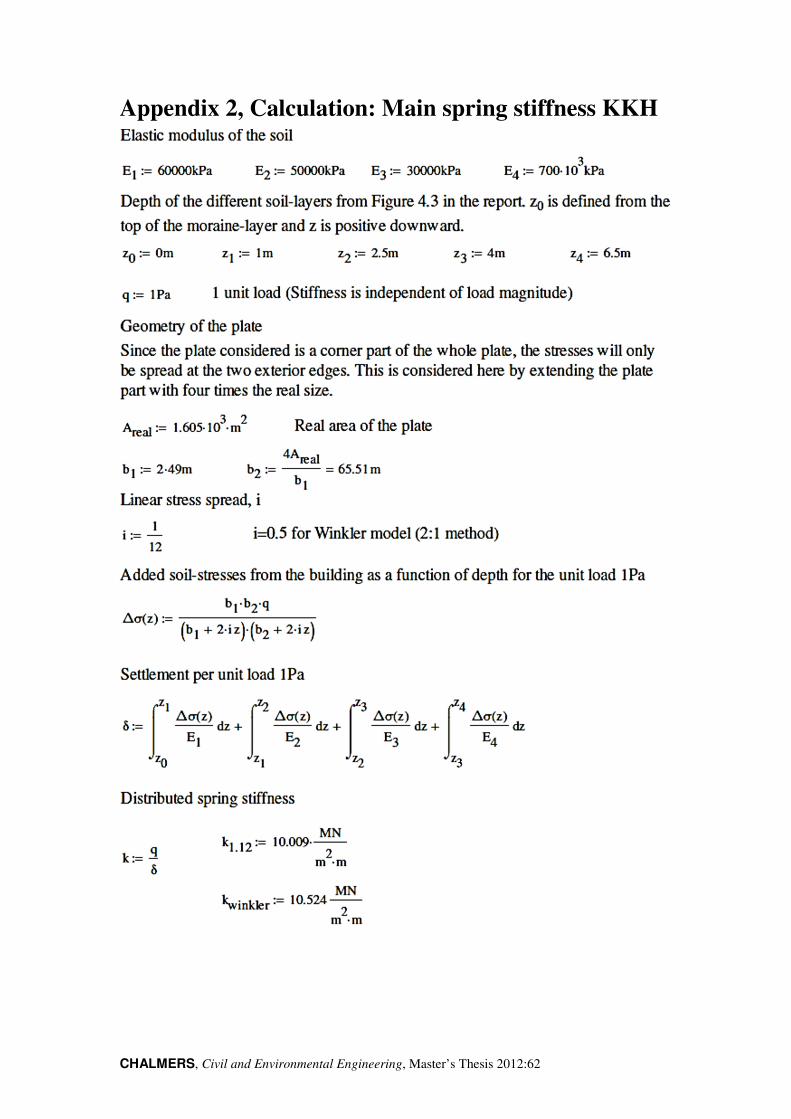
CHALMERS, Civil and Environmental Engineering, Master’s Thesis 2012:62
Appendix 2, Calculation: Main spring stiffness KKH
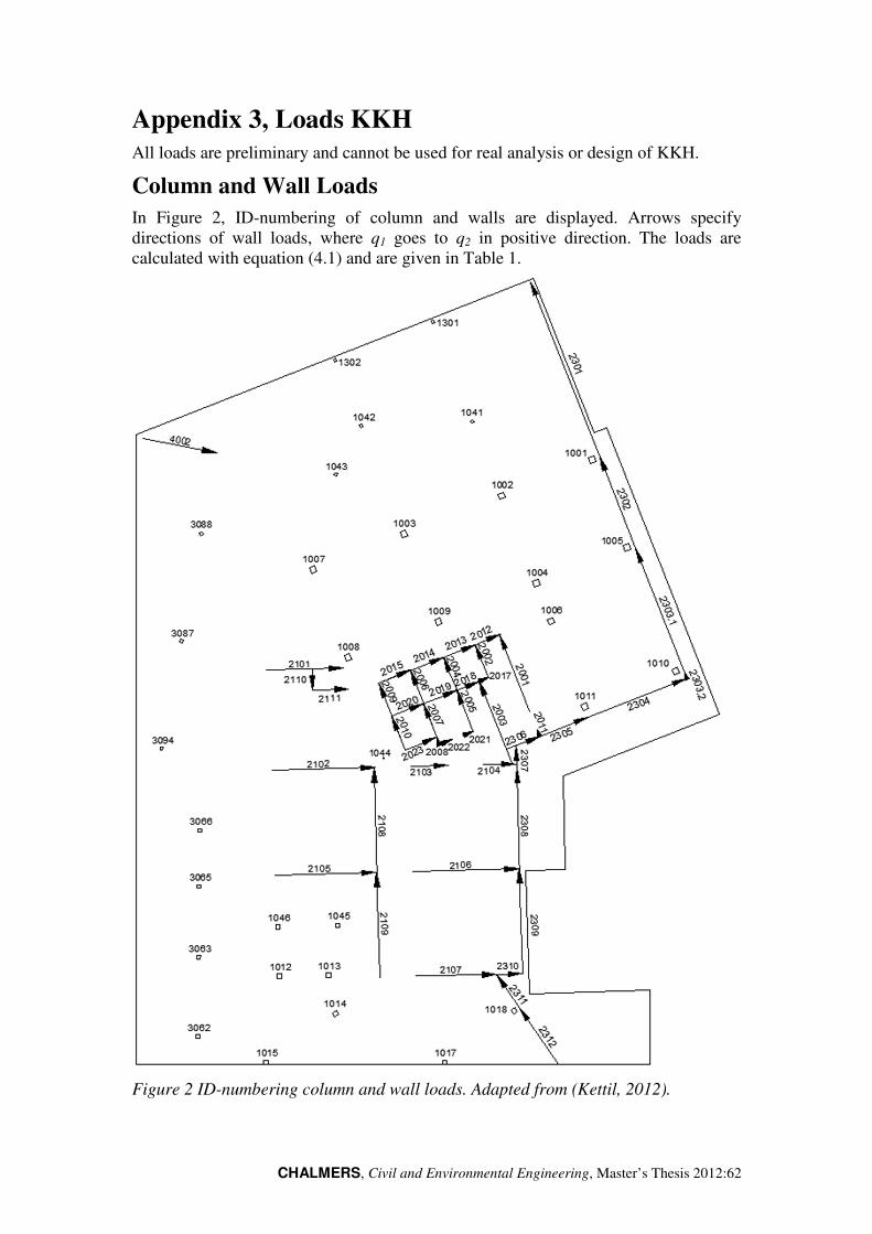
CHALMERS, Civil and Environmental Engineering, Master’s Thesis 2012:62
Appendix 3, Loads KKH
All loads are preliminary and cannot be used for real analysis or design of KKH.
Column and Wall Loads
In Figure 2, ID-numbering of column and walls are displayed. Arrows specify directions of wall loads, where q1 goes to q2 in positive direction. The loads are calculated with equation (4.1) and are given in Table 1.
Figure 2 ID-numbering column and wall loads. Adapted from (Kettil, 2012).
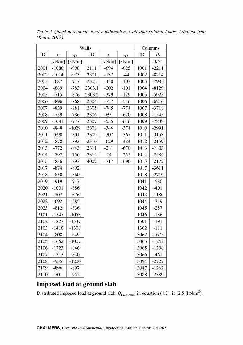
CHALMERS, Civil and Environmental Engineering, Master’s Thesis 2012:62
Table 1 Quasi-permanent load combination, wall and column loads. Adapted from
(Kettil, 2012).
Walls Columns
ID q1 q2 ID q1 q2 ID Pz
[kN/m] [kN/m] [kN/m] [kN/m] [kN]
2001 -1086 -998 2111 -694 -625 1001 -2211
2002 -1014 -973 2301 -137 -44 1002 -8214
2003 -687 -917 2302 -430 -103 1003 -7983
2004 -889 -783 2303.1 -202 -101 1004 -8129
2005 -715 -876 2303.2 -379 -129 1005 -5925
2006 -896 -868 2304 -737 -516 1006 -6216
2007 -839 -881 2305 -745 -774 1007 -3718
2008 -759 -786 2306 -691 -620 1008 -1545
2009 -1081 -977 2307 -555 -616 1009 -7838
2010 -848 -1029 2308 -346 -374 1010 -2991
2011 -690 -801 2309 -307 -367 1011 -3153
2012 -878 -893 2310 -629 -484 1012 -2159
2013 -772 -843 2311 -281 -670 1013 -1803
2014 -792 -756 2312 28 -255 1014 -2484
2015 -836 -797 4002 -717 -690 1015 -2172
2017 -874 -892
1017 -3611
2018 -850 -860 1018 -2719
2019 -919 -917 1041 -580
2020 -1001 -886 1042 -401
2021 -707 -676 1043 -1180
2022 -692 -585 1044 -319
2023 -812 -836 1045 -287
2101 -1547 -1058 1046 -186
2102 -1827 -1337 1301 -191
2103 -1416 -1308 1302 -111
2104 -808 -649 3062 -1675
2105 -1652 -1007 3063 -1242
2106 -1723 -846 3065 -1208
2107 -1313 -840 3066 -461
2108 -955 -1200 3094 -2727
2109 -896 -897 3087 -1262
2110 -701 -952 3088 -2389
Imposed load at ground slab
Distributed imposed load at ground slab, ��^�a��c in equation (4.2), is -2.5 [kN/m2].
CHALMERS, Civil and Environmental Engineering, Master’s Thesis 2012:62
Self-weight of ground slab
Permanent action � in equation (4.2), representing self-weight of the ground slab is calculated as ���! ( � ∗ � ∗ �
where:
Thickness of slab, � ( �olhk�
Density of concrete, � ( 2400 [kg/m3]
Acceleration of gravity, � ( -9.82 [m/s2]
Water load at ground slab
Water pressure in equation (4.2) is calculated as �d[`�]��! ( �� 8 1.5}! ∗ � ∗ �
where:
Thickness of the slab, � ( �olhk�
Density of water, � ( 1000 [kg/m3]
Acceleration of gravity, � ( 9.82 [m/s2]
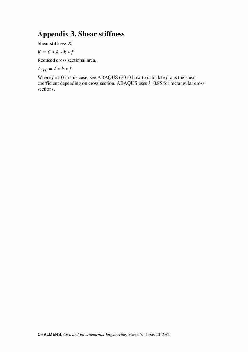
CHALMERS, Civil and Environmental Engineering, Master’s Thesis 2012:62
Appendix 3, Shear stiffness
Shear stiffness K, , ( � ∗ � ∗ � ∗ ~
Reduced cross sectional area, ���� ( � ∗ � ∗ ~
Where f =1.0 in this case, see ABAQUS (2010 how to calculate f. k is the shear coefficient depending on cross section. ABAQUS uses k=0.85 for rectangular cross sections.
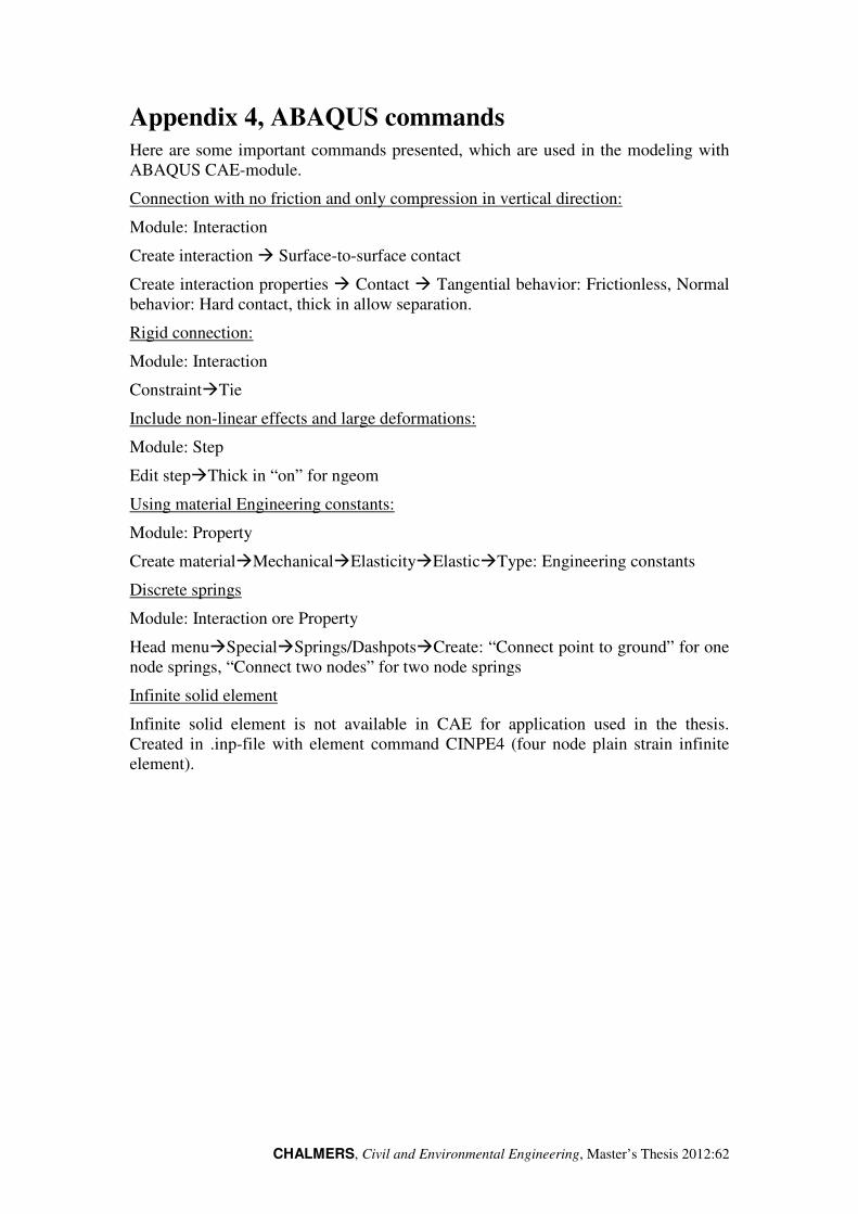
CHALMERS, Civil and Environmental Engineering, Master’s Thesis 2012:62
Appendix 4, ABAQUS commands
Here are some important commands presented, which are used in the modeling with ABAQUS CAE-module.
Connection with no friction and only compression in vertical direction:
Module: Interaction
Create interaction � Surface-to-surface contact
Create interaction properties � Contact � Tangential behavior: Frictionless, Normal behavior: Hard contact, thick in allow separation.
Rigid connection:
Module: Interaction
Constraint�Tie
Include non-linear effects and large deformations:
Module: Step
Edit step�Thick in “on” for ngeom
Using material Engineering constants:
Module: Property
Create material�Mechanical�Elasticity�Elastic�Type: Engineering constants
Discrete springs
Module: Interaction ore Property
Head menu�Special�Springs/Dashpots�Create: “Connect point to ground” for one node springs, “Connect two nodes” for two node springs
Infinite solid element
Infinite solid element is not available in CAE for application used in the thesis. Created in .inp-file with element command CINPE4 (four node plain strain infinite element).