STRUCTURAL EQUATION COVARIANCES Ke-Hai Yuan* Peter …

9STRUCTURAL EQUATIONMODELING WITH ROBUSTCOVARIANCES

Ke-Hai Yuan*Peter M. Bentler*

Existing methods for structural equation modeling involve fittingthe ordinary sample covariance matrix by a proposed structuralmodel. Since a sample covariance is easily influenced by a fewoutlying cases, the standard practice of modeling sample covari-ances can lead to inefficient estimates as well as inflated fit indi-ces. By giving a proper weight to each individual case, a robustcovariance will have a bounded influence function as well as anonzero breakdown point. These robust properties of the covari-ance estimators will be carried over to the parameter estimators inthe structural model if a technically appropriate procedure is used.We study such a procedure in which robust covariances replaceordinary sample covariances in the context of the Wishart likeli-hood function. This procedure is easy to implement in practice.Statistical properties of this procedure are investigated. A fit indexis given based on sampling from an elliptical distribution. An es-timating equation approach is used to develop a variety of robustcovariances, and consistent covariances of these robust estima-tors, needed for standard errors and test statistics, follow from thisapproach. Examples illustrate the inflated statistics and distortedparameter estimates obtained by using sample covariances when

This work was supported by National Institute on DrugAbuse Grants DA01070and DA00017. We gratefully acknowledge the help of Kenneth Bollen, Jodie Ullman,and Yiu-Fai Yung in supplying the raw data sets used in this paper, as well as thevaluable feedback by Adrian Raftery and three referees, which led to an improvedversion of the paper.

*University of California, Los Angeles

363

compared with those obtained by using robust covariances. Themerits of each method and its relevance to specific types of data arediscussed.

1. INTRODUCTION

Measurements in behavioral and social sciences generally contain randomerrors. Regression models and other models with independent or predictorvariables that contain errors of measurements are problematic because theylead to inconsistent estimators such as estimated regression coefficients.Incorrect inference in these situations can be avoided by modeling theunobserved latent variables and the error process. Since data collections inmany areas contain measurement errors, modeling with latent variables isemerging as a useful tool in diversified fields (e.g., Catalano and Ryan1992; Kendler et al. 1992; Muthén 1992; Tosteson et al. 1989). In thispaper we restrict ourselves to latent variable models of the covariancestructure type since these are among the most commonly used multivariateprocedures, as was shown by Gnanadesikan and Kettenring (1984) in theircomprehensive survey of multivariate techniques in applications. Theyreported that factor analysis was the most widely used multivariate method,and that in education, psychology, and sociology, factor analysis was muchmore extensively used than any other multivariate method. With the ad-vance of factor analytic models to more flexible and confirmatory models,and with the help of popular software like LISREL (Jöreskog and Sörbom1993) and EQS (Bentler 1995), the literature on structural equation mod-eling has increased dramatically in the past decade (e.g., see Austin &Calderón 1996). A new journalStructural Equation Modelinghas evenbeen created for the development and application of this class of models.

Classical structural equation models assume normality of latent vari-ables as well as measurement errors (Bollen 1989). In the context of co-variance structure analysis, parameters in a structural model can be estimatedby minimizing the Wishart likelihood function

F~S,S~u!! 5 tr$S21~u!S% 2 log6S21~u!S62 p (1)

for Zun, wherep is the number of observed variables,S is the sample co-variance matrix, andS~u! is the population covariance matrix that is pre-sumed to be generated by a hypothetical latent structure model such as aconfirmatory factor model. Under these conditions,TML 5 nF~S,S~ Zun!!can be used as a test statistic for evaluating the quality of the structural

364 YUAN AND BENTLER

model. Unfortunately, observed data rarely are normally distributed, im-plying that the assumption of normal latent variables and errors is alsounlikely to be true. Conditions exist for normal theory inference to be validfor nonnormal data with some specific models (e.g.,Anderson andAmemiya1988; Amemiya and Anderson 1990; Satorra and Bentler 1990), but it isnot known how to verify these conditions in practice, andTML is not reli-able at all with violated conditions (Hu et al. 1992).As reviewed by Bentlerand Dudgeon (1996), one solution to this problem has been the develop-ment of the asymptotically distribution free procedure of Browne (1982)and Chamberlain (1982), and, more recently, a finite sample variant thereof(Yuan and Bentler 1997). While this methodology requires no distribu-tional assumptions, it was not developed to deal with gross pathologies inthe data such as miscoded scores or outlier cases. For example, Yuan andBentler (1996) recently showed that a small proportion of outliers leads toinflated fit indices and biases in the estimates of parameters even if themodel is correct for the majority of the data. This is because the samplecovariance matrixSis unduly influenced by a small proportion of outliersand can be very inefficient when the sample comes from a distributionwith heavy tails (Tyler 1983). To deal with such problems, Jöreskog (1977)and Browne (1982) suggested the possibility of using a robust covarianceestimatorSn in (1) instead of the sample covariance matrixS. Huba andHarlow (1987) followed up these suggestions, and reported having exper-imented extensively with the use of resistant covariance matrices in placeof ordinary sample covariance matrices in standard structural modelingprograms. In spite of these early observations, made one to two decadesago, no technical development has emerged to clarify the precise effects ofsubstituting a robust estimator forS in (1) in the structural equation liter-ature. For example, the recent comprehensive review of mean and covari-ance structure methodology by Browne andArminger (1995) and the newlypublished book by Gnanadesikan (1997) on multivariate methods did notdiscuss this topic, which is the main focus of this paper.

There has been a limited development of robust methodology forlatent variable modeling. Yamaguchi and Watanabe (1993) used a covari-anceSn of MLE from a multivariatet-distribution along with (1). Theirempirical results indicate thatZun based on this covariance matrix is moreefficient than the corresponding estimator based on the sample covariancematrix S. Yuan and Bentler (forthcoming) studied methods of minimumchi-square and maximum likelihood based on an elliptical density. How-ever, using a robust covarianceSn in (1) is another approach to robustness

STRUCTURAL EQUATION MODELING WITH ROBUST COVARIANCES 365

and can be expected to give more stable solutions than the minimum chi-square method. Another advantage of usingSn in (1) is that such an ap-proach could be easily adapted into existing software such as EQS andLISREL, and hence can be made readily available to practitioners. Thisprovides another reason for studying this method.

Two important concepts in describing the robustness of a statisticare the influence function and breakdown point. For an estimatorT basedon data from a populationF, the associated influence functionIF ~x! is ameasure of the relative change inT with respect to the proportion of ob-servations that are not fromF but from a “contamination” point at thex.The IF ~x! gives an idea of how the estimatorT responds when an extraobservation atx is added to a sample. For example, when an observationxis added to a sample with sizen, the proportion ofx is 10~n 1 1!, therelative change in the sample mean is$~n PX1 x!0~n1 1! 2 PX%0$10~n1 1!%,which is unbounded inx for anyn. This is because the influence functionassociated with PX is IF ~x! 5 x 2 m, the limit of the relative change asngoes to infinity, wherem is the population mean ofF. The influence func-tion associated with the sample covarianceSis a quadratic function. For asample with sizen and an estimatorT, the finite sample breakdown pointen* is the smallest proportion of then observations which can render the

estimatorTmeaningless (e.g., becoming infinity). The (asymptotic) break-down point ofT is the limiting valuee * of en

* asn goes to infinity. Forexample, for both PX andS, en

*5 10n ande *5 0. Generally, a good robustestimator will have a bounded influence function as well as a nonzerobreakdown point—that is, for some constantc, 6 IF ~x!6, c for anyx ande *. 0. We refer readers to Staudte and Sheather (1990) and Hoaglin et al.(1983) for a discussion of the theory and application of robust methods.

The unbounded influence function and zero breakdown point of thesample covariance indicate thatSis very sensitive to outliers. On the otherhand, most robust covariancesSn have bounded influence functions aswell as nonzero breakdown points, and they are generally more efficientthanS when the underlying distribution has heavy tails. SinceZun is ob-tained through minimizing (1), these nice properties ofSn will be inheritedby Zun when Sn is used in (1). However, using a robustSn in (1) meansdropping the normality assumption, so that standard errors based on theinformation matrix and the likelihood ratio testTML for testingS 5 S~u!cannot be used any more. In fact, even if the sample is fromNp~m,S!, Sn

will be different from the sample covariance matrixS, so that inference onmodel structure and parameters based on normal theory cannot be used


without modification. In this paper, we will study inference problems as-sociated with using a robustSn in equation (1).

Outside the field of structural equation modeling, robust estima-tion of population means and covariances has attracted much attention.In particular, the influence functions and breakdown points of a varietyof estimators, including M-estimators, S-estimators, and other estima-tors, have been well studied (e.g., Maronna 1976; Lopuhaä 1989). BothM-estimators and S-estimators have bounded influence functions, the dif-ference between them being that the breakdown point of an M-estimatoris at most 10~ p 1 1!, which is restrictive in practice when the dimensionp is high. On the other hand, the breakdown point of an S-estimator isnot limited by the dimension of the data and can be as high as approxi-mately 102. Generally, the asymptotic efficiency of an S-estimator is re-lated to its breakdown point and it is impossible to obtain a highly efficientestimator with a breakdown point near 102. Among all the classes ofrobust estimators, M-estimators represent the primary class that has beenused in practical data analysis. Within the family of elliptical distribu-tions, Campbell (1980) and Devlin et al. (1981) empirically studied prin-cipal component analysis based on robust covariances. Being primarilyillustrations of exploratory data analysis, these references are only indi-rectly related to structural equation modeling. However, Tyler (1983)studied how to test explicit constraints on the elements ofS. Our work isrelated to his prior work as we shall show.

In order to make the following material self-contained, we would liketo give some details of notations that will be used later. IfA is ap3 p ma-trix, vec~A! is thep2-dimensional vector formed by stacking the columnsof A while vech~A! is thep*5 p~ p1 1!02-dimensional vector formed bythe nonduplicated elements ofA whenA is symmetric. For example, whenA5 ~aij ! is a 333 matrix, vec~A!5 ~a11a21a31a12a22a32a13a23a33!' andvech~A! 5 ~a11a21a31a22a32a33! ' . There exists a uniquep2 3 p* matrixDp such that vec~A!5Dp vech~A! and vech~A!5Dp

1 vec~A!,whereDp1 5

~Dp' Dp!21Dp

' is the generalized inverse ofDp. If A is am3 n matrix andB is ap3 q matrix, then themp3 nqmatrix ~aij B! is called the Kroneckerproduct ofA andB and is denoted byA J B. A good reference to these no-tations is Magnus and Neudecker (1988). We will uses~u! 5 vech~S~u!!and Ts~u! 5 vec~S~u!!. A function with dot on top means derivative—for example, ^ Ts~u! 5 ] Ts~u!0]u ' , G~x,m,s! 5 ]G~x,m,s!0]~ m ',s '!,\F~Sn,S~u!! 5 ]2F~Sn,S~u!!0]u]u ' , andSj ~u! 5 ]S~u!0]uj , the latter being

the derivative of the matrix function with respect to thejth element ofu.


When a function is evaluated at the true value of the parameter, we oftenreplace the argument with a subscript index such ass0 5 s~u0! or ^ Ts0 5^ Ts~u0!. There are three probabilistic notations:tn 5 op~an! meansantn ap-

proaches zero in probability asnapproaches infinity;tn5Op~an! meansantnis bounded in probability; andL && denotes convergence in distribu-tion. A classically good reference to these notations is Bishop et al. (1975,chap. 14).

In Section 2, we will study inference problems associated with usingSn. Specific types of robust covariances will be given in Section 3. Appli-cations of these results to covariance structures for some real data sets willbe presented in Section 4. In the development, we will emphasize resultsthat are relevant to applications. For regularity conditions, we will assumethat the population covariance matrixS0 exists and is nonsingular, and thatthe modelS~u! is identified. In order to minimize technical details, we alsoimplicitly assume some other standard regularity conditions that are hardto verify but are generally satisfied in applications. Readers can refer toMaronna (1976) and Lopuhaä (1989) for conditions on robust covariancesand Yuan and Bentler (1997) for conditions on structural models.

2. INFERENCE ON STRUCTURAL MODELS

Avariety of robust procedures have been proposed for estimating the meanvector and covariance matrix in a multivariate distribution. In the devel-opment of most of these procedures, an elliptically symmetric populationhas been a basic assumption (e.g., Maronna 1976), though this assumptionis seldom checked in applications (e.g., Campbell 1980; Devlin et al. 1981).The density of an elliptical distribution has a form

f ~x! 5 6S062102h$~x 2 m0!'S021~x 2 m0!%+ (2)

By adjusting the functionh~t!, we can assume cov~X!5S0 in (2).A robustestimator ZSn generally does not converge to the population covariance; itconverges instead to a constant times the population covariance matrix—aS0, wherea is a positive scalar. So the term “robust covariance” is vague,and sometimes another term, “robust dispersion,” is used instead. How-ever, the term—structural equation modeling with robust covariances—isstill well defined as long as the structural modelS~u! is invariant under aconstant scaling factor (ICSF). That is, for any parameter vectoru andpositive constanta, there exists a parameter vectoru* such thatS~u*! 5


aS~u!. So if a structural modelS~u! is ICSF, the model that holds for acovariance matrixS also holds for a rescaled version of the covariancematrixaS. As noted by Browne (1984:73), “Nearly all models for covari-ances matrices in current use are ICSF. Amongst the few exceptions aremodels which require certain elements ofS to have fixed nonzero valuesand restricted factor analysis models forS with some fixed nonzero factorloadings and fixed factor variances. These are seldom employed in prac-tice because of the difficulty of prespecifying nonzero parameter values.”

Even though an ICSF model that holds forS also holds foraS, u*

generally depends ona. So the ambiguity of robust covariance leaves itsheritage onto the parameteru* . In order to fully appreciate the effect of thisheritage, let us take the factor analysis model

X 5 m 1 Lf 1 e, (3)

as an example. With the typical hypothesis thatf andeare uncorrelated, wehave the following covariance structure

S~u! 5 LFL' 1 C, (4)

whereL is a factor loading matrix,F 5 cov~ f !, C 5 cov~e!, andu 5~ul' ,uf' ,uc

' !' consists of the unknown elements inL, F, andC, respec-tively. Two kinds of parameterizations in (4) are generally used in orderfor the model to be identified. The first is to fix all the factor variancesat 1 so thatF is a correlation matrix; the second is to fix one factorloading at 1 corresponding to each factor. Assuming that (4) is ICSF—that is, there is no prefixed nonzero element inL, F or C besides thoserequired for identification purposes—we will look at the relationship ofu* andu. WhenF is a correlation matrix, then

aS~u! 5 ~!aL!F~!aL!' 1 aC,

soul*5 !aul , uf

* 5 uf , anduc*5 auc in this case. When fixing one factor

loading at 1 for each factor, then

aS~u! 5 L~aF!L' 1 aC

and ul* 5 ul , uf

* 5 auf , anduc* 5 auc in this case. In either case, the

correlations among the variables (fromS or aS) remain invariant; thecorrelations among factors (fromF or aF) and residuals (fromC or aC)remain identical; and especially relevant, the standardized factor loadings,useful for interpretive reasons, remain invariant. The latter can be seen


from the rescaling ofR~u! 5 D~aS~u!!D, with R~u! being a correlationmatrix and

R~u! 5 ~D!aL!F~L'!aD! 1 aDCD 5 DLF DL' 1 aDCD,

where DL is the standardized factor pattern matrix. In addition, for either ofthese parameterizations, there will be no effect ofa on the following inter-esting relationships among parameters: (i) some factor loadings being zero,say,l ij 5 0; (ii) comparison among factor loadings, say,l i1 j1 5 l i2 j2; and(iii) magnitude of the coefficients of reliabilityri 5 ~var~xi ! 2 var~ei !!0var~xi !. It is also easy to see that the test statisticTML as well as a rescaledversion of it that will be introduced in the next section will not be influ-enced by the fact thatu* depends ona. Some functions of the param-eters will change witha—e.g., the ratio of a factor loading over the factorvariance—but it can be argued that this kind of function will never have anypractical interest.

We have used a factor model as an example to demonstrate theeffect of using a robust covariance. The effect on other types of models,such as LISREL types of models and linear covariance structure models, issimilar: That is, the ambiguity of a robust covariance may change param-eter estimates in a systematic way, but it does not change inference thattypically has substantive interest. Actually, the effect of using a robustcovariance for structural equation modeling is very similar to those ofusing robust covariances with other multivariate methods (e.g., Campbell1980; Devlin et al. 1981; Tyler 1983). For example, even though the vari-ances of principal components change witha, there will be no effect ofaon discovering a lower-dimensional space or on rules used for reduction ofdimensionality.

Let sn 5 vech~Sn! be a robust covariance estimator and satisfy

!n~sn 2 j0!L

&& N~0,G! (5)

with j05 as0 for a positivea. We can then useSn in equation (1) based onour above discussion. We do not need to know the value ofa if the modelS~u! is ICSF. Since usingkSn andk2G for any positivek will lead to thesame evaluation of the structural model and relationships among param-eters of interest, we may assumea 5 1 in the rest of this paper without lossof generality. For simplicity, we will keep the notations05 s~u0! in placeof j0 5 j~u0

* !+ So parameteru0 possesses some kind of generic meaning,but it is specific with a specific robust covariance matrix estimate.


Besides the ICSF condition, condition (5) is also essential for ourdevelopment. As we shall see in the next section, many robust estimatorssatisfy (5). It is obvious that sample covariances based on normal samplesas well as those based on nonnormal samples also satisfy (5), assumingfinite fourth-order moments with the latter. When condition (5) is satisfiedand we minimizeF~Sn,S~u!! for Zun, then Zun is consistent as long asS~u! isidentified (Kano 1986). Such anZun will also have the same breakdownpoint as that ofSn and a bounded influence function as long as the influ-ence function ofSn is bounded. We will mainly deal with the asymptoticdistribution of Zun and the test statistics associated withF~Sn,S~ Zun!! forevaluating the structureS0 5 S~u0!. Let

gnj ~u! 5 vec'~S j ~u!!$S21~u! J S21~u!%vec~Sn 2 S~u!! (6)

andgn~u! 5 ~gn1~u!,{{{,gnq~u!!' , whereq is the number of unknown pa-rameters inu. Then in practice Zun is obtained through solvinggn~ Zun! 5 0,which is the normal equation associated with minimizing (1). Using a Tay-lor expansion ongn~ Zun! 5 0, we obtain

!n~ Zun 2 u0! 5 A21~u0!!ngn~u0! 1 op~1!, (7)

whereA~u! 5 ~ajk~u!! with

ajk~u! 5 vec'~S j ~u!!$S21~u! J S21~u!%vec~Sk~u!!+

So matrixA corresponds to the information matrix associated with MLEbased on the normality assumption. Equations (5), (6), and (7) lead to

!n~ Zun 2 u0!L

&& N~0,V!, (8)

whereV 5 A21PA21 with

P 5 ^ Ts0' ~S0

21 J S021!DpGDp

' ~S021 J S0

21! ^ Ts0+

WhenSn 5 S is the sample covariance based on a sample fromN~m,S0!,thenP 5 2A, and (8) characterizes the asymptotic distribution of the nor-mal theory MLE. WhenSn5Sbut the data are nonnormal,V in (8) is of theform of the well-known sandwich type covariance matrix (e.g., Browne1984; Bentler and Dijkstra 1985; Arminger and Schoenberg 1989; Arm-inger and Sobel 1990). Generally,P Þ 2A for a robustSn even if thesample is from a normal distribution. Inference on parameters can be done


with (8) using a consistent estimatorZV, which is obtained in practice byreplacingA andP by their consistent estimates.

Because latent variable models usually involve many structural as-sumptions and hypothetical latent variables that cannot be observed, it iscritical, especially in applications, to have a goodness-of-fit index thatpermits an evaluation of the hypothesized modelS 5 S~u!. This can beobtained from knowledge of the distribution ofnF~Sn,S~ Zun!!, as will bedeveloped next. Using a Taylor expansion onF~Sn,S~ Zun!! at u0 and withS0 5 S~u0!, we obtain

F~Sn,S~ Zun!! 5 F~Sn,S0! 1 F '~Sn,S0!~ Zun 2 u0!

11

2~ Zun 2 u0!' \F~Sn,S~ Nun!!~ Zun 2 u0!, (9)

where Nun is a vector lying betweenu0 and Zun. Notice that

2 log6S021Sn65 2 log6 Ip 2 ~Ip 2 S0

21Sn!6,

using (5) and a matrix version of Taylor expansion (e.g., Muirhead 1982:363, eq. 15),

2 log6S021Sn65 tr~Ip 2 S0

21Sn! 11

2tr~Ip 2 S0

21Sn!2 1 OpS 1

n302D+(10)

It follows from (10) that

F~Sn,S0! 51

2tr~Ip 2 S0

21Sn!2 1 OpS 1

n302D+ (11)

Similarly,

F '~Sn,S0!~ Zun 2 u0! 5 2 vec'~Sn 2 S0!P vec~Sn 2 S0! 1 opS1

nD(12)


and

1

2~ Zun 2 u0!' \F~Sn,S~ Nun!!~ Zun 2 u0!

51

2vec'~Sn 2 S0!P vec~Sn 2 S0! 1 opS1

nD, (13)

where

P 5 ~S021 J S0

21! ^ Ts0$ ^ Ts0' ~S0

21 J S021! ^ Ts0%21 ^ Ts0

' ~S021 J S0

21!+

By putting (11), (12), and (13) into (9), we obtain

nF~Sn,S~ Zun!! 5 Zn' QZn 1 op~1!,

whereZn 5 G2102!n vech~Sn 2 S0! and

Q 51

2G102Dp

' $~S021 J S0

21! 2 P%DpG102+ (14)

It follows from (5) that ZnL

&& Np* ~0, I !+ When Sn 5 S is the samplecovariance based on a sample fromNp~m,S!, G 5 2Dp

1~S0 J S0! Dp1' ,Q

is a projection matrix of rankp* 2 q and consequently,nF~S,S~ Zun!!L

&&

xp*2q2 + Generally,Q is only a nonnegative definite matrix of rankp*2 q.

Let l1 $ {{{ $ lp*2q . 0 be the nonzero eigenvalues ofQ, then

nF~Sn,S~ Zun!!L

&& (j51

p*2q

l j x1j2 , (15)

wherex1j2 are independent chi-square variates with degree of freedom 1.

Unlessl1 5 {{{ 5 lp*2q, no commonly used distribution is available todescribe the behavior of the right-hand side of (15), which is a mixture ofchi-square distributions. Several approximations to a mixture of chi-squaredistributions were developed by Box (1954) and Satterthwaite (1941). An-other was studied by Bentler (1994) for approximating (15) withSn 5 Sbased on a sample from a nonnormal distribution. WhenS is based on asample from an elliptical distribution, Browne (1984) proposed a rescalingfactor tonF~S,S~ Zun!! using Mardia’s coefficient of kurtosis (Mardia et al.1979:31). Satorra and Bentler (1994) proposed a more general rescalingfactor to the likelihood ratio statistic. With a rescaling factor, Tyler (1983)


studied the likelihood ratio test for a specific function of elements of thepopulation covariance matrix. As we shall see in the next section, withinthe family of elliptical distributions, a similar correction applies tonF~Sn,S~ Zun!!.

3. ROBUST MEANS AND COVARIANCE MATRICES

We will emphasize two classes of robust estimators of mean and covari-ance in this section. One is the class of M-estimators, the other is the classof S-estimators. This is because robust properties of these estimators arewell studied and they satisfy condition (5), which is necessary for theirapplications in covariance structure analysis. We will use an estimatingequation approach in presenting these estimators. An advantage of thisapproach is that a consistent estimator for the matrixG can be obtained byidentifying the corresponding estimating equation for each estimator. Inaddition, we will state a common property of these estimators within thefamily of elliptical distributions. This will motivate us to find a way tomake use ofnF~Sn,S~ Zun!! in testing the quality of the model. Some ofthese estimators will be used in our examples in the next section.

Let X1, {{{, Xn be a given sample; many robust estimators~ [mn, ZSn!can then be obtained by simultaneously solving

1

n (i51

n

G1~Xi , [mn, ZSn! 5 0 (16)

and

1

n (i51

n

G2~Xi , [mn, ZSn! 5 0, (17)

whereG1~x,m,S! is a p 3 1 vector function andG2~x,m,S! is a p 3 pmatrix function. For example, if we let

d~x,m,S! 5 $~x 2 m!'S21~x 2 m!%102,

an M-estimator will then correspond to

G1~x,m,S! 5 u1$d~x,m,S!%~x 2 m! (18)


and

G2~x,m,S! 5 u2$d2~x,m,S!%~x 2 m!~x 2 m!' 2 S, (19)

whereu1~t! andu2~t! are univariate weight functions that will be givenwhen discussing different estimators below. Equations such as (16) and(17) are often called estimating equations because they are used to defineparameter estimators. A nice property of using these estimating equationsis that the asymptotic distribution of~ [mn, ZSn! can be presented in a unifiedway. If

G~x,m,s! 5 ~G1' ~x,m,S!,vech'$G2~x,m,S!%!',

then

!nS [mn 2 m0

[sn 2 s0D L

&& N~0,V !, (20)

whereV 5 H 21BH '21 with

H 5 E$G~X,m0,s0!% and B 5 E$G~X,m0,s0!G'~X,m0,s0!%+

Note that (20) holds as long asm0 andS0 satisfy E$G~X,m0,s0!% 5 0 andthe expectations withH andBexist.Also, since a proper weight is attachedto each individual case, we generally need to assume only that the secondmoment of the sampling population exists in order forB to exist for mostof the robust estimators. On the other hand, we need to assume that thefourth-order moment will be finite for the sampling distribution when usingthe sample covariance. A consistent estimate ofV can be obtained by usingconsistent estimates forH andB; these are given by

ZHn 51

n (i51

n

G~Xi , [mn, [sn! and

ZBn 51

n (i51

n

G~Xi , [mn, [sn!G'~Xi , [mn, [sn!+

Let V22 be the submatrix ofV corresponding to the asymptotic covari-ance of!n~ [sn 2 s0!; thenG 5 V22 and ZG 5 ZV22, which will be used inour applications.

Different G1 andG2 correspond to different estimators. Within theclass of M-estimators withG1 and G2 being given by (18) and (19), a


variety of weight functionsu1~t! and u2~t! lead to different types ofM-estimators (e.g., Hoaglin et al. 1983). The well-known Huber-typeM-estimator corresponds to

u1~d! 5 H 1, if d # r

r0d, if d . r

and u2~d2! 5 $u1~d !%20b (e.g., Tyler 1983), wherer 2 is given byP~xp

2 . r 2! 5 a, a is the percentage of outliers one wants to control inthe data, andb is a constant such that Exp

2u2~xp2! 5 p, which makes the

estimator ZSn unbiased if sampling from ap-variate normal distribution.If using u1~t! 5 u2~t 2! 5 2 2h~t 2!0h~t 2! in (18) and (19), we obtain themaximum likelihood estimator of~m,S! based on the elliptical densityin (2). When ap-variatet-distribution with degrees of freedomm is used,u1~d! 5 u2~d2! 5 ~ p 1 m!0~m1 d2!. The ZSn based on such a weight canbe rescaled bySn 5 k ZSn so thatSn is consistent for the population co-variance when sampling from a multivariate normal distribution. Theconstantk is a solution to E$~kxp

2!0~m1 kxp2!% 5 p0~m1 p!. However,

the constantsb andk are unnecessary if only considering inference onmodels and parameters as long asS~u! is ICSF. We shall use these scal-ings in our examples in the next section just for obtaining comparableparameter estimates.

For the functions given in (18) and (19),~ [mn, ZSn! defined in (16)and (17) satisfy

m 5 (i51

n

u1$d~Xi ,m,S!%XiY(i51

n

u1$d~Xi ,m,S!%,

and

S 5 (i51

n

u2$d2~Xi ,m,S!%~Xi 2 m!~Xi 2 m!'0n+

The above two equations are the usual way to define an M-estimator andgive an iterative algorithm for obtaining~ [mn, ZSn!. Motivated by the un-biasedness of the sample covariance, Campbell (1980) defined anotherform of M-estimator:

m 5 (i51

n

wi XiY(i51

n

wi (21)


and

S 5 (i51

n

wi2~Xi 2 m!~Xi 2 m!'YS(

i51

n

wi2 2 1D, (22)

wherewi 5 w$d~Xi ,m,S!% for a weight functionw~t!. The estimators de-fined in (21) and (22) correspond to the estimating equations (16) and (17)with

G1~x,m,S! 5 w~x,m,s!~x 2 m!

and

G2~x,m,S! 5 w2~x,m,s!~x 2 m!$~x 2 m!~x 2 m!' 2 S% 11

nS+

Campbell usedw~d! 5 v~d!0d and

v~d! 5 H d, if d # d0

d0 exp$2212~d 2 d0!20b2

2%, if d . d0, (23)

whered0 5 !p 1 b10#2, b1 andb2 are constants. Based on extensive em-pirical experience, proposed choices forb1 andb2 were given by Campbell(1980): (a)b15` corresponding to the usual sample covariance; (b)b152,b25` corresponding to a Huber-type M-estimator; (c)b152,b251+25corresponding to a Hampel-type redescending M-estimator (Hampel 1974).

Since the breakdown point of an M-estimator is limited by the di-mension of the data, other types of estimators with high breakdown pointshave been proposed. One such estimator is the well-studied S-estimator.Let r~t! be a continuously differentiable symmetric function that is alsostrictly increasing on@0,c0# and constant on@c0,`#. For a constantb0 (0,b0 , a0 5 r~c0!), an S-estimator of~m,S! is defined by minimizing6S6subject to the constraint

1

n (i51

n

r$d~Xi ,m,S!% 5 b0+

The breakdown point of the S-estimator is approximately given byb00r~c0! and can be as large as 102. Using Lagrange multipliers, Lopuhaä(1989) showed that an S-estimator~ [mn, ZSn! satisfies the estimating equa-tions (16) and (17) with


G1~x,m,S! 5 u$d~x,m,S!%~x 2 m!

and

G2~x,m,S! 5 pu$d~x,m,S!%~x 2 m!~x 2 m!' 2 v~d!S,

whereu~t! 5 _r~t!0t andv~t! 5 t _r~t! 2 r~t! 1 b0. A recommendedr~t! isTukey’s biweight function (e.g., Ruppert 1992)

rc0~t! 5 Ht 202 2 t 40~2c0

2! 1 t 60~6c04!, if t # c0

c0206, if t . c0

+

Note that equations (16) and (17) corresponding to an S-estimator will havemultiple solutions. A practical algorithm is needed for solving these equa-tions in order to obtain the S-estimator. We will use the SURREAL algo-rithm developed by Ruppert (1992) for our examples in the next section.

The family of elliptical distributions has been well explored inrobustness studies. This is because the distributions represented by (2)include multivariate normal as well as many multivariate nonnormal dis-tributions with heavy or light tails. Assuming that the sample is from(2), then for both M- and S-estimators the asymptotic distribution of~ [mn, ZSn! has a nice property. In particular,[mn and ZSn are asymptoticallyindependent with

!n~ [mn 2 m0!L

&& N~0,cS! and !n~ [sn 2 s0!L

&& N~0,G!,

where

G 5 2aDp1~S0 J S0!Dp

1'1 bDp1 vec~S0!vec'~S0!Dp

1' ,

anda, b, andc are constants depending on the specificG1 andG2 used inthe estimating equations (16) and (17). Specific forms ofa, b, andc can befound in Maronna (1976) and Tyler (1982) for M-estimators and in Lopu-haä (1989) for S-estimators; these are not required in our applications.Within the elliptical family, the statisticnF~Sn,S~ Zun!! also converges to anice form if the structureS~u! satisfies

S~u0! 5 c1S1~u0! 1 {{{ 1 cqSq~u0! (24)

for some constantsc1, {{{, cq. Condition (24) is implied by the ICSF con-dition and is consequently satisfied by almost all structural models in cur-


rent use. Under condition (24), it can be easily shown that all the nonzeroeigenvalues of the matrixQ in (14) are equal toa. In such a case,

nF~Sn,S~ Zun!!0a L&& xp*2q

2 .

A consistent estimate ofa is given by [a 5 tr~ ZQ!0~ p* 2 q!. So

T1 5 nF~Sn,S~ Zun!!0 [a (25)

can be used as a statistic for testing the hypothetical structureS~u!. Whenthe sample is not from an elliptically symmetric distribution,T1 generallywill not approachxp*2q

2 but will approach a distribution with meanp*2 qinstead. WhenSn 5 S is the sample covariance andZG 5 SY is the samplecovariance ofYi 5vech$~Xi 2 PX!~Xi 2 PX!'%, T1 is equivalent to the statisticTSB proposed by Satorra and Bentler (1994). Existing simulation studiesindicate thatTSB is very insensitive to various violations of elliptical sym-metry of the underlying distributions (Hu et al. 1992; Curran et al. 1996).We suspect a similar behavior forT1 using a robust covariance matrixSn.More research in this direction is needed.

4. EMPIRICAL EXAMPLES

We shall use some real data sets to demonstrate applications of the pro-cedures developed in the last two sections. In particular, we shall com-pare estimates and test statistics by using different robust estimators ofcovariances.

The first is a classical data set from Holzinger and Swineford (1939).The data set consists of mental ability tests scores of seventh- and eighth-grade children from two different schools. There are 26 variables and 145subjects from the Grant-White school. Jöreskog (1969) used 9 of the 26variables in studying the correlation structure with normal theory maximum-likelihood method. We shall also use these 9 variables in our application.The 9 variables are 1. Visual Perception, 2. Cubes, 3. Lozenges, 4. Para-graph Comprehension, 5. Sentence Completion, 6. Word Meaning, 7. Ad-dition, 8. Counting Dots, and 9. Straight-Curved Capitals. In Holzingerand Swineford’s original report, variables 1, 2, and 3 were designed tomeasure the spatial ability of the subjects; variables 4, 5, and 6 were de-signed to measure the verbal ability of the subjects; and variables 7, 8, and9 were designed to measure the speed factor of the subjects in performingthe tasks. LetX represent the 9 observed variables; the confirmatory factor


model, presented in (3), then represents the hypothesis of the original de-sign with

L 5 1l11 l21 l31 0 0 0 0 0 0

0 0 0 l42 l52 l62 0 0 0

0 0 0 0 0 0 l73 l83 l932'

+ (26)

We assume that the measurement errors are uncorrelated, withC 5 cov~e!being a diagonal matrix; for identification purposes, we also setF in (4) tobe a 33 3 correlation matrix. So there areq5 21 unknown parameters inu, nine of which are factor loadings.

Previous analyses of this classical data set have always assumed nor-mality, and hence we may wonder if a robust method is necessary.As is wellknown, a robust method generally gives smaller weights to observations thatdeviate from the majority of the data.After working on a number of real andsimulated data sets, Campbell (1980) concluded that theith case is an atyp-ical observation if the associated weightwi

2 in (22) is less than .30 withb152+0 andb25 1+25. The two smallest weights for this data set arew24

2 5 +072andw106

2 5 +121. So cases 24 and 106 may indicate the long tails of the un-derlying distribution of this data set, and a robust covariance estimator mayprovide a better estimate of the population covariance.

Several M-estimates and an S-estimate of covariances are used in(1) for fitting the factor model to this data set. The three M-estimates arebased on the multivariate t-distribution with degree of freedom 1 [Mt(1)],the Huber-type weight withq 5 +2 [Huber(.2)], and Campbell’s weightwith b1 5 2+0 andb2 5 ` [Campbell~2,`!]. For the S-estimate, the bi-weight function withc05 11+105 is used; this corresponds to a breakdownpoint of .2. For comparison purposes, we also include the normal theorymethod with the sample covariance matrixS. The estimated factor load-ings with their standard errors as well as the fit indices based on (25) aregiven in Table 1. As can be seen in the top part of the table, all the covari-ances give a similar pattern in estimates of factor loadings. With respect tofit indices, given in the last row of the table, the normal theory methodgives the largest test statistic for the structural model withTML 5 51+19.Referring to the chi-square distribution with 24 degrees of freedom, thiscorresponds to a p-value of .001. So we may reject the model structure in(4) and (26) if based on the normal theory method. However, using theSn

based on the multivariate Cauchy density, [Mt(1)] yields a fit statisticT1

that corresponds to a p-value of .03, indicating that the factor model is a


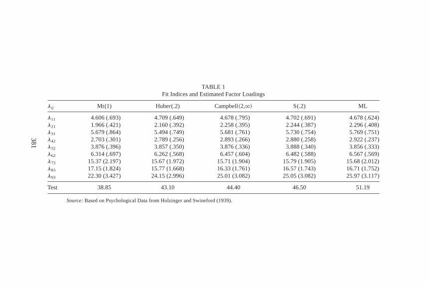
TABLE 1Fit Indices and Estimated Factor Loadings

l ij Mt(1) Huber(.2) Campbell~2,`! S(.2) ML

l11 4.606 (.693) 4.709 (.649) 4.678 (.795) 4.702 (.691) 4.678 (.624)l21 1.966 (.421) 2.160 (.392) 2.258 (.395) 2.244 (.387) 2.296 (.408)l31 5.679 (.864) 5.494 (.749) 5.681 (.761) 5.730 (.754) 5.769 (.751)l42 2.703 (.301) 2.789 (.256) 2.893 (.266) 2.880 (.258) 2.922 (.237)l52 3.876 (.396) 3.857 (.350) 3.876 (.336) 3.888 (.340) 3.856 (.333)l62 6.314 (.697) 6.262 (.568) 6.457 (.604) 6.482 (.588) 6.567 (.569)l73 15.37 (2.197) 15.67 (1.972) 15.71 (1.904) 15.79 (1.905) 15.68 (2.012)l83 17.15 (1.824) 15.77 (1.668) 16.33 (1.761) 16.57 (1.743) 16.71 (1.752)l93 22.30 (3.427) 24.15 (2.996) 25.01 (3.082) 25.05 (3.082) 25.97 (3.117)

Test 38.85 43.10 44.40 46.50 51.19

Source:Based on Psychological Data from Holzinger and Swineford (1939).

38

1

reasonable model. This supports the design of the original measurements.The statistics corresponding to the other three types of robust covariancescorrespond to p-values of .01, .007, and .004, respectively, which suggeststhat the model in (4) and (26) ranges from acceptable to barely acceptable.This reflects differences among the various robust covariances.

For this example, we used the model (4) withL in (26), whichrepresents the original design by Holzinger and Swineford (1939). Othermodels may also provide a good explanation of the measured variables, asdescribed in Jöreskog (1969). Our purpose here is to show that when ab-normal observations exist in a data set, using robust covariances with cor-rected inference procedures may lead to a better evaluation of modelstructure. On the other hand, the normal theory method is easily influencedby outliers so that a reasonable model that would fit the majority of thedata may be discredited by a few influential observations.

The data for our second example comes from Dukes et al. (1995),who studied the effect of the DrugAbuse Resistance Education (D.A.R.E.)program based on data obtained across four years from 440 classroomsand 10,000 students. Outcomes were evaluated by Dukes et al. on theclassroom level, using a Solomon four-group design with latent variables.For each cohort, the design had an experimental group and a control groupthat were pretested and posttested, as well as an experimental group and acontrol group that were not pretested (posttest only), permitting an isola-tion of pretest on posttest as well as maturation effects. Here we study onlythe posttest experimental group (group C) with sample sizen5 122, usinga standard confirmatory factor analysis model based on 12 variables and 4correlated common factors. The factors in this model represent self-esteem;resistance to peer pressure; family, police, and teacher bonds; and accep-tance of risky behavior, and have 2, 2, 3, and 5 univocal indicators. Themodel was justified by theoretical considerations, and it gives a reasonableexplanation of their data. As in the analysis of the first example, we wantto see whether the use of a robust method yields different conclusions fromthat found with the normal theory method. Using Campbell’s weight schemewith b1 5 2+0 andb2 5 1+25 (Campbell[2,1.5] ), the three smallest weightswi

2 as in (22) arew992 5 6+343 1027, w79

2 5 +041, andw432 5 +14. So cases

99, 79, and 43 are definitely atypical observations based on the criterion ofCampbell (1980). This may indicate that a robust covariance approachwould be useful for analyzing this data set.

As in the first example, four robust covariances as well as the sam-ple covariance are used to analyze this data set. The four robust covari-


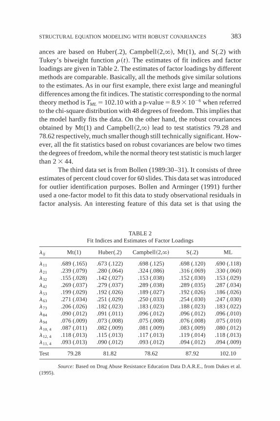
ances are based on Huber(.2), Campbell~2,`!, Mt(1), and S(.2) withTukey’s biweight functionr~t!. The estimates of fit indices and factorloadings are given in Table 2. The estimates of factor loadings by differentmethods are comparable. Basically, all the methods give similar solutionsto the estimates. As in our first example, there exist large and meaningfuldifferences among the fit indices. The statistic corresponding to the normaltheory method isTML 5 102+10 with a p-value5 8+93 1026 when referredto the chi-square distribution with 48 degrees of freedom. This implies thatthe model hardly fits the data. On the other hand, the robust covariancesobtained by Mt(1) and Campbell~2,`! lead to test statistics 79.28 and78.62 respectively, much smaller though still technically significant. How-ever, all the fit statistics based on robust covariances are below two timesthe degrees of freedom, while the normal theory test statistic is much largerthan 23 44.

The third data set is from Bollen (1989:30–31). It consists of threeestimates of percent cloud cover for 60 slides. This data set was introducedfor outlier identification purposes. Bollen and Arminger (1991) furtherused a one-factor model to fit this data to study observational residuals infactor analysis. An interesting feature of this data set is that using the

TABLE 2Fit Indices and Estimates of Factor Loadings

l ij Mt(1) Huber(.2) Campbell~2,`! S(.2) ML

l11 .689 (.165) .673 (.122) .698 (.125) .698 (.120) .690 (.118)l21 .239 (.079) .280 (.064) .324 (.086) .316 (.069) .330 (.060)l32 .155 (.028) .142 (.027) .153 (.038) .152 (.030) .153 (.029)l42 .269 (.037) .279 (.037) .289 (.038) .289 (.035) .287 (.034)l53 .199 (.029) .192 (.026) .189 (.027) .192 (.026) .186 (.026)l63 .271 (.034) .251 (.029) .250 (.033) .254 (.030) .247 (.030)l73 .206 (.026) .182 (.023) .183 (.023) .188 (.023) .183 (.022)l84 .090 (.012) .091 (.011) .096 (.012) .096 (.012) .096 (.010)l94 .076 (.009) .073 (.008) .075 (.008) .076 (.008) .075 (.010)l10, 4 .087 (.011) .082 (.009) .081 (.009) .083 (.009) .080 (.012)l12, 4 .118 (.013) .115 (.013) .117 (.013) .119 (.014) .118 (.013)l11, 4 .093 (.013) .090 (.012) .093 (.012) .094 (.012) .094 (.009)

Test 79.28 81.82 78.62 87.92 102.10

Source:Based on Drug Abuse Resistance Education Data D.A.R.E., from Dukes et al.(1995).


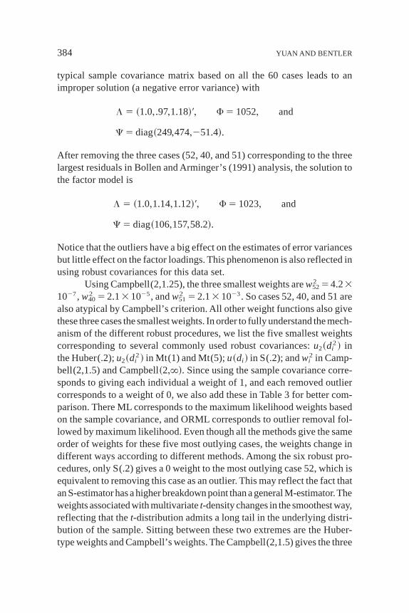
typical sample covariance matrix based on all the 60 cases leads to animproper solution (a negative error variance) with

L 5 ~1+0, +97,1+18!', F 5 1052, and

C 5 diag~249,474,251+4!+

After removing the three cases (52, 40, and 51) corresponding to the threelargest residuals in Bollen and Arminger’s (1991) analysis, the solution tothe factor model is

L 5 ~1+0,1+14,1+12!', F 5 1023, and

C 5 diag~106,157,58+2!+

Notice that the outliers have a big effect on the estimates of error variancesbut little effect on the factor loadings. This phenomenon is also reflected inusing robust covariances for this data set.

Using Campbell(2,1.25), the three smallest weights arew522 54+23

1027, w402 5 2+13 1025, andw51

2 5 2+13 1023. So cases 52, 40, and 51 arealso atypical by Campbell’s criterion. All other weight functions also givethese three cases the smallest weights. In order to fully understand the mech-anism of the different robust procedures, we list the five smallest weightscorresponding to several commonly used robust covariances:u2~di

2! inthe Huber(.2);u2~di

2! in Mt(1) and Mt(5);u~di ! in S(.2); andwi2 in Camp-

bell(2,1.5) and Campbell~2,`!. Since using the sample covariance corre-sponds to giving each individual a weight of 1, and each removed outliercorresponds to a weight of 0, we also add these in Table 3 for better com-parison. There ML corresponds to the maximum likelihood weights basedon the sample covariance, and ORML corresponds to outlier removal fol-lowed by maximum likelihood. Even though all the methods give the sameorder of weights for these five most outlying cases, the weights change indifferent ways according to different methods. Among the six robust pro-cedures, only S(.2) gives a 0 weight to the most outlying case 52, which isequivalent to removing this case as an outlier. This may reflect the fact thatan S-estimator has a higher breakdown point than a general M-estimator.Theweights associated with multivariatet-density changes in the smoothest way,reflecting that thet-distribution admits a long tail in the underlying distri-bution of the sample. Sitting between these two extremes are the Huber-type weights and Campbell’s weights. The Campbell(2,1.5) gives the three


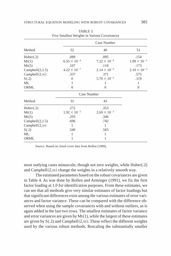
most outlying cases minuscule, though not zero weights, while Huber(.2)and Campbell~2,`! change the weights in a relatively smooth way.

The estimated parameters based on the robust covariances are givenin Table 4. As was done by Bollen and Arminger (1991), we fix the firstfactor loading at 1.0 for identification purposes. From these estimates, wecan see that all methods give very similar estimates of factor loadings butthat significant differences exist among the various estimates of error vari-ances and factor variance. These can be compared with the difference ob-served when using the sample covariances with and without outliers, as isagain added in the last two rows. The smallest estimates of factor varianceand error variances are given by Mt(1), while the largest of these estimatesare given by S(.2) and Campbell~2,`!. These reflect the different weightsused by the various robust methods. Rescaling the substantially smaller

TABLE 3Five Smallest Weights in Various Covariances

Case Number

Method 52 40 51

Huber(.2) .089 .095 .154Mt(1) 6.553 1024 7.223 1024 1.093 1023

Mt(5) .107 .118 .173Campbell(2,1.5) 4.223 1027 2.143 1025 2.103 1023

Campbell~2,`! .337 .371 .575S(.2) 0 5.703 1023 .119ML 1 1 1ORML 0 0 0

Case Number

Method 31 43

Huber(.2) .272 .353Mt(1) 1.923 1023 2.693 1023

Mt(5) .293 .346Campbell(2,1.5) .696 .742Campbell~2,`! 1 1S(.2) .540 .565ML 1 1ORML 1 1

Source:Based on cloud cover data from Bollen (1989).


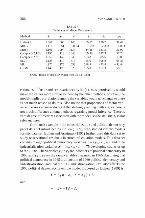
estimates of factor and error variances by Mt(1), as is permissible, wouldmake the values more similar to those by the other methods; however, themodel-implied correlations among the variables would not change so thereis not much reason to do this. Also notice that proportions of factor vari-ance to error variances do not differ strikingly among methods, so there isnot much difference among methods regarding model inference. There iszero degree of freedom associated with the model, so the statisticT1 is notrelevant here.

Our fourth example is the industrialization and political democracypanel data set introduced by Bollen (1989), who studied various modelsfor this data set. Bollen and Arminger (1991) further used this data set tostudy observational residuals in structural equation models. This data setconsists of eight political democracy variablesY5 ~ y1,{{{, y8!' and threeindustrialization variablesX5 ~x1, x2, x3!' in 75 developing countries upto the 1960s. The variablesy1 to y4 are indicators of political democracy in1960, andy5 to y8 are the same variables measured in 1965. Assuming thatpolitical democracy in 1965 is a function of 1960 political democracy andindustrialization, and that the 1960 industrialization level also affects the1960 political democracy level, the model proposed by Bollen (1989) is

Y 5 LYh 1 «, X 5 LXj 1 d,

and

h 5 Bh 1 Gj 1 z,

TABLE 4Estimates of Model Parameters

Method l2 l3 F c1 c2 c3

Huber(.2) 1.067 1.068 1148 69.67 136.7 38.44Mt(1) 1.118 1.051 31.31 1.198 2.388 1.063Mt(5) 1.101 1.094 1137 84.85 161.3 31.90Campbell(2,1.5) 1.136 1.113 1040 99.90 147.9 57.74Campbell~2,`! 1.059 1.142 1045 163.8 305.6 13.88S(.2) 1.128 1.110 1417 125.6 198.8 65.32ML .970 1.176 1052 248.8 473.8 251.44ORML 1.143 1.123 1023 105.8 157.3 58.15

Source:Based on cloud cover data from Bollen (1989).


where

LY 5 S1 l1 l2 l3 0 0 0 0

0 0 0 0 1 l1 l2 l3D', LX 5 ~1 l4 l5!',

B 5 S 0 0

b21 0D, G 5 ~g11 g21!

',

«, d, andz are vectors of errors. It is allowed that some error terms in« arecorrelated based on theoretical considerations; see Bollen (1989) for de-tails about the data and the model. Our interest here is to see the estimatesand fit indices associated with different methods.

Using Campbell(2,1.25) on this data set findswi2 5 1 for all the

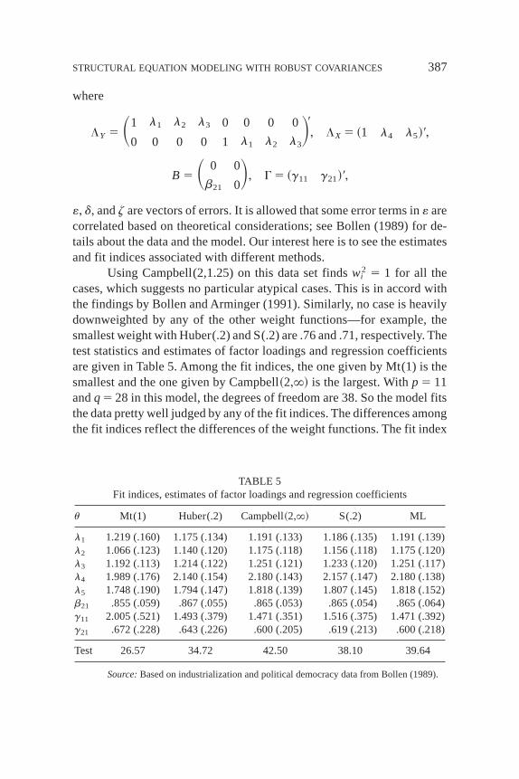
cases, which suggests no particular atypical cases. This is in accord withthe findings by Bollen and Arminger (1991). Similarly, no case is heavilydownweighted by any of the other weight functions—for example, thesmallest weight with Huber(.2) and S(.2) are .76 and .71, respectively. Thetest statistics and estimates of factor loadings and regression coefficientsare given in Table 5. Among the fit indices, the one given by Mt(1) is thesmallest and the one given by Campbell~2,`! is the largest. Withp 5 11andq5 28 in this model, the degrees of freedom are 38. So the model fitsthe data pretty well judged by any of the fit indices. The differences amongthe fit indices reflect the differences of the weight functions. The fit index

TABLE 5Fit indices, estimates of factor loadings and regression coefficients

u Mt(1) Huber(.2) Campbell~2,`! S(.2) ML

l1 1.219 (.160) 1.175 (.134) 1.191 (.133) 1.186 (.135) 1.191 (.139)l2 1.066 (.123) 1.140 (.120) 1.175 (.118) 1.156 (.118) 1.175 (.120)l3 1.192 (.113) 1.214 (.122) 1.251 (.121) 1.233 (.120) 1.251 (.117)l4 1.989 (.176) 2.140 (.154) 2.180 (.143) 2.157 (.147) 2.180 (.138)l5 1.748 (.190) 1.794 (.147) 1.818 (.139) 1.807 (.145) 1.818 (.152)b21 .855 (.059) .867 (.055) .865 (.053) .865 (.054) .865 (.064)g11 2.005 (.521) 1.493 (.379) 1.471 (.351) 1.516 (.375) 1.471 (.392)g21 .672 (.228) .643 (.226) .600 (.205) .619 (.213) .600 (.218)

Test 26.57 34.72 42.50 38.10 39.64

Source:Based on industrialization and political democracy data from Bollen (1989).


with the ML method is not the largest for this data set, which is related tothe fact that no particular observation is atypical. Regarding the estimatesof parameters, the regression coefficientsg11 and g21 by Mt(1) are thelargest whileb21 by Mt(1) is the smallest. Since each case in Camp-bell~2,`! gets a unit weight, the associated parameter estimates are iden-tical to those by ML. The fit index by Campbell~2,`! is a little larger thanthat by ML. This reflects the fact that the estimated[a in (25) associatedwith Campbell~2,`! is less than one. In general, the importance of thisexample is that it shows that our robust methods perform acceptably evenwhen they are technically not needed.

From the above four examples, we can see some differences betweenthe classical method and the robust methods on fit indices. There also existdifferences on parameter estimates among the various methods, though theseare not as impressive as those on the fit indices. In order to illustrate a moredramatic variation in parameter estimates by different methods, we presentanother example based on a real data set but with some added artificial out-liers. Mardia et al. (1979, table 1.2.1) give test scores ofn588 students onfive topics (Mechanics,Vectors,Algebra,Analysis, and Statistics). Becausethe first two topics were tested with closed book exams and the last threetopics with open book exams, this data set is sometimes referred to as theopen-closed book data. Since these two examination methods may tap dif-ferent abilities, a two-factor model was proposed and confirmed by Tanakaet al. (1991). The first two variables are indicators of the closed book factor,and the last three variables are indicators of the open book factor.The eighty-first case has previously been identified as the most influential point byvarious authors (Tanaka et al. 1991; Cadigan 1995; Lee and Wang 1996).Our analysis of the 88 cases shows that the weight associated with this caseusing Campbell(2,1.25) isw81

2 5 +415, indicating that even the most influ-ential point may not be really atypical. Actually, the two-factor model fitsthe data well judged by either the ML method or any of the robust methods.

In order to see the effect of different methods, we added a vector

X89 5 k~0, 0, 0, 11+49, 12+52!

to the original data set to make it a sample with sizen5 89. An illuminat-ing approach is to compare the different methods whenk changes. Fixingf115 f225 1 for identification purposes, we use the ML method as wellas different robust methods to evaluate the model. Since the results bydifferent robust methods gives similar information, we report only those


by Huber(.2) to save space. The results are presented in Table 6 in whichwe usek 5 0 to denote the original data set without the artificial outlier.The ML results are in the left part of the table. The effect of the one outlieron the ML method is obvious. Ask increases,c44 andc55 dramaticallyincrease at first, thenf12decreases andc11becomes negative (a Heywoodcase), finallyl32, f12, c22 become negative (another Heywood case). Inthe right part of the table are the estimates by Huber(.2). Ask increases,there is a minor effect on parameter estimates at the beginning and almostno difference whenk moves from 5 to 25. The effect on fit statistics issimilar to that on parameter estimates. With 4 degrees of freedom in thismodel, one outlier totally discredits an apparently good model when eval-uated by the ML method, and the more extreme the outlier, the worse theML test statistic is at describing the majority of the data. If evaluated byone of the robust methods, the effect of the outlier is basically eliminated.The unbounded influence function and zero breakdown point of the sam-ple covarianceS is also well illustrated through this example.

In summary, using robust covariances leads to smaller fit indicesfor the first two data sets. Even though the statistic corresponding to arobust method is still significant, a decrease in the fit index (from 102.10to 78.62 in the second example) gives us more statistical support for usinga theoretically justified model. For the third data set, using robust proce-dures automatically leads to a proper solution of estimates. These effectsreflect that a robust covariance can effectively downweight individual ob-servations that deviate from a proposed structure. In the fourth data set, thenormal theory method works well and no case was heavily downweightedby any of the robust methods, indicating that no particular observation isatypical. The last example demonstrates that there can be a dramatic dif-ference between the ML method and one of the robust methods, dependingon how outlying the atypical observation is. It also illustrates that a singleoutlier can totally ruin the performance of the classical method.

After seeing the effect of different estimators in these examples,it would be helpful to give some guidance on choice of estimators inpractice. In Huber-type estimators, the effect of abnormal cases is down-weighted but not eliminated. If data are near normal, the estimators basedon Huber-type weights are still highly efficient. So Huber-type weightfunctions—for example, Huber(.2) and Campbell~2,`!—are better usedfor data sets whose distributions are not too far away from normal. Inredescending weight functions, the effect of outlying cases is much smallerthan that in Huber-type weights (see the numerical weights in Table 3).


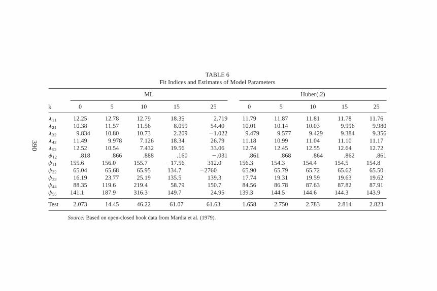
TABLE 6Fit Indices and Estimates of Model Parameters

ML Huber(.2)

k 0 5 10 15 25 0 5 10 15 25

l11 12.25 12.78 12.79 18.35 2.719 11.79 11.87 11.81 11.78 11.76l21 10.38 11.57 11.56 8.059 54.40 10.01 10.14 10.03 9.996 9.980l32 9.834 10.80 10.73 2.209 21.022 9.479 9.577 9.429 9.384 9.356l42 11.49 9.978 7.126 18.34 26.79 11.18 10.99 11.04 11.10 11.17l52 12.52 10.54 7.432 19.56 33.06 12.74 12.45 12.55 12.64 12.72f12 .818 .866 .888 .160 2.031 .861 .868 .864 .862 .861c11 155.6 156.0 155.7 217.56 312.0 156.3 154.3 154.4 154.5 154.8c22 65.04 65.68 65.95 134.7 22760 65.90 65.79 65.72 65.62 65.50c33 16.19 23.77 25.19 135.5 139.3 17.74 19.31 19.59 19.63 19.62c44 88.35 119.6 219.4 58.79 150.7 84.56 86.78 87.63 87.82 87.91c55 141.1 187.9 316.3 149.7 24.95 139.3 144.5 144.6 144.3 143.9

Test 2.073 14.45 46.22 61.07 61.63 1.658 2.750 2.783 2.814 2.823

Source:Based on open-closed book data from Mardia et al. (1979).

39

0

So Hampel-type weight functions—for example, Campbell(2,1.5)—canbe used for data sets with far outlying cases, but the estimators will losemore efficiency than those based on Huber-type weight functions whendata are approximately normal. The weight function based on a multi-variatet-distribution is best used for data sets whose discrepancy can beapproximately described by thet-distribution, or for data sets with long-tailed distribution but no obvious outliers (few cases sit far away fromthe cloud formed by the majority of the cases). S-estimators are de-signed for high-dimensional data with many outliers—that is, data thatare collected with many mishandlings. Of course, the best method to usewould be the normal theory method if we know that a data set is fairlynormal. The above discussion and recommendation are based on our lim-ited experience with these different weight functions. In practice, if notmuch is known about the quality or distribution of a data set, we suggestexperimenting with several of these methods, including the sample co-variance as well as the S-estimators, before finding the one that suits thedata set and theoretical models. If no case is particularly downweightedwith a robust approach (e.g., Campbell[2,1.25]), using the sample co-variance is probably enough. When many cases are heavily downweighted,it is necessary to use highly robust estimators, such as the S-estimators,in getting a reliable inference.

We have used Campbell’s weight to define atypical observations,primarily because he explicitly connected the magnitude ofwi

2 to abnor-mal observations. Any other robust procedure may work equally well for agiven data set.

5. DISCUSSION

Data in social and behavioral sciences are seldom normal, yet appropriateprocedures for dealing with such nonnormal data in the context of latentvariable structural modeling are only rarely used. When the data-generatingmechanism is smooth and there are no atypical observations, various meth-ods exist (reviewed by Bentler and Dudgeon 1996) that would give appro-priate inference in this situation. However, outlying and grossly distortingobservations seem to be typical in the social sciences. As noted by Wilcox(1996:xv) “recent investigations (cited in the text) indicate that outliers arevery common in the social sciences, and outliers can substantially reducepower and give a distorted view of data based on conventional measures oflocation and scale.” Thus motivated, we studied the technical and practical


aspects of a procedure that uses robust covariances in structural equationmodeling. Our examples show important differences between the classicalmethod and the various robust methods.

When facing a data set that comes from a distribution with long tailsor with outliers, the procedure of removing outliers followed by a classicalmethod is often used (e.g., Berkane and Bentler 1988). As discussed inHuber (1981:4–5), outlier rejection followed by a classical method maynot be a good statistical procedure, since the most influential points maynot be real outliers; these may only indicate the long tails of the underlyingdistribution. Actually, it is hard to make a clear distinction between outli-ers and typical observations. For example, Campbell (1980) suggested thata weightwi

2 below .30 is associated with an atypical observation, but hedid not give a suggestion about what to do with a weight of .31. On theother hand, using a robust covariance approach automatically generates aproper weight to each of the cases. The outlying cases are automaticallydownweighted. Also, the statistical theory for our robust procedures iswell developed, as given in Sections 2 and 3, while the theory that wouldhold for a two-step estimator involving outlier removal is not so clear.

A situation in which outlier detection may be useful is when one isfamiliar with the data collection process behind each individual case. Insuch a situation, identifying the most influential points may help the re-searcher to find extra information to explain these abnormal points. Eventhough using both the sample covariance and the robust covariances iden-tified the same set of most influential points in Table 3, this result will notalways be observed. Sometimes there may exist masking effects of mul-tiple outliers, as demonstrated by Rousseeuw and van Zomeren (1990) inseveral interesting examples. So a robust procedure is still preferable inpractice, if only to identify the “real outliers.”

Since most applications of structural equation modeling involvecovariance structures, we only studied the procedure of using a robustcovariance in the Wishart likelihood function. It will be apparent fromequation (11) that our development is equally applicable to the situationin which robust covariances are used in the normal theory generalizedleast squares (GLS) function12

_tr$W~Sn 2 S~u!!%2, whereW is a consis-tent estimator ofS0

21 + For exampleW5 Sn21 and the iteratively updated

W5 ZS021 define classical GLS and iteratively reweighted GLS functions

(Bentler 1995). The functions then can be corrected by[a as in (25) toyield an asymptotically equivalent test statistic.


Sometimes, a mean structure is also of substantive interest. Sincethe influence function associated with the sample mean is unbounded, itwould be preferable to develop a procedure that uses robust means andcovariances simultaneously in the normal theory likelihood function. How-ever, the fit statisticT1 cannot be generalized directly to mean and covari-ance structures. This aspect is still under further study.

As far as we know, no existing structural equation modeling soft-ware can compute the robust procedures described above. In order to makethese methods readily available, they are being incorporated into the newrelease 6.0 of EQS. Furthermore, to ensure that researchers can utilizethese statistics as they desire, all the key components (e.g., case weights,robust means and covariances, parameter estimates, asymptotic covari-ance matrices) will be writable to an external file. The methods will also beintegrated into EQS’s simulation module to permit Monte Carlo and re-sampling research on the performance of these methods under varyingconditions.

REFERENCES

Amemiya, Yasuo, and Theodore W.Anderson. 1990. “Asymptotic Chi-Square Tests fora Large Class of Factor Analysis Models.”Annals of Statistics18:1453–63.

Anderson, Theodore W., and Yasuo Amemiya. 1988. “The Asymptotic Normal Distri-bution of Estimators in Factor Analysis Under General Conditions.”Annals of Sta-tistics16:759–71.

Arminger, Gerhard, and Ronald J. Schoenberg. 1989. “Pseudo Maximum LikelihoodEstimation and a Test for Misspecification in Mean- and Covariance-Structure Mod-els.” Psychometrika54:409–25.

Arminger, Gerhard, and Michael Sobel. 1990. “Pseudo Maximum Likelihood Estima-tion of Mean and Covariance Structures with Missing Data.”Journal of the Amer-ican Statistical Association85:195–203.

Austin, James T., and Robert F. Calderón. 1996. “Theoretical and Technical Contribu-tions to Structural Equation Modeling:An UpdatedAnnotated Bibliography.”Struc-tural Equation Modeling3:105–75.

Bentler, Peter M. 1994. “A Testing Method for Covariance Structure Analysis.” Pp.123–35 inMultivariate Analysis and its Applications, vol. 24, edited by T. W. An-derson, K. T. Fang and I. Olkin. Hayward, CA: Institute of Mathematical Statistics.

———. 1995.EQS Structural Equations Program Manual. Encino, CA: MultivariateSoftware.

Bentler, Peter M., and Theo Dijkstra. 1985. “Efficient Estimation via Linearization inStructural Models.” Pp. 9–42 inMultivariate Analysis VI, edited by P. R. Krishna-iah. Amsterdam: North-Holland.


Bentler, Peter M., and Paul Dudgeon. 1996. “Covariance StructureAnalysis: StatisticalPractice, Theory, Directions.”Annual Review of Psychology47:563–92.

Berkane, Maia, and Peter M. Bentler. 1988. “Estimation of Contamination Parametersand Identification of Outliers in Multivariate Data.”Sociological Methods and Re-search17:55–64.

Bishop, Yvonne M. M., Stephen E. Fienberg, and Paul W. Holland. 1975.DiscreteMultivariate Analysis: Theory and Practice. Cambridge, MA: MIT Press.

Bollen, KennethA. 1989.Structural Equations with Latent Variables. NewYork: Wiley.Bollen, Kenneth A., and Gerhard Arminger. 1991. “Observational Residuals in Factor

Analysis and Structural Equation Models.” Pp. 235–62 inSociological Methodol-ogy 1991, edited by Peter V. Marsden. Cambridge, MA: Blackwell Publishers.

Box, George E. P. 1954. “Some Theorems on Quadratic Forms Applied in the Study ofAnalysis of Variance Problem: I. Effect of Inequality of Variance in the One-wayClassification.”Annals of Mathematical Statistics25:290–302.

Browne, Michael W. 1982. “Covariance Structures.” Pp. 72–141 inTopics in Multi-variate Analysis, edited by D. M. Hawkins. Cambridge, England: Cambridge Uni-versity Press.

———. 1984. “Asymptotic Distribution-Free Methods for the Analysis of CovarianceStructures.”British Journal of Mathematical and Statistical Psychology37:62–83.

Browne, Michael W., and Gerhard Arminger. 1995. “Specification and Estimation ofMean- and Covariance-Structure Models.” Pp. 185–249 inHandbook of StatisticalModeling for the Social and Behavioral Sciences, edited by G. Arminger, C. C.Clogg and M. E. Sobel. New York: Plenum.

Cadigan, Noel G. 1995. “Local Influence in Structural Equation Models.”StructuralEquation Modeling2:13–30.

Campbell, Norm A. 1980. “Robust Procedures in Multivariate Analysis I: Robust Co-variance Estimation.”Applied Statistics29:231–37.

Catalano, Paul J., and Louise M. Ryan. 1992. “Bivariate Latent Variable Models forClustered Discrete and Continuous Outcomes.”Journal of the American StatisticalAssociation87:651–58.

Chamberlain, Gary. 1982. “Multivariate Regression Models for Panel Data.”Journalof Econometrics18:5–46.

Curran, Patrick S., Stephen G. West, and John F. Finch. 1996. “The Robustness of TestStatistics to Nonnormality and Specification Error in Confirmatory Factor Analy-sis.” Psychological Methods1:16–29.

Devlin, Susan J., Ramanathan Gnanadesikan, and Jon R. Kettenring. 1981. “RobustEstimation of Dispersion Matrices and Principal Components.”Journal of the Amer-ican Statistical Association76:354–62.

Dukes, Richard L., Jodie Ullman, and JudyA. Stein. 1995. “An Evaluation of D.A.R.E.(Drug Abuse Resistance Education), Using a Solomon Four-Group Design withLatent Variables.”Evaluation Review19:409–35.

Gnanadesikan, Ramanathan. 1997.Methods for Statistical Data Analysis of Multivar-iate Observations. New York: Wiley.

Gnanadesikan, Ramanathan, and Jon R. Kettenring. 1984. “A Pragmatic Review ofMultivariate Methods in Applications.” Pp. 309–41 inStatistics: An Appraisal,edited by H. A. David and H. T. David. Ames, Iowa: Iowa State University Press.


Hampel, Frank R. 1974. “The Influence Curve and Its Role in Robust Estimation.”Journal of the American Statistical Association69:383–93.

Hoaglin, David C., Frederick Mosteller, and John W. Tukey. 1983.UnderstandingRobust and Exploratory Data Analysis. New York: Wiley.

Holzinger, Karl J., and Frances Swineford. 1939.A Study in Factor Analysis: TheStability of a Bi-factor Solution. University of Chicago, Supplementary Educa-tional Monographs, No. 48.

Hu, Li-tze, Peter M. Bentler, and Yutaka Kano. 1992. “Can Test Statistics in Covari-ance Structure Analysis Be Trusted?”Psychological Bulletin112:351–62.

Huba, George J., and Lisa L. Harlow. 1987. “Robust Structural Equation Models: Im-plications for Developmental Psychology.”Child Development58:147–66.

Huber, Peter J. 1981.Robust Statistics.New York: Wiley.Jöreskog, Karl G. 1969. “A General Approach to Confirmatory Maximum Likelihood

Factor Analysis.”Psychometrika34:183–202.———. 1977. “Structural Equation Models in the Social Sciences: Specification, Es-

timation and Testing.” Pp. 265–87 inApplications of Statistics, edited by P. R.Krishnaiah. Amsterdam: North Holland.

Jöreskog, Karl G., and Dag Sörbom. 1993.LISREL 8 User’s Reference Guide. Chicago:Scientific Software International.

Kano, Yutaka. 1986. “Conditions on Consistency of Estimators in Covariance Struc-ture Model.”Journal of the Japan Statistical Society16:75–80.

Kendler, Kenneth S., Andrew C. Heath, Michael C. Neale, Ronald C. Kessler, andLindon J. Eaves. 1992. “APopulation-Based Twin Study ofAlcoholism in Women.”Journal of the American Medical Association268:1877–82.

Lee, Sik-Yum., and Shu-Jia Wang. 1996. “Sensitivity Analysis of Structural EquationModels.”Psychometrika61:93–108.

Lopuhaä, Hendrik P. 1989. “On the Relation Between S-estimators and M-estimatorsof Multivariate Location and Covariances.”Annals of Statistics17:1662–83.

Magnus, Jan R., and Heinz Neudecker. 1988.Matrix Differential Calculus with Appli-cations in Statistics and Econometrics. New York: Wiley.

Mardia, Kanti V., John T. Kent, and John M. Bibby. 1979.Multivariate Analysis. NewYork: Academic Press.

Maronna, Ricardo A. 1976. “Robust M-estimators of Multivariate Location and Scat-ter.” Annals of Statistics4:51–67.

Muirhead, Robb J. 1982.Aspects of Multivariate Statistical Theory. New York: Wiley.Muthén, Bengt O. 1992. “Latent Variable Modeling in Epidemiology.”Alcohol Health

and Research World16:286–92.Rousseeuw, Peter J., and Bert C. van Zomeren. 1990. “Unmasking Multivariate Out-

liers and Leverage Points (with discussion).”Journal of the American StatisticalAssociation85:633–51.

Ruppert, David. 1992. “Computing S Estimators for Regression and MultivariateLocation0Dispersion.”Journal of Computational and Graphical Statistics1:253–70.

Satorra, Albert, and Peter M. Bentler. 1990. “Model Conditions for Asymptotic Ro-bustness in the Analysis of Linear Relations.”Computational Statistics and DataAnalysis10:235–49.


———. 1994. “Corrections to Test Statistics and Standard Errors in Covariance Struc-ture Analysis.” Pp. 399–419 inLatent Variables Analysis: Applications for Devel-opmental Research, edited by A. von Eye and C. C. Clogg. Thousand Oaks, CA:Sage.

Satterthwaite, Franklin E. 1941. “Synthesis of Variance.”Psychometrika,6:309–16.Staudte, Robert G., and Simon J. Sheather. 1990.Robust Estimation and Testing. New

York: Wiley.Tanaka, Yutaka, Shingo Watadani, and Sung H. Moon. 1991. “Influence in Covariance

Structure Analysis: With an Application to Confirmatory Factor Analysis.”Com-munication in Statistics-Theory and Method20:3805–21.

Tosteson, Tor, Leonard A. Stefanski, and Daniel W. Schafer. 1989. “A MeasurementError Model for Binary and Ordinal Regression.”Statistics in Medicine8:1139–47.

Tyler, David E. 1982. “Radial Estimates and the Test for Sphericity.”Biometrika69:429–36.

———. 1983. “Robustness and Efficiency Properties of Scatter Matrices.”Biometrika70:411–20.

Wilcox, Rand R. 1996.Statistics for the Social Sciences. San Diego: Academic Press.Yamaguchi, Kazunori, and Michko Watanabe. 1993. “The Efficiency of Estimation

Methods for Covariance Structure Models Under Multivariate t Distribution.” Pp.281–84 inProceedings of the Asian Conference on Statistical Computing, Inter-national Association for Statistical Computing.

Yuan, Ke-Hai, and Peter M. Bentler. Forthcoming. “Robust Methods for Mean andCovariance Structure Analysis.”British Journal of Mathematical and StatisticalPsychology.

———. 1996. “Effect of Outliers on Estimators and Test Statistics in Covariance Struc-ture Analysis.” Under review.

———. 1997. “Mean and Covariance Structure Analysis: Theoretical and PracticalImprovements.”Journal of the American Statistical Association92:767–74.


Documents

STRUCTURAL EQUATION COVARIANCES Ke-Hai Yuan* Peter …