Embed Size (px)
Citation preview
DEPARTAMENTO DE INGENIERÍA MECÁNICA
ESCUELA TÉCNICA SUPERIOR DE INGENIEROS INDUSTRIALES
STRUCTURAL HEALTH MONITORING BY USING TRANSMISSIBILITY
TESIS DOCTORAL
Autor: Yun Lai Zhou
Engineer
Director: Ricardo Perera Velamazán
Ph.D., Engineer
MADRID, SPAIN
2015

Tribunal nombrado por el Magfco. y Excmo. Sr. Rector de la Universidad Politécnica de Madrid el día…….. de………. de 2015.
Presidente: …………………………………………………………………………..
Vocal: ……………………………………………………………………………….
Vocal: ……………………………………………………………………………….
Vocal: ……………………………………………………………………………….
Secretario: ……………………………………………………………………………
Suplente: ……………………………………………………………………………..
Suplente: ……………………………………………………………………………..
Realizado el acto de defensa y lectura de la Tesis el día……. de…… de 2015 en la E.T.S. Ingenieros Industriales.
Calificación:
EL PRESIDENTE LOS VOCALES
EL SECRETARIO


To my parents, brother and sister

I
ACKNOWLEDGEMENTS
I would like to give special thanks to my supervisor, Prof. Ricardo Perera, for his
supervision and support at all levels during the period of research. He brought me into
this field of structural health monitoring, and guided me in the past years.
Thanks to Prof. Nuno M.M. Maia, for his supervision during the visiting stay in his
vibration laboratory in Instituto Superior Tecnico, Universidade de Lisboa. He shared
his experience of transmissibility study to me, which gave me a better understanding
of transmissibility. Thanks to the group members of Nuno M.M. Maia, Hugo Filipe
Dinis Policarpo for teaching me modal testing in laboratory; thanks to J.V. Araújo dos
Santos for teaching me speckle interferometry based damage identification.
A special thanks to be given to my forever professor and friend Eloi Figueriedo for
his teaching in experiment data analysis, paper writing and submission. And thanks to
him for supporting the experiment data and related simulation.
Thanks to Prof. Magd Abdel Wahab for his supervision during the visiting research in
Soete Lab of Ghent University, Belgium. He taught me ABAQUS, and he also taught
me fracture mechanics. Thanks to the group members of Prof. Magd Abdel Wahab,
Yue Tongyan, Hanan Alali, Phuc Phung Van, Tran Vinh Loc, Ibrahim Gadala, Kyvia
Pereira, Junyan Ni, and Jie Zhang as well for an unforgettable visiting stay in his
group.
Thanks to J.V. Araújo dos Santos, Rui Pedro Chedas Sampaio (Instituto Superior
Técnico, University of Lisbon, Portugal), Gilles Tondreau, Arnaud Deraemaeker
(Université Libre de Bruxelles, Belgium), H. M. R. Lopes (Polytechnic Institute of
Porto, Portugal) for experiment data support.
I highly appreciate the help from Prof. Enrique Alarcon, Prof. Alberto Fraile, Prof.
Consuelo and Prof. Amadeo Benament Climent for their advices and help during my
II
research. And especially thanks to Prof. Francisco Javier Montans Leal for his
teaching in nonlinear analysis, code writing, and advises in research.
Thanks to Francisco Javier Cara Cañas for his teaching in operational modal analysis.
I would like to acknowledge the support from China State Council (CSC) for the
whole Ph.D. research. Besides, I would like to acknowledge the support from Spanish
Ministry of Economy and Competitiveness (project BIA2010-20234-C03-01) during
the research. And it is also acknowledged that the visiting research is partially
supported by the Portuguese Science Foundation FCT, through IDMEC, under
LAETA, finally, financial support from CWO (Commissie Wetenschappelijk
Onderzoek), Faculty of Engineering and Architecture, Ghent University for a research
stay at Soete Laboratory is also acknowledged.
Finally, and most importantly, I would like to thank my family for their love and
support throughout all my studies.
Yun Lai Zhou
Madrid, Spain
Oct. 2015.
III
ABSTRACT
Structural health monitoring has experienced a huge development from several
decades ago since the cost of rehabilitation of structures such as oil pipes, bridges and
tall buildings is very high. In the last two decades, a lot of methods able to identify the
real stage of a structure have been developed basing on both models and experimental
data. Modal testing is the most common; by carrying out the experimental modal
analysis of a structure, some parameters, such as frequency, mode shapes and
damping, as well as the frequency response function of the structure can be obtained.
From these parameters, different damage indicators have been proposed.
However, for complex and large structures, any frequency domain approach that
relies on frequency response function estimation would be of difficult application
since an assumption of the input excitations to the system should be carried out.
Operational modal analysis uses only output signals to extract the structural dynamic
parameters and, therefore, to identify the structural stage. In this sense, within
operational modal analysis, transmissibility has attracted a lot of attention in the
scientific field in the last decade. In this work new damage detection approaches
based on transmissibility are developed.
Firstly, a new theory of transmissibility coherence is developed and it is tested with a
three-floor-structure both in simulation and in experimental data analysis; secondly,
Mahalanobis distance is taken into use with the transmissibility, and a free-free beam
is used to test the approach performance; thirdly, neural networks are used in
transmissibility for structural health monitoring; a simulated beam is used to validate
the proposed method.

IV
V
RESUMEN
El control del estado en el que se encuentran las estructuras ha experimentado un gran
auge desde hace varias décadas, debido a que los costes de rehabilitación de
estructuras tales como los oleoductos, los puentes, los edificios y otras más son muy
elevados. En las últimas dos décadas, se han desarrollado una gran cantidad de
métodos que permiten identificar el estado real de una estructura, basándose en
modelos físicos y datos de ensayos. El ensayo modal es el más común; mediante el
análisis modal experimental de una estructura se pueden determinar parámetros como
la frecuencia, los modos de vibración y la amortiguación y también la función de
respuesta en frecuencia de la estructura. Mediante estos parámetros se pueden
implementar diferentes indicadores de daño.
Sin embargo, para estructuras complejas y grandes, la implementación de
metodologías basadas en la función de respuesta en frecuencia requeriría realizar
hipótesis sobre la fuerza utilizada para excitar la estructura. Dado que el análisis
modal operacional utiliza solamente las señales de respuesta del sistema para extraer
los parámetros dinámicos estructurales y, por tanto, para evaluar el estado de una
estructura, el uso de la transmisibilidad sería posible. En este sentido, dentro del
análisis modal operacional, la transmisibilidad ha concentrado mucha atención en el
mundo científico en la última década. Aunque se han publicado muchos trabajos
sobre el tema, en esta Tesis se proponen diferentes técnicas para evaluar el estado de
una estructura basándose exclusivamente en la transmisibilidad.
En primer lugar, se propone un indicador de daño basado en un nuevo parámetro, la
coherencia de transmisibilidad; El indicador se ha valido mediante resultados
numéricos y experimentales obtenidos sobre un pórtico de tres pisos. En segundo
lugar, la distancia de Mahalanobis se aplica sobre la transmisibilidad como
procedimiento para detectar variaciones estructurales provocadas por el daño. Este
método se ha validado con éxito sobre una viga libre-libre ensayada
experimentalmente. En tercer lugar, se ha implementado una red neuronal basada en
medidas de transmisibilidad como metodología de predicción de daño sobre una viga

VI
simulada numéricamente.
VII
TABLE OF CONTENTS
ACKNOWLEDGEMENTS ..................................................................... I
ABSTRACT ........................................................................................... III
RESUMEN .............................................................................................. V
TABLE OF CONTENTS .................................................................... VII
LIST OF FIGURES ............................................................................... XI
LIST OF TABLES .............................................................................. XIII
NOMENCLATURES ........................................................................... XV
ACRONYMS .................................................................................... XVII
Chapter 1 Introduction ........................................................................... 1
1.1 Background .......................................................................................................... 1 1.2 Schemes of SHM ................................................................................................. 3 1.3 Literature review of transmissibility ................................................................... 4 1.4 Motivations and objectives .................................................................................. 6 1.5 Thesis dissertation ............................................................................................... 7
Chapter 2 Damage detection by transmissibility ................................ 11
2.1 Introduction ....................................................................................................... 11 2.2 Transmissibility ................................................................................................. 13
2.2.1 Transmissibility estimation ........................................................................ 13 2.2.2 Transmissibility mode shape ...................................................................... 16
2.3 Damage detection procedure ............................................................................. 19 2.3.1 Damage sensitive indicators ....................................................................... 19 2.3.2 Damage detection scheme .......................................................................... 20
2.4 Test specimen and experimental setup .............................................................. 21 2.5 Results and discussions ..................................................................................... 23
2.6.1 Transmissibility vs FRF ............................................................................. 23 2.6.2 Natural frequency identification comparison ............................................. 25 2.6.3 TMS vs MS comparison ............................................................................. 26 2.6.4 Natural frequency in damage detection ...................................................... 27 2.6.5 TMS based damage detection ..................................................................... 29
2.7 Conclusions ....................................................................................................... 31
Chapter 3 Damage detection and quantification using
VIII
transmissibility coherence analysis ...................................................... 33
3.1 Introduction ....................................................................................................... 33 3.2 Transmissibility based coherence ...................................................................... 36
3.2.1 Applicability of coherence in damage detection ........................................ 36 3.2.2 Transmissibility .......................................................................................... 37 3.2.3 Transmissibility coherence ......................................................................... 37
3.3 Damage identification based on TC .................................................................. 40 3.3.1 Damage indicators ...................................................................................... 40 3.3.2 Damage identification scheme ................................................................... 41
3.4 Numerical simulation ........................................................................................ 42 3.4.1 Model description ....................................................................................... 42 3.4.2 Transmissibility, TC and FRF coherence comparison ............................... 44
3.4.2.1 Transmissibility and TC comparison ....................................... 44 3.4.2.2 TC and FRF coherence comparison ........................................ 46
3.4.3 Damage identification procedure ............................................................... 49 3.5 Experimental verification .................................................................................. 51
3.5.1 Transmissibility, TC and FRF coherence comparison ............................... 54 3.5.1.1 Transmissibility and TC comparison ....................................... 54 3.5.1.2 FRF coherence and TC comparison ........................................ 56
3.5.2 Damage identification analysis in linear part ............................................. 59 3.5.3 Damage identification analysis in nonlinear part ....................................... 61
3.6 Conclusions ....................................................................................................... 63
Chapter 4 Damage detection in structures using a
transmissibility-based mahalanobis distance ...................................... 65
4.1 Introduction ....................................................................................................... 65 4.2 Theoretical background ..................................................................................... 67
4.2.1 Transmissibility .......................................................................................... 67 4.2.2 Mahalanobis squared distance (MSD) ........................................................ 67
4.3 The proposed damage detection method ........................................................... 68 4.3.1 MSD between undamaged and damaged transmissibility .......................... 68 4.3.2 Euclidean distance between undamaged and damaged transmissibility .... 69 4.3.3 Damage detection index ............................................................................. 70
4.4 Experimental validation ..................................................................................... 71 4.5 Discussion of Results ........................................................................................ 74
4.5.1 Importance of using data-normalization methods ...................................... 74 4.5.2 Applicability of the MSD as a damage-sensitive feature ........................... 75
4.5.2.1 Comparison between transmissibility-based MSD and ESD .. 76 4.5.2.2 Comparison between MSDs based on transmissibility and FRFs .................................................................................................... 77
4.5.3 Applicability of the DDI for damage detection .......................................... 78 4.5.4 Applicability of the ARI ............................................................................. 81

IX
4.5.5 Generalization performance ....................................................................... 83 4.6 Conclusions ....................................................................................................... 84
Chapter 5 Transmissibility based damage localization and
assessment by intelligent algorithm ..................................................... 87
5.1 Introduction ....................................................................................................... 87 5.2 Theoretical background ..................................................................................... 89
5.2.1 ANN ........................................................................................................... 89 5.2.2 PSDT .......................................................................................................... 91
5.3 Parameters for ANN .......................................................................................... 92 5.3.1 Inputs for ANN ........................................................................................... 92 5.3.2 Targets for ANN ......................................................................................... 94 5.3.3 ANN construction ....................................................................................... 96
5.4 Numerical study ............................................................................................... 100 5.4.1 Single damage .......................................................................................... 101 5.4.2 Multiple damages ..................................................................................... 104
5.5 Conclusions ..................................................................................................... 106
Chapter 6 Conclusions and future work ........................................... 107
6.1 Concluding remarks ......................................................................................... 107 6.2 Future work ..................................................................................................... 108
Capítulo 6 Conclusiones y trabajo futuro ......................................... 109
6.1 Conclusiones .................................................................................................... 109 6.2 Desarrollo futuro ............................................................................................. 110
Reference .............................................................................................. 111
Appendix 1. CV .................................................................................... 129

X
XI
LIST OF FIGURES
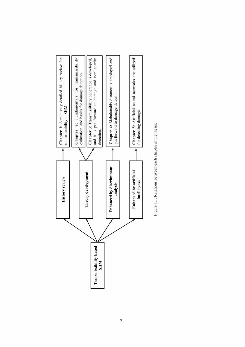
Figure 1.1. Relations between each chapter in the thesis. ..................................... 9
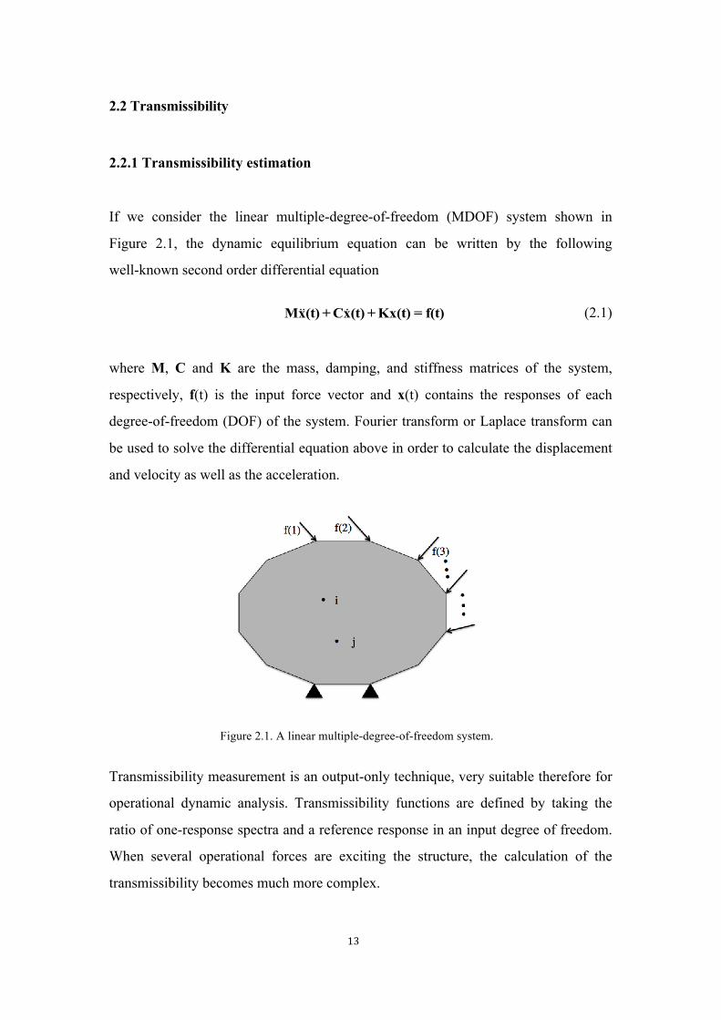
Figure 2.1. A linear multiple-degree-of-freedom system. ................................... 13 Figure 2.2. Flowchart for the damage detection procedure. ................................ 21 Figure 2.3. Schematic representation of the beam. ............................................. 22 Figure 2.4. T(i,7) (i=1,2,…,23) and FRF(i,7) (i=1,2,…,23) of first measurement
of damage scenario 0, 1 without artificial airflow. ...................................... 25 Figure 2.5. MSs derived from the numerical simulation. .................................... 27 Figure 2.6. TMSs derived from measurement 1 under intact condition without
artificial airflow. .......................................................................................... 27 Figure 2.7. Frequency decrease of mode 1. ......................................................... 28 Figure 2.8. Frequency decrease of mode 2. ......................................................... 28 Figure 2.9. Frequency decrease of mode 3. ......................................................... 28 Figure 2.10. Frequency decrease of mode 4. ....................................................... 28 Figure 2.11. Frequency decrease of mode 5. ....................................................... 29 Figure 2.12. Frequency decrease of mode 6. ....................................................... 29 Figure 2.13. TAC mode 1 for measurement 1 to 45. ........................................... 30 Figure 2.14. TAC mode 2 for measurement 1 to 45. ........................................... 30 Figure 2.15. TAC mode 3 for measurement 1 to 45. ........................................... 30 Figure 2.16. TAC mode 4 for measurement 1 to 45. ........................................... 31
Figure 3.1. (a). Shear-building model of a three-story structure. ........................ 42 Figure 3.1. (b). Excitation force. ......................................................................... 43 Figure 3.2. T(5,3) and T(5,2) for damage scenario D0, D1, D5 and D6 without
and with 5% random noise. ......................................................................... 45 Figure 3.3. (a) TC (5, 3) without noise; (b) TC (5, 3) with 5% random noise; (c)
TC (5, 2) without noise; (d) TC (5, 2) with 5% random noise. ................... 46 Figure 3.4. (a) FRF coherence (5,1) without noise; (b) FRF coherence (5,1)
with 5% random noise; (c) FRF coherence (3,1) without noise; (d) FRF coherence (3,1) with 5% random noise. ...................................................... 48
Figure 3.5. TC (5, 4) for damage scenario D0, D1, D5 and D6 without and with 5% random noise. ................................................................................ 48
Figure 3.6. TMAC (5, 3), TMAC (5, 2) for damage scenarios D0-D8. .............. 51 Figure 3.7. Schematic representation of the three-story building structure (all
dimensions are in cm). ................................................................................. 52 Figure 3.8. T (5, 3), T (5, 2), TC (5, 3), TC (5, 2) of measurement 1 of State #1,
2, 6 and 7. .................................................................................................... 55 Figure 3.9. FRF coherence (5, 1) of measurement 1 of States #1, 2, 6 and 7. .... 56 Figure 3.10. ATC (5, 3), ATC (5, 2), TMAC (5, 3), TMAC (5, 2) for State #1
to #9. ............................................................................................................ 61 Figure 3.11. (a) ATC (5, 2); (b) TMAC (5, 2); (c) ATC (5, 3); (d) TMAC (5, 3)
XII
for State #1 to #17. ...................................................................................... 62
Figure 4.1. Beam in transverse vibration. ............................................................ 72 Figure 4.2. A free-free beam experiment setup. .................................................. 73 Figure 4.3. (a) The transmissibility T(3,2); (b) The FRF(3,2) of the first
measurement under damage scenarios 5 to 8 along with undamaged condition without artificial airflow. ............................................................. 74
Figure 4.4. (a).Transmissibility-based MSD, (b).Transmissibility-based ESD in logarithm scale, derived from measurements under the damage scenario 1 and the undamaged condition, for the situations with and without airflow. ........................................................................................... 76
Figure 4.5. The FRF-based MSDs, in logarithm scale, derived from measurements under the damage scenario 1 and the undamaged condition, for the situations with and without airflow. ................................................. 77
Figure 4.6. (a). Transmissibility-based DDIs. (b). FRF-based DDIs, DDI under damage scenarios 5 to 8 along with the undamaged condition (“0”). ......... 81
Figure 4.7. (a). ARI based on transmissibility; (b). ARIs based on FRFs for the baseline condition (“0”) and damage scenarios 1 to 8. ................................ 82
Figure 4.8. (a). ARI based on transmissibility; (b). ARI based on FRFs, for the baseline condition (“0”) and damage scenarios 1 to 8 with 2% white noise. ............................................................................................................ 83
Figure 4.9. (a). ARI based on transmissibility; (b). ARI based on FRFs, for the baseline condition (“0”) and damage scenarios 1 to 8 with 5% white noise. ............................................................................................................ 84
Figure 5.1. Typical three-layer BP network. ....................................................... 90 Figure 5.2. Integration scale in transmissibility. ................................................. 93 Figure 5.3. Damage model for a saw cut. ............................................................ 95 Figure 5.4. A multi-sensor-system with four sensors. ......................................... 97 Figure 5.5. Flowchart for the damage detection procedure. ................................ 99 Figure 5.6. Two sided fixed beam model. ......................................................... 100 Figure5.7. TPMSs for first four modes. ............................................................ 101 Figure 5.8. Mode shapes for first four modes. .................................................. 101 Figure 5.9. Training regression result. ............................................................... 102 Figure 5.10. Damage prediction results for part I for the validation pattern. .... 103 Figure 5.11. Damage prediction for four parts for the validation pattern. ........ 103 Figure 5.12. Training regression result. ............................................................. 104 Figure 5.13. Damage prediction results for part I. ............................................ 105 Figure 5.14. Damage prediction for four parts for the validation pattern. ........ 105
XIII
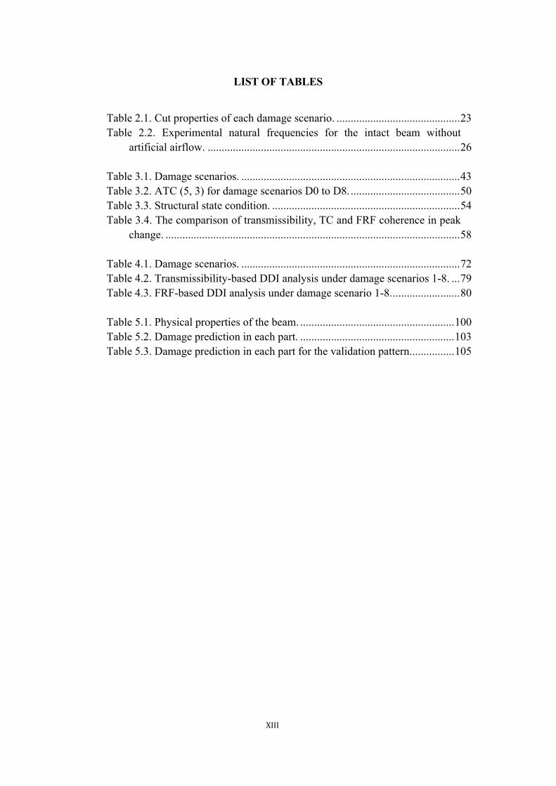
LIST OF TABLES
Table 2.1. Cut properties of each damage scenario. ............................................ 23 Table 2.2. Experimental natural frequencies for the intact beam without
artificial airflow. .......................................................................................... 26
Table 3.1. Damage scenarios. .............................................................................. 43 Table 3.2. ATC (5, 3) for damage scenarios D0 to D8. ....................................... 50 Table 3.3. Structural state condition. ................................................................... 54 Table 3.4. The comparison of transmissibility, TC and FRF coherence in peak
change. ......................................................................................................... 58 Table 4.1. Damage scenarios. .............................................................................. 72 Table 4.2. Transmissibility-based DDI analysis under damage scenarios 1-8. ... 79 Table 4.3. FRF-based DDI analysis under damage scenario 1-8. ........................ 80 Table 5.1. Physical properties of the beam. ....................................................... 100 Table 5.2. Damage prediction in each part. ....................................................... 103 Table 5.3. Damage prediction in each part for the validation pattern. ............... 105

XIV
XV
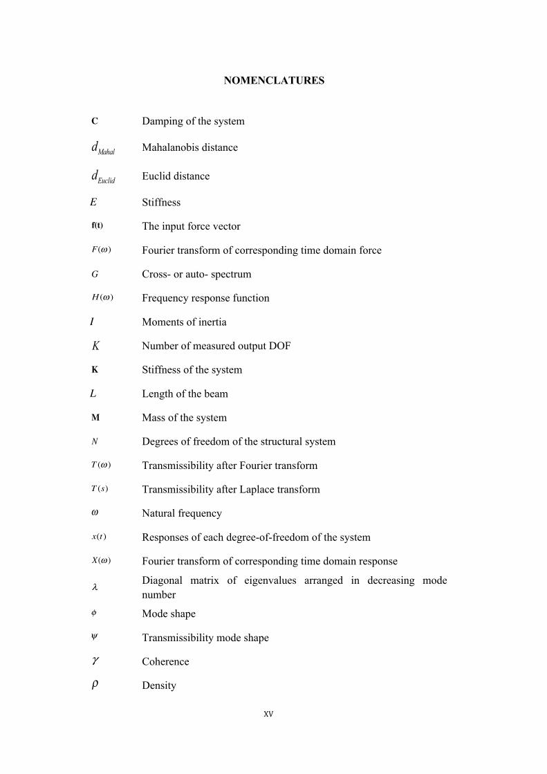
NOMENCLATURES
C Damping of the system
Mahald Mahalanobis distance
Euclidd Euclid distance
E Stiffness
f(t) The input force vector
F(ω ) Fourier transform of corresponding time domain force
G Cross- or auto- spectrum
H (ω ) Frequency response function
I Moments of inertia
K Number of measured output DOF
K Stiffness of the system
L Length of the beam
M Mass of the system
N Degrees of freedom of the structural system
T (ω ) Transmissibility after Fourier transform
T (s) Transmissibility after Laplace transform
ω Natural frequency
x(t) Responses of each degree-of-freedom of the system
X(ω ) Fourier transform of corresponding time domain response
λ Diagonal matrix of eigenvalues arranged in decreasing mode number
φ Mode shape
ψ Transmissibility mode shape
γ Coherence
ρ Density
XVI
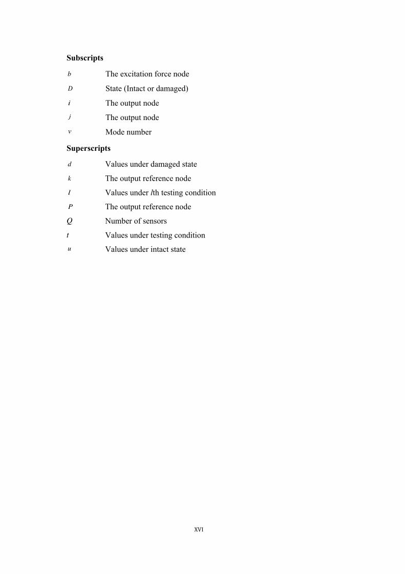
Subscripts
b The excitation force node
D State (Intact or damaged)
i The output node j The output node v Mode number
Superscripts
d Values under damaged state
k The output reference node
l Values under lth testing condition
P The output reference node
Q Number of sensors
t Values under testing condition u Values under intact state
XVII
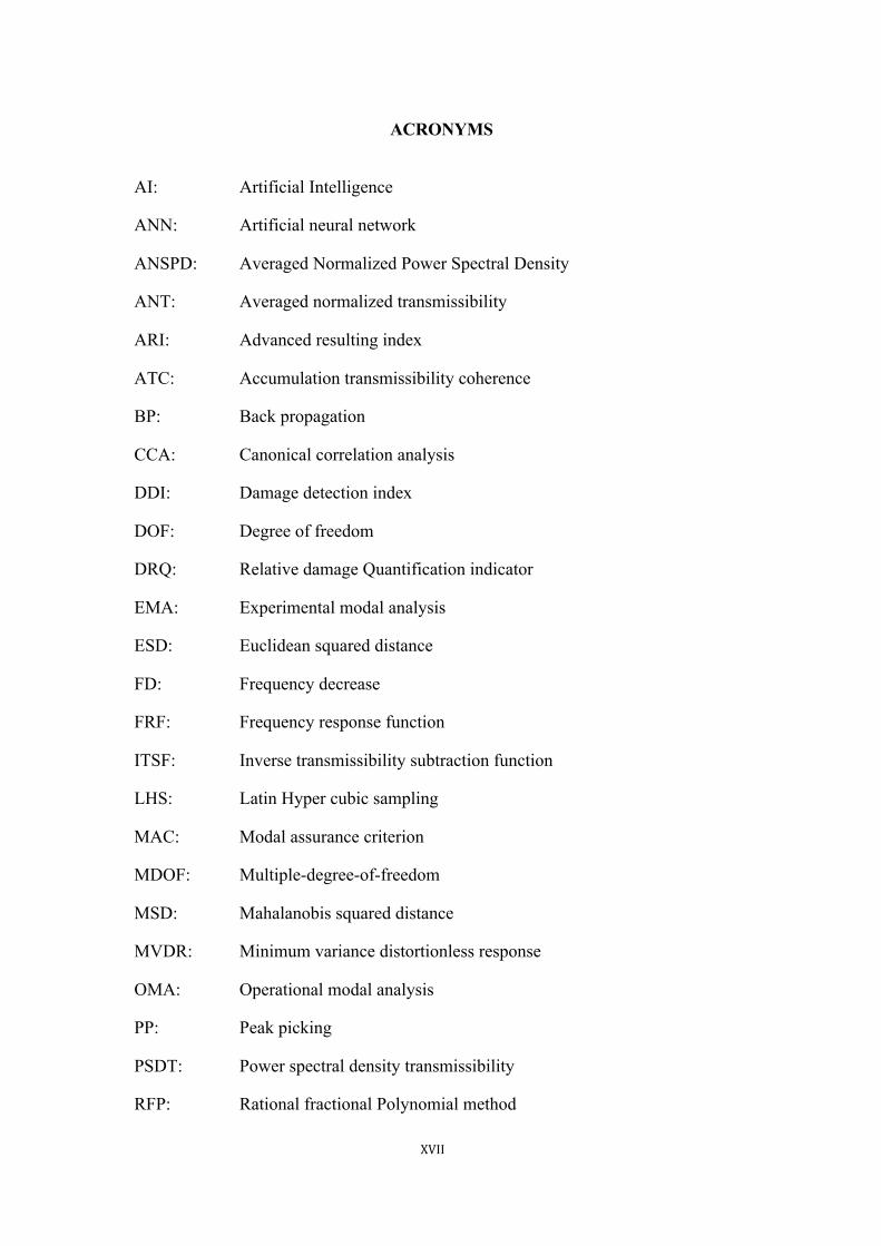
ACRONYMS
AI: Artificial Intelligence
ANN: Artificial neural network
ANSPD: Averaged Normalized Power Spectral Density
ANT: Averaged normalized transmissibility
ARI: Advanced resulting index
ATC: Accumulation transmissibility coherence
BP: Back propagation
CCA: Canonical correlation analysis
DDI: Damage detection index
DOF: Degree of freedom
DRQ: Relative damage Quantification indicator
EMA: Experimental modal analysis
ESD: Euclidean squared distance
FD: Frequency decrease
FRF: Frequency response function
ITSF: Inverse transmissibility subtraction function
LHS: Latin Hyper cubic sampling
MAC: Modal assurance criterion
MDOF: Multiple-degree-of-freedom
MSD: Mahalanobis squared distance
MVDR: Minimum variance distortionless response
OMA: Operational modal analysis
PP: Peak picking
PSDT: Power spectral density transmissibility
RFP: Rational fractional Polynomial method
XVIII
RVAC: Response Vector Assurance Criterion
SHM: Structural heath monitoring
SSI: Stochastic subspace identification
TAC: Transmissibility mode shape assurance criterion
TC: Transmissibility coherence
TMAC: Transmissibility modal assurance criterion
TMS: Transmissibility mode shape
TPMS: Transmissibility power mode shape
WOSA: Welch's overlapped segment averaging
1
CHAPTER 1 INTRODUCTION
1.1 Background
In the past decades, structural health monitoring (SHM), the process of implementing a
damage detection strategy for engineering infrastructure, has become a
multidisciplinary research focus to the scientific communities, due to the fact that the
engineering structures are commonly designed with more complexity and more
sophisticated newly invented material productions, and within daily use the structures
are usually and generally applied with higher operational loads, and are demanding for
longer lifecycle periods. Hence, numerous mechanical, civil and aerospace engineering
researchers extensively developed vast of approaches for analyzing the structural states,
which means to evaluate whether the structure is damaged or not, in order to prevent
the anticipated damage, which may cause a huge loss in human daily life. In the SHM
field, damage is normally defined as changes to the material and/or geometric
properties of a structural system, including changes to the boundary conditions and
system connectivity, which adversely affect the current or future performance of the
structure [1, 2].
To this objective, along with the development of the SHM methods history, visual
inspection approaches like penetrating liquids is the commonest and most traditional
and available technique, which will only be effective in those structures available for
using liquids. Then, static based and dynamic, or vibration-based methods are booming
especially after the advent of computer, with which signal processing can be analyzed.
Apart from this, in recent decades, taking advantage of the advancement of the science
and technology, local on-line non-destructive SHM becomes a main trend.
One direction to carry out in this line is to improve the measurement accuracy. Based
on this, numerous methods like vibration-based, strain-based, electrical
2
impedance-based, ultra-sonic or acoustic, lamb wave, eddy-current, X and gamma rays,
and laser measurement have been widely used in SHM.
On the other hand, various algorithms have been developed for analyzing the structural
states. Probability-based, statistical-based, machine learning, pattern recognition
methods and so on, have also been studied and a high quantity of papers, reports and
books have been published. A literature review about the SHM can be found in [1-2].
Along with the development of science and technology, to the earlier research in SHM,
among all the developed methodologies, modal testing and modal parameter
identification, due to its own advantages like easy conduction and better performance
in capturing the structural characteristics have been one core issue in dynamics-based
or so-called vibration-based SHM. And through measuring the input data of the
structural system or not, modal analysis can be divided into experimental modal
analysis (EMA) and operational modal analysis (OMA). The key difference is that the
EMA relies on the measurement of excitation and response, while the OMA only
depends on the structural dynamic responses. For modal testing, one possible book can
be referred to [3], where modal testing and related algorithms and directions are
discussed and summarized.
To EMA, normally the research object can be moved into the laboratory and modal
experiment is conducted in order to analyze the structural dynamical characteristics. And
from input and output measurement data, modal parameters can be obtained through the
frequency response function (FRF). Herein, a good deal of methods based on modal
analysis in damage detection, localization as well as quantification have been
implemented. Among these methods, mode shapes, modal damping and modal resonant
frequencies are the foundation or base. Various approaches like modal parameters and
their derivatives, for instance, the mode shape derivatives, for instance, first derivative
(rotations), second derivative (curvatures) and third and higher derivatives were utilized
for damage localization. FRF is another parameter commonly used in EMA. In order to
improve measurement accuracy, strain measurement gradually takes the place of the
3
acceleration and displacement. Actually, the displacement can be calculated from the
strain measurement along the span of the object.
However, damage identification under real operating conditions of the structure during its
daily use would be suitable and attractive to civil engineers due to the difficulty and
problems of carrying out controlled forced excitation tests on this kind of structures. In
this case, output-only response measurements would be available, and an output-only
damage identification procedure should be implemented. In this case, OMA has been
raised and studied. A lot of work has been done, and several methodologies have been
developed, like output reference based method.
1.2 Schemes of SHM
In SHM, damage identification is the key issue. And for damage identification, the
damage state of a system can be described as a five-step process along the lines of the
process discussed in Rytter (1993) [4]. The damage state is described by answering the
following questions [1]:
1) Is there damage in the system (existence)?
2) Where is the damage in the system (location)?
3) What kind of damage is present (type)?
4) How severe is the damage (extent)?
5) How much useful life remains (prognosis)?
In [1], SHM problem is described as one of statistical pattern recognition paradigm,
which consists of a four-part process:
1) Operational Evaluation;
2) Data Acquisition, Fusion, and Cleansing;
3) Feature Extraction and Information Condensation;
4) Statistical Mode Development for Feature Discrimination.
4
1.3 Literature review of transmissibility
Output-only SHM approaches were raised in order to avoid the excitation measurement,
as it is normally very difficult or even impossible to measure it in real engineering.
Motivated on avoiding the excitation measurement in real engineering, transmissibility
conception has been raised decades ago, but especially from the end of twenties century,
booming research on transmissibility has been intensively developed.
Different kinds of transmissibilities have been defined and developed, such as complex
transmissibility [5-6], transmittance [10], motion transmissibility [7], power
transmissibility [21], direct transmissibility, power density spectrum transmissibility [65]
and so on. For transmissibility estimation, in [77], the use of Hs estimator for
experimental assessment of transmissibility matrices is studied.
For the application of transmissibility, research can be divided into several directions:
vibration modal analysis, SHM damage identification, and others including some
multidisciplinary research.
For vibration modal analysis, the main work would be theory development from one
degree of freedom to multiple degrees of freedom, from simple structures to complex
structures, from force transmissibility to direct transmissibility. In this direction,
transmissibility has been analyzed with single point and multi-point acceleration
transmissibility [12], and foundation vibration analysis [22-23], and seat comfort, and
body vibration analysis [33, 36, 37, 43, 48, 55, 58]. For instance, in [5], complex
transmissibility is raised as an estimator with claiming the advantage that the dual signals
can be used in a statistical noise reduction process. In [9], transmissibility function is
defined as the ratio of FRFs, and the theory is firstly drawn out with a two connected
systems where the transmissibility function can be analytically expressed as a function of
only one system’s parameters. But this particular feature is based on the condition that the
two response points must be separated from the excitation point. In [12], motion
transmissibility concepts and related application to test environments are discussed; and
5
Q-Transmissibility approach is developed to analyze the dynamic performance of test
item.
Classical output-only techniques often require the operational forces to be white noise.
Herein, to transmissibility-based approaches, recent studies have suggested that the
unknown operational forces can be arbitrary as long as they are persistently exciting in
the frequency band of interest [35, 40-41]. And later intensive research on operational
modal analysis using transmissibility has been done [35, 40-41, 44, 46, 47, 50, 53, 69,
70, 78, 82].
Model updating is another aspect; and some studies use the anti-resonant frequencies,
or parameters identified from transmissibility [68]. Later, in [65], power spectrum
density transmissibility (PSDT) is firstly raised and analyzed for operational modal
analysis with comparing with peak picking (PP) algorithm and stochastic subspace
identification (SSI).
Another main direction is structural health monitoring with transmissibility [24-32, 34, 38,
39, 42, 45, 49, 51, 54, 56, 57, 66, 71, 74, 79, 80, 81, 88-90], in this direction, for damage
identification, transmissibility has been used directly [10, 13, 14], or incorporated with
other approaches like outlier analysis [15], neural networks [8], novelty measure [11, 25],
discriminant analysis. For instance, in [7], force transmissibility, motion transmissibility,
and energy transmissibility are discussed with a longitudinal bar model that includes both
stinger elastic and inertia properties. And two structures consisting of a rigid mass and a
double cantilever beam are analyzed to discuss the stinger’s axial transmissibilities. In
addition, the stinger influence in transmissibility is also drawn out. In [8], transmissibility
function is illustrated as potential features for damage detection. Continuously, in [11], a
novelty measure based on transmissibility is developed and is used for detecting structural
fault with using neural networks. On the other hand, transmittance is also developed for
detecting damage. In [10], transmittance function is constructed, while it shares the same
idea of transmissibility, and later it is developed for accurate health monitoring for large
structures. Later, in [13], transmittance is used for composite structures health monitoring
with piezoceramic patches. In [14], changes in transmittance function, curvature and
6
translation transmittance functions are used to detect, localize and assess the damage in a
simulated and experimented cantilever beam.
Apart from those issues discussed before, signal like response reconstruction is also
studied [52]; force reconstruction from force transmissibility is studied in [76]. Force
identification using the concept of displacement transmissibility is studied in [67].
Uncertainty quantification in the estimation of noisy contaminated measurements of
transmissibility is discussed in [60]. A sensitivity based damage identification method
using transmissibility is studied in [73].
In nonlinear part, study on the force and displacement transmissibility of a nonlinear
isolator is studied in [61]. And nonlinear identification of dynamic characteristics in
anti-vibration mounts using transmissibility is studied in [62]. In [64], a report for
nonlinear system identification for damage detection is delivered. Study about force
transmissibility estimated by nonlinear FRF is also done in [54].
Even studies on transmissibility have been processed decades, few reviews on
transmissibility can be found. In [59, 63], history of transmissibility is drawn out from its
inspiration to the development. In [71], a general review of transmissibility in SHM
especially damage identification is given. In [72], a correlation study of satellite finite
element model for coupled load analysis using transmissibility with modified correlation
measures is delivered. In [75], a comparison between force transmissibility and
displacement transmissibility is studied.
1.4 Motivations and objectives
In the past years, although many transmissibility-based SHM methods for damage
identification have been developed, no systematic method has been raised. Accuracy in
detecting, localizing and quantifying structural damages is still an open question
especially considering that the environmental variability affects to the measured
structural responses, especially in the earliest stages of damage identification.
7
On the other hand, even although a lot of studies have been done about the use of the
transmissibility for system identification procedures, few reviews can be found. This
thesis intends to pave the way of SHM using transmissibility, especially for damage
identification.
1.5 Thesis dissertation
This thesis includes, besides the introduction chapter, five chapters; an outline of their
contents is shown here.
Firstly, a transmissibility analysis, from its definition to its application based on OMA,
is addressed in Chapter 2. One transmissibility based damage detection procedure is
developed by using the structural dynamic characteristics estimated from
transmissibility. The procedure is validated on a beam numerically and experimentally
analyzed.
Chapter 3 discusses about the use of the transmissibility coherence as a parameters for
detecting and quantifying structural damage severities. Experimental results obtained
from a three-floor laboratory structure are used to validate the proposed methodology.
Chapter 4 intends to introduce linear discriminant analysis, especially squared
Mahalanobis distance, into transmissibility based structural damage severity detection
and quantification. A free-free steel beam is tested in laboratory and its results are used
to check the applicability of the developed approach.
Chapter 5 introduces artificial neural networks into transmissibility based damage
localization and quantification. The key issue is to construct the strong relation
between transmissibility and structural damage severities, i.e. input and output of
neural networks. And in this chapter, a clamped-clamped beam is simulated with Latin
Hyper cubic sampling (LHS) method for fifty different severities. Then, the structural
responses are analyzed with the developed approach for localizing and quantifying the
structural damage severity.

8
Finally, the main conclusions and achievements of the thesis are summarized in
Chapter 6. Additionally, a discussion of possible future research is also included in this
chapter.
9
Figu
re 1
.1. R
elat
ions
bet
wee
n ea
ch c
hapt
er in
the
thes
is.
2
Tran
smis
sibi
lity
base
d SH
M
The
ory
deve
lopm
ent
Cha
pter
1: R
elat
ion
betw
een
each
cha
pter
His
tory
rev
iew
Enh
ance
d by
dis
crim
inan
t an
alys
is
Enh
ance
d by
art
ifici
al
inte
llige
nce
Cha
pter
2:
Fu
ndam
enta
ls
for
tran
smis
sibi
lity
estim
atio
n, a
nd b
asic
s for
dam
age
dete
ctio
n.
Cha
pter
3: T
rans
mis
sibi
lity
cohe
renc
e is
dev
elop
ed,
and
it is
put
for
war
d to
dam
age
and
nonl
inea
rity
dete
ctio
n.
Cha
pter
1:
A r
elat
ivel
y de
taile
d hi
stor
y re
view
for
tra
nsm
issi
bilit
y in
SH
M.
Cha
pter
4:
Mah
alan
obis
dis
tanc
e is
em
ploy
ed a
nd
put f
orw
ard
to d
amag
e de
tect
ion.
Cha
pter
5:
Arti
ficia
l ne
ural
net
wor
ks a
re u
tiliz
ed
for d
etec
ting
dam
age.

10
11
CHAPTER 2 DAMAGE DETECTION BY TRANSMISSIBILITY
Summary
Damage identification under real operating conditions of the structure during its daily
use would be suitable and attractive to civil engineers due to the difficulty and problems
of carrying out controlled forced excitation tests on this kind of structures. In this case,
output-only response measurements would be available, and an output-only damage
identification procedure should be implemented. Transmissibility, since its advent
decades ago, has been extensively developed in a lot of directions like OMA, SHM, and
etc. Transmissibility, defined on an output-to-output relationship, is getting increased
attention in damage detection applications because of its dependence with output-only
data and its sensitivity to local structural changes. This chapter intends to give a clear
fundamental discussion of transmissibility in detecting damage. Firstly, transmissibility
definition and estimation methods are addressed; and later the transmissibility theory is
developed with proposing new damage sensitive indicators. Finally, the proposed
damage detection methodology is validated on an experimentally tested steel beam.
2.1 Introduction
Periodic inspection and maintenance of structures are essentials for the purpose of
ensuring their healthy operational condition. Many methods have been proposed in the
last years for the detection and location of damage in structural systems [83, 84]. These
methods include time and frequency domain techniques and empirical and model-based
approaches. The key point for most of the available techniques is the comparison
between features obtained from experimental response measurements and features
evaluated under normal working conditions.
12
Modal testing and modal parameter identification have been one core issue in
dynamics-based structural health monitoring. From input and output measurement data,
modal parameters can be obtained through the FRF. However, damage identification
under real engineering, i.e. operational condition, imposes difficulty in analyzing the
structure as it will be challenging to get the excitation on this kind of structures. In this
case, output-only response measurements would be available, and an output-only
damage identification procedure should be implemented.
Classical output-only techniques often require the operational forces to be white noise.
This is not necessary for the proposed transmissibility-based approach [39, 40, 50]. The
unknown operational forces can be arbitrary as long as they are persistently exciting in
the frequency band of interest. The transmissibility function, defined as the
frequency-domain ratio between two outputs, describes the relative admittance between
the two measurements and makes possible the damage detection without any assumption
about the nature of the excitations although different loading conditions have to be
obtained during the experiments. The scalar transmissibility is deterministic in case of
one single operational force. However, when several (uncorrelated) operational forces
are exciting the structure, the scalar transmissibility is in general not deterministic
anymore and the concept of multivariable transmissibility [46] is introduced increasing
the complexity of the problem.
In practice, a transmissibility measurement can be estimated in several ways although
the most common choice is using an estimator involving cross-and auto-power spectral
density functions of the output responses. Furthermore, any measurable output, such as
strain, displacement, acceleration, might be used to evaluate the spectral density
functions.
In this chapter, transmissibility has been put forward for detecting damage. Due to its
own characteristic depending on output only, it might be used in large civil engineering
structures.
13
2.2 Transmissibility
2.2.1 Transmissibility estimation
If we consider the linear multiple-degree-of-freedom (MDOF) system shown in
Figure 2.1, the dynamic equilibrium equation can be written by the following
well-known second order differential equation
M!!x(t) + C!x(t) + Kx(t) = f(t) (2.1)
where M, C and K are the mass, damping, and stiffness matrices of the system,
respectively, f(t) is the input force vector and x(t) contains the responses of each
degree-of-freedom (DOF) of the system. Fourier transform or Laplace transform can
be used to solve the differential equation above in order to calculate the displacement
and velocity as well as the acceleration.
Figure 2.1. A linear multiple-degree-of-freedom system.
Transmissibility measurement is an output-only technique, very suitable therefore for
operational dynamic analysis. Transmissibility functions are defined by taking the
ratio of one-response spectra and a reference response in an input degree of freedom.
When several operational forces are exciting the structure, the calculation of the
transmissibility becomes much more complex.
14
Herein, for a harmonic applied force at a given coordinate, the transmissibility
between point i and a reference point j can be defined as
T( i, j ) (ω ) =
Xi(ω )X j (ω )
(2.2)
where Xi and Xj are the complex amplitudes of the system responses, xi(t) and xj(t),
respectively, and ω is the frequency.
In order to calculate the transmissibility, no matter in real engineering or experiment
analysis, apart from its direct extracting from the two responses, it can be derived in
several ways:
Transmissibility estimation method I
By using FRFs,
( , )( , )
( , )
( )( ) ( ) / ( )( )( ) ( ) / ( ) ( )
i bi i bi j
j j b j b
HX X FTX X F H
ωω ω ωωω ω ω ω
= = =
(2.3)
where b is the single excitation node or one among the uncorrelated excitation nodes,
and H represents the FRF [8, 50].
Transmissibility estimation method II
Another way is to use auto-spectrum, or auto- and cross- spectrum.
( , )( , )
( , )
( )( ) ( ) ( )( )( ) ( ) ( ) ( )
i ii i ii j
j j j j j
GX X XTX X X G
ωω ω ωωω ω ω ω
×= = =×
(2.4)
or
T( i, j ) (ω ) =
Xi(ω )X j (ω )
=Xi(ω )× Xi(ω )X j (ω )× Xi(ω )
=G( i, i) (ω )G( j , i) (ω )
(2.5)
( , )( , )
( , )
( ) ( ) ( )( )( )( ) ( ) ( ) ( )
i j i jii j
j j j j j
X X GXTX X X G
ω ω ωωωω ω ω ω
×= = =
× (2.6)
15
where G means the auto- or cross- spectrum. Herein, Equation (2.5) and (2.6) can be
compared with the FRF estimation for avoiding noise influence, then transmissibility
coherence can be drawn out. Detailed analysis about it will be given in Chapter 3.
Transmissibility estimation method III
Recalling the second way for transmissibility estimation, Equations (2.5) and (2.6)
estimate the transmissibility taking as a reference node i or j. However, for the
comparison of more transmissibilities, it is usual to choose another output reference
node, for instance P, in transmissibility estimation. Then, each transmissibility can be
derived and denoted as
T( i, j )
P (ω ) =Xi(ω )X j (ω )
=Xi(ω )× X P(ω )X j (ω )× X P(ω )
=G( i,P) (ω )G( j ,P) (ω )
(2.7)
where T( i, j )
P (ω ) is also called PSDT [65].
Comparing Equation (2.7) with Equations (2.5) and (2.6), it is obvious that the only
difference between methods II and III is whether the third reference point belongs or
not to the two known nodes.
Besides, when the variable approaches system’s νth pole, denoted by λv, the following
equation is verified with Laplace transform [65] and Fourier transform [35, 40, 41] as
limT( i, j )
P
s→λv
=φ( i,v )
φ( j ,v )
(2.8)
where φ means mode shape. Therefore, if two different reference points, P1 and P2,
are chosen, by Laplace transform [65] or Fourier transform [35, 40, 41] the
subtraction of the two transmissibilities satisfies
lim(T( i, j )
P1 −T( i, j )P2 )
s→λv
=φ( i,v )
φ( j ,v )
−φ( i,v )
φ( j ,v )
= 0 (2.9)
16
This means that the system’s poles are zeros of the rational function
ΔT( i, j )
P1P2 = T( i, j )P1 −T( i, j )
P2 (2.10)
And its inverse [40, 41, 65], also called inverse transmissibility subtraction function
(ITSF) [65] is as
Δ−1T( i, j )P1P2 = 1
ΔT( i, j )P1P2
= 1T( i, j )
P1 −T( i, j )P2
= 1G( i,P1)
G( j ,P1)
−G( i,P2 )
G( j ,P2 )
=G( j ,P1)G( j ,P2 )
G( i,P1)G( j ,P2 ) −G( i,P2 )G( j ,P1)
(2.11)
Herein, through the equation above one can identify the natural frequencies via PP
method.
Note that the denominator of the equation above is result of a subtraction, which
might cause singularity if the reference is not well chosen or the transform is not well
chosen and made. Meanwhile, it can yield more roots than the system real roots,
which requires further work in validating the corresponding frequencies. Thirdly, all
the references like j and P (P1, P2, …) should be paid more attention, otherwise it
would be possible to miss some system roots. One possible solution is to use average
normalization ITSF [65], or to take all the ITSFs into consideration directly.
2.2.2 Transmissibility mode shape
Considering the linear MDOF system discussed above, the total transmissibility matrix
of the structural system corresponding to each test of all damaged and intact states can
be expressed as
17
T P(ω )D =
T(1, 1)P (ω ) T(1, 2)
P (ω ) ! T(1, N−1)P (ω )
T(2, 1)P (ω ) T(2, 2)
P (ω ) ! T(2, N−1)P (ω )
" " T( i, j )P (ω ) "
T( N−1, 1)P (ω )
T( N , 1)P (ω )
!!
!!
T( N−1, N−1)P (ω )
T( N , N−1)P (ω )
T(1, N )P (ω )
T(2, N )P (ω )
"T( N−1, N )
P (ω )
T( N , N )P (ω )
⎡
⎣
⎢⎢⎢⎢⎢⎢⎢⎢
⎤
⎦
⎥⎥⎥⎥⎥⎥⎥⎥
(2.12)
where N is the number of degrees of freedom of the structural system, and TP(ω)D is the
transmissibility matrix of the structural system referred to the state D (intact/damaged
structure).
As shown in the previous section, the transmissibility at the system poles is coincident
with values of the mode shape ratios, i.e. the values of the Τ(i,j)(ω) at the system poles are
directly related to the scalar operational mode-shape values, φ(i,v) and φ(j,v). Therefore,
once the resonant frequencies are identified by using averaged normalized ITSF or other
algorithms like Polymax, it would be possible to identify the relative mode shape vectors
from different transmissibilities.
In order to include all the natural modes in one transmissibility, in regarding to the
definition of Averaged Normalized Power Spectral Density (ANSPD) [1], by using
min-max normalization method, average normalized transmissibility might be
constructed by averaging the normalized transmissibilities in accordance to different
reference nodes (Pmin, Pmin+1, …, Pmax), which can be expressed as ANT
max
min
( , ) ( , )max min
1( ) ( ( ))1
PP
i j i jP
ANT NTP P
ω ω=− + ∑ (2.13)
Herein, by choosing a fixed reference node j and giving φ(j,v) a unit normalized value,
then the transmissibility vector (ANΤ(1, j)(ω), ANΤ(2, j)(ω), …,1,…, ANΤ(N, j)(ω)) can be
used for estimating the full-unscaled mode-shape (operational deflection) vector (φ(1,v),
φ(2,v), …,1,…, φ(K,v)) (K is the number of measured output DOFs). Herein, in Equation
(2.12), each column represents one transmissibility vector corresponding to an unscaled
mode-shape.
18
Then, by analogy with the concept of power mode shape presented in [85] and
transmissibility power mode shape in [86], and divided by the integration band for
averaging the estimation, a new concept of transmissibility mode shape (TMS) might be
defined from the transmissibility in the following way
( , )1 ( )H
L
vi i j
H L
TMS ANT dω
ωω ω
ω ω=
− ∫ (2.14)
where TMSiv is the ith component of the vth TMS and [ωL, ωH] is the frequency
integration band for the vth TMS. Herein, after setting the reference node j, if the width
of integration band is only one, then TMS will be exactly the estimation of relative mode
shape; if the width is slightly bigger, then TMS will be the averaged relative mode shape.
This is due to the fact that the different ITSFs will not yield in the exactly same roots,
small difference may occur in the roots identification, and then this slight average tries to
reduce the error in estimation.
Note that herein to estimate the TMSs by averaging one small area around the resonant
frequencies is due to the reason that in real engineering, the resonant frequencies
measurement and estimation might have some small errors. And by averaging the small
area around resonant frequencies might give a better resource of the TMS.
The main contribution of TMS here is that TMS might be used in OMA with the same
function of MS in EMA. This suggests a possible way of extending the MS based
methods into TMSs based OMA. On the other hand, by combining the TC developed
in Chapter 3, one might use TC, TMS in OMA as MS, FRF coherence in EMA.
Later, by assembling TMSiv for all the measured points considered in the structure, a
vth TMS vector is generated
TMS v{ } = (TMS1
v ,TMS2v ,...,1,...,TMSN
v ) (2.15)
The same procedure should be repeated for each TMS by choosing the appropriate
bandwidth affecting each system’s pole v. In this way, any of the damage criteria based
on mode shapes might be extended to include the TMSs.
19
2.3 Damage detection procedure
2.3.1 Damage sensitive indicators
Natural frequency estimation
From the discussion above, the peaks of ITSFs correspond to the natural frequencies,
i.e. ITSF parameter might be used to identify the natural frequencies. On the other
hand, PP method can also be used to derive the structural natural frequencies from
FRFs for comparison. An additional difficulty is about the identification of the natural
frequencies of interest; RFP method can resolve this with outputting the stabilization
diagram. In this way, the natural frequencies extracted by PP and RFP might serve as
comparison to those extracted with transmissibility.
As it is known that frequency will shift when damage occurs, one estimator for
quantifying the frequency decrease (FD) can be defined as
FDv =
(ω vu / 2π )− (ω v
d / 2π )ω v
u / 2π×100% (2.16)
where ω vu means frequency under intact state, and ω v
d represents frequency under
damaged state.
TMS based indicator
In order to show the variability of TMS between two different stages, modal
assurance criterion (MAC) [87] can be used by defining an indicator TAC
(transmissibility mode shape assurance criterion) as follows
TACv =(TMSv )d( )T
(TMSv )u( )2
(TMSv )d( )T(TMSv )d( )( ) (TMSv )u( )T
(TMSv )u( )( ) (2.17)
Herein, the TMS can be used in complete or in part under the condition before and
after deterioration, as it is common that modes might be hidden or terribly influenced
20
by environmental varieties or operational conditions in complete or in part.
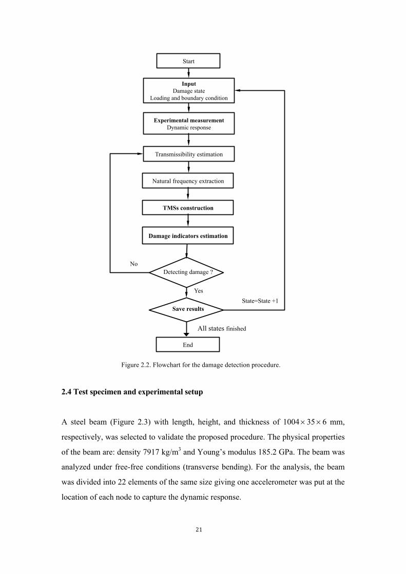
2.3.2 Damage detection scheme
Damage detection scheme will be conducted as follows:
Step 1: Natural frequencies estimation. As to the intact and damaged structural state,
PP method and RFP (Rational Fractional Polynomial) method and
transmissibility-based method are used to extract the natural frequencies.
Step 2: TMS construction. Once resonant frequencies have been identified, ANT will
be derived with Equation (2.13), and then TMSs will be computed via Equations
(2.14) and (2.15).
Step 3: Damage indicators estimation. For the different states to be compared, FD
and TAC indicators will be computed. In regard to the statistical pattern recognition
process for structural health monitoring [1], the extracted features, i.e. the indicators,
will be compared with checking their own performance in damage recognition.
Step 4: Detecting the damage. Once FD and TAC indicators have been computed,
basing on engineering experience or thresholds previously set, one can predict the
occurrence of the damage in the structural system.
A detailed flowchart for this damage detection procedure can be referred to Figure
2.2.
21
Figure 2.2. Flowchart for the damage detection procedure.
2.4 Test specimen and experimental setup
A steel beam (Figure 2.3) with length, height, and thickness of 1004 × 35 × 6 mm,
respectively, was selected to validate the proposed procedure. The physical properties
of the beam are: density 7917 kg/m3 and Young’s modulus 185.2 GPa. The beam was
analyzed under free-free conditions (transverse bending). For the analysis, the beam
was divided into 22 elements of the same size giving one accelerometer was put at the
location of each node to capture the dynamic response.
3
Transmissibility estimation
Experimental measurement Dynamic response
Natural frequency extraction
Detecting damage ?
Yes State=State +1
End
Damage indicators estimation
No
Save results
All states finished
Input Damage state
Loading and boundary condition
TMSs construction
Start Chapter 2: Flowchart of damage detection
22
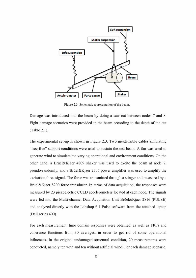
Figure 2.3. Schematic representation of the beam.
Damage was introduced into the beam by doing a saw cut between nodes 7 and 8.
Eight damage scenarios were provided in the beam according to the depth of the cut
(Table 2.1).
The experimental set-up is shown in Figure 2.3. Two inextensible cables simulating
“free-free” support conditions were used to sustain the test beam. A fan was used to
generate wind to simulate the varying operational and environment conditions. On the
other hand, a Brüel&Kjaer 4809 shaker was used to excite the beam at node 7,
pseudo-randomly, and a Brüel&Kjaer 2706 power amplifier was used to amplify the
excitation force signal. The force was transmitted through a stinger and measured by a
Brüel&Kjaer 8200 force transducer. In terms of data acquisition, the responses were
measured by 23 piezoelectric CCLD accelerometers located at each node. The signals
were fed into the Multi-channel Data Acquisition Unit Brüel&Kjaer 2816 (PULSE)
and analyzed directly with the Labshop 6.1 Pulse software from the attached laptop
(Dell series 400).
For each measurement, time domain responses were obtained, as well as FRFs and
coherence functions from 30 averages, in order to get rid of some operational
influences. In the original undamaged structural condition, 20 measurements were
conducted, namely ten with and ten without artificial wind. For each damage scenario,
23
five measurements were obtained with and without artificial wind. Finally, the
frequency analysis of the beam was carried out in a frequency range of 0-800 Hz
(3200 lines) with Hanning windows applied upon force time series as well as response
acceleration time series.
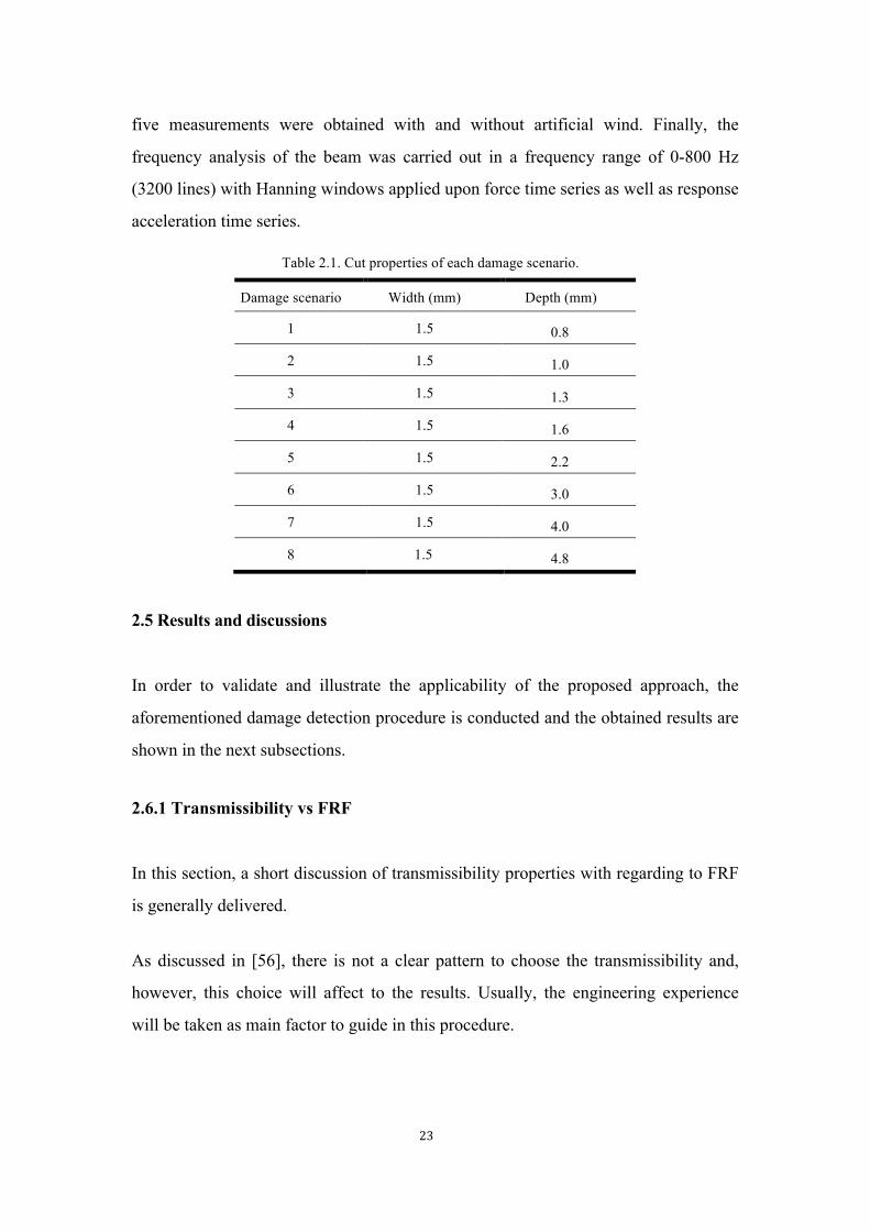
Table 2.1. Cut properties of each damage scenario.
Damage scenario Width (mm) Depth (mm)
1 1.5 0.8
2 1.5 1.0
3 1.5 1.3
4 1.5 1.6
5 1.5 2.2
6 1.5 3.0
7 1.5 4.0
8 1.5 4.8
2.5 Results and discussions
In order to validate and illustrate the applicability of the proposed approach, the
aforementioned damage detection procedure is conducted and the obtained results are
shown in the next subsections.
2.6.1 Transmissibility vs FRF
In this section, a short discussion of transmissibility properties with regarding to FRF
is generally delivered.
As discussed in [56], there is not a clear pattern to choose the transmissibility and,
however, this choice will affect to the results. Usually, the engineering experience
will be taken as main factor to guide in this procedure.
24
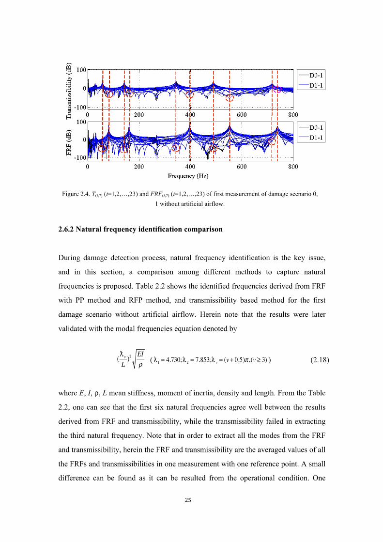
For analyzing the experimental data, Figure 2.4 shows T(i,7) (i=1,2,…,23) with
reference node three and FRF(i,7) (i=1,2,…,23) for the first damage scenario (D1) and
the intact beam (D0) when no artificial wind is applied.
From the figure one can find that: (i). For the slightest damage scenario 1, little or
even no change can be found in the transmissibility T(i,7) (i=1,2,…,23) with reference
node three and FRF(i,7) (i=1,2,…,23) with respect to the intact case. This suggests that
a further study should be made for extracting the most sensitive feature for damage
detection; (ii). The peaks of transmissibilities coincide with anti-resonances of some
FRFs, however, the peaks of FRFs, which agree with the resonant frequencies, do not
always coincide with the low peaks of some transmissibilities, for instance, no peak in
all the transmissibilities can be found to coincide with the last peak of FRFs; note that
the coincidence herein does not mean the correspondence between T(i, j) and FRF(i, j), it
means generally if we plot all the transmissibilities and FRFs of one dynamic system,
we can find anti-peaks in FRFs to coincide with the peaks in transmissibilities,
however, we might fail in finding anti-peaks in transmissibilities for coinciding with
the peaks of FRFs; (iii). The values of transmissibilities locate in a narrower band
than FRFs, i.e. the standard deviations of transmissibilities are smaller than those of
FRFs, which can be explained by the Equation (2.3), all the transmissibilities have
been condensed by one FRF; (iv). Not all the peaks of the FRFs correspond to natural
frequencies, i.e. fake, or pseudo peaks might appear in the FRFs. The same occurs for
the transmissibilities.
25
Figure 2.4. T(i,7) (i=1,2,…,23) and FRF(i,7) (i=1,2,…,23) of first measurement of damage scenario 0, 1 without artificial airflow.
2.6.2 Natural frequency identification comparison
During damage detection process, natural frequency identification is the key issue,
and in this section, a comparison among different methods to capture natural
frequencies is proposed. Table 2.2 shows the identified frequencies derived from FRF
with PP method and RFP method, and transmissibility based method for the first
damage scenario without artificial airflow. Herein note that the results were later
validated with the modal frequencies equation denoted by
(! vL)2 EI
ρ ( !1 = 4.730;! 2 = 7.853;! v = (v + 0.5)π ,(v ≥ 3) ) (2.18)
where E, I, ρ, L mean stiffness, moment of inertia, density and length. From the Table
2.2, one can see that the first six natural frequencies agree well between the results
derived from FRF and transmissibility, while the transmissibility failed in extracting
the third natural frequency. Note that in order to extract all the modes from the FRF
and transmissibility, herein the FRF and transmissibility are the averaged values of all
the FRFs and transmissibilities in one measurement with one reference point. A small
difference can be found as it can be resulted from the operational condition. One
26
small issue that to a given beam, the ratio between two nearly spaced frequencies can
be validated with the ratio between the corresponding !2 , this has also been used in
this study. And it performs well in unveiling some fake peaks.
Table 2.2. Experimental natural frequencies for the intact beam without artificial airflow.
Mode order
( v )
Frequency (Hz) identification
FRF* Transmissibility*
PP RFP Δ−1T(i, j )p1p2
1 31.750 31.250 31.000
2 82.250 82.250 83.000
3 161.500 161.250 -
4 267.500 266.250 267.000
5 397.000 397.000 398.500
6 552.250 552.000 553.250
*The averaged value for one measurement.
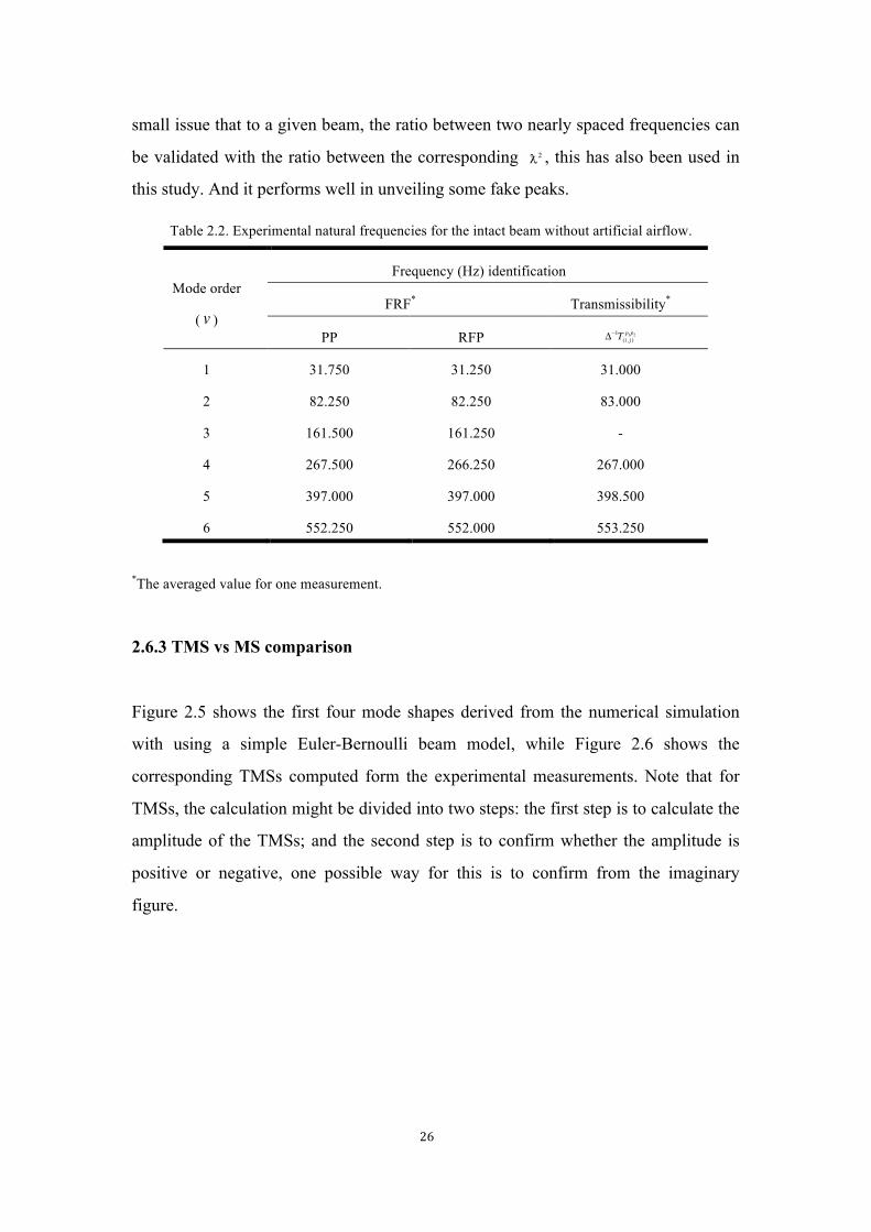
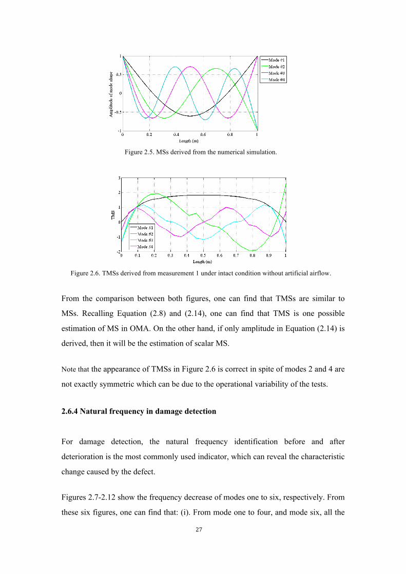
2.6.3 TMS vs MS comparison
Figure 2.5 shows the first four mode shapes derived from the numerical simulation
with using a simple Euler-Bernoulli beam model, while Figure 2.6 shows the
corresponding TMSs computed form the experimental measurements. Note that for
TMSs, the calculation might be divided into two steps: the first step is to calculate the
amplitude of the TMSs; and the second step is to confirm whether the amplitude is
positive or negative, one possible way for this is to confirm from the imaginary
figure.
27
Figure 2.5. MSs derived from the numerical simulation.
Figure 2.6. TMSs derived from measurement 1 under intact condition without artificial airflow.
From the comparison between both figures, one can find that TMSs are similar to
MSs. Recalling Equation (2.8) and (2.14), one can find that TMS is one possible
estimation of MS in OMA. On the other hand, if only amplitude in Equation (2.14) is
derived, then it will be the estimation of scalar MS.
Note that the appearance of TMSs in Figure 2.6 is correct in spite of modes 2 and 4 are
not exactly symmetric which can be due to the operational variability of the tests.
2.6.4 Natural frequency in damage detection
For damage detection, the natural frequency identification before and after
deterioration is the most commonly used indicator, which can reveal the characteristic
change caused by the defect.
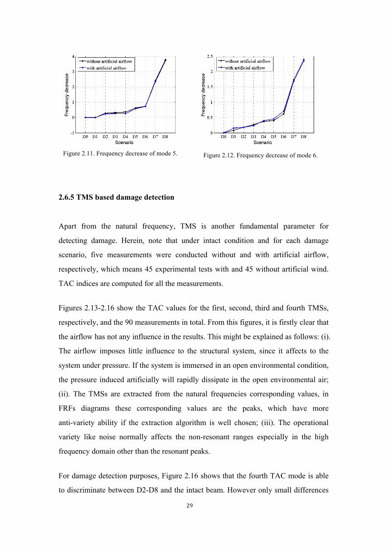
Figures 2.7-2.12 show the frequency decrease of modes one to six, respectively. From
these six figures, one can find that: (i). From mode one to four, and mode six, all the
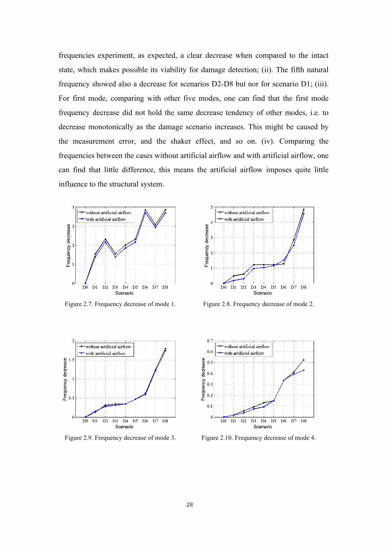
28
frequencies experiment, as expected, a clear decrease when compared to the intact
state, which makes possible its viability for damage detection; (ii). The fifth natural
frequency showed also a decrease for scenarios D2-D8 but nor for scenario D1; (iii).
For first mode, comparing with other five modes, one can find that the first mode
frequency decrease did not hold the same decrease tendency of other modes, i.e. to
decrease monotonically as the damage scenario increases. This might be caused by
the measurement error, and the shaker effect, and so on. (iv). Comparing the
frequencies between the cases without artificial airflow and with artificial airflow, one
can find that little difference, this means the artificial airflow imposes quite little
influence to the structural system.
Figure 2.7. Frequency decrease of mode 1. Figure 2.8. Frequency decrease of mode 2.
Figure 2.9. Frequency decrease of mode 3. Figure 2.10. Frequency decrease of mode 4.
29
Figure 2.11. Frequency decrease of mode 5. Figure 2.12. Frequency decrease of mode 6.
2.6.5 TMS based damage detection
Apart from the natural frequency, TMS is another fundamental parameter for
detecting damage. Herein, note that under intact condition and for each damage
scenario, five measurements were conducted without and with artificial airflow,
respectively, which means 45 experimental tests with and 45 without artificial wind.
TAC indices are computed for all the measurements.
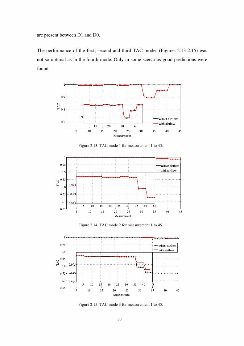
Figures 2.13-2.16 show the TAC values for the first, second, third and fourth TMSs,
respectively, and the 90 measurements in total. From this figures, it is firstly clear that
the airflow has not any influence in the results. This might be explained as follows: (i).
The airflow imposes little influence to the structural system, since it affects to the
system under pressure. If the system is immersed in an open environmental condition,
the pressure induced artificially will rapidly dissipate in the open environmental air;
(ii). The TMSs are extracted from the natural frequencies corresponding values, in
FRFs diagrams these corresponding values are the peaks, which have more
anti-variety ability if the extraction algorithm is well chosen; (iii). The operational
variety like noise normally affects the non-resonant ranges especially in the high
frequency domain other than the resonant peaks.
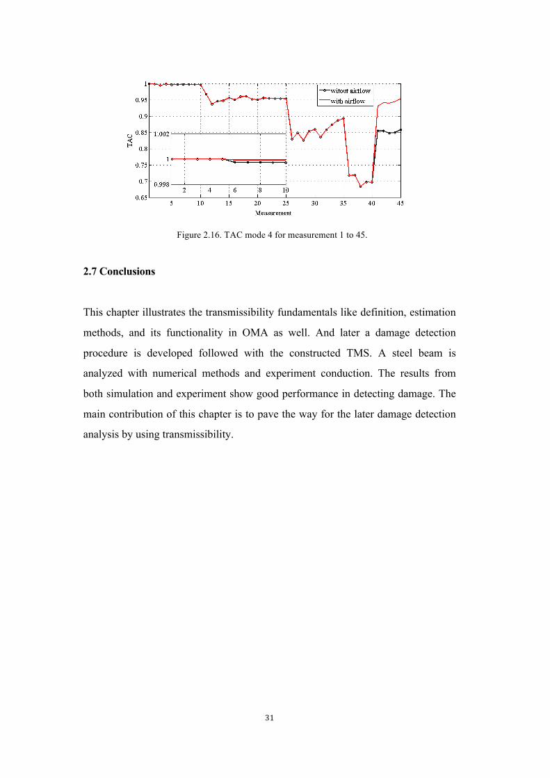
For damage detection purposes, Figure 2.16 shows that the fourth TAC mode is able
to discriminate between D2-D8 and the intact beam. However only small differences
30
are present between D1 and D0.
The performance of the first, second and third TAC modes (Figures 2.13-2.15) was
not so optimal as in the fourth mode. Only in some scenarios good predictions were
found.
Figure 2.13. TAC mode 1 for measurement 1 to 45.
Figure 2.14. TAC mode 2 for measurement 1 to 45.
Figure 2.15. TAC mode 3 for measurement 1 to 45.
31
Figure 2.16. TAC mode 4 for measurement 1 to 45.
2.7 Conclusions
This chapter illustrates the transmissibility fundamentals like definition, estimation
methods, and its functionality in OMA as well. And later a damage detection
procedure is developed followed with the constructed TMS. A steel beam is
analyzed with numerical methods and experiment conduction. The results from
both simulation and experiment show good performance in detecting damage. The
main contribution of this chapter is to pave the way for the later damage detection
analysis by using transmissibility.

32
33
CHAPTER 3 DAMAGE DETECTION AND QUANTIFICATION USING
TRANSMISSIBILITY COHERENCE ANALYSIS
Summary
In this chapter, a new transmissibility-based damage detection and quantification
approach is proposed. Based on the operational modal analysis, the transmissibility is
extracted from system responses and transmissibility coherence is defined and
analyzed. Afterwards, a sensitive-damage indicator is defined in order to detect and
quantify the severity of damage and compared with an indicator developed by other
authors. The proposed approach is validated on data from a physics-based numerical
model as well as experimental data from a three-story aluminum frame structure. For
both, numerical simulation and experiment the results, the new indicator reveals a
better performance than coherence measure proposed in [107-109] especially when
nonlinearity occurs, which might be further used in real engineering. The main
contribution of this chapter is the construction of the relation between transmissibility
coherence and frequency response function coherence, and the construction of an
effective indicators based on the transmissibility modal assurance criteria for damage
(especially for minor nonlinearity) detection as well as quantification.
3.1 Introduction
SHM has experienced a huge development from more than four decades ago since the
rehabilitation cost of oil pipes, bridges, tall buildings and so on rapidly increased. In
the last two decades, a lot of SHM methods have been developed based on both
physics- and data models. For instance, one systematic SHM solution for bridge
34
maintenance is presented in [91], where both kind of models are combined to identify
damage. Other SHM solutions can be found in [1, 92, 124, 125].
For large and complex structures the use of accelerometers has made possible the
development of vibration-based methods to analyze structures. Modal testing is the
most common; by carrying out the EMA of a structure, some modal parameters, such
as frequency, mass and damping, can be extracted and a FRF can be obtained. This
will make possible the construction of different damage indicators. Modal testing is
also conducted on structures in real operational conditions, within which the
excitation will be very difficult or even impossible to be measured; OMA uses the
response signals only to extract the structural dynamic parameters in order to assess
the structural states. In addition, for long-term operating structures, like oil pipes,
turbines or bridges, statistical methods are also developed for real-time online SHM
systems.
In real engineering, motivated on solving the difficulty in capturing the excitation, in
the middle of 1980s, transmissibility (or direct transmissibility) was raised. Instead of
considering the input and output signals of the structural system, transmissibility only
pays attention to the outputs, i.e. it concentrates on the interrelation of two outputs of
the structure, in order to create a connection with the structural dynamic characteristic.
Afterwards, a lot of researchers developed it for parameter identification [69], damage
detection as well as quantification [51], uncertainty analysis [60], and
response/excitation (i.e. force) reconstruction [76], and so on. In [69], relative mode
shape is extracted from the transmissibility in the natural resonant frequencies, which
avoids the use of FRF in mode shape estimation. In [51], a method of taking
advantage of Response Vector Assurance Criterion (RVAC) [92] was proposed,
replacing the FRF by transmissibility function in the indicator RVAC, and Detection
and Relative damage Quantification indicator (DRQ) [93], which is the average value
of RVAC along the frequency domain. The RVAC is a simplified form of FDAC,
which was defined by Heylen et al. [92]. The key idea is to use the sum of all
coordinates FRF before and after damage of all loading conditions in the form of
modal assurance criteria.
35
However, the detection of damage, at an early stage, is still a very difficult and
challenging task; therefore, it is very important the proposal of new indicators based
on dynamic responses that may be sensitive enough to minor damage. In this sense,
the coherence, as a function dependent on the frequency and able to analyze the
spatial correlation between two signals [94, 95] might be potentially a good starting
point to develop sensitive damage indicators.
The coherence function, formally defined by Wiener [96, 97], has been extensively
studied and used, especially after the development of the Fourier transform, in
different research fields, with extensions to the most modern wavelet coherence and
partial directed coherence: neurology, mostly in electroencephalography studies [98,
99, 100], like EEG microstates detection in insight and calm meditation [98].
Coherence is also used in skin blood oscillations analysis in human [101], nerve fiber
layer thickness quantification [102].
In another aspect, spatial coherence measure is also developed for signal enhancement
[103] by designing coherence-based post filters. In recent years, coherence function
has been used in mechanical engineering for damage identification, namely detection,
type and quantification [104-105, 107-109]. In [104], a coherence algorithm is
proposed for damage type recognition and damage localization for large flexible
structures with a nine-bay truss example; the key idea is to construct a connection
between coherence and transfer function, and the transfer function parameter change
is extracted for damage detection. In [105], local temporal coherence is developed and
extended to time-varying process with the basic coherence conception from the cross
correlation defined in [106], and the corresponding peak value is defined as peak
coherence, creating a connection with the temperature and introduced damage change,
i.e. the peak coherence for temperature/damage change is somewhat a function of
time. In addition, the peak performs well in distinguishing environmental change and
damage. In [107, 108], coherence is integrated in the frequency domain and set as an
indicator - coherence measure, as a sensitive enough indicator for quantifying the skin
damage and assessing restoration quality. In [109], coherence measure based method -
36
as a time series method, is developed for fault detection and identification in vibrating
structures.
In this chapter, coherence analysis of transmissibility is performed, and from it an
effective indicator for damage, especially nonlinearity, is proposed and compared
with the coherence measure raised in [107]. In order to test the feasibility of the
proposed approach, numerical simulation of a laboratory structure is carried out, and,
additionally, experimental measurements on a three-story aluminum structure are
used to check the applicability of the proposed indicator.
3.2 Transmissibility based coherence
As for vibration-based SHM, the core idea is to find a sensitive feature able to
discriminate a damaged structure when compared to the baseline structure (healthy
state); therefore the damage detection conclusion can be drawn out with choosing a
threshold of the change, before and after damage, considering the influence of
operational variability. As described in the introduction, lots of approaches, features
as well as measurement methodologies have been used in the past [2, 92, 110-111].
3.2.1 Applicability of coherence in damage detection
As commented in the introduction, coherence has been used in many applications. It
is useful to examine the correlation between two frequency signals, in a similar way
to the correlation coefficient in frequency. More details can be found in [112].
Coherence, as a complex measure, is estimated by dividing the square of the
cross-spectral density between two signals by the product of the auto-spectral
densities of both signals. Consequently, it will be sensitive to both changes in power
and phase relationships in one of the two signals [114].
The magnitude-squared coherence for the bivariate time series enables us to identify
significant frequency-domain correlation between the two time series [113]. For the
37
purpose of preventing obtaining an estimate of magnitude-squared coherence to be
identically 1 for all frequencies, an averaged magnitude-squared coherence estimator
has to be used. Both Welch's overlapped segment averaging (WOSA) and mulitaper
techniques are appropriate [113]. In this study, WOSA is utilized for the coherence
estimate. A detailed discussion of several seemingly disparate non-parametric
magnitude squared coherence estimation methods including Welch’s averaged
periodogram, the minimum variance distortionless response (MVDR), and the
canonical correlation analysis (CCA) can be found in [115].
For SHM purposes, the most important task is to find a structural feature sensitive to
the occurrence of damage. Methodologies involving coherence have been developed
in the past decades [104-105, 107-109, 116]. As proved in [107-109], a coherence
based damage indicator can be used in damage detection. The premise behind this is
that the coherence will decrease as nonlinearity increases.
3.2.2 Transmissibility
As discussed in Chapter 2, transmissibility can be estimated by FRFs,
T( i, j ) (ω ) =
Xi(ω ) / Fb(ω )X j (ω ) / Fb(ω )
=H( i,b) (ω )H( j ,b) (ω )
(3.1)
Note that herein the transmissibility is a norm that estimates the structural dynamic
responses.
3.2.3 Transmissibility coherence
Given the structural system described above with one single excitation, then the FRF
of point i to b can be calculated using two alternative expressions as follows
H1(ω ) =
G( i, b) (ω )G(b, b) (ω )
(3.2)
38
H2(ω ) =
G( i, i) (ω )G(b, i) (ω )
(3.3)
Correspondingly, the coherence function (or magnitude squared coherence function)
is indicated as [3, 117]:
γ 2 =
H1(ω )H2(ω )
=G( i, b) (ω )G(b, b) (ω )
G(b, i) (ω )G( i, i) (ω )
=G( i, b) (ω )G( i, i) (ω )
G( i, b)∗(ω )
G(b, b) (ω )=
G( i, b) (ω )2
G( i, i) (ω )G(b, b) (ω ) (3.4)
By analogy with Eq. (3.4), the transmissibility coherence (TC) can be defined from
Eq. (3.1) as follows
γ TC
2 =T1( i, j ) (ω )T2( i, j ) (ω )
=H1( i, b) (ω )H1( j , b) (ω )
/H2( i, b) (ω )H2( j , b) (ω )
=H1( i, b) (ω )H2( i, b) (ω )
H2( j , b) (ω )H1( j , b) (ω )
=γ ( i, l )
2
γ ( j , l )2
(3.5)
Herein, above all, transmissibility coherence means the magnitude squared coherence;
secondly, from the equation above, one can see that the TC can be calculated directly
from the coherence of corresponding FRFs, which gives a way for estimating the
transmissibility coherence in laboratory experiments analysis. Thirdly, note that
herein the TC, as an estimation indicator for transmissibility, i.e. coherence for two
outputs, is an indicator revealing the coherence/correlation between two outputs
considering the excitation point.
On the other hand, if direct transmissibility is directly estimated using two outputs, i.e.
not taking the FRFs into account, referring to the conception of coherence [96-97,
117], TC can be also derived solely by using the auto- and cross- spectrum of the two
responses signals.
T1( i, j ) =
Xi(ω )X j (ω )
X j (ω )X j (ω )
=G( i, j ) (ω )G( j , j ) (ω )
(3.6)
T2( i, j ) =
Xi(ω )X j (ω )
Xi(ω )Xi(ω )
=G( i, i) (ω )G( j , i) (ω )
(3.7)
39
From (3.6) and (3.7), TC will be expressed as
γ TC
2 =T1( i, j ) (ω )T2( i, j ) (ω )
=G( i, j ) (ω )G( j , j ) (ω )
/G( i, i) (ω )G( j , i) (ω )
=G( i, j ) (ω )G( j , i) (ω )G( j , j ) (ω )G( i, i) (ω )
=G( i, j ) (ω )
2
G( i, i) (ω )G( j , j ) (ω ) (3.8)
Fourier transform in (3.8) gives the frequency distribution of TC. For the TC
estimation, Welch method [118] and MVDR [119] method are commonly used.
As the coherence is a squared magnitude, TC is higher than zero. Comparing
Equations 3.5 and 3.8, one can observe that TC can be estimated in two ways: from
the coherence of FRF like in Equation 3.5; and from direct estimation, as described in
Equation 3.8. Similar to FRF coherence, the first function of TC is for checking
whether the experiment is well conducted. And basically, TC reveals the coherence of
two outputs, i.e. it indicates the interrelation of the dynamic characteristics of two
outputs. Therefore, it is assumed that when the damage occurs in a structure, TC, as a
sensitive indicator, will change compared to the baseline of the structural system, and
so, it might be used to detect structural damage.
Herein, note that the TC might be used for system identification, i.e. to identify the
resonant frequencies. Recalling the Equation (2.11), and by introducing TC into it,
one can get
Δ−1T( i, j )i, j = 1
T( i, j )i −T( i, j )
j = 1T2( i, j ) −T1( i, j )
= 1T2( i, j )
× 1
1−T1( i, j )
T2( i, j )
= 1T2( i, j )
× 11−γ TC
2
(3.9)
Herein, one might use TC in the resonant frequencies estimation; however, further
investigation should be conducted for a better understanding.
40
3.3 Damage identification based on TC
3.3.1 Damage indicators
By using a similar approach to [107-109], a TC damage indicator is defined here
based on the accumulation of TC along frequency domain (ATC) as follows
(3.10)
where the interval [fmin, fmax] is the frequency bandwidth of interest for our problem.
As TC>0, then ATC>0. Compared to the coherence measure in [107], the basic idea is
the same; being the main difference that ATC is computed from the coherence
between two output responses instead of the excitation-response.
Additionally, another indicator has been defined based on the MAC criterion
[120-123]. For its application, a vector is defined grouping the values of TC for each
spectrum line. Considering the same dimension for each TC set, a transmissibility
modal assurance criterion (TMAC) is defined as follows
TMAC =TC(ω )( )d( )T
TC(ω )( )u( )2
TC(ω )( )d( )T
TC(ω )( )d( )⎛⎝⎜
⎞⎠⎟
TC(ω )( )u( )T
TC(ω )( )u( )⎛⎝⎜
⎞⎠⎟
(3.11)
where ‘()d’ means the vector under damage scenario, and ‘()u’ means the vector under
healthy condition, and ‘()T’ means the transposed form of the vector.
Theoretically speaking, for each damage scenario, TMAC ∈[0,1] . If the TMAC is
‘1’, the structure is totally undamaged; if the TMAC is very close to ‘1’, it means that
the structure is confidently undamaged; and when the TMAC value decreases, it
means that damage or deterioration is occurring in the structure; as the TMAC gets
ATC = TCdffmin
fmax
∫
41
close to ‘0’, it means that the severity of damage increases. Finally, if the TMAC is
‘0’, the structure is severely damaged.
In conclusion, two different damage indicators based on TC have been proposed to
detect structural damage. The damage quantification indicators ATC and TMAC
intend to extract a global indicator, which might be monotonically related to the
structural damage. Basically, the indicator increases as the severity of damage or
nonlinearity increases. Due to this fundamental idea, the ATC performs by
accumulating all the coherence value to each measurement of damage scenarios,
which will reveal the whole interrelation of the two outputs. The TMAC performs
using the assurance criterion principles.
3.3.2 Damage identification scheme
Damage identification scheme will be conducted as follows:
Step 1: Response measurement. In this step, the vibration dynamic responses of the
studied structure will be captured.
Step 2: Transmissibility extraction. In this step, transmissibility will be estimated
via the Equation 3.1.
Step 3: Coherence estimation. Coherence will be estimated, and determine whether
the experiment is well conducted, if not, the step 1 will redo for a new measurement.
Step 4: Damage feature calculation. Regarding to the estimated coherence from
Step 3, damage sensitive features are calculated and analyzed for detecting the
potential damages.
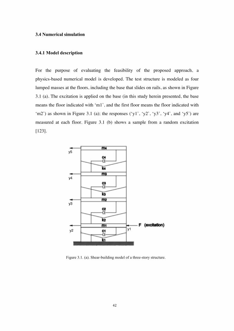
42
3.4 Numerical simulation
3.4.1 Model description
For the purpose of evaluating the feasibility of the proposed approach, a
physics-based numerical model is developed. The test structure is modeled as four
lumped masses at the floors, including the base that slides on rails, as shown in Figure
3.1 (a). The excitation is applied on the base (in this study herein presented, the base
means the floor indicated with ‘m1’, and the first floor means the floor indicated with
‘m2’) as shown in Figure 3.1 (a); the responses (‘y1’, ‘y2’, ‘y3’, ‘y4’, and ‘y5’) are
measured at each floor. Figure 3.1 (b) shows a sample from a random excitation
[123].
Figure 3.1. (a). Shear-building model of a three-story structure.
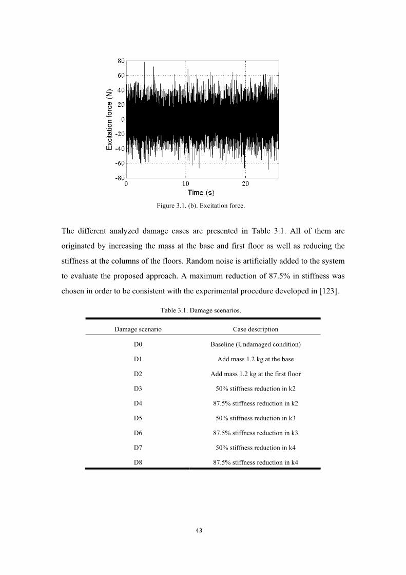
43
Figure 3.1. (b). Excitation force.
The different analyzed damage cases are presented in Table 3.1. All of them are
originated by increasing the mass at the base and first floor as well as reducing the
stiffness at the columns of the floors. Random noise is artificially added to the system
to evaluate the proposed approach. A maximum reduction of 87.5% in stiffness was
chosen in order to be consistent with the experimental procedure developed in [123].
Table 3.1. Damage scenarios.
Damage scenario Case description
D0 Baseline (Undamaged condition)
D1 Add mass 1.2 kg at the base
D2 Add mass 1.2 kg at the first floor
D3 50% stiffness reduction in k2
D4 87.5% stiffness reduction in k2
D5 50% stiffness reduction in k3
D6 87.5% stiffness reduction in k3
D7 50% stiffness reduction in k4
D8 87.5% stiffness reduction in k4
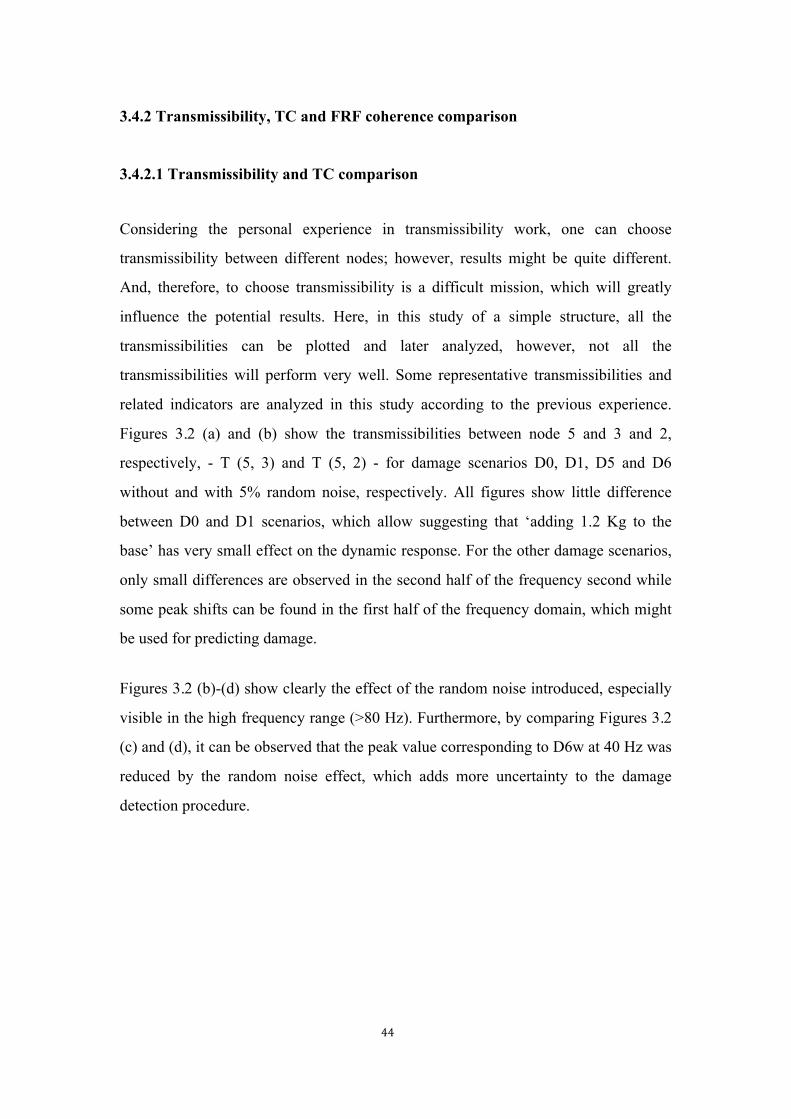
44
3.4.2 Transmissibility, TC and FRF coherence comparison
3.4.2.1 Transmissibility and TC comparison
Considering the personal experience in transmissibility work, one can choose
transmissibility between different nodes; however, results might be quite different.
And, therefore, to choose transmissibility is a difficult mission, which will greatly
influence the potential results. Here, in this study of a simple structure, all the
transmissibilities can be plotted and later analyzed, however, not all the
transmissibilities will perform very well. Some representative transmissibilities and
related indicators are analyzed in this study according to the previous experience.
Figures 3.2 (a) and (b) show the transmissibilities between node 5 and 3 and 2,
respectively, - T (5, 3) and T (5, 2) - for damage scenarios D0, D1, D5 and D6
without and with 5% random noise, respectively. All figures show little difference
between D0 and D1 scenarios, which allow suggesting that ‘adding 1.2 Kg to the
base’ has very small effect on the dynamic response. For the other damage scenarios,
only small differences are observed in the second half of the frequency second while
some peak shifts can be found in the first half of the frequency domain, which might
be used for predicting damage.
Figures 3.2 (b)-(d) show clearly the effect of the random noise introduced, especially
visible in the high frequency range (>80 Hz). Furthermore, by comparing Figures 3.2
(c) and (d), it can be observed that the peak value corresponding to D6w at 40 Hz was
reduced by the random noise effect, which adds more uncertainty to the damage
detection procedure.
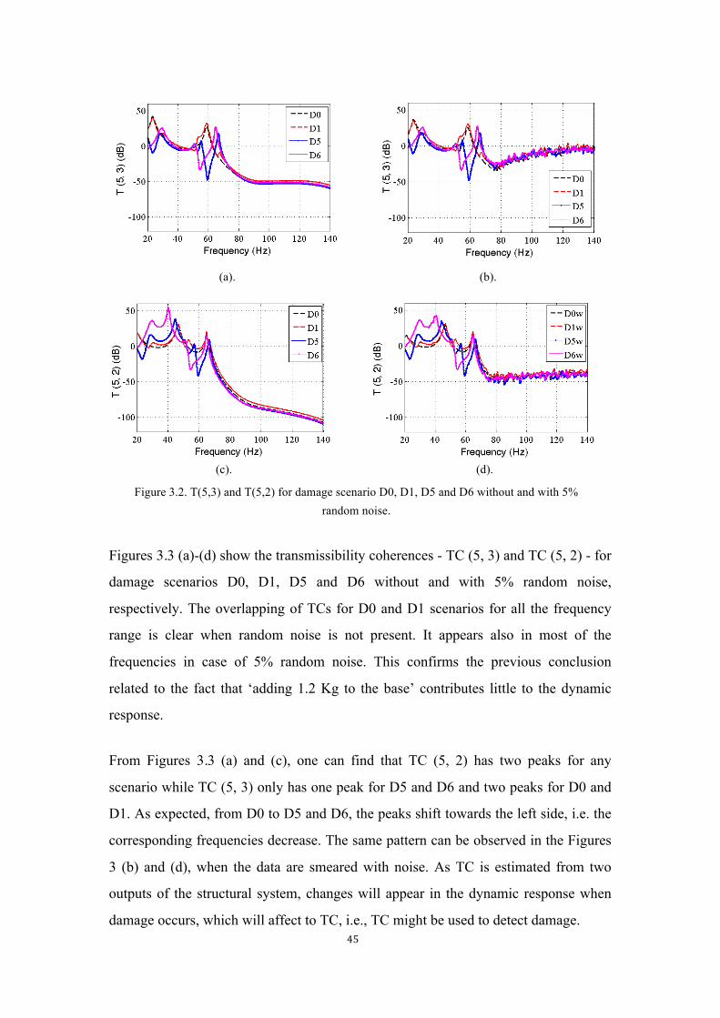
45
(a). (b).
(c). (d).
Figure 3.2. T(5,3) and T(5,2) for damage scenario D0, D1, D5 and D6 without and with 5% random noise.
Figures 3.3 (a)-(d) show the transmissibility coherences - TC (5, 3) and TC (5, 2) - for
damage scenarios D0, D1, D5 and D6 without and with 5% random noise,
respectively. The overlapping of TCs for D0 and D1 scenarios for all the frequency
range is clear when random noise is not present. It appears also in most of the
frequencies in case of 5% random noise. This confirms the previous conclusion
related to the fact that ‘adding 1.2 Kg to the base’ contributes little to the dynamic
response.
From Figures 3.3 (a) and (c), one can find that TC (5, 2) has two peaks for any
scenario while TC (5, 3) only has one peak for D5 and D6 and two peaks for D0 and
D1. As expected, from D0 to D5 and D6, the peaks shift towards the left side, i.e. the
corresponding frequencies decrease. The same pattern can be observed in the Figures
3 (b) and (d), when the data are smeared with noise. As TC is estimated from two
outputs of the structural system, changes will appear in the dynamic response when
damage occurs, which will affect to TC, i.e., TC might be used to detect damage.
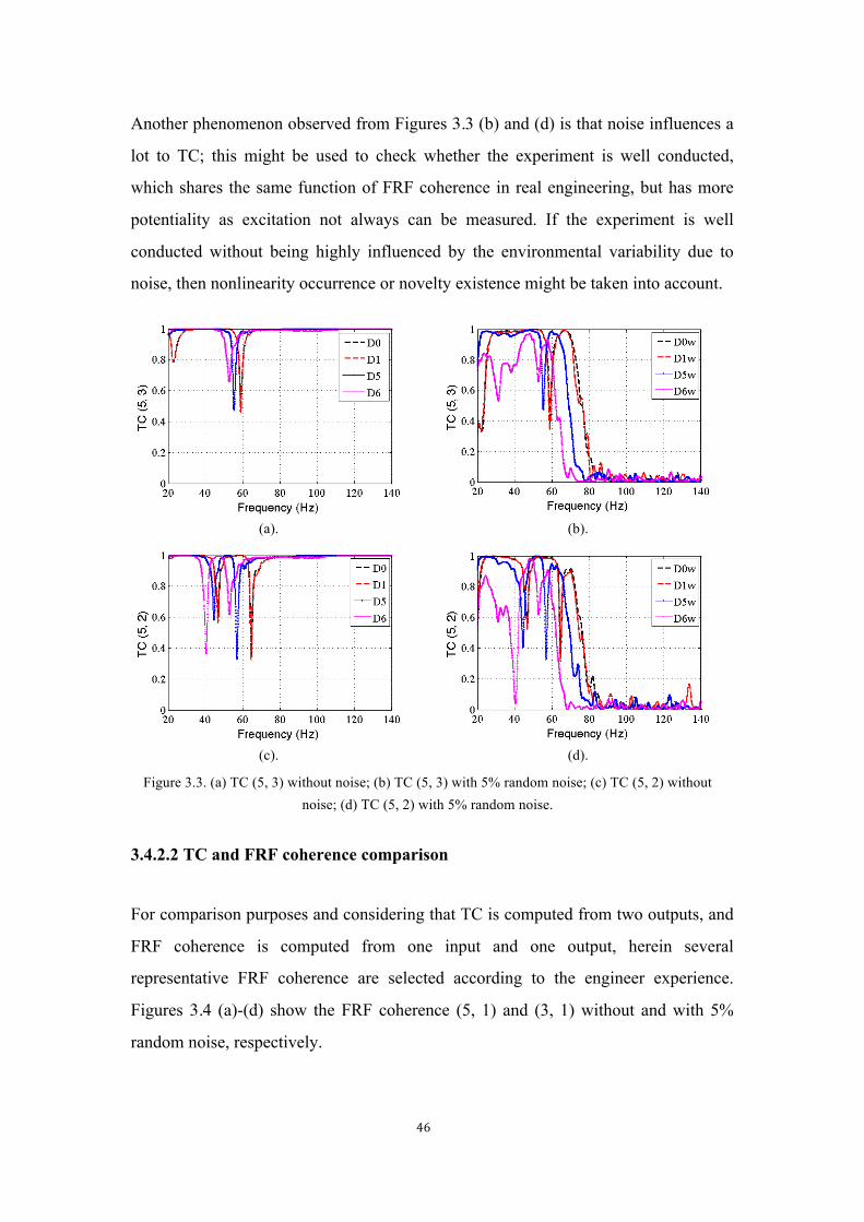
46
Another phenomenon observed from Figures 3.3 (b) and (d) is that noise influences a
lot to TC; this might be used to check whether the experiment is well conducted,
which shares the same function of FRF coherence in real engineering, but has more
potentiality as excitation not always can be measured. If the experiment is well
conducted without being highly influenced by the environmental variability due to
noise, then nonlinearity occurrence or novelty existence might be taken into account.
(a). (b).
(c). (d).
Figure 3.3. (a) TC (5, 3) without noise; (b) TC (5, 3) with 5% random noise; (c) TC (5, 2) without noise; (d) TC (5, 2) with 5% random noise.
3.4.2.2 TC and FRF coherence comparison
For comparison purposes and considering that TC is computed from two outputs, and
FRF coherence is computed from one input and one output, herein several
representative FRF coherence are selected according to the engineer experience.
Figures 3.4 (a)-(d) show the FRF coherence (5, 1) and (3, 1) without and with 5%
random noise, respectively.
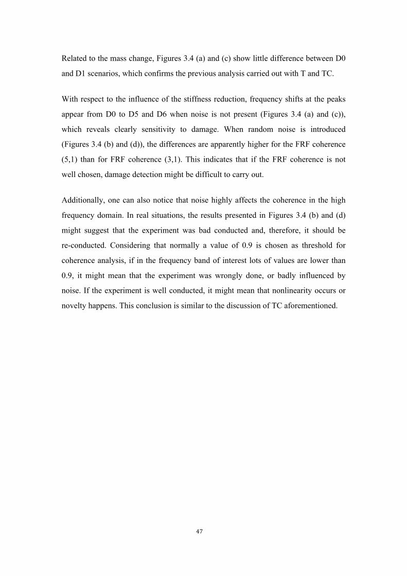
47
Related to the mass change, Figures 3.4 (a) and (c) show little difference between D0
and D1 scenarios, which confirms the previous analysis carried out with T and TC.
With respect to the influence of the stiffness reduction, frequency shifts at the peaks
appear from D0 to D5 and D6 when noise is not present (Figures 3.4 (a) and (c)),
which reveals clearly sensitivity to damage. When random noise is introduced
(Figures 3.4 (b) and (d)), the differences are apparently higher for the FRF coherence
(5,1) than for FRF coherence (3,1). This indicates that if the FRF coherence is not
well chosen, damage detection might be difficult to carry out.
Additionally, one can also notice that noise highly affects the coherence in the high
frequency domain. In real situations, the results presented in Figures 3.4 (b) and (d)
might suggest that the experiment was bad conducted and, therefore, it should be
re-conducted. Considering that normally a value of 0.9 is chosen as threshold for
coherence analysis, if in the frequency band of interest lots of values are lower than
0.9, it might mean that the experiment was wrongly done, or badly influenced by
noise. If the experiment is well conducted, it might mean that nonlinearity occurs or
novelty happens. This conclusion is similar to the discussion of TC aforementioned.
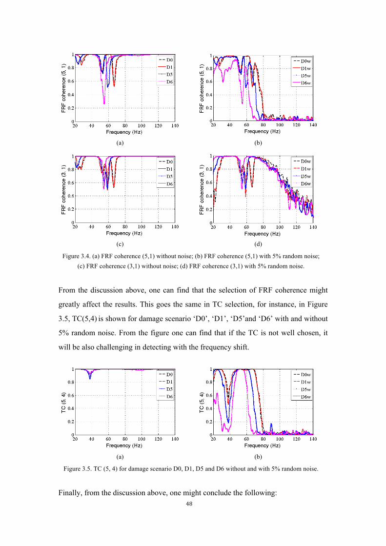
48
(a) (b)
(c) (d)
Figure 3.4. (a) FRF coherence (5,1) without noise; (b) FRF coherence (5,1) with 5% random noise; (c) FRF coherence (3,1) without noise; (d) FRF coherence (3,1) with 5% random noise.
From the discussion above, one can find that the selection of FRF coherence might
greatly affect the results. This goes the same in TC selection, for instance, in Figure
3.5, TC(5,4) is shown for damage scenario ‘D0’, ‘D1’, ‘D5’and ‘D6’ with and without
5% random noise. From the figure one can find that if the TC is not well chosen, it
will be also challenging in detecting with the frequency shift.
(a) (b)
Figure 3.5. TC (5, 4) for damage scenario D0, D1, D5 and D6 without and with 5% random noise.
Finally, from the discussion above, one might conclude the following:
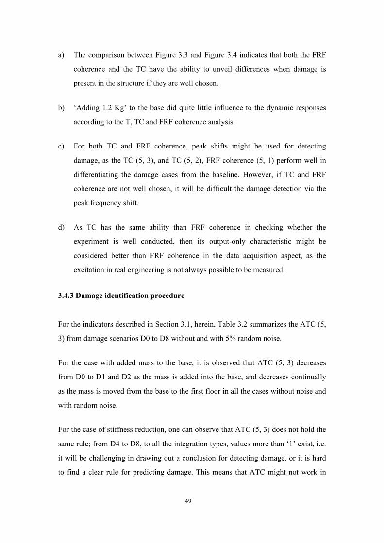
49
a) The comparison between Figure 3.3 and Figure 3.4 indicates that both the FRF
coherence and the TC have the ability to unveil differences when damage is
present in the structure if they are well chosen.
b) ‘Adding 1.2 Kg’ to the base did quite little influence to the dynamic responses
according to the T, TC and FRF coherence analysis.
c) For both TC and FRF coherence, peak shifts might be used for detecting
damage, as the TC (5, 3), and TC (5, 2), FRF coherence (5, 1) perform well in
differentiating the damage cases from the baseline. However, if TC and FRF
coherence are not well chosen, it will be difficult the damage detection via the
peak frequency shift.
d) As TC has the same ability than FRF coherence in checking whether the
experiment is well conducted, then its output-only characteristic might be
considered better than FRF coherence in the data acquisition aspect, as the
excitation in real engineering is not always possible to be measured.
3.4.3 Damage identification procedure
For the indicators described in Section 3.1, herein, Table 3.2 summarizes the ATC (5,
3) from damage scenarios D0 to D8 without and with 5% random noise.
For the case with added mass to the base, it is observed that ATC (5, 3) decreases
from D0 to D1 and D2 as the mass is added into the base, and decreases continually
as the mass is moved from the base to the first floor in all the cases without noise and
with random noise.
For the case of stiffness reduction, one can observe that ATC (5, 3) does not hold the
same rule; from D4 to D8, to all the integration types, values more than ‘1’ exist, i.e.
it will be challenging in drawing out a conclusion for detecting damage, or it is hard
to find a clear rule for predicting damage. This means that ATC might not work in
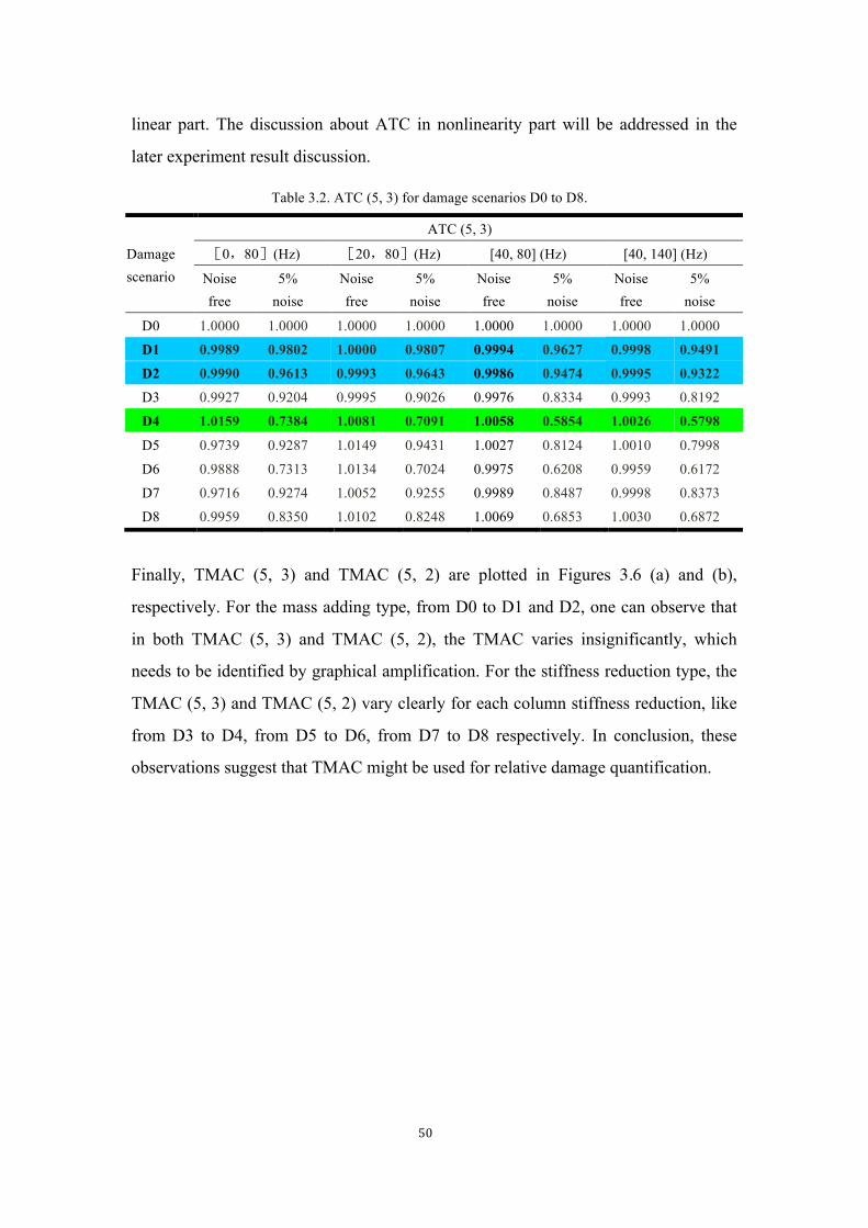
50
linear part. The discussion about ATC in nonlinearity part will be addressed in the
later experiment result discussion.
Table 3.2. ATC (5, 3) for damage scenarios D0 to D8.
Damage scenario
ATC (5, 3)
[0,80](Hz) [20,80](Hz) [40, 80] (Hz) [40, 140] (Hz)
Noise free
5% noise
Noise free
5% noise
Noise free
5% noise
Noise free
5% noise
D0 1.0000 1.0000 1.0000 1.0000 1.0000 1.0000 1.0000 1.0000
D1 0.9989 0.9802 1.0000 0.9807 0.9994 0.9627 0.9998 0.9491
D2 0.9990 0.9613 0.9993 0.9643 0.9986 0.9474 0.9995 0.9322
D3 0.9927 0.9204 0.9995 0.9026 0.9976 0.8334 0.9993 0.8192
D4 1.0159 0.7384 1.0081 0.7091 1.0058 0.5854 1.0026 0.5798
D5 0.9739 0.9287 1.0149 0.9431 1.0027 0.8124 1.0010 0.7998
D6 0.9888 0.7313 1.0134 0.7024 0.9975 0.6208 0.9959 0.6172
D7 0.9716 0.9274 1.0052 0.9255 0.9989 0.8487 0.9998 0.8373
D8 0.9959 0.8350 1.0102 0.8248 1.0069 0.6853 1.0030 0.6872
Finally, TMAC (5, 3) and TMAC (5, 2) are plotted in Figures 3.6 (a) and (b),
respectively. For the mass adding type, from D0 to D1 and D2, one can observe that
in both TMAC (5, 3) and TMAC (5, 2), the TMAC varies insignificantly, which
needs to be identified by graphical amplification. For the stiffness reduction type, the
TMAC (5, 3) and TMAC (5, 2) vary clearly for each column stiffness reduction, like
from D3 to D4, from D5 to D6, from D7 to D8 respectively. In conclusion, these
observations suggest that TMAC might be used for relative damage quantification.
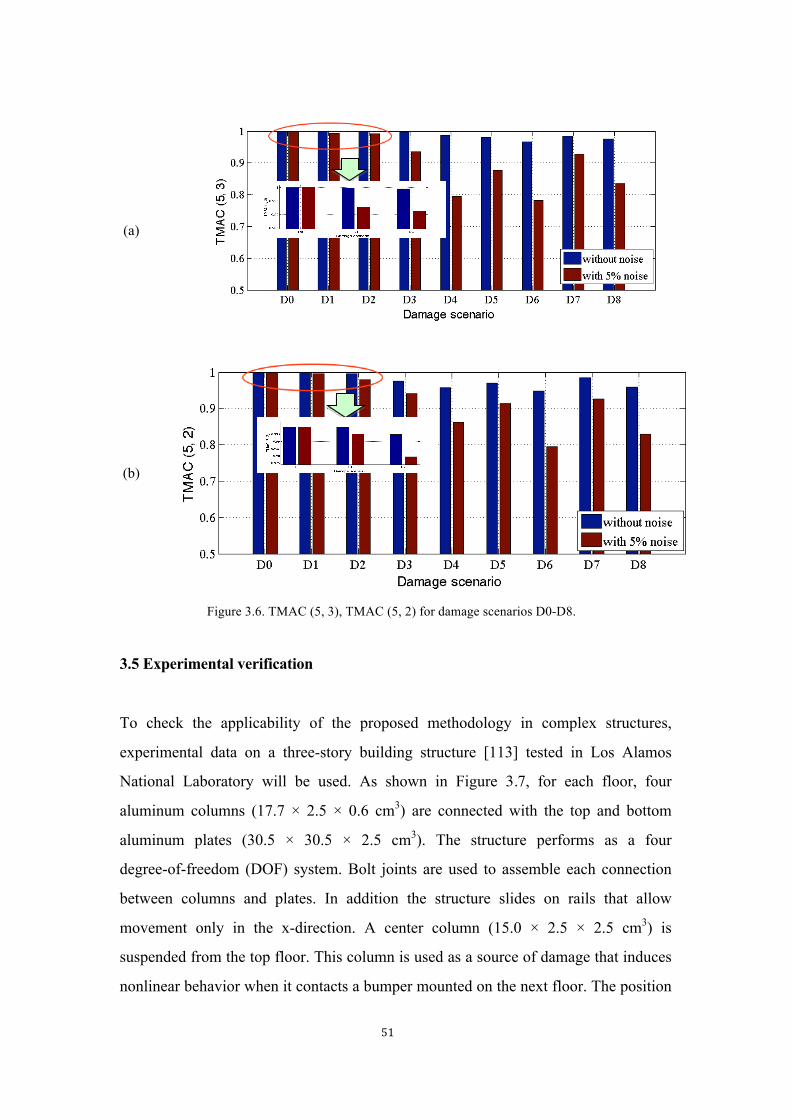
51
(a)
(b)
Figure 3.6. TMAC (5, 3), TMAC (5, 2) for damage scenarios D0-D8.
3.5 Experimental verification
To check the applicability of the proposed methodology in complex structures,
experimental data on a three-story building structure [113] tested in Los Alamos
National Laboratory will be used. As shown in Figure 3.7, for each floor, four
aluminum columns (17.7 × 2.5 × 0.6 cm3) are connected with the top and bottom
aluminum plates (30.5 × 30.5 × 2.5 cm3). The structure performs as a four
degree-of-freedom (DOF) system. Bolt joints are used to assemble each connection
between columns and plates. In addition the structure slides on rails that allow
movement only in the x-direction. A center column (15.0 × 2.5 × 2.5 cm3) is
suspended from the top floor. This column is used as a source of damage that induces
nonlinear behavior when it contacts a bumper mounted on the next floor. The position

52
of the bumper can be adjusted to vary the extent of impacting that occurs during a
particular excitation level.
An electro-dynamic shaker provides a lateral excitation to the base floor along the
centerline of the structure. The structure and shaker are mounted together on an
aluminum base plate (76.2 × 30.5 × 2.5 cm3) and the entire system rests on rigid foam.
The foam is intended to minimize extraneous sources of unmeasured excitation from
being introduced through the base of the system. A load cell (Channel 1) was attached
at the end of a stinger to measure the input force from the shaker to the structure. Four
accelerometers (Channels 2-5) with nominal sensitivities of 1000 mV/g were attached
at the centerline of each floor on the opposite side from the excitation source to
measure the system response.
Figure 3.7. Schematic representation of the three-story building structure (all dimensions are in
cm).
53
Force and acceleration time-series from 17 different structural state conditions were
collected as given in Table 3.3. For instance, the ‘State #4’ is described as ‘stiffness
reduction in column 1BD’, which means that there was an 87.5% stiffness reduction
(corresponding to a 50% reduction in the column thickness) in the column located
between the base and first floor at the intersection of plane B and D. For each
structural state condition, data were acquired from 50 separate tests. For each test, the
data correspond to a set of five time-series measured with the input force transducer
and the four accelerometers.
The structural state conditions can be categorized into four main groups. The first
group is the baseline condition. The baseline condition is the reference structural state
and is labeled ‘State#1’ in Table 3.3. The bumper and the suspended column are
included in the baseline condition, but the spacing between them was maintained in
such a way that there were no impacts during the excitation. The second group
includes the states with simulated operational and environmental variability. Such
variability often manifests itself in changes in the stiffness or mass distribution of the
structure. In order to simulate such operational and environmental condition changes,
tests were performed with different mass-loading and stiffness conditions (State #2–9).
The mass changes consisted of adding 1.2kg (approximately 19% of the total mass of
each floor) to the base and first floor. The stiffness changes were introduced by
reducing the stiffness of one or more of the columns by 87.5%. This process was
executed by replacing the corresponded column with one that had half the
cross-sectional thickness in the direction of shaking.
Those changes were designed to introduce variability in the fundamental natural
frequency up to, approximately, 7% from the baseline condition, which is within the
range normally observed in real-world structures. More details about the test structure
as well as data sets can be found in Figueiredo et al [123, 113].
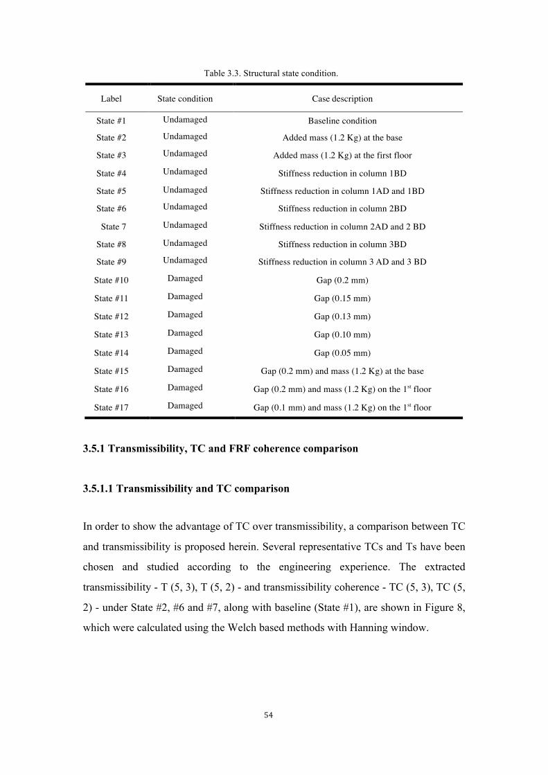
54
Table 3.3. Structural state condition.
Label State condition Case description
State #1 Undamaged Baseline condition
State #2 Undamaged Added mass (1.2 Kg) at the base
State #3 Undamaged Added mass (1.2 Kg) at the first floor
State #4 Undamaged Stiffness reduction in column 1BD
State #5 Undamaged Stiffness reduction in column 1AD and 1BD
State #6 Undamaged Stiffness reduction in column 2BD
State 7 Undamaged Stiffness reduction in column 2AD and 2 BD
State #8 Undamaged Stiffness reduction in column 3BD
State #9 Undamaged Stiffness reduction in column 3 AD and 3 BD
State #10 Damaged Gap (0.2 mm)
State #11 Damaged Gap (0.15 mm)
State #12 Damaged Gap (0.13 mm)
State #13 Damaged Gap (0.10 mm)
State #14 Damaged Gap (0.05 mm)
State #15 Damaged Gap (0.2 mm) and mass (1.2 Kg) at the base
State #16 Damaged Gap (0.2 mm) and mass (1.2 Kg) on the 1st floor
State #17 Damaged Gap (0.1 mm) and mass (1.2 Kg) on the 1st floor
3.5.1 Transmissibility, TC and FRF coherence comparison
3.5.1.1 Transmissibility and TC comparison
In order to show the advantage of TC over transmissibility, a comparison between TC
and transmissibility is proposed herein. Several representative TCs and Ts have been
chosen and studied according to the engineering experience. The extracted
transmissibility - T (5, 3), T (5, 2) - and transmissibility coherence - TC (5, 3), TC (5,
2) - under State #2, #6 and #7, along with baseline (State #1), are shown in Figure 8,
which were calculated using the Welch based methods with Hanning window.
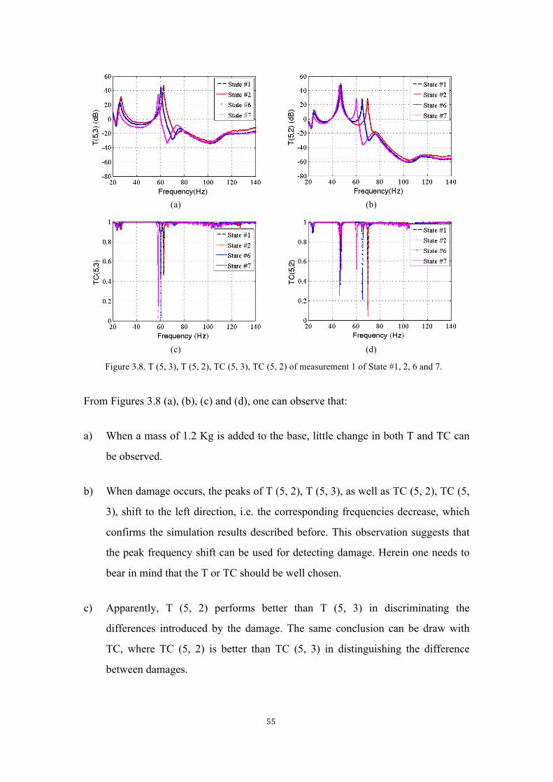
55
(a) (b)
(c) (d)
Figure 3.8. T (5, 3), T (5, 2), TC (5, 3), TC (5, 2) of measurement 1 of State #1, 2, 6 and 7.
From Figures 3.8 (a), (b), (c) and (d), one can observe that:
a) When a mass of 1.2 Kg is added to the base, little change in both T and TC can
be observed.
b) When damage occurs, the peaks of T (5, 2), T (5, 3), as well as TC (5, 2), TC (5,
3), shift to the left direction, i.e. the corresponding frequencies decrease, which
confirms the simulation results described before. This observation suggests that
the peak frequency shift can be used for detecting damage. Herein one needs to
bear in mind that the T or TC should be well chosen.
c) Apparently, T (5, 2) performs better than T (5, 3) in discriminating the
differences introduced by the damage. The same conclusion can be draw with
TC, where TC (5, 2) is better than TC (5, 3) in distinguishing the difference
between damages.
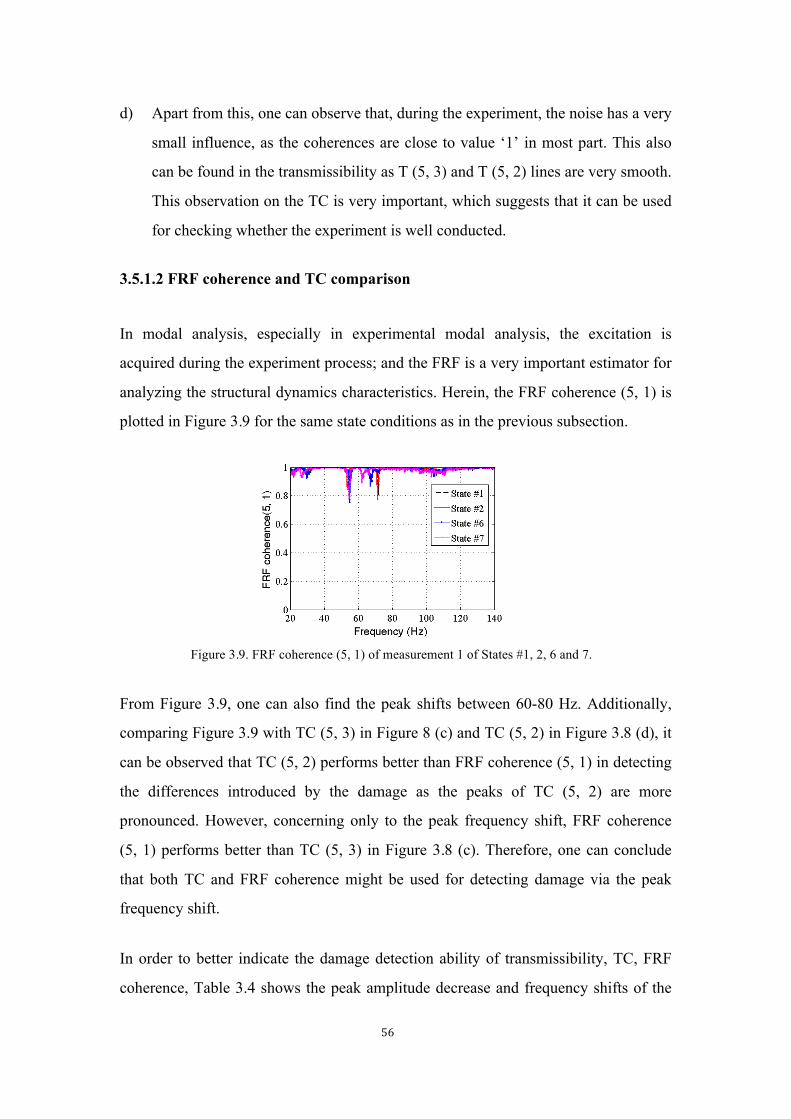
56
d) Apart from this, one can observe that, during the experiment, the noise has a very
small influence, as the coherences are close to value ‘1’ in most part. This also
can be found in the transmissibility as T (5, 3) and T (5, 2) lines are very smooth.
This observation on the TC is very important, which suggests that it can be used
for checking whether the experiment is well conducted.
3.5.1.2 FRF coherence and TC comparison
In modal analysis, especially in experimental modal analysis, the excitation is
acquired during the experiment process; and the FRF is a very important estimator for
analyzing the structural dynamics characteristics. Herein, the FRF coherence (5, 1) is
plotted in Figure 3.9 for the same state conditions as in the previous subsection.
Figure 3.9. FRF coherence (5, 1) of measurement 1 of States #1, 2, 6 and 7.
From Figure 3.9, one can also find the peak shifts between 60-80 Hz. Additionally,
comparing Figure 3.9 with TC (5, 3) in Figure 8 (c) and TC (5, 2) in Figure 3.8 (d), it
can be observed that TC (5, 2) performs better than FRF coherence (5, 1) in detecting
the differences introduced by the damage as the peaks of TC (5, 2) are more
pronounced. However, concerning only to the peak frequency shift, FRF coherence
(5, 1) performs better than TC (5, 3) in Figure 3.8 (c). Therefore, one can conclude
that both TC and FRF coherence might be used for detecting damage via the peak
frequency shift.
In order to better indicate the damage detection ability of transmissibility, TC, FRF
coherence, Table 3.4 shows the peak amplitude decrease and frequency shifts of the

57
two obvious peaks in transmissibility, TC and FRF coherence. From Table 3.4, one
can find, from T (5, 2), TC (5, 2) and FRFC (5, 1), that all can perform well in
damage detection with peak frequency shift and amplitude change. However, the
second peak frequency change is higher than the first one, while the first peak
amplitude changes more than the second one, with exception of TC (5, 2) in State #7.
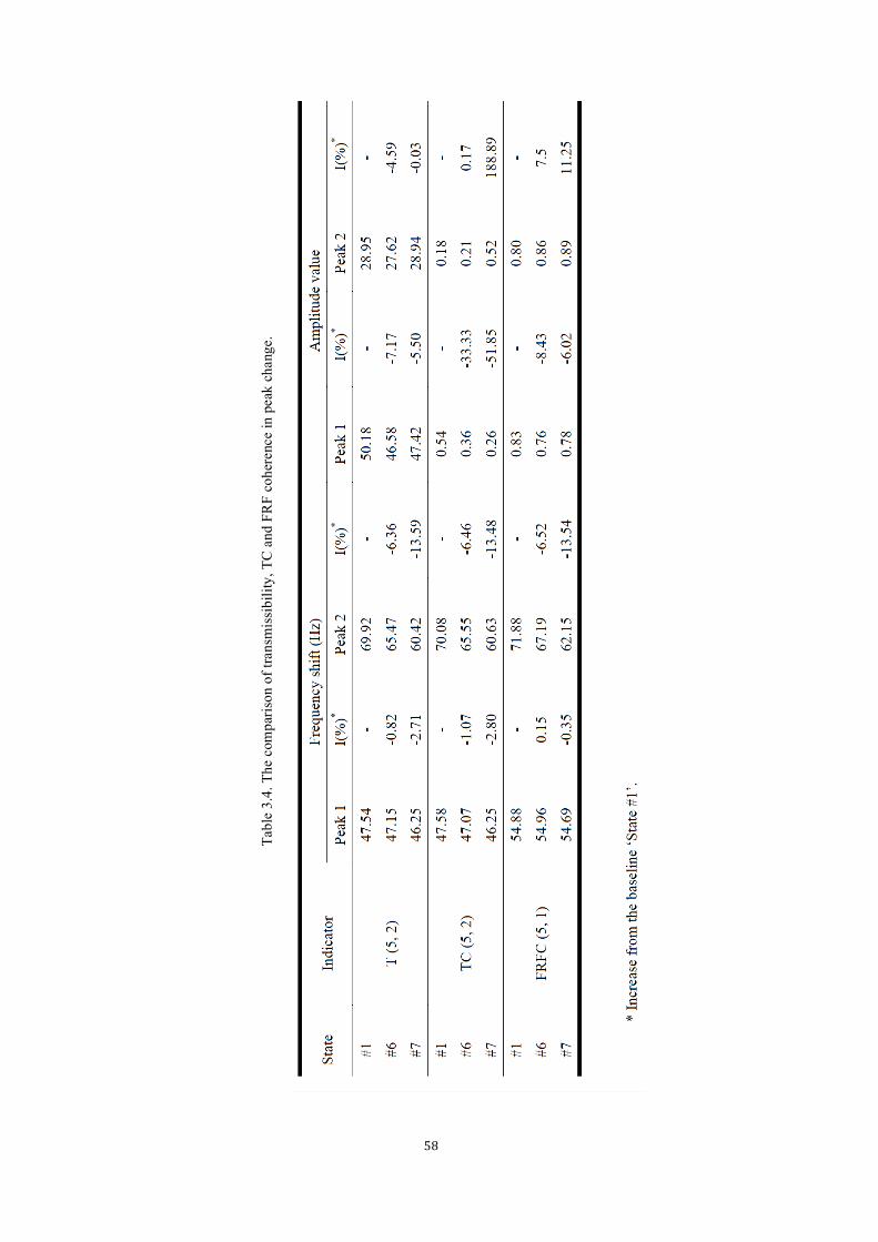
58
Tabl
e 3.
4. T
he c
ompa
rison
of t
rans
mis
sibi
lity,
TC
and
FR
F co
here
nce
in p
eak
chan
ge.
59
Note that in real engineering, especially in operational modal analysis, normally the
excitation cannot be measured. Thus, the FRF would be impossible to be used for
modal analysis. Therefore, the TC will perform in its perfect way, as transmissibility
is only depending on the structural responses, as well as TC.
3.5.2 Damage identification analysis in linear part
Damage detection plays a vital role in real-time SHM. As shown in Figures 3.8 (c)
and (d), TC might be used for detecting damages. Herein, ATC (5, 3) and ATC (5, 2)
as well as TMAC (5, 3) and TMAC (5, 2) are shown in Figures 3.10 (a)-(d) ,
respectively, for 50 measurements from each of the nine state conditions (State #1 to
9), with 450 measurements in total.
From a general perspective, one can observe that in both cases, ATC (ATC (5, 2),
ATC (5, 3)) and TMAC (TMAC (5, 2) and TMAC (5, 3)), the variability is relatively
small comparing with the reference value of unit, which suggests that these two
indicators do not perform very well in detecting damage.
In Figures 3.10 (a) and (b), for the mass type damage, i.e. from D0 to D1 and D2,
ATC (5, 3) and ATC (5, 2) increase when mass is added into the base structure, and
when the mass is moved into the first floor, both ATC (5, 3) and ATC (5, 2) decrease.
In this case, it would be hard to draw out a conclusion of mass influence into the
indicator ATC. For stiffness reduction type damage, based on ATC (5, 2) is also
difficult to conclude about the presence of damage as ATC (5, 2) of State #5 are
obviously larger than the ones from the baseline State #1. However, in the case of
ATC (5, 3), one might draw a conclusion that ATC (5, 3) can be used for detecting
damage related with stifiness reduction as to all the measurements from State #4-9,
the corresponding ATC (5, 3) are lower than the baseline. Another aspect is that ATC
(5, 3) might be also used to relatively quantify the damage as it varies proporcionally
to each state. One can also observe that for each state, the values of 50 measurements
vary not too much, which suggests that the experiment is conducted in a good
condition.
60
In Figures 3.10 (c) and (d), for the mass adding damage type, it is clear that from
State #1 to State #3, the TMAC (5, 3) and TMAC (5, 2) decreased as the mass 1.2 Kg
was added into the base in State #2, and later moved to first floor in State #3. For
stiffness reduction from State #4 to #9, one can find that both TMAC (5, 3) and
TMAC (5, 2) decrease as the stfiffness reduction increased from State #4 to #5, from
State #6 to #7, from State #8 to #9, respectively. In Figure 3.10 (c), one can also
observe that TMAC (5, 3) decreased clearly as the stiffness reduction changed from
the first story to the second story and from second story to third story. Comparing
State #6 and #8, one can see some decrease occuring in TMAC (5, 3). For TMAC (5,
2), in Figure 3.10 (d), it can be found that the TMAC (5, 2) decreases from State #4 to
#5, from State #6 to #7, from State #8 to #9, meaning that the TMAC (5, 2) can
relatively quantify the damage for each story. Comparing Figures 3.10 (c) and (d),
one might conclude that TMAC can be used for relatively quantifying damage. Note
that this also confirms the same conclusion drawn out in the simulation section
analysis.
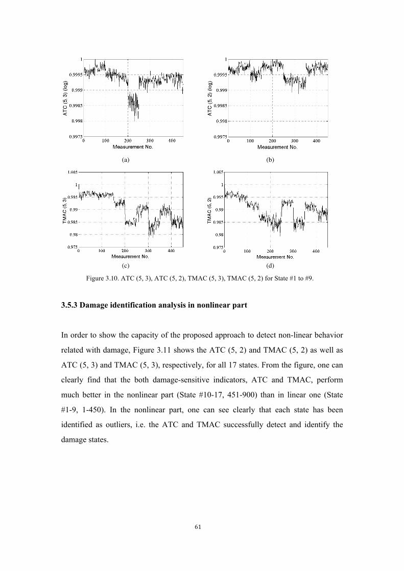
61
(a) (b)
(c) (d)
Figure 3.10. ATC (5, 3), ATC (5, 2), TMAC (5, 3), TMAC (5, 2) for State #1 to #9.
3.5.3 Damage identification analysis in nonlinear part
In order to show the capacity of the proposed approach to detect non-linear behavior
related with damage, Figure 3.11 shows the ATC (5, 2) and TMAC (5, 2) as well as
ATC (5, 3) and TMAC (5, 3), respectively, for all 17 states. From the figure, one can
clearly find that the both damage-sensitive indicators, ATC and TMAC, perform
much better in the nonlinear part (State #10-17, 451-900) than in linear one (State
#1-9, 1-450). In the nonlinear part, one can see clearly that each state has been
identified as outliers, i.e. the ATC and TMAC successfully detect and identify the
damage states.
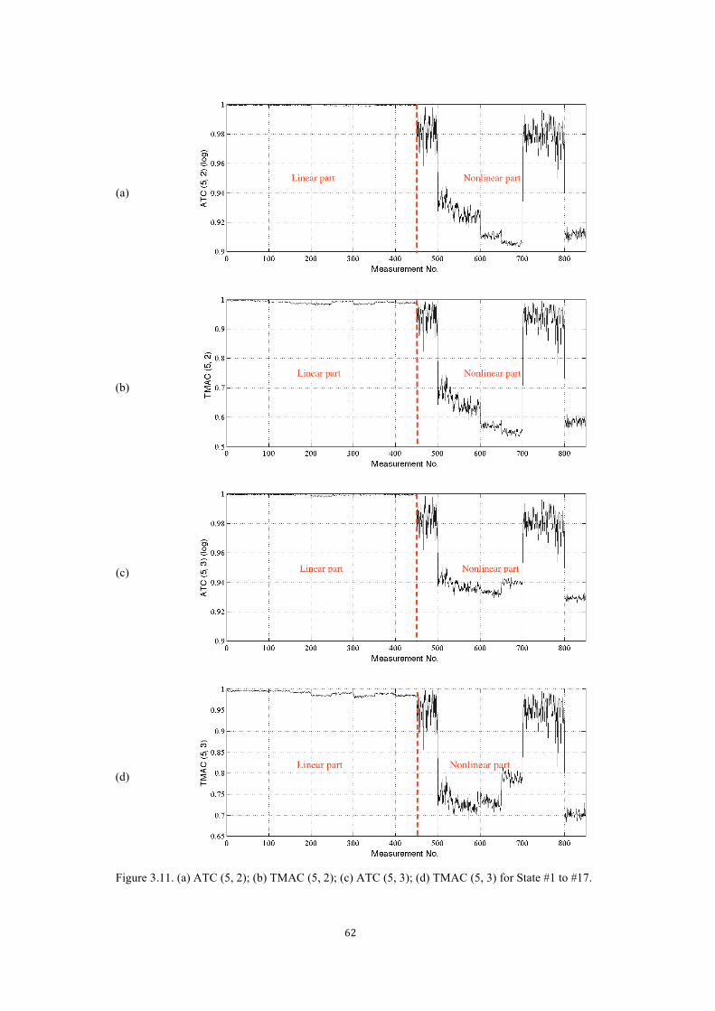
62
(a)
(b)
(c)
(d)
Figure 3.11. (a) ATC (5, 2); (b) TMAC (5, 2); (c) ATC (5, 3); (d) TMAC (5, 3) for State #1 to #17.
63
3.6 Conclusions
This chapter illustrated the coherence between two outputs using the transmissibility
coherence (TC) and its relation with the traditional FRF coherence in modal analysis
was set. A damage-sensitive indicator using the modal assurance criterion, for
detecting and relatively quantifying structural damages, was formulated from TC
The TC has an important advantage over the FRF coherence, as the former does not
need to know the input excitation to the system, which might be an important feature
for real-world applications. The TC can be used for checking whether the experiment
is well conducted, as it gives indications about the presence of noise in the system. It
may also be used for detecting damage using the frequency shift as damage indicator.
Additionally, the proposed ATC might be used for detecting damage especially in
nonlinear analysis; it was demonstrated that in nonlinear damage quantification it
performs well. In addition, the TC and related indicators are sensitive to environment
variety like noise, which might be used for monitoring the operational conditions.
The TMAC can be used to relatively quantify the damage. The results of both the
simulated frame and three-story frame structure reveal the good performance in
damage detection and quantification both in linear and nonlinear part; in the linear
part, all the damage scenarios were successfully detected and relatively well
quantified; it was also demonstrated that in the nonlinear part, the approach performs
much better than in linear part.
It is important to note that the proposed approach only requires minimum two-sensor
data acquisition in the structural system for detecting and relatively quantifying the
structural damage. Therefore, it shows promising future in real time SHM.
Finally, for both simulation and experiment, the good performance in detecting and
quantifying the damages shows great promising future in real engineering usage.

64
65
CHAPTER 4 DAMAGE DETECTION IN STRUCTURES USING A
TRANSMISSIBILITY-BASED MAHALANOBIS DISTANCE
Summary
In this Chapter, a damage detection approach using the Mahalanobis distance with
structural forced dynamic response data, in the form of transmissibility, is proposed.
Transmissibility, as a damage-sensitive feature, varies in accordance with the damage
level. Besides, Mahalanobis distance can distinguish the damaged structural state
condition from the undamaged one by condensing the baseline data. For comparison
reasons, the Mahalanobis distance results using transmissibility are compared with
those using Frequency Response Functions. The experiment results reveal quite a
significant capacity for damage detetion, and the comparison between the use of
transmissibility and Frequency Response Functions shows that, in both cases, the
different damage scenarios could be well detected.
4.1 Introduction
During the last two decades, SHM has become a research focus all over the world due
to the increasing demand to identify, at an early stage, structural damage, especially in
aeronautical and civil engineering, where the structures age and the costs of structural
maintenance are relatively high. For instance, in the bridge maintenance process, a
systematic SHM way is proposed by Figueiredo et al. to improve the existing bridge
management systems [126], in order to reduce costs and the frequency of the bridge
inspections.
66
In the past decades, a lot of vibration-based SHM methods have been developed [127,
128], where most of the approaches rely on the excitation source. Herein, the FRFs
are often used in order to set up the relationship between the input and output
responses. In the bridge engineering field, experimental modal analysis is widely used,
where output-only SHM approaches are raised in order to avoid the excitation
measurement, as it is normally very difficult or even impossible to measure. Thus,
transmissibility or direct transmissibility, depending on output data only, has been
used extensively in order to avoid the measurement of excitation. Usually the FRF is
used in experimental modal analysis where a lot of experiments are conducted in
laboratories, while transmissibility is used for operational modal analysis where the
structures are in real working conditions.
Transmissibility (direct transmissibility), defined as the ratio between two outputs,
has been a means of evaluating the structural condition without measuring the
excitation, which has been interesting for real engineering applications, such as bridge
monitoring, where the excitation is normally not measured. In recent years,
transmissibility has been widely studied, and some methods have been developed to
detect damage or assess the structural damage severity.
Most researchers are dealing with the transmissibility to extract model parameters,
propose some damage indicators, or use some artificial intelligent algorithms.
Nevertheless, few ones use discriminant analysis in transmissibility-based damage
identification techniques.
Discriminant analysis is a multivariate statistical method, which is commonly used for
building a predictive or descriptive model for group discrimination and group
classification. A thorough overview on these methods has been done by Farrar and
Worden [129]. An appropriate distance metric is a key issue in discriminant analysis,
and the Mahalanobis distance is a well-known statistical function, which is a way of
measuring the distance between two points in the feature space defined through
correlated variables.
67
Therefore, in this Chapter, a novel transmissibility-based damage detection approach
is proposed and outlined. Basically, the transmissibility is firstly calculated, and then
a set of transmissibility from the undamaged structure is set as the baseline, in order
to calculate the Mahalanobis squared distance between the baseline and any future
state condition. Two damage indicators are proposed and thresholds are set to predict
whether a future state is from the damaged or the undamaged structural condition. An
experiment is conducted to validate the damage detection approach. The experiment
is carried out with different operational conditions and for several damage scenarios.
The main contribution of this paper is the introduction of a linear discriminant
analysis in the context of the development of transmissibility-based damage detection
methods.
4.2 Theoretical background
4.2.1 Transmissibility
As discussed in Chapter 2, transmissibility can be estimated from FRFs as follows;
T( i, j ) (ω ) =
Xi(ω )X j (ω )
=Hib(ω )H jb(ω )
(4.1)
4.2.2 Mahalanobis squared distance (MSD)
The Mahalanobis distance is a well-known distance metric [130], which is defined as
a measure of the distance between two points in the feature space composed of two or
more variables. It differs from the Euclidean distance as it takes the correlation
between variables into account and it does not depend on the scale of the features.
The Mahalanobis distance is defined as
( ) ( )TMahald = − −∑-1X Z X Z (4.2)
68
where Z is the mean vector of the variables and X is the test vector. In our
particular case, Z is the mean value of the m transmissibilities for each frequency
and X in this application is the “test vector” of the transmissibilities; 1 1Cov− −=∑ is
the inverse covariance matrix of the m variables and the superscript T indicates
transposed, in our problem, the Mahalanobis distance is frequency dependent.
The covariance matrix and mean vector intend to embed the normal condition of the
structure. Basically, the assumption is that if a new observation X is obtained from
data collected on the damaged system that might include sources of operational and
environmental variability, the observation will be away from the mean of the normal
condition. On the other hand, if an observation is obtained from a system within its
undamaged condition, even with operational and environmental variability, it will be
close to the mean of the normal condition.
Alternatively, several authors [131, 132] have used extensively the MSD, which is
defined as
2 ( ) ( )TMahald = − −∑ -1X Z X Z (4.3)
Note that when = I∑ , the Mahalanobis distance coincides with the Euclidean
distance.
4.3 The proposed damage detection method
4.3.1 MSD between undamaged and damaged transmissibility
In order to calculate the MSD between the undamaged structural transmissibility and
the damaged structural transmissibility, one might set up three steps, as follows.
Step 1: A set of undamaged structural transmissibility Tnmu is established as the
baseline, and the average value will be calculated according to each variable, which
will be denoted as Tmu .
69
Step 2: Computation of −1∑ .
-1∑ = Cov−1(Tnmu )
=
C1,1 C1,2 ! C1,m
C2,1 ! ! C2,m
" " " "Cn−1,1
Cn,1
!!
!Cn,m−1
Cn−1,m
Cn,m
⎡
⎣
⎢⎢⎢⎢⎢⎢⎢
⎤
⎦
⎥⎥⎥⎥⎥⎥⎥
−1
(4.4)
where
( )( ),1
11
n
l k rl l rk kr
C T T T Tn =
= − −− ∑
(4.5)
Step 3: Calculation of the Mahalanobis distance and the MSD between one set of test
data Ts and the baseline each time, respectively:
( ) ( )1Tu uMahal s m s md −= − −∑T T T T
(4.6)
( ) ( )12 Tu uMahal s m s md −= − −∑T T T T
(4.7)
4.3.2 Euclidean distance between undamaged and damaged transmissibility
As defined, the Euclidean distance and Euclidean squared distance (ESD) between
undamaged and damaged transmissibility are, respectively:
( ) ( )Tu uEuclid s m s md = − −T T T T
(4.8)
( ) ( )2 Tu uEuclid s m s md = − −T T T T
(4.9)
70
4.3.3 Damage detection index
In order to take into account the operational and environmental conditions, one needs
to estimate the mean vector of Nn sample matrices from the undamaged condition
Tu(1) ,Tu(2) ,...,Tu( Nn ) , which will be set as the baseline for later analysis. Herein, N
means the number of the undamaged state observations; observation means a matrix
composed by time series from Q sensors and sample matrix means a matrix composed
by the transmissibility from m sensors, in the frequency domain.
Afterwards, the MSDs between the undamaged condition and the baseline could be
calculated and denoted as dMahalu(1) ,dMahal
u(2) ,!,dMahalu(Nn ) . Then, the highest value of each variable
under the undamaged state will be picked up and indicated as max(dMahalu(Q ) ) Q=1Nn . Here,
Q represents the Qth measurement. Henceforth, the maximum of this set will be taken
as boundary criteria between the damaged and undamaged conditions, which will be
denoted as max(max(dMahalu(Q ) ) Q=1Nn ) . Then, the MSD between each test condition and the
baseline will be calculated, and indicated as dMahalt (1) ,dMahal
t (2) ,!,dMahalt (Nt ) . Finally, a damage
detection index (DDI) DDI(ω ) is defined as
DDI(ω ) =dMahal
t ( l )
max(max(dMahalu(Q ) ) Q=1
Nn )
(4.10)
where l means the l th test MSD results for the l th Tt (l ) data group. Here it is clear
that dMahalt (l ) is frequency dependent, and due to this, the DDI is frequency dependent.
As max(max(dMahalu(Q ) ) Q=1Nn ) is the maximum value of MSD under undamaged condition,
and DDI is the ratio between MSD under test condition and the maximum value of
MSD under undamaged condition, then it is clear that DDI >1 (or in log scale
DDI > 0 ). Henceforth, referring to values in log scale, if DDI > 0 , it means that the
structure may be considered as “damaged”; if DDI >> 0 , it means that there is a high
confidence that the structure may be “damaged”. As the highest value of MSD under
undamaged condition is chosen, therefore, only the highest peak value should be
considered for comparison. Therefore, from the DDI , another amplitude reduction
71
indicator advanced resulting index (ARI) can be derived from the highest peak value
of DDI , which is the maximum of the DDI along the frequency:
max( )ARI DDIω
=
(4.11)
Although the DDI might show us a picture of the evolution of the index along the
frequency range, it is important to obtain a simple global number, which allows
deciding in a definite way whether the structure is damaged or not. That is the
objective of the ARI.
If ARI is close to 0, it means that the experiment has been conducted very well and
the systematic error or environmental influence is very small. If ARI is close to 1 (or
in log scale 0), it means that the experiment has been conducted under the same
condition as the chosen baseline, and the environmental influence is more or less the
same as the baseline. If ARI >1.0 (or in log scale ARI > 0 ), it means that the
experiment has been conducted unusually or the environmental influence is bigger
than the baseline, or some change happens in the structure, that is to say, the structure
may be considered as “damaged”. If ARI >>1.0 (or in log scale ARI >> 0 ), it means
that there is a very high confidence that the structure may be “damaged”, or
something from the environment greatly influenced the experiment.
Although the significance of DDI and ARI are the same, the DDI will reflect all
the information in the frequency range of the experimental results, and it can show
whether the response varies slightly or highly along the frequency, whereas the ARI
only demonstrates the highest value. However, as DDI varies with the frequency, the
conclusion may not be so clear when compared to the ARI .
4.4 Experimental validation
A laboratory experiment of a steel beam with rectangular cross-section, tested under
free-free conditions (transverse bending) as shown in Figure 1, was conducted to
validate the proposed method. The length, height, and thickness are 1004 mm, 35

72
mm, and 6 mm, respectively. The specific weight of the beam is 7.917 kg/m3 and the
Young’s modulus is 185.2 GPa. For the convenience in analyzing the beam, 23
equally spaced nodes (1-23), for translation response measurements, were considered.
Figure 4.1. Beam in transverse vibration.
The damage was introduced to the beam by a saw cut. Basically, a single cut, with
varying depths, between node 7 and 8 (Figure 4.1) was introduced into the beam in
order to create eight damage scenarios, as summarized in Table 4.1.
Table 4.1. Damage scenarios.
Damage scenarios Length (mm) Depth (mm) 1 1.5 0.8 2 1.5 1.0 3 1.5 1.3 4 1.5 1.6 5 1.5 2.2 6 1.5 3.0 7 1.5 4.0 8 1.5 4.8
As shown in Figure 4.2, two inextensible cables simulating “free-free” support
conditions were used to sustain the test beam. A fan was used to generate airflow in
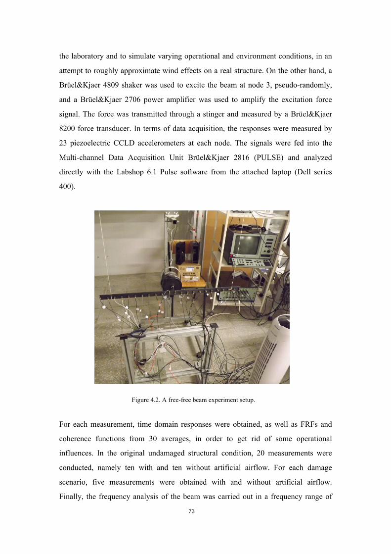
73
the laboratory and to simulate varying operational and environment conditions, in an
attempt to roughly approximate wind effects on a real structure. On the other hand, a
Brüel&Kjaer 4809 shaker was used to excite the beam at node 3, pseudo-randomly,
and a Brüel&Kjaer 2706 power amplifier was used to amplify the excitation force
signal. The force was transmitted through a stinger and measured by a Brüel&Kjaer
8200 force transducer. In terms of data acquisition, the responses were measured by
23 piezoelectric CCLD accelerometers at each node. The signals were fed into the
Multi-channel Data Acquisition Unit Brüel&Kjaer 2816 (PULSE) and analyzed
directly with the Labshop 6.1 Pulse software from the attached laptop (Dell series
400).
Figure 4.2. A free-free beam experiment setup.
For each measurement, time domain responses were obtained, as well as FRFs and
coherence functions from 30 averages, in order to get rid of some operational
influences. In the original undamaged structural condition, 20 measurements were
conducted, namely ten with and ten without artificial airflow. For each damage
scenario, five measurements were obtained with and without artificial airflow.
Finally, the frequency analysis of the beam was carried out in a frequency range of
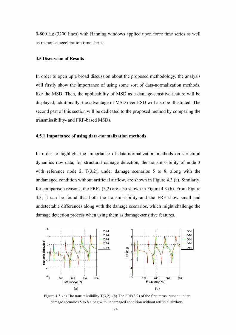
74
0-800 Hz (3200 lines) with Hanning windows applied upon force time series as well
as response acceleration time series.
4.5 Discussion of Results
In order to open up a broad discussion about the proposed methodology, the analysis
will firstly show the importance of using some sort of data-normalization methods,
like the MSD. Then, the applicability of MSD as a damage-sensitive feature will be
displayed; additionally, the advantage of MSD over ESD will also be illustrated. The
second part of this section will be dedicated to the proposed method by comparing the
transmissibility- and FRF-based MSDs.
4.5.1 Importance of using data-normalization methods
In order to highlight the importance of data-normalization methods on structural
dynamics raw data, for structural damage detection, the transmissibility of node 3
with reference node 2, T(3,2), under damage scenarios 5 to 8, along with the
undamaged condition without artificial airflow, are shown in Figure 4.3 (a). Similarly,
for comparison reasons, the FRFs (3,2) are also shown in Figure 4.3 (b). From Figure
4.3, it can be found that both the transmissibility and the FRF show small and
undetectable differences along with the damage scenarios, which might challenge the
damage detection process when using them as damage-sensitive features.
(a) (b)
Figure 4.3. (a) The transmissibility T(3,2); (b) The FRF(3,2) of the first measurement under damage scenarios 5 to 8 along with undamaged condition without artificial airflow.
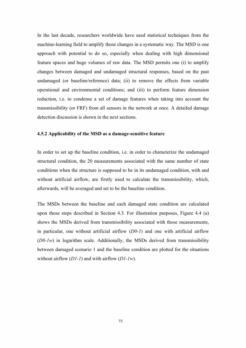
75
In the last decade, researchers worldwide have used statistical techniques from the
machine-learning field to amplify those changes in a systematic way. The MSD is one
approach with potential to do so, especially when dealing with high dimensional
feature spaces and huge volumes of raw data. The MSD permits one (i) to amplify
changes between damaged and undamaged structural responses, based on the past
undamaged (or baseline/reference) data; (ii) to remove the effects from variable
operational and environmental conditions; and (iii) to perform feature dimension
reduction, i.e. to condense a set of damage features when taking into account the
transmissibility (or FRF) from all sensors in the network at once. A detailed damage
detection discussion is shown in the next sections.
4.5.2 Applicability of the MSD as a damage-sensitive feature
In order to set up the baseline condition, i.e. in order to characterize the undamaged
structural condition, the 20 measurements associated with the same number of state
conditions when the structure is supposed to be in its undamaged condition, with and
without artificial airflow, are firstly used to calculate the transmissibility, which,
afterwards, will be averaged and set to be the baseline condition.
The MSDs between the baseline and each damaged state condition are calculated
upon those steps described in Section 4.3. For illustration purposes, Figure 4.4 (a)
shows the MSDs derived from transmissibility associated with those measurements,
in particular, one without artificial airflow (D0-1) and one with artificial airflow
(D0-1w) in logarithm scale. Additionally, the MSDs derived from transmissibility
between damaged scenario 1 and the baseline condition are plotted for the situations
without airflow (D1-1) and with airflow (D1-1w).
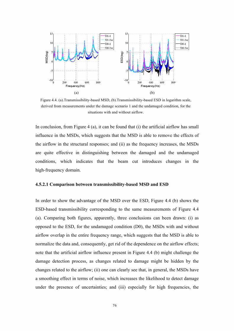
76
(a) (b)
Figure 4.4. (a).Transmissibility-based MSD, (b).Transmissibility-based ESD in logarithm scale, derived from measurements under the damage scenario 1 and the undamaged condition, for the
situations with and without airflow.
In conclusion, from Figure 4 (a), it can be found that (i) the artificial airflow has small
influence in the MSDs, which suggests that the MSD is able to remove the effects of
the airflow in the structural responses; and (ii) as the frequency increases, the MSDs
are quite effective in distinguishing between the damaged and the undamaged
conditions, which indicates that the beam cut introduces changes in the
high-frequency domain.
4.5.2.1 Comparison between transmissibility-based MSD and ESD
In order to show the advantage of the MSD over the ESD, Figure 4.4 (b) shows the
ESD-based transmissibility corresponding to the same measurements of Figure 4.4
(a). Comparing both figures, apparently, three conclusions can been drawn: (i) as
opposed to the ESD, for the undamaged condition (D0), the MSDs with and without
airflow overlap in the entire frequency range, which suggests that the MSD is able to
normalize the data and, consequently, get rid of the dependence on the airflow effects;
note that the artificial airflow influence present in Figure 4.4 (b) might challenge the
damage detection process, as changes related to damage might be hidden by the
changes related to the airflow; (ii) one can clearly see that, in general, the MSDs have
a smoothing effect in terms of noise, which increases the likelihood to detect damage
under the presence of uncertainties; and (iii) especially for high frequencies, the
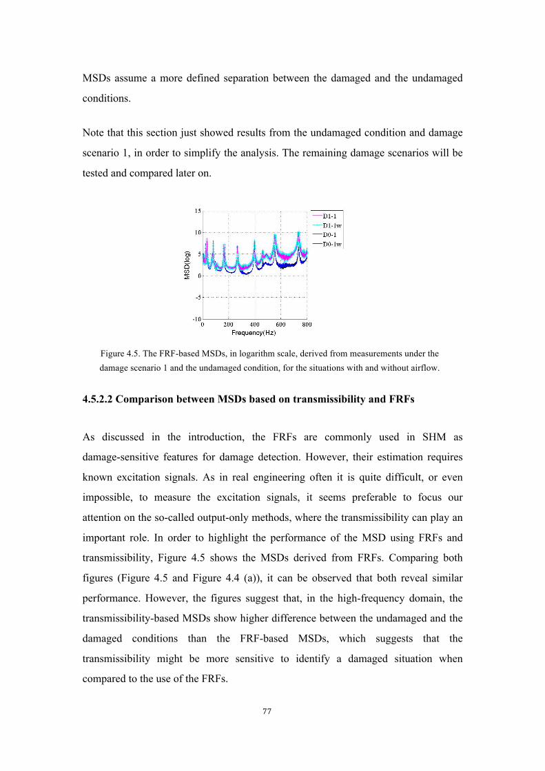
77
MSDs assume a more defined separation between the damaged and the undamaged
conditions.
Note that this section just showed results from the undamaged condition and damage
scenario 1, in order to simplify the analysis. The remaining damage scenarios will be
tested and compared later on.
Figure 4.5. The FRF-based MSDs, in logarithm scale, derived from measurements under the damage scenario 1 and the undamaged condition, for the situations with and without airflow.
4.5.2.2 Comparison between MSDs based on transmissibility and FRFs
As discussed in the introduction, the FRFs are commonly used in SHM as
damage-sensitive features for damage detection. However, their estimation requires
known excitation signals. As in real engineering often it is quite difficult, or even
impossible, to measure the excitation signals, it seems preferable to focus our
attention on the so-called output-only methods, where the transmissibility can play an
important role. In order to highlight the performance of the MSD using FRFs and
transmissibility, Figure 4.5 shows the MSDs derived from FRFs. Comparing both
figures (Figure 4.5 and Figure 4.4 (a)), it can be observed that both reveal similar
performance. However, the figures suggest that, in the high-frequency domain, the
transmissibility-based MSDs show higher difference between the undamaged and the
damaged conditions than the FRF-based MSDs, which suggests that the
transmissibility might be more sensitive to identify a damaged situation when
compared to the use of the FRFs.
78
4.5.3 Applicability of the DDI for damage detection
In accordance with section 3, the DDIs from damage scenarios 1 to 8 are calculated
from the corresponding transmissibility and FRFs, separately. Tables 4.2 and Table
4.3 show, respectively, the percentage of transmissibility-based and FRF-based DDIs
higher than zero in logarithmic scale (i.e. higher than one in linear scale) for all five
state conditions from damage scenarios 1 to 8 without and with artificial airflow.
From a general point of view, one can point out that: (i) in both cases, based on the
percentage of DDIs higher than zero, the method is able to identify correctly all
damage scenarios, i.e. is able to address successfully the first level of the damage
identification hierarchy – damage detection; (ii) the percentage of DDIs higher than
zero is very consistent within each damage scenario, which indicates that the data are
stationary for each damage scenario; (iii) the percentages of DDIs higher than zero
does not change significantly for the situations without and with artificial airflow,
which indicates that the DDIs are almost insensitive to the environmental conditions,
as the MSD is able to remove the effects of the airflow from the data; (iv) for the
damage scenario 3, the percentages of DDIs higher than zero is unexpectedly high
(>11%), when compared to the previous and next damage scenarios; the authors
speculate that this set of data might be strongly influenced by some operational effects
like either shaker instability or human interference during the data acquisition
process; and (v) in general, the percentages of FRF-based DDIs higher than zero are
higher than transmissibility-based DDI, which indicates than, in this case, the
FRF-based approach is more sensitive to identify all the damage scenarios.
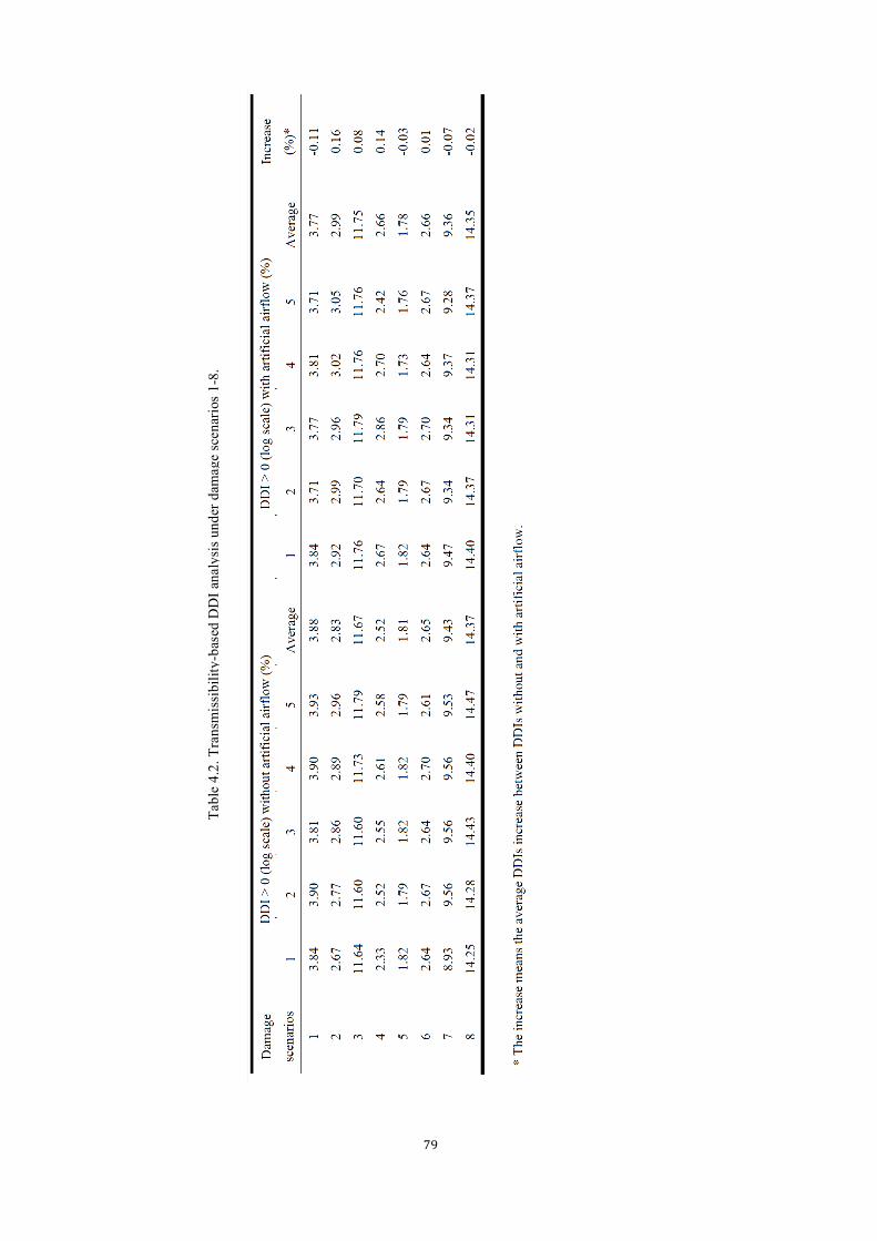
79
Tabl
e 4.
2. T
rans
mis
sibi
lity-
base
d D
DI a
naly
sis u
nder
dam
age
scen
ario
s 1-
8.
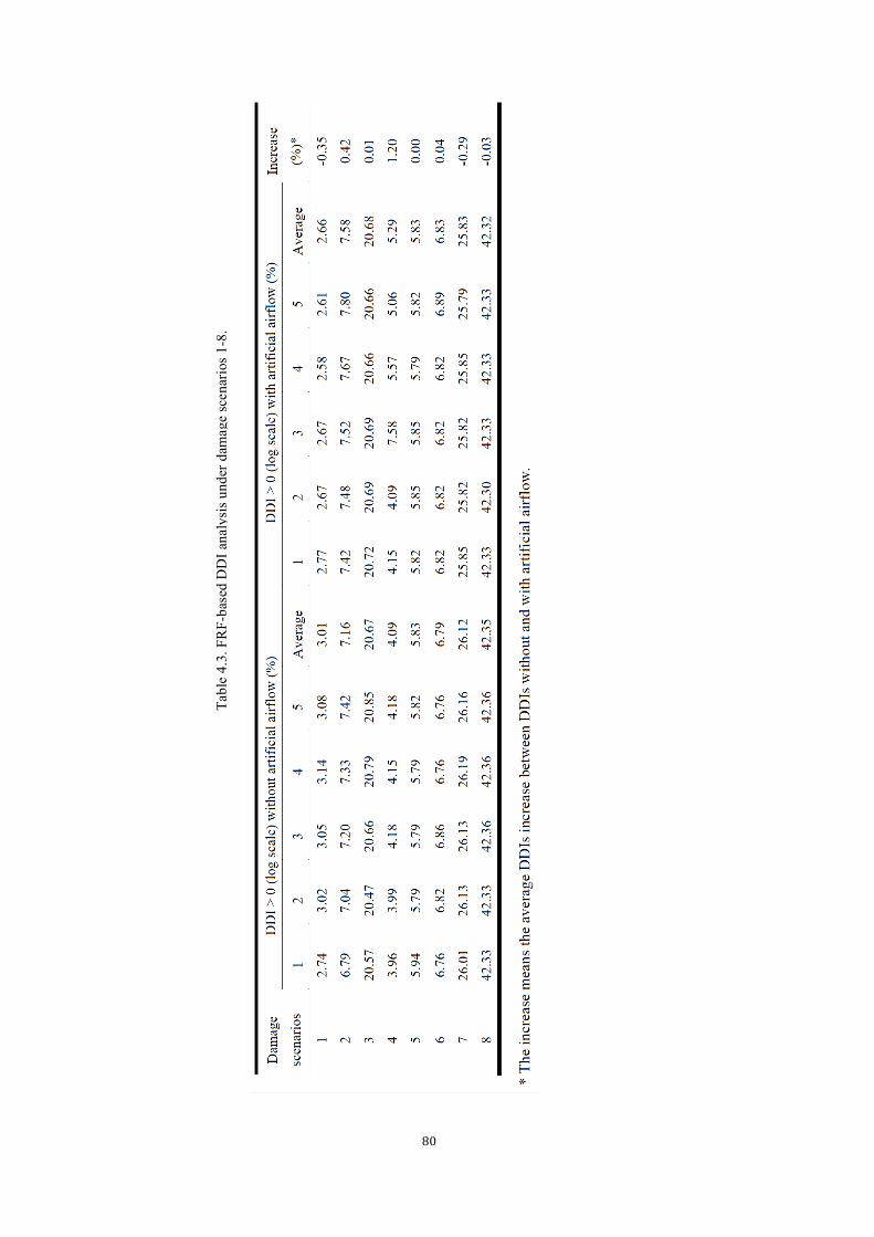
80
Tabl
e 4.
3. F
RF-
base
d D
DI a
naly
sis u
nder
dam
age
scen
ario
s 1-
8.
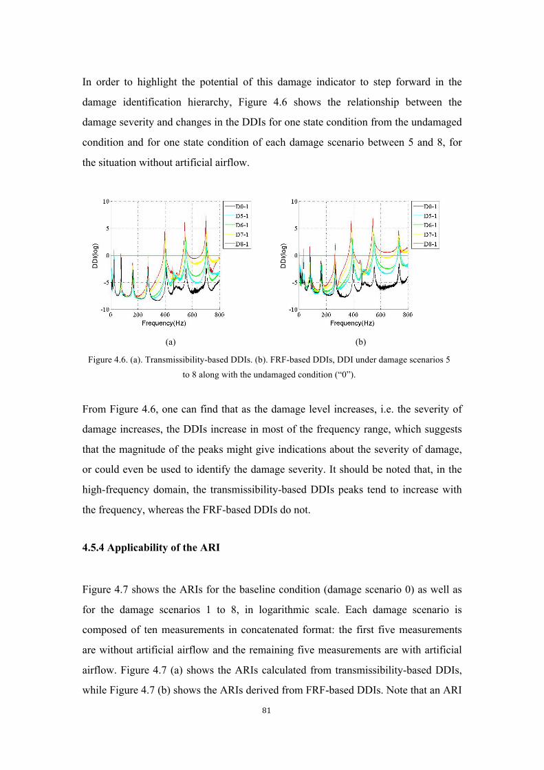
81
In order to highlight the potential of this damage indicator to step forward in the
damage identification hierarchy, Figure 4.6 shows the relationship between the
damage severity and changes in the DDIs for one state condition from the undamaged
condition and for one state condition of each damage scenario between 5 and 8, for
the situation without artificial airflow.
(a) (b)
Figure 4.6. (a). Transmissibility-based DDIs. (b). FRF-based DDIs, DDI under damage scenarios 5
to 8 along with the undamaged condition (“0”).
From Figure 4.6, one can find that as the damage level increases, i.e. the severity of
damage increases, the DDIs increase in most of the frequency range, which suggests
that the magnitude of the peaks might give indications about the severity of damage,
or could even be used to identify the damage severity. It should be noted that, in the
high-frequency domain, the transmissibility-based DDIs peaks tend to increase with
the frequency, whereas the FRF-based DDIs do not.
4.5.4 Applicability of the ARI
Figure 4.7 shows the ARIs for the baseline condition (damage scenario 0) as well as
for the damage scenarios 1 to 8, in logarithmic scale. Each damage scenario is
composed of ten measurements in concatenated format: the first five measurements
are without artificial airflow and the remaining five measurements are with artificial
airflow. Figure 4.7 (a) shows the ARIs calculated from transmissibility-based DDIs,
while Figure 4.7 (b) shows the ARIs derived from FRF-based DDIs. Note that an ARI
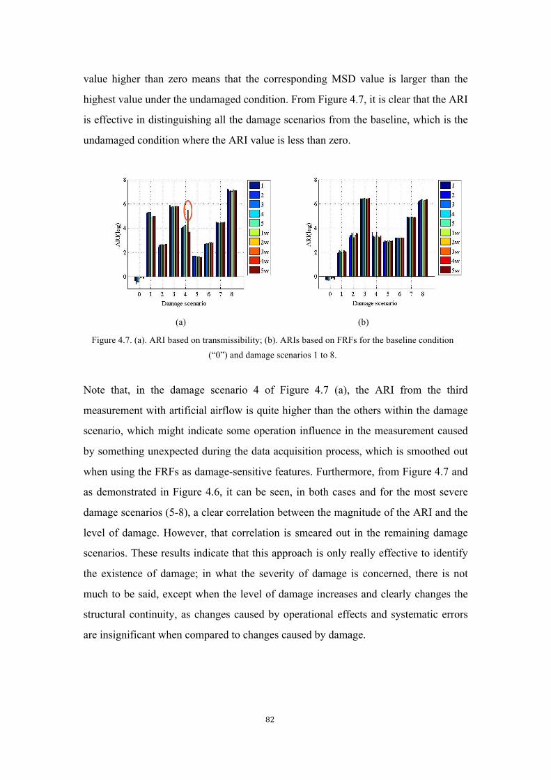
82
value higher than zero means that the corresponding MSD value is larger than the
highest value under the undamaged condition. From Figure 4.7, it is clear that the ARI
is effective in distinguishing all the damage scenarios from the baseline, which is the
undamaged condition where the ARI value is less than zero.
(a) (b) Figure 4.7. (a). ARI based on transmissibility; (b). ARIs based on FRFs for the baseline condition
(“0”) and damage scenarios 1 to 8.
Note that, in the damage scenario 4 of Figure 4.7 (a), the ARI from the third
measurement with artificial airflow is quite higher than the others within the damage
scenario, which might indicate some operation influence in the measurement caused
by something unexpected during the data acquisition process, which is smoothed out
when using the FRFs as damage-sensitive features. Furthermore, from Figure 4.7 and
as demonstrated in Figure 4.6, it can be seen, in both cases and for the most severe
damage scenarios (5-8), a clear correlation between the magnitude of the ARI and the
level of damage. However, that correlation is smeared out in the remaining damage
scenarios. These results indicate that this approach is only really effective to identify
the existence of damage; in what the severity of damage is concerned, there is not
much to be said, except when the level of damage increases and clearly changes the
structural continuity, as changes caused by operational effects and systematic errors
are insignificant when compared to changes caused by damage.
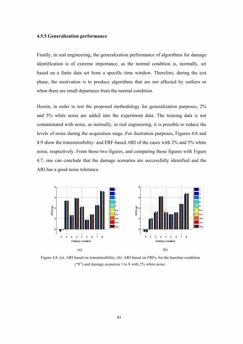
83
4.5.5 Generalization performance
Finally, in real engineering, the generalization performance of algorithms for damage
identification is of extreme importance, as the normal condition is, normally, set
based on a finite data set from a specific time window. Therefore, during the test
phase, the motivation is to produce algorithms that are not affected by outliers or
when there are small departures from the normal condition.
Herein, in order to test the proposed methodology for generalization purposes, 2%
and 5% white noise are added into the experiment data. The training data is not
contaminated with noise, as normally, in real engineering, it is possible to reduce the
levels of noise during the acquisition stage. For ilustration purposes, Figures 4.8 and
4.9 show the transmissibility- and FRF-based ARI of the cases with 2% and 5% white
noise, respectively. From those two figures, and comparing those figures with Figure
4.7, one can conclude that the damage scenarios are successfully identified and the
ARI has a good noise tolerance.
(a) (b) Figure 4.8. (a). ARI based on transmissibility; (b). ARI based on FRFs, for the baseline condition
(“0”) and damage scenarios 1 to 8 with 2% white noise.
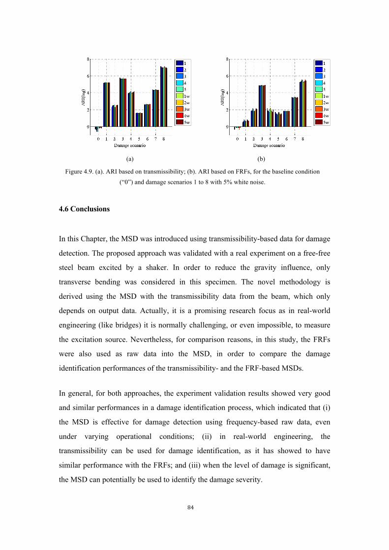
84
(a) (b) Figure 4.9. (a). ARI based on transmissibility; (b). ARI based on FRFs, for the baseline condition
(“0”) and damage scenarios 1 to 8 with 5% white noise.
4.6 Conclusions
In this Chapter, the MSD was introduced using transmissibility-based data for damage
detection. The proposed approach was validated with a real experiment on a free-free
steel beam excited by a shaker. In order to reduce the gravity influence, only
transverse bending was considered in this specimen. The novel methodology is
derived using the MSD with the transmissibility data from the beam, which only
depends on output data. Actually, it is a promising research focus as in real-world
engineering (like bridges) it is normally challenging, or even impossible, to measure
the excitation source. Nevertheless, for comparison reasons, in this study, the FRFs
were also used as raw data into the MSD, in order to compare the damage
identification performances of the transmissibility- and the FRF-based MSDs.
In general, for both approaches, the experiment validation results showed very good
and similar performances in a damage identification process, which indicated that (i)
the MSD is effective for damage detection using frequency-based raw data, even
under varying operational conditions; (ii) in real-world engineering, the
transmissibility can be used for damage identification, as it has showed to have
similar performance with the FRFs; and (iii) when the level of damage is significant,
the MSD can potentially be used to identify the damage severity.
85
In particular, this Chapter permitted one to conclude that the MSD is a very sensitive
and precise data normalization method, as it showed to have a better performance
than the ESD. In fact, the MSD showed to reduce the noise ratio during the damage
detection process. Afterwards, due to the sensitive factor of the MSD, two damage
detection indicators were defined (DDI and ARI) and tested, using both the
transmissibility- and the FRF-based MSD. It was shown that the damage detection
indicators are very sensitive to detect damage, as they were capable and effective to
detect all eight damage scenarios, even under operational and environmental
variability. Even though the ARI showed good generalization performance of the
algorithms, for damage detection, they were not widely efficient to step forward in the
hierarchy of damage identification, namely to identify the severity of damage for all
eight damage scenarios.

86
87
CHAPTER 5 TRANSMISSIBILITY BASED DAMAGE LOCALIZATION AND ASSESSMENT BY INTELLIGENT
ALGORITHM
Summary
In this Chapter, a new transmissibility-based approach for detecting the structural
damage using artificial neural network is presented. Due to its dependence on output
only, PSDT is utilized to draw out damage sensitive indicators according to the
operational response. Afterwards, an artificial neural network is implemented to
construct the interrelation between structural states and the damage sensitive indicators.
Once the neural network is trained, it will be used as a method of damage detection. A
two side-clamped beam simulation is used to test the applicability of the proposed
approach. The results show good performance in damage detection. The main
contribution of this Chapter is to construct a clear interrelation between the power
spectrum density transmissibility-based structural feature and structural state
(undamaged/damaged), and to propose a classifier, i.e. neural network in performing
damage detection. The good predictions obtained from the simulation show its possible
future applicability.
5.1 Introduction
Originally, motivated on avoiding the excitation measurement in real engineering,
transmissibility conception has been raised and related approaches are developed. The
transmissibility function, defined as the frequency-domain ratio between two outputs,
describes the relative admittance between two output measurements and makes possible
the damage detection without any assumption about the nature of the excitations, i.e.
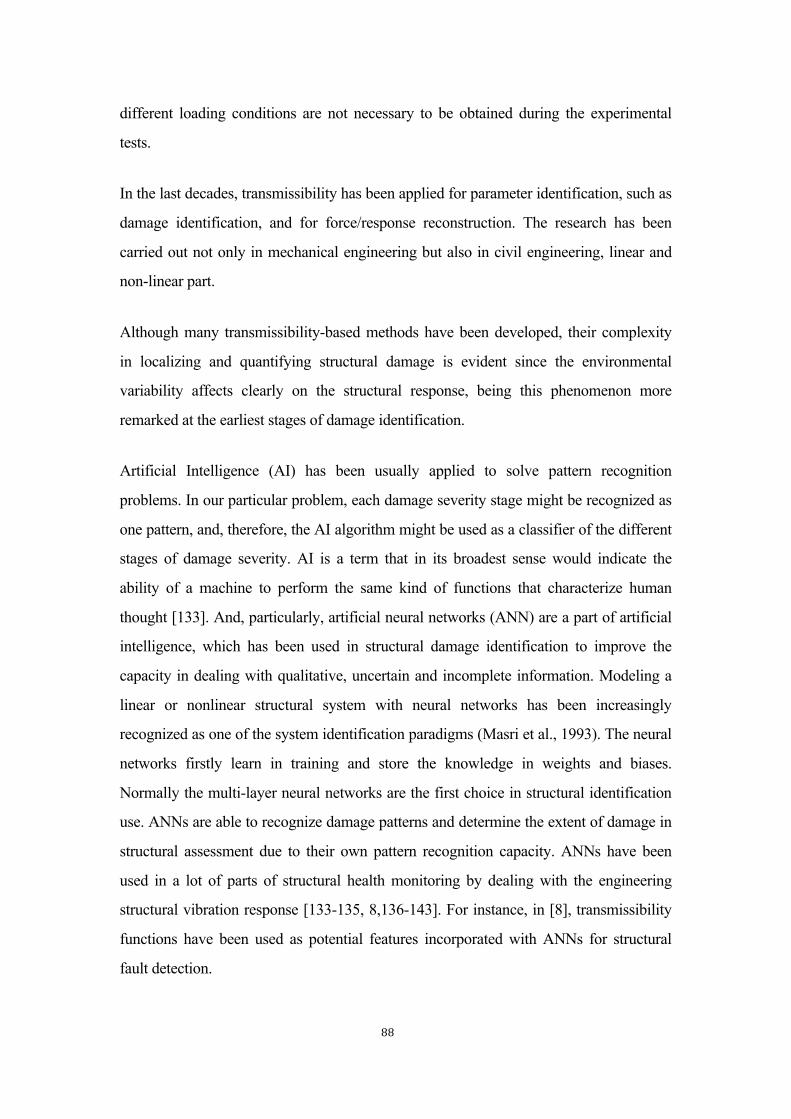
88
different loading conditions are not necessary to be obtained during the experimental
tests.
In the last decades, transmissibility has been applied for parameter identification, such as
damage identification, and for force/response reconstruction. The research has been
carried out not only in mechanical engineering but also in civil engineering, linear and
non-linear part.
Although many transmissibility-based methods have been developed, their complexity
in localizing and quantifying structural damage is evident since the environmental
variability affects clearly on the structural response, being this phenomenon more
remarked at the earliest stages of damage identification.
Artificial Intelligence (AI) has been usually applied to solve pattern recognition
problems. In our particular problem, each damage severity stage might be recognized as
one pattern, and, therefore, the AI algorithm might be used as a classifier of the different
stages of damage severity. AI is a term that in its broadest sense would indicate the
ability of a machine to perform the same kind of functions that characterize human
thought [133]. And, particularly, artificial neural networks (ANN) are a part of artificial
intelligence, which has been used in structural damage identification to improve the
capacity in dealing with qualitative, uncertain and incomplete information. Modeling a
linear or nonlinear structural system with neural networks has been increasingly
recognized as one of the system identification paradigms (Masri et al., 1993). The neural
networks firstly learn in training and store the knowledge in weights and biases.
Normally the multi-layer neural networks are the first choice in structural identification
use. ANNs are able to recognize damage patterns and determine the extent of damage in
structural assessment due to their own pattern recognition capacity. ANNs have been
used in a lot of parts of structural health monitoring by dealing with the engineering
structural vibration response [133-135, 8,136-143]. For instance, in [8], transmissibility
functions have been used as potential features incorporated with ANNs for structural
fault detection.
89
In this chapter, a new ANN based damage detection approach by using PSDT is
proposed directly from the forced vibration frequency-domain response. PSDT is
extracted after choosing a reference point via the vibration response, and later it is
averaged according to different references; afterwards, by using averaged PSDT,
damage indicators can be obtained. Therefore, defining the undamaged structural state as
baseline, parameters sensitive to damage, such as averaged PSDT, are chosen as input to
the network. The outputs or targets of the network will be the damage indicators,
which give the information about the existence of damage and its severity. To reach this
purpose, the ANN should be suitably trained by using different training patterns, for
which the input and output values to the network are defined.
5.2 Theoretical background
5.2.1 ANN
ANNs are networks of artificial neurons that suitably trained, constitute crude
approximations to the mechanism of working of the human brain. Hopfield [144]
made the mathematical foundation for studying the neural networks in 1982. And
later, Hopfield and Tank illustrated the application of the Hopfield network to the
travelling salesman problem in 1985. Kohonen [145] proposed unsupervised learning
networks for feature mapping into regular arrays of neurons.
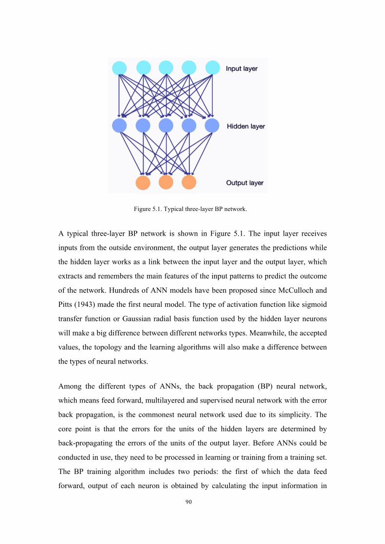
90
Figure 5.1. Typical three-layer BP network.
A typical three-layer BP network is shown in Figure 5.1. The input layer receives
inputs from the outside environment, the output layer generates the predictions while
the hidden layer works as a link between the input layer and the output layer, which
extracts and remembers the main features of the input patterns to predict the outcome
of the network. Hundreds of ANN models have been proposed since McCulloch and
Pitts (1943) made the first neural model. The type of activation function like sigmoid
transfer function or Gaussian radial basis function used by the hidden layer neurons
will make a big difference between different networks types. Meanwhile, the accepted
values, the topology and the learning algorithms will also make a difference between
the types of neural networks.
Among the different types of ANNs, the back propagation (BP) neural network,
which means feed forward, multilayered and supervised neural network with the error
back propagation, is the commonest neural network used due to its simplicity. The
core point is that the errors for the units of the hidden layers are determined by
back-propagating the errors of the units of the output layer. Before ANNs could be
conducted in use, they need to be processed in learning or training from a training set.
The BP training algorithm includes two periods: the first of which the data feed
forward, output of each neuron is obtained by calculating the input information in
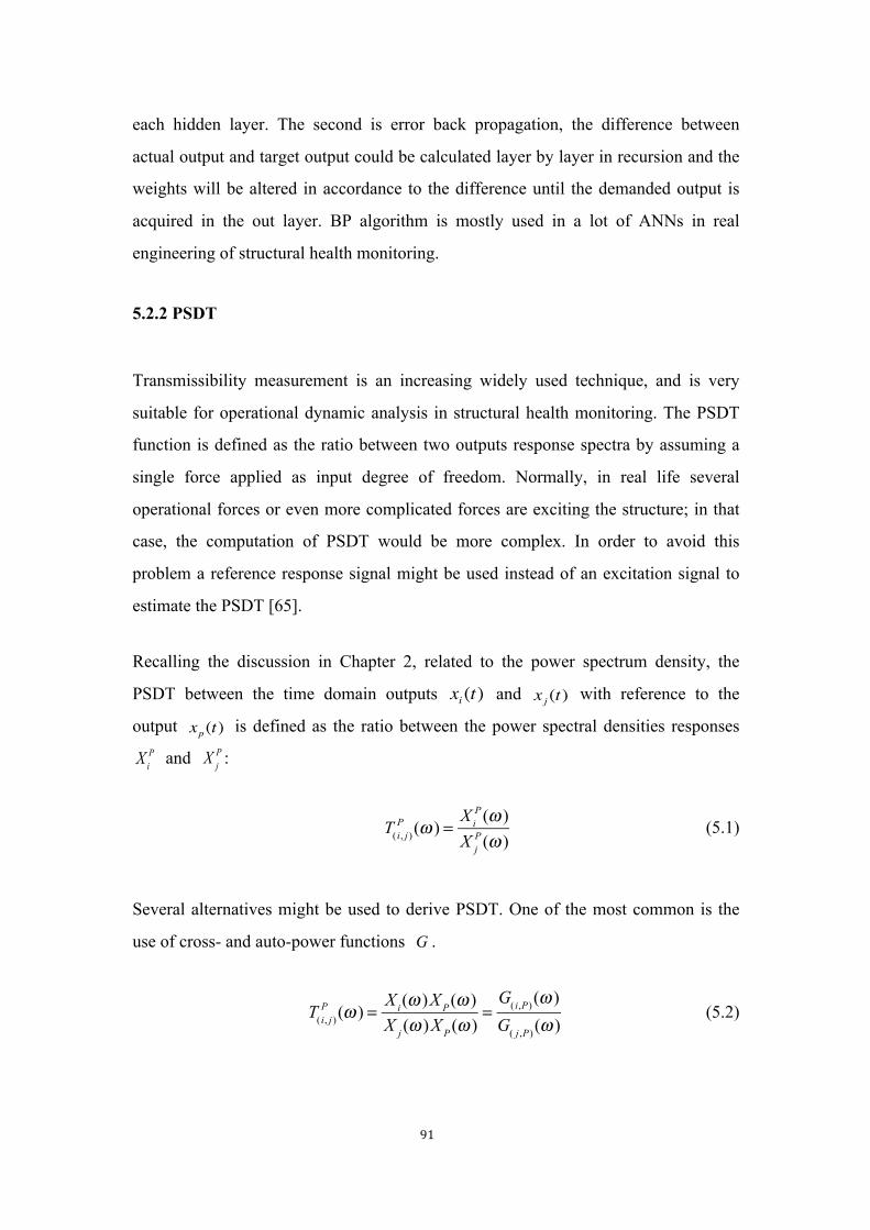
91
each hidden layer. The second is error back propagation, the difference between
actual output and target output could be calculated layer by layer in recursion and the
weights will be altered in accordance to the difference until the demanded output is
acquired in the out layer. BP algorithm is mostly used in a lot of ANNs in real
engineering of structural health monitoring.
5.2.2 PSDT
Transmissibility measurement is an increasing widely used technique, and is very
suitable for operational dynamic analysis in structural health monitoring. The PSDT
function is defined as the ratio between two outputs response spectra by assuming a
single force applied as input degree of freedom. Normally, in real life several
operational forces or even more complicated forces are exciting the structure; in that
case, the computation of PSDT would be more complex. In order to avoid this
problem a reference response signal might be used instead of an excitation signal to
estimate the PSDT [65].
Recalling the discussion in Chapter 2, related to the power spectrum density, the
PSDT between the time domain outputs xi (t) and x j (t) with reference to the
output xp (t) is defined as the ratio between the power spectral densities responses
XiP and
X jP :
T( i, j )
P (ω ) =Xi
P(ω )X j
P(ω ) (5.1)
Several alternatives might be used to derive PSDT. One of the most common is the
use of cross- and auto-power functions G .
T( i, j )
P (ω ) =Xi(ω )X P(ω )X j (ω )X P(ω )
=G( i,P) (ω )G( j ,P) (ω )
(5.2)
92
5.3 Parameters for ANN
The fundamental framework of implementation of an ANN can be divided into three
stages: training, validation, and testing. Before doing that, the architecture and the input
and output parameters of the network should be chosen conveniently.
5.3.1 Inputs for ANN
Step 1: Transmissibility Power Mode Shape (TPMS). The transmissibility at the system
poles agrees with values of the mode shape ratios, i.e. the values of the T(i, j) at the system
poles are directly related to the scalar operational mode-shape values φiv and φjv.
Therefore, once the resonant frequencies are identified through ANITSF, it is also
possible to identify the operational mode shape vectors from different PSDTs. By
choosing a fixed reference DOF j and giving φjv a normalized value of unit, the full
unscaled mode-shape (operational deflection) vector (φ1v, φ2v, …, 1, … , φKv) can be
constructed from the PSDT vector (T(1, j), T(2, j), …, 1, …, T(K, j)). Then, by analogy with
the concept of power mode shape presented in [85], a new concept of TPMS might be
defined from the PSDT in the following way:
TPMSi
v = T( i, j ) (ω )ωv1
ωv 2∫ dω (5.3)
where viTPMS is the ith component of the vth transmissibility power mode shape; and
[ωv1, ωv2] is the integrated frequency bandwidth for the vth TPMS. As shown in Figure
5.2, the integration area is around the peak value, however, this step depends on the
experience, which can highly influence the results.
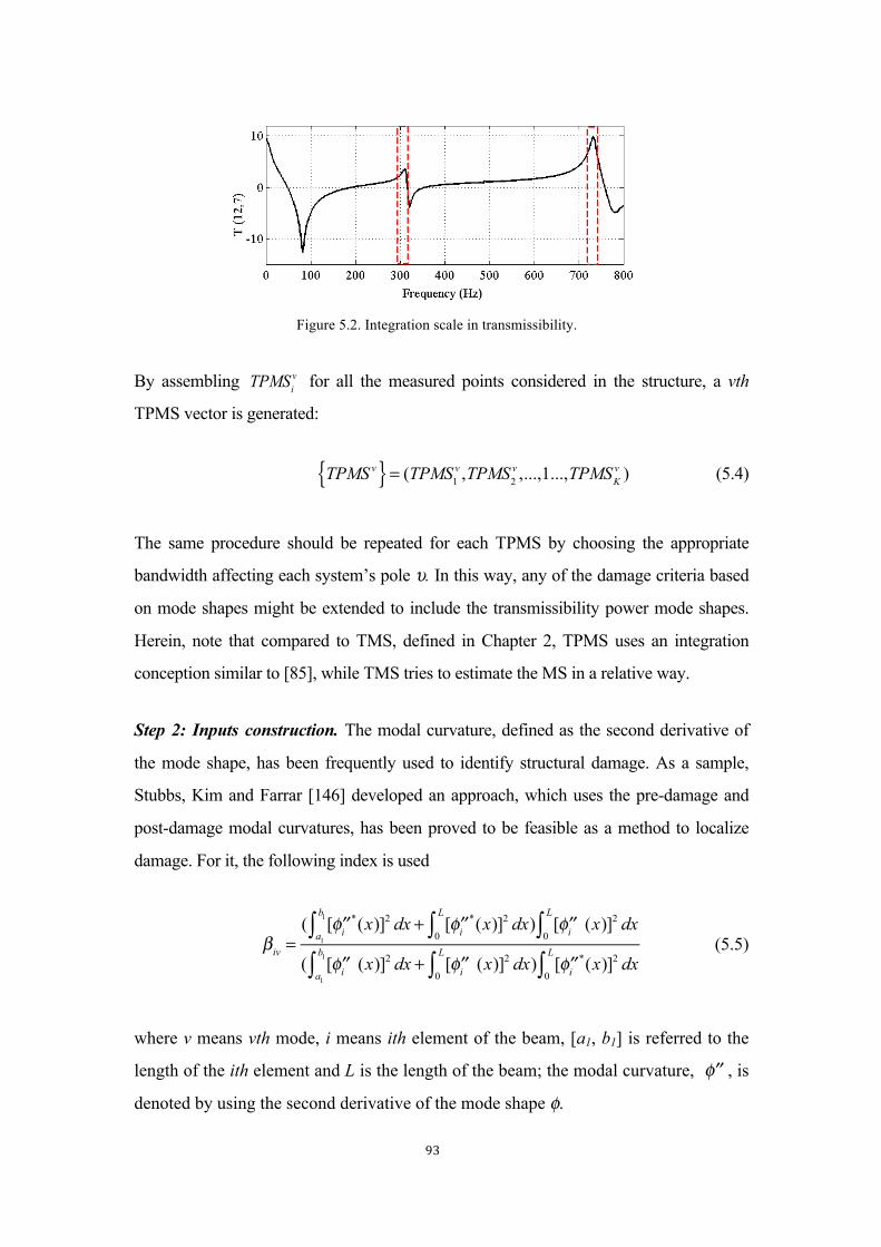
93
Figure 5.2. Integration scale in transmissibility.
By assembling TPMSiv for all the measured points considered in the structure, a vth
TPMS vector is generated:
TPMS v{ } = (TPMS1v ,TPMS2
v ,...,1...,TPMSKv ) (5.4)
The same procedure should be repeated for each TPMS by choosing the appropriate
bandwidth affecting each system’s pole υ. In this way, any of the damage criteria based
on mode shapes might be extended to include the transmissibility power mode shapes.
Herein, note that compared to TMS, defined in Chapter 2, TPMS uses an integration
conception similar to [85], while TMS tries to estimate the MS in a relative way.
Step 2: Inputs construction. The modal curvature, defined as the second derivative of
the mode shape, has been frequently used to identify structural damage. As a sample,
Stubbs, Kim and Farrar [146] developed an approach, which uses the pre-damage and
post-damage modal curvatures, has been proved to be feasible as a method to localize
damage. For it, the following index is used
βiv =( [ ′′φi
*(x)]2 dx + [ ′′φi*(x)]2 dx) [ ′′φi (x)]2 dx
0
L
∫0
L
∫a1
b1∫( [ ′′φi (x)]2 dx + [ ′′φi (x)]2 dx) [ ′′φi
*(x)]2 dx0
L
∫0
L
∫a1
b1∫ (5.5)
where v means vth mode, i means ith element of the beam, [a1, b1] is referred to the
length of the ith element and L is the length of the beam; the modal curvature, ′′φ , is
denoted by using the second derivative of the mode shape φ.
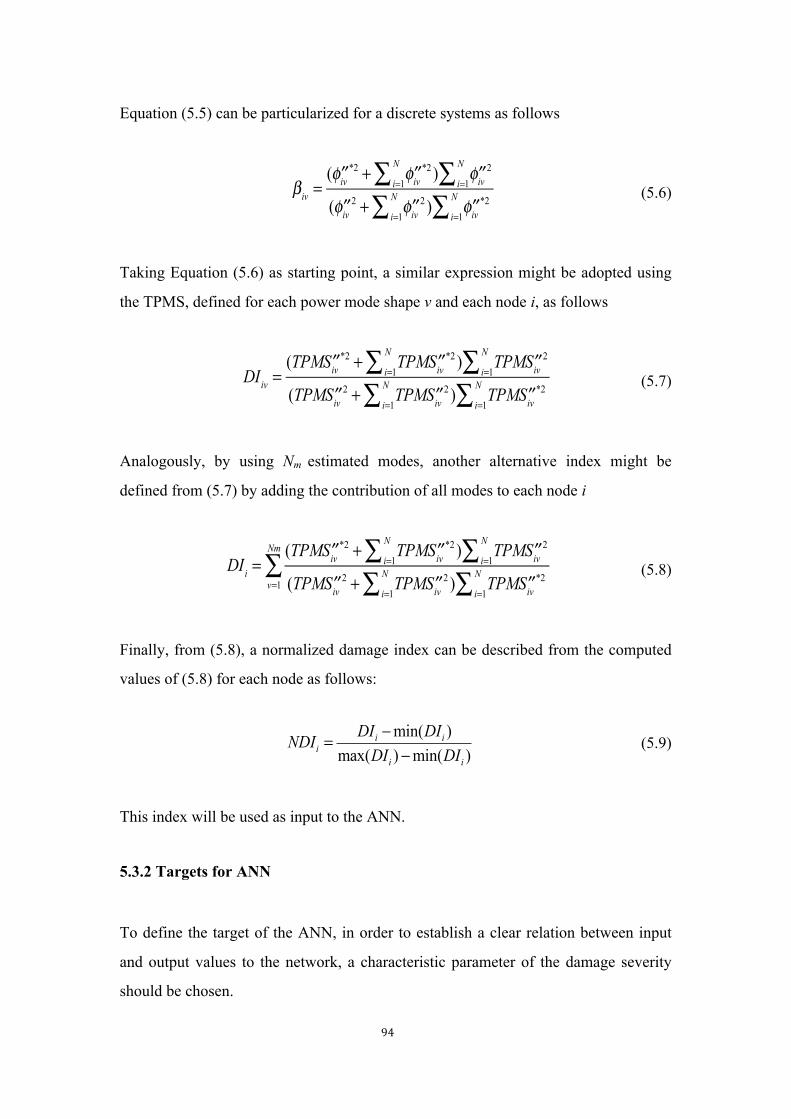
94
Equation (5.5) can be particularized for a discrete systems as follows
βiv =( ′′φiv
*2 + ′′φiv*2 ) ′′φiv
2i=1
N∑i=1
N∑( ′′φiv
2 + ′′φiv2 ) ′′φiv
*2i=1
N∑i=1
N∑ (5.6)
Taking Equation (5.6) as starting point, a similar expression might be adopted using
the TPMS, defined for each power mode shape v and each node i, as follows
DIiv =(TPM ′′Siv
*2 + TPM ′′Siv*2 ) TPM ′′Siv
2i=1
N∑i=1
N∑(TPM ′′Siv
2 + TPM ′′Siv2 ) TPM ′′Siv
*2i=1
N∑i=1
N∑ (5.7)
Analogously, by using Nm estimated modes, another alternative index might be
defined from (5.7) by adding the contribution of all modes to each node i
DIi =(TPM ′′Siv
*2 + TPM ′′Siv*2 ) TPM ′′Siv
2i=1
N∑i=1
N∑(TPM ′′Siv
2 + TPM ′′Siv2 ) TPM ′′Siv
*2i=1
N∑i=1
N∑v=1
Nm
∑ (5.8)
Finally, from (5.8), a normalized damage index can be described from the computed
values of (5.8) for each node as follows:
min( )max( ) min( )
i ii
i i
DI DINDIDI DI−=
− (5.9)
This index will be used as input to the ANN.
5.3.2 Targets for ANN
To define the target of the ANN, in order to establish a clear relation between input
and output values to the network, a characteristic parameter of the damage severity
should be chosen.
95
Figure 5.3. Damage model for a saw cut.
Figure 5.3 shows the damage model of a saw cut in a beam structure. To characterize
the damage severity, the following indicator might be used
severity = 1− (dL)3 (5.10)
Therefore, the target of the ANN can be set as follows
Tar =severity1
...severityNele
⎧
⎨⎪
⎩⎪
⎫
⎬⎪
⎭⎪
(5.11)
where Nele is the number of the elements in the structural system. In the study case,
Nele is defined to be equal to 20.
In order to localize the structural damage and increase the effectiveness of the ANN,
as described above, one can divide the structure into several parts, and assign to each
part a single indicator; one way of doing this is to sum all the element severities
included within each part as a target. For example, in our special case, the beam might
be divided into four parts or regions on average (Part I, Part II, Part III and Part IV,
detailed description can be referred to section 5.4). Within each region, a new damage
severity (SeverityI, SeverityII, SeverityIII, and SeverityIV) is defined by computing the
average of the severities of the elements included into it. These severities defined on
the regions are used as targets of the ANN. For the particular case shown in Figure
5.5, the target will be as follows
96
Tar =
Severity I
Severity II
Severity III
Severity IV
⎧
⎨⎪⎪
⎩⎪⎪
⎫
⎬⎪⎪
⎭⎪⎪
=
1N D1
severityw1
w1=1
5
∑1
N D2
severityw1
w1=6
10
∑1
N D3
severityw1
w1=11
15
∑1
N D4
severityw1
w1=16
20
∑
⎧
⎨
⎪⎪⎪⎪⎪
⎩
⎪⎪⎪⎪⎪
⎫
⎬
⎪⎪⎪⎪⎪
⎭
⎪⎪⎪⎪⎪
(5.12)
where ND1, ND2, ND3 and ND4 are the number of damaged elements belonging to each
region. A special case is the case with no damage, considering ND is denominator,
then it is defined that when no damage occurs, ND1=ND2= ND3= ND4=1. Then, for
instance, in our study, if single damage element occurs only in part I, then ND1=1,
ND2= ND3= ND4=1. If double damage elements occur only in Part II, then ND2=2, ND1=
ND3= ND4=1. This will result in that the target ranges in [0, 1], where ‘0’ means no
damage, ‘1’ means complete damage occurrence in the element.
During real calculation, one needs to firstly calculate the severity of each structural
area in order to give a final prediction about the severity of the structure.
5.3.3 ANN construction
Previous research has proven that multilayer-perceptron ANNs are feasible in pattern
recognition problems, such as damage detection [136, 137, 140]. Earlier studies of ANN
based methodologies mainly concentrate on using different ANN architectures, by
varying the number of inputs as well as outputs in order to obtain a better performance.
However, this kind of work has a critical shortcoming, within which the interrelation of
each input will be too complex to interpret and therefore it will require high computation
time, and reduce the effectiveness of the methodology. Motivated on solving a crates
damage detection problem in beverages, in [143], single- and dual-sensor-systems were
developed, in which each sensor performs as an individual ANN, and
dual-sensor-systems represent two single sensor working together as two inputs in the
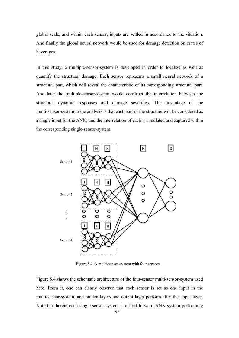
97
global scale, and within each sensor, inputs are settled in accordance to the situation.
And finally the global neural network would be used for damage detection on crates of
beverages.
In this study, a multiple-sensor-system is developed in order to localize as well as
quantify the structural damage. Each sensor represents a small neural network of a
structural part, which will reveal the characteristic of its corresponding structural part.
And later the multiple-sensor-system would construct the interrelation between the
structural dynamic responses and damage severities. The advantage of the
multi-sensor-system to the analysis is that each part of the structure will be considered as
a single input for the ANN, and the interrelation of each is simulated and captured within
the corresponding single-sensor-system.
Figure 5.4. A multi-sensor-system with four sensors.
Figure 5.4 shows the schematic architecture of the four-sensor multi-sensor-system used
here. From it, one can clearly observe that each sensor is set as one input in the
multi-sensor-system, and hidden layers and output layer perform after this input layer.
Note that herein each single-sensor-system is a feed-forward ANN system performing
!!!!!!!!!!
I� HH
I� HH
I� HH
OH
!!!!!!!!!!
!!!!!!!!!!
Sensor 1�
Sensor 2�
Sensor 4�
.
.
.�

98
for each part (Part I, Part II, Part III and Part IV), and BP algorithm is utilized. Three
layers of input, hidden and output layer constitute the single system.
This multi-sensor-system represents a different idea compared to the traditional ANN,
which treats the single-sensor-system as one input, and four single-sensor-systems make
a multi-sensor-system; within the multi-sensor-system, no connection between different
single-sensor-system exists, which will avoid the interaction influence between them. In
addition, due to the fact that each sensor of the multi-sensor-system reveals the
characteristic of the corresponding structural part, the multi-sensor-system might be used
to localize the structural damage.
As to identifying the damage, Figure 5.5 gives a flowchart of the damage detection
procedure, where note that to ANN, training and testing are very important steps before
giving a good prediction work. Note that the dot line is only for training and testing
phase.
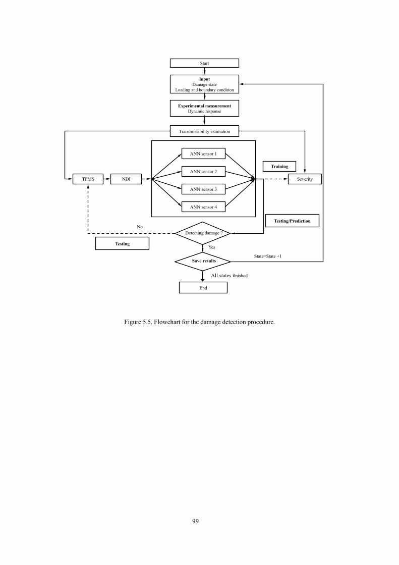
99
Figure 5.5. Flowchart for the damage detection procedure.
7
Transmissibility estimation
Experimental measurement Dynamic response
TPMS
Detecting damage ?
Yes
State=State +1
End
No
Save results
All states finished
Input Damage state
Loading and boundary condition
Start
ANN sensor 1
ANN sensor 2
ANN sensor 3
ANN sensor 4
Severity NDI
Training
Testing/Prediction
Testing
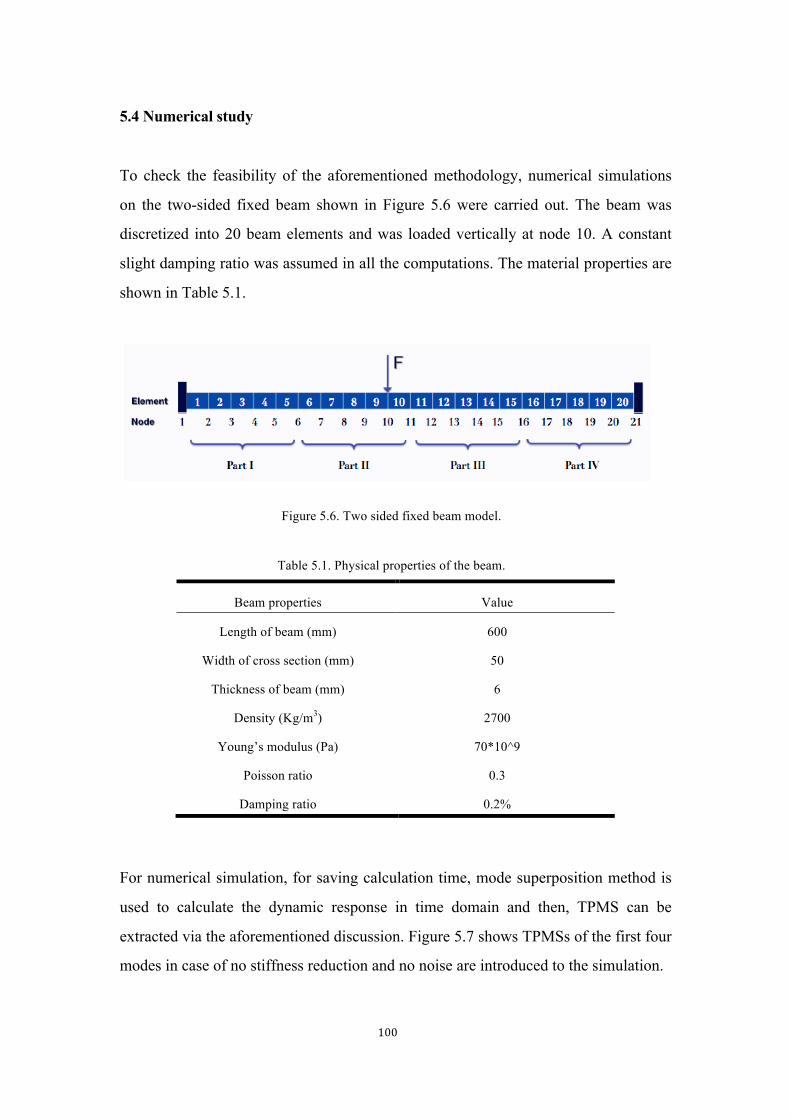
100
5.4 Numerical study
To check the feasibility of the aforementioned methodology, numerical simulations
on the two-sided fixed beam shown in Figure 5.6 were carried out. The beam was
discretized into 20 beam elements and was loaded vertically at node 10. A constant
slight damping ratio was assumed in all the computations. The material properties are
shown in Table 5.1.
Figure 5.6. Two sided fixed beam model.
Table 5.1. Physical properties of the beam.
Beam properties Value
Length of beam (mm) 600
Width of cross section (mm) 50
Thickness of beam (mm) 6
Density (Kg/m3) 2700
Young’s modulus (Pa) 70*10^9
Poisson ratio 0.3
Damping ratio 0.2%
For numerical simulation, for saving calculation time, mode superposition method is
used to calculate the dynamic response in time domain and then, TPMS can be
extracted via the aforementioned discussion. Figure 5.7 shows TPMSs of the first four
modes in case of no stiffness reduction and no noise are introduced to the simulation.
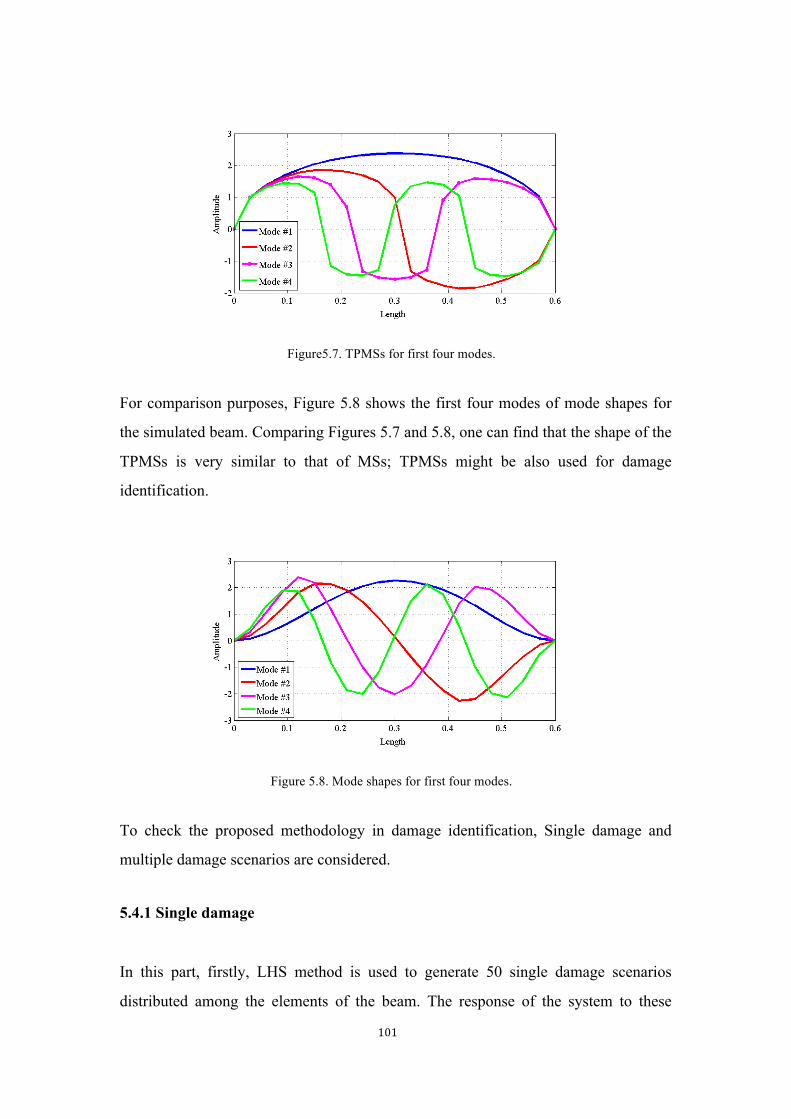
101
Figure5.7. TPMSs for first four modes.
For comparison purposes, Figure 5.8 shows the first four modes of mode shapes for
the simulated beam. Comparing Figures 5.7 and 5.8, one can find that the shape of the
TPMSs is very similar to that of MSs; TPMSs might be also used for damage
identification.
Figure 5.8. Mode shapes for first four modes.
To check the proposed methodology in damage identification, Single damage and
multiple damage scenarios are considered.
5.4.1 Single damage
In this part, firstly, LHS method is used to generate 50 single damage scenarios
distributed among the elements of the beam. The response of the system to these
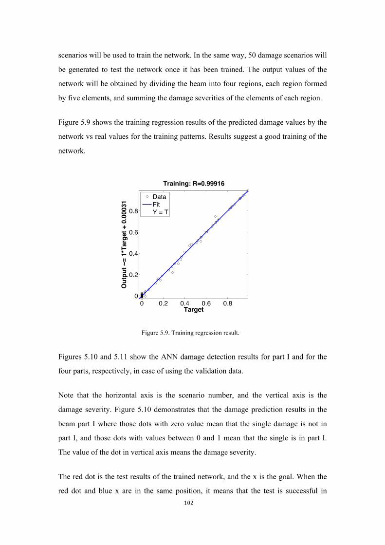
102
scenarios will be used to train the network. In the same way, 50 damage scenarios will
be generated to test the network once it has been trained. The output values of the
network will be obtained by dividing the beam into four regions, each region formed
by five elements, and summing the damage severities of the elements of each region.
Figure 5.9 shows the training regression results of the predicted damage values by the
network vs real values for the training patterns. Results suggest a good training of the
network.
Figure 5.9. Training regression result.
Figures 5.10 and 5.11 show the ANN damage detection results for part I and for the
four parts, respectively, in case of using the validation data.
Note that the horizontal axis is the scenario number, and the vertical axis is the
damage severity. Figure 5.10 demonstrates that the damage prediction results in the
beam part I where those dots with zero value mean that the single damage is not in
part I, and those dots with values between 0 and 1 mean that the single is in part I.
The value of the dot in vertical axis means the damage severity.
The red dot is the test results of the trained network, and the x is the goal. When the
red dot and blue x are in the same position, it means that the test is successful in
0 0.2 0.4 0.6 0.80
0.2
0.4
0.6
0.8
Target
Out
put ~
= 1*
Targ
et +
0.0
0031
Training: R=0.99916
DataFitY = T
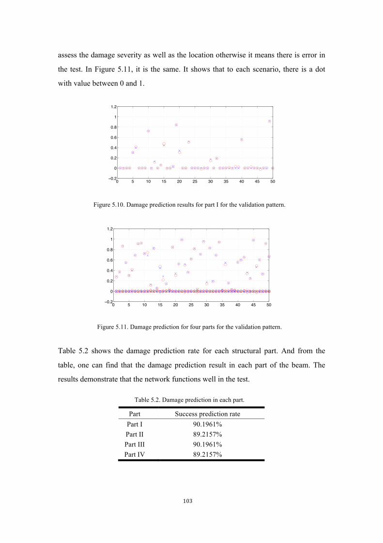
103
assess the damage severity as well as the location otherwise it means there is error in
the test. In Figure 5.11, it is the same. It shows that to each scenario, there is a dot
with value between 0 and 1.
Figure 5.10. Damage prediction results for part I for the validation pattern.
Figure 5.11. Damage prediction for four parts for the validation pattern.
Table 5.2 shows the damage prediction rate for each structural part. And from the
table, one can find that the damage prediction result in each part of the beam. The
results demonstrate that the network functions well in the test.
Table 5.2. Damage prediction in each part.
Part Success prediction rate Part I 90.1961% Part II 89.2157% Part III 90.1961% Part IV 89.2157%
0 5 10 15 20 25 30 35 40 45 50−0.2
0
0.2
0.4
0.6
0.8
1
1.2
0 5 10 15 20 25 30 35 40 45 50−0.2
0
0.2
0.4
0.6
0.8
1
1.2
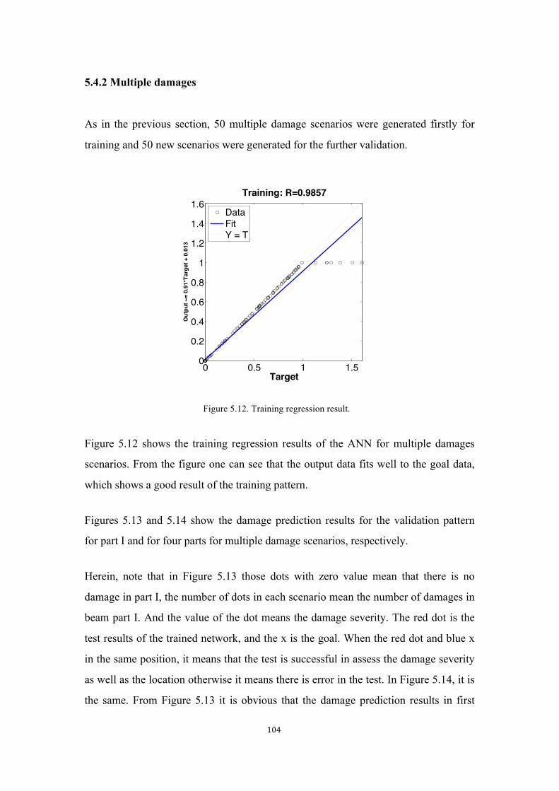
104
5.4.2 Multiple damages
As in the previous section, 50 multiple damage scenarios were generated firstly for
training and 50 new scenarios were generated for the further validation.
Figure 5.12. Training regression result.
Figure 5.12 shows the training regression results of the ANN for multiple damages
scenarios. From the figure one can see that the output data fits well to the goal data,
which shows a good result of the training pattern.
Figures 5.13 and 5.14 show the damage prediction results for the validation pattern
for part I and for four parts for multiple damage scenarios, respectively.
Herein, note that in Figure 5.13 those dots with zero value mean that there is no
damage in part I, the number of dots in each scenario mean the number of damages in
beam part I. And the value of the dot means the damage severity. The red dot is the
test results of the trained network, and the x is the goal. When the red dot and blue x
in the same position, it means that the test is successful in assess the damage severity
as well as the location otherwise it means there is error in the test. In Figure 5.14, it is
the same. From Figure 5.13 it is obvious that the damage prediction results in first
0 0.5 1 1.50
0.2
0.4
0.6
0.8
1
1.2
1.4
1.6
Target
Out
put ~
= 0.
91*T
arge
t + 0
.013
Training: R=0.9857
DataFitY = T
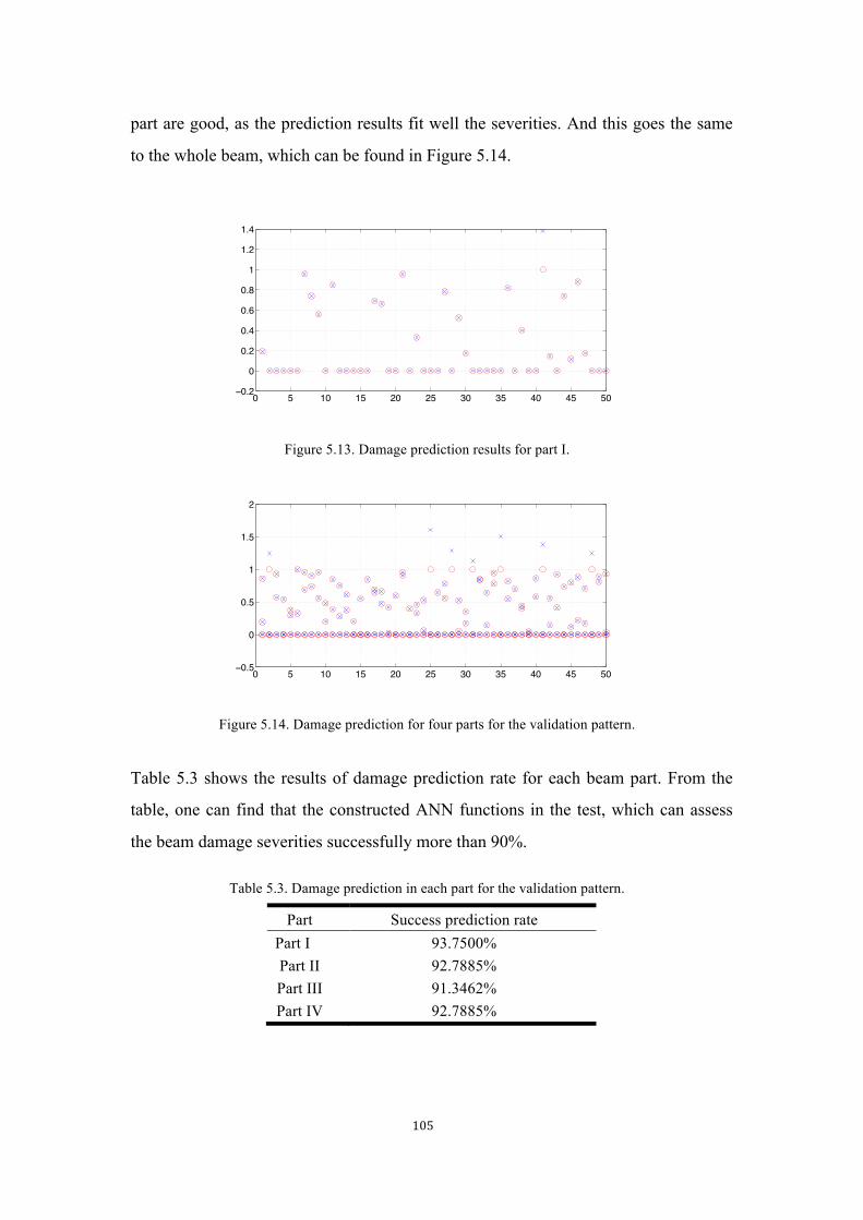
105
part are good, as the prediction results fit well the severities. And this goes the same
to the whole beam, which can be found in Figure 5.14.
Figure 5.13. Damage prediction results for part I.
Figure 5.14. Damage prediction for four parts for the validation pattern.
Table 5.3 shows the results of damage prediction rate for each beam part. From the
table, one can find that the constructed ANN functions in the test, which can assess
the beam damage severities successfully more than 90%.
Table 5.3. Damage prediction in each part for the validation pattern.
Part Success prediction rate Part I 93.7500% Part II 92.7885% Part III 91.3462% Part IV 92.7885%
0 5 10 15 20 25 30 35 40 45 50−0.2
0
0.2
0.4
0.6
0.8
1
1.2
1.4
0 5 10 15 20 25 30 35 40 45 50−0.5
0
0.5
1
1.5
2
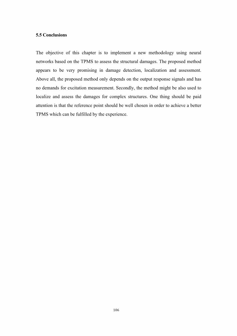
106
5.5 Conclusions
The objective of this chapter is to implement a new methodology using neural
networks based on the TPMS to assess the structural damages. The proposed method
appears to be very promising in damage detection, localization and assessment.
Above all, the proposed method only depends on the output response signals and has
no demands for excitation measurement. Secondly, the method might be also used to
localize and assess the damages for complex structures. One thing should be paid
attention is that the reference point should be well chosen in order to achieve a better
TPMS which can be fulfilled by the experience.
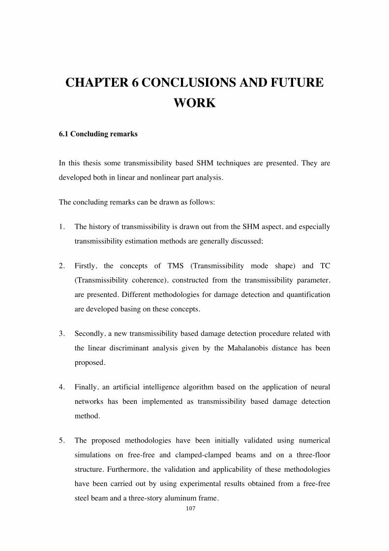
107
CHAPTER 6 CONCLUSIONS AND FUTURE WORK
6.1 Concluding remarks
In this thesis some transmissibility based SHM techniques are presented. They are
developed both in linear and nonlinear part analysis.
The concluding remarks can be drawn as follows:
1. The history of transmissibility is drawn out from the SHM aspect, and especially
transmissibility estimation methods are generally discussed;
2. Firstly, the concepts of TMS (Transmissibility mode shape) and TC
(Transmissibility coherence), constructed from the transmissibility parameter,
are presented. Different methodologies for damage detection and quantification
are developed basing on these concepts.
3. Secondly, a new transmissibility based damage detection procedure related with
the linear discriminant analysis given by the Mahalanobis distance has been
proposed.
4. Finally, an artificial intelligence algorithm based on the application of neural
networks has been implemented as transmissibility based damage detection
method.
5. The proposed methodologies have been initially validated using numerical
simulations on free-free and clamped-clamped beams and on a three-floor
structure. Furthermore, the validation and applicability of these methodologies
have been carried out by using experimental results obtained from a free-free
steel beam and a three-story aluminum frame.
108
6. The results from both simulations and experiments reveal good performance of
the methodologies presented in this thesis, which show promising future in real
engineering use.
6.2 Future work
The methodologies and applications herein presented and validated in this thesis have
shown that transmissibility is a promising direction in SHM. In order to make the
transmissibility based SHM more reliable and applicable in real engineering use, the
following points must be taken into consideration.
1. Uncertainty analysis should be paid attention to, as environmental changes can
largely affect the structural response, for instance, the temperature change
between summer and winter. This kind of change can impose high uncertainty
into SHM, and the problem of distinguishing the cause of environmental change
or structural deterioration would be an important issue.
2. Ability to analyze complex structures; until now, the proposed methodologies
have been only used in laboratory structures. However, for large and complex
structures, for instance, substructure SHM, the applicability still needs to be
tested and improved.
109
CAPÍTULO 6 CONCLUSIONES Y TRABAJO FUTURO
6.1 Conclusiones
En esta Tesis se han desarrollado metodologías de identificación de daño en
estructuras basándose en el concepto de transmisibilidad.
Como resultado del trabajo realizado, se pueden extraer las siguientes conclusiones:
1. La estimación de la transmisibilidad, enfocada como método de identificación de
daño en estructuras, se ha abordado desde distintos puntos de vista.
2. En primer lugar, se han presentado los conceptos de modo de vibración basado
en la transmisibilidad (TMS) y de coherencia de transmisibilidad (TC). Se han
propuesto diferentes metodologías de detección y cuantificación de daño,
basadas en estos dos conceptos.
3. En segundo lugar, se ha propuesto un nuevo método de detección de daño
basado en un análisis discriminante lineal calculado a partir de la distancia de
Mahalanobis.
4. Finalmente, se ha implementado un algoritmo basado en redes neuronales capaz
de detectar daño utilizando como datos de partida parámetros basados en la
transmisibilidad.
5. Las diferentes metodologías propuestas se han validado inicialmente mediante
simulaciones numéricas llevadas a cabo sobre vigas libre-libre y
empotrada-empotrada y sobre un pórtico de tres pisos. Posteriormente, la
validación y aplicabilidad de los diferentes esquemas propuestos se ha llevado a
110
cabo utilizando resultados de ensayos experimentales sobre una viga libre-libre y
un pórtico de aluminio de tres plantas.
6. Las predicciones obtenidas tanto para las simulaciones numéricas como para los
ensayos demuestran la bondad de los métodos propuestos y su posible
aplicabilidad futura sobre estructuras reales.
6.2 Desarrollo futuro
Las metodologías y aplicaciones presentadas y validadas en esta tesis han demostrado
que la transmisibilidad puede ser un parámetro muy adecuado para la monitorización
y el control del estado de las estructuras. Para que su uso sea más fiable y aplicable en
estructuras reales, algunos aspectos adicionales se deberían abordar con más
profundidad en el futuro:
1. Se debería prestar especial atención a la influencia que las distintas
incertidumbres pueden producir sobre la aplicabilidad de este parámetro. En
concreto, cómo discernir las variaciones en la transmisibilidad provocadas por
las incertidumbres derivadas del propio método de aquellas debidas
exclusivamente al daño.
2. Hasta ahora, la validación se ha hecho sólo sobre estructuras de laboratorio pero
sería deseable poder llevarla a cabo sobre estructuras más complejas como las
existentes en la realidad.
111
REFERENCE
[1] H. Sohn, C.R. Farrar, F.M. Hemez, D.D. Shunk, D.W. Stinemates, B.R. Nadler,
J.J. Czarnecki (2004). A Review of Structural Health Monitoring Literature: 1996 -
2001, Los Alamos National Laboratory Report, LA-13976-MS, 2004.
[2] S.W. Doebling, C.R. Farrar, M.B. Prime, D.W. Shevitz (1996). Damage
Identification and Health Monitoring of Structural and Mechanical Systems from
Changes in Their Vibration Characteristics: A Literature Review, Los Alamos
National Laboratory Report, LA-13070-MS, 1996.
[3] N.M.M. Maia, J.M.M. Silva (2003). Theoretical and Experimental Modal
Analysis (Mechanical Engineering Research Studies: Engineering Dynamics). Editor:
Research Studies Press (8 January 2003), Colección: Mechanical Engineering
Research Studies: Engineering Dynamics, ISBN-10: 0863802087, ISBN-13:
978-0863802089.
[4] A. Rytter (1993). Vibrational based inspection of civil engineering structures. PhD
thesis.
[5] O. Dossing, C.H. Staker (1987). Operational Deflection Shape: Background,
Measurement and Applications. In: Proceeding of 5th International Modal Analysis
conference (IMAC V), 1372-1378, London, England.
[6] P.L. McHargue, M.H. Richardson (1993). Operating deflection shapes from time
versus frequency domain measurement. In: Proceedings of 11th International Modal
Analysis conference (IMAC XI), Kissimmee, FL, Feb. 1993.
[7] X. Hu, K.G McConnell (1992). An advanced model for stinger force, motion and
energy transmissibilities. The international journal of analytical and experimental
modal analysis; (7) 4: 271-283.
[8] Q. Chen, Y.W. Chan, K. Worden, G.R. Tomlinson (1994). Structural fault
112
detection using neural networks trained on transmissibility functions. In: Proceedings
of the International Conference on Vibration Engineering, Beijing, China, 1994, p.p.
456-646.
[9] W. Liu, D.J Ewins (1998). Transmissibility Properties of MDOF Systems. In:
Proceedings of the 16th International Modal Analysis Conference (IMACXVI), p.p.
847-854, Santa Barbara, California, 1998.
[10] M.J. Schulz, A.S. Naser, P.F.Pai, M.S. Linville (1997). Detecting structural
damage using transmittance functions. In: Proceedings of the 15th International Modal
Analysis Conference (IMACXV), p.p. 638-644, Orlando, Florida, 1997.
[11] K. Worden (1997). Structural fault detection using a novelty measure. Journal of
Sound and Vibration; 201(1): 85-101.
[12] P.S. Varoto, K.G. McConnell (1998). Single point vs multi point acceleration
transmissibility concepts in vibration testing. In: Proceedings of the 16thInternational
Modal Analysis Conference (IMACXVI), p.p. 83-90, Santa Barbara, California, 1998.
[13] M. J. Schulz, P.F. Pai, D.J. Inman (1999). Health monitoring and active control
of composite structures using piezoceramic patches. Composites: Part B; (30):
713-725.
[14] H. Zhang, M. J. Schulz, F. Ferguson (1999). Structural health monitoring using
transmittance functions. Mechanical Systems and Signal Processing; 13(5): 765-787.
[15] K. Worden, G. Manson, N. R. J. Fieller (2000). Damage detection using outlier
analysis. Journal of Sound and Vibration; 229(3): 647-667.
[16] A. M. R. Ribeiro, J. M. M. Silva, N.M.M. Maia (2000). On the generalization of
the transmissibility concept. Mechanical Systems and Signal Processing; 14(1):
29-35.
113
[17] A.Ghoshal, M.J. Sundaresan, Mark J. Schulz, P. Frank Pai (2000). Structural
health monitoring techniques for wind turbine blades. Journal of Wind Engineering
and Industrial Aerodynamics; (85): 309-324.
[18] K. Worden, L.Y. Cheung, J.A. Rongong (2001). Damage detection in aircraft
component model. In: Proceedings of the 19th International Modal Analysis
Conference (IMACXIX), p.p. 1234-1241, Orlando, FL, USA, 2001.
[19] R.P.C. Sampaio, N.M.M. Maia, A.M.R. Ribeiro, J.M.M. Silva (2001).
Tramsmissibility techniques for damage detection. In: Proceedings of the 19th
International Modal Analysis Conference (IMACXIX), p.p. 1524-1527, Orlando, FL,
USA, 2001.
[20] N.M.M. Maia, J.M.M. Silva, A.M.R. Ribeiro (2001). The transmissibility
concept in multi-degree-of-freedom systems. Mechanical Systems and Signal
Processing; 15(1): 129-137.
[21] C.M. Mak, J.Su (2002). A power transmissibility method for assessing the
performance of vibration isolation of building services equipment. Applied Acoustics;
(63): 1281-1299.
[22] R.G. Dong, S. Rakheja, W.P. Smutz, A. Schopper, D. Welcome, J.Z. Wu (2002).
Effectiveness of a new method (TEAT) to assess vibration transmissibility of gloves.
International Journal of Industrial Ergonomics; (30): 33-48.
[23] Y. Du, R.A. Burdisso, E. Nikolaidis, D. Tiwari (2003). Effects of isolators
internal resonances on force transmissibility and radiated noise. Journal of Sound and
Vibration; (268): 751-778.
[24] R.L. Brown, D.E. Adams (2003). Equilibrium point damage prognosis models
for structural health monitoring. Journal of Sound and Vibration; (262): 591-611.
114
[25] K. Worden, G. Manson, D. Allman (2003). Experimental validation of a
structural health monitoring methodology: part I: novelty detection on a laboratory
structure. Journal of Sound and Vibration; 259(2): 323-343.
[26] K. Worden, G. Manson, D. Allman (2003). Experimental validation of a
structural health monitoring methodology: part II: novelty detection on a gnat aircraft.
Journal of Sound and Vibration; 259(2): 345-363.
[27] K. Worden, G. Manson, D. Allman (2003). Experimental validation of a
structural health monitoring methodology: part III: damage location on an aircraft
wing. Journal of Sound and Vibration; (2003) 259(2), 365-385.
[28] Q. Chen, Y.W. Chan, K. Worden (2003). Structural fault diagnosis and isolation
using neural networks based on response-only data. Computers and Structures; (81):
2165-2172.
[29] C.A. Morales (2003). Transmissibility concept to control base motion in isolated
structures. Engineering Structures; (25): 1325-1331.
[30] V. Caccese, R. Mewer, S. S. Vel (2004). Detection of bolt load loss in hybrid
composite/metal bolted connections. Engineering Structures; (26): 895-906.
[31] T.J. Johnson, R.L. Brown, D.E. Adams, Mark Schiefer (2004). Distributed
structural health monitoring with a smart sensor array. Mechanical Systems and
Signal Processing; (18): 555-572.
[32] M. Fontul, A.M.R. Ribeiro, J.M.M. Silva, N.M.M. Maia (2004). Transmissibility
matrix in harmonic and random processes. Shock and Vibration; (11): 563-571.
[33] A. Westhuizen, J. Niekerk (2006). Verification of seat effective amplitude
transmissibility (SEAT) value as a reliable metric to predict dynamic seat comfort.
Journal of Sound and Vibration; 295: 1060-1075.
115
[34] M. Haroon, D.E. Adams (2007). Time and frequency domain nonlinear system
characterization for mechanical fault identification. Nonlinear Dyn; (50): 387-408.
[35] C. Devriendt, P. Guillaume (2007). The use of transmissibility measurements in
output-only modal analysis. Mechanical Systems and Signal Processing; 21(7):
2689-2696.
[36] N. A. Abdul Jalil, M.J. Griffin (2007). Fore-and-aft transmissibility of backrests:
Effect of backrest inclination, seat-pan inclination, and measurement location.
Journal of Sound and Vibration; (299): 99-108.
[37] N.A.A. Jalil, M.J. Griffin (2007). Fore-and-aft transmissibility of backrests:
Variation with height above the seat surface and non-linearity. Journal of Sound and
Vibration; (299): 109-122.
[38] H.R. Kess, D.E. Adams (2007). Investigation of operational and environmental
variability effects on damage detection algorithms in a woven composite plate.
Mechanical Systems and Signal Processing; (21): 2394-2405.
[39] G. Steenackers, C. Devriendt, P. Guillaume (2007). On the use of transmissibility
measurements for finite element model updating. Journal of Sound and Vibration;
(303): 707-722.
[40] C. Devriendt, P. Guillaume (2008). Identification of modal parameters from
transmissibility measurements. Journal of Sound and Vibration; (314): 343-356.
[41] C. Devriendt, G. De Sitter, S. Vanlanduit, P. Guillaume (2009). Operational
modal analysis in the presence of harmonic excitations by the use of transmissibility
measurements. Mechanical Systems and Signal Processing; (23): 621-635.
[42] G. Canales, L. Mevel, M. Basseville (2009). Transmissibility based damage
detection. In: Proceedings of the IMAC-XXVII; February 9-12, 2009 Orlando, Florida
USA.
116
[43] Y. Huang, Michael J. Griffin (2009). Nonlinearity in apparent mass and
transmissibility of the supine human body during vertical whole-body vibration.
Journal of Sound and Vibration; (324): 429-452.
[44] Y. E. Lage, N.M.M. Maia, M.M. Neves, A. M. R. Ribeiro (2010). A force
identification approach with transmissibility concept for multiple-degree-of-freedom
systems. In: Proceedings of 17th international congress on sound and vibration, Cairo
18-22 July, 2010.
[45] E. Papatheou, G. Manson, R.J. Barthorpe, K. Worden (2010). The use of
pseudo-faults for novelty detection in SHM. Journal of Sound and Vibration; (329):
2349-2366.
[46] C. Devriendt, G. De Sitter, P. Guillaume (2010). An operational modal analysis
approach based on parametrically identified multivariable transmissibilities.
Mechanical Systems and Signal Processing; 24(5): 1250-1259.
[47] C. Devriendt, G. Steenackers, G. De Sitter, P. Guillaume (2010). From operating
deflection shapes towards mode shapes using transmissibility measurements.
Mechanical Systems and Signal Processing; (24): 665-677.
[48] S. Rahmatalla, J. DeShaw (2011). Effective seat-to-head transmissibility in
whole-body vibration: Effects of posture and arm position. Journal of Sound and
Vibration; (330): 6277-6286.
[49] T. Siebel, D. Mayer (2011). Damage Detection on a Truss Structure using
Transmissibility Functions. Proceedings of the 8th International Conference on
Structural Dynamics, EURODYN 2011, Leuven, Belgium, 4-6 July 2011.
[50] A. Urgueira, R. Almeida, N.M.M. Maia (2011). On the use of the transmissibility
concept for the evaluation of frequency response functions. Mechanical Systems and
Signal Processing; (25): 940-951.
117
[51] N.M.M. Maia, R. Almeida, A. Urgueira, R. Sampaio (2011). Damage detection
and quantification using transmissibility. Mechanical Systems and Signal Processing;
(25): 2475-2483.
[52] S.S. Law, J. Li, Y. Ding (2011). Structural response reconstruction with
transmissibility concept in frequency domain. Mechanical Systems and Signal
Processing; (25): 952-968.
[53] Z.K. Peng, Z.Q. Lang, L. Zhao, S.A. Billings, G.R. Tomlinson, P.F. Guo (2011).
The force transmissibility of MDOF structures with a non-linear viscous damping
device. International Journal of Non-Linear Mechanics; (46): 1305-1314.
[54] Z.Q. Lang, G. Park, C.R. Farrar, M.D. Todd, Z. Mao, L. Zhao, K. Worden (2011).
Transmissibility of non-linear output frequency response functions with application in
detection and location of damage in MDOF structural systems. International Journal
of Non-Linear Mechanics; (46): 841-853.
[55] S. Rahmatalla, J. De Shaw (2011). Effective seat-to-head transmissibility in
whole-body vibration: Effects of posture and arm position. Journal of Sound and
Vibration; (330): 6277-6286.
[56] Yun-Lai Zhou, E. Figueiredo, N.M. Maia, R. Perera (2015).Damage detection
and quantification using transmissibility coherence analysis, Shock and Vibration;
(2015), ID 290714.
[57] Y.-L. Zhou, E. Figueiredo, N. Maia, R. Sampaio, R. Perera (2015). Damage
detection in structures using a transmissibility-based Mahalanobis distance. Structural
Control and Health Monitoring; DOI: 10.1002/stc.1743 (In press).
[58] X.S. Xu, D. E. Welcome, T.W. McDowell, J.Z. Wu, B. Wimer, C. Warren, R.G.
Dong (2011). The vibration transmissibility and driving-point biodynamic response of
the hand exposed to vibration normal to the palm. International Journal of Industrial
Ergonomics; (41): 418-427.
118
[59] N.M.M. Maia, A.P.V. Urgueira, R.A.B. Almeida (2011). Whys and Wherefores
of Transmissibility. Vibration Analysis and Control - New Trends and Developments.
Edited by Francisco Beltran-Carbajal, ISBN 978-953-307-433-7, 364 pages, Publisher:
InTech, Chapters published September 06, 2011. DOI: 10.5772/924. pp 197-216.
[60] M. Zhu, M. Todd (2012). A model for quantifying uncertainty in the estimation
of noise-contaminated measurements of transmissibility. Mechanical Systems and
Signal Processing; (28): 470-481.
[61] A. Carrella, M.J. Brennan, T.P. Waters, V. Lopes Jr. (2012). Force and
displacement transmissibility of a nonlinear isolator with
high-static-low-dynamic-stiffness. International Journal of Mechanical Sciences; (55):
22-29.
[62] A. Carrella (2012). Nonlinear identifications using transmissibility: Dynamic
characterisation of Anti Vibration Mounts (AVMs) with standard approach and
nonlinear analysis. International Journal of Mechanical Sciences; (63): 74-85.
[63] N.M.M. Maia, Y.E. Lage, M.M. Neves (2012). Chapter 6: Recent Advances on
Force Identification in Structural Dynamics, DOI: 10.5772/51650. Book: Advances in
Vibration Engineering and Structural Dynamics, Edited by Francisco Beltran-Carbajal,
ISBN 978-953-51-0845-0, 378 pages, DOI: 10.5772/3421. Publisher: InTech,
pp.103-132.
[64] C.R. Farrar, K. Worden, M. Todd, G. Park, J. Nichols, D.E. Adams, M. Bement,
K. Farinholt (2007). Nonlinear System Identification for Damage
Detection.LA-14353, 2007.
[65] W.J. Yang, W.X. Ren (2012). Operational Modal Parameter Identification from
Power Spectrum Density Transmissibility. Computer-Aided Civil and Infrastructure
Engineering; 27(3): 202-217.
119
[66] X. Yi, D. Zhu, Y. Wang, J. Guo, K.-M. Lee (2010). Embedded transmissibility
function analysis for damage detection in a mobile sensor network. In: Proceedings of
SPIE; (7647): Sensors and Smart Structures Technologies for Civil, Mechanical, and
Aerospace Systems 2010. San Diego, California, USA, 2010.
[67] Y.E. Lage, N.M.M. Maia, M.M. Neves, A.M.R. Ribeiro (2013). Force
identification using the concept of displacement transmissibility. Journal of Sound
and Vibration; (332): 1674-1686.
[68] V. Meruane (2013). Model updating using antiresonant frequencies identified
from transmissibility functions. Journal of Sound and Vibration; (332): 807-820.
[69] W. Weijtjens, G. De Sitter, C. Devriendt, P. Guillaume (2013). Relative scaling
of mode shapes using transmissibility functions. Mechanical Systems and Signal
Processing; (40): 269-277.
[70] C. Devriendt, W. Weijtjens, G. De Sitter, P. Guillaume (2013). Combining
multiple single-reference transmissibility functions in a unique matrix formulation for
operational modal analysis. Mechanical Systems and Signal Processing; (40):
278-287.
[71] S. Chesné, A. Deraemaeker (2013). Damage localization using transmissibility
functions: A critical review. Mechanical Systems and Signal Processing; (38):
569-584.
[72] J. H. Lim (2014). A correlation study of satellite finite element model for
coupled load analysis using transmissibility with modified correlation measures.
Aerospace Science and Technology; (33): 82-91.
[73] H.-P. Zhu, L. Mao, S. Weng (2014). A sensitivity-based structural damage
identification method with unknown input excitation using transmissibility concept.
Journal of Sound and Vibration; (333): 7135-7150.
120
[74] J. Li, H. Hao, Y. Xia, H.-P. Zhu (2014). Damage detection of shear connectors
in bridge structures with transmissibility in frequency domain. International Journal
of Structural Stability and Dynamics; (14) 2: 1350061 (33 pages).
[75] Y.E. Lage, M.M. Neves, N.M.M. Maia, D. Tcherniak (2014). Force
transmissibility versus displacement transmissibility. Journal of Sound and Vibration;
(333): 5708-5722.
[76] Y. E. Lage, N. M. M. Maia, M. M. Neves (2014). Force Magnitude
Reconstruction Using the Force Transmissibility Concept. Shock and Vibration;
Volume 2014, Article ID 905912, 9 pages.
[77] Q. Leclère, N.B. Roozen, C. Sandier (2014). On the use of the Hs estimator for
the experimental assessment of transmissibility matrices. Mechanical Systems and
Signal Processing; (43): 237-245.
[78] I. G. Araújo, J. E. Laier (2014). Operational modal analysis using SVD of power
spectral density transmissibility matrices. Mechanical Systems and Signal Processing;
(46): 129-145.
[79] L. Feng, X. Yi, D. Zhu, X. Xie, Y. Wang (2015). Damage detection of metro
tunnel structure through transmissibility function and cross correlation analysis using
local excitation and measurement. Mechanical Systems and Signal Processing;
(60-61): 59-74.
[80] V. Meruane, A. Ortiz-Bernardin (2015). Structural damage assessment using
linear approximation with maximum entropy and transmissibility data. Mechanical
Systems and Signal Processing; (54-55): 210-223.
[81] J. Li, H. Hao, J.V. Lo (2015). Structural damage identification with power
spectral density transmissibility: numerical and experimental studies. Smart
Structures and Systems; (15) 1: 15-40.
121
[82] W. Weijtjens, G. De Sitter, C. Devriendt, P. Guillaume (2014). Operational
modal parameter estimation of MIMO systems using transmissibility functions.
Automatica; (50): 559-564.
[83] M.I. Friswell (2007). Damage identification using inverse methods.
Philosophical Transactions of the Royal Society; 365, 393-410.
[84] R. Perera, A. Ruiz, C. Manzano (2007). An evolutionary multiobjective
framework for structural damage localization and quantification. Engineering
Structures; 29, 2540-2550.
[85] S.-E. Fang, R. Perera (2009). Power mode shape for early damage detection in
linear structures. Journal of Sound and Vibration; 324: 40-56.
[86] Zhou Y.L., R. Perera (2014). Transmissibility based damage assessment by
intelligent algorithm. In: Proceedings of the 9th International Conference on
Structural Dynamics, EURODYN 2014. Porto, Portugal, July 2014. ISSN: 2311-9020;
ISBN: 978-972-752-165-4.
[87] R.J. Allemang, D.L. Brown (1982). A correlation for modal vector analysis.
Proceedings of 1st International Modal Analysis Conference, 110-116.
[88] Y.-L. Zhou, M. Abdel Wahab, R. Perera (2015). Damage detection by
transmissibility conception in beam-like structures. International Journal of Fracture
Fatigue and Wear. (In press)
[89] Y.L. Zhou, R. Perera (2013). Damage Localization via Transmissibility Power
Mode Shape. In: Proceedings of the 5th European-American Workshop on Reliability
of NDE; October 2013, Berlin, Germany.
[90] Y.L. Zhou, R. Perera, E. Sevillano (2012). Damage identification from power
spectrum density transmissibility. In: Proceedings of the 6th European Workshop on
Structural Health Monitoring and 1st European Conference of the Prognostics and
Health Management (PHM) Society; July 2012, Dresden, Germany.
122
[91] E. Figueiredo, I. Moldovan, M. B. Marques (2013). Condition Assessment of
Bridges: Past, Present, and Future. A Complementary Approach. Universidade
Católica Editora, ISBN: 978-972-54-0402-7.
[92] D. Montalvao, N.M.M. Maia, A.M.R. Ribeiro (2006). A review of
vibration-based structural health monitoring with special emphasis on composite
materials. The Shock and Vibration Digest; 38 (4): 295-324.
[93] R.P.C. Sampaio, N.M.M. Maia (2009). Strategies for an Efficient Indicator of
Structural Damage. Mechanical Systems and Signal Processing, special issue on
‘‘Inverse Problems’’; 23 (6): 1855-1869.
[94] AS Gevins (1987). Overview of computer analysis. In: Gevins AS and Remond
A, editors. Handbook of electroencephalography and clinical neurophysiology; rev.
ser., v.1. Vol. I. NY, USA: Elsevier, 1987: 31-83.
[95] MA Guevara, I Lorenzo, C Arce, J Ramos, M Corsi-Cabrera (1995). Inter- and
intrahemispheric EEG correlation during sleep and wakefulness. Sleep; 18:257-65.
[96] T. L. Paez (2006). The history of random vibrations through 1958. Mechanical
Systems and Signal Processing; 20: 1783-1818.
[97] E. A. Robinson (1982). A historical perspective of spectrum estimation.
Proceedings of the IEEE; 70 (9): 885-907.
[98] J. Kopal, O. Vysata, J. Burian, M. Schatz, A. Prochazka, M. Valis (2014).
Complex continuous wavelet coherence for EEG microstates detection in insight and
calm meditation. Consciousness and Cognition; 30: 13-23.
[99] R. Srinivasan, W. R. Winter, J. Ding, P. L. Nunez (2007). EEG and MEG
coherence: measures of functional connectivity at distinct spatial scales of neocortical
dynamics. Journal of Neuroscience Methods; 166: 41-52.
[100] V. Sakkalis, M. Zervakis (2009). Linear and nonlinear synchronization analysis
123
and visualization during altered states of consciousness. Recent advances in
biomedical engineering, ISBN: 978-953-307-004-9. Publisher: InTech, Chapters
published October 01, 2009 under CC BY-NC-SA 3.0 license. Chapter 25, pp.
493-517.
[101] A. V. Tankanag, A. A. Grinevich, T. V. Kirilina, G. V. Krasnikov, G.
M.Piskunova, N. K. Chemeris (2014). Wavelet phase coherence analysis of the skin
blood flow oscillations in human. Microvascular Research; 95: 53-59.
[102] JS Schuman, MR Hee, CA Puliafito, et al (1995). Quantification of nerve fiber
layer thickness in normal and glaucomatous eyes using optical coherence tomography.
Arch Ophthalmol; 113: 586 -596.
[103] J.-S. Hu, M.-T. Lee (2014). Multi-channel post-filtering based on spatial
coherence measure. Signal processing; 105: 338-349.
[104] J. S. Lew (1995). Using transfer function parameter changes for damage
detection of structures. AIAA Journal; 33 (11): 2189-2193. doi: 10.2514/3.12965
[105] J. E. Michaels, T. E. Michaels (2005). Detection of structural damage from the
local temporal coherence of diffuse ultrasonic signals. IEEE transactions on
ultrasonics, ferroelectrics, and frequency control; 52(10): 1769-1782.
[106] G. R. Cooper, C. D. McGillem (1971). Probabilistic Methods of Signal and
System Analysis. New York: Holt, Rinehart, Winston, 1971.
[107] D.D. Rizos, et al. (2007). Vibration-based skin damage statistical detection and
restoration assessment in a stiffened aircraft panel. Mechanical Systems and Signal
Processing. doi:10.1016/j.ymssp.2007.07.012
[108] D.D. Rizos, S.D. Fassois, Z.P. Marioli-Riga, A.N. Karanika (2002). Statistical
skin damage detection and restoration assessment for aircraft panels via vibration
testing. In: Proceedings of the First European Workshop on Structural Health
Monitoring; Paris, France, 2002, pp. 1211-1218.
124
[109] S. D Fassois, J. S Sakellariou (2007). Time-series methods for fault detection
and identification in vibrating structures. Philosophical Transactions of The Royal
Society A Mathematical Physical and Engineering Sciences; 365(1851): 411-48.
[110] E. Figueiredo, L. Radu, K. Worden, C.R. Farrar (2014). A Bayesian Approach
based on a Markov-chain Monte Carlo Method for Damage Detection under
Unknown Sources of Variability. Engineering Structures; 80, 1-10.
[111] E. Figueiredo, G. Park, C. R. Farrar, K. Worden, J. Figueiras (2011). Machine
Learning Algorithms for Damage Detection under Operational and Environmental
Variability. International Journal of Structural Health Monitoring; 10(6), 559-572.
[112] M. B. Priestley. Spectral Analysis and Time Series. Academic Press, 1981.
[113]<http://es.mathworks.com/help/signal/ug/cross-spectrum-and-magnitude-square
d-coherence.html>
[114] Vangelis Sakkalis, Michalis Zervakis (2009). Linear and nonlinear
synchronization analysis and visualization during altered states of consciousness. In
book: Recent Advances in Biomedical Engineering. Edited by Ganesh R Naik, ISBN
978-953-307-004-9, Published: October 1, 2009 under CC BY-NC-SA 3.0 license.
[115] C. Zheng, M. Zhou, X. Li (2008). On the relationship of non-parametric
methods for coherence function estimation. Signal Processing; (88) 2863-2867.
[116] Charles Joseph Schallhorn (2012). Localization of vibration-based damage
detection method in structural applications. MS (Master of Science) thesis, University
of Iowa, 2012.
[117] R. Bortel, P. Sovka (2013). Statistical evaluation of coherence estimated from
optimally beamformed signals. Computers in Biology and Medicine; 43: 1286-1292.
[118] P. D. Welch (1967). The use of fast Fourier transform for the estimation of
power spectra: A method based on time averaging over short, modified periodograms.
125
IEEE Transactions on Audio Electroacoustics; AU-15: 70-73, 1967.
[119] J. Capon (1969). High resolution frequency-wavenumber spectrum analysis. In:
Proceedings of the IEEE; 57 (8): 1408-1418, 1969.
[120] R J Allemang, D L Brown (1982). A Correlation Coefficient for Modal Vector
Analysis. In: Proceedings of the 1st International Modal Analysis Conference, pp.
110-116.
[121] R. Pascual, J. C. Golinval, M. Razeto (1997). A Frequency Domain Correlation
Technique for Model Correlation and Updating. In: Proceedings of the 15th
International Modal Analysis Conference; pp. 587-592.
[122] W. Heylen, P. Avitabile (1998). Correlation Considerations - Part 5 (Degree of
Freedom Correlation Techniques). In: Proceedings of the 16th International Modal
Analysis Conference, pp. 207-214.
[123] E Figueiredo, G Park, J Figueiras, C Farrar, K Worden (2009). Structural health
monitoring algorithm comparisons using standard data sets. Los Alamos National
Laboratory Report: LA-14393, 2009.
[124] E. Figueiredo, L. Radu, K. Worden, C.R. Farrar (2014).A Bayesian Approach
based on a Markov-chain Monte Carlo Method for Damage Detection under
Unknown Sources of Variability. Engineering Structures, 80, 1-10.
[125] E. Figueiredo, G. Park, C. R. Farrar, K. Worden, J. Figueiras (2011). Machine
Learning Algorithms for Damage Detection under Operational and Environmental
Variability. International Journal of Structural Health Monitoring; 10(6), 559-572.
[126] E. Figueiredo, I. Moldovan, M. B. Marques (2013). Condition Assessment of
Bridges: Past, Present, and Future. A Complementary Approach. Universidade
Católica Editora, 2013. ISBN: 978-972-54-0402-7.
126
[127] C. R. Farrar, K. Worden (2007). An introduction to structural health monitoring.
Philosophical Transactions of the Royal Society A 2007; 365: 303-315.
[128] C. R. Farrar, S.W. Doebling, D.A. Nix (2001). Vibration-based structural
damage identification. Philosophical Transactions of the Royal Society A 2001; 356
(1778): 131–149.
[129] C. R. Farrar, K. Worden (2013). Structural Health Monitoring: A Machine
Learning Perspective. Wiley. 2013. Print ISBN: 9781119994336. Online ISBN:
9781118443118.
[130] E. Figueiredo, G. Park, C. R. Farrar, K. Worden, J. Figueiras (2011). Machine
Learning Algorithms for Damage Detection under Operational and Environmental
Variability. STRUCTURAL HEALTH MONITORING-AN INTERNATIONAL
JOURNAL 2011; 10 (6): 559-572.
[131] K. Worden, G. Manson (2000). Damage Detection using Outlier Analysis.
Journal of Sound and Vibration 2000; 229 (3): 647-667.
[132] E. Figueiredo, E. Cross (2013). Linear Approaches to Modeling Nonlinearities
in Long-term Monitoring of Bridges. Journal of Civil Structural Health Monitoring
2013; 3(3): 187-194.
[133] R. Perera, A. Arteaga, A.D. Diego (2010). Artificial intelligence techniques for
prediction of the capacity of RC beams strengthened in shear with external FRP
reinforcement. Composite Structures; 92: 1169-1175.
[134] Z. Waszczyszyn, L. Ziemianski (2001). Neural networks in mechanics of
structures and materials-new results and prospects of applications. Computers &
Structures; 79 (22-25): 2261-2276.
[135] A. McNab, I. Doulop (1995). A review of artificial intelligence applied to
ultrasonic defect evalution. Insight; 37(1): 11-16 (Anglais).
127
[136] Q. Chen, Y.W. Chan, K. Worden (2003). Structural fault diagnosis and isolation
using neural networks based on response-only data. Computers and Structures; 81:
2165-2172.
[137] J. L. Zapico, M.P. Gonzalez, K. Worden (2003). Damage assessment using
neural networks. Mechanical Systems and Signal Processing; 17 (1): 119-125.
[138] M. P. Gonzalez, J.L. Zapico (2008). Seismic damage identification in buildings
using neural networks and modal data. Computers and Structures; 86: 416-426.
[139] D. Grvelli, M. Guagliano, A. Monici (2013). Development of an artificial
neural network processing technique for the analysis of damage evolution in
pultruded composites with acoustic emission. Composites: Part B; 56: 948-959.
[140] J. Shu, Z. Zhang, I. Gonzalez, R. Karoumi (2013). The application of a damage
detection method using Artificial Neural Network and train-induced vibrations on a
simplified railway bridge model. Engineering Structures; 52: 408-421.
[141] S. Na, H.K. Lee (2013). Neural network approach for damage area location
prediction of a composite plate using electromechanical impedance technique.
Composites Science and Technology; 88: 62-68.
[142] R. Machavaram, K. Shankar (2013). Joint damage identification using
Improved Radial Basis Function (IRBF) networks in frequency and time domain.
Applied Soft Computing; 13: 3366-3379.
[143] J. Zacharias, C. Hartmann, A. Delgado (2004). Damage detection on crates of
beverages by artificial neural networks trained with finite-element data. Computer
methods in applied mechanics and engineering; 193: 561-574.
[144] JJ. Hopfield (1982). Neural networks and to physical systems with emergent
collective computational abilities. Proceedings of the National Academy of Sciences;
79: 2554-2258.

128
[145] T. Kohonen (1984). Self-organization and associative memory. New York:
Springer; 1984.
[146] N. Stubbs, J.T. Kim, C. R. Farrar (1995). Field verification of a non-destructive
damage localization and severity estimation algorithm. In: Proceedings of the XIII
International Modal Analysis Conference; Nashville, USA.
129
APPENDIX 1. CV
ZHOU YUN LAI Dpt. Mechanical Engineering, ETSII, UPM
Calle José GutiérrezAbascal 2, 28006, Madrid, Spain [email protected]; [email protected]
EDUCATION Ph.D., Civil Engineering Technical University of Madrid (UPM), Spain Jan. 2012- Nov. 2015 Master of Civil Engineering, Soil and Structural seismic dynamics Technical University of Madrid (UPM), Spain Sept. 2010 -Dec. 2011 Bachelor of Science, Theoretical and Applied Mechanics (5/100 in China) Northwestern Polytechnic University (NWPU), Xi’an, China Sept. 2006 - Jul. 2010
VISITING RESEARCH Visiting Scholar, Vibration Laboratory Technical University of Lisbon (IST, UL), Portugal Jan. 2014 - Mar. 2014 Visiting Scholar, Soete Laboratory Ghent University (UGent), Belgium (Global ranking: 90th) Mar. 2015 -May 2015
PUBLICATIONS Journal: 1. Yun-Lai Zhou, E. Figueiredo, N. Maia, R. Sampaio, R. Perera (2015). Damage Detection in Structures using a Transmissibility-based Mahalanobis Distance. Structural Control and Health Monitoring. DOI: 10.1002/stc.1743 (Research article) (IF: 2.133, Q1) 2. Yun-Lai Zhou, E. Figueiredo, N. Maia, R. Perera (2015). Damage detection and quantification using transmissibility coherence analysis. Shock and Vibration. Volume 2015, Article ID 290714, 16 pages. DOI: 10.1155/2015/290714 (Research article) (IF: 0.722, Q3) 3. Yun-Lai Zhou, M. Abdel Wahab, R. Perera, N. Maia, R. Sampaio, E. Figueiredo (2015). Single side damage simulations and detection in beam-like structures. Journal of Physics Conference Series 628 (2015) 012036. DOI: 10.1088/1742-6596/ 628/1/012036 (SCI) 4. Yun-Lai Zhou, M. Abdel Wahab, R. Perera (2015). Damage detection by transmissibility conception in beam-like structures. International Journal of Fracture Fatigue and Wear, Volume 3. pp. 254-259, 2015. (EI) Conference: 1. Enrique Sevillano, Ricardo Perera, YunLai Zhou (2012). Damage assessment of
130
structures with uncertainty. Proceedings of the 6th European Workshop on Structural Health Monitoring and 1st European Conference of the Prognostics and Health Management (PHM) Society; July 2012, Dresden, Germany. 2. YunLai Zhou, Ricardo Perera, Enrique Sevillano (2012). Damage identification from power spectrum density transmissibility. Proceedings of the 6th European Workshop on Structural Health Monitoring and 1st European Conference of the Prognostics and Health Management (PHM) Society; July 2012, Dresden, Germany. 3. YunLai Zhou, Ricardo Perera (2012). A method to localize damage in a beam structures based on modal parameters. Proceedings of the 1st International Conference on Structural Health Monitoring and Integrity Management (ICSHMIM 2012); November 2012, Beijing, China. 4. YunLaiZhou, Ricardo Perera (2013). Damage Localization via Transmissibility Power Mode Shape. Proceedings of the 5th European-American Workshop on Reliability of NDE; October 2013, Berlin, Germany. 5. YunLai Zhou, Ricardo Perera (2014). Transmissibility based damage assessment by optimizing intelligent algorithm. Proceedings of the 9th European Conference on Structural Dynamics (EURODYN 2014); June 2014, Oporto, Portugal. 6. Y.L. Zhou, E. Figueiredo, N. Maia, R. Sampaio, R. Perera (2014). Transmissibility-based damage detection using linear discriminant analysis. Proceedings of the 2014 Leuven Conference on Noise and Vibration Engineering (ISMA 2014); September 2014, Leuven, Belgium. 7. Yun-Lai Zhou, E. Figueiredo, N. Maia, R. Perera (2015). Damage detection using transmissibility coherence. Proceedings of the International Conference on Structural Engineering Dynamics (ICEDyn 2015); June 2015, Lagos, Algarve, Portugal. 8. Yun-Lai Zhou, M. AbdelWahab, R. Perera(2015). Damage detection by transmissibility conception in beam-like structures. Proceedings of 4th InternationalConference on Fracture Fatigue and Wear (FFW 2015); Ghent University, Belgium, August 2015. 9. Yun-Lai Zhou, M. AbdelWahab, R. Perera, N. Maia, R. Sampaio, E. Figueiredo (2015). Single side damage simulations and detection in beam-like structures. Proceedings of 11th International Conference on Damage Assessment of Structures (DAMAS 2015); August 2015, Gent, Belgium.
HONORS 2013 China ChunHui program (1/2 in Spain) Jun. 2013
LANGUAGE AND OTHERS
Chinese: Mother tongue; English: Good spoken English and well in writing; Spanish: Fluent speaking, reading, level B1; Portuguese: Elementary, level A1; Computing skills: Experienced in use MATLAB, ABAQUS, ANSYS, Lab VIEW, SPSS, VB, C++, Auto CAD, LATEX

131