CAIT-UTC-NC61

Structural Health Monitoring of Representative Cracks in the Manhattan Bridge

FINAL REPORT January 2020

Submitted by: Saeed Babanajad1, PhD

Postdoctoral Research Associate

Franklin Moon1, PhD Professor of Civil Engineering

John Braley1, PhD

Postdoctoral Research Associate Farhad Ansari2, PhD

Professor of Civil Engineering

Emad Norouzzadeh2 PhD Candidate & Research Assistant

Todd Taylor2 Research Engineer

Sougata Roy1, PhD

Associate Professor of Civil Engineering Ali Maher1, PhD

Professor of Civil Engineering

NYCDOT Project Manager Kevin McAnulty

In cooperation with

Rutgers, The State University of New Jersey

And New York City (NYC)

Department of Transportation

2

Disclaimer Statement

The contents of this report reflect the views of the authors, who are responsible for the facts and the accuracy of the

information presented herein. This document is disseminated under the sponsorship of the Department of Transportation, University Transportation Centers Program, in the interest of

information exchange. The U.S. Government assumes no liability for the contents or use thereof.

The Center for Advanced Infrastructure and Transportation (CAIT) is a National UTC Consortium led by Rutgers, The State University. Members of the consortium are the University of Delaware, Utah State University, Columbia University, New Jersey Institute of Technology, Princeton University, University of Texas at El Paso, Virginia Polytechnic Institute, and University of South Florida. The Center is funded by the U.S. Department of Transportation.

3

1. Report No.

CAIT-UTC-NC61

2. Government Accession No. 3. Recipient’s Catalog No.

4. Title and Subtitle

Structural Health Monitoring of Representative Cracks in the Manhattan Bridge

5. Report Date

January 2020 6. Performing Organization Code

CAIT/Rutgers University 7. Author(s) 1Babanajad, S., 1Moon, F., 1Braley, J., 2Ansari, F., 2Norouzzadeh, E., 2Taylor, T., 1Sougata, R., and 1Maher, A.

8. Performing Organization Report No.

CAIT-UTC-NC61

9. Performing Organization Name and Address 1 Center for Advanced Infrastructure and Transportation (CAIT), Rutgers University, 100 Brett Rd., Piscataway, NJ 08854 2 Smart Sensors and NDT Laboratory, University of Illinois at Chicago (UIC), 2095 ERF, 842 W Taylor St., Chicago, IL 60607

10. Work Unit No. 11. Contract or Grant No.

DTRT13-G-UTC28

12. Sponsoring Agency Name and Address 13. Type of Report and Period Covered

Final Report 09/01/2018 - 06/30/2019 14. Sponsoring Agency Code

15. Supplementary Notes U.S. Department of Transportation/OST-R 1200 New Jersey Avenue, SE Washington, DC 20590-0001 16. Abstract

The Manhattan Bridge in NYC is spanning the East River and connecting the island of Manhattan to Brooklyn. It is subjected to repeated dynamic loads, especially by the transit system trains with the average daily traffic of 1,000 trains/85,000 automobiles per day. As a result of repeated loads, multitudes of cracks have been developed in the floor beams, at bottom cords of trusses, and stringers. In addition, it is clear that the discontinuities at the rail splice details cause significant dynamic amplification as the trains pass over them. As a result, a portion of this bridge was selected for monitoring in order to quantify the dynamic amplification associated with the rail joints and to closely monitor the behavior of existing cracks. This was accomplished by implementing a two-phase approach. During the initial phase, an initial vibration survey of the accessible approach spans was conducted to identify locations of high and low dynamic amplification. During the second phase, a long-term fiber optic sensing system was deployed in the regions identified in the first phase to quantify dynamic amplification as well as monitor the behavior of a few representative cracks. This second monitoring phase was carried out over several months and the results were later analyzed and discussed to assess the condition of the bridge. 17. Key Words

Manhattan Bridge, Structural Health Monitoring, Dynamic Amplification, Rail Splice, Structural Crack, Fiber Optic Sensing, Condition Assessment

18. Distribution Statement

19. Security Classification (of this report)

Unclassified 20. Security Classification (of this page)

Unclassified 21. No. of Pages

51 22. Price

Center for Advanced Infrastructure and Transportation Rutgers, The State University of New Jersey 100 Brett Road Piscataway, NJ 08854

Form DOT F 1700.7 (8-69)

4

Acknowledgments

The authors would like to express appreciation to New York City Department of Transportation (NYCDOT) officials, particularly Mr. Kevin McAnulty and Mr. Brian Gill, for providing access and general structural information regarding the Manhattan Bridge.

5

Table of Contents Introduction .................................................................................................................................................. 9 Research Objectives and Scope .................................................................................................................... 9 Overview of Test Segment .......................................................................................................................... 10 Phase 1 – Preliminary Assessment and Vibration Survey ........................................................................... 11

Visual Survey of Bridge Components ...................................................................................................... 11 Initial Monitoring Survey ........................................................................................................................ 13

Phase 2 – Long-term Monitoring ................................................................................................................ 16

Overview of Instrumentation Goals ........................................................................................................ 16 Instrumentation Layout .......................................................................................................................... 17 Sensing and Data Acquisition Systems.................................................................................................... 19

Processor Unit ..................................................................................................................................... 20 Remote Monitoring ............................................................................................................................. 20 Installed Monitoring System ............................................................................................................... 20

Monitoring Software ............................................................................................................................... 24 Data Acquisition Protocol ....................................................................................................................... 24

Results and Discussion ................................................................................................................................ 24

Transit Stringer Results ........................................................................................................................... 27 Floor Beam Results ................................................................................................................................. 37 Summary of Results for Transit and Floor Beams ................................................................................... 43 Crack Sensors Results .............................................................................................................................. 44 Analysis of Train Weight ......................................................................................................................... 46

Conclusions ................................................................................................................................................. 48 References .................................................................................................................................................. 50

6

List of Figures Figure 1 Overview of the Manhattan Bridge ................................................................................................ 9 Figure 2 Layout of the Manhattan Bridge ................................................................................................... 10 Figure 3 Plan view of the Manhattan approach (south side) ..................................................................... 10 Figure 4 Cross-section of the Manhattan approach (south side) ............................................................... 11 Figure 5 Layout view of the Manhattan approach ..................................................................................... 11 Figure 6 Layout view of the Manhattan approach (rail splice condition map) .......................................... 12 Figure 7 Problematic rail splicing joints ...................................................................................................... 13 Figure 8 Accelerometer locations (southbound) ........................................................................................ 14 Figure 9 PCB 393A03 accelerometer .......................................................................................................... 14 Figure 10 Sample of acceleration data ....................................................................................................... 15 Figure 11 Frequency content (FFT) of acceleration .................................................................................... 16 Figure 12 Designation of structural elements ............................................................................................ 17 Figure 13 Instrumentation layout for global response monitoring ............................................................ 18 Figure 14 Typical gage mounting locations ................................................................................................ 18 Figure 15 Instrumentation layout for fatigue crack monitoring ................................................................. 19 Figure 16 Typ. framing detail in locations with fatigue cracking ................................................................ 19 Figure 17 Typ. gage location for fatigue crack monitoring ......................................................................... 19 Figure 18 Micron Optics si155 Interrogator module .................................................................................. 20 Figure 19 Cellular modem and PC remote control interface ...................................................................... 20 Figure 20 NEMA enclosure housing the DAQ, processor, and communication systems ........................... 21 Figure 21 Sample layout of the SHM system .............................................................................................. 21 Figure 22 Sample of ruggedized and protected FBG sensor protected by NEMA enclosure box .............. 22 Figure 23 Paint removal to install FBG strain gage ..................................................................................... 22 Figure 24 Typical rosette gage installation ................................................................................................. 23 Figure 25 a-b) Samples of crack sizes, c) Sample of strain gage installed at the tip of an active crack ...... 23 Figure 26 Typical ENLIGHT display of sensor readings ............................................................................... 24 Figure 27 Representative of strain measurements from the transit stringers ........................................... 25 Figure 28 Representative of strain measurements from the transit stringers for a single train cross ...... 25 Figure 29 Raw and filtered flexural strain response in transit stringer near good condition splice .......... 26 Figure 30 Raw and filtered flexural strain response in transit stringer near misaligned splice ................. 26 Figure 31 Calculated DAF based on flexural strain measurement in transit stringer by sensor TB6-FB73 28 Figure 32 Calculated DAF based on flexural strain measurement in transit stringer by sensor TB6-FB71 28 Figure 33 Calculated DAF based on flexural strain measurement in transit stringer by sensor TB6-FB69 29 Figure 34 Measured maximum flexural strain in transit stringer by sensor TB6-FB73 .............................. 30 Figure 35 Measured maximum flexural strain in transit stringer by sensor TB6-FB71 .............................. 30 Figure 36 Measured maximum flexural strain in transit stringer by sensor TB6-FB69 .............................. 31 Figure 37 Close view of the transit stringer connection details ................................................................. 32 Figure 38 Statistical calculation of transit stringers’ DAFs for different splicing conditions ...................... 33 Figure 39 Raw shear strain response in transit stringer near fair, poor, and severe splices ...................... 34

7

Figure 40 Statistical calculation of transit stringers’ DAFs (shear strain) for different splicing conditions 34 Figure 41 Measured maximum shear strain in transit stringer by sensor TB6-FB73 ................................. 35 Figure 42 Measured maximum shear strain in transit stringer by sensor TB6-FB71 ................................. 36 Figure 43 Measured maximum shear strain in transit stringer by sensor TB6-FB69 ................................. 36 Figure 44 Calculated DAF based on flexural strain measurement in floor beam by sensor FB73-TB7 ...... 37 Figure 45 Calculated DAF based on flexural strain measurement in floor beam by sensor FB71-TB7 ...... 38 Figure 46 Calculated DAF based on flexural strain measurement in floor beam by sensor FB69-TB7 ...... 38 Figure 47 Statistical calculation of floor beams’ DAFs (flexural strain) for different splicing conditions ... 39 Figure 48 Measured maximum flexural strain in floor beam by sensor FB73-TB7 .................................... 40 Figure 49 Measured maximum flexural strain in floor beam by sensor FB71-TB7 .................................... 40 Figure 50 Measured maximum flexural strain in floor beam by sensor FB69-TB7 .................................... 41 Figure 51 Raw shear strain response in floor beam near “poor” (FB71) and “severe” (FB69) splices ....... 42 Figure 52 Measured maximum shear strain in floor beam by sensor FB71 ............................................... 42 Figure 53 Measured maximum shear strain in floor beam by sensor FB69 ............................................... 43 Figure 54 Measured strain at the crack tip in floor beam by sensor FB69-TS6 .......................................... 45 Figure 55 Measured strain at the crack tip in floor beam by sensor FB71-TN13 ....................................... 46 Figure 56 Calculated static strain response on a number of transit stringers ............................................ 47 Figure 57 Frequency histogram of strain response (flexural strain) on a number of transit stringers ...... 48

8

List of Tables Table 1 AASHTO constant amplitude fatigue threshold (CAFT) values ...................................................... 31 Table 2 Summary of DAF and maximum strain values for transit and floor beams ................................... 43

9

Introduction The Manhattan Bridge in New York City (NYC) is a major East River crossing that connects Manhattan to Brooklyn (Figure 1). Every weekday it carries approximately 1000 light rail trains and 85,000 automobiles. Due to the repeated train loads, some floor beams within the Manhattan and Brooklyn approaches have developed distortion-induced fatigue cracks. In addition, it is clear that the discontinuities at the rail splice details cause significant dynamic amplification as the trains pass over them. As a result, a portion of this bridge was selected for monitoring in order to quantify the dynamic amplification associated with the rail joints. The excessive dynamic loads may jeopardize the long-term performance of the bridge and have the potential to amplify its life-cycle cost if left unchecked.

Figure 1 Overview of the Manhattan Bridge

Research Objectives and Scope The main objective of this research project was to quantify the level of dynamic amplification due to the bolted rail splices. This was accomplished by implementing a two-phase approach. During the initial phase, the Rutgers team performed an initial vibration survey of the accessible approach spans to identify locations of high and low dynamic amplification. During Phase 2, a fiber optic sensing system was deployed in these regions identified in Phase 1 to quantify dynamic amplification (through comparing the response from the different locations). This second monitoring phase was carried out over several months to ensure the capture of a variety of train speeds that permitted the influence of train speed on dynamic amplification to be examined. A secondary objective of this study was to monitor the opening of the distortion-induced cracks to (a) identify whether or not they were active, and (b) to provide baseline data that could be used to quantify

10

the efficacy of mitigation strategies. To date, fatigue mitigation strategies have not yet been installed, but following their installation it will be possible to compare the pre-intervention and post-intervention response levels to verify effectiveness.

Overview of Test Segment Two spans within the Manhattan approach, which is indicated by a white strip in Figure 2, were the focus of this investigation. Figure 3 illustrates the structural layout of the south side of the Manhattan approach on which the majority of the investigation focused. The southbound side was chosen for detailed instrumentation due to the variety of rail splice conditions observed. Each side of the Manhattan approach (north and south) features four simply-supported trusses with moment release at the piers (Truss AB in south side and CD in north side) that span longitudinally between piers. A series of floor beams span transversely between these trusses, and carry four longitudinal transit stringers. As Figure 4 shows, the rails are located above each of the transit stringers and sit on timber ties that span between the transit stringers. The north side of the Manhattan approach is composed of the same framing system as the south side. A photo of the underside of the Manhattan approach showing the trusses, floor beams, and transit stringers is provided in Figure 5.

Figure 2 Layout of the Manhattan Bridge

Figure 3 Plan view of the Manhattan approach (south side)

11

Figure 4 Cross-section of the Manhattan approach (south side)

Figure 5 Layout view of the Manhattan approach

Phase 1 – Preliminary Assessment and Vibration Survey

Visual Survey of Bridge Components Before conducting any measurements, the research team surveyed the problematic rail splices on the first approach span on the Manhattan approach. Figure 6 schematically shows the location of problematic splice joints and ranks the severity of each joint using a range of color scale. The severity was determined

12

by visual inspection and qualitative assessment of the noise produced by a traversing train. Visual inspection of the rails was completed from the sidewalk (since this could be done without special access). Figure 7 provides photos of typical rail splices and illustrates the type of misalignment observed. The impact between the rail ends and the train wheel caused by misaligned joints amplifies the nominal stresses experienced by elements adjacent to these joints. During visual inspection, the joint misalignments were easily observed and the sound resulting from the impact of the train wheels was loud and clearly detectable. Furthermore, bolts, rail clips, and other pieces of hardware were observed on the roof beneath the problematic splices suggesting that the impact and resulting vibrations/stresses were causing these components to fail and fall from the structure.

Figure 6 Layout view of the Manhattan approach (rail splice condition map)

13

Figure 7 Problematic rail splicing joints

Initial Monitoring Survey In November 2018, a preliminary data survey was conducted on the Manhattan Bridge. The main purpose of this survey was to establish operational response levels and quantify the effect of rail irregularities at splice locations on bridge dynamic amplification. The test was conducted on the south side of the bridge between Division and East Broadway streets. The survey was performed to assess the suitability of locations for more in-depth instrumentation and to gain further understanding of the nature of the coupled dynamic system (train-bridge interaction). As shown in Figure 8, the accelerometers were installed on select floor beams at several locations. Magnetic mounts facilitated easy attachment and removal of the sensors. The sensors were located near misaligned splices, as well as regions that had no alignment issues, so measurements could be compared.

14

As shown in Figure 9, the sensors used were PCB (model 393A03) ceramic shear ICP accelerometers with a frequency range of 0.5 Hz to 2000 Hz and a measurement range of ±5g. The accelerometers were hardwired to a National Instruments data acquisition system (DAQ) capable of sampling at more than 3200 Hz. The high sampling rate was required to adequately capture the short duration effects caused by the track irregularities.

Figure 8 Accelerometer locations (southbound)

Figure 9 PCB 393A03 accelerometer

15

Over twenty sensors were deployed on the underside of the Manhattan Bridge. They were affixed to the bridge superstructure with magnets and were removed at the conclusion of the survey. Operational acceleration was recorded for 30 train crossings over the south side (H1 & H2 tracks). The resulting data confirmed that misaligned splices were consistently causing an increase in structural acceleration. The next phase of the monitoring aimed to quantify the impact of this amplification on the strain responses of the transit stringers and floor beams. Figure 10 provides a sample time history of acceleration during a train crossing. It is immediately obvious from the plot that the location with poor rail alignment is experiencing greater acceleration and in excess of 5g resulting in the “clipping” of data. This is due to the limitations of the sensor (±5g range). While the clipping reduces the accuracy of the data, it remains useful for our purposes of comparison as the clipping has little influence over the frequency content within the range of interest (< 50 Hz).

Figure 10 Sample of acceleration data

Figure 11 shows a fast Fourier transform (FFT) of acceleration time histories taken in the vicinity of smooth and misaligned joints from both transit stringers and floor beams. These plots shows how the amplitude of the acceleration varies with frequency. In general, the lower the frequency the more the corresponding amplitude contributes to both displacement and stress. In the case of the transit stringer response, the misaligned joint resulted in a significant (up to 100%) increase in amplitudes across all frequencies shown. In contrast, the responses of the floor beam show smaller increases in amplitude due to the misaligned joint, and these increases are focused in the 25-50 Hz range. This indicates that (as expected) the dynamic amplification that results from misaligned joint is not only attenuated as it passes from the transit stringers to the floor beams, but it is also filtered (essentially applying a band-pass filter with the 25-50 Hz range).

0 5 10 15 20 25 30 35

time (sec)

-5

0

5

acce

lera

tion

(g)

misaligned

smooth

16

Location Key

Location Key

Figure 11 Frequency content (FFT) of acceleration (red denotes good splice while the blue refers to bad splices)

The plots shown in Figure 11 are representative of all of the data acquired during this initial vibration survey. Using this data, the “grading” of the splices within the test segment shown in Figure 6 was confirmed. In all cases the measured acceleration records were consistent with the visual inspection results, which indicates that visually apparent misalignment and sound due to train impact appear to be reliable assessment approaches (or at least as reliable as measured accelerations).

Phase 2 – Long-term Monitoring

Overview of Instrumentation Goals The main objective of the Phase 2 instrumentation was to quantify the dynamic strain amplification associated with train crossings and estimate the impact on the long-term performance of the Manhattan Bridge. More specifically, this phase of monitoring aimed to:

• Quantify dynamic amplification of flexural stress in transit stringers (at good and poor splice locations)

• Quantify dynamic amplification of shear stress in transit stringers (good and poor splice locations)

• Quantify dynamic amplification of flexural stress in the floor beams • Quantify dynamic amplification of shear stress in the floor beams • Monitor crack opening in the web of floor beam caused by out-of-plane deformation • Compare the captured responses to established S-N curves to estimate fatigue life

0 10 20 30 40 50 60 70 80 90 100

Frequency (Hz)

0

10

20

in/s

ec2

Midspan of Transit Beams

misaligned

smooth

0 10 20 30 40 50 60 70 80 90 100

Frequency (Hz)

0

5

10

in/s

ec2

Floor Beams

misaligned

smooth

17

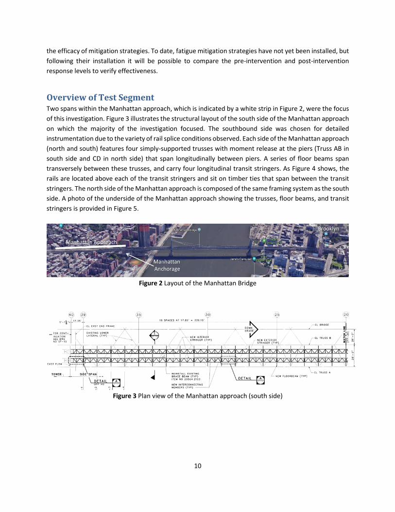
Instrumentation Layout Figure 12 below depicts the layout and designation of structural elements on the Manhattan approach. Figure 13 depicts the sensor layout, which is composed of 40 sensors. As shown in Figures 13 and 14, the instrumentation layout aimed to capture responses adjacent to Fair, Poor, and Severe splices (see Figure 6) as well as in high response regions or regions suspected to be particularly vulnerable to cracking. In total, the instrumentation plan was composed of 14 strain gages to capture flexural response, 16 strain gages to measure shear response (8 rosette sensors), six temperature sensors, and four crack gages.

Figure 12 Designation of structural elements

18

Figure 13 Instrumentation layout for global response monitoring

Figure 14 Typical gage mounting locations

The crack gages were installed at locations that have demonstrated to be prone to fatigue cracking. These cracks have occurred where the transit stringers frame into the floor beam, as detailed in the Figures 15-17 below. The connection detail features a stiffener plate terminating in the web of the floor beam, thereby applying large out-of-plane forces on the web. In some locations, the stiffener plate has been retrofitted to provide a connection to the bottom flange. Gages were installed in locations where cracking was observed as well as locations where the original detail was modified to provide continuity between the stiffener plate and the bottom flange of the floor beam.

19

Figure 15 Instrumentation layout for fatigue crack monitoring

Figure 16 Typ. framing detail in locations with

fatigue cracking Figure 17 Typ. gage location for fatigue crack

monitoring

Sensing and Data Acquisition Systems The fiber-optic based SHM system was chosen for their efficiency in terms of installation and cable management, and immunity to electrical/electromagnetic interference. The fiber-optic strain sensors employed had gage lengths of 75mm, sensitivities of 1:4 pm/με, and strain limits of ± 2,500 με. The optical interrogation unit (Micron Optics si155), as shown in Figure 18 is capable of monitoring 40-60 sensors, depending on sensor types. It can simultaneously accept data from strain gages, temperature gages, and other sensors. This unit has a bandwidth of 1460-1620 nm and a maximum sampling frequency of 1 kHz.

20

Figure 18 Micron Optics si155 Interrogator module

Processor Unit The central processing unit for this project is a Stealth.com Inc. Model: LPC-100G4 Ultra Small Mini PC with four Gigabit LAN ports. This device is equipped with a 2.26 GHz processor with 8 GB of RAM and a 120 GB Solid State hard drive. It uses a Windows 7 64-bit operating system and is loaded with the Micron Optics program ENLIGHT for interrogator interface and data acquisition.

Remote Monitoring An active internet connection was provided by the use of an industrial cellular modem (Figure 19). This unit allowed for remote collection of data from the interrogation unit.

Figure 19 Cellular modem and PC remote control interface

Installed Monitoring System Figure 20 shows the NEMA enclosure, which housed the optical interrogator, the central processing system and the cellular modem. Figure 21 and 22 show a typical sensor installation, which included flexible conduit to carry the armored optical fiber between small NEMA enclosures that protected each sensor. Figure 23 shows an installed strain gage prior to the attachment of the NEMA enclosure, and illustrates the removal of a 3 in. by 3in. area of paint to ensure the sensor was affixed to the substrate steel. All sensors were attached to the structure via microdot welding.

21

Figure 20 NEMA enclosure housing the DAQ, processor, and communication systems

Figure 21 Sample layout of the SHM system

22

Figure 22 Sample of ruggedized and protected FBG sensor protected by NEMA enclosure box

Figure 23 Paint removal to install FBG strain gage

Figure 24 shows the schematic of a rosette shear strain sensor that was arranged in an inverted delta configuration. Generalized strain-transformation equations were used to estimate the maximum shear strain in these locations.

23

Figure 24 Typical rosette gage installation

Figures 25(a) and (b) show typical cracks that have been located in the vicinity of floor beams, and Figure 25(c) shows a crack sensor installed at the tip of an existing crack.

Figure 25 a-b) Samples of crack sizes in the inspected members, c) Sample of strain gage installed at the

tip of an active crack

24

Monitoring Software The data acquisition system used a software package known as ENLIGHT provided by Micron Optics. ENLIGHT allows the user to define and configure all sensors and transforms the light-based measurements into useable strain data. It also permits data reporting and visualization as well as data transfer to third party software. Figure 26 shows a typical sensor response in the ENLIGHT software. The software was set to record 10 minutes of sensor data every two hours at a 100 Hz sample rate.

Figure 26 Typical ENLIGHT display of sensor readings

Data Acquisition Protocol Given that monitoring took place over the course of months, the system was set to automatically collect data at regular intervals as opposed to continuously. To that end, the data was continuously collected for the first 10 mins of every 2-hour period. Figure 27 provides a sample of data collected from the installed SHM system.

Results and Discussion The following bullets summarize a list of general information that has been captured by a detailed assessment of data collected through the May-June 2019 period:

• Approximately 250 trains pass per set of tracks every day • Most trains are of similar weight as determined by comparing strains induced by trains during

the rush hours (6 pm during weekdays) to those induced by trains that run near midnight (12 am)

• Train speed varies mainly between 5 and 25 mph

25

• Each train is usually composed of 10 cars, which creates 11 loading cycles. This results in over one million cycles per year for each track

Figure 27 Representative of strain measurements from the transit stringers

Simultaneous measurements from two flexural strain gages that were installed on the bottom flange of a transit stringer are shown in Figure 28. It should be noted that the measured strains have already been compensated for temperature effects and only reflect the structural response due to live load. Additionally, Figure 29 provides a closer look at one of the strain gages installed on the bottom flange of Transit Stringer 7 while the train was directly crossing over. By reviewing Figure 28 in more detail, the exact number of cars, train speed, as well as each car length could be estimated by determining the time difference between multiple cars crossing over the sensors (at a known spacing).

Figure 28 Representative of strain measurements from the transit stringers for a single train cross

26

One typical cycle from Figure 28 is displayed in Figures 29 and 30. It is composed of two superimposed cycles due to the close spacing of wheel carriages on adjacent cars. As it is the interest of this study to quantify the effect of rail splices on member responses, it is advantageous to estimate the static response to live loads so the dynamic component (and amplification) may be extracted. Perfect rail geometry should result in near unit dynamic amplification, and thus dynamic amplification of structural responses in the region of rail splices may provide reasonable measure of a splice’s effect on structural performance.

Figure 29 Raw and filtered flexural strain response in transit stringer near good condition splice

Figure 30 Raw and filtered flexural strain response in transit stringer near misaligned splice

27

One simple way of estimating static response from total response is to use signal processing techniques to filter out frequencies that correspond to the dynamic response of the structure while retaining content that is representative of the static response of the structure. In Figures 29 and 30, the dark blue color represents the raw strain gage reading while the light blue corresponds to an estimate of the static response obtained by implementing a low-pass filter. As can be seen in Figure 29, the dynamic response near a splice in good condition is not appreciably greater than the estimated static response. It may therefore be concluded that the dynamic amplification is low in this region. In contrast, the response in a region with a misaligned splice, as displayed in Figure 30, exhibits significant dynamic amplification as evidenced by the spikes in strain. These responses allow the quantification of the influence of misaligned splices that result in impacts as the train wheels cross them. To quantify dynamic effects, many studies have employed the dynamic impact factor for bridges subject to passing trucks [1-4]. The magnitude of the amplification of stress due to vehicle-bridge interaction (VBI) is often studied using the Dynamic Amplification Factor (DAF) [5-7]. Indeed, to quantify the dynamic portion of load effects on bridges, DAF has been extensively used in several studies [8-13]. DAF is defined as the ratio of the total load effect (including dynamic and static) to the static load effect for a particular loading scenario on the bridge, as follows:

𝐷𝐷𝐷𝐷𝐷𝐷 =𝑀𝑀𝑀𝑀𝑀𝑀𝑀𝑀𝑀𝑀𝑀𝑀𝑀𝑀 𝑅𝑅𝑅𝑅𝑅𝑅𝑅𝑅𝑅𝑅𝑅𝑅𝑅𝑅𝑅𝑅 𝑀𝑀𝑅𝑅𝑢𝑢𝑅𝑅𝑢𝑢 𝐿𝐿𝑀𝑀𝐿𝐿𝑅𝑅 𝐿𝐿𝑅𝑅𝑀𝑀𝑢𝑢

𝑆𝑆𝑆𝑆𝑀𝑀𝑆𝑆𝑀𝑀𝑆𝑆 𝑅𝑅𝑅𝑅𝑅𝑅𝑅𝑅𝑅𝑅𝑅𝑅𝑅𝑅𝑅𝑅

The DAF and maximum strain response were adopted as the key performance metrics to quantify the influence of rail splices. The following sections present these metrics for both transit stringers and floor beams.

Transit Stringer Results To quantify the influence of rail splices on the performance of the transit stringers, the DAFs were determined for multiple transit stringers (subjected to different splice conditions) and plotted in Figures 31-33. The plotted points in Figures 31-33 were calculated based on 120 hours of data recorded at 100 Hz during a 2-month period. A MATLAB program was developed in order to automatically analyze and separate each individual train passage over the instrumented transit stringers. Approximately 1220 single passages (events) were identified during the recorded 120 hours of data. This corresponds to an average daily estimate of 244 passages per track. As previously shown in Figure 28, each event is mostly composed of 11 train cycles. The velocity, maximum strain, as well as the DAF were calculated and plotted in Figures 31-36. The velocity of each cycle was estimated based on the time difference between the target strain gage and the adjacent strain gage, which was placed at a known distance. As noted earlier, the maximum strain was estimated after the gage response was compensated for temperature effects. Figures 31-36 include between 13,000 and 15,000 data points. Figures 31-33 are arranged in descending order of rail splice condition (“fair” to “severe”). As indicated in Figure 31, the DAF for the strain gage installed adjacent to a splice in “fair” condition falls in the range of

28

1.0-1.5 with an average of 1.2. The DAF ratio slightly increases for the sensors installed in the vicinity of a splice in “poor” condition, exhibiting a range of 1.1-1.6 with an average of 1.3 (see Figure 32). The DAF for the strain gage adjacent to the “severe” splice was estimated to be in the range of 1.5-3.0 with an average of 2.1 (Figure 33).

Figure 31 Calculated DAF based on flexural strain measurement in transit stringer by sensor TB6-FB73

(adjacent to a fair splice)

Figure 32 Calculated DAF based on flexural strain measurement in transit stringer by sensor TB6-FB71

(adjacent to a poor splice)

29

Figure 33 Calculated DAF based on flexural strain measurement in transit stringer by sensor TB6-FB69

(adjacent to a severe splice) Figures 34-36 present the peak strain per load cycle as a function of train speed and are arranged in descending order of rail splice condition (“fair” to “severe”). Given the transit stringers are steel with an elastic modulus of approximately 29,000 ksi, every 35 µɛ of strain corresponds to approximately 1 ksi of stress. Hence, the maximum strain illustrated in Figure 34, which is from a gage installed adjacent to a “fair” splice, corresponds to a stress range of 2.0-3.5 ksi with an average of 2.9 ksi (maximum response) and 2.5 ksi (static response). In the case of a strain gage in the vicinity of a “poor” splice (Figure 35), the stress in the transit stringer falls in the range of 2.0-3.0 ksi with an average of 2.2 ksi (maximum response) and 1.7 ksi (static response). For the gage located near the “severe” splice (Figure 36), the stress in the steel is estimated to be in the range of 2.3-4.0 ksi with an average of 3.1 ksi (maximum response) and 1.5 ksi (static response). As reported in the AASHTO Bridge Design Manual (Table of 6.6.1.2.3-2, reproduced in Table 1 below) [14], the constant amplitude fatigue threshold (or maximum permissible stress cycle for an indefinite fatigue life) falls in the range of 3-24 ksi depending on the detail category. As indicated in Figure 37, the majority of the connection details in transit stringers are made of high strength bolts and the fatigue-prone weld details are avoided. As a result, the transit stringer details fall under “A-D” AASHTO detail categories, which provide larger fatigue thresholds. Therefore, it is estimated that the maximum stress levels in the transit stringers (even near “severe” joints) fall under the corresponding constant amplitude fatigue threshold, and thus indicate infinite fatigue life. Importantly, this analysis is only for the transit stringers

30

and does not include the connecting elements that attach the rails to ties or the ties to the transit stringers.

Figure 34 Measured maximum flexural strain in transit stringer by sensor TB6-FB73 (adjacent to a fair

splice)

Figure 35 Measured maximum flexural strain in transit stringer by sensor TB6-FB71 (adjacent to a poor

splice)

31

Figure 36 Measured maximum flexural strain in transit stringer by sensor TB6-FB69 (adjacent to a severe

splice)

Table 1 AASHTO constant amplitude fatigue threshold (CAFT) values Detail Category Threshold (ksi)

A 24 B 16 B’ 12 C 10 C’ 12 D 7 E 4.5 E’ 2.6

32

Figure 37 Close view of the transit stringer connection details

The statistical summary of calculated DAF values and flexural strain gages versus the train velocity is shown in Figure 38, where the associated average was separately computed for multiple ranges of train velocities. As the train velocity increases, it is obvious the transit stringers experience higher rates of dynamic amplification and flexural strain due to the higher impact force induced by the train wheel traversing the rail splice. This is because the vertical deviation at the splice must be accommodated over a shorter time period with increased train speed. Since force may be expressed as the change in momentum divided by the time over which that change occurs, it follows that as the duration over which the train wheel traverses the splice decreases, the resulting impact force increases.

33

Figure 38 Statistical calculation of transit stringers’ DAFs for different splicing conditions

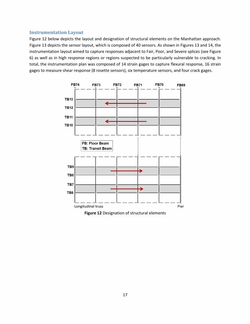
In addition to flexural strain measured at the bottom flange of the transit stringers, a few locations along the web of the transit stringers were instrumented using shear rosette sensors. In Figure 39, responses from three different rosette sensors installed on the web of transit stringers adjacent to “fair”, “poor”, and “severe” splices are shown. It is obvious that the dynamic response near a splice in “fair” condition is not appreciably greater than its static response. It may therefore be concluded that the dynamic amplification is low in this region. In contrast, the response in a region with a “severe” splice as displayed in Figure 39 exhibits a DAF of approximately 1.2-1.7, which is much less than observed for flexural responses. The statistical summary of calculated DAF values versus train velocity is shown in Figure 40, where the associated average DAFs were separately computed for multiple ranges of train velocities. As the train velocity increases, it is obvious that the transit stringers experience higher rates of dynamic amplification due to the higher impact force induced by the train wheel traversing the rail splice. As indicated in Figure 40, the DAF for the strain gage installed adjacent to a splice in “fair” condition falls in the range of 1.0-1.5 with an average of 1.2. The DAF ratio slightly increases for the sensors installed in the vicinity of a splice in “poor” condition, exhibiting a range of 1.1-1.6 with an average of 1.3. The DAF for the strain gage adjacent to a “severe” splice was estimated to be in the range of 1.2-2.0 with an average of 1.6.

34

Figure 39 Raw shear strain response in transit stringer near fair (TBS6-FB73), poor (TBS6-FB71), and

severe (TBS6-FB69) splices

Figure 40 Statistical calculation of transit stringers’ DAFs (shear strain) for different splicing conditions

35

Figures 41-43 refer to the maximum shear strain response measured from the rosette sensors. The figures are arranged in descending order of rail splice condition. Given the transit stringers are steel with a shear modulus of approximately 11.5 ksi, every 87 µɛ of strain corresponds to approximately 1 ksi of stress. Hence, the maximum strain illustrated in Figure 41, which is from a gage installed adjacent to a “fair” splice, corresponds to a stress range of 0.9-1.4 ksi with an average of 1.0 ksi (maximum response). In the case of a strain gage in the vicinity of a “poor” splice (Figure 42), the stress in the transit stringer falls in the range of 1.0-1.6 ksi with an average of 1.2 ksi (maximum response). For the gage located near the “severe” splice (Figure 43), the stress in the steel is estimated to be in the range of 1.0-1.8 ksi with an average of 1.3 ksi (maximum response).

Figure 41 Measured maximum shear strain in transit stringer by sensor TB6-FB73

36

Figure 42 Measured maximum shear strain in transit stringer by sensor TB6-FB71

Figure 43 Measured maximum shear strain in transit stringer by sensor TB6-FB69

37

Floor Beam Results Compared to transit stringers, it was anticipated that the floor beams would exhibit lower dynamic amplification as the dynamic response is expected to attenuate as it travels from the transit stringers to the floor beams. The DAF value for the floor beams were determined for multiple floor beams (subjected to different splice conditions) and are plotted in Figures 44-46. Figures 44-46 are arranged in descending order of rail splice condition (“fair” to “severe”). Alternatively, the statistical summary of calculated DAF values versus the train velocity is shown in Figure 47, where the associated average was separately computed for multiple ranges of train velocities. As indicated in Figure 44, the DAF for the strain gage installed adjacent to a splice in “fair” condition falls in the range of 1.0-1.25 with an average of 1.11. The DAF ratio slightly increases for the sensors installed in the vicinity of a splice in “poor” condition, exhibiting a range of 1.0-1.35 with an average of 1.14 (see Figure 45). The DAF for the strain gage adjacent to the severe splice was estimated to be in the range of 1.0-1.5 with an average of 1.22 (Figure 46). As expected, the DAF values for the floor beams were considerably less than for the transit stringers.

Figure 44 Calculated DAF based on flexural strain measurement in floor beam by sensor FB73-TB7

(adjacent to a fair splice)

38

Figure 45 Calculated DAF based on flexural strain measurement in floor beam by sensor FB71-TB7

(adjacent to a poor splice)

Figure 46 Calculated DAF based on flexural strain measurement in floor beam by sensor FB69-TB7

(adjacent to a severe splice)

39

Figure 47 Statistical calculation of floor beams’ DAFs (flexural strain) for different splicing conditions

Figures 48-50 illustrate the maximum flexural strain measured from the floor beams and are arranged in descending order of rail splice condition. In a similar procedure employed for transit stringers, the maximum strain illustrated in Figure 48 is from a gage installed adjacent to a “fair” splice, which corresponds to a stress range of 1.1-4.6 ksi with an average of 3.0 ksi (maximum response). In the case of a strain gage in the vicinity of a “poor” splice (Figure 49), the stress in the transit stringer falls in the range of 1.1-5.7 ksi with an average of 3.7 ksi (maximum response). For the gage located near a “severe” splice (Figure 50), the stress in the steel is estimated to be in the range of 1.1-3.4 ksi with an average of 2.3 ksi (maximum response). Similar to transit stringers, the majority of the connection details in floor beams are made of high strength bolts and the fatigue-prone weld details are avoided. Therefore, it is estimated that the maximum stress levels in the floor beams (even near “severe” splices) fall under the corresponding constant amplitude fatigue threshold. This analysis is limited to stress-induced fatigue, and not the distortion-induced fatigue that has already been identified as the root cause of the observed cracking.

40

Figure 48 Measured maximum flexural strain in floor beam by sensor FB73-TB7 (adjacent to a fair splice)

Figure 49 Measured maximum flexural strain in floor beam by sensor FB71-TB7 (adjacent to a poor

splice)

41

Figure 50 Measured maximum flexural strain in floor beam by sensor FB69-TB7 (adjacent to a severe

splice) In addition to flexural strain measured at the bottom flange of floor beams, a few locations along the web of the floor beams were instrumented using shear rosette sensors. In Figure 51, responses from two different rosette sensors installed on the web of floor beams adjacent to “poor” and “severe” splices are shown. As apparent in this figure, the shear response of the floor beam does not demonstrate any sensitivity to the type of splicing joints. This behavior is also apparent when examining the DAF and maximum strain values shown in Figures 52-53.

42

Figure 51 Raw shear strain response in floor beam near “poor” (FB71) and “severe” (FB69) splices

Figure 52 Measured maximum shear strain in floor beam by sensor FB71 (adjacent to a poor splice)

43

Figure 53 Measured maximum shear strain in floor beam by sensor FB69 (adjacent to a severe splice)

Summary of Results for Transit and Floor Beams Table 2 summarizes the final results of DAF (average) and maximum measured strain (average) for a representative number of sensors installed on transit and floor beams adjacent to splicing joints with different conditions.

Table 2 Summary of DAF and maximum strain values for transit and floor beams

Splice Condition

DAF - Flexural Strain

Maximum Flexural Strain-µɛ

(Stress-ksi) DAF - Shear Strain

Maximum Shear Strain-µɛ

(Stress-ksi) Transit stringer

Floor Beam

Transit stringer

Floor Beam

Transit stringer

Floor Beam

Transit stringer

Floor Beam

Fair 1.2 1.1 102 (2.9)

104 (3.0) 1.2 NA 91

(1.0) -

Poor 1.3 1.1 76 (2.2)

130 (3.7) 1.3 1.1 105

(1.2) 169 (1.9)

Severe 2.1 1.2 108 (3.1)

80 (2.3) 1.6 1.2 113

(1.3) 181 (2.1)

44

Crack Sensors Results One of the secondary objectives of this study was to monitor the opening of the distortion-induced fatigue cracks to (a) identify whether or not they were active, and (b) to provide baseline data that could be used to quantify the efficacy of mitigation strategies. Figures 15-17 as well as Figure 25 show the location and snapshots of the crack sensors installed at the tip of observed cracks. The installed gages were simply strain sensors installed across the crack (parallel to the crack opening direction). Given the discontinuity associated with cracks, the measured strain is not a direct indicator of actual stress, i.e., it cannot be used via the Elastic Modulus to estimate stress. However, it is indicative of the geometric opening of the crack when it is subjected to the train passage. Figure 54 demonstrates a random strain response measured during a train passage at the south side of the bridge. The strain values are fairly large (> 400 µɛ) and thus it can be reasonably concluded that these cracks remain active. It is interesting that even at this high-stress concentration, the effects of the severe rail splicing could be easily discerned from the rest of response. If it is of interest to the NYCDOT, a comparison between these measurements and those obtained following the retrofit of these regions would be a valuable indicator of the effectiveness of the mitigation strategy.

45

Figure 54 Measured strain at the crack tip in floor beam by sensor FB69-TS6 (adjacent to a severe splice) In addition, Figures 55 shows a sample strain measurement from a crack sensor installed at the north side of the bridge adjacent to a distortion-induced fatigue crack. As can be observed, in this case the amplitude of the strain response is approximately 1/3 of the amplitude measured in the vicinity of the crack along the south span. This discrepancy is likely due to the localized nature of this measurement, which attenuates rapidly as a function of distance from the crack tip.

46

Figure 55 Measured strain at the crack tip in floor beam by sensor FB71-TN13

Analysis of Train Weight To back calculate the weight of train with and without passengers, it is first necessary to ensure the static portion of the strain measurements truly portray the train weight. One way of validation is to investigate if the calculated static response is independent of the train velocity or not. Figure 56 shows the calculated static response on a number of transit stringers (calculated based on the filtering approach explained in Fig. 30) versus different velocity ranges as well as different rail splicing conditions. From this figure, it appears the average static strain is indeed independent of train velocity for each location/splice condition. The different strain levels apparent between the various locations shown in Figure 56 can be attributed to the particular location and the stress level induced at this location due to passing trains. As a result, it is concluded that the estimation of static responses are of sufficient accuracy to provide useful estimations of train relative weights.

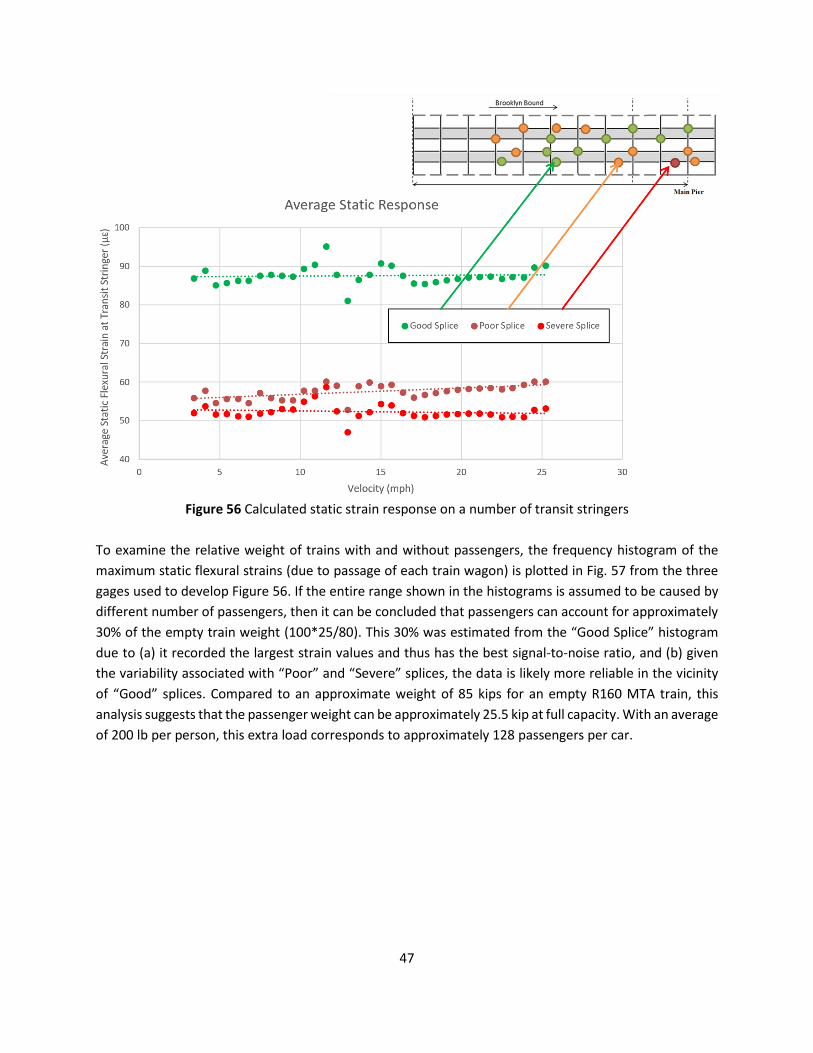
47

Figure 56 Calculated static strain response on a number of transit stringers

To examine the relative weight of trains with and without passengers, the frequency histogram of the maximum static flexural strains (due to passage of each train wagon) is plotted in Fig. 57 from the three gages used to develop Figure 56. If the entire range shown in the histograms is assumed to be caused by different number of passengers, then it can be concluded that passengers can account for approximately 30% of the empty train weight (100*25/80). This 30% was estimated from the “Good Splice” histogram due to (a) it recorded the largest strain values and thus has the best signal-to-noise ratio, and (b) given the variability associated with “Poor” and “Severe” splices, the data is likely more reliable in the vicinity of “Good” splices. Compared to an approximate weight of 85 kips for an empty R160 MTA train, this analysis suggests that the passenger weight can be approximately 25.5 kip at full capacity. With an average of 200 lb per person, this extra load corresponds to approximately 128 passengers per car.

48

Figure 57 Frequency histogram of strain response (flexural strain) on a number of transit stringers

Conclusions The main objective of this research project was to quantify the level of dynamic amplification due to the bolted rail splices. This was accomplished by implementing a two-phase approach. During the initial phase, the Rutgers team performed an initial vibration survey of the accessible approach spans to identify locations of high and low dynamic amplification. During Phase 2, a fiber optic sensing system was deployed in these regions identified in Phase 1 to quantify dynamic amplification (through comparing the response from the different locations). This second monitoring phase was carried out over several months to ensure the capture of a variety of train speeds that permitted the influence of train speed on dynamic amplification to be examined. A secondary objective of this study was to monitor the opening of the distortion-induced cracks to (a) identify whether or not they were active, and (b) to provide baseline data that could be used to quantify the efficacy of mitigation strategies. To date, fatigue mitigation strategies have not yet been installed, but following their installation it will be possible to compare the pre-intervention and post-intervention response levels to verify effectiveness. The following subsections summarize the conclusions drawn related to train loading, transit stringer performance, floor beam performance, distortion-induced fatigue, and other issues.

49

Observed Train Loading • During the monitoring period, approximately 250 train passed per set of rails daily. This

translates into approximately 1 million cycles per year (250 trains x 11 cycles per train x 365 days per year)

• The train weights appear somewhat dependent on the number of passengers, with train car weights varying from around 85 kips when empty to around 110 kip when full.

• During the monitoring period the speed of the trains varied between 5 and 25 mph, with approximately 85% of the traveling between 15 and 25 mph

Performance of Transit Stringers • Dynamic amplification levels in the transit stringer were well-correlated with the condition of

the splices as rated by acceleration data. Dynamic amplification values for trains running at between 15 and 25 mph, averaged 2.1 in the vicinity of “severe” splices, 1.4 in the vicinity of “poor” splices, and 1.1 in the vicinity of “fair” splices.

• The relatively large amplification observed during monitoring (as compared to design standards) was directly attributable to the condition of the splices in the vicinity of the gage. As a result, these results should not be taken as an indication that the assumed dynamic amplification for design (as prescribed in standards) are in error.

• The average observed dynamic amplification of the transit stringers was linearly correlated with the speed of the train.

• The maximum flexural strains measured in the transit stringers, even in the vicinity of “severe” splices, were below the constant amplitude fatigue threshold values as provided by AASHTO LRFD Bridge Design Specifications.

Performance of Floor Beams • The dynamic amplification observed in the transit stringers attenuated quickly as a function of

distance from “severe” splices, and thus the observed dynamic amplification of the floor beams was significantly lower than the transit stringers.

• Dynamic amplification of the floor beams for trains running at between 15 and 25 mph, averaged 1.2 in the vicinity of “severe” splices, 1.1 in the vicinity of “poor” splices, and 1.1 in the vicinity of “fair” splices.

• The maximum flexural strains measured in the floor beams, even in the locations closest to “severe” splices, were below the constant amplitude fatigue threshold values as provided by AASHTO LRFD Bridge Design Specifications.

Distortion-induced Fatigue • The large live load responses measured in the vicinity of distortion-induced fatigue cracks within

the floor beams indicated that these cracks remain active under repeated train loads.

50

• The response measurements in the vicinity of distortion-induced fatigue cracks varied significantly from location to location due primarily to the localized nature of these measurements.

Other • The level of sound (estimated qualitatively by members of the Rutgers team) emanating from

the splices during train passages was well-correlated with the measured acceleration and strain records subsequently recorded. This indicates that track inspection based on sound should have a similar reliability as acceleration or strain monitoring.

• If a continuous monitoring system is desired to track the misalignment of splices, an acoustic monitoring system should be investigated in lieu of an acceleration- or strain-based monitoring system.

• While the large dynamic amplifications in the vicinity of the “severe” splices should not impact the fatigue life of transit or floor beams, they do result in very high localized stresses in the elements that connect the rails to the timber ties and the timber ties to the transit stringers. These stresses result in the failure of bolts and clips. Unless left unchecked, these local failures do not pose a threat to the structure itself, but do pose a falling hazard to those underneath the structure.

References [1] C. Carey, E.J. O’Brien, A. Malekjafarian, M. Lydon, S. Taylor, Direct Field Measurement of the Dynamic Amplification in a Bridge, Mechanical Systems and Signal Processing, 85 (2017) 601-660. [2] S.S. Law, X.Q. Zhu, Bridge dynamic responses due to road surface roughness and braking of vehicle, Journal of Sound and Vibration, 282 (2005) 805-830. [3] L. Deng, Y. Yu, Q.L. Zou, C.S. Cai, State-of-the-Art Review of Dynamic Impact Factors of Highway Bridges, Journal of Bridge Engineering, 20 (2015). [4] W.S. Han, J. Wu, C.S. Cai, S.R. Chen, Characteristics and Dynamic Impact of Overloaded Extra Heavy Trucks on Typical Highway Bridges, Journal of Bridge Engineering, 20 (2015). [5] A. Gonzalez, P. Rattigan, E.J. OBrien, C. Caprani, Determination of bridge lifetime dynamic amplification factor using finite element analysis of critical loading scenarios, Engineering Structures, 30 (2008) 2330-2337. [6] Y.S. Park, D.K. Shin, T.J. Chung, Influence of road surface roughness on dynamic impact factor of bridge by full-scale dynamic testing, Canadian Journal of Civil Engineering, 32 (2005) 825-829. [7] C.C. Caprani, Lifetime highway bridge traffic load effect from a combination of traffic states allowing for dynamic amplification, Journal of Bridge Engineering, 18 (2012) 901-909. [8] C. Sukhen, The Design of Modern Steel Bridges, Boston: London Edinburgh, (1992). [9] Q.L. Zhang, A. Vrouwenvelder, J. Wardenier, Dynamic amplification factors and EUDL of bridges under random traffic flows, Engineering Structures, 23 (2001) 663-672. [10] P. Dawe, Research perspectives: Traffic loading on highway bridges, Thomas Telford, 2003.

51

[11] I. Paeglite, A. Paeglitis, J. Smirnovs, Dynamic amplification factor for bridges with span length from 10 to 35 meters, Engineering Structures and Technologies, (2015) 1-8. [12] F.H. Rich, Dynamic amplification factor for the design of reinforcement in the transverse direction of deck slab of box girder bridges, Bangladesh University of Engineering and Technology, MSc thesis, 2014. [13] C.C. Caprani, Lifetime Highway Bridge Traffic Load Effect from a Combination of Traffic States Allowing for Dynamic Amplification, Journal of Bridge Engineering, 18 (2013) 901-909. [14] LRFD Bridge Design Specification, 8th Ed., American Association of State Highway and Transportation Officials (AASHTO), Washington, DC (2017).