Structural Macroeconomics

Structural MacroeconomicsComputer Project

Macroeconomic TheoryProfessor: Roberto Chang

Freddy Rojas Cama1

Rutgers UniversityEmine Beyza Sato¼glu2

Rutgers UniversityHyun Gon Kim3

Rutgers University

December 18th, 2010

[email protected]@[email protected]

Contents

0.1 Section (i) . . . . . . . . . . . . . . . . . . . . . . . . . . . . . . . . . . . . . . . 30.1.1 Decisions and Sectors . . . . . . . . . . . . . . . . . . . . . . . . . . . . 30.1.2 Functional forms . . . . . . . . . . . . . . . . . . . . . . . . . . . . . . . 30.1.3 Dynamic Programming . . . . . . . . . . . . . . . . . . . . . . . . . . . 40.1.4 Steady State of variables . . . . . . . . . . . . . . . . . . . . . . . . . . . 60.1.5 Calibration . . . . . . . . . . . . . . . . . . . . . . . . . . . . . . . . . . 60.1.6 Linearization . . . . . . . . . . . . . . . . . . . . . . . . . . . . . . . . . 80.1.7 State Space . . . . . . . . . . . . . . . . . . . . . . . . . . . . . . . . . . 80.1.8 Solution method . . . . . . . . . . . . . . . . . . . . . . . . . . . . . . . 90.1.9 Policy functions . . . . . . . . . . . . . . . . . . . . . . . . . . . . . . . . 100.1.10 Calculations of moments . . . . . . . . . . . . . . . . . . . . . . . . . . . 110.1.11 Impulse Responses . . . . . . . . . . . . . . . . . . . . . . . . . . . . . . 160.1.12 HP-Filtered Data . . . . . . . . . . . . . . . . . . . . . . . . . . . . . . . 17

0.2 Section (ii) . . . . . . . . . . . . . . . . . . . . . . . . . . . . . . . . . . . . . . 190.3 Section (iii) . . . . . . . . . . . . . . . . . . . . . . . . . . . . . . . . . . . . . . 23

0.3.1 Explicit growth . . . . . . . . . . . . . . . . . . . . . . . . . . . . . . . . 230.3.2 Steady State . . . . . . . . . . . . . . . . . . . . . . . . . . . . . . . . . 260.3.3 Linearization . . . . . . . . . . . . . . . . . . . . . . . . . . . . . . . . . 270.3.4 State Space . . . . . . . . . . . . . . . . . . . . . . . . . . . . . . . . . . 270.3.5 Calibration . . . . . . . . . . . . . . . . . . . . . . . . . . . . . . . . . . 280.3.6 Policy Functions . . . . . . . . . . . . . . . . . . . . . . . . . . . . . . . 290.3.7 Calculation of moments . . . . . . . . . . . . . . . . . . . . . . . . . . . 300.3.8 Impulse Responses . . . . . . . . . . . . . . . . . . . . . . . . . . . . . . 30

0.4 Section (iv) . . . . . . . . . . . . . . . . . . . . . . . . . . . . . . . . . . . . . . 310.4.1 Greenwood, Hercowitz, and Hu¤man�s (GHH) preferences . . . . . . . . 310.4.2 Decisions and Sectors . . . . . . . . . . . . . . . . . . . . . . . . . . . . 320.4.3 Dynamic Programming . . . . . . . . . . . . . . . . . . . . . . . . . . . 320.4.4 Steady State of variables . . . . . . . . . . . . . . . . . . . . . . . . . . . 330.4.5 Linearization . . . . . . . . . . . . . . . . . . . . . . . . . . . . . . . . . 330.4.6 State Space . . . . . . . . . . . . . . . . . . . . . . . . . . . . . . . . . . 330.4.7 Calibration . . . . . . . . . . . . . . . . . . . . . . . . . . . . . . . . . . 340.4.8 Policy function . . . . . . . . . . . . . . . . . . . . . . . . . . . . . . . . 340.4.9 Calculation of moments . . . . . . . . . . . . . . . . . . . . . . . . . . . 350.4.10 Impulse Responses . . . . . . . . . . . . . . . . . . . . . . . . . . . . . . 35

0.5 Conclusions from our Computer Project . . . . . . . . . . . . . . . . . . . . . . 36

1

References 38

A Log-Linearization section i. 40

B Caveats with HP �lter 45

C Log-Linerization section iii 46

D Log-linearization in section iv 48

E Optimality conditions in section iv 51

F Steady State in section iv 52

G Implementation in Gensys for a System of dimension 6� 6 54

2

0.1 Section (i)

In this computer project, several tasks related to the Dynamic Stochastic General Equilibrium(DSGE) models have been completed. In our analysis, we used the tasks given in StructuralMacroeconometrics of Dejong and Dave as a reference source. Speci�cally, in this section weare going to replicate table 6.4 (page 138) of DeJong and Dave�s book.

0.1.1 Decisions and Sectors

Dejong and Dave (2007) [DD] started with the following environment; the aggregate economicactivity we are going to analize is mainly driven by decisions of a representative agent. Thehousehold has the objetive to maximize a stream of utility functions across time which iscomposed by decisions over consumption and leisure:

U = E0

1Xt=0

�tu (ct; lt)

� is the household�s subjective discount factor, it belongs to (0; 1) and a strictly positive valueindicates that future consumption matters for the individual. ct and lt denotes consumptionand leisure at time t. The household is equipped with a production or technology functionwhich is used to produce a good yt :

yt = ztf (kt; nt) (1)

kt and ; nt denote units of capital and labor e¤ective hours. zt denotes a random disturbance tothe productivity, as we see expression (1) shows as well that improvements are Hicks-neutral.A change is considered to be Hicks neutral if the change does not a¤ect the balance of laborand capital in the products production function. As [DD] would state within a period thehousehold has one unit of time available for division between labor and leisure activities

nt = 1� lt (2)

the output can be either consumed or invested:

yt = ct + it

The law motion of capital iskt+1 = it + (1� �) kt (3)

0.1.2 Functional forms

The utility function has the constant relative risk aversion (CRRA) preferences:

u (ct; lt) =

c't l

1�'t

1� �

!1��the production function is the Cobb-Douglas technology:

yt = ztk�t n

1��t

3

where � is the elasticity of production function to capital. The dynamic of shock is driven bythe following expression

log zt = (1� �) log z + � log zt + "t (4)

where "t s N�0; �2

�and � 2 (�1; 1) : A bar on variables denotes their steady state through

the document.

0.1.3 Dynamic Programming

We solve the models by using Dynamic Programming techniques. In this case the controlvariables are ct and nt, and the state variables are kt and zt: We set up the problem as follows

V (kt; zt) = u (ct; lt) + �V (kt+1; zt+1)

we have the �rst order conditions, for consumption

@v

@ct=hc't l

1�'t

i��c'�1t 'l1�'t +

�@v (kt+1;zt+1)

@kt+1

@kt+1@ct

= 0

@v

@ct=hc't l

1�'t

i��c'�1t 'l1�'t + �v

0(kt+1;zt+1) (�1) = 0 (5)

for leisure@v

@lt=hc't l

1�'t

i��c't (1� ')l

�'t + �v

0(kt+1;zt+1)

@kt+1@lt

= 0

@v

@lt=hc't l

1�'t

i��c't (1� ')l

�'t + �v

0(kt+1;zt+1) ztk

�t (1� �)n��t (�1) = 0 (6)

and for kt

@v

@kt=

�@v (kt+1;zt+1) @kt+1@kt+1@kt

= �v0(kt+1;zt+1)

�(1� �) + zt�k��1t n1��t

�(7)

we have the following expression from (5):hc't l

1�'t

i��c'�1t 'l1�'t = �v

0(kt+1;zt+1) (8)

From (6) we have the followinghc't l

1�'t

i��c't (1� ')l

�'t = �v

0(kt+1;zt+1) ztk

�t (1� �)n��t

We complete the system of equations with the Envelope Theorem

v0 (kt;zt) = �v0(kt+1;zt+1)

�(1� �) + zt�k��1t n1��t

�Then sub (5) into (7)

v0 (kt;zt) =hc't l

1�'t

i��c'�1t 'l1�'t

�(1� �) + zt�k��1t n1��t

�4

v0(kt+1;zt+1) =

hc't+1l

1�'t+1

i��c'�1t+1 'l

1�'t+1

�(1� �) + zt+1�k��1t+1 n

1��t+1

�Then into (5)h

c't l1�'t

i��c'�1t 'l1�'t = �

hc't+1l

1�'t+1

i��c'�1t+1 'l

1�'t+1

�(1� �) + zt+1�k��1t+1 n

1��t+1

�(9)

Combining expressions (6) on (8)hc't l

1�'t

i��c't (1� ')l

�'t =

hc't l

1�'t

i��c'�1t 'l1�'t ztk

�t (1� �)n��t

From (9)hc't l

1�'t

i��c'�1t 'l1�'t = �

hc't+1l

1�'t+1

i��c'�1t+1 'l

1�'t+1

�(1� �) + zt+1�k��1t+1 n

1��t+1

�(10)

So, the cross-section Euler equation is:

(1� ')'

= c�1t ltztk�t (1� �)n��t

ct(1� ')'

= ltztk�t (1� �)n��t (11)

In terms of labor hours, (9) is going to be expressed ashc't (1� nt)

1�'i��

c'�1t ' (1� nt)1�' = �hc't+1 (1� nt)

1�'i��

c'�1t+1 ' (1� nt+1)1�'

��(1� �) + zt+1�k��1t+1 n

1��t+1

�(12)

In the case of expression (11)

ct(1� ')'

= (1� nt) ztk�t (1� �)n��t (13)

Equations (12), (13), productivity AR(1), and low motion equation for kt; comform the system:The transversality condition is:

limT�!1

�TkT+1u (cT ) = 0

5

0.1.4 Steady State of variables

In Structural Macroeconomics, [DD] show the steady state of the system in 4 expressions;

y

n=

��

� + �

� �1��

i

n= �

��

� + �

� 11��

i

y= �

��

� + �

�n =

1

1 +�

11��

��1�''

� h1� �

��+�

�i' =

1

1 + 21��cy

DD �xed n, cy ;iy then they establish relationships between k, �; ' and � (see table 6.3 in DD).

0.1.5 Calibration

In this section we are going to do the calibration. We follow the DD procedure and we keepconstant the ratio c

y ;iy and n =

13 : Specially we keep

cy equal to 0:825: We replicate table 6.3

in [DD]and we present additional values of trade-o¤1

Table 1.1Trade-o¤s between �; � and '

� � '

0.0393 0.2200 0.34590.0289 0.2362 0.35070.0228 0.2525 0.35560.0189 0.2687 0.36070.0161 0.2850 0.36590.0140 0.3013 0.37120.0124 0.3175 0.37670.0111 0.3337 0.38240.0101 0.3500 0.38820.0091 0.3700 0.3957

In the next section, we represent the model in terms of deviations from trend. Tipically, thetrend comes from the productivity because it is supposed that the productivity always increasesalong time. Another way to represent (4) is:

zt = zo exp (wt) (14)

1See our matlab codes in nquestion_i

6

In this case the dynamic of productivity is an stationary realization. Expression (14) is impor-tant in section iii because we are going to include explicit growth. Now, we are going to workon stationary process, under this model the calibration parameters are (see DD);

[� � � ' � � �] = [0:240 0:990 1:50 0:353 0:0250 0.780 0 0067]

As we see in DD, the authors coduct a calibration process in order to get the ratio n = 13 : But,

we try a di¤erent (and useful) exercise of calibration and show how sensible the steady valueof n is, we �nd out that performing a mapping of n when we �xed ' = 0:353:(see �gure 1.1)

0.30

49

0.30

852

0.31

215

0.31

215

0.31

577

0.31

577

0.31

94

0.31

94

0.31

94

0.32

302

0.32

302

0.32

302

0.32

665

0.32

665

0.32

665

0.33

027

0.33

027

0.33

39

n

α

δ0 .0 1 0 .0 1 5 0 .0 2 0 .0 2 5 0 .0 3 0 .0 3 5 0 .0 4

0 .2 2

0 .2 4

0 .2 6

0 .2 8

0 .3

0 .3 2

0 .3 4

0 .0 1

0 .0 1 5

0 .0 20 .0 2 5

0 .0 3

0 .0 3 50 .0 4

0 .2 2

0 .2 4

0 .2 6

0 .2 8

0 .3

0 .3 2

0 .3 4

0 .2 8 5

0 .2 9

0 .2 9 5

0 .3

0 .3 0 5

0 .3 1

0 .3 1 5

0 .3 2

0 .3 2 5

0 .3 3

0 .3 3 5

δ

mapping of n

α

Figure 1.1: Mapping n

In this case the ratios cy are completely free; we present the range of values under the previouscalibration:

Table 1.2cy

iy

ky

max 0.8906 0.2794 17.4121min 0.7206 0.1094 4.3911

The map is a helpful tool because you only need to pick a value of n and see the combinationsof � and � which support that steady state. Likewise all the combinations in that map delivervalues of cy and

iy close to empirical values. Having a map with di¤erents (suitable) values of

consumption-output ratio is very convenient as long as we want to calibrate the model for othereconomies (low capital-output ratio economies or economies in transition or undeveloping).

7

0.1.6 Linearization

All details of linearization you may �nd them on the appendix. the vector of log-linearizedvariables is:

xt = [kt zt ct nt]0

In the linear system all the variables are in natural logs. Is valuable to mention that wegive importance to the ordering of the variables in the procedure, that is important for nextsteps2. Also, in comparison to the recitation clases we prefer to deal with a small dimensionof variables, this is 4 variables instead of 63. Then, we are going to have results using Delthamethod. The complete linearization is presented in the appendix of this section. We reportthe log-linearized equations of the system

� cect = kekt + nent + zezt

�$cect = $c0ect+1 +$k0ekt+1 +$nent +$n0ent+1 +$z0ezt+1

the law motion of capital and productivity

� cect = kekt + k0ekt+1 + nent + zeztezt+1 = �ezt + "t � "

where ext denotes the logarithm of the variable xt respect to the logarithm ot that variableevaluated in the steady state (xt). We denote xt as the steady state. All group of parameters� g0 $g0 g0 �g

�0 are de�ned in the appendix.0.1.7 State Space

We arrange the system and we put all the variables in state-space form (Sims, 2000)

�0xt+1 = �1xt + �+zt +��t

We use Sim�s representation in this section. In our system � = [0 0 0 0]0, and the entire systemis:26666664

0 0 � c � n 0 0� k0 0 � c � n 0 00 1 0 0 0 0�$k0 �$z0 �$c �$n �$c0 �$n0

0 0 1 0 0 00 0 0 1 0 0

37777775

26666664

kt+1zt+1ctntEtct+1Etnt+1

37777775 =26666664

k z 0 0 0 0 k z 0 0 0 00 � 0 0 0 00 0 0 0 0 00 0 0 0 1 00 0 0 0 0 1

37777775

26666664

ktztct�1nt�1Et�1ctEt�1nt

3777777526666664

00�000

37777775 "t +26666664

0 00 00 00 01 00 1

37777775��ct�nt

�

2 In the class and recitations the ordering is not relevant but for purposes of getting easily the policiy functionsthat matters.

3 standard procedure includes as restrictions the production function, investment identity, leisure-labor deci-sions, supply and demand (see [DD]).

8

0.1.8 Solution method

Having obtained the system in state space in the previous section we are conducting the solutionof the model by using the methods oulined in chapter 2 in DD. Here we are going to discuss 2methods: Sims�procedure and Perturbation4. We brie�y discuss the methods.

Sim�s method

First, we talk about Blanchard and Khan metodology and how Sims simpli�es the notation andprovide a straighforward representation to implement. The Blanchard and Kahn representationstates that you can easily discern the state variables from the jump (or control) variables. Theysuggest to write the system as

the steady space for Blanchard and Khan metodology is as follows:

�BK0

�St+1EtXt+1

�= �BK1

�StXt

�+ �+ zt (15)

where St is a vector of state (predetermined) variables at time t; X is a vector of jump (non-predetermined or control) variables at time t: zt is a vector of exogenous shocks (or variables)known at time t; which in many applications can be taken to be iid over time. EtXt+1 is avector that contains the agents expectations of Xt+1 at time t, � is a vector of constants, thatin many applications is simply a vector of zeros. The state-space representation is intuitive butin order to �nd the solution a recursive method is not going to work since the variables in theleft hand side of (15) are diferent from those appearing at �rst column vector in the right handside. We need to note that EtXt+1 and Xt+1 are two variables both known at time t that aredi¤erent (see Michelacci, 2006).

To avoid the problem Sims (2002) suggests to write the system in the following form:

�0

�St+1EtXt+1

�= �1

�StXt

�+ �+zt +��t

where (St EtXt)0 is a (n � 1) vector containing all variables determined at time t. The �rst

ns entries correspond to the variables that never enter the system with expectations, whichgenerally correspond to the predetermined variables at a given point in time (endogenous statevariables). The second nx entries correspond to the variables that (at least) sometimes enterwith an expectational term, which generally correspond to the jump (or control) variables. Thelast terms correspond to the variables with expectations. In terms of our computer project wehave the following state space under Sim�s representation:�

St+1EtXt+1

�=�kt+1 zt+1 ct nt Etct+1 Etnt+1

�0(16)

It is valuable to mention the properties of Sims�s procedure (Michelacci, 2006):

(i) In Sims�s representation we do not have to specify explicitly which variables are predeter-mined and which are jump variables or include explicitly the expectations in the state-control vector. But, sometimes is preferable to arrange the system as in expression (16)and then having directly the policy functions. In fact under that representation we wouldhave as solution a matrix with the last columns �lled in with zeros.

4Schmidtt-Grohe and Uribe (2001)

9

(ii). The notation is such that the time arguments relate consistently to the informationstructure: variables dated t are always known at t. Expectations of variabels are not thesame as thier value at time t.

(iii) Sims adds an equation of the type �t = EtXt+1�Xt; that de�nes the expectational error.

(iv). The expectational errors are endogenous. De�ning their structure is part of the solutionof the system. Michelacci, 2006 states that is an important aspect of the analysis that ishidden in the Blanchard-Kahn formulation.

(v) Given the convention about the ordering, the matrix consists of zeros except for the last nxrows that consist of an identity matrix of dimension equal to the number of expectationalerror in the system.

Perturbation

We consider as well the Uribe and Schmidt-Grohé (2003)�s methodology which states thatequilibrium conditions may be represented as follows

Etf (yt+1; yt; xt+1;xt) = 0 (17)

where Et denotes the mathematcal conditional expectation on information at time t. the vectorxt of predetermined variables has size nx, this vector can be split to endogenous and exogenousdetermined variables. The vector yt gathers control variables and it has size ny the solutionhas the following shape

yt = g(xt; �) (18)

xt+1 = h (xt; �) + ��"t+1 (19)

we look for an apporxiamtion of g y h around (x; �) = (x; 0), in order to get the solution Uribeand Schmidt-Grohé (2003)perform �rst and second order approximations (Schmitt-Grohe andUribe, 2004). Uribe and Schmidt-Grohé (2003)states that it is straightforward to apply themethod described thus far to higher-order approximations to the policy function. The authorsmention that given �rst and second-order terms of the Taylor expansions of h and g, the third-order terms can be identi�ed by solving a linear system of equations. Authors refer Collardand Juillard, 2001; and Judd, 1998 for details. Interesting results from this methodology ariseswhen second or third order approximation are applied to models; Rojas (2006) shows a lowerpower of Gali�s methodology for assesing rigidities in the economy when high moments areincluded in the policy function.

0.1.9 Policy functions

In this section we present the results and we choose to present those results under the formatof the methods we discussed before. All methods deliver the same results but they only di¤erin how they de�en the state and space or arrangment of matrices. We present results for Sims1, Sims 2, perturbation and Klein methodology. We use their notations of solution, thus wecan distinguish the format between methodologies.

10

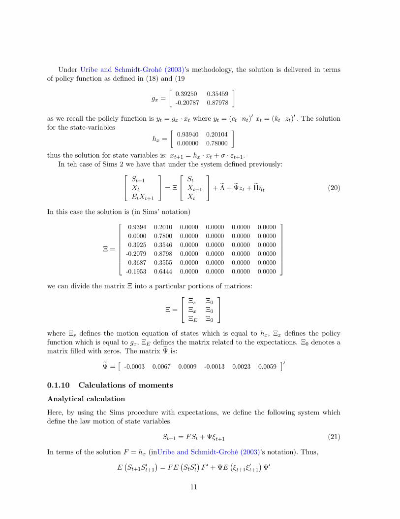
Under Uribe and Schmidt-Grohé (2003)�s methodology, the solution is delivered in termsof policy function as de�ned in (18) and (19

gx =

�0.39250 0.35459-0.20787 0.87978

�as we recall the policiy function is yt = gx � xt where yt = (ct nt)

0 xt = (kt zt)0 : The solution

for the state-variables

hx =

�0.93940 0.201040.00000 0.78000

�thus the solution for state variables is: xt+1 = hx � xt + � � "t+1:

In teh case of Sims 2 we have that under the system de�ned previously:24 St+1XtEtXt+1

35 = �24 StXt�1Xt

35+ e� + ezt + e��t (20)

In this case the solution is (in Sims�notation)

� =

26666664

0.9394 0.2010 0.0000 0.0000 0.0000 0.00000.0000 0.7800 0.0000 0.0000 0.0000 0.00000.3925 0.3546 0.0000 0.0000 0.0000 0.0000-0.2079 0.8798 0.0000 0.0000 0.0000 0.00000.3687 0.3555 0.0000 0.0000 0.0000 0.0000-0.1953 0.6444 0.0000 0.0000 0.0000 0.0000

37777775we can divide the matrix � into a particular portions of matrices:

� =

24 �s �0�x �0�E �0

35where �s de�nes the motion equation of states which is equal to hx; �x de�nes the policyfunction which is equal to gx, �E de�nes the matrix related to the expectations. �0 denotes amatrix �lled with zeros. The matrix e is:

e = � -0.0003 0.0067 0.0009 -0.0013 0.0023 0.0059�0

0.1.10 Calculations of moments

Analytical calculation

Here, by using the Sims procedure with expectations, we de�ne the following system whichde�ne the law motion of state variables

St+1 = FSt +�t+1 (21)

In terms of the solution F = hx (inUribe and Schmidt-Grohé (2003)�s notation): Thus,

E�St+1S

0t+1

�= FE

�StS

0t

�F 0 +E

��t+1�

0t+1

�0

11

where E��t+1�

0t+1

�is an identity matrix5. In conditional terms

�s = F�sF +0 (22)

where �s is the unconditional variance of the state variables. Hamilton (1995) provides a closedsolutions for expression (22)

vec (�s) = [I � F F ]�1 � vec�0

�we know that the solution for control variables is (in Uribe and Schmidt-Grohé (2003)�s nota-tion) :

Xt = gxSt (23)

and for state variables is:St = hxSt�1 + ��t

where � is the cholesky descomposition of variance of shocks6. In order to get the covariancesand variances we need to compute moments: we compute the following

XtX0t = gxStS

0tg0x

E�XtX

0t

�= gxE

�StS

0t

�g0x

= gx�sg0x

Also, we need the �rst-lag covariances for the states; we compute the moment and take expec-tations

StS0t�1 = hxSt�1S

0t�1 + ��tS

0t�1

E�StS

0t�1�= E

�hxSt�1S

0t�1 + ��tS

0t�1�

= hxE�St�1S

0t�1�+ �E

��tS

0t�1�

= hx�s

The previous result takes into account no correlation between past realization of steps andshocks, thus E

��tS

0t�1�= 0: Also, we need the �rst-lag covariances for the jump or control

variables. So, deriving the moment and taking expectations

XtX0t�1 = gxStX

0t�1

= gxStS0t�1g

0x

E�XtX

0t�1�= gxE

�StS

0t�1�g0x

= gxhx�sg0x

The previous expression also can be expressed in terms of �:7Also, we need the cross momentsbetween variables. So we compute XtS0t as follows:

XtS0t = gxStS

0t

5The stochastic process is Gaussian.6 In this case the dimension of the vector � is 4� 1; 4 variables in the system and just 1 shock.7XtX

0t�1 = gxStS

0t�1gx

0 = gxSt (S0t � �0t�0) (hx)

�1 gx0; In other terms XtX0t�1 = gxStS

0t (hx)

�1 gx0 �gxSt�

0t�

0 (hx)�1 gx0; Now we take expectations: E (XtX

0t�1) = gxE (StS

0t) (hx)

�1 gx0 � gxE (St�0t)�0 (hx)�1 gx0;

In this case E (St�0t) = �E (�t�0t) = �; Thus we have E (XtX

0t�1) = gx�s (hx)

�1 gx0 � gx��0 (hx)�1 gx

12

So, we take expectations

E�XtS

0t

�= E

�gxStS

0t

�(24)

= gx�s

In the case of moment E�StX

0t�1�we have the following:

StX0t�1 =

�ktzt

� �c0t�1 n0t�1

�=

�hx

�kt�1zt�1

�+ ��t

��c0t�1 n0t�1

�= hx

��kt�1zt�1

� �c0t�1 n0t�1

��+ �

��t�c0t�1 n0t�1

��taking into account the policy function in (23)

StX0t�1 = hx

��kt�1zt�1

� �k0t�1 n0t�1

�g0x

�+ �

��t�c0t�1 n0t�1

��In terms of matrices

StX0t�1 = hx

�St�1S

0t�1g

0x

�+ �x

��tX

0t�1�

the E��tX

0t�1�= 0 because

��tX

0t�1�= �tS

0t�1g

0x, then we take expectations

E��tX

0t�1�= E

��tS

0t�1�g0x = 0 (25)

: So, we have the following result:

E�StX

0t�1�= hx�sg

0x (26)

In the case of moment E�XtS

0t�1�we have the following calculation:

XtS0t�1 =

�ctnt

� �k0t�1 z0t�1

�=

�ctnt

� ��k0t z0t

�� 0t�0

� �h0x��1

In terms of matrices of states and controls and taking expectations we have

XtS0t�1 = XtS

0t

�h0x��1 �Xt�0t�0 �h0x��1

E�XtS

0t�1�= E

�XtS

0t

� �h0x��1 � E �Xt�0t��0 �h0x��1 (27)

So, E�Xt�

0t

�= gxE

�St�

0t

�and because E

�St�

0t

�= gxE

�St�1�

0t

�+ �E

��t�

0t

�and combining

expression (25) we have E�St�

0t

�= �: Then, E

�Xt�

0t

�= gx�; we submit those results into

expression (27)E�XtS

0t�1�= E

�XtS

0t

� �h0x��1 � gx��0 �h0x��1

then we consider calculation in expression (24):

E�XtS

0t�1�= gx�s

�h0x��1 � gx��0 �h0x��1

13

Deltha Method

We are going to use the policy function which we got from previous section. First, we needto approach the production function and law motion of capital by using a linear function,in the previous section of linearization we have those expressions. Remember that when werefer to linear systems the variables are in logs. We need to set up the following state spacerepresentation 2664

ytitctnt

3775 =2664

� 1 0 1� �1�hx11

1�hx12 0 0

0 0 1 00 0 0 1

37752664ktztctnt

3775 = P

�StXt

�(28)

we represent the above system as R = [yt it ct nt]0; M = [S0 X 0]0 where S = [yt it]

0 andX = [ct nt]:

R = PM

above expression show the system in (28). We calculate the moments as follows:

E�RtR

0t

�= E

�PMM 0P 0

�= P

�StXt

� �S0t X 0

t

�P 0

= PE

�StS

0t StX

0t

XtS0t XtX

0t

�P 0

by using notation in section "Analytical calculation"

E�RtR

0t

�= P

��s gx�s�0sg

0x �x

�P 0 (29)

We refer to this matrix as . In the case of the covariance with the �st lag

E�RtR

0t�1�= E

�PMtM

0t�1P

0�= E

�P

�StXt

� �S0t�1 X 0

t�1�P 0�

= PE

�StS

0t�1 StX

0t�1

XtS0t�1 XtX

0t�1

�P 0

Now, by using notation in section "Analytical calculation" we have the following

E�RtR

0t�1�= P

�hx�s hx�sg

0x

gx�s (h0x)�1 � gx��0 (h0x)

�1 gxhx�sg0x

�P 0 (30)

the �rst column of lower panel in DD�s table 6.2 is de�ned by

�0 = (diag0)

and each element is

�j0 =

q�j0

14

where �j denotes j denotes the entry of the vector �: Second column of lower panel in DD�stable 6.2 is de�ned by

�j;y = �j0

1

�10

In order to have the correlation we have that the expression for the covariance between thestates at period t and controls in period t-1 is in (26). The correlation implies that we mustdivide the covariance by each variance respectively. Thus we have

'j (1) =�j1�j0�

10

In teh case of the zero-order correlation 'j;y (0) we pull out the �st row of matrix 0 = E (RtR0t)

and we divide by �10 and for their espective standar deviation �j0: Thus we have

'j;y (0) =1j0�j0�

10

In teh case of the �rst-order correlation 'j;y (1) we pull out the �st row of matrix 1 =

E�RtR

0t�1�and we divide by �10 and and for their espective standar deviation �

j0: Thus we

have

'j;y (1) =1j1�j0�

10

we gather those matrices and we construct the following table:

DD�s Table 6.4Moments comparison

RBC model

j �j�j�y ' (1) 'j;y (0) 'j;y (1)

y 0.01842 1.00000 0.79470 1.00000 0.79470c 0.00852 0.46229 0.96010 0.77817 0.62437i 0.07995 4.34018 0.73672 0.94590 0.74862h 0.00867 0.47069 0.72904 0.91073 0.71984

where �j is the standard deviation j (y: output, c: consumption, i: investment, h: hoursto work), �j

�yis the ratio of standard deviation j to output. ' (1) is the �rst order serial

correlation; 'j;y (0) is the zero-th order correlation between j & y and 'j;y (1) is the �rst orderserial correlation (autocorrelation) between j & y. As we see the numbers in above table areidentical to DD�s table in the errata.

15

0.1.11 Impulse Responses

For the parametrization we have made in this section we have the following impulse responsesbased in 1% shock to the productivity from its steady state.

0 5 10 15 20 254.18

4.2

4.22

4.24Capital

0 5 10 15 20 25

1.01

1.015

1.02Productivity

0 5 10 15 20 250.508

0.51

0.512Consumption

0 5 10 15 20 250.61

0.62

0.63Output

0 5 10 15 20 250.1

0.11

Investment

0 5 10 15 20 250.33

0.335Labor

Figure 1.2: Impulse Responses

0 5 10 15 20 250.5

0

0.5

1

1.5

2

Quarters

Per

cent

Dev

iatio

ns

OutputConsumptionCapitalProductivityLabor

Figure 1.3: Impulse and Response of variables

16

In the results section we are going to compare these results with the model in section iv.

0.1.12 HP-Filtered Data

Before presenting our results about empirical moments, in this part of our project we willpresent a brief discussion about the data processes, particularly the functions of the Hodrick-Prescott �lter (Hodrick and Prescott, 1997). Then, we will also summarize the productivityshocks in the literature with reference to the [GHH] preferences. In Structural Macroecono-metrics, [DD] explains how to deal with the data, particularly in the context of the time seriesbusiness cycle analysis.8 To them, the most important principle is the symmetric treatmentof the actual data and their theoretical counterparts. To do that [DD]points out three stepsinvolving the data preparation. These are respectively,

1. The correspondence that must be set up between the model and the data. All ur calcu-lations are based in terms of deviations from steady state.

2. The removal of trends to work with stationary variables.

3. The isolation of cycles when the removal of trends does not automatically identify cyclicaldeviations. In that, frequencies of the recurrence of the cycles are important to isolatethem from the data. That is why we work with seasonally-adjusted data.

As pointed out by DD, eliminating trends and cycles are signi�cant steps of the datapreparation process and transforms the data into mean-zero covariance stationary stochasticprocesses �CSSPs. For this task, �rst, it is common to work with logged versions of the datato see growth rates of the variables, as well as it provides symmetric treatment of both sets ofvariables. Secondly, one of the following procedures is applied to the data in order to removetrends. In doing that, however, the problems given below may occur.

1. Detrending : Around a broken trend line, the detrended series result in spurious inferenceson the cyclical behavior.

2. Di¤erencing: On cyclicality the removal of a constant from �rst di¤erences of the datawill cause taint inferences.

3. The use of �lters that designed to separate trend from cycle

The most common �lter that has been used in business cycle applications to derive thecyclical component of a time series from raw data and to obtain a smoother representation oftime series is the one which is developed by Hodrick and Prescott, namely (H-P) �lter.

In this section we �ltered data and report moments and correlations of series. The datacome from [DD]�s series posted in their website. It is a prototypical data used to analize businesscycle behaviour. Brie�y the data consists of four time series: consumption of nondurables andservices; gross private domestic investment; output as a sum of consumption and investmentand hours of labor supplied in the nonfarm business sector. We use the detrended series byusing Hodrick Prescott �lter (see Canova, 1997).

8See detailed discussions in chapter , DD, 2007

17

Corollary 1 Trend and cycle are assumed to be uncorrelated. The trend is assumed to be asmoothed process. HP makes the smoothness by penalizing variations in the second di¤erenceof the trend. yx can be identi�ed and estimated by using the following program:

L = min (Y � Yx)0 (Y � Yx) + � (AYx)0 (AYx)

The �rst term of the equation is the sum of the squared deviations to penalize the cyclicalcomponent. The second term presents the sum of the squares of the trend component�s seconddi¤erences with a multiple � parameter. Here, the parameter � represents the penalty onvariation in the growth rate of the trend component. Therefore, the choice of the � is importantto have a smoothly evolving growth. (Dejong and Dave, 2007). The usual choice of the �lterweight is � =1600 for quarterly data. This number bases on the observation that with thisweight all cycles no longer than 32 quarters leaving shorter cycles unchanged. ((Heer andMaunner, 2009))

The H-P �lter identi�es the longer term �uctuations as part of the growth trend whileclassifying the shorter �uctuations as part of the cyclical component. In that, H-P �ltered datashows less �uctuation than �rst-di¤erenced data, since the H-P �lter pays less attention to highfrequency movements. H-P �ltered data also shows more serial correlation than �rst-di¤erenceddata. In matricial terms the matrix A is de�ned as:

AYx =

2666641 �2 1 0 ::: 0 0 00 1 �2 1 ::: 0 0 00 0 1 �2 ::: 0 0 0::: ::: ::: ::: ::: ::: ::: :::0 0 0 0 ::: 1 �2 1

377775 �266664y1xy2xy3x:::yTx

377775the �rst order condition is:

L = Y 0Y � 2Y 0xY + Y

0xYx + �Y

0xA

0AYx

@L

@Yx= �2Y + 2Yx + 2�A0AYx = 0

the solution is:

Yx =�I + �A0A

��1Y (31)

A important caveat rises from the HP �lter�s assumption. We formalize this caveat in thefollowing lemma,

Lemma 2 The trend produced by (31) is identical to one produced by UC decomposition whenthe drift is a random walk and the cyclical component is a white noise. In particular if the modelis yxt = yxt�1 + yt�1: Then yt = yt�1 + vt where vt � i:i:d

�0; �2v

�, and the cyclical component

yct = Dc (`) ect where ect � i:i:d

�0; �2c

�and if � = �2c

�2vand let T ! 1 HP �lter is the optimal

signal extraction method to recover the permanent component.

Proof: (see appendix). �

18

We present the series after removing the trend, we use the penalized parameter equal to16009

1950 1960 1970 1980 1990 20008

8.2

8.4

8.6

8.8

9

Output

1950 1960 1970 1980 1990 20007.8

8

8.2

8.4

8.6

8.8

Consumption Nondurables & Services

1950 1960 1970 1980 1990 2000

6

6.5

7

7.5

Gross Private Domestic Investment

1950 1960 1970 1980 1990 2000

3.4

3.45

3.5

3.55Labor Hours

HP detrended serie Serie

Figure 1.4: Detrending series

The table is:DD�s Table 6.4Moments comparison

HP-Filtered data

j �j�j�y ' (1) 'j;y (0) 'j;y (1)

y 0.01816 1.00000 0.85511 1.00000 0.85511c 0.00803 0.44234 0.82743 0.80852 0.72732i 0.07982 4.39498 0.78575 0.95151 0.79322h 0.01877 1.03329 0.89224 0.83284 0.61120

0.2 Section (ii)

In the previous section, we already replicated the table 6.4 given in page 138 of DeJong andDave�s Structural Macroeconometrics and now we are going to update the DD�s data up tothe 2010:II and recalculate the H-P Filtered serie of the table. To obtain these tables, wefollowed the data and the model of DD which is a simple real business cycle example with itstraditionally features: an environment with a labor-leisure trade-o¤ of decision makers, anduncertainty of technology. The data set consists of four time series:

9Canova, 1997 reports that the choice of � is not inocuous and implicit estimates of � obtained by Beveridgeand Nelson or Unobserved components decompositions are only in the range of [2; 8]

19

� Consumption of non-durables and services;

� Gross private domestic investment;

� Output, measured as the sum of consumption and investment;

� Hours of labor supplied in the non-farm business sector.

Each variable is real, measured in per capita terms, and is seasonally adjusted. The dataare quarterly, and span 1948:I through 2004:IV in the �rst table and through 2010:II in thesecond table. Our main source of data for series of consumption and investment is the ReserveBank of St. Louis10. In the case of consumption we use the Personal Consumption Expendi-tures in Nondurable Goods (PCND) and Services (PCESV), those series are in current dollars.We consider 2 de�ators in order to get the series in real terms; we consider the Chain-typeprice index and the implcit Price De�ator of Gross Domestic Product11. We put both seriesin percapita terms; we get population numbers from U.S Department of Commerce (CensusBureau)12. We adjusted the series according to the year base; as a result we have series whichare very close to DD�s series but they are not the same. It is evident we have a problem withthe de�ators; it is usual that throught the time statistics bureau changes the base year andthe composition of prices in the index. That would explain teh di¤erences in data. However,those constructed series are very close to the DD�series; even they are able to replicate themovements of those series (see �gure 2.1). Finally, we get the growth rates of the constructedseries and we merge both series.

10http://www.stlouisfed.org/11Those series can be found in the main source under the code GDPCTPI and GDPDEF.12Total Population: All Ages including Armed Forces Overseas. Further calculations were made considering

Civilian Non-institutional Population older than 16 years old, in that case we have close series as well but weshow results considering DD�s de�nition of variables. We undertook the calculations based on di¤erent de�nitionsof populations because of Prescott (2003) procedure in order to get labor hours data for RBC models.

20

1950 1960 1970 1980 1990 2000

6

6.2

6.4

6.6

6.8

7

7.2

7.4

7.6


DeJong & Dav eCons truc ted s erie

1950 1960 1970 1980 1990 20007.8

8

8.2

8.4

8.6

8.8

9



1960 1965 1970 1975 1980 1985 1990 1995 2000

3.4

3.45

3.5

3.55

Hours of Labor

DeJong & Dav ePres c ott s eries

1950 1960 1970 1980 1990 2000

8

8.2

8.4

8.6

8.8

9

9.2

Output


Figure 2.1: Constructed series

In the case of average labor hours we follow the procedure in Prescott and Ueberfeldt (2003).Although there are series in the Reserve Bank of St. Louis for nonfarm business, we donot take them because they are accumulated indices. We get the series of weekly hours inthe Bureau of Labor Statistics13. We proceed as Prescott suggest in order to get the averageweekly hours of labour. First, the given monthly data are converted into quarterly data. Ifno particular value for the average hours worked or the persons at work deviates to much, thevalue for the respective quarter is the average over all values, else the average is only takenover the two highest values. The aim is to sort out outliers on the lower side. Prescott andUeberfeldt (2003) states "Consider the following example of the year 1998 quarter III: hoursworked=(39.9, 39.9,36.8). Observe that in the next month hours worked were 39.5. With thegiven procedure we �lter out this deviation. Observe that captured deviations usually occur inthe third quarter and are due to a holiday in November falling in the sampling week". TheTotal hours worked per quarter are calculated using the formula:

thw = hpw � 524� pw

where thw is the total working hours, hpw denotes the horus per week and pw the number ofpersons at work. At �gure 2.2 we have the updated series for consumption, investment output14

13Code: empsit_ceseeb2. Table: AWHAETP14The sum of consumption and investment values (See DD).

21

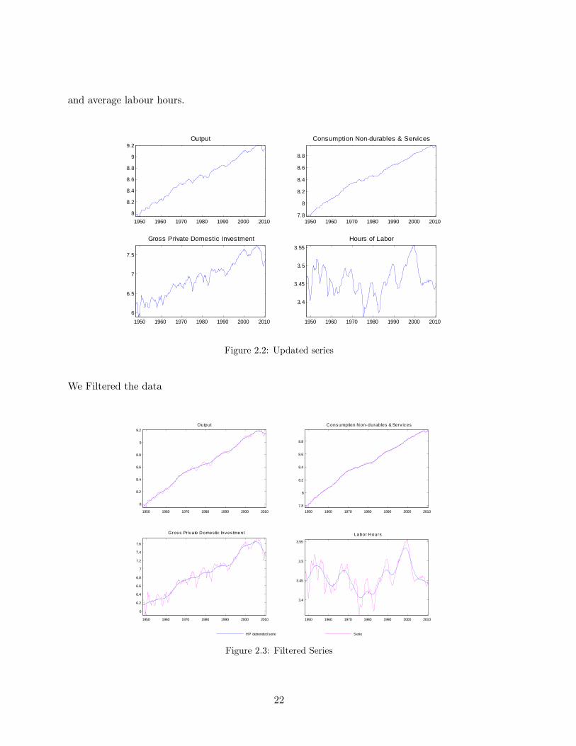
and average labour hours.

1950 1960 1970 1980 1990 2000 20106

6.5

7

7.5


1950 1960 1970 1980 1990 2000 20107.8

8

8.2

8.4

8.6

8.8


1950 1960 1970 1980 1990 2000 2010

3.4

3.45

3.5

3.55Hours of Labor

1950 1960 1970 1980 1990 2000 20108

8.2

8.4

8.6

8.8

9

9.2Output

Figure 2.2: Updated series

We Filtered the data

1950 1960 1970 1980 1990 2000 2010

8

8.2

8.4

8.6

8.8

9

9.2Output

1950 1960 1970 1980 1990 2000 20107.8

8

8.2

8.4

8.6

8.8

Consumption Nondurables & Serv ices

1950 1960 1970 1980 1990 2000 2010

6

6.2

6.4

6.6

6.8

7

7.2

7.4

7.6

Gross Pr ivate Domes tic Inves tment

1950 1960 1970 1980 1990 2000 2010

3.4

3.45

3.5

3.55

Labor Hours

HP detrended serie Serie

Figure 2.3: Filtered Series

22

and we recalculate the table as shown in DD:


HP-Filtered data

j �j�j�y ' (1) 'j;y (0) 'j;y (1)

y 0.01904 1.00000 0.86411 1.00000 0.86411c 0.00834 0.43835 0.83303 0.82054 0.73171i 0.08204 4.30895 0.79954 0.95488 0.80664h 0.01817 0.95425 0.89591 0.79701 0.58907

As we see, in comparison to the moments which were calculated by using a short sample ofdata, we can see that relative standard deviation by each serie does not change dramatically.But, we highlight the fact that there is a substantial decrease in the correlation of labour withthe lag of output. In this dataset we just added up 24 observations and it seems that �nancialcrisis at the end of 2008 has change the response of some variables to the lagged output. But,we need to take this results very carefully because we are using the HP �lter, as we know thisprocedure has series problems at the end and beginning of sample and we cannot take thosenumbers as �nal ones, instead we should take them as preliminaries values for the cycle (seeAppendix for a discussion about the Hodrick-Prescott �lter�s caveats).

0.3 Section (iii)

0.3.1 Explicit growth

We reconduct the calibration exercise of this section using the extension of the RBC modeloutlined in Chapter 5, Section 1 that explicitly incorporates long-term growth. We are goingto pay attention to the fact that equations [20] and [22] in DD, used to restrict the parameter-izations of �; � and ' will be altered given this extension. So too will be [24], which was usedto specify initial values for simulation (Dejong and Dave, 2007).

We consider �rst the dynamic of productivity shock;

zt = zo (1 + g)t exp (wt) (32)

where wt = �wt�1 + �t: If g = 0 we have log zt � log z0 = wt so we would have log zt � log z0 =� (log zt�1 � log z0) + �t: In any case we need to remove the trend from series, in the case ofproductivity shock the procedure is easy because this variable produces the trend, thus wedivide (32) by (1 + g)t

zt =zt

(1 + g)t= zo � exp (wt) (33)

z denotes this serie has a trend, zt is the serie without trend15. In the case of production wehave the following data generation process:

yt= zo (1 + g)

t exp (wt) k�t n

1��t

15 In general a notation x refers to x has a trend.

23

we remove the trend for the production serie

yt

(1 + g)t= zo exp (wt) k

�t n

1��t

in change percentage it is true that (considering that labor does not grow)

%yt � g = �%kt

In this case we have 1 equation and we need to at least determine one growth rate, in this casewe allow for %yt = %kt; thus we have that

%yt = g + �%kt

(1� �)%yt = g

%yt =g

(1� �)

we verify above with the following: If g(1��) is the rate which y and k grow so dividing each

variable by the growth rate we would have an steady state, thus y and k are O��1 + g

(1��)

�t�and z is O

�(1 + g)t

�:

yt�

1 + g1��

�t = zo(1 + g)t

(1 + g)texp (wt)

0B@ kt�1 + g

1��

�t1CA�

n1��t

�nallyyt = zo exp (wt) k

�t n

1��t (34)

We inspect the previous expression in terms of series�1 +

g

1� �

�t= (1 + g)t

�1 +

g

1� �

��t(35)

taking logs

t log

�1 +

g

1� �

�= t log (1 + g) + �t log

�1 +

g

1� �

�the left-hand side is t log (1 + g) + �t log

�1 + g

1��

�� tg + �tg

1�� ; thus tg +�tg1�� =

tg1�� which is

approximately t log�1 + g

1��

�: In the case of law of motion we have

kt+1 = (1� �) kt + it

we remove the trend from those series

kt+1�1 + g

1��

�t = (1� �) kt�1 + g

1��

�t + it�1 + g

1��

�t

24

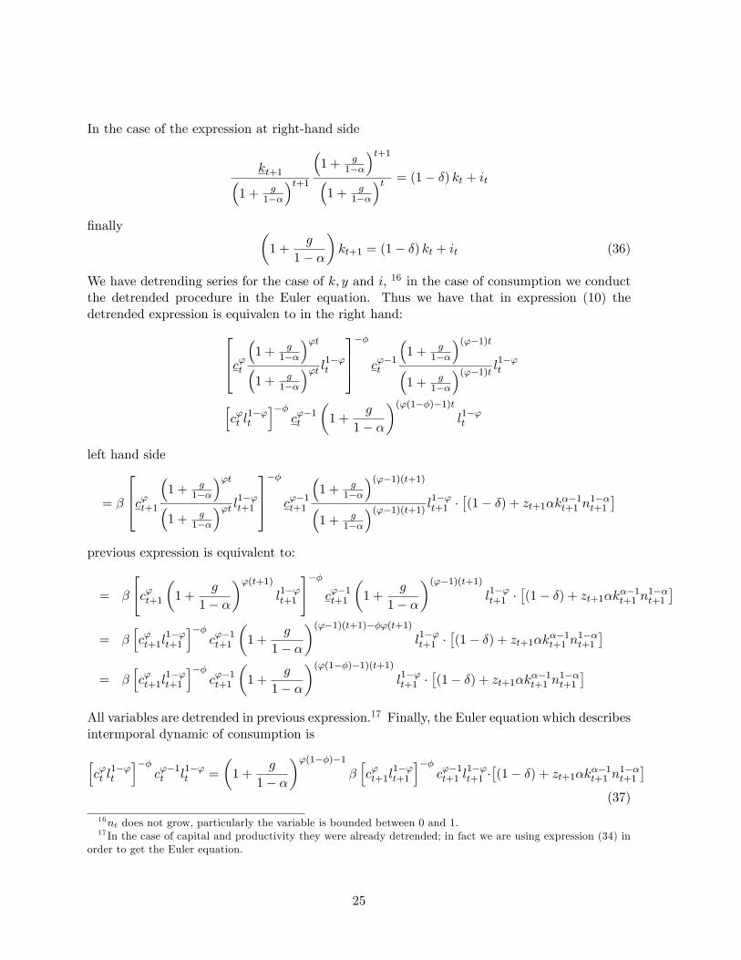
In the case of the expression at right-hand side

kt+1�1 + g

1��

�t+1�1 + g

1��

�t+1�1 + g

1��

�t = (1� �) kt + it

�nally �1 +

g

1� �

�kt+1 = (1� �) kt + it (36)

We have detrending series for the case of k; y and i; 16 in the case of consumption we conductthe detrended procedure in the Euler equation. Thus we have that in expression (10) thedetrended expression is equivalen to in the right hand:264c't

�1 + g

1��

�'t�1 + g

1��

�'t l1�'t

375��

c'�1t

�1 + g

1��

�('�1)t�1 + g

1��

�('�1)t l1�'t

hc't l

1�'t

i��c'�1t

�1 +

g

1� �

�('(1��)�1)tl1�'t

left hand side

= �

264c't+1�1 + g

1��

�'t�1 + g

1��

�'t l1�'t+1

375��

c'�1t+1

�1 + g

1��

�('�1)(t+1)�1 + g

1��

�('�1)(t+1) l1�'t+1 ��(1� �) + zt+1�k��1t+1 n

1��t+1

�previous expression is equivalent to:

= �

"c't+1

�1 +

g

1� �

�'(t+1)l1�'t+1

#��c'�1t+1

�1 +

g

1� �

�('�1)(t+1)l1�'t+1 �

�(1� �) + zt+1�k��1t+1 n

1��t+1

�= �

hc't+1l

1�'t+1

i��c'�1t+1

�1 +

g

1� �

�('�1)(t+1)��'(t+1)l1�'t+1 �

�(1� �) + zt+1�k��1t+1 n

1��t+1

�= �

hc't+1l

1�'t+1

i��c'�1t+1

�1 +

g

1� �

�('(1��)�1)(t+1)l1�'t+1 �

�(1� �) + zt+1�k��1t+1 n

1��t+1

�All variables are detrended in previous expression.17 Finally, the Euler equation which describesintermporal dynamic of consumption is

hc't l

1�'t

i��c'�1t l1�'t =

�1 +

g

1� �

�'(1��)�1�hc't+1l

1�'t+1

i��c'�1t+1 l

1�'t+1 �

�(1� �) + zt+1�k��1t+1 n

1��t+1

�(37)

16nt does not grow, particularly the variable is bounded between 0 and 1.17 In the case of capital and productivity they were already detrended; in fact we are using expression (34) in

order to get the Euler equation.

25

the cross section Euler equation expressed in (11):

ct(1� ')'

= ztk�t (1� �)n��t

which is equivalent to (see expression (35)):

ct(1� ')'

= ltztk�t (1� �)n��t (38)

The system for this particular problem is composed by expressions (36), (33), (37) and (38).

0.3.2 Steady State

As it is pointed out in DDthe steady state in this model is going to change becuase now we haveexplicit growth. Thus, by using expression (37) we have the following relation at the steadystate:

1 = �

�1 +

g

1� �

�h1� � + �zk��1n1��

irearranging terms and considering e� = �

�1 + g

1��

�1e� = 1� � + �zk��1n1��

rearranging terms

�z

�k

n

��1=

1e� � 1 + ��k

n

��1=

1� e� � e��z

k

n=

1� e� � e��

�z

! 1��1

k

n=

��

1� e� � e�� 1

1��

last expression considers z = 1. Now, from condition (38)

c(1� ')'

= lzk�(1� �)n��

c(1� ')'

= lz

�k

n

��(1� �)

Now, we consider kn = A =�

�

1�e��e�� 11��

and z = 1:

c

l=

'

(1� ')A� (1� �)

26

the law motion of capital �1 +

g

1� �

�k = (1� �) k + i�

1 +g

1� � � 1 + ��k = i

in terms of shares respect to output�1 +

g

1� � � 1 + ��k

y=i

y

�nally we close the model with the supply equal to demand

y = c+ i

For this system we �xed n; k and g, then we generate a serie of '; � and � as DD did with theimplicit-growth model. We show the relationship between those parameters in the calibrationsection.

0.3.3 Linearization

The complete linearization is presented in the appendix of this section. We report the log-linearized equations of the system

� gcect = gkekt + gnent + gzezt

�$gcect = $g

c0ect+1 +$gk0ekt+1 +$g

nent +$gn0ent+1 +$g

z0ezt+1the law motion of capital and productivity

� gcect = gkekt + gnent + gzezt

ezt = �gezt + "t � "where ex denotes the logarithm of the variable x respect to the logarithm ot that variableevaluated in the steady state (x). We denote x as the steady state. All group of parameters� g0 $g0 g0 �g

�0 are de�ned in the appendix.0.3.4 State Space

We present the state space, for this purpose we present the Sims�s representation. In our system� = [0 0 0 0]0, and the entire system is:26666664

0 0 � gc � gn 0 0� gk0 0 � gc � gn 0 00 1 0 0 0 0�$g

k0 �$gz0 �$g

c �$gn �$g

c0 �$gn0

0 0 1 0 0 00 0 0 1 0 0

37777775

26666664


37777775 =26666664

gk gz 0 0 0 0 gk gz 0 0 0 00 � 0 0 0 00 0 0 0 0 00 0 0 0 1 00 0 0 0 0 1

37777775

26666664


3777777527

26666664

00�000

37777775 "t +26666664

0 00 00 00 01 00 1

37777775��ct�nt

�

0.3.5 Calibration

We calibrate following the sugestion provided in the outline of computer project. We �x therest of parameters as in the section i. We consider the scenario as before but with explicitgrowth. in any case we �x the steady state of n = 1

3 and establish trade-o¤ between otherparameters in the space of parameters. We choose �; � and ' to illustrate pausible range ofvalues of parametres under the assumption of establishing a �xed steady-state and possiblevalues of g.

Table 3.1Trade O¤ between �; ' and � (values under di¤erent g)

� ' g = 0:0 g = 0:01 g = 0:025 g = 0:050

0.2000 0.3402 0.0707 0.0742 0.0799 0.09050.2063 0.3420 0.0566 0.0570 0.0579 0.06030.2125 0.3438 0.0471 0.0454 0.0431 0.04000.2188 0.3455 0.0404 0.0371 0.0325 0.02530.2250 0.3474 0.0354 0.0309 0.0244 0.0142

If we leave the restrictions and we map the space of parameters, we have the following relations

0.0445610.044561

0.037108

0.029656

0.0222040.022204

0.0147510.014751

0.0072987

0.00015363

0.007606 0.007606

0.015058 0.015058

0.022511 0.022511

Mapping of δg=0.05

α

Φ0.35 0.36 0.37 0.38 0.39 0.4

0.22

0.24

0.26

0.28

0.3

0.32

0.34

0.36

0.38

0.4

0.25

0.3

0.350.06

0.05

0.04

0.03

0.02

0.01

0

0.01

0.02

Φ

Mapping of δ

α

Figure 3.1: g = 0:01

28

0.0445610.044561

0.037108

0.029656

0.0222040.022204

0.0147510.014751

0.0072987

0.00015363

0.0076060.007606

0.0150580.015058

0.0225110.022511

Mapping ofδg=0.05

α

Φ0.35 0.36 0.37 0.38 0.39 0.4

0.22

0.24

0.26

0.28

0.3

0.32

0.34

0.350.36

0.370.38

0.390.4

0.22

0.24

0.26

0.28

0.3

0.32

0.34

0.06

0.05

0.04

0.03

0.02

0.01

0

0.01

0.02

Φ

Mapping ofδ

α

Figure 3.2: g = 0:05

The following table is made considering the baseline parameters, we note that under the para-meters given in exercise (1) there is no huge diference, so we keep that speci�cation

Table

Growth (g)

0.010 0.025 0.05iy 0.1805 0.1871 0.1918cy 0.8195 0.8129 0.8082

n 0.3331 0.3349 0.3361

The parameters we consider for this exercise are:

(� � � � � � g)0 = (0:23 0:99 1:5 0:0244 0.78 0.0067 0:025)0 (39)

0.3.6 Policy Functions

We present results using Schmiddt and Uribe�s procedure the solution in their notation is (theyare de�ned in (18) and (19));

gx =

�0.3780 0.4811-0.1856 0.6980




hx =

�0.8815 0.34130.00000 0.78000

�thus the solution for state variables is: xt+1 = hx � xt + � � "t+1:

29

0.3.7 Calculation of moments

we have the following results under the following parameters in (39)


RBC model

j �j�j�y ' (1) 'j;y (0) 'j;y (1)

y 0.0185 1.00000 0.7924 1.00000 0.7924c 0.0085 0.4594 0.9588 0.7781 0.6216i 0.0844 4.5566 0.7347 0.9454 0.7465h 0.0088 0.4729 0.7276 0.9122 0.7196

Under the calibration made �xing the steady state of nt and mapping the trade-o¤ between�; � and �:


Here impulse responses

0 10 20 303.9

3.95Capital

0 10 20 301

1.02

1.04Productivity

0 10 20 300.49

0.495Consumption

0 10 20 300.58

0.59

0.6Output

0 10 20 300.08

0.1

0.12Investment

0 10 20 300.325

0.33

0.335Labor

30

0 5 10 15 20 250.5

0

0.5

1

1.5

2

Quarters

Per

cent

Dev

iatio

ns


As we saw in class, the consumption converges slowly to the steady state. The response oflabor hours to one standard-deviation productivity shock produces an incentive to work morebut it vanishes quickly through the quarters; in fact in less of 5 quarters there is less than 10%of the shock in the response of labor hours. The output increases as long as the productivityrises and converges slowly to its steady state value at the long run.

0.4 Section (iv)

0.4.1 Greenwood, Hercowitz, and Hu¤man�s (GHH) preferences

In this part of our analysis, instead of using DD�s Cobb-Douglass preferences, we will deal withGreenwood, Hercowitz, and Hu¤man�s (GHH) preferences where the income e¤ect on laborsupply is zero. Before presenting our result, �rst it is signi�cant to make a brief discussionabout what is di¤erent in GHH model. (Jeremy Greenwood and Hu¤man, 1988).

Shocks to the Demand & Total Factor Productivity. In Solow growth model, growth hasbeen attributed whether to the capital accumulation or increase in labor. On the other hand,the change in productivity growth which refers to rising output occurring with constant laborcapital input is the Solow residual. It is called as a residual because this part of the growthcannot be explained well in the Solow�s model. However, in this model Solow residual -whichwas not based on empirical data- was an attempt to show the impact of �technology�growthrather than being the outcome of a theoretical analysis. (Acemoglu, 2009).

The models which we have used so far were de�ned Solow residual as exogenous shocks tothe production function and �rst developed by Finn Kydland and Edward Presscott (1982) andJohn Long and Charles Plosser (1983). The real business cycle literature following these studiesfocus on such peculiar technology shock that a¤ects business cycle activity. This shock whichis also sometimes called the Solow residual or the total factor productivity (TFP) shock is aHicks-neutral technology shock. (Dejong, et. al., 2000) To Hansen and Presscott (1993), these

31

exogenous shocks to the production function could also re�ect various changes in productionsuch as changes in prices non-measured inputs and changes in the rules of business environment.These types of impulses were actually rest in contrast with Keynesian explanation that shocksto the marginal e¢ ciency of investment (MEI) have key importance in output changes causingcycles while TFP shocks investment reacts to changes in output. Thus, to observe this role ofMEI Greenwood et. al. used this sort of shocks in RBC model that characterizing variablecapital utilization and depreciation. Thus, their model has three peculiar features that departit from a standard framework of RBC;

� As we have already described, economic �uctuations are attributable to a single shock toinvestment.

� Agents may change the rate of capital utilization as a response to the shocks.

� Higher rates of capital utilization stimulate higher rates of depreciation of the existingstock of capital.

In the light of these considerations, in this task of our project, we will apply to our previoussimple RBC model GHH preferences in which representative agents choose consumption andlabor to maximize the expected value of lifetime utility. A key feature of the period utilityfunction is that the marginal rate of the substitution between the consumption and the laboris completely depends on labor. In other words, income e¤ect does not a¤ect labor decision.(DeJong et. al., 2000) In other words, the agent does not make decision on consumption-leisurechoice and the expected future shocks are not responded by the labor supply

0.4.2 Decisions and Sectors

The representative agent�s lifetime utility function is:

U = E0

1Xt=0

�t�ct � �

� (1� lt)v�1��

1� � (40)

The technology available for production is the same as de�ned in (1). So, expressions (), (3),(2) de�nes the agent�s budget constraint, the law of motion and deciions for division betweenlabor and leisure activities respectively. The household�s problem is to maximize (40) subjectto (1) , (), (3) and (2) , taking k0 and z0 as given. The technology process evolves accordingto an AR(1) process in logs de�ned in (4).

0.4.3 Dynamic Programming

The Bellman equation in this particular problem is similar as we have seen in section (i):

V (kt; zt) = u (ct; lt) + �V (kt+1; zt+1)

We get the Euler equation as before but now with di¤erent preferences. DDreports the necessarycondition associated with the household�s problem wich are expressed in general way18:

@u (ct; lt)

@lt=@u (ct; lt)

@ct� @f (kt; nt)

@nt18See page 91 equations 5.11 and 5.12

32

@u (ct; lt)

@lt= �

@u (ct+1; lt+1)

@ct+1��@f (kt+1; nt+1)

@kt+1+ 1� �

�the Euler equations in this case are:h

ct ��

�(nt)

vi��

� (nt)v�1 =

hct �

�

�(nt)

vi��

ztk�t (1� �)n��t (41)h

ct ��

�(nt)

vi��

= �hct+1 �

�

�(nt+1)

vi��

��(�) zt+1k

��1t+1 n

1��t+1 + 1� �

�(42)

The complete derivation is in appendix by using lagrange procedure.

0.4.4 Steady State of variables

We present the steady state of variables in this section.

� (n)v�1 = zk�(1� �)n��

1 = � �h�zk

��1n1�� + 1� �

ithe steady-state relation which comes from the law mpotion of capital is the same as speci�edin (3), the same for the dynamic of the shocks which is speci�ed in (4).

0.4.5 Linearization

The complete linearization is presented in the appendix of this section. We report the log-linearized equations of the system

0 = Hkekt + Hn ent + zezt

$Hc ect = $H

c0 ect+1 +$Hk0ekt+1 +$H

n ent +$Hn0ent+1 +$H

z0 ezt+1the law motion of capital and productivity is as in the section i

Hc ect = Hkekt + Hn ent + Hz eztezt = �ezt + "t � "

where ex denotes the logarithm of the variable x respect to the logarithm ot that variavlevaluated in the steady state (x). We denote x as the steady state. All group of parameters� H0 $H0 H0 �

�0are de�ned in the appendix

0.4.6 State Space

We present the state space, for this purpose we present the Sims�s representation. In our system� = [0 0 0 0]0, and the entire system is:26666664

0 0 0 � Hn 0 0

� Hk0 0 Hc � Hn 0 00 1 0 0 0 0�$H

k0 �$Hz0 $H

c �$Hn �$H

c0 �$Hn0

0 0 1 0 0 00 0 0 1 0 0

37777775

26666664


37777775 =26666664

Hk Hz 0 0 0 0

Hk Hz 0 0 0 00 � 0 0 0 00 0 0 0 0 00 0 0 0 1 00 0 0 0 0 1

37777775

26666664


3777777533

26666664

00�000

37777775 "t +26666664

0 00 00 00 01 00 1

37777775��ct�nt

�

0.4.7 Calibration

We calibrate folowing the sugestion provided in the outline of computer project. We assume� = 1:5 and a value of � such that n = 1

3 : We �x the rest of parameters as in the section (i).Thus

[� � � � � �]0 = [0:24 0:99 1:5 0:025 0.78 0.0067]0

In this case the value of � is closed to 2:54.We consider another scenario as DDproposed; they �x the steady state of n = 1

3 andestablish trade-o¤ between other parameters in the space of parameters. In this case � doesnot play any role in the steady stae, instead of that we choose �; � and � to illustrate pausiblerange of values of parameters under the assumption of establishing a �xed steady-state.

0.003

2124

0.01

1398

0.011

398

0.01

9584

0.019

584

0.02

7769

0.027

7690.0

3595

5

0.03

5955

0.044

14

0.04

414

0.05

2326

0.06

0512

0.06

8697

δ

α

τ2.5 3 3.5

0.2

0.25

0.3

2.53

3.5

0.2

0.25

0.3

0.350.02

0

0.02

0.04

0.06

0.08

τ

Mapping of δ

α

0.4.8 Policy function

We present results using Schmiddt and Uribe�s procedure the solution in their notation is (theyare de�ned in (18) and (19));

gx =

�0.96597 0.427800.92361 0.42849




hx =

�0.99564 0.142000.00000 0.78000

�34

thus the solution for state variables is: xt+1 = hx � xt + � � "t+1:

0.4.9 Calculation of moments

we have the following results under the following parameters

(� � � � � � � �)0 = (0:24 0:99 1:5 2:45 1:5 0:025 0.78 0.0067)

0

Table 6.4Moments comparison

RBC model

j �j�j�y ' (1) 'j;y (0) 'j;y (1)

y 0.04707 1.00000 0.98153 1.00000 0.98153c 0.04513 0.95883 0.99793 0.97943 0.96771i 0.07530 1.59954 0.85925 0.80981 0.77632h 0.04320 0.91775 0.99775 0.98037 0.96849


Here impulse responses

0 10 20 307.3

7.35Capital

0 10 20 301

1.02

1.04Productivity

0 10 20 300.63

0.635

0.64Consumption

0 10 20 300.8

0.81

0.82Output

0 10 20 300.16

0.17

0.18Investment

0 10 20 300.305

0.31Labor

35

0 5 10 15 20 250.5

0

0.5

1

1.5

2

Quarters

Per

cent

Dev

iatio

ns


As we saw in class, the consumption converges slowly to the steady state. The response oflabor hours to one standard-deviation productivity shock produces an incentive to work morebut now it does not vanish quickly through the quarters as in the previous exercise; in factlabor tracks the consumption�s response and keep a path across quarters. The output increasesas long as the productivity rises and converges slowly to its steady state value at the long run.

0.5 Conclusions from our Computer Project

In our project, we�ve presented the results from the a classical RBC model (section i), HP-Filtered Data (section ii) and RBC model with GHH preferences (section iv). These tablesportray the statistics calculated by the data and calibration methods where:

1. �j : standard deviation j (y: output, c: consumption, i: investment, h: hours to work)

2. �j�y: the ratio standard deviation j to output

3. ' (0): �rst order serial correlation

4. 'j;y (0): zero-th order correlation between j & y:

5. 'j;y (0): �rst order serial correlation (autocorrelation) zero-th between j & y:

Under a productivity shock the most relevant result obtained by standard deviations isthe well known fact that investment is much more volatile than output and consumption isless since the people want to smooth their consumption. Both of the models performed fairlywell in this respect. To see this, the ratio of standard deviations also mimics this featurequantitatively. However, in terms of the standard deviation ratios, results obtained in the �rstmodel overestimates hours while the second model fails in consumption which is a consequenceof the structures of these models.

36

The most salient feature of the results of the GHH preference model is the high autocor-relation level between production and work hours. Due to our well-known fact that there isno income e¤ect in the model, a positive productivity shock has been responded by labor di-rectly. The representative agent prefers to work more, thus consume more, when there is anenvironment for earning more, in other words, people work more when real wages are higherand they are more productive. On the other hand, our basic RBC model was constructed withboth income and substitution e¤ect whose e¤ects are in opposite directions. Thus, the modelportrays a consumption-leisure trade-o¤ which is illustrated quantitatively with a lower �rstorder autocorrelation than the GHH model. The correlations of consumption and work hourswith output for the second model are almost 1 which can be expected by the construction ofthe model while the same correlations for the �rst model and its autocorrelation results bothremained lower. HP-Filtered data result for the autocorrelation of the hours is lower thanthe GHH model but higher than the �rst RBC model which can be expected. In addition,to the data results consumption is persistent and has a procyclical behavior. This feature isreproduced by all models. paper

In conclusion, the strongest response of hours worked occurs with GHH preferences. Inthis case, because of the lack of income e¤ect, hours worked are not stationary. They risepermanently in response to the permanent increase in the real wage rate.

37

References

Acemoglu, D. (2009). Introduction to Modern Economic Growth. Princeton University Press,Princeton University Press.

Canova, F. (2007). Methods for Applied Macroeconomic Research. Princeton University Press,Princeton University Press.

Collard and Juillard (2001). Perturbation methods for rational expectations. ManuscriptCEPREMAP.

Dejong, D. and Dave, C. (2007). Structural Macroeconomics. Princeton University Press,Pittsburg University.

Hamilton, J. (1994). Times Series Analysis. Princeton Press, Princeton Press.

Hansen, G. and Prescott, E. (1993). Did technology shocks cause the 1990-1991 recession? TheAmerican Economic Review.

Heer, B. and Maunner, A. (2009). Dynamic General Equilibrium Modeling ComputationalMethods and Applications. Springer Dordrecht, New York.

Hodrick, R. and Prescott, E. (1997). Postwar u.s. business cycles: An empirical investigation.Journal of Money, Credit and Banking 29 (1), 1-16.

Jeremy Greenwood, Z. H. and Hu¤man, G. (1988). Investment, capacity utilization, and thereal business cycle. The American Economic Review.

Judd, K. (1998). Numerical methods in economics. MIT press.

Kydland, F. E. and Prescott, E. (1982). Time to build and aggregate �uctuations. Economet-rica.

Long, J. B. and Plosser, C. I. (1983). Real business cycles. Journal of Political Economy.

Michelacci, C. (2006). Solving a system of linear equations with rational expectations. Mimeo.

Prescott, E. and Ueberfeldt, A. (2003). Us hours and productivity behaviour using cps hoursworked data: 1959:i to 2003:ii. Mimeograph.

Rojas, F. (2006). About the phillips curve. Universidad de Chile.

38

Schmitt-Grohe, S. and Uribe, M. (2004). Solving dynamic general equilibrium models using asecond-order approximation to the policy function. Journal of Economics Dynamics andCOntrol.

Sims, C. (2000). Solving linear rational expectations models. Sims�s web page.

39

Appendix A

Log-Linearization section i.

We linearized the model in this section of the appendix. For sake of simplicity and our purposeswe do a change-variable procedure

xt = elog xt

thus the linearization procedure will be easy. We consider the equation in expression (11) whichrelates the consumption and labor today (cross-section Euler dynamic equation). So, we have

elog ct(1� ')'

=�1� elognt

�elog zte� log kt (1� �) e�� lognt

0 = �elog ct (1� ')'

+�1� elognt

�elog zte� log kt (1� �) e�� lognt

We consider an Taylor�s expansion around the steady state

f(x) � f(x0) + f 0(x0)(x� x0)

we report f 0(x0)(x� x0) because f(x) = 0 and f(x0) = 0

0 = �elog co (1� ')'

[log ct � log c0] + ��1� elogn0

�elog z0e� log k0e�� logn0 (1� �) [log kt � log k0]

+�1� elogn0

�elog z0e� log k0 (1� �) e�� logn0 (��) [log nt � log n0]

+�1� elogn0

�elog z0e� log k0 (1� �) e�� logn0 [log zt � log z0]

�elogn0elog z0e� log k0 (1� �) e�� logn0 [log nt � log n0] (A.1)

Also, other way is possible, we can directly take logs to expression (11) and then we do the

just approximation around ss

log[(1� ')'

] + log ct = log(1� nt) + log zt + � log kt + log(1� �)� � log nt

40

Then in the steady state

log[(1� ')'

] + log c0 = log(1� n0) + log z0 + � log k0 + log(1� �)� � log n0

so substracting steady state,

log ct� log c0 = [log(1�nt)� log(1�n0)]+ [log zt� log z0]+�[log kt� log k0]��[log nt� log n0]

so (A.1) should look the same,

log ct � log c0 =��1� elogn0

�elog z0e� log k0 (1� �) e�� logn0

+elog c0 (1�')'

[log kt � log k0]

+��

�1� elogn0


+elog c0 (1�')'

[log nt � log n0]

+

�1� elogn0


+elog c0 (1�')'

[log zt � log z0]


+elog c0 (1�')'

[log nt � log n0]

We have used the following expression in order to get the Taylor�s expansion term f 0(x0)(x�x0)

for labor hours:

log�1� elognt

�� log(1� n0)�

1

(1� elogn0) [log nt � log n0]

[log nt � log n0] = �n0

1� n0[log nt � log n0]

We re-arrange result in (A.1)

log ct� log c0 = �[n0

1� n0][log nt� log n0]+ [log zt� log z0]+�[log kt� log k0]��[log nt� log n0]

Coming back to expression (A.1), we have the following as a result of linearize expression (11):

c = �elog c0 (1� ')'

k = ��1� elogn0

�elog z0e� log k0e�� logn0 (1� �)

n =�1� elogn0

�elog z0e� log k0 (1� �) e�� logn0 (��)

�elogn0elog z0e� log k0 (1� �) e�� logn0

z =�1� elogn0


41

Now, we linearize the Law of motion of capital which is expressed in (3),

kt+1 = (1� �) kt + ztk�t n1��t � ct

under the terms of of the same previous derivation,

elog kt+1 = (1� �)elog kt + elog zte� log kte(1��) lognt � elog ct

a Taylor�s expansion around steady state

0 = �elog k0 [log kt+1 � log k0]+(1� �)elog k0 + elog z0�elog k0e(1��) logn0[log kt � log k0]+elog z0e� log k0e(1��) logn0 [log zt � log z0]+elog z0e� log k0(1� �)e(1��) logn0 [log nt � log n0]�elog co [log ct � log co] (A.2)

Thus, we have the following as a result of linearize expression (11):

c = �elog co

k = (1� �)elog k0 + elog z0�elog k0e(1��) logn0

k0 = �elog k0

z = elog z0e� log k0e(1��) logn0

n = elog z0e� log k0(1� �)e(1��) logn0

so now, we do not have any problem with the law motion of productivity because it is alreadyin logs,

[log zt � log z0] = �[log zt�1 � log z0] + [et � e0]

In the case of the intertemporal dynamic equation for the consumption in expression (10) wehave the following:

0 = e��' log cte��(1�') log(1�elognt)e('�1) log cte(1�') log(1�e

lognt)

��"e�' log ct+1e��(1�') log(1�e

lognt+1)e('�1) log ct+1e(1�') log(1�elognt+1)

(1� �) + �elog zt+1e(��1) log kt+1e(1��) lognt+1

#

42


�(�'e��' log coe��(1�') log(1�elogno)e('�1) log c0e(1�') log(1�elogn0)

+e��' log coe��(1�') log(1�elogno) ('� 1) e('�1) log c0e(1�') log(1�elogn0)) [log ct � log c0]

��"


+e��' log coe��(1�') log(1�elogno) ('� 1) e('�1) log c0e(1�') log(1�elogn0)

#��

1� � + �elog z0e(��1) log k0e(1��) logn0�[log ct+1 � log c0]

��e��' log coe��(1�') log(1�e

logno)e('�1) log c0e(1�') log(1�elogn0)

��

� (�� 1) elog z0e(��1) log k0e(1��) logn0�[log kt+1 � log c0]

(� 1

1� noelogn0 (�� (1� ')) e��' log coe��(1�') log(1�elogno)e('�1) log c0e(1�') log(1�elogn0)

�e��' log coe��(1�') log(1�elogno)e('�1) log c0 (1� ') e(1�') log(1�elogn0) 1

1� noelogn0) �

[log nt � log c0] +

��(� 1


+e��' log coe��(1�') log(1�elogno)e('�1) log c0 (1� ') e(1�') log(1�elogn0) (�1)

1� noelogn0) ��

1� � + �elog z0e(��1) log k0e(1��) logn0�

��e��' log coe��(1�') log(1�e


��

� (1� �) elog z0e(��1) log k0e(1��) logn0�[log nt+1 � log z0] +

��e��' log coe��(1�') log(1�e


��

�elog z0e(��1) log k0e(1��) logn0�[log zt+1 � log z0]

43

Thus, we have the following parameters

$c = �(�'e��' log coe��(1�') log(1�elogno)e('�1) log c0e(1�') log(1�elogn0)

e��' log coe��(1�') log(1�elogno) ('� 1) e('�1) log c0e(1�') log(1�elogn0))

$c0 = ��"


+e��' log coe��(1�') log(1�elogno) ('� 1) e('�1) log c0e(1�') log(1�elogn0)

#��


$k0 = ��e��' log coe��(1�') log(1�e


��

� (�� 1) elog z0e(��1) log k0e(1��) logn0�

$n = (� 1


�e��' log coe��(1�') log(1�elogno)e('�1) log c0 (1� ') e(1�') log(1�elogn0) 1

1� noelogn0)

$n0 = ��(� 1


+e��' log coe��(1�') log(1�elogno)e('�1) log c0 (1� ') e(1�') log(1�elogn0) (�1)

1� noelogn0) ��


��e��' log coe��(1�') log(1�e


��

� (1� �) elog z0e(��1) log k0e(1��) logn0�

$z0 = ��e��' log coe��(1�') log(1�e


��

�elog z0e(��1) log k0e(1��) logn0�

44

Appendix B

Caveats with HP �lter

If the process for yxt � yxt�1 = y0 +1Pj=1

vt�j so yxt+1 � yxt = y0 +1Pj=1

vt+1�j ; therefore

�yxt+1 � yxt

��yxt � yxt�1

�= vt

TXt=0

��yxt+1 � yxt

��yxt � yxt�1

��2=

Xv2t (B.1)

the expectation is equal to T�2v and for expression E (yt � yxt )2 = �2c in the case of D

c (`) = I:Task: to obtain the expectations when Dc (`) 6= I:o the problem is a typical minimization ofsquares1. Getting back to our problem if the process is not a simply trend plus noise or whenthe cyclical component is not i:i:d the �lter is not longer optimal :Furthermore, rather thanestimating � the literature selects it a priori so to carve out particular frecuencies. For example� = 1600 -used for quarterly data- means that variance of the cycle is 1600 times larger thanvariance of the second di¤erence of the trend. The HP �lter is time dependent. Furthermore,its two sided, this property makes the �lter problematic at the beginning and ending of thesample. If we would have more data the permanent component for this part of the data wouldchange if they are in the middle of data. This creates distorsions when one is interested in theproperties of yt around of the end of the sample. (example: are we close to some recession orboom?).

1The set up of the problem is similar to the adverse-central-banker problem:

L = � (yt � y)2 + � (� � �)2

where yt � y is the output gap and � is the in�ation rate. � and � are deep parameters which can be calibratedin order to specify a degree of adversity to in�ationary paths.

45

Appendix C

Log-Linerization section iii

In this section we are going to linearize the equations in (36), (33), (37) and (38). In the caseof expression (38) we have the linear equation as in (A.1) The dynamics of shock is alreadylinear and we do not need to apply log-linearization procedure. In the case of expression (37)and (36) -which refers to cross-section Euler equation and law motion of capital- we need toset up a little modi�cation.

We linearize the expression (37); this procedure is simple because we note that term

��1 + g

1��

�'(1��)�1does not depend of some variable and we can treat it as a parameter

in this case we express that constant as e� in the equation, thus we have:hc't l

1�'t

i��c'�1t l1�'t = e� hc't+1l1�'t+1

i��c'�1t+1 l

1�'t+1 �

�(1� �) + zt+1�k��1t+1 n

1��t+1

�Under this speci�cation we conduct the same procedure as in the �rst section of this appendixand we got the following equivalences:

$gc = $c

$gc0 =

e��$c0

$gk0 =

e��$k0

$gn = $n

$gn0 =

e��$n0

$gz0 =

e��$z0

In the case of the law motion, we have the following expression ready for linearize�1 +

g

1� �

�kt+1 = (1� �) kt + ztk�t n1��t � ct

under the terms of of the same previous derivation,�1 +

g

1� �

�elog kt+1 = (1� �)elog kt + elog zte� log kte(1��) lognt � elog ct

46


0 = ��1 +

g

1� �

�elog k0 [log kt+1 � log k0]

+(1� �)elog k0 + elog z0�elog k0e(1��) logn0[log kt � log k0]+elog z0e� log k0e(1��) logn0 [log zt � log z0]+elog z0e� log k0(1� �)e(1��) logn0 [log nt � log n0]�elog co [log ct � log co] (C.1)

Thus, we have the following as a result of linearize expression (11):

gc = ��1 +

g

1� �

�elog co

gk = k

gk0 = k0

gz = z

gn = n

47

Appendix D

Log-linearization in section iv

The solution method requires the system of equations to be linear. The production function is:

yt = ztk�t (1� lt)

1�� = ztk�t n

1��t

The steady state is:�y = �z�k��n1��

let xt � �xext ;8x = k; c; y; i; n; z:

=) �yeyt � �zezt��k�e�kt

��n1��e(1��)nt

�=) �yeyt � �z�k��n1��ezt+�kt+(1��)nt

divided by steady state,=) eyt � e

zt+�kt+(1��)nt

) yt � zt + �kt + (1� �) nt (D.1)

Taking into consideration the Euler equation in (41), we linearize left hand side of that expres-sion by using a Taylor expansion.

�nv�1t = � �nv�1 + � (v � 1) �nv�2 (nt � �n)

�nv�1t � � �nv�1� �nv�1

=� (v � 1) �nv�2 (nt � �n) �n

� �nv�1�n= (v � 1) �n�1�nnt= (v � 1) nt

Linearize right hand side by Taylor expansion.

(1� �) zt(ktnt)� = (1� �) (

�k

�n)� + (1� �)�

� �k�n

��1�1

�n

��kt � �k

�� (1� �)�

� �k�n

��1� �k�n2

�(nt � �n) + (1� �) (

�k

�n)� (zt � �z)

48

=)(1� �) zt( ktnt )

� �h(1� �) ( �k�n)

�i

(1� �) ( �k�n)�=(1� �)�

��k�n

��1 �1�n

� �kt � �k

��k

(1� �) ( �k�n)��k�

(1� �)��k�n

��1 � �k�n2

�(nt � �n) �n

(1� �) ( �k�n)��n+(1� �) ( �k�n)

� (zt � �z) �z(1� �) ( �k�n)��z

= �kt � �nt + �zzt

left hand side = right hand side.

(v � 1) nt = �kt � �nt + �zzt

, (v � 1 + �) nt = �kt + zt (D.2)

Thus, we have the following

Hk = �

Hk = � (� � 1 + �) Hz = 1

Euler Equationhct �

�

�(1� lt)v

i��= Et�

hct+1 �

�

�(1� lt+1)v

i��[�zt+1k

��1t+1 (1� lt+1)

1�� + 1� �]

Linearize left hand side by Taylor expansion and considering that 1� l = �nhct �

�

�nvt

i��=h�c� �

��nvi��

��h�c� �

��nvi��1

(ct � �c)��h�c� �

��nvi��1

(��) �nv�1 (nt � �n)

dividing by��c� �

� �nv��

=)�ct � �

�nvt

�� c� �� n

v��

�c� �� n

v�� =

��c� �

� �nv��1

(ct � �c) �c��c� �

� �nv��

�c��c� �

� �nv��1

(��) �nv�1 (nt � �n) �n��c� �

� �nv��

�n

= ��h�c� �

��nvi�1

�cct � �h�c� �

��nvi�1

(��) �nvnt

Linearize right hand side by Taylor expansion:

Et�hct+1 �

�

�nvt+1

i��[�zt+1k

��1t+1 n

1��t+1 + 1� �]

= Et

266666664

��c� �

� �nv��

[��k��1�n1�� + 1� �]+�h��c� �

� �nv��1

[��k��1�n1�� + 1� �]i(ct+1 � �c)

+�h��c� �

� �nv��1

[��k��1�n1�� + 1� �]i(��) �nv�1 (nt+1 � �n)

+��c� �

� �nv��

��k��1�n1�� (zt+1 � �z)�

+��c� �

� �nv��

�(�� 1)�k��2�n1��kt+1 � �k

��

37777777549

=)Et�

�ct+1 � �

�nvt+1

��[�zt+1k

��1t+1 n

1��t+1 + 1� �]� Et�

��c� �

� �nv��

[��k��1�n1�� + 1� �]��c� �

� �nv��

[��k��1�n1�� + 1� �]

= Et

24 �� c� �� n

v��1

�cct+1 + �� nv��c� �

� �nv��1

nt+1 +[��k��1�n1��]

[��k��1�n1��+1��] zt+1

+�k[�(��1)�k��2�n1��][��k��1�n1��+1��] kt+1

35left hand side = right hand side.

��h�c� �

��nvi�1

�cct � �h�c� �

��nvi�1

(��) �nvnt

= Et

24 �� c� �� n

v��1

�cct+1 + �� nv��c� �

� �nv��1

nt+1 +[��k��1�n1��]

[��k��1�n1��+1��] zt+1+

[�(��1)�k��1�n1��][��k��1�n1��+1��] kt+1

35(D.3)To make it simple, let

G � �h�c� �

��nvi�1

�c

~G � �� nvh�c� �

��nvi�1

�G ��k��1�n1��

�[��k��1�n1�� + 1� �]

and�x;t = xt � Et�1xt;8x = c; n; z; k

So, last Euler Equation is:

�Gct + ~Gnt + �Gzt + (�� 1) �Gkt = Gct�1 + ~Gnt�1 �G�c;t + ~G�n;t + �G�z;t + �G�k;t+1

In terms of the parameters in our system, we have the following:

$Hc0 = �G

$Hc = G

$Hk0 = � (�� 1)

$Hn = � ~G

$Hn0 = � ~G

$Hz0 = �G

50

Appendix E

Optimality conditions in section iv

The associated Lagrangian of the problem is:

$ = E0

1Xt=0

�t

"�ct � �

� (1� lt)v�1��

1� � + �t

hztk

�t (1� lt)

1�� ct � kt+1 + (1� �) kti#

The associated F.O.C. are:

@$

@ct= �t

�hct �

�

�(1� lt)v

i�� t

�= 0

) �t =hct �

�

�(1� lt)v

i��which is the shadow value at t equivalent to marginal utility of consumption at t.

@$

@lt= �t

�� (1� lt)v�1

hct �

�

�(1� lt)v

i��hct �

�

�(1� lt)v

i��(1� �) zt

�kt

1� lt

��= 0

=) �t� (1� lt)v�1 = �t�(1� �) zt

�kt

1� lt

��which is labor supply function.

@$

@kt+1= �t [�t] + Et�

t+1�t+1[�zt+1k��1t+1 (1� lt+1)

1�� + 1� �]

=) �t = Et��t+1

h�zt+1k

��1t+1 (1� lt+1)

1�� + 1� �i

=)hct �

�

�(1� lt)v

i��= Et�

hct+1 �

�

�(1� lt+1)v

i��[�zt+1k

��1t+1 (1� lt+1)

1�� + 1� �]

which is Euler Equation. The transversality condition of the problem is:

limt!1

�t�tkt+1 = 0

51

Appendix F

Steady State in section iv

It is assumed that at the steady state of the model there are no shocks to the technologyprocess, �t = 0, and the long run level of technology is normalized to unity, �z = 1. The steadystate of Euler Equation is:

1 = �h��z�k��1

�1� �l

�1��+ 1� �

i

=) 1 = �

"�

� �k

1� �l

��1+ 1� �

#

=) 1

�� 1 + � = �

� �k

1� �l

��1

=) 1� � + ��

=

� �k

1� �l

��1

=)�k

1� �l=

��

1� � + ��

� 11��

= �A�::::::(13)

The steady state of labor supply function is:

��1� �l

�v�1= (1� �)A�

=)�1� �l

�v�1=1

�(1� �)A�

=) 1� �l =�1

�(1� �)A�

� 1v�1

) �l = 1��1

�(1� �)A�

� 1v�1

= �B�

)�k

1�B = A =) �k = A(1�B)::::::(14)

52

The steady state of output, investement and consumptions are:

�y = [A(1�B)]� [1�B]1�� ::::::(15)

�{ = ��k:::::::(16)

�c = �y � �{::::::(17)-Budget Constraint:

yt = ct + it:

The steady state is�y = �c+�{

let xt � �x(1 + xt);8 x = k; c; y; i; n; z:

�y (1 + yt) � �c (1 + ct) +�{�1 + it

�subtract the steady state,

) yt ��c

�yct +

�{

�y{t::::::(19)

-Capital law of motion:kt+1 = it + (1� �) kt

The steady state is�k = �{+ (1� �) �k = �{+ �k � ��k

do the same process as above.

�k�1 + kt+1

�= �{ (1 + {t) + (1� �) �k

�1 + kt

�=) kt+1 =

�{�k{t + (1� �) kt::::::(20)

-Technology process:

log zt = (1� �) log (�z) + � log zt�1 + �t

The steady state islog �z = (1� �) log (�z) + � log �z + �t

subtract from technology process to the steady state and let xt = log xt � log �x;8 x =k; c; y; i; n; z:

) zt = �zt�1 + �t::::::(21)

-Optimal labor supply:

��1� �l

�v�1= (1� �) zt(

kt1� lt

)�

() �nv�1t = (1� �) zt(ktnt)�

53

Appendix G

Implementation in Gensys for aSystem of dimension 6� 6

The solution method by Sims requires following form:

�0xt = �1xt�1 +zt +��t + C

For the model described above, letting

xt = [ct; it; yt; kt+1;zt;nt]

zt = [�t]

�t =��c;t; �i;t; �y;t; �k;t+1; �z;t; �n;t

�Using the equations in the order used between (18) and (23), the input matrices are de�ned

as follows:

�0 =

266666664

�c�y

�{�y �1 0 0 0

0 �{�k

0 1 0 0

0 0 0 0 1 00 0 1 0 �1 �� 10 0 0 0 �1 v � 1� ��G 0 0 0 �G ~G

377777775

�1 =

26666664

0 0 0 0 0 00 0 0 1� � 0 00 0 0 0 � 00 0 0 � 0 00 0 0 � 0 0

G 0 0 (�� 1) �G 0 ~G

37777775

54

=

26666664

001000

37777775

� =

26666664

0 0 0 0 0 00 0 0 0 0 00 0 0 0 0 00 0 0 0 0 00 0 0 0 0 0

�G 0 0 0 �G ~G

37777775

C =

26666664

000000

37777775

55

Documents

Structural Macroeconomics