Embed Size (px)
Citation preview
Structural Operational Semantics
Luca Aceto∗ Wan Fokkink† Chris Verhoef‡
Contents
1 Introduction 5
2 Preliminaries 82.1 Labelled Transition Systems . . . . . . . . . . . . . . . . . . . 82.2 Behavioural Equivalences and Preorders . . . . . . . . . . . . 102.3 Hennessy-Milner Logic . . . . . . . . . . . . . . . . . . . . . . 132.4 Term Algebras . . . . . . . . . . . . . . . . . . . . . . . . . . 142.5 Transition System Specifications . . . . . . . . . . . . . . . . 152.6 Examples of TSSs . . . . . . . . . . . . . . . . . . . . . . . . 16
2.6.1 Basic Process Algebra with Empty Process . . . . . . 162.6.2 Priorities . . . . . . . . . . . . . . . . . . . . . . . . . 162.6.3 Discrete Time . . . . . . . . . . . . . . . . . . . . . . . 17
3 The Meaning of TSSs 173.1 Model-Theoretic Answers . . . . . . . . . . . . . . . . . . . . 183.2 Proof-Theoretic Answers . . . . . . . . . . . . . . . . . . . . . 223.3 Answers Based on Stratification . . . . . . . . . . . . . . . . . 243.4 Evaluation of the Answers . . . . . . . . . . . . . . . . . . . . 253.5 Applications . . . . . . . . . . . . . . . . . . . . . . . . . . . . 26
∗BRICS (Basic Research in Computer Science), Centre of the Danish National Re-
search Foundation, Department of Computer Science, Aalborg University, Fredrik BajersVej 7-E, DK-9220 Aalborg Ø, Denmark. Email: [email protected]. Partially supported bya grant from the Italian CNR, Gruppo Nazionale per l’Informatica Matematica (GNIM).
†CWI, Department of Software Engineering, Kruislaan 413, 1098 SJ Amsterdam, TheNetherlands. Email: [email protected]. Partially supported by a grant from the Nuffield Foun-dation.
‡University of Amsterdam, Department of Computer Science, Programming ResearchGroup, Kruislaan 403, 1098 SJ Amsterdam, The Netherlands. Email: [email protected].
1
4 Conservative Extension 274.1 Operational Conservative Extension . . . . . . . . . . . . . . 294.2 Implications for Three-Valued Stable Models . . . . . . . . . 324.3 Applications to Axiomatizations . . . . . . . . . . . . . . . . 33
4.3.1 Axiomatic Conservative Extension . . . . . . . . . . . 334.3.2 Completeness of Axiomatizations . . . . . . . . . . . . 354.3.3 ω-Completeness of Axiomatizations . . . . . . . . . . . 36
4.4 Applications to Rewriting . . . . . . . . . . . . . . . . . . . . 384.4.1 Rewrite Conservative Extension . . . . . . . . . . . . . 384.4.2 Ground Confluence of CTRSs . . . . . . . . . . . . . . 39
5 Congruence Formats 405.1 Panth Format . . . . . . . . . . . . . . . . . . . . . . . . . . . 435.2 Ntree Format . . . . . . . . . . . . . . . . . . . . . . . . . . . 455.3 De Simone Format . . . . . . . . . . . . . . . . . . . . . . . . 46
5.3.1 De Simone Languages . . . . . . . . . . . . . . . . . . 465.3.2 Expressiveness of De Simone Languages . . . . . . . . 475.3.3 De Simone Languages and Process Algebras . . . . . . 51
5.4 GSOS Format . . . . . . . . . . . . . . . . . . . . . . . . . . . 545.4.1 GSOS Languages . . . . . . . . . . . . . . . . . . . . . 545.4.2 Junk Rules . . . . . . . . . . . . . . . . . . . . . . . . 555.4.3 Coding a Universal 2-Counter Machine . . . . . . . . . 575.4.4 Infinitary GSOS Languages Inducing Regular LTSs . . 585.4.5 Turning GSOS Rules into Equations . . . . . . . . . . 615.4.6 From Recursive GSOS to LTSs with Divergence . . . . 705.4.7 Other Results for GSOS Languages . . . . . . . . . . . 73
5.5 RBB Safe Format . . . . . . . . . . . . . . . . . . . . . . . . . 755.6 Precongruence Formats for Behavioural Preorders . . . . . . 80
5.6.1 Simulation . . . . . . . . . . . . . . . . . . . . . . . . 805.6.2 Ready Simulation . . . . . . . . . . . . . . . . . . . . 805.6.3 Decorated Traces . . . . . . . . . . . . . . . . . . . . . 815.6.4 Accepting Traces . . . . . . . . . . . . . . . . . . . . . 835.6.5 Traces . . . . . . . . . . . . . . . . . . . . . . . . . . . 84
5.7 Trace Congruences . . . . . . . . . . . . . . . . . . . . . . . . 85
6 Many-Sorted Higher-Order Languages 876.1 The Actual World . . . . . . . . . . . . . . . . . . . . . . . . 896.2 The Formal World . . . . . . . . . . . . . . . . . . . . . . . . 906.3 Actual and Formal Transition Rules . . . . . . . . . . . . . . 926.4 Operational Conservative Extension . . . . . . . . . . . . . . 93
2
7 Denotational Semantics 967.1 Preliminaries . . . . . . . . . . . . . . . . . . . . . . . . . . . 97
7.1.1 Σ-Domains . . . . . . . . . . . . . . . . . . . . . . . . 977.1.2 Prebisimulation . . . . . . . . . . . . . . . . . . . . . . 997.1.3 Finite Synchronization Trees . . . . . . . . . . . . . . 1007.1.4 A Domain of Synchronization Trees . . . . . . . . . . 102
7.2 From Recursive GSOS to Denotational Semantics . . . . . . . 104Index129
3
Abstract
Structural Operational Semantics (SOS) provides a framework togive an operational semantics to programming and specification lan-guages, which, because of its intuitive appeal and flexibility, has foundconsiderable application in the theory of concurrent processes. Eventhough SOS is widely used in programming language semantics atlarge, some of its most interesting theoretical developments have takenplace within concurrency theory. In particular, SOS has been success-fully applied as a formal tool to establish results that hold for wholeclasses of process description languages. The concept of rule formathas played a major role in the development of this general theory ofprocess description languages, and several such formats have been pro-posed in the research literature. This chapter presents an exposition ofexisting rule formats, and of the rich body of results that are guaran-teed to hold for any process description language whose SOS is withinone of these formats. As far as possible, the theory is developed forSOS with features like predicates and negative premises.
Keywords and Phrases: Structural Operational Semantics, La-belled Transition Systems, bisimulation, Hennessy-Milner logic, tran-sition system specifications, Basic Process Algebra, priorities, discretetime, stratification, conservative extensions, three-valued stable mod-els, equational logic, complete axiomatizations, ω-completeness, condi-tional term rewriting systems, ground confluence, panth format, ntreeformat, tyft/tyxt format, ntyft/ntyxt format, De Simone format, GSOSformat, regular processes, recursion, ruloids, rooted branching bisim-ulation, simulation, ready simulation, readies, ready traces, failures,accepting traces, traces, trace congruences, many-sorted higher-orderlanguages, denotational semantics, algebraic semantics, prebisimula-tion, synchronization trees, full abstraction.
4
1 Introduction
The importance of giving precise semantics to programming and specifica-tion languages was recognized since the sixties with the development of thefirst high-level programming languages (cf., e.g., [30, 215] for some early ac-counts). The use of operational semantics — i.e., of a semantics that explic-itly describes how programs compute in stepwise fashion, and the possiblestate-transformations they perform — was already advocated by McCarthyin [153], and elaborated upon in references like [147, 148]. Examples of full-blown languages that have been endowed with an operational semantics areAlgol 60 [144], PL/I [180], and CSP [185].
Structural operational semantics (SOS) [184] provides a framework togive an operational semantics to programming and specification languages.In particular, because of its intuitive appeal and flexibility, SOS has foundconsiderable application in the study of the semantics of concurrent pro-cesses, where, despite successful work by, among others, de Bakker, Zucker,Hennessy, and Abramsky (see, e.g., [1, 33, 121, 124, 126, 129, 156]), themethods of denotational semantics appear to be difficult to apply in gen-eral. SOS generates a labelled transition system, whose states are the closedterms over an algebraic signature, and whose transitions between states areobtained inductively from a collection of so-called transition rules of theform premises
conclusion . A typical example of a transition rule is
xa→ x′
x‖y a→ x′‖y
stipulating that if ta→ t′ holds for certain closed terms t and t′, then so
does t‖u a→ t′‖u for each closed term u. In general, validity of the premisesof a transition rule, under a certain substitution, implies validity of theconclusion of this rule under the same substitution.
Recently, SOS has been successfully applied as a formal tool to estab-lish results that hold for classes of process description languages. This hasallowed for the generalization of well-known results in the field of processalgebra, and for the development of a meta-theory for process calculi basedon the realization that many of the extant results in this field only dependupon general semantic properties of language constructs. The concept of arule format has played a major role in the development of the meta-theoryof process description languages, and several such formats have been pro-posed in the research literature. A principal aim of this chapter is to givean exposition on existing rule formats. Each of the formats surveyed here
5
comes equipped with a rich body of results that are guaranteed to hold forany process calculus whose SOS is within that format.
Predicates in SOS semantics can be coded as binary relations [115].Moreover, negative premises can often be expressed positively using pred-icates [27]. However, in the literature we see more and more that SOSdefinitions are decorated with predicates and/or negative premises. Forexample, predicates are used to express matters like (un)successful termi-nation, convergence, divergence [10], enabledness [43], maximal delay, andside conditions [171]. Negative premises are used to describe, e.g., deadlockdetection [141], sequencing [58], priorities [24, 69], probabilistic behaviour[143], urgency [61], and various real [140] and discrete time [23, 131, 232]settings. Since predicates and negative premises are so pervasive, and oftenlead to cleaner semantic descriptions for many features and constructs ofinterest, we present the theory of SOS in a setting that deals explicitly withthese notions as much as possible. We hope that this makes this chapter auseful reference guide to the literature on the use of SOS in process algebra.
The organization of this chapter is as follows. Sect. 2 presents the pre-liminaries of SOS theory, and contains some standard SOS definitions thatserve as running examples. Sect. 3 gives an overview of the different waysto give meaning to SOS definitions. Sect. 4 presents syntactic constraintsunder which an extension of an SOS definition does not influence some prop-erties of the original SOS definition. Sect. 5 studies a wide range of syntacticformats for SOS definitions that guarantee that the semantics of a term isdetermined by the semantics of its arguments, and focuses on the connec-tion between SOS semantics and complete proof systems. Sect. 6 describesa formalism to deal with variable binders explicitly. Finally, Sect. 7 paysattention to the automatic generation of fully abstract denotational modelsof process calculi from their SOS semantics.
On Terminology: Structural vs Structured Operational Seman-tics As mentioned above, in this chapter we shall use the acronym SOS tostand for Structural Operational Semantics. The adjective structural wasused by Plotkin in the title of his seminal set of lecture notes [184] as thisapproach to giving formal semantics for programming and specification lan-guages places great emphasis on defining the effect of running a program interms of its structure. Moreover, the term Structural Operational Semanticsis the most commonly used in the literature on semantics of programminglanguages and in various textbooks on this topic (see, e.g., [117, 123, 175]).The form of semantics we describe in this chapter is sometimes also called
6
“Plotkin-style” operational semantics because of the aforementioned influ-ential DAIMI report of Plotkin [184] and several papers in which he used thiskind of specification. Some authors (see, e.g., [117]) prefer to use the termtransition semantics to emphasize that transitions between program statesare the main objects of study in this form of semantics. This terminology,albeit more descriptive in this context than “structural” or “Plotkin-style”,has the drawback of being applicable to a range of operational semantics—such as those for automata and Petri nets [192]—that are rather different innature from those that we deal with in this chapter. In [114, 115], Grooteand Vaandrager used the acronym SOS to stand for Structured OperationalSemantics. Their aim was to emphasize that a transition system specifi-cation that leads to a transition system for which bisimulation equivalence[178] is not a congruence should not be called structured, even though it ispossibly compositional on the level of concrete transition systems. We haveshunned from adopting their terminology as it is only used in the processalgebra literature, and may be construed as suggesting that other forms ofoperational semantics are unstructured.
Disclaimer In this chapter, we focus on the results on the theory of SOSthat, we feel, have the most interest from the point of view of process alge-bra. It is, however, a sign of the maturity of this field that SOS has foundapplications in many other settings. The original motivation for the devel-opment of SOS was to give semantics to programming languages, and thesuccess of this endeavour is witnessed by the growing number of real-lifeprogramming languages that have been given usable semantic descriptionsby means of SOS (see, e.g., [45, 168, 180, 185, 194].) As other applicationsof SOS, we limit ourselves to mentioning here that:
• the operational approach to type soundness, pioneered in [245], is nowthe preferred choice over methods based upon denotational semantics;
• the correctness of hardware implementations of real-life programminglanguages, and of compilation techniques, has been established usingSOS [45, 223, 242];
• the fit between reasonable operational extensions for the language PCF[182] and Scott’s original lattice model for it has been studied in [48]within the framework of SOS;
• it has been observed that SOS is an appropriate style for static pro-gram analysis [145];
7
• the derivation of proof rules for functional languages from their oper-ational specifications has been investigated in [203], building upon thework in [8] (cf. Sect. 5.4.5).
These are only a few of the many interesting examples of applications ofSOS that are not covered in this chapter. We hope that the reader willbe tempted to explore them, and possibly to contribute to this fascinatingresearch area.
Acknowledgments Our thoughts on the theory of SOS have been shapedby the inspiring work of, and collaborations with, many researchers. We can-not thank them all explicitly here. However, it will be evident to the readersof this chapter that the theory we survey, and the presentation we give ofit, would not have been possible without the work of our colleagues. Inparticular, the ideas and work of Bard Bloom, Rob van Glabbeek (on whosework Sect. 3 is heavily based), Jan Friso Groote, Robert de Simone and FritsVaandrager have been most influential. We hope that the list of referenceswill prove useful in guiding the interested readers to the original sources forour subject matter. Finally, we thank Davide Marchignoli, Simone Tini andan anonymous referee for their thorough reading of a draft of this chapter.
2 Preliminaries
In this section we present the basic notions from process theory that areneeded in the remainder of this chapter. The presentation is necessarilybrief, and the interested reader is warmly encouraged to consult the refer-ences for much more information and motivation on the background materialto our subject matter. We hope, however, that the basic definitions and re-sults mentioned in this section will help the reader go through the materialpresented in this chapter with some ease.
2.1 Labelled Transition Systems
We begin by reviewing the model of labelled transition systems [138, 184],which are used to express the operational semantics of many process calculi.They consist of binary relations between states, carrying an action label, andpredicates on states. Intuitively, s
a→ s′ expresses that state s can evolveinto state s′ by the execution of action a, while sP expresses that predicateP holds in state s. For convenience of terminology, we refer to both binaryrelations and predicates on states as transitions.
8
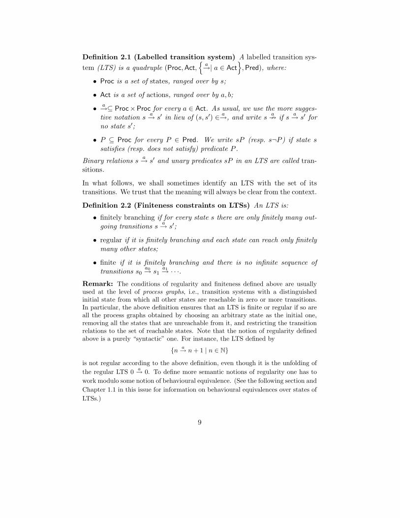
Definition 2.1 (Labelled transition system) A labelled transition sys-
tem (LTS) is a quadruple (Proc,Act,
a→| a ∈ Act
,Pred), where:
• Proc is a set of states, ranged over by s;
• Act is a set of actions, ranged over by a, b;
• a→⊆ Proc×Proc for every a ∈ Act. As usual, we use the more sugges-tive notation s
a→ s′ in lieu of (s, s′) ∈ a→, and write sa9 if s
a→ s′ forno state s′;
• P ⊆ Proc for every P ∈ Pred. We write sP (resp. s¬P ) if state ssatisfies (resp. does not satisfy) predicate P .
Binary relations sa→ s′ and unary predicates sP in an LTS are called tran-
sitions.
In what follows, we shall sometimes identify an LTS with the set of itstransitions. We trust that the meaning will always be clear from the context.
Definition 2.2 (Finiteness constraints on LTSs) An LTS is:
• finitely branching if for every state s there are only finitely many out-going transitions s
a→ s′;
• regular if it is finitely branching and each state can reach only finitelymany other states;
• finite if it is finitely branching and there is no infinite sequence oftransitions s0
a0→ s1a1→ · · ·.
Remark: The conditions of regularity and finiteness defined above are usuallyused at the level of process graphs, i.e., transition systems with a distinguishedinitial state from which all other states are reachable in zero or more transitions.In particular, the above definition ensures that an LTS is finite or regular if so areall the process graphs obtained by choosing an arbitrary state as the initial one,removing all the states that are unreachable from it, and restricting the transitionrelations to the set of reachable states. Note that the notion of regularity definedabove is a purely “syntactic” one. For instance, the LTS defined by
n a→ n + 1 | n ∈ N
is not regular according to the above definition, even though it is the unfolding of
the regular LTS 0a→ 0. To define more semantic notions of regularity one has to
work modulo some notion of behavioural equivalence. (See the following section and
Chapter 1.1 in this issue for information on behavioural equivalences over states of
LTSs.)
9
2.2 Behavioural Equivalences and Preorders
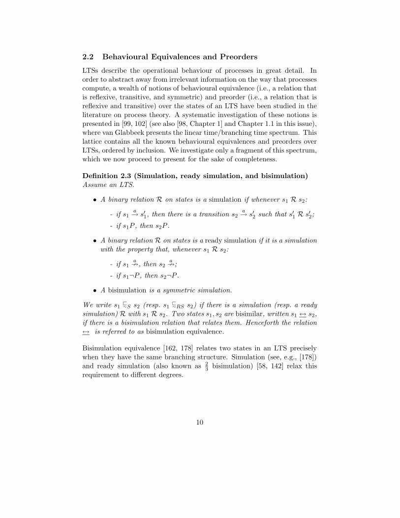
LTSs describe the operational behaviour of processes in great detail. Inorder to abstract away from irrelevant information on the way that processescompute, a wealth of notions of behavioural equivalence (i.e., a relation thatis reflexive, transitive, and symmetric) and preorder (i.e., a relation that isreflexive and transitive) over the states of an LTS have been studied in theliterature on process theory. A systematic investigation of these notions ispresented in [99, 102] (see also [98, Chapter 1] and Chapter 1.1 in this issue),where van Glabbeek presents the linear time/branching time spectrum. Thislattice contains all the known behavioural equivalences and preorders overLTSs, ordered by inclusion. We investigate only a fragment of this spectrum,which we now proceed to present for the sake of completeness.
Definition 2.3 (Simulation, ready simulation, and bisimulation)Assume an LTS.
• A binary relation R on states is a simulation if whenever s1 R s2:
- if s1a→ s′1, then there is a transition s2
a→ s′2 such that s′1 R s′2;
- if s1P , then s2P .
• A binary relation R on states is a ready simulation if it is a simulationwith the property that, whenever s1 R s2:
- if s1a9, then s2
a9;
- if s1¬P , then s2¬P .
• A bisimulation is a symmetric simulation.
We write s1 <∼S s2 (resp. s1 <
∼RS s2) if there is a simulation (resp. a readysimulation) R with s1 R s2. Two states s1, s2 are bisimilar, written s1 ↔ s2,if there is a bisimulation relation that relates them. Henceforth the relation↔ is referred to as bisimulation equivalence.
Bisimulation equivalence [162, 178] relates two states in an LTS preciselywhen they have the same branching structure. Simulation (see, e.g., [178])and ready simulation (also known as 2
3 bisimulation) [58, 142] relax thisrequirement to different degrees.
10
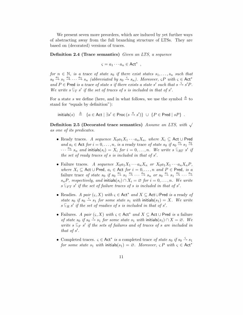
We present seven more preorders, which are induced by yet further waysof abstracting away from the full branching structure of LTSs. They arebased on (decorated) versions of traces.
Definition 2.4 (Trace semantics) Given an LTS, a sequence
ς = a1 · · · an ∈ Act∗ ,
for n ∈ N, is a trace of state s0 if there exist states s1, . . . , sn such thats0
a1→ s1a2→ · · · an→ sn (abbreviated by s0
ς→ sn). Moreover, ςP with ς ∈ Act∗
and P ∈ Pred is a trace of state s if there exists a state s′ such that sς→ s′P .
We write s <∼T s′ if the set of traces of s is included in that of s′.
For a state s we define (here, and in what follows, we use the symbol∆= to
stand for “equals by definition”):
initials(s)∆= a ∈ Act | ∃s′ ∈ Proc (s
a→ s′) ∪ P ∈ Pred | sP .
Definition 2.5 (Decorated trace semantics) Assume an LTS, with√
as one of its predicates.
• Ready traces. A sequence X0a1X1 · · · anXn, where Xi ⊆ Act ∪ Pred
and ai ∈ Act for i = 0, . . . , n, is a ready trace of state s0 if s0a1→ s1
a2→· · · an→ sn and initials(si) = Xi for i = 0, . . . , n. We write s <
∼RT s′ ifthe set of ready traces of s is included in that of s′.
• Failure traces. A sequence X0a1X1 · · · anXn or X0a1X1 · · · anXnP ,where Xi ⊆ Act ∪ Pred, ai ∈ Act for i = 0, . . . , n and P ∈ Pred, is afailure trace of state s0 if s0
a1→ s1a2→ · · · an→ sn or s0
a1→ s1a2→ · · · an→
snP , respectively, and initials(si) ∩Xi = ∅ for i = 0, . . . , n. We writes <∼FT s′ if the set of failure traces of s is included in that of s′.
• Readies. A pair (ς,X) with ς ∈ Act∗ and X ⊆ Act∪Pred is a ready of
state s0 if s0ς→ s1 for some state s1 with initials(s1) = X. We write
s <∼R s′ if the set of readies of s is included in that of s′.
• Failures. A pair (ς,X) with ς ∈ Act∗ and X ⊆ Act ∪ Pred is a failure
of state s0 if s0ς→ s1 for some state s1 with initials(s1) ∩X = ∅. We
write s <∼F s′ if the sets of failures and of traces of s are included in
that of s′.
• Completed traces. ς ∈ Act∗ is a completed trace of state s0 if s0
ς→ s1for some state s1 with initials(s1) = ∅. Moreover, ς P with ς ∈ Act
∗
11
and P ∈ Pred is a completed trace of state s0 if s0ς→ s1P for some
state s1. We write s <∼CT s′ if the set of completed traces of s is
included in that of s′.
• Accepting traces. ς ∈ Act∗ is an accepting trace of state s0 if s0
ς→ s1√
for some state s1. We write s <∼AT s′ if the set of accepting traces of s
is included in that of s′.
The decorated trace semantics defined above take predicates into account.However, most of the uses of these semantics in the literature on processtheory occur in settings without predicates. Our definition of completedtrace preorder agrees with the definition of this notion in, e.g., [150, 115], butdiffers from the one in [99], where it is required that not only the completedtraces but also the traces of s are included in that of s′. The notion of anaccepting trace is standard in formal language theory (see, e.g., [202]), buthas not received widespread treatment in the literature on process theory.
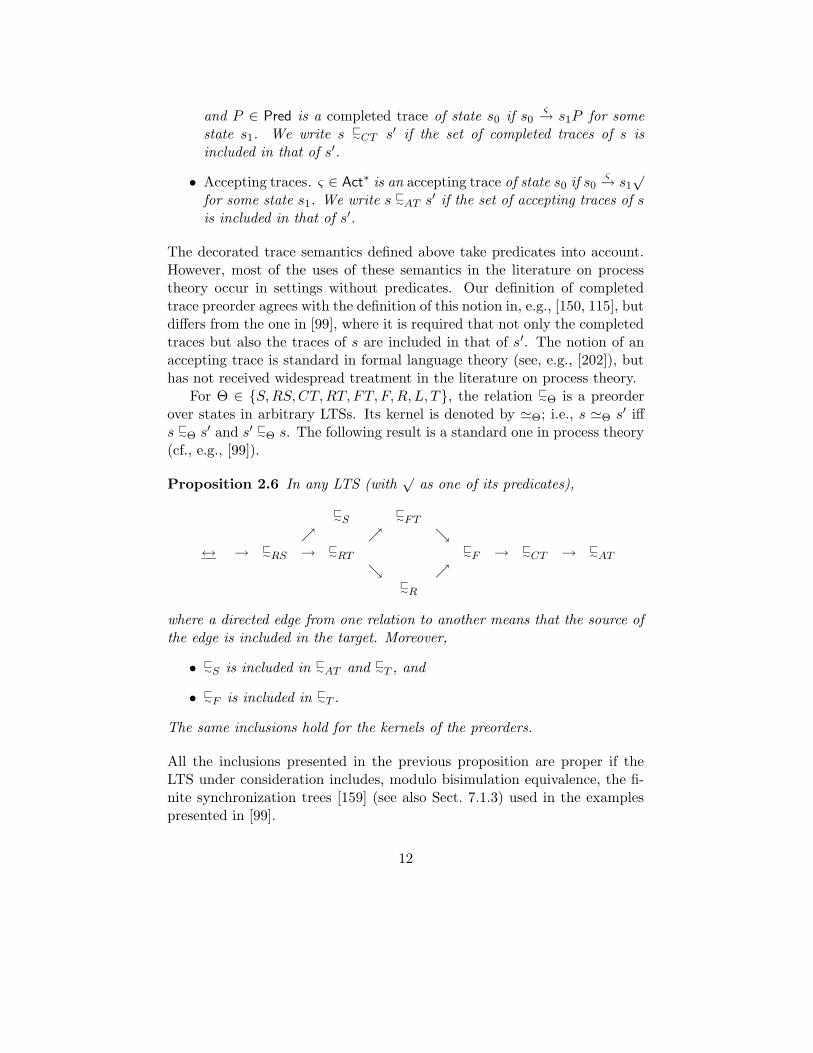
For Θ ∈ S,RS,CT,RT, FT, F,R, L, T, the relation <∼Θ is a preorder
over states in arbitrary LTSs. Its kernel is denoted by 'Θ; i.e., s 'Θ s′ iffs <∼Θ s′ and s′ <
∼Θ s. The following result is a standard one in process theory(cf., e.g., [99]).
Proposition 2.6 In any LTS (with√
as one of its predicates),
<∼S
<∼FT
↔ → <
∼RS → <∼RT
<∼F → <
∼CT → <∼AT
<∼R
where a directed edge from one relation to another means that the source ofthe edge is included in the target. Moreover,
• <∼S is included in <
∼AT and <∼T , and
• <∼F is included in <
∼T .
The same inclusions hold for the kernels of the preorders.
All the inclusions presented in the previous proposition are proper if theLTS under consideration includes, modulo bisimulation equivalence, the fi-nite synchronization trees [159] (see also Sect. 7.1.3) used in the examplespresented in [99].
12
2.3 Hennessy-Milner Logic
Modal and temporal logics of reactive programs have found considerableuse in the theory and practice of concurrency (see, e.g., [81, 186, 219]).One of the earliest and most influential connections between logics of reac-tive programs and behavioural relations was given by Hennessy and Milner[128], who introduced a multi-modal logic and showed that it characterizedbisimulation equivalence. We limit ourselves to briefly recalling the basicdefinitions and results on Hennessy-Milner logic. The interested reader isreferred to, e.g., [128, 218] for more details and motivation. The followingdefinition is standard, apart from the use of atomic propositions to cater forthe presence of predicates in LTSs.
Definition 2.7 (Hennessy-Milner logic) The set of HML formulae isgiven by the BNF grammar [18]
ϕ ::= true | P | ¬ϕ | ϕ1 ∧ ϕ2 | 〈a〉ϕ
where a and P range over Act and Pred, respectively.
Given an LTS, the states s that satisfy HML formula ϕ, written s |= ϕ, aredefined inductively by:
s |= true
s |= P ⇐⇒ sP
s |= ¬ϕ ⇐⇒ not s |= ϕ
s |= ϕ1 ∧ ϕ2 ⇐⇒ s |= ϕ1 and s |= ϕ2
s |= 〈a〉ϕ ⇐⇒ s′ |= ϕ for some s′ such that sa→ s′ .
Using negation and conjunction in HML, one can define the other standardboolean connectives. Two states s, s′ are considered equivalent with respectto HML, written s ∼HML s′, iff for all HML formulae ϕ: s |= ϕ ⇐⇒ s′ |= ϕ.The following seminal result is due to Hennessy and Milner [128].
Theorem 2.8 The equivalence relations ↔ and ∼HML coincide over fi-nitely branching LTSs.
The restriction to finitely branching LTSs in Thm. 2.8 can be dropped ifinfinitary conjunctions are allowed in the syntax of HML.
13
2.4 Term Algebras
This section reviews the basic notions of term algebras that will be needed inthis chapter. We start from a countably infinite set Var of variables, rangedover by x, y, z.
Definition 2.9 (Signature) A signature Σ is a set of function symbols,disjoint from Var, together with an arity mapping that assigns a naturalnumber ar(f) to each function symbol f . A function symbol of arity zerois called a constant, while function symbols of arity one and two are calledunary and binary, respectively.
The arity of a function symbol represents its number of arguments.
Definition 2.10 (Term) The set (Σ) of (open) terms over a signature Σ,ranged over by t, u, is the least set such that:
• each x ∈ Var is a term;
• f(t1, . . . , tar(f)) is a term, if f is a function symbol and t1, . . . , tar(f)are terms.
T(Σ) denotes the set of closed terms over Σ, i.e., terms that do not containvariables.
For a constant a, the term a() is abbreviated to a. By convention, wheneverwe write a term-like phrase (e.g., f(t, u)), we intend it to be a term (i.e., fis binary).
A substitution is a mapping σ : Var → (Σ). A substitution is closed ifit maps each variable to a closed term in T(Σ). A substitution extends to amapping from terms to terms as usual; the term σ(t) is obtained by replacingoccurrences of variables x in t by σ(x). A context C[x1, . . . , xn] denotes anopen term in which at most the distinct variables x1, . . . , xn appear. Theterm C[t1, . . . , tn] is obtained by replacing all occurrences of variables xi inC[x1, . . . , xn] by ti, for i = 1, . . . , n.
Definition 2.11 (Congruence) Assume a signature Σ. An equivalencerelation (resp. preorder) R over T(Σ) is a congruence (resp. precongruence)if, for all f ∈ Σ,
tiRui for i = 1, . . . , ar(f) implies f(t1, . . . , tar(f))Rf(u1, . . . , uar(f)) .
14
2.5 Transition System Specifications
In the remainder of this chapter, the set Proc of states will in general consistof the closed terms over some signature. We proceed to introduce the mainobject of study in the field of SOS, viz. a transition system specification,being a collection of inductive proof rules to derive the transitions over theset of closed terms.
Definition 2.12 (Transition system specification) Let Σ be a signa-ture, and let t and t′ range over (Σ). A transition rule ρ is of the formH/α, with H a set of positive premises t
a→ t′ and tP , and of negativepremises t
a9 and t¬P . Moreover, the conclusion α is of the form t
a→ t′
or tP . The left-hand side of the conclusion is the source of ρ, and if theconclusion is of the form t
a→ t′, then its right-hand side is the target of ρ.A transition rule is closed if it does not contain variables.
A transition system specification (TSS) is a set of transition rules. ATSS is positive if its transition rules do not contain negative premises.
For the sake of clarity, transition rules will often be displayed in the formHα, and the premises of a transition rule will not always be presented using
proper set notation. The first systematic study of TSSs may be found in[208], while the first study of TSSs with negative premises appeared in [57].
We proceed to define when a transition is provable from a TSS. The fol-lowing notion of a proof from [105] generalizes the standard definition (see,e.g., [115]) by allowing the derivation of closed transition rules. The deriva-tion of a transition α corresponds to the derivation of the closed transitionrule H/α with H = ∅. The case H 6= ∅ corresponds to the derivation of αunder the assumptions in H.
Definition 2.13 (Literal) Positive literals are transitions ta→ t′ and tP ,
while negative literals are expressions ta9 and t¬P , where t and t′ range
over the collection of closed terms. A literal is a positive or negative literal.
Definition 2.14 (Proof) Let T be a TSS. A proof of a closed transitionrule H/α from T is an upwardly branching tree without infinite branches,whose nodes are labelled by literals, where the root is labelled by α, and if Kis the set of labels of the nodes directly above a node with label β, then
1. either K = ∅ and β ∈ H,
2. or K/β is a closed substitution instance of a transition rule in T .
If a proof of H/α from T exists, then H/α is provable from T , notationT ` H/α.
15
2.6 Examples of TSSs
In this section we present some TSSs from the literature, which will serve asrunning examples in sections to come. Abundant examples of the systematicuse of SOS can be found, e.g., in [28, 232] and elsewhere in this handbook.Hartel [119] recently developed a tool environment LETOS for the animationof such TSSs, based on functional programming languages.
2.6.1 Basic Process Algebra with Empty Process
The signature of Basic Process Algebra with empty process [238], denotedby BPAε, consists of the following operators:
- a set Act of constants, representing indivisible behaviour;
- a special constant ε, called empty process, representing successful ter-mination;
- a binary operator +, called alternative composition, where a termt1 + t2 represents the process that executes either t1 or t2;
- a binary operator ·, called sequential composition, where a term t1 · t2represents the process that executes first t1 and then t2.
So the BNF grammar for BPAε is (with a ∈ Act):
t ::= a | ε | t1 + t2 | t1 · t2 .
The intuition above for the operators in BPAε is formalized by the transitionrules in Table 1 from [29], which constitute the TSS for BPAε. This TSSdefines transitions t
a→ t′ to express that term t can evolve into term t′ bythe execution of action a ∈ Act, and transitions t
√to express that term t
can terminate successfully. The variables x, x′, y, and y′ in the transitionrules range over the collection of closed terms, while the a ranges over Act.
2.6.2 Priorities
The language BPAεθ is obtained by adding the priority operator θ from [24]to BPAε. This function symbol assumes a partial order < on Act. Intuitively,the process θ(t) is obtained by eliminating all transitions s
a→ s′ from the
process t for which there is a transition sb→ s′′ with a < b. For example,
if a < b then θ(a + b) can execute the action b but not the action a. Thesemantics of the priority operator is captured by the transition rules in Table2. The TSS for BPAεθ consists of the transition rules in Tables 1 and 2.
16

aa→ ε ε
√
x√
x+ y√ x
a→ x′
x+ ya→ x′
y√
x+ y√ y
a→ y′
x+ ya→ y′
x√
y√
x · y√x√
ya→ y′
x · y a→ y′x
a→ x′
x · y a→ x′ · y
Table 1: Transition Rules for BPAε.
x√
θ(x)√ x
a→ x′ xb
9 for a < b
θ(x)a→ θ(x′)
Table 2: Transition Rules for the Priority Operator.
2.6.3 Discrete Time
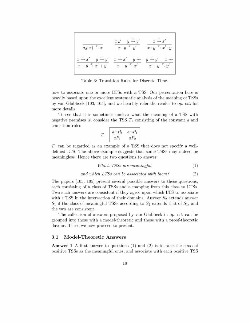
Our final example is the TSS for an extension of BPAε with relative discretetime, denoted by BPAdtε [23]. Time progresses in distinct time steps, wherea transition t
σ→ t′ denotes passing to the next time slice. The syntax ofBPAdtε consists of the operators from BPAε together with a unary operatorσd to represent a delay of one time unit. That is, a term σd(t) can executeall transitions of t delayed by one time step. A term t + t′ can evolveinto the next time slice if t or t′ can evolve into the next time slice. Thetransition rules dealing with time steps are presented in Table 3. The TSSfor BPAdtε consists of the transition rules in Tables 1 and 3.
3 The Meaning of TSSs
A positive TSS specifies an LTS in a straightforward way as the set of allprovable transitions (cf. Def. 2.14). However, as Groote [111, 112] pointedout, it is much less trivial to associate an LTS with a TSS containing negativepremises. Several solutions were investigated in [59, 60, 111, 112], mostlyoriginating from logic programming. This section presents an overview of
17
σd(x)σ→ x
x√
yσ→ y′
x · y σ→ y′x
σ→ x′
x · y σ→ x′ · y
xσ→ x′ y
σ→ y′
x+ yσ→ x′ + y′
xσ→ x′ y
σ9
x+ yσ→ x′
yσ→ y′ x
σ9
x+ yσ→ y′
Table 3: Transition Rules for Discrete Time.
how to associate one or more LTSs with a TSS. Our presentation here isheavily based upon the excellent systematic analysis of the meaning of TSSsby van Glabbeek [103, 105], and we heartily refer the reader to op. cit. formore details.
To see that it is sometimes unclear what the meaning of a TSS withnegative premises is, consider the TSS T1 consisting of the constant a andtransition rules
T1a¬P2aP1
a¬P1aP2
T1 can be regarded as an example of a TSS that does not specify a well-defined LTS. The above example suggests that some TSSs may indeed bemeaningless. Hence there are two questions to answer:
Which TSSs are meaningful, (1)
and which LTSs can be associated with them? (2)
The papers [103, 105] present several possible answers to these questions,each consisting of a class of TSSs and a mapping from this class to LTSs.Two such answers are consistent if they agree upon which LTS to associatewith a TSS in the intersection of their domains. Answer S2 extends answerS1 if the class of meaningful TSSs according to S2 extends that of S1, andthe two are consistent.
The collection of answers proposed by van Glabbeek in op. cit. can begrouped into those with a model-theoretic and those with a proof-theoreticflavour. These we now proceed to present.
3.1 Model-Theoretic Answers
Answer 1 A first answer to questions (1) and (2) is to take the class ofpositive TSSs as the meaningful ones, and associate with each positive TSS
18
the LTS consisting of the provable transitions.
Since negative premises make it possible to give a clean description of im-portant constructs found in programming and specification languages, theabove answer is not really satisfactory. More general answers to questions(1) and (2) have been proposed in the literature. Before reviewing them, werecall two criteria from [58, 59] that can be imposed on reasonable answers.
Definition 3.1 (Entailment) For an LTS L and a set of literals H, wewrite L |= H if:
- α ∈ L for all positive literals α in H;
- ta→ t′ 6∈ L for all negative literals t
a9 in H and all closed terms t′;
- tP 6∈ L for all negative literals t¬P in H.
Definition 3.2 (Supported model) Let T be a TSS and L an LTS.
• L is a model of T if α ∈ L whenever there is a closed substitutioninstance H/α of a transition rule in T with L |= H.
• L is supported by T if whenever α ∈ L there is a closed substitutioninstance H/α of a transition rule in T with L |= H.
The first requirement, of being a model, says that L contains all transi-tions for which T offers a justification. The second requirement, of beingsupported, says that L only contains transitions for which T offers a justi-fication. Note that the LTS containing all possible transitions is a model ofany TSS, while the LTS containing no transitions is supported by any TSS.
The following result is standard, and has its roots in the classic theoryof inductive definitions.
Proposition 3.3 Let T be a positive TSS and L the set of transitions prov-able from T . Then L is a supported model of T . Moreover, L is the leastmodel of T .
Starting from Prop. 3.3, there are two ways to generalize Answer 1 to TSSswith negative premises.
Answer 2 A TSS is meaningful iff it has a least model.
Answer 3 A TSS is meaningful iff it has a least supported model.
19
Note that, in general, no unique least (supported) model may exist. Acounter-example is given by the TSS T1, which has two least models, namelyaP1 and aP2, both of which are supported. Answers 2 and 3 are incom-parable. For example, the TSS T2 below has aP1 as its least model, butno supported models. On the other hand, the TSS T3 has two least models,namely aP1 and aP2, of which only the first one is supported, and thisis its least supported model.
T2a¬P1aP1
T3a¬P2aP1
Answers 2 and 3 both extend Answer 1, but they are inconsistent with eachother. For example, the TSS T4 below has a least model aP1 and a leastsupported model aP1, aP2.
T4a¬P1aP1
aP2aP1
aP2aP2
In [57, 58] the following answer was proposed.
Answer 4 A TSS is meaningful iff it has a unique supported model.
The positive TSS T5 below has two supported models, viz. ∅ and aP1, soAnswer 4 does not extend Answer 1.
T5aP1aP1
For the GSOS languages considered in op. cit. (cf. Sect. 5.4), Answer 4 coin-cides with all acceptable answers mentioned in this section. Note, however,that the least supported model of T4 is also its unique supported model.This seems to entail that Answer 4 is not satisfactory for TSSs in general.
Fages [83] proposed a strengthening of the notion of support, in thesetting of logic programming. Being supported means that a transition mayonly be present if there is a non-empty proof of its presence, starting fromtransitions that are also present. These premises in the proof may includethe transition under derivation, thereby allowing loops, as in the case of T4.The notion of a well-supported model is based on the idea that the absenceof a transition may be assumed a priori, provided that this assumption isconsistent, but the presence of a transition needs to be proven, in the senseof Def. 2.14, building upon a set of assumptions that only contains negativeliterals.
20
Definition 3.4 (Well-supported model) An LTS L is a well-supportedmodel of a TSS T if it is a model of T and for each transition α in L, Tproves a closed transition rule N/α where N only contains negative literalsand L |= N .
A stable model, developed by Gelfond and Lifschitz [95] in the area of logicprogramming, and adapted to TSSs in [59, 60], only allows transitions thatare well-supported.
Definition 3.5 (Stable model) An LTS L is a stable model of a TSS Tif a transition α is in L iff T proves a closed transition rule N/α where Ncontains only negative literals and L |= N .
An LTS is a stable model of a TSS T iff it is a well-supported model of T[103, 105].
Answer 5 A TSS is meaningful iff it has a unique stable model.
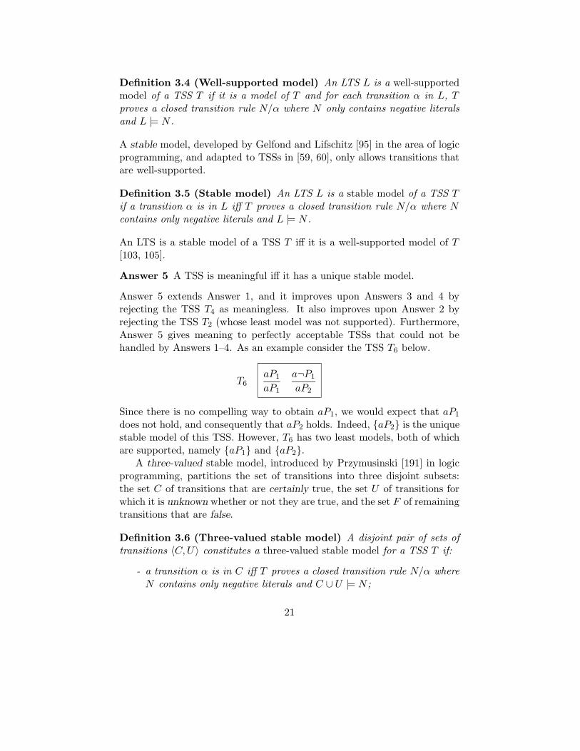
Answer 5 extends Answer 1, and it improves upon Answers 3 and 4 byrejecting the TSS T4 as meaningless. It also improves upon Answer 2 byrejecting the TSS T2 (whose least model was not supported). Furthermore,Answer 5 gives meaning to perfectly acceptable TSSs that could not behandled by Answers 1–4. As an example consider the TSS T6 below.
T6aP1aP1
a¬P1aP2
Since there is no compelling way to obtain aP1, we would expect that aP1does not hold, and consequently that aP2 holds. Indeed, aP2 is the uniquestable model of this TSS. However, T6 has two least models, both of whichare supported, namely aP1 and aP2.
A three-valued stable model, introduced by Przymusinski [191] in logicprogramming, partitions the set of transitions into three disjoint subsets:the set C of transitions that are certainly true, the set U of transitions forwhich it is unknown whether or not they are true, and the set F of remainingtransitions that are false.
Definition 3.6 (Three-valued stable model) A disjoint pair of sets oftransitions 〈C,U〉 constitutes a three-valued stable model for a TSS T if:
- a transition α is in C iff T proves a closed transition rule N/α whereN contains only negative literals and C ∪ U |= N ;
21
- a transition α is in C ∪ U iff T proves a closed transition rule N/αwhere N contains only negative literals and C |= N .
Each TSS has one or more three-valued stable models. For example, theTSS T1 has 〈aP1,∅〉, 〈aP2,∅〉, and 〈∅, aP1, aP2〉 as its three-valuedstable models. Each TSS T affords an (information-)least three-valued stablemodel 〈C,U〉, in the sense that the set U is maximal. Przymusinski [191]showed that this least three-valued stable model coincides with the so-calledwell-founded model that was introduced by van Gelder, Ross, and Schlipf[93, 94] in logic programming.
Answer 6 A TSS is meaningful iff its least three-valued stable model doesnot contain unknown transitions. The associated LTS consists of the truetransitions in this three-valued stable model.
Answer 6 extends Answer 1 and is extended by Answer 5, but it is inconsis-tent with Answers 2–4. In particular, the TSSs T1, T2, and T4 are outsideits domain, while it associates aP1 to T3, ∅ to T5, and aP2 to T6. InSect. 5, Answer 6 will stand us in good stead, as it is used in the formula-tion of congruence results in the presence of negative premises (cf. Thm. 5.3,Thm. 5.49, and Thm. 5.53), where Answers 1–5 would all be unsatisfactory.
3.2 Proof-Theoretic Answers
Note for the Reader. In this section only we extend the notion of negativeliterals to expressions of the form t
a9 t′. Intuitively, this expression denotes
that term t cannot evolve to term t′ by the execution of action a.
This section reviews possible answers to questions (1) and (2) based on ageneralization of the concept of proof. In [105], van Glabbeek proposedtwo generalizations of the concept of a proof in Def. 2.14, to enable thederivation of negative literals. These two generalizations are based on thenotions of supported model (Def. 3.2) and well-supported model (Def. 3.4),respectively.
Definition 3.7 (Denying literal) The following pairs of literals deny eachother:
- ta→ t′ and t
a9 t′;
- ta→ t′ and t
a9;
- tP and t¬P .
22
Definition 3.8 (Supported proof) A supported proof of a literal α froma TSS T is like a proof (see Def. 2.14), but with one extra clause:
3. β is negative, and for each closed substitution instance H ′/γ of a tran-sition rule in T such that γ denies β, a literal in H ′ denies one in K.
We write T `s α if a supported proof of α from T exists.
Definition 3.9 (Well-supported proof) A well-supported proof of a lit-eral α from a TSS T is like a proof (Def. 2.14), but with one extra clause:
3. β is negative, and for each set N of negative literals such that T ` N/γfor γ a literal denying β, a literal in N denies one in K.
We write T `ws α if a well-supported proof of α from T exists.
Clause 3 in Def. 3.9 allows one to infer ta9 t′ or t¬P whenever it is manifestly
impossible to infer ta→ t′ or tP , respectively. Clause 3 in Def. 3.8 allows such
inferences only if the impossibility to derive ta→ t′ or tP can be detected by
examining all possible proofs that consist of one step only. As a consequence,for each TSS, `s is included in `ws. The following results stem from [105].
Proposition 3.10 For each TSS, the induced relation `ws does not containdenying literals.
Proposition 3.11 For any TSS T and literal α:
1. T `s α implies L |= α for each supported model L of T ;
2. T `ws α implies L |= α for each well-supported model L of T .
Following [105], we now introduce the concept of a complete TSS, in whichevery transition is either provable or refutable.
Definition 3.12 (Completeness) A TSS T is x-complete (x ∈ s, ws)if for any transition t
a→ t′ (resp. tP ) either T `x ta→ t′ (resp. T `x tP ) or
T `x ta9 t′ (resp. T `x t¬P ).
Answer 7 A TSS is meaningful iff it is s-complete. The associated LTSconsists of the s-provable transitions.
Answer 8 A TSS is meaningful iff it is ws-complete. The associated LTSconsists of the ws-provable transitions.
23
From now on, by ‘complete’ we shall mean ‘ws-complete’.A TSS is complete iff its least three-valued stable model does not contain
any unknown transitions (see [103]), so Answer 6 agrees with Answer 8.Moreover, Answer 8 extends Answer 7. In [59], an example in the area ofprocess theory was given (viz. the modelling of a priority operator in basicprocess algebra with silent step) that can be handled by Answer 8 but notby Answer 7, showing that the full generality of Answer 8 can be useful inapplications.
We proceed to show how to associate an LTS with any TSS, using theconcept of a well-supported proof. As illustrated by the TSSs T1 and T2,such an LTS cannot always be a supported model. Since being a model isa basic requirement, van Glabbeek [105] proposed a universal answer thatgives up the requirement of supportedness. Let us examine T1. Since theassociated LTS should be a model, it must contain either aP1 or aP2. Bysymmetry, the associated LTS should include both transitions. As thereis no reason to include any more transitions, the LTS associated with T1should be aP1, aP2. These considerations lead to the following proposal.
Answer 9 Any TSS is meaningful. The associated LTS consists of thetransitions for which none of the denying negative literals are ws-provable.
Answer 9 is inspired by the observation in [105] that for each TSS, the set oftransitions for which none of the denying negative literals are ws-provableconstitutes a model. Answer 9 extends Answer 8, but it is inconsistent withAnswers 2–5. Answer 9 associates the LTS aP1, aP2 with T1, and the LTSaP1 with T2 and T4.
3.3 Answers Based on Stratification
Finally, we review two methods to assign meaning to TSSs based on thetechnique of (local) stratification, as proposed in the setting of logic pro-gramming by Przymusinski [190]. This technique was adapted to TSSs in[111, 112].
Definition 3.13 (Stratification) A mapping S from transitions to ordi-nal numbers is a stratification of a TSS T if for every transition rule H/αin T and every closed substitution σ:
• for positive premises β in H, S(σ(β)) ≤ S(σ(α)); and
• for negative premises ta9 and t¬P in H, S(σ(t)
a→ t′) < S(σ(α)) forall closed terms t′ and S(σ(t)P ) < S(σ(α)), respectively.
24
A stratification is strict if S(σ(β)) < S(σ(α)) also holds for all the positivepremises β in H. A TSS with a (strict) stratification is (strictly) stratifiable.
In a stratifiable TSS no transition depends negatively on itself. An LTSassociated with such a TSS may be built one stratum of transitions withthe same S-value at a time. A transition with S-value zero is present onlyif it is provable in the sense of Def. 2.14, and as soon as the validity of alltransitions with S-value no greater than κ is known for some ordinal numberκ, the validity of closed instantiations of negative premises that could occurin a proof of a transition with S-value κ+1 is known, which determines thevalidity of those transitions.
Let T be a TSS with a stratification S. The stratum Lκ of transitions,for an ordinal number κ, is defined thus (using ordinal induction):
α ∈ Lκ iff S(α) = κ and T proves a closed transition rule H/α with∪µ<κLµ |= H.
Similarly, for a TSS T with a strict stratification S, the stratum Mκ of tran-sitions, for an ordinal number κ, is defined thus (using ordinal induction):
α ∈ Mκ iff S(α) = κ and there is a closed substitution instance H/αof a transition rule in T with ∪µ<κMµ |= H.
Groote [111, 112] proved that the sets ∪κLκ and ∪κMκ are independentof the chosen (strict) stratification. This justifies the following answers toquestions (1) and (2).
Answer 10 A TSS is meaningful iff it is stratifiable. The associated LTSis ∪κLκ.
Answer 11 A TSS is meaningful iff it is strictly stratifiable. The associatedLTS is ∪κMκ.
Answer 10 extends Answer 1 and is extended by Answer 8. Answer 11 isextended by Answers 7 and 10.
3.4 Evaluation of the Answers
We have presented several possible answers to the questions of which TSSsare meaningful and which LTSs are associated with them.
Answer 1 (positive) is the classical interpretation of TSSs without neg-ative premises, and Answers 2 (least model) and 3 (least supported model)
25
are two straightforward generalizations. Answer 4 (unique supported model)stems from [57], where it was used to ascertain that TSSs in GSOS format(cf. Sect. 5.4) are meaningful. The TSS T4, however, shows that Answer 4yields counter-intuitive results in general. Fortunately, TSSs in GSOS for-mat are even strictly stratifiable, which is one of the most restrictive criteriafor meaningful TSSs considered. For GSOS languages with recursion, how-ever, it is no longer straightforward to find an associated LTS (see, e.g.,[58]). A solution for this, involving a special divergence predicate, will bediscussed in Sect. 5.4.6.
Answer 5 (unique stable) is generally considered to be the most generalacceptable answer available. Answer 8 (complete) is the most general answerwithout undesirable properties. Answer 8 is based on a concept of provabilityincorporating the notion of negation as failure of Clark [67]. Answer 6(no unknown transitions) agrees with Answer 8; i.e., a TSS is complete iffits least three-valued stable model does not contain unknown transitions.Answer 7 (complete with support) only yields unique supported models.Moreover, it is based on a notion of provability that is somewhat simpler toapply, and only incorporates the notion of negation as finite failure [67].
Answer 9 (irrefutable), which gives a meaning to each TSS, has the dis-advantage that it sometimes yields unstable models, and even unsupportedmodels. A good example from process algebra of a TSS without supportedmodels is BPA with the priority operator, unguarded recursion, and renam-ing, as defined in [111, 112]. Although Answer 9 gives a meaning to thisTSS, it appears rather arbitrary and not very useful. In particular, recur-sively defined processes do not satisfy their defining equations—a highlyundesirable feature by all accounts.
Answer 10 (stratification) is perhaps the best known answer in logicprogramming. A variant that only allows TSSs with a unique supportedmodel is Answer 11 (strict stratification). Answers 10 and 11 are of practicalimportance, because they are extended by Answer 8. Thus, giving a (strict)stratification is a useful tool for showing that a TSS is complete, and thistechnique is applied in several examples in the remainder of this chapter.
3.5 Applications
We show that the three TSSs from Sect. 2.6 are complete, using a stratifi-cation. We use the fact that Answer 8 extends Answers 1 and 10.
BPA with Empty Process The TSS for BPAε is positive.
26
Priorities The TSS for BPAεθ is complete, which can be seen by giving asuitable stratification S, counting the number of occurrences of the priorityoperator in the left-hand side of a transition. That is, if the closed term tcontains n occurrences of θ, then S(t
a→ t′) = n and S(t√) = n. Consider
for instance the second transition rule in Table 2:
xa→ x′ x
b9 for a < b
θ(x)a→ θ(x′)
Clearly S(ta→ t′) < S(θ(t)
a→ θ(t′)) and S(tb→ u) < S(θ(t)
a→ θ(t′)) forall closed terms t, t′, and u, because θ(t) contains one more occurrence ofthe priority operator than t. In a similar fashion it can be verified for theother transition rules of BPAεθ that S is a stratification. Hence, the TSSfor BPAεθ is complete.
Discrete Time The TSS for BPAdtε is complete, which can be seen bygiving a suitable stratification S, counting the occurrences of alternativecomposition on the left-hand side of a timed transition. That is, if theclosed term t contains n occurrences of +, then S(t
σ→ t′) = n. Moreover,S(t
a→ t′) = 0 for a ∈ Act. Consider for instance the last transition rule inTable 3:
yσ→ y′ x
σ9
x+ yσ→ y′
Clearly S(uσ→ u′) < S(t + u
σ→ u′) and S(tσ→ t′) < S(t + u
σ→ u′) for allclosed terms t, t′, u, and u′, because t+ u contains more occurrences of thealternative composition than t and u. In a similar fashion it can be verifiedfor the other transition rules of BPAdtε that S is a stratification. Hence, theTSS for BPAdtε is complete.
4 Conservative Extension
Over and over again, process calculi such as CCS [164], CSP [196], andACP [29] have been extended with new features, and the original TSSs,which provide the semantics for these process algebras, were extended withtransition rules to describe these features; see, e.g., [28] for a systematicapproach. A question that arises naturally is whether or not the LTSsassociated with the original and with the extended TSS contain the sametransitions t
a→ t′ and tP for closed terms t in the original domain. Usually
27
it is desirable that an extension is operationally conservative, meaning thatthe provable transitions for an original term are the same both in the originaland in the extended TSS.
Groote and Vaandrager [115, Thm. 7.6] proposed syntactic restrictionson a TSS, which automatically yield that an extension of this TSS withtransition rules that contain fresh function symbols in their sources is op-erationally conservative (cf. the notion of a disjoint extension from [8] inDef. 5.31). Bol and Groote [60, 112] supplied this conservative extensionformat with negative premises. Verhoef [236] showed that, under certainconditions, a transition rule in the extension can be allowed to have anoriginal term as its source. D’Argenio and Verhoef [73, 74] formulated ageneralization in the context of inequational specifications. Fokkink andVerhoef [90] relaxed the syntactic restrictions on the original TSS, and liftedthe operational conservative extension result to higher-order languages (seeSect. 6.4).
Operational conservative extension seems such a natural notion that inthe literature this property is often a hidden assumption: its formulationand proof are omitted without justification. For example, this happens inthe design of process algebras, and in applications of a strategy to proveω-completeness mentioned in Sect. 4.3.3. Paying attention to operationalconservative extension not only leads to more accurate contemplations onconcurrency theory, but is also beneficial in other respects. Namely, oper-ational conservative extension can be applied to obtain results in processalgebra that are much harder to obtain using more classical term rewritingapproaches or customized techniques.
The organization of this section is as follows. Sect. 4.1 presents syntacticconstraints to ensure that an extension of a TSS is operationally conserva-tive. Sect. 4.2 studies the relation between the three-valued stable modelsof a TSS and of its operational conservative extension. Sects. 4.3 and 4.4show how operational conservative extension can be applied to derive usefulproperties concerning axiomatizations and term rewriting systems.
As related work we mention that Mosses [172] introduced the conceptof Modular SOS, in which transition labels are the arrows of a category,and adjacent labels in computations are required to be composable. Intu-itively, transition labels are then used to represent information processingsteps. Mosses argues that Modular SOS ensures a high degree of modularity:when one extends or changes the described language, its Modular SOS canbe extended or changed accordingly, without reformulation. Degano andPriami [78, 189] introduced the concept of Enhanced Operational Seman-tics, in which transitions are labelled by encodings of their proofs. Enhanced
28
Operational Semantics supports parametricity, as it enables to express dif-ferent views on the same system that are consistent with one another, andto retrieve these views from a single concrete specification.
4.1 Operational Conservative Extension
Often one wants to add new operators and rules to a given TSS. Therefore,a natural operation on TSSs is to take their componentwise union. Thefollowing definition stems from [115].
Definition 4.1 (Sum of TSSs) Let T0 and T1 be TSSs whose signaturesΣ0 and Σ1 agree on the arity of the function symbols in their intersection.We write Σ0 ⊕ Σ1 for the union of Σ0 and Σ1.
The sum of T0 and T1, notation T0⊕T1, is the TSS over signature Σ0⊕Σ1containing the rules in T0 and T1.
An operational conservative extension requires that an original TSS andits extension prove exactly the same closed transition rules that have onlynegative premises and an original closed term as their source. This notionof an operational conservative extension is related to an equivalence no-tion for TSSs in [88, 103] (see also Thm. 5.6): two TSSs are equivalent ifthey prove exactly the same closed transition rules that have only negativepremises. Such a definition is inspired by the notion of a well-supportedproof in Def. 3.9.
Definition 4.2 (Operational conservative extension) A TSS T0 ⊕ T1is an operational conservative extension of TSS T0 if for each closed transi-tion rule N/α such that:
- N contains only negative literals;
- the left-hand side of α is in T(Σ0);
- T0 ⊕ T1 ` N/α;
we have that T0 ` N/α.
We proceed to define the notion of a source-dependent variable [90, 101],which will be an important ingredient of a rule format to ensure that anextension of a TSS is operationally conservative (see Thm. 4.4). In orderto conclude that an extended TSS is operationally conservative over theoriginal TSS, we need to know that the variables in the original transitionrules are source-dependent. In the literature this criterion is sometimes
29
neglected. For example, in [174] an extended TSS is considered in whicheach transition rule in the extension contains a fresh operator in its source,and from this fact alone it is concluded that the extension is operationallyconservative. In general, however, this characteristic is not sufficient, as isshown in the next example.
Example: Let a and b be constants. Consider the TSS over signaturea that consists of the transition rule xP/aP . Extend this TSS with theTSS over signature b that consists of the transition rule ∅/bP , whichcontains the fresh constant b in its source. The transition aP can be provenin the extended TSS, but not in the original one, so this extension is notoperationally conservative. ¤
Definition 4.3 (Source-dependency) The source-dependent variables ina transition rule ρ are defined inductively as follows:
- all variables in the source of ρ are source-dependent;
- if ta→ t′ is a premise of ρ and all variables in t are source-dependent,
then all variables in t′ are source-dependent.
A transition rule is source-dependent if all its variables are.
Note that the transition rule xP/aP from the example above is not source-dependent, because its variable x is not.
Thm. 4.4 below, which stems from [90], formulates sufficient criteria fora TSS T0 ⊕ T1 to be an operational conservative extension of TSS T0. Wesay that a term in (Σ0 ⊕Σ1) is fresh if it contains a function symbol fromΣ1\Σ0. Similarly, an action or predicate symbol in T1 is fresh if it does notoccur in T0.
Theorem 4.4 Let T0 and T1 be TSSs over signatures Σ0 and Σ1, respec-tively. Under the following conditions, T0⊕T1 is an operational conservativeextension of T0.
1. Each ρ ∈ T0 is source-dependent.
2. For each ρ ∈ T1,
• either the source of ρ is fresh,
• or ρ has a premise of the form ta→ t′ or tP , where:
– t ∈ (Σ0);
30
– all variables in t occur in the source of ρ;
– t′, a, or P is fresh.
We apply Thm. 4.4 to our running examples from Sect. 2.6.
BPA with Empty Process The transition rules for BPAε are all source-dependent. For example, consider the third transition rule for sequentialcomposition in Table 1:
xa→ x′
x · y a→ x′ · yThe variables x and y are source-dependent, because they occur in thesource. Moreover, since x is source-dependent, the premise x
a→ x′ ensuresthat x′ is source-dependent. Since the three variables x, x′, and y in thistransition rule are source-dependent, the transition rule is source-dependent.
BPA with Empty Process and Silent Step The process algebra BPAετ
is obtained by extending the syntax of BPAε with a fresh constant τ calledthe silent step (see Sect. 5.5 for details on the intuition behind this constant).The TSS for BPAετ is the TSS for BPAε in Table 1, with the proviso thata ranges over Act∪τ. We make the following observations concerning theextra transition rules in the TSS for BPAετ :
• the source of the transition rule ∅/ττ→ ε for the silent step contains
the fresh constant τ ;
• each transition rule for alternative or sequential composition with τ -transitions, such as
xτ→ x′
x+ yτ→ x′
contains a premise with the fresh relation symbolτ→ and with as left-
hand side a variable from the source.
Hence, since the transition rules for BPAε are source-dependent, Thm. 4.4implies that BPAετ is an operational conservative extension of BPAε.
Priorities The two transition rules for the priority operator in Table 2contain the fresh function symbol θ in their sources. Hence, since the tran-sition rules for BPAε are source-dependent, Thm. 4.4 implies that BPAεθ isan operational conservative extension of BPAε.
31
Discrete Time As for the TSS for BPAdtε in Table 3, we make the follow-ing observations. First, the transition rule for the delay operator containsthe fresh operator σd in its source. Second, the transition rules for sequen-tial composition and the three transition rules for alternative composition(which do not have a fresh operator in their sources) all contain the premisex
σ→ x′ or yσ→ y′, where the relation symbol
σ→ is fresh and the variable onthe left-hand side occurs in the source. Hence, since the transition rules forBPAε are source-dependent, Thm. 4.4 implies that BPAdtε is an operationalconservative extension of BPAε.
4.2 Implications for Three-Valued Stable Models
In [90] it was noted that the operational conservative extension notion asformulated in Def. 4.2 implies a conservativity property for three-valuedstable models (cf. Def. 3.6). If an extended TSS is operationally conservativeover the original TSS, in the sense of Def. 4.2, and if a three-valued stablemodel of the extended TSS is restricted to those transitions that have anoriginal term as left-hand side, then the result is a three-valued stable modelof the original TSS.
Proposition 4.5 Let T0 ⊕ T1 be an operational conservative extension ofT0. If 〈C,U〉 is a three-valued stable model of T0 ⊕ T1, then
C ′ ∆= α ∈ C | the left-hand side of α is in T(Σ0)
U ′ ∆= α ∈ U | the left-hand side of α is in T(Σ0)
is a three-valued stable model of T0.
The converse of Prop. 4.5 also holds, in the following sense. If an extendedTSS is operationally conservative over the original TSS, then each three-valued stable model of the original TSS can be obtained by restricting somethree-valued stable model of the extended TSS to those transitions that havean original term as left-hand side.
Proposition 4.6 Let T0⊕T1 be an operational conservative extension of T0.If 〈C,U〉 is a three-valued stable model of T0, then there exists a three-valuedstable model 〈C ′, U ′〉 of T0 ⊕ T1 such that
C∆= α ∈ C ′ | the left-hand side of α is in T(Σ0)
U∆= α ∈ U ′ | the left-hand side of α is in T(Σ0) .
32
Corollary 4.7 Let T0 ⊕ T1 be an operational conservative extension of T0.If 〈C,U〉 is the least three-valued stable model of T0 ⊕ T1, then
C ′ ∆= α ∈ C | the left-hand side of α is in T(Σ0)
U ′ ∆= α ∈ U | the left-hand side of α is in T(Σ0)
is the least three-valued stable model of T0.
It is easy to see that Prop. 4.5 also holds for stable models (cf. Def. 3.5). Thefollowing example, however, shows that Prop. 4.6 does not hold for stablemodels.
Example: Let T0 be the empty TSS. Obviously, the empty LTS is a stablemodel of T0. Let a be a constant, and let T1 consist of the single transitionrule a¬P/aP . According to Thm. 4.4, T0⊕T1 is an operational conservativeextension of T0. However, T0 ⊕ T1 does not have a stable model (but onlythe three-valued stable model 〈∅, aP〉). ¤
4.3 Applications to Axiomatizations
This section discusses how operational conservative extension can be used toderive that an extension of an axiomatization is so-called axiomatically con-servative, or that an axiomatization is complete or ω-complete with respectto some behavioural equivalence.
4.3.1 Axiomatic Conservative Extension
Definition 4.8 (Axiomatization) A (conditional) axiomatization over asignature Σ consists of a set of (conditional) equations, called axioms, of theform t0 = u0 ⇐ t1 = u1, . . . , tn = un with ti, ui ∈ (Σ) for i = 0, . . . , n.
An axiomatization gives rise to a binary equality relation = on (Σ) thus:
• if t0 = u0 ⇐ t1 = u1, . . . , tn = un is an axiom, and σ a substitutionsuch that σ(ti) = σ(ui) for i = 1, . . . , n, then σ(t0) = σ(u0);
• the relation = is closed under reflexivity, symmetry, and transitivity;
• if f is a function symbol and u = u′, then
f(t1, . . . , ti−1, u, ti+1, . . . , tar(f)) = f(t1, . . . , ti−1, u′, ti+1, . . . , tar(f)).
33
Definition 4.9 (Soundness and completeness) Assume an axiomatiza-tion E, together with an equivalence relation ∼ on T(Σ).
1. E is sound modulo ∼ iff t = u implies t ∼ u for all t, u ∈ T(Σ).
2. E is complete modulo ∼ iff t ∼ u implies t = u for all t, u ∈ T(Σ).
Note that the above definitions of soundness and completeness, albeit stan-dard in the literature on process algebras, are weaker than the classic onesin logic and universal algebra, where they are required to apply to arbitraryopen expressions.
Definition 4.10 (Axiomatic conservative extension) Let E0 and E1 beaxiomatizations over signatures Σ0 and Σ0 ⊕ Σ1, respectively. Their unionE0 ∪ E1 is an axiomatic conservative extension of E0 if every equality t = uwith t, u ∈ T(Σ0) that can be derived from E0 ∪ E1 can also be derived fromE0.
The next theorem from [236] can be used to derive that an extension of anaxiomatization is axiomatically conservative.
Theorem 4.11 Let ∼ be an equivalence relation on T(Σ0 ⊕ Σ1). Assumeaxiomatizations E0 and E1 over Σ0 and Σ0 ⊕ Σ1, respectively, such that:
1. E0 ∪ E1 is sound over T(Σ0 ⊕ Σ1) modulo ∼;
2. E0 is complete over T(Σ0) modulo ∼.
Then E0 ∪ E1 is an axiomatic conservative extension of E0.
The idea behind Thm. 4.11 is as follows. Suppose t = u can be derived fromE0 ∪ E1 for t, u ∈ T(Σ0). Soundness of E0 ∪ E1 (requirement 1) yields t ∼ u.Hence, completeness of E0 (requirement 2) yields that t = u can be derivedfrom E0.
Thm. 4.11 is particularly helpful in the case of an operational conserva-tive extension of a TSS. Namely, assume TSSs T0 and T1 over signaturesΣ0 and Σ0 ⊕ Σ1, respectively, where T0 ⊕ T1 is an operational conservativeextension of T0. Moreover, let ∼ be an equivalence relation on states inLTSs. Since the states in the LTSs associated with T0 and T0⊕T1 are closedterms, the equivalence relation ∼ carries over to T(Σ0) and T(Σ0 ⊕ Σ1),respectively. Owing to operational conservativity, the equivalence relation∼ on T(Σ0) as induced by T0 agrees with this equivalence relation on T(Σ0)
34
as induced by T0 ⊕ T1. Applications of Thm. 4.11 in process algebra, in thepresence of an operational conservative extension of a TSS, are abundant inthe literature; we give a typical example.
Example: Using Thm. 4.4 it is easily seen that the process algebra ACPθ
[24] is an operational conservative extension of ACP. Baeten, Bergstra,and Klop presented in op. cit. an axiomatization E0 that is complete overACP modulo bisimulation equivalence, and an axiomatization E0∪E1 that issound over ACPθ modulo bisimulation equivalence. Hence, Thm. 4.11 saysthat E0 ∪ E1 is an axiomatic conservative extension of E0. (In [24], fifteenpages were needed to prove this fact for the more general case of open terms,by means of a term rewriting analysis.) ¤
4.3.2 Completeness of Axiomatizations
The next theorem from [236] can be used to derive that an axiomatizationis complete.
Theorem 4.12 Let ∼ be an equivalence relation on T(Σ0 ⊕ Σ1). Assumeaxiomatizations E0 and E1 over Σ0 and Σ0 ⊕ Σ1, respectively, such that:
1. E0 ∪ E1 is sound over T(Σ0 ⊕ Σ1) modulo ∼;
2. E0 is complete over T(Σ0) modulo ∼;
3. for each t ∈ T(Σ0 ⊕ Σ1) there is a t′ ∈ T(Σ0) such that t = t′ can bederived from E0 ∪ E1.
Then E0 ∪ E1 is complete over T(Σ0 ⊕ Σ1) modulo ∼.
The idea behind Thm. 4.12 is as follows. Let t, u ∈ T(Σ0 ⊕ Σ1) with t ∼u. There exist terms t′, u′ ∈ T(Σ0) such that E0 ∪ E1 proves t = t′ andu = u′ (requirement 3). Soundness of E0 ∪ E1 (requirement 1) yields t ∼ t′
and u ∼ u′, which together with t ∼ u implies t′ ∼ u′. Finally, owing tocompleteness of E0 over T(Σ0) (requirement 2), we may derive t′ = u′, andthus t = t′ = u′ = u.
Similar to Thm. 4.11, Thm. 4.12 is particularly helpful in the case ofan operational conservative extension of a TSS. In order to clarify the linkbetween Thm. 4.12 and operational conservative extensions, we reiterate thefollowing observation from Sect. 4.3.1. Assume TSSs T0 and T1 over signa-tures Σ0 and Σ0⊕Σ1, respectively, where T0⊕T1 is an operational conserva-tive extension of T0. Moreover, let ∼ be an equivalence relation on states in
35
LTSs. Since the states in the LTSs associated with T0 and T0⊕T1 are closedterms, the equivalence relation ∼ carries over to T(Σ0) and T(Σ0 ⊕ Σ1),respectively. Owing to operational conservativity, the equivalence relation∼ on T(Σ0) as induced by T0 agrees with this equivalence relation on T(Σ0)as induced by T0 ⊕ T1. Applications of Thm. 4.12 in process algebra, in thepresence of an operational conservative extension of a TSS, are abundant inthe literature; we give a typical example.
Example: Using Thm. 4.4 it is easily seen that the process algebra ACP [39]is an operational conservative extension of BPAδ. Bergstra and Klop pre-sented in op. cit. an axiomatization E0 that is complete over BPAδ mod-ulo bisimulation equivalence, and an axiomatization E0 ∪ E1 that is soundover ACP modulo bisimulation equivalence, and that satisfies requirement3 above. Hence, Thm. 4.12 says that E0 ∪ E1 is complete over ACP modulobisimulation equivalence. ¤
For the precise proofs of Thm. 4.11 and Thm. 4.12, and for more detailedinformation such as generalizations of these results to axiomatizations basedon inequalities, the reader is referred to [73, 74, 236].
4.3.3 ω-Completeness of Axiomatizations
Definition 4.13 (ω-completeness) An axiomatization E over a signatureΣ is ω-complete if an equation t = u with t, u ∈ (Σ) can be derived from Ewhenever σ(t) = σ(u) can be derived from E for all closed substitutions σ.
Milner [165] introduced a technique to derive ω-completeness of an axiom-atization using SOS. The idea is to give a semantics to open (as opposed toclosed) terms; in particular, variables need to be incorporated in the transi-tion rules. See, e.g., [9, 100] for further applications of this technique in therealm of process algebra.
The next theorem can be used to derive that an axiomatization is ω-complete.
Theorem 4.14 Let ∼ be an equivalence relation on (Σ). Suppose that forall t, u ∈ (Σ), t ∼ u whenever σ(t) ∼ σ(u) for all closed substitutions σ. IfE is an axiomatization over Σ such that
1. E is sound over T(Σ) modulo ∼, and
2. E is complete over (Σ) modulo ∼,
then E is ω-complete.
36
The idea behind Thm. 4.14 is as follows. Let t, u ∈ (Σ) and supposeσ(t) = σ(u) can be derived from E for all closed substitutions σ. Soundnessof E over T(Σ) modulo ∼ (requirement 1) yields σ(t) ∼ σ(u) for all closedsubstitutions σ, so t ∼ u. Then completeness of E over (Σ) modulo ∼(requirement 2) yields that t = u can be derived from E .
Thm. 4.14 is particularly helpful in the case of an operational conser-vative extension of a TSS. Namely, assume a TSS T0 over a signature Σ,and let T0 be extended with a TSS T1 that provides semantics to variables;thus, T0 ⊕ T1 gives semantics to open terms in (Σ). Suppose T0 ⊕ T1 is anoperational conservative extension of T0. Moreover, let ∼ be an equivalencerelation on states in LTSs. Since the states in the LTSs associated with T0and T0⊕T1 are closed and open terms, respectively, the equivalence relation∼ carries over to T(Σ) and (Σ). Owing to operational conservativity, theequivalence relation ∼ on T(Σ) as induced by T0 agrees with this equiva-lence relation on T(Σ) as induced by T0 ⊕ T1. Applications of Thm. 4.14 inprocess algebra are abundant in the literature; we give a typical example.
Example: Extend the TSS for BPAε in Table 1 by letting the symbol arange not only over the set Act of actions, but also over the set Var ofvariables. In a sense this means that variables are considered to be constants.This extension is operationally conservative, which follows from Thm. 4.4by the following facts:
• the transition rules for BPAε are source-dependent;
• the sources of transition rules zz→ ε for variables z are fresh;
• each transition rule for alternative or sequential composition with z-transitions, such as
xz→ x′
x+ yz→ x′
contains a premise with the fresh relation symbolz→ and as left-hand
side a variable from the source.
Furthermore, the following properties can be derived for the axiomatizationE of BPAε in [238]:
1. E is sound over BPAε modulo bisimulation equivalence;
2. open terms t and u in BPAε are bisimilar whenever σ(t) and σ(u) arebisimilar for all closed substitutions σ;
37
3. E is complete over the open terms in BPAε modulo bisimulation equiv-alence.
So Thm. 4.14 implies that E is ω-complete over BPAε modulo bisimulationequivalence. ¤
4.4 Applications to Rewriting
This section discusses how operational conservative extension can be used toderive that an extension of a conditional term rewriting system is so-calledrewrite conservative, or that a conditional term rewriting system is groundconfluent.
4.4.1 Rewrite Conservative Extension
Definition 4.15 (Conditional term rewriting system) Assume a sig-nature Σ. A conditional term rewriting system (CTRS) [17, 40] over Σconsists of a set of rewrite rules
t0 → u0 ⇐ t1 →∗ u1, . . . , tn →∗ un
with ti, ui ∈ (Σ) for i = 0, . . . , n.
Intuitively, a rewrite rule is a directed axiom that can only be applied fromleft to right. A CTRS induces a binary rewrite relation→∗ on terms, similarto the way that an axiomatization induces an equality relation on terms (theonly difference is that the rewrite relation is not closed under symmetry),thus:
• if t0 → u0 ⇐ t1 →∗ u1, . . . , tn →∗ un is a rewrite rule, and σ asubstitution such that σ(ti) →∗ σ(ui) for i = 1, . . . , n, then σ(t0) →∗
σ(u0);
• the relation →∗ is closed under reflexivity and transitivity;
• if f is a function symbol and u→∗ u′, then
f(t1, . . . , ti−1, u, ti+1, . . . , tar(f))→∗ f(t1, . . . , ti−1, u′, ti+1, . . . , tar(f)).
Definition 4.16 (Rewrite conservative extension) Let R0 and R1 beCTRSs over signatures Σ0 and Σ0 ⊕Σ1, respectively. Their union R0 ⊕R1is a rewrite conservative extension of R0 if every rewrite relation t →∗ uwith t ∈ T(Σ0) that can be derived from R0 ⊕ R1 can also be derived fromR0.
38
The conservative extension theorem for TSSs, Thm. 4.4, applies to CTRSsjust as well; see [91] for more details, and for applications of this result inthe realm of software renovation (see, e.g., [63]). Note that the definitionof source-dependent variables in transition rules, Def. 4.3, also applies torewrite rules (where, in a rewrite rule t0 → u0 ⇐ t1 →∗ u1, . . . , tn →∗ un,the expression t0 → u0 is the conclusion and the ti →∗ ui for i = 1, . . . , nare the premises).
Theorem 4.17 Let R0 and R1 be CTRSs over signatures Σ0 and Σ0⊕Σ1,respectively. Under the following conditions, R0 ⊕R1 is a rewrite conserva-tive extension of R0.
1. Each ρ ∈ R0 is source-dependent.
2. For each ρ ∈ T1,
• either the source of ρ is fresh,
• or ρ has a premise of the form t→ t′ where:
– t ∈ (Σ0);
– all variables in t occur in the source of ρ;
– t′ is fresh.
4.4.2 Ground Confluence of CTRSs
A CTRS is ground confluent if for all t, t0, t1 ∈ T(Σ) with t →∗ t0 andt →∗ t1 there is a u ∈ T(Σ) with t0 →∗ u and t1 →∗ u. Ground confluenceis an important property, for instance, to prove that an axiomatization iscomplete modulo some behavioural equivalence relation.
The next theorem from [236] can be used to derive that a CTRS is groundconfluent. We say that a CTRS R is sound modulo an equivalence relation∼ on T(Σ) if t→∗ u implies t ∼ u for all t, u ∈ T(Σ).
Theorem 4.18 Let ∼ be an equivalence relation on T(Σ0 ⊕ Σ1). AssumeCTRSs R0 and R1 over Σ0 and Σ0 ⊕ Σ1, respectively, such that:
1. R0 ⊕R1 is sound over T(Σ0 ⊕ Σ1) modulo ∼;
2. if t, t′ ∈ T(Σ0) with t ∼ t′, then there is a u ∈ T(Σ0) such that t→∗ uand t′ →∗ u can be derived from R0;
3. for each t ∈ T(Σ0 ⊕Σ1) there is a t′ ∈ T(Σ0) such that t→∗ t′ can bederived from R0 ⊕R1.
39
Then R0 ⊕R1 is ground confluent over T(Σ0 ⊕ Σ1).
The idea behind Thm. 4.18 is as follows. Let t ∈ T(Σ0 ⊕ Σ1) such thatt→∗ t0 and t→∗ t1 can be derived from R0⊕R1. There exist t′0, t
′1 ∈ T(Σ0)
such that t0 →∗ t′0 and t1 →∗ t′1 can be derived from R0 ⊕R1 (requirement3). Soundness of R0⊕R1 (requirement 1) yields t ∼ t0 ∼ t′0 and t ∼ t1 ∼ t′1,so t′0 ∼ t′1. Then there exists a u ∈ T(Σ0) such that t′0 →∗ u and t′1 →∗ u(requirement 2). Hence, t0 →∗ u and t1 →∗ u.
Similar to Thm. 4.11 and Thm. 4.12, Thm. 4.18 is particularly helpfulin the case of an operational conservative extension of a TSS. In order toclarify the link between Thm. 4.18 and operational conservative extensions,we reiterate the following observation from Sect. 4.3.1. Assume TSSs T0and T1 over signatures Σ0 and Σ0 ⊕ Σ1, respectively, where T0 ⊕ T1 is anoperational conservative extension of T0. Moreover, let ∼ be an equivalencerelation on states in LTSs. Since the states in the LTSs associated withT0 and T0 ⊕ T1 are closed terms, the equivalence relation ∼ carries over toT(Σ0) and T(Σ0 ⊕ Σ1), respectively. Owing to operational conservativity,the equivalence relation ∼ on T(Σ0) as induced by T0 agrees with this equiv-alence relation on T(Σ0) as induced by T0⊕T1. Applications of Thm. 4.18, inthe presence of an operational conservative extension of a TSS, are abundantin the literature; we give a typical example.
Example: Using Thm. 4.4 it is easily seen that the process algebra ACP[39] is an operational conservative extension of BPAδ. Bergstra and Kloppresented in op. cit. an (unconditional) CTRS R0⊕R1 for the process algebraACP, which reduces each closed term in ACP to a closed term in BPAδ.Moreover, R0⊕R1 is sound over ACP modulo bisimulation equivalence, andit is easily shown that R0 can reduce bisimilar closed terms in BPAδ to thesame closed term in BPAδ. Hence, Thm. 4.11 says that R0 ⊕ R1 is groundconfluent. (In [39, p. 122], a term rewriting analysis of about 400 cases wasneeded to prove this fact for the more general case of open terms.) ¤
5 Congruence Formats
The development of process theory in the 1980s led to several process de-scription languages and a large body of results. As the field of processtheory matured, it became apparent that many similar results proven fordifferent languages in different papers in the research literature were, infact, instances of more general theorems which are independent of the cho-sen process description language. This realization paved the way to the
40

development of a meta-theory of process description languages in which onecan prove theorems for whole classes of languages at the same time. Indeed,as it is the case in science and mathematics, when asked to produce oneor more results, it is usual to generalize the problem, and to consider theseresults as specific instances of more general problems. In following such amore abstract approach to the development of our theories, we have twoobligations:
1. to be very specific as to how we generalize, i.e., we have to choose thewider class of problems carefully and to define it explicitly, becauseour arguments must apply to the whole class;
2. to choose a generalization that is helpful to our purpose.
Process description languages are often equipped with an SOS. Thus, thisway of giving operational semantics to terms has been a natural handle toestablish results that hold for all process calculi whose transition rules fit acertain rule format, imposing syntactic constraints on the form of the allowedrules. Rule formats have proven to be suitable tools for the generalizationof specific results in process theory. A central issue in the area of SOS isto define rule formats ensuring that a behavioural equivalence relation is acongruence, meaning that each function symbol respects this equivalence.This section presents an overview of the congruence formats for TSSs thathave been studied in the literature, and hints at results that have beenproven for them.
The most basic rule format to guarantee that bisimulation equivalenceis a congruence is the De Simone format [210]. The GSOS format [57,58] allows negative premises but no look-ahead, and the tyft/tyxt format[114, 115] allows look-ahead but no negative premises. The positive GSOSformat is, so the speak, the greatest common divisor of the GSOS andthe tyft/tyxt format. The ntyft/ntyxt format [112] extends the tyft/tyxtformat with negative premises. Finally, the path format [27] generalizes thetyft/tyxt format with predicates, while the panth format [235, 237] extendsthe ntyft/ntyxt format with predicates. Figure 1 presents the lattice ofcongruence formats for bisimulation equivalence. An arrow from one ruleformat to another indicates that all transition rules in the first format arealso in the second format. If there are no arrows connecting two rule formats,then they are (syntactically) incomparable.
If a TSS is both panth and (ws-)complete (in the sense of Def. 3.12),then bisimulation equivalence is a congruence with respect to all the func-tion symbols in the signature. The panth format is the most general known
41
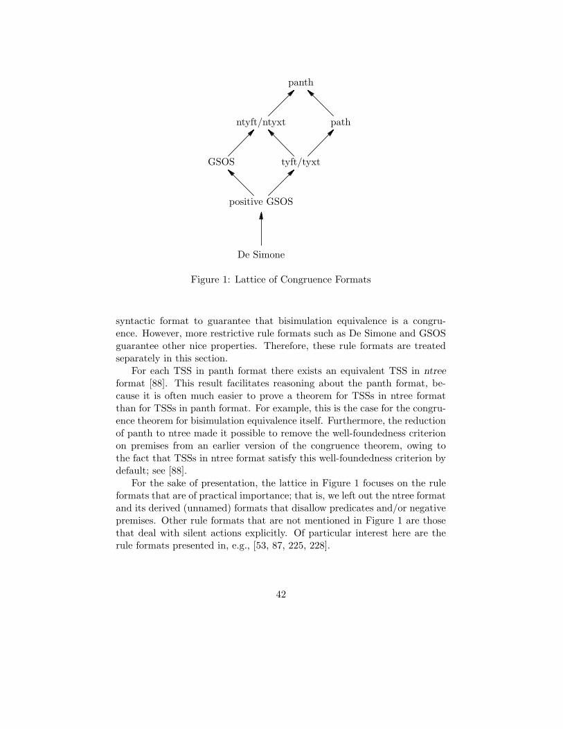
De Simone
positive GSOS
tyft/tyxtGSOS
ntyft/ntyxt path
panth
Figure 1: Lattice of Congruence Formats
syntactic format to guarantee that bisimulation equivalence is a congru-ence. However, more restrictive rule formats such as De Simone and GSOSguarantee other nice properties. Therefore, these rule formats are treatedseparately in this section.
For each TSS in panth format there exists an equivalent TSS in ntreeformat [88]. This result facilitates reasoning about the panth format, be-cause it is often much easier to prove a theorem for TSSs in ntree formatthan for TSSs in panth format. For example, this is the case for the congru-ence theorem for bisimulation equivalence itself. Furthermore, the reductionof panth to ntree made it possible to remove the well-foundedness criterionon premises from an earlier version of the congruence theorem, owing tothe fact that TSSs in ntree format satisfy this well-foundedness criterion bydefault; see [88].
For the sake of presentation, the lattice in Figure 1 focuses on the ruleformats that are of practical importance; that is, we left out the ntree formatand its derived (unnamed) formats that disallow predicates and/or negativepremises. Other rule formats that are not mentioned in Figure 1 are thosethat deal with silent actions explicitly. Of particular interest here are therule formats presented in, e.g., [53, 87, 225, 228].
42
The organization of this section is as follows. Sect. 5.1 presents thepanth format, while Sect. 5.2 deals with the equally expressive ntree for-mat. Sects. 5.3 and 5.4 study De Simone languages and GSOS languages,respectively. Sect. 5.5 introduces a congruence format in the presence ofsilent actions, while Sect. 5.6 presents congruence formats for a wide rangeof behavioural preorders. Finally, Sect. 5.7 studies the completed trace con-gruence induced by a number of congruence formats.
5.1 Panth Format
This section presents the panth format, and states a congruence theorem(cf. Def. 2.11) from [60, 115, 237] with respect to bisimulation equivalence(cf. Def. 2.3).
Definition 5.1 (Panth format) A transition rule ρ is in panth format ifit satisfies the following three restrictions:
1. for each positive premise ta→ t′ of ρ, the right-hand side t′ is a single
variable;
2. the source of ρ contains no more than one function symbol;
3. the variables that occur as right-hand sides of positive premises or inthe source of ρ are all distinct.
A TSS is in panth format if it consists of panth rules only.
The three subformats path, ntyft/ntyxt, and tyft/tyxt of the panth formatdo not allow negative premises and/or predicates.
Definition 5.2 (Path, ntyft/ntyxt, and tyft/tyxt format) A TSS isin path format if it is in panth format and positive.
A TSS is in ntyft/ntyxt format if it is in panth format and its transitionrules do not contain predicates.
A TSS is in tyft/tyxt format if it is both path and ntyft/ntyxt.A TSS is in tyft format if it is tyft/tyxt and the source of each rule
contains exactly one function symbol.
Theorem 5.3 If a TSS is complete and panth, then bisimulation equiva-lence is a congruence with respect to the LTS associated with it.
43
The interested reader is referred to [88, 115, 237] for a proof of Thm. 5.3.Groote and Vaandrager [115] presented a string of examples of TSSs whichshow that all syntactic requirements of the panth format are essential forthe congruence result in Thm. 5.3. We give an example to show that therestriction in Thm. 5.3 to complete TSSs is essential. In particular, it cannotbe relaxed to TSSs that have exactly one (not necessarily least) three-valuedstable model that does not contain unknown transitions. The example isderived from [60, Ex. 8.12].
Example: Let the signature consist of constants a, b and of a unary functionsymbol f . Moreover, let P , Q1, and Q2 be predicates. Consider the followingTSS in panth format:
aP bP
xP f(x)¬Q1 f(a)¬Q2f(x)Q2
xP f(x)¬Q2 f(b)¬Q1f(x)Q1
Its least three-valued stable model contains the following unknown transi-tions: f(a)Q1, f(a)Q2, f(b)Q1, and f(b)Q2. So the TSS is not complete.
However, the TSS does have a three-valued stable model in which the setof unknown transitions is empty, and aP , bP , f(a)Q1, and f(b)Q2 are thetrue transitions. a ↔ b but f(a) ↔/ f(b) with respect to this three-valuedstable model. ¤
In [176], van Oostrom and de Vink generalized the tyft/tyxt format (soin the absence of predicates and negative premises) to the stalk format, bysomewhat relaxing the constraint that sources of transition rules can containno more than one function symbol. They proved that the congruence resultin Thm. 5.3 holds for the stalk format.
We apply the congruence theorem for the panth format to the runningexamples from Sect. 2.6.
Basic Process Algebra The TSS for BPAε in Table 1 is panth. Forexample, the transition rule
xa→ x′
x · y a→ x′ · y
for sequential composition is panth, because the right-hand side of its premiseis a single variable x′, its source contains only one function symbol (sequen-tial composition), and the variables in the right-hand side of its premise (x′)and in its source (x and y) are distinct. It is left to the reader to verify thatthe remaining transition rules in Table 1 are panth.
44
The TSS for BPAε is positive, so it is complete. Since this TSS is bothpanth and complete, Thm. 5.3 says that bisimulation equivalence is a con-gruence with respect to BPAε.
Priorities It is not hard to check that the TSS for BPAεθ in Table 2 ispanth. Furthermore, it was noted in Sect. 3.5 that the TSS for BPAεθ iscomplete. Hence, by Thm. 5.3, bisimulation equivalence is a congruencewith respect to BPAεθ.
Discrete Time It is not hard to check that the TSS for BPAdtε in Table 3is panth. Furthermore, it was noted in Sect. 3.5 that the TSS for BPAdtε iscomplete. Hence, by Thm. 5.3, bisimulation equivalence is a congruencewith respect to BPAdtε .
5.2 Ntree Format
In this section we present a result from [85, 88] to the effect that for eachTSS in panth format there exists an equivalent TSS in the more restrictiventree format. The following terminology originates from [58, 115].
Definition 5.4 (Variable dependency graph) The variable dependencygraph of a set S of premises is a directed graph, with the set of variables asvertices, and with as edges the set
〈x, y〉 | there is a ta→ t′ in S such that x occurs in t and y in t′ .
S is well-founded if any backward chain of edges in its variable dependencygraph is finite.
A transition rule is pure if its set of premises is well-founded and more-over each variable in the rule occurs in the source or as the right-hand sideof a positive premise.
Typical examples of sets of premises that are not well-founded are y a→ y,y1 a→ y2, y2
b→ y1, and yi+1 a→ yi | i ∈ N.
Definition 5.5 (Ntree format) A transition rule ρ is in ntree format ifit satisfies the following three criteria:
1. ρ is panth;
2. ρ is pure;
45
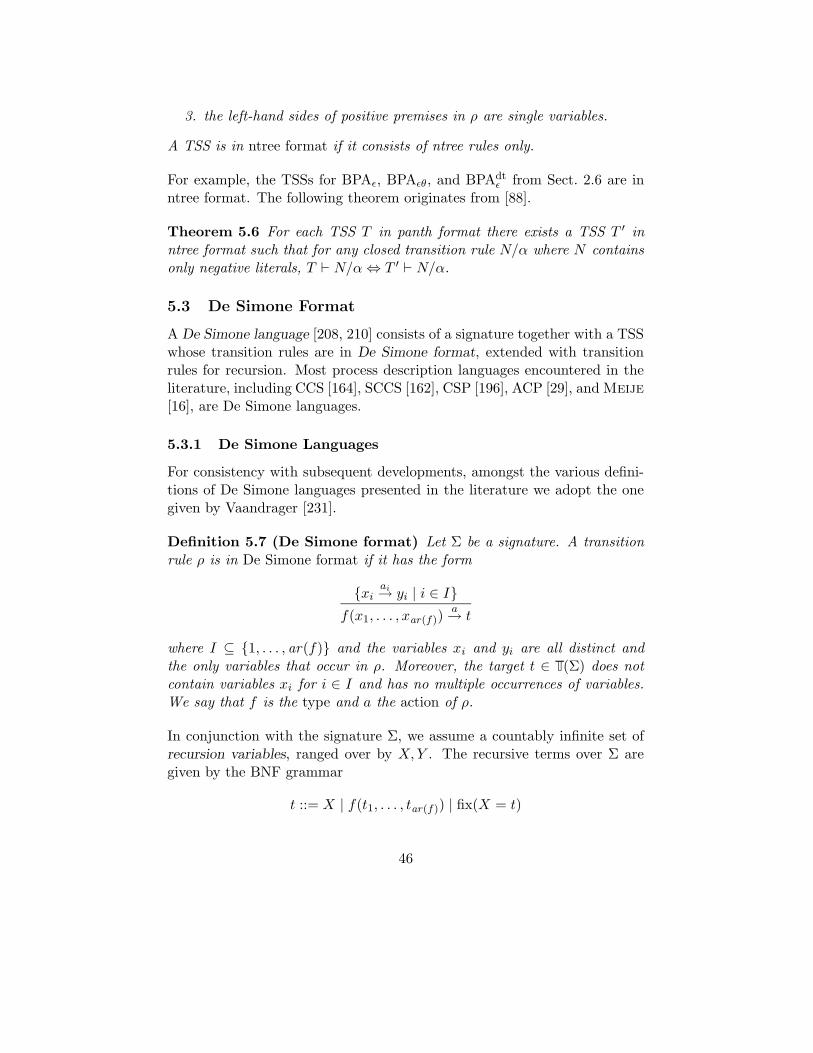
3. the left-hand sides of positive premises in ρ are single variables.
A TSS is in ntree format if it consists of ntree rules only.
For example, the TSSs for BPAε, BPAεθ, and BPAdtε from Sect. 2.6 are inntree format. The following theorem originates from [88].
Theorem 5.6 For each TSS T in panth format there exists a TSS T ′ inntree format such that for any closed transition rule N/α where N containsonly negative literals, T ` N/α⇔ T ′ ` N/α.
5.3 De Simone Format
A De Simone language [208, 210] consists of a signature together with a TSSwhose transition rules are in De Simone format, extended with transitionrules for recursion. Most process description languages encountered in theliterature, including CCS [164], SCCS [162], CSP [196], ACP [29], andMeije[16], are De Simone languages.
5.3.1 De Simone Languages
For consistency with subsequent developments, amongst the various defini-tions of De Simone languages presented in the literature we adopt the onegiven by Vaandrager [231].
Definition 5.7 (De Simone format) Let Σ be a signature. A transitionrule ρ is in De Simone format if it has the form
xiai→ yi | i ∈ I
f(x1, . . . , xar(f))a→ t
where I ⊆ 1, . . . , ar(f) and the variables xi and yi are all distinct andthe only variables that occur in ρ. Moreover, the target t ∈ (Σ) does notcontain variables xi for i ∈ I and has no multiple occurrences of variables.We say that f is the type and a the action of ρ.
In conjunction with the signature Σ, we assume a countably infinite set ofrecursion variables, ranged over by X,Y . The recursive terms over Σ aregiven by the BNF grammar
t ::= X | f(t1, . . . , tar(f)) | fix(X = t)
46
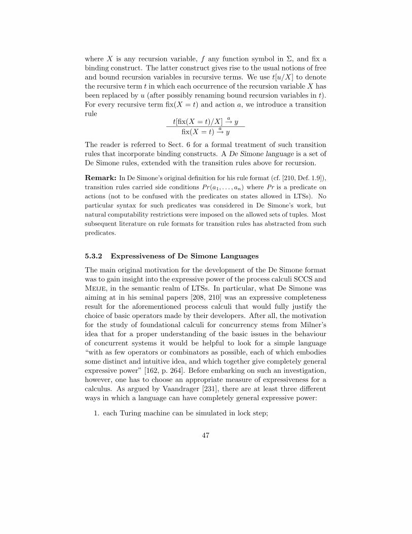
where X is any recursion variable, f any function symbol in Σ, and fix abinding construct. The latter construct gives rise to the usual notions of freeand bound recursion variables in recursive terms. We use t[u/X] to denotethe recursive term t in which each occurrence of the recursion variable X hasbeen replaced by u (after possibly renaming bound recursion variables in t).For every recursive term fix(X = t) and action a, we introduce a transitionrule
t[fix(X = t)/X]a→ y
fix(X = t)a→ y
The reader is referred to Sect. 6 for a formal treatment of such transitionrules that incorporate binding constructs. A De Simone language is a set ofDe Simone rules, extended with the transition rules above for recursion.
Remark: In De Simone’s original definition for his rule format (cf. [210, Def. 1.9]),transition rules carried side conditions Pr(a1, . . . , an) where Pr is a predicate on
actions (not to be confused with the predicates on states allowed in LTSs). No
particular syntax for such predicates was considered in De Simone’s work, but
natural computability restrictions were imposed on the allowed sets of tuples. Most
subsequent literature on rule formats for transition rules has abstracted from such
predicates.
5.3.2 Expressiveness of De Simone Languages
The main original motivation for the development of the De Simone formatwas to gain insight into the expressive power of the process calculi SCCS andMeije, in the semantic realm of LTSs. In particular, what De Simone wasaiming at in his seminal papers [208, 210] was an expressive completenessresult for the aforementioned process calculi that would fully justify thechoice of basic operators made by their developers. After all, the motivationfor the study of foundational calculi for concurrency stems from Milner’sidea that for a proper understanding of the basic issues in the behaviourof concurrent systems it would be helpful to look for a simple language“with as few operators or combinators as possible, each of which embodiessome distinct and intuitive idea, and which together give completely generalexpressive power” [162, p. 264]. Before embarking on such an investigation,however, one has to choose an appropriate measure of expressiveness for acalculus. As argued by Vaandrager [231], there are at least three differentways in which a language can have completely general expressive power:
1. each Turing machine can be simulated in lock step;
47
2. each recursively enumerable LTS can be specified up to some notionof behavioural equivalence;
3. each operation in a “natural” class of operations is realizable by meansof the primitive operations in the language up to some notion of be-havioural equivalence.
Since most languages that have been proposed in the literature are com-pletely expressive in the first sense, this criterion does not offer a usefulmeans to classify the expressiveness of languages. (This is what Meyer [155]calls the “Turing tarpit”.) The remaining two criteria have been investi-gated by De Simone in op. cit., and, since then, by several other authors.Indeed, this kind of expressiveness results has, to the best of our knowledge,only been developed for De Simone languages, and similar investigationsare lacking for more general rule formats. For this reason, the rest of thissection is devoted to a brief review of such results. The other results thathave been developed for this format are instances of theorems for the moregeneral formats we survey.
The question of whether there exists a process description languagewhich is completely expressive with respect to the collection of operationsdefinable by means of De Simone rules has been addressed by several au-thors since De Simone’s original work. In op. cit., De Simone showed thefollowing result.
Theorem 5.8 Let Act be a finite set of actions. Let f be specified by aDe Simone language containing only finitely many rules. Then f can beexpressed, up to bisimulation equivalence, in the calculi SCCS and Meije.
As a corollary of this expressiveness result pertaining to the class of oper-ators specifiable in SCCS and Meije, De Simone was able to prove thatthe calculi SCCS and Meije, and, a fortiori, reasonably expressive De Si-mone languages, can denote every recursively enumerable LTS up to graphisomorphism.
Definition 5.9 (Properties of LTSs) An LTS is:
• countably branching if for every state s there are at most countablymany outgoing transitions s
a→ s′;
• recursively enumerable if there exists an algorithm enumerating alltransitions s
a→ s′;
48
• decidable if there exists an algorithm that determines for every tran-sition whether it is in the LTS;
• computable [25] if there exists an algorithm that computes for everystate s its complete finite list of outgoing transitions s
a→ s′;
• primitive recursive [187] if there is such an algorithm that is primitiverecursive.
Note that “computable” is a stronger requirement than “decidable andfinitely branching” (cf. Def. 2.2). The following result is from [210, Thm. 3.2].
Theorem 5.10 Every recursively enumerable LTS can be realized by a re-cursive term in SCCS-Meije up to graph isomorphism.
Several variations on Thm. 5.10 have been presented in the literature. Be-fore stating some of these results, we need to introduce some preliminarydefinitions from [231].
Definition 5.11 (Testing arguments) Assume a De Simone language.A function symbol f tests its ith argument if one of the De Simone ruleshas a source f(x1, . . . , xar(f)) and a premise xi
ai→ yi.
Definition 5.12 (Guardedness) Assume a De Simone language. For re-cursive terms t, the sets U(t) of unguarded recursion variables are definedthus:
U(X)∆= X
U(f(t1, . . . , tar(f)))∆= U(ti1) ∪ · · · ∪ U(tik) if f tests arguments i1, . . . , ik
U(fix(X = t))∆= U(t)\X .
A recursive term t is guarded if for every subterm fix(X = t′) of t we haveX 6∈ U(t′).
In particular, if a function symbol f tests none of its arguments, then owingto the second clause in Def. 5.12 no recursion variable is unguarded in arecursive term of the form f(t1, . . . , tar(f)).
Guarded recursive specifications in any De Simone language have uniquesolutions up to bisimulation equivalence. That is, let t be a guarded recur-sive term with no other free recursion variables than X, and let u and u′
be recursive terms without free recursion variables. If u ↔ t[u/X] andu′ ↔ t[u′/X], then u ↔ u′ (cf. [164, Sect. 4.5]).
49
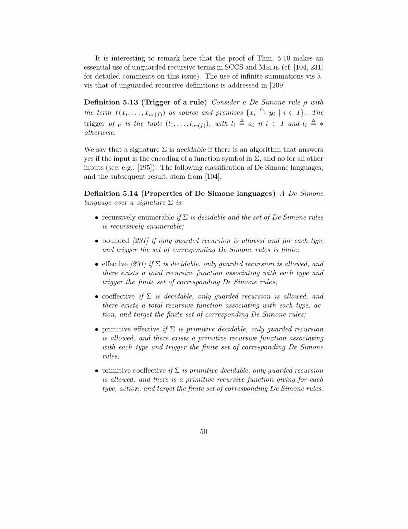
It is interesting to remark here that the proof of Thm. 5.10 makes anessential use of unguarded recursive terms in SCCS andMeije (cf. [104, 231]for detailed comments on this issue). The use of infinite summations vis-a-vis that of unguarded recursive definitions is addressed in [209].
Definition 5.13 (Trigger of a rule) Consider a De Simone rule ρ with
the term f(xi, . . . , xar(f)) as source and premises xiai→ yi | i ∈ I. The
trigger of ρ is the tuple (l1, . . . , lar(f)), with li∆= ai if i ∈ I and li
∆= ∗
otherwise.
We say that a signature Σ is decidable if there is an algorithm that answersyes if the input is the encoding of a function symbol in Σ, and no for all otherinputs (see, e.g., [195]). The following classification of De Simone languages,and the subsequent result, stem from [104].
Definition 5.14 (Properties of De Simone languages) A De Simonelanguage over a signature Σ is:
• recursively enumerable if Σ is decidable and the set of De Simone rulesis recursively enumerable;
• bounded [231] if only guarded recursion is allowed and for each typeand trigger the set of corresponding De Simone rules is finite;
• effective [231] if Σ is decidable, only guarded recursion is allowed, andthere exists a total recursive function associating with each type andtrigger the finite set of corresponding De Simone rules;
• coeffective if Σ is decidable, only guarded recursion is allowed, andthere exists a total recursive function associating with each type, ac-tion, and target the finite set of corresponding De Simone rules;
• primitive effective if Σ is primitive decidable, only guarded recursionis allowed, and there exists a primitive recursive function associatingwith each type and trigger the finite set of corresponding De Simonerules;
• primitive coeffective if Σ is primitive decidable, only guarded recursionis allowed, and there is a primitive recursive function giving for eachtype, action, and target the finite set of corresponding De Simone rules.
50
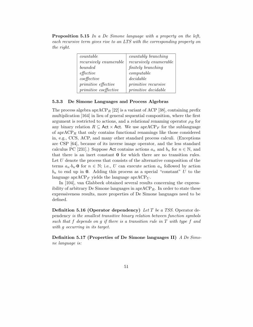
Proposition 5.15 In a De Simone language with a property on the left,each recursive term gives rise to an LTS with the corresponding property onthe right.
countable countably branchingrecursively enumerable recursively enumerablebounded finitely branchingeffective computablecoeffective decidableprimitive effective primitive recursiveprimitive coeffective primitive decidable
5.3.3 De Simone Languages and Process Algebras
The process algebra aprACPR [22] is a variant of ACP [38], containing prefixmultiplication [164] in lieu of general sequential composition, where the firstargument is restricted to actions, and a relational renaming operator ρR forany binary relation R ⊆ Act × Act. We use aprACPF for the sublanguageof aprACPR that only contains functional renamings like those consideredin, e.g., CCS, ACP, and many other standard process calculi. (Exceptionsare CSP [64], because of its inverse image operator, and the less standardcalculus PC [231].) Suppose Act contains actions an and bn for n ∈ N, andthat there is an inert constant 0 for which there are no transition rules.Let U denote the process that consists of the alternative composition of theterms an·bn·0 for n ∈ N; i.e., U can execute action an followed by actionbn to end up in 0. Adding this process as a special “constant” U to thelanguage aprACPF yields the language aprACPU .
In [104], van Glabbeek obtained several results concerning the express-ibility of arbitrary De Simone languages in aprACPR. In order to state theseexpressiveness results, more properties of De Simone languages need to bedefined.
Definition 5.16 (Operator dependency) Let T be a TSS. Operator de-pendency is the smallest transitive binary relation between function symbolssuch that f depends on g if there is a transition rule in T with type f andwith g occurring in its target.
Definition 5.17 (Properties of De Simone languages II) A De Simo-ne language is:
51
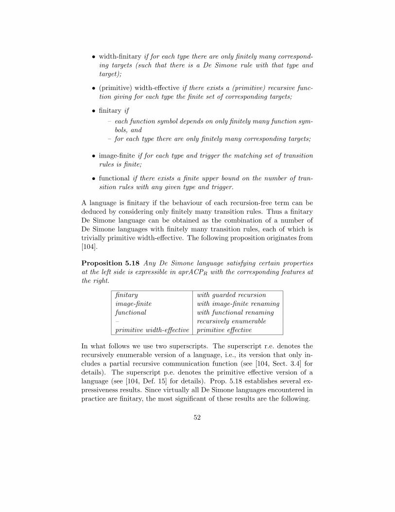
• width-finitary if for each type there are only finitely many correspond-ing targets (such that there is a De Simone rule with that type andtarget);
• (primitive) width-effective if there exists a (primitive) recursive func-tion giving for each type the finite set of corresponding targets;
• finitary if
– each function symbol depends on only finitely many function sym-bols, and
– for each type there are only finitely many corresponding targets;
• image-finite if for each type and trigger the matching set of transitionrules is finite;
• functional if there exists a finite upper bound on the number of tran-sition rules with any given type and trigger.
A language is finitary if the behaviour of each recursion-free term can bededuced by considering only finitely many transition rules. Thus a finitaryDe Simone language can be obtained as the combination of a number ofDe Simone languages with finitely many transition rules, each of which istrivially primitive width-effective. The following proposition originates from[104].
Proposition 5.18 Any De Simone language satisfying certain propertiesat the left side is expressible in aprACPR with the corresponding features atthe right.
finitary with guarded recursionimage-finite with image-finite renamingfunctional with functional renaming– recursively enumerableprimitive width-effective primitive effective
In what follows we use two superscripts. The superscript r.e. denotes therecursively enumerable version of a language, i.e., its version that only in-cludes a partial recursive communication function (see [104, Sect. 3.4] fordetails). The superscript p.e. denotes the primitive effective version of alanguage (see [104, Def. 15] for details). Prop. 5.18 establishes several ex-pressiveness results. Since virtually all De Simone languages encountered inpractice are finitary, the most significant of these results are the following.
52
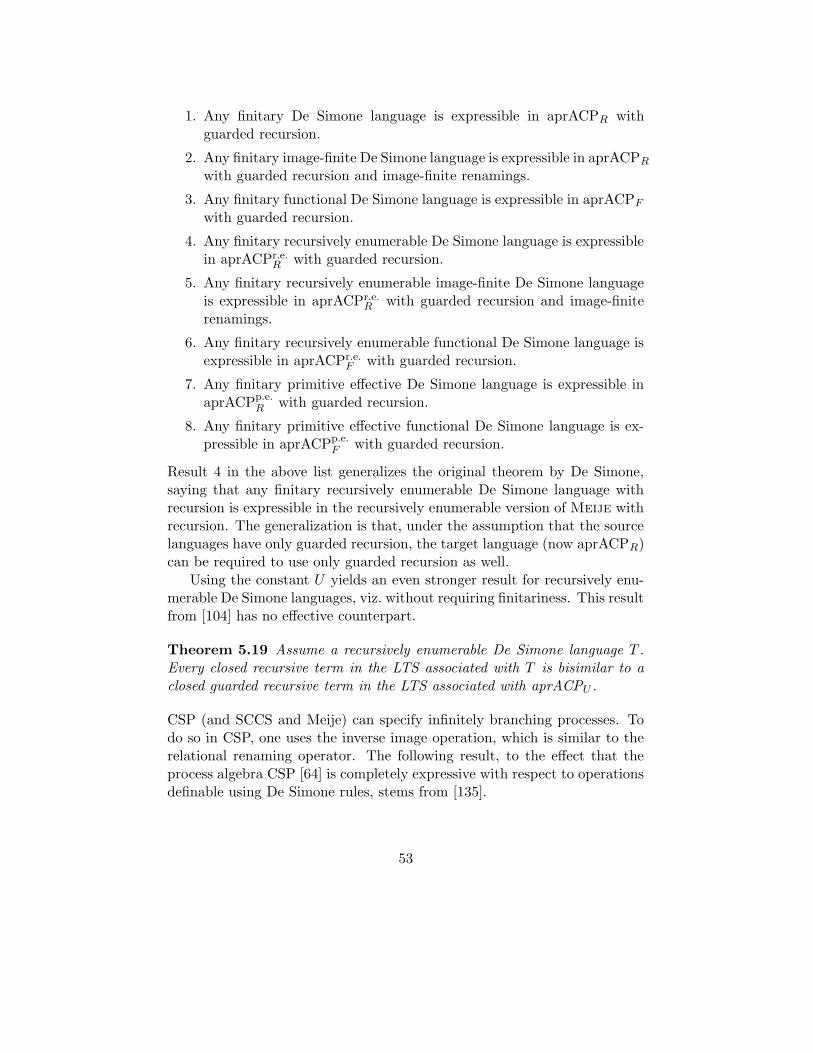
1. Any finitary De Simone language is expressible in aprACPR withguarded recursion.
2. Any finitary image-finite De Simone language is expressible in aprACPR
with guarded recursion and image-finite renamings.
3. Any finitary functional De Simone language is expressible in aprACPF
with guarded recursion.
4. Any finitary recursively enumerable De Simone language is expressiblein aprACPr.e.R with guarded recursion.
5. Any finitary recursively enumerable image-finite De Simone languageis expressible in aprACPr.e.R with guarded recursion and image-finiterenamings.
6. Any finitary recursively enumerable functional De Simone language isexpressible in aprACPr.e.F with guarded recursion.
7. Any finitary primitive effective De Simone language is expressible inaprACPp.e.R with guarded recursion.
8. Any finitary primitive effective functional De Simone language is ex-pressible in aprACPp.e.F with guarded recursion.
Result 4 in the above list generalizes the original theorem by De Simone,saying that any finitary recursively enumerable De Simone language withrecursion is expressible in the recursively enumerable version of Meije withrecursion. The generalization is that, under the assumption that the sourcelanguages have only guarded recursion, the target language (now aprACPR)can be required to use only guarded recursion as well.
Using the constant U yields an even stronger result for recursively enu-merable De Simone languages, viz. without requiring finitariness. This resultfrom [104] has no effective counterpart.
Theorem 5.19 Assume a recursively enumerable De Simone language T .Every closed recursive term in the LTS associated with T is bisimilar to aclosed guarded recursive term in the LTS associated with aprACPU .
CSP (and SCCS and Meije) can specify infinitely branching processes. Todo so in CSP, one uses the inverse image operation, which is similar to therelational renaming operator. The following result, to the effect that theprocess algebra CSP [64] is completely expressive with respect to operationsdefinable using De Simone rules, stems from [135].
53
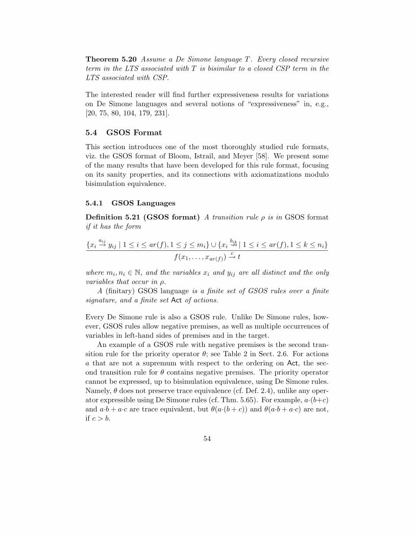
Theorem 5.20 Assume a De Simone language T . Every closed recursiveterm in the LTS associated with T is bisimilar to a closed CSP term in theLTS associated with CSP.
The interested reader will find further expressiveness results for variationson De Simone languages and several notions of “expressiveness” in, e.g.,[20, 75, 80, 104, 179, 231].
5.4 GSOS Format
This section introduces one of the most thoroughly studied rule formats,viz. the GSOS format of Bloom, Istrail, and Meyer [58]. We present someof the many results that have been developed for this rule format, focusingon its sanity properties, and its connections with axiomatizations modulobisimulation equivalence.
5.4.1 GSOS Languages
Definition 5.21 (GSOS format) A transition rule ρ is in GSOS formatif it has the form
xiaij→ yij | 1 ≤ i ≤ ar(f), 1 ≤ j ≤ mi ∪ xi
bik9 | 1 ≤ i ≤ ar(f), 1 ≤ k ≤ ni
f(x1, . . . , xar(f))c→ t
where mi, ni ∈ N, and the variables xi and yij are all distinct and the onlyvariables that occur in ρ.
A (finitary) GSOS language is a finite set of GSOS rules over a finitesignature, and a finite set Act of actions.
Every De Simone rule is also a GSOS rule. Unlike De Simone rules, how-ever, GSOS rules allow negative premises, as well as multiple occurrences ofvariables in left-hand sides of premises and in the target.
An example of a GSOS rule with negative premises is the second tran-sition rule for the priority operator θ; see Table 2 in Sect. 2.6. For actionsa that are not a supremum with respect to the ordering on Act, the sec-ond transition rule for θ contains negative premises. The priority operatorcannot be expressed, up to bisimulation equivalence, using De Simone rules.Namely, θ does not preserve trace equivalence (cf. Def. 2.4), unlike any oper-ator expressible using De Simone rules (cf. Thm. 5.65). For example, a·(b+c)and a·b+ a·c are trace equivalent, but θ(a·(b+ c)) and θ(a·b+ a·c) are not,if c > b.
54
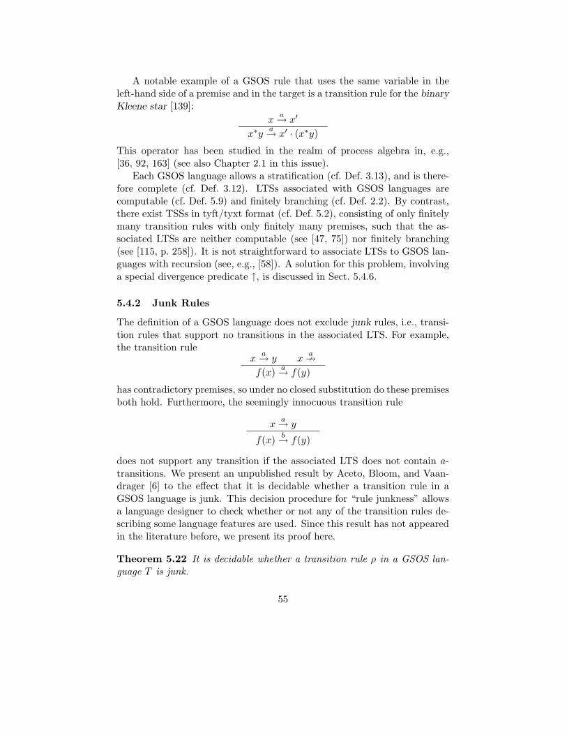
A notable example of a GSOS rule that uses the same variable in theleft-hand side of a premise and in the target is a transition rule for the binaryKleene star [139]:
xa→ x′
x∗ya→ x′ · (x∗y)
This operator has been studied in the realm of process algebra in, e.g.,[36, 92, 163] (see also Chapter 2.1 in this issue).
Each GSOS language allows a stratification (cf. Def. 3.13), and is there-fore complete (cf. Def. 3.12). LTSs associated with GSOS languages arecomputable (cf. Def. 5.9) and finitely branching (cf. Def. 2.2). By contrast,there exist TSSs in tyft/tyxt format (cf. Def. 5.2), consisting of only finitelymany transition rules with only finitely many premises, such that the as-sociated LTSs are neither computable (see [47, 75]) nor finitely branching(see [115, p. 258]). It is not straightforward to associate LTSs to GSOS lan-guages with recursion (see, e.g., [58]). A solution for this problem, involvinga special divergence predicate ↑, is discussed in Sect. 5.4.6.
5.4.2 Junk Rules
The definition of a GSOS language does not exclude junk rules, i.e., transi-tion rules that support no transitions in the associated LTS. For example,the transition rule
xa→ y x
a9
f(x)a→ f(y)
has contradictory premises, so under no closed substitution do these premisesboth hold. Furthermore, the seemingly innocuous transition rule
xa→ y
f(x)b→ f(y)
does not support any transition if the associated LTS does not contain a-transitions. We present an unpublished result by Aceto, Bloom, and Vaan-drager [6] to the effect that it is decidable whether a transition rule in aGSOS language is junk. This decision procedure for “rule junkness” allowsa language designer to check whether or not any of the transition rules de-scribing some language features are used. Since this result has not appearedin the literature before, we present its proof here.
Theorem 5.22 It is decidable whether a transition rule ρ in a GSOS lan-guage T is junk.
55
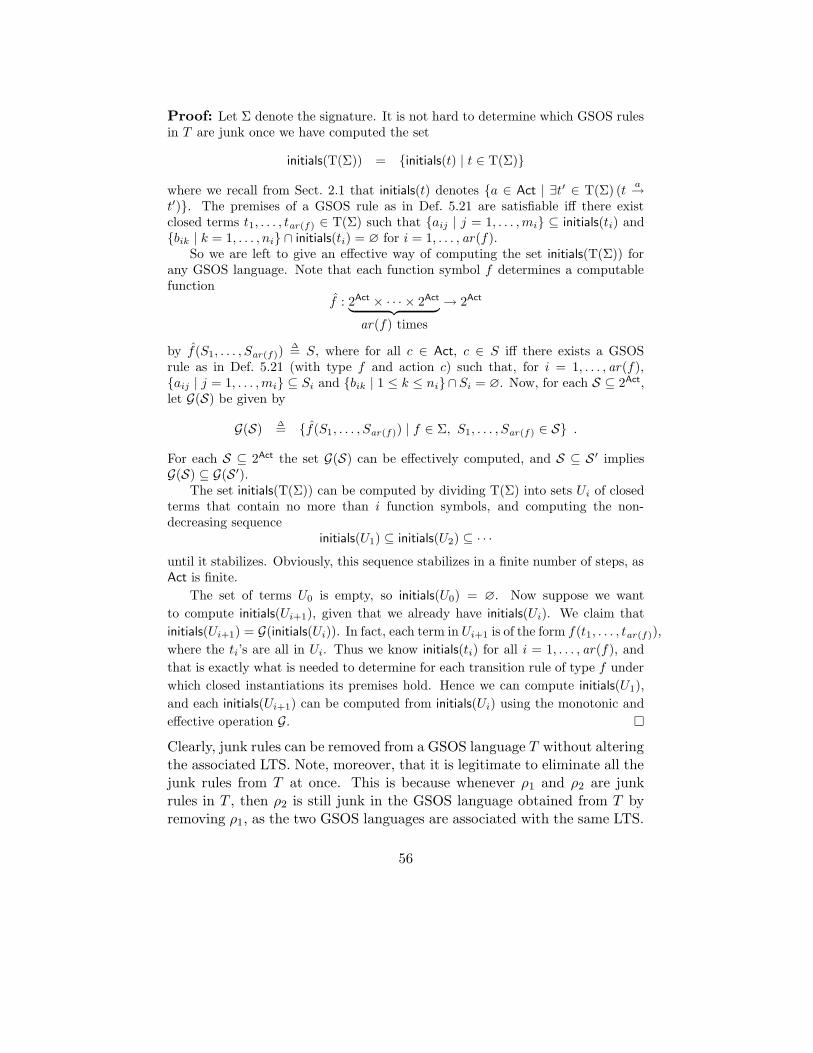
Proof: Let Σ denote the signature. It is not hard to determine which GSOS rulesin T are junk once we have computed the set
initials(T(Σ)) = initials(t) | t ∈ T(Σ)
where we recall from Sect. 2.1 that initials(t) denotes a ∈ Act | ∃t′ ∈ T(Σ) (ta→
t′). The premises of a GSOS rule as in Def. 5.21 are satisfiable iff there existclosed terms t1, . . . , tar(f) ∈ T(Σ) such that aij | j = 1, . . . ,mi ⊆ initials(ti) andbik | k = 1, . . . , ni ∩ initials(ti) = ∅ for i = 1, . . . , ar(f).
So we are left to give an effective way of computing the set initials(T(Σ)) forany GSOS language. Note that each function symbol f determines a computablefunction
f : 2Act × · · · × 2Act
︸ ︷︷ ︸
ar(f) times
→ 2Act
by f(S1, . . . , Sar(f))∆
= S, where for all c ∈ Act, c ∈ S iff there exists a GSOSrule as in Def. 5.21 (with type f and action c) such that, for i = 1, . . . , ar(f),aij | j = 1, . . . ,mi ⊆ Si and bik | 1 ≤ k ≤ ni ∩Si = ∅. Now, for each S ⊆ 2Act,let G(S) be given by
G(S) ∆
= f(S1, . . . , Sar(f)) | f ∈ Σ, S1, . . . , Sar(f) ∈ S .
For each S ⊆ 2Act the set G(S) can be effectively computed, and S ⊆ S ′ impliesG(S) ⊆ G(S ′).
The set initials(T(Σ)) can be computed by dividing T(Σ) into sets Ui of closedterms that contain no more than i function symbols, and computing the non-decreasing sequence
initials(U1) ⊆ initials(U2) ⊆ · · ·until it stabilizes. Obviously, this sequence stabilizes in a finite number of steps, asAct is finite.
The set of terms U0 is empty, so initials(U0) = ∅. Now suppose we want
to compute initials(Ui+1), given that we already have initials(Ui). We claim that
initials(Ui+1) = G(initials(Ui)). In fact, each term in Ui+1 is of the form f(t1, . . . , tar(f)),
where the ti’s are all in Ui. Thus we know initials(ti) for all i = 1, . . . , ar(f), and
that is exactly what is needed to determine for each transition rule of type f under
which closed instantiations its premises hold. Hence we can compute initials(U1),
and each initials(Ui+1) can be computed from initials(Ui) using the monotonic and
effective operation G. ¤
Clearly, junk rules can be removed from a GSOS language T without alteringthe associated LTS. Note, moreover, that it is legitimate to eliminate all thejunk rules from T at once. This is because whenever ρ1 and ρ2 are junkrules in T , then ρ2 is still junk in the GSOS language obtained from T byremoving ρ1, as the two GSOS languages are associated with the same LTS.
56
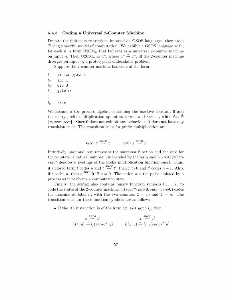
5.4.3 Coding a Universal 2-Counter Machine
Despite the finiteness restrictions imposed on GSOS languages, they are aTuring powerful model of computation. We exhibit a GSOS language with,for each n, a term U2CMn that behaves as a universal 2-counter machineon input n. Then U2CMn ↔–– aω, where aω
a→ aω, iff the 2-counter machinediverges on input n, a prototypical undecidable problem.
Suppose the 2-counter machine has code of the form:
l1: if I=0 goto l5l2: inc I
l3: dec J
l4: goto l7...
lk: halt
We assume a toy process algebra containing the inactive constant 0 andthe unary prefix multiplication operators zero · and succ · , while Act
∆=
a, succ, zero. Since 0 does not exhibit any behaviour, it does not have anytransition rules. The transition rules for prefix multiplication are
succ · x succ→ x zero · x zero→ x
Intuitively, succ and zero represent the successor function and the zero forthe counters: a natural number n is encoded by the term succn·zero·0 (wheresuccn denotes n nestings of the prefix multiplication function succ). Thus,
if a closed term t codes n and tsucc→ t′, then n > 0 and t′ codes n− 1. Also,
if t codes n, then tzero→ 0 iff n = 0. The action a is the pulse emitted by a
process as it performs a computation step.Finally, the syntax also contains binary function symbols l1, . . . , lk to
code the states of the 2-counter machine: li(succm·zero·0, succn·zero·0) codes
the machine at label li, with the two counters I = m and J = n. Thetransition rules for these function symbols are as follows.
• If the ith instruction is of the form if I=0 goto lj , then
xzero→ x′
li(x, y)a→ lj(zero·x′, y)
xsucc→ x′
li(x, y)a→ li+1(succ·x′, y)
57
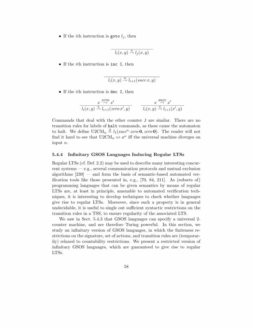
• If the ith instruction is goto lj , then
li(x, y)a→ lj(x, y)
• If the ith instruction is inc I, then
li(x, y)a→ li+1(succ·x, y)
• If the ith instruction is dec I, then
xzero→ x′
li(x, y)a→ li+1(zero·x′, y)
xsucc→ x′
li(x, y)a→ li+1(x
′, y)
Commands that deal with the other counter J are similar. There are notransition rules for labels of halt commands, as these cause the automatonto halt. We define U2CMn
∆= l1(succ
n·zero·0, zero·0). The reader will notfind it hard to see that U2CMn ↔–– aω iff the universal machine diverges oninput n.
5.4.4 Infinitary GSOS Languages Inducing Regular LTSs
Regular LTSs (cf. Def. 2.2) may be used to describe many interesting concur-rent systems — e.g., several communication protocols and mutual exclusionalgorithms [239] — and form the basis of semantic-based automated ver-ification tools like those presented in, e.g., [70, 84, 211]. As (subsets of)programming languages that can be given semantics by means of regularLTSs are, at least in principle, amenable to automated verification tech-niques, it is interesting to develop techniques to check whether languagesgive rise to regular LTSs. Moreover, since such a property is in generalundecidable, it is useful to single out sufficient syntactic restrictions on thetransition rules in a TSS, to ensure regularity of the associated LTS.
We saw in Sect. 5.4.3 that GSOS languages can specify a universal 2-counter machine, and are therefore Turing powerful. In this section, westudy an infinitary version of GSOS languages, in which the finiteness re-strictions on the signature, set of actions, and transition rules are (temporar-ily) relaxed to countability restrictions. We present a restricted version ofinfinitary GSOS languages, which are guaranteed to give rise to regularLTSs.
58
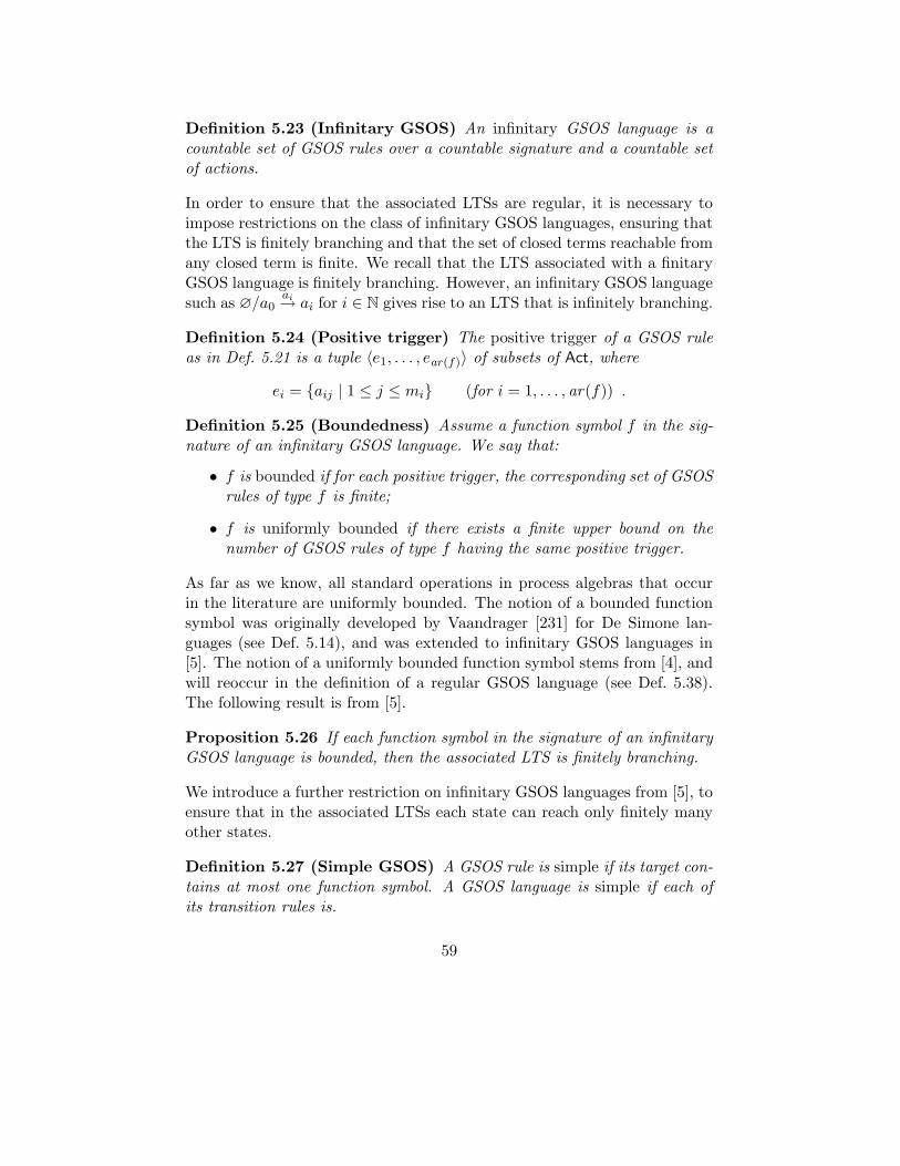
Definition 5.23 (Infinitary GSOS) An infinitary GSOS language is acountable set of GSOS rules over a countable signature and a countable setof actions.
In order to ensure that the associated LTSs are regular, it is necessary toimpose restrictions on the class of infinitary GSOS languages, ensuring thatthe LTS is finitely branching and that the set of closed terms reachable fromany closed term is finite. We recall that the LTS associated with a finitaryGSOS language is finitely branching. However, an infinitary GSOS languagesuch as ∅/a0
ai→ ai for i ∈ N gives rise to an LTS that is infinitely branching.
Definition 5.24 (Positive trigger) The positive trigger of a GSOS ruleas in Def. 5.21 is a tuple 〈e1, . . . , ear(f)〉 of subsets of Act, where
ei = aij | 1 ≤ j ≤ mi (for i = 1, . . . , ar(f)) .
Definition 5.25 (Boundedness) Assume a function symbol f in the sig-nature of an infinitary GSOS language. We say that:
• f is bounded if for each positive trigger, the corresponding set of GSOSrules of type f is finite;
• f is uniformly bounded if there exists a finite upper bound on thenumber of GSOS rules of type f having the same positive trigger.
As far as we know, all standard operations in process algebras that occurin the literature are uniformly bounded. The notion of a bounded functionsymbol was originally developed by Vaandrager [231] for De Simone lan-guages (see Def. 5.14), and was extended to infinitary GSOS languages in[5]. The notion of a uniformly bounded function symbol stems from [4], andwill reoccur in the definition of a regular GSOS language (see Def. 5.38).The following result is from [5].
Proposition 5.26 If each function symbol in the signature of an infinitaryGSOS language is bounded, then the associated LTS is finitely branching.
We introduce a further restriction on infinitary GSOS languages from [5], toensure that in the associated LTSs each state can reach only finitely manyother states.
Definition 5.27 (Simple GSOS) A GSOS rule is simple if its target con-tains at most one function symbol. A GSOS language is simple if each ofits transition rules is.
59
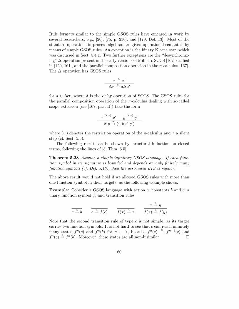
Rule formats similar to the simple GSOS rules have emerged in work byseveral researchers, e.g., [20], [75, p. 230], and [179, Def. 13]. Most of thestandard operations in process algebras are given operational semantics bymeans of simple GSOS rules. An exception is the binary Kleene star, whichwas discussed in Sect. 5.4.1. Two further exceptions are the “desynchroniz-ing” ∆ operation present in the early versions of Milner’s SCCS [162] studiedin [120, 161], and the parallel composition operation in the π-calculus [167].The ∆ operation has GSOS rules
xa→ x′
∆xa→ δ∆x′
for a ∈ Act, where δ is the delay operation of SCCS. The GSOS rules forthe parallel composition operation of the π-calculus dealing with so-calledscope extrusion (see [167, part II]) take the form
xv(w)→ x′ y
v(w)→ y′
x|y τ→ (w)(x′|y′)
where (w) denotes the restriction operation of the π-calculus and τ a silentstep (cf. Sect. 5.5).
The following result can be shown by structural induction on closedterms, following the lines of [5, Thm. 5.5].
Theorem 5.28 Assume a simple infinitary GSOS language. If each func-tion symbol in its signature is bounded and depends on only finitely manyfunction symbols (cf. Def. 5.16), then the associated LTS is regular.
The above result would not hold if we allowed GSOS rules with more thanone function symbol in their targets, as the following example shows.
Example: Consider a GSOS language with action a, constants b and c, aunary function symbol f , and transition rules
ca→ b c
a→ f(c) f(x)a→ x
xa→ y
f(x)a→ f(y)
Note that the second transition rule of type c is not simple, as its targetcarries two function symbols. It is not hard to see that c can reach infinitelymany states fn(c) and fn(b) for n ∈ N, because fn(c)
a→ fn+1(c) andfn(c)
a→ fn(b). Moreover, these states are all non-bisimilar. ¤
60
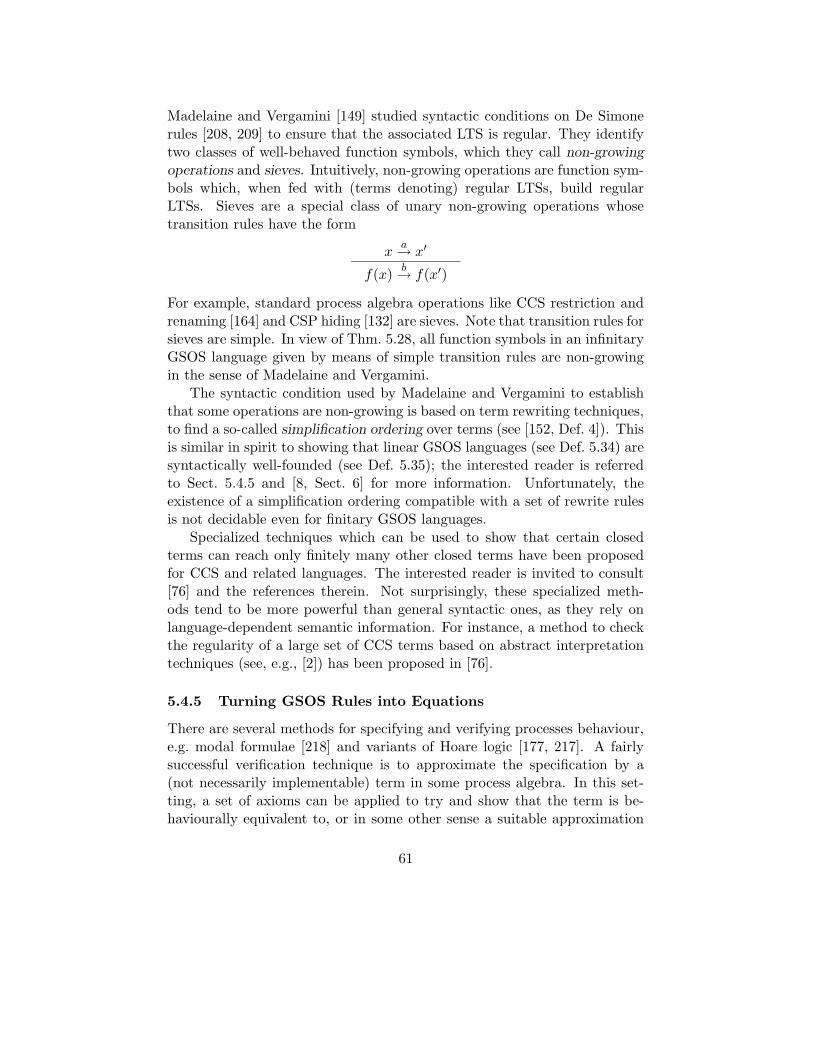
Madelaine and Vergamini [149] studied syntactic conditions on De Simonerules [208, 209] to ensure that the associated LTS is regular. They identifytwo classes of well-behaved function symbols, which they call non-growingoperations and sieves. Intuitively, non-growing operations are function sym-bols which, when fed with (terms denoting) regular LTSs, build regularLTSs. Sieves are a special class of unary non-growing operations whosetransition rules have the form
xa→ x′
f(x)b→ f(x′)
For example, standard process algebra operations like CCS restriction andrenaming [164] and CSP hiding [132] are sieves. Note that transition rules forsieves are simple. In view of Thm. 5.28, all function symbols in an infinitaryGSOS language given by means of simple transition rules are non-growingin the sense of Madelaine and Vergamini.
The syntactic condition used by Madelaine and Vergamini to establishthat some operations are non-growing is based on term rewriting techniques,to find a so-called simplification ordering over terms (see [152, Def. 4]). Thisis similar in spirit to showing that linear GSOS languages (see Def. 5.34) aresyntactically well-founded (see Def. 5.35); the interested reader is referredto Sect. 5.4.5 and [8, Sect. 6] for more information. Unfortunately, theexistence of a simplification ordering compatible with a set of rewrite rulesis not decidable even for finitary GSOS languages.
Specialized techniques which can be used to show that certain closedterms can reach only finitely many other closed terms have been proposedfor CCS and related languages. The interested reader is invited to consult[76] and the references therein. Not surprisingly, these specialized meth-ods tend to be more powerful than general syntactic ones, as they rely onlanguage-dependent semantic information. For instance, a method to checkthe regularity of a large set of CCS terms based on abstract interpretationtechniques (see, e.g., [2]) has been proposed in [76].
5.4.5 Turning GSOS Rules into Equations
There are several methods for specifying and verifying processes behaviour,e.g. modal formulae [218] and variants of Hoare logic [177, 217]. A fairlysuccessful verification technique is to approximate the specification by a(not necessarily implementable) term in some process algebra. In this set-ting, a set of axioms can be applied to try and show that the term is be-haviourally equivalent to, or in some other sense a suitable approximation
61
of, the required specification. Indeed, one of the major schools of theoreticalconcurrency and its applications, that of ACP [21, 29], takes the notion ofbehavioural equivalence as primary, and defines operational semantics to fitits axioms.
A logic of programs is complete (relative to a programming language) ifall true formulas of the language are provable in the logic. As properties ofinterest are generally non-recursive, we are often obliged to have infinitaryor other non-recursive rules in our logics to achieve completeness.
This section presents results from [7, 8], which offer an algorithmic so-lution to the problem of computing a sound and complete axiomatization(possibly including one infinitary conditional axiom) for any GSOS language,modulo bisimulation equivalence. That is, two closed terms can be equatedby the axiom system iff they are bisimilar in the associated LTS (cf. Def. 4.9).The procedure introduces fresh function symbols as needed. Completenessresults for axiomatizations have become rather standard in many cases. Thegeneralization of extant completeness results given in [8] shows that, at leastin principle, this burden can be completely removed if one gives GSOS rulesfor a process algebra. Of course, this does not mean that there is noth-ing to do on specific process algebras. For instance, sometimes it may bepossible to eliminate some of the auxiliary function symbols (we will see anexample of this later on in this section), or the infinitary conditional axiom.(The interested reader will find many results on complete axiomatizationsof behavioural equivalences over several process algebras elsewhere in thishandbook.)
We first define the GSOS language TFINTREE, which is a fragment of CCSsuitable for expressing finite LTSs (cf. Def. 2.2). Its signature ΣFINTREE
consists of:
- the constant 0, denoting the inactive process;
- binary alternative composition x+y, which chooses non-deterministical-ly between x and y;
- unary prefix multiplication a·x for a ∈ Act, which executes action aand thereafter behaves as x.
The constant 0 does not exhibit any behaviour and consequently does nothave any transition rules. The transition rules of alternative compositionand prefix multiplication have been formulated earlier in this chapter (seeTable 1 in Sect. 2.6, and Sect. 5.4.3, respectively). Most process algebrascontain the function symbols above, either directly or as derived operations.The following completeness result (cf. Def. 4.9) is well-known [127, 164].
62
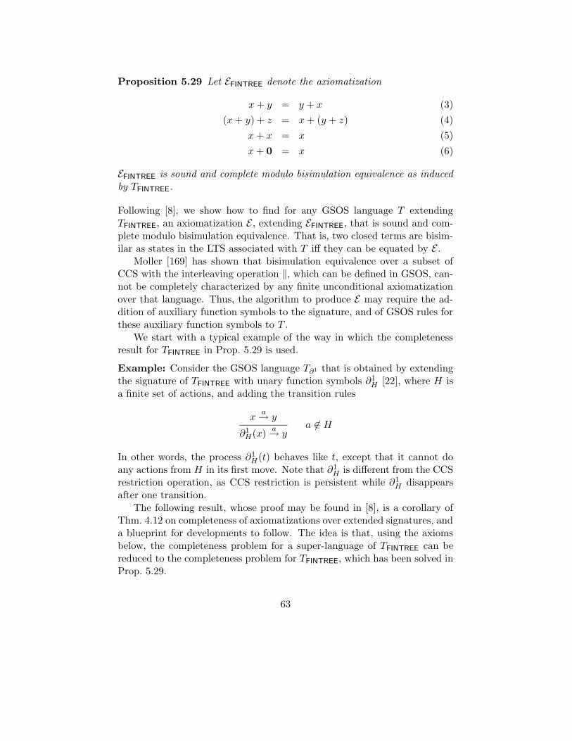
Proposition 5.29 Let EFINTREE denote the axiomatization
x+ y = y + x (3)
(x+ y) + z = x+ (y + z) (4)
x+ x = x (5)
x+ 0 = x (6)
EFINTREE is sound and complete modulo bisimulation equivalence as inducedby TFINTREE.
Following [8], we show how to find for any GSOS language T extendingTFINTREE, an axiomatization E , extending EFINTREE, that is sound and com-plete modulo bisimulation equivalence. That is, two closed terms are bisim-ilar as states in the LTS associated with T iff they can be equated by E .
Moller [169] has shown that bisimulation equivalence over a subset ofCCS with the interleaving operation ‖, which can be defined in GSOS, can-not be completely characterized by any finite unconditional axiomatizationover that language. Thus, the algorithm to produce E may require the ad-dition of auxiliary function symbols to the signature, and of GSOS rules forthese auxiliary function symbols to T .
We start with a typical example of the way in which the completenessresult for TFINTREE in Prop. 5.29 is used.
Example: Consider the GSOS language T∂1 that is obtained by extendingthe signature of TFINTREE with unary function symbols ∂1H [22], where H isa finite set of actions, and adding the transition rules
xa→ y
∂1H(x)a→ y
a 6∈ H
In other words, the process ∂1H(t) behaves like t, except that it cannot doany actions from H in its first move. Note that ∂1H is different from the CCSrestriction operation, as CCS restriction is persistent while ∂1H disappearsafter one transition.
The following result, whose proof may be found in [8], is a corollary ofThm. 4.12 on completeness of axiomatizations over extended signatures, anda blueprint for developments to follow. The idea is that, using the axiomsbelow, the completeness problem for a super-language of TFINTREE can bereduced to the completeness problem for TFINTREE, which has been solved inProp. 5.29.
63
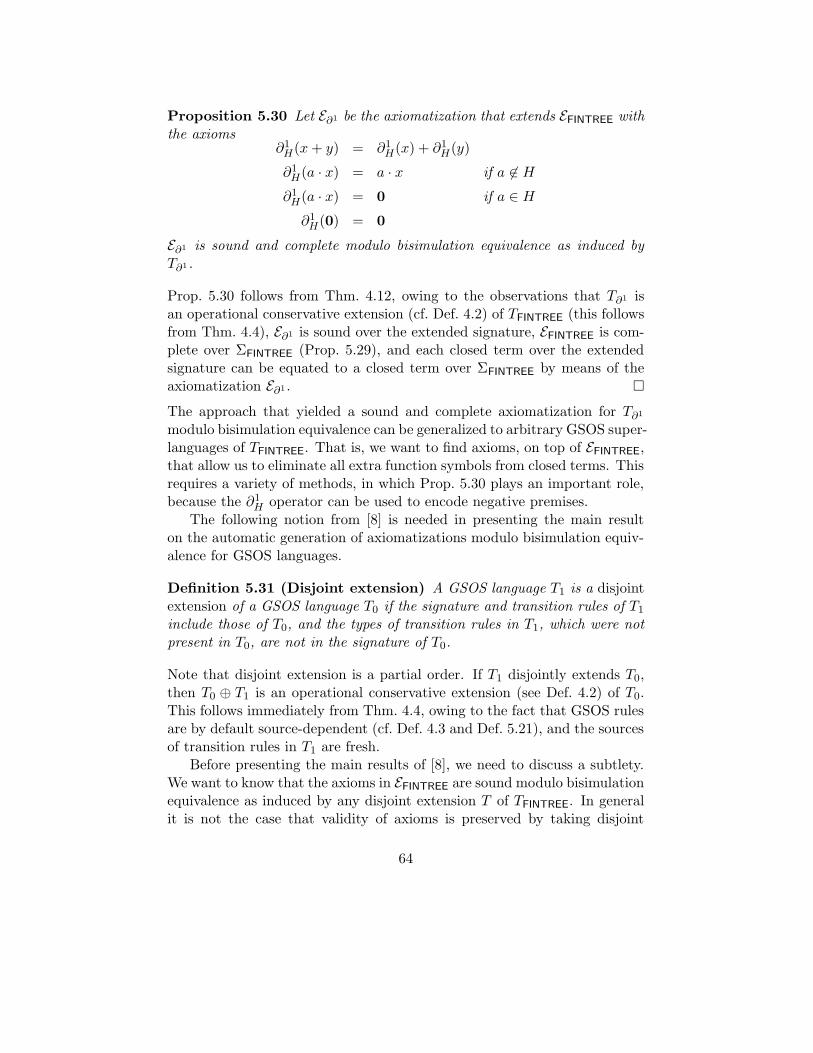
Proposition 5.30 Let E∂1 be the axiomatization that extends EFINTREE withthe axioms
∂1H(x+ y) = ∂1H(x) + ∂1H(y)
∂1H(a · x) = a · x if a 6∈ H
∂1H(a · x) = 0 if a ∈ H
∂1H(0) = 0
E∂1 is sound and complete modulo bisimulation equivalence as induced byT∂1.
Prop. 5.30 follows from Thm. 4.12, owing to the observations that T∂1 isan operational conservative extension (cf. Def. 4.2) of TFINTREE (this followsfrom Thm. 4.4), E∂1 is sound over the extended signature, EFINTREE is com-plete over ΣFINTREE (Prop. 5.29), and each closed term over the extendedsignature can be equated to a closed term over ΣFINTREE by means of theaxiomatization E∂1 . ¤
The approach that yielded a sound and complete axiomatization for T∂1
modulo bisimulation equivalence can be generalized to arbitrary GSOS super-languages of TFINTREE. That is, we want to find axioms, on top of EFINTREE,that allow us to eliminate all extra function symbols from closed terms. Thisrequires a variety of methods, in which Prop. 5.30 plays an important role,because the ∂1H operator can be used to encode negative premises.
The following notion from [8] is needed in presenting the main resulton the automatic generation of axiomatizations modulo bisimulation equiv-alence for GSOS languages.
Definition 5.31 (Disjoint extension) A GSOS language T1 is a disjointextension of a GSOS language T0 if the signature and transition rules of T1include those of T0, and the types of transition rules in T1, which were notpresent in T0, are not in the signature of T0.
Note that disjoint extension is a partial order. If T1 disjointly extends T0,then T0 ⊕ T1 is an operational conservative extension (see Def. 4.2) of T0.This follows immediately from Thm. 4.4, owing to the fact that GSOS rulesare by default source-dependent (cf. Def. 4.3 and Def. 5.21), and the sourcesof transition rules in T1 are fresh.
Before presenting the main results of [8], we need to discuss a subtlety.We want to know that the axioms in EFINTREE are sound modulo bisimulationequivalence as induced by any disjoint extension T of TFINTREE. In generalit is not the case that validity of axioms is preserved by taking disjoint
64
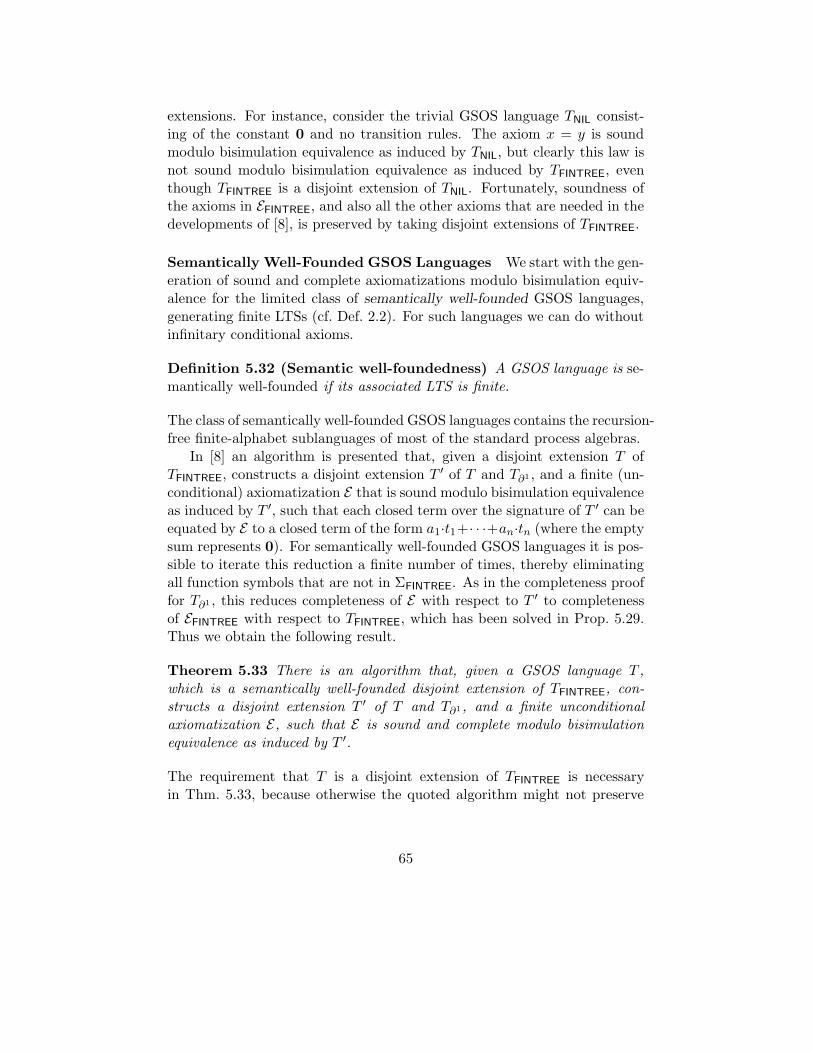
extensions. For instance, consider the trivial GSOS language TNIL consist-ing of the constant 0 and no transition rules. The axiom x = y is soundmodulo bisimulation equivalence as induced by TNIL, but clearly this law isnot sound modulo bisimulation equivalence as induced by TFINTREE, eventhough TFINTREE is a disjoint extension of TNIL. Fortunately, soundness ofthe axioms in EFINTREE, and also all the other axioms that are needed in thedevelopments of [8], is preserved by taking disjoint extensions of TFINTREE.
Semantically Well-Founded GSOS Languages We start with the gen-eration of sound and complete axiomatizations modulo bisimulation equiv-alence for the limited class of semantically well-founded GSOS languages,generating finite LTSs (cf. Def. 2.2). For such languages we can do withoutinfinitary conditional axioms.
Definition 5.32 (Semantic well-foundedness) A GSOS language is se-mantically well-founded if its associated LTS is finite.
The class of semantically well-founded GSOS languages contains the recursion-free finite-alphabet sublanguages of most of the standard process algebras.
In [8] an algorithm is presented that, given a disjoint extension T ofTFINTREE, constructs a disjoint extension T ′ of T and T∂1 , and a finite (un-conditional) axiomatization E that is sound modulo bisimulation equivalenceas induced by T ′, such that each closed term over the signature of T ′ can beequated by E to a closed term of the form a1·t1+· · ·+an·tn (where the emptysum represents 0). For semantically well-founded GSOS languages it is pos-sible to iterate this reduction a finite number of times, thereby eliminatingall function symbols that are not in ΣFINTREE. As in the completeness prooffor T∂1 , this reduces completeness of E with respect to T ′ to completenessof EFINTREE with respect to TFINTREE, which has been solved in Prop. 5.29.Thus we obtain the following result.
Theorem 5.33 There is an algorithm that, given a GSOS language T ,which is a semantically well-founded disjoint extension of TFINTREE, con-structs a disjoint extension T ′ of T and T∂1, and a finite unconditionalaxiomatization E, such that E is sound and complete modulo bisimulationequivalence as induced by T ′.
The requirement that T is a disjoint extension of TFINTREE is necessaryin Thm. 5.33, because otherwise the quoted algorithm might not preserve
65
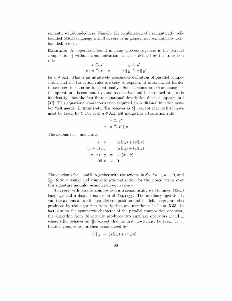
semantic well-foundedness. Namely, the combination of a semantically well-founded GSOS language with TFINTREE is in general not semantically well-founded; see [8].
Example: An operation found in many process algebras is the parallelcomposition ‖ without communication, which is defined by the transitionrules
xa→ x′
x ‖ y a→ x′ ‖ yy
a→ y′
x ‖ y a→ x ‖ y′
for a ∈ Act. This is an intuitively reasonable definition of parallel compo-sition, and the transition rules are easy to explain. It is somewhat harderto see how to describe it equationally. Some axioms are clear enough—the operation ‖ is commutative and associative, and the stopped process isits identity—but the first finite equational description did not appear until[37]. This equational characterization required an additional function sym-bol “left merge” . Intuitively, t u behaves as t‖u except that its first movemust be taken by t. For each a ∈ Act, left merge has a transition rule
xa→ x′
x ya→ x′ ‖ y
The axioms for ‖ and are:
x ‖ y = (x y) + (y x)
(x+ y) z = (x z) + (y z)
(a · x) y = a · (x ‖ y)0 x = 0
These axioms for ‖ and , together with the axioms in E∂1 for +, a · , 0, and∂1H , form a sound and complete axiomatization for the closed terms overthis signature modulo bisimulation equivalence.
TFINTREE with parallel composition is a semantically well-founded GSOSlanguage and a disjoint extension of TFINTREE. The auxiliary operator ,and the axioms above for parallel composition and the left merge, are alsoproduced by the algorithm from [8] that was mentioned in Thm. 5.33. Infact, due to the symmetric character of the parallel composition operator,the algorithm from [8] actually produces two auxiliary operators and ,where t u behaves as t‖u except that its first move must be taken by u.Parallel composition is then axiomatized by
x ‖ y = (x y) + (x y) .
66
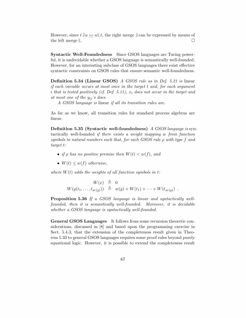
However, since t u ↔ u t, the right merge can be expressed by means ofthe left merge . ¤
Syntactic Well-Foundedness Since GSOS languages are Turing power-ful, it is undecidable whether a GSOS language is semantically well-founded.However, for an interesting subclass of GSOS languages there exist effectivesyntactic constraints on GSOS rules that ensure semantic well-foundedness.
Definition 5.34 (Linear GSOS) A GSOS rule as in Def. 5.21 is linearif each variable occurs at most once in the target t and, for each argumenti that is tested positively (cf. Def. 5.11), xi does not occur in the target andat most one of the yij’s does.
A GSOS language is linear if all its transition rules are.
As far as we know, all transition rules for standard process algebras arelinear.
Definition 5.35 (Syntactic well-foundedness) A GSOS language is syn-tactically well-founded if there exists a weight mapping w from functionsymbols to natural numbers such that, for each GSOS rule ρ with type f andtarget t:
• if ρ has no positive premise then W (t) < w(f), and
• W (t) ≤ w(f) otherwise,
where W (t) adds the weights of all function symbols in t:
W (x)∆= 0
W (g(t1, . . . , tar(g)))∆= w(g) +W (t1) + · · ·+W (tar(g)) .
Proposition 5.36 If a GSOS language is linear and syntactically well-founded, then it is semantically well-founded. Moreover, it is decidablewhether a GSOS language is syntactically well-founded.
General GSOS Languages It follows from some recursion theoretic con-siderations, discussed in [8] and based upon the programming exercise inSect. 5.4.3, that the extension of the completeness result given in Theo-rem 5.33 to general GSOS languages requires some proof rules beyond purelyequational logic. However, it is possible to extend the completeness result
67
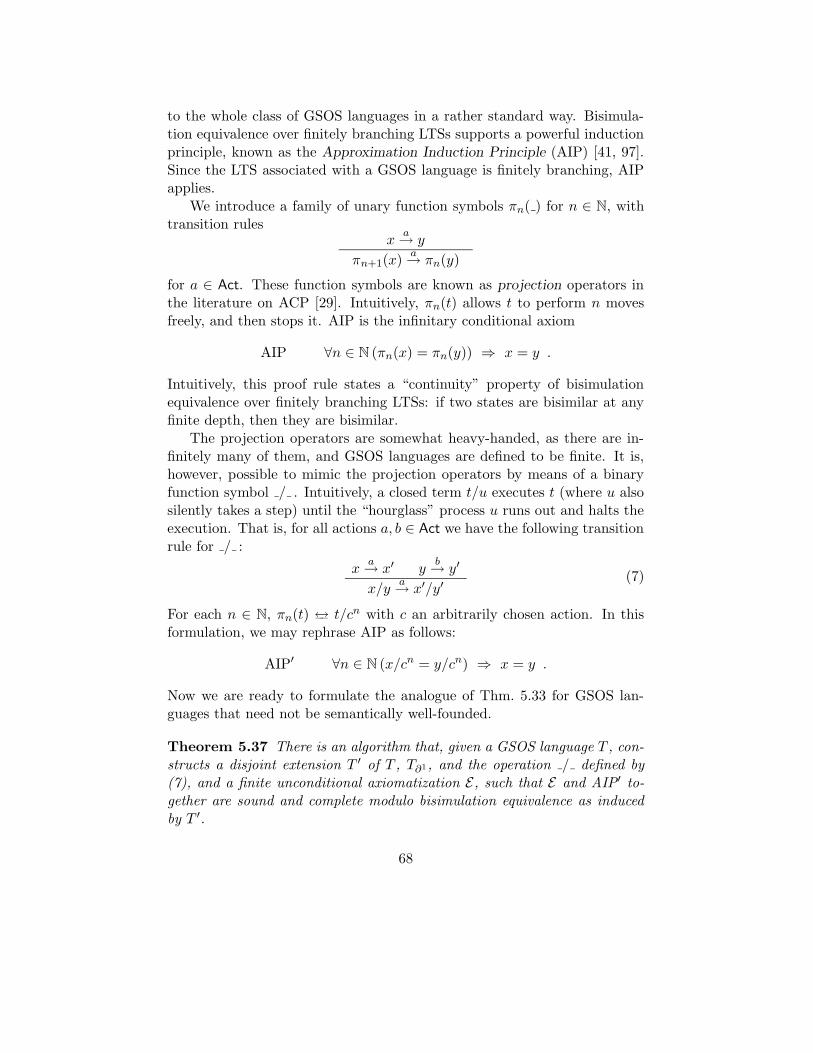
to the whole class of GSOS languages in a rather standard way. Bisimula-tion equivalence over finitely branching LTSs supports a powerful inductionprinciple, known as the Approximation Induction Principle (AIP) [41, 97].Since the LTS associated with a GSOS language is finitely branching, AIPapplies.
We introduce a family of unary function symbols πn( ) for n ∈ N, withtransition rules
xa→ y
πn+1(x)a→ πn(y)
for a ∈ Act. These function symbols are known as projection operators inthe literature on ACP [29]. Intuitively, πn(t) allows t to perform n movesfreely, and then stops it. AIP is the infinitary conditional axiom
AIP ∀n ∈ N (πn(x) = πn(y)) ⇒ x = y .
Intuitively, this proof rule states a “continuity” property of bisimulationequivalence over finitely branching LTSs: if two states are bisimilar at anyfinite depth, then they are bisimilar.
The projection operators are somewhat heavy-handed, as there are in-finitely many of them, and GSOS languages are defined to be finite. It is,however, possible to mimic the projection operators by means of a binaryfunction symbol / . Intuitively, a closed term t/u executes t (where u alsosilently takes a step) until the “hourglass” process u runs out and halts theexecution. That is, for all actions a, b ∈ Act we have the following transitionrule for / :
xa→ x′ y
b→ y′
x/ya→ x′/y′
(7)
For each n ∈ N, πn(t) ↔–– t/cn with c an arbitrarily chosen action. In thisformulation, we may rephrase AIP as follows:
AIP′ ∀n ∈ N (x/cn = y/cn) ⇒ x = y .
Now we are ready to formulate the analogue of Thm. 5.33 for GSOS lan-guages that need not be semantically well-founded.
Theorem 5.37 There is an algorithm that, given a GSOS language T , con-structs a disjoint extension T ′ of T , T∂1, and the operation / defined by(7), and a finite unconditional axiomatization E, such that E and AIP′ to-gether are sound and complete modulo bisimulation equivalence as inducedby T ′.
68
Term rewriting properties of the axiomatizations generated by (variationson) the methods we have just surveyed have been studied by Bosscher [62].Ulidowski [226] proposed a modification of the approach in [8] that producescomplete axiomatizations for a subclass of the De Simone languages, modulothe refusal simulation preorder from [225] that takes into account the silentstep τ (cf. Sect. 5.5).
Regular GSOS Languages In [4] it was shown that for a subclass ofinfinitary recursive GSOS languages generating regular LTSs it is possible toobtain sound and complete axiomatizations modulo bisimulation equivalencethat do not rely on infinitary proof rules like AIP. The following definitionintroduces the class of regular GSOS languages that is considered in op. cit.,which is a subclass of the simple infinitary GSOS languages (cf. Def. 5.27).
Definition 5.38 (Regular GSOS) An infinitary GSOS language is regu-lar if it is simple and for each function symbol f in its signature:
1. f is uniformly bounded (cf. Def. 5.25);
2. f depends on only finitely many function symbols (cf. Def. 5.16);
3. there is a finite upper bound on the number of positive premises intransition rules with type f .
Most of the TSSs for standard process algebras in the literature are regular.It follows immediately from the theory outlined in Sect. 5.4.4 that everyregular GSOS language induces a regular LTS. In [4] it was shown how toreduce the completeness problem for regular GSOS languages to that forregular LTSs, which was solved earlier in [42, 163].
We recall from Sect. 5.3.1 on De Simone languages that the recursiveterms over a signature Σ are given by the BNF grammar
t ::= X | f(t1, . . . , tar(f)) | fix(X = t)
where X ranges over a countably infinite set of recursion variables, f rangesover the signature Σ, and fix is a binding construct. The latter constructgives rise to the usual notions of free and bound recursion variables in re-cursive terms. For every recursive term fix(X = t) there is a transitionrule
t[fix(X = t)/X]a→ y
fix(X = t)a→ y
69
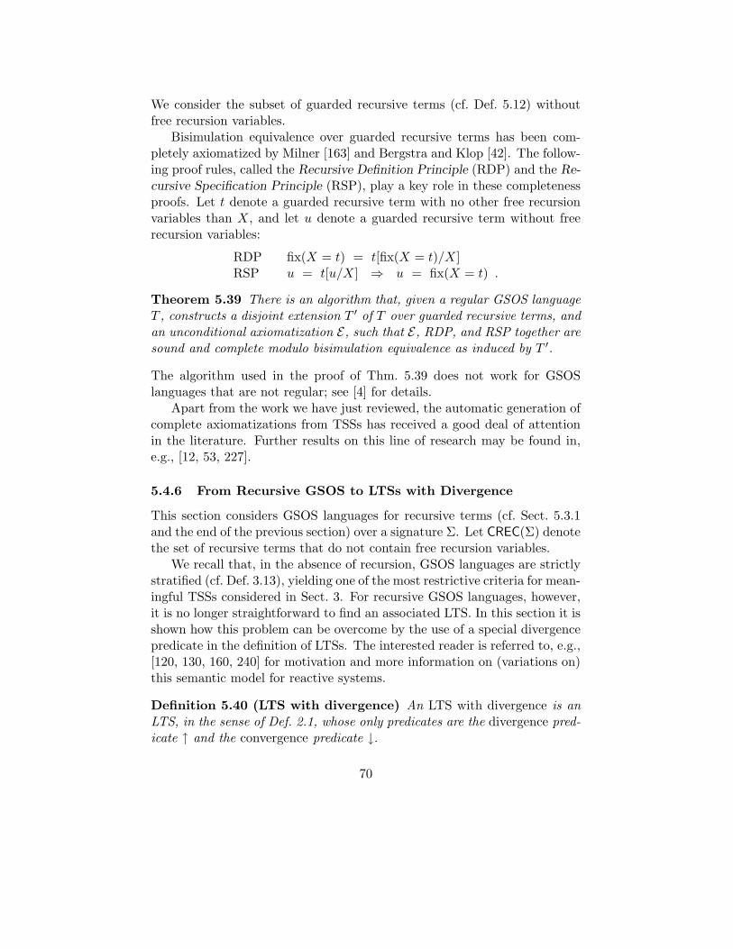
We consider the subset of guarded recursive terms (cf. Def. 5.12) withoutfree recursion variables.
Bisimulation equivalence over guarded recursive terms has been com-pletely axiomatized by Milner [163] and Bergstra and Klop [42]. The follow-ing proof rules, called the Recursive Definition Principle (RDP) and the Re-cursive Specification Principle (RSP), play a key role in these completenessproofs. Let t denote a guarded recursive term with no other free recursionvariables than X, and let u denote a guarded recursive term without freerecursion variables:
RDP fix(X = t) = t[fix(X = t)/X]RSP u = t[u/X] ⇒ u = fix(X = t) .
Theorem 5.39 There is an algorithm that, given a regular GSOS languageT , constructs a disjoint extension T ′ of T over guarded recursive terms, andan unconditional axiomatization E, such that E, RDP, and RSP together aresound and complete modulo bisimulation equivalence as induced by T ′.
The algorithm used in the proof of Thm. 5.39 does not work for GSOSlanguages that are not regular; see [4] for details.
Apart from the work we have just reviewed, the automatic generation ofcomplete axiomatizations from TSSs has received a good deal of attentionin the literature. Further results on this line of research may be found in,e.g., [12, 53, 227].
5.4.6 From Recursive GSOS to LTSs with Divergence
This section considers GSOS languages for recursive terms (cf. Sect. 5.3.1and the end of the previous section) over a signature Σ. Let CREC(Σ) denotethe set of recursive terms that do not contain free recursion variables.
We recall that, in the absence of recursion, GSOS languages are strictlystratified (cf. Def. 3.13), yielding one of the most restrictive criteria for mean-ingful TSSs considered in Sect. 3. For recursive GSOS languages, however,it is no longer straightforward to find an associated LTS. In this section it isshown how this problem can be overcome by the use of a special divergencepredicate in the definition of LTSs. The interested reader is referred to, e.g.,[120, 130, 160, 240] for motivation and more information on (variations on)this semantic model for reactive systems.
Definition 5.40 (LTS with divergence) An LTS with divergence is anLTS, in the sense of Def. 2.1, whose only predicates are the divergence pred-icate ↑ and the convergence predicate ↓.
70
In [11, 12] it is shown how a recursive GSOS language specifies an LTSwith divergence over CREC(Σ). The recursive GSOS languages consideredin op. cit. contain a special constant Ω that is akin to the constant 0 fromCCS; i.e., there are no transition rules of type Ω. (The difference between0 and Ω is that whereas the former denotes the convergent process with-out transitions, the latter stands for the divergent stopped process.) Thetransition rules in a recursive GSOS language are used to define a diver-gence (or under-specification) predicate on CREC(Σ). In fact, as is commonpractice in the literature on process algebras, we first define the notion ofconvergence, and use it to define the divergence predicate.
Definition 5.41 (Convergence) Assume a recursive GSOS language overa signature Σ. The convergence predicate ↓ is defined to be the least predicateover the set of closed recursive terms CREC(Σ) that satisfies the followingclauses:
1. f(t1, . . . , tar(f)) ↓ if
(a) f 6= Ω, and
(b) for every argument i of f , if f tests i (cf. Def. 5.11) then ti ↓;
2. fix(X = t) ↓ if t[fix(X = t)/X] ↓.
We write t ↑ if it is not the case that t ↓.
The motivation for the above definition is the following: a term t is divergentif its initial transitions are not fully specified. This occurs either when theinitial behaviour of term t depends on under-specified arguments like Ω,or in the presence of unguarded recursive definitions (cf. Def. 5.12). Forexample, the terms fix(X = X) and fix(X = a.0 + X) are not convergent,as the initial behaviours of these terms depend on themselves. We remarkhere that, when applied to SCCS [162] and the version of CCS considered in[240], the above definition delivers exactly the convergence predicates givenby Hennessy [120] and Walker [240], respectively.
We hint at how an LTS with divergence can be associated with a re-cursive GSOS language — the interested reader is referred to [11, 12] forfull technical details. We want the LTS with divergence to be at least asupported model in the sense of Def. 3.2. Moreover, reminiscent of posi-tive TSSs, we want to associate the least such LTS with the recursive GSOSlanguage in question. As described in, e.g., [58], this is not possible in the ab-sence of divergence. However, the extra structure given by the convergence
71
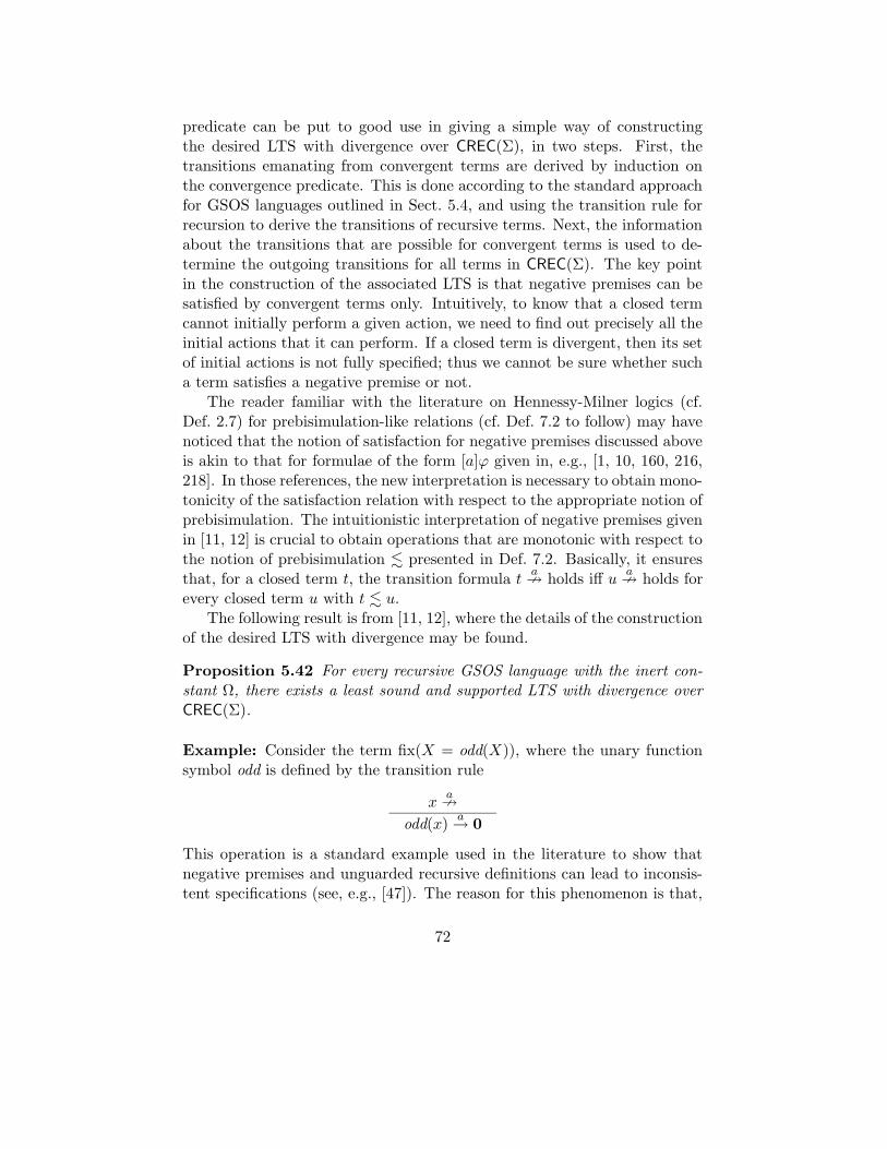
predicate can be put to good use in giving a simple way of constructingthe desired LTS with divergence over CREC(Σ), in two steps. First, thetransitions emanating from convergent terms are derived by induction onthe convergence predicate. This is done according to the standard approachfor GSOS languages outlined in Sect. 5.4, and using the transition rule forrecursion to derive the transitions of recursive terms. Next, the informationabout the transitions that are possible for convergent terms is used to de-termine the outgoing transitions for all terms in CREC(Σ). The key pointin the construction of the associated LTS is that negative premises can besatisfied by convergent terms only. Intuitively, to know that a closed termcannot initially perform a given action, we need to find out precisely all theinitial actions that it can perform. If a closed term is divergent, then its setof initial actions is not fully specified; thus we cannot be sure whether sucha term satisfies a negative premise or not.
The reader familiar with the literature on Hennessy-Milner logics (cf.Def. 2.7) for prebisimulation-like relations (cf. Def. 7.2 to follow) may havenoticed that the notion of satisfaction for negative premises discussed aboveis akin to that for formulae of the form [a]ϕ given in, e.g., [1, 10, 160, 216,218]. In those references, the new interpretation is necessary to obtain mono-tonicity of the satisfaction relation with respect to the appropriate notion ofprebisimulation. The intuitionistic interpretation of negative premises givenin [11, 12] is crucial to obtain operations that are monotonic with respect tothe notion of prebisimulation . presented in Def. 7.2. Basically, it ensuresthat, for a closed term t, the transition formula t
a9 holds iff u
a9 holds for
every closed term u with t . u.The following result is from [11, 12], where the details of the construction
of the desired LTS with divergence may be found.
Proposition 5.42 For every recursive GSOS language with the inert con-stant Ω, there exists a least sound and supported LTS with divergence overCREC(Σ).
Example: Consider the term fix(X = odd(X)), where the unary functionsymbol odd is defined by the transition rule
xa9
odd(x)a→ 0
This operation is a standard example used in the literature to show thatnegative premises and unguarded recursive definitions can lead to inconsis-tent specifications (see, e.g., [47]). The reason for this phenomenon is that,
72
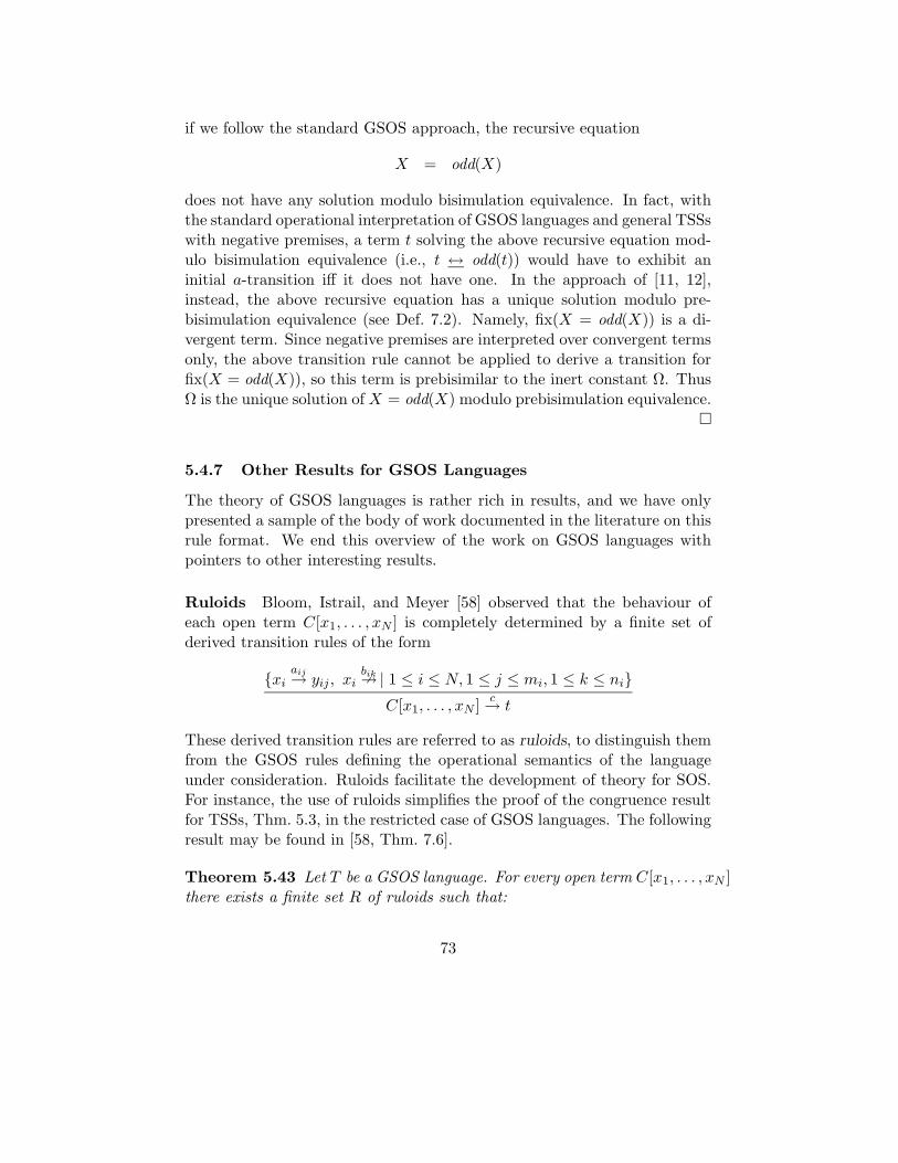
if we follow the standard GSOS approach, the recursive equation
X = odd(X)
does not have any solution modulo bisimulation equivalence. In fact, withthe standard operational interpretation of GSOS languages and general TSSswith negative premises, a term t solving the above recursive equation mod-ulo bisimulation equivalence (i.e., t ↔ odd(t)) would have to exhibit aninitial a-transition iff it does not have one. In the approach of [11, 12],instead, the above recursive equation has a unique solution modulo pre-bisimulation equivalence (see Def. 7.2). Namely, fix(X = odd(X)) is a di-vergent term. Since negative premises are interpreted over convergent termsonly, the above transition rule cannot be applied to derive a transition forfix(X = odd(X)), so this term is prebisimilar to the inert constant Ω. ThusΩ is the unique solution of X = odd(X) modulo prebisimulation equivalence.
¤
5.4.7 Other Results for GSOS Languages
The theory of GSOS languages is rather rich in results, and we have onlypresented a sample of the body of work documented in the literature on thisrule format. We end this overview of the work on GSOS languages withpointers to other interesting results.
Ruloids Bloom, Istrail, and Meyer [58] observed that the behaviour ofeach open term C[x1, . . . , xN ] is completely determined by a finite set ofderived transition rules of the form
xiaij→ yij , xi
bik9 | 1 ≤ i ≤ N, 1 ≤ j ≤ mi, 1 ≤ k ≤ ni
C[x1, . . . , xN ]c→ t
These derived transition rules are referred to as ruloids, to distinguish themfrom the GSOS rules defining the operational semantics of the languageunder consideration. Ruloids facilitate the development of theory for SOS.For instance, the use of ruloids simplifies the proof of the congruence resultfor TSSs, Thm. 5.3, in the restricted case of GSOS languages. The followingresult may be found in [58, Thm. 7.6].
Theorem 5.43 Let T be a GSOS language. For every open term C[x1, . . . , xN ]there exists a finite set R of ruloids such that:
73
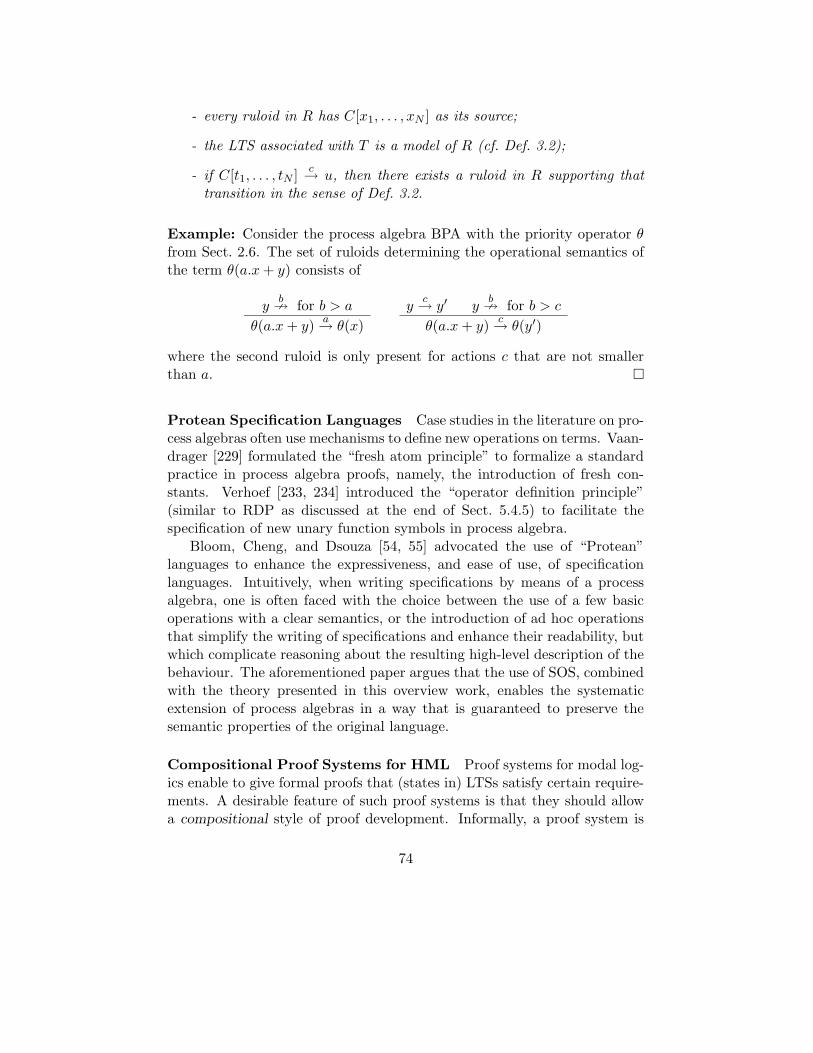
- every ruloid in R has C[x1, . . . , xN ] as its source;
- the LTS associated with T is a model of R (cf. Def. 3.2);
- if C[t1, . . . , tN ]c→ u, then there exists a ruloid in R supporting that
transition in the sense of Def. 3.2.
Example: Consider the process algebra BPA with the priority operator θfrom Sect. 2.6. The set of ruloids determining the operational semantics ofthe term θ(a.x+ y) consists of
yb
9 for b > a
θ(a.x+ y)a→ θ(x)
yc→ y′ y
b9 for b > c
θ(a.x+ y)c→ θ(y′)
where the second ruloid is only present for actions c that are not smallerthan a. ¤
Protean Specification Languages Case studies in the literature on pro-cess algebras often use mechanisms to define new operations on terms. Vaan-drager [229] formulated the “fresh atom principle” to formalize a standardpractice in process algebra proofs, namely, the introduction of fresh con-stants. Verhoef [233, 234] introduced the “operator definition principle”(similar to RDP as discussed at the end of Sect. 5.4.5) to facilitate thespecification of new unary function symbols in process algebra.
Bloom, Cheng, and Dsouza [54, 55] advocated the use of “Protean”languages to enhance the expressiveness, and ease of use, of specificationlanguages. Intuitively, when writing specifications by means of a processalgebra, one is often faced with the choice between the use of a few basicoperations with a clear semantics, or the introduction of ad hoc operationsthat simplify the writing of specifications and enhance their readability, butwhich complicate reasoning about the resulting high-level description of thebehaviour. The aforementioned paper argues that the use of SOS, combinedwith the theory presented in this overview work, enables the systematicextension of process algebras in a way that is guaranteed to preserve thesemantic properties of the original language.
Compositional Proof Systems for HML Proof systems for modal log-ics enable to give formal proofs that (states in) LTSs satisfy certain require-ments. A desirable feature of such proof systems is that they should allowa compositional style of proof development. Informally, a proof system is
74
compositional if it builds a proof for a property of an LTS out of proofs forproperties of certain sub-LTSs.
The work presented in [212] is based upon the realization that, in thecontext of pure first-order logic, the issue of compositionality was addressedby Gentzen [96] in his work on the sequent calculus. There, compositionalityis obtained via cut-elimination. In [212], Simpson developed a sequent cal-culus for showing that closed terms in a process algebra with its operationalsemantics specified in the GSOS format satisfy assertions of the modal logicHML (see Sect. 2.3). Such process algebras provide interesting examples,because of the well-known difficulties in giving proof rules for flavours ofparallel composition [216, 243]. As usual, the benefit of working with anarbitrary GSOS language is that one obtains a generic proof system that isapplicable to a wide class of process algebras.
Binary Decision Diagrams from GSOS Languages Binary decisiondiagrams [66] are widely used to represent LTSs symbolically in the secondgeneration of verification tools for concurrent processes — see, e.g., McMil-lan’s textbook on the model checker SMV [154]. A binary decision diagramfor such an application is often generated from an LTS over the closed termsin some process calculus, which in turn is generated using the transition rulesdefining the operational semantics of this calculus. Such a two-step approachcan be avoided by using a direct construction of the binary decision diagramfrom the transition rules. This is the approach followed in [79] for GSOSlanguages. The results in op. cit. suggest that this general procedure yieldsbinary decision diagrams that are of comparable quality to those generatedfor specific process calculi by ad hoc methods (cf., e.g., [82]).
5.5 RBB Safe Format
In order to abstract away from internal actions, Milner [159] introduceda special action τ , called the silent step. The relation symbol
τ→ intu-itively represents an internal computation. A number of equivalence notionshave been developed to identify states in LTSs that incorporate silent steps,such as weak bisimulation [128] and branching bisimulation [107, 108]. In[53, 225, 228], rule formats have been introduced to ensure that weak andbranching bisimulation equivalence are a congruence (cf. Def. 2.11). How-ever, in general such equivalences are not a congruence with respect to mostprocess algebras, because of the pre-emptive power of silent steps (see, e.g.,[164, Sect. 2.3] for an intuitive discussion of this phenomenon). For this
75
reason it has become standard practice to impose a rootedness condition onequivalences for the silent step [164].
Bloom [53] presented a rule format to ensure that rooted branchingbisimulation is a congruence, imposing additional requirements on the GSOSformat. The rule format recognizes so-called patience rules, via which aclosed term can inherit the τ -transitions of its arguments. The RBB safeformat [87] relaxes some syntactic restrictions of Bloom’s rule format, im-posing additional requirements on the panth format. Notably, certain argu-ments of function symbols are labelled ‘liquid’, and this labelling is used torestrict occurrences of variables in targets and in left-hand sides of premises.If a TSS is complete (cf. Def. 3.12) and satisfies the syntactic restrictionsof the RBB safe format, then rooted branching bisimulation with respect tothe associated LTS is a congruence.
Rooted Branching Bisimulation We assume that Act is extended witha special action τ , representing the silent step. The reflexive and transitiveclosure of the relation
τ→ is denoted byε→. First, we define the notion of
branching bisimulation [107, 108].
Definition 5.44 (Branching bisimulation) Assume an LTS. A binaryrelation B on states is a branching bisimulation if it is symmetric and,whenever s1 B s2:
- if s1a→ s′1, then either
1. a = τ and s′1 B s2, or
2. there are transitions s2ε→ s′2
a→ s′′2 such that s1 B s′2 and s′1 B s′′2;
- if s1P , then there are transitions s2ε→ s′2P such that s1 B s′2.
Two states s1, s2 are branching bisimilar, written s1 ↔ b s2, if there existsa branching bisimulation relation that relates them.
Branching bisimulation is an equivalence relation; see [35]. However, branch-ing bisimulation equivalence is not a congruence with respect to some stan-dard operations in process algebras. For example, in BPAετ (see Sect. 2.6)with constants a and c, a ↔ b a and c ↔ b τc, but a+ c and a+ τc are notbranching bisimilar. Therefore, we introduce a rootedness condition.
Definition 5.45 (Rooted branching bisimulation) Assume an LTS. Abinary relation R on states is a rooted branching bisimulation if it is sym-metric and, whenever s1 R s2,
76
- if s1a→ s′1, then there is a transition s2
a→ s′2 such that s′1 ↔ b s′2;
- if s1P , then s2P .
Two states s1, s2 are rooted branching bisimilar, written s1 ↔ rb s2, if thereexists a rooted branching bisimulation relation that relates them.
Since branching bisimulation is an equivalence relation, it is easy to see thatrooted branching bisimulation is also an equivalence relation.
RBB Safe We proceed to present a congruence format for rooted branch-ing bisimulation equivalence from [87]. Let C[] denote a context, viz. a termwith one occurrence of the context symbol [] (cf. Sect. 2.4). We assume thatevery argument of each function symbol is labelled either frozen or liquid. Acontext is liquid if the context symbol occurs inside a nested string of liquidarguments.
Definition 5.46 (Liquid context) The set of liquid contexts over a sig-nature Σ is defined inductively by:
1. [] is liquid;
2. if C[] is liquid, and argument i of function symbol f ∈ Σ is liquid, thenf(t1, . . . , ti−1, C[], ti+1, . . . , tar(f)) is liquid.
A patience rule for an argument i of a function symbol f implies that aclosed term f(t1, . . . , tar(f)) inherits the τ -transitions of its argument ti.
Definition 5.47 (Patience rule) A patience rule for the ith argument ofa function symbol f is a GSOS rule of the form
xiτ→ y
f(x1, . . . , xar(f))τ→ f(x1, . . . , xi−1, y, xi+1, . . . , xar(f))
Now we are in a position to present the RBB safe format, which imposesadditional restrictions on the panth format (cf. Def. 5.1).
Definition 5.48 (RBB safe) A TSS T in panth format is RBB safe ifthere exists a frozen/liquid labelling of arguments of function symbols suchthat each of its transition rules ρ is
1. either a patience rule for a liquid argument of a function symbol,
77
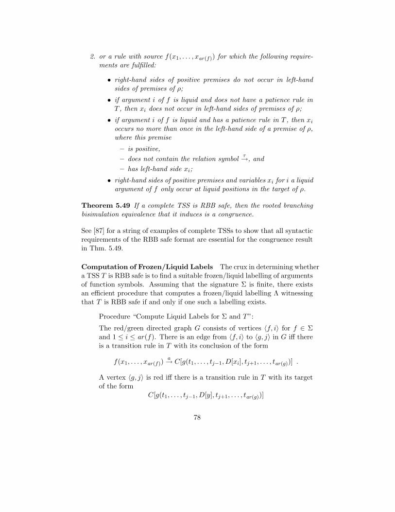
2. or a rule with source f(x1, . . . , xar(f)) for which the following require-ments are fulfilled:
• right-hand sides of positive premises do not occur in left-handsides of premises of ρ;
• if argument i of f is liquid and does not have a patience rule inT , then xi does not occur in left-hand sides of premises of ρ;
• if argument i of f is liquid and has a patience rule in T , then xi
occurs no more than once in the left-hand side of a premise of ρ,where this premise
– is positive,
– does not contain the relation symbolτ→, and
– has left-hand side xi;
• right-hand sides of positive premises and variables xi for i a liquidargument of f only occur at liquid positions in the target of ρ.
Theorem 5.49 If a complete TSS is RBB safe, then the rooted branchingbisimulation equivalence that it induces is a congruence.
See [87] for a string of examples of complete TSSs to show that all syntacticrequirements of the RBB safe format are essential for the congruence resultin Thm. 5.49.
Computation of Frozen/Liquid Labels The crux in determining whethera TSS T is RBB safe is to find a suitable frozen/liquid labelling of argumentsof function symbols. Assuming that the signature Σ is finite, there existsan efficient procedure that computes a frozen/liquid labelling Λ witnessingthat T is RBB safe if and only if one such a labelling exists.
Procedure “Compute Liquid Labels for Σ and T”:
The red/green directed graph G consists of vertices 〈f, i〉 for f ∈ Σand 1 ≤ i ≤ ar(f). There is an edge from 〈f, i〉 to 〈g, j〉 in G iff thereis a transition rule in T with its conclusion of the form
f(x1, . . . , xar(f))a→ C[g(t1, . . . , tj−1, D[xi], tj+1, . . . , tar(g))] .
A vertex 〈g, j〉 is red iff there is a transition rule in T with its targetof the form
C[g(t1, . . . , tj−1, D[y], tj+1, . . . , tar(g))]
78
where y is the right-hand side of a positive premise of this rule. Allother vertices in G are coloured green.
The procedure turns green vertices in G red as follows. If a vertex〈f, i〉 is red, and there exists an edge in G from 〈f, i〉 to a green vertex〈g, j〉, then 〈g, j〉 is coloured red.
The procedure terminates if none of the green vertices can be colouredred anymore, at which point it outputs the red/green directed graph.
Λ labels argument i of function symbol f ‘liquid’ iff the vertex 〈f, i〉 in theoutput graph of the procedure above is red.
We proceed to apply Thm. 5.49 to two of the TSSs from Sect. 2.6, extendedwith the silent step.
BPA with Empty Process and Silent Step The process algebra BPAετ
is obtained from BPAε by extending Act with the silent step τ . The TSS forBPAετ is the TSS for BPAε in Table 1, with the proviso that a ranges overAct ∪ τ.
It was noted in Sect. 5.1 that the TSS in Table 1 is panth. The procedureto calculate a frozen/liquid labelling for TSS produces the following result:the first argument of sequential composition is liquid (because of the targetx′ · y in the third transition rule for sequential composition), while botharguments of alternative composition and the second argument of sequentialcomposition are frozen. The TSS in Table 1, with a ranging over Act∪ τ,is RBB safe with respect to this frozen/liquid labelling. As an example, forsequential composition we have that:
- its third transition rule with a = τ constitutes a patience rule for thefirst argument of sequential composition;
- in its first two transition rules, and in its third transition rule witha 6= τ , the variable x in the liquid argument of the source occurs asthe left-hand side of one positive premise, which does not contain therelation symbol
τ→;
- in its third transition rule, the variable x′ in the right-hand side of thepremise occurs in a liquid position of the target.
It is left to the reader to verify that the remaining transition rules in Table 1are RBB safe. It was proven in Sect. 3.5 that the TSS in Table 1 is complete.Hence, according to Thm. 5.49, rooted branching bisimulation equivalenceis a congruence with respect to BPAετ .
79
Priorities with Silent Step In general, rooted branching bisimulationequivalence is not a congruence with respect to the priority operator. Forexample, suppose b < c; then a·(τ ·(b+c)+b) and a·(b+c) are rooted branch-ing bisimilar, but θ(a·(τ ·(b+c)+b)) and θ(a·(b+c)) are not rooted branchingbisimilar. Consequently, in view of Thm. 5.49, the TSS for BPAετθ in Table2 (with a and b ranging over Act ∪ τ) cannot be in the RBB safe format.
Since the second transition rule in Table 2 has target θ(x′), the procedurein Sect. 5.5 labels the argument of θ liquid. So, assuming there are one ormore actions b greater than action a with respect to the ordering on Act, theliquid argument x in the source of this transition rule occurs as the left-hand
side of the negative premises xb
9. This violates the RBB safe format.
5.6 Precongruence Formats for Behavioural Preorders
The literature on SOS is particularly rich in results on (pre)congruenceformats for behavioural equivalences and preorders, mostly in the absenceof predicates. This section presents precongruence formats for simulationand ready simulation from [101], for decorated trace preorders from [56],for accepting trace preorder from [86], and for trace preorder from [56].Vaandrager [230] moreover showed that the De Simone format constitutesa precongruence format for the external trace, external failure, and must[77, 122] preorders. We note that if a preorder is a precongruence, then itskernel is a congruence.
5.6.1 Simulation
Path (cf. Def. 5.2) is a precongruence format for simulation preorder (cf.Def. 2.3). (According to van Glabbeek [101], path is actually a congruenceformat for all n-nested simulation equivalences [115].)
Theorem 5.50 If a TSS is in path format, then the simulation preorderthat it induces is a precongruence.
For example, since the TSS for BPAε from Sect. 2.6 is in path format,Thm. 5.50 implies that simulation preorder is a precongruence with respectto BPAε.
5.6.2 Ready Simulation
A precongruence format for ready simulation preorder (cf. Def. 2.3) is ob-tained by disallowing look-ahead in panth rules.
80
Definition 5.51 (No look-ahead) A transition rule has no look-ahead ifthe variables occurring in the right-hand sides of its positive premises do notoccur in the left-hand sides of its premises.
Definition 5.52 (Ready simulation format) A panth rule is in readysimulation if it has no look-ahead. A TSS is in ready simulation format ifall its transition rules are.
Theorem 5.53 If a complete TSS is in ready simulation format, then theready simulation preorder that it induces is a precongruence.
For example, the TSS for BPAε from Sect. 2.6 is positive and so complete.Furthermore, it is in path format, and none of its transition rules containslook-ahead. Hence, Thm. 5.53 implies that ready simulation preorder is aprecongruence with respect to BPAε.
The following counter-example shows that the omission of look-aheadfrom the ready simulation format is essential.
Example: Let Act = a, b, c and let f be a unary function symbol. Extendthe TSS for BPAε with
xa→ y
f(x)a→ f(y)
xb→ y y
c→ z
f(x)√
Note that the premises of the second transition rule contain look-ahead.Clearly, a·(b+ b·c) + a·b and a·(b+ b·c) are ready simulation equivalent.
However, f(a·(b + b·c) + a·b) and f(a·(b + b·c)) are not ready simulationequivalent. Namely, the transition f(a·(b + b·c) + a·b) a→ f(b) can only besimulated by f(a·(b+ b·c)) a→ f(b + b·c), but f(b) has no initial transitionswhile f(b+ b·c)√. ¤
5.6.3 Decorated Traces
This section presents precongruence formats for ready trace, failure trace,readies and failures preorder (cf. Def. 2.5) from [56]. These formats, whichre-use the notion of a liquid context (cf. Def. 5.46), were obtained by acareful study of the modal characterizations of the preorders in question.The ready trace, readies, and failures formats generalize earlier formats byvan Glabbeek [101], Bloom [50], and De Simone [230], respectively. (In[101], van Glabbeek sketched a congruence format for failures equivalence;that format, however, is flawed [106].)
81
Definition 5.54 (Ntytt) An ntytt rule is a transition rule in which theright-hand sides of positive premises are variables that are all distinct, andthat do not occur in the source.
Definition 5.55 (Propagation and polling) An occurrence of a variablein an ntytt rule is propagated if the occurrence is either in the target, or inthe left-hand side of a positive premise of which the right-hand side occursin the target. An occurrence of a variable in an ntytt rule is polled if the oc-currence is in the left-hand side of a premise that does not have a right-handside occurring in the target.
Intuitively, the precongruence formats for the four decorated trace preordersoperate by keeping track of which variables represent running processes, andwhich do not. For example, it is semantically reasonable to copy a processbefore it starts. However, copying a running process would give informationabout the branching structure of the process, which is incompatible withany form of decorated trace semantics. A floating variable may representa running process. This notion assumes a predicate Λ on arguments offunction symbols; if Λ(f, i) then we say that argument i of f is liquid, andotherwise it is frozen (cf. Sect. 5.5).
Definition 5.56 (Floating variable) A variable in an ntytt rule is float-ing if either it occurs as the right-hand side of a positive premise, or it occursexactly once in the source, at a liquid position (cf. Def. 5.46).
Definition 5.57 (Decorated trace safe) Let Λ be a predicate on argu-ments of function symbols. An ntytt rule is Λ-ready trace safe if
• it has no look-ahead (cf. Def. 5.51), and
• each floating variable is propagated at most once, and at a liquid posi-tion.
The rule is Λ-readies safe if
• it is Λ-ready trace safe, and
• each floating variable is not both propagated and polled.
The rule is Λ-failure trace safe if
• it is Λ-readies safe, and
82
• each floating variable is polled at most once, at a liquid position in apositive premise.
The second restriction on “Λ-ready trace safe” guarantees that a runningprocess is never copied, and continued to be marked as running after ithas executed. The “Λ-readies safe” restriction ensures that only at the endof its execution a running process is tested multiple times. The “Λ-failuretrace safe” restriction further limits to a positive test on a single action orpredicate.
Definition 5.58 (Decorated trace formats) A TSS is in ready traceformat if it is in ntyft/ntyxt format and its rules are Λ-ready trace safewith respect to some Λ. A TSS is in readies format if it is in ntyft/ntyxtformat and its rules are Λ-readies safe with respect to some Λ. A TSS is infailure trace format if it is in ntyft/ntyxt format and its rules are Λ-failuretrace safe with respect to some Λ.
Theorem 5.59 If a TSS is in ready trace format, then the ready trace pre-order that it induces is a precongruence.
Theorem 5.60 If a TSS is in readies format, then the readies preorder thatit induces is a precongruence.
Theorem 5.61 If a TSS is in failure trace format, then the failure traceand failure preorders that it induces are precongruences.
5.6.4 Accepting Traces
Similar to the RBB safe format, a precongruence format for accepting tracepreorder (cf. Def. 2.5) from [86] is based on a frozen/liquid labelling ofarguments of function symbols.
Definition 5.62 (L cool) A TSS in path format is L cool if there exists afrozen/liquid labelling of arguments of function symbols such that each of itstransition rules ρ satisfies the following syntactic restrictions:
• each variable in ρ that occurs in a liquid argument of the source, oras the right-hand side of a premise, occurs exactly once either as theleft-hand side of a premise or at a liquid position (see Def. 5.46) inthe target of ρ;
• the variable dependency graph (see Def. 5.4) of the set of premises ofρ does not contain an infinite forward chain of edges.
83
Theorem 5.63 If a TSS is in L cool format, then the accepting trace pre-order that it induces is a precongruence.
The following counter-example shows that the L cool format cannot allowan infinite forward chain of edges in the variable dependency graph of thepremises of a transition rule.
Example: Let Act = a, f a unary function symbol, and b and c constants.Consider the TSS
ba→ b
xia→ xi+1 | i ∈ Nf(x0)
√
Note that the edges 〈xi, xi+1〉 for i ∈ N in the variable dependency graph ofthe premises of the second transition rule form an infinite forward chain.
The terms b and c are accepting trace equivalent, because they both haveno accepting traces. However, f(b) and f(c) are not accepting trace equiv-alent, as f(b) has the accepting empty trace ε while f(c) has no acceptingtraces. ¤
See [86] for further examples of TSSs showing that all the syntactic require-ments of the L cool format are essential for the precongruence result inThm. 5.63. Similar to the procedure for the RBB safe format in Sect. 5.5,there exists an efficient procedure to compute a frozen/liquid labelling Λwitnessing that T is L cool if and only if such a labelling exists; see [86].
Example: The TSS for BPAε from Sect. 2.6 is in path format, and for eachtransition rule the variable dependency graph of its premises does not con-tain an infinite forward chain of edges. Take the first argument of sequentialcomposition to be liquid, and the two arguments of alternative compositionand the second argument of sequential composition to be frozen. It is nothard to see, for the TSS of BPAε, that if a variable occurs in a liquid argu-ment of the source or as the right-hand side of a premise of a transition rule,then it occurs exactly once either as the left-hand side of a premise or at aliquid position in the target of this transition rule. Hence, Thm. 5.63 impliesthat accepting trace preorder is a precongruence with respect to BPAε. ¤
5.6.5 Traces
Bloom [52] formulated a congruence format for trace equivalence (cf. Def. 2.4),generalizing an earlier precongruence format for trace preorder by Vaan-drager [230].
84
Definition 5.64 (Trace format) A finite TSS in tyft format (cf. Def. 5.2)is in trace format if each transition rule satisfies the following three restric-tions:
- it contains finitely many premises;
- each variable occurs either as the right-hand side of a premise or inthe source;
- no variable occurs more than once in the left-hand sides of the premisesand in the target.
Theorem 5.65 If a TSS is in trace format, then the trace equivalence thatit induces is a congruence.
Although the definition of completed trace equivalence (cf. Def. 2.5) is closelyrelated to that for (accepting) trace equivalence, the L cool and trace formatsdo not constitute congruence formats for completed trace equivalence. Thefollowing counter-example, featuring the encapsulation operator [39, 159],shows that one cannot really hope to formulate a general congruence formatfor completed trace equivalence (see also [230]).
Example: Let Act = a, b, c, and add the unary encapsulation operator∂c to BPAε. The LTS for a term ∂c(t) is obtained from the LTS for tby excluding all c-transitions. This is expressed by three transition rules for∂c, which are added to the TSS for BPAε:
xa→ y
∂c(x)a→ ∂c(y)
xb→ y
∂c(x)b→ ∂c(y)
x√
∂c(x)√
Clearly, a·b + a·c and a·(b + c) are completed trace equivalent. However,∂c(a·b+ a·c) and ∂c(a·(b+ c)) are not completed trace equivalent: a is acompleted trace of ∂c(a·b+ a·c), but not of ∂c(a·(b+ c)). ¤
5.7 Trace Congruences
One of the original aims for the development of the theory of GSOS lan-guages was to characterize the observational congruence induced by a rea-sonable notion of CCS-like operations, under the assumption that what wecan directly observe from the behaviour of a process is its set of completedtraces (see Def. 2.5 for the definition of completed trace equivalence 'CT ).
85
Intuitively, two closed terms t and u are completed trace congruent withrespect to a TSS if, for every context C[x], the completed traces of C[t] andC[u] in the associated LTS coincide. We proceed to formulate the notion ofcompleted trace congruence induced by a rule format.
Definition 5.66 (Completed trace congruence) Let F be some rule for-mat and T0 a TSS in F format over a signature Σ0. Two closed terms tand u are completed trace congruent with respect to T0 and F , notationt 'F
CT u, if for every TSS T1 in F format over some signature Σ1 that canbe added in an operationally conservative fashion to T0 (cf. Def. 4.2), andfor every context C[] over Σ0 ⊕ Σ1, the LTS associated with T0 ⊕ T1 yieldsC[t] 'CT C[u].
Bloom, Istrail, and Meyer [57, 58] characterized the completed trace congru-ence induced by the GSOS format in terms of the equivalence correspondingto the following sublanguage of the modal logic HML (cf. Def. 2.7).
Definition 5.67 (Denial formula) The set D of denial formulae over Act
is given by the following BNF grammar, with a ∈ Act:
ϕ ::= true | ϕ1 ∧ ϕ2 | 〈a〉ϕ | ¬〈a〉true .
In particular, a state satisfies formula ¬〈a〉true iff a is not one of its initialactions. The equivalence relation ∼D is defined over states in LTSs in asimilar fashion as the equivalence relation ∼HML (see Sect. 2.3): s ∼D s′ ifffor all denial formulae ϕ we have s |= ϕ ⇐⇒ s′ |= ϕ.
Theorem 5.68 Let T be a GSOS language. The equivalence relation ∼D
induced by the LTS associated with T coincides with the completed tracecongruence 'GSOSCT with respect to T and the GSOS format.
The interested reader is referred to op. cit. and [115] for proofs of the aboveresult, and further discussion. Here we limit ourselves to remarking that,perhaps surprisingly, negative premises do not add anything to the discrim-inating power of the GSOS format. In fact, the GSOS operators used inthe aforementioned references for testing denial formulae do not make useof negative premises at all. Indeed, the use they make of copying in eitherthe premises or the conclusions of transition rules is rather minimal. Thereader might also recall that negative premises were not used in the codingof a universal 2-counter machine presented in Sect. 5.4.3.
Larsen and Skou [142] gave the following characterization of denial equiv-alence, which provides additional insight into the behavioural nature of thecompleted trace congruences induced by GSOS languages.
86
Theorem 5.69 In every finitely branching LTS (cf. Def. 2.2), two statesare ready simulation equivalent (cf. Def. 2.3) iff they satisfy exactly the samedenial formulae.
Thus the GSOS completed trace congruence is the equivalence induced bythe ready simulation preorder, which prompted the authors of [58] to coin theslogan “bisimulation can’t be traced”. The following result, due to Groote[112], shows that bisimulation equivalence can indeed be traced, providedthat the power of negative premises offered by the pure ntyft/ntyxt format(cf. Def. 5.2 and Def. 5.4) is available.
Theorem 5.70 Assume a stratifiable TSS (cf. Def. 3.13) in pure ntyft/ntyxtformat containing at least one constant in its signature. Then, for every pairof closed terms t, u,
t 'pure ntyft/ntyxtCT u ⇐⇒ t ∼HML u .
In view of Thm. 2.8 this means that the completed trace congruence inducedby the pure ntyft/ntyxt format coincides with bisimulation equivalence if theLTS associated with the TSS in question is finitely branching.
The use of negative premises appears to be necessary in order to testfor bisimulation equivalence. Indeed, Groote and Vaandrager [115] char-acterized the completed trace congruence induced by the tyft/tyxt formatthus.
Theorem 5.71 Assume a TSS in pure tyft/tyxt format whose associatedLTS is finitely branching. Then, for every pair of closed terms t, u,
t 'pure tyft/tyxtCT u ⇐⇒ t and u are 2-nested simulation equivalent .
We refer the interested reader to op. cit. (and Chapter 1.1 in this issue) forthe definition of 2-nested simulation equivalence, and for more details oncompleted trace congruences.
6 Many-Sorted Higher-Order Languages
This section presents a formal framework to describe TSSs in the style ofPlotkin, allowing one to express many-sortedness, general binding mech-anisms, and substitutions. Such variable binding mechanisms are widelyused in SOS semantics for, e.g., concurrent and functional programming
87
languages [34, 168, 185, 194, 206], the π-calculus [167], value-passing pro-cess algebras [113, 125, 126], process algebras with recursion [132, 164], andtimed process algebra [89]. See [110] for a collection of articles about re-cent developments in operational semantics for higher-order programminglanguages.
Several concepts in the setting of operational semantics with variablebinding, which seem to be intuitively clear at first sight, turn out to beambiguous when studied more carefully. In order to obtain a formal frame-work in which transition rules with a variable binding mechanism can beexpressed rigorously, we distinguish between actual and formal variables,following conventions from programming languages, and formalize the bind-ing construct t[u/x] in transition rules. In many programming languagesthere are actual parameters and formal parameters. The formal parametersare used to define procedures or functions; the actual parameters are the“real” variables to be used in the main program. In the main program theformal parameters are bound to the actual parameters. When discussingprocedures on a conceptual level, it is often useful to introduce a notationaldistinction between formal and actual parameters; see for instance [241]. Atransition rule can be thought of as a procedure to establish a transitionrelation by means of substituting (actual) terms for the (formal) variables.The following example illustrates that it is useful to make a notational dis-tinction between actual and formal variables.
Example: Consider the transition rule
y[z/x]P1yP2
where x, y, z are variables and y[z/x] is a standard notation that binds thex in y and replaces it by z. Application of a substitution σ to this transitionrule yields
σ(y)[σ(z)/x]P1σ(y)P2
¤
The example above highlights two matters.
1. The expression y[z/x] is not a substitution (for then it would equaly), but a syntactic construct with a suggestive form, called a substi-tution harness. Only after application of a substitution σ, the resultσ(y)[σ(z)/x] can be evaluated to a term.
88
2. Substitutions only apply to part of the variables that occur in a tran-sition rule. In order to distinguish such formal variables in a transitionrule, they are marked with an asterisk.
Hence, the transition rule above takes the form
y∗[z∗/x]P1y∗P2
The use of formal variables in SOS with variable binding was proposed in,e.g., [90, 133, 204].
The organization of this section is as follows. Sect. 6.1 introduces ac-tual terms, while Sect. 6.2 introduces formal terms. Sect. 6.3 describes theframework for many-sorted higher-order SOS definitions. Finally, Sect. 6.4explains how the operational conservative extension format from Thm. 4.4carries over to this higher-order setting.
Binding mechanisms exist in many and diverse forms. Here, these mech-anisms are described using a notational approach, based on [15], for theNuprl proof development system [71]. An alternative formalism would ofcourse be the λ-calculus [34].
6.1 The Actual World
We assume a set of sorts together with a countably infinite set Var of sortedactual variables. The actual world contains actual terms, actual substitu-tions, and so forth. Let ~O denote a sequence O1 · · ·Ok, and ~Oi a sequenceOi1 · · ·Oik, with k ∈ N.
Definition 6.1 (Many-sorted higher-order signature) A many-sortedhigher-order signature Σ is a set of function symbols
f : ~S1.S1 × · · · × ~Sar(f).Sar(f) → S,
where the Sij, the Si, and S are sorts.
The intuitive idea embodied by the above definition is that a function symbolf denotes an operation that takes functions of type ~Si → Si as arguments,and delivers a result of sort S.
Definition 6.2 (Actual term) Let Σ be a many-sorted higher-order sig-nature. The collection A(Σ) of actual terms over Σ is the least set satisfying:
• each actual variable from Var is in A(Σ);
89
• for each function symbol f : ~S1.S1 × · · · × ~Sar(f).Sar(f) → S, the ex-pression f(~x1.t1, . . . , ~xar(f).tar(f)) is an actual term of sort S, if
- the ti are actual terms of sort Si, and
- each sequence ~xi consists of distinct actual variables in Var ofsorts ~Si.
Free occurrences of actual variables in actual terms are defined inductivelyas expected:
• x occurs free in x for each x ∈ Var;
• if x occurs free in ti, and x does not occur in the sequence ~xi, then xoccurs free in f(~x1.t1, . . . , ~xar(f).tar(f)).
An actual term is closed if it does not contain any free occurrences of actualvariables.
An actual substitution is a sort preserving mapping σ : Var → A(Σ),where sort preserving means that x and σ(x) are always of the same sort.An actual substitution extends to a mapping from actual terms to actualterms; the actual term σ(t) is obtained by replacing free occurrences ofactual variables x in t by σ(x). As usual, [t/x] is the postfix notation forthe actual substitution that maps x to t and is inert otherwise. Such postfixdenoted actual substitutions are called explicit (as opposed to implicit actualsubstitutions σ).
In the definition of actual substitutions on actual terms there is a well-known complication. Namely, consider an actual term σ(t), and let x occurfree in t. After x in t has been replaced by σ(x), actual variables y that oc-cur in σ(x) are bound in actual subterms such as f(y.u) of t. A solution forthis problem, which originates from the λ-calculus, is to allow unrestrictedsubstitution by applying α-conversion; that is, by renaming bound actualvariables. From now on, actual terms are considered modulo α-conversion,and when an actual substitution is applied, bound actual variables are re-named. Stoughton [222] presented a clean treatment of this technique.
6.2 The Formal World
We argued that it is a good idea to distinguish between formal and actualvariables when discussing transition rules with variable bindings and sub-stitutions on an abstract level. A formal term t∗ is an actual term withpossible occurrences of formal variables and substitution harnesses.
90
Assume a many-sorted higher-order signature Σ. The set Var∗ of formal
variables is defined as x∗ | x ∈ Var, where x∗ and x are of the same sort.
Definition 6.3 (Formal term) The collection F(Σ) of formal terms overa many-sorted higher-order signature Σ is the least set satisfying:
• each actual variable from Var is in F(Σ);
• each formal variable from Var∗ is in F(Σ);
• for each function symbol f : ~S1.S1 × · · · × ~Sar(f).Sar(f) → S, the ex-pression f(~x1.t
∗1, . . . , ~xar(f).t
∗ar(f)) is a formal term of sort S, if
- the t∗i are formal terms of sort Si, and
- each ~xi consists of distinct actual variables in Var of sorts ~Si,
• if t∗ and u∗ are formal terms of sorts S0 and S1 respectively, andx ∈ Var is of sort S1, then t∗[u∗/x] is a formal term of sort S0.
A formal substitution is a sort preserving mapping σ∗ : Var∗ → A(Σ). It
extends to a mapping σ∗ : F(Σ) → A(Σ), where the actual term σ∗(t∗)is obtained from the formal term t∗ as follows. First replace each formalvariable x∗ in t∗ by σ∗(x∗). Then the substitution harnesses in t∗ becomeexplicit actual substitutions, so that the result evaluates to an actual term.
Example: An example of a formal term is y∗[z∗/x], which evaluates tothe actual constant a after application of a formal substitution σ∗ withσ∗(z∗) = a and σ∗(y∗) = x. Namely, the implicit formal substitution σ∗
turns the substitution harness y∗[z∗/x] into the actual term x[a/x], where[a/x] is an explicit actual substitution, which evaluates to a. ¤
We summarize the various notions of substitutions, and briefly discuss theirdifferences. There are four notions in two worlds: implicit and explicit actualsubstitutions (which are semantically the same), formal substitutions, andsubstitution harnesses.
• Implicit actual substitutions σ and explicit actual substitutions [t/x]both denote mappings from actual variables to actual terms.
• Formal substitutions σ∗ are mappings from formal variables to actualterms.
91
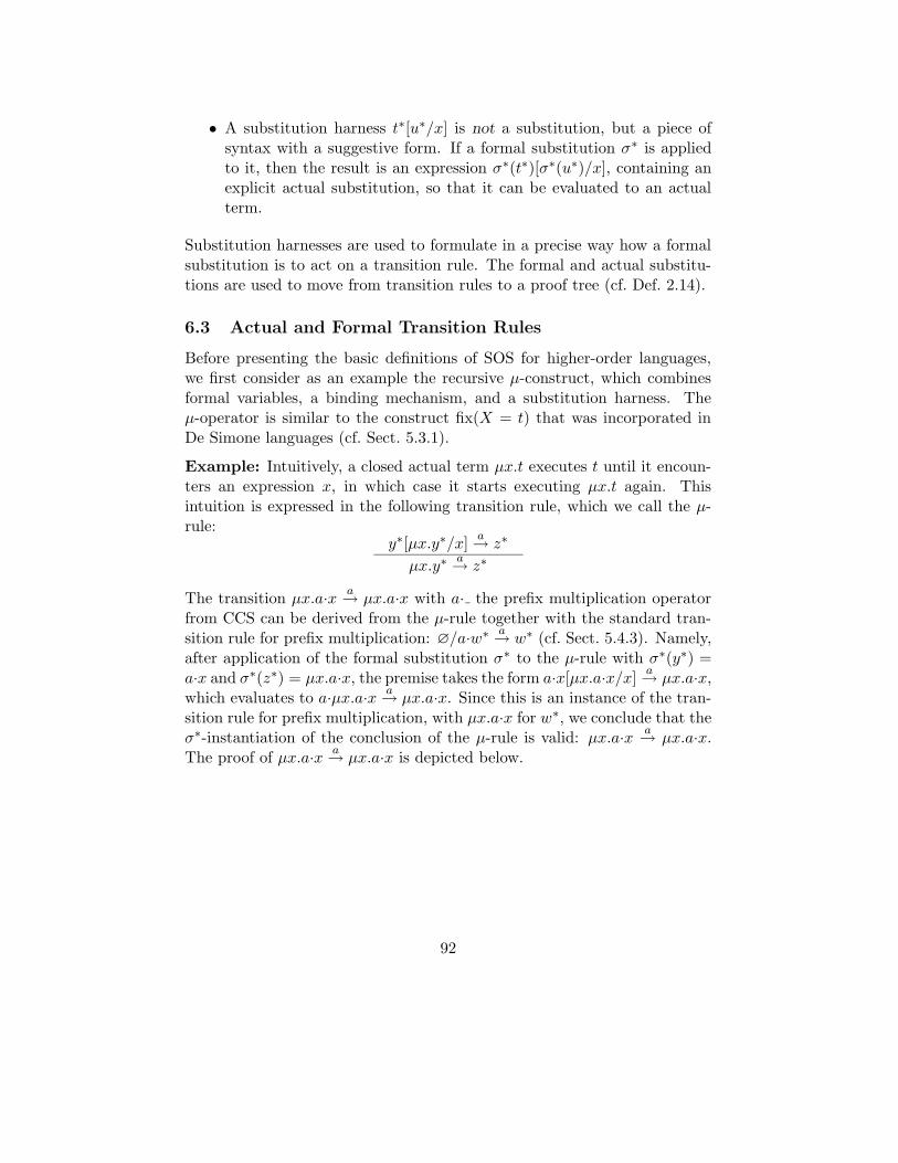
• A substitution harness t∗[u∗/x] is not a substitution, but a piece ofsyntax with a suggestive form. If a formal substitution σ∗ is appliedto it, then the result is an expression σ∗(t∗)[σ∗(u∗)/x], containing anexplicit actual substitution, so that it can be evaluated to an actualterm.
Substitution harnesses are used to formulate in a precise way how a formalsubstitution is to act on a transition rule. The formal and actual substitu-tions are used to move from transition rules to a proof tree (cf. Def. 2.14).
6.3 Actual and Formal Transition Rules
Before presenting the basic definitions of SOS for higher-order languages,we first consider as an example the recursive µ-construct, which combinesformal variables, a binding mechanism, and a substitution harness. Theµ-operator is similar to the construct fix(X = t) that was incorporated inDe Simone languages (cf. Sect. 5.3.1).
Example: Intuitively, a closed actual term µx.t executes t until it encoun-ters an expression x, in which case it starts executing µx.t again. Thisintuition is expressed in the following transition rule, which we call the µ-rule:
y∗[µx.y∗/x]a→ z∗
µx.y∗a→ z∗
The transition µx.a·x a→ µx.a·x with a· the prefix multiplication operatorfrom CCS can be derived from the µ-rule together with the standard tran-sition rule for prefix multiplication: ∅/a·w∗ a→ w∗ (cf. Sect. 5.4.3). Namely,after application of the formal substitution σ∗ to the µ-rule with σ∗(y∗) =a·x and σ∗(z∗) = µx.a·x, the premise takes the form a·x[µx.a·x/x] a→ µx.a·x,which evaluates to a·µx.a·x a→ µx.a·x. Since this is an instance of the tran-sition rule for prefix multiplication, with µx.a·x for w∗, we conclude that theσ∗-instantiation of the conclusion of the µ-rule is valid: µx.a·x a→ µx.a·x.The proof of µx.a·x a→ µx.a·x is depicted below.
92
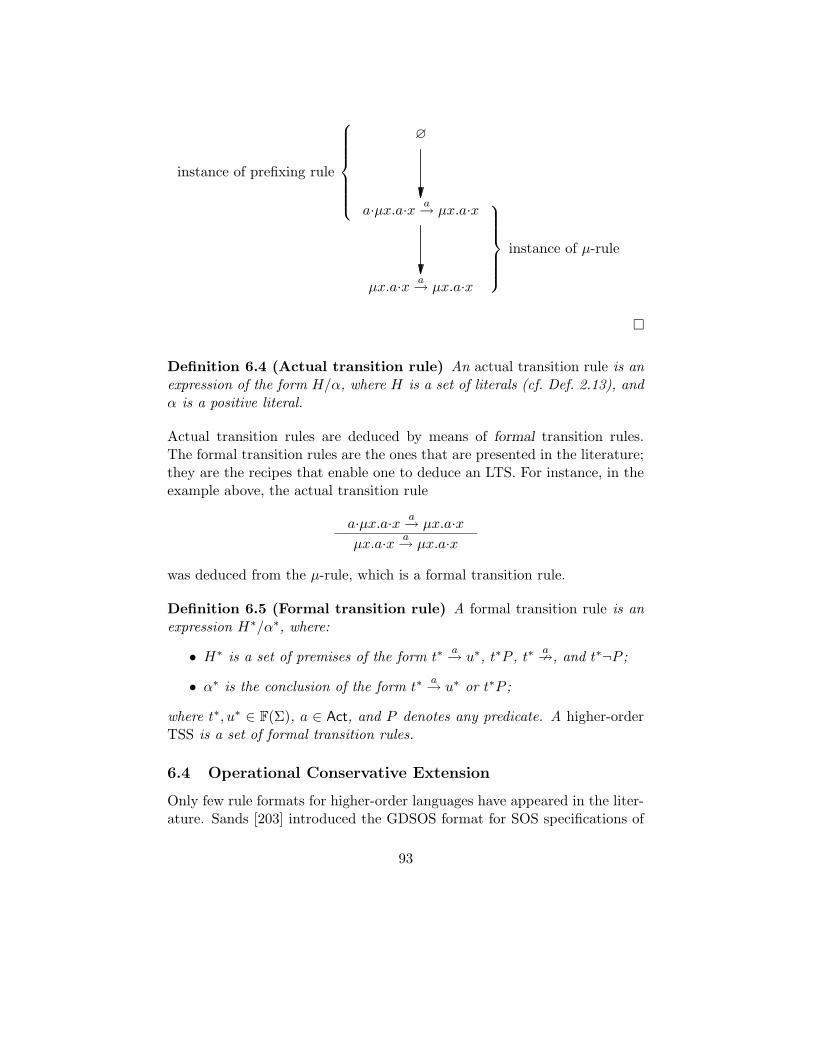
µx.a·x a→ µx.a·x
a·µx.a·x a→ µx.a·x
∅
instance of µ-rule
instance of prefixing rule
¤
Definition 6.4 (Actual transition rule) An actual transition rule is anexpression of the form H/α, where H is a set of literals (cf. Def. 2.13), andα is a positive literal.
Actual transition rules are deduced by means of formal transition rules.The formal transition rules are the ones that are presented in the literature;they are the recipes that enable one to deduce an LTS. For instance, in theexample above, the actual transition rule
a·µx.a·x a→ µx.a·xµx.a·x a→ µx.a·x
was deduced from the µ-rule, which is a formal transition rule.
Definition 6.5 (Formal transition rule) A formal transition rule is anexpression H∗/α∗, where:
• H∗ is a set of premises of the form t∗a→ u∗, t∗P , t∗
a9, and t∗¬P ;
• α∗ is the conclusion of the form t∗a→ u∗ or t∗P ;
where t∗, u∗ ∈ F(Σ), a ∈ Act, and P denotes any predicate. A higher-orderTSS is a set of formal transition rules.
6.4 Operational Conservative Extension
Only few rule formats for higher-order languages have appeared in the liter-ature. Sands [203] introduced the GDSOS format for SOS specifications of
93
functional languages and established some proof principles that are soundfor all languages expressible in this format. Howe [133] presented a congru-ence format for higher-order TSSs with respect to bisimulation equivalence,which shows a strong resemblance with the tyft/tyxt format from Grooteand Vaandrager (cf. Def. 5.2). Rensink [193] obtained congruence results forthree extensions of bisimilation equivalence to open terms, in the presenceof recursion. Interestingly, Bernstein [44] showed that in many cases thesemantics of a higher-order language can be captured by a first-order TSSwith terms as transition labels. It appears that existing rule formats can beextended with terms as transition labels in a straightforward manner; see[44, 90]. Thus, it might be the case that current first-order rule formats aresufficient to deal with higher-order languages. Another reference of interestin Bloom [51] Bloom proposed a general definition of higher-order processcalculi and investigated its basic properties. He gave sufficient conditionsunder which a calculus is finitely-branching and effective, and showed thata suitable notion of higher-order bisimulation is a congruence for a subclassof higher-order calculi.
We proceed to present a generalization from [90] of the operational con-servative extension format (see Sect. 4) to a higher-order setting. This gen-eralization is based on an adaptation of the notion of source-dependency (cf.Def. 4.3), requiring a distinction between occurrences of formal variables in-and outside the substitution harnesses of a formal term. FV (t∗) denotes theset of formal variables that occur in the formal term t∗.
Definition 6.6 (The set FV (t∗)) The sets FV (t∗) are defined inductivelyby:
FV (x∗)∆= x∗
FV (f(~x1.t∗1, . . . , ~xar(f).t
∗ar(f)))
∆= FV (t∗1) ∪ · · · ∪ FV (t∗
ar(f))
FV (t∗[s∗/x])∆= FV (t∗) ∪ FV (s∗) .
For example, FV (f(v.x∗[y∗/w])) = x∗, y∗. By contrast, EV (t∗) denotes amore restricted set of formal variables in the formal term t∗, which does nottake into account formal variables that occur inside a substitution harness.
Definition 6.7 (The set EV (t∗)) The sets EV (t∗) are defined inductivelyby:
EV (x∗)∆= x∗
EV (f(~x1.t∗1, . . . , ~xar(f).t
∗ar(f)))
∆= EV (t∗1) ∪ · · · ∪ EV (t∗
ar(f))
EV (t∗[s∗/x])∆= EV (t∗) .
94
For example, EV (f(v.x∗[y∗/w])) = x∗. The sets FV (t∗) and EV (t∗) areused in the definition of source-dependent variables in a formal transitionrule.
Definition 6.8 (Source dependency) For a formal transition rule ρ∗,the formal variables in ρ∗ that are source-dependent are defined inductivelyby:
1. if t∗ is the source of ρ∗, then all formal variables in EV (t∗) are source-dependent in ρ∗;
2. if t∗a→ u∗ is a premise of ρ∗, and all formal variables in FV (t∗)
are source-dependent in ρ∗, then all formal variables in EV (u∗) aresource-dependent in ρ∗.
A formal transition rule ρ∗ is source-dependent if so are all the variables inFV (ρ∗).
Thm. 6.9 formulates sufficient criteria for a higher-order TSS T0⊕T1 to be anoperational conservative extension of T0 (see Def. 4.2); it extends Thm. 4.4to higher-order languages. We say that a formal term in F(Σ1) is fresh if itcontains a function symbol from Σ1\Σ0 outside its substitution harnesses.Similarly, an action or predicate symbol in T1 is fresh if it does not occur inT0.
Theorem 6.9 Let T0 and T1 be higher-order TSSs over many-sorted higher-order signatures Σ0 and Σ0 ⊕ Σ1, respectively. Under the following condi-tions, T0 ⊕ T1 is an operational conservative extension of T0.
1. Each ρ∗ ∈ T0 is source-dependent.
2. For each ρ∗ ∈ T1,
• either the source of ρ∗ is fresh,
• or ρ∗ has a premise of the form t∗0a→ t∗1 or t∗0P , where
– t∗0 ∈ F(Σ0);
– FV (t∗0) ⊆ EV (u∗), where u∗ denotes the source of ρ∗;
– t∗1, a, or P is fresh.
Theorem 6.9 can be applied to extensions of higher-order TSSs such asprocess algebra with time [89, 174] or data [113], where binding constructsenable one to parameterize processes over the time or data domain, processalgebra with a recursive operator like the µ-construct [122, 126, 206], theπ-calculus [167, 205], and the lazy λ-calculus [124, 204].
95
7 Denotational Semantics
Following a bias towards operational methods in process theory that datesback to Milner’s original development of the theory of CCS [159, 166], mostof the work in the field of the meta-theory of process description languagesreported in this chapter is concerned with operational and axiomatic seman-tics for terms and the relationships between the two. In particular, it is bynow clear that it is often possible to automatically translate an operationaltheory of processes into an axiomatic one [8]. Moreover, in certain circum-stances it is also possible to derive an SOS semantics from an axiomatic one,as witnessed by the developments in [8, 136].
Axiomatic semantics and proof systems for programming and specifica-tion languages are often closely related to denotational semantics for them,particularly if the Scott-Strachey approach [207] is followed. A paradigmaticexample of the development of a semantic theory of processes in which op-erational, axiomatic, and denotational semantics coexist harmoniously, andmay be used to highlight different aspects of process behaviours, is the the-ory of testing equivalence developed by De Nicola and Hennessy [77, 122].In this theory, a process can be characterized operationally by means of itsreaction to experiments, and denotationally as an acceptance tree [121]. Ac-ceptance trees allow one to fully describe the behaviour of a process whileabstracting away from the operational details of its interactions with all thepossible testers. Moreover, the domain-theoretic properties of this modelallow one to establish properties of the behavioural semantics that wouldbe very difficult to derive using purely operational methods (see, e.g., theresults in [122, Sect. 4.5].)
To our mind, the coincidence of operational, axiomatic, and denota-tional semantics enjoyed by the theory of processes presented in [122] doesnot only reinforce the naturalness of the chosen notion of program seman-tics, but allows one to make good use of the complementary benefits affordedby these semantic descriptions in establishing properties of processes. How-ever, developing these three views of processes for each process descrip-tion language from scratch and proving their coincidence is hard, subtlework; in addition, to quote from [155], giving denotational semantics toprogramming languages using the Scott-Strachey approach “involves an ar-mamentarium of mathematical weapons otherwise unfamiliar in ComputerScience”. It would therefore be beneficial to develop systematic ways of giv-ing denotational semantics to process description languages, following theScott-Strachey approach, starting from their SOS descriptions. Of course,this is only worthwhile if the denotational semantics produced by the pro-
96
posed techniques is automatically guaranteed to be in agreement with thebehavioural and axiomatic views of processes. In particular, we would liketo generate a denotational semantics that matches exactly our operationalintuition about process behaviour, i.e., that is fully abstract in the sense ofMilner and Plotkin [157, 158, 182, 221], with respect to a reasonable notionof behavioural semantics.
This section reviews results from [11, 12], where it is shown how to gen-erate a fully abstract denotational semantics from a class of recursive GSOSlanguages (cf. Sect. 5.4.5). Usually denotational semantics deals with recur-sion implicitly, by setting up a framework within which reasoning about re-cursion can be reduced to reasoning about recursion-free approximations. Inline with this approach, a denotational semantics is first given to recursion-free terms from GSOS languages. Next, recursion-free approximations areused to extend this result to recursive terms over recursive GSOS languages.
7.1 Preliminaries
7.1.1 Σ-Domains
We assume familiarity with the basic notions of ordered and continuous al-gebras (see, e.g., [116, 122, 134]); however, in what follows we give a quickoverview of the way a denotational semantics can be given to a recursivelanguage following the standard lines of algebraic semantics [116]. The in-terested reader is invited to consult [122] for an explanation of the theory.
Let Σ denote a signature, in the sense of Sect. 2.4, which includes adistinguished constant Ω. A Σ-algebra consists of a carrier set A, where foreach function symbol f ∈ Σ there is given an operator fA : Aar(f) → A. Amapping ϕ : A → B between two Σ-algebras is a Σ-homomorphism if forevery f ∈ Σ and elements d1, . . . , dar(f) ∈ A:
ϕ(fA(d1, . . . , dar(f))) = fB(ϕ(d1), . . . , ϕ(dar(f))) .
We recall (from Sect. 2.4) that T(Σ) denotes the set of closed terms over Σ.We use T(Σ,RVar) to denote the set of closed terms over Σ that may containoccurrences from a countably infinite set RVar of recursion variables, rangedover by X,Y .
A Σ-domain [122] (A,vA) is a Σ-algebra whose carrier (A,vA) is analgebraic complete partial order (cpo) (see, e.g., [183]) and whose operationsare interpreted as continuous functions (in the sense of, e.g., [122, p. 123]).We require that Ω is ⊥A, viz. the least element in the algebraic cpo (A,vA).The notion of a Σ-poset (resp. Σ-preorder) may be defined in a similar way
97
by requiring that (A,vA) be a partially ordered (resp. preordered) set andthat the operators be monotonic. The notion of Σ-homomorphism extendsto the ordered Σ-structures in the obvious way by requiring that such mapspreserve the underlying order-theoretic structure as well as the Σ-structure.
The interpretation A[[·]] of T(Σ,RVar) in a Σ-algebra A associates eachterm in T(Σ,RVar) with a mapping from substitutions (going from recursionvariables to A) to A. This interpretation is defined by induction as follows,where σ is any mapping from recursion variables to A:
A[[X]]σ∆= σ(X)
A[[f(t1, . . . , tn)]]σ ∆= fA(A[[t1]]σ, . . . ,A[[tn]]σ) ,
where n = ar(f). We recall that the recursive terms over Σ are given bythe BNF grammar
t ::= X | f(t1, . . . , tar(f)) | fix(X = t)
where X is any recursion variable, f any function symbol in Σ, and fix abinding construct. The latter construct gives rise to the usual notions offree and bound recursion variables in recursive terms. CREC(Σ) denotes theset of recursive terms that do not contain free recursion variables. Further-more, t[u/X] denotes the recursive term t in which each occurrence of therecursion variable X has been replaced by u. If A is a Σ-domain, then theinterpretation A[[·]] extends to the set of recursive terms over Σ by
A[[fix(X = t)]]σ∆= Yλd.A[[t]]σ′
where Y denotes the least fixed-point operator, d is a metavariable rangingover A, σ′(X)
∆= d, and σ′(Y )
∆= σ(Y ) for Y 6= X. Note that for each
t ∈ CREC(Σ), A[[t]]σ does not depend on σ.In what follows, we make use of some general results about the semantic
mappings defined above, which may be found in [72, 116, 122]. The firstresult states that for any recursive term t (possibly containing free recursionvariables) there is a sequence of finite approximations tn ∈ T(Σ,RVar) forn ∈ N such that, for any Σ-domain A,
A[[t]] =⊔
n∈N
A[[tn]] .
(That is, the interpretation of the term t in A is the least upper bound ofthe interpretations of its finite approximations.) The second result states
98
that if ≤Ω is the least precongruence (cf. Def. 2.11) satisfying
fix(X = t) ≤Ω t[fix(X = t)/X]
t[fix(X = t)/X] ≤Ω fix(X = t)
Ω ≤Ω X
then tn ≤Ω t for every n ∈ N.For any binary relationR over CREC(Σ), the algebraic part ofR, denoted
by RA, is defined as follows [122]:
t RA u ⇔ ∀n ∈ N ∃m ∈ N (tn R um) .
We say that R is algebraic if R is equal to RA. Intuitively, a relation isalgebraic if it is completely determined by how it behaves on recursion-freeterms. Every denotational interpretation A[[·]] induces a preorder vA overCREC(Σ) by:
t vA u ⇔ A[[t]] vA A[[u]] .
The following result characterizes a class of denotational interpretationswhich induce relations over terms that are algebraic.
Lemma 7.1 Let A be a Σ-domain. If A[[t]] is a compact element in A forevery t ∈ T(Σ) (see, e.g., [122, p. 130]), then vA is algebraic.
In view of the above general lemma, the relations over the recursive termsin CREC(Σ) induced by a denotational semantics are always algebraic, pro-vided that the denotations of the recursion-free terms in T(Σ) are compactelements in the algebraic cpo A.
7.1.2 Prebisimulation
We consider LTSs with divergence from Def. 5.40, which include a specialdivergence predicate ↑. The convergence predicate ↓ holds in a state iffthe divergence predicate does not hold in this same state (cf. Def. 5.41).The behavioural relation over LTSs with divergence that we study in thissection is that of prebisimulation [120, 130, 160, 240] (also known as partialbisimulation [1]). We recall (from Def. 2.1) that Proc and Act denote the setsof states and actions, respectively, of the LTS with divergence in question.Let Rel(Proc) denote the set of binary relations over Proc.
99
Definition 7.2 (Prebisimulation) Assume an LTS with divergence. Thefunctional G : Rel(Proc)→ Rel(Proc) is defined as follows. Given a relationR ∈ Rel(Proc), we have s1G(R) s2 whenever:
- if s1a→ s′1, then there is a transition s2
a→ s′2 such that s′1 R s′2;
- if s1 ↓, then s2 ↓;
- if s1 ↓ and s2a→ s′2, then there is a transition s1
a→ s′1 such thats′1 R s′2.
A relation R is a prebisimulation iff R ⊆ G(R). We write s1 . s2 if thereexists a prebisimulation R such that s1 R s2.
The relation . is a preorder over Proc; its kernel is denoted by '. Pre-bisimulation is similar in spirit to the notion of bisimulation (cf. Def. 2.3).Intuitively, s1 . s2 if the behaviour of s2 is at least as specified as that ofs1, and s1 and s2 can simulate each other when restricted to the part oftheir behaviour that is fully specified. A divergent state s with no outgoingtransition intuitively corresponds to a process whose behaviour is totallyunspecified — essentially an operational version of the bottom element ⊥ inScott’s theory of domains [183, 207, 220].
The following precongruence result for . with respect to recursive GSOSlanguages including the inert constant Ω originates from [11, 12].
Proposition 7.3 . is a precongruence with respect to the LTS with diver-gence over CREC(Σ) associated with a recursive GSOS language includingthe inert constant Ω (cf. Prop. 5.42).
7.1.3 Finite Synchronization Trees
A useful source of examples for LTSs with divergence is the set of finitesynchronization trees [159].
Definition 7.4 (Finite synchronization tree) The set of finite synchro-nization trees over a set of actions Act, denoted by ST(Act), is defined in-ductively by:
1. ∅ ∈ ST(Act);
2. if S ∈ ST(Act), then S ∪ ⊥ ∈ ST(Act);
100
3. if a1, . . . , an ∈ Act and S1, . . . , Sn ∈ ST(Act), then
〈a1, S1〉, . . . , 〈an, Sn〉 ∈ ST(Act) .
The symbol ⊥ is used to represent that a finite synchronization tree is di-vergent. The set of finite synchronization trees ST(Act) can be turned intoan LTS with divergence by stipulating that, for S ∈ ST(Act):
• S ↑ iff ⊥ ∈ S;
• Sa→ S′ iff 〈a, S′〉 ∈ S.
When relating behavioural semantics based upon bisimulation-like relationswith denotational semantics (usually based upon algebraic domains), one isfaced with the following mismatch:
1. on the one hand, in an algebraic domain d v e iff every compactelement smaller than or equal to d is also dominated by e;
2. on the other hand, there are closed terms that have the same finiteapproximations, but that are not bisimilar.
This implies that bisimulation is not algebraic, and thus cannot be capturedin a standard domain theoretic framework. One way to address this prob-lem is to study its finitary part. To this end, it is generally agreed uponin the literature that finite synchronization trees are a natural operationalcounterpart of compact elements.
In what follows, we are interested in relating the notion of prebisimula-tion to a preorder on finite synchronization trees induced by a denotationalsemantics given by means of an algebraic domain. As such preorders arecompletely determined by how they act on finite processes, we are inter-ested in comparing them with the “finitely observable”, or finitary, part ofthe bisimulation in the sense of, e.g., [116, 120]. The following definitionfrom [1] is inspired by property 1 above for algebraic domains.
Definition 7.5 (Finitary preorder) The finitary preorder .F is definedon any LTS by
s1 .F s2 ⇐⇒ ∀S ∈ ST(Act) (S . s1 ⇒ S . s2) .
Since it is, in general, technically difficult to work with .F , it is commonpractice to try and obtain an alternative characterization of the finitarypreorder (see, e.g., [13]). An alternative method for using the functionalG : Rel(Proc) → Rel(Proc) from Def. 7.2 to obtain a preorder is to apply itinductively as follows:
101
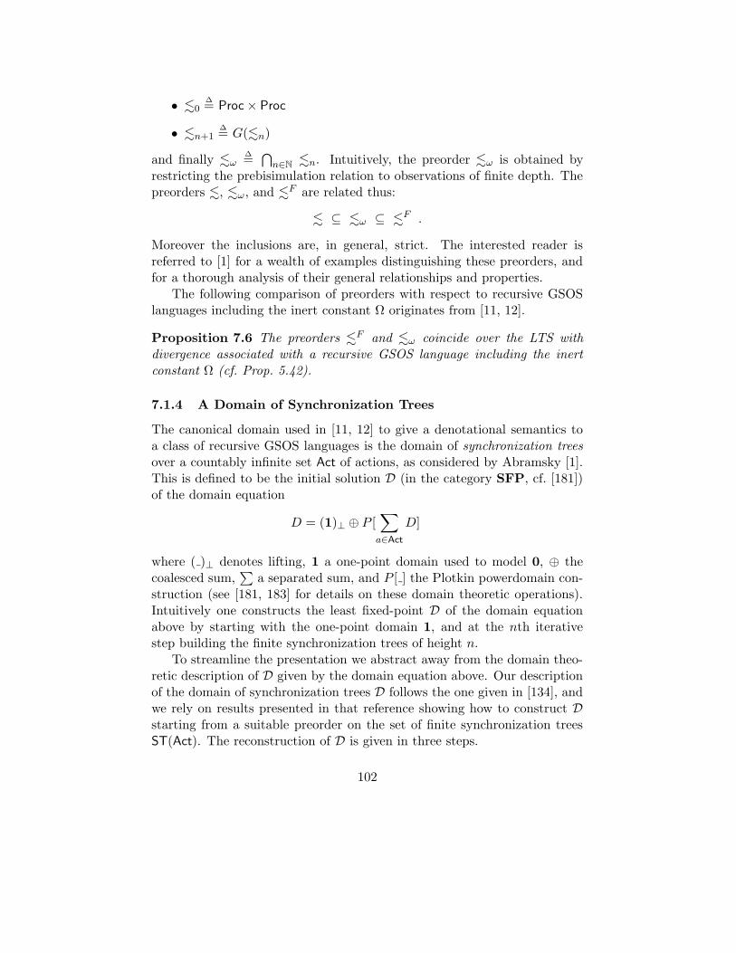
• .0 ∆= Proc× Proc
• .n+1∆= G(.n)
and finally .ω∆=
⋂
n∈N.n. Intuitively, the preorder .ω is obtained by
restricting the prebisimulation relation to observations of finite depth. Thepreorders ., .ω, and .
F are related thus:
. ⊆ .ω ⊆ .F .
Moreover the inclusions are, in general, strict. The interested reader isreferred to [1] for a wealth of examples distinguishing these preorders, andfor a thorough analysis of their general relationships and properties.
The following comparison of preorders with respect to recursive GSOSlanguages including the inert constant Ω originates from [11, 12].
Proposition 7.6 The preorders .F and .ω coincide over the LTS withdivergence associated with a recursive GSOS language including the inertconstant Ω (cf. Prop. 5.42).
7.1.4 A Domain of Synchronization Trees
The canonical domain used in [11, 12] to give a denotational semantics toa class of recursive GSOS languages is the domain of synchronization treesover a countably infinite set Act of actions, as considered by Abramsky [1].This is defined to be the initial solution D (in the category SFP, cf. [181])of the domain equation
D = (1)⊥ ⊕ P [∑
a∈Act
D]
where ( )⊥ denotes lifting, 1 a one-point domain used to model 0, ⊕ thecoalesced sum,
∑a separated sum, and P [ ] the Plotkin powerdomain con-
struction (see [181, 183] for details on these domain theoretic operations).Intuitively one constructs the least fixed-point D of the domain equationabove by starting with the one-point domain 1, and at the nth iterativestep building the finite synchronization trees of height n.
To streamline the presentation we abstract away from the domain theo-retic description of D given by the domain equation above. Our descriptionof the domain of synchronization trees D follows the one given in [134], andwe rely on results presented in that reference showing how to construct Dstarting from a suitable preorder on the set of finite synchronization treesST(Act). The reconstruction of D is given in three steps.
102
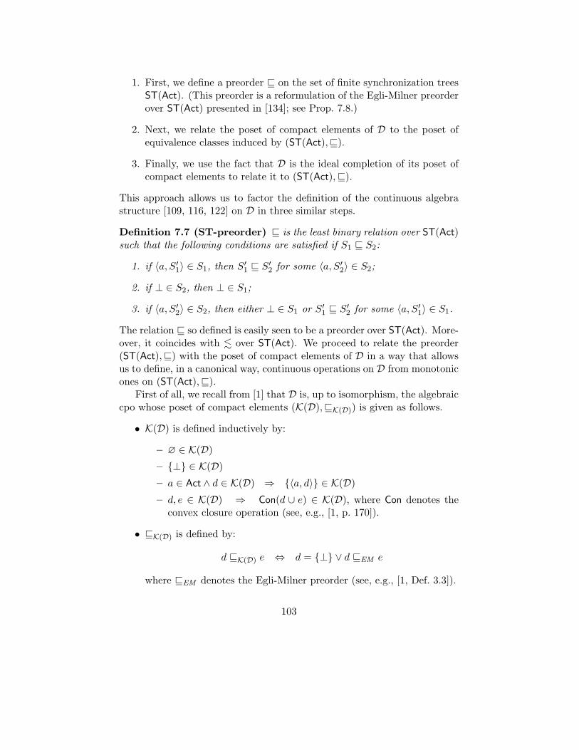
1. First, we define a preorder v on the set of finite synchronization treesST(Act). (This preorder is a reformulation of the Egli-Milner preorderover ST(Act) presented in [134]; see Prop. 7.8.)
2. Next, we relate the poset of compact elements of D to the poset ofequivalence classes induced by (ST(Act),v).
3. Finally, we use the fact that D is the ideal completion of its poset ofcompact elements to relate it to (ST(Act),v).
This approach allows us to factor the definition of the continuous algebrastructure [109, 116, 122] on D in three similar steps.
Definition 7.7 (ST-preorder) v is the least binary relation over ST(Act)such that the following conditions are satisfied if S1 v S2:
1. if 〈a, S ′1〉 ∈ S1, then S′
1 v S′2 for some 〈a, S ′
2〉 ∈ S2;
2. if ⊥ ∈ S2, then ⊥ ∈ S1;
3. if 〈a, S ′2〉 ∈ S2, then either ⊥ ∈ S1 or S′
1 v S′2 for some 〈a, S ′
1〉 ∈ S1.
The relation v so defined is easily seen to be a preorder over ST(Act). More-over, it coincides with . over ST(Act). We proceed to relate the preorder(ST(Act),v) with the poset of compact elements of D in a way that allowsus to define, in a canonical way, continuous operations on D from monotonicones on (ST(Act),v).
First of all, we recall from [1] that D is, up to isomorphism, the algebraiccpo whose poset of compact elements (K(D),vK(D)) is given as follows.
• K(D) is defined inductively by:
– ∅ ∈ K(D)– ⊥ ∈ K(D)– a ∈ Act ∧ d ∈ K(D) ⇒ 〈a, d〉 ∈ K(D)– d, e ∈ K(D) ⇒ Con(d ∪ e) ∈ K(D), where Con denotes the
convex closure operation (see, e.g., [1, p. 170]).
• vK(D) is defined by:
d vK(D) e ⇔ d = ⊥ ∨ d vEM e
where vEM denotes the Egli-Milner preorder (see, e.g., [1, Def. 3.3]).
103
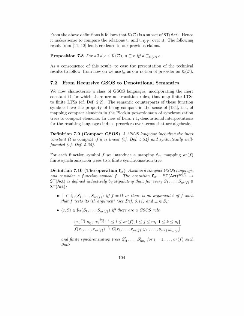
From the above definitions it follows that K(D) is a subset of ST(Act). Henceit makes sense to compare the relations v and vK(D) over it. The followingresult from [11, 12] lends credence to our previous claims.
Proposition 7.8 For all d, e ∈ K(D), d v e iff d vK(D) e.
As a consequence of this result, to ease the presentation of the technicalresults to follow, from now on we use v as our notion of preorder on K(D).
7.2 From Recursive GSOS to Denotational Semantics
We now characterize a class of GSOS languages, incorporating the inertconstant Ω for which there are no transition rules, that map finite LTSsto finite LTSs (cf. Def. 2.2). The semantic counterparts of these functionsymbols have the property of being compact in the sense of [134], i.e., ofmapping compact elements in the Plotkin powerdomain of synchronizationtrees to compact elements. In view of Lem. 7.1, denotational interpretationsfor the resulting languages induce preorders over terms that are algebraic.
Definition 7.9 (Compact GSOS) A GSOS language including the inertconstant Ω is compact if it is linear (cf. Def. 5.34) and syntactically well-founded (cf. Def. 5.35).
For each function symbol f we introduce a mapping fST, mapping ar(f)finite synchronization trees to a finite synchronization tree.
Definition 7.10 (The operation fST) Assume a compact GSOS language,and consider a function symbol f . The operation fST : ST(Act)ar(f) →ST(Act) is defined inductively by stipulating that, for every S1, . . . , Sar(f) ∈ST(Act):
• ⊥ ∈ fST(S1, . . . , Sar(f)) iff f = Ω or there is an argument i of f suchthat f tests its ith argument (see Def. 5.11) and ⊥ ∈ Si;
• 〈c, S〉 ∈ fST(S1, . . . , Sar(f)) iff there are a GSOS rule
xiaij→ yij , xi
bik9 | 1 ≤ i ≤ ar(f), 1 ≤ j ≤ mi, 1 ≤ k ≤ ni
f(x1, . . . , xar(f))c→ C[x1, . . . , xar(f), y11, . . . , yar(f)m
ar(f)]
and finite synchronization trees S ′i1, . . . , S
′imi
for i = 1, . . . , ar(f) suchthat:
104
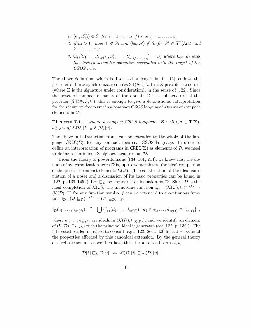
1. 〈aij , S′ij〉 ∈ Si for i = 1, . . . , ar(f) and j = 1, . . . ,mi;
2. if ni > 0, then ⊥ 6∈ Si and 〈bik, S′〉 6∈ Si for S′ ∈ ST(Act) andk = 1, . . . , ni;
3. CST[S1, . . . , Sar(f), S′11, . . . , S
′ar(f)m
ar(f)] = S, where CST denotes
the derived semantic operation associated with the target of theGSOS rule.
The above definition, which is discussed at length in [11, 12], endows thepreorder of finite synchronization trees ST(Act) with a Σ-preorder structure(where Σ is the signature under consideration), in the sense of [122]. Sincethe poset of compact elements of the domain D is a substructure of thepreorder (ST(Act),v), this is enough to give a denotational interpretationfor the recursion-free terms in a compact GSOS language in terms of compactelements in D.
Theorem 7.11 Assume a compact GSOS language. For all t, u ∈ T(Σ),t .ω u iff K(D)[[t]] v K(D)[[u]].
The above full abstraction result can be extended to the whole of the lan-guage CREC(Σ), for any compact recursive GSOS language. In order todefine an interpretation of programs in CREC(Σ) as elements of D, we needto define a continuous Σ-algebra structure on D.
From the theory of powerdomains [134, 181, 214], we know that the do-main of synchronization trees D is, up to isomorphism, the ideal completionof the poset of compact elements K(D). (The construction of the ideal com-pletion of a poset and a discussion of its basic properties can be found in[122, p. 139–145].) Let vD be standard set inclusion on D. Since D is theideal completion of K(D), the monotonic function fST : (K(D),v)ar(f) →(K(D),v) for any function symbol f can be extended to a continuous func-tion fD : (D,vD)
ar(f) → (D,vD) by:
fD(e1, . . . , ear(f))∆=
⋃fST(d1, . . . , dar(f)) | d1 ∈ e1, . . . , dar(f) ∈ ear(f)
,
where e1, . . . , ear(f) are ideals in (K(D),vK(D)), and we identify an elementof (K(D),vK(D)) with the principal ideal it generates (see [122, p. 139]). Theinterested reader is invited to consult, e.g., [122, Sect. 3.3] for a discussion ofthe properties afforded by this canonical extension. By the general theoryof algebraic semantics we then have that, for all closed terms t, u,
D[[t]] vD D[[u]] ⇔ K(D)[[t]] v K(D)[[u]] .
105
In view of Thm. 7.11, the desired full abstraction result follows if we provethat the preorder .ω is algebraic. Namely, owing to our constructions eachclosed term t is interpreted as a compact element of D, so Lem. 7.1 impliesthat the relation vD is algebraic. And two algebraic relations that coincideover the collection of closed terms T(Σ) do, in fact, coincide over the wholeof CREC(Σ).
The key to the proof of algebraicity of .ω is the following general theo-rem from [11, 12], providing a partial completeness result for . in the senseof Hennessy [10, 120] for arbitrary compact GSOS languages. This axioma-tizability result uses the fact that . is a precongruence with respect to theLTS with divergence associated with a recursive GSOS language includingthe inert constant Ω; see Prop. 7.3.
Proposition 7.12 Let G be a compact recursive GSOS language. Thenthere exists a compact recursive GSOS language H over a signature Σ′,being a disjoint extension (cf. Def. 5.31) of G and TFINTREE (cf. Sect. 5.4.5),together with a set I of inequalities between recursive terms over Σ′, suchthat for all t ∈ T(Σ′) and u ∈ CREC(Σ′):
H induces t . u iff I ` t ≤ u .
Apart from its intrinsic interest, the main consequence of Prop. 7.12 is thefollowing key result from [11, 12], essentially stating that, for any compactGSOS language, finite synchronization trees are compact elements with re-spect to the preorder ..
Proposition 7.13 Assume a compact recursive GSOS language. If S ∈ST(Act) and t ∈ CREC(Σ), then S .F t iff there exists a finite approximationtn of t such that S .F tn.
The above result, in conjunction with Prop. 7.6, yields that .ω is indeedalgebraic.
Proposition 7.14 .ω is algebraic over the LTS with divergence associatedwith a compact recursive GSOS language.
In light of Thm. 7.11 and Prop. 7.14, for any compact recursive GSOSlanguage the induced denotational semantics over CREC(Σ) is fully abstractwith respect to .ω.
Theorem 7.15 Assume a compact recursive GSOS language. For all t, u ∈CREC(Σ), t .ω u iff D[[t]] vD D[[u]].
106
When applied to the version of SCCS considered by Abramsky [1], the tech-niques we have presented deliver a denotational semantics that is exactlythe one given in op. cit.
Related Work The work reported in this section is by no means the onlyattempt to systematically derive denotational models from SOS languagespecifications. The main precursors to this work in the field of the meta-theory of process description languages may be found in the work by Bloom[49] and Rutten [198, 199, 200, 201]. In his unpublished paper [49], Bloomgives operational, logical, relational, and three denotational semantics forGSOS languages without negative premises and unguarded recursion, andshows that they coincide. Bloom’s work is based on the behavioural no-tion of simulation [128], and two of his denotational semantics are givenby means of Scott domains based on finite synchronization trees. On theother hand, the work by Rutten [198, 199, 200] gives methods for deriv-ing a denotational semantics based on complete metric spaces and Aczel’snon-well-founded sets [14] for languages specified by means of subformats ofthe tyft/tyxt format (cf. Def. 5.2). In particular, the reference [200] gives adetailed and clear introduction to a technique, called “processes as terms”,for the definition of operations on semantic models from transition rules.Rutten’s general “processes as terms” approach could have been applied toyield an equivalent formulation of the semantic operations on finite syn-chronization trees given above. The work presented in the aforementionedpapers has been generalized by Rutten and Turi [201]. Ibidem it is shownhow TSSs in tyft/tyxt format induce a denotational semantics, and the es-sential properties of semantic domains that make their definitions possibleare investigated in a categorical perspective.
Abramsky and Vickers [3] consider various notions of process observa-tions in a uniform algebraic framework provided by the theory of quantales(see, e.g., [197]). The methods developed in [3] yield, in a uniform fashion,observational logics and denotational models for each notion of process ob-servation they consider. Their work is, however, semantic in nature, andignores the algebraic structure of process expressions.
In the area of the semantics of functional programs, developments thatare somewhat similar in spirit to those given above are presented in [151,213]. Those papers study natural notions of preorder over programs writtenin a simple functional programming language, and show how any orderingon programs with certain basic properties can be extended to a term modelthat is fully abstract with respect to it.
107
The issue of defining abstract mathematical models for, rather than from,operational semantics has also received some attention. We refer the inter-ested reader to, e.g., [19, 224], and the references therein, for details on thisline of investigation.
References
[1] S. Abramsky, A domain equation for bisimulation, Information andComputation, 92 (1991), pp. 161–218.
[2] S. Abramsky and C. Hankin, Abstract Interpretation of DeclarativeLanguages, Ellis Horwood, 1987.
[3] S. Abramsky and S. Vickers, Quantales, observational logic andprocess semantics, Mathematical Structures in Computer Science, 3(1993), pp. 161–227.
[4] L. Aceto, Deriving complete inference systems for a class of GSOSlanguages generating regular behaviours, in Jonsson and Parrow [137],pp. 449–464.
[5] , GSOS and finite labelled transition systems, Theoretical Com-put. Sci., 131 (1994), pp. 181–195.
[6] L. Aceto, B. Bloom, and F. Vaandrager, Checking equations inGSOS systems, 1992. Unpublished working paper.
[7] , Turning SOS rules into equations, in LICS92 [146], pp. 113–124.Preliminary version of [8].
[8] , Turning SOS rules into equations, Information and Computa-tion, 111 (1994), pp. 1–52.
[9] L. Aceto, W. Fokkink, R. v. Glabbeek, andA. Ingolfsdottir, Axiomatizing prefix iteration with silentsteps, Information and Computation, 127 (1996), pp. 26–40.
[10] L. Aceto and M. Hennessy, Termination, deadlock and divergence,J. Assoc. Comput. Mach., 39 (1992), pp. 147–187.
[11] L. Aceto and A. Ingolfsdottir, CPO models for a class of GSOSlanguages, in Mosses et al. [173], pp. 439–453. Preliminary version of[12].
108
[12] , CPO models for compact GSOS languages, Information andComputation, 129 (1996), pp. 107–141.
[13] , A characterization of finitary bisimulation, Inf. Process. Lett.,64 (1997), pp. 127–134.
[14] P. Aczel, Non-well-founded Sets, vol. 14 of CSLI Lecture Notes, Stan-ford University, 1988.
[15] S. Allen, R. Constable, D. Howe, and W. Aitken, The se-mantics of reflected proof, in Proceedings 5th Symposium on Logic inComputer Science, Philadelphia, PA, IEEE Computer Society Press,1990, pp. 95–105.
[16] D. Austry and G. Boudol, Algebre de processus et synchronisa-tions, Theoretical Comput. Sci., 30 (1984), pp. 91–131.
[17] F. Baader and T. Nipkow, Term Rewriting and All That, Cam-bridge University Press, 1998.
[18] J. Backus, The syntax and semantics of the proposed internationalalgebraic language of the Zurich ACM-GAMM conference, in Proceed-ings ICIP, Unesco, 1960, pp. 125–131.
[19] E. Badouel, Conditional rewrite rules as an algebraic semantics ofprocesses, Research Report 1226, INRIA Rennes, 1990.
[20] E. Badouel and P. Darondeau, Structural operational specifica-tions and trace automata, in Cleaveland [68], pp. 302–316.
[21] J. Baeten, ed., Applications of Process Algebra, Cambridge Tracts inTheoretical Computer Science 17, Cambridge University Press, 1990.
[22] J. Baeten and J. Bergstra, A survey of axiom systems for processalgebras, Report P9111, University of Amsterdam, Amsterdam, 1991.
[23] , Discrete time process algebra, in Cleaveland [68], pp. 401–420.
[24] J. Baeten, J. Bergstra, and J. W. Klop, Syntax and definingequations for an interrupt mechanism in process algebra, FundamentaInformaticae, IX (1986), pp. 127–168.
[25] , On the consistency of Koomen’s fair abstraction rule, Theoreti-cal Comput. Sci., 51 (1987), pp. 129–176.
109
[26] J. Baeten and J. W. Klop, eds., Proceedings 1st Conference onConcurrency Theory, Amsterdam, The Netherlands, vol. 458 of Lec-ture Notes in Computer Science, Springer-Verlag, 1990.
[27] J. Baeten and C. Verhoef, A congruence theorem for structuredoperational semantics with predicates, in Best [46], pp. 477–492.
[28] , Concrete process algebra, in Handbook of Logic in ComputerScience, S. Abramsky, D. Gabbay, and T. Maibaum, eds., vol. IV,Oxford University Press, 1995, pp. 149–268.
[29] J. Baeten and P. Weijland, Process Algebra, Cambridge Tracts inTheoretical Computer Science 18, Cambridge University Press, 1990.
[30] J. d. Bakker, Semantics of programming languages, Advances inInformation Systems Science, 2 (1969), pp. 173–227.
[31] J. d. Bakker, W. d. Roever, and G. Rozenberg, eds., Proceed-ings REX Workshop on Semantics: Foundations and Applications,Beekbergen, The Netherlands, June 1992, vol. 666 of Lecture Notes inComputer Science, Springer-Verlag, 1993.
[32] , eds., Proceedings REX School/Symposium on A Decade of Con-currency: Reflections and Perspectives, Noordwijkerhout, The Nether-lands, vol. 803 of Lecture Notes in Computer Science, Springer-Verlag,1994.
[33] J. d. Bakker and J. Zucker, Processes and the denotational se-mantics of concurrency, Information and Control, 54 (1982), pp. 70–120.
[34] H. Barendregt, The Lambda Calculus, Its Syntax and Semantics,vol. 103 of Studies in Logic and the Foundation of Mathematics, North-Holland, Amsterdam, 1984.
[35] T. Basten, Branching bisimilarity is an equivalence indeed!, Infor-mation Processing Letters, 58 (1996), pp. 141–147.
[36] J. Bergstra, I. Bethke, and A. Ponse, Process algebra with iter-ation and nesting, Computer Journal, 37 (1994), pp. 243–258.
[37] J. Bergstra and J. W. Klop, Fixed point semantics in processalgebras, Report IW 206, Mathematisch Centrum, Amsterdam, 1982.
110
[38] , The algebra of recursively defined processes and the algebraof regular processes, in Proceedings 11th Colloquium on Automata,Languages and Programming, Antwerp, Belgium, J. Paredaens, ed.,vol. 172 of Lecture Notes in Computer Science, Springer-Verlag, 1984,pp. 82–95.
[39] , Process algebra for synchronous communication, Informationand Control, 60 (1984), pp. 109–137.
[40] , Conditional rewrite rules: Confluence and termination, J. Com-put. System Sci., 32 (1986), pp. 323–362.
[41] , Verification of an alternating bit protocol by means of process al-gebra, in Spring School on Mathematical Methods of Specification andSynthesis of Software Systems, Wendisch-Rietz, Germany, W. Bibeland K. Jantke, eds., no. 215 in Lecture Notes in Computer Science,Springer-Verlag, 1986, pp. 9–23.
[42] , A complete inference system for regular processes with silentmoves, in Proceedings Logic Colloquium 1986, F. Drake and J. Truss,eds., Hull, 1988, North-Holland, pp. 21–81.
[43] J. Bergstra, A. Ponse, and J. v. Wamel, Process algebra withbacktracking, in Bakker et al. [32], pp. 46–91.
[44] K. Bernstein, A congruence theorem for structured operational se-mantics of higher-order languages, in Proceedings 13th Symposiumon Logic in Computer Science, Indianapolis, Indiana, IEEE ComputerSociety Press, 1998, pp. 153–164.
[45] G. Berry, A hardware implementation of Pure Esterel, Rapport deRecherche 06/91, Ecole des Mines, CMA, Sophia-Antipolis, France,1991.
[46] E. Best, ed., Proceedings 4th Conference on Concurrency Theory,Hildesheim, Germany, vol. 715 of Lecture Notes in Computer Science,Springer-Verlag, 1993.
[47] B. Bloom, Ready Simulation, Bisimulation, and the Semantics ofCCS-like Languages, PhD thesis, Department of Electrical Engineeringand Computer Science, Massachusetts Institute of Technology, 1989.
[48] , Can LCF be topped? Flat lattice models of typed λ-calculus,Information and Computation, 87 (1990), pp. 263–300.
111
[49] , Many meanings of monosimulation: denotational, operational,and logical characterizations of a notion of simulation of concurrentprocesses, 1991. Unpublished manuscript.
[50] , Ready, set, go: structural operational semantics for linear-timeprocess algebras, Report TR 93-1372, Cornell University, Ithaca, NewYork, 1993.
[51] , CHOCOLATE: Calculi of Higher Order COmmunication andLAmbda TErms, in Conference Record 21st ACM Symposium on Prin-ciples of Programming Languages, Portland, Oregon, 1994, pp. 339–347.
[52] , When is partial trace equivalence adequate?, Formal Aspects ofComputing, 6 (1994), pp. 317–338.
[53] , Structural operational semantics for weak bisimulations, Theo-retical Comput. Sci., 146 (1995), pp. 25–68.
[54] , Structured operational semantics as a specification language, inConference Record 22nd ACM Symposium on Principles of Program-ming Languages, San Francisco, California, 1995, pp. 107–117.
[55] B. Bloom, A. Cheng, and A. Dsouza, Using a protean languageto enhance expressiveness in specification, IEEE Transactions on Soft-ware Engineering, 23 (1997), pp. 224–234.
[56] B. Bloom, W. Fokkink, and R. v. Glabbeek, Precongruenceformats for decorated trace preorders, in Proceedings 15th Symposiumon Logic in Computer Science, Santa Barbara, California, IEEE Com-puter Society Press, 2000, pp. 107–118.
[57] B. Bloom, S. Istrail, and A. Meyer, Bisimulation can’t be traced:preliminary report, in Conference Record 15th ACM Symposium onPrinciples of Programming Languages, San Diego, California, 1988,pp. 229–239. Preliminary version of [58].
[58] , Bisimulation can’t be traced, J. Assoc. Comput. Mach., 42(1995), pp. 232–268.
[59] R. Bol and J. F. Groote, The meaning of negative premises intransition system specifications (extended abstract), in Proceedings18th Colloquium on Automata, Languages and Programming, Madrid,
112

Spain, J. Leach Albert, B. Monien, and M. Rodrıguez, eds., vol. 510 ofLecture Notes in Computer Science, Springer-Verlag, 1991, pp. 481–494. Preliminary version of [60].
[60] , The meaning of negative premises in transition system specifi-cations, J. Assoc. Comput. Mach., 43 (1996), pp. 863–914.
[61] T. Bolognesi and F. Lucidi, Timed process algebras with urgent in-teractions and a unique powerful binary operator, in Proceedings REXWorkshop on Real-Time: Theory in Practice, Mook, The Netherlands,June 1991, J. d. Bakker, C. Huizing, W. d. Roever, and G. Rozenberg,eds., vol. 600 of Lecture Notes in Computer Science, Springer-Verlag,1992, pp. 124–148.
[62] D. Bosscher, Term rewriting properties of SOS axiomatisations, inHagiya and Mitchell [118], pp. 425–439.
[63] M. v. d. Brand, P. Klint, and C. Verhoef, Reverse engineeringand system renovation – annotated bibliography, Software EngineeringNotes, 22 (1997), pp. 56–67.
[64] S. Brookes, C. Hoare, and A. Roscoe, A theory of communicat-ing sequential processes, J. Assoc. Comput. Mach., 31 (1984), pp. 560–599.
[65] S. Brookes, M. Main, A. Melton, M. Mislove, andD. Schmidt, eds., Proceedings 7th Conference on Mathematical Foun-dations of Programming Semantics, Pittsburgh, PA, vol. 598 of Lec-ture Notes in Computer Science, Springer-Verlag, 1992.
[66] R. Bryant, Graph-based algorithms for boolean function manipula-tion, IEEE Trans. Comput., C-35 (1986), pp. 677–691.
[67] K. Clark, Negation as failure, in Logic and Databases, H. Gallaireand J. Minker, eds., Plenum Press, New York, 1978, pp. 293–322.
[68] R. Cleaveland, ed., Proceedings 3rd Conference on ConcurrencyTheory, Stony Brook, NY, vol. 630 of Lecture Notes in ComputerScience, Springer-Verlag, 1992.
[69] R. Cleaveland and M. Hennessy, Priorities in process algebras,Information and Computation, 87 (1990), pp. 58–77.
113
[70] R. Cleaveland, J. Parrow, and B. Steffen, The concurrencyworkbench: A semantics-based verification tool for finite state systems,ACM Trans. Prog. Lang. Syst., 15 (1993), pp. 36–72.
[71] R. Constable, S. Allen, H. Bromley, R. Cleaveland, J. Cre-mer, R. Harper, D. Howe, T. Knoblock, N. Mendler,P. Panangaden, J. Sasaki, and S. Smith, Implementing Mathe-matics with the Nuprl Proof Development System, Prentice Hall, 1986.
[72] B. Courcelle and M. Nivat, Algebraic families of interpretations,in Proceedings 17th Symposium on Foundations of Computer Science,Houston, Texas, IEEE, 1976, pp. 137–146.
[73] P. D’Argenio, A general conservative extension theorem in pro-cess algebras with inequalities, in Proceedings 2nd Workshop on theAlgebra of Communicating Processes, Eindhoven, The Netherlands,A. Ponse, C. Verhoef, and B. v. Vlijmen, eds., Report CS-95-14, Eind-hoven University of Technology, 1995, pp. 67–79.
[74] P. D’Argenio and C. Verhoef, A general conservative extensiontheorem in process algebras with inequalities, Theoretical Comput. Sci.,177 (1997), pp. 351–380.
[75] P. Darondeau, Concurrency and computability, in Semantics of Sys-tems of Concurrent Processes, Proceedings LITP Spring School onTheoretical Computer Science, La Roche Posay, France, I. Guessarian,ed., vol. 469 of Lecture Notes in Computer Science, Springer-Verlag,1990, pp. 223–238.
[76] N. De Francesco and P. Inverardi, Proving finiteness of CCSprocesses by non-standard semantics, Acta Informatica, 31 (1994),pp. 55–80.
[77] R. De Nicola and M. Hennessy, Testing equivalences for processes,Theoretical Comput. Sci., 34 (1984), pp. 83–133.
[78] P. Degano and C. Priami, Enhanced operational semantics, ACMComputing Surveys, 28 (1996), pp. 352–354.
[79] A. Dsouza and B. Bloom, Generating BDD models for process al-gebra terms, in Proceedings 7th Conference on Computer Aided Ver-ification, Liege, Belgium, P. Wolper, ed., vol. 939 of Lecture Notes inComputer Science, Springer Verlag, 1995, pp. 16–30.
114
[80] , On the expressive power of CCS, in Proceedings 15th Conferenceon Foundations of Software Technology and Theoretical ComputerScience, Bangalore, India, P. Thiagarajan, ed., vol. 1026 of LectureNotes in Computer Science, Springer-Verlag, 1995, pp. 309–323.
[81] A. Emerson, Automated temporal reasoning about reactive systems,in Moller and Birtwistle [170], pp. 41–101.
[82] R. Enders, T. Filkorn, and D. Taubner, Generating BDDs forsymbolic model checking in CCS, Distributed Computing, 6 (1993),pp. 155–164.
[83] F. Fages, A new fixpoint semantics for general logic programs com-pared with the well-founded and the stable model semantics, New Gen-eration Computing, 9 (1991), pp. 425–443.
[84] J.-C. Fernandez, Aldebaran: a tool for verification of communicat-ing processes, technical report SPECTRE c14, LGI–IMAG, Grenoble,1989.
[85] W. Fokkink, The tyft/tyxt format reduces to tree rules, in Hagiyaand Mitchell [118], pp. 440–453. Preliminary version of [88].
[86] , Language preorder as a precongruence, Theoretical Comput.Sci., 243 (2000), pp. 391–408.
[87] , Rooted branching bisimulation as a congruence, J. Comput. Sys-tem Sci., 60 (2000), pp. 13–37.
[88] W. Fokkink and R. v. Glabbeek, Ntyft/ntyxt rules reduce to ntreerules, Information and Computation, 126 (1996), pp. 1–10.
[89] W. Fokkink and S. Klusener, An effective axiomatization for realtime ACP, Information and Computation, 122 (1995), pp. 286–299.
[90] W. Fokkink and C. Verhoef, A conservative look at operationalsemantics with variable binding, Information and Computation, 146(1998), pp. 24–54.
[91] , Conservative extension in positive/negative conditional termrewriting with applications to software renovation factories, in Pro-ceedings 2nd Conference on Fundamental Approaches to Software En-gineering, Amsterdam, The Netherlands, J.-P. Finance, ed., vol. 1577of Lecture Notes in Computer Science, Springer-Verlag, 1999, pp. 98–113.
115
[92] W. Fokkink and H. Zantema, Basic process algebra with iteration:Completeness of its equational axioms, Computer Journal, 37 (1994),pp. 259–267.
[93] A. v. Gelder, K. Ross, and J. Schlipf, Unfounded sets and well-founded semantics for general logic programs, in Proceedings 7th ACMSymposium on Principles of Database Systems, Austin, Texas, ACM,1988, pp. 221–230. Preliminary version of [94].
[94] , The well-founded semantics for general logic programs, J. Assoc.Comput. Mach., 38 (1991), pp. 620–650.
[95] M. Gelfond and V. Lifschitz, The stable model semantics for logicprogramming, in Proceedings 5th Conference on Logic Programming,Seattle, Washington, R. Kowalski and K. Bowen, eds., MIT Press,1988, pp. 1070–1080.
[96] G. Gentzen, Investigations into logical deduction, in The CollectedPapers of Gerhard Gentzen, M. Szabo, ed., North-Holland, 1969,pp. 68–128.
[97] R. v. Glabbeek, Bounded nondeterminism and the approximationinduction principle in process algebra, in Proceedings 4th Sympo-sium on Theoretical Aspects of Computer Science, Passau, Germany,F. Brandenburg, G. Vidal-Naquet, and M. Wirsing, eds., vol. 247 ofLecture Notes in Computer Science, Springer-Verlag, 1987, pp. 336–347.
[98] , Comparative Concurrency Semantics and Refinement of Ac-tions, PhD thesis, Free University, Amsterdam, 1990.
[99] , The linear time – branching time spectrum, in Baeten and Klop[26], pp. 278–297.
[100] , A complete axiomatization for branching bisimulation con-gruence of finite-state behaviours, in Proceedings 18th Symposiumon Mathematical Foundations of Computer Science 1993, Gdansk,Poland, A. Borzyszkowski and S. SokoÃlowski, eds., vol. 711 of Lec-ture Notes in Computer Science, Springer-Verlag, 1993, pp. 473–484.
[101] , Full abstraction in structural operational semantics (extendedabstract), in Proceedings 3rd Conference on Algebraic Methodologyand Software Technology, Enschede, The Netherlands, M. Nivat,
116
C. Rattray, T. Rus, and G. Scollo, eds., Workshops in Computing,Springer-Verlag, 1993, pp. 77–84.
[102] , The linear time – branching time spectrum II: the semantics ofsequential processes with silent moves, in Best [46], pp. 66–81.
[103] , The meaning of negative premises in transition system spec-ifications II, Report STAN-CS-TN-95-16, Department of ComputerScience, Stanford University, 1995.
[104] , On the expressiveness of ACP, in Ponse et al. [188], pp. 188–217.
[105] , The meaning of negative premises in transition system specifi-cations II (extended abstract), in Automata, Languages and Program-ming, 23rd Colloquium, F. Meyer auf der Heide and B. Monien, eds.,vol. 1099 of Lecture Notes in Computer Science, Paderborn, Germany,1996, Springer-Verlag, pp. 502–513.
[106] , Personal communication, March 1999.
[107] R. v. Glabbeek and P. Weijland, Branching time and abstractionin bisimulation semantics (extended abstract), in Information Process-ing 89, G. Ritter, ed., North-Holland, 1989, pp. 613–618. Preliminaryversion of [108].
[108] , Branching time and abstraction in bisimulation semantics,J. Assoc. Comput. Mach., 43 (1996), pp. 555–600.
[109] J. Goguen, J. Thatcher, E. Wagner, and J. Wright, Initialalgebra semantics and continuous algebras, J. Assoc. Comput. Mach.,24 (1977), pp. 68–95.
[110] A. Gordon and A. Pitts, eds., Higher Order Operational Tech-niques in Semantics, Cambridge University Press, 1998.
[111] J. F. Groote, Transition system specifications with negative premises(extended abstract), in Baeten and Klop [26], pp. 332–341. Preliminaryversion of [112].
[112] , Transition system specifications with negative premises, Theo-retical Comput. Sci., 118 (1993), pp. 263–299.
[113] J. F. Groote and A. Ponse, The syntax and semantics of µCRL,in Ponse et al. [188], pp. 26–62.
117
[114] J. F. Groote and F. Vaandrager, Structured operational seman-tics and bisimulation as a congruence (extended abstract), in Proceed-ings 16th Colloquium on Automata, Languages and Programming,Stresa, Italy, G. Ausiello, M. Dezani-Ciancaglini, and S. Ronchi DellaRocca, eds., vol. 372 of Lecture Notes in Computer Science, Springer-Verlag, 1989, pp. 423–438. Preliminary version of [115].
[115] , Structured operational semantics and bisimulation as a congru-ence, Information and Computation, 100 (1992), pp. 202–260.
[116] I. Guessarian, Algebraic Semantics, vol. 99 of Lecture Notes in Com-puter Science, Springer-Verlag, 1981.
[117] C. A. Gunter, Semantics of Programming Languages: Structuresand Techniques, Foundations of Computing, MIT Press, 1992.
[118] M. Hagiya and J. Mitchell, eds., Proceedings 2nd Symposium onTheoretical Aspects of Computer Software, Sendai, Japan, vol. 789 ofLecture Notes in Computer Science, Springer-Verlag, 1994.
[119] P. Hartel, LETOS – a lightweight execution tool for operational se-mantics, Software: Practice and Experience, 29 (1999), pp. 1379–1416.
[120] M. Hennessy, A term model for synchronous processes, Informationand Control, 51 (1981), pp. 58–75.
[121] , Acceptance trees, J. Assoc. Comput. Mach., 32 (1985), pp. 896–928.
[122] , Algebraic Theory of Processes, MIT Press, Cambridge, Mas-sachusetts, 1988.
[123] , The Semantics of Programming Languages — An ElementaryIntroduction Using Structural Operational Semantics, John Wiley &Sons, Chichester, England, 1990.
[124] , A fully abstract denotational model for higher-order processes,Information and Computation, 112 (1994), pp. 55–95.
[125] M. Hennessy and A. Ingolfsdottir, Communicating processeswith value-passing and assignment, Formal Aspects of Computing, 5(1993), pp. 432–466.
[126] , A theory of communicating processes with value-passing, Infor-mation and Computation, 107 (1993), pp. 202–236.
118
[127] M. Hennessy and R. Milner, On observing nondeterminism andconcurrency, in Proceedings 7th Colloquium on Automata, Languagesand Programming, Noorwijkerhout, The Netherlands, J. d. Bakkerand J. v. Leeuwen, eds., vol. 85 of Lecture Notes in Computer Science,Springer-Verlag, 1980, pp. 299–309. Preliminary version of [128].
[128] , Algebraic laws for nondeterminism and concurrency, J. Assoc.Comput. Mach., 32 (1985), pp. 137–161.
[129] M. Hennessy and G. Plotkin, Full abstraction for a simple pro-gramming language, in Proceedings 8th Symposium on Mathemat-ical Foundations of Computer Science, Olomouc, Czechoslovakia,J. Becvar, ed., vol. 74 of Lecture Notes in Computer Science, Springer-Verlag, 1979, pp. 108–120.
[130] , A term model for CCS, in Proceedings 9th Symposium onMathematical Foundations of Computer Science, Rydzyna, Poland,P. Dembinski, ed., vol. 88 of Lecture Notes in Computer Science,Springer-Verlag, 1980, pp. 261–274.
[131] M. Hennessy and T. Regan, A process algebra for timed systems,Information and Computation, 117 (1995), pp. 221–239.
[132] C. Hoare, Communicating Sequential Processes, Prentice-Hall Inter-national, Englewood Cliffs, 1985.
[133] D. Howe, Proving congruence of bisimulation in functional program-ming languages, Information and Computation, 124 (1996), pp. 103–112.
[134] A. Ingolfsdottir, Semantic Models for Communicating Processwith Value-Passing, PhD thesis, School of Cognitive and ComputingSciences, University of Sussex, 1994.
[135] A. Jeffrey, CSP is completely expressive, Computer Science Tech-nical Report 92:02, School of Cognitive and Computing Sciences, Uni-versity of Sussex, 1992.
[136] H. Jifeng and C. Hoare, From algebra to operational semantics,Inf. Process. Lett., 45 (1993), pp. 75–80.
[137] B. Jonsson and J. Parrow, eds., Proceedings 5th Conference onConcurrency Theory, Uppsala, Sweden, vol. 836 of Lecture Notes inComputer Science, Springer-Verlag, 1994.
119
[138] R. Keller, Formal verification of parallel programs, Comm. ACM,19 (1976), pp. 371–384.
[139] S. Kleene, Representation of events in nerve nets and finite au-tomata, in Automata Studies, C. Shannon and J. McCarthy, eds.,Princeton University Press, 1956, pp. 3–41.
[140] S. Klusener, Completeness in real time process algebra, in Proceed-ings 2nd Conference on Concurrency Theory, Amsterdam, The Nether-lands, J. Baeten and J. F. Groote, eds., vol. 527 of Lecture Notes inComputer Science, Springer-Verlag, 1991, pp. 376–392.
[141] K. G. Larsen, Modal specifications, Tech. Rep. R 89-09, Institute forElectronic Systems, University of Aalborg, 1989.
[142] K. G. Larsen and A. Skou, Bisimulation through probabilistic test-ing, Information and Computation, 94 (1991), pp. 1–28.
[143] , Compositional verification of probabilistic processes, in Cleave-land [68], pp. 456–471.
[144] L. Lauer, Formal definition of Algol 60, Technical Report TR.25.088,IBM Lab. Vienna, 1968.
[145] D. Le Metayer and D. Schmidt, Structural operational semanticsas a basis for static program analysis, ACM Computing Surveys, 28(1996), pp. 340–343.
[146] Logic in Computer Science, Proceedings 7th Symposium, Santa Cruz,California, IEEE Computer Society Press, 1992.
[147] P. Lucas, Formal definition of programming languages and systems,in Proceedings of the IFIP Congress 1971, North Holland, 1972,pp. 291–297.
[148] , On program correctness and the stepwise development of imple-mentations, in Proceedings of the Convegno di Informatica Teorica,University of Pisa, March 1973, 1973, pp. 219–251.
[149] E. Madelaine and D. Vergamini, Finiteness conditions and struc-tural construction of automata for all process algebras, DIMACS Seriesin Discrete Mathematics and Theoretical Computer Science, 3 (1991),pp. 275–292.
120
[150] M. Main, Trace, failure, and testing equivalences for communicatingsystems, International Journal of Parallel Programming, 16 (1988),pp. 383–401.
[151] I. Mason, S. Smith, and C. Talcott, From operational semanticsto domain theory, Information and Computation, 128 (1996), pp. 26–47.
[152] S. Mauw and G. Veltink, An introduction to PSFd, in Proceedings3rd Conference on Theory and Practice of Software Development, Vol.2, Barcelona, Spain, J. Dıaz and F. Orejas, eds., vol. 352 of LectureNotes in Computer Science, Springer-Verlag, 1989, pp. 272–285.
[153] J. McCarthy, Towards a mathematical science of computation, inInformation Processing 1962, C. Popplewell, ed., 1963, pp. 21–28.
[154] K. McMillan, Symbolic Model Checking, Kluwer Academic Publish-ers, 1993.
[155] A. Meyer, Semantical paradigms: notes for an invited lecture, in Pro-ceedings 3rd Symposium on Logic in Computer Science, Edinburgh,IEEE Computer Society Press, 1988, pp. 236–242.
[156] G. Milne and R. Milner, Concurrent processes and their syntax,J. Assoc. Comput. Mach., 26 (1979), pp. 302–321.
[157] R. Milner, Processes: A mathematical model of computing agents, inProceedings Logic Colloquium 1973, Bristol, UK, H. Rose and J. Shep-herdson, eds., North-Holland, 1973, pp. 158–173.
[158] , Fully abstract models of typed λ-calculi, Theoretical Comput.Sci., 4 (1977), pp. 1–22.
[159] , A Calculus of Communicating Systems, vol. 92 of Lecture Notesin Computer Science, Springer-Verlag, 1980.
[160] , A modal characterisation of observable machine behaviour, in6th Colloquium on Trees in Algebra and Programming, Genoa, Italy,E. Astesiano and C. Bohm, eds., vol. 112 of Lecture Notes in ComputerScience, Springer-Verlag, 1981, pp. 25–34.
[161] , On relating synchrony and asynchrony, Tech. Rep. CSR–75–80,Department of Computer Science, University of Edinburgh, 1981.
121

[162] , Calculi for synchrony and asynchrony, Theoretical Comput. Sci.,25 (1983), pp. 267–310.
[163] , A complete inference system for a class of regular behaviours,J. Comput. System Sci., 28 (1984), pp. 439–466.
[164] , Communication and Concurrency, Prentice-Hall International,Englewood Cliffs, 1989.
[165] , A complete axiomatisation for observational congruence offinite-state behaviors, Information and Computation, 81 (1989),pp. 227–247.
[166] , Elements of interaction (Turing Award Lecture), Comm. ACM,36 (1993), pp. 78–89.
[167] R. Milner, J. Parrow, and D. Walker, A calculus of mobile pro-cesses, part I + II, Information and Computation, 100 (1992), pp. 1–77.
[168] R. Milner, M. Tofte, R. Harper, and D. MacQueen, TheDefinition of Standard ML (Revised), MIT Press, 1997.
[169] F. Moller, The importance of the left merge operator in process al-gebras, in Proceedings 17th Colloquium on Automata, Languages andProgramming, Warwick, UK, M. Paterson, ed., vol. 443 of LectureNotes in Computer Science, Springer-Verlag, 1990, pp. 752–764.
[170] F. Moller and G. Birtwistle, eds., Logics for Concurrency:Structure versus Automata, vol. 1043 of Lecture Notes in ComputerScience, Springer-Verlag, 1996.
[171] F. Moller and C. Tofts, A temporal calculus of communicatingsystems, in Baeten and Klop [26], pp. 401–415.
[172] P. Mosses, Foundations of modular SOS (extended abstract), in Pro-ceedings 24th Symposium on Mathematical Foundations of ComputerScience, Szklarska Poreba, Poland, M. KutyÃlowski, L. Pacholski, andT. Wierzbicki, eds., vol. 1672 of Lecture Notes in Computer Science,Springer-Verlag, 1999, pp. 70–80.
[173] P. Mosses, M. Nielsen, and M. Schwartzbach, eds., Proceed-ings 6th Conference on Theory and Practice of Software Development,Arhus, Denmark, vol. 915 of Lecture Notes in Computer Science,Springer-Verlag, 1995.
122
[174] X. Nicollin and J. Sifakis, The algebra of timed processes, ATP:theory and application, Information and Computation, 114 (1994),pp. 131–178.
[175] H. Nielson and F. Nielson, Semantics with Applications: A For-mal Introduction, Wiley Professional Computing, John Wiley & Sons,Chichester, England, 1992.
[176] V. v. Oostrom and E. d. Vink, Transition system specificationsin stalk format with bisimulation as a congruence, in Proceedings11th Symposium on Theoretical Aspects of Computer Science, Caen,France, P. Enjalbert, E. Mayr, and K. Wagner, eds., vol. 775 of LectureNotes in Computer Science, Springer-Verlag, 1994, pp. 569–580.
[177] S. Owicki and D. Gries, An axiomatic proof technique for parallelprograms, Acta Inf., 6 (1976), pp. 319–340.
[178] D. Park, Concurrency and automata on infinite sequences, in 5th GIConference, Karlsruhe, Germany, P. Deussen, ed., vol. 104 of LectureNotes in Computer Science, Springer-Verlag, 1981, pp. 167–183.
[179] J. Parrow, The expressive power of parallelism, Future GenerationComputer Systems, 6 (1990), pp. 271–285.
[180] PL/I Definition Group, Formal definition of PL/I version 1, Re-port TR25.071, American Nat. Standards Institute, 1986.
[181] G. Plotkin, A powerdomain construction, SIAM J. Comput., 5(1976), pp. 452–487.
[182] , LCF considered as a programming language, Theoretical Com-put. Sci., 5 (1977), pp. 223–256.
[183] , Lecture notes in domain theory, 1981. University of Edinburgh.
[184] , A structural approach to operational semantics, Report DAIMIFN-19, Computer Science Department, Aarhus University, 1981.
[185] , An operational semantics for CSP, in Proceedings IFIP TC2Working Conference on Formal Description of Programming Con-cepts – II, Garmisch-Partenkirchen, Germany, D. Bjørner, ed., North-Holland, 1983, pp. 199–225.
123
[186] A. Pnueli, The temporal logic of programs, in Proceedings 18th Sym-posium on Foundations of Computer Science, Providence, Rhode Is-land, IEEE, 1977, pp. 46–57.
[187] A. Ponse, Computable processes and bisimulation equivalence, FormalAspects of Computing, 8 (1996), pp. 648–678.
[188] A. Ponse, C. Verhoef, and B. v. Vlijmen, eds., Proceedings 1stWorkshop on the Algebra of Communicating Processes, Utrecht, TheNetherlands, Workshops in Computing, Springer-Verlag, 1995.
[189] C. Priami, Enhanced Operational Semantics for Concurrency, PhDthesis, Department of Computer Science, University of Pisa, 1996.
[190] T. Przymusinski, On the declarative semantics of deductivedatabases and logic programs, in Foundations of Deductive Databasesand Logic Programming, J. Minker, ed., Morgan Kaufmann Publish-ers, Inc., Los Altos, California, 1988, pp. 193–216.
[191] , The well-founded semantics coincides with the three-valued sta-ble semantics, Fundamenta Informaticae, 13 (1990), pp. 445–463.
[192] W. Reisig, Petri nets – an introduction, EATCS Monographs on The-oretical Computer Science, Volume 4, Springer-Verlag, 1985.
[193] A. Rensink, Bisimilarity of open terms, in Proceedings 4th Workshopon Expressiveness in Concurrency, Santa Margherita Ligure, Italy,C. Palamidessi and J. Parrow, eds., vol. 7 of Electronic Notes in The-oretical Computer Science, Elsevier, 1997.
[194] J. Reppy, CML: A higher-order concurrent language, in ProgrammingLanguage Design and Implementation, SIGPLAN, 1991, pp. 293–305.
[195] H. Rogers, Theory of Recursive Functions and Effective Computabil-ity, McGraw-Hill Book Co., 1967.
[196] A. Roscoe, The Theory and Practice of Concurrency, Prentice-HallInternational, 1998.
[197] K. Rosenthal, Quantales and their Applications, Research Notes inMathematics, Pitman, London, 1990.
[198] J. Rutten, Deriving denotational models for bisimulation from struc-tured operational semantics, in Ten Years of Concurrency Semantics:
124
Selected Papers of the Amsterdam Concurrency Group, J. d. Bakkerand J. Rutten, eds., World Scientific, 1992, pp. 425–441.
[199] , Nonwellfounded sets and programming language semantics, inBrookes et al. [65], pp. 193–206.
[200] , Processes as terms: non-well-founded models for bisimulation,Mathematical Structures in Computer Science, 2 (1992), pp. 257–275.
[201] J. Rutten and D. Turi, Initial algebra and final coalgebra semanticsfor concurrency, in Bakker et al. [32], pp. 530–581.
[202] A. Salomaa, Theory of Automata, vol. 100 of International Seriesof Monographs in Pure and Applied Mathematics, Pergamon Press,Oxford, 1969.
[203] D. Sands, From SOS rules to proof principles: An operationalmetatheory for functional languages, in Conference Record 24th ACMSymposium on Principles of Programming Languages, Paris, France,1997, pp. 428–441.
[204] D. Sangiorgi, The lazy lambda calculus in a concurrency scenario,Information and Computation, 111 (1994), pp. 120–153.
[205] , πI: A symmetric calculus based on internal mobility, in Mosseset al. [173], pp. 172–186.
[206] S. Schneider, An operational semantics for timed CSP, Informationand Computation, 116 (1995), pp. 193–213.
[207] D. Scott and C. Strachey, Towards a mathematical semantics forcomputer languages, in Proceedings Symposium on Computers andAutomata, vol. 21 of Microwave Research Institute Symposia Series,1971.
[208] R. d. Simone, Calculabilite et Expressivite dans l’Algebre de ProcessusParalleles Meije, these de 3e cycle, Univ. Paris 7, 1984.
[209] , On Meije and SCCS: infinite sum operators vs. non-guardeddefinitions, Theoretical Comput. Sci., 30 (1984), pp. 133–138.
[210] , Higher-level synchronising devices in Meije–SCCS, TheoreticalComput. Sci., 37 (1985), pp. 245–267.
125
[211] R. d. Simone and D. Vergamini, Aboard AUTO, Tech. Rep. 111,INRIA, Centre Sophia-Antipolis, Valbonne Cedex, 1989.
[212] A. Simpson, Compositionality via cut-elimination: Hennessy-Milnerlogic for an arbitrary GSOS, in Proceedings 10th Symposium on Logicin Computer Science, San Diego, California, 1995, IEEE ComputerSociety Press, pp. 420–430.
[213] S. Smith, From operational to denotational semantics, in Brookeset al. [65], pp. 54–76.
[214] M. Smyth, Powerdomains, J. Comput. System Sci., 16 (1978), pp. 23–36.
[215] T. Steel, ed., Formal Language Description Languages for ComputerProgramming. Proceedings of the IFIP Working Conference on FormalLanguage Description Languages, North-Holland, 1966.
[216] C. Stirling, Modal logics for communicating systems, TheoreticalComput. Sci., 49 (1987), pp. 311–347.
[217] , A generalization of Owicki-Gries’s Hoare logic for a concurrentwhile-language, Theoretical Comput. Sci., 58 (1988), pp. 347–359.
[218] , Modal and temporal logics, in Handbook of Logic in ComputerScience, S. Abramsky, D. Gabbay, and T. Maibaum, eds., vol. 2, Ox-ford University Press, 1992, pp. 477–563.
[219] , Modal and temporal logics for processes, in Moller and Birtwistle[170], pp. 149–237.
[220] V. Stoltenberg-Hansen, I. Lindstrom, and E. Griffor, Math-ematical Theory of Domains, Cambridge Tracts in Theoretical Com-puter Science 22, Cambridge University Press, 1994.
[221] A. Stoughton, Fully abstract models of programming languages, Re-search Notes in Theoretical Computer Science, Pitman, London, 1988.
[222] , Substitution revisited, Theoretical Comput. Sci., 59 (1988),pp. 317–325.
[223] S. Tini, Structural Operational Semantics for Synchronous Languages,PhD thesis, Department of Computer Science, University of Pisa,2000.
126
[224] D. Turi and G. Plotkin, Towards a mathematical operational se-mantics, in Proceedings 12th Symposium on Logic in Computer Sci-ence, Warsaw, Poland, 1997, IEEE Computer Society Press, pp. 280–291.
[225] I. Ulidowski, Equivalences on observable processes, in LICS92 [146],pp. 148–159.
[226] , Axiomatisations of weak equivalences for De Simone languages,in Proceedings 6th Conference on Concurrency Theory, Philadelphia,PA, I. Lee and S. Smolka, eds., vol. 962 of Lecture Notes in ComputerScience, Springer-Verlag, 1995, pp. 219–233.
[227] , Finite axiom systems for testing preorder and De Simone processlanguages, in Wirsing and Nivat [244], pp. 210–224.
[228] I. Ulidowski and I. Phillips, Formats of ordered SOS rules withsilent actions, in Proceedings 7th Conference on Theory and Practiceof Software Development, Lille, France, M. Bidoit and M. Dauchet,eds., vol. 1214 of Lecture Notes in Computer Science, Springer-Verlag,1997, pp. 297–308.
[229] F. Vaandrager, Process algebra semantics of POOL, in Baeten [21],pp. 173–236.
[230] , On the relationship between process algebra and input/outputautomata (extended abstract), in Proceedings 6th Symposium on Logicin Computer Science, Amsterdam, The Netherlands, IEEE ComputerSociety Press, 1991, pp. 387–398.
[231] , Expressiveness results for process algebras, in Bakker et al. [31],pp. 609–638.
[232] J. J. Vereijken, Discrete-Time Process Algebra, PhD thesis, Eind-hoven University of Technology, 1997.
[233] C. Verhoef, An operator definition principle (for process algebras),Report P9105, Programming Research Group, University of Amster-dam, 1991.
[234] , Linear Unary Operators in Process Algebra, PhD thesis, Uni-versity of Amsterdam, 1992.
127
[235] , A congruence theorem for structured operational semanticswith predicates and negative premises, in Jonsson and Parrow [137],pp. 433–448. Preliminary version of [237].
[236] , A general conservative extension theorem in process algebra, inProceedings 3rd IFIP Working Conference on Programming Concepts,Methods and Calculi, San Miniato, Italy, E.-R. Olderog, ed., IFIPTransactions A-56, Elsevier, 1994, pp. 149–168.
[237] , A congruence theorem for structured operational semantics withpredicates and negative premises, Nordic Journal of Computing, 2(1995), pp. 274–302.
[238] J. Vrancken, The algebra of communicating processes with emptyprocess, Theoretical Comput. Sci., 177 (1997), pp. 287–328.
[239] D. Walker, Automated analysis of mutual exclusion algorithms usingCCS, Formal Aspects of Computing, 1 (1989), pp. 273–292.
[240] , Bisimulation and divergence, Information and Computation, 85(1990), pp. 202–241.
[241] D. Watt, Programming Concepts and Paradigms, Prentice Hall, 1990.
[242] S. Weber, B. Bloom, and G. Brown, Compiling Joy into silicon:an exercise in applied structural operational semantics, in Bakker et al.[31], pp. 639–659.
[243] G. Winskel, A complete proof system for SCCS with modal asser-tions, Fundamenta Informaticae, IX (1986), pp. 401–420.
[244] M. Wirsing and M. Nivat, eds., Proceedings 5th Conference onAlgebraic Methodology and Software Technology, Munich, Germany,vol. 1101 of Lecture Notes in Computer Science, Springer-Verlag, 1996.
[245] A. Wright and M. Felleisen, A syntactic approach to type sound-ness, Information and Computation, 115 (1994), pp. 38–94.
128
Index∆=, 11a→, 9
<∼S , 10<∼RS , 10↔ , 10ς→, 11
<∼T , 11√, 11
<∼RT , 11<∼FT , 11<∼R, 11<∼F , 11<∼CT , 12<∼AT , 12|=, 13, 19∼HML, 13Σ, 14ar(f), 14(Σ), 14
T(Σ), 14a9, 15¬P , 15`, 15ε, 16θ, 16σd, 17`s, 23`ws, 23⊕, 29=, 33→∗, 38U(t), 49ρR, 510, 51TFINTREE, 62ΣFINTREE, 62EFINTREE, 63
T∂1 , 63
∂1H , 63
E∂1 , 64‖, 66, 66
, 66
πn, 68
↑, 70↓, 70Ω, 71
τ , 75ε→, 76
↔ b , 76
↔ rb, 77
'FCT , 86
∼D, 86
A(Σ), 89
F(Σ), 91
FV (t∗), 95
EV (t∗), 95
fA, 98
T(Σ,RVar), 98
vA, 98
A[[·]], 98., 100
', 101ST(Act), 101
.F , 102
.ω, 102
v, 103K(D), 104vK(D), 104
vEM , 104
fST, 105
fD, 106
accepting trace, 12
129
Act, 9
action, 9, 46
fresh, 30
AIP, 68
algebraic relation, 99
alternative composition, 16
Approximation Induction Principle,see AIP
aprACPF , 51
aprACPR, 51
aprACPU , 51
argument, 14
frozen, 77
liquid, 77
test of an, 49
arity, 14
axiom, 33
axiomatization, 33
complete, 34
ω-complete, 36
sound, 34
Basic Process Algebra, 16
behavioural equivalence, 10
behavioural preorder, 10
binary decision diagram, 75
binary Kleene star, 55
bisimulation, 10
BPAε, 16
BPAdtε , 17
BPAθ, 16
branching bisimulation, 76
rooted, 76
complete partial order, 98
completed trace, 11
conclusion, 15
conditional term rewriting system,see CRTS
congruence, 14
completed trace, 86conservative extension
axiomatic, 34operational, 29rewrite, 38
constant, 14context, 14
liquid, 77CREC(Σ), 70CTRS, 38
De Simone format, 46De Simone language, 47
bounded, 50coeffective, 50primitive, 50
effective, 50primitive, 50
finitary, 52functional, 52image-finite, 52recursively enumerable, 50width-effective, 52primitive, 52
width-finitary, 52denial formula, 86disjoint extension, 64
Egli-Milner preorder, 104empty process, 16encapsulation, 85equality relation, 33
failure, 11failure trace, 11failure trace format, 83finitary preorder, 102fix(X = t), 46function symbol, 14
binary, 14bounded, 59
130
uniformly, 59unary, 14
ground confluence, 39GSOS format, 54GSOS language, 54
compact, 105infinitary, 59linear, 67regular, 69semantically well-founded, 65simple, 59syntactically well-founded, 67
Hennessy-Milner logic, 13HML formula, 13
initials(), 11
L cool format, 83labelled transition system, see LTSleft merge, 66literal, 15
denying, 22negative, 15positive, 15
look-ahead, 81LTS, 9
computable, 49countably branching, 48decidable, 49finite, 9finitely branching, 9primitive recursive, 49recursively enumerable, 48regular, 9with divergence, 70
model, 19stable, 21three-valued, 21
supported, 19well-supported, 21
ntree format, 45ntyft/ntyxt format, 43ntytt rule, 82
Λ-failure trace safe, 82Λ-readies safe, 82Λ-ready trace safe, 82
operator dependency, 51
panth format, 43parallel composition, 66path format, 43polling, 82prebisimulation, 100precongruence, 14Pred, 9predicate
convergence, 70divergence, 70fresh, 30
prefix multiplication, 51premise, 15
negative, 15positive, 15
priority, 16Proc, 9projection, 68proof, 15
supported, 23well-supported, 23
propagation, 82Protean language, 74
quantales, 108
RBB safe format, 77RDP, 70readies format, 83
131
ready, 11
ready simulation, 10
format, 81
ready trace, 11
ready trace format, 83
Recursive Definition Principle, seeRDP
Recursive Specification Principle,see RSP
relational renaming, 51
rewrite relation, 38
rewrite rule, 38
RSP, 70
rule format, 41
ruloid, 73
sequential composition, 16
Σ-algebra, 98
Σ-domain, 98
Σ-homomorphism, 98
Σ-poset, 98
Σ-preorder, 98
signature, 14
many-sorted higher-order, 89
silent step, 75
simplification ordering, 61
simulation, 10
source, 15
stalk format, 44
state, 9
stratification, 24
strict, 25
substitution, 14
actual, 90
closed, 14
formal, 91
synchronization tree, 103
finite, 101
target, 15
term, 14actual, 89closed, 14formal, 91fresh, 30open, 14recursive, 46guarded, 49
trace, 11trace format, 85transition, 9transition rule, 15
actual, 93junk, 55patience, 77pure, 45source-dependent, 30
transition system specification, seeTSS
trigger, 50positive, 59
TSS, 15complete, 24positive, 15s-complete, 23stratifiable, 25strictly, 25
ws-complete, 23tyft format, 43tyft/tyxt format, 43type, 46
Var, 14Var
∗, 91variable, 14
actual, 89floating, 82formal, 91recursion, 46unguarded, 49
132

source-dependent, 30variable dependency graph, 45
well-founded, 45
133