Structural proteomics lecture 4:Biophysical dissection of protein

complexes

• “Protein complexes and their interactions are the basis of all biology”

• True understanding of cellular processes requires understanding of the underlying molecular mechanisms

• BUT… molecules should not be seen in isolation!

T cell Surface CompositionT cell Surface Organisation

e.g. a key complex: the T cell receptor

or

One per complex Dimer of heterodimers

What’s in the complex – how is it assembled? Need to understand this to know how it can signal.

How does it bind its ligand – how is it so specific? What is the effective range of affinities? etc etc

Biophysical in vitro techniques to dissect protein complexes & their interactions

1. AUC

2. SPR

3. ITC

4. FRET / BRET

5. Single molecule microscopy (?)

1. AUC

(Analytical Ultracentrifugation)

What is Analytical Ultracentrifugation for?

The measurement of properties of molecular species such as mass and shape constants and their alteration with concentration (e.g. during self-association or multi-component assembly)

Why use Analytical Ultracentrifugation ?

The possible mechanisms of protein complex function will often be limited by its organisation: AUC can assess complex size and degree of self-association as well as giving a measure of monodispersity of in vitro reagents.

Ultracentrifugation

• Preparative– separate complex mixtures

– fractionate cellular components

– density gradients to separate by molecular mass

• Analytical– sedimentation equilibration

• Thermodynamic

• Absolute MW

• Shape independent

• Aggregation

• Protein-protein interactions

– sedimentation velocity

• Hydrodynamic

• Relative MW

• Molecular shape

• Aggregation behavior

Theory: The Svedberg equation• Consider a particle m in a

centrifuge tube filled with a liquid.

• The particle (m) is acted on by three forces: – FC: the centrifugal force – FB: the buoyant force

(Archimedes principle) – Ff: the frictional force

between the particle and the liquid

• Will reach constant velocity where forces balance:

• Define s, the sedimentation coefficient:

s =

• s is a constant for a given particle/solvent, has units of seconds, but use Svedberg (S) units (10–13 s).

• Cytochrome s=1S, ribosome s=70S, composed of 50S and 30S subunits (s does not vary linearly with Mr)

• Values for most biomolecules betwwen 1 and 10000 S

Theory: The Svedberg equation

Theory: The Svedberg equation

S =

f RT

ND

D = diffusion coefficient, N = Avogadro’s number

sm0(1 )

RT NDor

RTs NDm0(1 )

Mr RTs

D(1 )

• Therefore can directly determine Mr in solution by measuring physical properties of the particle (s and v) under known experimental conditions (D, T and ),

• c.f. PAGE, chromatography – comparative & non-native

(Because Mr = Nm0)

Equipment

• E.g. Beckman XL-A (or XL-I) analytical ultracentrifuge

• Samples loaded into special centrifuge cells with transparent windows for optical measurements.

• The distribution of solute molecules during the experiment is monitored by an optical system. The cells are scanned across their entire radius and data automatically collected for subsequent analysis

1A. Equilibrium sedimentation

• Moderate centrifuge speed• After sufficient time, an

equilibrium is reached between sedimentation & diffusion, resulting in a montonic solute distribution across the cell

Cell bottomMeniscus

• Non-linear curve fitting can rigorously determine:– the solution molecular

weight– association state– equilibrium constant for

complex formation

Equilibrium sedimentation – monomer-dimer equilibrium

• Data for transferrin at three loading concentrations. All three datasets were fit simultaneously to a monomer-dimer equilibrium model. The fit returned a Kd of about 100 mM for the dimerization. 

• The relatively small and randomly distributed residuals indicate that the model provided a good fit to the data.

Experimental considerations• Wavelength for detection (280nm – 230nm)• Choice of buffer - typically PBS, pH 7.0, 200 mM NaCl

– Tris buffer can be used at 280 nm. (interferes at 230 nm)– If a reducing agent is needed, -mercaptoethanol is

better than dithiothreitol as it doesn’t absorb at 280 nm.

• Protein concentration– Ensure detection at wavelength chosen– Sufficient range to detect association

• Temperature• Equilibrium time – typically 18-24 hours

– depends on length of cell, viscoity etc.

• Rotor Speed

Rotor speed selection chart

Data collection• Sample preparation: Dialyze against buffer, scan from 350 to 200 nm

to test for contaminants & test for aggregation by micro-centrifugation.

• Sample loading: Reference cell side by side with sample, with slightly more volume (105ul c.f. 100ul). If using multiple chambers, place most concentrated sample closest to the center of rotation.

• Calibration: radial & wavelength calibration on first use or rotor change

• Experiment: set vacuum, temperature & speed and read every 2-3 hours, two identical readings = equilibrium, repeat at further speeds.

• Stability test: check equilibrium again after an additional 10-12 hour spin

• Baseline: Repeat reading at very high speeds when all solute at base.

12 mm 3 mm

Data analysis

• Editing the raw data

• Baseline correction

• Test mass recovery

• Data modeling

Editing raw data

• Remove the meniscus

• Remove the bottom of the cell

• Remove the bumps and spikes

Baseline correction• Deplete all macromolecular components using v. high speeds• Record baseline absorbance • Subtract this from observed absorbances

Test mass recovery Initial absorbance x volume of the sample = total mass• Integration of experimental plot of absorbance vs squared

radial position is used to monitor recovery of total mass• Large loss of mass after an increase in the speed suggests

occurrence of aggregation/precipitation• An increase in recovery at higher speed is suggestive of

breakdown of the molecules

Data modeling

• A plot of ln(c) vs r2 should be a straight line with a slope proportional to molecular weight

Single ideal homogeneous species Mp(1- ) = d ln(c) 2RT d r2 2

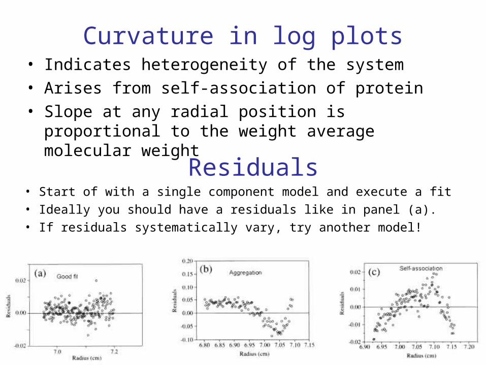
Curvature in log plots• Indicates heterogeneity of the system• Arises from self-association of protein• Slope at any radial position is proportional to the weight

average molecular weight

Residuals• Start of with a single component model and execute a fit• Ideally you should have a residuals like in panel (a).• If residuals systematically vary, try another model!

Lymphotactin

little or no curvature

10 ºC, 200 mM NaCl 40 ºC, 100 mM NaCl

26K

19K

31K

40K

obvious curvature – mass also lost after spin

Direct fitting:Self association at 10 ºC & 200 mM NaCl

10 ºC, 200 mM NaCl

40 ºC, 100 mM NaCl

Effect of salt & temperature on aggregation

Affinity/avidity and function in costimulation

Bivalency: stabilizes complexes ~100-fold

But are B7-1 and B7-2 really different (proposed from crystals) ?

Protein concentration (mg/ml)

6

5

4

3

20 1.0 2.0

Mw

,ap

p(D

a/1

04)

sB7-1

Importance of valency: Dimerization of sB7-1

Importance of valency: sB7-2 & LICOS are monomers

sB7-2 sLICOS

Concentration (mg/ml) Concentration (mg/ml)

Mw(k

Da)

Mw(k

Da)

0 1 2 3 4 0 1 2 3 4

80

60

40

20

0

80

60

40

20

0

1B. Velocity sedimentation

• High centrifuge speed• Forms a sharp boundary between

solute depleted region (at top) and a region of uniform solute concn (at bottom)

• The concentration gradient (dc/dr) defines the boundary position

• Non-linear curve fitting can rigorously determine:– number of mass species – molecular weight – shape information for a

molecule of known mass

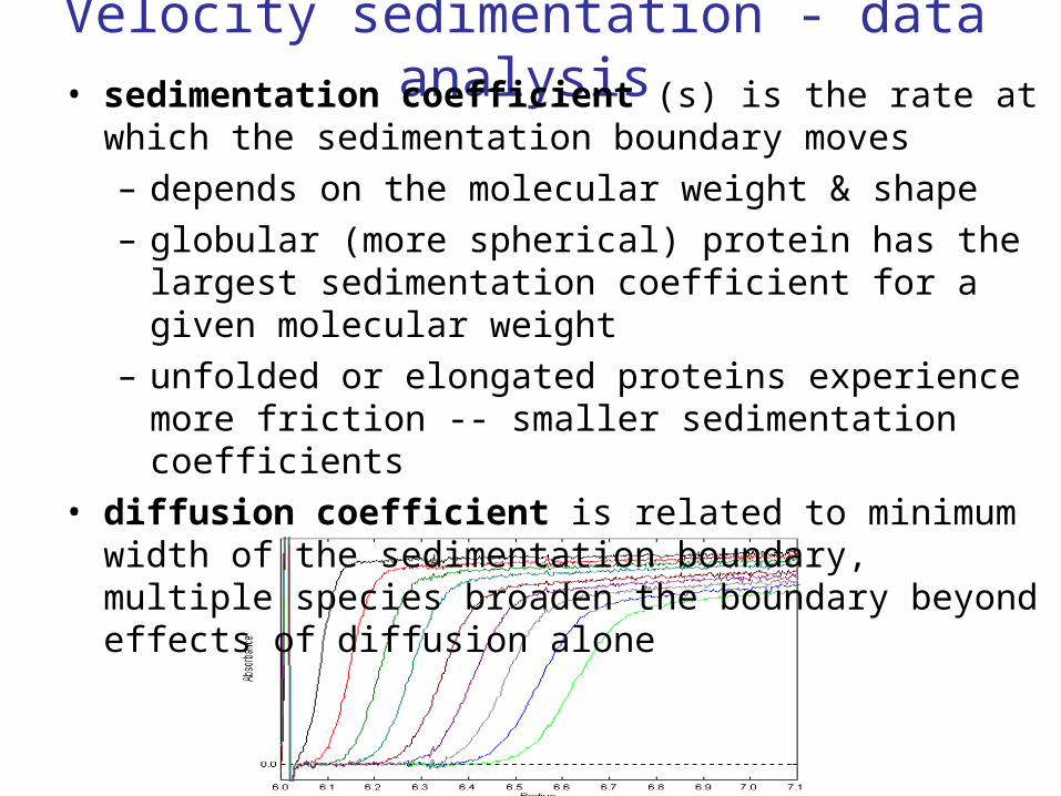
Velocity sedimentation - data analysis• sedimentation coefficient (s) is the rate at which the

sedimentation boundary moves – depends on the molecular weight & shape– globular (more spherical) protein has the largest

sedimentation coefficient for a given molecular weight– unfolded or elongated proteins experience more friction --

smaller sedimentation coefficients• diffusion coefficient is related to minimum width of the

sedimentation boundary, multiple species broaden the boundary beyond effects of diffusion alone

Velocity sedimentation - data analysis

g(s*) distribution

• This antibody gives only one distinct peak, centered at s ~ 6.5 S, which corresponds to the native antibody 'monomer‘. This is low for a 150 kDa species due to its highly asymmetric 'Y' shape.

• However, a more detailed analysis quickly reveals that this sample is not homogeneous. The red curve is a fit of these data as a single species. It does not match the data in the region from 8-12 S, indicating the presence of some multimer.

• From the width of the main peak we can calculate the apparent diffusion coefficient (D) of the monomer. From the ratio of s to D we can calculate a mass of 151 kDa for this species, which matches the known value well within 3-5% error expected for masses determined in this fashion.

Mr RTs

D(1 )

Velocity sedimentation - data analysis

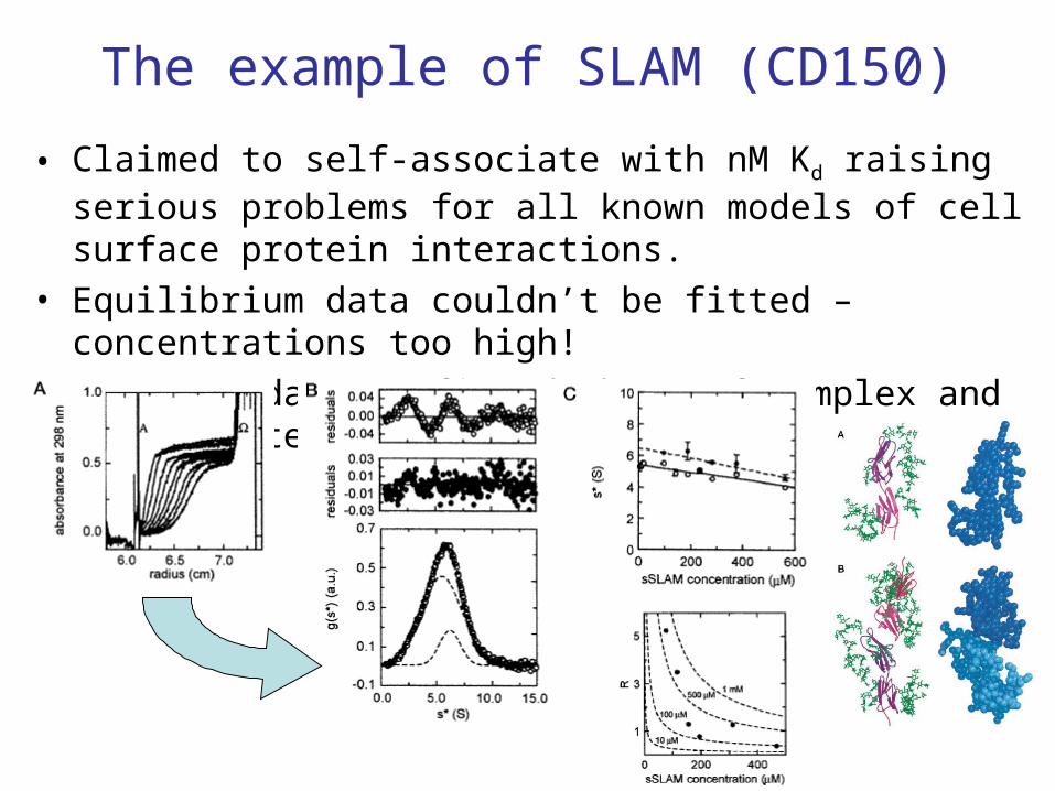
The example of SLAM (CD150)

• Claimed to self-associate with nM Kd raising serious problems for all known models of cell surface protein interactions.

• Equilibrium data couldn’t be fitted – concentrations too high!• Velocity data confirmed shape of complex and approximate

strength of association

2. SPR / BIAcore

(Surface Plasmon Resonance)

What is Surface Plasmon Resonance for?

The accurate measurement of the properties of inter-molecular interactions without a wash step.(Contrast with interaction screens and crude measurements of bond strength e.g. AUC or washed systems like ELISA)

Why use Surface Plasmon Resonance?

A full understanding of the function of proteins requires accurate knowledge of the nature of their interactions.

3D Kd (M)

110100 0.11000

hCD2TCRCD28

CTLA-4KIRCD8SLAM

CD4 rCD2

The range of affinities seen fortransient interactions at the cell

surface

Ab:Ag

Inactive LFA-1 fully active LFA-1fully active Mac-1

Selectins

BIAcore

Why use Surface Plasmon Resonance?

A full understanding of the function of proteins requires accurate knowledge of the nature of their interactions.

Example: Costimulation vs. Inhibition (again!)B7.1 and B7.2 both bind to CD28 and CTLA-4.

BUT

B7.2 & CD28 are constitutively expressed, others on activationB7.1 is dimeric, B7.2 is notCD28, although dimeric, is monovalentCTLA-4 binds its ligands much more strongly than CD28B7.1 binds its ligands more strongly than B7.2

RESULT: The inhibitory B7.1:CTLA-4 complex is ~1000 times more stable than the costimulatory B7.2:CD28 complex.

Principle of Surface Plasmon Resonance

Angle of ‘dip’ affected by:1) Wavelength of light2) Temperature3) Refractive index n2

Dip in light intensity

Surface Plasmon Resonance in the BIAcore

Basic Idea…

NB 4 channels (‘flow cells’) per ‘chip’

2 steps:

• Immobilisation: Stick something (or up to 3 things) to the chip(NB also stick a control down)

• Inject analyte: Inject something else and see if it binds, how much binds and how fast it binds

Immobilisation

2 Main options:• Direct:

Covalently bind your molecule to the chip• Indirect:

First immobilise something that binds your molecule with high affinity e.g. streptavidin / antibodies

Direct: Indirect:

Immobilisation: Carboxymethyl binding

CM5 Sensor Chip

N.B. Carboxymethyl groups are on a dextran matrix: This is negatively charged =>Need to do a “preconcentration” test to determine optimum pH for binding (molecule needs to be +ve)

Immobilisation: Other sensor chips

SA

NTA

HPA

Sensorgrams (raw data)

4.0 4.5 5.0 5.5pH:

Pre-concentration: An antibody was diluted in buffers of different pH and injected over an non-activated chip.Maximum electrostatic attraction occurs at pH 5

15,400 RU

A B C D

Immobilisation: A. Inject 70l 1:1 EDC:NHSB. Inject 7l mAb in pH5 buffer

(in this case @370g/ml)C. Inject 70l EthanolamineD. Inject 30l 10mM Glycine pH2.5

Sensorgrams – ligand binding

“Specific” Binding• Each chip has four ‘flow-cells’• Immobilise different molecules in each flow-cell• Must have a ‘control’ flowcell• ‘Specific binding’ is the response in flow-cell of

interest minus response in the control flowcell

Response in control / empty flowcell due to viscosity of protein solution injected – therefore ‘control’ response DOES increase with concentration (this is NOT binding!!)

Specific response in red flowcell

Measured response

Is it specific?

Equilibrium Binding Analysis

N.B. Measurement of affinities etc. should usually be done at physiological temperature (i.e. 37°C), although this is more difficult.Sometimes 25°C data can be used to compare fold differences in binding or to test for any binding at all (i.e. specificity studies).

0 100 200 300 400 500 600 7000

300

600

900

1200

R.U

.

Time (s)

Equilibrium Binding Analysis - continued

Binding curve can be fitted with a Langmuir binding isotherm (assuming a 1:1 binding with a single affinity)

d

Max

KA

ARBound

][

][

Scatchard plot: rearrangement of binding isotherm to give a linear plot. Not so good for calculating Kd, as gives undue weight to least reliable points (low concentration)

Plot Bound/Free against BoundGradient = 1/Kd

dd

Max

K

Bound

K

R

A

Bound

][

Kinetics

HarderCase:2B4

binding CD48

Potential pitfalls• Protein Problems: Aggregates (common)

Concentration errorsArtefacts of construct

• Importance of controls: Bulk refractive index issuesControl analyteDifferent levels of immobilisationUse both orientations (if pos.)

• Mass Transport: Rate of binding limited by rate of injection: kon will be

underestimated• Rebinding: Analyte rebinds before leaving

chipkoff will be underestimated

Last two can be spotted if measured kon and koff vary with immobilisation level (hence importance of controls)

Less common applications

1. Temperature dependence of binding

van’t Hoff analysis: STHKRTG a )ln(

R

S

TR

HKa

1

)ln(

Gradient

Intercept

Less common applications

1. Temperature dependence of binding

Non-linearvan’t Hoff analysis:

0,0,,, ln)(

00 T

TCTTTCSTHG vHpvHpTvHTvH

Less common applications

2. Combination with mutagenesis

Q30R Q40K R87A

Binding of CD2 by CD48 mutants at 25°C (WT Kd = 40M)

Reduce / abolish bindingDo not affect bindingNot yet tested

Less common applications

3. Estimation of valency

Less common applications

3. Screening

Newer BIAcore machines are capable of high throughput injection. With target immobilised, many potential partners / drugs can be tested for binding.

4. Identification of unknown ligands

Mixtures e.g. cell lysates, tcs, food samples etc. can be injected over a target and bound molecules can then be eluted into tandem mass spectroscopy for identification.

One last warning: take care

CD48 binding to immobilised CD2(van der Merwe et al.)

What a lot of people would have used(straight out of the freezer)

Correct result

3. ITC

(Isothermal Titration Calorimetry)

What is Isothermal Titration Calorimetry for?

The direct measurement of heat released from a reaction (e.g. a binding event) allowing the calculation of thermodynamic parameters (enthalpy & entropy)

Why use Isothermal Titration Calorimetry ?

The thermodynamics of an interaction can give clues to the mechanisms involved. ITC also has the advantage of testing affinity in solution using unlabelled protein (but lots of it!!).

Isothermal Titration Microcalorimetry:

Using the heat of complex formation to report on a binding interaction.

The Basic Experiment:1. Fill the upper syringe with ligand at high

concentrations.2. Fill the larger lower reservoir with protein

at a lower concentration.3. Titrate small aliquots of ligand into protein.4. After each addition, the instrument returns

the reservoir temperature to the temperature of the control cell and measures the heat required to cause this change.

5. Typically, subtract appropriate blank titrations (ligand into buffer & buffer into protein) to control for heats of dilution.

Data Analysis• Get a plot of heat (J or Cal) / s following each injection,

integrate each peak for total heat released and plot against concentration of protein injected – binding isotherm.

c = concn / Kd

Data Analysis – e.g. of B7-1 & CTLA-4• Curve fitting gives values for H (enthalpy) and G (Gibbs

free energy, related to affinity) – from these one can also calculateS (entropy).

0 1 2 3 4

-12

-8

-4

0

kcal/m

ole

of

inje

ctant

molarratio

H = -11.6 G = -8.9 TS = -2.7 kcal/mol-1

Calculating heat capacity• H and S are not constant with temperature, hence direct

measurement by ITC is better than deriving them from binding data across several temperatures (e.g. by SPR)

• Relationship of DH to temperature can be used to calculate heat capacity change on binding (Cp)

TCR recognition

Willcox et al. (1999) Immunity 10:357

TCR recognition

Willcox et al. (1999) Immunity 10:357

4. FRET / BRET

(Forster / Bioluminescence resonance energy transfer)

What is FRET?

• Förster Resonance Energy Transfer– Fluorescence if both Donor and Acceptor are

fluorescent

• Radiation-less energy transition between a Donor and Acceptor occurring finite probability based on proximity

• Energy is transferred through the resonant coupling of the dipole moments of the Donor & Acceptor

The beginning…

• Theodor Förster, 1940s– proposed a mathematical law for dependence of

fluorescence decay of donor (D) on the concentration of acceptor (A), assuming a dipole-dipole interaction in solution (J.Phys.Chem. 1965, 69, 1061-1062)

Exponential decay for one Donor molecule

Impact of FRET

• After the initial fuss about the validity of Förster’s derivations, little else.

• Resurgence in past several years, especially in biology/biochemistry/biophysics thanks to:– FRET capable spectral GFP mutants– Engineering of peptides with novel fluorescent

reagents– Ability to couple this phenomenon to different

imaging techniques– AND the need to “see” finer details

Power of FRET

• Probe macromolecular interactions– Interaction assumed upon fluorescence

decay

• Study kinetics of association/dissociation between macromolecules

• Estimation of distances (?)

• In vitro OR on live cells

• Single molecule studies

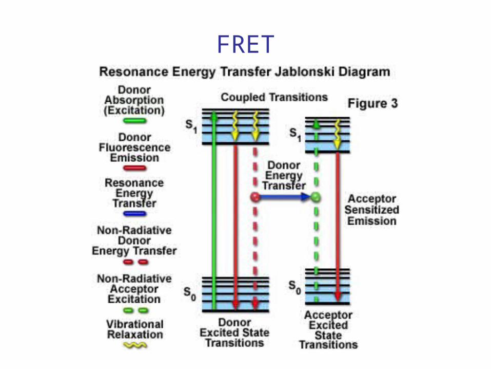
FRET

Effects of FRET

• Intensity of Donor decreases• Sensitized fluorescence of Acceptor

appears upon Donor excitation• Lifetime of Donor excited stated decreases• Polarization anisotropy increases• Taking advantage of these points…

– Curr. Opin. Immun. 2004, 16, 418-427

FRET Efficiency (E)

Measuring FRET efficiency• Measure acceptor emissions – can

be measured in solution, no confoccal but background high due to overlap of frequencies.

• Measure increase in donor emissions after photobleaching acceptor - usually done with high power laser setting in confocal on cell surface molecules.

• FLIM (fluorescence lifetime imaging) – measure lifetime of donor excited state in presence & absence of acceptor.

Live cell FRET imagingDoes CD4 specifically associate with the TCR/CD3 complex on triggering?

Non-specific peptide Specific peptide

• * marks contacts between cells. • High FRET signal between CD4 and CD3 when correct antigen is present but not with non-specific antigen.

DeepBlueC hf1 hf2

Luciferase >10nm

GFP2

BRET: Bioluminescence Resonance Energy Transfer

BRET analysis of human B7-1 dimerizationat the cell surface

B7-1luc:B7-1YFP

CTLA-4luc:CTLA-4YFP

B7-1luc

B7-1luc:CTLA-4YFP

YFP

luc

B7-1YFPB7-1luc

substrateh2 (530 nm)

h1 (470 nm)

BRET Theory

16

0

1

R

rBRET

R0

BRET vs. FRET

BRET analysis can be achieved at physiological levels of protein expression

No problems with photobleaching or photoconversion seen in FRET techinques

Both methods involve the same physical processes and so can be analysed in a similar manner

BRET cannot be used in microscopy-based techniques such as FRAP or FLIP, or FACS-based analysis

Construction of Fusion Proteins

The gene of interest is fused to both luciferase (donor) and GFP (acceptor) in two separate vectors

A positive control is used to determine maximal BRET

B7-Family BRETEnergy transfer can occur solely by random

interactions

Quantitative (F)RET Analysis

Random InteractionsDimer Interactions

As more acceptors are present at the cell surface, BRET increases as more donors are paired with an acceptor, to the point where every donor is productively paired (saturation)

Decreasing the numbers of donors does not affect average distance between donors and acceptor molecules

Quantitative BRET Analysis

The relative ratio of the luciferase (donor) and GFP (acceptor) can be systemically varied at a constant total surface expression

Energy transfer from oligomeric interactions are predicted to depend on this ratio in a hyperbolic manner

Random interactions should be insensitive to these changes in ratio

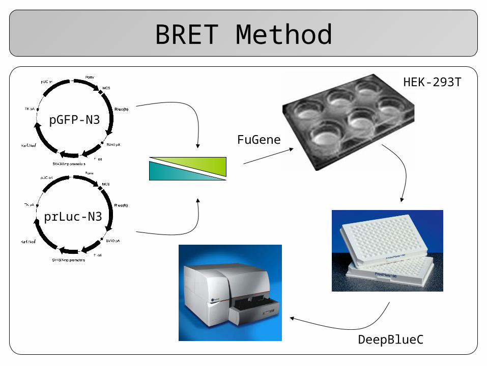
BRET Method

pGFP-N3

HEK-293T

prLuc-N3

FuGene

DeepBlueC

Comparison to T cell surface molecules with known oligomerisation status!

Strong dimers

Weak dimer

Monomers

T Cell Interactions

Goodness of fit to the two alternative models clearly demonstrates CD86 is monomeric

Ligand binding causes specific increase in dimerisation

0 1 2 3 4 50.0

0.1

0.2

0.3

0.4

0.5

BR

ET

Rat

io

GFP / Rluc

hCD80 - CTLA-4 hCD80 + CTLA-4 hCD86 - CTLA-4 hCD86 + CTLA-4

Specific ligand engagement can be observed when receptor is presented in solution or cell-surface bound

GPCRs Are Likely To Be Monomeric

Two GPCRs exhibit no dependence on the acceptor:donor ratio

Equivalent BRET is seen when GPCR is co-expressed with CD2, demonstrating random interaction

A BRET survey of the T cell surface

The majority of T cell surface molecules are monomeric at the cell surface

5. Single molecule microscopy

Single Molecule Spectroscopy

T cell activation occurs at the level of single molecules, i.e., TCR complex binding to pMHC

There are almost no methods to probe cell surface to this level of detail in living cells, or to deal with complexes larger than the 10nm limit of FRET/BRET

Need to understand the interactions that occur in order to build a realistic model of T cell activation

New therapeutic agents may rely more and more on targetting our immune response by precisely altering these interactions

Single Molecule Spectroscopy

10 fl (10-8l)0.25m2 of cell surface

Single Molecule Method

Antibodies are fragmented to Fabs and labelled with bright fluorescent dyes, Alexa 488 and Alexa 647

T cell hybridomas are incubated with labelled Fabs to saturation

Two lasers are focussed on the apical membrane of cell

Movement of Fab-labelled molecules can be recorded in real time to single molecule precision

Single Molecule Confocal Microscopy

10 fl (10-8l)0.25m2 of cell surface

Controls for Coincidence Detection

No peaks are observed without Fab labels

Fab binding was specific to Vb8 TCR

Fluorescence was only detected at the proximal and apical membranes

PFA-fixed cells displayed constant fluorescence

Changes in laser power did not affect results

TCR complex diffused at expected rate

Blocking internalisation did not alter signal observed

Coincident events can be detected

Molecules in complex have higher coincidence

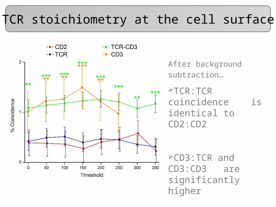
TCR stoichiometry at the cell surface

After background

subtraction…

TCR:TCR coincidence is identical to CD2:CD2

CD3:TCR and CD3:CD3 are significantly higher

Total Internal Reflection Microscopy

Extension of coincidence detection using TIR microscopy, allowing tracking of molecules in real time

Models of T cell activation can be directly tested

Techniques you may need…

• Probing molecular interactions: SPR

• Probing homodimeric interactions: AUC

• Probing size & shape of complexes: AUC

• Probing detailed thermodynamics: ITC

• Probing oligomerisation state or associations in cell or on their surface: FRET / BRET

• Probing for longer range associations or assocaitions between things you can’t make: single molecule microscopy