Structural Recovery in Second-growth Forests on Lyell Island, Haida Gwaii

Final Technical Report

FSP Project Y092147

April 30th

, 2009

Audrey F. Pearson

Ecologia

#3 – 2475 W. 1st Ave.,

Vancouver BC V6K 1G5

ph (604) 732-1256

email: ecologia@telus.net

2

Abstract

The keystone value for biodiversity in forests is structure. Second-growth forests have very

simplified structure compared to old-growth forests, but how to best restore structural and

compositional complexity is not well known and we have few baselines. In order to determine

the effectiveness of stand-level attributes for maintaining biodiversity, we need baseline

information for such assessments. Spatially-referenced data for assessing trends in biodiversity

are rare globally, especially in comparison with original old-growth forest reference conditions.

In order to investigate these questions, I gathered field-based measures of forest structure and

composition for riparian and upland forests in three eras of logging; pre-1937; 1937-1966 and

1966-1987 as well as information from old-growth control sites. Cedar is regenerating in old

second-growth forests, establishing from 1880s to 1980. Contrary to what is commonly thought

despite the presence of introduced deer, cedar has been regenerating in second-growth forests on

Lyell Island over the past century. Further, cedar is regenerating on sites that were originally

old-growth cedar. Culls were left standing rather than cut so there are often abundant living

residual trees and large snags. Understory species are abundant on stumps in old second growth.

As a consequence, second-growth forest structure is highly variable, especially in the riparian

zone, as a function of logging methods and residual trees and contains higher values for

biodiversity than is generally recognized.

Introduction

In forests, disturbances create and maintain structure and structural diversity, the keystone

elements for biodiversity, including provision of habitats and functions (Franklin et al. 2002).

Second-growth forests are generally considered to have simplified structure in comparison to

old-growth forests. However, that view is largely based on the effects of modern clearcutting as

a disturbance agent, where all standing trees and snags were removed over large areas, usually at

the same time. For logging that prior to the modern era, such as A-framing and early truck

logging, widespread areas were not necessarily clearcut. The logging techniques at the time did

not have that capacity to do so and frequently there was no desire to take all the trees. Often,

3

specific sizes or species (such as “airplane” spruce) were taken and the remaining forest left

standing. Second-growth forests that generated from logging prior to the modern era may

contain residual structures, which we now recognize have high biodiversity value.

The purpose of this project is to provide baseline data on second-growth structural and

compositional recovery for both tree and understorey species (defined as ecosystem recovery) in

riparian and upland forests. We have do not have a good understanding of the habitat potential of

second-growth forests, including riparian forests, or reference data for determining targets for

restoring structural complexity and compositional diversity associated with the original old-

growth forests in second-growth forests. Many of our riparian areas in coastal BC are second-

growth because those forests had the most accessible, highest volumes of timber and were

logged first. However, these are also the most productive forest sites so the greatest potential for

ecosystem recovery, especially since they are often our oldest second-growth. The Millennium

Ecosystem Assessment, an analysis of the state of the world’s ecosystems, concluded there were

virtually no environmental baseline data - essential for accurately assessing conditions and trends

in biodiversity over time (Millennium Ecosystem Assessment 2005). In order to determine the

effectiveness of stand-level attributes for maintaining biodiversity, we need such baseline data on

stand-level attributes to develop targets and management guidelines.

Methods

Study area

Tllga Kun Gwaay.Yaay, Lyell Island, is located in Gwaii Haanas National Park Reserve and

Haida Heritage Site on Haida Gwaii (The Queen Charlotte Islands) (Fig 1), the traditional

territory of the Haida Nation. Lyell Island is situated in the Skidegate Plateau (Holland 1976),

the most productive physiographic region on Haida Gwaii for forests. Further, Lyell is a large

island (17,300 ha) with a diverse topography and range of sites and forest types.

The region has a typical coastal climate. Mean annual temperature is 8oC and days below 0

oC

are rare (Environment Canada 1993). Total precipitation ranges from 1000–4500 mm,

4

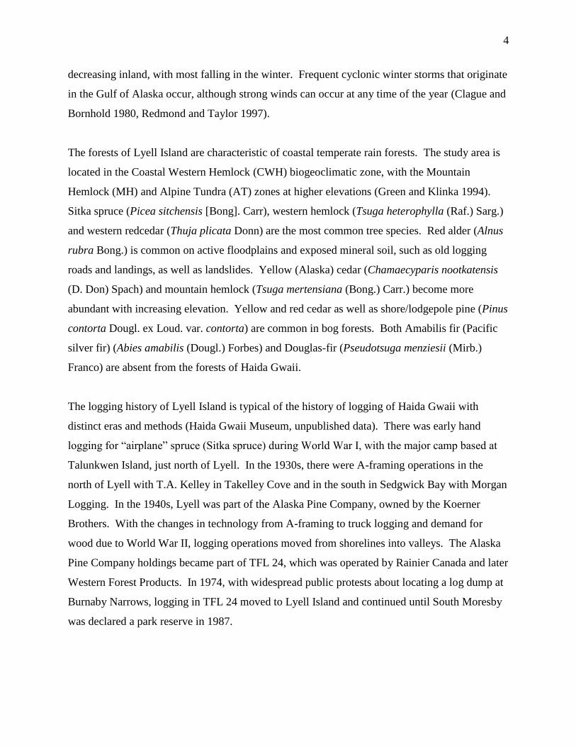
decreasing inland, with most falling in the winter. Frequent cyclonic winter storms that originate

in the Gulf of Alaska occur, although strong winds can occur at any time of the year (Clague and

Bornhold 1980, Redmond and Taylor 1997).

The forests of Lyell Island are characteristic of coastal temperate rain forests. The study area is

located in the Coastal Western Hemlock (CWH) biogeoclimatic zone, with the Mountain

Hemlock (MH) and Alpine Tundra (AT) zones at higher elevations (Green and Klinka 1994).

Sitka spruce (Picea sitchensis [Bong]. Carr), western hemlock (Tsuga heterophylla (Raf.) Sarg.)

and western redcedar (Thuja plicata Donn) are the most common tree species. Red alder (Alnus

rubra Bong.) is common on active floodplains and exposed mineral soil, such as old logging

roads and landings, as well as landslides. Yellow (Alaska) cedar (Chamaecyparis nootkatensis

(D. Don) Spach) and mountain hemlock (Tsuga mertensiana (Bong.) Carr.) become more

abundant with increasing elevation. Yellow and red cedar as well as shore/lodgepole pine (Pinus

contorta Dougl. ex Loud. var. contorta) are common in bog forests. Both Amabilis fir (Pacific

silver fir) (Abies amabilis (Dougl.) Forbes) and Douglas-fir (Pseudotsuga menziesii (Mirb.)

Franco) are absent from the forests of Haida Gwaii.

The logging history of Lyell Island is typical of the history of logging of Haida Gwaii with

distinct eras and methods (Haida Gwaii Museum, unpublished data). There was early hand

logging for “airplane” spruce (Sitka spruce) during World War I, with the major camp based at

Talunkwen Island, just north of Lyell. In the 1930s, there were A-framing operations in the

north of Lyell with T.A. Kelley in Takelley Cove and in the south in Sedgwick Bay with Morgan

Logging. In the 1940s, Lyell was part of the Alaska Pine Company, owned by the Koerner

Brothers. With the changes in technology from A-framing to truck logging and demand for

wood due to World War II, logging operations moved from shorelines into valleys. The Alaska

Pine Company holdings became part of TFL 24, which was operated by Rainier Canada and later

Western Forest Products. In 1974, with widespread public protests about locating a log dump at

Burnaby Narrows, logging in TFL 24 moved to Lyell Island and continued until South Moresby

was declared a park reserve in 1987.

5

Sampling design

Sampling was focused on four areas 1) Windy Bay (old-growth control) and Gate Creek (old-

growth in 1937 and logged in 1966; 2) Sedgwick Bay (old-growth in 1937 and logged in 1966;

logged post 1966); 3) Powrivco Bay (old-growth in 1937 and logged in 1966; logged post 1966)

and 4) Takelley Cove (logged pre-1937 and logged post 1966) (Fig 2).

Field methods

There were two types of field data – transects and stand structure and composition plots. Field

methods followed standard methods (Spies and Franklin 1991, Lertzman et al. 1996) We

established 9400 m of second-growth tree transects and 50 detailed stand structure plots (Tables

1 and 2). There were no riparian forests that were old-growth in 1966 and now logged that were

accessible. Transects, 10 m wide, were established in the polygon of interest following a

compass bearing that traversed the polygon while avoiding any potential bias (e.g. traversing

rather than along a slope contour, variable distance from the stream etc.) All living trees > 1.4 m

in height within the 10m transect were surveyed for species and dbh for alternating 50 m transect

segments.

Each stand structure plot was a 500m2

circular plot divided into four quadrants. The dbh and

canopy layer of all trees > 1.4 m high were measured for the entire plot. The height of small trees

(understorey, suppressed) were measured for the first quadrant. The heights of large trees were

measured for the first two quadrants. We cored all second-growth cedar trees that occurred

within the plot. Decay class, diameter, species and height (snags) or length (coarse woody

debris) were recorded. If the dead wood originated from logging (stump or log) was also

recorded. Decay classes followed standard wildlife tree classifications. Seedlings (trees < 1.4 m

high) were tallied by height class (< 10 cm and > 10 cm) and species in five 1 m2 randomly

located subplots. Total numbers of all understorey species (shrubs, herbs, mosses) were recorded

in the 1 m2 subplots. Understorey species were also tallied for the first ten stumps encountered in

the plot.

6

The objectives of the analyses were to characterize second-growth stand-level attributes. I

explored for patterns in the input variables (riparian/upland, logging and forest type) to

determine any significant relationships in second-growth structure and composition and how

values compare to the old-growth control. Forests with the largest trees (live and dead) have the

highest standard deviation in dbh (Spies and Franklin 1991). Thus, maximum tree size and mean

and standard deviation of tree, snag and wood diameter were explored between the forest types.

Cedar cores

(Prepared by Sonya Powell)

One hundred and fifty six western red cedar trees and were cored. All increment cores were

mounted and dried on wooden supports and sanded with a belt sander using successively finer

sand paper to 400 grit (Stokes and Smiley, 1968). Rings were visually crossdated using the list

method and each tree was assigned a calendar year for the innermost ring or the pith

(Yamaguchi, 1991; Swetnam et al., 1985). To assess the age structure of second growth trees,

tree ages were calculated using the following equation (Wong and Lertzman, 2001):

Agetotal = Agecore height + eestimate of missing/false rings + eestimate of years to pith + hc [1]

Where:

eestimate of missing/false rings = the estimated number of false and missing rings found by visual

crossdating procedures.

eestimate of years to pith = the estimated number of years from the last full measured ring to the

pith.

hc = number of years required to reach core height

For cores that intercepted the pith, eestimate of years to pith was zero and age was calculated

using the following equation:

Age core height = 2007 – pith year + 1 [2]

For tree cores that do not contain the pith, Duncan’s (1989) method was used to

approximate the number of missing rings using the following equation:

Number of rings to pith = eestimate of years to pith = [L2/8H] + H/2 [3]

X

Where:

L = length of the innermost incomplete ring on the core

7

H = height of the innermost incomplete ring on the core

X = mean ring width of three rings adjacent to the innermost incomplete ring

This equation estimates the number of rings from the last complete ring observed on the

increment core to the pith. The calculated number of missed rings was added to the number of

rings visible to estimate the age of the tree at core height. In the cases where the arcs are really

wide and the heights of the arcs are low, accuracy decreases and number of rings are over

estimated.

Core height was 0.3 meters from the point of germination. The number of years required for a

seedling to reach core height, or hc at 0.3 m, is unknown. A red cedar seedling or sapling can

exist in a suppressed state in the understory below breast height for decades to centuries before a

disturbance increases light availability, at which point the sapling can accumulate basal and

lateral growth, thus "release" (Passmore, 2007). In this study, we assumed hc = 0 since we do not

have a seedling-to-core-height correction factor.

Results

Understorey species

Understorey species show a strong response to stumps as growing sites, especially for species >

10 cm in height (Table 3). This is especially the case of shrubs. Despite the second-growth

forests ranging in age from 50 – 70 years (so “closed canopy” conditions), understorey species

are present on stumps in the closed canopy. These “stump” refugia contribute to the overall

diversity in second-growth forests and are potentially a focus for restoration efforts. The

understorey species may eventually be shaded out with canopy closure over time.

Second-growth forest structure

There is a broad range in values of tree diameters in the second-growth tree transects (Table 4).

With three exceptions, all second-growth transects have a maximum tree dbh > 100 cm, while

the exceptions have a maximum tree dbh > 80 cm. Living residuals of all species are a

significant component of second-growth stands. The extent of residual structure is second-

8

growth forests is also evident on the 1966 forest cover maps. According to the forest cover

maps, the total area logged (including before 1937) is 3170 ha; of that 617 ha (20%) is marked as

polygons containing vets. The area logged between 1937 and by 1966 is 2336 ha; of which 600

ha (25%) is polygons containing vets. However for areas logged before 1937 (834 ha), there was

only 17 ha or 2% of the areas with vets – an order of magnitude less than post 1937.

One of the defining characteristics of old-growth forests is structural diversity, which can be

described statistically as large standard deviations. The results from this study are no exception,

with old-growth forest trees having the highest standard deviation for both riparian and upland

sites (Table 5). However, the oldest second-growth (logged pre-1937) does not contain the

second-highest values even though they are the second oldest forests. In the oldest second-

growth riparian plots, 70% of the trees were alder. In the upland sites, only 17% were alder but

the average dbh exceeded that of the conifers. For the old second-growth sites (logged 1937-

1966), alder was 9.5% of trees in the riparian forests and 5.6% in the upland forests. The

average dbh in the second-growth riparian forests exceeded that of the old-growth sites, although

standard deviation is only half. The average dbh of the old second growth conifers in riparian

forests also exceeded that of the oldest second-growth, despite being similar sites and the old-

second is at minimum 20 years younger. The extent of alder in the oldest second-growth riparian

sites is affecting conifer re-establishment. However, all the oldest second-growth forest areas

were typed as “deciduous” on the modern forest cover maps. Despite the abundance of alder,

there are conifers regenerating.

The differences between old-growth and second-growth forests were more pronounced with the

snags but not with the coarse debris (Tables 6 and 7). There were fewer snags in the old-growth

forests, but they were larger and taller than the other forest types. Again, the old second-growth

riparian forest (logged between 1937 and 1966) and the highest values (mean snag height and

standard deviation) next to the old-growth sites although the old second-growth riparian forest

had three times the density of snags of the old-growth riparian forest. While the old-growth

riparian sites had the largest mean and standard deviation of coarse woody debris, the differences

with the other forest types were not as pronounced as with the vertical structure (trees and

snags).

9

Establishment and extent of second-growth cedar

A total of 156 cores were used to contribute to age data at fifteen second-growth sites on Lyell

Island, (Table 8). The majority of tree cores showed evidence of fast initial tree growth,

indicating high light and open canopy conditions at the time of seedling establishment. No trees

showed narrow tree rings close to the pith, indicating that none of the samples were advanced

regeneration and all samples germinated from seed post-harvest.

Tree ages varied within and among sites. No species-specific landscape-level master

chronologies for Haida Gwaii are available at this time for comparison against sampled tree-ring

series. The sample depth per site, length, and quality of cores collected was not sufficiently

robust to create highly intercorrelated master chronologies. Age data were garnered from visual

crossdating which is less accurate than statistical crossdating. Data have been sorted into cores

which correlate well with other cores from the same site and thus are high quality (HQ) vs cores

which do not correlate well, cores from sites with low sample sizes, and cores which are broken

and missing information which give us only a minimum estimate (ME) of tree age (Table 8).

The majority of cores (106) were of high quality and fewer cores (51) provided minimum age

estimates only. Should a species-specific landscape-level master chronology for Lyell Island be

created or become available, the proportion of high quality cores could be increased.

The earliest high quality western red cedar innermost ring years were 1881 and 1885 from site

32. Red cedar establishment on Lyell Island ranged from the late 19th

century to the present with

most recent establishment occurring at site 14 where all trees established post-1980. A pulse of

establishment following 1940 occurred and establishment continued until the present with a

second pulse of establishment occurring following 1980 (Fig. 3). The majority of trees sampled

established post-1940. Given that cores were taken at 30 cm above the point of germination (hc),

these trees initiated growth prior to these dates, however the amount of error is yet unknown.

Since trees showed rapid initial growth, the amount of error is likely low and within 10 years of

the pith date.

10

There is further evidence of the extent of cedar in second-growth forests on the 1966 forest cover

maps. There is 3170 ha of second-growth on the forest cover maps (areas logged by 1966). Of

that second-growth, 295 ha are cedar-leading, 512 ha cedar as a second-species, 622 ha cedar

third for a total of 1429 ha or 45% of the second-growth contains cedar according to the forest

cover map. However, for areas logged before 1937, the polygon area containing cedar is 17%

but between 1937 and 1966, the area is 55%. Density of cedar appears to have actually increased

in second-growth forests with time, which is counterintuitive given the population of introduced

deer has increased with time. Further, of the second-growth polygons containing cedar, 63.3%

were cedar-leading for the corresponding old-growth area as determined from the original forest

cover on the 1937 air photos, 24.6% were cedar as second-species and 16.4 were cedar as third

species. Cedar does appear to be regenerating after logging on sites where it originally occurred.

Discussion

There is abundant and diverse residual structure in second-growth forests on Lyell Island, which

is supported by results for both field measures and values in GIS database. Understorey species

persist on stump refugia. The canopy is not universally closed and the understorey universally

depauperate. There are large residual trees and snags, especially in second-growth riparian

forests. Second-growth forests are not monolithic but their structure and composition are a

result of past disturbances and since past logging practices have varied, so too does second-

growth structure. This aspect of second-growth forest ecology needs to be considered in

management, especially for second-growth riparian forests which potentially have high value for

biodiversity.

Western red cedar regenerated in second growth stands on Lyell Island, beginning in 1881 and

continuing to the present. This finding is counter to the idea that cedar regeneration ceased once

deer were introduced. Future work to further refine these findings and determine spatial and

temporal patterns in second-growth cedar regeneration could include:

1. Collect 20 to 30 red cedar cores at the Windy Bay old growth control site to

create a species-specific master chronology.

11

2. 10 to 20 old growth red cedar cores of adjacent to each harvested site must be

collected in order to create site-specific master chronologies.

3. These data can be combined with the Windy Bar old growth master

chronology to create a landscape-level master chronology which can be used to

estimate the number of missing or false rings (eestimate of missing/false rings) in each

individual tree ring series by statistical crossdating procedures.

4. Seedlings must be used to estimate a seedling-to-core-height correction factor

(hc), the number of years it takes a seedling to reach core height at 30

centimeters (Veblen et al., 1991). Since we found fast growth near the pith in

most samples, I recommend collecting and examining the age of thirty -30 cm

tall red cedar seedlings growing in open conditions

5. Core trees as close to the point of germination as possible (hc = 0) to determine

if regeneration in second growth stands was due to growth of seed stock or

advanced regeneration.

By completing studies 1 we could create a lengthy and robust species-specific master

chronology. By completing study 2, we would be able to determine age structures, stand history,

and stand dynamics at each site. By completing study 3, we could examine landscape-level

climate-driven signals in the tree ring record. These signals would be present in the second-

growth tree ring record and could then be excluded from the analysis, making the stand dynamic

signals more clear. Old-growth master chronologies could also be applied to cross-dating

culturally modified trees. By investigating age to core height in study 4, we could add a

correction value to our innermost ring estimates thus increasing the precision of our individual

tree and stand age estimates. Question 5 can be answered by examining the initial growth (near

the pith) of regenerated red cedar. Red cedars that regenerate from seed following the harvesting

event will have wide innermost rings indicating that they are growing in open-canopy and high

light conditions. Individuals which have grown as advanced regeneration have very suppressed

tree rings near the pith indicating low-light and closed canopy conditions. The suppression is

typically released following the year of harvest when light resources increase substantially and

the individual can sequester and store large amounts of carbon, thus increasing its biomass.

12

Conclusions and management implications

There are several management implications from the results of this study. First, there is a

diversity of forest structure in second-growth forests (both living trees and snags) and

understorey species still persisting on old stumps. There is a wide range of potential treatments

for restoration of structural and compositional diversity using these residual structures, such as

opening the canopy around residual stumps to ensure the understorey species are not shaded out,

retention of large snags and wood, underplanting conifers, especially in the oldest-second growth

forest types. Areas logged pre-1937 need to be re-typed to more accurately reflect the current

forest cover between alder and conifer trees, especially in upland forests. Any planning for

restoration based on the current forest cover maps will not accurately assess the current state of

ecosystem recovery.

Second, cedar has been regenerating in second-growth forests on Lyell Island for approximately

100 years, despite the introduction of deer about a century ago. Further, cedar is regenerating on

sites that originally were old-growth cedar forests and the regeneration began after logging, not

from residuals released during the logging operation. Lyell Island has a complex topography and

not all areas would be readily accessible to deer. Further, it is a considerable distance from the

location of the first introduction on Massett Island (far northern tip of Haida Gwaii). The

relationship between deer and extent of cedar regeneration is more complex than original

thought, with distance from the introduction, time since introduction and site being factors. It is

not simply a matter that all cedar seedlings were browsed once the deer arrived.

Literature Cited

Clague, J. J., and B. D. Bornhold. 1980. Morphological and littoral processes of the Pacific Coast

of Canada. Pages 339-380 in S. B. McCann, editor. The Coastline of Canada. Geological

Survey of Canada.

Environment Canada 1993. Canadian Climate Normals: 1961 - 1990. Atmospheric Environment

Service, Ottawa, Ontario.

Franklin, J. F., T. A. Spies, R. v. Pelt, A. B. Carey, D. A. Thornburgh, D. R. Berg, D. B.

Lindemayer, M. E. Harmon, W. S. Keeton, D. C. Shaw, K. Bible, and J. Chen. 2002.

Disturbances and structural development of natural forest ecosystems with silvicultural

implications, using Douglas-fir forests as an example. Forest Ecology and Management

155:399 - 423.

13

Green, R. N., and K. Klinka. 1994. A field guide to site identification and interpretation for the

Vancouver Forest Region. Land Management Report 28, BC Forest Service, Victoria BC.

Holland, S. S. 1976. Landforms of British Columbia: A Physiographic Outline. Bulletin No. 48,

BC Department of Mines and Petroleum Resources, Victoria, BC.

Lertzman, K. P., G. D. Sutherland, A. Inselberg, and S. C. Saunders. 1996. Canopy gaps and the

landscape mosaic in a coastal temperate rainforest. Ecology 77:1254 - 1270.

Millennium Ecosystem Assessment 2005. Millennium Ecosystem Assessment Synthesis Report.

United Nations, New York, NY.

Passmore, J. 2007. Response of Seedlings and Saplings in Canopy Gaps to Coastal Old Growth

Forests. Masters Thesis. Submitted to: Simon Fraser University. Burnaby, BC

Redmond, K., and G. Taylor. 1997. Climate of the Coastal Temperate Rain Forest. Pages 25-42

in P. K. Schoonmaker, B. von Hagen, and E. C. Wolf, editors. The Rain Forests of Home:

Profile of a North American Bioregion. Island Press, Washington DC.

Spies, T. A., and J. F. Franklin. 1991. The structure of natural, young, mature and old-growth

Douglas-fir forests in Oregon and Washington. Pages 91 - 109 in L. F. Ruggerio, K. B.

Aubry, A. B. Carey, and M. H. Huff, editors. Wildlife and Vegetation of Unmanaged

Douglas-fir Forests. USDA Forest Service, Portland, OR.

Stokes, M. A. and T. L. Smiley. 1968. An Introduction to Tree Ring Dating. University of

Chicago Press. Chicago, Illinois, USA.

Swetnam, T. W., Thompson, M. A., and E. K. Sutherland. 1985. Using dendrochronology to

measure radial growth of defoliated trees. U.S. Dept. of Agriculture, Forest Service,

Cooperative State Research Service, Washington, D.C.

Veblen, T. T., Hadley, K. S., Reid, M. S., and A. J. Rebertus. 1991. The response of subalpine

forests to spruce beetle outbreak in Colorado. Ecology 72: 213-231

Wong, C. M. and K. P. Lertzman. 2001. Errors in estimating tree age: Implications for studies of

stand dynamics. Canadian Journal of Forest Research 31: 1262-1271

Yamaguchi, D. 1991. A simple method for cross-dating increment cores from living trees.

Canadian Journal of Forest Research 21: 414-416

14

Table 1. Transects established by forest type and total distance.

Category Forest type Total distance

(m)

old 1966 logged now upland 1200

old growth control riparian 500

upland 1250

old growth control Total 1750

old second growth (logged

1937-1966)

riparian 2100

riparian/upland 2400

upland 750

old second growth Total 5250

oldest second growth (logged

pre-1937)

riparian 450

upland 750

oldest second growth Total 1200

TOTAL all transects 9400

Table 2. Plots established by forest type.

Category

Forest

type No of Plots

old growth control riparian 4

upland 4

oldest second growth riparian 6

(logged pre-1937) upland 9

old second growth riparian 12

(logged 1937-1966) upland 8

young second growth upland 7

(logged 1966-1987)

Grand Total

50

Table 3. Density (number per m2) of understorey species (herbs, tree seedlings, shrubs and all species) for forest floor and stumps for

old-growth and second-growth forests.

Forest type,

era of

logging and

substrate

Herbs

(# per m2)\

Seedlings

(# per m2)

Shrubs

(# per m2)

Total all understorey

species

< 10cm

ht

>10cm ht < 10cm ht >10cm ht < 10cm ht >10cm ht < 10cm ht >10cm ht

Old-growth

forest floor

2.35 0.75 11.35 1.58 4.78 0.78 18.48 3.10

Second-

growth pre-

1937 forest

floor

2.36 0.08 0.00 0.04 0.12 0.00 2.48 0.12

Second-

growth pre-

1937 stumps

1.33 2.53 0.07 0.20 0.07 2.80 1.47 5.53

Second-

growth 1937-

1966 forest

floor

1.73 0.67 0.27 0.20 0.67 0.20 2.67 1.07

Second-

growth 1937

-1966 stumps

0.00 0.45 0.00 0.45 0.15 2.54 0.15 3.43

Second-

growth post

1966 forest

floor

8.00 1.60 4.20 2.50 8.50 0.20 20.70 4.30

Second-

growth post-

1966 stumps

0.00 0.16 1.11 0.95 7.78 2.62 8.89 3.73

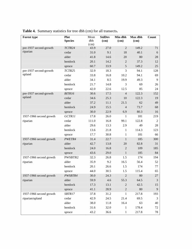
Table 4. Summary statistics for tree dbh (cm) for all transects.

Forest type Plot

Species

Mean

dbh

(cm)

StdDev

(cm)

Min dbh

(cm)

Max dbh

(cm)

Count

pre-1937 second-growth

riparian

TCTR24 43.9 27.0 2 149.2 71

cedar 31.0 9.1 18 40.1 6

alder 41.8 14.6 20 80 28

hemlock 20.1 14.2 2 37.3 12

spruce 60.7 33.9 5 149.2 25

pre-1937 second-growth

upland

TCTR25 32.9 18.3 3 94.1 128

cedar 33.8 16.8 10.2 94.1 69

alder 34.1 8.5 19.9 49.3 9

hemlock 21.7 14.8 3 69 26

spruce 42.0 22.6 12.5 85 24

pre-1937 second-growth

upland

BITR16 30.6 17.5 4 122.3 152

cedar 34.6 25.3 10 122.3 19

alder 37.2 11.1 21.5 62 49

hemlock 24.9 15.5 4 73.7 68

spruce 30.0 22.9 6.9 80.3 16

1937-1966 second growth GCTR11 17.8 26.0 1 181 219

riparian cedar 111.0 16.8 99.1 122.8 2

alder 29.6 13.3 2.9 49 28

hemlock 13.6 21.8 1 114.3 123

spruce 17.7 30.8 1 181 66

1937-1966 second growth PWETR4 31.4 22.7 1 185 300

riparian alder 42.7 13.8 20 82.8 31

hemlock 24.0 16.8 2 109 185

spruce 43.6 29.0 1 185 84

1937-1966 second growth PWSBTR2 32.3 26.8 1.5 174 194

riparian alder 35.9 9.2 16.5 56.4 52

hemlock 20.1 26.6 1.5 174 77

spruce 44.0 30.5 1.5 115.4 65

1937-1966 second growth PWSBTR4 30.0 24.3 2 80 27

riparian alder 59.9 4.6 55.3 64.5 3

hemlock 17.3 13.1 2 42.5 15

spruce 41.1 28.9 2 80 9

1937-1966 second growth SBTR17 37.8 31.2 1 217.8 193

riparian/upland cedar 42.9 24.5 21.4 69.5 3

alder 38.0 11.8 16.4 63 40

hemlock 31.6 32.0 1 178.4 72

spruce 43.2 36.6 1 217.8 78

17

Forest type Plot

Species

Mean

dbh

(cm)

StdDev

(cm)

Min dbh

(cm)

Max dbh

(cm)

Count

1937-1966 second growth

riparian/upland

SBWTR22 33.4 18.2 7 102.8 134

cedar 53.9 33.5 27 102.8 4

alder 43.6 11.8 26.8 69.8 21

hemlock 30.6 16.0 8.5 87 88

spruce 31.4 23.4 7 99.7 21

1937-1966 second growth

riparian/upland

SITR18 35.9 27.2 3.5 125.8 70

cedar 20.2 1.6 19 21.3 2

alder 51.7 15.9 38.5 72.7 4

hemlock 27.3 19.8 3.5 104.8 46

spruce 55.8 34.9 19.7 125.8 18

1937-1966 second growth

upland

PWERCTR6 18.5 22.7 2 140.5 126

cedar 27.9 34.9 4 140.5 24

alder 16.3 12.7 5.9 51 10

hemlock 15.1 18.0 2 128.2 87

spruce 38.4 19.7 14.5 61 5

1937-1966 second growth

upland

PWRCT7 30.2 38.5 2 181 70

cedar 88.2 72.2 14.5 181 9

alder 24.3 5.9 18.7 33.4 5

hemlock 19.9 17.7 2 75 54

spruce 61.6 74.2 9.1 114 2

1937-1966 second growth

upland

PWSBT5 27.2 15.8 6.5 80.5 66

alder 29.5 n/a 29.5 29.5 1

hemlock 22.6 14.3 6.5 80.5 49

spruce 41.1 12.5 22 66.2 16

old-growth

riparian

WBTR10 42.8 52.9 1 305 125

cedar 157.1 151.6 2 305 3

alder 51.4 17.6 26.2 65 6

hemlock 36.9 41.5 1 208 103

spruce 59.4 79.8 1 242 13

old-growth

upland

WBTR13 15.5 26.5 0.5 179.7 448

cedar 26.2 20.4 4 58.5 6

alder 37.5 15.7 5.8 54 9

hemlock 12.7 21.8 0.5 108.5 376

spruce 29.8 44.8 0.5 179.7 57

old-growth

upland

WBTR14 33.3 51.4 1 340 194

cedar 160.6 127.5 28.2 340 7

alder 47.6 10.3 35.7 54 3

hemlock 20.8 27.5 1 123.5 161

spruce 80.3 68.0 8 226.5 23

Table 5. Summary statistics for tree diameter for all forest types for riparian and upland forests.

Forest type Site type Species Tree dbh mean+ sd (cm) Count

Old-growth riparian all 34.7 + 56.5 72

upland all 44.6 + 58.4 71

Oldest second-growth

(logged pre-1937)

riparian alder 38.3 + 10.3 43

conifer 33.2 + 24.1 19

all 36.8 +16.0 62

upland alder 44.3 + 12.8 17

conifer 32.6 +19.6 162

all 33.7 + 19.3 179

Old second-growth

(logged 1937-1966)

riparian alder 38.8 + 7.3 16

conifer 43.6 + 25.1 153

all 43.2 + 24.0 169

upland alder 34. + 8.5 15

conifer 28.7 + 18.6 250

all 29.1 18.3 265

Young second-growth

(logged 1966-1987)

upland all 6.5 + 5.1 310

19

Table 6. Summary statistics for snags; mean, standard deviation of diameter and height and density of snags per ha for each forest

type and riparian and upland forests.

Forest type Site type Snag diameter

mean+ sd (cm)

Snag height

mean+ sd (cm)

Density snags

(# per ha)

Count

Old-growth riparian 82.7 + 55.3 8.7 + 9.3 95 19

upland 56.0 + 27.1 10.6 + 21.6 110 22

Oldest second-growth (logged

pre-1937

riparian 16.3 + 11.5 3.6 + 2.6 93 14

upland 16.0 + 18.1 5.4 + 3.7 270 81

Old second-growth (logged

1937-1966)

riparian 25.6 + 42.0 8.0 + 6.5 320 144

upland 13.7 + 19.7 5.3 + 4.7 385 154

Young second-growth (logged

1966-1987)

upland 8.1 + 21.2 1.7 + 1.0 1072 134

Table 7. Summary statistics for coarse woody debris (CWD) for each forest type and riparian and upland forests.

Forest type Site type CWD diameter

mean+ sd (cm)

Count

Old-growth riparian 40.8+ 20.8 31

upland 35.5 + 16.8 26

Oldest second-growth (logged

pre-1937

riparian 27.3 + 17.0 42

upland 30.1 + 25.1 65

Old second-growth (logged

1937-1966)

riparian 31.8 + 19.9 119

upland 29.5 + 16.5 97

Young second-growth (logged

1966-1987)

upland 33.5 + 18.9 80

20

Table 8. Summary statistics for tree cores. Number of cores which intercepted the pith and which were corrected using Duncan’s

(1989) method, including average and range of years added to cores at each site. Number of cores which were visually crossdated and

of high quality (HQ) vs minimum estimate (ME) cores. Marker years found at sites with n ≥ 8.

Site

No.

Speci

es

Total

Cores

No.

No Arc

Cannot

Correct

No. With

Pith

Present

Corrected

No.

Correction

Factor (Years)

High

Quality

(HQ)

Minimum

Estimate

(ME)

Marker

Years

Range Mean

4 Cw 1 - - 1 - 2 - 1 -

5 Cw 1 - - 1 - 2 - 1 -

11 Cw 32 4 3 25 1 - 9 5 24 8 2003, 2002, 1997, 1982, 1969, 1958

12 Cw 10 - - 10 2 - 8 4 10 - 2004, 2003, 1988, 1986, 1969

13 Cw 2 - 1 1 - 0 - 2 -

14 Cw 28 - 9 19 1 - 4 2 21 7 2007, 2003, 1989

16 Cw 1 1 - - - - - 1 -

18 Cw 8 1 - 7 4 - 10 7 7 1 1998

19 Cw 6 2 - 4 3 - 5 4 0 6

26 Cw 8 3 - 5 2 - 14 5 5 3 1998, 1990, 1972, 1958

27 Cw

Ss

30

1

1

-

2

-

27

1

1 – 10

-

4

8

28

1

2

-

2005, 1990, 1985, 1974 (75),

1969, 1958

28 Cw 1 - - 1 - 3 - 1 -

29 Cw 13 7 - 6 3 - 14 6 5 8 2005, 1998, 1986, 1961, 1958

30 Cw 4 3 - 1 - 6 - 4 -

32 Cw 11 5 - 6 2 - 44 12 4 7 1989, 1986, 1985, 1975

Total - 157 27 15 115 106 51 1990, 1986, 1969, 1958

21

133o51’W 54o16’N 130o43’W 54o25’N

133o24’W 51o46’N 130o26’W 51o55’N

Old Massett

Masset

SandspitSkidegateQueen Charlotte

Lyell

Island

Figure 1. Location of Lyell Island.

22

Takelley Cove

Powrivco

Bay

Windy

Bay

Gate

Creek

Sedgwick

Bay

Figure 2. Location of transects and plots and logging sampling areas.

23

Calendar Year

1840 1860 1880 1900 1920 1940 1960 1980 2000 2020

Fre

qu

en

cy

0

5

10

15

20

25

30

35

Figure 3. Date of establishment of second-growth cedar trees as determined by tree cores for all

plots.