WP/16/96

Structural Reform in Germany

by Tom Krebs and Martin Scheffel

IMF Working Papers describe research in progress by the author(s) and are published to elicit comments and to encourage debate. The views expressed in IMF Working Papers are those of the author(s) and do not necessarily represent the views of the IMF, its Executive Board, or IMF management.

© 2016 International Monetary Fund WP/16/96

IMF Working Paper

Research Department

Structural Reform in Germany

Prepared by Tom Krebs1 and Martin Scheffel

Authorized for distribution by Romain Duval

April 2016

Abstract

This paper provides a quantitative evaluation of the macroeconomic, distributional, and fiscal effects of three reform proposals for Germany: i) a reduction in the social security tax in the low-wage sector, ii) a publicly financed expansion of full-day child care and full-day schooling, and iii) the further deregulation of the professional services sector. The analysis is based on a macroeconomic model with physical capital, human capital, job search, and household heterogeneity. All three reforms have positive short-run and long-run effects on employment, wages, and output. The quantitative effects of the deregulation reform are relatively small due to the smal size of professional services in Germany. Policy reforms i) and ii) have substantial macroeconomic effects and positive distributional consequences. Ten years after implementation, reforms i) and ii) taken together increase employment by 1.6 percent, potential output by 1.5 percent, real hourly pre-tax wages in the low-wage sector by 3 percent, and real hourly pre-tax wages of women with children by 2.7 percent. The two reforms create fiscal deficits in the short run, but they also generate substantial fiscal surpluses in the long-run. They are fiscally efficient in the sense that the present value of short-term fiscal deficits and long-term surpluses is positive for any interest (discount) rate less than 9 percent.

JEL Classification Numbers: E24, E60, J2, J3

Keywords: Structural reform, macroeconomic model, Germany, labor tax, professional services, child care, schooling

Author’s E-Mail Address: tkrebs@uni-mannheim.de; scheffel@wiso.uni-koeln.de

1 This paper is based on research conducted for the German Ministry for Economic Affairs and Energy (BMWi). We thank members of the ministry, in particular Kai Hielscher, Christoph Menzel, Stefan Profit, and Jeromin Zettelmeyer, for numerous suggestions and comments. Tom Krebs thanks the IMF Research Department for its hospitality, and Enrica Detragiache and Romain Duval for useful comments. The usual disclaimer applies.

IMF Working Papers describe research in progress by the author(s) and are published to elicit comments and to encourage debate. The views expressed in IMF Working Papers are those of the author(s) and do not necessarily represent the views of the IMF, its Executive Board, or IMF management.

Contents Page

1. Introduction ....................................................................................................................................1

2. Model .............................................................................................................................................6 2.1 Goods Production......................................................................................................................7 2.2 Households ................................................................................................................................8 2.3 Equilibrium ...............................................................................................................................12 2.4 Characterization of Household Problem ...................................................................................13 2.5 Equilibrium Characterization ....................................................................................................17

3. Calibrating the Model ....................................................................................................................203.1 Search Technology and Transition Rates Across Employment States ............................20 3.2 Search Preferences ...........................................................................................................22 3.3 Wage Risk ........................................................................................................................24 3.4 Government Policy Parameters ........................................................................................24 3.5 Production Technology ....................................................................................................25 3.6 Implied Wage Differentials ..............................................................................................25

4. Reform of Social Security Taxes for Low-Wage Jobs ..................................................................264.1 Current Situation ..............................................................................................................26 4.2 Reform Description ..........................................................................................................27 4.3 Results ..............................................................................................................................28

5. Public Expansion of Full-Day School Programs ...........................................................................315.1 Current Situation ..............................................................................................................31 5.2 Reform Description ..........................................................................................................31 5.3 Results ..............................................................................................................................32

6. Deregulation of the Professional Services .....................................................................................356.1 Current Situation ..............................................................................................................35 6.2 Reform Description ..........................................................................................................35 6.3 Results ..............................................................................................................................36

7. A Reform Package .........................................................................................................................38

References ..........................................................................................................................................39

Tables

1. Reform of Social Security Taxes for Low-Wage Jobs ..................................................................432. Social Security Taxes Reform .......................................................................................................443. Public Full-Day School Program ...................................................................................................45

4. Deregulation of Professional Services ...........................................................................................46 5. Reform Package (Social Security Tax and Public Full-Day School Program) .............................47 Figures 1. Social Security Tax Reform ...........................................................................................................48 2. Unemployment Rate (Social Security Tax Reform) ......................................................................48 3. Employment: Full Time Equivalent Jobs (Social Security Tax Reform) ......................................49 4. Hourly Pre-Tax Wage (Social Security Tax Reform) ....................................................................49 5. Output (Social Security Tax Reform) ............................................................................................50 6. Fiscal Effects (Social Security Tax Reform) .................................................................................50 7. Unemployment Rate (Public Full-Day School Program) ..............................................................51 8. Employment: Full-Time Equivalent Jobs (Public Full-Day School Program) ..............................51 9. Hourly Pre-Tax Wage (Public Full-Day School Program) ............................................................52 10. Output (Public Full-Day School Program) ..................................................................................52 11. Fiscal Effects (Public Full-Day School Program .........................................................................53 12. Unemployment Rate (Deregulation of Professional Services) ....................................................53 13. Employment: Full-Time Equivalent Jobs (Deregulation of Professional Services) ....................54 14. Hourly Pre-Tax Wage (Deregulation of Professional Services ...................................................54 15. Output (Deregulation of Professional Services ............................................................................55 16. Fiscal Effects (Deregulation of Professional Services) ...............................................................55

1. Introduction

At first sight, Germany looks like a model for economic prosperity: the unemployment rate

has dropped to 4.6 percent, the government budget is in surplus, and annual per capita

output growth has averaged 2.2 percent since the Great Recession.1 However, a second look

at the German economy reveals two structural weaknesses. First, the dramatic ageing of

the German population will act as a severe drag on future economic growth and is bound

to put strain on future government finances. Second, a large number of jobs in Germany

are marginal jobs (so-called mini-jobs) and part-time jobs that have low productivity and

pay low hourly wages.2 In this paper, we analyze reform proposals for Germany that can

help overcome these two structural weaknesses. Specifically, we consider structural reforms

that boost employment and hourly wages by moving workers from low-wage marginal jobs to

high-wage full-time jobs, and also generate fiscal surpluses in the long-run (fiscal efficiency).

In addition, we discuss the distributional consequences of the reform proposals.

We consider three reform proposals. Two of the three reforms increase labor supply in

a way that reduces unemployment and increases the share of full-time employment. The

first is a reduction in the social security tax in the low-wage sector. This reform increases

the incentive for unemployed workers to engage in job search and it increases the incentive

for marginally employed workers to search for part-time or full-time employment. The

second reform is a publicly financed expansion of full-day child care and full-day school

1The unemployment rate is the harmonized unemployment rate according to the OECD statistics in2015. Note that in line with an exceptionally low unemployment rate, the employment rate in Germany isquite high (74 percent in 2014 and in Q3 2015 according to OECD statistics). The budget surplus of theGerman government amounted to 0.6 percent of GDP in 2015 according to the German Statistical Office(Statistisches Bundesamt). The average growth rate of per capital output is computed for the 6-year period2010-2015 using data from the German Statistical Office.

2In 2014, 22 percent of employment in Germany was part-time employment and 12 percent was marginalemployment (mini-jobs) according to the German Statistical Office. See Krebs and Scheffel (2015) for adetailed discussion of the data on marginal employment and part-time employment.

1

programs. This reform helps women with children to balance work and family life, and

it therefore increases their incentives to move from marginal employment to part-time or

full-time employment. We also study a third reform proposal that increases labor demand.

Specifically, we consider the deregulation of the professional services (lawyers, accountants,

architects, engineers) in Germany. This reform enhances efficiency and improves productivity

of firms using the professional services as an input factor.3

Our analysis is based on simulations of a calibrated macroeconomic model with physical

capital, human capital, and job search (frictional labor market). Households are ex-ante

heterogenous differing with respect to their family type (single, couple, children) and the

education level of their adult household members. Households are also ex-post heteroge-

nous in the sense that unemployed workers engage in job search with uncertain outcome.

Similarly, a fraction of the marginally employed and part-employed workers desire to ex-

tend their working hours and search for full-time work, but the success of their search effort

is uncertain. Households make a consumption-saving decision and employed workers have

the opportunity to invest in their human capital through on-the-job-training. In line with

the empirical evidence, the model generates an endogenous wage penalty for marginal and

part-time employment since full-time employed workers have the largest incentive to invest

in on-the-job training. The final-goods sector is perfectly competitive and the intermediate-

goods sector (professional services) is imperfectly competitive with a mark-up that depends

on the level of regulation (entry barriers). The model economy is calibrated to match a

number of micro-level and macro-level facts of the German economy.4

3We focus on the professional services since this sector has often been singled out as one of the servicesectors in Germany with the largest potential for deregulation (Arentz et al., 2015, and Canton, et al., 2014).

4The model neglects several channels that could further increase the economic benefits of the three reformproposals, and in this sense the results presented here provide a lower bound on the true benefits of reform.Specifically, the analysis neither takes into account the effect of schooling on the human capital of childrennor does it allow for a labor-leisure choice along the intensive margin. Further, the macroeconomic modelanalyzed here does not have a Keynesian aggregate demand channel.

2

The first reform proposal consists of a reduction in the employee contribution to the

social security tax for (most) workers with monthly earnings less than 2, 000 Euro. Currently

the employee contribution to the social security tax in Germany is 20 percent for monthly

wages higher than 850 Euro, nothing (exemption) for monthly wages below 450 Euro (so-

called mini-jobs), and linearly increasing in the range between 450 Euro and 850 Euro.

We consider a reform that replaces the current social security tax system with a system in

which the employee contribution increases linearly with earnings reaching its maximal value

of 20 percent at monthly earnings of 2, 000 Euro. The reform reduces the social security

tax for full-time work in the low-wage sector and for the majority of part-time work, and

it increases the tax on marginal employment since it removes the tax exception for mini-

jobs. Thus, the reform gives marginally employed workers a stronger incentive to search for

part-time employment and full-time employment, and induces unemployed workers to search

harder for jobs since the average social security tax on employment is reduced.

The social security tax reform has positive macroeconomics effects that are quite sub-

stantial. Specifically, employment, wages, and output increase in the short-run and in the

long-run. Ten years after reform implementation, employment has increased by 0.8 percent,

average real hourly pre-tax wages have risen by 0.6 percent, and potential output has ex-

panded by 0.8 percent. The reform has also positive distributional consequences since pay

raises are concentrated in the low-wage sector. Ten years after the reform, real hourly pre-tax

wages in the low-wage sector have gained 1.7 percent. Finally, the fiscal implications of the

reform are positive. The reform generates a fiscal deficit of 0.4 percent of GDP in the first

year, yields a balanced budget 9 years after implementation, and produces fiscal surpluses

afterwards. For any real interest rate (discount rate) lower than 9 percent, the proposed

social security reform is fiscally efficient in the sense that the present value of fiscal deficits

and fiscal surpluses is positive. Put differently, from a fiscal point of view the reform yields

an internal rate of return of 9 percent.

3

The second reform proposal is a publicly financed expansion of full-day child care and

full-day school programs. Currently, only 40 percent of school children attend a full-day

school in Germany and less than 40 percent of the children ages 3 to 6 attend a full-day

child care program. We consider a public program that expands access to full-day facilities

so that after the reform 80 percent of children in Germany attend full-day child care or

full-day schools. To achieve this goal, about 4 million half-day spots have to be transformed

into full-day spots. According to estimates in the literature, this expansion program will

create additional annual fiscal cost of about 6 Billion Euro (0.2 percent of German GDP),

mainly for teacher salaries, and a one-time fiscal cost of about 20 Billion Euro (0.66 percent

of German GDP), mainly for new buildings and other capital goods. This reform helps

women with children to balance work and family life, and increases their incentive to search

for work if unemployed or to search for work with longer work hours if already employed.

The expansion of full-day child care and full-day school programs has positive macroe-

conomics effects that are quite substantial. Employment, wages, and output increase in the

short-run and in the long-run. Ten years after the reform implementation, employment has

increased by 0.8 percent, average real hourly after-tax wages have risen by 0.4 percent, and

potential output has expanded by 0.7 percent. The reform has also positive distributional

consequences since pay raises are concentrated among women with children, a group that

traditionally has struggled with low hourly wages. Ten years after the reform, real hourly

wages for women with children have gained 0.8 percent. Finally, the fiscal implications of

the reform are positive. The reform generates initial fiscal deficits due to additional public

expenditures, but also generates additional tax revenues so that the government budget is

balanced after 4 years and in surplus thereafter. For any real interest rate (discount rate)

lower than 11.86 percent, the proposed public expansion program is fiscally efficient in the

sense that the present value of fiscal deficits and fiscal surpluses is positive. In other words,

this public investment program yields an internal rate of return of 11.9 percent for the

4

government.

We also consider a reform package that combines the tax reduction program with the

expansion of full-day school/child care. Though the model underlying our analysis allows

for non-linear household behavior and non-linear interaction effects between labor, capital,

and goods markets, we find that the macroeconomic effects of the two reforms combined are

roughly the sum of the individual effects of the two reforms considered separately. In other

words, the combination of individual reforms to reform packages does not generate either

significant “crowding out” effects or positive spill-over effects. Specifically, 10 years after the

reform package has been implemented, employment has increased by 1.8 percent, average

real hourly after-tax wages have risen by 1 percent, and potential output has expanded by

1.5 percent. Further, though the reform package generates short-run fiscal deficits, it also

produces substantial fiscal surpluses in the long-run. For any real interest rate (discount

rate) lower than 9.4 percent, the proposed reform package is fiscally efficient in the sense

that the present value of fiscal deficits and fiscal surpluses is positive. Thus, the reform

package yields an internal rate of return of 9.4 percent for the government. Finally, the

reform package has positive distributional consequences in the sense that workers in the

low-wage sector and women with children experience substantial gains in hourly wages.

The third reform proposal is the further deregulation of the professional services (lawyers,

accountants, architects, engineers) in Germany. This reform enhances efficiency and im-

proves productivity of firms using the professional services as an input factor. We find that

the macroeconomic effects of this reform are positive in the short- and long-run, but quan-

titatively the effects are relatively small due to the small size of the sector of professional

services in Germany (around 3 percent of GDP). Specifically, 10 years after reform imple-

mentation, employment has increased by 0.02 percent, average real hourly after-tax wages

5

have risen by 0.15 percent, and potential output has expanded by 0.14 percent.5

There are several important issues that are not addressed in this paper because of space

limitations. First, we only consider one particular reform of the social security system that

increases the incentive of workers to move from low-wage marginal jobs to part-time or

full-time employment. Clearly, there are other social security reforms that are potentially

beneficial, and a comparison of the various alternatives would yield additional insights.

Second, we do not use our micro-founded macroeconomic model to conduct a welfare analysis.

Third, we take the large share of marginal jobs and part-time jobs in Germany as given and

do not attempt to provide a quantitative account of the observed secular increase in marginal

jobs and part-time work. The analysis of these and other important issues is left for future

research.

2. Model

This section develops the model and defines our equilibrium concept. The framework is based

on Krebs and Scheffel (2013), which combines the incomplete-market model with human

capital developed in Krebs (2003) with a search model along the lines of Ljungqvist and

Sargent (1998).6 For notational simplicity, we only discuss stationary equilibria (aggregate

ratio variables are constant over time). The definitions and results are, mutatis mutandis,

the same for non-stationary equilibria.

5IMF (2014) considers a deregulation of the German service sector and finds positive output effects thatare much larger than the 0.14 percent we find here. However, the analysis in IMF (2014) assumes that thederegulation reform can reduce markups substantially in the entire service sector, which comprises morethan half of the German economy, whereas the current paper considers the deregulation of the professionalservice sector, which only comprises 3 percent of the German economy. Note also that our analysis does nottake into account entry and exit of firms, a channel through which deregulation could improve aggregateTFP in the professional service sector itself.

6An extensive literature review can be found in Krebs and Scheffel (2015).

6

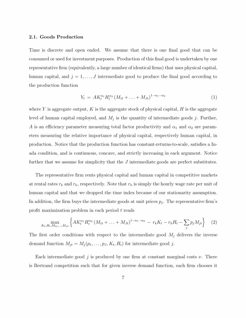
2.1. Goods Production

Time is discrete and open ended. We assume that there is one final good that can be

consumed or used for investment purposes. Production of this final good is undertaken by one

representative firm (equivalently, a large number of identical firms) that uses physical capital,

human capital, and j = 1, . . . , J intermediate good to produce the final good according to

the production function

Yt = AKα1t Hα2

t (M1t + . . .+MJt)1−α1−α2 (1)

where Y is aggregate output, K is the aggregate stock of physical capital, H is the aggregate

level of human capital employed, and Mj is the quantity of intermediate goods j. Further,

A is an efficiency parameter measuring total factor productivity and α1 and α2 are param-

eters measuring the relative importance of physical capital, respectively human capital, in

production. Notice that the production function has constant-returns-to-scale, satisfies a In-

ada condition, and is continuous, concave, and strictly increasing in each argument. Notice

further that we assume for simplicity that the J intermediate goods are perfect substitutes.

The representative firm rents physical capital and human capital in competitive markets

at rental rates rk and rh, respectively. Note that rh is simply the hourly wage rate per unit of

human capital and that we dropped the time index because of our stationarity assumption.

In addition, the firm buys the intermediate goods at unit prices pj. The representative firm’s

profit maximization problem in each period t reads

maxKt,Ht,M1t,...,MJt

AKα1

t Hα2t (M1t + . . .+MJt)

1−α1−α2 − rkKt − rhHt −∑

j

pjMjt

(2)

The first order conditions with respect to the intermediate good Mj delivers the inverse

demand function Mjt = Mj(p1, . . . , pJ ,Kt,Ht) for intermediate good j.

Each intermediate good j is produced by one firm at constant marginal costs ν. There

is Bertrand competition such that for given inverse demand function, each firm chooses it

7

price level to maximize profits. Specifically, in each period t the intermediate good firm j

maximizes

maxpj

pjMj(p1, . . . , pJ ,Kt,Ht) − νMj(p1, . . . , pJ ,Kt,Ht)

(3)

For our quantitative policy analysis, we identify the intermediate-good sector with the sector

of “Professional Services” consisting of tax accountants, lawyers, engineers, and architects

(see Section 6).

2.2 Households

There are a large number of households who differ with respect to their family type s1.

There are six different family types, s1 ∈ sn, ska, skn, cn, cka, kcn, corresponding to the

types “single without school children (kids)”, “single with school children and access to

full-day school program”, “single with school children and no access to full-day school pro-

gram”,“couple without school children”, “couple with school children and access to full-day

school program”, and “couple with school children and no access to full-day school program”.

Households do not change their family type and in this sense s1 describes ex-ante hetero-

geneity of households. The distribution of households over family types s1 is exogenous and

will be chosen to match the empirical distribution over family types – see the calibration

section for details.

Households also differ according to their employment status, s2. A single-household can

be short-term unemployed, s2 = su, long-term unemployed, s2 = lu, full-time employed,

s2 = 1e, part-time employed, s2 = 0.5e, or marginally employed, s2 = 0.25e. For the couple-

household the different employment states are defined as the combination of the employment

states of the two adult household members. The employment state of an individual household

changes over time and the associated stochastic process is a Markov process with stationary

transition function that depends on search effort, l, of the household. Specifically, households

can exert job search effort that determines the likelihood to transit to an employment state

8

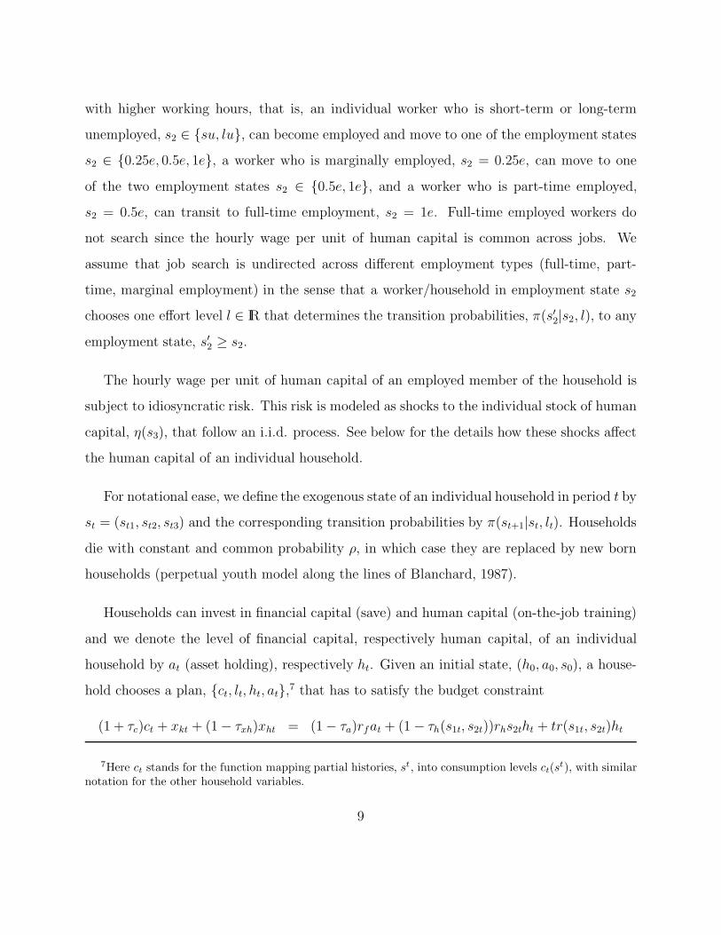
with higher working hours, that is, an individual worker who is short-term or long-term

unemployed, s2 ∈ su, lu, can become employed and move to one of the employment states

s2 ∈ 0.25e, 0.5e, 1e, a worker who is marginally employed, s2 = 0.25e, can move to one

of the two employment states s2 ∈ 0.5e, 1e, and a worker who is part-time employed,

s2 = 0.5e, can transit to full-time employment, s2 = 1e. Full-time employed workers do

not search since the hourly wage per unit of human capital is common across jobs. We

assume that job search is undirected across different employment types (full-time, part-

time, marginal employment) in the sense that a worker/household in employment state s2

chooses one effort level l ∈ IR that determines the transition probabilities, π(s′2|s2, l), to any

employment state, s′2 ≥ s2.

The hourly wage per unit of human capital of an employed member of the household is

subject to idiosyncratic risk. This risk is modeled as shocks to the individual stock of human

capital, η(s3), that follow an i.i.d. process. See below for the details how these shocks affect

the human capital of an individual household.

For notational ease, we define the exogenous state of an individual household in period t by

st = (st1, st2, st3) and the corresponding transition probabilities by π(st+1|st, lt). Households

die with constant and common probability ρ, in which case they are replaced by new born

households (perpetual youth model along the lines of Blanchard, 1987).

Households can invest in financial capital (save) and human capital (on-the-job training)

and we denote the level of financial capital, respectively human capital, of an individual

household by at (asset holding), respectively ht. Given an initial state, (h0, a0, s0), a house-

hold chooses a plan, ct, lt, ht, at,7 that has to satisfy the budget constraint

(1 + τc)ct + xkt + (1 − τxh)xht = (1 − τa)rfat + (1 − τh(s1t, s2t))rhs2tht + tr(s1t, s2t)ht

7Here ct stands for the function mapping partial histories, st, into consumption levels ct(st), with similarnotation for the other household variables.

9

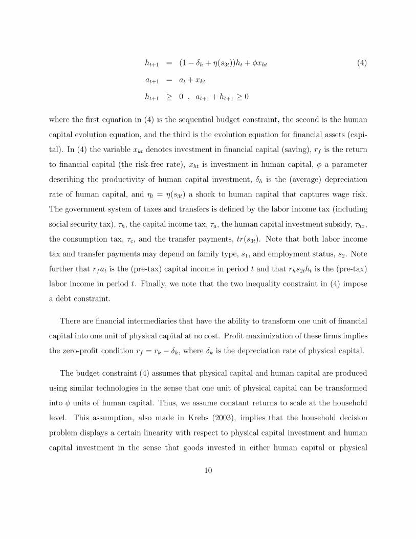
ht+1 = (1 − δh + η(s3t))ht + φxht (4)

at+1 = at + xkt

ht+1 ≥ 0 , at+1 + ht+1 ≥ 0

where the first equation in (4) is the sequential budget constraint, the second is the human

capital evolution equation, and the third is the evolution equation for financial assets (capi-

tal). In (4) the variable xkt denotes investment in financial capital (saving), rf is the return

to financial capital (the risk-free rate), xht is investment in human capital, φ a parameter

describing the productivity of human capital investment, δh is the (average) depreciation

rate of human capital, and ηt = η(s3t) a shock to human capital that captures wage risk.

The government system of taxes and transfers is defined by the labor income tax (including

social security tax), τh, the capital income tax, τa, the human capital investment subsidy, τhx,

the consumption tax, τc, and the transfer payments, tr(s3t). Note that both labor income

tax and transfer payments may depend on family type, s1, and employment status, s2. Note

further that rfat is the (pre-tax) capital income in period t and that rhs2tht is the (pre-tax)

labor income in period t. Finally, we note that the two inequality constraint in (4) impose

a debt constraint.

There are financial intermediaries that have the ability to transform one unit of financial

capital into one unit of physical capital at no cost. Profit maximization of these firms implies

the zero-profit condition rf = rk − δk, where δk is the depreciation rate of physical capital.

The budget constraint (4) assumes that physical capital and human capital are produced

using similar technologies in the sense that one unit of physical capital can be transformed

into φ units of human capital. Thus, we assume constant returns to scale at the household

level. This assumption, also made in Krebs (2003), implies that the household decision

problem displays a certain linearity with respect to physical capital investment and human

capital investment in the sense that goods invested in either human capital or physical

10

capital generate returns that are independent of household size, where size is measured by

total wealth (see below).8 In conjunction with the constant-returns-to-scale assumption for

the aggregate production function F it implies that the model exhibits endogenous growth.

The assumptions we make in (4) have the advantage that they keep the model highly

tractable, which, as we argued before, is essential for the quantitative analysis conducted in

this paper. Tractability in the general case requires that we do not impose a restriction on

the ability of households to decumulate human capital. However, in the calibrated model

economy used for our quantitative analysis, the restriction that human capital investment

is always non-negative, xh ≥ 0, is always satisfied in equilibrium; that is, it holds for all

household types and all realizations of uncertainty.9

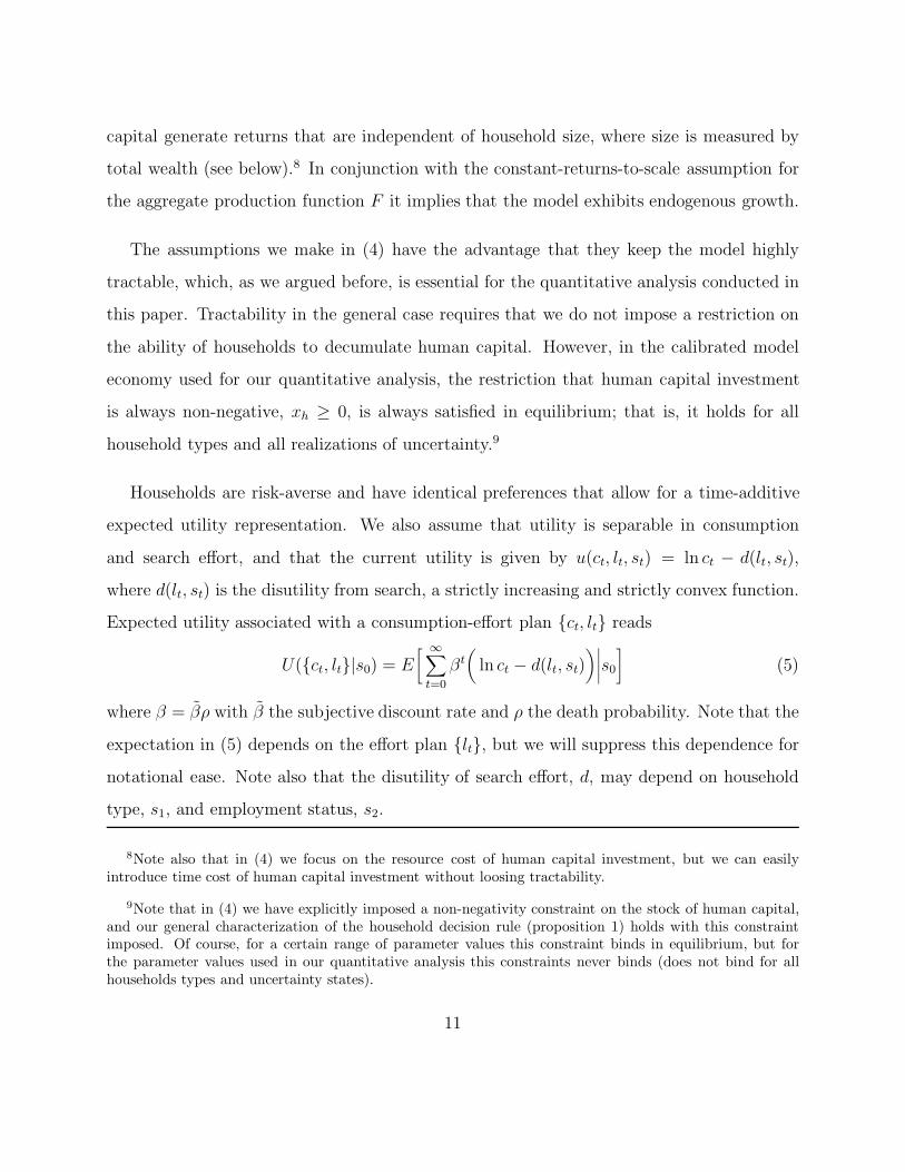
Households are risk-averse and have identical preferences that allow for a time-additive

expected utility representation. We also assume that utility is separable in consumption

and search effort, and that the current utility is given by u(ct, lt, st) = ln ct − d(lt, st),

where d(lt, st) is the disutility from search, a strictly increasing and strictly convex function.

Expected utility associated with a consumption-effort plan ct, lt reads

U(ct, lt|s0) = E[ ∞∑

t=0

βt(

ln ct − d(lt, st))∣∣∣∣s0

](5)

where β = βρ with β the subjective discount rate and ρ the death probability. Note that the

expectation in (5) depends on the effort plan lt, but we will suppress this dependence for

notational ease. Note also that the disutility of search effort, d, may depend on household

type, s1, and employment status, s2.

8Note also that in (4) we focus on the resource cost of human capital investment, but we can easilyintroduce time cost of human capital investment without loosing tractability.

9Note that in (4) we have explicitly imposed a non-negativity constraint on the stock of human capital,and our general characterization of the household decision rule (proposition 1) holds with this constraintimposed. Of course, for a certain range of parameter values this constraint binds in equilibrium, but forthe parameter values used in our quantitative analysis this constraints never binds (does not bind for allhouseholds types and uncertainty states).

11

Households choose a consumption-effort-investment plan, ct, lt, ht, at, to maximize ex-

pected lifetime utility (5) subject to the budget constraint (4).

2.3 Equilibrium

The initial distribution, µ0, of households over states, (h0, a0, s0), in conjunction with the

transition functions, π(st+1|st, lt), and the equilibrium effort plans, lt, induce a sequence of

equilibrium joint distributions, µt, over (h0, a0, s0, st). Assuming a law of large numbers,

aggregate variables in any period t can be found by taking the expectation with respect to

the joint distribution µt. For example, the aggregate level of financial capital of households

in period t is Kt = E[at] and the aggregate level of employed human capital is Ht = E[s2tht]

In equilibrium, human capital demanded by the firm must be equal to the corresponding

aggregate stock of human capital supplied by households. Similarly, the physical capital

demanded by the firm must equal the aggregate net financial wealth supplied by households.

That is, in equilibrium we must have for all t

Kt = E[at] (6)

Ht = E[s2tht]

To sum up, we have the following equilibrium definition:

Definition A stationary (balanced growth) equilibrium is a pair of rental rates, (rk, rh), a

vector of intermediate good prices, (p1, . . . , pJ ), a sequence of physical and human capital

stocks, Kt,Ht, and a family of household plans, ct, ht, at, lt, such that

i) Utility maximization of households: for each initial state, (h0, a0, s0), and given rental

rate rh and interest rate rf = rk − δk, the household plan, ct, ht, at, lt, maximizes expected

lifetime utility (5) subject to the sequential budget constraint (4).

ii) Profit maximization of final-good firms: the sequence Kt,Ht solves problem (2)

iii) Profit maximization of intermediate-good firms: the price pj solves the problem (3) for

12

all j = 1, . . . , J .

iv) Market clearing: equations (6) holds for all t.

A stationary recursive equilibrium is a stationary equilibrium in which household plans

are generated by policy functions. Note that in a stationary equilibrium, the extensive-

form aggregate variables Kt, Ht, Mjt, Xkt, Xkt, and Ct all grow at a common rate and

the intensive-form aggregate variables (ratio variables) are constant over time – see the

equilibrium characterization below. Note further that the equilibrium growth rate of all

extensive-form aggregate variables is endogenous – see Krebs (2003) for a detailed discussion

of the equilibrium behavior of this class of endogenous growth models with idiosyncratic

risk.

In our definition of equilibrium, we have not included the government budget constraint.

The government budget constraint reads:

τcE[ct] + rhE[τh(s1t, s2t)s2t)ht] + τarfE[at] = τhxE[xht] + E[tr(s1t, s2t)ht] (7)

In our policy analysis below, we impose the budget constraint for the pre-reform equilibrium,

but do not impose the constraint post-reform. This means that we assume that the govern-

ment can borrow and lend in international financial markets and uses this ability to finance

any reform-induced budget deficits and to invest any reform-induced budget surpluses. Note

that a standard argument shows that in an equilibrium with (7) the goods market clearing

condition (aggregate resource constraint) holds:

Ct +Xkt +Xht = Yt −∑

j

Mjt (8)

2.4. Characterization of Household Problem

We next show that optimal consumption choices are linear in total wealth (human plus

financial) and portfolio and effort choices are independent of wealth. This property of the

13

optimal policy function allows us to solve the quantitative model, which has considerable

household heterogeneity and three inter-temporal choice variables (h, k, l), without using

approximation methods. The property also implies that the household decision problem is

convex and the first-order approach can be utilized.

To state the characterization result, denote total wealth (human plus financial) of a

household at the beginning of the period by wt = 1−τhx

φht + at. Note that φ measures the

productivity of goods investment in human capital and 1/φ is the shadow price of one unit

of human capital in terms of the consumption/capital good. Denote the portfolio share of

physical capital by θt = at/wt. Note that this definition in conjunction with the definition

of w imply that the portfolio share of human capital is given by 1 − θt = (1−τhx)ht

φwt. The

sequential budget constraint (4) then reads:

wt+1 = (1 + r(θt, st))wt − ct (9)

ct ≥ 0 , wt+1 ≥ 0 , 1 − θt+1 ≥ 0

with

r(θt, st).= θtrf + (1 − θt)rh(st)

rh(st).=

φ

1 − τhx[(1 − τh(s1t, s2t))rhs2t + tr(s1t, s2t)] − δh + η(s3t)

Clearly, (9) is the budget constraint corresponding to an inter-temporal portfolio choice

problem with linear investment opportunities and no exogenous source of income, where the

return to physical capital investment (saving) is rf and the risky return to human capital

investment is rh(s). Note that these returns also depend on the tax and transfer system, a

dependence that we suppress for notational ease. Note also that the more time a household

spend working (the larger s2t), the higher is the return to human capital investment.

The representation of the household budget constraint shows that (w, θ, s) can be used

as individual state variable for the recursive formulation of the utility maximization prob-

14

lem. Specifically, the Bellman equation associated with the household utility maximization

problem is

V (w, θ, s) = maxc,w′,θ′,l

ln c− d(l, s) + β

∑s′ V (w′, θ′, s′)π(s′|s, l)

(10)

subject to w′ = (1 + r(θ, s))w − (1 + τc)c

where for simplicity we assume that the continuation value in the case of death is zero. We

have the following characterization result for the solution to the household decision problem.

Proposition 1. The value function and the optimal policy function are given by

V (w, θ, s) = V (s) +1

1 − β(ln(1 + r(θ, s)) + lnw)

c(w, θ, s) =1 − β

1 + τc(1 + r(θ, s))w (11)

θ′(w, θ, s) = θ′(s)

l(w, θ, s) = l(s)

w′(w, θ, s) = β (1 + r(θ, s))w

where the intensive-form value function, V (s), the optimal portfolio choice, θ′, and the

optimal effort choice, l, are the solution to the intensive-form Bellman equation

V (s) = maxθ′ ,l

− d(l, s) + ln

1 − β

1 + τc+

β

1 − βlnβ +

β

1 − β

∑

s′ln(1 + r(θ′, s′))π(s′|s, l) + β

∑

s′V (s′)π(s′|s, l)

(12)

Proof : The proof is an extension of the proof given in Krebs and Scheffel (2013).

The maximization problem (12) is a convex problem so that first-order conditions are

sufficient. Thus, to find the optimal portfolio and effort choice we can confine attention to

the first-order conditions with respect to the portfolio choice and search effort, which read

0 =∑

s′

rh(s′) − rk

(1 + r(θ′, s′))π(s′|s, l) (13)

15

∂d(l, s)

∂l= β

∑

s′

(ln(1 + r(θ′, s′))

1 − β+ V (s′)

)∂π(s′|s, l)

∂l

Note that the first equation in (13) states that marginal utility weighted expected returns

on the two investment opportunities (human capital and financial capital) are equalized –

a standard optimality condition in portfolio theories (the marginal utility of future con-

sumption is equal to ((1 − β)(1 + r′)β(1 + r)w)−1 and therefore proportional to (1 + r′)−1).

Equation (13) in conjunction with equation (12) without the max operator determine the

equilibrium values of θ, l, and V (.) for given rental rates rk and rh (partial equilibrium).

The first equation in (13) implies that in equilibrium part-time employed workers invest

less in human capital (less on-the-job training) than full-time workers. To see this, note

that the human capital return of part-time employed workers is less than the human capital

return of full-time employed workers, rh(s2 = 0.5) < rh(s2 = 1), since the additional labor

income generated by the human capital investment is smaller: 0.5 · rh · h < 1 · rh · h. Thus,

part-time employed workers have a smaller incentive to invest in human capital than full-time

employed workers, and part-time jobs are therefore less productive, and pay lower hourly

wages, than full-time jobs. Clearly, the same argument implies that marginally employed

workers, s2 = 0.25, have the smallest incentive to invest in human capital and end up being

the least productive workers with the lowest hourly wages. These equilibrium properties are

essential for some of the results to follow and can be derived formally using the first equation

in (13). It is also in line with the empirical evidence – see our discussion of the empirical

literature in Section 3.6.

Equation (13) is also useful to discuss the direct effects of the two reforms that increase

labor supply. First, consider the effect of the reduction in the social security tax for workers

with low earnings. In this case, for the affected workers the after-tax hourly wage, (1 −

τh(s1, s2))rh, goes up. This has two consequences. First, unemployed workers have a stronger

incentive to search for a job and workers who are marginally or part-time employed have

16

a stronger incentive to search for a full-time job. Second, the return to human capital

investment goes up and the incentive of employed workers to invest in human capital therefore

increases. As a result, search effort, l, goes up and investment in human capital, (1 − θ),

goes up. These two results can be formally shown using equation (13).

Consider now the second reform, the increase in public spending on schooling so that more

schools in Germany will offer a full-day school program. This reform changes the distribution

of households over s1. Specifically, after the reform a larger fraction of households with kids

have access to full-day school programs and members of those households who are not full-

time employed have a stronger incentive to search for full-time employment.

Proposition 1 provides a convenient characterization of the solution to the household

decision problem for given investment returns (partial equilibrium) and is useful for two

reasons. First, it reduces the problem of solving the Bellman equation (7) to the much

simpler problem of solving the intensive-form Bellman equation (8). Second, it states that

the consumption and saving choices are linear in wealth, and that the portfolio and effort

choices are independent of wealth. This property allows us to solve for the general equilibrium

without knowledge of the endogenous wealth distribution. We next turn to the general

equilibrium analysis.

2.5. Equilibrium Characterization

In the previous section we characterized the solution to the household problem. Consider now

the maximization problem of the final-good producer (2) and intermediate-good producers

(3). For the intermediate good sector, we focus attention on symmetric equilibria, pj = p

and Xjt = Xt, for all j = 1, . . . , J . Using the first-order conditions associated with the

maximization problems (2) and (3) and the symmetry condition, in the Appendix we show

17

that the price for each intermediate good satisfies

p =J

J − α1 + α2ν (14)

.= (1 + ϕ(J))ν

where ϕ(J) = JJ−α1+α2

− 1 defines the mark-up. This mark-up is decreasing in the number

of firms, J , and therefore decreasing in the degree of competition in the intermediate-good

sector (i.e. the professional services). In Section 6, we discuss how the deregulation of the

market for professional services affects the economy by increasing the degree of competition,

J , and therefore decreasing the mark-up.

Using the pricing condition (14) and the first-order condition of the final-good producer,

we find the following relationship between rental rates rk and rh and the firm’s capital-to-

labor ratio K = KH

:

rk = α1 A K1+

α1α2 (15)

rh = α2AKα1

α1+α2

A.= A

1α1+α2

(1 − α1 − α2

(1 + ϕ)ν

)(1−α1−α2)/(α1+α2)

Equation (15) shows that a reduction in mark-up, ϕ, in the intermediate goods sector

is equivalent to an increase in productivity, A, in the final goods sector. Thus, a dereg-

ulation of the intermediate goods sector (professional services) that increases competition

and the number of competing firms J will reduce cost and increase effective productivity,

A in the final good sector, which in turn increases labor demand through (15). This is the

policy experiment analyzed in Section 6 when we consider the (further) deregulation of the

professional services in Germany.

To complete the equilibriumcharacterization, we define the share of aggregate total wealth

18

of households in state s as

Ω(s).=

E [(1 + r)w|s] π(s)∑

sE [(1 + r)w|s]π(s)

where π is the stationary distribution of the equilibrium transition function over s. Note that

(1+r)w is total wealth of an individual household after assets have paid off (after production

has taken place and depreciation has been taken into account). Note also that∑

s Ω(s) = 1

by construction. Further, Ω is finite-dimensional, whereas the set of distributions over (w, s)

is infinite-dimensional. Using the wealth shares Ω, we show in the Appendix that the market

clearing condition (6) can be written as:

K =(1 − τhx)

∑s θ(s)Ω(s)

φ(1 − θ(s))s2Ω(s)(16)

and that stationary Ω-distribution is the solution to

Ω(s′) =ρ∑

s π(s′|s, l(s))(1 + r(θ(s), s))Ω(s) + (1 − ρ)ψµnew(s′)

ρ∑

s,s′ π(s′|s, l(s))(1 + r(θ(s), s))Ω(s) + (1 − ρ)ψµnew(s′)(17)

where µnew determines how the wealth of dying households is distributed among new-born

households and ψ < 1 is a parameter that measures the fraction of wealth that is passed on

to the new generation.

Summing up, we have the following equilibrium characterization result:

Proposition 2. Suppose that (θ, l, V , K,Ω) solve (12),(15), (16), and (17). Then the se-

quence Kt,Ht and the family of household plans, ct, ht, kt, lt, induced by (θ, l, V , K,Ω)

together with the corresponding rental rates, (rk, rh) and inter-mediate goods prices (p1, . . . , pJ )

given by (14) define a stationary (balanced growth) equilibrium.

Proof . The proof is an extension of the proof given in Krebs and Scheffel (2013).

Proposition 2 shows that the stationary equilibrium can be found without knowledge

of the infinite-dimensional wealth distribution; only the finite dimensional distribution of

19

wealth across family types Ω matters. The is because the linearity of the policy functions in

wealth make the infinite dimensional distribution of wealth across households of a given type

irrelevant. Proposition 2 facilitates our quantitative analysis significantly since it implies that

there is no need to approximate an infinite dimensional distribution over financial wealth

and human wealth when computing equilibria.

3. Calibrating the Model

The calibration is based on macro- and microeconomic evidence from various sources. Specif-

ically, the cross-sectional distribution of households over family types and employment states

are taken from the 2010 Micro-census provided by the Federal Office of Statistics (Statis-

tisches Bundesamt). Data on labor market dynamics are generally taken from the Federal

Employment Agency (Bundesagentur fuer Arbeit) and policy variables, including benefits,

labor taxes and social security contributions are taken from the OECD Tax Benefit Model.

See Krebs and Scheffel for a detailed description of the data sources and a discussion of the

various empirical distributions.

3.1 Search Technology and Transition Rates Across Employment States

We set the period length to one quarter. We use a standard convention and define long-

term unemployment as any unemployment spell that lasts longer than 12 months. Thus, we

choose π(su|lu) = 0.25.

We assume an exponential specification for the probability of an unemployed worker

finding a job as a function of effort:

π(s2 ∈ 1e, 0.5e, 0.25e|su, l) = 1 − e−λ(su)l (18)

π(s2 ∈ 1.0e, 0.5e, 0.25e|lu, l) = 1 − e−λ(lu)l

In search models with only one employment state, the exponential formulation is often used in

20

the literature (Hopenhayn and Nicolini, 1997, Lentz, 2009, and Shimer and Werning, 2008).

Specification (12) is the generalization of this approach to the case of multiple employment

states if there is undirected search for different employment opportunities (full time, part

time, marginal employment). We choose the values λ(su) and λ(lu) so that the job finding

probabilities (12) match the corresponding quarterly job finding rates in 2010 provided by

the Federal Employment Agency (Bundesagentur fuer Arbeit). In 2010, these quarterly job

finding rates were 0.36 for the short-term unemployed and 0.09 for the long-term unemployed.

Specification (18) determines the average job finding probability, but does not pin down

what type of job is found in case job search was successful (full time, part time, marginal

employment). We assume that the arrival rate of the different employment states is the

same:

π(s2 = 1e|su, l) = π(s2 = 0.5e|su, l) = π(s2 = 0.25e|su, l) (19)

π(s2 = 1e|lu, l) = π(s2 = 0.5e|lu, l) = π(s2 = 0.25e|lu, l)

This assumption can be easily relaxed from a modelling point of view, but we are not aware

of any micro-level evidence that would allow us to calibrate the additional parameters of the

richer model structure. For this reason, we confine attention to specification (19).

There is little empirical evidence regarding the transition rates from marginal employ-

ment, s2 = 0.25e, to either part-time employment, s2 = 0.5e, or full-time employment,

s2 = 1e, and regarding the transition rate from part-time employment, s2 = 0.5e, to full-time

employment, s2 = 1e. Caliendo, Kuenn, and Uhlendorff (2012) show that the probability

of a marginally employed worker to move to a higher employment state (i.e. part-time or

full-time employment) is not different from the job finding rate of an unemployed worker.

Motivated by this evidence, we set the probability of moving from s2 = 0.25e to either

s2 = 0.5e or s2 = 1e equal to the job finding rate of a short-term unemployed worker. In

addition, we also set the probability of moving from s2 = 0.5e to s2 = 1e equal to the job

21

finding rate of short-term unemployed workers.

We choose the job destruction rates, i.e. the flow rates from the employment states

s2 = 1e, 0.5e, 0.25e to unemployment s2 = su, so that we match the empirical distribution

of households over employment states s2. In addition, we calibrate the transition rate from

long-term to short-term unemployment to match the composition of the unemployment pool

in the data. Specifically, conditional on the family and skill type, we target a value of 50

percent for the fraction of long-term unemployed workers in the pool of all unemployed

workers. The only exception are single parents, a group for which the large majority of

unemployed are long-term unemployed. In line with the data, for single parents we use a

share of 86 percent long-term unemployment as our target.

We also allow for one-step transitions from higher to lower employment levels, that is, we

allow for transitions from full-time employment to part-time employment (1.0e→ 0.5e) and

from part-time employment to marginal employment (0.5e → 0.25e). For lack of evidence,

we assume that for each family type these transitions rates are equal to the corresponding

job destruction rates (i.e. the transition rate from the employment state to unemployment).

3.2 Search Preferences

We assume that disutility of search effort is

d(l, s1) = d0lγ − d1(s1)

It is well-known that with the above specification the parameters λ(su) and λ(lu) and d0 are

not separately identified. We choose a numerically convenient normalization of d0 = 1. We

choose the curvature parameter γ to match a given value of the elasticity of the job finding

rate with respect to benefit payments for the short-term unemployed, where we choose as

target the micro elasticity holding constant the labor market state. This target elasticity is

chosen as follows.

22

For the US, there are a number of empirical micro studies estimating the search elasticity

directly. The best known studies are Moffitt (1985) and Meyer (1990) who estimate an

elasticity of around −0.9. Meyer and Krueger (2002) survey the literature and suggest an

elasticity of −1, whereas Chetty (2008) suggests a value of −0.5. Card et al. (2015) provide

new evidence using administrative data from the state of Missouri covering the period 2003-

2013. Based on identification coming from a regression kink design, they find an elasticity

of around −0.35 before the recession and an elasticity between −0.65 and −0.9 after the

recession. Krueger and Mueller (2010) analyze time use data and find that the level of

unemployment benefits has a large negative effect on the time unemployed workers spent

searching for a job, a finding that broadly supports the basic channel we emphasize in this

paper.

There is much less work on this issue for Germany. Hunt (1995) finds estimates for Ger-

many that are in line with the US estimates of Moffitt (1985) and Meyer (1990). Addison,

Centeno, and Portugal (2008), who use a structural search model and the European Com-

munity Household Panel (ECHP), find values of the search elasticity ranging from −1.14 to

−1.66 for Germany. Consistent with this finding are the results reported in Hofmann (2012)

and Mueller and Steiner (2008) who find that imposing benefit sanctions/reduction long-term

unemployed for non-compliance has significant effects on the unemployment-to-employment

transition in Germany. With the exception of these last two studies, the empirical litera-

ture has focused on unemployed workers who are short-term unemployed according to our

definition (less than one year of unemployment). Guided by the evidence, for our baseline

calibration we choose a conservative value for the target elasticity of −0.7 for the short-term

unemployed.

For the disutility-term d1(s) we choose the specification d1(s) = d11(s1) + d12s2, where

s1 denotes the family type and s2 the employment status. We choose the value of d12

23

consistent with the disutility of work used in the RBC literature, e.g. Cooley and Prescott

(1995). We choose the values of d11(s1) to match the empirical ratio of full-time employment

to the sum of part-time and marginal employment for each family type s2. Note that this

approach ensures that the model matches the significant empirical difference in employment

type between women with kids who have access to full-day school and women with kids who

do not have access to full-day school. See Krebs and Scheffel (2015) for a detailed discussion

of the empirical evidence on this issue.

3.3 Wage Risk

One can show (Krebs 2003) that the assumption of i.i.d human capital shocks, η, implies

that the log of labor wages of individual households follows approximately a random walk

with innovation term ε = (1 − θ)η. For the US, the random walk component of individual

labor income has been estimated by a number of empirical studies using data drawn from

the PSID, and estimates of σε for the US are in the range of .15 for annual wage changes,

which amounts to quarterly standard deviation of 0.15/2 = 0.075. For Germany, Krebs and

Yao (2016) and Fuchs-Schuendeln, Krueger, and Sommer (2009) find similar values, and we

therefore choose this value as a target for σε.

3.4 Government Policy Parameters

We set the capital income tax at τk = 0.20, which is at the upper end of the range of

capital income taxes reported by the OECD. We set the schedule of labor income taxes and

social security contributions, τh(s1, s2), consistent with numbers computed from the OECD

tax calculator and the social security tax schedule. We choose the unemployment benefit

parameters that are a part of the transfer system, tr(s1, s2), to match the net replacement

rate for the short-term and long-term unemployed taken from Krebs and Scheffel (2013).

The remaining parameters of the transfer system are set so that the model’s implications for

24

labor income after taxes and transfers are consistent with the data drawn from the German

“Mikrozensus”. Finally, we choose the value of the consumption tax, τc, to ensure that the

government budget constraint is satisfied.

3.5 Production Technology

We set α1

α1+α2to match the share of labor income in the data and 1 − α1 − α2 to match

the share of the sector professional services in the German economy, which is 3 percent.

We choose the remaining technology parameters to match capital-to-output ratio of 2.5, an

annual physical capital return of 4 percent and an annual average human capital return of

8 percent (human capital risk premium of 4 percent).

3.6 Implied Wage Differentials

As discussed in Section 2, the model implies that marginally employed workers have the

smallest incentive to invest in human capital (on-the-job training) and full-time employed

workers the largest incentive. As a result, marginally employed workers are the least produc-

tive workers and are paid the lowest hourly wage and full-time employed workers have the

highest productivity and are paid the highest hourly wage. Thus, the model generates an en-

dogenous wage penalty for marginal employment and part-time employment. According to

the calibrated model economy, this wage penalty is 15 percent for marginal employment and

48 percent for part-time employment. This implication of the calibrated model is consistent

with the available empirical evidence in the following sense.

Data provided by the German Statistical Agency show that in 2014 the average hourly

wage of full-time employed workers was 23 percent higher than the average hourly wage for

part-time workers (Statistisches Bundesamt, 2014). Data drawn from the SOEP for the year

2010 show an average part-time wage penalty of 22 percent (Brenke, 2012). For marginally

employed workers the wage penalty is even larger: the average hourly wage of full-time

25

employed workers is 93 percent higher than the average hourly wage of workers whose only

job is a so-called mini-job (Eichhorst et al. 2012), which is the relevant group for calibrating

the model. Thus, the data indicate a substantial wage penalty for part-time work and a very

large wage penalty for marginally employed workers.

The above numbers are simple averages and do not take into account that observed

wage differentials between full-time work and part-time work or mini-jobs might be due

to differences in worker characteristics (education, experience) or firm characteristics (firm

size) or labor market characteristics (sector, occupation). There is a substantial amount of

empirical work on the part-time wage penalty for US workers (Hirsch, 2005, Moffitt, 1984)

and also British workers (Ermisch and Wright, 1993, and Manning and Petrongolo, 2008).

The results of this literature can be summarized as follows. First, there is a large unadjusted

wage penalty for part-time workers (20-30 percent) that is larger for men than for women.

Second, controlling for worker, firm and labor-market characteristics roughly halves the part-

time wage penalty. For Germany, the study by Wolf (2002, 2010) finds that, in line with

the international evidence, after controlling for worker and firm characteristics the part-time

wage penalty is 11 percent for women and 25 men. Unfortunately, there is no empirical work

on the wage penalty for marginally employed workers, but extrapolation from the results on

part-time work would suggest that the adjusted wage penalty is about half of the unadjusted

wage penalty (i.e. half of 93 percent).

4. Reform of Social Security Taxes for Low-Wage Jobs

4.1 Current Situation

In Germany, the social security system covers public pension, health insurance, unemploy-

ment insurance, accident/disability insurance, and elderly nursing care insurance. The total

social security contributions from employers and employees add up to roughly 40 percent

26

of earnings for monthly earnings exceeding 850 Euro, where the employee contribution is

slightly less than 20 percent and the employer contribution is somewhat higher than 20

percent. For all monthly earnings below 450 Euro (marginal employment also called mini-

jobs), there is no employee contribution to social security. For monthly earnings between

450 Euro and 850 Euro, the employee contribution increases linearly with earnings. See

Figure 1 for a graphical representation of the employee contribution to the social security

tax in Germany. The limit of the amount of earnings subject to social security taxation, the

so-called contribution and benefit base, is 72, 600 Euro for West Germany and 62, 400 for

East Germany.

Labor income taxes (excluding the social security tax) are relatively low for workers with

monthly wages less than 2,000 Euro. For example, for a single person without children

(highest tax burden) monthly earnings of up to 700 Euro are exempt from income tax,

and the average income tax rate is 11 percent for monthly earnings of 1, 500 Euro and 15

percent for monthly earnings of 2, 000 Euro. Thus, for low-wage jobs, the social security tax

dominates the labor income tax, and any tax reduction program that wants to target the

low-wage sector has to focus on the social security tax. Such a reform of the social security

tax will be discussed next.

4.2 Reform Description

We consider a reform that replaces the current social security tax system with a system in

which the employee contribution increases linearly with earnings reaching its maximal value

of 20 percent at monthly earnings of 2, 000 Euro. See Figure 1 for a graphical representation

of the effect of the reform on the employee contribution to the social security tax. To

implement the reform, we use micro-level earnings data and first compute for every family

type s1 and employment state s2 the reform-induced average change in the social security

tax for workers of a given family type and employment status. We then feed these changes

27

into the calibrated model and compute the equilibrium effects.

To gain a better understanding of the reform effects discussed below, Table 1 shows

the average change in the social security tax for marginally employed workers (mini jobs),

part-time employed workers, and full-time employed workers (averaged over all workers of

all family types). The reform substantially lowers the social security tax for many part-

time and full-time employed workers, and increases the social security tax for marginally

employed workers since it removes the tax exemption for mini-jobs. Thus, the reform will

give marginally employed workers a stronger incentive to search for part-time employment

and full-time employment. Further, unemployed workers will on average search harder for

jobs since the average social security tax on employment is reduced (the population weighted

average in Table 1 is negative).

4.3 Results

The macroeconomic, distributional, and fiscal effects of the reform are shown in Table 2

and Figures 2 - 6. Figure 2 shows that the reform leads to a substantial reduction in the

unemployment rate: the unemployment rate falls by 0.08 percentage points in the short-run

(in the first year), by 0.25 percent in the medium run (after 5 years), and by 0.30 percent in

the long-run (after 10 years). The intuition underlying the decline in the unemployment rate

is simple. The reduction in the social security tax increases the attractiveness of work rela-

tive to unemployment, which improves search incentives and therefore induces unemployed

workers to increase their search effort. An improvement in search effort, in turn, increases

job finding rates and reduces unemployment.

Figure 3 shows the time path of employment after the reform. Employment increases by

0.22 percent in the first year, 0.72 percent after 5 years, and 0.87 percent after 10 years.

Less than half of the increase in employment is caused by the reduction in unemployment

28

depicted in figure 2. The rest is explained by an increase in full-time employment relative

to marginal employment (part-time employment remains roughly constant – see figure 3).

There is a simple reason behind the increase in full-time employment relative to marginal

employment: the reform reduces the social security tax for most full-time employed workers

in the low-wage sector, but increases the social security tax for the marginally employed – see

table 1. Thus, the reform increases the incentive for marginally employed workers to look

for full-time employment, and the transition rate from marginal employment to full-time

employment (and part-time employment) goes up.

We next turn to a discussion of the wage effect of the reform. There are three forces

that act upon hourly pre-tax wages. First, the increase in labor supply tends to reduce

wages because the marginal product of labor is diminishing in employment. Second, the

reform-induced increase in employment increases the marginal product of capital, which

induces firms to increase their labor demand – this force tends to push up wages. In a

standard neoclassical model with frictionless labor markets and fixed human capital, the

negative wage effect dominates in the short-run and the two effects cancel each other out

in the long-run. However, the current model assumes a frictional labor market with search

unemployment and the employment adjustment therefore takes time (see figures 1 and 2).

In addition, there is a third effect on wages because workers invest in their human capital

(on-the-job training) and the incentive to invest in human capital is stronger for full-time

employed workers than for marginally employed workers – see also our discussion in Section

2.4. Thus, this third effect tends to push up hourly wages since the reform increases the

share of full-time employed workers relative to marginally employed workers (see figure 3).

Figure 4 depicts the development of hourly pre-tax wages after the reform (relative to

trend wage growth). The graph shows that the net effect on wages is positive in the short-

run and in the long-run. In other words, the two positive effects on hourly wages discussed

29

in the preceding paragraph dominate the negative effect on wages. Specifically, hourly pre-

tax wages increase by 0.15 percent in the short-run, by 0.42 percent in the medium run,

and by 0.63 percent in the long-run. Figure 4 also shows that the reform has desirable

distributional consequences in the sense that the rise in wages is concentrated in the low-

wage sector. Specifically, hourly pre-tax wages in the low-wage sector increase by 0.40 in the

first year, by 1.13 percent after five years, and by 1.71 percent after 10 years.10

Figure 5 shows the time path of output after the reform (relative to trend output growth).

There are three reasons why the reduction in the social security tax considered here will

raise output. First, the employment increase discussed above increases output. Second, the

physical capital stock increases, which increases labor productivity and therefore output.

Third, the human capital stock increases because marginal employment is replaced by full

employment, which increases labor productivity and therefore output. Figure 5 shows that

the output effects are substantial: output increases by 0.26 percent in the short-run, by 0.63

percent in the medium run, and by 0.82 percent in the long-run.

Finally, in Figure 6 we turn to the fiscal effects of the reform. Without adjustment of

labor or capital, the tax reduction program generates a fiscal deficit due to forgone tax

revenues. However, the reform-induced increase in employment and hourly wages discussed

above raises tax revenues. Figure 6 shows that in the first year the negative fiscal effect

dominates and the reform generates a fiscal deficit of 0.39 percent of output. However,

the increase in tax revenues generated by the expansion in employment and hourly wages

increases over time, and this increase is strong enough so that after 9 years the fiscal budget

is balanced and generates surpluses thereafter. In other words, after 9 years the economy

is on the upward-sloping part of the Laffer-curve. For any real interest rate less than 9.02

10We follow the standard approach and define low-wage sector as all workers whose monthly (pre-tax)earnings is below 2/3 of the monthly median earnings. We compute these numbers based on the modeldistribution.

30

percent, the reform is fiscally efficient in the sense that the present value of fiscal deficits

and fiscal surpluses is positive. Put differently, this reform yields an internal rate of return

of 9.02 percent for the government.

5. Public Expansion of Full-Day School Programs

5.1 Current Situation

In Germany, only one third of schools offer some version of full-day school program, and two

thirds of schools are half-day schools – dismissal of school children is at 1 pm or earlier. If

we add other types of after-school programs not offered by the school itself, then at best 40

of the school children in Germany can take advantage of a full-day (i.e. until 4 pm) school

program. In contrast, around 80 percent of women with children in Germany would like

their children to attend a full-day school (Klemm, 2014). This indicates that there is a large

demand for public full-day schools in Germany that is not satisfied. The situation is similar

for child care programs for children ages 3− 6: less than 40 percent have access to a full-day

program, but a large majority of women with children would like to use a full-day child care

program. See Krebs and Scheffel (2015) for a detailed discussion of the evidence on this

issue.

5.2 Reform Description

We consider a publicly financed expansion of full-day schools from the current status quo,

in which 40 percent of children have a full-day spot, to a situation in which 80 percent

of children have a full-day spot. We also assume that for children ages 3 − 6 a similar

expansion in full-day spots takes place in child care centers. To achieve this goal, about 4

million half-day spots in schools and child care centers have to be transformed into full-day

spots (Klemm, 2014). The annual running cost of this expansion program is about 6 Billion

Euro per year (0.2 percent of German GDP), where the largest part of this cost is wages

31

for teachers/educators.11 In addition, there is a one-time (sunk) cost for initial investment

in school buildings and other capital goods, which we assume to be 20 Billion Euro (0.66

percent of GDP). See Krebs and Scheffel (2015) for a detailed discussion of the costs of

transforming half-day spots into full-day spots. This program will increase (female) labor

supply in the sense that unemployed or marginally employed women with children will have

a stronger incentive to search for part-time or full-time employment. See our discussion of

this effect in Section 2.4.

5.3 Results

The macroeconomic, distributional, and fiscal effects of the public expansion program are

shown in Table 3 and Figures 7 to 11. Figure 7 shows that the reform leads to a substantial

reduction in the unemployment rate: the unemployment rate falls by 0.11 percentage points

in the short-run (in the first year), by 0.33 percent in the medium run (after 5 years), and

by 0.38 percent in the long-run (after 10 years). The intuition underlying the decline in the

unemployment rate is simple. The expansion of full-day school programs by the government

improves the family situation for many unemployed women with children. These women will

increase their search effort, which increases job finding rates and reduces unemployment.

Figure 8 shows the time path of employment after the reform. Employment increases by

0.23 percent in the first year, 0.79 percent after 5 years, and 0.95 percent after 10 years.

About one half of the increase in employment is caused by the reduction in unemployment

pictured in figure 7. The other half is explained by an increase in full-time employment

relative to marginal employment (and part-time employment – see Figure 8). There is a

simple reason behind the increase in full-time employment relative to marginal employment.

For many marginally employed women with children, the reform improves their ability to

11We assume that this cost is 0.2 percent of GDP in all future years, which means that we assume that itrises in step with the growth of GDP.

32

combine family with work and a significant fraction of these women begin to search for

part-time work or full-time work. This, in turn, leads to an increase in the transition rate

from marginal employment to part-time and full-time employment, and an increase in the

transitions from part-time employment to full-time employment.

We next discuss the wage effect of the reform. As in the case of the tax reduction analyzed

in the previous section, there are three forces that act upon hourly pre-tax wages. First,

the increase in labor supply tends to reduce wages because the marginal product of labor is

diminishing in employment. Second, the reform-induced increase in employment increases

the marginal product of capital, which induces firms to increase their labor demand – this

force tends to push up wages. In a standard neoclassical model with frictionless labor markets

and fixed human capital, the negative wage effect dominates in the short-run and the two

effects cancel each other out in the long-run. However, in the current model the labor market

has search frictions and the employment adjustment therefore takes time (see Figures 7 and

8). In addition, there is a third effect on wages because workers invest in their human capital

(on-the-job training) and the incentive to invest in human capital is stronger for full-time

employed workers than for marginally employed workers – see also our discussion in Section

2.4. Thus, this third effect tends to push up hourly wages since the reform increases the

share of full-time employed workers relative to marginally employed workers (see Figure 8).

Figure 9 depicts the development of hourly pre-tax wages after the expansion of public

full-day school programs (relative to trend growth). The graph shows that the net effect

on wages is positive in the short-run and in the long-run. In other words, the two positive

effects on hourly wages discussed in the preceding paragraph dominate the negative effect on

wages. Specifically, hourly wages increase by 0.12 percent in the short-run, by 0.38 percent

in the medium run, and by 0.40 percent in the long-run. Figure 9 also shows that the reform

has desirable distributional consequences in the sense that the rise in wages is concentrated

33

among women with children, whose hourly wage is significantly lower than the average wage

of all workers. Specifically, hourly wages for women with children increase by 0.25 in the

first year, by 0.59 percent after five years, and by 0.84 percent after 10 years.

Figure 10 shows the time path of output after the reform (relative to trend growth). There

are three reasons why the reform considered here will raise output. First, the employment

increase discussed above increases output. Second, the physical capital stock increases, which

increases labor productivity. Third, the human capital stock increases because marginal

employment is replaced by full employment, which increase labor productivity and therefore

output. Figure 10 shows that the output effects are substantial: output increases by 0.22

percent in the short-run, by 0.52 percent in the medium run, and by 0.67 percent in the

long-run.

Finally, in Figure 11 we turn to the fiscal effects of the expansion of full-day child care and

full-day schools. Without adjustment of labor or capital, the reform generates a fiscal deficit

due the public expenditure associated with the expansion of full-day programs, which has

two components: an annual running cost of 0.2 percent GDP (salaries of teachers/educators)

and a one-time (sunk) cost for initial investment in school buildings and other capital goods

of 0.66 percent of GDP. However, the reform-induced increase in employment and hourly

wages discussed above raises tax revenues. Figure 11 shows fiscal cost and benefits. In the

first few years, the negative fiscal effect dominates, but the increase in tax revenues generated

by the expansion in employment and hourly wages is strong enough so that after 4 years the

fiscal budget is balanced. In other words, after 4 years the economy is on the upward-sloping

part of the Laffer-curve. For any real interest rate less than 11.86 percent, the reform is

fiscally efficient in the sense that the present value of fiscal deficits and fiscal surpluses is

positive. Put differently, this public investment program yields an internal rate of return of

11.86 percent for the government.

34

6. Deregulation of the Professional Services

6.1 Current Situation

In Germany, the professional services (lawyers, accountants, architects, engineers) produce

about 3 percent of GDP. Further, more than 90 of these services are produced for upstream

firms, that is, these services are mainly intermediate goods. Until the 1990s the professional

services in Germany were heavily regulated, but a number of deregulation reforms led to

substantial improvements. However, even though there have been improvements, the current

level of regulation in Germany is only in line with the EU average and is still much heavier

than the regulation levels in the UK or Netherlands – see Krebs and Scheffel (2015) for

a detailed description of the German professional service and a survey of the literature.

Further, the average profit margin for the professional services in Germany is 24 percent,

which is roughly in line with EU-average, but significantly larger than the profit margin

for professional services in Netherlands (8 percent) and also significantly larger than the

profit margin in other knowledge-intensive service sectors in Germany (16 percent). Overall,

the available evidence indicates that current profit levels in the professional service sector

in Germany still contain a substantial mark-up component (i.e. rent), and that further

deregulation of this sector would lead to a reduction in mark-ups and a corresponding increase

in production efficiency.

6.2 Reform Description

We consider a de-regulation of the professional services in Germany that reduces the OECD-

regulation index from its current value of 2.65 to a value of 1.65, which corresponds to a

reform that reduces the distance between regulation in Germany and regulation in the two

best-performers UK and Netherlands by half (Krebs and Scheffel, 2015). Based on empirical

evidence between the relationship between the OECD regulation index and mark-ups, such

35

an improvement in the regulatory framework is expected to reduce the by 4 percentage points

– see Krebs and Scheffel for a detailed discussion. As discussed in Section 2.5, the reduction

in mark-ups is formally equivalent to an increase in total factor productivity in the final

goods sector, which in turn increases labor demand. We next analyze the economic impact

of this deregulation reform.

6.3 Results

The results are shown in Table 4 and Figures 12 to 16. Figure 12 shows that the reform

leads to a modest reduction in the unemployment rate: the unemployment rate falls by 0.01

percentage points in the short-run (in the first year), by 0.02 percent in the medium run

(after 5 years), and by 0.02 percent in the long-run (after 10 years). The intuition under-

lying the decline in the unemployment rate is simple. The deregulation of the professional

services reduces the input cost for the producers of final goods, which is equivalent to an

increase in total factor productivity in the final goods sector – see Section 2.5 for the formal

argument. The productivity increase in turn leads to an increase in labor demand and a

corresponding increase in hourly wages (see below), which improves search incentives and

reduces unemployment.

Figure 13 shows the time path of employment after the reform. Employment increases

by 0.01 percent in the first year, 0.02 percent after 5 years, and 0.02 percent after 10 years.

About one half of the increase in employment is caused by the reduction in unemployment

pictured in Figure 12. The other half is explained by an increase in full-time employment

relative to marginal employment (part-time employment remains roughly constant – see

Figure 12). There is a simple reason behind the increase in full-time employment relative

to marginal employment. The reform increases hourly wages by a constant amount for

all types of employment, which implies that the gain for full-time employed workers is on

average four times larger than for marginally employed workers. Thus, the attractiveness of

36

full-time employment relative to marginal employment increases, and this to higher search

effort among the marginally employed and a corresponding increase in the transition rate

from marginal employment to full-time employment (and part-time employment).

We next turn to a discussion of the wage effect of the reform. As already mentioned,

the reform increases total factor productivity and therefore hourly wages. This is a short-

run effect. In addition, there are two long-run effects that push up hourly wages. First,

the increase in employment shown above increases the marginal product of capital, which

induces firms to increase their labor demand. Second, workers invest in their human capital

(on-the-job training) and the incentive to invest in human capital is stronger for full-time

employed workers than for marginally employed workers – see also our discussion in Section

2.4. Thus, this effect also pushes up hourly wages since the reform increases the share of full-

time employed workers relative to marginally employed workers (see Figure 13). Figure 14

depicts the development of hourly wages after the reform (relative to trend growth). Hourly

wages increase by 0.13 percent in the short-run, by 0.14 percent in the medium run, and by

0.15 percent in the long-run.

Figure 15 shows the time path of output after the reform (relative to trend output growth).

There are four reasons why the reform considered here will raise output. First, the increase

in total factor productivity increases output. Second, the employment increase discussed

above increases output. Third, the physical capital stock increases, which increases labor

productivity. Finally, the human capital stock increases because marginal employment is

replaced by full employment, which increase labor productivity and therefore output. Figure

15 shows that the cumulative output effect of the reform is relatively modest, but somewhat

larger than the increase in employment: output increases by 0.13 percent in the short-run,

by 0.14 percent in the medium run, and by 0.14 percent in the long-run.

Finally, in Figure 16 we turn to the fiscal effects of the reform. The reform increase tax

37

revenues in the short-run and in the long-run. Specifically, the fiscal surplus generated by

the reform is 0.00 percent of GDP in the short-run, 0.01 percent in the medium run, and

0.01 percent in the long-run.

7. A Reform Package

In this section, we consider a reform package that combines the tax reduction program with

the expansion of full-day school/child care. Table 5 summarizes the results. Though the

model underlying our analysis allows for non-linear household behavior and non-linear in-

teraction effects between labor, capital, and goods markets, we find that the macroeconomic

effects of the two reforms combined are roughly the sum of the individual effects of the two

reforms considered separately. In other words, the combination of individual reforms to re-

form packages does not generate either significant “crowding out” effects or positive spill-over

effects. Specifically, 10 years after the reform package has been implemented, employment

has increased by 1.78 percent, average real hourly after-tax wages have risen by 1.01 percent,

and potential output has expanded by 1.46 percent. Further, the reform package generates

a balanced budget after 7 years and produces a fiscal surplus of 0.11 percent of GDP after

10 years. For any real interest rate (discount rate) lower than 9.37 percent, the proposed

reform package is fiscally efficient in the sense that the present value of fiscal deficits and

fiscal surpluses is positive. Thus, from a fiscal point of view the reform package yields an

internal rate of return of 9.37 percent. Finally, the reform package has positive distributional

consequences in the sense that the low-wage sector and women with children experience the

largest gains wages: hourly pre-tax wages increase by 3.08 percent in the low-wage sector

and by 2.68 percent for women with children.

38

References

Arentz, O., Manner, H., Muenstermann, L., Recker, C., Roth, S., and A. Wambach (2015)

“Services Liberalization in Germany: Overviwe and Potential for Deregulation,” Discussion

Paper – Institute for Economic Policy, Cologne.

Brenke, K (2012) “Geringe Stundenloehne, lange Arbeitszeiten” DIW Wochenbericht

21/2012.

Caliendo, M., Kuenn, S., and A. Uhlendorff (2012) “Marginal Employment, Unemploy-

ment Duration, and Job Match Quality,” IZA Discussion Paper Nr 6499.

Canton, E., Ciriiaci, D., and I. Solera (2014) “The Economic Impact of Professional Sevice

Liberalization,” European Commission Discussion Paper 533.

Card, D., A. Johnston, P. Leung, A. Mas, and Z. Pei (2015) “The Effect of Unemploy-

ment Benefits on the Duration of Unemployment Insurance Receipt: New Evidence form a

Regression Kink Design in Missouri, 2003-2013,”American Economic Review 105: 126-130.

Chetty, R. (2008) “Moral Hazard vs Liquidity and Optimal Unemployment Insurance,”Journal

of Political Economy 116: 173-234.

Cooley, T. and E. Prescott (1995) “Economic Growth and Business Cycles,”in: T Cooley,

Frontiers of Business Cycle Research.

Eichhorst, W., Hinz, T., Marx, P., Peichl, A., Pestel, N., Siegloch, S., Thode, E., and

V. Tobsch (2012) “Geringfuegige Beschaeftigung: Situation und Gestaltungsoptionen,” IZA

Research Report No. 47.

Ermisch, J. and R. Wright (1993) “Wage Offers and Full-Time and Part-Time Employ-

ment by Britisch Women,” Journal of Human Resources 28: 111-133.

39

Hirsch, B. (2005) “Why Do Part-Time Workers Earn Less? The Role of Worker and Job

Skills,” Industrial and Labor Relations Review 58: 525-551.

Hofmann, B. (2012) “Short- and Long-Term ex Post Effects of Unemployment Insurance

Sanctions,”Journal of Economics and Statistics 232: 31-60.

Hopenhayn, H., and J. Nicolini (1997) “Optimal Unemployment Insurance,”Journal of

Political Economy 105: 412-438.

Hunt, J. (1995) “The Effect of Unemployment Compensation on Unemployment Duration

in Germany,”Journal of Labor Economics 13: 88-120.

International Monetary Fund (2014) “Staff Report for the 2014 Article IV Consultation

– Germany,” Washington DC.

Jones, E., and J. Lang (1979) “Part-Week Work and Human Capital Investment by

Married Women,” The Journal of Human Resources 14: 563-578.

Klemm, K. (2014) “Ganztagsschulen in Deutschland: Die Ausbaudynamik ist erlahmt,”Studie

im Auftrag der Bertelsmannstiftung.

Krause, M. and H. Uhlig (2012) “Transitions in the German Labor Market: Structure

and Crisis,”Journal of Monetary Economics 59: 64-79.

Krebs, T. (2003) “Human Capital Risk and Economic Growth,”The Quarterly Journal

of Economics 118: 709-745.

Krebs, T., and M. Scheffel (2013) “Macroeconomic Evaluation of Labor Market Reform

in Germany,”IMF Economic Review 61: 664-701.

Krebs, T., and M. Scheffel (2015) “Macroeconomic Evaluation of Selected Reform Pro-

posal for Germany,” Report commissioned by the German Ministry for Economic Affairs

40

and Energy (BMWi).

Krebs, T., and Y. Yao (2016) “Labor Market Risk in Germany,” Working Paper.

Krueger, A. and A. Mueller (2010) “Job Search and Unemployment Insurance: New

Evidence from Time Use Data,”Journal of Public Economics 94: 298-302.

Lentz, R. (2009) “Optimal Unemployment Insurance in an Estimated Job-Search Model

with Savings,”Review of Economic Dynamics, Vol. 12: 37-57.

Ljungqvist, L., and T. Sargent (1998) “The European Unemployment Dilemma,”Journal

of Political Economy 106: 514-550.

Manning, A. and B. Petrongolo (2008) “Part-Time Pay Penalty for Women in Britain,”

Economic Journal 118: F28-F51.

Meyer, B. (1990) “Unemployment Insurance and Unemployment Spells,”Econometrica

58: 757-782.

Meyer, B. and A. Krueger (2002) “Labor Supply Effects of Social Insurance,”Handbook

of Public Economics.

Mincer, J., and S. Polachek “Family Investment in Human Capital: Earnings of Women,”

Journal of Political Economy 62: 76-108.

Moffitt, R (1984) “The Estimation of a Wage-Hours Labor Supply Model,” Journal of

Labor Economics 2: 550-566.

Moffitt, R. (1985) “Unemployment insurance and the distribution of unemployment

spells,”Journal of Econometrics 28: 85-101.

Mueller, K. and V. Steiner (2008) “Imposed Benefit Sanctions and the Unemployment-

41

to-Employment Transition: The German Experience,”DIW Discussion Paper 792.

Shimer, R. and I. Werning (2008) “Liquidity and Insurance for Unemployed Work-

ers,”American Economic Review 98: 1922-1942.

Statisches Bundesamt (2014) “Verdienste und Arbeitskosten – Arbeitnehmerverdienste”.

Wolf, E (2002) “Lower Wages for Lesser Hours? A Simulattaneous Wage-Hours Model

for Germany,” Labour Economcis 9: 643-663.

Wolf, E. (2010) “Lohndifferenziale zwischen Vollzeit- und Teilzeitbeschaeftigten in Ost-

und Westdeutschland,” WSI Discussion Papers Nr. 174.

42

Table 1: Reform of Social Security Taxes for Low-Wage Jobs

change in average social security tax

full-time employment −0.92%

part-time employment −1.73%

marginal employment +1.90%

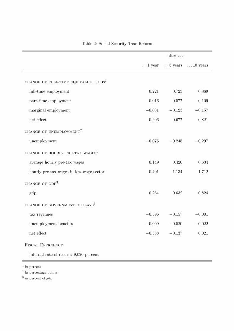
Table 2: Social Security Taxe Reform

after . . .

. . . 1 year . . . 5 years . . . 10 years

change of full-time equivalent jobs1

full-time employment 0.221 0.723 0.869

part-time employment 0.016 0.077 0.109

marginal employment −0.031 −0.123 −0.157

net effect 0.206 0.677 0.821

change of unemployment2

unemployment −0.075 −0.245 −0.297

change of hourly pre-tax wages1

average hourly pre-tax wages 0.149 0.420 0.634

hourly pre-tax wages in low-wage sector 0.401 1.134 1.712

change of gdp3

gdp 0.264 0.632 0.824

change of government outlays3

tax revenues −0.396 −0.157 −0.001

unemployment benefits −0.009 −0.020 −0.022

net effect −0.388 −0.137 0.021

Fiscal Efficiency

internal rate of return: 9.020 percent

1 in percent

2 in percentage points

3 in percent of gdp

Table 3: Public Full-Day School Program

after . . .

. . . 1 year . . . 5 years . . . 10 years

change of full-time equivalent jobs1

full-time employment 0.234 0.793 0.954

part-time employment −0.024 −0.061 −0.062

marginal employment −0.012 −0.058 −0.078

net effect 0.198 0.675 0.813

change of unemployment2

unemployment −0.108 −0.329 −0.381

change of hourly pre-tax wages1

average hourly pre-tax wages 0.121 0.280 0.400

hourly pre-tax wages for women with kids 0.253 0.588 0.839

change of gdp3

gdp 0.217 0.523 0.673

change of government outlays3

tax revenues 0.091 0.218 0.271

unemployment benefits −0.015 −0.031 −0.033

cost −0.660 −0.200 −0.200

net effect −0.554 0.049 0.104

Fiscal Efficiency

internal rate of return: 11.858 percent

1 in percent

2 in percentage points

3 in percent of gdp

Table 4: Deregulation of Professional Services

after . . .

. . . 1 year . . . 5 years . . . 10 years

change of full-time equivalent jobs1

full-time employment 0.005 0.019 0.023

part-time employment 0.000 0.001 0.001

marginal employment 0.000 0.000 −0.000

net effect 0.006 0.020 0.024

change of unemployment2

unemployment −0.007 −0.020 −0.023

change of hourly pre-tax wages1

average hourly pre-tax wages 0.129 0.140 0.145

change of gdp3

gdp 0.127 0.137 0.142

change of government outlays3

tax revenues 0.003 0.007 0.009

unemployment benefits −0.001 −0.002 −0.002

net effect 0.004 0.009 0.011

Fiscal Efficiency

internal rate of return: N/A

1 in percent

2 in percentage points

3 in percent of gdp

Table 5: Reform Package (Social Security Tax and Public Full-Day School Program)

after . . .

. . . 1 year . . . 5 years . . . 10 years

change of full-time equivalent jobs1

full-time employment 0.457 1.499 1.786

part-time employment −0.008 0.012 0.036

marginal employment −0.044 −0.181 −0.231

net effect 0.404 1.330 1.591

change of unemployment2

unemployment −0.182 −0.556 −0.647

change of hourly pre-tax wages1

average hourly pre-tax wages 0.268 0.685 1.005

hourly pre-tax wages in low-wage sector 0.821 2.100 3.082

hourly pre-tax wages for women with kids 0.713 1.825 2.679

change of gdp3

gdp 0.479 1.133 1.455

change of government outlays3

tax revenues −0.308 0.050 0.253

unemployment benefits −0.024 −0.049 −0.052

cost −0.660 −0.200 −0.200

net effect −0.485 −0.101 0.105

Fiscal Efficiency

internal rate of return: 9.369 percent

1 in percent

2 in percentage points

3 in percent of gdp

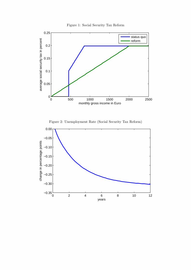
Figure 1: Social Security Tax Reform

0 500 1000 1500 2000 25000

0.05

0.1

0.15

0.2

0.25

monthly gross income in Euro

aver

age

soci

al s

ecur

ity ta

x in

per

cent

status quoreform

Figure 2: Unemployment Rate (Social Security Tax Reform)

0 2 4 6 8 10 12−0.35

−0.30

−0.25

−0.20

−0.15

−0.10

−0.05

0.00

years

chan

ge in

per

cent

age

poin

ts

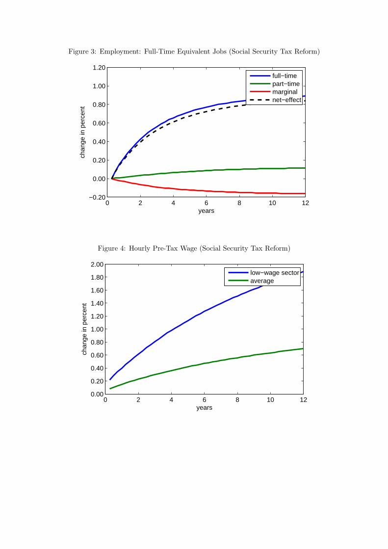
Figure 3: Employment: Full-Time Equivalent Jobs (Social Security Tax Reform)

0 2 4 6 8 10 12−0.20

0.00

0.20

0.40

0.60

0.80

1.00

1.20

years

chan

ge in

per

cent

full−timepart−timemarginalnet−effect

Figure 4: Hourly Pre-Tax Wage (Social Security Tax Reform)

0 2 4 6 8 10 120.00

0.20

0.40

0.60

0.80

1.00

1.20

1.40

1.60

1.80

2.00

years

chan

ge in

per

cent

low−wage sectoraverage

Figure 5: Output (Social Security Tax Reform)

0 2 4 6 8 10 120.10

0.20

0.30

0.40

0.50

0.60

0.70

0.80

0.90

years

chan

ge in

per

cent

Figure 6: Fiscal Effects (Social Security Tax Reform)

0 2 4 6 8 10 12−0.50

−0.40

−0.30

−0.20

−0.10

0.00

0.10

0.20

years

chan

ge in

per

cent

of g

dp

tax revenuesunemployment outlaysnet−effect

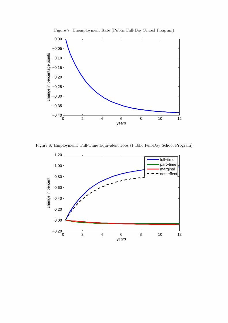
Figure 7: Unemployment Rate (Public Full-Day School Program)

0 2 4 6 8 10 12−0.40

−0.35

−0.30

−0.25

−0.20

−0.15

−0.10

−0.05

0.00

years

chan

ge in

per

cent

age

poin

ts

Figure 8: Employment: Full-Time Equivalent Jobs (Public Full-Day School Program)

0 2 4 6 8 10 12−0.20

0.00

0.20

0.40

0.60

0.80

1.00

1.20

years

chan

ge in

per

cent

full−timepart−timemarginalnet−effect

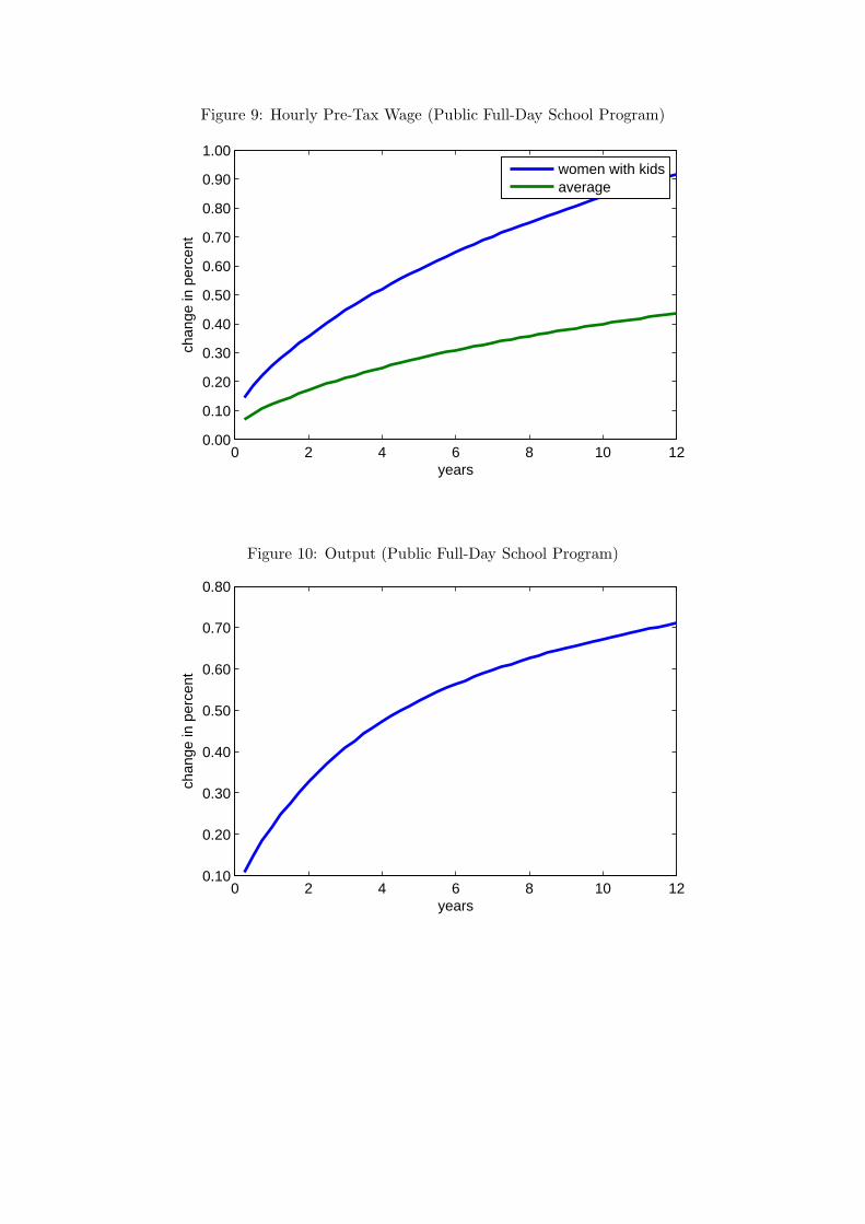
Figure 9: Hourly Pre-Tax Wage (Public Full-Day School Program)

0 2 4 6 8 10 120.00

0.10

0.20

0.30

0.40

0.50

0.60

0.70

0.80

0.90

1.00

years

chan

ge in

per

cent

women with kidsaverage

Figure 10: Output (Public Full-Day School Program)

0 2 4 6 8 10 120.10

0.20

0.30

0.40

0.50

0.60

0.70

0.80

years

chan

ge in

per

cent

Figure 11: Fiscal Effects (Public Full-Day School Program)

0 2 4 6 8 10 12

−0.60

−0.50

−0.40

−0.30

−0.20

−0.10

0.00

0.10

0.20

0.30

years

chan

ge in

per

cent

of g

dp

tax revenuesunemployment outlaysdirect costsnet−effect

Figure 12: Unemployment Rate (Deregulation of Professional Services)

0 2 4 6 8 10 12−0.025

−0.020

−0.015

−0.010

−0.005

0.000

years

chan

ge in

per

cent

age

poin

ts

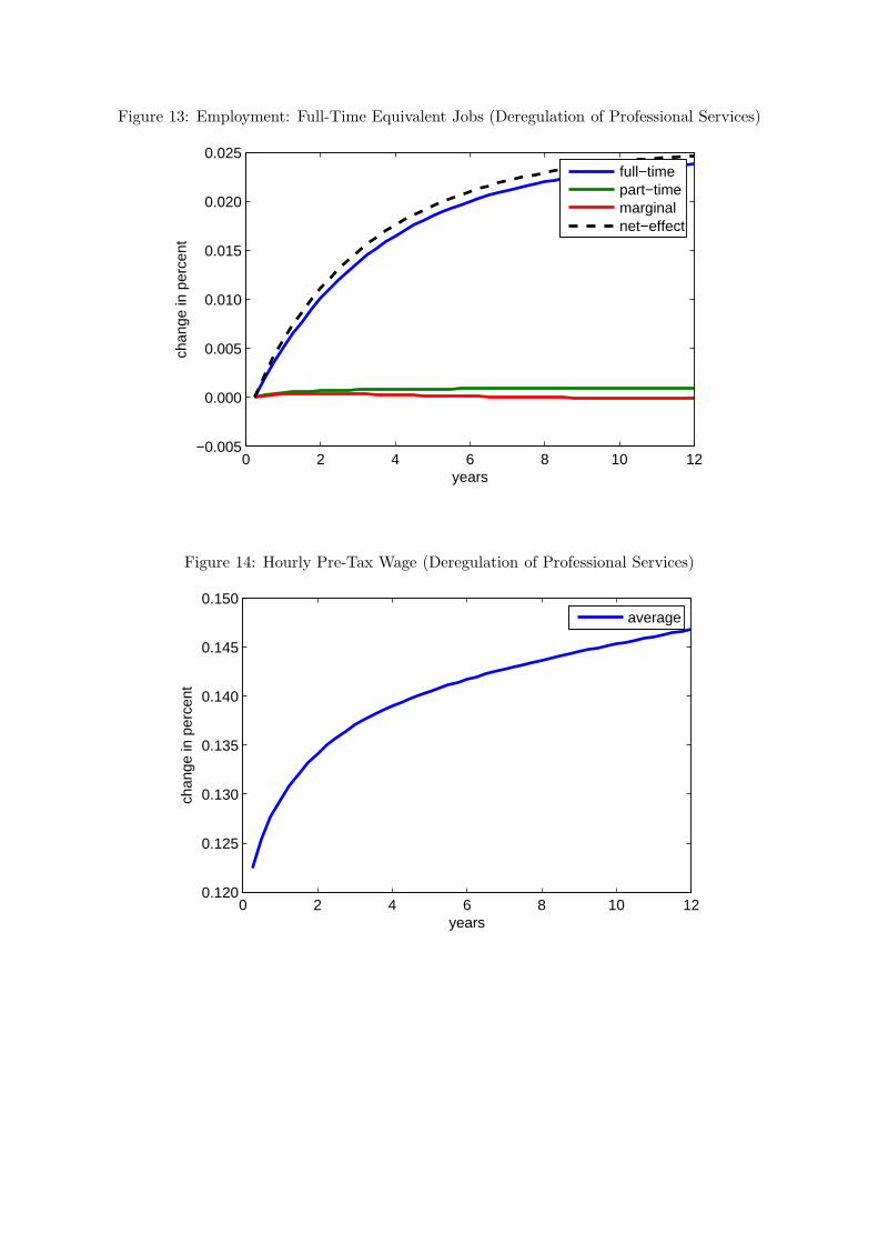
Figure 13: Employment: Full-Time Equivalent Jobs (Deregulation of Professional Services)

0 2 4 6 8 10 12−0.005

0.000

0.005

0.010

0.015

0.020

0.025

years

chan

ge in

per

cent

full−timepart−timemarginalnet−effect

Figure 14: Hourly Pre-Tax Wage (Deregulation of Professional Services)

0 2 4 6 8 10 120.120

0.125

0.130

0.135

0.140

0.145

0.150

years

chan

ge in

per

cent

average

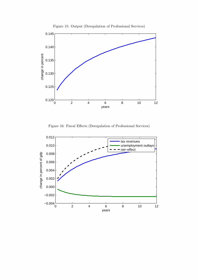
Figure 15: Output (Deregulation of Professional Services)

0 2 4 6 8 10 120.120

0.125

0.130

0.135

0.140

0.145

years

chan

ge in

per

cent

Figure 16: Fiscal Effects (Deregulation of Professional Services)

0 2 4 6 8 10 12−0.004

−0.002

0.000

0.002

0.004

0.006

0.008

0.010

0.012

years

chan

ge in

per

cent

of g

dp

tax revenuesunemployment outlaysnet−effect