R. & M. No. 3729

'~i ' , tl "~q' J

M I N I S T R Y OF D E F E N C E ( P R O C U R E M E N T EXECUTIVE)

AERONAUTICAL RESEARCH COUNCIL REPORTS AND MEMORANDA

Structural Representation in Aeroelastic Calculations

BY LL. T. NIBLETT

Structures Dept., R.A.E., Farnborough

LONDON: HER MAJESTY'S STATIONERY OFFICE

1973

PRICE 50p NET

Structural Representation in Aeroelastic Calculations BY LL. T. NIBLETT

Structures Dept., R.A.E., Farnborough

Reports and Memoranda No. 3729* January, 1972

Summary

The practicability of allowing approximately for the higher-frequency normal modes of a structure by using a residual flexibility matrix is examined somewhat philosophically. There appears to be a better method of approximation, which retains the concept of residual flexibility, and arguments in favour of it are given.

I. Introduction

2. Residual Flexibility Matrices

2.1 Derivation

2.2 Application

2.3 Criticism

3. Calculation of Normal Modes

4. Suggested Structural Representation

5. Advantages of Normal Modes

6. Conclusions

References

Detachable Abstract Cards

LIST OF CONTENTS

I. Introduction

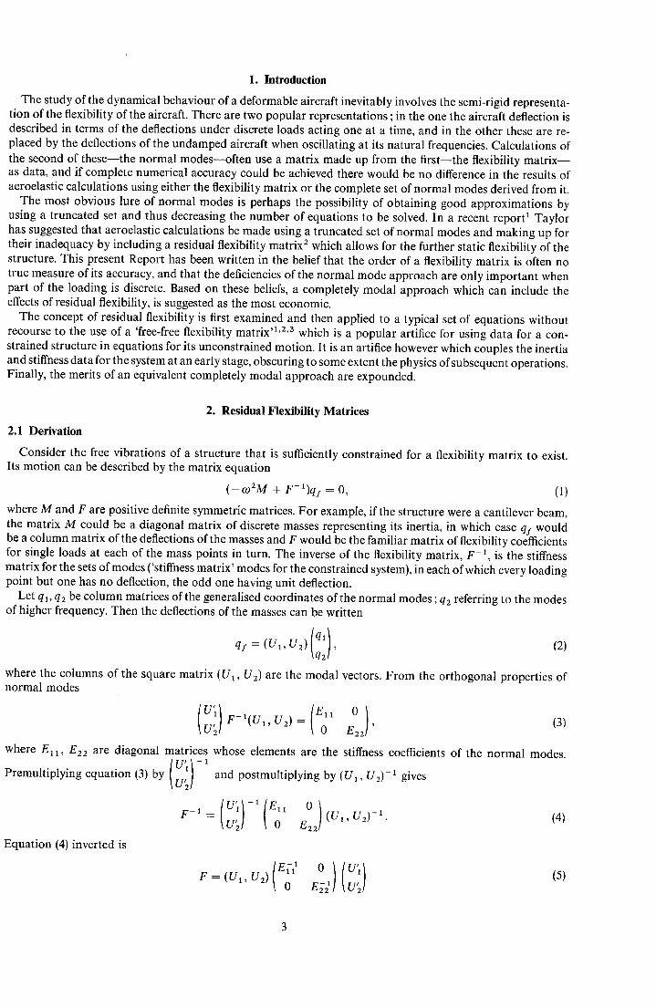
The study of the dynamical behaviour of a deformable aircraft inevitably involves the semi-rigid representa- tion of the flexibility of the aircraft. There are two popular representations ; in the one the aircraft deflection is described in terms of the deflections under discrete loads acting one at a time, and in the other these are re- placed by the deflections of the undamped aircraft when oscillating at its natural frequencies. Calculations of the second of these-- the normal modes--often use a matrix made up from the first--the flexibility matr ix-- as data, and if complete numerical accuracy could be achieved there would be no difference in the results of aeroelastic calculations using either the flexibility matrix or the complete set of normal modes derived from it.

The most obvious lure of normal modes is perhaps the possibility of obtaining good approximations by using a truncated set and thus decreasing the number of equations to be solved. In a recent report 1 Taylor has suggested that aeroelastic calculations be made using a truncated set of normal modes and making up for their inadequacy by including a residual flexibility matrix 2 which allows for the further static flexibility of the structure. This present Report has been written in the belief that the order of a flexibility matrix is often no true measure of its accuracy, and that the deficiencies of the normal mode approach are only important when part of the loading is discrete. Based on these beliefs, a completely modal approach which can include the effects of residual flexibility, is suggested as the most economic.

The concept of residual flexibility is first examined and then applied to a typical set of equations without recourse to the use of a 'free-free flexibility matrix q,2,3 which is a popular artifice for using data for a con- strained structure in equations for its unconstrained motion. It is an artifice however which couples the inertia and stiffness data for the system at an early stage, obscuring to some extent the physics of subsequent operations. Finally, the merits of an equivalent completely modal approach are expounded.

2. Residual Flexibility Matrices

2.1 Derivation

Consider the free vibrations of a structure that is sufficiently constrained for a flexibility matrix to exist. Its motion can be described by the matrix equation

( - ~ 2 M + F-1)qf = 0, (1)

where M and F are positive definite symmetric matrices. For example, if the structure were a cantilever beam, the matrix M could be a diagonal matrix of discrete masses representing its inertia, in which case qf would be a column matrix of the deflections of the masses and F would be the familiar matrix of flexibility coefficients for single loads at each of the mass points in turn. The inverse of the flexibility matrix, F - 1 is the stiffness matrix for the sets of modes ('stiffness matrix' modes for the constrained system), in each of which every loading point but one has no deflection, the odd one having unit deflection.

Let ql, q2 be column matrices of the generalised coordinates of the normal modes ; q2 referring to the modes of higher frequency. Then the deflections of the masses can be written

qf=(U1, U2)(ql), q2

where the columns of the square matrix (U1, U2) are the modal normal modes

u;!

where El l , E22 are diagonal matrices whose elements are the

Premultiplying equation (3) by ' ' [U'll -1 and postmultiplying by u'21

= 1 (U1, U2 )- 1 (4) U'2] E22

Equation (4) inverted is

EH ~u~/

(2)

vectors, From the orthogonal properties of

o) E2 2 , (3)

stiffness coefficients of the normal modes.

(U1, U2 )- 1 gives

(5)

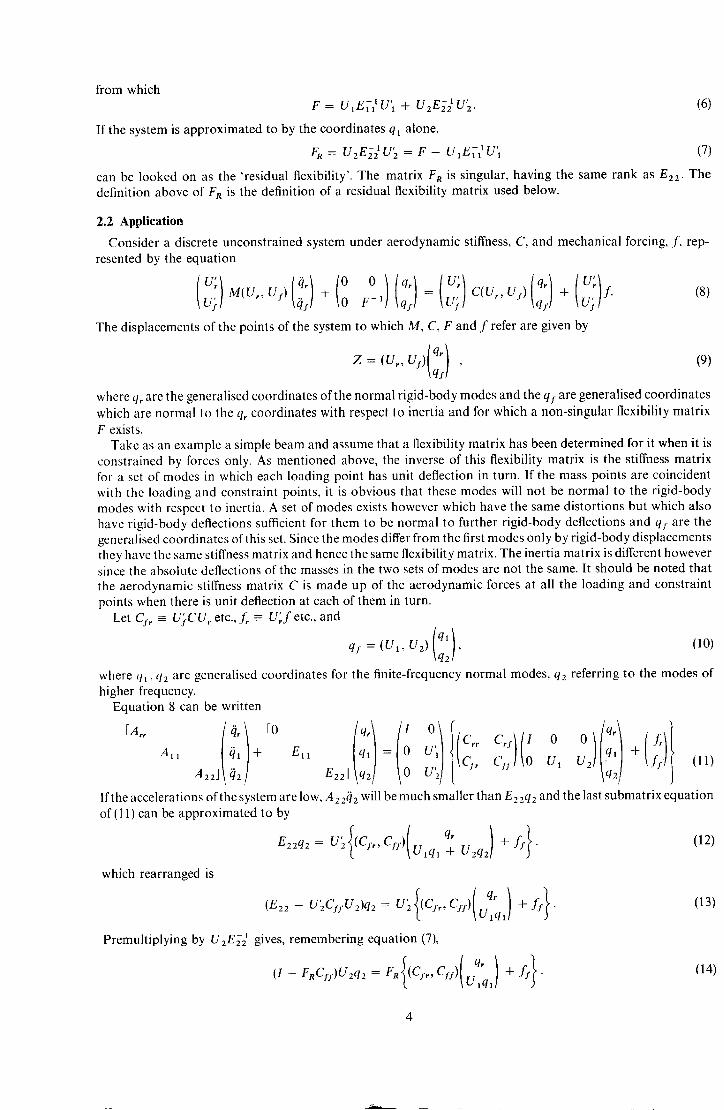
from which F = U , E ; ; U'~ + UzE~)U'z. (6)

If the system is approximated to by the coordinates ql alone,

FR = U 2 E ; ) U ' 2 = F - U I E I I U ' I (7)

can be looked on as the 'residual flexibility'. The matrix F g is singular, having the same rank as E22. The definition above of F R is the definition of a residual flexibility matrix used below.

2.2 Application

Consider a discrete unconstrained system under aerodynamic stiffness, C, and mechanical forcing, f , rep- resented by the equation

~U'j.] ~]y F -1 qf ~U'j.] C(Ur, Uf ) qf Jr- U'y r f. (8)

The displacements of the points of the system to which M, C, F and f refer are given by

U "[q'~ Z = (U,, y)[qf] , (9)

where qr are the generalised coordinates of the normal rigid-body modes and the qs are generalised coordinates which are normal to the qr coordinates with respect to inertia and for which a non-singular flexibility matrix F exists.

Take as an example a simple beam and assume that a flexibility matrix has been determined for it when it is constrained by forces only. As mentioned above, the inverse of this flexibility matrix is the stiffness matrix for a set of modes in which each loading point has unit deflection in turn. If the mass points are coincident with the loading and constraint points, it is obvious that these modes will not be normal to the rigid-body modes with respect to inertia. A set of modes exists however which have the same distortions but which also have rigid-body deflections sufficient for them to be normal to further rigid-body deflections and qf are the generalised coordinates of this set. Since the modes differ from the first modes only by rigid-body displacements they have the same stiffness matrix and hence the same flexibility matrix. The inertia matrix is different however since the absolute deflections of the masses in the two sets of modes are not the same. It should be noted that the aerodynamic stiffness matrix C is made up of the aerodynamic forces at all the loading and constraint points when there is unit deflection at each of them in turn.

Let Cf, -= U)CU, etc., J~ -= U;fe tc . , and

q f = ( U 1 , U2)( ql ), (10) q2

where ql, q2 are generalised coordinates for the finite-frequency normal modes, q2 referring to the modes of

/1223 q2 E22] q2 U~2/ Cfr Cff] U1 U2 2 . " (11)

If the accelerations of the system are low, A22q2 will be much smaller than E22q2 and the last submatrix equation of (11) can be approximated to by

{ ( q ) + 4 . E22q2 = U 2 (Cf,,Cfz) Ulqa + U2q2

which rearranged is

I • (E22 -- S'2Cyfg2)q2 = 02 (G'" Cff) Uaql

Premultiplying by U2E2~ gives, remembering equation (7),

{ (0)+4- (I - FRCIf)U2q2 = FR (Cfr, Cfy) U,ql

higher frequency. Equation 8 can be written

and hence

( )( )(0) q, I 0 q, +

Ulq 1 d- U2q 2 IFRCft I q- IF R glq 1 IF R

where i = (I -- FRC::)-1. Note that

I + iFRC:: = i .

(To prove this premultiply the equation by i - 1 ). From equations (11) and (15)

I q, [Arr A:,J(~])-I-(E10ql) = (I 00]){(;2[ Cry, Ctfl ('FRCf, ~)(Ulql) -t- (]FORff) + (~)}" Hence

- ( q ' ) + f ' U l q l A,,gl, = (C,, + C,:IFRC:,, C,:I)

(15)

(16)

(17)

(18)

{ ,19, A l l g h + Ex:q~ = U'~ [(I + CffIFR)C:~, Cf:I] U:q,

Note that C::I = C::(I - FRC::) -1 = (I - C::FR)-:C:: = IC:: {say) and that

I + iC::F R = i . (20)

Hence equation (19) can be written

,-{ ( q. )+::}. AI~? h + E:lq~ = U , I (C:,, C::) U:ql

By ignoring the inertia forces in the less-grave normal modes, equation (11) has been replaced by equations (18) and (21).

Thus the full number of equations has been reduced to the number that have non-negligible inertia co- efficients but the coefficients of these new equations are evaluated from matrices whose order is the same as that of the flexibility matrix. It can be seen from equation (7) that the residual flexibility matrix describes the flexibility that is left when the system is constrained so that it cannot deflect in its graver modes. Thus, even the simplest loading of the residual system will lead to a complicated deflection since the deflection can only be described in terms of the shapes of the higher-frequency modes.

Associated with this residual flexibility matrix is an aerodynamic stiffness matrix of the same order. Any ihcrease in accuracy due to the inclusion of the residual flexibility is likely to be lost if this aerodynamic stiffness matrix is not accurate enough for the aerodynamic stiffnesses in the higher-frequency modes to be obtained. Thus a large number of collocation points will be needed in the application of the aerodynamic theory if the order of the matrices is at all large and, whether or not the necessary accuracy is achieved, the calculation will be expensive in time and effort.

2.3 Criticism

Flexibility matrices are generally ill-conditioned. This is essentially the result of the loadings used in their determination, and these are about the worst possible from this point of view. If the deflection of the structure under a discrete load is regarded as an arbitrary mode, the column of the deflections at the loading points can be expressed as Zarby = ~ ,~ 1 e,Z, where z, is a column of the deflections in the rth normal mode and ~, is a scalar. Since the load is single, it is likely that cq will be the largest ~ and c~ will decrease as r increases. In a sense the usual flexibility matrix contains too much information on the amount of energy needed to distort the structure into a simple shape and too little about the more complicated shapes. The result of this is that what is left of the flexibility matrix gets less and less accurate as the graver modes are extracted. Minhinnick has suggested 4 that about one significant decimal figure is lost when each normal mode is found. Thus the number of significant figures to which the flexibility coefficients are determined certainly puts an upper limit on the number of normal modes that can be found accurately. When this limit is reached the residual flexibility

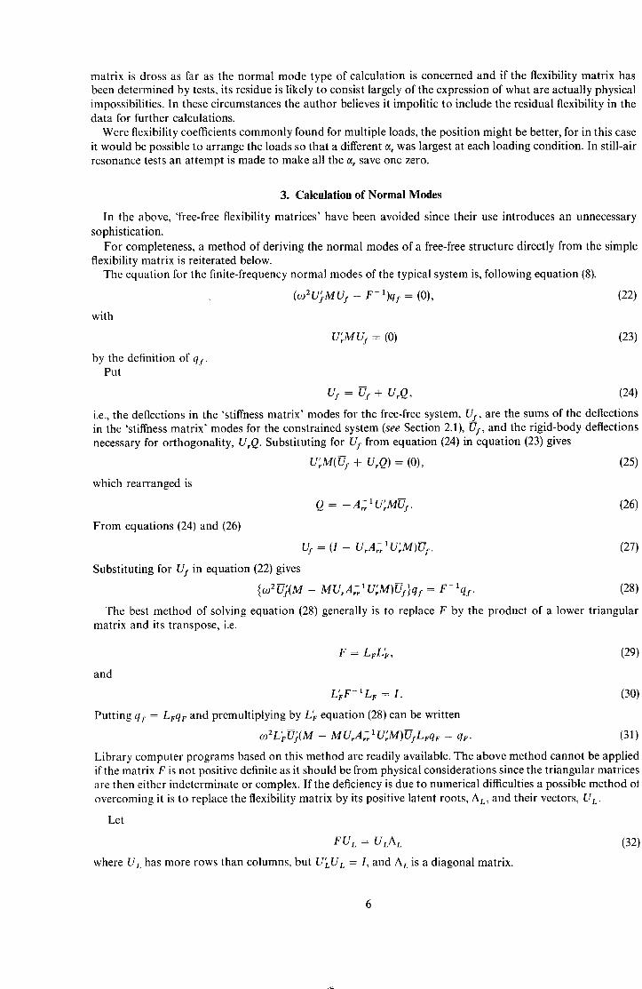
matrix is dross as far as the normal mode type of calculation is concerned and if the flexibility matrix has been determined by tests, its residue is likely to consist largely of the expression of what are actually physical impossibilities. In these circumstances the author believes it impolitic to include the residual flexibility in the data for further calculations.

Were flexibility coefficients commonly found for multiple loads, the position might be better, for in this case it would be possible to arrange the loads so that a different a, was largest at each loading condition. In still-air resonance tests an attempt is made to make all the a, save one zero.

3. Calculation of Normal Modes

In the above, 'free-free flexibility matrices' have been avoided since their use introduces an unnecessary sophistication.

For completeness, a method of deriving the normal modes of a free-free structure directly from the simple flexibility matrix is reiterated below.

The equation for the finite-frequency normal modes of the typical system is, following equation (8),

(~o 2 U'fMU: - F - 1)qf = (0), (22)

with

by the definition of q:. Put

U'~MU: = (0)

U: = U: + UrQ, (24)

i.e., the deflections in the 'stiffness matrix' modes for the free-free system, U:, are the sums of the deflections in the 'stiffness matrix" modes for the constrained system (see Section 2.1), U:, and the rigid-body deflections necessary for orthogonality, UrQ. Substituting for U: from equation (24) in equation (23) gives

which rearranged is

C;M(U: + C,Q.) = (o),

From equations (24) and (26)

(2 = - A 2 ~ U ; M U s ,

Us = (I - UrA~ 1U;M)U:. (27)

Substituting for Us in equation (22) gives

{092 U}(M - MU, A~ 1U;M)U:}q: = F - Xq:. (28)

The best method of solving equation (28) generally is to replace F by the product of a lower triangular matrix and its transpose, i.e.

¢ F = LrL ~, (29)

and

L'rF- 1Lv = I. (30)

Putting q: = Lvq v and premultiplying by L~ equation (28) can be written

co2 L,eU)(M _ MUrA~, 1U,M)UyLvqv = q~. (31)

Library computer programs based on this method are readily available. The above method cannot be applied if the matrix F is not positive definite as it should be from physical considerations since the triangular matrices are then either indeterminate or complex. If the deficiency is due to numerical difficulties a possible method ol overcoming it is to replace the flexibility matrix by its positive latent roots, A L, and their vectors, UL.

Let

F U L = ULAL

where U L has more rows than columns, but U'LUL = I, and A g is a diagonal matrix.

/'

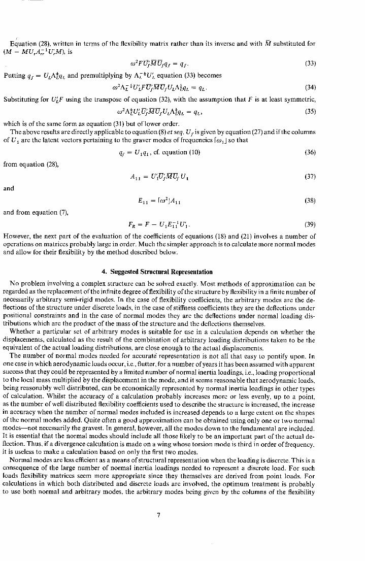
Equation (28), written in terms of the flexibility matrix rather than its inverse and with M substituted for ( m - M U r A ~ ~ U',M), is

o)2FUjeMUsqs = qf ' (33) ½ Putting qs = ULALqL and premultiplying by AZ~Uk equation (33) becomes

(-o2A-£ ½U'LFU}MUsULA~qL = qL. (34)

Substituting for U~F using the transpose of equation (32), with the assumption that F is at least symmetric,

co2A[U'L [-J)MUyULA[qL = qL, (35)

which is of the same form as equation (31) but of lower order. The above results are directly applicable to equation (8) et seq. U s is given by equation (27) and if the columns

of Ux are the latent vectors pertaining to the graver modes of frequencies [COx] so that

qs = U l q l , cf. equation (10) (36)

from equation (28),

and from equation (7),

A ~ = UiU)MU s U~ (37)

Ell = [co2]All (38)

F R = F - U1E-[11U',. (39)

However, the next part of the evaluation of the coefficients of equations (18) and (21) involves a number of operations on matrices probably large in order. Much the simpler approach is to calculate more normal modes and allow for their flexibility by the method described below.

4. Suggested Structural Representation

No problem involving a complex structure can be solved exactly. Most methods of approximation can be regarded as the replacement of the infinite degree of flexibility of the structure by flexibility in a finite number of necessarily arbitrary semi-rigid modes. In the case of flexibility coefficients, the arbitrary modes are the de- flections of the structure under discrete loads, in the case of stiffness coefficients they are the deflections under positional constraints and in the case of normal modes they are the deflections under normal loading dis- tributions which are the product of the mass of the structure and the deflections themselves.

Whether a parti,cular set of arbitrary modes is suitable for use in a calculation depends on whether the displacements, calculated as the result of the combination of arbitrary loading distributions taken to be the equivalent of the actual loading distributions, are close enough to the actual displacements.

The number of normal modes needed for accurat~ representation is not all that easy to pontify upon. In one case in which aerodynamic loads occur, i.e., flutter, for a number of years it has been assumed with apparent success that they could he represented by a limited number of normal inertia loadings, i.e., loading proportional to the local mass multiplied by the displacement in the mode, and it seems reasonable that aerodynamic loads, being reasonably well distributed, can be economically represented by normal inertia loadings in other types of calculation. Whilst the accuracy of a calculation probably increases more or less evenly, up to a point, as the number of well distributed flexibility coefficients used to describe the structure is increased, the increase in accuracy when the number of normal modes included is increased depends to a large extent on the shapes of the normal modes added. Quite often a good approximation can be obtained using only one or two normal modes--not necessarily the gravest. In general, however, all the modes down to the fundamental are included. It is essential that the normal modes should include all those likely to be an important part of the actual de- flection. Thus, if a divergence calculation is made on a wing whose torsion mode is third in order of frequency, it is useless to make a calculation based on only the first two modes.

Normal modes are less efficient as a means of structural representation when the loading is discrete. This is a consequence of the large number of normal inertia loadings needed to represent a discrete load. For such loads flexibility matrices seem more appropriate since they themselves are derived from point loads. For calculations in which both distributed and discrete loads are involved, the optimum treatment is probably to use both normal and arbitrary modes, the arbitrary modes being given by the columns of the flexibility

matrix for the points at which the discrete loads act. This would have the disadvantage of introducing structural couplings into the equations and worsen their condition but some idea of the possible advantages is given by the example quoted by Schwendler and MacNeal z of a cantilevered torsion bar, with an oscillating load at its free end at half the frequency of the fundamental mode. The exact mechanical admittance (O, ip/T) of this system is 1-27324; the admittance when only the fundamental mode is involved is 1.08076 which becomes 1-27019 when residual flexibility is added but the admittance when only the fundamental and a mode of linear twist between root and tip are included is 1.27321. The author intends to test this artifice more fully in the case of the allied problem of the flutter of wings with stores whose mass can be varied. The discrete-load modes could be modified to modes that are normal to each other and the true normal modes, either with respect to inertia only or to both inertia and stiffness, but this should be done only if they cannot be included otherwise.

5. Advantages of Normal Modes

The overriding requirement of any calculation is that the results should be what they purport to be. It is far better to have no results than results that are wrong but not suspect. Thus every opportunity should be taken to apply checks, particularly those which involve some thought. Ocular examination of flexibility matrices is unrewarding, being limited simply to a check of symmetry and the absence of gross errors. The matrix can be checked for positive-definiteness but if it fails this check there is little that can be done to correct the fault on a physical basis with only the raw matrix as evidence. If the normal modes are found, the structural data are then available in a form which has enough character for a judgement of its accuracy to be made on past experience and physical intuition. If the flexibility matrix is not positive definite, one or more of the latent roots of the dynamical matrix will be negative and a decision can be made according to the order of the negative root and the shapes of the modes as to whether the fault is fundamental or due to numerical deficiencies such as round-off error. If the latter is the case it will be possible to continue into further calculation, if sufficient plausible modes have been obtained, without further tampering with the data. The results of still-air resonance test s are generally available in the case of actual aircraft for an overall check of the representation of the structure.

The inclusion of aerodynamic forces and residual flexibility is easier if the representation is by normal modes. Rewrite equation (8) as

,40, 0 E2z xq2 LC2~ C22] q2 f21

where C,~ - U',CU~, .f, - U' , f and here the qx modes include the q, modes. C,~ is the matrix of generalised aerodynamic stiffness based on the work done in the modes r by the aerodynamic forces which arise from deflections in the modes s. These can be calculated as best thought fit, bearing in mind the complexity of the modes, and it is possible for some of the elements of the matrices to be treated as negligible. It follows im- mediately that

(E22 -- CEz)q 2 : C21ql - I - f2 (41)

and

( -coZAl l + El t )q l = {Cll + C12(E22 - C22)-lCE1}q1 + f l + C12(Ea2 - C22)-1f2 (42)

which replace equations (13) and (18) respectively. (E22 -- C22) will be singular only if C22 is appropriate to a critical static divergence speed in the q2 coordinates alone.

The representation of structural damping is always a difficulty. In calculations based on normal modes it is often assumed that the modes are orthogonal with respect to the damping as well as the stiffness and inertia. This is undoubtedly an oversimplification but on the face of it normal modes provide a better basis for representation of damping than influence matrices.

Finally some account should be taken of economy. A unified approach to flutter calculations on the one hand and stability and control problems on the other has long been advocated. To the flutter engineer, basically studying maintained oscillations at a single frequency, normal modes appear to have no real com- petitors as far as structural representation is concerned. Hence the normal modes of aircraft will be found in any case and their use as data in other aeroelastic calculations should not incur extra work.

6. Conclusions

It is advantageous to use normal modes rather than influence matrices for structural representations in aeroelastic calculations for the following reasons:

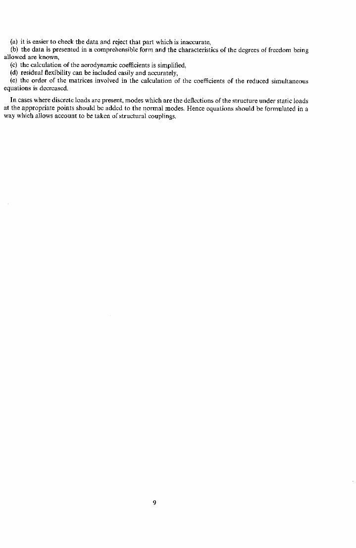
(a) it is easier to check the data and reject that part which is inaccurate, (b) the data is presented in a comprehensible form and the characteristics of the degrees of freedom being

allowed are known, (c) the calculation of the aerodynamic coefficients is simplified, (d) residual flexibility can be included easily and accurately, (e) the order of the matrices involved in the calculation of the coefficients of the reduced simultaneous

equations is decreased.

In cases where discrete loads are present, modes which are the deflections of the structure under static loads at the appropriate points should be added to the normal modes. Hence equations should be formulated in a way which allows account to be taken of structurai couplings.

No. Author(s)

1 A.S. Taylor . . . .

2 R .G . Schwendler and R. H. MacNeal

R. L. Bisplinghoff, H. Ashley and R. L. Halfman

4 I .T . Minhinnick . . . .

REFERENCES

Title, etc.

The mathematical foundation to an integrated approach to the dynamical problems of deformable aircraft.

R.A.E. Technical Report 71131 A.R.C. 33600 (1971).

Opt imum structural representation in aeroelastic analyses. Wright-Patterson Air Force Base ASD-TDR-61-680 (1962).

Aeroelasticity, p. 106. Cambridge, Mass. Addison-Wesley (1955).

The theoretical determination of normal modes and frequencies of vibration.

AGARD Report 36 (1965).

Printed in England for Her Majesty's Stationery Office by J. W. Arrowsmith Ltd., Bristol 3.

Dd 505715 K5 8/73

10

R o & M . No° 3 7 2

© Crown copyright 1973

HER MAJESTY'S STATIONERY OFFICE

Government Bookshops

49 High Holborn, London WCIV 6HB 13a Castle Street, Edinburgh EH2 3AR

109 St Mary Street, Cardi f fCFI 1JW Brazennose Street, Manchester M60 8AS

50 Fairfax Street, Bristol BSI 3DE 258 Broad Street, Birmingham B1 2HE 80 Chichester Street, Belfast BTI 4JY

Gorernment publications are also avai&ble through booksellers

R. & M . Noo 3 7 :

SBN 11 470529 ......