Embed Size (px)
Citation preview
ANALYSIS OF STRUCTURAL TIMBER JOINTS
MADE WITH GLASS FIBRE / EPOXY
BRUNO MASSE
A thesis submitted in partial fulfilment
of the University's requirements
for the Degree of Doctor of Philosophy
JUNE 2003
COVENTRY UNIVERSITY
ABSTRACT
This study investigates the potential of using glass fibre and epoxy resin to join
timber members of the same thickness in the same plane. A total of 64 full-scale
wood/glass/epoxy adhesive joints made with unidirectional or bidirectional glass
fibres were fabricated. Joints with the load applied parallel to the grain or applied
at 90°, 60° and 30° to the grain were tested in static tension. Results of strength and
stiffness were compared between joint configurations.
The strength and stiffness of wood/glass/epoxy joints are mainly driven by the bond
quality. The load capacity is governed by the shear strength of the timber, which
appeared to be slightly affected by the grain orientation.
Finite element analysis was used to model the joints and confirmed the non-uniform
load transfer that occurs on adhesive joints such as wood/glass/epoxy joints. An
internal bending effect occurring at the overlap was also identified in the FE analysis.
The results derived from finite element models correlate well with experimental
results obtained from the sample tests.
Finally the fatigue resistance of wood/glass/epoxy joints was assessed. A total of
13 full-scale wood/glass/epoxy joints (with straight configuration) were tested in
cyclic tension-tension at R = 0.1. The fatigue tests were carried out at a frequency of
0.33 Hz. Wood/glass/epoxy joints exhibit good fatigue resistance compared to other
mechanical timber joints. The fatigue resistance was found dominated by the
composite behaviour rather than the timber. Based on references, it was concluded
that the joints fatigue resistance could be improved further by increasing the length
of composite.
TABLE OF CONTENTS
INTRODUCTION...............................................................................................1
1.1. Introduction...................................................................................................................... 1
1.2. Reader’s guide.................................................................................................................. 4
LITERATURE REVIEW...................................................................................5
2.1. Introduction...................................................................................................................... 5
2.2. Construction environment .............................................................................................. 7
2.2.1. Structural member applications........................................................................... 8
2.2.2. Structural joint applications ................................................................................ 13
2.2.3. Nail plate connections ......................................................................................... 18
2.3. Mechanical Environment ................................................................................................ 21
2.4. Review on fatigue............................................................................................................. 24
2.5. Summary .......................................................................................................................... 28
MATERIALS, PROPERTIES AND CHARACTERISTICS..........................29
3.1. Introduction...................................................................................................................... 29
3.2. Material properties .......................................................................................................... 30
3.2.1. Timber.................................................................................................................. 30
3.2.1.1. General................................................................................................... 30
3.2.1.2. Selected timber ...................................................................................... 35
3.2.2. Glass fibres .......................................................................................................... 37
3.2.2.1. General................................................................................................... 37
3.2.2.2. Selected glass fibres............................................................................... 39
3.2.3. Epoxy resin .......................................................................................................... 42
3.2.3.1. General................................................................................................... 42
3.2.3.2. Selected epoxy resin .............................................................................. 45
3.2.4. Glass fibre/epoxy composite ................................................................................ 48
3.2.4.1. General................................................................................................... 48
3.2.4.2. Selected glass fibre/epoxy composite .................................................... 54
3.3. Summary .......................................................................................................................... 55
i
EXPERIMENTAL PROGRAMME..................................................................56
4.1. Introduction...................................................................................................................... 56
4.2. Testing of glass fibre/epoxy composite........................................................................... 56
4.3. Wood/glass/epoxy joints .................................................................................................. 60
4.3.1. Joint geometry requirements ............................................................................... 60
4.3.2. Types of test ......................................................................................................... 65
4.3.2.1. The choice of tests ................................................................................. 65
4.3.2.2. Tension capacity test with load parallel to the grain.............................. 68
4.3.2.3. Tension capacity test with load perpendicular to the grain.................... 72
4.3.2.4. Tension capacity test with load at 60° angle to the grain ...................... 74
4.3.2.5. Tension capacity test with load at 30° angle to the grain ...................... 77
4.3.3. Number of samples tested .................................................................................... 81
4.3.4. Testing equipment (LVDT, Translog 500, tension rig, frame)............................. 83
4.3.5. Sample fabrication process.................................................................................. 91
4.3.5.1. Straight configuration ............................................................................ 93
4.3.5.2. Angle configuration............................................................................... 98
4.3.5.3. Samples with strain gauges.................................................................... 102
4.4. Timber properties testing................................................................................................ 104
4.4.1. Timber conditioning and preliminary grading .................................................... 105
4.4.2. Determination of timber mechanical properties.................................................. 106
4.4.2.1. Determination of modulus of elasticity in bending................................ 107
4.4.2.2. Determination of modulus of elasticity and strength in tension
parallel to the grain ................................................................................ 110
4.4.2.3. Determination of modulus of elasticity and strength in tension
perpendicular to the grain ...................................................................... 113
4.4.2.3.1. EN 1193: 1997 Standard test ................................................... 113
4.4.2.3.2. Alternative test......................................................................... 115
4.4.2.4. Determination of shear strength parallel to the grain............................. 118
4.5. Summary .......................................................................................................................... 119
EXPERIMENTAL RESULTS...........................................................................120
5.1. Introduction...................................................................................................................... 120
5.2. Preliminary tests .............................................................................................................. 120
5.2.1. Test of wood/glass/epoxy samples with varying lengths of composite................. 120
5.2.2. Test of wood/glass/epoxy samples for experimental adjustments ........................ 123
5.3. Timber grading tests........................................................................................................ 127
5.4. Tension parallel to the grain tests................................................................................... 129
ii
5.4.1. TPU00 and TPB00 Tests ..................................................................................... 129
5.4.2. TPU10 and TPB30 Tests ..................................................................................... 140
5.4.3. Discussion............................................................................................................ 149
5.5. Tension not parallel to the grain tests ............................................................................ 153
5.5.1. TNU90 and TNB90 Tests ..................................................................................... 153
5.5.2. TNU60 and TNB60 Tests ..................................................................................... 163
5.5.3. TNU30 and TNB30 Tests ..................................................................................... 172
5.5.4. Discussion............................................................................................................ 182
5.6. Samples tested with strain gauges .................................................................................. 187
5.7. Strength determination and timber grading ................................................................. 192
5.7.1. Small clear sample tests....................................................................................... 192
5.7.2. Principles and methods........................................................................................ 196
5.7.3. Small clear sample test results............................................................................. 201
5.7.3.1. Static Bending tests................................................................................ 201
5.7.3.2. Tension parallel to the grain tests .......................................................... 202
5.7.3.3. Tension perpendicular to the grain tests ................................................ 204
5.7.3.4. Shear parallel to the grain tests .............................................................. 206
5.7.4. Comparison and discussion................................................................................. 207
5.8. Conclusion ........................................................................................................................ 219
THEORETICAL AND FINITE ELEMENT ANALYSES .............................221
6.1. Introduction...................................................................................................................... 221
6.2. Theoretical approach to structural adhesive joints ...................................................... 222
6.2.1. Anisotropic and orthotropic materials ................................................................ 223
6.2.2. Micromechanics of composite materials ............................................................. 235
6.2.2.1. Stiffness approach to lamina with uniaxial fibres.................................. 237
6.2.2.2. Stiffness approach to lamina with biaxial fibres.................................... 244
6.2.3. Double lap joints.................................................................................................. 246
6.2.3.1. Load transfer mechanisms in double lap joints...................................... 249
6.2.3.2. Wood/glass/epoxy joints........................................................................ 253
6.2.3.3. Existing comparable results ................................................................... 256
6.3. Finite element modelling ................................................................................................. 261
6.3.1. Introduction ......................................................................................................... 261
6.3.2. FEM procedures .................................................................................................. 261
6.3.2.1. Analysis type ......................................................................................... 261
6.3.2.2. Elements and mesh types....................................................................... 265
6.3.3. Joints with load parallel to the grain................................................................... 268
6.3.3.1. Configuration with uniaxial fibres TPU00 ............................................ 273
iii
6.3.3.1.1. 2-Dimensional model............................................................... 273
6.3.3.1.2. 3-Dimensional model............................................................... 280
6.3.3.2. Configuration with biaxial fibres TPB00............................................... 287
6.3.3.2.1. 2-Dimensional model............................................................... 287
6.3.3.2.2. 3-Dimensional model............................................................... 292
6.3.4. Joints with load not parallel to the grain ............................................................ 298
6.3.4.1. Load applied perpendicular to the grain ................................................ 298
6.3.4.1.1. Configuration with uniaxial fibres TNU90.............................. 298
6.3.4.1.2. Configuration with biaxial fibres TNB90................................ 304
6.3.4.2. Load applied with an angle of 60 degrees to the grain .......................... 309
6.3.4.2.1. Configuration with uniaxial fibres TNU60.............................. 309
6.3.4.2.2. Configuration with biaxial fibres TNB60................................ 315
6.3.4.3. Load applied with an angle of 30 degrees to the grain .......................... 321
6.3.4.3.1. Configuration with uniaxial fibres TNU30.............................. 321
6.3.4.3.2. Configuration with biaxial fibres TNB30................................ 327
6.4. Internal bending effects................................................................................................... 334
6.5. Discussion and conclusion ............................................................................................... 336
FATIGUE ASSESSMENT OF WOOD/GLASS/EPOXY JOINTS................340
7.1. Introduction...................................................................................................................... 340
7.2. Fatigue test programme .................................................................................................. 341
7.2.1. Methodology ........................................................................................................ 341
7.2.2. Testing equipment................................................................................................ 345
7.2.3. Joint properties and configurations..................................................................... 347
7.3. Test results........................................................................................................................ 351
7.3.1. Preliminary results .............................................................................................. 352
7.3.2. Fatigue properties and S-N curve........................................................................ 355
7.3.2.1. Experimental results .............................................................................. 355
7.3.2.2. Fatigue properties of materials .............................................................. 358
7.3.2.3. Relationship with current design codes ................................................. 374
7.3.3. Other wood/glass/epoxy joints fatigue results ..................................................... 379
7.4. Conclusion ........................................................................................................................ 387
iv
v
CONCLUSIONS .................................................................................................391
8.1. General conclusions ......................................................................................................... 391
8.2. Suggestions for future work............................................................................................ 393
REFERENCES....................................................................................................394
APPENDIX ..........................................................................................................403
A. Strains results from static tensile tests of wood/glass/epoxy joints.............................. 403
B. Results of small clear samples tests ................................................................................ 406
B.1. Static bending tests results................................................................................... 406
B.2. Tension parallel to the grain tests results............................................................ 407
B.3. Tension perpendicular to the grain tests results.................................................. 408
B.4. Shear parallel to the grain tests results ............................................................... 409
C. Example of in-plane and out-of-plane bending moment calculations ......................... 410
D. Technical details for FE models...................................................................................... 411
D.1. Models with load parallel to the grain TPU/B00 – 2D models ........................... 411
D.2. Models with load parallel to the grain TPU/B00 – 3D models ........................... 413
D.3. Models with load perpendicular to the grain TNU/B90 – 3D models ................. 415
D.4. Models with load at 60° to the grain TNU/B60 – 3D models.............................. 417
D.5. Models with load at 30° to the grain TNU/B30 – 3D models.............................. 420
LIST OF FIGURES
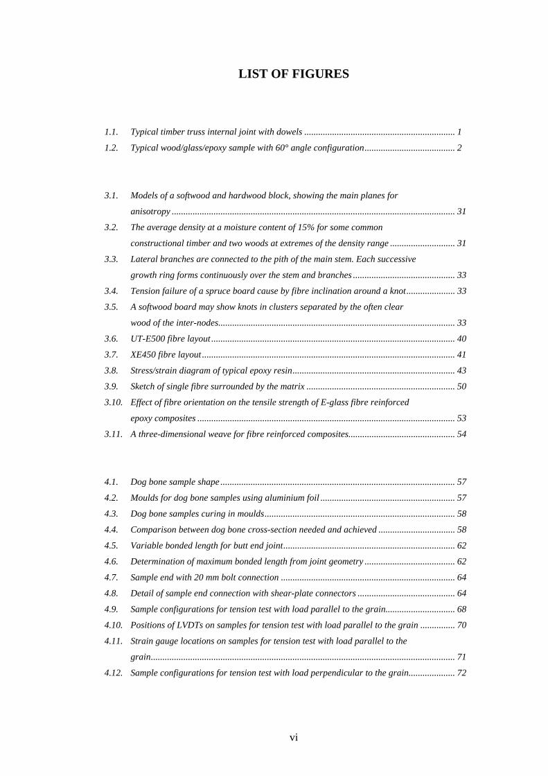
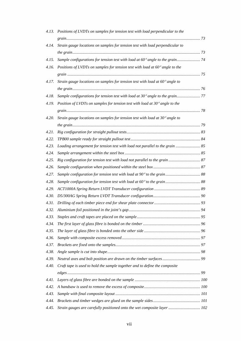
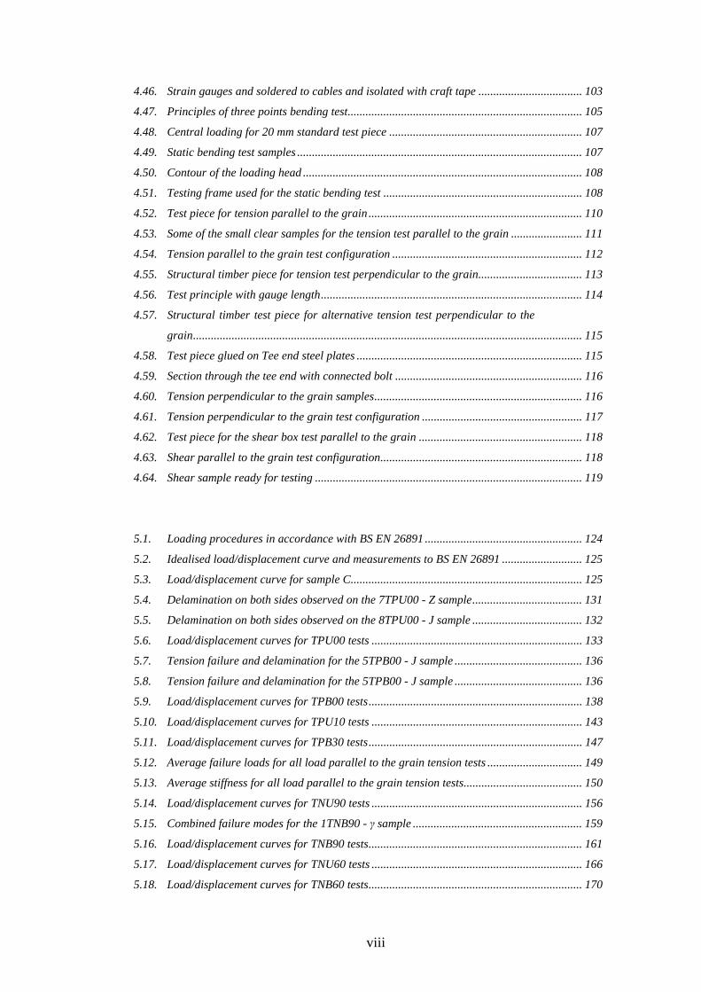
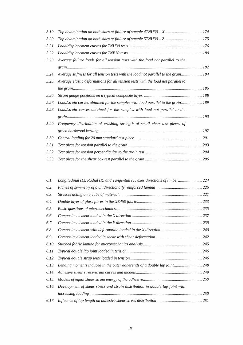
1.1. Typical timber truss internal joint with dowels ................................................................. 1
1.2. Typical wood/glass/epoxy sample with 60° angle configuration....................................... 2
3.1. Models of a softwood and hardwood block, showing the main planes for
anisotropy .......................................................................................................................... 31
3.2. The average density at a moisture content of 15% for some common
constructional timber and two woods at extremes of the density range ............................ 31
3.3. Lateral branches are connected to the pith of the main stem. Each successive
growth ring forms continuously over the stem and branches ............................................ 33
3.4. Tension failure of a spruce board cause by fibre inclination around a knot..................... 33
3.5. A softwood board may show knots in clusters separated by the often clear
wood of the inter-nodes...................................................................................................... 33
3.6. UT-E500 fibre layout ......................................................................................................... 40
3.7. XE450 fibre layout ............................................................................................................. 41
3.8. Stress/strain diagram of typical epoxy resin...................................................................... 43
3.9. Sketch of single fibre surrounded by the matrix ................................................................ 50
3.10. Effect of fibre orientation on the tensile strength of E-glass fibre reinforced
epoxy composites ............................................................................................................... 53
3.11. A three-dimensional weave for fibre reinforced composites.............................................. 54
4.1. Dog bone sample shape ..................................................................................................... 57
4.2. Moulds for dog bone samples using aluminium foil .......................................................... 57
4.3. Dog bone samples curing in moulds.................................................................................. 58
4.4. Comparison between dog bone cross-section needed and achieved ................................. 58
4.5. Variable bonded length for butt end joint.......................................................................... 62
4.6. Determination of maximum bonded length from joint geometry ....................................... 62
4.7. Sample end with 20 mm bolt connection ........................................................................... 64
4.8. Detail of sample end connection with shear-plate connectors .......................................... 64
4.9. Sample configurations for tension test with load parallel to the grain.............................. 68
4.10. Positions of LVDTs on samples for tension test with load parallel to the grain ............... 70
4.11. Strain gauge locations on samples for tension test with load parallel to the
grain................................................................................................................................... 71
4.12. Sample configurations for tension test with load perpendicular to the grain.................... 72
vi
4.13. Positions of LVDTs on samples for tension test with load perpendicular to the
grain................................................................................................................................... 73
4.14. Strain gauge locations on samples for tension test with load perpendicular to
the grain............................................................................................................................. 73
4.15. Sample configurations for tension test with load at 60° angle to the grain....................... 74
4.16. Positions of LVDTs on samples for tension test with load at 60° angle to the
grain .................................................................................................................................. 75
4.17. Strain gauge locations on samples for tension test with load at 60° angle to
the grain............................................................................................................................. 76
4.18. Sample configurations for tension test with load at 30° angle to the grain....................... 77
4.19. Position of LVDTs on samples for tension test with load at 30° angle to the
grain................................................................................................................................... 78
4.20. Strain gauge locations on samples for tension test with load at 30° angle to
the grain............................................................................................................................. 79
4.21. Rig configuration for straight pullout tests........................................................................ 83
4.22. TPB00 sample ready for straight pullout test .................................................................... 84
4.23. Loading arrangement for tension test with load not parallel to the grain ........................ 85
4.24. Sample arrangement within the steel box .......................................................................... 85
4.25. Rig configuration for tension test with load not parallel to the grain ............................... 87
4.26. Sample configuration when positioned within the steel box .............................................. 87
4.27. Sample configuration for tension test with load at 90° to the grain .................................. 88
4.28. Sample configuration for tension test with load at 60° to the grain .................................. 88
4.29. ACT1000A Spring Return LVDT Transducer configuration ............................................. 89
4.30. D5/300AG Spring Return LVDT Transducer configuration.............................................. 90
4.31. Drilling of each timber piece end for shear plate connector ............................................. 93
4.32. Aluminium foil positioned in the joint’s gap...................................................................... 94
4.33. Staples and craft tapes are placed on the sample.............................................................. 95
4.34. The first layer of glass fibre is bonded on the timber ........................................................ 96
4.35. The layer of glass fibre is bonded onto the other side ....................................................... 96
4.36. Sample with composite excess removed............................................................................. 97
4.37. Brackets are fixed onto the samples................................................................................... 97
4.38. Angle sample is cut into shape........................................................................................... 98
4.39. Neutral axes and bolt position are drawn on the timber surfaces ..................................... 99
4.40. Craft tape is used to hold the sample together and to define the composite
edges .................................................................................................................................. 99
4.41. Layers of glass fibre are bonded on the sample ................................................................ 100
4.42. A handsaw is used to remove the excess of composite....................................................... 100
4.43. Sample with final composite layout ................................................................................... 101
4.44. Brackets and timber wedges are glued on the sample sides .............................................. 101
4.45. Strain gauges are carefully positioned onto the wet composite layer ............................... 102
vii
4.46. Strain gauges and soldered to cables and isolated with craft tape ................................... 103
4.47. Principles of three points bending test............................................................................... 105
4.48. Central loading for 20 mm standard test piece ................................................................. 107
4.49. Static bending test samples ................................................................................................ 107
4.50. Contour of the loading head .............................................................................................. 108
4.51. Testing frame used for the static bending test ................................................................... 108
4.52. Test piece for tension parallel to the grain ........................................................................ 110
4.53. Some of the small clear samples for the tension test parallel to the grain ........................ 111
4.54. Tension parallel to the grain test configuration ................................................................ 112
4.55. Structural timber piece for tension test perpendicular to the grain................................... 113
4.56. Test principle with gauge length........................................................................................ 114
4.57. Structural timber test piece for alternative tension test perpendicular to the
grain................................................................................................................................... 115
4.58. Test piece glued on Tee end steel plates ............................................................................ 115
4.59. Section through the tee end with connected bolt ............................................................... 116
4.60. Tension perpendicular to the grain samples...................................................................... 116
4.61. Tension perpendicular to the grain test configuration ...................................................... 117
4.62. Test piece for the shear box test parallel to the grain ....................................................... 118
4.63. Shear parallel to the grain test configuration.................................................................... 118
4.64. Shear sample ready for testing .......................................................................................... 119
5.1. Loading procedures in accordance with BS EN 26891 ..................................................... 124
5.2. Idealised load/displacement curve and measurements to BS EN 26891 ........................... 125
5.3. Load/displacement curve for sample C.............................................................................. 125
5.4. Delamination on both sides observed on the 7TPU00 - Z sample..................................... 131
5.5. Delamination on both sides observed on the 8TPU00 - J sample ..................................... 132
5.6. Load/displacement curves for TPU00 tests ....................................................................... 133
5.7. Tension failure and delamination for the 5TPB00 - J sample ........................................... 136
5.8. Tension failure and delamination for the 5TPB00 - J sample ........................................... 136
5.9. Load/displacement curves for TPB00 tests........................................................................ 138
5.10. Load/displacement curves for TPU10 tests ....................................................................... 143
5.11. Load/displacement curves for TPB30 tests........................................................................ 147
5.12. Average failure loads for all load parallel to the grain tension tests ................................ 149
5.13. Average stiffness for all load parallel to the grain tension tests........................................ 150
5.14. Load/displacement curves for TNU90 tests ....................................................................... 156
5.15. Combined failure modes for the 1TNB90 - γ sample ......................................................... 159
5.16. Load/displacement curves for TNB90 tests........................................................................ 161
5.17. Load/displacement curves for TNU60 tests ....................................................................... 166
5.18. Load/displacement curves for TNB60 tests........................................................................ 170
viii
5.19. Top delamination on both sides at failure of sample 4TNU30 – X.................................... 174
5.20. Top delamination on both sides at failure of sample 5TNU30 – Z .................................... 175
5.21. Load/displacement curves for TNU30 tests ....................................................................... 176
5.22. Load/displacement curves for TNB30 tests........................................................................ 180
5.23. Average failure loads for all tension tests with the load not parallel to the
grain................................................................................................................................... 182
5.24. Average stiffness for all tension tests with the load not parallel to the grain.................... 184
5.25. Average elastic deformations for all tension tests with the load not parallel to
the grain............................................................................................................................. 185
5.26. Strain gauge positions on a typical composite layer. ........................................................ 188
5.27. Load/strain curves obtained for the samples with load parallel to the grain.................... 189
5.28. Load/strain curves obtained for the samples with load not parallel to the
grain................................................................................................................................... 190
5.29. Frequency distribution of crushing strength of small clear test pieces of
green hardwood keruing.................................................................................................... 197
5.30. Central loading for 20 mm standard test piece ................................................................. 201
5.31. Test piece for tension parallel to the grain ........................................................................ 203
5.32. Test piece for tension perpendicular to the grain test ....................................................... 204
5.33. Test piece for the shear box test parallel to the grain ....................................................... 206
6.1. Longitudinal (L), Radial (R) and Tangential (T) axes directions of timber....................... 224
6.2. Planes of symmetry of a unidirectionally reinforced lamina ............................................. 225
6.3. Stresses acting on a cube of material ................................................................................ 227
6.4. Double layer of glass fibres in the XE450 fabric............................................................... 233
6.5. Basic questions of micromechanics ................................................................................... 235
6.6. Composite element loaded in the X direction .................................................................... 237
6.7. Composite element loaded in the Y direction .................................................................... 239
6.8. Composite element with deformation loaded in the X direction ........................................ 240
6.9. Composite element loaded in shear with shear deformation............................................. 242
6.10. Stitched fabric lamina for micromechanics analysis ......................................................... 245
6.11. Typical double lap joint loaded in tension......................................................................... 246
6.12. Typical double strap joint loaded in tension...................................................................... 246
6.13. Bending moments induced in the outer adherends of a double lap joint........................... 248
6.14. Adhesive shear stress-strain curves and models................................................................ 249
6.15. Models of equal shear strain energy of the adhesive......................................................... 250
6.16. Development of shear stress and strain distribution in double lap joint with
increasing loading ............................................................................................................. 250
6.17. Influence of lap length on adhesive shear stress distribution............................................ 251
ix
6.18. Ideal models of thickness distribution of glass fibre and epoxy resin................................ 254
6.19. Adhesive shear stress distributions in aluminium-aluminium joints.................................. 256
6.20. Adhesive shear stress distributions in CFRP-CFRP joints................................................ 256
6.21. Adherend tensile stress distributions in CFRP-CFRP double lap joints ........................... 257
6.22. Adhesive shear stress distributions in cross-ply CFRP-CFRP and
unidirectional CFRP-CFRP double lap joints................................................................... 258
6.23. Adhesive shear stress distributions in aluminium-CFRP double lap joints....................... 258
6.24. Adhesive shear stress distributions in aluminium-CFRP double lap joints
with equal and matched adherends ................................................................................... 259
6.25. Example of 2D configuration for straight joint ................................................................. 263
6.26. Example of 2D configuration and symmetry for straight joint .......................................... 264
6.27. Example of 3D configuration and symmetry for straight joint .......................................... 264
6.28. Example of 2D straight joint model with rectangular mesh .............................................. 268
6.29. Another example of 2D straight joint model with rectangular mesh ................................. 268
6.30. Example of 2D straight joint model with a coarse-to-fine mesh........................................ 269
6.31. Another example of 2D straight joint model with a coarse-to-fine mesh .......................... 269
6.32. Example of 2D straight joint model with free quadrilateral mesh generated
using SmartMeshing .......................................................................................................... 270
6.33. Convergence graph of longitudinal strain recorded on node A ........................................ 271
6.34. Convergence graph of longitudinal strain recorded on node B ........................................ 271
6.35. Refined of 2D straight joint model with free quadrilateral mesh
(18499 elements)................................................................................................................ 272
6.36. Zooms of the 2D straight joint model (18499 elements) showing locations of
nodes A and B .................................................................................................................... 272
6.37. Zooms of the 2D straight joint model (18499 elements) showing locations of
nodes A and B .................................................................................................................... 272
6.38. Graphical results of the 2D model type TPU00................................................................. 274
6.39. Deformed shape at composite left end of the 2D model type TPU00 ................................ 275
6.40. Tensile stress distributions at the interface between the composite and the
timber................................................................................................................................. 276
6.41. Shear stress distributions at the interface between the composite and the
timber................................................................................................................................. 278
6.42. Longitudinal tensile strain distribution on glass fibre/epoxy surface................................ 279
6.43. Graphical results of the 3D model type TPU00................................................................. 281
6.44. Tensile stress distributions at the interface between the composite and the
timber................................................................................................................................. 282
6.45. Shear stress distributions at the interface between the composite and the
timber................................................................................................................................. 284
6.46. Longitudinal tensile strain distribution on glass fibre/epoxy surface................................ 285
6.47. Graphical results of the 2D model type TPB00 ................................................................. 288
x
6.48. Tensile stress distributions at the interface between the composite and the
timber................................................................................................................................. 289
6.49. Shear stress distributions at the interface between the composite and the
timber................................................................................................................................. 290
6.50. Longitudinal tensile strain distribution on glass fibre/epoxy surface................................ 291
6.51. Graphical results of the 3D model type TPB00 ................................................................. 293
6.52. Tensile stress distributions at the interface between the composite and the
timber................................................................................................................................. 294
6.53. Shear stress distributions at the interface between the composite and the
timber................................................................................................................................. 295
6.54. Longitudinal tensile strain distribution on glass fibre/epoxy surface................................ 296
6.55. Graphical results of the 3D model type TNU90 ................................................................ 299
6.56. Tensile stress distributions at the interface between the composite and the
timber................................................................................................................................. 300
6.57. Shear stress distributions at the interface between the composite and the
timber................................................................................................................................. 302
6.58. Tensile strain distribution on glass fibre/epoxy surface .................................................... 303
6.59. Graphical results of the 3D model type TNB90................................................................. 305
6.60. Tensile stress distributions at the interface between the composite and the
timber................................................................................................................................. 306
6.61. Shear stress distributions at the interface between the composite and the
timber................................................................................................................................. 307
6.62. Longitudinal tensile strain distribution on glass fibre/epoxy surface................................ 308
6.63. Graphical results of the 3D model type TNU60 ................................................................ 310
6.64. Tensile stress distributions at the interface between the composite and the
timber................................................................................................................................. 311
6.65. Shear stress distributions at the interface between the composite and the
timber................................................................................................................................. 313
6.66. Longitudinal tensile strain distribution on glass fibre/epoxy surface................................ 314
6.67. Graphical results of the 3D model type TNB60................................................................. 316
6.68. Tensile stress distributions at the interface between the composite and the
timber................................................................................................................................. 317
6.69. Shear stress distributions at the interface between the composite and the
timber................................................................................................................................. 318
6.70. Longitudinal tensile strain distribution on glass fibre/epoxy surface................................ 319
6.71. Graphical results of the 3D model type TNU30 ................................................................ 322
6.72. Tensile stress distributions at the interface between the composite and the
timber................................................................................................................................. 323
6.73. Shear stress distributions at the interface between the composite and the
timber................................................................................................................................. 325
xi
6.74. Longitudinal tensile strain distribution on glass fibre/epoxy surface................................ 326
6.75. Graphical results of the 3D model type TNB30................................................................. 328
6.76. Tensile stress distributions at the interface between the composite and the
timber................................................................................................................................. 329
6.77. Shear stress distributions at the interface between the composite and the
timber................................................................................................................................. 331
6.78. Longitudinal tensile strain distribution on glass fibre/epoxy surface................................ 332
6.79. Deformed shape with lateral deformation ∆ω of the 2D FE model
type TPU00 ........................................................................................................................ 334
7.1. Typical saw tooth stress versus time waveform ................................................................. 343
7.2. Set of σ-log N curves for tension-tension (R = 0.1, 0.3 and 0.5) and
tension-compression (R = -0.5 and -1) cyclic stress configurations ................................. 344
7.3. The J.J. Lloyds machine during the fatigue test of one of the sample ............................... 346
7.4. Sample configuration type TPU00 for fatigue test ............................................................ 348
7.5. LVDTs and strain gauges positions on fatigue test samples.............................................. 349
7.6. Strain gauges positions on fatigue test samples ................................................................ 349
7.7. Sample in position ready for the fatigue test ..................................................................... 350
7.8. Three points bending test of one timber plank before joint fabrication............................. 352
7.9. S-N logarithmic curves for wood/glass/epoxy joints tested in
tension-tension at R = 0.1.................................................................................................. 356
7.10. Typical S-N curves for 1045 Steel and 2014-T6 Aluminium alloy..................................... 359
7.11. S-N curves of reversed axial stresses for mild steel (•) and
24S-T3 aluminium alloy (×) ............................................................................................... 359
7.12. S-N curves for various construction materials at R = 0.1 ................................................. 360
7.13. S-N curves for sliced Khaya laminates tested in bending at R = 0.................................... 361
7.14. S-N curves for Khaya axially loaded at R = -1, -2, -10 and 10 ......................................... 362
7.15. S-N curves for Khaya and Douglas fir tested in tension-compression
at R = -1............................................................................................................................. 362
7.16. S-N curves for Khaya tested in shear at R = 0.1 ............................................................... 363
7.17. S-N curves for laminated Khaya tested in tension-tension at R = 0.1 ............................... 364
7.18. Maximum and minimum strain plotted versus log cycles for three Khaya
samples tested in tension-tension fatigue at R = 0.1 and peak stress
of 55 MPa .......................................................................................................................... 365
7.19. S-N curves for laminated Douglas fir tested at R = 0.1..................................................... 365
7.20. S-N curves for timber at various frequencies .................................................................... 366
7.21. Fatigue failure mechanisms in composites ........................................................................ 367
7.22. Fatigue life diagram with damage mechanisms for a unidirectional
composite subjected to tension-tension stresses ................................................................ 368
xii
7.23. Normalised S-N curves for three unidirectional composite materials............................... .369
7.24. Extremes of normalised S-N tensile fatigue data from glass fibre laminate at
R = 0.1 ............................................................................................................................... 371
7.25. The fatigue sensitivity coefficient for unidirectional glass fibre laminates as a
function of fibre content at R = 0.1.................................................................................... 372
7.26. Effect of matrix material on tensile fatigue in glass fibre laminates with
0° and ±45° plies at R = 0.1 .............................................................................................. 373
7.27. kfat-log N relationship from EC5: Pt 2 combined with bonded-in rod
connections test results ...................................................................................................... 375
7.28. kfat-log N relationship from EC5: Pt 2 combined with bonded-in rod
connection test results by failure modes ............................................................................ 376
7.29. kfat-log N relationship from EC5: Pt 2 and combined with the tension fatigue
test results of wood/glass/epoxy joints at R = 0.1.............................................................. 377
7.30. Maximum gap strain recorded for maximum cyclic loads for several
wood/glass/epoxy joints tested in tension-tension at R = 0.1 ............................................ 379
7.31. Maximum and minimum gap displacements recorded at maximum and
minimum cyclic loads of 17.5 kN and 1.5 kN for two wood/glass/epoxy joints
tested in tension-tension at R = 0.1 ................................................................................... 380
7.32. Maximum and minimum gap displacements recorded at maximum and
minimum cyclic loads of 16 kN and 1.4 kN for three wood/glass/epoxy joints
tested in tension-tension at R = 0.1 ................................................................................... 381
7.33. Maximum and minimum middle and end strains recorded at maximum and
minimum cyclic loads of 18.5 kN and 1.6 kN for sample 4B tested in tension-
tension at R = 0.1............................................................................................................... 382
7.34. Maximum and minimum middle and end strains recorded at maximum and
minimum cyclic loads of 16 kN and 1.4 kN for sample 11A tested in tension-
tension at R = 0.1............................................................................................................... 383
7.35. Visible damage in the gap zone of the composite layer after the fatigue test .................... 384
7.36. Matrix/fibre debonding details at the interface with the timber (underside of
the composite layer) in the gap zone.................................................................................. 385
7.37. Matrix/fibre debonding details at the interface with the timber (underside of
the composite layer) in the gap zone.................................................................................. 385
7.38. Other matrix/fibre debonding details at the interface with the timber
(underside of the composite layer) in the gap zone ........................................................... 385
7.39. Other matrix/fibre debonding details at the interface with the timber
(underside of the composite layer) in the gap zone ........................................................... 385
7.40. Fibre breaking and local debonding details at the interface with the timber in
the gap zone ....................................................................................................................... 386
7.41. Fibre breaking and local debonding details at the interface with the timber in
the gap zone ....................................................................................................................... 386
xiii
xiv
7.42. S-N normalised curves for wood/glass/epoxy joints tested in tension-tension
at R = 0.1 ........................................................................................................................... 387
A.1. Strain gauges positions on a typical composite layer........................................................ 403
D.1. Forces, restraints and symmetries for TPU/B00 – 2D models .......................................... 411
D.2. Node locations for TPU/B00 – 2D models ........................................................................ 412
D.3. Forces, restraints and symmetries for TPU/B00 – 3D models .......................................... 413
D.4. Node locations for TPU/B00 – 3D models ........................................................................ 414
D.5. Forces, restraints and symmetries for TNU/B90 – 3D models .......................................... 415
D.6. Node locations for TNU/B90 – 3D models ........................................................................ 416
D.7. Forces, restraints and symmetries for TNU/B60 – 3D models .......................................... 417
D.8. Node locations for TNU/B60 – 3D models ........................................................................ 418
D.9. Forces, restraints and symmetries for TNU/B30 – 3D models .......................................... 420
D.10. Node locations for TNU/B30 – 3D models ........................................................................ 421
LIST OF TABLES
3.1. Grade stresses and moduli of elasticity for strength classes: for dry exposure
condition. ........................................................................................................................... 36
3.2. Strength classes and characteristic values for coniferous species .................................... 36
3.3. Mechanical properties of typical E-glass and S-glass fibres............................................. 38
3.4. UT-E500 mechanical properties........................................................................................ 40
3.5. Component properties for Spabond 120 resin ................................................................... 46
3.6. Working properties vs. temperature for Spabond 120 resin.............................................. 46
3.7. Cured system properties for Spabond 120 resin................................................................ 47
3.8. Typical mechanical properties for unidirectional glass fibre reinforced epoxy
composite ........................................................................................................................... 49
3.9. Mechanical properties for UT-E500 and XE-450 with Ampreg 20 resin
composites.......................................................................................................................... 55
4.1. Summary table of wood/glass/epoxy joints test programme.............................................. 82
4.2. Summary of small clear timber sample tests...................................................................... 106
5.1. Test results of wood/glass/epoxy samples with varying lengths of composite ................... 121
5.2. Test results of wood/glass/epoxy samples for loading procedure adjustments.................. 123
5.3. Bending moduli for TPU00 and TPB00 samples............................................................... 127
5.4. Bending moduli for TPU10 and TPB30 samples............................................................... 127
5.5. Bending moduli for TNU30 and TNB30 samples .............................................................. 128
5.6. Bending moduli for TNU60 and TNB60 samples .............................................................. 128
5.7. Bending moduli for TNU90 and TNB90 samples .............................................................. 128
5.8. Results from TPU00 tests................................................................................................... 130
5.9. Failure modes from TPU00 tests ....................................................................................... 131
5.10. Results from TPB00 tests ................................................................................................... 135
5.11. Failure modes from TPB00 tests ....................................................................................... 136
5.12. Results from TPU10 tests................................................................................................... 141
5.13. Failure modes from TPU10 tests ....................................................................................... 142
5.14. Results from TPB30 tests ................................................................................................... 145
5.15. Failure modes from TPB30 tests ....................................................................................... 146
5.16. Results from TNU90 tests .................................................................................................. 154
5.17. Failure modes from TNU90 tests....................................................................................... 155
5.18. Results from TNB90 tests ................................................................................................... 158
xv
5.19. Failure modes from TNB90 tests ....................................................................................... 159
5.20. Results from TNU60 tests .................................................................................................. 164
5.21. Failure modes from TNU60 tests....................................................................................... 165
5.22. Results from TNB60 tests ................................................................................................... 168
5.23. Failure modes from TNB60 tests ....................................................................................... 169
5.24. Results from TNU30 tests .................................................................................................. 173
5.25. Failure modes from TNU30 tests....................................................................................... 174
5.26. Results from TNB30 tests ................................................................................................... 178
5.27. Failure modes from TNB30 tests ....................................................................................... 179
5.28. Table of the strain gauges positions for each tested sample.............................................. 187
5.29. Summary of small clear timber sample tests...................................................................... 192
5.30. Changes in derivation of design stresses over the period before 1973 to 2005 ................ 194
5.31. Summary table for grading requirements .......................................................................... 199
5.32. Summary results of the static bending tests ....................................................................... 202
5.33. Summary results of the tension parallel to the grain tests ................................................. 203
5.34. Summary results of the tension perpendicular to the grain tests ....................................... 205
5.35. Summary results of the shear parallel to the grain tests.................................................... 206
5.36. Summary table of mean values and standard deviations for the timber
properties obtained from the small clear sample tests ...................................................... 207
5.37. Average values (upper) and standard deviation (lower) of various
mechanical properties for selected timbers at 12% moisture content from
small clear test pieces ........................................................................................................ 208
5.38. Tensile strength parallel to the grain of certain timbers using small clear test
pieces ................................................................................................................................. 208
5.39. Approximate change (%) of clear wood properties for a one percent change
of moisture content. Basis is properties at 12%................................................................. 210
5.40. Basic and graded values of small clear timber sample properties at 10.2%
and 18% moisture content ................................................................................................. 211
5.41. Dry basic and grade 65 stresses and moduli of elasticity for various species
of softwoods having a moisture content not exceeding 18% ............................................. 211
5.42. Summary results of the full-size bending tests ................................................................... 212
5.43. Bending MOE and density of the full-size bending tests at 11.44% and 12%
moisture content................................................................................................................. 214
5.44. Basic values of bending MOR and MOE from small clear samples based on
the lower 5-percentile at 10.2% and 12% moisture content.............................................. 214
5.45. Characteristic values obtained from results compared with characteristic
values given for some strength classes of poplar and conifer species............................... 216
5.46. Orthotropic properties determined for various species..................................................... 219
5.47. Timber orthotropic properties used for the FEA ............................................................... 220
xvi
6.1. Contracted notation for stresses and strains ..................................................................... 228
6.2. Thickness measurement of glass fibres and composites used in
wood/glass/epoxy joints ..................................................................................................... 253
6.3. Comparison of strains results obtained from experiments and from the FE
model.................................................................................................................................. 280
6.4. Comparison of strains results obtained from experiments and from the FE
model.................................................................................................................................. 286
6.5. Comparison of strains results obtained from experiments and from the FE
model.................................................................................................................................. 292
6.6. Comparison of strains results obtained from experiments and from the FE
model.................................................................................................................................. 297
6.7. Comparison of strains results obtained from experiments and from the FE
model.................................................................................................................................. 304
6.8. Comparison of strains results obtained from experiments and from the FE
model.................................................................................................................................. 308
6.9. Comparison of strains results obtained from experiments and from the FE
model.................................................................................................................................. 315
6.10. Comparison of strains results obtained from experiments and from the FE
model.................................................................................................................................. 320
6.11. Comparison of strains results obtained from experiments and from the FE
model.................................................................................................................................. 327
6.12. Comparison of strains results obtained from experiments and from the FE
model.................................................................................................................................. 333
6.13. Comparison of lateral deformation ∆ω obtained from experiments and from
2D FE model type TPU00.................................................................................................. 335
7.1. Summary table of cycle-profiles used for the fatigue tests................................................. 345
7.2. Cyclic loading ranges for the fatigue tests ........................................................................ 351
7.3. Preliminary results from fatigue tests................................................................................ 353
7.4. Tests results of loading ranges and cycles to failure ......................................................... 355
7.5. Results of the static tension test for sample 12 and 13 ...................................................... 357
7.6. Relationship between kfat and the number of cycles N and the
corresponding values of kfat,∞ as presented in EC5: Part 2: 1997..................................... 374
xvii
xviii
A.1. Strain results obtained from samples made with uniaxial glass fibre ............................... 404
A.2. Strain results obtained from samples made with biaxial glass fibre ................................. 405
B.1. Results obtained from the static bending tests ................................................................... 406
B.2. Results obtained from the tension parallel to the grain tests............................................. 407
B.3. Results obtained from the tension perpendicular to the grain tests................................... 408
B.4. Results obtained from the shear parallel to the grain tests ............................................... 409
D.1. Materials properties for TPU00 – 2D models ................................................................... 412
D.2. Materials properties for TPB00 – 2D models.................................................................... 412
D.3. Nodes coordinates for TPU/B00 – 2D models................................................................... 412
D.4. Materials properties for TPU00 – 3D models ................................................................... 414
D.5. Materials properties for TPB00 – 3D models.................................................................... 414
D.6. Nodes coordinates for TPU/B00 – 3D models................................................................... 414
D.7. Materials properties for TNU90 – 3D models ................................................................... 416
D.8. Materials properties for TNB90 – 3D models ................................................................... 416
D.9. Nodes coordinates for TNU/B90 – 3D models .................................................................. 416
D.10. Materials properties for TNU60 – 3D models ................................................................... 418
D.11. Materials properties for TNB60 – 3D models ................................................................... 418
D.12. Nodes coordinates for TNU/B60 – 3D models .................................................................. 419
D.13. Materials properties for TNU30 – 3D models ................................................................... 421
D.14. Materials properties for TNB30 – 3D models ................................................................... 421
D.15. Nodes coordinates for TNU/B30 – 3D models .................................................................. 422
CHAPTER 1
INTRODUCTION
1.1. Introduction
Timber is a material widely used in the construction industry. Because of the very
low energy required to produce timber and its fully renewable capacity, the use of
this naturally grown material is likely to become more and more significant,
particularly with today’s environmental issues.
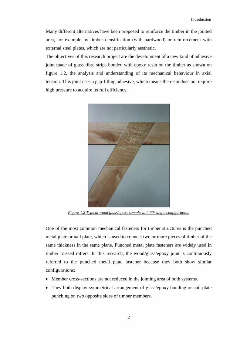
In structural timber engineering, connections are often the weakest part of the
structure, mainly because of the wood anisotropy and its non-linear mechanical
behaviour. There are many different types of joint in timber structures and most of
them are mechanically fastened. The use of plates, dowels (as shown in figure 1.1) or
bolts normally induces a reduction of the member’s cross-section in the jointed area.
Therefore larger timber sections are necessary to satisfy the member as well as the
joint designs. In other words, the strength capacity of the timber is not fully exploited
with mechanically fastened joints.
Figure 1.1 Typical timber truss internal joint with dowels (Dayer, 1994).
1
Introduction
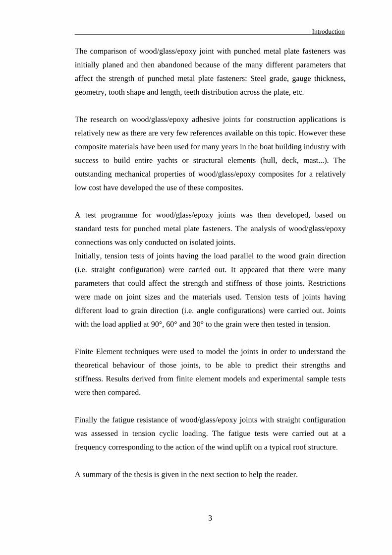
Many different alternatives have been proposed to reinforce the timber in the jointed
area, for example by timber densification (with hardwood) or reinforcement with
external steel plates, which are not particularly aesthetic.
The objectives of this research project are the development of a new kind of adhesive
joint made of glass fibre strips bonded with epoxy resin on the timber as shown on
figure 1.2, the analysis and understanding of its mechanical behaviour in axial
tension. This joint uses a gap-filling adhesive, which means the resin does not require
high pressure to acquire its full efficiency.
Figure 1.2 Typical wood/glass/epoxy sample with 60° angle configuration.
One of the most common mechanical fasteners for timber structures is the punched
metal plate or nail plate, which is used to connect two or more pieces of timber of the
same thickness in the same plane. Punched metal plate fasteners are widely used in
timber trussed rafters. In this research, the wood/glass/epoxy joint is continuously
referred to the punched metal plate fastener because they both show similar
configurations:
• Member cross-sections are not reduced in the jointing area of both systems.
• They both display symmetrical arrangement of glass/epoxy bonding or nail plate
punching on two opposite sides of timber members.
2
Introduction
The comparison of wood/glass/epoxy joint with punched metal plate fasteners was
initially planed and then abandoned because of the many different parameters that
affect the strength of punched metal plate fasteners: Steel grade, gauge thickness,
geometry, tooth shape and length, teeth distribution across the plate, etc.
The research on wood/glass/epoxy adhesive joints for construction applications is
relatively new as there are very few references available on this topic. However these
composite materials have been used for many years in the boat building industry with
success to build entire yachts or structural elements (hull, deck, mast...). The
outstanding mechanical properties of wood/glass/epoxy composites for a relatively
low cost have developed the use of these composites.
A test programme for wood/glass/epoxy joints was then developed, based on
standard tests for punched metal plate fasteners. The analysis of wood/glass/epoxy
connections was only conducted on isolated joints.
Initially, tension tests of joints having the load parallel to the wood grain direction
(i.e. straight configuration) were carried out. It appeared that there were many
parameters that could affect the strength and stiffness of those joints. Restrictions
were made on joint sizes and the materials used. Tension tests of joints having
different load to grain direction (i.e. angle configurations) were carried out. Joints
with the load applied at 90°, 60° and 30° to the grain were then tested in tension.
Finite Element techniques were used to model the joints in order to understand the
theoretical behaviour of those joints, to be able to predict their strengths and
stiffness. Results derived from finite element models and experimental sample tests
were then compared.
Finally the fatigue resistance of wood/glass/epoxy joints with straight configuration
was assessed in tension cyclic loading. The fatigue tests were carried out at a
frequency corresponding to the action of the wind uplift on a typical roof structure.
A summary of the thesis is given in the next section to help the reader.
3
Introduction
4
1.2. Reader’s guide
• The review of all literature used for the development of this research is presented
in chapter 2. References on the materials, on the theoretical approach of
composite joints and on the fatigue resistance of materials are described.
• The characteristics and properties of the materials that compose the
wood/glass/epoxy joints are presented in chapter 3. Wood, glass fibre and epoxy
resin are described as materials in general terms as well as the specific products
that were used in this research.
• The complete experimental programme is presented in chapter 4. From the
development to the joint fabrication, all wood/glass/epoxy joint configurations
that were tested in static tension are described.
• The results obtained from the experimental programme are presented and
analysed in chapter 5.
• The theoretical and finite element analyses are presented in chapter 6. A
theoretical approach to structural mechanics of the wood/glass/epoxy joints is
given. Then the development and the results of finite element models are
described and analysed, for each joint configuration that was previously tested.
• A preliminary investigation of the fatigue resistance of wood/glass/epoxy joints is
presented in chapter 7.
• The conclusion and recommendations for future work are presented in
chapter 8.
• Finally the references are listed, the results of strain gauges obtained
experimentally are given in appendix A and the full results of small clear sample
tests are given in appendix B.
Note: All the research work contained in this PhD thesis was carried out between
November 1997 and December 2001 and refers to codes of practice that were current
standards at the time. Nowadays some of them may be superseded, such as the BS
5268: Pt2: 1996, which is now replaced by the BS 5268: Pt2: 2002.
CHAPTER 2
LITERATURE REVIEW
2.1. Introduction
Research in composite materials has been developed for many years in a wide range
of engineering fields. It started in the late 1930s, Dorman (1969) cites
Dr. Pierre Castan who first synthesised epoxy resins in 1936. According to Adams et
al. (1997), the first design theory of composite adhesive joint appeared with the
Volkersen’s analysis in 1938 of single lap joint. At this time, words like adherends
and structural adhesive were first used. Then development of adhesive defined as a
polymeric material was on its way:
“In 1938, an American company called Owens-Corning Fiberglas Corporation first
produced and sold glass fibre and glass fibre products” (Mettes, 1969).
“In 1948, the first commercial epoxy resins became available in United States”
(Dorman, 1969).
“Composites materials such as glass fibre and epoxy resins have many attractive
properties such as high mechanical properties, light weight, good thermal properties,
moisture, corrosion and chemical resistance. Glass fibres have relatively low cost,
excellent electrical characteristics and behave perfectly elastically” (Mettes, 1969).
“Epoxy resins exhibit outstanding characteristics compared to other resins: They
have a wide range of forms (resins, hardeners and modifiers), curing conditions
(rapidly or slowly at almost any temperature between 5 and 180°C), low shrinkage,
good toughness and strong adhesive bond” (Dorman, 1969).
Consequently these advantages of using composites, especially glass/resin
combination, have developed their applications in military, transportation,
construction, aircraft, aerospace, marine, electrical and goods industries.
“Research has been undertaken to develop other composite materials such as carbon
fibre, graphite, boron, Aramid (Kevlar), titanium…and other adhesives like
polyurethane, phenolic, polyamide or polycarbonate adhesive” (Mallick, 1997).
5

Literature Review
During the last 40 years, glass fibre/epoxy has been widely used in ship and boat
building, mainly for hulls and masts. Bonding glass fibre/epoxy on a wood hull
makes the structure much stronger, protects the wood from salt corrosion and water
penetration and consequently reduces the maintenance of the boat.
Structural wood/glass/epoxy joints have been used on boats but no records of design
methods or research exist in this field. In other words, there is no background
research on structural wood/glass/epoxy joints except from Claisse and Davis (1998),
who have seen in this adhesive joint a potential for use in the construction industry.
They tested different configurations but irregular results were recorded. They found
that wood/glass/epoxy joints are highly rigid and have good mechanical
characteristics.
It was essential to review all research in which the three materials wood glass fibre
and epoxy have been involved, even if it did not concern directly this particular
jointing system. Such review lead to a better understanding of those materials and
their properties and helped to establish a reliable research process. Further review
was required about other comparable jointing system for timber structures, such as
punched metal plate fasteners in order to draw an acceptable performance
comparison.
Because of the lack of background for this research, the review of papers was
concentrated in different engineering fields:
• The construction environment, about the structural use of wood, glass fibre and
epoxy resin materials, the punched metal plate fasteners in timber trusses and
other related subjects.
• The mechanical environment (aircraft, aerospace...) for the use of structural
adhesive composite joints.
Finally, the review of papers and literature dealing with the fatigue of timber
structures and adhesive joints is presented at the end of this chapter, as the fatigue
resistance of wood/glass/epoxy joints was also assessed in this research project.
6
Literature Review
2.2. Construction environment
The use of epoxy resins in the construction industry has been mainly limited to
structural applications (load bearing supports for bridge structures, repair and
resurfacing of highways, roads and timber structures…) and decorative and efficient
structures (epoxy floors, epoxy-aggregate walls…). On the other hand, glass fibre
and GRP (Glass Reinforced Plastic) have been used in thermal applications (glass
wool, insulation components…) and construction elements (panels, roofing,
structural shapes, concrete pouring forms…).
Nowadays, the cost of epoxy is relatively low compared to 30 years ago because of
its universal use. For the last ten years, glass-epoxy has been used more and more in
other applications such as coating concrete structures in order to protect the concrete
surface and to increase its strength and durability.
The use of composite materials to reinforce structural wood members is reviewed in
the following section. This review is concentrated on the use of glass fibre and epoxy
resin.
7
Literature Review
2.2.1. Structural member applications
Using glass fibre to reinforce wood materials began in the early 1960s with
Wangaard (1964) and Biblis (1965). They analysed wood-glass fibre composite
beams in elastic deflection but also in the plastic region for Biblis (1965). Both
reinforced various species of wood by applying unidirectional glass fibre strands
impregnated with epoxy resin to the top and bottom surface. Their studies were
examining analysis techniques when core specific gravity varied from 0.08 to 1.14,
using different assumptions such as neglecting or taking into consideration the shear
strain, which acts in the core and contributes to the deflection. The analysis
techniques gave reasonably accurate results.
Theakston (1965) first examined reinforcing laminated timber beams with glass
fibre. He considered both a water base adhesive and an epoxy resin. The water base
adhesive was rejected because of poor performance. He used different types of glass
fibre such as roving mats, woven roving mats, cloth mats, and chopped strand mats.
Unidirectional non-woven roving mats were found the most suitable. Strength and
stiffness improvements were reported when the member was wrapped in the glass
fibre/epoxy composite or when the composite was placed between horizontal
laminations.
Further studies were developed for laminated timber using different kind of adhesive
(polyester, vinyl-ester, phenol-resorcinol resins…) as described in the excellent
review from Bulleit (1984). He also mentioned research for wood/glass fibre
composites in other applications:
• Glass Fibre Reinforced Plastics (GFRP) were used to reinforce wood transmission
poles in the early 1970s. Plywood was overlaid with glass fibre (in-depth series of
tests performed by the American Plywood Association in 1972 and 1973). This
reinforced board was used in the transportation industry and was extensively used
in cargo shipping containers, railroad cars and vans.
• An extensive study was performed in Germany using solid wood, plywood and
particleboard in 1974-1976. GFRP incorporating a polyester resin was bonded to
the surfaces of the core material in a wet process. A considerable improvement in
8
Literature Review
the strength and the stiffness properties was obtained and a significant reduction
in creep was reported.
A method and a prototype machine were developed by Saucier and Holman (1975) to
produce structural members such as 2 by 4 inch beams made from wood particles on
a continuous-belt press with special provision for incorporating continuous glass
strands of high tensile strength into the structure, parallel to its length. The strands
were prestressed and coated with resin. It produced poor boards when urea-melamine
resin was used and slightly higher quality boards when a phenolic resin was used. No
further works have followed this attempt.
Spaun (1981) undertook a study using glass fibre with phenol-resorcinol
formaldehyde resin to increase the tension and bending strength of impression finger
joints. Composite members were made of a core wood material (finger joint) with
veneers on each side and glass fibre layers sandwiched between veneer and core. The
strengths were increased from 10 to 40% over unreinforced joints, using only a glass
fibre reinforcement level of 3.5% and 7% by volume. Spaun noticed that a maximum
of 80% of the glass fibre strength capacity was effective in these tests.
The use of fibre reinforcement for laminated veneer lumber was evaluated by
Laufenberg et al. (1984). They assessed the economic feasibility of that kind of
products with different type of fibres (E-glass, S-glass, carbon and graphite). Axial,
bending and concentrated stress tests were undertaken. The study revealed that the
cost of E-glass reinforcement with phenol-formaldehyde resin was the cheapest for
the range of strength properties obtained.
The technical feasibility of producing internally reinforced laminated beams was
evaluated experimentally in a large programme performed by Rowlands et al. (1986).
Ten adhesives (three epoxy resins, two resorcinol formaldehydes, two phenol
resorcinol formaldehydes, two isocyanates and one phenol formaldehyde) and
numerous types of fibre reinforcements (unidirectional and cross-woven glass,
graphite and Kevlar) were evaluated. Reinforced laminates were tested in tension and
three-point bending, with and without finger joints. They concluded that fibre
reinforcements could be very advantageous in regions of stress concentration (bolted
9
Literature Review
joints, etc). Glass reinforcement was technically and economically superior for wood
structures. Under normal dry conditions, epoxies exhibited superb performance with
all fibre materials tested. Glass fibre reinforced Douglas fir (18% of glass by volume
using epoxies) produced a 40% stiffness enhancement and doubled the strength over
similar unreinforced wood.
Van de Kuilen (1991) developed a theory to predict the ultimate bending strength of
laminated timber beams reinforced with glass fibre/polyester resin on the bottom face
and both top and bottom faces. An experimental research program was undertaken by
the TNO (Timber Research Institute - Holland) on glass fibre reinforced laminated
beams. The research demonstrated that laying glass fibres in the glue lines has little
effect on the stiffness of the beam. Bonding glass fibre with polyester resin on the
top and bottom faces of the beam increased the stiffness by 17% having 4% of the
initial height reinforced and by 55% having 16% of the initial height reinforced.
The bonding properties of the reinforcement are critical parameters in laminated
timber beams. Gustafsson and Enquist (1993) produced a report, which assessed the
adherence of reinforcement to wood in this matter. The experiments were
concentrated on shear (tension) test with reinforcement bonded to the wood,
perpendicular to the grain. They were using glass fibre/polyester and different
softwood species. The failure always developed along the bond surface, and they
concluded the bond strength was governed by the shear properties of the wood. The
study is supported with a substantial theoretical shear analysis.
Another way of strengthening laminated timber was performed by Sonti and
GangaRao (1995) with the use of composite wraps. Two materials were used: glass
and carbon fibre. The composites were wrapped all around the laminated beams with
an epoxy-based resin, and tested in bending to failure. Low increments in stiffness
and high increments in strength were reported. Experimentally, the use of carbon
fibre did not show a very large improvement of mechanical properties compare to the
glass fibre (5% in stiffness and 15% in strength).
10
Literature Review
Alternatively Dorey and Cheng (1996) examined the potential for glass fibre
reinforcement for laminated timber beams using the same adhesive phenolic
resorcinol formaldehyde. The laminated beam was tested in four-point bending with
the glass fibre bonded on its bottom side. They showed that the fibre fraction plays a
major role in the mechanical capacity of the reinforced member. A range of fibre
fractions was studied to determine the optimum percentage. The maximum strength
and stiffness improvements of 127% and 104% respectively, were achieved by using
a fibre fraction of 8.23%.
The use of composite fabrics to reinforce wood crossties was developed by
GangaRao et al. (1996). They investigated the feasibility of hand wrapping for
GFRC (Glass Fibre Reinforced Composites)/wood crosstie and experimentally
evaluated their mechanical behaviour. Northern red oak wood and unidirectional
E-glass/epoxy reinforcement were used. Results of the experimental tests indicated
that only one layer of reinforcement provided noticeable enhancement to both
strength and stiffness. Average increase in stiffness of 15 to 41% and strength of
14 to 31% were achieved.
The same year, the same team Sonti et al. (1996) produced a paper about accelerated
ageing of wood-composites members. Using red oak wood as a core and two types of
composite fabrics (glass and carbon) as external reinforcements, they undertook
series of shear strength tests. Several adhesives for bonding were used. The results
showed that phenolic-based resins had higher retention of shear strength after being
subjected to ageing conditions. The ageing process was composed of six cycles of
swelling and shrinkage effects. The best combinations were wood/glass/epoxy and
wood/carbon/epoxy, which retained nearly 50% of their shear strength capacity after
the ageing process.
The performance of fibre reinforced polymer composites used with wood was
reviewed by Hota and GangaRao (1997). Strength, stiffness and accelerated ageing
response of sawn and laminated wood beams wrapped with glass composites and
bonded in place with polymeric resins were reported. They concluded that hybrid
wood components exhibit increases in strength and stiffness of up to 40 and 70%
respectively, over non-wrapped wood beams for a constant volume percent of fabric.
11
Literature Review
These mechanical properties could be increased further with the addition of more
layers of fabric.
Finally these papers are reviewing different applications for reinforcing wood
members, considering diverse material characteristics such as strength, stiffness,
ageing (long term durability) and creep…
A preference appears frequently in these papers for E-glass fibre rather than carbon
fibre or any other fibrous materials, because of a fairly cheap cost related to the
strength properties obtained. Similarly the epoxy resin is often used with fibrous
materials because of its high strength properties, chemical and water resistance, and
high bonding interaction, either through the composite matrix or with wood (and
wood-based) materials. Using epoxy resin is preferred when the bond strength is a
major criterion. On the other hand, its use is limited by a relatively high cost,
compared with other common wood adhesives, such as the phenol resorcinol
formaldehyde resin.
Composite materials were also used in different ways to fabricate or reinforce
structural joints in wood structures. The papers about this research area are reviewed
in the following section.
12
Literature Review
2.2.2. Structural joint applications
Because of its outstanding properties and particularly its high bonding strength with
wood, epoxy resin has been considered for the repair of timber structures. Avent et
al. (1978, 1984, 1985 and 1986) undertook a large research programme on
epoxy-repaired timber structures. The five following papers are some of the most
relevant of this programme and raise different aspects of epoxy repair capabilities.
Using pressure injected epoxy to restore deteriorated timber structures,
Avent et al. (1978) analysed the behaviour of epoxy-repaired full-scale timber
trusses. They conducted an experimental study to determine the effectiveness of this
repair method. They tested two types of trusses: Fink trusses (triangular truss with
inclined internal members) and Pratt trusses (rectangular truss with inclined internal
members). Some of them were made with new timber, and the epoxy repair method
was applied to bolted and damaged joints. The method restored strength to a level
approximately equal to the original. The results showed that the epoxy repair method
was very effective: Not a single repaired joint failed during the load tests. Other tests
were carried out on 30 years old timber trusses. To increase the wood deterioration,
these trusses were stored outside and exposed to weather for a two years period.
Bolted and split ring connections were badly rotted and damaged. The epoxy repair
method was less successful and marginal at best. They acknowledged the difficulty
to assess joint damage, identified the poor bonding of epoxy on highly rotted
material and concluded of the high effectiveness of the epoxy repair process.
Six years later, Avent et al. (1984) investigated the fire resistance of epoxy-repaired
timber. The structural efficiency and economical consideration have brought the
epoxy repair for timber structure as a reliable technique of restoration. In this
investigation, they conducted an experimental and theoretical programme. They
determined the wood/epoxy bond strength on small shear block specimens over a
wide range of temperatures, and the time required for full sized epoxy-repaired joints
to fail when subjected to a sudden elevated temperature. They developed a
mathematical model, which predicts with approximate accuracy the strength and
duration of load for joints exposed to a sudden high heat condition. By comparison
with the experiments, a 30 minutes fire rating was obtained for the glue line at
13
Literature Review
3 in. (76mm) from the heated surface and 60 minutes rating was obtained with a glue
line at 4 in. (102mm) from the surface. Further investigations were required because
this was one of the first studies on fire resistance for epoxy repair timber. They
concluded that members with interior glue lines will not fail immediately and higher
fire ratings could be predicted.
Avent (1985) conducted an experimental investigation to evaluate the effects of
weathering and decay on the epoxy repair of timber. Unprotected epoxy repaired
joints were exposed to natural weathering in the southern United States. Joints were
periodically loaded over a 4½ years period and correlated to accelerated weathering
tests on small epoxy bonded shear block samples. The strength of the repaired joints
compared well with that of undamaged material. However the author concluded with
the three following recommendations:
• The dry condition design shear strength of epoxy-repaired Southern pine should
be reduced by 33% when the repaired member is exposed to natural weathering
typical of the southern U.S.
• Preservative treatments that prevent wood decay are required on exposed timber if
the expected repair life is longer than just a few years.
• Normal precautions for protecting wood will serve well in protecting
epoxy-repaired timber.
One year later, Avent (1986) published a paper about an investigation into the factors
affecting the strength of epoxy-repaired timber structures. He evaluated two aspects:
The repair methodology and the effects of member configuration. The methodology
consisted of four steps: special member preparation, joint sealing, epoxy injection
and finishing. Each of these steps is described in detail with recommended
procedures. To evaluate the various joint configuration parameters affecting the
behaviour of epoxy-repaired timber, 200 full sized repaired members and 100 shear
blocks of Southern pine were tested. The effects of mechanical connectors, length of
overlap, member thickness, grain orientation, timber age and glue line thickness were
considered. The author concluded that the shear bond strength was of the order of the
shear strength of the wood, and the primary factors affecting strength were the ratio
of lap length to member thickness and grain orientation.
14
Literature Review
Finally Avent (1986) presented a study into the design criteria for epoxy repair of
timber structures. Based on theoretical and experimental studies (cited in the report),
the author exposed a methodology for computing both actual and allowable glue line
shear stresses. He assumed the actual glue line as an average shear stress. He
established some formulae to work out the allowable shear stress. These formulae are
functions of the wood species, grain orientation, allowable wood shear stress and lap
length to member thickness ratio. Several epoxy formulations were considered and
method for evaluating other epoxies is presented. The predicted values obtained
through those formulae matched approximately the experimental results.
In this large research programme sponsored by the United States Air Force
Directorate of Civil Engineering, Avent et al. brought forward a new era of jointing
structures. At this stage, they thought of using bonded joints for timber repair and
investigated most of the parameters, which rule the design of that kind of joint.
Using glued joints in timber structures requires a substantial analysis involving many
parameters to ensure the reliability of the connection. For example, design rules for
steel joints are not applicable because of different materials characteristics and a
fairly complex stress combination in glued timber joints. Glos and Horstmann (1991)
assessed the requirements for the design of glued joints in timber structures. In order
to produce a design proposal for glued joints in timber trusses, they tested over
500 full size samples and analysed the stress distribution using the finite element
modelling. They assessed the effects of joint geometry, glued area geometry and
grain orientation. Their design proposal presented is very similar to the one from
Avent (1986), using a wide range of safety factors.
Alternatively in the following sections, the authors thought of using composites and
not as adhesive joints but as mechanically fastened joints for timber structures.
Dmitriev et al. (1991) investigated the potential of non-metallic fastening units made
of high strength plastics and GFRP. The authors presented experimental research on
full-size trusses under short-term and long-term loading. The fastening pieces as well
as bolts, pegs, nails or straps were made in glass fibre, produced with a hot moulding
process. They tested different truss configurations, detailing each jointing system.
15
Literature Review
Entirely made without metal, the connections had similar configurations to the usual
ones in metal, but bolts were replaced by GFRP dowels or pegs glued in the wood.
The results were satisfactory, but the cost of the final trusses was relatively high. The
authors suggested this jointing system as a alternative method of producing wood
trusses if corrosion resistance, non-magnetism and radio interference are key criteria
for the structure.
Composite materials can also be used as a wood reinforcement for mechanically
fastened joints. Haller et al. (1996) developed joints for timber truss structures. They
presented a study on glass fibre reinforced and densified timber joints. In other
words, connections were reinforced either by bonding glass fibre fabrics with epoxy
resin on the wood members, or by removing layers of wood in the timber section on
both opposite bearing sides, then bonding glass fibre fabrics in between. The
densification was achieved by thermo-mechanical compression of the wood
(160ºC and 10 MPa of pressure). The two alternatives showed remarkable
enhancement in load bearing capacity and deformation. Ultimate strength and
deformation capacity were doubled. These results were obtained from tests on
bottom chord joint having two bracing members. The mechanical joints were made
of steel plates and dowels.
Beyond the high strength capacity obtained with glass fibre reinforcement, the
embedded strength was also improved. This is an important parameter when steel
fasteners are used for the connection especially when the loading acts perpendicular
to the grain. Chen (1996) proposed to reinforce laterally assembled timber elements
with glass fibre fabrics and epoxy resin. The premature failure was therefore avoided
due to the lateral reinforcement: The member strength and stiffness was enhanced,
and it prevented the splitting of timber: For example, a bolted joint tested in tension
or compression parallel to the grain showed a significant ductility when the wood
was reinforced with glass fibres.
Finally Claisse and Davis (1998) performed a comparison of high performance
jointing systems for timber. Four different jointing systems were tested and one of
them was made of uniaxial glass fibre and epoxy. Tests in tension for butt and scarf
joints with varying bonded length were undertaken. The results showed that
16
Literature Review
wood/glass/epoxy joints offered some of the best performance: High stiffness and
strength. However very small joint slips were recorded at failure (< 1.5 mm), which
seemed to reflect a brittle failure mechanism. Therefore the authors concluded that
wood/glass/epoxy joints have great potential that could be limited to some
applications.
The purpose of this research in wood/glass/epoxy joints is in the continuity of Claisse
and Davis’s work.
Some of the research achieved on nail plate connectors, which are probably the most
comparable timber jointing system with wood/glass/epoxy joints, are reviewed in the
following section.
17
Literature Review
2.2.3. Nail plate connections
Nail plates have been investigated for the last 50 years in Europe as well as North
America. Intensive research has been carried out in this area for several reasons: The
use of nail plates is probably the cheapest way to connect timber pieces. It is
relatively easy to manufacture with just one material involved and one component,
the steel plate.
The first nail plates were made of a steel plate perforated with a grillage of holes.
Nails were used to connect the plate to the timber. Nowadays the nails are part of the
steel plate: the plate is cut in order to give the shape of the nails, which are bent
afterwards to become the teeth. The manufacturing process remains simple, but the
truss fabrication is made easier and quicker. The nail plate is punched into the timber
pieces using a hydraulic press. That is why the nail plate is also called the punched
metal plate. However the plate dimensions, the properties of the steel used, the
number, the spacing, the dimensions and the shape of the teeth are some of many
parameters which affect the strength of this connection system. Such variations
justify the research achieved around the nail plate, particularly to produce reliable
and general design methods.
Nowadays punched metal plate fasteners are widely used and mainly for timber
trussed rafters. Most timber truss manufacturers use their own design procedures and
products, and the design methods given by the codes are used as guidance rather than
standard design procedures.
The following papers are representative of this research and contribute to the
comparison with wood/glass/epoxy joint, which will be carried out further on in this
thesis.
Destructive testing of punched metal plate connectors in wood truss joints were
undertaken by Gupta and Gebremedhin (1990) to demonstrate the partially rigid
behaviour of this joint type. Tension splice joints, heel joints and web at bottom
chord joints were tested (50 samples per joint configuration). Joints were fabricated
from the same softwood (Southern Pine) in 2 by 4 inch using the same metal plate
characteristics but different sizes. Joints were tested in a steel frame designed to
apply in-plane loads in order to simulate the loads carried by truss members. Average
18
Literature Review
strengths (and stiffnesses) under axial force for tension splice, heel and web at
bottom chord joints were recorded as 27.0 kN (and 52.8 kN/mm), 22.7 kN (and
41.2 kN/mm) and 16.7 kN (and 3.8 kN/mm), respectively. Ductile failure for heel
joints and brittle failure for tension splice and web at bottom chord joints were
recorded as well as the fact that joint failure was mainly due to a combination of
wood and teeth failure. However such uniform failure behaviour was achieved
because all joints tested had a configuration used in the design of an 8.5 m span Fink
truss with 5/12 roof slope. Note that all the joints were fabricated by commercial
truss manufacturers.
The same year, Cramer et al. (1990) published a paper about theoretical
consideration of metal-plate connected wood-splice joints in tensile and bending
analysis. A typical splice joint connected with metal-plate fasteners was presented as
a finite element model. A non-linear plane stress finite element formulation was used
for this model to allow computation of internal deformations, stress conditions and
ultimate strength. Different stiffnesses for the wood in the contact area, the steel plate
and the tooth-wood interface were considered in the analysis. The model showed a
strong plate-size effect in the lateral load resistance (based on strength per tooth).
This research showed that current design assumptions represent realistic
approximations of behaviour for small plate connections, but unrealistic ones for
connectors with larger plates. Therefore this research confirmed that refinement was
required in the design procedure of long span trusses containing large metal-plate
connectors. Unfortunately the research only included a comparison with
experimental results from references.
Gebremedhin and Crovella (1991) investigated the load distribution in metal-plate
connectors of tension joints in wood trusses. By testing tension splice joints they
showed the non-uniformity of load distribution along the plate member, using
different plate type. The samples were made with 4 different plate types on
2 by 4 inch Southern Yellow Pine wood. The row of teeth next to the centreline was
found to transfer the highest load (or to be the most highly stressed). One plate type,
which had uniform tooth layout, was modified to achieve better stress distribution,
by reducing gradually the number of teeth from the end to the plate centreline. The
same plate type was also studied to examine the effect of tooth damage on load
19
Literature Review
redistribution. By removing 3 teeth in one row, and varying the row at each test, no
substantial load redistribution was observed. Tension joints stiffnesses varying from
70.2 kN/mm to 93.5 kN/mm for a failure load from 20.7 kN to 31.7 kN were
recorded for each joint configuration.
Groom and Polensek (1992) developed a theoretical model for predicting
mechanisms of load transfer between a wood member and a metal-punched truss
plate. The model treated a plate tooth as a beam on an inelastic foundation of wood,
which predicted the load-displacement trace and the ultimate load of joints. It took
into account the inelastic behaviour of the tooth due to the wood embedment
(variation of bearing pressure along the tooth length) and the changing moment of
inertia along the tooth length. The model was verified with the testing of 8 truss-plate
joint types, 3 with variable number of teeth and 5 with different plates and wood
grain angles. Theoretical and experimental load/displacement graphs showed good
agreement. The theoretical model accurately predicted the ultimate load and failure
modes of joints (tooth withdrawal or plate tensile failure for straight pullout joints,
side grain failure perpendicular to the grain for square pullout joints).
These papers show some of the research on metal-plate connectors and also the new
approach of metal plate design, which seems to be needed by the truss manufacturing
industry. The non-uniformity of load transfer in the metal plate, the
partially-rigid behaviour as well as the fact that tension test is the most relevant test
to establish the joint strength and stiffness, are important criteria which are taken into
account in this research about wood/glass/epoxy joints. Also the experimental
programme was inspired by some of the procedures presented here.
The research in mechanical engineering on composite jointing is also a fundamental
reference for the research in wood/glass/epoxy joints. Some of the most relevant
papers are presented in the following section.
20
Literature Review
2.3. Mechanical Environment
The use of glass fibre and epoxy resin has been highly developed in engineering for
40 years in so many different applications that it would be irrelevant to summarise
them here. In the automotive, boats, aircraft, aerospace and others industries, glass
fibre and epoxy resin have been used as materials for a wide range of parts and
components because of outstanding properties (as listed before). However, these
composite materials have been used for jointing elements of different materials, with
capacity to transfer significant loads and stresses. The review is therefore
concentrated on this particular field of mechanical engineering, which deals with
structural adhesive joints, because of the similarities with the present research.
The five following papers show a part of the research in composite joints achieved in
the past 10-20 years. Since the late 1970s with the development of computer, the use
of finite element methods have solved many theoretical problems too complex to be
dealt with classical analysis, such as anisotropic and non-linear behaviour of
composite.
In the early 1980s, Matthews et al. (1982) published an excellent review of the
strength of joints in fibre-reinforced plastics. Most of the published work, mainly
theoretical and relating to all aspects of adhesively bonded joints in composite
material is presented. Classical analytical and finite element methods applied to
metals and composites, adhesive properties and joint design procedures are reviewed
considering both linear and non-linear analyses. This paper also refers to books,
which are the foundation of the theoretical principles raised in this report. Most of
the papers listed in this review are linked to the research in the aeronautic industry.
The same year, Marloff (1982) published a paper about finite element analysis of
biaxial stress test specimen for graphite/epoxy and glass fabric/epoxy composite. A
diametrically loaded circular specimen was proposed to test composite materials
under biaxial stress. Using finite element analysis, a model of the specimen was
developed with isoparametric mesh, refined step by step in the highly stressed areas
to obtain an optimum shape for the specimen. Using elastic behaviour only, linear
analysis but considering the material orthotropy, the model gave accurate results
21
Literature Review
compared to the experimental results obtained from strain gauges fixed on the test
specimen. But the finite element procedure developed in this research is the most
relevant point, with its meshing assumptions, choice of element and theoretical
background. Nevertheless the failure mode could not be accurately predicted because
non-linear behaviour of the composite was ignored.
Failure prediction of composite was overcome two years later by Harris and Adams
(1984) who published a paper about strength prediction of bonded single lap joints
by non-linear finite element methods. Single lap joints made of four aluminium
alloys and four epoxy adhesives were tested and the results obtained compared with
finite element models. The program used for the finite element analysis was able to
take into account the large displacement rotations that occurred in single lap joint and
allowed the effects of elasto-plasticity in both the adhesive and the adherends to be
modelled. Therefore a realistic stress-strain curve of composite was obtained. A
failure criterion based on the uniaxial tensile properties of the adhesive was used
(modified Von Mises failure criterion) to achieve accurate failure prediction.
The two following papers were published by the same Authors, Gilibert et al. (1988)
and are related to the mechanical behaviour assessment of the double lap joint using
epoxy adhesive on steel or aluminium adherends. Taking into account the
non-linear behaviour of the bond (i.e. non-uniform load transfer distribution),
specimens were tested in axial tension while strain gauges positioned at different
locations on the outer face of adherends recorded the strain distribution. Finite
element method was not used in these papers but classical analytic method.
According to the authors, the non-linear behaviour maybe due to the opening of
micro-cracks at overlap ends.
In the second paper, different joint configuration (thinner joint) was tested. Also a
different method of analysis was used. Reasonable accuracy was obtained between
experiment and theory in both papers. However the theoretical analysis was
developed using assumptions on parameters such as the strain distribution through
the thickness of the adhesive, which could not be evaluated.
22
Literature Review
These papers are some examples of the wide research developed in the last 50 years
on composite adhesive joints in different fields of engineering. Most methods
developed were based on principles of mechanics of materials as shown in those
papers.
References to several books of mechanics of composite were also made for the
theoretical analyses that are presented throughout this thesis to describe the
mechanical behaviour of wood/glass/epoxy joints.
The research papers and literature dealing specifically with the fatigue of timber
structure and composite joints is presented in the following section.
23
Literature Review
2.4. Review on fatigue
The behaviour of the wood/glass/epoxy joint under fatigue was carried out as part of
this project and is presented in Chapter 7. The performance of the joints was assessed
in cyclic loading to establish their fatigue resistance.
The papers reviewed in this section were used to identify and understand the fatigue
behaviour of the timber material and composites materials. Furthermore books were
selected because of their excellent review of the research carried out on fatigue.
These books and papers are used as references in the literature review presented in
chapter 7. Some of the books are presented below.
In his assessment of timber’s nature and behaviour, Dinwoodie (2000) defines
fatigue and the theory around it, which is used to evaluate the timber’s fatigue
resistance. The author refers to several papers of recent work carried out to assess the
fatigue life of timber materials. The conclusions from these investigations can be
summarised as follow:
• Fatigue resistance is dependent on the timber species, but reduces with increasing
moisture content.
• Fatigue resistance is considerably higher for axially loaded timber in tension than
in compression.
The author investigates the modelling and failure criteria in fatigue, referring to other
work carried out to evaluate fatigue: The use of alternative S-N curves, models based
on elastic and visco-elastic work, etc are presented.
Ansell (in Timber Engineering STEP1, 1995) assesses the fatigue design for timber
and wood based material and describes the life prediction techniques. The author
relates the fatigue to the crack propagation (fracture mechanics) first and then
introduced the S-N curves and R ratios. He refers to some of his substantial research
work, and explains the constant life-lines and life prediction techniques in details.
In a book dealing with composite materials, Chawla (1998) investigates how fatigue
affects composite materials. The author introduces the S-N curves, the fatigue crack
propagation. He describes the fatigue behaviour of various composite materials, such
24
Literature Review
as ceramic matrix composites, particles composites and hybrids. He exposes theories
of damage mechanics of fatigue, fatigue due to thermal effects and creep.
Other books are referred to in chapter 7. They are not presented in this review
because of the minor references made to them.
In addition to those books, research papers were used as part of this project to
understand the experimental procedures of fatigue tests. These papers are dealing
with fatigue of timber, glass fibre and epoxy, as single materials or composites, as
well as with fatigue of bonded-in rods in timber connections and punched metal plate
fasteners. They are reviewed as follow:
By testing different species of timber (Sitka spruce, laminated Khaya and beech)
under load control in four-point bending and at five different R ratios and three
different moisture contents, Tsai and Ansell (1990) found that fatigue lives were
independent from the species and were reducing with increasing moisture content.
They have showed that the most severe mode of cyclic loading for wood material is
the fully reverse loading (R = -1). As for the mechanical properties, the moisture
content seems to be an outstanding parameter that affects the fatigue life of wood.
They also found that the fatigue damage accumulation at cellular level was
associated with the formation of kinks in the cell walls, compression creases and
cracks in the wood.
As part of a research program for the needs of the wind turbine blade industry in the
UK, Bonfield and Ansell (1991) explored the fatigue in constant amplitude tests in
axial tension, compression and shear for both Douglas fir and Khaya using various R
ratios. They found and confirmed that fatigue lives measured in all-tension loading
are significantly longer than those in all-compression tests. The fatigue resistance of
Khaya appeared to be significantly higher in all compression than in reverse modes.
Finally the laminated Khaya was tested in shear in all-tension tests (R = 0.1). The
fatigue resistance in shear was measured along two shear plane orientations: The
shear fatigue resistance of Khaya was found to be significantly higher along the
Tangential/Longitudinal plane than the Radial/Longitudinal plane.
25
Literature Review
Hacker and Ansell (2001) have investigated property changes and fatigue damage
accumulation of wood-epoxy laminates under constant amplitude fatigue tests in
tension-tension (R = 0.1), compression-compression (R = 10) and reverse loading
(R = -1). They also found that the reverse loading is the most severe mode of cyclic
loading. The wood appeared to be more tolerant in compression-compression than in
tension-tension. Maximum and minimum fatigue strains were monitored during the
fatigue tests. In tension-tension (R = 0.1), the strains remained constant through the
test, but they increase significantly close to failure. The sudden increases of strains
were found to correspond to the initiation and growth of fatigue cracks along the
wood grain, as each crack initiation causes a small step in strain.
Spera et al. (1990) investigated the laminated Douglas fir/epoxy as materials of
choice for wind turbine blades. They characterised the fatigue properties of Douglas
fir/epoxy joints. They tested scarf and butt joints in tension-tension at R = 0.1 with
respect of grades and joint sizes. It appeared that the veneer grades do not govern the
joint fatigue resistance: For the butt joints, the grade A veneer outperformed the
grade A+ veneer, which is a higher quality grade. A further effect that the increased
surface area of the scarf joints did not translate into an increase in strength and
fatigue resistance. This could be due the fact that larger bonded areas contain more
voids and therefore the bond was significantly degraded.
Sutherland (1999) presented in his report a large research program about the
applications of glass fibres to built wind turbine blades that was undertaken in the
early 1990s in United States. This program aimed at the development of a glass fibre
composite database for wind turbine applications. The DOE/MSU database for
E-glass composites contains over 4500 data points for 130 material systems tested.
A high frequency database provides a significant data set for unidirectional
composites to 108 cycles. The database explores material parameters such as
reinforcement fabric architecture, fibre content, matrix materials and loading
parameters (R values). The results derived from this database are widely presented in
chapter 7.
26
Literature Review
Fatigue tests were carried out by Bainbridge et al. (2000) on bonded-in rods in glued
laminated timber, using three different types of adhesives: Epoxy, polyurethane and
phenol resorcinol formaldehyde. Mild and high strength steel threaded rods were
axially loaded in tension parallel to the grain of the timber at a frequency of 1Hz. S-
N curves are presented for an R ratio of 0.1. The authors investigate the relationship
between experimental results and the design code basis, trying to establish fatigue
coefficients by comparison of the results with existing data. Fatigue coefficients were
not evaluated because of lack of high number of load cycles.
The punched metal plate fasteners were tested in fatigue loading by Karadelis and
Brown (2000), on two types of fasteners (two different steel grades). The joints were
tested in tension from 0.78 to 7.75 kN at a frequency of 1 to 2 Hz, corresponding to
one-fifth of the failure tension load. The joints were tested up to 105 cycles and
strains in the fasteners were recorded. Larger strains occurring in the centre of the
fastener than at the edges were observed and joint slips reach a peak at 60000 cycles
and then reduce.
The experimental data from those papers were used as comparison with the results
obtained from the wood/glass/epoxy fatigue tests that are presented in chapter 7.
27

Literature Review
28
2.5. Summary
The research in wood/glass/epoxy joint seems to be a relatively new idea particularly
in timber engineering. In the construction environment, glass fibre and epoxy are
increasingly used in various applications. This recent development is probably due to
a reduction in cost of those materials compared to 10-15 years ago. Nevertheless
jointing timber with glass fibre and epoxy has been a common jointing system in the
boat industry for many years. Nowadays, boats are entirely made with composite
materials and timber is not used anymore to form the frame skeleton. Nevertheless
the properties of those materials are well known and they have been used in other
engineering fields. Using glass fibre and epoxy to reinforce timber members have
been studied for a long time without being developed up to a design procedure.
Again this is due to a high cost compared to the performance enhancement. However
using glass fibre/epoxy as an alternative to nail plates is a way to optimise the
strength and the quantity of timber used, while maintaining the cost relatively low.
There are also further applications in which this research could be used, particularly
in the repair of damaged timber structures, reinforcement of existing structures or
reinforcement of mechanically fastening joints.
CHAPTER 3
MATERIALS, PROPERTIES AND CHARACTERISTICS
3.1. Introduction
The joint performance is dependent of the materials and their properties. These joints
are fabricated with three different materials: timber, epoxy resin and glass fibre. The
timber is the material to be connected therefore it is an adherend. The glass fibre is
also an adherend and connects the timber pieces together in order to transfer the
stresses from one piece to the other. The glass fibre can be called the connecting
material. The epoxy resin is the adhesive, which ensures the “link” between the
timber and the glass fibre. But the epoxy is much more than a simple adhesive. In
fact the glass fibre and the epoxy can be seen as only one component: the glass
fibre/epoxy composite. While the glass fibre is embedded in the resin, the properties
of both materials combine together to create the composite, with the fibres being the
principal load-carrying component. The matrix properties are enhanced in
comparison to the properties of either material. In fact, the joint could be seen as
composed of two materials: the timber and the glass fibre/epoxy composite, the
epoxy having a double function as an adhesive between the timber and the composite
and as part of the composite itself. It is therefore relevant to summarise the
characteristic and properties for each of these materials and also for the glass
fibre/epoxy composite.
29
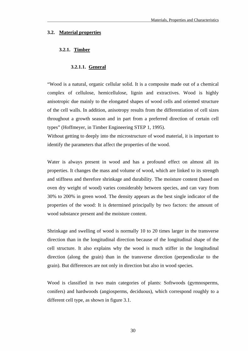
Materials, Properties and Characteristics
3.2. Material properties
3.2.1. Timber
3.2.1.1. General
“Wood is a natural, organic cellular solid. It is a composite made out of a chemical
complex of cellulose, hemicellulose, lignin and extractives. Wood is highly
anisotropic due mainly to the elongated shapes of wood cells and oriented structure
of the cell walls. In addition, anisotropy results from the differentiation of cell sizes
throughout a growth season and in part from a preferred direction of certain cell
types” (Hoffmeyer, in Timber Engineering STEP 1, 1995).
Without getting to deeply into the microstructure of wood material, it is important to
identify the parameters that affect the properties of the wood.
Water is always present in wood and has a profound effect on almost all its
properties. It changes the mass and volume of wood, which are linked to its strength
and stiffness and therefore shrinkage and durability. The moisture content (based on
oven dry weight of wood) varies considerably between species, and can vary from
30% to 200% in green wood. The density appears as the best single indicator of the
properties of the wood: It is determined principally by two factors: the amount of
wood substance present and the moisture content.
Shrinkage and swelling of wood is normally 10 to 20 times larger in the transverse
direction than in the longitudinal direction because of the longitudinal shape of the
cell structure. It also explains why the wood is much stiffer in the longitudinal
direction (along the grain) than in the transverse direction (perpendicular to the
grain). But differences are not only in direction but also in wood species.
Wood is classified in two main categories of plants: Softwoods (gymnosperms,
conifers) and hardwoods (angiosperms, deciduous), which correspond roughly to a
different cell type, as shown in figure 3.1.
30
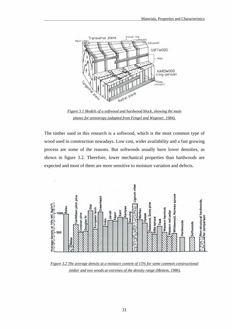
Materials, Properties and Characteristics
Figure 3.1 Models of a softwood and hardwood block, showing the main
planes for anisotropy (adapted from Fengel and Wegener, 1984).
The timber used in this research is a softwood, which is the most common type of
wood used in construction nowadays. Low cost, wider availability and a fast growing
process are some of the reasons. But softwoods usually have lower densities, as
shown in figure 3.2. Therefore, lower mechanical properties than hardwoods are
expected and most of them are more sensitive to moisture variation and defects.
Figure 3.2 The average density at a moisture content of 15% for some common constructional
timber and two woods at extremes of the density range (Mettem, 1986).
31

Materials, Properties and Characteristics
Within the softwood category, there are still large variations in properties from one
species to another, and even in selected species, within a specific tree: From sapwood
to heartwood, where the sensitivity to moisture decreases and from earlywood to
latewood, which corresponds to the growth throughout the season. When the tree
grows quickly, the density remains low (during spring and summer) and as the
growing process slows down (late summer and autumn) the density increases. The
latewood appears in the growth rings (darker material), also called annual rings. The
characteristics of the rings also reflect the wood density: Thick rings show a fast
growing process in the latewood, therefore the average density of the tree is likely to
be relatively low. The number of rings reflects the age of the tree but rings spacing
also show whether the wood has a high density or not. Large spacing corresponds to
a fast growing process and low density on average.
The durability of timber can be threatened by certain organisms. Some species of
destructive fungi damage the wood. These organisms develop in specific moisture
content, temperature and air conditions. To control the moisture content (below 20%)
is a way to prevent the decay of the wood.
Wood-boring insects also affect the durability of timber, by reducing the
cross-sectional area of the timber, thus its strength. To prevent infestation of timber,
preservatives are used either to cure damage wood or as a preventive measure
(preservative impregnation) which are usually adequate unless infestation is severe.
Wood is a grown material and therefore natural defects occur such as knots. A knot
is the part of the branch continuity within the main trunk as shown on the figure 3.3.
“Knots are, by far, the single most important defect affecting mechanical properties
of timber” (Hoffmeyer, in Timber Engineering STEP 1, 1995).
“There are many descriptions of types of knots, however generally fall into two
categories. A “live” knot has complete continuity between the fibres of the branch
and the tree. A “dead” knot occurs where a dead stub of a branch has been
overgrown. This has no connections with the new wood formed annually, and
consequently can become loose and fall out” (Reece, 1949).
32
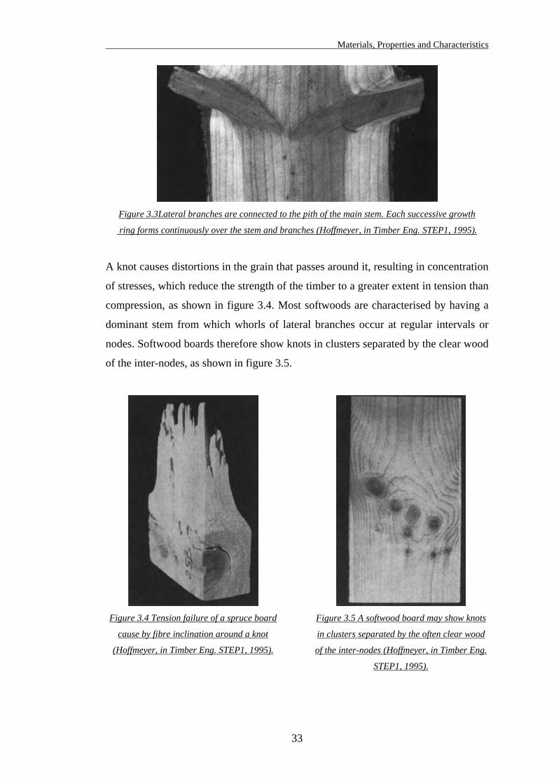
Materials, Properties and Characteristics
Figure 3.3Lateral branches are connected to the pith of the main stem. Each successive growth
ring forms continuously over the stem and branches (Hoffmeyer, in Timber Eng. STEP1, 1995).
A knot causes distortions in the grain that passes around it, resulting in concentration
of stresses, which reduce the strength of the timber to a greater extent in tension than
compression, as shown in figure 3.4. Most softwoods are characterised by having a
dominant stem from which whorls of lateral branches occur at regular intervals or
nodes. Softwood boards therefore show knots in clusters separated by the clear wood
of the inter-nodes, as shown in figure 3.5.
Figure 3.4 Tension failure of a spruce board
cause by fibre inclination around a knot
(Hoffmeyer, in Timber Eng. STEP1, 1995).
Figure 3.5 A softwood board may show knots
in clusters separated by the often clear wood
of the inter-nodes (Hoffmeyer, in Timber Eng.
STEP1, 1995).
33
Materials, Properties and Characteristics
34
The standards, which deal with grading of timber, contain restrictions on the
proportion of knots permitted in a cross-sectional area of timber, as described further
on.
Other natural defects of timber are cracks and fissures. They can occur in various
part of the tree, usually along the wood fibres and have specific names: checks,
shakes and splits reduce the timber resistance in shear, due to the reduction of
cross-section in the radial or tangential direction. “Heart” shakes occur in the centre
of the trunk, and can indicate the presence or beginnings of decay. Resin pockets are
fissures containing resin, a defect that can results in strength reduction of timber
depending of the number and sizes of pockets.
However restrictions on the proportion of cracks and fissures permitted in a
cross-sectional area of timber are given in the standards for timber grading.
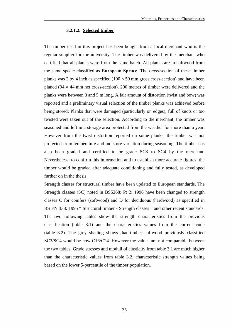
Materials, Properties and Characteristics
35
3.2.1.2. Selected timber
The timber used in this project has been bought from a local merchant who is the
regular supplier for the university. The timber was delivered by the merchant who
certified that all planks were from the same batch. All planks are in softwood from
the same specie classified as European Spruce. The cross-section of these timber
planks was 2 by 4 inch as specified (100 × 50 mm gross cross-section) and have been
planed (94 × 44 mm net cross-section). 200 metres of timber were delivered and the
planks were between 3 and 5 m long. A fair amount of distortion (twist and bow) was
reported and a preliminary visual selection of the timber planks was achieved before
being stored: Planks that were damaged (particularly on edges), full of knots or too
twisted were taken out of the selection. According to the merchant, the timber was
seasoned and left in a storage area protected from the weather for more than a year.
However from the twist distortion reported on some planks, the timber was not
protected from temperature and moisture variation during seasoning. The timber has
also been graded and certified to be grade SC3 to SC4 by the merchant.
Nevertheless, to confirm this information and to establish more accurate figures, the
timber would be graded after adequate conditioning and fully tested, as developed
further on in the thesis.
Strength classes for structural timber have been updated to European standards. The
Strength classes (SC) noted in BS5268: Pt 2: 1996 have been changed to strength
classes C for conifers (softwood) and D for deciduous (hardwood) as specified in
BS EN 338: 1995 “ Structural timber - Strength classes ” and other recent standards.
The two following tables show the strength characteristics from the previous
classification (table 3.1) and the characteristics values from the current code
(table 3.2). The grey shading shows that timber softwood previously classified
SC3/SC4 would be now C16/C24. However the values are not comparable between
the two tables: Grade stresses and moduli of elasticity from table 3.1 are much higher
than the characteristic values from table 3.2, characteristic strength values being
based on the lower 5-percentile of the timber population.
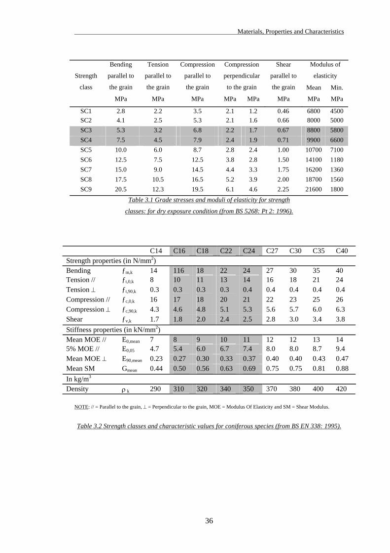
Materials, Properties and Characteristics
36
Modulus of
elasticity
Bending
parallel to
the grain
Tension
parallel to
the grain
Compression
parallel to
the grain
Compression
perpendicular
to the grain
Shear
parallel to
the grain
Strength
class
MPa MPa MPa MPa MPa MPa
Mean
MPa
Min.
MPa
SC1 2.8 2.2 3.5 2.1 1.2 0.46 6800 4500 SC2 4.1 2.5 5.3 2.1 1.6 0.66 8000 5000 SC3 5.3 3.2 6.8 2.2 1.7 0.67 8800 5800 SC4 7.5 4.5 7.9 2.4 1.9 0.71 9900 6600 SC5 10.0 6.0 8.7 2.8 2.4 1.00 10700 7100 SC6 12.5 7.5 12.5 3.8 2.8 1.50 14100 1180SC7 15.0 9.0 14.5 4.4 3.3 1.75 16200 1360SC8 17.5 10.5 16.5 5.2 3.9 2.00 18700 1560SC9 20.5 12.3 19.5 6.1 4.6 2.25 21600 1800
Table 3.1 Grade stresses and moduli of elasticity for strength
classes: for dry exposure condition (from BS 5268: Pt 2: 1996).
C14 C16 C18 C22 C24 C27 C30 C35 C40 Strength properties (in N/mm2) Bending ƒm,k 14 116 18 22 24 27 30 35 40 Tension // ƒt,0,k 8 10 11 13 14 16 18 21 24 Tension ⊥ ƒt,90,k 0.3 0.3 0.3 0.3 0.4 0.4 0.4 0.4 0.4 Compression // ƒc,0,k 16 17 18 20 21 22 23 25 26 Compression ⊥ ƒc,90,k 4.3 4.6 4.8 5.1 5.3 5.6 5.7 6.0 6.3 Shear ƒv,k 1.7 1.8 2.0 2.4 2.5 2.8 3.0 3.4 3.8 Stiffness properties (in kN/mm2) Mean MOE // E0,mean 7 8 9 10 11 12 12 13 14 5% MOE // E0,05 4.7 5.4 6.0 6.7 7.4 8.0 8.0 8.7 9.4 Mean MOE ⊥ E90,mean 0.23 0.27 0.30 0.33 0.37 0.40 0.40 0.43 0.47 Mean SM Gmean 0.44 0.50 0.56 0.63 0.69 0.75 0.75 0.81 0.88 In kg/m3 Density ρ k 290 310 320 340 350 370 380 400 420
NOTE: // = Parallel to the grain, ⊥ = Perpendicular to the grain, MOE = Modulus Of Elasticity and SM = Shear Modulus.
Table 3.2 Strength classes and characteristic values for coniferous species (from BS EN 338: 1995).
Materials, Properties and Characteristics
37
3.2.2. Glass fibres
3.2.2.1. General
Glass fibres are filaments or fibres of glass.
“The commonly accepted definition of glass is an inorganic product of fusion which,
when cooled, becomes rigid without crystallising (its atoms never arrange themselves
into an orderly crystalline pattern)” (Dorman, 1969).
“Glass composition: The major constituent of most inorganic glasses is silica. The
silicon dioxide molecule has a tetrahedral configuration consisting of a central silicon
ion surrounded by four oxygen ions. The three-dimensional network of silica
tetrahedra is the basis of the various and unusual properties of glass. By addition of
modifying ingredients such as metallic oxides, which may become part of the silica
network or disrupt it, the properties of the amorphous glass can be varied and
adjusted to various levels of performance” (Dorman, 1969).
In other words, specific chemical and physical properties of glass fibres are
controlled and altered through the process by which the fibres are drawn, but several
properties remain characteristic of all types of glass fibres:
• High tensile strength to weight ratios.
• Perfect elasticity: Hooke’s law applies to glass fibres, without even developing
plasticity or partial plasticity near failure. Typical glass fibres have a maximum
elongation of 5% at break, they do not shrink or stretch.
• Moisture resistance: Glass fibres do not absorb moisture. In contact with moisture,
fibres chemical composition remains identical. This is one of the main
characteristics, which justifies the wide use of glass fibres in the boat industry.
• Thermal properties: Glass fibres are incombustible, with a low coefficient of
thermal expansion and a high thermal conductivity. Typical fibres retain 50% of
their strength at 350°C and up to 25% at 550°C.
• Corrosion resistance: Glass fibres do not rot or deteriorate and resist all organic
solvents and most acids and alkalis.
• Electrical properties: Glass fibres have high dielectric strengths and low dielectric
constants.
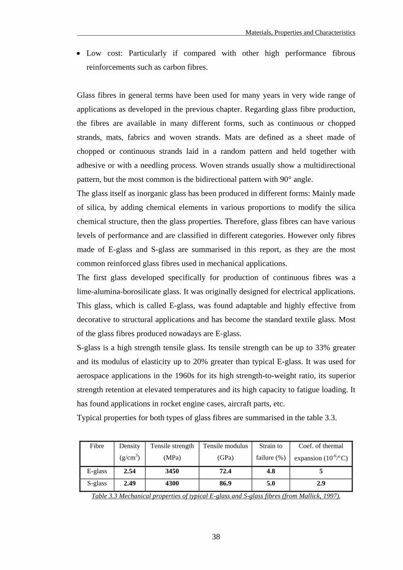
Materials, Properties and Characteristics
38
• Low cost: Particularly if compared with other high performance fibrous
reinforcements such as carbon fibres.
Glass fibres in general terms have been used for many years in very wide range of
applications as developed in the previous chapter. Regarding glass fibre production,
the fibres are available in many different forms, such as continuous or chopped
strands, mats, fabrics and woven strands. Mats are defined as a sheet made of
chopped or continuous strands laid in a random pattern and held together with
adhesive or with a needling process. Woven strands usually show a multidirectional
pattern, but the most common is the bidirectional pattern with 90° angle.
The glass itself as inorganic glass has been produced in different forms: Mainly made
of silica, by adding chemical elements in various proportions to modify the silica
chemical structure, then the glass properties. Therefore, glass fibres can have various
levels of performance and are classified in different categories. However only fibres
made of E-glass and S-glass are summarised in this report, as they are the most
common reinforced glass fibres used in mechanical applications.
The first glass developed specifically for production of continuous fibres was a
lime-alumina-borosilicate glass. It was originally designed for electrical applications.
This glass, which is called E-glass, was found adaptable and highly effective from
decorative to structural applications and has become the standard textile glass. Most
of the glass fibres produced nowadays are E-glass.
S-glass is a high strength tensile glass. Its tensile strength can be up to 33% greater
and its modulus of elasticity up to 20% greater than typical E-glass. It was used for
aerospace applications in the 1960s for its high strength-to-weight ratio, its superior
strength retention at elevated temperatures and its high capacity to fatigue loading. It
has found applications in rocket engine cases, aircraft parts, etc.
Typical properties for both types of glass fibres are summarised in the table 3.3.
Fibre Density
(g/cm3)
Tensile strength
(MPa)
Tensile modulus
(GPa)
Strain to
failure (%)
Coef. of thermal
expansion (10-6/°C)
E-glass 2.54 3450 72.4 4.8 5
S-glass 2.49 4300 86.9 5.0 2.9
Table 3.3 Mechanical properties of typical E-glass and S-glass fibres (from Mallick, 1997).
Materials, Properties and Characteristics
39
3.2.2.2. Selected glass fibres
The types of glass fibres used in these experiments have been selected according to
the following criteria:
• The glass fibre has to be a relatively standard product, in other words a product
already available in its existing form, which is used for other applications.
• The fibres must be continuous, as well as having the same dimensions and
properties. The uniformity of the reinforcement is essential for a better
understanding of the composite. Chopped strands and random arrangement of
fibres cannot be considered here because the fibre orientation is a key parameter
in the joint configuration as explained further on.
• The practicality of handling the material is also significant. The feasibility and
simplicity of fabrication are considered. Therefore, the glass fibre as a roller of
continuous strand cannot be considered, it has to come as a fabric or sheet of
woven or “needled” strands. In that case, just cutting the sheet to the appropriate
dimensions can ensure the uniformity of the material over the whole joint.
The glass fibres used have been supplied by SP Systems, Composite Engineering
Materials, which is a large company of composite materials manufacturing. Their
activities are mainly mechanical engineering in boat industry and in high
performance applications such high-tech boats and cars for racing, wind power
station (propellers and masts design), etc. They produce a wide range of composite
materials, S-glass, E-glass, carbon, aramid fibres in various forms and sizes, as well
as pre-impregnated fibres. Also they blend the adhesives required to bond the
reinforcement from polyesters to epoxies.
Reinforcements made of E-glass were considered, for cost purposes and also to test a
standard type of composite widely available nowadays. Two different types of fibre
orientations were selected, unidirectional and bidirectional fabrics. This choice was
based on the following assumptions:
• The fibre orientations may have a significant effect in the load transfer through the
joint.
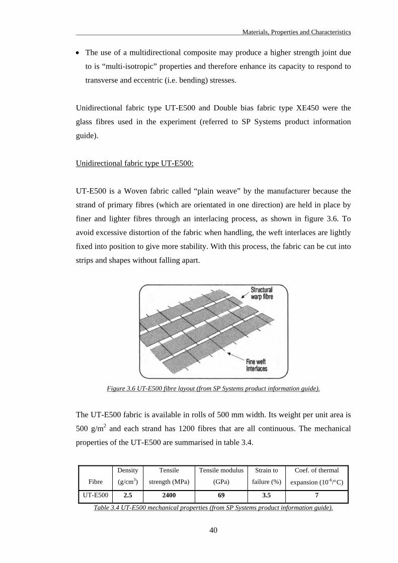
Materials, Properties and Characteristics
40
• The use of a multidirectional composite may produce a higher strength joint due
to is “multi-isotropic” properties and therefore enhance its capacity to respond to
transverse and eccentric (i.e. bending) stresses.
Unidirectional fabric type UT-E500 and Double bias fabric type XE450 were the
glass fibres used in the experiment (referred to SP Systems product information
guide).
Unidirectional fabric type UT-E500:
UT-E500 is a Woven fabric called “plain weave” by the manufacturer because the
strand of primary fibres (which are orientated in one direction) are held in place by
finer and lighter fibres through an interlacing process, as shown in figure 3.6. To
avoid excessive distortion of the fabric when handling, the weft interlaces are lightly
fixed into position to give more stability. With this process, the fabric can be cut into
strips and shapes without falling apart.
Figure 3.6 UT-E500 fibre layout (from SP Systems product information guide).
The UT-E500 fabric is available in rolls of 500 mm width. Its weight per unit area is
500 g/m2 and each strand has 1200 fibres that are all continuous. The mechanical
properties of the UT-E500 are summarised in table 3.4.
Fibre
Density
(g/cm3)
Tensile
strength (MPa)
Tensile modulus
(GPa)
Strain to
failure (%)
Coef. of thermal
expansion (10-6/°C)
UT-E500 2.5 2400 69 3.5 7
Table 3.4 UT-E500 mechanical properties (from SP Systems product information guide).
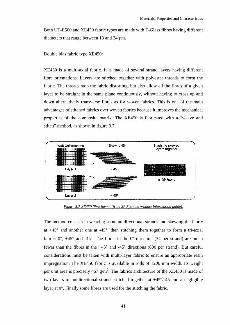
Materials, Properties and Characteristics
41
Both UT-E500 and XE450 fabric types are made with E-Glass fibres having different
diameters that range between 13 and 24 µm.
Double bias fabric type XE450:
XE450 is a multi-axial fabric. It is made of several strand layers having different
fibre orientations. Layers are stitched together with polyester threads to form the
fabric. The threads stop the fabric distorting, but also allow all the fibres of a given
layer to be straight in the same plane continuously, without having to cross up and
down alternatively transverse fibres as for woven fabrics. This is one of the main
advantages of stitched fabrics over woven fabrics because it improves the mechanical
properties of the composite matrix. The XE450 is fabricated with a “weave and
stitch” method, as shown in figure 3.7.
Figure 3.7 XE450 fibre layout (from SP Systems product information guide).
The method consists in weaving some unidirectional strands and skewing the fabric
at +45° and another one at -45°, then stitching them together to form a tri-axial
fabric: 0°, +45° and -45°. The fibres in the 0° direction (34 per strand) are much
fewer than the fibres in the +45° and -45° directions (600 per strand). But careful
considerations must be taken with multi-layer fabric to ensure an appropriate resin
impregnation. The XE450 fabric is available in rolls of 1200 mm width. Its weight
per unit area is precisely 467 g/m2. The fabrics architecture of the XE450 is made of
two layers of unidirectional strands stitched together at +45°/-45°and a negligible
layer at 0°. Finally some fibres are used for the stitching the fabric.
Materials, Properties and Characteristics
42
3.2.3. Epoxy resin
3.2.3.1. General
“An epoxy resin is a polymer containing two or more epoxy groups:
Such groups are also referred to as epoxide, ethylene Oxide, or
oxirane and may be by terminal, internal, or cyclic structures. Epoxy resin is used to
designate both the uncured or thermoplastic polymer as well as the cured (hardened)
or thermosetting material” (Dorman, 1969).
CC
O
Epoxies are some of the most efficient resin types currently available in terms of
mechanical properties and resistance to environment degradation. They are mainly
classified are thermosetting material, which means once the resin and the hardener
are mixed, a non-reversible chemical reaction occurs. The non-reversible reaction is
the main difference between thermosetting and thermoplastic material. As
thermosetting material, once the system has cured, it will not become liquid again if
heated, the process of crossing the melting point can not be repeated again (and this
without modifying the material properties) as it would be for a thermoplastic
material. However above a specific temperature the mechanical properties of an
epoxy system will change significantly (strength and stiffness). This temperature is
known as the Glass Transition Temperature (Tg) and the change in mechanical
properties is reversible once the temperature is below Tg.
The properties and characteristics of epoxy resins are as described in the following
section:
• Versatility is probably the most outstanding characteristic of epoxy resins. They
can have a wide variety of forms as far as the resin type is concerned but also their
hardeners and modifiers allow them to be used in various applications, from very
low viscosity to high-melting point solid.
• Curing range: Dependent upon the selection of hardener, systems can cure rapidly
(or slowly) at almost any temperature from 5 to 180°C.
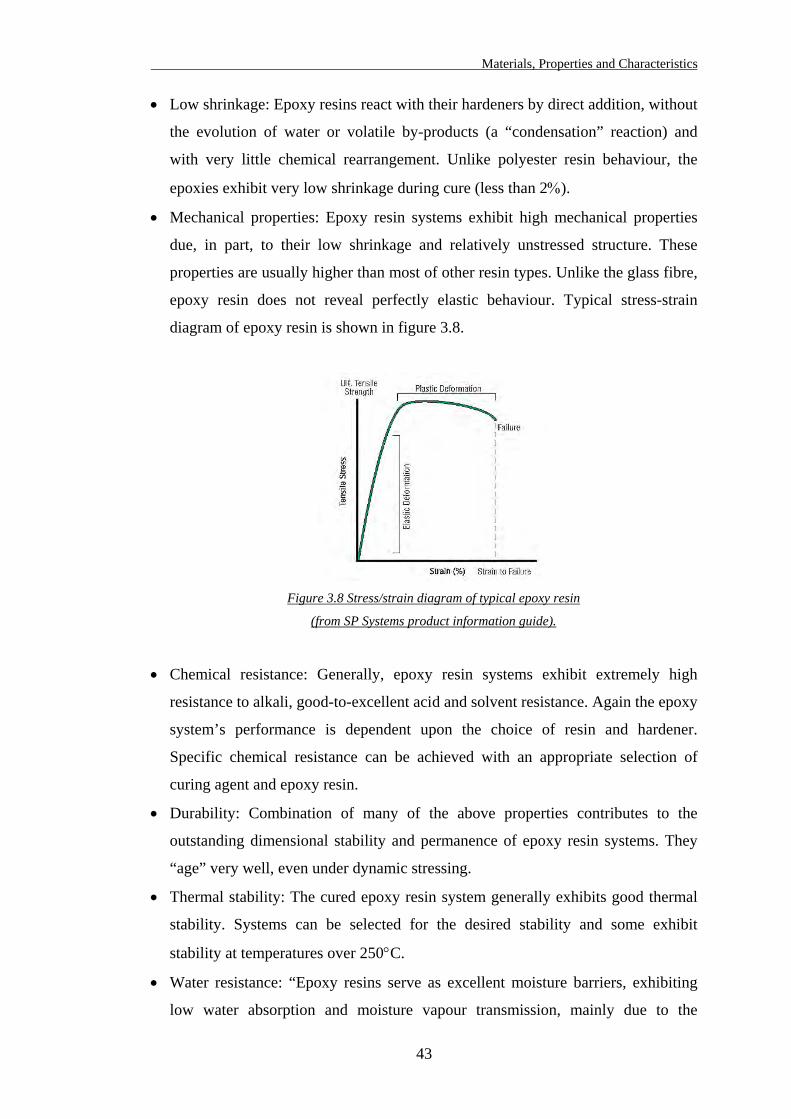
Materials, Properties and Characteristics
43
• Low shrinkage: Epoxy resins react with their hardeners by direct addition, without
the evolution of water or volatile by-products (a “condensation” reaction) and
with very little chemical rearrangement. Unlike polyester resin behaviour, the
epoxies exhibit very low shrinkage during cure (less than 2%).
• Mechanical properties: Epoxy resin systems exhibit high mechanical properties
due, in part, to their low shrinkage and relatively unstressed structure. These
properties are usually higher than most of other resin types. Unlike the glass fibre,
epoxy resin does not reveal perfectly elastic behaviour. Typical stress-strain
diagram of epoxy resin is shown in figure 3.8.
Figure 3.8 Stress/strain diagram of typical epoxy resin
(from SP Systems product information guide).
• Chemical resistance: Generally, epoxy resin systems exhibit extremely high
resistance to alkali, good-to-excellent acid and solvent resistance. Again the epoxy
system’s performance is dependent upon the choice of resin and hardener.
Specific chemical resistance can be achieved with an appropriate selection of
curing agent and epoxy resin.
• Durability: Combination of many of the above properties contributes to the
outstanding dimensional stability and permanence of epoxy resin systems. They
“age” very well, even under dynamic stressing.
• Thermal stability: The cured epoxy resin system generally exhibits good thermal
stability. Systems can be selected for the desired stability and some exhibit
stability at temperatures over 250°C.
• Water resistance: “Epoxy resins serve as excellent moisture barriers, exhibiting
low water absorption and moisture vapour transmission, mainly due to the
Materials, Properties and Characteristics
44
absence of ester groups in the reaction (in comparison with polyester resin)”
(Dorman, 1969).
Epoxies are cured by a hardener, which is often an amine, and by chemical reaction,
both materials combined together. The chemistry of this reaction shows that there are
usually two epoxy groups binding to each amine group. Each amine group co-reacts
with epoxy groups in a fixed ratio, therefore, to ensure that complete reaction occurs,
it is essential to use the correct mix ratio. If not, unreacted resin or hardener will
remain in the matrix and this will affect the properties of the cured system.
Epoxies are used on a wide variety of substrates including metals, glass, wood,
concrete and masonry. In any engineered fields (aircraft, aerospace, automotive, etc)
where epoxy properties are relevant (such as high strength to weight ratios) and in
composite structures, epoxy resins are used efficiently with strong reinforcements
such as carbon, boron or glass fibres. They have applications in many industries for a
multitude of bonding operations.
The outstanding adhesive strengths are due primarily to the thorough wetting,
polarity and low shrinkage during cure. The good wetting assures that the adhesive
will closely contact the adherends so that the strong adhesive forces may become
active. This close contact is maintained after cure, and stresses, which may tend to
disrupt the adhesive forces are minimised by the low shrinkage of the epoxy system.
Epoxies are especially useful for the bonding of dissimilar materials, such as
honeycomb structures, and where high-strength joints are required.
Materials, Properties and Characteristics
45
3.2.3.2. Selected epoxy resin
The epoxy resin used is called Spabond 120 and was supplied by SP Systems.
Spabond 120 is recommended by the manufacturer as a perfect adhesive to bond a
wide range of high strength materials, particularly GRP (Glass Reinforced Plastic),
concrete, wood and composite components. Having been used in the boat industry
for many years, Spabond 120 is ideal for all wood bonding operation, including
hardwood such as teak, iroko, oak, etc. To ensure the best workability and
performance of the resin, the following recommendations must be followed:
• Use the product at temperature between 15 and 25°C. Below this range, the resin
will thicken and workability will become difficult (mixing procedure).
• Use the appropriate mix ratio between resin and hardener:
Resin/Hardener ratio: 2/1 by volume or 100/44 by weight.
• The choice of hardener depends whether the system needs to be cured rapidly. In
the purpose of this research, slow hardener was used because the curing time was
not essential, but also because a resin system cured with a slow hardener exhibits
better mechanical properties and durability.
• The surface to be bonded should be prepared: For timber, it is recommended to
sand the surface across the grain, to degrease and clean with water any oily and
resinous timber surface.
Spabond 120 can be used for gluing, fillet bonding and fibre reinforcement.
Spabond 120 has a high shear strength and toughness, which makes it suitable for
bonding both high strength materials and dissimilar materials. However to optimise
the resin consistency, a range of filler powders is available and will make the mix
thicker. To enhance the strength of the resin, micro-fibres can be added to the mix.
Acting as filler, the micro-fibres will thicken the mix but also will reinforce the
adhesive against micro-cracks propagation. With its relatively low viscosity,
Spabond 120 can be used with fibre reinforcement.
The following tables 3.5, 3.6 and 3.7 summarise respectively the main component
properties, working properties and cured system properties of the Spabond 120
epoxy, as given by the manufacturer.
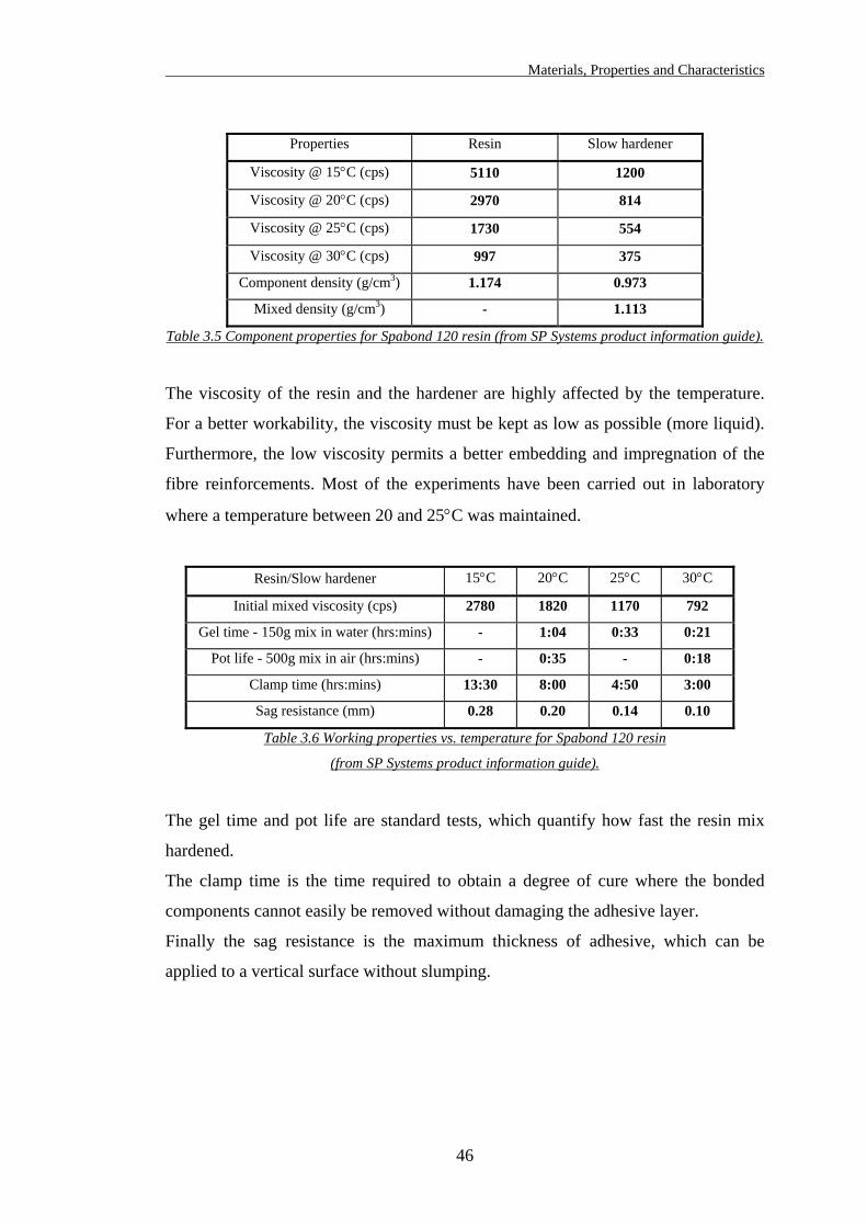
Materials, Properties and Characteristics
46
Properties Resin Slow hardener
Viscosity @ 15°C (cps) 5110 1200
Viscosity @ 20°C (cps) 2970 814
Viscosity @ 25°C (cps) 1730 554
Viscosity @ 30°C (cps) 997 375
Component density (g/cm3) 1.174 0.973
Mixed density (g/cm3) - 1.113
Table 3.5 Component properties for Spabond 120 resin (from SP Systems product information guide).
The viscosity of the resin and the hardener are highly affected by the temperature.
For a better workability, the viscosity must be kept as low as possible (more liquid).
Furthermore, the low viscosity permits a better embedding and impregnation of the
fibre reinforcements. Most of the experiments have been carried out in laboratory
where a temperature between 20 and 25°C was maintained.
Resin/Slow hardener 15°C 20°C 25°C 30°C
Initial mixed viscosity (cps) 2780 1820 1170 792
Gel time - 150g mix in water (hrs:mins) - 1:04 0:33 0:21
Pot life - 500g mix in air (hrs:mins) - 0:35 - 0:18
Clamp time (hrs:mins) 13:30 8:00 4:50 3:00
Sag resistance (mm) 0.28 0.20 0.14 0.10
Table 3.6 Working properties vs. temperature for Spabond 120 resin
(from SP Systems product information guide).
The gel time and pot life are standard tests, which quantify how fast the resin mix
hardened.
The clamp time is the time required to obtain a degree of cure where the bonded
components cannot easily be removed without damaging the adhesive layer.
Finally the sag resistance is the maximum thickness of adhesive, which can be
applied to a vertical surface without slumping.
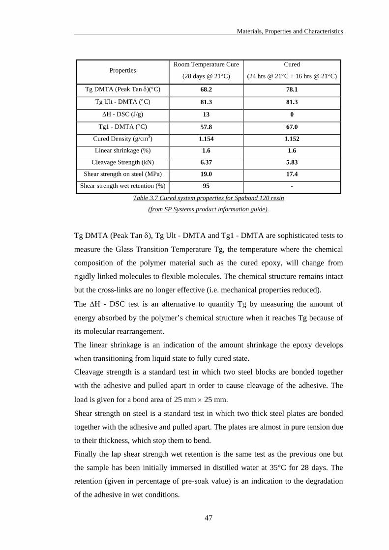
Materials, Properties and Characteristics
47
Properties Room Temperature Cure
(28 days @ 21°C)
Cured
(24 hrs @ 21°C + 16 hrs @ 21°C)
Tg DMTA (Peak Tan δ)(°C) 68.2 78.1
Tg Ult - DMTA (°C) 81.3 81.3
∆H - DSC (J/g) 13 0
Tg1 - DMTA (°C) 57.8 67.0
Cured Density (g/cm3) 1.154 1.152
Linear shrinkage (%) 1.6 1.6
Cleavage Strength (kN) 6.37 5.83
Shear strength on steel (MPa) 19.0 17.4
Shear strength wet retention (%) 95 -
Table 3.7 Cured system properties for Spabond 120 resin
(from SP Systems product information guide).
Tg DMTA (Peak Tan δ), Tg Ult - DMTA and Tg1 - DMTA are sophisticated tests to
measure the Glass Transition Temperature Tg, the temperature where the chemical
composition of the polymer material such as the cured epoxy, will change from
rigidly linked molecules to flexible molecules. The chemical structure remains intact
but the cross-links are no longer effective (i.e. mechanical properties reduced).
The ∆H - DSC test is an alternative to quantify Tg by measuring the amount of
energy absorbed by the polymer’s chemical structure when it reaches Tg because of
its molecular rearrangement.
The linear shrinkage is an indication of the amount shrinkage the epoxy develops
when transitioning from liquid state to fully cured state.
Cleavage strength is a standard test in which two steel blocks are bonded together
with the adhesive and pulled apart in order to cause cleavage of the adhesive. The
load is given for a bond area of 25 mm × 25 mm.
Shear strength on steel is a standard test in which two thick steel plates are bonded
together with the adhesive and pulled apart. The plates are almost in pure tension due
to their thickness, which stop them to bend.
Finally the lap shear strength wet retention is the same test as the previous one but
the sample has been initially immersed in distilled water at 35°C for 28 days. The
retention (given in percentage of pre-soak value) is an indication to the degradation
of the adhesive in wet conditions.
Materials, Properties and Characteristics
48
3.2.4. Glass fibre/epoxy composite
3.2.4.1. General
The mechanical properties of the glass fibre/epoxy matrix or lamina are much higher
than the mechanical properties of the epoxy resin itself. Therefore the fibres have a
predominant role in the composite behaviour. In fact, with the lamina in tension, the
fibres carry most of the load as the resin only hold the fibres together. On the other
hand, with the lamina in compression (or in bending), the fibres behave like axially
loaded columns and then the resin must resists the fibres buckling. Therefore the
fibre/resin adhesion becomes an important parameter. However, different behaviours
apply to the resin and fibres for adhesive joints bonded with composite, and this will
be covered in the theoretical analysis of wood/glass/epoxy joints, later in this thesis.
The mechanical properties of a lamina are governed by some of the following
factors:
• Mechanical properties of the fibre and the resin.
• The amount of fibre in the matrix, evaluated as the Fibre Volume Fraction (FVF).
• The fibre/matrix interaction such as bond strength.
• The fibre orientation within the lamina.
• The fibre layout (woven, needled, fabric, etc) within the matrix.
The mechanical properties of fibre and resin are usually given by manufacturers and
are based on experimental testing rather than theoretical estimations. Properties are
always based on a specific fibre volume fraction, as the ratio of fibre in the
composite does reflect on the mechanical properties. Mechanical properties of
composites can be separated in two categories: basic or static properties (elastic
modulus and strength) and advanced or dynamic properties (fatigue, impact, creep
and vibration behaviours). Fatigue properties were investigated in this research
further to the static tests of wood/glass/epoxy joints (see chapter 7). Typical static
mechanical properties of unidirectional fibre reinforced composites are density, fibre
volume fraction, longitudinal/transverse tension/compression strengths, in-
plane/interlaminar shear strengths, longitudinal/transverse/shear moduli, and
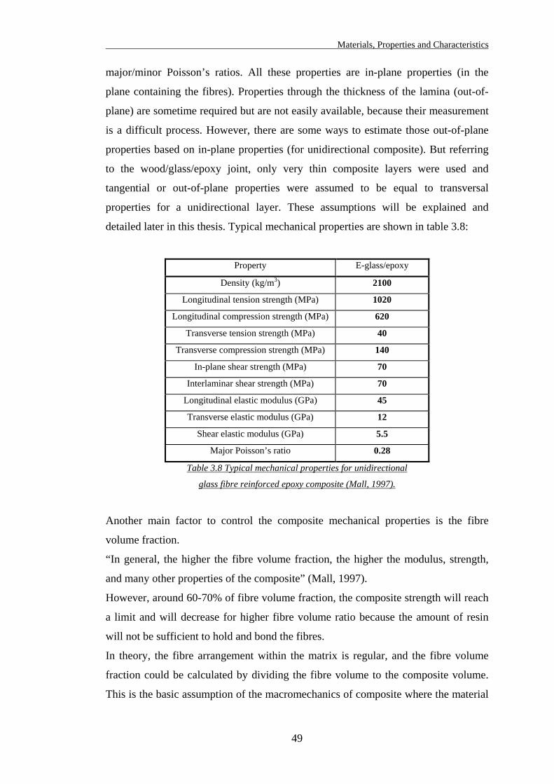
Materials, Properties and Characteristics
49
major/minor Poisson’s ratios. All these properties are in-plane properties (in the
plane containing the fibres). Properties through the thickness of the lamina (out-of-
plane) are sometime required but are not easily available, because their measurement
is a difficult process. However, there are some ways to estimate those out-of-plane
properties based on in-plane properties (for unidirectional composite). But referring
to the wood/glass/epoxy joint, only very thin composite layers were used and
tangential or out-of-plane properties were assumed to be equal to transversal
properties for a unidirectional layer. These assumptions will be explained and
detailed later in this thesis. Typical mechanical properties are shown in table 3.8:
Property E-glass/epoxy
Density (kg/m3) 2100
Longitudinal tension strength (MPa) 1020
Longitudinal compression strength (MPa) 620
Transverse tension strength (MPa) 40
Transverse compression strength (MPa) 140
In-plane shear strength (MPa) 70
Interlaminar shear strength (MPa) 70
Longitudinal elastic modulus (GPa) 45
Transverse elastic modulus (GPa) 12
Shear elastic modulus (GPa) 5.5
Major Poisson’s ratio 0.28
Table 3.8 Typical mechanical properties for unidirectional
glass fibre reinforced epoxy composite (Mall, 1997).
Another main factor to control the composite mechanical properties is the fibre
volume fraction.
“In general, the higher the fibre volume fraction, the higher the modulus, strength,
and many other properties of the composite” (Mall, 1997).
However, around 60-70% of fibre volume fraction, the composite strength will reach
a limit and will decrease for higher fibre volume ratio because the amount of resin
will not be sufficient to hold and bond the fibres.
In theory, the fibre arrangement within the matrix is regular, and the fibre volume
fraction could be calculated by dividing the fibre volume to the composite volume.
This is the basic assumption of the macromechanics of composite where the material
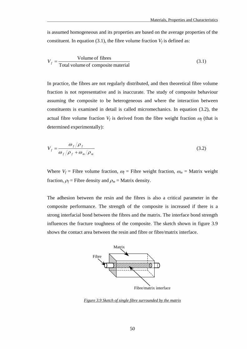
Materials, Properties and Characteristics
50
is assumed homogeneous and its properties are based on the average properties of the
constituent. In equation (3.1), the fibre volume fraction Vf is defined as:
material composite of volumeTotalfibres of Volume
=fV (3.1)
In practice, the fibres are not regularly distributed, and then theoretical fibre volume
fraction is not representative and is inaccurate. The study of composite behaviour
assuming the composite to be heterogeneous and where the interaction between
constituents is examined in detail is called micromechanics. In equation (3.2), the
actual fibre volume fraction Vf is derived from the fibre weight fraction ωf (that is
determined experimentally):
mmff
fffV
ρωρωρω
+= (3.2)
Where Vf = Fibre volume fraction, ωf = Fibre weight fraction, ωm = Matrix weight
fraction, ρf = Fibre density and ρm = Matrix density.
The adhesion between the resin and the fibres is also a critical parameter in the
composite performance. The strength of the composite is increased if there is a
strong interfacial bond between the fibres and the matrix. The interface bond strength
influences the fracture toughness of the composite. The sketch shown in figure 3.9
shows the contact area between the resin and fibre or fibre/matrix interface.
Fibre/matrix interface
Fibre
Matrix
Figure 3.9 Sketch of single fibre surrounded by the matrix
Materials, Properties and Characteristics
51
The interface properties affect the crack propagation in the composite. For example,
in unidirectional composite loaded in tension, the cracks occur in the transverse
direction.
“If the interface debonds relatively easily, the crack propagation is interrupted by the
debonding process and instead of moving through the fibre, the crack moves along
the fibre surface, allowing the fibre to carry higher loads” (Mallick, 1997).
Then the fibre pullout and break occur, leading to a wider crack and finally a
premature failure.
“If the pullout occurs against high frictional forces or shear stresses at the interface,
there may be a significant increase in fracture toughness of the composite” (Mallick,
1997).
In normal conditions, the interface bond strength is mechanically achieved during the
curing process. This bond is formed by the differential shrinkage of the matrix,
which has a higher coefficient of thermal expansion than the fibres. Therefore the
matrix shrinks more than the fibres during the temperature cooling down and this
creates some residual stresses within the composite, which take part of the interface
bond strength.
“In many polymeric matrix composites, increased interfacial bond strength is
achieved by fibre surface treatment, which helps in forming a chemical linkage
between the fibres and the matrix across the interface” (Mallick, 1997).
There are several methods to evaluate the fibre/matrix bond strength through series
of tests, which attempt to measure interfacial shear strength (IFSS) or to measure
interface-sensitive properties and microscopic inspection of failure surfaces.
Eventually highly sophisticated equipment is required to carry out those tests
therefore the fibre/matrix bond strength will not be assessed in the purpose of this
research. However, one of the most commonly used tests is the fragmentation test:
“A single filament is embedded in the resin, which is moulded into a tensile
dogbone. The coupon is pulled in tension until the filament fractures numerous
times, causing the fibre to break into shorter and shorter lengths. Eventually a length
is attained, called the critical length (lc), which is too short to develop enough tensile
stress for failure. This tensile stress is generated by shear loads at the fibre/matrix
interface, so higher values of IFSS will produce shorter critical length” (Mallick,
1997).
Materials, Properties and Characteristics
52
The equation (3.3) relates the IFSS to the critical length lc is:
×
=
c
f
ldIFSS
2σ
(3.3)
Where lc is the critical length, d is the fibre diameter and σf is the fibre strength.
The fibre length and diameter have also an implication in the composite strength.
Fibres can be short, long or even discontinuous. Their dimensions are often
characterised by the aspect ratio l/d, where l is the fibre length and d is the diameter.
Typical fibres have diameters from 10 microns (10E-3 mm) to 150 microns
(150E-3 mm). If the fibre length l is smaller than lc, little reinforcement effect is
observed; if l is greater than 15×lc, the fibre behaves almost as if it were continuous.
The strength of the composite σc can be estimated from equation (3.4):
mmc
ffc fl
lf σσσ +
−=
21 (3.4)
Where σm is the stress in the matrix when the fibres break,
ff is the force carried by the fibres, fm is the force carried by the matrix.
Note that the total force acting on the composite fcomposite = ff + fm (from Askeland,
1996).
The fibre orientation within the lamina is also a critical parameter in the strength
properties of the composite. Short or randomly orientated fibres can be introduced
easily into the matrix and give relatively isotropic (in-plane properties) behaviour in
the composite. With long or continuous fibres, arranged regularly in the same
direction, the composite shows anisotropic behaviour but with particularly good
strength and stiffness properties if the load is applied in the fibre direction. On the
other hand, poor properties are observed with the load applied in the perpendicular
direction of the fibres. The figure 3.10 shows the effect of fibre orientation on
unidirectional composites.
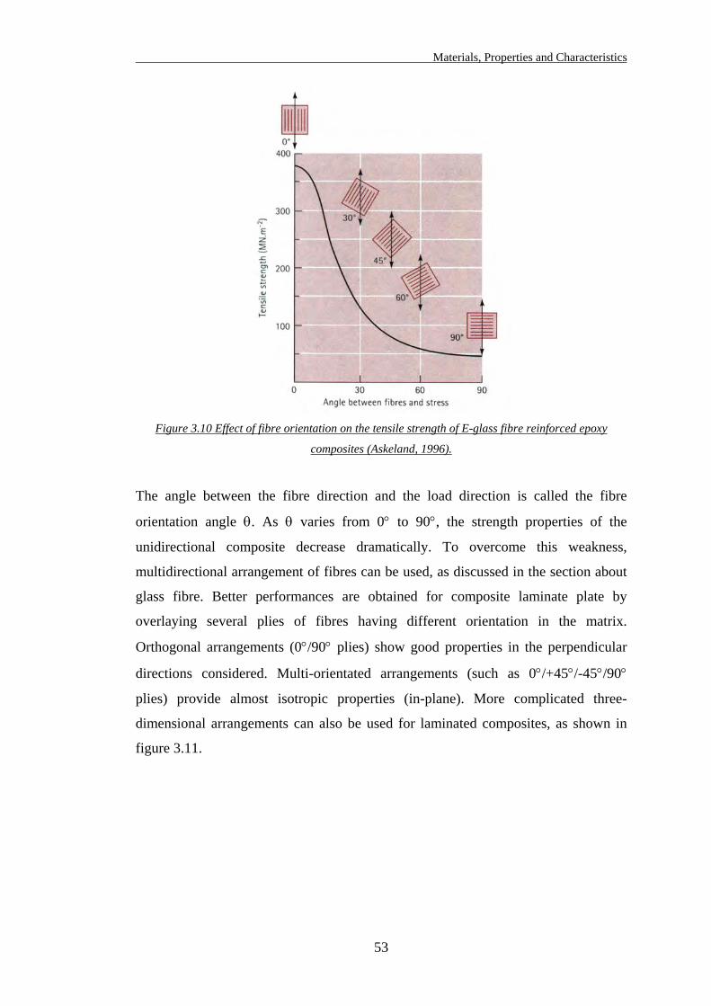
Materials, Properties and Characteristics
53
Figure 3.10 Effect of fibre orientation on the tensile strength of E-glass fibre reinforced epoxy
composites (Askeland, 1996).
The angle between the fibre direction and the load direction is called the fibre
orientation angle θ. As θ varies from 0° to 90°, the strength properties of the
unidirectional composite decrease dramatically. To overcome this weakness,
multidirectional arrangement of fibres can be used, as discussed in the section about
glass fibre. Better performances are obtained for composite laminate plate by
overlaying several plies of fibres having different orientation in the matrix.
Orthogonal arrangements (0°/90° plies) show good properties in the perpendicular
directions considered. Multi-orientated arrangements (such as 0°/+45°/-45°/90°
plies) provide almost isotropic properties (in-plane). More complicated three-
dimensional arrangements can also be used for laminated composites, as shown in
figure 3.11.
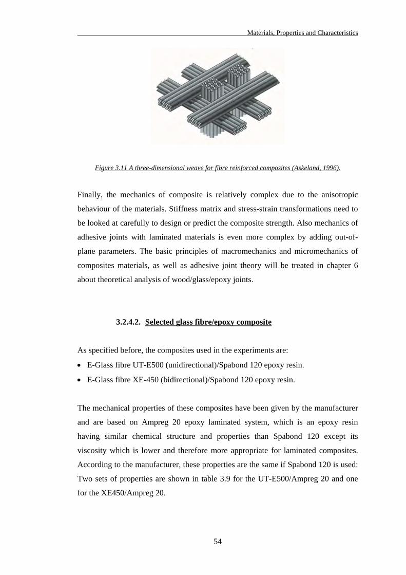
Materials, Properties and Characteristics
54
Figure 3.11 A three-dimensional weave for fibre reinforced composites (Askeland, 1996).
Finally, the mechanics of composite is relatively complex due to the anisotropic
behaviour of the materials. Stiffness matrix and stress-strain transformations need to
be looked at carefully to design or predict the composite strength. Also mechanics of
adhesive joints with laminated materials is even more complex by adding out-of-
plane parameters. The basic principles of macromechanics and micromechanics of
composites materials, as well as adhesive joint theory will be treated in chapter 6
about theoretical analysis of wood/glass/epoxy joints.
3.2.4.2. Selected glass fibre/epoxy composite
As specified before, the composites used in the experiments are:
• E-Glass fibre UT-E500 (unidirectional)/Spabond 120 epoxy resin.
• E-Glass fibre XE-450 (bidirectional)/Spabond 120 epoxy resin.
The mechanical properties of these composites have been given by the manufacturer
and are based on Ampreg 20 epoxy laminated system, which is an epoxy resin
having similar chemical structure and properties than Spabond 120 except its
viscosity which is lower and therefore more appropriate for laminated composites.
According to the manufacturer, these properties are the same if Spabond 120 is used:
Two sets of properties are shown in table 3.9 for the UT-E500/Ampreg 20 and one
for the XE450/Ampreg 20.
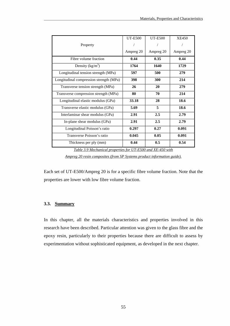
Materials, Properties and Characteristics
55
Property
UT-E500
/
Ampreg 20
UT-E500
/
Ampreg 20
XE450
/
Ampreg 20
Fibre volume fraction 0.44 0.35 0.44
Density (kg/m3) 1764 1640 1729
Longitudinal tension strength (MPa) 597 500 279
Longitudinal compression strength (MPa) 398 300 214
Transverse tension strength (MPa) 26 20 279
Transverse compression strength (MPa) 80 70 214
Longitudinal elastic modulus (GPa) 33.18 28 18.6
Transverse elastic modulus (GPa) 5.69 5 18.6
Interlaminar shear modulus (GPa) 2.91 2.5 2.79
In-plane shear modulus (GPa) 2.91 2.5 2.79
Longitudinal Poisson’s ratio 0.297 0.27 0.091
Transverse Poisson’s ratio 0.045 0.05 0.091
Thickness per ply (mm) 0.44 0.5 0.54
Table 3.9 Mechanical properties for UT-E500 and XE-450 with
Ampreg 20 resin composites (from SP Systems product information guide).
Each set of UT-E500/Ampreg 20 is for a specific fibre volume fraction. Note that the
properties are lower with low fibre volume fraction.
3.3. Summary
In this chapter, all the materials characteristics and properties involved in this
research have been described. Particular attention was given to the glass fibre and the
epoxy resin, particularly to their properties because there are difficult to assess by
experimentation without sophisticated equipment, as developed in the next chapter.
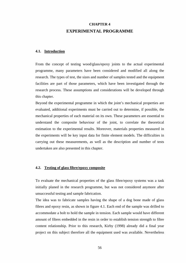
CHAPTER 4
EXPERIMENTAL PROGRAMME
4.1. Introduction
From the concept of testing wood/glass/epoxy joints to the actual experimental
programme, many parameters have been considered and modified all along the
research. The types of test, the sizes and number of samples tested and the equipment
facilities are part of those parameters, which have been investigated through the
research process. These assumptions and considerations will be developed through
this chapter.
Beyond the experimental programme in which the joint’s mechanical properties are
evaluated, additional experiments must be carried out to determine, if possible, the
mechanical properties of each material on its own. These parameters are essential to
understand the composite behaviour of the joint, to correlate the theoretical
estimation to the experimental results. Moreover, materials properties measured in
the experiments will be key input data for finite element models. The difficulties in
carrying out these measurements, as well as the description and number of tests
undertaken are also presented in this chapter.
4.2. Testing of glass fibre/epoxy composite
To evaluate the mechanical properties of the glass fibre/epoxy systems was a task
initially planed in the research programme, but was not considered anymore after
unsuccessful testing and sample fabrication.
The idea was to fabricate samples having the shape of a dog bone made of glass
fibres and epoxy resin, as shown in figure 4.1. Each end of the sample was drilled to
accommodate a bolt to hold the sample in tension. Each sample would have different
amount of fibres embedded in the resin in order to establish tension strength to fibre
content relationship. Prior to this research, Kirby (1998) already did a final year
project on this subject therefore all the equipment used was available. Nevertheless
56
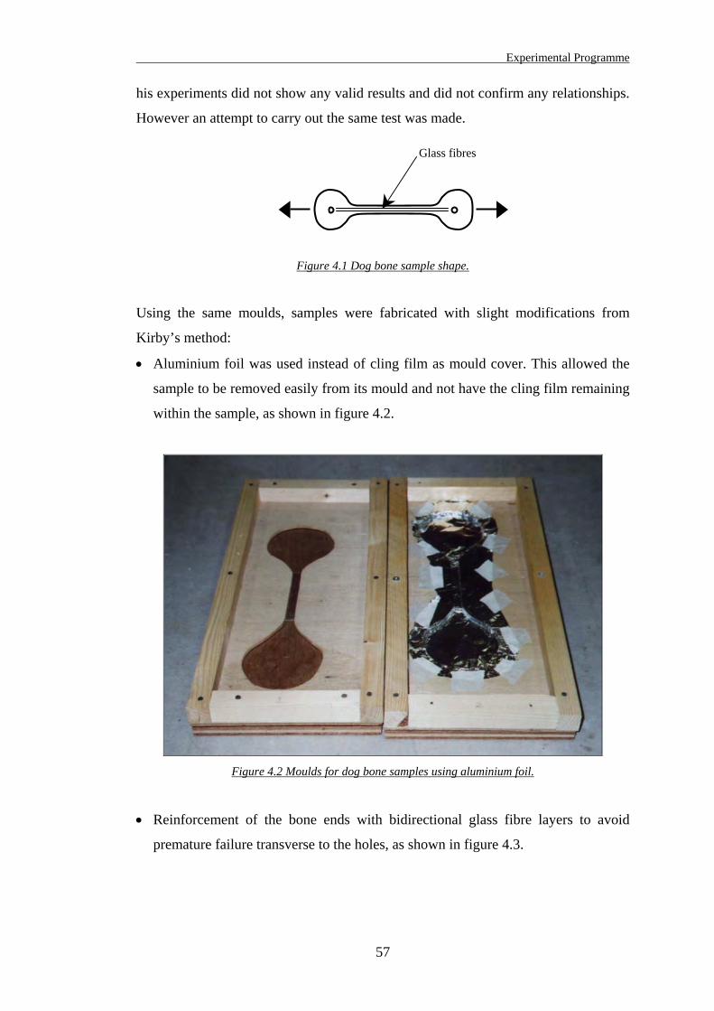
Experimental Programme
his experiments did not show any valid results and did not confirm any relationships.
However an attempt to carry out the same test was made.
Glass fibres
Figure 4.1 Dog bone sample shape.
Using the same moulds, samples were fabricated with slight modifications from
Kirby’s method:
• Aluminium foil was used instead of cling film as mould cover. This allowed the
sample to be removed easily from its mould and not have the cling film remaining
within the sample, as shown in figure 4.2.
Figure 4.2 Moulds for dog bone samples using aluminium foil.
• Reinforcement of the bone ends with bidirectional glass fibre layers to avoid
premature failure transverse to the holes, as shown in figure 4.3.
57
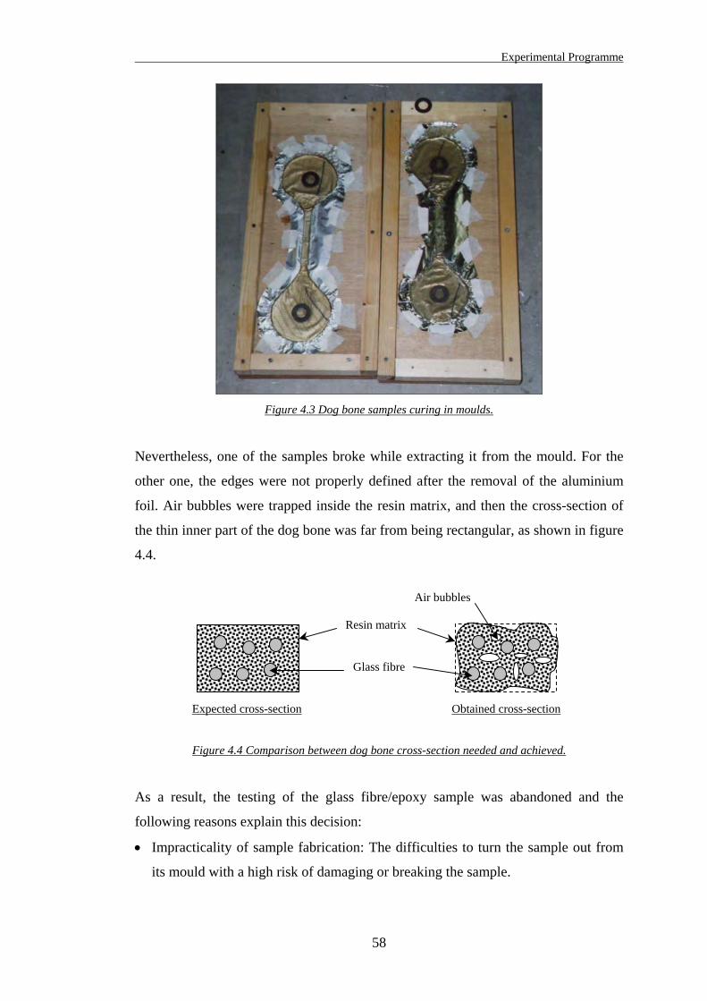
Experimental Programme
Figure 4.3 Dog bone samples curing in moulds.
Nevertheless, one of the samples broke while extracting it from the mould. For the
other one, the edges were not properly defined after the removal of the aluminium
foil. Air bubbles were trapped inside the resin matrix, and then the cross-section of
the thin inner part of the dog bone was far from being rectangular, as shown in figure
4.4.
Air bubbles
Obtained cross-section Expected cross-section
Glass fibre
Resin matrix
Figure 4.4 Comparison between dog bone cross-section needed and achieved.
As a result, the testing of the glass fibre/epoxy sample was abandoned and the
following reasons explain this decision:
• Impracticality of sample fabrication: The difficulties to turn the sample out from
its mould with a high risk of damaging or breaking the sample.
58
Experimental Programme
• The wooden moulds were inadequate to create the samples shape required. It was
not truly symmetrical therefore bones heads did not have the same shape.
Aluminium or stainless steel mould fabricated with precise dimensioning to
0.1 mm or less tolerance would have been ideal.
• With imprecise dimensions, it was difficult to measure the cross-sectional area.
• There was no system to ensure a good fibre impregnation (such as using a roller
or a vibrating system) and remove the air trapped within the resin matrix.
• Maintaining the fibres in position near the cross-section neutral axis, parallel to
the sample was almost impossible to achieve.
• Some extra fibres were placed in the sample bones ends to avoid tension failure
around the bolt connection, therefore the amount of resin was difficult to measure,
especially the exact amount, which would lead to the sample failure in the thinner
part of the dog bone.
Under those considerations, the most reliable way to find out about the glass
fibre/epoxy properties was to use the properties given by the manufacturer. Usually
properties from manufacturers are slightly over estimated (for commercial purposes)
and do not always reflect realistic conditions. However SP Systems is a large
company based in the Isle of Wight, which fabricates its own products but also runs a
design office. All their materials are tested and properties established experimentally
with appropriate methods and equipment in order to be used for design purposes. The
properties given by SP Systems are not the ones commonly given for commercial use
and are therefore accurate and representative of experimental conditions. They have
been recommended by SP design office for use in this research.
At this stage of the research process, it was decided to use those properties instead of
measuring them for the theoretical analysis and finite element modelling.
59
Experimental Programme
4.3. Wood/glass/epoxy joints
The testing of wood/glass/epoxy joints was elaborated according to various
parameters such as types of test, joint geometry, number of samples per type of test,
standard testing method of mechanically fastened timber joints, standard testing
method of adhesive joints, etc.
The programme was initially based on Claisse and Davis (1998) who looked at butt
or scarf ends timber members, fully or partially connected with glass fibre/epoxy
layers of various length, tested in static tension. Most of the information obtained
through this research has been taken into account to develop this experimental
programme, as explained in the following sections.
4.3.1. Joint geometry requirements
The initial application of wood/glass/epoxy was thought to be an alternative to
mechanical fastened timber joints, particularly for timber frame such as trussed
rafters. The most common jointing system used for timber truss connection is the
punched metal plate. It can only be used if the members connected have the same
thickness, which is normally the case for trussed rafters. The plates are ‘punched’ or
nailed on two opposite faces of the timber members and the member cross-sections
are not reduced, as it would be if bolts or dowels were used. For these reasons, the
punched metal plate is probably the most comparable jointing system with
wood/glass/epoxy joints in terms of geometrical configuration.
In timber frames such as trusses, connected members have different orientations,
therefore glass fibre/epoxy layers can only be bonded on the two opposite sides of
each members, which are in the same plane. In order to obtain an efficient bond
between the composite layer and the timber, the connected members must have the
same thickness.
The strength of punched metal plate timber joints varies with the member orientation.
This is reflected through the anisotropic timber properties, which are a function of its
grain orientation. Therefore, punched metal plate timber joints are generally tested
for different grain orientation.
60
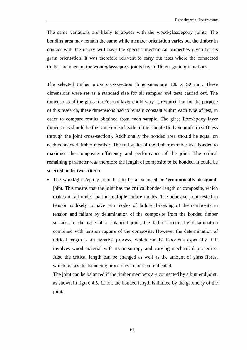
Experimental Programme
The same variations are likely to appear with the wood/glass/epoxy joints. The
bonding area may remain the same while member orientation varies but the timber in
contact with the epoxy will have the specific mechanical properties given for its
grain orientation. It was therefore relevant to carry out tests where the connected
timber members of the wood/glass/epoxy joints have different grain orientations.
The selected timber gross cross-section dimensions are 100 × 50 mm. These
dimensions were set as a standard size for all samples and tests carried out. The
dimensions of the glass fibre/epoxy layer could vary as required but for the purpose
of this research, these dimensions had to remain constant within each type of test, in
order to compare results obtained from each sample. The glass fibre/epoxy layer
dimensions should be the same on each side of the sample (to have uniform stiffness
through the joint cross-section). Additionally the bonded area should be equal on
each connected timber member. The full width of the timber member was bonded to
maximise the composite efficiency and performance of the joint. The critical
remaining parameter was therefore the length of composite to be bonded. It could be
selected under two criteria:
• The wood/glass/epoxy joint has to be a balanced or ‘economically designed’
joint. This means that the joint has the critical bonded length of composite, which
makes it fail under load in multiple failure modes. The adhesive joint tested in
tension is likely to have two modes of failure: breaking of the composite in
tension and failure by delamination of the composite from the bonded timber
surface. In the case of a balanced joint, the failure occurs by delamination
combined with tension rupture of the composite. However the determination of
critical length is an iterative process, which can be laborious especially if it
involves wood material with its anisotropy and varying mechanical properties.
Also the critical length can be changed as well as the amount of glass fibres,
which makes the balancing process even more complicated.
The joint can be balanced if the timber members are connected by a butt end joint,
as shown in figure 4.5. If not, the bonded length is limited by the geometry of the
joint.
61
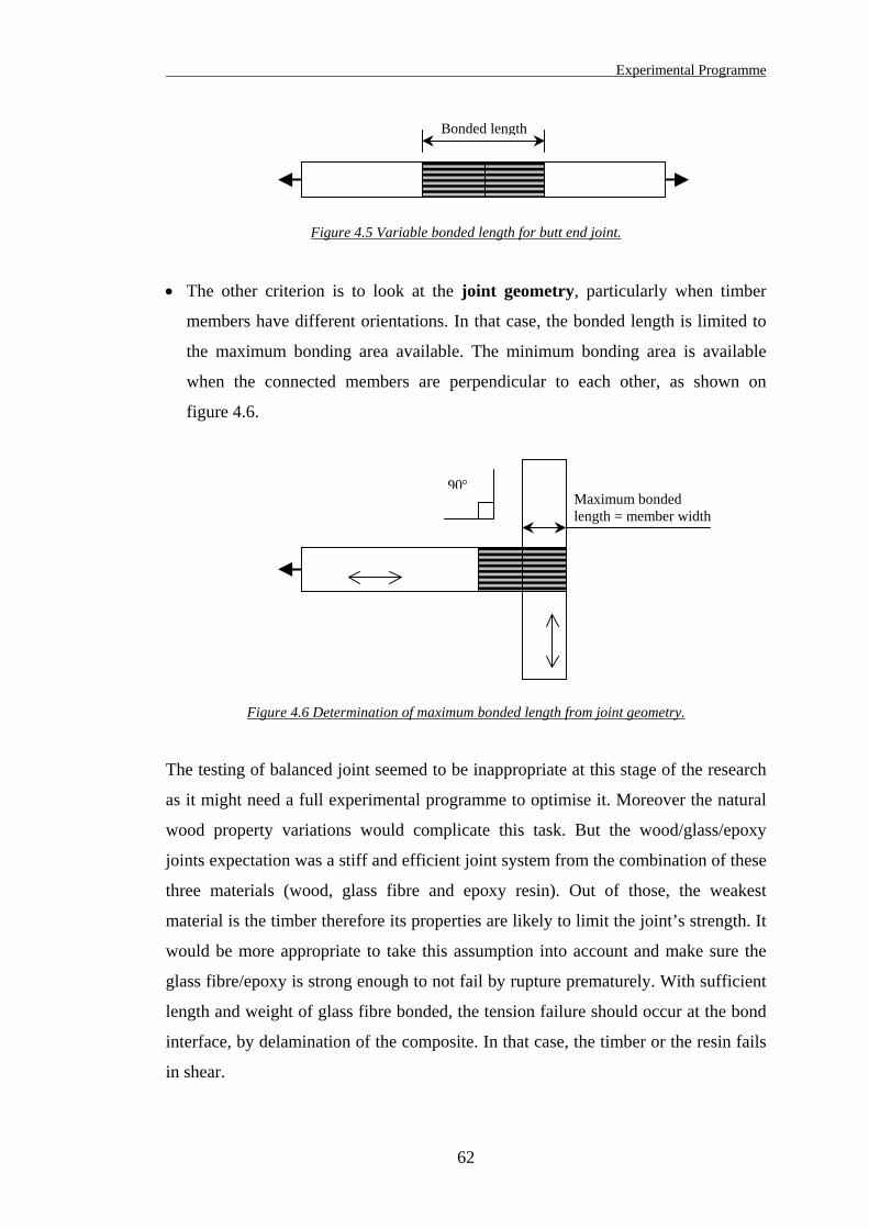
Experimental Programme
Bonded length
Figure 4.5 Variable bonded length for butt end joint.
• The other criterion is to look at the joint geometry, particularly when timber
members have different orientations. In that case, the bonded length is limited to
the maximum bonding area available. The minimum bonding area is available
when the connected members are perpendicular to each other, as shown on
figure 4.6.
90°Maximum bonded length = member width
Figure 4.6 Determination of maximum bonded length from joint geometry.
The testing of balanced joint seemed to be inappropriate at this stage of the research
as it might need a full experimental programme to optimise it. Moreover the natural
wood property variations would complicate this task. But the wood/glass/epoxy
joints expectation was a stiff and efficient joint system from the combination of these
three materials (wood, glass fibre and epoxy resin). Out of those, the weakest
material is the timber therefore its properties are likely to limit the joint’s strength. It
would be more appropriate to take this assumption into account and make sure the
glass fibre/epoxy is strong enough to not fail by rupture prematurely. With sufficient
length and weight of glass fibre bonded, the tension failure should occur at the bond
interface, by delamination of the composite. In that case, the timber or the resin fails
in shear.
62
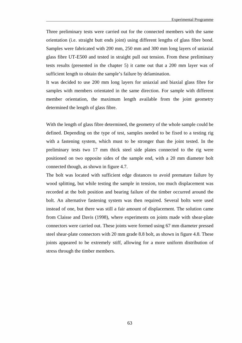
Experimental Programme
Three preliminary tests were carried out for the connected members with the same
orientation (i.e. straight butt ends joint) using different lengths of glass fibre bond.
Samples were fabricated with 200 mm, 250 mm and 300 mm long layers of uniaxial
glass fibre UT-E500 and tested in straight pull out tension. From these preliminary
tests results (presented in the chapter 5) it came out that a 200 mm layer was of
sufficient length to obtain the sample’s failure by delamination.
It was decided to use 200 mm long layers for uniaxial and biaxial glass fibre for
samples with members orientated in the same direction. For sample with different
member orientation, the maximum length available from the joint geometry
determined the length of glass fibre.
With the length of glass fibre determined, the geometry of the whole sample could be
defined. Depending on the type of test, samples needed to be fixed to a testing rig
with a fastening system, which must to be stronger than the joint tested. In the
preliminary tests two 17 mm thick steel side plates connected to the rig were
positioned on two opposite sides of the sample end, with a 20 mm diameter bolt
connected though, as shown in figure 4.7.
The bolt was located with sufficient edge distances to avoid premature failure by
wood splitting, but while testing the sample in tension, too much displacement was
recorded at the bolt position and bearing failure of the timber occurred around the
bolt. An alternative fastening system was then required. Several bolts were used
instead of one, but there was still a fair amount of displacement. The solution came
from Claisse and Davis (1998), where experiments on joints made with shear-plate
connectors were carried out. These joints were formed using 67 mm diameter pressed
steel shear-plate connectors with 20 mm grade 8.8 bolt, as shown in figure 4.8. These
joints appeared to be extremely stiff, allowing for a more uniform distribution of
stress through the timber members.
63
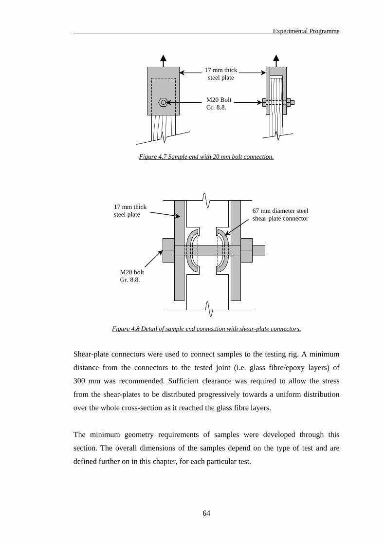
Experimental Programme
17 mm thick steel plate
M20 Bolt Gr. 8.8.
Figure 4.7 Sample end with 20 mm bolt connection.
M20 bolt Gr. 8.8.
17 mm thick steel plate 67 mm diameter steel
shear-plate connector
Figure 4.8 Detail of sample end connection with shear-plate connectors.
Shear-plate connectors were used to connect samples to the testing rig. A minimum
distance from the connectors to the tested joint (i.e. glass fibre/epoxy layers) of
300 mm was recommended. Sufficient clearance was required to allow the stress
from the shear-plates to be distributed progressively towards a uniform distribution
over the whole cross-section as it reached the glass fibre layers.
The minimum geometry requirements of samples were developed through this
section. The overall dimensions of the samples depend on the type of test and are
defined further on in this chapter, for each particular test.
64
Experimental Programme
4.3.2. Types of test
4.3.2.1. The choice of tests
Wood/glass/epoxy joint strength properties depend on the materials jointed:
• Timber species, density, moisture content, mechanical properties, aspects and
defects,
• Types of glass fibre, density and mechanical properties,
• Type of epoxy resin, the amount used in the joint, its density and mechanical
properties.
The strength properties of wood/glass/epoxy joints also depend on the overall size,
thickness, width and configuration of the joint and also on loading direction and
exposure conditions to which the joint is subject in service.
There are so many factors, which can affect the strength of wood/glass/epoxy joints
that restrictions such as the type and size of the glass fibre, the size of the samples
and the number of specimens tested were taken in order to set up a feasible testing
programme. Dimension requirements were developed in the previous section and the
number of samples tested is discussed later.
To define the types of test to carry out in this programme, it was essential to recall
the aim of this research, which was to develop tests to determine strength properties,
capacity and stiffness of joints made of glass fibre bonded with epoxy resin for
applications in load bearing timber structures.
Testing samples is an alternative way to recreate a joint within a timber structure
without having to test the whole structure. Testing joints is more practical and it
reduces secondary effects or problems which tend to occur in the testing of large
frames, such as lateral stability, support conditions, member buckling etc. In full
frame tests, the joints do not always behave as they would if they were ‘isolated’
from the frame. In fact it is difficult to recreate a true in-situ conditions for a full
structure, such as providing a timber truss with adequate lateral restraints of the
rafters (normally due to the purlins) without altering the loading conditions.
65
Experimental Programme
Wood/glass/epoxy joints in a frame would act in a way similar to mechanically
fastened joints. They would be subject to axial forces, shear forces and bending
moments. In trussed frames, joints are usually assumed as pinned joints. In fact, the
frame is usually designed as a pinned frame and bending moments are only taken
into account in the member design. The joints are assumed to be free to rotate, but in
reality they can only rotate to a nominal degree, which depends on the type of
connection, the number of fasteners, etc. However a very small amount of rotation
would release partially a joint from any bending moment. This explains why it is so
difficult to design a fully rigid joint, which will always have some degree of rotation
and then will never attract the full bending moment it has been designed for.
When ‘isolated’ joints are tested, bending moments can be developed from eccentric
axial force (i.e. axial force not distributed uniformly through the member
cross-section), but such bending would remain small in comparison to the axial force
if appropriate attention is taken to minimise that effect.
In that instance, wood/glass/epoxy joints needed to be tested under axial loading.
Tests in flexion would be unrepresentative of their actual behaviour within a frame.
Considerations were taken to minimise any bending moment effects due to axial
force eccentricity. Axial loading meant the joints could be tested in tension as well as
in compression.
The tension test means to pull one of the connected members from the other, in
which the composite bond will resist, stretch under load until it reaches some
plasticity and then fail.
In compression tests, one of the connected members must be ‘pushed’ against the
other, in which the composite will have no immediate effect. The compressive stress
will be transferred directly by the bearing of the timber members end to the other,
which means that the compression capacity will be limited to the compression
resistance of the timber. The composite will act in flexion by resisting the buckling
of the joint, with in-plane shear stresses if the connected members have different
orientations.
The structural role of the composite is more complex in a joint tested in compression
because the composite will be subject to stresses resulting from a combination of
compression, shear and possibly bending.
As part of the preliminary tests, one sample made with a straight configuration
(i.e. connected members with same orientation) was tested in compression. The
66
Experimental Programme
sample failed after the timber started splitting in the joint area. As the sample was
buckling, one of the composite layers partially broke in tension. The test was stopped
at this stage before the complete failure occurred. However no measurements such as
the failure load were recorded because this test was carried out at an early stage of
the research, simply to observe and understand the joint behaviour.
The compression test was then excluded from the testing programme because of the
complexity of the joint behaviour and for the reasons previously described.
As a result, the testing programme was then concentrated on tension tests
exclusively. The main objective was to analyse the effect of glass fibre orientation
with the wood grain orientation on timber samples tested in tension.
The measurements to be carried out were:
• The load-slip capacity and maximum load resulting from tension test at various
angles between the direction of the applied force and glass fibre orientation (α)
and the direction of the applied force and the grain of the timber (β),
• Strain values throughout the composite layers at specific locations to identify how
the stresses are distributed within the composite.
The types of tests were selected among a large number of test options to reduce the
experiments to a feasible programme. Each test had samples made with uniaxial and
biaxial glass fibre. They are presented and developed in the following sections.
67
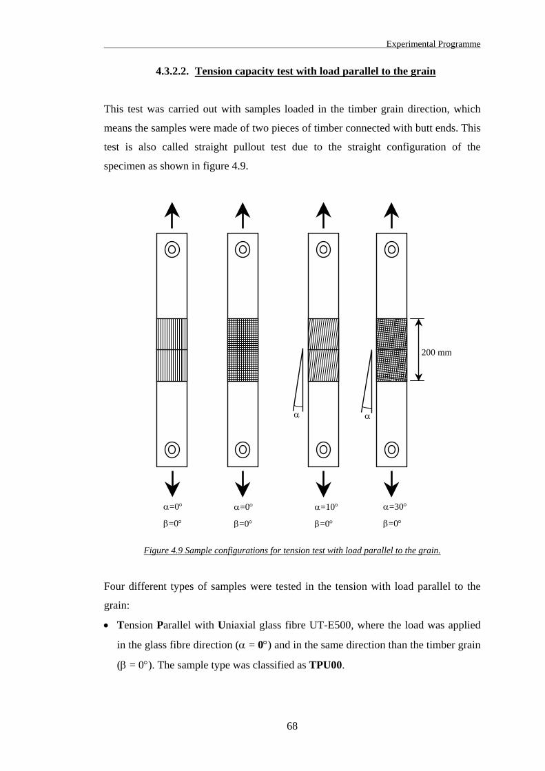
Experimental Programme
4.3.2.2. Tension capacity test with load parallel to the grain
This test was carried out with samples loaded in the timber grain direction, which
means the samples were made of two pieces of timber connected with butt ends. This
test is also called straight pullout test due to the straight configuration of the
specimen as shown in figure 4.9.
α=30°
β=0°
α=10°
β=0°
α=0°
β=0°
α=0°
β=0°
αα
200 mm
Figure 4.9 Sample configurations for tension test with load parallel to the grain.
Four different types of samples were tested in the tension with load parallel to the
grain:
• Tension Parallel with Uniaxial glass fibre UT-E500, where the load was applied
in the glass fibre direction (α = 0°) and in the same direction than the timber grain
(β = 0°). The sample type was classified as TPU00.
68
Experimental Programme
• Tension Parallel with Biaxial glass fibre XE450, where the load was applied in
the glass fibre direction (α = 0°) and in the same direction than the timber grain
(β = 0°). The sample type was classified as TPB00.
• Tension Parallel with Uniaxial glass fibre UT-E500, where the glass fibres were
orientated 10° from the load direction (α = 10°), but the load was parallel to the
timber grain (β = 0°). This 10° angle represented a possible misalignment of the
fibres with the timber grain and the load direction. The aim of this test was to
assess the implication of fibre misalignment for the joint strength. The sample
type was classified as TPU10.
• Tension Parallel with Biaxial glass fibre XE450, where the glass fibres were
orientated 30° from the load direction (α = 30°), but the load was parallel to the
timber grain (β = 0°). With the biaxial glass fibre, the properties were the same in
orthogonal directions, therefore α = 0° and α = 90° show exactly the same
configuration. For 0° < α < 45°, the sample had different properties but for
α > 45°, the same properties applied by orthogonal symmetry. For example, with
the selected angle of α = 30°, it was the same configuration for α = 60°.
Combined with the test where α = 0°, this value of 30° allowed the assessment of
four different configurations, α = 0, 30, 60 and 90° with only two different sample
tested. The sample type was classified as TPB30.
Measurements were carried out on these samples during test. The testing rig and the
equipment used is explained and developed in detail further on in this chapter, but it
is relevant in this section to identify which type of measurements were carried out
during those tests.
As the load applied to the sample was recorded, displacements or strains at specific
locations on the joint were measured. Two different types of devices were used to
carry out those measurements:
• Linear Voltage Displacement Transducers or LVDTs were glued (with quick
setting epoxy resin) onto the timber at various locations, using PVC and steel
brackets fabricated for this purpose. These transducers measured displacements
between the brackets located on either piece of timber. They measured the
displacement around the gap position (small side LVDTs) and were fixed in a
symmetrical arrangement to check any misalignment of the sample. For the
69
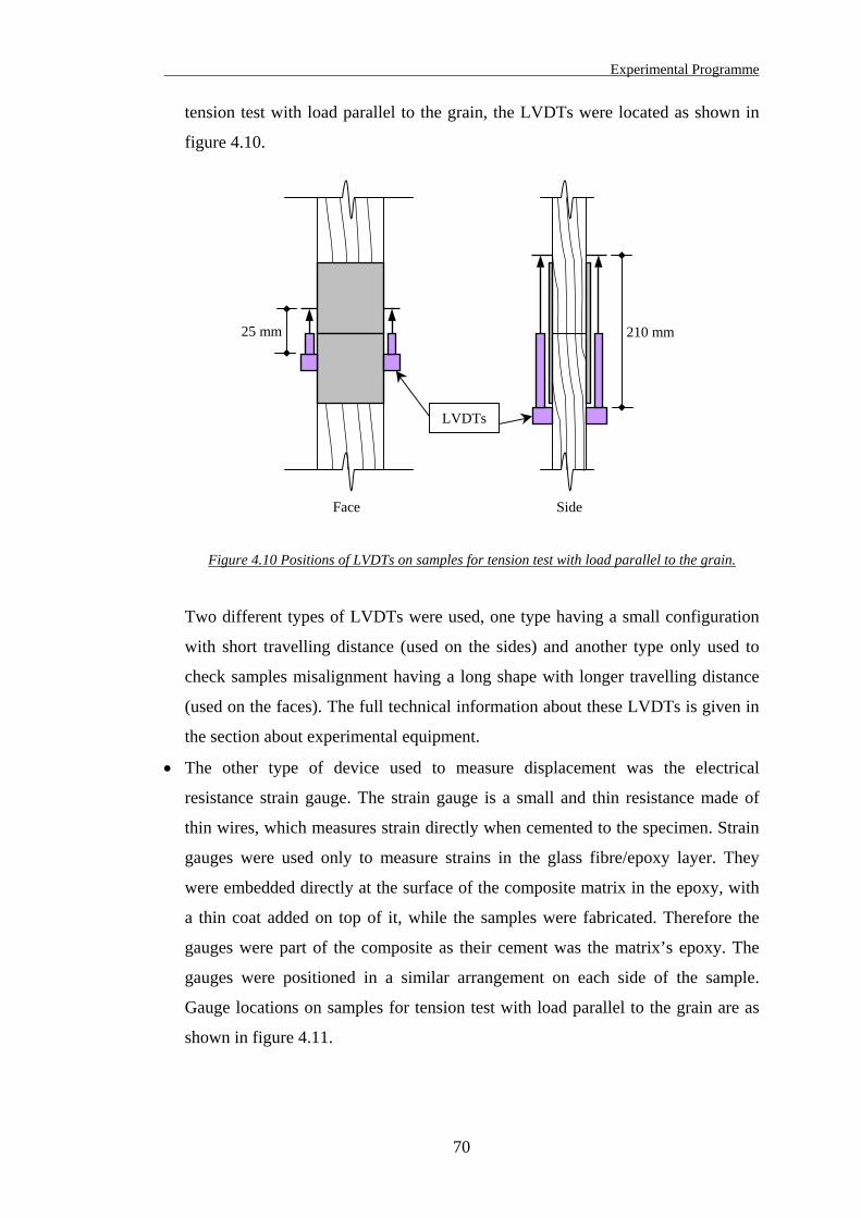
Experimental Programme
tension test with load parallel to the grain, the LVDTs were located as shown in
figure 4.10.
25 mm 210 mm
LVDTs
SideFace
Figure 4.10 Positions of LVDTs on samples for tension test with load parallel to the grain.
Two different types of LVDTs were used, one type having a small configuration
with short travelling distance (used on the sides) and another type only used to
check samples misalignment having a long shape with longer travelling distance
(used on the faces). The full technical information about these LVDTs is given in
the section about experimental equipment.
• The other type of device used to measure displacement was the electrical
resistance strain gauge. The strain gauge is a small and thin resistance made of
thin wires, which measures strain directly when cemented to the specimen. Strain
gauges were used only to measure strains in the glass fibre/epoxy layer. They
were embedded directly at the surface of the composite matrix in the epoxy, with
a thin coat added on top of it, while the samples were fabricated. Therefore the
gauges were part of the composite as their cement was the matrix’s epoxy. The
gauges were positioned in a similar arrangement on each side of the sample.
Gauge locations on samples for tension test with load parallel to the grain are as
shown in figure 4.11.
70
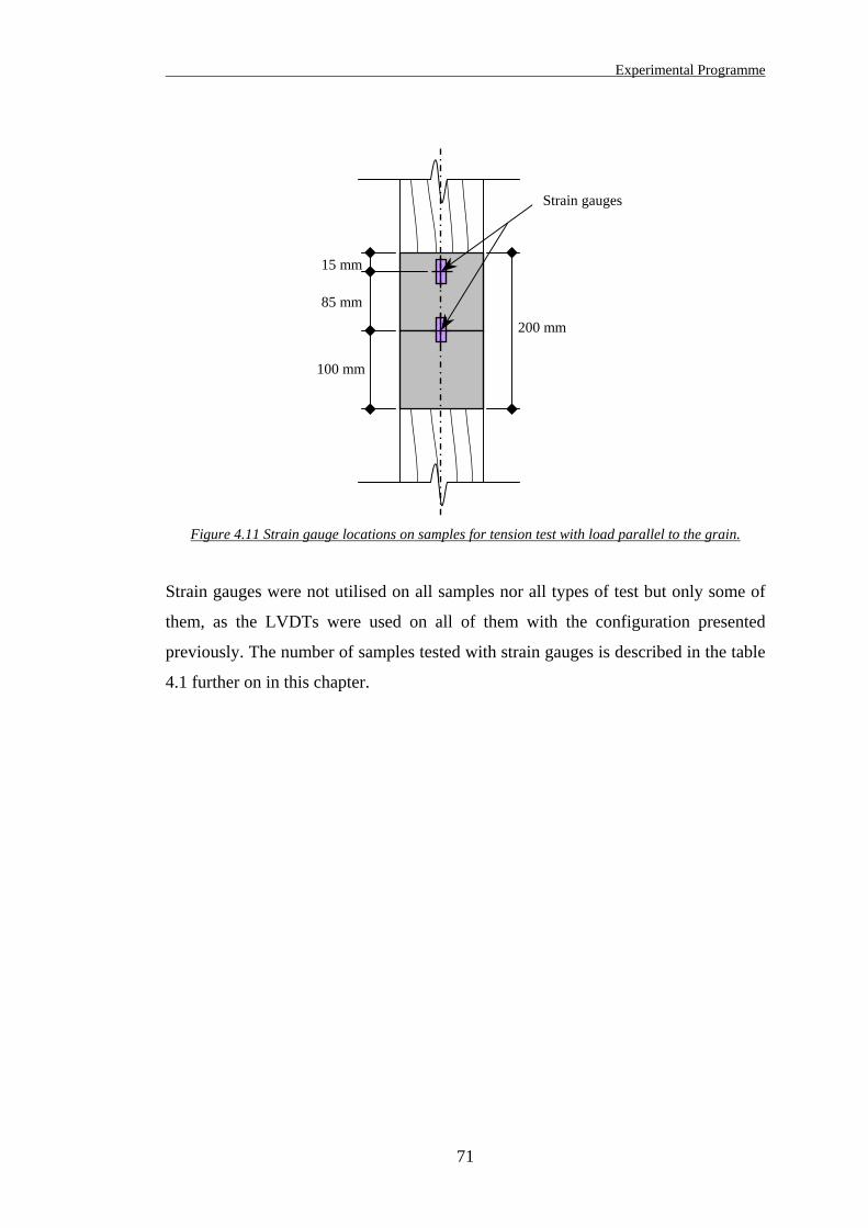
Experimental Programme
Strain gauges
100 mm
85 mm
15 mm
200 mm
Figure 4.11 Strain gauge locations on samples for tension test with load parallel to the grain.
Strain gauges were not utilised on all samples nor all types of test but only some of
them, as the LVDTs were used on all of them with the configuration presented
previously. The number of samples tested with strain gauges is described in the table
4.1 further on in this chapter.
71
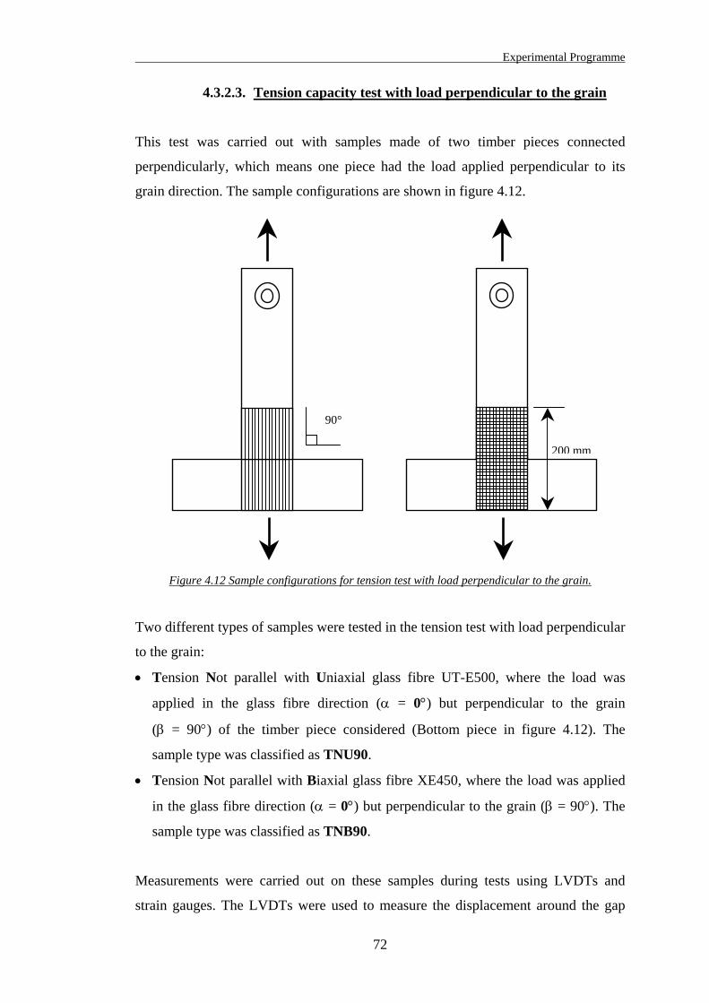
Experimental Programme
4.3.2.3. Tension capacity test with load perpendicular to the grain
This test was carried out with samples made of two timber pieces connected
perpendicularly, which means one piece had the load applied perpendicular to its
grain direction. The sample configurations are shown in figure 4.12.
200 mm
90°
Figure 4.12 Sample configurations for tension test with load perpendicular to the grain.
Two different types of samples were tested in the tension test with load perpendicular
to the grain:
• Tension Not parallel with Uniaxial glass fibre UT-E500, where the load was
applied in the glass fibre direction (α = 0°) but perpendicular to the grain
(β = 90°) of the timber piece considered (Bottom piece in figure 4.12). The
sample type was classified as TNU90.
• Tension Not parallel with Biaxial glass fibre XE450, where the load was applied
in the glass fibre direction (α = 0°) but perpendicular to the grain (β = 90°). The
sample type was classified as TNB90.
Measurements were carried out on these samples during tests using LVDTs and
strain gauges. The LVDTs were used to measure the displacement around the gap
72

Experimental Programme
between the two timber pieces and were located according to the sample
configuration shown in figure 4.13.
25 mm
Face
LVDTs
Figure 4.13 Positions of LVDTs on samples for tension test with load perpendicular to the grain.
Only two small LVDTs could be used for this test on the sample sides because the
loading rig in which the sample was held did not have sufficient clearance space to
accommodate any LVDTs on the faces.
Strain gauges were used on both faces of the sample and embedded in the composite
layer as explained previously. Two strain gauges were placed on each face to
measure the strain of the composite layer in the zone bonded perpendicular to the
grain. They were positioned as shown in figure 4.14.
Strain gauges
100
85
15
200
Figure 4.14 Strain gauge locations on samples for tension test with load perpendicular to the grain.
73
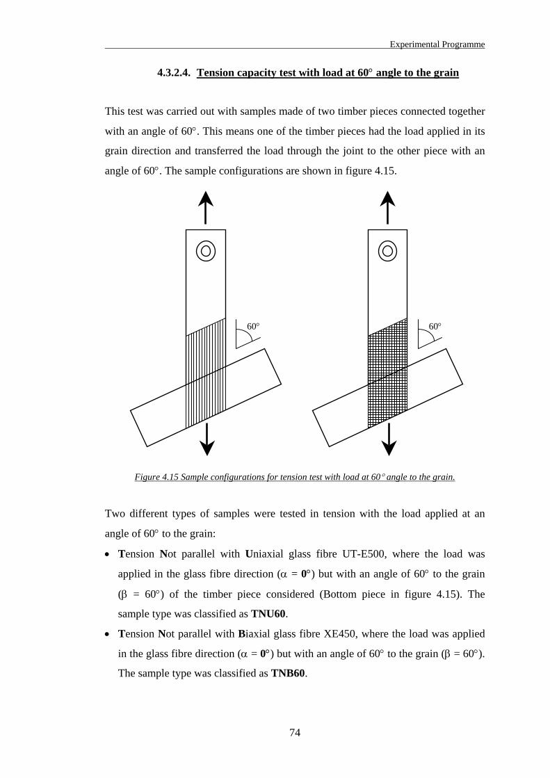
Experimental Programme
4.3.2.4. Tension capacity test with load at 60° angle to the grain
This test was carried out with samples made of two timber pieces connected together
with an angle of 60°. This means one of the timber pieces had the load applied in its
grain direction and transferred the load through the joint to the other piece with an
angle of 60°. The sample configurations are shown in figure 4.15.
60°60°
Figure 4.15 Sample configurations for tension test with load at 60° angle to the grain.
Two different types of samples were tested in tension with the load applied at an
angle of 60° to the grain:
• Tension Not parallel with Uniaxial glass fibre UT-E500, where the load was
applied in the glass fibre direction (α = 0°) but with an angle of 60° to the grain
(β = 60°) of the timber piece considered (Bottom piece in figure 4.15). The
sample type was classified as TNU60.
• Tension Not parallel with Biaxial glass fibre XE450, where the load was applied
in the glass fibre direction (α = 0°) but with an angle of 60° to the grain (β = 60°).
The sample type was classified as TNB60.
74

Experimental Programme
Measurements were carried out on these samples during test using LVDTs and strain
gauges. The LVDTs were used to measure the displacement at the gap between the
two timber pieces and were located according to the sample configuration shown in
figure 4.16.
25 mm
25 mm
Wood wedge
LVDTs
Figure 4.16 Positions of LVDTs on samples for tension test with load at 60° angle to the grain.
Only two small LVDTs were used for this test on the sample sides because the
loading rig in which the sample was held did not have sufficient clearance space to
accommodate any LVDTs on the faces. Timber wedges were fabricated to provide
the flat contact surface perpendicular to the LVDT’s end, and allow a more accurate
reading of displacement. Those wedges were also bonded on the timber with quick
setting epoxy resin.
Strain gauges were used on both faces of the sample and embedded in the composite
layer as explained previously. Two strain gauges and one strain rosette were placed
on each face to measure the strain of the composite layer in the zone bonded at an
angle of 60° to the grain. They were located as shown in figure 4.17.
75
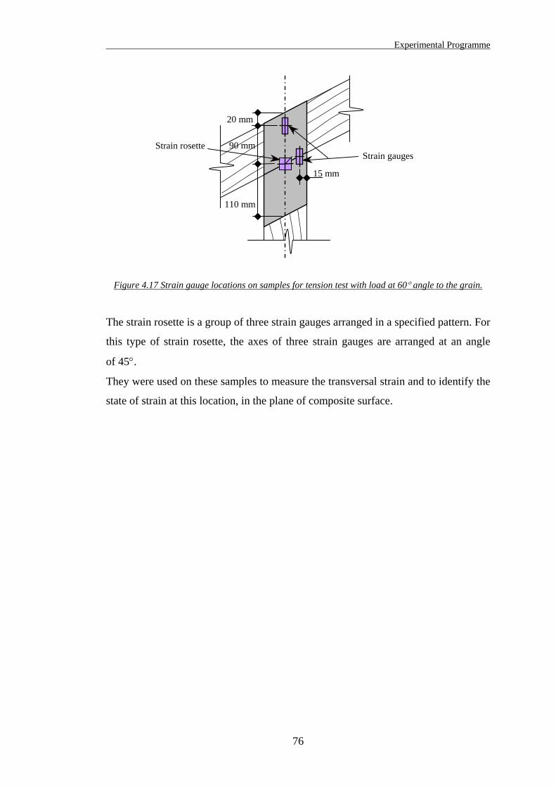
Experimental Programme
Strain gauges Strain rosette
20 mm
90 mm
110 mm
15 mm
Figure 4.17 Strain gauge locations on samples for tension test with load at 60° angle to the grain.
The strain rosette is a group of three strain gauges arranged in a specified pattern. For
this type of strain rosette, the axes of three strain gauges are arranged at an angle
of 45°.
They were used on these samples to measure the transversal strain and to identify the
state of strain at this location, in the plane of composite surface.
76

Experimental Programme
4.3.2.5. Tension capacity test with load at 30° angle to the grain
This test was carried out with samples made of two timber pieces connected together
with an angle of 30°. This means one of the timber pieces had the load applied in its
grain direction and transferred the load through the joint to the other piece with an
angle of 30°. The sample configurations are shown in figure 4.18.
30°30°
Figure 4.18 Sample configurations for tension test with load at 30° angle to the grain.
Two different types of samples were tested in tension with the load applied at an
angle of 30° to the grain:
• Tension Not parallel with Uniaxial glass fibre UT-E500, where the load was
applied in the glass fibre direction (α = 0°) but with an angle of 30° to the grain
(β = 30°) of the timber piece considered (Bottom piece in figure 4.18). The
sample type was classified as TNU30.
77
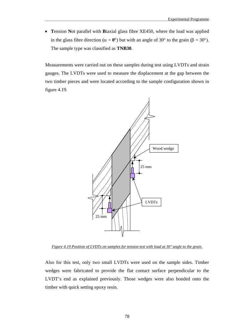
Experimental Programme
• Tension Not parallel with Biaxial glass fibre XE450, where the load was applied
in the glass fibre direction (α = 0°) but with an angle of 30° to the grain (β = 30°).
The sample type was classified as TNB30.
Measurements were carried out on these samples during test using LVDTs and strain
gauges. The LVDTs were used to measure the displacement at the gap between the
two timber pieces and were located according to the sample configuration shown in
figure 4.19.
25 mm
25 mm
Wood wedge
LVDTs
Figure 4.19 Position of LVDTs on samples for tension test with load at 30° angle to the grain.
Also for this test, only two small LVDTs were used on the sample sides. Timber
wedges were fabricated to provide the flat contact surface perpendicular to the
LVDT’s end as explained previously. Those wedges were also bonded onto the
timber with quick setting epoxy resin.
78
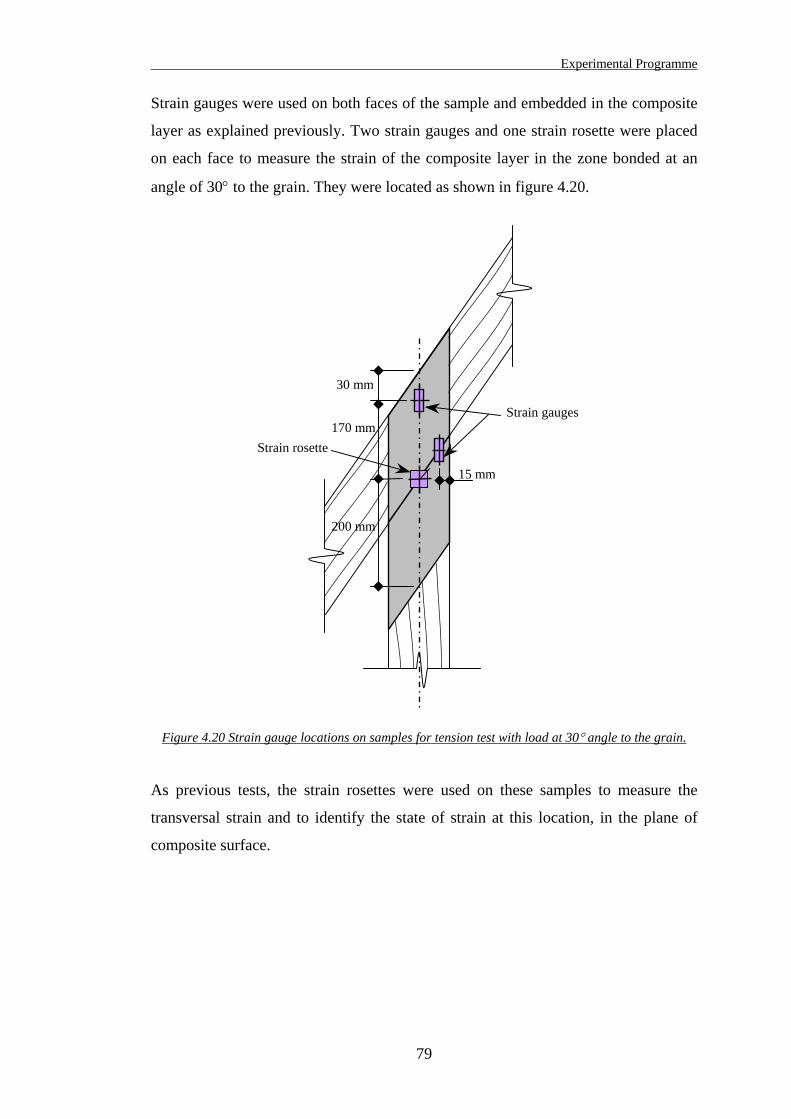
Experimental Programme
Strain gauges were used on both faces of the sample and embedded in the composite
layer as explained previously. Two strain gauges and one strain rosette were placed
on each face to measure the strain of the composite layer in the zone bonded at an
angle of 30° to the grain. They were located as shown in figure 4.20.
Strain gauges
Strain rosette
200 mm
170 mm
30 mm
15 mm
Figure 4.20 Strain gauge locations on samples for tension test with load at 30° angle to the grain.
As previous tests, the strain rosettes were used on these samples to measure the
transversal strain and to identify the state of strain at this location, in the plane of
composite surface.
79
Experimental Programme
Finally there were four different types of test, which were carried out on
wood/glass/epoxy joints. All the samples tested were made of two timber pieces
connected together. Therefore only two-member joints were considered in this
experimental programme. Joints made of three or more members are more
complicated to test because sophisticated loading rig is required to ensure that:
• The sample is tested with realistic loading conditions.
• The loads are applied axially to each member.
But in theory a multi-member joint is a combination of several two-member joints. It
could be modelled as a superposition of two-member joints. But this would be
regardless of the fact that the same composite layer connects all the members
together. The single layer of composite would be subject to a large number of
stresses, which would complicate significantly the joint behaviour and analysis.
Multi-member joints made of wood/glass/epoxy are beyond the scope of this
research and could be part of further research on this topic.
Several parameters still needed to be considered for the tests carried out, such as the
number of samples tested for each series of test.
80
Experimental Programme
4.3.3. Number of samples tested
Codes of practice BS 6948: 1989 “Methods of test for mechanically fastened joints in
timber and wood-based materials” gives minimum number of samples to be tested to
obtain basic strength data of a particular fastener and they are:
• Not less than 15 specimens of a particular type to be tested for lateral strength.
• Not less than 20 specimens of a particular type for withdrawal and pull-through
strength.
The large number of specimens required by the code is evidence of the wide
variations observed with timber materials. But it is assumed through the standard,
that the results obtained from those tests will be used for design purposes. It seemed
difficult to carry out such series of testing for each type of tests. It was impractical in
terms of costs, materials required, experimental time span, etc. Further more, the aim
of this research was not orientated to design at this stage, but only to understand the
structural behaviour of wood/glass/epoxy joint.
In this experimental programme, minimums of six specimens were tested in each
series. It was insufficient to draw statistics out of the results, but according to the
wide range of varying parameters and the limited knowledge of wood/glass/epoxy
joints, it provided adequate information for a preliminary analysis. Then with
minimums of six specimens per type of test, all samples were tested using Linear
Voltage Differential Transducers (LVDTs) to record displacements.
Strain gauges were only provided on some of them in addition to the LVDTs because
of their costs and the fact that strain gauges are not reusable. The numbers of
specimens tested in respect of the type of test and measurement devices are
summarised in the table 4.1. The sample symbol definition is given as follow:
Sample number
Tension test
Load Parallel or Not parallel to the grain
Uniaxial or Biaxial glass fibre
Load/grain angle (º)
Timber type
4 T N U 60 – β
Sample symbol definition.
81
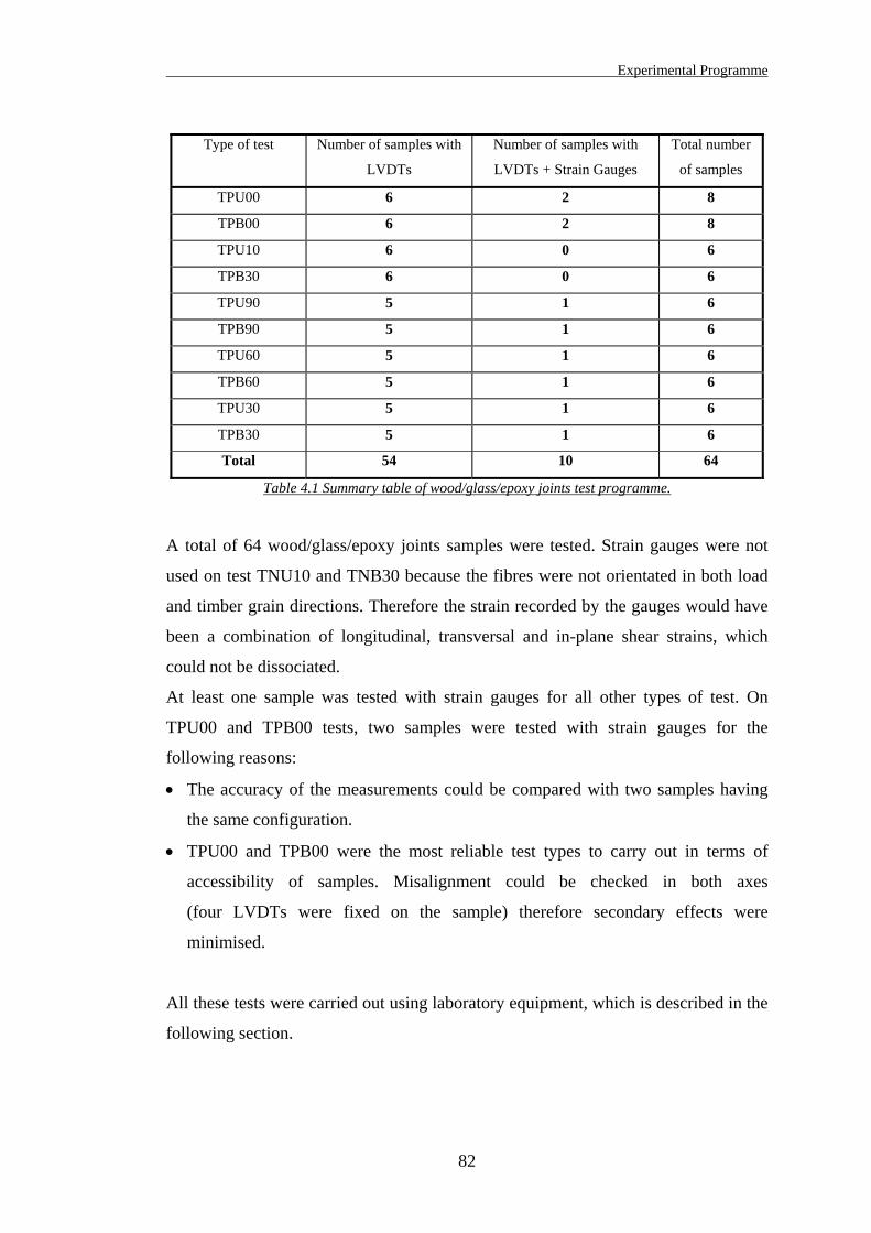
Experimental Programme
Type of test Number of samples with
LVDTs
Number of samples with
LVDTs + Strain Gauges
Total number
of samples
TPU00 6 2 8
TPB00 6 2 8
TPU10 6 0 6
TPB30 6 0 6
TPU90 5 1 6
TPB90 5 1 6
TPU60 5 1 6
TPB60 5 1 6
TPU30 5 1 6
TPB30 5 1 6
Total 54 10 64
Table 4.1 Summary table of wood/glass/epoxy joints test programme.
A total of 64 wood/glass/epoxy joints samples were tested. Strain gauges were not
used on test TNU10 and TNB30 because the fibres were not orientated in both load
and timber grain directions. Therefore the strain recorded by the gauges would have
been a combination of longitudinal, transversal and in-plane shear strains, which
could not be dissociated.
At least one sample was tested with strain gauges for all other types of test. On
TPU00 and TPB00 tests, two samples were tested with strain gauges for the
following reasons:
• The accuracy of the measurements could be compared with two samples having
the same configuration.
• TPU00 and TPB00 were the most reliable test types to carry out in terms of
accessibility of samples. Misalignment could be checked in both axes
(four LVDTs were fixed on the sample) therefore secondary effects were
minimised.
All these tests were carried out using laboratory equipment, which is described in the
following section.
82
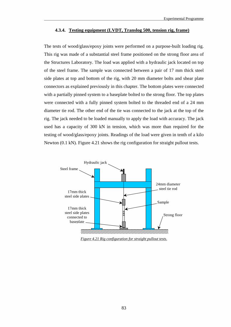
Experimental Programme
4.3.4. Testing equipment (LVDT, Translog 500, tension rig, frame)
The tests of wood/glass/epoxy joints were performed on a purpose-built loading rig.
This rig was made of a substantial steel frame positioned on the strong floor area of
the Structures Laboratory. The load was applied with a hydraulic jack located on top
of the steel frame. The sample was connected between a pair of 17 mm thick steel
side plates at top and bottom of the rig, with 20 mm diameter bolts and shear plate
connectors as explained previously in this chapter. The bottom plates were connected
with a partially pinned system to a baseplate bolted to the strong floor. The top plates
were connected with a fully pinned system bolted to the threaded end of a 24 mm
diameter tie rod. The other end of the tie was connected to the jack at the top of the
rig. The jack needed to be loaded manually to apply the load with accuracy. The jack
used has a capacity of 300 kN in tension, which was more than required for the
testing of wood/glass/epoxy joints. Readings of the load were given in tenth of a kilo
Newton (0.1 kN). Figure 4.21 shows the rig configuration for straight pullout tests.
Strong floor
17mm thick steel side plates
connected to baseplate
Hydraulic jackSteel frame
24mm diameter steel tie rod
Sample
17mm thick steel side plates
Figure 4.21 Rig configuration for straight pullout tests.
83
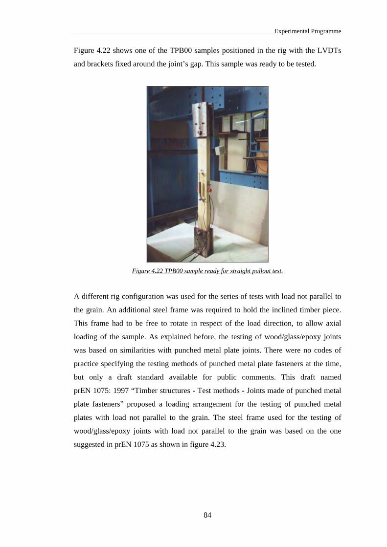
Experimental Programme
Figure 4.22 shows one of the TPB00 samples positioned in the rig with the LVDTs
and brackets fixed around the joint’s gap. This sample was ready to be tested.
Figure 4.22 TPB00 sample ready for straight pullout test.
A different rig configuration was used for the series of tests with load not parallel to
the grain. An additional steel frame was required to hold the inclined timber piece.
This frame had to be free to rotate in respect of the load direction, to allow axial
loading of the sample. As explained before, the testing of wood/glass/epoxy joints
was based on similarities with punched metal plate joints. There were no codes of
practice specifying the testing methods of punched metal plate fasteners at the time,
but only a draft standard available for public comments. This draft named
prEN 1075: 1997 “Timber structures - Test methods - Joints made of punched metal
plate fasteners” proposed a loading arrangement for the testing of punched metal
plates with load not parallel to the grain. The steel frame used for the testing of
wood/glass/epoxy joints with load not parallel to the grain was based on the one
suggested in prEN 1075 as shown in figure 4.23.
84
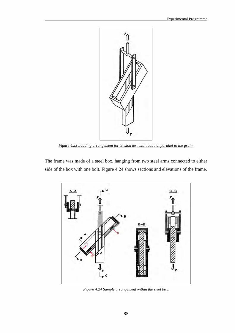
Experimental Programme
Figure 4.23 Loading arrangement for tension test with load not parallel to the grain.
The frame was made of a steel box, hanging from two steel arms connected to either
side of the box with one bolt. Figure 4.24 shows sections and elevations of the frame.
Figure 4.24 Sample arrangement within the steel box.
85

Experimental Programme
The bolts were not tightened and were located on the same axes to allow the box to
rotate. M20 grade 8.8 bolts were used at top and bottom of the arms. The frame was
designed to resist a tension force of 100 kN.
The sample was placed inside the steel box, and the inclined timber piece was
supported at equal distance to the bolt centreline with hardwood plates. The internal
forces in the box are the two reactions from the hardwood supports (shown as R in
figure 4.24) and the reaction from the steel box side (shown as T in figure 4.24).
With F as the applied tension force, the equilibrium of the forces gives for the
reactions:
2sin βFR = and βcosFT = (4.1)
Where β is the angle between the load direction and the timber grain.
There was a continuous edge around the bottom of the steel box to support the
hardwood plates (see section A-A in figure 4.24). The supports were made of
hardwood and not steel to minimise the local deformation in the inclined timber
piece. To ensure that the hardwood supports remained at their initial location during
the test, they were drilled at their centre. A nail fixed to the underside of the inclined
timber piece was positioned into that hole to keep the sample in the centreline of the
steel box and also to hold the support in position during the test. While the tension
was applied to the sample, the inclined timber piece deflected. To reduce this sagging
effect, which creates some eccentricity in the load direction, the hardwood supports
were positioned on each side of the joint, as closely as possible. If any eccentricity of
load was developed in the joint, it produced bending moments. In that case, the joint
was not tested in strictly pure tension. Some small bending moments were measured
on the samples, due to minor eccentricities. These bending moments were so small
compared to the tension force applied to the sample that they were considered as
negligible.
An example of in-plane and out-of-plane bending moment calculations using LVDTs
readings is presented in Appendix C.
86

Experimental Programme
The figure 4.25 shows the rig configuration for tension test with load not parallel to
the grain.
Strong floor
17 mm thick steel side plates
connected to baseplate
Hydraulic jackSteel frame
Sample
Steel box frame with pinned arms
24 mm diameter steel tie rod
Figure 4.25 Rig configuration for tension test with load not parallel to the grain.
The figure 4.26 shows a sample ready to be placed within the steel box. In this
picture, some steel plates were used on top of the hardwood supports to adjust the
height of the sample inside the box. They were placed the wrong way around and
should have been located underneath the hardwood plate.
Figure 4.26 Sample configuration when positioned within the steel box.
Figure 4.26 also shows the set of brackets used to hold the LVDTs in position to
measure displacements. A red circle is also visible on the glass fibre, almost in the
middle of the timber piece. This circle was drawn onto the timber before the sample
87
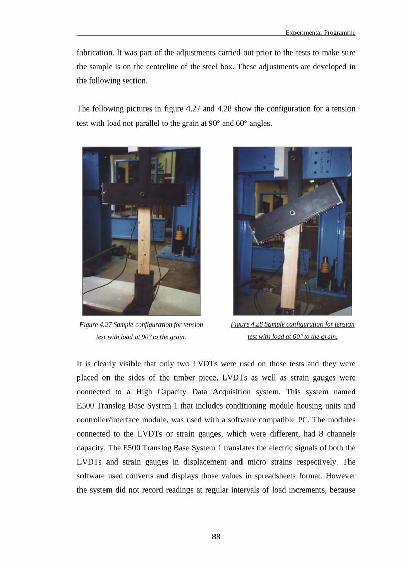
Experimental Programme
fabrication. It was part of the adjustments carried out prior to the tests to make sure
the sample is on the centreline of the steel box. These adjustments are developed in
the following section.
The following pictures in figure 4.27 and 4.28 show the configuration for a tension
test with load not parallel to the grain at 90° and 60° angles.
Figure 4.27 Sample configuration for tension
test with load at 90° to the grain.
Figure 4.28 Sample configuration for tension
test with load at 60° to the grain.
It is clearly visible that only two LVDTs were used on those tests and they were
placed on the sides of the timber piece. LVDTs as well as strain gauges were
connected to a High Capacity Data Acquisition system. This system named
E500 Translog Base System 1 that includes conditioning module housing units and
controller/interface module, was used with a software compatible PC. The modules
connected to the LVDTs or strain gauges, which were different, had 8 channels
capacity. The E500 Translog Base System 1 translates the electric signals of both the
LVDTs and strain gauges in displacement and micro strains respectively. The
software used converts and displays those values in spreadsheets format. However
the system did not record readings at regular intervals of load increments, because
88
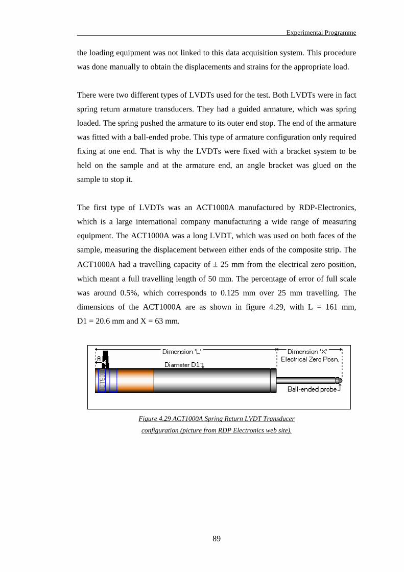
Experimental Programme
89
the loading equipment was not linked to this data acquisition system. This procedure
was done manually to obtain the displacements and strains for the appropriate load.
There were two different types of LVDTs used for the test. Both LVDTs were in fact
spring return armature transducers. They had a guided armature, which was spring
loaded. The spring pushed the armature to its outer end stop. The end of the armature
was fitted with a ball-ended probe. This type of armature configuration only required
fixing at one end. That is why the LVDTs were fixed with a bracket system to be
held on the sample and at the armature end, an angle bracket was glued on the
sample to stop it.
The first type of LVDTs was an ACT1000A manufactured by RDP-Electronics,
which is a large international company manufacturing a wide range of measuring
equipment. The ACT1000A was a long LVDT, which was used on both faces of the
sample, measuring the displacement between either ends of the composite strip. The
ACT1000A had a travelling capacity of ± 25 mm from the electrical zero position,
which meant a full travelling length of 50 mm. The percentage of error of full scale
was around 0.5%, which corresponds to 0.125 mm over 25 mm travelling. The
dimensions of the ACT1000A are as shown in figure 4.29, with L = 161 mm,
D1 = 20.6 mm and X = 63 mm.
Figure 4.29 ACT1000A Spring Return LVDT Transducer
configuration (picture from RDP Electronics web site).
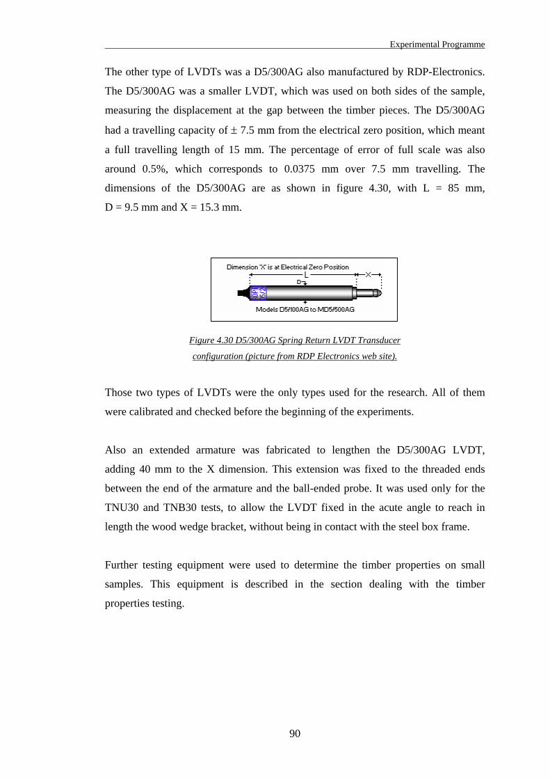
Experimental Programme
90
The other type of LVDTs was a D5/300AG also manufactured by RDP-Electronics.
The D5/300AG was a smaller LVDT, which was used on both sides of the sample,
measuring the displacement at the gap between the timber pieces. The D5/300AG
had a travelling capacity of ± 7.5 mm from the electrical zero position, which meant
a full travelling length of 15 mm. The percentage of error of full scale was also
around 0.5%, which corresponds to 0.0375 mm over 7.5 mm travelling. The
dimensions of the D5/300AG are as shown in figure 4.30, with L = 85 mm,
D = 9.5 mm and X = 15.3 mm.
Figure 4.30 D5/300AG Spring Return LVDT Transducer
configuration (picture from RDP Electronics web site).
Those two types of LVDTs were the only types used for the research. All of them
were calibrated and checked before the beginning of the experiments.
Also an extended armature was fabricated to lengthen the D5/300AG LVDT,
adding 40 mm to the X dimension. This extension was fixed to the threaded ends
between the end of the armature and the ball-ended probe. It was used only for the
TNU30 and TNB30 tests, to allow the LVDT fixed in the acute angle to reach in
length the wood wedge bracket, without being in contact with the steel box frame.
Further testing equipment were used to determine the timber properties on small
samples. This equipment is described in the section dealing with the timber
properties testing.
Experimental Programme
91
4.3.5. Sample fabrication process
The fabrication of the samples was a long and carefully elaborated process, in which
a large amount of time was spent. The fabrication was a repetitive procedure because
it has to be done for each sample. Therefore the samples were fabricated in series
corresponding to the type of test, which means for each type of test all the samples
were fabricated at the same time. There were some advantages to fabricate the
samples in this manner:
• It saved on the amount of resin, as it is difficult to estimate the quantity of resin
required for a particular number of samples. There was always some resin left
over, which could not be kept for further fabrication because it cured.
• It minimised the variation of moisture content in the glass fibre, which was cut
from a large roll and for all the samples before the gluing process. Each strip of
glass fibre was in the same conditions of temperature and humidity. However,
these parameters did not have any significant effect on the composite strength.
• It minimised the variation in timber moisture content from one sample to another,
for the particular type of test. The wood was preliminary conditioned before the
sample fabrication, which took place in the wood workshop of the structures
laboratory. There was not enough space available in the control temperature room
to carry out the gluing process on the samples. The gluing was done in the labs,
which meant the samples were not any longer in a controlled environment and this
during the 48 hours required for complete drying of the resin. However the same
temperature was maintained in the labs, but the relative humidity was not
controlled. By fabricating all the samples of a particular type of test at the same
time meant they were all in the same conditions of temperature and humidity.
Regarding the humidity in the laboratory, this had a minor effect on the samples
compared to the heat produced by the thermosetting of the epoxy resin. Because it
was not possible to re-condition the samples after fabrication, it was decided to
measure the moisture content of the samples as soon as they were tested. On each
tested sample, a small piece of wood was sawn very close to the jointing area. Its
dimensions, wet weight and dry weight were recorded. The dry weight was measured
after few days in the oven at a temperature of 103 ± 2°C, in accordance with the
relevant timber code of practice.
Experimental Programme
92
Prior to the sample fabrication, the selection of timber planks was carried out. This
procedure is developed in the section about timber conditioning and grading. Timber
planks were selected from the batch by visual inspection. The selected planks were
conditioned for several weeks, then cut into smaller length corresponding to the full
size of one sample and tested in three points bending for grading. Each plank was
numbered to identify from which timber piece the plank came. At this stage the
sample fabrication began.
The fabrication process was relatively similar for each type of test with some
variations between straight and angle sample configuration. The procedure is
developed for both configurations in the following sections.
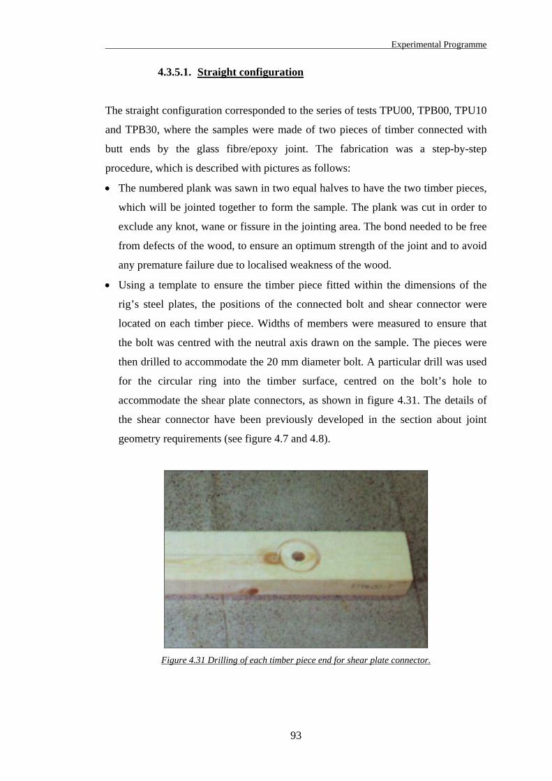
Experimental Programme
93
4.3.5.1. Straight configuration
The straight configuration corresponded to the series of tests TPU00, TPB00, TPU10
and TPB30, where the samples were made of two pieces of timber connected with
butt ends by the glass fibre/epoxy joint. The fabrication was a step-by-step
procedure, which is described with pictures as follows:
• The numbered plank was sawn in two equal halves to have the two timber pieces,
which will be jointed together to form the sample. The plank was cut in order to
exclude any knot, wane or fissure in the jointing area. The bond needed to be free
from defects of the wood, to ensure an optimum strength of the joint and to avoid
any premature failure due to localised weakness of the wood.
• Using a template to ensure the timber piece fitted within the dimensions of the
rig’s steel plates, the positions of the connected bolt and shear connector were
located on each timber piece. Widths of members were measured to ensure that
the bolt was centred with the neutral axis drawn on the sample. The pieces were
then drilled to accommodate the 20 mm diameter bolt. A particular drill was used
for the circular ring into the timber surface, centred on the bolt’s hole to
accommodate the shear plate connectors, as shown in figure 4.31. The details of
the shear connector have been previously developed in the section about joint
geometry requirements (see figure 4.7 and 4.8).
Figure 4.31 Drilling of each timber piece end for shear plate connector.

Experimental Programme
94
• On the other butt end of the timber pieces, in the jointing area, a sheet of
aluminium foil was positioned as shown in figure 4.32.
Figure 4.32 Aluminium foil positioned in the joint’s gap.
The foil was clamped between the butt ends of the timber pieces to stop the epoxy
resin bonding the butt ends together. During the bonding process, some epoxy
resin could seep into the gap in an unknown proportion and this would strengthen
the joint. Because the cross-sectional area of bonding in the gap could not be
evaluated, this was a varying parameter of joint strength from one sample to
another. Therefore the foil was placed to prevent butt ends bonding. If any resin
seeped into the gap, it could bond the timber butts ends but with the aluminium
foil in between and the resin did not bond to the aluminium foil.
• The two timber pieces were placed on a flat surface to optimise straightness of the
sample. The timber pieces were jointed together by stapling their sides using
paper staples, with the aluminium foil still positioned in the gap, as shown in
figure 4.33. The staples were small and did not connect the timber pieces with
strength, but they were sufficiently strong to hold the sample during the
fabrication. The staples were removed afterwards. Then the dimensions of the
bond were measured and drawn onto the timber surface to locate the exact
position of the composite. If the fibre orientation was not parallel to the grain (i.e.
TNU10 and TNB30 tests), lines were drawn showing the orientation in which the
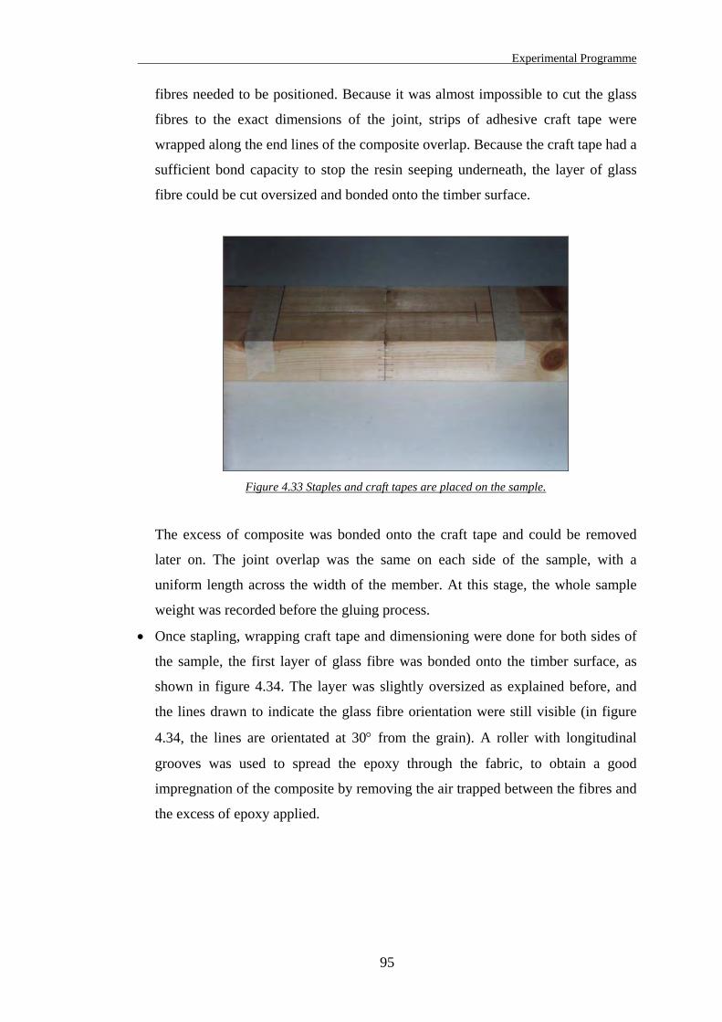
Experimental Programme
95
fibres needed to be positioned. Because it was almost impossible to cut the glass
fibres to the exact dimensions of the joint, strips of adhesive craft tape were
wrapped along the end lines of the composite overlap. Because the craft tape had a
sufficient bond capacity to stop the resin seeping underneath, the layer of glass
fibre could be cut oversized and bonded onto the timber surface.
Figure 4.33 Staples and craft tapes are placed on the sample.
The excess of composite was bonded onto the craft tape and could be removed
later on. The joint overlap was the same on each side of the sample, with a
uniform length across the width of the member. At this stage, the whole sample
weight was recorded before the gluing process.
• Once stapling, wrapping craft tape and dimensioning were done for both sides of
the sample, the first layer of glass fibre was bonded onto the timber surface, as
shown in figure 4.34. The layer was slightly oversized as explained before, and
the lines drawn to indicate the glass fibre orientation were still visible (in figure
4.34, the lines are orientated at 30° from the grain). A roller with longitudinal
grooves was used to spread the epoxy through the fabric, to obtain a good
impregnation of the composite by removing the air trapped between the fibres and
the excess of epoxy applied.
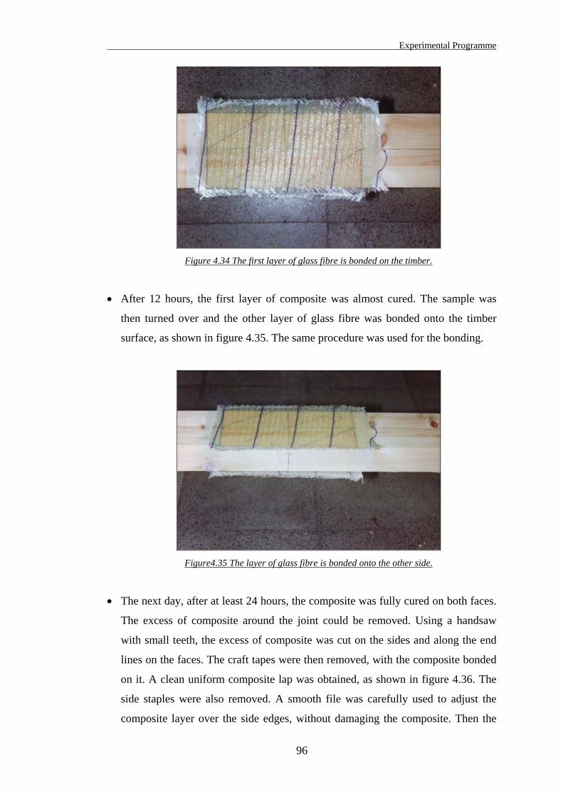
Experimental Programme
96
Figure 4.34 The first layer of glass fibre is bonded on the timber.
• After 12 hours, the first layer of composite was almost cured. The sample was
then turned over and the other layer of glass fibre was bonded onto the timber
surface, as shown in figure 4.35. The same procedure was used for the bonding.
Figure4.35 The layer of glass fibre is bonded onto the other side.
• The next day, after at least 24 hours, the composite was fully cured on both faces.
The excess of composite around the joint could be removed. Using a handsaw
with small teeth, the excess of composite was cut on the sides and along the end
lines on the faces. The craft tapes were then removed, with the composite bonded
on it. A clean uniform composite lap was obtained, as shown in figure 4.36. The
side staples were also removed. A smooth file was carefully used to adjust the
composite layer over the side edges, without damaging the composite. Then the
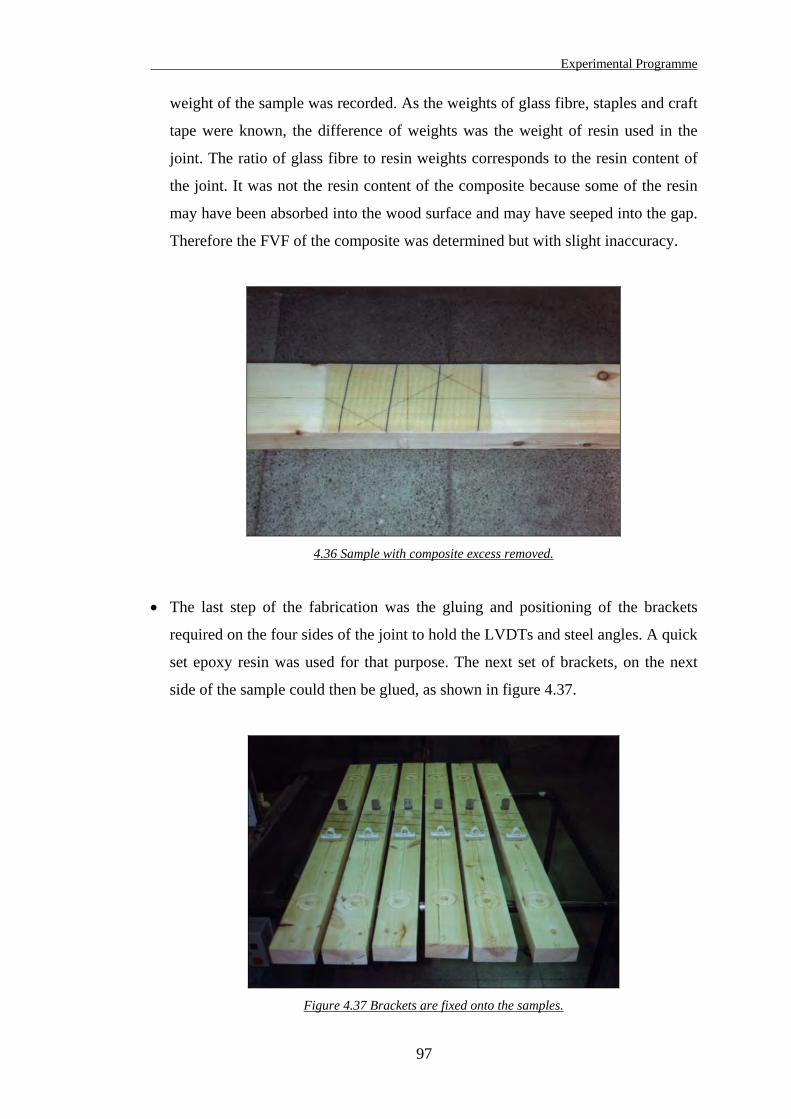
Experimental Programme
97
weight of the sample was recorded. As the weights of glass fibre, staples and craft
tape were known, the difference of weights was the weight of resin used in the
joint. The ratio of glass fibre to resin weights corresponds to the resin content of
the joint. It was not the resin content of the composite because some of the resin
may have been absorbed into the wood surface and may have seeped into the gap.
Therefore the FVF of the composite was determined but with slight inaccuracy.
4.36 Sample with composite excess removed.
• The last step of the fabrication was the gluing and positioning of the brackets
required on the four sides of the joint to hold the LVDTs and steel angles. A quick
set epoxy resin was used for that purpose. The next set of brackets, on the next
side of the sample could then be glued, as shown in figure 4.37.
Figure 4.37 Brackets are fixed onto the samples.
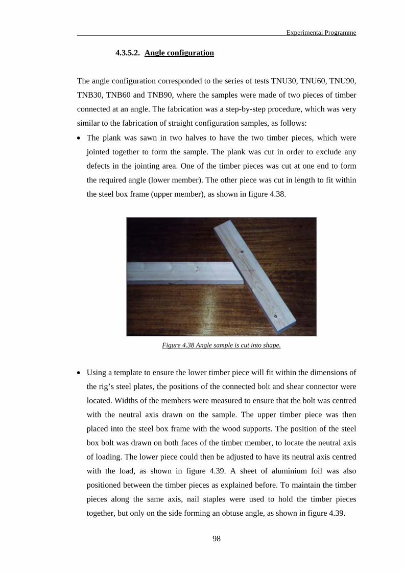
Experimental Programme
98
4.3.5.2. Angle configuration
The angle configuration corresponded to the series of tests TNU30, TNU60, TNU90,
TNB30, TNB60 and TNB90, where the samples were made of two pieces of timber
connected at an angle. The fabrication was a step-by-step procedure, which was very
similar to the fabrication of straight configuration samples, as follows:
• The plank was sawn in two halves to have the two timber pieces, which were
jointed together to form the sample. The plank was cut in order to exclude any
defects in the jointing area. One of the timber pieces was cut at one end to form
the required angle (lower member). The other piece was cut in length to fit within
the steel box frame (upper member), as shown in figure 4.38.
Figure 4.38 Angle sample is cut into shape.
• Using a template to ensure the lower timber piece will fit within the dimensions of
the rig’s steel plates, the positions of the connected bolt and shear connector were
located. Widths of the members were measured to ensure that the bolt was centred
with the neutral axis drawn on the sample. The upper timber piece was then
placed into the steel box frame with the wood supports. The position of the steel
box bolt was drawn on both faces of the timber member, to locate the neutral axis
of loading. The lower piece could then be adjusted to have its neutral axis centred
with the load, as shown in figure 4.39. A sheet of aluminium foil was also
positioned between the timber pieces as explained before. To maintain the timber
pieces along the same axis, nail staples were used to hold the timber pieces
together, but only on the side forming an obtuse angle, as shown in figure 4.39.
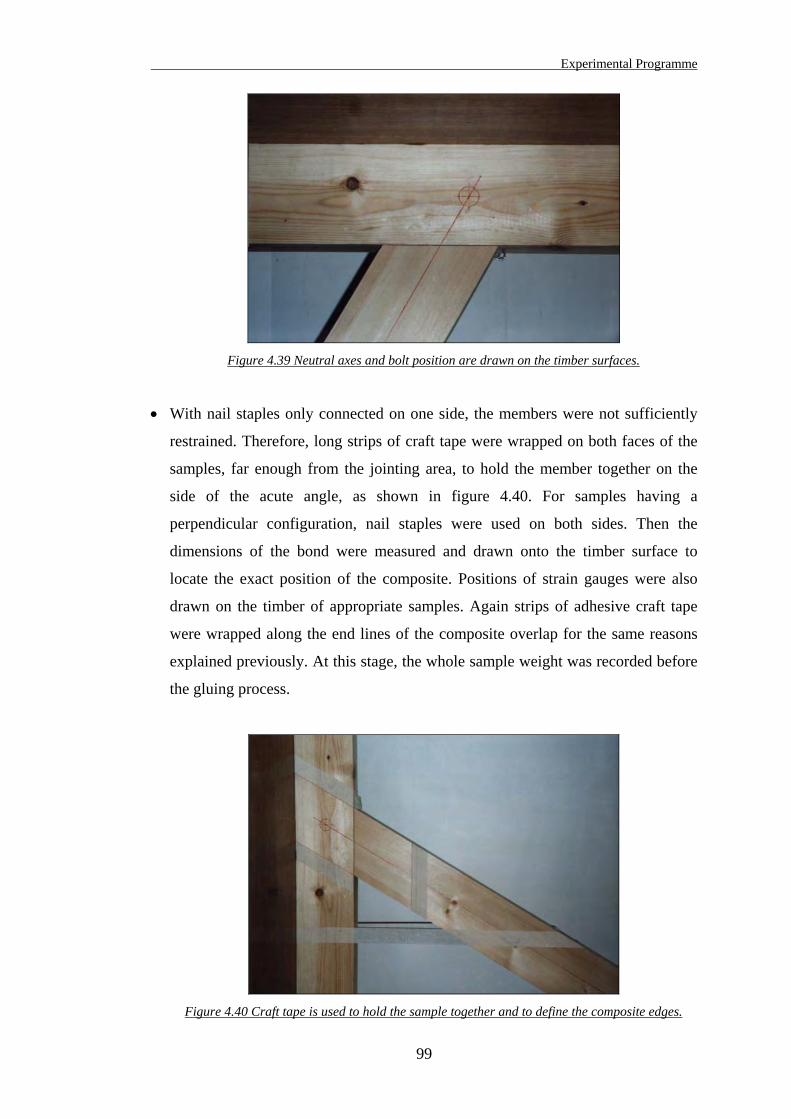
Experimental Programme
99
Figure 4.39 Neutral axes and bolt position are drawn on the timber surfaces.
• With nail staples only connected on one side, the members were not sufficiently
restrained. Therefore, long strips of craft tape were wrapped on both faces of the
samples, far enough from the jointing area, to hold the member together on the
side of the acute angle, as shown in figure 4.40. For samples having a
perpendicular configuration, nail staples were used on both sides. Then the
dimensions of the bond were measured and drawn onto the timber surface to
locate the exact position of the composite. Positions of strain gauges were also
drawn on the timber of appropriate samples. Again strips of adhesive craft tape
were wrapped along the end lines of the composite overlap for the same reasons
explained previously. At this stage, the whole sample weight was recorded before
the gluing process.
Figure 4.40 Craft tape is used to hold the sample together and to define the composite edges.
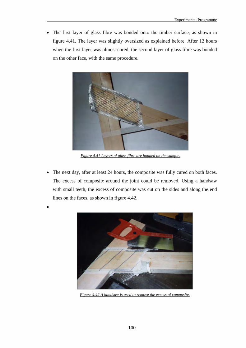
Experimental Programme
100
• The first layer of glass fibre was bonded onto the timber surface, as shown in
figure 4.41. The layer was slightly oversized as explained before. After 12 hours
when the first layer was almost cured, the second layer of glass fibre was bonded
on the other face, with the same procedure.
Figure 4.41 Layers of glass fibre are bonded on the sample.
• The next day, after at least 24 hours, the composite was fully cured on both faces.
The excess of composite around the joint could be removed. Using a handsaw
with small teeth, the excess of composite was cut on the sides and along the end
lines on the faces, as shown in figure 4.42.
•
Figure 4.42 A handsaw is used to remove the excess of composite.
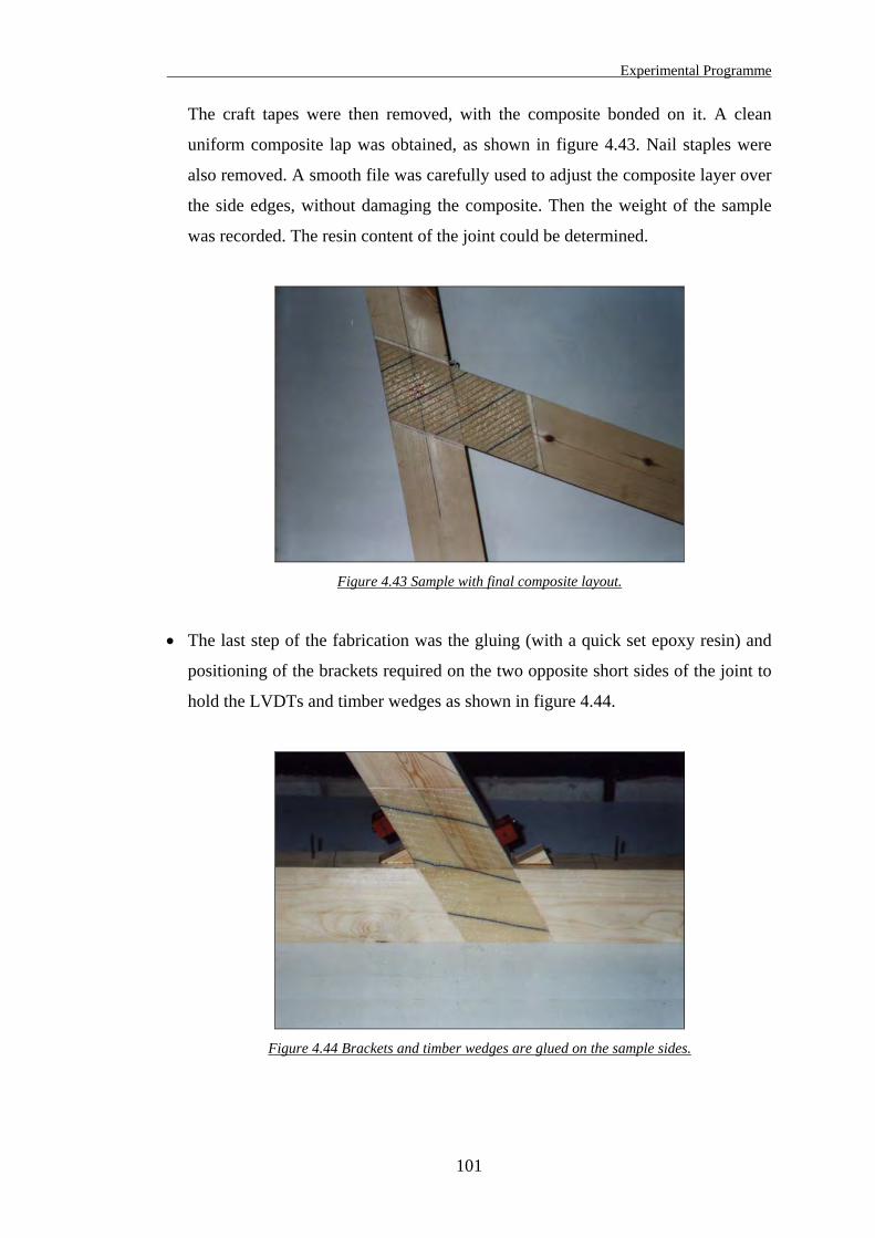
Experimental Programme
101
The craft tapes were then removed, with the composite bonded on it. A clean
uniform composite lap was obtained, as shown in figure 4.43. Nail staples were
also removed. A smooth file was carefully used to adjust the composite layer over
the side edges, without damaging the composite. Then the weight of the sample
was recorded. The resin content of the joint could be determined.
Figure 4.43 Sample with final composite layout.
• The last step of the fabrication was the gluing (with a quick set epoxy resin) and
positioning of the brackets required on the two opposite short sides of the joint to
hold the LVDTs and timber wedges as shown in figure 4.44.
Figure 4.44 Brackets and timber wedges are glued on the sample sides.
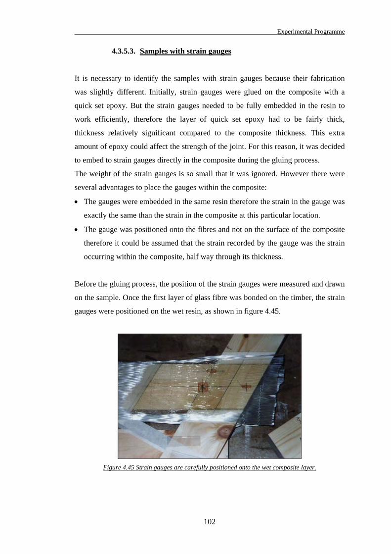
Experimental Programme
102
4.3.5.3. Samples with strain gauges
It is necessary to identify the samples with strain gauges because their fabrication
was slightly different. Initially, strain gauges were glued on the composite with a
quick set epoxy. But the strain gauges needed to be fully embedded in the resin to
work efficiently, therefore the layer of quick set epoxy had to be fairly thick,
thickness relatively significant compared to the composite thickness. This extra
amount of epoxy could affect the strength of the joint. For this reason, it was decided
to embed to strain gauges directly in the composite during the gluing process.
The weight of the strain gauges is so small that it was ignored. However there were
several advantages to place the gauges within the composite:
• The gauges were embedded in the same resin therefore the strain in the gauge was
exactly the same than the strain in the composite at this particular location.
• The gauge was positioned onto the fibres and not on the surface of the composite
therefore it could be assumed that the strain recorded by the gauge was the strain
occurring within the composite, half way through its thickness.
Before the gluing process, the position of the strain gauges were measured and drawn
on the sample. Once the first layer of glass fibre was bonded on the timber, the strain
gauges were positioned on the wet resin, as shown in figure 4.45.
Figure 4.45 Strain gauges are carefully positioned onto the wet composite layer.
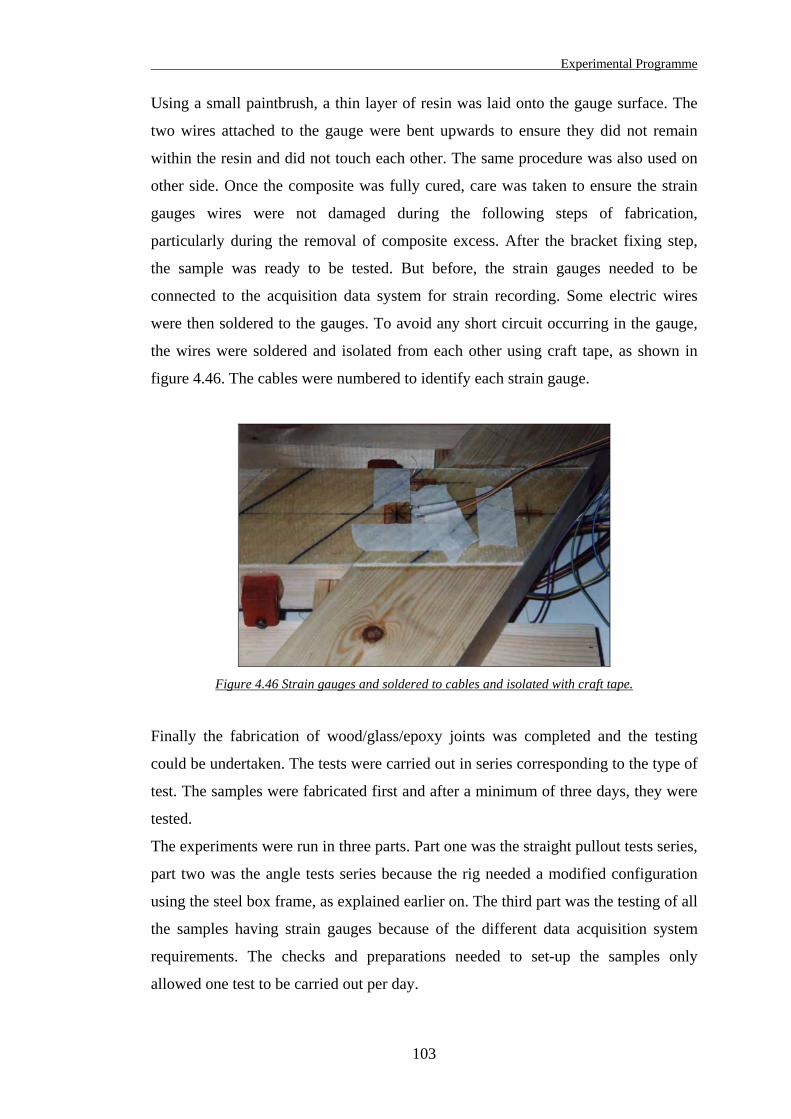
Experimental Programme
103
Using a small paintbrush, a thin layer of resin was laid onto the gauge surface. The
two wires attached to the gauge were bent upwards to ensure they did not remain
within the resin and did not touch each other. The same procedure was also used on
other side. Once the composite was fully cured, care was taken to ensure the strain
gauges wires were not damaged during the following steps of fabrication,
particularly during the removal of composite excess. After the bracket fixing step,
the sample was ready to be tested. But before, the strain gauges needed to be
connected to the acquisition data system for strain recording. Some electric wires
were then soldered to the gauges. To avoid any short circuit occurring in the gauge,
the wires were soldered and isolated from each other using craft tape, as shown in
figure 4.46. The cables were numbered to identify each strain gauge.
Figure 4.46 Strain gauges and soldered to cables and isolated with craft tape.
Finally the fabrication of wood/glass/epoxy joints was completed and the testing
could be undertaken. The tests were carried out in series corresponding to the type of
test. The samples were fabricated first and after a minimum of three days, they were
tested.
The experiments were run in three parts. Part one was the straight pullout tests series,
part two was the angle tests series because the rig needed a modified configuration
using the steel box frame, as explained earlier on. The third part was the testing of all
the samples having strain gauges because of the different data acquisition system
requirements. The checks and preparations needed to set-up the samples only
allowed one test to be carried out per day.
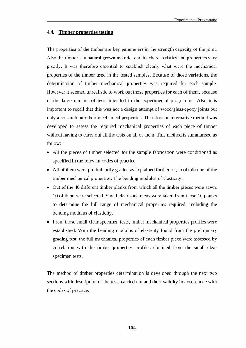
Experimental Programme
104
4.4. Timber properties testing
The properties of the timber are key parameters in the strength capacity of the joint.
Also the timber is a natural grown material and its characteristics and properties vary
greatly. It was therefore essential to establish clearly what were the mechanical
properties of the timber used in the tested samples. Because of those variations, the
determination of timber mechanical properties was required for each sample.
However it seemed unrealistic to work out those properties for each of them, because
of the large number of tests intended in the experimental programme. Also it is
important to recall that this was not a design attempt of wood/glass/epoxy joints but
only a research into their mechanical properties. Therefore an alternative method was
developed to assess the required mechanical properties of each piece of timber
without having to carry out all the tests on all of them. This method is summarised as
follow:
• All the pieces of timber selected for the sample fabrication were conditioned as
specified in the relevant codes of practice.
• All of them were preliminarily graded as explained further on, to obtain one of the
timber mechanical properties: The bending modulus of elasticity.
• Out of the 40 different timber planks from which all the timber pieces were sawn,
10 of them were selected. Small clear specimens were taken from those 10 planks
to determine the full range of mechanical properties required, including the
bending modulus of elasticity.
• From those small clear specimen tests, timber mechanical properties profiles were
established. With the bending modulus of elasticity found from the preliminary
grading test, the full mechanical properties of each timber piece were assessed by
correlation with the timber properties profiles obtained from the small clear
specimen tests.
The method of timber properties determination is developed through the next two
sections with description of the tests carried out and their validity in accordance with
the codes of practice.
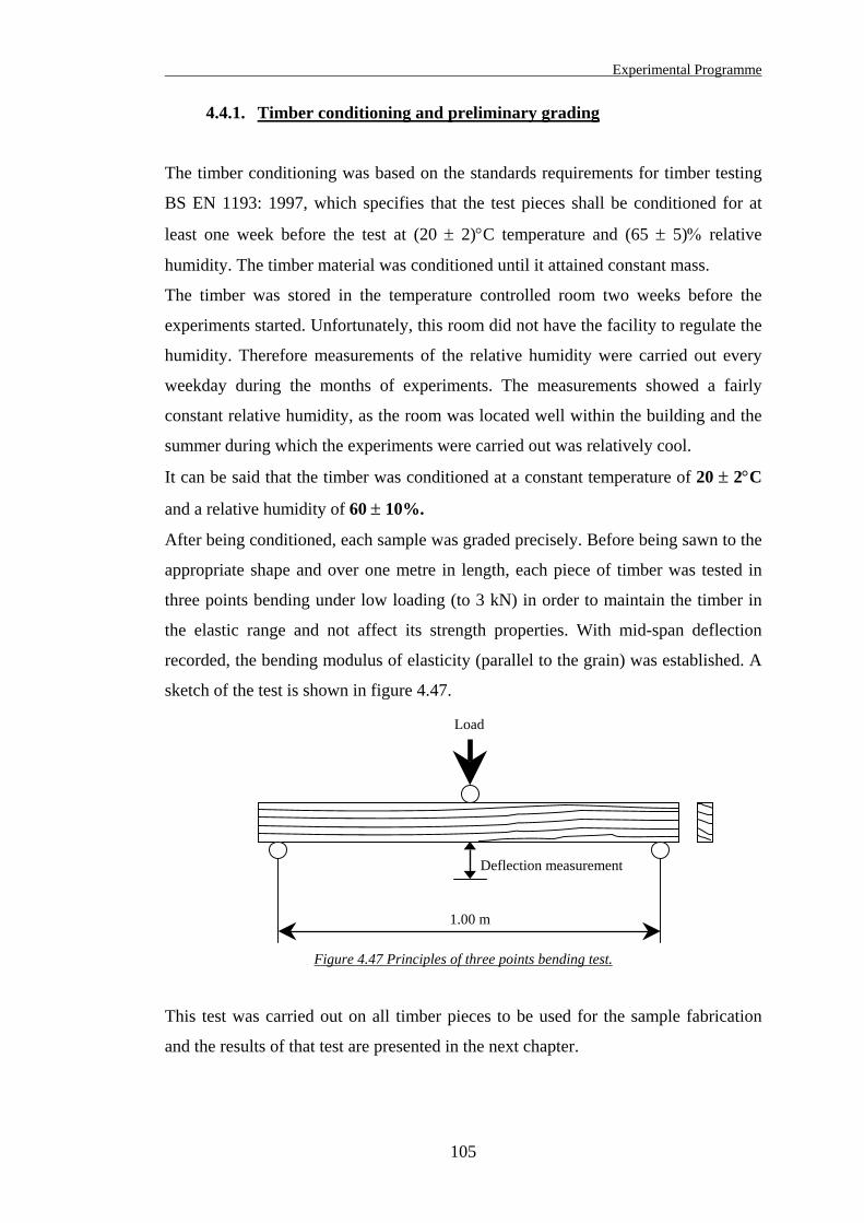
Experimental Programme
105
4.4.1. Timber conditioning and preliminary grading
The timber conditioning was based on the standards requirements for timber testing
BS EN 1193: 1997, which specifies that the test pieces shall be conditioned for at
least one week before the test at (20 ± 2)°C temperature and (65 ± 5)% relative
humidity. The timber material was conditioned until it attained constant mass.
The timber was stored in the temperature controlled room two weeks before the
experiments started. Unfortunately, this room did not have the facility to regulate the
humidity. Therefore measurements of the relative humidity were carried out every
weekday during the months of experiments. The measurements showed a fairly
constant relative humidity, as the room was located well within the building and the
summer during which the experiments were carried out was relatively cool.
It can be said that the timber was conditioned at a constant temperature of 20 ± 2°C
and a relative humidity of 60 ± 10%.
After being conditioned, each sample was graded precisely. Before being sawn to the
appropriate shape and over one metre in length, each piece of timber was tested in
three points bending under low loading (to 3 kN) in order to maintain the timber in
the elastic range and not affect its strength properties. With mid-span deflection
recorded, the bending modulus of elasticity (parallel to the grain) was established. A
sketch of the test is shown in figure 4.47.
Deflection measurement
Load
1.00 m
Figure 4.47 Principles of three points bending test.
This test was carried out on all timber pieces to be used for the sample fabrication
and the results of that test are presented in the next chapter.
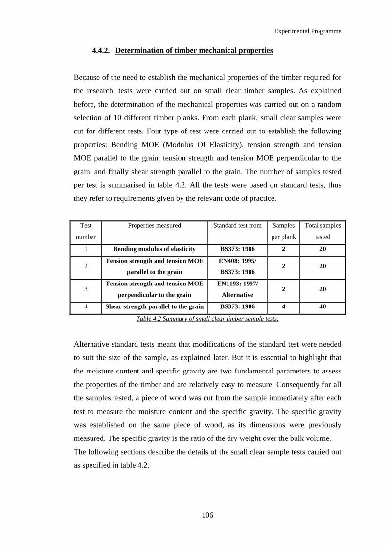
Experimental Programme
106
4.4.2. Determination of timber mechanical properties
Because of the need to establish the mechanical properties of the timber required for
the research, tests were carried out on small clear timber samples. As explained
before, the determination of the mechanical properties was carried out on a random
selection of 10 different timber planks. From each plank, small clear samples were
cut for different tests. Four type of test were carried out to establish the following
properties: Bending MOE (Modulus Of Elasticity), tension strength and tension
MOE parallel to the grain, tension strength and tension MOE perpendicular to the
grain, and finally shear strength parallel to the grain. The number of samples tested
per test is summarised in table 4.2. All the tests were based on standard tests, thus
they refer to requirements given by the relevant code of practice.
Test
number
Properties measured Standard test from Samples
per plank
Total samples
tested
1 Bending modulus of elasticity BS373: 1986 2 20
2 Tension strength and tension MOE
parallel to the grain
EN408: 1995/
BS373: 1986 2 20
3 Tension strength and tension MOE
perpendicular to the grain
EN1193: 1997/
Alternative 2 20
4 Shear strength parallel to the grain BS373: 1986 4 40
Table 4.2 Summary of small clear timber sample tests.
Alternative standard tests meant that modifications of the standard test were needed
to suit the size of the sample, as explained later. But it is essential to highlight that
the moisture content and specific gravity are two fundamental parameters to assess
the properties of the timber and are relatively easy to measure. Consequently for all
the samples tested, a piece of wood was cut from the sample immediately after each
test to measure the moisture content and the specific gravity. The specific gravity
was established on the same piece of wood, as its dimensions were previously
measured. The specific gravity is the ratio of the dry weight over the bulk volume.
The following sections describe the details of the small clear sample tests carried out
as specified in table 4.2.
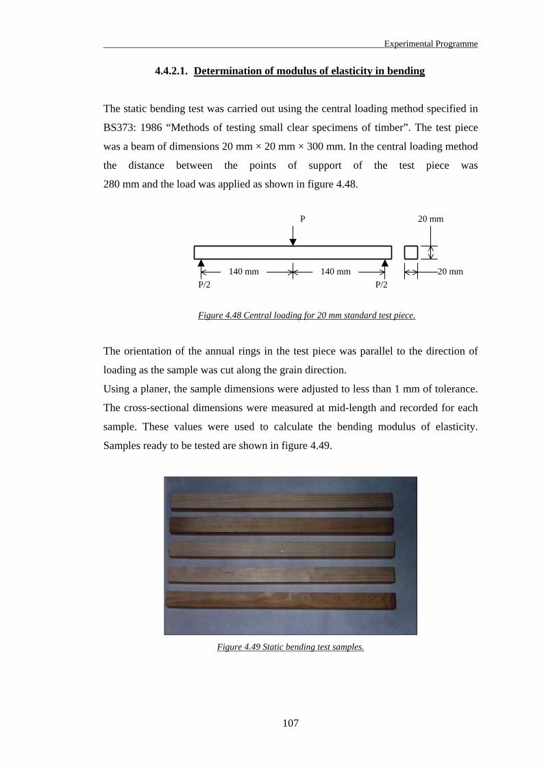
Experimental Programme
107
4.4.2.1. Determination of modulus of elasticity in bending
The static bending test was carried out using the central loading method specified in
BS373: 1986 “Methods of testing small clear specimens of timber”. The test piece
was a beam of dimensions 20 mm × 20 mm × 300 mm. In the central loading method
the distance between the points of support of the test piece was
280 mm and the load was applied as shown in figure 4.48.
140 mm 140 mm
20 mm
20 mm
P
P/2 P/2
Figure 4.48 Central loading for 20 mm standard test piece.
The orientation of the annual rings in the test piece was parallel to the direction of
loading as the sample was cut along the grain direction.
Using a planer, the sample dimensions were adjusted to less than 1 mm of tolerance.
The cross-sectional dimensions were measured at mid-length and recorded for each
sample. These values were used to calculate the bending modulus of elasticity.
Samples ready to be tested are shown in figure 4.49.
Figure 4.49 Static bending test samples.
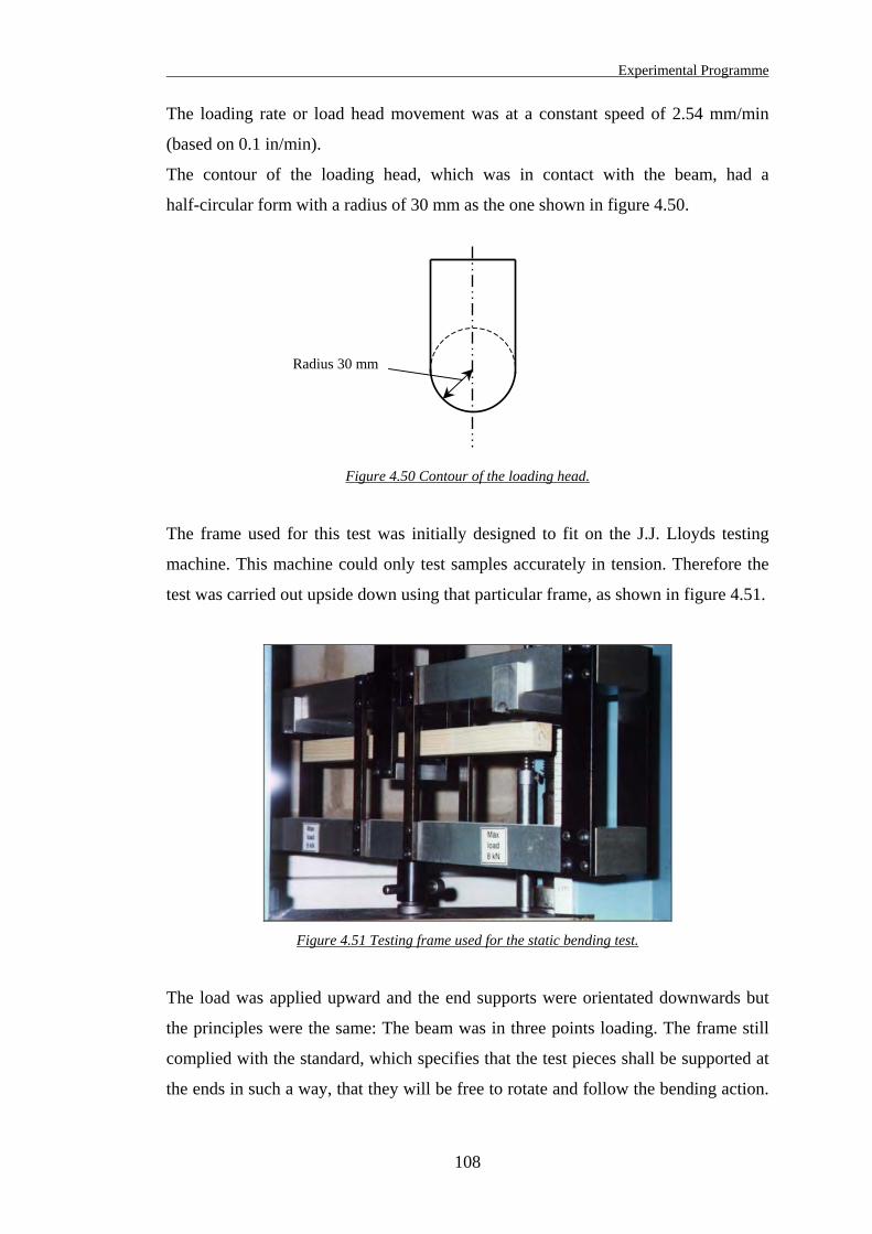
Experimental Programme
108
The loading rate or load head movement was at a constant speed of 2.54 mm/min
(based on 0.1 in/min).
The contour of the loading head, which was in contact with the beam, had a
half-circular form with a radius of 30 mm as the one shown in figure 4.50.
Radius 30 mm
Figure 4.50 Contour of the loading head.
The frame used for this test was initially designed to fit on the J.J. Lloyds testing
machine. This machine could only test samples accurately in tension. Therefore the
test was carried out upside down using that particular frame, as shown in figure 4.51.
Figure 4.51 Testing frame used for the static bending test.
The load was applied upward and the end supports were orientated downwards but
the principles were the same: The beam was in three points loading. The frame still
complied with the standard, which specifies that the test pieces shall be supported at
the ends in such a way, that they will be free to rotate and follow the bending action.
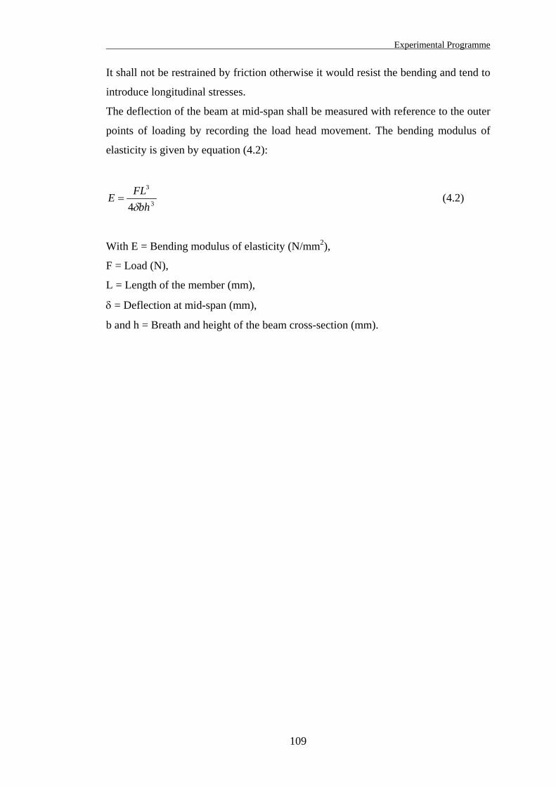
Experimental Programme
109
It shall not be restrained by friction otherwise it would resist the bending and tend to
introduce longitudinal stresses.
The deflection of the beam at mid-span shall be measured with reference to the outer
points of loading by recording the load head movement. The bending modulus of
elasticity is given by equation (4.2):
3
3
4 bhFLEδ
= (4.2)
With E = Bending modulus of elasticity (N/mm2),
F = Load (N),
L = Length of the member (mm),
δ = Deflection at mid-span (mm),
b and h = Breath and height of the beam cross-section (mm).
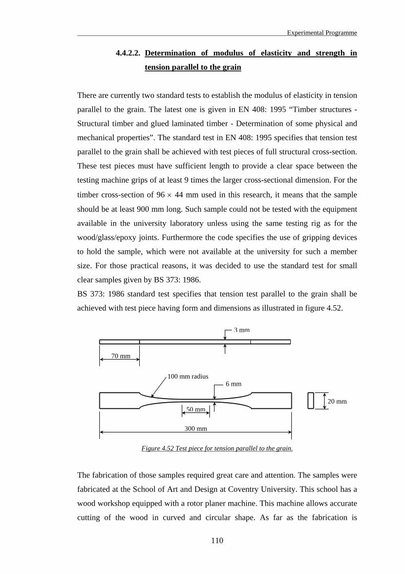
Experimental Programme
110
4.4.2.2. Determination of modulus of elasticity and strength in
tension parallel to the grain
There are currently two standard tests to establish the modulus of elasticity in tension
parallel to the grain. The latest one is given in EN 408: 1995 “Timber structures -
Structural timber and glued laminated timber - Determination of some physical and
mechanical properties”. The standard test in EN 408: 1995 specifies that tension test
parallel to the grain shall be achieved with test pieces of full structural cross-section.
These test pieces must have sufficient length to provide a clear space between the
testing machine grips of at least 9 times the larger cross-sectional dimension. For the
timber cross-section of 96 × 44 mm used in this research, it means that the sample
should be at least 900 mm long. Such sample could not be tested with the equipment
available in the university laboratory unless using the same testing rig as for the
wood/glass/epoxy joints. Furthermore the code specifies the use of gripping devices
to hold the sample, which were not available at the university for such a member
size. For those practical reasons, it was decided to use the standard test for small
clear samples given by BS 373: 1986.
BS 373: 1986 standard test specifies that tension test parallel to the grain shall be
achieved with test piece having form and dimensions as illustrated in figure 4.52.
20 mm
300 mm
50 mm
6 mm100 mm radius
3 mm
70 mm
Figure 4.52 Test piece for tension parallel to the grain.
The fabrication of those samples required great care and attention. The samples were
fabricated at the School of Art and Design at Coventry University. This school has a
wood workshop equipped with a rotor planer machine. This machine allows accurate
cutting of the wood in curved and circular shape. As far as the fabrication is
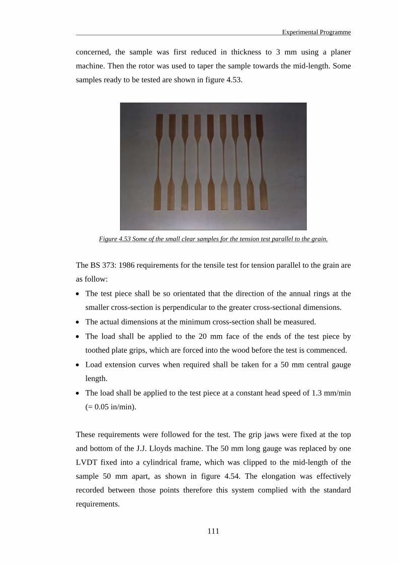
Experimental Programme
111
concerned, the sample was first reduced in thickness to 3 mm using a planer
machine. Then the rotor was used to taper the sample towards the mid-length. Some
samples ready to be tested are shown in figure 4.53.
Figure 4.53 Some of the small clear samples for the tension test parallel to the grain.
The BS 373: 1986 requirements for the tensile test for tension parallel to the grain are
as follow:
• The test piece shall be so orientated that the direction of the annual rings at the
smaller cross-section is perpendicular to the greater cross-sectional dimensions.
• The actual dimensions at the minimum cross-section shall be measured.
• The load shall be applied to the 20 mm face of the ends of the test piece by
toothed plate grips, which are forced into the wood before the test is commenced.
• Load extension curves when required shall be taken for a 50 mm central gauge
length.
• The load shall be applied to the test piece at a constant head speed of 1.3 mm/min
(= 0.05 in/min).
These requirements were followed for the test. The grip jaws were fixed at the top
and bottom of the J.J. Lloyds machine. The 50 mm long gauge was replaced by one
LVDT fixed into a cylindrical frame, which was clipped to the mid-length of the
sample 50 mm apart, as shown in figure 4.54. The elongation was effectively
recorded between those points therefore this system complied with the standard
requirements.
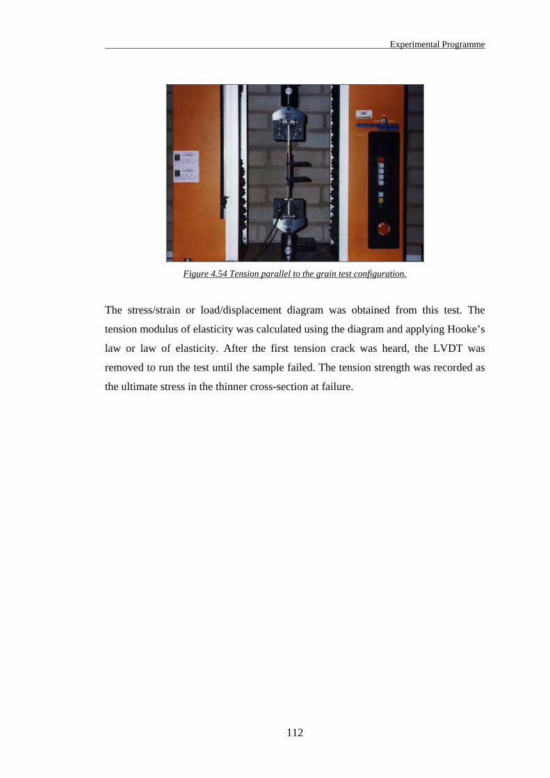
Experimental Programme
112
Figure 4.54 Tension parallel to the grain test configuration.
The stress/strain or load/displacement diagram was obtained from this test. The
tension modulus of elasticity was calculated using the diagram and applying Hooke’s
law or law of elasticity. After the first tension crack was heard, the LVDT was
removed to run the test until the sample failed. The tension strength was recorded as
the ultimate stress in the thinner cross-section at failure.
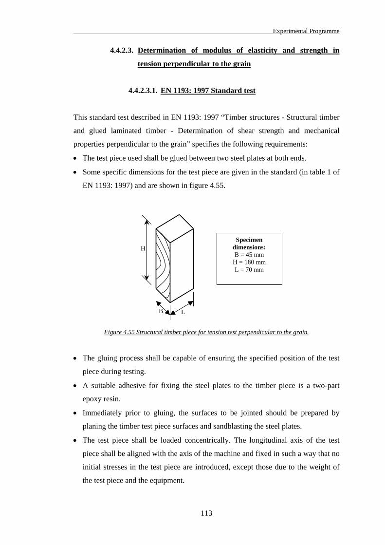
Experimental Programme
113
4.4.2.3. Determination of modulus of elasticity and strength in
tension perpendicular to the grain
4.4.2.3.1. EN 1193: 1997 Standard test
This standard test described in EN 1193: 1997 “Timber structures - Structural timber
and glued laminated timber - Determination of shear strength and mechanical
properties perpendicular to the grain” specifies the following requirements:
• The test piece used shall be glued between two steel plates at both ends.
• Some specific dimensions for the test piece are given in the standard (in table 1 of
EN 1193: 1997) and are shown in figure 4.55.
Specimen dimensions: B = 45 mm
H = 180 mm L = 70 mm
LB
H
Figure 4.55 Structural timber piece for tension test perpendicular to the grain.
• The gluing process shall be capable of ensuring the specified position of the test
piece during testing.
• A suitable adhesive for fixing the steel plates to the timber piece is a two-part
epoxy resin.
• Immediately prior to gluing, the surfaces to be jointed should be prepared by
planing the timber test piece surfaces and sandblasting the steel plates.
• The test piece shall be loaded concentrically. The longitudinal axis of the test
piece shall be aligned with the axis of the machine and fixed in such a way that no
initial stresses in the test piece are introduced, except those due to the weight of
the test piece and the equipment.
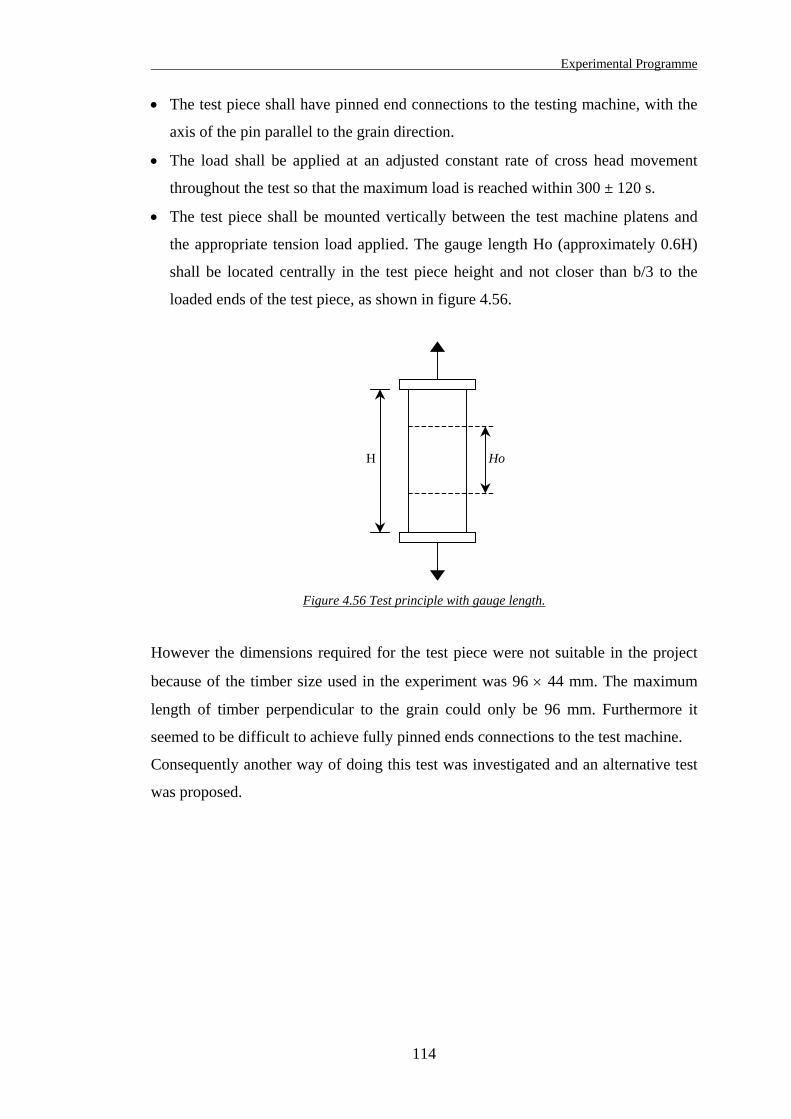
Experimental Programme
114
• The test piece shall have pinned end connections to the testing machine, with the
axis of the pin parallel to the grain direction.
• The load shall be applied at an adjusted constant rate of cross head movement
throughout the test so that the maximum load is reached within 300 ± 120 s.
• The test piece shall be mounted vertically between the test machine platens and
the appropriate tension load applied. The gauge length Ho (approximately 0.6H)
shall be located centrally in the test piece height and not closer than b/3 to the
loaded ends of the test piece, as shown in figure 4.56.
HoH
Figure 4.56 Test principle with gauge length.
However the dimensions required for the test piece were not suitable in the project
because of the timber size used in the experiment was 96 × 44 mm. The maximum
length of timber perpendicular to the grain could only be 96 mm. Furthermore it
seemed to be difficult to achieve fully pinned ends connections to the test machine.
Consequently another way of doing this test was investigated and an alternative test
was proposed.
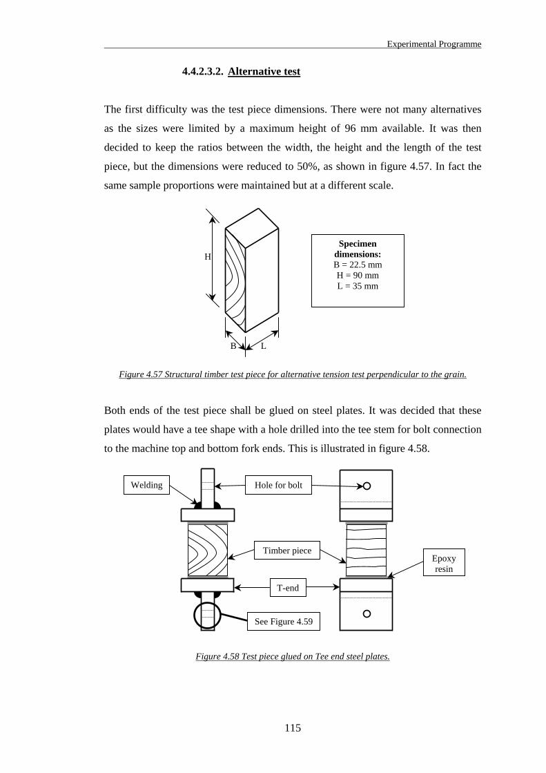
Experimental Programme
115
4.4.2.3.2. Alternative test
The first difficulty was the test piece dimensions. There were not many alternatives
as the sizes were limited by a maximum height of 96 mm available. It was then
decided to keep the ratios between the width, the height and the length of the test
piece, but the dimensions were reduced to 50%, as shown in figure 4.57. In fact the
same sample proportions were maintained but at a different scale.
Specimen dimensions: B = 22.5 mm H = 90 mm L = 35 mm
LB
H
Figure 4.57 Structural timber test piece for alternative tension test perpendicular to the grain.
Both ends of the test piece shall be glued on steel plates. It was decided that these
plates would have a tee shape with a hole drilled into the tee stem for bolt connection
to the machine top and bottom fork ends. This is illustrated in figure 4.58.
T-end
Epoxy resin
Welding Hole for bolt
Timber piece
See Figure 4.59
Figure 4.58 Test piece glued on Tee end steel plates.
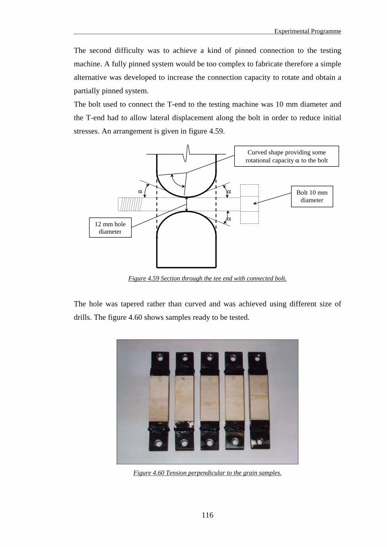
Experimental Programme
116
The second difficulty was to achieve a kind of pinned connection to the testing
machine. A fully pinned system would be too complex to fabricate therefore a simple
alternative was developed to increase the connection capacity to rotate and obtain a
partially pinned system.
The bolt used to connect the T-end to the testing machine was 10 mm diameter and
the T-end had to allow lateral displacement along the bolt in order to reduce initial
stresses. An arrangement is given in figure 4.59.
Curved shape providing some
rotational capacity α to the bolt
αα
α
Bolt 10 mm diameter
12 mm hole diameter
Figure 4.59 Section through the tee end with connected bolt.
The hole was tapered rather than curved and was achieved using different size of
drills. The figure 4.60 shows samples ready to be tested.
Figure 4.60 Tension perpendicular to the grain samples.
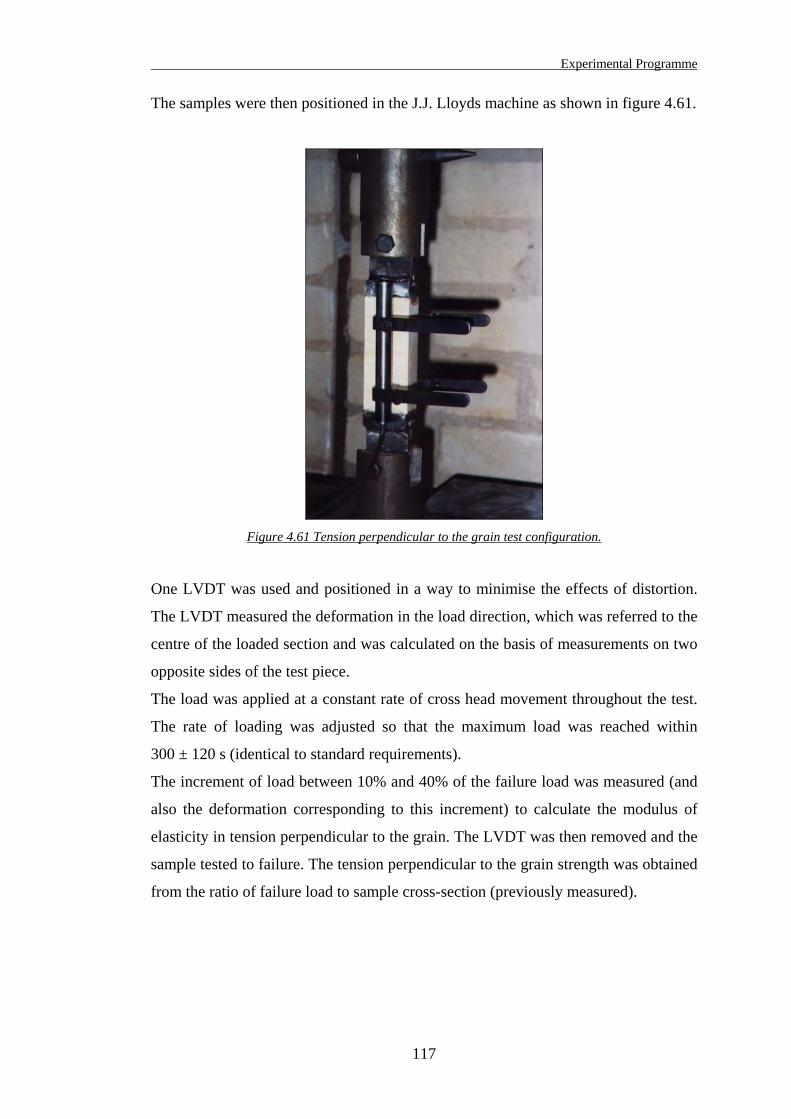
Experimental Programme
117
The samples were then positioned in the J.J. Lloyds machine as shown in figure 4.61.
Figure 4.61 Tension perpendicular to the grain test configuration.
One LVDT was used and positioned in a way to minimise the effects of distortion.
The LVDT measured the deformation in the load direction, which was referred to the
centre of the loaded section and was calculated on the basis of measurements on two
opposite sides of the test piece.
The load was applied at a constant rate of cross head movement throughout the test.
The rate of loading was adjusted so that the maximum load was reached within
300 ± 120 s (identical to standard requirements).
The increment of load between 10% and 40% of the failure load was measured (and
also the deformation corresponding to this increment) to calculate the modulus of
elasticity in tension perpendicular to the grain. The LVDT was then removed and the
sample tested to failure. The tension perpendicular to the grain strength was obtained
from the ratio of failure load to sample cross-section (previously measured).
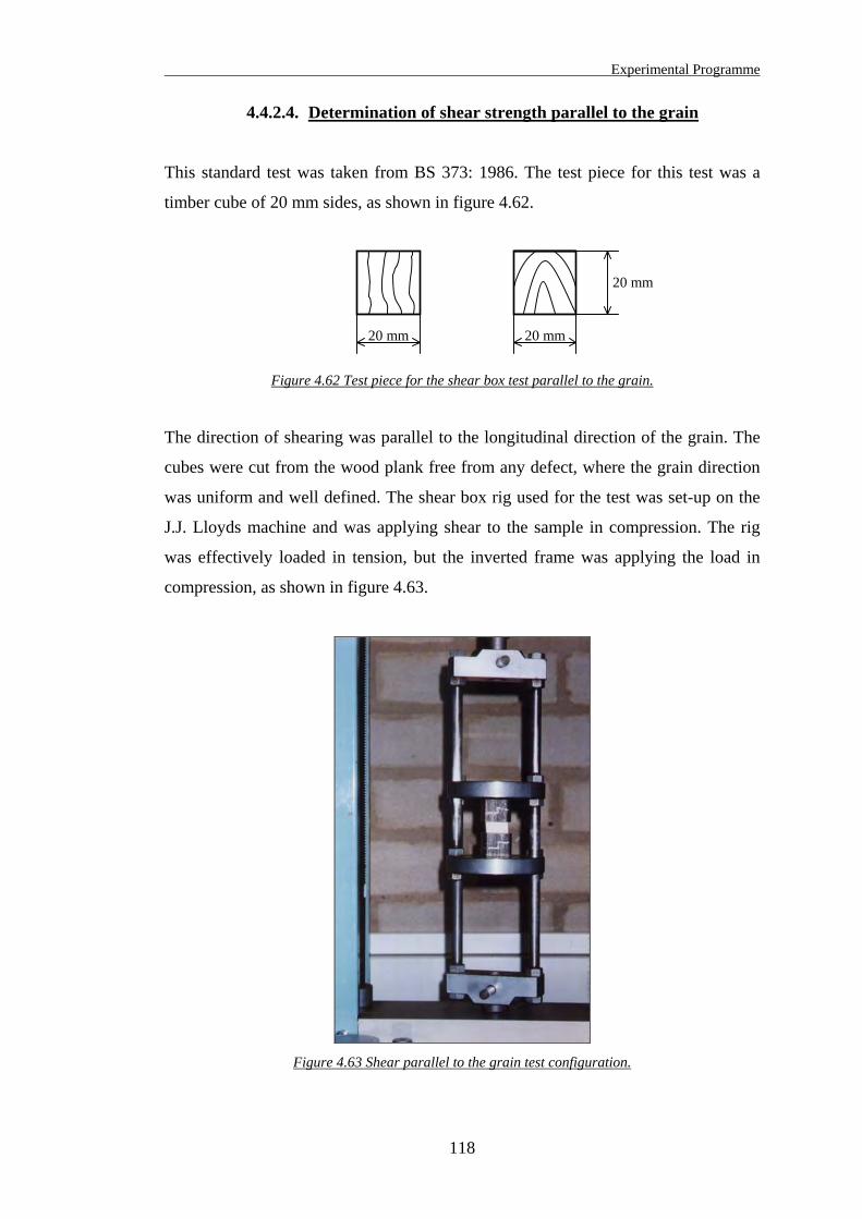
Experimental Programme
118
4.4.2.4. Determination of shear strength parallel to the grain
This standard test was taken from BS 373: 1986. The test piece for this test was a
timber cube of 20 mm sides, as shown in figure 4.62.
20 mm 20 mm
20 mm
Figure 4.62 Test piece for the shear box test parallel to the grain.
The direction of shearing was parallel to the longitudinal direction of the grain. The
cubes were cut from the wood plank free from any defect, where the grain direction
was uniform and well defined. The shear box rig used for the test was set-up on the
J.J. Lloyds machine and was applying shear to the sample in compression. The rig
was effectively loaded in tension, but the inverted frame was applying the load in
compression, as shown in figure 4.63.
Figure 4.63 Shear parallel to the grain test configuration.
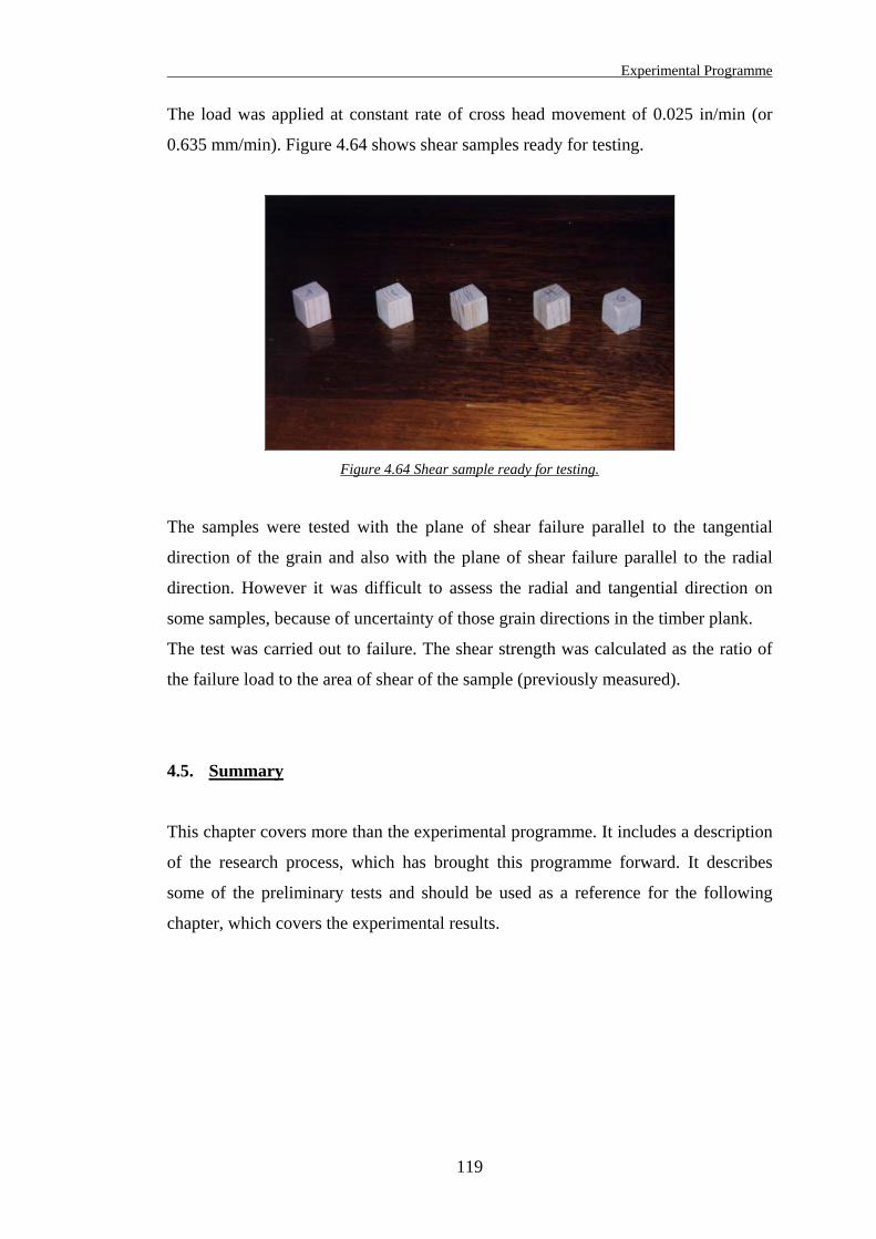
Experimental Programme
119
The load was applied at constant rate of cross head movement of 0.025 in/min (or
0.635 mm/min). Figure 4.64 shows shear samples ready for testing.
Figure 4.64 Shear sample ready for testing.
The samples were tested with the plane of shear failure parallel to the tangential
direction of the grain and also with the plane of shear failure parallel to the radial
direction. However it was difficult to assess the radial and tangential direction on
some samples, because of uncertainty of those grain directions in the timber plank.
The test was carried out to failure. The shear strength was calculated as the ratio of
the failure load to the area of shear of the sample (previously measured).
4.5. Summary
This chapter covers more than the experimental programme. It includes a description
of the research process, which has brought this programme forward. It describes
some of the preliminary tests and should be used as a reference for the following
chapter, which covers the experimental results.
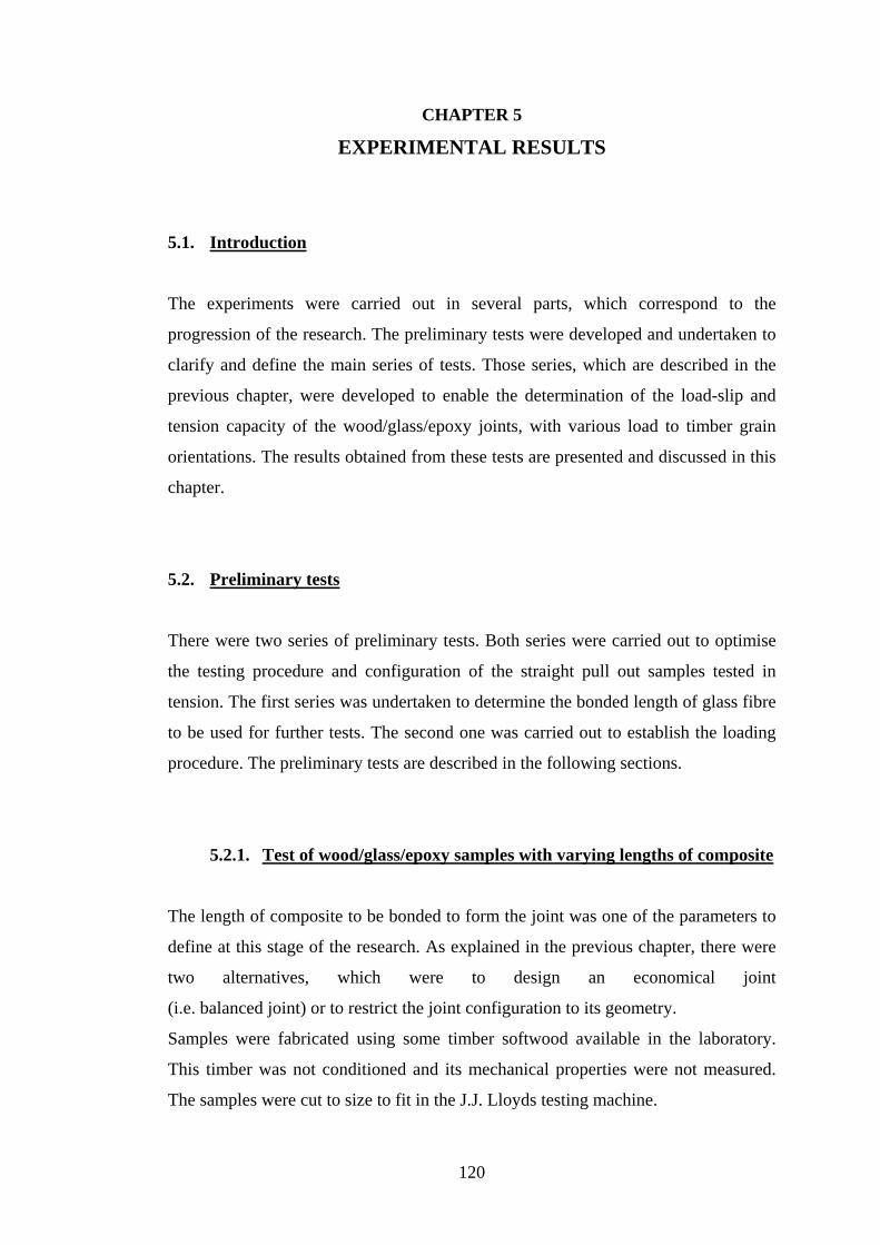
CHAPTER 5
EXPERIMENTAL RESULTS
5.1. Introduction
The experiments were carried out in several parts, which correspond to the
progression of the research. The preliminary tests were developed and undertaken to
clarify and define the main series of tests. Those series, which are described in the
previous chapter, were developed to enable the determination of the load-slip and
tension capacity of the wood/glass/epoxy joints, with various load to timber grain
orientations. The results obtained from these tests are presented and discussed in this
chapter.
5.2. Preliminary tests
There were two series of preliminary tests. Both series were carried out to optimise
the testing procedure and configuration of the straight pull out samples tested in
tension. The first series was undertaken to determine the bonded length of glass fibre
to be used for further tests. The second one was carried out to establish the loading
procedure. The preliminary tests are described in the following sections.
5.2.1. Test of wood/glass/epoxy samples with varying lengths of composite
The length of composite to be bonded to form the joint was one of the parameters to
define at this stage of the research. As explained in the previous chapter, there were
two alternatives, which were to design an economical joint
(i.e. balanced joint) or to restrict the joint configuration to its geometry.
Samples were fabricated using some timber softwood available in the laboratory.
This timber was not conditioned and its mechanical properties were not measured.
The samples were cut to size to fit in the J.J. Lloyds testing machine.
120
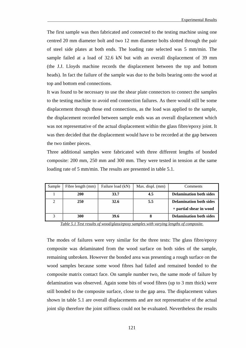
Experimental Results
The first sample was then fabricated and connected to the testing machine using one
centred 20 mm diameter bolt and two 12 mm diameter bolts slotted through the pair
of steel side plates at both ends. The loading rate selected was 5 mm/min. The
sample failed at a load of 32.6 kN but with an overall displacement of 39 mm
(the J.J. Lloyds machine records the displacement between the top and bottom
heads). In fact the failure of the sample was due to the bolts bearing onto the wood at
top and bottom end connections.
It was found to be necessary to use the shear plate connectors to connect the samples
to the testing machine to avoid end connection failures. As there would still be some
displacement through those end connections, as the load was applied to the sample,
the displacement recorded between sample ends was an overall displacement which
was not representative of the actual displacement within the glass fibre/epoxy joint. It
was then decided that the displacement would have to be recorded at the gap between
the two timber pieces.
Three additional samples were fabricated with three different lengths of bonded
composite: 200 mm, 250 mm and 300 mm. They were tested in tension at the same
loading rate of 5 mm/min. The results are presented in table 5.1.
Sample Fibre length (mm) Failure load (kN) Max. displ. (mm) Comments
1 200 33.7 4.5 Delamination both sides
2 250 32.6 5.5 Delamination both sides
+ partial shear in wood
3 300 39.6 8 Delamination both sides
Table 5.1 Test results of wood/glass/epoxy samples with varying lengths of composite.
The modes of failures were very similar for the three tests: The glass fibre/epoxy
composite was delaminated from the wood surface on both sides of the sample,
remaining unbroken. However the bonded area was presenting a rough surface on the
wood samples because some wood fibres had failed and remained bonded to the
composite matrix contact face. On sample number two, the same mode of failure by
delamination was observed. Again some bits of wood fibres (up to 3 mm thick) were
still bonded to the composite surface, close to the gap area. The displacement values
shown in table 5.1 are overall displacements and are not representative of the actual
joint slip therefore the joint stiffness could not be evaluated. Nevertheless the results
121
Experimental Results
show that the overall sample displacement increased with the composite length. In
fact the contact area was larger therefore the load, which was transferred from one
timber piece to the other, was distributed over a larger area, thus reducing the shear
stresses. With a larger bond, the shear stress occurring at the interface is normally
reduced for a given load. Higher failure load was obtained with 300 mm composite
length, but smaller load with 250 mm length compared to 200 mm. This was
probably due to the wood properties of the sample number two which were certainly
lower than the ones for sample number one and number three.
Resulting from those tests, it was decided to use 200 mm of composite length,
mainly for geometrical reasons (as explained in the previous chapter) but also it
appeared that increasing the length of composite did not strengthen the joint
sufficiently for the extra amount of material added to it. All three joints failed by
delamination with no rupture in the composite. In other words the joints were
unbalanced for the three bond lengths proposed, as the composite was much stronger
than the interface bond with the wood. For the design of a balanced joint, it would
have been necessary to either reduce the composite cross-section (i.e. reduce glass
fibre density) or increase the bond length of composite further than 300 mm. As the
glass fibre used was a commercial product, reducing and adjusting its density was
not a practical option. Increasing the length of the composite was therefore the only
alternative, but there would have been no possible comparison between different
tests. The choice of using 200 mm bonded length was discussed and finally justified
with the two following reasons:
• The samples had the same area of glass fibre bonded for two test configurations,
with the load parallel to the grain and with the load perpendicular to the grain.
• For all the samples, both connected timber pieces had an equal bonded area of
composite.
122
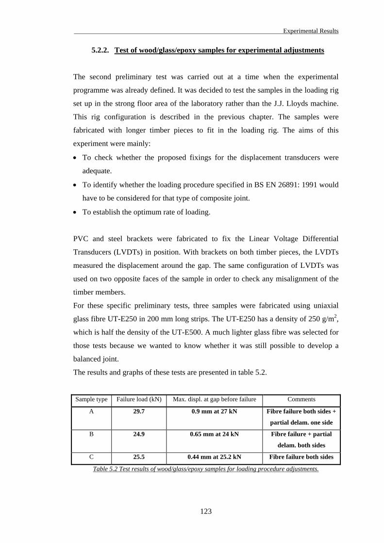
Experimental Results
5.2.2. Test of wood/glass/epoxy samples for experimental adjustments
The second preliminary test was carried out at a time when the experimental
programme was already defined. It was decided to test the samples in the loading rig
set up in the strong floor area of the laboratory rather than the J.J. Lloyds machine.
This rig configuration is described in the previous chapter. The samples were
fabricated with longer timber pieces to fit in the loading rig. The aims of this
experiment were mainly:
• To check whether the proposed fixings for the displacement transducers were
adequate.
• To identify whether the loading procedure specified in BS EN 26891: 1991 would
have to be considered for that type of composite joint.
• To establish the optimum rate of loading.
PVC and steel brackets were fabricated to fix the Linear Voltage Differential
Transducers (LVDTs) in position. With brackets on both timber pieces, the LVDTs
measured the displacement around the gap. The same configuration of LVDTs was
used on two opposite faces of the sample in order to check any misalignment of the
timber members.
For these specific preliminary tests, three samples were fabricated using uniaxial
glass fibre UT-E250 in 200 mm long strips. The UT-E250 has a density of 250 g/m2,
which is half the density of the UT-E500. A much lighter glass fibre was selected for
those tests because we wanted to know whether it was still possible to develop a
balanced joint.
The results and graphs of these tests are presented in table 5.2.
Sample type Failure load (kN) Max. displ. at gap before failure Comments
A 29.7 0.9 mm at 27 kN Fibre failure both sides +
partial delam. one side
B 24.9 0.65 mm at 24 kN Fibre failure + partial
delam. both sides
C 25.5 0.44 mm at 25.2 kN Fibre failure both sides
Table 5.2 Test results of wood/glass/epoxy samples for loading procedure adjustments.
123
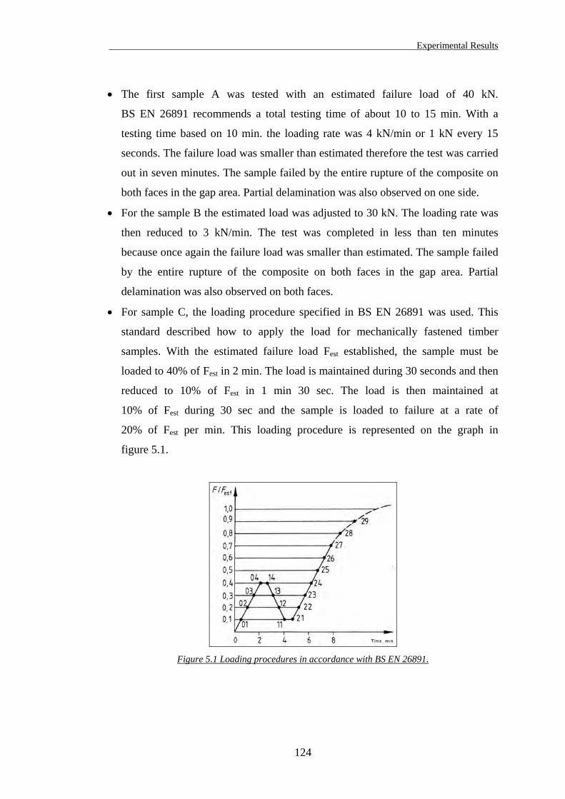
Experimental Results
• The first sample A was tested with an estimated failure load of 40 kN.
BS EN 26891 recommends a total testing time of about 10 to 15 min. With a
testing time based on 10 min. the loading rate was 4 kN/min or 1 kN every 15
seconds. The failure load was smaller than estimated therefore the test was carried
out in seven minutes. The sample failed by the entire rupture of the composite on
both faces in the gap area. Partial delamination was also observed on one side.
• For the sample B the estimated load was adjusted to 30 kN. The loading rate was
then reduced to 3 kN/min. The test was completed in less than ten minutes
because once again the failure load was smaller than estimated. The sample failed
by the entire rupture of the composite on both faces in the gap area. Partial
delamination was also observed on both faces.
• For sample C, the loading procedure specified in BS EN 26891 was used. This
standard described how to apply the load for mechanically fastened timber
samples. With the estimated failure load Fest established, the sample must be
loaded to 40% of Fest in 2 min. The load is maintained during 30 seconds and then
reduced to 10% of Fest in 1 min 30 sec. The load is then maintained at
10% of Fest during 30 sec and the sample is loaded to failure at a rate of
20% of Fest per min. This loading procedure is represented on the graph in
figure 5.1.
Figure 5.1 Loading procedures in accordance with BS EN 26891.
124
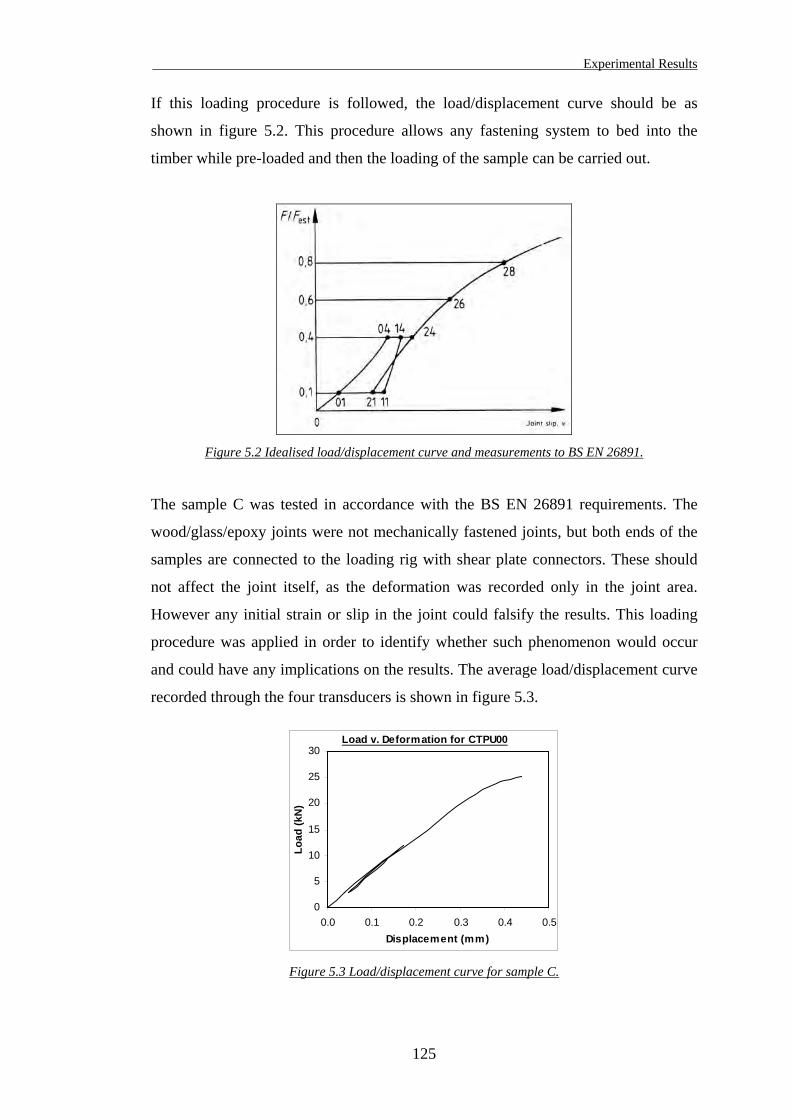
Experimental Results
If this loading procedure is followed, the load/displacement curve should be as
shown in figure 5.2. This procedure allows any fastening system to bed into the
timber while pre-loaded and then the loading of the sample can be carried out.
Figure 5.2 Idealised load/displacement curve and measurements to BS EN 26891.
The sample C was tested in accordance with the BS EN 26891 requirements. The
wood/glass/epoxy joints were not mechanically fastened joints, but both ends of the
samples are connected to the loading rig with shear plate connectors. These should
not affect the joint itself, as the deformation was recorded only in the joint area.
However any initial strain or slip in the joint could falsify the results. This loading
procedure was applied in order to identify whether such phenomenon would occur
and could have any implications on the results. The average load/displacement curve
recorded through the four transducers is shown in figure 5.3.
Load v. Deformation for CTPU00
0
5
10
15
20
25
30
0.0 0.1 0.2 0.3 0.4 0.5Displacement (mm)
Load
(kN
)
Figure 5.3 Load/displacement curve for sample C.
125
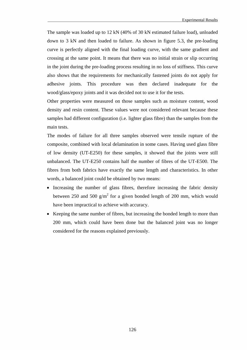
Experimental Results
The sample was loaded up to 12 kN (40% of 30 kN estimated failure load), unloaded
down to 3 kN and then loaded to failure. As shown in figure 5.3, the pre-loading
curve is perfectly aligned with the final loading curve, with the same gradient and
crossing at the same point. It means that there was no initial strain or slip occurring
in the joint during the pre-loading process resulting in no loss of stiffness. This curve
also shows that the requirements for mechanically fastened joints do not apply for
adhesive joints. This procedure was then declared inadequate for the
wood/glass/epoxy joints and it was decided not to use it for the tests.
Other properties were measured on those samples such as moisture content, wood
density and resin content. These values were not considered relevant because these
samples had different configuration (i.e. lighter glass fibre) than the samples from the
main tests.
The modes of failure for all three samples observed were tensile rupture of the
composite, combined with local delamination in some cases. Having used glass fibre
of low density (UT-E250) for these samples, it showed that the joints were still
unbalanced. The UT-E250 contains half the number of fibres of the UT-E500. The
fibres from both fabrics have exactly the same length and characteristics. In other
words, a balanced joint could be obtained by two means:
• Increasing the number of glass fibres, therefore increasing the fabric density
between 250 and 500 g/m2 for a given bonded length of 200 mm, which would
have been impractical to achieve with accuracy.
• Keeping the same number of fibres, but increasing the bonded length to more than
200 mm, which could have been done but the balanced joint was no longer
considered for the reasons explained previously.
126
Experimental Results
5.3. Timber grading tests
As explained in the previous chapter, each timber sample was graded precisely after
their temperature and humidity conditioning. Before being sawn to the appropriate
shape and over one metre in length, each piece of timber was tested in three points
bending with records of mid-span deflection under load. The load and mid-span
deflection would allow the calculation of the bending modulus of elasticity (parallel
to the grain) for each sample.
The tests were carried out at very low loading (up to 3 kN maximum). For each
1 kN of load applied, the mid-span deflection was recorded. At the end of the test the
residual deflection was also measured.
This test was carried out on all timber pieces to be used for the sample fabrication.
The results of that test are presented in tables 5.3, 5.4, 5.5, 5.6 and 5.7.
Sample number
Tension test
Load Parallel or Not parallel to the grain
Uniaxial or Biaxial glass fibre
Load/grain angle (º)
Timber type
4 T N U 60 – β
Sample symbol definition.
Sample Wood MOE (kN/mm2) Sample Wood MOE (kN/mm2) 1TPU00 O 8.63 1TPB00 E 10.62 2TPU00 I 8.42 2TPB00 M 7.06 3TPU00 H 8.52 3TPB00 L 7.66 4TPU00 N 7.04 4TPB00 C 8.97 5TPU00 A 8.46 5TPB00 J 7.40 6TPU00 P 7.21 6TPB00 G 8.88 7TPU00 Z 6.44 7TPB00 α 7.03 8TPU00 J 7.88 8TPB00 $ 6.71
Table 5.3 Bending moduli for TPU00 and TPB00 samples.
Sample Wood MOE (kN/mm2) Sample Wood MOE (kN/mm2) 1TPU10 I 9.38 1TPB30 L 6.70 2TPU10 O 6.27 2TPB30 K 8.52 3TPU10 E 8.71 3TPB30 E 9.66 4TPU10 D 7.85 4TPB30 C 8.08 5TPU10 N 8.12 5TPB30 M 7.04 6TPU10 F 6.35 6TPB30 G 10.94
Table 5.4 Bending moduli for TPU10 and TPB30 samples.
127
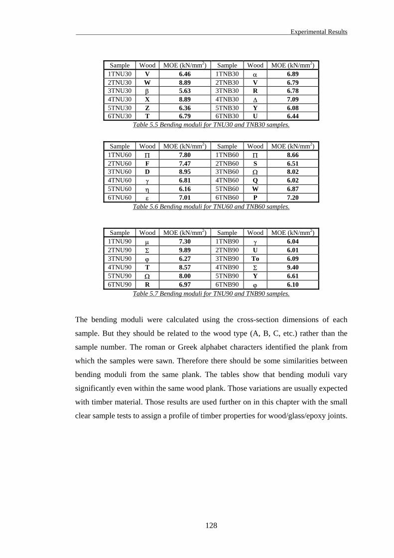
Experimental Results
Sample Wood MOE (kN/mm2) Sample Wood MOE (kN/mm2) 1TNU30 V 6.46 1TNB30 α 6.89 2TNU30 W 8.89 2TNB30 V 6.79 3TNU30 β 5.63 3TNB30 R 6.78 4TNU30 X 8.89 4TNB30 ∆ 7.09 5TNU30 Z 6.36 5TNB30 Y 6.08 6TNU30 T 6.79 6TNB30 U 6.44
Table 5.5 Bending moduli for TNU30 and TNB30 samples.
Sample Wood MOE (kN/mm2) Sample Wood MOE (kN/mm2)
1TNU60 Π 7.80 1TNB60 Π 8.66 2TNU60 F 7.47 2TNB60 S 6.51 3TNU60 D 8.95 3TNB60 Ω 8.02 4TNU60 γ 6.81 4TNB60 Q 6.02 5TNU60 η 6.16 5TNB60 W 6.87 6TNU60 ε 7.01 6TNB60 P 7.20
Table 5.6 Bending moduli for TNU60 and TNB60 samples.
Sample Wood MOE (kN/mm2) Sample Wood MOE (kN/mm2) 1TNU90 µ 7.30 1TNB90 γ 6.04 2TNU90 Σ 9.89 2TNB90 U 6.01 3TNU90 ϕ 6.27 3TNB90 To 6.09 4TNU90 T 8.57 4TNB90 Σ 9.40 5TNU90 Ω 8.00 5TNB90 Y 6.61 6TNU90 R 6.97 6TNB90 ϕ 6.10
Table 5.7 Bending moduli for TNU90 and TNB90 samples.
The bending moduli were calculated using the cross-section dimensions of each
sample. But they should be related to the wood type (A, B, C, etc.) rather than the
sample number. The roman or Greek alphabet characters identified the plank from
which the samples were sawn. Therefore there should be some similarities between
bending moduli from the same plank. The tables show that bending moduli vary
significantly even within the same wood plank. Those variations are usually expected
with timber material. Those results are used further on in this chapter with the small
clear sample tests to assign a profile of timber properties for wood/glass/epoxy joints.
128
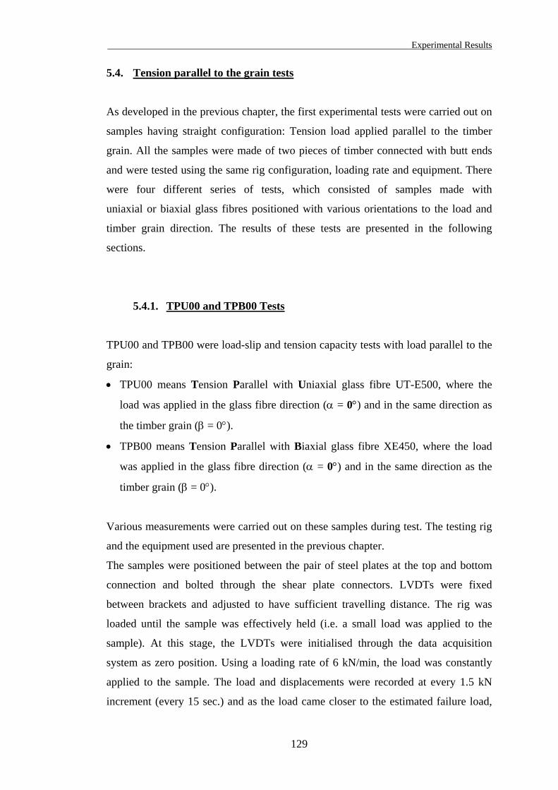
Experimental Results
5.4. Tension parallel to the grain tests
As developed in the previous chapter, the first experimental tests were carried out on
samples having straight configuration: Tension load applied parallel to the timber
grain. All the samples were made of two pieces of timber connected with butt ends
and were tested using the same rig configuration, loading rate and equipment. There
were four different series of tests, which consisted of samples made with
uniaxial or biaxial glass fibres positioned with various orientations to the load and
timber grain direction. The results of these tests are presented in the following
sections.
5.4.1. TPU00 and TPB00 Tests
TPU00 and TPB00 were load-slip and tension capacity tests with load parallel to the
grain:
• TPU00 means Tension Parallel with Uniaxial glass fibre UT-E500, where the
load was applied in the glass fibre direction (α = 0°) and in the same direction as
the timber grain (β = 0°).
• TPB00 means Tension Parallel with Biaxial glass fibre XE450, where the load
was applied in the glass fibre direction (α = 0°) and in the same direction as the
timber grain (β = 0°).
Various measurements were carried out on these samples during test. The testing rig
and the equipment used are presented in the previous chapter.
The samples were positioned between the pair of steel plates at the top and bottom
connection and bolted through the shear plate connectors. LVDTs were fixed
between brackets and adjusted to have sufficient travelling distance. The rig was
loaded until the sample was effectively held (i.e. a small load was applied to the
sample). At this stage, the LVDTs were initialised through the data acquisition
system as zero position. Using a loading rate of 6 kN/min, the load was constantly
applied to the sample. The load and displacements were recorded at every 1.5 kN
increment (every 15 sec.) and as the load came closer to the estimated failure load,
129
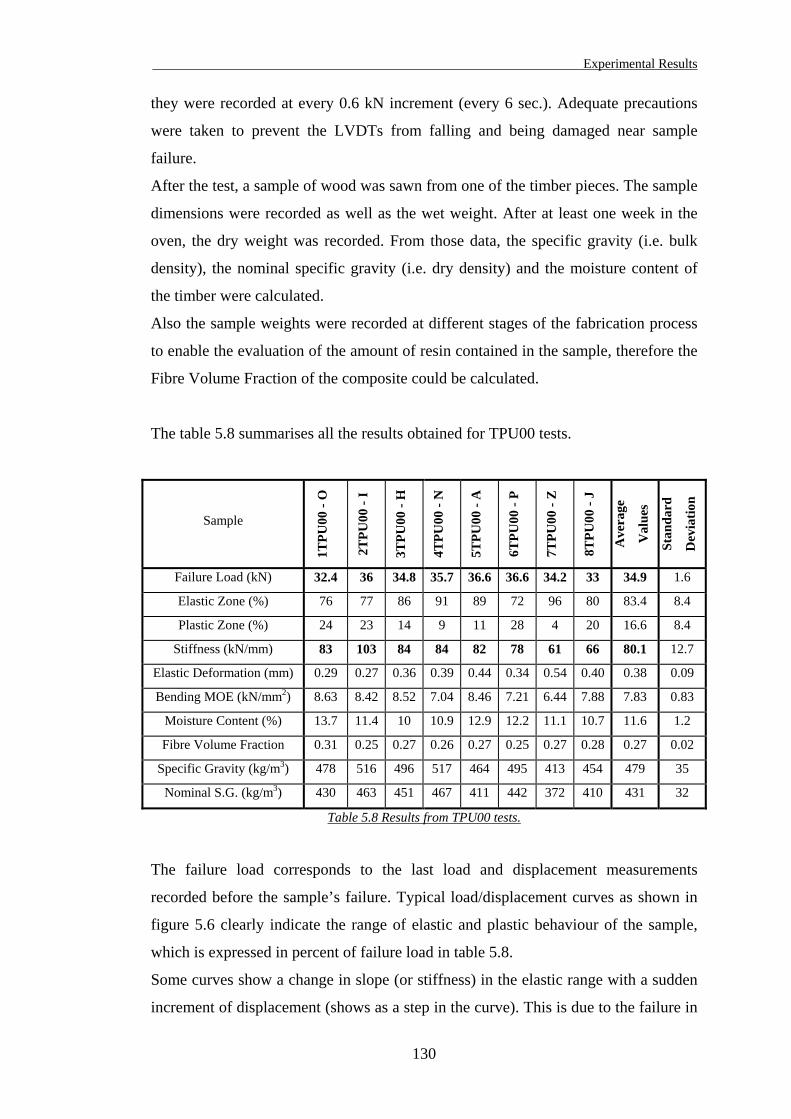
Experimental Results
they were recorded at every 0.6 kN increment (every 6 sec.). Adequate precautions
were taken to prevent the LVDTs from falling and being damaged near sample
failure.
After the test, a sample of wood was sawn from one of the timber pieces. The sample
dimensions were recorded as well as the wet weight. After at least one week in the
oven, the dry weight was recorded. From those data, the specific gravity (i.e. bulk
density), the nominal specific gravity (i.e. dry density) and the moisture content of
the timber were calculated.
Also the sample weights were recorded at different stages of the fabrication process
to enable the evaluation of the amount of resin contained in the sample, therefore the
Fibre Volume Fraction of the composite could be calculated.
The table 5.8 summarises all the results obtained for TPU00 tests.
Sample
1TPU
00 -
O
2TPU
00 -
I
3TPU
00 -
H
4TPU
00 -
N
5TPU
00 -
A
6TPU
00 -
P
7TPU
00 -
Z
8TPU
00 -
J
Ave
rage
Val
ues
Stan
dard
Dev
iatio
n
Failure Load (kN) 32.4 36 34.8 35.7 36.6 36.6 34.2 33 34.9 1.6
Elastic Zone (%) 76 77 86 91 89 72 96 80 83.4 8.4
Plastic Zone (%) 24 23 14 9 11 28 4 20 16.6 8.4
Stiffness (kN/mm) 83 103 84 84 82 78 61 66 80.1 12.7
Elastic Deformation (mm) 0.29 0.27 0.36 0.39 0.44 0.34 0.54 0.40 0.38 0.09
Bending MOE (kN/mm2) 8.63 8.42 8.52 7.04 8.46 7.21 6.44 7.88 7.83 0.83
Moisture Content (%) 13.7 11.4 10 10.9 12.9 12.2 11.1 10.7 11.6 1.2
Fibre Volume Fraction 0.31 0.25 0.27 0.26 0.27 0.25 0.27 0.28 0.27 0.02
Specific Gravity (kg/m3) 478 516 496 517 464 495 413 454 479 35
Nominal S.G. (kg/m3) 430 463 451 467 411 442 372 410 431 32
Table 5.8 Results from TPU00 tests.
The failure load corresponds to the last load and displacement measurements
recorded before the sample’s failure. Typical load/displacement curves as shown in
figure 5.6 clearly indicate the range of elastic and plastic behaviour of the sample,
which is expressed in percent of failure load in table 5.8.
Some curves show a change in slope (or stiffness) in the elastic range with a sudden
increment of displacement (shows as a step in the curve). This is due to the failure in
130
Experimental Results
tension of some epoxy resin infiltrated accidentally between the timber piece butt
ends (in the gap).
The joint stiffness was calculated over the elastic range of the sample.
The modes of failure of each sample were also recorded during the tests and are
summarised in table 5.9.
Samples Failure Load (kN) Modes of failure
1TPU00 - O 32.4 Delamination both sides
2TPU00 - I 36 Delamination both sides
3TPU00 - H 34.8 Delamination both sides
4TPU00 - N 35.7 Top shear plate connector failure
5TPU00 - A 36.6 Delamination both sides
6TPU00 - P 36.6 Delamination both sides
7TPU00 - Z 34.2 Delamination both sides
8TPU00 - J 33 Delamination both sides
Table 5.9 Failure modes from TPU00 tests.
The modes of failure observed through the tests were very consistent and of the same
nature for most of the samples. The samples failed by delamination of the composite
layers from the timber surface on both sides. Figures 5.4 and 5.5 show some of the
TPU00 samples after failure.
Figure 5.4 Delamination on both sides observed on the 7TPU00 - Z sample.
131
Experimental Results
Figure 5.5 Delamination on both sides observed on the 8TPU00 - J sample.
Except on the sample shown in figure 5.5, there was no longitudinal shear failure
detected in the composite layer. This means the tension stresses at failure in the
composite were fairly uniformly distributed on each face and across the width. There
might be two reasons for that:
• The samples tested were in fact axially loaded or “tension only”, with a negligible
eccentricity if there was any.
• There was effectively an eccentricity of the load, but the longitudinal shear
resistance of the composite layer was high enough to re-distribute the stresses
across the whole width and enable the composite layer to delaminate entirely at
failure.
Figure 5.6 summarises the load/displacement curves obtained for the samples from
the TPU00 tests.
132
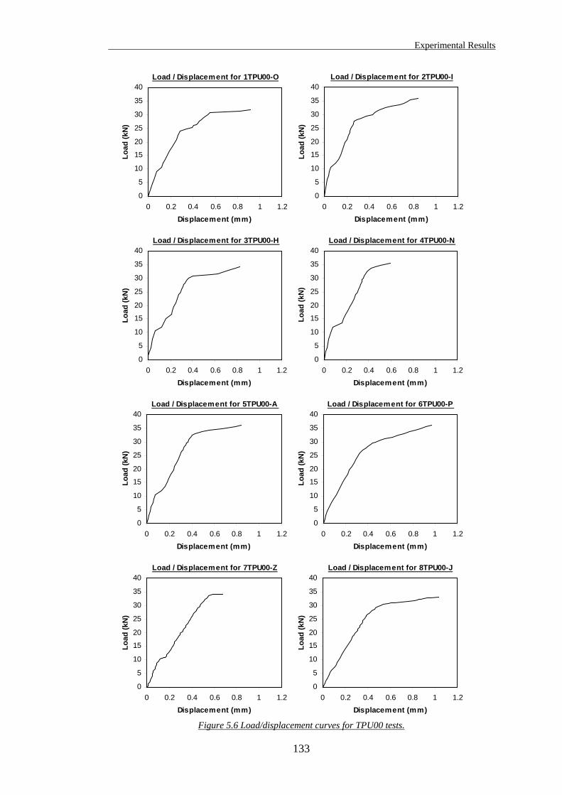
Experimental Results
Load / Displacement for 1TPU00-O
0
5
10
15
20
25
30
35
40
0 0.2 0.4 0.6 0.8 1 1.2
Displacement (mm)
Load
(kN
)
Load / Displacement for 2TPU00-I
0
5
10
15
20
25
30
35
40
0 0.2 0.4 0.6 0.8 1 1.2
Displacement (mm)
Load
(kN
)
Load / Displacement for 3TPU00-H
0
5
10
15
20
25
30
35
40
0 0.2 0.4 0.6 0.8 1 1.2
Displacement (mm)
Load
(kN
)
Load / Displacement for 4TPU00-N
0
5
10
15
20
25
30
35
40
0 0.2 0.4 0.6 0.8 1 1.2
Displacement (mm)
Load
(kN
)
Load / Displacement for 5TPU00-A
0
5
10
15
20
25
30
35
40
0 0.2 0.4 0.6 0.8 1 1.2
Displacement (mm)
Load
(kN
)
Load / Displacement for 6TPU00-P
0
5
10
15
20
25
30
35
40
0 0.2 0.4 0.6 0.8 1 1.2
Displacement (mm)
Load
(kN
)
Load / Displacement for 7TPU00-Z Load / Displacement for 8TPU00-J
133
0
5
10
15
20
25
30
35
40
0 0.2 0.4 0.6 0.8 1 1.2
Displacement (mm)
Load
(kN
)
0
5
10
15
20
25
30
35
40
0 0.2 0.4 0.6 0.8 1 1.2
Displacement (mm)
Load
(kN
)
Figure 5.6 Load/displacement curves for TPU00 tests.
Experimental Results
The displacements were measured using the average readings from the small LVDTs
positioned on the samples sides. However strain gauges were also used on some of
the tested samples, such as samples 7TPU00 - Z and 8TPU00 - J of the TPU00 Test.
Measurements of strains were carried out at precise locations on the surface of the
glass fibre/epoxy composite layers. Strain gauges were used on the sample shown in
figures 5.4 and 5.5.
These results are presented later in this chapter, in § 5.6.
The load/displacement curves for the TPU00 tests show that the displacements
recorded around the gap between the connected members never exceed 1.1 mm,
which is a very small value of slip at failure in comparison with mechanically
fastened timber joints such as bolted connection.
The failure loads recorded for the eight samples are relatively uniform, ranging
between 32.4 and 36.6 kN.
The elastic behaviour of the samples exceeds 72% of the overall recorded joint slip
for a maximum elastic displacement of 0.54 mm.
The samples develop a plastic behaviour generally, except on samples No 4 and No 7
where the curves stop suddenly as they start to show some plasticity. In fact the
curves do not reflect the full behaviour, especially as the load reached its maximum.
The equipment did record the load at 1.5 kN increment and at 0.6 kN increment as
the sample came up to the failure load. Therefore the position where the curve
stopped corresponds to the last load/displacement record before the failure. Most of
the time, the exact failure load was higher than this value but not high enough to
reach the next 0.6 kN increment. As a consequence, the exact displacement at failure
could not be measured and therefore could be much larger than the recorded value,
especially as the sample developed plasticity.
The comparison of various parameters obtained from these tests is presented in the
discussion section, in § 5.4.3.
134

Experimental Results
The same tests were carried out on the TPB00 samples. The table 5.10 summarises
all the results obtained for the TPB00 tests.
Sample number
Tension test
Load Parallel or Not parallel to the grain
Uniaxial or Biaxial glass fibre
Load/grain angle (º)
Timber type
4 T N U 60 – β
Sample symbol definition.
Sample
1TPB
00 -
E
2TPB
00 -
M
3TPB
00 -
L
4TPB
00 -
C
5TPB
00 -
J
6TPB
00 -
G
7TPB
00 - α
8TPB
00 -
$
Ave
rage
Val
ues
Stan
dard
Dev
iatio
n
Failure Load (kN) 26.4 28.2 26.1 28.5 28.2 26.4 24.6 28.8 27.2 1.5
Elastic Zone (%) 84 87 87 78 83 86 85 87 84.6 3.1
Plastic Zone (%) 16 13 13 22 17 14 15 13 15.4 3.1
Stiffness (kN/mm) 60 50 54 58 55 64 60 56 57.1 4.3
Elastic Deformation (mm) 0.35 0.49 0.42 0.38 0.43 0.36 0.35 0.45 0.40 0.05
Bending MOE (kN/mm2) 10.62 7.06 7.66 8.97 7.4 8.88 7.03 6.71 8.04 1.34
Moisture Content (%) 13.9 13.1 12.7 12.3 12.8 13.8 10.3 10.7 12.5 1.3
Fibre Volume Fraction 0.29 0.28 0.27 0.27 0.27 0.3 0.27 0.29 0.28 0.01
Specific Gravity (kg/m3) 505 499 503 447 445 494 468 485 481 24
Nominal S.G. (kg/m3) 443 442 446 398 394 434 425 439 428 21
Table 5.10 Results from TPB00 tests.
The failure load corresponds to the last load and displacement measurements
recorded before the sample’s failure. Typical load/displacement curves as shown in
figure 5.9 clearly indicate the range of elastic and plastic behaviour of the sample,
which is expressed in percent of failure load in table 5.10.
As explained before, some curves show a change in slope (or stiffness) in the elastic
range with a sudden increment of displacement that is due to the failure in tensile
failure of some epoxy resin infiltrated between the timber piece butt ends.
The joint stiffness was calculated over the elastic range of the sample.
135
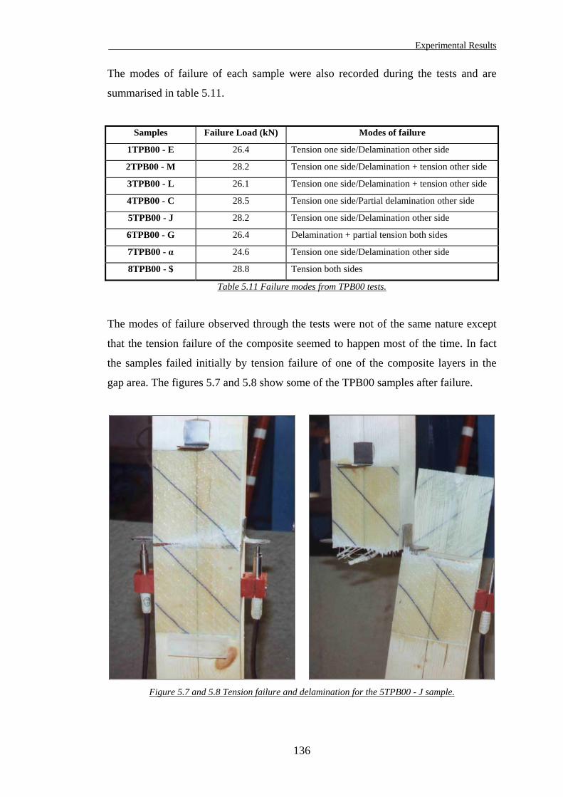
Experimental Results
The modes of failure of each sample were also recorded during the tests and are
summarised in table 5.11.
Samples Failure Load (kN) Modes of failure
1TPB00 - E 26.4 Tension one side/Delamination other side
2TPB00 - M 28.2 Tension one side/Delamination + tension other side
3TPB00 - L 26.1 Tension one side/Delamination + tension other side
4TPB00 - C 28.5 Tension one side/Partial delamination other side
5TPB00 - J 28.2 Tension one side/Delamination other side
6TPB00 - G 26.4 Delamination + partial tension both sides
7TPB00 - α 24.6 Tension one side/Delamination other side
8TPB00 - $ 28.8 Tension both sides
Table 5.11 Failure modes from TPB00 tests.
The modes of failure observed through the tests were not of the same nature except
that the tension failure of the composite seemed to happen most of the time. In fact
the samples failed initially by tension failure of one of the composite layers in the
gap area. The figures 5.7 and 5.8 show some of the TPB00 samples after failure.
Figure 5.7 and 5.8 Tension failure and delamination for the 5TPB00 - J sample.
136
Experimental Results
Only half of the fibres were orientated in the load direction with the biaxial glass
fibre fabric. The other half was orientated perpendicular to the grain and was
providing strength only to transversal effects or stresses, which are minimal in a
tension only test of that configuration. It shows that this type of joint was still
unbalanced, with insufficient amount of fibres provided in the loading direction.
When the composite layer of one side of the joint failed in tension as shown in
figure 5.7, all tension stresses were then transferred to the other layer, which failed
soon after in multiple modes of failure. This was probably due to the suddenness of
this high stress transfer from one face to the other. In figure 5.8, the other layer failed
by Delamination.
There was generally no longitudinal shear failure detected in the composite layer.
Figure 5.9 summarises the load/displacement curves obtained for the samples from
the TPB00 tests.
137
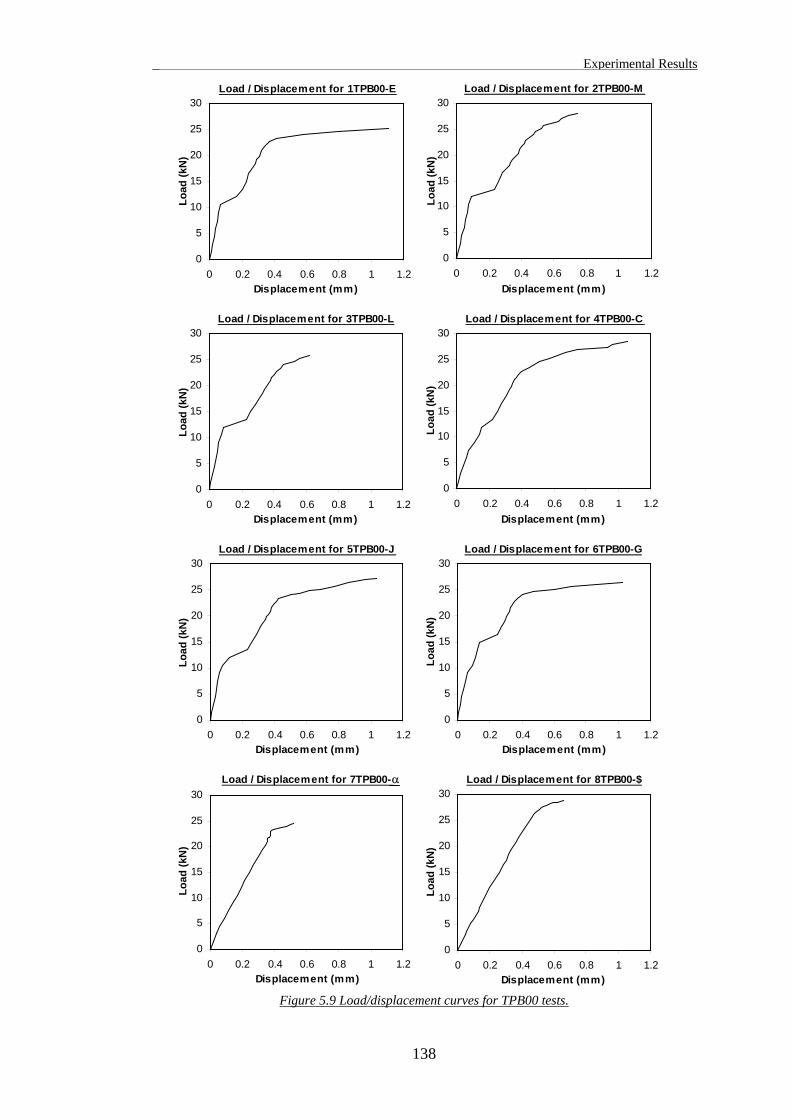
Experimental Results
Load / Displacement for 1TPB00-E
0
5
10
15
20
25
30
0 0.2 0.4 0.6 0.8 1 1.2Displacement (mm)
Load
(kN
)
Load / Displacement for 2TPB00-M
0
5
10
15
20
25
30
0 0.2 0.4 0.6 0.8 1 1.2Displacement (mm)
Load
(kN
)
Load / Displacement for 3TPB00-L
0
5
10
15
20
25
30
0 0.2 0.4 0.6 0.8 1 1.2Displacement (mm)
Load
(kN
)
Load / Displacement for 4TPB00-C
0
5
10
15
20
25
30
0 0.2 0.4 0.6 0.8 1 1.2Displacement (mm)
Load
(kN
)
Load / Displacement for 5TPB00-J
0
5
10
15
20
25
30
0 0.2 0.4 0.6 0.8 1 1.2Displacement (mm)
Load
(kN
)
Load / Displacement for 6TPB00-G
0
5
10
15
20
25
30
0 0.2 0.4 0.6 0.8 1 1.2Displacement (mm)
Load
(kN
)
Load / Displacement for 7TPB00 Load / Displacement for 8TPB00-$- α
138
Figure 5.9 Load/displacement curves for TPB00 tests.
0
5
10
15
20
25
30
0 0.2 0.4 0.6 0.8 1 1.2Displacement (mm)
Load
(kN
)
0
5
10
15
20
25
30
0 0.2 0.4 0.6 0.8 1 1.2Displacement (mm)
Load
(kN
)
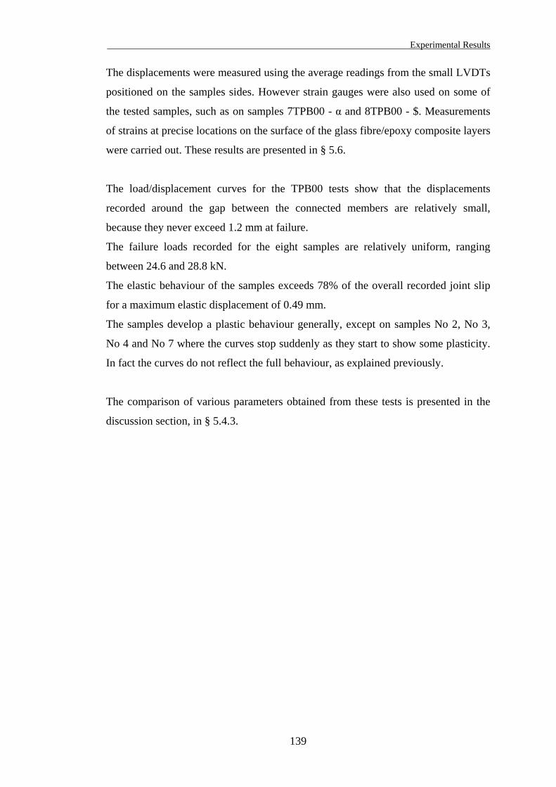
Experimental Results
The displacements were measured using the average readings from the small LVDTs
positioned on the samples sides. However strain gauges were also used on some of
the tested samples, such as on samples 7TPB00 - α and 8TPB00 - $. Measurements
of strains at precise locations on the surface of the glass fibre/epoxy composite layers
were carried out. These results are presented in § 5.6.
The load/displacement curves for the TPB00 tests show that the displacements
recorded around the gap between the connected members are relatively small,
because they never exceed 1.2 mm at failure.
The failure loads recorded for the eight samples are relatively uniform, ranging
between 24.6 and 28.8 kN.
The elastic behaviour of the samples exceeds 78% of the overall recorded joint slip
for a maximum elastic displacement of 0.49 mm.
The samples develop a plastic behaviour generally, except on samples No 2, No 3,
No 4 and No 7 where the curves stop suddenly as they start to show some plasticity.
In fact the curves do not reflect the full behaviour, as explained previously.
The comparison of various parameters obtained from these tests is presented in the
discussion section, in § 5.4.3.
139
Experimental Results
5.4.2. TPU10 and TPB30 Tests
As explained previously, TPU10 and TPB30 tests were load-slip and tension
capacity tests with load parallel to the grain but the glass fibre direction was
orientated with an angle to the load:
• Tension Parallel with Uniaxial glass fibre UT-E500, where the glass fibres were
orientated 10° from the load direction (α = 10°), but the load was parallel to the
timber grain (β = 0°). This 10° angle represented a possible misalignment of the
fibres with the timber grain and the load direction. The aim of this test was to
assess the implication of fibre misalignment for the joint strength. The sample
type was classified as TPU10.
• Tension Parallel with Biaxial glass fibre XE450, where the glass fibres were
orientated 30° from the load direction (α = 30°), but the load was parallel to the
timber grain (β = 0°). With the biaxial glass fibre, the properties were the same in
orthogonal directions, therefore α = 0° and α = 90° showed exactly the same
configuration. For 0° < α < 45°, the sample had different properties but for
α > 45°, the same properties applied by orthogonal symmetry. For example, with
the selected angle of α = 30°, it was the same configuration for α = 60°.
Combined with the test where α = 0°, this value of 30° allowed the assessment of
four different configurations, α = 0, 30, 60 and 90° with only two different sample
tested. The sample type was classified as TPB30.
Various measurements were carried out on these samples during test. The testing rig
and the equipment used are presented in the previous chapter.
The samples positioning, displacement measurements using LVDTs through the data
acquisition system, loading rates, the moisture content, density and
FVF measurements were all carried out as for TPU00 and TPB00 tests.
140
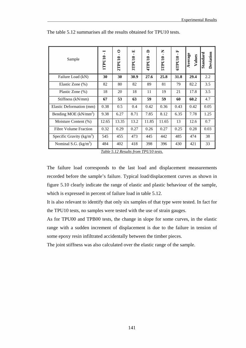
Experimental Results
The table 5.12 summarises all the results obtained for TPU10 tests.
Sample
1TPU
10 -
I
2TPU
10 -
O
3TPU
10 -
E
4TPU
10 -
D
5TPU
10 -
N
6TPU
10 -
F
Ave
rage
Val
ues
Stan
dard
Dev
iatio
n
Failure Load (kN) 30 30 30.9 27.6 25.8 31.8 29.4 2.2
Elastic Zone (%) 82 80 82 89 81 79 82.2 3.5
Plastic Zone (%) 18 20 18 11 19 21 17.8 3.5
Stiffness (kN/mm) 67 53 63 59 59 60 60.2 4.7
Elastic Deformation (mm) 0.38 0.5 0.4 0.42 0.36 0.43 0.42 0.05
Bending MOE (kN/mm2) 9.38 6.27 8.71 7.85 8.12 6.35 7.78 1.25
Moisture Content (%) 12.65 13.35 13.2 11.85 11.65 13 12.6 0.7
Fibre Volume Fraction 0.32 0.29 0.27 0.26 0.27 0.25 0.28 0.03
Specific Gravity (kg/m3) 545 455 473 445 442 485 474 38
Nominal S.G. (kg/m3) 484 402 418 398 396 430 421 33
Table 5.12 Results from TPU10 tests.
The failure load corresponds to the last load and displacement measurements
recorded before the sample’s failure. Typical load/displacement curves as shown in
figure 5.10 clearly indicate the range of elastic and plastic behaviour of the sample,
which is expressed in percent of failure load in table 5.12.
It is also relevant to identify that only six samples of that type were tested. In fact for
the TPU10 tests, no samples were tested with the use of strain gauges.
As for TPU00 and TPB00 tests, the change in slope for some curves, in the elastic
range with a sudden increment of displacement is due to the failure in tension of
some epoxy resin infiltrated accidentally between the timber pieces.
The joint stiffness was also calculated over the elastic range of the sample.
141
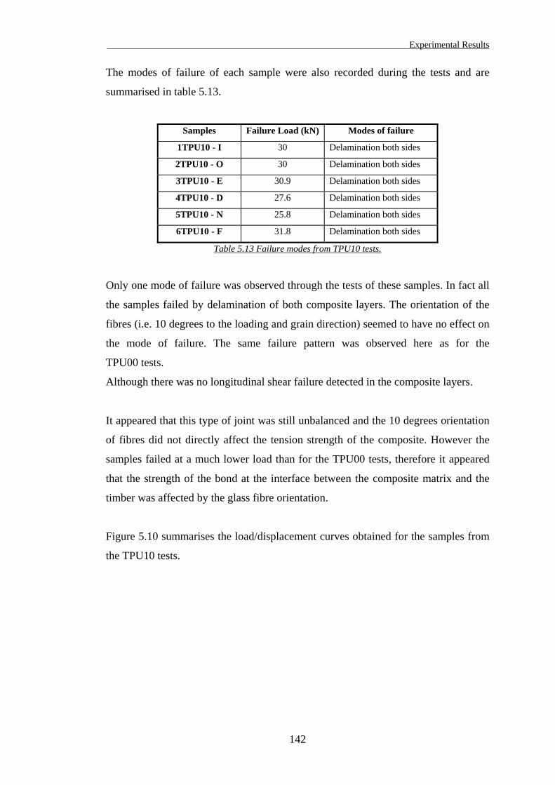
Experimental Results
The modes of failure of each sample were also recorded during the tests and are
summarised in table 5.13.
Samples Failure Load (kN) Modes of failure
1TPU10 - I 30 Delamination both sides
2TPU10 - O 30 Delamination both sides
3TPU10 - E 30.9 Delamination both sides
4TPU10 - D 27.6 Delamination both sides
5TPU10 - N 25.8 Delamination both sides
6TPU10 - F 31.8 Delamination both sides
Table 5.13 Failure modes from TPU10 tests.
Only one mode of failure was observed through the tests of these samples. In fact all
the samples failed by delamination of both composite layers. The orientation of the
fibres (i.e. 10 degrees to the loading and grain direction) seemed to have no effect on
the mode of failure. The same failure pattern was observed here as for the
TPU00 tests.
Although there was no longitudinal shear failure detected in the composite layers.
It appeared that this type of joint was still unbalanced and the 10 degrees orientation
of fibres did not directly affect the tension strength of the composite. However the
samples failed at a much lower load than for the TPU00 tests, therefore it appeared
that the strength of the bond at the interface between the composite matrix and the
timber was affected by the glass fibre orientation.
Figure 5.10 summarises the load/displacement curves obtained for the samples from
the TPU10 tests.
142
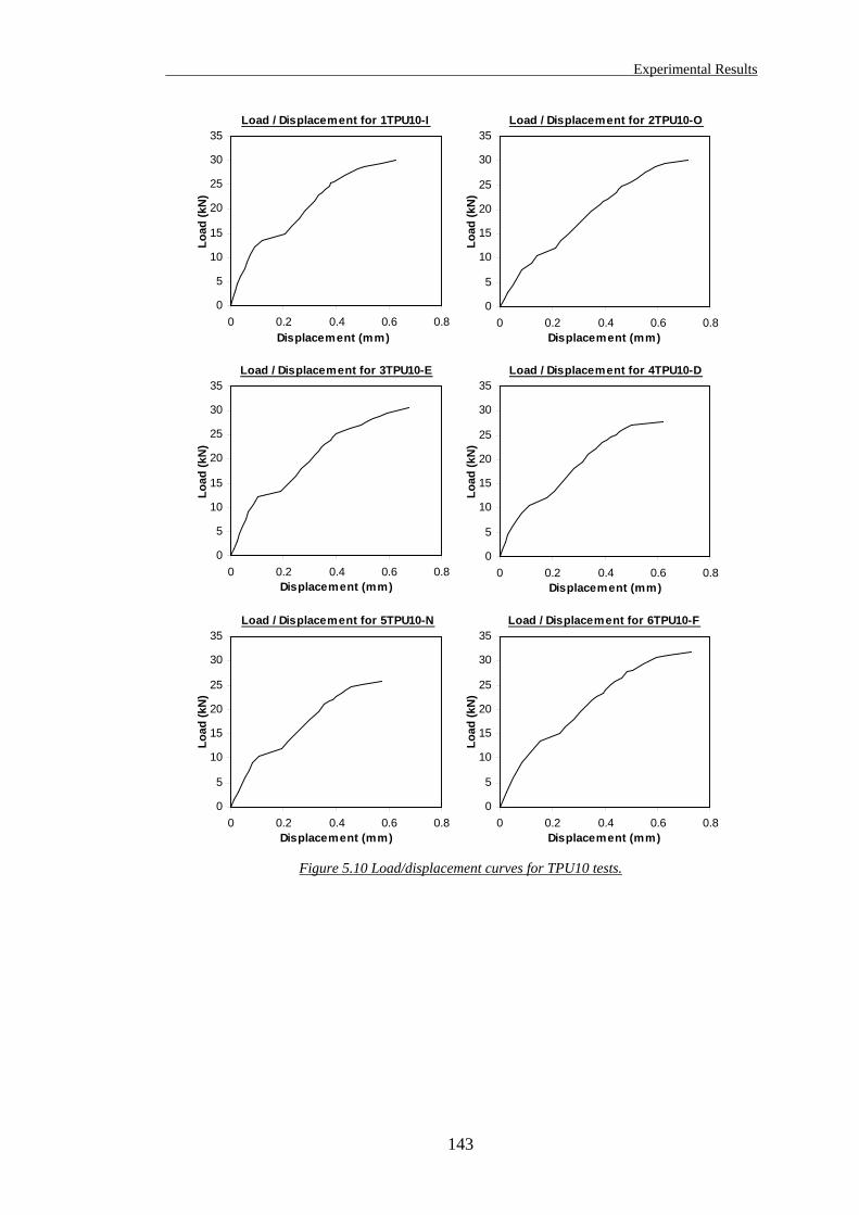
Experimental Results
Load / Displacement for 2TPU10-O
0
5
10
15
20
25
30
35
0 0.2 0.4 0.6 0.8Displacement (mm)
Load
(kN
)
Load / Displacement for 4TPU10-D
0
5
10
15
20
25
30
35
0 0.2 0.4 0.6 0.8Displacement (mm)
Load
(kN
)
Load / Displacement for 6TPU10-F
Load / Displacement for 1TPU10-I
0
5
10
15
20
25
30
35
0 0.2 0.4 0.6 0.8Displacement (mm)
Load
(kN
)
Load / Displacement for 3TPU10-E
0
5
10
15
20
25
30
35
0 0.2 0.4 0.6 0.8Displacement (mm)
Load
(kN
)
Load / Displacement for 5TPU10-N
Figure 5.10 Load/displacement curves for TPU10 tests.
0
5
10
15
20
25
30
35
0 0.2 0.4 0.6 0.8Displacement (mm)
Load
(kN
)
0
5
10
15
20
25
30
35
0 0.2 0.4 0.6 0.8Displacement (mm)
Load
(kN
)
143
Experimental Results
The displacements were measured using the average readings from the small LVDTs
positioned on the samples sides. However strain gauges were not used on the tested
samples of the TPU10 tests, mainly because the glass fibres were not orientated in
the same direction than the load. Standard strain gauges are measuring strain in their
longitudinal direction. With a strain gauge orientated 10 degrees to the load
direction, there is no direct relation between the tension load and the strain recorded
by the gauge. The use of strain rosette, which is a strain gauge reading strains from
three directions and giving the state of strain at a point, would have been more
appropriate. However strain rosettes tend to work efficiently on homogeneous and
isotropic materials, but not for composite or anisotropic materials. This was the main
reason for not using strain gauges on the TPU10 tests.
The load/displacement curves for the TPU10 tests show that the displacements
recorded around the gap between the connected members are even smaller than for
TPU00 tests, because they never exceed 0.75 mm at failure.
The failure loads recorded for the six samples are relatively uniform and are also
lower than for TPU00 tests, ranging between 25.8 and 31.8 kN.
The elastic behaviour of the samples exceeds 79% of the overall recorded joint slip
for a maximum elastic displacement of 0.50 mm.
All the samples develop a plastic behaviour generally in a fairly similar pattern.
Although the curves are reflecting a more elastic-plastic behaviour than for the
TPU00 and TPB00 tests, because of the absence of point of flexure between the
linear elastic and the plastic parts of the curve. In fact the transition appears to be
progressive and therefore not leading to full plasticity.
The comparison of various parameters obtained from these tests is presented in the
discussion section, in § 5.4.3.
144
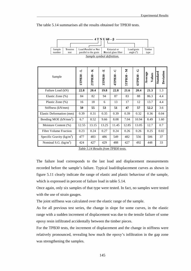
Experimental Results
The table 5.14 summarises all the results obtained for TPB30 tests.
Sample number
Tension test
Load Parallel or Not parallel to the grain
Uniaxial or Biaxial glass fibre
Load/grain angle (º)
Timber type
4 T N U 60 – β
Sample symbol definition.
Sample 1T
PB30
- L
2TPB
30 -
K
3TPB
30 -
E
4TPB
30 -
C
5TPB
30 -
M
6TPB
30 -
G
Ave
rage
Val
ues
Stan
dard
Dev
iatio
n
Failure Load (kN) 22.8 20.4 19.8 22.8 21.6 20.4 21.3 1.3
Elastic Zone (%) 84 82 94 87 83 88 86.3 4.4
Plastic Zone (%) 16 18 6 13 17 12 13.7 4.4
Stiffness (kN/mm) 50 55 53 51 47 57 52.2 3.6
Elastic Deformation (mm) 0.39 0.31 0.35 0.39 0.39 0.32 0.36 0.04
Bending MOE (kN/mm2) 6.7 8.52 9.66 8.08 7.04 10.94 8.49 1.60
Moisture Content (%) 12.55 13.15 13.25 11.45 12.85 13.05 12.7 0.7
Fibre Volume Fraction 0.23 0.24 0.27 0.24 0.26 0.26 0.25 0.02
Specific Gravity (kg/m3) 477 483 486 549 482 556 506 37
Nominal S.G. (kg/m3) 424 427 429 488 427 492 448 33
Table 5.14 Results from TPB30 tests.
The failure load corresponds to the last load and displacement measurements
recorded before the sample’s failure. Typical load/displacement curves as shown in
figure 5.11 clearly indicate the range of elastic and plastic behaviour of the sample,
which is expressed in percent of failure load in table 5.14.
Once again, only six samples of that type were tested. In fact, no samples were tested
with the use of strain gauges.
The joint stiffness was calculated over the elastic range of the sample.
As for all previous test series, the change in slope for some curves, in the elastic
range with a sudden increment of displacement was due to the tensile failure of some
epoxy resin infiltrated accidentally between the timber pieces.
For the TPB30 tests, the increment of displacement and the change in stiffness were
relatively pronounced, revealing how much the epoxy’s infiltration in the gap zone
was strengthening the samples.
145
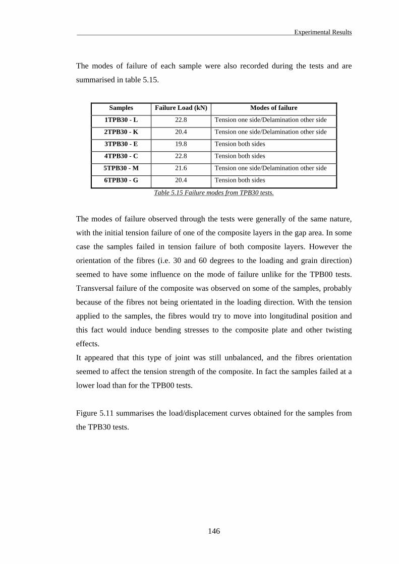
Experimental Results
The modes of failure of each sample were also recorded during the tests and are
summarised in table 5.15.
Samples Failure Load (kN) Modes of failure
1TPB30 - L 22.8 Tension one side/Delamination other side
2TPB30 - K 20.4 Tension one side/Delamination other side
3TPB30 - E 19.8 Tension both sides
4TPB30 - C 22.8 Tension both sides
5TPB30 - M 21.6 Tension one side/Delamination other side
6TPB30 - G 20.4 Tension both sides
Table 5.15 Failure modes from TPB30 tests.
The modes of failure observed through the tests were generally of the same nature,
with the initial tension failure of one of the composite layers in the gap area. In some
case the samples failed in tension failure of both composite layers. However the
orientation of the fibres (i.e. 30 and 60 degrees to the loading and grain direction)
seemed to have some influence on the mode of failure unlike for the TPB00 tests.
Transversal failure of the composite was observed on some of the samples, probably
because of the fibres not being orientated in the loading direction. With the tension
applied to the samples, the fibres would try to move into longitudinal position and
this fact would induce bending stresses to the composite plate and other twisting
effects.
It appeared that this type of joint was still unbalanced, and the fibres orientation
seemed to affect the tension strength of the composite. In fact the samples failed at a
lower load than for the TPB00 tests.
Figure 5.11 summarises the load/displacement curves obtained for the samples from
the TPB30 tests.
146
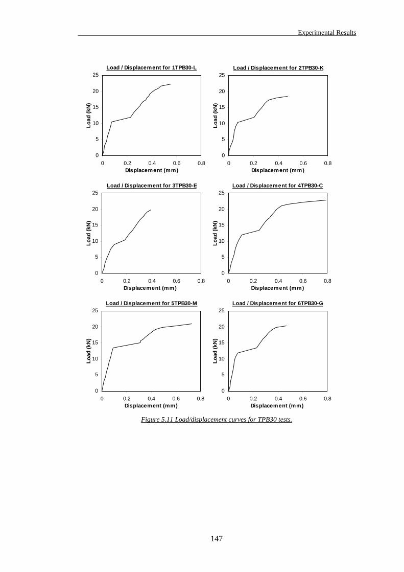
Experimental Results
Load / Displacement for 1TPB30-L
0
5
10
15
20
25
0 0.2 0.4 0.6 0.8Displacement (mm)
Load
(kN
)
Load / Displacement for 2TPB30-K
0
5
10
15
20
25
0 0.2 0.4 0.6 0.8Displacement (mm)
Load
(kN
)
Load / Displacement for 3TPB30-E
0
5
10
15
20
25
0 0.2 0.4 0.6 0.8Displacement (mm)
Load
(kN
)
Load / Displacement for 4TPB30-C
0
5
10
15
20
25
0 0.2 0.4 0.6 0.8Displacement (mm)
Load
(kN
)
Load / Displacement for 5TPB30-M Load / Displacement for 6TPB30-G
Figure 5.11 Load/displacement curves for TPB30 tests.
0
5
10
15
20
25
0 0.2 0.4 0.6 0.8Displacement (mm)
Load
(kN
)
0
5
10
15
20
25
0 0.2 0.4 0.6 0.8Displacement (mm)
Load
(kN
)
147
Experimental Results
The displacements were measured using the average readings from the small LVDTs
positioned on the samples sides. However strain gauges were not used on the tested
samples of the TPU10 tests for the same reasons explained before. Because both
perpendicular strands glass fibres strands of the biaxial fabric were not orientated in
the loading direction, significant bending and twisting effects have occurred during
the test within the composite layers. This would have made the use of strain gauges
even more ineffective.
The load/displacement curves for the TPB30 tests show that the displacements
recorded around the gap between the connected members are even smaller than for
TPB00 tests, because they never exceed 0.8 mm at failure.
The failure loads recorded for the six samples are relatively uniform and are also
lower than for TPB00 tests, ranging between 19.8 and 22.8 kN.
The elastic behaviour of the samples exceeds 82% of the overall recorded joint slip
for a maximum elastic displacement of 0.39 mm.
All the samples develop a plastic behaviour. As mentioned before, the sudden
increment of displacement due to the tension failure of the epoxy resin infiltrated in
the gap area is dramatically affecting the stiffness of the samples. This change of
slope (and stiffness) is bringing the curve towards the horizontal, which may be
assumed as an elastic-plastic behaviour. In fact the sample is still behaving elastically
and unlike for the TPU10 tests, the curves generally show a point of flexure between
the linear elastic and the plastic parts of the curve.
The comparison of various parameters obtained from these tests are presented and
discussed in the following section.
148
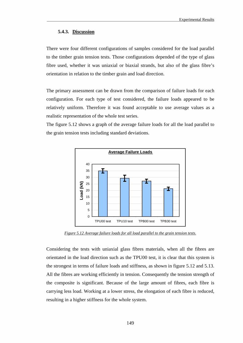
Experimental Results
5.4.3. Discussion
There were four different configurations of samples considered for the load parallel
to the timber grain tension tests. Those configurations depended of the type of glass
fibre used, whether it was uniaxial or biaxial strands, but also of the glass fibre’s
orientation in relation to the timber grain and load direction.
The primary assessment can be drawn from the comparison of failure loads for each
configuration. For each type of test considered, the failure loads appeared to be
relatively uniform. Therefore it was found acceptable to use average values as a
realistic representation of the whole test series.
The figure 5.12 shows a graph of the average failure loads for all the load parallel to
the grain tension tests including standard deviations.
Average Failure Loads
0
5
10
15
20
25
30
35
40
TPU00 test TPU10 test TPB00 test TPB30 test
Load
(kN
)
Figure 5.12 Average failure loads for all load parallel to the grain tension tests.
Considering the tests with uniaxial glass fibres materials, when all the fibres are
orientated in the load direction such as the TPU00 test, it is clear that this system is
the strongest in terms of failure loads and stiffness, as shown in figure 5.12 and 5.13.
All the fibres are working efficiently in tension. Consequently the tension strength of
the composite is significant. Because of the large amount of fibres, each fibre is
carrying less load. Working at a lower stress, the elongation of each fibre is reduced,
resulting in a higher stiffness for the whole system.
149
Experimental Results
The figure 5.13 shows a graph of the average stiffness for all the load parallel to the
grain tension tests including standard deviations.
Average Stiffness
010
2030
4050
6070
8090
100
TPU00 test TPU10 test TPB00 test TPB30 test
Stiff
ness
(kN
/mm
)
Figure 5.13 Average stiffness for all load parallel to the grain tension tests.
Looking at the TPU10 test, the only difference from the previous test is that the
fibres were bonded to the timber with an inclination of 10 degrees to the grain and
load direction. It results in failure loads more than 15% lower and in stiffness more
than 25% lower than for the TPU00 test. The slight orientation of fibres is weakening
the system significantly. The same mode of failure by delamination occurred for
TPU00 and TPU10 Tests, revealing that the tension strength of the composite matrix
is still higher than the bond strength.
As explained before, premature delamination is observed on the TPU10 test because
the system is not tension only any longer. With the load applied, the composite layer
appeared to be “pulled” in the longitudinal direction. In fact, with tension applied
longitudinally, the anisotropy of the composite does not allow it to resist the tension
directly. Only the fibres are able to carry a substantial amount of tension in the
composite layer, but because of their orientation, only a reduced area of the
composite is effective. The “reduced” composite plate is subject to a combination of
tension and bending stresses. This combined system is leading to the premature
failure by delamination at the interface between the composite and the wood.
The maximum slip in the gap at failure did not exceed 0.75 mm for the TPU10 test,
which is to be compared with the maximum slip of 1.1 mm for TPU00 test. However
the maximum elastic displacement calculated from the curves, did not exceed
150
Experimental Results
0.5 mm for the TPU10 test, which is to be compared with the maximum 0.54 mm for
TPU00 test. The fact that the TPU10 test had a limited slip at failure compared to the
TPU00 test, and that the elastic slip for TPU10 and TPU00 tests were of the same
magnitude, confirmed the premature failure of the TPU10 tests in relation to its
strength. Moreover the curves of TPU10 test showed that the samples did not reach a
plastic behaviour and only remained in an elastic/plastic stage before failure, as
explained previously.
Considering now the tests with biaxial glass fibres materials, when half the fibres are
orientated in one direction and the other half in the perpendicular direction. For the
TPB00 test, half of the fibres were orientated in the load direction, the other half
were perpendicular to it. Because of the configuration, which was a tension only test,
the fibres in the load direction were effectively carrying all the loads. With a smaller
amount of fibres working than for the TPU00 test, the fibres were exposed to higher
stresses and thus the tension capacity of the composite was reduced. On the other
hand, the bonding area remained the same and if the fibres of the TPB00 test could
carry the load, the same range of failure load than TPU00 test could be expected. The
mode of failure observed for TPB00 test was however tension rupture of the fibres
and delamination. These reasons explained why the failure loads obtained from the
TPB00 test were lower than for TPU00 test.
Working at high stresses, the elongation of each fibre in the load direction was
significant, resulting in a high slip in the gap area, with a maximum of 1.2 mm,
similar value to TPU00 test. High slip but lower failure load would give the
TPB00 test a lower stiffness than the TPU00 test, as shown in figure 5.13.
Finally, the TPB30 test was a variation where one half of the fibres was orientated
30 degrees from the grain and load direction and because they were perpendicular,
the other half of the fibres was orientated 60 degrees from the grain and load
direction. The modes of failure observed here were similar to the TPB00 test because
of the tension failure of the fibres and partial Delamination. As a result, transversal
rupture of the fibres was observed (due to the combined failure modes), following
the orientation to the load direction (30 degrees).
The failure load was generally 20% lower than for the TPB00 test. Once again, it
seemed that premature failure was due to the fibre orientation, which weakened the
151
Experimental Results
joint significantly. The slip-load curves showed an elastic and plastic behaviour
before failure. The maximum displacement did not exceed 0.8 mm, a much smaller
value than for the TPB00 test. The stiffness based on elastic behaviour was only
10% less than for the TPB00 test. The fact that both strands of fibres were bonded to
the timber with an angular orientation to the load (unlike TPB00 configuration where
only one strand is in fact loaded) improved the stiffness of the system.
Probably the combination of stresses was less significant at the interface between the
composite and the wood, as it was for the TPU10 test. Because of the two strands,
the combined stresses partially cancelled each other in a way, but the fibres were still
trying to reach a longitudinal position, within the composite. This explained the
tension rupture and the partial Delamination, which occurred at failure.
Those four series of tests were only considering the tension load applied in the
timber grain direction. The series of tests presented in the next section were carried
out to assess the effects on joints where the tension load was applied with an angle to
the timber grain direction.
152
Experimental Results
5.5. Tension not parallel to the grain tests
The second experimental tests with load not parallel to the grain were carried out on
samples made of two timber pieces connected together with a defined angle. In fact,
one of the timber pieces had the load applied in its grain direction and transferred the
load through the joint to the other piece with that defined angle. A different rig
configuration was used for this series of tests. An additional steel frame including a
steel box was required to hold the inclined timber piece. This frame had to be free to
rotate in respect of the load direction, to allow axial loading of the sample, as
explained in details in chapter 4. There were six different series of tests, which
consisted of samples made with uniaxial and biaxial glass fibres positioned with
various orientations to the timber grain direction. The results of these tests are
presented in the following sections.
5.5.1. TNU90 and TNB90 Tests
These tests were carried out with samples made of two timber pieces connected
perpendicularly, which means that one piece had the load applied perpendicular to its
grain direction. Two different types of samples were tested in tension with the load
applied perpendicular to the grain:
• Tension Not parallel with Uniaxial glass fibre UT-E500, where the load was
applied in the glass fibre direction (α = 0°) but perpendicular to the grain
(β = 90°) of the timber piece considered. The sample type was classified as
TNU90.
• Tension Not parallel with Biaxial glass fibre XE450, where the load was applied
in the glass fibre direction (α = 0°) but perpendicular to the grain (β = 90°). The
sample type was classified as TNB90.
Various measurements were carried out on these samples during test. The testing rig
and the equipment used were presented in the previous chapter.
The bottom piece of the sample was positioned between the pair of steel plates and
bolted through the shear plate connectors. The top piece was fitted within the steel
153
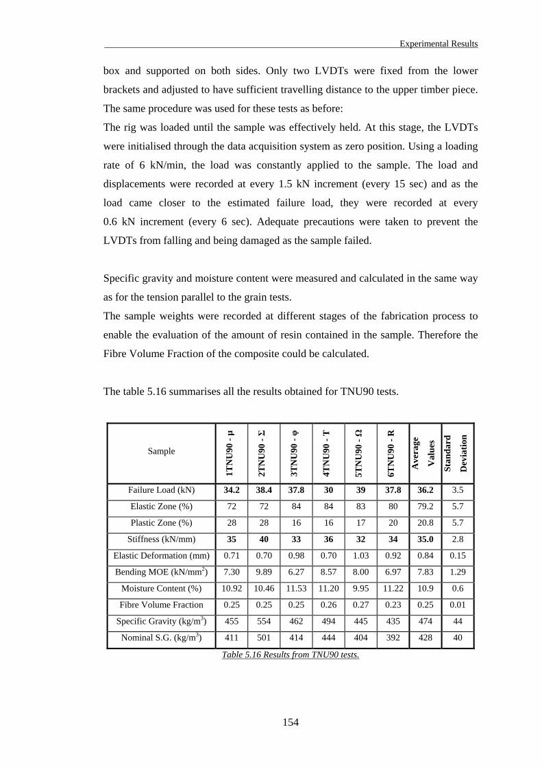
Experimental Results
box and supported on both sides. Only two LVDTs were fixed from the lower
brackets and adjusted to have sufficient travelling distance to the upper timber piece.
The same procedure was used for these tests as before:
The rig was loaded until the sample was effectively held. At this stage, the LVDTs
were initialised through the data acquisition system as zero position. Using a loading
rate of 6 kN/min, the load was constantly applied to the sample. The load and
displacements were recorded at every 1.5 kN increment (every 15 sec) and as the
load came closer to the estimated failure load, they were recorded at every
0.6 kN increment (every 6 sec). Adequate precautions were taken to prevent the
LVDTs from falling and being damaged as the sample failed.
Specific gravity and moisture content were measured and calculated in the same way
as for the tension parallel to the grain tests.
The sample weights were recorded at different stages of the fabrication process to
enable the evaluation of the amount of resin contained in the sample. Therefore the
Fibre Volume Fraction of the composite could be calculated.
The table 5.16 summarises all the results obtained for TNU90 tests.
Sample
1TN
U90
- µ
2TN
U90
- Σ
3TN
U90
- φ
4TN
U90
- T
5TN
U90
- Ω
6TN
U90
- R
Ave
rage
Val
ues
Stan
dard
Dev
iatio
n
Failure Load (kN) 34.2 38.4 37.8 30 39 37.8 36.2 3.5
Elastic Zone (%) 72 72 84 84 83 80 79.2 5.7
Plastic Zone (%) 28 28 16 16 17 20 20.8 5.7
Stiffness (kN/mm) 35 40 33 36 32 34 35.0 2.8
Elastic Deformation (mm) 0.71 0.70 0.98 0.70 1.03 0.92 0.84 0.15
Bending MOE (kN/mm2) 7.30 9.89 6.27 8.57 8.00 6.97 7.83 1.29
Moisture Content (%) 10.92 10.46 11.53 11.20 9.95 11.22 10.9 0.6
Fibre Volume Fraction 0.25 0.25 0.25 0.26 0.27 0.23 0.25 0.01
Specific Gravity (kg/m3) 455 554 462 494 445 435 474 44
Nominal S.G. (kg/m3) 411 501 414 444 404 392 428 40
Table 5.16 Results from TNU90 tests.
154
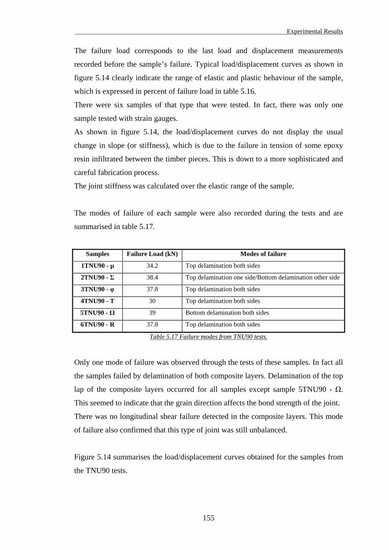
Experimental Results
The failure load corresponds to the last load and displacement measurements
recorded before the sample’s failure. Typical load/displacement curves as shown in
figure 5.14 clearly indicate the range of elastic and plastic behaviour of the sample,
which is expressed in percent of failure load in table 5.16.
There were six samples of that type that were tested. In fact, there was only one
sample tested with strain gauges.
As shown in figure 5.14, the load/displacement curves do not display the usual
change in slope (or stiffness), which is due to the failure in tension of some epoxy
resin infiltrated between the timber pieces. This is down to a more sophisticated and
careful fabrication process.
The joint stiffness was calculated over the elastic range of the sample.
The modes of failure of each sample were also recorded during the tests and are
summarised in table 5.17.
Samples Failure Load (kN) Modes of failure
1TNU90 - µ 34.2 Top delamination both sides
2TNU90 - Σ 38.4 Top delamination one side/Bottom delamination other side
3TNU90 - φ 37.8 Top delamination both sides
4TNU90 - T 30 Top delamination both sides
5TNU90 - Ω 39 Bottom delamination both sides
6TNU90 - R 37.8 Top delamination both sides
Table 5.17 Failure modes from TNU90 tests.
Only one mode of failure was observed through the tests of these samples. In fact all
the samples failed by delamination of both composite layers. Delamination of the top
lap of the composite layers occurred for all samples except sample 5TNU90 - Ω.
This seemed to indicate that the grain direction affects the bond strength of the joint.
There was no longitudinal shear failure detected in the composite layers. This mode
of failure also confirmed that this type of joint was still unbalanced.
Figure 5.14 summarises the load/displacement curves obtained for the samples from
the TNU90 tests.
155
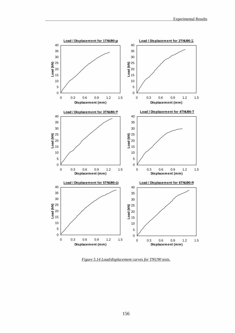
Experimental Results
Load / Displacement for 1TNU90-
0
5
10
15
20
25
30
35
40
0 0.3 0.6 0.9 1.2 1.5Displacement (mm)
Load
(kN
)
Load / Displacement for 2TNU90-
0
5
10
15
20
25
30
35
40
0 0.3 0.6 0.9 1.2 1.5Displacement (mm)
Load
(kN
)
Load / Displacement for 3TNU90-
0
5
10
15
20
25
30
35
40
0 0.3 0.6 0.9 1.2 1.5Displacement (mm)
Load
(kN
)
Load / Displacement for 4TNU90-T
0
5
10
15
20
25
30
35
40
0 0.3 0.6 0.9 1.2 1.5Displacement (mm)
Load
(kN
)
Load / Displacement for 5TNU90- Load / Displacement for 6TNU90-R
φ
Σ
Ω
µ
0
5
10
15
20
25
30
35
40
0 0.3 0.6 0.9 1.2Displacement (mm)
Load
(kN
)
Figure 5.14 Load/di
1.50
5
10
15
20
25
30
35
40
0 0.3 0.6 0.9 1.2 1.5Displacement (mm)
Load
(kN
)
splacement curves for TNU90 tests.
156
Experimental Results
The displacements were measured using the average readings from the small LVDTs
positioned on the samples sides. However strain gauges were also used on of the
tested samples, the sample 5TNU90 - Ω. Measurements of strains at precise locations
on the surface of the glass fibre/epoxy composite layers were carried out. These
results are presented later in this chapter, in § 5.6.
The load/displacement curves for the TNU90 tests show that the displacements
recorded around the gap between the connected members never exceed 1.4 mm at
failure.
The failure loads recorded for the six samples are relatively uniform, ranging
between 30 and 39 kN.
The elastic behaviour of the samples exceeds 72% of the overall recorded joint slip
for a maximum elastic displacement of 1.03 mm.
Not all the samples seemed to reach a plastic behaviour at failure. The curves are
reflecting an elastic-plastic behaviour, in a similar manner than the TPU10 tests.
Even the curve from the sample 3TNU90 - φ is not showing any sign of plasticity.
The absence of point of flexure shows that the transition is progressive and does not
highlight the plastic region.
The comparison of various parameters obtained from these tests is presented in the
discussion section, in § 5.5.4.
157
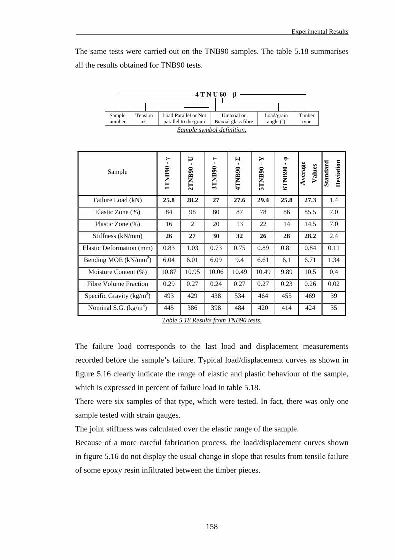
Experimental Results
The same tests were carried out on the TNB90 samples. The table 5.18 summarises
all the results obtained for TNB90 tests.
Sample number
Tension test
Load Parallel or Not parallel to the grain
Uniaxial or Biaxial glass fibre
Load/grain angle (º)
Timber type
4 T N U 60 – β
Sample symbol definition.
Sample 1T
NB
90 - γ
2TN
B90
- U
3TN
B90
- τ
4TN
B90
- Σ
5TN
B90
- Y
6TN
B90
- φ
Ave
rage
Val
ues
Stan
dard
Dev
iatio
n
Failure Load (kN) 25.8 28.2 27 27.6 29.4 25.8 27.3 1.4
Elastic Zone (%) 84 98 80 87 78 86 85.5 7.0
Plastic Zone (%) 16 2 20 13 22 14 14.5 7.0
Stiffness (kN/mm) 26 27 30 32 26 28 28.2 2.4
Elastic Deformation (mm) 0.83 1.03 0.73 0.75 0.89 0.81 0.84 0.11
Bending MOE (kN/mm2) 6.04 6.01 6.09 9.4 6.61 6.1 6.71 1.34
Moisture Content (%) 10.87 10.95 10.06 10.49 10.49 9.89 10.5 0.4
Fibre Volume Fraction 0.29 0.27 0.24 0.27 0.27 0.23 0.26 0.02
Specific Gravity (kg/m3) 493 429 438 534 464 455 469 39
Nominal S.G. (kg/m3) 445 386 398 484 420 414 424 35
Table 5.18 Results from TNB90 tests.
The failure load corresponds to the last load and displacement measurements
recorded before the sample’s failure. Typical load/displacement curves as shown in
figure 5.16 clearly indicate the range of elastic and plastic behaviour of the sample,
which is expressed in percent of failure load in table 5.18.
There were six samples of that type, which were tested. In fact, there was only one
sample tested with strain gauges.
The joint stiffness was calculated over the elastic range of the sample.
Because of a more careful fabrication process, the load/displacement curves shown
in figure 5.16 do not display the usual change in slope that results from tensile failure
of some epoxy resin infiltrated between the timber pieces.
158
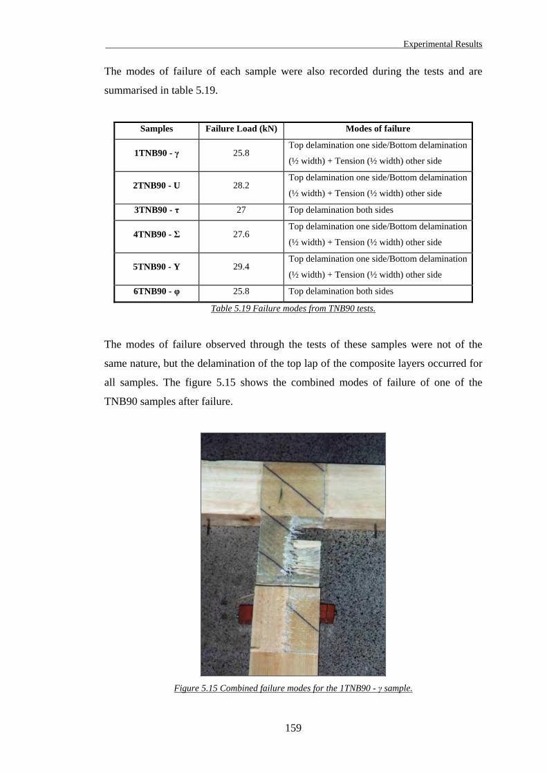
Experimental Results
The modes of failure of each sample were also recorded during the tests and are
summarised in table 5.19.
Samples Failure Load (kN) Modes of failure
1TNB90 - γ 25.8 Top delamination one side/Bottom delamination
(½ width) + Tension (½ width) other side
2TNB90 - U 28.2 Top delamination one side/Bottom delamination
(½ width) + Tension (½ width) other side
3TNB90 - τ 27 Top delamination both sides
4TNB90 - Σ 27.6 Top delamination one side/Bottom delamination
(½ width) + Tension (½ width) other side
5TNB90 - Y 29.4 Top delamination one side/Bottom delamination
(½ width) + Tension (½ width) other side
6TNB90 - φ 25.8 Top delamination both sides
Table 5.19 Failure modes from TNB90 tests.
The modes of failure observed through the tests of these samples were not of the
same nature, but the delamination of the top lap of the composite layers occurred for
all samples. The figure 5.15 shows the combined modes of failure of one of the
TNB90 samples after failure.
Figure 5.15 Combined failure modes for the 1TNB90 - γ sample.
159
Experimental Results
It was difficult to identify which part of the composite failed first because the joint
was hidden by the steel box. However it is likely that the delamination at the top of
one side occurred first, all the loads were then transferred to the other layer, which
failed soon after in multiple modes of failure. With such high loads applied to only
one layer, rupture of the fibres would have started and followed by the delamination.
Because only half the width failed by fibre rupture, longitudinal shear failure
occurred as a result of the delamination of the other half width. In figure 5.15, the
broken fibres along the middle of the bottom lap of the composite are confirming
these comments.
Because the joint failed in delamination and tension modes, with the composite
failing in the top and bottom zones, this type of joint could be considered as
balanced.
Figure 5.16 summarises the load/displacement curves obtained for the samples from
the TNB90 tests.
160

Experimental Results
Load / Displacement for 1TNB90-
0
5
10
15
20
25
30
0 0.2 0.4 0.6 0.8 1 1.2 1.4Displacement (mm)
Load
(kN
)
Load / Displacement for 2TNB90-U
0
5
10
15
20
25
30
0 0.2 0.4 0.6 0.8 1 1.2 1.4Displacement (mm)
Load
(kN
)
Load / Displacement for 3TNB90-
0
5
10
15
20
25
30
0 0.2 0.4 0.6 0.8 1 1.2 1.4Displacement (mm)
Load
(kN
)
Load / Displacement for 4TNB90-
0
5
10
15
20
25
30
0 0.2 0.4 0.6 0.8 1 1.2 1.4Displacement (mm)
Load
(kN
)
Load / Displacement for 5TNB90-Y Load / Displacement for 6TNB90-
τ Σ
φ
γ
Figure 5.16 Load/displacement curves for TNB90 tests.
0
5
10
15
20
25
30
0 0.2 0.4 0.6 0.8 1 1.2 1.4Displacement (mm)
Load
(kN
)
0
5
10
15
20
25
30
0 0.2 0.4 0.6 0.8 1 1.2 1.4Displacement (mm)
Load
(kN
)
161
Experimental Results
The displacements were measured using the average readings from the small LVDTs
positioned on the samples sides. However strain gauges were also used on of the
tested samples, the sample 6TNB90 - φ. Measurements of strains at precise locations
on the surface of the glass fibre/epoxy composite layers were carried out. These
results are presented in § 5.6.
The load/displacement curves for the TNB90 tests show that the displacements
recorded around the gap between the connected members never exceed 1.4 mm at
failure.
The failure loads recorded for the six samples are relatively uniform, ranging
between 25.8 and 29.4 kN.
The elastic behaviour of the samples exceeds 78% of the overall recorded joint slip
for a maximum elastic displacement of 1.03 mm.
Here again, not all the samples seemed to reach a plastic behaviour at failure. The
curves are reflecting an elastic-plastic behaviour, in a similar manner than the
TNU90 tests. However four samples out of the six showed significant signs of
plasticity at failure. Even two of them displayed a point of flexure, confirming that
some plastic behaviour was occurring at failure and that the transition is less
progressive than for the TNU90 tests.
The comparison of various parameters obtained from these tests is presented in the
discussion section, in § 5.5.4.
162
Experimental Results
5.5.2. TNU60 and TNB60 Tests
As explained previously, TNU60 and TNB60 tests were carried out with samples
made of two timber pieces connected together with an angle of 60 degrees. This
means one of the timber pieces had the load applied in its grain direction and
transferred the load through the joint to the other piece with an angle of 60 degrees.
Two different types of samples were tested in tension with the load applied at an
angle of 60 degrees to the grain:
• Tension Not parallel with Uniaxial glass fibre UT-E500, where the load was
applied in the glass fibre direction (α = 0°) but with an angle of 60° to the grain
(β = 60°) of the timber piece considered. The sample type was classified as
TNU60.
• Tension Not parallel with Biaxial glass fibre XE450, where the load was applied
in the glass fibre direction (α = 0°) but with an angle of 60° to the grain (β = 60°).
The sample type was classified as TNB60.
Various measurements were carried out on these samples during test. The testing rig
and the equipment used were presented in the previous chapter.
The samples positioning, displacement measurements using LVDTs through the data
acquisition system, loading rates, the moisture content, density and
FVF measurements were all carried out as for TNU90 and TNB90 tests.
163
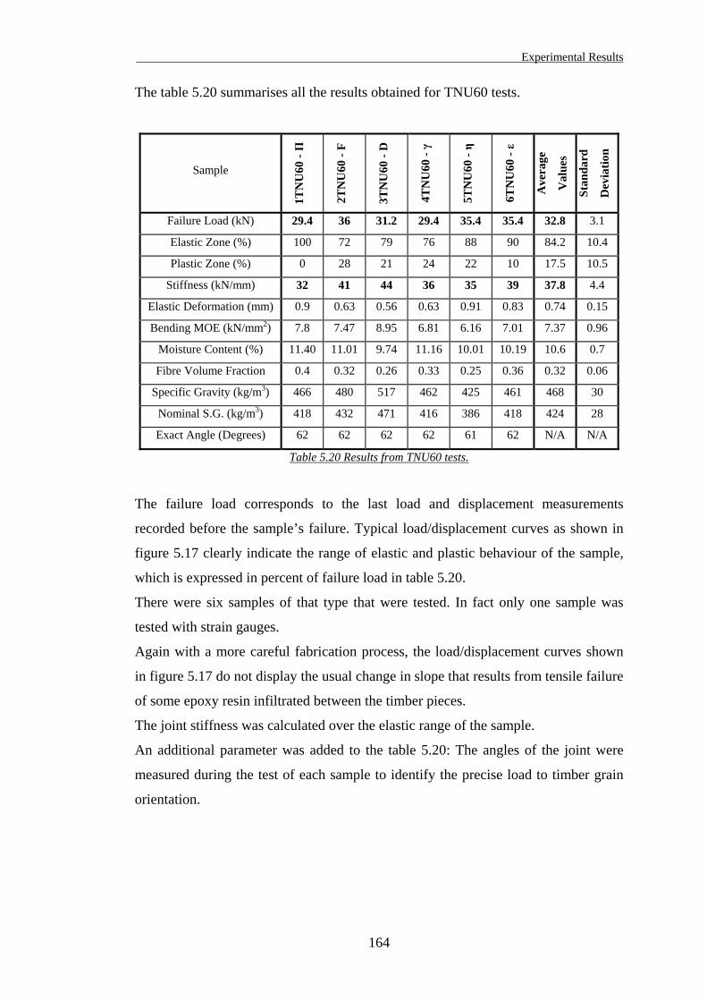
Experimental Results
The table 5.20 summarises all the results obtained for TNU60 tests.
Sample
1TN
U60
- Π
2TN
U60
- F
3TN
U60
- D
4TN
U60
- γ
5TN
U60
- η
6TN
U60
- ε
Ave
rage
Val
ues
Stan
dard
Dev
iatio
n
Failure Load (kN) 29.4 36 31.2 29.4 35.4 35.4 32.8 3.1
Elastic Zone (%) 100 72 79 76 88 90 84.2 10.4
Plastic Zone (%) 0 28 21 24 22 10 17.5 10.5
Stiffness (kN/mm) 32 41 44 36 35 39 37.8 4.4
Elastic Deformation (mm) 0.9 0.63 0.56 0.63 0.91 0.83 0.74 0.15
Bending MOE (kN/mm2) 7.8 7.47 8.95 6.81 6.16 7.01 7.37 0.96
Moisture Content (%) 11.40 11.01 9.74 11.16 10.01 10.19 10.6 0.7
Fibre Volume Fraction 0.4 0.32 0.26 0.33 0.25 0.36 0.32 0.06
Specific Gravity (kg/m3) 466 480 517 462 425 461 468 30
Nominal S.G. (kg/m3) 418 432 471 416 386 418 424 28
Exact Angle (Degrees) 62 62 62 62 61 62 N/A N/A
Table 5.20 Results from TNU60 tests.
The failure load corresponds to the last load and displacement measurements
recorded before the sample’s failure. Typical load/displacement curves as shown in
figure 5.17 clearly indicate the range of elastic and plastic behaviour of the sample,
which is expressed in percent of failure load in table 5.20.
There were six samples of that type that were tested. In fact only one sample was
tested with strain gauges.
Again with a more careful fabrication process, the load/displacement curves shown
in figure 5.17 do not display the usual change in slope that results from tensile failure
of some epoxy resin infiltrated between the timber pieces.
The joint stiffness was calculated over the elastic range of the sample.
An additional parameter was added to the table 5.20: The angles of the joint were
measured during the test of each sample to identify the precise load to timber grain
orientation.
164
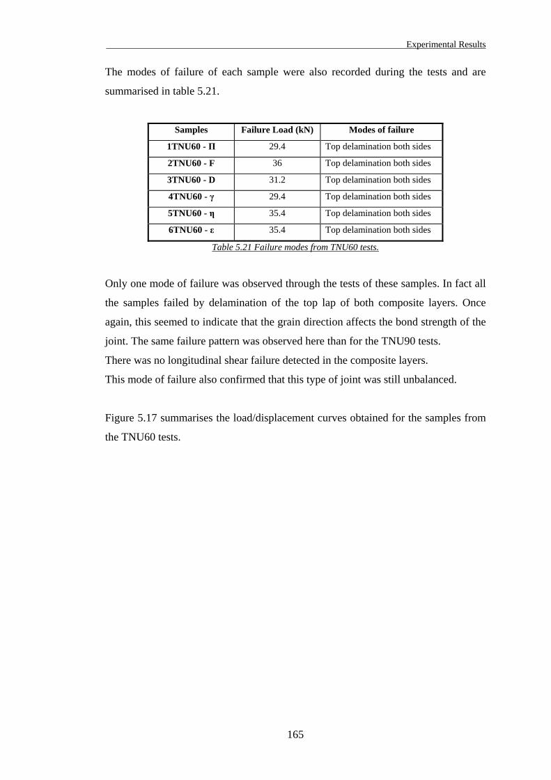
Experimental Results
The modes of failure of each sample were also recorded during the tests and are
summarised in table 5.21.
Samples Failure Load (kN) Modes of failure
1TNU60 - Π 29.4 Top delamination both sides
2TNU60 - F 36 Top delamination both sides
3TNU60 - D 31.2 Top delamination both sides
4TNU60 - γ 29.4 Top delamination both sides
5TNU60 - η 35.4 Top delamination both sides
6TNU60 - ε 35.4 Top delamination both sides
Table 5.21 Failure modes from TNU60 tests.
Only one mode of failure was observed through the tests of these samples. In fact all
the samples failed by delamination of the top lap of both composite layers. Once
again, this seemed to indicate that the grain direction affects the bond strength of the
joint. The same failure pattern was observed here than for the TNU90 tests.
There was no longitudinal shear failure detected in the composite layers.
This mode of failure also confirmed that this type of joint was still unbalanced.
Figure 5.17 summarises the load/displacement curves obtained for the samples from
the TNU60 tests.
165
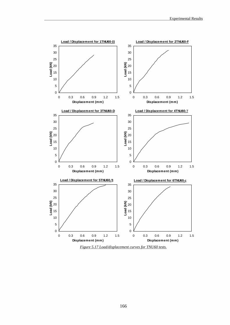
Experimental Results
Load / Displacement for 1TNU60-
0
5
10
15
20
25
30
35
0 0.3 0.6 0.9 1.2 1.5Displacement (mm)
Load
(kN
)
Load / Displacement for 2TNU60-F
0
5
10
15
20
25
30
35
0 0.3 0.6 0.9 1.2 1.5Displacement (mm)
Load
(kN
)
Load / Displacement for 3TNU60-D
0
5
10
15
20
25
30
35
0 0.3 0.6 0.9 1.2 1.5Displacement (mm)
Load
(kN
)
Load / Displacement for 4TNU60-
0
5
10
15
20
25
30
35
0 0.3 0.6 0.9 1.2 1.5Displacement (mm)
Load
(kN
)
Load / Displacement for 5TNU60-η
Π
γ
Figure 5.17 Load/displacement curves for TNU60 tests.
0
5
10
15
20
25
30
35
0 0.3 0.6 0.9 1.2 1.5Displacement (mm)
Load
(kN
)
Load / Displacement for 6TNU60
0
5
10
15
20
25
30
35
0 0.3 0.6 0.9 1.2Displacement (mm)
Load
(kN
)
ε
166
-
1.5
Experimental Results
The displacements were measured using the average readings from the small LVDTs
positioned on the samples sides. However strain gauges were also used on of the
tested samples, the sample 5TNU60 - η. Measurements of strains at precise locations
on the surface of the glass fibre/epoxy composite layers were carried out. These
results are presented in § 5.6.
The load/displacement curves for the TNU60 tests show that the displacements
recorded around the gap between the connected members never exceed 1.5 mm at
failure.
The failure loads recorded for the six samples are relatively uniform, ranging
between 29.4 and 35.4 kN.
The elastic behaviour of the samples exceeds 72% of the overall recorded joint slip
for a maximum elastic displacement of 0.91 mm.
Here again, not all the samples seemed to reach a plastic behaviour at failure. The
curves are reflecting an elastic-plastic behaviour, in a similar manner than the
TNU90 tests. However the last two samples failed at a higher load than the curves
end indicated on the graph, because of large deformation occurring before failure.
Points of flexure are visible, particularly on sample No 3, 4 and 5. This confirms that
some plastic behaviour developed at failure, and the transition was less progressive
than for the TNU90 tests.
The comparison of various parameters obtained from these tests is presented in the
discussion section, in § 5.5.4.
167
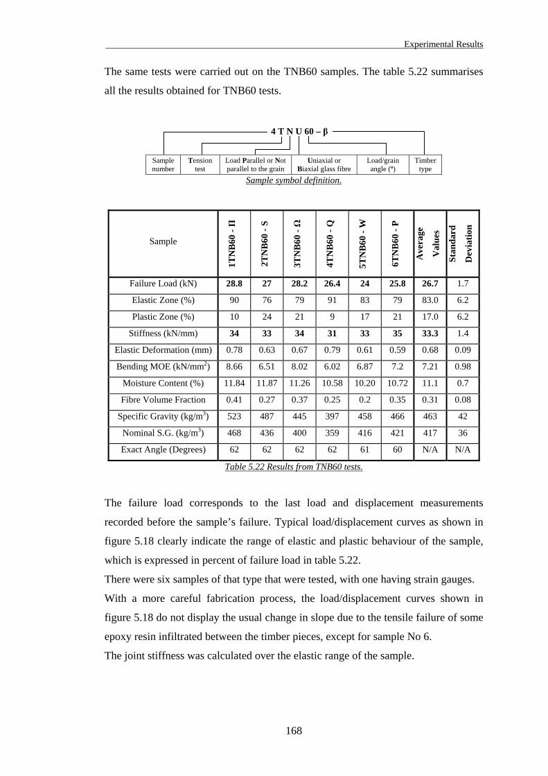
Experimental Results
The same tests were carried out on the TNB60 samples. The table 5.22 summarises
all the results obtained for TNB60 tests.
Sample number
Tension test
Load Parallel or Not parallel to the grain
Uniaxial or Biaxial glass fibre
Load/grain angle (º)
Timber type
4 T N U 60 – β
Sample symbol definition.
Sample 1T
NB
60 - Π
2TN
B60
- S
3TN
B60
- Ω
4TN
B60
- Q
5TN
B60
- W
6TN
B60
- P
Ave
rage
Val
ues
Stan
dard
Dev
iatio
n
Failure Load (kN) 28.8 27 28.2 26.4 24 25.8 26.7 1.7
Elastic Zone (%) 90 76 79 91 83 79 83.0 6.2
Plastic Zone (%) 10 24 21 9 17 21 17.0 6.2
Stiffness (kN/mm) 34 33 34 31 33 35 33.3 1.4
Elastic Deformation (mm) 0.78 0.63 0.67 0.79 0.61 0.59 0.68 0.09
Bending MOE (kN/mm2) 8.66 6.51 8.02 6.02 6.87 7.2 7.21 0.98
Moisture Content (%) 11.84 11.87 11.26 10.58 10.20 10.72 11.1 0.7
Fibre Volume Fraction 0.41 0.27 0.37 0.25 0.2 0.35 0.31 0.08
Specific Gravity (kg/m3) 523 487 445 397 458 466 463 42
Nominal S.G. (kg/m3) 468 436 400 359 416 421 417 36
Exact Angle (Degrees) 62 62 62 62 61 60 N/A N/A
Table 5.22 Results from TNB60 tests.
The failure load corresponds to the last load and displacement measurements
recorded before the sample’s failure. Typical load/displacement curves as shown in
figure 5.18 clearly indicate the range of elastic and plastic behaviour of the sample,
which is expressed in percent of failure load in table 5.22.
There were six samples of that type that were tested, with one having strain gauges.
With a more careful fabrication process, the load/displacement curves shown in
figure 5.18 do not display the usual change in slope due to the tensile failure of some
epoxy resin infiltrated between the timber pieces, except for sample No 6.
The joint stiffness was calculated over the elastic range of the sample.
168
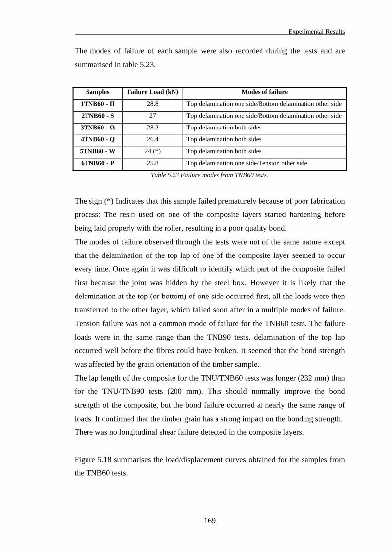
Experimental Results
The modes of failure of each sample were also recorded during the tests and are
summarised in table 5.23.
Samples Failure Load (kN) Modes of failure
1TNB60 - Π 28.8 Top delamination one side/Bottom delamination other side
2TNB60 - S 27 Top delamination one side/Bottom delamination other side
3TNB60 - Ω 28.2 Top delamination both sides
4TNB60 - Q 26.4 Top delamination both sides
5TNB60 - W 24 (*) Top delamination both sides
6TNB60 - P 25.8 Top delamination one side/Tension other side
Table 5.23 Failure modes from TNB60 tests.
The sign (*) Indicates that this sample failed prematurely because of poor fabrication
process: The resin used on one of the composite layers started hardening before
being laid properly with the roller, resulting in a poor quality bond.
The modes of failure observed through the tests were not of the same nature except
that the delamination of the top lap of one of the composite layer seemed to occur
every time. Once again it was difficult to identify which part of the composite failed
first because the joint was hidden by the steel box. However it is likely that the
delamination at the top (or bottom) of one side occurred first, all the loads were then
transferred to the other layer, which failed soon after in a multiple modes of failure.
Tension failure was not a common mode of failure for the TNB60 tests. The failure
loads were in the same range than the TNB90 tests, delamination of the top lap
occurred well before the fibres could have broken. It seemed that the bond strength
was affected by the grain orientation of the timber sample.
The lap length of the composite for the TNU/TNB60 tests was longer (232 mm) than
for the TNU/TNB90 tests (200 mm). This should normally improve the bond
strength of the composite, but the bond failure occurred at nearly the same range of
loads. It confirmed that the timber grain has a strong impact on the bonding strength.
There was no longitudinal shear failure detected in the composite layers.
Figure 5.18 summarises the load/displacement curves obtained for the samples from
the TNB60 tests.
169
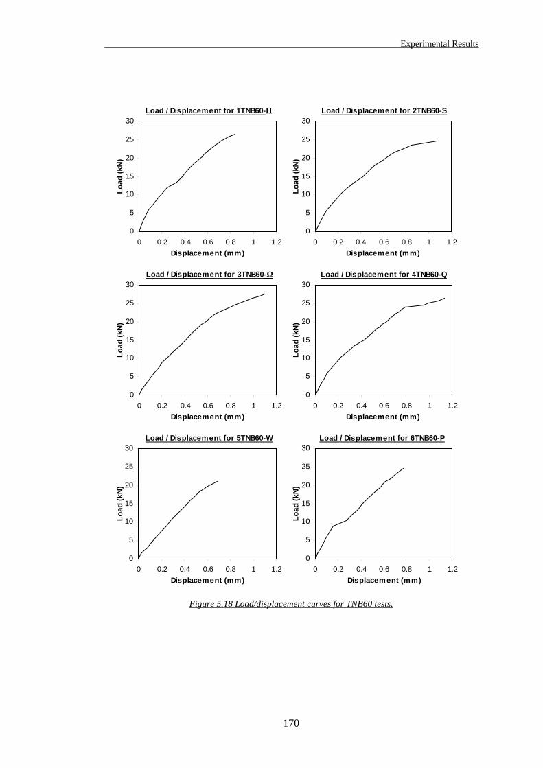
Experimental Results
Figure 5.18 Load/displacement curves for TNB60 tests.
Load / Displacement for 1TNB60-
0
5
10
15
20
25
30
0 0.2 0.4 0.6 0.8 1 1.2Displacement (mm)
Load
(kN
)Load / Displacement for 2TNB60-S
0
5
10
15
20
25
30
0 0.2 0.4 0.6 0.8 1 1.2Displacement (mm)
Load
(kN
)
Load / Displacement for 3TNB60-
0
5
10
15
20
25
30
0 0.2 0.4 0.6 0.8 1 1.2Displacement (mm)
Load
(kN
)
Load / Displacement for 4TNB60-Q
0
5
10
15
20
25
30
0 0.2 0.4 0.6 0.8 1 1.2Displacement (mm)
Load
(kN
)
Load / Displacement for 5TNB60-W
0
5
10
15
20
25
30
0 0.2 0.4 0.6 0.8 1 1.2Displacement (mm)
Load
(kN
)
Load / Displacement for 6TNB60-P
0
5
10
15
20
25
30
0 0.2 0.4 0.6 0.8 1 1.2Displacement (mm)
Load
(kN
)
Π
Ω
170
Experimental Results
The displacements were measured using the average readings from the small LVDTs
positioned on the samples sides. However strain gauges were also used on of the
tested samples, the sample 5TNB60 - W. Measurements of strains at precise
locations on the surface of the glass fibre/epoxy composite layers were carried out.
These results are presented in § 5.6.
The load/displacement curves for the TNB60 tests show that the displacements
recorded around the gap between the connected members never exceed 1.2 mm at
failure.
The failure loads recorded for the six samples are relatively uniform, ranging
between 24 and 28.8 kN.
The elastic behaviour of the samples exceeds 76% of the overall recorded joint slip
for a maximum elastic displacement of 0.79 mm.
Here again, not all the samples seemed to reach a plastic behaviour at failure. The
curves are still reflecting an elastic-plastic behaviour, in a similar manner than the
TNU90 tests. However the first and last two samples failed at a higher load than the
curves end indicated on the graph, because of large deformation occurring before
failure. Only sample No 4 displayed a point of flexure, confirming that some plastic
behaviour was occurring at failure. The curves show that the transition between
elastic and plastic is progressive and does lead to some plasticity at failure.
The comparison of various parameters obtained from these tests is presented in the
discussion section, in § 5.5.4.
171
Experimental Results
5.5.3. TNU30 and TNB30 Tests
As explained previously, TNU30 and TNB30 tests were carried out with samples
made of two timber pieces connected together with an angle of 30 degrees. This
means one of the timber pieces had the load applied in its grain direction and
transferred the load through the joint to the other piece with an angle of 30 degrees.
Two different types of samples were tested in tension with the load applied at an
angle of 30 degrees to the grain:
• Tension Not parallel with Uniaxial glass fibre UT-E500, where the load was
applied in the glass fibre direction (α = 0°) but with an angle of 30° to the grain
(β = 30°) of the timber piece considered. The sample type was classified as
TNU30.
• Tension Not parallel with Biaxial glass fibre XE450, where the load was applied
in the glass fibre direction (α = 0°) but with an angle of 30° to the grain (β = 30°).
The sample type was classified as TNB30.
Various measurements were carried out on these samples during test. The testing rig
and the equipment used are presented in the previous chapter.
The samples positioning, displacement measurements using LVDTs through the data
acquisition system, loading rates, the moisture content, density and
FVF measurements were all carried out as for TNU90 and TNB90 tests.
172
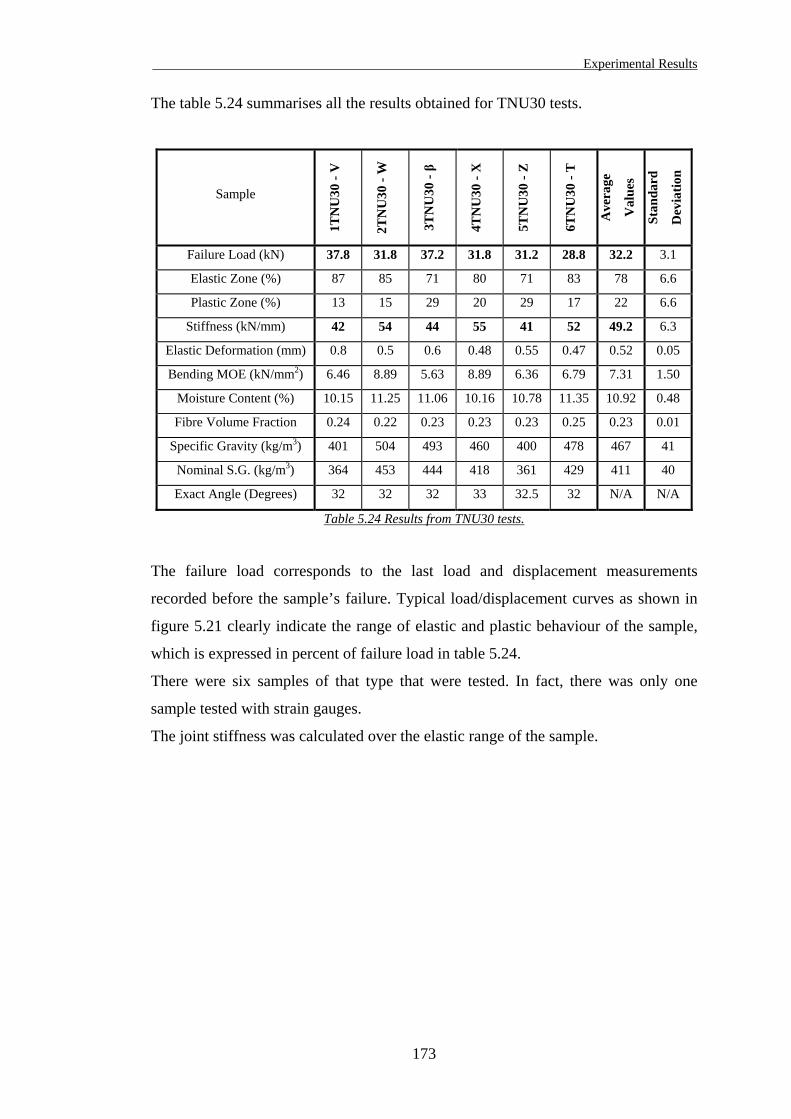
Experimental Results
The table 5.24 summarises all the results obtained for TNU30 tests.
Sample
1TN
U30
- V
2TN
U30
- W
3TN
U30
- β
4TN
U30
- X
5TN
U30
- Z
6TN
U30
- T
Ave
rage
Val
ues
Stan
dard
Dev
iatio
n
Failure Load (kN) 37.8 31.8 37.2 31.8 31.2 28.8 32.2 3.1
Elastic Zone (%) 87 85 71 80 71 83 78 6.6
Plastic Zone (%) 13 15 29 20 29 17 22 6.6
Stiffness (kN/mm) 42 54 44 55 41 52 49.2 6.3
Elastic Deformation (mm) 0.8 0.5 0.6 0.48 0.55 0.47 0.52 0.05
Bending MOE (kN/mm2) 6.46 8.89 5.63 8.89 6.36 6.79 7.31 1.50
Moisture Content (%) 10.15 11.25 11.06 10.16 10.78 11.35 10.92 0.48
Fibre Volume Fraction 0.24 0.22 0.23 0.23 0.23 0.25 0.23 0.01
Specific Gravity (kg/m3) 401 504 493 460 400 478 467 41
Nominal S.G. (kg/m3) 364 453 444 418 361 429 411 40
Exact Angle (Degrees) 32 32 32 33 32.5 32 N/A N/A
Table 5.24 Results from TNU30 tests.
The failure load corresponds to the last load and displacement measurements
recorded before the sample’s failure. Typical load/displacement curves as shown in
figure 5.21 clearly indicate the range of elastic and plastic behaviour of the sample,
which is expressed in percent of failure load in table 5.24.
There were six samples of that type that were tested. In fact, there was only one
sample tested with strain gauges.
The joint stiffness was calculated over the elastic range of the sample.
173
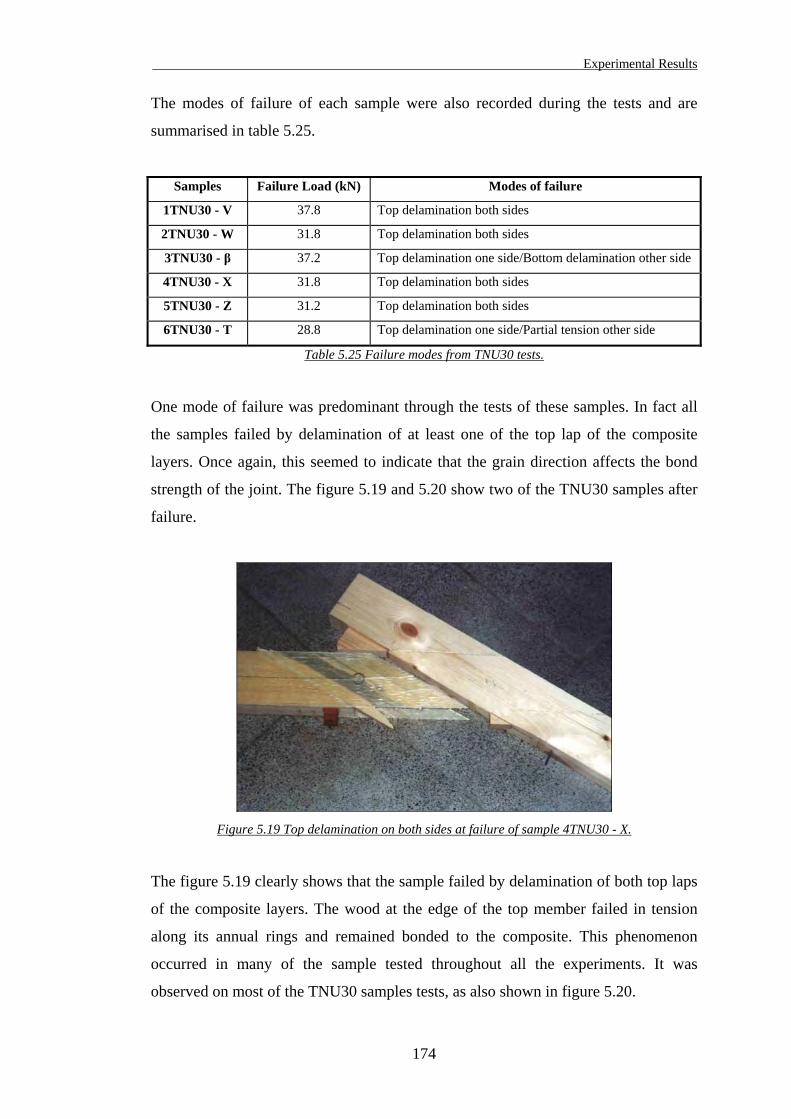
Experimental Results
The modes of failure of each sample were also recorded during the tests and are
summarised in table 5.25.
Samples Failure Load (kN) Modes of failure
1TNU30 - V 37.8 Top delamination both sides
2TNU30 - W 31.8 Top delamination both sides
3TNU30 - β 37.2 Top delamination one side/Bottom delamination other side
4TNU30 - X 31.8 Top delamination both sides
5TNU30 - Z 31.2 Top delamination both sides
6TNU30 - T 28.8 Top delamination one side/Partial tension other side
Table 5.25 Failure modes from TNU30 tests.
One mode of failure was predominant through the tests of these samples. In fact all
the samples failed by delamination of at least one of the top lap of the composite
layers. Once again, this seemed to indicate that the grain direction affects the bond
strength of the joint. The figure 5.19 and 5.20 show two of the TNU30 samples after
failure.
Figure 5.19 Top delamination on both sides at failure of sample 4TNU30 - X.
The figure 5.19 clearly shows that the sample failed by delamination of both top laps
of the composite layers. The wood at the edge of the top member failed in tension
along its annual rings and remained bonded to the composite. This phenomenon
occurred in many of the sample tested throughout all the experiments. It was
observed on most of the TNU30 samples tests, as also shown in figure 5.20.
174
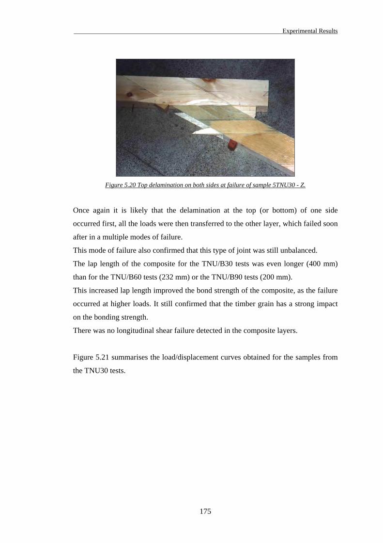
Experimental Results
Figure 5.20 Top delamination on both sides at failure of sample 5TNU30 - Z.
Once again it is likely that the delamination at the top (or bottom) of one side
occurred first, all the loads were then transferred to the other layer, which failed soon
after in a multiple modes of failure.
This mode of failure also confirmed that this type of joint was still unbalanced.
The lap length of the composite for the TNU/B30 tests was even longer (400 mm)
than for the TNU/B60 tests (232 mm) or the TNU/B90 tests (200 mm).
This increased lap length improved the bond strength of the composite, as the failure
occurred at higher loads. It still confirmed that the timber grain has a strong impact
on the bonding strength.
There was no longitudinal shear failure detected in the composite layers.
Figure 5.21 summarises the load/displacement curves obtained for the samples from
the TNU30 tests.
175
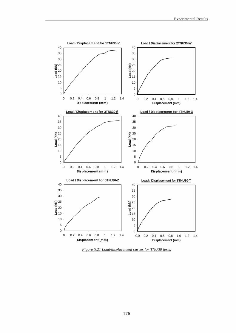
Experimental Results
Load / Displacement for 1TNU30-V
0
5
10
15
20
25
30
35
40
0 0.2 0.4 0.6 0.8 1 1.2 1.4Displacement (mm)
Load
(kN
)
Load / Displacement for 2TNU30-W
0
5
10
15
20
25
30
35
40
0 0,2 0,4 0,6 0,8 1 1,2 1,4Displacement (mm)
Load
(kN
)
Load / Displacement for 3TNU30-
0
5
10
15
20
25
30
35
40
0 0.2 0.4 0.6 0.8 1 1.2 1.4Displacement (mm)
Load
(kN
)
Load / Displacement for 4TNU30-X
0
5
10
15
20
25
30
35
40
0 0.2 0.4 0.6 0.8 1 1.2 1.4Displacement (mm)
Load
(kN
)
Load / Displacement for 5TNU30-Z
0
5
10
15
20
25
30
35
40
0 0.2 0.4 0.6 0.8 1 1.2 1.4Displacement (mm)
Load
(kN
)
Load / Displacement for 6TNU30-T
0
5
10
15
20
25
30
35
40
0,0 0,2 0,4 0,6 0,8 1,0 1,2 1,4Displacement (mm)
Load
(kN
)
β
Figure 5.21 Load/displacement curves for TNU30 tests.
176
Experimental Results
The displacements were measured using the average readings from the small LVDTs
positioned on the samples sides. However strain gauges were also used on of the
tested samples, the sample 1TNU30 - V. Measurements of strains at precise locations
on the surface of the glass fibre/epoxy composite layers were carried out. These
results are presented in § 5.6.
The load/displacement curves for the TNU30 tests show that the displacements
recorded around the gap between the connected members never exceed 1.4 mm at
failure.
The failure loads recorded for the six samples are relatively uniform, ranging
between 28.8 and 37.8 kN.
The elastic behaviour of the samples exceeds 71% of the overall recorded joint slip
for a maximum elastic displacement of 0.8 mm.
The samples developed a plastic behaviour generally. The curves are still reflecting
an elastic-plastic behaviour. However samples No 2, 4, 5 and 6 failed at a higher load
than the curves end indicated on the graph, because of large deformation occurring
before failure. The absence of point of flexure shows that the transition between
elastic and plastic is progressive and do lead to some plasticity at the failure.
The comparison of various parameters obtained from these tests is presented in the
discussion section, in § 5.5.4.
177
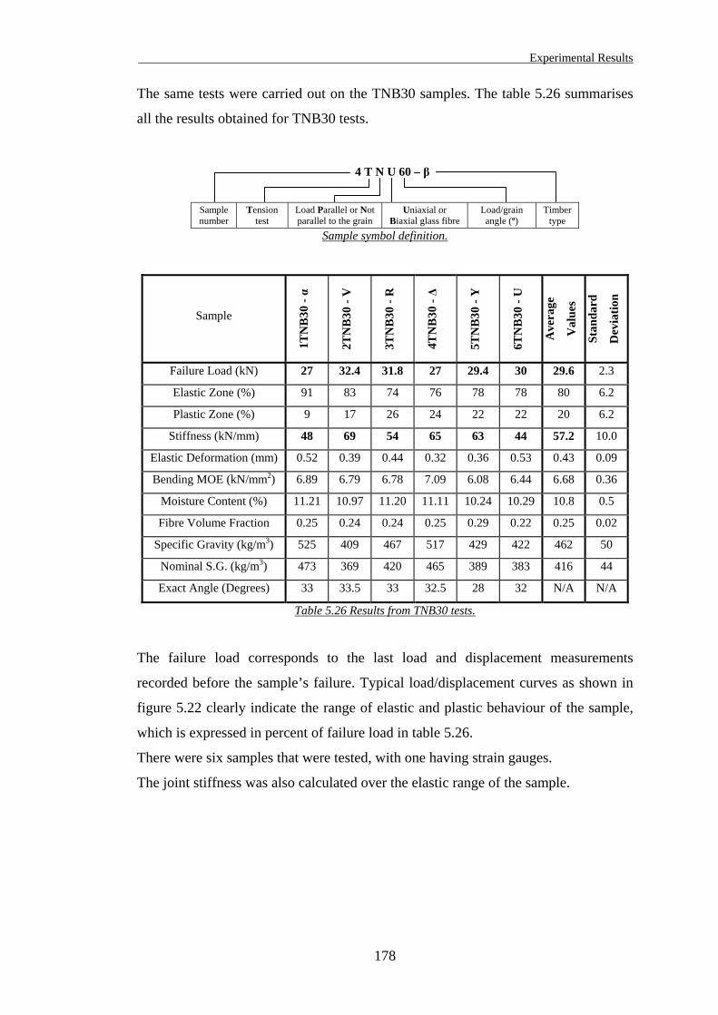
Experimental Results
The same tests were carried out on the TNB30 samples. The table 5.26 summarises
all the results obtained for TNB30 tests.
Sample number
Tension test
Load Parallel or Not parallel to the grain
Uniaxial or Biaxial glass fibre
Load/grain angle (º)
Timber type
4 T N U 60 – β
Sample symbol definition.
Sample 1T
NB
30 - α
2TN
B30
- V
3TN
B30
- R
4TN
B30
- ∆
5TN
B30
- Y
6TN
B30
- U
Ave
rage
Val
ues
Stan
dard
Dev
iatio
n
Failure Load (kN) 27 32.4 31.8 27 29.4 30 29.6 2.3
Elastic Zone (%) 91 83 74 76 78 78 80 6.2
Plastic Zone (%) 9 17 26 24 22 22 20 6.2
Stiffness (kN/mm) 48 69 54 65 63 44 57.2 10.0
Elastic Deformation (mm) 0.52 0.39 0.44 0.32 0.36 0.53 0.43 0.09
Bending MOE (kN/mm2) 6.89 6.79 6.78 7.09 6.08 6.44 6.68 0.36
Moisture Content (%) 11.21 10.97 11.20 11.11 10.24 10.29 10.8 0.5
Fibre Volume Fraction 0.25 0.24 0.24 0.25 0.29 0.22 0.25 0.02
Specific Gravity (kg/m3) 525 409 467 517 429 422 462 50
Nominal S.G. (kg/m3) 473 369 420 465 389 383 416 44
Exact Angle (Degrees) 33 33.5 33 32.5 28 32 N/A N/A
Table 5.26 Results from TNB30 tests.
The failure load corresponds to the last load and displacement measurements
recorded before the sample’s failure. Typical load/displacement curves as shown in
figure 5.22 clearly indicate the range of elastic and plastic behaviour of the sample,
which is expressed in percent of failure load in table 5.26.
There were six samples that were tested, with one having strain gauges.
The joint stiffness was also calculated over the elastic range of the sample.
178
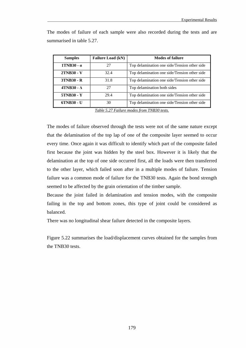
Experimental Results
The modes of failure of each sample were also recorded during the tests and are
summarised in table 5.27.
Samples Failure Load (kN) Modes of failure
1TNB30 - α 27 Top delamination one side/Tension other side
2TNB30 - V 32.4 Top delamination one side/Tension other side
3TNB30 - R 31.8 Top delamination one side/Tension other side
4TNB30 - ∆ 27 Top delamination both sides
5TNB30 - Y 29.4 Top delamination one side/Tension other side
6TNB30 - U 30 Top delamination one side/Tension other side
Table 5.27 Failure modes from TNB30 tests.
The modes of failure observed through the tests were not of the same nature except
that the delamination of the top lap of one of the composite layer seemed to occur
every time. Once again it was difficult to identify which part of the composite failed
first because the joint was hidden by the steel box. However it is likely that the
delamination at the top of one side occurred first, all the loads were then transferred
to the other layer, which failed soon after in a multiple modes of failure. Tension
failure was a common mode of failure for the TNB30 tests. Again the bond strength
seemed to be affected by the grain orientation of the timber sample.
Because the joint failed in delamination and tension modes, with the composite
failing in the top and bottom zones, this type of joint could be considered as
balanced.
There was no longitudinal shear failure detected in the composite layers.
Figure 5.22 summarises the load/displacement curves obtained for the samples from
the TNB30 tests.
179
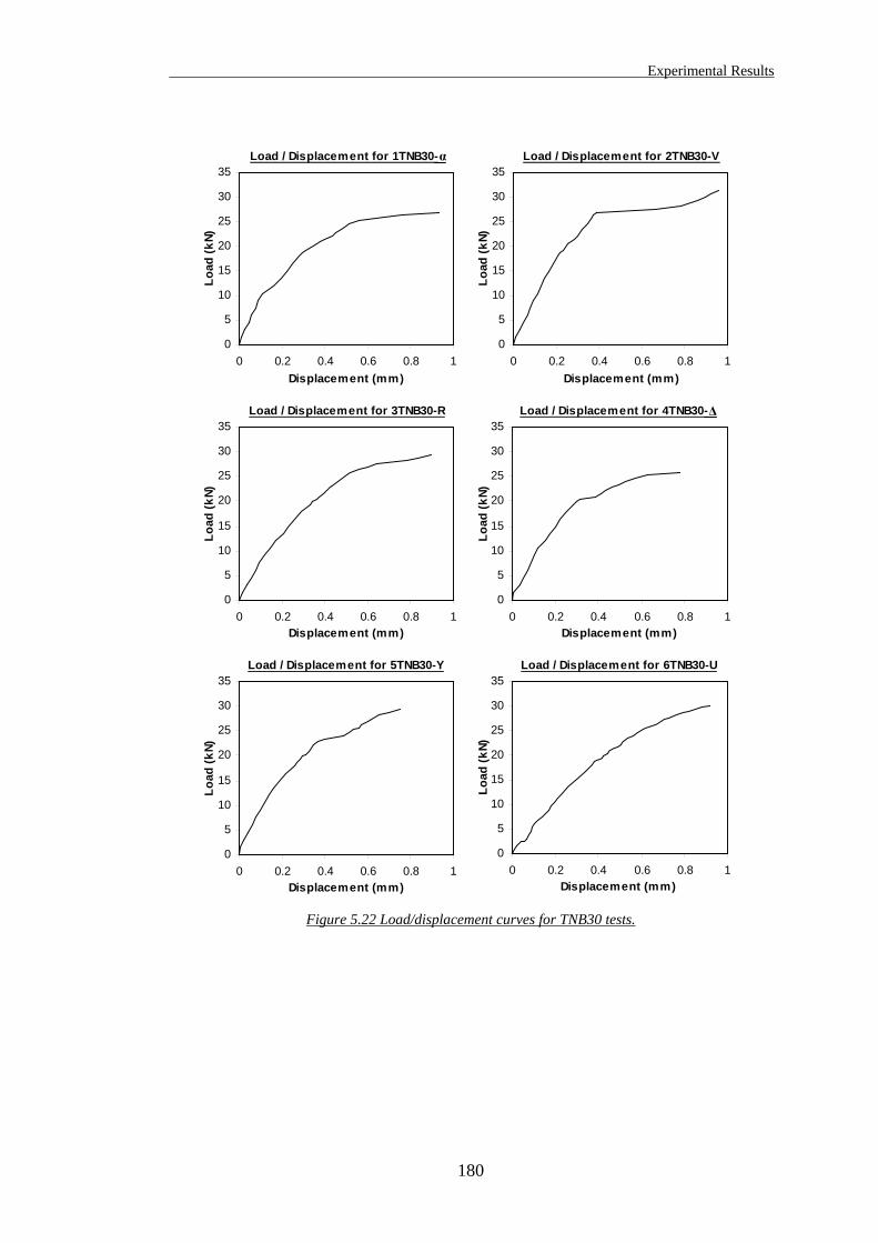
Experimental Results
Load / Displacement for 1TNB30
0
5
10
15
20
25
30
35
0 0.2 0.4 0.6 0.8 1Displacement (mm)
Load
(kN)
Load / Displacement for 2TNB30-V
0
5
10
15
20
25
30
35
0 0.2 0.4 0.6 0.8 1Displacement (mm)
Load
(kN)
Load / Displacement for 3TNB30-R
0
5
10
15
20
25
30
35
0 0.2 0.4 0.6 0.8 1Displacement (mm)
Load
(kN)
Load / Displacement for 4TNB30-
0
5
10
15
20
25
30
35
0 0.2 0.4 0.6 0.8 1Displacement (mm)
Load
(kN)
Load / Displacement for 5TNB30-Y
0
5
10
15
20
25
30
35
0 0.2 0.4 0.6 0.8 1Displacement (mm)
Load
(kN)
Load / Displacement for 6TNB30-U
0
5
10
15
20
25
30
35
0 0.2 0.4 0.6 0.8 1Displacement (mm)
Load
(kN)
∆
-α
Figure 5.22 Load/displacement curves for TNB30 tests.
180
Experimental Results
The displacements were measured using the average readings from the small LVDTs
positioned on the samples sides. However strain gauges were also used on of the
tested samples, the sample 6TNB30 - U. Measurements of strains at precise locations
on the surface of the glass fibre/epoxy composite layers were carried out. These
results are presented in § 5.6.
The load/displacement curves for the TNB30 tests show that the displacements
recorded around the gap between the connected members never exceed 1 mm at
failure.
The failure loads recorded for the six samples are relatively uniform, ranging
between 27 and 32.4 kN.
The elastic behaviour of the samples exceeds 74% of the overall recorded joint slip
for a maximum elastic displacement of 0.53 mm.
The samples develop a plastic behaviour generally. The curves are still reflecting an
elastic-plastic behaviour. Three samples displayed a point of flexure, confirming that
some plastic behaviour was occurring at failure. The other curves shows that the
transition between elastic and plastic is progressive and do lead to some plasticity at
the failure.
The comparison of various parameters obtained from these tests are presented and
discussed in the following section.
181
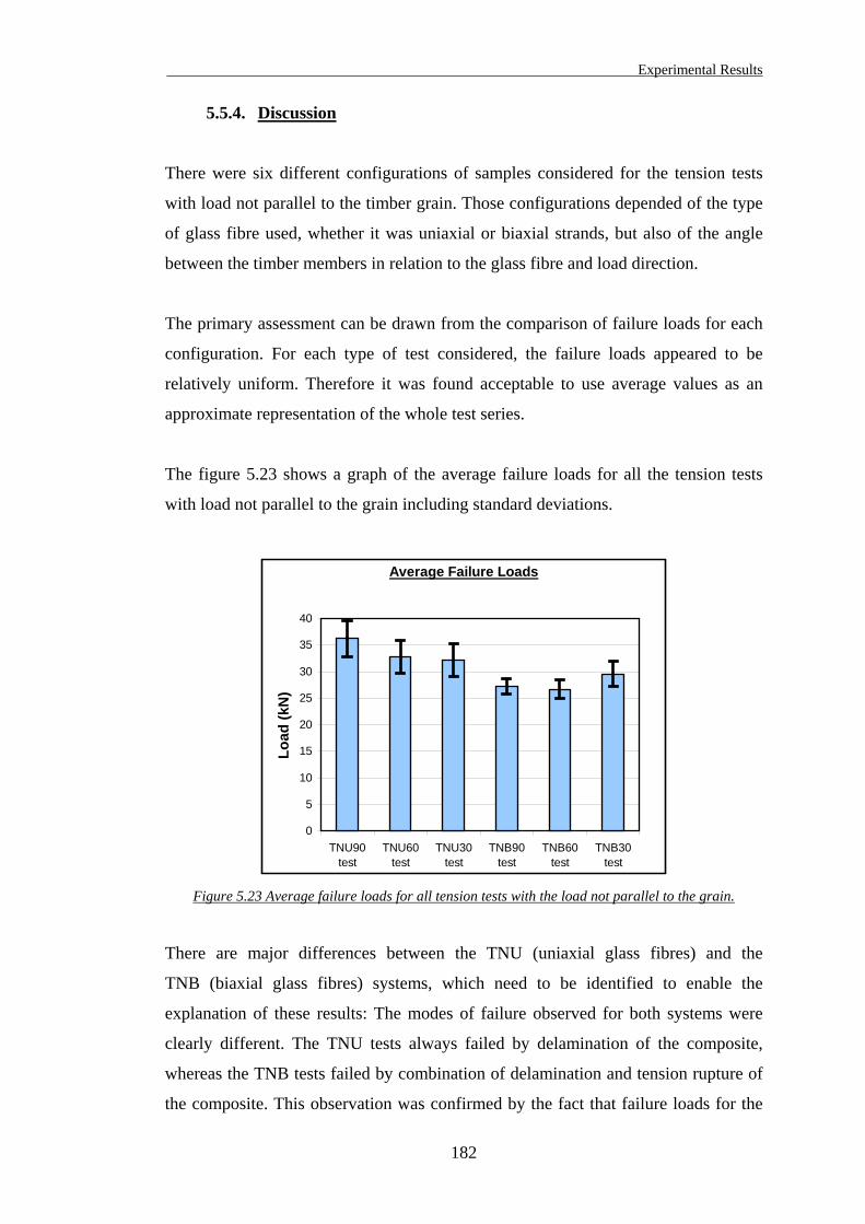
Experimental Results
5.5.4. Discussion
There were six different configurations of samples considered for the tension tests
with load not parallel to the timber grain. Those configurations depended of the type
of glass fibre used, whether it was uniaxial or biaxial strands, but also of the angle
between the timber members in relation to the glass fibre and load direction.
The primary assessment can be drawn from the comparison of failure loads for each
configuration. For each type of test considered, the failure loads appeared to be
relatively uniform. Therefore it was found acceptable to use average values as an
approximate representation of the whole test series.
The figure 5.23 shows a graph of the average failure loads for all the tension tests
with load not parallel to the grain including standard deviations.
Average Failure Loads
0
5
10
15
20
25
30
35
40
TNU90test
TNU60test
TNU30test
TNB90test
TNB60test
TNB30test
Load
(kN
)
Figure 5.23 Average failure loads for all tension tests with the load not parallel to the grain.
There are major differences between the TNU (uniaxial glass fibres) and the
TNB (biaxial glass fibres) systems, which need to be identified to enable the
explanation of these results: The modes of failure observed for both systems were
clearly different. The TNU tests always failed by delamination of the composite,
whereas the TNB tests failed by combination of delamination and tension rupture of
the composite. This observation was confirmed by the fact that failure loads for the
182
Experimental Results
TNB tests were lower than failure loads for the TNU tests, whatever angle
configuration was considered. In fact for the TNU tests, all the fibres of the uniaxial
glass are orientated in the load direction: They are working to lower stresses than the
fibres in the TNB tests where the biaxial glass allow only 50% of the fibres to work
directly in tension. With fewer fibres available to transfer the loads, the TNB tests
failed at lower loads, whether it was delamination failure or fibre rupture.
Considering all joint configurations, the length of the composite layer was defined by
the geometry of the joints. For the 90 degrees grain/load angle, the length of
composite was of 200 mm, the same length than for the load parallel to the grain
tension tests. But for other grain/load angles, different lengths of composite were
used: 232 mm long for the 60 degrees and 400 mm long for the 30 degrees.
Consequently the bonding length and area were increased for those types of tests,
resulting in a potentially higher bond strength capacity. For example, in a system
where the joint is unbalanced so that it always fails by delamination (i.e. bond stress
failure), by increasing the length of composite, the joint would develop higher bond
capacity. With higher bond capacity and sufficient fibre strength, the joint should
have failed at higher loads. But this was not the case for the TNU and TNB tests.
For the TNU tests, where the joints were clearly unbalanced (the joints always failed
by Delamination), the failure loads seemed to decrease as the grain/load angle
reduced from 90 to 30 degrees. In this situation, the longer the composite layers, the
lower the failure loads. In fact the grain orientation was an important parameter to
take into account: Failure by delamination always occurred on the timber members,
where the composite was orientated with an angle to the grain. This indicated that the
bond strength of the composite was reduced when the timber grain was not orientated
in the same direction than the composite fibres and the loading. When the fibres are
orientated perpendicular to the timber grain direction such as the TNU90 test, it is
clear that this system is the strongest in terms of failure loads, as shown in
figure 5.23. The average failure loads decrease as the angle to the grain reduces. But
this reduction is not as significant as it could be, if the length of composite were
equal for all the TNU tests.
The situation was rather different for the TNB tests. The modes of failure were less
consistent and were generally combinations of various modes, such as fibre tension
rupture, delamination and longitudinal shear failures. As a result, the failure loads did
not decrease as the grain/load angle reduced from 90 to 30 degrees. The failure loads
183
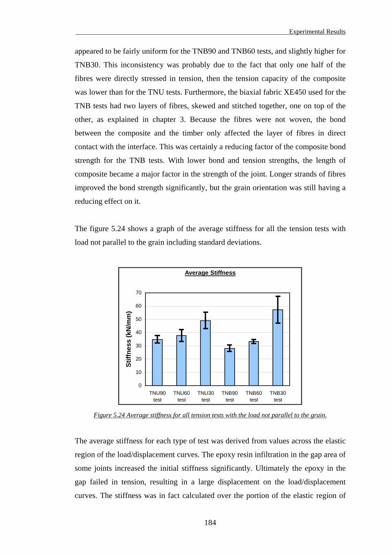
Experimental Results
appeared to be fairly uniform for the TNB90 and TNB60 tests, and slightly higher for
TNB30. This inconsistency was probably due to the fact that only one half of the
fibres were directly stressed in tension, then the tension capacity of the composite
was lower than for the TNU tests. Furthermore, the biaxial fabric XE450 used for the
TNB tests had two layers of fibres, skewed and stitched together, one on top of the
other, as explained in chapter 3. Because the fibres were not woven, the bond
between the composite and the timber only affected the layer of fibres in direct
contact with the interface. This was certainly a reducing factor of the composite bond
strength for the TNB tests. With lower bond and tension strengths, the length of
composite became a major factor in the strength of the joint. Longer strands of fibres
improved the bond strength significantly, but the grain orientation was still having a
reducing effect on it.
The figure 5.24 shows a graph of the average stiffness for all the tension tests with
load not parallel to the grain including standard deviations.
Average Stiffness
0
10
20
30
40
50
60
70
TNU90test
TNU60test
TNU30test
TNB90test
TNB60test
TNB30test
Stiff
ness
(kN
/mm
)
Figure 5.24 Average stiffness for all tension tests with the load not parallel to the grain.
The average stiffness for each type of test was derived from values across the elastic
region of the load/displacement curves. The epoxy resin infiltration in the gap area of
some joints increased the initial stiffness significantly. Ultimately the epoxy in the
gap failed in tension, resulting in a large displacement on the load/displacement
curves. The stiffness was in fact calculated over the portion of the elastic region of
184
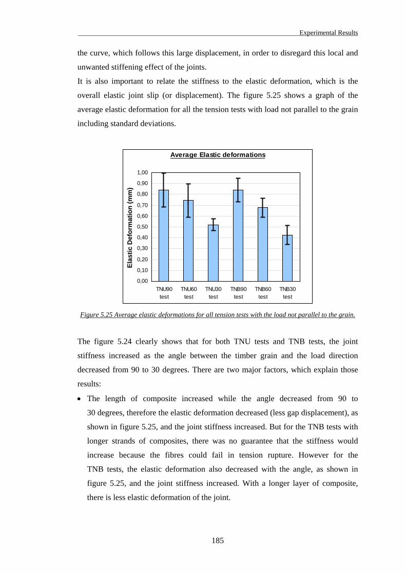
Experimental Results
the curve, which follows this large displacement, in order to disregard this local and
unwanted stiffening effect of the joints.
It is also important to relate the stiffness to the elastic deformation, which is the
overall elastic joint slip (or displacement). The figure 5.25 shows a graph of the
average elastic deformation for all the tension tests with load not parallel to the grain
including standard deviations.
Average Elastic deformations
0,00
0,10
0,20
0,30
0,40
0,50
0,60
0,70
0,80
0,90
1,00
TNU90test
TNU60test
TNU30test
TNB90test
TNB60test
TNB30test
Elas
tic D
efor
mat
ion
(mm
)
Figure 5.25 Average elastic deformations for all tension tests with the load not parallel to the grain.
The figure 5.24 clearly shows that for both TNU tests and TNB tests, the joint
stiffness increased as the angle between the timber grain and the load direction
decreased from 90 to 30 degrees. There are two major factors, which explain those
results:
• The length of composite increased while the angle decreased from 90 to
30 degrees, therefore the elastic deformation decreased (less gap displacement), as
shown in figure 5.25, and the joint stiffness increased. But for the TNB tests with
longer strands of composites, there was no guarantee that the stiffness would
increase because the fibres could fail in tension rupture. However for the
TNB tests, the elastic deformation also decreased with the angle, as shown in
figure 5.25, and the joint stiffness increased. With a longer layer of composite,
there is less elastic deformation of the joint.
185
Experimental Results
• The timber grain orientation has a direct effect on the joint stiffness. For the
TNU90 and TNB90 tests, when the load was applied perpendicular to the grain,
the elastic deformations were the largest, as shown in figure 5.25. The timber
properties are generally much lower in the radial or tangential directions than in
the longitudinal direction of the grain.
“Approximate values of the moduli of elasticity may be found by taking
EL (longitudinal modulus of elasticity) equal to 1.1 times the bending modulus,
E (tangential modulus of elasticity) equal to 0.05 × EL and ER (radial modulus of
elasticity) equal to 0.10 × EL.” (Booth et al., 1967). T
As for the moduli of elasticity, tension strength of the timber in the tangential or
radial direction is significantly lower than in the longitudinal direction. Based on
the Hooke’s Law of elasticity (σ = E × ε), if the modulus of elasticity E is
reduced, the strain ε must increase to achieve the same stress σ. The larger elastic
deformations observed on the tension tests with load perpendicular to the grain
TNU90 and TNB90 indicate that larger strains occur in the timber materials. As
the load/grain angle reduce from 90 to 30 degrees, the timber properties would
improve, as they are optimum in the grain direction. With higher tension strength,
then higher modulus of elasticity, the strain would be reduced to achieve an
equivalent stress. Consequently the elastic deformation reduces with the
load/grain angle.
The length of the composite layer and the timber grain orientation are the parameters,
which affect the failure loads, the stiffness and elastic deformations of the joints
tested in tension with load not parallel to the grain.
The results of the tension tests with load parallel and with load not parallel to the
grain are summarised in the conclusion of this thesis.
The results of all the samples tested with the use of strain gauges are presented and
discussed in the following section.
186
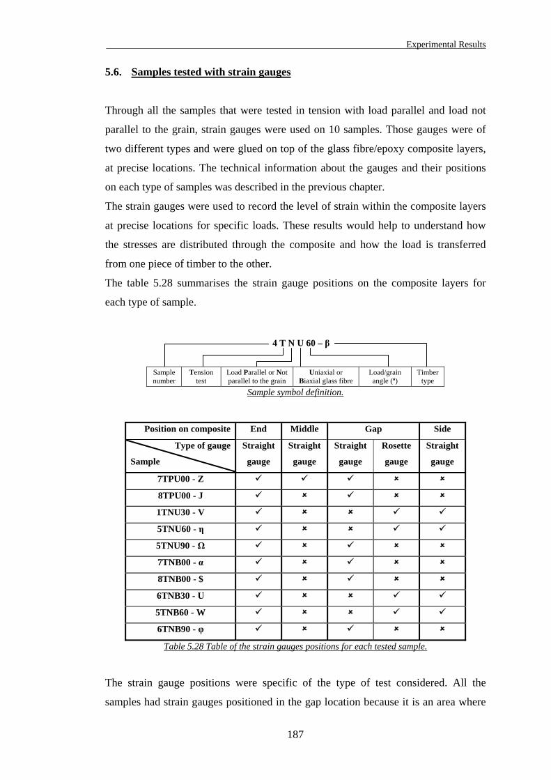
Experimental Results
5.6. Samples tested with strain gauges
Through all the samples that were tested in tension with load parallel and load not
parallel to the grain, strain gauges were used on 10 samples. Those gauges were of
two different types and were glued on top of the glass fibre/epoxy composite layers,
at precise locations. The technical information about the gauges and their positions
on each type of samples was described in the previous chapter.
The strain gauges were used to record the level of strain within the composite layers
at precise locations for specific loads. These results would help to understand how
the stresses are distributed through the composite and how the load is transferred
from one piece of timber to the other.
The table 5.28 summarises the strain gauge positions on the composite layers for
each type of sample.
Sample number
Tension test
Load Parallel or Not parallel to the grain
Uniaxial or Biaxial glass fibre
Load/grain angle (º)
Timber type
4 T N U 60 – β
Sample symbol definition.
Position on composite End Middle Gap Side
Type of gauge
Sample
Straight
gauge
Straight
gauge
Straight
gauge
Rosette
gauge
Straight
gauge
7TPU00 - Z
8TPU00 - J
1TNU30 - V
5TNU60 - η
5TNU90 - Ω
7TNB00 - α
8TNB00 - $
6TNB30 - U
5TNB60 - W
6TNB90 - φ
Table 5.28 Table of the strain gauges positions for each tested sample.
The strain gauge positions were specific of the type of test considered. All the
samples had strain gauges positioned in the gap location because it is an area where
187
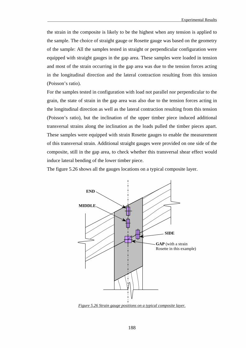
Experimental Results
the strain in the composite is likely to be the highest when any tension is applied to
the sample. The choice of straight gauge or Rosette gauge was based on the geometry
of the sample: All the samples tested in straight or perpendicular configuration were
equipped with straight gauges in the gap area. These samples were loaded in tension
and most of the strain occurring in the gap area was due to the tension forces acting
in the longitudinal direction and the lateral contraction resulting from this tension
(Poisson’s ratio).
For the samples tested in configuration with load not parallel nor perpendicular to the
grain, the state of strain in the gap area was also due to the tension forces acting in
the longitudinal direction as well as the lateral contraction resulting from this tension
(Poisson’s ratio), but the inclination of the upper timber piece induced additional
transversal strains along the inclination as the loads pulled the timber pieces apart.
These samples were equipped with strain Rosette gauges to enable the measurement
of this transversal strain. Additional straight gauges were provided on one side of the
composite, still in the gap area, to check whether this transversal shear effect would
induce lateral bending of the lower timber piece.
The figure 5.26 shows all the gauges locations on a typical composite layer.
Figure 5.26 Strain gauge positions on a typical composite layer.
MIDDLE
END
SIDE
GAP (with a strain Rosette in this example)
188
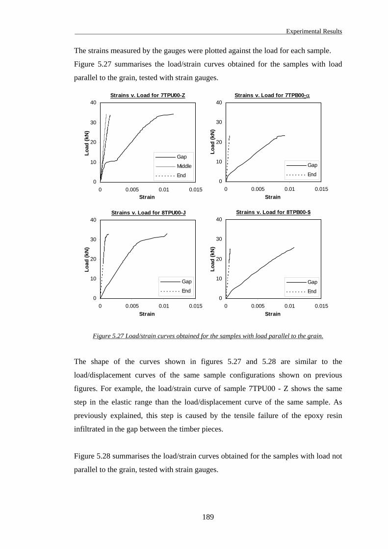
Experimental Results
The strains measured by the gauges were plotted against the load for each sample.
Figure 5.27 summarises the load/strain curves obtained for the samples with load
parallel to the grain, tested with strain gauges.
Strains v. Load for 7TPU00-Z
0
10
20
30
40
0 0.005 0.01 0.015Strain
Load
(kN
)
Gap
Middle
End
Strains v. Load for 7TPB00-
0
10
20
30
40
0 0.005 0.01 0.015Strain
Load
(kN
)
Gap
End
Strains v. Load for 8TPU00-J
0
10
20
30
40
0 0.005 0.01 0.015Strain
Load
(kN
)
Gap
End
Strains v. Load for 8TPB00-$
0
10
20
30
40
0 0.005 0.01 0.015Strain
Load
(kN
)
Gap
End
α
Figure 5.27 Load/strain curves obtained for the samples with load parallel to the grain.
The shape of the curves shown in figures 5.27 and 5.28 are similar to the
load/displacement curves of the same sample configurations shown on previous
figures. For example, the load/strain curve of sample 7TPU00 - Z shows the same
step in the elastic range than the load/displacement curve of the same sample. As
previously explained, this step is caused by the tensile failure of the epoxy resin
infiltrated in the gap between the timber pieces.
Figure 5.28 summarises the load/strain curves obtained for the samples with load not
parallel to the grain, tested with strain gauges.
189
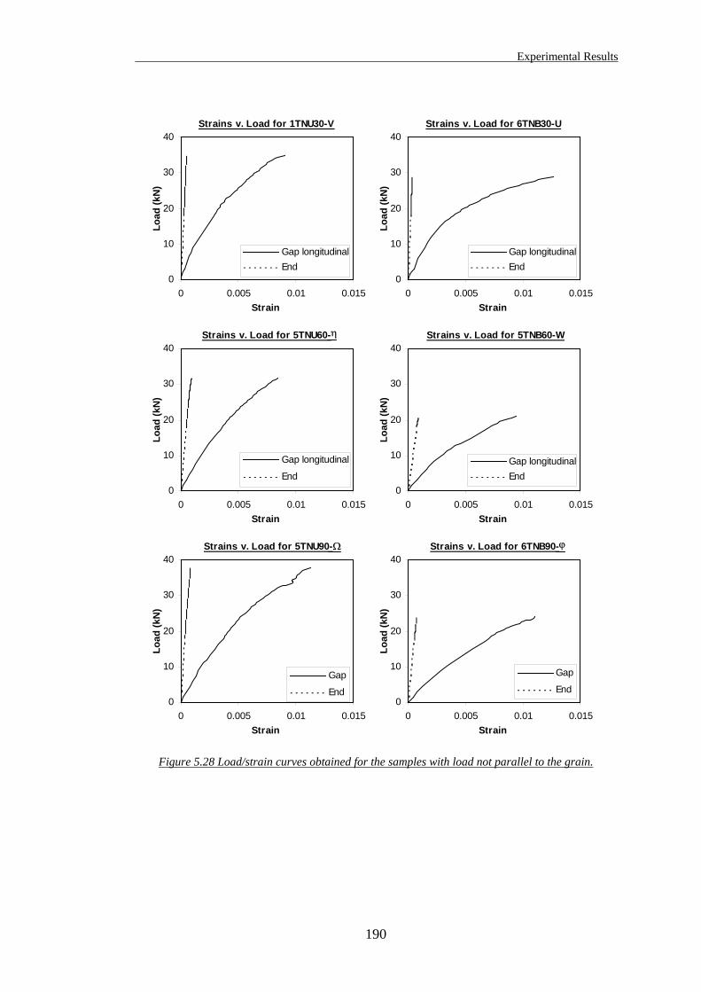
Experimental Results
Strains v. Load for 1TNU30-V
0
10
20
30
40
0 0.005 0.01 0.015Strain
Load
(kN
)
Gap longitudinalEnd
Strains v. Load for 6TNB30-U
0
10
20
30
40
0 0.005 0.01 0.015Strain
Load
(kN
)
Gap longitudinalEnd
Strains v. Load for 5TNU60-
0
10
20
30
40
0 0.005 0.01 0.015Strain
Load
(kN
)
Gap longitudinal
End
Strains v. Load for 5TNB60-W
0
10
20
30
40
0 0.005 0.01 0.015Strain
Load
(kN
)
Gap longitudinalEnd
Strains v. Load for 5TNU90-
0
10
20
30
40
0 0.005 0.01 0.015Strain
Load
(kN
)
Gap
End
Strains v. Load for 6TNB90-
0
10
20
30
40
0 0.005 0.01 0.015Strain
Load
(kN
)
Gap
End
η
ϕ Ω
Figure 5.28 Load/strain curves obtained for the samples with load not parallel to the grain.
190
Experimental Results
The strain gauges were used on some of the samples in order to identify how the
stresses are distributed through the composite. The strain gauges were positioned on
top of the composite layer. It would have been interesting to place some strain
gauges as well at the interface between the timber and the composite to evaluate
whether the strain was varying through the thickness of the composite. However it
was impractical to do so, because of the gauge wires to be connected to the data
acquisition system. The wires could not be driven through the composite without
affecting the quality of the bond. Furthermore strain gauges do not behave properly
on timber, as the glue used for the bond is always of much higher stiffness than the
wood itself. Nevertheless the composite was a very thin layer of material (less than
1 mm) and it is reasonable to assume that the strain would only vary by a slight
amount across the thickness.
The load transfer through double lap bonded joints such as the wood/glass/epoxy
joints is generally non linear. The shear stress observed at the interface when the
joint was loaded in tension varied along the length of the lap: It was high in the gap
area and then decreased towards the middle of the lap length and increased as it
reached the end of the lap. This distribution depended on the lap length and also of
the loading applied.
The strains recorded from two oppositely positioned strain gauges on the composite
layers of a sample were of similar magnitude for a given load, except at high loads
when the sample reached failure. It showed that the tension applied through the
samples was equally distributed between both layers.
The results of the strain values obtained through those tests are summarised in a table
presented in Appendix A. Only the values recorded for loads of 6, 12, 18, 24 and
30 kN are reported. This data will be used as a comparison for the results obtained
from the finite element modelling of the samples. The theoretical approach and the
FE modelling process are described in the chapter 6.
The properties of timber were derived mainly from small clear sample tests. The
results are presented and discussed in the following section, which deals with timber
grading.
191
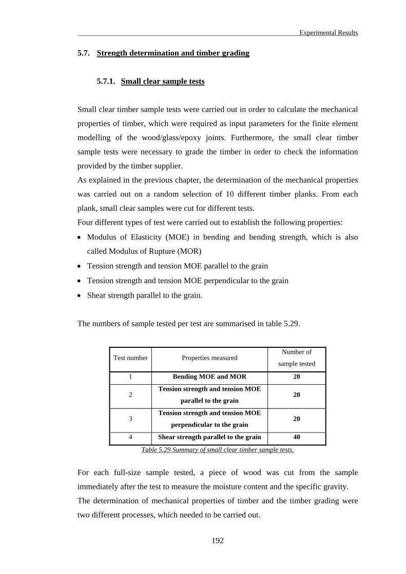
Experimental Results
5.7. Strength determination and timber grading
5.7.1. Small clear sample tests
Small clear timber sample tests were carried out in order to calculate the mechanical
properties of timber, which were required as input parameters for the finite element
modelling of the wood/glass/epoxy joints. Furthermore, the small clear timber
sample tests were necessary to grade the timber in order to check the information
provided by the timber supplier.
As explained in the previous chapter, the determination of the mechanical properties
was carried out on a random selection of 10 different timber planks. From each
plank, small clear samples were cut for different tests.
Four different types of test were carried out to establish the following properties:
• Modulus of Elasticity (MOE) in bending and bending strength, which is also
called Modulus of Rupture (MOR)
• Tension strength and tension MOE parallel to the grain
• Tension strength and tension MOE perpendicular to the grain
• Shear strength parallel to the grain.
The numbers of sample tested per test are summarised in table 5.29.
Test number Properties measured Number of
sample tested
1 Bending MOE and MOR 20
2 Tension strength and tension MOE
parallel to the grain 20
3 Tension strength and tension MOE
perpendicular to the grain 20
4 Shear strength parallel to the grain 40
Table 5.29 Summary of small clear timber sample tests.
For each full-size sample tested, a piece of wood was cut from the sample
immediately after the test to measure the moisture content and the specific gravity.
The determination of mechanical properties of timber and the timber grading were
two different processes, which needed to be carried out.
192
Experimental Results
The tests used to evaluate the timber properties were mainly undertaken on small
clear timber samples, based on the existing code BS 373:1986. One test not based on
this standard was the MOE and tension strength perpendicular to the grain test,
which was an adapted test from the standard on structural-size timber given by the
code EN 1193: 1997. The facilities to fabricate the samples required for the tension
perpendicular to the grain in the code BS 373: 1986 were not available. The
alternative was to use the standard test on structural-size timber given by the code
EN 1193: 1997 but the sizes of timber available were too small to satisfy the
standards requirements. By scaling down the sample sizes, the test could not be
considered as a standard test any longer. Nevertheless the pieces of timber selected
for this test were defect-free therefore this test could also be treated as a small clear
sample test.
The timber properties could have been calculated from structural-size timber tests,
but the equipment required for such test is relatively sophisticated and is usually
available in specialised timber research laboratories.
From a design consideration, small clear sample tests have been superseded in the
timber industry since the mid-1970s by the structural-size timber tests. But they
remain valid for characterising timber and for academic purposes. Small clear
samples are defect-free pieces carefully selected to provide the best quality of timber
that can be obtained. In fact they do not reflect the quality of structural-size timber.
Before 1973, small clear sample tests were carried out to obtain the working stresses
of the timber. Because the samples were not representative of structural-size timber,
several reduction factors were used to take into account the defects of the wood
material.
After 1973 the tests on structural-size timber were developed as a radical change of
method to establish the timber working stresses occurred.
“The realisation in the 1970s that the duration of load values derived from testing of
small clear test pieces were not appropriate for structural timber led to the derivation
of grade stresses directly from actual structural-size timber” (Dinwoodie, 2000).
It was then necessary to develop the process of timber grading, with the visual or
mechanical methods. Although before 1973, visual grading was already part of the
derivation of the timber grade stresses. The small clear sample tests enabled the
calculation of basic stresses, on which reduction factors based on the visual grading
of the corresponding full-size timber were applied to obtain grade stresses. The
193
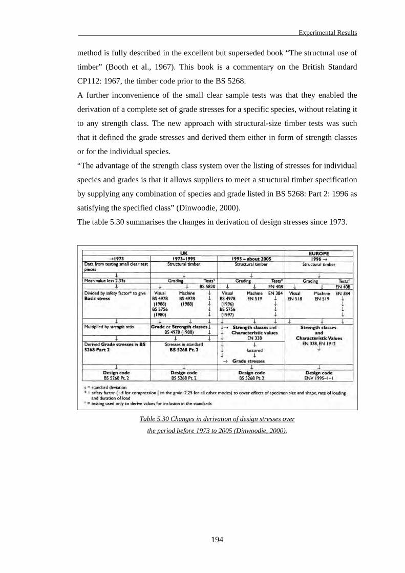
Experimental Results
method is fully described in the excellent but superseded book “The structural use of
timber” (Booth et al., 1967). This book is a commentary on the British Standard
CP112: 1967, the timber code prior to the BS 5268.
A further inconvenience of the small clear sample tests was that they enabled the
derivation of a complete set of grade stresses for a specific species, without relating it
to any strength class. The new approach with structural-size timber tests was such
that it defined the grade stresses and derived them either in form of strength classes
or for the individual species.
“The advantage of the strength class system over the listing of stresses for individual
species and grades is that it allows suppliers to meet a structural timber specification
by supplying any combination of species and grade listed in BS 5268: Part 2: 1996 as
satisfying the specified class” (Dinwoodie, 2000).
The table 5.30 summarises the changes in derivation of design stresses since 1973.
Table 5.30 Changes in derivation of design stresses over
the period before 1973 to 2005 (Dinwoodie, 2000).
194
Experimental Results
The current British European Standard EN 384: 1995 which deals with the
determination of characteristic values of mechanical properties and density of timber,
does not cover the use of small clear samples if they are used on their own. This
standard clearly states: “Factors to determine characteristic values of bending
strength and modulus of elasticity may be derived where both small, clear and
structural size data are available for at least three other species”. In other words, the
current code does not recommend the derivation of timber properties if only small
clear sample tests are carried out.
The determination of the timber mechanical properties used in this research was thus
based on the method from small clear sample tests given in CP112: 1967 “The
Structural Use of Timber”. This method provided:
• The timber mechanical properties necessary for the finite element modelling. The
properties were the mean values of the results obtained from the tests.
• The grade stresses for the timber, which were used to check the strength class
given by the timber suppliers. However the grade stresses had no direct use for the
research in wood/glass/epoxy joints: Grade stresses are useful as far as design is
concerned, but this research did not take into account any design consideration.
The investigation on wood/glass/epoxy joints was too preliminary to get into
design matters.
The following section deals with the grading process used to relate results derived
from small clear sample tests with current standards specifications.
195
Experimental Results
5.7.2. Principles and methods
The timber Code of Practice CP112: 1967 gives the definitions of those two types of
stresses:
• The basic stress in timber is the stress, which can safely be permanently sustained
by timber containing no strength reducing characteristics.
• The grade stress in timber is the stress, which can safely be permanently sustained
by timber of a particular grade.
The first definition clearly identifies the basic stresses as the stresses derived for the
material itself. The method employed for the calculation of the basic stresses is based
on the results obtained from tests on small clear samples of timber. A number of
reduction factors would then be applied to these results to take into account several
strength-reducing effects that timber can endure during its design life. Those factors
are the moisture content, the load duration, the size and shape of the members, the
variability of strength and the factor of safety.
As timber is a naturally grown material, wide variations of properties are observed
within a particular species, even within the same tree. Rate of growth, age, knots and
defects are some of the factors, which increase those variations. However if more and
more samples of the same timber are tested, the variations will progressively show a
Gaussian distribution curve on which the standard methods of statistical analysis are
used. The figure 5.29 shows an example of frequency distribution of maximum
crushing strength, tested from small clear samples of green tropical hardwood
Keruing. It becomes clear that for any number of samples tested, there will be always
one or more samples, which will not fall above an acceptable level. Using the
properties of the Gaussian distribution, it is possible to calculate the failure level at
which there is a specified probability of a sample failing.
The mean values and the standard deviation from the results are then calculated. The
mean value m and the standard deviation s are defined as:
nx
m ∑= (5.1)
196
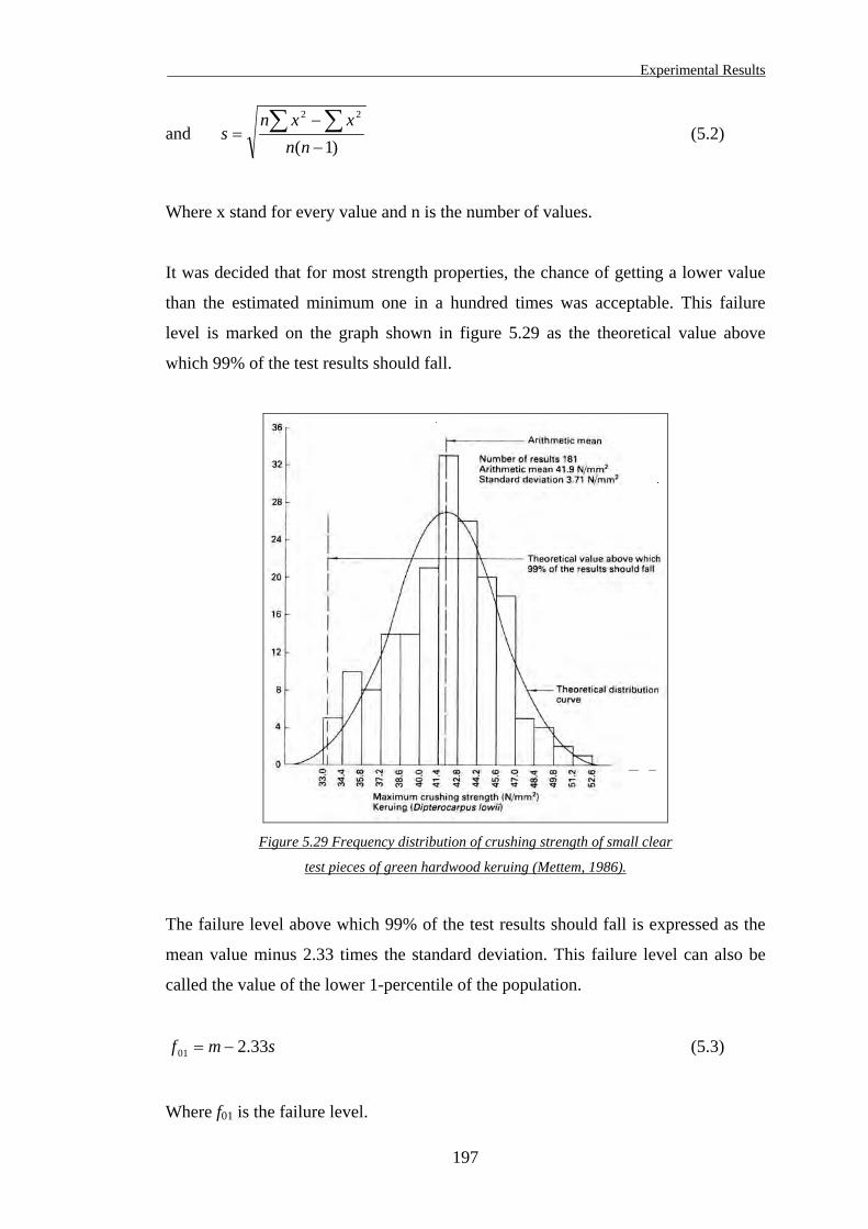
Experimental Results
and )1(
22
−
−= ∑∑
nnxxn
s (5.2)
Where x stand for every value and n is the number of values.
It was decided that for most strength properties, the chance of getting a lower value
than the estimated minimum one in a hundred times was acceptable. This failure
level is marked on the graph shown in figure 5.29 as the theoretical value above
which 99% of the test results should fall.
Figure 5.29 Frequency distribution of crushing strength of small clear
test pieces of green hardwood keruing (Mettem, 1986).
The failure level above which 99% of the test results should fall is expressed as the
mean value minus 2.33 times the standard deviation. This failure level can also be
called the value of the lower 1-percentile of the population.
smf 33.201 −= (5.3)
Where f01 is the failure level.
197
Experimental Results
In the current British Standards and Eurocodes, when the test are carried out on
structural-size samples, the same procedure is applied using the value of the lower
5-percentile of the population instead.
A reduction factor is then applied to the minimum value calculated with the equation
(5.3) above. This factor allows for the load duration, the sample size and shape as
well as a factor of safety. It is taken as 1.4 for compression strength and 2.25 for all
other strengths. However this factor of safety does not apply to modulus of elasticity,
which can be expressed as a mean value and a standard deviation. Depending on the
requirements, it can also be expressed as a mean value and a minimum value
calculated as the lower 1-percentile of the population.
The values obtained from the previous calculations are known as basic stresses. In
this research, the tests were carried out on small clear samples cut from seasoned dry
timber, which means the timber moisture content did not exceed 18%. Therefore the
basic stresses are in fact dry basic stresses.
The next step is to grade the timber in order to derive the grade stresses.
Grade stresses in timber are related to the basic stresses of the individual species and
are governed by the effect of visible gross features such as knots, sloping grain, etc.
The grade stresses are derived from the basic stresses using strength ratios. Those
ratios are assigned to grade numbers: 40, 50, 65 and 75. The grading rules were
given in CP112: 1967. The four grades are allocated in relation to the requirements
of each timber characteristic defined as follow:
• Rate of growth. Measurement of the rate of growth is carried out at one end of a
timber section, over a straight line 3 inches long (76.2 mm), normal to the growth
rings and passing through the centre of the member. The table 5.31 gives
minimum number of growth rings per inch to qualify for a particular grade.
• Fissures. Measurement of fissures is carried out at one end of the member,
between lines enclosing the fissures. Fissures occurring on the surface should be
measured to assess its depth. The table 5.31 gives maximum size of fissure
expressed as a fraction of the member thickness to qualify for a particular grade.
• Slope of grain. Measurement is carried out using a grain detector. The table 5.31
gives maximum slope of grain that a member should not exceed to qualify for a
particular grade.
198
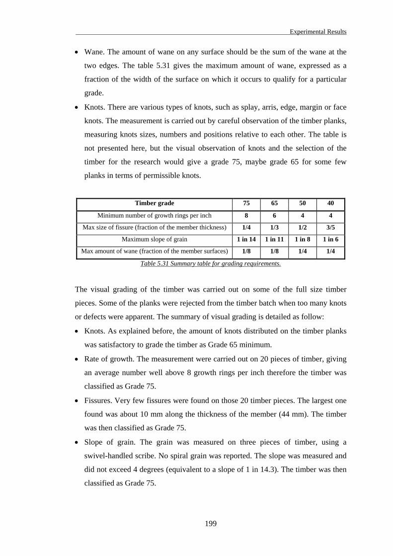
Experimental Results
• Wane. The amount of wane on any surface should be the sum of the wane at the
two edges. The table 5.31 gives the maximum amount of wane, expressed as a
fraction of the width of the surface on which it occurs to qualify for a particular
grade.
• Knots. There are various types of knots, such as splay, arris, edge, margin or face
knots. The measurement is carried out by careful observation of the timber planks,
measuring knots sizes, numbers and positions relative to each other. The table is
not presented here, but the visual observation of knots and the selection of the
timber for the research would give a grade 75, maybe grade 65 for some few
planks in terms of permissible knots.
Timber grade 75 65 50 40
Minimum number of growth rings per inch 8 6 4 4
Max size of fissure (fraction of the member thickness) 1/4 1/3 1/2 3/5
Maximum slope of grain 1 in 14 1 in 11 1 in 8 1 in 6
Max amount of wane (fraction of the member surfaces) 1/8 1/8 1/4 1/4
Table 5.31 Summary table for grading requirements.
The visual grading of the timber was carried out on some of the full size timber
pieces. Some of the planks were rejected from the timber batch when too many knots
or defects were apparent. The summary of visual grading is detailed as follow:
• Knots. As explained before, the amount of knots distributed on the timber planks
was satisfactory to grade the timber as Grade 65 minimum.
• Rate of growth. The measurement were carried out on 20 pieces of timber, giving
an average number well above 8 growth rings per inch therefore the timber was
classified as Grade 75.
• Fissures. Very few fissures were found on those 20 timber pieces. The largest one
found was about 10 mm along the thickness of the member (44 mm). The timber
was then classified as Grade 75.
• Slope of grain. The grain was measured on three pieces of timber, using a
swivel-handled scribe. No spiral grain was reported. The slope was measured and
did not exceed 4 degrees (equivalent to a slope of 1 in 14.3). The timber was then
classified as Grade 75.
199
Experimental Results
• Wane. No wanes were found on the selected timber planks. The timber was then
classified as Grade 75.
Finally the visual grading demonstrated that the timber had a limited amount of
defects, providing the pieces were selected from the whole batch. The overall timber
grade is taken as Grade 65, mainly because of the sizes and amount of knots
observed on some planks.
The basic and grade stresses calculated from the results of the small clear sample
tests as well as the comparison with published data on softwoods are presented in the
following section.
200
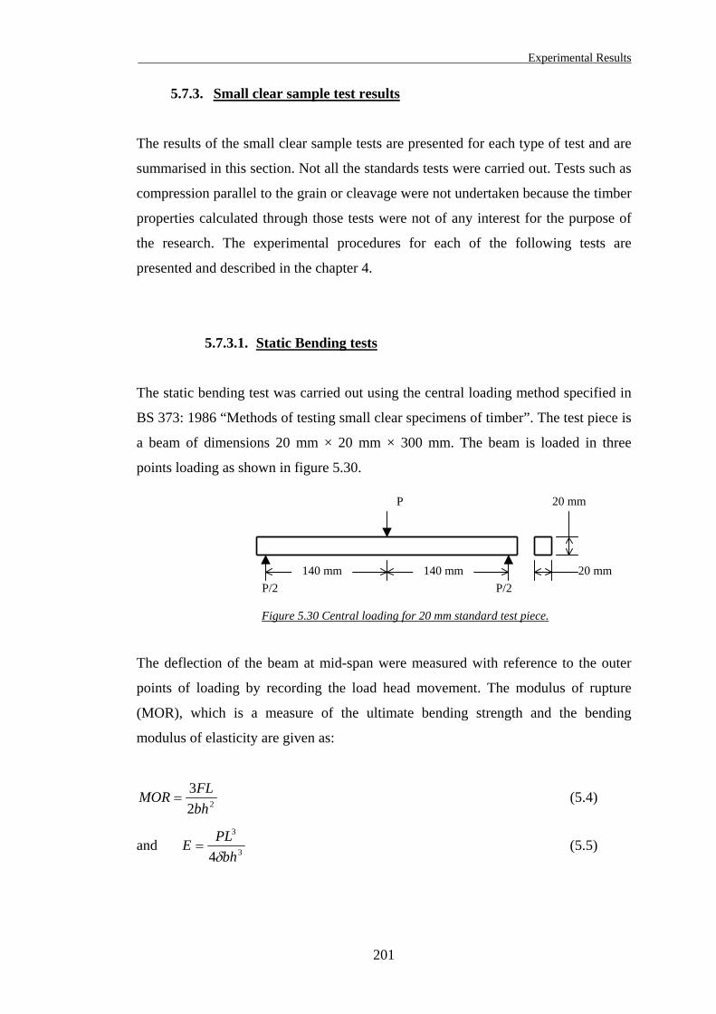
Experimental Results
5.7.3. Small clear sample test results
The results of the small clear sample tests are presented for each type of test and are
summarised in this section. Not all the standards tests were carried out. Tests such as
compression parallel to the grain or cleavage were not undertaken because the timber
properties calculated through those tests were not of any interest for the purpose of
the research. The experimental procedures for each of the following tests are
presented and described in the chapter 4.
5.7.3.1. Static Bending tests
The static bending test was carried out using the central loading method specified in
BS 373: 1986 “Methods of testing small clear specimens of timber”. The test piece is
a beam of dimensions 20 mm × 20 mm × 300 mm. The beam is loaded in three
points loading as shown in figure 5.30.
140 mm 140 mm
20 mm
20 mm
P
P/2 P/2
Figure 5.30 Central loading for 20 mm standard test piece.
The deflection of the beam at mid-span were measured with reference to the outer
points of loading by recording the load head movement. The modulus of rupture
(MOR), which is a measure of the ultimate bending strength and the bending
modulus of elasticity are given as:
223bhFLMOR = (5.4)
and 3
3
4 bhPLEδ
= (5.5)
201
Experimental Results
Where MOR = Modulus of Rupture or bending strength (N/mm2),
E = Modulus of Elasticity in bending (N/mm2),
F = Load at failure (N),
L = Length of the member (mm),
P = Change of load in elastic range (N),
δ = Change of deflection at mid-span in elastic range (mm),
b and h = Breath and height of the beam cross-section (mm).
A total of 20 sample beams were tested and the full results are available in
Appendix B.1. The summary of the results is presented in table 5.32.
E (N/mm2) MOR (N/mm2)
Mean value 8283 81
Standard deviation 1551 8.73
Reduction factor 1 2.25
Basic value 4669 27.1
Grade 65 value N/A 17.6
Table 5.32 Summary results of the static bending tests.
These results are discussed in the section § 5.7.4.
5.7.3.2. Tension parallel to the grain tests
This test was carried out using the tension parallel to the grain tests for small clear
samples given in BS 373: 1986 “Methods of testing small clear specimens of
timber”. The standard test pieces had the forms and dimensions as illustrated in
figure 5.31.
The tension modulus of elasticity E// was calculated using the diagram of
load/displacement recorded using a LVDT positioned in the 50 mm long thinner
central region of the sample. The calculations of modulus of elasticity were based on
elastic range values. The tension strength σ// was recorded as the ultimate stress in the
thinner cross-section at failure. These two parameters are given as:
202
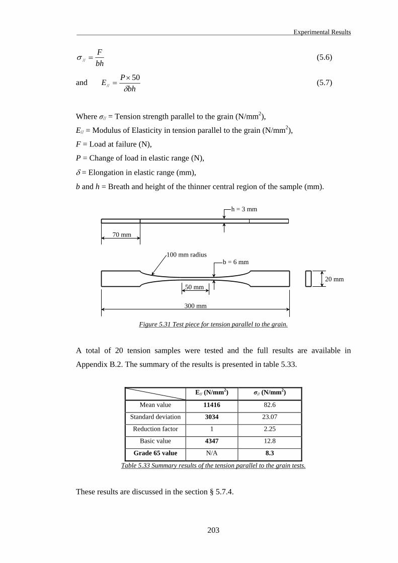
Experimental Results
bhF
=//σ (5.6)
and bh
PEδ
50//
×= (5.7)
Where σ// = Tension strength parallel to the grain (N/mm2),
E// = Modulus of Elasticity in tension parallel to the grain (N/mm2),
F = Load at failure (N),
P = Change of load in elastic range (N),
δ = Elongation in elastic range (mm),
b and h = Breath and height of the thinner central region of the sample (mm).
300 mm
100 mm radius
20 mm
b = 6 mm
h = 3 mm
50 mm
70 mm
Figure 5.31 Test piece for tension parallel to the grain.
A total of 20 tension samples were tested and the full results are available in
Appendix B.2. The summary of the results is presented in table 5.33.
E// (N/mm2) σ// (N/mm2)
Mean value 11416 82.6
Standard deviation 3034 23.07
Reduction factor 1 2.25
Basic value 4347 12.8
Grade 65 value N/A 8.3
Table 5.33 Summary results of the tension parallel to the grain tests.
These results are discussed in the section § 5.7.4.
203
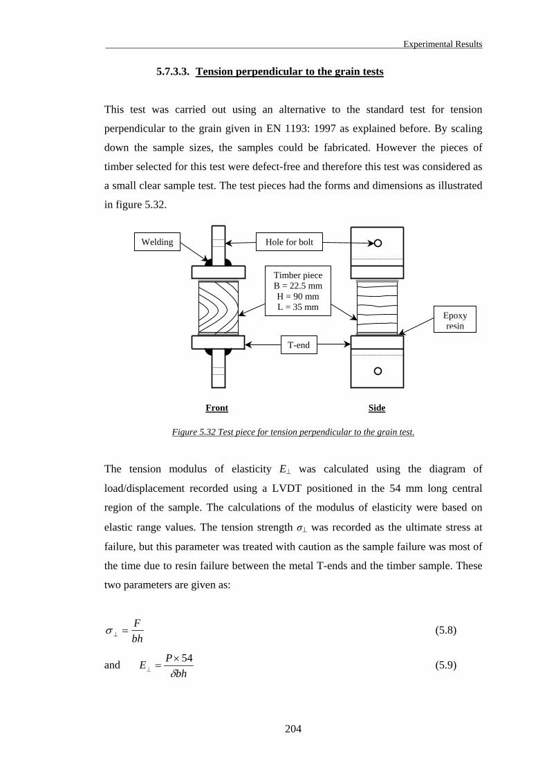
Experimental Results
5.7.3.3. Tension perpendicular to the grain tests
This test was carried out using an alternative to the standard test for tension
perpendicular to the grain given in EN 1193: 1997 as explained before. By scaling
down the sample sizes, the samples could be fabricated. However the pieces of
timber selected for this test were defect-free and therefore this test was considered as
a small clear sample test. The test pieces had the forms and dimensions as illustrated
in figure 5.32.
Side Front
T-end
Epoxy resin
Welding Hole for bolt
Timber piece B = 22.5 mmH = 90 mm L = 35 mm
Figure 5.32 Test piece for tension perpendicular to the grain test.
The tension modulus of elasticity E⊥ was calculated using the diagram of
load/displacement recorded using a LVDT positioned in the 54 mm long central
region of the sample. The calculations of the modulus of elasticity were based on
elastic range values. The tension strength σ⊥ was recorded as the ultimate stress at
failure, but this parameter was treated with caution as the sample failure was most of
the time due to resin failure between the metal T-ends and the timber sample. These
two parameters are given as:
bhF
=⊥σ (5.8)
and bh
PEδ
54×=⊥ (5.9)
204
Experimental Results
Where σ⊥ = Tension strength perpendicular to the grain (N/mm2),
E⊥ = Modulus of Elasticity in tension perpendicular to the grain (N/mm2),
F = Load at failure (N),
P = Change of load in elastic range (N),
δ = Elongation in elastic range (mm),
b and h = Breath and height of the thinner central region of the sample (mm).
A total of 20 tension samples were tested and the full results are available in
Appendix B.3. The summary of the results is presented in table 5.34.
E⊥ (N/mm2) σ⊥ (N/mm2)
Mean value 227 1.86
Standard deviation 63 0.61
Reduction factor 1 2.25
Basic value 81 0.20
Grade 65 value N/A 0.13
Table 5.34 Summary results of the tension perpendicular to the grain tests.
These results are discussed in the section § 5.7.4.
205
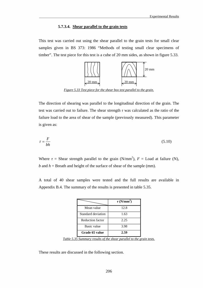
Experimental Results
5.7.3.4. Shear parallel to the grain tests
This test was carried out using the shear parallel to the grain tests for small clear
samples given in BS 373: 1986 “Methods of testing small clear specimens of
timber”. The test piece for this test is a cube of 20 mm sides, as shown in figure 5.33.
20 mm 20 mm
20 mm
Figure 5.33 Test piece for the shear box test parallel to the grain.
The direction of shearing was parallel to the longitudinal direction of the grain. The
test was carried out to failure. The shear strength τ was calculated as the ratio of the
failure load to the area of shear of the sample (previously measured). This parameter
is given as:
bhF
=τ (5.10)
Where τ = Shear strength parallel to the grain (N/mm2), F = Load at failure (N),
b and h = Breath and height of the surface of shear of the sample (mm).
A total of 40 shear samples were tested and the full results are available in
Appendix B.4. The summary of the results is presented in table 5.35.
τ (N/mm2)
Mean value 12.8
Standard deviation 1.63
Reduction factor 2.25
Basic value 3.98
Grade 65 value 2.59
Table 5.35 Summary results of the shear parallel to the grain tests.
These results are discussed in the following section.
206
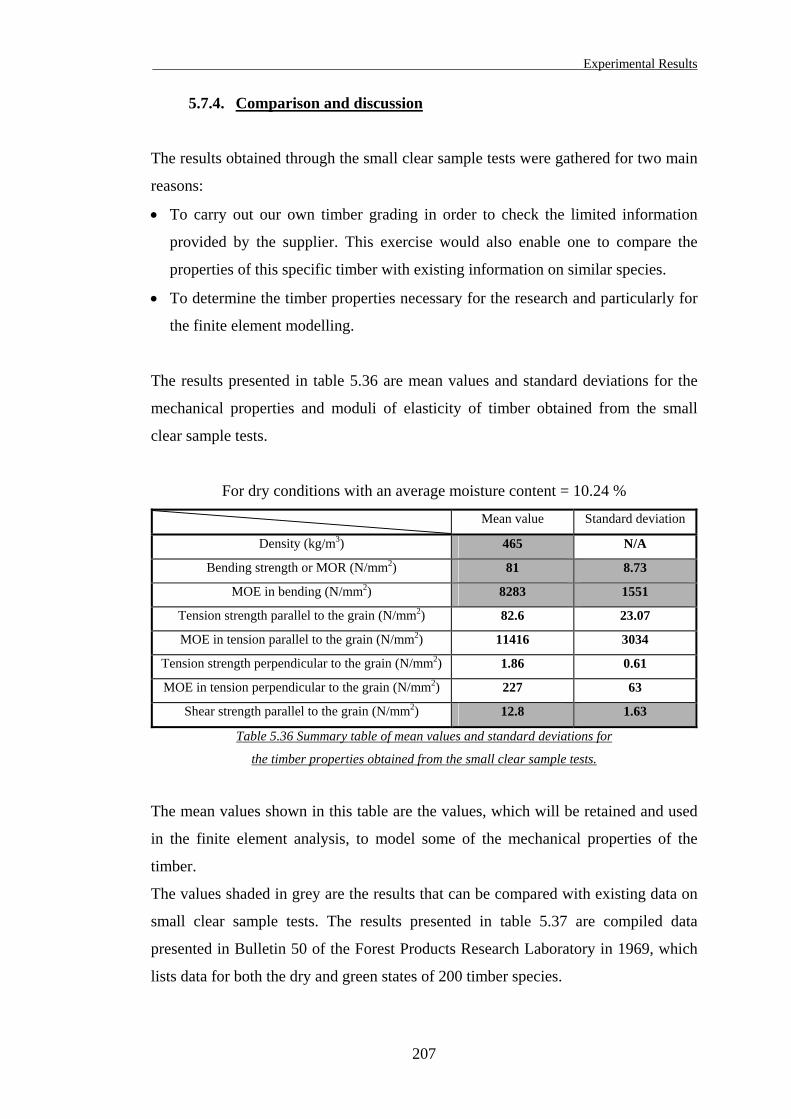
Experimental Results
5.7.4. Comparison and discussion
The results obtained through the small clear sample tests were gathered for two main
reasons:
• To carry out our own timber grading in order to check the limited information
provided by the supplier. This exercise would also enable one to compare the
properties of this specific timber with existing information on similar species.
• To determine the timber properties necessary for the research and particularly for
the finite element modelling.
The results presented in table 5.36 are mean values and standard deviations for the
mechanical properties and moduli of elasticity of timber obtained from the small
clear sample tests.
For dry conditions with an average moisture content = 10.24 %
Mean value Standard deviation
Density (kg/m3) 465 N/A
Bending strength or MOR (N/mm2) 81 8.73
MOE in bending (N/mm2) 8283 1551
Tension strength parallel to the grain (N/mm2) 82.6 23.07
MOE in tension parallel to the grain (N/mm2) 11416 3034
Tension strength perpendicular to the grain (N/mm2) 1.86 0.61
MOE in tension perpendicular to the grain (N/mm2) 227 63
Shear strength parallel to the grain (N/mm2) 12.8 1.63
Table 5.36 Summary table of mean values and standard deviations for
the timber properties obtained from the small clear sample tests.
The mean values shown in this table are the values, which will be retained and used
in the finite element analysis, to model some of the mechanical properties of the
timber.
The values shaded in grey are the results that can be compared with existing data on
small clear sample tests. The results presented in table 5.37 are compiled data
presented in Bulletin 50 of the Forest Products Research Laboratory in 1969, which
lists data for both the dry and green states of 200 timber species.
207
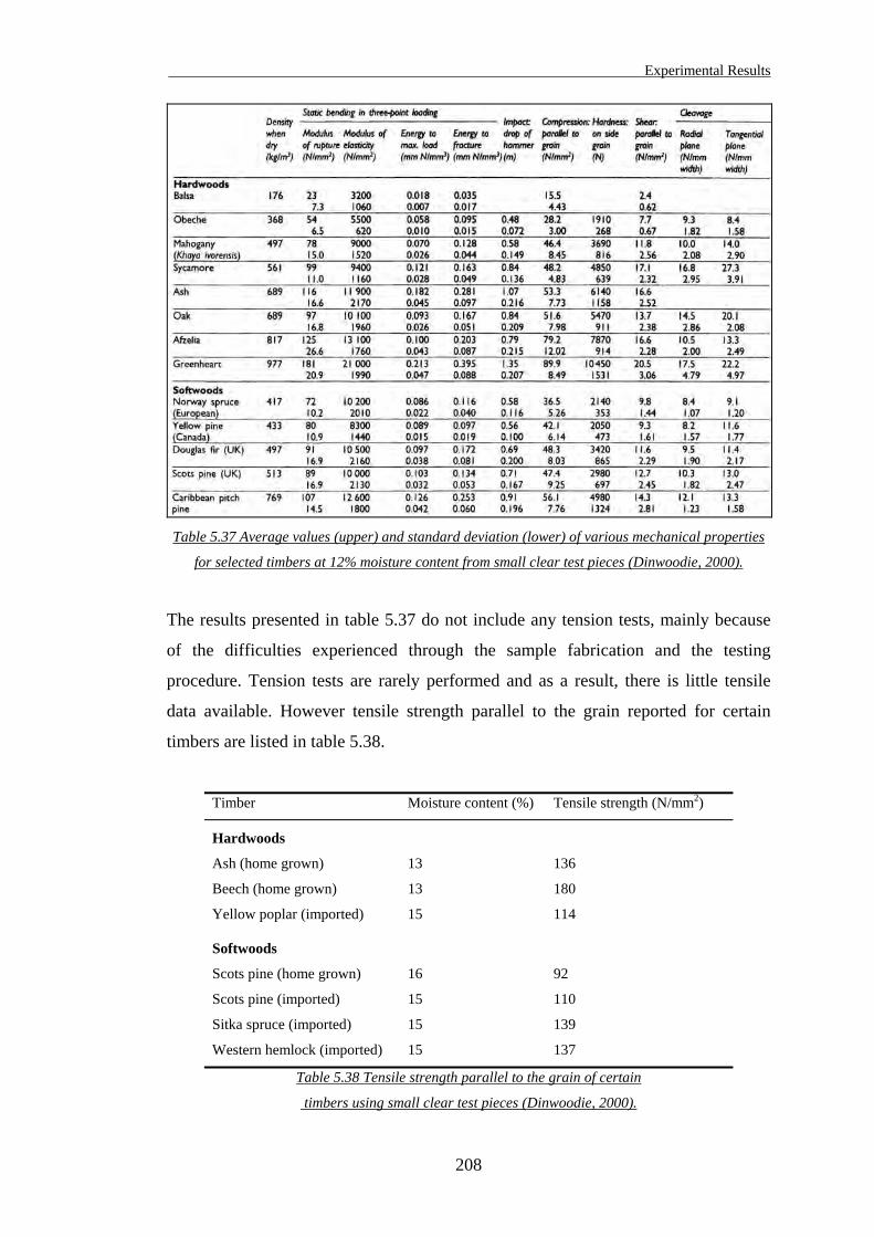
Experimental Results
Table 5.37 Average values (upper) and standard deviation (lower) of various mechanical properties
for selected timbers at 12% moisture content from small clear test pieces (Dinwoodie, 2000).
The results presented in table 5.37 do not include any tension tests, mainly because
of the difficulties experienced through the sample fabrication and the testing
procedure. Tension tests are rarely performed and as a result, there is little tensile
data available. However tensile strength parallel to the grain reported for certain
timbers are listed in table 5.38.
Table 5.38 Tensile strength parallel to the grain of certain
Timber Moisture content (%) Tensile strength (N/mm2)
Hardwoods
Ash (home grown) 13 136
Beech (home grown) 13 180
Yellow poplar (imported) 15 114
Softwoods
Scots pine (home grown) 16 92
Scots pine (imported) 15 110
Sitka spruce (imported) 15 139
Western hemlock (imported) 15 137
timbers using small clear test pieces (Dinwoodie, 2000).
208
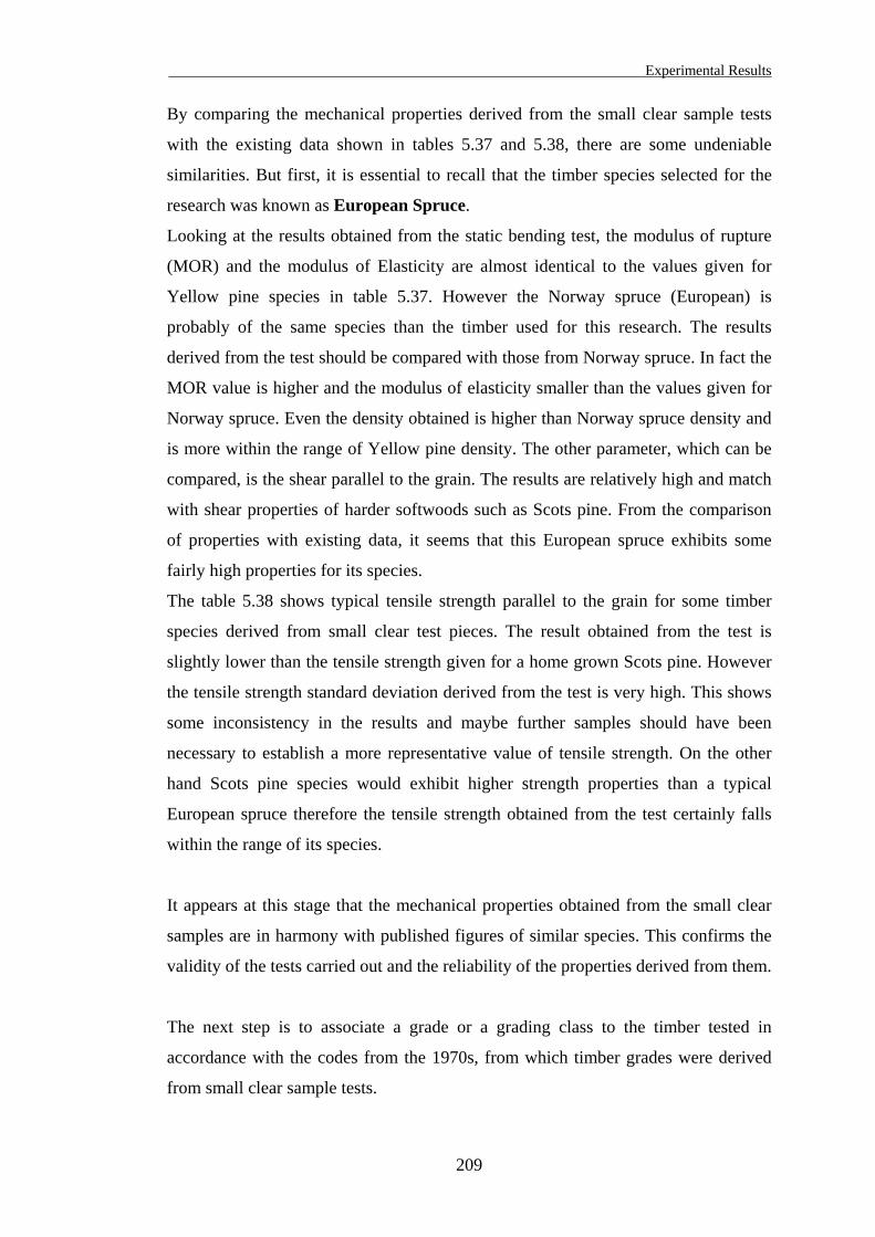
Experimental Results
By comparing the mechanical properties derived from the small clear sample tests
with the existing data shown in tables 5.37 and 5.38, there are some undeniable
similarities. But first, it is essential to recall that the timber species selected for the
research was known as European Spruce.
Looking at the results obtained from the static bending test, the modulus of rupture
(MOR) and the modulus of Elasticity are almost identical to the values given for
Yellow pine species in table 5.37. However the Norway spruce (European) is
probably of the same species than the timber used for this research. The results
derived from the test should be compared with those from Norway spruce. In fact the
MOR value is higher and the modulus of elasticity smaller than the values given for
Norway spruce. Even the density obtained is higher than Norway spruce density and
is more within the range of Yellow pine density. The other parameter, which can be
compared, is the shear parallel to the grain. The results are relatively high and match
with shear properties of harder softwoods such as Scots pine. From the comparison
of properties with existing data, it seems that this European spruce exhibits some
fairly high properties for its species.
The table 5.38 shows typical tensile strength parallel to the grain for some timber
species derived from small clear test pieces. The result obtained from the test is
slightly lower than the tensile strength given for a home grown Scots pine. However
the tensile strength standard deviation derived from the test is very high. This shows
some inconsistency in the results and maybe further samples should have been
necessary to establish a more representative value of tensile strength. On the other
hand Scots pine species would exhibit higher strength properties than a typical
European spruce therefore the tensile strength obtained from the test certainly falls
within the range of its species.
It appears at this stage that the mechanical properties obtained from the small clear
samples are in harmony with published figures of similar species. This confirms the
validity of the tests carried out and the reliability of the properties derived from them.
The next step is to associate a grade or a grading class to the timber tested in
accordance with the codes from the 1970s, from which timber grades were derived
from small clear sample tests.
209
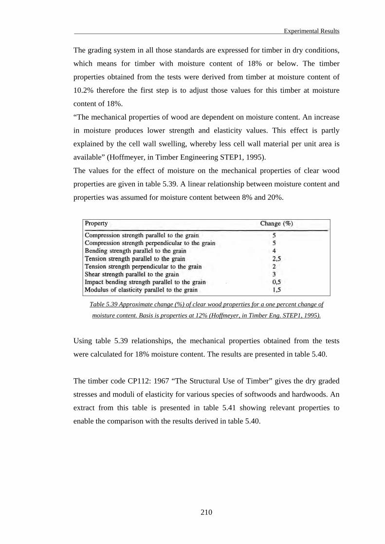
Experimental Results
The grading system in all those standards are expressed for timber in dry conditions,
which means for timber with moisture content of 18% or below. The timber
properties obtained from the tests were derived from timber at moisture content of
10.2% therefore the first step is to adjust those values for this timber at moisture
content of 18%.
“The mechanical properties of wood are dependent on moisture content. An increase
in moisture produces lower strength and elasticity values. This effect is partly
explained by the cell wall swelling, whereby less cell wall material per unit area is
available” (Hoffmeyer, in Timber Engineering STEP1, 1995).
The values for the effect of moisture on the mechanical properties of clear wood
properties are given in table 5.39. A linear relationship between moisture content and
properties was assumed for moisture content between 8% and 20%.
Table 5.39 Approximate change (%) of clear wood properties for a one percent change of
moisture content. Basis is properties at 12% (Hoffmeyer, in Timber Eng. STEP1, 1995).
Using table 5.39 relationships, the mechanical properties obtained from the tests
were calculated for 18% moisture content. The results are presented in table 5.40.
The timber code CP112: 1967 “The Structural Use of Timber” gives the dry graded
stresses and moduli of elasticity for various species of softwoods and hardwoods. An
extract from this table is presented in table 5.41 showing relevant properties to
enable the comparison with the results derived in table 5.40.
210
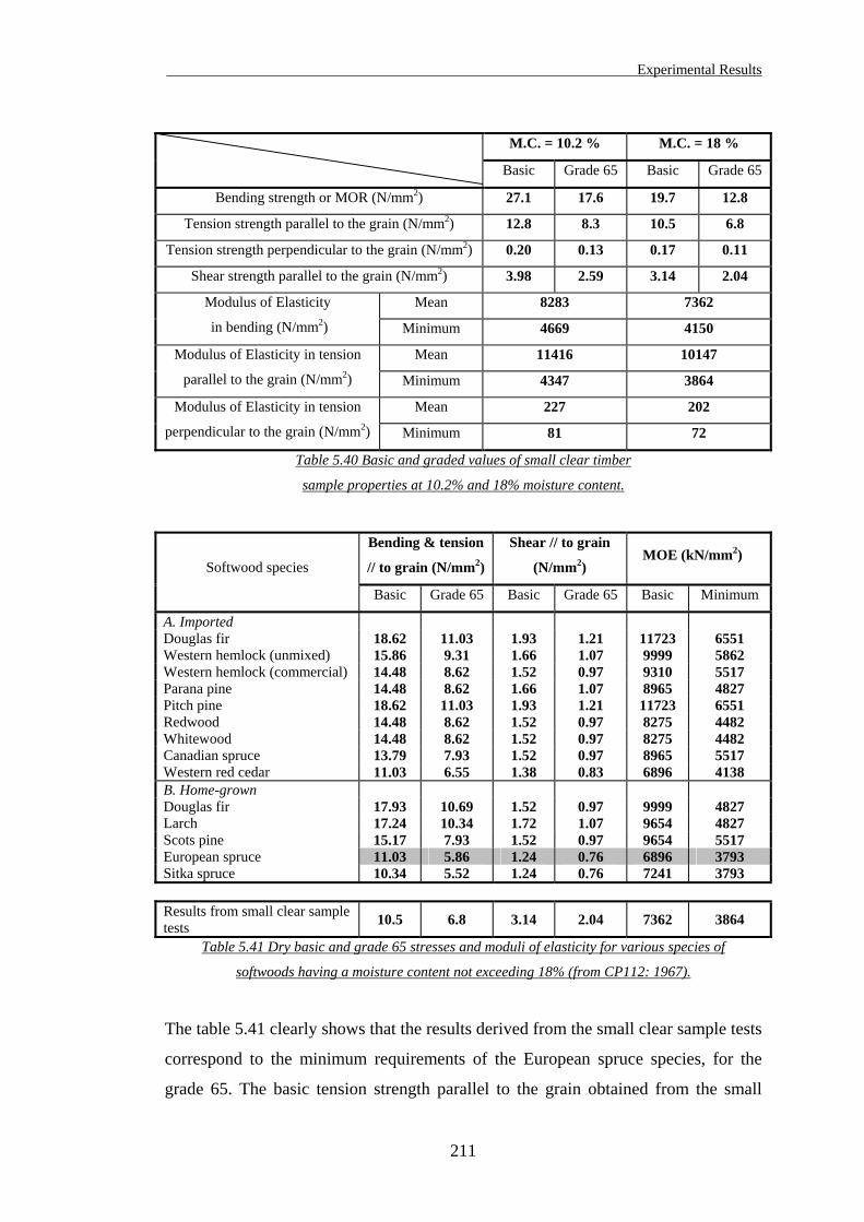
Experimental Results
M.C. = 10.2 % M.C. = 18 %
Basic Grade 65 Basic Grade 65
Bending strength or MOR (N/mm2) 27.1 17.6 19.7 12.8
Tension strength parallel to the grain (N/mm2) 12.8 8.3 10.5 6.8
Tension strength perpendicular to the grain (N/mm2) 0.20 0.13 0.17 0.11
Shear strength parallel to the grain (N/mm2) 3.98 2.59 3.14 2.04
Mean 8283 7362 Modulus of Elasticity
in bending (N/mm2) Minimum 4669 4150
Mean 11416 10147 Modulus of Elasticity in tension
parallel to the grain (N/mm2) Minimum 4347 3864
Mean 227 202 Modulus of Elasticity in tension
perpendicular to the grain (N/mm2) Minimum 81 72
Table 5.40 Basic and graded values of small clear timber
sample properties at 10.2% and 18% moisture content.
Bending & tension
// to grain (N/mm2)
Shear // to grain
(N/mm2) MOE (kN/mm2)
Softwood species
Basic Grade 65 Basic Grade 65 Basic Minimum
A. Imported Douglas fir 18.62 11.03 1.93 1.21 11723 6551 Western hemlock (unmixed) 15.86 9.31 1.66 1.07 9999 5862 Western hemlock (commercial) 14.48 8.62 1.52 0.97 9310 5517 Parana pine 14.48 8.62 1.66 1.07 8965 4827 Pitch pine 18.62 11.03 1.93 1.21 11723 6551 Redwood 14.48 8.62 1.52 0.97 8275 4482 Whitewood 14.48 8.62 1.52 0.97 8275 4482 Canadian spruce 13.79 7.93 1.52 0.97 8965 5517 Western red cedar 11.03 6.55 1.38 0.83 6896 4138 B. Home-grown Douglas fir 17.93 10.69 1.52 0.97 9999 4827 Larch 17.24 10.34 1.72 1.07 9654 4827 Scots pine 15.17 7.93 1.52 0.97 9654 5517 European spruce 11.03 5.86 1.24 0.76 6896 3793 Sitka spruce 10.34 5.52 1.24 0.76 7241 3793 Results from small clear sample tests 10.5 6.8 3.14 2.04 7362 3864
Table 5.41 Dry basic and grade 65 stresses and moduli of elasticity for various species of
softwoods having a moisture content not exceeding 18% (from CP112: 1967).
The table 5.41 clearly shows that the results derived from the small clear sample tests
correspond to the minimum requirements of the European spruce species, for the
grade 65. The basic tension strength parallel to the grain obtained from the small
211
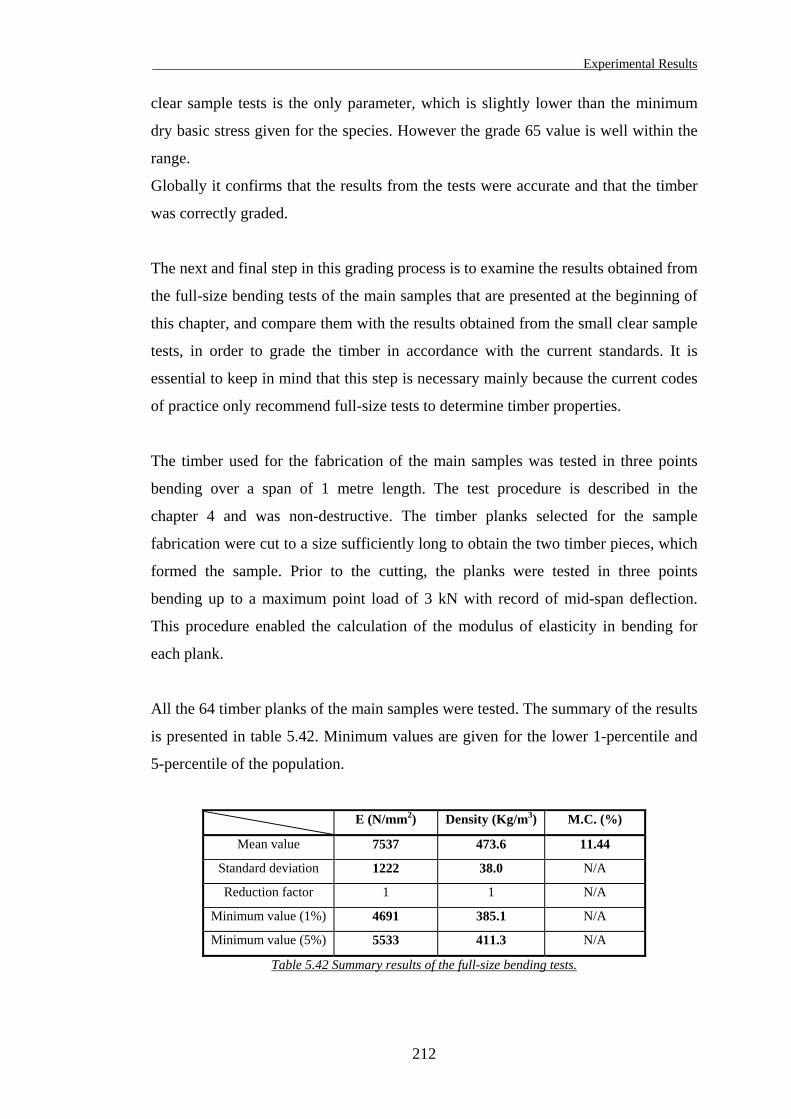
Experimental Results
clear sample tests is the only parameter, which is slightly lower than the minimum
dry basic stress given for the species. However the grade 65 value is well within the
range.
Globally it confirms that the results from the tests were accurate and that the timber
was correctly graded.
The next and final step in this grading process is to examine the results obtained from
the full-size bending tests of the main samples that are presented at the beginning of
this chapter, and compare them with the results obtained from the small clear sample
tests, in order to grade the timber in accordance with the current standards. It is
essential to keep in mind that this step is necessary mainly because the current codes
of practice only recommend full-size tests to determine timber properties.
The timber used for the fabrication of the main samples was tested in three points
bending over a span of 1 metre length. The test procedure is described in the
chapter 4 and was non-destructive. The timber planks selected for the sample
fabrication were cut to a size sufficiently long to obtain the two timber pieces, which
formed the sample. Prior to the cutting, the planks were tested in three points
bending up to a maximum point load of 3 kN with record of mid-span deflection.
This procedure enabled the calculation of the modulus of elasticity in bending for
each plank.
All the 64 timber planks of the main samples were tested. The summary of the results
is presented in table 5.42. Minimum values are given for the lower 1-percentile and
5-percentile of the population.
E (N/mm2) Density (Kg/m3) M.C. (%)
Mean value 7537 473.6 11.44
Standard deviation 1222 38.0 N/A
Reduction factor 1 1 N/A
Minimum value (1%) 4691 385.1 N/A
Minimum value (5%) 5533 411.3 N/A
Table 5.42 Summary results of the full-size bending tests.
212
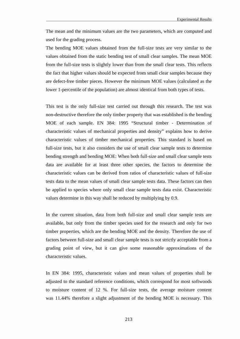
Experimental Results
The mean and the minimum values are the two parameters, which are computed and
used for the grading process.
The bending MOE values obtained from the full-size tests are very similar to the
values obtained from the static bending test of small clear samples. The mean MOE
from the full-size tests is slightly lower than from the small clear tests. This reflects
the fact that higher values should be expected from small clear samples because they
are defect-free timber pieces. However the minimum MOE values (calculated as the
lower 1-percentile of the population) are almost identical from both types of tests.
This test is the only full-size test carried out through this research. The test was
non-destructive therefore the only timber property that was established is the bending
MOE of each sample. EN 384: 1995 “Structural timber - Determination of
characteristic values of mechanical properties and density” explains how to derive
characteristic values of timber mechanical properties. This standard is based on
full-size tests, but it also considers the use of small clear sample tests to determine
bending strength and bending MOE: When both full-size and small clear sample tests
data are available for at least three other species, the factors to determine the
characteristic values can be derived from ratios of characteristic values of full-size
tests data to the mean values of small clear sample tests data. These factors can then
be applied to species where only small clear sample tests data exist. Characteristic
values determine in this way shall be reduced by multiplying by 0.9.
In the current situation, data from both full-size and small clear sample tests are
available, but only from the timber species used for the research and only for two
timber properties, which are the bending MOE and the density. Therefore the use of
factors between full-size and small clear sample tests is not strictly acceptable from a
grading point of view, but it can give some reasonable approximations of the
characteristic values.
In EN 384: 1995, characteristic values and mean values of properties shall be
adjusted to the standard reference conditions, which correspond for most softwoods
to moisture content of 12 %. For full-size tests, the average moisture content
was 11.44% therefore a slight adjustment of the bending MOE is necessary. This
213
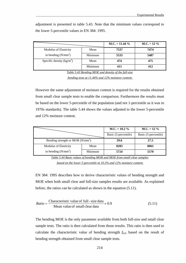
Experimental Results
adjustment is presented in table 5.43. Note that the minimum values correspond to
the lower 5-percentile values in EN 384: 1995.
M.C. = 11.44 % M.C. = 12 %
Mean 7537 7474 Modulus of Elasticity
in bending (N/mm2) Minimum 5533 5487
Mean 474 475 Specific density (kg/m3)
Minimum 411 412
Table 5.43 Bending MOE and density of the full-size
bending tests at 11.44% and 12% moisture content.
However the same adjustment of moisture content is required for the results obtained
from small clear sample tests to enable the comparison. Furthermore the results must
be based on the lower 5-percentile of the population (and not 1-percentile as it was in
1970s standards). The table 5.44 shows the values adjusted to the lower 5-percentile
and 12% moisture content.
M.C. = 10.2 % M.C. = 12 %
Basic (5-percentile) Basic (5-percentile)
Bending strength or MOR (N/mm2) 29.6 27.5
Mean 8283 8061 Modulus of Elasticity
in bending (N/mm2) Minimum 5724 5570
Table 5.44 Basic values of bending MOR and MOE from small clear samples
based on the lower 5-percentile at 10.2% and 12% moisture content.
EN 384: 1995 describes how to derive characteristic values of bending strength and
MOE when both small clear and full-size samples results are available. As explained
before, the ratios can be calculated as shown in the equation (5.11).
9.0dataclear small of Mean value
data size-full of valuesticCharacteri×=Ratio (5.11)
The bending MOE is the only parameter available from both full-size and small clear
sample tests. The ratio is then calculated from those results. This ratio is then used to
calculate the characteristic value of bending strength fm,k based on the result of
bending strength obtained from small clear sample tests.
214
Experimental Results
0.6139.080615487
=×=Ratio
Hence 2
, N/mm 16.95.27613.0 =×=kmf
When no full-size results are available for other timber properties, EN 384: 1995
recommends that characteristic values shall be determined from the characteristic
values of bending strength fm,k, mean modulus of elasticity E0,mean and density ρk.
Note that the characteristic density ρk is the lower 5-percentile value of density.
These characteristic values are:
2
, N/mm 16.9=kmf
2,0 N/mm 7474=meanE
3kg/m 412=kρ
This method of determining the timber properties is probably more accurate than
applying the ratio to the properties derived from small clear sample tests. In fact,
full-size tests to determine other relevant properties, such as tension parallel or
tension perpendicular to the grain strengths, etc, are entirely different from
equivalent small clear sample tests used to determine the same properties.
The characteristic values of tension strength parallel to grain ft,0,k, tension strength
perpendicular to grain ft,90,k, compression strength parallel to grain fc,0,k, compression
strength perpendicular to grain fc,90,k, shear strength fv,k, mean MOE perpendicular to
grain E90,mean and shear modulus Gmean shall be calculated from the equations
(5.12) to (5.18) respectively:
kmkt ff ,,0, 6.0= (5.12)
kktf ρ001.0,90, = (5.13)
45.0,,0, )(5 kmkc ff = (5.14)
kkcf ρ015.0,90, = (5.15)
215
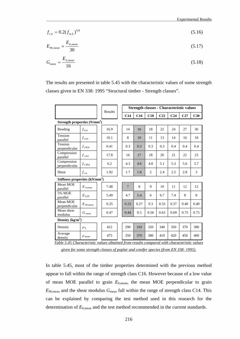
Experimental Results
8.0,, )(2.0 kmkv ff = (5.16)
30,0
,90mean
mean
EE = (5.17)
16,0 mean
mean
EG = (5.18)
The results are presented in table 5.45 with the characteristic values of some strength
classes given in EN 338: 1995 “Structural timber - Strength classes”.
Strength classes - Characteristic values
Results
C14 C16 C18 C22 C24 C27 C30
Strength properties (N/mm2)
Bending f m,k 16.9 14 16 18 22 24 27 30
Tension parallel f t,0,k 10.1 8 10 11 13 14 16 18
Tension perpendicular f t,90,k 0.41 0.3 0.3 0.3 0.3 0.4 0.4 0.4
Compression parallel f c,0,k 17.8 16 17 18 20 21 22 23
Compression perpendicular f c,90,k 6.2 4.3 4.6 4.8 5.1 5.3 5.6 5.7
Shear f v,k 1.92 1.7 1.8 2 2.4 2.5 2.8 3
Stiffness properties (kN/mm2) Mean MOE parallel E 0,mean 7.48 7 8 9 10 11 12 12
5% MOE parallel E 0,05 5.49 4.7 5.4 6 6.7 7.4 8 8
Mean MOE perpendicular E 90,mean 0.25 0.23 0.27 0.3 0.33 0.37 0.40 0.40
Mean shear modulus G mean 0.47 0.44 0.5 0.56 0.63 0.69 0.75 0.75
Density (kg/m3)
Density ρ k 412 290 310 320 340 350 370 380
Average density ρ mean 475 350 370 380 410 420 450 460
Table 5.45 Characteristic values obtained from results compared with characteristic values
given for some strength classes of poplar and conifer species (from EN 338: 1995).
In table 5.45, most of the timber properties determined with the previous method
appear to fall within the range of strength class C16. However because of a low value
of mean MOE parallel to grain E0,mean, the mean MOE perpendicular to grain
E90,mean and the shear modulus Gmean fall within the range of strength class C14. This
can be explained by comparing the test method used in this research for the
determination of E0,mean and the test method recommended in the current standards.
216
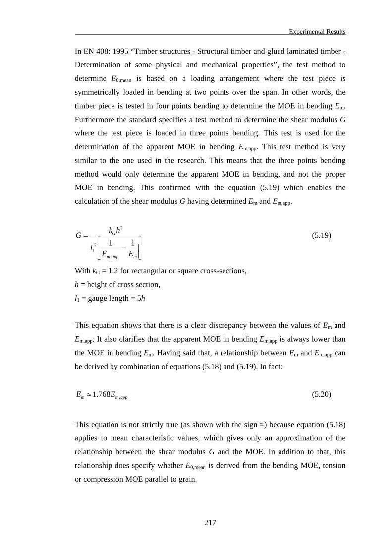
Experimental Results
In EN 408: 1995 “Timber structures - Structural timber and glued laminated timber -
Determination of some physical and mechanical properties”, the test method to
determine E0,mean is based on a loading arrangement where the test piece is
symmetrically loaded in bending at two points over the span. In other words, the
timber piece is tested in four points bending to determine the MOE in bending Em.
Furthermore the standard specifies a test method to determine the shear modulus G
where the test piece is loaded in three points bending. This test is used for the
determination of the apparent MOE in bending Em,app. This test method is very
similar to the one used in the research. This means that the three points bending
method would only determine the apparent MOE in bending, and not the proper
MOE in bending. This confirmed with the equation (5.19) which enables the
calculation of the shear modulus G having determined Em and Em,app.
−
=
mappm
G
EEl
hkG11
,
21
2
(5.19)
With kG = 1.2 for rectangular or square cross-sections,
h = height of cross section,
l1 = gauge length = 5h
This equation shows that there is a clear discrepancy between the values of Em and
Em,app. It also clarifies that the apparent MOE in bending Em,app is always lower than
the MOE in bending Em. Having said that, a relationship between Em and Em,app can
be derived by combination of equations (5.18) and (5.19). In fact:
appmm EE ,768.1≈ (5.20)
This equation is not strictly true (as shown with the sign ≈) because equation (5.18)
applies to mean characteristic values, which gives only an approximation of the
relationship between the shear modulus G and the MOE. In addition to that, this
relationship does specify whether E0,mean is derived from the bending MOE, tension
or compression MOE parallel to grain.
217
Experimental Results
All things considered, the characteristic value of MOE parallel to grain E0,mean is
based on bending test carried out using the three points bending method. Therefore
the value of E0,mean may reflect an apparent bending MOE, which would explain the
relatively low figure shown in table 5.45.
As a result it can be confirmed that the timber used in the research corresponds to the
strength class C16.
Finally the results obtained from the small clear sample tests reflect how
representative they are in the grading process in accordance to the 1970s standards.
When the timber properties are derived from the ratio obtained from full-size
bending tests to enable the grading in accordance with current standards, the results
are also relevant as they confirm the strength class C16 that corresponds to the
strength class SC3 given initially by the timber supplier.
The timber properties, which are to be retained for the finite element analysis, are
summarised in the conclusion.
218

Experimental Results
5.8. Conclusion
Timber is not a truly elastic material as its behaviour is time dependent. The load
duration has an effect on its deformation, which defines the material as
viscoelastic. However timber is treated as elastic in timber design codes using safety
factors to take into account the duration of load. The theory of elasticity will be used
for the finite element analysis, allowing for the anisotropy of the material.
Wood is often considered as an orthotropic material, which means that the material
has symmetry about three orthogonal planes. The assumption is made that the three
principal elasticity directions coincide with the longitudinal, radial and tangential
directions in the tree. The mechanical behaviour of wood is explained in detail in the
following chapter.
Orthotropic materials are characterised by six moduli of elasticity, three in the
principal directions E and three in the orthotropic planes G. The orthotropic materials
are also characterised by having six Poisson’s ratios. Three of them are independent
because they are linked with the three moduli of elasticity E. The three others can be
derived accordingly.
The table 5.46 shows orthotropic properties measured for various species.
Table 5.46 Orthotropic properties determined for various species (Dinwoodie, 2000).
219
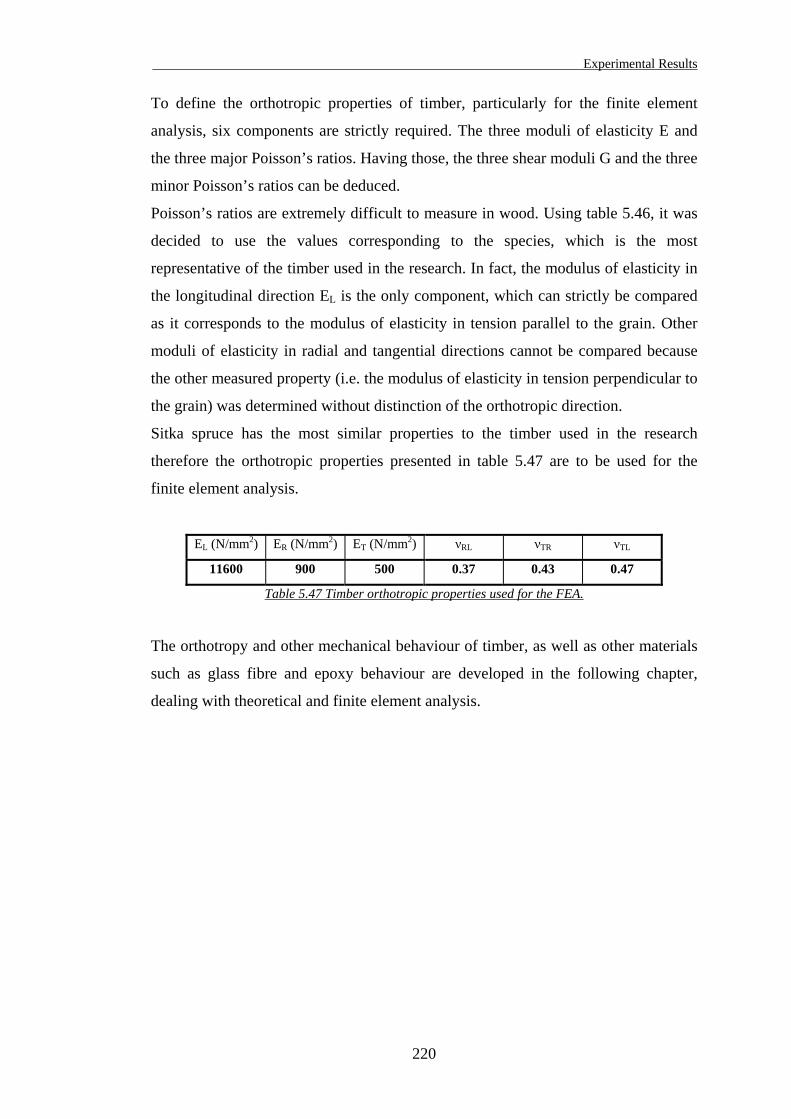
Experimental Results
220
To define the orthotropic properties of timber, particularly for the finite element
analysis, six components are strictly required. The three moduli of elasticity E and
the three major Poisson’s ratios. Having those, the three shear moduli G and the three
minor Poisson’s ratios can be deduced.
Poisson’s ratios are extremely difficult to measure in wood. Using table 5.46, it was
decided to use the values corresponding to the species, which is the most
representative of the timber used in the research. In fact, the modulus of elasticity in
the longitudinal direction EL is the only component, which can strictly be compared
as it corresponds to the modulus of elasticity in tension parallel to the grain. Other
moduli of elasticity in radial and tangential directions cannot be compared because
the other measured property (i.e. the modulus of elasticity in tension perpendicular to
the grain) was determined without distinction of the orthotropic direction.
Sitka spruce has the most similar properties to the timber used in the research
therefore the orthotropic properties presented in table 5.47 are to be used for the
finite element analysis.
EL (N/mm2) ER (N/mm2) ET (N/mm2) νRL νTR νTL
11600 900 500 0.37 0.43 0.47
Table 5.47 Timber orthotropic properties used for the FEA.
The orthotropy and other mechanical behaviour of timber, as well as other materials
such as glass fibre and epoxy behaviour are developed in the following chapter,
dealing with theoretical and finite element analysis.
CHAPTER 6
THEORETICAL AND FINITE ELEMENT ANALYSES
6.1. Introduction
The theory behind the wood/glass/epoxy joint is based on principles of structural and
solid mechanics. The anisotropy of the timber and the glass fibre/epoxy composite
materials makes the theoretical analysis even more complex and cannot be
approached by simple calculations.
The mechanics of the wood/glass/epoxy joint will be developed in this chapter as
well as the theoretical analysis, which will be carried out using finite element
modelling (FEM). The computer software used for the FEM is the ANSYS package
product, version 5.4.
The finite element modelling enables the theoretical analysis of the joint with the
computer carrying the fastidious calculations to a degree of accuracy, which could
not be reached otherwise. There are many parameters, which must be set to an
appropriate level in order to obtain accurate and reliable results. These parameters
are specific for each model and will be identified and developed in this chapter.
The mechanical behaviour of the joints will be studied in the elastic and plastic
range, but the finite element modelling will not be considered for plasticity. This is
justified by the fact that the joints did not develop plasticity to any extent, which
would enable the analysis to be carried out in that range. Modelling the non-linear
behaviour of the joints would have required different experimental procedures, such
as using many more strain gauges to measure the state of strain throughout the joints.
The objectives are the global understanding of the mechanical behaviour of the joints
rather than the achievement of accurate finite element models. Other reasons to limit
the FEM to the elastic range lie in the true nature of wood material, which is fairly
complex, when the material develops creep and its microscopic structure start to
change. These are the subjects that are developed in the following sections.
221
Theoretical and Finite Element Analyses
6.2. Theoretical approach to structural adhesive joints
Structural adhesive joints have been used for many years in the industry. In wood
structures, it started many centuries ago with carpentry joints. At that time
carpenter’s glue was used, but it was only to prevent mechanical joints made for
example with a tenon to become loose. Load-bearing structural adhesive joints are a
recent innovation. They were initially studied for wood structures in the 1950s and
were becoming essential with the development of composite materials. The wide
range of applications of composite materials to high-tech industries such as
aerospace and aircraft engineering have brought much research and many
developments in this area. Structural adhesive joints appeared to have a great
advantage over mechanically fastened joints: uniform stress transfer (i.e. no stress
concentration around a fastener) resulting in greater fatigue resistance.
Today structural adhesive joints are well understood and Computer Aided Design
(CAD) tools can help engineers to design very efficient adhesive joints without
having to derive by hand and therefore by trial and error, the principles of mechanics,
which apply to those joints. However it is necessary to understand clearly how the
joints behave under load in order to use the appropriate assumptions for an accurate
design.
This section will describe the theory that applies to wood/glass/epoxy joints. But first
it is necessary to introduce the principles of mechanics for anisotropic materials such
as wood and glass fibre/epoxy composites.
222
Theoretical and Finite Element Analyses
6.2.1. Anisotropic and orthotropic materials
A material, which has the same properties at any point, is known as homogeneous.
And if the properties are the same in any direction, the material is isotropic. Many
metals and ceramics are approximately isotropic. Amorphous materials such as glass
are also isotropic. Isotropic laws of elasticity (e.g. Hooke’s Law) are generally used
for those materials.
The behaviour of wood and glass fibre/epoxy composites, which are the components
of the wood/glass/epoxy joints, is presented in this section.
Wood is known as a highly anisotropic material because of the orientation of its
wood cells, as discussed in chapter 3. Wood is a homogenous material, but the
properties vary with the direction considered, therefore it is anisotropic.
The load-deformation relationship for wood is rather complex, as the material
behaviour is time dependent. In fact timber does not behave in a truly elastic mode
and is defined as a viscoelastic material. Timber will deform under load but if the
load is maintained in time, the deformation increases but the rate of deformation
decreases with time. This is the effect of creep. On removal of the load, the
deformation decreases by a proportion approximately equal to the initial elastic
deformation. The remaining deformation will decrease with time until no further
reduction occurs. This is known as a delayed-elastic behaviour. The remaining
deformation, which will not be recovered, is known as plastic or viscous
deformation.
Many factors can also affect the timber response under load. These factors are part of
the material properties, such as grain orientation or density. Other factors are
dependent on the environment in which the wood is used: Moisture content (relative
humidity) and temperature. With such complexity in its behaviour, wood is usually
treated in design terms as an elastic material.
“Perhaps the greatest incentive for this viewpoint is the fact that classical elasticity
theory is well established and, when applied to timber, has been shown to work very
well. The question of time in any stress analysis can be accommodated by the use of
safety factors in design calculations” (Dinwoodie, 2000).
223
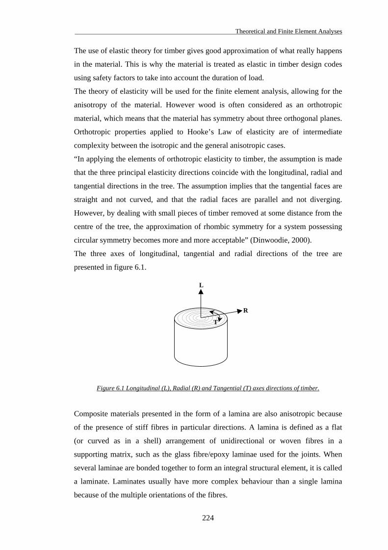
Theoretical and Finite Element Analyses
The use of elastic theory for timber gives good approximation of what really happens
in the material. This is why the material is treated as elastic in timber design codes
using safety factors to take into account the duration of load.
The theory of elasticity will be used for the finite element analysis, allowing for the
anisotropy of the material. However wood is often considered as an orthotropic
material, which means that the material has symmetry about three orthogonal planes.
Orthotropic properties applied to Hooke’s Law of elasticity are of intermediate
complexity between the isotropic and the general anisotropic cases.
“In applying the elements of orthotropic elasticity to timber, the assumption is made
that the three principal elasticity directions coincide with the longitudinal, radial and
tangential directions in the tree. The assumption implies that the tangential faces are
straight and not curved, and that the radial faces are parallel and not diverging.
However, by dealing with small pieces of timber removed at some distance from the
centre of the tree, the approximation of rhombic symmetry for a system possessing
circular symmetry becomes more and more acceptable” (Dinwoodie, 2000).
The three axes of longitudinal, tangential and radial directions of the tree are
presented in figure 6.1.
L
T
R
Figure 6.1 Longitudinal (L), Radial (R) and Tangential (T) axes directions of timber.
Composite materials presented in the form of a lamina are also anisotropic because
of the presence of stiff fibres in particular directions. A lamina is defined as a flat
(or curved as in a shell) arrangement of unidirectional or woven fibres in a
supporting matrix, such as the glass fibre/epoxy laminae used for the joints. When
several laminae are bonded together to form an integral structural element, it is called
a laminate. Laminates usually have more complex behaviour than a single lamina
because of the multiple orientations of the fibres.
224
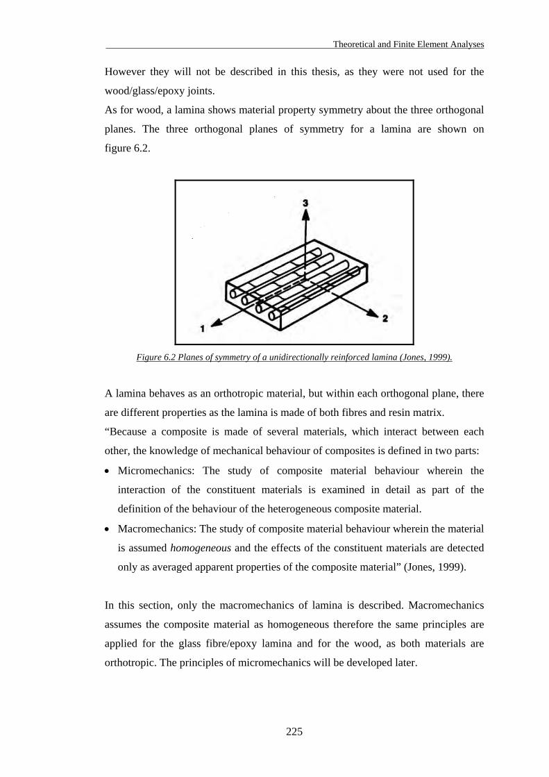
Theoretical and Finite Element Analyses
However they will not be described in this thesis, as they were not used for the
wood/glass/epoxy joints.
As for wood, a lamina shows material property symmetry about the three orthogonal
planes. The three orthogonal planes of symmetry for a lamina are shown on
figure 6.2.
Figure 6.2 Planes of symmetry of a unidirectionally reinforced lamina (Jones, 1999).
A lamina behaves as an orthotropic material, but within each orthogonal plane, there
are different properties as the lamina is made of both fibres and resin matrix.
“Because a composite is made of several materials, which interact between each
other, the knowledge of mechanical behaviour of composites is defined in two parts:
• Micromechanics: The study of composite material behaviour wherein the
interaction of the constituent materials is examined in detail as part of the
definition of the behaviour of the heterogeneous composite material.
• Macromechanics: The study of composite material behaviour wherein the material
is assumed homogeneous and the effects of the constituent materials are detected
only as averaged apparent properties of the composite material” (Jones, 1999).
In this section, only the macromechanics of lamina is described. Macromechanics
assumes the composite material as homogeneous therefore the same principles are
applied for the glass fibre/epoxy lamina and for the wood, as both materials are
orthotropic. The principles of micromechanics will be developed later.
225
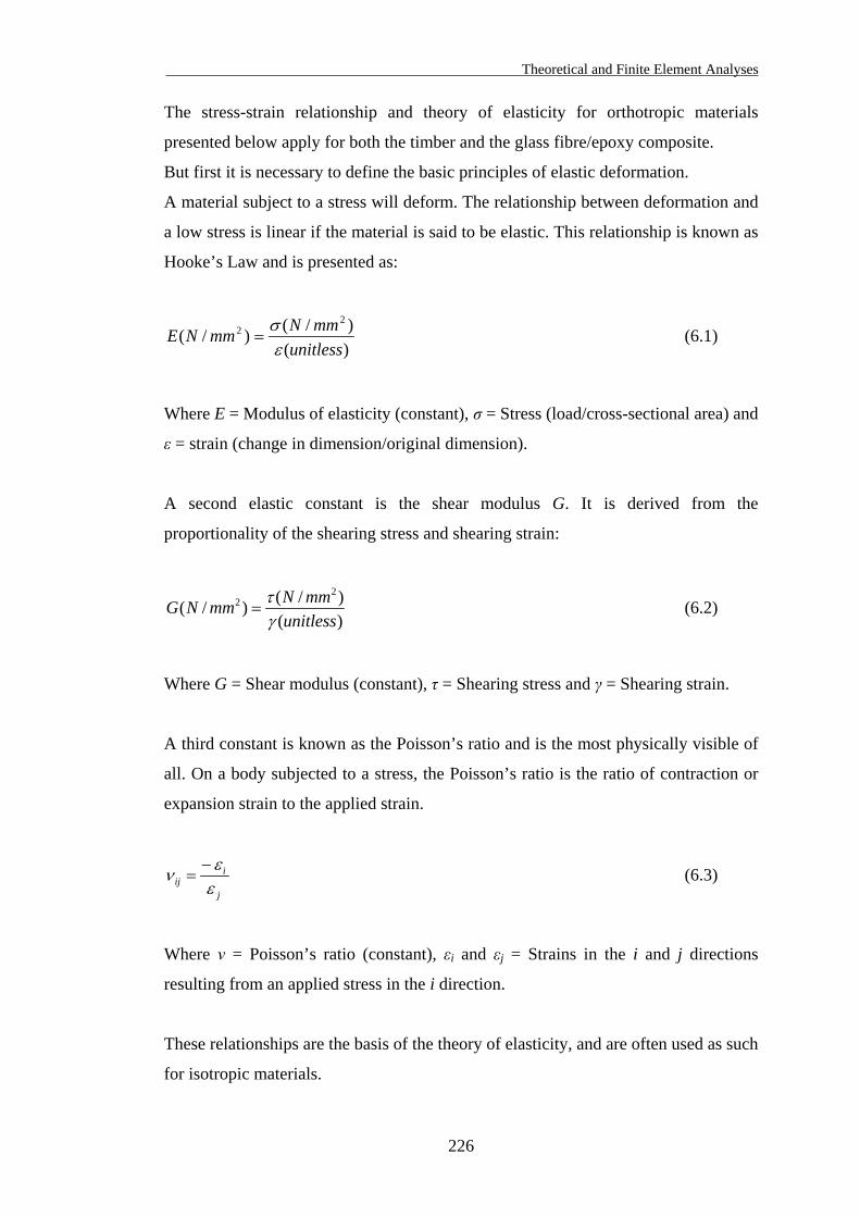
Theoretical and Finite Element Analyses
The stress-strain relationship and theory of elasticity for orthotropic materials
presented below apply for both the timber and the glass fibre/epoxy composite.
But first it is necessary to define the basic principles of elastic deformation.
A material subject to a stress will deform. The relationship between deformation and
a low stress is linear if the material is said to be elastic. This relationship is known as
Hooke’s Law and is presented as:
)()/()/(
22
unitlessmmNmmNE
εσ
= (6.1)
Where E = Modulus of elasticity (constant), σ = Stress (load/cross-sectional area) and
ε = strain (change in dimension/original dimension).
A second elastic constant is the shear modulus G. It is derived from the
proportionality of the shearing stress and shearing strain:
)()/()/(
22
unitlessmmNmmNG
γτ
= (6.2)
Where G = Shear modulus (constant), τ = Shearing stress and γ = Shearing strain.
A third constant is known as the Poisson’s ratio and is the most physically visible of
all. On a body subjected to a stress, the Poisson’s ratio is the ratio of contraction or
expansion strain to the applied strain.
j
iij ε
εν −= (6.3)
Where ν = Poisson’s ratio (constant), εi and εj = Strains in the i and j directions
resulting from an applied stress in the i direction.
These relationships are the basis of the theory of elasticity, and are often used as such
for isotropic materials.
226
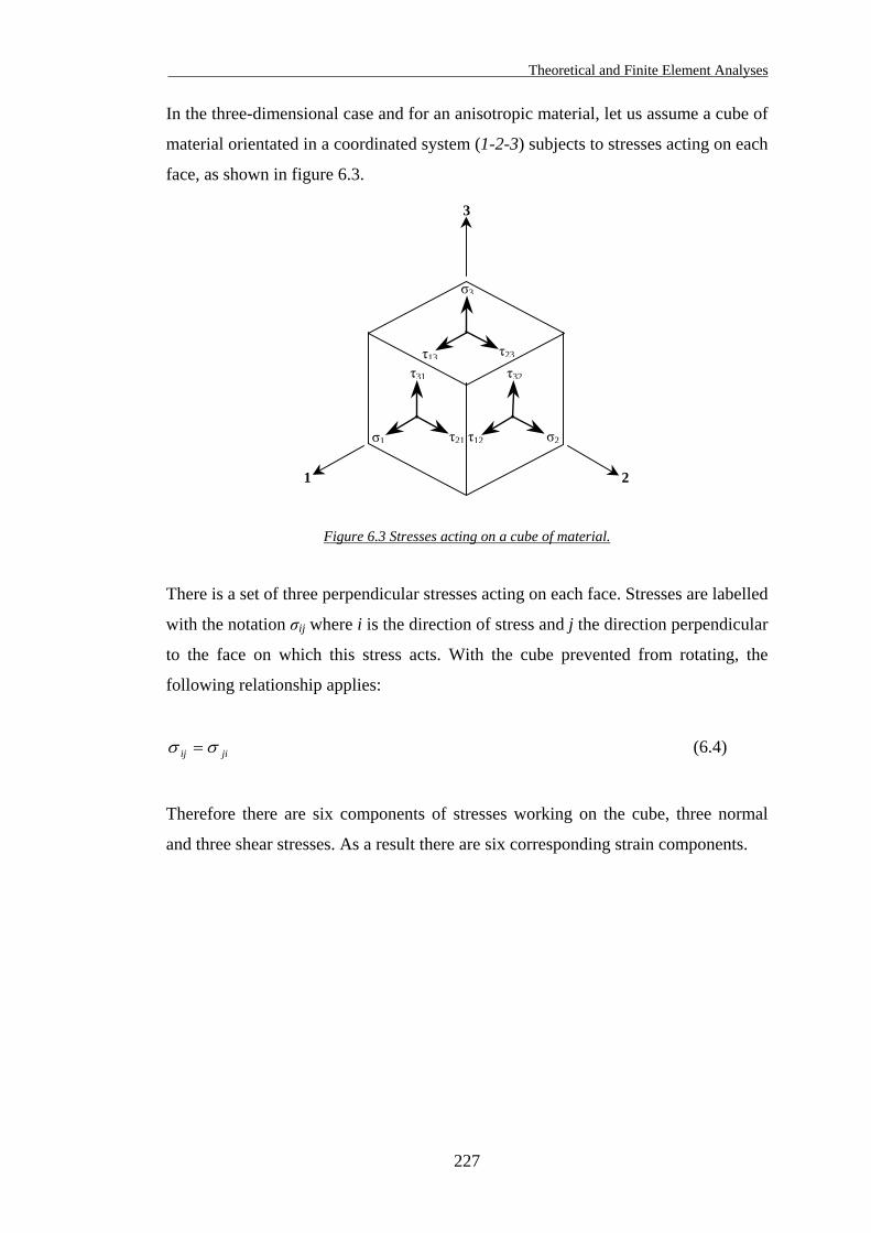
Theoretical and Finite Element Analyses
In the three-dimensional case and for an anisotropic material, let us assume a cube of
material orientated in a coordinated system (1-2-3) subjects to stresses acting on each
face, as shown in figure 6.3.
3
1 2
τ31
τ13
τ32
τ21
τ23
τ12
σ3
σ2σ1
Figure 6.3 Stresses acting on a cube of material.
There is a set of three perpendicular stresses acting on each face. Stresses are labelled
with the notation σij where i is the direction of stress and j the direction perpendicular
to the face on which this stress acts. With the cube prevented from rotating, the
following relationship applies:
jiij σσ = (6.4)
Therefore there are six components of stresses working on the cube, three normal
and three shear stresses. As a result there are six corresponding strain components.
227
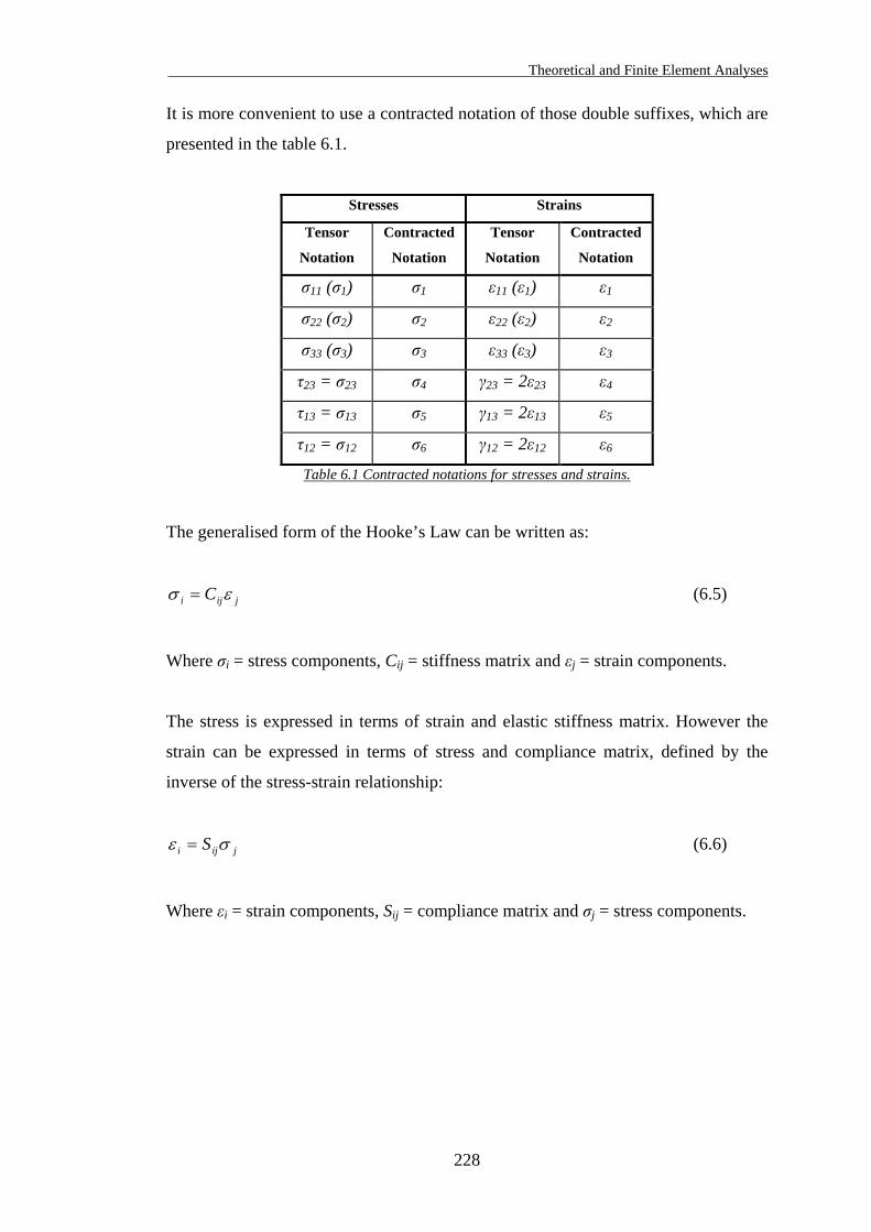
Theoretical and Finite Element Analyses
It is more convenient to use a contracted notation of those double suffixes, which are
presented in the table 6.1.
Stresses Strains
Tensor
Notation
Contracted
Notation
Tensor
Notation
Contracted
Notation
σ11 (σ1) σ1 ε11 (ε1) ε1
σ22 (σ2) σ2 ε22 (ε2) ε2
σ33 (σ3) σ3 ε33 (ε3) ε3
τ23 = σ23 σ4 γ23 = 2ε23 ε4
τ13 = σ13 σ5 γ13 = 2ε13 ε5
τ12 = σ12 σ6 γ12 = 2ε12 ε6
Table 6.1 Contracted notations for stresses and strains.
The generalised form of the Hooke’s Law can be written as:
jiji C εσ = (6.5)
Where σi = stress components, Cij = stiffness matrix and εj = strain components.
The stress is expressed in terms of strain and elastic stiffness matrix. However the
strain can be expressed in terms of stress and compliance matrix, defined by the
inverse of the stress-strain relationship:
jiji S σε = (6.6)
Where εi = strain components, Sij = compliance matrix and σj = stress components.
228
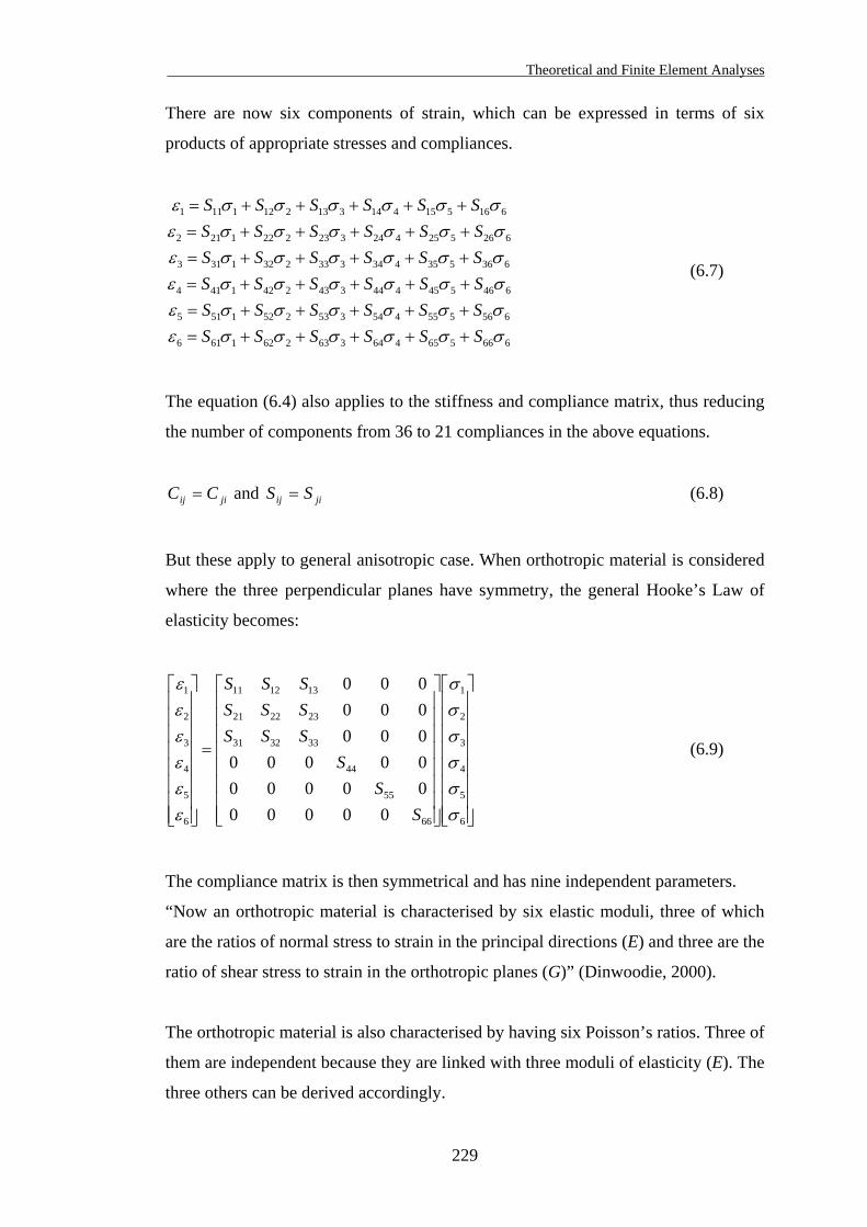
Theoretical and Finite Element Analyses
There are now six components of strain, which can be expressed in terms of six
products of appropriate stresses and compliances.
6665654643632621616
6565554543532521515
6465454443432421414
6365354343332321313
6265254243232221212
6165154143132121111
σσσσσσεσσσσσσεσσσσσσεσσσσσσεσσσσσσεσσσσσσε
SSSSSSSSSSSSSSSSSSSSSSSSSSSSSSSSSSSS
+++++=+++++=+++++=+++++=+++++=+++++=
(6.7)
The equation (6.4) also applies to the stiffness and compliance matrix, thus reducing
the number of components from 36 to 21 compliances in the above equations.
jiij CC = and (6.8) jiij SS =
But these apply to general anisotropic case. When orthotropic material is considered
where the three perpendicular planes have symmetry, the general Hooke’s Law of
elasticity becomes:
=
6
5
4
3
2
1
66
55
44
333231
232221
131211
6
5
4
3
2
1
000000000000000000000000
σσσσσσ
εεεεεε
SS
SSSSSSSSSS
(6.9)
The compliance matrix is then symmetrical and has nine independent parameters.
“Now an orthotropic material is characterised by six elastic moduli, three of which
are the ratios of normal stress to strain in the principal directions (E) and three are the
ratio of shear stress to strain in the orthotropic planes (G)” (Dinwoodie, 2000).
The orthotropic material is also characterised by having six Poisson’s ratios. Three of
them are independent because they are linked with three moduli of elasticity (E). The
three others can be derived accordingly.
229
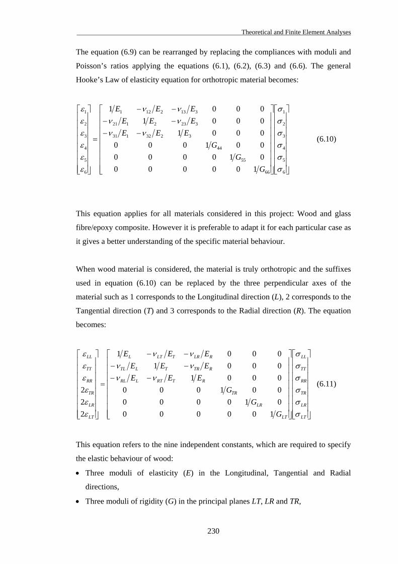
Theoretical and Finite Element Analyses
The equation (6.9) can be rearranged by replacing the compliances with moduli and
Poisson’s ratios applying the equations (6.1), (6.2), (6.3) and (6.6). The general
Hooke’s Law of elasticity equation for orthotropic material becomes:
−−−−−−
=
6
5
4
3
2
1
66
55
44
3232131
3232121
3132121
6
5
4
3
2
1
100000010000001000000100010001
σσσσσσ
νννννν
εεεεεε
GG
GEEE
EEEEEE
(6.10)
This equation applies for all materials considered in this project: Wood and glass
fibre/epoxy composite. However it is preferable to adapt it for each particular case as
it gives a better understanding of the specific material behaviour.
When wood material is considered, the material is truly orthotropic and the suffixes
used in equation (6.10) can be replaced by the three perpendicular axes of the
material such as 1 corresponds to the Longitudinal direction (L), 2 corresponds to the
Tangential direction (T) and 3 corresponds to the Radial direction (R). The equation
becomes:
−−−−−−
=
LT
LR
TR
RR
TT
LL
LT
LR
TR
RTRTLRL
RTRTLTL
RLRTLTL
LT
LR
TR
RR
TT
LL
GG
GEEE
EEEEEE
σσσσσσ
νννννν
εεε
εεε
100000010000001000000100010001
222
(6.11)
This equation refers to the nine independent constants, which are required to specify
the elastic behaviour of wood:
• Three moduli of elasticity (E) in the Longitudinal, Tangential and Radial
directions,
• Three moduli of rigidity (G) in the principal planes LT, LR and TR,
230
Theoretical and Finite Element Analyses
• Three of the six Poisson’s ratio, knowing that three can be related to three others
with the relationship given in equation (6.12). The set of three Poisson’s ratios
νRT, νLR and νTL or νTR, νRL and νLT will have to be specified.
Due to the symmetry of the matrix presented in the equation (6.8), the relationship
between dependent Poisson’s ratios is:
j
ji
i
ij
EEνν
= (6.12)
The properties used to model the wood material are presented in the previous
chapter. They are the input values for the finite element modelling as the analysis is
applying the orthotropic theory of elasticity presented here.
When glass fibre/epoxy composite matrix is considered, there are two different cases
to specify:
• Uniaxial glass fibre UT-E500/epoxy matrix,
• Biaxial glass fibre XE450/epoxy matrix.
These two types of lamina were used in this project and they have to be treated
separately as they have different properties.
The UT-E500 is a unidirectional glass fibre fabric. When presented in a single layer
with an epoxy resin matrix, such as used for the wood/glass/epoxy joints, it can be
represented as shown in figure 6.2.
The lamina is orientated in the three perpendicular axes (1-2-3). The fibres are
orientated in the 1 axis direction, but there are no fibres in the 2 and 3 axes
directions. It means that similar properties are expected in the 2 and 3 directions. The
material is known as transversely isotropic because the material has an axis of
material symmetry (axis 1 in this particular case) in addition of the three
perpendicular planes of symmetry.
Transversely isotropic material has five independent constants. In this particular case
the 2-3 plane becomes an isotropic plane therefore properties in the 2 and 3
directions are equal.
231
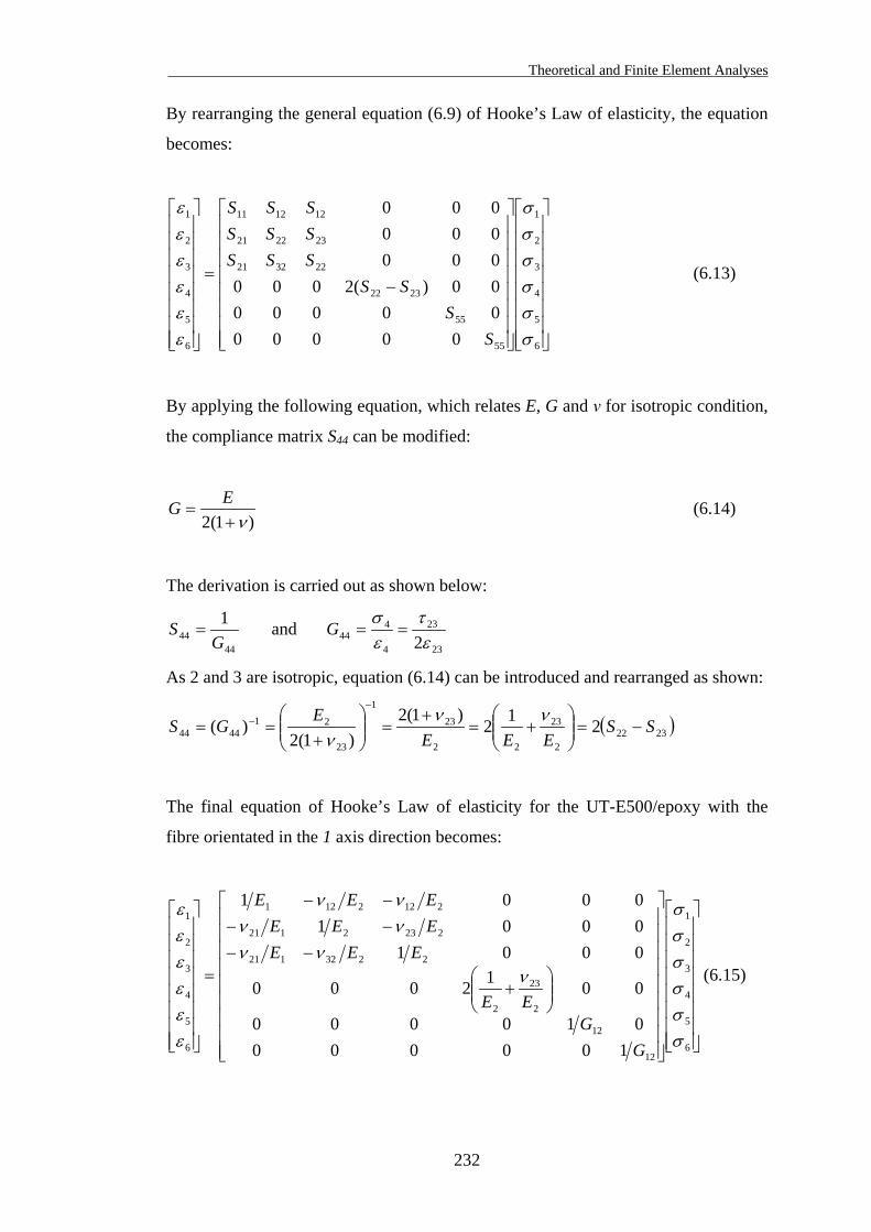
Theoretical and Finite Element Analyses
By rearranging the general equation (6.9) of Hooke’s Law of elasticity, the equation
becomes:
−=
6
5
4
3
2
1
55
55
2322
223221
232221
121211
6
5
4
3
2
1
000000000000)(2000000000000
σσσσσσ
εεεεεε
SS
SSSSSSSSSSS
(6.13)
By applying the following equation, which relates E, G and ν for isotropic condition,
the compliance matrix S44 can be modified:
)1(2 ν+=
EG (6.14)
The derivation is carried out as shown below:
4444
1G
S = and 23
23
4
444 2ε
τεσ
==G
As 2 and 3 are isotropic, equation (6.14) can be introduced and rearranged as shown:
( )23222
23
22
23
1
23
214444 212
)1(2)1(2
)( SSEEE
EGS −=
+=
+=
+
==−
− ννν
The final equation of Hooke’s Law of elasticity for the UT-E500/epoxy with the
fibre orientated in the 1 axis direction becomes:
+
−−−−−−
=
6
5
4
3
2
1
12
12
2
23
2
2232121
2232121
2122121
6
5
4
3
2
1
100000010000
0012000
000100010001
σσσσσσ
ννν
νννν
εεεεεε
GG
EE
EEEEEEEEE
(6.15)
232
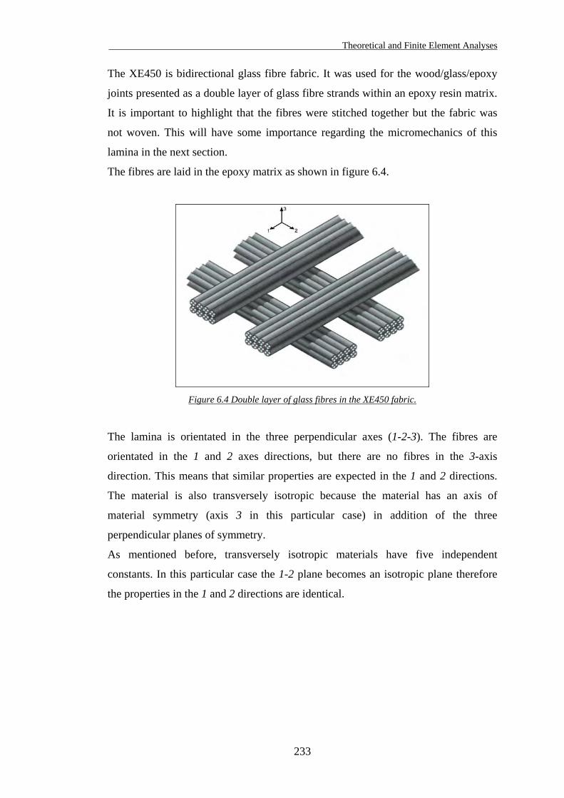
Theoretical and Finite Element Analyses
The XE450 is bidirectional glass fibre fabric. It was used for the wood/glass/epoxy
joints presented as a double layer of glass fibre strands within an epoxy resin matrix.
It is important to highlight that the fibres were stitched together but the fabric was
not woven. This will have some importance regarding the micromechanics of this
lamina in the next section.
The fibres are laid in the epoxy matrix as shown in figure 6.4.
Figure 6.4 Double layer of glass fibres in the XE450 fabric.
The lamina is orientated in the three perpendicular axes (1-2-3). The fibres are
orientated in the 1 and 2 axes directions, but there are no fibres in the 3-axis
direction. This means that similar properties are expected in the 1 and 2 directions.
The material is also transversely isotropic because the material has an axis of
material symmetry (axis 3 in this particular case) in addition of the three
perpendicular planes of symmetry.
As mentioned before, transversely isotropic materials have five independent
constants. In this particular case the 1-2 plane becomes an isotropic plane therefore
the properties in the 1 and 2 directions are identical.
233
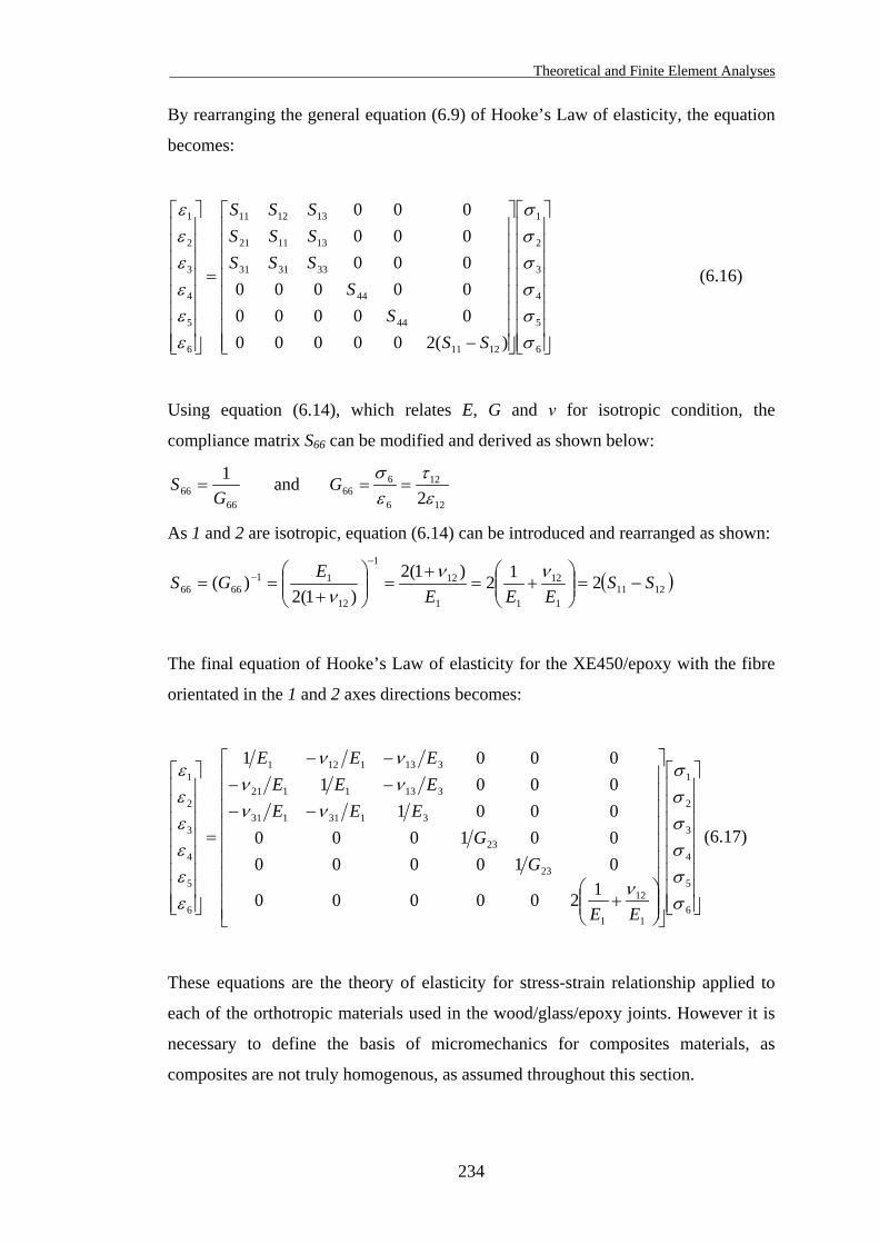
Theoretical and Finite Element Analyses
By rearranging the general equation (6.9) of Hooke’s Law of elasticity, the equation
becomes:
−
=
6
5
4
3
2
1
1211
44
44
333131
131121
131211
6
5
4
3
2
1
)(2000000000000000000000000
σσσσσσ
εεεεεε
SSS
SSSSSSSSSS
(6.16)
Using equation (6.14), which relates E, G and ν for isotropic condition, the
compliance matrix S66 can be modified and derived as shown below:
6666
1G
S = and 12
12
6
666 2ε
τεσ
==G
As 1 and 2 are isotropic, equation (6.14) can be introduced and rearranged as shown:
( )12111
12
11
12
1
12
116666 212)1(2
)1(2)( SS
EEEEGS −=
+=
+=
+
==−
− ννν
The final equation of Hooke’s Law of elasticity for the XE450/epoxy with the fibre
orientated in the 1 and 2 axes directions becomes:
+
−−−−−−
=
6
5
4
3
2
1
1
12
1
23
23
3131131
3131121
3131121
6
5
4
3
2
1
1200000
010000001000000100010001
σσσσσσ
ν
νννννν
εεεεεε
EE
GG
EEEEEEEEE
(6.17)
These equations are the theory of elasticity for stress-strain relationship applied to
each of the orthotropic materials used in the wood/glass/epoxy joints. However it is
necessary to define the basis of micromechanics for composites materials, as
composites are not truly homogenous, as assumed throughout this section.
234
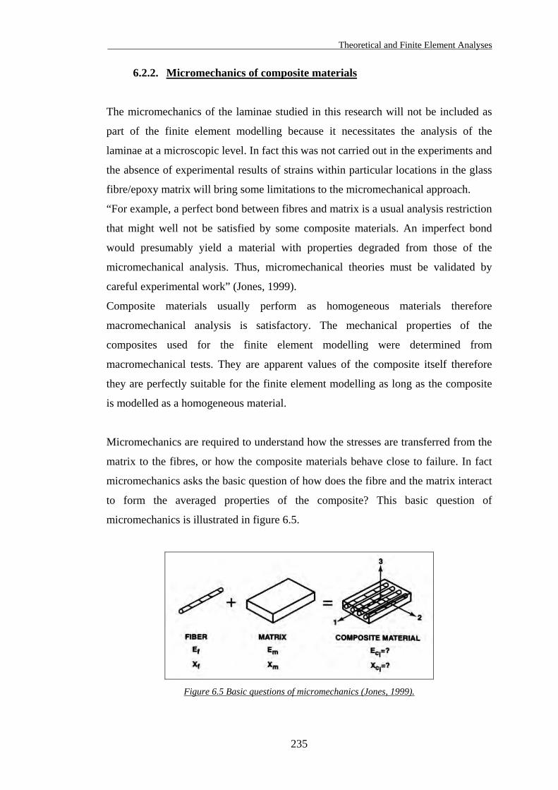
Theoretical and Finite Element Analyses
6.2.2. Micromechanics of composite materials
The micromechanics of the laminae studied in this research will not be included as
part of the finite element modelling because it necessitates the analysis of the
laminae at a microscopic level. In fact this was not carried out in the experiments and
the absence of experimental results of strains within particular locations in the glass
fibre/epoxy matrix will bring some limitations to the micromechanical approach.
“For example, a perfect bond between fibres and matrix is a usual analysis restriction
that might well not be satisfied by some composite materials. An imperfect bond
would presumably yield a material with properties degraded from those of the
micromechanical analysis. Thus, micromechanical theories must be validated by
careful experimental work” (Jones, 1999).
Composite materials usually perform as homogeneous materials therefore
macromechanical analysis is satisfactory. The mechanical properties of the
composites used for the finite element modelling were determined from
macromechanical tests. They are apparent values of the composite itself therefore
they are perfectly suitable for the finite element modelling as long as the composite
is modelled as a homogeneous material.
Micromechanics are required to understand how the stresses are transferred from the
matrix to the fibres, or how the composite materials behave close to failure. In fact
micromechanics asks the basic question of how does the fibre and the matrix interact
to form the averaged properties of the composite? This basic question of
micromechanics is illustrated in figure 6.5.
Figure 6.5 Basic questions of micromechanics (Jones, 1999).
235
Theoretical and Finite Element Analyses
“The objective of all micromechanics approaches is to determine the elastic moduli
or stiffnesses or compliances of a composite material in terms of the elastic moduli
of the constituent materials” (Jones, 1999).
The following assumptions must be considered to validate any micromechanics
approaches:
• The fibres are homogeneous, linear elastic, isotropic, regularly spaced, perfectly
aligned and perfectly bonded (without voids),
• The matrix is homogeneous, linear elastic, isotropic and void-free,
• The whole lamina is initially stress-free, linear elastic and macroscopically
homogeneous and orthotropic.
For the purpose of this research, only in-plane tension stress of lamina with
unidirectional and bidirectional fibres will be considered. Compression stress, out of
plane stress, bending or buckling of the lamina will not be treated, as the glass
fibre/epoxy overlaps used in the wood/glass/epoxy joints are not directly subjected to
that type of loading. All additional stresses, which occur on structural adhesive joints
such as the wood/glass/epoxy joints, will be presented later in this chapter.
The principles of mechanics of materials to determine the stiffness of unidirectional
and bidirectional laminae are presented and discussed in the following sections. The
bound solution using energy equations, approximate and exact solution approaches
will not be discussed here, as these methods are largely specific to composite
material design as they were derived from experimental work.
236
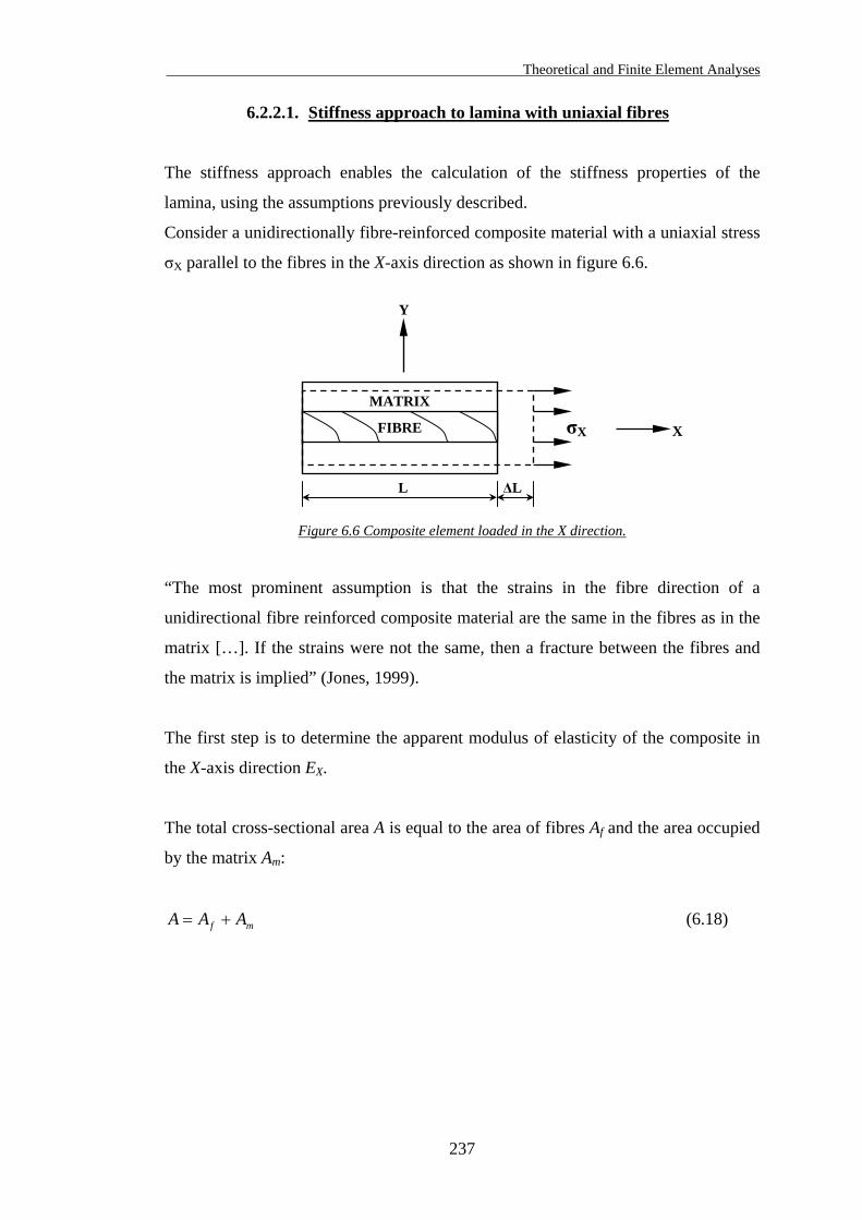
Theoretical and Finite Element Analyses
6.2.2.1. Stiffness approach to lamina with uniaxial fibres
The stiffness approach enables the calculation of the stiffness properties of the
lamina, using the assumptions previously described.
Consider a unidirectionally fibre-reinforced composite material with a uniaxial stress
σX parallel to the fibres in the X-axis direction as shown in figure 6.6.
Y
MATRIX
σXFIBRE
∆L L
X
Figure 6.6 Composite element loaded in the X direction.
“The most prominent assumption is that the strains in the fibre direction of a
unidirectional fibre reinforced composite material are the same in the fibres as in the
matrix […]. If the strains were not the same, then a fracture between the fibres and
the matrix is implied” (Jones, 1999).
The first step is to determine the apparent modulus of elasticity of the composite in
the X-axis direction EX.
The total cross-sectional area A is equal to the area of fibres Af and the area occupied
by the matrix Am:
mf AAA += (6.18)
237
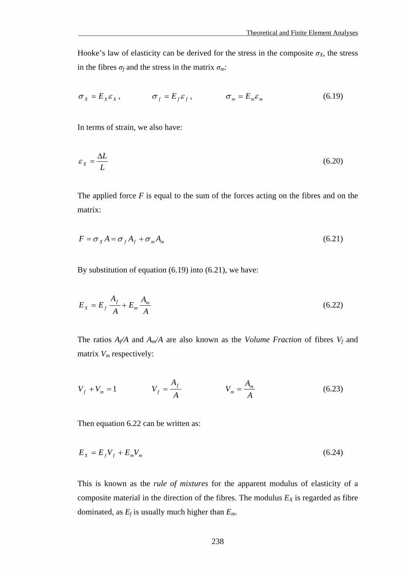
Theoretical and Finite Element Analyses
Hooke’s law of elasticity can be derived for the stress in the composite σX, the stress
in the fibres σf and the stress in the matrix σm:
XXX E εσ = , fff E εσ = , mmm E εσ = (6.19)
In terms of strain, we also have:
LL
X∆
=ε (6.20)
The applied force F is equal to the sum of the forces acting on the fibres and on the
matrix:
mmffX AAAF σσσ +== (6.21)
By substitution of equation (6.19) into (6.21), we have:
AA
EA
AEE m
mf
fX += (6.22)
The ratios Af/A and Am/A are also known as the Volume Fraction of fibres Vf and
matrix Vm respectively:
1=+ mf VV A
AV f
f = A
AV m
m = (6.23)
Then equation 6.22 can be written as:
mmffX VEVEE += (6.24)
This is known as the rule of mixtures for the apparent modulus of elasticity of a
composite material in the direction of the fibres. The modulus EX is regarded as fibre
dominated, as Ef is usually much higher than Em.
238
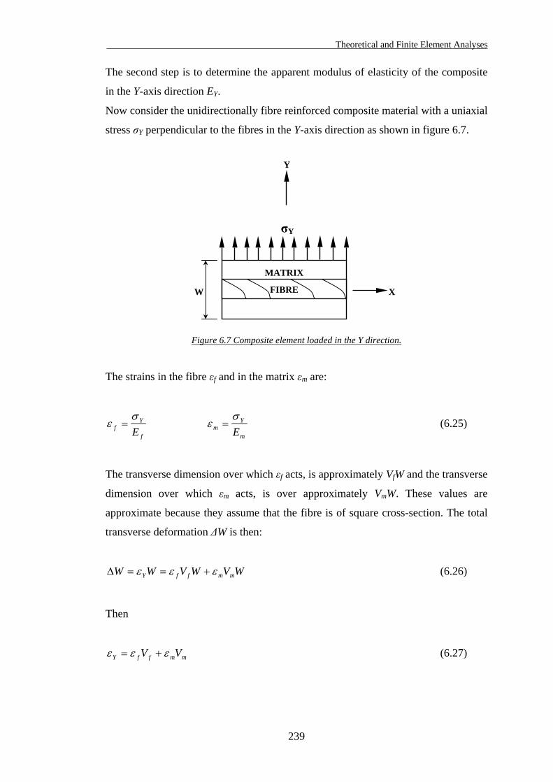
Theoretical and Finite Element Analyses
The second step is to determine the apparent modulus of elasticity of the composite
in the Y-axis direction EY.
Now consider the unidirectionally fibre reinforced composite material with a uniaxial
stress σY perpendicular to the fibres in the Y-axis direction as shown in figure 6.7.
Y
MATRIX
σY
FIBRE W
X
Figure 6.7 Composite element loaded in the Y direction.
The strains in the fibre εf and in the matrix εm are:
f
Yf E
σε =
m
Ym E
σε = (6.25)
The transverse dimension over which εf acts, is approximately VfW and the transverse
dimension over which εm acts, is over approximately VmW. These values are
approximate because they assume that the fibre is of square cross-section. The total
transverse deformation ∆W is then:
WVWVWW mmffY εεε +==∆ (6.26)
Then
mmffY VV εεε += (6.27)
239
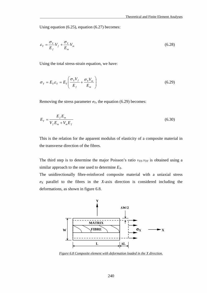
Theoretical and Finite Element Analyses
Using equation (6.25), equation (6.27) becomes:
mm
Yf
f
YY V
EV
Eσσ
ε += (6.28)
Using the total stress-strain equation, we have:
+==
m
mY
f
fYYYYY E
VE
VEE
σσεσ (6.29)
Removing the stress parameter σY, the equation (6.29) becomes:
fmmf
mfY EVEV
EEE
+= (6.30)
This is the relation for the apparent modulus of elasticity of a composite material in
the transverse direction of the fibres.
The third step is to determine the major Poisson’s ratio νXY.νXY is obtained using a
similar approach to the one used to determine EX.
The unidirectionally fibre-reinforced composite material with a uniaxial stress
σX parallel to the fibres in the X-axis direction is considered including the
deformations, as shown in figure 6.8.
Y
∆W/2
W
MATRIX
σXFIBRE
∆L L
X
Figure 6.8 Composite element with deformation loaded in the X direction.
240
Theoretical and Finite Element Analyses
The major Poisson’s ratio νXY is expressed as:
X
YXY ε
εν −= (6.31)
Assuming the fibre strain is identical to the matrix strain (as assumed before), the
transverse deformation ∆W can be expressed as:
XXYY WWW ενε =−=∆ (6.32)
But at microscopic level, the transverse deformation ∆W is also equal:
mWfWW ∆+∆=∆ (6.33)
The transverse deformation of the fibre ∆fW and the matrix ∆mW can be approximately
expressed as previously carried out for the determination of EY.
XfffW WV εν=∆ XmmmW WV εν=∆ (6.34)
Combining equations (6.32), (6.33) and (6.34), it becomes:
XmmXffXXY WVWVW ενενεν += (6.35)
Dividing equation (6.35) by WεX, the Poisson’s ratio νXY can finally be expressed as:
mmffXY VV ννν += (6.36)
This is known as the rule of mixtures for the major Poisson’s ratio of a composite
material in the direction of the fibres. The Poisson’s ratio of the fibre νf and the
Poisson’s ratio of the matrix νm are usually not significantly different therefore the
composite material major Poisson’s ratio is considered as neutral in terms of
domination of one of the two constituents.
241
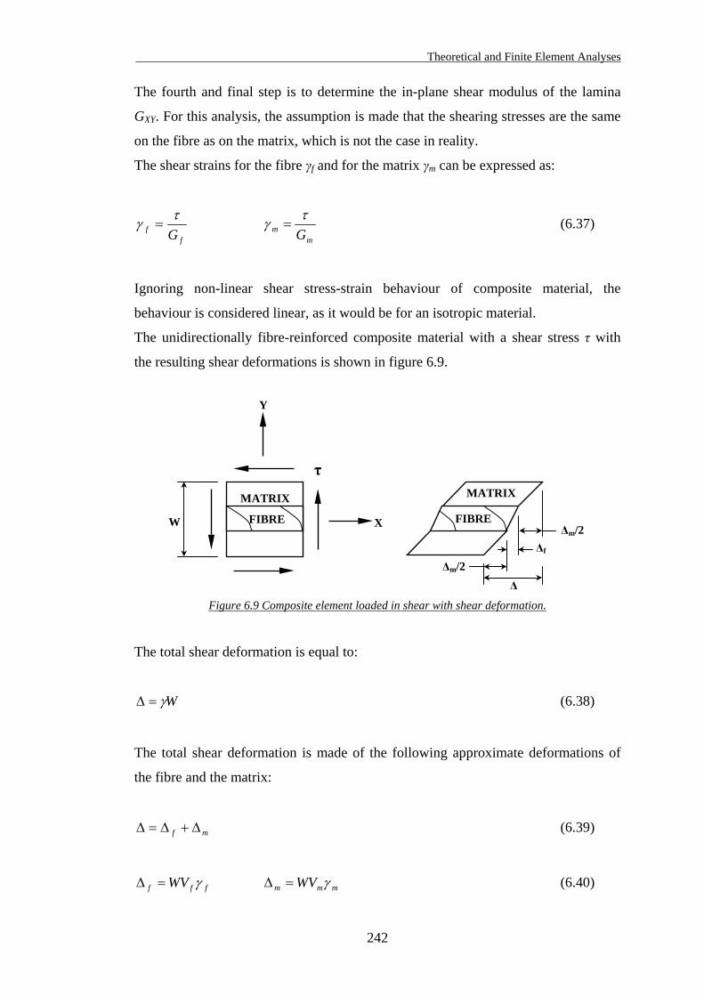
Theoretical and Finite Element Analyses
The fourth and final step is to determine the in-plane shear modulus of the lamina
GXY. For this analysis, the assumption is made that the shearing stresses are the same
on the fibre as on the matrix, which is not the case in reality.
The shear strains for the fibre γf and for the matrix γm can be expressed as:
ff G
τγ = m
m Gτγ = (6.37)
Ignoring non-linear shear stress-strain behaviour of composite material, the
behaviour is considered linear, as it would be for an isotropic material.
The unidirectionally fibre-reinforced composite material with a shear stress τ with
the resulting shear deformations is shown in figure 6.9.
Y
∆m/2∆f
MATRIX
FIBRE W
MATRIX
τ
X FIBRE
∆
∆m/2
Figure 6.9 Composite element loaded in shear with shear deformation.
The total shear deformation is equal to:
Wγ=∆ (6.38)
The total shear deformation is made of the following approximate deformations of
the fibre and the matrix:
mf ∆+∆=∆ (6.39)
fff WV γ=∆ mmm WV γ=∆ (6.40)
242
Theoretical and Finite Element Analyses
Combining equations (6.39) and (6.40) and dividing by W, it becomes:
mmff VV γγγ += (6.41)
Using the general equation of shear modulus:
XYGτγ = (6.42)
Equation (6.41) can be written as:
mm
ff
XY GV
GV
Gτττ
+= (6.43)
Removing the shear stress τ, the shear modulus GXY becomes:
fmmf
mfXY VGVG
GGG
+= (6.44)
This equation is of the same form as the equation obtained for the transverse
modulus of elasticity EY.
The calculation of the moduli of elasticity in two directions, the major Poisson’s ratio
and the shear modulus are the basic stiffness properties of a unidirectional lamina.
These calculations are taking a series of assumptions into account, which are not
realistic in practical terms. However these calculations are recognised as reliable and
give generally accurate approximations of the exact values.
The next step is the presentation and discussion of the principles of mechanics of
materials to determine the stiffness of bidirectional lamina.
243
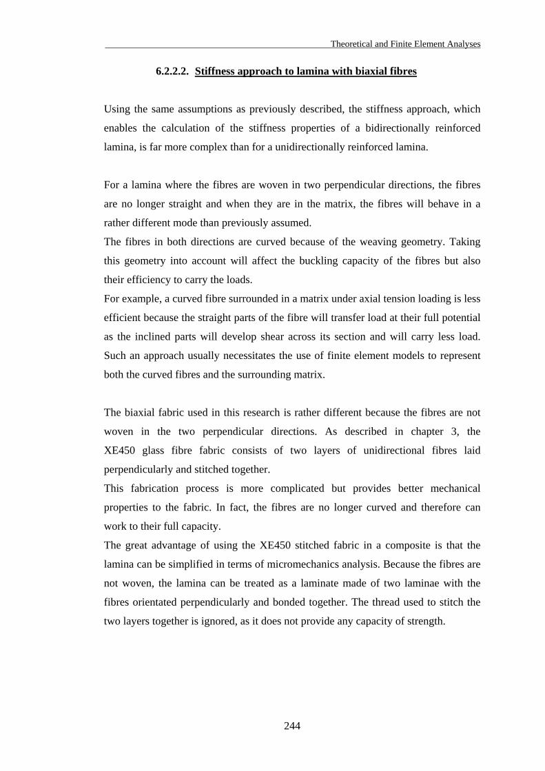
Theoretical and Finite Element Analyses
6.2.2.2. Stiffness approach to lamina with biaxial fibres
Using the same assumptions as previously described, the stiffness approach, which
enables the calculation of the stiffness properties of a bidirectionally reinforced
lamina, is far more complex than for a unidirectionally reinforced lamina.
For a lamina where the fibres are woven in two perpendicular directions, the fibres
are no longer straight and when they are in the matrix, the fibres will behave in a
rather different mode than previously assumed.
The fibres in both directions are curved because of the weaving geometry. Taking
this geometry into account will affect the buckling capacity of the fibres but also
their efficiency to carry the loads.
For example, a curved fibre surrounded in a matrix under axial tension loading is less
efficient because the straight parts of the fibre will transfer load at their full potential
as the inclined parts will develop shear across its section and will carry less load.
Such an approach usually necessitates the use of finite element models to represent
both the curved fibres and the surrounding matrix.
The biaxial fabric used in this research is rather different because the fibres are not
woven in the two perpendicular directions. As described in chapter 3, the
XE450 glass fibre fabric consists of two layers of unidirectional fibres laid
perpendicularly and stitched together.
This fabrication process is more complicated but provides better mechanical
properties to the fabric. In fact, the fibres are no longer curved and therefore can
work to their full capacity.
The great advantage of using the XE450 stitched fabric in a composite is that the
lamina can be simplified in terms of micromechanics analysis. Because the fibres are
not woven, the lamina can be treated as a laminate made of two laminae with the
fibres orientated perpendicularly and bonded together. The thread used to stitch the
two layers together is ignored, as it does not provide any capacity of strength.
244
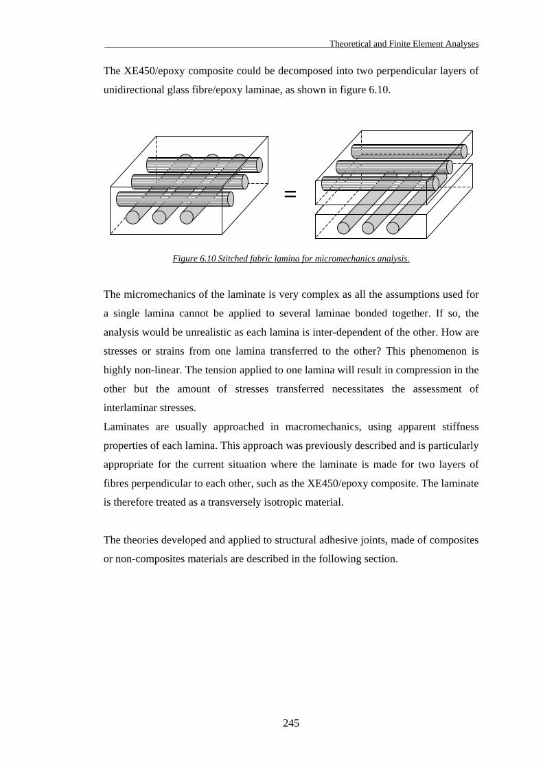
Theoretical and Finite Element Analyses
The XE450/epoxy composite could be decomposed into two perpendicular layers of
unidirectional glass fibre/epoxy laminae, as shown in figure 6.10.
=
Figure 6.10 Stitched fabric lamina for micromechanics analysis.
The micromechanics of the laminate is very complex as all the assumptions used for
a single lamina cannot be applied to several laminae bonded together. If so, the
analysis would be unrealistic as each lamina is inter-dependent of the other. How are
stresses or strains from one lamina transferred to the other? This phenomenon is
highly non-linear. The tension applied to one lamina will result in compression in the
other but the amount of stresses transferred necessitates the assessment of
interlaminar stresses.
Laminates are usually approached in macromechanics, using apparent stiffness
properties of each lamina. This approach was previously described and is particularly
appropriate for the current situation where the laminate is made for two layers of
fibres perpendicular to each other, such as the XE450/epoxy composite. The laminate
is therefore treated as a transversely isotropic material.
The theories developed and applied to structural adhesive joints, made of composites
or non-composites materials are described in the following section.
245
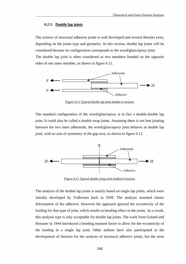
Theoretical and Finite Element Analyses
6.2.3. Double lap joints
The science of structural adhesive joints is well developed and several theories exist,
depending on the joints type and geometry. In this section, double lap joints will be
considered because its configuration corresponds to the wood/glass/epoxy joint.
The double lap joint is often considered as two members bonded on the opposite
sides of one inner member, as shown in figure 6.11.
Adhesive
Adherends
F 2F
F
Figure 6.11 Typical double lap joint loaded in tension.
The standard configuration of the wood/glass/epoxy is in fact a double-double lap
joint. It could also be called a double strap joints. Assuming there is not butt jointing
between the two inner adherends, the wood/glass/epoxy joint behaves as double lap
joint, with an axis of symmetry in the gap area, as shown in figure 6.12.
¢
Adhesive
Adherends
2F 2F
Figure 6.12 Typical double strap joint loaded in tension.
The analysis of the double lap joints is mainly based on single lap joints, which were
initially developed by Volkersen back in 1938. The analysis assumed elastic
deformation of the adhesive. However the approach ignored the eccentricity of the
loading for that type of joint, which results in bending effect in the joints. As a result,
this analysis type is only acceptable for double lap joints. The work from Goland and
Reissner in 1944 introduced a bending moment factor to allow for the eccentricity of
the loading in a single lap joint. Other authors have also participated in the
development of theories for the analysis of structural adhesive joints, but the most
246
Theoretical and Finite Element Analyses
comprehensive analytical approach of adhesive joints was mainly developed by
Hart-Smith in the 1970s and remains the most accessible theory nowadays. Other
attempts were made to represent non-linear behaviour of the adhesive, such as shear
stress/shear strain relationship, through the thickness stress distributions but these
theories are too complex to be used analytically.
The Hart-Smith analysis of double lap joints is summarised in this section, with
additional work and research from Baker (1997) and Adams et al. (1997).
The Hart-Smith analysis is based on the non-linear elastic/plastic behaviour of the
adhesive. The theory is based on the fact that adequate joint design should be based
on the adhesive strength being much higher that the adherends’ strengths to avoid
peel stresses failure. Therefore the adhesive failure depends on the shear strain
applied to the adhesive.
“Inevitably, many of the complications in real joints are neglected or inadequately
dealt with in these relatively simple studies. These include:
1. Through the thickness variation of shear stresses
2. Through the thickness stresses
3. The stress-free state at the ends of the adhesive
4. The (highly beneficial) effect of adhesive spew, excess adhesive that forms a fillet
at the edge of the joint
5. True shear stress/strain behaviour, including time dependency” (Baker, 1997).
The through the thickness stress variations are ignored but these effects are
significant. One example is the effect of bending in double lap joints. It was
previously highlighted than double lap joints are not subject to direct loading
eccentricity as for single lap joints, resulting in bending of the whole joint.
“Although there is no net bending moment on a symmetrical double lap joint, as
there is with single lap joint, because the load is applied through the adhesive to the
adherend plates away from their neutral axes, the double lap joint experiences
internal bending […]. In a symmetrical double lap joint, the centre adherend
experiences no net bending moment, but the outer adherends bend, giving rise to
tensile stresses across the adhesive layer at the end of the overlap where they are not
loaded, and compressive stresses at the end where they are loaded […]” (Adams et
al., 1997).
247
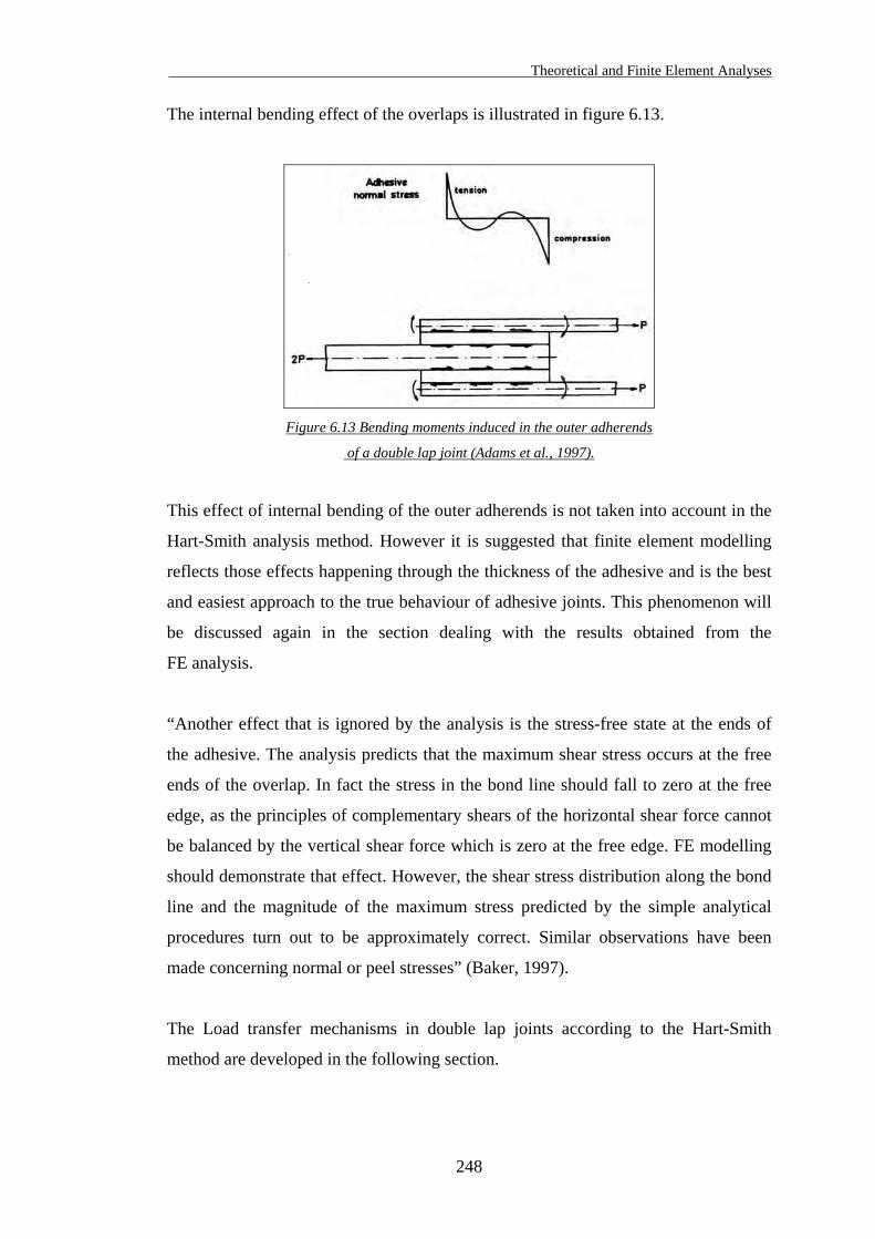
Theoretical and Finite Element Analyses
The internal bending effect of the overlaps is illustrated in figure 6.13.
Figure 6.13 Bending moments induced in the outer adherends
of a double lap joint (Adams et al., 1997).
This effect of internal bending of the outer adherends is not taken into account in the
Hart-Smith analysis method. However it is suggested that finite element modelling
reflects those effects happening through the thickness of the adhesive and is the best
and easiest approach to the true behaviour of adhesive joints. This phenomenon will
be discussed again in the section dealing with the results obtained from the
FE analysis.
“Another effect that is ignored by the analysis is the stress-free state at the ends of
the adhesive. The analysis predicts that the maximum shear stress occurs at the free
ends of the overlap. In fact the stress in the bond line should fall to zero at the free
edge, as the principles of complementary shears of the horizontal shear force cannot
be balanced by the vertical shear force which is zero at the free edge. FE modelling
should demonstrate that effect. However, the shear stress distribution along the bond
line and the magnitude of the maximum stress predicted by the simple analytical
procedures turn out to be approximately correct. Similar observations have been
made concerning normal or peel stresses” (Baker, 1997).
The Load transfer mechanisms in double lap joints according to the Hart-Smith
method are developed in the following section.
248
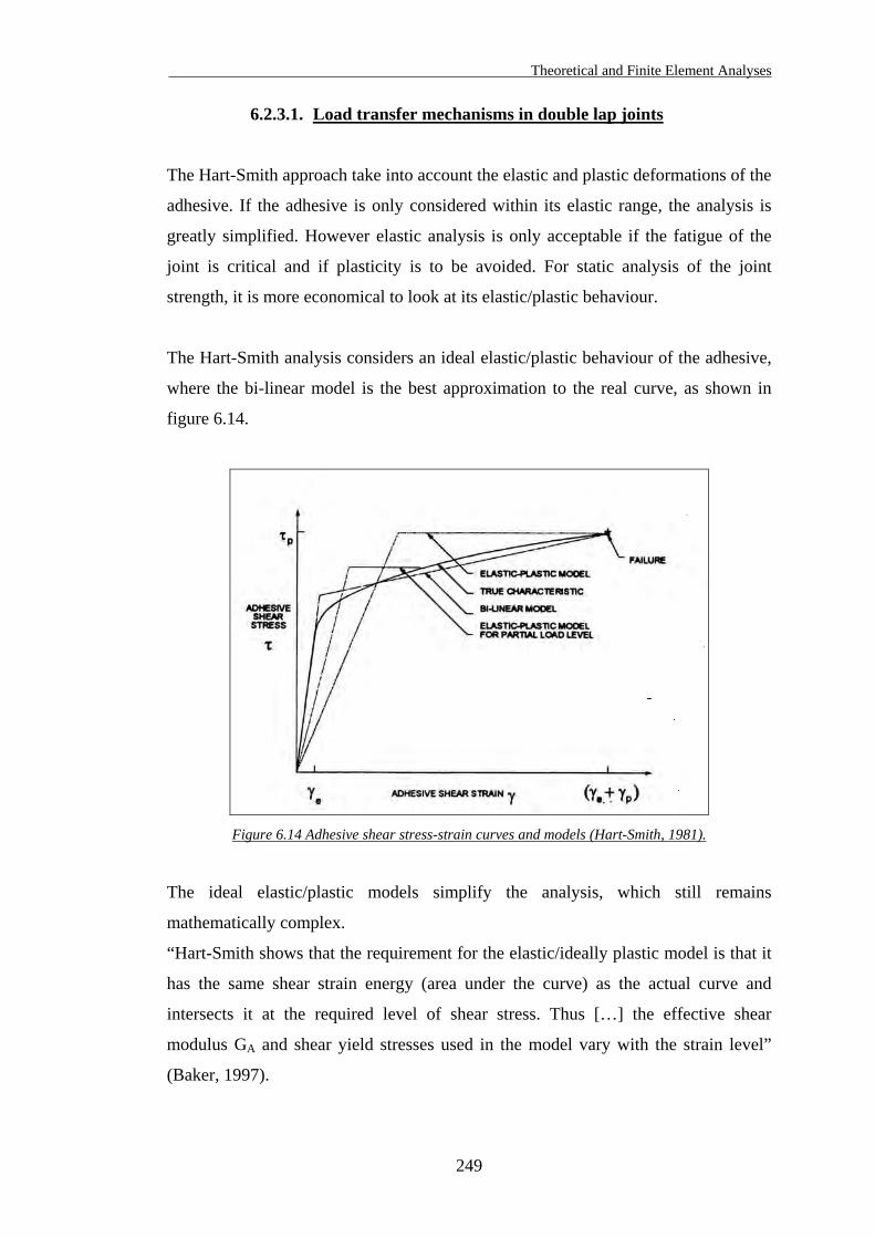
Theoretical and Finite Element Analyses
6.2.3.1. Load transfer mechanisms in double lap joints
The Hart-Smith approach take into account the elastic and plastic deformations of the
adhesive. If the adhesive is only considered within its elastic range, the analysis is
greatly simplified. However elastic analysis is only acceptable if the fatigue of the
joint is critical and if plasticity is to be avoided. For static analysis of the joint
strength, it is more economical to look at its elastic/plastic behaviour.
The Hart-Smith analysis considers an ideal elastic/plastic behaviour of the adhesive,
where the bi-linear model is the best approximation to the real curve, as shown in
figure 6.14.
Figure 6.14 Adhesive shear stress-strain curves and models (Hart-Smith, 1981).
The ideal elastic/plastic models simplify the analysis, which still remains
mathematically complex.
“Hart-Smith shows that the requirement for the elastic/ideally plastic model is that it
has the same shear strain energy (area under the curve) as the actual curve and
intersects it at the required level of shear stress. Thus […] the effective shear
modulus GA and shear yield stresses used in the model vary with the strain level”
(Baker, 1997).
249
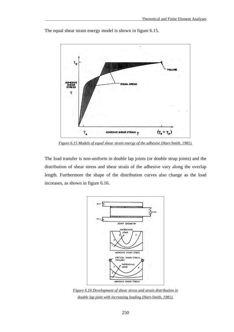
Theoretical and Finite Element Analyses
The equal shear strain energy model is shown in figure 6.15.
Figure 6.15 Models of equal shear strain energy of the adhesive (Hart-Smith, 1981).
The load transfer is non-uniform in double lap joints (or double strap joints) and the
distribution of shear stress and shear strain of the adhesive vary along the overlap
length. Furthermore the shape of the distribution curves also change as the load
increases, as shown in figure 6.16.
Figure 6.16 Development of shear stress and strain distribution in
double lap joint with increasing loading (Hart-Smith, 1981).
250
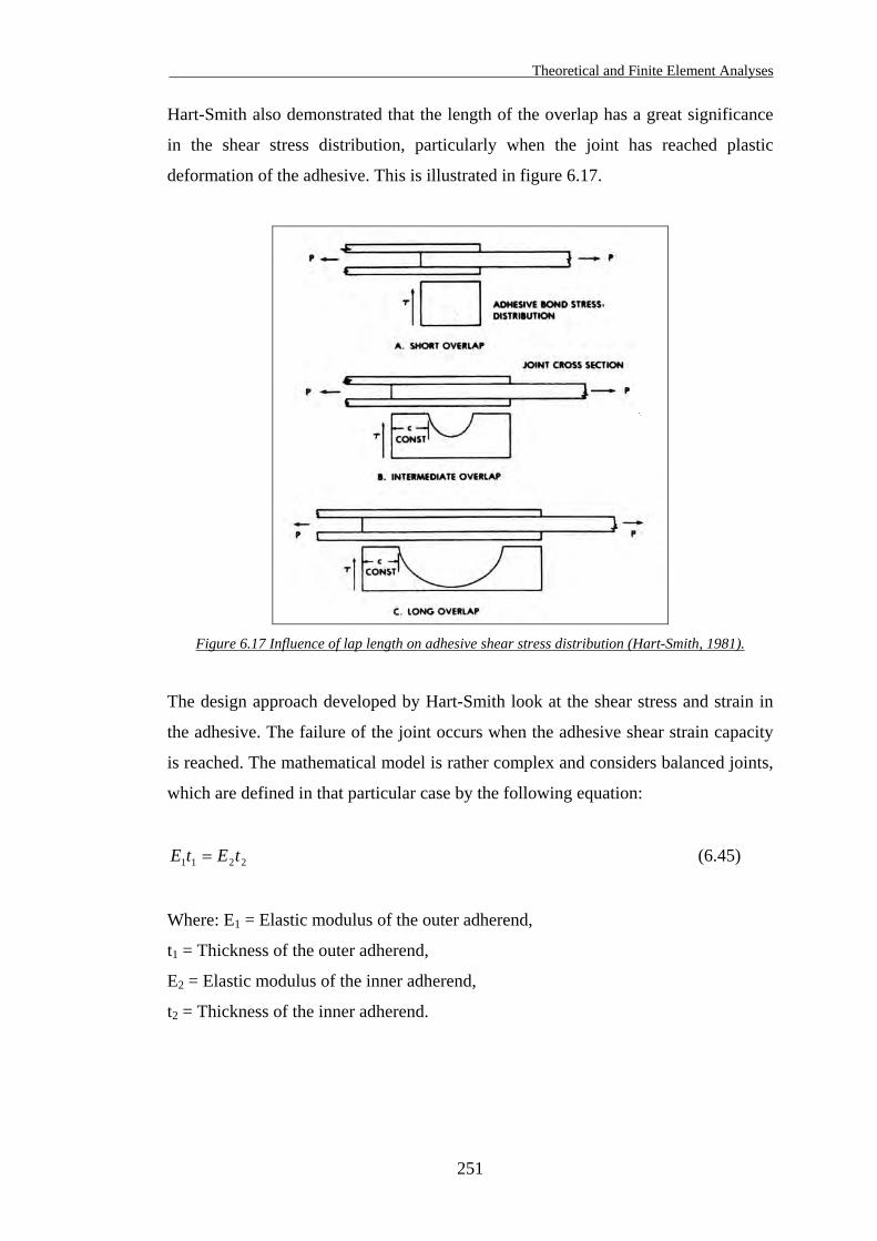
Theoretical and Finite Element Analyses
Hart-Smith also demonstrated that the length of the overlap has a great significance
in the shear stress distribution, particularly when the joint has reached plastic
deformation of the adhesive. This is illustrated in figure 6.17.
Figure 6.17 Influence of lap length on adhesive shear stress distribution (Hart-Smith, 1981).
The design approach developed by Hart-Smith look at the shear stress and strain in
the adhesive. The failure of the joint occurs when the adhesive shear strain capacity
is reached. The mathematical model is rather complex and considers balanced joints,
which are defined in that particular case by the following equation:
2211 tEtE = (6.45)
Where: E1 = Elastic modulus of the outer adherend,
t1 = Thickness of the outer adherend,
E2 = Elastic modulus of the inner adherend,
t2 = Thickness of the inner adherend.
251
Theoretical and Finite Element Analyses
The model becomes even more complex when the joint is unbalanced. The
equations, which enable the calculations of the joint strength, are not presented in
this report because they cannot be used to establish the strength of the
wood/glass/epoxy joints. These equations require the measurement of shear strain in
the adhesive developed in the elastic range γe and in the plastic range γp. In fact, none
of those values were recorded during the test. Values of shear strain in the bond line
are highly inpractical to measure because of the infinitely small thickness of the
adhesive. It is obviously not possible to position a strain rosette vertically in the
adhesive layer (in order to measure shear strain acting across the thickness of the
adhesive), the alternative would have been to place two strain gauges on top and
underneath the adhesive layer. However this was also inpractical to achieve for the
same reasons.
The elastic/plastic analysis developed by Hart-Smith ignores all through the
thickness stresses and strain, as mentioned previously.
“[…] the basic Hart-Smith approach entails neglecting the normal or ‘peel’ stresses
acting across the glue line. However, in practice these may be the main contributors
to joint failure, even in double lap joints. Hart-Smith has recognised this possibility
and in one of his analyses (1972) combined elastic peel stresses with plastic shear
stresses” (Adams et al., 1997).
The formulation proposed is not presented in this report but reflects that the thickness
of the outer adherends has an effect on the ‘peel’ stresses. In fact, the thinner the
outer adherends, the less critical the ‘peeling’ stresses.
There are significant differences between the double lap joint as it is presented in this
section and the wood/glass/epoxy joints. Those differences, as well as the effect they
have on the joint are described in the following section.
252
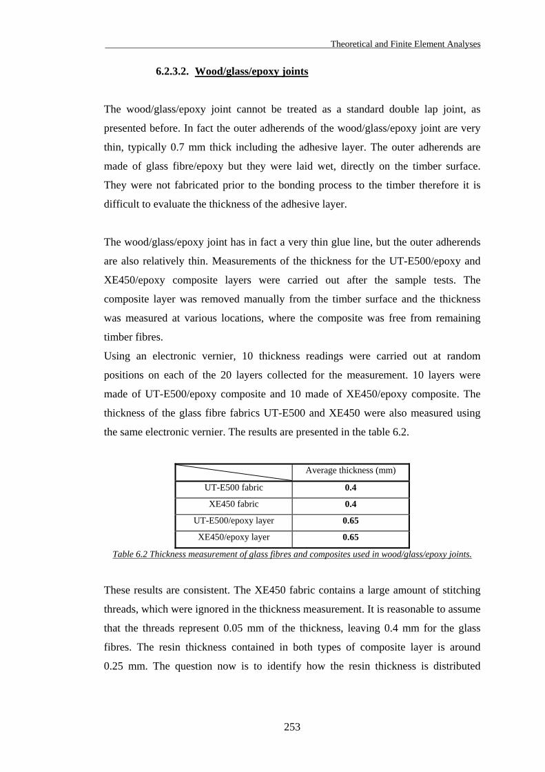
Theoretical and Finite Element Analyses
6.2.3.2. Wood/glass/epoxy joints
The wood/glass/epoxy joint cannot be treated as a standard double lap joint, as
presented before. In fact the outer adherends of the wood/glass/epoxy joint are very
thin, typically 0.7 mm thick including the adhesive layer. The outer adherends are
made of glass fibre/epoxy but they were laid wet, directly on the timber surface.
They were not fabricated prior to the bonding process to the timber therefore it is
difficult to evaluate the thickness of the adhesive layer.
The wood/glass/epoxy joint has in fact a very thin glue line, but the outer adherends
are also relatively thin. Measurements of the thickness for the UT-E500/epoxy and
XE450/epoxy composite layers were carried out after the sample tests. The
composite layer was removed manually from the timber surface and the thickness
was measured at various locations, where the composite was free from remaining
timber fibres.
Using an electronic vernier, 10 thickness readings were carried out at random
positions on each of the 20 layers collected for the measurement. 10 layers were
made of UT-E500/epoxy composite and 10 made of XE450/epoxy composite. The
thickness of the glass fibre fabrics UT-E500 and XE450 were also measured using
the same electronic vernier. The results are presented in the table 6.2.
Average thickness (mm)
UT-E500 fabric 0.4
XE450 fabric 0.4
UT-E500/epoxy layer 0.65
XE450/epoxy layer 0.65
Table 6.2 Thickness measurement of glass fibres and composites used in wood/glass/epoxy joints.
These results are consistent. The XE450 fabric contains a large amount of stitching
threads, which were ignored in the thickness measurement. It is reasonable to assume
that the threads represent 0.05 mm of the thickness, leaving 0.4 mm for the glass
fibres. The resin thickness contained in both types of composite layer is around
0.25 mm. The question now is to identify how the resin thickness is distributed
253
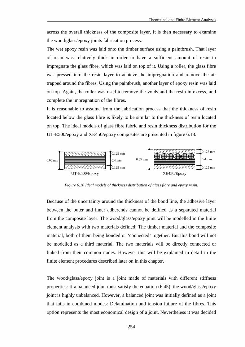
Theoretical and Finite Element Analyses
across the overall thickness of the composite layer. It is then necessary to examine
the wood/glass/epoxy joints fabrication process.
The wet epoxy resin was laid onto the timber surface using a paintbrush. That layer
of resin was relatively thick in order to have a sufficient amount of resin to
impregnate the glass fibre, which was laid on top of it. Using a roller, the glass fibre
was pressed into the resin layer to achieve the impregnation and remove the air
trapped around the fibres. Using the paintbrush, another layer of epoxy resin was laid
on top. Again, the roller was used to remove the voids and the resin in excess, and
complete the impregnation of the fibres.
It is reasonable to assume from the fabrication process that the thickness of resin
located below the glass fibre is likely to be similar to the thickness of resin located
on top. The ideal models of glass fibre fabric and resin thickness distribution for the
UT-E500/epoxy and XE450/epoxy composites are presented in figure 6.18.
0.65 mm
0.125 mm
0.4 mm
0.125 mm
0.65 mm
0.125 mm
0.4 mm
0.125 mm
UT-E500/Epoxy XE450/Epoxy
Figure 6.18 Ideal models of thickness distribution of glass fibre and epoxy resin.
Because of the uncertainty around the thickness of the bond line, the adhesive layer
between the outer and inner adherends cannot be defined as a separated material
from the composite layer. The wood/glass/epoxy joint will be modelled in the finite
element analysis with two materials defined: The timber material and the composite
material, both of them being bonded or ‘connected’ together. But this bond will not
be modelled as a third material. The two materials will be directly connected or
linked from their common nodes. However this will be explained in detail in the
finite element procedures described later on in this chapter.
The wood/glass/epoxy joint is a joint made of materials with different stiffness
properties: If a balanced joint must satisfy the equation (6.45), the wood/glass/epoxy
joint is highly unbalanced. However, a balanced joint was initially defined as a joint
that fails in combined modes: Delamination and tension failure of the fibres. This
option represents the most economical design of a joint. Nevertheless it was decided
254
Theoretical and Finite Element Analyses
that tension failure of the fibres was a mode of failure to avoid, in order to limit the
joint strength to the timber capacity.
The outer adherends as well as the bond line are very thin in the wood/glass/epoxy
joint. The Hart-Smith theory ignores the through the thickness stresses and strains,
which can be significant in terms of joint strength. However with thin bond line and
outer adherends, the stress and strain variations through the thickness are limited
because of the small amount of material (in thickness). As a result, the Hart-Smith
analysis would probably suit better the wood/glass/epoxy joint than a typical double
lap joint with thicker bond line and outer adherends.
The stresses and strains acting through the thickness of the material will be taken into
account because the finite element modelling will allow for all mechanical effects
occurring on the joint: The analysis will show how the stresses and strains vary
through the thickness of the composite layer.
Internal bending of the outer adherends was previously defined and is a characteristic
of double lap joints. For the wood/glass/epoxy joint, which has very thin outer
adherends, this effect is likely to be more significant because the moment of inertia
of the outer adherends is relatively small. Once again the finite element analysis will
probably highlight this effect.
The finite element analysis of the wood/glass/epoxy joint will show how the joint
behaves under tension load. It should provide information on stress and strain
distribution over the whole joint.
As no other research work was found on that particular subject, comparison will have
to be drawn, based on experimental results available for other types of double lap
joints. The following section summarises the experimental results found on double
lap joints, which could be relevant for the comparison with the wood/glass/epoxy
joint.
255
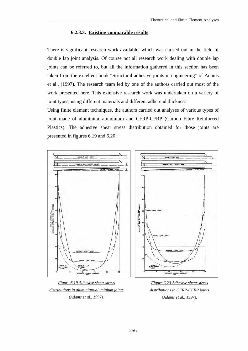
Theoretical and Finite Element Analyses
6.2.3.3. Existing comparable results
There is significant research work available, which was carried out in the field of
double lap joint analysis. Of course not all research work dealing with double lap
joints can be referred to, but all the information gathered in this section has been
taken from the excellent book “Structural adhesive joints in engineering” of Adams
et al., (1997). The research team led by one of the authors carried out most of the
work presented here. This extensive research work was undertaken on a variety of
joint types, using different materials and different adherend thickness.
Using finite element techniques, the authors carried out analyses of various types of
joint made of aluminium-aluminium and CFRP-CFRP (Carbon Fibre Reinforced
Plastics). The adhesive shear stress distribution obtained for those joints are
presented in figures 6.19 and 6.20.
Figure 6.19 Adhesive shear stress
distributions in aluminium-aluminium joints
(Adams et al., 1997).
Figure 6.20 Adhesive shear stress
distributions in CFRP-CFRP joints
(Adams et al., 1997).
256
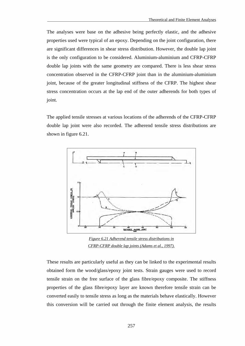
Theoretical and Finite Element Analyses
257
The analyses were base on the adhesive being perfectly elastic, and the adhesive
properties used were typical of an epoxy. Depending on the joint configuration, there
are significant differences in shear stress distribution. However, the double lap joint
is the only configuration to be considered. Aluminium-aluminium and CFRP-CFRP
double lap joints with the same geometry are compared. There is less shear stress
concentration observed in the CFRP-CFRP joint than in the aluminium-aluminium
joint, because of the greater longitudinal stiffness of the CFRP. The highest shear
stress concentration occurs at the lap end of the outer adherends for both types of
joint.
The applied tensile stresses at various locations of the adherends of the CFRP-CFRP
double lap joint were also recorded. The adherend tensile stress distributions are
shown in figure 6.21.
Figure 6.21 Adherend tensile stress distributions in
CFRP-CFRP double lap joints (Adams et al., 1997).
These results are particularly useful as they can be linked to the experimental results
obtained form the wood/glass/epoxy joint tests. Strain gauges were used to record
tensile strain on the free surface of the glass fibre/epoxy composite. The stiffness
properties of the glass fibre/epoxy layer are known therefore tensile strain can be
converted easily to tensile stress as long as the materials behave elastically. However
this conversion will be carried out through the finite element analysis, the results
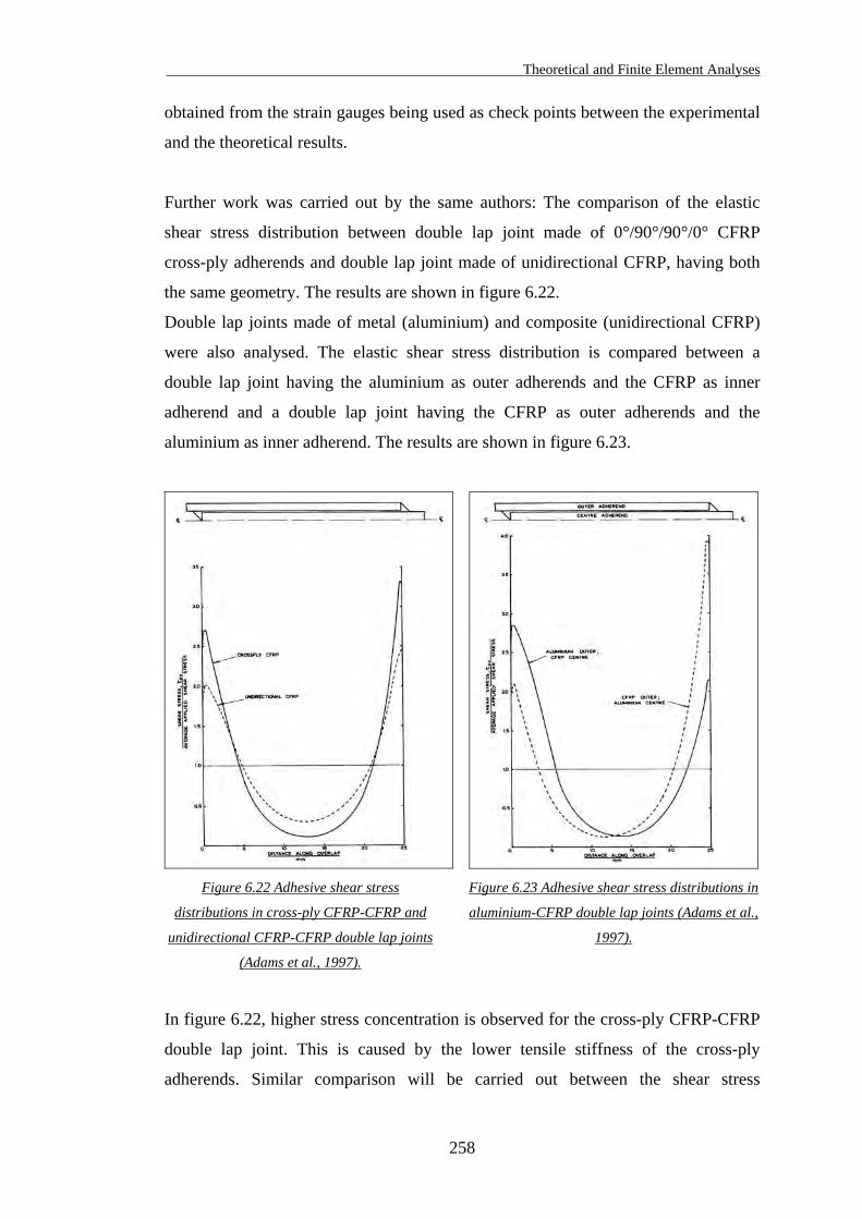
Theoretical and Finite Element Analyses
obtained from the strain gauges being used as check points between the experimental
and the theoretical results.
Further work was carried out by the same authors: The comparison of the elastic
shear stress distribution between double lap joint made of 0°/90°/90°/0° CFRP
cross-ply adherends and double lap joint made of unidirectional CFRP, having both
the same geometry. The results are shown in figure 6.22.
Double lap joints made of metal (aluminium) and composite (unidirectional CFRP)
were also analysed. The elastic shear stress distribution is compared between a
double lap joint having the aluminium as outer adherends and the CFRP as inner
adherend and a double lap joint having the CFRP as outer adherends and the
aluminium as inner adherend. The results are shown in figure 6.23.
Figure 6.22 Adhesive shear stress
distributions in cross-ply CFRP-CFRP and
unidirectional CFRP-CFRP double lap joints
(Adams et al., 1997).
Figure 6.23 Adhesive shear stress distributions in
aluminium-CFRP double lap joints (Adams et al.,
1997).
In figure 6.22, higher stress concentration is observed for the cross-ply CFRP-CFRP
double lap joint. This is caused by the lower tensile stiffness of the cross-ply
adherends. Similar comparison will be carried out between the shear stress
258
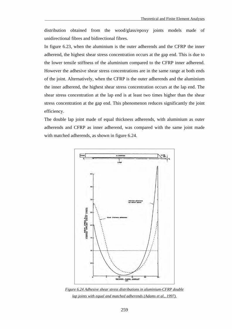
Theoretical and Finite Element Analyses
259
distribution obtained from the wood/glass/epoxy joints models made of
unidirectional fibres and bidirectional fibres.
In figure 6.23, when the aluminium is the outer adherends and the CFRP the inner
adherend, the highest shear stress concentration occurs at the gap end. This is due to
the lower tensile stiffness of the aluminium compared to the CFRP inner adherend.
However the adhesive shear stress concentrations are in the same range at both ends
of the joint. Alternatively, when the CFRP is the outer adherends and the aluminium
the inner adherend, the highest shear stress concentration occurs at the lap end. The
shear stress concentration at the lap end is at least two times higher than the shear
stress concentration at the gap end. This phenomenon reduces significantly the joint
efficiency.
The double lap joint made of equal thickness adherends, with aluminium as outer
adherends and CFRP as inner adherend, was compared with the same joint made
with matched adherends, as shown in figure 6.24.
Figure 6.24 Adhesive shear stress distributions in aluminium-CFRP double
lap joints with equal and matched adherends (Adams et al., 1997).
Theoretical and Finite Element Analyses
260
To optimise the use of high strength CFRP (typical yield strength of 1550 MPa) with
aluminium (typical yield strength of 325 MPa), the thickness of the CFRP must be
reduced to about one quarter of the thickness of the aluminium. This was carried out
to match the adherends, as shown in figure 6.24. The aluminium outer adherends are
1.5 mm thick each, and the CFRP inner adherend is only 0.75 mm thick. As a result,
the shear stress concentration of the adhesive is reduced at the gap end but
significantly increased at the lap end. This shows that adherend thickness affects
considerably the shear strain distribution in the adhesive.
There are many factors, which affect the double lap joint. Those factors are
multiplied when the joint is made of different materials, with different thickness and
if it is unbalanced. The wood/glass/epoxy joint is certainly behaving like a very
unbalanced double lap joint and the finite element analysis, which is presented in the
next section, will expose its mechanical behaviour under tension load.
Theoretical and Finite Element Analyses
261
6.3. Finite element modelling
6.3.1. Introduction
The finite element modelling was performed using the professional edition of the
ANSYS software, version 5.4.
The advantages of using a well-known FEA product were the wide range of
capabilities offered to the user to develop the models, to run the analysis and to make
the most of the results obtained.
One finite element model was developed and analysed for each wood/glass/epoxy
joint configuration that was elaborated in experiments. In other words there are eight
models that were analysed. The results obtained are presented throughout this
chapter and are compared thereafter with experimental results.
But firstly, many other models were built up and “tested” until the final ones were
achieved. This procedure was a long exercise in model development, as various types
of analysis, element types, and mesh sizes were looked at and compared. The
following section summarises most procedures, which have lead to the model
development.
6.3.2. FEM procedures
6.3.2.1. Analysis type
A fundamental premise of using finite element modelling is that the model is
subdivided into small discrete regions known as finite elements. These elements are
defined by nodes and interaction functions. Equations are written for each element
and these elements are combined in a global matrix. Loads and constraints are
applied and the solution is then determined.
There are various types of structural analysis available in most FE programs. For the
purpose of modelling wood/glass/epoxy joint loaded in tension, a linear static
analysis was performed. The static analysis can be defined as an analysis, which
determines primarily displacements under static loading conditions. Other quantities,
Theoretical and Finite Element Analyses
262
such as strains, stresses and reaction forces are then derived from the displacements.
When only linear static analysis is carried out, the stress-strain relationship and
theory of elasticity are applied to the models. On the other hand, when non-linear
static analysis is carried out, the non-linearities are defined as plasticity, stress
stiffening, large deflection, large strain, creep, etc. A non-linear analysis consists of a
set of simultaneous linear analysis, which predicts the response of the model.
However a non-linear behaviour cannot be represented directly with a simple set of
linear equations: Successive linear approximations with corrections are needed.
Non-linear solutions can be approached using load increments, which means
breaking the load into a series of load steps. For each load step, the program adjusts
the stiffness matrix to reflect the non-linear behaviour and converges to a solution
before proceeding to the next load increment. It means that the non-linear behaviour
of the model must be predicted by the user, prior to the analysis.
The tension tests of wood/glass/epoxy joints revealed that plastic behaviour occurred
at a very late stage of the test, just before the failure of the samples. The main
difficulty encountered was the recording of strains and displacement in the plastic
region: The equipment used was recording strains and displacements for every load
increment of 1.5 kN. When plastic behaviour occurs, the strains and displacements
keep increasing, as the load remains approximately identical. In fact, the equipment
did not record strains and displacements while the samples were developing plastic
behaviour because the load was not increasing anymore. As a result, insufficient data
are available to predict the plastic response of the wood/glass/epoxy joints. The
load/displacement graphs presented in chapter 5 confirm this lack of results.
The finite element analysis was then limited to a simple linear static analysis, mainly
because of this inability of measuring the plastic behaviour of wood/glass/epoxy
joints. Further reasons were based on the objectives of using the FEA in the first
instance: FEA was a tool to be used for understanding how stresses and strains are
distributed across the joints, in order to compare them with data collected from the
experimental tests. The FEA was not considered as a way to design or to achieve the
design of the joint. The approach is rather different: If joint design is considered, the
FEA is a tool to predict its strength and behaviour, with possible improvements. In
order to make the analysis reliable, the behaviour of the joint must be predicted
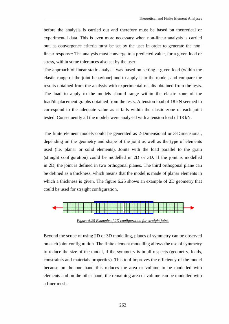
Theoretical and Finite Element Analyses
263
before the analysis is carried out and therefore must be based on theoretical or
experimental data. This is even more necessary when non-linear analysis is carried
out, as convergence criteria must be set by the user in order to generate the non-
linear response: The analysis must converge to a predicted value, for a given load or
stress, within some tolerances also set by the user.
The approach of linear static analysis was based on setting a given load (within the
elastic range of the joint behaviour) and to apply it to the model, and compare the
results obtained from the analysis with experimental results obtained from the tests.
The load to apply to the models should range within the elastic zone of the
load/displacement graphs obtained from the tests. A tension load of 18 kN seemed to
correspond to the adequate value as it falls within the elastic zone of each joint
tested. Consequently all the models were analysed with a tension load of 18 kN.
The finite element models could be generated as 2-Dimensional or 3-Dimensional,
depending on the geometry and shape of the joint as well as the type of elements
used (i.e. planar or solid elements). Joints with the load parallel to the grain
(straight configuration) could be modelled in 2D or 3D. If the joint is modelled
in 2D, the joint is defined in two orthogonal planes. The third orthogonal plane can
be defined as a thickness, which means that the model is made of planar elements in
which a thickness is given. The figure 6.25 shows an example of 2D geometry that
could be used for straight configuration.
Figure 6.25 Example of 2D configuration for straight joint.
Beyond the scope of using 2D or 3D modelling, planes of symmetry can be observed
on each joint configuration. The finite element modelling allows the use of symmetry
to reduce the size of the model, if the symmetry is in all respects (geometry, loads,
constraints and materials properties). This tool improves the efficiency of the model
because on the one hand this reduces the area or volume to be modelled with
elements and on the other hand, the remaining area or volume can be modelled with
a finer mesh.
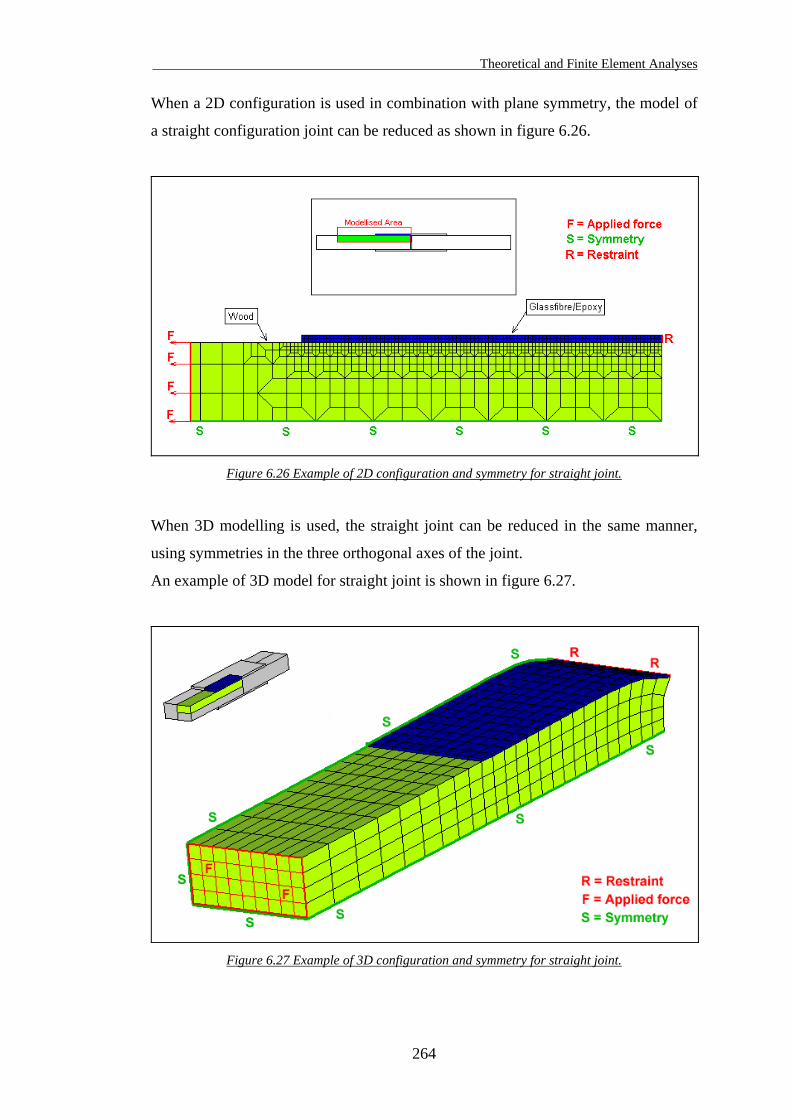
Theoretical and Finite Element Analyses
264
When a 2D configuration is used in combination with plane symmetry, the model of
a straight configuration joint can be reduced as shown in figure 6.26.
Figure 6.26 Example of 2D configuration and symmetry for straight joint.
When 3D modelling is used, the straight joint can be reduced in the same manner,
using symmetries in the three orthogonal axes of the joint.
An example of 3D model for straight joint is shown in figure 6.27.
Figure 6.27 Example of 3D configuration and symmetry for straight joint.
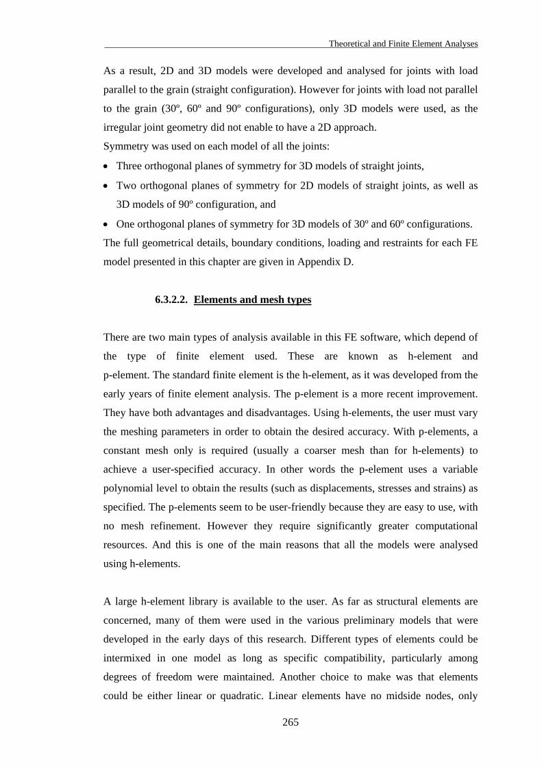
Theoretical and Finite Element Analyses
265
As a result, 2D and 3D models were developed and analysed for joints with load
parallel to the grain (straight configuration). However for joints with load not parallel
to the grain (30º, 60º and 90º configurations), only 3D models were used, as the
irregular joint geometry did not enable to have a 2D approach.
Symmetry was used on each model of all the joints:
• Three orthogonal planes of symmetry for 3D models of straight joints,
• Two orthogonal planes of symmetry for 2D models of straight joints, as well as
3D models of 90º configuration, and
• One orthogonal planes of symmetry for 3D models of 30º and 60º configurations.
The full geometrical details, boundary conditions, loading and restraints for each FE
model presented in this chapter are given in Appendix D.
6.3.2.2. Elements and mesh types
There are two main types of analysis available in this FE software, which depend of
the type of finite element used. These are known as h-element and
p-element. The standard finite element is the h-element, as it was developed from the
early years of finite element analysis. The p-element is a more recent improvement.
They have both advantages and disadvantages. Using h-elements, the user must vary
the meshing parameters in order to obtain the desired accuracy. With p-elements, a
constant mesh only is required (usually a coarser mesh than for h-elements) to
achieve a user-specified accuracy. In other words the p-element uses a variable
polynomial level to obtain the results (such as displacements, stresses and strains) as
specified. The p-elements seem to be user-friendly because they are easy to use, with
no mesh refinement. However they require significantly greater computational
resources. And this is one of the main reasons that all the models were analysed
using h-elements.
A large h-element library is available to the user. As far as structural elements are
concerned, many of them were used in the various preliminary models that were
developed in the early days of this research. Different types of elements could be
intermixed in one model as long as specific compatibility, particularly among
degrees of freedom were maintained. Another choice to make was that elements
could be either linear or quadratic. Linear elements have no midside nodes, only
Theoretical and Finite Element Analyses
266
corner nodes. For example, a linear triangular 2D element would have 3 corner nodes
and the equivalent quadratic element would have 3 corner nodes and 3 midside
nodes. Linear elements usually give an accurate solution in a reasonable amount of
computer time, and quadratic elements give a more precise solution in a longer
computer time, for a similar model. However both types have their own
characteristics, which can improve or worsen the analysis depending on what is
needed. Some examples of models where various element types for structural static
analysis were used are presented as follow:
• Planar elements, having either a triangular or quadrilateral geometry, are used for
2D modelling. Planar elements with 4 nodes usually yield more accurate results
than with 3 nodes in static analysis. Therefore they were used for all 2D models
that were developed for straight configuration models.
• Solid elements, having either tetrahedral or hexahedron geometry, are used for
3D solid modelling. Solid hexahedron elements have 8 nodes if linear and
20 nodes if quadratic. Solid tetrahedral elements have 4 nodes if linear and
10 nodes if quadratic. These elements were always used to model the wood
material of all 3D models. Solid elements were also used at a final stage to model
the glass fibre/epoxy composite.
• Shell elements, having either a triangular or quadrilateral geometry, to be used in
2D or 3D modelling. Shell elements are defined as a plate (4 nodes if
quadrilateral, etc) with a thickness. These elements were used to model the glass
fibre/epoxy composite in 3D models. However there was some incompatibility at
the interface with the solid elements used for the wood. This incompatibility was
mainly due to a different number of degrees of freedom between the jointed
elements. Another reason is that one particular solid element was used throughout
the FE models as it showed the best results in a reasonable amount of computer
time. This element type could not be connected to any different element type
without causing erroneous results: The model had insufficient rigid body
constraints. Finally, the glass fibre/epoxy composite was modelled with the same
solid elements and shell elements were not used.
• Composite elements were available in the library. They are highly specialised
elements called layered elements. They are specially designed to model a
laminate. In other words composite elements could be used when each layer of a
Theoretical and Finite Element Analyses
267
laminate have different orientations, with different orthotropic properties. Because
the glass fibre/epoxy composites used in this research are made of either one or
two perpendicular layers of fibres, there was no need of using those elements.
All the models presented in this chapter were finally developed in 3D, with either
linear or quadratic solid elements, depending on the complexity of the model, and
enabling anisotropic material properties.
The mesh density is another important point to consider in order to obtain reasonably
good results. This is one of the most fundamental questions that arise in finite
element analysis. In theory, the finer is the mesh, the more accurate the results are. If
the mesh is too coarse, the results can contain serious errors and if the mesh is too
fine, it will waste computer time, and the model could be to large to run on a normal
computer. As a result, the mesh density becomes a key issue during the model
generation.
Various meshing techniques were used through the modelling process, mainly
because the software offers different ways of mesh generation. But firstly, it is
important to understand that the mesh geometry and density must always satisfy
some rules in order to be acceptable as far as the analysis is concerned. Each element
type has some geometric restrictions, which are known as the aspect ratio. The aspect
ratio is characterised by the element shape: The height to width ratio, the angle
between two adjacent ridges, etc. An element having an aspect ratio that falls outside
the limits set for its type would be too distorted and therefore would produce
erroneous results. For the FE models that were developed in this research, structural
stress analysis was used to determine the stress (or strain) at particular locations. For
that particular use of FE analysis, poorly shaped elements would generally produce
more severe errors than for any other type of analysis (deflection, modal, thermal
analysis, etc). In other words, special attention was given to mesh density in order to
avoid element shape errors. For each model developed, they were preliminarily
developed using very coarse mesh, gradually refined until the results obtained were
accurate enough without showing any errors or warning in the mesh density.
The preliminary models developed for the joints with load parallel to the grain
summarises the different meshing techniques used throughout the research. They are
presented in the following section.
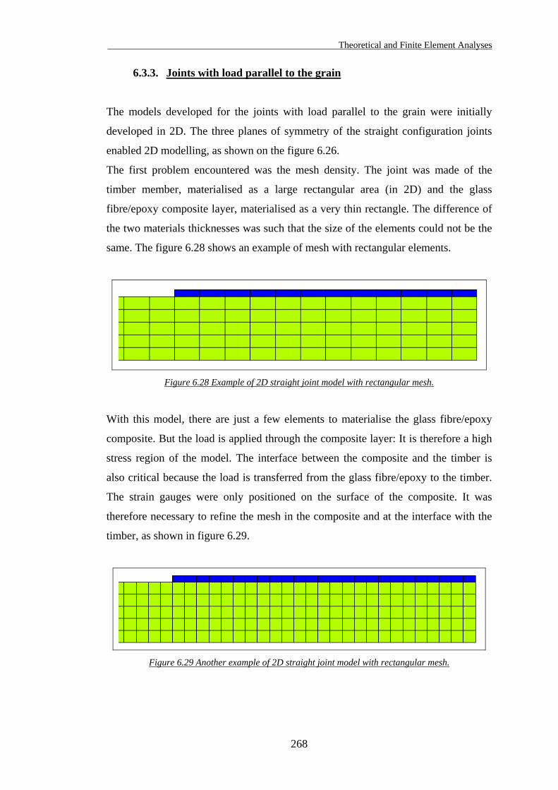
Theoretical and Finite Element Analyses
268
6.3.3. Joints with load parallel to the grain
The models developed for the joints with load parallel to the grain were initially
developed in 2D. The three planes of symmetry of the straight configuration joints
enabled 2D modelling, as shown on the figure 6.26.
The first problem encountered was the mesh density. The joint was made of the
timber member, materialised as a large rectangular area (in 2D) and the glass
fibre/epoxy composite layer, materialised as a very thin rectangle. The difference of
the two materials thicknesses was such that the size of the elements could not be the
same. The figure 6.28 shows an example of mesh with rectangular elements.
Figure 6.28 Example of 2D straight joint model with rectangular mesh.
With this model, there are just a few elements to materialise the glass fibre/epoxy
composite. But the load is applied through the composite layer: It is therefore a high
stress region of the model. The interface between the composite and the timber is
also critical because the load is transferred from the glass fibre/epoxy to the timber.
The strain gauges were only positioned on the surface of the composite. It was
therefore necessary to refine the mesh in the composite and at the interface with the
timber, as shown in figure 6.29.
Figure 6.29 Another example of 2D straight joint model with rectangular mesh.
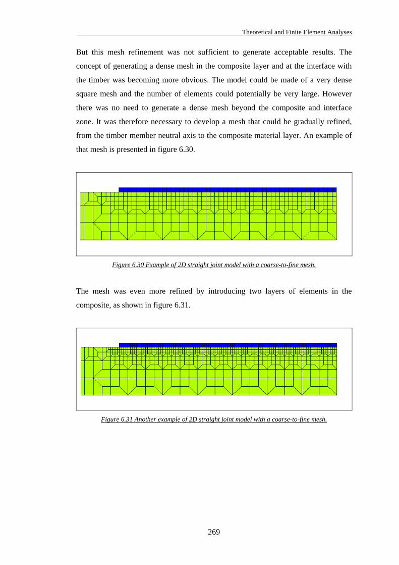
Theoretical and Finite Element Analyses
269
But this mesh refinement was not sufficient to generate acceptable results. The
concept of generating a dense mesh in the composite layer and at the interface with
the timber was becoming more obvious. The model could be made of a very dense
square mesh and the number of elements could potentially be very large. However
there was no need to generate a dense mesh beyond the composite and interface
zone. It was therefore necessary to develop a mesh that could be gradually refined,
from the timber member neutral axis to the composite material layer. An example of
that mesh is presented in figure 6.30.
Figure 6.30 Example of 2D straight joint model with a coarse-to-fine mesh.
The mesh was even more refined by introducing two layers of elements in the
composite, as shown in figure 6.31.
Figure 6.31 Another example of 2D straight joint model with a coarse-to-fine mesh.
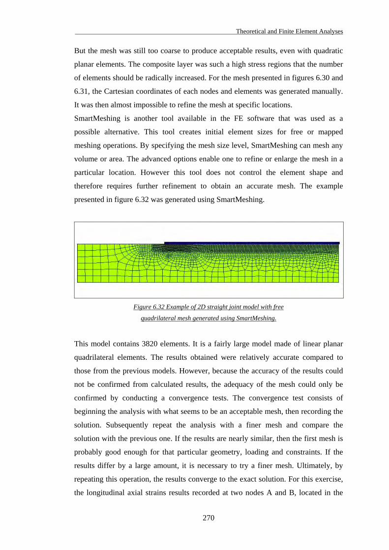
Theoretical and Finite Element Analyses
270
But the mesh was still too coarse to produce acceptable results, even with quadratic
planar elements. The composite layer was such a high stress regions that the number
of elements should be radically increased. For the mesh presented in figures 6.30 and
6.31, the Cartesian coordinates of each nodes and elements was generated manually.
It was then almost impossible to refine the mesh at specific locations.
SmartMeshing is another tool available in the FE software that was used as a
possible alternative. This tool creates initial element sizes for free or mapped
meshing operations. By specifying the mesh size level, SmartMeshing can mesh any
volume or area. The advanced options enable one to refine or enlarge the mesh in a
particular location. However this tool does not control the element shape and
therefore requires further refinement to obtain an accurate mesh. The example
presented in figure 6.32 was generated using SmartMeshing.
Figure 6.32 Example of 2D straight joint model with free
quadrilateral mesh generated using SmartMeshing.
This model contains 3820 elements. It is a fairly large model made of linear planar
quadrilateral elements. The results obtained were relatively accurate compared to
those from the previous models. However, because the accuracy of the results could
not be confirmed from calculated results, the adequacy of the mesh could only be
confirmed by conducting a convergence tests. The convergence test consists of
beginning the analysis with what seems to be an acceptable mesh, then recording the
solution. Subsequently repeat the analysis with a finer mesh and compare the
solution with the previous one. If the results are nearly similar, then the first mesh is
probably good enough for that particular geometry, loading and constraints. If the
results differ by a large amount, it is necessary to try a finer mesh. Ultimately, by
repeating this operation, the results converge to the exact solution. For this exercise,
the longitudinal axial strains results recorded at two nodes A and B, located in the
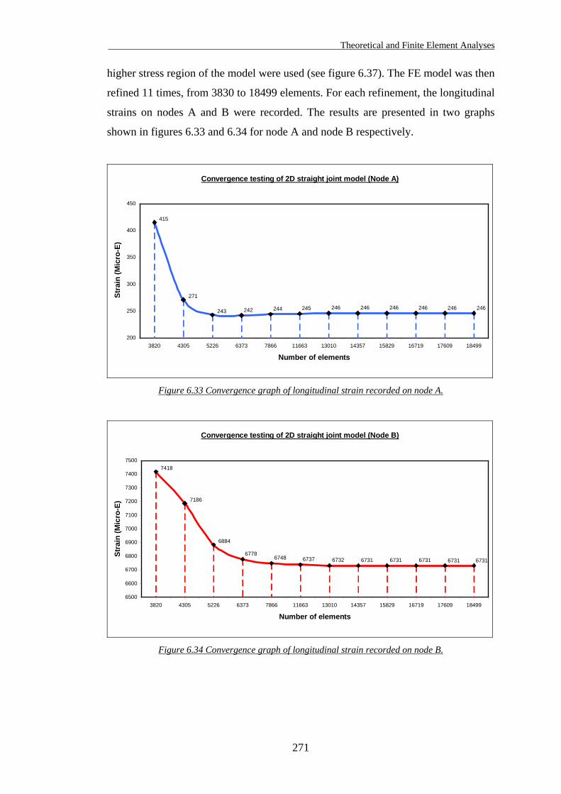
Theoretical and Finite Element Analyses
271
higher stress region of the model were used (see figure 6.37). The FE model was then
refined 11 times, from 3830 to 18499 elements. For each refinement, the longitudinal
strains on nodes A and B were recorded. The results are presented in two graphs
shown in figures 6.33 and 6.34 for node A and node B respectively.
Convergence testing of 2D straight joint model (Node A)
246246243
415
271
246246245244242 246 246
200
250
300
350
400
450
3820 4305 5226 6373 7866 11663 13010 14357 15829 16719 17609 18499
Number of elements
Stra
in (M
icro
-E)
Figure 6.33 Convergence graph of longitudinal strain recorded on node A.
Convergence testing of 2D straight joint model (Node B)
6731673167316731
6884
7418
7186
67316732673767486778
6500
6600
6700
6800
6900
7000
7100
7200
7300
7400
7500
3820 4305 5226 6373 7866 11663 13010 14357 15829 16719 17609 18499
Number of elements
Stra
in (M
icro
-E)
Figure 6.34 Convergence graph of longitudinal strain recorded on node B.
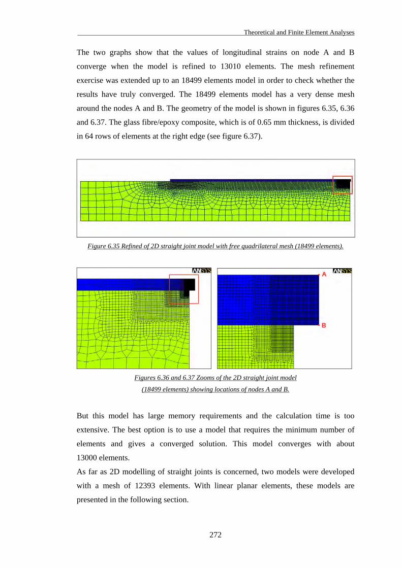
Theoretical and Finite Element Analyses
272
The two graphs show that the values of longitudinal strains on node A and B
converge when the model is refined to 13010 elements. The mesh refinement
exercise was extended up to an 18499 elements model in order to check whether the
results have truly converged. The 18499 elements model has a very dense mesh
around the nodes A and B. The geometry of the model is shown in figures 6.35, 6.36
and 6.37. The glass fibre/epoxy composite, which is of 0.65 mm thickness, is divided
in 64 rows of elements at the right edge (see figure 6.37).
Figure 6.35 Refined of 2D straight joint model with free quadrilateral mesh (18499 elements).
Figures 6.36 and 6.37 Zooms of the 2D straight joint model
(18499 elements) showing locations of nodes A and B.
But this model has large memory requirements and the calculation time is too
extensive. The best option is to use a model that requires the minimum number of
elements and gives a converged solution. This model converges with about
13000 elements.
As far as 2D modelling of straight joints is concerned, two models were developed
with a mesh of 12393 elements. With linear planar elements, these models are
presented in the following section.
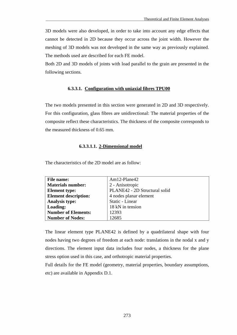
Theoretical and Finite Element Analyses
273
3D models were also developed, in order to take into account any edge effects that
cannot be detected in 2D because they occur across the joint width. However the
meshing of 3D models was not developed in the same way as previously explained.
The methods used are described for each FE model.
Both 2D and 3D models of joints with load parallel to the grain are presented in the
following sections.
6.3.3.1. Configuration with uniaxial fibres TPU00
The two models presented in this section were generated in 2D and 3D respectively.
For this configuration, glass fibres are unidirectional: The material properties of the
composite reflect these characteristics. The thickness of the composite corresponds to
the measured thickness of 0.65 mm.
6.3.3.1.1. 2-Dimensional model
The characteristics of the 2D model are as follow:
File name: Materials number: Element type: Element description: Analysis type: Loading: Number of Elements: Number of Nodes:
Am12-Plane42 2 - Anisotropic PLANE42 - 2D Structural solid 4 nodes planar element Static - Linear 18 kN in tension 12393 12685
The linear element type PLANE42 is defined by a quadrilateral shape with four
nodes having two degrees of freedom at each node: translations in the nodal x and y
directions. The element input data includes four nodes, a thickness for the plane
stress option used in this case, and orthotropic material properties.
Full details for the FE model (geometry, material properties, boundary assumptions,
etc) are available in Appendix D.1.
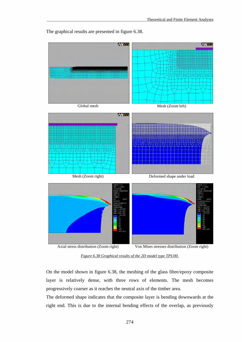
Theoretical and Finite Element Analyses
274
The graphical results are presented in figure 6.38.
Global mesh
Mesh (Zoom left)
Mesh (Zoom right)
Deformed shape under load
Axial stress distribution (Zoom right)
Von Mises stresses distribution (Zoom right)
Figure 6.38 Graphical results of the 2D model type TPU00.
On the model shown in figure 6.38, the meshing of the glass fibre/epoxy composite
layer is relatively dense, with three rows of elements. The mesh becomes
progressively coarser as it reaches the neutral axis of the timber area.
The deformed shape indicates that the composite layer is bending downwards at the
right end. This is due to the internal bending effects of the overlap, as previously
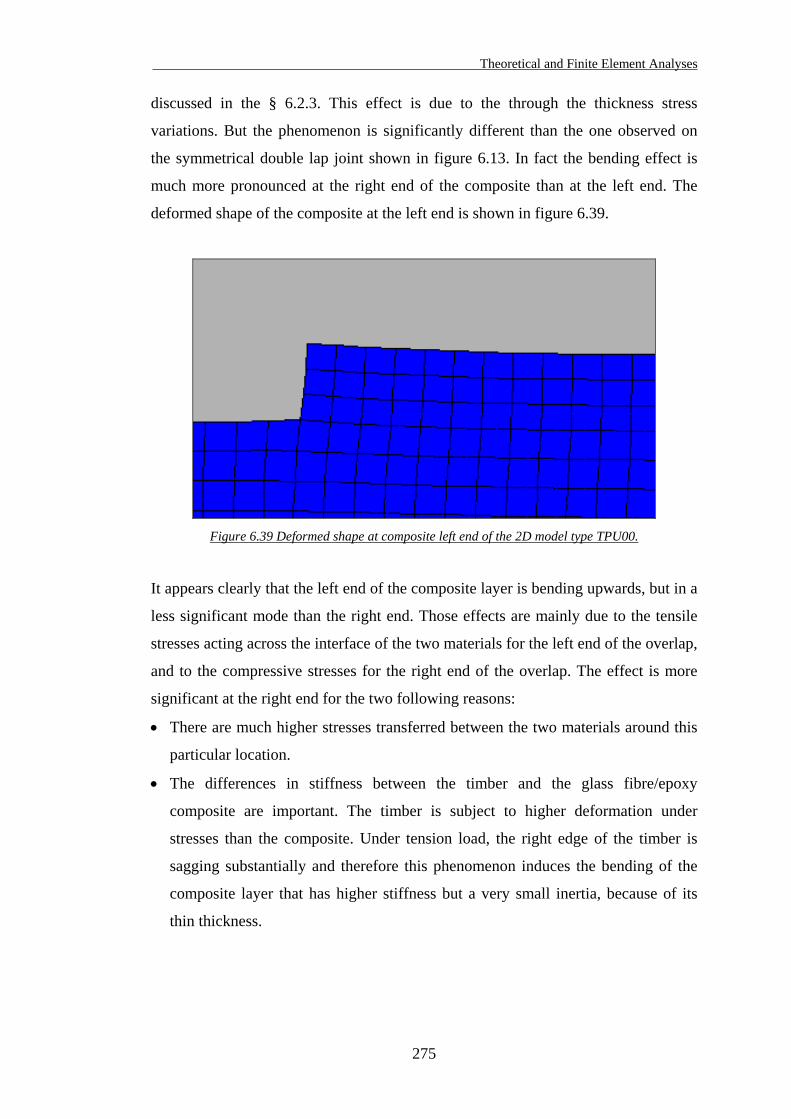
Theoretical and Finite Element Analyses
275
discussed in the § 6.2.3. This effect is due to the through the thickness stress
variations. But the phenomenon is significantly different than the one observed on
the symmetrical double lap joint shown in figure 6.13. In fact the bending effect is
much more pronounced at the right end of the composite than at the left end. The
deformed shape of the composite at the left end is shown in figure 6.39.
Figure 6.39 Deformed shape at composite left end of the 2D model type TPU00.
It appears clearly that the left end of the composite layer is bending upwards, but in a
less significant mode than the right end. Those effects are mainly due to the tensile
stresses acting across the interface of the two materials for the left end of the overlap,
and to the compressive stresses for the right end of the overlap. The effect is more
significant at the right end for the two following reasons:
• There are much higher stresses transferred between the two materials around this
particular location.
• The differences in stiffness between the timber and the glass fibre/epoxy
composite are important. The timber is subject to higher deformation under
stresses than the composite. Under tension load, the right edge of the timber is
sagging substantially and therefore this phenomenon induces the bending of the
composite layer that has higher stiffness but a very small inertia, because of its
thin thickness.

Theoretical and Finite Element Analyses
276
Experimental measurement of the internal bending effects of the overlap was carried
out on one of the sample to confirm whether the results given by the FE models were
acceptable. This experiment and results are presented and discussed in § 6.4.
The axial and shear stress distributions are obviously affected by this fact. The
following graphs presented in figures 6.40 and 6.41 indicate the tensile and shear
stress distribution calculated by the FE model at the interface between the composite
and the timber.
0
50
100
150
200
250
300
350
50 75 100 125 150
Distance on G/E (mm)
Tens
ile s
tres
s (N
/mm
2)
Tensile stress distribution on glass fibre/epoxy interface
0
10
20
30
40
50
60
70
80
90
100
0 25 50 75 100 125 150
Distance on timber (mm)
Tens
ile s
tres
s (N
/mm
2)
Tensile stress distribution on timber interface
X
0 50 150
X
0 50 150
Figure 6.40 Tensile stress distributions at the interface between the composite and the timber.
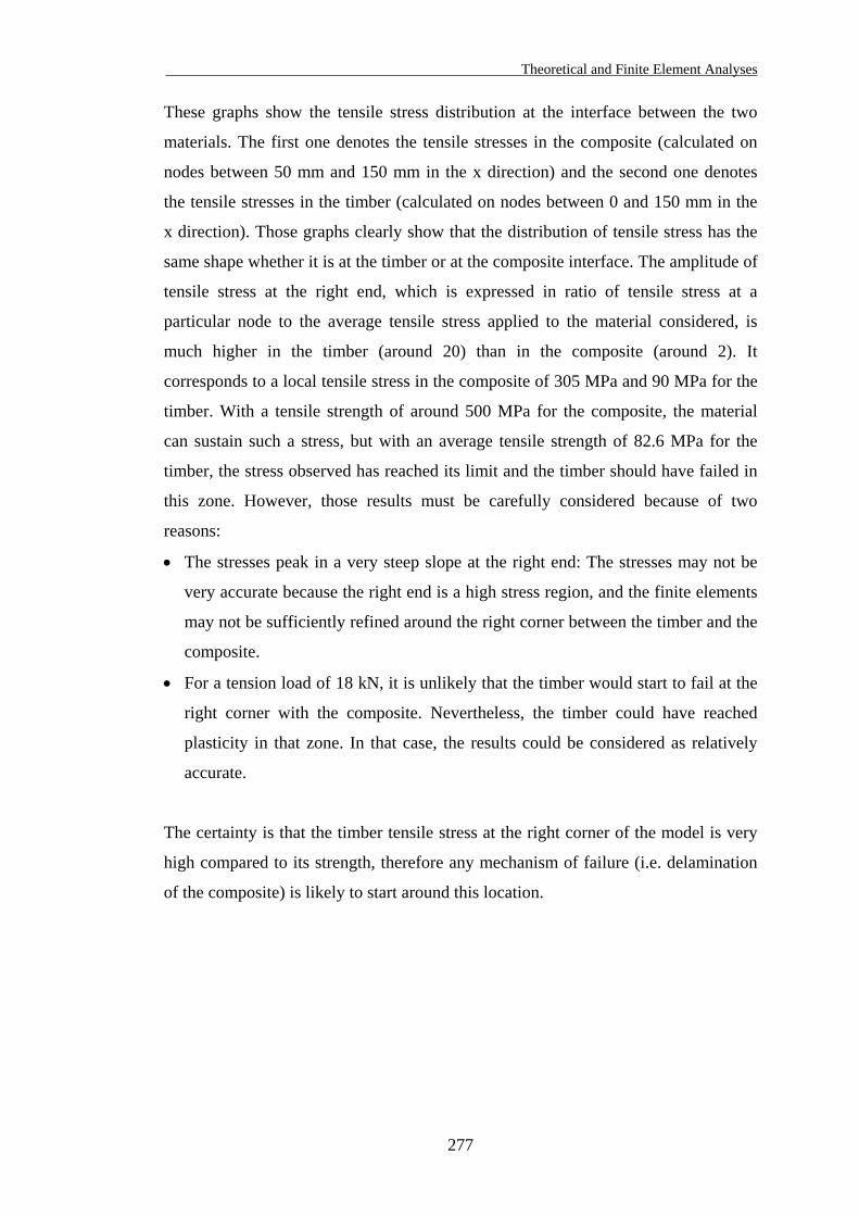
Theoretical and Finite Element Analyses
277
These graphs show the tensile stress distribution at the interface between the two
materials. The first one denotes the tensile stresses in the composite (calculated on
nodes between 50 mm and 150 mm in the x direction) and the second one denotes
the tensile stresses in the timber (calculated on nodes between 0 and 150 mm in the
x direction). Those graphs clearly show that the distribution of tensile stress has the
same shape whether it is at the timber or at the composite interface. The amplitude of
tensile stress at the right end, which is expressed in ratio of tensile stress at a
particular node to the average tensile stress applied to the material considered, is
much higher in the timber (around 20) than in the composite (around 2). It
corresponds to a local tensile stress in the composite of 305 MPa and 90 MPa for the
timber. With a tensile strength of around 500 MPa for the composite, the material
can sustain such a stress, but with an average tensile strength of 82.6 MPa for the
timber, the stress observed has reached its limit and the timber should have failed in
this zone. However, those results must be carefully considered because of two
reasons:
• The stresses peak in a very steep slope at the right end: The stresses may not be
very accurate because the right end is a high stress region, and the finite elements
may not be sufficiently refined around the right corner between the timber and the
composite.
• For a tension load of 18 kN, it is unlikely that the timber would start to fail at the
right corner with the composite. Nevertheless, the timber could have reached
plasticity in that zone. In that case, the results could be considered as relatively
accurate.
The certainty is that the timber tensile stress at the right corner of the model is very
high compared to its strength, therefore any mechanism of failure (i.e. delamination
of the composite) is likely to start around this location.
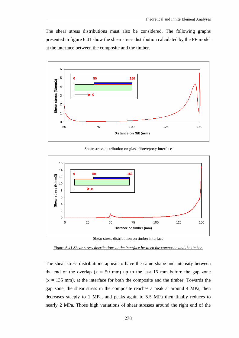
Theoretical and Finite Element Analyses
278
The shear stress distributions must also be considered. The following graphs
presented in figure 6.41 show the shear stress distribution calculated by the FE model
at the interface between the composite and the timber.
0
1
2
3
4
5
6
50 75 100 125 150
Distance on G/E (mm)
Shea
r str
ess
(N/m
m2)
Shear stress distribution on glass fibre/epoxy interface
0
2
4
6
8
10
12
14
16
0 25 50 75 100 125 150
Distance on timber (mm)
Shea
r str
ess
(N/m
m2)
Shear stress distribution on timber interface
X
0 50 150
X
0 50 150
Figure 6.41 Shear stress distributions at the interface between the composite and the timber.
The shear stress distributions appear to have the same shape and intensity between
the end of the overlap (x = 50 mm) up to the last 15 mm before the gap zone
(x = 135 mm), at the interface for both the composite and the timber. Towards the
gap zone, the shear stress in the composite reaches a peak at around 4 MPa, then
decreases steeply to 1 MPa, and peaks again to 5.5 MPa then finally reduces to
nearly 2 MPa. Those high variations of shear stresses around the right end of the
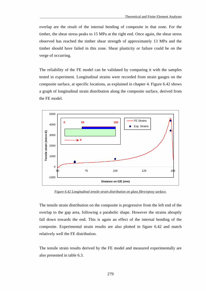
Theoretical and Finite Element Analyses
279
overlap are the result of the internal bending of composite in that zone. For the
timber, the shear stress peaks to 15 MPa at the right end. Once again, the shear stress
observed has reached the timber shear strength of approximately 13 MPa and the
timber should have failed in this zone. Shear plasticity or failure could be on the
verge of occurring.
The reliability of the FE model can be validated by comparing it with the samples
tested in experiment. Longitudinal strains were recorded from strain gauges on the
composite surface, at specific locations, as explained in chapter 4. Figure 6.42 shows
a graph of longitudinal strain distribution along the composite surface, derived from
the FE model.
-1000
0
1000
2000
3000
4000
5000
50 75 100 125 150
Distance on G/E (mm)
Tens
ile s
trai
n (m
icro
-E)
Strains
Exp. Strains
FE
X
0 50 150
Figure 6.42 Longitudinal tensile strain distribution on glass fibre/epoxy surface.
The tensile strain distribution on the composite is progressive from the left end of the
overlap to the gap area, following a parabolic shape. However the strains abruptly
fall down towards the end. This is again an effect of the internal bending of the
composite. Experimental strain results are also plotted in figure 6.42 and match
relatively well the FE distribution.
The tensile strain results derived by the FE model and measured experimentally are
also presented in table 6.3.
Theoretical and Finite Element Analyses
280
End strain gauge Middle strain gauge Gap strain gaugeSample
x = 65 mm x = 100 mm x = 150 mm
7TPU00 - Z 503 758 4376
8TPU00 - J 428 N/A 3433
Plane42 FE model 347 585 4607
Table 6.3 Comparison of strains results obtained from experiments and from the FE model.
Strain gauge positions are described in § 4.3.2.2. The results of tensile strains
obtained from the FE model are relatively close to those obtained from experiments.
However, the FE results tend to be lower for end and middle strains and higher for
the gap strain. These results have to be compared with those obtained from the
3-dimensional FE model that is presented in the next section.
6.3.3.1.2. 3-Dimensional model
The characteristics of the 3D model are as follow:
File name: Materials number: Element type: Element description: Analysis type: Loading: Number of Elements: Number of Nodes:
Am01-solid72 2 - Anisotropic SOLID72 - 3D Structural solid 4 nodes tetrahedral solid element with rotations Static - Linear 18 kN in tension 58886 11788
The linear element type SOLID72 is defined by a tetrahedral solid shape with four
nodes having six degrees of freedom at each node: translations in the nodal x, y and z
directions and rotations about the nodal x, y and z directions. The element input data
includes four nodes and orthotropic material properties. The element is well suited to
model irregular meshes because of its tetrahedral geometry. It can often be replaced
by the SOLID92 element, which is a quadratic tetrahedral solid element, with
10 nodes. Although SOLID72 has additional degrees of freedom per node, it is not as
accurate as the SOLID92 element. This model was initially developed using the
SOLID92 (quadratic) element. In order to enable the analysis of the model in an
acceptable computer time, the mesh was initially reduced. However the composite
layer was not refined enough to give accurate results, and using mesh refinements in
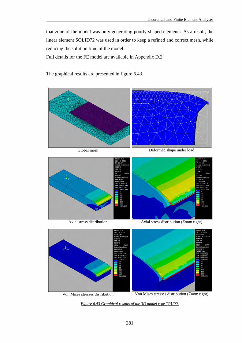
Theoretical and Finite Element Analyses
281
that zone of the model was only generating poorly shaped elements. As a result, the
linear element SOLID72 was used in order to keep a refined and correct mesh, while
reducing the solution time of the model.
Full details for the FE model are available in Appendix D.2.
The graphical results are presented in figure 6.43.
Global mesh
Deformed shape under load
Axial stress distribution
Axial stress distribution (Zoom right)
Von Mises stresses distribution
Von Mises stresses distribution (Zoom right)
Figure 6.43 Graphical results of the 3D model type TPU00.
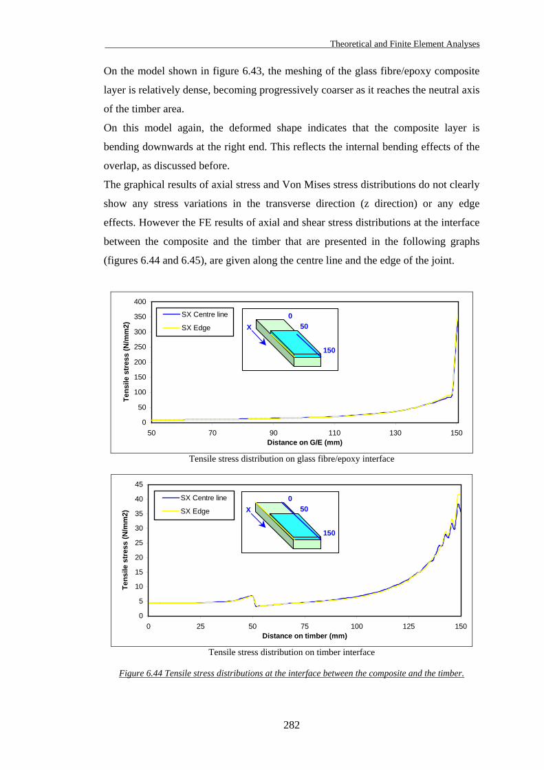
Theoretical and Finite Element Analyses
282
On the model shown in figure 6.43, the meshing of the glass fibre/epoxy composite
layer is relatively dense, becoming progressively coarser as it reaches the neutral axis
of the timber area.
On this model again, the deformed shape indicates that the composite layer is
bending downwards at the right end. This reflects the internal bending effects of the
overlap, as discussed before.
The graphical results of axial stress and Von Mises stress distributions do not clearly
show any stress variations in the transverse direction (z direction) or any edge
effects. However the FE results of axial and shear stress distributions at the interface
between the composite and the timber that are presented in the following graphs
(figures 6.44 and 6.45), are given along the centre line and the edge of the joint.
0
50
100
150
200
250
300
350
400
50 70 90 110 130 150Distance on G/E (mm)
Tens
ile s
tres
s (N
/mm
2)
SX Centre line
SX Edge 50
150
0X
Tensile stress distribution on glass fibre/epoxy interface
0
5
10
15
20
25
30
35
40
45
0 25 50 75 100 125 150Distance on timber (mm)
Tens
ile s
tres
s (N
/mm
2)
SX Centre line
SX Edge 50
150
0X
Tensile stress distribution on timber interface
Figure 6.44 Tensile stress distributions at the interface between the composite and the timber.
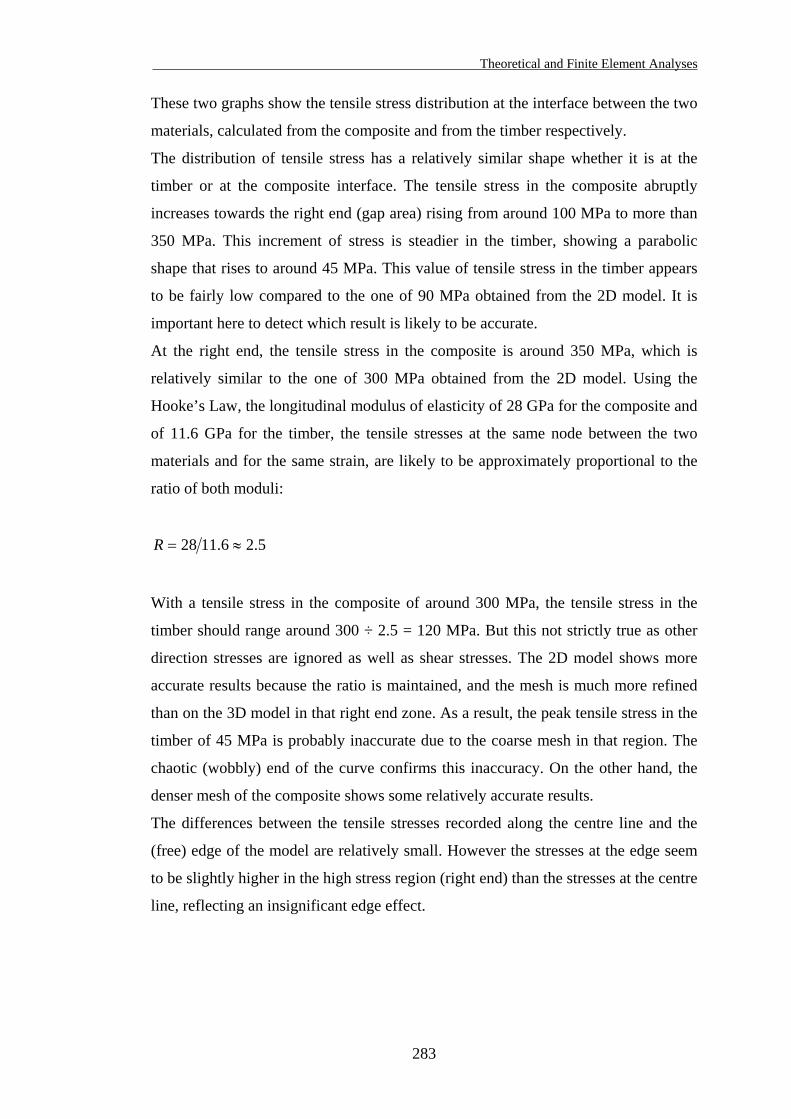
Theoretical and Finite Element Analyses
283
These two graphs show the tensile stress distribution at the interface between the two
materials, calculated from the composite and from the timber respectively.
The distribution of tensile stress has a relatively similar shape whether it is at the
timber or at the composite interface. The tensile stress in the composite abruptly
increases towards the right end (gap area) rising from around 100 MPa to more than
350 MPa. This increment of stress is steadier in the timber, showing a parabolic
shape that rises to around 45 MPa. This value of tensile stress in the timber appears
to be fairly low compared to the one of 90 MPa obtained from the 2D model. It is
important here to detect which result is likely to be accurate.
At the right end, the tensile stress in the composite is around 350 MPa, which is
relatively similar to the one of 300 MPa obtained from the 2D model. Using the
Hooke’s Law, the longitudinal modulus of elasticity of 28 GPa for the composite and
of 11.6 GPa for the timber, the tensile stresses at the same node between the two
materials and for the same strain, are likely to be approximately proportional to the
ratio of both moduli:
5.26.1128 ≈=R
With a tensile stress in the composite of around 300 MPa, the tensile stress in the
timber should range around 300 ÷ 2.5 = 120 MPa. But this not strictly true as other
direction stresses are ignored as well as shear stresses. The 2D model shows more
accurate results because the ratio is maintained, and the mesh is much more refined
than on the 3D model in that right end zone. As a result, the peak tensile stress in the
timber of 45 MPa is probably inaccurate due to the coarse mesh in that region. The
chaotic (wobbly) end of the curve confirms this inaccuracy. On the other hand, the
denser mesh of the composite shows some relatively accurate results.
The differences between the tensile stresses recorded along the centre line and the
(free) edge of the model are relatively small. However the stresses at the edge seem
to be slightly higher in the high stress region (right end) than the stresses at the centre
line, reflecting an insignificant edge effect.
Theoretical and Finite Element Analyses
284
The shear stress distributions calculated by the FE model at the interface between the
composite and the timber are presented in figure 6.45.
-2
0
2
4
6
8
10
12
14
50 70 90 110 130 150
Distance on G/E (mm)
Shea
r str
ess
(N/m
m2)
SXY Centre line
SXY Edge 50
150
0X
Shear stress distribution on glass fibre/epoxy interface
-1
0
1
2
3
4
5
0 25 50 75 100 125 150
Distance on timber (mm)
Shea
r str
ess
(N/m
m2)
SXY Centre line
SXY Edge 50
150
0X
Shear stress distribution on timber interface
Figure 6.45 Shear stress distributions at the interface between the composite and the timber.
The shear stress distributions appear to be similar in terms of shape and intensity
except around both ends of the overlap (around x = 50 mm for the left end and
x = 140 mm for the right end). Towards the right end (gap zone), the shear stress in
the composite reaches a peak at around 3.5 MPa, then decreases steeply to around
- 0.7 MPa and peaks again to 12 MPa. Those high variations of shear stresses around
the right end of the overlap are the result of the internal bending of composite in that
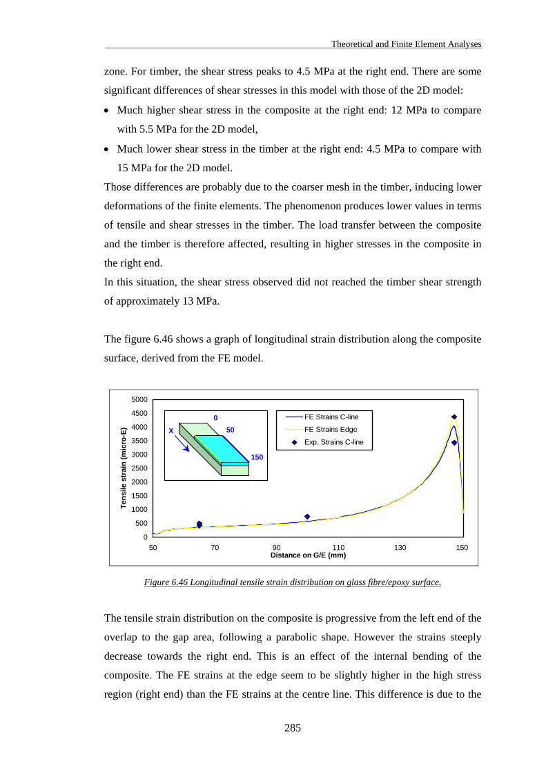
Theoretical and Finite Element Analyses
285
zone. For timber, the shear stress peaks to 4.5 MPa at the right end. There are some
significant differences of shear stresses in this model with those of the 2D model:
• Much higher shear stress in the composite at the right end: 12 MPa to compare
with 5.5 MPa for the 2D model,
• Much lower shear stress in the timber at the right end: 4.5 MPa to compare with
15 MPa for the 2D model.
Those differences are probably due to the coarser mesh in the timber, inducing lower
deformations of the finite elements. The phenomenon produces lower values in terms
of tensile and shear stresses in the timber. The load transfer between the composite
and the timber is therefore affected, resulting in higher stresses in the composite in
the right end.
In this situation, the shear stress observed did not reached the timber shear strength
of approximately 13 MPa.
The figure 6.46 shows a graph of longitudinal strain distribution along the composite
surface, derived from the FE model.
0
500
1000
1500
2000
2500
3000
3500
4000
4500
5000
50 70 90 110 130 150Distance on G/E (mm)
Tens
ile s
trai
n (m
icro
-E)
FE Strains C-line
FE Strains Edge
Exp. Strains C-line
50
150
0
X
Figure 6.46 Longitudinal tensile strain distribution on glass fibre/epoxy surface.
The tensile strain distribution on the composite is progressive from the left end of the
overlap to the gap area, following a parabolic shape. However the strains steeply
decrease towards the right end. This is an effect of the internal bending of the
composite. The FE strains at the edge seem to be slightly higher in the high stress
region (right end) than the FE strains at the centre line. This difference is due to the
Theoretical and Finite Element Analyses
286
edge effect. Internal bending effects are discussed in greater details in § 6.4.
Experimental strain results are also plotted in figure 6.46 and match relatively well
the FE distribution.
The tensile strain results derived by the FE model and measured experimentally are
also presented in table 6.4.
End strain gauge Middle strain gauge Gap strain gaugeSample
x = 65 mm x = 100 mm x = 150 mm
7TPU00 - Z 503 758 4376
8TPU00 - J 428 N/A 3433
Solid72 FE model 354 578 4031
Table 6.4 Comparison of strains results obtained from experiments and from the FE model.
Strain gauge positions are described in § 4.3.2.2. The results of tensile strains
obtained from the FE model tend to be lower for end and middle strains. However,
the strain result obtained for the gap is relatively close to those obtained from
experiments.
Finally the comparison between the 2D and 3D models shows that the results
obtained are relatively similar except in the high stress region, i.e. the gap zone.
Advantages and disadvantages of both models can be considered:
• The strains and stresses are of comparable magnitude except in the high stress
region where there are large differences: The 3D model shows inaccurate results
due to its relatively coarse mesh, compared to those obtained with the finer mesh
of the 2D model.
• The 2D model does not show whether the strain and stresses vary across the width
of the joint. In fact the 3D model reveals that there is a relatively small edge effect
in the high stress region, as strains and stresses are slightly higher along the edge
than along the centre line of the joint.
Theoretical and Finite Element Analyses
287
6.3.3.2. Configuration with biaxial fibres TPB00
The two models presented in this section were generated in 2D and 3D respectively.
The glass fibres are bidirectional, therefore the material properties of the composite
reflect these characteristics (identical material properties in the x and z directions).
The thickness of the composite corresponds to the measured thickness of 0.65 mm,
which is the same than the one measured for uniaxial fibres samples TPU00.
6.3.3.2.1. 2-Dimensional model
The characteristics of the 2D model are as follow:
File name: Materials number: Element type: Element description: Analysis type: Loading: Number of Elements: Number of Nodes:
Am14-plane42 2 - Anisotropic PLANE42 - 2D Structural solid 4 nodes plane element Static - Linear 18 kN in tension 12393 12685
The PLANE42 linear element characteristics are already defined in § 6.3.3.1.1.
Full details for the FE model (geometry, material properties, boundary assumptions,
etc) are available in Appendix D.1.
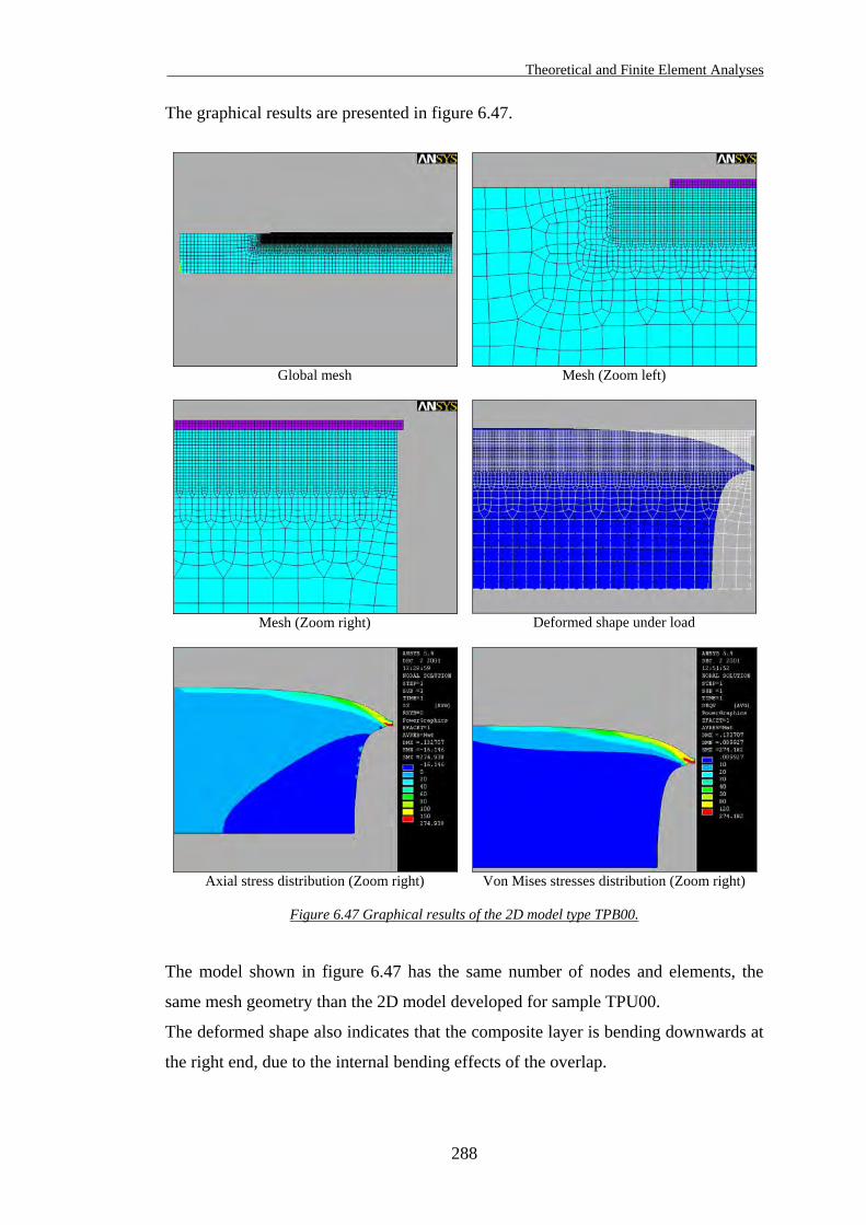
Theoretical and Finite Element Analyses
288
The graphical results are presented in figure 6.47.
Global mesh
Mesh (Zoom left)
Mesh (Zoom right)
Deformed shape under load
Axial stress distribution (Zoom right)
Von Mises stresses distribution (Zoom right)
Figure 6.47 Graphical results of the 2D model type TPB00.
The model shown in figure 6.47 has the same number of nodes and elements, the
same mesh geometry than the 2D model developed for sample TPU00.
The deformed shape also indicates that the composite layer is bending downwards at
the right end, due to the internal bending effects of the overlap.
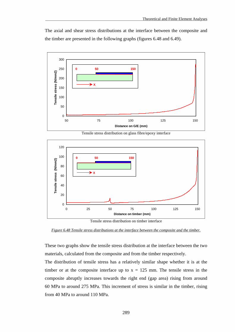
Theoretical and Finite Element Analyses
289
The axial and shear stress distributions at the interface between the composite and
the timber are presented in the following graphs (figures 6.48 and 6.49).
0
50
100
150
200
250
300
50 75 100 125 150
Distance on G/E (mm)
Tens
ile s
tres
s (N
/mm
2)
Tensile stress distribution on glass fibre/epoxy interface
0
20
40
60
80
100
120
0 25 50 75 100 125 150Distance on timber (mm)
Tens
ile s
tres
s (N
/mm
2)
Tensile stress distribution on timber interface
X
0 50 150
X
0 50 150
Figure 6.48 Tensile stress distributions at the interface between the composite and the timber.
These two graphs show the tensile stress distribution at the interface between the two
materials, calculated from the composite and from the timber respectively.
The distribution of tensile stress has a relatively similar shape whether it is at the
timber or at the composite interface up to x = 125 mm. The tensile stress in the
composite abruptly increases towards the right end (gap area) rising from around
60 MPa to around 275 MPa. This increment of stress is similar in the timber, rising
from 40 MPa to around 110 MPa.
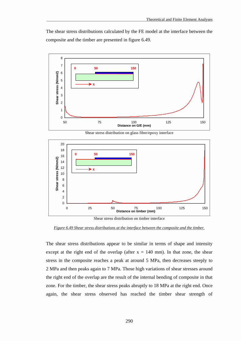
Theoretical and Finite Element Analyses
290
The shear stress distributions calculated by the FE model at the interface between the
composite and the timber are presented in figure 6.49.
0
1
2
3
4
5
6
7
8
50 75 100 125 150Distance on G/E (mm)
Shea
r str
ess
(N/m
m2)
Shear stress distribution on glass fibre/epoxy interface
0
2
4
6
8
10
12
14
16
18
20
0 25 50 75 100 125 150Distance on timber (mm)
Shea
r str
ess
(N/m
m2)
Shear stress distribution on timber interface
X
0 50 150
X
0 50 150
Figure 6.49 Shear stress distributions at the interface between the composite and the timber.
The shear stress distributions appear to be similar in terms of shape and intensity
except at the right end of the overlap (after x = 140 mm). In that zone, the shear
stress in the composite reaches a peak at around 5 MPa, then decreases steeply to
2 MPa and then peaks again to 7 MPa. Those high variations of shear stresses around
the right end of the overlap are the result of the internal bending of composite in that
zone. For the timber, the shear stress peaks abruptly to 18 MPa at the right end. Once
again, the shear stress observed has reached the timber shear strength of
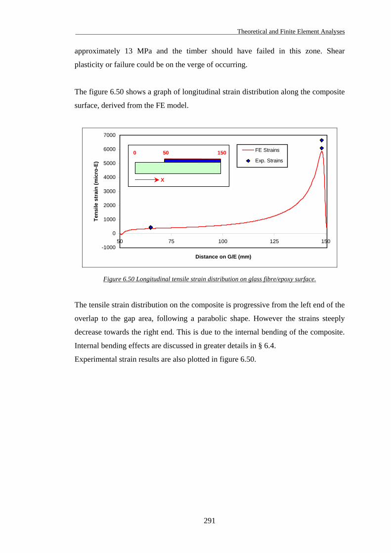
Theoretical and Finite Element Analyses
291
approximately 13 MPa and the timber should have failed in this zone. Shear
plasticity or failure could be on the verge of occurring.
The figure 6.50 shows a graph of longitudinal strain distribution along the composite
surface, derived from the FE model.
-1000
0
1000
2000
3000
4000
5000
6000
7000
50 75 100 125 150
Distance on G/E (mm)
Tens
ile s
trai
n (m
icro
-E)
FE Strains
Exp. Strains
X
0 50 150
Figure 6.50 Longitudinal tensile strain distribution on glass fibre/epoxy surface.
The tensile strain distribution on the composite is progressive from the left end of the
overlap to the gap area, following a parabolic shape. However the strains steeply
decrease towards the right end. This is due to the internal bending of the composite.
Internal bending effects are discussed in greater details in § 6.4.
Experimental strain results are also plotted in figure 6.50.
Theoretical and Finite Element Analyses
292
The tensile strain results derived by the FE model and measured experimentally are
presented in table 6.5.
End strain gauge Gap strain gauge Sample
x = 65 mm x = 150 mm
7TPB00 - α 411 6093
8TPB00 - $ 463 6653
Plane42 FE model 361 5840
Table 6.5 Comparison of strains results obtained from experiments and from the FE model.
Strain gauge positions are described in § 4.3.2.2. The results of tensile strains
obtained from the FE model tend to be lower than those measured in experiments but
remain within the range.
These results must be compared with those obtained from the 3-dimensional FE
model that is presented in the next section.
6.3.3.2.2. 3-Dimensional model
The characteristics of the 3D model are as follow:
File name: Materials number: Element type: Element description: Analysis type: Loading: Number of Elements: Number of Nodes:
Am02-solid72 2 - Anisotropic SOLID72 - 3D Structural solid 4 nodes tetrahedral solid element with rotations Static - Linear 18 kN in tension 58886 11788
The SOLID72 linear element characteristics are already defined in § 6.3.3.1.2.
Full details for the FE model are available in Appendix D.2.
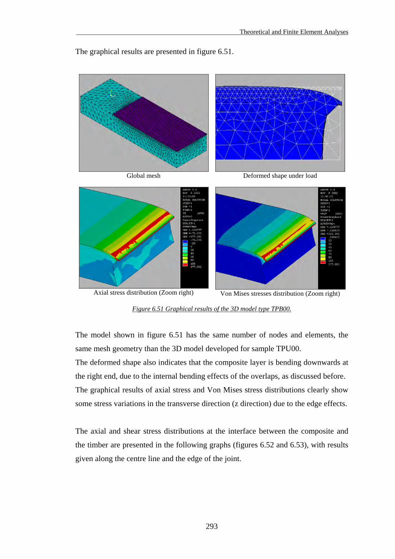
Theoretical and Finite Element Analyses
293
The graphical results are presented in figure 6.51.
Global mesh
Deformed shape under load
Axial stress distribution (Zoom right)
Von Mises stresses distribution (Zoom right)
Figure 6.51 Graphical results of the 3D model type TPB00.
The model shown in figure 6.51 has the same number of nodes and elements, the
same mesh geometry than the 3D model developed for sample TPU00.
The deformed shape also indicates that the composite layer is bending downwards at
the right end, due to the internal bending effects of the overlaps, as discussed before.
The graphical results of axial stress and Von Mises stress distributions clearly show
some stress variations in the transverse direction (z direction) due to the edge effects.
The axial and shear stress distributions at the interface between the composite and
the timber are presented in the following graphs (figures 6.52 and 6.53), with results
given along the centre line and the edge of the joint.
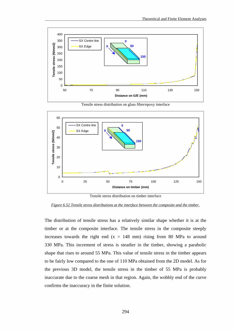
Theoretical and Finite Element Analyses
294
0
50
100
150
200
250
300
350
400
50 70 90 110 130 150
Distance on G/E (mm)
Tens
ile s
tres
s (N
/mm
2)
SX Centre line
SX Edge 50
150
0X
Tensile stress distribution on glass fibre/epoxy interface
0
10
20
30
40
50
60
0 25 50 75 100 125 150
Distance on timber (mm)
Tens
ile s
tres
s (N
/mm
2)
SX Centre line
SX Edge 50
150
0X
Tensile stress distribution on timber interface
Figure 6.52 Tensile stress distributions at the interface between the composite and the timber.
The distribution of tensile stress has a relatively similar shape whether it is at the
timber or at the composite interface. The tensile stress in the composite steeply
increases towards the right end (x = 148 mm) rising from 80 MPa to around
330 MPa. This increment of stress is steadier in the timber, showing a parabolic
shape that rises to around 55 MPa. This value of tensile stress in the timber appears
to be fairly low compared to the one of 110 MPa obtained from the 2D model. As for
the previous 3D model, the tensile stress in the timber of 55 MPa is probably
inaccurate due to the coarse mesh in that region. Again, the wobbly end of the curve
confirms the inaccuracy in the finite solution.
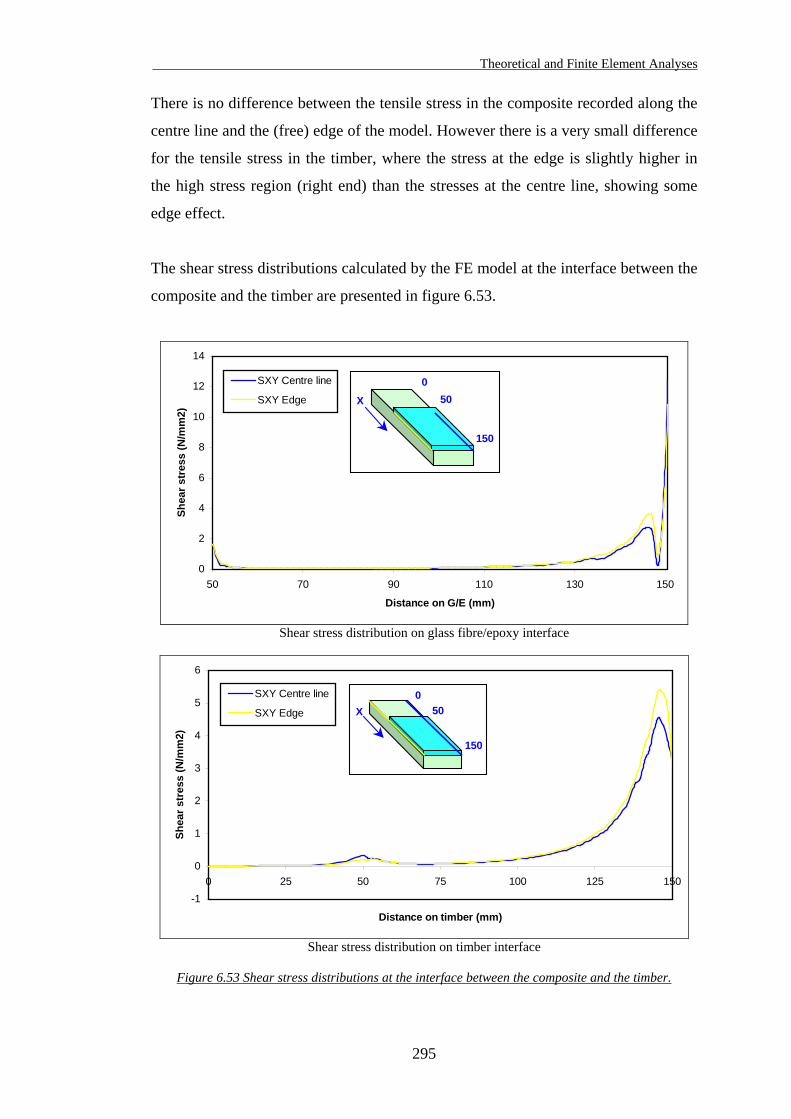
Theoretical and Finite Element Analyses
295
There is no difference between the tensile stress in the composite recorded along the
centre line and the (free) edge of the model. However there is a very small difference
for the tensile stress in the timber, where the stress at the edge is slightly higher in
the high stress region (right end) than the stresses at the centre line, showing some
edge effect.
The shear stress distributions calculated by the FE model at the interface between the
composite and the timber are presented in figure 6.53.
0
2
4
6
8
10
12
14
50 70 90 110 130 150
Distance on G/E (mm)
Shea
r str
ess
(N/m
m2)
SXY Centre line
SXY Edge 50
150
0
X
Shear stress distribution on glass fibre/epoxy interface
-1
0
1
2
3
4
5
6
0 25 50 75 100 125 150
Distance on timber (mm)
Shea
r str
ess
(N/m
m2)
SXY Centre line
SXY Edge 50
150
0X
Shear stress distribution on timber interface
Figure 6.53 Shear stress distributions at the interface between the composite and the timber.
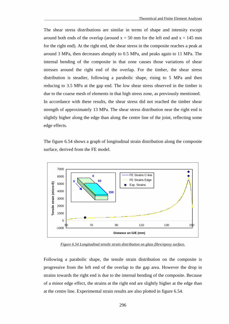
Theoretical and Finite Element Analyses
296
The shear stress distributions are similar in terms of shape and intensity except
around both ends of the overlap (around x = 50 mm for the left end and x = 145 mm
for the right end). At the right end, the shear stress in the composite reaches a peak at
around 3 MPa, then decreases abruptly to 0.5 MPa, and peaks again to 11 MPa. The
internal bending of the composite in that zone causes those variations of shear
stresses around the right end of the overlap. For the timber, the shear stress
distribution is steadier, following a parabolic shape, rising to 5 MPa and then
reducing to 3.5 MPa at the gap end. The low shear stress observed in the timber is
due to the coarse mesh of elements in that high stress zone, as previously mentioned.
In accordance with these results, the shear stress did not reached the timber shear
strength of approximately 13 MPa. The shear stress distribution near the right end is
slightly higher along the edge than along the centre line of the joint, reflecting some
edge effects.
The figure 6.54 shows a graph of longitudinal strain distribution along the composite
surface, derived from the FE model.
-1000
0
1000
2000
3000
4000
5000
6000
7000
50 70 90 110 130 150
Distance on G/E (mm)
Tens
ile s
trai
n (m
icro
-E)
FE Strains C-lineFE Strains EdgeExp. Strains
50
150
0X
Figure 6.54 Longitudinal tensile strain distribution on glass fibre/epoxy surface.
Following a parabolic shape, the tensile strain distribution on the composite is
progressive from the left end of the overlap to the gap area. However the drop in
strains towards the right end is due to the internal bending of the composite. Because
of a minor edge effect, the strains at the right end are slightly higher at the edge than
at the centre line. Experimental strain results are also plotted in figure 6.54.
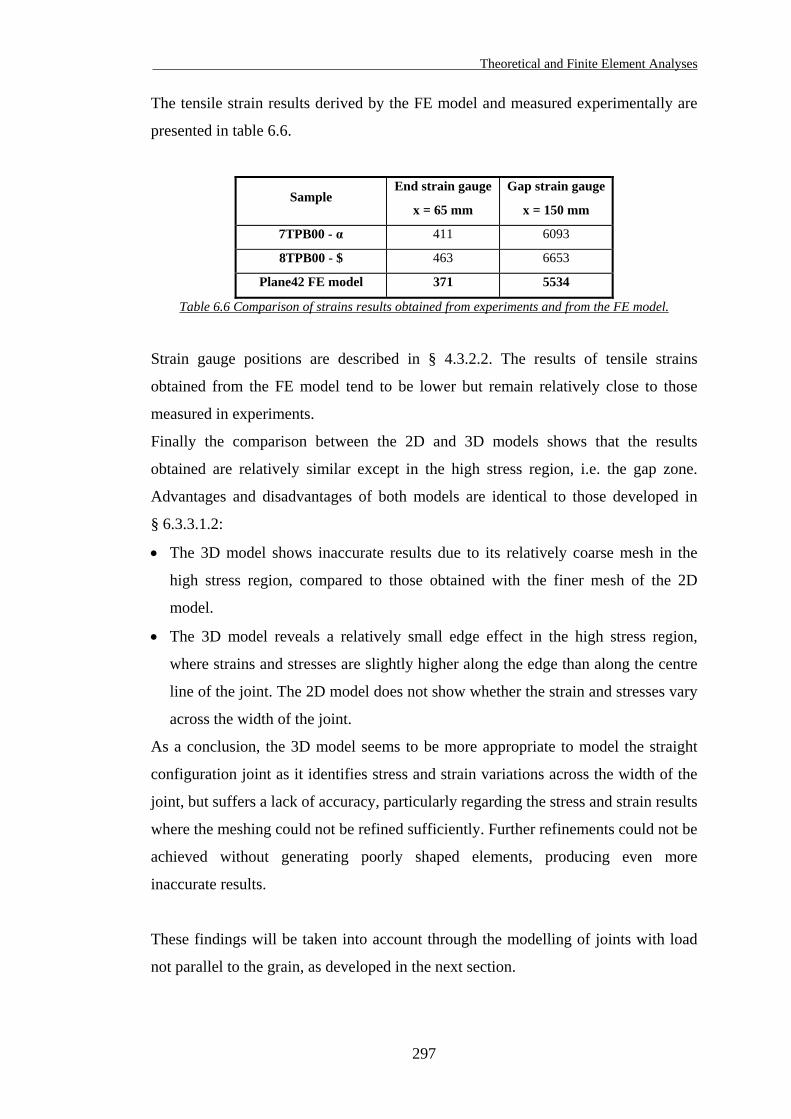
Theoretical and Finite Element Analyses
297
The tensile strain results derived by the FE model and measured experimentally are
presented in table 6.6.
End strain gauge Gap strain gauge Sample
x = 65 mm x = 150 mm
7TPB00 - α 411 6093
8TPB00 - $ 463 6653
Plane42 FE model 371 5534
Table 6.6 Comparison of strains results obtained from experiments and from the FE model.
Strain gauge positions are described in § 4.3.2.2. The results of tensile strains
obtained from the FE model tend to be lower but remain relatively close to those
measured in experiments.
Finally the comparison between the 2D and 3D models shows that the results
obtained are relatively similar except in the high stress region, i.e. the gap zone.
Advantages and disadvantages of both models are identical to those developed in
§ 6.3.3.1.2:
• The 3D model shows inaccurate results due to its relatively coarse mesh in the
high stress region, compared to those obtained with the finer mesh of the 2D
model.
• The 3D model reveals a relatively small edge effect in the high stress region,
where strains and stresses are slightly higher along the edge than along the centre
line of the joint. The 2D model does not show whether the strain and stresses vary
across the width of the joint.
As a conclusion, the 3D model seems to be more appropriate to model the straight
configuration joint as it identifies stress and strain variations across the width of the
joint, but suffers a lack of accuracy, particularly regarding the stress and strain results
where the meshing could not be refined sufficiently. Further refinements could not be
achieved without generating poorly shaped elements, producing even more
inaccurate results.
These findings will be taken into account through the modelling of joints with load
not parallel to the grain, as developed in the next section.
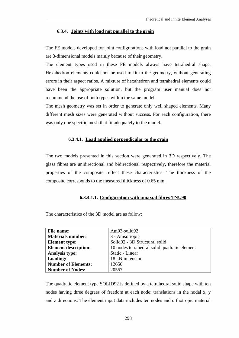
Theoretical and Finite Element Analyses
298
6.3.4. Joints with load not parallel to the grain
The FE models developed for joint configurations with load not parallel to the grain
are 3-dimensional models mainly because of their geometry.
The element types used in these FE models always have tetrahedral shape.
Hexahedron elements could not be used to fit to the geometry, without generating
errors in their aspect ratios. A mixture of hexahedron and tetrahedral elements could
have been the appropriate solution, but the program user manual does not
recommend the use of both types within the same model.
The mesh geometry was set in order to generate only well shaped elements. Many
different mesh sizes were generated without success. For each configuration, there
was only one specific mesh that fit adequately to the model.
6.3.4.1. Load applied perpendicular to the grain
The two models presented in this section were generated in 3D respectively. The
glass fibres are unidirectional and bidirectional respectively, therefore the material
properties of the composite reflect these characteristics. The thickness of the
composite corresponds to the measured thickness of 0.65 mm.
6.3.4.1.1. Configuration with uniaxial fibres TNU90
The characteristics of the 3D model are as follow:
File name: Materials number: Element type: Element description: Analysis type: Loading: Number of Elements: Number of Nodes:
Am03-solid92 3 - Anisotropic Solid92 - 3D Structural solid 10 nodes tetrahedral solid quadratic element Static - Linear 18 kN in tension 12650 20557
The quadratic element type SOLID92 is defined by a tetrahedral solid shape with ten
nodes having three degrees of freedom at each node: translations in the nodal x, y
and z directions. The element input data includes ten nodes and orthotropic material
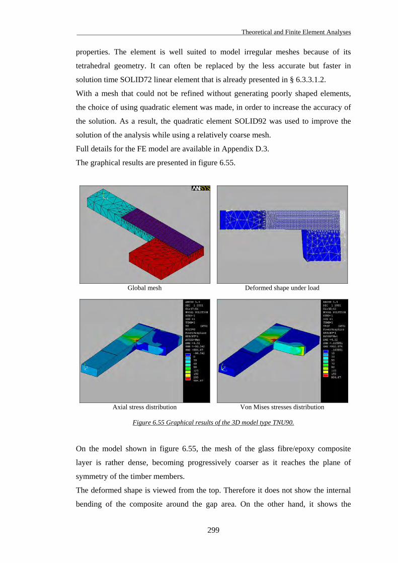
Theoretical and Finite Element Analyses
299
properties. The element is well suited to model irregular meshes because of its
tetrahedral geometry. It can often be replaced by the less accurate but faster in
solution time SOLID72 linear element that is already presented in § 6.3.3.1.2.
With a mesh that could not be refined without generating poorly shaped elements,
the choice of using quadratic element was made, in order to increase the accuracy of
the solution. As a result, the quadratic element SOLID92 was used to improve the
solution of the analysis while using a relatively coarse mesh.
Full details for the FE model are available in Appendix D.3.
The graphical results are presented in figure 6.55.
Global mesh
Deformed shape under load
Axial stress distribution
Von Mises stresses distribution
Figure 6.55 Graphical results of the 3D model type TNU90.
On the model shown in figure 6.55, the mesh of the glass fibre/epoxy composite
layer is rather dense, becoming progressively coarser as it reaches the plane of
symmetry of the timber members.
The deformed shape is viewed from the top. Therefore it does not show the internal
bending of the composite around the gap area. On the other hand, it shows the
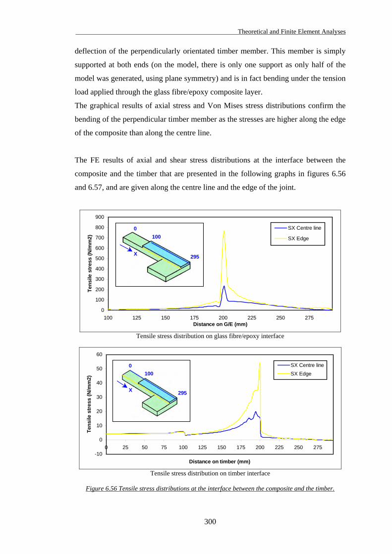
Theoretical and Finite Element Analyses
300
deflection of the perpendicularly orientated timber member. This member is simply
supported at both ends (on the model, there is only one support as only half of the
model was generated, using plane symmetry) and is in fact bending under the tension
load applied through the glass fibre/epoxy composite layer.
The graphical results of axial stress and Von Mises stress distributions confirm the
bending of the perpendicular timber member as the stresses are higher along the edge
of the composite than along the centre line.
The FE results of axial and shear stress distributions at the interface between the
composite and the timber that are presented in the following graphs in figures 6.56
and 6.57, and are given along the centre line and the edge of the joint.
0
100
200
300
400
500
600
700
800
900
100 125 150 175 200 225 250 275Distance on G/E (mm)
Tens
ile s
tres
s (N
/mm
2)
SX Centre line
SX Edge
0100
295X
Tensile stress distribution on glass fibre/epoxy interface
-10
0
10
20
30
40
50
60
0 25 50 75 100 125 150 175 200 225 250 275
Distance on timber (mm)
Tens
ile s
tres
s (N
/mm
2)
SX Centre lineSX Edge
0100
295X
Tensile stress distribution on timber interface
Figure 6.56 Tensile stress distributions at the interface between the composite and the timber.
Theoretical and Finite Element Analyses
301
The distribution of tensile stress is significantly different in shape and intensity
whether it is at the timber or at the composite interface.
The tensile stress in the composite abruptly increases towards the gap zone
(x = 200 mm). Along the centre line, the tensile stress rises from 50 MPa to around
240 MPa, and along the edge, it rises from 80 MPa to nearly 760 MPa.
For the tensile stress in the timber, the progression of stress is steadier and rises to
20 MPa along the centre line. Along the edge, it rises to 55 MPa. Because of a coarse
mesh of elements in the timber, it was already established that the stresses are under-
estimated. Furthermore, the bending under load of the perpendicular timber member
increases the gap in stress distribution between the edge and the centre line. In other
words, the edge effect is amplified by the bending of the perpendicular timber
member. The tensile stresses of the composite observed in the gap zone are very high
along the edge (760 MPa) and reach the tensile strength of the composite, and this
for a tension load of 18 kN. But the average failure load of the TNU90 tests is
36.2 kN and the failure mode consists of delamination of the composite. This means
that for a tension load of 18 kN, the composite tension stress of 760 MPa is probably
over-estimated. As a result, the mesh size is not sufficiently refined in that zone.
Theoretical and Finite Element Analyses
302
The shear stress distributions calculated by the FE model at the interface between the
composite and the timber are presented in figure 6.57.
-30
-20
-10
0
10
20
30
40
50
60
70
100 125 150 175 200 225 250 275
Distance on G/E (mm)
Shea
r str
ess
(N/m
m2)
Centre line
Edge
0100
295X
Shear stress distribution on glass fibre/epoxy interface
-8-7-6-5-4-3-2-101234
0 25 50 75 100 125 150 175 200 225 250 275
Distance on timber (mm)
Shea
r str
ess
(N/m
m2)
Centre line
Edge
0100
295X
Shear stress distribution on timber interface
Figure 6.57 Shear stress distributions at the interface between the composite and the timber.
The shear stress distributions are very different in terms of shape and intensity.
For the composite, the shear stress along the centre line peaks to 20 MPa in the gap
zone (x = 200 mm) and becomes negative (close to zero) in the perpendicularly
orientated timber member (between x = 200 mm and x = 294 mm). For the timber,
the shear stress along the centre line rises progressively to 3.5 MPa in the gap zone
and peaks to -2 MPa then increasing progressively to zero. The negative shear stress
indicates the change in direction of shear, due to the fact that the “pulling action” of
Theoretical and Finite Element Analyses
303
the composite on the timber is acting in the opposite direction in the perpendicularly
orientated timber member.
Looking at the shear stress distributions along the edge, the results are more
inconsistent. The shear stress is in fact distorted by the bending of the perpendicular
timber member, and those distortions are visible on the graphs: In the composite
interface, the chaotic part of the curve (right hand side) reflects insufficient mesh
refinement but still give some reasonable results. In the timber interface, the curve on
the right hand side is very chaotic due to a combination of complex stress variations
(i.e. member bending) and insufficient mesh refinement.
The shear stress distribution along the edge is always higher than along the centre
line of the joint, for the reasons explained previously.
The figure 6.58 shows a graph of longitudinal strain distribution along the composite
surface, derived from the FE model.
-2000
0
2000
4000
6000
8000
10000
12000
100 125 150 175 200 225 250 275
Distance on G/E (mm)
Tens
ile s
trai
n (m
icro
-E)
FE Strains Edge
FE Strains C-line
Exp. Strains C-line
295
1000
X
Figure 6.58 Longitudinal tensile strain distribution on glass fibre/epoxy surface.
Following a parabolic shape, the tensile strain distributions on the composite are
progressive from the left end of the overlap (x = 100 mm) and peak in the gap zone.
Then the strain reduces gradually to zero, on the right hand side of the model (to x =
294 mm). The internal bending of the composite in the gap zone still occurs but does
not appear on the graph because the bending effect of the perpendicular timber
member is prominent. As a result the FE strains along the edge are much higher in
the high stress region (gap zone) than the FE strains along the centre line. The
Theoretical and Finite Element Analyses
304
experimental strain results are also plotted in figure 6.58 and are very close to the FE
results.
The tensile strain results derived by the FE model and measured experimentally are
presented in table 6.7.
Gap strain gauge End strain gauge Sample
x = 200 mm x = 280 mm
5TNU90 - Ω 3738 325
Solid92 FE model 3845 284
Table 6.7 Comparison of strains results obtained from experiments and from the FE model.
Strain gauge positions are described in § 4.3.2.3. The results of tensile strains
obtained from the FE model are relatively close to those measured in experiments.
6.3.4.1.2. Configuration with biaxial fibres TNB90
The characteristics of the 3D model are as follow:
File name: Materials number: Element type: Element description: Analysis type: Loading: Number of Elements: Number of Nodes:
Am04-solid92 3 - Anisotropic Solid92 - 3D Structural solid 10 nodes tetrahedral solid quadratic element Static - Linear 18 kN in tension 12650 20557
The quadratic element type SOLID92 was defined in the previous section.
Full details for the FE model (geometry, material properties, boundary assumptions,
etc) are available in Appendix D.3.
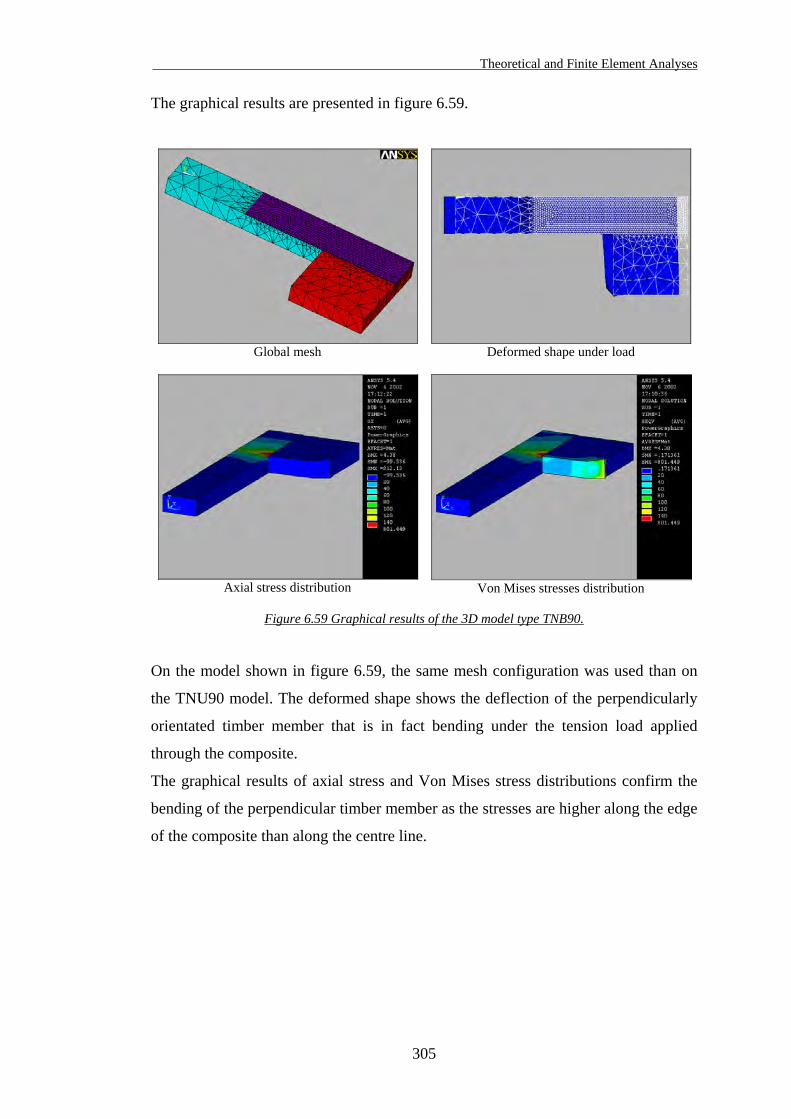
Theoretical and Finite Element Analyses
305
The graphical results are presented in figure 6.59.
Global mesh
Deformed shape under load
Axial stress distribution
Von Mises stresses distribution
Figure 6.59 Graphical results of the 3D model type TNB90.
On the model shown in figure 6.59, the same mesh configuration was used than on
the TNU90 model. The deformed shape shows the deflection of the perpendicularly
orientated timber member that is in fact bending under the tension load applied
through the composite.
The graphical results of axial stress and Von Mises stress distributions confirm the
bending of the perpendicular timber member as the stresses are higher along the edge
of the composite than along the centre line.
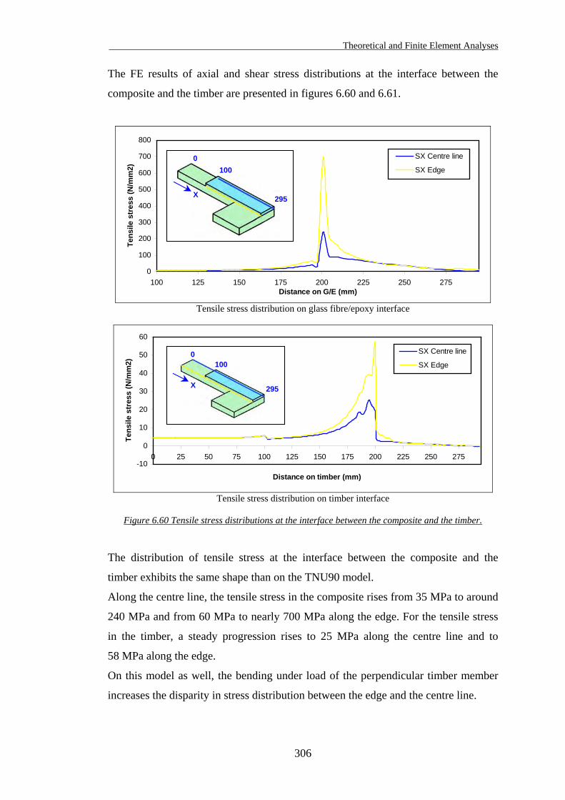
Theoretical and Finite Element Analyses
306
The FE results of axial and shear stress distributions at the interface between the
composite and the timber are presented in figures 6.60 and 6.61.
0
100
200
300
400
500
600
700
800
100 125 150 175 200 225 250 275Distance on G/E (mm)
Tens
ile s
tres
s (N
/mm
2)
SX Centre line
SX Edge0
100
295X
Tensile stress distribution on glass fibre/epoxy interface
-10
0
10
20
30
40
50
60
0 25 50 75 100 125 150 175 200 225 250 275
Distance on timber (mm)
Tens
ile s
tres
s (N
/mm
2)
SX Centre line
SX Edge0
100
295X
Tensile stress distribution on timber interface
Figure 6.60 Tensile stress distributions at the interface between the composite and the timber.
The distribution of tensile stress at the interface between the composite and the
timber exhibits the same shape than on the TNU90 model.
Along the centre line, the tensile stress in the composite rises from 35 MPa to around
240 MPa and from 60 MPa to nearly 700 MPa along the edge. For the tensile stress
in the timber, a steady progression rises to 25 MPa along the centre line and to
58 MPa along the edge.
On this model as well, the bending under load of the perpendicular timber member
increases the disparity in stress distribution between the edge and the centre line.
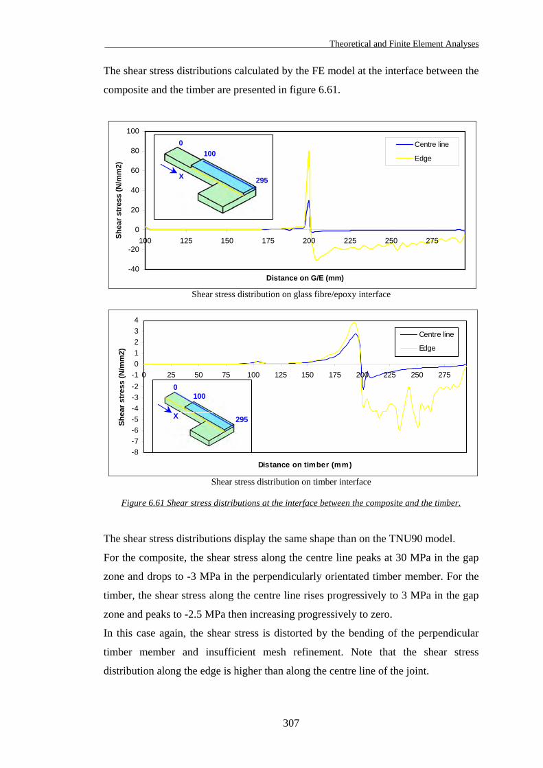
Theoretical and Finite Element Analyses
307
The shear stress distributions calculated by the FE model at the interface between the
composite and the timber are presented in figure 6.61.
-40
-20
0
20
40
60
80
100
100 125 150 175 200 225 250 275
Distance on G/E (mm)
Shea
r str
ess
(N/m
m2)
Centre line
Edge
0100
295X
Shear stress distribution on glass fibre/epoxy interface
-8-7-6-5-4-3-2-101234
0 25 50 75 100 125 150 175 200 225 250 275
Distance on timber (mm)
Shea
r str
ess
(N/m
m2)
Centre line
Edge
0100
295X
Shear stress distribution on timber interface
Figure 6.61 Shear stress distributions at the interface between the composite and the timber.
The shear stress distributions display the same shape than on the TNU90 model.
For the composite, the shear stress along the centre line peaks at 30 MPa in the gap
zone and drops to -3 MPa in the perpendicularly orientated timber member. For the
timber, the shear stress along the centre line rises progressively to 3 MPa in the gap
zone and peaks to -2.5 MPa then increasing progressively to zero.
In this case again, the shear stress is distorted by the bending of the perpendicular
timber member and insufficient mesh refinement. Note that the shear stress
distribution along the edge is higher than along the centre line of the joint.
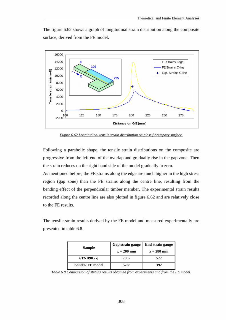
Theoretical and Finite Element Analyses
308
The figure 6.62 shows a graph of longitudinal strain distribution along the composite
surface, derived from the FE model.
-2000
0
2000
4000
6000
8000
10000
12000
14000
16000
100 125 150 175 200 225 250 275
Distance on G/E (mm)
Tens
ile s
trai
n (m
icro
-E)
FE Strains Edge
FE Strains C-line
Exp. Strains C-line
295
1000
X
Figure 6.62 Longitudinal tensile strain distribution on glass fibre/epoxy surface.
Following a parabolic shape, the tensile strain distributions on the composite are
progressive from the left end of the overlap and gradually rise in the gap zone. Then
the strain reduces on the right hand side of the model gradually to zero.
As mentioned before, the FE strains along the edge are much higher in the high stress
region (gap zone) than the FE strains along the centre line, resulting from the
bending effect of the perpendicular timber member. The experimental strain results
recorded along the centre line are also plotted in figure 6.62 and are relatively close
to the FE results.
The tensile strain results derived by the FE model and measured experimentally are
presented in table 6.8.
Gap strain gauge End strain gauge Sample
x = 200 mm x = 280 mm
6TNB90 - φ 7007 522
Solid92 FE model 5788 392
Table 6.8 Comparison of strains results obtained from experiments and from the FE model.
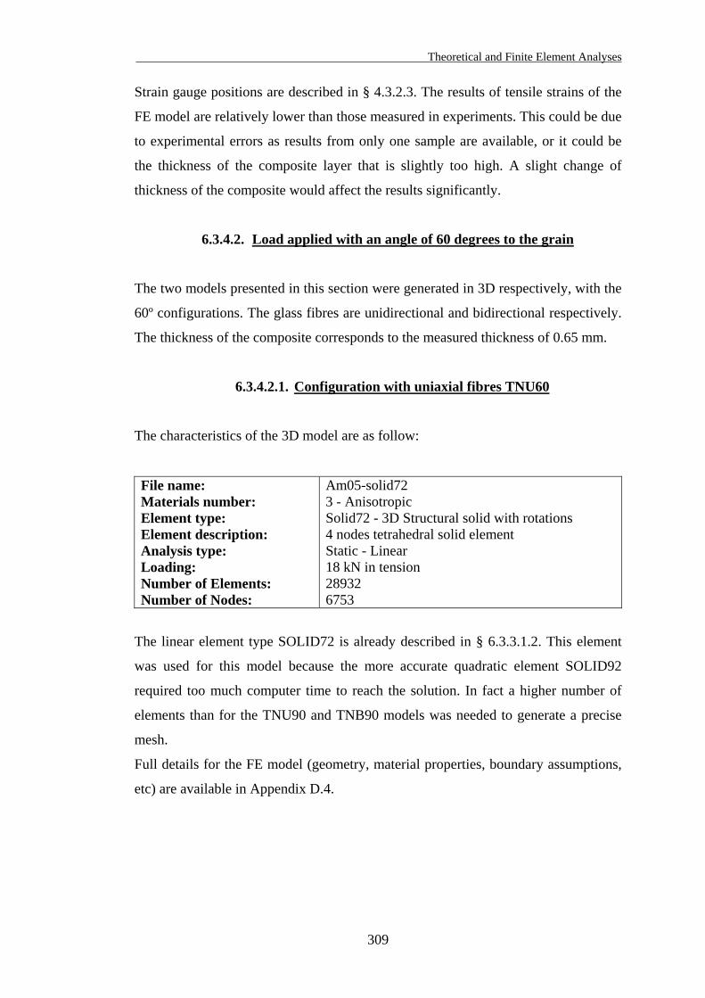
Theoretical and Finite Element Analyses
309
Strain gauge positions are described in § 4.3.2.3. The results of tensile strains of the
FE model are relatively lower than those measured in experiments. This could be due
to experimental errors as results from only one sample are available, or it could be
the thickness of the composite layer that is slightly too high. A slight change of
thickness of the composite would affect the results significantly.
6.3.4.2. Load applied with an angle of 60 degrees to the grain
The two models presented in this section were generated in 3D respectively, with the
60º configurations. The glass fibres are unidirectional and bidirectional respectively.
The thickness of the composite corresponds to the measured thickness of 0.65 mm.
6.3.4.2.1. Configuration with uniaxial fibres TNU60
The characteristics of the 3D model are as follow:
File name: Materials number: Element type: Element description: Analysis type: Loading: Number of Elements: Number of Nodes:
Am05-solid72 3 - Anisotropic Solid72 - 3D Structural solid with rotations 4 nodes tetrahedral solid element Static - Linear 18 kN in tension 28932 6753
The linear element type SOLID72 is already described in § 6.3.3.1.2. This element
was used for this model because the more accurate quadratic element SOLID92
required too much computer time to reach the solution. In fact a higher number of
elements than for the TNU90 and TNB90 models was needed to generate a precise
mesh.
Full details for the FE model (geometry, material properties, boundary assumptions,
etc) are available in Appendix D.4.
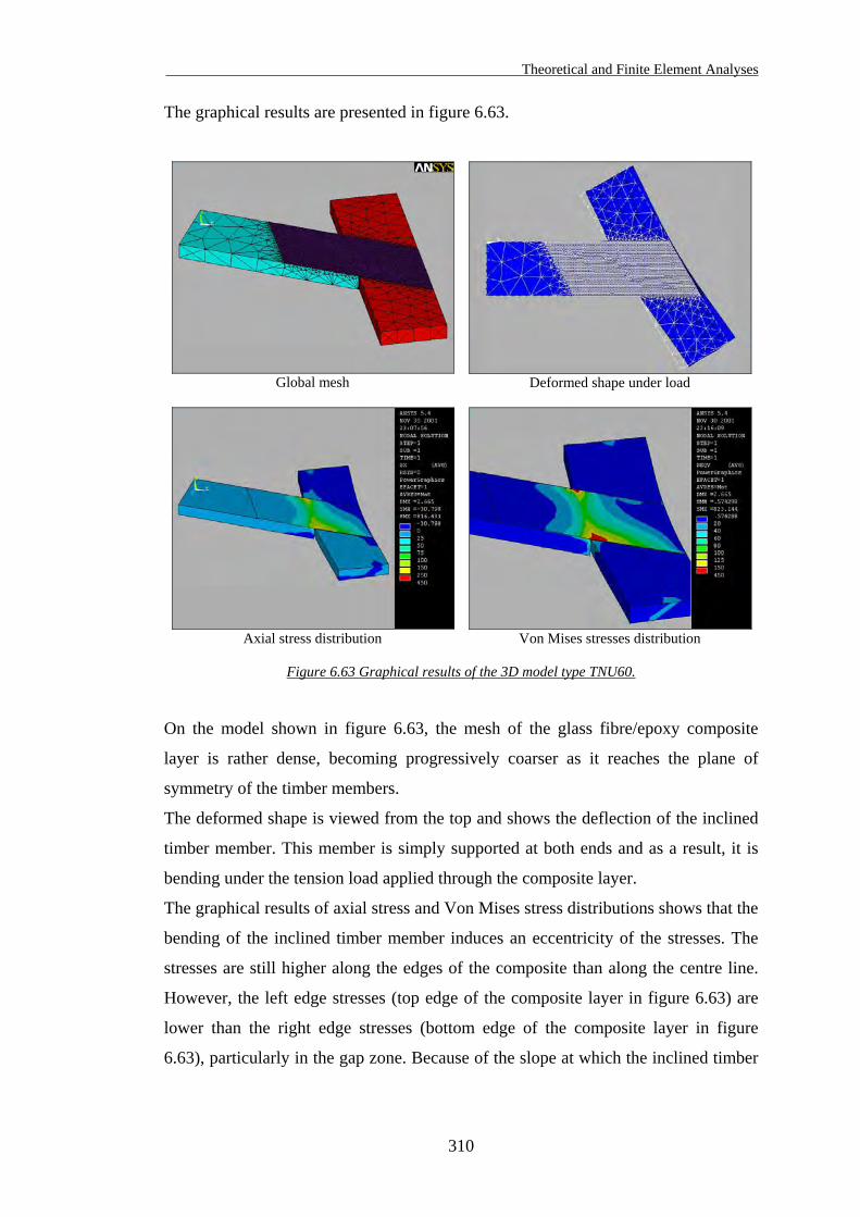
Theoretical and Finite Element Analyses
310
The graphical results are presented in figure 6.63.
Global mesh
Deformed shape under load
Axial stress distribution
Von Mises stresses distribution
Figure 6.63 Graphical results of the 3D model type TNU60.
On the model shown in figure 6.63, the mesh of the glass fibre/epoxy composite
layer is rather dense, becoming progressively coarser as it reaches the plane of
symmetry of the timber members.
The deformed shape is viewed from the top and shows the deflection of the inclined
timber member. This member is simply supported at both ends and as a result, it is
bending under the tension load applied through the composite layer.
The graphical results of axial stress and Von Mises stress distributions shows that the
bending of the inclined timber member induces an eccentricity of the stresses. The
stresses are still higher along the edges of the composite than along the centre line.
However, the left edge stresses (top edge of the composite layer in figure 6.63) are
lower than the right edge stresses (bottom edge of the composite layer in figure
6.63), particularly in the gap zone. Because of the slope at which the inclined timber
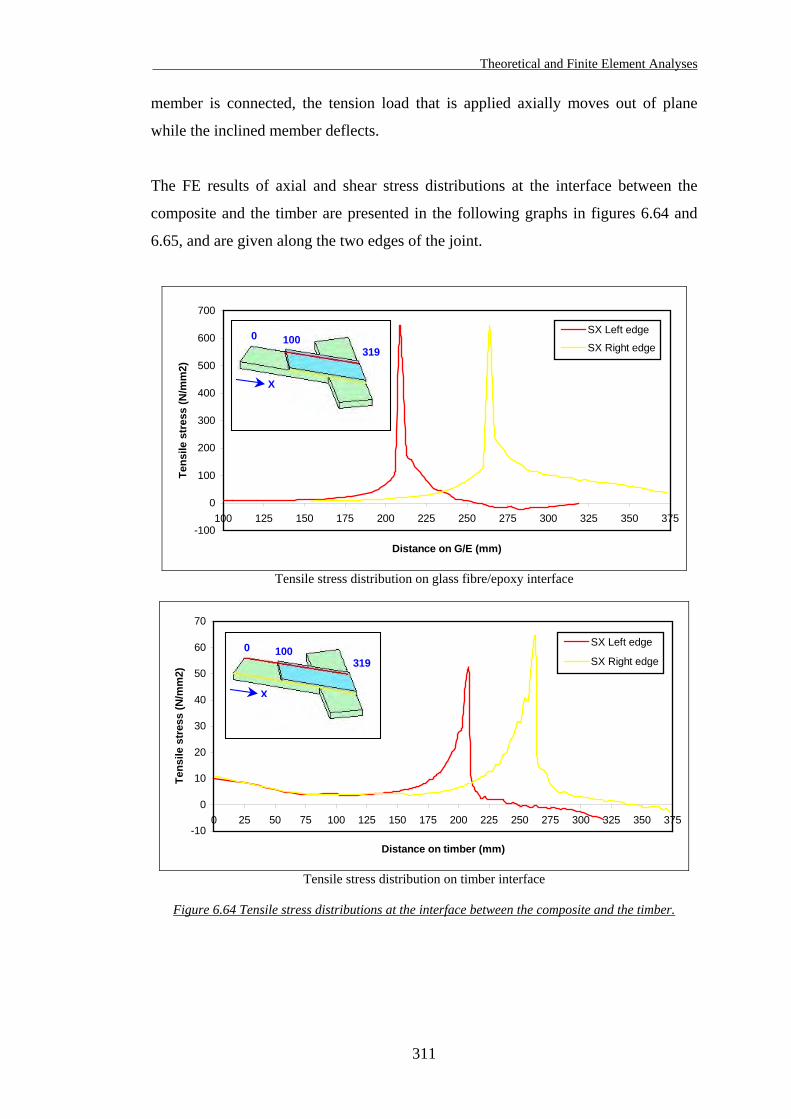
Theoretical and Finite Element Analyses
311
member is connected, the tension load that is applied axially moves out of plane
while the inclined member deflects.
The FE results of axial and shear stress distributions at the interface between the
composite and the timber are presented in the following graphs in figures 6.64 and
6.65, and are given along the two edges of the joint.
-100
0
100
200
300
400
500
600
700
100 125 150 175 200 225 250 275 300 325 350 375
Distance on G/E (mm)
Tens
ile s
tres
s (N
/mm
2)
SX Left edge
SX Right edge1000
319
X
Tensile stress distribution on glass fibre/epoxy interface
-10
0
10
20
30
40
50
60
70
0 25 50 75 100 125 150 175 200 225 250 275 300 325 350 375
Distance on timber (mm)
Tens
ile s
tres
s (N
/mm
2)
SX Left edge
SX Right edge1000
X
319
Tensile stress distribution on timber interface
Figure 6.64 Tensile stress distributions at the interface between the composite and the timber.
Theoretical and Finite Element Analyses
312
The tensile stress distribution in the composite interface has the same shape and
intensity whether it is along the left or right edges. The results could not be derived
along the centre line, as the element nodes are not positioned along that axis.
The tensile stresses along both edges rise progressively to approximately 100 MPa,
peak to 640 MPa in the gap zone and drop to roughly 200 MPa. Then the stress
reduces progressively across the inclined timber member and becomes compressive
towards the end.
The tensile stress distribution in the timber interface has also a similar shape along
the left or right edges, but reach a higher peak on the right edge than on the left edge.
The tensile stresses along both edges rise progressively following a parabolic curve
to approximately 60 MPa in the gap zone and drops abruptly. Then the stress reduces
progressively across the inclined timber member and becomes compressive towards
the end.
Tensile stress distributions appear to be accurate, except in the gap zone: Peak stress
values are probably over-estimated due to the finite element coarse mesh size in that
high stress region. However the inclined timber member is bending under the tension
load therefore peak stresses at both ends of the gap zone are expected to be relatively
high. Peak stresses along the right and left edges are certainly much higher that along
the centre line.
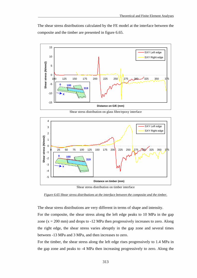
Theoretical and Finite Element Analyses
313
The shear stress distributions calculated by the FE model at the interface between the
composite and the timber are presented in figure 6.65.
-15
-10
-5
0
5
10
15
100 125 150 175 200 225 250 275 300 325 350 375
Distance on G/E (mm)
Shea
r str
ess
(N/m
m2)
SXY Left edge
SXY Right edge
1000319
X
Shear stress distribution on glass fibre/epoxy interface
-5
-4
-3
-2
-1
0
1
2
3
4
0 25 50 75 100 125 150 175 200 225 250 275 300 325 350 375
Distance on timber (mm)
Shea
r str
ess
(N/m
m2)
SXY Left edge
SXY Right edge
1000
X
319
Shear stress distribution on timber interface
Figure 6.65 Shear stress distributions at the interface between the composite and the timber.
The shear stress distributions are very different in terms of shape and intensity.
For the composite, the shear stress along the left edge peaks to 10 MPa in the gap
zone (x = 200 mm) and drops to -12 MPa then progressively increases to zero. Along
the right edge, the shear stress varies abruptly in the gap zone and several times
between -13 MPa and 3 MPa, and then increases to zero.
For the timber, the shear stress along the left edge rises progressively to 1.4 MPa in
the gap zone and peaks to -4 MPa then increasing progressively to zero. Along the
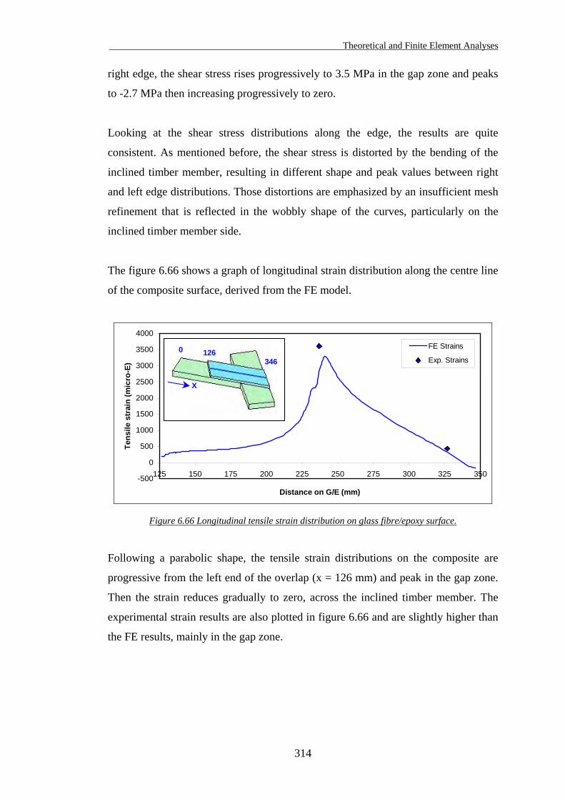
Theoretical and Finite Element Analyses
314
right edge, the shear stress rises progressively to 3.5 MPa in the gap zone and peaks
to -2.7 MPa then increasing progressively to zero.
Looking at the shear stress distributions along the edge, the results are quite
consistent. As mentioned before, the shear stress is distorted by the bending of the
inclined timber member, resulting in different shape and peak values between right
and left edge distributions. Those distortions are emphasized by an insufficient mesh
refinement that is reflected in the wobbly shape of the curves, particularly on the
inclined timber member side.
The figure 6.66 shows a graph of longitudinal strain distribution along the centre line
of the composite surface, derived from the FE model.
-500
0
500
1000
1500
2000
2500
3000
3500
4000
125 150 175 200 225 250 275 300 325 350
Distance on G/E (mm)
Tens
ile s
trai
n (m
icro
-E)
FE Strains
Exp. Strains3461260
X
Figure 6.66 Longitudinal tensile strain distribution on glass fibre/epoxy surface.
Following a parabolic shape, the tensile strain distributions on the composite are
progressive from the left end of the overlap (x = 126 mm) and peak in the gap zone.
Then the strain reduces gradually to zero, across the inclined timber member. The
experimental strain results are also plotted in figure 6.66 and are slightly higher than
the FE results, mainly in the gap zone.
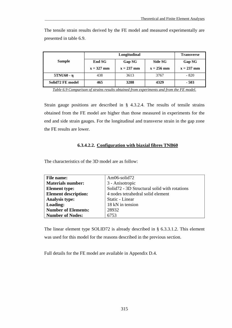
Theoretical and Finite Element Analyses
315
The tensile strain results derived by the FE model and measured experimentally are
presented in table 6.9.
Longitudinal Transverse
End SG Gap SG Side SG Gap SG Sample
x = 327 mm x = 237 mm x = 256 mm x = 237 mm
5TNU60 - η 438 3613 3767 - 820
Solid72 FE model 465 3288 4329 - 503 Table 6.9 Comparison of strains results obtained from experiments and from the FE model.
Strain gauge positions are described in § 4.3.2.4. The results of tensile strains
obtained from the FE model are higher than those measured in experiments for the
end and side strain gauges. For the longitudinal and transverse strain in the gap zone
the FE results are lower.
6.3.4.2.2. Configuration with biaxial fibres TNB60
The characteristics of the 3D model are as follow:
File name: Materials number: Element type: Element description: Analysis type: Loading: Number of Elements: Number of Nodes:
Am06-solid72 3 - Anisotropic Solid72 - 3D Structural solid with rotations 4 nodes tetrahedral solid element Static - Linear 18 kN in tension 28932 6753
The linear element type SOLID72 is already described in § 6.3.3.1.2. This element
was used for this model for the reasons described in the previous section.
Full details for the FE model are available in Appendix D.4.
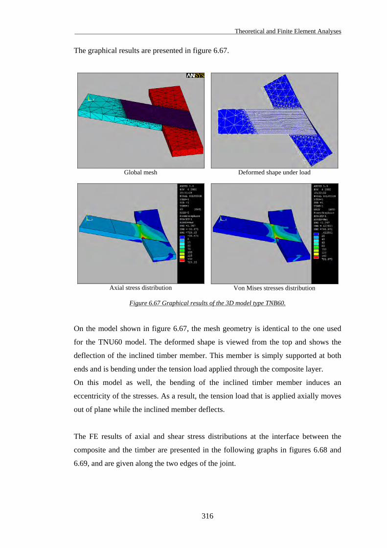
Theoretical and Finite Element Analyses
316
The graphical results are presented in figure 6.67.
Global mesh
Deformed shape under load
Axial stress distribution
Von Mises stresses distribution
Figure 6.67 Graphical results of the 3D model type TNB60.
On the model shown in figure 6.67, the mesh geometry is identical to the one used
for the TNU60 model. The deformed shape is viewed from the top and shows the
deflection of the inclined timber member. This member is simply supported at both
ends and is bending under the tension load applied through the composite layer.
On this model as well, the bending of the inclined timber member induces an
eccentricity of the stresses. As a result, the tension load that is applied axially moves
out of plane while the inclined member deflects.
The FE results of axial and shear stress distributions at the interface between the
composite and the timber are presented in the following graphs in figures 6.68 and
6.69, and are given along the two edges of the joint.
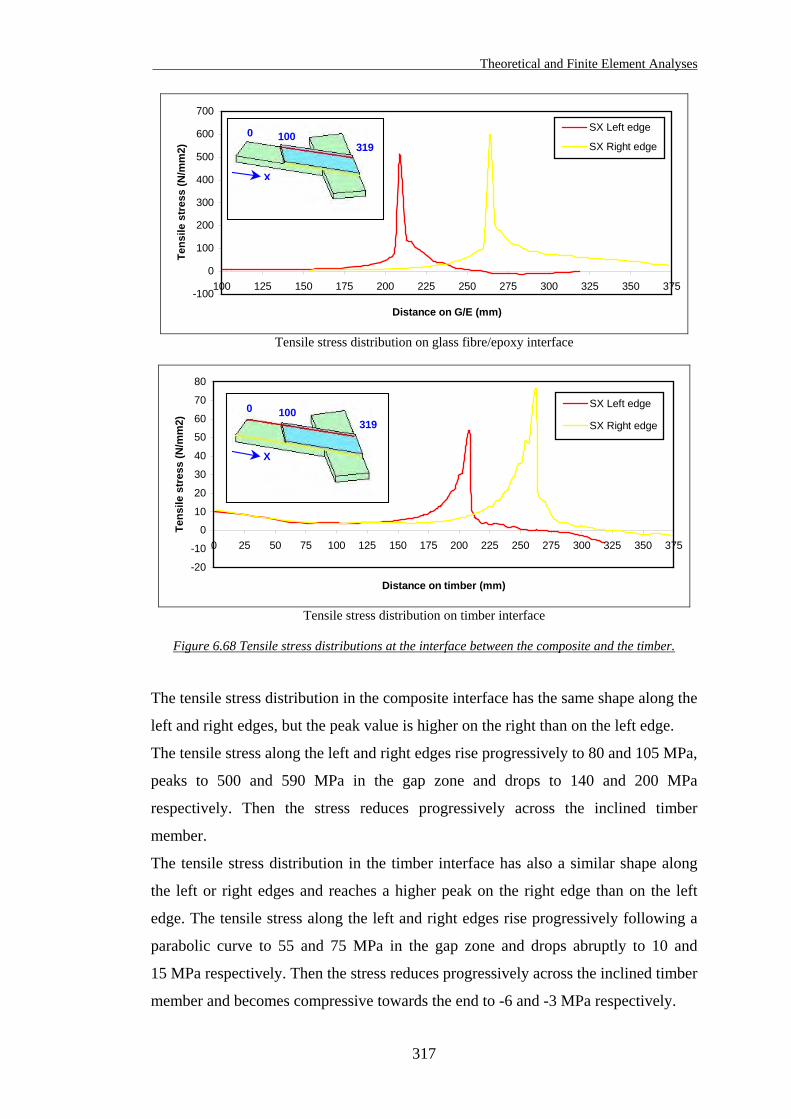
Theoretical and Finite Element Analyses
317
-100
0
100
200
300
400
500
600
700
100 125 150 175 200 225 250 275 300 325 350 375
Distance on G/E (mm)
Tens
ile s
tres
s (N
/mm
2)
SX Left edge
SX Right edge1000
319
X
Tensile stress distribution on glass fibre/epoxy interface
-20
-10
0
10
20
30
40
50
60
70
80
0 25 50 75 100 125 150 175 200 225 250 275 300 325 350 375
Distance on timber (mm)
Tens
ile s
tres
s (N
/mm
2)
SX Left edge
SX Right edge1000
X
319
Tensile stress distribution on timber interface
Figure 6.68 Tensile stress distributions at the interface between the composite and the timber.
The tensile stress distribution in the composite interface has the same shape along the
left and right edges, but the peak value is higher on the right than on the left edge.
The tensile stress along the left and right edges rise progressively to 80 and 105 MPa,
peaks to 500 and 590 MPa in the gap zone and drops to 140 and 200 MPa
respectively. Then the stress reduces progressively across the inclined timber
member.
The tensile stress distribution in the timber interface has also a similar shape along
the left or right edges and reaches a higher peak on the right edge than on the left
edge. The tensile stress along the left and right edges rise progressively following a
parabolic curve to 55 and 75 MPa in the gap zone and drops abruptly to 10 and
15 MPa respectively. Then the stress reduces progressively across the inclined timber
member and becomes compressive towards the end to -6 and -3 MPa respectively.
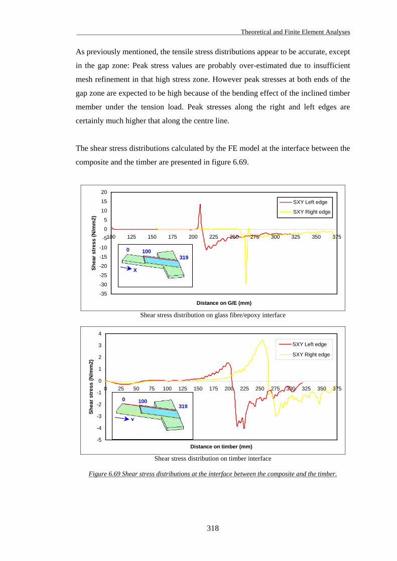
Theoretical and Finite Element Analyses
318
As previously mentioned, the tensile stress distributions appear to be accurate, except
in the gap zone: Peak stress values are probably over-estimated due to insufficient
mesh refinement in that high stress zone. However peak stresses at both ends of the
gap zone are expected to be high because of the bending effect of the inclined timber
member under the tension load. Peak stresses along the right and left edges are
certainly much higher that along the centre line.
The shear stress distributions calculated by the FE model at the interface between the
composite and the timber are presented in figure 6.69.
-35
-30
-25
-20
-15
-10
-5
0
5
10
15
20
100 125 150 175 200 225 250 275 300 325 350 375
Distance on G/E (mm)
Shea
r str
ess
(N/m
m2)
SXY Left edge
SXY Right edge
1000319
X
Shear stress distribution on glass fibre/epoxy interface
-5
-4
-3
-2
-1
0
1
2
3
4
0 25 50 75 100 125 150 175 200 225 250 275 300 325 350 375
Distance on timber (mm)
Shea
r str
ess
(N/m
m2)
SXY Left edge
SXY Right edge
1000
X
319
Shear stress distribution on timber interface
Figure 6.69 Shear stress distributions at the interface between the composite and the timber.
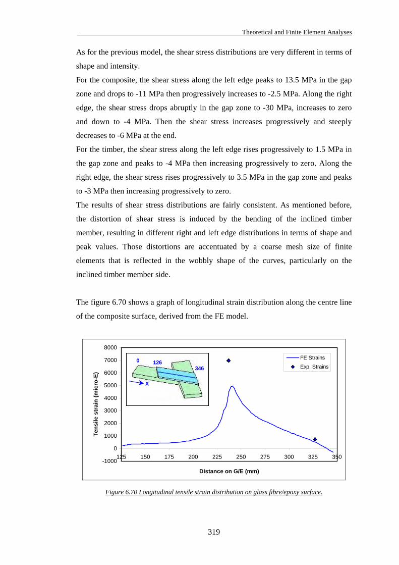
Theoretical and Finite Element Analyses
319
As for the previous model, the shear stress distributions are very different in terms of
shape and intensity.
For the composite, the shear stress along the left edge peaks to 13.5 MPa in the gap
zone and drops to -11 MPa then progressively increases to -2.5 MPa. Along the right
edge, the shear stress drops abruptly in the gap zone to -30 MPa, increases to zero
and down to -4 MPa. Then the shear stress increases progressively and steeply
decreases to -6 MPa at the end.
For the timber, the shear stress along the left edge rises progressively to 1.5 MPa in
the gap zone and peaks to -4 MPa then increasing progressively to zero. Along the
right edge, the shear stress rises progressively to 3.5 MPa in the gap zone and peaks
to -3 MPa then increasing progressively to zero.
The results of shear stress distributions are fairly consistent. As mentioned before,
the distortion of shear stress is induced by the bending of the inclined timber
member, resulting in different right and left edge distributions in terms of shape and
peak values. Those distortions are accentuated by a coarse mesh size of finite
elements that is reflected in the wobbly shape of the curves, particularly on the
inclined timber member side.
The figure 6.70 shows a graph of longitudinal strain distribution along the centre line
of the composite surface, derived from the FE model.
-1000
0
1000
2000
3000
4000
5000
6000
7000
8000
125 150 175 200 225 250 275 300 325 350
Distance on G/E (mm)
Tens
ile s
trai
n (m
icro
-E)
FE Strains
Exp. Strains3461260
X
Figure 6.70 Longitudinal tensile strain distribution on glass fibre/epoxy surface.
Theoretical and Finite Element Analyses
320
Following a parabolic shape, the tensile strain distributions on the composite are
progressive from the left end of the overlap (x = 126 mm) and peak in the gap zone.
Then the strain reduces gradually to zero, across the inclined timber member. The
experimental strain results are also plotted in figure 6.70 and are much higher than
the FE results in the gap zone.
The tensile strain results derived by the FE model and measured experimentally are
presented in table 6.10.
Longitudinal Transverse
End SG Gap SG Side SG Gap SG Sample
x = 327 mm x = 237 mm x = 256 mm x = 237 mm
5TNB60 - W 731 6981 6364 - 466
Solid72 FE model 679 4966 6095 - 368 Table 6.10 Comparison of strains results obtained from experiments and from the FE model.
Strain gauge positions are described in § 4.3.2.4. The results of tensile strains
obtained from the FE model are lower than those measured in experiments. This
could be due to experimental errors or it could be the thickness of the composite
layer that is slightly too thin. A slight change of thickness of the composite would
affect the results significantly.
Theoretical and Finite Element Analyses
321
6.3.4.3. Load applied with an angle of 30 degrees to the grain
The two models presented in this section were generated in 3D respectively, with the
30º configurations. The glass fibres are unidirectional and bidirectional respectively.
The thickness of the composite corresponds to the measured thickness of 0.65 mm.
6.3.4.3.1. Configuration with uniaxial fibres TNU30
The characteristics of the 3D model are as follow:
File name: Materials number: Element type: Element description: Analysis type: Loading: Number of Elements: Number of Nodes:
Am07-solid72 3 - Anisotropic Solid72 - 3D Structural solid with rotations 4 nodes tetrahedral solid element Static - Linear 18 kN in tension 67687 15253
The linear element type SOLID72 is already described in § 6.3.3.1.2. This element
was used for this model because of the large number of elements that was required to
generate an adequate mesh. The more accurate quadratic element SOLID92 required
too much computer time to reach the solution.
Full details for the FE model (geometry, material properties, boundary assumptions,
etc) are available in Appendix D.5.
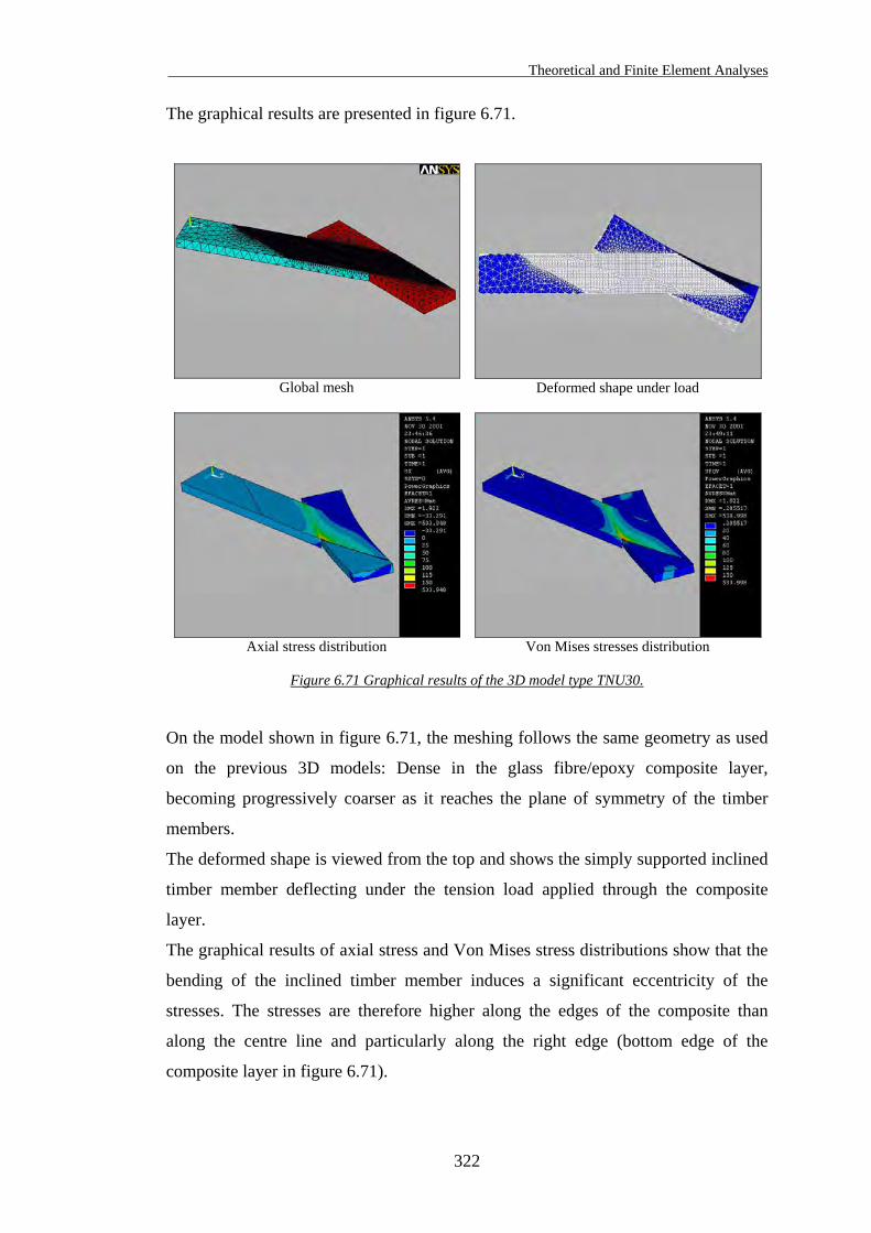
Theoretical and Finite Element Analyses
322
The graphical results are presented in figure 6.71.
Global mesh
Deformed shape under load
Axial stress distribution
Von Mises stresses distribution
Figure 6.71 Graphical results of the 3D model type TNU30.
On the model shown in figure 6.71, the meshing follows the same geometry as used
on the previous 3D models: Dense in the glass fibre/epoxy composite layer,
becoming progressively coarser as it reaches the plane of symmetry of the timber
members.
The deformed shape is viewed from the top and shows the simply supported inclined
timber member deflecting under the tension load applied through the composite
layer.
The graphical results of axial stress and Von Mises stress distributions show that the
bending of the inclined timber member induces a significant eccentricity of the
stresses. The stresses are therefore higher along the edges of the composite than
along the centre line and particularly along the right edge (bottom edge of the
composite layer in figure 6.71).
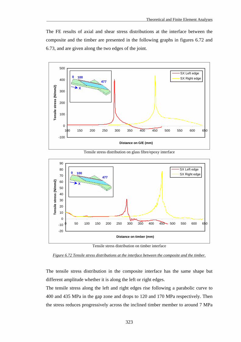
Theoretical and Finite Element Analyses
323
The FE results of axial and shear stress distributions at the interface between the
composite and the timber are presented in the following graphs in figures 6.72 and
6.73, and are given along the two edges of the joint.
-100
0
100
200
300
400
500
100 150 200 250 300 350 400 450 500 550 600 650
Distance on G/E (mm)
Tens
ile s
tres
s (N
/mm
2)
SX Left edgeSX Right edge1000
477
X
Tensile stress distribution on glass fibre/epoxy interface
-20
-10
0
10
20
30
40
50
60
70
80
90
0 50 100 150 200 250 300 350 400 450 500 550 600 650
Distance on timber (mm)
Tens
ile s
tres
s (N
/mm
2)
SX Left edgeSX Right edge100
X
4770
Tensile stress distribution on timber interface
Figure 6.72 Tensile stress distributions at the interface between the composite and the timber.
The tensile stress distribution in the composite interface has the same shape but
different amplitude whether it is along the left or right edges.
The tensile stress along the left and right edges rise following a parabolic curve to
400 and 435 MPa in the gap zone and drops to 120 and 170 MPa respectively. Then
the stress reduces progressively across the inclined timber member to around 7 MPa
Theoretical and Finite Element Analyses
324
along the right edge, and becomes compressive to -25 MPa then reduces towards the
end to -7 MPa along the left edge.
The tensile stress distribution in the timber interface has also a similar shape along
the left or right edges, but reach a higher peak on the right edge than on the left edge.
The tensile stress along the left edge rises progressively following a parabolic curve
from 4 MPa to 32 MPa in the gap zone and drops steeply to -3 MPa. Then the stress
fluctuates in compressive zone across the inclined timber member and reaches -8
MPa at the end. The tensile stress along the right edge follows the same shape, rising
progressively from 4 MPa to 76 MPa in the gap zone and decreases progressively to
zero.
As notified on previous models, tensile stress distributions seem to be relatively
accurate in terms of shape but the peak values that occur in the gap zone are certainly
over-estimated. Whether this is due to insufficient mesh refinement, peak stresses at
both ends of the gap zone are expected to be much higher than along the centre line.
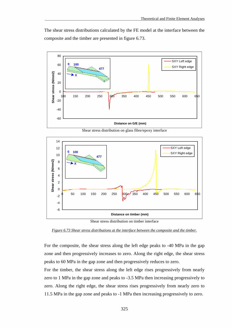
Theoretical and Finite Element Analyses
325
The shear stress distributions calculated by the FE model at the interface between the
composite and the timber are presented in figure 6.73.
-60
-40
-20
0
20
40
60
80
100 150 200 250 300 350 400 450 500 550 600 650
Distance on G/E (mm)
Shea
r str
ess
(N/m
m2)
SXY Left edge
SXY Right edge1000
477
X
Shear stress distribution on glass fibre/epoxy interface
-6
-4
-2
0
2
4
6
8
10
12
14
0 50 100 150 200 250 300 350 400 450 500 550 600 650
Distance on timber (mm)
Shea
r str
ess
(N/m
m2)
SXY Left edge
SXY Right edge100
X
4770
Shear stress distribution on timber interface
Figure 6.73 Shear stress distributions at the interface between the composite and the timber.
For the composite, the shear stress along the left edge peaks to -40 MPa in the gap
zone and then progressively increases to zero. Along the right edge, the shear stress
peaks to 60 MPa in the gap zone and then progressively reduces to zero.
For the timber, the shear stress along the left edge rises progressively from nearly
zero to 1 MPa in the gap zone and peaks to -3.5 MPa then increasing progressively to
zero. Along the right edge, the shear stress rises progressively from nearly zero to
11.5 MPa in the gap zone and peaks to -1 MPa then increasing progressively to zero.
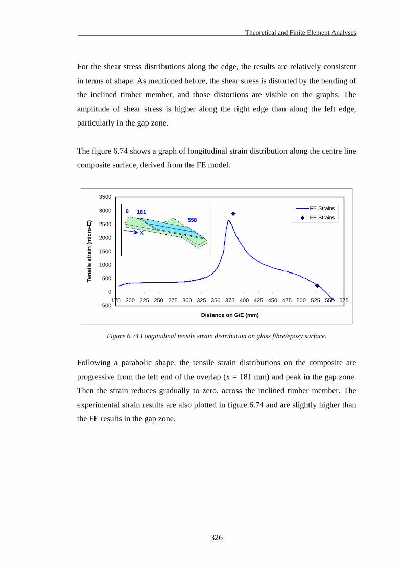
Theoretical and Finite Element Analyses
326
For the shear stress distributions along the edge, the results are relatively consistent
in terms of shape. As mentioned before, the shear stress is distorted by the bending of
the inclined timber member, and those distortions are visible on the graphs: The
amplitude of shear stress is higher along the right edge than along the left edge,
particularly in the gap zone.
The figure 6.74 shows a graph of longitudinal strain distribution along the centre line
composite surface, derived from the FE model.
-500
0
500
1000
1500
2000
2500
3000
3500
175 200 225 250 275 300 325 350 375 400 425 450 475 500 525 550 575
Distance on G/E (mm)
Tens
ile s
trai
n (m
icro
-E)
FE Strains
FE Strains181
X
5580
Figure 6.74 Longitudinal tensile strain distribution on glass fibre/epoxy surface.
Following a parabolic shape, the tensile strain distributions on the composite are
progressive from the left end of the overlap (x = 181 mm) and peak in the gap zone.
Then the strain reduces gradually to zero, across the inclined timber member. The
experimental strain results are also plotted in figure 6.74 and are slightly higher than
the FE results in the gap zone.
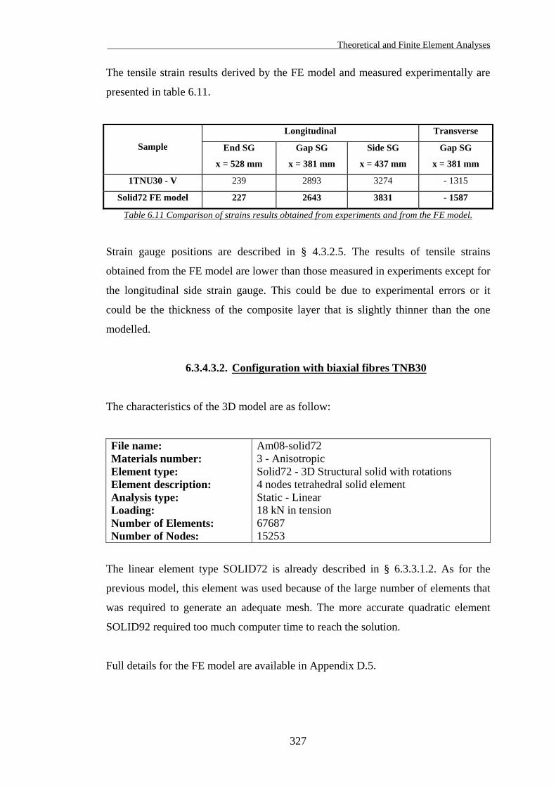
Theoretical and Finite Element Analyses
327
The tensile strain results derived by the FE model and measured experimentally are
presented in table 6.11.
Longitudinal Transverse
End SG Gap SG Side SG Gap SG Sample
x = 528 mm x = 381 mm x = 437 mm x = 381 mm
1TNU30 - V 239 2893 3274 - 1315
Solid72 FE model 227 2643 3831 - 1587
Table 6.11 Comparison of strains results obtained from experiments and from the FE model.
Strain gauge positions are described in § 4.3.2.5. The results of tensile strains
obtained from the FE model are lower than those measured in experiments except for
the longitudinal side strain gauge. This could be due to experimental errors or it
could be the thickness of the composite layer that is slightly thinner than the one
modelled.
6.3.4.3.2. Configuration with biaxial fibres TNB30
The characteristics of the 3D model are as follow:
File name: Materials number: Element type: Element description: Analysis type: Loading: Number of Elements: Number of Nodes:
Am08-solid72 3 - Anisotropic Solid72 - 3D Structural solid with rotations 4 nodes tetrahedral solid element Static - Linear 18 kN in tension 67687 15253
The linear element type SOLID72 is already described in § 6.3.3.1.2. As for the
previous model, this element was used because of the large number of elements that
was required to generate an adequate mesh. The more accurate quadratic element
SOLID92 required too much computer time to reach the solution.
Full details for the FE model are available in Appendix D.5.
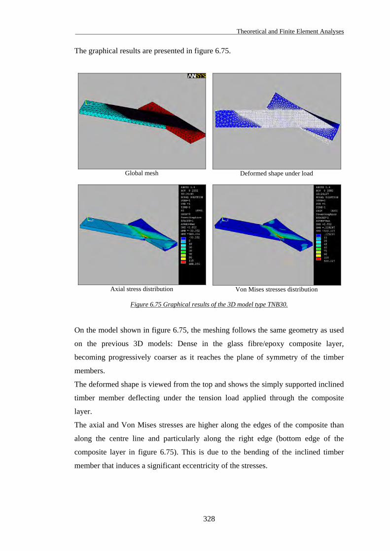
Theoretical and Finite Element Analyses
328
The graphical results are presented in figure 6.75.
Global mesh
Deformed shape under load
Axial stress distribution
Von Mises stresses distribution
Figure 6.75 Graphical results of the 3D model type TNB30.
On the model shown in figure 6.75, the meshing follows the same geometry as used
on the previous 3D models: Dense in the glass fibre/epoxy composite layer,
becoming progressively coarser as it reaches the plane of symmetry of the timber
members.
The deformed shape is viewed from the top and shows the simply supported inclined
timber member deflecting under the tension load applied through the composite
layer.
The axial and Von Mises stresses are higher along the edges of the composite than
along the centre line and particularly along the right edge (bottom edge of the
composite layer in figure 6.75). This is due to the bending of the inclined timber
member that induces a significant eccentricity of the stresses.
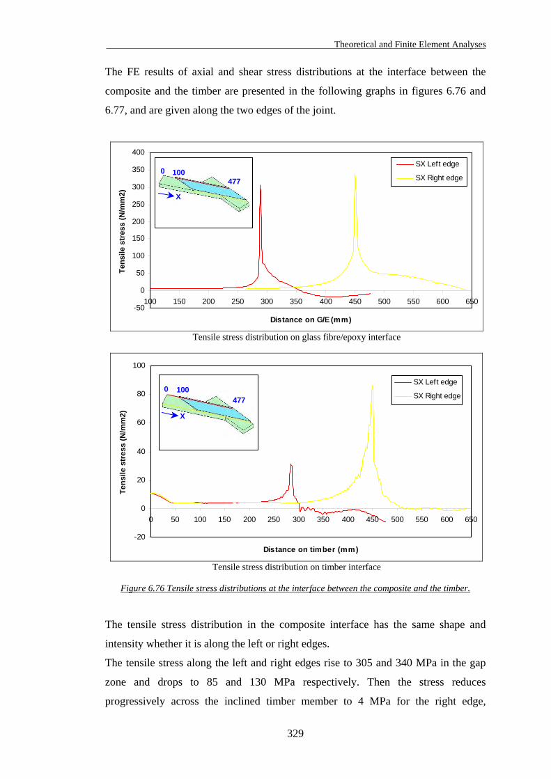
Theoretical and Finite Element Analyses
329
The FE results of axial and shear stress distributions at the interface between the
composite and the timber are presented in the following graphs in figures 6.76 and
6.77, and are given along the two edges of the joint.
-50
0
50
100
150
200
250
300
350
400
100 150 200 250 300 350 400 450 500 550 600 650
Distance on G/E (mm)
Tens
ile s
tres
s (N
/mm
2)
SX Left edge
SX Right edge1000
477
X
Tensile stress distribution on glass fibre/epoxy interface
-20
0
20
40
60
80
100
0 50 100 150 200 250 300 350 400 450 500 550 600 650
Distance on timber (mm)
Tens
ile s
tres
s (N
/mm
2)
SX Left edge
SX Right edge100
X
4770
Tensile stress distribution on timber interface
Figure 6.76 Tensile stress distributions at the interface between the composite and the timber.
The tensile stress distribution in the composite interface has the same shape and
intensity whether it is along the left or right edges.
The tensile stress along the left and right edges rise to 305 and 340 MPa in the gap
zone and drops to 85 and 130 MPa respectively. Then the stress reduces
progressively across the inclined timber member to 4 MPa for the right edge,
Theoretical and Finite Element Analyses
330
becomes compressive to -18 MPa then reduces towards the end to -7 MPa for the left
edge.
The tensile stress distribution in the timber interface has also a similar shape along
the both edges, but reach a much higher peak on the right edge than on the left edge.
The tensile stress along the left edge rises progressively following a parabolic curve
to 31 MPa in the gap zone and drops steeply to -2 MPa. Then the stress fluctuates in
compression across the inclined timber member and reaches -9 MPa at the end.
The tensile stress along the right edge follow the same shape, rising progressively to
86 MPa in the gap zone and reduces gradually to zero.
As mentioned before, tensile stress distributions seem to be relatively accurate in
terms of shape but the peak values that occur in the gap zone are certainly over-
estimated. This is probably due to insufficient mesh refinement. However the peak
stresses at both ends of the gap zone are expected to be relatively high and certainly
much higher than at the centre line. This is due to the bending effect of the inclined
timber member.
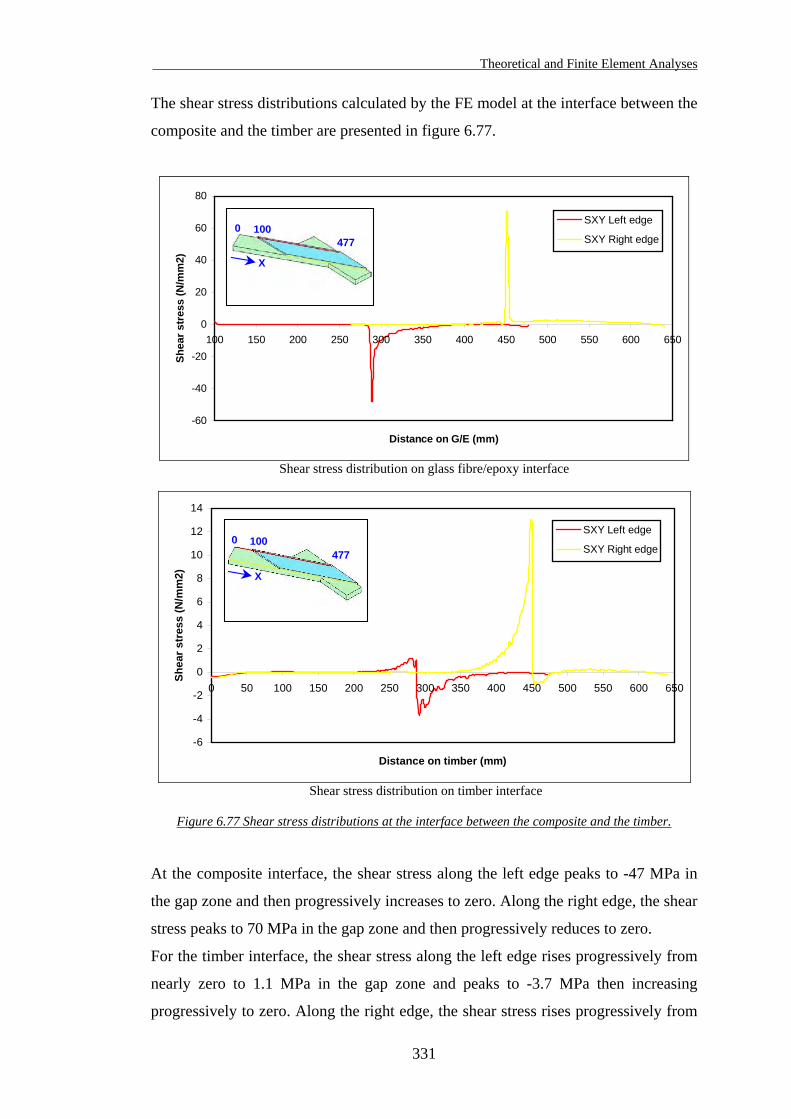
Theoretical and Finite Element Analyses
331
The shear stress distributions calculated by the FE model at the interface between the
composite and the timber are presented in figure 6.77.
-60
-40
-20
0
20
40
60
80
100 150 200 250 300 350 400 450 500 550 600 650
Distance on G/E (mm)
Shea
r str
ess
(N/m
m2)
SXY Left edge
SXY Right edge1000
477
X
Shear stress distribution on glass fibre/epoxy interface
-6
-4
-2
0
2
4
6
8
10
12
14
0 50 100 150 200 250 300 350 400 450 500 550 600 650
Distance on timber (mm)
Shea
r str
ess
(N/m
m2)
SXY Left edge
SXY Right edge100
X
4770
Shear stress distribution on timber interface
Figure 6.77 Shear stress distributions at the interface between the composite and the timber.
At the composite interface, the shear stress along the left edge peaks to -47 MPa in
the gap zone and then progressively increases to zero. Along the right edge, the shear
stress peaks to 70 MPa in the gap zone and then progressively reduces to zero.
For the timber interface, the shear stress along the left edge rises progressively from
nearly zero to 1.1 MPa in the gap zone and peaks to -3.7 MPa then increasing
progressively to zero. Along the right edge, the shear stress rises progressively from
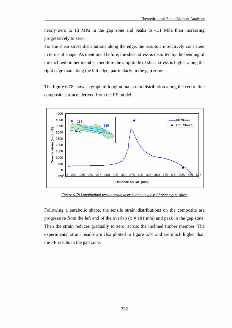
Theoretical and Finite Element Analyses
332
nearly zero to 13 MPa in the gap zone and peaks to -1.1 MPa then increasing
progressively to zero.
For the shear stress distributions along the edge, the results are relatively consistent
in terms of shape. As mentioned before, the shear stress is distorted by the bending of
the inclined timber member therefore the amplitude of shear stress is higher along the
right edge than along the left edge, particularly in the gap zone.
The figure 6.78 shows a graph of longitudinal strain distribution along the centre line
composite surface, derived from the FE model.
-500
0
500
1000
1500
2000
2500
3000
3500
4000
4500
175 200 225 250 275 300 325 350 375 400 425 450 475 500 525 550 575
Distance on G/E (mm)
Tens
ile s
trai
n (m
icro
-E)
FE StrainsExp. Strains
181
X
5580
Figure 6.78 Longitudinal tensile strain distribution on glass fibre/epoxy surface.
Following a parabolic shape, the tensile strain distributions on the composite are
progressive from the left end of the overlap (x = 181 mm) and peak in the gap zone.
Then the strain reduces gradually to zero, across the inclined timber member. The
experimental strain results are also plotted in figure 6.78 and are much higher than
the FE results in the gap zone.
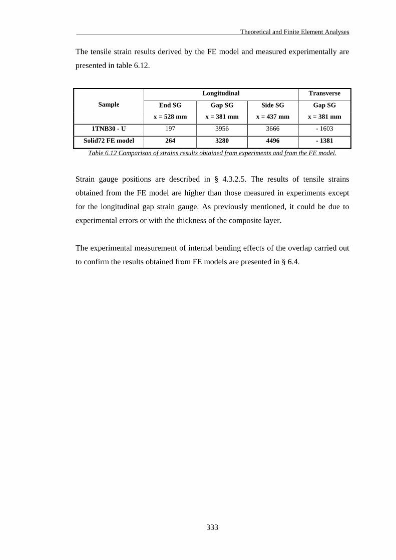
Theoretical and Finite Element Analyses
333
The tensile strain results derived by the FE model and measured experimentally are
presented in table 6.12.
Longitudinal Transverse
End SG Gap SG Side SG Gap SG Sample
x = 528 mm x = 381 mm x = 437 mm x = 381 mm
1TNB30 - U 197 3956 3666 - 1603
Solid72 FE model 264 3280 4496 - 1381
Table 6.12 Comparison of strains results obtained from experiments and from the FE model.
Strain gauge positions are described in § 4.3.2.5. The results of tensile strains
obtained from the FE model are higher than those measured in experiments except
for the longitudinal gap strain gauge. As previously mentioned, it could be due to
experimental errors or with the thickness of the composite layer.
The experimental measurement of internal bending effects of the overlap carried out
to confirm the results obtained from FE models are presented in § 6.4.

Theoretical and Finite Element Analyses
334
6.4. Internal bending effects
All the FE models presented throughout this chapter displayed to some extent
internal bending of the composite overlap in the gap region. Less significant bending
effects were also observed at the free ends of each composite overlap.
The stress and strain distributions in the load transfer of most FE models were so
affected by the internal bending effects of the outer adherends that experimental
verification was necessary. It was then decided to load one of the spare
wood/glass/epoxy joints in order to measure the internal bending effects of the outer
adherends in the gap zone. One sample type TPU00 was used for this experiment and
was positioned in the J.J. Lloyds machine ready for the test. Using a micrometer, the
thickness of the sample was measured across the joint in the gap zone at various
tension loads, in order to establish the lateral deformation defined as ∆ω on
figure 6.79.
Figure 6.79 Deformed shape with lateral deformation ∆ω of the 2D FE model type TPU00.
Figure 6.79 indicates the location of the lateral deformation ∆ω on the deformed
shape of the 2D FE model type TPU00. This FE model was presented in § 6.3.3.1.1.
The lateral deformation ∆ω was measured at four different positions along the gap
zone of the joint. The values of ∆ω presented in table 6.13 are average values from
those positions for each given load.
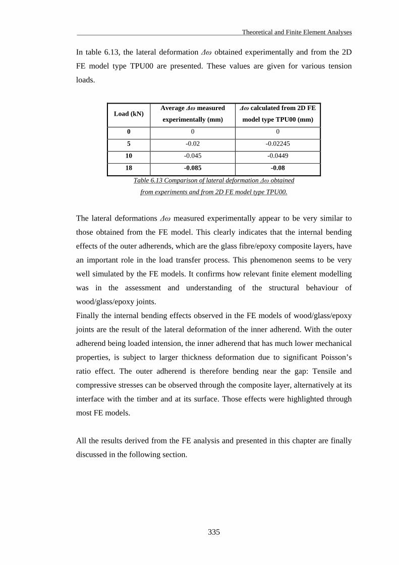
Theoretical and Finite Element Analyses
335
In table 6.13, the lateral deformation ∆ω obtained experimentally and from the 2D
FE model type TPU00 are presented. These values are given for various tension
loads.
Load (kN) Average ∆ω measured
experimentally (mm)
∆ω calculated from 2D FE
model type TPU00 (mm)
0 0 0
5 -0.02 -0.02245
10 -0.045 -0.0449
18 -0.085 -0.08
Table 6.13 Comparison of lateral deformation ∆ω obtained
from experiments and from 2D FE model type TPU00.
The lateral deformations ∆ω measured experimentally appear to be very similar to
those obtained from the FE model. This clearly indicates that the internal bending
effects of the outer adherends, which are the glass fibre/epoxy composite layers, have
an important role in the load transfer process. This phenomenon seems to be very
well simulated by the FE models. It confirms how relevant finite element modelling
was in the assessment and understanding of the structural behaviour of
wood/glass/epoxy joints.
Finally the internal bending effects observed in the FE models of wood/glass/epoxy
joints are the result of the lateral deformation of the inner adherend. With the outer
adherend being loaded intension, the inner adherend that has much lower mechanical
properties, is subject to larger thickness deformation due to significant Poisson’s
ratio effect. The outer adherend is therefore bending near the gap: Tensile and
compressive stresses can be observed through the composite layer, alternatively at its
interface with the timber and at its surface. Those effects were highlighted through
most FE models.
All the results derived from the FE analysis and presented in this chapter are finally
discussed in the following section.
Theoretical and Finite Element Analyses
336
6.5. Discussion and conclusion
Considering the straight joint configurations TPU00 and TPB00, both 2D and 3D
models were developed.
The 2D models were generated based on a convergence testing that was carried out
in order to establish how refined the meshing needed to be to generate an accurate
solution. But with 2D models, the stress variations across the width of the joint could
not be identified, therefore 3D model were necessary.
The development of 3D model was even more restrictive. With straight or angle joint
configurations, the geometry only allowed tetrahedral meshing, hexahedron elements
could be used but they always exceeded their aspect ratio limits. Another obstacle
was that convergence testing could not be carried out: Only a few meshing
configurations could be used without generating errors, and the number of elements
was limited by the solution time and computer memory capacity.
Nevertheless, all the 3D models that are presented in this chapter produced some
solutions without errors or warnings. The accuracy of these solutions must be
examined carefully, particularly in the high stress regions where the meshes are often
not sufficiently refined.
The comparison between the 2D and the 3D models developed for the TPU00 and
TPB00 configurations are a good start for identifying the accuracy of the results.
Looking at the maximum tensile stresses observed at the composite interface, the
results are:
• For the TPU00 configuration, the 2D model give 305 MPa and the 3D model
350 MPa,
• For the TPB00 configuration, the 2D model give 275 MPa and the 3D model
305 MPa,
The results are relatively close, with a slight over-estimation from the 3D models.
The same comparison can be made for the maximum tensile stresses observed at the
timber interface:
Theoretical and Finite Element Analyses
337
• For the TPU00 configuration, the 2D model gives 90 MPa and the 3D model
45 MPa,
• For the TPB00 configuration, the 2D model gives 105 MPa and the 3D model
55 MPa.
In this case, the results are very different. In fact the 3D models peak results are only
approximately half the 2D models results.
Similar disparities in results can be observed comparing the maximum shear results
from both 2D and 3D models. In other words, the 2D models generally show higher
results of maximum shear and tensile stresses in the timber, and lower results of
maximum shear and tensile stresses in the composite than 3D models.
3D models would normally generate more accurate results than 2D models because
they take into account edge effects and stress variations through the third dimension.
But surprisingly in this FE analysis, the 2D models generate more accurate solutions
(particularly in high stress regions) than 3D models mainly because convergence
testing was preliminarily carried out. It is clear that the results obtained from the 3D
models tend to over-estimate the stresses in the composite and under-estimate the
stresses in the timber. Those considerations need to be taken into account in the
analysis of the results obtained from the 3D models, particularly for the joints with
load not parallel to the grain, because of the lack of convergence testing as explained
before. Another argument is that displacements (i.e. strains solutions) usually
converged more rapidly than stresses, in finite element analysis.
The FE results of strains are relatively consistent with those obtained from the tests.
They are very close as far as the joints made of unidirectional glass fibre are
concerned. However the FE results are generally lower than those measured for the
joints made of bidirectional glass fibre. There might be different reasons for that:
• The thickness of the bidirectional glass fibre could well be slightly thicker than
0.65 mm. The stitching threads were ignored when the glass fabric thickness
measurement was carried out. The threads have no mechanical purposes, they are
just keeping the fibres in position. In other words, they thickened the composite
locally up to 0.75 mm. Therefore the average composite thickness could well be
around 0.7 mm.
Theoretical and Finite Element Analyses
338
• The material properties of the glass fibre/epoxy composite could be
over-estimated. In fact the fibre volume fractions (FVF) measured on the samples
were slightly lower than those given for the mechanical properties that were used
in the FE analysis.
Finally, it is clear that for the joints with load not parallel to the grain, the bending of
the inclined timber member under load affects the results. However, there was also a
slight eccentricity of the load during the experiments, but it was not that pronounced:
The rig was made in order to always keep the sample in-line with the load. (i.e. by
rotation of the pins that were holding the frame).
Nevertheless the interpretation of the results shows some relevant findings:
• The peak tensile stress in the timber interface appears to decrease with the angle
of load to the grain. This is due to the tension strength of the timber that is high
when parallel to the grain (low tensile stress) and low when perpendicular to the
grain (high tensile stress).
• Alternatively the peak tensile stress in the composite interface appears to increase
with the angle of load to the grain.
• The results of shear stresses are more difficult to analyse, as they are often
inconsistent, mainly because of the bending of the inclined timber member.
As a conclusion, the FE analysis confirmed the non-uniform load transfer that occur
on double lap joints, such as the wood/glass/epoxy joints that were tested in this
research. However the distribution of shear stress at the interface between the
composite and the timber is fairly different in terms of shape and range than those
observed on CFRP joints presented in § 6.2.3. In fact the thickness of the composite
layer (outer adherend) is so thin compared to the timber member (inner adherend)
that the distribution of shear along the interface reach its maximum in the gap zone
of the joint. At the end of the overlap, the shear always peaks but never exceeds the
value in the gap zone. This is significantly different than for the joints presented in
§ 6.2.3, where the shear stress tend to peak at the end of the overlap. The reasons for
that are:
Theoretical and Finite Element Analyses
339
• The two adherends on the wood/glass/epoxy joints are significantly different in
terms of cross-sections: The inner adherend (the timber) cross-section is nearly
34 times larger than the outer adherend cross-section. The mechanical properties
of the timber are lower than those of the composite, but with a lower multiplying
factor. As a result the distribution of stresses can be more dispersed through the
timber than through the composite.
• The inertia of the composite “plate” is very low because of its thin thickness. The
plate is therefore very sensitive to the internal bending generated by the
double-lap joint. For the joints presented in § 6.2.3, internal bending of the outer
adherend were ignored in the analysis, as well as the stress variations through the
thickness of the adherends. The FE models take those behaviours into account,
which cause the peaks of stresses observed in the gap region.
The following chapter investigates another characteristic of the wood/glass/epoxy
joint, which is essential to enable the use and design of this type of joint: The
capacity of the wood/glass/epoxy joint to resist cyclic loading, in other words, its
fatigue resistance.
CHAPTER 7
FATIGUE ASSESSMENT OF WOOD/GLASS/EPOXY JOINTS
7.1. Introduction
Wood/glass/epoxy joints were tested and analysed in static tension tests. The joints
were loaded to failure at a specific rate in order to assess their strength and stiffness.
However the strength of structural joints also depends on other factors.
For example, a structural joint can be efficient and suitable to connect members, but
it may not have the capacity to withstand the load more than for a period of time. In
other words, material strength can be affected by the load duration: This is known as
creep, when the deformation increases with time under a constant load. Wood is
subject to creep because of its viscoelastic response under load. The rate of creep in
wood is influenced by the load duration, the moisture content, the temperature and
the level of stress. Nevertheless creep contributes to affect the strength of wood.
There are other parameters that can change the strength of a structural joint. One of
them is considered as extremely important in order to validate the design potential of
a structural joint: This parameter is known as the fatigue resistance. When a joint is
subject to a number of varying stress cycles, its mechanical properties can be
weakened and degraded. This phenomenon is identified as fatigue.
“It has been, estimated that at least 75% of all machine and structural failures have
been caused by some form of fatigue” (Benham et al., 1996).
It is therefore essential to investigate the fatigue resistance of any material that will
to be used for design purposes. As a result, it was decided to investigate the fatigue
response of the wood/glass/epoxy joint before the research could be taken any
further. In fact, a design method could not be developed for those adhesive joints
without knowing whether their fatigue resistance is sufficient for their design life.
In this chapter, the experimental programme and the results are presented, including
a detailed literature review used as background information for the results. In other
words, a comprehensive assessment of the fatigue resistance of the wood/glass/epoxy
joint is presented.
340
Fatigue Assessment of Wood/Glass/Epoxy Joints
7.2. Fatigue test programme
7.2.1. Methodology
To investigate the fatigue response of wood/glass/epoxy joint, the cyclic pattern of
stress has to be established. It is essential to highlight that fatigue failure of material
occurs while the material is exposes to cyclic stress where the peak values are always
lower than the material strength. Fatigue failure is a consequence of the progressive
degradation of the material due to cyclic stresses that inevitably weakens its
mechanical properties.
“Wooden structures are frequently subjected to dynamic loads, for example vehicle
loads on factory floors and bridges and wind loads acting on timber roofs” (Ansell,
Timber Engineering STEP 2, 1995).
Based on the potential use of wood/glass/epoxy joints for timber structures and
particularly for timber trusses, it was decided that the joints would be loaded in order
to simulate the fatigue behaviour of the connections under the effects of wind. In fact
the wind is the appropriate dynamic load that could reasonably cause fatigue to the
joints for building applications. To investigate the effects of dynamic loads on the
joints under seismic conditions was not considered at this stage of the research.
To establish a realistic fatigue loading, the frequency of the loads has to be defined in
order to simulate uplift or reversal load on the joints.
The wind is a dynamic load that acts on any structure with variable intensity in time.
It has been monitored and studied for many years by the Meteorological Office in the
U.K. and particularly by the Building Research Establishment, for the construction
industry applications. Codes of practice such as CP3: Ch 5: Pt 2 “Code of basic data
for design of buildings: Wind loads” and more recently BS6399: Pt 2 “Code of
practice for wind loads” are the design standards for wind loading. The most relevant
information was given in CP3: Ch 5: Pt 2, where the gust and wind speed averaging
time are presented and developed in the codes appendix:
Maximum gust of the day and the mean hourly wind speed have been monitored for
many years throughout the U.K using the network of anemograph stations. It was
found that the maximum gust speed represents the mean wind speed averaged over
about 3 seconds. Other research about the incidence and spread of gusts over a
building suggested that the time interval over which maximum wind speeds should
341

Fatigue Assessment of Wood/Glass/Epoxy Joints
be averaged will depend on the building size or part of the structure under
consideration.
The standards adopted in CP3: Ch 5: Pt 2 are:
• The maximum 3-seconds gust speeds for all unit of glazing, cladding or roofing,
whatever the size or portion of the building concerned,
• A wind speed with 5 seconds averaging time is used for the structural design of
buildings or structures where neither the greatest horizontal nor vertical dimension
exceed 50 m.
• For buildings or structures whose greatest horizontal or vertical dimension
exceeds 50 m, a wind speed of 15 seconds averaging time is used.
The maximum 3-seconds gust duration is based on a 50 years design life, which
corresponds to the average lifetime of most buildings according to the codes.
It was then decided to apply the 3-seconds loading period to the fatigue tests. In other
words, the frequency proposed for the cyclic tests was:
HzN 33.031
== (7.1)
With the frequency defined, it was then important to define the loading configuration
in order to establish whether the load would be of varying amplitude, reversed, etc.
Wood/glass/epoxy joints were analysed in tension only throughout this research,
fatigue tests should then be carried out in tension only. To develop fatigue tests in
compression could not be considered because static compression tests were not
investigated. The results had to be interrelated with the research previously carried
out.
The loading condition that simulates the effect of wind in a fatigue mode would be a
loaded-unloaded cyclic pattern, where the minimum stress would correspond to
10% of the maximum stress. With this arrangement, the wood/glass/epoxy joint
would remain in tension all the time. This cyclic pattern would have a “saw tooth”
shape with constant amplitude, and the period would be of 3 seconds. It would be a
similar loading pattern to the waveform shown in figure 7.1.
342
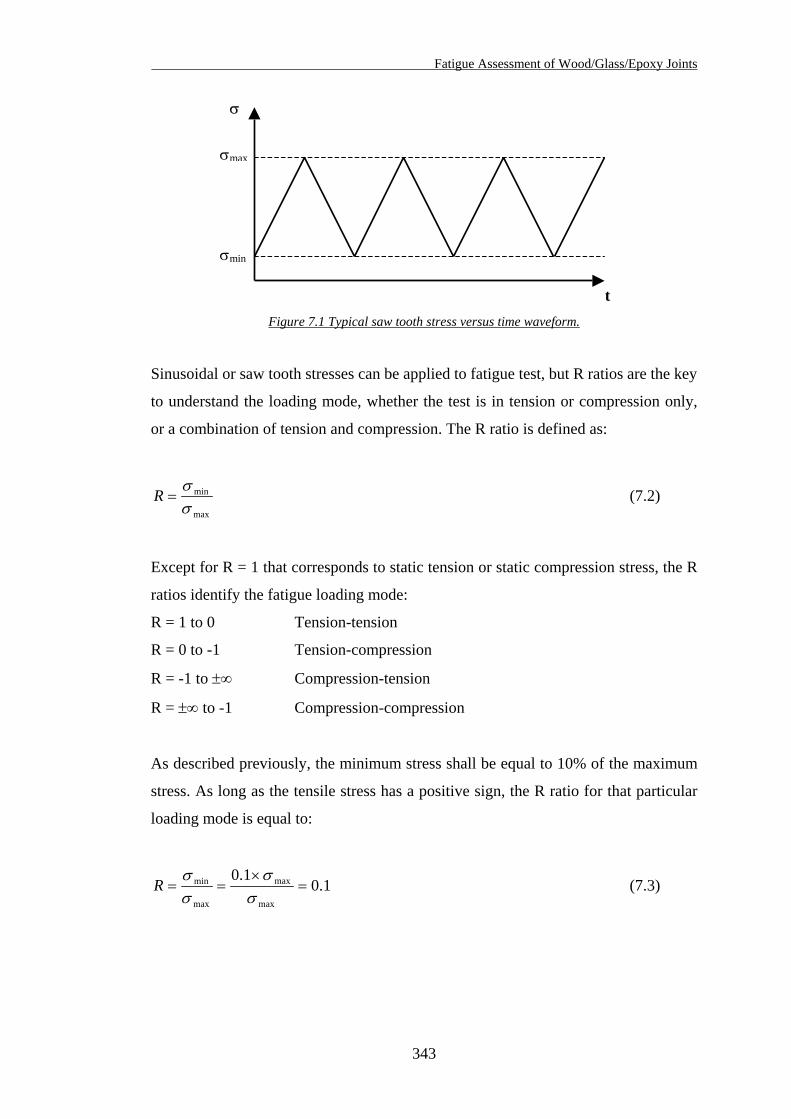
Fatigue Assessment of Wood/Glass/Epoxy Joints
σ
t
σmin
σmax
Figure 7.1 Typical saw tooth stress versus time waveform.
Sinusoidal or saw tooth stresses can be applied to fatigue test, but R ratios are the key
to understand the loading mode, whether the test is in tension or compression only,
or a combination of tension and compression. The R ratio is defined as:
max
min
σσ
=R (7.2)
Except for R = 1 that corresponds to static tension or static compression stress, the R
ratios identify the fatigue loading mode:
R = 1 to 0 Tension-tension
R = 0 to -1 Tension-compression
R = -1 to ±∞ Compression-tension
R = ±∞ to -1 Compression-compression
As described previously, the minimum stress shall be equal to 10% of the maximum
stress. As long as the tensile stress has a positive sign, the R ratio for that particular
loading mode is equal to:
1.01.0
max
max
max
min =×
==σ
σσσR (7.3)
343
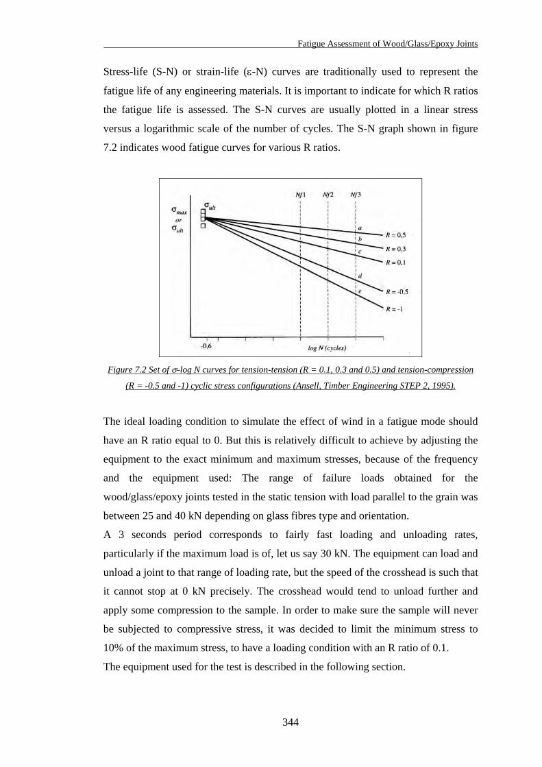
Fatigue Assessment of Wood/Glass/Epoxy Joints
Stress-life (S-N) or strain-life (ε-N) curves are traditionally used to represent the
fatigue life of any engineering materials. It is important to indicate for which R ratios
the fatigue life is assessed. The S-N curves are usually plotted in a linear stress
versus a logarithmic scale of the number of cycles. The S-N graph shown in figure
7.2 indicates wood fatigue curves for various R ratios.
Figure 7.2 Set of σ-log N curves for tension-tension (R = 0.1, 0.3 and 0.5) and tension-compression
(R = -0.5 and -1) cyclic stress configurations (Ansell, Timber Engineering STEP 2, 1995).
The ideal loading condition to simulate the effect of wind in a fatigue mode should
have an R ratio equal to 0. But this is relatively difficult to achieve by adjusting the
equipment to the exact minimum and maximum stresses, because of the frequency
and the equipment used: The range of failure loads obtained for the
wood/glass/epoxy joints tested in the static tension with load parallel to the grain was
between 25 and 40 kN depending on glass fibres type and orientation.
A 3 seconds period corresponds to fairly fast loading and unloading rates,
particularly if the maximum load is of, let us say 30 kN. The equipment can load and
unload a joint to that range of loading rate, but the speed of the crosshead is such that
it cannot stop at 0 kN precisely. The crosshead would tend to unload further and
apply some compression to the sample. In order to make sure the sample will never
be subjected to compressive stress, it was decided to limit the minimum stress to
10% of the maximum stress, to have a loading condition with an R ratio of 0.1.
The equipment used for the test is described in the following section.
344
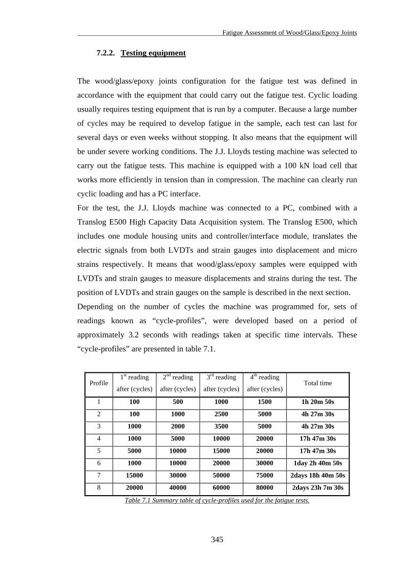
Fatigue Assessment of Wood/Glass/Epoxy Joints
7.2.2. Testing equipment
The wood/glass/epoxy joints configuration for the fatigue test was defined in
accordance with the equipment that could carry out the fatigue test. Cyclic loading
usually requires testing equipment that is run by a computer. Because a large number
of cycles may be required to develop fatigue in the sample, each test can last for
several days or even weeks without stopping. It also means that the equipment will
be under severe working conditions. The J.J. Lloyds testing machine was selected to
carry out the fatigue tests. This machine is equipped with a 100 kN load cell that
works more efficiently in tension than in compression. The machine can clearly run
cyclic loading and has a PC interface.
For the test, the J.J. Lloyds machine was connected to a PC, combined with a
Translog E500 High Capacity Data Acquisition system. The Translog E500, which
includes one module housing units and controller/interface module, translates the
electric signals from both LVDTs and strain gauges into displacement and micro
strains respectively. It means that wood/glass/epoxy samples were equipped with
LVDTs and strain gauges to measure displacements and strains during the test. The
position of LVDTs and strain gauges on the sample is described in the next section.
Depending on the number of cycles the machine was programmed for, sets of
readings known as “cycle-profiles”, were developed based on a period of
approximately 3.2 seconds with readings taken at specific time intervals. These
“cycle-profiles” are presented in table 7.1.
Profile 1st reading
after (cycles)
2nd reading
after (cycles)
3rd reading
after (cycles)
4th reading
after (cycles) Total time
1 100 500 1000 1500 1h 20m 50s
2 100 1000 2500 5000 4h 27m 30s
3 1000 2000 3500 5000 4h 27m 30s
4 1000 5000 10000 20000 17h 47m 30s
5 5000 10000 15000 20000 17h 47m 30s
6 1000 10000 20000 30000 1day 2h 40m 50s
7 15000 30000 50000 75000 2days 18h 40m 50s
8 20000 40000 60000 80000 2days 23h 7m 30s
Table 7.1 Summary table of cycle-profiles used for the fatigue tests.
345
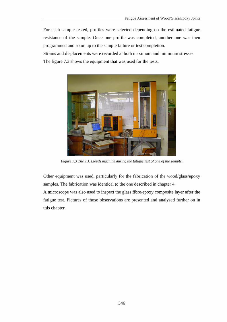
Fatigue Assessment of Wood/Glass/Epoxy Joints
For each sample tested, profiles were selected depending on the estimated fatigue
resistance of the sample. Once one profile was completed, another one was then
programmed and so on up to the sample failure or test completion.
Strains and displacements were recorded at both maximum and minimum stresses.
The figure 7.3 shows the equipment that was used for the tests.
Figure 7.3 The J.J. Lloyds machine during the fatigue test of one of the sample.
Other equipment was used, particularly for the fabrication of the wood/glass/epoxy
samples. The fabrication was identical to the one described in chapter 4.
A microscope was also used to inspect the glass fibre/epoxy composite layer after the
fatigue test. Pictures of those observations are presented and analysed further on in
this chapter.
346
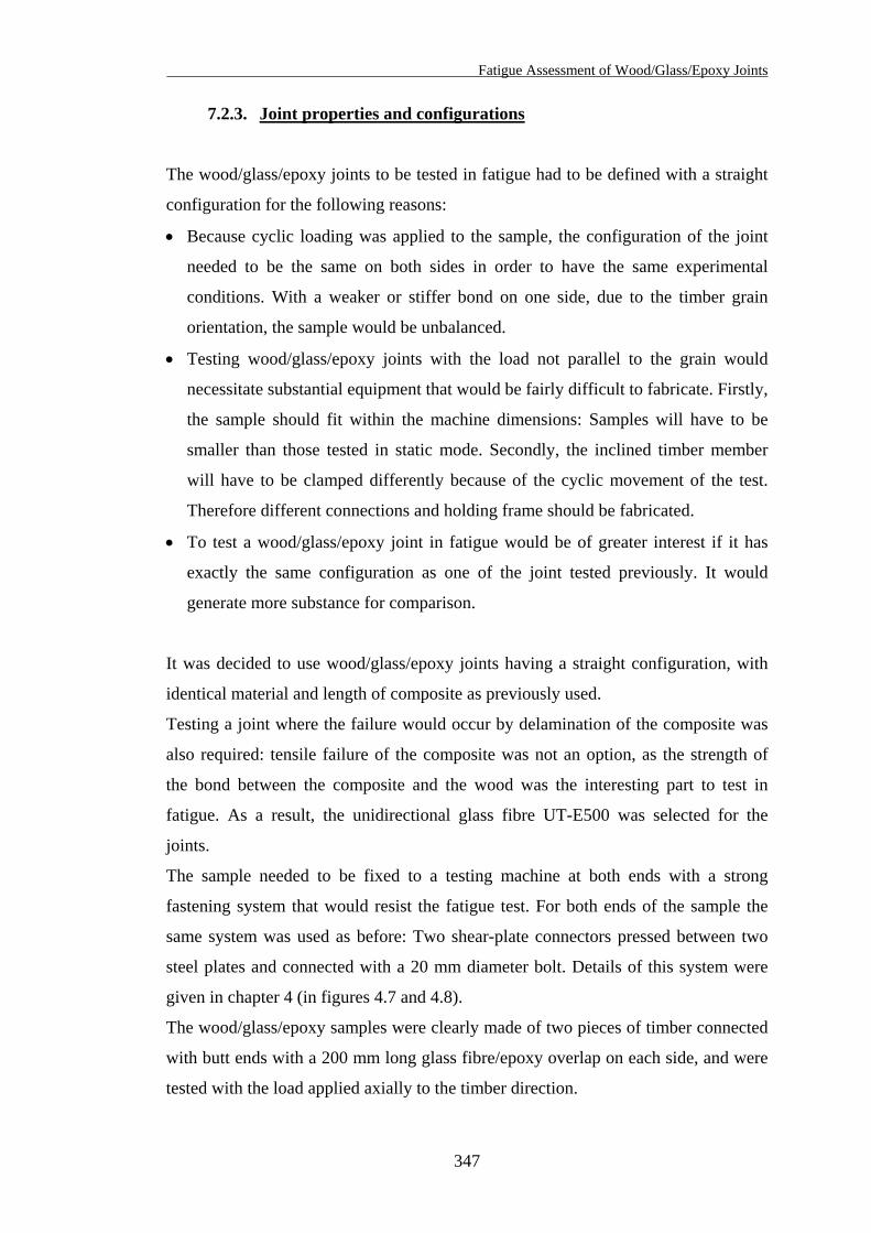
Fatigue Assessment of Wood/Glass/Epoxy Joints
7.2.3. Joint properties and configurations
The wood/glass/epoxy joints to be tested in fatigue had to be defined with a straight
configuration for the following reasons:
• Because cyclic loading was applied to the sample, the configuration of the joint
needed to be the same on both sides in order to have the same experimental
conditions. With a weaker or stiffer bond on one side, due to the timber grain
orientation, the sample would be unbalanced.
• Testing wood/glass/epoxy joints with the load not parallel to the grain would
necessitate substantial equipment that would be fairly difficult to fabricate. Firstly,
the sample should fit within the machine dimensions: Samples will have to be
smaller than those tested in static mode. Secondly, the inclined timber member
will have to be clamped differently because of the cyclic movement of the test.
Therefore different connections and holding frame should be fabricated.
• To test a wood/glass/epoxy joint in fatigue would be of greater interest if it has
exactly the same configuration as one of the joint tested previously. It would
generate more substance for comparison.
It was decided to use wood/glass/epoxy joints having a straight configuration, with
identical material and length of composite as previously used.
Testing a joint where the failure would occur by delamination of the composite was
also required: tensile failure of the composite was not an option, as the strength of
the bond between the composite and the wood was the interesting part to test in
fatigue. As a result, the unidirectional glass fibre UT-E500 was selected for the
joints.
The sample needed to be fixed to a testing machine at both ends with a strong
fastening system that would resist the fatigue test. For both ends of the sample the
same system was used as before: Two shear-plate connectors pressed between two
steel plates and connected with a 20 mm diameter bolt. Details of this system were
given in chapter 4 (in figures 4.7 and 4.8).
The wood/glass/epoxy samples were clearly made of two pieces of timber connected
with butt ends with a 200 mm long glass fibre/epoxy overlap on each side, and were
tested with the load applied axially to the timber direction.
347
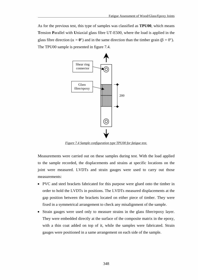
Fatigue Assessment of Wood/Glass/Epoxy Joints
As for the previous test, this type of samples was classified as TPU00, which means
Tension Parallel with Uniaxial glass fibre UT-E500, where the load is applied in the
glass fibre direction (α = 0°) and in the same direction than the timber grain (β = 0°).
The TPU00 sample is presented in figure 7.4.
Glass fibre/epoxy
Shear ring connector
200
Figure 7.4 Sample configuration type TPU00 for fatigue test.
Measurements were carried out on these samples during test. With the load applied
to the sample recorded, the displacements and strains at specific locations on the
joint were measured. LVDTs and strain gauges were used to carry out those
measurements:
• PVC and steel brackets fabricated for this purpose were glued onto the timber in
order to hold the LVDTs in positions. The LVDTs measured displacements at the
gap position between the brackets located on either piece of timber. They were
fixed in a symmetrical arrangement to check any misalignment of the sample.
• Strain gauges were used only to measure strains in the glass fibre/epoxy layer.
They were embedded directly at the surface of the composite matrix in the epoxy,
with a thin coat added on top of it, while the samples were fabricated. Strain
gauges were positioned in a same arrangement on each side of the sample.
348
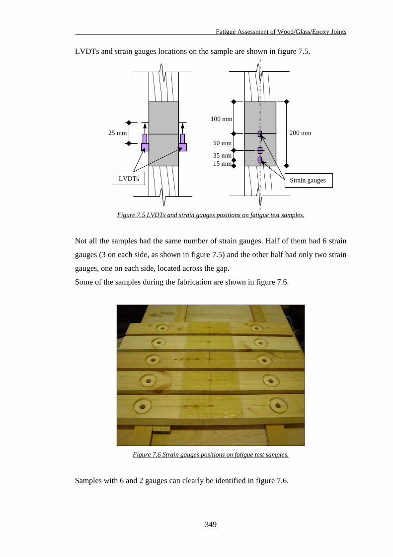
Fatigue Assessment of Wood/Glass/Epoxy Joints
LVDTs and strain gauges locations on the sample are shown in figure 7.5.
Figure 7.5 LVDTs and strain gauges positions on fatigue test samples.
50 mm 25 mm
Strain gauges
100 mm
15 mm35 mm
200 mm
LVDTs
Not all the samples had the same number of strain gauges. Half of them had 6 strain
gauges (3 on each side, as shown in figure 7.5) and the other half had only two strain
gauges, one on each side, located across the gap.
Some of the samples during the fabrication are shown in figure 7.6.
Figure 7.6 Strain gauges positions on fatigue test samples.
Samples with 6 and 2 gauges can clearly be identified in figure 7.6.
349
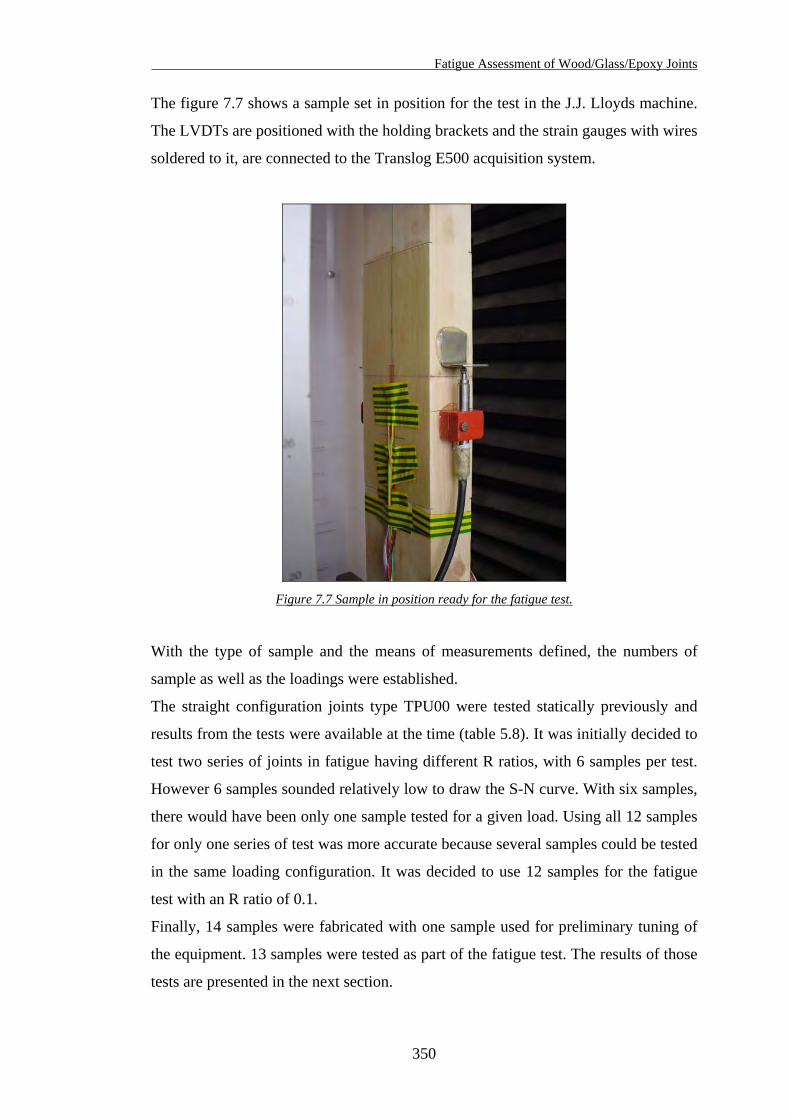
Fatigue Assessment of Wood/Glass/Epoxy Joints
The figure 7.7 shows a sample set in position for the test in the J.J. Lloyds machine.
The LVDTs are positioned with the holding brackets and the strain gauges with wires
soldered to it, are connected to the Translog E500 acquisition system.
Figure 7.7 Sample in position ready for the fatigue test.
With the type of sample and the means of measurements defined, the numbers of
sample as well as the loadings were established.
The straight configuration joints type TPU00 were tested statically previously and
results from the tests were available at the time (table 5.8). It was initially decided to
test two series of joints in fatigue having different R ratios, with 6 samples per test.
However 6 samples sounded relatively low to draw the S-N curve. With six samples,
there would have been only one sample tested for a given load. Using all 12 samples
for only one series of test was more accurate because several samples could be tested
in the same loading configuration. It was decided to use 12 samples for the fatigue
test with an R ratio of 0.1.
Finally, 14 samples were fabricated with one sample used for preliminary tuning of
the equipment. 13 samples were tested as part of the fatigue test. The results of those
tests are presented in the next section.
350
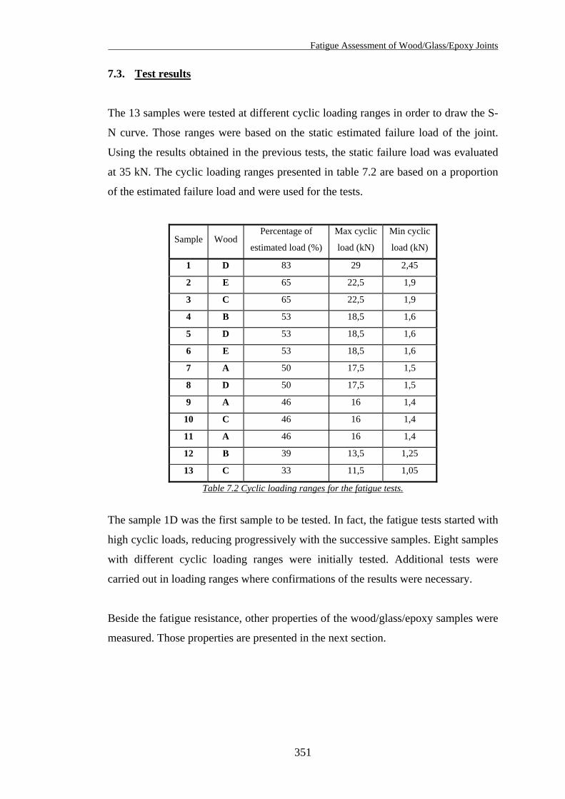
Fatigue Assessment of Wood/Glass/Epoxy Joints
7.3. Test results
The 13 samples were tested at different cyclic loading ranges in order to draw the S-
N curve. Those ranges were based on the static estimated failure load of the joint.
Using the results obtained in the previous tests, the static failure load was evaluated
at 35 kN. The cyclic loading ranges presented in table 7.2 are based on a proportion
of the estimated failure load and were used for the tests.
Sample Wood Percentage of
estimated load (%)
Max cyclic
load (kN)
Min cyclic
load (kN)
1 D 83 29 2,45
2 E 65 22,5 1,9
3 C 65 22,5 1,9
4 B 53 18,5 1,6
5 D 53 18,5 1,6
6 E 53 18,5 1,6
7 A 50 17,5 1,5
8 D 50 17,5 1,5
9 A 46 16 1,4
10 C 46 16 1,4
11 A 46 16 1,4
12 B 39 13,5 1,25
13 C 33 11,5 1,05
Table 7.2 Cyclic loading ranges for the fatigue tests.
The sample 1D was the first sample to be tested. In fact, the fatigue tests started with
high cyclic loads, reducing progressively with the successive samples. Eight samples
with different cyclic loading ranges were initially tested. Additional tests were
carried out in loading ranges where confirmations of the results were necessary.
Beside the fatigue resistance, other properties of the wood/glass/epoxy samples were
measured. Those properties are presented in the next section.
351
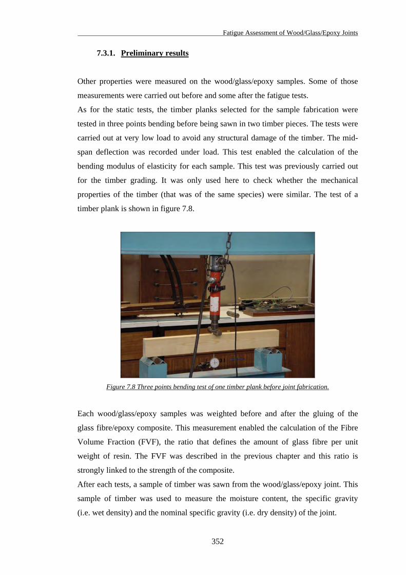
Fatigue Assessment of Wood/Glass/Epoxy Joints
7.3.1. Preliminary results
Other properties were measured on the wood/glass/epoxy samples. Some of those
measurements were carried out before and some after the fatigue tests.
As for the static tests, the timber planks selected for the sample fabrication were
tested in three points bending before being sawn in two timber pieces. The tests were
carried out at very low load to avoid any structural damage of the timber. The mid-
span deflection was recorded under load. This test enabled the calculation of the
bending modulus of elasticity for each sample. This test was previously carried out
for the timber grading. It was only used here to check whether the mechanical
properties of the timber (that was of the same species) were similar. The test of a
timber plank is shown in figure 7.8.
Figure 7.8 Three points bending test of one timber plank before joint fabrication.
Each wood/glass/epoxy samples was weighted before and after the gluing of the
glass fibre/epoxy composite. This measurement enabled the calculation of the Fibre
Volume Fraction (FVF), the ratio that defines the amount of glass fibre per unit
weight of resin. The FVF was described in the previous chapter and this ratio is
strongly linked to the strength of the composite.
After each tests, a sample of timber was sawn from the wood/glass/epoxy joint. This
sample of timber was used to measure the moisture content, the specific gravity
(i.e. wet density) and the nominal specific gravity (i.e. dry density) of the joint.
352
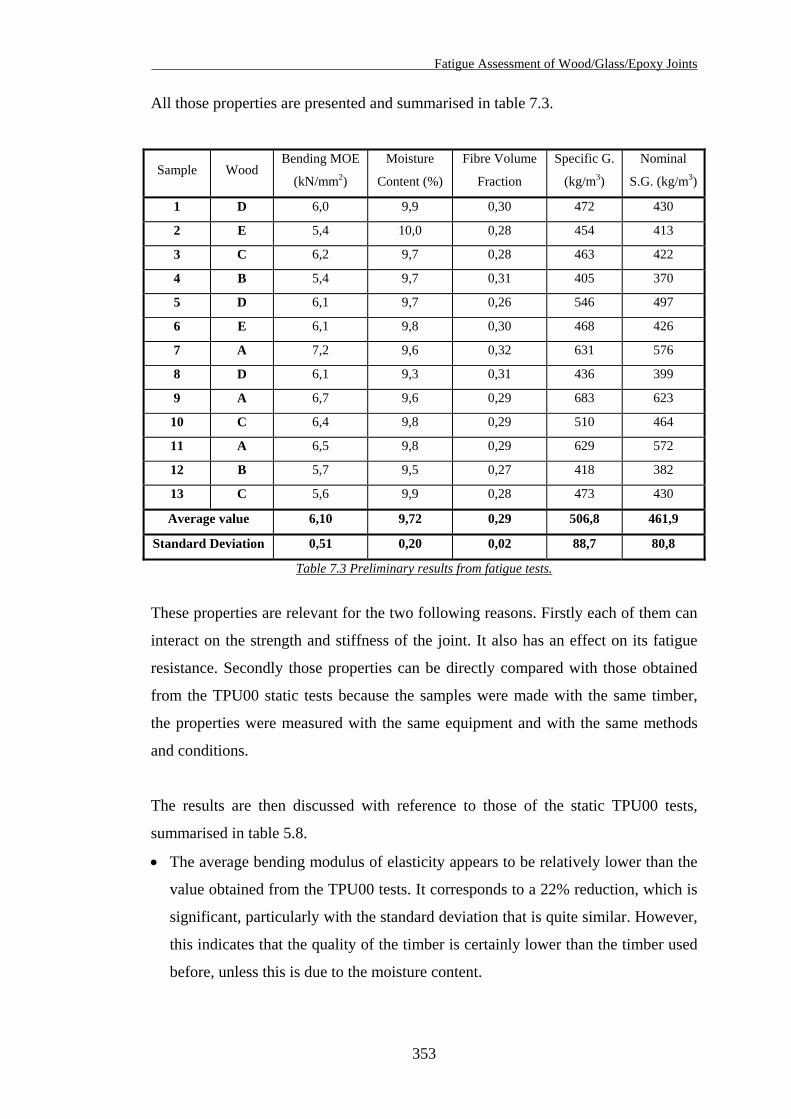
Fatigue Assessment of Wood/Glass/Epoxy Joints
All those properties are presented and summarised in table 7.3.
Sample Wood Bending MOE
(kN/mm2)
Moisture
Content (%)
Fibre Volume
Fraction
Specific G.
(kg/m3)
Nominal
S.G. (kg/m3)
1 D 6,0 9,9 0,30 472 430
2 E 5,4 10,0 0,28 454 413
3 C 6,2 9,7 0,28 463 422
4 B 5,4 9,7 0,31 405 370
5 D 6,1 9,7 0,26 546 497
6 E 6,1 9,8 0,30 468 426
7 A 7,2 9,6 0,32 631 576
8 D 6,1 9,3 0,31 436 399
9 A 6,7 9,6 0,29 683 623
10 C 6,4 9,8 0,29 510 464
11 A 6,5 9,8 0,29 629 572
12 B 5,7 9,5 0,27 418 382
13 C 5,6 9,9 0,28 473 430
Average value 6,10 9,72 0,29 506,8 461,9
Standard Deviation 0,51 0,20 0,02 88,7 80,8
Table 7.3 Preliminary results from fatigue tests.
These properties are relevant for the two following reasons. Firstly each of them can
interact on the strength and stiffness of the joint. It also has an effect on its fatigue
resistance. Secondly those properties can be directly compared with those obtained
from the TPU00 static tests because the samples were made with the same timber,
the properties were measured with the same equipment and with the same methods
and conditions.
The results are then discussed with reference to those of the static TPU00 tests,
summarised in table 5.8.
• The average bending modulus of elasticity appears to be relatively lower than the
value obtained from the TPU00 tests. It corresponds to a 22% reduction, which is
significant, particularly with the standard deviation that is quite similar. However,
this indicates that the quality of the timber is certainly lower than the timber used
before, unless this is due to the moisture content.
353
Fatigue Assessment of Wood/Glass/Epoxy Joints
• The measurement of moisture content indicates that the timber is drier than for the
TPU00 tests. With almost 2% lower average moisture content and a very low
standard deviation, the timber was left in dry conditions for a long time before the
test and perhaps in slightly too dry conditions. With lower moisture content, the
timber properties should be slightly better, but this is not the case. The quality of
the timber is therefore lower than that used previously.
• The results of FVF are very close to those derived for the TPU00 tests. This
confirms that the method used, the type of glass fibre and the resin are identical as
before.
• The measurements of specific gravity and nominal specific gravity indicate fairly
high average values for lower quality of timber than used for the static tests. The
comparison of the standard deviation shows that the timber density is more
variable in this test than in the previous static tests. More variations correspond to
more discrepancy in the timber quality. However high values of specific gravity
correspond to high values of bending modulus of elasticity. It confirms the
accuracy of the experimental methods used to carry out those measurements.
Finally the results are all consistent considering the values obtained for the standard
deviations.
The main test developed to evaluate the fatigue life of those joints is presented in the
following section.
354
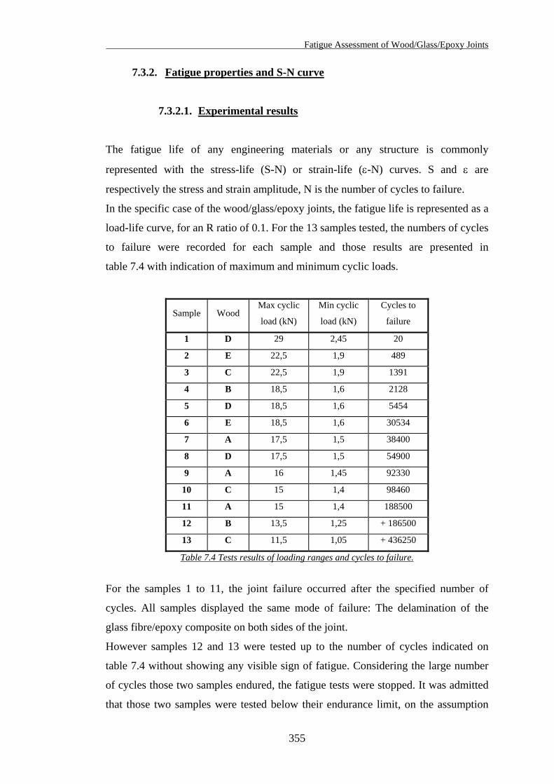
Fatigue Assessment of Wood/Glass/Epoxy Joints
7.3.2. Fatigue properties and S-N curve
7.3.2.1. Experimental results
The fatigue life of any engineering materials or any structure is commonly
represented with the stress-life (S-N) or strain-life (ε-N) curves. S and ε are
respectively the stress and strain amplitude, N is the number of cycles to failure.
In the specific case of the wood/glass/epoxy joints, the fatigue life is represented as a
load-life curve, for an R ratio of 0.1. For the 13 samples tested, the numbers of cycles
to failure were recorded for each sample and those results are presented in
table 7.4 with indication of maximum and minimum cyclic loads.
Sample Wood Max cyclic
load (kN)
Min cyclic
load (kN)
Cycles to
failure
1 D 29 2,45 20
2 E 22,5 1,9 489
3 C 22,5 1,9 1391
4 B 18,5 1,6 2128
5 D 18,5 1,6 5454
6 E 18,5 1,6 30534
7 A 17,5 1,5 38400
8 D 17,5 1,5 54900
9 A 16 1,45 92330
10 C 15 1,4 98460
11 A 15 1,4 188500
12 B 13,5 1,25 + 186500
13 C 11,5 1,05 + 436250
Table 7.4 Tests results of loading ranges and cycles to failure.
For the samples 1 to 11, the joint failure occurred after the specified number of
cycles. All samples displayed the same mode of failure: The delamination of the
glass fibre/epoxy composite on both sides of the joint.
However samples 12 and 13 were tested up to the number of cycles indicated on
table 7.4 without showing any visible sign of fatigue. Considering the large number
of cycles those two samples endured, the fatigue tests were stopped. It was admitted
that those two samples were tested below their endurance limit, on the assumption
355
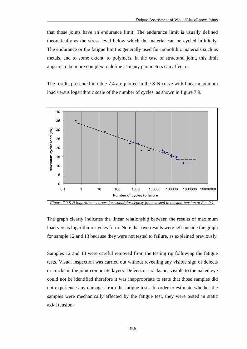
Fatigue Assessment of Wood/Glass/Epoxy Joints
that those joints have an endurance limit. The endurance limit is usually defined
theoretically as the stress level below which the material can be cycled infinitely.
The endurance or the fatigue limit is generally used for monolithic materials such as
metals, and to some extent, to polymers. In the case of structural joint, this limit
appears to be more complex to define as many parameters can affect it.
The results presented in table 7.4 are plotted in the S-N curve with linear maximum
load versus logarithmic scale of the number of cycles, as shown in figure 7.9.
Figure 7.9 S-N logarithmic curves for wood/glass/epoxy joints tested in tension-tension at R = 0.1.
The graph clearly indicates the linear relationship between the results of maximum
load versus logarithmic cycles form. Note that two results were left outside the graph
for sample 12 and 13 because they were not tested to failure, as explained previously.
Samples 12 and 13 were careful removed from the testing rig following the fatigue
tests. Visual inspection was carried out without revealing any visible sign of defects
or cracks in the joint composite layers. Defects or cracks not visible to the naked eye
could not be identified therefore it was inappropriate to state that those samples did
not experience any damages from the fatigue tests. In order to estimate whether the
samples were mechanically affected by the fatigue test, they were tested in static
axial tension.
356
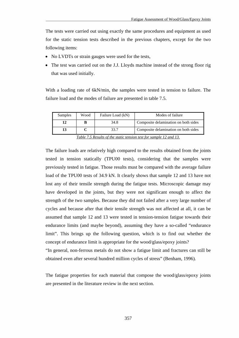
Fatigue Assessment of Wood/Glass/Epoxy Joints
The tests were carried out using exactly the same procedures and equipment as used
for the static tension tests described in the previous chapters, except for the two
following items:
• No LVDTs or strain gauges were used for the tests,
• The test was carried out on the J.J. Lloyds machine instead of the strong floor rig
that was used initially.
With a loading rate of 6kN/min, the samples were tested in tension to failure. The
failure load and the modes of failure are presented in table 7.5.
Samples Wood Failure Load (kN) Modes of failure
12 B 34.8 Composite delamination on both sides
13 C 33.7 Composite delamination on both sides
Table 7.5 Results of the static tension test for sample 12 and 13.
The failure loads are relatively high compared to the results obtained from the joints
tested in tension statically (TPU00 tests), considering that the samples were
previously tested in fatigue. Those results must be compared with the average failure
load of the TPU00 tests of 34.9 kN. It clearly shows that sample 12 and 13 have not
lost any of their tensile strength during the fatigue tests. Microscopic damage may
have developed in the joints, but they were not significant enough to affect the
strength of the two samples. Because they did not failed after a very large number of
cycles and because after that their tensile strength was not affected at all, it can be
assumed that sample 12 and 13 were tested in tension-tension fatigue towards their
endurance limits (and maybe beyond), assuming they have a so-called “endurance
limit”. This brings up the following question, which is to find out whether the
concept of endurance limit is appropriate for the wood/glass/epoxy joints?
“In general, non-ferrous metals do not show a fatigue limit and fractures can still be
obtained even after several hundred million cycles of stress” (Benham, 1996).
The fatigue properties for each material that compose the wood/glass/epoxy joints
are presented in the literature review in the next section.
357
Fatigue Assessment of Wood/Glass/Epoxy Joints
7.3.2.2. Fatigue properties of materials
It is necessary to identify the fatigue properties of each material (i.e. wood,
wood/epoxy and glass fibre/epoxy) that compose the wood/glass/epoxy joints to
understand the overall behaviour of the joints under fatigue.
Most fatigue theories usually admitted a so-called endurance limit for a monolithic
material that was cycled 1 to 100 million times without failure, depending on the
material considered.
But first it is essential to highlight that the use of S-N curves to assess the fatigue
properties of a material is fully valid when the applied cyclic stress remains within
the elastic range and the number of cycles to failure is large: This is known as the
high-endurance fatigue. High-endurance fatigue relates to the endurance of a
material from about 104 cycles to ‘infinity’. Alternatively low-endurance fatigue
relates to the high cyclic stress to failure part of the curve (usually up to 104 cycles).
The approach regarding those two ranges of endurance is rather different:
• A material subjected to low-endurance fatigue is under high cyclic stresses and
strains. In other words, significant plastic deformation is occurring in every cycle,
resulting in strain-hardening or softening effects of the material. Plastic
deformation is usually represented in the form of a stress/strain hysteresis loop.
However stress/strain hysteresis loops were not produced during testing of
wood/glass/epoxy joints because the measuring equipment could not monitor
displacements and strains continuously or at very close intervals, considering it
must record several readings for each cycle that last for 3 seconds.
• A material subjected to high-endurance fatigue is under low cyclic stresses and
strains. Because the cyclic loading remains essentially elastic, the S-N curve
approach is best suited for the high-endurance fatigue analysis. By reducing the
cyclic stress level, the S-N curve of a material either becomes parallel to the
N-axis or continues with a steadily decreasing slope. This is the case respectively
for materials having an endurance limit such as steel, and for materials not having
any endurance limit such as aluminium. This is confirmed on the
S-N curves presented in figures 7.10 and 7.11 for both steel and aluminium
materials.
358
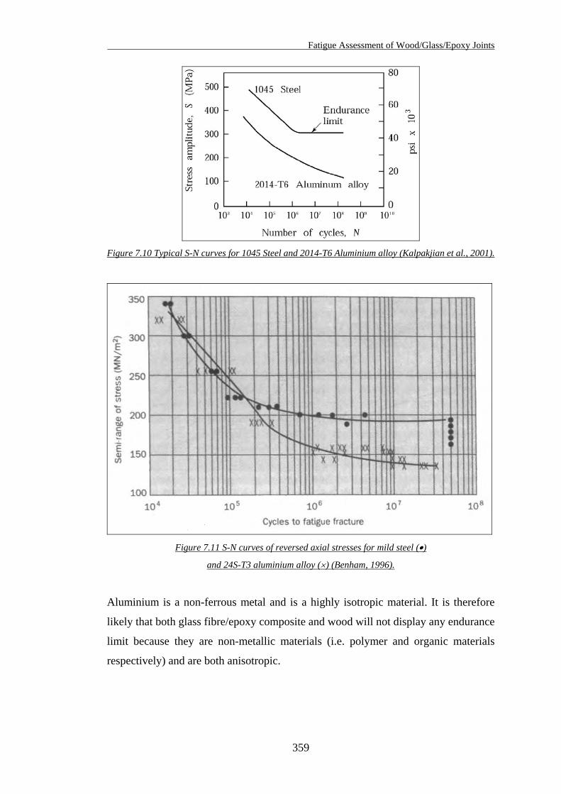
Fatigue Assessment of Wood/Glass/Epoxy Joints
Figure 7.10 Typical S-N curves for 1045 Steel and 2014-T6 Aluminium alloy (Kalpakjian et al., 2001).
Figure 7.11 S-N curves of reversed axial stresses for mild steel (•)
and 24S-T3 aluminium alloy (×) (Benham, 1996).
Aluminium is a non-ferrous metal and is a highly isotropic material. It is therefore
likely that both glass fibre/epoxy composite and wood will not display any endurance
limit because they are non-metallic materials (i.e. polymer and organic materials
respectively) and are both anisotropic.
359
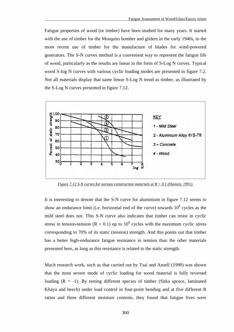
Fatigue Assessment of Wood/Glass/Epoxy Joints
Fatigue properties of wood (or timber) have been studied for many years. It started
with the use of timber for the Mosquito bomber and gliders in the early 1940s, to the
more recent use of timber for the manufacture of blades for wind-powered
generators. The S-N curves method is a convenient way to represent the fatigue life
of wood, particularly as the results are linear in the form of S-Log N curves. Typical
wood S-log N curves with various cyclic loading modes are presented in figure 7.2.
Not all materials display that same linear S-Log N trend as timber, as illustrated by
the S-Log N curves presented in figure 7.12.
Figure 7.12 S-N curves for various construction materials at R = 0.1 (Hansen, 1991).
It is interesting to denote that the S-N curve for aluminium in figure 7.12 seems to
show an endurance limit (i.e. horizontal end of the curve) towards 108 cycles as the
mild steel does not. This S-N curve also indicates that timber can resist in cyclic
stress in tension-tension (R = 0.1) up to 108 cycles with the maximum cyclic stress
corresponding to 70% of its static (tension) strength. And this points out that timber
has a better high-endurance fatigue resistance in tension than the other materials
presented here, as long as this resistance is related to the static strength.
Much research work, such as that carried out by Tsai and Ansell (1990) was shown
that the most severe mode of cyclic loading for wood material is fully reversed
loading (R = -1). By testing different species of timber (Sitka spruce, laminated
Khaya and beech) under load control in four-point bending and at five different R
ratios and three different moisture contents, they found that fatigue lives were
360
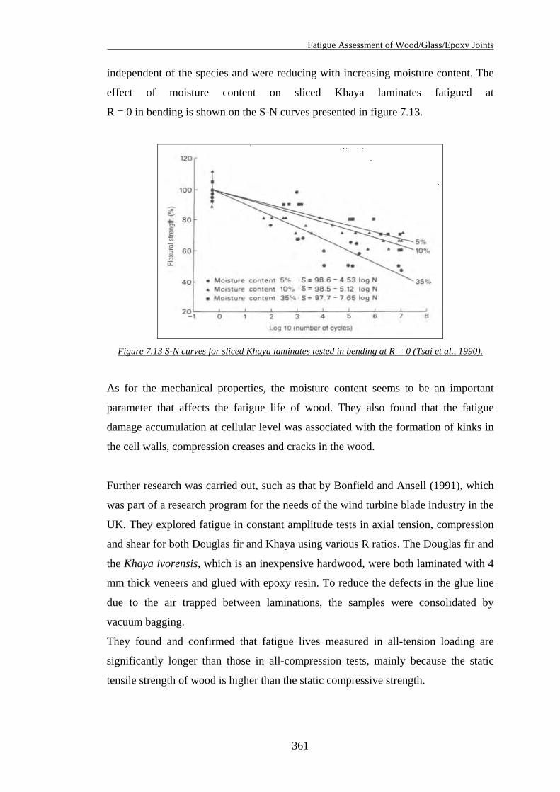
Fatigue Assessment of Wood/Glass/Epoxy Joints
independent of the species and were reducing with increasing moisture content. The
effect of moisture content on sliced Khaya laminates fatigued at
R = 0 in bending is shown on the S-N curves presented in figure 7.13.
Figure 7.13 S-N curves for sliced Khaya laminates tested in bending at R = 0 (Tsai et al., 1990).
As for the mechanical properties, the moisture content seems to be an important
parameter that affects the fatigue life of wood. They also found that the fatigue
damage accumulation at cellular level was associated with the formation of kinks in
the cell walls, compression creases and cracks in the wood.
Further research was carried out, such as that by Bonfield and Ansell (1991), which
was part of a research program for the needs of the wind turbine blade industry in the
UK. They explored fatigue in constant amplitude tests in axial tension, compression
and shear for both Douglas fir and Khaya using various R ratios. The Douglas fir and
the Khaya ivorensis, which is an inexpensive hardwood, were both laminated with 4
mm thick veneers and glued with epoxy resin. To reduce the defects in the glue line
due to the air trapped between laminations, the samples were consolidated by
vacuum bagging.
They found and confirmed that fatigue lives measured in all-tension loading are
significantly longer than those in all-compression tests, mainly because the static
tensile strength of wood is higher than the static compressive strength.
361
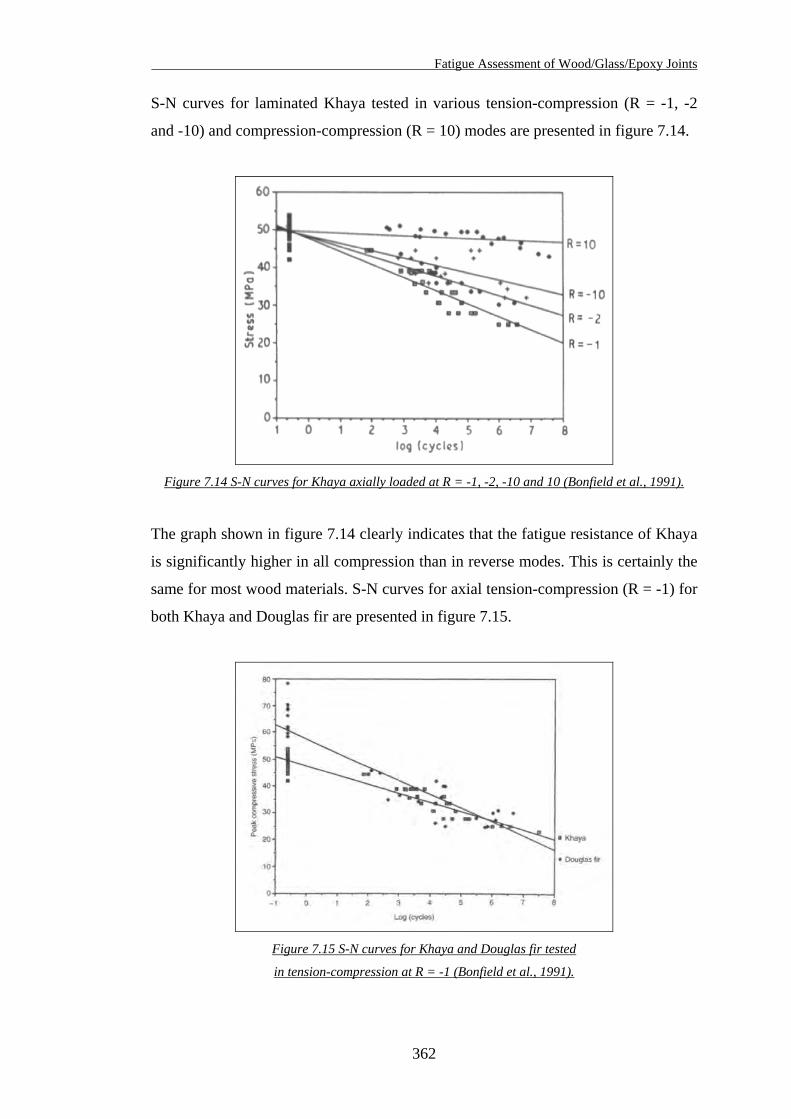
Fatigue Assessment of Wood/Glass/Epoxy Joints
S-N curves for laminated Khaya tested in various tension-compression (R = -1, -2
and -10) and compression-compression (R = 10) modes are presented in figure 7.14.
Figure 7.14 S-N curves for Khaya axially loaded at R = -1, -2, -10 and 10 (Bonfield et al., 1991).
The graph shown in figure 7.14 clearly indicates that the fatigue resistance of Khaya
is significantly higher in all compression than in reverse modes. This is certainly the
same for most wood materials. S-N curves for axial tension-compression (R = -1) for
both Khaya and Douglas fir are presented in figure 7.15.
Figure 7.15 S-N curves for Khaya and Douglas fir tested
in tension-compression at R = -1 (Bonfield et al., 1991).
362
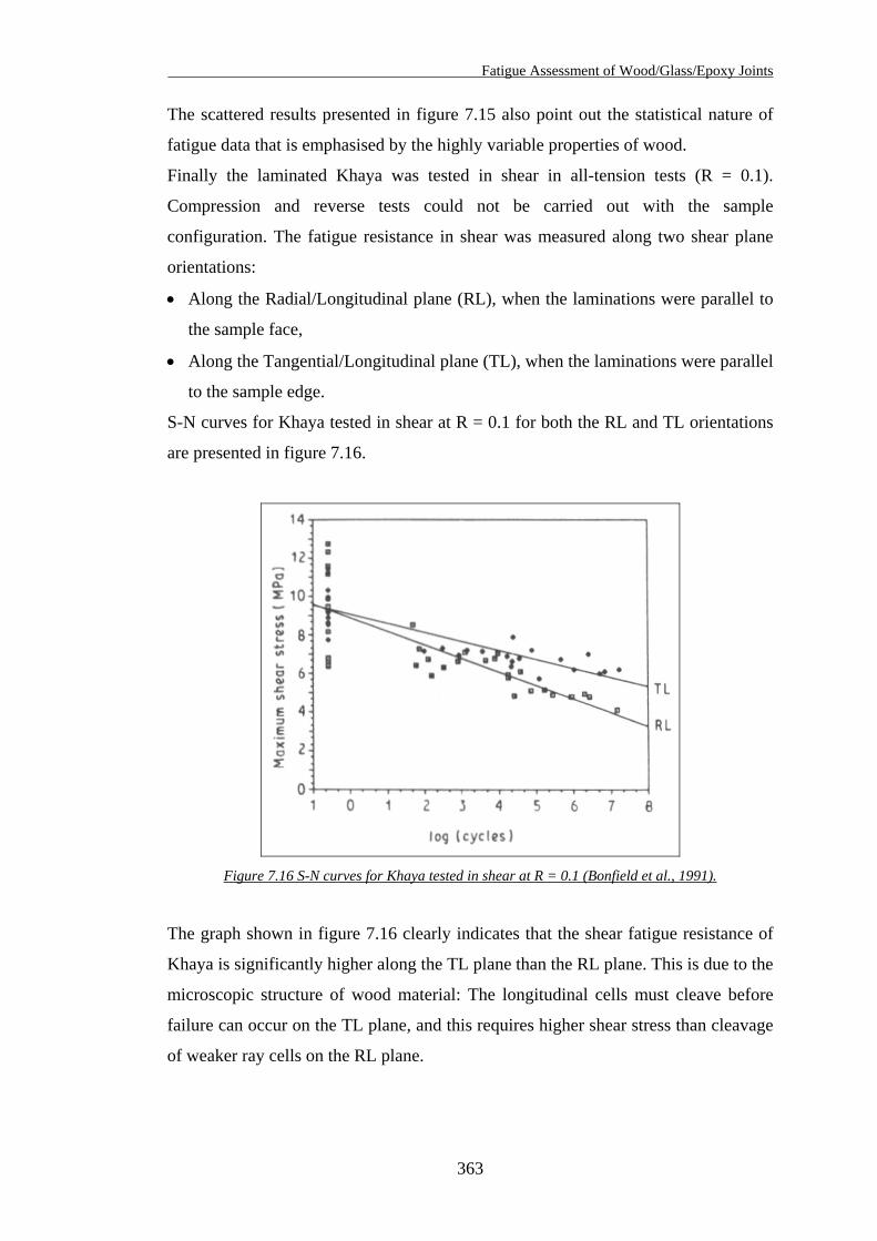
Fatigue Assessment of Wood/Glass/Epoxy Joints
The scattered results presented in figure 7.15 also point out the statistical nature of
fatigue data that is emphasised by the highly variable properties of wood.
Finally the laminated Khaya was tested in shear in all-tension tests (R = 0.1).
Compression and reverse tests could not be carried out with the sample
configuration. The fatigue resistance in shear was measured along two shear plane
orientations:
• Along the Radial/Longitudinal plane (RL), when the laminations were parallel to
the sample face,
• Along the Tangential/Longitudinal plane (TL), when the laminations were parallel
to the sample edge.
S-N curves for Khaya tested in shear at R = 0.1 for both the RL and TL orientations
are presented in figure 7.16.
Figure 7.16 S-N curves for Khaya tested in shear at R = 0.1 (Bonfield et al., 1991).
The graph shown in figure 7.16 clearly indicates that the shear fatigue resistance of
Khaya is significantly higher along the TL plane than the RL plane. This is due to the
microscopic structure of wood material: The longitudinal cells must cleave before
failure can occur on the TL plane, and this requires higher shear stress than cleavage
of weaker ray cells on the RL plane.
363
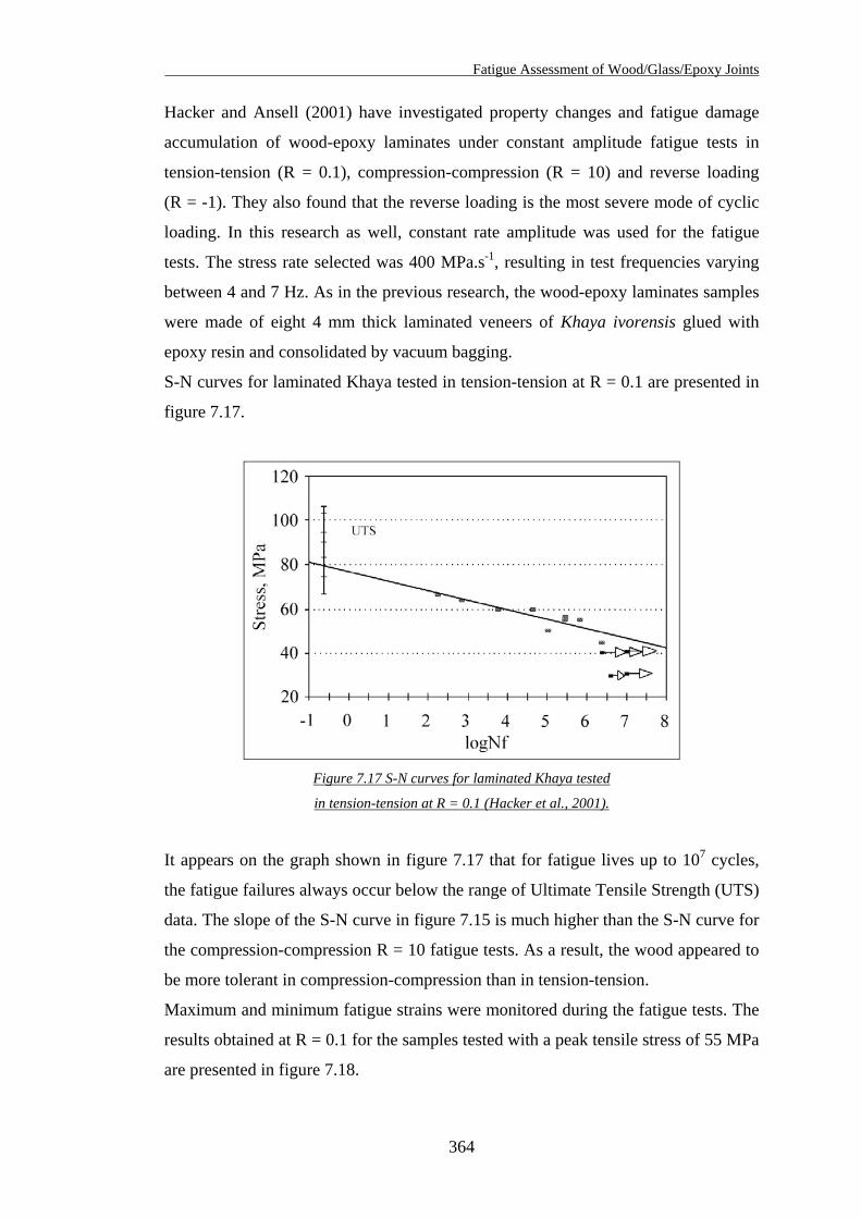
Fatigue Assessment of Wood/Glass/Epoxy Joints
Hacker and Ansell (2001) have investigated property changes and fatigue damage
accumulation of wood-epoxy laminates under constant amplitude fatigue tests in
tension-tension (R = 0.1), compression-compression (R = 10) and reverse loading
(R = -1). They also found that the reverse loading is the most severe mode of cyclic
loading. In this research as well, constant rate amplitude was used for the fatigue
tests. The stress rate selected was 400 MPa.s-1, resulting in test frequencies varying
between 4 and 7 Hz. As in the previous research, the wood-epoxy laminates samples
were made of eight 4 mm thick laminated veneers of Khaya ivorensis glued with
epoxy resin and consolidated by vacuum bagging.
S-N curves for laminated Khaya tested in tension-tension at R = 0.1 are presented in
figure 7.17.
Figure 7.17 S-N curves for laminated Khaya tested
in tension-tension at R = 0.1 (Hacker et al., 2001).
It appears on the graph shown in figure 7.17 that for fatigue lives up to 107 cycles,
the fatigue failures always occur below the range of Ultimate Tensile Strength (UTS)
data. The slope of the S-N curve in figure 7.15 is much higher than the S-N curve for
the compression-compression R = 10 fatigue tests. As a result, the wood appeared to
be more tolerant in compression-compression than in tension-tension.
Maximum and minimum fatigue strains were monitored during the fatigue tests. The
results obtained at R = 0.1 for the samples tested with a peak tensile stress of 55 MPa
are presented in figure 7.18.
364
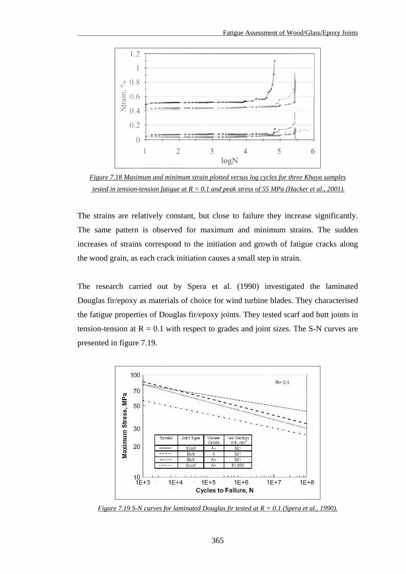
Fatigue Assessment of Wood/Glass/Epoxy Joints
Figure 7.18 Maximum and minimum strain plotted versus log cycles for three Khaya samples
tested in tension-tension fatigue at R = 0.1 and peak stress of 55 MPa (Hacker et al., 2001).
The strains are relatively constant, but close to failure they increase significantly.
The same pattern is observed for maximum and minimum strains. The sudden
increases of strains correspond to the initiation and growth of fatigue cracks along
the wood grain, as each crack initiation causes a small step in strain.
The research carried out by Spera et al. (1990) investigated the laminated
Douglas fir/epoxy as materials of choice for wind turbine blades. They characterised
the fatigue properties of Douglas fir/epoxy joints. They tested scarf and butt joints in
tension-tension at R = 0.1 with respect to grades and joint sizes. The S-N curves are
presented in figure 7.19.
Figure 7.19 S-N curves for laminated Douglas fir tested at R = 0.1 (Spera et al., 1990).
365
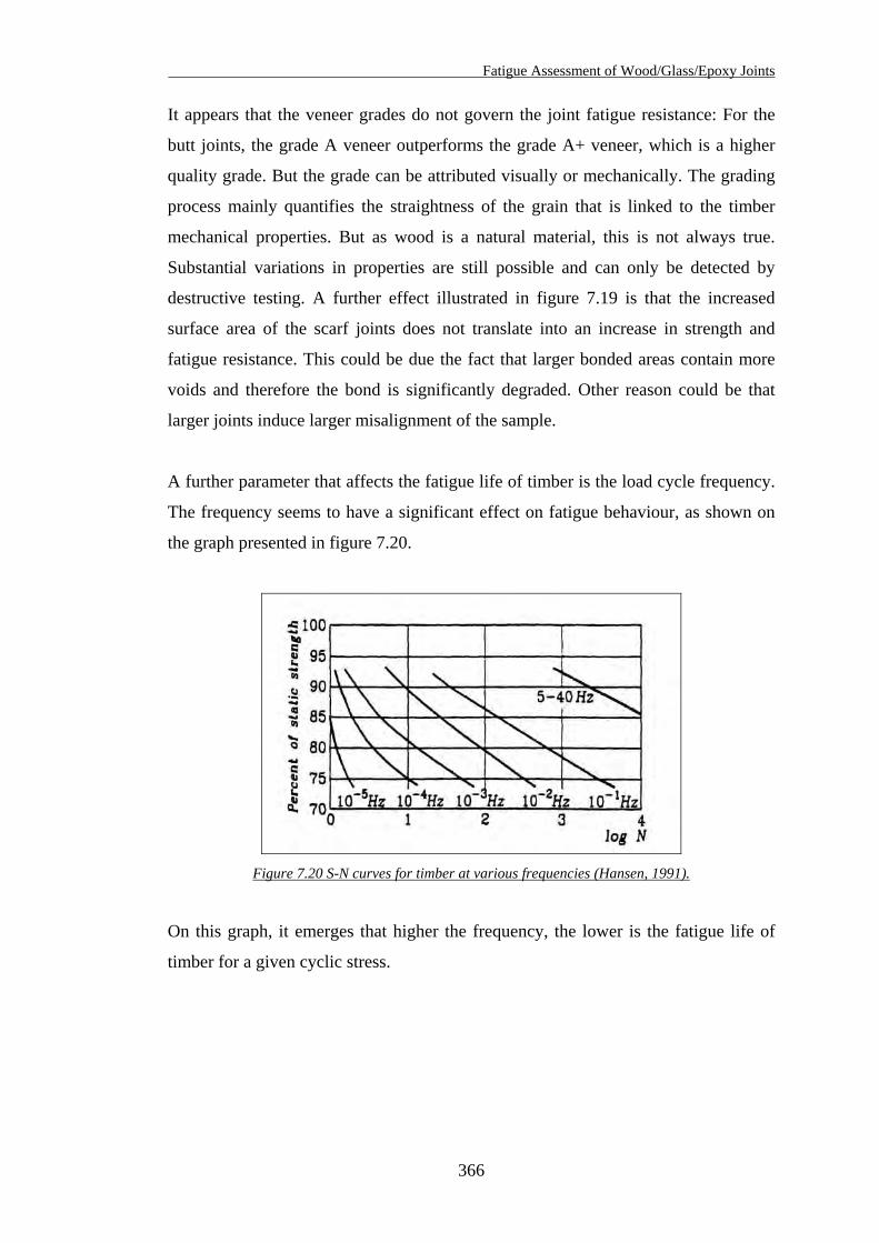
Fatigue Assessment of Wood/Glass/Epoxy Joints
It appears that the veneer grades do not govern the joint fatigue resistance: For the
butt joints, the grade A veneer outperforms the grade A+ veneer, which is a higher
quality grade. But the grade can be attributed visually or mechanically. The grading
process mainly quantifies the straightness of the grain that is linked to the timber
mechanical properties. But as wood is a natural material, this is not always true.
Substantial variations in properties are still possible and can only be detected by
destructive testing. A further effect illustrated in figure 7.19 is that the increased
surface area of the scarf joints does not translate into an increase in strength and
fatigue resistance. This could be due the fact that larger bonded areas contain more
voids and therefore the bond is significantly degraded. Other reason could be that
larger joints induce larger misalignment of the sample.
A further parameter that affects the fatigue life of timber is the load cycle frequency.
The frequency seems to have a significant effect on fatigue behaviour, as shown on
the graph presented in figure 7.20.
Figure 7.20 S-N curves for timber at various frequencies (Hansen, 1991).
On this graph, it emerges that higher the frequency, the lower is the fatigue life of
timber for a given cyclic stress.
366
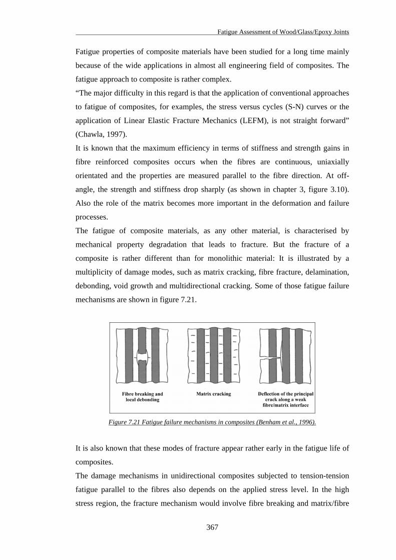
Fatigue Assessment of Wood/Glass/Epoxy Joints
Fatigue properties of composite materials have been studied for a long time mainly
because of the wide applications in almost all engineering field of composites. The
fatigue approach to composite is rather complex.
“The major difficulty in this regard is that the application of conventional approaches
to fatigue of composites, for examples, the stress versus cycles (S-N) curves or the
application of Linear Elastic Fracture Mechanics (LEFM), is not straight forward”
(Chawla, 1997).
It is known that the maximum efficiency in terms of stiffness and strength gains in
fibre reinforced composites occurs when the fibres are continuous, uniaxially
orientated and the properties are measured parallel to the fibre direction. At off-
angle, the strength and stiffness drop sharply (as shown in chapter 3, figure 3.10).
Also the role of the matrix becomes more important in the deformation and failure
processes.
The fatigue of composite materials, as any other material, is characterised by
mechanical property degradation that leads to fracture. But the fracture of a
composite is rather different than for monolithic material: It is illustrated by a
multiplicity of damage modes, such as matrix cracking, fibre fracture, delamination,
debonding, void growth and multidirectional cracking. Some of those fatigue failure
mechanisms are shown in figure 7.21.
Figure 7.21 Fatigue failure mechanisms in composites (Benham et al., 1996).
It is also known that these modes of fracture appear rather early in the fatigue life of
composites.
The damage mechanisms in unidirectional composites subjected to tension-tension
fatigue parallel to the fibres also depends on the applied stress level. In the high
stress region, the fracture mechanism would involve fibre breaking and matrix/fibre
367
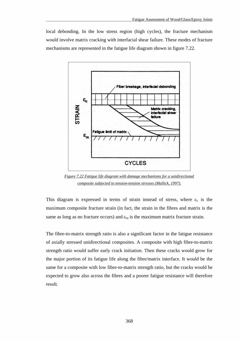
Fatigue Assessment of Wood/Glass/Epoxy Joints
local debonding. In the low stress region (high cycles), the fracture mechanism
would involve matrix cracking with interfacial shear failure. These modes of fracture
mechanisms are represented in the fatigue life diagram shown in figure 7.22.
Figure 7.22 Fatigue life diagram with damage mechanisms for a unidirectional
composite subjected to tension-tension stresses (Mallick, 1997).
This diagram is expressed in terms of strain instead of stress, where εc is the
maximum composite fracture strain (in fact, the strain in the fibres and matrix is the
same as long as no fracture occurs) and εm is the maximum matrix fracture strain.
The fibre-to-matrix strength ratio is also a significant factor in the fatigue resistance
of axially stressed unidirectional composites. A composite with high fibre-to-matrix
strength ratio would suffer early crack initiation. Then these cracks would grow for
the major portion of its fatigue life along the fibre/matrix interface. It would be the
same for a composite with low fibre-to-matrix strength ratio, but the cracks would be
expected to grow also across the fibres and a poorer fatigue resistance will therefore
result.
368
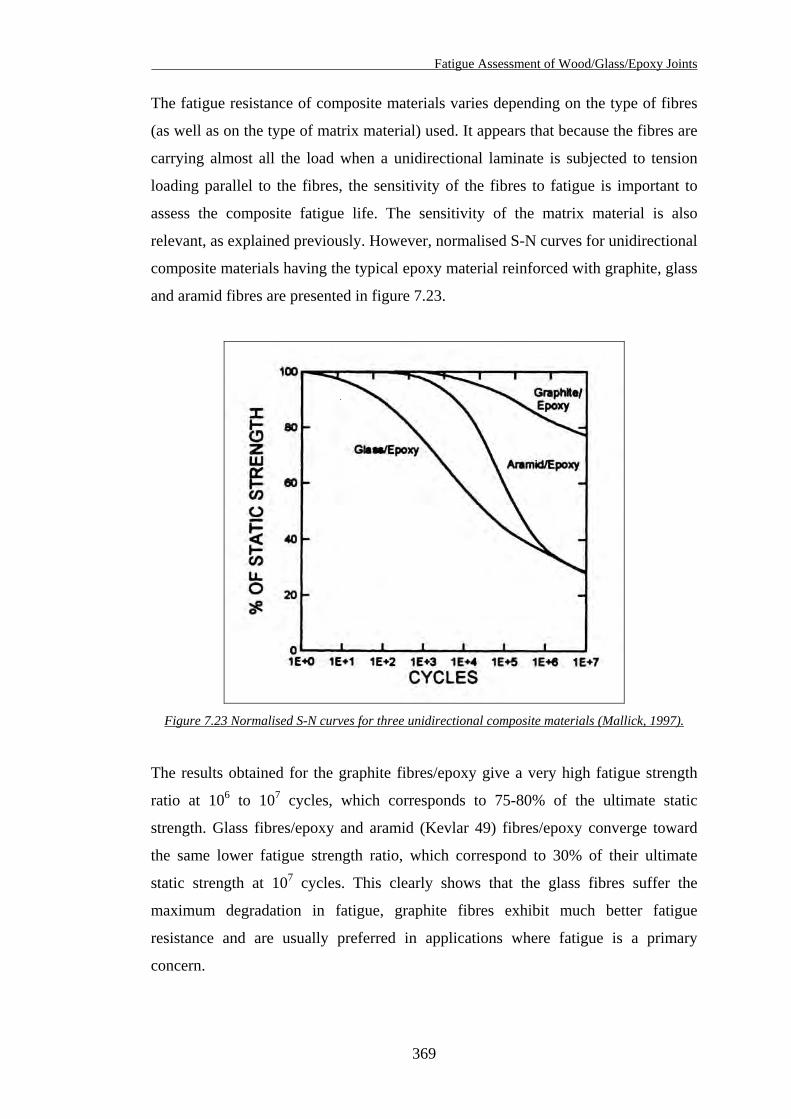
Fatigue Assessment of Wood/Glass/Epoxy Joints
The fatigue resistance of composite materials varies depending on the type of fibres
(as well as on the type of matrix material) used. It appears that because the fibres are
carrying almost all the load when a unidirectional laminate is subjected to tension
loading parallel to the fibres, the sensitivity of the fibres to fatigue is important to
assess the composite fatigue life. The sensitivity of the matrix material is also
relevant, as explained previously. However, normalised S-N curves for unidirectional
composite materials having the typical epoxy material reinforced with graphite, glass
and aramid fibres are presented in figure 7.23.
Figure 7.23 Normalised S-N curves for three unidirectional composite materials (Mallick, 1997).
The results obtained for the graphite fibres/epoxy give a very high fatigue strength
ratio at 106 to 107 cycles, which corresponds to 75-80% of the ultimate static
strength. Glass fibres/epoxy and aramid (Kevlar 49) fibres/epoxy converge toward
the same lower fatigue strength ratio, which correspond to 30% of their ultimate
static strength at 107 cycles. This clearly shows that the glass fibres suffer the
maximum degradation in fatigue, graphite fibres exhibit much better fatigue
resistance and are usually preferred in applications where fatigue is a primary
concern.
369
Fatigue Assessment of Wood/Glass/Epoxy Joints
Another property that characterised the fatigue resistance of composite is the high
damping and low thermal conductivity of the polymeric matrix. This means that
under cyclic stress, the heat generated is not dissipated quickly. This can cause a
temperature difference between the interior and the surface of the composite that can
lead to thermal softening failure if no precautions are taken to dissipate the heat.
However, the internal heating phenomenon depends on the cyclic frequency the
composite is subject to.
“For frequencies less than 20 Hz, the internal heating effects are negligible. For a
given stress level, this temperature difference increases with increasing frequency”
(Chawla, 1997).
As a result, thermal stress was not a concern through the fatigue tests of the
wood/glass/epoxy joints because of the very low frequency of 0.33 Hz used for the
cyclic loads.
Much research work has been carried out on the fatigue of composites, and
particularly on glass fibre composites. Out of this research, one has to be mentioned
because of its relevance to the subject: It is a large research programme about the
applications of glass fibres to build wind turbine blades. This research programme
that is presented in the report from Sutherland (1999) was undertaken in the early
1990s in the United States, sponsored by the Department Of Energy (DOE) and the
Montana State University (MSU). This program aimed at the development of a glass
fibre composite database for wind turbine applications. The DOE/MSU database for
E-glass composites contains over 4500 data points for 130 material systems tested.
A high frequency database provides a significant data set for unidirectional
composites to 108 cycles. The database explores material parameters such as
reinforcement fabric architecture, fibre content, matrix materials and loading
parameters (R values).
The S-N behaviour of composite materials at a constant R value is typically
characterised using either of the two following equations:
( ) (Nm
C log1'loglog0
−=
σσ ) (7.4)
370
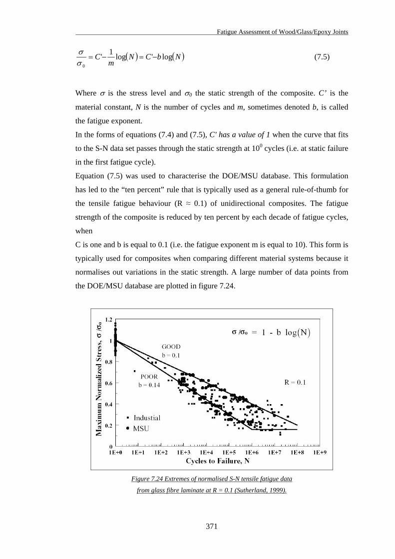
Fatigue Assessment of Wood/Glass/Epoxy Joints
( ) (NbCNm
C log'log1'0
−=−=σ
)σ (7.5)
Where σ is the stress level and σ0 the static strength of the composite. C’ is the
material constant, N is the number of cycles and m, sometimes denoted b, is called
the fatigue exponent.
In the forms of equations (7.4) and (7.5), C' has a value of 1 when the curve that fits
to the S-N data set passes through the static strength at 100 cycles (i.e. at static failure
in the first fatigue cycle).
Equation (7.5) was used to characterise the DOE/MSU database. This formulation
has led to the “ten percent” rule that is typically used as a general rule-of-thumb for
the tensile fatigue behaviour (R ≈ 0.1) of unidirectional composites. The fatigue
strength of the composite is reduced by ten percent by each decade of fatigue cycles,
when
C is one and b is equal to 0.1 (i.e. the fatigue exponent m is equal to 10). This form is
typically used for composites when comparing different material systems because it
normalises out variations in the static strength. A large number of data points from
the DOE/MSU database are plotted in figure 7.24.
Figure 7.24 Extremes of normalised S-N tensile fatigue data
from glass fibre laminate at R = 0.1 (Sutherland, 1999).
371
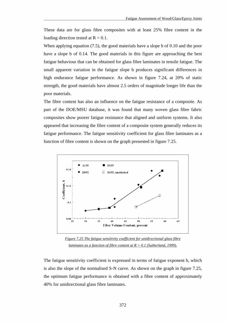
Fatigue Assessment of Wood/Glass/Epoxy Joints
These data are for glass fibre composites with at least 25% fibre content in the
loading direction tested at R = 0.1.
When applying equation (7.5), the good materials have a slope b of 0.10 and the poor
have a slope b of 0.14. The good materials in this figure are approaching the best
fatigue behaviour that can be obtained for glass fibre laminates in tensile fatigue. The
small apparent variation in the fatigue slope b produces significant differences in
high endurance fatigue performance. As shown in figure 7.24, at 20% of static
strength, the good materials have almost 2.5 orders of magnitude longer life than the
poor materials.
The fibre content has also an influence on the fatigue resistance of a composite. As
part of the DOE/MSU database, it was found that many woven glass fibre fabric
composites show poorer fatigue resistance that aligned and uniform systems. It also
appeared that increasing the fibre content of a composite system generally reduces its
fatigue performance. The fatigue sensitivity coefficient for glass fibre laminates as a
function of fibre content is shown on the graph presented in figure 7.25.
Figure 7.25 The fatigue sensitivity coefficient for unidirectional glass fibre
laminates as a function of fibre content at R = 0.1 (Sutherland, 1999).
The fatigue sensitivity coefficient is expressed in terms of fatigue exponent b, which
is also the slope of the normalised S-N curve. As shown on the graph in figure 7.25,
the optimum fatigue performance is obtained with a fibre content of approximately
40% for unidirectional glass fibre laminates.
372

Fatigue Assessment of Wood/Glass/Epoxy Joints
Finally, the influence of the matrix material is the last parameter revealed from the
DOE/MSU database that is of interest in the review of glass fibre composite this
chapter. Three matrix materials are commonly used in the construction of composite,
particularly for wind turbine blades. They are vinyl ester, polyester and epoxy resins.
The effect of matrix material on tensile fatigue in glass fibre laminates with 0° and
±45° plies (for R = 0.1) are presented in figure 7.26.
Figure 7.26 Effect of matrix material on tensile fatigue in glass fibre
laminates with 0° and ±45° plies at R = 0.1 (Sutherland, 1999).
The matrix material has minimal effect on the static and fatigue properties, because
the composite used are unidirectional and mainly stressed in the fibre direction. Note
that the laminates used in figure 7.26 were unstitched 0°/±45°/0° composite plies.
Similar results were obtained in both compressive and reverse loading.
The review of fatigue properties of wood, wood/epoxy laminates, glass fibre/epoxy
composites presented in this section have shown many characteristics that can be
found in wood/glass/epoxy joints. The next step before the fatigue characteristics of
wood/glass/epoxy joints can be drawn, is to identify how fatigue is defined and
applied in the current timber design codes.
373
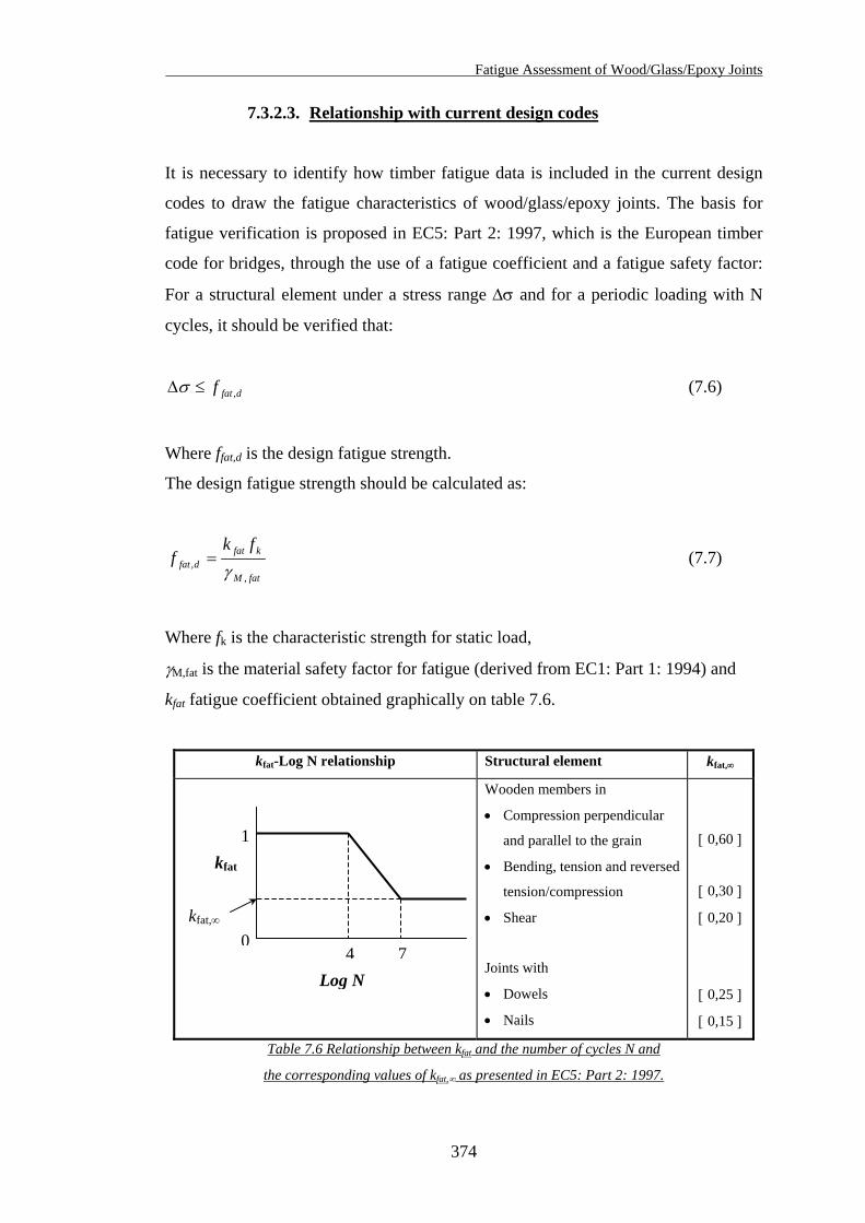
Fatigue Assessment of Wood/Glass/Epoxy Joints
7.3.2.3. Relationship with current design codes
It is necessary to identify how timber fatigue data is included in the current design
codes to draw the fatigue characteristics of wood/glass/epoxy joints. The basis for
fatigue verification is proposed in EC5: Part 2: 1997, which is the European timber
code for bridges, through the use of a fatigue coefficient and a fatigue safety factor:
For a structural element under a stress range ∆σ and for a periodic loading with N
cycles, it should be verified that:
dfatf ,≤∆σ (7.6)
Where ffat,d is the design fatigue strength.
The design fatigue strength should be calculated as:
fatM
kfatdfat
fkf
,, γ
= (7.7)
Where fk is the characteristic strength for static load,
γM,fat is the material safety factor for fatigue (derived from EC1: Part 1: 1994) and
kfat fatigue coefficient obtained graphically on table 7.6.
kfat-Log N relationship Structural element kfat,∞
Wooden members in
• Compression perpendicular
and parallel to the grain
• Bending, tension and reversed
tension/compression
• Shear
Joints with
• Dowels
• Nails
[ 0,60 ]
[ 0,30 ]
[ 0,20 ]
[ 0,25 ]
[ 0,15 ]
0
1kfat
kfat,∞
4 7Log N
Table 7.6 Relationship between kfat and the number of cycles N and
the corresponding values of kfat, ∞ as presented in EC5: Part 2: 1997.
374
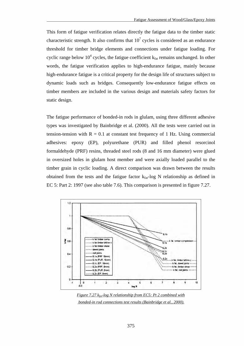
Fatigue Assessment of Wood/Glass/Epoxy Joints
This form of fatigue verification relates directly the fatigue data to the timber static
characteristic strength. It also confirms that 107 cycles is considered as an endurance
threshold for timber bridge elements and connections under fatigue loading. For
cyclic range below 104 cycles, the fatigue coefficient kfat remains unchanged. In other
words, the fatigue verification applies to high-endurance fatigue, mainly because
high-endurance fatigue is a critical property for the design life of structures subject to
dynamic loads such as bridges. Consequently low-endurance fatigue effects on
timber members are included in the various design and materials safety factors for
static design.
The fatigue performance of bonded-in rods in glulam, using three different adhesive
types was investigated by Bainbridge et al. (2000). All the tests were carried out in
tension-tension with R = 0.1 at constant test frequency of 1 Hz. Using commercial
adhesives: epoxy (EP), polyurethane (PUR) and filled phenol resorcinol
formaldehyde (PRF) resins, threaded steel rods (8 and 16 mm diameter) were glued
in oversized holes in glulam host member and were axially loaded parallel to the
timber grain in cyclic loading. A direct comparison was drawn between the results
obtained from the tests and the fatigue factor kfat-log N relationship as defined in
EC 5: Part 2: 1997 (see also table 7.6). This comparison is presented in figure 7.27.
Figure 7.27 kfat-log N relationship from EC5: Pt 2 combined with
bonded-in rod connections test results (Bainbridge et al., 2000).
375
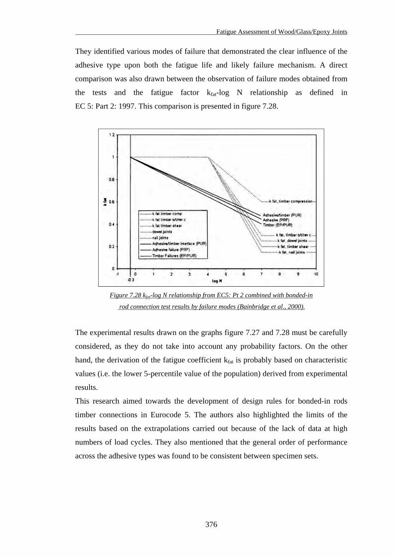
Fatigue Assessment of Wood/Glass/Epoxy Joints
They identified various modes of failure that demonstrated the clear influence of the
adhesive type upon both the fatigue life and likely failure mechanism. A direct
comparison was also drawn between the observation of failure modes obtained from
the tests and the fatigue factor kfat-log N relationship as defined in
EC 5: Part 2: 1997. This comparison is presented in figure 7.28.
Figure 7.28 kfat-log N relationship from EC5: Pt 2 combined with bonded-in
rod connection test results by failure modes (Bainbridge et al., 2000).
The experimental results drawn on the graphs figure 7.27 and 7.28 must be carefully
considered, as they do not take into account any probability factors. On the other
hand, the derivation of the fatigue coefficient kfat is probably based on characteristic
values (i.e. the lower 5-percentile value of the population) derived from experimental
results.
This research aimed towards the development of design rules for bonded-in rods
timber connections in Eurocode 5. The authors also highlighted the limits of the
results based on the extrapolations carried out because of the lack of data at high
numbers of load cycles. They also mentioned that the general order of performance
across the adhesive types was found to be consistent between specimen sets.
376
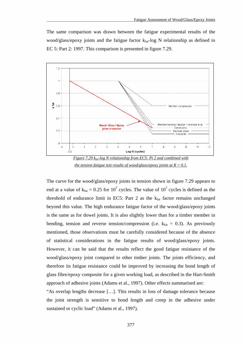
Fatigue Assessment of Wood/Glass/Epoxy Joints
The same comparison was drawn between the fatigue experimental results of the
wood/glass/epoxy joints and the fatigue factor kfat-log N relationship as defined in
EC 5: Part 2: 1997. This comparison is presented in figure 7.29.
Figure 7.29 kfat-log N relationship from EC5: Pt 2 and combined with
the tension fatigue test results of wood/glass/epoxy joints at R = 0.1.
The curve for the wood/glass/epoxy joints in tension shown in figure 7.29 appears to
end at a value of kfat = 0.25 for 107 cycles. The value of 107 cycles is defined as the
threshold of endurance limit in EC5: Part 2 as the kfat factor remains unchanged
beyond this value. The high endurance fatigue factor of the wood/glass/epoxy joints
is the same as for dowel joints. It is also slightly lower than for a timber member in
bending, tension and reverse tension/compression (i.e. kfat = 0.3). As previously
mentioned, those observations must be carefully considered because of the absence
of statistical considerations in the fatigue results of wood/glass/epoxy joints.
However, it can be said that the results reflect the good fatigue resistance of the
wood/glass/epoxy joint compared to other timber joints. The joints efficiency, and
therefore its fatigue resistance could be improved by increasing the bond length of
glass fibre/epoxy composite for a given working load, as described in the Hart-Smith
approach of adhesive joints (Adams et al., 1997). Other effects summarised are:
“As overlap lengths decrease […]. This results in loss of damage tolerance because
the joint strength is sensitive to bond length and creep in the adhesive under
sustained or cyclic load” (Adams et al., 1997).
377
Fatigue Assessment of Wood/Glass/Epoxy Joints
The results presented in figure 7.29 can be directly compared with those from
Bainbridge et al. (2000), previously presented, for the following reasons:
• The fatigue tests were carried out in tension-tension with the same loading mode
of R = 0.1.
• The fatigue tests were also carried out at similar frequency range (i.e. 0.33 Hz for
the wood/glass/epoxy joints and 1 Hz for the bonded-in rods connections).
The fatigue results from bonded-in rod connections appear to display higher fatigue
resistance than the wood/glass/epoxy joints, whether the comparison is made with
the results obtained for various bonded-in rod configurations (see figure 7.27) or with
the results obtained for various adhesive types (see figure 7.28). But here again, the
anchorage length of the rods used (160 mm), their diameters (16 mm for 6.1 results
and 8 mm for the 6.2 results) and the section of timber used (120 × 120 mm for
6.1 results and 70 × 70 mm for the 6.2 results) must be brought forward to enable a
potential comparison of both systems.
Sections of timber are of the same size range as those used for the wood/glass/epoxy
joints. However the anchorage length of the rods used is greater compared to the 100
mm length of composite bonded on both faces of either timber piece that compose
the wood/glass/epoxy joints. As a result, the bonded-in rod connections and the
wood/glass/epoxy joints cannot be compared because their geometrical
configurations are radically different. However, in relation to their static failure
loads, the fatigue resistance of bonded-in rods connections is generally higher than
for the wood/glass/epoxy joints.
Other properties of the wood/glass/epoxy joints were also measured during the
fatigue tests as described in the following section.
378
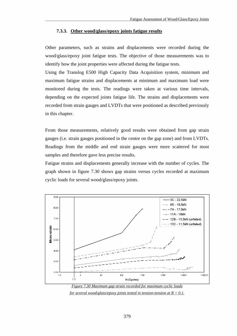
Fatigue Assessment of Wood/Glass/Epoxy Joints
7.3.3. Other wood/glass/epoxy joints fatigue results
Other parameters, such as strains and displacements were recorded during the
wood/glass/epoxy joint fatigue tests. The objective of those measurements was to
identify how the joint properties were affected during the fatigue tests.
Using the Translog E500 High Capacity Data Acquisition system, minimum and
maximum fatigue strains and displacements at minimum and maximum load were
monitored during the tests. The readings were taken at various time intervals,
depending on the expected joints fatigue life. The strains and displacements were
recorded from strain gauges and LVDTs that were positioned as described previously
in this chapter.
From those measurements, relatively good results were obtained from gap strain
gauges (i.e. strain gauges positioned in the centre on the gap zone) and from LVDTs.
Readings from the middle and end strain gauges were more scattered for most
samples and therefore gave less precise results.
Fatigue strains and displacements generally increase with the number of cycles. The
graph shown in figure 7.30 shows gap strains versus cycles recorded at maximum
cyclic loads for several wood/glass/epoxy joints.
Figure 7.30 Maximum gap strain recorded for maximum cyclic loads
for several wood/glass/epoxy joints tested in tension-tension at R = 0.1.
379
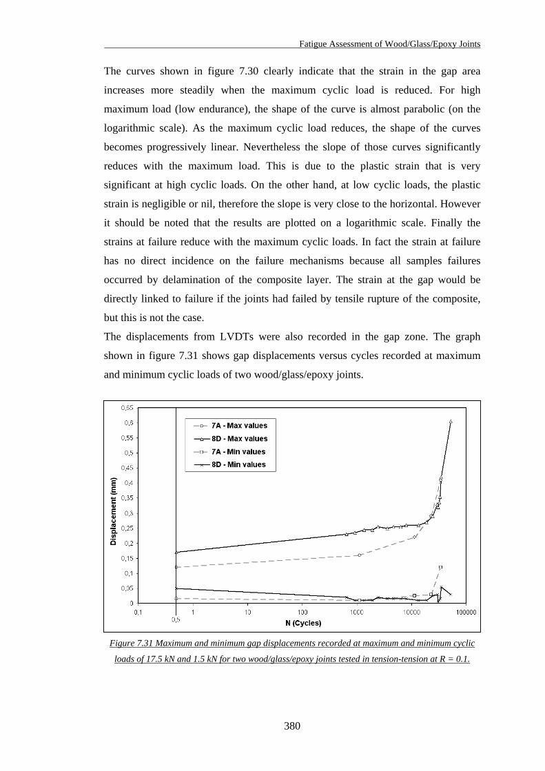
Fatigue Assessment of Wood/Glass/Epoxy Joints
The curves shown in figure 7.30 clearly indicate that the strain in the gap area
increases more steadily when the maximum cyclic load is reduced. For high
maximum load (low endurance), the shape of the curve is almost parabolic (on the
logarithmic scale). As the maximum cyclic load reduces, the shape of the curves
becomes progressively linear. Nevertheless the slope of those curves significantly
reduces with the maximum load. This is due to the plastic strain that is very
significant at high cyclic loads. On the other hand, at low cyclic loads, the plastic
strain is negligible or nil, therefore the slope is very close to the horizontal. However
it should be noted that the results are plotted on a logarithmic scale. Finally the
strains at failure reduce with the maximum cyclic loads. In fact the strain at failure
has no direct incidence on the failure mechanisms because all samples failures
occurred by delamination of the composite layer. The strain at the gap would be
directly linked to failure if the joints had failed by tensile rupture of the composite,
but this is not the case.
The displacements from LVDTs were also recorded in the gap zone. The graph
shown in figure 7.31 shows gap displacements versus cycles recorded at maximum
and minimum cyclic loads of two wood/glass/epoxy joints.
Figure 7.31 Maximum and minimum gap displacements recorded at maximum and minimum cyclic
loads of 17.5 kN and 1.5 kN for two wood/glass/epoxy joints tested in tension-tension at R = 0.1.
380
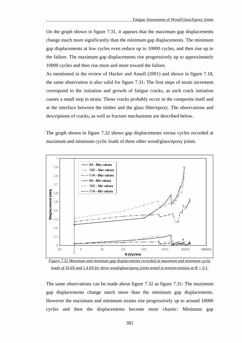
Fatigue Assessment of Wood/Glass/Epoxy Joints
On the graph shown in figure 7.31, it appears that the maximum gap displacements
change much more significantly than the minimum gap displacements. The minimum
gap displacements at low cycles even reduce up to 10000 cycles, and then rise up to
the failure. The maximum gap displacements rise progressively up to approximately
10000 cycles and then rise more and more toward the failure.
As mentioned in the review of Hacker and Ansell (2001) and shown in figure 7.18,
the same observation is also valid for figure 7.31: The first steps of strain increment
correspond to the initiation and growth of fatigue cracks, as each crack initiation
causes a small step in strain. Those cracks probably occur in the composite itself and
at the interface between the timber and the glass fibre/epoxy. The observations and
descriptions of cracks, as well as fracture mechanisms are described below.
The graph shown in figure 7.32 shows gap displacements versus cycles recorded at
maximum and minimum cyclic loads of three other wood/glass/epoxy joints.
Figure 7.32 Maximum and minimum gap displacements recorded at maximum and minimum cyclic
loads of 16 kN and 1.4 kN for three wood/glass/epoxy joints tested in tension-tension at R = 0.1.
The same observations can be made about figure 7.32 as figure 7.31: The maximum
gap displacements change much more than the minimum gap displacements.
However the maximum and minimum strains rise progressively up to around 10000
cycles and then the displacements become more chaotic: Minimum gap
381
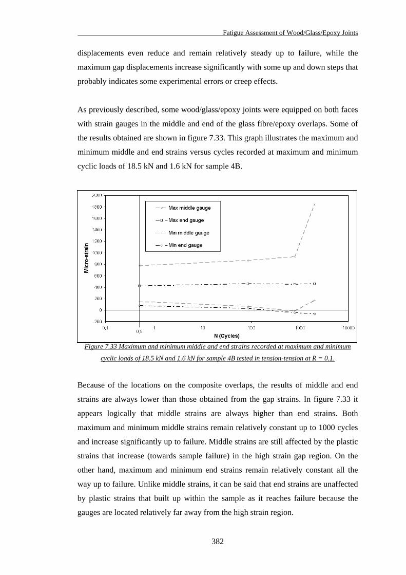
Fatigue Assessment of Wood/Glass/Epoxy Joints
displacements even reduce and remain relatively steady up to failure, while the
maximum gap displacements increase significantly with some up and down steps that
probably indicates some experimental errors or creep effects.
As previously described, some wood/glass/epoxy joints were equipped on both faces
with strain gauges in the middle and end of the glass fibre/epoxy overlaps. Some of
the results obtained are shown in figure 7.33. This graph illustrates the maximum and
minimum middle and end strains versus cycles recorded at maximum and minimum
cyclic loads of 18.5 kN and 1.6 kN for sample 4B.
Figure 7.33 Maximum and minimum middle and end strains recorded at maximum and minimum
cyclic loads of 18.5 kN and 1.6 kN for sample 4B tested in tension-tension at R = 0.1.
Because of the locations on the composite overlaps, the results of middle and end
strains are always lower than those obtained from the gap strains. In figure 7.33 it
appears logically that middle strains are always higher than end strains. Both
maximum and minimum middle strains remain relatively constant up to 1000 cycles
and increase significantly up to failure. Middle strains are still affected by the plastic
strains that increase (towards sample failure) in the high strain gap region. On the
other hand, maximum and minimum end strains remain relatively constant all the
way up to failure. Unlike middle strains, it can be said that end strains are unaffected
by plastic strains that built up within the sample as it reaches failure because the
gauges are located relatively far away from the high strain region.
382
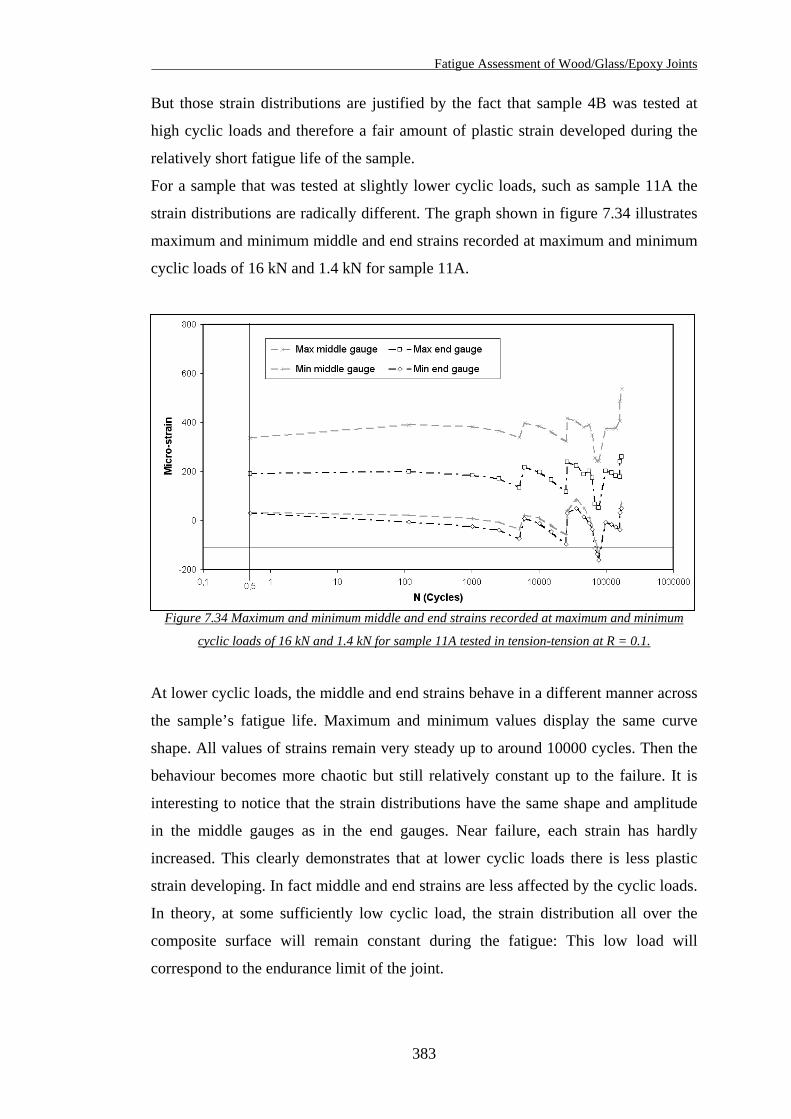
Fatigue Assessment of Wood/Glass/Epoxy Joints
But those strain distributions are justified by the fact that sample 4B was tested at
high cyclic loads and therefore a fair amount of plastic strain developed during the
relatively short fatigue life of the sample.
For a sample that was tested at slightly lower cyclic loads, such as sample 11A the
strain distributions are radically different. The graph shown in figure 7.34 illustrates
maximum and minimum middle and end strains recorded at maximum and minimum
cyclic loads of 16 kN and 1.4 kN for sample 11A.
Figure 7.34 Maximum and minimum middle and end strains recorded at maximum and minimum
cyclic loads of 16 kN and 1.4 kN for sample 11A tested in tension-tension at R = 0.1.
At lower cyclic loads, the middle and end strains behave in a different manner across
the sample’s fatigue life. Maximum and minimum values display the same curve
shape. All values of strains remain very steady up to around 10000 cycles. Then the
behaviour becomes more chaotic but still relatively constant up to the failure. It is
interesting to notice that the strain distributions have the same shape and amplitude
in the middle gauges as in the end gauges. Near failure, each strain has hardly
increased. This clearly demonstrates that at lower cyclic loads there is less plastic
strain developing. In fact middle and end strains are less affected by the cyclic loads.
In theory, at some sufficiently low cyclic load, the strain distribution all over the
composite surface will remain constant during the fatigue: This low load will
correspond to the endurance limit of the joint.
383
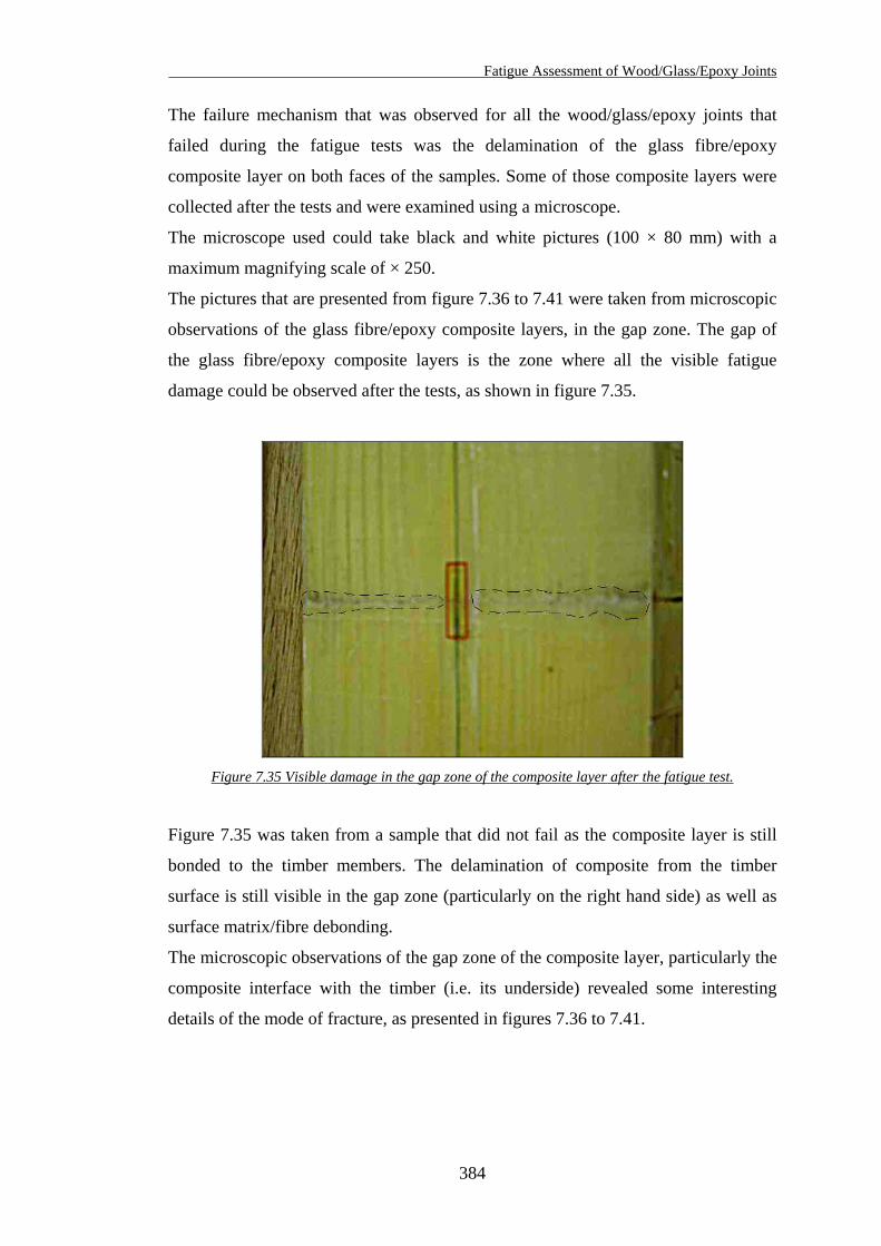
Fatigue Assessment of Wood/Glass/Epoxy Joints
The failure mechanism that was observed for all the wood/glass/epoxy joints that
failed during the fatigue tests was the delamination of the glass fibre/epoxy
composite layer on both faces of the samples. Some of those composite layers were
collected after the tests and were examined using a microscope.
The microscope used could take black and white pictures (100 × 80 mm) with a
maximum magnifying scale of × 250.
The pictures that are presented from figure 7.36 to 7.41 were taken from microscopic
observations of the glass fibre/epoxy composite layers, in the gap zone. The gap of
the glass fibre/epoxy composite layers is the zone where all the visible fatigue
damage could be observed after the tests, as shown in figure 7.35.
Figure 7.35 Visible damage in the gap zone of the composite layer after the fatigue test.
Figure 7.35 was taken from a sample that did not fail as the composite layer is still
bonded to the timber members. The delamination of composite from the timber
surface is still visible in the gap zone (particularly on the right hand side) as well as
surface matrix/fibre debonding.
The microscopic observations of the gap zone of the composite layer, particularly the
composite interface with the timber (i.e. its underside) revealed some interesting
details of the mode of fracture, as presented in figures 7.36 to 7.41.
384
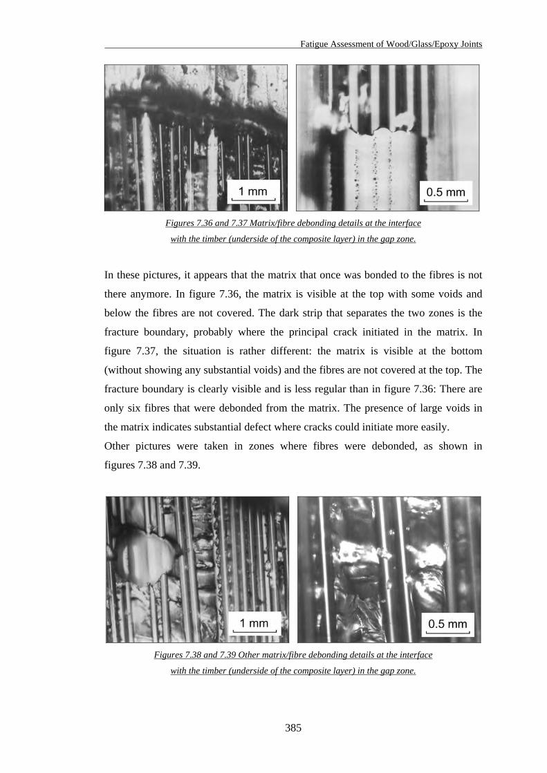
Fatigue Assessment of Wood/Glass/Epoxy Joints
Figures 7.36 and 7.37 Matrix/fibre debonding details at the interface
with the timber (underside of the composite layer) in the gap zone.
In these pictures, it appears that the matrix that once was bonded to the fibres is not
there anymore. In figure 7.36, the matrix is visible at the top with some voids and
below the fibres are not covered. The dark strip that separates the two zones is the
fracture boundary, probably where the principal crack initiated in the matrix. In
figure 7.37, the situation is rather different: the matrix is visible at the bottom
(without showing any substantial voids) and the fibres are not covered at the top. The
fracture boundary is clearly visible and is less regular than in figure 7.36: There are
only six fibres that were debonded from the matrix. The presence of large voids in
the matrix indicates substantial defect where cracks could initiate more easily.
Other pictures were taken in zones where fibres were debonded, as shown in
figures 7.38 and 7.39.
Figures 7.38 and 7.39 Other matrix/fibre debonding details at the interface
with the timber (underside of the composite layer) in the gap zone.
385
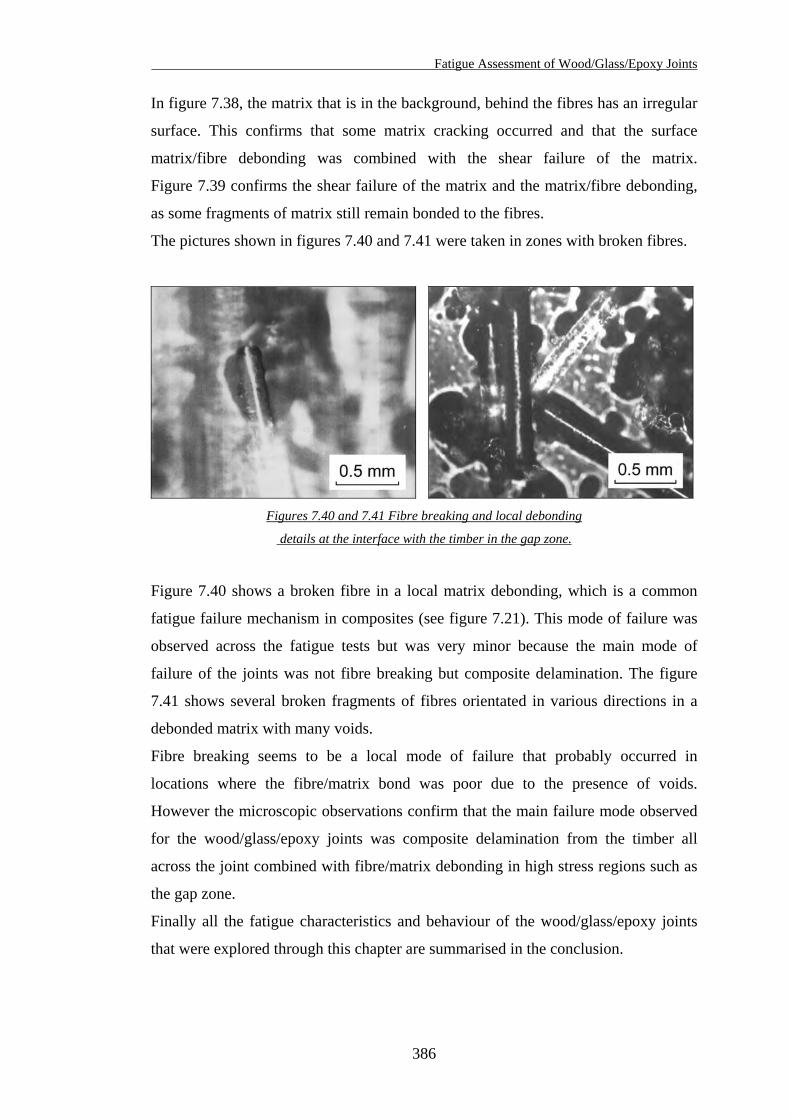
Fatigue Assessment of Wood/Glass/Epoxy Joints
In figure 7.38, the matrix that is in the background, behind the fibres has an irregular
surface. This confirms that some matrix cracking occurred and that the surface
matrix/fibre debonding was combined with the shear failure of the matrix.
Figure 7.39 confirms the shear failure of the matrix and the matrix/fibre debonding,
as some fragments of matrix still remain bonded to the fibres.
The pictures shown in figures 7.40 and 7.41 were taken in zones with broken fibres.
Figures 7.40 and 7.41 Fibre breaking and local debonding
details at the interface with the timber in the gap zone.
Figure 7.40 shows a broken fibre in a local matrix debonding, which is a common
fatigue failure mechanism in composites (see figure 7.21). This mode of failure was
observed across the fatigue tests but was very minor because the main mode of
failure of the joints was not fibre breaking but composite delamination. The figure
7.41 shows several broken fragments of fibres orientated in various directions in a
debonded matrix with many voids.
Fibre breaking seems to be a local mode of failure that probably occurred in
locations where the fibre/matrix bond was poor due to the presence of voids.
However the microscopic observations confirm that the main failure mode observed
for the wood/glass/epoxy joints was composite delamination from the timber all
across the joint combined with fibre/matrix debonding in high stress regions such as
the gap zone.
Finally all the fatigue characteristics and behaviour of the wood/glass/epoxy joints
that were explored through this chapter are summarised in the conclusion.
386
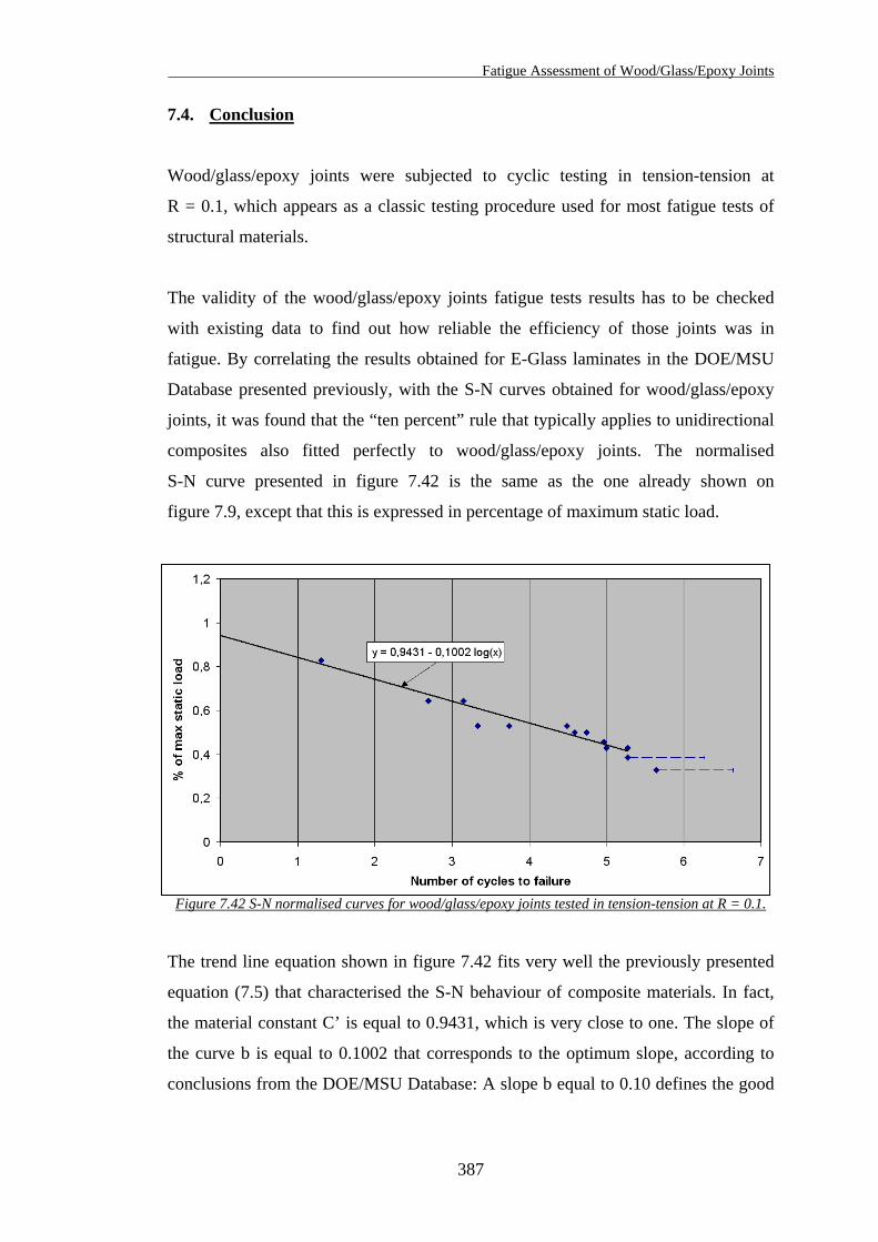
Fatigue Assessment of Wood/Glass/Epoxy Joints
7.4. Conclusion
Wood/glass/epoxy joints were subjected to cyclic testing in tension-tension at
R = 0.1, which appears as a classic testing procedure used for most fatigue tests of
structural materials.
The validity of the wood/glass/epoxy joints fatigue tests results has to be checked
with existing data to find out how reliable the efficiency of those joints was in
fatigue. By correlating the results obtained for E-Glass laminates in the DOE/MSU
Database presented previously, with the S-N curves obtained for wood/glass/epoxy
joints, it was found that the “ten percent” rule that typically applies to unidirectional
composites also fitted perfectly to wood/glass/epoxy joints. The normalised
S-N curve presented in figure 7.42 is the same as the one already shown on
figure 7.9, except that this is expressed in percentage of maximum static load.
Figure 7.42 S-N normalised curves for wood/glass/epoxy joints tested in tension-tension at R = 0.1.
The trend line equation shown in figure 7.42 fits very well the previously presented
equation (7.5) that characterised the S-N behaviour of composite materials. In fact,
the material constant C’ is equal to 0.9431, which is very close to one. The slope of
the curve b is equal to 0.1002 that corresponds to the optimum slope, according to
conclusions from the DOE/MSU Database: A slope b equal to 0.10 defines the good
387
Fatigue Assessment of Wood/Glass/Epoxy Joints
materials as the curve is approaching the best fatigue behaviour that can be obtained
for glass fibre laminates in tensile fatigue (see figure 7.24).
The similarities between the equations of the S-N curves indicate that the results
obtained from the fatigue tests are reliable and reflect the fatigue response of well-
fabricated wood/glass/epoxy joints. It also highlights that the fatigue response of
wood/glass/epoxy joints is dominated by the composite behaviour rather than the
main material that is timber.
Using the results obtained from the fatigue tests with the background information
presented and described in the literature review of this chapter, the characteristics
that define the fatigue response of the wood/glass/epoxy joints could then be drawn.
The factors that affect the fatigue behaviour of the wood/glass/epoxy joints are
related to the materials that compose the joints. The fatigue characteristics presented
in the following bullet points were described in the papers review throughout this
chapter
• Fatigue characteristics linked to the timber material:
- Timber is a naturally grown material therefore its mechanical properties are
very variable. It must always be graded according to the standards before being
used for construction.
- Tsai and Ansell (1990) found that fatigue life of timber is independent of the
species and is affected by the moisture content. The fatigue life reduces with
increasing moisture content (above 12%).
- Tsai and Ansell (1990) identified that the fatigue damage accumulation at
cellular level is associated with the formation of kinks in the cell walls,
compression creases and cracks in the timber. As timber is an anisotropic
material, the damage is of different nature depending on the stress direction.
- Hansen (1991) highlighted that the fatigue resistance of timber is affected by
the loading frequency. As a result, the higher the frequency, the lower is the
fatigue life of timber for a given cyclic stress.
- Tsai and Ansell (1990), as well as Hacker and Ansell (2001) observed that the
most severe mode of cyclic loading for timber is the fully reversed loading at
R = -1.
388
Fatigue Assessment of Wood/Glass/Epoxy Joints
- Bonfield and Ansell (1991) identified that fatigue lives measured in all-tension
are significantly longer than all-compression tests.
- Bonfield and Ansell (1991) found that the fatigue resistance of shear was
higher along the TL plane than the RL plane for Khaya wood. Assuming the
same behaviour could be obtained for European spruce, the fatigue resistance
of wood/glass/epoxy joints could be improved as the delamination of the
composite produced shear action of the timber members along the RL plane.
• Fatigue characteristics linked to the glass fibre/epoxy composite:
- Maximum efficiency in terms of stiffness and strength is obtained with
continuous, unidirectionally orientated fibres and properties measured parallel
to the fibre direction. At off-angle, the strength and stiffness decrease (as
shown in chapter 3, figure 3.10). Then the role of the matrix material becomes
more important in the deformation and failure processes.
- As a result, many woven glass fibre fabric composites show poorer fatigue
resistance than unidirectional systems.
- Matrix material has minimal effect on the static and fatigue properties in
unidirectional composites loaded parallel to the fibres. However for the
wood/glass/epoxy joints, the matrix has a prominent role because it bonds the
materials together and carries the load from the timber to the composite.
- There are many damage modes in composites, such as matrix cracking, fibre
fracture, delamination, debonding, void growth and multidirectional cracking.
Most of those damage modes were observed on the wood/glass/epoxy joints.
- The fibre content is a significant parameter of composites fatigue resistance.
Sutherland (1999) highlighted that increasing the fibre content of a composite
system generally reduces its fatigue performance. The optimum fatigue
performance is obtained with a fibre content of approximately 40% for
unidirectional glass fibre laminates.
- The fibre-to-matrix strength ratio is also a major factor in the fatigue resistance
of axially stressed unidirectional composites. Composite with high fibre-to-
matrix strength ratio will have higher fatigue resistance than the same
composite with lower fibre-to-matrix strength ratio.
389
Fatigue Assessment of Wood/Glass/Epoxy Joints
390
• Fatigue characteristics linked to the wood/glass/epoxy joints composite:
- The quality of fabrication and particularly the bond of the glass fibre/epoxy
composite to the timber are essential to the static and fatigue resistance of the
wood/glass/epoxy joints.
- The failure modes of the wood/glass/epoxy joints can be summarised as fatigue
cracks initiation and growth that developed at the interface between the timber
and the composite in the gap zone. Those cracks also occur in the composite
itself in the gap zone, particularly where the composite has defects (air voids,
unbonded matrix/fibre zones, etc). However the main damage mode that lead
to failure of the joint is only the interface failure between the timber and the
composite in the gap zone.
- The distribution of stresses in the composite, further away from the gap zone is
only significant a high cyclic loads. At low cyclic loads, most of the tensile
stress is transferred from the composite to the timber in the gap zone. The
length of composite has therefore a major role in the fatigue resistance of the
joint. The Hart-Smith approach summarised by Adams et al. (1997) explains
that increasing the composite length would always improve the fatigue
resistance of structural adhesive joints, and therefore for wood/glass/epoxy
joints.
- Wood/glass/epoxy joints were found to have a good fatigue resistance
compared to other timber joints, according to the EC5: Part 2: 1997
recommendations.
CHAPTER 8
CONCLUSIONS
8.1. General conclusions
The general conclusions summarise all the relevant results that were obtained
throughout the research:
• Wood/glass/epoxy joints with uniaxial glass fibre tested in tension with load
parallel to the grain were found the strongest in terms of failure loads and
stiffness. Misalignment of glass fibres to the load and wood grain direction
reduced significantly the strength and stiffness.
• Wood/glass/epoxy joints with biaxial glass fibre tested in tension with load
parallel to the grain failed at lower loads because only half the amount of fibres
was orientated in the load direction. However with the fibres orientated at 30
degrees to the load and the grain, the failure load was even lower but with higher
stiffness.
• The joints were then tested in tension with load not parallel to the grain. For
wood/glass/epoxy joints made of uniaxial glass fibre, the ones tested in tension at
90 degrees to the grain were the strongest in terms of failure loads and stiffness.
Failure loads seemed to decrease as the grain/load angle reduced from 90 to 30
degrees.
• For wood/glass/epoxy joints made of biaxial glass fibre and tested in tension with
load not parallel to the grain, Failure loads were fairly similar at 90 and 60
degrees, and slightly higher at 30 degrees to the grain.
• Performance of wood/glass/epoxy joints is mainly driven by the quality of the
composite to timber bond. The load capacity is governed by the shear strength of
the timber, which is not too affected by the grain orientation. This is confirmed in
391
Conclusions
the work by Gustafsson and Enquist (1993) and Avent (1986) presented in the
literature review.
• The mechanical properties obtained from the small clear samples were in harmony
with published figures of similar species. It confirms the validity of the tests and
that the timber was correctly graded.
• More accurate finite element results were obtained with the 2D models than 3D
models because convergence testing was carried out. FE results were very close to
experimental results for joints made of uniaxial glass fibre and were generally
lower for joints made of biaxial glass fibre.
• The FE analysis confirmed the non-uniform load transfer that occurs on double
lap joints such as wood/glass/epoxy joints. The internal bending effect of the
overlap was identified in the FE analysis and confirmed experimentally. This
phenomenon strongly affected the stress and strain distribution in the joint.
• The S-N curve obtained from the fatigue tests of wood/glass/epoxy joints was
compared with references and indicated that the results were reliable and were
reflecting the fatigue response of well-fabricated joints. The fatigue of
wood/glass/epoxy joints is dominated by the composite behaviour rather than the
timber. The length of composite was found to have a major role in the fatigue
resistance of the joint. Based on literature references (Adams et al., 1997),
improving the fatigue resistance of the wood/glass/epoxy joints for a given cyclic
loading could be achieved by increasing the composite length.
• Finally, the quality of fabrication and particularly the bond of the glass
fibre/epoxy composite to the timber were found to be essential to the static and
fatigue resistance of the joints and should be taken into consideration for design.
The timber surface to be bonded with glass fibres should be preliminary planned
or sanded down, free from defects and excessive humidity.
392
Conclusions
393
8.2. Suggestions for future work
There are several research subjects that should be investigated before a full design
method for wood/glass/epoxy joints could be developed:
• Structural analysis of wood/glass/epoxy joints should be investigated in bending
and compression. The glass fibre/epoxy composite will have a major role to
overcome the premature buckling of the connected timber members (due to joint
misalignment).
• Wood/glass/epoxy joints made of different species (particularly hardwoods) could
be tested to investigate whether the differences between species or timber cell
structures are affecting the strength and durability of the joints.
• Structural analysis of wood/glass/epoxy joints could be investigated with different
bonded lengths and types of glass fibres and different resin types.
• Fatigue analysis of wood/glass/epoxy joints should be investigated in other
loading modes, in compression and particularly in reverse mode (R = -1) as it
appeared in all cited references that this mode is the most severe for fatigue
resistance.
• The behaviour of wood/glass/epoxy joints under fire conditions should also be
explored, in order to give a fire rating for that type of structural joint.
• In a broader research area, the effects of using glass fibres bonded on timber could
also be investigated with the combination of mechanically fastened jointing
systems. In other words, to investigate mechanical joints for wood/glass/epoxy
structural material.
REFERENCES
1. Adams, R.D.; Comyn, J. and Wake, W.C. 1997. Structural adhesive joints in
engineering. Second Edition, Chapman & Hall, London, U.K., 1997.
2. Allwork, M. 1997. Research into the use of epoxy resin and glass fibre
reinforcing joints. BEng Civil Engineering Project Report, Coventry University,
U.K.
3. Ashbee, K. 1993. Fundamental principles of fiber reinforced composites.
Second Edition, Technomic, Pennsylvania, U.S.A., 1993.
4. Askeland, D.R. 1996. The science and engineering of materials. Third Edition,
Chapman & Hall, London, U.K., 1996.
5. Avent R.R.; Emkin, L.Z. and Sanders, P.H. 1978. Behaviour of epoxy repaired
full-scale timber trusses. ASCE Journal of Structural Engineering, Proceedings
of the ASCE, 104(ST6): 933-951.
6. Avent R.R. and Issa, C.A. 1984. Effect of fire on epoxy-repaired timber. ASCE
Journal of Structural Engineering, 110(12): 2858-2875.
7. Avent R.R. 1985. Decay, weathering and epoxy repair of timber. ASCE Journal
of Structural Engineering, 111(2): 328-342.
8. Avent R.R. 1986. Factors affecting strength of epoxy-repaired timber. ASCE
Journal of Structural Engineering, 112(2): 207-221.
9. Avent R.R. 1986. Design criteria for epoxy repair of timber structures. ASCE
Journal of Structural Engineering, 112(2): 222-240.
10. Baker, A. 1997. Joining and repair of aircraft composite structures. Composites
Engineering Handbook, Edited by Mallick, P.K., New York, U.S.A., 1997.
394
References
11. Barbero, E.J. 1999. Introduction to composite materials design. Taylor &
Francis, Philadelphia, U.S.A., 1999.
12. Benham P.P., Crawford R.J. and Armstrong C.G. 1996. Mechanics of
engineering materials. Second Edition, Longman Group, Harlow, U.K., 1996.
13. Biblis, E.J. 1965. Analysis of wood-fiberglass composite beams within and
beyond the elastic region. Forest Products Journal 15(2): 81-88.
14. Bonfield, P.W. and Ansell, M.P. 1991. The fatigue properties of wood in
tension, compression and shear. J. Mat. Sci., 26, 4765-4773, 1991.
15. Booth, L.G. and Reece, P.O. 1967. The structural use of timber. Spon, London,
U.K., 1967.
16. BS EN 408: 1995. Timber structures – Structural timber and glued laminated
timber – Determination of some physical and mechanical properties. British
Standards Institution, London, 1995.
17. BS EN 1193: 1997. Timber structures – Structural timber and glued laminated
timber – Determination of shear strength and mechanical properties
perpendicular to the grain. British Standards Institution, London, 1995.
18. BS EN 26891: 1991. Timber structures – Joints made with mechanical fasteners
– General principles for the determination of strength and deformation
characteristics. British Standards Institution, London, 1995.
19. BS 373: 1957. Methods of testing small clear specimens of timber. British
Standards Institution, London, 1957.
20. BS 5268: Part 2: 1996. Structural use of timber. Part 2. Code of practice for
permissible stress design, materials and workmanship. British Standards
Institution, London, 1996.
395
References
21. BS 5268: Part 3: 1985. Structural use of timber. Part 3. Code of practice for
trussed rafter roofs. British Standards Institution, London, 1985.
22. BS 6399: Part 2: 1995. Code of practice for wind loads. British Standards
Institution, London, 1995.
23. BS 6948: 1989. Mechanically fastened joints in timber and wood-based
materials. British Standards Institution, London, 1989.
24. Bull, J.W. 1994. The practical design of structural elements in timber. Second
Edition, Gower, Aldershot, U.K., 1994.
25. Bulleit, W.M. 1984. Reinforcement of wood materials: A review. Wood and
Fiber Science, 16(3): 391-397.
26. Chawla, K.K. 1998. Composite materials, science and engineering. Second
Edition, Springer-Verlag, New York, U.S.A., 1997.
27. Chen, C.J. 1996. An optimisation of timber joint by fiberglass reinforcements.
Proceedings pp. 811-818, Advanced Composite Materials in Bridges and
Structures, 2nd Int. Conf., Montreal, Canada, 1996.
28. Claisse, P.A. and Davis T.J. 1998. High performance jointing systems for
timber. Construction and Building Materials 12 (1998): 415-425.
29. CP3: Chapter V: Part 2: 1972. Code of basic data for the design of buildings:
Wind loads. British Standards Institution, London, 1972.
30. Cramer, S.M., Shrestha, D. and Fohrell, W.B. 1990. Theoretical consideration of
metal-plate connected wood-splice joints. ASCE Journal of Structural
Engineering, 116(12): 3458-3474.
31. Davis, T.J. 1997. An analysis of the performance of joints in wood composites.
EPSRC Report, Coventry University, 1997.
396
References
32. Dayer, P. 1994. Renforcement par fibre de verre d’assemblages dans la
construction en bois. Mémoire de Diplôme, EPFL (Swiss Federal Institute of
Technology), IBOIS, Lausanne, Switzerland.
33. DD ENV 1991-1: 1994. Eurocode 1 – Basis of design and actions on structures:
Part 1: Basis of design. European Committee for standardisation, Brussels,
1994.
34. DD ENV 1995-1-1: 1994. Eurocode 5 – Design of timber structures: Part 1.1:
General rules and rules for buildings. European Committee for standardisation,
Brussels, 1994.
35. DD ENV 1995-2: 1997. Eurocode 5 – Design of timber structures: Part 2:
Bridges. European Committee for standardisation, Brussels, 1997.
36. Dinwoodie, J.M. 2000. Timber: Its nature and behaviour. E & FN Spon,
London, U.K., 2000.
37. Dmitriev, P.A.; Strizhakov, Y.D. and Ushakov, V.I. 1991. Wooden constructions
with glass-reinforced plastic fastening units. Proceedings vol. 3, pp. 157-163,
Timber Engineering Conference, London, U.K., 1991.
38. Dorey, A.B. and Cheng, J.J.R. 1996. The behavior of GFRP glued laminated
timber beams. Proceedings pp. 787-794, Advanced Composite Materials in
Bridges and Structures, 2nd Int. Conf., Montreal, Canada, 1996.
39. Dorman, E.N. 1969. Epoxy resins. Handbook of Fiberglass and Advanced
Plastic Composites, Edited by Lubin, G., New York, U.S.A., 1969.
40. Dowling, N.E. 1999. Mechanical behavior of materials - Engineering methods
for deformation, fracture and fatigue. Second Edition, Prentice Hall, New
Jersey, U.S.A., 1999.
397
References
41. EN 28970: 1991. Timber structures – Testing of joints made with mechanical
fasteners – Requirements for wood density. European Committee for
standardisation, Brussels, 1991.
42. GangaRao, H.V.S.; Sonti, S.S. and Superfesky, M.C. 1996. Static response of
wood crossties reinforced with composite fabrics. Proceedings pp. 1291-1303,
41st International SAMPE Symposium, March 24-28, 1996.
43. Gebremedhin, K.G. and Crovella, P.L. 1991. Load distribution in metal plate
connectors of tension joints in wood trusses. ASAE (American Society of
Agricultural Engineers), Structures and Environment Division 34(1): 281-287.
44. Gilibert, Y.; Klein, M.L.L. and Rigolot, A. 1988. Mechanical behavior
assessment of epoxy adhesive in double-lap joint. Adhesively Bonded Joints:
Testing, Analysis and design, ASTM STP 981, Philadelphia, 1988, pp.39-53.
45. Glos, P. and Horstmann, H. 1991. Design of glued joints. In proceedings vol. 3,
pp. 77-84, Timber Engineering Conference, London, U.K., 1991.
46. Grimes, G.C. and Bronstad, M.E.1969. Test methods for composites. Handbook
of Fiberglass and Advanced Plastic Composites, Edited by Lubin, G., New
York, U.S.A., 1969.
47. Grinius, V.G. and Noyes, J.V.1969. Design of composite materials. Handbook
of Fiberglass and Advanced Plastic Composites, Edited by Lubin, G., New
York, U.S.A., 1969.
48. Groom, L. and Polensek, A. 1992. Nonlinear modelling of truss-plate joints.
ASCE Journal of Structural Engineering, 118(9): 2514-2530.
49. Gupta, R. and Gebremedhin, K.G. 1990. Destructive testing of metal-plate
connected wood truss joints. ASCE Journal of Structural Engineering, 116(7):
1971-1982.
398
References
50. Gustafsson, J. and Enquist, B. 1993. Adherence of reinforcement to wood.
Advanced materials based on straw and wood – Fibre reinforcement of glulam.
Report No 7, Lund University, Sweden, 1993.
51. Hacker, C.L. and Ansell, M.P. 2001. Fatigue damage and hysteresis in wood-
epoxy laminates. J. Mat. Sci., 36, 609-621, 2001.
52. Haller, P.; Chen, C.J. and Natterer, J. 1996. Experimental study on fiberglass
reinforced and densified timber joints. Proceedings pp. 308-314, Fourth Wood
Engineering Conf., Oct. 28-31, New Orleans, U.S.A., 1996.
53. Hamid, J.H.A. 1997. Stress analysis on adhesive joints. BEng Mechanical
Engineering Project Report, Coventry University, U.K.
54. Hansen, L.P. 1991. Experimental investigation of fatigue properties of laminated
wood beams. Proceedings of the 1991 International Timber Engineering
Conference 4, (Sub-Conference 15), 4.203 - 4.210, London, U.K.
55. Harris, J.A. and Adams, R.D. 1984. Strength prediction of bonded single lap
joints by non-linear finite element methods. Int. Journal of Adhesion and
Adhesives, 4: 65-78.
56. Hibbeler, R.C. 1997. Mechanics of materials. Third Edition, Prentice Hall, New
Jersey, U.S.A., 1997.
57. Hota, V.S. and GangaoRao, P.E. 1997. Sawn and laminated wood beams
wrapped with fiber reinforced plastic composites. Wood design Focus, fall 1997,
pp. 13-18.
58. Jones, R.M. 1999. Mechanics of composite materials. Second Edition, Taylor &
Francis, Philadelphia, U.S.A., 1999.
399

References
59. Juska, T.D. and Puckett, P.M. 1997. Matrix resins and fiber/matrix adhesion.
Composites Engineering Handbook, Edited by Mallick, P.K., New York, U.S.A.,
1997.
60. Kalpakjian, S. and Schmid, S.R. 2001. Manufacturing engineering and
technology. Prentice Hall, New Jersey, U.S.A., 2001.
61. Kaw, A.K. 1997. Mechanics of composite materials. CRC Press, New York,
U.S.A., 1997.
62. Kirby, R. 1998. An investigation into the strength of glass fibre and epoxy resin
composites, and their use for the reinforcement of timber beams. BEng Civil
Engineering Project Report, Coventry University, U.K.
63. Van de Kuilen, J-W.G. 1991. Theoretical and experimental research on glass
fibre reinforced laminated timber beams. Proceedings vol. 3, pp. 226-233,
Timber Engineering Conference, London, U.K., 1991.
64. Laufenberg, T.L.; Rowlands, R.E. and Krueger, G.P. 1984. Economic feasibility
of synthetic fiber reinforced laminated veneer lumber (LVL). Forest Products
Journal, 34(4): 15-22.
65. MacLeod, I.A. 1990. Analytical modelling of structural systems. Ellis Horwood,
Chichester, U.K., 1990.
66. Mall, S. 1997. Laminated polymer matrix composites. Composites Engineering
Handbook, Edited by Mallick, P.K., New York, U.S.A., 1997.
67. Mallick, P.K. 1997. Definitions, classifications and applications. Composites
Engineering Handbook, Edited by Mallick, P.K., New York, U.S.A., 1997.
68. Matthews, F.L. 1987. Jointing fibre-reinforced plastics. Elsevier Applied
Science, London, U.K., 1987.
400
References
69. Matthews, F.L.; Kilty, P.F. and Godwin, E.W. 1982. A review of the strength of
joints in fibre-reinforced plastics. Part 2. Adhesively bonded joints. Composites
31: 29-37.
70. Mettem, C.J. 1986. Structural timber design and technology. Longman
Scientific & Technical, TRADA, Harlow, U.K., 1986.
71. Mettes, D.G. 1969. Glass fibers. Handbook of fiberglass and advanced plastic
composites, Edited by Lubin, G., New York, U.S.A., 1969.
72. Partridge, I.K. 1989. Advanced composites. Elsevier Applied Science, London,
U.K., 1989.
73. prEN 1075: March 1997. Timber structures – Test methods – Joints made of
punched metal plate fasteners. Draft for Public Comment. European Committee
for standardisation, Brussels, 1997.
74. Richards, J.P. 1994. A preliminary investigation into the use of glass fibre
bonded to composite timber sections under simple loading conditions. BEng
Civil Engineering Project Report, Coventry University, U.K.
75. Rowlands, R.E.; Van Deweghe, R.P.; Laufenberg, T.L. and Krueger, G.P. 1986.
Fiber-reinforced wood composites. Wood and Fiber Science, 18(1): 39-57.
76. Saucier, J.R. and Holman, J.A. 1975. Structural particleboard reinforced with
glass fiber – Progress in its development. Forest Products Journal 25(9): 69-72.
77. Sonti, S.S. and GangaRao, H.V.S. 1995. Strength and stiffness evaluations of
wood laminates with composite wraps. Proceedings of the 50th Annual
Conference, Composite Institute, The society of the plastics industry, Inc. Jan.
30-Feb. 1, 1995.
401
References
402
78. Sonti, S.S.; GangaRao, H.V.S. and Talakanti, D.R. 1996. Accelerated aging of
wood-composite members. Proceedings pp. 1632-1641, 41st International
SAMPE Symposium, March 24-28, 1996.
79. Spera, D.A.; Esgar, J.B.; Gougeon, M. and Zuteck, M.D. 1990. Structural
properties of laminated Douglas fir/epoxy composite material. DOE/NASA
Reference Publication 1236, DOE/NASA/20320-76, Cleveland, 1990.
80. Spaun, F.D. 1981. Reinforcement of wood with fiberglass. Forest Products
Journal 31(4): 26-33.
81. Staab, G.H. 1999. Laminar Composites. Butterworth-Heinemann, Woburn,
U.S.A., 1999.
82. Sutherland, H.J. 1999. On the fatigue analysis of wind turbines. SAND99-0089,
Sandia National Laboratories, Albuquerque, New Mexico, 1999.
83. Theakston, F.H. 1965. A feasible Study for strengthening timber beams with
fiberglass. Canadian Agricultural Engineering, Jan. 1965, pp. 17-19.
84. Timber Engineering STEP 1. Basis of design, materials properties, structural
components and joints. First Edition, Centrum Hout, The Netherlands, 1995.
85. Timber Engineering STEP 2. Design – Details and structural systems. First
Edition, Centrum Hout, The Netherlands, 1995.
86. Tsai, K.T. and Ansell, M.P. 1990. The fatigue properties of wood in flexure. J.
Mat. Sci., 22, 865-878, 1990.
87. Wangaard, F.F. 1964. Elastic deflection of wood-fiberglass composite beams.
Forest Products Journal 14(6): 256-260.
88. WIS (Wood information Sheets) 2/3 – 53. Connectors and metal plate fasteners
for structural timber. TRADA, High Wycombe, U.K., 1996.
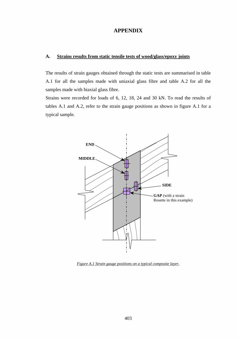
APPENDIX
A. Strains results from static tensile tests of wood/glass/epoxy joints
The results of strain gauges obtained through the static tests are summarised in table
A.1 for all the samples made with uniaxial glass fibre and table A.2 for all the
samples made with biaxial glass fibre.
Strains were recorded for loads of 6, 12, 18, 24 and 30 kN. To read the results of
tables A.1 and A.2, refer to the strain gauge positions as shown in figure A.1 for a
typical sample.
MIDDLE
END
SIDE
GAP (with a strain Rosette in this example)
Figure A.1 Strain gauge positions on a typical composite layer.
403
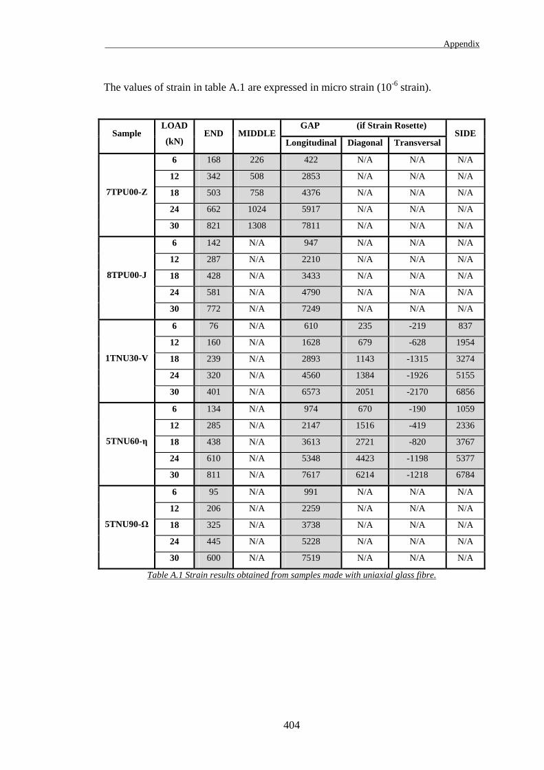
Appendix
The values of strain in table A.1 are expressed in micro strain (10-6 strain).
GAP (if Strain Rosette) Sample
LOAD
(kN) END MIDDLE
Longitudinal Diagonal Transversal SIDE
6 168 226 422 N/A N/A N/A
12 342 508 2853 N/A N/A N/A
18 503 758 4376 N/A N/A N/A
24 662 1024 5917 N/A N/A N/A
7TPU00-Z
30 821 1308 7811 N/A N/A N/A
6 142 N/A 947 N/A N/A N/A
12 287 N/A 2210 N/A N/A N/A
18 428 N/A 3433 N/A N/A N/A
24 581 N/A 4790 N/A N/A N/A
8TPU00-J
30 772 N/A 7249 N/A N/A N/A
6 76 N/A 610 235 -219 837
12 160 N/A 1628 679 -628 1954
18 239 N/A 2893 1143 -1315 3274
24 320 N/A 4560 1384 -1926 5155
1TNU30-V
30 401 N/A 6573 2051 -2170 6856
6 134 N/A 974 670 -190 1059
12 285 N/A 2147 1516 -419 2336
18 438 N/A 3613 2721 -820 3767
24 610 N/A 5348 4423 -1198 5377
5TNU60-η
30 811 N/A 7617 6214 -1218 6784
6 95 N/A 991 N/A N/A N/A
12 206 N/A 2259 N/A N/A N/A
18 325 N/A 3738 N/A N/A N/A
24 445 N/A 5228 N/A N/A N/A
5TNU90-Ω
30 600 N/A 7519 N/A N/A N/A
Table A.1 Strain results obtained from samples made with uniaxial glass fibre.
404
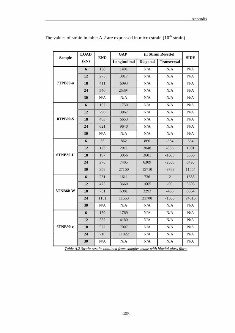
Appendix
The values of strain in table A.2 are expressed in micro strain (10-6 strain).
GAP (if Strain Rosette) Sample
LOAD
(kN) END
Longitudinal Diagonal Transversal SIDE
6 138 1401 N/A N/A N/A
12 275 3817 N/A N/A N/A
18 411 6093 N/A N/A N/A
24 540 25394 N/A N/A N/A
7TPB00-α
30 N/A N/A N/A N/A N/A
6 152 1750 N/A N/A N/A
12 296 3967 N/A N/A N/A
18 463 6653 N/A N/A N/A
24 621 9640 N/A N/A N/A
8TPB00-$
30 N/A N/A N/A N/A N/A
6 55 862 866 -364 834
12 123 2011 2048 -856 1991
18 197 3956 3681 -1603 3666
24 276 7405 6309 -2565 6495
6TNB30-U
30 358 27160 15710 -3783 11554
6 231 1611 736 2 1653
12 475 3660 1665 -90 3606
18 731 6981 3293 -466 6364
24 1151 11553 21708 -1506 24316
5TNB60-W
30 N/A N/A N/A N/A N/A
6 159 1769 N/A N/A N/A
12 332 4180 N/A N/A N/A
18 522 7007 N/A N/A N/A
24 710 11022 N/A N/A N/A
6TNB90-φ
30 N/A N/A N/A N/A N/A
Table A.2 Strain results obtained from samples made with biaxial glass fibre.
405
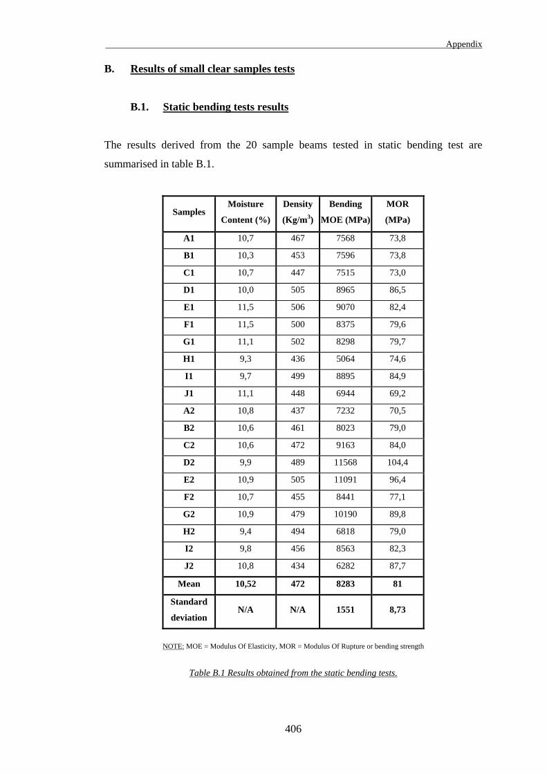
Appendix
B. Results of small clear samples tests
B.1. Static bending tests results
The results derived from the 20 sample beams tested in static bending test are
summarised in table B.1.
Samples Moisture
Content (%)
Density
(Kg/m3)
Bending
MOE (MPa)
MOR
(MPa)
A1 10,7 467 7568 73,8
B1 10,3 453 7596 73,8
C1 10,7 447 7515 73,0
D1 10,0 505 8965 86,5
E1 11,5 506 9070 82,4
F1 11,5 500 8375 79,6
G1 11,1 502 8298 79,7
H1 9,3 436 5064 74,6
I1 9,7 499 8895 84,9
J1 11,1 448 6944 69,2
A2 10,8 437 7232 70,5
B2 10,6 461 8023 79,0
C2 10,6 472 9163 84,0
D2 9,9 489 11568 104,4
E2 10,9 505 11091 96,4
F2 10,7 455 8441 77,1
G2 10,9 479 10190 89,8
H2 9,4 494 6818 79,0
I2 9,8 456 8563 82,3
J2 10,8 434 6282 87,7
Mean 10,52 472 8283 81
Standard
deviation N/A N/A 1551 8,73
NOTE: MOE = Modulus Of Elasticity, MOR = Modulus Of Rupture or bending strength
Table B.1 Results obtained from the static bending tests.
406
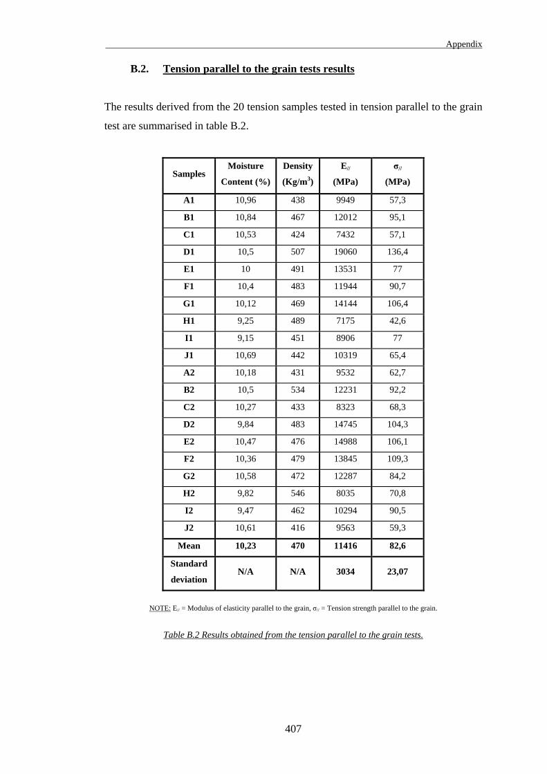
Appendix
B.2. Tension parallel to the grain tests results
The results derived from the 20 tension samples tested in tension parallel to the grain
test are summarised in table B.2.
Samples Moisture
Content (%)
Density
(Kg/m3)
E//
(MPa)
σ//
(MPa)
A1 10,96 438 9949 57,3
B1 10,84 467 12012 95,1
C1 10,53 424 7432 57,1
D1 10,5 507 19060 136,4
E1 10 491 13531 77
F1 10,4 483 11944 90,7
G1 10,12 469 14144 106,4
H1 9,25 489 7175 42,6
I1 9,15 451 8906 77
J1 10,69 442 10319 65,4
A2 10,18 431 9532 62,7
B2 10,5 534 12231 92,2
C2 10,27 433 8323 68,3
D2 9,84 483 14745 104,3
E2 10,47 476 14988 106,1
F2 10,36 479 13845 109,3
G2 10,58 472 12287 84,2
H2 9,82 546 8035 70,8
I2 9,47 462 10294 90,5
J2 10,61 416 9563 59,3
Mean 10,23 470 11416 82,6
Standard
deviation N/A N/A 3034 23,07
NOTE: E// = Modulus of elasticity parallel to the grain, σ// = Tension strength parallel to the grain.
Table B.2 Results obtained from the tension parallel to the grain tests.
407
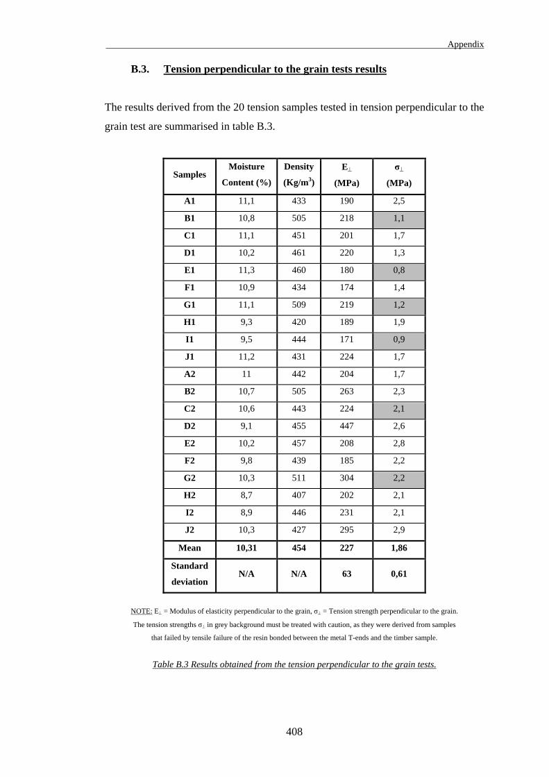
Appendix
B.3. Tension perpendicular to the grain tests results
The results derived from the 20 tension samples tested in tension perpendicular to the
grain test are summarised in table B.3.
Samples Moisture
Content (%)
Density
(Kg/m3)
E⊥
(MPa)
σ⊥
(MPa)
A1 11,1 433 190 2,5
B1 10,8 505 218 1,1
C1 11,1 451 201 1,7
D1 10,2 461 220 1,3
E1 11,3 460 180 0,8
F1 10,9 434 174 1,4
G1 11,1 509 219 1,2
H1 9,3 420 189 1,9
I1 9,5 444 171 0,9
J1 11,2 431 224 1,7
A2 11 442 204 1,7
B2 10,7 505 263 2,3
C2 10,6 443 224 2,1
D2 9,1 455 447 2,6
E2 10,2 457 208 2,8
F2 9,8 439 185 2,2
G2 10,3 511 304 2,2
H2 8,7 407 202 2,1
I2 8,9 446 231 2,1
J2 10,3 427 295 2,9
Mean 10,31 454 227 1,86
Standard
deviation N/A N/A 63 0,61
NOTE: E⊥ = Modulus of elasticity perpendicular to the grain, σ⊥ = Tension strength perpendicular to the grain.
The tension strengths σ⊥ in grey background must be treated with caution, as they were derived from samples
that failed by tensile failure of the resin bonded between the metal T-ends and the timber sample.
Table B.3 Results obtained from the tension perpendicular to the grain tests.
408
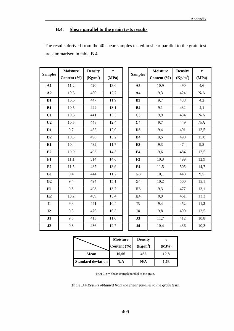
Appendix
B.4. Shear parallel to the grain tests results
The results derived from the 40 shear samples tested in shear parallel to the grain test
are summarised in table B.4.
Samples Moisture
Content (%)
Density
(Kg/m3)
τ
(MPa) Samples
Moisture
Content (%)
Density
(Kg/m3)
τ
(MPa)
A1 11,2 420 13,0 A3 10,9 490 4,6
A2 10,6 480 12,7 A4 9,3 424 N/A
B1 10,6 447 11,9 B3 9,7 438 4,2
B1 10,5 444 13,1 B4 9,1 432 4,1
C1 10,8 441 13,3 C3 9,9 434 N/A
C2 10,5 448 12,4 C4 9,7 449 N/A
D1 9,7 482 12,9 D3 9,4 491 12,5
D2 10,3 496 13,2 D4 9,5 490 15,0
E1 10,4 482 11,7 E3 9,3 474 9,8
E2 10,9 493 14,5 E4 9,6 484 12,5
F1 11,1 514 14,6 F3 10,3 499 12,9
F2 11,5 487 13,9 F4 11,5 505 14,7
G1 9,4 444 11,2 G3 10,1 448 9,5
G2 9,4 494 15,1 G4 10,2 500 15,1
H1 9,5 498 13,7 H3 9,3 477 13,1
H2 10,2 489 13,4 H4 8,9 461 13,2
I1 9,3 441 10,4 I3 9,4 452 11,2
I2 9,3 476 16,3 I4 9,8 490 12,5
J1 9,5 413 11,0 J3 11,7 412 10,8
J2 9,8 436 12,7
J4 10,4 436 10,2
Moisture
Content (%)
Density
(Kg/m3)
τ
(MPa)
Mean 10,06 465 12,8
Standard deviation N/A N/A 1,63
NOTE: τ = Shear strength parallel to the grain.
Table B.4 Results obtained from the shear parallel to the grain tests.
409
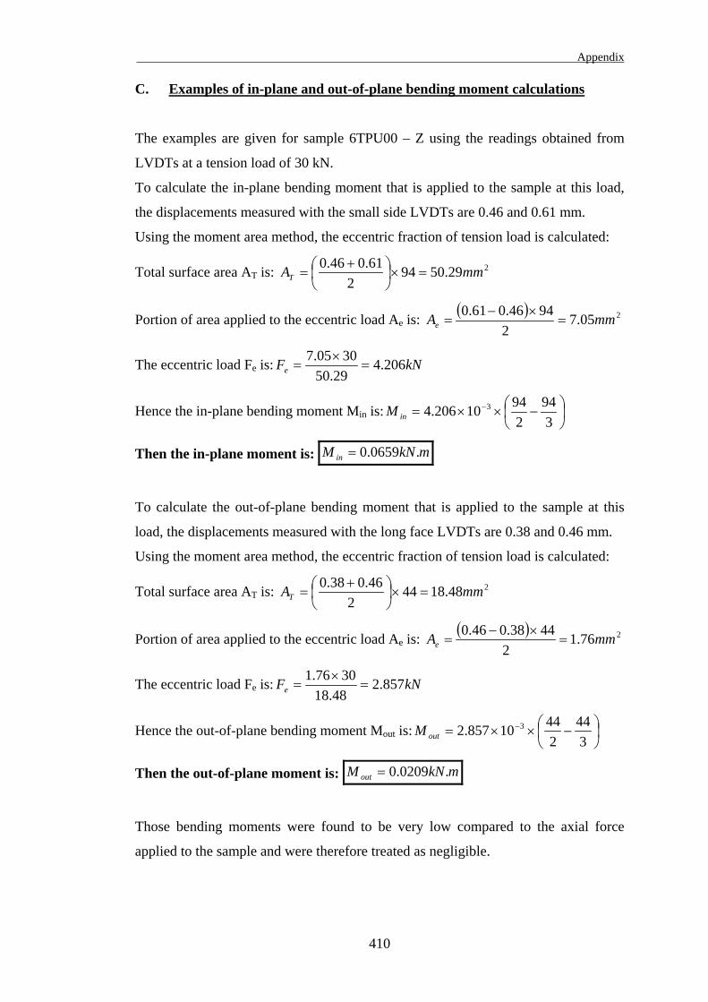
Appendix
C. Examples of in-plane and out-of-plane bending moment calculations
The examples are given for sample 6TPU00 – Z using the readings obtained from
LVDTs at a tension load of 30 kN.
To calculate the in-plane bending moment that is applied to the sample at this load,
the displacements measured with the small side LVDTs are 0.46 and 0.61 mm.
Using the moment area method, the eccentric fraction of tension load is calculated:
Total surface area AT is: 229.50942
61.046.0 mmAT =×
+
=
Portion of area applied to the eccentric load Ae is: ( ) 205.72
9446.061.0 mmAe =×−
=
The eccentric load Fe is: kNFe 206.429.50
3005.7=
×=
Hence the in-plane bending moment Min is:
−××= −
394
29410206.4 3
inM
Then the in-plane moment is: mkNM in .0659.0=
To calculate the out-of-plane bending moment that is applied to the sample at this
load, the displacements measured with the long face LVDTs are 0.38 and 0.46 mm.
Using the moment area method, the eccentric fraction of tension load is calculated:
Total surface area AT is: 248.18442
46.038.0 mmAT =×
+
=
Portion of area applied to the eccentric load Ae is: ( ) 276.12
4438.046.0 mmAe =×−
=
The eccentric load Fe is: kNFe 857.248.18
3076.1=
×=
Hence the out-of-plane bending moment Mout is:
−××= −
344
24410857.2 3
outM
Then the out-of-plane moment is: mkNM out .0209.0=
Those bending moments were found to be very low compared to the axial force
applied to the sample and were therefore treated as negligible.
410
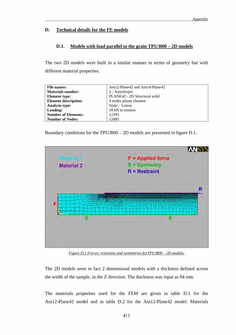
Appendix
D. Technical details for the FE models
D.1. Models with load parallel to the grain TPU/B00 – 2D models
The two 2D models were built in a similar manner in terms of geometry but with
different material properties.
File names: Materials number: Element type: Element description: Analysis type: Loading: Number of Elements: Number of Nodes:
Am12-Plane42 and Am14-Plane42 2 - Anisotropic PLANE42 - 2D Structural solid 4 nodes planar element Static - Linear 18 kN in tension 12393 12685
Boundary conditions for the TPU/B00 – 2D models are presented in figure D.1.
Figure D.1 Forces, restraints and symmetries forTPU/B00 – 2D models.
The 2D models were in fact 2 dimensional models with a thickness defined across
the width of the sample, in the Z direction. The thickness was input as 94 mm.
The materials properties used for the FEM are given in table D.1 for the
Am12-Plane42 model and in table D.2 for the Am12-Plane42 model. Materials
411
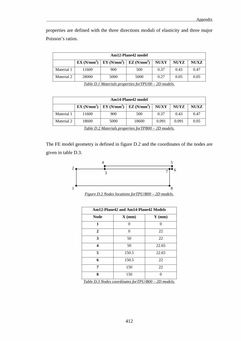
Appendix
properties are defined with the three directions moduli of elasticity and three major
Poisson’s ratios.
Am12-Plane42 model
EX (N/mm2) EY (N/mm2) EZ (N/mm2) NUXY NUYZ NUXZ
Material 1 11600 900 500 0.37 0.43 0.47
Material 2 28000 5000 5000 0.27 0.05 0.05
Table D.1 Materials properties forTPU00 – 2D models.
Am14-Plane42 model
EX (N/mm2) EY (N/mm2) EZ (N/mm2) NUXY NUYZ NUXZ
Material 1 11600 900 500 0.37 0.43 0.47
Material 2 18600 5000 18600 0.091 0.091 0.05
Table D.2 Materials properties forTPB00 – 2D models.
The FE model geometry is defined in figure D.2 and the coordinates of the nodes are
given in table D.3.
4 5 2
3 7
8
6
1Figure D.2 Nodes locations forTPU/B00 – 2D models.
Am12-Plane42 and Am14-Plane42 Models
Node X (mm) Y (mm)
1 0 0
2 0 22
3 50 22
4 50 22.65
5 150.5 22.65
6 150.5 22
7 150 22
8 150 0
Table D.3 Nodes coordinates forTPU/B00 – 2D models.
412
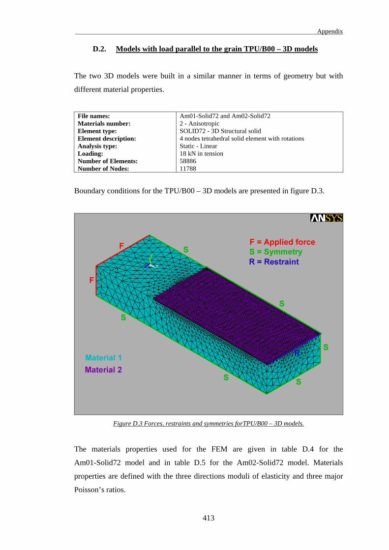
Appendix
D.2. Models with load parallel to the grain TPU/B00 – 3D models
The two 3D models were built in a similar manner in terms of geometry but with
different material properties.
File names: Materials number: Element type: Element description: Analysis type: Loading: Number of Elements: Number of Nodes:
Am01-Solid72 and Am02-Solid72 2 - Anisotropic SOLID72 - 3D Structural solid 4 nodes tetrahedral solid element with rotations Static - Linear 18 kN in tension 58886 11788
Boundary conditions for the TPU/B00 – 3D models are presented in figure D.3.
Figure D.3 Forces, restraints and symmetries forTPU/B00 – 3D models.
The materials properties used for the FEM are given in table D.4 for the
Am01-Solid72 model and in table D.5 for the Am02-Solid72 model. Materials
properties are defined with the three directions moduli of elasticity and three major
Poisson’s ratios.
413
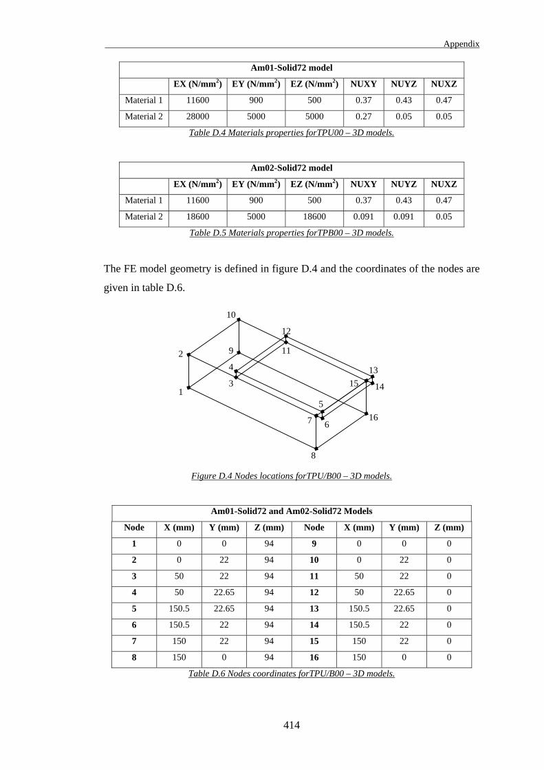
Appendix
Am01-Solid72 model
EX (N/mm2) EY (N/mm2) EZ (N/mm2) NUXY NUYZ NUXZ
Material 1 11600 900 500 0.37 0.43 0.47
Material 2 28000 5000 5000 0.27 0.05 0.05
Table D.4 Materials properties forTPU00 – 3D models.
Am02-Solid72 model
EX (N/mm2) EY (N/mm2) EZ (N/mm2) NUXY NUYZ NUXZ
Material 1 11600 900 500 0.37 0.43 0.47
Material 2 18600 5000 18600 0.091 0.091 0.05
Table D.5 Materials properties forTPB00 – 3D models.
The FE model geometry is defined in figure D.4 and the coordinates of the nodes are
given in table D.6.
3
9
16
15 14
13
12
11
10
8
7 6
5
4
2
1
Figure D.4 Nodes locations forTPU/B00 – 3D models.
Am01-Solid72 and Am02-Solid72 Models
Node X (mm) Y (mm) Z (mm) Node X (mm) Y (mm) Z (mm)
1 0 0 94 9 0 0 0
2 0 22 94 10 0 22 0
3 50 22 94 11 50 22 0
4 50 22.65 94 12 50 22.65 0
5 150.5 22.65 94 13 150.5 22.65 0
6 150.5 22 94 14 150.5 22 0
7 150 22 94 15 150 22 0
8 150 0 94 16 150 0 0
Table D.6 Nodes coordinates forTPU/B00 – 3D models.
414
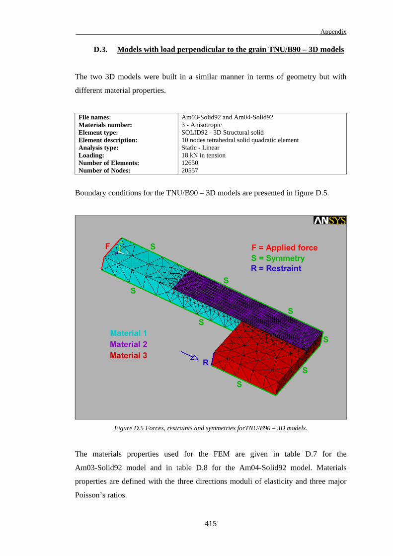
Appendix
D.3. Models with load perpendicular to the grain TNU/B90 – 3D models
The two 3D models were built in a similar manner in terms of geometry but with
different material properties.
File names: Materials number: Element type: Element description: Analysis type: Loading: Number of Elements: Number of Nodes:
Am03-Solid92 and Am04-Solid92 3 - Anisotropic SOLID92 - 3D Structural solid 10 nodes tetrahedral solid quadratic element Static - Linear 18 kN in tension 12650 20557
Boundary conditions for the TNU/B90 – 3D models are presented in figure D.5.
Figure D.5 Forces, restraints and symmetries forTNU/B90 – 3D models.
The materials properties used for the FEM are given in table D.7 for the
Am03-Solid92 model and in table D.8 for the Am04-Solid92 model. Materials
properties are defined with the three directions moduli of elasticity and three major
Poisson’s ratios.
415
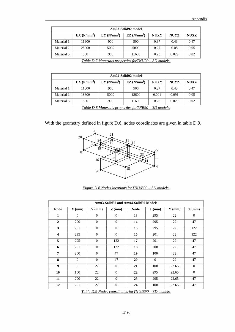
Appendix
Am03-Solid92 model
EX (N/mm2) EY (N/mm2) EZ (N/mm2) NUXY NUYZ NUXZ
Material 1 11600 900 500 0.37 0.43 0.47
Material 2 28000 5000 5000 0.27 0.05 0.05
Material 3 500 900 11600 0.25 0.029 0.02
Table D.7 Materials properties forTNU90 – 3D models.
Am04-Solid92 model
EX (N/mm2) EY (N/mm2) EZ (N/mm2) NUXY NUYZ NUXZ
Material 1 11600 900 500 0.37 0.43 0.47
Material 2 18600 5000 18600 0.091 0.091 0.05
Material 3 500 900 11600 0.25 0.029 0.02
Table D.8 Materials properties forTNB90 – 3D models.
With the geometry defined in figure D.6, nodes coordinates are given in table D.9.
16
15
24
23
21
22
20
1718
1910
1112
1314
9
8
7
1
6
5
3
4
2
Figure D.6 Nodes locations forTNU/B90 – 3D models.
Am03-Solid92 and Am04-Solid92 Models
Node X (mm) Y (mm) Z (mm) Node X (mm) Y (mm) Z (mm)
1 0 0 0 13 295 22 0
2 200 0 0 14 295 22 47
3 201 0 0 15 295 22 122
4 295 0 0 16 201 22 122
5 295 0 122 17 201 22 47
6 201 0 122 18 200 22 47
7 200 0 47 19 100 22 47
8 0 0 47 20 0 22 47
9 0 22 0 21 100 22.65 0
10 100 22 0 22 295 22.65 0
11 200 22 0 23 295 22.65 47
12 201 22 0 24 100 22.65 47
Table D.9 Nodes coordinates forTNU/B90 – 3D models.
416
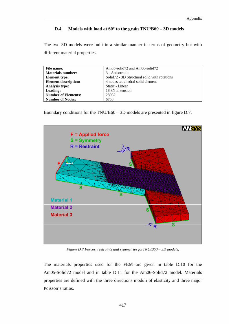
Appendix
D.4. Models with load at 60° to the grain TNU/B60 – 3D models
The two 3D models were built in a similar manner in terms of geometry but with
different material properties.
File name: Materials number: Element type: Element description: Analysis type: Loading: Number of Elements: Number of Nodes:
Am05-solid72 and Am06-solid72 3 - Anisotropic Solid72 - 3D Structural solid with rotations 4 nodes tetrahedral solid element Static - Linear 18 kN in tension 28932 6753
Boundary conditions for the TNU/B60 – 3D models are presented in figure D.7.
Figure D.7 Forces, restraints and symmetries forTNU/B60 – 3D models.
The materials properties used for the FEM are given in table D.10 for the
Am05-Solid72 model and in table D.11 for the Am06-Solid72 model. Materials
properties are defined with the three directions moduli of elasticity and three major
Poisson’s ratios.
417
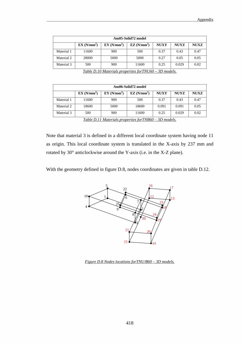
Appendix
Am05-Solid72 model
EX (N/mm2) EY (N/mm2) EZ (N/mm2) NUXY NUYZ NUXZ
Material 1 11600 900 500 0.37 0.43 0.47
Material 2 28000 5000 5000 0.27 0.05 0.05
Material 3 500 900 11600 0.25 0.029 0.02
Table D.10 Materials properties forTNU60 – 3D models.
Am06-Solid72 model
EX (N/mm2) EY (N/mm2) EZ (N/mm2) NUXY NUYZ NUXZ
Material 1 11600 900 500 0.37 0.43 0.47
Material 2 18600 5000 18600 0.091 0.091 0.05
Material 3 500 900 11600 0.25 0.029 0.02
Table D.11 Materials properties forTNB60 – 3D models.
Note that material 3 is defined in a different local coordinate system having node 11
as origin. This local coordinate system is translated in the X-axis by 237 mm and
rotated by 30° anticlockwise around the Y-axis (i.e. in the X-Z plane).
With the geometry defined in figure D.8, nodes coordinates are given in table D.12.
24
20
15
3
2
11
25 23
22
21
10
17
18
19
6 12 13
14
5
8
71
94
16
Figure D.8 Nodes locations forTNU/B60 – 3D models.
418
Appendix
Am05-Solid72 and Am06-Solid72 Models
Node X (mm) Y (mm) Z (mm) Nodes in local coordinated system 11
1 0 0 0 Node X (mm) Y (mm) Z (mm)
2 208.54 0 0 12 0 0 -147.865
3 262.81 0 94 13 94 0 -147.865
4 0 0 94 14 94 0 202.135
5 0 22 0 15 0 0 202.135
6 100 22 0 16 0 22 -147.865
7 208.54 22 0 17 94 22 -147.865
8 262.81 22 94 18 94 22 0
9 154.27 22 94 19 94 22 108.54
10 0 22 94 20 94 22 202.135
11 237 0 47 21 0 22 202.135
22 100 22.65 0 23 94 22.65 0
25 154.27 22.65 94 24 94 22.65 108.54
Table D.12 Nodes coordinates forTNU/B60 – 3D models.
419
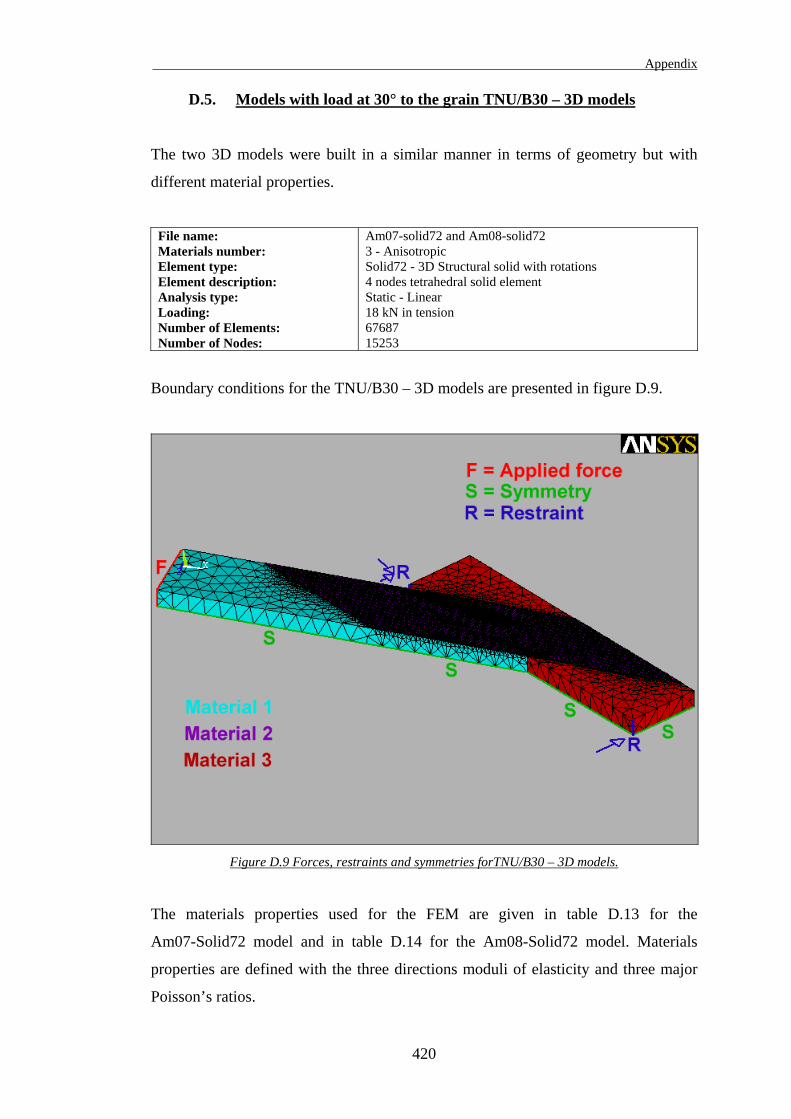
Appendix
D.5. Models with load at 30° to the grain TNU/B30 – 3D models
The two 3D models were built in a similar manner in terms of geometry but with
different material properties.
File name: Materials number: Element type: Element description: Analysis type: Loading: Number of Elements: Number of Nodes:
Am07-solid72 and Am08-solid72 3 - Anisotropic Solid72 - 3D Structural solid with rotations 4 nodes tetrahedral solid element Static - Linear 18 kN in tension 67687 15253
Boundary conditions for the TNU/B30 – 3D models are presented in figure D.9.
Figure D.9 Forces, restraints and symmetries forTNU/B30 – 3D models.
The materials properties used for the FEM are given in table D.13 for the
Am07-Solid72 model and in table D.14 for the Am08-Solid72 model. Materials
properties are defined with the three directions moduli of elasticity and three major
Poisson’s ratios.
420
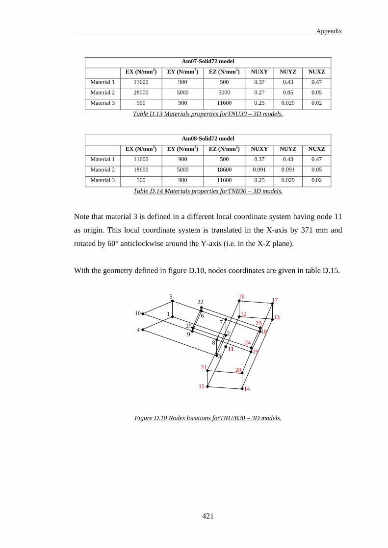
Appendix
Am07-Solid72 model
EX (N/mm2) EY (N/mm2) EZ (N/mm2) NUXY NUYZ NUXZ
Material 1 11600 900 500 0.37 0.43 0.47
Material 2 28000 5000 5000 0.27 0.05 0.05
Material 3 500 900 11600 0.25 0.029 0.02
Table D.13 Materials properties forTNU30 – 3D models.
Am08-Solid72 model
EX (N/mm2) EY (N/mm2) EZ (N/mm2) NUXY NUYZ NUXZ
Material 1 11600 900 500 0.37 0.43 0.47
Material 2 18600 5000 18600 0.091 0.091 0.05
Material 3 500 900 11600 0.25 0.029 0.02
Table D.14 Materials properties forTNB30 – 3D models.
Note that material 3 is defined in a different local coordinate system having node 11
as origin. This local coordinate system is translated in the X-axis by 371 mm and
rotated by 60° anticlockwise around the Y-axis (i.e. in the X-Z plane).
With the geometry defined in figure D.10, nodes coordinates are given in table D.15.
24
20
15
3
2
11
25 23
22
21
10
17
18
19
6 12 13
14
5
8
71
94
16
Figure D.10 Nodes locations forTNU/B30 – 3D models.
421
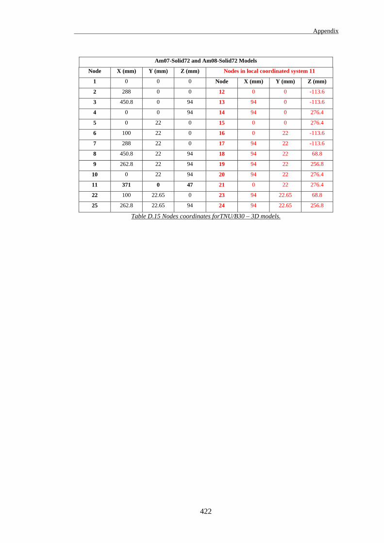
Appendix
422
Am07-Solid72 and Am08-Solid72 Models
Node X (mm) Y (mm) Z (mm) Nodes in local coordinated system 11
1 0 0 0 Node X (mm) Y (mm) Z (mm)
2 288 0 0 12 0 0 -113.6
3 450.8 0 94 13 94 0 -113.6
4 0 0 94 14 94 0 276.4
5 0 22 0 15 0 0 276.4
6 100 22 0 16 0 22 -113.6
7 288 22 0 17 94 22 -113.6
8 450.8 22 94 18 94 22 68.8
9 262.8 22 94 19 94 22 256.8
10 0 22 94 20 94 22 276.4
11 371 0 47 21 0 22 276.4
22 100 22.65 0 23 94 22.65 68.8
25 262.8 22.65 94 24 94 22.65 256.8
Table D.15 Nodes coordinates forTNU/B30 – 3D models.