Structure and Power in Multilateral Negotiations:

An Application to French Water Policy

Leo Simon, Rachael Goodhue, Gordon Rausser, Sophie Thoyer, Sylvie Morardet, and Patrick Rio

September 13, 2006

JEL CODES:C78 Bargaining Theory; Matching TheoryQ25 Renewable resources: water and airD78 Positive Analysis of Policymaking and Implementation

Contact author: Leo Simon. 207 Giannini Hall, University of California at Berkeley, Berkeley, CA 94720.Email: simon@are.berkeley.edu. Phone: (510) 642 8230. Fax: 510 643 8911.

The authors thank Jeffrey Williams, Susan Stratton, two anonymous referees and seminar audiences at UC

Berkeley and UC Davis for helpful comments. Funding for this research was provided by the France-Berkeley Fund,

the Rizome Fund, Cemagref, INRA (Action Scientifique Structurante AQUAE), and the Giannini Foundation of

Agricultural Economics. Simon, Goodhue and Rausser are members of the Giannini Foundation.

ABSTRACT

Stakeholder negotiation is an increasingly important policymaking tool. However, relatively littleis understood about the relationship between the structure of the negotiating process and theeffectiveness with which participating stakeholders can pursue their individual interests. In thispaper, we apply the Rausser-Simon multilateral bargaining model to a specific negotiation process,involving water storage capacity and use in the upper part of the Adour Basin in south-westernFrance. In the Rausser-Simon model, the elements of negotiation structure include: the list ofparticipants at the bargaining table; the set of issues being negotiated; the decision rule; politicalweights (“access”); and the nature of the outcome if agreement cannot be reached. The richnessof the data and institutional information available to us provides a realistic environment in whichto examine the effect of negotiation structure on participant power. We focus in particular onthe three farmer stakeholder groups. Because their interests are aligned but distinct, they form anatural negotiating coalition. We construct experiments that enable us to evaluate the effects ofnegotiation structure on the effectiveness of this coalition.

Our comparative statics experiments highlight a number of aspects of the relationship betweennegotiation structure and bargaining power. In addition to the standard indices of bargainingpower—the distribution of access and players’ utilities in the event that negotiations break down—our analysis identifies a number of other, less obvious, sources of power. First, we show thata coalition member may obtain a better bargaining outcome when his access is reduced, if theredistribution increases the access of another coalition member who has a more favorable “strategiclocation.” Second, we show that the interests of the coalition as a whole will usually, but notalways, be advanced if its members cede access to a “spokesman” representing their commoninterests. However, some coalition members may be adversely affected. Third, we consider theeffect on the coalition of restricting the set of proposals that may be placed on the bargainingtable. In particular, we impose increasingly tight restrictions on the extent to which coalitionmembers can make bargaining proposals that further their own individual interests at the expenseof the interests of other coalition members. We find that usually, but not always, such restrictionsharm the coalition as a whole.

1

1. Introduction

Many areas of public policy are characterized by an increasing emphasis on devolution, i.e., direct

stakeholder participation in the policy formation process. In some cases, this participation extends

to the actual design of the policies that will ultimately be implemented. The trend toward devolu-

tion has been particularly significant in the area of water policy design, where the goal is to design

policies that are not only environmentally and economically sustainable, but also politically viable.

Examples abound, ranging from Armenia to Palestine to the U.S.A. One such collective negotiation

among stakeholders, the so-called Three-Way Negotiations which took place in the early 1990s in

California, was analyzed in Adams, Rausser and Simon (1996). Other, more recent examples of

devolution include large-scale rural-urban water transfers in the U.S.-Mexico border region, ex-

amined in Frisvold and Emerick (2006), the San Francisco Estuary Project and the Sacramento

Water Forum. In France, the idea of devolution has been institutionalized in the Water Law pro-

mulgated in 1992. This law specifies that specific development plans be set up at the level of each

hydrological basin, and that water regulations be negotiated at the smaller, cachment scale. It is

required that regulations be negotiated locally between all stakeholders under the supervision of

local authorities.1

Although stakeholder negotiation is an increasingly important policymaking tool, relatively little is

understood about the interactions between the structure of the negotiating process and the interests

of the participating stakeholders. How do these considerations influence the negotiated outcome?

In this paper we analyze the nature of stakeholder power within a negotiation, focusing on how

this power is affected by the structure of the negotiation process and the relationship between

the interests of the participants. Understanding these interactions is important for negotiation

participants, and for policymakers designing such processes.

1 Loi N92-3 du 3 janvier 1992, Journal Officiel de la Republique Francaise du 4 janvier 1992. See also Jiang (1993)

2

For our purposes, we define bargaining power as the capacity of a stakeholder to influence the

negotiated outcome in order to increase the utility he receives in the equilibrium of the negotiation

game. In this paper, we are interested in the bargaining power wielded by a subset of stakeholders,

whose interests are sufficiently aligned that they may be thought of as a loose coalition. In our

case, the coalition consists of farmers who are located at different points along a river. While

these farmers compete with each other for water, their interests are more closely aligned with

each other than with the other stakeholders at the table, including in particular those representing

environmental and other non-agricultural uses of water. We analyze three questions related to the

bargaining power of our coalition. First, what are the sources of bargaining power, and how do

they interact? Second, is it ever advantageous for some or all of the coalition members to cede

their seats at the bargaining table to a “spokesman,” charged with the task of representing their

joint interests? Third, how does the definition of the bargaining space—i.e., the vector of variables

over which negotiations take place, and the restrictions imposed on these variables—affect the

bargaining power and resulting utilities of participants? In particular, in some of the bargaining

spaces we consider, individual farmers are permitted to pursue their own interests at the expense of

the interests of the coalition as a whole, by allocating more water to their own subbasins at lower

prices than other farmers pay. Do coalition members benefit when restrictions are imposed on the

degree to which they can distinguish their own interests from those of other farmers?

Understanding the factors determining the answers to such questions will facilitate the design of

negotiation processes that represent the interests of all stakeholders in an implementable and sus-

tainable fashion. At an intuitive level, stakeholders’ power in the negotiation process is measured

by their “access” to the decision-making process. Access is a catch-all term for many considera-

tions, including the number of representatives included in the process, the capacity to set agendas,

placement on key committees, etc. We demonstrate that the prima facie benefits of access can be

3

dominated by other, more subtle kinds of negotiating power, arising from the nature of the interac-

tions between stakeholders and from the structure of the bargaining environment. If a negotiation

process is to fairly represent all interests, these interactions must be taken into consideration when

policymakers design the negotiation process.

In order to address these questions, we model a specific instance of negotiations over the use and

storage of water in the upper Adour basin in south-western France. The upper Adour basin is

a water cachment area that extends from the Adour’s source in the Pyrenees mountains to its

junction with the Midouze River. The upper Adour basin consists of three subbasins, separated

by points where minimum water flows are measured by the French government. For our purposes,

this negotiation process has a number of advantages as a research topic. First, the negotiation

process is well-defined and relatively transparent. The national government clearly specified the

rules determining participants, as well as the outcome in the event that the parties are unable to

negotiate a solution. Under the specified structure, the participants reached an initial agreement

regarding the guiding principles of the negotiation process within a year: they agreed to initiate

and fund studies regarding future water needs and supplies, farmers agreed to fund a significant

share of management and maintenance costs, and stakeholders agreed on a total water volume for

consumptive purposes, which is one of the three critical variables we model. However, the second

stage of negotiations deadlocked over the other two critical issues we examine here: allocating

water among farmers, and managing limited supplies during droughts (Thoyer, Morardet, Rio and

Goodhue, 2004). Second, our modeling task is facilitated by the availability of extensive information

regarding the scientific and economic relationships that affect stakeholder preferences (Gleyses and

Morardet, 1997; Faysse, 1997). The underlying hydrology of the river basin is well-documented

(Faysse and Morardet, 1999). A great deal of information is available regarding the agricultural

use of water, in terms of both quantities used and the value of the resulting production. This

information provides us with hydrological and economic parameters for our simulation analysis.

4

Third, two types of environmental goals are recognized explicitly by participants: the value of

“residual flows”2 which promote aquatic life, and the scenic costs of dams, which destroy attractive

valley landscapes. These two goals compete with each other, and with farmers’ use of water for

production purposes. Finally, the natural division of farmers by subbasin provides us with a subset

of “natural allies,” or coalition, consisting of stakeholders whose interests are similar, but not

perfectly aligned. The quality of the data and institutional information provides us with a rich and

realistic simulation environment for examining the effect of process structure on participant power.

The paper is organized as follows. In section 2, we review the Rausser-Simon multilateral bargaining

model (MB), which provides the theoretical basis for this application. Section 3 relates the MB

model to the literature on multilateral negotiations. Section 4 introduces the Adour Basin, explains

the nature of the negotiations and describes our simulation model of the bargaining problem.

Section 5 contains our comparative statics analysis. Section 6 concludes.

2. The Underlying Bargaining Framework

The analytical framework for this paper is the non-cooperative multilateral bargaining model (MB)

developed in Rausser and Simon (1999) and applied in Adams et al. (1996). In this section, we

review the main features of the model, drawing extensively from the presentation in §2 of Adams

et al. (1996). Complementing the vast theoretical literature on bilateral bargaining spawned by the

seminal work of Rubinstein (1982), the MB framework is designed specifically as an applications

tool, to analyze complex multi-issue, multiplayer bargaining problems. It has no closed form

solution, and so must be solved using computational techniques.

The specification of a multilateral bargaining problem includes a finite set of players, denoted by

I = {1, · · · , I} and indexed by i. The players meet together to select a policy vector from some set

X of possible alternatives. X is assumed to be a compact, convex subset of n-dimensional Euclidean

2 I.e., total flows net of agricultural usage. See p. 20 for a more complete definition

5

space, where n is the cardinality of the vector of issues being negotiated. The policy vector x yields

player i a utility of ui(x), where ui(·) is assumed to be strictly concave on X. We denote by u0 the

vector of disagreement payoffs, i.e., the payoffs players receive if they fail to negotiate an agreement.

Throughout this paper, we will assume that decisions are reached by unanimity, i.e., an element of

X can be selected as the solution to the bargaining problem only if it is accepted by all parties at

the bargaining table.

A bargaining game is derived from a bargaining problem by superimposing upon it a “negotiation

process.” We begin by formulating a bargaining game with a finite number, T , of bargaining

rounds. Under the conditions we assume, each such game has a unique limit dominance solvable

(LDS) equilibrium.3 We then define the solution to the limit bargaining game to be the limit of

these finite-round equilibria. At the beginning of the t ≤ T ’th round of the finite game, provided

that the game has not already concluded by this round, nature chooses at random some player to be

the proposer for this round. Nature’s choice is governed by an exogenously probability distribution,

w = (wi)i∈I , where wi ∈ [0, 1]—player i is chosen with probability wi—and∑

iwi = 1. The vector

w is interpreted as a distribution of access to the political system, and wi is referred to as player

i’s access probability.4 The player selected by nature makes a proposal, which is a policy vector

in X, and all players vote on whether or not to accept it. The game concludes in this round if

and only if all players vote to accept the proposal; if some player votes against it, play proceeds

to the next round. If the T ’th round of the game is reached, and if the proposal put forward in

this round is rejected, then players receive the vector of disagreement payoffs, u0. To avoid dealing

with degenerate special cases, we will assume throughout that the set X contains a proposal that

strictly Pareto dominates u0.5

3 Limit dominance solvability is a solution concept that extends in an intuitive way the finite-game notion of trembling-handperfection (Selten, 1975) to extensive form games with a continuum of actions. We prove in Rausser and Simon (1999) thatevery bargaining game satisfying the conditions assumed in this paper has a unique LDS equilibrium.

4 Access probabilities are referred to as “recognition probabilities” in the literature spawned by Baron and Ferejohn (1987).While some branches of the political economy literature treat the distribution of political power as endogenous, our paper,along with the other bargaining papers reviewed in §3, treats this distribution as externally determined.

6

There is a simple characterization of the unique LDS equilibrium strategies for a game with T rounds

of bargaining. This characterization is given by the following, backward inductive construction: a

proposal made by player i in period T is accepted if and only if it yields each player j 6= i a utility

level at least as great as j’s disagreement utility, u0j . Similarly, in round t < T , a proposal by i is

accepted if and only if it yields each j a utility level at least as great as j’s expected utility from

playing the subgame starting from round t+ 1.6 Thus the game can be solved recursively, starting

from the last round: in each round t, player i computes the policy vector that maximizes i’s utility,

subject to the constraint that for each j 6= i, the vector yields player j no less than j’s default

utility (if t = T ) or j’s expected utility conditional on reaching the next round (if t < T ). Thus the

task for i in each round is to solve a classical non-linear programming problem: maximize a strictly

concave function on a convex set.7 Our conditions ensure that in each round, the unique solution

to this problem will yield i greater utility than i’s expected utility, conditional on reaching the next

round. It follows from this construction that for every finite game there is a unique, stochastic

outcome vector, consisting of a point in X for each player, which will be proposed by that player

if he is chosen in the first round to be the proposer. With probability one, players in round one

accept whichever proposal is made. Given a sequence of finite-round bargaining games, all identical

except that the number of bargaining periods increases without bound, any sequence of outcome

vectors for these games has a unique, deterministic limit in X, i.e., all players’ first-round proposals

converge to the same point in X. Formal details of this construction are provided in Rausser and

Simon (1999).

5 It should be emphasized that this last assumption is not a necessary one; given our other assumptions, however, it isnecessary and sufficient to ensure the existence of a unique negotiated agreement.

6 In round t+1, player i is chosen with probability wi to be the proposer. Under the conditions we assume in this paper, everyproposal that is part of an LDS equilibrium profile is accepted. Therefore, j’s expected utility from playing the subgamestarting at t + 1 is the w-weighted sum of the utilities he obtains from all parties’ proposals in this round.

7 The feasible set is convex because it is the intersection of upper contour sets for the other players; these sets are convexbecause all players’ utilities are concave and hence quasi-concave.

7

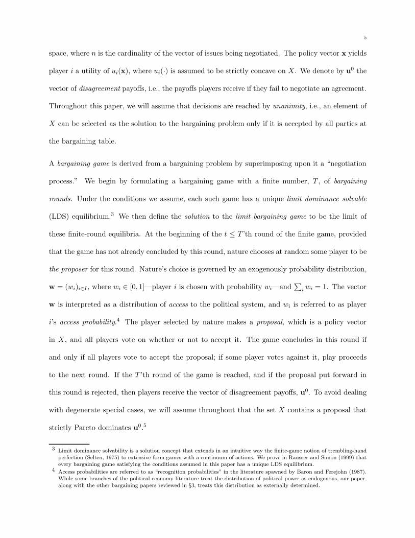
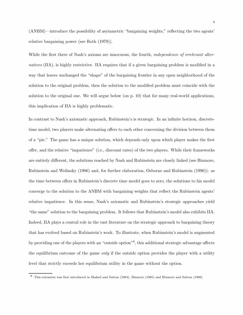
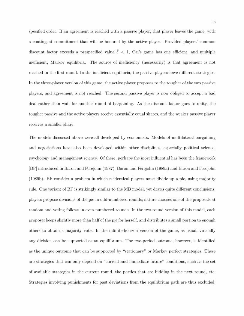
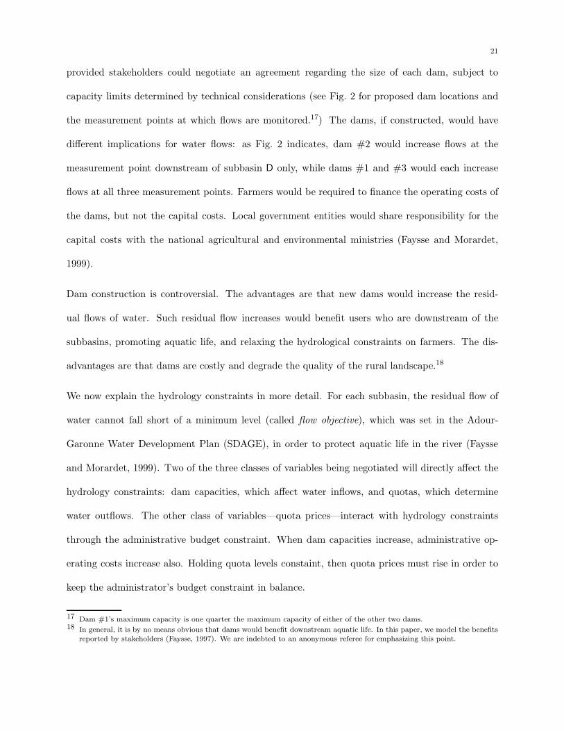
Player #1’s ideal point

Player #2’s ideal point Player #3’s ideal point

I1,T

I2,TI3,T

I1,T−1

I2,T−1I3,T−1x1,T

x2,T

x3,T

x1,T−1

x2,T−1

x3,T−1x∗

Figure 1. An illustration of the Rausser-Simon model (Fig 1. in Adams et. al. (1996))

We now provide an elementary example, designed to provide some intuition for the basic mechanics

of the model. The example, reproduced from Adams et al. (1996), belongs to the class of problems

known as spatial problems, in which the policy space consists of alternative locations. Each player

has a most preferred location, called her ideal point. We assume that the utility derived by a player

from a particular location is a decreasing function of the Euclidean distance between this location

and the player’s ideal point. The example illustrates why a deterministic limit solution must exist.

There are three players. The space of possible locations is represented by a triangle in Figure 1.

Players’ ideal points are at the vertices of the triangle. Player i’s access probability will be denoted

by wi. Consider a game with T rounds of bargaining. For each j, the line Ij,T in Figure 1 is the

level set corresponding to player j’s reservation utility in the last round of bargaining: any proposal

on this line yields player j a utility level equal to j’s disagreement utility. This line is the boundary

of player j’s participation constraint on negotiations in round T . Player i’s task in this round is

8

to choose the point closest to her ideal point that satisfies both of the other agents’ participation

constraints.

The outcome conditional on reaching round T is that proposal xj,T will be agreed upon with

probability wj. Clearly, player i’s expected utility conditional on reaching this round is strictly

higher than u0i , since each of the xj,T ’s yields i at least u0

i while i’s own proposal yields her a utility

strictly higher than u0i . Thus, her participation constraint in round T−1 will be strictly “tighter”

than in round T . This is illustrated in Fig. 1: the set of proposals for which unanimous agreement

can be obtained—i.e., the set bounded by the Ij,T−1’s—is strictly contained in the set bounded by

the Ij,T ’s. Accordingly the distance between players’ proposals in round T−1 is also smaller than

in round T . Clearly, however, it is strictly better for agent i to propose an alternative that will be

accepted in the current round, rather than take her chances in the following round. Proceeding by

backward induction from round T−1 to the first round, this distance between proposals continues

to shrink. Thus, if T is sufficiently large, the maximum distance between any two players’ proposals

in the first round of bargaining will be arbitrarily small. This is the intuition for why in the limit

as T goes to infinity, the solution to the game is deterministic, i.e., all negotiators propose the same

alternative in the first round.

3. Related Literature

Compared with the voluminous literature on bargaining between two players over a single dimen-

sion, the literature on multi-player, multi-issue bargaining problems is relatively sparse. We begin

with a discussion of the two seminal papers in the former literature—Nash (1950) and Rubinstein

(1982)—which have strongly influenced the directions in which the latter has evolved. Nash’s

approach is axiomatic: given a set S of possible utility pairs, and a disagreement outcome (or

default payoff) d, Nash identified a unique outcome in S that satisfies four axioms about bar-

gaining outcomes. Extensions of Nash’s original paper—the asymmetric Nash Bargaining Model

9

(ANBM)—introduce the possibility of asymmetric “bargaining weights,” reflecting the two agents’

relative bargaining power (see Roth (1979)).

While the first three of Nash’s axioms are innocuous, the fourth, independence of irrelevant alter-

natives (IIA), is highly restrictive. IIA requires that if a given bargaining problem is modified in a

way that leaves unchanged the “shape” of the bargaining frontier in any open neighborhood of the

solution to the original problem, then the solution to the modified problem must coincide with the

solution to the original one. We will argue below (on p. 10) that for many real-world applications,

this implication of IIA is highly problematic.

In contrast to Nash’s axiomatic approach, Rubinstein’s is strategic. In an infinite horizon, discrete-

time model, two players make alternating offers to each other concerning the division between them

of a “pie.” The game has a unique solution, which depends only upon which player makes the first

offer, and the relative “impatience” (i.e., discount rates) of the two players. While their frameworks

are entirely different, the solutions reached by Nash and Rubinstein are closely linked (see Binmore,

Rubinstein and Wolinsky (1986) and, for further elaboration, Osborne and Rubinstein (1990)): as

the time between offers in Rubinstein’s discrete time model goes to zero, the solutions to his model

converge to the solution to the ANBM with bargaining weights that reflect the Rubinstein agents’

relative impatience. In this sense, Nash’s axiomatic and Rubinstein’s strategic approaches yield

“the same” solution to the bargaining problem. It follows that Rubinstein’s model also exhibits IIA.

Indeed, IIA plays a central role in the vast literature on the strategic approach to bargaining theory

that has evolved based on Rubinstein’s work. To illustrate, when Rubinstein’s model is augmented

by providing one of the players with an “outside option”8, this additional strategic advantage affects

the equilibrium outcome of the game only if the outside option provides the player with a utility

level that strictly exceeds her equilibrium utility in the game without the option.

8 This extension was first introduced in Shaked and Sutton (1984), Binmore (1985) and Binmore and Sutton (1989)

10

Both the Nash and the Rubinstein approaches have been extended to a multi-player context. Thom-

son and Lensberg (1989) includes an extensive treatment of n-person axiomatic bargaining theory,

including Nash Bargaining. Krishna and Serrano (1996) [KS] construct a generalization of Rubin-

stein’s game to n players in which the unique solution to the problem of sharing a pie corresponds

to the solution of the n-person ANBM. In KS’s model, each player can accept or reject the current

pie division proposal. Players who accept exit the game and immediately consume their shares

of the pie; the remaining players continue to bargain over what remains. Thus unanimity is not

required for agreement. The “pie-eating” structure of this setup is clearly restrictive: i’s utility

from consuming her share is independent of whether or not other players are consuming also, so

that the possibility of interpersonal externalities is excluded. Kultti and Vartiainen (2004) have

generalized KS’s equivalence result to a general context that admits interpersonal externalities.

The Rausser-Simon multilateral bargaining (MB) model applied in the present paper represents a

departure from the Nash-Rubinstein tradition in that its solution does not exhibit independence

of irrelevant alternatives. In particular, equilibrium outcomes in the MB model depend a great

deal on the nature of the offers that are made in the final rounds of negotiations. By contrast, the

absolute levels of offers made in the tail of a sequence of Rubinstein offers have no influence on the

nature of offers made at the head of the sequence (i.e., the equilibrium offers).9 This distinction has

important implications for the applicability of Rubinstein-type models to the study of certain real-

world multilateral bargaining situations. In the context of collective decision-making, an impending

deadline can provide a dramatic impetus to compromise: witness the frequency of last-minute

resolutions of Congressional deadlocks, and of post-midnight compromises in wage negotiations

when strikes are scheduled for the following morning. To the extent that the threats and counter-

threats made in these final moments of negotiations involve proposals that are outside of some

9 More precisely, the relationship between equilibrium offers and those made in the final rounds of the finite-horizon gamesthat approximate Rubinstein’s model becomes vanishingly small as the time horizon increases (Fudenberg and Levine, 1983).

11

neighborhood of the ultimate compromise, the solutions of models consistent with Nash’s IIA

axiom must be invariant with respect to the way events unfold at the “eleventh hour.” In the MB

model, by contrast, these events can have a dramatic impact on equilibrium outcomes.10 11

Of the other multi-player non-cooperative bargaining theoretic papers, most involve some kind of

modification of Rubinstein’s alternating-offer framework. Binmore (1985) considers several alterna-

tive extensions of Rubinstein’s analysis to the problem of “three players and three pies:” each pair

of players exercises control over the division of a different pie, only one of which can be divided. A

result attributed to Shaked12 shows that in any infinite-horizon, alternating-offer, three-player pure-

division problem, if unanimity is required for agreement, and if players are not extremely impatient,

then any division of the pie can be implemented by subgame perfect equilibrium strategies.13

An interesting n-player variant of the alternating-offer model, called the “Proposal-Making Model,”

has been advanced by Selten (1981). A player is selected by nature to make the first proposal. She

proposes a utility vector, a coalition and a “responder.” The responder either accepts or rejects. If

she rejects, the responder then proposes a new utility vector, a new coalition and a new responder.

If she accepts, the responder designates another member of the coalition as the next responder, and

so on until all members of a coalition have agreed to some proposal. This model has been studied

extensively in Chatterjee et al. (1987) and by Bennett, writing alone and with various coauthors.14

10 It should be emphasized at this point that in the equilibria of the MB model—and all other complete information bargainingmodels—agreement is always reached in the first round of bargaining, so that last-minute equilibrium agreements never arise.The distinction between Rubinstein’s and the MB models arises from out-of-equilibrium interactions at the eleventh hour,which, in the latter but not the former, are transmitted via backward induction to be beginning of the game.

11 Applied economists are generally highly skeptical of arguments that involve long and intricate backward inductive chains.To some extent, this justifiable skepticism may be mitigated when applied to the MB model, because, typically, the basic“shape” of the solution is more or less determined after only a few rounds of backward induction (see §5 below). Thisfact may also reassure experimentalists, since there is overwhelming evidence that experimental subjects seem unable tobackward induct much beyond three periods. (See for example Neelin et al. (1988), Speigel et al. (1990), Binmore et al.(2002) and Johnson et al. (2002).)

12 Proposition 3.7 in Osborne and Rubinstein (1990). The result is also discussed in Sutton (1986)13 Sutton (1986) and Osborne and Rubinstein (1990) note that Shaked’s result can be easily extended to n players.14 Bennett (1991b), Bennett (1991a), Bennett and Houba (1987), Bennett and Damme (1991)

12

Manzini and Mariotti have studied multilateral bargaining in which an n-member alliance negotiates

with another party. In their framework, bargaining proceeds in two stages. The “outer stage” is

a standard Rubinstein two-person alternating offer bargaining game. During the “inner stage,”

alliance members negotiate among themselves over the choice of a proposal; once they have agreed,

the proposal is offered to the other party as part of the outer stage. In Manzini and Mariotti

(2005), the authors discuss in abstract terms the method by which alliance members decide on

a proposal, considering a variety of different “internal procedures.” The main finding in this

paper is that procedures requiring a unanimous agreement by alliance members result in more

aggressive bargaining stances than procedures based on majority rule. In Manzini and Mariotti

(2003), the model is applied to the problem of negotiations between an alliance of polluting firms

and a regulator. Using a unanimity procedure, they find that the outcome of negotiations is entirely

determined by the preferences of the “toughest” alliance member.

One advantage of Manzini-Mariotti’s framework relative to many others in the multilateral bargain-

ing literature is that it delivers a unique solution to the bargaining problem, even when decision-

making within the alliance is governed by majority rule. This advantage, however, has a significant

cost. Technically, the result is obtained by separating into distinct rounds the multilateral bar-

gaining within the alliance and the (bilateral) bargaining between the alliance, acting as a unit,

and the other party. This structure, however, limits the applicability of their framework. In many

bargaining situations, such as the one we study in this paper, the distinction between an alliance

and “the other side” is far from clearcut, and “alliance” members interact with each other within

plenary negotiating sessions, without ever constituting themselves as a distinct group with a unitary

“voice.”

Cai (2003) also studies bargaining between a single, “active” player against an (implicit) alliance

of many “passive” players, who exhibit different degrees of toughness (see also Cai (2000)). In

Cai’s model, the active player negotiates with each of the passive players in turn, in an exogenously

13

specified order. If an agreement is reached with a passive player, that player leaves the game, with

a contingent commitment that will be honored by the active player. Provided players’ common

discount factor exceeds a prespecified value δ < 1, Cai’s game has one efficient, and multiple

inefficient, Markov equilibria. The source of inefficiency (necessarily) is that agreement is not

reached in the first round. In the inefficient equilibria, the passive players have different strategies.

In the three-player version of this game, the active player proposes to the tougher of the two passive

players, and agreement is not reached. The second passive player is now obliged to accept a bad

deal rather than wait for another round of bargaining. As the discount factor goes to unity, the

tougher passive and the active players receive essentially equal shares, and the weaker passive player

receives a smaller share.

The models discussed above were all developed by economists. Models of multilateral bargaining

and negotiations have also been developed within other disciplines, especially political science,

psychology and management science. Of these, perhaps the most influential has been the framework

[BF] introduced in Baron and Ferejohn (1987), Baron and Ferejohn (1989a) and Baron and Ferejohn

(1989b). BF consider a problem in which n identical players must divide up a pie, using majority

rule. One variant of BF is strikingly similar to the MB model, yet draws quite different conclusions;

players propose divisions of the pie in odd-numbered rounds; nature chooses one of the proposals at

random and voting follows in even-numbered rounds. In the two-round version of this model, each

proposer keeps slightly more than half of the pie for herself, and distributes a small portion to enough

others to obtain a majority vote. In the infinite-horizon version of the game, as usual, virtually

any division can be supported as an equilibrium. The two-period outcome, however, is identified

as the unique outcome that can be supported by “stationary” or Markov perfect strategies. These

are strategies that can only depend on “current and immediate future” conditions, such as the set

of available strategies in the current round, the parties that are bidding in the next round, etc.

Strategies involving punishments for past deviations from the equilibrium path are thus excluded.

14

Also excluded, however, are strategies that exploit impending deadlines, since a player’s strategy

cannot depend on the number of remaining bargaining rounds. Because of this choice of solution

concept, the BF and MB models have strikingly different properties, in spite of their very similar

extensive forms.

BF’s model has spawned a very large literature. We mention here only a small selection. Eraslan

(2002) and Eraslan and McLennan (2005) have shown that a unique stationary equilibrium exists

for the BF model under quite general conditions. Jackson and Moselle (2002) extend the bar-

gaining space of BF’s model to two dimensions, an ideological and a distributive dimension, and

study the stationary equilibria of this model. Players’ preferences are separable across the two

dimensions. Along the distributive dimension, each bargainer prefers the largest possible share,

and is indifferent with respect to the distribution of the share that he does not receive. Along the

ideological dimension, each player has single-peaked preference, as in the standard uni-dimensional

voting model. While proposals may be linked or decoupled, equilbrium proposals are always linked.

Norman (2002) focuses on the finite-horizon version of the BF game. When all players have identical

discount rates, he establishes that when there are at least five bargainers (n ≥ 5) who are sufficiently

patient, any division of the pie in which each player receives a positive share can be supported as an

equilibrium when the time horizon is sufficiently long. The proof of this multiplicity result involves

an argument quite different from the one used to establish multiplicity in an infinite horizon game:

it depends critically on the fact that proposers are indifferent with respect to the compositions of

the coalitions that support their proposals, and so can be modeled as selecting coalitions in ways

that support the punishment of deviations from the equilibrium path. On the other hand, when

players’ discount rates differ, he shows that except for a measure zero set of discount rate vectors,

there is a unique vector of subgame perfect equilibrium payoffs for each finite horizon game when

n ≥ 5. While Norman’s generic eradication of the multiplicity problem is potentially encouraging, it

exhibits the unsatisfactory property that equilibrium outcomes fluctuate dramatically with respect

15

to the time horizon of the game: players who have the lowest equilibrium payoffs in the T -period

game will be the cheapest ones to bribe in the first round of the T+1-period game, hence will

be selected by all proposers in that round, and will have the highest equilibrium payoffs in that

game. In this sense, this model, while interesting, has essentially no predictive power because

the outcome is so sensitive to perturbations in T . This oscillatory property appears to be an

unavoidable consequence of assuming decision-making by majority rule. It is precisely to avoid

such oscillations that we assume in the current application of the MB model that proposals must

be accepted unanimously.

We complete this review of the bargaining theory literature with a brief discussion of some other

papers developed by non-economists. In Doron and Sened (1995) and Doron and Sened (2001),

the political bargaining process is characterized as distinct from economic bargaining in several

dimensions: it is usually more complex; it often involves numerous actors who are endowed with

unequal skills, leverage and information; it is typically dynamic, and tends to yield non-unique

outcomes; the participants are rarely of equal status; they often act on behalf of an undefined

“public interest,” or in the name of the uninformed population of voters and supporters. The

resources allocated are a mix of tangible and intangible goods which often cannot be ascribed fixed

prices or comparable values. Political commodities such as sovereignty, independence, equality or

legitimacy are all unlikely to have a market determined value. They must be provided to the public

through institutionalized and non-voluntary mechanisms.

Stokman and van Oosten (1994) develop an exchange model of policy networks, which assumes

that players reach collective decisions after using threats and conflict. de Mesquita (1985) and

de Mesquita (1990) model political decision makers as expected utility maximizers. Each actor will

calculate the utility it will attain from making different offers and from possible offers made by the

other actors, and selects the route that will result in the highest expected utility. The bargaining

process can be then viewed as a search by the actors among different alternatives, according to

16

their perceptions of what the outcome will be in each situation. Druckman (1994) conducts a meta-

analysis of the literature on bargaining experiments to identify which variables have the strongest

effect on compromising behavior and time-to-resolution in bargaining; his findings suggest that the

initial distance between positions, time pressure and the negotiator’s orientation are among the

strongest determinants of the outcome.

The economic literature applying bargaining theory and game theory to negotiations over water

scarcity has grown as such negotiations have become more common. One strand of this literature

has focused on the application of cooperative game theory to water negotiations. Dinar, Ratner

and Yaron (1992) provide an extensive survey of work in this area, and Parrachino, Dinar and

Patrone (2006) summarize more recent developments. Dinar, Farolfi, Patrone and Rowntree (2006)

compare the cooperative approach to a negotiated approach utilizing interactions between analysts

and stakeholders for allocating water in the Kat basin in South Africa. They find that results are

similar, and that cooperative game theoretic modeling may complement an interactive stakeholder

negotiation approach.

Carraro et al. (2005) is an extensive examination of the applications of negotiation theory to prob-

lems involving water management. After surveying the literature on standard theoretical models,

and noting that the predictions of these models are often not realized in real negotiation processes,

attention is turned to the relatively new field of research on Negotiation Support System (NSS)

tools. These tools, developed by computer scientists, political scientists and engineers to assist

negotiators, are essentially computer models that support the negotiation process by performing

constrained optimization with multiple objectives and multiple issues. The survey reports on a

number of studies which address topics closely related to the one analysed in this paper. Becu

et al. (2003) developed a Multi-Agent System to facilitate water management in Thailand. The

model includes a biophysical module and a social module and and is designed to simulate different

water management scenarios. Barreteau et al. (2003) develop an Agent-Based Simulation tool to

17

support negotiations over water allocation among farmers in the Drome valley in France. Computer

models assess the collective consequences of alternative water allocation scenarios under different

assumptions about water availability. The results are presented to stakeholders in the negotia-

tions and the issue space is modified according to their reactions. Other support system tools

are designed to be used interactively. For example, Thiesse et al. (1998) created the Interactive

Computer-Assisted Negotiation Support System to provide real-time assistance to parties on all

sides of the negotiating process, facilitating the selection of a mutually beneficial agreement. Ne-

gotiators are presented with different alternatives that emerge from their preferences on the issue

space and the physical constraints. The effectiveness of this tool was tested in controlled experi-

ments with two parties and up to seven issues. A limitation of the approach is that equity issues

cannot be incorporated; also the system relies heavily on truthful revelation by participants about

their rankings over alternatives.

4. Adour River Negotiations

We will apply the model introduced in §2 to a specific negotiation in Southern France over water

use, water storage capacity, and user prices. Our analysis is based on extensive background research

regarding the hydrology, agriculture and political economy of the upstream part of the Adour river

basin in southwestern France, from its origin in the Pyrenees to its junction with the Midouze

river. A detailed discussion of the institutional background is provided in Goodhue et al. (1999).

See Faysse (1997), Faysse and Morardet (1999), Cemegraf (1994) and Gleyses and Morardet (1997)

for additional information regarding institutions, and extensive discussions of technical, agricultural

and hydrological parameters, stakeholder groups and preferences.

4.1. Background. Under the national French water law passed in 1992, water is a national re-

source, and stakeholders are assigned responsibility for designing the regulations governing its use,

subject to the overall guideline that these regulations will balance the needs of water users against

18

environmental considerations. The national law requires that specific water development plans be

formulated for each hydrological basin and that the regulations to implement these plans must be

designed and enforced at the cachment level. The Adour basin is one such cachment area. At

this more localized level, regulations must be negotiated among all stakeholders under conditions

defined by the relevant government authorities.

Use of the river water from the Adour basin for irrigation has increased substantially over the past

twenty years, and is now its most important use by volume, accounting for roughly two-thirds of

total water use. Agriculture uses water primarily in the dry summer months of July and August,

when the river flow is low. Corn is the most important irrigated agricultural crop, followed by

soybeans. Increased irrigation has led to a water shortage in the basin equal to roughly a fifth

of annual agricultural use. Several environmental groups have been concerned over the effect of

irrigation-induced reductions in river flows on the welfare of aquatic life. One proposed solution to

these concerns has been to construct one or more dams that would capture water during the wet

months, and then release it in July and August. Other environmental groups have opposed this

proposal, because of the expected impact of dam construction on the natural landscape. To resolve

the issue, a negotiation has been initiated, to be conducted according to a process mandated by

the national government.

The water development plan for the Adour basin required stakeholders to consider whether or not

to build one or more dams, and how the operating costs of these dams would be allocated among

users. The variables to be negotiated included river flow requirements (and hence irrigation quo-

tas) and quota prices. Specifically, Adour basin stakeholders were charged with determining the

amount of water that should be allocated to irrigation, how this water should be allocated among

agricultural users, and the price that users should pay for this water. The parties at the negotiating

table included: elected representatives of agricultural producers; environmental interests; a group

19

representing the interests of all non-agricultural water users in the basin, including urban and recre-

ational users downstream from our study area; representatives of agricultural and environmental

agencies from local and central governments; representatives of elected local governments; and the

manager of the semi-public Adour Basin water authority that maintains infrastructure, delivers

water, and monitors river flow.

4.2. Model. Applying the MB framework reviewed in 2, we developed a stylized computer sim-

ulation model of the negotiation problem described in §4.1, the results of which are presented in

§5. In this subsection we describe the components of the simulation model. Many of the details,

suppressed here to save space, are available elsewhere ((Goodhue et al., 1999), (Thoyer et al., 2001)).

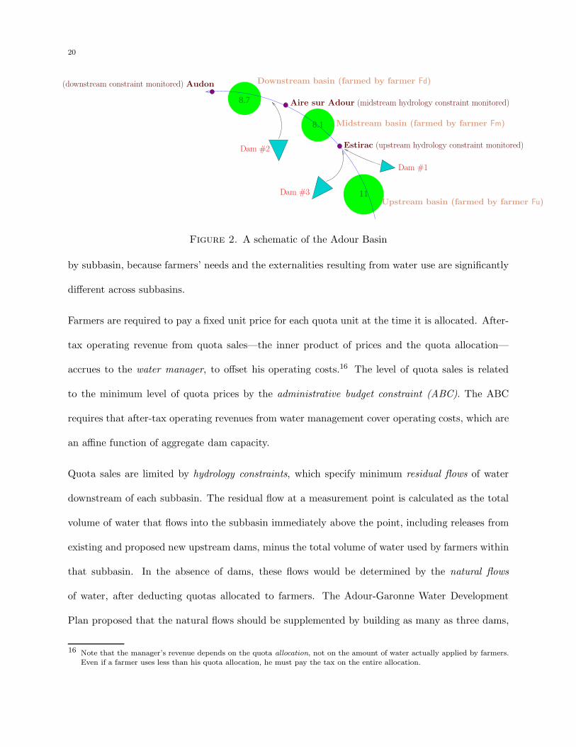
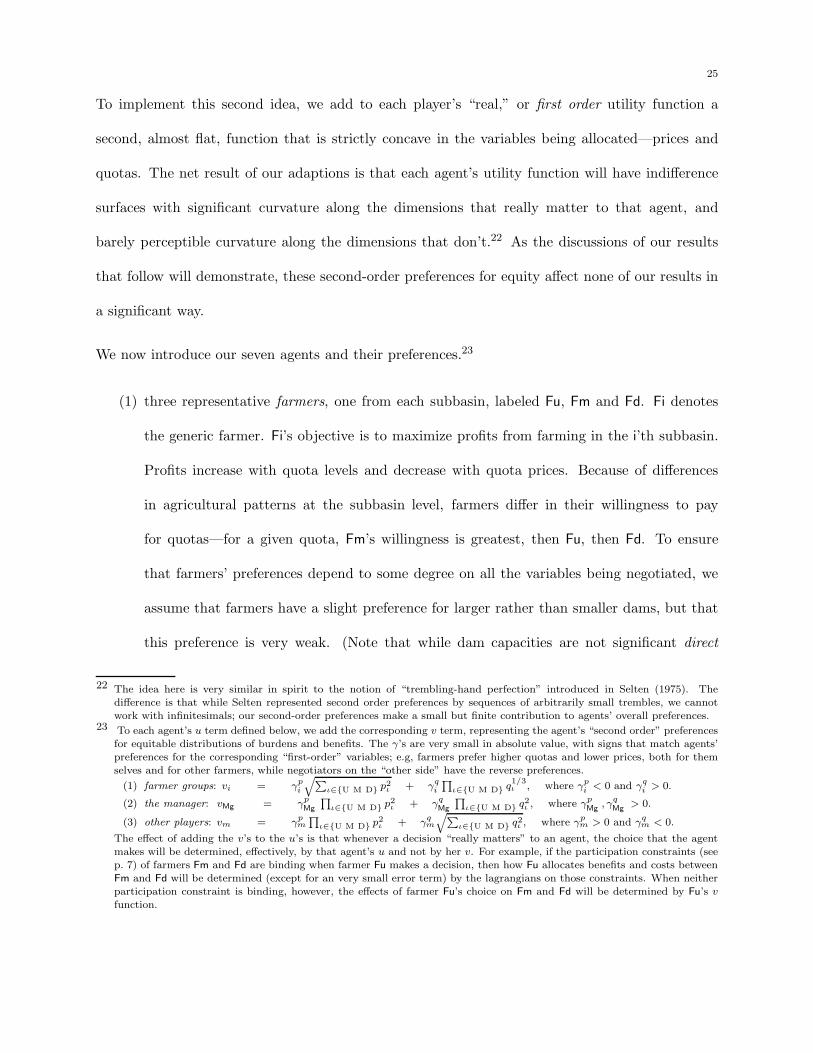
Structure of the Problem: The Adour Basin consists of three subbasins (see Fig. 2), separated by

flow points. The label inside each circle indicates the number of hectares (in thousands) under

irrigation in each subbasin. We will label these by U, M and D, for “upstream,” “midstream”

and “downstream.” The upstream subbasin is above Estirac. The midstream subbasin is below

Estirac and above Aire sur Adour. The downstream subbasin is below Aire sur Adour and above

Audon, where the Midouze joins the Adour. As Fig. 2 indicates, the sizes of the three subbasins

differ substantially. In particular, Fu’s subbasin is larger than the other two. We assume that

corresponding to each subbasin there is a single representative farmer, labeled, respectively, Fu, Fm

and Fd. The pattern of agricultural activity differs across subbasins.

Farmers in each subbasin negotiate over the quota allocation they will receive. The negotiated

quota allocation determines the maximum amount of water that a farmer is entitled to use, per

eligible hectare farmed.15 The quota does not depend on technical parameters, such as the crops a

farmer intends to grow, or the on-farm technical efficiency of water use. Quotas may, however, vary

15 In practice, the actual water used during the two-month period modeled is between 64% and 70% of the quota allocation.Generally, water is scarce enough that farmers use their entire purchased allocation over the entire growing season.

20

11

8.7

8.1

Downstream basin (farmed by farmer Fd)

Midstream basin (farmed by farmer Fm)

Upstream basin (farmed by farmer Fu)

Estirac (upstream hydrology constraint monitored)

Aire sur Adour (midstream hydrology constraint monitored)

(downstream constraint monitored) Audon

Dam #1

Dam #2

Dam #3

Figure 2. A schematic of the Adour Basin

by subbasin, because farmers’ needs and the externalities resulting from water use are significantly

different across subbasins.

Farmers are required to pay a fixed unit price for each quota unit at the time it is allocated. After-

tax operating revenue from quota sales—the inner product of prices and the quota allocation—

accrues to the water manager, to offset his operating costs.16 The level of quota sales is related

to the minimum level of quota prices by the administrative budget constraint (ABC). The ABC

requires that after-tax operating revenues from water management cover operating costs, which are

an affine function of aggregate dam capacity.

Quota sales are limited by hydrology constraints, which specify minimum residual flows of water

downstream of each subbasin. The residual flow at a measurement point is calculated as the total

volume of water that flows into the subbasin immediately above the point, including releases from

existing and proposed new upstream dams, minus the total volume of water used by farmers within

that subbasin. In the absence of dams, these flows would be determined by the natural flows

of water, after deducting quotas allocated to farmers. The Adour-Garonne Water Development

Plan proposed that the natural flows should be supplemented by building as many as three dams,

16 Note that the manager’s revenue depends on the quota allocation, not on the amount of water actually applied by farmers.Even if a farmer uses less than his quota allocation, he must pay the tax on the entire allocation.

21

provided stakeholders could negotiate an agreement regarding the size of each dam, subject to

capacity limits determined by technical considerations (see Fig. 2 for proposed dam locations and

the measurement points at which flows are monitored.17) The dams, if constructed, would have

different implications for water flows: as Fig. 2 indicates, dam #2 would increase flows at the

measurement point downstream of subbasin D only, while dams #1 and #3 would each increase

flows at all three measurement points. Farmers would be required to finance the operating costs of

the dams, but not the capital costs. Local government entities would share responsibility for the

capital costs with the national agricultural and environmental ministries (Faysse and Morardet,

1999).

Dam construction is controversial. The advantages are that new dams would increase the resid-

ual flows of water. Such residual flow increases would benefit users who are downstream of the

subbasins, promoting aquatic life, and relaxing the hydrological constraints on farmers. The dis-

advantages are that dams are costly and degrade the quality of the rural landscape.18

We now explain the hydrology constraints in more detail. For each subbasin, the residual flow of

water cannot fall short of a minimum level (called flow objective), which was set in the Adour-

Garonne Water Development Plan (SDAGE), in order to protect aquatic life in the river (Faysse

and Morardet, 1999). Two of the three classes of variables being negotiated will directly affect the

hydrology constraints: dam capacities, which affect water inflows, and quotas, which determine

water outflows. The other class of variables—quota prices—interact with hydrology constraints

through the administrative budget constraint. When dam capacities increase, administrative op-

erating costs increase also. Holding quota levels constaint, then quota prices must rise in order to

keep the administrator’s budget constraint in balance.

17 Dam #1’s maximum capacity is one quarter the maximum capacity of either of the other two dams.18 In general, it is by no means obvious that dams would benefit downstream aquatic life. In this paper, we model the benefits

reported by stakeholders (Faysse, 1997). We are indebted to an anonymous referee for emphasizing this point.

22

The Bargaining Space: There are three classes of negotiated variables: prices, quotas and dam

capacities. There are three proposed dams, and three price-quota pairs, one for each subbasin. In

the bargaining games we simulate, we distinguish between three bargaining regimes, identified as

CPCQ, CPIQ and IPCQ. The regimes differ in the flexibility they provide a representative from

one subbasin to differentiate that subbasin’s treatment under the bargaining outcome from the

treatment that the other subbasins receive. In regime CPCQ (common prices, common quotas),

the bargaining space is restricted so that a common price and a common quota applies to all

subbasins. In regime CPIQ (common prices, individual quotas), the price remains common but

bargainers are allowed to specify distinct quota levels for each subbasin. In regime IPCQ (individual

prices, common quotas), prices are common and quotas are distinct. In both CPIQ and IPCQ, we

impose (and, in §5.3 vary) a heterogeneity bound on the degree to which subbasin-specific negotiated

variables can be differentiated from each other.19 In the absence of such a bound, each subbasin

representative would attempt to acquire for his own subbasin the highest possible quota at the

lowest possible price, offloading the entire scarcity (in CPIQ) or cost (in IPCQ) burden onto the

other subbasins to the maximum extent allowed by their participation constraints. By varying these

bounds continuously, we can conduct comparative statics experiments on the impact of restricting

players’ flexibility within the bargaining space.

Analyzing these three distinct regimes enables us to explore the effect on bargaining performance

of different institutional specifications of the bargaining space. In particular, we test the natural

conjecture that if farmers are limited by institutional constraints on the extent to which they can

pursue their own interests at the expense of their “coalition partners,” then their performance as a

group will be enhanced.

19 Specifically, in regime CPIQ (IPCQ), we impose a bound on the variance of the three quotas (prices) announced in a givenproposal.

23

Each regime is examined under both normal and drought conditions. Historically, in eight out of

ten years, rainfall in the Adour Basin has been sufficient to provide farmers with adequate water

without violating the hydrology constraints. We refer to conditions in these years as “normal” and

calibrate our model so that under normal conditions, the hydrology constraints are not binding

in equilibrium (although they may bind off the equilibrium path). By contrast, our calibration of

“drought conditions” ensures that at least one of the hydrology constraints binds in equilibrium.

These two scenarios represent alternative operating assumptions on which negotiations might be

based: rational stakeholders would adopt quota proposals consistent with binding flow constraints

if and only if they collectively acknowledged the possibility of drought conditions.20 As will become

apparent below, the negotiating environment—and hence the comparative statics properties of our

model—will be quite sensitive to this critical assumption.

Bargaining Participants and their payoff functions: There are seven “players,” each one represent-

ing either a single stakeholder or a composite of stakeholders. Because the distribution of political

power among these stakeholders is not a primary consideration in this study, we specify exoge-

nously that each player in our benchmark model has the same access probability. (This assumption

is standard in the literature, cf. Baron and Ferejohn (1987) and the large literature that it spawned).

Each player has a strictly concave utility (or payoff) function defined on the space of bargaining

proposals. In multilateral, multi-issue bargaining contexts such as ours, weak concavity would be

a more natural assumption, since many dimensions of the bargaining space, though of critical im-

portance to some negotiators, will have no impact at all on others. However, strict concavity is

required in the MB model if we are to obtain unique solutions and hence meaningful comparative

20 In the actual negotiation procedure on which this study was based, no provision was made for assigning quotas conditional onrainfall levels. As a result, the agreed-upon total consumptive use would result, under drought conditions, in unsustainablelevels of water usage, reducing residual flows to below government-defined crisis flow levels. In such an event, the watermanager would be authorized to halt all irrigation. This rigidity in the negotiating procedure has an obvious and unfortunateconsequence: if the assumptions on which farmers base their negotiating positions are too conservative, they will deprivethemselves of available water under normal conditions; if the assumptions are not conservative enough, farmers risk thepossibility of catastrophic shut-downs under drought conditions. In turn, this rigidity contributed to the deadlocking of thenegotiations.

24

statics. The problem with weak concavity is that decisions which have a significant impact on

one party may be determined by an arbitrary resolution of indifference by another.21 Indeed, in a

computational model such as ours, the numerical solution algorithm may resolve indifference in a

significantly different way in response to an insignificant change in parameter specifications, gen-

erating a comparative statics effect that appears to be dramatic but is in fact completely artificial.

When we impose strict concavity on a problem involving the allocation of a burden (or benefit)

among multiple parties, we encounter two distinct kinds of problems. The first is a general one,

common to all multi-issue problems: typically, not every negotiator necessarily cares about each one

of the variables being negotiated. The second is special to allocation problems: when the burden

is being shared among a some or all of the negotiating parties, the most parsimonious assumptions

are: an individual who bears a portion of the burden cares about the size of her share, but is

indifferent between alternative distributions of the remaining share; for an individual who bears

none of the burden, the aggregate size of the burden may matter, but how the burden is allocated

is of no consequence.

It is relatively easy to resolve the first, general problem: we model each agent as having non-

degenerate preferences over all “aggregate” variables in the bargaining space, but, to sharpen our

analysis, we weight variables that are less important for that agent by negligibly small coefficients.

For example, each farmer in our model is primarily concerned about the price and quota she

negotiates for herself, but also has a negligible preference for larger over smaller dams. To resolve

the second, special problem, we assume, without particularly strong foundations, that negotiators

have an extremely mild, “second-order” preference for “equity”; that is, we assume that each agent

obtains a vanishingly small increment in utility from a symmetric allocation of a given residual

burden (i.e., excluding her own share) relative to an asymmetric allocation of the same residual.

21 A precisely analogous problem is endemic in extensive form game-theory, though it arises in a quite different context:decisions made by one agent at “off-the-equilibrium-path” decision nodes are of no consequence to that agent, but will ingeneral have a significant impact on the set of opportunities available to other agents.

25

To implement this second idea, we add to each player’s “real,” or first order utility function a

second, almost flat, function that is strictly concave in the variables being allocated—prices and

quotas. The net result of our adaptions is that each agent’s utility function will have indifference

surfaces with significant curvature along the dimensions that really matter to that agent, and

barely perceptible curvature along the dimensions that don’t.22 As the discussions of our results

that follow will demonstrate, these second-order preferences for equity affect none of our results in

a significant way.

We now introduce our seven agents and their preferences.23

(1) three representative farmers, one from each subbasin, labeled Fu, Fm and Fd. Fi denotes

the generic farmer. Fi’s objective is to maximize profits from farming in the i’th subbasin.

Profits increase with quota levels and decrease with quota prices. Because of differences

in agricultural patterns at the subbasin level, farmers differ in their willingness to pay

for quotas—for a given quota, Fm’s willingness is greatest, then Fu, then Fd. To ensure

that farmers’ preferences depend to some degree on all the variables being negotiated, we

assume that farmers have a slight preference for larger rather than smaller dams, but that

this preference is very weak. (Note that while dam capacities are not significant direct

22 The idea here is very similar in spirit to the notion of “trembling-hand perfection” introduced in Selten (1975). Thedifference is that while Selten represented second order preferences by sequences of arbitrarily small trembles, we cannotwork with infinitesimals; our second-order preferences make a small but finite contribution to agents’ overall preferences.

23 To each agent’s u term defined below, we add the corresponding v term, representing the agent’s “second order” preferencesfor equitable distributions of burdens and benefits. The γ’s are very small in absolute value, with signs that match agents’preferences for the corresponding “first-order” variables; e.g, farmers prefer higher quotas and lower prices, both for themselves and for other farmers, while negotiators on the “other side” have the reverse preferences.

(1) farmer groups: vi = γpi

q

P

ι∈{U M D} p2ι + γq

i

Q

ι∈{U M D} q1/3

ι , where γpi < 0 and γq

i > 0.

(2) the manager: vMg = γpMg

Q

ι∈{U M D} p2ι + γq

Mg

Q

ι∈{U M D} q2ι , where γp

Mg, γq

Mg> 0.

(3) other players: vm = γpm

Q

ι∈{U M D} p2ι + γq

m

q

P

ι∈{U M D} q2ι , where γp

m > 0 and γqm < 0.

The effect of adding the v’s to the u’s is that whenever a decision “really matters” to an agent, the choice that the agentmakes will be determined, effectively, by that agent’s u and not by her v. For example, if the participation constraints (seep. 7) of farmers Fm and Fd are binding when farmer Fu makes a decision, then how Fu allocates benefits and costs betweenFm and Fd will be determined (except for an very small error term) by the lagrangians on those constraints. When neitherparticipation constraint is binding, however, the effects of farmer Fu’s choice on Fm and Fd will be determined by Fu’s vfunction.

26

contributors to farmers’ utilities, they do have an important, indirect effect through the

model’s constraint structure.)

Formally, Fi’s first order utility is translog in his quota price pi and quota level qi:

ln

(

ui(pi, qi,d)

)

= a0i +

5∑

k=1

aki x

ki (pi, qi) +

3∑

j=1

bji ln(1 + dj), where

xi(pi, qi) =

(

ln(1 + pi) ln(1 + p2i ) ln(1 + qi) ln(1 + q2i ) ln((1 + pi)(1 + qi))

)

.

The vector ai ∈ R6 is estimated from linear programming simulations based on microeco-

nomic farm models (Gleyses and Morardet, 1997); the vector d = (dj)3j=1, where dj is the

capacity of the j’th dam, expressed as a fraction of its maximum feasible capacity. The bji ’s

are only negligibly larger than zero. It should be noted that the arguments of Fi’s utility

are not the regular inputs and output of an agricultural production function. Rather, once

quotas have been negotiated, the maximum quota level available to Fi, qi will be a constraint

on production. Moreover, since Fi must pay for the quota level he has agreed to, regardless

of his actual production level, he will view piqi as a sunk cost.

(2) an environmentalist (Ev). This stakeholder, a composite of diverse environmental inter-

ests, is primarily concerned about the quality of the rural landscape, and secondarily about

maintaining adequate river flow rates. Since the rural landscape is negatively impacted by

dam construction, Ev’s CES utility function is decreasing in the vector d and increasing in

the vector r: dj is the capacity of the j’th dam, expressed as a fraction of its maximum

feasible capacity; ri is the residual flow of water in the i’th subbasin, again expressed as

a fraction of the maximum feasible residual flow.24 (Note that players do not explicitly

propose values for the residual flow vector, r; rather, each proposal implies a unique value

for r, which increases with proposed dam capacities and decreases with proposed quotas.)

24 This maximum is attained when dams are built to their maximum capacity and farmers use no water.

27

Clearly, Ev’s two goals can be reconciled only by reducing the water used by farmers.

In our specification of nonfarmers’ utilities, the capacities of dams #1 and #2 are viewed as

virtually perfect substitutes for one another, and imperfect substitutes for the capacity of

dam #3. (The qualifier “virtually” is required to ensure strict rather than weak preference

concavity.) Dam #3 is treated specially because its construction would have a particularly

significant negative impact on the landscape—it is located in the mountains in a very scenic

valley. Also residual flows in subbasins U and Mas virtually perfect substitutes for one an-

other, and imperfect substitutes for residual flows below subbasin D. Flows below subbasin

D are tread specially because they are considered particularly important for maintaining

aquatic life and recreational activities.

We assume that Ev has a very weak preference for higher rather than lower levels of

total revenue from quota sales,∑3

i=1 piqi; local authorities tax these sales at a propor-

tional rate, and utilize the tax receipts for maintaining the river; Ev obtains some utility

from these tax-financed government services. In symbols, let φ(x) and ψ(x) denote, re-

spectively, strictly concave and strictly convex functions that are both arbitrarily close to

the function∑n

j=1 xj. Now define uEv (d, r) =

(

a0i

∑5k=1 a

kEv

(

xkEv (d, r)

)ρEv)1/ρEv

, where

xEv (d, r) =

(

φ(rU, rM), rD, (2 − ψ(d1, d2)), (1 − d3),∑3

i=1 piqi

)

and aEv ∈ R5++

with a5Ev � a1

Ev , a2Ev � a3

Ev , a4Ev and a5

Ev ≈ 0. Note that increases in proposed dam

capacities affect utility positively through the first two arguments of uEv , and negatively

through the third and fourth. When a dam is small, its net effect on uEv is positive, but

there may exist a critical size beyond which its net effect becomes negative.

Lacking quantitative data data from which to estimate Ev’s preferences, we assign values to

the weights aEv which reflect in a qualitative way the relative importance that Ev assigns

to different concerns, as elicited from stakeholder interviews (Faysse, 1997). We proceed in

the same way for the remaining three players described below.

28

(3) a downstream user (Ds). There are stakeholders in the Adour basin that are primarily

concerned with minimizing demands on water flows in the three subbasins. These include

downstream water users, recreational users of the river and environmentalists concerned

with downstream aquatic wildlife. We combine these stakeholders into a composite “down-

stream user,” Ds. While Ds’s utility has the same functional form as Ev’s, he ranks water

flows as significantly more important than preserving the rural landscape. (Recall that

Ev, by contrast, was significantly more concerned about rural landscape.) Specifically, we

assume that a1Ds , a

2Ds � a3

Ds , a4Ds � a5

Ds , with a5Ds ≈ 0. Since Ds has a higher “willingness-

to-pay” for residual flows in terms of larger dams, the net effect of a unit increase in dam

capacity for uDs is either more positive or less negative than for uEv .

(4) a manager (Mg). Mg administers the distribution of water in the district. For statutory

reasons, he is equally concerned with avoiding budget deficits and budget surpluses. Further,

he derives utility from increasing the scope of the water system he administers. That is,

he prefers a larger operation, and therefore higher dam capacities. Mg’s CES utility is

uMg (p,q,d) =

(

a0Mg

∑2k=1 a

kMg

(

xkMg (d,p,q)

)ρMg)1/ρMg

where aMg ∈ R2+, x1

Mg = φ(d)

and x2Mg decreases in the distance between the manager’s realized and his target return

on operations. Note that in addition to his role as a player, Mg impacts the bargaining

through the administrative budget constraint (see p. 19).

(5) the taxpayer (Tp). The taxpayer in our model represents interests that are primarily non-

local and non-agricultural.25 This player’s goals are to minimize the burden on French

taxpayers, by limiting expenditures on local dams, and to maximize benefits to non-farm

users, by increasing residual flows. Like Ev and Ds, Tp has a very weak positive preference

for higher rather than local local tax revenues. Formally, Tp’s CES utility is uTp (r, c) =

25 In actual negotiations, these interests might be represented by a bureaucrat from Paris, charged with ensuring that thenegotiation process is not captured by either farmers or by local political interests.

29

(

a0Tp

∑4k=1 a

kTp

(

xkTp (r, c)

)ρTp)1/ρTp

where xTp (r, c) =

(

(φ(rU, rM), rD, (3−ψ(c)),∑3

i=1 piqi

)

,

where cj is the construction cost of the j’th dam, expressed as a fraction of the cost of con-

structing to their maximum admissible capacity, and aTp ∈ R4++ with a4

Tp � a1Tp , a

2Tp �

a3Tp and a4

Tp ≈ 0.

Note that under this specification, all players have non-degenerate preferences over all classes of

variables, with the qualifications that farmers care only about the quotas that affect their own sub-

basins, and non-farm players care only about the inner-product of quota prices and and quantities.

With the addition of second-order preferences (footnote 23) to these “first-order” preferences, each

player’s preferences are strictly concave in all variables.

The preference profile specified above gives rise to a clear-cut conflict between farmers on the one

hand, and Ev, Ds and Tp on the other. (For this reason, we shall sometimes refer to the latter

group of three players as the anti-farmer group). Farmers prefer higher quotas, and, when the

hydrology constraints are binding, prefer greater dam capacity to less. Ev, Ds and Tp prefer lower

quotas, because quotas and residual flows are negatively related, and less dam capacity, either to

preserve the rural landscape or to lower the tax burden. The relationship between the manager

and the farmers is more complex. Like the farmers, the manager prefers higher quotas and more

dam capacity, but, in contrast to the farmers, he also prefers higher prices.

Projecting Preferences onto price-quota space: Because the dimensionality of our bargaining space

is so large (R7), it is difficult to obtain much intuition by studying players’ full-dimensional proposals

directly. Fortunately, one can gain a great deal of intuition for the comparative statics results

discussed in §5 by projecting players’ preferences onto price-quota space. (This simplification does,

however, obscure some interesting subtleties.) The projection is immediate for farmers, at least in

regime CPCQ, and quite simple for Tp and Mg. For Ds and Ev, however, it is obtained indirectly

30

through the constraint system, since these players derive first-order utility from residual flows and

landscape quality, caring barely at all about prices.

In order to understand how Ds and Ev’s preferences are projected, consider regime CPCQ and

assume that the ABC is binding.26 Letting i denote either Ds or Ev, player i’s concerns can be

mapped into preferences over prices and quotas as follows. Starting from a given utility level ui, a

unit increase in the common quota reduces residual flows; hence i’s utility declines, and the only

variables on the bargaining table that can perhaps increase it back up to ui are dam capacities.

(Recall from p. 27 that, holding quotas constant, if the initial capacity of dams is sufficiently small,

the net effect of dam capacity increases on ui is positive.) Now consider a unit increase in quotas,

an increase in dam capacity that exactly offsets the resulting loss in residual flows would leave i’s

utility below its initial level ui, since i dislikes dams. So dams must be increased by more than this

level, to the point that the resulting net increase in residual flows is sufficient to compensate i for

his utility loss due to larger dams. Since administrative operating costs increase with dam capacity,

and the ABC is binding, larger dams require higher quota prices. Thus, the ABC, together with

the technological relationships between quotas, dams and residual flows, induce utility levels for i

in price-quota space which decrease with quotas and, provided that the derivative of ui with respect

to some dam capacity is positive, increase with prices (that is, i’s indifference curves in price-quota

space are positively sloped). If, however, dam sizes reach levels such that i’s utility declines with

any further increase in their sizes, then farmers cannot “purchase” from i any further increase in

quota levels at any price.

The shape of i’s induced preferences in price-quota space depend on his relative preference for

residual flows and rural landscape. It follows from our comparison of Ds and Ev on p. 27 that a

unit increase in quotas hurts Ds less than Ev, while, holding quotas constant, a unit increase in dam

capacity benefits Ds more. Therefore, the range of dam sizes for which Ev’s indifference curves in

26 See p. 19. The ABC is almost always binding when farmers make proposals.

31

price-quota space will be positively sloped is smaller than the range for Ds, and they will be more

steeply sloped whenever they are positive. To summarize the preceding discussion, while there is no

economic marketplace in which farmers can “buy” quotas from either Ds or Ev, there is, in effect,

a political marketplace in which quotas can be “purchased” from either of these “suppliers,” by

increasing dam size (and residual flows), and a range of dam sizes for which the “political supply

schedule” for quotas is upward sloping. Having made this distinction, we can now proceed as if

farmers were buyers of quotas, and non-farmers were sellers.

The slope of the political supply schedule may become considerably steeper when hydrology con-

straints are binding, which in drought conditions is usually the case. For example, on p. 50 below,

we discuss in some detail the predicament facing farmers in regime IPCQ under drought conditions:

(a) at the proposed quota and dam levels, the residual flow below either subbasin M or U is at its

minimal admissible level; (b) player Ds’s participation constraint is binding; (c) dams #1 and #3

are so large that Ds’s utility declines with a further increase in either; (d) an increase in dam #2

increases Ds’s utility. In this situation, the only way a farmer can induce Ds to agree to “supply”

still more quotas is to offer to expand the size of dam #2. However, an increase in the common

quota decreases residual flows below each of the subbasins, while the expansion in dam #2 increases

only the flow below subbasin D (see Fig. 2). Consequently, to restore the flows below the other sub-

basins to their minimal admissible levels, either dam #1 or dam #3 must be increased as well. But

by (c), these secondary increases negatively impact Ds’s utility, so that dam #2 must be increased

still further to compensate him. That is, because of the hydrology constraints, a unit increase in

quotas requires three “rounds” of dam increases rather than the single one that would be required

under normal conditions. Because each additional increase in dam size raises operating costs, and

part of each increase in dam capacity must be “bought” by devoting part of the capacity increase

to increasing residual flows, three rounds of quota price increases are required as well. In this way,

the hydrology constraints steepen the slope of the “political supply schedule” facing farmers.

32

5. Comparative Statics Analysis

In this section, the institutional setting described in §4 provides a context within which we explore

a number of questions relating to bargaining power. To obtain the results reported in this section,

we solved our computer simulation model for a variety of benchmark specifications, then succes-

sively increased one parameter (e.g., some player’s access probability) and re-solved the model to

obtain numerical comparative statics properties. We will summarize the results of three simulation

experiments, each one consisting of a large number of individual simulations. Our primary objective

in this paper is to provide intuitions for our key findings. Accordingly, we will suppress all but

essential details of our numerical results, and focus almost exclusively on the effect of perturbing

certain parameters on the final rounds of bargaining. (Many of these suppressed details are docu-

mented in the papers cited on p. 18.) In §5.1, we introduce our method of analysis with a stripped

down model in which only three players participate. In §5.2, we compare the performance of the

farmer coalition when farmers participate independently in the bargaining process, versus when the

coalition is represented by a spokesman, charged with maximizing the joint interests of all farmers.

Finally, in §5.3, we consider how the specification of the bargaining space affects player utilities. In

particular, we examine whether farmers’ bargaining power is increased if the maximum permissible

degree of heterogeneity across water prices or quotas is restricted.

5.1. Shifting Access: an heuristic example. To introduce our method of analysis, we begin

with a simple example. The example serves an heuristic purpose, but also makes a substantive

point. As an instructive device, the example illustrates in a simplified context how comparative

statics exercises are conducted and analyzed in this paper. In particular, it illustrates the role that

backward induction plays in the MB model, and demonstrates how effects in the last rounds of the

game “build on each other,” creating a “snowball effect” that become magnified as we move back-

wards through the game tree. The substantive contribution is to highlight a striking characteristic

of the Rausser-Simon model, which distinguishes it from axiomatic models of bargaining such as

33

the Nash bargaining model, and strategic models such as Rubinstein’s that implement the “Nash

program” (Osborne and Rubinstein, 1990). In all of those models, there is a monotone increas-

ing relationship between a player’s equilibrium payoffs and his traditional, exogenously specified

measures of bargaining power: his bargaining weight and his “default payoff,” i.e., the payoff he

receives if the bargaining phase ends without an agreement being reached. In the MB model, there

are additional, less transparent, sources of bargaining advantage, so that the relationship between

payoffs and traditional measures of power is more delicate. In particular, the relationship between

payoffs and power as traditionally measured need no longer be monotone.

The example in this subsection compares the equilibria of two games which are identical except

for the players’ access probabilities. In both games, farmers as a group have the same aggregate

access, but in the second, the distribution among them is shifted in favor of a farmer who has

a strategic advantage relative to the others, arising from his “location” in preference space. To

reduce the problem to its barest essentials, we strip down our model by excluding four of our seven

players from the bargaining process, leaving only Fu, Fm and Ds. Assume also that there is only

one dam (#1) whose size is being negotiated. The comparative statics experiment we consider

is a shift in access from Fu to Fm in the CPCQ regime.27 (Recall that access probabilities were

introduced on p. 5. and that regime CPCQ is defined by the condition that prices and quotas must

be equal across subbasins.) To further simplify the exposition, we project all players’ preferences

onto price-quota space, in the manner described on pp. 29-31. Intuitively, one would expect that

a shift in access from Fu to Fm would increase Fm’s utility while decreasing Fu’s. In fact, the

outcome is that both Fm and Fu benefit from the shift! The key to the argument is that Fm’s

participation in the negotiations generates, in effect, a positive externality for Fu. When Fm gains

access at the expense of Fu, there are, in all but the last round of bargaining, multiple effects on

27 The reader should be advised that we use the word “shift” for expositional convenience: we are not suggesting that theaccess probability vector is a variable over which farmers have some control. The exercise considered here is a routinecomparative statics one, in which one exogenous parameter of the model—the distribution of power between farmers—isvaried.

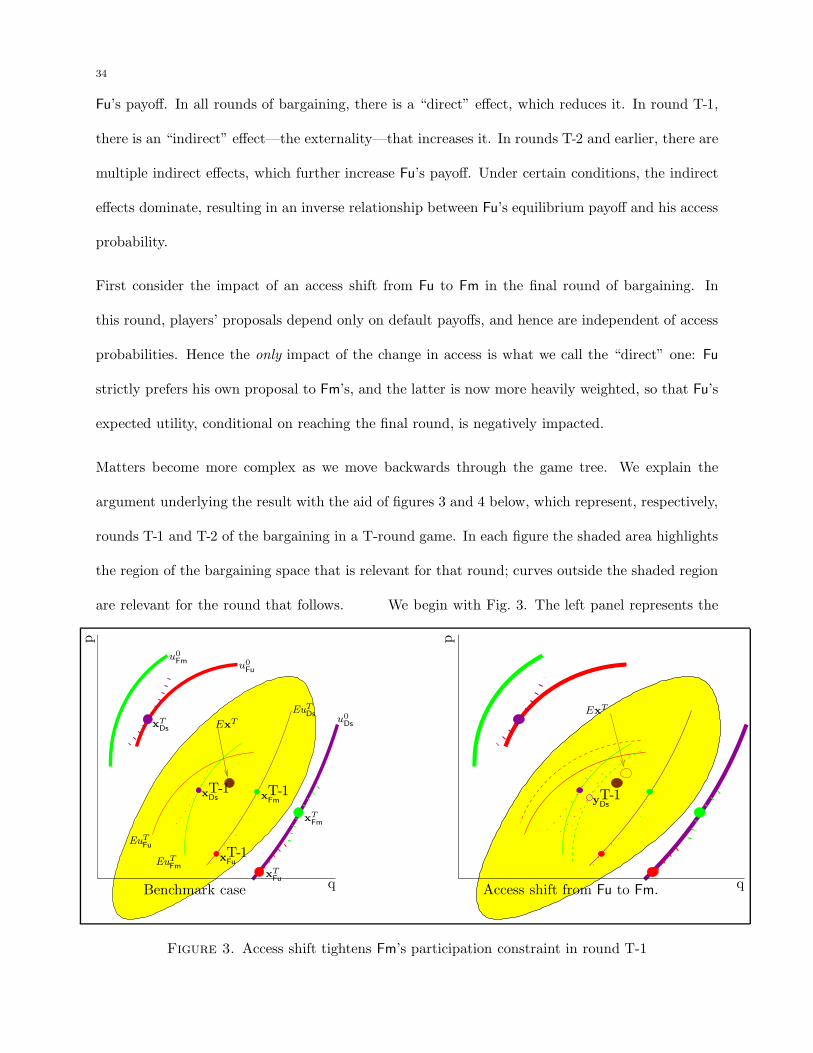
34

Fu’s payoff. In all rounds of bargaining, there is a “direct” effect, which reduces it. In round T-1,

there is an “indirect” effect—the externality—that increases it. In rounds T-2 and earlier, there are

multiple indirect effects, which further increase Fu’s payoff. Under certain conditions, the indirect

effects dominate, resulting in an inverse relationship between Fu’s equilibrium payoff and his access

probability.

First consider the impact of an access shift from Fu to Fm in the final round of bargaining. In

this round, players’ proposals depend only on default payoffs, and hence are independent of access

probabilities. Hence the only impact of the change in access is what we call the “direct” one: Fu

strictly prefers his own proposal to Fm’s, and the latter is now more heavily weighted, so that Fu’s

expected utility, conditional on reaching the final round, is negatively impacted.

Matters become more complex as we move backwards through the game tree. We explain the

argument underlying the result with the aid of figures 3 and 4 below, which represent, respectively,

rounds T-1 and T-2 of the bargaining in a T-round game. In each figure the shaded area highlights

the region of the bargaining space that is relevant for that round; curves outside the shaded region

are relevant for the round that follows. We begin with Fig. 3. The left panel represents the

p

q

u0

Ds

u0

Fu

u0

Fm

EuTDs

EuTFu

EuTFm

xTFm

xTFu

xTDs

xT-1Fm

xT-1Fu

xT-1Ds

ExT

Benchmark case

p

q

yT-1Ds

ExT

Access shift from Fu to Fm.

Figure 3. Access shift tightens Fm’s participation constraint in round T-1

35

bargaining for our benchmark vector of access probabilities. The three solid thick curves (labelled

u0r) outside the shaded region represent the three players’ participation constraints in the round T

of bargaining, i.e., any price-quota pair on u0r yields player r the same payoff as the disagreement

outcome. Note that Fm’s constraint is steeper than Fu’s, reflecting Fm’s higher willingness-to-pay

for the marginal quota (for the reason explained on p. 25). The players’ T-round proposals are

indicated by the xTr ’s. The large dot in the center of the left panel denotes the weighted average,

ExT , of these proposals, where the weights are the players’ access probabilities. The three solid

thin curves (labelled EuTr ) in the left panel represent participation constraints in round T-1, i.e.,

any price-quota pair on EuTr yields player r the same payoff as r’s expected payoff from the lottery

in round T generated by the xTr ’s. Note in particular that while the relative locations of u0

Fm and

u0Fu are determined by the exogenously specified disagreement payoffs, the locations of the curves

EuTFm and EuT

Fu relative to point ExT depend on agents’ risk aversion. The more risk-averse is

agent r, the greater will be the minimum distance between ExT and the curve EuTr . Unless Fm

is significantly more risk averse than Fu, Fm’s participation constraint in round T-1 must lie, as it

does in the figure, to the south-east of Fu’s in the region of the figure to the south of ExT . The

level sets of Ds’s payoff function are relatively steep, in fact they are almost vertical. (This means

that if the size of dam #1 is increased by one unit, the resulting increment in water flows holding

quotas constant raises Ds’s utility by an amount only barely greater than the amount by which Ds’s

utility declines because dams despoil the landscape. The gap between these two amounts is the

“surplus utility” generated by the dam increase, which can be “soaked up” by an increase in quota

allocation, leaving Ds indifferent. In this instance, the surplus amount is tiny.) Now, since Fm’s

level sets are steeper than Fu’s, Fm’s participation constraint must be binding on Ds, while Fu’s

must be slack. It follows that Ds’s proposal in round T-1 will be independent of the precise location

of Fu’s participation constraint in round T (EuTFu ), but will be affected by any small change in the

location of Fm’s (EuTFm ).

36

The right panel of Fig. 3 indicates schematically the effect of a shift in access from Fu to Fm on the

bargaining in round T-1. The expected price-quota pair in round T shifts to the north-east (i.e.,

from the solid dot to the open dot), reflecting Fm’s relative preference, now more heavily weighted,

for higher quotas at higher prices. To reduce clutter in this panel, we have omitted the labels

on the lines representing participation constraints. The dashed lines parallel to the two farmers’

thin solid lines represent their participation constraints after the access shift: necessarily, Fm’s

constraint tightens while Fu’s slackens. The widely spaced dotted curves represent the proposers’

indifference curves through their respective optimal proposals. Since Ds is bound by Fm’s constraint

and unaffected by Fu’s, the effect of the access shift is that Ds now proposes the open dot yT-1Ds

rather than the (unlabeled) solid dot representing xT-1Ds . Thus, relative to the benchmark case, the

lottery now facing players, conditional on reaching round T-1, is unambiguously more favorable for

Fm, and less favorable for Ds. For Fu, the net effect is indeterminate. Once again, the direct effect

of the access shift is negative: Fu prefers his own proposal to Fm’s, and weight initially assigned

to the former is now assigned to the latter. But in this round, there is an additional, “indirect”

effect, associated with the shift in Ds’s proposal. Because the perturbed proposal is prefered by Fu

to Ds’s original proposal, this effect benefits Fm.

These changes in round T-1 impact the locations of players’ participation constraints in round

T-2. Fig. 4 depicts the bargaining in this round; we include the participation constraints for

round T-1 as well for reference. The left panel represents the benchmark case; the participation

constraint for player r in round T-2 is represented by the thick curve EuT−1r . The right panel

indicates the cumulative effect of the access shift by round T-2. As in the right panel of Fig. 3,

participation constraints in the benchmark case are represented by solid lines; those after the access

shift by dashed lines. Once again, each widely spaced dotted curve represents the indifference curve

through some player’s optimal proposal. Reflecting the remarks above, Ds’s participation constraint

is slacker than in the benchmark case, while Fm’s is tighter. As we have noted, Fu’s constraint

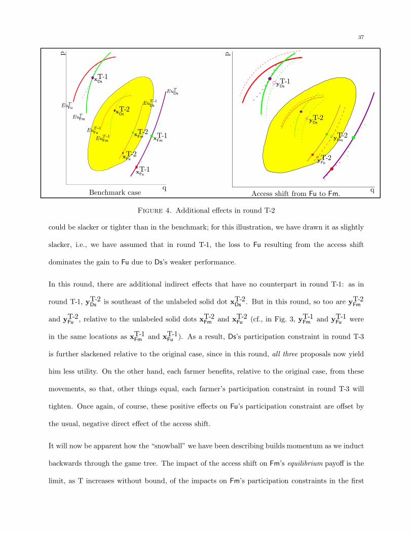
37

p

q

EuTDs

EuT−1

Ds

EuT−1

Fu

EuTFu

EuTFm

EuT−1

FmxT-1Fm

xT-1Fu

xT-1Ds

xT-2Fm

xT-2Fu

xT-2Ds

Benchmark case

p

q

yT-1Ds

yT-2Fm

yT-2Fu

yT-2Ds

Access shift from Fu to Fm.

Figure 4. Additional effects in round T-2

could be slacker or tighter than in the benchmark; for this illustration, we have drawn it as slightly

slacker, i.e., we have assumed that in round T-1, the loss to Fu resulting from the access shift

dominates the gain to Fu due to Ds’s weaker performance.

In this round, there are additional indirect effects that have no counterpart in round T-1: as in

round T-1, yT-2Ds is southeast of the unlabeled solid dot xT-2

Ds . But in this round, so too are yT-2Fm

and yT-2Fu , relative to the unlabeled solid dots xT-2

Fm and xT-2Fu (cf., in Fig. 3, yT-1

Fm and yT-1Fu were

in the same locations as xT-1Fm and xT-1

Fu ). As a result, Ds’s participation constraint in round T-3

is further slackened relative to the original case, since in this round, all three proposals now yield

him less utility. On the other hand, each farmer benefits, relative to the original case, from these

movements, so that, other things equal, each farmer’s participation constraint in round T-3 will

tighten. Once again, of course, these positive effects on Fu’s participation constraint are offset by

the usual, negative direct effect of the access shift.

It will now be apparent how the “snowball” we have been describing builds momentum as we induct

backwards through the game tree. The impact of the access shift on Fm’s equilibrium payoff is the

limit, as T increases without bound, of the impacts on Fm’s participation constraints in the first

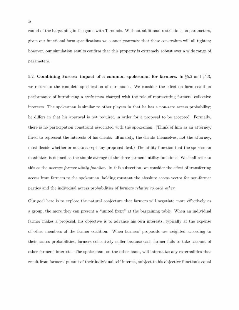
38

round of the bargaining in the game with T rounds. Without additional restrictions on parameters,

given our functional form specifications we cannot guarantee that these constraints will all tighten;

however, our simulation results confirm that this property is extremely robust over a wide range of

parameters.

5.2. Combining Forces: impact of a common spokesman for farmers. In §5.2 and §5.3,

we return to the complete specification of our model. We consider the effect on farm coalition

performance of introducing a spokesman charged with the role of representing farmers’ collective

interests. The spokesman is similar to other players in that he has a non-zero access probability;

he differs in that his approval is not required in order for a proposal to be accepted. Formally,

there is no participation constraint associated with the spokesman. (Think of him as an attorney,

hired to represent the interests of his clients: ultimately, the clients themselves, not the attorney,

must decide whether or not to accept any proposed deal.) The utility function that the spokesman

maximizes is defined as the simple average of the three farmers’ utility functions. We shall refer to

this as the average farmer utility function. In this subsection, we consider the effect of transferring

access from farmers to the spokesman, holding constant the absolute access vector for non-farmer

parties and the individual access probabilities of farmers relative to each other.

Our goal here is to explore the natural conjecture that farmers will negotiate more effectively as

a group, the more they can present a “united front” at the bargaining table. When an individual

farmer makes a proposal, his objective is to advance his own interests, typically at the expense

of other members of the farmer coalition. When farmers’ proposals are weighted according to

their access probabilities, farmers collectively suffer because each farmer fails to take account of

other farmers’ interests. The spokesman, on the other hand, will internalize any externalities that

result from farmers’ pursuit of their individual self-interest, subject to his objective function’s equal

39

weighting of the three farmers’ utilities. We would expect, therefore, that the equilibrium value of

the average farmer utility function will increase with the spokesman’s access.

A number of questions arise in the context of our particular model: Does the spokesman always

improve coalition performance? Under what conditions will the spokesman’s contributions have

the greatest impact? Which farmers benefit from the spokesman’s participation, which, if any,

lose, and why? The “why” question is, in our view, particularly interesting, because it focuses

attention on the precise nature of the externalities that are internalized by the spokesman, how

these externalities differentially affect the different members of the farmer coalition and, most

importantly, how they impact the bargaining performance of the farmer coalition.

We address these questions for six specifications, varying both the issue space (CPCQ, CPIQ,

IPCQ) and hydrological conditions (normal vs. drought). Throughout §5.2 (and §5.3 as well), we

focus on the case in which Ds is default strong, across all six specifications. (We say that a member

of the anti-farmer group (as defined on p. 28) is default strong if his participation constraint is

binding on all farmers and the spokesman in the final round of negotiations.28) The results of our

simulation experiments are summarized below. Most striking is the counter-intuitive result that

in regime IPCQ under normal conditions, all farmers’ utilities actually decline as the spokesman

gains access! Our other results are: (i) comparing his effect on farmer coalition performance in

regime CPCQ relative to the other two regimes, the spokesman has a negligible effect under normal

conditions, and no effect whatever under drought conditions. As the spokesman gains access in

regimes IPCQ and CPIQ; (ii) Fu’s equilibrium utility always declines; (iii) Fm’s, Fd’s and the

average farmer’s equilibrium utilities increase except in regime IPCQ, normal conditions; and (iv)

equilibrium utilities for all members of the anti-farmer group move in the opposite direction from

the change in the average farmer’s utility.

28 Surprisingly, we find that changing the identity of the default strong player has little impact on our results.

40

One can obtain intuition for each of these results through a detailed study of players’ final round

proposals. Once these final round details are well understood, most of the equilibrium comparative

statics properties can be deduced readily by applying the usual backward induction logic, taking

into account the “snowball” effects illustrated in §5.1. To illustrate how this logic works, we shall

see that in the final round (round T), the spokesman discriminates against Fu to the benefit of

other farmers, so that Fu’s participation constraint in round T-1 becomes slacker as the spokesman

gains access. In the penultimate round, typically, the spokesman again discriminates against Fu,

and for the same reason. (The degree of discrimination will typically be less dramatic in round

T-1 than in T, because participation constraints become tighter as we move backward through the

inductive chain, leaving the spokesman with less room to maneuver.) Thus in round T-1 there will

be two reinforcing effects—his slacker participation constraint and the discrimination against him

by the spokesman—that contribute to a weaker performance by Fu. Typically, this weakness will

compound as we work back through the inductive chain to the solution: the result, typically, will

be that as the spokesman gains access, Fu’s expected solution payoff will decline. We emphasize the

qualification “typically” because for some parameter values, countervailing effects can reverse the

impact of the last round effects. Since no such reversals arise in the experiments reported in this

paper, the details we overlook by focusing on the final round, though interesting, are not critical.

Regime CPCQ: In this regime under normal conditions, the farmer coalition’s welfare increases.

with the spokesman’s involvement. Under drought conditions, it makes no difference whatsoever.

The explanation for this difference is as follows. In the absence of hydrology constraints, farmers

maximize their utilities subject to a common “political supply schedule” for quotas (see pp. 29-31).

Because farmers have different optimal locations along this schedule, their proposals will differ. If

hydrology constraints bind sufficiently tightly, however, the lowest quota level on the schedule that

will satisfy these constraints will exceed even the level that would be optimal for Fm, who has

the highest willingness to pay for quotas. Under these circumstances, all preference differences

41

between farmers will be suppressed at the bargaining table, since all farmers will be obliged to

propose the same, super-optimal quota level. When the spokesman participates, he will be subject

to exactly the same constraints; hence his proposal will be indistinguishable from the common

proposal offered by farmers. For this reason, if the drought is sufficiently intense, the transfer of

access to the spokesman will have no impact at all. (For the same reason, the bargaining outcome

will also be independent of the distribution of access across farmers)

Under normal conditions, when the hydrology constraints do not bind, the preference variation

between farmers is no longer suppressed, and the spokesman can make a difference. Not surpris-

ingly, however, his role in regime CPCQ is relatively insignificant since farmers in this regime are

constrained to treat themselves and other farmers equally; there are, simply, no opportunities for

self-promotion at the expense of the group. The spokesman’s role is limited to merely reducing

risk. As noted above, in the absence of hydrology constraints, farmers’ final round proposals will

differ in accordance with their willingness-to-pay: Fm proposes the highest quotas, prices and dam

capacity levels, and Fd the lowest. When the spokesman’s access increases, farmers’ expected utili-

ties increase somewhat because their risk exposure is reduced: their utilities from the spokesman’s

proposal exceeds average of their utilities from all three farmers’ proposals. For the model specifi-

cations we consider, this reduction in risk translates into an increase in farmers’ solution payoffs.

We should not expect, however, that this property will be robust across a wide range of parameter

specifications, since other parties at the bargaining table also benefit from the spokesman’s partic-

ipation: as his access increases, the variance of farmers’ proposals decreases to the benefit of all

risk averse parties. Had the other negotiators been significantly more risk averse than the farmers,

their gain from the reduction in risk might have exceeded the farmers’ gain, inducing, possibly, a

decline in farmers’ solution payoffs as the spokesman’s access increased.

In contrast to CPCQ, each farmer in regime CPIQ or IPCQ has ample opportunity to pursue

his own interests at the expense of other farmers. He does so by proposing either low quotas

42

(in CPIQ) or high prices (in IPCQ) for other farmers, and either a high quota or a low price

for himself. We refer to this individually rational pursuit of self-interest as beggar-thy-neighbor

behavior. Its implications, explored below, are subtle and diverse, and vary depending on the regime

and hydrological conditions. As noted earlier, much can be learned by comparing the spokesman’s

proposal in the final round of bargaining to the average of farmers’ individual proposals in that

round.

In the discussion of regime CPIQ that follows, we will consider three kinds of averages. For a

given farmer, we consider the mean of the three subbasin quota proposals made by that farmer,

and refer to this the farmer’s mean quota. For a given subbasin, we will examine the average of

the three farmers’ quota proposals for that basin and refer to this to as an average subbasin quota

proposal. Each average subbasin proposal will be compared to the spokesman’s proposal for that

basin. Finally, we will examine the average of these subbasin averages, and refer to this as the

farmers’ the overall average quota proposal. This last scalar will be compared to the average of the

quotas that the spokesman proposes for the three basins.

Regime CPIQ: In regime CPIQ, we shall focus exclusively on normal conditions, since in this

regime, the spokesman’s role is independent of hydrological conditions. In each case, the overall

average quota proposal in the final round is inefficient from a coalition perspective, because the

differences between the average subbasin proposals do not efficiently reflect the different costs that

quotas in different subbasins impose on the environment. To illuminate this inefficiency, Fig. 5

compares the proposals made by farmers and the spokesman in the final round of bargaining,

under normal conditions. The upper panel of figure Fig. 5 depicts graphically, from left to right,

the final round proposals made by each of the three farmers, the spokesman’s proposal, and the

average of the three proposals by farmers. The bar heights are normalized so that the height of each

class of variable represents the player’s proposal relative to the average of four proposals, consisting

of the three proposals by individual farmers and one by the spokesman; e.g., farmer i’s quota for

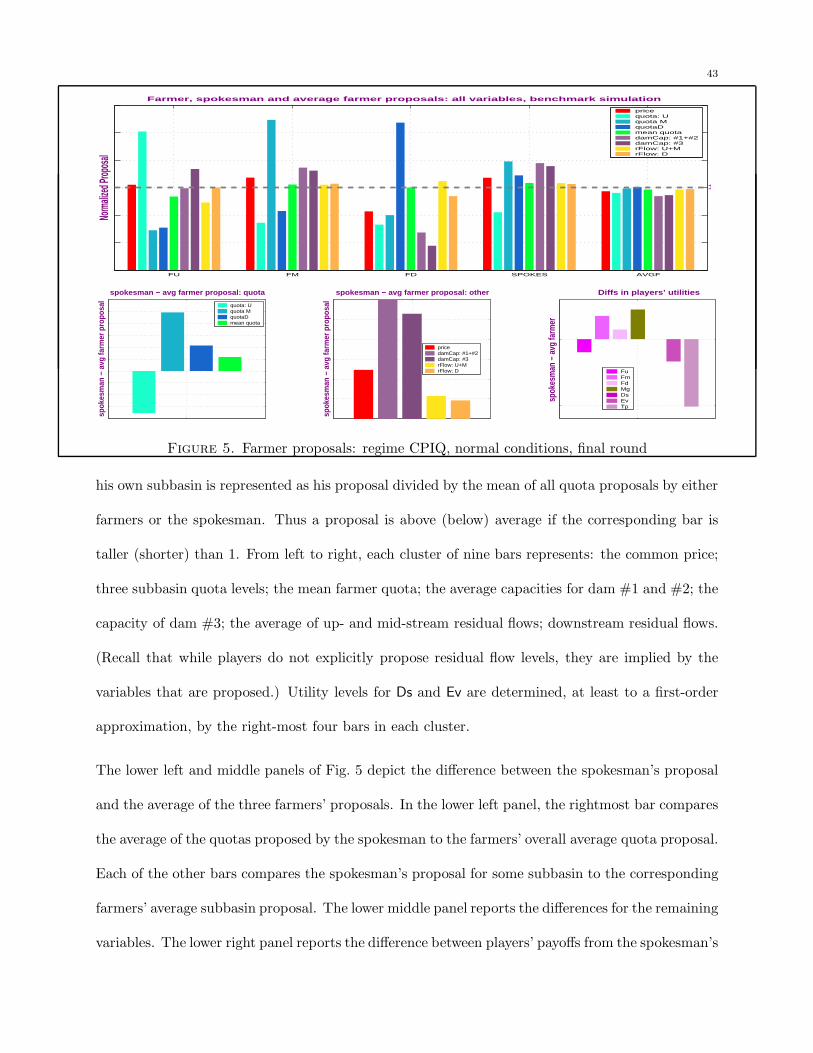
43

FU FM FD SPOKES AVGF

Farmer, spokesman and average farmer proposals: all variables, benchmark simulation

1

Norm

alized

Propos

alpricequota: Uquota MquotaDmean quotadamCap: #1+#2damCap: #3rFlow: U+MrFlow: D

spokesman − avg farmer proposal: quota

spok

esm

an −

avg

farm

er p

ropo

sal quota: U

quota MquotaDmean quota

spok

esm

an −

avg

farm

er p

ropo

sal

spokesman − avg farmer proposal: other

pricedamCap: #1+#2damCap: #3rFlow: U+MrFlow: D

spok

esm

an −

avg

farm

er

Diffs in players’ utilities

FuFmFdMgDsEvTp

Figure 5. Farmer proposals: regime CPIQ, normal conditions, final round

his own subbasin is represented as his proposal divided by the mean of all quota proposals by either

farmers or the spokesman. Thus a proposal is above (below) average if the corresponding bar is

taller (shorter) than 1. From left to right, each cluster of nine bars represents: the common price;

three subbasin quota levels; the mean farmer quota; the average capacities for dam #1 and #2; the

capacity of dam #3; the average of up- and mid-stream residual flows; downstream residual flows.

(Recall that while players do not explicitly propose residual flow levels, they are implied by the

variables that are proposed.) Utility levels for Ds and Ev are determined, at least to a first-order

approximation, by the right-most four bars in each cluster.

The lower left and middle panels of Fig. 5 depict the difference between the spokesman’s proposal

and the average of the three farmers’ proposals. In the lower left panel, the rightmost bar compares

the average of the quotas proposed by the spokesman to the farmers’ overall average quota proposal.

Each of the other bars compares the spokesman’s proposal for some subbasin to the corresponding

farmers’ average subbasin proposal. The lower middle panel reports the differences for the remaining

variables. The lower right panel reports the difference between players’ payoffs from the spokesman’s

44

proposal and the average of their payoffs from the farmers’ proposals. Since the experiment involves

a shift in access away from farmers towards the spokesman, a player’s participation constraint in

the penultimate round will tighten (slacken) if and only if the player’s bar in this panel is positive

(negative).

Figure 5 illustrates a number of significant points. First, Fd’s proposal is much more “efficient”

than Fu’s, and somewhat more efficient than Fm’s, in terms of its impact on dam capacities and

hence prices. Specifically, while Fd’s mean quota proposal is almost as high as Fm’s and much

higher than Fu’s, the residual flows implied by Fd’s proposal are roughly comparable with those

implied by the other farmers’ proposals; moreover Fd’s proposed dam capacities and, consequently,

proposed common price are much lower. These differences arise because whenever residual flows

are reduced at some location along the river, flows at every measurement point downstream from

that point are reduced as well. Thus, flow reductions from subbasin U imply matching reductions

in subbasins M and D, while reductions from subbasin D have no impact on the flows through

subbasins further upstream. For this reason, a unit of quota assigned to Fd has, very roughly,

one-third the total environmental impact of a unit assigned to Fu. Consequently, Fd can “acquire”

for his subbasin essentially the same total level of quotas as can the other two farmers, but with

much less dam capacity, and hence, since prices rise with dam capacity, a much lower price as well.

The remaining three points illustrated by Figure 5 are all closely related to the point just discussed.

Second, comparing the spokesman’s proposal to the average of the farmers’ proposals, observe that

Fu is the clear loser: the spokesman’s price is higher than the average price, while the spokesman

allocates a quota to Fu that is much lower than the farmers’ average subbasin U quota proposal.

This difference can be traced to the relative environmental cost considerations noted above: quotas

assigned to subbasin U are the most environmentally costly of all quotas.

45

Third, note from the top panel of Figure 5 that the spokesman can induce Ds to accept a higher

overall average quota level than that proposed by the farmers, and at a slightly lower price. The

spokesman can accomplish this because he allocates quotas across subbasins more efficiently than

do the farmers. In particular, he discriminates against player Fu, so that under his proposal,

residual flows below the environmentally sensitive subbasin D are higher than under Fm’s proposal.

Fourth, while each farmer proposes a much larger quota for his own subbasin, there is little variation

between the farmers’ three average subbasin proposals. On the other hand, while the spokesman’s

quota allocation is more evenly distributed across farmers than is any individual farmer’s, it is

much less evenly distributed than the average subbasin proposals. Once again, this reflects the

fact that the spokesman’s proposal efficiently balances the relative environmental costs of assigning

quotas to different farmers against the relative benefits that farmers derive from them.

The question arises: why don’t individual farmers take into account at least the relative environ-

mental costs of assigning quotas to other farmers? For example, why does Fm assign roughly equal

quota levels to Fu and Fd? The explanation can be traced to “beggar-thy-neighbor” behavior: un-

like the spokesman, each individual farmer assigns to himself the highest possible quota; as a result,

the heterogeneity bound on individual proposals (p. 22) prevents him from optimally differentiating

the quotas assigned to the other two farmers.

Our final observation relates to the lower middle and right panels of the figure. Relative to the

farmers’ average proposal, the spokesman negotiates significantly higher levels of dam capacities,

in exchange for slightly higher levels of residual flows. This tradeoff leaves Ds indifferent, because

his participation constraint is binding in the final round, but negatively impacts Ev who, relative

to Ds, is concerned more about dam capacities and less about residual flows. Similarly, while Tp

derives some benefit under the spokesman’s proposal from the increase in residual flows, his primary

concern is to reduce the tax burden; consequently, this benefit is more than offset by the negative

tax implications of the increase in dam construction under the spokesman’s proposal.

46

The end result of all these considerations is that as the spokesman’s access increases, there is an

increase in Fm’s and Fd’s expected utilities conditional on reaching the final round of bargain-

ing. Mg’s expected utility increases also, because of the additional dam construction under the

spokesman’s proposal. Ds is unaffected in this round by the participation of the spokesman, be-

cause his participation constraint is binding on the spokesman as well as all farmers. (In earlier

rounds, however, his utility declines.) Ev’s, Tp’s and Fu’s expected utilities decline. Under normal

conditions, these qualitative effects are all reinforced as we move backward up the inductive chain

to the solution of the game. Under drought conditions, the effect of the spokesman’s participation

on the solution is comparable, except for a couple of relatively insignificant differences.

Regime IPCQ: In our discussion of regime IPCQ, we again refer to several different averages. We

will maintain a parallel terminological convention to the previous one, distinguishing this time

between the average subbasin price, the farmer mean price and the overall average price. We shall

also compare the average common quota proposed by farmers to the common quota proposed by

the spokesman.

In contrast to regime CPIQ, the qualitative impact of the spokesman in this regime depends very

much on hydrological conditions. The similarities and differences are once again revealed by an

examination of the final round of bargaining. The details of the discussion below can be summarized

as follows. Under both drought and normal conditions, individual farmers pursue collectively

inefficient beggar-thy-neighbor strategies, proposing low prices for themselves and high prices for

others. In both scenarios, the spokesman’s participation mitigates this inefficiency. There is,

however, a second impact of the spokesman’s involvement. In normal conditions, it is a negative

one for farmers, which dominates the benefit of the first impact. Specifically, the spokesman’s

common quota proposal in drought conditions is greater than the farmers’ average common quota,

while in normal conditions, his proposal is less than this average. Since Ds’s constraint is binding

on all farmers and the spokesman, and he dislikes the marginal quotas less than either Ev or Tp,

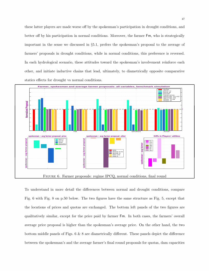
47

these latter players are made worse off by the spokesman’s participation in drought conditions, and

better off by his participation in normal conditions. Moreover, the farmer Fm, who is strategically

important in the sense we discussed in §5.1, prefers the spokesman’s proposal to the average of

farmers’ proposals in drought conditions, while in normal conditions, this preference is reversed.

In each hydrological scenario, these attitudes toward the spokesman’s involvement reinforce each

other, and initiate inductive chains that lead, ultimately, to diametrically opposite comparative

statics effects for drought vs normal conditions.

FU FM FD SPOKES AVGF

Farmer, spokesman and average farmer proposals: all variables, benchmark simulation

1

Norm

alized

Propos

al

quotaprice: Uprice MpriceDmean pricedamCap: #1+#2damCap: #3rFlow: U+MrFlow: D

spokesman − avg farmer proposal: price

spok

esm

an −

avg

farm

er p

ropo

sal price: U

price MpriceDmean price

spok

esm

an −

avg

farm

er p

ropo

sal

spokesman − avg farmer proposal: other

quotadamCap: #1+#2damCap: #3rFlow: U+MrFlow: D

spok

esm

an −

avg

farm

er

Diffs in Players’ utilities

FuFmFdMgDsEvTp

Figure 6. Farmer proposals: regime IPCQ, normal conditions, final round

To understand in more detail the differences between normal and drought conditions, compare

Fig. 6 with Fig. 8 on p.50 below. The two figures have the same structure as Fig. 5, except that

the locations of prices and quotas are exchanged. The bottom left panels of the two figures are

qualitatively similar, except for the price paid by farmer Fm. In both cases, the farmers’ overall

average price proposal is higher than the spokesman’s average price. On the other hand, the two

bottom middle panels of Figs. 6 & 8 are diametrically different. These panels depict the difference

between the spokesman’s and the average farmer’s final round proposals for quotas, dam capacities

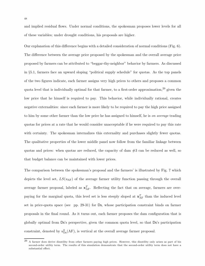
48

and implied residual flows. Under normal conditions, the spokesman proposes lower levels for all

of these variables; under drought conditions, his proposals are higher.

Our explanation of this difference begins with a detailed consideration of normal conditions (Fig. 6).

The difference between the average price proposed by the spokesman and the overall average price

proposed by farmers can be attributed to “beggar-thy-neighbor” behavior by farmers. As discussed

in §5.1, farmers face an upward sloping “political supply schedule” for quotas. As the top panels

of the two figures indicate, each farmer assigns very high prices to others and proposes a common

quota level that is individually optimal for that farmer, to a first-order approximation,29 given the

low price that he himself is required to pay. This behavior, while individually rational, creates

negative externalities: since each farmer is more likely to be required to pay the high price assigned

to him by some other farmer than the low price he has assigned to himself, he is on average trading

quotas for prices at a rate that he would consider unacceptable if he were required to pay this rate

with certainty. The spokesman internalizes this externality and purchases slightly fewer quotas.

The qualitative properties of the lower middle panel now follow from the familiar linkage between

quotas and prices: when quotas are reduced, the capacity of dam #3 can be reduced as well, so

that budget balance can be maintained with lower prices.

The comparison between the spokesman’s proposal and the farmers’ is illustrated by Fig. 7 which

depicts the level set, LS(uAF) of the average farmer utility function passing through the overall

average farmer proposal, labeled as xTAF. Reflecting the fact that on average, farmers are over-

paying for the marginal quota, this level set is less steeply sloped at xTAF than the induced level

set in price-quota space (see pp. 29-31) for Ds, whose participation constraint binds on farmer

proposals in the final round. As it turns out, each farmer proposes the dam configuration that is

globally optimal from Ds’s perspective, given the common quota level, so that Ds’s participation

constraint, denoted by u0Ds(AF), is vertical at the overall average farmer proposal.

29 A farmer does derive disutility from other farmers paying high prices. However, this disutility only arises as part of hissecond-order utility term. The results of this simulation demonstrate that the second-order utility term does not have asubstantial effect.

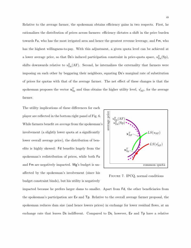
49

Relative to the average farmer, the spokesman obtains efficiency gains in two respects. First, he

rationalizes the distribution of prices across farmers: efficiency dictates a shift in the price burden

towards Fu, who has the most irrigated area and hence the greatest revenue leverage, and Fm, who

has the highest willingness-to-pay. With this adjustment, a given quota level can be achieved at

a lower average price, so that Ds’s induced participation constraint in price-quota space, u0Ds(Sp),

shifts downwards relative to u0Ds(AF). Second, he internalizes the externality that farmers were

imposing on each other by beggaring their neighbors, equating Ds’s marginal rate of substitution

of prices for quotas with that of the average farmer. The net effect of these changes is that the

spokesman proposes the vector xTSp and thus obtains the higher utility level, u′AF, for the average

farmer.

The utility implications of these differences for eachav

erag

epri

ce

common quota

u0Ds(AF)u0

Ds(Sp)

xTAF

xTSp

LS(uAF)

LS(u′AF)

Figure 7. IPCQ, normal conditions

player are reflected in the bottom right panel of Fig. 6.

While farmers benefit on average from the spokesman’s

involvement (a slightly lower quota at a significantly

lower overall average price), the distribution of ben-

efits is highly skewed: Fd benefits hugely from the

spokesman’s redistribution of prices, while both Fu

and Fm are negatively impacted. Mg’s budget is un-

affected by the spokesman’s involvement (since his

budget constraint binds), but his utility is negatively

impacted because he prefers larger dams to smaller. Apart from Fd, the other beneficiaries from

the spokesman’s participation are Ev and Tp. Relative to the overall average farmer proposal, the

spokesman reduces dam size (and hence lowers prices) in exchange for lower residual flows, at an

exchange rate that leaves Ds indifferent. Compared to Ds, however, Ev and Tp have a relative

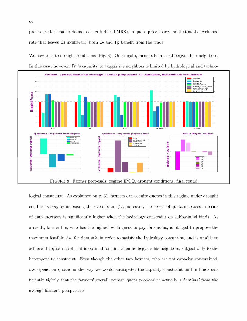
50

preference for smaller dams (steeper induced MRS’s in quota-price space), so that at the exchange

rate that leaves Ds indifferent, both Ev and Tp benefit from the trade.

We now turn to drought conditions (Fig. 8). Once again, farmers Fu and Fd beggar their neighbors.

In this case, however, Fm’s capacity to beggar his neighbors is limited by hydrological and techno-

FU FM FD SPOKES AVGF

Farmer, spokesman and average Farmer proposals: all variables, benchmark simulation

1

Norm

alized

Propos

al

quotaprice: Uprice MpriceDmean pricedamCap: #1+#2damCap: #3rFlow: U+MrFlow: D

spokesman − avg farmer proposal: price

spok

esm

an −

avg

farm

er p

ropo

sal price: U

price MpriceDmean price

spok

esm

an −

avg

farm

er p

ropo

sal

spokesman − avg farmer proposal: other

quotadamCap: #1+#2damCap: #3rFlow: U+MrFlow: D

spok

esm

an −

avg

farm

er

Diffs in Players’ utilities

FuFmFdMgDsEvTp

Figure 8. Farmer proposals: regime IPCQ, drought conditions, final round

logical constraints. As explained on p. 31, farmers can acquire quotas in this regime under drought

conditions only by increasing the size of dam #2; moreover, the “cost” of quota increases in terms

of dam increases is significantly higher when the hydrology constraint on subbasin M binds. As

a result, farmer Fm, who has the highest willingness to pay for quotas, is obliged to propose the

maximum feasible size for dam #2, in order to satisfy the hydrology constraint, and is unable to

achieve the quota level that is optimal for him when he beggars his neighbors, subject only to the

heterogeneity constraint. Even though the other two farmers, who are not capacity constrained,

over-spend on quotas in the way we would anticipate, the capacity constraint on Fm binds suf-

ficiently tightly that the farmers’ overall average quota proposal is actually suboptimal from the

average farmer’s perspective.

51

The result is that in contrast to normal conditions,

aver

age

pri

ce

common quota

u0Ds(AF)

u0Ds(Sp)

xTAF

xTSp

LS(uAF)

LS(u′AF)

Figure 9. IPCQ, drought conditions

the indifference curve of the average farmer utility

function passing through the overall average farmer

proposal is steeper at this point than Ds’s partici-

pation constraint. That is, because of Fm’s techno-

logical constraint, the average farmer would in this

instance choose to buy more quotas than he is pur-

chasing under the overall average farmer proposal

(see Fig. 9). Once again, the spokesman achieves

two kinds of efficiency gains, relative to the average farmer. As in normal conditions, he rational-

izes the distribution of prices across farmers, so that a given quota level can be acquired at a lower

average price. But in contrast to normal conditions, he now proposes slightly more quotas than the

average farmer.30 The implications of these differences are reflected in the bottom-right panel of

Fig. 8. In all critical respects (Fd and Fu are not critical), the signs are the reverse of those in Fig. 6:

Fm in this case prefers the spokesman’s proposal to the average farmer’s; Ds is unaffected by the

spokesman’s involvement because his participation constraint binds; because quotas increase rather

than decrease, Ev and Tp are negatively rather than positively impacted; Mg’s budget remains in

balance, but benefits from the increase in dam capacity.

Now compare the implications of the bottom-right panels of Figs. 6 & 8 for the penultimate and

earlier rounds of bargaining. We begin with normal conditions. Except for player Fd,31 whose

strategic role is minimal in this scenario, the qualitative effects reported above on all of the play-

ers are reinforced by secondary effects in the penultimate round: Tp’s participation constraint,

30 Like Fm, Sp is unable to achieve a tangency with Ds’s participation constraint, because he has pushed dam #2 to itsmaximum feasible size.

31 Fd is negatively impacted by the all of the changes in participation constraints; however, his benefit from the spokesman’srationalization of prices relative to the overall average farmer proposal is large enough to dominate all these negative effects.But since Fd’s participation constraint is never binding in the critical final rounds of bargaining, these effects do not impactthe outcome of the bargaining.

52

which is binding on all farmers in this round, becomes tighter with the spokesman’s involvement

and this weakens all farmers’ proposals. The constraints that bind Mg are Ev’s and Tp’s, so his

proposal is weaker as well. Fm’s constraint, which is binding on all non-farmers, becomes slacker

as the spokesman’s access increases, and this strengthens all non-farmers’ proposals. These qual-

itative penultimate round net effects are all transmitted back to the solution of the game: as the

spokesman’s access probability increases, all non-farmers gain, while Mg and all farmers except Fd

lose.

Under drought conditions, Fm’s and Mg’s penultimate round participation constraints become

tighter as the spokesman’s access increases; since both players’ constraints are binding on the anti-

farmer group, this group does worse in the penultimate round as the spokesman’s access increases.

On the other hand, Ev’s constraint becomes slacker while Ds’s is unchanged, and this benefits all

farmers. For Fm and Fd, this effect reinforces the positive effects that occurred in the final round,

and occur in this round as well. For Fu, however, the negative impact of the redistribution of the

price burden dominates the benefit from Ev’s slacker constraint, and the net effect of the spokesman

on this player is negative. These effects are transmitted backwards through the inductive chain,

so that in the solution to the game, all members of the anti-farmer group are negatively impacted

by the spokesman’s involvement, while Fm and Fd benefit. Fu is negatively impacted. Because

subbasin U has the largest irrigated area, the spokesman “sacrifices” Fu by assigning him a very

high quota price.

Summary and Discussion: The qualitative comparative statics results we obtain in this experiment

reveal that in negotiations where there is significant scope for divergent behavior among coalition

members (i.e. our regimes IPCQ and CPIQ), the intervention of a spokesman will usually, but not

necessarily, benefit the coalition as a group. In the experiments we consider, the impact of the

spokesman’s participation on the coalition’s equilibrium payoff depends, basically, on two factors:

his impact on the expected quota proposal and on Fm’s expected utility conditional on reaching the

53

final round of bargaining. The expected quota proposal is important because it impacts, through

its effect on dam capacities and residual flows, the wellbeing of the non-farmer players Ev and Tp,

whose participation constraints are slack in the final round, but bind in all earlier rounds. Any

proposal that leaves Dsindifferent makes these two players better off. Fm’s conditional expected

utility plays a pivotal role for precisely the reason that we identified in the stripped down context

of §5.1: because Fm’s constraint is binding on the anti-farmer group in the penultimate round of

bargaining, Fm’s performance in the final round is a primary determinant of all farmers’ expected

performance in the penultimate and earlier rounds. In all the experiments we report here, these

two effects reinforce each other. For other parameterizations, however, this need not be the case,

in which case our analysis of the spokesman’s impact would require much more delicacy.

It is significant that when the coalition does benefit from the spokesman’s participation, it does

so only because he can discriminate against one of the coalition members. As we have observed,

Fu is always the target of discrimination by the spokesman, since the constraints that bind him

will be relaxed by a mean-preserving perturbation in subbasin prices (quotas) involving an increase

(decrease) in Fu’s price (quota): in IPCQ, a unit increase in Fu’s price raises more revenue than

a unit increase in either one of the other farmers’ prices; in CPIQ, a unit increase in Fu’s quota

requires a larger increase in dam capacity than a unit increase in either one of the other farmers’

quotas. Hence the spokesman, whose task is to maximize the sum of farmers’ utilities, assigns a

higher price and lower quota to Fu. Anticipating this discrimination, we would expect that Fu

would not agree to the appointment of a spokesman of the kind we model. (Of course, whenever

the farmer group does better on average with the spokesman, Fu could in principle be sufficiently

compensated with side-payments that all coalition members would benefit from the spokesman’s

participation.)

Our spokesman experiment illustrates dramatically the extreme sensitivity of our results to factors

whose importance one would not necessarily anticipate in the absence of a computational model. We

54

observed that all of our comparative statics results are reversed in regime IPCQ when hydrological

conditions change from normal to drought. We traced this reversal to the apparently inconsequential

fact that in the final round of bargaining under drought conditions, Fm proposes the maximum

feasible capacity level for dam #2. This single technological constraint limits the extent to which

Fm can squander the other farmers’ money, and a chain of significant consequences follow.

We emphasize this example because it highlights the complex, delicate and highly nonlinear nature

of player interactions when they negotiate with each other in a environment such as the present

one, characterized by high dimensionality and multiple “sharp edges.” This environment contrasts

sharply with the smooth, low-dimensional, stylized characterizations of the world that one is obliged

to construct in order to generate analytical comparative statics results. While environments of the

latter kind are more elegant and transparent than ours, and more likely to yield robust results,

in many instances the cost of these positive attributes is that the simpler models fail to reflect

the full richness of economic actors’ interactions either with each other or with the institutional

contexts within which they must operate. In the experiment we have just discussed, a technological

constraint that might have been assumed away in order to construct a simplified model with

analytical comparative statics results proved to be an important determinant of the negotiated

outcome.

Finally, our results in regime IPCQ provide a counter-example to the intuitively self-evident con-

jecture we proposed on p. 38 that the spokesman’s participation will always benefit the farmer

coalition. It is true that when members of this coalition pursue their individual self-interests,

the expected result of their activities will generally be sub-optimal from the perspective of the

coalition as a whole. For example, each farmer in IPCQ proposes a higher quota level than he

would have proposed if he were required to pay his fair share of quota costs.32 The conjecture

mentioned above is intuitively obvious precisely because we would expect the spokesman always

32 We reiterate (cf p. 48) that it is the political supply schedule for quotas that is upward sloping.

55

to internalize any negative externalities arising from beggar-thy-neighbor behavior by individual

farmers. Indeed, the spokesman does exactly this. Our conjecture fails in regime IPCQ, however,

in part33 because the externality that is negative in this narrow sense turns out to be positive in a

broader sense—beggar-thy-neighbor behavior hurts Ds, Ev and Tp more than it hurts the farmers,

and in fact benefits the manager—so that when the spokesman internalizes it, the farmer coalition’s

equilibrium performance actually declines. On reflection, this result should not be at all surprising:

a fundamental lesson from game theory is that behavior which is suboptimal by decision-theoretic

criteria can in a game-theoretic context increase a player’s equilibrium payoff relative to behavior

that is decision-theoretically optimal.34

5.3. Limiting dissention: reducing the degree of proposal heterogeneity. As we observed

in §5.2, the spokesman’s role was essentially negligible in regime CPCQ, but significant in the other

two regimes. It seems probable, therefore that in regimes IPCQ and CPIQ, reducing the degree

of permissible heterogeneity among player proposals will have similar effects. As we have noted

above (page 22), players in our base-case scenarios for regimes IPCQ and CPIQ are constrained

in the extent to which they can pursue their own subbasins’ interests at the expense of other

subbasins. Specifically, in regime CPIQ (IPCQ), the specification of the bargaining space includes

an upper bound on the standard deviation of the three quotas (prices) proposed by any player. In

this subsection, we explore the impact of successively relaxing these bounds, again restricting our

attention to the case in which, in the final round of bargaining, Ds’s constraint is binding on all

farmers and on Mg.

A natural conjecture arising from §5.2 is that farmers’ utilities will increase or decrease on average

as these restrictions become tighter, depending on whether the average farmer benefits from the

33 A second factor is that while the spokesman enhances average farmer utility, in normal conditions he reduces Fm’s utility,and it is this utility rather than farmers’ average that matters in the final round of the game. Cf section §5.1

34 See for example, the vast literature on reputation building beginning with Kreps and Wilson (1982) and Milgrom andRoberts (1982).

56

participation of the spokesman. In regime CPIQ, for example, we observed from the spokesman ex-

periment that self-interested, beggar-thy-neighbor behavior by individual farmers served to weaken

the performance of the farmer coalition. In the present experiment, we test the conjecture that

when we successively tighten our bound on the extent of heterogeneity among proposals, and thus

increasingly proscribe this kind of behavior, farmers will on average do better in equilibrium. It

is less straightforward to make predictions for regime IPCQ, since in this case the impact of the

spokesman turned out to be counter-intuitive, at least under normal conditions. Even so, it still

seems intuitive that when we limit the extent to which each farmer can favor his own subbasin at

the expense of the others, farmers will again do better on average.

Except for one of the four scenarios we discuss in this subsection—CPIQ, normal conditions—these

conjectures are not supported by our simulation experiments. In regime CPIQ, farmers benefit on

average when the heterogeneity bound is tightened under normal conditions, but do worse when

it is tightened in drought conditions. In regime IPCQ under both normal and drought conditions,

the average farmer does monotonically worse as the bound tightens. Moreover, an analysis of our

simulation results reveals that the forces driving our comparative statics results are quite different

from the ones we anticipated.

Why in regime CPIQ are farmers positively impacted by a tighter bound in normal conditions, but

negatively impacted in drought conditions? To answer this question, we focus as usual on the final

round of negotiations. We restrict our attention to farmer Fd, for whom the effect of hydrological

conditions is most dramatic. In the discussion which follows, it is important to keep in mind the

topography of the Adour Basin (see Fig. 2 on p. 19), noting in particular that both Fd’s quota

allocation and the capacity of dam #2 affect residual flows only below subbasin D.

On pp. 29-31 of §4, we discussed how to project players’ preferences onto price-quota space in

regime CPCQ. We now extend this discussion to the more complex situation that arises in regime

57

CPIQ. Fig. 10 collapses Fd’s optimization problem down to two dimensions. The curve labeled

“water supply function” maps the proposed capacity of dam #2 (on the vertical axis) to water

flows gross of farm quotas below subbasin D (on the horizontal axis). Non-farmers care about

residual water flows, which are gross flows minus any quotas allocated to farmers. The curve

labeled “Ds’s participation constraint” is the level set of Ds’s utility function at his default utility,

representing his willingness to trade off dam size against residual flow. The slope of Ds’s level

set is steeper than the slope of the “supply function” if and only if the increase in residual flows

resulting from an expansion of the dam’s size increases Ds’s utility at a faster rate than the rate

at which Ds’s utility declines because he dislikes dams. For any given capacity for dam #2, farmer

Fd can assign quotas that sum to the horizontal distance between Ds’s level set and the water

supply function. The heterogeneity constraint restricts the fraction of this distance that Fd can

assign to his own subbasin. In Fig. 10, the heterogeneity bound determines the lengths of the solid,

horizontal, double-ended arrows (Fd’s quota) relative to the lengths of the dotted arrows (Fm and

Fu’s quotas). As the constraint tightens, this fraction shrinks. The key point to note here is that

since each farmer, naturally, assigns the largest fraction of total quotas to his own subbasin, a

tightening of the heterogeneity bound means that aggregate quotas must be increased in order to

deliver to a given farmer the same quota level he was receiving initially. It necessarily follows that

as the heterogeneity bound tightens, there is an increase in the tension between farmers and those

stakeholders who value residual flows.

Since ceteris paribus (c.p), the capacity of dam #2 determines the common quota price through

the administrative budget constraint, we can reinterpret Fig. 10 to represent the tradeoff facing

farmer Fd, which is, essentially, between quota and price. When considering Fd’s options, mentally

relabel the vertical axis as the quota price implied by the given dam capacity, and the horizontal

axis as quotas, then interpret all curves associated with Fd as either opportunity sets or indifference

curves in price-quota space. Assuming that from Fd’s perspective, quotas are optimally divided

58

among farmers Fu and Fm, we can trace out the frontier of the choice set available to Fd. For

our baseline case, this is indicated by the solid line labeled “Fd’s feasible set: loose constraint;”

when the constraint tightens the feasible set contracts, as indicated by the dashed line labeled “Fd’s

feasible set: tight constraint.” Note that the feasible set is “backward-bending” if and only if at

the margin, Ds’s dislike of dam #2 exceeds his fondness for residual flows. The solid and dashed

lines labeled “Fd’s indifference curve” indicate the indifference curves determining the location of

Fd’s optimal proposals, both before and after the heterogeneity constraint tightens. The tangency

points, indicated by oval-shaped dots, are characterized by the property that the marginal cost to

Fd—incurred because the common quota price must increase to satisfy the administrator’s budget

constraint—of a further increase in the dam’s size just offsets the marginal benefit to Fd from

proposing additional quotas for his own subbasin, taking into account the increases in Fm’s and

Fu’s quotas that he must also propose in order to satisfy the heterogeneity constraint. When the

constraint tightens, Fd pays a higher unit price for fewer quotas, reflecting the fact that both quotas

and the residual numeraire are normal goods.

It should be emphasized that the two-dimensional Fig. 10 is only an partial representation of

the problem being modeled. In particular, the location of Ds’s participation constraint is not

independent of the allocation of quotas among farmers, and hence depends on the heterogeneity

bound. Specifically, note in Fig. 10 that pressure on upstream residual flows increases with the

lengths of the horizontal dashed arrows, but is independent of the lengths of the solid arrows. This

implies that when the constraint tightens, holding everything else in the figure constant, the line

labeled “Ds’s participation constraint” now represents a lower level of utility, because Ds cares

also about upstream flows. In other words, Ds’s actual constraint moves to the right as the bound

shrinks. Note also that if farmer Fd were replaced in the figure by Fu, then the relationship between

the heterogeneity bound and Ds’s constraint would be reversed: in this case, a tightening of the

bound would shift Ds’s constraint to the left.

59

We say that “drought conditions” apply when at least one of the hydrology constraints are binding.

In our benchmark simulation of drought conditions, the hydrology constraints bind at the mid-

and down-stream measurement points; the up-stream constraint is slack. When the heterogeneity

bound tightens under these circumstances, farmer Fd is in an especially difficult position: to satisfy

a tighter heterogeneity bound, he must reduce the quotas he assigns to himself and increase the

quotas he assigns to upstream farmers. As we have noted above, a one-to-one transfer of quotas

upstream either doubles or triples the burden of satisfying residual flow requirements. Moreover,

in our simulation, dam #1 is already at full capacity, while dam #3 is already so large that the net

marginal benefit to user Ds of increasing it still further is negative. Since dam #2 services only the

down-stream basin, farmer Fd cannot increase the supply of water to the up- and mid-stream basins

without reducing Ds’s utility (cf. in normal conditions, an increase in dam #3 created a net surplus

utility for Ds, which gave Fd room to maneuver.) Since Ds’s participation constraint is binding,

he must be compensated somehow for this loss. By a process of elimination, the only feasible way

that Fd can provide this compensation is to reduce the mean quota allocation he proposes and to

reduce the size of dam #2.

To summarize, Fd’s response in normal conditions is to buy fewer quotas for his own subbasin,

at a higher price, and to increase the size of dam #3 to accommodate the increased pressure on

residual flows induced by the forced reallocation of the quotas he proposes. In drought conditions,

he has less room to maneuver, and is obliged to reduce the size of dam #2. As we have discussed

many times, when a farmer adjusts dam sizes and residual flows, he does it on terms that leave user

Ds indifferent. But Ev and Tp dislike dams more than Ds—if they had been included in Fig. 10,

their participation constraints would be flatter than Ds’s—so that they benefit (suffer) whenever a

farmer reduces (increases) a dam size.

We now broaden our discussion to include the other players, considering each scenario in turn.

For the four cases we consider, the effects of the heterogeneity restriction in the final round of

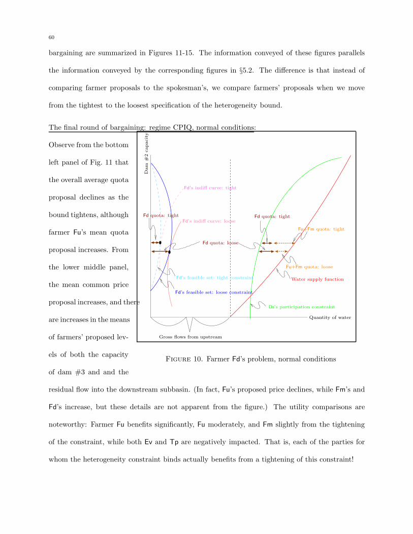
60

bargaining are summarized in Figures 11-15. The information conveyed of these figures parallels

the information conveyed by the corresponding figures in §5.2. The difference is that instead of

comparing farmer proposals to the spokesman’s, we compare farmers’ proposals when we move

from the tightest to the loosest specification of the heterogeneity bound.

The final round of bargaining: regime CPIQ, normal conditions:

Gross flows from upstream

Quantity of water

Water supply function

Dam

#2

capacity

Fd’s feasible set: loose constraint

Fd’s feasible set: tight constraint

Fd’s indiff curve: loose

Fd’s indiff curve: tight

Ds’s participation constraint

Fu+Fm quota: loose

Fu+Fm quota: tight

Fd quota: loose

Fd quota: tightFd quota: tight

Figure 10. Farmer Fd’s problem, normal conditions

Observe from the bottom

left panel of Fig. 11 that

the overall average quota

proposal declines as the

bound tightens, although

farmer Fu’s mean quota

proposal increases. From

the lower middle panel,

the mean common price

proposal increases, and there

are increases in the means

of farmers’ proposed lev-

els of both the capacity

of dam #3 and and the

residual flow into the downstream subbasin. (In fact, Fu’s proposed price declines, while Fm’s and

Fd’s increase, but these details are not apparent from the figure.) The utility comparisons are

noteworthy: Farmer Fu benefits significantly, Fu moderately, and Fm slightly from the tightening

of the constraint, while both Ev and Tp are negatively impacted. That is, each of the parties for

whom the heterogeneity constraint binds actually benefits from a tightening of this constraint!

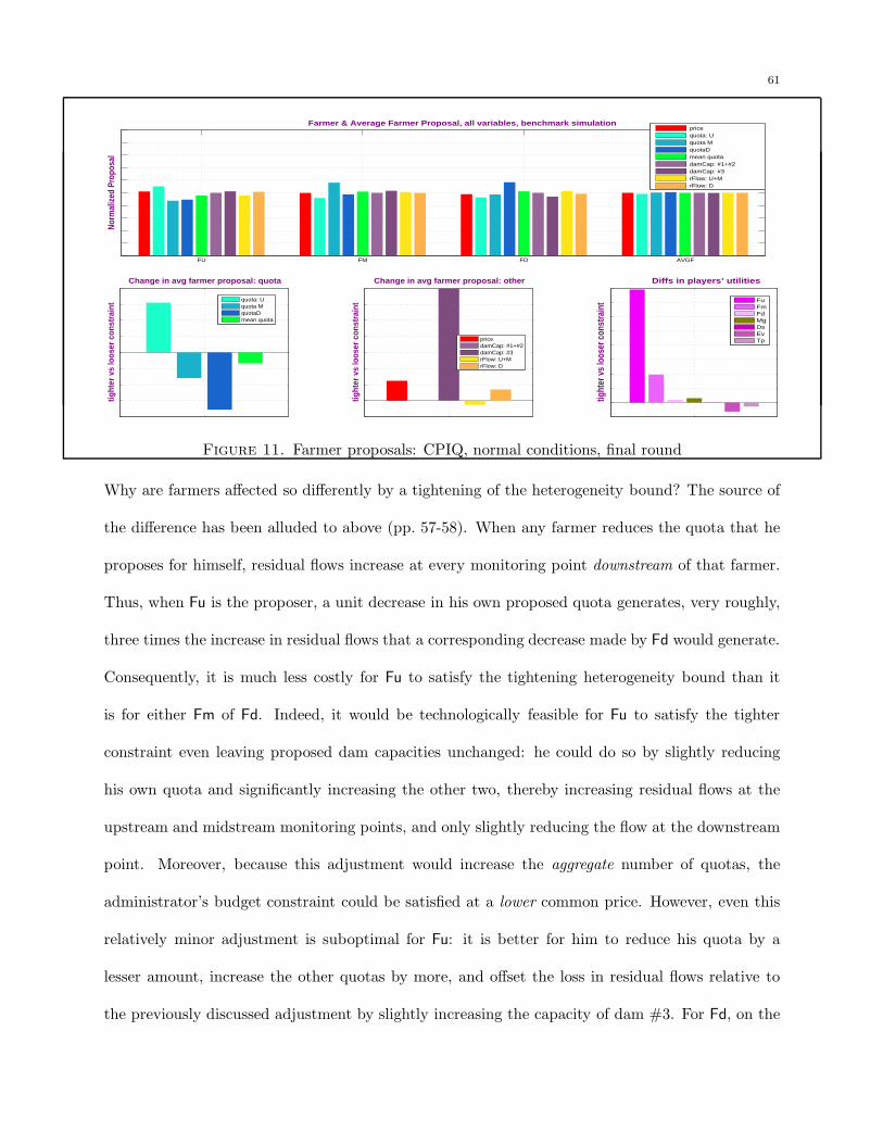
61

FU FM FD AVGF

Nor

mal

ized

Pro

posa

lFarmer & Average Farmer Proposal, all variables, benchmark simulation

pricequota: Uquota MquotaDmean quotadamCap: #1+#2damCap: #3rFlow: U+MrFlow: D

osetig

hter

vs

loos

er c

onst

rain

t

Change in avg farmer proposal: quota

quota: Uquota MquotaDmean quota

)

tight

er v

s lo

oser

con

stra

int

Change in avg farmer proposal: other

pricedamCap: #1+#2damCap: #3rFlow: U+MrFlow: D

tight

er v

s lo

oser

con

stra

int

Diffs in players’ utilities

FuFmFdMgDsEvTp

Figure 11. Farmer proposals: CPIQ, normal conditions, final round

Why are farmers affected so differently by a tightening of the heterogeneity bound? The source of

the difference has been alluded to above (pp. 57-58). When any farmer reduces the quota that he

proposes for himself, residual flows increase at every monitoring point downstream of that farmer.

Thus, when Fu is the proposer, a unit decrease in his own proposed quota generates, very roughly,

three times the increase in residual flows that a corresponding decrease made by Fd would generate.

Consequently, it is much less costly for Fu to satisfy the tightening heterogeneity bound than it

is for either Fm of Fd. Indeed, it would be technologically feasible for Fu to satisfy the tighter

constraint even leaving proposed dam capacities unchanged: he could do so by slightly reducing

his own quota and significantly increasing the other two, thereby increasing residual flows at the

upstream and midstream monitoring points, and only slightly reducing the flow at the downstream

point. Moreover, because this adjustment would increase the aggregate number of quotas, the

administrator’s budget constraint could be satisfied at a lower common price. However, even this

relatively minor adjustment is suboptimal for Fu: it is better for him to reduce his quota by a

lesser amount, increase the other quotas by more, and offset the loss in residual flows relative to

the previously discussed adjustment by slightly increasing the capacity of dam #3. For Fd, on the

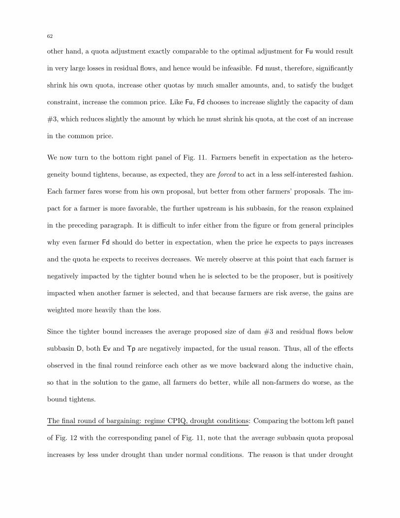
62

other hand, a quota adjustment exactly comparable to the optimal adjustment for Fu would result

in very large losses in residual flows, and hence would be infeasible. Fd must, therefore, significantly

shrink his own quota, increase other quotas by much smaller amounts, and, to satisfy the budget

constraint, increase the common price. Like Fu, Fd chooses to increase slightly the capacity of dam

#3, which reduces slightly the amount by which he must shrink his quota, at the cost of an increase

in the common price.

We now turn to the bottom right panel of Fig. 11. Farmers benefit in expectation as the hetero-

geneity bound tightens, because, as expected, they are forced to act in a less self-interested fashion.

Each farmer fares worse from his own proposal, but better from other farmers’ proposals. The im-

pact for a farmer is more favorable, the further upstream is his subbasin, for the reason explained

in the preceding paragraph. It is difficult to infer either from the figure or from general principles

why even farmer Fd should do better in expectation, when the price he expects to pays increases

and the quota he expects to receives decreases. We merely observe at this point that each farmer is

negatively impacted by the tighter bound when he is selected to be the proposer, but is positively

impacted when another farmer is selected, and that because farmers are risk averse, the gains are

weighted more heavily than the loss.

Since the tighter bound increases the average proposed size of dam #3 and residual flows below

subbasin D, both Ev and Tp are negatively impacted, for the usual reason. Thus, all of the effects

observed in the final round reinforce each other as we move backward along the inductive chain,

so that in the solution to the game, all farmers do better, while all non-farmers do worse, as the

bound tightens.

The final round of bargaining: regime CPIQ, drought conditions: Comparing the bottom left panel

of Fig. 12 with the corresponding panel of Fig. 11, note that the average subbasin quota proposal

increases by less under drought than under normal conditions. The reason is that under drought

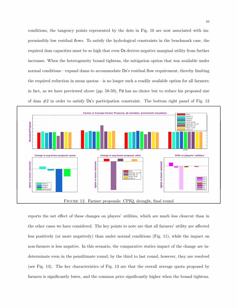
63

conditions, the tangency points represented by the dots in Fig. 10 are now associated with im-

permissibly low residual flows. To satisfy the hydrological constraints in the benchmark case, the

required dam capacities must be so high that even Ds derives negative marginal utility from further

increases. When the heterogeneity bound tightens, the mitigation option that was available under

normal conditions—expand dams to accommodate Ds’s residual flow requirement, thereby limiting

the required reduction in mean quotas—is no longer such a readily available option for all farmers;

in fact, as we have previewed above (pp. 58-59), Fd has no choice but to reduce his proposed size

of dam #2 in order to satisfy Ds’s participation constraint. The bottom right panel of Fig. 12

FU FM FD AVGF

Nor

mal

ized

Pro

posa

l

Farmer & Average Farmer Proposal, all variables, benchmark simulationpricequota: Uquota MquotaDmean quotadamCap: #1+#2damCap: #3rFlow: U+MrFlow: D

tight

er v

s lo

oser

con

stra

int

Change in avg farmer proposal: quota

quota: Uquota MquotaDmean quota

price

tight

er v

s lo

oser

con

stra

int

Change in avg farmer proposal: other

pricedamCap: #1+#2damCap: #3rFlow: U+MrFlow: D

tight

er v

s lo

oser

con

stra

int

Diffs in players’ utilities

FuFmFdMgDsEvTp

Figure 12. Farmer proposals: CPIQ, drought, final round

reports the net effect of these changes on players’ utilities, which are much less clearcut than in

the other cases we have considered. The key points to note are that all farmers’ utility are affected

less positively (or more negatively) than under normal conditions (Fig. 11), while the impact on

non-farmers is less negative. In this scenario, the comparative statics impact of the change are in-

determinate even in the penultimate round; by the third to last round, however, they are resolved

(see Fig. 13). The key characteristics of Fig. 13 are that the overall average quota proposed by

farmers is significantly lower, and the common price significantly higher when the bound tightens.

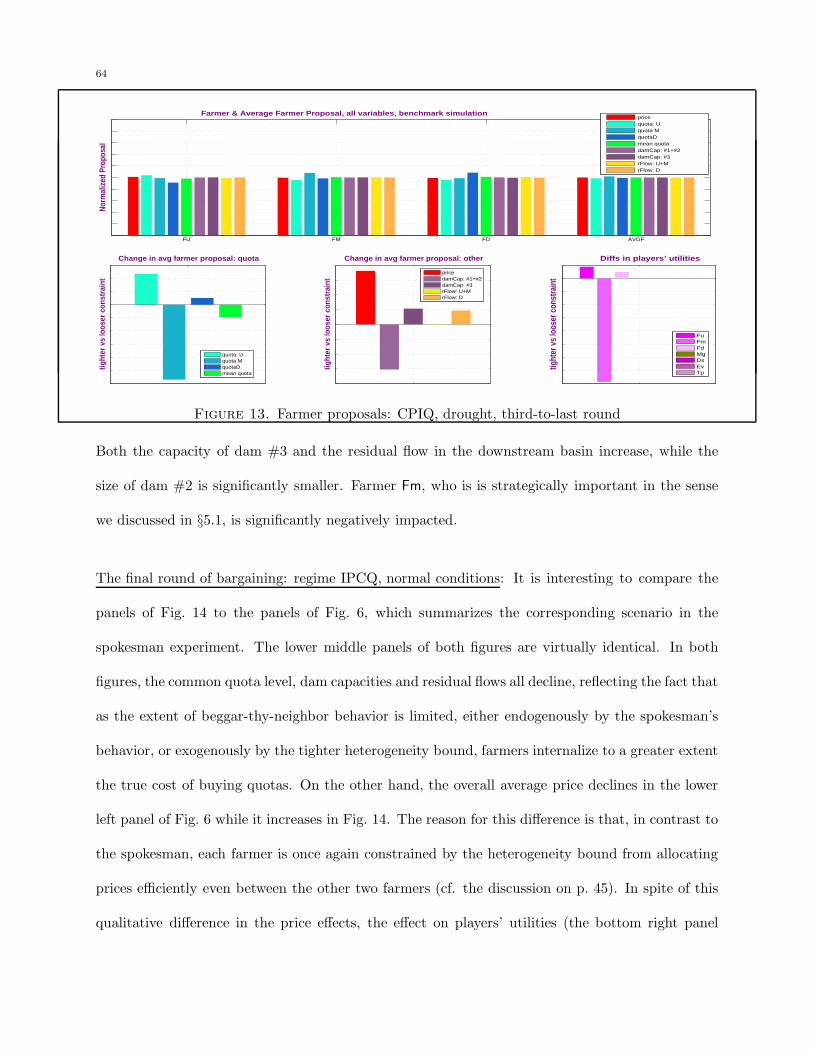
64

FU FM FD AVGF

Nor

mal

ized

Pro

posa

lFarmer & Average Farmer Proposal, all variables, benchmark simulation

pricequota: Uquota MquotaDmean quotadamCap: #1+#2damCap: #3rFlow: U+MrFlow: D

osetig

hter

vs

loos

er c

onst

rain

t

Change in avg farmer proposal: quota

quota: Uquota MquotaDmean quota

)

tight

er v

s lo

oser

con

stra

int

Change in avg farmer proposal: other

pricedamCap: #1+#2damCap: #3rFlow: U+MrFlow: D

tight

er v

s lo

oser

con

stra

int

Diffs in players’ utilities

FuFmFdMgDsEvTp

Figure 13. Farmer proposals: CPIQ, drought, third-to-last round

Both the capacity of dam #3 and the residual flow in the downstream basin increase, while the

size of dam #2 is significantly smaller. Farmer Fm, who is is strategically important in the sense

we discussed in §5.1, is significantly negatively impacted.

The final round of bargaining: regime IPCQ, normal conditions: It is interesting to compare the

panels of Fig. 14 to the panels of Fig. 6, which summarizes the corresponding scenario in the

spokesman experiment. The lower middle panels of both figures are virtually identical. In both

figures, the common quota level, dam capacities and residual flows all decline, reflecting the fact that

as the extent of beggar-thy-neighbor behavior is limited, either endogenously by the spokesman’s

behavior, or exogenously by the tighter heterogeneity bound, farmers internalize to a greater extent

the true cost of buying quotas. On the other hand, the overall average price declines in the lower

left panel of Fig. 6 while it increases in Fig. 14. The reason for this difference is that, in contrast to

the spokesman, each farmer is once again constrained by the heterogeneity bound from allocating

prices efficiently even between the other two farmers (cf. the discussion on p. 45). In spite of this

qualitative difference in the price effects, the effect on players’ utilities (the bottom right panel

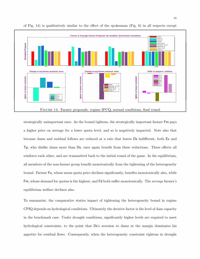
65

of Fig. 14) is qualitatively similar to the effect of the spokesman (Fig. 6) in all respects except

FU FM FD AVGF

Nor

mal

ized

Pro

posa

l

Farmer & Average Farmer Proposal, all variables, benchmark simulationquotaprice: Uprice MpriceDmean pricedamCap: #1+#2damCap: #3rFlow: U+MrFlow: D

tight

er v

s lo

oser

con

stra

int

Change in avg farmer proposal: price

price: Uprice MpriceDmean price

AF

tight

er v

s lo

oser

con

stra

int

Change in avg farmer proposal: other

quotadamCap: #1+#2damCap: #3rFlow: U+MrFlow: D

tight

er v

s lo

oser

con

stra

int

Diffs in players’ utilities

FuFmFdMgDsEvTp

Figure 14. Farmer proposals: regime IPCQ, normal conditions, final round

strategically unimportant ones. As the bound tightens, the strategically important farmer Fm pays

a higher price on average for a lower quota level, and so is negatively impacted. Note also that

because dams and residual follows are reduced at a rate that leaves Ds indifferent, both Ev and

Tp, who dislike dams more than Ds, once again benefit from these reductions. These effects all

reinforce each other, and are transmitted back to the initial round of the game. In the equilibrium,

all members of the non-farmer group benefit monotonically from the tightening of the heterogeneity

bound. Farmer Fu, whose mean quota price declines significantly, benefits monotonically also, while

Fm, whose demand for quotas is the highest, and Fd both suffer monotonically. The average farmer’s

equilibrium welfare declines also.

To summarize, the comparative statics impact of tightening the heterogeneity bound in regime

CPIQ depends on hydrological conditions. Ultimately the decisive factor is the level of dam capacity

in the benchmark case. Under drought conditions, significantly higher levels are required to meet

hydrological constraints, to the point that Ds’s aversion to dams at the margin dominates his

appetite for residual flows. Consequently, when the heterogeneity constraint tightens in drought

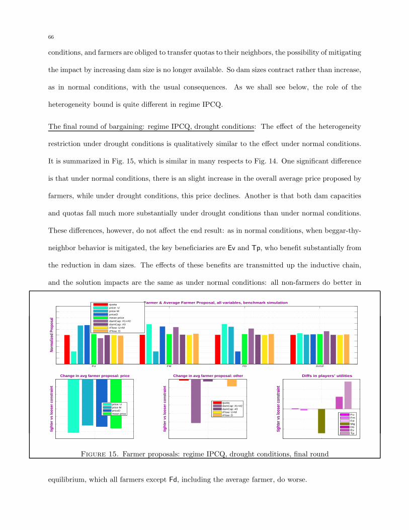
66

conditions, and farmers are obliged to transfer quotas to their neighbors, the possibility of mitigating

the impact by increasing dam size is no longer available. So dam sizes contract rather than increase,

as in normal conditions, with the usual consequences. As we shall see below, the role of the

heterogeneity bound is quite different in regime IPCQ.

The final round of bargaining: regime IPCQ, drought conditions: The effect of the heterogeneity

restriction under drought conditions is qualitatively similar to the effect under normal conditions.

It is summarized in Fig. 15, which is similar in many respects to Fig. 14. One significant difference

is that under normal conditions, there is an slight increase in the overall average price proposed by

farmers, while under drought conditions, this price declines. Another is that both dam capacities

and quotas fall much more substantially under drought conditions than under normal conditions.

These differences, however, do not affect the end result: as in normal conditions, when beggar-thy-

neighbor behavior is mitigated, the key beneficiaries are Ev and Tp, who benefit substantially from

the reduction in dam sizes. The effects of these benefits are transmitted up the inductive chain,

and the solution impacts are the same as under normal conditions: all non-farmers do better in

FU FM FD AVGF

Nor

mal

ized

Pro

posa

l

Farmer & Average Farmer Proposal, all variables, benchmark simulationquotaprice: Uprice MpriceDmean pricedamCap: #1+#2damCap: #3rFlow: U+MrFlow: D

tight

er v

s lo

oser

con

stra

int

Change in avg farmer proposal: price

price: Uprice MpriceDmean price

tight

er v

s lo

oser

con

stra

int

Change in avg farmer proposal: other

quotadamCap: #1+#2damCap: #3rFlow: U+MrFlow: D

tight

er v

s lo

oser

con

stra

int

Diffs in players’ utilities

FuFmFdMgDsEvTp

Figure 15. Farmer proposals: regime IPCQ, drought conditions, final round

equilibrium, which all farmers except Fd, including the average farmer, do worse.

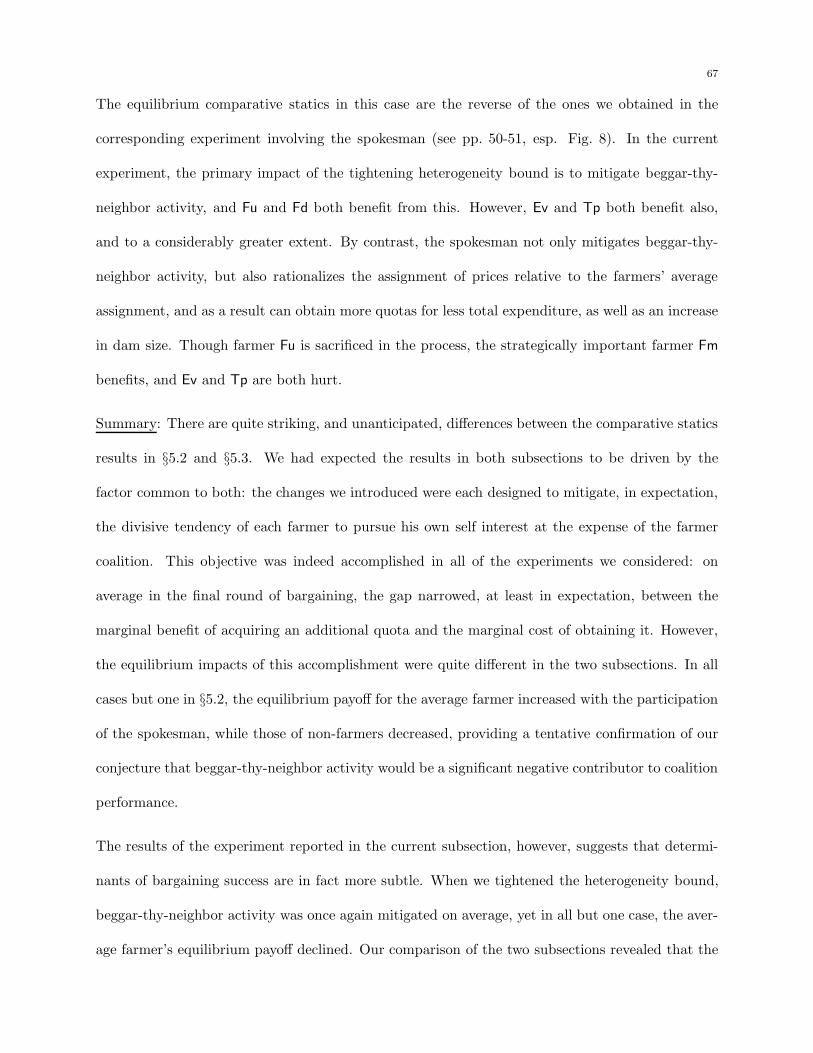
67

The equilibrium comparative statics in this case are the reverse of the ones we obtained in the

corresponding experiment involving the spokesman (see pp. 50-51, esp. Fig. 8). In the current

experiment, the primary impact of the tightening heterogeneity bound is to mitigate beggar-thy-

neighbor activity, and Fu and Fd both benefit from this. However, Ev and Tp both benefit also,

and to a considerably greater extent. By contrast, the spokesman not only mitigates beggar-thy-

neighbor activity, but also rationalizes the assignment of prices relative to the farmers’ average

assignment, and as a result can obtain more quotas for less total expenditure, as well as an increase

in dam size. Though farmer Fu is sacrificed in the process, the strategically important farmer Fm

benefits, and Ev and Tp are both hurt.

Summary: There are quite striking, and unanticipated, differences between the comparative statics

results in §5.2 and §5.3. We had expected the results in both subsections to be driven by the

factor common to both: the changes we introduced were each designed to mitigate, in expectation,

the divisive tendency of each farmer to pursue his own self interest at the expense of the farmer

coalition. This objective was indeed accomplished in all of the experiments we considered: on

average in the final round of bargaining, the gap narrowed, at least in expectation, between the

marginal benefit of acquiring an additional quota and the marginal cost of obtaining it. However,

the equilibrium impacts of this accomplishment were quite different in the two subsections. In all

cases but one in §5.2, the equilibrium payoff for the average farmer increased with the participation

of the spokesman, while those of non-farmers decreased, providing a tentative confirmation of our

conjecture that beggar-thy-neighbor activity would be a significant negative contributor to coalition

performance.

The results of the experiment reported in the current subsection, however, suggests that determi-

nants of bargaining success are in fact more subtle. When we tightened the heterogeneity bound,

beggar-thy-neighbor activity was once again mitigated on average, yet in all but one case, the aver-

age farmer’s equilibrium payoff declined. Our comparison of the two subsections revealed that the

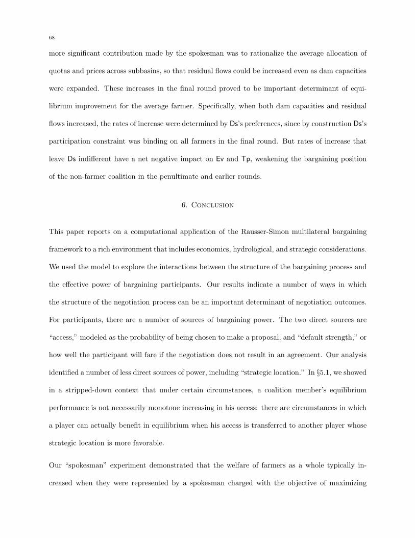
68

more significant contribution made by the spokesman was to rationalize the average allocation of

quotas and prices across subbasins, so that residual flows could be increased even as dam capacities

were expanded. These increases in the final round proved to be important determinant of equi-

librium improvement for the average farmer. Specifically, when both dam capacities and residual

flows increased, the rates of increase were determined by Ds’s preferences, since by construction Ds’s

participation constraint was binding on all farmers in the final round. But rates of increase that

leave Ds indifferent have a net negative impact on Ev and Tp, weakening the bargaining position

of the non-farmer coalition in the penultimate and earlier rounds.

6. Conclusion

This paper reports on a computational application of the Rausser-Simon multilateral bargaining

framework to a rich environment that includes economics, hydrological, and strategic considerations.

We used the model to explore the interactions between the structure of the bargaining process and

the effective power of bargaining participants. Our results indicate a number of ways in which

the structure of the negotiation process can be an important determinant of negotiation outcomes.

For participants, there are a number of sources of bargaining power. The two direct sources are

“access,” modeled as the probability of being chosen to make a proposal, and “default strength,” or

how well the participant will fare if the negotiation does not result in an agreement. Our analysis

identified a number of less direct sources of power, including “strategic location.” In §5.1, we showed

in a stripped-down context that under certain circumstances, a coalition member’s equilibrium

performance is not necessarily monotone increasing in his access: there are circumstances in which

a player can actually benefit in equilibrium when his access is transferred to another player whose

strategic location is more favorable.

Our “spokesman” experiment demonstrated that the welfare of farmers as a whole typically in-

creased when they were represented by a spokesman charged with the objective of maximizing

69

farmers’ average welfare. The spokesman improved average farmer welfare in three out of four

scenarios. We identified two main reasons for this improvement. First, the spokesman mitigated,

in an expected sense, the tendency of individual farmers to adopt beggar-thy-neighbor bargaining

strategies: in our baseline parameterization for regime IPCQ, each farmer in effect purchased quo-

tas with other farmers’ money, and consequently purchased more than he would have done had

he been obliged to use his own money; in regime CPIQ, each farmer kept for himself a dispropor-

tionate share of the total number of quotas, thus lowering for himself the per unit cost of quotas

and raising it for others. Second, the spokesman rationalized the allocation of prices and quotas

across subbasins. There were, however, winners and losers from this rationalization, so that the

spokesman’s successes were always obtained at the expense of one of the farmers. This suggests

that in order to obtain the coalition’s unanimous endorsement of a spokesman’s participation, side

payments would typically be required in order to compensate the losers.

Our “heterogeneity bound” experiment was designed to mimic the impact of the spokesman by

limiting exogenously the extent to which farmers could engage in beggar-thy-neighbor behavior.

Our exogenous restriction did indeed limit this behavior; however, the equilibrium consequences

of doing so were unexpected. We found that in three out of four scenarios, farmers’ equilibrium

welfare actually declined as farmers were forced to act in a less selfish manner. The unanticipated

lesson from this experiment was that, while farmers might collectively benefit from a restriction

that obliged them to act less selfishly, “the opposition” might benefit even more so. (Recall that

“acting less selfishly” meant purchasing fewer quotas, and this benefited both Ev and Tp, while

leaving Ds indifferent.)

We conclude that the decisive contribution made by the spokesman was that he was more effective

at distributing prices and quotas efficiently across subbasins than farmers were when they acted

as self-interested individuals. A careful reading of §5 suggests, however, that the implications for

coalition performance of even this contribution are unlikely to be very robust. As we observed in

70

§5.2, farmer Fm was, typically, a beneficiary of the spokesman’s efficiency improvements, while Fu

was typically a loser. Fortunately for the farmers, it was Fm rather than Fu who was strategically

important in the sense we identified in section §5.1. Had the interrelationship between hydrological

and agricultural conditions been different, Fu might have been the strategically important farmer,

in which case the spokesman’s participation might have had the opposite effect on equilibrium

payoffs.

Linking our analysis to the real-world negotiation process it models, we can identify some potential

reasons for the deadlock in the second stage of negotiations, and some recommendations for altering

the structure of the negotiation process in order to increase the probability of its success. First,

given that the interests of farmers are imperfectly allied, the selection of specific negotiation partic-

ipants is an important consideration. However, the lack of robustness regarding the effects of the

spokesman’s participation on farmers’ welfare does not provide firm recommendations regarding

the selection process, and the appropriate level of aggregation for farmers’ heterogeneous interests.

On the other hand, the results of the spokesman experiment suggest that the negotiation process

should be expanded to allow for side payments among participants in order to increase efficiency

while maintaining unanimity regarding the negotiation outcome. Second, an explicit specification

of the permissible range of outcomes may facilitate agreement about allocating water across farm-

ers in a manner acceptable to non-farmer stakeholders; no such specification existed in the real

negotiation process. Third, the only tool the water management agency can use in the real world

to allocate limited water during a drought is to shut water off completely. This enforces consistency

across farmers regarding their water use during a drought, and likely was the primary cause of the

failure to come to agreement regarding how to allocate limited supplies during a drought. If all irri-

gation was stopped in order to protect in-stream flows, the costs would vary widely across farmers,

making it difficult for them to agree on any proposal that would simultaneously satisfy the other

stakeholders. Our analysis illustrated the value of negotiating explicitly over quotas and prices for

71

drought conditions separately from normal conditions. Doing so allows the farmers’ quotas and

prices to reflect the marginal value of the water in production they each have, while simultaneously

meeting hydrological constraints and satifying the other stakeholders.

Overall, our analysis suggests that indirect sources of bargaining power may critically influence the

outcome of a negotiation process. Comparing our results to the stalled Adour negotiation suggests

that when designing a negotiation process, policymakers must pay attention to the structural details

that interact with these indirect sources of bargaining power in order to ensure that the structure

will guide the stakeholders to an agreement.

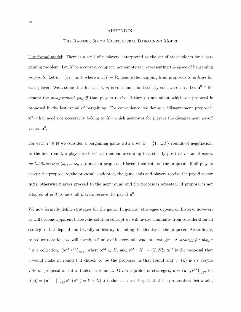
72

APPENDIX:

The Rausser Simon Multilateral Bargaining Model

The formal model: There is a set I of n players, interpreted as the set of stakeholders for a bar-

gaining problem. Let X be a convex, compact, non-empty set, representing the space of bargaining

proposals. Let u = (u1, ...un), where ui : X → R, denote the mapping from proposals to utilities for

each player. We assume that for each i, ui is continuous and strictly concave on X. Let u0 ∈ Rn

denote the disagreement payoff that players receive if they do not adopt whichever proposal is

proposed in the last round of bargaining. For convenience, we define a “disagreement proposal”

x0—that need not necessarily belong to X—which generates for players the disagreement payoff

vector u0.

For each T ∈ N we consider a bargaining game with a set T = {1, ..., T} rounds of negotiation.

In the first round, a player is chosen at random, according to a strictly positive vector of access

probabilities ωωω = (ω1, ..., ωn), to make a proposal. Players then vote on the proposal. If all players

accept the proposal x, the proposal is adopted, the game ends and players receive the payoff vector

u(x), otherwise players proceed to the next round and the process is repeated. If proposal is not

adopted after T rounds, all players receive the payoff u0.

We now formally define strategies for the game. In general, strategies depend on history; however,

as will become apparent below, the solution concept we will invoke eliminates from consideration all

strategies that depend non-trivially on history, including the identity of the proposer. Accordingly,

to reduce notation, we will specify a family of history-independent strategies. A strategy for player

i is a collection,(

xi,t, vi,t)

t∈T, where xi,t ∈ X, and vi,t : X → {Y,N}; xi,t is the proposal that

i would make in round t if chosen to be the proposer in that round and vi,t(x) is i’s yes/no

vote on proposal x if it is tabled in round t. Given a profile of strategies, s =(

xi,t, vi,t)

t∈T, let

X(s) = {xi,t :∏

r∈Ivr,t(xr,t) = Y }; X(s) is the set consisting of all of the proposals which would,

73

under the strategy profile s, be proposed by some player in some round, if that round were ever

reached, and, if proposed, would be adopted. Now define the mapping A(s) : I × T → {0, 1},

by Ai,t(s) =

1 if xi,t ∈ X(s)

0 otherwise

. Ai,t(s) is one if i’s proposal in round t is adopted, otherwise

it is zero. Next, define the ex ante probability that the outcome xi,t ∈ X(s) will be proposed

(and then adopted) as µ(xi,t|s) =

ωi if t = 1

∏t−1t′=1

(

1 −∑

r∈IωrA

r,t′(s))

ωi if t > 1. In words, µ(xi,t|s)

is the probability that no agreement is reached in any round prior to t, times the conditional

probability that player i is chosen as the proposer in round t, given that this period is reached.

Let µ(x0|s) = 1 −∑

x∈X(s) µ(x|s) denote the probability that no proposal is ever adopted. For a

T -period multilateral bargaining game, we can now define the payoff function mapping strategy

profiles to expected payoff vectors by

P(s) =∑

x∈X(s)∪{x0}

u(x)µ(x|s)

A Nash Equilibrium is a strategy profile s such that for each i and each strategy s′i for i,

Pi(s) ≥ Pi(s′i, s¬i). The standard solution concept for games of this kind is subgame perfection. A

strategy profile is a subgame perfect equilibrium if the strategies form a Nash equilibrium, starting

from any subgame of the game.

In the present context, sub-game perfection is an inadequate solution concept. To see this, note

that in any T -round MB game with at least three players, there is a subgame perfect equilibrium

which implements the default outcome, regardless of the possible Pareto gains to bargaining. One

such equilibrium is the profile in which all players reject all proposals; since at least two acceptances

are required before a proposal can be adopted, no individual player can benefit by accepting any

proposal. Similarly, for any proposal x such that u(x) ≥ u0, and any t ∈ T, there is a subgame

perfect equilibrium in which x is adopted in round t.

74

Intuitively, almost none of these subgame perfect equilibria would be robust to “trembles” in the

sense of “trembling hand perfection” (THP). For continuous action games, however, the known

sufficient conditions for existence of THP equilibria are not satisfied by games of the kind we are

considering (Simon and Stinchcombe, 1995). Accordingly, we propose a new, quite stringent equilib-

rium refinement—we call it “limit dominance solvability”—which reflects the intuition underlying

THP, and isolates a unique bargaining outcome. This concept extends to games with an infinite

number of strategies the solution concept for finite games known as “dominance solvability.”

In finite games, the idea of reducing the set of equilibria by iterated elimination of weakly dominated

strategies35 is well established. In general, this procedure yields indeterminate results, because the

order in which strategies are eliminated may affect the outcome of the procedure. On the other

hand, a game with finitely many actions is said to be dominance solvable “if all players are indifferent

between all outcomes that survive the iterative procedure in which all the weakly dominated actions

of each player are eliminated at each stage.”36 That is, in a dominance solvable game, the order in

which weakly dominated strategies are eliminated is immaterial. We will refer to an outcome that

survives such a procedure as a dominance solvable outcome and the payoffs associated with such

an outcome as a dominance solvable payoff vector.

To our knowledge, the concept of dominance solvability for infinite games has not been system-

atically explored. However, the following extension of the finite concept to our particular infinite

game is very natural. For each T , we will consider sequences of bargaining games that are identical

to our original specification, except that proposers are restricted to choose from increasingly large,

but finite proposal spaces, which converge to our original proposal space X in the sense of Haus-

dorff.37 Dominance solvability is a well-defined concept for these approximating games, since they

35 A strategy si is weakly dominated by s′i if P (si, s−i) ≤ P (s′i, s−i), for all s−i ∈ S−i , and, for some s−i ∈ S−i,

P (si, s−i) < P (s′i, s−i)36 The concept of dominance solvability was first proposed by Moulin (1979). The quote is from (Osborne and Rubinstein, 1994)

75

have finite strategy sets. Of course, not all approximating games are dominance solvable. However,

we provide a simple inductive construction for constructing dominance solvable approximations.

We then say that a T -round MB game is limit dominance solvable if there exists a unique payoff

vector that is the limit of dominance solvable payoff vectors for any sequence of dominance solvable

approximating games.

Our interest is in the outcomes of games with arbitrarily large numbers of bargaining rounds.

Accordingly, we define a solution to the MB model to be a limit, as T goes to infinity, of dominance

solvable payoff vectors from a sequence of T -round, limit dominance solvable bargaining games. We

will prove below that under the assumptions we impose, each MB model has a unique, deterministic

solution: if there is no proposal that weakly Pareto dominates the disagreement payoff vector u0,

then each round ends with disagreement, and u0 is realized with certainty; otherwise, there is a

unique element x∗ of X, which each player proposes, and all others accept, in the first round of

bargaining. The solution to the MB model is then the payoff vector u(x∗).

We establish the existence of the unique solution vector x∗ in three steps. Each step specifies

an inductive algorithm. Our first algorithm identifies the proposal x∗, without using any game-

theoretic concepts. Second, we demonstrate the existence of a sequence of dominance solvable finite

games that approximate, increasingly closely, our original infinite game. Third, we show that any

sequence of dominance solvable outcomes for these approximating games indeed converges to the

solution vector x∗.

In contrast to the formal specification on pp. 72-73, the time index in the algorithm below runs

backwards. To emphasize the distinction we index time with the symbol τ rather than t.

37 Given two sets Y1 and Y2 and a metric d on both of them, the Hausdorff distance between these sets less than δ if for i = 12,and any element y ∈ Yi there is some point y′ ∈ Y3−i such that d(y, y′) < δ.

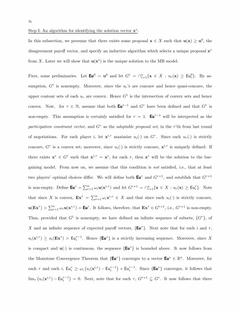
76

Step I: An algorithm for identifying the solution vector x∗:

In this subsection, we presume that there exists some proposal x ∈ X such that u(x) ≥ u0, the

disagreement payoff vector, and specify an inductive algorithm which selects a unique proposal x∗

from X. Later we will show that u(x∗) is the unique solution to the MB model.

First, some preliminaries. Let EuEuEu0 = u0 and let G1 = ∩nr=1{x ∈ X : ur(x) ≥ Eu0

r}. By as-

sumption, G1 is nonempty. Moreover, since the ur’s are concave and hence quasi-concave, the

upper contour sets of each ur are convex. Hence G1 is the intersection of convex sets and hence

convex. Now, for τ ∈ N, assume that both EuEuEuτ−1 and Gτ have been defined and that Gτ is

non-empty. This assumption is certainly satisfied for τ = 1. EuEuEuτ−1 will be interpreted as the

participation constraint vector, and Gτ as the adoptable proposal set, in the τ ’th from last round

of negotiations. For each player i, let xi,τ maximize ui(·) on Gτ . Since each ur(·) is strictly

concave, Gτ is a convex set; moreover, since ui(·) is strictly concave, xi,τ is uniquely defined. If

there exists x∗ ∈ Gτ such that xr,τ = x∗, for each r, then x∗ will be the solution to the bar-

gaining model. From now on, we assume that this condition is not satisfied, i.e., that at least

two players’ optimal choices differ. We will define both EuEuEuτ and Gτ+1, and establish that Gτ+1

is non-empty. Define EuEuEuτ =∑n

r=1 ωru(xr,τ ) and let Gτ+1 = ∩nr=1{x ∈ X : ur(x) ≥ Euτ

r}. Note

that since X is convex, Exτ =∑n

r=1 ωrxr,τ ∈ X and that since each ui(·) is strictly concave,

u(Exτ ) >∑n

r=1 ωru(xr,τ ) = EuEuEuτ . It follows, therefore, that Exτ ∈ Gτ+1, i.e., Gτ+1 is non-empty.

Thus, provided that G1 is nonempty, we have defined an infinite sequence of subsets, {Gτ}, of

X and an infinite sequence of expected payoff vectors, {EuEuEuτ}. Next note that for each i and τ ,

ui(xi,τ ) ≥ ui(Exτ ) > Euτ−1

i . Hence {EuEuEuτ} is a strictly increasing sequence. Moreover, since X

is compact and u(·) is continuous, the sequence {EuEuEuτ} is bounded above. It now follows from

the Monotone Convergence Theorem that {EuEuEuτ} converges to a vector EuEuEu∗ ∈ Rn. Moreover, for

each τ and each i, Euτi ≥ ωi

(

ui(xi,τ ) − Euτ−1

i

)

+ Euτ−1i . Since {EuEuEuτ} converges, it follows that

limτ

(

ui(xi,τ ) − Euτ−1

i

)

= 0. Next, note that for each τ , Gτ+1 ( Gτ . It now follows that there

77

exists x∗ ∈ X such that ∩∞τ=1G

τ = x∗. (Suppose to the contrary that ∩∞τ=1G

τ contains two distinct

points x and x′. In this case, since ui(·) is strictly concave, there exists ε > 0 s.t. for each i and τ ,

uτi (xi,τ ) ≥ ui(0.5(x + x′)) − ε ≥ min(ui(x), ui(x

′)) ≥ Eu∗i ≥ Euτ−1i .

But this is impossible, since we have established that limτ

(

ui(xi,τ ) − Euτ−1

i

)

= 0.) We will establish

below that as the number of bargaining rounds increases without bound, in any equilibrium of our

bargaining game, each player in the first round makes some proposal arbitrarily close to x∗, and

this proposal is adopted immediately.

Step II: An algorithm for constructing a dominance solvable finite game:

For an arbitrary finite game, Rochet (1980) shows that condition (R) below is sufficient for domi-

nance solvability.

for all s, s′ ∈ S, for all i, if Pi(s) = Pi(s′) then P(s) = P(s′) (R)

Condition R states that if the vectors of payoffs associated with two strategy profiles differ in one

component, then they differ in all components. We now provide an algorithm for constructing a

finite game with a property which is slightly stronger than (R). Recalling the definition of µ(·|s)

from page 73, the condition is:

for all s, s′ ∈ S, µ(·|s) 6= µ(·|s′) implies that (R′)

each element of P(s) differs from the corresponding element of P(s′)

To see that (R′) implies (R), observe that if (R′) is satisfied, then Pi(s) = Pi(s′) implies

µ(·|s) = µ(·|s′), in which case P(s) = P(s′).

We first specify some notation for T -round multi-lateral bargaining games in which proposers are

restricted to select from a finite set of proposals. Given a finite subset Y of X, let S|Y ⊂ S denote

the (finite) set of strategies with the property that all proposers in all periods choose proposals

78

from Y . A game in which proposers are so restricted will be called a bargaining game played on

Y . Now let M|Y denote the set of all probability measures on X ∪ {x0} that can be generated by

some profile of strategies in S|Y . (Recall that x0 is the “disagreement proposal” defined on p 72.)

Necessarily, M|Y is a finite set. If Y ∪ {x0} is enumerated as {x1, ...,x#Y ,x0}, then each element

µ ∈M|Y uniquely defines a vector σσσµ ∈ ∆#Y , the #Y -dimensional unit simplex, with the property

that for η = 1, ...,#Y , σµη = µ(xη). Finally, define the expected payoff mapping ΠΠΠ(·|Y ) : M|Y → Rn

by

ΠΠΠ(µ|Y ) =∑

x∈Y ∪{x0}

u(x)µ(x) =

#Y +1∑

η=1

u(xη)σµη

Note that the image of ΠΠΠ(·|Y ) is identically equal to the image of P(·); the difference between the

two mappings is that the argument of P is a strategy profile, while the argument of ΠΠΠ(·|Y ) is a

probability measure generated by a strategy profile. Note also that if Y ′ is a perburbation of the

set Y with the same number of elements, then the set of all probability measures on X ∪{x0} that

can be generated by some profile of strategies in S|Y ′ can be recovered from the set {σσσµ : µ ∈M|Y }.

We now provide an inductive construction that will result in a finite set Y ⊂ X with the property

that any bargaining game played on Y exhibits property (R′). First, select a finite subset X0 of X

and a scalar ε0 > 0 with the following properties.

(1) x 6= x′ ∈ X0 and i ∈ I implies ui(x) 6= ui(x′).

(2) for all i ∈ I and all µ, µ′ ∈ M|X0, Πi(µ) 6= Πi(µ

′) implies |Πi(µ) − Πi(µ′)| > ε0 (ε0 exists

because M|X0is a finite set).

79

Let M denote the subset of M|X0×M|X0

consisting of pairs µµµ = {µv, µw}, v < w. Enumerate the

distinct elements of M as {µµµ1, ...,µµµ#M}. Now fix m ∈ {1, ...,#M} and assume that

(1) εm−1 > 0 and Xm−1 have been defined.

(2) for each 1 ≤ m′ < m, each i and pair µµµm′= (µv′ , µw′

),∣

∣

∣Πi(µ

v′ |Xm−1) − Πi(µw′|Xm−1)

∣

∣

∣>

εm−1

For m = 1, the first condition is clearly satisfied, while the second condition is satisfied vacuously.

We’ll now define εm > 0 and Xm such that #Xm = #Xm−1 and

for each 1 ≤ m′ ≤ m, each i and each pair µµµm′= (µv′ , µw′

), (1)

∣

∣

∣Πi(µ

v′ |Xm) − Πi(µw′|Xm)

∣

∣

∣> εm.

First, write µµµm as (µv, µw). Now pick γ ≤ εm−1 such that Πi(µv|Xm−1) 6= Πi(µ

w|Xm−1) implies

∣

∣ Πi(µv|Xm−1) − Πi(µ

w|Xm−1)∣

∣ > 2γ. There are now two cases to consider.

Case A: Πi(µv|Xm−1) 6= Πi(µ

w|Xm−1) for all i;

Case B: there exists i such that Πi(µv|Xm−1) = Πi(µ

w|Xm−1);

In Case A, define εm = γ, Xm = Xm−1. Now suppose that Case B obtains. In this case, pick

x ∈ Xm−1 such that µv(x) 6= µw(x). Since µv is distinct from µw, such an x necessarily exists.

Choose x′ near x such that for all i ∈ I, 0 < |ui(x′) − ui(x)| < γ. Define Xm to be equal to Xm−1

except that x′ replaces x. Now observe that for all i such that Πi(µv|Xm−1) = Πi(µ

w|Xm−1),

Πi(µv|Xm) = Πi(µ

v|Xm−1) + µv(x)(ui(x′) − ui(x))

6= Πi(µw|Xm−1) + µw(x)(ui(x

′) − ui(x)) = Πi(µw|Xm)

while for all i such that Πi(µv|Xm−1) 6= Πi(µ

w|Xm−1),

Πi(µv|Xm) − Πi(µ

w|Xm)

= Πi(µv|Xm−1) − Πi(µ

w|Xm−1) + (µv(x) − µw(x))(ui(x′) − ui(x))

> 2γ − γ > 0

80

Finally pick εm ≤ γ such that for all i, |Πi(µv|Xm) − Πi(µ

w|Xm)| > εm and observe that since

εm ≤ εm−1, condition (1) is indeed satisfied for both Cases A and B above. To complete the

inductive construction, define Y = X#M, and note that condition (R′) is satisfied for the game

played on Y . Since our starting set X0 was an arbitrary finite subset of X, we can use the above

construction to build a sequence of finite games that converge to X in the sense of Hausdorff.

Step III: Existence of a unique limit of limit dominance solvable payoff vectors:

Fix T and consider a sequence Xk of finite subsets of X that Hausdorff converge to X. Assume for

convenience that for each k ∈ N, there exists x ∈ Xk such that u(x) ≥ u0 = EuEuEu0. Assume also that

for each k ∈ N, the T -period MB game played on Xk is dominance solvable. (Step II established

the existence of such a game.) We will show that the sequence of dominance solvable payoff vectors

for these approximating games converges to EuEuEuT , which is the T ’th element of the sequence {EuEuEuτ}

of vectors uniquely identified by the algorithm constructed in Step I. The notation we use in this

section will parallel the notation used on pp. 75-77, with the addition of “k” superscripts to index

the finite approximating proposal spaces.

For each k ∈ N, set EuEuEu0,k equal to the disagreement payoff EuEuEu0. Let τ ∈ {1, ..., T−1} denote the

τ ’th-from-last round of negotiations (i.e., τ = 1 denotes the final round of negotiations in a T -

period game). Now assume that for the game played on Xk, after 2(τ−1) rounds of elimination

of weakly dominated strategies, the following is true for any profile of strategies that has survived

these elimination rounds (henceforth referred to as “surviving strategy profiles”): (a) if a proposal

is not adopted in this round, the continuation payoff vector is EuEuEuτ−1,k; (b){

EuEuEuτ−1,k}

→k EuEuEuτ−1,

where EuEuEuτ−1 was defined on p. 76. Both these assumptions are certainly satisfied for τ = 1. We

will now define, for each k ∈ N, the vector EuEuEuτ,k with the property that for the game played on Xk,

after 2t rounds of elimination of weakly dominated strategies, the following is true for any surviving

81

strategy profile: (a) if a proposal is not adopted in the τ+1’th-from-last round of bargaining, the

continuation payoff is EuEuEuτ,k; (b){

EuEuEuτ,k}

→k EuEuEuτ .

First, define Gτ,k = ∩nr=1{x ∈ Xk : ur(x) > Euτ−1,k

r }. Let Sτ,kN denote the set of all surviving

strategies in S|Xk which vote “N” in the τ ’th-from-last round on some proposal x ∈ Gτ,k. Clearly,

each strategy sr ∈ Sτ,kN is weakly dominated for player r by the surviving strategy that is identical

to sr, except that it votes “Y ” on every x ∈ Gτ,k in the τ ’th-from last round. Similarly, let Sτ,kr,Y

denote the set of surviving strategies that votes “Y ” in the τ ’th-from-last round on a proposal

x ∈ Xk such that ur(x) < Euτ−1,kr . Once again, each strategy sr ∈ S

τ,kr,Y is weakly dominated

for player r by the surviving strategy that is identical to sr, but in this round votes “N” on

{x ∈ Xk : ur(x) < Euτ−1,kr }. Now, for each player r, eliminate all strategies in S

τ,kN ∪ Sτ,k

r,Y . Call

this the (τ, 1)’th round of elimination. After the (τ, 1)’th round of elimination, a proposal x by

i in the τ ’th-from-last round will be adopted if x ∈ Gτ,k and rejected by at least one player if

x ∈ ∪nr=1{x ∈ Xk : ur(x) < Euτ−1,k

r }. It now follows that a necessary condition for a strategy si to

be undominated after the (τ, 1)’th round of elimination is that

i’s proposal x in the τ ’th-from-last round satisfies:

u(x) ≥ Euτ−1,k and ui(x) ≥ ui(x′), for all x′ ∈ Gτ,k. (2)

Now eliminate all strategies for player i that fail to satisfy condition (2); call this the (τ, 2)’th round

of elimination.

For each k ∈ N, consider a strategy si that survives the (τ, 2)′th round of elimination and let xi,τ,k

denote the proposal specified by si for presentation in the τ ’th-from-last round. We will argue that

{xi,τ,k} →k xi,τ , where xi,τ was defined on p. 76. Suppose to the contrary that there exists ε > 0

and a subsequence, again indexed by k, such that for all k, ||xi,τ,k −xi,τ || > ε. Since X is compact,

this sequence contains a convergent subsequence: let yi,τ denote its limit. Now from the definition

82

of Gτ (p. 76), since the Xk’s converge to X and, by assumption,{

EuEuEuτ−1,k}

→k EuEuEuτ−1, we have

cl(

∪kGτ,k

)

= Gτ . It follows, therefore, that yi,τ ∈ Gτ , and ui(yi,τ ) ≥ ui(x

′), for all x′ ∈ Gτ .

However, by definition, the same properties hold for xi,τ . But this is a contradiction because, since

ui(·) is strictly concave, it has a unique maximizer on Gτ .

This completes the inductive argument: we have proved that for all ε > 0, there exists τ and a

sequence {Kτ} such that for τ > τ and k > Kτ , ||EuEuEu∗ − EuEuEuτ,k|| < ε. This establishes that the

T -round MB game is limit dominance solvable, and that the sequence of limit dominance solvable

payoff vectors converges to EuEuEu∗.

References

Adams, G., Rausser, G. C. and Simon, L. K. (1996). Modelling multilateral negotiations: An application to California

water policy, Journal of Economic Behavior and Organization 30(1): 97–111.

Baron, D. P. and Ferejohn, J. A. (1987). Bargaining and agenda formation in legislatures, American Economic Review,

Papers and Proceedings 77(2): 303–309.

Baron, D. P. and Ferejohn, J. A. (1989a). Bargaining in legislatures, American Political Science Review 83(4): 1181–

1206.

Baron, D. P. and Ferejohn, J. A. (1989b). The power to propose, in P. C. Ordeshook (ed.), Models of Strategic Choice

in Politics, University of Michigan Press, Ann Arbor.

Barreteau, O., Garin, P., Dumontier, P. A. and Arami, G. (2003). Agent based facilitation of water allocation: case

study in the drome river valley, Group Decision and Negotiations 12: 441–461.

Becu, N., Perez, P., Walker, A., Barreteau, O. and Page, C. L. (2003). Agent based simulation of a small catch-

ment water river management in northern thailand: description of the catchscape model, Ecological Modelling

170: 319–331.

Bennett, E. (1991a). Multilateral bargaining problems, Working paper.

Bennett, E. (1991b). Three approaches to bargaining in ntu games, in R. Selten (ed.), Strategic Bargaining, Springer

Verlag, Berlin.

83

Bennett, E. and Damme, E. V. (1991). Demand commitment bargaining: The case of apex games.”, in R. Selten

(ed.), Strategic Bargaining, Springer Verlag, Berlin.

Bennett, E. and Houba, H. (1987). ”odd man out: The proposal making model”.

Binmore, K. (1985). Bargaining and coalitions, in A. E. Roth” (ed.), Game Theoretic Models of Bargaining, Cambridge

University Press, Cambridge.

Binmore, K., McCarthy, J., Ponti, G., Samuelson, L. and Shaked, A. (2002). A Backward Induction Experiment,

Journal of Economic Theory 104: 48–88.

Binmore, K., Rubinstein, A. and Wolinsky, A. (1986). The nash bargaining solution in economic modelling, Rand

Journal of Economics 17: 176–18.

Binmore, K., S. A. and Sutton, J. (1989). An outside option experiment, Quarterly Journal of Economics 104: 753–

770.

Cai, H. (2000). Delay in Multilateral Bargaining under Complete Information, Journal of Economic Theory 93: 260–

276.

Cai, H. (2003). Inefficient Markov perfect equilibria in multilateral bargaining, Economic Theory 22: 583–606.

Carraro, C., Marchiori, C. and Sgobbi, A. (2005). Applications of negotiation theory to water issues, Working Paper

65.2005, FEEM.

Cemegraf (1994). Schema directeur de gestion des etiages de l’adour.

Chatterjee, K., Dutta, B., Ray, D. and Sengupta, D. (1987). A noncooperative theory of caolitional bargaining,

Working paper.

de Mesquita, B. (1985). The war trap revisited: A revised expected utility model, The American Political Science

Review 79(1): 156–177.

de Mesquita, B. (1990). Multilateral negotiations: An analysis of the arab-israeli dispute, International Organization

44(3): 317–340.

Dinar, A., Farolfi, S., Patrone, P. and Rowntree, K. (2006). Negotiation vs. game theory outcomes for water allocation

problems in the kat basin, south africa, Prepared for the Sixth Meeting on Game Theory and Practice, Zaragoza,

Spain.

Dinar, A., Ratner, A. and Yaron, D. (1992). Evaluating cooperative game theory in water resources, Theory an.d

Decision 32: 1–20.

Doron, G. and Sened, I. (1995). Cooperative and non-cooperative bargaining models in political science, Journal of

Theoretical Politics 7(3): 235–243.

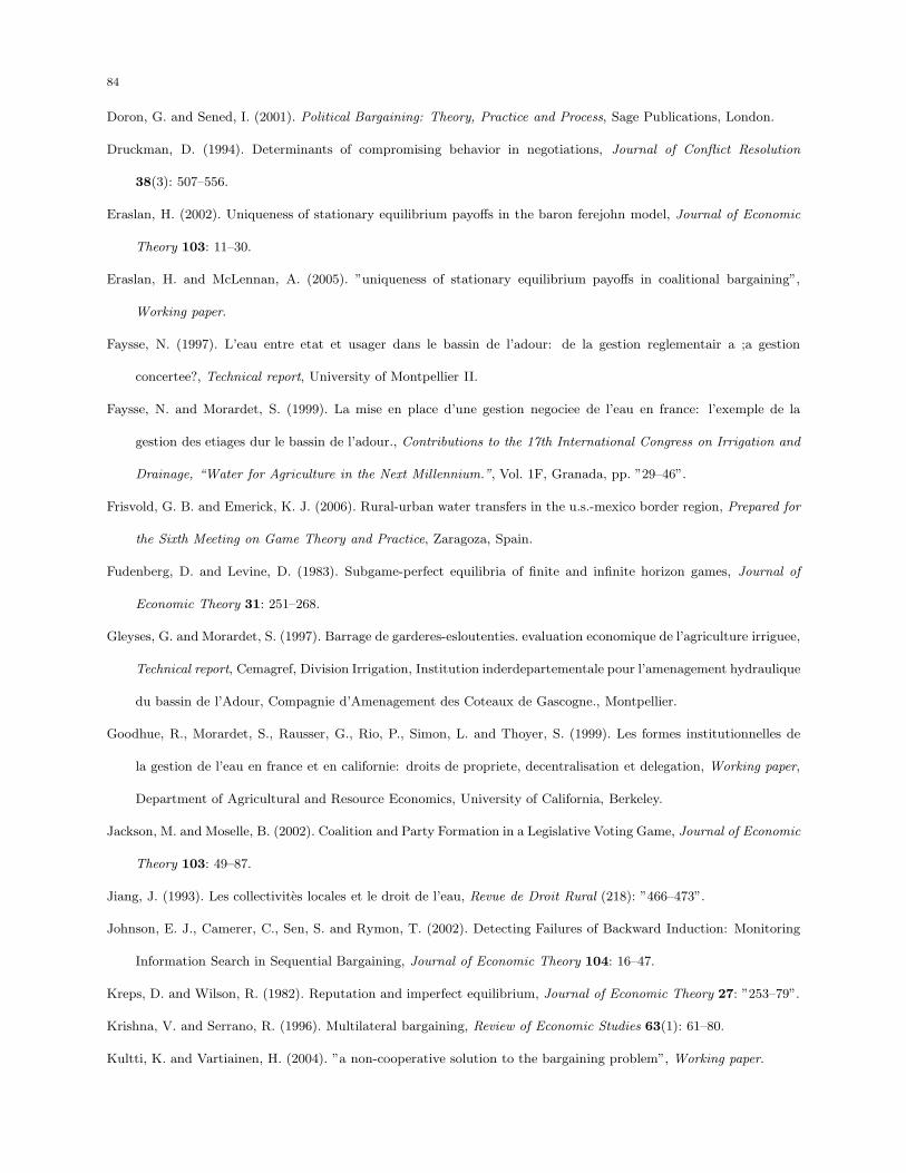
84

Doron, G. and Sened, I. (2001). Political Bargaining: Theory, Practice and Process, Sage Publications, London.

Druckman, D. (1994). Determinants of compromising behavior in negotiations, Journal of Conflict Resolution

38(3): 507–556.

Eraslan, H. (2002). Uniqueness of stationary equilibrium payoffs in the baron ferejohn model, Journal of Economic

Theory 103: 11–30.

Eraslan, H. and McLennan, A. (2005). ”uniqueness of stationary equilibrium payoffs in coalitional bargaining”,

Working paper.

Faysse, N. (1997). L’eau entre etat et usager dans le bassin de l’adour: de la gestion reglementair a ;a gestion

concertee?, Technical report, University of Montpellier II.

Faysse, N. and Morardet, S. (1999). La mise en place d’une gestion negociee de l’eau en france: l’exemple de la

gestion des etiages dur le bassin de l’adour., Contributions to the 17th International Congress on Irrigation and

Drainage, “Water for Agriculture in the Next Millennium.”, Vol. 1F, Granada, pp. ”29–46”.

Frisvold, G. B. and Emerick, K. J. (2006). Rural-urban water transfers in the u.s.-mexico border region, Prepared for

the Sixth Meeting on Game Theory and Practice, Zaragoza, Spain.

Fudenberg, D. and Levine, D. (1983). Subgame-perfect equilibria of finite and infinite horizon games, Journal of

Economic Theory 31: 251–268.

Gleyses, G. and Morardet, S. (1997). Barrage de garderes-esloutenties. evaluation economique de l’agriculture irriguee,

Technical report, Cemagref, Division Irrigation, Institution inderdepartementale pour l’amenagement hydraulique

du bassin de l’Adour, Compagnie d’Amenagement des Coteaux de Gascogne., Montpellier.

Goodhue, R., Morardet, S., Rausser, G., Rio, P., Simon, L. and Thoyer, S. (1999). Les formes institutionnelles de

la gestion de l’eau en france et en californie: droits de propriete, decentralisation et delegation, Working paper,

Department of Agricultural and Resource Economics, University of California, Berkeley.

Jackson, M. and Moselle, B. (2002). Coalition and Party Formation in a Legislative Voting Game, Journal of Economic

Theory 103: 49–87.

Jiang, J. (1993). Les collectivites locales et le droit de l’eau, Revue de Droit Rural (218): ”466–473”.

Johnson, E. J., Camerer, C., Sen, S. and Rymon, T. (2002). Detecting Failures of Backward Induction: Monitoring

Information Search in Sequential Bargaining, Journal of Economic Theory 104: 16–47.

Kreps, D. and Wilson, R. (1982). Reputation and imperfect equilibrium, Journal of Economic Theory 27: ”253–79”.

Krishna, V. and Serrano, R. (1996). Multilateral bargaining, Review of Economic Studies 63(1): 61–80.

Kultti, K. and Vartiainen, H. (2004). ”a non-cooperative solution to the bargaining problem”, Working paper.

85

Manzini, P. and Mariotti, M. (2003). A bargaining model of voluntary environmental agreements, Journal of Public

Economics 87: 2725–2736.

Manzini, P. and Mariotti, M. (2005). Alliances and negotiations, Journal of Economic Theory 121: 128–141.

Milgrom, P. and Roberts, J. (1982). Predation, reputation and entry deterrence, Journal of Economic Theory

27: ”280–312”.

Moulin, H. (1979). Dominance Solvable Voting Schemes, Econometrica 47: 1337–1351.

Nash, J. F. (1950). The bargaining problem, Econometrica 18(2): 155–162.

Neelin, J., Sonnenschein, H. and Speigel, M. (1988). A further test of noncooperative bargaining theory, American

Economic Review 78: 824–836.

Norman, P. (2002). Legistlative Bargaining and Coalition Formation, Journal of Economic Theory 102: 322–353.

Osborne, M. J. and Rubinstein, A. (1990). Bargaining and Markets, Academic Press, San Diego.

Osborne, M. J. and Rubinstein, A. (1994). A Course in Game Theory, MIT Press, Cambridge, MA.

Parrachino, I., Dinar, A. and Patrone, P. (2006). Cooperative game theory and its application to natural, environ-

mental, and water resource issues: 3. application to water resources, Prepared for the Sixth Meeting on Game

Theory and Practice, Zaragoza, Spain.

Rausser, G. C. and Simon, L. K. (1999). A non-cooperative model of collective decision making: A multilateral

bargaining approach, Technical report, University of California at Berkeley.

Rochet, J. (1980). Selection of an Unique Equilibrium Value for Extensive Games with Perfect Information, Discussion

paper, Ceremade, Universite Paris IX.

Roth, A. (1979). Axiomatic Models of Bargaining, Springer Verlag, Berlin.

Rubinstein, A. (1982). Perfect equilibrium in a bargaining model, Econometrica 50: 97–109.

Selten, R. (1975). Re-examination of the perfectness concept for equilibrium points in extensive games, International

Journal of Game Theory 4: ”25–55”.

Selten, R. (1981). A noncooperative model of characteristic funcction bargaining, in V. Boehm and H. Nachtkamp

(eds), Essays in Game Theory ad Mathematical Economics in Honor of Oskar Morgenstern, Wissenschaftsverlag

Bibliographisches Institut Mannheim, Wien-Zurich, pp. 131–151.

Shaked, A. and Sutton, J. (1984). The Semi-Walrasian Economy, Technical report, D.P. 84/98, Suntory Toyota

International Centre for Economics and Related Disciplines, London School of Economics.

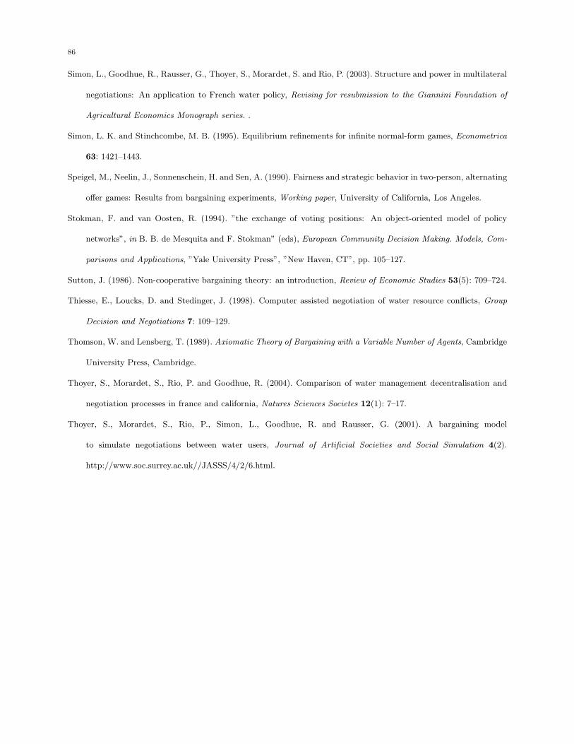
86

Simon, L., Goodhue, R., Rausser, G., Thoyer, S., Morardet, S. and Rio, P. (2003). Structure and power in multilateral

negotiations: An application to French water policy, Revising for resubmission to the Giannini Foundation of

Agricultural Economics Monograph series. .

Simon, L. K. and Stinchcombe, M. B. (1995). Equilibrium refinements for infinite normal-form games, Econometrica

63: 1421–1443.

Speigel, M., Neelin, J., Sonnenschein, H. and Sen, A. (1990). Fairness and strategic behavior in two-person, alternating

offer games: Results from bargaining experiments, Working paper, University of California, Los Angeles.

Stokman, F. and van Oosten, R. (1994). ”the exchange of voting positions: An object-oriented model of policy

networks”, in B. B. de Mesquita and F. Stokman” (eds), European Community Decision Making. Models, Com-

parisons and Applications, ”Yale University Press”, ”New Haven, CT”, pp. 105–127.

Sutton, J. (1986). Non-cooperative bargaining theory: an introduction, Review of Economic Studies 53(5): 709–724.

Thiesse, E., Loucks, D. and Stedinger, J. (1998). Computer assisted negotiation of water resource conflicts, Group

Decision and Negotiations 7: 109–129.

Thomson, W. and Lensberg, T. (1989). Axiomatic Theory of Bargaining with a Variable Number of Agents, Cambridge

University Press, Cambridge.

Thoyer, S., Morardet, S., Rio, P. and Goodhue, R. (2004). Comparison of water management decentralisation and

negotiation processes in france and california, Natures Sciences Societes 12(1): 7–17.

Thoyer, S., Morardet, S., Rio, P., Simon, L., Goodhue, R. and Rausser, G. (2001). A bargaining model

to simulate negotiations between water users, Journal of Artificial Societies and Social Simulation 4(2).

http://www.soc.surrey.ac.uk//JASSS/4/2/6.html.