1

Structure-Aware Sparse Reconstruction and

Applications to Passive Multi-Static RadarYimin D. Zhang, Senior Member, IEEE, Moeness G. Amin, Fellow, IEEE,

and Braham Himed, Fellow, IEEE

Abstract

In this article, we introduce the concept of sparse signal reconstruction and its applications to

passive multi-static radar. The emphasis is on the sparse Bayesian learning techniques that exploit signal

structures in terms of their group sparsity and/or target structures. These techniques offer: (a) high

range and angular resolution beyond the Fourier based resolution bounds which are limited by the array

aperture and signal bandwidth; (b) less sensitivity to the coherency of dictionary entries as compared

to other compressive sensing methods; (c) effective combining of multiple measurement signals with

diverse reflection coefficients associated with different transmit sources, signal aspect angles, frequencies,

and/or polarizations; and (d) utilization of signal and target structures for improved signal recovery. For

demonstration of these offerings, we provide a number of examples for passive multi-static radar systems,

including synthetic aperture radar (SAR) imaging and space-time adaptive processing (STAP).

Index Terms

Bayesian compressive sensing, passive multi-static radar, synthetic aperture radar (SAR), space-time

adaptive processing (STAP), target tracking.

The work of Y. D. Zhang and M. G. Amin was supported in part by a subcontract with Defense Engineering Corporation for

research sponsored by the Air Force Research Laboratory under Contract FA8650-12-D-1376.

Y. D. Zhang is with the Department of Electrical and Computer Engineering, College of Engineering, Temple University,

Philadelphia, PA 19122, USA (email: ydzhang@temple.edu).

M. G. Amin is with the Center for Advanced Communications, Villanova University, Villanova, PA 19085, USA.

B. Himed is with the RF Technology Branch, Air Force Research Lab (AFRL/RYMD), WPAFB, OH 45433, USA.

2

I. INTRODUCTION

Passive radar systems operate by exploiting signals of opportunity that are designed for other applica-

tions such as broadcasting, communications, and satellite navigation. Passive radars have recently attracted

much attention in military applications, mainly because of their covertness, low-cost implementation and

no requirement of signal emissions [1, 2]. Whereas the primary use of passive radars is currently in

the defense sector, these same features also make them attractive in commercial applications. Unlike

conventional active radar systems, which typically operate in a monostatic mode, passive radar can

operate in a multi-static mode (thus referred to as passive multi-static radar, or PMR) by utilizing multiple

transmitters. Multiple networked receivers can also be exploited for an expanded size of PMR network.

In addition to multi-static operations consisting of multiple bistatic pairs, PMRs distinguish themselves

from conventional active radars in a number of aspects. In particular, the range resolution is limited

due to the narrow signal bandwidth (typically from several MHz to tens MHz) as compared to that of

nominal active radar systems (from hundreds MHz to a few GHz). This limitation leads to undesirable

performance in various applications. For example, in synthetic aperture radar (SAR) and inverse SAR

(ISAR) applications, PMRs would provide a coarse image resolution. In target localization and tracking,

the system may fail to separate multiple closely located targets. In space-time adaptive processing (STAP),

it becomes difficult to secure a sufficient number of secondary data from neighboring range cells required

for effective clutter suppression. These shortcomings call for novel signal processing methods which offer

capabilities and performance beyond those provided by traditional methods.

The challenges associated with passive radars can be overcome through the use of sparse reconstruction

and compressive sensing (CS) techniques [3–6]. These techniques enable recovery of signals which are

sparse in their nominal basis or in a transformed sparsifying basis from far fewer samples than required

by the Shannon-Nyquist sampling theorem.

While the development of CS and sparse reconstruction techniques was first motivated for image

processing, these techniques have become attractive in many other areas, such as radar signal processing,

biomedical signal processing, time-frequency analysis, and anti-jam satellite navigation. In radar signal

processing, the objectives are typically the detection, localization, and imaging of targets which assume

sparsity in the space and/or parameter domains. The sparsity includes spatial occupancy, motion

parameters, and time and spatial variations. On the other hand, large data requirements may compel

reduced sampling along the space, frequency, and time dimensions. In addition, there are a number of

application scenarios where data collections are limited by signal properties, such as the case of passive

radar narrow signal bandwidth. Data insufficiency and target sparsity invite sparse reconstruction and CS

3

to play a fundamental and key role in the broad areas of radar signal processing, including SAR and

ISAR imaging [7–10], direction-of-arrival estimation [11–13], target localization and tracking [14, 15],

and time-frequency analysis [16–18]. Note that, while the terms CS and sparse reconstruction are often

used interchangeably, the former usually refers to data under-sampling for achieving feasible sampling

and reducing storage complexity, whereas the latter emphasizes the recovery from an under-determined

linear model associated with limited data observations.

A number of algorithms have been proposed for sparse signal recovery. Commonly used algorithms

include greedy algorithms (e.g., orthogonal matching pursuit (OMP) [19]) and dynamic programming

algorithms (e.g., basis pursuit (BP) [20] and Lasso algorithm [21]). Bayesian CS (BCS) or sparse Bayesian

learning (SBL) approaches form a different class of sparse signal reconstruction algorithms based on the

maximum a posteriori (MAP) criterion [22–24]. BCS algorithms provide effective solutions to a large

class of problems based on non-parametric CS framework, and thus have the capabilities to infer the

sparsity parameters while avoiding the nuisance parameters. BCS methods can incorporate measurements

and target structures by defining priors in the signal model and have successfully demonstrated their

superior performance over other CS approaches.

In this article, we employ sparse signal reconstruction for PMRs. The emphasis of this article is on

the BCS techniques that exploit signal structures in terms of their group sparsity and/or target structures.

These techniques offer: (a) high range and angular resolution beyond the Fourier based resolution bounds

which are limited by the array aperture and signal bandwidth; (b) less sensitivity to the coherency of

dictionary entries as compared to other compressive sensing methods; (c) effective combining of multiple

measurement signals with diverse reflection coefficients associated with different transmit sources, signal

aspect angles, frequencies, and/or polarizations; and (d) utilization of signal and target structures for

improved signal recovery. For demonstration of these offerings, we provide a number of examples for PMR

systems, including synthetic aperture radar (SAR) imaging and clutter mitigation and motion parameter

estimation in space-time adaptive processing (STAP).

Notations: We use lower-case (upper-case) bold characters to represent vectors (matrices). In particular,

IN denotes the N × N identity matrix. (.)∗ represents complex conjugation, whereas (.)T and (.)H ,

respectively, denote the transpose and conjugate transpose of a matrix or vector. diag(x) represents a

diagonal matrix that uses the elements of x as its diagonal entries, and ‖ · ‖p denotes the `p-norm of a

vector for p = 0, 1 and 2. p(·) stands for a probability density function (pdf). N (x|a, b) and CN (x|a, b)

denote that random variable x respectively follows real and complex Gaussian distributions with mean

a and variance b. Bern(x|π) implies that random variable x follows a Bernoulli distribution with weight

π, and δ(x) represents the Dirac delta function. We use ⊗ and ◦ to denote the Kronecker product and

4

Rx1Tx

P

t1

2Tx

2Ty

px

py1t

r

t2

rRx

1tR2tRrR

z

x

y1Tx mTx Rv

RH1tH

2tHr

Fig. 1: Multi-static passive radar geometry.

element-wise multiplication, respectively, and Re(·) and Im(·) denote the real and imaginary parts of a

complex value.

II. SIGNAL MODEL OF MULTI-STATIC PASSIVE RADAR

A. Radar Geometry

Consider a multi-static radar scene consisting of K stationary transmitters and a moving receiver

as depicted in Fig. 1. The ith transmitter is assumed to be located at a known position pTi =

[pTi,x, pTi,y, pTi,z]T and uses a single antenna to emit a signal at frequency fi, i = 1, ...,K.

We consider a receiver that consists of an antenna or an antenna array to receive the reference signal

directly from the transmitters, and an antenna or an antenna array to receive the target signal. We refer

to them as the reference channel and the surveillance channel, respectively. As a common assumption,

we consider that these two channels are properly conditioned, i.e., the signal waveform transmitted from

each illuminator is perfectly reconstructed at the reference channel, whereas the contribution of the direct

signal in the surveillance channel is negligible [25].

Let the moving receiver utilizes an N -element uniform linear array (ULA) with inter-element spacing

d. A stationary receiver can be considered as a special case with zero velocity, whereas a single-antenna

receiver only uses the first sensor of the receiver array.

For convenience of notation and without loss of generality, we assume that the receiver moves in

the x-direction. The initial position of the receiver is expressed in the Cartesian coordinate system as

pR(0) = [pR,x(0), 0, HR]T , and the velocity vector is vR = [vR, 0, 0]T . As such, the position of the

receiver at time instant t is expressed as pR(t) = [pR,x(0) + vRt, 0, HR]T .

5

B. Sparse Target Signal Model

We first consider a model where stationary targets are sparsely presented in a scene. For simplicity,

no clutter is assumed. This model and its extensions can be used to handle various radar applications.

For example, ISAR images are sparse and clutter-free. For SAR imaging of moving targets, these targets

are sparse after clutter removal through, e.g., STAP as demonstrated in Section V-C. Clutter suppression

using the displaced phase center antenna (DPCA) [26] is also reported in [27].

Assume that Q0 ground targets where the qth ground target is located at pq = [xq, yq, zq]T . The target

signal us(t) received at the receiver is expressed as

us(t) =

K∑k=1

uks(t) =

K∑k=1

Q0∑q=1

√PTk

Gkqσkq

rTkqrqRsk[t− τTkq − τqR(t)]e−j2πfk[τTkq+τqR(t)]ak(φq), (1)

where PTkis the transmit signal power of the kth illuminator, Gkq represents the antenna gain of the kth

illuminator in the direction of the qth target, and σkq is a complex reflection coefficient associated with

the radar cross section (RCS) of the qth target and depends on the specific illuminator k because the

RCS varies with the aspect angle. In addition, sk(t) is the waveform transmitted from the kth illuminator,

τTkq = rTkq/c and τqR(t) = rqR(t)/c are the time delays respectively corresponding to the range between

the kth illuminator and the qth moving target, rTkq = ‖pTk−pq‖, and the range between the qth moving

target and the receiver, rqR(t) = ‖pq −pR(t)‖, where c is the speed of light. Furthermore, ak(φq) is the

steering vector of the receive array toward the direction of the target with a direction-of-arrival (DOA) φq,

which is defined as the cone angle of the qth target with respect to the x-axis. In the above expression,

κk = 2π/λk is the wavenumber with λk = c/fk denoting the wavelength of the signal transmitted from

the kth illuminator. Note that, the DOA is assumed to be time-invariant in the sense that its change during

the coherent processing interval (CPI) is negligible.

For a given area specified by delay τi,n for the nth bistatic range bin of the ith bistatic pair, i = 1, ...,K,

we perform matched filtering to us(t) by using the reconstructed waveform of the signal emitted from

the ith illuminator as the reference signal. For a specific CPI, the matched filter output at the L azimuth

time instants tl = lT , l = 0, ..., L− 1, is given by [28]

y(n)is (tl) =

Q∑q=1

√PTi

Giqσiq

rTiqrqRρiai(φq)e

j2πνiq[tl−(L−1)T/2], (2)

where Q is the number of targets that fall in the nth bistaic range bin, and ρi is the signal energy which

is practically independent of tl as most digital waveforms have a stable auto-correlation property [29]. In

addition, νiq denotes the Doppler frequency of the qth target which is determined by the rate of change

of the combined bistatic range due to the motion of the receiver platform.

6

Stack y(n)is (tl) over the L collected azimuth time samples as

y(n)is =

[[y

(n)is (t0)]

T , [y(n)is (t1)]

T , ..., [y(n)is (tL−1)]

T]T

=

Q∑q=1

√PTi

Giqσiq

rTiqrqRρih(νiq, φq), (3)

where h(νiq, φq) = b(νiq) ⊗ a(φq) ∈ CNL is the spatio-temporal signature of the qth target, with

b(νiq) =[e−j2πνiq(L−1)T/2, e−j2πνiq(L−3)T/2, ..., ej2πνiq(L−1)T/2

]Tdenoting its temporal signature vector.

Equation (3) can be formulated as the following format:

y(n)is = Hisxis, (4)

where xis =√PTi

ρi[Gi1σi1/(rTi1r1R), ..., GiQσiQ/(rTiQrQR)]T is a vector containing all Q non-zero

target entries, whereas the qth column of matrix His = [h(νi1, φ1), ...,h(νiQ, φQ))] represents the spatio-

temporal signature corresponding to the qth target.

For sparse reconstruction, we reformulate (4) as the following standard CS model:

y(n)is = Φ

(n)is x

(n)is + n, (5)

where x(n)is is an over-determined vector to be estimated, and its dimension is B × 1 with B � Q. Its

entries represent the reflection coefficients of all possible target positions in the nth bistatic range bin

and corresponding to the ith bistatic pair. Because the target scene is sparse, vector x(n)is is sparse as

well, i.e., most of its entries are zero or negligible. Φ(n)is is the NL × B dictionary matrix which is

similar to His, but its columns represent the spatio-temporal signature corresponding to all hypothetic

target pixels defined in x(n)is . Note that the dictionary matrix Φ

(n)is is known because both spatial and

temporal signature vectors can be computed for each hypothetic target pixel. In addition, n represents

the additive noise vector, whose elements are characterized as independent and identically distributed

complex Gaussian with zero mean.

C. Clutter Model

For clutter components in the nth bistatic range bin, the received signal is considered as a summation of

Nc statistically independent scatterers. Similar to (4), we can formulate the matched filtered and stacked

output of the clutter component as

y(n)ic = Hicxic, (6)

where xic contains the reflection coefficients of all Nc scatterers, and Hic = [h(νic1 , φc1), ...,h(νicNc, φcNc

))]

with h(νicm , φcm) = b(νicm)⊗ai(φcm) denoting the spatio-temporal signature of the mth scatterer defined

with respect to its DOA φcm and Doppler frequency νicm .

7

In contrast to the target model described in Section II-B where the target are sparsely present in the

spatial domain, the Nc clutter scatterers generally spread over the entire range cell. Therefore, if we

similarly introduce a vector as in (5) for all spatial positions, the vector is not sparse and thus sparse

reconstruction techniques cannot be applied. On the other hand, it is known that the clutter is sparse in

the angle-Doppler domain with respect to DOA and Doppler frequency (see examples in Section V-C)

[30]. As such, we can define an over-determined vector x(n)ic in the joint angle-Doppler domain [28]:

y(n)ic = Φ

(n)ic x

(n)ic + n. (7)

where x(n)ic denotes the unknown sparse vector whose entries are the coefficients in the discretized angle-

Doppler domain. For the convenience of unified mathematical representations, we denote the dimension

of x(n)ic as B × 1 where B is usually much larger than NL to achieve a high resolution in the estimated

clutter angle-Doppler signature. The dimension of Φ(n)ic is NL×B, and n accounts for the additive noise.

III. STRUCTURE-AWARE SPARSE BAYESIAN LEARNING

CS techniques provide the capability to recover signals from a set of undersampled (sub-Nyquist)

measurement samples with a high probability, provided that the signals are sparse or can be sparsely

represented in some known domain. In this section, we describe a single measurement vector (SMV)

model and its solution using the Bayesian CS methods. The signal model with multiple measurements

is described in the following section.

A. Concept of Compressive Sensing and Sparse Reconstruction

A general SMV model is given as,

y = Φx + n, (8)

where y is an M × 1 measured data vector, Φ is a known directory matrix of dimension M × B with

M � B, and x is a B × 1 unknown sparse vector for which the number of non-zero entries is upper

bounded by D with D < M . In addition, n is an M × 1 unknown zero-mean Gaussian noise vector.

The objective of sparse signal reconstruction is to estimate the sparse weight vector x from y. Ideally,

the dictionary matrix Φ has to satisfy the restricted isometry property (RIP) which ensures sparse signal

recovery with a high probability [3]. However, in practical radar applications, this assumption is often

violated when a high-resolution solution is desired.

Given the CS model in (8), the sparse signal vector x can be recovered uniquely with a high probability

from the measurement vector y provided that the matrix Φ has some desirable attributes and the dimension

8

M of the measurement vector y is at least of the order of D log(B/D) [31]. Ideally, this problem is

formulated as the following `0-norm optimization problem:

minimizex

‖ x ‖0 subject to ‖ y −Φx ‖22≤ ε0, (9)

where ε0 is a regularization parameter.

Because the above problem is NP-hard, it is often relaxed by replacing the `0-norm by the

computationally more attractive `1 norm in the above formulation, i.e.,

minimizex

‖ x ‖1 subject to ‖ y −Φx ‖22≤ ε0, (10)

The relaxed problem becomes convex, and a number of sparse reconstruction algorithms are available in

the literature, ranging from those based on `1-norm convex optimization to iterative greedy algorithms.

There are many solvers of the `1-regularized formulation in (9) or its variants, such as LASSO [21]. On

the other hand, greedy algorithms, such as OMP [19], iteratively build the sparse solution by identifying

the support set, either one or multiple terms at a time.

B. Bayesian Compressive Sensing Methods

In this subsection, we first consider a real-valued model for (8). Its extension to the complex-valued

model is considered later. The BCS methods estimate the sparse vector x as the maximum a posteriori

(MAP) solution of (8) for x expressed as

x = arg maxx

p(x|y)

= arg minx{− ln p(y|x)− ln p(x)}

= arg minx

{12 ‖y −Φx‖22 − λ ln p(x)

},

where λ is a regularization parameter that balances distortion and sparsity. Assume the likelihood model

as [32]

p (y; x, γ0) = N (Φx, γ0I), (11)

where γ0 is the variance of the additive noise. The maximum likelihood estimation of x and γ0 will

generally lead to severe overfitting. Therefore, we place a Gaussian prior over the sparse solution vector

x, i.e., p (x;γ) =∏Bb=1N (xb |0, γb ) , where xb is the bth element of x, and γ = [γ1, . . . , γB]T is a vector

of B hyper-parameters that controls the prior variance of each weight. Further, to acquire a trackable

prior of γ and γ0, each is assumed to follow the inverse-gamma distribution (i.e., their inverse follow a

gamma distribution), which is conjugate to the Gaussian distribution.

9

This problem is often solved using the type-II maximum likelihood approach. With the use of hyper-

parameters γ0 and γ, the MAP problem can be rewritten as

(x, γ, γ0) = arg maxx,γ,γ0

p(x,γ, γ0|y) = arg maxx,γ,γ0

p(x|yγ, γ0)p(γ, γ0|y). (12)

Given γ and γ0, we can obtain p(x|y,γ, γ0) = N (µ,Σ) where µ = γ−10 ΣxΦTy, Σx = (γ−1

0 ΦTΦ+

Γ−1x )−1, and Γ = diag(γ). On the other hand, γ and γ0 can be numerically estimated based on the

knowledge of Γx and µ. As such, the problem in (12) is solved iteratively between these two steps

[22, 32]. Upon convergence, the estimate of µ is used as the sparse solution of w. Note that small values

are discarded in the iterative process so as to keep the solution sparse. The entry vectors in the dictionary

corresponding to the surviving elements are referred to as relevance vectors in the context of relevance

vector machine (RVM).

BCS offers several advantages over other CS methods. First, BCS methods approach the `0 solution

when noise is negligible [32, 33]. As such, solutions are more robust and accurate, compared with `1-

norm based methods. Second, as we will see in the next section, BCS approaches are very flexible and

can be easily modified by using different priors to account for group sparsity and target structures.

IV. EXPLOITATION OF GROUP SPARSITY AND SIGNAL STRUCTURES

Fundamentally, CS and sparse reconstruction algorithms solve the problems by identifying two major

sub-problems. The first one is to identify the support, i.e., the positions of non-zero entries in the unknown

sparse vector, whereas the second one is to determine the exact values of these non-zero entries. The

first one is unique and is more important in CS and sparse reconstruction.

Passive radar can greatly benefit from certain known characteristics involved in the systems and/or

the targets to improve the sparse reconstruction performance. Two important classes of structures are

particularly useful. The first class is the group sparsity, i.e., a certain subset of entries share the same

support. The other class is related to the target continuity, i.e., target with a spatial extent would have

continuous support. These characteristics can be exploited to improve performance because information

related to multiple sparse entries is used for the support estimation. In particular, in the group sparse

problem, the number of unique supports is reduced by the number of groups; thus making reliable support

estimation possible with a far less number of measurements [34, 35].

These two characteristics are discussed in Sections IV-A and IV-B, respectively. The combination of

these two classes is considered in Section IV-C. In addition, the consideration of complex values in the

context of group sparsity between real and imaginary components is discussed in Section IV-D.

10

A. Group Sparsity

The group sparsity implies that members of a certain subset of entries share the same support. That is,

the entries in each group appear as non-zero simultaneously. Note that the values associated with different

members are generally different. An example for such a group sparsity is the scattering coefficients of the

same target in the radar image domain corresponding to different sensing frequencies. In this case, a target

generates non-zero scattering coefficients in its position, but the exact value of the coefficient values differ

for each frequency. Similarly, if a target does not have a strong spatial selectivity, its support is shared

by the multiple bistatic pairs corresponding to different transmitter/receiver pairs, but their values would

be different for each bistatic pair. The group sparsity is also shared by target reflections corresponding to

different polarizations [36, 37]. In such scenarios, the structure of the subset members is known a priori.

Consider a multiple measurement sparse reconstruction problem with L sets of observations,

yl = Φlxl + nl, 1 ≤ l ≤ L. (13)

The L sets of observations can be made available by utilizing, e.g., multi-static observations (with respect

to i in (5) and (7)), multiple polarizations [36, 37], and clutter across multiple bistatic range cells (with

respect to n in (7)). In a single-receiver single-polarization PMR system, L denotes the number of

available illuminators, and xl represents the reflection coefficients of a sparse scene for different bistatic

pairs. In this case, the dictionary matrices Φl differ for each bistatic pair [28]. On the other hand, when

two polarizations are used for SAR imaging, the same dictionary matrix would be shared by the L = 2

observations [36, 37].

Denote supp(xl) as a binary support vector of xl. The bth element of supp(xl) is one if the bth element

of xl takes a non-zero entry, whereas it is zero when the bth element of xl is zero or a negligible value.

Vectors xl, l = 1, ..., L, are referred to as “group sparse” when they have the same sparsity support, i.e.,

supp(x1) = supp(x2) = ... = supp(xL). In other words, the respective positions of the non-zero entries

are the same for the L observations. Note that the exact values of xl, including both magnitudes and

phases, generally vary with l. When Φl, l = 1, ..., L, take the same value, i.e., Φl = Φ for all l, the

group sparse problem is also referred to as multiple measurement vector (MMV) [38].

While group sparse problems may generally allow different numbers of members in each subset, we

consider the most popular group sparse problem, where each subset has the same number of members.

A number of algorithms have been proposed to recover group sparse signals. In the context of BCS,

the MT-BCS algorithm (which is referred to as mt-CS in the original paper [34]) provides solutions to a

large class of group sparse problems. MT-BCS considers such group sparsity by placing the same prior

vector γ to all the L groups of xl, for l = 1, ..., L. As such, all members in the L groups, xb1, ...., xbL

11

contribute to the determination of the prior of γb corresponding to the bth entry in each group, where

b = 1, ..., B.

B. Target Continuity

The second class of characteristics refers to the dependence of target entries with their neighbors.

In practice, most targets of interests are spatially extended, i.e., the sparse entries exhibit a clustering

property. A representative example is the case where sparse targets, e.g., vehicles or aircrafts, have an

extended spatial occupancy, forming a cluster. In this case, their non-zero entries are clustered in a spatial

region, but the exact size and shape are difficult to specify in advance [8, 9].

In the first class of group sparsity discussed in Section IV-A, the structure and the size of each group

can be easily determined in advance. For example, the number of groups in a PMR is determined by the

number of illuminators being utilized. This is not the case in the second class, where the structure and

the size are uncertain. Therefore, the approaches applied in the first class cannot be used in this class.

BCS algorithms are suited to handle this type of clustering problems because they have the flexibility

to exploit the underlying signal structures. For example, the block sparse Bayesian learning algorithm

(BSBL) uses the intra-block correlation to improve the signal reconstruction performance [39]. In addition,

Bayesian group-sparse modeling based on variational inference (GS-VB) [24] was developed based on

the Laplace prior to recover group sparse signals, whereas the work in [40] uses the spike-and-slab prior

to recover sparse signal with the group structure. In the following, we introduce an approach based on

the spike-and-slab prior [41–44].

For the SMV model described in (8), to encourage the sparse continuity, we place the following

spike-and-slab prior on x, i.e.,

p(x|π,γ) =

B∏b=1

[(1− πb)δ(xb) + πbN (xb|0, γb)] , (14)

where πb is the prior probability of xb, the bth element of x. A large weight πb corresponds to a high

probability that the entry takes a non-zero value, whereas a small πb tends to generate a zero entry. In

addition, γb is the variance of Gaussian distribution.

To infer this problem, we assume a Gaussian random vector θ = [θ1, ..., θB]T , with p(θ) =∏Bb=1N (θb|0, γb), and a Bernoulli random support vector z = [z1, ..., zB]T , with p(z) =

∏Bb=1 Bern(zb|πb),

where zb = 1 corresponds to a non-zero entry in the bth position. The product of these latent vectors θ◦z

12

(a) Pattern 1: strong rejection (b) Pattern 2: neutral (c) Pattern 3: strong acceptance

Fig. 2: Three cluster patterns for 1-D signal.

forms a new random vector that follows the pdf in (14), i.e., x = θ ◦ z. Consider the strong correlation

between θ and z, the following paired spike-and-slab prior p(θ, z) is introduced,

p(θ, z) =

B∏b=1

[N (θb|0, γb)]zb πzbb (1− πb)1−zb . (15)

Similar to the discussion in Section III, we place inverse-gamma priors on γb, b = 1, ..., B, and γ0.

Consider the simple one-dimensional example, depicted in Fig. 2, where each pixel is neighbored by

two pixels [45]. Depending on the number of non-zero neighboring pixels, we categorize the relationship

into three different patterns, i.e., strong rejection, neutral, and strong acceptance. We place different priors

on πb such that it takes a small value in the first category, and a large value in the last category.

C. MT-BCS with Both Inter- and Intra-Task Dependencies

Because the group sparsity relates entries between different groups (tasks), it can be considered as

“inter-task” dependency [46]. Similarly, the target continuity can be considered as “intra-task” dependency.

Many problems can have both types of dependency in place. For example, PMR observing a spatially

extended target, such as an aircraft, can simultaneously enjoy the group sparsity due to multi-static

observations, and the target continuity due to the target spatial extent.

The combination of these two dependencies are considered in [46]. In this case, the signal model is

similar to the MT-BCS model expressed in (13), and the spike-and-slab prior in (14) is modified as

p(xl|π,γ) =

B∏b=1

[(1− πb)δ(xbl) + πbN (xbl|0, γb)] , (16)

where the subscript l denotes the lth task. In this case, we introduce θl for the lth task, l = 1, ..., L,

whereas the same support vector z is shared for all the L tasks so that the group sparsity is ensured.

Note that, in radar imaging, the sparse scenes are often two-dimensional. In this case, an image pixel

would have more immediate neighboring pixels, thus the definition of the patterns could be more flexible.

In addition, pixels with a higher distance may also be used. In these cases, a higher number of patterns can

be considered. One convenient way is to define the priors of πb as a monotonic and non-linear function

of the number of non-zero neighboring pixels so that a pixel with a high number of non-zero neighboring

pixels is encouraged to take a non-zero value [36]. In [47], the target structure is generalized to a broader

13

neighboring area, where a location-dependent Gaussian kernel is used to determine the support of a pixel

by giving a higher weight to pixels with a closer distance.

D. Sparse Bayesian Learning with Complex-Valued Problems

The MT-BCS algorithms in [34] was developed using real-valed observations and sparse vectors. In

the underlying passive radar problems, the source data as well as the observations are generally complex-

valued. A simple approach to deal with such complex problems is to decompose a complex value into

independent real and imaginary components [11]. Consider equation (8) for example, which can be

rewritten as Re(y)

Im(y)

=

Re(Φ) −Im(Φ)

Im(Φ) Re(Φ)

Re(x)

Im(x)

+

Re(n)

Im(n)

. (17)

However, such an approach does not utilize the fact that the real and imaginary components are merely

the projection of the same complex value into two orthogonal axes and thus share the same sparsity

pattern. As such, it unnecessarily double the number of sparse entries and thus degrades the recovery

performance.

In [48], an effective complex multitask Bayesian compressive sensing (CMT-BCS) algorithm is

proposed to recover complex sparse signals in the MMV model, by exploiting the fact that the real

and imaginary vectors Re(x) and Im(x) share group sparsity. That is, the same prior vector γ is shared

by Re(x) and Im(x). Alternatively, the complex valued BCS problem can be considered in the context

of complex Gaussian distribution [49].

V. APPLICATION EXAMPLES

In this section, several simulation results are provided to demonstrate the effectiveness of the BCS

approaches, and the offerings of the signal and target structures in enhancing the sparse reconstruction

performance. The SAR imaging example in Section V-A demonstrates significant resolution improvement

of an artificial sparse scene by the CMT-BCS, which exploits the group sparsity between different bistatic

pairs as well as between the real and imaginary components, as compared with conventional methods

such as the filtered back-projection (FBP) [50]. The results also outperform the conventional MT-BCS

approach without utilizing the group sparsity between real and imaginary components, group Lasso (a

Lasso-based group sparse algorithm and will be abbreviated as gLasso) [51], block OMP (an OMP-based

group sparse algorithm and will be abbreviated as BOMP) [52]. Section V-B presents an example with

synthetic data of an oil tanker to show the capability of the structure-aware BCS method for robust SAR

imaging reconstruction. Section V-C provides an example of clutter profile estimation and suppression

in PMR STAP.

14

x

yz

o6km

8km

50

450

-450

Azimuth position (m)

Ran

ge p

ositi

on (m

)

-10 0 10

-10

0

10

(a) (b)

Fig. 3: Geometry and scattering coefficients of a SAR imaging system [53]. (a) Geometry of PMR SAR system;

(b) Scattering coefficients of the scene corresponding to the first bistatic pair.

A. SAR Imaging of a Sparse Scene

In the first example [53], DVB-T signals with a carrier frequency of 850 MHz and a bandwidth of

7.8 MHz are used. The simulation scene is illustrated in Fig. 3(a), where the azimuth angle width of

the receiver corresponding to each illuminator is 5◦, and thus the conventional azimuth resolutions are

around 5 m. The three illuminators are located 10 km away from the scene center with their respective

aspect angles of −45◦, 0◦, and 45◦. These illuminators emit their individual DVB-T waveforms to the

scene with different frequencies. The complex scattering coefficients assume the same value over the

5◦ angle for each illuminator, but vary with different illuminators due to the distinct aspect angles. 64

synthetic aperture positions are acquired by uniformly dividing the synthetic aperture width. The sparse

scene being considered consists of 32×32 pixels, where Q = 19 sparse targets are present. The inter-pixel

spacings are 1m in both range and azimuth. The scene is depicted in Fig. 3(b) corresponding to the first

bistatic pair between the first illuminator and the receiver.

According to the conventional SAR imaging principle, a high resolution is achieved by exploiting a

wide coherent synthetic aperture. However, we cannot coherently accumulate the data acquired in all

bistatic pairs because the scattering coefficients are angle-dependent. As such, without considering the

group sparsity, we form individual images separately for each bistatic pair, based on CMT-BCS with

L = 1. The resulting image after incoherently fusing these three sub-images is shown in Fig. 4(b). It

is clear that the fused image resolves targets within one conventional range cell (20 m), but with much

more spurious targets.

15

Azimuth position (m)

Ran

ge p

ositi

on (m

)

-10 0 10

-10

0

10

Azimuth position (m)

Ran

ge p

ositi

on (m

)

-10 0 10

-10

0

10

Azimuth position (m)

Ran

ge p

ositi

on (m

)

-10 0 10

-10

0

10

(a) (b) (c)

Azimuth position (m)

Ran

ge p

ositi

on (m

)

-10 0 10

-10

0

10

Azimuth position (m)

Ran

ge p

ositi

on (m

)

-10 0 10

-10

0

10

Azimuth position (m)

Ran

ge p

ositi

on (m

)

-10 0 10

-10

0

10

(d) (e) (f)

Fig. 4: Reconstruction results in the passive multi-static SAR system [53]. (a) Reconstructed result based on CMT-

BCS. (b) Fused image based on three sub-images. (c) Reconstructed result based on MT-BCS. (d) Reconstructed

result based on gLasso. (e) Reconstructed result based on BOMP. (f) Reconstructed result based on FBP.

Next, we compare the performance of the CMT-BCS approach to selected existing techniques, including

the MT-BCS, gLasso, BOMP, and FBP. Fig. 4 compares the resulting images where, for group sparse

methods, each pixel represents the l2-norm of the results obtained from different bistatic pairs. Clearly,

the FBP and BOMP algorithms yield very poor image qualities. Among them, the FBP imaging algorithm

has no super-resolution capability and all targets in the same range resolution cell cannot be resolved. The

BOMP algorithm is suited to recover sparse signals when the measurement matrix has a low coherence.

In the underlying scenario, however, the coherence between the columns of the measurement matrix Φ

is as high as 0.97. The gLasso is able to recover moderately separated targets but fails to resolve closely

spaced targets. The MT-BCS algorithm has a better performance than the other three algorithms. However,

because it treats the real and imaginary components of the reflection coefficients independently, the MT-

BCS result yields a number of undesired spurious targets. In conclusion, the CMT-BCS algorithm achieves

improved capability of reconstructing super-resolution imaging in a multi-static scenario characterized

by a complex group sparsity model.

16

Azimuth position (m)

Ran

ge p

ositi

on (

m)

−50 0 50

−100

−50

0

50

100 −15

−10

−5

0

Azimuth position (m)

Ran

ge p

ositi

on (

m)

−100 −50 0 50 100

−60

−40

−20

0

20

40

60 −15

−10

−5

0

Azimuth position (m)

Ran

ge p

ositi

on (

m)

−100 −50 0 50 100

−60

−40

−20

0

20

40

60 −15

−10

−5

0

(a) (b) (c)

Fig. 5: Reconstructed results based on the oil tanker ship SAR image [47]. (a) Original oil tanker ship SAR image;

(b) Reconstructed result based on the structure-aware CMT-BCS with location-dependent Gaussian kernel; and (c)

Reconstructed result based on CMT-BCS without exploiting the target structure.

B. SAR Imaging of a Spatially Extended Target

In the second example, a synthetic multi-angle synthetic dataset is generated based on the TerraSAR-X

SAR oil tanker imagery [54, 55]. The size of the synthetic data scene is 64× 64, which is shown in Fig.

5(a). The range and azimuth resolution of the original SAR image is 1.5 m ×2 m. It is observed that the

oil tanker ship body has considerately strong reflectivities due to the metallic material and strong corner

reflections, compared to the weak reflections from the sea clutter. Therefore, it is reasonable to consider

the ship target as sparse within the image.

In the experiment, two transmitters and one moving receiver are considered. We generate another

synthetic observation dataset by randomly altering the phase and adding random perturbation on the

original SAR imagery. Other radar system parameters follow those of Section V-A. The results obtained

from the structure-aware BCS algorithm proposed in [47] are shown in Fig. 5(b). As mentioned in Section

IV-C, this approach uses a location-dependent Gaussian kernel to determines the support of a pixel based

on the support of pixels located in a broader neighboring areas. In comparison, the results obtained from

MT-BCS, which does not exploit the structure of the target, show a high level of background noise as

in Fig. 5(c).

C. Clutter Suppression and Target Motion Parameter Estimation in STAP

For effective clutter suppression, a STAP system is required to estimate the clutter profile in a range cell

with the target signal excluded. Conventional STAP methods estimates the clutter subspace by utilizing

the clutter data corresponding to a large number of secondary range cells. As we described earlier, in

passive radar systems, it is often impractical to utilize data from a large number of secondary range cells.

17

To overcome this problem, an effective approach is proposed in [28], which uses a very small number of

secondary range cells, where the group sparsity of the angle-Doppler domain clutter profile over close

range cells (with respect to n in x(n)ic described in (5)) is assumed. In this approach, a two-stage processing

is applied in each bistitic pair. In the first step, the common clutter support is estimated from a small

number of secondary range cells. In the second step, the clutter profile is reconstructed from the current

range cell under test, where the clutter support is confined within that obtained from the secondary range

cells in the first step to ensure that target signals are excluded from the estimate clutter profile.

Consider a PMR system consisting of K = 4 stationary illuminators and a moving receiver. The

illuminators are located several kilometers away from the scene center with a height of 150 m, and their

respective aspect angles are 0◦, 90◦, −150◦ and −45◦. These illuminators emit DVB-T signals with their

respective carrier frequencies from 800 MHz to 860 MHz with a 20 MHz frequency interval. The initial

position of the receiver is [0, 6 ,8] km, and the receiver is equipped with a 20-element ULA whose

inter-element spacing is half of the minimum wavelength. The velocity of the receiver is vR = [100, 0, 0]

m/s. The azimuth sampling frequency is 600 Hz, yielding an un-aliased observation of Doppler frequency

between −300 Hz and 300 Hz. 30 azimuthal samples are used to perform STAP. As such, a total number

of NL = 600 spatio-temporal samples is adopted.

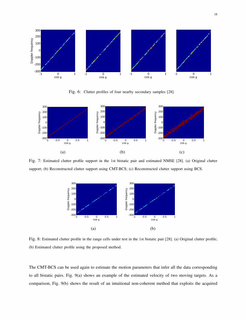
In Fig. 6, we show the clutter profiles in the 1st bistatic pair with nt = 4 nearby secondary samples in

the angle-Doppler domain, where each scatterer coefficient is drawn from a complex Gaussian distribution.

The angle-Doppler profile of the clutter is discretized into a grid of Nd = 90 Doppler bins from −300

Hz to 300 Hz and Ns = 40 angle bins from −180◦ to 180◦, yielding 3600 entries. The simulated clutter

profiles in each angular bin are represented by two adjacent non-zero random complex entries in each

bistatic pair, and thus the total number of non-zero entries is 80. It is observed that these clutter profiles

in the nearby range cells share the same group sparsity. In addition, a complex Gaussian noise is added

and the clutter-to-noise ratio (CNR) is 40 dB.

Fig. 7 shows the actual clutter support, together with their estimates obtained from four secondary

range cells by the CMT-BCS, and that obtained from a single secondary range cell by the CMT-BCS.

The exploitation of group sparsity is evident. Based on the clutter profile shown in Fig. 7(b), the clutter

profile at the range cell under test is obtained and is shown in Fig. 8. The estimated clutter profile can

be used for effective clutter suppression.

The resulting clutter-free data over multiple bistatic pairs can be fused to estimate the motion parameters

(e.g., two-dimensional velocity) of the moving targets. Because the motion parameters of the targets are

shared by all bistatic pairs but the reflection coefficients differ, a group sparse reconstruction problem can

be formulated where the unknown sparse vector represent motion parameters defined over a dense grid.

18

cos

Dop

pler

freq

uenc

y

-1 0 1-300

-200

-100

0

100

200

cos -1 0 1

cos -1 0 1

cos -1 0 1

300

Fig. 6: Clutter profiles of four nearby secondary samples [28].

cos

Dop

pler

freq

uenc

y

-1 -0.5 0 0.5 1-300

-200

-100

0

100

200

300

cos

Dop

pler

freq

uenc

y

-1 -0.5 0 0.5 1-300

-200

-100

0

100

200

cos

Dop

pler

freq

uenc

y

-1 -0.5 0 0.5 1-300

-200

-100

0

100

200

300

(a) (b) (c)

Fig. 7: Estimated clutter profile support in the 1st bistatic pair and estimated NMSE [28]. (a) Original clutter

support; (b) Reconstructed clutter support using CMT-BCS; (c) Reconstructed clutter support using BCS.

cos

Dop

pler

freq

uenc

y

-1 -0.5 0 0.5 1-300

-200

-100

0

100

200

300

cos

Dop

pler

freq

uenc

y

-1 -0.5 0 0.5 1-300

-200

-100

0

100

200

300

(a) (b)

Fig. 8: Estimated clutter profile in the range cells under test in the 1st bistatic pair [28]. (a) Original clutter profile;

(b) Estimated clutter profile using the proposed method.

The CMT-BCS can be used again to estimate the motion parameters that infer all the data corresponding

to all bistatic pairs. Fig. 9(a) shows an example of the estimated velocity of two moving targets. As a

comparison, Fig. 9(b) shows the result of an intuitional non-coherent method that exploits the acquired

19

Vx (m/s)

Vy

(m/s

)

-20 0 20-30

-20

-10

0

10

20

30

-15

-10

-5

0

-7 -6 -5171819

14 15 169

1011

dBVx (m/s)

Vy

(m/s

)

-20 0 20-30

-20

-10

0

10

20

30

-15

-10

-5

0

True objects

dB

(a) (b)

Fig. 9: Motion parameter estimation in two-target scene [28]. (a) Based on CMT-BCS method; (b) Based on

non-coherent fusion.

images in each bistatic pair. It is difficult to estimate the motion parameter from this result because of

the presence of four bistatic pairs and two targets.

VI. CONCLUDING REMARKS

In this article, we have introduced the offerings of compressive sensing in passive multi-static radar

applications. It was pointed out that many passive multi-static radar signals exhibit certain signal

structures, such as the group sparsity and target continuity, in practical applications. Among many

different compressive sensing methods that are available in the literature, we focused on the Bayesian

compressive sensing framework due to its superior performance and flexibility to account for different

signal structures. A number of structure-aware Bayesian compressive sensing algorithms were introduced

which offer attractive advantages over conventional methods for improved image resolution, reduced

requirement of data samples, and effective inference of multi-static data.

It is noted that the CMT-BCS algorithm generally requires a higher computation complexity than some

commonly used CS algorithms, such as block OMP and group Lasso. In addition, the advantages of group

sparsity is offered only when the target scattering characteristics satisfy a common support requirement

(e.g., most target pixels reflect to all bistatic pairs), whereas the utilization of target continuity would not

be beneficial if targets do not exhibit such continuity.

REFERENCES

[1] H. Griffiths and N. Long, “Television-based bistatic radar,” Proc. IEE-Radar Sonar Navig., vol. 133, no. 7,

pp. 649–657, 1986.

[2] H. D. Griffths and C. J. Baker, “Passive coherent location radar systems. part 1: Performance prediction,”

Proc. IEE-Radar Sonar Navig., vol. 152, no. 3, pp. 153–159, 2005.

20

[3] D. L. Donoho, “Compressed sensing,” IEEE Trans. Info. Theory, vol. 52, no. 4, pp. 1289–1306, 2006.

[4] R. G. Baraniuk, “Compressive sampling,” IEEE Signal Process. Mag., vol. 24, no. 4, pp. 118–124, 2007.

[5] E. Candes and M. Wakin, “An introduction to compressive sampling,” IEEE Signal Processing Mag., vol. 25,

no. 2, pp. 21–30, 2008.

[6] Y. C. Eldar and G. Kutyniok, Compressed Sensing: Theory and Applications. Cambridge Univ. Press, 2012.

[7] L. Poli, G. Oliveri, F. Viani, and A. Massa, “MT-BCS-based microwave imaging approach through minimum-

norm current expansion,” IEEE Trans. Antennas Propagat., vol. 61, no. 9, pp. 4722–4732, Sept. 2013.

[8] M. Leigsnering, F. Ahmad, M. G. Amin, and A. M. Zoubir, “Compressive sensing based specular multipath

exploitation for through-the-wall radar imaging,” in Proc. IEEE ICASSP, (Vancouver, Canada), pp. 6004–6008,

May 2013.

[9] L. Wang, L. Zhao, G. Bi, C. Wan, and L. Yang, “Enhanced ISAR imaging by exploiting the continuity of the

target scene,” IEEE Trans. Geosci. Remote Sens., vol. 52, no. 9, pp. 5736–5750, 2014.

[10] G. Li, P. K. Varshney, and Y. D. Zhang, “Multistatic radar imaging via decentralized and collaborative subspace

pursuit,” in Proc. Int. Conf. on Digital Signal Processing, (Hong Kong, China), Aug. 2014.

[11] M. Carlin, P. Rocca, G. Oliveri, F. Viani, and A. Massa, “Directions-of-arrival estimation through Bayesian

compressive sensing strategies,” IEEE Trans. Antennas Propagat., vol. 61, no. 7, pp. 3828–3838, 2013.

[12] S. Qin, Y. D. Zhang, and M. G. Amin, “Generalized coprime array configurations for direction-of-arrival

estimation,” IEEE Trans. Signal Process., vol. 63, no. 6, pp. 1377–1390, 2015.

[13] S. Qin, Y. D. Zhang, Q. Wu, and M. G. Amin, “DOA estimation of nonparametric spreading spatial spectrum

based on Bayesian compressive sensing exploiting intra-task dependency,” in Proc. IEEE ICASSP, (Brisbane,

Australia), pp. 2399–2403, April 2015.

[14] S. Qin, Y. D. Zhang, Q. Wu, and M. G. Amin, “Structure-aware Bayesian compressive sensing for near-field

source localization based on sensor-angle distributions,” Int. J. Antennas and Propagation, vol. 2015, Article

ID 783467, 15 pages, March 2015.

[15] S. Subedi, Y. D. Zhang, M. G. Amin, and B. Himed, “Group sparsity based multi-target tracking in

passive multi-static radar systems using Doppler-only measurements,” IEEE Trans. Signal Processing, vol. 64,

pp. 3619–3634, July 2016.

[16] Y. D. Zhang, M. G. Amin, and B. Himed, “Reduced interference time-frequency representations and sparse

reconstruction of undersampled data,” in Proc. European Signal Process. Conf., (Marrakech, Morocco), pp. 1–

5, Sept. 2013.

[17] L. Stankovic, S. Stankovic, I. Orovic, and Y. D. Zhang, “Time-frequency analysis of micro-Doppler signals

based on compressive sensing,” in M. Amin (ed.): Compressive Sensing for Urban Radars, (CRC Press), 2014.

[18] M. G. Amin, B. Jakonovic, Y. D. Zhang, and F. Ahmad, “A sparsity-perspective to quadratic time-frequency

distributions,” Digital Signal Processing, vol. 46, pp. 175–190, 2015.

[19] J. A. Tropp and A. C. Gilbert, “Signal recovery from partial information via orthogonal matching pursuit,”

IEEE Trans. Info. Theory, vol. 53, no. 12, pp. 4655–4666, 2007.

21

[20] E. V. D. Berg and M. Friedlander, “Probing the pareto frontier for basis pursuit solutions,” SIAM Journal on

Scientific Computing, vol. 31, no. 2, pp. 890–912, 2008.

[21] R. Tibshirani, “Regression shrinkage and selection via the Lasso,” J. Royal. Statist. Soc., vol. 58, no. 1,

pp. 267–288, 1996.

[22] M. E. Tipping, “Sparse Bayesian shrinkage and selection learning and the relevance vector machine,” J.

Machine Learning Research, vol. 1, no. 9, pp. 211–244, 2001.

[23] S. Ji, Y. Xue, and L. Carin, “Bayesian compressive sensing,” IEEE Trans. Signal Proc., vol. 56, no. 6,

pp. 2346–2356, 2008.

[24] S. D. Babacan, S. Nakajima, and M. N. Do, “Bayesian group-sparse modeling and variational inference,”

IEEE Trans. Signal Proc., vol. 62, no. 11, pp. 2906–2921, 2014.

[25] C. R. Berger, B. Demissie, J. Heckenbach, P. Willett, and S. Zhou, “Signal processing for passive radar using

OFDM waveforms,” IEEE J. Selected Topics in Signal Proc., vol. 4, no. 1, pp. 226–238, 2010.

[26] C. E. Muehe and M. Labitt, “Displaced-phase-center antenna technique,” Lincoln Laboratory Journal, vol. 12,

no. 2, pp. 281–296, 2000.

[27] B. Dawidowicz, K. Kulpa, M. Malanowski, and M. Smolarczyk, “DPCA detection of moving targets in airborne

passive radar,” IEEE Trans. Aerospace and Electronic Systems, vol. 48, no. 2, pp. 1347–1357, 2012.

[28] Q. Wu, Y. D. Zhang, M. G. Amin, and B. Himed, “Space-time adaptive processing and motion parameter

estimation in multistatic passive radar using sparse bayesian learning,” IEEE Trans. Geosci. Remote Sens.,

vol. 64, no. 2, pp. 944–957, 2016.

[29] N. J. Willis and H. D. G. (eds.), Advances in Bistatic Radar. SciTech, 2007.

[30] J. R. Guerci, Space-Time Adaptive Processing for Radar. Artech House, 2003.

[31] R. Baraniuk, M. Davenport, R. DeVore, and M. Wakin, “A simple proof of the restricted isometry property

for random matrices,” Constructive Approximation, vol. 28, pp. 253–263, Dec. 2008.

[32] D. P. Wipf and B. D. Rao, “l0-norm minimization for basis selection,” in Proc. Adv. Neural Info. Proc. Syst.,

(Vancouver, Canada), Dec. 2004.

[33] Y. Shen, J. Fang, and H. Li, “Exact reconstruction analysis of log-sum minimization for compressed sensing,”

IEEE Signal Process. Lett., vol. 20, no. 12, pp. 1223–1226, 2013.

[34] S. Ji, D. Dunson, and L. Carin, “Multitask compressive sensing,” IEEE Trans. Signal Proc., vol. 57, no. 1,

pp. 92–106, 2009.

[35] J. Huang and T. Zhang, “The benefit of group sparsity,” Ann. Statist., vol. 38, no. 4, pp. 1978–2004, 2010.

[36] Q. Wu, Y. D. Zhang, F. Ahmad, and M. G. Amin, “Compressive sensing based high-resolution polarimetric

through-the-wall radar imaging exploiting target characteristics,” IEEE Antennas and Wireless Propagat. Lett.,

vol. 14, pp. 1043–1047, 2015.

[37] W. Qiu, H. Zhao, J. Zhou, and Q. Fu, “High-resolution fully polarimetric ISAR imaging based on compressive

sensing,” IEEE Trans. Geoscience and Remote Sensing, vol. 52, no. 10, pp. 6119–6131, 2014.

[38] J. Yang, A. Bouzerdoum, F. H. C. Tivive, and M. G. Amin, “Multiple-measurement vector model and its

22

application to through-the-wall radar imaging,” in Proc. IEEE ICASSP, (Prague, Czech Republic), pp. 2672–

2675, May 2011.

[39] Z. Zhang and B. D. Rao, “Sparse signal recovery with temporally correlated source vector using sparse

Bayesian learning,” IEEE J. Sel. Topics in Signal Proc., vol. 5, no. 5, pp. 912–926, 2011.

[40] M. K. Titsias and M. Lazaro-Gredilla, “Spike and slab variational inference for multi-task and multiple kernel

learning,” in Proc. Adv. Neural Info. Proc. Syst., (Granada, Spain), pp. 2339–2347, Dec. 2011.

[41] E. I. George and R. E. Mcculloch, “Variable selection via Gibbs sampling,” J. American Statist. Assoc., vol. 88,

no. 423, pp. 881–889, 1993.

[42] T. J. Mitchell and J. J. Beauchamp, “Bayesian variable selection in linear regression,” J. American Statist.

Assoc., vol. 83, no. 404, pp. 1023–1032, 1988.

[43] L. Yu, J. P. Barbot, G. Zheng, and H. Sun, “Compressive sensing for cluster structured

sparse signals: Variational Bayes approach,” Technical Report, 2011. Available at http://hal.archives-

ouvertes.fr/docs/00/57/39/53/PDF/cluss vb.pdf.

[44] M. Zhou, H. Chen, J. Paisley, L. Ren, L. Li, Z. Xing, D. Dunson, G. Sapiro, and L. Carin, “Nonparametric

Bayesian dictionary learning for analysis of noisy and incomplete images,” IEEE Trans. Image Proc., vol. 21,

no. 2, pp. 130–144, 2012.

[45] L. Yu, H. Sun, J. P. Barbot, and G. Zheng, “Bayesian compressive sensing for cluster structured sparse signals,”

Signal Proc., vol. 92, no. 1, pp. 259–269, 2012.

[46] Q. Wu, Y. D. Zhang, M. G. Amin, and B. Himed, “Mutli-task Bayesian compressive sensing exploiting

intra-task dependency,” IEEE Signal Proc. Lett., vol. 22, no. 4, pp. 430–434, 2015.

[47] Q. Wu, Y. D. Zhang, M. G. Amin, and B. Himed, “High-resolution passive SAR imaging exploiting structured

Bayesian compressive sensing,” IEEE J. Sel. Topics in Signal Process., vol. 9, pp. 1484–1497, Dec. 2015.

[48] Q. Wu, Y. D. Zhang, M. G. Amin, and B. Himed, “Complex multitask Bayesian compressive sensing,” in

Proc. IEEE ICASSP, (Florence, Italy), pp. 3375–3379, May 2014.

[49] D. Wipf and S. Nagarajan, “Beamforming using the relevance vector machine,” in Proc. Int. Conf. Machine

Learning, pp. 1023–1030, 2007.

[50] L. Wang, C. E. Yarmanb, and B. Yazici, “Doppler-hitchhiker: A novel passive synthetic aperture radar using

ultranarrowband sources of opportunity,” IEEE Trans. Geosci. Remote Sens., vol. 49, no. 10, pp. 3521–3537,

2011.

[51] L. Jacob, G. Obozinski, and J. Vert, “Group Lasso with overlap and graph Lasso,” in Proc. Int. Conf. Machine

Learning, (Montreal, Canada), pp. 433–440, Jun. 2009.

[52] M. Yuan and Y. Lin, “Model selection and estimation in regression with grouped variables,” J. Royal Statist.

Soc. Series B, vol. 68, no. 1, pp. 49–67, 2006.

[53] Q. Wu, Y. D. Zhang, M. G. Amin, and B. Himed, “Multi-static passive radar SAR imaging based on Bayesian

compressive sensing,” in Proc. SPIE 9109, Compressive Sensing III, (Baltimore, MD), pp. 910902–1–910902–

9, May 2014.

23

[54] S. Brusch, S. Lehner, T. Fritz, M. Soccorsi, A. Soloviev, and B. V. Schie, “Ship surveillance with TerraSAR-X,”

IEEE Trans. Geosci. Remote Sens., vol. 49, no. 3, pp. 1092–1103, 2011.

[55] X. Xing, K. Ji, H. Zou, W. Chen, and J. Sun, “Ship classification in TerraSAR-X images with feature space

based sparse representation,” IEEE Geosci. Remote Sens. Lett., vol. 10, no. 6, pp. 1562–1566, 2013.